Physics-Aware Query-Conditioned Graph Attention Networks
for Radio Map Estimation
Abstract
Radio map estimation from sparse measurements is fundamental to wireless network planning, optimization, and localized map updating. Most recent learning-based approaches formulate the problem as dense map completion over a predefined grid, whereas many practical deployments require estimating transmitter-specific received signal strength only at queried locations or refining an existing map after local changes. This paper proposes a physics-aware query-conditioned hierarchical graph attention network for transmitter-resolved point-wise radio map estimation. For each queried target–transmitter pair, the proposed encoder constructs a bounded local graph over sampled reference observations and aggregates reference-to-query evidence through transmitter-referenced geometric descriptors. A global graph then exchanges representation-level context among nearby target locations to improve neighborhood consistency without revisiting a large number of reference measurements. On top of this shared architecture, we instantiate three operating regimes: direct RSS estimation, prior-conditioned residual correction, and post-hoc gated attenuation of the learned correction. The framework uses only measurement-side quantities and does not rely on environment-side inputs. Simulations on the DeepMIMO scenario show that, in the direct regime, the proposed HGAT achieves the lowest RMSE and MAE among the evaluated learning-based baselines on all reported sites. When conventional prior estimate is available, the residual and gated regimes further reduce the prior error.
I Introduction
Radio maps (RMs) characterize radio quantities such as received signal strength (RSS) or channel gain over a geographic region [30, 27], and they are fundamental to network planning [28], resource management [5], localization [40], and CSI feedback reduction [6]. The core problem of radio map estimation (RME) is to infer unobserved map values from sparse and irregularly distributed measurements. This task is intrinsically difficult because measurement budgets are limited, propagation conditions are spatially heterogeneous, and the radio field can exhibit strongly non-uniform local statistics. Recent theoretical analysis has further shown that the complexity of RME is tightly related to the spatial variability of the field and becomes more pronounced when the sources are closer to the mapped region, which motivates estimators that can adapt to non-uniform local structure rather than relying on a single global smoothness assumption [25].
Existing RME methods can be broadly grouped into three categories. The first category is model-based estimation, including inverse-distance weighting [15], matrix completion [38, 32, 9], kriging methods [19, 36], and kernel-based cartography [26, 11], just to name a few. These methods embed useful geometric or statistical priors, but their performance may degrade when the assumed stationarity, smoothness, or propagation model is mismatched to realistic blockage and shadowing. The second category is data-driven estimation, where deep neural networks learn to recover a radio map from sparse observations [18, 20, 22, 13, 34, 24, 7]. Such methods can model highly nonlinear propagation patterns, yet they are usually more data-hungry and may generalize poorly across environments or sampling patterns. The third category is the hybrid approach, where model-based estimates or physically derived structures are incorporated into the learning pipeline [44, 37, 16, 14, 29, 4]. Representative hybrid couplings intervene at different levels of the estimation process. For example, neural network residual kriging improves the path-loss before kriging is applied to the remaining spatial component [29], whereas kriging convolutional networks absorb kriging-like behavior into a query-centered local graph predictor [4].
However, most existing formulations are designed for dense map completion over a predefined spatial grid. This is natural when the deployment objective is to reconstruct an entire radio map, but it is not always the most relevant operating regime. In many practical workflows, only a limited set of queried locations is needed, or an existing map must be refreshed after localized environmental changes. In such cases, a query-conditioned point-wise estimator that balances predictive performance and computational cost is more favorable. Recent work has started to move in this direction. In particular, [35] formulates RME as a gridless attention-based predictor that estimates radio quantities only at queried locations from sparse measurements and their coordinates.
Another distinction concerns the field being estimated. The majority of prior studies target either an aggregate or occupancy-style radio map whose value at each location reflects the combined contribution of all active transmitters, e.g., [31, 14, 16, 35]. By contrast, this paper considers a transmitter-resolved setting and estimates the field associated with a designated transmitter at queried locations. The two formulations serve different deployment purposes: aggregate maps are natural when transmitter identities or powers are unavailable, whereas transmitter-resolved maps are preferable when cell-specific coverage analysis, interference attribution, or localized map updates are needed. When needed, transmitter-resolved received-power fields can be combined in the linear-power domain to synthesize an aggregate map under a simplified superposition model. The inverse decomposition from aggregate observations to transmitter-specific fields, however, generally requires additional assumptions and is outside the scope of this paper.
Among learning-based methods, graph-based approaches are especially relevant because they can handle irregular sampling without requiring all data to lie on a dense regular image grid; related graph learning on irregular domains has also been explored in kriging-like settings [39]. Early work viewed the radio map as a graph signal and used graph construction tailored to interpolation [23]. More recent GNN-based methods build graphs using building-aware LoS/NLoS connectivity [7], or physics-informed structures derived from building masks, urban maps, radio-depth maps, and superpixels [13, 34, 14, 16]. Although it is clear that graph construction is central to RME performance, two limitations remain important for practical deployment. First, many recent methods ingest environment-side inputs such as building maps and depth features. Such information can improve accuracy, but it is not universally available in measurement-driven RME pipelines [43]. This view is also consistent with 3GPP-related documents; the minimization of drive test (MDT) measurement collection specification and the 5GS architecture specification are centered on UE- and network-side measurements and standardized system functions, rather than assuming direct access to rich environmental databases [1, 2]. Second, existing graph estimators often exploit heterogeneous spatial dependencies through a fixed graph construction, a single graph scale, or a generic repeated hierarchy. Without claiming that they exhaust the full relational structure of RME, we find it useful to distinguish at least two interactions in point-wise estimation: measurement-to-query relations, which determine how observed RSS values should support a specific query, and target-to-target relations, which provide neighborhood context among nearby targets associated with the same transmitter. We model these two interactions with distinct message-passing procedures. Compared with hierarchical graph formulations such as 5GNN [41], our design differs in the sense that both graph construction and attention are conditioned on the current target–transmitter query pair and its transmitter-referenced geometry.
Motivated by these observations, we propose a physics-aware query-conditioned hierarchical graph attention network (HGAT) for point-wise RME. We first form a sampled reference set from historical measurements using spatially uniform sampling. For each target–transmitter pair, a local pair-conditioned graph is instantiated from nearby admissible references, and a local pair-conditioned graph-attention block aggregates measurement-level evidence toward the current target. The resulting local embedding is then refined by a same-transmitter global graph-attention block that exchanges representation-level context among nearby target nodes. Given the resulting hierarchical embeddings, a regime-specific MLP fusion head outputs the final estimate. Notably, the node and edge attributes used by the proposed framework are constructed only from quantities naturally available in measurement-driven RME, such as observed RSS, entity locations, derived distances, and relative bearings.
On top of the shared HGAT encoder, we study three estimation regimes motivated by the complementarity between classical prior-based and learning-based estimators. A classical prior can provide a stable coarse trend and an interpretable baseline, whereas a learned predictor can adapt to localized environment-specific effects that are difficult to encode analytically. Rather than forcing one of these views to dominate, we evaluate the same encoder in three settings. In the direct regime, the graph network predicts RSS itself from the learned hierarchical representation. In the prior-conditioned residual regime, an external baseline such as kriging is kept explicit, and the HGAT learns only the mismatch residual relative to that baseline; the final estimate is then obtained by adding the predicted residual to the prior estimate. In the post-hoc gated regime, the learned residual correction is not assumed to be uniformly beneficial at all queried points. After the residual predictor is fixed, a lightweight gate predicts a bounded attenuation factor from the explicit prior, the frozen residual prediction, its magnitude, and local prior-variation descriptors, and then calibrates the correction strength by minimizing the final recomposition error. Together, these regimes span stand-alone estimation, explicit prior-assisted refinement, and post-hoc correction-strength calibration under a shared architecture.
The main contributions of this paper are summarized as follows:
-
•
We propose a physics-aware hierarchical graph attention encoder that decomposes point-wise RME into pair-conditioned local evidence aggregation and same-transmitter global contextual refinement. The local stage constructs query-specific reference pages using target–reference, reference–transmitter, and target–transmitter geometric descriptors, while the global stage exchanges representation-level context among nearby target locations.
-
•
We instantiate prior-assisted refinement on top of the same encoder by keeping a classical prior explicit, learning the structured residual relative to that prior, and calibrating the frozen residual correction through a lightweight post-hoc attenuation gate.
-
•
We evaluate the framework using DeepMIMO datasets under a unified measurement-only protocol across seen and held-out sites. The direct HGAT achieves the lowest error among the evaluated learning-based baselines, while explicit residual correction and the final gated regime further reduce the ordinary-kriging prior error.
The remainder of this paper is organized as follows. Section II introduces the problem formulation, prior residual structure, and estimation regimes. Section III presents the query-conditioned hierarchical graph attention encoder. The regime-specific prediction heads, inference complexity, and training protocol are then described in Section IV, followed by the simulation results and qualitative comparisons in Section V.
II Problem Formulation, Prior Residuals, and Estimation Regimes
II-A Transmitter-Resolved Point-Wise RME Setting
We formulate transmitter-resolved point-wise RME as learning, from the observation set associated with transmitter , an operator that predicts the RSS of the designated transmitter at queried locations. Consider a two-dimensional region of interest and a set of transmitters that are deployed at different locations. For each transmitter , let
| (1) |
denote the underlying received-signal-strength (RSS) field. Let
| (2) |
be the full set of observed measurements associated with transmitter , where denotes an observed location and the corresponding RSS value. Let
| (3) |
be the set of target locations at which RSS values are to be estimated. The ground-truth label at query location is denoted by . Further defining the admissible target–transmitter pair set as
| (4) |
the point-wise learning problem is to construct an estimator
| (5) |
and fit its parameters by minimizing the following objective over the available training pairs:
| (6) |
where denotes the regression loss and . In case where an aggregate map is needed, the simplified superposition form can be adopted
| (7) |
Note that the inverse decomposition from aggregate observations to transmitter-specific fields is generally underdetermined without additional structural assumptions, and is therefore outside the scope of this work.
On the other hand, we do not claim that query-conditioned point-wise estimation universally dominates dense map completion. Dense estimators remain natural when the deployment objective is to reconstruct an entire map over a fixed grid. Our focus is a complementary regime: when only a limited set of targeted locations is needed, or when an existing radio map must be refreshed after localized environmental changes, it can be more efficient to evaluate a query-conditioned predictor only on the affected points than to recompute the full map. Unlike dense map completion methods that are often tied to a predefined grid resolution, query-conditioned point-wise estimation is naturally grid-free and can be evaluated at arbitrary coordinates.
II-B Priors and Residual Field
When a classical estimator is available, we treat it as an explicit prior and define the induced residual field as the object to be corrected. Let denote a classical estimator indexed by ; although the formulation allows any externally computed classical prior, we use kriging as an example in this paper. For each admissible pair , the corresponding prior estimate is denoted by
| (8) |
and the induced prior residual field is written as
| (9) |
This decomposition makes the estimation target explicit: direct prediction aims at the field value itself, whereas prior-conditioned correction aims at the mismatch field . Keeping the prior explicit is a task-decoupling design choice, i.e., the correction branch is asked to model baseline mismatch while the prior remains separately accessible during inference.
II-C Empirical Structure of Prior Residuals

Our hypothesis is that prior residual is spatially structured, rather than behaving as spatially white noise. Fig. 1 provides a representative diagnostic using aligned heatmaps. Two patterns are especially relevant. First, narrow high-power regions produced by reflection often induce localized signed residual structures that are difficult for globally smooth priors to capture. Second, abrupt attenuation changes near blockage boundaries or other propagation transitions tend to appear as coherent residual bands aligned with large prior gradients. These observations suggest that the prior residual is not merely unstructured noise, but a learnable mismatch field shaped by local propagation conditions.
This view is consistent with prior studies on interpolation over discontinuous spatial fields. In urban surface reconstruction, smoothed interpolators, blur sharp edges and yield their largest errors near facades, roof ridges, and other discontinuities [10]. More generally, for fields containing fronts or region boundaries, kriging and related smoothing methods tend to smear across the discontinuity unless boundaries or region-specific statistics are modeled explicitly [33]. Existing remedies mainly focuses on improving the interpolator itself, whereas our goal is different: the conventional interpolator only provides coarse prior estimates, and we omit variogram design or discontinuity-aware geostatistical optimization. Instead, we keep the prior explicit and focus on learning the structured residual left after interpolation. This motivates studying explicit residual correction in addition to direct field estimation.
II-D Estimation Regimes
In this paper, we study three regimes under a shared HGAT architecture: direct field estimation, explicit prior-conditioned residual correction, and post-hoc gating of the learned correction.
More specifically, in the direct regime, the model predicts the field value itself for each queried target–transmitter pair. In the prior-conditioned residual regime, the task is to estimate the residual induced by an explicit prior:
| (10) |
And the final estimate is summed between the prior estimate and the residual, i.e.,
| (11) |
Finally, in the post-hoc gated regime, we further acknowledge that the learned correction need not be equally reliable at all queried points. A learned attenuation factor is therefore used to calibrate how strongly the residual correction should be applied at each point:
| (12) |
The direct and prior-conditioned regimes define the primary estimation tasks, whereas the gated regime is a post-hoc calibration layer on top of the residual estimator. How these tasks are realized by regime-specific heads and training protocols is discussed in Section IV.
III Query-Conditioned Hierarchical Graph Attention Encoder
This section presents the shared HGAT encoder architecture used in all three estimation regimes. The encoder generally follows a two-stage design: it first aggregates target-specific local evidence from nearby reference observations, and then refines the resulting representation through same-transmitter neighborhood interaction among nearby targets. For an arbitrary pair , the shared encoder produces a local embedding and a global embedding,
| (13) |
summarizes target-conditioned evidence aggregated from nearby references, whereas further refines this representation through same-transmitter interactions among nearby targets. These two embeddings form the shared interface to the regime-specific heads introduced in Section IV. Figure 2 summarizes the resulting two-stage encoder.
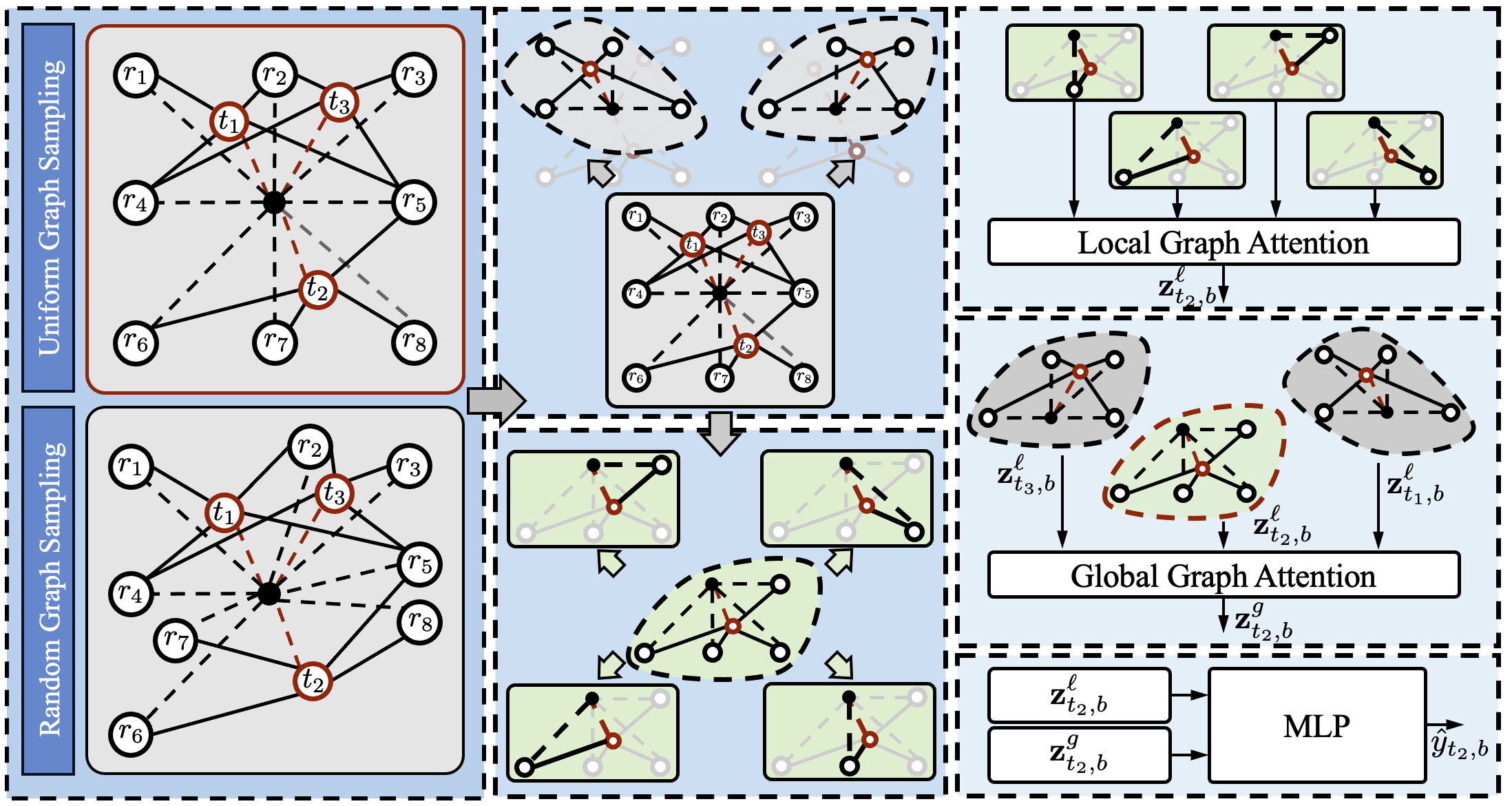
III-A Reference Scaffold, Geometry, and Page Construction
For the sake of efficient data budget utilization, we first construct a bounded transmitter-specific reference scaffold:
| (14) |
denotes the reference sampler for transmitter , and is the retained reference budget. In practice, can be implemented, for example, by random or spatially uniform coverage sampling. The scaffold serves as a bounded evidence set, so that target-time computation scales with the retained reference budget rather than the full observation set. Such concept relates to graph sampling strategies used in large-graph learning, where bounded node or subgraph subsets are retained to control computational cost while preserving representative coverage [12, 42, 8]. For the -th target, the local stage activates the references nearest to the target location, i.e.,
| (15) |
In order to enable the RSS observation and geometrical relationship between different nodes to be exploitable in the graph, we define the following entities with their features. A transmitter node is represented by a transmitter-side descriptor that simply incorporates the coordinates, and the corresponding transmitter embedding is
| (16) |
with denoting a learnable transmitter encoder. Also, we design the reference node to be represented by
| (17) |
where and denotes the observed RSS of transmitter at reference . The corresponding reference embedding is
| (18) |
is a learnable reference encoder. It is worth noting that the target node does not carry an observed RSS value; its role enters through query-conditioned geometry (please see (20)).
To facilitate the discussion on the query-conditioned geometry, we define for any ordered node pair the following pairwise geometric descriptor:
| (19) |
with denoting the geometric angle between the location of two nodes. For each selected reference , the local stage forms one reference page on the triad :
| (20) |
The first two terms in (20) describe the target-reference and reference-transmitter relations, and the third stands for the target-transmitter anchor relation that is shared by all pages for the same pair . Similarly, the local edge embedding is obtained by
| (21) |
Here, denotes a learnable geometric encoder that maps the query-conditioned page descriptor to a local edge embedding. Together with and , it lifts transmitter coordinates, reference observations, and query-conditioned geometry to the latent space used by the local attention block. The concrete parameterization of these encoders is implementation-specific and is therefore deferred to Section V.
When an auxiliary per-link LoS indicator between the query and the reference is available, is enriched by a discrete LoS-state agreement embedding alongside the continuous geometric descriptors in . Given the binary target-side flag and reference-side flag , the agreement state selects one of four learnable prototype vectors ; the selected prototype is concatenated with the continuous geometric slot embeddings before the final fusion step in . We emphasize that the LoS indicator referred to here is a per-link wireless-state attribute accompanying the RSS measurement at a given pair, rather than an environment-side descriptor such as depth map [14]; in measurement campaigns it can be derived from cues such as first-path dominance in angular or delay-spread estimates.
It is worth noting that in the local stage, each selected reference is treated as an individual evidence page conditioned on the current pair . We intentionally postpone any mixing across different references until their relevance to the current query has been weighted through attention. This keeps each evidence path explicitly query-dependent and avoids prematurely averaging references that may correspond to different local propagation conditions.
III-B Local Pair-Conditioned Attention over Reference Pages
For each selected reference , we combine the earlier-mentioned reference and edge embeddings to form the corresponding page vector:
| (22) |
The local attention score of the -th page is given by
| (23) |
and are local-stage graph attention parameters, and denotes the element-wise nonlinear function. Although (23) has the same additive-attention form as GATv2, the attended unit here is no longer a neighboring node feature alone. Instead, it is a query-conditioned reference page that jointly incorporates reference content and pairwise geometry relative to the current query. The resulting coefficient therefore measures the relevance of an entire evidence path to the queried target–transmitter pair.
Denoting as the softmax-normalized local coefficient that is derived based on (23), the local embedding is given by
| (24) |
denotes the linear local-stage message transform and the summation aggregates all attended reference-page messages. It is worth noting that in (24), the local center state is initialized from the transmitter embedding rather than from a target feature.
III-C Global Context Refinement
The local stage processes each queried target independently and therefore captures direct evidence without enforcing cross-target consistency. However, nearby targets associated with the same transmitter often exhibit correlated propagation behavior and similar residual patterns. The global stage is introduced to exploit this dependence at the representation level: instead of revisiting raw reference observations, it exchanges local embeddings among neighboring targets to refine the estimate for the current target.
For a fixed transmitter , the global graph uses target locations in as nodes, and the node feature of target is its local embedding . The center target is connected to its same-transmitter neighbors by
| (25) |
The global edge embedding between the center target and its neighbor is
| (26) |
maps target–target relative geometry to a global edge embedding. In implementation, the training-time instantiation of in (25) is mini-batch dependent; the detailed construction is given in Section V. It follows the same encoder design principle as in the local stage, while using only the geometry relevant to center-neighbor target interactions. The global pair vector for neighbor is
| (27) |
Similar to the local attention procedure, the global attention score is calculated by
| (28) |
and are global-stage attention parameters, distinct from their local-stage counterparts. We denote as the normalized attention score. For message aggregation, only the neighbor local embedding and the global edge embedding are transformed:
| (29) |
The global embedding is then obtained by
| (30) |
Unlike the local stage, is intentionally avoided in (30); this is because we employ the residual connection by passing directly to the readout through the concatenated state in (31). Therefore, is reserved for the context imported from neighboring same-transmitter targets, while preserves the center-specific local evidence. This separation avoids duplicating the center state in the global branch and keeps the roles of the local and global embeddings explicit.
IV Regime-Specific Readout, Calibration, and Training

Section III provides, for each query pair , a local embedding and a global embedding . As summarized in Fig. 3, all three regimes share the same HGAT architecture while their input features to the readout MLP differ. The direct regime predicts RSS from the hierarchical representation alone, whereas the prior-assisted regimes additionally condition the readout on the explicit prior . Throughout this section, when the prior type is fixed, we omit the superscript for readability sake. We also suppress the shared standardization notation and write the readout relations in the scale of the original RSS variable.
IV-A Direct Radio Map Estimation
To facilitate the following discussions, we define
| (31) |
In the direct regime, the model acts as a stand-alone predictor of the RSS field itself. The readout head therefore maps the hierarchical representation directly to the final estimate:
| (32) |
The corresponding training objective compares this prediction with the ground-truth RSS,
| (33) |
where denotes the point-wise regression loss, such as Huber or MSE loss.
IV-B Prior-Conditioned Correction and Post-hoc Calibration
When an external prior is available, we keep it explicit and train the HGAT encoder to estimate only the residual defined in (9). The residual readout head therefore takes both the hierarchical representation and the prior value as input:
| (34) |
In comparison with the direct head that consumes only the hierarchical representation , the residual head additionally ingests the scalar prior at its input. It makes the role of the prior transparent and forces the learned branch to focus on baseline mismatch rather than relearning the full field from scratch. Correspondingly, the final estimate is the sum of the prior estimate and the learned residual, i.e.,
| (35) |
The residual branch is trained against the ground-truth residual, which is denoted by , with the following loss function,
| (36) |
The gated regime starts from this residual estimate and then attenuates it when the correction appears unreliable. With the gating mechanism, the final estimation is written as
| (37) |
The notation is used for the post-hoc attenuation factor to distinguish it from the local attention coefficient in (24). One may argue that the residual MLP can in principle absorb the same side information used by the gate, but doing so would entangle correction prediction with reliability assessment. We therefore keep the gate as a post-hoc calibration layer. Under this decomposition, the residual branch learns to compensate given the hierarchical query representation and the explicit prior, whereas the gate learns to control how much of that compensation should be applied at the current query. This modular design preserves the explicit prior-plus-correction interpretation and allows calibration to be fitted after the residual predictor has been frozen.
The gate itself is implemented by a lightweight MLP fed with a feature vector devised to reflect the structure of residual error,
where denotes simple local variation descriptors of the prior around the query, e.g., derivative-based cues computed from a small neighborhood of the prior field such as gradient-related descriptor. With the encoder and residual head frozen, the gate is fitted by minimizing the final squared recomposition error,
| (38) |
denotes the supervised training-query pairs reused to fit the post-hoc gate after the encoder and residual head have been frozen. The pair-wise loss in (38) can be straightforwardly derived as
| (39) |
whenever . Hence minimizing the final recomposition error is equivalent to a weighted MSE on . The corresponding per-sample minimizer under the attenuation-only constraint is
| (40) |
where projects the unconstrained coefficient onto the interval , and is a small numerical stability threshold used to avoid unstable ratios when the predicted correction magnitude is close to zero. When , the residual correction is treated as negligible and the oracle attenuation is set to zero. Negative ratios indicate that the predicted correction has the wrong sign and should be suppressed, whereas ratios above one are saturated at one under the attenuation-only constraint adopted in (37). In implementation, this equivalence allows the gate to be fitted either by the recomposition loss in (38) or by a weighted regression to the clipped target ; the latter is used in our experiments with a robust Huber loss.
IV-C Complexity Analysis
Once the sampled reference scaffold and the associated neighborhood retrieval structures have been fixed, the online query-time cost is governed by the bounded local and global neighborhood budgets rather than by the full observation set. For the center target, the local stage aggregates over reference pages, and the global stage exchanges representation-level messages with same-transmitter target neighbors. If the local embeddings of those global neighbors are precalculated, the dominant encoder-side cost is
| (41) |
where the first term comes from the local stage, the second from the global stage, and denotes the latent embedding dimension. If the local embeddings of the global neighbors must also be computed on the fly, then each such neighbor incurs an additional local-stage cost over its own references, which leads to
| (42) |
The above expressions characterize the online encoder-side cost after scaffold construction. Nearest-neighbor retrieval is handled by prebuilt spatial indexing or precomputed adjacency and is therefore not counted separately in the dominant term. Training cost scales linearly with the number of supervised target–transmitter pairs and the same bounded neighborhood budgets, up to standard constants from batching and back-propagation. In the prior-assisted regimes, the additional cost of computing the external prior is determined by the chosen classical estimator and is therefore separate from the HGAT encoder cost. The residual head adds only a readout MLP, while the gated regime further adds a low-dimensional gate MLP and, when used, the computation or lookup of local prior-variation descriptors.
V Simulation Setup and Performance Evaluation
V-A Scenario Configuration, Data Splits, and Training Protocol
Data preparation and discretization
We utilize datasets generated by the DeepMIMO platform for computer simulations and performance evaluation[3]. For a particular scenario, the UE-level measurements are aggregated into a coordinate-indexed table by discretizing the covered area into spatial bins. For each occupied bin, the received signal strength is aggregated by averaging the linear-scale powers of all UEs assigned to that bin and then converting the result back to dBm. In the current experimental pipeline, this discretization is used to standardize data export, sample indexing, and evaluation. However, the proposed HGAT is query-conditioned and coordinate-driven, and is therefore not intrinsically tied to this specific spatial resolution. In the reported setup, each site is modeled as a single-antenna transmitter with isotropic radiation, so that each site contributes one transmitter-specific measurement stream in the processed dataset.
Scenario-wise site partition
Instead of training a universal model across heterogeneous scenarios, for each scenario, we train one shared model over multiple sites within the same geographical region. This arrangement strikes a balance between algorithmic generalization capability and practical deployment cost: it exploits cross-site generalization within a region defined by the scenario and avoids the data transfer and coordination overhead required by inter-region model training. In the reported experiments, site IDs follow the dataset-defined indexing, and odd-numbered sites are assigned to the seen set, whereas even-numbered sites are assigned to the held-out set. The seen sites provide both sparse reference observations and supervised training queries, whereas held-out sites provide sparse reference observations only. Consequently, the seen-site results quantify performance on sites participating in supervision, whereas the held-out-site results evaluate intra-scenario regional generalization to sites whose labels are never exposed during training.
The roles of observations and supervised targets are explicitly decoupled. The former is used only as observed support for graph construction and message passing, whereas the latter is used only to define regression targets. We select of the available samples as sparse observations using a spatially uniform sampler for each site-specific dataset. For seen sites, of the remaining samples are further allocated as supervised training queries, while the rest form the evaluation pool. Unless otherwise stated, the same site partition, the same observation and target allocation protocol are used for all baselines as well as for all proposed regimes during their performance evaluation. In the following, the terms seen and held-out refer specifically to whether a site contributes supervised training queries; held-out sites may still provide sparse local reference observations during inference and evaluation. Both the direct and residual regime are trained in an end-to-end manner and the RMSE and MAE are reported for performance evaluation.
During training, the global neighborhood in (25) is instantiated from the targets available in the current mini-batch rather than from the entire target set. Specifically, for a mini-batch index set , we define
| (43) |
and form the training-time global neighborhood as
| (44) |
At inference, is instantiated by the target set under evaluation. This mini-batch construction provides a stochastic approximation to the full target graph and affects only the representation-level global stage; the local evidence aggregation still uses the transmitter-specific reference scaffold .
As for the gated regime, it departs from the above end-to-end scheme and is instead fitted as a post-hoc calibration stage. Specifically, after the encoder together with the residual head has converged under (36), all their parameters are frozen. The gate is then fitted using the point-wise table generated from the supervised training-query pairs already present in the residual-training pipeline. Therefore, the gated regime reuses the original training-query labels and introduces no additional measurement or supervised-query budget. The fitted gate is finally applied, without further updates, to both the intra-domain evaluation table and the held-out-site evaluation table.
V-B Algorithm Implementations
The HGAT encoder realizes four learnable functions that lift transmitter descriptors, reference observations, and query-conditioned geometric relations to a common latent dimension . The transmitter encoder is implemented as a single linear projection of the transmitter coordinates. The reference encoder uses two feature-specific branches, one for the relative position and one for the observed RSS; their outputs are concatenated and fused by a two-layer MLP with activation. All spatial coordinates are normalized by a scalar , and all geometric bearings are wrapped to .
The local edge encoder acts on the composite descriptor , which stacks three ordered pairwise relations, namely , , and . Each relation contributes two geometric components—distance and bearing—so the descriptor contains six scalar components in total. Distances are first squashed by and then encoded by learnable uniform codebooks[21], whereas bearings are encoded by circularly interpolated embeddings to preserve continuity across the wrap-around[17]. A four-state LoS-state agreement embedding is appended to the geometric code. Because both the local and global stages encode the same primitive object, namely pairwise geometry, the global edge encoder follows the same geometric encoding scheme and activates only the target-to-target relation in the global stage. Both local and global stages use single-head GATv2-style additive attention, while the remaining architecture and optimization settings are summarized in Table I.
| Item | Setting |
|---|---|
| Latent dimension | |
| edge embedding dimension | (per component) |
| LoS-state agreement embedding | |
| Feature-wise bin number | (per edge component) |
| Reference fusion MLP | hidden width , |
| Edge fusion MLP | hidden width , |
| Reference number per target | |
| Neighbor number per target | |
| Readout heads | single-hidden-layer MLP |
| Loss | Huber |
| Optimizer | Adam |
| Training epochs | |
| Mini-batch size |
For the post-hoc gated regime, the gate MLP is fitted only after the HGAT encoder operating in the residual-regime being trained. We deploy ordinary kriging as the realization to obtain the prior estimate. In implementation, the clipped attenuation target in (40) is fitted with weighted Huber regression, and no encoder or residual-head parameter is updated in this stage.
V-C Baseline Instantiations
To reduce heterogeneity induced by side information, all learning-based baselines are instantiated under the same measurement-driven contract as HGAT: only sparse RSS observations, spatial coordinates and LoS indicator are provided, while building maps, depth features, and other environment-side inputs are removed. All methods follow the same site split strategy, data usage budget for training. And the trained model parameter set is selected as the one that offers the best validation performance during training. Instead of reproducing the absolute best-case performance of each baseline under its original assumptions, our goal is to compare representative architectural families under a unified input and data-budget regime. To this end, we restrict modifications to the minimum required by the common input and evaluation protocol, while retaining the backbone architecture of each method.
GNN (GCN)
We retain the original two-stage local–global graph-learning backbone and instantiate it under the common measurement-driven protocol above.
RadioGAT
We retain the graph-attention backbone and instantiate it without environment-side graph features under the same common protocol.
DCAE
We retain the convolutional autoencoder completion structure and apply it to the sparse heatmap/mask representation used under the common protocol.
RobUNet
We retain the UNet encoder–decoder backbone together with its residual, channel-attention, and pixel-attention modules under the same common protocol.
STORM
We retain the causal-transformer backbone for sequence-based, measurement-driven prediction under the same common protocol.
In addition to these learning-based baselines, we also report ordinary kriging and universal kriging as conventional model-based baselines under the same data budget.
V-D Direct Estimation Results


| Scenario | HGAT (Ours) | GNN | DCAE | STORM | Ordinary Kriging | Universal Kriging | RadioGAT | RobUNet | ||||||||
|---|---|---|---|---|---|---|---|---|---|---|---|---|---|---|---|---|
| RMSE | MAE | RMSE | MAE | RMSE | MAE | RMSE | MAE | RMSE | MAE | RMSE | MAE | RMSE | MAE | RMSE | MAE | |
| Denver Site 1 (seen) | 6.20 | 3.92 | 11.14 | 8.64 | 9.17 | 6.87 | 8.51 | 6.37 | 6.17 | 3.94 | 5.93 | 3.69 | 9.49 | 7.03 | 7.84 | 5.68 |
| Denver Site 3 (seen) | 5.99 | 3.99 | 13.78 | 11.49 | 9.59 | 7.12 | 8.18 | 6.01 | 5.87 | 3.80 | 5.87 | 3.80 | 10.13 | 7.49 | 8.32 | 5.79 |
| Denver Site 2 (held-out) | 6.62 | 4.44 | 8.91 | 6.78 | 13.49 | 10.75 | 7.81 | 6.02 | 6.36 | 4.07 | 6.36 | 4.07 | 9.04 | 6.78 | 7.32 | 5.25 |
Table II reports the site-wise RMSE and MAE of all compared methods on the three sites in the Denver scenario. Among the learning-based baselines, the proposed HGAT delivers the lowest RMSE and MAE on every site. On the two seen sites, Sites 1 and 3, HGAT attains and in (RMSE, MAE), respectively; on the held-out Site 2, it attains . Relative to the best competing learned baseline for each site and metric, HGAT improves RMSE by dB on Site 1, dB on Site 3, and dB on the held-out Site 2, with corresponding MAE reductions of dB, dB, and dB. The advantage is also clear against STORM, the closest measurement-driven point-wise baseline in our benchmark: HGAT reduces RMSE by – dB and MAE by – dB across the three sites. These site-wise results indicate that the proposed hierarchical encoder generalizes across sites within the same scenario rather than merely memorizing supervised layouts.
Kriging nevertheless remains slightly stronger overall in this direct-estimation setting. Averaged over the three site-wise rows, HGAT attains dB RMSE and dB MAE, while the best kriging baseline on each site remains ahead by only – dB in RMSE and – dB in MAE. Rather than weakening the case for HGAT, this result clarifies the role of the direct regime: it isolates the contribution of the shared encoder itself and motivates the residual and gated regimes, where a strong classical prior is kept explicit and only its structured mismatch is learned.
The representative seen-site visualization in Fig. 4 is consistent with the quantitative trend. Compared with GNN, DCAE, STORM, RadioGAT, and RobUNet, HGAT more accurately reconstructs the narrow vertical high-power corridor and the transverse band around the scene center. In particular, GNN exhibits the diffusion behavior typically associated with GCN-style neighborhood averaging, which broadens sharp transitions and causes high-power regions to leak into adjacent blocks. RadioGAT preserves parts of the coarse structure but produces less coherent contours near sharp boundaries, while STORM captures the large-scale trend but remains visibly smoother around local transitions. These qualitative differences are consistent with the role of the local stage, which aggregates evidence through query-conditioned reference pages rather than averaging neighboring observations in a single flat pass.
The representative held-out-site visualization in Fig. 5 highlights a similar pattern under regional generalization. Among the learned baselines, HGAT most closely matches the width and location of the dominant vertical corridor and better preserves the surrounding attenuation transitions. By contrast, GNN and RadioGAT exhibit stronger side leakage, whereas DCAE, STORM, and RobUNet produce more diffused transitions. This behavior is consistent with the hierarchical combination of pair-conditioned local evidence aggregation and same-transmitter global neighborhood regularization: the local stage preserves target-specific sharp structures, while the global stage improves neighborhood consistency without revisiting large numbers of raw reference observations.
V-E Performance Evaluation for Residual Regimes
| Scenario | Ordinary Kriging Prior | HGAT Residual | HGAT Residual + Gate | |||
|---|---|---|---|---|---|---|
| RMSE | MAE | RMSE | MAE | RMSE | MAE | |
| Denver Site 1 (seen) | 6.17 | 3.94 | 5.87 | 3.81 | 5.83 | 3.73 |
| Denver Site 3 (seen) | 5.87 | 3.80 | 5.41 | 3.61 | 5.37 | 3.56 |
| Denver Site 2 (held-out) | 6.36 | 4.07 | 6.25 | 4.15 | 6.18 | 4.04 |


Table III evaluates the prior-conditioned residual regime using the same Denver site partition as in Table II. The ordinary-kriging columns correspond to the explicit prior, while the two HGAT columns keep this prior fixed and add either an ungated residual correction or a post-hoc gated correction. Compared with the ordinary-kriging prior, the ungated residual head reduces RMSE from to dB on Site 1, from to dB on Site 3, and from to dB on the held-out Site 2. These correspond to RMSE reductions of , , and dB, respectively. Thus, even when ordinary kriging provides a strong prior, its residual remains structured enough to be learned by the query-conditioned HGAT encoder.
The MAE results add a useful qualification. On the two seen sites, the ungated residual head also reduces MAE, from to dB on Site 1 and from to dB on Site 3. On the held-out Site 2, however, ungated residual correction lowers RMSE but increases MAE from to dB. Since RMSE is more sensitive to large errors than MAE, this split suggests that the ungated residual branch suppresses some high-magnitude localized errors on the held-out site while introducing small absolute-error increases over a broader set of points.
The post-hoc gate resolves this RMSE–MAE tension. It further improves RMSE over the ungated residual estimate by , , and dB on Sites 1, 3, and 2, respectively, and it also reduces MAE by , , and dB. In particular, on the held-out site, the gate changes the MAE from the ungated value of dB to dB, slightly below the ordinary-kriging prior. This confirms that the main improvement comes from explicit residual learning, while the gate acts as a lightweight calibration layer that limits over-application of the frozen correction without introducing additional supervised-query budget.
The qualitative maps in Fig. 6 explain the source of the residual-regime gain. Ordinary kriging captures the smooth large-scale trend, but its signed residual still contains coherent spatial structures near sharp propagation transitions. The ungated residual branch reduces these structured residuals and yields positive absolute-error reduction over broad regions of the evaluated map. Fig. 7 visualizes the subsequent calibration stage: the learned gate does not replace the residual predictor, but attenuates its point-wise correction before recomposition.
VI Conclusion
In this paper, we proposed a physics-aware query-conditioned HGAT framework for transmitter-resolved point-wise radio map estimation from sparse measurements. The proposed architecture combines pair-conditioned local evidence aggregation over reference pages with same-transmitter global contextual refinement among nearby target locations. On top of this shared encoder, we studied three operating regimes: direct RSS prediction, ordinary-kriging-conditioned residual correction, and post-hoc gated attenuation of the learned correction. This design keeps the estimator grid-free, measurement-driven, and compatible with both stand-alone prediction and prior-assisted map refinement. Simulation results showed that in the direct regime, HGAT achieves the strongest performance among the evaluated learning-based baselines and better preserves sharp propagation transitions, confirming the benefit of query-conditioned graph construction and hierarchical aggregation. Meanwhile, the comparison with kriging shows that classical priors remain highly competitive under sparse observations. Second, in the residual regime, keeping ordinary kriging explicit and learning only its structured mismatch further reduces the prior error on both seen and held-out sites. The post-hoc gate further calibrates the frozen correction and mitigates the RMSE–MAE imbalance observed for ungated correction on the held-out site.
References
- [1] Radio measurement collection for Minimization of Drive Tests (MDT); Overall description; Stage 2. Note: 3GPP TS 37.320Available from the 3GPP specification portal Cited by: §I.
- [2] System architecture for the 5G System (5GS). Note: 3GPP TS 23.501Available from the 3GPP specification portal Cited by: §I.
- [3] (2019-02) DeepMIMO: a generic deep learning dataset for millimeter wave and massive MIMO applications. In Proc. Inf. Theory Appl. Workshop (ITA), San Diego, CA, pp. 1–8. Cited by: §V-A.
- [4] (2020-Apr.) Kriging convolutional networks. Proceed. AAAI Conf. Artif. Intell. 34 (04), pp. 3187–3194. External Links: Document, Link Cited by: §I.
- [5] (2019) Engineering radio maps for wireless resource management. IEEE Wireless Commun. 26 (2), pp. 133–141. External Links: Document Cited by: §I.
- [6] (2025) Rem-based channel awareness in time-varying environments for CSI feedback reduction. In IEEE Int. Conf. Commun., pp. 1912–1917. External Links: Document Cited by: §I.
- [7] (2023-05) A graph neural network based radio map construction method for urban environment. IEEE Commun. Lett. 27 (5), pp. 1327–1331. External Links: Document Cited by: §I, §I.
- [8] (2018) FastGCN: fast learning with graph convolutional networks via importance sampling. In Int. Conf. Learn. Representations, External Links: Link Cited by: §III-A.
- [9] (2025) Integrated interpolation and matrix completion for radio map estimation: a convex optimization approach. In IEEE Int. Conf. Acoust., Speech Signal Process. (ICASSP), pp. 1–5. External Links: Document Cited by: §I.
- [10] (2006) Analysis of interpolation errors in urban digital surface models created from LIDAR data. In 7th Int. Symp. spatial accuracy assessment in natural resources and environmental sciences, pp. 160–168. Cited by: §II-C.
- [11] (2017) Non-parametric spectrum cartography using adaptive radial basis functions. In IEEE Int. Conf. Acoust., Speech Signal Process. (ICASSP), pp. 3599–3603. External Links: Document Cited by: §I.
- [12] (2017) Inductive representation learning on large graphs. In Advances Neural Inf. Pross. Syst., I. Guyon, U. V. Luxburg, S. Bengio, H. Wallach, R. Fergus, S. Vishwanathan, and R. Garnett (Eds.), Vol. 30. External Links: Link Cited by: §III-A.
- [13] (2021-02) RadioUNet: fast radio map estimation with convolutional neural networks. IEEE Trans. Wireless Commun. 20 (6), pp. 4001–4015. External Links: Document Cited by: §I, §I.
- [14] (2024-09) RadioGAT: A joint model-based and data-driven framework for multi-band radiomap reconstruction via graph attention networks. IEEE Trans. Wireless Commun. 23 (11), pp. 17777–17792. External Links: Document Cited by: §I, §I, §I, §III-A.
- [15] (2008) An adaptive inverse-distance weighting spatial interpolation technique. Comput. Geosci. 34 (9), pp. 1044–1055. External Links: ISSN 0098-3004, Document, Link Cited by: §I.
- [16] (2025-08) Dual-GRE: Dual-phase enhancement in radiomap estimation based on graph attention. IEEE Wireless Commun. Lett. 14 (8), pp. 2646–2650. External Links: Document Cited by: §I, §I, §I.
- [17] (2022-07) Instant neural graphics primitives with a multiresolution hash encoding. ACM Trans. Graph. 41 (4). External Links: ISSN 0730-0301, Document, Link Cited by: §V-B.
- [18] (2018) RecNet: a convolutional network for efficient radiomap reconstruction. In 2018 IEEE Int. Conf. Commun. (ICC), pp. 1–7. External Links: Document Cited by: §I.
- [19] (1990) Kriging: a method of interpolation for geographical information systems. Int. J. Geograph. Inf. Syst. 4 (3), pp. 313–332. External Links: Document Cited by: §I.
- [20] (2020-06) Transfer learning for tilt-dependent radio map prediction. IEEE Trans. Cogn. Commun. Netw. 6 (2), pp. 829–843. External Links: Document Cited by: §I.
- [21] (2020) Exploring the limits of transfer learning with a unified text-to-text transformer. J. Mach. Learn. Res. 21 (140), pp. 1–67. External Links: Link Cited by: §V-B.
- [22] (2021-12) FadeNet: deep learning-based mm-wave large-scale channel fading prediction and its applications. IEEE Access 9, pp. 3278–3290. External Links: Document Cited by: §I.
- [23] (2018-10) Radio map interpolation using graph signal processing. IEEE Commun. Lett. 22 (1), pp. 153–156. External Links: Document Cited by: §I.
- [24] (2024-03) Deep-learning-based radio map reconstruction for V2X communications. IEEE Trans. Veh. Technol. 73 (3), pp. 3863–3871. External Links: Document Cited by: §I.
- [25] (2024-05) Theoretical analysis of the radio map estimation problem. IEEE Trans. Wireless Commun. 23 (10), pp. 13722–13737. External Links: Document Cited by: §I.
- [26] (2017-05) Learning power spectrum maps from quantized power measurements. IEEE Trans. Signal Process. 65 (10), pp. 2547–2560. External Links: Document Cited by: §I.
- [27] (2022-10) Radio map estimation: A data-driven approach to spectrum cartography. IEEE Signal Process. Mag. 39 (6), pp. 53–72. External Links: Document Cited by: §I.
- [28] (2022) Aerial base station placement leveraging radio tomographic maps. In IEEE Int. Conf. Acoust., Speech Signal Process. (ICASSP), pp. 5358–5362. External Links: Document Cited by: §I.
- [29] (2019) On the performance of neural network residual kriging in radio environment mapping. IEEE Access 7, pp. 94557–94568. External Links: Document Cited by: §I.
- [30] (2023-01) Spectrum surveying: active radio map estimation with autonomous UAVs. IEEE Trans. Wireless Commun. 22 (1), pp. 627–641. External Links: Document Cited by: §I.
- [31] (2022-01) Deep spectrum cartography: completing radio map tensors using learned neural models. IEEE Trans. Signal Process. 70, pp. 1170–1184. External Links: Document Cited by: §I.
- [32] (2022) Propagation map reconstruction via interpolation assisted matrix completion. IEEE Trans. Signal Process. 70, pp. 6154–6169. External Links: Document Cited by: §I.
- [33] (2006) Variational approaches on discontinuity localization and field estimation in sea surface temperature and soil moisture. IEEE Trans. Geosci. Remote Sens. 44 (2), pp. 336–350. Cited by: §II-C.
- [34] (2022-08) Deep completion autoencoders for radio map estimation. IEEE Trans. Wireless Commun. 21 (3), pp. 1710–1724. External Links: Document Cited by: §I, §I.
- [35] (2025) Spatial transformers for radio map estimation. In IEEE Int. Conf. Commun., pp. 6155–6160. External Links: Document Cited by: §I, §I.
- [36] (2003) Ordinary kriging. In Multivariate geostatistics: an introduction with applications, pp. 79–88. Cited by: §I.
- [37] (2025-01) Two-stage radio map construction with real environments and sparse measurements. IEEE Wireless Commun. Lett. 14 (4), pp. 969–973. External Links: Document Cited by: §I.
- [38] (2021) Fast construction of the radio map based on the improved low-rank matrix completion and recovery method for an indoor positioning system. J. Sensors 2021 (1), pp. 2017208. External Links: Document Cited by: §I.
- [39] (2021-05) Inductive graph neural networks for spatiotemporal kriging. Proc. AAAI Conf. Artif. Intell. 35 (5), pp. 4478–4485. External Links: Document, Link Cited by: §I.
- [40] (2023-12) Real-time outdoor localization using radio maps: a deep learning approach. IEEE Trans. Wireless Commun. 22 (12), pp. 9703–9717. External Links: Document Cited by: §I.
- [41] (2022) 5GNN: extrapolating 5G measurements through GNNs. In Proc. 1st Int. Workshop Graph Neural Netw., GNNet ’22, New York, NY, USA, pp. 36–41. External Links: Document, ISBN 9781450399333, Link Cited by: §I.
- [42] (2020) GraphSAINT: graph sampling based inductive learning method. In Int. Conf. Learn. Representations, External Links: Link Cited by: §III-A.
- [43] (2024-02) A tutorial on environment-aware communications via channel knowledge map for 6G. IEEE Commun. Surv. Tut. 26 (3), pp. 1478–1519. External Links: Document Cited by: §I.
- [44] (2023-10) RME-GAN: a learning framework for radio map estimation based on conditional generative adversarial network. IEEE Int. Things J. 10 (20), pp. 18016–18027. External Links: Document Cited by: §I.