The double Schwarzschild solution in bispherical coordinates
Abstract.
The double Schwarzschild solution in the equal mass case is studied in bispherical coordinates. An explicit conformal transformation from cylindrical Weyl coordinates to bispherical coordinates is given in terms of elliptic functions. A multi-domain spectral method for spacetimes in bispherical coordinates is presented to numerically reconstruct this solution.
1. Introduction
Binary black holes systems are among the strongest sources for gravitational radiation in our universe, and consequently, the first gravitational waves to be recorded in [17] originate from such a system. The Einstein equations for binary black hole systems are complicated and can only be solved numerically for the time being. In an earlier stage of the evolution of such a system, a quasi-stationary phase is expected where the change of radius due to emitted radiation is small over one complete turn. Detweiler [13, 7, 14] suggested to approximate this stage by a spacetime with a helical symmetry where the outgoing radiation is exactly compensated by incoming gravitational waves. Such an approach had been previously applied to binary charges of opposite sign in Maxwell theory by Schönberg [35] and Schild [34].
In a numerical context, spacetimes with a helical Killing vector have been studied in [19, 22, 23, 1, 10, 38, 18, 6, 37, 39, 5, 9, 4, 29, 30, 8] and references therein. A formulation of the Einstein equations in vacuum in the presence of a helical Killing vector was given in [26] by applying Ehler’s projection formalism [15], see also [20]. This led to a formulation of the Einstein equations in the form of an Ernst equation [16], see also the discussion in [25]. In this formalism, binary black hole spacetimes with a helical Killing vector are potentially singular at the horizons of the black holes that are Killing horizons and the light cylinder, where observers stationary with respect to the horizons rotate with the velocity of light. Null infinity cannot be regular in these spacetimes, see [21, 2] since there will be incoming radiation to compensate the emitted radiation from the binary system. In the Ernst formalism the zeros of the Killing vector lead to Fuchsian singularities of the resulting equations which where studied in a formal expansion in [26].
In addition to the potential application of helical Killing vectors in an early stage of a binary system, there is also a mathematical interest in such systems since they are of mixed type (elliptic in the interior of the light cylinder and hyperbolic in the exterior). To construct such spacetimes numerically, it will be necessary to solve a 3D system of nonlinear equations with Fuchsian singularities at the boundary and non regular infinity. As a first step towards this problem, we studied numerically in [3] the case of a single Kerr black hole in a rotating frame. Since the angular velocity of the frame was chosen to equal the formal angular velocity of the horizon, this corresponded to a situation where the horizon is a Killing horizon, and where there is a second surface of cylindrical topology, the light cylinder, where the Killing vector changes its causal nature. Since the solution is explicitly known, this provided an interesting test of the numerical algorithms.
In the present paper we want to consider an explicitly known test case with two Killing horizons. To this end we consider the well known static double Schwarzschild solution [27], see also [28], where the black holes are separated by a conic singularity on the axis, a Weyl strut. This spacetime was studied via ray tracing in [12]. The solution is given in cylindrical Weyl coordinates where the horizons form intervals on the symmetry axis. Since this is numerically not a convenient setting, we establish first an exact conformal transformation to bispherical coordinates where the horizons of spherical topology are on constant coordinate surfaces. In these coordinates infinity is compactified to a point in the computational domain. An explicit form of the double Schwarzschild solution in bispherical coordinates is given for the first time in terms of Jacobi elliptic functions. We numerically reproduce this solution with an approach similar to Grandclément’s Kadath [24], a multi-domain spectral approach. It is shown that the regular part of the exactly known metric can be reproduced numerically to machine precision with this approach.
The paper is organised as follows: in section 2 we review stationary axisymmetric spacetimes in the Ernst formalism and the double Schwarzschild solution in Weyl coordinates. In section 3 we present a short overview on bispherical coordinates. In section 4 we construct the conformal transformation from Weyl coordinates to bispherical ones for the double Schwarzschild solution. The numerical methods to be used are outlined in section 5. In section 6 we solve the Einstein equations in bispherical coordinates for the double Schwarzschild solution. In section 7, we add some concluding remarks. Details on the solution in terms of elliptic functions are presented in an appendix.
2. Double Schwarzschild solution in Weyl coordinates
In this section, we collect a few facts on static axisymmetric vacuum spacetimes and the double Schwarzschild solution.
In the static axisymmetric case in vacuum, the metric can be written in Weyl-Lewis-Papapetrou form, see [28],
| (1) |
here the cylindrical Weyl coordinates are such that measures the distance to the symmetry axis parameterized by , and and correspond to the static and the axisymmetric Killing vector respectively. The metric functions and depend on and , but not on and . The potential satisfies the axisymmetric Laplace (or Euler-Darboux) equation,
| (2) |
Writing the metric function in the form , one finds that, from Einstein’s equations, satisfies the equation
| (3) |
i.e., the 2D Laplace equation. An obvious solution vanishing on the axis is . It is convenient to introduce complex notation, . In this case the metric function is given for known and in terms of quadratures,
| (4) |
In other words, the Einstein equations in vacuum are equivalent to being a harmonic function, satisfying the Euler-Darboux equation and being given in terms of quadratures of these functions. The complex notation introduced above will facilitate the finding of a conformal transformation to bispherical coordinates below.
It is well known that the static axisymmetric Einstein equations in vacuum are completely integrable, see for instance [16, 28, 25] for references. Mathematically so-called multi-black hole solutions are multi-solitons. In the static case, they correspond to exact solutions having disconnected horizons on the symmetry axis where vanishes on intervals. Here we concentrate on the equal mass case (for which the solution has an equatorial symmetry), where we follow the presentation in [32].
The solution is parameterized by three parameters , corresponding to the Komar masses of the two black holes (put ), and a distance . We have
| (5) |
as well as
| (6) | ||||
Then the metric functions for the double Schwarzschild solution can be written as
| (7) |
We show the metric functions for the example and in Fig. 1.


There are two horizons located on the symmetry axis between and . Both functions, and , vanish there. The solution is asymptotically flat. On the regular part of the axis, here for , the metric function vanishes. However, this is not the case between the two horizons, for in the example, where, is constant, but not equal to zero. This corresponds to a conical singularity in the space-time, a Weyl strut, which keeps the situation static despite the two black holes attracting each other.
3. Bispherical coordinates
In this section we collect some basic facts on bispherical coordinates. Since the double Schwarzschild metric contains two distinct horizons with spherical topology, it is natural to introduce bispherical coordinates for the description of this spacetime. Starting from Cartesian coordinates , bispherical coordinates are defined as follows. Let
where is a parameter; these points are called the focal points of the bispherical coordinate system. For any point , define

Here, and denote the Euclidean distances from to and , respectively. If denotes the azimuthal angle around the -axis, then are called the bispherical coordinates of . These coordinates are described in more detail in [33]. The surfaces are nested spheres with center and radius
except in the case , which corresponds to the plane .


In these coordinates, the Cartesian coordinates are given by
| (8) |
where
| (9) |
In the axisymmetric case, by setting the radial coordinate , one has
| (10) |
and
| (11) |
This implies that infinity is reached in these coordinates in the limit and . Thus bispherical coordinates lead in a natural way to a compactification of .
4. Metric in bispherical coordinates
For the equal-mass case, Weyl and bispherical coordinates are related by the conformal map constructed in Appendix A:
with
| (12) |
where
and where , with being the standard Jacobi elliptic function (for a detailed definition see appendix A or [31]). The horizons are located at , and spatial infinity corresponds to the pole .


In order to better observe how the Weyl coordinates vary with respect to the bispherical coordinates, it is convenient to normalize them by the factor defined in (9), since it vanishes at the pole with the same order, as shown in Appendix C.


Denoting by
| (13) |
the spatial part of the metric, up to the conformal factor , in Weyl coordinates, one finds that the metric in bispherical coordinates can be written as
From the expression for in (12), one finds
| (14) |
where
We show the metric potentials and in bispherical coordinates in Fig. 7. They vanish on the horizons . The function has a visible cusp for , the point corresponding to spatial infinity. The quantity is discontinuous at the corners of the domain . It is also less than on the axis between the black holes at , which corresponds to the Weyl strut.


Note that the boundary of the domains in Fig. 7 corresponds in Weyl coordinates to the axis: the two horizons are now given by , the regular part of the axis including infinity to , and the part of the axis between the horizons where the Weyl strut is located at .


5. Numerical approach in a single domain
In this section we introduce the numerical approach to be applied in the following, a Chebyshev collocation method as in [3] and [24]. With this approach in a single domain, we reconstruct the metric function .
5.1. Chebyshev collocation method
The basic idea of a Chebyshev collocation method is to map an interval for some variable via to the interval where . For we introduce the usual Chebyshev collocation points , , . Standard Lagrange interpolation of a function on these collocation points allows for an approximation of the derivative of the function via the derivative of the interpolation polynomial, which is equivalent to the action of Chebyshev differentiation matrices on the vector with components , see [36]. Note that the conditioning of Chebyshev differentiation matrices is of the order of .
This approach is equivalent to the expansion of the function in terms of Chebyshev polynomials , ,
| (15) |
In a collocation approach, the spectral coefficients , are obtained by imposing relation (15) as an equality on the collocation points,
| (16) |
The spectral coefficients can be computed with a Fast Cosine Transform (FCT) that is related to the Fast Fourier Transform. It is known, see for instance [36], that they decrease exponentially with for analytic functions which is called spectral convergence. Thus the numerical error is indicated by the coefficients with the highest index. We always aim at a numerical resolution of the order of machine precision which is in Matlab roughly (due to the mentioned conditioning of the differentiation matrices, achievable accuracy is typically limited to ).
Boundary or matching conditions are implemented with Lanczos’ -method, see [36]. This means that the boundary conditions are discretised in the same way as the to be solved differential equation, and that the line(s) in the differentiation matrices corresponding to the boundary are replaced by the condition.
In two spatial dimensions, say and , one simply takes a tensor grid: , and similarly for the differentiation matrices.
5.2. The potential
If a conformal transformation of the standard Weyl cylindrical coordinates to bispherical coordinates is considered, the form of the Einstein equations does not change in the quotient space approach. Thus we have that is again a harmonic function. For the numerical treatment, we take explicit care of the singularities of this function which vanishes at the horizons and the axis . Thus we make the following ansatz for ,
| (17) |
motivated by the form of in bispherical coordinates in flat space.
With this ansatz we get for the 2D Laplace equation
| (18) |
It is convenient to introduce the coordinate which leads for (18) to a less singular equation,
| (19) |
This is a singular linear equation, the singularities being , and . The equation is homogeneous in . This means that a unique solution is expected as for instance in the case of the hypergeometric equation if the value of the solution is fixed at some of the singularities as in [11].
5.3. Numerical solution for the function
We introduce the standard Chebyshev collocation points for and . For the example and which corresponds to and , we show the function in Fig. 9, where we have normalized to 1 at infinity. With and , the spectral coefficients shown on the right of the same figure decrease to machine precision.


The corresponding solution for is shown on the left of Fig. 10. It vanishes as expected on the boundary of the computational domain. The difference between the numerical and the exact solution is shown on the right. As expected from the spectral coefficients, it is of the order of .


6. Multi-domain spectral approach
In this section we will summarise basic concepts of the multi-domain spectral approach which is also the basis of Kadath [24].
6.1. Domains
Spectral methods as discussed in the previous section are very efficient in approximating smooth functions. In contrast they are only of first order in application to discontinuous functions as the function , where a Gibbs phenomenon will be observed. Since this is due to the singular Weyl strut that keeps the spacetime static, we will not discuss this case here.
A possible way to address non-smoothness with a spectral method is to introduce several domains where the considered function is smooth in each of them. This has also the benefit to reduce the number of Chebyshev polynomials needed to numerically resolve a given function which is interesting because of the mentioned conditioning problems of Chebyshev differentiation matrices. The problem to be addressed here is the function that has a cusp at infinity as can be seen in Fig. 7. This is due to the asymptotic behavior of , where since is not a smooth function of and near the origin in this coordinate system, see (11).
To avoid this problem, we cut out a rectangle near infinity similar
to the approach in [24], where a curvilinear
rectangle was used. We introduce in the following positive
and and with this the five domains,
see Fig. 11:
I. , ;
II. , ;
III. , ;
IV. , ;
V. , .

At the boundaries between these domains, the functions have to be in the respective variable, say between domains I and II, the functions have to be differentiable in . At the boundaries to the domain containing infinity, the exact solution is imposed. These conditions will be again implemented with a -method. At the rectangle cut out near infinity, the exact solution will be imposed.
6.2. The Ernst potential
In order to take care of the horizons where vanishes, we make the ansatz
| (20) |
and get for the Ernst equation
| (21) |
This leads with (17) to
| (22) |
a singular linear equation with a source term which will be solved for with a vanishing condition at infinity (U vanishes at infinity since f goes to 1 there). But since we cut out the white rectangle in Fig. 11 containing infinity, we impose instead boundary conditions at the common boundaries of the rectangle with domains II, IV and V. We use the exact solution for U as a boundary condition.
In Fig. 12 we show the spectral coefficients for the exact solution in domains I, II and IV (for symmetry reasons we do not show the ones in domain III and IV). In all domains we apply Chebyshev polynomials in , and in domain I in , in domain II in , and in domain IV 100 in . This gives an indication of the needed spectral resolution in the studied example.


6.3. Numerical solution for
The numerical solution with the above numerical parameters can be seen in Fig. 13 on the left. The small cut out domain near infinity is visible. The more one avoids the cusp singularity at infinity, i.e., the larger and the smaller are chosen, the lower the needed resolution. The difference between the exact and the numerical solution is shown on the right of Fig. 13. For the shown parameters, it is of the order of , the main difference appearing at the horizon where the Ernst potential vanishes.


The solution for the Ernst equation itself is shown in Fig. 14 on the left. The difference between the exact and the numerical solution is of the order of as can be seen on the right of the same figure. Here the main error is near the infinite domain.


7. Outlook
In this paper we have given an explicit representation of the double Schwarzschild solution in bispherical coordinates in terms of Jacobi elliptic functions. The boundary of the computational domain is given by the horizons and the symmetry axis, infinity corresponding to a point of the boundary. The Einstein equations reduce in this case to being given by a harmonic function with a vanishing condition on the boundary of the computational domain and the Euler-Darboux equation for the logarithm of the (real) Ernst potential. If the behavior of these two functions at the horizons and the axis is addressed by an explicit ansatz for these functions, the Einstein equations reduce to a set of coupled linear equations with Fuchsian singularities at the horizons and the axis.
These two equations were solved with a multi-domain spectral method which led to a reproduction of the exact solution to the order of . The third metric function is given in terms of quadratures of the first two functions. Since it is discontinuous due to the singular Weyl strut separating the two horizons, it was not considered here.
This work is intended to be a preparatory step to treat binary black holes with a helical Killing vector in the Ernst formulation, see [26]. The idea is to make a similar ansatz for the Ernst potential and the metric near the horizon which will lead to a Fuchsian nonlinear system. This will be solved as in [3] with a modified Newton iteration to take care of the light cylinder where the equations are also singular. Near infinity, a rectangle will be cut out as in [24] and the present paper where we impose either a type N solution obtained by solving the linearized Einstein equations in the presence of a helical Killing vector as in [26] or a standard asymptotically flat metric (this would assume that the helical symmetry only holds in the vicinity of the black holes). This will be the subject of future work.
Appendix A Construction of the conformal map
In the equal-mass double Schwarzschild case, it is possible to construct a conformal map such that
where ranges over
as varies in
for some parameter . Since Weyl coordinates are unbounded, the map must have a pole, representing spatial infinity in bispherical coordinates. By axial symmetry, one may identify with . Moreover, these coordinates should represent the two horizons as the spheres and .
The problem is therefore to construct a conformal map from onto , that is, a map from a rectangle to the right half-plane. In order for the horizons to be represented by two spheres, the two vertical edges of must be mapped to two segments of the imaginary axis. The remaining edges must be mapped to the complementary parts of the imaginary axis. This requires
where
A convenient way to proceed is to use the analytic continuation of the Jacobi elliptic function , see [31]. For all , define
where
is the incomplete elliptic integral of the first kind, and is the modulus. Let
denote the complete elliptic integral of the first kind, and define
It can then be shown that conformally maps the domain
onto the lower half-plane, with a pole at . Moreover, the boundary is mapped as follows:
To obtain the right half-plane, it is sufficient to multiply by , which corresponds to a rotation of the image by . Since the map is defined on , one first introduces a linear transformation
mapping onto . A direct computation shows that
Furthermore, since
the map must be scaled by the factor . This leads to the relation
from which one obtains
Hence the conformal map is given by
Using the identity
this expression can be rewritten in the simpler form
| (23) |
where . Finally, we define
The map has a pole at , which corresponds to spatial infinity.

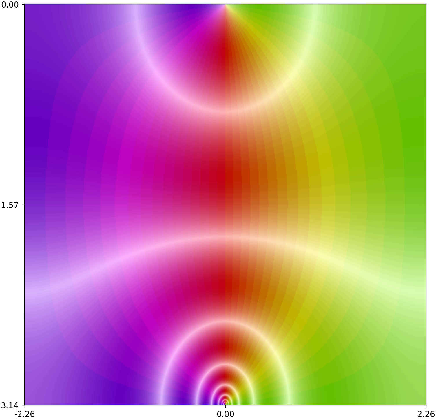
Fig. 15 above shows how horizontal and vertical lines in the domain are transformed by the conformal map . However, this map can also be represented using a domain-coloring plot, as shown below in Fig. 16. The colors represent the phase, and the white lines represent curves of equal amplitude. One can clearly see the pole at and the zero at .
Appendix B Uniqueness of the conformal map
The map is in fact the unique conformal map that preserves the structure of the horizons in Weyl coordinates. Indeed, suppose that there exists another conformal map
such that
Then the map
is a conformal automorphism of the half-plane fixing the four points
Since every conformal automorphism of the half-plane is a Möbius transformation, and since fixes at least three distinct points (for ), it follows that
Therefore, , which proves the uniqueness of the conformal map.
Appendix C Behavior near infinity
In bispherical coordinates, spatial infinity corresponds to the pole , where tends to infinity. In order to study the behavior of the coordinates and the metric near infinity, one uses the expansion
Therefore, at leading order, one has
From (8), one sees that by choosing
one obtains a natural interpretation of these bispherical coordinates: sufficiently far from the black holes, they reduce to the standard bispherical coordinate transformation in flat space, since and, from (14),
Here is the spatial metric defined in (13). The azimuthal component can be expressed as
One thus recovers the flat metric in standard bispherical coordinates, i.e. the metric is asymptotically flat. This justifies why it is convenient to normalize the Weyl coordinates by the factor in Figure 6.
Appendix D Behavior on the axis
In bispherical coordinates, the axis is given by in the exterior region and by between the horizons. Thus, to study the behavior of the metric near the axis, one has to examine how the conformal map in (23) behaves at and . First, let us consider the following expansion:
Therefore, and can be expressed at leading order as
Since is conformal, one can write its derivative as . Therefore, to leading order,
It is well known that, on the axis, the Weyl potential is constant along the axis and is equal to in the exterior region. Hence the metric takes the form
with . One can see that the metric is locally elementary flat near the axis, with as the conformal factor. Next, let us consider the axis between the horizons. The expansion of at is
where the relation has been used. One can simplify this further by using the identities, valid for all , see [31],
and obtain
Therefore,
In the same way, one finds the expression for near the axis:
It is possible to compute the potential on the axis between the horizons using (7) for and , and one finds that
One therefore obtains the metric components
with . Since , the metric is no longer locally conformally flat near the axis between the horizons; this naturally corresponds to the Weyl strut.
Appendix E Behavior on the horizons
In bispherical coordinates, the horizons are defined by . The following discussion focuses only on the case ; the other case is symmetric. Let . The expansion of at will be used:
where has been used in the first equality. Then, by using the quarter-period shift and the pure imaginary argument formulas, see [31], one can show that
with . Hence
and therefore
Since is conformal, one can write its derivative as . Therefore, to leading order,
In order to determine how the metric behaves near the horizon, one must examine how the Weyl potential behaves as . From the expressions of and in (6) and the expressions of and above, one finds
From the expressions of and , one obtains the simple expansions near the horizon:
This gives the following expressions for the metric:
References
- [1] (2003) Physical Review D 70, pp. 064001. Cited by: §1.
- [2] (1978) Journal of Mathematical Physics 19, pp. 2216. Cited by: §1.
- [3] (2016) . Physical Review D 93, pp. 124001. Cited by: §1, §5, §7.
- [4] (2007) Physical Review D 76, pp. 084016. Cited by: §1.
- [5] (2006) Physical Review D 74, pp. 024013. Cited by: §1.
- [6] (2005) Physical Review D 72, pp. 024002. Cited by: §1.
- [7] (1992) Physical Review D 46, pp. 2318. Cited by: §1.
- [8] (2007) Classical and Quantum Gravity 24 (16). Cited by: §1.
- [9] (2005) Physical Review D 71, pp. 104017. Cited by: §1.
- [10] (2006) Physical Review D 74, pp. 064011. Cited by: §1.
- [11] (2019) . Numerical Algorithms 84(1), pp. 1–35. Cited by: §5.2.
- [12] (2025) . External Links: 2512.12032, Link Cited by: §1.
- [13] (1989) . In Frontiers in Numerical Relativity, C. R. Evans, L. S. Finn, and D. W. Hobill (Eds.), pp. 43. Cited by: §1.
- [14] (1994) Physical Review D 50, pp. 4929. Cited by: §1.
- [15] (1957) Konstruktion und charakterisierungen von lösungen der einstein’schen gravitationsgleichungen. Ph.D. Thesis, University of Hamburg. Note: Dissertation (in German) Cited by: §1.
- [16] (1968) Physical Review 167, pp. 1175. Cited by: §1, §2.
- [17] (2016) Observation of gravitational waves from a binary black hole merger. Physical Review Letters 116, pp. 061102. Cited by: §1.
- [18] (2006) Physical Review D 73, pp. 104039. Cited by: §1.
- [19] (2002) Physical Review D 65, pp. 064035. Cited by: §1.
- [20] (1971) Journal of Mathematical Physics 12, pp. 918. Cited by: §1.
- [21] (1984) Absence of asymptotically flat solutions of einstein’s equations which are periodic and empty near infinity. In Classical General Relativity, W. Bonnor, J. Islam, and M. MacCallum (Eds.), pp. 77. Cited by: §1.
- [22] (2002) Physical Review D 65, pp. 044020. Cited by: §1.
- [23] (2002) Physical Review D 65, pp. 044021. Cited by: §1.
- [24] (2010) Journal of Computational Physics 220, pp. 3334. Cited by: §1, §5, §6.1, §6, §7.
- [25] (2005) Ernst equation and riemann surfaces. Lecture Notes in Physics, Vol. 685, Springer, Berlin. Cited by: §1, §2.
- [26] (2004) . Physical Review D 70, pp. 124026. Cited by: §1, §7.
- [27] (1980) . Physics Letters A 75, pp. 259. Cited by: §1.
- [28] (1980) Exact solutions of einstein’s field equations. Cambridge University Press, Cambridge. Cited by: §1, §2, §2.
- [29] (2007) Journal of Computational Physics 227 (2), pp. 1126. Cited by: §1.
- [30] (2012) Journal of Computational Physics 231 (22), pp. 7695. Cited by: §1.
- [31] (1989) Elliptic functions and applications. Applied Mathematical Sciences, Vol. 80, Springer, New York. Cited by: Appendix A, Appendix D, Appendix E, §4.
- [32] (2019) . Physics Letters B 794, pp. 36–40. Cited by: §2.
- [33] (1961) Field theory handbook. pp. 110–112. Cited by: §3.
- [34] (1963) Physical Review 131, pp. 2762. Cited by: §1.
- [35] (1946) Physical Review 69, pp. 211. Cited by: §1.
- [36] (2000) Spectral methods in matlab. SIAM, Philadelphia, PA. Cited by: §5.1, §5.1, §5.1.
- [37] (2010) Physical Review D 82, pp. 104054. Cited by: §1.
- [38] (2009) Physical Review D 80, pp. 124004. Cited by: §1.
- [39] (2006) Classical and Quantum Gravity 23 (16). Cited by: §1.