arxiv.org preprint
Explainable Iterative Data Visualisation Refinement via an LLM Agent
Abstract
Exploratory analysis of high-dimensional data relies on embedding the data into a low-dimensional space (typically 2D or 3D), based on which visualization plot is produced to uncover meaningful structures and to communicate geometric and distributional data characteristics. However, finding a suitable algorithm configuration, particularly hyperparameter setting, to produce a visualization plot that faithfully represents the underlying reality and encourages pattern discovery remains challenging. To address this challenge, we propose an agentic AI pipleline that leverages a large language model (LLM) to bridge the gap between rigorous quantitative assessment and qualitative human insight. By treating visualization evaluation and hyperparameter optimization as a semantic task, our system generates a multi-faceted report that contextualizes hard metrics with descriptive summaries, and suggests actionable recommendation of algorithm configuration for refining data visualization. By implementing an iterative optimization loop of this process, the system is able to produce rapidly a high-quality visualization plot, in full automation.
Exploratory data analysis of high-dimensional datasets relies heavily on projecting data into low-dimensional spaces (typically 2D or 3D) to uncover latent structures. It is a common practice to use dimensionality reduction (DR) algorithms such as PCA, t-SNE [1] and UMAP [2] to compute 2D or 3D embeddings, and then to visualize those points on scatter plots so that it gets down to a human-interpretable level visually. The primary goal of this visualization process is not merely to partition data, but to achieve a holistic understanding of diverse data characteristics, e.g., identifying clusters, hierarchies, anomalies, and continuous manifolds. However, using DR algorithms for visualization is not a straightforward process as each algorithms involves their own hyperparemeters that govern the computed embeddings, and the outcomes are often highly sensitive to the hyperparameter configuration. Although default settings are typically provided with these algorithms, they are frequently sub-optimal choices and seldom produce the best visualization results in practical applications. In most cases, a careful tuning of hyperparameters is required for the considered DR algorithm, in order to obtain informative and high-quality visualization from the input raw data. Although grid search provides a simple and systematic search strategy, grid-search-based tuning heavily relies on user preferences, such as defining the search ranges, step sizes and are demanding at computational power as they enumerate hyperparameter combinations one-by-one. More sophisticated search and optimization algorithms like Bayesian optimization, evolutionary optimization, and reinforcement learning based search require highly specialized knowledge and dedicated design on algorithms.
In addition to the challenge of identifying suitable hyperparameter configuration, evaluating whether a given visualization is able to faithfully represent the high-dimensional reality, covering the underlying geometric, topological and distributional characteristics of the high-dimensional data constitutes another challenge. A "good looking" visualization might not be the best representation of the underlying data, as the used DR method can potentially create artifacts including artificial clusters, false neighbors and incorrect cluster hierarchies. Current evaluation practices are bifurcated and often disconnected, which we expand below.
On one hand, analysts employ quantitative validity indices. These include DR metrics (e.g., Stress, Trustworthiness) and, frequently, clustering metrics (e.g., Silhouette score) used as proxies for visual separability. While these metrics provide objective scores, they suffer from significant limitations. First, they are often reductive, as a single scalar value cannot capture the nuance of complex topologies. Second, reliance on clustering-specific metrics implicitly assumes that the data should form discrete groups, penalizing valid non-convex structures, gradients, or continuous trajectories that are crucial for data understanding [3]. Most critically, these numbers lack explanatory power. For instance, a low Trustworthiness score can indicate a problem, but often fails to explain where or why the distortion is occurring.
On the other hand, analysts rely on qualitative visual inspection of visualization plots produced by e.g., t-SNE and UMAP. Humans are adept at recognizing complex Gestalt patterns, such as semantic relationships between neighboring groups or subtle outlier formations, which are difficult to formalize algorithmically [4]. Yet, this approach is subjective and susceptible to misinterpretation of DR artifacts, where the visual density or inter-cluster distances may not reflect the true high-dimensional relationships [1].
Such disconnect leads to the following five core problems in data visualization and understanding:
(i) Lack of Explanatory Power: Quantitative metrics are not self-explanatory and fail to describe the nature of structural distortions.
(ii) Lack of Automated Hyperparameter Tuning: Determining satisfactory hyperparameter configuration requires human effort. Even with a hyperparameter tuning algorithm, it still needs manual definition of some constraints and human effort in search algorithm design. The process becomes computationally more expensive as the tuning becomes more fine-grained.
(iii) Oversimplification of Structure: Relying solely on clustering metrics ignores other vital structural forms, such as continuous manifolds or hierarchies.
(iv) Fragmented Evaluation: Analysts must manually integrate insights from abstract metrics and visual patterns, lacking support from a unified framework.
(v) Ambiguity in Diagnosis: It is difficult to discern whether a confused visualization stems from inherent data ambiguity or sub-optimal DR hyperparameters.
Our goal is to develop a visualization framework that is easy to use and efficient at producing an informative and high-quality visualization plot, addressing the above identified limitations. Specifically, we propose a novel framework for iterative hyperparameter optimization and visualization refinement using AI agents, taking advantage of the strong pattern recognition, contextual reasoning, and broad domain knowledge encoded in a modern large language model (LLM). In our framework, we prompt an LLM agent with a carefully designed context containing mathematical algorithms for computing metrics, hierarchy diagrams, embedding coordinates and visualization plot, and ask the agent to optimize hyperparameters of a given DR algorithm supported by appropriate rationale and reasoning process. The resulting visualization generated with the suggested hyperparameter setting by the agent should keep domain-relevant aspects while avoid algorithm-related artifacts. We emphasize system explainability by providing rationale for every change, particularly the reasoning and references to related quantitative metrics, hierarchy changes and visual effects for every parameter sweep.
To validate the efficacy of the proposed framework, we evaluate our system on complex, high-dimensional single-cell RNA sequencing datasets. Our experimental results demonstrate that the agentic pipeline rapidly navigates the hyperparameter search spaces of diverse dimensionality reduction algorithms, including t-SNE, UMAP, and PaCMAP, achieving high-quality convergence typically within a few iterations. Furthermore, comparative analysis between implicit LLM reasoning and explicit mathematical scoring reveals that the agent successfully identifies and resolves detailed visual artifacts such as artificial fragmentation and class dominance that rigid objective functions often overlook. Ultimately, the framework effectively balances local neighborhood preservation with global geometric fidelity, generating biologically faithful, interpretable visualization plots in full automation while providing clear, actionable rationales for every refinement step.
RELATED WORK
DR and Visualization Evaluation
While non-linear DR algorithms, notably t-SNE [1], UMAP [2] and PaCMAP [5], are powerful tools to analyze high-dimensional data in terms of their global topologies, local structures, and multi-scale cluster arrangement, etc., they are sensitive to their hyperparameter configurations. A suboptimal hyperparameter setting typically lead to visual artifacts, such as artificial cluster fragments or false continuous manifolds [6]. The low-dimensional embeddings computed by these algorithms are often evaluated using structural preservation metrics such as Trustworthiness, Continuity and Kruskal’s Stress [7]. Although these metrics are capable of indicating distortion occurred during the DR process, they fail to diagnose specific visual artifacts and provide actionable guidance on hyperparameter correction suitable for improving algorithm behavior.
Unsupervised Hyperparameter Optimization
Automating the selection of DR hyperparameters is a challenging problem due to the highly subjective nature of visual interpretation, particularly in the absence of ground truth to establish an objective standard to inform the evaluation. Conventional hyperparameter optimization (HPO) techniques, such as grid search and random search [8] or Bayesian optimization [9], require a strict, scalar objective function that can be either computed or measured. In the context of data visualization, a common practice is to combine competing quality metrics, e.g., maximizing Trustworthiness while minimizing Stress. However, such rigid formulation can fail to capture the nuanced, multi-faceted requirements of exploratory data analysis, where analysts might prioritize resolving specific cluster overlaps over global geometric fidelity. In general, HPO methods grounded purely in numerical criteria are unlikely to replicate the qualitative and semantic reasoning that an expert human analyst applies during iterative refinement.
LLMs as Autonomous Agents
The LLM advent has catalyzed a shift from traditional Automated Machine Learning (AutoML) to agentic AI systems capable of complex reasoning, tool use, and iterative planning [10]. While these studies are taking place, there are also efforts to use agentic frameworks for data analysis and visualization purposes, employing frameworks to implement code and automate visualization [11] and making visualization process prompt-driven [12]. However, hyperparameter optimization was not a primary challenge tackled by those studies. Liu et. al. [13] developed AgentHPO (Agent-based Hyperparameter Optimization) to provide a generic hyperparameter tuning framework but it has been tested with result driven machine learning tasks and not directed into data visualization domain, which does not have ground truth outputs to measure accuracy directly.
WHAT/HOW TO INSPECT?
When looking into a scatter plot of 2D embeddings generated from high-dimensional data by a DR algorithm, one expects to establish a comprehensive understanding of the data, by identifying and analyzing hierarchies of clusters, cluster formation and separation, data density variation and potential anomalies, as well as local neighborhood and manifold properties. In addition to visual inspection facilitated by color, point size and line/curve based highlights, a visualization should be accompanied by data analysis tools to formalize such patterns of interest.
Specifically, we can compute a cluster hierarchy by applying a hierachical clustering algorithm, e.g., UPGMA (Unweighted Pair Group Method with Arithmetic Mean) [14]. In addition to highlighting the clusters in color, the result can be separately visualized as a dendrogram (tree diagram), supplementing the scatter plot. With respect to cluster arrangement, quantitative metrics that assess cluster quality in terms of intra-cluster tightness and inter-cluster separation, e.g., Silhouette scores [15], can be presented. To track data density variation and flag potential outliers, the local outlier factor (LOF) algorithm [16] can be used. It compares the local data density of a point to the densities of its neighbors, and flags points with less densities as outliers. To examine and quantify characteristics of local neighborhood and manifold structure, we can calculate statistics that measure agreements between the ground truth neighbors indicated by the original high-dimensional data points and the observed neighbors based on the 2D embeddings, and assess consistency between pairwise distances in the original and 2D spaces. Examples of such statistics include trustworthiness, continuity and stress scores [7], which we will further explain in the next section.
In our agentic visualization pipeline design, we provide to our AI agent a comprehensive collection of results produced by aforementioned data analysis tools, to supplement the visualization plot and 2D embedding coordinates. This provides a richer context for the agent to reason.
VISUALIZATION RELIABILITY
In addition to the ability to visually interpret and reason about a visualization plot, it is essential to understand the reliability of the information communicated by the 2D embeddings that generate the visualization. It is well known that a substantial reduction of high dimensionalities into two (or three) inevitably introduces information distortion when representing complex high-dimensional data patterns. To evaluate the reliability of the 2D embeddings, we consider metrics that examine both global and local structure preservation. Specifically, global metrics assess the preservation of pairwise relationships across the entire dataset, while local metrics assess the fidelity of neighborhood structures around each point. As shown in our later pipeline design, these metrics are used to encourage the AI agent to produce more reliable visualization.
Global Reliability Metrics
Spearman Distance Score [17] computes the Spearman’s rank correlation coefficient for distance ranks. Specifically, we compute the rank difference by comparing the pairwise distance ranks in the original high-dimensional space and in the reduced low-dimensional space, yielding
| (1) |
where and denote the ranks of pairwise distances between points and in the high-dimensional and low-dimensional spaces, respectively, and is the number of data points. A higher value of , e.g., being closer to 1, indicates that the relative ordering of the pairwise distances is overall well preserved for all the point pairs in the data.
Stress Score [7] quantifies distance distortion from the high-dimensional space to the low-dimensional space. It penalizes distance deviations in proportional scaling, given as
| (2) |
where and denote the normalized pairwise distances in the high-dimensional and low-dimensional spaces. The stress score provides an overall examination of embedding fidelity. A lower value indicates a better preservation of the original data geometry.
Mean Distance Ratio focuses on assessing the scaling change of pairwise distance in from the high-dimensional space to low-dimensional space, computed by
| (3) |
where is the total number of unique point pairs. This ratio examines the compression (or expansion) of the data region coverage before and after DR, providing an interpretable measure of global scaling distortion. A high value, e.g., , indicates a low distortion of the overall distance scale.
Local Reliability Metrics
Trustworthiness Score [7] measures how many of the nearest neighbors in the low-dimensional space are not neighbors in the original high-dimensional space, computed by
| (4) |
where is the set of points that are among the -nearest neighbors of in the low-dimensional space but not in the high-dimensional space, and denotes the rank of the point in the high-dimensional ordering around . The score quantifies the amount of spurious local structure introduced by the embedding. A higher value, e.g., being closer to 1, indicates a better precision of local neighborhood preservation, thus fewer false neighbors accordingly.
Continuity Score [7] complements the trustworthiness, measuring how many of the true neighbors in the high-dimensional space remain neighbors in the low-dimensional space. It computes the recall of neighborhood preservation, given as
| (5) |
where is the set of points that are among the -nearest neighbors of in the high-dimensional space but not in the low-dimensional space, and is the rank of in the low-dimensional neighborhood of . Higher continuity implies that the embedding can successfully retain the original neighbors.
| Metric | Measures | Ideal | Aspect |
|---|---|---|---|
| \colrule | Rank consistency | High () | Global order |
| Metric distortion | Low () | Global geom. | |
| Scaling exp/comp | Global scale | ||
| False neighbors | High () | Local prec. | |
| True neighbors | High () | Local recall | |
| \botrule |
HYPERPARAMETER OPTIMIZATION
There exists a broad family of DR algorithms that can be used to generate visualization plots for high-dimensional data. However, the visualization plots produced by sophisticated algorithms are often sensitive to the setting of their key hyperparameters.
For example, representative hyperparameters of the linear algorithm PCA include the number of principal components and the solver to use. The setting of component number depends on the purpose of using PCA in visualization. It is strictly set to 2 if we ought to use PCA to directly generate a 2D visualization. If it is used as a pre-processing step in DR algorithms like t-SNE and UMAP for denoising purpose, high values are allowed, which is however associated with a computational cost trade-off. Regarding the solver, it is typically based on singular value decomposition (SVD). The solver choices usually include the ‘full’ option that leads to the exact SVD with a higher complexity, and the ‘randomized’ option that uses an approximated method that is computationally more efficient.
For non-linear algorithms such as t-SNE and UMAP, their hyperparameters are more sensitive to visual artifacts and distortions on global spatial relationships. Example hyperparameters of t-SNE include perplexity and learning rate. Perplexity is certainly the most important t-SNE parameter with a heavy impact on the visualization output. It sets the target number of effective nearest neighbors for each data point, balancing the algorithm’s attention between local and global structures. Lower values (e.g. ) usually result in fragmenting continuous manifolds into isolated and noisy clusters, while higher values (e.g. ) focus on global structure while merging separate clusters into a single mass. The learning rate of t-SNE determines the step size of its weight update during KL divergence minimization. A high rate might cause t-SNE fail to converge, which can cause the data to collapse into being nearly uniformly distributed over a ball. An overly low rate might cause the points to be compressed into a dense cloud with a few outliers, which is a result of the algorithm getting stuck in a suboptimal local minimum before forming natural clusters. Example hyperparameters of UMAP include the neighbor number and . Being similar to perplexity, the UMAP neighbor number contrains the size of local neighborhood. Small values restrict the algorithm to a localized view and preserve fine-grained details and local neighborhoods in the data. On the contrary, higher values focus on global structure of the data and preserve better the global skeleton of the manifold. The choice of controls the minimum allowed Euclidian distance between points in the low-dimensional space. Lower values (e.g. 0.1) allow points to pack densely, while higher values (e.g. 0.5) prevent tight packing and intend to preserve the broad and continuous global shape of the data. Selecting an appropriate hyperparameter setting for a used DR algorithm, which we refer to as deciding the algorithm configuration, is a delicate art. When done properly, it helps the viewer form an accurate understanding of the data, meanwhile inspire meaningful discoveries. Traditionally, hyperparameter selection is formulated as an optimization problem. It searches the optimal values in a pre-identified hyperparameter space by minimizing (or maximizing) a designed objective function, which, for example, can be a composite score function linearly combining those reliability metrics introduced earlier. Let denote the vector of hyperparameter values, the hyperparameter space, the 2D embeddings computed by a DR algorihtm , and a penalty score that evaluates the computed embeddings. Assuming that we consider a set of score functions covering different evaluation aspects, one way to formulate a hyperparameter optimization problem is
| (6) |
where denotes the weight assigned to a score function, controlling its contribution to the optimization.
Implementing such a hyperparameter optimization process requires prior knowledge on choices of the score functions and weight assignment , as well as a pre-identified hyperparameter space to ease the search challenge while not to miss promising settings. This either requires strong expert knowledge on DR algorithm behavior and downstream expectation of the visualization result, or induces another level of optimization process to find the best configuration of , and . This is challenging for both algorithm design engineers and downstream visualization users. Therefore, it motivates us to design an agentic AI pipeline to facilitate this process. For any given DR algorithm , the pipeline exploits an LLM agent to reason on algorithm behavior and user need, then come up with implicit (or explicit) scoring schemes to guide the hyperparameter search, and rapidly find satisfactory hyperparameter setting in few iterations.
AGENTIC AI PIPELINE DESIGN
Our method formalizes the visualization generation process as an iterative optimization loop guided by an LLM agent. Instead of relying on manual trial-and-error hyperparameter selection for a DR algorithm, we propose an automated pipeline that takes multi-modal input and employs an LLM agent to act as the expert evaluator. The agent continuously refines the DR algorithm configuration by taking into account (i) the generated visualization plot, (ii) the 2D embedding source used for producing the plot, and (iii) a collection of metrics and extracted quantities summarizing the geometric and distributional information of the data.

Iterative LLM-Guided Pipeline
Our proposed pipeline consists of three phases, including visualization generation, multi-modal evaluation, and hyperparameter refinement, which is illustrated in Figure 1. In each iteration, a DR & visualization engine computes 2D embeddings from the high-dimensional data using a specific DR configuration, and produces the corresponding visualization plot using the embeddings. The resulting embeddings are processed by a quantitative analyst engine and a clustering engine. The obtained results, together with the embedding coordinates and visualization plot, are fed into the LLM agent to produce a structured JSON report that dictates the parameter search for the subsequent iteration. This process repeats until the visualization and embedding quality meets the required standard or stabilizes.
Multi-Modal Input of LLM Agent
To enable the LLM agent to act as a comprehensive visual diagnostician, we supply it with a rich context comprising four distinct data modalities for it to reason:
Quantitative Metrics: The quantitative analyst engine implements a collection of data analysis tools as explained earlier. It computes the trustworthiness , continuity , Stress , and Silhouette scores, as well as LOF-based outlier statistics to quantify embedding quality at both local and global scales.
Cluster Dendrograms: The clustering engine produces two hierarchical clustering trees (dendrograms) using the original high-dimensional data and the 2D embeddings, respectively. This allows the LLM agent to assess structural agreement and identify specific cluster (or sub-cluster) ordering.
Embedding Coordinates: The 2D embedding coordinates, along with summary quantities such as embeddings statistics and centroid of labeled data groups when label information is available, are provided to the LLM agent. This helps ground its spatial reasoning.
Visualization Plot: The rendered visualization of the 2D embeddings enables the LLM agent to process Gestalt patterns, crowding, and visual artifacts that numerical numbers might fail to capture.
Structured JSON Diagnostics
The LLM agent is prompted to produce a structured JSON report based on the multi-modal input. This JSON format ensures parsing reliability for the automated pipeline. The diagnostic JSON report includes:
Overall Assessment & Quality Score: The LLM agent is prompted to produce a high-level numerical score supported by rationale in text description. The score is required to balance between local preservation, global distortion, and cluster/class separation.
Structural & Visual Inspection: The LLM agent is also prompted to provide a detailed comparison between the dendrograms computed from the high-dimensional data and 2D embeddings, to identify visual artifacts, e.g., crowding, artificial bridges, and to investigate domain-specific patterns, e.g., biological cell-type relationships. The findings are presented as text description, which is also taken into account by the agent to form the quality score.
Outlier Forensics: An assessment of LOF distributions is asked, which should flag potentially concerning patterns or data quality issues.
Actionable Recommendation: The most importantly, the LLM agent is prompted to produce a prioritized list of hyperparameter adjustments, e.g., the suggested setting of n_neighbors, min_dist, n_pcs and other parameters for UMAP, alongside the rationale and expected impact in text description. The suggested hyperparameter setting is to be used by the DR and visualization engine for computing 2D embeddings and producing visualization plot in the next pipeline iteration.
LLM AGENT INPUT/OUTPUT FORMAT
Input Format (State Representation)
At the beginning of each iteration, the pipeline compiles a “master prompt” containing the current algorithm parameters alongside an exhaustive suite of quantitative metrics. To convey hierarchical structures without visual plots, the agent is supplied with Newick tree string representations of both the high-dimensional data and the current 2D embedding. The input schema is structured as follows:
Output Format (Diagnostic Response)
The LLM acts as an expert diagnostician, producing a detailed analysis report by reasoning about the input metrics and the visual plot (processed via vision capabilities). The agent is constrained to output a structured JSON response that articulates the reasoning before making actionable hyperparameter recommendations. This structure allows the pipeline to parse the suggested parameters programmatically for the next iteration, which is detailed below:
Overall, by forcing the LLM to populate the dendrogram_comparison and visual_inspection fields before generating the recommendations array, the agent engages in a chain-of-thought diagnostic process. This ensures that the suggested hyperparameter updates are directly tied to resolving specific structural distortions or visual artifacts identified in the current iteration.


Dendrogram Comparison
-
•
Agreement Level: Moderate
-
•
Key Similarities:
-
1.
Immune grouping preserved: NK with (B, T) in both trees.
-
2.
Distal/collecting relationships appear in both.
-
•
Key Differences:
-
1.
MNP: HD tree groups MNP with immune branch; 2D tree pulls MNP toward endothelial/mesangial block.
-
2.
PC neighborhood: HD links PC with DCT/CTAL; 2D places PC nearer CNT/ICs.
-
3.
Proximal Tubule: HD tree pairs PT with podocyte/LOH-like; 2D separates PT early.
Visual Inspection
-
•
Cluster Separation: Good
-
•
Cluster Compactness: Moderate
-
•
Notable Patterns:
-
1.
Immune triad (NK/B/T) cleanly separated.
-
2.
Distal nephron chain (DCT, cTAL, CNT, IC, PC) visible.
-
3.
MNP visually distant from other immune cells, likely artifact.
-
4.
Podocyte () forms a tiny island near LOH-like.
EXPERIMENTS AND RESULTS
To validate our iterative LLM-in-the-loop framework, we apply it to visualize high-dimensional biological datasets on single-cell RNA sequencing (scRNA-seq) of kidney cells. The studied data patterns are particularly challenging due to severe class imbalance and the biological requirement to preserve both distinct cell types (clustering) and developmental trajectories (continuums). The framework is tested on multiple DR algorithms and state-of-the-art LLMs, based on two scoring schemes (implicit vs. explicit) Experiments are conducted to test the speed of the automated refinement, i.e., the number of iterations taken by the LLM agent to find a satisfactory hyperparameter setting, and compare the optimization trajectories of implicit versus explicit LLM-guided scoring mechanisms.
Datasets:We study two datasets. One is Healthy Human Kidney (Sex-Based Profiling) sourced from the study “Single-cell profiling of healthy human kidney reveals features of sex-based transcriptional programs and tissue-specific immunity” [18]. This dataset consists of cells with distinct type labels but suffers from extreme class imbalance; Proximal Tubule (PT) cells dominate approximately 75% of the space. It presents challenges in preserving distinct, highly localized immune cell clusters alongside broader sex-based transcriptional differences. The other dataset is Mature Human Kidney (Immune Zonation) sourced from the study “Spatio-temporal immune zonation of the human kidney” [19]. It features complex continuous trajectories representing immune zonation, rigorously testing the pipeline’s ability to preserve global manifold structures without artificial fragmentation. Both datasets are found and downloaded from UCSC Cell Browser [20].
DR Algorithms: The framework is tested on three distinct non-linear DR alogorithms including UMAP, t-SNE, and PaCMAP (Pairwise Controlled Manifold Approximation). Each algorithm presents a fundamentally different hyperparameter search space (e.g., perplexity and learning rate for t-SNE; neighborhood size and minimum distance for UMAP and PaCMAP), allowing us to test the agent’s adaptability.
LLM Agents: To understand the impact of the underlying reasoning engine on hyperparameter search efficiency, we compare the pipeline based on three frontier LLMs, including GPT-5.2, Gemini-3-Pro-Preview, and Claude-Opus-4.5.
Implicit vs. Explicit Scoring: We experiment with two distinct prompting strategies to generate the optimization trajectories, in order to determine the most effective way for an LLM to evaluate visualization quality. One is implicit scoring, where the LLM acts as a holistic visual diagnostician. It outputs a single, subjective quality score based on the multi-modal input. The other is explicit scoring, where the LLM acts as a quantitative strategist. It initially defines a weight vector to formulate the composite objective function based on the quantitative metrics of Trustworthiness, Continuity, and Stress. The LLM recommends hyperparameters specifically to optimize this composite objective function.
A Case Study for t-SNE Visualization
| GPT-5.2 | Gemini-3-Pro-Preview | Claude-Opus-4.5 | |||||
|---|---|---|---|---|---|---|---|
| Dataset | DR Method | Implicit | Explicit | Implicit | Explicit | Implicit | Explicit |
| Healthy Human Kidney (Sex-Based Profiling) | UMAP | 7.60 8.90 | 8.15 8.47 | 7.50 8.50 | 8.31 8.29 | 7.20 7.20 | 8.23 8.28 |
| t-SNE | 6.80 8.90 | 6.80 8.50 | 6.00 7.50 | 7.02 8.27 | 5.50 7.20 | 7.06 8.22 | |
| PaCMAP | 8.30 9.00 | 8.40 8.57 | 8.50 8.80 | 8.53 8.78 | 7.50 7.50 | 8.52 8.65 | |
| Mature Human Kidney (Immune Zonation) | UMAP | 6.60 7.60 | 6.83 6.79 | 6.50 8.50 | 7.08 7.74 | 5.50 6.50 | 7.08 7.45 |
| t-SNE | 6.00 7.60 | 6.98 8.49 | 7.50 7.90 | 7.63 7.79 | 6.50 6.50 | 7.37 7.41 | |
| PaCMAP | 6.70 7.10 | 7.41 6.89 | 7.00 7.50 | 7.66 7.23 | 6.50 6.50 | 7.50 7.50 | |
Note: Values indicate initial and final converged scores out of 10. Higher scores indicate better overall performance in global topology, local neighborhood and hierarchy preservation.
We exemplify the use of our proposed framework by testing it on t-SNE to visualize the healthy human kidney single-cell RNA sequence data [18]. The pipeline is initiated with an evaluation of a baseline t-SNE configuration, e.g., , , . The LLM evaluated this initial embedding and generated a comprehensive JSON diagnostic report. Figure 2 presents the initial visualization result together with the LLM diagnostic report. A quality score of 6.8 has been assigned. The baseline successfully preserved local neighborhoods, evidenced by an exceptional Trustworthiness score of 0.9952. However, the LLM identified fairly high global distortion and weak label separation, reflected in a Stress score of 0.5863, a moderate Spearman correlation of 0.5564, and a low Silhouette score of 0.0556.
LLM Diagnosis and Analysis
Through the synthesis of dendrograms and visual metrics, the LLM identified specific failure modes caused by the dataset’s imbalance and algorithm settings:
-
•
(i) Class Dominance: The dataset suffers from extreme class imbalance, with the Proximal Tubule (PT) representing 75% of cells. It forms a large, internally heterogeneous “continent” that compresses the dynamic range of the visual space and lowers label-based separation.
-
•
(ii) Sub-optimal Separability: The Silhouette score was exceptionally low (0.0556), indicating substantial within-label dispersion and overlapping between related tubular segments.
-
•
(iii) Structural Discrepancies: While some local sub-trees were consistent, the LLM detected higher-level hierarchy distortions. For instance, the high-dimensional PCA dendrogram grouped MNP cells coherently with the immune branch, whereas the 2D layout placed them in a different branch. Furthermore, LOH-like and Endothelial populations showed distorted topologies compared to the original high-dimensional space.
-
•
(iv) Visual Artifacts: The inspection noted several thin, “stringy” structures among immune and collecting-related groups, strongly suggesting optimization under-convergence or overly aggressive Barnes-Hut approximations.
Hyperparameter Refinement Strategy
Based on these diagnostics, the LLM outputted a prioritized list of specific hyperparameter adjustments to guide the next pipeline iteration. These include:
-
•
(i) Increase Perplexity (). Assigned a high priority, this change was recommended to increase the effective neighborhood size, improving global organization and reducing the fragmentation of gradients and higher-level relationships.
-
•
(ii) Increase Iterations (). Recommended to address the elongated “threads” and ensure complete convergence for a dataset of this size and complexity, leading to more stable islands.
-
•
(iii) Increase Learning Rate (). Suggested to accelerate clean separation, reduce optimization artifacts, and prevent the algorithm from settling into crowded, stringy layouts.
-
•
(iv) Increase Principal Components (). Assigned to better capture the subtle but true transcriptomic variation before applying t-SNE, specifically aiming to resolve the internal states of the dominant PT cluster.
To ensure these parameter updates achieved the desired biological fidelity without degrading topology, the LLM dynamically generated follow-up metrics for the next iteration. These included tracking Trustworthiness at a larger neighborhood scale () to verify mid-range structure preservation, computing the Spearman correlation strictly within the PT cells to monitor internal gradient representation, and calculating the Silhouette score on finer subclusters to separate true biological mixing from label coarseness. The finally generated visualization along with the LLM comments are presented in Figure 3, gaining improved quality metrics.
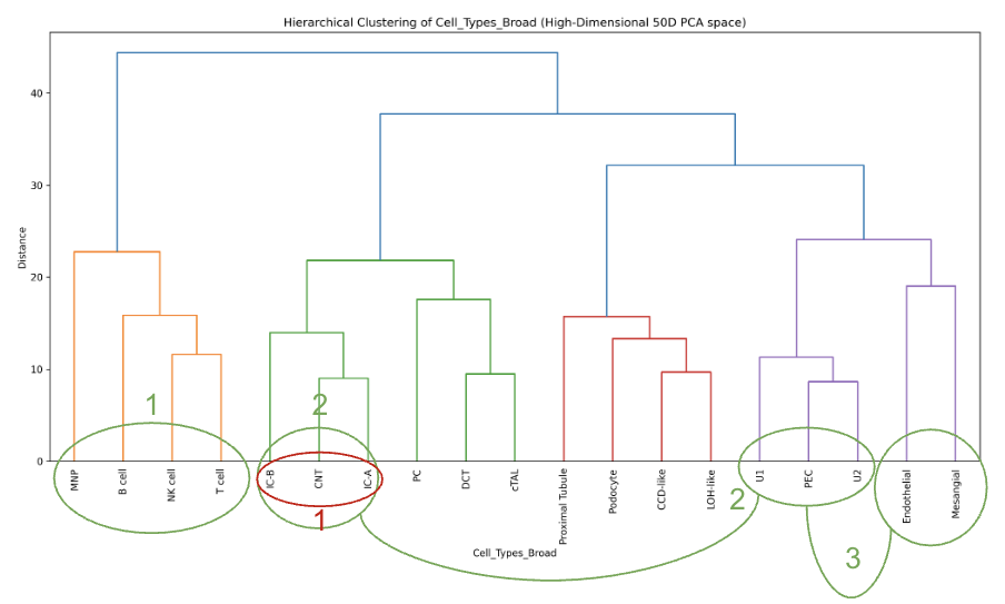
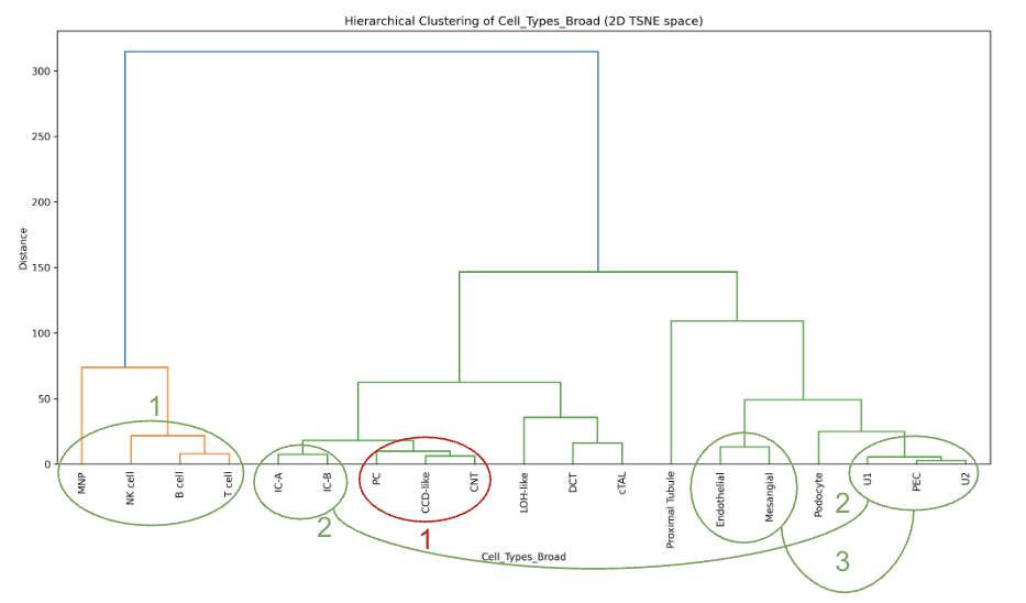

Dendrogram Comparison
-
•
Agreement Level: High
-
•
Key Similarities:
-
1.
Top-level immune grouping is consistent: MNP clusters with (NK, (B,T)) in both 2D and PCA dendrograms (8 with (10,(0,15)) motif preserved).
-
2.
IC-A and IC-B remain a tight pair (5,6) and sit with PC/U1/U2/PEC-related branch similarly in both dendrograms.
-
3.
Endothelial with Mesangial (4,9) and U1/U2/PEC sub-branch (16,(12,17)) align between 2D and PCA, indicating good hierarchy preservation.
-
•
Key Differences:
-
1.
Small rearrangements inside the distal/collecting subtree: 2D groups (11,(1,2)) earlier than PCA’s ((6,(2,5))…)—minor and likely within expected uncertainty for very small clusters.
-
2.
Leaf ordering differs locally but major clades are consistent.
Visual Inspection
-
•
Cluster Separation: Excellent
-
•
Cluster Compactness: Good
-
•
Notable Patterns:
-
1.
Clear distal nephron banding at the top: LOH-like, cTAL, DCT/CNT/CCD-like/IC-A/IC-B/PC cluster in a coherent neighborhood.
-
2.
Immune compartment is cleanly separated (B/T/NK with nearby MNP), aiding annotation QC.
-
3.
Vascular/stromal region (Endothelial, Mesangial, Podocyte, PEC) sits near each other as expected, with plausible proximities.
Other Comparative Analysis
To further understand the behavior of different LLMs in guiding the dimensionality reduction process, we analyzed their optimization trajectories and the explicit scoring weights formulated by each model.
Explicit Weighting Strategies: When prompted to act as quantitative strategists, the three LLMs designed noticeably different composite objective functions to evaluate the 2D embeddings. GPT-5.2 prioritized local neighborhood preservation and cluster separation, assigning the highest weights to Trustworthiness (0.30) and the Silhouette Score (0.30), while heavily discounting outlier detection (LOF Median: 0.05). Claude-Opus-4.5 demonstrated a strong bias toward strict clustering and identifying density anomalies, assigning 0.35 to the Silhouette Score and 0.20 to LOF, but placing less emphasis on global geometric preservation (Stress-1: 0.10). In contrast, Gemini-3-Pro-Preview adopted the most balanced optimization strategy, distributing weights relatively evenly across local topology (Trustworthiness: 0.25), clustering (Silhouette: 0.25), and global structure metrics (Spearman: 0.20, Stress-1: 0.15, LOF: 0.15).
Optimization Trajectories: By overlapping the implicit and explicit score trajectories alongside the quantitative metrics over iterations, distinct convergence patterns emerged.
Figure 4 illustrates the iterative optimization trajectories for Gemini-3-Pro-Preview, GPT-5.2, and Claude-Opus-4.5. By plotting both the implicit LLM Quality Score and the explicit Composite Quantitative Score alongside the raw metric values, several distinct behavioral patterns and optimization trade-offs emerge.
Model Performance and Convergence Strategies: The three agents exhibited markedly different exploration strategies and convergence rates:
-
•
Gemini-3-Pro-Preview (5 iterations): This model demonstrated the most effective balance of exploration and exploitation. It quickly reached a peak LLM Quality Score of 8.00 at iteration 3. The raw metrics reveal that this peak coincided with a significant minimization of Stress-1 (dropping to 0.323) and a high Spearman Correlation (0.773), indicating excellent global structure recovery.
-
•
GPT-5.2 (9 iterations): GPT-5.2 exhibited a highly exploratory, volatile trajectory. It sustained a long search process, with raw metrics fluctuating significantly—most notably the Stress-1 and Spearman Correlation scores. Despite reaching an early peak LLM score of 7.40 at iteration 3, the agent continued to experiment, ultimately converging at an LLM score of 7.00, reflecting a struggle to stabilize competing spatial constraints.
-
•
Claude-Opus-4.5 (3 iterations): Claude adopted a highly conservative, early-stopping strategy. The trajectory flatlined at an LLM score of 6.50 by iteration 2. Notably, despite assigning the highest explicit weight to the Silhouette Score (35%), the model’s chosen hyperparameters resulted in a steady decline in both Trustworthiness and Silhouette scores, favoring a linear increase in Spearman Correlation instead.
Implicit vs. Explicit Scoring Dynamics: The dual-line plots (top row of each figure) highlight the inherent tension between mathematically rigid objective functions and holistic visual evaluation. Across all models, there is a visible "disagreement gap" (shaded in grey), particularly in the early iterations. For instance, Claude-Opus-4.5 initially assigned a harsh implicit score of 5.50, while the mathematical composite score rated the same embedding at 7.08. This divergence underscores the limitation of pure mathematical scoring: while the metrics may indicate a mathematically sound embedding, the LLM’s implicit score penalizes visual artifacts (such as crowding or artificial cluster bridges) that the composite formula fails to capture.
Trade-offs in Quantitative Metrics: The metric subplots reveal the fundamental geometric trade-offs inherent in dimensionality reduction. In almost all trajectories, improving global topology (reflected by decreasing Stress-1 and increasing Spearman Correlation) comes at the direct expense of local structure (Trustworthiness and Silhouette Score). For example, in the Gemini trajectory, as Stress-1 reaches its absolute minimum at iteration 3 (0.323), the Silhouette Score simultaneously hits a severe low (0.013). This confirms that forcing the DR algorithm to perfectly unroll the global manifold often shatters tight local clusters, a trade-off the LLM agents had to dynamically navigate throughout the pipeline.


CONCLUSION
Exploratory analysis and visualization of high-dimensional data is frequently bottlenecked by the subjective, labor intensive process of hyperparameter tuning for dimension reduction algorithms. In this paper, we introduced a fully automated, agentic AI pipeline that leverages Large Language Models to refine and explain this visualization process. By integrating quantitative reliability metrics, hierarchical dendrogram comparisons, and visual plots into a unified multi-modal context, our system enables LLM agents to act as expert visual diagnosticians.
Our experiments on complex biological datasets demonstrate that frontier models can rapidly navigate complex hyperparameter spaces across different DR algorithms (t-SNE, UMAP, and PaCMAP). The comparative analysis of implicit and explicit scoring mechanisms reveals that while explicit metric weighting offers a predictable, math-driven optimization route, implicit holistic reasoning better captures and corrects nuanced visual artifacts. When both scores compared, we also demonstrate the strong correlation between them as similar trends appear in both scores over multiple iterations.
Ultimately, this explainable, iterative framework bridges the gap between rigorous mathematical evaluation and qualitative human insight. By providing a clear rationale for every parameter adjustment, the pipeline ensures that the resulting scatter plots faithfully represent the underlying high-dimensional reality, accelerating pattern discovery without the need for exhaustive manual tuning.
ACKNOWLEDGMENTS
This work is supported by the Bicentenary PhD Studentship from Faculty of Science and Engineering, University of Manchester.
REFERENCES
- [1] L. van der Maaten and G. Hinton, “Visualizing data using t-SNE,” J. Mach. Learn. Res., vol. 9, no. 86, pp. 2579–2605, Nov. 2008. [Online]. Available: http://jmlr.org/papers/v9/vandermaaten08a.html
- [2] L. McInnes, J. Healy, and J. Melville, “UMAP: Uniform manifold approximation and projection for dimension reduction,” arXiv preprint arXiv:1802.03426, 2020. [Online]. Available: https://arxiv.org/abs/1802.03426
- [3] O. Arbelaitz, I. Gurrutxaga, J. Muguerza, J. M. Pérez, and I. Perona, “An extensive comparative study of cluster validity indices,” Pattern Recognit., vol. 46, no. 1, pp. 243–256, Jan. 2013. [Online]. Available: https://doi.org/10.1016/j.patcog.2012.07.021
- [4] T. Chari and L. Pachter, “The specious art of single-cell genomics,” PLoS Comput. Biol., vol. 19, no. 10, p. e1011288, Oct. 2023. [Online]. Available: https://doi.org/10.1371/journal.pcbi.1011288
- [5] Y. Wang, H. Huang, C. Rudin, and Y. Shaposhnik, “Understanding how dimension reduction tools work: An empirical approach to deciphering t-SNE, UMAP, TriMAP, and PaCMAP for data visualization,” J. Mach. Learn. Res., vol. 22, no. 1, pp. 9129–9201, 2021. [Online]. Available: https://arxiv.org/abs/2012.04456
- [6] M. Wattenberg, F. Viégas, and I. Johnson, “How to use t-SNE effectively,” Distill, 2016. [Online]. Available: https://doi.org/10.23915/distill.00002
- [7] J. Venna and S. Kaski, “Local multidimensional scaling,” Neural Netw., vol. 19, no. 8, pp. 1189–1199, Oct. 2006. [Online]. Available: https://doi.org/10.1016/j.neunet.2006.06.014
- [8] J. Bergstra and Y. Bengio, “Random search for hyper-parameter optimization,” J. Mach. Learn. Res., vol. 13, no. 10, pp. 281–305, Feb. 2012. [Online]. Available: http://jmlr.org/papers/v13/bergstra12a.html
- [9] J. Snoek, H. Larochelle, and R. P. Adams, “Practical Bayesian optimization of machine learning algorithms,” in Adv. Neural Inf. Process. Syst. (NeurIPS), vol. 25, 2012, pp. 2951–2959.
- [10] L. Wang et al., “A survey on large language model based autonomous agents,” Front. Comput. Sci., vol. 18, no. 6, pp. 1–26, Dec. 2024. [Online]. Available: https://doi.org/10.1007/s11704-024-40231-1
- [11] Z. Yang et al., “MatPlotAgent: Method and evaluation for LLM-based agentic scientific data visualization,” in Findings of the Assoc. for Comput. Linguistics: ACL 2024, Bangkok, Thailand, Aug. 2024, pp. 11789–11804. [Online]. Available: https://aclanthology.org/2024.findings-acl.701/
- [12] Z. Chen et al., “Coda: Agentic systems for collaborative data visualization,” arXiv preprint arXiv:2510.03194, 2025. [Online]. Available: https://arxiv.org/abs/2510.03194
- [13] S. Liu, C. Gao, and Y. Li, “AgentHPO: Large language model agent for hyper-parameter optimization,” in Proc. Conf. Parsimony and Learn. (CPAL), vol. 280, 2025, pp. 1146–1169. [Online]. Available: https://proceedings.mlr.press/v280/liu25c.html
- [14] R. R. Sokal and C. D. Michener, “A statistical method for evaluating systematic relationships,” Univ. Kans. Sci. Bull., vol. 38, pp. 1409–1438, 1958.
- [15] P. J. Rousseeuw, “Silhouettes: A graphical aid to the interpretation and validation of cluster analysis,” J. Comput. Appl. Math., vol. 20, pp. 53–65, Nov. 1987. [Online]. Available: https://doi.org/10.1016/0377-0427(87)90125-7
- [16] M. M. Breunig, H.-P. Kriegel, R. T. Ng, and J. Sander, “LOF: Identifying density-based local outliers,” SIGMOD Rec., vol. 29, no. 2, pp. 93–104, May 2000. [Online]. Available: https://doi.org/10.1145/335191.335388
- [17] C. Spearman, “The proof and measurement of association between two things,” Amer. J. Psychol., vol. 15, no. 1, pp. 72–101, Jan. 1904. [Online]. Available: https://doi.org/10.2307/1412159
- [18] C. M. McEvoy et al., “Single-cell profiling of healthy human kidney reveals features of sex-based transcriptional programs and tissue-specific immunity,” Nat. Commun., vol. 13, no. 1, p. 7634, Dec. 2022. [Online]. Available: https://doi.org/10.1038/s41467-022-35297-z
- [19] B. J. Stewart et al., “Spatiotemporal immune zonation of the human kidney,” Science, vol. 365, no. 6459, pp. 1461–1466, Sep. 2019. [Online]. Available: https://doi.org/10.1126/science.aat5031
- [20] M. L. Speir et al., “UCSC Cell Browser: Visualize your single-cell data,” Bioinformatics, vol. 37, no. 23, pp. 4578–4580, Dec. 2021. [Online]. Available: https://doi.org/10.1093/bioinformatics/btab503 {IEEEbiography}Burak Susam is a post-graduate researcher at the University of Manchester, UK. His current research interests include data visualization, agentic AI and dimension reduction algorithms. Author received the MSc degree in Computer Science from the University of Minnesota. Contact him at burak.susam@postgrad.manchester.ac.uk IEEEbiography {IEEEbiography}Tingting Mu, Assoc. Prof., is a Senior Lecturer at the University of Manchester, UK. Her current research interests include data visualization, representation learning and reinforcement learning. Author received the Ph.D. degree in Computer Science from the University of Liverpool. She is a a Turing Fellow and an Honorary Research Fellow on Representation Learning at UoM Harwell. Contact her at tingting.mu@manchester.ac.uk.