Hidden Quantum Advantage near the Decoding Threshold
of Decoded Quantum Interferometry
Abstract
Where is the true boundary of the quantum advantage region of decoded quantum interferometry (DQI)? The best existing answer is provided by Theorem 7.1 in the Supplementary Material of Jordan et al. [undef], yet we show that this answer systematically underestimates the extent of quantum advantage. On the standard partial-win LDPC benchmark instance, there exist 26 consecutive parameter points () at which Jordan’s analysis declares no quantum advantage (), while quantum advantage is in fact present with an approximation ratio reaching . The root cause is that Jordan’s bound penalizes the entire system with the worst-case Hamming-layer decoding failure rate , discarding the spectral structure of the DQI tridiagonal matrix. Exploiting the concentration of the Perron eigenvector, we replace the uniform penalty with the weighted average and establish a unified lower bound (Master Theorem) valid over arbitrary finite fields , proving that it strictly improves upon the relaxed form of Jordan’s bound by replacing the operator-norm penalty with a tighter Rayleigh-quotient penalty .
Keywords: quantum advantage, decoded quantum interferometry, imperfect decoding, eigenvector weighting, LDPC codes
1 Introduction
Decoded Quantum Interferometry (DQI) is a quantum optimization framework introduced by Jordan et al. [undef]. Drawing on ideas from Regev’s reduction [undefa], DQI constructs polynomial interference states of degree to achieve quantum advantage over classical random assignment for constraint satisfaction problems such as MAX-XORSAT [undefb]. Under perfect decoding, the approximation ratio of DQI follows a semicircle law that improves steadily with [undef]. When the polynomial degree exceeds the threshold set by the dual distance of the code, however, the classical decoder fails on high Hamming-weight layers [undefc, undefd], and the resulting decoding failure rates degrade the fidelity of the quantum state construction. Jordan et al.’s Theorem 7.1 (stated for in the Supplementary Material of [undef]) gives a two-step chain of lower bounds:
| (1) |
where is the principal eigenvector of the DQI tridiagonal matrix , is its largest eigenvalue, and (Lemma 7.7 of [undef]). The second inequality relaxes the denominator to . Jordan et al. employ this relaxed form (the right-hand side) in their asymptotic statement. This bound is clean and broadly applicable, but it suffers from an analytical blind spot near the decoding threshold: as grows rapidly with , the penalty term quickly exceeds , rendering the bound vacuous. In this region, quantum advantage may well exist yet remain undetectable by the original analysis.
Since its introduction, DQI has stimulated a substantial body of follow-up work [undefe, undeff, undefg, undefh, undefi, undefj, undefk, undefl], investigating its capabilities and limitations from multiple angles. On the methodological side, Chailloux and Tillich [undefe] broadened the quantum advantage parameter range via soft decoders for Reed–Solomon codes, Gu and Jordan [undeff] extended DQI to algebraic geometry codes (HOPI), Schmidhuber et al. [undefg] developed Hamiltonian DQI for general Pauli Hamiltonians, and Bu et al. [undefh] analyzed the effects of physical noise on DQI. On the hardness side, Kramer et al. [undefi] proved tight inapproximability for MAX-LINSAT based on Håstad’s theorem [undefm], establishing the worst-case barrier; Anschuetz et al. [undefj] showed via the overlap gap property [undefn] that DQI is obstructed on unstructured random instances; Parekh [undefk] proved that DQI offers no quantum advantage for MaxCut; and Marwaha et al. [undefl] placed DQI within low levels of the polynomial hierarchy. These works focus on the scope and complexity-theoretic status of DQI, whereas the present paper addresses an orthogonal dimension: improving the performance analysis itself under imperfect decoding, thereby revealing quantum advantage regions overlooked by the original bound.
This blind spot is far from inconsequential. The decoding threshold is precisely the critical band where DQI transitions from winning to failing, and understanding the exact location of this transition bears directly on practical assessments of DQI. We show that this blind spot indeed conceals quantum advantage that the original analysis fails to capture, and the evidence comes from Jordan et al.’s own experimental data.
On the partial-win LDPC instance of Jordan et al. (, BP decoding), we apply both Jordan’s Theorem 7.1 and our Master Theorem (Theorem 3.1) at each value of , revealing 26 consecutive data points in the range where Jordan’s bound yields (vacuous), while our bound gives , certifying significant quantum advantage (Figure 1). The most striking case occurs at : Jordan’s bound gives , whereas ours gives , a compression of the effective error rate by 91.3%. These are not hypothetical constructions but publicly available benchmark data—the quantum advantage has been there all along; the original analytical tools simply could not see it.
The root cause lies in the choice . In bounding the quadratic form by the operator norm , Jordan’s proof discards the structural information of the leading eigenvector . Yet the leading eigenvector of the DQI matrix is far from arbitrary: it satisfies (Lemma S2.1), and exhibits a sharply unimodal distribution centered at with effective width (Lemma S2.2). This means that although the failure rate at high-weight layers can be large, the corresponding weight decays exponentially, so that its actual impact on DQI performance is far smaller than suggests. Replacing the quadratic form with the operator norm amounts to assuming that aligns with the worst-case direction of , but the tridiagonal structure ensures that naturally avoids the high-error region—ignoring this structure is the source of the blind spot.
We exploit this spectral structure by defining the weighted failure rate and establishing the unified lower bound
| (2) |
where (Theorem 3.1). This bound holds for arbitrary finite fields and arbitrary diagonal offsets , and strictly improves upon the relaxed form of Jordan’s bound (the right-hand side of (1)) via a single structural replacement (Theorem 3.2): the operator-norm penalty is replaced by the Rayleigh-quotient penalty . This replacement simultaneously contracts the max-failure rate to the weighted average () and rescales the multiplier from to . On the standard LDPC benchmark instance, it reveals 26 quantum advantage points missed by the original analysis. The conclusion is that the quantum advantage region of DQI has been underestimated, and eigenvector weighting is the only analytical tool capable of detecting the hidden quantum advantage near the decoding threshold.
The remainder of this paper is organized as follows. Section 2 introduces the basic setup of the DQI framework. Section 3 states the main results. Section 4 presents concrete evidence from Jordan’s experimental data. Section 5 discusses implications and outlook. Complete proofs, eigenvector property analysis, seven groups of numerical experiments, and auxiliary data are provided in the supplementary material.

2 Setup
Given a parity-check matrix over a finite field and a target vector , the MAX-LINSAT problem asks for maximizing the number of satisfied constraints . The objective function is related to by , and random assignment achieves an expected satisfaction ratio of . The DQI algorithm constructs polynomial interference states of degree , whose performance is governed by the largest eigenvalue of the following matrix.
Definition 2.1 (DQI matrix).
is a real symmetric tridiagonal matrix of size with diagonal entries and off-diagonal entries , where is the number of constraints, is the polynomial degree, and is the offset parameter.
When , DQI requires a classical decoder. The decoding failure rate at Hamming layer is , and the expected post-decoding matrix decomposes as [undef]
| (3) |
where is a symmetric matrix with zero diagonal and off-diagonal entries satisfying . Jordan et al. then obtained the relaxed form by taking (via Gershgorin’s bound on ) and relaxing the denominator to (see (1)). Jordan et al. proved Theorem 7.1 for . The same argument produces the factor above for general , and we adopt this convention throughout the paper.
3 Main results
Let be the normalized leading eigenvector of and the corresponding eigenvalue. Define the weighted failure rate and the weighted failure moment .
Theorem 3.1 (Master Theorem).
Suppose for all (guaranteed by Lemma S2.1). For uniformly random ,
| (4) |
The key idea of the proof is as follows (see Supplementary Material S1 for the full derivation). We choose as the test vector for the Rayleigh quotient; the denominator evaluates to (Jordan relaxes this to ). The error quadratic form in the numerator requires an upper bound: Jordan controls it via the operator norm , whereas we expand it directly and exploit the eigenvector equation , which splits the error sum into and yields exact cancellations in the overlapping range, ultimately giving . This cancellation is an algebraic consequence of the tridiagonal structure, and it makes the weighted quantity emerge naturally.
For , , the bound simplifies to . In the asymptotic limit, (Lemma S2.3), and the approximation ratio becomes
| (5) |
which reduces to the semicircle law when .
Theorem 3.2 (Strict improvement).
For any decoding scheme with , the bound (4) is at least as tight as Jordan’s bound, and strictly tighter unless is identical for all and . Relative to Jordan’s relaxed form (the right-hand side of (1)), the improvement decomposes into two components: (i) the structural replacement of the operator-norm penalty by the Rayleigh-quotient penalty , which simultaneously replaces by and rescales to ; and (ii) retaining the exact denominator that Jordan’s relaxed form bounds below by . Relative to Jordan’s tight form (the middle expression), only (i) remains, since (ii) is common to both. Quantitative estimates are given in Supplementary Material S4.
The proof and quantitative analysis are given in Supplementary Material S4.
4 Evidence from Jordan’s data
We use the partial-win LDPC benchmark instance from [undef] (, rate-, BP decoding). The per-layer decoding failure rates are taken directly from the BP shot data released by Jordan et al. in their xortools repository [undef] (the partial-win BP shot-log file, see Supplementary Material S6 for the exact filename), setting where is the empirical BP success rate at Hamming weight . For each , we construct the profile, compute the leading eigenvector of the DQI matrix, and apply both bounds. Results are summarized in Table 1.
| Jordan | Ours | Status | |||||
|---|---|---|---|---|---|---|---|
| 620 | 0.124 | 0.100 | 0.0072 | 0.072 | 0.613 | 0.661 | Both valid |
| 635 | 0.127 | 0.200 | 0.0241 | 0.121 | 0.564 | 0.660 | Both valid |
| 642 | 0.128 | 0.500 | 0.0436 | 0.087 | 0.415 | 0.658 | Blind spot |
| 650 | 0.130 | 0.500 | 0.1035 | 0.207 | 0.416 | 0.647 | Blind spot |
| 660 | 0.132 | 0.600 | 0.2373 | 0.396 | 0.367 | 0.615 | Blind spot |
| 665 | 0.133 | 0.700 | 0.3347 | 0.478 | 0.318 | 0.583 | Blind spot |
The comparison at is particularly striking. The worst-layer failure rate already exceeds the critical threshold of Jordan’s bound, and Theorem 7.1 yields —well below the random assignment level of . Yet the weighted failure rate is only (8.7% of ), and the Master Theorem gives , within of the semicircle law value under perfect decoding. Despite a 50% worst-layer failure rate, the effective error rate acting on DQI performance is merely 4.36%.
Figure 2 reveals why the weighting mechanism is effective. Taking as an example, the peak of is located at with effective width approximately , while becomes nonzero starting from . In the region , the failure rate increases sharply, but has already passed its peak and decays, so high error rates are exponentially suppressed. This natural avoidance of the high-error region by the eigenvector peak is an intrinsic property of the tridiagonal structure: the leading eigenvector is determined by Krawtchouk polynomials, and its location depends only on and , not on decoder performance.

On the main instance of Jordan et al. (; Figure 3), the improvement at the conservative operating point () is modest (), but it grows rapidly with increasing : at , (). Jordan et al. chose the conservative operating point precisely because Theorem 7.1 becomes vacuous at larger ; the Master Theorem provides theoretical justification for selecting more aggressive operating points.

5 Discussion
The quantum advantage region of DQI has been systematically underestimated. Jordan et al.’s Theorem 7.1 suffers from an analytical blind spot near the decoding threshold, caused by the loss of spectral structural information; within this region, quantum advantage exists but cannot be detected by the original analysis. The Master Theorem exploits the tridiagonal structure and the concentration of the Perron eigenvector to fill this blind spot: on the standard LDPC benchmark instance, 26 parameter points are promoted from vacuous to certifiable quantum advantage, with the effective error rate compressed by up to 91.3% in the most extreme case.
These results also have limitations. At the conservative operating point chosen by Jordan et al. (, ), the improvement is only , and the main value is concentrated in the degraded regime. The correction term does not contribute when . Whether the Master Theorem is the tightest possible bound within the Rayleigh quotient framework remains an open question.
These results have direct implications for the practical strategy of DQI. Jordan et al. [undef] chose a conservative operating point , a choice constrained precisely by the failure of Theorem 7.1 at larger . The Master Theorem indicates that the viable operating range of DQI is wider than suggested by this conservative choice: on the main instance, can be safely increased from 6350 to approximately 6530 while maintaining certifiable quantum advantage, corresponding to . In other words, the analytical improvement presented here is not merely a tightening of the bound but an expansion of DQI’s accessible parameter space, making higher-degree interference states a theoretically supported option—this directly affects comparative assessments of DQI against competing approaches such as QAOA [undefo, undefp] and related quantum optimization methods [undefq].
The above results also suggest several directions for future work. Phase diagram analysis (Supplementary Material S5, Experiment 4) indicates that the shape of the BP decoding threshold directly influences the size of the blind spot; whether one can conversely design codes to minimize is a coding-theoretic question. A positive diagonal offset can expand the quantum advantage region by 65% (Supplementary Material S5, Experiment 6), and whether structures such as folded codes can introduce positive offsets in DQI merits further investigation [undeff]. Analysis of DQI under physical noise [undefh] and the imperfect decoding analysis of this work are naturally complementary. The existence of 26 blind-spot points also suggests that the behavior of DQI near the decoding threshold may be richer than what current analyses can describe.
References
- [undef] Stephen P. Jordan, Noah Shutty, Mary Wootters, Adam Zalcman, Alexander Schmidhuber, Robbie King, Sergei V. Isakov, Tanuj Khattar and Ryan Babbush “Optimization by decoded quantum interferometry” In Nature 646.8086, 2025, pp. 831–836 DOI: 10.1038/s41586-025-09527-5
- [undefa] Oded Regev “Quantum Computation and Lattice Problems” In SIAM Journal on Computing 33.3, 2004, pp. 738–760 DOI: 10.1137/S0097539703440678
- [undefb] Takashi Yamakawa and Mark Zhandry “Verifiable Quantum Advantage without Structure” In Journal of the ACM 71.3, 2024, pp. 1–50 DOI: 10.1145/3658665
- [undefc] Robert G. Gallager “Low-density parity-check codes” In IRE Transactions on Information Theory 8.1, 1962, pp. 21–28 DOI: 10.1109/TIT.1962.1057683
- [undefd] Thomas J. Richardson, M. Shokrollahi and Rüdiger L. Urbanke “Design of capacity-approaching irregular low-density parity-check codes” In IEEE Transactions on Information Theory 47.2, 2001, pp. 619–637 DOI: 10.1109/18.910578
- [undefe] André Chailloux and Jean-Pierre Tillich “Quantum Advantage from Soft Decoders” In Proceedings of the 57th Annual ACM Symposium on Theory of Computing (STOC ’25) ACM, 2025, pp. 738–749 DOI: 10.1145/3717823.3718319
- [undeff] Andi Gu and Stephen P. Jordan “Algebraic Geometry Codes and Decoded Quantum Interferometry”, 2025 arXiv:2510.06603 [quant-ph]
- [undefg] Alexander Schmidhuber, Jonathan Z. Lu, Noah Shutty, Stephen Jordan, Alexander Poremba and Yihui Quek “Hamiltonian Decoded Quantum Interferometry”, 2025 arXiv:2510.07913 [quant-ph]
- [undefh] Kaifeng Bu, Weichen Gu, Dax Enshan Koh and Xiang Li “Decoded quantum interferometry under noise” In Quantum Science and Technology 11.2, 2026, pp. 025010 DOI: 10.1088/2058-9565/ae4536
- [undefi] Maximilian J. Kramer, Carsten Schubert and Jens Eisert “Tight inapproximability of max-LINSAT and implications for decoded quantum interferometry”, 2026 arXiv:2603.04540 [quant-ph]
- [undefj] Eric R. Anschuetz, David Gamarnik and Jonathan Z. Lu “Decoded Quantum Interferometry Requires Structure”, 2025 arXiv:2509.14509 [quant-ph]
- [undefk] Ojas Parekh “No Quantum Advantage in Decoded Quantum Interferometry for MaxCut”, 2025 arXiv:2509.19966 [quant-ph]
- [undefl] Kunal Marwaha, Bill Fefferman, Alexandru Gheorghiu and Vojtech Havlicek “On the Complexity of Decoded Quantum Interferometry”, 2025 arXiv:2509.14443 [quant-ph]
- [undefm] Johan Håstad “Some optimal inapproximability results” In Journal of the ACM 48.4, 2001, pp. 798–859 DOI: 10.1145/502090.502098
- [undefn] David Gamarnik “The overlap gap property: A topological barrier to optimizing over random structures” In Proceedings of the National Academy of Sciences 118.41, 2021, pp. e2108492118 DOI: 10.1073/pnas.2108492118
- [undefo] Edward Farhi, Jeffrey Goldstone and Sam Gutmann “A Quantum Approximate Optimization Algorithm”, 2014 arXiv:1411.4028 [quant-ph]
- [undefp] Edward Farhi, Jeffrey Goldstone, Sam Gutmann and Leo Zhou “The Quantum Approximate Optimization Algorithm and the Sherrington–Kirkpatrick Model at Infinite Size” In Quantum 6, 2022, pp. 759 DOI: 10.22331/q-2022-07-07-759
- [undefq] Amira Abbas, Andris Ambainis, Brandon Augustino, Andreas Bärtschi, Harry Buhrman, Carleton Coffrin, Giorgio Cortiana, Vedran Dunjko, Daniel J. Egger and Bruce G. Elmegreen “Challenges and opportunities in quantum optimization” In Nature Reviews Physics 6.12, 2024, pp. 718–735 DOI: 10.1038/s42254-024-00770-9
- [undefr] Felix R. Gantmacher and Mark G. Krein “Oscillation Matrices and Kernels and Small Vibrations of Mechanical Systems” Revised edition; original Russian edition 1950 American Mathematical Society, 2002
- [undefs] Beresford N. Parlett “The Symmetric Eigenvalue Problem” SIAM, 1998
- [undeft] Mourad E.. Ismail and Plamen Simeonov “Strong asymptotics for Krawtchouk polynomials” In Journal of Computational and Applied Mathematics 100.2, 1998, pp. 121–144 DOI: 10.1016/S0377-0427(98)00183-6
- [undefu] Changyan Di, David Proietti, İ. Telatar, Thomas J. Richardson and Rüdiger L. Urbanke “Finite-length analysis of low-density parity-check codes on the binary erasure channel” In IEEE Transactions on Information Theory 48.6, 2002, pp. 1570–1579 DOI: 10.1109/TIT.2002.1003839
- [undefv] Yury Polyanskiy, H. Poor and Sergio Verdú “Channel Coding Rate in the Finite Blocklength Regime” In IEEE Transactions on Information Theory 56.5, 2010, pp. 2307–2359 DOI: 10.1109/TIT.2010.2043769
Supplementary Material
Appendix S1 Complete proof of the Master Theorem
Proof of Theorem 3.1.
The proof proceeds in four steps.
Step 1: Choose as the test vector for the Rayleigh quotient:
| (S1) |
where the denominator is .
Step 2: By the tridiagonal zero-diagonal structure of and :
| (S2) |
Step 3: Using the eigenvector equation , decompose the right-hand side of (S2) into and . For , substitute using the eigenvector equation:
| (S3) |
For , re-index with : . Exact cancellation occurs in the range . Using the boundary condition , we obtain
| (S4) |
and hence .
Appendix S2 Eigenvector properties
Lemma S2.1 (Positivity).
Let be a real symmetric tridiagonal matrix with positive off-diagonal entries and arbitrary diagonal entries. Then is simple and the leading eigenvector satisfies for all .
Proof.
Jordan et al. implicitly invoke the Perron–Frobenius theorem, which requires matrix nonnegativity and thus applies only when . Lemma S2.1 holds for arbitrary .
Lemma S2.2 (Concentration).
As with fixed, is unimodal about , with effective width and Gaussian decay away from the peak.
This follows from the correspondence between the eigenvectors of and Krawtchouk polynomials [undeft].
Lemma S2.3 (Eigenvalue asymptotics).
.
Appendix S3 Analysis of the blind spot in Jordan’s bound
The critical value at which Jordan’s bound becomes vacuous is, in the asymptotic limit, . For example, at , : ; a failure rate exceeding approximately 33.3% at any single layer renders the entire bound vacuous.
Jordan’s proof chain is (via Gershgorin discs). The first inequality discards the information about , and the second discards the layer-to-layer variation of . The proof of the Master Theorem diverges from Jordan’s at the very first step: it directly expands and exploits the eigenvector equation, simultaneously preserving the structure of and the layer-wise variation of .
In the parameter plane, the blind spot corresponds to the region between two critical curves: the boundary of Jordan’s bound and the boundary of the Master Theorem (Figure S1).

Appendix S4 Quantitative comparison with Jordan’s bound
The difference in asymptotic approximation ratios is
| (S5) |
Taking Jordan’s relaxed form (the right-hand side of (1)) as the reference, the total improvement at , , is driven by the Rayleigh-quotient replacement of the operator-norm penalty. This single replacement simultaneously produces the max-to-weighted shrinkage and the norm-to-Rayleigh rescaling . In the degraded regime (), the max-to-weighted contraction dominates and accounts for roughly of the gap to the relaxed form.
Appendix S5 Numerical experiments
Seven groups of experiments comprehensively verify the theoretical predictions. All experiments are implemented in Python (NumPy/SciPy), with sparse decomposition used for large matrices.
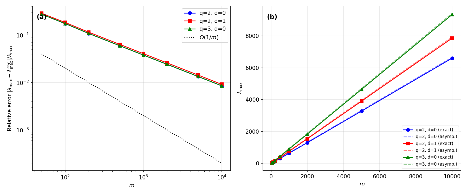
S5.1 Experiment 1: Eigenvector verification
Ten parameter sets (, , ) all pass the positivity test (Figure S2). The effective width scales as , and narrows the distribution. The asymptotic accuracy of converges at rate (Figure S3).

S5.2 Experiment 2: Weighted failure rate
At , the range is swept over 150 points (Figure S4). The ratio drops as low as in the degraded regime.

S5.3 Experiment 3: Four-line comparison
Figure S5 displays the semicircle law, the Master Theorem bound, Jordan’s bound, and the exact Rayleigh quotient value. The hierarchy Semicircle Ours Jordan holds strictly throughout. The exact value is consistently close to the Master Theorem bound (gap ).

S5.4 Experiment 4: Phase diagram
The three-region partition of the plane is shown in Figure S1. The optimal operating point stabilizes at approximately (Figure S7).
![[Uncaptioned image]](2604.15025v2/fig4_regime_classification.png)
![[Uncaptioned image]](2604.15025v2/fig4_optimal_mu.png)
S5.5 Experiment 5: Large-scale instance
At , validation is performed using 139 measured data points (Figure S8). Comparison across shows that the blind spot appears earlier for larger (Figure S9).


S5.6 Experiment 6: Diagonal offset
Positive expands the effective region: at , the range extends from to (+65%), and at increases from 0.664 to 0.727 (Figure S10).

S5.7 Experiment 7: Finite- verification
The finite- exact formula and the asymptotic formula are in close agreement at (Figure S11), with the blind spot identical under both computations.

Appendix S6 Decoding failure rates: data sources
The per-layer BP failure rates used throughout this paper come from two sources, depending on whether an experiment targets a specific published instance or a range of synthetic code parameters.
Direct BP shot data (§4 and Table 1).
For the blind-spot experiment in §4, which uses the partial-win instance of Jordan et al. (, rate- irregular LDPC, rank ), we take directly from the BP shot data released in their xortools repository [undef]. From the file
noah_code_1e4_rate_one_half_3_1000_6_100.load_decode
we parse each line “” (Hamming weight , empirical BP success rate , shot count ) and set
| (S6) |
The worst-layer rate and weighted rate used in the bounds are then
| (S7) |
following Lemma 7.7 of [undef]. No fitting, smoothing, or tunable parameter enters this pipeline. The number of shots per layer ranges from to , so individual carry statistical uncertainty of order –; the qualitative conclusions reported in §4 ( blind-spot points in ; ratio remaining small; Jordan’s bound turning vacuous at ) are robust to this noise, as they depend on the cumulative maximum rather than any single .
Three-stage parametric BP model (other figures).
For experiments that scan over a wide range of synthetic values, or smooth across the main instance (, , whose BP data only covers ), we use a three-stage parametric model that captures the qualitative threshold behaviour of BP decoding [undefc, undefd]:
| (S8) |
with default parameters (for ): , , , , . For an analysis of how finite-length BP performance deviates from the asymptotic threshold, see [undefu, undefv]. These parameters are consistent with the threshold parameters reported by Jordan et al.
Appendix S7 Complete data
| Jordan | Ours | |||||
|---|---|---|---|---|---|---|
| 610 | 0.122 | 0.000 | 0.000 | — | 0.661 | 0.661 |
| 615 | 0.123 | 0.100 | 0.001 | 0.012 | 0.612 | 0.662 |
| 620 | 0.124 | 0.100 | 0.007 | 0.072 | 0.613 | 0.661 |
| 625 | 0.125 | 0.100 | 0.013 | 0.134 | 0.613 | 0.661 |
| 630 | 0.126 | 0.100 | 0.017 | 0.169 | 0.614 | 0.661 |
| 635 | 0.127 | 0.200 | 0.024 | 0.121 | 0.564 | 0.660 |
| 640 | 0.128 | 0.200 | 0.036 | 0.178 | 0.565 | 0.659 |
| 642 | 0.128 | 0.500 | 0.044 | 0.087 | 0.415 | 0.658 |
| 645 | 0.129 | 0.500 | 0.064 | 0.128 | 0.415 | 0.654 |
| 650 | 0.130 | 0.500 | 0.103 | 0.207 | 0.416 | 0.647 |
| 655 | 0.131 | 0.500 | 0.157 | 0.313 | 0.416 | 0.636 |
| 660 | 0.132 | 0.600 | 0.237 | 0.396 | 0.367 | 0.615 |
| 665 | 0.133 | 0.700 | 0.335 | 0.478 | 0.318 | 0.583 |
| No. | Content | Output | |||
|---|---|---|---|---|---|
| 1 | Eigenvector verification | 100–5000 | 2,3,5 | – | Figs. S2, S3 |
| 2 | Weighted failure rate | 50000 | 2 | 0 | Fig. S4 |
| 3 | Four-line comparison | 200–5000 | 2 | 0 | Fig. S5 |
| 4 | Phase diagram | 5000 | 2 | 0 | Figs. S1–S7 |
| 5 | Large-scale instance | 50000 | 2–7 | 0 | Figs. S8, S9 |
| 6 | Diagonal offset | 5000 | 2 | – | Fig. S10 |
| 7 | Finite- verification | 5000/50000 | 2 | 0 | Fig. S11 |