Reconstruction of a 3D wireframe from a single line drawing
via generative depth estimation
Abstract
The conversion of 2D freehand sketches into 3D models remains a pivotal challenge in computer vision, bridging the gap between fluent sketching and CAD. Traditional monocular depth reconstruction techniques are not suitable for line drawing interpretation. We propose a generative approach by framing reconstruction as a conditional dense depth estimation task. To achieve this, we implemented a Latent Diffusion Model (LDM) with a conditioning framework to resolve the inherent ambiguities of orthographic projections. We trained our model using a dataset of over one million image-depth pairs. Our framework demonstrated robust performance across varying shape complexities, with 5.3 percent average depth error.

1 Introduction
Sketching has long been an intuitive and effective form of interaction for humans to express ideas and design [4]. Within the process of computer-aided design (CAD), these sketches are often then converted into 3D models to further applications in engineering, manufacturing, and other domains. Humans can intuitively understand this conversion from 2D to 3D [17]. However, implementing this conversion computationally has been a long standing issue; it is unintuitive to draw in 3D, and CAD tools are difficult to use, requiring significant skill to convert complex sketches into 3D [12].
Recent years have shown a massive surge in deep learning-based 3D reconstruction models [32]; however, the wireframe line drawings that outline CAD models are inherently incompatible with the natural images that deep learning vision models expect [10]. A few differences include the sparseness of sketches, lack of shading, and the explicit geometric constraints associated with CAD models. Thus, the development of a reliable system that can convert such 2D wireframe drawings into 3D is crucial for any design process in manufacturing and engineering.
Indeed, approaches designed specifically to work with wireframe line drawings have emerged. Wang et al. [29] built specialized transformers to identify wireframe faces, and Li et al. [12] developed a framework to convert a sketch directly into a sequence of CAD commands, both serving as successful avenues of 3D wireframe sketch reconstruction. The increasing success of models designed specifically for wireframe line drawings has carved out a space dedicated to CAD-related computer vision [36].
However, these approaches unfortunately suffer from the structural constraints of parametric modeling. Approaches working directly in CAD constrain the output to a fixed vocabulary of CAD primitives/mesh topologies [31]. Face identification methodologies require sketches to have a set of connecting faces, which many rough or intermediary sketches may lack [29]. Generally, current methods require users to sketch out complete structural components before reconstructing, lacking the ability to quickly sketch, reconstruct, then sketch again. In these paradigms, a user is unable to truly “draw in 3D.”
As a result, we instead take a much more direct approach by framing the problem as a dense depth estimation task. Provided a depth map of a wireframe sketch, it is relatively straightforward to reconstruct the sketch into 3D. By predicting the per-pixel depth of each sketched stroke, our system can adapt to arbitrary topologies and organic forms that cannot be represented with standard CAD operations. In doing so, any intermediary processing is removed, enabling a smooth and iterative sketch-reconstruct-sketch workflow to truly “draw in 3D” (Figure 2).
Additionally, by framing the problem in such a way, our approach can tap into a large existing body of techniques and foundational models designed for both image generation and depth estimation [22, 34]. While per-pixel depth estimation has traditionally been a deterministic learning task, we instead frame it as a generative one due to the ill-posed nature of orthographic wireframe line drawings [7]. Natural images contain photometric and perspective cues that enable deterministic prediction, but orthographic line drawings lack these priors, theoretically resulting in an infinite number of valid 3D interpretations per 2D sketch [33]. Thus, we implement a variational autoencoder (VAE) and a conditioned denoising U-Net for generative depth estimation.
Our work generates a diverse dataset of one million image-depth pairs to simulate a wide variety of line drawings. To enable the ability to continue sketching onto a reconstructed 3D shape (or the sketch-reconstruct-sketch again pipeline), we further augment our dataset with cases of sketches with “partial depth.”
In summary, the main contributions of this paper include:
-
•
A simple depth-based approach to wireframe line drawing reconstruction via diffusion-based depth estimation.
-
•
The capacity to “draw in 3D,” enabling sequential sketching via partial depth and the potential for infinitely complex sketches.
2 Related Work
| Reference | Technique | Weaknesses | Dataset Size | Source Code | Most Complex |
|---|---|---|---|---|---|
| Huffman (1971) [6] | Qualitative labeling of lines | Cannot determine specific 3D shape. | N/A (Symbolic Logic) | N/A | |
| Lipson & Shpitalni (1996) [13, 14] | Optimization using geometric priors. | Brittle; requires clean vector graphs; fails on noise. | N/A (Analytical) | N/A | ![[Uncaptioned image]](2604.13549v2/lipson_sample.png) |
| Sketch2CAD (2020) [11] | Generates a sequence of CAD commands. | Constrained to specific trained primitives | 40,000 | Open | ![[Uncaptioned image]](2604.13549v2/sketch2cad.png) |
| DeepCAD (2021) [31] | Generates a sequence of CAD commands. | Limits organic shapes. | 178,238 | Open | ![[Uncaptioned image]](2604.13549v2/deepcad.png) |
| Free2CAD (2022) [12] | Groups strokes into geometric compounds. | Limited by predefined primitives. | 210k (synthetic) | Open | ![[Uncaptioned image]](2604.13549v2/free2cad.png) |
| Neural Face Identification (2022) [29] | Predicts topological connectivity. | Requires valid closed graphs. | 9,370 (ABC) | Open | ![[Uncaptioned image]](2604.13549v2/face_id.png) |
| Ours (this paper) | Monocular depth estimation. | Potential fidelity loss. | 1,004,051 (ABC) | Open | ![[Uncaptioned image]](2604.13549v2/qual_results/shape_00074280__seed_2588324/01_sketch_mask.png) |
2.1 Constraint-Based and Optimization Approaches
Before the advent of data-driven deep learning, the reconstruction of 3D objects from 2D line drawings was primarily formulated as a problem of symbolic logic and geometric optimization [13]. These methods treated a line drawing as an “inverse problem” solvable by enforcing specific geometric priors, including planarity, orthogonality, and symmetry.
While early works like Huffman [6] and Sugihara [27] focused on qualitative line labeling to validate topology, the dominant paradigm for metric recovery was established by Lipson and Shpitalni [13]. Their approach modeled reconstruction as an energy minimization task, searching for the 3D structure that maximized geometric regularity. While this method produced mathematically precise CAD models with flat faces, it was fundamentally brittle; it relied on clean vector graphs and often failed to converge when applied to noisy sketches containing stroke wobble or vertex drift. This brittleness highlights the necessity for modern data-driven approaches.
2.2 Deep Single-View Reconstruction
The advent of deep learning shifted the field from hand-crafted constraints to data-driven priors. Breakthroughs in single-view reconstruction (SVR) focused primarily on natural images. Pixel2Mesh [28] introduced a graph-based convolutional network to deform an initial ellipsoid into a target 3D mesh. More recently, foundational models like Zero123 [15] and Trellis [32] have leveraged large-scale diffusion priors to perform novel-view synthesis and 3D asset generation from just a single viewpoint.
However, a significant domain gap exists between natural images and wireframe sketches. As discussed, standard SVR models rely heavily on photometric cues, such as shading, texture gradients, and occlusions, that do not exist in wireframe line drawings [10]. Consequently, standard SVR models fail to generalize to the wireframe/sketch domain [24].
2.3 Sketch-Based and CAD Reconstruction
Recognizing the distinct properties of wireframe line drawings, recent works have developed specialized architectures to reconstruct them in 3D. Many past works model reconstruction as a sequence-to-sequence problem within the CAD space. DeepCAD [31] and Sketch2CAD [11] treat reconstruction as generating a sequence of CAD commands (e.g., “Extrude,” “Fillet”). Free2CAD [12] further advanced this by grouping strokes into geometric compounds to handle messier inputs. In addition to sequential methods, topological approaches like Neural Face Identification [29] utilize transformers to predict the connectivity of wireframe faces directly from 2D graphs.

While effective, these methods suffer from the “vocabulary bottleneck” of parametric modeling. Sequential methods are constrained to the specific primitives upon which they were trained, and topological methods require inputs to form valid, closed graphs. These constraints limit the user’s ability to freely “draw in 3D,” as organic or non-standard topologies often break the predefined logical rules of the reconstruction or CAD engine itself.
2.4 Monocular Depth Estimation
Instead of regressing parameters or meshes, our approach leverages dense depth estimation. Monocular depth estimation was revolutionized by early multi-scale networks [3] and since then has traditionally been a discriminative task, with models like MiDaS [21] and Depth Anything [34] achieving robust results on natural images by learning from massive, diverse datasets.
However, depth estimation for wireframes is inherently ill-posed. A lack of perspective cues means a single orthographic drawing can mathematically correspond to infinite 3D structures. While only a small subset of these infinite possibilities represent plausible human design intent, an orthographic projection guarantees at least two equally likely reconstructions—famously illustrated by the “Necker Cube” illusion [20, 17]. To address this, we build upon newly emerging probabilistic depth models. Recent works, such as Marigold [7], have demonstrated that diffusion-based generative models can solve ill-posed depth tasks by sampling plausible high-frequency details based on learned priors. By adapting this generative paradigm to the wireframe domain, we enable the reconstruction of arbitrary topologies with pixel-level correspondence, avoiding the rigid constraints of CAD-based baselines.

3 Problem Formulation
We frame the task of wireframe reconstruction as a conditional dense depth estimation problem. Unlike traditional CAD reconstruction, which aims to recover a sequence of parameters or a graph of discrete geometric primitives, our goal is to learn a mapping from a 2D raster sketch to a continuous 3D surface representation via per-pixel depth.
Let represent a 2D raster sketch of a wireframe object. This input is assumed to be a projection of an underlying 3D ground truth geometry . Our objective is to recover the depth map corresponding to the camera viewpoint of the projection . The value represents the normalized distance from the camera plane to the geometry at pixel coordinates .
The fundamental challenge in single-view wireframe reconstruction is that the mapping from is ill-posed. Under orthographic projection, visual cues such as perspective foreshortening are absent. Consequently, a single 2D wireframe may mathematically correspond to multiple valid 3D interpretations (e.g., the Necker Cube ambiguity). Because a deterministic regression model would tend to average these multimodal possibilities, we instead formulate the problem as learning the conditional probability distribution:
This probabilistic formulation allows the model to generate a specific and valid 3D structure by sampling from the learned distribution of valid geometries.
To support the “sketch-reconstruct-sketch” workflow, we introduce a secondary conditioning variable, the partial depth map and a validity mask . These variables represent sparse or incomplete 3D information (e.g., existing geometry from a previous iteration of the design). The input to our model is thus a combination of , where:
-
•
is the current binary input sketch mask.
-
•
is the existing/partial depth.
-
•
is the validity mask indicating which partial depth pixels can be fully trusted.
The full objective is to model the conditional distribution .
4 Reconstruction of Wireframe Sketches via Monocular Depth Estimation
Following widely successful diffusion-based approaches [5], we model the conditional posterior distribution using a Latent Diffusion Model (LDM) designed for high-resolution image synthesis [22].
4.1 Latent Diffusion Framework
To maintain computational efficiency while preserving fine-grained geometric details, we perform the diffusion process in a compressed latent space. We utilize a variational autoencoder (VAE) [8] consisting of an encoder and a decoder . The target depth map is encoded into a latent representation , where is spatially downsampled by a factor of .
The diffusion process is modeled as a Markov chain that incrementally destroys the structure of by adding Gaussian noise over timesteps, resulting in a sequence , where .
The generative process is learned by training a time-conditional denoising network to predict the noise component added to a noisy latent , conditioned on the timestep and our geometric conditions . The objective function is the standard noise-prediction loss:
4.2 Network Architecture and Conditioning
Our denoising backbone follows the U-Net architecture [23] used in Stable Diffusion, featuring alternating ResNet blocks and spatial self-attention mechanisms.
ControlNet-Style Injection. Unlike semantic text conditioning, which is typically handled via cross-attention, sketch conditioning requires strict spatial alignment between the input strokes and the output geometry. To enforce this pixel-to-pixel correspondence, we adopt a ControlNet-style conditioning mechanism [35]. The ControlNet encoder extracts a set of multi-scale conditional feature maps, collectively denoted as , at various spatial resolutions. These hierarchical representations are then added directly to the corresponding intermediate hidden states of the U-Net decoder (Figure 3).
4.3 Conditioning Encoder Variants
The choice of is critical for interpreting the sparse, abstract nature of wireframe drawings. Considering the domain shift of line drawings compared to natural images, we investigate three distinct architectures for the conditioning branch:
-
1.
Latent Encoder (VAE-KL): We initialize using the weights of the primary VAE encoder, representing an encoder pre-trained specifically to understand underlying wireframe geometries.
-
2.
Vision Transformer (ViT): We employ a standard ViT architecture trained from scratch [2].
-
3.
Pre-trained DinoV2: We leverage a ViT pre-trained with the DinoV2 objective [18]. Despite being trained on natural images, DinoV2 encodes rich, generalized visual representations that surpass what a wireframe-only encoder can initially capture. Thus, we fine-tune this expansive prior specifically to the wireframe domain.
4.4 Geometric Representation: Fixed-Range Normalized Disparity
A critical design choice in our reconstruction pipeline is the representation of geometry. Rather than predicting metric depth directly, we predict a normalized disparity field derived from inverse depth. This choice compresses the dynamic range of the target and places all training examples into a consistent bounded interval.
Let denote the rendered depth at pixel . For foreground pixels, we first convert depth to raw disparity via inverse depth, and then normalize it using fixed near and far depth planes, and . In our implementation, to satisfy global orthographic constraints, these are defined as global constants rather than object-specific bounds. The target is therefore defined as:
5 Dataset Generation
To train a robust generative model capable of generalizing to diverse mechanical topologies, we construct a large-scale dataset of wireframe-depth pairs derived from the ABC Dataset [9]. For benchmarking and proof-of-concept purposes, we used the same dataset and rendering as Wang et al. [29], who filtered out unnecessarily complex shapes (over 42 faces or 37 edges) and ran additional filters to remove duplicates, resulting in a dataset of 10,076 unique shapes. Among these 10,076 shapes, we built a 9,068/504/504 split for training/validation/testing.

5.1 Rendering Pipeline
For each valid CAD, we render 2D wireframe projections and corresponding ground truth depth maps by modifying the rasterization pipeline in Wang et al. [29] built on PythonOCC (Figure 4).
-
•
Camera Model: We utilize an orthographic projection camera and sample viewpoints uniformly from a hemisphere. Each wireframe was rendered from 100 randomly sampled views. Additionally, for shapes of high complexity, we further randomly chose samples to augment with zoom to focus on finer details of an expansive sketch.
-
•
Depth Maps: Ground truth depth maps are generated via Z-buffering.
Example renders at each stage of the pipeline are shown in Figure 4.
5.2 Simulating Partial Depth
A key contribution of our method is the ability to reconstruct from partial depth. To train this capability, we must simulate realistic intermediate states of a drawing.
Naive random masking (e.g., dropping 50% of pixels) fails to capture human drawing behavior, as users typically draw connected strokes rather than scattered pixels. We instead propose a graph-based masking strategy:
-
1.
We construct the edge-vertex graph of the visible wireframe.
-
2.
For 50% of training samples, we select a random “start node” .
-
3.
We perform a breadth-first search (BFS) traversal starting from .
-
4.
We retain the depth values for all edges visited by the BFS until a random threshold of the total wireframe is covered.
5.3 Dataset Statistics
The final dataset consists of 1,004,051 unique pairs. This represents a magnitude increase over the approximately 10,076 samples used in previous wireframe-specific works [29].
6 Experimental Setup
6.1 Implementation Details
We implement our framework using PyTorch [19] and the Hugging Face library [30], leveraging the latter to integrate pre-trained backbones (e.g., DinoV2) for the conditioning encoder. All models are trained on input wireframe sketches and depth maps resized to a spatial resolution of pixels.
We utilize the AdamW optimizer [16] for training. To preserve the learned features of pre-trained encoders (such as DinoV2 or the VAE-KL encoder), we apply a differential learning rate strategy: the learning rate for the pre-trained conditioning encoder is set one order of magnitude lower than that of the randomly initialized denoising U-Net.
Training was performed on a cluster of NVIDIA RTX 4090 GPUs, with a batch size of 192 for 100 epochs. Total training time was about 128 GPU hours for smaller models (VAE and small ViTs) and about 336 hours for the larger scale U-Nets with the DinoV2-Base configuration. For our largest model, we upgraded to a NVIDIA RTX 5090 rig, with a total training time of 240 GPU hours.
6.2 Benchmarking Setup & Evaluation Metrics
Using the 504 shapes inside our dedicated test dataset, we render four isometric viewpoints per shape resulting in a benchmarking dataset of 2016 unique viewpoints. We apply a slight random jitter of five degrees to ensure entire edges are not obscured. Then, to quantitatively evaluate the geometric accuracy of the reconstructed depth maps, we report standard depth estimation metrics. To account for the stochastic nature of the diffusion process, we generate five predictions per sample, reporting both the average and the best-case performance. Let denote the ground truth normalized disparity and denote the predicted disparity at pixel , for a total of valid pixels.
1. Mean Absolute Error (MAE): This metric measures the raw magnitude of errors in a set of predictions in units of globally normalized disparity.
2. Normalized MAE (NMAE): This metric normalizes the MAE to each image’s disparity range. Most shapes would not fill the global disparity bound; thus, this metric is necessary for per image understanding.
3. Absolute Relative Error (AbsRel): This metric normalizes the error relative to the ground truth value, penalizing errors more heavily in regions of lower disparity (further depth).
4. Threshold Accuracy (): We measure the percentage of pixels where the ratio between the predicted and ground truth values is within a specific threshold. We report the standard metric :
where is the indicator function.
In total, we run experiments covering each conditioning encoder (VAE-KL, ViT small scratch, DinoV2). Then, we perform additional ablations studies on the DinoV2 model by halving the dataset size and testing the newer DinoV3 encoder instead [26]. Lastly, to determine how the model reacts to compute scaling, we provide DinoV2 and V3 base models with 3 and 6 larger variants.
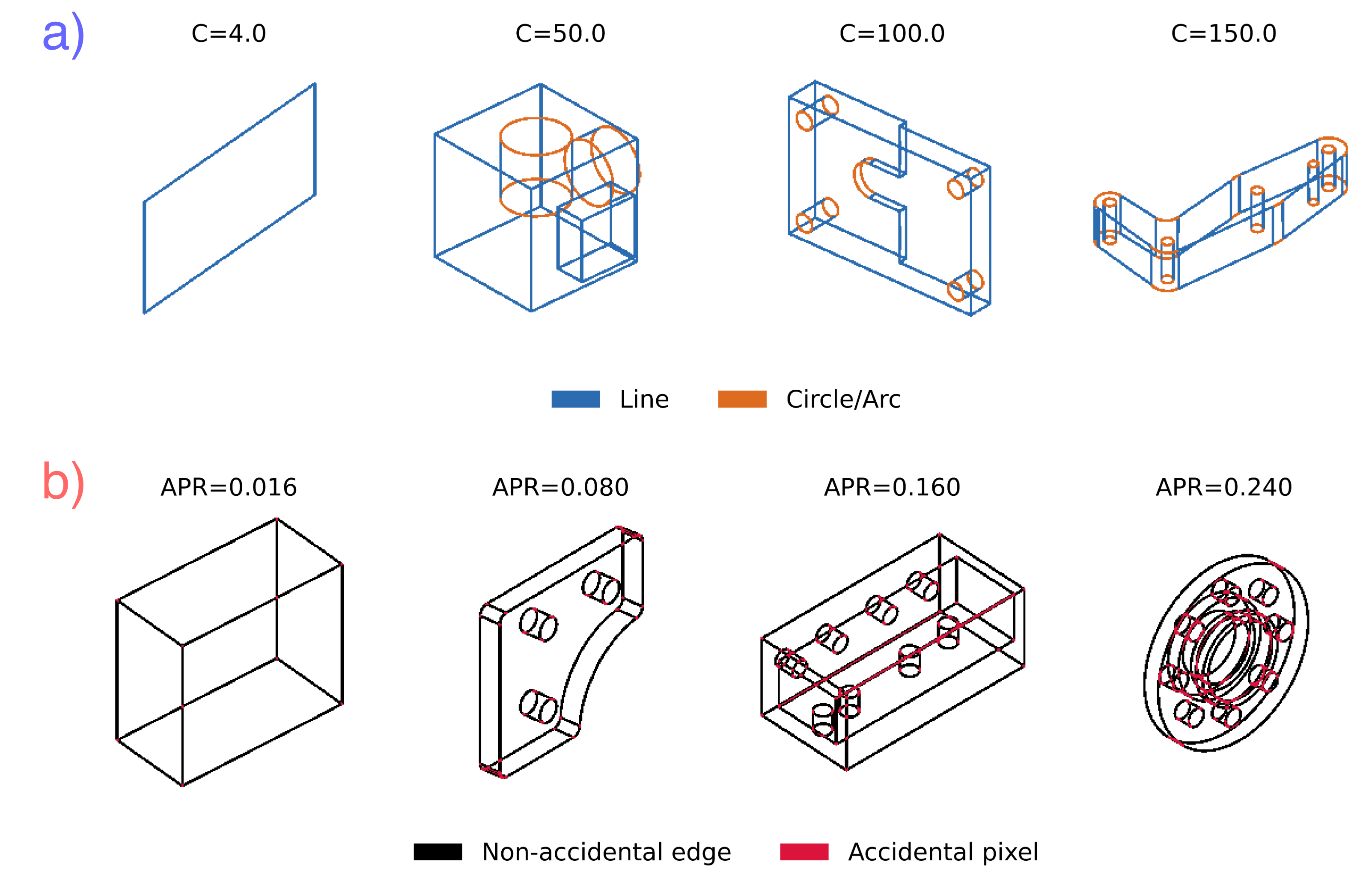
In addition, to gauge how the model performs against shapes of various complexity, we provide two additional parameters: accidental pixel ratio (APR) and curve complexity. APR is computed as the proportion of all foreground pixels that occlude one or more components, while curve complexity ratio is a summation of the per-edge primitive costs. To keep calculations simple and robust to potentially unclean CAD data, we assign a score of 1 to lines and a score of 3 to non-lines. Figure 5 displays example shapes of various shape complexities and APRs.
7 Results & Discussion
7.1 Comparison with Baseline and Off-the-Shelf Approaches
To evaluate the efficacy of our generative diffusion-based approach, we first compare our pipeline against deterministic models and state-of-the-art, off-the-shelf depth and 3D reconstruction frameworks.
Deterministic Regression: As established, the orthographic projection of wireframes creates an inherently ill-posed problem, as a single 2D sketch can mathematically correspond to multiple valid 3D interpretations. When we attempted to train a standard deterministic regression model to map , the network consistently failed to resolve these ambiguities, instead converging to the mean of all possible modes.
| Model Details | Average Prediction | Best Prediction | |||||||
| Model | Params | Data | GPU Hrs | NMAE | AbsRel | NMAE | AbsRel | ||
| Baseline (average) | - | - | - | ||||||
| Depth Anything V2 [34] | 98M | - | - | ||||||
| VAE encoder | 63M | 1M | 112 | ||||||
| ViT small scratch | 84M | 1M | 128 | ||||||
| DinoV2 small | 84M | 500K | 128 | ||||||
| DinoV2 small | 84M | 1M | 128 | ||||||
| DinoV3 small | 84M | 1M | 128 | ||||||
| DinoV2 base | 227M | 1M | 336 | ||||||
| DinoV3 base | 227M | 1M | 336 | ||||||
| DinoV2 base XL | 496M | 1M | 240 (5090) | ||||||
| DinoV3 base XL | 496M | 1M | 240 (5090) | ||||||
Comparison with Off-the-Shelf Frameworks: We further trialed our wireframe inputs against leading zero-shot vision models. Initially, we attempted to use an off-the-shelf depth estimator, namely the widely successful Depth Anything V2 [34]. While Depth Anything understands basic semantics of near and far regions, it is clearly unsuited to the unique visual domain of wireframe projections (Figure 6).
Additionally, we performed inference on Microsoft’s Trellis [32] in an attempt to generate a 3D wireframe asset directly. Not only was the generation process too slow to support our intended “sketch-reconstruct-sketch” pipeline, but the results exhibited severe geometric distortions, underscoring a clear input unsuitability (Figure 6).

7.2 Hyperparameter Analysis: Conditioning Encoders, Dataset Size, and Model Size
The choice of the conditioning encoder () dictates how effectively the U-Net denoiser can interpret the sparse, abstract nature of wireframe drawings. We tested three distinct encoder architectures: a Latent Encoder (VAE-KL), a ViT small trained from scratch, and a pre-trained DinoV2 backbone (Table 2).
Quantitative results (Table 2) indicate that the DinoV2 encoder achieved the best performance across all metrics. While the simpler, CNN-based VAE-KL encoder displayed an initially faster convergence speed than the DinoV2 encoder, DinoV2 eventually reached a lower final loss. This suggests that although modern foundation models are trained primarily on natural images, their learned representations translate to wireframe domains given sufficient fine-tuning. However, DinoV2’s superior performance does not necessarily imply that a natural image prior is strictly better than a purely geometric prior, as architectural differences (ViT vs. CNN) play a significant role. Rather, the VAE-KL encoder’s rapid initial convergence points to the ideal necessity of a wireframe-specific ViT backbone—one conditioned first on natural images and subsequently fine-tuned on geometric wireframes. Indeed, the fine-tuned DinoV2 encoder utilized in this work fills precisely this gap, representing a preliminary step toward a wireframe-specific vision foundation model.
Ultimately, while encoders trained on natural images provide a suitable foundation, they are limited in the long run. Even as we ran a benchmark with the newer DinoV3, there was virtually no improvement in the small and base models and a significant deterioration in the base XL. Thus, to improve performance in wireframe specific tasks, it is not enough to simply build an encoder better for natural images; it is instead required to build better wireframe specific foundation models. The necessity for a wireframe specific model is even more crucial when considering the DinoV3, trained on nearly 12 the amount of data compared to the V2 and fully specialized to natural images, was unable to provide any meaningful improvement.

Furthermore and predictably, increasing model size improved performance while decreasing dataset size harmed performance. This behavior indicates that the LDM likely follows the scaling laws commonly observed in large language and generative vision models [1]. Whereas approaches dependent on stroke primitives must be manually adapted and retrained for new curve topologies, our approach offers a straightforward path for continuous improvement via increased computational capacity, either in parameter size or dataset size.
7.3 Evaluation of Partial Depth and Sequential Sketching
A key contribution of our method is the ability to intuitively reconstruct from partial depth, enabling a “sketch-reconstruct-sketch” workflow. To validate this, we evaluated the model’s performance while varying the partial depth threshold using our graph-based BFS masking strategy.
As the percentage of provided partial depth () increases, the NMAE predictably decreases, with every model appearing to converge toward 0 ((Figure 7)). However, this decrease is non-linear. Providing the depth of just 10% of the sketch acts as a geometric “anchor” that sufficiently boosts performance, while providing 25% of the sketch achieves similar performance to providing 75%.
However, between the 25% and 85% thresholds, there exists an interesting plateau and even slight degradation in performance. This plateau suggests that once the global structural details are anchored (accounted for in the first 10% to 25%), remaining errors are likely concentrated on smaller structural details that are objectively more difficult to predict, such as a disjointed chunk of the wireframe’s edges.
These results confirm that partial depth cues provide massive aid to the drawing process, validating the success of the “sketch-reconstruct-sketch” workflow. Supporting iterative sketching not only allows the user to comfortably tackle complex objects in stages, but the iterative geometric anchoring ensures the model autoregressively avoids compounding structural mistakes.
The partial depth curves also illuminate an interesting finding. The first jump in model size (from 84M to 227M) was marked primarily by an increase in zero-shot performance (0% completion ratio), while the second jump in model size (from 227M to 496M) was marked primarily by increases in non-zero-shot tasks where there was existing partial depth.
7.4 Robustness to Complexity
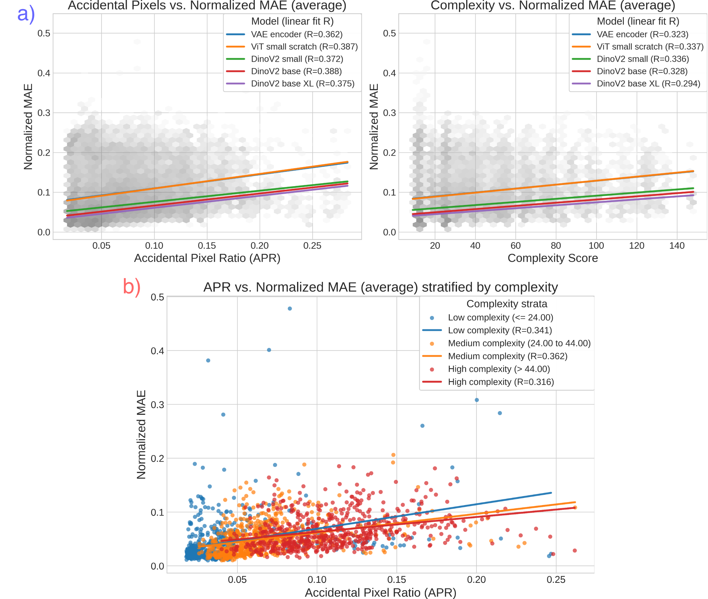
To test the robustness of our pipeline against sketches of varying difficulty, we segmented our test set by shape complexity and APR (Figure 8).
There exists a positive relationship between predictive error and both shape complexity (–) and APR (–) (Figure 8a, implying the model is understandbly prone to both parameters. However, while shape complexity is constant and unchangeable, APR can be decreased and mediated by strategies such as drawing from better viewpoints, increasing input resolution, and lowering stroke thickness.
The APR and the complexity of the shape are naturally correlated; thus, the question becomes whether reducing the APR can lower the error for shapes of various complexities. If so, the strategies presented provide a straightforward way to improve the model. Thus, in Figure 8b, we show that regardless of the low / medium / high complexity shapes, the APR and the error continue to be correlated; therefore, by reducing the APR even for the high complexity shapes, we can effectively reduce the error.
Ultimately, while the complexity of a shape is a main driver for error, APR makes up a significant portion of why complexity is such a significant cause for high error.
| Input 2D Sketch | Predicted Depth | 3D Reconstruction (Top: Wireframe, Bottom: Point Cloud) | Input 2D Sketch | Predicted Depth | 3D Reconstruction (Top: Wireframe, Bottom: Point Cloud) |
 |
 |
 |
 |
 |
 |
 |
 |
 |
 |
 |
 |
 |
 |
 |
|
 |
 |
 |
 |
 |
 |
 |
 |
 |
 |
 |
 |
 |
 |
7.5 Qualitative Results
Lastly, we display sample qualitative reconstruction results from the pipeline, showcasing the predicted point cloud and a generated wireframe graph (Figure 9). The wireframe was constructed using a preliminary fitting scheme by identifying the endpoints of the sketch, assigning 3D points and predicted depth to each edge, and finally fitting an edge that minimizes the distance to the predicted point cloud.
Overall, the model displayed several high-quality reconstructions. However, as deduced in the previous sections, reconstruction fidelity remains heavily dependent on the quality of the input sketch. These qualitative results visually confirm that failures are primarily driven by 1) the proportion of accidental pixels and 2) the sketch conditioner’s fixed image resolution. Accidental pixels introduce significant ambiguity because the binary input sketch mask cannot differentiate between overlapping 2D strokes. As seen in (Figure 9), areas of high pixel density directly correspond to noisy or inaccurate 3D point clouds. Because image resolution is directly linked to reconstruction granularity, upgrading the input resolution would afford the network the necessary visual separation to resolve dense, complex structures with much lower error.
8 Limitations and Future Work
Although our framework presents a highly flexible alternative for the 2D-to-3D reconstruction of wireframes, it also highlights specific challenges inherent to depth-based representations.
Sketch input noise. Human freehand sketches are inherently noisy and highly dependent on an individual’s drawing skill. Because our current model is trained exclusively on clean, perfect wireframe projections, it can struggle to generalize to highly irregular or inaccurate freehand input, manifesting in wiggly lines and geometry distortions. To mitigate this, our current interface provides drawing assisting features, such as stroke normalization, endpoint snapping, and an isometric grid, to guide user measurements. Our current model faithfully reconstructs the input exactly as drawn, preserving any user-introduced noise. To truly develop an end-to-end framework capable of capturing a user’s underlying design intent, future iterations of the diffusion model must learn to map noisy inputs to idealized clean geometries. Training such a model requires perturbing clean wireframes with simulated noise (e.g., vertex jitter and edge wobble). Preliminary experiments suggest a complex spectrum of “noise,” ranging from high-frequency stroke perturbations (wobbly lines) to low-frequency structural distortions (e.g., skewing a rectangular face into a parallelogram). Consequently, future models may require explicit noise-conditioning scalars and must learn stronger geometric priors to regularize internal topologies toward what makes an “ideal” CAD shape.
Model size and resolution. Upon scaling our architecture to a larger parameter count, we observed a distinct improvement in our accuracy metrics. This indicates that our framework likely benefits from the scaling laws commonly observed in large foundation models, offering a straightforward path to improved performance via increased computational capacity [1]. More importantly, future iterations should prioritize higher input and output spatial resolutions. While our current resolution is sufficient for the autoregressive estimation of complex objects via partial depth, higher resolution conditioning inherently mitigates the APR that currently bottleneck one-shot performance on dense structures.
Post-processing and mesh conversion. In this work, we applied a preliminary, heuristic-based scheme to convert predicted point clouds back into vector wireframes. Implementing sophisticated parametric curve fitting represents a clear avenue for future improvement. Furthermore, once a mathematically precise wireframe is established, inferring which planar cycles constitute solid faces is required to generate a final, watertight mesh. In this regard, our generative depth approach could be highly complementary when paired with topological sequence models like Neural Face Identification [29], or even more traditional face identification techniques like in Shpitalni & Lipson [25]. However, aggressive post-processing introduces a philosophical tradeoff: enforcing rigid parametric constraints diminishes the primary advantage of our generative approach—its ability to model unbounded, organic topologies without predefined vocabularies. Navigating this balance will ultimately depend on the specific downstream needs of the end user.
Conditioning input. To maintain a fully unconstrained pipeline, we deliberately limited our geometric conditioning inputs to binary input sketch masks and partial depth. However, providing explicit stroke-level instance segmentation (i.e., mapping specific pixels to individual strokes and providing the order of strokes drawn) could resolve significant geometric ambiguities. This would alleviate granularity bottlenecks, allowing the network to easily disentangle dense pixel clusters into distinct edges. While requiring users to draw each edge with a single, continuous stroke aligns well with natural human drawing behavior, it reintroduces a subtle operational constraint, lightly compromising the vision of a purely unconstrained predictive pipeline.
9 Conclusions
In this paper, we presented a generative framework for 3D wireframe reconstruction that addresses the inherent limitations of traditional CAD modeling. By reframing reconstruction as a conditional dense depth estimation task, we successfully transitioned from rigid parametric constraints and symbolic logic to a flexible, data-driven generative prior. Our approach utilizes an LDM with ControlNet-style conditioning to navigate the ill-posed nature of orthographic projections, allowing the system to sample structurally plausible and geometrically consistent 3D structures from ambiguous 2D inputs.
Our experimental results, conducted on a massive dataset of one million image-depth pairs derived from the ABC Dataset, demonstrate that a high-capacity model leveraging a DinoV2-based conditioning encoder can effectively bridge the domain gap between natural images and sparse wireframes. We showed that the model is robust to shape complexity, and that providing even minimal partial depth cues geometrically anchors the reconstruction, validating our proposed “sketch-reconstruct-sketch” workflow.
Ultimately, this work provides a scalable alternative to traditional parametric modeling by enabling the reconstruction of arbitrary and organic topologies without the “vocabulary bottleneck” of standard CAD primitives. By removing the technical barriers between a 2D stroke and its 3D realization, we move closer to a truly intuitive interface where users can fluidly and iteratively “draw in 3D.”
10 Acknowledgements
This work was supported by the US National Science Foundation (NSF) AI Institute for Dynamical Systems (DynamicsAI.org) under grant 2112085. Code is available at https://eltonc01.github.io/sketch-depth-diffusion
References
- [1] (2024) DeepSeek llm: scaling open-source language models with longtermism. arXiv preprint arXiv:2401.02954. Cited by: §7.2, §8.
- [2] (2020) An image is worth 16x16 words: transformers for image recognition at scale. arXiv preprint arXiv:2010.11929. Cited by: item 2.
- [3] (2014) Depth map prediction from a single image using a multi-scale deep network. In Advances in Neural Information Processing Systems (NeurIPS), Cited by: §2.4.
- [4] (2008) Sketching: drawing techniques for product designers. BIS Publishers. Cited by: §1.
- [5] (2020) Denoising diffusion probabilistic models. In Advances in Neural Information Processing Systems (NeurIPS), Cited by: §4.
- [6] (1971) Impossible objects as nonsense sentences. Machine Intelligence 6, pp. 295–323. Cited by: §2.1, Table 1.
- [7] (2024) Repurposing diffusion-based image generators for monocular depth estimation. In Proceedings of the IEEE/CVF Conference on Computer Vision and Pattern Recognition, pp. 9492–9502. Cited by: §1, §2.4.
- [8] (2019) An introduction to variational autoencoders. Foundations and Trends in Machine Learning 12 (4), pp. 307–392. Cited by: §4.1.
- [9] (2019) ABC: a big cad model dataset for geometric deep learning. In Proceedings of the IEEE/CVF Conference on Computer Vision and Pattern Recognition, pp. 9601–9611. Cited by: §5.
- [10] (2025) SketchFusion: learning universal sketch features through fusing foundation models. In Proceedings of the IEEE/CVF Conference on Computer Vision and Pattern Recognition, pp. 2556–2567. Cited by: §1, §2.2.
- [11] (2020) Sketch2CAD: sequential cad modeling by sketching in context. ACM Transactions on Graphics (TOG) 39 (6), pp. 1–14. Cited by: §2.3, Table 1.
- [12] (2022) Free2CAD: parsing freehand drawings into cad commands. ACM Transactions on Graphics (TOG) 41 (4), pp. 1–16. Cited by: §1, §1, §2.3, Table 1.
- [13] (1996) Optimization-based reconstruction of a 3d object from a single freehand line drawing. Computer-Aided Design 28 (8), pp. 651–663. Cited by: §2.1, §2.1, Table 1.
- [14] (2007) Correlation-based reconstruction of a 3d object from a single freehand sketch. In ACM SIGGRAPH 2007 Courses, pp. 44–es. Cited by: Table 1.
- [15] (2023) Zero-1-to-3: zero-shot one image to 3d object. In Proceedings of the IEEE/CVF International Conference on Computer Vision, pp. 9298–9309. Cited by: §2.2.
- [16] (2017) Decoupled weight decay regularization. arXiv preprint arXiv:1711.05101. Cited by: §6.1.
- [17] (2013) Structure-aware shape processing. Eurographics State of the Art Reports 32 (2), pp. 1–21. Cited by: §1, §2.4.
- [18] (2023) DINOv2: learning robust visual features without supervision. arXiv preprint arXiv:2304.07193. Cited by: item 3.
- [19] (2019) PyTorch: an imperative style, high-performance deep learning library. In Advances in Neural Information Processing Systems (NeurIPS), Cited by: §6.1.
- [20] (1958) Impossible objects: a special type of visual illusion. British Journal of Psychology 49 (1), pp. 31–33. Cited by: §2.4.
- [21] (2020) Towards robust monocular depth estimation: mixing datasets for zero-shot cross-dataset transfer. IEEE Transactions on Pattern Analysis and Machine Intelligence 44 (3), pp. 1623–1637. Cited by: §2.4.
- [22] (2022) High-resolution image synthesis with latent diffusion models. In Proceedings of the IEEE/CVF Conference on Computer Vision and Pattern Recognition, pp. 10684–10695. Cited by: §1, §4.
- [23] (2015) U-net: convolutional networks for biomedical image segmentation. In Medical Image Computing and Computer-Assisted Intervention–MICCAI 2015, pp. 234–241. Cited by: §4.2.
- [24] (2023) Sketch-a-shape: zero-shot sketch-to-3d shape generation. arXiv preprint arXiv:2307.03869. Cited by: §2.2.
- [25] (1996) Identification of faces in a 2d line drawing projection of a wireframe object. IEEE Transactions on Pattern Analysis and Machine Intelligence 18 (10), pp. 1000–1012. Cited by: §8.
- [26] (2025) DINOv3. arXiv preprint arXiv:2508.10104. Cited by: §6.2.
- [27] (1986) Machine interpretation of line drawings. MIT Press. Cited by: §2.1.
- [28] (2018) Pixel2Mesh: generating 3d mesh models from single rgb images. In Proceedings of the European Conference on Computer Vision (ECCV), pp. 52–67. Cited by: §2.2.
- [29] (2022) Neural face identification in a 2d wireframe projection of a manifold object. IEEE Transactions on Visualization and Computer Graphics. Cited by: §1, §1, §2.3, Table 1, §5.1, §5.3, §5, §8.
- [30] (2019) HuggingFace’s transformers: state-of-the-art natural language processing. arXiv preprint arXiv:1910.03771. Cited by: §6.1.
- [31] (2021) DeepCAD: a deep generative network for computer-aided design models. In Proceedings of the IEEE/CVF International Conference on Computer Vision and Pattern Recognition, pp. 6772–6782. Cited by: §1, §2.3, Table 1.
- [32] (2025) Structured 3d latents for scalable and versatile 3d generation. In Proceedings of the IEEE/CVF International Conference on Computer Vision and Pattern Recognition, pp. 21469–21480. Cited by: §1, §2.2, §7.1.
- [33] (1994) Efficient algorithm for the reconstruction of 3d objects from orthographic projections. Computer-Aided Design 26 (9), pp. 699–717. Cited by: §1.
- [34] (2024) Depth anything: unleashing the power of large-scale unlabeled data. In Proceedings of the IEEE/CVF Conference on Computer Vision and Pattern Recognition, pp. 10371–10381. Cited by: §1, §2.4, §7.1, Table 2.
- [35] (2023) Adding conditional control to text-to-image diffusion models. In Proceedings of the IEEE/CVF International Conference on Computer Vision, pp. 3836–3847. Cited by: §4.2.
- [36] (2023) Computer vision techniques in manufacturing. IEEE Transactions on Systems, Man, and Cybernetics: Systems 53 (1), pp. 105–117. Cited by: §1.