Spectral analysis of multivariate stationary Hawkes processes

Yifu Tang Department of Mathematics and Statistics, University of Otago, New Zealand Conor Kresin Department of Mathematics and Statistics, University of Otago, New Zealand Boris Baeumer Department of Mathematics and Statistics, University of Otago, New Zealand Ting Wang Department of Mathematics and Statistics, University of Otago, New Zealand

Abstract

We establish the asymptotic validity of frequency-domain inference for stationary multivariate Hawkes processes under mild conditions, bridging the gap between theory and application. By developing upper-bounds on the reduced cumulant measures from the cluster representation of the Hawkes processes, we prove a functional central limit theorem and, as a consequence, consistency of the Whittle estimator under stationarity alone (i.e., the spectral radius of the interactions matrix $\rho(\boldsymbol{\nu})<1$ ), applicable to Hawkes processes with heavy-tailed mutual-excitation kernels. Under mild extra moment conditions, we further obtain asymptotic normality with an explicit limiting covariance in terms of second- and fourth-order cumulant spectral densities. We also propose a simple frequency-domain method to detect joint independence of subprocesses of a multivariate Hawkes process. The performance of the Whittle estimator and the test of independence are demonstrated via simulation studies.

1 Introduction

Hawkes processes (Hawkes, 1971) are a prominent class of self- and mutually-exciting point-process models with broad applications (e.g. seismology, finance, and neuroscience; see Reinhart (2018) for a comprehensive review). Despite their popularity, likelihood-based inference (Ogata, 1978) can be computationally burdensome at large event counts and in higher dimensions: even with algorithmic improvements, likelihood evaluation and optimization can remain a bottleneck for large-scale multivariate data (Kresin and Schoenberg, 2023). This has motivated a wide range of alternative estimators, including approximate-likelihood methods (Schoenberg, 2013), as well as Bayesian approaches relying on numerical approximation (Rasmussen, 2013).

Frequency-domain methods offer a powerful alternative to likelihood-based inference for dependent data. A central tool is the Whittle likelihood (Whittle, 1953, 1954), which replaces the exact likelihood by a Gaussian likelihood of the Fourier transform of the observations. This approximation yields computationally inexpensive estimators with strong statistical properties in many settings (Dahlhaus, 1988; Brillinger, 2001). For temporal point processes, the natural quantity of interest in the frequency domain is the Bartlett spectral density (and, in the multivariate case, the Bartlett spectral density matrix), defined as the Fourier transform of the second-order reduced cumulant measures (Bartlett, 1963; Brillinger, 1972; Daley and Vere-Jones, 2003).

A multivariate stationary Hawkes process is uniquely defined by its first- and second-order statistics (Bacry and Muzy, 2016, Corollary 1). This makes Whittle likelihood particularly useful for inference of Hawkes processes because it concerns only the first- and second-order information. Indeed, the Whittle likelihood leverages the Bartlett spectral density matrix, which for stationary multivariate linear Hawkes processes admits an explicit analytic form (Daley and Vere-Jones, 2003, Example 8.3(c)). To our knowledge, the first ever use of Whittle likelihood in fitting Hawkes processes is Adamopoulos (1976) who studied earthquake data. However, rigorous asymptotic theory for Whittle estimation of Hawkes processes has developed more slowly than its time-series counterpart. Tuan (1981) first proved some asymptotic properties of the Whittle estimator of univariate Hawkes processes under strong assumptions on the self-excitation kernel. Cheysson. and Lang (2022) studied the binned observations of a univariate Hawkes process, which is equivalent to a realization of an integer-valued time series, and managed to establish the $\alpha$ -mixing of the time series by assuming the existence of certain moments of the self-excitation kernel. Then the asymptotic properties of the Whittle estimator can then be shown by employing known results in time series analysis (see e.g. Dzhaparidze (1986)). Yang and Guan (2026) derived asymptotic properties related to Whittle likelihood for spatial point processes (with univariate Hawkes processes as special examples) by imposing conditions such as $\alpha$ -mixing of the point process, and integrability and smoothness of cumulant spectral density functions. However, the assumptions made in these papers exclude Hawkes processes with heavy-tailed mutual excitation kernels (e.g. kernels which do not admit first moment) representing long-lasting effects. This kind of kernels have proven useful in fields such as seismology and finance, and continue to gain popularity. (Vere-Jones and Davies 1966; Hawkes 2018; Chen et al. 2021; Davis et al. 2024; Dupret and Hainaut 2025; Gupta and Maheshwari 2026).

In this paper, we develop frequency-domain asymptotic theory for stationary multivariate linear Hawkes processes observed in continuous time: we observe the marked event sequence (event times and types) on $[0,T]$ and let $T\to\infty$ . We consider Whittle estimation based on a parametric family of Bartlett spectral density matrices $\{\Psi_{\theta}(\omega):\theta\in\Theta\}$ induced by a parametric Hawkes specification (e.g. $\theta$ collects background rates, branching coefficients, and any kernel-shape parameters), and we also develop a simple frequency-domain test of independence of subprocesses of Hawkes process. Our analysis builds on the cumulant framework initiated by Brillinger (1972) and developed for Hawkes processes via explicit tree representations of cumulant measures derived in (Jovanović et al., 2015). The main contributions are:

1.

We study a spectral empirical process, defined as the sum of quadratic form of finite Fourier transform over Fourier frequencies, and establish a functional Central Limit Theorem (CLT) under slight conditions on mutual-excitation kernels. The proof is based on results pertaining to reduced cumulant measures without invoking $\alpha$ -mixing.
2.

We define the Whittle likelihood and estimator with the help of the spectral empirical process. The consistency is then proven under the sole requirement of stationarity. In our normalized-kernel parameterization, this essentially means that the only assumption needed to establish consistency is $\rho(\boldsymbol{\nu})<1$ , where $\boldsymbol{\nu}$ is the interactions matrix and $\rho(\cdot)$ denotes the spectral radius.
3.

Under additional, and yet still mild moment conditions on the mutual-excitation kernels, we derive asymptotic normality of the Whittle estimator with an explicit limiting covariance expressed in terms of second- and fourth-order cumulant spectral densities thanks to the functional CLT of the spectral empirical process.
4.

We construct a simple test of independence of subprocesses of a multivariate stationary Hawkes process based on an estimation procedure for the spectral density matrix at frequency $0$ inspired by McElroy and Politis (2025).

The remainder of the paper proceeds from probabilistic structure to inferential consequences. Section 2 introduces multivariate Hawkes processes, cumulant measures, and the finite Fourier transform. Section 3 then develops the frequency-domain machinery: Section 3.1 establishes weak convergence of the spectral empirical process, Section 3.2 develops the Whittle likelihood and proves consistency and asymptotic normality, and Section 3.3 proposes a simple frequency-domain test of independence among subprocesses. Numerical experiments are presented in Section 4, and Section 5 concludes. Tables and figures, technical proofs and auxiliary results on cumulant measures, Fourier-transform cumulants, and deterministic approximation bounds are collected in the Appendices.

2 Multivariate Hawkes processes and preliminary notation

This section first defines stationary multivariate Hawkes processes (Hawkes, 1971) and recalls their cluster representation (Hawkes and Oakes, 1974). We then introduce cumulant and reduced cumulant measures, whose finiteness is the key structural input behind our frequency-domain asymptotics. Finally, we define the cumulant spectral densities and the finite Fourier transform, which are the main ingredients in Sections 3.1–3.3.

A $D$ -variate temporal point process $N=(N_{1},\ldots,N_{D})$ on $\mathbb{R}$ can be viewed as a collection of random counting measures, where $N_{j}(B)$ counts the number of type- $j$ events falling in a Borel set $B\subset\mathbb{R}$ . $N_{1},\ldots,N_{D}$ are often called subprocesses of $N$ . We say that $N$ is (strictly) stationary if for every $s\in\mathbb{N}$ , every choice of indices $(j_{1},\ldots,j_{s})$ , and every collection of Borel sets $(B_{1},\ldots,B_{s})$ , the joint law of $(N_{j_{1}}(B_{1}),\ldots,N_{j_{s}}(B_{s}))$ is invariant under common time shifts (Daley and Vere-Jones, 2003, Section 3.2), i.e.

(N_{j_{1}}(B_{1}),\ldots,N_{j_{s}}(B_{s}))\stackrel{{\scriptstyle d}}{{=}}(N_{j_{1}}(B_{1}+t),\ldots,N_{j_{s}}(B_{s}+t)),\qquad t\in\mathbb{R}.

We will now introduce the point process model of interest to this paper.

Definition 1 (Multivariate (linear) Hawkes process).

Let $N=(N_{1},\ldots,N_{D})$ be a $D$ -variate simple point process on $\mathbb{R}$ with natural filtration $\mathcal{H}_{t-}=\sigma\{N_{j}((-\infty,s]):s<t,\ j=1,\ldots,D\}$ . Denote by $(t^{(j)}_{k})_{k\geq 1}$ the event times of $N_{j}$ . We say that $N$ is a (linear) Hawkes process with background rate $\boldsymbol{\mu}=(\mu_{1},\ldots,\mu_{D})^{\top}$ , interactions matrix $\boldsymbol{\nu}=\{\nu_{ij}\}_{i,j=1,\cdots,D}$ , and mutual-excitation kernels $\boldsymbol{G}=\{g_{ij}\}_{i,j=1}^{D}$ if its conditional intensities satisfy, for $i=1,\ldots,D$ ,

\lambda_{i}(t\mid\mathcal{H}_{t-})=\mu_{i}+\sum_{j=1}^{D}\nu_{ij}\sum_{k:t^{(j)}_{k}<t}g_{ij}(t-t^{(j)}_{k}).

Here $\mu_{i}>0$ , $\nu_{ij}\geq 0$ , and each $g_{ij}:\mathbb{R}\to[0,\infty)$ satisfies $\int_{0}^{\infty}g_{ij}(u)\,du=1$ and $g(x)=0$ for $x<0$ . The conditional intensity is understood in the usual sense: for each $i$ ,

\mathrm{E}[N_{i}((t,t+\Delta])\mid\mathcal{H}_{t-}]=\int_{t}^{t+\Delta}\lambda_{i}(s\mid\mathcal{H}_{s-})\,ds=\lambda_{i}(t\mid\mathcal{H}_{t-})\Delta+o(\Delta),\qquad\Delta\downarrow 0,

where $\mathrm{E}$ is the expectation operator. If the spectral radius of $\boldsymbol{\nu}$ , denoted by $\rho(\boldsymbol{\nu})$ , is smaller than 1, then a stationary version exists (and is unique in law); see Daley and Vere-Jones (2003, Example 8.3(c)) or Hawkes (1971).

The stationary temporal Hawkes processes admit a Poisson cluster representation (Daley and Vere-Jones, 2003, Example 8.3(c)), which mimics many real-world phenomena, such as the triggering-triggered effect in epidemics and seismology (Reinhart, 2018). To facilitate exposition, we view multivariate processes as point processes on $\mathbb{R}\times\{1,\cdots,D\}$ endowed with base measure $l_{\mathrm{Leb}}\times\#$ , where $l_{\mathrm{Leb}}$ is the Lebesgue measure on $\mathbb{R}$ and $\#$ is the counting measure on $\{1,\cdots,D\}$ .

Concretely, a multivariate stationary Hawkes process is a collection of immigrants and offspring. The immigrants form a Poisson process with intensity $r_{b}((t,i))=\mu_{i}$ . Each immigrant $(t_{\ast},j)$ then independently produces offspring according to an inhomogeneous Poisson process with intensity

r_{d}((t,i)\mid(t_{\ast},j))=\nu_{ij}g_{ij}(t-t_{\ast}).

Offspring reproduce in the same manner, generating i.i.d. clusters attached to each immigrant. Let $\rho(\cdot)$ denote the spectral radius. The interactions matrix $\boldsymbol{\nu}=\{\nu_{ij}\}_{i,j=1,\cdots,D}$ is therefore the mean offspring (branching) matrix, and the condition $\rho(\boldsymbol{\nu})<1$ ensures subcriticality, finiteness of clusters almost surely, and existence of a stationary version.

In line with Brillinger (1972) and Tuan (1981), we will rely on the (reduced) cumulant measure of Hawkes processes and their Fourier transforms in the proofs. Recall (cf. equation (2.3.1) of Brillinger (2001)) that the joint cumulant of (complex-valued) random variables $X_{1},\cdots,X_{s}$ is defined as

\displaystyle\mathrm{cum}(X_{1},\cdots,X_{s})=\sum_{q=1}^{s}(-1)^{q-1}(q-1)!\sum_{\{\Xi_{1},\cdots,\Xi_{q}\}}\left(\mathrm{E}\prod_{r\in\Xi_{1}}X_{r}\right)\cdots\left(\mathrm{E}\prod_{r\in\Xi_{q}}X_{r}\right),

(2.1)

where the summation $\sum_{\{\Xi_{1},\cdots,\Xi_{q}\}}$ is over all partitions of $\{1,\cdots,s\}$ with $q$ blocks. This concept can be extended to point processes in the following way.

Definition 2 (Cumulant measure and reduced cumulant measure).

Let $N$ be a $D$ -variate stationary process. For any $s\in\mathbb{N}$ and any $j_{1},\cdots,j_{s}\in\{1,\cdots,D\}$ , the $j_{1}\cdots j_{s}$ -th cumulant measure $C_{j_{1}\cdots j_{s}}$ of $N$ is defined for Borel rectangles $A_{1}\times\cdots\times A_{s}$ by

\displaystyle C_{j_{1}\cdots j_{s}}(A_{1}\times\cdots\times A_{s})=\mathrm{cum}(N_{j_{1}}(A_{1}),\cdots,N_{j_{s}}(A_{s})),

(2.2)

and extended to a signed measure on the product Borel $\sigma$ -algebra in $\mathbb{R}^{s}$ . $C_{j_{1}\cdots j_{s}}$ exists provided that the expectations on the right-hand side of (2.2) exist. We refer to section 9.5 of Daley and Vere-Jones (2008) for more information about the above-mentioned expectations.

For $s\geqslant 2$ , since the cumulant measure is translation invariant due to the stationarity of $N$ , there exists a signed measure $C_{j_{1}\cdots j_{s}}^{\mathrm{red}}$ defined on $\mathbb{R}^{s-1}$ such that

\displaystyle\mathrm{d}C_{j_{1}\cdots j_{s}}(x_{1},\cdots,x_{s})=\mathrm{d}C_{j_{1}\cdots j_{s}}^{\mathrm{red}}(x_{1}-x_{s},\cdots,x_{s-1}-x_{s})\mathrm{d}x_{s},

if ${C}_{j_{1}\cdots j_{s}}$ exists. We call $C_{j_{1}\cdots j_{s}}^{\mathrm{red}}$ a reduced cumulant measure.

By combining (2.1), (2.2) and the Campbell theorem (see equations (9.5.2) and (9.5.9) of Daley and Vere-Jones (2008)), it can be seen that if the cumulant measure $C_{j_{1}\cdots j_{s}}(\cdot)$ of $N$ exists, then the following equation holds:

\displaystyle\mathrm{cum}\left\{\int_{\mathbb{R}}h_{k}(x)\mathrm{d}N_{j_{k}}(x),k=1,\cdots,s\right\}=\int_{\mathbb{R}^{s}}\prod_{k=1}^{s}h_{k}(x_{k})\mathrm{d}C_{j_{1}\cdots j_{s}}(x_{1},\cdots,x_{s}),

(2.3)

where $h_{1},\cdots,h_{s}$ are any bounded measurable (complex-valued) functions with bounded support. Equation (2.3) is important to our proofs as it connects the cumulant of stochastic integrals to a signed measure which is much easier to deal with.

When $s=1$ , the stationarity of $N$ means that the first-order cumulant measure $C_{j}(\cdot)=\mathrm{E}N_{j}(\cdot)$ is invariant under translation, which in turn implies that $C_{j}=\lambda_{j}l_{\mathrm{Leb}}$ , $j=1,\cdots,D$ , where $\lambda_{j}=\mathrm{E}N_{j}((0,1))$ is the average intensity of $N_{j}$ and $l_{\mathrm{Leb}}$ is the Lebesgue measure on $\mathbb{R}$ (see e.g. Theorem A.1.8 of Brémaud (2020)). In particular, the average intensity vector of a multivariate stationary Hawkes process satisfies $\boldsymbol{\lambda}=(\lambda_{1},\cdots,\lambda_{D})^{\top}=(\boldsymbol{\mathrm{I}}_{D}-\boldsymbol{\nu})^{-1}\boldsymbol{\mu}$ (Daley and Vere-Jones, 2003, Example 8.3(c)), where $\boldsymbol{\mathrm{I}}_{D}$ is $D\times D$ identity matrix, $\boldsymbol{\nu}$ and $\boldsymbol{\mu}$ are given in Definition 1. For $s\geqslant 2$ , it turned out that the reduced cumulant measures of a multivariate stationary Hawkes process are finite measures.

Proposition 2.1.

Let $N$ be a multivariate stationary Hawkes process in Definition 1. For any integer $s\geqslant 2$ and any $j_{1},\cdots,j_{s}\in\{1,\cdots,D\}$ , the reduced cumulant measure $C_{j_{1}\cdots j_{s}}^{\mathrm{red}}$ of $N$ in Definition 2 exists and is a finite measure. Moreover, we have

\displaystyle C_{j_{1}\cdots j_{s}}^{\mathrm{red}}(\mathbb{R}^{s-1})\leqslant C_{0}^{s}(s-1)!,

where $C_{0}>0$ is a constant solely determined by $D$ , $\boldsymbol{\mu}$ and $\boldsymbol{\nu}$ which are given in Definition 1.

The proof is given in Section B.1 of the Appendices. Basically, Proposition 2.1 is a direct consequence of the tree representation pertaining to the cumulant measures proven in Jovanović et al. (2015).

Remark.

A common route to frequency-domain limit theory is to assume a Brillinger-type cumulant condition, namely that for each order $s\geqslant 2$ the reduced cumulant measures are finite (or have summable densities), which provides control of long-range dependence and ensures well-behaved cumulants of finite Fourier transforms; see Brillinger (1972). For stationary multivariate Hawkes processes, Proposition 2.1 implies precisely this kind of cumulant summability: for every $s\geqslant 2$ , the reduced cumulant measures $C^{\mathrm{red}}_{j_{1}\cdots j_{s}}$ exist and are finite, with explicit factorial growth bounds. These bounds can be viewed as an analogue of Brillinger’s mixing conditions which are stated in terms of reduced factorial cumulant measures (see e.g. Definition 1 of Heinrich (2016)) and serve as the main input for our non-asymptotic cumulant bounds and the ensuing functional CLT for the spectral empirical process, without requiring $\alpha$ -mixing assumptions (see e.g. Cheysson. and Lang (2022)).

Our limit theory concerning Hawkes processes is formulated in the frequency domain, where higher-order cumulants control non-Gaussian fluctuations of the finite Fourier transforms of the point processes. The Fourier transforms of reduced cumulant measures are very useful in this regard.

Definition 3 (Cumulant spectral density).

For any integer $s\geqslant 2$ and any $j_{1},\cdots,j_{s}\in\{1,\cdots,D\}$ , the cumulant spectral density $f_{j_{1}\cdots j_{s}}$ of order $(j_{1},\cdots,j_{s})$ of a stationary multivariate Hawkes process $N$ is defined as the Fourier transform of reduced cumulant measures $C_{j_{1}\cdots j_{s}}^{\mathrm{red}}$ , that is,

\displaystyle f_{j_{1}\cdots j_{s}}(\omega_{1},\cdots,\omega_{s-1})=\int_{\mathbb{R}^{s-1}}\exp\left(-\mathrm{i}\sum_{j=1}^{s-1}\omega_{j}x_{j}\right)\mathrm{d}C_{j_{1}\cdots j_{s}}^{\mathrm{red}}(x_{1},\cdots,x_{s-1}),

where $\mathrm{i}$ is the imaginary unit. Specifically, when $s=2$ , we call $f_{j_{1}j_{2}}$ the $(j_{1},j_{2})$ -th Bartlett spectral density (or simply spectral density) of the Hawkes process and the matrix $\boldsymbol{f}_{2}=(f_{j_{1}j_{2}})_{j_{1},j_{2}=1,\cdots,D}$ the spectral density matrix.

Remark.

For general multivariate stationary point processes, the coherence $|f_{j_{1}j_{2}}|/\sqrt{f_{j_{1}j_{1}}f_{j_{2}j_{2}}}$ , similar to the correlation of two random variables, is a measurement of linear dependency between $N_{j_{1}}$ and $N_{j_{2}}$ , while $f_{j_{1}\cdots j_{s}}$ ( $s\geqslant 3$ ) governs higher-order dependence. In particular, $f_{j_{1}j_{2}j_{3}j_{4}}$ appears in the covariance structure of quadratic forms in finite Fourier transforms (cf. Theorem 3.1). Surprisingly, for Hawkes processes, as will be shown in Section 3.3, the condition that $f_{j_{1}j_{2}}(0)=0$ for any $j_{1}\neq j_{2}$ in fact implies the independence of $N_{1},\cdots,N_{D}$ .

The Bartlett spectral density matrix $\boldsymbol{f}_{2}$ deserves special attention as this is the object of interest of this manuscript. As shown in Example 8.3(c) of Daley and Vere-Jones (2003), $\boldsymbol{f}_{2}$ can be expressed in terms of $\boldsymbol{\mu}$ , $\boldsymbol{\nu}$ and $\boldsymbol{G}$ given in Definition 1:

	$\displaystyle\boldsymbol{f}_{2}(\omega)=(\boldsymbol{\mathrm{I}}_{D}-\boldsymbol{\nu}\odot\hat{\boldsymbol{G}}(\omega))^{-1}\mathrm{Diag}(\boldsymbol{\lambda})(\boldsymbol{\mathrm{I}}_{D}-(\boldsymbol{\nu}\odot\hat{\boldsymbol{G}}(-\omega))^{\top})^{-1}$
	$\displaystyle=(\boldsymbol{\mathrm{I}}_{D}-\boldsymbol{\nu}\odot\hat{\boldsymbol{G}}(\omega))^{-1}\mathrm{Diag}(\boldsymbol{\lambda})\left[(\boldsymbol{\mathrm{I}}_{D}-\boldsymbol{\nu}\odot\hat{\boldsymbol{G}}(\omega))^{-1}\right]^{H},$		(2.4)

where $\boldsymbol{\mathrm{I}}_{D}$ is $D\times D$ dimensional identity matrix, $\boldsymbol{\lambda}=(\boldsymbol{\mathrm{I}}_{D}-\boldsymbol{\nu})^{-1}\boldsymbol{\mu}$ is the vector of average intensity, $\hat{g}_{ij}({\omega})=\int_{\mathbb{R}}\exp(-\mathrm{i}{\omega}x)g_{ij}(x)\mathrm{d}x$ is the Fourier transform of the mutual-excitation kernel $g_{ij}$ , $\hat{\boldsymbol{G}}=\{\hat{g}_{ij}\}_{i,j=1,\cdots,D}$ and $\odot$ means the Hadamard (element-wise) product of matrices, and $\boldsymbol{A}^{H}$ denotes the conjugate transpose of matrix $\boldsymbol{A}$ . It can be easily seen that $\boldsymbol{f}_{2}({\omega})$ is Hermitian positive-definite for any ${\omega}\in\mathbb{R}$ .

Here is an example of a class of multivariate stationary Hawkes processes.

Example 1 (Multivariate Fractional Hawkes process).

Let

\displaystyle E_{a,b}(z)=\sum_{n=0}^{\infty}\frac{z^{n}}{\Gamma(an+b)}

be the (two-parameter) Mittag-Leffler function. This function appears frequently in the solution of a variety of fractional differential equations. Recently, this function was employed in constructing a new family of Hawkes processes (see Chen et al. (2021), Habyarimana et al. (2023) and Davis et al. (2024)). Let $\mathds{1}_{A}$ be the indicator function of set $A$ . It can be verified that $f_{\mathrm{ML}}(x;\beta,c)=c^{\beta}x^{\beta-1}E_{\beta,\beta}(-(cx)^{\beta})\mathds{1}_{\{x>0\}}$ , $c>0,\beta\in(0,1]$ is a probability density function on $(0,+\infty)$ and we call the distribution corresponding to $f_{\mathrm{ML}}(x;c,\beta)$ the Mittag-Leffler distribution. Let $g_{ij}(x)=f_{\mathrm{ML}}(x;\beta_{ij},c_{ij})$ , $c_{ij}>0,\beta_{ij}\in(0,1]$ , $i,j=1,\cdots,D$ , be the mutual-excitation kernels in Definition 1, then the resulting Hawkes process is called a multivariate Fractional Hawkes process (Davis et al., 2026). It is worth noting that if $\beta=1$ , $f_{\mathrm{ML}}(x;1,c)$ is exactly the probability density function of an exponential distribution. It follows that the multivariate Fractional Hawkes process can be viewed as a generalization of the classical Hawkes process (see e.g. Hawkes (1971)). When $\beta<1$ , the corresponding Mittag-Leffler distribution is heavy-tailed (i.e. $\int_{0}^{\infty}x^{\alpha}f_{\mathrm{ML}}(x;\beta,c)\mathrm{d}x=\infty$ for any $\alpha\geqslant\beta$ ).

According to Kozubowski (2001), the Mittag-Leffler distribution is a geometric stable distribution and hence its Fourier transform can be explicitly expressed as

\hat{f}_{\mathrm{ML}}(\omega;\beta,c)=\int_{0}^{\infty}\exp(-\mathrm{i}\omega x)f_{\mathrm{ML}}(x;\beta,c)\mathrm{d}x=[1+c^{-\beta}(\mathrm{i}\omega)^{\beta}]^{-1}.

With this result, the expression of the spectral density matrix of the multivariate Fractional Hawkes process is readily available and is easy to calculate. Computation of the Mittag-Leffler function, on the other hand, is often practically onerous, despite various algorithms for evaluating $E_{a,b}(z)$ (cf. Gorenflo et al. (2002) and Garrappa (2015)).

Suppose $\{t_{1}^{k_{1}},\cdots,t_{n}^{k_{n}}\}$ , $k_{1},\cdots,k_{n}\in\{1,\cdots,D\}$ is a realization of a multivariate Hawkes process $N=(N_{1},\cdots,N_{D})^{\top}$ on time interval $(0,T)$ . The finite Fourier transform associated with the realization is defined as $J_{T}(\omega):=(J_{T}^{1}(\omega),\cdots,J_{T}^{D}(\omega))^{\top}$ , where

\displaystyle J_{T}^{j}(\omega)=T^{-\frac{1}{2}}\sum_{l=1}^{n}\exp(-\mathrm{i}\omega t_{l}^{k_{l}})\mathds{1}_{\{k_{l}=j\}}=T^{-\frac{1}{2}}\int_{0}^{T}\exp(-\mathrm{i}\omega t)N_{j}(\mathrm{d}t).

As shown in the following section, the finite Fourier transform is a basic yet powerful tool for estimating the spectral density matrix and investigating other features reflected in the second-order properties.

3 Spectral empirical process, the Whittle likelihood and their applications

The periodogram matrix $J_{T}(\omega)J_{T}^{H}(\omega)$ is not, by itself, a consistent estimator of $\boldsymbol{f}_{2}(\omega)$ at a fixed frequency. The basic idea of the frequency-domain approach is therefore to aggregate information across Fourier frequencies. This leads to the spectral empirical process, which behaves like a Riemann-sum approximation to an integrated spectral functional and provides the bridge from finite Fourier transforms to estimation and testing. We first study this process in Section 3.1, then use it in Section 3.2 to analyze the Whittle likelihood, and finally apply the same frequency-domain viewpoint in Section 3.3 to construct an independence test.

3.1 Spectral empirical process

The spectral empirical process is defined as

\displaystyle A_{T}(\Phi)=\frac{1}{T}\sum_{p=1}^{M_{T}}J_{T}^{H}(\omega_{p})\Phi(\omega_{p})J_{T}(\omega_{p}),

(3.1)

where $\omega_{p}=2\pi p/T$ is the Fourier frequencies, $M_{T}$ is the number of Fourier frequencies used to construct the spectral empirical process and $\Phi(\cdot)=\{\phi_{ij}(\cdot)\}_{i,j=1,\cdots,D}$ is a matrix of (complex-valued) functions. Heuristically, $A_{T}(\Phi)$ is a data-based Riemann-sum approximation of the integrated functional

\frac{1}{2\pi}\int_{0}^{2\pi L}\text{tr}\big(\Phi(\omega)\boldsymbol{f}_{2}(\omega)\big)d\omega,

with $L=\lim_{T\rightarrow\infty}M_{T}/T$ .

For a stationary multivariate Hawkes process, the spectral empirical process enjoys desirable asymptotic properties summarized in the following Theorem 3.1, which is a uniform functional Central Limit Theorem (CLT) for $A_{T}(\cdot)$ , whose proof can be found in Section E.2 of the Appendices. Thanks to Proposition 2.1, the proof requires minimal stationarity assumptions and relies only on cumulant summability rather than $\alpha$ -mixing.

Theorem 3.1 (CLT for the spectral empirical process).

Let $\Theta\subset\mathbb{R}^{d}$ be compact. $\Phi_{\theta}(\cdot)=\{\phi_{\theta,ab}(\cdot)\}_{a,b=1,\cdots,D}$ is an Hermitian matrix of continuous, bounded functions on $\mathbb{R}$ satisfying $\tau_{0}:=\sup_{\theta\in\Theta}\max_{a,b=1,\cdots,D}\|\phi_{\theta,ab}\|_{\infty}<\infty$ . Moreover, there exist constants $C,\beta>0$ such that for any $\theta_{1},~\theta_{2}\in\Theta$ , $\max_{a,b=1,\cdots,D}\|\phi_{\theta_{1},ab}-\phi_{\theta_{2},ab}\|_{\infty}\leqslant C\|\theta_{1}-\theta_{2}\|^{\beta}$ . Suppose also $M_{T}/T\rightarrow L<\infty$ . Then

\displaystyle T^{1/2}(A_{T}(\Phi_{\cdot})-\mathrm{E}A_{T}(\Phi_{\cdot}))\rightarrow G(\cdot)\mathrm{~~weakly~in~}l^{\infty}(\Theta),

where $l^{\infty}(\Theta)$ is the set of all uniformly bounded, real functions on $\Theta$ endowed with uniform distance, $\{G(\theta):\theta\in\Theta\}$ denotes a tight, mean zero Gaussian process with covariance structure

		$\displaystyle\mathrm{cov}(G(\theta_{1}),G(\theta_{2}))$
	$\displaystyle=$	$\displaystyle\frac{1}{(2\pi)^{2}}\int_{[0,2\pi L]^{2}}\sum_{a_{1}=1}^{D}\sum_{a_{2}=1}^{D}\sum_{b_{1}=1}^{D}\sum_{b_{2}=1}^{D}\phi_{\theta_{1},a_{2}a_{1}}(\omega_{1})\phi_{\theta_{2},b_{2}b_{1}}(\omega_{2})f_{a_{1}a_{2}b_{1}b_{2}}(\omega_{1},-\omega_{1},\omega_{2})\mathrm{d}\omega_{1}\mathrm{d}\omega_{2}$
		$\displaystyle+\frac{1}{2\pi}\int_{[0,2\pi L]}\sum_{a_{1}=1}^{D}\sum_{a_{2}=1}^{D}\sum_{b_{1}=1}^{D}\sum_{b_{2}=1}^{D}\phi_{\theta_{1},a_{2}a_{1}}(\omega)\phi_{\theta_{2},b_{2}b_{1}}(\omega)f_{a_{1}b_{2}}(\omega)f_{a_{2}b_{1}}(-\omega)\mathrm{d}\omega$

3.2 Whittle likelihood and estimator

We now specialize the spectral empirical process to the model-based choice $\Phi=\Psi_{\theta}^{-1}$ , which yields the Whittle objective. This converts the second-order structure of the Hawkes process into a tractable frequency-domain criterion. We first study its deterministic limit (which plays the role of a frequency-domain Kullback Leibler contrast), and then use that limit to establish consistency and asymptotic normality of the resulting estimator.

Inspired by Theorem 4.2 of Brillinger (1972) which basically states that the finite Fourier transforms $J_{T}(x_{1}),\cdots,J_{T}(x_{k})$ with distinct positive frequencies $x_{1},\cdots,x_{k}$ are asymptotically independent complex normal variates, we define the negative log-Whittle likelihood as a consequence of pseudo-Gaussian likelihood:

\displaystyle l_{W}(\theta)=A_{T}(\Psi_{\theta}^{-1})+\frac{1}{T}\sum_{p=1}^{M_{T}}\log\det\Psi_{\theta}(\omega_{p})=\frac{1}{T}\sum_{p=1}^{M_{T}}\left[J_{T}^{H}(\omega_{p})\Psi_{\theta}^{-1}(\omega_{p})J_{T}(\omega_{j})+\log\det\Psi_{\theta}(\omega_{p})\right],

(3.2)

where $\{\Psi_{\theta}:\theta\in\Theta\}$ is a family of spectral density matrices of stationary Hawkes processes and $\Theta\subset\mathbb{R}^{d}$ is the parameter space. The Whittle estimator $\hat{\theta}_{W}$ is the minimizer of $l_{W}$ . We will later impose suitable conditions to ensure the existence and uniqueness of $\hat{\theta}_{W}$ .

Remark.

The Whittle likelihood replaces the point-process likelihood by a frequency-domain pseudo-likelihood built from (approximately) uncorrelated Fourier ordinates. If the number of Fourier frequencies $M_{T}$ satisfies $M_{T}/T\rightarrow L\in(0,+\infty)$ when $T\rightarrow\infty$ , then the negative log-Whittle likelihood can be shown to converge in probability to

\displaystyle h_{L}(\theta)=\frac{1}{2\pi}\int_{0}^{2\pi L}\left[\log\det\Psi_{\theta}(x)+\mathrm{tr}(\boldsymbol{f}_{2}(x)\Psi_{\theta}^{-1}(x))\right]\mathrm{d}x.

(3.3)

Equation (3.3) can be regarded as a matrix-valued KL-type divergence on a frequency band $[0,2\pi L]$ . The following Proposition 3.1 indicates that (3.3) is minimized uniquely when $\Psi_{\theta}(\omega)=\boldsymbol{f}_{2}(\omega)$ on the band. The limit $L$ of $M_{T}/T$ controls the asymptotic frequency range used by the estimator.

Proposition 3.1.

Suppose $\inf_{\theta\in\Theta}\inf_{x\in\mathbb{R}}\det\Psi_{\theta}(x)>0$ and $\Psi_{\theta}(\cdot)$ is continuous for each $\theta\in\Theta$ , then

\displaystyle h_{L}(\theta)\geqslant\frac{1}{2\pi}\int_{0}^{2\pi L}\log\det\boldsymbol{f}_{2}(x)\mathrm{d}x+LD.

The above inequality becomes an equation if and only if $\Psi_{\theta}(x)=\boldsymbol{f}_{2}(x)$ for all $x\in[0,2\pi L]$ .

Proof.

Note that we can re-write $h_{L}$ as

	$\displaystyle h_{L}(\theta)=\frac{1}{2\pi}\int_{0}^{2\pi L}\left[-\log\det\boldsymbol{f}_{2}^{1/2}(x)\Psi_{\theta}^{-1}(x)\boldsymbol{f}_{2}^{1/2}(x)+\mathrm{tr}(\boldsymbol{f}_{2}^{1/2}(x)\Psi_{\theta}^{-1}(x)\boldsymbol{f}_{2}^{1/2}(x))\right]\mathrm{d}x$
	$\displaystyle+\frac{1}{2\pi}\int_{0}^{2\pi L}\log\det\boldsymbol{f}_{2}(x)\mathrm{d}x.$

The desired inequality can then be obtained by applying Proposition D.1 in the Appendices. Note that $\boldsymbol{f}_{2}^{1/2}(\cdot)\Psi_{\theta}^{-1}(\cdot)\boldsymbol{f}_{2}^{1/2}(\cdot)$ is positive-definite and $\log\det\Psi_{\theta}(\cdot)+\mathrm{tr}(\boldsymbol{f}_{2}(\cdot)\Psi_{\theta}^{-1}(\cdot))$ is a continuous function for each $\theta\in\Theta$ . The condition for the equality to hold also follows from Proposition D.1. ∎

Here are some basic assumptions on the model. When deriving the asymptotic normality of the Whittle likelihood, we will make additional assumptions about the smoothness of $\Psi_{\theta}$ with respect to $\theta$ .

Assumption 1.

The following regularity conditions are assumed for the remainder of this paper:

(1)

The parameter space $\Theta\subset\mathbb{R}^{d}$ is compact.
(2)

$\Psi_{\theta}^{-1}(\cdot)$ exists and is an Hermitian matrix of uniformly continuous, bounded functions. Moreover, all eigenvalues of $\Psi_{\theta}^{-1}(\omega)$ are bounded from below by a constant $c_{1}>0$ and from above by a constant $c_{2}>0$ uniformly in $\omega$ and $\theta$ , and there exist constants $C,\beta>0$ such that for any $\tau_{1},~\tau_{2}\in\Theta$ , $\max_{a,b}\|[\Psi_{\tau_{1}}^{-1}(\cdot)]_{ab}-[\Psi_{\tau_{2}}^{-1}(\cdot)]_{ab}\|_{\infty}\leqslant C\|\tau_{1}-\tau_{2}\|^{\beta}$ .
(3)

There exists $\theta_{0}$ lying in the interior of $\Theta$ such that $\boldsymbol{f}_{2}(x)=\Psi_{\theta_{0}}(x)$ for all $x\in\mathbb{R}$ . Moreover, there exists a constant $L>0$ such that for any $\theta\neq\theta_{0}$ , we have $h_{L}(\theta)>h_{L}(\theta_{0})$ .

Remark.

As a consequence of Assumption 1.(2), we have $\max_{a,b}\sup_{\theta\in\Theta}\|[\Psi_{\theta}^{-1}(\cdot)]_{ab}\|_{\infty}<\infty$ and $\inf_{\theta\in\Theta}\inf_{x\in\mathbb{R}}\det\Psi_{\theta}^{-1}(x)>0$ . Assumption 1.(3) says that $\theta_{0}$ is a unique global minimum point of $h_{L}(\cdot)$ on $\Theta$ for some $L>0$ , which ensures model identifiability. Proposition 3.1 and Assumption 1.(3) together guarantee that if $L$ satisfies Assumption 1.(3), then any $\tilde{L}>L$ also satisfies Assumption 1.(3).

The following theorem states the consistency of the Whittle estimator when the underlying Hawkes process is stationary and the parametric family satisfies the regularity conditions in Assumption 1.

Theorem 3.2 (Consistency of Whittle estimator).

Suppose Assumption 1 holds. Let $L$ be the constant in Assumption 1.(3). Provided that $M_{T}/T\rightarrow L<\infty$ when $T\rightarrow\infty$ , we will have $\hat{\theta}_{W}\rightarrow\theta_{0}$ in $\mathrm{P}$ -probability.

Proof.

It can be derived from Theorems E.1 and D.1 in the Appendices that

\displaystyle\sup_{\theta\in\Theta}\left|l_{W}(\theta)-h_{L}(\theta)\right|\rightarrow 0

in $\mathrm{P}$ -probability, where $l_{W}$ is the negative log-Whittle likelihood defined in (3.2). Recall that $\hat{\theta}_{W}$ and $\theta_{0}$ are minimizers of $l_{W}$ and $h_{L}$ , respectively. Therefore,

	$\displaystyle 0\leqslant h_{L}(\hat{\theta}_{W})-h_{L}(\theta_{0})=(h_{L}(\hat{\theta}_{W})-l_{W}(\hat{\theta}_{W}))+(l_{W}(\hat{\theta}_{W})-l_{W}(\theta_{0}))+(l_{W}(\theta_{0})-h_{L}(\theta_{0}))$
	$\displaystyle\leqslant 2\sup_{\theta\in\Theta}\left\|h_{L}(\theta)-l_{W}(\theta)\right\|\rightarrow 0$

in $\mathrm{P}$ -probability. As $\theta_{0}$ is the unique minimizer of $h_{L}$ lying in the interior of $\Theta$ by assumption and that $h_{L}$ is continuous on $\Theta$ , we get $\hat{\theta}_{W}\rightarrow\theta_{0}$ in $\mathrm{P}$ -probability. ∎

We can further derive the asymptotic normality of the Whittle estimator. However, stronger assumptions such as some smoothness requirements with respect to both the parameter and frequency on the model and the true spectral density matrix need to be imposed. Let $\partial_{i}=\frac{\partial}{\partial\theta_{i}}$ , $\partial_{ij}=\frac{\partial^{2}}{\partial\theta_{i}\theta_{j}}$ , $\nabla=(\partial_{1},\cdots,\partial_{d})^{\top}$ and $\nabla^{2}=\{\partial_{ij}\}_{i,j=1\cdots,d}$ . For any $i,j=1,\cdots,d$ , denote $\partial_{i}\Psi_{\theta}^{-1}(\cdot)=\{\partial_{i}[\Psi_{\theta}^{-1}(\cdot)]_{ab}\}_{a,b=1,\cdots,D}$ and $\partial_{ij}\Psi_{\theta}^{-1}(\cdot)=\{\partial_{ij}[\Psi_{\theta}^{-1}(\cdot)]_{ab}\}_{a,b=1,\cdots,D}$ .

Theorem 3.3.

Suppose Assumption 1 holds. Moreover, for any $i,j=1\cdots,d$ and any $a,b=1,\cdots,D$ , $\partial_{ij}[\Psi_{\theta}^{-1}(\omega)]_{ab}$ exists and is uniformly continuous in $\omega$ and Hölder continuous in $\theta$ . Additionally, there exist constants $C>0$ and $\beta>1/2$ such that $\max_{i}\max_{a,b}\sup_{\theta\in\Theta}|[\partial_{i}\Psi_{\theta}^{-1}(x)]_{ab}-[\partial_{i}\Psi_{\theta}^{-1}(y)]_{ab}|\leqslant C|x-y|^{\beta}$ .

We further assume that the mutual-excitation functions of the underlying Hawkes process satisfy $\int_{\mathbb{R}}|x|^{\alpha}g_{ab}(x)\mathrm{d}x<\infty$ , $a,b=1,\cdots,D$ , for some $\alpha>1/2$ . Let $L$ be the constant in Assumption 1.(3). Provided that $|M_{T}/T-L|=o(T^{-1/2})$ when $T\rightarrow\infty$ , $\sqrt{T}(\hat{\theta}_{W}-\theta_{0})$ converges in distribution to $N(\boldsymbol{0}_{d\times 1},\boldsymbol{\Gamma}^{-1}\boldsymbol{V}\boldsymbol{\Gamma}^{-1})$ , where $\boldsymbol{\Gamma}=\nabla^{2}h_{L}(\theta_{0})$ , $\boldsymbol{V}=\{v_{ij}\}_{i,j=1,\cdots,d}$ ,

	$\displaystyle v_{ij}=\frac{1}{(2\pi)^{2}}\int_{[0,2\pi L]^{2}}\sum_{a_{1}=1}^{D}\sum_{a_{2}=1}^{D}\sum_{b_{1}=1}^{D}\sum_{b_{2}=1}^{D}[\partial_{i}\Psi_{\theta_{0}}^{-1}(\omega_{1})]_{a_{2}a_{1}}[\partial_{j}\Psi_{\theta_{0}}^{-1}(\omega_{2})]_{b_{2}b_{1}}f_{a_{1}a_{2}b_{1}b_{2}}(\omega_{1},-\omega_{1},\omega_{2})\mathrm{d}\omega_{1}\mathrm{d}\omega_{2}$
	$\displaystyle+\frac{1}{2\pi}\int_{[0,2\pi L]}\sum_{a_{1}=1}^{D}\sum_{a_{2}=1}^{D}\sum_{b_{1}=1}^{D}\sum_{b_{2}=1}^{D}[\partial_{i}\Psi_{\theta_{0}}^{-1}(\omega)]_{a_{2}a_{1}}[\partial_{j}\Psi_{\theta_{0}}^{-1}(\omega)]_{b_{2}b_{1}}f_{a_{1}b_{2}}(\omega)f_{a_{2}b_{1}}(-\omega)\mathrm{d}\omega.$

Proof.

First, note that since $\theta_{0}$ lies in the interior of $\Theta$ and minimizes $h_{L}$ , the twice continuous differentiability of $h_{L}$ implies that the gradient $\nabla h_{L}(\theta_{0})=\boldsymbol{0}_{d\times 1}$ and the Hessian matrix $\nabla^{2}h_{L}(\theta_{0})$ is positive definite. By Theorem 3.2, $\hat{\theta}_{W}\rightarrow\theta_{0}$ in $\mathrm{P}$ -probability. This implies that the probability of $\partial_{i}l_{W}(\hat{\theta}_{W})=0$ for all $i=1,\cdots,d$ tends to 1 when $T\rightarrow\infty$ . Therefore, by the mean value theorem,

\displaystyle-\partial_{i}l_{W}(\theta_{0})=\partial_{i}l_{W}(\hat{\theta}_{W})-\partial_{i}l_{W}(\theta_{0})=(\nabla\partial_{i}l_{W}(\xi_{T}^{(i)}))^{\top}(\hat{\theta}_{W}-\theta_{0})

with $\|\xi_{T}^{(i)}-\theta_{0}\|\leqslant\|\hat{\theta}_{W}-\theta_{0}\|$ for $i=1,\cdots,d$ hold with probability tending to 1. Therefore, for each $i=1,\cdots,d$ , $\xi_{T}^{(i)}\rightarrow\theta_{0}$ in probability. We can re-write the above equations in matrix form, namely

\displaystyle-\nabla l_{W}(\theta_{0})=\boldsymbol{\Gamma}_{T}(\hat{\theta}_{W}-\theta_{0}),

where $[\boldsymbol{\Gamma}_{T}]_{ij}=\partial_{ij}l_{W}(\xi_{T}^{(j)})$ . Note that by assumption, $[\partial_{ij}\Psi_{\theta}^{-1}(\omega)]_{ab}$ is uniformly continuous in $\omega$ and Hölder continuous in $\theta$ . Theorems E.1 and D.1 in the Appendices, and the Leibniz integral rule together imply

\displaystyle\sum_{i,j=1}^{d}\sup_{\theta\in\Theta}|\partial_{ij}l_{W}(\theta)-\partial_{ij}h_{L}(\theta)|\rightarrow 0

in probability. An application of the continuous mapping theorem then shows $\boldsymbol{\Gamma}_{T}\rightarrow\nabla^{2}h_{L}(\theta_{0})=\boldsymbol{\Gamma}$ in probability. Finally, due to the assumption that $[\partial_{i}\Psi_{\theta}^{-1}(\omega)]_{ab}$ is $\beta$ -Hölder continuous in $\omega$ with $\beta>1/2$ and a finite Hölder coefficient independent of $\theta$ , we have by Theorem D.2 in the Appendices that $\sqrt{T}(\mathrm{E}\nabla l_{W}(\theta_{0})-\nabla h_{L}(\theta_{0}))\rightarrow\boldsymbol{0}_{d\times 1}$ . The proof is concluded by noting that $\sqrt{T}(\nabla l_{W}(\theta_{0})-\mathrm{E}\nabla l_{W}(\theta_{0}))$ converges in distribution to $N(\boldsymbol{0}_{d\times 1},\boldsymbol{V})$ due to Theorem 3.1 and the Cramér-Wold device, and $\nabla h_{L}(\theta_{0})=\boldsymbol{0}_{d\times 1}$ .

∎

3.3 Simple test of independence

In real-world applications, people are often interested in finding out if the subprocesses of a multivariate point process are independent as it may be related to some scientific questions or it could greatly simplify the inference procedure. For instance, earthquakes in a region often occur along several fault segments, so the associated earthquake catalog may naturally be viewed as a multivariate point process whose labels correspond to the fault segments. Testing for independence among the subprocesses is therefore of practical importance, as it can substantially simplify the modeling task by allowing earthquakes from different fault segments to be treated separately. In the class of stationary multivariate Hawkes process, the independence of subprocesses is in fact encoded in the spectral density matrix at frequency $0$ . Let $N=(N_{1},\cdots,N_{D})$ be a stationary multivariate Hawkes process. In view of the conditional intensity of $N$ in Definition 1 and the fact that the probability structure of $N$ is uniquely determined by the conditional intensity (Daley and Vere-Jones, 2003, Proposition 7.3.IV), one can see that $N_{1},\cdots,N_{D}$ are independent if and only if the interactions matrix $\boldsymbol{\nu}$ is diagonal (i.e. there will be no cross-excitation). Noting that when evaluating the spectral density matrix at frequency $0$ (cf. Equation (2.4)), we have

\displaystyle\boldsymbol{f}_{2}(0)=\big(\boldsymbol{\mathrm{I}}_{D}-\boldsymbol{\nu}\big)^{-1}\text{Diag}(\boldsymbol{\lambda})\big[(\boldsymbol{\mathrm{I}}_{D}-\boldsymbol{\nu})^{-1}\big]^{\top}.

Clearly, a diagonal $\boldsymbol{\nu}$ leads to $\boldsymbol{f}_{2}(0)$ being diagonal. Conversely, if $\boldsymbol{f}_{2}(0)$ is diagonal, Proposition E.5 in the Appendices guarantees that there is only one nonnegative matrix $\boldsymbol{\nu}$ with spectral radius smaller than 1 satisfying the above equation and this $\boldsymbol{\nu}$ has to be diagonal. Therefore, the independence of the subprocesses of $N$ is equivalent to $\boldsymbol{f}_{2}(0)$ being diagonal. If there is a consistent estimator $\hat{\boldsymbol{f}}_{2}(0)$ of $\boldsymbol{f}_{2}(0)$ , we could tell whether the subprocesses are independent by assessing the deviation of $\hat{\boldsymbol{f}}_{2}(0)$ from a diagonal matrix.

If we are to derive an estimator of $\boldsymbol{f}_{2}(0)$ using the Fourier transform $J_{T}^{u}(\omega)$ , $u=1,\cdots,D$ , setting $\omega$ to $0$ is never a good idea as $J_{T}^{u}(0)=N_{u}((0,T))/T$ reflects the mean intensity of the process rather than the second-order properties. However, considering the Fourier frequencies $\omega_{p}=2\pi p/T$ , $p=1,\cdots,M_{T}$ with $M_{T}\rightarrow\infty$ and $M_{T}/T\rightarrow 0$ , we observe that for any $u,v=1,\cdots,D$ ,

\displaystyle\left|\frac{1}{M_{T}}\sum_{p=1}^{M_{T}}f_{uv}(\omega_{p})-f_{uv}(0)\right|\leqslant\sup_{\omega\in[0,2\pi M_{T}/T]}|f_{uv}(\omega)-f_{uv}(0)|\rightarrow 0

when $T\rightarrow\infty$ due to the fact that the cross spectral density $f_{uv}$ , which is the Fourier transform of a finite measure, is uniformly continuous at frequency 0. This observation prompts us to use Fourier transform with Fourier frequencies close to $0$ to construct an estimator of $\boldsymbol{f}_{2}(0)$ . Motivated by the Taylor expansion of the spectral density of time series at frequency 0, McElroy and Politis (2025) studied the following linear regression problem $\mathrm{Re}J_{T}^{u}(\omega_{p})J_{T}^{v}(-\omega_{p})=a_{0}+a_{1}\omega_{p}^{2}+\epsilon_{s}$ , $p=1,\cdots,M_{T}$ and claimed that the resulting intercept $\hat{a}_{0}$ is a consistent estimator for $[\boldsymbol{f}_{2}(0)]_{uv}$ . We will show that for a stationary multivariate Hawkes process, the estimators produced by this procedure are also consistent. We further show the asymptotic normality pertaining to the estimators of the off-diagonal entries of $\boldsymbol{f}_{2}(0)$ under the assumption that the subprocesses are independent. As a consequence, a simple test is then derived from the asymptotic normality.

Let $K$ be an non-negative, bounded function defined on $[-1,1]$ satisfying $K(-x)=K(x)$ for any $x\in[-1,1]$ and $\int_{0}^{1}K(t)\mathrm{d}t>0$ . $K$ is often called kernel function in the literature. For any $\delta>0$ , define $K_{\delta}(x)=(2\pi\delta)^{-1}K(x/(2\pi\delta))$ . Let $\mathbf{X}$ be a $M_{T}\times 2$ matrix with the first column $(1,\cdots,1)^{\top}$ and second column $(\omega_{1}^{2},\cdots,\omega_{M_{T}}^{2})^{\top}$ , $\mathbf{y}_{uv}=(\mathrm{Re}J_{T}^{u}(\omega_{1})J_{T}^{v}(-\omega_{1}),\cdots,\mathrm{Re}J_{T}^{u}(\omega_{M_{T}})J_{T}^{v}(-\omega_{M_{T}}))^{\top}$ and $\mathbf{W}=\text{Diag}(K_{\delta_{T}}(\omega_{1}),\cdots,K_{\delta_{T}}(\omega_{M_{T}}))$ , where $\delta_{T}=M_{T}/T$ . Then the weighted least squares (WLS) estimate of the intercept of the above linear regression problem is $\hat{\phi}_{uv}=(1,0)(\mathbf{X}^{\top}\mathbf{W}\mathbf{X})^{-1}\mathbf{X}^{\top}\mathbf{W}\mathbf{y}_{uv}$ . The ordinary least squares estimate can be obtained by letting $K(x)=1$ . We have the following theorem whose proof can be found in Section E.3.1 in the Appendices.

Theorem 3.4.

Let $\hat{\boldsymbol{\Phi}}=\{\hat{\phi}_{uv}\}_{u,v=1\cdots,D}$ . If $M_{T}\rightarrow\infty$ and $\delta_{T}\rightarrow 0$ when $T\rightarrow\infty$ , then

(a)

$\hat{\boldsymbol{\Phi}}$ converges in probability to $\boldsymbol{f}_{2}(0)$ .

(b)

If the underlying multivariate Hawkes process has diagonal interactions matrix, then the vector $(\sqrt{M_{T}}\hat{\phi}_{uv})_{1\leqslant u<v\leqslant D}=(\sqrt{M_{T}}\hat{\phi}_{12},\cdots,\sqrt{M_{T}}\hat{\phi}_{1D},\sqrt{M_{T}}\hat{\phi}_{23},\cdots,\sqrt{M_{T}}\hat{\phi}_{2D},\cdots,\sqrt{M_{T}}\hat{\phi}_{D-1~D})^{\top}$ converges in distribution to $(z_{uv})_{1\leqslant u<v\leqslant D}$ , which is jointly normally distributed with $\mathrm{E}z_{uv}=0$ and

\displaystyle\mathrm{cov}(z_{uv},z_{pq})=\begin{cases}\frac{1}{2}f_{uu}(0)f_{vv}(0)\int_{0}^{1}\left(\frac{(H_{4}-H_{2}x^{2})K(x)}{H_{4}H_{0}-H_{2}^{2}}\right)^{2}\mathrm{d}x,&\text{if }u=p\text{ and }v=q.\\ 0,&\text{otherwise}.\end{cases}

for any $1\leqslant u<v\leqslant D,~1\leqslant p<q\leqslant D$ , where $H_{2l}=\int_{0}^{1}K(x)x^{2l}\mathrm{d}x$ , $l=0,1,2$ .

Consequently, under the assumption that the subprocesses of the underlying multivariate stationary Hawkes process are jointly independent,

\displaystyle M_{T}\frac{2}{\int_{0}^{1}\left(\frac{(H_{4}-H_{2}x^{2})K(x)}{H_{4}H_{0}-H_{2}^{2}}\right)^{2}\mathrm{d}x}\sum_{1\leqslant u<v\leqslant D}\frac{\hat{\phi}_{uv}^{2}}{f_{uu}(0)f_{vv}(0)}

(3.4)

asymptotically follows a chi-square distribution with degrees of freedom $D(D-1)/2$ . This allows us to make a judgment on whether the subprocesses are independent based on the p-value calculated using the data. In practice, since $f_{uu}(0)$ , $u=1,\cdots,D$ are not known in general, we may substitute $f_{uu}(0)$ with $\hat{\phi}_{uu}$ in Equation (3.4) when calculating the p-value.

4 Numerical results

In this section, we will demonstrate the proposed methods via a variety of numerical experiments. The behavior of an estimator $\hat{\boldsymbol{\theta}}=(\hat{\theta}_{1},\cdots,\hat{\theta}_{d})^{\top}$ will be assessed in terms of its relative error defined as

\displaystyle\mathrm{Relative~error}=\sum_{j=1}^{d}\frac{|\hat{\theta}_{j}-\theta_{0,j}|}{|\theta_{0,j}|},

(4.1)

where $\boldsymbol{\theta}_{0}=(\theta_{0,1},\cdots,\theta_{0,d})^{\top}$ is the true value of the parameter. The figures and tables summarizing the numerical results can be found in Appendix A.

4.1 Univariate Fractional Hawkes process

Let $N$ be a univariate Fractional Hawkes process considered in Example 1. It can be shown that a necessary and sufficient condition for $N$ to be stationary is $0\leqslant\nu_{11}<1$ . The spectral density function of $N$ is

\displaystyle f_{11}(\omega)=\frac{\mu_{1}}{1-\nu_{11}}\frac{1}{|1-\nu_{11}\hat{f}_{\mathrm{ML}}(\omega;\beta_{11},c_{11})|^{2}}.

Suppose $\{t_{1},\cdots,t_{N(T)}\}$ is a realization of $N$ on $(0,T)$ . We will compute Whittle estimator (WE) and the exact maximum likelihood estimator (MLE) based on the observations and compare their performance. The MLE is the minimizer of the negative log-likelihood (given in equation (7.2.4) of Daley and Vere-Jones (2003)):

\displaystyle l(\theta)=-\sum_{k=1}^{N(T)}\log(\lambda_{1}(t_{k}|\mathcal{H}_{t_{k}-}))+\int_{0}^{T}\lambda_{1}(t|\mathcal{H}_{t-})\mathrm{d}t,

(4.2)

where the conditional intensity $\lambda_{1}(t|\mathcal{H}_{t-})$ is given in Definition 1 and $\boldsymbol{\theta}=(\mu_{1},\nu_{11},\beta_{11},c_{11})$ . For efficient computation, the R code for computing the Mittag-Leffler function is adapted from function mlf in MittagLeffleR R package (Gill and Straka (2018)) which is based on the Laplace-Inversion algorithm by Garrappa (2015). In order to compare the performance of WE with that of MLE, we consider 4 univariate Fractional Hawkes processes FH $1.$ –FH $4.$ as data generating processes (DGP): Let $(b_{1},b_{2},b_{3},b_{4})=(0.4,0.5,0.6,0.9)$ . For $i=1,2,3,4$ , the parameters of Hawkes process FH $i.$ are

\mu_{1}=1,\nu_{11}=0.5,\beta_{11}=b_{i},c_{11}=1.

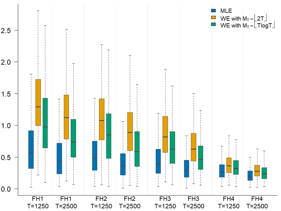
Clearly, the four Hawkes processes FH ${1.}$ –FH ${4.}$ share the same background rate $\mu_{1}$ , branching ratio $\nu_{11}$ and the scale parameter of the Mittag-Leffler kernel $c_{11}$ but differ in the tail of the ML kernel, which is controlled by $\beta_{11}$ . It can be seen that Theorem 3.3, which states the asymptotic normality of the WE, does not hold for FH1 and FH2 because $\int_{0}^{\infty}x^{\alpha}f_{\mathrm{ML}}(x;\beta_{11},c_{11})\mathrm{d}x=\infty$ for any $\alpha>0.5$ implied by $\beta_{11}\leqslant 0.5$ . From FH1 to FH4, the tail of the kernel becomes lighter. For each of the univariate Fractional Hawkes process, we generate 1000 independent copies on $(0,T)$ with $T=1250,2500$ . To study the effect of the number of Fourier frequencies, we choose $M_{T}=\lfloor 2T\rfloor$ and $\lfloor T\log T\rfloor$ . Table 1 of Appendix A contains the median (IQR) of the relative errors for all 1000 independent copies of each DGP. Table 2 of Appendix A contains the corresponding runtime for obtaining the estimates. Figure 1 of Appendix A is a graphical complement to Table 1.

Figure 1 and Tables 1–2 show a clear accuracy–speed tradeoff. The MLE is uniformly more accurate, but it is substantially slower to compute. This is unsurprising: under correct specification the MLE is asymptotically efficient, whereas its evaluation here requires repeated computation of (4.2), which is expensive because of the $O(n^{2})$ cost in the event count $n$ and the numerical burden of evaluating the Mittag-Leffler function. As the self-excitation kernel becomes lighter-tailed, the gap in accuracy between MLE and WE narrows. Regarding the choice of $M_{T}$ , both choices appear consistent, but $M_{T}=\lfloor T\log T\rfloor$ is usually slightly more accurate than $M_{T}=\lfloor 2T\rfloor$ ; that difference becomes small in the lighter-tailed cases. This is consistent with the findings of Bonnet et al. (2025, Section 5.1.2), who study the exponentially decaying case.

4.2 Bivariate Fractional Hawkes process

Let $N$ be a bivariate Fractional Hawkes process considered in Example 1. It can be shown that a necessary and sufficient condition for $N$ to be stationary is $0\leqslant\nu_{11},\nu_{22}<1$ , $\nu_{12}\nu_{21}<(1-\nu_{11})(1-\nu_{22})$ . The spectral density matrix is

\displaystyle\boldsymbol{f}_{2}(\omega)=\begin{pmatrix}f_{11}(\omega)&f_{12}(\omega)\\ f_{21}(\omega)&f_{22}(\omega)\end{pmatrix},

where

\displaystyle\boldsymbol{\lambda}=\begin{pmatrix}\lambda_{1}\\ \lambda_{2}\end{pmatrix}=(\boldsymbol{\mathrm{Id}}_{2}-\boldsymbol{\nu})^{-1}\boldsymbol{\mu}=\frac{1}{(1-\nu_{11})(1-\nu_{22})-\nu_{12}\nu_{21}}\begin{pmatrix}\mu_{1}(1-\nu_{22})+\mu_{2}\nu_{12}\\ \mu_{2}(1-\nu_{11})+\mu_{1}\nu_{21}\end{pmatrix},

\displaystyle f_{11}(\omega)=\frac{\lambda_{1}|1-\nu_{22}\hat{f}_{\mathrm{ML}}(\omega;\beta_{22},c_{22})|^{2}+\lambda_{2}|\nu_{12}\hat{f}_{\mathrm{ML}}(\omega;\beta_{12},c_{12})|^{2}}{|(1-\nu_{11}\hat{f}_{\mathrm{ML}}(\omega;\beta_{11},c_{11}))(1-\nu_{22}\hat{f}_{\mathrm{ML}}(\omega;\beta_{22},c_{22}))-\nu_{12}\hat{f}_{\mathrm{ML}}(\omega;\beta_{12},c_{12})\nu_{21}\hat{f}_{\mathrm{ML}}(\omega;\beta_{21},c_{21})|^{2}},

\displaystyle f_{12}(\omega)=\frac{\lambda_{1}(1-\nu_{22}\hat{f}_{\mathrm{ML}}(-\omega;\beta_{22},c_{22}))\nu_{21}\hat{f}_{\mathrm{ML}}(\omega;\beta_{21},c_{21})+\lambda_{2}\nu_{12}\hat{f}_{\mathrm{ML}}(-\omega;\beta_{12},c_{12})(1-\nu_{11}\hat{f}_{\mathrm{ML}}(-\omega;\beta_{11},c_{11}))}{|(1-\nu_{11}\hat{f}_{\mathrm{ML}}(\omega;\beta_{11},c_{11}))(1-\nu_{22}\hat{f}_{\mathrm{ML}}(\omega;\beta_{22},c_{22}))-\nu_{12}\hat{f}_{\mathrm{ML}}(\omega;\beta_{12},c_{12})\nu_{21}\hat{f}_{\mathrm{ML}}(\omega;\beta_{21},c_{21})|^{2}},

$f_{21}(\omega)=f_{12}(-\omega)$ and $f_{22}$ is obtained by swapping indices $1$ and $2$ in the expression of $f_{11}$ .

To demonstrate the consistency of the Whittle estimator, we consider the following data generating process:

FH5.

$N=(N_{1},N_{2})$ is a bivariate Fractional Hawkes process with $\boldsymbol{\mu}=(0.2,0.1)^{\top}$ (or equivalently, $\boldsymbol{\lambda}=(13/3,17/6)^{\top}$ ),

\displaystyle\boldsymbol{\nu}=\begin{pmatrix}0.3&1\\ 0.5&0.2\end{pmatrix},~\begin{pmatrix}c_{11}&c_{12}\\ c_{21}&c_{22}\end{pmatrix}=\begin{pmatrix}0.8&1.0\\ 0.9&1.1\end{pmatrix},~\begin{pmatrix}\beta_{11}&\beta_{12}\\ \beta_{21}&\beta_{22}\end{pmatrix}=\begin{pmatrix}0.75&0.85\\ 0.8&0.9\end{pmatrix}.

The parameters to be estimated are $\boldsymbol{\theta}=(\lambda_{1}^{-1},\lambda_{2}^{-1},\nu_{11},\nu_{21},\nu_{12},\nu_{22},\beta_{11},\beta_{21},\beta_{12},\beta_{22},c_{11},c_{21},c_{12},c_{22})$ . We generate $1000$ independent copies of $N$ on $(0,T)$ with $T=1250,~2500$ . Whittle estimator (WE) is then calculated for each of the copy. We choose $M_{T}=\lfloor 2T\rfloor$ and $\lfloor T\log T\rfloor$ for this experiment. The median and IQR (in brackets) of the relative errors are presented in Table 3 of Appendix A. A summary of the runtime is recorded in Table 4 of Appendix A. It seems that both choices of $M_{T}$ make the estimator consistent and the performance of WE with $M_{T}=\lfloor T\log T\rfloor$ is slightly better than that with $M_{T}=\lfloor 2T\rfloor$ .

4.3 Detecting independence among subprocesses

In this section, we will assess the performance of the simple test statistic (3.4), we consider the following multivariate stationary Fractional Hawkes processes:

FH6.

$N=(N_{1},N_{2})^{\top}$ is a class of bivariate stationary fractional Hawkes processes with $\boldsymbol{\mu}=(0.5,0.5)^{\top}$ ,

\displaystyle\boldsymbol{\nu}=\begin{pmatrix}1/2&a\\ b&1/2\end{pmatrix},~\begin{pmatrix}c_{11}&c_{12}\\ c_{21}&c_{22}\end{pmatrix}=\begin{pmatrix}1&1.1\\ 0.9&1\end{pmatrix},~\begin{pmatrix}\beta_{11}&\beta_{12}\\ \beta_{21}&\beta_{22}\end{pmatrix}=\begin{pmatrix}1&0.9\\ 0.8&1\end{pmatrix},

where $a,b\geqslant 0$ , $ab<1/4$ .

We can show that $\boldsymbol{\lambda}=(1/4-ab)^{-1}(1/4+a/2,1/4+b/2)^{\top}$ and therefore,

\displaystyle f_{12}(0)=f_{21}(0)=\frac{ab/2+(a+b)/8}{(1/4-ab)^{3}}.

(4.3)

It is easy to see that $f_{12}(0)$ is nonnegative, and equals $0$ if any only if $a=b=0$ . For any fixed $a$ (respectively $b$ ), $f_{12}(0)$ is a strictly monotonically increasing function of $b$ (respectively $a$ ). Moreover, the larger $a+b$ is, the more dependent $N_{1}$ and $N_{2}$ will be.

We select a set of grid points $a,b=0,0.1,0.2,0.3$ , resulting in 16 bivariate stationary Hawkes processes. For each process, we generate 1000 independent copies of $N$ on $(0,T)$ , where $T=5000$ . The number of Fourier frequencies is chosen to be $M_{T}=\lfloor 10\sqrt{T}\rfloor$ . For each realization, we calculate the p-value associated with (3.4) and reject the null hypothesis of independence when the p-value is less than $0.05$ . For simplicity, we adopt the ordinary least squares estimates when computing the test statistic (i.e. the kernel function is $K(x)=1$ ). In Table 5 of Appendix A, we report the percentage of realizations for which independence is rejected. Judging from Table 5, when $N_{1}$ and $N_{2}$ are indeed independent (i.e. $(a,b)=(0,0)$ ), only 22 out of 1000 realizations lead to rejection, which is reasonably close to the nominal $5\%$ level. When $\{a,b\}=\{0,0.1\}$ , the subprocesses are dependent but only weakly so in view of (4.3), and the test nevertheless rejects independence in over $90\%$ of realizations. For the remaining cases, the dependence signal reflected by (4.3) is strong enough that dependence is detected in every realization.

5 Discussion and outlook

In this paper, we established consistency and asymptotic normality of the Whittle estimator for multivariate stationary Hawkes processes. Our results accommodate heavy tailed kernels, a regime that while important to many applications (e.g. seismology), is often excluded from existing asymptotic theory. We use the reduced cumulant measures to yield frequency-domain asymptotics without relying on strong mixing and moment assumptions as in Cheysson. and Lang (2022). Finally, we showed that the same cumulant-based approach also leads to a simple and effective frequency-domain test for independence among subprocesses.

Recent years have seen proliferation of nonparametric inference of mutual-excitation kernels of Hawkes processes (Bonnet and Sangnier, 2025; Kim and Iwata, 2026) as well as the spectral density of time series (Tang et al., 2026). Despite the fact that this paper concerns parametric inference of Hawkes processes using Whittle likelihood, we believe the Whittle likelihood can also facilitate nonparametric modeling of Hawkes processes via Bartlett spectral density in terms of both theoretical soundness and computational cost.

Cross-validation is an important way to assess statistical model’s ability of prediction and is known to be difficult when there is only one realization of a point process. Recently, Herrera and Cheysson (2026) proposed a frequency-domain penalized least-square estimation procedure for Hawkes processes and conduct cross-validation with the help of a thinning mechanism inspired by Cronie et al. (2024). We anticipate that the proof techniques used in this paper can be of great help in discovering the asymptotic properties of the said cross-validation procedure. Furthermore, we believe that the Whittle estimation proposed in this paper will certainly benefit from the cross-validation procedure when applying to real-world data.

6 Acknowledgments

This work was supported by the Royal Society of New Zealand Marsden Fund under grants MFP-UOO2323 and MFP-UOO2518. The authors wish to acknowledge use of the eResearch Infrastructure Platform hosted by the Crown company, Research and Education Advanced Network New Zealand (REANNZ) Ltd., and funded by the Ministry of Business, Innovation & Employment. URL: https://www.reannz.co.nz

References

L. Adamopoulos (1976) Cluster models for earthquakes: regional comparisons. Journal of the International Association for Mathematical Geology 8, pp. 463–475. Cited by: §1.
E. Bacry and J.-F. Muzy (2016) First- and second-order statistics characterization of Hawkes processes and non-parametric estimation. IEEE Transactions on Information Theory 62 (4), pp. 2184–2202. Cited by: §1.
M. S. Bartlett (1963) The spectral analysis of point processes. Journal of the Royal Statistical Society - Series B 25, pp. 264–296. Cited by: §1.
A. Bonnet, F. Cheysson, M. M. Herrera, and M. Sangnier (2025) Spectral analysis for noisy hawkes processes inference. Scandinavian Journal of Statistics 52 (4), pp. 2061–2109. Cited by: §4.1.
A. Bonnet and M. Sangnier (2025) Nonparametric estimation of Hawkes processes with RKHSs. In Proceedings of The 28th International Conference on Artificial Intelligence and Statistics, Y. Li, S. Mandt, S. Agrawal, and E. Khan (Eds.), Proceedings of Machine Learning Research, Vol. 258, pp. 3574–3582. Cited by: §5.
P. Brémaud (2020) Point process calculus in time and space: an introduction with applications. edition, Vol. , Springer Cham, . Cited by: §2.
D. R. Brillinger (1972) The spectral analysis of stationary interval functions. In Proceedings of the Sixth Berkeley Symposium on Mathematical Statistics and Probability, Volume 1: Theory of Statistics, L. M. Le Cam, J. Neyman, and E. L. Scott (Eds.), pp. 483–513. Cited by: §1, §1, §2, §3.2, Remark.
D. R. Brillinger (2001) Time series: Data analysis and theory. edition, Society for Industrial and Applied Mathematic, Philadelphia, PA. Cited by: §E.2, §E.3.1, Proposition E.3, Appendix F, §1, §2.
J. Chen, A. G. Hawkes, and E. Scalas (2021) A fractional Hawkes process. In Nonlocal and Fractional Operators, L. Beghin, F. Mainardi, and R. Garrappa (Eds.), pp. 121–131. Cited by: §1, Example 1.
F. Cheysson. and G. Lang (2022) Spectral estimation of Hawkes processes from count data. The Annals of Statistics 50, pp. 1722–1746. Cited by: §1, §5, Remark.
O. Cronie, M. Moradi, and C. A. N. Biscio (2024) A cross-validation-based statistical theory for point processes. Biometrika 111 (2), pp. 625–641. Cited by: §5.
R. Dahlhaus and W. Polonik (2009) Empirical spectral processes for locally stationary time series. Bernoulli 15 (1), pp. 1–39. Cited by: Theorem E.1.
R. Dahlhaus (1988) Empirical spectral processes and their applications to time series analysis. Stochastic Processes and their Applications 30, pp. 69–83. Cited by: Proposition E.4, §1.
D. Daley and D. Vere-Jones (2003) An introduction to the theory of point processes. 2nd edition, Vol. 1, Springer-Verlag, New York. Cited by: §1, §1, §2, §2, §2, §2, §3.3, §4.1, Definition 1.
D. Daley and D. Vere-Jones (2008) An introduction to the theory of point processes. 2nd edition, Vol. 2, Springer, New York. Cited by: §2, Definition 2.
J. Davidson (1994) Stochastic limit theory: an introduction for econometricians. edition, Oxford University press, New York. Cited by: Theorem D.1.
L. Davis, B. Baeumer, and T. Wang (2024) A fractional Hawkes process model for earthquake aftershock sequences. Journal of the Royal Statistical Society Series C: Applied Statistics 73 (5), pp. 1185–1202. Cited by: §1, Example 1.
L. Davis, B. Baeumer, and T. Wang (2026) A multivariate fractional Hawkes process for multiple earthquake mainshock aftershock sequences. The American Statistician. External Links: Document Cited by: Example 1.
J.-L. Dupret and D. Hainaut (2025) A fractional Hawkes process for illiquidity modeling. Mathematics and Financial Economics 19 (), pp. 143–181. Cited by: §1.
K. Dzhaparidze (1986) Parameter estimation and hypothesis testing in spectral analysis of stationary time series. edition, Springer, New York. Cited by: §1.
J. Felsenstein (2004) Inferring phylogenies. edition, Sinauer Associates, Sunderland, Massachusetts. Cited by: §B.1.
R. Garrappa (2015) Numerical evaluation of two and three parameter Mittag-Leffler functions. SIAM Journal on Numerical Analysis 53 (3), pp. 1350–1369. Cited by: §4.1, Example 1.
G. Gill and P. Straka (2018) MittagLeffleR: using the Mittag-Leffler distributions in R. External Links: Link, Document Cited by: §4.1.
C. Godsil and G. F. Royle (2013) Algebraic graph theory. Vol. 207, Springer Science & Business Media. Cited by: Remark.
R. Gorenflo, J. Loutchko, and Y. Luchko (2002) Computation of the Mittag-Leffler function $E_{\alpha,\beta}(z)$ and its derivative. Fractional Calculus and Applied Analysis 5 (4), pp. 491–518. Cited by: Example 1.
N. Gupta and A. Maheshwari (2026) Tempered fractional Hawkes process and its generalizations. Journal of Mathematical Analysis and Applications 554 (2), pp. 129996. Cited by: §1.
C. Habyarimana, J. A. Aduda, E. Scalas, J. Chen, A. G. Hawkes, and F. Polito (2023) A fractional Hawkes process II: Further characterization of the process. Physica A 615 (), pp. 128596. Cited by: Example 1.
A. G. Hawkes and D. Oakes (1974) A cluster process representation of a self-exciting process. Journal of Applied Probability 11 (3), pp. 493–503. Cited by: §2.
A. G. Hawkes (1971) Spectra of some self-exciting and mutually exciting point processes. Biometrika 58, pp. 83–90. Cited by: §1, §2, Definition 1, Example 1.
A. G. Hawkes (2018) Hawkes processes and their applications to ﬁnance: a review. Quantitative Finance 18 (2), pp. 193–198. Cited by: §1.
M. Hazewinkel (1997) Encyclopedia of Mathematics, Supplement I. Kluwer Academic Publishers, Dordrehct. Cited by: Proposition E.3.
L. Heinrich (2016) On the strong Brillinger-mixing property of $\alpha$ -determinantal point processes and some applications. Applications of Mathematics 61 (4), pp. 443–461. Cited by: Remark.
M. M. Herrera and F. Cheysson (2026) Ridge-penalised spectral least-squares estimation for point processes. External Links: 2601.07490, Link Cited by: §5.
S. Jovanović, J. Hertz, and S. Rotter (2015) Cumulants of Hawkes point processes. Physical Review E 91, pp. 042802. Cited by: §B.1, §B.1, §B.1, Proposition B.2, §1, §2.
H. Kim and T. Iwata (2026) A representer theorem for Hawkes processes via penalized least squares minimization. In The Fourteenth International Conference on Learning Representations, Cited by: §5.
A. N. Kolmogorov and V. M. Tihomirov (1961) $\epsilon$ -Entropy and $\epsilon$ -capacity of sets in functional space. American Mathematical Society Translations 2 (17), pp. 277–364. Cited by: Theorem E.1.
V. Kotesovec (2014) Schroeder’s fourth problem, Entry A000311 in The On-Line Encyclopedia of Integer Sequences. Note: https://oeis.org/A000311Accessed: 2025-11-07 Cited by: §B.1.
T. J. Kozubowski (2001) Fractional moment estimation of Linnik and Mittag-Leffler parameters. Mathematical and Computer Modelling 34 (), pp. 1023–1035. Cited by: Example 1.
C. Kresin and F. Schoenberg (2023) Parametric estimation of spatial–temporal point processes using the Stoyan–Grabarnik statistic. Annals of the Institute of Statistical Mathematics 75 (6), pp. 887–909. Cited by: §1.
T. Leblanc (2024) Exponential moments for Hawkes processes under minimal assumptions. Electronic Communications in Probability 29 (), pp. 1–11. Cited by: §B.1.
T. McElroy and D. N. Politis (2025) Local quadratic spectral and covariance matrix estimation. Journal of Time Series Analysis 46 (), pp. 674–691. Cited by: §E.3.1, item 4, §3.3.
OEIS (2025) The on-line encyclopedia of integer sequences. Note: http://oeis.orgAccessed: 2025-11-07 Cited by: §B.1.
Y. Ogata (1978) The asymptotic behaviour of maximum likelihood estimators for stationary point processes. Annals of the Institute of Statistical Mathematics 30 (1), pp. 243–261. Cited by: §1.
J. G. Rasmussen (2013) Bayesian inference for Hawkes processes. Methodology and Computing in Applied Probability 15 (3), pp. 623–642. Cited by: §1.
A. Reinhart (2018) A review of self-exciting spatio-temporal point processes and their applications. Statistical Science 33 (3), pp. 299–318. Cited by: §1, §2.
F. P. Schoenberg (2013) Facilitated estimation of ETAS. Bulletin of the Seismological Society of America 103 (1), pp. 601–605. Cited by: §1.
Y. Tang, C. Kirch, J. E. Lee, and R. Meyer (2026) Bayesian nonparametric spectral analysis of locally stationary processes. Journal of the American Statistical Association. External Links: Document Cited by: §5.
P. Tuan (1981) Estimation of the spectral parameters of a stationary point process. The Annals of Statistics 9, pp. 615–627. Cited by: §1, §2.
A. van der Vaart and J. Wellner (1996) Weak convergence and empirical processes: with applications to statistics. edition, Springer, . Cited by: §E.2.
D. Vere-Jones and R. Davies (1966) A statistical survey of earthquakes in the main seismic region of New Zealand: part 2–Time series analyses. New Zealand Journal of Geology and Geophysics 9 (3), pp. 251–284. Cited by: §1.
P. Whittle (1953) The analysis of multiple stationary time series. Journal of the Royal Statistical Society: Series B (Methodological) 15 (1), pp. 125–139. Cited by: §1.
P. Whittle (1954) On stationary processes in the plane. Biometrika 41 (3–4), pp. 434–449. Cited by: §1.
J. Yang and Y. Guan (2026) Fourier analysis of spatial point processes. Bernoulli 32 (1), pp. 370–392. Cited by: §1.
V. A. Zorich (2015) Mathematical analysis. 6th edition, Vol. I, Springer, Burlington, Vermont, USA. Cited by: Remark.

\appendixpage

Appendix A Tables and figures

Refer to caption — Figure 1: The boxplot of relative errors (defined in (4.1)) of the estimates in Section 4.1. For the sake of visualization, the y-axis represents $\log(1+\mathrm{Relative~error)}$ . MLE is indicated by blue, WE with $M_{T}=\lfloor 2T\rfloor$ is in orange, and WE with $M_{T}=\lfloor T\log T\rfloor$ is in green.

Table 1: Median and IQR (in brackets) of relative errors (defined in (4.1)) of the Whittle and maximum likelihood estimates in Section 4.1.

DGP	MLE	WE with $M_{T}=\lfloor 2T\rfloor$	WE with $M_{T}=\lfloor T\log T\rfloor$
FH1. $T=1250$	0.7722(1.1229)	2.6463(2.8904)	1.6567(2.2685)
FH1. $T=2500$	0.5542(0.7814)	2.0731(2.1956)	1.0941(1.3383)
FH2. $T=1250$	0.6287(0.7856)	1.9359(1.9593)	1.3410(1.6462)
FH2. $T=2500$	0.4334(0.4999)	1.4316(1.5055)	0.8018(1.0401)
FH3. $T=1250$	0.4761(0.5885)	1.2638(1.3663)	0.8732(0.9758)
FH3. $T=2500$	0.3364(0.3676)	0.8732(0.8504)	0.5884(0.6160)
FH4. $T=1250$	0.3120(0.2614)	0.4386(0.3395)	0.3787(0.3088)
FH4. $T=2500$	0.2175(0.1827)	0.3227(0.2292)	0.2671(0.2244)

Table 2: Median and IQR (in brackets) of runtime (in minutes) of calculating the Whittle and maximum likelihood estimates in Section 4.1. For comparison, we use a fixed initial value for optimization procedure across all realizations.

DGP	MLE	WE with $M_{T}=\lfloor 2T\rfloor$	WE with $M_{T}=\lfloor T\log T\rfloor$
FH1. $T=1250$	3.0165(1.4670)	0.0117(0.0021)	0.0383(0.0063)
FH1. $T=2500$	10.9002(5.8283)	0.0405(0.0039)	0.1616(0.0141)
FH2. $T=1250$	2.4757(1.2086)	0.0119(0.0019)	0.0410(0.0064)
FH2. $T=2500$	7.9377(3.0711)	0.0422(0.0036)	0.1592(0.0120)
FH3. $T=1250$	3.4843(1.9421)	0.0111(0.0017)	0.0393(0.0045)
FH3. $T=2500$	9.4609(3.6281)	0.0399(0.0026)	0.1524(0.0089)
FH4. $T=1250$	3.6125(1.7914)	0.0116(0.0015)	0.0420(0.0041)
FH4. $T=2500$	15.7390(5.2685)	0.0447(0.0030)	0.1630(0.0081)

Table 3: Median and IQR (in brackets) of relative errors (defined in (4.1)) of the Whittle estimates in Section 4.2.

DGP	WE with $M_{T}=\lfloor 2T\rfloor$	WE with $M_{T}=\lfloor T\log T\rfloor$
FH5. $T=1250$	2.0966(0.9756)	1.7695(0.8302)
FH5. $T=2500$	1.5519(0.7381)	1.2824(0.6272)

Table 4: Median and IQR (in brackets) of runtime (in minutes) of calculating the Whittle and maximum likelihood estimates in Section 4.2. For comparison, we use a fixed initial value for the optimization procedure across all realizations.

DGP	WE with $M_{T}=\lfloor 2T\rfloor$	WE with $M_{T}=\lfloor T\log T\rfloor$
FH5. $T=1250$	0.0121(0.0012)	0.0423(0.0056)
FH5. $T=2500$	0.0238(0.0021)	0.0776(0.0319)

Table 5: Percentage of realizations in Section 4.3 for which the null hypothesis of independence is rejected at level

0.05

	0	0.1	0.2	0.3
0	2.2%	92.9%	100%	100%
0.1	96%	100%	100%	100%
0.2	100%	100%	100%	100%
0.3	100%	100%	100%	100%

Appendix B Results concerning the reduced cumulant measures and associated quantities

B.1 Proof of Proposition 2.1

For any $s\geqslant 2$ and any $j_{1},\cdots,j_{s}\in\{1,\cdots,D\}$ , $C_{j_{1}\cdots j_{s}}$ , and consequently $C_{j_{1}\cdots j_{s}}^{\mathrm{red}}$ exist because $\mathrm{E}\exp(a\sum_{j=1}^{D}N_{j}(A))<\infty$ for some $a>0$ and any bounded $A\subset\mathbb{R}$ (see Theorem 1 of Leblanc [2024]). The non-negativity of $C_{j_{1}\cdots j_{s}}$ and $C_{j_{1}\cdots j_{s}}^{\mathrm{red}}$ can be seen from equation (24) of Jovanović et al. [2015]. In order to show the finiteness of $C_{j_{1}\cdots j_{s}}^{\mathrm{red}}$ , we need some notation. Let $k^{j_{1}\cdots j_{s}}(x_{1},\cdots,x_{s})$ be defined in equation (21) of Jovanović et al. [2015]. Then we have $\mathrm{d}C_{j_{1}\cdots j_{s}}(x_{1},\cdots,x_{s})=k^{j_{1}\cdots j_{s}}(x_{1},\cdots,x_{s})\mathrm{d}x_{1}\cdots\mathrm{d}x_{s}$ . Therefore, we only need to show that

\displaystyle C_{j_{1}\cdots j_{s}}^{\mathrm{red}}(\mathbb{R}^{s-1})=\int_{\mathbb{R}^{s-1}}k^{j_{1}\cdots j_{s}}(x_{1},\cdots,x_{s-1},x_{s})\mathrm{d}x_{1}\cdots\mathrm{d}x_{s-1}

is finite. Note that the right-hand side of the equation is invariant with respect to $x_{s}$ due to the stationarity of $N$ . The finiteness of the right-hand side can be seen from equation (50) of Jovanović et al. [2015].

To derive a stronger upperbound, we need to delve into the crucial tree representation of the cumulant measures derived in Jovanović et al. [2015]. Recall that $\boldsymbol{\nu}=(\nu_{ij})_{i,j=1,\cdots,D}$ happens to be the integral of the excitation matrix over $\mathbb{R}$ (i.e. the matrix $\mathbf{G}$ in equation (13) of Jovanović et al. [2015]). Let $\boldsymbol{\Psi}=\sum_{k=1}^{\infty}\boldsymbol{\nu}^{k}$ , $\mathbf{R}=\boldsymbol{\Psi}+\boldsymbol{\mathrm{I}}_{D}$ , $R=\max_{1\leqslant i,j\leqslant D}[\mathbf{R}]_{ij}$ , $\psi=\max_{1\leqslant i,j\leqslant D}[\boldsymbol{\Psi}]_{ij}$ and $\lambda=\max_{1\leqslant i\leqslant D}[\mathbf{R}\boldsymbol{\mu}]_{i}$ , where $\boldsymbol{\mu}$ is the vector of background rates and $\boldsymbol{\mathrm{I}}_{D}$ is the $D$ -dimensional identity matrix. The above Neumann series is convergent due to the fact that the spectral radius of $\boldsymbol{\nu}$ is smaller than 1. It is worth noting that $R>\max\{1,\psi\}$ . In view of the algorithm at the end of section 3 of Jovanović et al. [2015], we have $C_{j_{1}\cdots j_{s}}^{\mathrm{red}}(\mathbb{R}^{s-1})=\sum_{i}\int_{\mathbb{R}^{s-1}}k_{i}^{j_{1}\cdots j_{s}}(x_{1},\cdots,x_{s})\mathrm{d}x_{1}\cdots\mathrm{d}x_{s-1}$ , where $k_{i}^{j_{1}\cdots j_{s}}$ is generated by steps (2) and (3) of the above-mentioned algorithm and the summation is over all rooted multifurcation trees with $s$ labelled leaves. According to Chapter 3 of Felsenstein [2004], the number of internal nodes $m_{i}$ of tree $i$ (with which $k_{i}^{j_{1}\cdots j_{s}}$ is associated) ranges from $1$ to $s-1$ . Moreover, it can be seen from Section 4 of Jovanović et al. [2015] that

	$\displaystyle\int_{\mathbb{R}^{s-1}}k_{i}^{j_{1}\cdots j_{s}}(x_{1},\cdots,x_{s})\mathrm{d}x_{1}\cdots\mathrm{d}x_{s-1}$
	$\displaystyle\leqslant\sum_{p_{1},\cdots,p_{m_{i}}=1}^{D}\lambda R^{s}\psi^{m_{i}-1}=\lambda R^{s}D^{m_{i}}\psi^{m_{i}-1}\leqslant\lambda R^{s+m_{i}-1}D^{m_{i}}\leqslant\lambda R^{2s-2}D^{s-1}.$

Note that the right-hand side of the inequality is independent of $i$ . Therefore, we get $C_{j_{1}\cdots j_{s}}^{\mathrm{red}}(\mathbb{R}^{s-1})\leqslant\lambda R^{2s-2}D^{s-1}T_{s}$ , where $T_{s}$ is the number of rooted multifurcation trees with $s$ labelled leaves. Although there is no closed-form formula for $T_{s}$ , it is known (see e.g. entry A000311 of On-Line Encyclopedia of Integer Sequences [OEIS, 2025]) that $T_{s}\sim s^{s-1}2^{-1/2}\exp(-s)(2\log 2-1)^{-s+1/2}$ [Kotesovec, 2014] when $s\rightarrow\infty$ . This asymptotic relation, in conjunction with the Stirling’s formula $s!\sim\sqrt{2\pi}s^{s+1/2}\exp(-s)$ , imply that there exists constant $C_{0}>0$ such that

\displaystyle C_{j_{1}\cdots j_{s}}^{\mathrm{red}}(\mathbb{R}^{s-1})\leqslant C_{0}^{s}(s-1)!.

B.2 Second-order tail measures

The first proposition reveals the connection between the moments of mutual-excitation kernels and that of the convolution of the kernels, which plays an important role in the construction of cumulant density of Hawkes processes.

Proposition B.1.

Let $\boldsymbol{K}(\cdot)=\boldsymbol{\nu}\odot\boldsymbol{G}(\cdot)$ , where $\boldsymbol{\nu}=\{\nu_{ij}\}_{i,j=1,\cdots,D}$ is a $D\times D$ matrix whose entries are all nonnegative, $\boldsymbol{G}(\cdot)=\{g_{ij}(\cdot)\}_{i,j=1,\cdots,D}$ is a $D\times D$ matrix of probability density functions satisfying $\max_{i,j}\int_{\mathbb{R}}|x|^{\alpha}g_{ij}(x)\mathrm{d}x<\infty$ for some $0<\alpha\leqslant 1$ , and $\odot$ means the Hadamard (element-wise) product of matrices. Let $\boldsymbol{K}^{*1}(\cdot)=\boldsymbol{K}(\cdot)$ , $\boldsymbol{K}^{*(m+1)}(x)=\int_{\mathbb{R}}\boldsymbol{K}^{*(m)}(x-y)\boldsymbol{K}(y)\mathrm{d}y$ , $k\in\mathbb{N}$ . Then for any $m\in\mathbb{N}$ and any $i,j=1,\cdots,D$ , $\int_{\mathbb{R}}|x|^{\alpha}[\boldsymbol{K}^{*m}(x)]_{ij}\mathrm{d}x\leqslant m[\boldsymbol{\nu}^{m}]_{ij}\max_{a,b}\int_{\mathbb{R}}|x|^{\alpha}g_{ab}(x)\mathrm{d}x$ .

Proof.

First, note that $\int_{\mathbb{R}}\boldsymbol{K}^{*(m)}(x)\mathrm{d}x=\boldsymbol{\nu}^{m}$ as the convolution of probability density functions is again a probability density function. We will now prove the proposition by induction.

When $m=1$ , the proposition can be verified directly. Suppose now the proposition holds for $m=n$ , then when $m=n+1$ , since $|u+v|^{\alpha}\leqslant|u|^{\alpha}+|v|^{\alpha}$ for any $u,v\in\mathbb{R}$ , we have

	$\displaystyle\int_{\mathbb{R}}\|x\|^{\alpha}[\boldsymbol{K}^{(n+1)}(x)]_{ij}\mathrm{d}x=\int_{\mathbb{R}}\int_{\mathbb{R}}\|x\|^{\alpha}[\boldsymbol{K}^{(n)}(x-y)\boldsymbol{K}(y)]_{ij}\mathrm{d}y\mathrm{d}x$
	$\displaystyle\leqslant\int_{\mathbb{R}}\int_{\mathbb{R}}\|z\|^{\alpha}[\boldsymbol{K}^{(n)}(z)\boldsymbol{K}(y)]_{ij}\mathrm{d}y\mathrm{d}z+\int_{\mathbb{R}}\int_{\mathbb{R}}\|y\|^{\alpha}[\boldsymbol{K}^{(n)}(z)\boldsymbol{K}(y)]_{ij}\mathrm{d}y\mathrm{d}z$
	$\displaystyle=\sum_{k=1}^{D}\int_{\mathbb{R}}\|z\|^{\alpha}[\boldsymbol{K}^{(n)}(z)]_{ik}\mathrm{d}z\int_{\mathbb{R}}[\boldsymbol{K}(y)]_{kj}\mathrm{d}y+\sum_{k=1}^{D}\int_{\mathbb{R}}[\boldsymbol{K}^{(n)}(z)]_{ik}\mathrm{d}z\int_{\mathbb{R}}[\|y\|^{\alpha}\boldsymbol{K}(y)]_{kj}\mathrm{d}y$
	$\displaystyle\leqslant n\left(\sum_{k=1}^{D}[\boldsymbol{\nu}^{n}]_{ik}\nu_{kj}\right)\max_{a,b}\int_{\mathbb{R}}\|x\|^{\alpha}g_{ab}(x)\mathrm{d}x+\left(\sum_{k=1}^{D}[\boldsymbol{\nu}^{n}]_{ik}\nu_{kj}\right)\max_{a,b}\int_{\mathbb{R}}\|x\|^{\alpha}g_{ab}(x)\mathrm{d}x$
	$\displaystyle=(n+1)[\boldsymbol{\nu}^{n+1}]_{ij}\max_{a,b}\int_{\mathbb{R}}\|x\|^{\alpha}g_{ab}(x)\mathrm{d}x$

for any $i,j=1,\cdots,D$ . This concludes the proof. ∎

Proposition B.2.

If the mutual-excitation kernels $g_{ij}$ , $i,j=1,\cdots,D$ of the Hawkes process satisfy $\max_{i,j}\int_{\mathbb{R}}|x|^{\beta}g_{ij}(x)\mathrm{d}x<\infty$ for some $0<\beta\leqslant 1$ , then $\sum_{i,j}\int_{\mathbb{R}}|u|^{\beta}\mathrm{d}C_{ij}^{\mathrm{red}}(u)<\infty$ .

Proof.

Let $\boldsymbol{K}(\cdot)=\boldsymbol{\nu}\odot\boldsymbol{G}(\cdot)$ , $\boldsymbol{\lambda}=(\lambda_{1},\cdots,\lambda_{D})^{\top}=(\boldsymbol{\mathrm{I}}_{D}-\boldsymbol{\nu})^{-1}\boldsymbol{\mu}$ where $\boldsymbol{\nu}$ , $\boldsymbol{\mu}$ and $\boldsymbol{G}(\cdot)$ are defined in Definition 1. Define $\Psi_{t}^{ij}=[\sum_{n=1}^{\infty}\boldsymbol{K}^{*n}(t)]_{ij}$ and $R_{t}^{ij}=\mathds{1}_{\{i=j\}}\delta(t)+\Psi_{t}^{ij}$ , $i,j=1,\cdots,D$ , where $\boldsymbol{K}^{*n}(\cdot)$ is the matrix function convolution defined in Proposition B.1 and $\delta(\cdot)$ is the Dirac delta function. It is worth noting that $\int_{\mathbb{R}}\Psi_{t}^{ij}\mathrm{d}t=\sum_{n=1}^{\infty}[\boldsymbol{\nu}^{n}]_{ij}=[(\boldsymbol{\mathrm{I}}_{D}-\boldsymbol{\nu})^{-1}\boldsymbol{\nu}]_{ij}$ in view of the proof of Proposition B.1 and the fact that the spectral radius of $\boldsymbol{\nu}$ is smaller than 1. Taking into account equation (37) of Jovanović et al. [2015] and $|x+y|^{\beta}\leqslant|x|^{\beta}+|y|^{\beta}$ for any $x,y\in\mathbb{R}$ , we have

	$\displaystyle\int_{\mathbb{R}}\|u\|^{\beta}\mathrm{d}C_{ij}^{\mathrm{red}}(u)=\sum_{m=1}^{D}\lambda_{m}\int_{\mathbb{R}}\int_{\mathbb{R}}\|u\|^{\beta}R_{u-v}^{im}R_{-v}^{mj}\mathrm{d}v\mathrm{d}u$
	$\displaystyle=\sum_{m=1}^{D}\lambda_{m}\int_{\mathbb{R}}\int_{\mathbb{R}}\|u\|^{\beta}\Psi_{u+v}^{im}\Psi_{v}^{mj}\mathrm{d}v\mathrm{d}u+(\lambda_{i}+\lambda_{j})\int_{\mathbb{R}}\|u\|^{\beta}\Psi_{u}^{ij}\mathrm{d}u$
	$\displaystyle\leqslant\sum_{m=1}^{D}\lambda_{m}\int_{\mathbb{R}}\int_{\mathbb{R}}\|x\|^{\beta}\Psi_{x}^{im}\Psi_{y}^{mj}\mathrm{d}x\mathrm{d}y+\sum_{m=1}^{D}\lambda_{m}\int_{\mathbb{R}}\int_{\mathbb{R}}\|y\|^{\beta}\Psi_{x}^{im}\Psi_{y}^{mj}\mathrm{d}x\mathrm{d}y+(\lambda_{i}+\lambda_{j})\int_{\mathbb{R}}\|u\|^{\beta}\Psi_{u}^{ij}\mathrm{d}u$
	$\displaystyle\leqslant\sum_{m=1}^{D}\lambda_{m}[(\boldsymbol{\mathrm{I}}_{D}-\boldsymbol{\nu})^{-1}\boldsymbol{\nu}]_{mj}\int_{\mathbb{R}}\|x\|^{\beta}\Psi_{x}^{im}\mathrm{d}x+\sum_{m=1}^{D}\lambda_{m}[(\boldsymbol{\mathrm{I}}_{D}-\boldsymbol{\nu})^{-1}\boldsymbol{\nu}]_{im}\int_{\mathbb{R}}\|y\|^{\beta}\Psi_{y}^{mj}\mathrm{d}y+(\lambda_{i}+\lambda_{j})\int_{\mathbb{R}}\|u\|^{\beta}\Psi_{u}^{ij}\mathrm{d}u$

for any $i,j=1,\cdots,D$ . The proof is completed by noting that

	$\displaystyle\int_{\mathbb{R}}\|x\|^{\beta}\Psi_{x}^{pq}\mathrm{d}x=\sum_{l=1}^{\infty}\int_{\mathbb{R}}\|x\|^{\beta}[\boldsymbol{K}^{*l}(x)]_{pq}\mathrm{d}x\leqslant\left(\sum_{l=1}^{\infty}l[\boldsymbol{\nu}^{l}]_{pq}\right)\max_{a,b}\int_{\mathbb{R}}\|x\|^{\alpha}g_{ab}(x)\mathrm{d}x$
	$\displaystyle=[(\boldsymbol{\mathrm{I}}_{D}-\boldsymbol{\nu})^{-2}\boldsymbol{\nu}]_{pq}\max_{a,b}\int_{\mathbb{R}}\|x\|^{\alpha}g_{ab}(x)\mathrm{d}x<\infty$

for any $p,q=1,\cdots,D$ due to Proposition B.1. ∎

Appendix C Cumulants of finite Fourier transform and the Whittle likelihood

This section contains results about the asymptotic behavior of the cumulants of the finite Fourier transform. There are the building blocks of the functional CLT of the spectral empirical process.

C.1 Decompositions concerning second-order cumulants

The following function is needed in the decomposition of the second-order cumulants of the finite Fourier transform.

Proposition C.1.

	$\displaystyle R_{T,2}(u,\bar{\omega}):=\int_{\mathbb{R}}(\mathds{1}_{\{0<\frac{u+v}{T}<1\}}-1)\mathds{1}_{\{0<\frac{v}{T}<1\}}\exp(-\mathrm{i}\bar{\omega}v)\mathrm{d}v$
	$\displaystyle=-\mathds{1}_{\{\|u\|\geqslant T\}}\Delta_{T}(\bar{\omega})-\mathds{1}_{\{\|u\|<T\}}S_{T,2}(u,\bar{\omega}).$

where $\Delta_{T}(\bar{\omega})=\int_{0}^{T}\exp(-\mathrm{i}\bar{\omega}v)\mathrm{d}v$ is the Dirichlet kernel,

		$\displaystyle S_{T,2}(u,\bar{\omega}):=\mathds{1}_{\{u\geqslant 0\}}\int_{T-u}^{T}\exp(-\mathrm{i}\bar{\omega}v)\mathrm{d}v+\mathds{1}_{\{u<0\}}\int_{0}^{-u}\exp(-\mathrm{i}\bar{\omega}v)\mathrm{d}v$		(C.1)
		$\displaystyle=\mathds{1}_{\{\bar{\omega}=0\}}\|u\|+\mathds{1}_{\{\bar{\omega}\neq 0\}}\left(\mathds{1}_{\{u\geqslant 0\}}\frac{\exp(-\mathrm{i}\bar{\omega}T)(1-\exp(\mathrm{i}\bar{\omega}u))}{-\mathrm{i}\bar{\omega}}+\mathds{1}_{\{u<0\}}\frac{1-\exp(\mathrm{i}\bar{\omega}u)}{\mathrm{i}\bar{\omega}}\right)$

satisfying $|S_{T,2}(u,\bar{\omega})|\leqslant|u|$ for any $u,\bar{\omega}\in\mathbb{R}$ .

Proof.

	$\displaystyle\int_{\mathbb{R}}(\mathds{1}_{\{0<\frac{u+v}{T}<1\}}-1)\mathds{1}_{\{0<\frac{v}{T}<1\}}\exp(-\mathrm{i}\bar{\omega}v)\mathrm{d}v=\int_{0}^{T}(\mathds{1}_{\{0<\frac{u+v}{T}<1\}}-1)\exp(-\mathrm{i}\bar{\omega}v)\mathrm{d}v$
	$\displaystyle=-\mathds{1}_{\{u\geqslant 0\}}\int_{\max\{T-u,0\}}^{T}\exp(-\mathrm{i}\bar{\omega}v)\mathrm{d}v-\mathds{1}_{\{u<0\}}\int_{0}^{\min\{-u,T\}}\exp(-\mathrm{i}\bar{\omega}v)\mathrm{d}v.$

When $|u|\geqslant T$ , we have

	$\displaystyle-\mathds{1}_{\{u\geqslant 0\}}\int_{\max\{T-u,0\}}^{T}\exp(-\mathrm{i}\bar{\omega}v)\mathrm{d}v-\mathds{1}_{\{u<0\}}\int_{0}^{\min\{-u,T\}}\exp(-\mathrm{i}\bar{\omega}v)\mathrm{d}v$
	$\displaystyle=-\int_{0}^{T}\exp(-\mathrm{i}\bar{\omega}v)\mathrm{d}v=-\Delta_{T}(\bar{\omega}).$

When $|u|<T$ ,

	$\displaystyle-\mathds{1}_{\{u\geqslant 0\}}\int_{\max\{T-u,0\}}^{T}\exp(-\mathrm{i}\bar{\omega}v)\mathrm{d}v-\mathds{1}_{\{u<0\}}\int_{0}^{\min\{-u,T\}}\exp(-\mathrm{i}\bar{\omega}v)\mathrm{d}v$
	$\displaystyle=-\mathds{1}_{\{u\geqslant 0\}}\int_{T-u}^{T}\exp(-\mathrm{i}\bar{\omega}v)\mathrm{d}v-\mathds{1}_{\{u<0\}}\int_{0}^{-u}\exp(-\mathrm{i}\bar{\omega}v)\mathrm{d}v=-S_{T,2}(u,\bar{\omega}).$

Moreover,

	$\displaystyle\|S_{T,2}(u,\bar{\omega})\|=\left\|\mathds{1}_{\{u\geqslant 0\}}\int_{T-u}^{T}\exp(-\mathrm{i}\bar{\omega}v)\mathrm{d}v+\mathds{1}_{\{u<0\}}\int_{0}^{-u}\exp(-\mathrm{i}\bar{\omega}v)\mathrm{d}v\right\|$
	$\displaystyle\leqslant\mathds{1}_{\{u\geqslant 0\}}\int_{T-u}^{T}\mathrm{d}v+\mathds{1}_{\{u<0\}}\int_{0}^{-u}\mathrm{d}v\leqslant\|u\|$

holds for any $u,\bar{\omega}\in\mathbb{R}$ . When $\bar{\omega}=0$ , $S_{T,2}(u,\bar{\omega})=|u|$ . When $\bar{\omega}\neq 0$ , straightforward calculations yield Equation (C.1). ∎

The following proposition introduces a useful decomposition of the second-order cumulants of the finite Fourier transform.

Proposition C.2.

For any $\omega_{1},~\omega_{2}\in\mathbb{R}$ and any $j_{1},j_{2}\in\{1,\cdots,D\}$ ,

	$\displaystyle\mathrm{cum}(J_{T}^{j_{1}}(\omega_{1}),J_{T}^{j_{2}}(\omega_{2}))=T^{-1}\Delta_{T}(\omega_{1}+\omega_{2})\left(f_{j_{1}j_{2}}(\omega_{1})-\int_{\|u\|\geqslant T}\exp(-\mathrm{i}\omega_{1}u)\mathrm{d}C_{j_{1}j_{2}}^{\mathrm{red}}(u)\right)$
	$\displaystyle-T^{-1}\int_{\|u\|<T}S_{T,2}(u,\omega_{1}+\omega_{2})\exp(-\mathrm{i}\omega_{1}u)\mathrm{d}C_{j_{1}j_{2}}^{\mathrm{red}}(u),$

where $\Delta_{T}(\bar{\omega})$ and $S_{T,2}(u,\bar{\omega})$ are defined in Proposition C.1.

Proof.

In view of Definition 2 and Equation (2.3), we have by direct calculation

	$\displaystyle\mathrm{cum}(J_{T}^{j_{1}}(\omega_{1}),J_{T}^{j_{2}}(\omega_{2}))=T^{-1}\int_{0}^{T}\int_{0}^{T}\exp(-\mathrm{i}\omega_{1}x)\exp(-\mathrm{i}\omega_{2}y)\mathrm{d}C_{j_{1}j_{2}}(x,y)$
	$\displaystyle=T^{-1}\int_{\mathbb{R}}\int_{\mathbb{R}}\mathds{1}_{\{0<x<T\}}\mathds{1}_{\{0<y<T\}}\exp(-\mathrm{i}\omega_{1}x)\exp(-\mathrm{i}\omega_{2}y)\mathrm{d}C_{j_{1}j_{2}}^{\mathrm{red}}(x-y)\mathrm{d}y$
	$\displaystyle=T^{-1}\int_{\mathbb{R}}\int_{\mathbb{R}}\mathds{1}_{\{0<u+v<T\}}\mathds{1}_{\{0<v<T\}}\exp(-\mathrm{i}\omega_{1}u)\exp(-\mathrm{i}(\omega_{1}+\omega_{2})v)\mathrm{d}C_{j_{1}j_{2}}^{\mathrm{red}}(u)\mathrm{d}v$
	$\displaystyle=T^{-1}\int_{\mathbb{R}}\exp(-\mathrm{i}\omega_{1}u)\int_{\mathbb{R}}\mathds{1}_{\{0<u+v<T\}}\mathds{1}_{\{0<v<T\}}\exp(-\mathrm{i}(\omega_{1}+\omega_{2})v)\mathrm{d}v\mathrm{d}C_{j_{1}j_{2}}^{\mathrm{red}}(u)$
	$\displaystyle=T^{-1}\int_{\mathbb{R}}\exp(-\mathrm{i}\omega_{1}u)\left(R_{T,2}(u,\omega_{1}+\omega_{2})+\Delta_{T}(\omega_{1}+\omega_{2})\right)\mathrm{d}C_{j_{1}j_{2}}^{\mathrm{red}}(u)$
	$\displaystyle=T^{-1}\Delta_{T}(\omega_{1}+\omega_{2})\int_{\mathbb{R}}\exp(-\mathrm{i}\omega_{1}u)\mathrm{d}C_{j_{1}j_{2}}^{\mathrm{red}}(u)+T^{-1}\int_{\mathbb{R}}\exp(-\mathrm{i}\omega_{1}u)R_{T,2}(u,\omega_{1}+\omega_{2})\mathrm{d}C_{j_{1}j_{2}}^{\mathrm{red}}(u)$
	$\displaystyle=T^{-1}\Delta_{T}(\omega_{1}+\omega_{2})f_{j_{1}j_{2}}(\omega_{1})+T^{-1}\int_{\mathbb{R}}\exp(-\mathrm{i}\omega_{1}u)R_{T,2}(u,\omega_{1}+\omega_{2})\mathrm{d}C_{j_{1}j_{2}}^{\mathrm{red}}(u),$

where $f_{j_{1}j_{2}}$ comes from Definition 3. Since $R_{T,2}(u,\bar{\omega})=-\mathds{1}_{\{|u|\geqslant T\}}\Delta_{T}(\bar{\omega})-\mathds{1}_{\{|u|<T\}}S_{T,2}(u,\bar{\omega})$ according to Proposition C.1, we get

	$\displaystyle\int_{\mathbb{R}}\exp(-\mathrm{i}\omega_{1}u)R_{T,2}(u,\omega_{1}+\omega_{2})\mathrm{d}C_{j_{1}j_{2}}^{\mathrm{red}}(u)$
	$\displaystyle=-\Delta_{T}(\omega_{1}+\omega_{2})\int_{\|u\|\geqslant T}\exp(-\mathrm{i}\omega_{1}u)\mathrm{d}C_{j_{1}j_{2}}^{\mathrm{red}}(u)-\int_{\|u\|<T}S_{T,2}(u,\omega_{1}+\omega_{2})\exp(-\mathrm{i}\omega_{1}u)\mathrm{d}C_{j_{1}j_{2}}^{\mathrm{red}}(u).$

Putting things together, we finally have

	$\displaystyle\mathrm{cum}(J_{T}(\omega_{1}),J_{T}(\omega_{2}))=T^{-1}f_{j_{1}j_{2}}(\omega_{1})\Delta_{T}(\omega_{1}+\omega_{2})$
	$\displaystyle-T^{-1}\Delta_{T}(\omega_{1}+\omega_{2})\int_{\|u\|\geqslant T}\exp(-\mathrm{i}\omega_{1}u)\mathrm{d}C_{j_{1}j_{2}}^{\mathrm{red}}(u)-T^{-1}\int_{\|u\|<T}S_{T,2}(u)\exp(-\mathrm{i}\omega_{1}u)\mathrm{d}C_{j_{1}j_{2}}^{\mathrm{red}}(u)$
	$\displaystyle=T^{-1}\Delta_{T}(\omega_{1}+\omega_{2})\left(f_{j_{1}j_{2}}(\omega_{1})-\int_{\|u\|\geqslant T}\exp(-\mathrm{i}\omega_{1}u)\mathrm{d}C_{j_{1}j_{2}}^{\mathrm{red}}(u)\right)-T^{-1}\int_{\|u\|<T}S_{T,2}(u)\exp(-\mathrm{i}\omega_{1}u)\mathrm{d}C_{j_{1}j_{2}}^{\mathrm{red}}(u).$

∎

Corollary C.1.

For any $s_{1},s_{2}\in\mathbb{Z}$ , $j_{1},j_{2}\in\{1,\cdots,D\}$ ,

		$\displaystyle\mathrm{cum}(J_{T}^{j_{1}}(2\pi s_{1}/T),J_{T}^{j_{2}}(2\pi s_{2}/T))=\mathds{1}_{\{s_{1}+s_{2}=0\}}\left(f_{j_{1}j_{2}}(2\pi s_{1}/T)-\int_{\|u\|\geqslant T}\exp(-\mathrm{i}2\pi s_{1}u/T)\mathrm{d}C_{j_{1}j_{2}}^{\mathrm{red}}(u)\right)$
		$\displaystyle-T^{-1}\int_{\|u\|<T}S_{T,2}(u,2\pi(s_{1}+s_{2})/T)\exp(-\mathrm{i}2\pi s_{1}u/T)\mathrm{d}C_{j_{1}j_{2}}^{\mathrm{red}}(u)$		(C.2)
		$\displaystyle=\mathds{1}_{\{s_{1}+s_{2}=0\}}\left(f_{j_{1}j_{2}}(2\pi s_{1}/T)-\int_{\|u\|\geqslant T}\exp(-\mathrm{i}2\pi s_{1}u/T)\mathrm{d}C_{j_{1}j_{2}}^{\mathrm{red}}(u)-\frac{1}{T}\int_{\|u\|<T}\|u\|\exp(-\mathrm{i}2\pi s_{1}u/T)\mathrm{d}C_{j_{1}j_{2}}^{\mathrm{red}}(u)\right)$
		$\displaystyle-\mathds{1}_{\{s_{1}+s_{2}\neq 0\}}V_{T}^{j_{1}j_{2}}(s_{1},s_{2}),$		(C.3)

where

\displaystyle V_{T}^{j_{1}j_{2}}(s_{1},s_{2})=\frac{1}{T}\int_{|u|<T}\left(-\mathds{1}_{\{u\geqslant 0\}}+\mathds{1}_{\{u<0\}}\right)\frac{1-\exp(\mathrm{i}2\pi(s_{1}+s_{2})u/T)}{\mathrm{i}2\pi(s_{1}+s_{2})/T}\mathrm{d}C_{j_{1}j_{2}}^{\mathrm{red}}(u).

Furthermore, we have $\mathds{1}_{\{s_{1}+s_{2}\neq 0\}}V_{T}^{j_{1}j_{2}}(s_{1},s_{2})=o(1)$ and

\displaystyle\mathrm{cum}(J_{T}^{j_{1}}(2\pi s_{1}/T),J_{T}^{j_{2}}(2\pi s_{2}/T))=\mathds{1}_{\{s_{1}+s_{2}=0\}}(f_{j_{1}j_{2}}(2\pi s_{1}/T)+o(1))+\mathds{1}_{\{s_{1}+s_{2}\neq 0\}}o(1).

All $o$ and $O$ terms are independent of $s_{1}$ , $s_{2}$ .

Proof.

Notice that $\Delta_{T}(2\pi s/T)=T\mathds{1}_{\{s=0\}}$ for any $s\in\mathbb{Z}$ , then (C.1) is a direct consequence of Proposition C.2. (C.3) can be derived from (C.1) and (C.1) by noting

	$\displaystyle S_{T,2}(u,2\pi(s_{1}+s_{2})/T)=\mathds{1}_{\{s_{1}+s_{2}=0\}}\|u\|$
	$\displaystyle+\mathds{1}_{\{s_{1}+s_{2}\neq 0\}}\left(\mathds{1}_{\{u\geqslant 0\}}\frac{1-\exp(\mathrm{i}2\pi(s_{1}+s_{2})u/T)}{-\mathrm{i}2\pi(s_{1}+s_{2})/T}+\mathds{1}_{\{u<0\}}\frac{1-\exp(\mathrm{i}2\pi(s_{1}+s_{2})u/T)}{\mathrm{i}2\pi(s_{1}+s_{2})/T}\right).$

Recall that the cumulant measure $C_{j_{1}j_{2}}$ of the Hawkes process is a finite measure (see Proposition 2.1), we first have

\displaystyle\left|\int_{|u|\geqslant T}\exp(-\mathrm{i}2\pi s_{1}u/T)\mathrm{d}C_{j_{1}j_{2}}^{\mathrm{red}}(u)\right|\leqslant C_{j_{1}j_{2}}^{\mathrm{red}}((-\infty,-T]\cup[T,\infty))=o(1).

Since $|S_{T,2}(u,2\pi(s_{1}+s_{2})/T)|\leqslant|u|$ according to Proposition C.1, then for any $u\in\mathbb{R}$ , we have $\mathds{1}_{\{|u|/T<1\}}(|u|/T)\leqslant 1$ , where the right-hand side is $C_{j_{1}j_{2}}^{\mathrm{red}}$ -integrable and $\mathds{1}_{\{|u|/T<1\}}(|u|/T)\rightarrow 0$ when $T\rightarrow\infty$ . By the dominated convergence theorem, we get

	$\displaystyle\mathds{1}_{\{s_{1}+s_{2}\neq 0\}}\|V_{T}^{j_{1}j_{2}}(s_{1},s_{2})\|\leqslant\frac{1}{T}\left\|\int_{\|u\|<T}S_{T,2}(u,2\pi(s_{1}+s_{2})/T)\exp(-\mathrm{i}2\pi s_{1}u/T)\mathrm{d}C_{j_{1}j_{2}}^{\mathrm{red}}(u)\right\|$
	$\displaystyle\leqslant\int_{\|u\|<T}\frac{\|u\|}{T}\mathrm{d}C_{j_{1}j_{2}}^{\mathrm{red}}(u)=o(1).$

The proof is finished by noting the above two $o(1)$ bounds and (C.3).

∎

Remark.

For the sake of readability, there are a few details we didn’t explicitly mention in the above proof. The dominated convergence theorem only allows us to show that for arbitrary positive sequence $\{T_{n}\}_{n\in\mathbb{N}}$ with $T_{n}\rightarrow\infty$ when $n\rightarrow\infty$ , we have $\lim_{n\rightarrow\infty}\int_{|u|<T_{n}}(|u|/T_{n})\mathrm{d}C_{j_{1}j_{2}}^{\mathrm{red}}(u)=0$ . To further claim $\lim_{T\rightarrow\infty}\int_{|u|<T}(|u|/T)\mathrm{d}C_{j_{1}j_{2}}^{\mathrm{red}}(u)=0$ , we need to invoke Heine’s theorem (see e.g. Zorich [2015, Proposition 1, Section 3.2.1]).

Corollary C.2.

If $\sum_{j_{1},j_{2}=1\cdots,D}\int_{\mathbb{R}}|u|^{\beta}\mathrm{d}C_{j_{1}j_{2}}^{\mathrm{red}}(u)<\infty$ for some $1/2<\beta\leqslant 1$ . Then for any $s\in\mathbb{N}$ ,

\displaystyle\mathrm{cum}(J_{T}^{j_{1}}(2\pi s/T),J_{T}^{j_{2}}(-2\pi s/T))=f_{j_{1}j_{2}}(2\pi s/T)+o(1/\sqrt{T}),

where the little o term is independent of $j_{1},j_{2}$ and $s$ . Furthermore, $f_{j_{1}j_{2}}$ is Hölder continuous satisfying $\max_{j_{1},j_{2}=1,\cdots,D}|f_{j_{1}j_{2}}(u)-f_{j_{1}j_{2}}(v)|\leqslant C|u-v|^{\beta}$ for any $u,v\in\mathbb{R}$ and some $C>0$ .

Proof.

According to Corollary C.1,

	$\displaystyle\mathrm{cum}(J_{T}^{j_{1}}(2\pi s/T),J_{T}^{j_{2}}(-2\pi s/T))$
	$\displaystyle=f_{j_{1}j_{2}}(2\pi s/T)-\int_{\|u\|\geqslant T}\exp(-\mathrm{i}2\pi su/T)\mathrm{d}C_{j_{1}j_{2}}^{\mathrm{red}}(u)-\frac{1}{T}\int_{\|u\|<T}\|u\|\exp(-\mathrm{i}2\pi su/T)\mathrm{d}C_{j_{1}j_{2}}^{\mathrm{red}}(u).$

The first claim can be shown by noticing that

\displaystyle\int_{|u|\geqslant T}\mathrm{d}C_{j_{1}j_{2}}^{\mathrm{red}}(u)\leqslant\frac{1}{\sqrt{T}}\int_{|u|\geqslant T}\sqrt{u}\mathrm{d}C_{j_{1}j_{2}}^{\mathrm{red}}(u)\leqslant\frac{1}{\sqrt{T}}\int_{|u|\geqslant T}\sqrt{u}\sum_{j_{1},j_{2}}\mathrm{d}C_{j_{1}j_{2}}^{\mathrm{red}}(u)=o(1/\sqrt{T}),

and

\displaystyle\frac{1}{\sqrt{T}}\int_{|u|<T}|u|\mathrm{d}C_{j_{1}j_{2}}^{\mathrm{red}}(u)\leqslant\frac{1}{\sqrt{T}}\int_{|u|<T}|u|\sum_{j_{1},j_{2}}\mathrm{d}C_{j_{1}j_{2}}^{\mathrm{red}}(u)=o(1),

where the second equation is due to the dominated convergence theorem since $\mathds{1}_{\{|u|<T\}}|u|/\sqrt{T}\rightarrow 0$ for any $u\in\mathbb{R}$ , $\mathds{1}_{\{|u|<T\}}|u|/\sqrt{T}\leqslant\sqrt{|u|}$ and $\sqrt{|u|}$ is integrable with respect to $\sum_{j_{1},j_{2}}\mathrm{d}C_{j_{1}j_{2}}^{\mathrm{red}}(u)$ under the current assumption.

We will now show the Hölder continuity of $f_{j_{1}j_{2}}$ . Recall that $C_{j_{1}j_{2}}^{\mathrm{red}}$ are finite measures according to Proposition 2.1, then for any $u,v\in\mathbb{R}$ ,

	$\displaystyle\|f_{j_{1}j_{2}}(u)-f_{j_{1}j_{2}}(v)\|=\left\|\int_{\mathbb{R}}(\cos(xu)-\cos(yu))\mathrm{d}C_{j_{1}j_{2}}^{\mathrm{red}}(u)-\mathrm{i}\int_{\mathbb{R}}(\sin(xu)-\sin(yu))\mathrm{d}C_{j_{1}j_{2}}^{\mathrm{red}}(u)\right\|$
	$\displaystyle\leqslant\int_{\mathbb{R}}\|\cos(xu)-\cos(yu)\|\mathrm{d}C_{j_{1}j_{2}}^{\mathrm{red}}(u)+\int_{\mathbb{R}}\|\sin(xu)-\sin(yu)\|\mathrm{d}C_{j_{1}j_{2}}^{\mathrm{red}}(u)$
	$\displaystyle=2\int_{\mathbb{R}}\left\|\sin\left(\frac{x+y}{2}u\right)\sin\left(\frac{x-y}{2}u\right)\right\|\mathrm{d}C_{j_{1}j_{2}}^{\mathrm{red}}(u)+2\int_{\mathbb{R}}\left\|\cos\left(\frac{x+y}{2}u\right)\sin\left(\frac{x-y}{2}u\right)\right\|\mathrm{d}C_{j_{1}j_{2}}^{\mathrm{red}}(u)$
	$\displaystyle\leqslant 2^{2-\beta}\|x-y\|^{\beta}\int_{\mathbb{R}}\|u\|^{\beta}\mathrm{d}C_{j_{1}j_{2}}^{\mathrm{red}}(u)\leqslant C\|x-y\|^{\beta},$

where the last inequality is due to $|\sin x|\leqslant\min\{1,|x|^{\beta}\}$ for any $x\in\mathbb{R}$ and $C=2^{2-\beta}\max_{j_{1},j_{2}}\int_{\mathbb{R}}|u|^{\beta}\mathrm{d}C_{j_{1}j_{2}}^{\mathrm{red}}(u)$ . ∎

C.2 Decompositions concerning higher order cumulants

To prove the asymptotic normality, we need information about the cumulants of all orders of the finite Fourier transform. To this end, we will decompose the higher-order cumulants in a manner similar to the previous section.

Proposition C.3.

Let $l\geqslant 2$ . For any $\omega_{1},\cdots,\omega_{l-1}\in\mathbb{R}$ , and any $k_{1},\cdots,k_{l}\in\{1,\cdots,D\}$ ,

	$\displaystyle\mathrm{cum}(J_{T}^{k_{j}}(\omega_{j});j=1,\cdots,l)$
	$\displaystyle=T^{-\frac{l}{2}}\left(f_{k_{1}\cdots k_{l}}(\omega_{1},\cdots,\omega_{l-1})-\int_{\cup_{j=1}^{l-1}\{\|y_{j}\|>T\}}\exp\left(-\mathrm{i}\sum_{j=1}^{l-1}\omega_{j}y_{j}\right)\mathrm{d}C_{k_{1}\cdots k_{l}}^{\mathrm{red}}(y_{1},\cdots,y_{l-1})\right)\Delta_{T}\left(\sum_{j=1}^{l}\omega_{j}\right)$
	$\displaystyle-T^{-\frac{l}{2}}\int_{[-T,T]^{l-1}}\exp\left(-\mathrm{i}\sum_{j=1}^{l-1}\omega_{j}y_{j}\right)S_{T,l}(y_{1},\cdots,y_{l-1};\sum_{j=1}^{l}\omega_{j})\mathrm{d}C_{k_{1}\cdots k_{l}}^{\mathrm{red}}(y_{1},\cdots,y_{l-1}),$

where

\displaystyle S_{T,l}(y_{1},\cdots,y_{l-1};\bar{\omega})=\mathds{1}_{\cap_{j=1}^{l-1}\{|y_{j}|\leqslant T\}}\int_{0}^{T}\mathds{1}_{\cup_{j=1}^{l-1}\{v\leqslant-y_{j}\}\cup\{v\geqslant T-y_{j}\}}\exp\left(-\mathrm{i}\bar{\omega}v\right)\mathrm{d}v

satisfies $S_{T,l}(y_{1},\cdots,y_{l-1};\bar{\omega})\leqslant\mathds{1}_{\cap_{j=1}^{l-1}\{|y_{j}|\leqslant T\}}\sum_{j=1}^{l-1}|y_{j}|$ . Moreover, we can derive the following expression:

	$\displaystyle S_{T,l}(y_{1},\cdots,y_{l-1};\bar{\omega})$
	$\displaystyle=\left[\left(\max_{j:y_{j}<0}\|y_{j}\|+\max_{j:y_{j}\geqslant 0}\|y_{j}\|\right)\mathds{1}_{\{\max_{j:y_{j}<0}\|y_{j}\|+\max_{j:y_{j}\geqslant 0}\|y_{j}\|\leqslant T\}}\right.$
	$\displaystyle\left.+T\mathds{1}_{\cap_{j=1}^{l-1}\{\|y_{j}\|\leqslant T\}\cap\{\max_{j:y_{j}<0}\|y_{j}\|+\max_{j:y_{j}\geqslant 0}\|y_{j}\|>T\}}\right]\mathds{1}_{\{\bar{\omega}=0\}}$
	$\displaystyle+\left[\frac{1-\exp(-\mathrm{i}\bar{\omega}T)}{\mathrm{i}\bar{\omega}}\mathds{1}_{\cap_{j=1}^{l-1}\{\|y_{j}\|\leqslant T\}\cap\{\max_{j:y_{j}<0}\|y_{j}\|+\max_{j:y_{j}\geqslant 0}\|y_{j}\|>T\}}\right.$
	$\displaystyle\left.\left(\frac{1-\exp(-\mathrm{i}\bar{\omega}\max_{j:y_{j}<0}\|y_{j}\|)}{\mathrm{i}\bar{\omega}}+\exp(-\mathrm{i}\bar{\omega}T)\frac{\exp(\mathrm{i}\bar{\omega}\max_{j:y_{j}\geqslant 0}\|y_{j}\|)-1}{\mathrm{i}\bar{\omega}}\right)\mathds{1}_{\{\max_{j:y_{j}<0}\|y_{j}\|+\max_{j:y_{j}\geqslant 0}\|y_{j}\|\leqslant T\}}\right]\mathds{1}_{\{\bar{\omega}\neq 0\}}.$

In the expressions above, we adopt the convention that $\max_{j\in\emptyset}a_{j}=0$ .

Proof.

	$\displaystyle\mathrm{cum}(J_{T}^{k_{j}}(\omega_{j});j=1,\cdots,l)=T^{-\frac{l}{2}}\int_{(0,T)^{l}}\exp\left(-\mathrm{i}\sum_{j=1}^{l}\omega_{j}x_{j}\right)\mathrm{d}C_{k_{1}\cdots k_{l}}^{\mathrm{red}}(x_{1}-x_{l},\cdots,x_{l-1}-x_{l})\mathrm{d}x_{l}$
	$\displaystyle=T^{-\frac{l}{2}}\int_{\mathbb{R}^{l}}\mathds{1}_{\cap_{j=1}^{l-1}\{0<y_{j}+y_{l}<T\}}\mathds{1}_{\{0<y_{l}<T\}}\exp\left(-\mathrm{i}\sum_{j=1}^{l-1}\omega_{j}y_{j}\right)\exp\left(-\mathrm{i}y_{l}\sum_{j=1}^{l}\omega_{j}\right)\mathrm{d}C_{k_{1}\cdots k_{l}}^{\mathrm{red}}(y_{1},\cdots,y_{l-1})\mathrm{d}y_{l}$
	$\displaystyle=T^{-\frac{l}{2}}\int_{\mathbb{R}^{l-1}}\exp\left(-\mathrm{i}\sum_{j=1}^{l-1}\omega_{j}y_{j}\right)\mathrm{d}C_{k_{1}\cdots k_{l}}^{\mathrm{red}}(y_{1},\cdots,y_{l-1})\mathrm{d}y_{1}\cdots\mathrm{d}y_{l-1}\Delta_{T}\left(\sum_{j=1}^{l}\omega_{j}\right)$
	$\displaystyle+T^{-\frac{l}{2}}\int_{\mathbb{R}^{l-1}}\exp\left(-\mathrm{i}\sum_{j=1}^{l-1}\omega_{j}y_{j}\right)R_{T,l}(y_{1},\cdots,y_{l-1};\sum_{j=1}^{l}\omega_{j})\mathrm{d}C_{k_{1}\cdots k_{l}}^{\mathrm{red}}(y_{1},\cdots,y_{l-1})$
	$\displaystyle=T^{-\frac{l}{2}}f_{k_{1}\cdots k_{l}}(\omega_{1},\cdots,\omega_{l-1})\Delta_{T}\left(\sum_{j=1}^{l}\omega_{j}\right)$
	$\displaystyle+T^{-\frac{l}{2}}\int_{\mathbb{R}^{l-1}}\exp\left(-\mathrm{i}\sum_{j=1}^{l-1}\omega_{j}y_{j}\right)R_{T,l}(y_{1},\cdots,y_{l-1};\sum_{j=1}^{l}\omega_{j})\mathrm{d}C_{k_{1}\cdots k_{l}}^{\mathrm{red}}(y_{1},\cdots,y_{l-1}),$

where

\displaystyle R_{T,l}(y_{1},\cdots,y_{l-1};\bar{\omega})=\int_{0}^{T}\left(\mathds{1}_{\cap_{j=1}^{l-1}\{0<y_{j}+v<T\}}-1\right)\exp\left(-\mathrm{i}\bar{\omega}v\right)\mathrm{d}v.

If $\max_{j=1,\cdots,l-1}|y_{j}|>T$ , then $\mathds{1}_{\cap_{j=1}^{l-1}\{0<y_{j}+v<T\}}=0$ for any $v\in(0,T)$ . Therefore,

	$\displaystyle R_{T,l}(y_{1},\cdots,y_{l-1};\bar{\omega})=-\mathds{1}_{\cup_{j=1}^{l-1}\{\|y_{j}\|>T\}}\int_{0}^{T}\exp\left(-\mathrm{i}\bar{\omega}v\right)\mathrm{d}v-\mathds{1}_{\cap_{j=1}^{l-1}\{\|y_{j}\|\leqslant T\}}S_{T,l}(y_{1},\cdots,y_{l-1};\bar{\omega})$
	$\displaystyle=-\mathds{1}_{\cup_{j=1}^{l-1}\{\|y_{j}\|>T\}}\Delta_{T}\left(\bar{\omega}\right)-\mathds{1}_{\cap_{j=1}^{l-1}\{\|y_{j}\|\leqslant T\}}S_{T,l}(y_{1},\cdots,y_{l-1};\bar{\omega}),$

where

\displaystyle S_{T,l}(y_{1},\cdots,y_{l-1};\bar{\omega})=\mathds{1}_{\cap_{j=1}^{l-1}\{|y_{j}|\leqslant T\}}\int_{0}^{T}\mathds{1}_{\cup_{j=1}^{l-1}\{v\leqslant-y_{j}\}\cup\{v\geqslant T-y_{j}\}}\exp\left(-\mathrm{i}\bar{\omega}v\right)\mathrm{d}v.

Under the condition $\max_{j=1,\cdots,l-1}|y_{j}|\leqslant T$ , we have

	$\displaystyle\cup_{j=1}^{l-1}\{v\leqslant-y_{j}\}\cap\{0<v<T\}=\cup_{j:y_{j}<0}\{0<v\leqslant-y_{j}\}=\{0<v\leqslant\max_{j:y_{j}<0}\{-y_{j}\}\}$
	$\displaystyle=\{0<v\leqslant\max_{j:y_{j}<0}\|y_{j}\|\}$

and

	$\displaystyle\cup_{j=1}^{l-1}\{v\geqslant T-y_{j}\}\cap\{0<v<T\}=\cup_{j:y_{j}\geqslant 0}\{T-y_{j}\leqslant v<T\}=\{\min_{j:y_{j}\geqslant 0}\{T-y_{j}\}\leqslant v<T\}$
	$\displaystyle=\{T-\max_{j:y_{j}\geqslant 0}\|y_{j}\|\leqslant v<T\}.$

In the expressions above, we adopt the convention that $\cup_{j\in\emptyset}A_{j}=\emptyset$ . Therefore,

	$\displaystyle\|S_{T,l}(y_{1},\cdots,y_{l-1};\bar{\omega})\|\leqslant\mathds{1}_{\cap_{j=1}^{l-1}\{\|y_{j}\|\leqslant T\}}\int_{0}^{T}\left(\mathds{1}_{\{0<v\leqslant\max_{j:y_{j}<0}\|y_{j}\|\}}+\mathds{1}_{\{T-\max_{j:y_{j}\geqslant 0}\|y_{j}\|\leqslant v<T\}}\right)\mathrm{d}v$
	$\displaystyle=\mathds{1}_{\cap_{j=1}^{l-1}\{\|y_{j}\|\leqslant T\}}\left(\max_{j:y_{j}<0}\|y_{j}\|+\max_{j:y_{j}\geqslant 0}\|y_{j}\|\right)\leqslant\mathds{1}_{\cap_{j=1}^{l-1}\{\|y_{j}\|\leqslant T\}}\sum_{j=1}^{l-1}\|y_{j}\|.$

We now further decompose $S_{T,l}$ . When $\max_{j:y_{j}<0}|y_{j}|+\max_{j:y_{j}\geqslant 0}|y_{j}|>T$ , we have

\displaystyle\int_{0}^{T}\mathds{1}_{\cup_{j=1}^{l-1}\{v\leqslant-y_{j}\}\cup\{v\geqslant T-y_{j}\}}\exp\left(-\mathrm{i}\bar{\omega}v\right)\mathrm{d}v=\int_{0}^{T}\exp\left(-\mathrm{i}\bar{\omega}v\right)\mathrm{d}v=T\mathds{1}_{\{\bar{\omega}=0\}}+\frac{1-\exp(-\mathrm{i}\bar{\omega}T)}{\mathrm{i}\bar{\omega}}\mathds{1}_{\{\bar{\omega}\neq 0\}}.

When $\max_{j:y_{j}<0}|y_{j}|+\max_{j:y_{j}\geqslant 0}|y_{j}|\leqslant T$ ,

	$\displaystyle\int_{0}^{T}\mathds{1}_{\cup_{j=1}^{l-1}\{v\leqslant-y_{j}\}\cup\{v\geqslant T-y_{j}\}}\exp\left(-\mathrm{i}\bar{\omega}v\right)\mathrm{d}v=\int_{0}^{\max_{j:y_{j}<0}\|y_{j}\|}\exp\left(-\mathrm{i}\bar{\omega}v\right)\mathrm{d}v+\int_{T-\max_{j:y_{j}\geqslant 0}\|y_{j}\|}^{T}\exp\left(-\mathrm{i}\bar{\omega}v\right)\mathrm{d}v$
	$\displaystyle=\left(\max_{j:y_{j}<0}\|y_{j}\|+\max_{j:y_{j}\geqslant 0}\|y_{j}\|\right)\mathds{1}_{\{\bar{\omega}=0\}}$
	$\displaystyle+\left(\frac{1-\exp(-\mathrm{i}\bar{\omega}\max_{j:y_{j}<0}\|y_{j}\|)}{\mathrm{i}\bar{\omega}}+\exp(-\mathrm{i}\bar{\omega}T)\frac{\exp(\mathrm{i}\bar{\omega}\max_{j:y_{j}\geqslant 0}\|y_{j}\|)-1}{\mathrm{i}\bar{\omega}}\right)\mathds{1}_{\{\bar{\omega}\neq 0\}}.$

∎

Corollary C.3.

Let $\omega_{i}=2\pi i/T$ , where $i\in Q$ , $Q=[i_{1},\cdots,i_{l}]$ is a multi-subset of $\mathbb{Z}$ (i.e. the elements of $Q$ are integers and we allow multiple instances) with cardinality (the sum of the multiplicities of all elements) $|Q|=l\geqslant 2$ . Then for any $k_{1},\cdots,k_{l}\in\{1,\cdots,D\}$ ,

	$\displaystyle\mathrm{cum}(J_{T}^{k_{j}}(\omega_{i_{j}});j=1,\cdots,l)$
	$\displaystyle=T^{1-\frac{l}{2}}\left[f_{k_{1}\cdots k_{l}}(\omega_{i_{1}},\cdots,\omega_{i_{l-1}})-\int_{\{\max_{j:y_{j}<0}\|y_{j}\|+\max_{j:y_{j}\geqslant 0}\|y_{j}\|>T\}}\exp\left(-\mathrm{i}\sum_{j=1}^{l-1}\omega_{i_{j}}y_{j}\right)\mathrm{d}C_{k_{1}\cdots k_{l}}^{\mathrm{red}}(y_{1},\cdots,y_{l-1})\right.$
	$\displaystyle\left.-\frac{1}{T}\int_{\{\max_{j:y_{j}<0}\|y_{j}\|+\max_{j:y_{j}\geqslant 0}\|y_{j}\|\leqslant T\}}\left(\max_{j:y_{j}<0}\|y_{j}\|+\max_{j:y_{j}\geqslant 0}\|y_{j}\|\right)\exp\left(-\mathrm{i}\sum_{j=1}^{l-1}\omega_{i_{j}}y_{j}\right)\mathrm{d}C_{k_{1}\cdots k_{l}}^{\mathrm{red}}(y_{1},\cdots,y_{l-1})\right]\mathds{1}_{\{\sum_{i\in Q}i=0\}}$
	$\displaystyle+T^{-\frac{l}{2}}U_{T,l}^{k_{1}\cdots k_{l}}\left(Q\right)\mathds{1}_{\{\sum_{i\in Q}i\neq 0\}}$

with

	$\displaystyle U_{T,l}^{k_{1}\cdots k_{l}}\left(Q\right)$
	$\displaystyle=\int_{\{\max_{j:y_{j}<0}\|y_{j}\|+\max_{j:y_{j}\geqslant 0}\|y_{j}\|\leqslant T\}}\left\{\frac{\exp\left[\mathrm{i}\left(\sum_{i\in Q}\omega_{i}\right)\left(\max_{j:y_{j}\geqslant 0}\|y_{j}\|\right)\right]-\exp\left[-\mathrm{i}\left(\sum_{i\in Q}\omega_{i}\right)\left(\max_{j:y_{j}<0}\|y_{j}\|\right)\right]}{\mathrm{i}\sum_{i\in Q}\omega_{i}}\right.$
	$\displaystyle\left.\exp\left(-\mathrm{i}\sum_{j=1}^{l-1}\omega_{i_{j}}y_{j}\right)\right\}\mathrm{d}C_{k_{1}\cdots k_{l}}^{\mathrm{red}}(y_{1},\cdots,y_{l-1}).$

Moreover,

(a)

We have

\displaystyle\left|\int_{\{\max_{j:y_{j}<0}|y_{j}|+\max_{j:y_{j}\geqslant 0}|y_{j}|>T\}}\exp\left(-\mathrm{i}\sum_{j=1}^{l-1}\omega_{i_{j}}y_{j}\right)\mathrm{d}C_{k_{1}\cdots k_{l}}^{\mathrm{red}}(y_{1},\cdots,y_{l-1})\right|=o(1),

\displaystyle\frac{1}{T}\left|\int_{\{\max_{j:y_{j}<0}|y_{j}|+\max_{j:y_{j}\geqslant 0}|y_{j}|\leqslant T\}}\left(\max_{j:y_{j}<0}|y_{j}|+\max_{j:y_{j}\geqslant 0}|y_{j}|\right)\exp\left(-\mathrm{i}\sum_{j=1}^{l-1}\omega_{i_{j}}y_{j}\right)\mathrm{d}C_{k_{1}\cdots k_{l}}^{\mathrm{red}}(y_{1},\cdots,y_{l-1})\right|=o(1)

and

\displaystyle U_{T,l}^{k_{1}\cdots k_{l}}\left(Q\right)=o(T)

when $T\rightarrow\infty$ . Consequently,

	$\displaystyle\mathrm{cum}(J_{T}^{k_{j}}(\omega_{i_{j}});j=1,\cdots,l)=T^{1-\frac{l}{2}}\left[\left(f_{k_{1}\cdots k_{l}}(\omega_{i_{1}},\cdots,\omega_{i_{l-1}})+o(1)\right)\mathds{1}_{\{\sum_{i\in Q}i=0\}}+o(1)\mathds{1}_{\{\sum_{i\in Q}i\neq 0\}}\right]$
	$\displaystyle=T^{1-\frac{l}{2}}\left[O(1)\mathds{1}_{\{\sum_{i\in Q}i=0\}}+o(1)\mathds{1}_{\{\sum_{i\in Q}i\neq 0\}}\right],$

where the big O and little o terms might depend on $l$ but do not depend on $Q$ or $k_{1},\cdots,k_{l}$ .

(b)

Also,

	$\displaystyle\left\|f_{k_{1}\cdots k_{l}}(\omega_{i_{1}},\cdots,\omega_{i_{l-1}})-\int_{\{\max_{j:y_{j}<0}\|y_{j}\|+\max_{j:y_{j}\geqslant 0}\|y_{j}\|>T\}}\exp\left(-\mathrm{i}\sum_{j=1}^{l-1}\omega_{i_{j}}y_{j}\right)\mathrm{d}C_{k_{1}\cdots k_{l}}^{\mathrm{red}}(y_{1},\cdots,y_{l-1})\right.$
	$\displaystyle\left.-\frac{1}{T}\int_{\{\max_{j:y_{j}<0}\|y_{j}\|+\max_{j:y_{j}\geqslant 0}\|y_{j}\|\leqslant T\}}\left(\max_{j:y_{j}<0}\|y_{j}\|+\max_{j:y_{j}\geqslant 0}\|y_{j}\|\right)\exp\left(-\mathrm{i}\sum_{j=1}^{l-1}\omega_{i_{j}}y_{j}\right)\mathrm{d}C_{k_{1}\cdots k_{l}}^{\mathrm{red}}(y_{1},\cdots,y_{l-1})\right\|$
	$\displaystyle\leqslant C_{k_{1}\cdots k_{l}}^{\mathrm{red}}\left(\mathbb{R}^{l-1}\right),$

and

\displaystyle|U_{T,l}^{k_{1}\cdots k_{l}}\left(Q\right)|\leqslant T\frac{C_{k_{1}\cdots k_{l}}^{\mathrm{red}}\left(\mathbb{R}^{l-1}\right)}{\pi}\frac{1}{|\sum_{j\in Q}j|}.

As a result,

\displaystyle|\mathrm{cum}(J_{T}^{k_{j}}(\omega_{i_{j}});j=1,\cdots,l)|\leqslant T^{1-\frac{l}{2}}C_{k_{1}\cdots k_{l}}^{\mathrm{red}}\left(\mathbb{R}^{l-1}\right)\left(\mathds{1}_{\{\sum_{i\in Q}i=0\}}+\frac{1}{|\sum_{j\in Q}j|}\mathds{1}_{\{\sum_{i\in Q}i\neq 0\}}\right)

Proof.

First, for Fourier frequencies $\omega_{j}=2\pi j/T$ , $j\in Q$ , we have $\Delta_{T}(\sum_{j\in Q}\omega_{j})=T\mathds{1}_{\{\sum_{j\in Q}\omega_{j}=0\}}=T\mathds{1}_{\{\sum_{j\in Q}j=0\}}$ and $\exp(-\mathrm{i}T\sum_{j\in Q}\omega_{j})=1$ . Moreover, since $\cup_{j=1}^{l-1}\{|y_{j}|>T\}\subset\{\max_{j:y_{j}<0}|y_{j}|+\max_{j:y_{j}\geqslant 0}|y_{j}|>T\}$ , we have $\cup_{j=1}^{l-1}\{|y_{j}|>T\}\cup\left(\cap_{j=1}^{l-1}\{|y_{j}|\leqslant T\}\cap\{\max_{j:y_{j}<0}|y_{j}|+\max_{j:y_{j}\geqslant 0}|y_{j}|>T\}\right)=\{\max_{j:y_{j}<0}|y_{j}|+\max_{j:y_{j}\geqslant 0}|y_{j}|>T\}$ . Then the first equation is a direct consequence of Proposition C.3.

Regarding part (a), notice that

	$\displaystyle\left\|\int_{\{\max_{j:y_{j}<0}\|y_{j}\|+\max_{j:y_{j}\geqslant 0}\|y_{j}\|>T\}}\exp\left(-\mathrm{i}\sum_{j=1}^{l-1}\omega_{i_{j}}y_{j}\right)C_{k_{1}\cdots k_{l}}^{\mathrm{red}}(y_{1},\cdots,y_{l-1})\right\|$
	$\displaystyle\leqslant C_{k_{1}\cdots k_{l}}^{\mathrm{red}}\left(\left\{\max_{j:y_{j}<0}\|y_{j}\|+\max_{j:y_{j}\geqslant 0}\|y_{j}\|>T\right\}\right)\leqslant C_{k_{1}\cdots k_{l}}^{\mathrm{red}}\left(\cup_{j=1}^{l-1}\left\{\|y_{j}\|>\frac{T}{2}\right\}\right)=o(1),$

where the last equation is due to the fact that $C_{k_{1}\cdots k_{l}}^{\mathrm{red}}$ is a finite measure (see Proposition 2.1). The second equation of part (a) can be proven by noticing

	$\displaystyle\frac{1}{T}\left\|\int_{\{\max_{j:y_{j}<0}\|y_{j}\|+\max_{j:y_{j}\geqslant 0}\|y_{j}\|\leqslant T\}}\left(\max_{j:y_{j}<0}\|y_{j}\|+\max_{j:y_{j}\geqslant 0}\|y_{j}\|\right)\exp\left(-\mathrm{i}\sum_{j=1}^{l-1}\omega_{i_{j}}y_{j}\right)\mathrm{d}C_{k_{1}\cdots k_{l}}^{\mathrm{red}}(y_{1},\cdots,y_{l-1})\right\|$
	$\displaystyle\leqslant\frac{1}{T}\int_{\{\max_{j:y_{j}<0}\|y_{j}\|+\max_{j:y_{j}\geqslant 0}\|y_{j}\|\leqslant T\}}\left(\max_{j:y_{j}<0}\|y_{j}\|+\max_{j:y_{j}\geqslant 0}\|y_{j}\|\right)\mathrm{d}C_{k_{1}\cdots k_{l}}^{\mathrm{red}}(y_{1},\cdots,y_{l-1})$

and applying the dominated convergence theorem in the same manner as the proof of Corollary C.1 (a). The third equation can be derived similarly by noting

\displaystyle|U_{T,l}^{k_{1}\cdots k_{l}}\left(Q\right)|\leqslant\int_{\{\max_{j:y_{j}<0}|y_{j}|+\max_{j:y_{j}\geqslant 0}|y_{j}|\leqslant T\}}\left(\max_{j:y_{j}<0}|y_{j}|+\max_{j:y_{j}\geqslant 0}|y_{j}|\right)\mathrm{d}C_{k_{1}\cdots k_{l}}^{\mathrm{red}}(y_{1},\cdots,y_{l-1}).

For part (b), by direct calculations,

	$\displaystyle\left\|f_{k_{1}\cdots k_{l}}(\omega_{i_{1}},\cdots,\omega_{i_{l-1}})-\int_{\{\max_{j:y_{j}<0}\|y_{j}\|+\max_{j:y_{j}\geqslant 0}\|y_{j}\|>T\}}\exp\left(-\mathrm{i}\sum_{j=1}^{l-1}\omega_{i_{j}}y_{j}\right)\mathrm{d}C_{k_{1}\cdots k_{l}}^{\mathrm{red}}(y_{1},\cdots,y_{l-1})\right.$
	$\displaystyle-\left.\frac{1}{T}\int_{\{\max_{j:y_{j}<0}\|y_{j}\|+\max_{j:y_{j}\geqslant 0}\|y_{j}\|\leqslant T\}}\left(\max_{j:y_{j}<0}\|y_{j}\|+\max_{j:y_{j}\geqslant 0}\|y_{j}\|\right)\exp\left(-\mathrm{i}\sum_{j=1}^{l-1}\omega_{i_{j}}y_{j}\right)\mathrm{d}C_{k_{1}\cdots k_{l}}^{\mathrm{red}}(y_{1},\cdots,y_{l-1})\right\|$
	$\displaystyle=\left\|\int_{\{\max_{j:y_{j}<0}\|y_{j}\|+\max_{j:y_{j}\geqslant 0}\|y_{j}\|\leqslant T\}}\left[1-\frac{1}{T}\left(\max_{j:y_{j}<0}\|y_{j}\|+\max_{j:y_{j}\geqslant 0}\|y_{j}\|\right)\right]\exp\left(-\mathrm{i}\sum_{j=1}^{l-1}\omega_{i_{j}}y_{j}\right)\mathrm{d}C_{k_{1}\cdots k_{l}}^{\mathrm{red}}(y_{1},\cdots,y_{l-1})\right\|$
	$\displaystyle\leqslant C_{k_{1}\cdots k_{l}}^{\mathrm{red}}\left(\left\{\max_{j:y_{j}<0}\|y_{j}\|+\max_{j:y_{j}\geqslant 0}\|y_{j}\|\leqslant T\right\}\right)\leqslant C_{k_{1}\cdots k_{l}}^{\mathrm{red}}\left(\mathbb{R}^{l-1}\right)$

and

	$\displaystyle\|U_{T,l}^{k_{1}\cdots k_{l}}\left(Q\right)\|\leqslant 2C_{k_{1}\cdots k_{l}}^{\mathrm{red}}\left(\left\{\max_{j:y_{j}<0}\|y_{j}\|+\max_{j:y_{j}\geqslant 0}\|y_{j}\|\leqslant T\right\}\right)\frac{1}{\|\sum_{i\in Q}\omega_{i}\|}$
	$\displaystyle=T\frac{1}{\pi}C_{k_{1}\cdots k_{l}}^{\mathrm{red}}\left(\left\{\max_{j:y_{j}<0}\|y_{j}\|+\max_{j:y_{j}\geqslant 0}\|y_{j}\|\leqslant T\right\}\right)\frac{1}{\|\sum_{i\in Q}i\|}\leqslant T\frac{C_{k_{1}\cdots k_{l}}^{\mathrm{red}}\left(\mathbb{R}^{l-1}\right)}{\pi}\frac{1}{\|\sum_{i\in Q}i\|}.$

∎

Appendix D Results concerning deterministic terms

This section contains inequalities and results about the convergence (rate) of sequences of deterministic functions.

Proposition D.1.

Suppose $\boldsymbol{A}$ is a $D\times D$ matrix whose eigenvalues are all positive. Then we have

\mathrm{tr}(\boldsymbol{A})-\log\det\boldsymbol{A}\geqslant D,

where the equality holds if and only if the eigenvalues of $\boldsymbol{A}$ are all $1$ .

Proof.

Let $\lambda_{1},\cdots,\lambda_{D}$ be the eigenvalues of $\boldsymbol{A}$ . Then by AM-GM inequality,

\displaystyle\frac{1}{D}\mathrm{tr}(\boldsymbol{A})=\frac{1}{D}\sum_{j=1}^{D}\lambda_{j}\geqslant\left(\prod_{j=1}^{D}\lambda_{j}\right)^{\frac{1}{D}}=(\det\boldsymbol{A})^{\frac{1}{D}}.

Combining the above inequality and $x-1\geqslant\log x$ for any $x>0$ , we therefore have

\displaystyle\frac{1}{D}\mathrm{tr}(\boldsymbol{A})-1\geqslant\log\left(\frac{1}{D}\mathrm{tr}(\boldsymbol{A})\right)\geqslant\log\left[(\det\boldsymbol{A})^{\frac{1}{D}}\right]=\frac{1}{D}\log\det\boldsymbol{A}.

The target inequality can then be obtained by simple re-arrangements. For the equality to hold, $\boldsymbol{A}$ should have identical eigenvalues and at the same time satisfies $\mathrm{tr}(\boldsymbol{A})/D=1$ . These two conditions together lead to $\lambda_{1}=\cdots=\lambda_{D}=1$ .

∎

D.1 Convergence of Riemann integral and expected empirical process

This subsection is devoted to proving the convergence of deterministic terms including the expectation of the spectral empirical process and other related quantities.

The following proposition describes the convergence of Riemann sum to Riemann integral.

Proposition D.2.

Let $\phi:\mathbb{R}\rightarrow\mathbb{C}$ be uniformly continuous. For any $\epsilon>0$ , there exists $t_{0}>0$ such that for any $T>t_{0}$ , we have

\displaystyle\left|\frac{1}{T}\sum_{p=1}^{M_{T}}\phi(\omega_{p})-\frac{1}{2\pi}\int_{0}^{2\pi\frac{M_{T}}{T}}\phi(x)\mathrm{d}x\right|\leqslant\frac{1}{2\pi}\frac{M_{T}}{T}\epsilon,

where $\omega_{p}=2\pi p/T$ are the Fourier frequencies.

Proof.

\displaystyle\frac{1}{T}\sum_{p=1}^{M_{T}}\phi(\omega_{p})=\frac{1}{2\pi}\sum_{p=1}^{M_{T}}\int_{\omega_{p-1}}^{\omega_{p}}\phi(\omega_{p})\mathrm{d}x

and

\displaystyle\frac{1}{2\pi}\int_{0}^{2\pi\frac{M_{T}}{T}}\phi(x)\mathrm{d}x=\frac{1}{2\pi}\sum_{p=1}^{M_{T}}\int_{\omega_{p-1}}^{\omega_{p}}\phi(x)\mathrm{d}x.

Therefore,

\displaystyle\left|\frac{1}{T}\sum_{p=1}^{M_{T}}\phi(\omega_{p})-\frac{1}{2\pi}\int_{0}^{2\pi\frac{M_{T}}{T}}\phi(x)\mathrm{d}x\right|\leqslant\frac{1}{2\pi}\sum_{p=1}^{M_{T}}\int_{\omega_{p-1}}^{\omega_{p}}|\phi(\omega_{p})-\phi(x)|\mathrm{d}x.

By the uniform continuity of $\phi$ , for any $\epsilon>0$ , there exists $\delta>0$ such that for any $x,~y$ satisfying $|x-y|<\delta$ , we have $|\phi(x)-\phi(y)|<\epsilon$ . Since for any $x\in[\omega_{p-1},\omega_{p}]$ , we have $|\omega_{p}-x|\leqslant 2\pi/T$ . Hence, when $T>t_{0}:=2\pi/\delta$ , we get $|\phi(\omega_{p})-\phi(x)|<\epsilon$ . Consequently,

\displaystyle\left|\frac{1}{T}\sum_{p=1}^{M_{T}}\phi(\omega_{p})-\frac{1}{2\pi}\int_{0}^{2\pi\frac{M_{T}}{T}}\phi(x)\mathrm{d}x\right|\leqslant\frac{1}{2\pi}\sum_{p=1}^{M_{T}}\int_{\omega_{p-1}}^{\omega_{p}}|\phi(\omega_{p})-\phi(x)|\mathrm{d}x\leqslant\frac{1}{2\pi}\frac{M_{T}}{T}\epsilon.

∎

The following result for 2D integral also holds. The proof is similar to the that of the above proposition and hence is omitted.

Proposition D.3.

Let $\phi:\mathbb{R}^{2}\rightarrow\mathbb{C}$ be continuous on a sufficiently large compact neighborhood of the origin. If $M_{T}/T\rightarrow L<\infty$ when $T\rightarrow\infty$ ,

\displaystyle\left|\frac{1}{T^{2}}\sum_{p_{1}=1}^{M_{T}}\sum_{p_{2}=1}^{M_{T}}\phi(\omega_{p_{1}},\omega_{p_{2}})-\frac{1}{(2\pi)^{2}}\int_{[0,2\pi L]^{2}}\phi(x_{1},x_{2})\mathrm{d}x_{1}\mathrm{d}x_{2}\right|\rightarrow 0,

where $\omega_{p}=2\pi p/T$ are the Fourier frequencies.

Theorem D.1.

Let $\Theta\subset\mathbb{R}^{d}$ be a compact set (equipped with the Euclidean norm). For each $\theta\in\Theta$ , $\Phi_{\theta}(\cdot)=\{\phi_{\theta,ab}(\cdot)\}_{a,b=1,\cdots,D}$ is a matrix of uniformly continuous, bounded (complex-valued) functions satisfying $\max_{a,b=1\cdots,D}\sup_{\theta\in\Theta}\|\phi_{\theta,ab}\|_{\infty}<\infty$ . Moreover, there exist constants $C,\alpha>0$ such that for any $\theta_{1},~\theta_{2}\in\Theta$ , $\max_{a,b=1,\cdots,D}\|\phi_{\theta_{1},ab}-\phi_{\theta_{2},ab}\|_{\infty}\leqslant C\|\theta_{1}-\theta_{2}\|^{\alpha}$ . Provided that $M_{T}/T\rightarrow L<\infty$ when $T\rightarrow\infty$ , we will have

\displaystyle\sup_{\theta\in\Theta}\left|\mathrm{E}A_{T}(\Phi_{\theta})-\frac{1}{2\pi}\int_{0}^{2\pi L}\sum_{a=1}^{D}\sum_{b=1}^{D}\phi_{\theta,ab}(x)f_{ba}(x)\mathrm{d}x\right|\rightarrow 0,

(D.1)

where $A_{T}(\cdot)$ is defined in Equation 3.1 and $f_{ab}$ , $a,b=1,\cdots,D$ are the Bartlett spectral density of the underlying Hawkes process. In addition, if $\Phi_{\theta}(\cdot)$ is positive-definite and $\inf_{\theta\in\Theta}\inf_{x\in\mathbb{R}}\det\Phi_{\theta}(x)>0$ , we also have

\displaystyle\sup_{\theta\in\Theta}\left|\frac{1}{T}\sum_{p=1}^{M_{T}}\log\det\Phi_{\theta}(\omega_{p})-\frac{1}{2\pi}\int_{0}^{2\pi L}\log\det\Phi_{\theta}(x)\mathrm{d}x\right|\rightarrow 0.

(D.2)

Proof.

By Corollary C.1, we have for any $s\in\mathbb{Z}$ , $s\neq 0$ ,

\displaystyle\mathrm{E}J_{T}^{a}(2\pi s/T)J_{T}^{b}(-2\pi s/T)=\mathrm{cum}(J_{T}^{a}(2\pi s/T),J_{T}^{b}(-2\pi s/T))=f_{ab}(2\pi s/T)+o(1)

due to the fact that $\mathrm{E}J_{T}^{a}(2\pi s/T)=0$ for any $s\in\mathbb{Z}$ and $a=1,\cdots,D$ ; and

	$\displaystyle\mathrm{E}A_{T}(\Phi_{\theta})=\frac{1}{T}\sum_{p=1}^{M_{T}}\sum_{a=1}^{D}\sum_{b=1}^{D}\phi_{\theta,ba}(\omega_{p})\mathrm{E}J_{T}^{b}(-\omega_{p})J_{T}^{a}(\omega_{p})$
	$\displaystyle=\frac{1}{T}\sum_{p=1}^{M_{T}}\sum_{a=1}^{D}\sum_{b=1}^{D}\phi_{\theta,ab}(\omega_{p})f_{ba}(\omega_{p})+o(1)\frac{1}{T}\sum_{p=1}^{M_{T}}\sum_{a=1}^{D}\sum_{b=1}^{D}\phi_{\theta,ab}(\omega_{p}).$

Since

\displaystyle\sup_{\theta\in\Theta}\left|o(1)\frac{1}{T}\sum_{p=1}^{M_{T}}\sum_{a=1}^{D}\sum_{b=1}^{D}\phi_{\theta,ab}(\omega_{p})\right|\leqslant o(1)\frac{M_{T}}{T}D\max_{a,b=1,\cdots,D}\sup_{\theta\in\Theta}\|\phi_{\theta,ab}\|_{\infty}\rightarrow 0

when $T\rightarrow\infty$ , (D.1) reduces to

\displaystyle\sup_{\theta\in\Theta}\left|\frac{1}{T}\sum_{p=1}^{M_{T}}\sum_{a=1}^{D}\sum_{b=1}^{D}\phi_{\theta}(\omega_{p})f_{ba}(\omega_{p})-\frac{1}{2\pi}\int_{0}^{2\pi L}\sum_{a=1}^{D}\sum_{b=1}^{D}\phi_{\theta,ab}(x)f_{ba}(x)\mathrm{d}x\right|\rightarrow 0.

As both $\phi_{\theta,ab}$ and $f_{ab}$ are uniformly continuous and bounded, their product is also uniformly continuous and bounded. Therefore, for each $\theta\in\Theta$ , Proposition D.2 and the boundedness of $\phi_{\theta,ab}f_{ab}$ together yield

\displaystyle\left|\frac{1}{T}\sum_{p=1}^{M_{T}}\sum_{a=1}^{D}\sum_{b=1}^{D}\phi_{\theta,ab}(\omega_{p})f_{ba}(\omega_{p})-\frac{1}{2\pi}\int_{0}^{2\pi L}\sum_{a=1}^{D}\sum_{b=1}^{D}\phi_{\theta,ab}(x)f_{ba}(x)\mathrm{d}x\right|\rightarrow 0.

We now verify the equicontinuity of the left-hand side of the above equation. For any $\theta_{1},~\theta_{2}\in\Theta$ ,

	$\displaystyle\left\|\frac{1}{T}\sum_{p=1}^{M_{T}}\sum_{a=1}^{D}\sum_{b=1}^{D}\phi_{\theta_{1},ab}(\omega_{p})f_{ba}(\omega_{p})-\frac{1}{T}\sum_{p=1}^{M_{T}}\sum_{a=1}^{D}\sum_{b=1}^{D}\phi_{\theta_{2},ab}(\omega_{p})f_{ba}(\omega_{p})\right\|\leqslant\frac{1}{T}\sum_{p=1}^{M_{T}}\sum_{a=1}^{D}\sum_{b=1}^{D}\|f_{ba}(\omega_{p})\|\\|\phi_{\theta_{1},ab}-\phi_{\theta_{2},ab}\\|_{\infty}$
	$\displaystyle\leqslant O(1)\\|\theta_{1}-\theta_{2}\\|^{\alpha}.$

Here, we utilized the Hölder continuity of $\{\phi_{\theta,ab}\}_{\theta\in\Theta}$ and the boundedness of $f_{ba}$ . Similarly,

\displaystyle\left|\frac{1}{2\pi}\int_{0}^{2\pi L}\sum_{a=1}^{D}\sum_{b=1}^{D}\phi_{\theta_{1},ab}(x)f_{ba}(x)\mathrm{d}x-\frac{1}{2\pi}\int_{0}^{2\pi L}\sum_{a=1}^{D}\sum_{b=1}^{D}\phi_{\theta_{2},ab}(x)f_{ba}(x)\mathrm{d}x\right|\leqslant O(1)\|\theta_{1}-\theta_{2}\|^{\alpha}.

The equicontinuity is verified by combining the two inequalities. The proof of (D.1) is concluded by an application of the Arzelà-Ascoli theorem (see e.g. Theorem 21.7 of Davidson [1994]).

As for (D.2), in view of the above derivation, it suffices to verify that for each $\theta\in\Theta$ , $\log\det\Phi_{\theta}(\cdot)$ is uniformly continuous and the family $\{\log\det\Phi_{\theta}\}_{\theta\in\Theta}$ is Hölder continuous. Since $1-1/u\leqslant\log u\leqslant u-1$ for any $u>0$ ,

	$\displaystyle\|\log\det\Phi_{\theta}(x)-\log\det\Phi_{\theta}(y)\|\leqslant\max\left\{\left\|1-\frac{\det\Phi_{\theta}(y)}{\det\Phi_{\theta}(x)}\right\|,\left\|\frac{\det\Phi_{\theta}(x)}{\det\Phi_{\theta}(y)}-1\right\|\right\}$
	$\displaystyle\leqslant\frac{1}{\inf_{v\in\Theta}\inf_{u\in\mathbb{R}}\det\Phi_{v}(u)}\|\det\Phi_{\theta}(x)-\det\Phi_{\theta}(y)\|$

holds for any $x,~y\in\mathbb{R}$ and any $\theta\in\Theta$ . This shows that $\log\det\Phi_{\theta}(\cdot)$ is uniformly continuous due to the uniform continuity of $\phi_{\theta,ab}(\cdot)$ . Similarly, for any $\theta_{1},~\theta_{2}\in\Theta$ , we have

\displaystyle\|\log\det\Phi_{\theta_{1}}-\log\det\Phi_{\theta_{2}}\|_{\infty}\leqslant\frac{1}{\inf_{v\in\Theta}\inf_{u\in\mathbb{R}}\det\Phi_{v}(u)}\|\det\Phi_{\theta_{1}}-\det\Phi_{\theta_{2}}\|_{\infty},

implying that $\{\log\det\Phi_{\theta}\}_{\theta\in\Theta}$ inherits Hölder continuity from $\{\phi_{\theta,ab}\}_{\theta\in\Theta}$ . ∎

D.2 Deterministic convergence rate

Proposition D.4.

Suppose $\phi:\mathbb{R}\rightarrow\mathbb{C}$ satisfies that for any $|x-y|\leqslant 1$ , $|\phi(x)-\phi(y)|\leqslant b|x-y|^{\beta}$ , where $b>0$ and $0<\beta\leqslant 1$ . Then for sufficiently large $T$ ,

\displaystyle\left|\frac{1}{T}\sum_{p=1}^{M_{T}}\phi(\omega_{p})-\frac{1}{2\pi}\int_{0}^{2\pi\frac{M_{T}}{T}}\phi(x)\mathrm{d}x\right|\leqslant b\frac{(2\pi)^{\beta}M_{T}}{(\beta+1)T^{\beta+1}},

where $\omega_{p}=2\pi p/T$ are the Fourier frequencies.

Proof.

\displaystyle\frac{1}{T}\sum_{p=1}^{M_{T}}\phi(\omega_{p})=\frac{1}{2\pi}\sum_{p=1}^{M_{T}}\int_{\omega_{p-1}}^{\omega_{p}}\phi(\omega_{p})\mathrm{d}x

and

\displaystyle\frac{1}{2\pi}\int_{0}^{2\pi\frac{M_{T}}{T}}\phi(x)\mathrm{d}x=\frac{1}{2\pi}\sum_{p=1}^{M_{T}}\int_{\omega_{p-1}}^{\omega_{p}}\phi(x)\mathrm{d}x.

Therefore, for any $T>2\pi$ ,

	$\displaystyle\left\|\frac{1}{T}\sum_{p=1}^{M_{T}}\phi(\omega_{p})-\frac{1}{2\pi}\int_{0}^{2\pi\frac{M_{T}}{T}}\phi(x)\mathrm{d}x\right\|\leqslant\frac{1}{2\pi}\sum_{p=1}^{M_{T}}\int_{\omega_{p-1}}^{\omega_{p}}\|\phi(\omega_{p})-\phi(x)\|\mathrm{d}x$
	$\displaystyle\leqslant\frac{b}{2\pi}\sum_{p=1}^{M_{T}}\int_{\omega_{p-1}}^{\omega_{p}}(\omega_{p}-x)^{\beta}\mathrm{d}x=b\frac{(2\pi)^{\beta}M_{T}}{(\beta+1)T^{\beta+1}}.$

∎

Theorem D.2.

Let $\Theta\subset\mathbb{R}^{d}$ be a compact set (equipped with the Euclidean norm). For each $\theta\in\Theta$ , $\Phi_{\theta}(\cdot)=\{\phi_{\theta,ab}(\cdot)\}_{a,b=1,\cdots,D}$ is a matrix of uniformly continuous, bounded (complex-valued) functions satisfying $\max_{a,b}\sup_{\theta\in\Theta}\|\phi_{\theta,ab}\|_{\infty}<\infty$ and for any $x,y\in\mathbb{R}$ , there exist $b>0$ and $1/2<\beta\leqslant 1$ such that $\max_{a,b}\sup_{\theta\in\Theta}|\phi_{\theta,ab}(x)-\phi_{\theta,ab}(y)|\leqslant B_{1}|x-y|^{\beta}$ . Provided that $|M_{T}/T-L|=o(T^{-1/2})$ and $\max_{a,b}\int_{\mathbb{R}}|u|^{\beta}\mathrm{d}C_{ab}^{\mathrm{red}}(u)<\infty$ , we will have

\displaystyle\sup_{\theta\in\Theta}\left|\mathrm{E}A_{T}(\Phi_{\theta})-\frac{1}{2\pi}\int_{0}^{2\pi L}\sum_{a=1}^{D}\sum_{b=1}^{D}\phi_{\theta,ab}(x)f_{ba}(x)\mathrm{d}x\right|=o(1/\sqrt{T}),

(D.3)

where $A_{T}(\cdot)$ is defined in Equation 3.1 and $\boldsymbol{f}_{2}=\{f_{ab}\}_{a,b=1,\cdots,D}$ is the the Bartlett spectral density matrix of the underlying Hawkes process. In addition, if $\inf_{\theta\in\Theta}\inf_{x\in\mathbb{R}}\det\Phi_{\theta}(x)>0$ , we also have

\displaystyle\sup_{\theta\in\Theta}\left|\frac{1}{T}\sum_{p=1}^{M_{T}}\log\det\Phi_{\theta}(\omega_{p})-\frac{1}{2\pi}\int_{0}^{2\pi L}\log\det\Phi_{\theta}(x)\mathrm{d}x\right|=o(1/\sqrt{T}).

(D.4)

Proof.

By Proposition C.2 and direct calculation, we have

\displaystyle\mathrm{E}A_{T}(\Phi_{\theta})=\frac{1}{T}\sum_{p=1}^{M_{T}}\sum_{a=1}^{D}\sum_{b=1}^{D}\phi_{\theta,ab}(\omega_{p})f_{ab}(\omega_{p})+o(M_{T}/T^{3/2}),

and $\max_{a,b}|f_{ab}(u)-f_{ab}(v)|\leqslant B_{2}|u-v|^{\beta}$ for some $B_{2}>0$ and any $u,v\in\mathbb{R}$ .

For any $|x-y|\leqslant 1$ ,

	$\displaystyle\|\phi_{\theta,ab}(x)f_{ba}(x)-\phi_{\theta,ab}(y)f_{ba}(y)\|\leqslant\|\phi_{\theta,ab}(x)\|\|f_{ba}(x)-f_{ba}(y)\|+\|f_{ba}(y)\|\|\phi_{\theta,ab}(x)-\phi_{\theta,ab}(y)\|$
	$\displaystyle\leqslant B_{2}\\|\phi_{\theta,ab}\\|_{\infty}\|x-y\|^{\beta}+B\\|f_{ba}\\|_{\infty}\|x-y\|^{\beta}\leqslant(\max_{a,b}B_{2}\sup_{\theta\in\Theta}\\|\phi_{\theta,ab}\\|_{\infty}+B\\|f_{ba}\\|_{\infty})\|x-y\|^{\beta}.$

This in fact shows that the product of two Hölder continuous functions with exponent $\beta$ is also Hölder continuous with exponent $\beta$ . Therefore, Proposition D.4 yields

	$\displaystyle\sup_{\theta\in\Theta}\left\|\frac{1}{T}\sum_{p=1}^{M_{T}}\sum_{a=1}^{D}\sum_{b=1}^{D}\phi_{\theta,ab}(\omega_{p})f_{ba}(\omega_{p})-\frac{1}{2\pi}\int_{0}^{2\pi\frac{M_{T}}{T}}\sum_{a=1}^{D}\sum_{b=1}^{D}\phi_{\theta,ab}(x)f_{ba}(x)\mathrm{d}x\right\|$
	$\displaystyle\leqslant D^{2}\max_{a,b}(B_{2}\sup_{\theta\in\Theta}\\|\phi_{\theta,ab}\\|_{\infty}+B\\|f_{ba}\\|_{\infty})\frac{(2\pi)^{\beta}}{(\beta+1)T^{\beta}}\frac{M_{T}}{T}=o(1/\sqrt{T}).$

Also,

	$\displaystyle\sup_{\theta\in\Theta}\left\|\frac{1}{2\pi}\int_{0}^{2\pi\frac{M_{T}}{T}}\sum_{a=1}^{D}\sum_{b=1}^{D}\phi_{\theta,ab}(x)f_{ba}(x)\mathrm{d}x-\frac{1}{2\pi}\int_{0}^{2\pi L}\sum_{a=1}^{D}\sum_{b=1}^{D}\phi_{\theta,ab}(x)f_{ba}(x)\mathrm{d}x\right\|$
	$\displaystyle\leqslant D^{2}\max_{a,b}\sup_{\theta\in\Theta}\\|\phi_{\theta,ab}\\|_{\infty}\\|f_{ba}\\|_{\infty}\left\|\frac{M_{T}}{T}-L\right\|=o(1/\sqrt{T}).$

The desired result is obtained by adding the above two equations.

The proof of (D.4) is similar. Noting that since $1-1/u\leqslant\log u\leqslant u-1$ for any $u>0$ , we have for any $x,y\in\mathbb{R}$ ,

	$\displaystyle\|\log\det\Phi_{\theta}(x)-\log\det\Phi_{\theta}(y)\|\leqslant\max\left\{\left\|1-\frac{\det\Phi_{\theta}(y)}{\det\Phi_{\theta}(x)}\right\|,\left\|\frac{\det\Phi_{\theta}(x)}{\det\Phi_{\theta}(y)}-1\right\|\right\}$
	$\displaystyle\leqslant\frac{1}{\inf_{v\in\Theta}\inf_{u\in\mathbb{R}}\det\Phi_{v}(u)}\|\det\Phi_{\theta}(x)-\det\Phi_{\theta}(y)\|\leqslant\frac{C}{\inf_{v\in\Theta}\inf_{u\in\mathbb{R}}\det\Phi_{v}(u)}\|x-y\|^{\beta},$

where $C>0$ is a constant and the last inequality is due to the fact that the product of Hölder continuous functions with exponent $\beta$ is again Hölder continuous with exponent $\beta$ . ∎

Appendix E Weak convergence of the spectral empirical process

This section is devoted to showing the CLT of the empirical process using the results in Sections C and D.

E.1 Useful results

Proposition E.1.

For any Fourier frequencies $\omega_{s_{1}}=2\pi s_{1}/T,~\omega_{s_{2}}=2\pi s_{2}/T,~s_{1},s_{2}\in\mathbb{N}$ , and $j_{1},j_{2},k_{1},k_{2}\in\{1,\cdots,D\}$ ,

	$\displaystyle\mathrm{cov}(J_{T}^{j_{1}}(\omega_{s_{1}})J_{T}^{j_{2}}(-\omega_{s_{1}}),J_{T}^{k_{1}}(\omega_{s_{2}})J_{T}^{k_{2}}(-\omega_{s_{2}}))=T^{-1}(f_{j_{1}j_{2}k_{1}k_{2}}(\omega_{s_{1}},-\omega_{s_{1}},\omega_{s_{2}})+o(1))$
	$\displaystyle+\mathds{1}_{\{s_{1}+s_{2}\neq 0\}}V_{T}^{j_{1}k_{1}}(s_{1},s_{2})V_{T}^{j_{2}k_{2}}(-s_{1},-s_{2})$
	$\displaystyle+\mathds{1}_{\{s_{1}-s_{2}=0\}}(f_{j_{1}k_{2}}(\omega_{s_{1}})+o(1))(f_{j_{2}k_{1}}(-\omega_{s_{1}})+o(1))+\mathds{1}_{\{s_{1}-s_{2}\neq 0\}}V_{T}^{j_{1}k_{2}}(s_{1},-s_{2})V_{T}^{j_{2}k_{1}}(-s_{1},s_{2}).$

where $V_{T}$ is defined in Corollary C.1 and the $o(1)$ terms are independent of $s_{1}$ , $s_{2}$ .

Proof.

We have

	$\displaystyle\mathrm{cov}(J_{T}^{j_{1}}(\omega_{s_{1}})J_{T}^{j_{2}}(-\omega_{s_{1}}),J_{T}^{k_{1}}(\omega_{s_{2}})J_{T}^{k_{2}}(-\omega_{s_{2}}))=\mathrm{cum}(J_{T}^{j_{1}}(\omega_{s_{1}}),J_{T}^{j_{2}}(-\omega_{s_{1}}),J_{T}^{k_{1}}(\omega_{s_{2}}),J_{T}^{k_{2}}(-\omega_{s_{2}}))$
	$\displaystyle+\mathrm{cum}(J_{T}^{j_{1}}(\omega_{s_{1}}),J_{T}^{k_{1}}(\omega_{s_{2}}))\mathrm{cum}(J_{T}^{j_{2}}(-\omega_{s_{1}}),J_{T}^{k_{2}}(-\omega_{s_{2}}))+\mathrm{cum}(J_{T}^{k_{1}}(\omega_{s_{1}}),J_{T}^{j_{2}}(-\omega_{s_{2}}))\mathrm{cum}(J_{T}^{j_{2}}(-\omega_{s_{1}}),J_{T}^{k_{1}}(\omega_{s_{2}})).$

In the above expression, the terms involving first cumulants vanish because $\mathrm{E}J_{T}^{j}(2\pi s/T)=0$ for $|s|=1,2,\cdots$ and $j\in\{1,\cdots,D\}$ . According to Corollary C.3, the fourth cumulant satisfies

\displaystyle\mathrm{cum}(J_{T}^{j_{1}}(\omega_{s_{1}}),J_{T}^{j_{2}}(-\omega_{s_{1}}),J_{T}^{k_{1}}(\omega_{s_{2}}),J_{T}^{k_{2}}(-\omega_{s_{2}}))=T^{-1}\left(f_{j_{1}j_{2}k_{1}k_{2}}(\omega_{s_{1}},-\omega_{s_{1}},\omega_{s_{2}})+o(1)\right).

By Corollary C.1, we get

	$\displaystyle\mathrm{cum}(J_{T}^{j_{1}}(\omega_{s_{1}}),J_{T}^{k_{1}}(\omega_{s_{2}}))\mathrm{cum}(J_{T}^{j_{2}}(-\omega_{s_{1}}),J_{T}^{k_{2}}(-\omega_{s_{2}}))$
	$\displaystyle=\mathds{1}_{\{s_{1}+s_{2}=0\}}(f_{j_{1}k_{1}}(\omega_{s_{1}})+o(1))(f_{j_{2}k_{2}}(-\omega_{s_{1}})+o(1))+\mathds{1}_{\{s_{1}+s_{2}\neq 0\}}V_{T}^{j_{1}k_{1}}(s_{1},s_{2})V_{T}^{j_{2}k_{2}}(-s_{1},-s_{2})$
	$\displaystyle=\mathds{1}_{\{s_{1}+s_{2}\neq 0\}}V_{T}^{j_{1}k_{1}}(s_{1},s_{2})V_{T}^{j_{2}k_{2}}(-s_{1},-s_{2})$

and

	$\displaystyle\mathrm{cum}(J_{T}^{j_{1}}(\omega_{s_{1}}),J_{T}^{k_{2}}(-\omega_{s_{2}}))\mathrm{cum}(J_{T}^{j_{2}}(-\omega_{s_{1}}),J_{T}^{k_{1}}(\omega_{s_{2}}))$
	$\displaystyle=\mathds{1}_{\{s_{1}-s_{2}=0\}}(f_{j_{1}k_{2}}(\omega_{s_{1}})+o(1))(f_{j_{2}k_{1}}(-\omega_{s_{1}})+o(1))+\mathds{1}_{\{s_{1}-s_{2}\neq 0\}}V_{T}^{j_{1}k_{2}}(s_{1},-s_{2})V_{T}^{j_{2}k_{1}}(-s_{1},s_{2}).$

All the $o(1)$ terms above are independent of $\omega_{1}$ , $\omega_{2}$ . ∎

Proposition E.2.

Let

\displaystyle A_{T}(\Phi)=\frac{1}{T}\sum_{p=1}^{M_{T}}J_{T}^{H}(\omega_{p})\Phi(\omega_{p})J_{T}(\omega_{p}),

where $\omega_{p}=2\pi p/T$ , $p=1,2,\cdots$ are the Fourier frequencies and $\Phi(\cdot)=\{\phi_{ij}(\cdot)\}_{i,j=1,\cdots,D}$ is a $D\times D$ matrix whose elements are functions. Then for any matrices of continuous and bounded (complex-valued) functions $\Phi_{j}=\{\phi_{jk}^{(r)}\}_{j,k=1,\cdots D}$ , $r=1,2$ , we have

(a)

\displaystyle\left|\mathrm{cum}(A_{T}(\Phi_{1}),A_{T}(\Phi_{2}))\right|\leqslant\max_{r_{1},s_{1},r_{2},s_{2}\in\{1,\cdots,D\}}\|\phi_{r_{1}s_{1}}^{(1)}\|_{\infty}\|\phi_{r_{2}s_{2}}^{(2)}\|_{\infty}(O(M_{T}^{2}/T^{3})+O(M_{T}/T^{2})),

where the big O terms do not depend on $j_{1},j_{2},k_{1},k_{2}$ in view of Proposition 2.1.

(b)

Moreover, when $M_{T}/T\rightarrow L\in(0,+\infty)$ , we have

	$\displaystyle\mathrm{cum}(\sqrt{T}A_{T}(\Phi_{1}),\sqrt{T}A_{T}(\Phi_{2}))\rightarrow$
	$\displaystyle\frac{1}{(2\pi)^{2}}\int_{[0,2\pi L]^{2}}\sum_{j_{1}=1}^{D}\sum_{j_{2}=1}^{D}\sum_{k_{1}=1}^{D}\sum_{k_{2}=1}^{D}\phi_{j_{2}j_{1}}^{(1)}(\omega_{1})\phi_{k_{2}k_{1}}^{(2)}(\omega_{2})f_{j_{1}j_{2}k_{1}k_{2}}(\omega_{1},-\omega_{1},\omega_{2})\mathrm{d}\omega_{1}\mathrm{d}\omega_{2}$
	$\displaystyle+\frac{1}{2\pi}\int_{[0,2\pi L]}\sum_{j_{1}=1}^{D}\sum_{j_{2}=1}^{D}\sum_{k_{1}=1}^{D}\sum_{k_{2}=1}^{D}\phi_{j_{2}j_{1}}^{(1)}(\omega)\phi_{k_{2}k_{1}}^{(2)}(\omega)f_{j_{1}k_{2}}(\omega)f_{j_{2}k_{1}}(-\omega)\mathrm{d}\omega$

when $T\rightarrow\infty$ .

Proof.

First, note that we can expand

\displaystyle A_{T}(\Phi)=\frac{1}{T}\sum_{p=1}^{M_{T}}\sum_{j_{2}=1}^{D}\sum_{j_{1}=1}^{D}J_{T}^{j_{2}}(-\omega_{p})\phi_{j_{2}j_{1}}(\omega_{p})J_{T}^{j_{1}}(\omega_{p})=\frac{1}{T}\sum_{j_{1}=1}^{D}\sum_{j_{2}=1}^{D}\sum_{p=1}^{M_{T}}J_{T}^{j_{1}}(\omega_{p})J_{T}^{j_{2}}(-\omega_{p})\phi_{j_{2}j_{1}}(\omega_{p})

and consequently,

	$\displaystyle\mathrm{cum}(A_{T}(\Phi_{1}),A_{T}(\Phi_{2}))$
	$\displaystyle=\sum_{j_{1}=1}^{D}\sum_{j_{2}=1}^{D}\sum_{k_{1}=1}^{D}\sum_{k_{2}=1}^{D}\left[T^{-2}\sum_{p_{1}=1}^{M_{T}}\sum_{p_{2}=1}^{M_{T}}\phi_{j_{2}j_{1}}^{(1)}(\omega_{p_{1}})\phi_{k_{2}k_{1}}^{(2)}(\omega_{p_{2}})\mathrm{cum}\left(J_{T}^{j_{1}}(\omega_{p_{1}})J_{T}^{j_{2}}(-\omega_{p_{1}}),J_{T}^{k_{1}}(\omega_{p_{2}})J_{T}^{k_{2}}(-\omega_{p_{2}})\right)\right].$

By Proposition E.1 and direct calculations, for any $r_{1},s_{1},r_{2},s_{2}\in\{1,\cdots,D\}$ , we have

	$\displaystyle T^{-2}\sum_{p_{1}=1}^{M_{T}}\sum_{p_{2}=1}^{M_{T}}\phi_{j_{2}j_{1}}^{(1)}(\omega_{p_{1}})\phi_{k_{2}k_{1}}^{(2)}(\omega_{p_{2}})\mathrm{cum}\left(J_{T}^{j_{1}}(\omega_{p_{1}})J_{T}^{j_{2}}(-\omega_{p_{1}}),J_{T}^{k_{1}}(\omega_{p_{2}})J_{T}^{k_{2}}(-\omega_{p_{2}})\right)$
	$\displaystyle=T^{-2}\sum_{p_{1}=1}^{M_{T}}\sum_{p_{2}=1}^{M_{T}}\phi_{j_{2}j_{1}}^{(1)}(\omega_{p_{1}})\phi_{k_{2}k_{1}}^{(2)}(\omega_{p_{2}})[T^{-1}(f_{j_{1}j_{2}k_{1}k_{2}}(\omega_{p_{1}},-\omega_{p_{1}},\omega_{p_{2}})+o(1))]$
	$\displaystyle+T^{-2}\sum_{p_{1}=1}^{M_{T}}\sum_{p_{2}=1}^{M_{T}}\phi_{j_{2}j_{1}}^{(1)}(\omega_{p_{1}})\phi_{k_{2}k_{1}}^{(2)}(\omega_{p_{2}})V_{T}^{j_{1}k_{1}}(p_{1},p_{2})V_{T}^{j_{2}k_{2}}(-p_{1},-p_{2})$
	$\displaystyle+T^{-2}\sum_{p_{1}=1}^{M_{T}}\sum_{p_{2}=1}^{M_{T}}\mathds{1}_{\{p_{1}-p_{2}=0\}}\phi_{j_{2}j_{1}}^{(1)}(\omega_{p_{1}})\phi_{k_{2}k_{1}}^{(2)}(\omega_{p_{2}})(f_{j_{1}k_{2}}(\omega_{p_{1}})+o(1))(f_{j_{2}k_{1}}(-\omega_{p_{1}})+o(1))$
	$\displaystyle+T^{-2}\sum_{p_{1}=1}^{M_{T}}\sum_{p_{2}=1}^{M_{T}}\mathds{1}_{\{p_{1}-p_{2}\neq 0\}}\phi_{j_{2}j_{1}}^{(1)}(\omega_{p_{1}})\phi_{k_{2}k_{1}}^{(2)}(\omega_{p_{2}})V_{T}^{j_{1}k_{2}}(p_{1},-p_{2})V_{T}^{j_{2}k_{1}}(-p_{1},p_{2})$
	$\displaystyle=T^{-3}\sum_{p_{1}=1}^{M_{T}}\sum_{p_{2}=1}^{M_{T}}\phi_{j_{2}j_{1}}^{(1)}(\omega_{p_{1}})\phi_{k_{2}k_{1}}^{(2)}(\omega_{p_{2}})f_{j_{1}j_{2}k_{1}k_{2}}(\omega_{p_{1}},-\omega_{p_{1}},\omega_{p_{2}})+\\|\phi_{j_{2}j_{1}}^{(1)}\\|_{\infty}\\|\phi_{k_{2}k_{1}}^{(2)}\\|_{\infty}o(M_{T}^{2}/T^{3})$
	$\displaystyle+T^{-2}\sum_{p_{1}=1}^{M_{T}}\sum_{p_{2}=1}^{M_{T}}\phi_{j_{2}j_{1}}^{(1)}(\omega_{p_{1}})\phi_{k_{2}k_{1}}^{(2)}(\omega_{p_{2}})V_{T}^{j_{1}k_{1}}(p_{1},p_{2})V_{T}^{j_{2}k_{2}}(-p_{1},-p_{2})$
	$\displaystyle+T^{-2}\sum_{p=1}^{M_{T}}\phi_{j_{2}j_{1}}^{(1)}(\omega_{p})\phi_{k_{2}k_{1}}^{(2)}(\omega_{p})f_{j_{1}k_{2}}(\omega_{p})f_{j_{2}k_{1}}(-\omega_{p})+\\|\phi_{j_{2}j_{1}}^{(1)}\phi_{k_{2}k_{1}}^{(2)}\\|_{\infty}o(M_{T}/T^{2})$
	$\displaystyle+T^{-2}\sum_{\begin{subarray}{c}p_{1},p_{2}=1\\ p_{1}\neq p_{2}\end{subarray}}^{M_{T}}\phi_{j_{2}j_{1}}^{(1)}(\omega_{p_{1}})\phi_{k_{2}k_{1}}^{(2)}(\omega_{p_{2}})V_{T}^{j_{1}k_{2}}(p_{1},-p_{2})V_{T}^{j_{2}k_{1}}(-p_{1},p_{2}).$

For part (a), first notice that from Definition 3, we get

\displaystyle T^{-3}\left|\sum_{p_{1}=1}^{M_{T}}\sum_{p_{2}=1}^{M_{T}}\phi_{j_{2}j_{1}}^{(1)}(\omega_{p_{1}})\phi_{k_{2}k_{1}}^{(2)}(\omega_{p_{2}})f_{j_{1}j_{2}k_{1}k_{2}}(\omega_{p_{1}},-\omega_{p_{1}},\omega_{p_{2}})\right|\leqslant\frac{M_{T}^{2}}{T^{3}}\|\phi_{j_{2}j_{1}}^{(1)}\|_{\infty}\|\phi_{k_{2}k_{1}}^{(2)}\|_{\infty}C_{j_{1}j_{2}k_{1}k_{2}}^{\mathrm{red}}(\mathbb{R}^{3}),

and

\displaystyle T^{-2}\left|\sum_{p=1}^{M_{T}}\phi_{j_{2}j_{1}}^{(1)}(\omega_{p})\phi_{k_{2}k_{1}}^{(2)}(\omega_{p})f_{j_{1}k_{2}}(\omega_{p})f_{j_{2}k_{1}}(-\omega_{p})\right|\leqslant\frac{M_{T}}{T^{2}}\|\phi_{j_{2}j_{1}}^{(1)}\|_{\infty}\|\phi_{k_{2}k_{1}}^{(2)}\|_{\infty}C_{j_{1}k_{2}}^{\mathrm{red}}(\mathbb{R})C_{j_{2}k_{1}}^{\mathrm{red}}(\mathbb{R}).

From the definition of $V_{T}^{\cdot\cdot}(\cdot,\cdot)$ in Corollary C.1, we get for any $j_{1},j_{2}\in\{1,\cdots,D\}$ and any $p_{1},p_{2}\in\mathbb{Z}$ ,

\displaystyle|V_{T}^{j_{1}j_{2}}(p_{1},p_{2})|\leqslant\frac{C_{j_{1}j_{2}}^{\mathrm{red}}(\mathbb{R})}{\pi}\frac{1}{|p_{1}+p_{2}|}.

(E.1)

Therefore, by Corollary F.1 (1), we have

	$\displaystyle T^{-2}\left\|\sum_{\begin{subarray}{c}p_{1},p_{2}=1\\ p_{1}\neq p_{2}\end{subarray}}^{M_{T}}\phi_{j_{2}j_{1}}^{(1)}(\omega_{p_{1}})\phi_{k_{2}k_{1}}^{(2)}(\omega_{p_{2}})V_{T}^{j_{1}k_{2}}(p_{1},-p_{2})V_{T}^{j_{2}k_{1}}(-p_{1},p_{2})\right\|\leqslant\\|\phi_{j_{2}j_{1}}^{(1)}\\|_{\infty}\\|\phi_{k_{2}k_{1}}^{(2)}\\|_{\infty}O\left(T^{-2}\sum_{\begin{subarray}{c}p_{1},p_{2}=1\\ p_{1}\neq p_{2}\end{subarray}}^{M_{T}}\frac{1}{\|p_{1}-p_{2}\|^{2}}\right)$
	$\displaystyle=\\|\phi_{j_{2}j_{1}}^{(1)}\\|_{\infty}\\|\phi_{k_{2}k_{1}}^{(2)}\\|_{\infty}O\left(M_{T}/T^{2}\right),$

and

\displaystyle T^{-2}\left|\sum_{p_{1},p_{2}=1}^{M_{T}}\phi_{j_{2}j_{1}}^{(1)}(\omega_{p_{1}})\phi_{k_{2}k_{1}}^{(2)}(\omega_{p_{2}})V_{T}^{j_{1}k_{2}}(p_{1},p_{2})V_{T}^{j_{2}k_{2}}(-p_{1},-p_{2})\right|\leqslant\|\phi_{j_{2}j_{1}}^{(1)}\|_{\infty}\|\phi_{k_{2}k_{1}}^{(2)}\|_{\infty}O\left(\ln M_{T}/T^{2}\right).

The above results together yield

\displaystyle\left|\mathrm{cov}(A_{T}(\Phi_{1}),A_{T}(\Phi_{2}))\right|\leqslant\max_{r_{1},s_{1},r_{2},s_{2}\in\{1,\cdots,D\}}\|\phi_{r_{1}s_{1}}^{(1)}\|_{\infty}\|\phi_{r_{2}s_{2}}^{(2)}\|_{\infty}(O(M_{T}^{2}/T^{3})+O(M_{T}/T^{2})),

where the big O terms do not depend on $j_{1},j_{2},k_{1},k_{2}$ in view of Proposition 2.1.

As for part (b),

	$\displaystyle\mathrm{cum}(\sqrt{T}A_{T}(\Phi_{1}),\sqrt{T}A_{T}(\Phi_{2}))=T\mathrm{cum}(A_{T}(\Phi_{1}),A_{T}(\Phi_{2}))$
	$\displaystyle=\sum_{j_{1}=1}^{D}\sum_{j_{2}=1}^{D}\sum_{k_{1}=1}^{D}\sum_{k_{2}=1}^{D}$
	$\displaystyle=\left[T^{-2}\sum_{p_{1}=1}^{M_{T}}\sum_{p_{2}=1}^{M_{T}}\phi_{j_{2}j_{1}}^{(1)}(\omega_{p_{1}})\phi_{k_{2}k_{1}}^{(2)}(\omega_{p_{2}})f_{j_{1}j_{2}k_{1}k_{2}}(\omega_{p_{1}},-\omega_{p_{1}},\omega_{p_{2}})+\\|\phi_{j_{2}j_{1}}^{(1)}\\|_{\infty}\\|\phi_{k_{2}k_{1}}^{(2)}\\|_{\infty}o(M_{T}^{2}/T^{2})\right.$
	$\displaystyle+T^{-1}\sum_{p_{1}=1}^{M_{T}}\sum_{p_{2}=1}^{M_{T}}\phi_{j_{2}j_{1}}^{(1)}(\omega_{p_{1}})\phi_{k_{2}k_{1}}^{(2)}(\omega_{p_{2}})V_{T}^{j_{1}k_{1}}(p_{1},p_{2})V_{T}^{j_{2}k_{2}}(-p_{1},-p_{2})$
	$\displaystyle+T^{-1}\sum_{p=1}^{M_{T}}\phi_{j_{2}j_{1}}^{(1)}(\omega_{p})\phi_{k_{2}k_{1}}^{(2)}(\omega_{p})f_{j_{1}k_{2}}(\omega_{p})f_{j_{2}k_{1}}(-\omega_{p})+\\|\phi_{j_{2}j_{1}}^{(1)}\phi_{k_{2}k_{1}}^{(2)}\\|_{\infty}o(M_{T}/T)$
	$\displaystyle\left.+T^{-1}\sum_{\begin{subarray}{c}p_{1},p_{2}=1\\ p_{1}\neq p_{2}\end{subarray}}^{M_{T}}\phi_{j_{2}j_{1}}^{(1)}(\omega_{p_{1}})\phi_{k_{2}k_{1}}^{(2)}(\omega_{p_{2}})V_{T}^{j_{1}k_{2}}(p_{1},-p_{2})V_{T}^{j_{2}k_{1}}(-p_{1},p_{2})\right].$

In view of the fact that the cumulant density functions are bounded and continuous (due to Proposition 2.1) and the proof of part (a), we have

	$\displaystyle T^{-2}\sum_{p_{1}=1}^{M_{T}}\sum_{p_{2}=1}^{M_{T}}\phi_{j_{2}j_{1}}^{(1)}(\omega_{p_{1}})\phi_{k_{2}k_{1}}^{(2)}(\omega_{p_{2}})f_{j_{1}j_{2}k_{1}k_{2}}(\omega_{p_{1}},-\omega_{p_{1}},\omega_{p_{2}})$
	$\displaystyle\rightarrow\frac{1}{(2\pi)^{2}}\int_{[0,2\pi L]^{2}}\phi_{j_{2}j_{1}}^{(1)}(\omega_{1})\phi_{k_{2}k_{1}}^{(2)}(\omega_{2})f_{j_{1}j_{2}k_{1}k_{2}}(\omega_{1},-\omega_{1},\omega_{2})\mathrm{d}\omega_{1}\mathrm{d}\omega_{2},$

\displaystyle T^{-1}\sum_{p=1}^{M_{T}}\phi_{j_{2}j_{1}}^{(1)}(\omega_{p})\phi_{k_{2}k_{1}}^{(2)}(\omega_{p})f_{j_{1}k_{2}}(\omega_{p})f_{j_{2}k_{1}}(-\omega_{p})\rightarrow\frac{1}{2\pi}\int_{[0,2\pi L]}\phi_{j_{2}j_{1}}^{(1)}(\omega)\phi_{k_{2}k_{1}}^{(2)}(\omega)f_{j_{1}k_{2}}(\omega)f_{j_{2}k_{1}}(-\omega)\mathrm{d}\omega,

and

\displaystyle T^{-1}\left|\sum_{p_{1},p_{2}=1}^{M_{T}}\phi_{j_{2}j_{1}}^{(1)}(\omega_{p_{1}})\phi_{k_{2}k_{1}}^{(2)}(\omega_{p_{2}})V_{T}^{j_{1}k_{2}}(p_{1},p_{2})V_{T}^{j_{2}k_{2}}(-p_{1},-p_{2})\right|\leqslant\|\phi_{j_{2}j_{1}}^{(1)}\|_{\infty}\|\phi_{k_{2}k_{1}}^{(2)}\|_{\infty}O\left(\ln M_{T}/T\right)=o(1)

when $T\rightarrow\infty$ . Moreover, we know from Corollary C.1 that

\displaystyle T^{-1}\sum_{\begin{subarray}{c}p_{1},p_{2}=1\\ p_{1}\neq p_{2}\end{subarray}}^{M_{T}}\phi_{j_{2}j_{1}}^{(1)}(\omega_{p_{1}})\phi_{k_{2}k_{1}}^{(2)}(\omega_{p_{2}})V_{T}^{j_{1}k_{2}}(p_{1},-p_{2})V_{T}^{j_{2}k_{1}}(-p_{1},p_{2})=\int_{\mathbb{R}^{2}}\varphi_{T}(u,v)\mathrm{d}C_{j_{1}k_{2}}^{\mathrm{red}}(u)\mathrm{d}C_{j_{2}k_{1}}^{\mathrm{red}}(v),

where

	$\displaystyle\varphi_{T}(u,v)=\left\{\frac{4}{T^{3}}\sum_{\begin{subarray}{c}p_{1},p_{2}=1\\ p_{1}\neq p_{2}\end{subarray}}^{M_{T}}\phi_{j_{2}j_{1}}^{(1)}(\omega_{p_{1}})\phi_{k_{2}k_{1}}^{(2)}(\omega_{p_{2}})\left[\left(-\mathds{1}_{\{u\geqslant 0\}}+\mathds{1}_{\{u<0\}}\right)\frac{1-\exp(\mathrm{i}(\omega_{p_{1}}-\omega_{p_{2}})u)}{\mathrm{i}(\omega_{p_{1}}-\omega_{p_{2}})}\right]\right.$
	$\displaystyle\left.\left[\left(-\mathds{1}_{\{v\geqslant 0\}}+\mathds{1}_{\{v<0\}}\right)\frac{1-\exp(\mathrm{i}(\omega_{p_{2}}-\omega_{p_{1}})v)}{\mathrm{i}(\omega_{p_{2}}-\omega_{p_{1}})}\right]\right\}\mathds{1}_{\{(u,v)\in(-T,T)^{2}\}}.$

Since $|1-\exp(\mathrm{i}\omega u)|/|\omega|\leqslant|u|$ and $|1-\exp(\mathrm{i}\omega u)|\leqslant 2$ for any $u,\omega\in\mathbb{R}$ , we have

\displaystyle|\varphi_{T}(u,v)|\leqslant 4\|\phi_{j_{2}j_{1}}^{(1)}\|_{\infty}\|\phi_{k_{2}k_{1}}^{(2)}\|_{\infty}\frac{M_{T}^{2}}{T^{3}}|u||v|\mathds{1}_{\{(u,v)\in(-T,T)^{2}\}}\rightarrow 0

when $T\rightarrow\infty$ , and

	$\displaystyle\|\varphi_{T}(u,v)\|\leqslant\frac{16}{T^{3}}\\|\phi_{j_{2}j_{1}}^{(1)}\\|_{\infty}\\|\phi_{k_{2}k_{1}}^{(2)}\\|_{\infty}\sum_{\begin{subarray}{c}p_{1},p_{2}=1\\ p_{1}\neq p_{2}\end{subarray}}^{M_{T}}\frac{1}{\|\omega_{p_{1}}-\omega_{p_{2}}\|^{2}}\mathds{1}_{\{(u,v)\in(-T,T)^{2}\}}$
	$\displaystyle=\frac{4}{\pi^{2}}\\|\phi_{j_{2}j_{1}}^{(1)}\\|_{\infty}\\|\phi_{k_{2}k_{1}}^{(2)}\\|_{\infty}\frac{1}{T}\sum_{\begin{subarray}{c}p_{1},p_{2}=1\\ p_{1}\neq p_{2}\end{subarray}}^{M_{T}}\frac{1}{\|p_{1}-p_{2}\|^{2}}\mathds{1}_{\{(u,v)\in(-T,T)^{2}\}}=O(M_{T}/T)\mathds{1}_{\{(u,v)\in(-T,T)^{2}\}}$

because of Corollary F.1 (1). Notice that $\mathds{1}_{\{(u,v)\in(-T,T)^{2}\}}$ is integrable with respect to $C_{j_{1}k_{2}}^{\mathrm{red}}\times C_{j_{2}k_{1}}^{\mathrm{red}}$ . Therefore, an application of the dominated convergence theorem yields

\displaystyle T^{-1}\left|\sum_{\begin{subarray}{c}p_{1},p_{2}=1\\ p_{1}\neq p_{2}\end{subarray}}^{M_{T}}\phi_{j_{2}j_{1}}^{(1)}(\omega_{p_{1}})\phi_{k_{2}k_{1}}^{(2)}(\omega_{p_{2}})V_{T}^{j_{1}k_{2}}(p_{1},-p_{2})V_{T}^{j_{2}k_{1}}(-p_{1},p_{2})\right|\leqslant o(M_{T}^{2}/T^{2})\|\phi_{j_{2}j_{1}}^{(1)}\|_{\infty}\|\phi_{k_{2}k_{1}}^{(2)}\|_{\infty}=o(1).

Hence,

	$\displaystyle\mathrm{cov}(\sqrt{T}A_{T}(\Phi_{1}),\sqrt{T}A_{T}(\Phi_{2}))\rightarrow\frac{1}{(2\pi)^{2}}\int_{[0,2\pi L]^{2}}\sum_{j_{1}=1}^{D}\sum_{j_{2}=1}^{D}\sum_{k_{1}=1}^{D}\sum_{k_{2}=1}^{D}\phi_{j_{2}j_{1}}^{(1)}(\omega_{1})\phi_{k_{2}k_{1}}^{(2)}(\omega_{2})f_{j_{1}j_{2}k_{1}k_{2}}(\omega_{1},-\omega_{1},\omega_{2})\mathrm{d}\omega_{1}\mathrm{d}\omega_{2}$
	$\displaystyle+\frac{1}{2\pi}\int_{[0,2\pi L]}\sum_{j_{1}=1}^{D}\sum_{j_{2}=1}^{D}\sum_{k_{1}=1}^{D}\sum_{k_{2}=1}^{D}\phi_{j_{2}j_{1}}^{(1)}(\omega)\phi_{k_{2}k_{1}}^{(2)}(\omega)f_{j_{1}k_{2}}(\omega)f_{j_{2}k_{1}}(-\omega)\mathrm{d}\omega.$

∎

Proposition E.3.

Let

\displaystyle A_{T}(\Phi)=\frac{1}{T}\sum_{p=1}^{M_{T}}J_{T}^{H}(\omega_{p})\Phi(\omega_{p})J_{T}(\omega_{p}),

where $\omega_{p}=2\pi p/T$ , $p=1,2,\cdots$ are the Fourier frequencies and $\Phi(\cdot)=\{\phi_{ij}(\cdot)\}_{i,j=1,\cdots,D}$ is a $D\times D$ matrix whose elements are functions. Suppose $\Phi_{j}=\{\phi_{jk}^{(r)}\}_{j,k=1,\cdots D}$ , $r=1,\cdots$ are any matrices of continuous and bounded (complex-valued) functions, and $M_{T}/T=O(1)$ .

(a)

For $l\geqslant 3$ ,

\displaystyle\left|\mathrm{cum}\left(T^{1/2}(A_{T}(\Phi_{i})-\mathrm{E}A_{T}(\Phi_{i});i=1,\cdots,l)\right)\right|=\max\{1,M_{T}/T\}^{l}o(1).

(b)

For sufficiently large $T$ ,

	$\displaystyle\left\|\mathrm{cum}\left(T^{1/2}(A_{T}(\Phi_{i})-\mathrm{E}A_{T}(\Phi_{i});i=1,\cdots,l)\right)\right\|$
	$\displaystyle\leqslant\max_{j_{11},\cdots,j_{2l}=1,\cdots,D}\prod_{i=1}^{l}\\|\phi_{j_{2i}j_{1i}}^{(i)}\\|_{\infty}\max\{1,M_{T}/T\}^{l}C_{1}^{l}(2l-1)!,$

holds for any $l\geqslant 2$ , where $C_{1}=2C_{0}^{2}D^{2}$ , $C_{0}$ is the constant in Proposition 2.1.

(c)

Moreover, for any matrix of continuous and bounded (complex-valued) functions $\Phi$ , we also have

\displaystyle\left|\mathrm{E}\left[T^{1/2}(A_{T}(\Phi)-\mathrm{E}A_{T}(\Phi))\right]^{l}\right|\leqslant\left(\max_{j_{1},j_{2}=1,\cdots,D}\|\phi_{j_{2}j_{1}}\|_{\infty}\right)^{l}\max\{1,M_{T}/T\}^{l}C_{1}^{l}(2l)!.

Proof.

We have by direct calculations that

	$\displaystyle\left\|\mathrm{cum}\left(T^{1/2}(A_{T}(\Phi_{j})-\mathrm{E}A_{T}(\Phi_{j});j=1,\cdots,l)\right)\right\|=T^{l/2}\|\mathrm{cum}\left(A_{T}(\phi_{j});j=1,\cdots,l\right)\|$
	$\displaystyle=T^{-l/2}\left\|\sum_{j_{21}=1}^{D}\sum_{j_{11}=1}^{D}\cdots\sum_{j_{2l}=1}^{D}\sum_{j_{1l}=1}^{D}\sum_{p_{1}=1}^{M_{T}}\cdots\sum_{p_{l}=1}^{M_{T}}\left(\prod_{i=1}^{l}\phi_{j_{2i}j_{1i}}^{(i)}(\omega_{p_{i}})\right)\mathrm{cum}(J_{T}^{j_{11}}(\omega_{p_{1}})J_{T}^{j_{21}}(-\omega_{p_{1}}),\cdots,J_{T}^{j_{1l}}(\omega_{p_{l}})J_{T}^{j_{2l}}(-\omega_{p_{l}}))\right\|$
	$\displaystyle\leqslant T^{-l/2}\sum_{j_{21}=1}^{D}\sum_{j_{11}=1}^{D}\cdots\sum_{j_{2l}=1}^{D}\sum_{p_{1}=1}^{M_{T}}\cdots\sum_{p_{l}=1}^{M_{T}}\prod_{i=1}^{l}\left\|\phi_{j_{2i}j_{1i}}^{(i)}(\omega_{p_{i}})\right\|\left\|\mathrm{cum}(J_{T}^{j_{11}}(\omega_{p_{1}})J_{T}^{j_{21}}(-\omega_{p_{1}}),\cdots,J_{T}^{j_{1l}}(\omega_{p_{l}})J_{T}^{j_{2l}}(-\omega_{p_{l}}))\right\|$
	$\displaystyle\leqslant\max_{j_{11},\cdots,j_{2l}=1,\cdots,D}\prod_{i=1}^{l}\\|\phi_{j_{2i}j_{1i}}^{(i)}\\|_{\infty}$
	$\displaystyle\sum_{j_{21}=1}^{D}\sum_{j_{11}=1}^{D}\cdots\sum_{j_{2l}=1}^{D}\left[T^{-l/2}\sum_{p_{1}=1}^{M_{T}}\cdots\sum_{p_{l}=1}^{M_{T}}\left\|\mathrm{cum}(J_{T}^{j_{11}}(\omega_{p_{1}})J_{T}^{j_{21}}(-\omega_{p_{1}}),\cdots,J_{T}^{j_{1l}}(\omega_{p_{l}})J_{T}^{j_{2l}}(-\omega_{p_{l}}))\right\|\right].$

By applying the product theorem for cumulants (see Theorem 2.3.2 of Brillinger [2001]), we get

	$\displaystyle\left\|\mathrm{cum}(J_{T}^{j_{11}}(\omega_{p_{1}})J_{T}^{j_{21}}(-\omega_{p_{1}}),\cdots,J_{T}^{j_{1l}}(\omega_{p_{l}})J_{T}^{j_{2l}}(-\omega_{p_{l}}))\right\|$
	$\displaystyle\leqslant\sum_{\textrm{ i.p.}}\|\mathrm{cum}(J_{T}^{\cdot}(2\pi i/T);i\in Q_{1})\|\cdots\|\mathrm{cum}(J_{T}^{\cdot}(2\pi i/T);i\in Q_{r})\|,$

where $J_{T}^{\cdot}(2\pi p_{k}/T)=J_{T}^{j_{1k}}(2\pi p_{k}/T)$ , $J_{T}^{\cdot}(-2\pi p_{k}/T)=J_{T}^{j_{2k}}(-2\pi p_{k}/T)$ , and the sum is over all indecomposable partitions $\{Q_{1},\cdots,Q_{r}\}$ with $|Q_{j}|\geqslant 2$ of the following table

\displaystyle\begin{matrix}&p_{1}&-p_{1}\\ &\vdots&\vdots\\ &p_{l}&-p_{l}\end{matrix}.

The reason we don’t need to consider partitions with singleton block is because $\mathrm{cum}(J_{T}^{j}(2\pi p/T))=\mathrm{E}J_{T}^{j}(2\pi p/T)=0$ for $p\in\mathbb{Z}\setminus\{0\}$ and $j=1,\cdots,D$ . This cardinality restriction also leads to $r\leqslant l$ . Corollary C.3 (b) and Proposition 2.1 together ensure that there exists a constant $C_{0}>0$ such that for any block $Q$ of any indecomposable partition,

\displaystyle|\mathrm{cum}(J_{T}^{\cdot}(2\pi i/T),i\in Q)|\leqslant T^{1-|Q|/2}C_{0}^{|Q|}(|Q|-1)!\left(\mathds{1}_{\{\sum_{i\in Q}i=0\}}+\frac{1}{|\sum_{i\in Q}i|}\mathds{1}_{\{\sum_{i\in Q}i\neq 0\}}\right)

Therefore,

	$\displaystyle T^{-l/2}\sum_{p_{1}=1}^{M_{T}}\cdots\sum_{p_{l}=1}^{M_{T}}\sum_{\textrm{ i.p.}}\|\mathrm{cum}(J_{T}^{\cdot}(2\pi i/T);i\in Q_{1})\|\cdots\|\mathrm{cum}(J_{T}^{\cdot}(2\pi i/T);i\in Q_{r})\|$
	$\displaystyle\leqslant C_{0}^{2l}\sum_{\textrm{ i.p.}}\left(\prod_{j=1}^{r}(\|Q_{j}\|-1)!\right)T^{-l/2+r-l}\sum_{p_{1}=1}^{M_{T}}\cdots\sum_{p_{l}=1}^{M_{T}}\prod_{j=1}^{r}\left(\mathds{1}_{\{\sum_{i\in Q_{j}}i=0\}}+\frac{1}{\|\sum_{i\in Q_{j}}i\|}\mathds{1}_{\{\sum_{i\in Q_{j}}i\neq 0\}}\right).$		(E.2)

To prove part (a), by direct expansion and applying Proposition F.1, when $r=1$ ,

	$\displaystyle T^{-l/2+r-l}\sum_{p_{1}=1}^{M_{T}}\cdots\sum_{p_{l}=1}^{M_{T}}\left(\mathds{1}_{\{\sum_{i\in Q_{1}}i=0\}}+\frac{1}{\|\sum_{i\in Q_{1}}i\|}\mathds{1}_{\{\sum_{i\in Q_{1}}i\neq 0\}}\right)$
	$\displaystyle=T^{1-l/2}(M_{T}/T)^{l}\leqslant T^{1-l/2}\max\{1,(M_{T}/T)^{l}\};$

when $r=2$ ,

	$\displaystyle T^{-l/2+r-l}\sum_{p_{1}=1}^{M_{T}}\cdots\sum_{p_{l}=1}^{M_{T}}\prod_{j=1}^{2}\left(\mathds{1}_{\{\sum_{i\in Q_{j}}i=0\}}+\frac{1}{\|\sum_{i\in Q_{j}}i\|}\mathds{1}_{\{\sum_{i\in Q_{j}}i\neq 0\}}\right)$
	$\displaystyle\leqslant T^{2-3l/2}(M_{T}^{l-1}+4M_{T}^{l-1})=5T^{1-l/2}(M_{T}/T)^{l-1}\leqslant 5T^{1-l/2}\max\{1,(M_{T}/T)^{l}\};$

when $r\geqslant 3$ ,

	$\displaystyle\sum_{p_{1}=1}^{M_{T}}\cdots\sum_{p_{l}=1}^{M_{T}}\prod_{j=1}^{r}\left(\mathds{1}_{\{\sum_{i\in Q_{j}}i=0\}}+\frac{1}{\|\sum_{i\in Q_{j}}i\|}\mathds{1}_{\{\sum_{i\in Q_{j}}i\neq 0\}}\right)$
	$\displaystyle\leqslant T^{r-3l/2}\left(M_{T}^{l-r+1}+{r\choose 2}4M_{T}^{l-r+1}+\sum_{q=3}^{r}{r\choose q}4^{q-1}M_{T}^{l-r+1}(\log M_{T})^{q-1}\right)$
	$\displaystyle\leqslant T^{1-l/2}(1+4\log M_{T})^{r}(M_{T}/T)^{l-r+1}\leqslant o(1)\max\{1,(M_{T}/T)^{l}\}.$

Therefore, the right-hand side of (E.2) is upperbounded by $\max\{1,(M_{T}/T)^{l}\}o(1)$ in view of the fact that $l\geqslant 3$ and $M_{T}/T=O(1)$ . Part (a) can then be proven by noticing that the $o(1)$ term is independent of $j_{1k},j_{2k},k=1,\cdots,l$ .

As for part (b), note that from the above derivation, for sufficiently large $T$ ,

\displaystyle T^{-l/2+r-l}\sum_{p_{1}=1}^{M_{T}}\cdots\sum_{p_{l}=1}^{M_{T}}\left(\mathds{1}_{\{\sum_{i\in Q_{j}}i=0\}}+\frac{1}{|\sum_{i\in Q_{j}}i|}\mathds{1}_{\{\sum_{i\in Q_{j}}i\neq 0\}}\right)\leqslant\max\{1,(M_{T}/T)^{l}\}

holds for any $l\geqslant 2$ , and consequently,

	$\displaystyle\left\|\mathrm{cum}\left(T^{1/2}(A_{T}(\Phi_{i})-\mathrm{E}A_{T}(\Phi_{i});i=1,\cdots,l)\right)\right\|$
	$\displaystyle\leqslant\max_{j_{11},\cdots,j_{2l}=1,\cdots,D}\prod_{i=1}^{l}\\|\phi_{j_{2i}j_{1i}}^{(i)}\\|_{\infty}\max\{1,(M_{T}/T)^{l}\}\sum_{j_{21}=1}^{D}\sum_{j_{11}=1}^{D}\cdots\sum_{j_{2l}=1}^{D}C_{0}^{2l}\sum_{\textrm{ i.p.}}\left(\prod_{j=1}^{r}(\|Q_{j}\|-1)!\right)$
	$\displaystyle=\max_{j_{11},\cdots,j_{2l}=1,\cdots,D}\prod_{i=1}^{l}\\|\phi_{j_{2i}j_{1i}}^{(i)}\\|_{\infty}\max\{1,(M_{T}/T)^{l}\}(C_{0}D)^{2l}\sum_{\textrm{ i.p.}}\left(\prod_{j=1}^{r}(\|Q_{j}\|-1)!\right).$

Note that

\displaystyle\sum_{\textrm{ i.p.}}\prod_{j=1}^{r}(|Q_{j}|-1)!\leqslant\sum_{\nu_{1},\cdots,\nu_{w}}\prod_{v=1}^{w}(|\nu_{v}|-1)!=\sum_{k=1}^{2l}B_{2l,k}(0!,1!,\cdots,(2l-k)!)=(2l)!,

where $\nu_{1},\cdots,\nu_{w}$ is a partition of $\{1,2,\cdots,2l\}$ and the sum at the right-hand side of the first inequality is over all partitions of $\{1,2,\cdots,2l\}$ , $B_{n,k}$ is the $(n,k)$ -th partial exponential Bell polynomial. The last two equalities are due to the combinatorial meaning of $B_{n,k}$ (see e.g. Hazewinkel [1997, pp. 95–97]). The proof of part (b) is concluded by noting $2l\leqslant 2^{l}$ and letting $C_{1}=2C_{0}^{2}D^{2}$ .

As for part (c), we again use the product theorem for cumulants and part (b) to get

	$\displaystyle\left\|\mathrm{E}\left[T^{1/2}(A_{T}(\Phi)-\mathrm{E}A_{T}(\Phi))\right]^{l}\right\|=\left\|\sum_{\mu_{1},\cdots,\mu_{m}}\prod_{j=1}^{m}\mathrm{cum}_{\|\mu_{j}\|}\left(T^{1/2}(A_{T}(\Phi)-\mathrm{E}A_{T}(\Phi))\right)\right\|$
	$\displaystyle\leqslant\sum_{\mu_{1},\cdots,\mu_{m}}\prod_{j=1}^{m}\left\|\mathrm{cum}_{\|\mu_{j}\|}\left(T^{1/2}(A_{T}(\phi)-\mathrm{E}A_{T}(\phi))\right)\right\|$
	$\displaystyle\leqslant\max_{j_{11},\cdots,j_{2l}=1,\cdots,D}\prod_{i=1}^{l}\\|\phi_{j_{2i}j_{1i}}\\|_{\infty}\max\{1,M_{T}/T\}^{l}C_{1}^{l}\sum_{\mu_{1},\cdots,\mu_{m}}(2\|\mu_{1}\|-1)!\cdots(2\|\mu_{m}\|-1)!$
	$\displaystyle\leqslant\left(\max_{j_{1},j_{2}=1,\cdots,D}\\|\phi_{j_{2}j_{1}}\\|_{\infty}\right)^{l}\max\{1,M_{T}/T\}^{l}C_{1}^{l}\sum_{\mu_{1},\cdots,\mu_{m}}(2\|\mu_{1}\|-1)!\cdots(2\|\mu_{m}\|-1)!,$

where $\mathrm{cum}_{n}(X)$ is the cumulant of $n$ copies of $X$ , $\mu_{1},\cdots,\mu_{m}$ is a partition of $\{1,2,\cdots,l\}$ and the sums are over all such partitions. Let $\tilde{\mu}_{1},\cdots,\tilde{\mu}_{m}$ be a partition of $\{1,\cdots,2l\}$ constructed based on $\mu_{1},\cdots,\mu_{m}$ by mapping $i$ to $(i,l+i)$ (i.e. if $i\in\mu_{j}$ for some $j$ , then $i,l+i\in\tilde{\mu}_{j}$ ), we then get

\displaystyle\sum_{\mu_{1},\cdots,\mu_{m}}(2|\mu_{1}|-1)!\cdots(2|\mu_{m}|-1)!=\sum_{\tilde{\mu}_{1},\cdots,\tilde{\mu}_{m}}(|\tilde{\mu}_{1}|-1)!\cdots(|\tilde{\mu}_{m}|-1)!\leqslant(2l)!.

∎

Proposition E.4 (Exponential inequality).

Let

\displaystyle A_{T}(\Phi)=\frac{1}{T}\sum_{p=1}^{M_{T}}J_{T}^{H}(\omega_{p})\Phi(\omega_{p})J_{T}(\omega_{p}),

where $\omega_{p}=2\pi p/T$ , $p=1,2,\cdots$ are the Fourier frequencies and $\Phi(\cdot)=\{\phi_{ij}(\cdot)\}_{i,j=1,\cdots,D}$ is a $D\times D$ matrix whose elements are continuous (complex-valued) functions. For any $\epsilon>0$ and sufficiently large $T$ ,

\displaystyle\mathrm{P}\left(|\sqrt{T}(A_{T}(\Phi)-\mathrm{E}A_{T}(\Phi))|\geqslant\epsilon\right)\leqslant 96\exp\left(-\frac{1}{2}\left(\frac{\epsilon}{C_{1}\max_{j_{1},j_{2}=1,\cdots,D}\|\phi_{j_{2}j_{1}}\|_{\infty}\max\{1,M_{T}/T\}}\right)^{\frac{1}{2}}\right),

where $C_{1}>0$ is a constant introduced in Proposition E.3.

Proof.

The proof of the inequality is similar to the proof of Lemma 2.3 in Dahlhaus [1988]. Let

\displaystyle S=T^{1/2}(A_{T}(\Phi)-\mathrm{E}A_{T}(\Phi)).

Then for any $\epsilon>0$ and $t>0$ ,

	$\displaystyle\mathrm{P}\left(\|S\|\geqslant\epsilon\right)=\mathrm{P}\left(\exp\left[t(\|S\|^{\frac{1}{2}}-\epsilon^{\frac{1}{2}})\right]\geqslant 1\right)\leqslant\exp(-t\epsilon^{\frac{1}{2}})\mathrm{E}\exp(t\|S\|^{\frac{1}{2}})$
	$\displaystyle=\exp(-t\epsilon^{\frac{1}{2}})\sum_{k=0}^{\infty}\frac{t^{k}}{k!}\mathrm{E}\|S\|^{\frac{k}{2}}$

With the help of Proposition E.3 (c), it can be shown that for any positive integer $l$ and $j\in\{1,2,3\}$ ,

\displaystyle\mathrm{E}|S|^{\frac{4l+j}{2}}\leqslant\left(\mathrm{E}S^{2l+2}\right)^{\frac{4l+j}{4l+4}}\leqslant\left(\max_{j_{1},j_{2}=1,\cdots,D}\|\phi_{j_{2}j_{1}}\|_{\infty}\max\{1,M_{T}/T\}C_{1}\right)^{\frac{4l+j}{2}}(4l+4)!.

Therefore,

\displaystyle\mathrm{P}\left(|S|\geqslant\epsilon\right)\leqslant\exp(-t\epsilon^{\frac{1}{2}})\sum_{k=0}^{\infty}t^{k}\left(\max_{j_{1},j_{2}=1,\cdots,D}\|\phi_{j_{2}j_{1}}\|_{\infty}\max\{1,M_{T}/T\}C_{1}\right)^{\frac{k}{2}}(k+1)(k+2)(k+3).

Choosing $t=(4\max_{j_{1},j_{2}=1,\cdots,D}\|\phi_{j_{2}j_{1}}\|_{\infty}\max\{1,M_{T}/T\}C_{1})^{-1/2}$ , we then have

	$\displaystyle\mathrm{P}\left(\|S\|\geqslant\epsilon\right)\leqslant\exp\left(-(4C_{1})^{-\frac{1}{2}}\left(\max_{j_{1},j_{2}=1,\cdots,D}\\|\phi_{j_{2}j_{1}}\\|_{\infty}\right)^{-\frac{1}{2}}\max\{1,M_{T}/T\}^{-\frac{1}{2}}\epsilon^{\frac{1}{2}}\right)\sum_{k=0}^{\infty}2^{-k}(k+1)(k+2)(k+3)$
	$\displaystyle\leqslant 96\exp\left(-\frac{1}{2}\left(\frac{\epsilon}{C_{1}\max_{j_{1},j_{2}=1,\cdots,D}\\|\phi_{j_{2}j_{1}}\\|_{\infty}\max\{1,M_{T}/T\}}\right)^{\frac{1}{2}}\right).$

∎

Theorem E.1 (Maximal inequality).

Let $\Theta\subset\mathbb{R}^{d}$ be a compact set (equipped with the Euclidean norm). For each $\theta\in\Theta$ , $\Phi_{\theta}(\cdot)=\{\phi_{\theta,ab}(\cdot)\}_{a,b=1,\cdots,D}$ is a Hermitian matrix of continuous, bounded functions satisfying $\tau_{0}:=\sup_{\theta\in\Theta}\max_{a,b=1,\cdots,D}\|\phi_{\theta,ab}\|_{\infty}<\infty$ . Moreover, there exist constants $C,\beta>0$ such that for any $\theta_{1},~\theta_{2}\in\Theta$ , $\max_{a,b=1,\cdots,D}\|\phi_{\theta_{1},ab}-\phi_{\theta_{2},ab}\|_{\infty}\leqslant C\|\theta_{1}-\theta_{2}\|^{\beta}$ .

Suppose $M_{T}/T\rightarrow L<\infty$ . Then there exists $c_{1},c_{2},c_{3}>0$ such that for any $\eta,\tau_{0}>0$ and any sufficiently large $T$ , we have

\displaystyle\mathrm{P}\left(\sup_{\theta\in\Theta}|T^{1/2}(A_{T}(\Phi_{\theta})-\mathrm{E}A_{T}(\Phi_{\theta}))|>\eta,\mathcal{B}_{T}\right)\leqslant\frac{c_{1}}{\tau_{0}^{c_{3}}}\exp(-c_{2}\sqrt{\eta/\tau_{0}}),

where $A_{T}(\cdot)$ is defined in Proposition E.4, and $\mathcal{B}_{T}$ is a sequence of sets (independent of $\Theta$ ) satisfying $\mathrm{P}(\mathcal{B}_{T})\rightarrow 1$ .

Proof.

The proof is similar to that of Dahlhaus and Polonik [2009, Theorem 2.9]. Let $S_{T}(\Phi_{\theta})=T^{1/2}(A_{T}(\Phi_{\theta})-\mathrm{E}A_{T}(\Phi_{\theta}))$ . Then Proposition E.4, in conjunction with the assumption $M_{T}/T\rightarrow L$ , show that there exists constant $\tau_{1}>0$ such that for sufficiently large $T$ ,

\displaystyle\mathrm{P}\left(|S_{T}(\Phi_{\theta})|\geqslant\epsilon\right)\leqslant 96\exp\left(-\tau_{1}\sqrt{\frac{\epsilon}{\max_{a,b=1,\cdots,D}\|\phi_{\theta_{,}ab}\|_{\infty}}}\right),

We will rely on chaining technique to prove the maximal inequality. First, define

\displaystyle\mathcal{B}_{T}=\left\{A_{T}(\boldsymbol{\mathrm{I}}_{D})+\mathrm{E}A_{T}(\boldsymbol{\mathrm{I}}_{D})\leqslant\frac{5}{2}\int_{0}^{2\pi L}\sum_{a=1}^{D}|f_{aa}(x)|\mathrm{d}x\right\},

where $\boldsymbol{\mathrm{I}}_{D}$ is $D\times D$ identity matrix. Note that $A_{T}(\boldsymbol{\mathrm{I}}_{D})=\sum_{p=1}^{M_{T}}\boldsymbol{J}_{T}^{H}(\omega_{p})\boldsymbol{J}_{T}(\omega_{p})/T$ is non-negative. Then Propositions E.4, C.2 and D.2 jointly imply $\mathrm{P}(\mathcal{B}_{T})\rightarrow 1$ . Let $\{\delta_{j}\}_{j\geqslant 0}$ be a sequence satisfying $\delta_{j}>0$ , $\delta_{j+1}\leqslant\delta_{j}/2$ for any $j\geqslant 0$ . So we know $\{\delta_{j}\}_{j\geqslant 0}$ is strictly decreasing and $\delta_{j}\leqslant\delta_{0}/2^{j}$ . Denote by $\mathcal{N}(r,\Theta,\|\cdot\|)$ the covering number of $\Theta$ with radius $r$ . For each $\delta_{j}$ , choose a set $\mathcal{A}_{j}\subset\Theta$ of cardinality $|\mathcal{A}_{j}|=\mathcal{N}(\delta_{j},\Theta,\|\cdot\|)$ consisting of centers of Euclidean balls with radius $\delta_{j}$ such that these balls form a cover of $\Theta$ . The for any $\theta\in\Theta$ , we can always select $\theta_{j}$ from $\mathcal{A}_{j}$ such that $\|\theta-\theta_{j}\|_{\infty}<\delta_{j}$ . For any fixed $T$ , under $\mathcal{B}_{T}$ , we have

	$\displaystyle\|S_{T}(\Phi_{\theta}-\Phi_{\theta_{j}})\|=\|S_{T}(\Phi_{\theta})-S_{T}(\Phi_{j})\|$
	$\displaystyle\leqslant T^{1/2}\|A_{T}(\Phi_{\theta})-A_{T}(\Phi_{\theta_{j}})\|+T^{1/2}\mathrm{E}\|A_{T}(\Phi_{\theta})-A_{T}(\Phi_{\theta_{j}})\|$
	$\displaystyle\leqslant T^{1/2}(A_{T}(\boldsymbol{\mathrm{I}}_{D})+\mathrm{E}A_{T}(\boldsymbol{\mathrm{I}}_{D}))\max_{a,b=1,\cdots,D}\\|\phi_{\theta,ab}-\phi_{\theta_{j},ab}\\|_{\infty}$
	$\displaystyle\leqslant\left(T^{1/2}\frac{5}{2}\int_{0}^{2\pi L}\sum_{a=1}^{D}\|f_{aa}(x)\|\mathrm{d}x\right)CD\\|\theta-\theta_{j}\\|^{\beta}$
	$\displaystyle\leqslant CD\left(T^{1/2}\frac{5}{2}\int_{0}^{2\pi L}\sum_{a=1}^{D}\|f_{aa}(x)\|\mathrm{d}x\right)\delta_{j}^{\beta}\leqslant CD\left(T^{1/2}\frac{5}{2}\int_{0}^{2\pi L}\sum_{a=1}^{D}\|f_{aa}(x)\|\mathrm{d}x\right)\delta_{0}^{\beta}2^{-\beta j}$

for any $j$ . Note that although the choice of $\theta_{j}$ may depend on $\theta$ , the rightmost-hand side of above inequalities is independent of $\theta$ and is summable with respect to $j$ . Therefore, we can write $S_{T}(\Phi_{\theta})$ as a telescoping series

\displaystyle S_{T}(\Phi_{\theta})=S_{T}(\Phi_{\theta_{0}})+\sum_{j=0}^{\infty}S_{T}(\Phi_{\theta_{j+1}}-\Phi_{\theta_{j}}).

Notice that the choice of $\{\Phi_{\theta_{j}}\}_{j\geqslant 0}$ described above implies $\|\theta_{j+1}-\theta_{j}\|<\delta_{j+1}+\delta_{j}$ . Thus,

	$\displaystyle\mathrm{P}\left(\sup_{\theta\in\Theta}\|S_{T}(\Phi_{\theta})\|>\eta,B_{T}\right)\leqslant\mathrm{P}\left(\sup_{\theta\in\Theta}\|S_{T}(\Phi_{\theta_{0}})\|>\frac{\eta}{2}\right)+\mathrm{P}\left(\sum_{j=0}^{\infty}\sup_{\theta\in\Theta}\left\|S_{T}(\Phi_{\theta_{j+1}}-\Phi_{\theta_{j}})\right\|>\frac{\eta}{2}\right)$
	$\displaystyle\leqslant\mathrm{P}\left(\sup_{\theta\in\Theta}\|S_{T}(\Phi_{\theta_{0}})\|>\frac{\eta}{2}\right)+\sum_{j=0}^{\infty}\mathrm{P}\left(\sup_{\theta\in\Theta}\left\|S_{T}(\Phi_{\theta_{j+1}}-\Phi_{\theta_{j}})\right\|>\frac{\eta}{2^{j+2}}\right)$
	$\displaystyle\leqslant\mathrm{P}\left(\max_{\theta_{0}\in\mathcal{A}_{0}}\|S_{T}(\Phi_{\theta_{0}})\|>\frac{\eta}{2}\right)+\sum_{j=0}^{\infty}\mathrm{P}\left(\max_{\begin{subarray}{c}\theta_{j}\in\mathcal{A}_{j},\theta_{j+1}\in\mathcal{A}_{j+1}\\ \\|\theta_{j+1}-\theta_{j}\\|<\delta_{j+1}+\delta_{j}\end{subarray}}\left\|S_{T}(\Phi_{\theta_{j+1}}-\Phi_{\theta_{j}})\right\|>\frac{\eta}{2^{j+2}}\right)$
	$\displaystyle\leqslant\|\mathcal{A}_{0}\|\max_{\theta_{0}\in\mathcal{A}_{0}}\mathrm{P}\left(\|S_{T}(\Phi_{\theta_{0}})\|>\frac{\eta}{2}\right)+\sum_{j=0}^{\infty}\|\mathcal{A}_{j}\|\|\mathcal{A}_{j+1}\|\max_{\begin{subarray}{c}\theta_{j}\in\mathcal{A}_{j},\theta_{j+1}\in\mathcal{A}_{j+1}\\ \\|\theta_{j+1}-\theta_{j}\\|<\delta_{j+1}+\delta_{j}\end{subarray}}\mathrm{P}\left(\left\|S_{T}(\Phi_{\theta_{j+1}}-\Phi_{\theta_{j}})\right\|>\frac{\eta}{2^{j+2}}\right)$
	$\displaystyle\leqslant 96\exp\left[\log\|\mathcal{A}_{0}\|-\tau_{1}\frac{\eta^{\frac{1}{2}}}{\sqrt{2}}\left(\max_{\theta_{0}\in\mathcal{A}_{0}}\max_{a,b=1,\cdots,D}\\|\phi_{\theta_{0},ab}\\|_{\infty}\right)^{-\frac{1}{2}}\right]$
	$\displaystyle+96\sum_{j=0}^{\infty}\exp\left[\log\|\mathcal{A}_{j}\|+\log\|\mathcal{A}_{j+1}\|-\tau_{1}\frac{\eta^{\frac{1}{2}}}{2^{\frac{j+2}{2}}}\left(\max_{\begin{subarray}{c}\theta_{j}\in\mathcal{A}_{j},\theta_{j+1}\in\mathcal{A}_{j+1}\\ \\|\theta_{j+1}-\theta_{j}\\|<\delta_{j+1}+\delta_{j}\end{subarray}}\max_{a,b=1,\cdots,D}\\|\phi_{\theta_{j+1},ab}-\phi_{\theta_{j},ab}\\|_{\infty}\right)^{-\frac{1}{2}}\right]$
	$\displaystyle\leqslant 96\exp\left(\log\|\mathcal{A}_{0}\|-\tau_{0}^{-\frac{1}{2}}\tau_{1}\frac{\eta^{\frac{1}{2}}}{\sqrt{2}}\right)+96\sum_{j=0}^{\infty}\exp\left(\log\|\mathcal{A}_{j}\|+\log\|\mathcal{A}_{j+1}\|-C^{-\frac{1}{2}}\tau_{1}\frac{\eta^{\frac{1}{2}}}{2^{\frac{j+2}{2}}}(\delta_{j}+\delta_{j+1})^{-\frac{\beta}{2}}\right)$
	$\displaystyle=I+II.$

Since there exists $\tilde{C}>0$ such that $\log|\mathcal{A}_{j}|\leqslant\log\tilde{C}-d\log\delta_{j}$ according to equation (37) of Kolmogorov and Tihomirov [1961]. It is easy to see that

\displaystyle I\leqslant 96\tilde{C}\delta_{0}^{-d}\exp(-2^{-\frac{1}{2}}\tau_{1}\sqrt{\eta/\tau_{0}}).

As for $II$ , we need to design $\{\delta_{j}\}_{j\geqslant 1}$ so that the desired result can be achieved. In the following derivation, we use $c$ to represent generic positive constants independent of $j$ , $\eta$ and $\tau_{0}$ . So if there are multiple $c$ in the same equation, they might be different. Let $\delta_{0}=\tau_{0}^{\frac{1}{\beta}}$ , $\delta_{j}=2^{-\frac{4}{\beta}j}\delta_{0}$ . For $\eta>0$ ,

	$\displaystyle\exp\left(\log\|\mathcal{A}_{j}\|+\log\|\mathcal{A}_{j+1}\|-C^{-\frac{1}{2}}\tau_{1}\frac{\eta^{\frac{1}{2}}}{2^{\frac{j+2}{2}}}(\delta_{j}+\delta_{j+1})^{-\frac{\beta}{2}}\right)$
	$\displaystyle\leqslant\exp\left(2\log\|\mathcal{A}_{j+1}\|-C^{-\frac{1}{2}}\tau_{1}\frac{\eta^{\frac{1}{2}}}{2^{\frac{j+2}{2}}}(\frac{3}{2}\delta_{j})^{-\frac{\beta}{2}}\right)\leqslant c\exp\left(-c\log\delta_{j+1}-c\frac{\eta^{\frac{1}{2}}}{2^{\frac{j}{2}}}\delta_{j}^{-\frac{\beta}{2}}\right)$
	$\displaystyle\leqslant\frac{c}{\tau_{0}^{c}}\exp\left(cj-c\sqrt{\eta/\tau_{0}}2^{\frac{3}{2}j}\right)\leqslant\frac{c}{\tau_{0}^{c}}\exp\left(-c\sqrt{\eta/\tau_{0}}2^{\frac{j}{2}}\right)\leqslant\frac{c}{\tau_{0}^{c}}\exp\left[-c\eta^{\frac{1}{2}}(j+2)\right].$

Therefore,

\displaystyle II\leqslant\frac{c}{\tau_{0}^{c}}\sum_{j=0}^{\infty}\exp[-c\sqrt{\eta/\tau_{0}}(j+2)]=\frac{c}{\tau_{0}^{c}}\frac{\exp(-2c\sqrt{\eta/\tau_{0}})}{1-\exp(-c\sqrt{\eta/\tau_{0}})}\leqslant\frac{c}{\tau_{0}^{c}}\exp(-c\sqrt{\eta/\tau_{0}}).

Finally, it is clear that there exists $c_{1},c_{2},c_{3}>0$ such that

\displaystyle I+II\leqslant\frac{c_{1}}{\tau_{0}^{c_{3}}}\exp(-c_{2}\sqrt{\eta/\tau_{0}}).

∎

E.2 Proof of Theorem 3.1

Let $S_{T}(\Phi_{\cdot})=T^{1/2}(A_{T}(\Phi_{\cdot})-\mathrm{E}A_{T}(\Phi_{\cdot}))$ . It is worth noting that $S_{T}(\Phi_{\cdot})$ is real due to the fact that $\Phi_{\cdot}$ is Hermitian. According to Theorems 1.5.4 and 1.5.7 of van der Vaart and Wellner [1996], in order to show the weak convergence of $S_{T}(\Phi_{\cdot})$ , we need to establish weak convergence of the finite-dimensional distributions and asymptotic equicontinuity in probability of $S_{T}(\Phi_{\cdot})$ . Convergence of the finite-dimensional distributions can be seen from Propositions E.2 and E.3, and Lemma P4.5 of Brillinger [2001]. The covariance structure can be obtained from Proposition E.2 (b). As for the asymptotic equicontinuity, we need to show that for any $\eta,\epsilon>0$ , there exists a $\tau>0$ , such that

\displaystyle\limsup_{T\rightarrow\infty}\mathrm{P}\left(\sup_{\|\theta_{1}-\theta_{2}\|<\tau}|S_{T}(\Phi_{\theta_{1}})-S_{T}(\Phi_{\theta_{2}})|>\eta\right)<\epsilon.

To this end, we apply Proposition E.1. Let $\tilde{\Theta}_{\tau}=\{(\theta_{1},\theta_{2})\in\Theta\times\Theta:\|\theta_{1}-\theta_{2}\|<\tau\}$ and $\tilde{\Phi}_{(\theta_{1},\theta_{2})}=\Phi_{\theta_{1}}-\Phi_{\theta_{2}}$ Note that $\tilde{\Phi}_{\cdot}$ is also Hermitian satisfying the assumptions in Theorem E.1. Therefore, we have

	$\displaystyle\limsup_{T\rightarrow\infty}\mathrm{P}\left(\sup_{\\|\theta_{1}-\theta_{2}\\|<\tau}\|S_{T}(\Phi_{\theta_{1}})-S_{T}(\Phi_{\theta_{2}})\|>\eta\right)$
	$\displaystyle\leqslant\limsup_{T\rightarrow\infty}\mathrm{P}\left(\sup_{(\theta_{1},\theta_{2})\in\tilde{\Theta}_{\tau}}\|S_{T}(\tilde{\Phi}_{(\theta_{1},\theta_{2})})\|>\eta,\mathcal{B}_{T}\right)+\lim_{T\rightarrow\infty}\mathrm{P}(\mathcal{B}_{T}^{c})$
	$\displaystyle\leqslant\frac{\tilde{c}_{1}}{\tau^{\tilde{c}_{3}}}\exp(-\tilde{c}_{2}\sqrt{\eta/\tau}),$

where $\tilde{c}_{1},\tilde{c}_{2},\tilde{c}_{3}>0$ are constants. Apparently, we can choose sufficiently small $\tau$ such that the right-hand side of the inequality is smaller than $\epsilon$ .

E.3 Proof of Theorem 3.4 and related results

E.3.1 Proof of Theorem 3.4

Similar to McElroy and Politis [2025], let $c_{2l,T}=M_{T}^{-1}\sum_{s=1}^{M_{T}}K_{\delta_{T}}(\omega_{s})\omega_{s}^{2l}$ , $l=0,1,2$ , and $g_{T}(\omega)=(c_{4,T}-c_{2,T}\omega^{2})K_{\delta_{T}}(\omega)/(c_{4,T}c_{0,T}-c_{2,T}^{2})$ . Then we can write

\displaystyle\hat{\phi}_{uv}=\frac{1}{M_{T}}\sum_{s=1}^{M_{T}}g_{T}(\omega_{s})\mathrm{Re}J_{T}^{u}(\omega_{s})J_{T}^{v}(-\omega_{s})=\frac{\xi_{uv}+\bar{\xi}_{uv}}{2}=\frac{\xi_{uv}+\xi_{vu}}{2}.

where $\xi_{uv}=(1/M_{T})\sum_{s=1}^{M_{T}}g_{T}(\omega_{s})J_{T}^{u}(\omega_{s})J_{T}^{v}(-\omega_{s})$ , and $\bar{\xi}_{uv}$ is the complex conjugate of $\xi_{uv}$ . To further analyze $\hat{\phi}_{uv}$ , we need to derive several properties of $g_{T}$ . An obvious one is $\sum_{s=1}^{M_{T}}g_{T}(\omega_{s})=1$ . Let $H_{2l,T}=M_{T}^{-1}\sum_{s=1}^{M_{T}}K(s/M_{T})(s/M_{T})^{2l}$ , $l=0,1,2$ . Then we have $c_{2l,T}=(2\pi\delta_{T})^{2l-1}H_{2l,T}$ and $H_{2l,T}\rightarrow H_{2l}:=\int_{0}^{1}K(x)x^{2l}\mathrm{d}x$ when $T\rightarrow\infty$ . Moreover, $H_{4,T}H_{0,T}-H_{2,T}^{2}>0$ and $H_{4}H_{0}-H_{2}^{2}>0$ due to the Cauchy-Schwarz inequality. Consequently, there exists $C_{1}=2(H_{4}+H_{2})\|K\|_{\infty}/(H_{4}H_{0}-H_{2}^{2})$ such that

\displaystyle\sup_{\omega\in[0,2\pi\delta_{T}]}|g_{T}(\omega)|\leqslant\frac{c_{4,T}+c_{2,T}(2\pi\delta_{T})^{2}}{c_{4,T}c_{0,T}-c_{2,T}^{2}}\frac{1}{2\pi\delta_{T}}\|K\|_{\infty}=\frac{H_{4,T}+H_{2,T}}{H_{4,T}H_{0,T}-H_{2,T}^{2}}\|K\|_{\infty}\leqslant C_{1}

(E.3)

holds for sufficiently large $T$ .

We will now prove part (a) of the theorem by analyzing the first- and second-order properties of $\{\hat{\phi}_{uv}\}_{u,v=1,\cdots,D}$ . Notice that $f_{uv}(0)=f_{vu}(0)$ , we have by Corollary C.1 that

	$\displaystyle\|\mathrm{E}\hat{\phi}_{uv}-f_{uv}(0)\|=\left\|\frac{1}{M_{T}}\sum_{s=1}^{M_{T}}g_{T}(\omega_{s})\left(\frac{f_{uv}(\omega_{s})+f_{vu}(-\omega_{s})}{2}+o(1)\right)-f_{uv}(0)\right\|$
	$\displaystyle\leqslant\frac{C_{1}}{2}\left(\sup_{\omega\in[0,2\pi\delta_{T}]}\|f_{uv}(\omega)-f_{uv}(0)\|+\sup_{\omega\in[0,2\pi\delta_{T}]}\|f_{vu}(-\omega)-f_{uv}(0)\|\right)+o(1)=o(1)$

as both $f_{uv}$ and $f_{vu}$ are uniformly continuous and $\delta_{T}\rightarrow 0$ . To prove the convergence in probability, it suffices to show

\displaystyle\mathrm{var}(\hat{\phi}_{uv})=\frac{1}{4}\mathrm{cum}(\xi_{uv},\xi_{uv})+\frac{1}{4}\mathrm{cum}(\bar{\xi}_{uv},\bar{\xi}_{uv})+\frac{1}{2}\mathrm{cum}(\xi_{uv},\bar{\xi}_{uv})\rightarrow 0

when $T\rightarrow\infty$ for any $u,v=1,\cdots,D$ . In view of Equation (E.3) and the fact that $\xi_{uv}=(T/M_{T})(1/T)\sum_{s=1}^{M_{T}}g_{T}(\omega_{s})J_{T}^{u}(\omega_{s})J_{T}^{v}(-\omega_{s})$ , we deduce

\displaystyle 0\leqslant\mathrm{var}(\hat{\phi}_{uv})\leqslant(T/M_{T})^{2}(O(M_{T}^{2}/T^{3})+O(M_{T}/T^{2}))=O(1/T)+O(1/M_{T})=o(1)

in a manner similar to the proof of Proposition E.2 (a).

To prove part (b) of the theorem, we first notice that the subprocesses of the underlying multivariate stationary Hawkes process are jointly independent due to the diagonality of the interactions matrix. Therefore, for any $1\leqslant u<v\leqslant D$ ,

\displaystyle\mathrm{E}\xi_{uv}=\frac{1}{M_{T}}\sum_{s=1}^{M_{T}}g_{T}(\omega_{s})\mathrm{E}[J_{T}^{u}(\omega_{s})J_{T}^{v}(-\omega_{s})]=\frac{1}{M_{T}}\sum_{s=1}^{M_{T}}g_{T}(\omega_{s})\mathrm{E}[J_{T}^{u}(\omega_{s})]\mathrm{E}[J_{T}^{v}(-\omega_{s})]=0.

This implies that $\mathrm{E}\sqrt{M_{T}}\hat{\phi}_{uv}=0$ , $1\leqslant u<v\leqslant D$ . We now study the second-order properties. Let $1\leqslant u_{1}<v_{1}\leqslant D$ , $1\leqslant u_{2}<v_{2}\leqslant D$ . If the sets $\{u_{1},v_{1}\}$ and $\{u_{2},v_{2}\}$ are not identical, then we have

	$\displaystyle\mathrm{cum}(\sqrt{M_{T}}\xi_{u_{1}v_{1}},\sqrt{M_{T}}\xi_{u_{2}v_{2}})$
	$\displaystyle=\frac{1}{M_{T}}\sum_{s_{1}=1}^{M_{T}}\sum_{s_{2}=1}^{M_{T}}g_{T}(\omega_{s_{1}})g_{T}(\omega_{s_{2}})\mathrm{cum}(J_{T}^{u_{1}}(\omega_{s_{1}})J_{T}^{v_{1}}(-\omega_{s_{1}}),J_{T}^{u_{2}}(\omega_{s_{2}})J_{T}^{v_{2}}(-\omega_{s_{2}}))=0,$

due to the independence of subprocesses, and $\mathrm{cum}(\sqrt{M_{T}}\xi_{u_{1}v_{1}},\sqrt{M_{T}}\bar{\xi}_{u_{2}v_{2}})=0$ similarly. Therefore, $\mathrm{cov}(\sqrt{M_{T}}\hat{\phi}_{u_{1}v_{1}},\sqrt{M_{T}}\hat{\phi}_{u_{2}v_{2}})=0$ when $\{u_{1},v_{1}\}\neq\{u_{2},v_{2}\}$ . We now consider the case when $u_{1}=u_{2}=u$ and $v_{1}=v_{2}=v$ . Notice that

\displaystyle\frac{1}{M_{T}}\sum_{s=1}^{M_{T}}g_{T}^{2}(\omega_{s})=\frac{1}{M_{T}}\sum_{s=1}^{M_{T}}\left(\frac{(H_{4,T}-H_{2,T}(s/M_{T})^{2})K(s/M_{T})}{H_{4,T}H_{0,T}-H_{2,T}^{2}}\right)^{2}\rightarrow\int_{0}^{1}\left(\frac{(H_{4}-H_{2}x^{2})K(x)}{H_{4}H_{0}-H_{2}^{2}}\right)^{2}\mathrm{d}x

and

\displaystyle\frac{1}{M_{T}}\sum_{s=1}^{M_{T}}g_{T}^{2}(\omega_{s})f_{uu}(\pm\omega_{s})f_{vv}(\mp\omega_{s})\rightarrow f_{uu}(0)f_{vv}(0)\int_{0}^{1}\left(\frac{(H_{4}-H_{2}x^{2})K(x)}{H_{4}H_{0}-H_{2}^{2}}\right)^{2}\mathrm{d}x,

then similar to the proof of Proposition E.2 (b), we get

	$\displaystyle\mathrm{cum}(\sqrt{M_{T}}\xi_{uv},\sqrt{M_{T}}\bar{\xi}_{uv})$
	$\displaystyle=\frac{1}{M_{T}}\sum_{s_{1}=1}^{M_{T}}\sum_{s_{2}=1}^{M_{T}}g_{T}(\omega_{s_{1}})g_{T}(\omega_{s_{2}})\mathrm{cum}(J_{T}^{u}(\omega_{s_{1}})J_{T}^{v}(-\omega_{s_{1}}),J_{T}^{u}(-\omega_{s_{2}})J_{T}^{v}(\omega_{s_{2}}))$
	$\displaystyle=\frac{1}{M_{T}}\sum_{s_{1}=1}^{M_{T}}\sum_{s_{2}=1}^{M_{T}}g_{T}(\omega_{s_{1}})g_{T}(\omega_{s_{2}})\mathrm{cum}(J_{T}^{u}(\omega_{s_{1}}),J_{T}^{u}(-\omega_{s_{2}}))\mathrm{cum}(J_{T}^{v}(-\omega_{s_{1}}),J_{T}^{v}(\omega_{s_{2}}))$
	$\displaystyle\rightarrow f_{uu}(0)f_{vv}(0)\int_{0}^{1}\left(\frac{(H_{4}-H_{2}x^{2})K(x)}{H_{4}H_{0}-H_{2}^{2}}\right)^{2}\mathrm{d}x$

and

	$\displaystyle\mathrm{cum}(\sqrt{M_{T}}\xi_{uv},\sqrt{M_{T}}\xi_{uv})$
	$\displaystyle=\frac{1}{M_{T}}\sum_{s_{1}=1}^{M_{T}}\sum_{s_{2}=1}^{M_{T}}g_{T}(\omega_{s_{1}})g_{T}(\omega_{s_{2}})\mathrm{cum}(J_{T}^{u}(\omega_{s_{1}})J_{T}^{v}(-\omega_{s_{1}}),J_{T}^{u}(\omega_{s_{2}})J_{T}^{v}(-\omega_{s_{2}}))$
	$\displaystyle=\frac{1}{M_{T}}\sum_{s_{1}=1}^{M_{T}}\sum_{s_{2}=1}^{M_{T}}g_{T}(\omega_{s_{1}})g_{T}(\omega_{s_{2}})\mathrm{cum}(J_{T}^{u}(\omega_{s_{1}}),J_{T}^{u}(\omega_{s_{2}}))\mathrm{cum}(J_{T}^{v}(-\omega_{s_{1}}),J_{T}^{v}(-\omega_{s_{2}}))$
	$\displaystyle=o(1).$

These results lead to

\displaystyle\mathrm{var}(\sqrt{M_{T}}\hat{\phi}_{uv})\rightarrow\frac{1}{2}f_{uu}(0)f_{vv}(0)\int_{0}^{1}\left(\frac{(H_{4}-H_{2}x^{2})K(x)}{H_{4}H_{0}-H_{2}^{2}}\right)^{2}\mathrm{d}x

for any $1\leqslant u<v\leqslant D$ . As for higher order mixed cumulant, we have for any $1\leqslant u_{k}<v_{k}\leqslant D$ , $k=1,\cdots,l$ , $l\geqslant 3$ ,

\displaystyle\mathrm{cum}(\sqrt{M_{T}}\hat{\phi}_{u_{1}v_{1}},\cdots,\sqrt{M_{T}}\hat{\phi}_{u_{l}v_{l}})=o(1)

when $T\rightarrow\infty$ and the proof can be carried out in a manner resembling that of Proposition E.3 (a) in view of Equation (E.2). The asymptotic normality can be proved by combining the above results regarding cumulants with Lemma P4.5 of Brillinger [2001].

E.3.2 Unique solution of the matrix equation

Proposition E.5.

Let $\boldsymbol{\nu}$ be an element-wise nonnegative matrix with spectral radius smaller than 1 satisfying

\displaystyle(\boldsymbol{\mathrm{I}}_{D}-\boldsymbol{\nu})^{-1}\boldsymbol{\Lambda}[(\boldsymbol{\mathrm{I}}_{D}-\boldsymbol{\nu})^{-1}]^{\top}=\boldsymbol{D},

where $\boldsymbol{\Lambda}$ and $\boldsymbol{D}$ are diagonal matrices with positive diagonal elements, and $[\boldsymbol{\Lambda}]_{ii}/[\boldsymbol{D}]_{ii}\leqslant 1$ for $i=1,\cdots,D$ . Then $\boldsymbol{\nu}$ has to be a diagonal matrix.

Proof.

The given equation is equivalent to $\boldsymbol{Q}\boldsymbol{Q}^{\top}=\boldsymbol{\mathrm{I}}_{D}$ , where $\boldsymbol{Q}=\boldsymbol{D}^{-\frac{1}{2}}(\boldsymbol{\mathrm{I}}_{D}-\boldsymbol{\nu})^{-1}\boldsymbol{\Lambda}^{\frac{1}{2}}$ . This indicates that $\boldsymbol{Q}$ is an orthogonal matrix. Since $(\boldsymbol{\mathrm{I}}_{D}-\boldsymbol{\nu})^{-1}=\sum_{n\geqslant 0}\boldsymbol{\nu}^{n}$ is a nonnegative matrix, $\boldsymbol{Q}$ consequently should be nonnegative. It is known that a nonnegative orthogonal matrix has to be a permutation matrix (i.e. a matrix having exactly one entry of 1 in each row and each column with all other entries 0). If $\boldsymbol{Q}$ is a permutation matrix other than the identity matrix, we observe that $\boldsymbol{\nu}=\boldsymbol{\mathrm{I}}_{D}-\boldsymbol{\Lambda}^{\frac{1}{2}}\boldsymbol{Q}^{\top}\boldsymbol{D}^{-\frac{1}{2}}$ has at least one negative off-diagonal entry, contradicting the nonnegativity of $\boldsymbol{\nu}$ . Therefore, we have $\boldsymbol{Q}=\boldsymbol{\mathrm{I}}_{D}$ and $\boldsymbol{\nu}=\boldsymbol{\mathrm{I}}_{D}-\boldsymbol{\Lambda}^{\frac{1}{2}}\boldsymbol{D}^{-\frac{1}{2}}$ is a nonnegative diagonal matrix. ∎

Appendix F Indecomposable partitions

This appendix formalizes the “indecomposable” (equivalently, “hooked”) condition used in Appendix E to glue the signs in the constraints $\sum_{p_{i}\in Q_{j}}p_{i}-\sum_{-p_{i}\in Q_{j}}p_{i}=0$ . We recast a partition $\{Q_{1},\dots,Q_{r}\}$ of the two-column table $\{p_{i},-p_{i}\}_{i=1}^{l}$ as a labelled multigraph on the blocks $Q_{j}$ and observe that the constraint matrix $A$ is, up to column sign choices, an oriented incidence matrix of this graph. This viewpoint yields a clean rank formula and clarifies why indecomposability corresponds to connectivity cf. Brillinger [2001, Theorem 2.3.2].

If the associated graph has $c$ connected components (loops ignored), then $\mathrm{rank}(A)=r-c$ ; in particular, an indecomposable partition (connected graph) gives $\mathrm{rank}(A)=r-1$ .

Fix an integer $l\geq 1$ . Consider the two-column table whose $i$ th row is

R_{i}=\{p_{i},-p_{i}\},\qquad i=1,\dots,l,

and let $\{Q_{1},\dots,Q_{r}\}$ be a partition of

\displaystyle\begin{matrix}&p_{1}&-p_{1}\\ &\vdots&\vdots\\ &p_{l}&-p_{l}\end{matrix}

into $r\geq 1$ nonempty blocks. Following the main text, each block $Q_{j}$ induces a linear constraint

P_{j}:\quad\sum_{p_{i}\in Q_{j}}p_{i}\;-\!\!\!\sum_{-p_{i}\in Q_{j}}p_{i}\;=\;0,

and we collect these constraints in a matrix $A\in\mathbb{R}^{r\times l}$ via

A_{j,i}\;=\;\begin{cases}\phantom{-}1,&p_{i}\in Q_{j},\\ -1,&-p_{i}\in Q_{j},\\ \phantom{-}0,&\text{otherwise}.\end{cases}

Thus column $i$ has a $+1$ at the row of the block holding $p_{i}$ and a $-1$ at the row of the block holding $-p_{i}$ . If $p_{i}$ and $-p_{i}$ lie in the same block, the $i$ th column is the zero column.

We can encode the partition by a multigraph $G$ on the vertex set $\{1,\dots,r\}$ . Specifically, for each $i\in\{1,\dots,l\}$ , if $p_{i}\in Q_{a}$ and $-p_{i}\in Q_{b}$ with $a\neq b$ , add an (undirected) edge between $a$ and $b$ labelled $i$ , and if $p_{i},-p_{i}\in Q_{a}$ , add a self-loop at vertex $a$ labelled $i$ . With an arbitrary orientation chosen (recall Boris’ observation about multiplying by $-1$ ) for each nonloop edge, $A$ is an oriented incidence matrix of $G$ . Loops correspond to zero columns and do not affect rank or connectivity.

Definition 4 (Indecomposable partition).

We say $\{Q_{1},\dots,Q_{r}\}$ is indecomposable if there is no strict subfamily $\{Q_{j_{1}},\dots,Q_{j_{s}}\}$ , $1\leq s<r$ , whose union equals a union of whole rows $\bigcup_{i\in S}R_{i}$ for some $S\subset\{1,\dots,l\}$ .

A nonloop edge labelled $i$ says: $p_{i}$ and $-p_{i}$ live in different blocks and therefore column $i$ of $A$ is $e_{a}-e_{b}$ (up to sign). A loop labelled $i$ means $p_{i}$ and $-p_{i}$ live in the same block and therefore column $i$ of $A$ is the zero vector.

Lemma F.1 identifies indecomposability with graph connectivity; Lemma F.2 describes the kernel of $A^{\top}$ ; Theorem F.1 then gives $\mathrm{rank}(A)=r-c$ .

Lemma F.1 (Indecomposable $\iff$ connected).

Let $G$ be the graph defined above (ignore loops when talking about connectivity). Then the partition is indecomposable if and only if $G$ is connected.

Proof.

( $\Rightarrow$ ) Suppose, towards a contradiction, that $G$ is disconnected. Take the vertex set $V_{1}$ of any nonempty proper connected component. Because edges never cross between components, every row $R_{i}=\{p_{i},-p_{i}\}$ is either entirely supported on blocks indexed by $V_{1}$ or entirely on blocks indexed by the complement $V_{1}^{c}$ . Therefore

\bigcup_{j\in V_{1}}Q_{j}\;=\;\bigcup_{i:R_{i}\subset\cup_{j\in V_{1}}Q_{j}}R_{i}

is a union of whole rows, contradicting indecomposability.

( $\Leftarrow$ ) Conversely, suppose some strict subfamily $\{Q_{j_{1}},\dots,Q_{j_{s}}\}$ equals a union of whole rows. Then no row $R_{i}$ is split across this subfamily and its complement; equivalently, there is no edge in $G$ joining $\{j_{1},\dots,j_{s}\}$ to its complement. Hence $G$ is disconnected. ∎

Lemma F.2 (Kernel description).

Let $c$ be the number of connected components of $G$ (again, loops ignored). Then

\ker(A^{\top})=\left\{x\in\mathbb{R}^{r}:\ x\text{ is constant on each connected component of }G\right\},

so $\dim\ker(A^{\top})=c$ .

Proof.

Every nonloop column of $A$ has the form $e_{a}-e_{b}$ for some edge $\{a,b\}$ , so $A^{\top}x=0$ forces $x_{a}=x_{b}$ on every edge. Moving along paths, $x$ must be constant on each component. Loops give zero columns and impose no constraint. The converse is immediate: if $x$ is componentwise constant, then $x_{a}-x_{b}=0$ on every edge, hence $A^{\top}x=0$ . ∎

Theorem F.1 (Rank formula).

Let $c$ be the number of connected components of $G$ . Then

\mathrm{rank}(A)=r-c.

In particular, for an indecomposable partition (i.e. a connected graph), $\mathrm{rank}(A)=r-1$ .

Proof.

By Lemma F.2 and rank–nullity, $\mathrm{rank}(A)=r-\dim\ker(A^{\top})=r-c.$ ∎

Remark.

The identity $\mathrm{rank}(A)=r-c$ for an oriented incidence matrix is standard in algebraic graph theory; cf. Theorem 8.3.1 of Godsil and Royle [2013]. For the $0$ – $1$ (unoriented) incidence matrix $B$ , the rank is $r-c_{0}$ , where $c_{0}$ is the number of bipartite components; see Thm. 8.2.1 of the same text. Loops contribute zero columns in either model and do not affect the rank or connectivity.

Example 2 (Example A (indecomposable; $r=2$ )).

Q_{1}=\{p_{1},-p_{1},p_{2},p_{3}\},\qquad Q_{2}=\{-p_{2},-p_{3}\}.

Edges: $i=2$ and $i=3$ join $Q_{2}$ to $Q_{1}$ ; $i=1$ is a loop at $Q_{1}$ .

A=\begin{pmatrix}0&1&1\\ 0&-1&-1\end{pmatrix},\qquad\mathrm{rank}(A)=1=r-c\ (c=1).

A key observation from the above example is that for any block of an indecomposable partition (say $Q_{1}$ ), the linear constraint associated with the block (e.g. $\sum_{i\in Q_{1}}i=k$ for some $k$ ) will restrict exactly one variable. This observation will help us prove the following proposition which is important to the proof of asymptotic normality.

Proposition F.1.

Let $Q_{1},\cdots,Q_{r}$ be an indecomposable partition of of the following table

\displaystyle\begin{matrix}&p_{1}&-p_{1}\\ &\vdots&\vdots\\ &p_{l}&-p_{l}\end{matrix}

with $l\geqslant 2$ and $|Q_{j}|\geqslant 2$ , $j=1,\cdots,r$ . Let $M_{T}$ be a sufficiently large positive integer.

When $l=2$ , we have

\displaystyle\sum_{p_{1}=1}^{M_{T}}\sum_{p_{2}=1}^{M_{T}}\frac{1}{|p_{1}-p_{2}||-p_{1}+p_{2}|}\mathds{1}_{\{p_{1}-p_{2}\neq 0\}\cap\{-p_{1}+p_{2}\neq 0\}}\leqslant 4M_{T}

and

\displaystyle\sum_{p_{1}=1}^{M_{T}}\sum_{p_{2}=1}^{M_{T}}\frac{1}{|p_{1}+p_{2}||-p_{1}-p_{2}|}\mathds{1}_{\{p_{1}+p_{2}\neq 0\}\cap\{-p_{1}-p_{2}\neq 0\}}\leqslant 4\log M_{T}.

When $r\geqslant 2$ ,

\displaystyle\sum_{p_{1}=1}^{M_{T}}\cdots\sum_{p_{l}=1}^{M_{T}}\mathds{1}_{\cap_{j=1}^{r}\{\sum_{i\in Q_{j}}i=0\}}\leqslant M_{T}^{l-r+1}.

Suppose $l\geqslant 3$ . If $r=2$ ,

\displaystyle\sum_{p_{1}=1}^{M_{T}}\cdots\sum_{p_{l}=1}^{M_{T}}\frac{1}{|\sum_{i\in Q_{1}}i||\sum_{i\in Q_{2}}i|}\mathds{1}_{\cap_{j=1}^{2}\{\sum_{i\in Q_{j}}i\neq 0\}}\leqslant 4M_{T}^{l-1}.

If $r\geqslant 3$ ,

\displaystyle\sum_{p_{1}=1}^{M_{T}}\cdots\sum_{p_{l}=1}^{M_{T}}\frac{1}{|\sum_{i\in Q_{1}}i|\cdots|\sum_{i\in Q_{r}}i|}\mathds{1}_{\cap_{j=1}^{r}\{\sum_{i\in Q_{j}}i\neq 0\}}\leqslant 4^{r-1}M_{T}^{l-r+1}(\log M_{T})^{r-1}.

When $l\geqslant 3$ and $1\leqslant q\leqslant r-1$ ,

	$\displaystyle\sum_{p_{1}=1}^{M_{T}}\cdots\sum_{p_{l}=1}^{M_{T}}\frac{1}{\|\sum_{i\in Q_{1}}i\|\cdots\|\sum_{i\in Q_{q}}i\|}\mathds{1}_{\cap_{j=1}^{q}\{\sum_{i\in Q_{j}}i\neq 0\}\cap\cap_{j=q+1}^{r}\{\sum_{i\in Q_{j}}i=0\}}$
	$\displaystyle\leqslant\left\{\begin{aligned} &0\quad&q=1\\ &4M_{T}^{l-r+1}\quad&q=2\\ &4^{q-1}M_{T}^{l-r+1}(\log M_{T})^{q-1}\quad&3\leqslant q\leqslant r-1\end{aligned}\right..$

Proof.

We first introduce some notation. Let $\|\{\sum_{i\in Q}i=k\}\|:=\sum_{p_{1}=1}^{M_{T}}\cdots\sum_{p_{l}=1}^{M_{T}}\mathds{1}_{\{\sum_{i\in Q}i=k\}}$ . Then $\|\{\sum_{i\in Q}i=k\}\|$ is the number of solutions of $\sum_{i\in Q}i=k$ as an equation of $p_{1},\cdots,p_{l}$ with $p_{j}=1,\cdots,M_{T}$ , $j=1,\cdots,l$ . For example, $\|\{p_{1}-p_{2}=0\}\|=M_{T}$ and $\|\{p_{1}+p_{2}+p_{3}=3\}\|=1$ . It should be kept in mind that $\|\{\sum_{i\in Q}i=k\}\|$ is not a function of $p_{1},\cdots,p_{l}$ .

For the proof of part 1, by direct calculations,

	$\displaystyle\sum_{p_{1}=1}^{M_{T}}\sum_{p_{2}=1}^{M_{T}}\frac{1}{\|p_{1}-p_{2}\|\|-p_{1}+p_{2}\|}\mathds{1}_{\{p_{1}-p_{2}\neq 0\}\cap\{-p_{1}+p_{2}\neq 0\}}\ =\sum_{k=1}^{M_{T}-1}\frac{\\|\{p_{1}-p_{2}=k\}\\|+\\|\{p_{1}-p_{2}=-k\}\\|}{k^{2}}$
	$\displaystyle=\sum_{k=1}^{M_{T}-1}\frac{2(M_{T}-k)}{k^{2}}\leqslant 4M_{T}$

and

	$\displaystyle\sum_{p_{1}=1}^{M_{T}}\sum_{p_{2}=1}^{M_{T}}\frac{1}{\|p_{1}+p_{2}\|\|-p_{1}-p_{2}\|}\mathds{1}_{\{p_{1}+p_{2}\neq 0\}\cap\{-p_{1}-p_{2}\neq 0\}}=\sum_{k=2}^{2M_{T}}\frac{\\|\{p_{1}+p_{2}=k\}\\|}{k^{2}}$
	$\displaystyle\leqslant\sum_{k=2}^{2M_{T}}\frac{{k-1\choose 1}}{k^{2}}\leqslant 4\log M_{T}.$

To prove part 2, note that in view of the fact that $p_{j}\in\{1,\cdots,M_{T}\}$ for any $j=1,\cdots,r$ and Theorem F.1, either $\cap_{j=1}^{r}\{\sum_{i\in Q_{j}}i=0\}=\emptyset$ or the system of equations $\sum_{i\in Q_{j}}i=0$ , $j=1,\cdots,r$ contains exactly $r-1$ distinct constraints. This leads to $\sum_{p_{1}=1}^{M_{T}}\cdots\sum_{p_{l}=1}^{M_{T}}\mathds{1}_{\cap_{j=1}^{r}\{\sum_{i\in Q_{j}}i=0\}}\leqslant M_{T}^{l-r+1}$ .

Regarding part 3, when $r=2$ , note that since $Q_{1}\cap Q_{2}=\emptyset$ and $Q_{1}\cup Q_{2}$ is the whole table, we have $\sum_{i\in Q_{1}}i+\sum_{i\in Q_{2}}i=0$ (i.e., the linear constraints induced by $Q_{1}$ and $Q_{2}$ are identical). Therefore,

	$\displaystyle\sum_{p_{1}=1}^{M_{T}}\cdots\sum_{p_{l}=1}^{M_{T}}\frac{1}{\|\sum_{i\in Q_{1}}i\|\|\sum_{i\in Q_{2}}i\|}\mathds{1}_{\{\sum_{i\in Q_{1}}i\neq 0\}\cap\{\sum_{i\in Q_{2}}i\neq 0\}}=\sum_{p_{1}=1}^{M_{T}}\cdots\sum_{p_{l}=1}^{M_{T}}\frac{1}{\|\sum_{i\in Q_{1}}i\|^{2}}\mathds{1}_{\{\sum_{i\in Q_{1}}i\neq 0\}}$
	$\displaystyle\leqslant\sum_{k=1}^{\|Q_{1}\|M_{T}}\frac{\\|\{\sum_{i\in Q_{1}}i=k\}\\|+\\|\{\sum_{i\in Q_{1}}i=-k\}\\|}{k^{2}}.$

Notice that due to the indecomposability of the partition, $Q_{1}$ confines exactly one variable via $\sum_{i\in Q_{1}}i=\pm k$ . Therefore, $\|\{\sum_{i\in Q_{1}}i=k\}\|,~\|\{\sum_{i\in Q_{1}}i=-k\}\|\leqslant M_{T}^{l-1}$ and consequently, $\sum_{k=1}^{|Q_{1}|M_{T}}(\|\{\sum_{i\in Q_{1}}i=k\}\|+\|\{\sum_{i\in Q_{1}}i=-k\}\|)/k^{2}\leqslant\sum_{k}2M_{T}^{l-1}/k^{2}\leqslant 4M_{T}^{l-1}$ . When $r\geqslant 3$ , it is worth noting that unlike the case of $r=2$ , the blocks of the partition will no longer lead to identical constraints (If there exist $Q_{i}$ and $Q_{j}$ leading to the same constraint, then $Q_{i}$ and $Q_{j}$ together form a partition of some rows, contradicting the indecomposability). Moreover, Theorem F.1 and the fact that $\sum_{j=1}^{r}\sum_{i\in Q_{j}}i=0$ jointly reveal that the first $r-1$ constraints are distinct, and $\sum_{i\in Q_{r}}i=-\sum_{j=1}^{r-1}\sum_{i\in Q_{j}}i$ . Therefore, we can write

	$\displaystyle\sum_{p_{1}=1}^{M_{T}}\cdots\sum_{p_{l}=1}^{M_{T}}\frac{1}{\|\sum_{i\in Q_{1}}i\|\cdots\|\sum_{i\in Q_{r}}i\|}\mathds{1}_{\cap_{j=1}^{r}\{\sum_{i\in Q_{j}}i\neq 0\}}$
	$\displaystyle=\sum_{p_{1}=1}^{M_{T}}\cdots\sum_{p_{l}=1}^{M_{T}}\frac{1}{\|\sum_{i\in Q_{1}}i\|\cdots\|\sum_{i\in Q_{r-1}}i\|\|\sum_{j=1}^{r-1}\sum_{i\in Q_{j}}i\|}\mathds{1}_{\cap_{j=1}^{r-1}\{\sum_{i\in Q_{j}}i\neq 0\}\cap\{\sum_{j=1}^{r-1}\sum_{i\in Q_{j}}i\neq 0\}}$
	$\displaystyle\leqslant\sum_{p_{1}=1}^{M_{T}}\cdots\sum_{p_{l}=1}^{M_{T}}\frac{1}{\|\sum_{i\in Q_{1}}i\|\cdots\|\sum_{i\in Q_{r-1}}i\|}\mathds{1}_{\cap_{j=1}^{r-1}\{\sum_{i\in Q_{j}}i\neq 0\}}$
	$\displaystyle\leqslant 2^{r-1}M_{T}^{l-r+1}\sum_{k_{1}=1}^{\|Q_{1}\|M_{T}}\cdots\sum_{k_{r-1}=1}^{\|Q_{r-1}\|M_{T}}\frac{1}{k_{1}\cdots k_{r-1}}\leqslant 4^{r-1}M_{T}^{l-r+1}(\log M_{T})^{r-1}.$

where the second-to-last inequality is due to the fact that the number of variables confined by the first $r-1$ constraints is $r-1$ .

Finally, to prove part 4, we first note that when $q=1$ , $\{\sum_{i\in Q_{1}}i\neq 0\}\cap\cap_{j=2}^{r}\{\sum_{i\in Q_{j}}i=0\}=\emptyset$ due to the fact that $\sum_{i\in Q_{1}}i=-\sum_{j=2}^{r}\sum_{i\in Q_{j}}i$ . When $2\leqslant q\leqslant r-1$ , there will be $r-q$ equations (with $1\leqslant r-q\leqslant r-2$ ) forming $r-q$ distinct linear constraints due to Theorem F.1. Without loss of generality, suppose $p_{1},\cdots,p_{r-q}$ are subject to the $r-q$ linear constraints. If we substitute $p_{1},\cdots,p_{r-q}$ in the $q$ inequalities, we will then have $q$ inequalities associated with an indecomposable partition of the following $(l-r+q)\times 2$ table

\displaystyle\begin{matrix}&p_{r-q+1}&-p_{r-q+1}\\ &\vdots&\vdots\\ &p_{l}&-p_{l}\end{matrix}

with $q$ blocks. We will explain why it is the case. Suppose $p_{1}$ is restricted by $\sum_{i\in Q_{1}}i=0$ . Then $-p_{1}$ must also occur in another block (say, $Q_{2}$ ). This indicates that $Q_{1}$ and $Q_{2}$ hook in row $\{p_{1},-p_{1}\}$ . Substituting $p_{1}$ in $\sum_{i\in Q_{2}}i$ according to $\sum_{i\in Q_{1}}i=0$ is equivalent to merging $Q_{1}$ and $Q_{2}$ and deleting the row $\{p_{1},-p_{1}\}$ . We call the new block resulting from the operations $\tilde{Q}_{1}$ . It is easy to see that $\tilde{Q}_{1},Q_{3},\cdots,Q_{l}$ form an indecomposable partition of the $(l-1)\times 2$ table $\{p_{j},-p_{j}\}_{j=2}^{l}$ . We can also describe the procedure in the language of multigraph. There is an edge connecting vertices $1$ and $2$ due to the fact that $Q_{1}$ and $Q_{2}$ hook. If we glue vertices $1$ and $2$ to form a new vertex $\tilde{1}$ , then the edge connecting vertices $1$ and $2$ becomes a self-loop. After deleting this self-loop, the final graph corresponds to an indecomposable partition of a $(l-1)\times 2$ table.

After the subsequent substitutions, we get

	$\displaystyle\sum_{p_{1}=1}^{M_{T}}\cdots\sum_{p_{l}=1}^{M_{T}}\frac{1}{\|\sum_{i\in Q_{1}}i\|\cdots\|\sum_{i\in Q_{q}}i\|}\mathds{1}_{\cap_{j=1}^{q}\{\sum_{i\in Q_{j}}i\neq 0\}\cap\cap_{j=q+1}^{r}\{\sum_{i\in Q_{j}}i=0\}}$
	$\displaystyle=\sum_{p_{r-q+1}=1}^{M_{T}}\cdots\sum_{p_{l}=1}^{M_{T}}\frac{1}{\|\sum_{i\in\tilde{Q}_{1}}i\|\cdots\|\sum_{i\in\tilde{Q}_{q}}i\|}\mathds{1}_{\cap_{j=1}^{q}\{\sum_{i\in\tilde{Q}_{j}}i\neq 0\}}$

Notice that $l-r+q\geqslant 2$ . Then part 3 shows that the above sum can be bounded by $4M_{T}^{l-r+1}$ when $q=2$ , or $4^{q-1}M_{T}^{l-r+1}(\log M_{T})^{q-1}$ when $q\geqslant 3$ .

∎

	$\displaystyle\int_{\mathbb{R}}\|x\|^{\alpha}[\boldsymbol{K}^{(n+1)}(x)]_{ij}\mathrm{d}x=\int_{\mathbb{R}}\int_{\mathbb{R}}\|x\|^{\alpha}[\boldsymbol{K}^{(n)}(x-y)\boldsymbol{K}(y)]_{ij}\mathrm{d}y\mathrm{d}x$
	$\displaystyle\leqslant\int_{\mathbb{R}}\int_{\mathbb{R}}\|z\|^{\alpha}[\boldsymbol{K}^{(n)}(z)\boldsymbol{K}(y)]_{ij}\mathrm{d}y\mathrm{d}z+\int_{\mathbb{R}}\int_{\mathbb{R}}\|y\|^{\alpha}[\boldsymbol{K}^{(n)}(z)\boldsymbol{K}(y)]_{ij}\mathrm{d}y\mathrm{d}z$
	$\displaystyle=\sum_{k=1}^{D}\int_{\mathbb{R}}\|z\|^{\alpha}[\boldsymbol{K}^{(n)}(z)]_{ik}\mathrm{d}z\int_{\mathbb{R}}[\boldsymbol{K}(y)]_{kj}\mathrm{d}y+\sum_{k=1}^{D}\int_{\mathbb{R}}[\boldsymbol{K}^{(n)}(z)]_{ik}\mathrm{d}z\int_{\mathbb{R}}[\|y\|^{\alpha}\boldsymbol{K}(y)]_{kj}\mathrm{d}y$
	$\displaystyle\leqslant n\left(\sum_{k=1}^{D}[\boldsymbol{\nu}^{n}]_{ik}\nu_{kj}\right)\max_{a,b}\int_{\mathbb{R}}\|x\|^{\alpha}g_{ab}(x)\mathrm{d}x+\left(\sum_{k=1}^{D}[\boldsymbol{\nu}^{n}]_{ik}\nu_{kj}\right)\max_{a,b}\int_{\mathbb{R}}\|x\|^{\alpha}g_{ab}(x)\mathrm{d}x$
	$\displaystyle=(n+1)[\boldsymbol{\nu}^{n+1}]_{ij}\max_{a,b}\int_{\mathbb{R}}\|x\|^{\alpha}g_{ab}(x)\mathrm{d}x$

	$\displaystyle\int_{\mathbb{R}}\|u\|^{\beta}\mathrm{d}C_{ij}^{\mathrm{red}}(u)=\sum_{m=1}^{D}\lambda_{m}\int_{\mathbb{R}}\int_{\mathbb{R}}\|u\|^{\beta}R_{u-v}^{im}R_{-v}^{mj}\mathrm{d}v\mathrm{d}u$
	$\displaystyle=\sum_{m=1}^{D}\lambda_{m}\int_{\mathbb{R}}\int_{\mathbb{R}}\|u\|^{\beta}\Psi_{u+v}^{im}\Psi_{v}^{mj}\mathrm{d}v\mathrm{d}u+(\lambda_{i}+\lambda_{j})\int_{\mathbb{R}}\|u\|^{\beta}\Psi_{u}^{ij}\mathrm{d}u$
	$\displaystyle\leqslant\sum_{m=1}^{D}\lambda_{m}\int_{\mathbb{R}}\int_{\mathbb{R}}\|x\|^{\beta}\Psi_{x}^{im}\Psi_{y}^{mj}\mathrm{d}x\mathrm{d}y+\sum_{m=1}^{D}\lambda_{m}\int_{\mathbb{R}}\int_{\mathbb{R}}\|y\|^{\beta}\Psi_{x}^{im}\Psi_{y}^{mj}\mathrm{d}x\mathrm{d}y+(\lambda_{i}+\lambda_{j})\int_{\mathbb{R}}\|u\|^{\beta}\Psi_{u}^{ij}\mathrm{d}u$
	$\displaystyle\leqslant\sum_{m=1}^{D}\lambda_{m}[(\boldsymbol{\mathrm{I}}_{D}-\boldsymbol{\nu})^{-1}\boldsymbol{\nu}]_{mj}\int_{\mathbb{R}}\|x\|^{\beta}\Psi_{x}^{im}\mathrm{d}x+\sum_{m=1}^{D}\lambda_{m}[(\boldsymbol{\mathrm{I}}_{D}-\boldsymbol{\nu})^{-1}\boldsymbol{\nu}]_{im}\int_{\mathbb{R}}\|y\|^{\beta}\Psi_{y}^{mj}\mathrm{d}y+(\lambda_{i}+\lambda_{j})\int_{\mathbb{R}}\|u\|^{\beta}\Psi_{u}^{ij}\mathrm{d}u$

	$\displaystyle\|f_{j_{1}j_{2}}(u)-f_{j_{1}j_{2}}(v)\|=\left\|\int_{\mathbb{R}}(\cos(xu)-\cos(yu))\mathrm{d}C_{j_{1}j_{2}}^{\mathrm{red}}(u)-\mathrm{i}\int_{\mathbb{R}}(\sin(xu)-\sin(yu))\mathrm{d}C_{j_{1}j_{2}}^{\mathrm{red}}(u)\right\|$
	$\displaystyle\leqslant\int_{\mathbb{R}}\|\cos(xu)-\cos(yu)\|\mathrm{d}C_{j_{1}j_{2}}^{\mathrm{red}}(u)+\int_{\mathbb{R}}\|\sin(xu)-\sin(yu)\|\mathrm{d}C_{j_{1}j_{2}}^{\mathrm{red}}(u)$
	$\displaystyle=2\int_{\mathbb{R}}\left\|\sin\left(\frac{x+y}{2}u\right)\sin\left(\frac{x-y}{2}u\right)\right\|\mathrm{d}C_{j_{1}j_{2}}^{\mathrm{red}}(u)+2\int_{\mathbb{R}}\left\|\cos\left(\frac{x+y}{2}u\right)\sin\left(\frac{x-y}{2}u\right)\right\|\mathrm{d}C_{j_{1}j_{2}}^{\mathrm{red}}(u)$
	$\displaystyle\leqslant 2^{2-\beta}\|x-y\|^{\beta}\int_{\mathbb{R}}\|u\|^{\beta}\mathrm{d}C_{j_{1}j_{2}}^{\mathrm{red}}(u)\leqslant C\|x-y\|^{\beta},$

	$\displaystyle S_{T,l}(y_{1},\cdots,y_{l-1};\bar{\omega})$
	$\displaystyle=\left[\left(\max_{j:y_{j}<0}\|y_{j}\|+\max_{j:y_{j}\geqslant 0}\|y_{j}\|\right)\mathds{1}_{\{\max_{j:y_{j}<0}\|y_{j}\|+\max_{j:y_{j}\geqslant 0}\|y_{j}\|\leqslant T\}}\right.$
	$\displaystyle\left.+T\mathds{1}_{\cap_{j=1}^{l-1}\{\|y_{j}\|\leqslant T\}\cap\{\max_{j:y_{j}<0}\|y_{j}\|+\max_{j:y_{j}\geqslant 0}\|y_{j}\|>T\}}\right]\mathds{1}_{\{\bar{\omega}=0\}}$
	$\displaystyle+\left[\frac{1-\exp(-\mathrm{i}\bar{\omega}T)}{\mathrm{i}\bar{\omega}}\mathds{1}_{\cap_{j=1}^{l-1}\{\|y_{j}\|\leqslant T\}\cap\{\max_{j:y_{j}<0}\|y_{j}\|+\max_{j:y_{j}\geqslant 0}\|y_{j}\|>T\}}\right.$
	$\displaystyle\left.\left(\frac{1-\exp(-\mathrm{i}\bar{\omega}\max_{j:y_{j}<0}\|y_{j}\|)}{\mathrm{i}\bar{\omega}}+\exp(-\mathrm{i}\bar{\omega}T)\frac{\exp(\mathrm{i}\bar{\omega}\max_{j:y_{j}\geqslant 0}\|y_{j}\|)-1}{\mathrm{i}\bar{\omega}}\right)\mathds{1}_{\{\max_{j:y_{j}<0}\|y_{j}\|+\max_{j:y_{j}\geqslant 0}\|y_{j}\|\leqslant T\}}\right]\mathds{1}_{\{\bar{\omega}\neq 0\}}.$

	$\displaystyle\left\|f_{k_{1}\cdots k_{l}}(\omega_{i_{1}},\cdots,\omega_{i_{l-1}})-\int_{\{\max_{j:y_{j}<0}\|y_{j}\|+\max_{j:y_{j}\geqslant 0}\|y_{j}\|>T\}}\exp\left(-\mathrm{i}\sum_{j=1}^{l-1}\omega_{i_{j}}y_{j}\right)\mathrm{d}C_{k_{1}\cdots k_{l}}^{\mathrm{red}}(y_{1},\cdots,y_{l-1})\right.$
	$\displaystyle-\left.\frac{1}{T}\int_{\{\max_{j:y_{j}<0}\|y_{j}\|+\max_{j:y_{j}\geqslant 0}\|y_{j}\|\leqslant T\}}\left(\max_{j:y_{j}<0}\|y_{j}\|+\max_{j:y_{j}\geqslant 0}\|y_{j}\|\right)\exp\left(-\mathrm{i}\sum_{j=1}^{l-1}\omega_{i_{j}}y_{j}\right)\mathrm{d}C_{k_{1}\cdots k_{l}}^{\mathrm{red}}(y_{1},\cdots,y_{l-1})\right\|$
	$\displaystyle=\left\|\int_{\{\max_{j:y_{j}<0}\|y_{j}\|+\max_{j:y_{j}\geqslant 0}\|y_{j}\|\leqslant T\}}\left[1-\frac{1}{T}\left(\max_{j:y_{j}<0}\|y_{j}\|+\max_{j:y_{j}\geqslant 0}\|y_{j}\|\right)\right]\exp\left(-\mathrm{i}\sum_{j=1}^{l-1}\omega_{i_{j}}y_{j}\right)\mathrm{d}C_{k_{1}\cdots k_{l}}^{\mathrm{red}}(y_{1},\cdots,y_{l-1})\right\|$
	$\displaystyle\leqslant C_{k_{1}\cdots k_{l}}^{\mathrm{red}}\left(\left\{\max_{j:y_{j}<0}\|y_{j}\|+\max_{j:y_{j}\geqslant 0}\|y_{j}\|\leqslant T\right\}\right)\leqslant C_{k_{1}\cdots k_{l}}^{\mathrm{red}}\left(\mathbb{R}^{l-1}\right)$