Private Federated Learning for High-dimensional
Time Series
Abstract
In the era of big data, leveraging information from multiple clients while preserving data privacy has emerged as a critical challenge in modern statistical modeling and forecasting. This paper introduces a privacy-preserving federated learning framework for high-dimensional vector autoregressive models, where each client’s dynamics are characterized by a common low-rank structure augmented with sparse client-specific deviations. We develop a two-stage estimation procedure that integrates differentially private representation learning for the shared component with local personalization for client-specific adjustments, enabling effective information pooling under selective privacy constraints. Non-asymptotic error bounds are established for both the single-client and federated estimators to characterize the inherent privacy-utility trade-off, and consistency of a ridge-type rank selection criterion is proved. Simulation studies demonstrate that federation substantially improves estimation accuracy when local sample sizes are limited. Two empirical applications to analyzing electricity-economy linkages across U.S. states and conducting multi-task macroeconomic forecasting across countries, highlight the superior predictive accuracy of the proposed method over existing single-client benchmarks.
Keywords: differential privacy; federated learning; high-dimensional time series; non-asymptotic properties; vector autoregression.
1 Introduction
Recent advances in data collection and statistical processing have substantially improved data quality, making increasingly rich and high-dimensional datasets central to policy design and decision-making by governments, regulators, and local administrators (phillips2020evidence). At the subnational level, economic variables are particularly valuable as they provide a granular view of local economic conditions and enable targeted policy interventions. In practice, however, the sample size available for a small region is often limited. When the number of economic variables collected for such a region is large relative to its sample size, relying solely on local data may be insufficient for reliable inference or effective policy design. A natural remedy is to pool information across economically similar regions. However, many informative variables for small regions, such as local purchasing managers’ indexes, local electricity consumption, employment, and energy-use measures, are often not publicly available or directly shareable due to confidentiality or disclosure-risk concerns (matthews2011confidentiality; young2022using). This practical need for cross-region information sharing for high-dimensional forecasting under the constraints of data privacy motivates the framework developed in this paper.
Federated learning provides a natural framework for decentralized and privacy-constrained settings, where data remain stored at local clients, and a global model is learned via iterative client-server communication instead of raw data centralization (mcmahan2017communication; zhang2021survey). In standard federated learning, each client transmits local parameters or gradients to the server for aggregation, but these transmissions lack formal privacy protection, as sensitive information about local datasets may still be inferred from the transmitted parameters or gradients (kairouz2021advances). To address this limitation, a growing body of research integrates differential privacy (DP) into federated learning (geyer2017differentially). Classical DP provides a rigorous framework for protecting individual records (dwork2006calibrating; dwork2014algorithmic), which requires that the output of a randomized algorithm does not change substantially when any single record is modified. In practice, DP is implemented by injecting carefully calibrated random noise into the information transmitted by each client, ensuring that the contribution of any individual user is formally protected while still allowing the model to effectively utilize each client’s data information (geyer2017differentially).
However, most existing theoretical work on privacy-preserving federated learning assumes independent observations. Examples include federated linear regression (cai2021cost; liu2023near; li2024federated), federated ReLU regression (ding2025nearly), and federated covariance estimation (li2024federatedpca). By contrast, federated methods and guarantees for multivariate time series remain scarce. Moreover, extending DP to dependent time series introduces additional challenges. Even when dependent or sequential data are considered, the privacy notion is typically still defined via neighboring datasets that differ only at a single time point, without explicitly accounting for how such a perturbation propagates through the underlying dynamic system and influences subsequent observations (cardoso2022differentially; huang2023shuffled). This gap motivates the need for a privacy-preserving federated framework specifically designed for high-dimensional time series forecasting.
Vector autoregressive (VAR) models provide a natural and widely used framework for multivariate time series forecasting (lutkepohl2005new; zivot2006vector; hamilton2020time). However, when the number of variables is large relative to the available sample size, the forecasting problem becomes inherently high-dimensional. To address this issue, recent work has developed high-dimensional VAR models that can capture complex dynamic dependencies even with limited observations. One prominent line of work assumes sparsity in the transition matrices, assuming that only a small fraction of lagged cross-variable effects are nonzero; see, e.g., basu2015regularized and kock2015oracle. A complementary line exploits low-rank structure to capture low-dimensional common cross-equation dependence in large VAR systems; see, e.g., reinsel1998multiple and wang2022high. In many forecasting applications, however, it is often more realistic to model VAR transition matrices with a low-rank plus sparse decomposition, where the low-rank part captures common low-dimensional dependence, while the sparse part accommodates idiosyncratic effects that cannot be well represented by a low-rank structure alone; see, e.g., basu2019low and bai2023multiple. Intuitively, the low-rank component represents common latent forces that induce broad comovement across series, while the sparse component captures a limited number of direct dynamic interactions. Ignoring either component can lead to model misspecification.
Motivated by the challenges outlined above, this paper develops a novel privacy-preserving federated framework for high-dimensional time series forecasting based on VAR models. This framework jointly captures cross-client commonality and client-specific heterogeneity in decentralized settings where sensitive local data cannot be directly shared and privacy protection is required. Specifically, for each client, we model the local time series using a VAR specification in which the transition matrices admit a low-rank-plus-sparse decomposition. To facilitate effective information sharing across clients while preserving heterogeneity, we assume the low-rank component is common across all clients to capture shared latent dynamics, whereas the sparse components are client-specific to accommodate individual deviations. We propose a two-stage estimation method with formal privacy guarantees, and provide a single client learning as a baseline. Theoretical comparisons reveal that the proposed federated approach outperforms single client learning when the privacy cost is moderate, client-specific sparse components are small, and the pooled sample is sufficiently large. We demonstrate the empirical effectiveness of the proposed framework through simulation studies and two real applications. The numerical results show that our method can improve forecasting accuracy in data-scarce local environments while maintaining formal privacy protection. Our main contributions are threefold.
-
(i)
We introduce a privacy-preserving federated framework for high-dimensional VAR forecasting that jointly models cross-client commonality and client-specific heterogeneity. Notably, when privacy protection is not required, our framework naturally reduces to a personalized multi-task learning approach, providing a useful tool for improving prediction accuracy in multi-task settings.
-
(ii)
We propose a regularized single-client estimator as a baseline, and develop a privacy-preserving two-stage federated procedure: Stage I performs private representation learning to estimate the common structure under federated constraints, while Stage II refines client-specific dynamics via local personalization without sharing raw data.
-
(iii)
Non-asymptotic properties are established for the single client learning and federated methods. We quantify the estimation errors of both approaches, and explicitly characterize the impact of privacy noise, cross-client information aggregation, and high dimensionality. Our analysis clarifies when federated learning improves over purely local estimation and how privacy protection affects statistical accuracy.
The rest of this paper is organized as follows. Section 2 introduces the proposed methodology, including the model setting, the single client learning procedure, and the federated learning method across multiple clients. Section 3 discusses implementation issues, including the computational algorithm, rank selection, and the selection of tuning parameters and initialization. Section 4 presents the theoretical analysis, including error bounds for the single-client and federated estimators, as well as the consistency of rank selection procedure. Section 5 reports simulation results for both the single-client and federated settings. Section 6 presents two empirical applications, including a selective federated learning analysis of electricity-economy linkages and an application to macroeconomic forecasting in the multi-task learning setting. Additional technical details and proofs are provided in the Supplementary Material.
Throughout the paper, vectors and matrices are denoted by boldface lowercase and uppercase letters, respectively (e.g., , , , ). For a vector , its Euclidean norm is denoted by . For a matrix , we denote its transpose, Frobenius norm, and nuclear norm by , , and , respectively. For , the norm of is defined as ; the same formula for defines the entrywise quasi-norm. When , is the number of nonzero entries of . Moreover, let denote the best rank- approximation of obtained from its singular value decomposition, where is the -th singular value, and and are the corresponding left and right singular vectors. For a rank- matrix with singular value decomposition , its tangent space is defined as . The projection of onto the tangent space is given by . For sequences and , we write if there exists a constant such that for all , and if both and hold. The dataset in Section 6 and computer programs for the analysis are available at https://github.com/CKKQ/FL-VAR.
2 Methodology
2.1 Model Setting
Consider a federated learning scenario with clients, indexed by . For each client , we observe a -dimensional time series of length , which follows a vector autoregressive (VAR) model of order :
| (1) |
where with are the client-specific transition matrices, are independent and identically distributed () innovations with zero mean and finite covariance matrix , and are mutually independent across clients. While the sample size can vary from client to client, all clients share a common lag order for model parsimony. In practice, individual clients with a smaller true order are accommodated by setting the corresponding higher-lag matrices for to zero.
Let be the lagged variable vector and be the stacked transition matrix. Then model (1) can be written as
| (2) |
To handle the high-dimensionality and enable information sharing across clients, we assume that each client-specific coefficient matrix admits a low-dimensional structure as follows:
| (3) |
where is an exactly low-rank matrix that captures the common temporal dynamics across all clients, and is a client-specific and weakly sparse deviation matrix. This structure allows for effective information sharing across clients via while accommodating individual client characteristics through . It is important to note that itself is not required to be uniquely identifiable; see also xu2025multitask and huang2025optimal.
In the following, we consider two approaches for estimating the client-specific VAR models introduced in (2) under the structured decomposition (3). The first relies solely on local data to estimate , serving as a baseline. The second, which is our primary focus, is a federated method that leverages data from all clients while adhering to privacy constraints.
2.2 Single Client Learning
We first consider a baseline approach where each client’s VAR model, as specified in (2) under the decomposition (3), is estimated using only its locally available data. For client , the single-client estimator of is defined as , where is obtained by solving the following regularized optimization problem:
| (4) |
subject to . The subscript in emphasizes that this estimate of the common structure is derived solely from client ’s own data. The tuning parameters , and control distinct aspects of regularization. The nuclear-norm penalty induces low-rankness in the shared component , while the entrywise -norm penalty promotes sparsity in the client-specific deviation . The constraint serves to control the spikiness of the low-rank component, preventing it from concentrating excessively on a small number of entries, see, e.g., agarwal2012noisy.
The optimization problem in (4) is convex and can be solved using standard first-order proximal gradient methods. In our implementation, we employ an alternating direction method of multipliers (ADMM) to calculate for simplicity; further details are provided in Section 3.1 of the Supplementary materials.
As established in Proposition 1, the estimation error of the single-client estimator is fundamentally limited by the local sample size . Consequently, in practical settings where is relatively small, this approach may yield unsatisfactory estimation and prediction accuracy. To address this limitation and improve performance for each client, we next propose a federated learning method that enables information sharing across clients with data-privacy protection.
2.3 Federated Learning via Multiple Clients
Building on the limitations of local learning, we now develop a privacy-preserving federated procedure that leverages data across all clients. Our approach employs a two-stage estimation strategy including differentially private representation learning for the shared low-rank component, and a personalized refinement step for each client.
-
•
Stage I: Differentially Private Representation Learning. To estimate the low-rank common coefficient matrix under privacy constraints, we propose a differentially private federated procedure based on noisy aggregated gradients; see Algorithm 3.1.
-
•
Stage II: Personalized Refinement. Given the estimated common matrix , each client then solves a regularized local optimization problem to obtain an entrywise sparse deviation and, consequently, its client-specific coefficient matrix ; see Algorithm 3.1.
We now describe each stage in detail. Stage I aims to estimate the common low-rank matrix using a privacy-preserving gradient-based procedure by applying the Gaussian mechanism to the projected local gradients. To isolate this common structure , we treat the client-specific deviations in decomposition (3) as nuisance parameters. This allows us to rewrite the original model (2) as with , where the composite error term absorbs both the client-specific deviation and the innovation. Based on the reformulated model, for each client we define the local least-squares loss and its gradient . Denote by the estimate of at iteration , and let be the sensitivity of the local gradient .
At each iteration , client computes its local gradient and adds an Gaussian noise matrix to ensure differential privacy. The noisy gradient is then projected onto the tangent space as follows:
| (5) |
where the noise variance is calibrated according to the desired privacy parameters and the sensitivity of the local gradient. The rank of the common matrix is a key structural parameter, and its selection is discussed in Section 3.2. The server collects the privatized gradients from all clients, and performs a weighted aggregation using sample-size weights , where is the total sample size. A gradient descent step is then taken, followed by a projection onto the rank- manifold via singular value decomposition:
| (6) |
with step size . The operator guarantees that the updated iterate remains low-rank, leading to the best rank- approximation of and enabling efficient Riemannian-style updates. The weight , proportional to the sample size of client , ensures that clients with more data contribute proportionally more to the global update. We stop updating after iterations, and set as the estimated common matrix of . The complete description of this stage is detailed in Algorithm 3.1.
Given the estimated common low-rank matrix from Stage I, Stage II aims to recover client-specific deviations and the corresponding personalized coefficient matrices . For each client , we define the personalized estimator of as the minimizer of a penalized local empirical loss as follows:
| (7) |
where is a client-specific regularization parameter. The -norm penalty promotes entrywise sparsity in , aligning with the assumption that each client’s deviation from the common structure is weakly sparse. Note that the optimization problem in (7) is convex and amenable to efficient first-order methods. We adopt a FISTA-based algorithm to solve it and denote the algorithmic solution by ; see Algorithm 3.1 for details. Then the personalized estimator of matrix is given by
3 Implementary Issues
3.1 Algorithm
This section presents two algorithms for the two-stage privacy-preserving federated method. Practical considerations, including initialization strategies and the selection of rank and regularization parameters, are discussed in Sections 3.2 and 3.3.
Algorithm 3.1 performs differentially private representation learning to estimate the shared low-rank matrix by aggregating noisy projected gradients from all clients.
Algorithm 1 Differentially Private Representation Learning at Stage I
Given the estimated common structure from Stage I, Algorithm 3.1 refines the estimate locally for each client via a FISTA-based algorithm, yielding sparse deviations and the final client-specific matrices . For each client , define the empirical loss function conditioned on as , and let denote its gradient with respect to . Following the standard FISTA algorithm (beck2009fast), each iteration of the optimization proceeds in two steps. First, we perform a proximal gradient update. Starting from the extrapolated point , we take a gradient step with respect to and apply the soft-thresholding operator to enforce entrywise sparsity:
| (8) |
where . Second, we update the momentum parameter and the extrapolated iterate according to the standard FISTA extrapolation rule:
| (9) |
These extrapolation steps accelerate convergence while maintaining the simplicity of first-order methods; see beck2009fast for further discussions on the momentum parameter and extrapolated iterate in FISTA. The full procedure is detailed in Algorithm 3.1.
Algorithm 2 Personalized Refinement at Stage II
3.2 Rank Selection
The estimation of the common low-rank matrix in Stage I depends critically on the choice of its rank . We estimate using a two-step procedure based on the ridge-type ratio criterion (xia2015consistently). First, for each client , we obtain a candidate rank by minimizing the ratio of successive singular values of the local estimator :
| (10) |
where denotes the -th singular value of defined in (4), and the term is a ridge-type penalty that stabilizes the ratio. Based on the consistency conditions for ridge-type ratio estimators established in Theorem 3, we recommend setting . Next, to achieve a robust global estimate, we aggregate these client-specific ranks by taking their mode
The mode is chosen for its robustness against potentially noisy or uninformative individual estimates. This estimated rank is then employed in the federated learning of Stage I.
3.3 Tuning Parameter Selection and Initialization
All tuning parameters in the proposed method, including , and in (4) for the single-client estimator and in (7) for Stage II of the federated learning procedure, are selected via cross-validation based on a rolling forecasting procedure. Specifically, for each client, we choose the optimal parameters by minimizing the one-step-ahead prediction error over a prespecified grid of candidate values.
For Stage I in Algorithm 3.1, the initial value is taken as the single-client estimator from the client with the largest sample size , which satisfies the condition on in Theorem 1 when is large enough. This choice is motivated by the error bound in Proposition 1, which suggests that clients with more data provide a more reliable initial estimate of the common structure . The number of global iterations is set to with , in accordance with the logarithmic iteration requirement in Theorem 1. The step size is selected by cross-validation, which naturally satisfies the condition on in Theorem 1. For differential privacy, the standard deviation of the Gaussian noise is calibrated as , where is chosen adaptively based on the scale of the data, following the Gaussian mechanism (see, e.g., dwork2014algorithmic).
For Stage II in Algorithm 3.1, the local deviation for each client is initialized as , which aligns with the conditions required in Theorem 2. The number of local iterations is set to , as we observe empirically that the algorithm typically converges within iterations. This choice balances computational efficiency with solution accuracy. The step size is set to as required in Theorem 2, which corresponds to the inverse of twice the Lipschitz constant and ensures convergence of the FISTA procedure.
4 Theoretical Analysis
We begin by formalizing the key structural assumptions underlying the decomposition in (3). Throughout this section, we use the superscript to denote the true underlying parameters. The shared matrix is assumed to be exactly low rank with for some integer . For each client , the deviation matrix is assumed to be entrywise weakly sparse and lie in an ball for some . More precisely, there exists a constant such that for all ,
This -ball condition provides a convenient unified control over the magnitude of the deviations. In particular, it implies a uniform bound on their Frobenius norms: for any and , we have for all , where is a uniform upper bound on the Frobenius norms . This bound will be used repeatedly in our subsequent error analysis.
To address the inherent non-identifiability between the low-rank structure and the sparse deviations , we impose an entrywise bound on . Specifically, we assume for some constants . This constraint controls the spikiness of , preventing it from concentrating excessively on a few entries and thus ensuring stable estimation; see, e.g., agarwal2012noisy for a detailed discussion.
4.1 Single Client Error Bounds
In this section, we establish theoretical error bounds for the single-client estimator defined in (4) for each client. These results serve as baselines for the proposed federated learning. We begin by introducing two key assumptions on the data-generating process.
Assumption 1 (Stationarity).
For each client , the matrix-valued autoregressive polynomial satisfies for all .
Assumption 2.
For each client , let , where are across both and , with and , and is a positive definite matrix. Moreover, the entries of are mutually independent and -sub-Gaussian, i.e., , for any , , , and .
Assumption 1 ensures that the VAR process for each client is stable and stationary, a standard condition in time series analysis; see, e.g., lutkepohl2005new for details. Assumption 2 imposes a standard sub-Gaussian tail condition on the innovation process, which is commonly adopted in high-dimensional time series analysis to facilitate concentration inequalities. The independence of innovations across clients simplifies the analysis, while this condition can be relaxed to allow for -mixing dependence across clients using techniques similar to those in merlevede2011bernstein.
Under Assumptions 1 and 2, we introduce several constants that characterize the VAR process for each client . Define the spectral quantities and , where denotes the conjugate transpose. It can be shown that under Assumption 1; see, e.g., Proposition 2.2 in basu2015regularized. This positivity ensures that the process has a well-defined spectral density. Based on these quantities and the innovation covariance , we define the following positive constants
The constant will play a key role in establishing the restricted strong convexity property of the loss function. Importantly, we allow and to grow with the dimension .
Proposition 1.
Proposition 1 provides a non-asymptotic error bound for the local estimator . The error bound consists of two terms. The first term, , is the standard rate for recovering the exactly low-rank matrix under nuclear-norm regularization. The second term, , corresponds to the estimation error for the entrywise weakly sparse deviation , which lies in an ball. In the special case of strict sparsity with , this term matches the standard upper bound for -regularized estimation. It is worth noting that the overall error bound depends critically on the local sample size . When is small, the bound becomes large, indicating that reliable estimation of both and is difficult using only local data. This limitation is also corroborated by the simulation results in Section 5.1, motivating the need for federated information sharing.
Since the optimization problem in (4) is convex, standard convergence results for the ADMM guarantee that the optimization error can be made negligible relative to the statistical error by running a sufficient number of iterations. For brevity, we therefore omit a detailed analysis of the optimization error here.
4.2 Federated Error Bounds
We begin this section by formalizing privacy protection in our federated time-series setting. In many practical applications, only certain coordinates of a multivariate time series contain sensitive information, while others may be non-sensitive. To accommodate this, we introduce a sensitive index set , indicating that only the coordinates of indexed by require protection. In our parametric VAR models, variations in the series are driven by the underlying innovations . Consequently, we define privacy at the innovation level, which provides a natural and tractable framework for theoretical analysis.
Before stating the formal definition of differential privacy, we first specify the notion of neighboring datasets under this selective protection requirement. For each client , let denote its local dataset, comprising both the initial observations and the innovation sequence. We say that two datasets and are neighboring with respect to the sensitive index set , denoted , if they differ only in the sensitive coordinates of the innovation at a single time point. More precisely, this requires the existence of some such that: (i) ; (ii) for all ; and (iii) for all . Given this concept, we introduce the following definitions.
Definition 1 (Selective federated -DP).
Fix a sensitive index set and consider clients, where client holds a local dataset . Let denote the output space of client . A collection of randomized local mechanisms is said to satisfy selective federated -differential privacy on if, for every client , all neighboring datasets , and all measurable sets ,
The parameters quantify the strength of the privacy guarantee (see, e.g., dwork2006calibrating; dwork2014algorithmic). A smaller corresponds to stronger privacy, as it forces the output distributions under neighboring datasets to be closer. The parameter allows a small probability of failure of the pure DP guarantee, and setting recovers the standard -DP. In general, smaller values of provide stronger privacy protection for the local mechanism.
Definition 2 (Sensitivity).
Fix a sensitive index set . For client and iteration , let denote the local gradient evaluated at using dataset . We define the sensitivity as any deterministic upper bound of .
The sensitivity quantifies the maximum possible change in the gradient message transmitted from client to the server when the underlying dataset is replaced by a neighboring one. This quantity plays a crucial role in calibrating the Gaussian mechanism: a larger sensitivity requires injecting more noise into the transmitted gradient to achieve the desired -DP guarantee, which in turn increases the privacy-utility trade-off in Stage I.
To state the federated error bound concisely, we first introduce the following global constants
Theorem 1 (Private Representation Learning).
Assume that Assumptions 1 and 2 hold. Suppose Algorithm 3.1 satisfies: the initialization , the iteration number , the step size , the heterogeneity measure for some small , and the standard deviation of Gaussian noise with sensitivities for . Then Algorithm 3.1 satisfies selective federated -DP on the sensitive index set . Moreover, if the total sample size satisfies , then with probability at least , the following error bound holds:
where , , and
Theorem 1 establishes a non-asymptotic error bound for the Stage I private representation estimator , and decomposes the estimation error into three interpretable components:
-
(i)
Statistical estimation error (): This component corresponds to the standard error rate for estimating a rank- matrix from pooled data.
-
(ii)
Client heterogeneity error (): This term reflects the mismatch between the client-specific coefficient matrix and the shared low-rank representation . It is governed by the deviation magnitude , which measures the overall scale of the client-specific deviations . In the current bound, scales with , but this dependence can be removed when the client sample sizes satisfy the standard sample size requirement in high-dimensional low-rank matrix estimation, as shown in Theorem 2.
-
(iii)
DP Gaussian-noise error (): This term quantifies the additional error incurred by injecting Gaussian noise to enforce selective federated -DP on the sensitive index set . As expected, it grows with stronger privacy (smaller and/or ) and with the number of protected coordinates , capturing the fundamental privacy-utility trade-off.
Theorem 2 (Personalized Refinement).
Assume that the conditions of Theorem 1 hold. Suppose Algorithm 3.1 is initialized with for each client . Let the step size be , and choose the number of local iterations as with . If the per-client sample size satisfies , and the regularization parameter is chosen as , then, with probability at least , we have for all . Moreover, with probability at least , we have
Theorem 2 provides a non-asymptotic error bound for the personalized estimator . Both and arise from Stage I and capture the privacy cost and statistical estimation error for the common component . The refined heterogeneity error () quantifies the bias due to client-to-client mismatch. Unlike in Theorem 1, this refined term no longer carries the factor by imposing a sufficiently large per-client sample size . The personalization error () arises in Stage II when estimating the client-specific deviation via the -regularized refinement. It consists of a statistical estimation error associated with the weakly sparse coefficient deviation in the high-dimensional VAR model, and an optimization error induced by the FISTA algorithm in Algorithm 3.1.
A fundamental question in federated learning is when it outperforms a single client learning. We now address this question by comparing the error bounds for the personalized federated estimator (Theorem 2) and the single-client estimator (Proposition 1) for a fixed client . Let denote the right-hand side upper bound in Theorem 2. Note that the second term of the local error bound satisfies . To facilitate comparison, we assume so that this second term is dominated by the same rate as the personalization error . Consequently, the comparison between and reduces to comparing the first term of with the sum of the first three terms in (). Then, it can be verified that holds when the following two conditions are satisfied:
-
(a)
(Sufficient pooled sample size). To ensure both and are smaller than (the first term of ), the total sample size should be large enough:
-
(b)
(Sufficient similarity across clients). To guarantee that is dominated by (the first term of ), the client deviations should be small enough:
When these conditions are met, the federated procedure effectively leverages cross-client information to reduce the estimation error beyond what is achievable with local data alone. Conversely, if either condition fails, i.e., if the pooled sample is too small, the privacy cost is too high, or the clients are too heterogeneous, then federation may not improve, and could even degrade, the estimation accuracy for client .
4.3 Rank Selection Consistency
This section establishes the consistency of the rank selection criterion proposed in Section 3.2.
Theorem 3 (Rank selection consistency).
Let be the true rank of , with . Under the conditions of Proposition 1, if for each client , the ridge-type penalty satisfies
then as for each .
Theorem 3 establishes that the proposed ridge-type ratio criterion consistently recovers the true rank of the common low-rank matrix . The two-sided condition on in Theorem 3 has a clear interpretation. The lower bound enforces that the stochastic perturbation of the local singular values (as controlled by Proposition 1) is dominated by , so that the ridge-type ratio is not driven by noise-induced tail singular values. The upper bound requires to remain sufficiently small relative to the population singular-value separation among the leading components of . Intuitively, this condition may be violated if the smallest nonzero singular value is too small, or if there is an abrupt drop in magnitude between two adjacent singular values. In either case, the ridge-type ratio becomes less informative for identifying the true rank .
5 Simulation
This section conducts six simulation experiments to illustrate the finite sample performance of the proposed methods. The first two experiments in Section 5.1, evaluate the proposed single-client estimator and the consistency of the associated rank selection procedure. The remaining four experiments in Section 5.2 assess the performance of the federated method. For each setting, the experiment is repeated over 1,000 replications. All tuning parameters are chosen following the guidelines in Section 3.3 unless otherwise specified.
The data are generated from the VAR model in (1) with dimension and lag order . The innovations are drawn as -dimensional standard Gaussian random vectors, independent across both time and clients . Unless otherwise specified, we set the sample size per client to for all , the privacy budget to , and the number of clients to . The client-specific transition matrices are constructed as . We generate the common component by drawing its entries independently from a standard Gaussian distribution and then enforcing unless specified otherwise. Each deviation matrix is initially drawn from a standard Gaussian distribution, then normalized to satisfy the weak sparsity constraint . We then rescale each so that the Frobenius-norm ratio satisfies . Finally, we rescale to ensure that the resulting VAR processes are stationary, as required by Assumption 1.
The theoretical analysis in Theorem 1 provides an order-wise characterization of the Gaussian noise level in terms of the sensitivities . However, the leading constants involve unknown problem-specific quantities and are therefore difficult to calibrate exactly in practice. To isolate and illustrate the effect of the privacy parameters in our simulation, we simply set for all and to evaluate the privacy-utility trade-off. This choice can be viewed as a conservative benchmark, as it does not leverage the potentially smaller sensitivity that arises when clients are similar and sample sizes are sufficiently large. In such favorable settings, the actual noise required for a given could be much smaller, leading to improved empirical performance relative to the results reported here.
5.1 Single Client Estimation and Rank Selection
We conduct two experiments to examine the estimation accuracy and rank selection consistency for a single client using only its local data. The single-client estimator in (4) is obtained via ADMM algorithm; see Section S.6 of the Supplementary Material for implementation details.
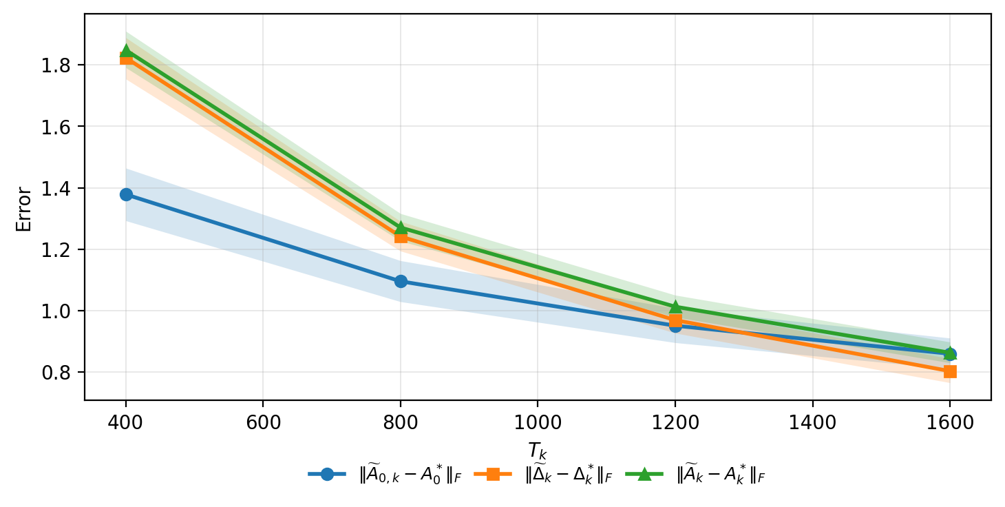
Figure 1 reports the average Frobenius-norm estimation errors of the single-client estimators and , computed over 1,000 replications, with the 5th–95th percentile bands shown as shaded regions. All errors decrease as increases, confirming that larger local datasets lead to more accurate estimation. For small , the total error closely tracks the deviation error , indicating that the total estimation error is dominated by the difficulty of recovering the client-specific sparse deviation when data are scarce. As becomes larger, the deviation error decreases faster, while the total error remains slightly larger due to the estimation error in the common component . Finally, the 5th–95th percentile bands become narrower as increases, indicating improved statistical stability of the single-client estimator with larger sample sizes.
Table 1 reports the correct selection rates of the proposed ridge-type rank estimator in (10) across different sample sizes and true ranks . For any given , the correct selection rate improves as increases, confirming the rank-selection consistency established in Theorem 3. At a given sample size, correctly identifying a larger true rank is generally more challenging, leading to lower selection accuracy when is small. However, the selector remains consistent, as evidenced by the rapid improvement in selection rates as grows across all rank values.
| 400 | 800 | 1200 | 1600 | |
| 1 | 68.20 | 99.40 | 100.00 | 100.00 |
| 2 | 42.90 | 86.30 | 98.40 | 100.00 |
| 3 | 41.80 | 85.50 | 99.00 | 100.00 |
5.2 Federated Estimation
We conduct four experiments to assess the finite-sample performance of the proposed federated method from four perspectives: (i) the impact of the privacy budget on the number of iterations required in Stage I; (ii) the estimation errors under varying privacy budgets ; (iii) the estimation errors under varying numbers of clients ; and (iv) the effect of client-specific sample sizes on estimation accuracy. In all experiments, the common component is obtained by Algorithm 3.1, the client-specific deviations are calculated using Algorithm 3.1, and the personalized coefficient matrices are given by .
Figure 2 illustrates the average Frobenius-norm estimation error of with respect to the iteration number for different privacy budgets, computed over 1,000 replications, with the 5th–95th percentile bands shown as shaded regions. Smaller values of and (i.e., more stringent privacy) lead to higher estimation errors and more volatile convergence behavior. This is consistent with Theorem 1, where the privacy-induced term dominates and increases sharply as the privacy budget tightens. For larger (i.e., weaker privacy), the federated estimator achieves lower errors and smoother convergence than the single-client initialization.

Figure 3 displays the average estimation errors for , , and under different privacy budgets , and the benefit of the federated method over the single-client baseline in (4), based on 1,000 replications. The benefit for a generic parameter matrix is defined as
| (11) |
where , or for all . It can be seen that all the estimation errors decrease as and/or increase (i.e., the privacy constraint is relaxed). The benefit heatmaps further validate the expected privacy-utility trade-off. Under stringent privacy (e.g., small ), the federated method may fail to outperform the single-client baseline, particularly for the common component . However, once the privacy budget is moderately relaxed, the federated procedure delivers clear improvements over local learning across most configurations.

Figure 4 shows the average Frobenius-norm estimation errors versus the number of clients , with for all and , averaged over 1,000 replications. In Figure 4, the label represents the average error , and the other labels are defined analogously. We can see that increasing leads to a noticeable reduction in the federated estimation error for the shared structure , as a larger provides more cross-client information for estimating . In contrast, the errors for the deviation and the overall client-specific matrix , remain nearly unchanged as grows. This is because the deviation component is client-specific and must be estimated from the local data of client alone. With held fixed, adding more clients does not reduce the statistical difficulty of estimating each , so the average error remains stable. Moreover, as observed in Figure 1, when is relatively small, the estimation error of is dominated by the error in estimating , which is consistent with the pattern seen here.

Figure 5 compares the average Frobenius-norm estimation errors of the federated and single-client methods versus the local sample size , with and , averaged over 1,000 replications. All clients share the same for simplicity. In each panel, “Federated” and “Local” denote the average estimation errors of the corresponding estimators for the coefficient matrix indicated in the subtitle, while “Benefit” quantifies the improvement of the federated method over the local baseline as defined in (11).
Figure 5 shows that all three components benefit from federated estimation, though the benefit patterns differ across panels. For the shared component (left panel), the benefit decreases as increases. This aligns with the error bounds in Proposition 1 and Theorem 1. With fixed, the federated estimator pools samples, starting from a much lower error level. While its error continues to decrease with , the reduction is less pronounced than that of the single-client estimator, whose error is governed solely by . As a result, the benefit shrinks as grows. In contrast, the benefit for the client-specific deviation (middle panel) and the full transition matrix (right panel) initially increases with and then gradually plateaus. When is small, remains noisy, limiting the improvement passed to . As increases, becomes more accurate and stable, enhancing the estimation of . Once is estimated accurately enough, the dominant constraint for estimating shifts to the local sample size itself, so further improvements in Stage I yield only marginal gains in Stage II, stabilizing the benefit. Finally, as observed in Figure 1, the estimation error of is largely driven by that of when is small, explaining why the error and benefit patterns for closely mirror those for .

6 Empirical Analysis
We illustrate the practical utility of our federated VAR framework through two empirical studies. Section 6.1, investigates the relationship between electricity consumption and economic indicators across U.S. states, a setting motivated by privacy-sensitive scenarios where raw local data cannot be directly shared. Section 6.2 then considers macroeconomic forecasting across multiple countries. Although privacy protection is not the primary concern here, this application illustrates the broader utility of our framework as a personalized multi-task learning approach that operates without privacy constraints.
The two datasets are constructed from publicly available sources. The first combines data from the U.S. Energy Information Administration (EIA) (https://www.eia.gov/electricity/data/eia861m/) and Federal Reserve Economic Data (FRED) (https://fred.stlouisfed.org/), while the second is compiled from the OECD Economic Outlook database (https://www.oecd.org/economic-outlook/). For each client, we align all variables to a common sample period, allowing sample sizes and time spans to vary across clients; see Table S.1 in the Supplementary Material. All data are then preprocessed by possible seasonal adjustment and transformations to remove non-stationarity, followed by standardization to zero mean and unit variance. Variable definitions, category labels, and preprocessing details are provided in Tables S.2 and S.3 of the Supplementary Material.
For each application, we compare the forecasting performance of our federated VAR method with several single-client benchmarks: the combined nuclear-norm and -regularized VAR (Nuc+) introduced in Section 2.2, the nuclear-norm-regularized VAR (Nuc), the -regularized VAR (), and the unregularized least-squares VAR (LS). For our federated method, we evaluate the privacy-utility trade-off by adding Gaussian noise with standard deviation for all and , and report results under three privacy configurations: , , and a non-private case (NDP) without noise. Following koop2013forecasting, all methods use a VAR(4) specification in both applications. Hyperparameters and initialization for our methods follow the procedure described in Section 3.3, while tuning parameters for the single-client benchmarks are chosen by standard cross-validation.
To evaluate the forecasting performance, we use the root mean squared forecast error (RMSFE) for each variable, computed via an expanding window approach. Specifically, for each forecast origin, the model is re-estimated using all available data up to that point, and one-step-ahead forecasts are generated for the last 20 observations. The RMSFE is then computed as the square root of the average squared forecast errors across these 20 forecast origins.
6.1 Federated Learning for Electricity and Economic Activity
We apply our federated VAR method to study the linkage between electricity consumption and economic indicators across U.S. states. Electricity data are valuable for macroeconomic analysis, serving as timely proxies for local economic activity (arora2016electricity). However, at finer geographic levels such as counties, cities, or utility service territories, the data are often subject to proprietary restrictions, regulatory limits, or data-sharing constraints, as public release could expose information about individual entities. By contrast, state-level aggregates are more readily available, as they are reported over a large and diverse user base that masks individual-level information. The U.S. Energy Information Administration publishes such state-level statistics on electricity sales, revenue, customer counts, and prices. While our empirical analysis uses these publicly accessible aggregates as a reproducible proxy, the modeling rationale directly mirrors the privacy-sensitive settings for which our method is designed.
The five states in our study, Indiana, Ohio, Wisconsin, Michigan, and Illinois are all located in the Great Lakes region. As documented by ahking2014economies, the business cycles of these states are substantially synchronized, though Michigan and Illinois exhibit distinct patterns from the others. This combination of shared dynamics and state-specific characteristics makes them well-suited for our personalized federated learning framework, which is designed to leverage cross-state information while preserving local heterogeneity. For each state, we construct a 12-dimensional monthly time series that includes electricity sales, revenue, prices, and key economic indicators such as employment, industrial production, and retail sales; see Table S.2 in the Supplementary Material for details. Using a VAR(4) specification, the ridge-type ratio rank selection criterion in (10) selects for the common component in Stage I, with all other tuning parameters chosen as described at the beginning of this section.
Table 2 reports the forecasting performance of our federated method and the single-client benchmarks across the five states. We have the following findings. First, the non-private federated estimator (NDP) achieves the lowest RMSFE for four of the five states, outperforming all single-client benchmarks. This suggests that borrowing information across economically related states is beneficial for state-level forecasting if the states are sufficiently similar and local sample sizes are moderate. Second, under moderate privacy noise, the federated estimator remains highly competitive and still outperforms the single-client methods in most cases. Notably, for Michigan, the private federated estimator under even slightly outperforms the non-private version. This suggests that appropriately calibrated Gaussian noise can act as an implicit regularizer, mitigating overfitting and improving out-of-sample generalization (boursier2024utility). Third, stronger privacy protection degrades forecasting performance. Increasing the noise level from to leads to uniformly higher RMSFE across all five states. This pattern reflects the standard privacy-utility trade-off: while modest noise may occasionally improve generalization through implicit regularization, excessive noise obscures the shared signal in Stage I and deteriorates forecast accuracy.
Fed-VAR Single-VAR State NDP Nuc + Nuc LS Illinois 44 0.751 0.780 0.813 0.857 0.881 0.798 3.437 Indiana 44 1.379 1.387 1.564 1.577 1.487 1.389 4.311 Michigan 44 0.598 0.592 0.617 0.608 0.607 0.613 1.816 Ohio 44 0.911 0.965 1.015 0.986 0.983 0.994 2.910 Wisconsin 44 0.725 0.735 0.784 0.828 0.916 0.917 2.874 Average 44 0.914 0.933 1.013 1.024 1.016 0.977 3.176
Figure 6 presents heatmaps of the estimated shared component and two representative state-specific deviations, and , under . Together with Table 2, this figure provides structural insight into why electricity data are useful for predicting state-level economic conditions.
The top panel reveals that exhibits a clear dependence pattern across electricity variables and macroeconomic indicators, indicating that lagged electricity-market variables carry predictive information for current economic outcomes. Several features are noteworthy. First, the strongest common signals are concentrated in the rows corresponding to unemployment, payroll employment, and the coincident index, indicating that current economic conditions are systematically related to lagged electricity and macroeconomic variables. Second, the largest coefficients appear primarily in the first one or two lag blocks, suggesting that the predictive linkage between electricity variables and economic indicators is primarily short-run. This pattern aligns with the view that changes in electricity usage and electricity-market activity are closely connected to near-term fluctuations in employment and overall economic activity.
The lower two panels in Figure 6 show that the state-specific deviations are much more localized. Most entries in and are close to zero, with only a limited subset exhibiting noticeable departures from the shared structure. Notably, appears more diffuse and contains more visible nonzero entries than , indicating that Illinois deviates more substantially from the common Great Lakes pattern. This aligns with ahking2014economies’ finding that Illinois is not fully homogeneous with the other Great Lakes states.

6.2 Macroeconomic Forecasting
We apply our federated VAR method to macroeconomic forecasting across eight countries: the United States, Australia, Canada, Germany, Korea, Norway, Sweden, and Denmark. For each country, we construct a 25-dimensional quarterly macroeconomic panel including real activity, trade, production and sales, housing, interest rates, labour markets, prices, and financial indicators; see Table S.3 in the Supplementary Material for details. The sample size varies across countries, with the United States having the longest series and Denmark the shortest. Under a VAR(4) specification, the ridge-type ratio rank selection criterion in (10) selects for the common component in Stage I, with other tuning parameters chosen as described at the beginning of this section.
Table 3 reports the forecasting performance of our federated method and the single-client benchmarks across the eight countries. The results exhibit patterns broadly similar to those observed in Section 6.1. Specifically, the non-private federated estimator (NDP) achieves the lowest average RMSFE across countries and outperforms the single-client benchmarks in most cases. Under moderate privacy noise with , the federated method remains highly competitive, attaining the best performance for several countries. In contrast, under stronger privacy protection with , the forecasting accuracy deteriorates noticeably across all countries, which again reflects the standard privacy-utility trade-off.
Fed-VAR Single-VAR Country NDP Nuc + Nuc LS United States 212 1.771 1.766 2.069 1.784 1.771 1.810 3.222 Australia 152 1.382 1.388 1.593 1.396 1.384 1.409 2.727 Canada 128 1.733 1.749 1.942 1.774 1.825 1.801 5.566 Germany 124 1.498 1.495 1.727 1.573 1.608 1.564 3.800 Korea 88 1.055 1.075 1.201 1.092 1.162 1.119 2.561 Norway 88 1.244 1.268 1.464 1.328 1.308 1.321 3.128 Sweden 84 1.284 1.304 1.516 1.390 1.362 1.361 2.651 Denmark 72 1.219 1.227 1.425 1.318 1.272 1.258 1.739 Average 118 1.418 1.428 1.639 1.474 1.479 1.474 3.347
To provide a structural insight into the forecasting results in Table 3, Figure 7 illustrates heatmaps of the estimated shared component and two representative client-specific deviations, and . The top panel shows that exhibits a clear and non-negligible dependence pattern across variable groups and lag blocks, providing visual evidence of a common dynamic structure shared across countries. Several features are noteworthy. First, stronger entries appear around export, import, and industrial production variables, particularly in the first lag block, indicating a common short-run predictive linkage between external demand and production activity across countries. Second, the rows and columns associated with inflation and housing-related variables display relatively strong and persistent signals, suggesting these variables form an important shared dynamic block. Third, unemployment shows several negative coefficients, while employment, hourly earnings, and unit labor cost display more positive interactions with activity and price variables, reflecting coherent labor-market dynamics. By contrast, the lower two panels reveal that the client-specific deviations are much more localized. Most entries in and are close to zero, with only a limited subset exhibiting noticeable deviations from the shared structure. This pattern visually supports our personalized federated decomposition. Moreover, the degree of heterogeneity differs across countries. Australia’s deviation matrix contains more visible nonzero entries than that of the United States, indicating that Australia requires a richer client-specific correction, whereas U.S. dynamics are comparatively well captured by the common structure with only localized adjustments.

7 Conclusion and Discussion
This paper develops a privacy-preserving personalized federated learning framework for high-dimensional VAR models. The proposed method leverages a low-rank common structure shared across clients to capture global dynamics, while allowing sparse client-specific deviations to accommodate heterogeneity. The framework operates in two stages: differentially private representation learning for the shared component via noisy gradient aggregation, followed by local personalization for client-specific sparse deviations. We establish non-asymptotic error bounds for both the single-client and federated estimators, and prove consistency of the associated rank selection procedure. A central insight from our theoretical comparison is that the federated estimator outperforms its single-client counterpart when the pooled sample is sufficiently large and client heterogeneity is modest. Simulation results corroborate these findings, showing substantial improvements in estimation accuracy when local sample sizes are limited. Empirical applications to state-level electricity–economy linkages and cross-country macroeconomic forecasting further demonstrate the superior forecasting performance of the proposed method, underscoring its practical value in privacy-sensitive and heterogeneous data environments.
Several promising directions remain for future research. First, the proposed federated learning framework can be extended to more complex time series structures, such as matrix- or tensor-valued time series models, where the shared component may exhibit multi-way low-rank structure. Second, given the heavy-tailed nature of many economic and financial time series, integrating robust loss functions or truncation-based methods into the proposed two-stage estimation could improve stability and ensure theoretical guarantees under relaxed moment conditions. Third, extending the privacy-preserving federated learning framework to time-varying second moments, such as multivariate volatility and covariance dynamics, would enable privacy-aware risk monitoring and portfolio applications using decentralized financial data.
Appendix
This appendix provides technical details, proofs and additional simulation results supporting the main paper. Section S.1 introduces the essential notation and preliminaries. Section S.2 presents primary lemmas that form the theoretical foundation for our main results. Section S.3 contains proofs of all theorems and propositions. Section S.4 provides detailed proofs of the primary lemmas from Section S.2. Section S.5 collects technical lemmas and provides corresponding proofs for stationary VAR processes that are of independent interest and broadly applicable. Section S.6 presents the ADMM algorithm for solving the local estimation problem (4). Finally, Section S.7 provides additional data description tables for the empirical studies in Section 6.
Appendix S.1 Notation and Preliminaries
Throughout the appendix, vectors and matrices are denoted by boldface lowercase and uppercase letters, respectively (e.g., , , , ). For a vector , its Euclidean norm is denoted by . For a matrix , we denote its transpose, Frobenius norm, nuclear norm, and operator norm by , , , and , respectively. For , the norm of is defined as ; the same formula for defines the entrywise quasi-norm. When , is the number of nonzero entries of . When , is the entrywise maximum norm. Moreover, let denote the best rank- approximation of obtained from its singular value decomposition, where is the -th singular value, and and are the corresponding left and right singular vectors.
For any subspace , let denote its closure and its orthogonal complement. For a rank- matrix with singular value decomposition , its tangent space is defined as , and its orthogonal complement (with respect to the Frobenius inner product) is . The projection of onto the tangent space is denoted as .
Define the following spaces of square-summable sequences of real vectors:
Both spaces are equipped with the natural inner product and form Hilbert spaces of square-summable real vector-valued sequences.
For a random variable or random vector , and denote their sub-Gaussian Orlicz norms, respectively. For sequences and , we write if there exists a constant such that for all , and if both and hold. Throughout the appendix, and similar symbols denote positive constants whose values may change from line to line unless otherwise specified.
Appendix S.2 Primary Lemmas
In this section, we present primary lemmas that form the theoretical foundation for our main results. Lemmas S.1 and S.2 provide high-probability bounds for the -norm of sub-Gaussian vectors and the spectral norm of Gaussian random matrices, respectively. Lemmas S.3 and S.4 are key technical results that characterize the geometry of low-rank matrix spaces and the contraction properties of projections onto tangent spaces. Lemma S.5 is a matrix perturbation result that controls the error of low-rank approximations under perturbations. Finally, Lemmas S.6 and S.7 establish concentration inequalities for sample covariance matrices and restricted strong convexity conditions for VAR processes, which are crucial for our error analysis. Detailed proofs of these lemmas are provided in Section S.4.
Lemma S.1 (Sub-Gaussian -norm tail bound).
Let be mean-zero and sub-Gaussian with . Then for , there exists a constant such that
| (S.1) |
Lemma S.2 (High-probability spectral-norm bound for an Gaussian matrix).
Let have entries . Then there exist constants such that
Lemma S.3 (Adapted from wei2016guarantees, Lemma 4.1).
Let have rank . Let have rank with . Then
where denotes the orthogonal complement of the tangent space at .
Lemma S.4.
Let be symmetric. Fix any rank- matrix . Then for every ,
| (S.2) |
Lemma S.5 (shen2025compu, Lemma 14).
Suppose has rank and admits the singular value decomposition ,, and . For any satisfying ,
Lemma S.6.
Lemma S.7.
Lemma S.8.
Lemma S.9.
Lemma S.10.
Lemma S.11.
Lemma S.12.
Let be a mean-zero random variable. Fix and . The following two conditions are equivalent.
-
(i)
(Two-regime Bernstein tail) There exists a constant such that for all ,
(S.7) -
(ii)
(Local sub-exponential mgf) is sub-exponential with Bernstein parameters , i.e., there exist constants such that for all ,
(S.8)
Lemma S.13 (Gaussian mechanism for propagation DP).
Fix a client and consider a deterministic mapping . Assume that for all neighboring datasets with . Define the randomized mechanism by , where has independent Gaussian entries and is independent of . Then is -DP if
| (S.9) |
Appendix S.3 Proofs of Main Results
Proof of Proposition 1.
Fix an arbitrary client . By construction, both and satisfy the constraint and hence are feasible for (4). Therefore, by the optimality of , we have
Rearranging the terms yields
Considering for any vectors , , and note that , we have
| (S.10) |
For the inner product terms on the left-hand side, we have
and similarly, . Then, rearranging the terms in (S.3) and applying the Hölder’s inequality yields
| (S.11) |
To bound the right-hand side of (S.3), we begin by deriving the constrained space for the estimators and . To this end, we define the coordinate subspace induced by the large entries of . Specifically, for a given threshold , let
| (S.12) |
and let denote the closed orthogonal complement of , namely
| (S.13) |
For any , we write for the restriction of to the coordinates with , i.e., if and otherwise, and define analogously.
We also introduce the low-rank model subspace associated with . Let be an SVD and denote by and the matrices collecting the first left and right singular vectors of , respectively. Define
and let denote the closed orthogonal complement of , that is,
For any , we write for the orthogonal projection of onto , and write for the orthogonal projection onto . Then, by the decomposability of the nuclear norm and the norm, for the first two terms on the right-hand side of (S.3), we have
| (S.14) |
The last equality follows from the fact that the nuclear norm and the norm are both decomposable with respect to the defined subspaces, i.e., and .
Next, we bound the deviation terms. By Lemmas S.8 and S.9, there exist constants such that, with probability at least ,
Consistent with the prescribed rates of and , we choose the tuning parameters with sufficiently large constants, namely and . Then, on the same event,
| (S.15) |
For the last two terms on the right-hand side of (S.3), using these bounds and the decomposability of the norms again, we have, with probability at least ,
| (S.16) | ||||
Combining (S.3), (S.3), and (S.16) yields
Rearranging the terms, we obtain the following cone-type inequality
| (S.17) |
Next, we derive the upper bound for the estimation error in this constrained space. By just plugging in (S.15) into the right-hand side of (S.3), we have
| (S.18) |
Then, we derive the lower bound for the left-hand side of (S.3). This can be achieved by two steps. First, by Lemma S.7, there exists a constant such that, given the sample size condition , with probability at least ,
| (S.19) |
Second, noting that for any matrices of the same dimension, we have
| (S.20) |
By the Hölder’s inequality, we have
Since is feasible for (4), we have . Moreover, . Then, by the prescribed choice of the tuning parameter as in Proposition 1, we can pick a constant such that
| (S.21) |
Consequently, combining (S.21) with (S.3) yields
| (S.22) |
Combining (S.19) and (S.3), we have, with probability at least ,
| (S.23) |
Finally, combining (S.3) and (S.3) yields
| (S.24) |
Inequality follows from the cone-type bound (S.3). Inequality follows from the rank condition and the restriction , together with the fact that for any matrix with . Moreover, since , we have . Considering the threshold of the sparse space , by the definition of in Section 4, we have , and thus . Then, it follows that . Besides,
To conclude the derivation, we translate the preceding inequality (S.3) into an explicit error bound. For brevity, let and . Consequently, (S.3) further implies
| (S.25) |
Using , we further obtain that for any ,
Choosing and substituting these two inequalities into (S.25) yields
Rearranging the terms and absorbing absolute constants into , we have
Then, choosing and returning and to their matrix notations, we have
Furthermore, using the inequalities and for , we have
Combining the above bound with the sample size conditions as well as the probability with respect to the deviation bounds (S.15) and the RSC bound (S.19). This concludes the proof. ∎
Proof of Theorem 1.
The proof proceeds in three parts. In Part I, we derive the upper bound for with respect to and . In Part II, we prove by induction that both and the estimation error remain uniformly bounded with high probability over all . In Part III, we select a suitable iteration number to derive the final error bound.
Part I (Sensitivity characterization). Consider and the neighboring local data set with respect to the sensitive index set at client , i.e., . Fix a sensitive index set and let . For any vector , denote by the subvector obtained by restricting to the coordinates indexed by , and similarly for . There exists such that for all and , where is an copy of . Moreover, for all . The perturbed trajectory is generated by the same VAR model with the same coefficient and the same future innovations, for , using the same initial values as for .
Without loss of generality, after applying a fixed permutation of coordinates, we assume . Let and . Without loss of generality, we assume the first coordinates of and are the sensitive coordinates, and the remaining coordinates are non-sensitive. Then, the primitive discrepancy is the selective innovation difference , and thus . Consequently, for and .
Consider a fixed , under Assumption 1, there are no roots in the closed unit disk , hence every root satisfies . Therefore, the quantity is well-defined, equals when has no roots, and otherwise equals the minimum modulus among the finitely many roots; in particular . Fix any radius . Define the uniform transfer-function bound
| (S.26) |
which is finite because is continuous on the compact circle .
Note that Algorithm 3.1 only enforces differential privacy on each client’s local dataset through the gradient-transfer step. Therefore, only are related to sensitivities, where and denote the corresponding full gradients computed at client from and . Hereafter, we derive an upper bound for in terms of the estimation error . To control the discrepancy induced by the difference of and , we use a geometric bound on the impulse-response coefficients associated with in Lemma S.24. Specifically, set . For any , the inverse lag polynomial admits the power-series expansion , and the corresponding impulse-response coefficients satisfy the geometric decay bound:
| (S.27) |
Before the proof, we first provide high-probability upper bounds for and that will be repeatedly used later. By Assumption 2 and Lemma S.16, is a mean-zero sub-Gaussian random vector with sub-Gaussian constant . Moreover, by Assumption 2 and Lemma S.17, the stacked lag vector is also sub-Gaussian with sub-Gaussian constant , where . We can now utilize these sub-Gaussian properties to derive uniform-in-time -norm bounds. Applying Lemma S.1 to with dimension and sub-Gaussian constant , we obtain that for any there exists a constant such that
| (S.28) |
Similarly, applying Lemma S.1 to with dimension and sub-Gaussian constant yields
| (S.29) |
For , we now derive a high-probability upper bound for . Note that where is an copy of . Since , it suffices to control the -dimensional vector . For any and , so that . Then, by the sub-additivity of the Orlicz norm,
Therefore, is a mean-zero sub-Gaussian random vector in with vector sub-Gaussian constant . By the standard -net argument (as in the proof of Lemma S.16), there exists a constant such that
| (S.30) |
Let . For each client , define the event
| (S.31) |
where , and . Then, by a union bound over the three high-probability bounds above, there exists a constant such that
| (S.32) |
Hereafter, we derive upper bounds for conditional on the event . We begin by deriving the upper bounds for . Recall that and differ only on the sensitive coordinates at time , i.e., for all and . Consequently, the induced trajectory difference has the following three cases:
-
(i)
Pre-change (). Since the innovations coincide up to time , the two trajectories coincide as well, hence .
-
(ii)
Change time (). The only discrepancy is the replaced innovation, so .
-
(iii)
Post-change (). The discrepancy propagates through the VAR() process.
To formalize (iii), we write the VAR() model for client via the lag polynomial :
By the stationarity condition in Assumption 1, for . Applying the inverse linear filter yields
| (S.33) |
Considering that holds if and only if . Therefore,
| (S.34) |
Then, combining (S.33) and (S.34) and writing , we obtain for all , . Therefore, using the impulse-response bound (S.27),
| (S.35) |
Next, we derive the upper bounds for . Recall and note that for . These together with (S.35) imply that
| (S.36) |
Now we bound the geometric sum in (S.3). For , then and
For , then and
Denote for any . Combining the two cases yields
| (S.37) |
Plugging (S.37) into (S.3) and taking square roots gives
| (S.38) |
For , note that , since .
Recall that for each , the unprojected gradient of the squared loss with respect to is . Thus, with , denote and . Then, expanding the product yields
| (S.39) |
By the additivity of the projection operator and the sub-additivity of the Frobenius norm , we have
where the last equality holds because and for all , and thus for all . Next, we derive a Frobenius-norm bound for the projected gradient discrepancy , which will be summed over in the subsequent step. Since is a non-expansive orthogonal projection, i.e., for all . Hence . Therefore, it suffices to bound for each fixed time . We treat two cases separately: the injection time , where the innovation is replaced, and the propagation regime , where the discrepancy evolves through the VAR process.
At , we have and . Plugging into (S.39), only the second term remains and simplifies to . Recall that for any vectors , , then we have
| (S.40) |
The last inequality holds because event in (S.31) ensures and .
For , the neighboring datasets differ only at time , . Therefore, with . Consequently, we have and . Recall that for any vectors , , and for any matrix and vector , . Then, plugging the above identities into (S.39) and using the sub-additivity of the Frobenius norm, we have
| (S.41) |
Conditional on the event in (S.31), we have and for all . Then, substituting these bounds into (S.3) and summing over from to yields
| (S.42) |
Thus, it suffices to bound and . By (S.38) and implied by the event in (S.31), for with , we have
where . Consequently,
Using the deterministic geometric-sum bounds, we have
Plugging these into (S.3) yields, conditional on in (S.31),
| (S.43) | ||||
Finally, combining the bounds (S.40) and (S.3) yields, conditional on in (S.31),
| (S.44) |
For convenience, define the two deterministic factors
Then, conditional on in (S.31), (S.3) can be rewritten as
| (S.45) |
Part II (High-probability bounds via induction). Next, we establish high-probability control of the estimation error together with the sensitivity by mathematical induction. Fix an iteration and assume that
| (S.46) |
Conditional on the high-probability event , we will show that satisfies the same upper bound as well. Since this part does not need the neighboring-dataset definition of differential privacy, we abbreviate as for notational simplicity.
Note that
| (S.47) |
Moreover, using , the local gradient admits the decomposition
| (S.48) |
Thus, combining (S.47) and (S.3), we have
| (S.49) |
where and . Next, we bound each of the four terms in turn.
For term I, we further decompose the expression and upper bound each component separately. In particular, we first rewrite the following quantity into a sum of terms:
| Term I | |||
The last equality holds because , and the projection acts as the identity on its range, i.e., for any , .
For term I(a), by Lemma S.3, we have
For term I(b), note that . Applying Lemma S.4 with , and together with the non-expansiveness of the projection in Frobenius norm, we have
| Term I(b) | |||
For term I(c), by the non-expansiveness of the projection in Frobenius norm, and Lemma S.3, we have
| Term I(c) | |||
Therefore, combining the three components yields
| Term I | ||||
| (S.50) |
For term II, by the sub-additivity of the Frobenius norm, the non-expansiveness of the projection in Frobenius norm and the inequality , we have
| (S.51) |
where and . Moreover, note that for each and . Therefore, for each fixed we have , which implies
| (S.52) |
By Lemma S.10, with probability at least ,
| (S.53) |
For , by Lemma S.23, we have for each client . Since , it follows that
| (S.54) |
Combining (S.52), (S.53) and (S.54), and given , we conclude that with probability at least ,
| (S.55) |
Plugging (S.55) into (S.51) and noting that for any yields that, with probability at least ,
| (S.56) |
For Term III, note that the tangent space consists of matrices of rank at most . Then, by the non-expansiveness of the projection in operator norm and the inequality , we have
| (S.57) |
This together with Lemma S.11, and given , there exists a constant such that, with probability at least ,
| (S.58) |
For Term IV, note that with . Recall (S.45), we then derive the upper bound for . By the induction hypothesis in (S.46), we have . Moreover, note that the personalization deviation satisfies , for all . Therefore, by the sub-additiveness of Frobenius norm, for any , . Then, with and . Recall that , , and . By direct substitution of and absorbing constants into , we have
| (S.59) | ||||
| (S.60) |
where we use , and . Let . Then,
| (S.61) |
By the non-expansiveness of the projection in Frobenius norm and the inequality , we have
| Term IV | (S.62) |
For each client , has entries distributed as . To achieve -DP for each client , by Lemma S.13, it suffices to set . Denote . Since are independent across , for each fixed , we have , with . Hence has entries following . Applying Lemma S.2 to , there exists a constant such that with probability at least ,
| (S.63) |
Note that the aggregated noise scale satisfies
| (S.64) |
Recall that . Then we have
| (S.65) |
Then, coditional on , combining (S.62), (S.63), (S.64) and (S.65) yields that, with probability at least ,
| Term IV | ||||
| (S.66) |
Denote with . Thus, combining the bounds for Term I–Term IV in (S.3), (S.56), (S.58), and (S.3), we conclude that on an event of probability at least ,
| (S.67) |
Set . Then, we show that for any . By Lemma S.10, given , there exist constants , with probability at least ,
| (S.68) |
By Lemma S.23, for each client , we have . Recall that . Therefore,
| (S.69) |
Next, since both and are symmetric, Weyl’s inequality (weyl1912asymptotische) together with (S.68) implies that, with probability at least ,
| (S.70) |
Combining (S.69) and (S.70) yields that, with probability at least ,
| (S.71) |
Finally, taking sufficiently large so that and . Then, (S.71) simplifies to
| (S.72) |
Donote as the set of eigenvalues of . Hence, for any , , and also . Note that if , then . If , then , and since , we have . Therefore, in either case, . With the choice , we have
| (S.73) |
Moreover, under the induction hypothesis, we have
| (S.74) |
For , using , we have
| (S.75) |
Then, plugging (S.73), (S.74) and (S.75) into yields
| (S.76) |
Recall that , where . Note that the condition in Theorem 1 implies that . Moreover, provided , we have . Consequently, conditional on and under the induction hypothesis (S.46) , and by the choice of , we have
This together with Lemma S.5 by setting and implies that
| (S.77) | ||||
This completes the induction.
Note that all high probability events needed in the induction holds uniformly for any iteration . Hence, these events can be fixed throughout the induction, and the probability does not accumulate with the number of iterations. For clarity, we still state the corresponding probabilistic inequalities at each step to indicate where they are invoked.
Part III (Final results). Note that for each client the gradient-transfer mechanism is -DP. Therefore, by the basic composition theorem for differential privacy, e.g., dwork2014algorithmic, the overall algorithm obtained by composing these rounds is -DP for each client .
To conclude, we choose an appropriate rate of the iteration number to derive the final error bound. Note that for all under the induction hypothesis, and thus . Then, by the non-expansiveness of in Frobenius norm and (S.3) under (S.3), we have, with probability at least ,
Now let , we have which can be absorbed by the last error term, indicating that there is no improvement by running the algorithm after iterations. Thus, given , with
we have conditional on the event , with probability at least ,
To ensure that and vanish as , it suffices to require
Moreover, by (S.32) and the Bonferroni inequality, we have
Combining the above arguments, we conclude that with probability at least ,
This concludes the proof. ∎
Proof of Theorem 2.
Fix an arbitrary client . Note that the total estimation error can be decomposed into an optimization (algorithmic) error and a statistical error:
Accordingly, we first establish a bound for the statistical error , and then control the optimization error using the convergence guarantee of FISTA.
Part I (Statistical error). By the optimality of in (7), we have
Note that , then we have
This together with the above optimality inequality yields
| (S.78) |
For the first inner-product term in the right-hand side of (S.3), by Hölder’s inequality, we have
For the second inner-product term in the right-hand side of (S.3), by Young’s inequality, i.e., , we have
Plugging the above bounds for the two inner-product terms into (S.3), we have
Rearranging the terms and moving the quadratic term in to the left-hand side yields
| (S.79) |
Recall the predefined subspace and its closed orthogonal complement in (S.12) and (S.13), i.e.,
Then, for the first term in (S.3), using the decomposability of the entrywise norm with respect to the pair , we have
| (S.80) |
By Lemma S.8, there exists a constant such that, given , with probability at least ,
Given the rate of in Thoerem 2, we choose . Then, with probability at least , we have
| (S.81) |
Then, combining (S.3), (S.3) and (S.81), with probability at least ,
Then, we have the cone-type inequality
| (S.82) |
Consequently, plugging (S.81) and (S.82) into (S.3) yields
| (S.83) |
Then, we derive the lower bound for . Given the sample size condition , by Lemma S.7, with probability at least , the following RSC condition holds:
| (S.84) |
Then, combining (S.3) and (S.84) yields
| (S.85) |
Considering the threshold of the sparse space , by the definition of , we have , and thus . Then, it follows that . Besides,
Then, it follows from (S.85) that
| (S.86) |
Note that for any , we have
| (S.87) |
Then, substituting (S.3) into (S.86) and rearranging terms, we have
Then, choosing yields
| (S.88) |
It remains to control the last term in (S.88) involving . Note that
where the inequality follows from . Moreover, combining implied by Lemma S.23 given and Lemma S.3, with probability at least , we have
Consequently, combining the above inequalities, . Substituting this bound into (S.88) and collecting the sample-size conditions and probability bounds from the preceding steps, provided , with probability at least , we have
| (S.89) |
Part II (Optimization error). Now, we turn to control the optimization error based on the convergence guarantee of FISTA. To this end, we rewrite (7) in a compact matrix form. Denote and . Then (7) is equivalent to
| (S.90) |
Denote , and . We first verify the Lipschitz continuity of the gradient of . A direct calculation yields
and hence, for any ,
Therefore, is Lipschitz continuous with constant conditional on .
Although the analysis in beck2009fast is presented for vector-valued variables, Remark 2.1 therein notes that the key inequalities and lemmas underlying the FISTA rate extend verbatim to any Hilbert space equipped with an inner product. Since endowed with the Frobenius inner product is a finite-dimensional Hilbert space, the same convergence analysis applies to our matrix-valued optimization problem. Then it suffices to verify the conditions for applying the FISTA convergence guarantee.
Since is convex but nonsmooth and is continuously differentiable with an -Lipschitz continuous gradient, the objective fits the standard FISTA framework. Note that are the iterates generated by Algorithm 3.1 with stepsize . Then, by beck2009fast together with Remark 2.1 therein, for any ,
In particular, under the initialization in Algorithm 3.1 and , we have
| (S.91) |
Next, we relate to . For any , a direct expansion of at gives
| (S.92) |
Moreover, is convex but non-smooth. By the subgradient inequality of norm, for any and any , for any . Applying this inequality with and yields
| (S.93) |
Combining (S.92) and (S.93), we obtain the following lower bound for :
| (S.94) |
Since minimizes the convex function , the first-order optimality condition ensures that there exists such that
| (S.95) |
Plugging (S.95) into (S.94) leads to
| (S.96) |
Finally, by taking , the RSC condition in Lemma S.7 together with (S.91) yields that, with probability at least ,
| (S.97) |
Moreover, as implied by Lemma S.6 and Lemma S.23, given , there exists a constant such that, with probability at least ,
Then, substituting this bound into (S.97), and noting that , , , we have, with probability at least ,
| (S.98) |
Recall (S.89), we have , and hence (S.98) implies
Consequently, we have
Finally, taking . Given this choice, the optimization error is negligible relative to the statistical error, i.e.,
Noting that and , we have . Hence, by for any , we have
To conclude the proof, we further control Term II appearing in the bound for in the proof of Theorem 1. Given for all , Lemma S.6 and Lemma S.23 imply that with probability at least . Consequently, by applying this bound to (S.56), we have that, with probability at least , Term II in the proof of Theorem 1 admits the following tighter upper bound:
| (S.99) |
Therefore, under the the event in (S.99) and conditions of Theorem 1, with probability at least , we have
where . Combining all high probability events required in the proof yields that, with probability at least ,
This completes the proof. ∎
Proof of Theorem 3.
Fix an arbitrary client . Note that . By Proposition 1, under the stated conditions, we have
with probability tending to as . Then by Weyl’s inequality (weyl1912asymptotische), we have
Note that . Then, for each , we have the following cases:
-
(a)
For , since and , the term dominates in , i.e., ;
-
(b)
For , since and , the term dominates in , i.e., .
Recall the rank estimator
The above analysis in (a) and (b) implies the following limits in probability as :
Part I (). Both and are dominated by , and hence
Part II (). Both and are dominated by and , respectively, so that
Part III (). The numerator is dominated by , while the denominator is dominated by , and hence
Moreover, the condition
in Theorem 3 implies . Therefore, . Combining parts (I)–(III), it follows that, with probability tending to , is the unique minimizer of , which yields . This proves that as . ∎
Appendix S.4 Proofs of Primary Lemmas
Proof of Lemma S.1.
Following a standard property of the sub-Gaussian Orlicz norm: if a scalar random variable satisfies , then there exists a constant such that for ,
Fix any . Since , we have . Hence, for any ,
| (S.100) |
Let be a -net of under -norm. It is well known that such a net exists with and that for any , . Therefore,
| (S.101) |
Now set . Then, (S.4) implies that for any ,
Since , absorbing constants into yields
| (S.102) |
Finally, by a union bound over , we have
Adjusting constants so that , which proves (S.1). ∎
Proof of Lemma S.2.
Write , where has entries. Then . Since each is sub-Gaussian with for a constant , we may apply the bound for matrices with independent mean-zero sub-Gaussian entries, i.e., Theorem 4.4.5 of vershynin2018high, which states that for ,
Absorbing into , we have
Multiplying the above inequality by and setting yields the desired bound. ∎
Proof of Lemma S.4.
Since is the orthogonal projector onto , we have the orthogonal decomposition for any and any . Therefore,
| (S.103) |
where the last equality holds because is orthogonal to . Since is symmetric, for any we have
| (S.104) |
where the first and last equalities follow from (S.103), while the middle equality uses the symmetry of . Consequently, the map is self-adjoint on . Hence it admits an orthonormal eigenbasis with real eigenvalues satisfying . For any , write . Since is orthonormal under , we have
| (S.105) |
Moreover, we have
and therefore
Taking the Frobenius norm and expanding using orthonormality gives
| (S.106) |
By (S.105), the right-hand side equals .
Proof of Lemma S.6.
Fix any client . Let be the Euclidean unit sphere in . Fix any and choose such that . Then, for any symmetric matrix ,
Therefore, for any and the corresponding ,
where we used and . Taking the supremum over yields
Thus, after rearranging the terms, we have
Then, take and let be a corresponding -net with . With , we have , so that . Applying this bound to the symmetric matrix gives
Fix any with . Applying Lemma S.21 yields that for every ,
Note that
We now choose and hence and . With this choice, the two terms in the Bernstein minimum become
Hence, given , we have
after adjusting absolute constants. Consequently, taking a union bound over with yields
for some constant . Absorbing the prefactor into the absolute constant in the operator-norm bound concludes the proof. ∎
Proof of Lemma S.7.
Fix any client . Note that
| (S.108) | ||||
Under the sample size condition in Lemma S.7, i.e., , we have in particular , and hence there exists a constant such that
Therefore, by Lemma S.6, since and hence , there exist a constant such that, with probability at least ,
| (S.109) |
Moreover, by Lemma S.23, we have . Combining this with (S.109) in Weyl’s inequality yields
Plugging this bound into (S.4) concludes the proof. ∎
Proof of Lemma S.8.
Proof of Lemma S.9.
Fix any client . Let and be the Euclidean unit spheres. Fix , and let and be -nets with and . A standard net argument implies
Fix . Applying Lemma S.22 with yields, for any ,
Then, setting yields
| (S.111) |
Hence, given , absorbing the constants , and into yields
Consequently, taking a union bound over with yields
for some constant , which proves (S.6). ∎
Proof of Lemma S.10.
Fix any client . Let and be the Euclidean unit spheres. Fix , and let be an -net with . Note that is symmetric. Then, following the standard net argument as in the proof of Lemma S.6 yields
| (S.112) |
Fix any with and define for each . Consequently, we have . Under Assumption 2, the innovations are independent across clients , hence are independent for each fixed . Moreover, denote , and . Then, by Lemma S.21, we have, for and any ,
Hence by Lemma S.12, is sub-exponential with Bernstein parameters . Consequently, Bernstein’s inequality for sums of independent sub-exponential variables, e.g., Eq. (2.18) in wainwright2019high, yields that, for any ,
| (S.113) |
Noting that and , we choose . Then, the two terms in the Bernstein minimum become
Hence, given , we have
Recall that , then for any , we have
Consequently, taking a union bound over with yields
Combining this with the -net reduction (S.112) and absorbing the factor into the leading constant concludes the proof. ∎
Proof of Lemma S.11.
Fix , and let and be -nets with and . Then, following the standard net argument as in the proof of Lemma S.9 yields
| (S.114) |
Fix any with and define for each . Consequently, we have . Moreover, denote , and . Then, by Lemma S.22, we have, for and any ,
Hence, by Lemma S.12, is sub-exponential with Bernstein parameters . Note that under Assumption 2, the innovations are independent across clients , hence are independent for each fixed . Consequently, Bernstein’s inequality for sums of independent sub-exponential variables, e.g., Eq. (2.18) in wainwright2019high, yields that, for any ,
| (S.115) |
Noting that and , we choose . Then, the two terms in the Bernstein minimum become
Hence, given , we have
Recall that , then for any , we have
Consequently, taking a union bound over with yields
Combining this with the -net reduction (S.114) and absorbing the factor into the leading constant concludes the proof. ∎
Proof of Lemma S.12.
We begin by the proof of (S.7) (S.8). Assume (S.7). To prove (S.8), we first bound moments using the two-regime tail. For any integer , the tail integral formula gives . Let so that . Splitting at and using for and for , we have
We now evaluate the two integrals in closed form up to Gamma factors. For the first term, set . Then,
The penultimate equality follows from the change of variables , under which and . Similarly, set for the second term. Then,
The penultimate equality follows from the change of variables , under which . Putting the two parts together,
| (S.116) |
It remains to upper bound the Gamma factors in the right-hand side of (S.116). Note that by Stirling’s formula for the Gamma function (see equation (1.1) in nemes2010more), we have
and thus there exist constants such that for all , . Dropping the factors , and absorbing into , we obtain that there exists a constant such that for all , . Applying this bound with and gives the desired bounds for and . Hence
for . Similarly,
for . Combining these bounds yields that there exists a constant such that for all integers ,
Now fix with sufficiently small. Since , the Taylor expansion yields
where and .
To control ,the Stirling bound yields . Writing , under and , we have and thus . Consequently, .
Next, for we use again to obtain . Let and define , so that . Decompose into even and odd terms:
For the even terms, the Stirling’s formula implies , we have , hence . For the odd terms, gives . Therefore .
We now show that there exists a constant such that
| (S.117) |
for all . Indeed, for , we have and , so the left side is at most , while . Choosing yields .
For , note that and , so . If we take , then for all . Moreover, since , we have , and thus . Combining the last two displays yields . Taking makes (S.117) hold for all . Consequently .
Putting the bounds together, we have, for all ,
Since , the term is absorbed into by adjusting absolute constants. Hence there exists a constant such that for all ,
which establishes (S.8).
Proof of Lemma S.13.
Denote
where is an independent copy of . Note that both and are Gaussian random matrices in the sense that their vectorized versions, and , are multivariate Gaussian. Specifically, and , where is the identity matrix with . Consequently, we have the following closed-form expressions for the densities of and :
Then, the log-likelihood ratio at is
By the Cauchy-Schwarz inequality and the condition that , we have
Next, fix any and define the good region . For any measurable set , decomposing and integrating with respect to the densities yields
| (S.118) | ||||
where we used that conditional on , we have . Hence, the desired -DP inequality will follow, once we control the probability of the bad event . To this end, define the privacy-loss random variable
Then, substituting into the explicit expression for the log-likelihood ratio yields
Note that is Gaussian with mean and variance , while the random variable is Gaussian with mean and variance . Let . For the Gaussian mechanism, . Moreover, the function attains its minimum over at whenever . In particular, this condition is implied by (S.9). Therefore, the worst case over neighboring pairs is attained at , and
Applying the Gaussian tail bound for yields
Consequently, to ensure , it suffices to bound the right-hand side by , which is equivalent to . A convenient sufficient condition is
| (S.119) |
Rearranging (S.119) gives the exact requirement of in (S.9). Therefore, under (S.9),
| (S.120) |
Substituting this bound (S.120) into (S.4) yields, for any measurable , . Therefore, if (S.9) holds, then
This proves that the mechanism is -DP. ∎
Appendix S.5 Technical Lemmas for Stationary VAR Processes
This section collects several technical lemmas for stationary VAR() processes that are repeatedly used in the concentration analysis of the main results. Lemma S.14 links the spectral behavior of to that of . Lemma S.15 then transfers the frequency-domain bounds in Lemma S.14 to the Toeplitz matrix generated by the VAR coefficients. Lemmas S.16 and S.17 establish sub-Gaussianity for the innovation vector and the stacked lag vector, respectively, which provides the probabilistic foundation for subsequent tail bounds. Lemmas S.18 and S.19 derive quadratic and bilinear innovation representations for and . These representations allow us to invoke the infinite-dimensional Hanson-Wright inequality in Lemma S.20, which in turn yields the high-probability quadratic-form bound in Lemma S.21 and the corresponding cross-term concentration result in Lemma S.22. Finally, Lemma S.23 establishes the positive definiteness and eigenvalue bounds of the stacked lag covariance matrix , which is used to verify the restricted strong convexity-type conditions needed in the estimation analysis.
Lemma S.14.
Let the VAR() process be stationary with AR polynomial and its determinant for all . Define
Then, we have
Proof of Lemma S.14.
For , is invertible by stationarity. Using the identity for any invertible matrix , we have
Note that and have identical eigenvalues, i.e.,
Therefore, for any fixed , we have
and
The last equalities in the above two hold owing to and for any invertible matrix . Taking and on both sides yields the stated identities with and . ∎
Lemma S.15.
Let and define the semi-infinite Toeplitz matrix as
Then, for any , the following two side spectral bounds hold:
Proof of Lemma S.15.
Take any and define
Set , i.e., . Then, by the Toeplitz lower triangular structure of , for any , we have , where for is assumed here for notational convenience. Set . Since the inner summation for is finite, it is legal to interchange the order of summations, yielding
Using the Parseval’s identity for the elements of each , we have
For the symmetric matrix , applying the Rayleigh-Ritz theorem yields
Note that the eigenvalues of are identical to those of . Thus, integrating the above inequality with respect to and taking the supremum and infimum over of and respectively yields
For the integral term in the above inequality, by the Parseval’s identity again, we have
Combining the above results, we have
Since the above inequality holds for every , it yields a uniform lower and upper bound for the quadratic form associated with . By the variational characterization of eigenvalues, the desired spectral bounds follow immediately. ∎
Lemma S.16.
Suppose are mutually independent and for all . Then, is a sub-Gaussian random vector with
for some constant . In addition, for ,
Proof of Lemma S.16.
Fix any and denote the scalar projection . Then, by mutual independence of , for any , we have
Hence is sub-Gaussian with variance proxy . By the equivalence between the variance proxy of a sub-Gaussian random variable and the Orlicz norm, e.g., vershynin2018high, Section 2.5.2, there exists a constant such that . Taking the supremum over yields the vector sub-Gaussian constant
Finally, note that for and any ,
Consequently, we have
Lemma S.17.
For the stationary VAR() process with its vector moving average representation , suppose that are sub-Gaussian random vectors with the vector sub-Gaussian constant , i.e., . Then, the stacked vector is also sub-Gaussian with
for any , where is defined in Lemma S.14. Moreover, if with defined in Lemma S.16, then
Proof of Lemma S.17.
For any with each , we have
The second to last equality holds by changing the index and the last equality holds since for . For each fixed , define . Then, we have with being mutually independent across and . By the union bound for sums of independent sub-Gaussian random variables, e.g., vershynin2018high, Proposition 2.6.1, we have
| (S.121) |
Note that Proposition 2.6.1 in vershynin2018high concerns finite sums, but the same result holds for infinite sums as long as the right-hand side is finite which is verified as follows. First, define the polynomials
Recalling that for , we have
Using the Parseval’s identity for the elements of each , we have
For the symmetric matrix , applying the Rayleigh-Ritz theorem yields
Note that the eigenvalues of are identical to those of . Thus, integrating the above inequality with respect to and taking the supremum over of yields
For the integral term in the above inequality, by the Parseval’s identity again, we have
Combining the above results and noting that from Lemma S.14, we have
| (S.122) |
Thus, substituting the above inequality into the earlier bound (S.121) for , we have
The last claim follows by substituting the upper bound for in Lemma S.16. ∎
Lemma S.18.
Let be a stationary VAR() process with VMA() representation , where is absolutely summable. Suppose , where has independent coordinates, is across , and satisfies for all and all . Fix an integer and define the stacked lag vector . Let be the data matrix with -th row . For any fixed , set . Then there exist a semi-infinite innovation vector and a deterministic positive semidefinite matrix , such that
Here, is the semi-infinite block Toeplitz matrix
| (S.123) |
with . Moreover, satisfies the norm bounds
where is defined in Lemma S.14.
Proof of Lemma S.18.
We begin by deriving the equivalence representation of the quadratic form . Recall that and for . Then, for ,
| (S.124) |
where . Thus, the data vector can be expressed as , where and is defined in (S.123) so that for . Note that and define the semi-infinite innovation vector . Then , and thus
The positive semidefinite matrix is denoted as for notation convenience. Next, we derive the operator and Frobenius norm bounds for . By the sub-multiplicative property of matrix norms, we have
| (S.125) | ||||
| (S.126) |
Hereafter, we focus on deriving upper bounds for and . Define the bi-infinite block Toeplitz operator by
with the convention for . For any , the -th coordinate of is . By the absolute summability of and finite , we have . Consequently, the series converges absolutely for each , and is a bounded linear operator on .
Thus is a infinite-by-infinite block Toeplitz convolution operator on . The finite matrix is the one-sided compression of that keeps only the first output rows while restricting the columns to the past indices that match the stacking order in ; concretely, , where extracts rows and keeps the column index set . Then, by the definition of operator norm, we have .
Define and . Then . By Parseval’s identity applied to and its Fourier series , we have
Again, by Parseval’s identity, we have . Hence, for every such , , which implies . Combining this with yields that
| (S.127) |
Next, we derive a uniform upper bound for . Recall that , for any , and adopt the convention for all ; in particular, this implies . Then, we have
where . Note that . Then, using the Rayleigh-Ritz theorem together with Lemma S.14, we have
| (S.128) |
Moreover, since , applying the subadditivity of the -norm and Cauchy-Schwarz inequality, we have
| (S.129) |
Therefore, combining (S.128) and (S.129), we have, for any ,
and hence, taking the supremum over and combining this with (S.127) yields
| (S.130) |
Lemma S.19.
Let be a stationary VAR() process with VMA() representation , where is absolutely summable. Suppose , where has independent coordinates, is across , and satisfies for all and all . Fix an integer and define the stacked lag vector . Let be the data matrix with -th row and be the innovation matrix with -th row . Then for any fixed and , there exist a semi-infinite innovation vector and a deterministic matrix , such that
Here is the semi-infinite block lower-triangular Toeplitz matrix from Lemma S.18 and is the block-diagonal matrix
Moreover, satisfies the norm bounds
Proof of Lemma S.19.
We begin by deriving the equivalence representation of . Define the semi-infinite innovation vector . As the equation (S.5) in the proof of Lemma S.18, there exists a semi-infinite block Toeplitz matrix , generated by with , such that for each ,
Besides, under the definition of . Consequently, we have
Note that and defining , we have , and hence
with denoted as for notation convenience. Next, we derive the operator and Frobenius norm bounds for . By the sub-multiplicative property of matrix norms, we have
| (S.132) | ||||
| (S.133) |
Note that , so in (S.132) and (S.133) can be replaced by . We now derive upper bounds for and . For the operator norm, (S.130) yields , while for the Frobenius norm, (S.131) gives . Substituting these bounds into (S.132) and (S.133) yields
which are exactly the claimed bounds. ∎
Lemma S.20 (Infinite-dimensional quadratic Hanson-Wright inequality).
Let be a countable index set and let be independent random variables such that there exists a constant with for all . Let be a symmetric linear operator on satisfying and . For any finite subset , let denote the truncated vector and let denote the corresponding truncated matrix. Set . Then is a Cauchy sequence in , and hence there exists a limit in , which admits the representation in the sense of convergence. Moreover, for any ,
Proof of Lemma S.20.
The proof of this lemma consists of three parts: first we establish the well-definedness of , then we derive a finite-dimensional Hanson-Wright inequality for the truncations , and finally we pass to the limit to obtain the desired bound for .
Step 1 (Well-definedness of ). For any finite subset , define . We first show that is a Cauchy net in . For finite sets , we have
For notational convenience, set . Then, we have
Since the are independent with mean zero, we have unless the indices come in pairs. In all nonzero cases we may bound the fourth moments crudely using the sub-Gaussian assumption: there exists a constant such that for . Consequently,
for some constant . Since , the tail sum tends to as . Hence , so is a Cauchy net in . Therefore, there exists such that in as . By construction,
Consequently, the infinite quadratic form is well defined in .
Step 2 (Finite-dimensional Hanson-Wright inequality).
For each finite , the vector is a -dimensional vector with independent sub-Gaussian entries, and is a symmetric matrix with and .
By the classical Hanson-Wright inequality, e.g., vershynin2018high, Theorem 6.2.1, there exists a constant such that, for any ,
Using the bounds and , we have
| (S.134) |
which holds uniformly over all finite and .
Step 3 (Passing to ).
From Step 1 we know that in , and hence in probability and thus as . We now pass from the finite-dimensional inequality (S.134) to the infinite-dimensional bound. Fix and choose any . Since in , there exists a finite subset such that for all ,
| (S.135) |
By the Cauchy-Schwarz inequality, we have
for all such . Define . Then we can decompose . Therefore, for every ,
| (S.136) |
Next, we bound the second probability. By the triangle inequality, we have . For all sufficiently large we have , and hence . Therefore, for such ,
where we used Chebyshev’s inequality and (S.135). Substituting this bound into (S.136), we have, for any ,
Then, applying (S.134) with replaced by yields
Introduce . Then, the previous inequality can be written as . Now choose . For this choice, we have . Consequently, we have . Then, we conclude that there exists a constant such that for ,
This is exactly the desired bound, and completes the proof. ∎
Lemma S.21 (Hanson-Wright type bound for VAR quadratic forms).
Let be a stationary VAR() process with VMA() representation , where is absolutely summable. Suppose , where has independent coordinates, is across , and satisfies for all and all . Define the stacked lag vector , and let be the data matrix with -th row . Then, for any fixed , there exists a constant such that, for ,
where and is defined in Lemma S.14.
Proof of Lemma S.21.
Under the stated assumptions, Lemma S.18 yields a semi-infinite innovation vector and a deterministic positive semidefinite matrix such that
Since are independent and sub-Gaussian with , the entries of are independent and satisfy the same bound.
Lemma S.22 (Hanson-Wright type bound for VAR cross terms).
Let be a stationary VAR() process with VMA() representation , where is absolutely summable. Suppose , where has independent coordinates, is across , and satisfies for all and all . Define the stacked lag vector , and let be the data matrix with -th row . Let be the innovation matrix with -th row . Then, for any fixed and , there exists a constant such that, for every ,
where and is defined in Lemma S.14.
Proof of Lemma S.22.
Under the stated assumptions, Lemma S.19 yields a semi-infinite innovation vector and a deterministic matrix such that .
Moreover, note that for each the stacked lag vector is measurable with respect to the -field generated by , whereas is independent of the past with . Hence, for any fixed , we have
where denotes the -field generated by . Summing over gives
Define . Then, we have . Since the coordinates are independent and sub-Gaussian with , the entries of are independent and satisfy the same bound. Moreover, Lemma S.19 provides the operator and Frobenius norm bounds for , and taking the symmetric part does not increase either norm. Consequently, and . Applying Lemma S.20 with and yields, for ,
Substituting the bounds on and yields
This completes the proof. ∎
Lemma S.23 (Positive definiteness and eigenvalue bounds of the stacked lag covariance).
Let be a stationary VAR() process with AR polynomial , satisfying for all . Let the corresponding VMA() representation be , , where is absolutely summable. Assume is with and . For a fixed integer , define the stacked lag vector , and its covariance matrix . Then . Moreover, with and with and are defined in Lemma S.14.
Proof of Lemma S.23.
Fix any nonzero and write with . Considering and the convention for ,
where with the convention for . Since are independent with covariance , we have
| (S.137) |
Note that , then we have
| (S.138) |
where and are the minimum and maximum eigenvalues of , respectively.
Next, recall the previously defined for and . Then, we have
By Parseval’s identity for vector-valued sequences, we have
| (S.139) |
Moreover, since , it follows that
By Lemma S.14, we have
Therefore,
Integrating and using Parseval again for , we have
Consequently, we have
| (S.140) |
Combining (S.138) and (S.140) yields
Taking the infimum and supremum over completes the proof. ∎
Lemma S.24.
Let and define by (S.26). With , the power-series coefficients in the expansion , for , satisfy the bound
| (S.141) |
Proof of Lemma S.24.
Since is analytic on , the Cauchy coefficient formula yields
Parametrize the circle by for , so that and . For any unit vector , we have
Hence, by thes sub-additivity of Bochner integrals and , we have
Taking the supremum over all with yields
Combining this with , and using and , we have
where we used the definition and . ∎
Appendix S.6 ADMM for Single Client Estimation
In this section, we present the ADMM algorithm for solving the single-client estimation problem in (4) and derive the corresponding closed-form updates. For notational simplicity, we suppress the client index and write and for the design matrix and response matrix of a fixed client, respectively. Recall that the single-client estimator solves
| (S.142) |
subject to .
To obtain separable subproblems, we introduce an auxiliary variable with . Then the single-client estimator can be equivalently written as
Let be the scaled dual variable for the constraint . For a penalty parameter , the scaled augmented Lagrangian is
| (S.143) |
where the indicator function of the -ball is defined by
We now derive the ADMM updates by minimizing the scaled augmented Lagrangian in (S.143) with respect to each primal variable in turn while keeping the remaining variables fixed. This leads to the following simple subproblems. The resulting procedure is summarized in Algorithm S.6.
(I) -update. The -subproblem is
This is a strictly convex quadratic problem. The first-order optimality condition gives
and hence
(II) -update. The -subproblem is
Ignoring the constraint, this is the proximal mapping of the nuclear norm. Therefore,
Then imposing the constraint amounts to projecting onto the -ball. Hence,
(III) -update. The -subproblem is
which is the proximal mapping of the entrywise norm. Therefore,
(IV) Dual update. The scaled dual variable is updated by
Algorithm 3 Single-client ADMM for low-rank + sparse VAR coefficient estimation
Here, denotes the entrywise soft-thresholding operator, i.e.,
where . denotes the singular-value soft-thresholding operator: for a matrix with singular value decomposition ,
Finally, denotes the projection onto the -ball, which is given by entrywise clipping.
Appendix S.7 Additional Tables
In this section, we summarize the data description for the two empirical applications reported in the main paper. Table S.1 lists the sampling frequency and sample period for each dataset. The state-level application uses monthly series for five Great Lakes states (Illinois, Indiana, Michigan, Ohio, and Wisconsin) over 2020–01 to 2023–12. The cross-country application uses quarterly national-level series for a set of advanced economies, with sample periods varying by country depending on data availability.
| State-level dataset | National dataset | ||||
| State | Frequency | Sample period | Nation | Frequency | Sample period |
| Illinois | Monthly | 2020-01 – 2023-12 | United States | Quarterly | 1970-Q1 – 2023-Q4 |
| Indiana | Monthly | 2020-01 – 2023-12 | Australia | Quarterly | 1985-Q1 – 2023-Q4 |
| Michigan | Monthly | 2020-01 – 2023-12 | Canada | Quarterly | 1991-Q1 – 2023-Q4 |
| Ohio | Monthly | 2020-01 – 2023-12 | Germany | Quarterly | 1992-Q1 – 2023-Q4 |
| Wisconsin | Monthly | 2020-01 – 2023-12 | Korea | Quarterly | 2001-Q1 – 2023-Q4 |
| Norway | Quarterly | 2001-Q1 – 2023-Q4 | |||
| Sweden | Quarterly | 2002-Q1 – 2023-Q4 | |||
| Denmark | Quarterly | 2005-Q1 – 2023-Q4 | |||
| Japan | Quarterly | 2003-Q1 – 2019-Q4 | |||
| United Kingdom | Quarterly | 2011-Q1 – 2023-Q4 | |||
Tables S.2 and S.3 summarize the variables and preprocessing rules used in our two empirical applications. Table S.2 reports the monthly state-level electricity and macroeconomic variables, together with their category labels and preprocessing rules. In particular, electricity-market variables are treated as privacy-sensitive, whereas the macroeconomic controls are publicly available and treated as non-sensitive. Table S.3 reports the quarterly cross-country macroeconomic variables, grouped into standard economic categories. For both datasets, we record whether a series is seasonally adjusted and specify the transformation applied prior to estimation, with the transformation rule chosen consistently within each dataset to ensure comparability across units.
| Abbreviation | C | S | T | Description |
| Revenue_R | 1 | 1 | 2 | Residential electricity revenue |
| Sales_R | 1 | 1 | 2 | Residential electricity sales |
| Price_R | 1 | 1 | 2 | Residential average retail electricity price |
| Revenue_C | 1 | 1 | 2 | Commercial electricity revenue |
| Sales_C | 1 | 1 | 2 | Commercial electricity sales |
| Price_C | 1 | 1 | 2 | Commercial average retail electricity price |
| Revenue_I | 1 | 1 | 2 | Industrial electricity revenue |
| Sales_I | 1 | 1 | 2 | Industrial electricity sales |
| Price_I | 1 | 1 | 1 | Industrial average retail electricity price |
| unemployment_rate | 2 | 0 | 1 | State unemployment rate |
| payroll_employment | 2 | 0 | 2 | Total nonfarm payroll employment |
| coincident_index | 2 | 0 | 1 | Coincident economic activity index |
| Abbreviation | C | S | T | Description |
| GDP | 1 | 1 | 2 | Real Gross Domestic Product |
| CE:H | 1 | 1 | 2 | Household final consumption expenditure |
| CE:G | 1 | 1 | 2 | Government final consumption expenditure |
| INV | 1 | 1 | 2 | Gross fixed capital formation (investment) |
| EXP | 2 | 1 | 2 | Exports of goods and services |
| IMP | 2 | 1 | 2 | Imports of goods and services |
| NEER | 2 | 0 | 2 | Nominal effective exchange rate |
| CA | 2 | 0 | 1 | Current account balance (as % of GDP) |
| IP:T | 3 | 1 | 2 | Industrial production index: total |
| IP:MF | 3 | 1 | 2 | Industrial production index: manufacturing |
| PV:C | 3 | 1 | 2 | Production volume index: construction |
| RT | 3 | 1 | 2 | Retail trade volume index |
| RHP | 4 | 0 | 2 | Real house price index |
| PIR | 4 | 0 | 2 | House price-to-income ratio |
| IRST | 5 | 0 | 1 | Short-term interest rate |
| IRLT | 5 | 0 | 1 | Long-term interest rate |
| EMP | 6 | 1 | 2 | Employment rate |
| UNRATE | 6 | 1 | 1 | Unemployment rate |
| HE | 7 | 1 | 2 | Hourly earnings |
| ULC | 7 | 1 | 2 | Unit labor cost |
| CPI:T | 7 | 0 | 2 | Consumer Price Index: total |
| CPI:core | 7 | 0 | 2 | Core Consumer Price Index: excluding food and energy |
| CPI:energy | 7 | 0 | 2 | Consumer Price Index: energy component |
| SP | 8 | 0 | 2 | Share price index |
| COM | 8 | 0 | 2 | Commodity price index |
