What Makes Good Multilingual Reasoning?
Disentangling Reasoning Traces with Measurable Features
Abstract
Large Reasoning Models (LRMs) still exhibit large performance gaps between English and other languages, yet much current work assumes these gaps can be closed simply by making reasoning in every language resemble English reasoning. This work challenges this assumption by asking instead: what actually characterizes effective reasoning in multilingual settings, and to what extent do English‑derived reasoning features genuinely help in other languages? We first define a suite of measurable reasoning features spanning multilingual alignment, reasoning step, and reasoning flow aspects of reasoning traces, and use logistic regression to quantify how each feature associates with final answer accuracy. We further train sparse autoencoders over multilingual traces to automatically discover latent reasoning concepts that instantiate or extend these features. Finally, we use the features as test-time selection policies to examine whether they can steer models toward stronger multilingual reasoning. Across two mathematical reasoning benchmarks, four LRMs, and 10 languages, we find that most features are positively associated with accuracy, but the strength of association varies considerably across languages and can even reverse in some. Our findings challenge English-centric reward designs and point toward adaptive objectives that accommodate language-specific reasoning patterns, with concrete implications for multilingual benchmark and reward design.111Code and data available at https://github.com/dayeonki/multilingual_reasoning.
1 Introduction
Advancing multilingual reasoning is critical for deploying Large Reasoning Models (LRMs) across diverse languages and improving user experiences worldwide (shi2022languagemodelsmultilingualchainofthought; ghosh-etal-2025-survey). Yet substantial performance and behavioral gaps remain when LRMs are queried in languages other than English (huang-etal-2025-benchmax; tam2025languagemattersmultilingualinput), leading to lower reasoning accuracy (wang2025polymath; luo-etal-2025-mmath) and systematic mismatches between reasoning traces and final answers (ovalle2026begdifferunderstandingreasoninganswer; reddy2026effectscriptsformatsllm).
Recent approaches to closing these gaps often project reasoning in other languages into English space: they translate queries into English (zhu-etal-2024-question; ko-etal-2025-understand; liu2026selfimprovingmultilinguallongreasoning), or reward traces that are structurally (lai-nissim-2024-mcot) or semantically similar to English reasoning (she-etal-2024-mapo; faisal2025aligningmultilingualreasoningverifiable; zhang2026thinknativelyunlockingmultilingual; sutawika2026gainedtranslationprivilegedpairwise). While these methods can reduce accuracy gaps, they implicitly assume that the features signaling “good” reasoning in English transfer unchanged to other languages. This assumption is fragile: emerging evidence suggests models can sometimes reason more effectively in the original language instead of translating to English (gao2025thinkingmultilinguallyempowerllm), and that traces when queried in other languages may follow distinct but equally valid reasoning trajectories, particularly for typologically distant languages (tam2025languagemattersmultilingualinput). Blindly rewarding English-like reasoning therefore risks obscuring or even penalizing language-specific reasoning behaviors that support correct answers.
This raises a central question: what actually characterizes effective reasoning in multilingual settings, and to what extent do English-derived reasoning features transfer across languages? Answering this requires moving beyond final answer accuracy alone toward a more systematic analysis of reasoning traces themselves. In this work, we take a first step by analyzing multilingual traces through a suite of measurable, human-interpretable features, studying not only how these features relate to accuracy but also whether they can be used at test time to steer models toward higher accuracy.
As illustrated in Figure 1, we first define a set of measurable reasoning features spanning multilingual alignment, reasoning step, and reasoning flow aspects of reasoning traces (§3.1). We then quantify how each feature relates to per-language accuracy using univariate logistic regression (§3.2). To move beyond this hand-designed set, we train sparse autoencoders (SAEs) over multilingual reasoning traces to automatically discover latent reasoning concepts, testing whether they recover and extend the same patterns (§3.3). Finally, we use these features as test-time selection policies: for each language, we generate multiple candidate reasoning traces, re-rank them by each feature value, and measure the resulting accuracy as a probe of whether the feature can steer models toward improved multilingual reasoning performance (§3.4).
Across two multilingual mathematical reasoning benchmarks, four LRMs, and 10 languages (§4), we find that most features are positively associated with accuracy, but the strength of this association varies considerably and can even reverse in some languages (§5.1). SAE-derived latent concepts qualitatively confirm these patterns and reveal additional behaviors not captured by our hand-designed features (§5.2). In test-time selection, the conventional choice of semantic similarity to English traces is competitive but not universally best; for some models, alternative features such as utility yield higher accuracy (§5.3).
Together, our findings challenge assumptions that uncritically favor English-like traces and instead point toward adaptive objectives that accommodate language-specific reasoning patterns, with concrete implications for multilingual benchmark and reward design (§6).

2 Related Work
2.1 Multilingual Reasoning
A growing body of work documents substantial performance and behavioral gaps across languages in LRMs (tam2025languagemattersmultilingualinput; qi-etal-2025-models; wang2025polymath; luo-etal-2025-mmath). To mitigate these gaps, training-time approaches typically operationalize effective multilingual reasoning through English-centric signals: they translate queries into English before reasoning (zhu-etal-2024-question; ko-etal-2025-understand; liu2026selfimprovingmultilinguallongreasoning; huang2026tapotranslationaugmentedpolicy), or design rewards that favor cross-lingual semantic similarity to English reference traces, via LLM-as-a-judge scores (zhang2026thinknativelyunlockingmultilingual; sutawika2026gainedtranslationprivilegedpairwise) or cosine embedding similarity (faisal2025aligningmultilingualreasoningverifiable; liu2026selfimprovingmultilinguallongreasoning). We question this design choice by asking how other properties of multilingual reasoning traces—beyond semantic similarity to English—actually relate to reasoning performance, and aim to provide a more nuanced account of what constitutes effective multilingual reasoning.
2.2 Disentangling Reasoning Traces
Recent work decomposes LRM traces into intermediate steps to characterize their structural and behavioral properties (lanham2023measuring; paul2024making). A diverse set of step-level evaluation criteria has been proposed, including factuality (golovneva2022roscoe), informativeness (prasad-etal-2023-receval), relevance (jacovi2024chain), utility and validity (lee-hockenmaier-2025-evaluating), and coherence (do2025definesgoodreasoningllms). Structural analyses further link graph structure (jiang-etal-2025-makes; gandhi2025cognitive; li2025llms) and self-revision patterns (feng2025characterizeseffectivereasoningrevisiting) to performance through correlational methods. Separately, sparse autoencoders (SAEs; cunningham2023sparse) have been used to extract interpretable latent features that both explain reasoning behavior (galichin2025icoveredbaseshere) and steer models toward higher performance (ma2026falsifyingsparseautoencoderreasoning). However, this literature is almost entirely confined to English, operating on English datasets and feature spaces, leaving generalization to multilingual settings largely unexplored. Our work bridges this gap by examining how these features transfer across languages and relate to multilingual reasoning performance.
3 Method
Our goal is to characterize what constitutes effective reasoning in multilingual settings. To this end, we first independently prompt each LRM with queries in each target language to produce reasoning traces and final answers, which serve as inputs to all subsequent analyses. We then ➊ define a set of measurable reasoning features (§3.1), quantify how each feature relates to accuracy via ➋ regression-based feature analysis (§3.2) and ➌ SAE analysis (§3.3), and use ➍ test-time selection to probe whether features can steer models toward higher accuracy (§3.4), as illustrated in Figure 1. All prompts are provided in Appendix C.
| Feature | Description | Range |
![[Uncaptioned image]](/html/2604.04720/assets/figures/logo/multilingual.png) Multilingual Alignment Multilingual Alignment
|
||
| COMET-QE | Translation quality of non-English queries, measured with COMET-QE (rei-etal-2020-comet) | [0,1] |
| Structural Similarity | Structural alignment between English and non-English reasoning traces, measured via Smith-Waterman local sequence alignment algorithm (smith1981identification) | [0,1] |
| Semantic Similarity | Cosine similarity between English and non-English reasoning traces, using LaBSE as the embedding model (feng-etal-2022-language) | [0,1] |
![[Uncaptioned image]](/html/2604.04720/assets/figures/logo/intermediate.png) Reasoning Step Reasoning Step
|
||
| Num. Steps | Number of reasoning steps in the trace, segmented by \n\n (xu2025mind) | [0, |
| Validity | Logical consistency of a step with respect to its dependencies; proportion of dependency steps that entail the step (zeroed if any step is labeled as “contradiction”) (prasad-etal-2023-receval; you-etal-2025-probabilistic), measured with an off-the-shelf NLI model (manakul2023selfcheckgpt) | [0,1] |
| Direct Utility | Degree to which reasoning steps directly contribute to getting the final answer (lee-hockenmaier-2025-evaluating); proportion of steps lying on a dependency path to the last step labeled “Final Answer Emission” (including the last step itself) | [0,1] |
| Indirect Utility | Proportion of steps that lie on a dependency path to a direct utility step (i.e., they support steps that directly contribute to the final answer) | [0,1] |
| -Information | Extent to which a reasoning trace increases the model ()’s confidence in the gold answer ; defined as , where is the query | |
![[Uncaptioned image]](/html/2604.04720/assets/figures/logo/cognitive.png) Reasoning Flow Reasoning Flow
|
||
| Self-Checking | Steps that verify previous steps, check calculations, and re-confirm | [0,1] |
| Active Computation | Steps that perform algebra, calculations, manipulations toward the answer | [0,1] |
| Problem Setup | Steps that parse or rephrase the problem (initial reading or comprehension) | [0,1] |
| Plan Generation | Steps that state or decide on a plan of action (often meta-reasoning) | [0,1] |
| Final Answer Emission | Steps that explicitly state the final boxed answer or earlier sentences that contain the final answer | [0,1] |
| Fact Retrieval | Steps that recall facts, formulas, problem details (without immediate computation) | [0,1] |
| Result Consolidation | Steps that aggregate intermediate results, summarize, or prepare the final answer | [0,1] |
| Uncertainty Management | Steps that express confusion, re-evaluate, and propose alternative plans (including backtracking) | [0,1] |
3.1 Define Measurable Reasoning Features
We curate a set of 16 reasoning features spanning three dimensions of multilingual reasoning, applied to the traces generated for each query; the full list is provided in Table 1:
-
•
Multilingual Alignment (=3): Motivated by prior evidence that query understanding is a key bottleneck in multilingual reasoning (zhu-etal-2024-question), and by reward designs that privilege similarity to English traces (zhang2026thinknativelyunlockingmultilingual; sutawika2026gainedtranslationprivilegedpairwise), we define features that capture how faithfully queries and traces in other languages align with their English counterparts, both structurally and semantically.
-
•
Reasoning Step (=5): To test whether step quality measures developed for English traces transfer to other languages (§2.2), we define step-level features that quantify trace length, logical consistency, informativeness, and usefulness. Dependencies are annotated with GPT-4o (openai2024gpt4ocard) and per-step scores are aggregated by averaging.
-
•
Reasoning Flow (=8): Following bogdan2025thoughtanchorsllmreasoning, we annotate eight high-level cognitive-behavioral patterns characterizing the model’s reasoning flow (e.g., planning, self-checking, fact retrieval) using GPT-4o.222Prior work shows that GPT-4o is strong at both (i) accurately annotating cognitive-behavioral tags for individual reasoning steps (bogdan2025thoughtanchorsllmreasoning) and (ii) detecting dependencies in reasoning traces (mukherjee2025premiseaugmented). Our human verification of GPT-4o annotations on a subset of languages and traces confirms high agreement with human judgments (Appendix D.1). Each feature is represented as the proportion of steps in the trace assigned that tag.
3.2 Feature Analysis
We analyze how each measurable reasoning feature relates to final answer accuracy using univariate logistic regression (movva2025whatshumanfeedbacklearning), applied separately per language and feature over the generated traces. For each query, let denote whether the model’s final answer is correct and let denote the value of feature . We first standardize each continuous feature to zero mean and unit variance within a language:
| (1) |
For each model and language , we fit a univariate logistic regression for each feature :333We use the univariate setup for two reasons: (i) it isolates each feature’s marginal relationship to accuracy without interference from other, potentially correlated features (e.g., direct and indirect utility) (williams2012margins; long2014regression), and (ii) it avoids multicollinearity issues that can obscure individual effect sizes (Kim2019Multicollinearity). We report consistent trends with smaller effect sizes under multivariate logistic regression in Appendix D.2.
| (2) |
where is the logistic sigmoid, is a language-specific intercept, and captures the association between feature and accuracy in language . We summarize the effect of feature by the discrete change in predicted accuracy when moving from one standard deviation below () to one above () the mean:
| (3) |
where . Intuitively, a positive indicates that higher values of feature are associated with higher predicted accuracy in language .
To assess whether a feature’s effect differs significantly between English and other languages, we fit a pooled interaction logistic regression with an interaction term for each feature across all languages:
| (4) |
where indicates whether the reasoning trace is from English queries. We report Wald-style -values for the interaction coefficient , which tests whether the association between feature and accuracy differs significantly between English and non-English traces.
3.3 Sparse Autoencoder (SAE) Analysis
We complement the hand-designed feature analysis with a finer-grained, representation-driven approach by training sparse autoencoders (SAEs) over multilingual reasoning traces. Following recent work using SAEs for hypothesis generation from text (movva2025whatshumanfeedbacklearning; movva2025sparse), we treat each reasoning trace as input and final answer accuracy as the target, and learn a set of sparse, interpretable latent concepts that explain variation in accuracy.
For each model and language, we chunk each reasoning trace into segments of up to 400 words, encode each chunk with LaBSE embeddings (feng-etal-2022-language), and train a Batch TopK SAE (bussmann2024batchtopk) to reconstruct them. Each chunk inherits the accuracy label of its parent trace. We then identify predictive SAE neurons via a correlation-based criterion: for each neuron, we compute the Pearson correlation between its activation vector and the binary accuracy label, and retain the top-20 neurons by absolute correlation.
To interpret each neuron, we prompt GPT-4o with the 10 chunks that most strongly activate it alongside 10 randomly sampled non-activating chunks, and ask for a short natural language description of the distinguishing concept. For each concept, we report its separation score (the difference in accuracy when the concept is present vs. absent) and its prevalence (the fraction of examples in which it appears). Finally, we compare the learned concepts to our features to assess the extent to which SAEs recover the same underlying patterns.444Ablations used to select this specific SAE configuration are provided in Appendix D.3.
3.4 Test-Time Selection
We cast test-time selection as a best-of- problem (charniak2005coarse; lightman2024lets; wang-etal-2024-math; rajaee-etal-2026-best), using our reasoning features as selection policies to probe whether they can steer models toward better multilingual reasoning at inference time. Specifically, for a fixed model and language, we generate candidate reasoning traces per query under the same prompt and decoding setup, drawing 8 independent samples at each temperature (feng2025characterizeseffectivereasoningrevisiting). Given these 32 candidates, we select a subset of 6 hand-designed features with the most salient negative, neutral, and positive values as selection policies. For a given feature , we use its value as a selection score, re-rank all candidates accordingly, and take the top-scoring trace as the final output. We report pass@1, the fraction of queries for which the selected trace yields a correct final answer, and compare against a random-selection baseline to quantify how effectively each feature serves as a test-time selection policy.
4 Experiment Setup
Dataset. We evaluate on two multilingual mathematical reasoning benchmarks of varying difficulty: MGSM-Rev2 (peter2025mindgapnottranslation) and AIME 2024–25 (qi-etal-2025-models). MGSM-Rev2 is a revised version of MGSM (shi2022languagemodelsmultilingualchainofthought) that corrects translation errors and ambiguities, updating 15.8% of queries on average; it contains human-translated middle-school-level problems. AIME consists of challenging high-school-level competition problems originally written in English and machine-translated into other languages using GPT-4o-mini. Detailed dataset statistics are provided in Appendix Table 4-5.
Languages. We study ten languages representing diverse resource levels, language families, writing scripts, and linguistic typologies: Bengali (bn), English (en), German (de), Spanish (es), French (fr), Russian (ru), Swahili (sw), Telugu (te), Thai (th), and Chinese (zh). Per-language characteristics are detailed in Appendix Table 6.
Models. We use four open-weight LRMs varying in size, degree of multilinguality, and training data: Distill-Qwen 1.5b, 7b (deepseekai2025deepseekr1incentivizingreasoningcapability), Qwen-3 4b, and 8b (yang2025qwen3). Model details are provided in Appendix Table 7.
5 Results


We begin by comparing feature analysis results for reasoning traces from English and non-English queries, then examine per-language effects (§5.1). We test whether our SAE analysis recovers these findings (§5.2) and align them with our test-time selection results (§5.3).
5.1 RQ1: What Characterize Effective Multilingual Reasoning? [Feature Analysis]
Figure 2 shows the feature analysis results for English versus non-English languages on MGSM-Rev2 and AIME. We highlight several interesting findings below:
Feature analysis recovers patterns from prior work. The number of reasoning steps feature (num. steps) is associated with near-zero for both English and non-English languages, suggesting that the previously reported weak relationship between trace length and accuracy in English (vanhoyweghen2025lexicalhintsaccuracyllm) extends to other languages. We also find that all Multilingual Alignment features induce positive : positive COMET-QE values suggest that accurate translation of non-English queries is crucial, consistent with prior findings that query understanding is a key bottleneck in multilingual reasoning (peter2025mindgapnottranslation; kang2026multilingualreasoninggapsemerge), and semantic similarity helps explain the accuracy gains from English-similarity-based training objectives (zhang2026thinknativelyunlockingmultilingual; sutawika2026gainedtranslationprivilegedpairwise).
We further find that structural similarity to English traces is similarly important and, in some cases, even more predictive of accuracy. On the more challenging AIME benchmark, structural similarity yields higher than semantic similarity for all four LRMs, plausibly because AIME traces are much longer on average (275 steps) than MGSM-Rev2 traces (19 steps), making local sequence matching easier than aligning the overall semantics.


Features show near-zero effects for English MGSM-Rev2 traces. As shown in the top panel of Figure 2, English traces on MGSM-Rev2 cluster tightly around near-zero , indicating that none of our features strongly predicts accuracy. This contrasts with non-English traces on the same dataset and with traces on AIME. A plausible explanation is that MGSM-Rev2 queries are easy enough in English that LRMs frequently solve problems via latent reasoning with minimal reliance on explicit trace behaviors. Indeed, this is consistent with prior evidence that models can compute answers directly in their latent representations and then use traces primarily to surface the answer, especially for English and simpler benchmarks like MGSM-Rev2 (liu2026largereasoningmodelsnot).
Most features share directional effects across English and other languages. All Reasoning Step features, including validity, direct and indirect utility, and -Information, generally induce positive for both English and other languages across all models. On MGSM-Rev2, non-English languages typically show larger effect sizes, plausibly because English already benefits from strong latent reasoning. On AIME, the pattern reverses, with validity consistently showing a significantly stronger effect for English.
Reasoning Flow features follow a similar pattern: English and non-English traces largely share the same direction of effect, with variation in magnitude. For instance, traces with more steps performing calculations (active computation) or aggregating intermediate results (result consolidation) are generally associated with positive , while steps expressing confusion or exploring alternatives (uncertainty management) tend to yield negative .
Language-level analysis reveals conflicts. Decomposing feature effects by language in Figure 3 reveals patterns that diverge from the aggregate English vs. non-English view. On MGSM-Rev2 (top), while most features behave consistently, several show clear conflicts between English and other specific languages: for instance, more self-checking steps improve for English but are associated with negative in Swahili and Telugu. These conflicts are more pronounced on AIME (bottom), where language-level divergences are more frequent: validity is near one for English but can be negatively associated with accuracy in other languages, and more steps explicitly stating the final answer (final answer emission) are beneficial in English yet sometimes harmful in other languages. We show several qualitative examples in Appendix D.5.
Together, our feature analysis shows that most reasoning features have consistent directional effects, but their magnitudes vary substantially and can even conflict across languages.
| Lang. | Concept (↑ preferred, ↓ dispreferred) | Sep. | Prev. |
| MGSM-Rev2 | |||
| Bengali | Explicitly questions or re-interprets problem statement for contradiction or inconsistencies | -39% | 13% |
| Bengali | Discuss potential translation errors in the problem statement | -28% | 79% |
| English | Engages in self-questioning and reconsideration of problem interpretations | +24% | 92% |
| German | Repeats the same phrase or reasoning step multiple times verbatim within the trace | -82% | 13% |
| Swahili | Include formatted final answer statement using “**Final Answer**” with a boxed numeric result | +10% | 19% |
| Telugu | Translates problem statement from Telugu to English to clarify ambiguous terms | +2% | 50% |
| Thai | Mixes multiple languages within the reasoning trace | -36% | 90% |
| Chinese | Breaks down a multi-step into explicitly named sequential parts, with ordinal adverbs such as “first”, “second”, “next” and “finally” | +31% | 54% |
| AIME | |||
| Bengali | Makes repeated corrections to earlier reasoning steps throughout the trace | -12% | 90% |
| English | Uses iterative reasoning and re-evaluation of previous steps in the calculations | +14% | 99% |
| German | Explicitly uses logarithmic identities to manipulate equations and solve for variables | +11% | 18% |
| Spanish | Frequently uses the phrase “Wait” to indicate reconsideration of previous steps | -17% | 83% |
| Chinese | Uses a series of logical deductions and checks to verify previous calculations | +38% | 62% |
5.2 RQ2: Can We Automatically Discover Reasoning Features? [SAE Analysis]
Table 2 presents a sample of latent reasoning concepts discovered for each dataset, several of which we discuss below:
SAE analysis confirms findings from feature analysis. SAEs trained over multilingual reasoning traces largely recover the patterns identified by our hand-designed features. On MGSM-Rev2, concepts associated with uncertainty management, such as “questioning the problem statement” (-39%) or “repeating the same phrase” (-82%), tend to show negative for most non-English languages, while the corresponding feature is associated only with positive for English, aligning with the preferred concept “engages in self-questioning and reconsideration of problem interpretations” (+24%). Concepts related to high COMET-QE are similarly consistent: “discussing potential translation errors” (-28%) is dispreferred for non-English traces while “translating the problem into English” (+2%) is preferred. We observe analogous patterns in AIME: behaviors linked to uncertainty management such as “making repeated corrections” (-12%) or “frequently using the wait phrase” (-17%) are likewise dispreferred, consistent with their negative from feature analysis, while behaviors related to active computation such as “using logarithmic identities” (+11%), are preferred.
SAE analysis discovers new reasoning patterns. Beyond corroborating our feature analysis, SAE also refines and extends it with finer-grained reasoning patterns. For example, while our feature analysis captures the benefits of informative reasoning steps (via validity and utility) likely associated with active computation or result consolidation, SAE reveals how these behaviors concretely manifest in traces, such as “breaking down multi-step reasoning with ordinal adverbs” (+31%) or “using a series of logical deductions” (+38%). It also surfaces behaviors not covered by our hand-designed feature set, including “mixing multiple languages within a single reasoning trace” (-36%), associated with lower accuracy.
5.3 RQ3: Can Features Steer Models Toward Higher Accuracy? [Test-Time Selection]
Having identified features associated with higher or lower accuracy through both feature (§5.1) and SAE analysis (§5.2), we now ask whether these features can steer models toward better multilingual reasoning at inference time. Results are shown in Figure 4.
On MGSM-Rev2 (left), semantic similarity to English traces is a competitive selector over the random baseline, especially for Distill-Qwen 1.5b, but does not consistently improve accuracy across other models. Aside from uncertainty management, which consistently yields significantly lower accuracy than the baseline (at most -2.7%), most features achieve similar pass@1 to random selection, consistent with our earlier finding that MGSM-Rev2 shows near-zero effects across features (§5.1). This suggests that on relatively easy benchmarks like MGSM-Rev2, feature-based selection offers limited gains over random choice, and that improving multilingual reasoning performance may instead require stronger changes to training objectives or model architectures.

The more challenging AIME benchmark (right) makes these differences more pronounced. While structural and semantic similarity offer modest, non-significant gains, direct utility, indirect utility, and result consolidation consistently yield significantly higher accuracy than the random baseline across all models. Features with neutral or negative , such as num.steps and uncertainty management, also show correspondingly stronger effects in the direction of lower accuracy.555To assess the practicality of our test-time selection policies, we ablate , the number of sampled generations, across the range of temperatures used. Detailed results are provided in Appendix D.6.
Overall, these results confirm that our features can meaningfully steer model behavior, particularly on harder benchmarks: selecting by direct utility alone improves accuracy by up to 10% with a simple inference-time strategy. At the same time, the limited gains from semantic similarity challenge reward designs that uncritically favor English-like traces, and point instead toward objectives that accommodate language-specific reasoning behaviors.
6 Discussion & Conclusion
We discuss important implications of our findings for advancing multilingual reasoning.
Reasoning Benchmark Design. (1) The positive associated with COMET-QE underscores that benchmark queries in languages other than English should be accurately rendered, ideally via human translation (shi2022languagemodelsmultilingualchainofthought) or human verification on a representative subset (chen-etal-2024-breaking; wang2025polymath; dobler2026multilingualreasoninggymmultilingual). (2) Our findings suggest that Reasoning Step measures of step-level correctness (zeng2025mrgsmk; li2025thinkbenchevaluatingthinkingefficiency), originally developed for English meta-reasoning benchmarks (mirzadeh2024gsm; xia2025evaluating; zheng2025processbench; song-etal-2025-prmbench), transfer well across languages: these features, especially utility-based signals, consistently induce positive , supporting their use as language-agnostic evaluation tools.
Reward Model Design. (1) Both our feature analysis (§5.1) and test-time selection experiments (§5.3) show that rewarding semantic similarity to English traces, while competitive, is not a universally effective steering signal. Alternative signals, such as direct and indirect utility or result consolidation, can yield stronger multilingual reasoning performance, especially on challenging benchmarks like AIME. This motivates training objectives that explicitly incorporate these signals rather than relying on semantic similarity alone. (2) As shown in Figure 3, the same feature can induce conflicting effects across languages, highlighting the need to encourage language-specific reasoning patterns. Together with recent work on adaptive reasoning (wu2025arm; gao2026explangimprovedexplorationexploitation), we point toward adaptive reward designs that flexibly decide when to remain in the original language, when to translate, and which feature signals to prioritize.
Overall, we present a systematic study of what characterizes effective reasoning in multilingual settings by decomposing reasoning traces into measurable features and relating them to accuracy. We find mostly consistent directional effects but language-varying, and sometimes conflicting, effect sizes. Test-time selection shows that while rewarding semantic similarity to English traces is often competitive, utility and active computation features can better steer models for higher accuracy in some languages. Our findings challenge English-centric assumptions about what constitutes “good” reasoning, and argue for multilingual benchmarks and adaptive reward designs that explicitly accommodate language-specific reasoning patterns.
7 Limitations
Limited scope.
Our analysis is constrained to the current experimental setup. First, our hand-designed feature set includes 16 measurable reasoning features, which is necessarily non-exhaustive and does not cover the full space of potentially informative signals for multilingual reasoning. Second, we focus exclusively on mathematical reasoning benchmarks, which offer several advantages: (i) parallel queries across a representative set of languages, (ii) a clear verifiable correctness signal (accuracy), and (iii) typically multi-step problems that make them a natural testbed for our Reasoning Flow features. However, our findings may not directly transfer to non-mathematical domains such as commonsense, legal, or multi-hop QA, where both the nature of reasoning and the most informative feature space may differ. Finally, our experiments are limited to four LRMs, so the observed patterns may not hold for other architectures or training regimes; we view our work as an initial step toward broader investigations.
Reliance on GPT-4o annotation.
Many of our core features, including Reasoning Step features such as validity and utility, as well as Reasoning Flow features, rely on GPT-4o-based annotation. This choice is motivated by prior evidence that GPT-4o can reliably perform fine-grained reasoning-trace tagging for mathematical problems in English using the same prompt template in Prompt C.1 (bogdan2025thoughtanchorsllmreasoning). To partially address its generalization to languages other than English, we conduct human verification on a small subset of traces from non-English queries and report high agreement with human judgments in Appendix D.1, yet a comprehensive assessment of multilingual annotation reliability remains future work.
Acknowledgments
We thank the members of the CLIP lab at the University of Maryland for their valuable feedback and support, with special thanks to Calvin Bao and Hieu Tran for their comments on an earlier draft.
Appendix A Measurable Reasoning Feature Details
A.1 Multilingual Alignment
Structural Similarity.
We define structural similarity as how closely the sequence of Reasoning Flow tags in a non-English trace matches that of its English counterpart. For each query, we annotate every step in both the English and non-English reasoning traces with Reasoning Flow tags using GPT-4o, yielding two tag sequences and . We then compute the Smith–Waterman (smith1981identification) local alignment score between these sequences using a match score of and penalties of for both mismatches and gaps. Finally, we normalize this local alignment score by the maximum possible score , yielding a ratio in , where values near 1 indicate nearly identical reasoning structure and values near 0 indicate no meaningful shared subsequence.
A.2 Reasoning Step
For both Reasoning Step and Reasoning Flow features, we use GPT-4o to segment and annotate each step in a reasoning trace with its corresponding dependency relationships and Reasoning Flow tags, following the prompt in Appendix C (bogdan2025thoughtanchorsllmreasoning).
Validity.
We quantify step-level validity using an off-the-shelf Natural Language Inference (NLI) model (manakul2023selfcheckgpt). For each step, we treat all prior steps it depends on as premises and the step itself as the hypothesis, run a pre-trained DeBERTa-v3 MNLI classifier666https://huggingface.co/potsawee/deberta-v3-large-mnli, and count how many dependencies are labeled as entailment, neutral, or contradiction. We then compute the entailment, neutral, and contradiction rates over its dependencies, and define the validity score as 0 if any dependency is a contradiction, and otherwise as the entailment rate (i.e., the proportion of dependencies that entail the step) (prasad-etal-2023-receval).
Direct/Indirect Utility.
We compute both direct and indirect utility from the dependency graph over steps. First, we locate the step tagged as “Final Answer Emission” and collect all its ancestors by recursively following the links labeled as “depends on”. These steps (including the final step itself) are assigned direct utility 1, and all others 0, yielding the direct utility score as the fraction of steps with direct utility (lee-hockenmaier-2025-evaluating). Next, any step that is a dependency of a direct utility step is assigned indirect utility 1 (supporting steps), and the indirect utility score is the fraction of such steps in the trace.
-Information.
We measure how much a reasoning trace increases a model ’s confidence in the final answer . Concretely, for each query , we construct two prompts: one that includes the full reasoning trace inside a <think><\think> block before the final answer, and one that omits the trace and presents only the query. For each LRM, using vLLM with sampling temperature as 0.0, we compute the log-probability of the gold answer tokens under both prompts and define
Positive values indicate that providing the trace makes the model assign higher probability to the correct answer, while negative values indicate that the trace reduces its confidence.
A.3 Reasoning Flow
Example for each tag is shown in Table 3.
| Tag | Examples |
| Self-Checking | Let me verify: . Correct. |
| Active Computation | Substituting . |
| Problem Setup | I need to find the area of a circle with radium cm. |
| Plan Generation | I’ll solve this by applying the area formula. |
| Final Answer Emission | Therefore, the answer is … |
| Fact Retrieval | The formula for the area of a circle is . |
| Result Consolidation | So the area is square cm which is approximately … |
| Uncertainty Management | Wait, I think I made a mistake earlier when substituting . Let me reconsider … |
Appendix B Experiment Setup Details
For all models, we adopt the sampling configuration recommended in their respective technical reports. Using the vLLM setup (kwon2023efficient), we set the maximum generation length to 32,768 tokens, temperature of 0.6, top-p value of 0.95, top-k value of 20, min-p value of 0.0, presence penalty of 0.0, and generate 3 responses per query to compute accuracy. We use math-verify777https://github.com/huggingface/Math-Verify for extracting the \\boxed{} answer from the final response. We show prompt templates used for each language in Appendix C.
| Dataset | # Queries | Translation |
| MGSM-Rev2 | 250 | Human-translated by professional translators (shi2022languagemodelsmultilingualchainofthought) |
| AIME | 60 (30+30) | Machine-translated with GPT-4o-mini (qi-etal-2025-models) |
| Language | COMET (AIME) | COMET (MGSM) | COMET (Rev2) | GEMBA (MGSM) | GEMBA (Rev2) | # Updated (%) |
| Bengali | 0.814 | 0.872 | 0.874 | 99.2 | 99.4 | 46 (18.4%) |
| English | - | - | - | - | - | 22 (8.80%) |
| German | 0.815 | 0.846 | 0.847 | 98.6 | 99.2 | 35 (14.0%) |
| Spanish | 0.820 | 0.865 | 0.865 | 99.3 | 99.5 | 38 (15.2%) |
| French | 0.834 | 0.864 | 0.864 | 98.8 | 99.4 | 45 (18.0%) |
| Russian | 0.822 | 0.855 | 0.855 | 99.2 | 99.5 | 32 (12.8%) |
| Swahili | 0.790 | 0.823 | 0.825 | 97.2 | 97.8 | 43 (17.2%) |
| Telugu | 0.788 | 0.848 | 0.850 | 99.1 | 99.4 | 52 (20.8%) |
| Thai | 0.795 | 0.832 | 0.833 | 98.8 | 99.1 | 40 (16.0%) |
| Chinese | 0.809 | 0.848 | 0.848 | 98.7 | 99.3 | 43 (17.2%) |
| Language Family | Language | Script | Synthesis | Word Order | Resource Level | # Speakers | # Wikipedia Size |
| Indo-European | English | Latin | analytic | SVO | high | 1,130M | 5,758,285 |
| French | Latin | fusional | SVO | high | 398M | 2,325,608 | |
| Spanish | Latin | fusional | SVO | high | 592M | 1,669,181 | |
| German | Latin | fusional | SVO, SOV | mid | 178M | 2,651,352 | |
| Russian | Cyrillic | fusional | SVO | mid | 260M | 1,476,045 | |
| Bengali | Bengali | fusional | SOV | low | 337M | 63,762 | |
| Sino-Tibetan | Chinese | Chinese | analytic | SVO | high | 1,350M | 1,246,389 |
| Niger-Congo | Swahili | Latin | agglutinative | SVO | low | 83M | 47,793 |
| Dravidian | Telugu | Telugu | agglutinative | SOV | low | 96M | 66,353 |
| Kra-Dai | Thai | Thai | analytic | SVO | low | 72M | 128,179 |
| Model | Context Length | Vocab. Size | HuggingFace Model Identifier |
![[Uncaptioned image]](/html/2604.04720/assets/figures/logo/padlock-unlock.png) Distill-Qwen 1.5b Distill-Qwen 1.5b
|
128K | 152K | deepseek-ai/DeepSeek-R1-Distill-Qwen-1.5B |
|
Distill-Qwen 7b
|
128K | 152K | deepseek-ai/DeepSeek-R1-Distill-Qwen-7B |
|
Qwen-3 4B
|
33K | 152K | Qwen/Qwen3-4B |
|
Qwen-3 8B
|
33K | 152K | Qwen/Qwen3-8B |
Appendix C Prompts
We provide the prompt templates used to sample generations for each language in our main experiments in Figure 5. We follow provider-recommended prompting practices to standardize output format (deepseekai2025deepseekr1incentivizingreasoningcapability; yang2025qwen3).
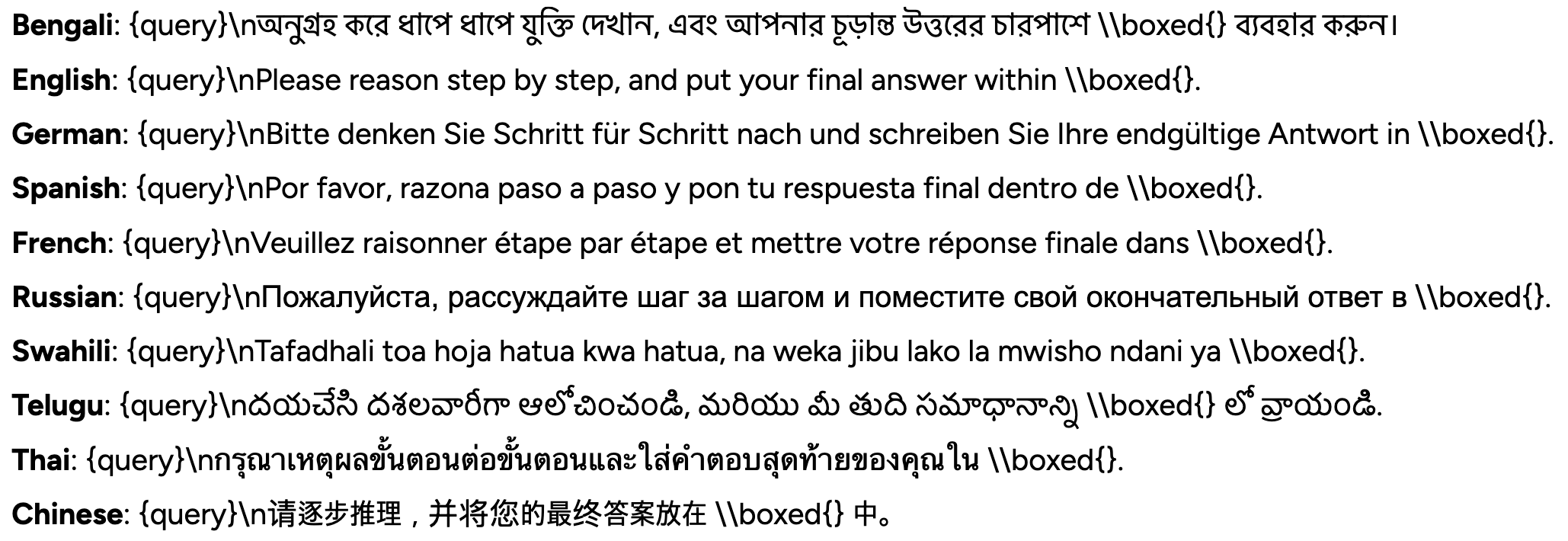
We also show the prompt template used to annotate Reasoning Flow features for each reasoning step with GPT-4o in Prompt C.1. We adapt the prompt from bogdan2025thoughtanchorsllmreasoning. We use a sampling temperature of 0.0.
Appendix D Detailed Results
D.1 Human Verification of GPT-4o Annotation
We conduct a human verification study of GPT-4o-based annotations on a small subset of reasoning traces in languages other than English. To ensure that annotators can comfortably inspect an entire trace in a single sitting, we sample traces from MGSM-Rev2, whose traces are substantially shorter on average than those from AIME (19 vs. 275). We focus on French, Russian, and Chinese, for which we could reliably recruit native speaker participants online.
We design the survey in Qualtrics888https://www.qualtrics.com to recruit participants via Prolific999https://www.prolific.com who self-report the target language as their first and primary language and also report fluency in English. We restrict to participants with at least 20 prior submission and a 95% approval rate for quality control. Since annotating even a single reasoning trace is time-consuming, we limit the evaluation to 2 traces per language, selecting one trace with more reasoning steps than the language-specific average and one with fewer. As illustrated in Figure 7, each annotator is asked to judge (1) whether the annotated Reasoning Flow tag is appropriate (Yes/Not sure/No) and (2) whether the dependency path annotation is appropriate (Yes/Not sure/No). We recruit 3 annotators per language and compensate each with 3 USD (equivalent to 18 USD/hour), with a median completion time of 10 minutes.
As shown in Table 8, we observe high inter-annotator agreement within each language (measured using Fleiss’s 101010https://www.statsmodels.org/statsmodels.stats.inter-rater.fleiss-kappa.html), as well as strong agreement between human judgments and GPT-4o annotations (measured using majority voting).
| Language | Fleiss’s | Majority Voting | |||
| Q1 | Q2 | Q1 | Q2 | Avg. | |
| French | 0.455 | 0.618 | 0.875 | 0.875 | 0.875 |
| Russian | 0.671 | 0.705 | 0.938 | 0.875 | 0.907 |
| Chinese | 0.752 | 0.733 | 1.000 | 0.875 | 0.938 |
D.2 Multivariate Logistic Regression
For our feature analysis (§3.2), we fit separate univariate logistic regressions to isolate each feature’s marginal relationship to accuracy and avoid multicollinearity between potentially correlated features. For completeness, we also fit a single multivariate logistic regression per model and language using all features jointly.
Let denote the final answer correctness and let denote the vector of feature values. As before, we standardize each continuous feature to zero mean and unit variance within each language:
| (5) |
For each model and language , we fit a multivariate logistic regression over all features jointly:
| (6) |
where is the logistic sigmoid, is a language-specific intercept, and captures the association between feature and accuracy in language after controlling for all other features. We use -regularization to stabilize estimation given the number of features relative to per-language sample sizes.
We summarize the effect of feature by discrete change in predicted accuracy when varying between and while holding all other features at their observed values:
| (7) |
where denotes all features except and
| (8) |
As shown in Figure 6, comparing to the per-language univariate results in Figure 3 we observe the following trends:
-
•
Core patterns are preserved. Features with the strongest positive in the univariate regression, such as semantic similarity, direct utility, and indirect utility, remain strongly positive in the multivariate setting, while features with negative , including problem setup and uncertainty management, generally remain negative.
-
•
Effect sizes are smaller in magnitude. Per-language effect sizes are typically attenuated under multivariate regression, as coefficients now reflect partial effects conditioned on all other features (Wang2017Inconsistency).
-
•
Reasoning flow features show more mixed behavior. Since many Reasoning Flow features co-occur within the same traces, their effects can be partially redistributed across correlated features in the multivariate setting, leading to trends that differ from the univariate analysis.


D.3 SAE Analysis Ablations
We perform ablation studies to identify the SAE configuration used in our main analysis (§5.2). We summarize the configuration space in the HypotheSAEs implementation in Table 11; all options are drawn from movva2025sparse.111111https://github.com/rmovva/HypotheSAEs We also report our qualitative observations and the rationales behind our final configuration choices.
Batch TopK SAE works as follows: given a batch of size and sparsity target , Batch TopK keeps only the largest activations across the batch and sets all others to zero, and at inference time applies a learned global threshold so that each chunk activates on average concepts.
D.4 Feature Values & Accuracy
D.5 Qualitative Analysis of Traces
We show side-by-side qualitative examples of reasoning traces from queries in English versus in languages other than English in Table 14. We include (i) pairs where both traces reach the correct final answer but exhibit different reasoning behaviors, and (ii) pairs where one trace is correct and the other incorrect despite displaying similar reasoning behaviors.
For the first example (both ✓), the English trace begins with explicit plan generation followed by active computation, whereas the Bengali trace immediately performs active computation and follows a different logarithmic route to the correct answer. Similarly for the second example, the English trace contains substantial uncertainty management (14 steps), which ultimately leads the model to re-check its interpretation before emitting the final answer, whereas the French trace reaches the same correct answer without any steps labeled as uncertainty management. In the third example (English ✗, non-English ✓), both traces start with problem setup, proceed through active computation and fact retrieval, and solve for the same variable (the number of 30-minute episodes), but the English trace fails to incorporate the Thursday and Friday information and thus outputs an incorrect answer.
D.6 Test-time Selection Policy Ablations
We set in our main test-time selection experiments, sampling 8 independent candidate reasoning traces at each temperature , following prior work on multi-temperature test-time scaling (feng2025characterizeseffectivereasoningrevisiting). However, in practical deployment scenarios, sampling and re-ranking 32 candidates per query can be computationally expensive. To study the trade-off between compute and performance, we additionally evaluate smaller budgets , sampling traces at each temperature and reporting compute time in Table 9 and pass@1 in Table 10. As increases, we observe higher computational overhead but also larger pass@1 gains over the random selection baseline, illustrating a compute-performance trade-off.
| Dataset | Model | ||||
| MGSM-Rev2 | Distill-Qwen 1.5b | 03:32 | 06:15 | 08:01 | 09:27 |
| Distill-Qwen 7b | 04:38 | 05:48 | 07:39 | 09:25 | |
| Qwen3 4b | 01:35 | 04:19 | 05:50 | 07:11 | |
| Qwen3 8b | 04:20 | 07:57 | 11:21 | 14:46 | |
| AIME | Distill-Qwen 1.5b | 06:32 | 14:09 | 19:26 | 23:58 |
| Distill-Qwen 7b | 19:40 | 41:27 | 60:03 | 77:32 | |
| Qwen3 4b | 11:46 | 24:59 | 36:16 | 47:27 | |
| Qwen3 8b | 26:43 | 52:10 | 79:07 | 106:49 |
| Model | Random | Struc. | Sem. | Num. | Direct | Indirect | Result | Uncertainty | |
| MGSM-Rev2 | |||||||||
| Distill-Qwen 1.5b | 4 | 0.366 | 0.367 | 0.378 | 0.367 | 0.381 | 0.381 | 0.360 | 0.360 |
| 8 | 0.368 | 0.367 | 0.395 | 0.367 | 0.387 | 0.383 | 0.360 | 0.349 | |
| 16 | 0.365 | 0.365 | 0.402 | 0.361 | 0.396 | 0.387 | 0.361 | 0.351 | |
| 32 | 0.369 | 0.371 | 0.430 | 0.360 | 0.402 | 0.391 | 0.368 | 0.343 | |
| Distill-Qwen 8b | 4 | 0.627 | 0.623 | 0.630 | 0.622 | 0.633 | 0.604 | 0.623 | 0.633 |
| 8 | 0.623 | 0.622 | 0.626 | 0.629 | 0.641 | 0.612 | 0.612 | 0.636 | |
| 16 | 0.625 | 0.615 | 0.632 | 0.632 | 0.639 | 0.600 | 0.626 | 0.607 | |
| 32 | 0.623 | 0.589 | 0.640 | 0.617 | 0.651 | 0.609 | 0.615 | 0.596 | |
| Qwen3 4b | 4 | 0.747 | 0.755 | 0.755 | 0.734 | 0.756 | 0.759 | 0.755 | 0.737 |
| 8 | 0.748 | 0.756 | 0.756 | 0.735 | 0.746 | 0.746 | 0.754 | 0.732 | |
| 16 | 0.740 | 0.755 | 0.758 | 0.732 | 0.748 | 0.747 | 0.754 | 0.730 | |
| 32 | 0.745 | 0.753 | 0.753 | 0.723 | 0.761 | 0.743 | 0.746 | 0.727 | |
| Qwen3 8b | 4 | 0.733 | 0.739 | 0.746 | 0.735 | 0.741 | 0.736 | 0.739 | 0.721 |
| 8 | 0.732 | 0.743 | 0.740 | 0.738 | 0.740 | 0.738 | 0.741 | 0.728 | |
| 16 | 0.738 | 0.741 | 0.743 | 0.733 | 0.749 | 0.739 | 0.744 | 0.721 | |
| 32 | 0.738 | 0.756 | 0.751 | 0.726 | 0.756 | 0.741 | 0.747 | 0.717 | |
| AIME | |||||||||
| Distill-Qwen 1.5b | 4 | 0.181 | 0.184 | 0.192 | 0.136 | 0.210 | 0.218 | 0.202 | 0.181 |
| 8 | 0.184 | 0.181 | 0.196 | 0.124 | 0.221 | 0.222 | 0.208 | 0.183 | |
| 16 | 0.181 | 0.188 | 0.199 | 0.122 | 0.223 | 0.224 | 0.211 | 0.176 | |
| 32 | 0.183 | 0.204 | 0.200 | 0.133 | 0.246 | 0.228 | 0.221 | 0.175 | |
| Distill-Qwen 7b | 4 | 0.247 | 0.272 | 0.254 | 0.212 | 0.324 | 0.319 | 0.267 | 0.245 |
| 8 | 0.243 | 0.277 | 0.257 | 0.204 | 0.327 | 0.325 | 0.292 | 0.240 | |
| 16 | 0.241 | 0.281 | 0.266 | 0.201 | 0.331 | 0.331 | 0.295 | 0.227 | |
| 32 | 0.244 | 0.297 | 0.297 | 0.186 | 0.351 | 0.342 | 0.311 | 0.202 | |
| Qwen3 4b | 4 | 0.402 | 0.411 | 0.404 | 0.411 | 0.407 | 0.431 | 0.410 | 0.400 |
| 8 | 0.390 | 0.418 | 0.406 | 0.391 | 0.425 | 0.455 | 0.403 | 0.367 | |
| 16 | 0.404 | 0.424 | 0.411 | 0.378 | 0.423 | 0.483 | 0.457 | 0.333 | |
| 32 | 0.397 | 0.480 | 0.422 | 0.364 | 0.489 | 0.505 | 0.523 | 0.319 | |
| Qwen3 8b | 4 | 0.457 | 0.466 | 0.459 | 0.459 | 0.488 | 0.488 | 0.482 | 0.444 |
| 8 | 0.460 | 0.469 | 0.461 | 0.455 | 0.495 | 0.503 | 0.489 | 0.437 | |
| 16 | 0.453 | 0.471 | 0.461 | 0.417 | 0.504 | 0.516 | 0.492 | 0.441 | |
| 32 | 0.458 | 0.477 | 0.469 | 0.390 | 0.512 | 0.549 | 0.504 | 0.383 | |
| Configuration | Options | Rationale |
| Chunking Method | Following recommendations in movva2025sparse, we split long inputs (reasoning traces) into chunks of roughly 250-500 words for better feature interpretation. We do not use sentence-level tokenization or splitting on our reasoning trace separator (\n\n), as these create many short segments and substantially increase the number of embedding calls. We also avoid using a separate LLM to summarize the input texts, both to preserve as much of the original information as possible and to limit the number of additional LLM calls. In practice, a chunk size of about 400 words (allowing the threshold to fall within a word) was computationally efficient. | |
| Embedding Model | {RoBERTa, ModernBERT, LaBSE, OpenAI text-embedding-3} | We use LaBSE embeddings as our embedding model for three reasons: (i) it is explicitly trained for multilingual sentence representations and covers all languages in our tested datasets, (ii) it provides off-the-shelf embeddings without requiring additional API calls or model fine-tuning, and (iii) in our qualitative observations, it produced more coherent reasoning concepts than the monolingual (RoBERTa/ModernBERT) alternatives. |
| SAE Parameters | {Vanilla TopK, Matryoshka TopK, Batch TopK} | We follow the rules of thumb from movva2025sparse, where (the total number of concepts) and (the number of active concepts per example) control concept granularity and sparsity. Larger allows the SAE to represent more fine-grained reasoning patterns across the inputs, while larger enables each trace to be decomposed into a richer combination of concepts. For our dataset size and chunked trace length, we select and as a middle ground: this is large enough to separate broad phenomena into distinct concepts without oversplitting into nearly-identical concepts. |
| Selection Method | {Correlation, LASSO, Separation score} | We use the correlation-based selector, which ranks neurons by the Pearson correlation between their activations and the target label. We find that this method is fast, simplest to implement, and gives relatively good balance of effect size and prevalence. It was suitable for our setting where we need to screen many neurons across 10 languages and 4 models without incurring the additional optimization overhead of LASSO. |
| Interpreter Model | {LLaMA-3.3 70b, GPT-4o} | We test two models for generating interpretations: one open-weight model (LLaMA-3.3 70b) that can be run within our compute budget, and one closed-source model (GPT-4o). We use GPT-4o since sampling from LLaMA-3.3 70b was substantially slower and its generated concept descriptions were generally less detailed (e.g., “engages in multi-step reasoning”). |
| Lang. |
Alignment
|
Reasoning Step
|
Reasoning Flow
|
Acc. | |||||||||||||
| C | St | Se | # | V | D | I | S | A | P | Pl | F | Fa | R | U | |||
| Distill-Qwen 1.5b | |||||||||||||||||
| bn | 0.874 | 0.450 | 0.744 | 41 | 0.192 | 0.518 | 0.440 | -9.49 | 0.037 | 0.234 | 0.237 | 0.099 | 0.044 | 0.083 | 0.071 | 0.162 | 0.240 |
| de | 0.847 | 0.590 | 0.801 | 4 | 0.326 | 0.779 | 0.578 | 2.54 | 0.008 | 0.344 | 0.282 | 0.127 | 0.031 | 0.089 | 0.111 | 0.007 | 0.432 |
| en | — | — | — | 32 | 0.199 | 0.802 | 0.670 | -6.40 | 0.068 | 0.309 | 0.127 | 0.152 | 0.041 | 0.087 | 0.127 | 0.084 | 0.876 |
| es | 0.865 | 0.571 | 0.832 | 5 | 0.300 | 0.874 | 0.674 | -2.10 | 0.000 | 0.357 | 0.273 | 0.094 | 0.038 | 0.140 | 0.094 | 0.004 | 0.592 |
| fr | 0.864 | 0.600 | 0.831 | 5 | 0.332 | 0.770 | 0.579 | -2.34 | 0.020 | 0.309 | 0.244 | 0.185 | 0.041 | 0.093 | 0.095 | 0.014 | 0.496 |
| ru | 0.855 | 0.543 | 0.796 | 13 | 0.292 | 0.734 | 0.593 | -8.84 | 0.019 | 0.303 | 0.225 | 0.140 | 0.064 | 0.118 | 0.092 | 0.036 | 0.524 |
| sw | 0.825 | 0.424 | 0.653 | 24 | 0.210 | 0.216 | 0.178 | 7.29 | 0.005 | 0.136 | 0.398 | 0.076 | 0.042 | 0.059 | 0.051 | 0.137 | 0.024 |
| te | 0.850 | 0.495 | 0.678 | 41 | 0.222 | 0.264 | 0.209 | -6.44 | 0.002 | 0.201 | 0.344 | 0.092 | 0.044 | 0.109 | 0.077 | 0.056 | 0.056 |
| th | 0.833 | 0.467 | 0.578 | 27 | 0.203 | 0.236 | 0.175 | -1.19 | 0.007 | 0.170 | 0.286 | 0.073 | 0.074 | 0.061 | 0.054 | 0.016 | 0.124 |
| zh | 0.848 | 0.557 | 0.824 | 27 | 0.236 | 0.821 | 0.658 | -12.6 | 0.039 | 0.344 | 0.197 | 0.082 | 0.044 | 0.109 | 0.119 | 0.062 | 0.680 |
| Distill-Qwen 7b | |||||||||||||||||
| bn | 0.874 | 0.604 | 0.737 | 5 | 0.388 | 0.791 | 0.591 | -9.66 | 0.003 | 0.261 | 0.371 | 0.070 | 0.052 | 0.102 | 0.103 | 0.028 | 0.540 |
| de | 0.847 | 0.559 | 0.794 | 5 | 0.355 | 0.878 | 0.654 | -6.59 | 0.002 | 0.329 | 0.248 | 0.133 | 0.026 | 0.131 | 0.129 | 0.002 | 0.764 |
| en | — | — | — | 29 | 0.089 | 0.760 | 0.702 | -5.31 | 0.150 | 0.239 | 0.087 | 0.106 | 0.054 | 0.092 | 0.139 | 0.130 | 0.956 |
| es | 0.865 | 0.597 | 0.816 | 5 | 0.289 | 0.892 | 0.679 | -3.57 | 0.001 | 0.403 | 0.268 | 0.096 | 0.039 | 0.109 | 0.082 | 0.003 | 0.824 |
| fr | 0.864 | 0.564 | 0.816 | 5 | 0.322 | 0.815 | 0.638 | -5.13 | 0.001 | 0.345 | 0.191 | 0.150 | 0.037 | 0.184 | 0.091 | 0.002 | 0.804 |
| ru | 0.855 | 0.575 | 0.787 | 5 | 0.325 | 0.897 | 0.673 | -5.55 | 0.003 | 0.374 | 0.244 | 0.117 | 0.033 | 0.084 | 0.138 | 0.006 | 0.816 |
| sw | 0.825 | 0.526 | 0.669 | 10 | 0.300 | 0.378 | 0.296 | -11.4 | 0.009 | 0.182 | 0.399 | 0.065 | 0.024 | 0.113 | 0.086 | 0.032 | 0.108 |
| te | 0.850 | 0.515 | 0.759 | 10 | 0.314 | 0.589 | 0.451 | -9.20 | 0.007 | 0.258 | 0.332 | 0.092 | 0.034 | 0.133 | 0.084 | 0.041 | 0.288 |
| th | 0.833 | 0.550 | 0.734 | 8 | 0.322 | 0.624 | 0.496 | -8.59 | 0.020 | 0.244 | 0.302 | 0.136 | 0.037 | 0.157 | 0.072 | 0.026 | 0.608 |
| zh | 0.848 | 0.551 | 0.802 | 9 | 0.278 | 0.920 | 0.721 | -4.85 | 0.025 | 0.377 | 0.233 | 0.068 | 0.046 | 0.106 | 0.116 | 0.028 | 0.824 |
| Qwen-3 8b | |||||||||||||||||
| bn | 0.874 | 0.425 | 0.914 | 25 | 0.106 | 0.760 | 0.686 | -6.47 | 0.128 | 0.201 | 0.149 | 0.111 | 0.043 | 0.090 | 0.060 | 0.218 | 0.900 |
| de | 0.847 | 0.487 | 0.940 | 13 | 0.162 | 0.823 | 0.698 | -4.25 | 0.158 | 0.215 | 0.191 | 0.144 | 0.032 | 0.098 | 0.041 | 0.121 | 0.968 |
| en | — | — | — | 26 | 0.090 | 0.748 | 0.687 | -4.69 | 0.145 | 0.194 | 0.090 | 0.095 | 0.062 | 0.086 | 0.089 | 0.238 | 0.988 |
| es | 0.865 | 0.492 | 0.940 | 14 | 0.149 | 0.837 | 0.722 | -4.52 | 0.144 | 0.224 | 0.175 | 0.135 | 0.035 | 0.088 | 0.045 | 0.155 | 0.968 |
| fr | 0.864 | 0.487 | 0.935 | 15 | 0.135 | 0.824 | 0.716 | -5.58 | 0.156 | 0.219 | 0.179 | 0.141 | 0.034 | 0.081 | 0.050 | 0.140 | 0.956 |
| ru | 0.855 | 0.449 | 0.865 | 20 | 0.110 | 0.794 | 0.709 | -7.26 | 0.166 | 0.238 | 0.130 | 0.118 | 0.059 | 0.081 | 0.060 | 0.148 | 0.956 |
| sw | 0.825 | 0.340 | 0.837 | 41 | 0.098 | 0.744 | 0.691 | -9.22 | 0.048 | 0.138 | 0.203 | 0.076 | 0.032 | 0.082 | 0.028 | 0.391 | 0.372 |
| te | 0.850 | 0.435 | 0.907 | 20 | 0.150 | 0.767 | 0.666 | -6.90 | 0.112 | 0.197 | 0.211 | 0.106 | 0.028 | 0.092 | 0.044 | 0.209 | 0.840 |
| th | 0.833 | 0.453 | 0.924 | 18 | 0.133 | 0.834 | 0.736 | -11.1 | 0.127 | 0.198 | 0.164 | 0.130 | 0.040 | 0.106 | 0.050 | 0.186 | 0.900 |
| zh | 0.848 | 0.394 | 0.851 | 26 | 0.074 | 0.695 | 0.636 | -2.76 | 0.140 | 0.185 | 0.084 | 0.092 | 0.062 | 0.085 | 0.069 | 0.283 | 0.964 |
| Qwen-3 14b | |||||||||||||||||
| bn | 0.874 | 0.440 | 0.925 | 20 | 0.119 | 0.765 | 0.677 | -5.98 | 0.136 | 0.231 | 0.164 | 0.120 | 0.044 | 0.091 | 0.058 | 0.156 | 0.940 |
| de | 0.847 | 0.455 | 0.941 | 17 | 0.126 | 0.783 | 0.693 | -3.97 | 0.162 | 0.196 | 0.139 | 0.118 | 0.053 | 0.113 | 0.055 | 0.163 | 0.968 |
| en | — | — | — | 33 | 0.089 | 0.697 | 0.648 | -0.51 | 0.149 | 0.198 | 0.085 | 0.091 | 0.056 | 0.091 | 0.108 | 0.222 | 0.984 |
| es | 0.865 | 0.487 | 0.941 | 16 | 0.139 | 0.823 | 0.716 | -5.16 | 0.157 | 0.225 | 0.158 | 0.120 | 0.042 | 0.102 | 0.059 | 0.136 | 0.984 |
| fr | 0.864 | 0.484 | 0.934 | 16 | 0.136 | 0.833 | 0.724 | -5.32 | 0.157 | 0.212 | 0.174 | 0.116 | 0.038 | 0.086 | 0.057 | 0.159 | 0.968 |
| ru | 0.855 | 0.447 | 0.938 | 21 | 0.109 | 0.788 | 0.708 | -5.59 | 0.159 | 0.215 | 0.120 | 0.115 | 0.059 | 0.091 | 0.070 | 0.172 | 0.984 |
| sw | 0.825 | 0.381 | 0.875 | 34 | 0.111 | 0.738 | 0.668 | -8.01 | 0.084 | 0.169 | 0.166 | 0.103 | 0.037 | 0.108 | 0.047 | 0.281 | 0.644 |
| te | 0.850 | 0.416 | 0.918 | 25 | 0.113 | 0.725 | 0.652 | -5.68 | 0.120 | 0.206 | 0.147 | 0.111 | 0.051 | 0.105 | 0.066 | 0.194 | 0.908 |
| th | 0.833 | 0.432 | 0.930 | 23 | 0.113 | 0.773 | 0.690 | -2.48 | 0.132 | 0.196 | 0.133 | 0.125 | 0.047 | 0.119 | 0.064 | 0.184 | 0.960 |
| zh | 0.848 | 0.381 | 0.852 | 38 | 0.064 | 0.586 | 0.544 | -1.35 | 0.151 | 0.195 | 0.064 | 0.081 | 0.053 | 0.082 | 0.101 | 0.271 | 0.972 |
| Lang. |
Alignment
|
Reasoning Step
|
Reasoning Flow
|
Acc. | |||||||||||||
| C | St | Se | # | V | D | I | S | A | P | Pl | F | Fa | R | U | |||
| Distill-Qwen 1.5b | |||||||||||||||||
| bn | 0.814 | 0.282 | 0.865 | 354 | 0.018 | 0.674 | 0.668 | -1.86 | 0.020 | 0.264 | 0.030 | 0.100 | 0.009 | 0.133 | 0.083 | 0.204 | 0.167 |
| de | 0.815 | 0.491 | 0.825 | 181 | 0.088 | 0.624 | 0.575 | 20.9 | 0.023 | 0.317 | 0.117 | 0.171 | 0.024 | 0.152 | 0.073 | 0.064 | 0.117 |
| en | — | — | — | 424 | 0.008 | 0.565 | 0.562 | 1.81 | 0.049 | 0.227 | 0.019 | 0.096 | 0.006 | 0.172 | 0.080 | 0.086 | 0.233 |
| es | 0.820 | 0.424 | 0.865 | 303 | 0.056 | 0.542 | 0.511 | 10.6 | 0.009 | 0.232 | 0.095 | 0.118 | 0.019 | 0.123 | 0.083 | 0.091 | 0.117 |
| fr | 0.834 | 0.407 | 0.864 | 208 | 0.101 | 0.625 | 0.598 | 14.5 | 0.053 | 0.269 | 0.102 | 0.171 | 0.026 | 0.127 | 0.096 | 0.098 | 0.167 |
| ru | 0.822 | 0.339 | 0.827 | 275 | 0.008 | 0.370 | 0.367 | 0.54 | 0.037 | 0.228 | 0.015 | 0.095 | 0.009 | 0.145 | 0.064 | 0.110 | 0.100 |
| sw | 0.790 | 0.340 | 0.853 | 256 | 0.079 | 0.485 | 0.468 | 10.3 | 0.024 | 0.220 | 0.089 | 0.105 | 0.008 | 0.128 | 0.083 | 0.197 | 0.067 |
| te | 0.788 | 0.310 | 0.851 | 262 | 0.043 | 0.473 | 0.466 | -4.51 | 0.016 | 0.237 | 0.085 | 0.089 | 0.011 | 0.091 | 0.074 | 0.235 | 0.050 |
| th | 0.795 | 0.350 | 0.761 | 147 | 0.085 | 0.340 | 0.316 | 14.4 | 0.019 | 0.245 | 0.161 | 0.109 | 0.061 | 0.095 | 0.043 | 0.127 | 0.067 |
| zh | 0.809 | 0.284 | 0.854 | 203 | 0.019 | 0.525 | 0.519 | 3.72 | 0.067 | 0.286 | 0.024 | 0.141 | 0.016 | 0.147 | 0.097 | 0.159 | 0.200 |
| Distill-Qwen 7b | |||||||||||||||||
| bn | 0.814 | 0.303 | 0.903 | 258 | 0.018 | 0.683 | 0.672 | -10.1 | 0.043 | 0.307 | 0.041 | 0.130 | 0.014 | 0.130 | 0.086 | 0.138 | 0.300 |
| de | 0.815 | 0.390 | 0.866 | 263 | 0.039 | 0.610 | 0.594 | -7.92 | 0.033 | 0.333 | 0.038 | 0.110 | 0.016 | 0.156 | 0.097 | 0.066 | 0.333 |
| en | — | — | — | 395 | 0.012 | 0.526 | 0.522 | -7.30 | 0.045 | 0.271 | 0.013 | 0.101 | 0.007 | 0.131 | 0.104 | 0.064 | 0.433 |
| es | 0.820 | 0.334 | 0.903 | 350 | 0.015 | 0.657 | 0.650 | -7.98 | 0.032 | 0.273 | 0.039 | 0.123 | 0.010 | 0.155 | 0.095 | 0.073 | 0.367 |
| fr | 0.834 | 0.362 | 0.895 | 331 | 0.030 | 0.588 | 0.581 | -10.2 | 0.037 | 0.300 | 0.039 | 0.105 | 0.009 | 0.110 | 0.093 | 0.091 | 0.433 |
| ru | 0.822 | 0.377 | 0.837 | 276 | 0.017 | 0.472 | 0.464 | -6.18 | 0.026 | 0.322 | 0.041 | 0.118 | 0.011 | 0.152 | 0.072 | 0.084 | 0.283 |
| sw | 0.790 | 0.309 | 0.846 | 276 | 0.054 | 0.653 | 0.639 | -12.5 | 0.026 | 0.252 | 0.064 | 0.095 | 0.011 | 0.154 | 0.066 | 0.149 | 0.117 |
| te | 0.788 | 0.342 | 0.876 | 300 | 0.029 | 0.611 | 0.604 | -12.3 | 0.025 | 0.333 | 0.044 | 0.114 | 0.010 | 0.139 | 0.091 | 0.136 | 0.250 |
| th | 0.795 | 0.375 | 0.856 | 171 | 0.031 | 0.534 | 0.520 | -11.5 | 0.061 | 0.319 | 0.037 | 0.163 | 0.017 | 0.138 | 0.083 | 0.139 | 0.300 |
| zh | 0.809 | 0.337 | 0.859 | 202 | 0.012 | 0.580 | 0.574 | -9.80 | 0.057 | 0.328 | 0.023 | 0.145 | 0.012 | 0.152 | 0.102 | 0.121 | 0.333 |
| Qwen-3 8b | |||||||||||||||||
| bn | 0.814 | 0.310 | 0.901 | 258 | 0.025 | 0.663 | 0.657 | -11.0 | 0.057 | 0.290 | 0.027 | 0.147 | 0.011 | 0.156 | 0.071 | 0.152 | 0.500 |
| de | 0.815 | 0.320 | 0.931 | 284 | 0.021 | 0.721 | 0.716 | -8.85 | 0.038 | 0.309 | 0.016 | 0.123 | 0.009 | 0.232 | 0.073 | 0.147 | 0.617 |
| en | — | — | — | 257 | 0.023 | 0.712 | 0.705 | -8.40 | 0.073 | 0.312 | 0.019 | 0.164 | 0.012 | 0.164 | 0.080 | 0.105 | 0.700 |
| es | 0.820 | 0.349 | 0.941 | 269 | 0.013 | 0.724 | 0.718 | -8.92 | 0.057 | 0.331 | 0.016 | 0.164 | 0.010 | 0.157 | 0.074 | 0.085 | 0.683 |
| fr | 0.834 | 0.318 | 0.931 | 266 | 0.017 | 0.807 | 0.801 | -8.43 | 0.071 | 0.334 | 0.032 | 0.156 | 0.010 | 0.174 | 0.071 | 0.099 | 0.667 |
| ru | 0.822 | 0.313 | 0.860 | 237 | 0.020 | 0.716 | 0.711 | -6.25 | 0.108 | 0.319 | 0.018 | 0.159 | 0.009 | 0.157 | 0.088 | 0.123 | 0.583 |
| sw | 0.790 | 0.292 | 0.893 | 278 | 0.016 | 0.688 | 0.683 | -14.0 | 0.041 | 0.285 | 0.036 | 0.117 | 0.007 | 0.134 | 0.061 | 0.212 | 0.317 |
| te | 0.788 | 0.308 | 0.903 | 255 | 0.041 | 0.665 | 0.657 | -11.3 | 0.056 | 0.294 | 0.035 | 0.113 | 0.012 | 0.152 | 0.066 | 0.186 | 0.383 |
| th | 0.795 | 0.308 | 0.917 | 314 | 0.022 | 0.655 | 0.650 | -14.2 | 0.048 | 0.253 | 0.036 | 0.111 | 0.008 | 0.193 | 0.079 | 0.152 | 0.567 |
| zh | 0.809 | 0.248 | 0.859 | 288 | 0.009 | 0.645 | 0.642 | -16.3 | 0.053 | 0.260 | 0.020 | 0.159 | 0.012 | 0.188 | 0.076 | 0.214 | 0.533 |
| Qwen-3 14b | |||||||||||||||||
| bn | 0.814 | 0.329 | 0.904 | 298 | 0.019 | 0.744 | 0.738 | -5.17 | 0.047 | 0.360 | 0.024 | 0.131 | 0.010 | 0.162 | 0.089 | 0.092 | 0.567 |
| de | 0.815 | 0.340 | 0.927 | 285 | 0.016 | 0.708 | 0.703 | -6.76 | 0.050 | 0.339 | 0.033 | 0.128 | 0.009 | 0.162 | 0.078 | 0.095 | 0.650 |
| en | — | — | — | 262 | 0.015 | 0.692 | 0.688 | -2.49 | 0.106 | 0.320 | 0.014 | 0.133 | 0.008 | 0.146 | 0.078 | 0.081 | 0.667 |
| es | 0.820 | 0.357 | 0.937 | 277 | 0.015 | 0.819 | 0.814 | -5.16 | 0.062 | 0.357 | 0.036 | 0.117 | 0.009 | 0.179 | 0.065 | 0.107 | 0.717 |
| fr | 0.834 | 0.358 | 0.937 | 285 | 0.024 | 0.750 | 0.744 | -5.38 | 0.063 | 0.339 | 0.024 | 0.159 | 0.008 | 0.137 | 0.094 | 0.106 | 0.733 |
| ru | 0.822 | 0.334 | 0.900 | 247 | 0.024 | 0.713 | 0.707 | -7.13 | 0.060 | 0.400 | 0.025 | 0.168 | 0.010 | 0.119 | 0.080 | 0.102 | 0.617 |
| sw | 0.790 | 0.284 | 0.897 | 302 | 0.032 | 0.710 | 0.705 | -8.36 | 0.041 | 0.319 | 0.023 | 0.131 | 0.008 | 0.172 | 0.066 | 0.152 | 0.417 |
| te | 0.788 | 0.292 | 0.898 | 286 | 0.023 | 0.646 | 0.641 | -8.38 | 0.067 | 0.283 | 0.025 | 0.153 | 0.008 | 0.144 | 0.074 | 0.175 | 0.483 |
| th | 0.795 | 0.310 | 0.914 | 321 | 0.015 | 0.716 | 0.711 | -1.92 | 0.049 | 0.298 | 0.016 | 0.146 | 0.008 | 0.178 | 0.076 | 0.125 | 0.583 |
| zh | 0.809 | 0.287 | 0.858 | 339 | 0.008 | 0.649 | 0.646 | -8.57 | 0.041 | 0.255 | 0.022 | 0.152 | 0.011 | 0.157 | 0.096 | 0.167 | 0.533 |
| Model / Language | Query | Reasoning trace (English) | Reasoning trace (Non-English) |
| Correct answers, Different reasoning | |||
| Distill-Qwen 7b (Bengali) | Lloyd has an egg farm. His chickens produce 252 eggs per day and he sells them for 2 per dozen. How much does Lloyd make on eggs per week? | First, determine how many eggs Lloyd sells each week. He has 252 eggs per day, and there are 7 days in a week, so multiplying 252 by 7 gives the total number of eggs per week. Next, since eggs are sold by the dozen, divide the total number of eggs by 12 to find out how many dozens of eggs are sold each week. Finally, multiply the number of dozens by the selling price per dozen, which is 2, to calculate the total earnings per week. ✓ | The number of eggs they produce per day is 252. Eggs are sold at 2 dollars per dozen. One dozen contains 12 eggs. Therefore, the selling price per egg is 2 dollars 12 = 1/6 dollar. So, if 252 eggs are sold per day, the income is 252 (1/6) = 42 dollars. There are 7 days in a week, so the total weekly income is 42 7 = 294 dollars. ✓ |
| Qwen3 4b (French) | Janet buys a brooch for her daughter. She pays $500 for the material to make it and then another $800 for the jeweler to construct it. After that, she pays 10% of that to get it insured. How much did she pay? | Okay, let me try to figure out how much Janet paid in total for the brooch. So, the problem says she buys a brooch for her daughter. She pays $500 for the material, then another $800 for the jeweler to construct it. Then she pays 10% of that to get it insured. The question is asking how much she paid altogether. First, I need to make sure I understand all the parts of the problem. Let me break it down step by step. First expense is the material, which is $500. Then the construction cost is $800. So, those are two separate costs. Then, after that, she pays 10% of ‘that‘ to get it insured. Wait, ‘that‘ – does that refer to the total of the material and construction costs, or just one of them? The wording says ‘10% of that to get it insured.‘ The ‘that‘ is probably referring to the total amount she paid for the material and the jeweler. Let me check the original sentence again: ‘She pays $500 for the material to make it and then another $800 for the jeweler to construct it. After that, she pays 10% of that to get it insured.‘So ‘that‘ is referring to the previous total. So the ‘that‘ is the total of the material and the construction. So, $500 + $800 = $1300. Then 10% of that is 10% of $1300. So, the insurance cost is 10% of $1300. Then, the total amount she paid would be the sum of the material, construction, and insurance.Alternatively, maybe ‘that‘ refers to the construction cost? But the wording is ‘after that,‘ which would refer to the previous two payments. So, after paying for the material and the jeweler, she pays 10% of that total. So, that makes sense. So, the insurance is 10% of the total of the material and construction. So, let me compute that. First, the material is $500, construction is $800. So total of those two is 500 + 800 = 1300. Then, 10% of 1300 is 0.10 * 1300 = 130. So, the insurance is $130. Therefore, total amount paid is 500 + 800 + 130 = 1430. Wait, but let me check again. […] Alternatively, maybe the problem is trying to trick me? […] Therefore, the answer is \\boxed{1430}. ✓ | Okay, let me try to figure out how much Janet spent in total. So, the problem says she buys a brooch for her daughter. First, she spends $500 on materials for the crafting. Then, she spends an additional $800 for the jewelry maker to do the work. After that, she spends 10% of that total amount on insurance. The question is asking for the total amount she spent. Hmm, let me break this down step by step. First, the initial costs: $500 for materials and $800 for the jewelry maker. So, adding those together, that would be 500 + 800. Let me calculate that: 500 + 800 is 1300. So, the first two parts total $1300. Then, she spends 10% of this sum on insurance. Wait, the problem says “10% de cette somme”, which translates to 10% of this amount. The “cette somme” here refers to the total of the first two expenses, right? So, 10% of $1300. Let me compute that. 10% of 1300 is 0.10 * 1300, which equals 130. So, she spends an additional $130 on insurance. Now, to find the total amount spent, I need to add the initial $1300 to the insurance cost of $130. That would be 1300 + 130. Let me add those numbers: 1300 + 130 is 1430. So, the total amount Janet spent is $1430. Wait, let me double-check to make sure I didn’t make a mistake. The first two expenses are definitely 500 + 800 = 1300. Then 10% of 1300 is 130. Adding them together gives 1300 + 130 = 1430. Yeah, that seems right. The insurance is 10% of the total of the materials and the jewelry work, not 10% of each separately. So, the answer should be $1430. ✓ |
| Different answers, Similar reasoning | |||
| Qwen3 8b (Chinese) | Frankie watches TV after he finishes his homework every night. On Monday and Tuesday, he watched a 1-hour episode of his favorite show each night. On Wednesday, he watched a few episodes of a 30-minute show. On Thursday, he finished homework early and watched a 1-hour episode and a 30-minute show. On Friday, he got to stay up late for the weekend, so he watched two 1-hour episodes. If he watched 7 hours of TV in all, how many 30-minute episodes did he watch on Wednesday? | First, I’ll calculate the total TV time Frankie spent on each day. On Monday and Tuesday, he watched a 1-hour episode each night, which totals 2 hours. On Wednesday, he watched either a few 30-minute episodes or a combination of 1-hour and 30-minute shows. Since the total TV time is 7 hours, I’ll subtract the known time from Wednesday to find out how much time was spent on Wednesday. Subtracting the known time (1 hour for the 1-hour episode) from the total, we have 6 hours remaining for Wednesday. Let () represent the number of 30-minute episodes Frankie watched on Wednesday. Each 30-minute episode is 0.5 hours, so the time spent on 30-minute episodes is hours. The equation becomes: . Solving for : , , . Therefore, Frankie watched 10 episodes of the 30-minute show on Wednesday. ✗ | First, let’s assume he watched x episodes of 30-minute programs on Wednesday. On Monday and Tuesday, he watched 1 episode each day, for a total of 1 hour each day, or 2 hours in total. On Wednesday, he watched x episodes, each 30 minutes long, for a total of hours. On Thursday, he watched one 1-hour episode and one 30-minute episode, for a total of 1.5 hours. On Friday, he watched 2 episodes, each 1 hour long, for a total of 2 hours. Adding all the times together gives a total of 7 hours: . Solving the equation: , , . Therefore, on Wednesday he watched 3 episodes, each 30 minutes long. ✓ |
![[Uncaptioned image]](/html/2604.04720/assets/figures/task_instruction.png)
![[Uncaptioned image]](/html/2604.04720/assets/figures/example_1.png)

