跳到论文正文
W Papers独立论文阅读器 arXiv:2604.04272 论文正文 计算阅读时间 · 0%
引用这篇论文根据当前论文元数据生成,正式投稿前建议核对。


Theoretical Foundations of
Principal Manifold Estimation
with Non-Euclidean Templates

Kun Meng Affiliation: Department of Statistics, Florida State University Affiliation: Correspondence: 117 N. Woodward Ave, Tallahassee, FL 32306, USA. Email: kmeng@fsu.edu.    Christopher Perez Affiliation: Department of Statistics, Florida State University
Abstract

We develop a rigorous theoretical framework for principal manifold estimation that recovers a latent low-dimensional manifold from a point cloud observed in a high-dimensional ambient space. Our framework accommodates manifolds with general, potentially non-Euclidean topology, which can be inferred using tools from topological data analysis. Using the theory of Sobolev spaces on Riemannian manifolds, we establish that the proposed principal manifolds are well defined, prove convergence of the iterative algorithm used to compute them, and show consistency of the finite-sample estimator. Furthermore, we introduce a novel method for selecting the complexity level of a fitted manifold, which addresses the shortcomings of the classical fitting-error criterion. We also provide a detailed geometric interpretation of the penalty term in our framework. In addition to the theoretical developments, we present extensive numerical experiments supporting our results. This article provides theoretical foundations for approaches that have been used in applications such as robotics. More importantly, it extends these approaches to general topological settings with potential applications across a broad range of disciplines, including neuroimaging and shape data analysis.

Keywords: Manifold learning; Riemannian geometry; Sobolev spaces; topological data analysis.

1 Introduction

Manifold learning refers to a broad class of methods for modeling high-dimensional data under the manifold hypothesis—“high-dimensional data tend to lie in the vicinity of a low-dimensional manifold” (narayanan2010sample, fefferman2016testing, fefferman2025fitting). In recent years, manifold learning has found applications across a wide range of scientific disciplines, including sleep stage assessment (e.g., lederman2015alternating), robotics (e.g., gao2023k, gao2024bi), neuroimaging (e.g., yue2016parameterization, busch2023multi, zielinski2024longitudinal), single-cell biology (e.g., yao2024single, ding2023learning, ding2025kernel, liu2025assessing), and metabolomics (e.g., li2025manifold). Within statistical methodology, manifold learning also plays a foundational role in numerous established frameworks. For example, shape data analysis focuses on the study of curves and surfaces, each of which is naturally modeled as a manifold (kurtek2011elastic, kurtek2012statistical, srivastava2016functional). In many applications, a necessary first step for downstream shape data analysis is to learn the underlying shape representation from an observed point cloud, a task that can naturally be formulated as a manifold learning problem.

Consider a point cloud (i.e., a set of data points) observed in a high-dimensional Euclidean space, i.e., in ℝD\mathbb{R}^{D} with DD large (the ambient space with the ambient dimension DD). As noted in the literature (e.g., meng_principal_2021, yao2024single, li2025manifold), there are two primary directions in manifold learning from a methodological viewpoint. The first focuses on nonlinear dimension reduction, aiming to derive a low-dimensional representation from high-dimensional data. Numerous widely adopted methods exemplify this direction, e.g., ISOMAP (tenenbaum2000global) and locally linear embedding (roweis2000nonlinear, wu2018think). However, these methods do not estimate the underlying manifold ℳ\mathcal{M} as a submanifold of the ambient space ℝD\mathbb{R}^{D}. In contrast, the second direction, manifold fitting, seeks to reconstruct the underlying manifold ℳ\mathcal{M} as a submanifold of ℝD\mathbb{R}^{D}. This direction will be the primary focus of this article. One family of methods in manifold fitting is known as principal manifold estimation (PME), which can be understood as a generalization of linear principal component analysis (PCA; pearson1901liii). While many PME methods exhibit convincing empirical performance in numerical experiments and have found practical success in applications (e.g., yue2016parameterization, gao2023k, gao2024bi, zielinski2024longitudinal), their theoretical foundations remain underdeveloped (as detailed in Section 1.2). Moreover, existing PME methods do not incorporate the topological information latent in data; as a result, they fail to account for the global topology of the underlying manifold and do not take advantage of the tools developed by the topological data analysis (TDA) community (e.g., fasy2014confidence, bubenik2015statistical, fasy2021tda, roycraft2023bootstrapping, meng2025randomness). In this article, we address these limitations by developing comprehensive and mathematically rigorous theoretical foundations for PME, while also providing a framework that naturally incorporates tools from TDA.

1.1 Overview of Principal Manifold Estimation

We first provide an overview of works under the PME umbrella that are closely related to our contributions in this paper. These works model the underlying manifold ℳ\mathcal{M} as the image of an ℝD\mathbb{R}^{D}-valued function 𝒇∗\boldsymbol{f}^{*} satisfying the conditions specified in each work.

PME originated with the framework of principal curves (Hastie1984PrincipalCurves, hastie1989principal), which fits a smooth curve that passes through the “middle” of a DD-dimensional point cloud (e.g., Figure 1.1) and investigates the fitting-error functional

𝒟​(𝒇)=𝔼​{‖𝑿−Π𝒇​(𝑿)‖2},\displaystyle\mathcal{D}(\boldsymbol{f})=\mathbb{E}\left\{\|\boldsymbol{X}-\Pi_{\boldsymbol{f}}(\boldsymbol{X})\|^{2}\right\}, (1.1)

where 𝑿\boldsymbol{X} represents data observed in the ambient space ℝD\mathbb{R}^{D}, the function 𝒇:ℑ→ℝD\boldsymbol{f}:\mathfrak{I}\rightarrow\mathbb{R}^{D} is defined on a prespecified interval ℑ⊆ℝ1\mathfrak{I}\subseteq\mathbb{R}^{1}, and Π𝒇​(𝑿)\Pi_{\boldsymbol{f}}(\boldsymbol{X}) denotes the nearest-point projection of 𝑿\boldsymbol{X} on the image 𝒇​(ℑ):={𝒇​(m):m∈ℑ}\boldsymbol{f}(\mathfrak{I}):=\{\boldsymbol{f}(m):m\in\mathfrak{I}\}, illustrated in Figure 1.1. The manifold hypothesis posits that data 𝑿\boldsymbol{X} lie near an underlying manifold 𝒇∗​(ℑ)\boldsymbol{f}^{*}(\mathfrak{I}), resulting in a small fitting error 𝒟​(𝒇∗)\mathcal{D}(\boldsymbol{f}^{*}). A tentative approach is to use a minimizer of 𝒟​(𝒇)\mathcal{D}(\boldsymbol{f}) to estimate the underlying manifold, which may correspond to a critical point of 𝒟​(𝒇)\mathcal{D}(\boldsymbol{f}) (i.e., a function-valued point where the Gâteaux derivative of 𝒟​(𝒇)\mathcal{D}(\boldsymbol{f}) vanishes). In particular, a principal curve may be equivalently defined as the image of a function that is a critical point of 𝒟​(𝒇)\mathcal{D}(\boldsymbol{f}) (hastie1989principal, Proposition 4).

While the principal curve framework resembles a regression model that minimizes fitting error, it does not assign roles to “predictors” and “responses.” Therefore, this framework is an unsupervised learning method, like linear PCA. Notably, the initial work by hastie1989principal opens the door to nonlinear extensions of linear PCA. Following this initial work, the principal curve framework has been further developed by numerous researchers from both theoretical and applied perspectives (e.g., tibshirani1992principal, banfield1992ice, leblanc1994adaptive, de1999principal, delicado2001another, caffo2008case, ozertem2011locally, gerber2013regularization, yue2016parameterization, kirov2017multiple, lee2020spherical, lee2023robust).

However, as duchamp1996extremal show by computing the second variation of 𝒟​(𝒇)\mathcal{D}(\boldsymbol{f}), this framework has a theoretical flaw: principal curves are never local minima of 𝒟​(𝒇)\mathcal{D}(\boldsymbol{f}), while they are critical points of 𝒟​(𝒇)\mathcal{D}(\boldsymbol{f}). Specifically, they are saddle points, and 𝒟​(𝒇)\mathcal{D}(\boldsymbol{f}) lacks a minimizer. This property stands in contrast to the regression setting and underscores a fundamental distinction between nonlinear supervised and unsupervised learning. To address the nonexistence of a minimizer, kegl2000learning introduce a penalty term on curve length. Specifically, they define a principal curve as a minimizer of the following functional and establish its existence rigorously.

𝒟​(𝒇)+λ⋅∫‖𝒇′​(m)‖​𝑑m,\displaystyle\mathcal{D}(\boldsymbol{f})+\lambda\cdot\int\|\boldsymbol{f}^{\prime}(m)\|\,dm, (1.2)

where the first term is the fitting-error functional defined in (1.1), the integral of the derivative in the second term is equal to the length of the curve 𝒇​(ℑ)\boldsymbol{f}(\mathfrak{I}) (doCarmo1976DifferentialGeometry, Chapter 1), and λ>0\lambda>0 is a tuning parameter. smola2001regularized propose substituting the L1L^{1} norm in (1.2) with a Hilbert space norm and replacing the first derivative operator with a projection operator, which leads to the application of reproducing kernel Hilbert spaces (RKHSs; wahba1990spline, chen2025probabilistic).

Motivated by the approaches of kegl2000learning and smola2001regularized, meng_principal_2021 replace the penalty term ∫‖𝒇′​(m)‖​𝑑m\int\|\boldsymbol{f}^{\prime}(m)\|\,dm in (1.2) with a roughness penalty ∫‖𝒇′′​(m)‖2​𝑑m\int\|\boldsymbol{f}^{\prime\prime}(m)\|^{2}\,dm, defined as the integral of the squared second derivative, which is an unsupervised analogue of smoothing splines (wahba1990spline, ma2015efficient, meng2020more). More importantly, they extend the classical notion of principal curves (intrinsic dimension d=1d=1) to principal manifolds of intrinsic dimension d<4d<4 by minimizing the following penalized functional in an RKHS, subject to appropriate constraints

ℒλ​(𝒇)=𝔼​{‖𝑿−Π𝒇​(𝑿)‖2}+λ⋅∫‖∇2𝒇​(𝒎)‖2​𝑑𝒎,\displaystyle\mathcal{L}_{\lambda}(\boldsymbol{f})=\mathbb{E}\left\{\|\boldsymbol{X}-\Pi_{\boldsymbol{f}}(\boldsymbol{X})\|^{2}\right\}+\lambda\cdot\int\|\nabla^{2}\boldsymbol{f}(\boldsymbol{m})\|^{2}\;d\boldsymbol{m}, (1.3)

where 𝒇:ℝd→ℝD\boldsymbol{f}:\mathbb{R}^{d}\rightarrow\mathbb{R}^{D} with d<min⁡{4,D}d<\min\{4,D\}, the first term is a higher-dimensional analogue of the fitting error defined in (1.1), and ∇2=(∂i∂j)1≤i,j≤d\nabla^{2}=(\partial_{i}\partial_{j})_{1\leq i,j\leq d} denotes the Hessian matrix defined using ordinary Euclidean coordinates. Although the framework introduced by meng_principal_2021 has been applied successfully to both robotics (gao2023k, gao2024bi) and neuroimaging (zielinski2024longitudinal), its theoretical foundation remains underdeveloped, as will be elaborated in Section 1.2.

𝒇​(ℑ)⊆ℝD\boldsymbol{f}(\mathfrak{I})\subseteq\mathbb{R}^{D}𝑿\boldsymbol{X}Π𝒇​(𝑿)=𝒇​(𝝅𝒇​(𝑿))\Pi_{\boldsymbol{f}}(\boldsymbol{X})=\boldsymbol{f}(\boldsymbol{\pi}_{\boldsymbol{f}}\left(\boldsymbol{X})\right)‖𝑿−Π𝒇​(𝑿)‖\|\boldsymbol{X}-\Pi_{\boldsymbol{f}}(\boldsymbol{X})\|
Figure 1.1: A curve f​(ℑ)f(\mathfrak{I}) (black) fitted to a point cloud (orange), represented as the image of a function 𝒇:ℑ→ℝD\boldsymbol{f}:\mathfrak{I}\rightarrow\mathbb{R}^{D}. For an observation 𝑿\boldsymbol{X}, the point Π𝒇​(𝑿)\Pi_{\boldsymbol{f}}(\boldsymbol{X}) (red) is its nearest-point projection onto the curve, and 𝝅𝒇​(𝑿)\boldsymbol{\pi}_{\boldsymbol{f}}(\boldsymbol{X}) is the projection index defined in Section 2.3. The residual 𝑿−Π𝒇​(𝑿)\boldsymbol{X}-\Pi_{\boldsymbol{f}}(\boldsymbol{X}) (blue) is perpendicular to the curve at the projection Π𝒇​(𝑿)\Pi_{\boldsymbol{f}}(\boldsymbol{X}) (right-angle marker), and the brace indicates the error ‖𝑿−Πf​(𝑿)‖\|\boldsymbol{X}-\Pi_{f}(\boldsymbol{X})\|.

1.2 Contributions

We use the work of meng_principal_2021 as an illustrative example to highlight some underdeveloped aspects of the PME framework and to demonstrate how the present article addresses these limitations.

1.2.1 Non-Euclidean Templates

Recall that the PME framework models an underlying manifold as the image of an ℝD\mathbb{R}^{D}-valued function 𝒇∗\boldsymbol{f}^{*}. A basic limitation of many existing PME works is that the domain, denoted by 𝔐\mathfrak{M}, on which such a function 𝒇∗\boldsymbol{f}^{*} is defined is usually taken to be a subset of Euclidean space. For example, the principal curves proposed by (hastie1989principal) are defined on an interval such as 𝔐=[0,1]\mathfrak{M}=[0,1], and the work of meng_principal_2021 uses 𝔐=ℝd\mathfrak{M}=\mathbb{R}^{d} with d<min⁡{4,D}d<\min\{4,D\} as the domain. While such choices are convenient, they are too restrictive for many latent manifolds arising in practice, especially when the latent manifold has non-Euclidean topology (e.g., the closed surface of a hippocampus; zhang2023lesa). Specifically, the shape data analysis community (srivastava2016functional) suggests choosing the domain 𝔐\mathfrak{M}, referred to as a template, to be a manifold that is diffeomorphic to the underlying manifold. For example, one may choose 𝔐=𝕊2\mathfrak{M}=\mathbb{S}^{2}, the unit sphere, when the underlying manifold is a closed surface with genus zero (e.g., kurtek2011elastic).

Accordingly, when the template 𝔐\mathfrak{M} is non-Euclidean, the Hessian operator ∇2\nabla^{2} utilized by meng_principal_2021 in (1.3) cannot be defined using ordinary Euclidean coordinates. Moreover, the integration ∫(⋅)​𝑑𝒎\int(\cdot)\,d\boldsymbol{m} in (1.3) should also be reformulated to reflect the geometry of 𝔐\mathfrak{M}.

To this end, we propose a framework that allows the template 𝔐\mathfrak{M} to be any compact Riemannian manifold, thereby extending the existing PME works beyond the Euclidean templates. Such an extension is necessary when the underlying manifold of interest has non-Euclidean topology. Importantly, this extension incorporates the information about the global topology of the underlying manifold, which can be learned using TDA tools (e.g., fasy2014confidence), and remains consistent with the shape representation approach used in shape data analysis (srivastava2016functional).

1.2.2 Existence of Minimizer

Similar to the approach of kegl2000learning, meng_principal_2021 define a principal manifold as a minimizer of the penalized functional in (1.3). However, unlike kegl2000learning, their work lacks a proof of the existence of such a minimizer. This gap may weaken the theoretical foundation of the framework developed by meng_principal_2021.

In this article, we first generalize the functional in (1.3) to accommodate functions defined on a general compact Riemannian manifold 𝔐\mathfrak{M}, which need not possess Euclidean topology. We then define a principal manifold as a minimizer of this generalized functional. Importantly, using Sobolev space theory (hebey2000nonlinear), we provide a rigorous proof of the existence of such a minimizer, which serves as the cornerstone of the generalized PME framework.

1.2.3 Convergence of the Iterative Estimation Algorithm

Unlike in the regression setting, there is currently no direct method for computing a minimizer of the functional in (1.3) or of its generalized counterpart for a non-Euclidean template. smola2001regularized suggest an iterative procedure, known as the projection-adaptation (PA) algorithm, to approximate such a minimizer numerically. Using this algorithm, meng_principal_2021 conduct a range of numerical experiments and observe empirical convergence in their numerical experiments. However, a rigorous proof of the convergence of the PA algorithm remains unavailable. It is worth noting that the PA algorithm generalizes the principal curve algorithm (Hastie1984PrincipalCurves, hastie1989principal), for which a theoretical proof of convergence is likewise still unavailable.

As discussed in Sections 1.2.1 and 1.2.2, this article extends the functional in (1.3) to a general template manifold that need not have Euclidean topology. We then prove that, provided the initialization lies within a suitable neighborhood of a minimizer, the iterations generated by the PA algorithm converge to a minimizer of the generalized functional. To our knowledge, this is the first convergence result for the PA algorithm in the PME literature.

1.2.4 Consistency

In the work of meng_principal_2021, a principal manifold is first defined at the population level with respect to an underlying distribution ℙ\mathbb{P}. In practice, however, when only a sample {𝑿i}i∈[N]⊆ℝD\{\boldsymbol{X}_{i}\}_{i\in[N]}\subseteq\mathbb{R}^{D} is observed (where [N]:={1,…,N}[N]:=\{1,\ldots,N\}), the principal manifold is computed at the empirical level using the empirical distribution ℙN=1N​∑i=1Nδ𝑿i\mathbb{P}_{N}=\frac{1}{N}\sum_{i=1}^{N}\delta_{\boldsymbol{X}_{i}}. This raises a consistency question that remains unresolved in the work of meng_principal_2021—does the principal manifold computed at the empirical level converge to its population-level counterpart as the sample size N→∞N\rightarrow\infty? In this article, we answer this question in the affirmative by establishing a rigorous proof of consistency using the argmax theorem (van1996weak, Section 3.2) and the Rellich–Kondrachov compact embedding theorem (Theorem 2.1; hebey2000nonlinear).

1.2.5 Geometric Interpretation of the Penalty

The penalty term in (1.3), used by meng_principal_2021, is motivated by thin-plate splines (Duchon1977Splines, wahba1990spline). However, their work refers to this term simply as the “roughness” of a fitted manifold and does not offer a precise interpretation in terms of the geometry of the manifold. Consequently, it remains unclear which geometric features of the fitted manifold are being penalized by this term. In this article, we first generalize the penalty term in (1.3) to accommodate a general template 𝔐\mathfrak{M}. We then provide a precise geometric interpretation of the generalized penalty using the second fundamental form and the Riemannian metric of the fitted manifold. In addition, we examine the relationship between the generalized penalty, the curve-length penalty introduced by kegl2000learning, and the Laplace-Beltrami operator on 𝔐\mathfrak{M}. This interpretation yields a deeper geometric understanding of the PME framework.

1.2.6 Model Complexity Selection

The work of meng_principal_2021 does not fully address the selection of the tuning parameter λ\lambda in (1.3). In particular, it continues to use the fitting-error functional defined in (1.1) to assess the quality of a fit. As noted above, duchamp1996extremal point out that this functional does not have a minimizer and may lead to overfitting. More broadly, the selection of model complexity has long been recognized as an unresolved problem in the PME literature, as observed by duchamp1996extremal—“to our knowledge, nobody has as yet suggested a reasonably motivated automatic method for choice of model complexity in the context of manifold estimation or orthogonal distance regression. This remains an important open problem.” In this article, we propose a method for selecting the tuning parameter λ\lambda, avoiding the use of the fitting-error functional defined in (1.1), and provide a corresponding theoretical justification.

1.2.7 Notations and Paper Organization

Throughout this article, we adopt the following standard notation: (i) for any positive integer II, denote [I]:={1,…,I}[I]:=\{1,\ldots,I\}; (ii) ∼i​i​d\overset{iid}{\sim} indicates that observations are independent and identically distributed (iid) draws from a distribution.

We organize the remainder of this article as follows. Section 2 introduces the necessary preliminaries from Riemannian geometry, topology, and Sobolev space theory, together with the assumptions used throughout the paper. These preliminaries are essential for formulating our proposed generalization of the functional in (1.3) to accommodate non-Euclidean templates. Section 3 presents the theoretical foundations of PME developed in this article, addressing the issues discussed in Sections 1.2.2, 1.2.3, and 1.2.4. Section 4 provides a detailed geometric interpretation of the penalty term in our proposed framework. Section 5 proposes a novel method for selecting the tuning parameter, thereby addressing the issue discussed in Section 1.2.6. Section 6 concludes the paper and discusses directions for future research. Appendix A provides a list of the notation used in this article for the reader’s convenience. Appendix B presents details on the application of RKHS theory to our proposed PME framework. Appendix C contains details on the implementation and initialization of the PA algorithm. Appendix D provides additional numerical experiments. Appendix E contains the proofs of all theorems, lemmas, and key equations.

2 Mathematical Preliminaries

This section collects the mathematical preliminaries used throughout the paper. We also explain the role of TDA (fasy2014confidence, fasy2021tda) in the PME framework and extend the notion of the projection index previously introduced by Hastie1984PrincipalCurves, hastie1989principal, and meng_principal_2021.

2.1 Riemannian Manifolds and Their Topology

2.1.1 Template Manifolds

In the PME framework, the underlying manifold of interest is modeled as the image of an ℝD\mathbb{R}^{D}-valued map defined on a “template.” For instance, hastie1989principal primarily take the compact interval [0,1][0,1] as the template (e.g., the curve in Figure 1.1 is the image of such a map 𝒇:[0,1]→ℝ2\boldsymbol{f}:[0,1]\rightarrow\mathbb{R}^{2}), and meng_principal_2021 use ℝd\mathbb{R}^{d} with d<min⁡{4,D}d<\min\{4,D\} as the template. In this article, we treat the template as a general Riemannian manifold (𝔐,g)(\mathfrak{M},g), which we call a template manifold. Specifically, we assume the following throughout the article.

Assumption 1.

The template manifold (𝔐,g)(\mathfrak{M},g) is compact, orientable, connected, and smooth. Additionally, its boundary ∂𝔐\partial\mathfrak{M} is either empty or smooth.

In this article, the Riemannian metric gg may be selected arbitrarily, provided that Assumption 1 is satisfied. The book by lee2018riemannian serves as a comprehensive reference for the foundational concepts related to Riemannian manifolds.

The compactness requirement in Assumption 1 is typically appropriate in applications and is widely adopted in the theoretical manifold learning literature (e.g., wu2018think, dunson2021inferring). Although meng_principal_2021 consider a non-compact template manifold ℝd\mathbb{R}^{d}, they assume the support of the data-generating distribution is compact; thus, our compactness condition is consistent with the spirit of their framework. The orientability assumption on the template manifold helps avoid pathological cases in which TDA descriptors (e.g., estimated Betti numbers, fasy2014confidence, fasy2021tda) fail to distinguish certain manifolds, as discussed later in Section 2.1.2. The smoothness assumption is standard in the literature (e.g., hastie1989principal, wu2018think, fefferman2025fitting, dunson2021inferring), and it allows us to study the curvature of the underlying manifold of interest. Lastly, the assumption of connectedness can be verified using TDA (fasy2014confidence, fasy2021tda), as discussed in Section 2.1.2.

In manifold learning tasks, the template manifold is specified by the user (e.g., the unit interval [0,1][0,1] employed by hastie1989principal) and may potentially be informed by TDA descriptors (as discussed later in Section 2.1.2). Beyond the unit interval [0,1][0,1], common choices for template manifolds include the unit circle 𝕊1\mathbb{S}^{1} and the unit sphere 𝕊2\mathbb{S}^{2}.

2.1.2 Topology

Suppose ℳ\mathcal{M} is a submanifold of ℝD\mathbb{R}^{D} representing the underlying manifold of interest. That is, the data points observed in ℝD\mathbb{R}^{D} lie in a small neighborhood of ℳ\mathcal{M}. Throughout this article, we work under the following topological assumption

Assumption 2.

The underlying manifold ℳ\mathcal{M} is diffeomorphic to the prespecified template manifold 𝔐\mathfrak{M}.

Assumption 2 is often artificially imposed in the manifold learning literature rather than inferred from observed data (e.g., hastie1989principal). With advances in TDA over the past two decades (e.g., fasy2014confidence), in many cases, we can learn the topology of ℳ\mathcal{M} and choose a template manifold accordingly under Assumptions 1 and 2. Specifically, the R package TDA (fasy2021tda), in conjunction with observed data, can be implemented to learn the Betti numbers {βk​(ℳ)}k≥0\{\beta_{k}(\mathcal{M})\}_{k\geq 0} of the underlying manifold ℳ\mathcal{M}. Informally, βk​(ℳ)\beta_{k}(\mathcal{M}) is the number of kk-dimensional homology features of ℳ\mathcal{M}. Based on the classification of curves and surfaces (e.g., lee2000introduction), one- and two-dimensional template manifolds are selected according to the learned Betti numbers, as described below.

  1. i)

    β0​(ℳ)=\beta_{0}(\mathcal{M})= the number of connected components of ℳ\mathcal{M}, and β0​(ℳ)=1\beta_{0}(\mathcal{M})=1 means that ℳ\mathcal{M} is connected. When β0​(ℳ)>1\beta_{0}(\mathcal{M})>1, we may apply clustering methods to identify each connected component of ℳ\mathcal{M} and focus on estimating individual connected components. Hence, we assume β0​(ℳ)=1\beta_{0}(\mathcal{M})=1 hereafter, which is consistent with Assumptions 1 and 2.

  2. ii)

    When dim(ℳ)=1\dim(\mathcal{M})=1, the first Betti number β1​(ℳ)=\beta_{1}(\mathcal{M})= the number of circle components. Hence, β1​(ℳ)=0\beta_{1}(\mathcal{M})=0 indicates an interval-type template, which suggests the choice 𝔐=[0,1]\mathfrak{M}=[0,1], and β1​(ℳ)=1\beta_{1}(\mathcal{M})=1 indicates a circle-type template, which suggests the choice 𝔐=𝕊1\mathfrak{M}=\mathbb{S}^{1}. Figure 2.1 provides an example. For the point cloud (black dots) in panel (b), its persistence diagram (PD; edelsbrunner2010computational) is shown in panel (a). The PD indicates that the manifold ℳ\mathcal{M} underlying the point cloud has no significant one-dimensional homology feature, suggesting that β1​(ℳ)=0\beta_{1}(\mathcal{M})=0 (the notion of significance is explained by fasy2014confidence). Accordingly, we choose [0,1][0,1] as the template for fitting the point cloud. By contrast, the PD of the point cloud in panel (e) exhibits a significant one-dimensional homology feature, indicating that β1​(ℳ)=1\beta_{1}(\mathcal{M})=1. We therefore choose 𝕊1\mathbb{S}^{1} as the template for fitting the points in panel (e).

  3. iii)

    When dim(ℳ)=2\dim(\mathcal{M})=2 and ℳ\mathcal{M} is assumed closed (i.e., compact and no boundary, a standard assumption in the literature, e.g., wu2018think, dunson2021spectral, dunson2022graph, dunson2021inferring), the orientability (see Assumptions 1 and 2) implies β2​(ℳ)=1\beta_{2}(\mathcal{M})=1 and β1​(ℳ)=\beta_{1}(\mathcal{M})= twice the genus of ℳ\mathcal{M} (intuitively, the number of “holes” of ℳ\mathcal{M}). Hence, β1​(ℳ)=0\beta_{1}(\mathcal{M})=0 suggests 𝔐=\mathfrak{M}= the unit sphere 𝕊2\mathbb{S}^{2} (no hole), and β1​(ℳ)=2\beta_{1}(\mathcal{M})=2 suggests the torus 𝕋2\mathbb{T}^{2} (one hole). Figure 5.2 provides an illustrative example. Panel (vi) of Figure 5.2 displays the PD for the point cloud (black dots) shown in the second row (the four panels depict the same point cloud). The PD indicates that the underlying manifold ℳ\mathcal{M} has no significant one-dimensional homological feature, suggesting that β1​(ℳ)=0\beta_{1}(\mathcal{M})=0. Accordingly, we choose 𝕊2\mathbb{S}^{2} as the template for fitting the point cloud.

In general, Betti numbers alone are insufficient to determine the topology of a three-dimensional manifold. The classification of compact three-dimensional manifolds up to homeomorphism is a deep area of pure mathematics (e.g., morgan2007ricci).

Refer to caption
Figure 2.1: The point clouds in panels (b,e) are generated via the mechanisms described in Appendices F.1 and F.2, respectively. The persistent diagrams (PDs; fasy2014confidence) corresponding to these two point clouds are shown in panels (a,d), respectively. The significant homology features in the PDs correctly identify the topologies of the manifolds underlying the point clouds. The curves displayed in panels (b,e) are fitted using the PA algorithm (Algorithm C.1) and correspond to an excessively small, moderate, and excessively large λ\lambda value. These numerical results validate Theorem 3.2. Note that the moderate value of λ\lambda is not optimal. The optimal choice of λ\lambda is described in Section 5 and indicated in Figure 5.1. Panels (c,f) display the nonincreasing values of the cost functional {ℒN,λ​(𝒇N,λ(n))}n∈ℕ\{\mathcal{L}_{N,\lambda}(\boldsymbol{f}^{(n)}_{N,\lambda})\}_{n\in\mathbb{N}}, where the penalty term ‖∇𝒇N,λ(n)2‖L2​(𝔐)2\|\nabla{}^{2}\boldsymbol{f}^{(n)}_{N,\lambda}\|^{2}_{L^{2}(\mathfrak{M})} is computed using Lemma B.3. Theorem 3.3 implies that ℒN,λ​(𝒇N,λ(n))\mathcal{L}_{N,\lambda}(\boldsymbol{f}^{(n)}_{N,\lambda}) converges to ℒN,λ​(𝒇N,λ∗)\mathcal{L}_{N,\lambda}(\boldsymbol{f}^{*}_{N,\lambda}), as the number of iterations n→∞n\rightarrow\infty, under the regularity conditions specified in Theorem 3.3, where 𝒇N,λ∗=arg⁡min𝒇∈ℱ​(ℙN)⁡ℒN,λ​(𝒇)\boldsymbol{f}^{*}_{N,\lambda}=\operatorname*{\arg\!\min}_{\boldsymbol{f}\in\mathscr{F}(\mathbb{P}_{N})}\,\mathcal{L}_{N,\lambda}(\boldsymbol{f}) and ℙN:=1N​∑i=1Nδ𝑿i\mathbb{P}_{N}:=\frac{1}{N}\sum_{i=1}^{N}\delta_{\boldsymbol{X}_{i}}.

2.1.3 Norms

We introduce the pointwise and L2L^{2} norms of tensor fields in preparation for defining Sobolev spaces. Let TT be a (0,2)(0,2)-tensor field on the template manifold (𝔐,g)(\mathfrak{M},g), i.e., T∈Γ​(T∗​𝔐⊗T∗​𝔐)T\in\Gamma(T^{*}\mathfrak{M}\otimes T^{*}\mathfrak{M}), where Γ​(⋅)\Gamma(\cdot) denotes the space of smooth sections of a tensor bundle. The pointwise norm of TT with respect to the Riemannian metric gg is defined by

|T​(𝒎)|g2:=∑i,k=1d(T​(ei,ek))2 for any ​𝒎∈𝔐,\displaystyle\lvert T(\boldsymbol{m})\rvert_{g}^{2}:=\sum_{i,k=1}^{d}\bigl(T(e_{i},e_{k})\bigr)^{2}\ \ \text{ for any }\boldsymbol{m}\in\mathfrak{M}, (2.1)

where {ek}k∈[d]\{e_{k}\}_{k\in[d]} is any gg-orthonormal basis of the tangent space T𝒎​𝔐T_{\boldsymbol{m}}\mathfrak{M} at 𝒎\boldsymbol{m}. Equivalently, in local coordinates with components Ti​kT_{ik} and inverse metric (gi​k)(g^{ik}),

|T​(𝒎)|g2=∑i,k,a,bgi​a​(𝒎)​gk​b​(𝒎)​Ti​k​(𝒎)​Ta​b​(𝒎) for all ​𝒎∈𝔐.\displaystyle\lvert T(\boldsymbol{m})\rvert_{g}^{2}=\sum_{i,k,a,b}g^{ia}(\boldsymbol{m})\,g^{kb}(\boldsymbol{m})\,T_{ik}(\boldsymbol{m})\,T_{ab}(\boldsymbol{m})\quad\text{ for all }\boldsymbol{m}\in\mathfrak{M}. (2.2)

More generally, let 𝑱=(J1,…,JD)∈(Γ​(T∗​𝔐⊗T∗​𝔐))D\boldsymbol{J}=(J_{1},\dots,J_{D})\in\bigl(\Gamma(T^{*}\mathfrak{M}\otimes T^{*}\mathfrak{M})\bigr)^{D}, i.e., each component Jj∈Γ​(T∗​𝔐⊗T∗​𝔐)J_{j}\in\Gamma(T^{*}\mathfrak{M}\otimes T^{*}\mathfrak{M}). The pointwise norm of 𝑱\boldsymbol{J} is defined by |𝑱​(𝒎)|g2:=∑j=1D|Jj​(𝒎)|g2\lvert\boldsymbol{J}(\boldsymbol{m})\rvert_{g}^{2}:=\sum_{j=1}^{D}\lvert J_{j}(\boldsymbol{m})\rvert_{g}^{2}. The corresponding L2L^{2}-norm is

∥𝑱∥L2​(𝔐)2:=∫𝔐|𝑱​(𝒎)|g2​𝑑volg​(𝒎),\displaystyle\lVert\boldsymbol{J}\rVert_{L^{2}(\mathfrak{M})}^{2}:=\int_{\mathfrak{M}}\lvert\boldsymbol{J}(\boldsymbol{m})\rvert_{g}^{2}\,\,d\mathrm{vol}_{g}(\boldsymbol{m}), (2.3)

where d​volgd\mathrm{vol}_{g} denotes the Riemannian volume measure induced by the metric gg (lee2018riemannian, Proposition 2.41). Further information regarding the introduced norms is available in hebey2000nonlinear.

2.2 Sobolev Spaces on Riemannian Manifolds

Sobolev spaces, initially defined on Euclidean spaces, are motivated by partial differential equations (e.g., evans1998pde, li2016global). Because many Sobolev spaces are also RKHSs, their theory has found applications in statistics (wahba1990spline). Advances in geometric analysis have spurred the development of Sobolev spaces on Riemannian manifolds (hebey2000nonlinear). In this section, we provide the preliminaries of Sobolev spaces on compact Riemannian manifolds that are necessary for our proposed theoretical foundations for PME.

Hereafter, ∇\nabla denotes the Levi–Civita connection of the metric gg on 𝔐\mathfrak{M} (hebey2000nonlinear, Section 1.2). Let 𝒇=(f1,…,fD):𝔐→ℝD\boldsymbol{f}=(f_{1},\dots,f_{D}):\mathfrak{M}\to\mathbb{R}^{D} be a smooth map. Naturally, its L2L^{2} norm is defined as

‖𝒇‖L2​(𝔐)2:=∑j=1D∫𝔐|fj​(𝒎)|2​𝑑volg​(𝒎).\displaystyle\|\boldsymbol{f}\|_{L^{2}(\mathfrak{M})}^{2}:=\sum_{j=1}^{D}\int_{\mathfrak{M}}|f_{j}(\boldsymbol{m})|^{2}\,\,d\mathrm{vol}_{g}(\boldsymbol{m}). (2.4)

For each scalar component fj:𝔐→ℝf_{j}:\mathfrak{M}\to\mathbb{R}, its Hessian is the symmetric (0,2)(0,2)-tensor defined by

∇fj2​(u,v):=u​(v​fj)−(∇uv)​fj for all ​u,v∈Γ​(T​𝔐).\displaystyle\nabla{}^{2}f_{j}(u,v):=u(vf_{j})-(\nabla_{u}v)f_{j}\ \ \text{ for all }u,v\in\Gamma(T\mathfrak{M}). (2.5)

Define the vector-valued Hessian of 𝒇\boldsymbol{f} by stacking the components, i.e.,

∇𝒇2\displaystyle\nabla{}^{2}\boldsymbol{f} :=(∇f12,…,∇fD2)∈(Γ​(T∗​𝔐⊗T∗​𝔐))D.\displaystyle:=\big(\nabla{}^{2}f_{1},\dots,\nabla{}^{2}f_{D}\big)\in\bigl(\Gamma(T^{*}\mathfrak{M}\otimes T^{*}\mathfrak{M})\bigr)^{D}. (2.6)

By (2.3), its L2L^{2} norm is defined by

‖∇𝒇2‖L2​(𝔐)2\displaystyle\|\nabla{}^{2}\boldsymbol{f}\|^{2}_{L^{2}(\mathfrak{M})} :=∫𝔐|∇𝒇2​(𝒎)|g2​𝑑volg​(𝒎)=∑j=1D∫𝔐|∇fj2​(𝒎)|g2​𝑑volg​(𝒎).\displaystyle:=\int_{\mathfrak{M}}|\nabla{}^{2}\boldsymbol{f}(\boldsymbol{m})|^{2}_{g}\,\,d\mathrm{vol}_{g}(\boldsymbol{m})=\sum_{j=1}^{D}\int_{\mathfrak{M}}|\nabla{}^{2}f_{j}(\boldsymbol{m})|^{2}_{g}\,\,d\mathrm{vol}_{g}(\boldsymbol{m}). (2.7)

Then, we define the Sobolev norm ∥⋅∥H2​(𝔐)\|\cdot\|_{H^{2}(\mathfrak{M})} by

‖𝒇‖H2​(𝔐):=(‖𝒇‖L2​(𝔐)2+‖∇𝒇2‖L2​(𝔐)2)1/2.\displaystyle\|\boldsymbol{f}\|_{H^{2}(\mathfrak{M})}:=\left(\|\boldsymbol{f}\|_{L^{2}(\mathfrak{M})}^{2}+\|\nabla{}^{2}\boldsymbol{f}\|_{L^{2}(\mathfrak{M})}^{2}\right)^{1/2}.

The Sobolev space H2​(𝔐;ℝD)H^{2}(\mathfrak{M};\,\mathbb{R}^{D}) is the completion of C∞​(𝔐;ℝD)C^{\infty}(\mathfrak{M};\,\mathbb{R}^{D}) with respect to ∥⋅∥H2​(𝔐)\|\cdot\|_{H^{2}(\mathfrak{M})}, where C∞​(𝔐;ℝD)C^{\infty}(\mathfrak{M};\,\mathbb{R}^{D}) denotes the collection of all smooth 𝔐→ℝD\mathfrak{M}\to\mathbb{R}^{D} maps (hebey2000nonlinear, Definition 2.1). The Sobolev space H2​(𝔐;ℝ1)H^{2}(\mathfrak{M};\mathbb{R}^{1}) of scalar-valued functions is defined analogously; informally, it is the special case D=1D=1. Throughout this article, by a slight abuse of notation, we use H2​(𝔐)H^{2}(\mathfrak{M}) to denote either H2​(𝔐;ℝD)H^{2}(\mathfrak{M};\mathbb{R}^{D}) or H2​(𝔐;ℝ1)H^{2}(\mathfrak{M};\mathbb{R}^{1}), whenever no confusion is likely to arise. The norm ∥⋅∥H2​(𝔐)\|\cdot\|_{H^{2}(\mathfrak{M})} is formally defined using the Riemannian metric gg, as shown in (2.4) and (2.7). Nevertheless, since 𝔐\mathfrak{M} is compact, the Sobolev space H2​(𝔐)H^{2}(\mathfrak{M}), considered as a set, does not depend on the choice of metric gg (hebey2000nonlinear, Proposition 2.2).

We next introduce the space of continuous functions and its norm. Let C​(𝔐;ℝD)C(\mathfrak{M};\mathbb{R}^{D}) denote the set of all continuous maps from 𝔐\mathfrak{M} into ℝD\mathbb{R}^{D}. For each 𝒇∈C​(𝔐;ℝD)\boldsymbol{f}\in C(\mathfrak{M};\mathbb{R}^{D}), define its supremum norm by ‖𝒇‖C​(𝔐;ℝD):=max𝒎∈𝔐⁡‖𝒇​(𝒎)‖\|\boldsymbol{f}\|_{C(\mathfrak{M};\mathbb{R}^{D})}:=\max_{\boldsymbol{m}\in\mathfrak{M}}\|\boldsymbol{f}(\boldsymbol{m})\|. Similarly, let C​(𝔐;ℝ1)C(\mathfrak{M};\mathbb{R}^{1}) denote the space of all scalar-valued continuous functions on 𝔐\mathfrak{M}, equipped with the corresponding supremum norm. By a slight abuse of notation, we write C​(𝔐)C(\mathfrak{M}) to denote either C​(𝔐;ℝD)C(\mathfrak{M};\mathbb{R}^{D}) or C​(𝔐;ℝ)C(\mathfrak{M};\mathbb{R}).

Hereafter, we assume that d:=dim(𝔐)d:=\dim(\mathfrak{M}), the intrinsic dimension, is less than four, i.e., d<min⁡{4,D}d<\min\{4,D\}. This dimension restriction is motivated in part by the need to avoid exotic smooth structures (e.g., Milnor’s exotic spheres, milnor1956manifolds). Specifically, according to Moise’s theorem (moise1952affine), every topological manifold of dimension less than four admits a unique smooth structure up to diffeomorphism, thereby ruling out exotic smooth structures in these dimensions. More importantly, when the intrinsic dimension is less than four, we have the following theorem.

Theorem 2.1 (Rellich–Kondrachov theorem).

Let (𝔐,g)(\mathfrak{M},g) be a compact dd-dimensional Riemannian manifold with d<4d<4. Suppose its boundary ∂𝔐\partial\mathfrak{M} is either empty (i.e., 𝔐\mathfrak{M} is a closed manifold in this case) or smooth. Then, H2​(𝔐)⊆C​(𝔐)H^{2}(\mathfrak{M})\subseteq C(\mathfrak{M}), and the inclusion map ι:H2​(𝔐)→C​(𝔐)\iota:\,H^{2}(\mathfrak{M})\rightarrow C(\mathfrak{M}) is compact with respect to the topologies of H2​(𝔐)H^{2}(\mathfrak{M}) and C​(𝔐)C(\mathfrak{M}).

Theorem 2.1 holds in both cases H2​(𝔐)=H2​(𝔐;ℝ1)H^{2}(\mathfrak{M})=H^{2}(\mathfrak{M};\mathbb{R}^{1}) and H2​(𝔐)=H2​(𝔐;ℝD)H^{2}(\mathfrak{M})=H^{2}(\mathfrak{M};\mathbb{R}^{D}). It is implicitly stated and proved by hebey2000nonlinear. For the reader’s convenience, we provide a complete and explicit proof of Theorem 2.1 in Appendix E. The compactness of the inclusion map ι\iota in Theorem 2.1 plays a critical role in our proposed theoretical foundations for PME and will be utilized in the proofs of several key theorems throughout this article. Furthermore, the compactness of the inclusion map (equivalently, Lemma E.1) leads to the following inequality

max𝒎∈𝔐∥𝒇(𝒎)∥=:∥𝒇∥C​(𝔐)≤C⋅∥𝒇∥H2​(𝔐) for all 𝒇∈H2(𝔐),\displaystyle\max_{\boldsymbol{m}\in\mathfrak{M}}\|\boldsymbol{f}(\boldsymbol{m})\|=:\|\boldsymbol{f}\|_{C(\mathfrak{M})}\leq C\cdot\|\boldsymbol{f}\|_{H^{2}(\mathfrak{M})}\ \ \text{ for all }\boldsymbol{f}\in H^{2}(\mathfrak{M}),

where CC is a constant, thereby demonstrating that H2​(𝔐)H^{2}(\mathfrak{M}) is an RKHS. The RKHS structure of H2​(𝔐)H^{2}(\mathfrak{M}) enables the application of the representer theorem (wahba1990spline, Theorem 1.3.1), which is crucial for the estimation of principal manifolds (see Section 3.3 and Appendix B).

2.3 Projection Indices

In this section, we generalize the notion of the projection index, first introduced by Hastie1984PrincipalCurves. Given a point 𝒙∈ℝD\boldsymbol{x}\in\mathbb{R}^{D} and a continuous map 𝒇:𝔐→ℝD\boldsymbol{f}:\mathfrak{M}\rightarrow\mathbb{R}^{D}, the projection index 𝝅𝒇​(𝒙)\boldsymbol{\pi}_{\boldsymbol{f}}(\boldsymbol{x}) may be viewed informally as a point 𝒎~∈𝔐\tilde{\boldsymbol{m}}\in\mathfrak{M} for which 𝒇​(𝒎~)\boldsymbol{f}(\tilde{\boldsymbol{m}}) is nearest to 𝒙\boldsymbol{x}, as illustrated in Figure 1.1. Let 𝒇∈H2​(𝔐)\boldsymbol{f}\in H^{2}(\mathfrak{M}), and Theorem 2.1 implies that 𝒇\boldsymbol{f} is continuous. Then, the following set of arguments of the minima is nonempty and compact

arg⁡min𝒎∈𝔐⁡‖𝒙−𝒇​(𝒎)‖:={𝒎∈𝔐:‖𝒙−𝒇​(𝒎)‖=min𝒎′∈𝔐⁡‖𝒙−𝒇​(𝒎′)‖}.\displaystyle\operatorname*{\arg\!\min}_{\boldsymbol{m}\in\mathfrak{M}}\|\boldsymbol{x}-\boldsymbol{f}(\boldsymbol{m})\|:=\left\{\boldsymbol{m}\in\mathfrak{M}:\,\|\boldsymbol{x}-\boldsymbol{f}(\boldsymbol{m})\|=\min_{\boldsymbol{m}^{\prime}\in\mathfrak{M}}\|\boldsymbol{x}-\boldsymbol{f}(\boldsymbol{m}^{\prime})\|\right\}.

Note that this set may contain multiple elements (e.g., see Figure 2.2). When the template manifold 𝔐\mathfrak{M} is the one-dimensional compact interval [0,1][0,1], Hastie1984PrincipalCurves and hastie1989principal define the projection index 𝝅𝒇:ℝD→[0,1]\boldsymbol{\pi}_{\boldsymbol{f}}:\mathbb{\mathbb{R}}^{D}\rightarrow[0,1] of 𝒇\boldsymbol{f} by

𝝅𝒇​(𝒙):=max⁡{arg⁡minm∈[0,1]⁡‖𝒙−𝒇​(m)‖}.\displaystyle\boldsymbol{\pi}_{\boldsymbol{f}}(\boldsymbol{x}):=\max\left\{\operatorname*{\arg\!\min}_{m\in[0,1]}\|\boldsymbol{x}-\boldsymbol{f}(m)\|\right\}. (2.8)

Importantly, Hastie1984PrincipalCurves shows that 𝝅𝒇\boldsymbol{\pi}_{\boldsymbol{f}} is a measurable function of 𝒙\boldsymbol{x} (Hastie1984PrincipalCurves, Theorem 4.1). meng_principal_2021 extend the projection index 𝝅𝒇\boldsymbol{\pi}_{\boldsymbol{f}} to cases where the intrinsic dimension of the template manifold is greater than one and demonstrate the associated measurability. When a data point is represented as an ℝD\mathbb{R}^{D}-valued random variable 𝑿\boldsymbol{X}, the measurability of the projection index 𝝅𝒇\boldsymbol{\pi}_{\boldsymbol{f}} guarantees that 𝝅𝒇​(𝑿)\boldsymbol{\pi}_{\boldsymbol{f}}(\boldsymbol{X}) is also a random variable in the measure-theoretic sense. This property provides a theoretical foundation for certain statistical summaries in applied contexts, such as the parameterization of manifold-like white matter tracts constructed by yue2016parameterization.

In the PME literature, it is sufficient for the projection index 𝝅𝒇\boldsymbol{\pi}_{\boldsymbol{f}} of 𝒇\boldsymbol{f} to satisfy only two properties: (i) 𝝅𝒇​(𝒙)∈arg⁡min𝒎∈𝔐⁡‖𝒙−𝒇​(𝒎)‖\boldsymbol{\pi}_{\boldsymbol{f}}(\boldsymbol{x})\in\operatorname*{\arg\!\min}_{\boldsymbol{m}\in\mathfrak{M}}\|\boldsymbol{x}-\boldsymbol{f}(\boldsymbol{m})\| and (ii) that 𝝅𝒇:ℝD→𝔐\boldsymbol{\pi}_{\boldsymbol{f}}:\mathbb{R}^{D}\rightarrow\mathfrak{M} is measurable, regardless of its specific definition. Therefore, the technical definition of 𝝅𝒇\boldsymbol{\pi}_{\boldsymbol{f}} via (sequential) maximization by Hastie1984PrincipalCurves, hastie1989principal, and meng_principal_2021 (e.g., (2.8)) is not necessary and may preclude other valid constructions of 𝝅𝒇\boldsymbol{\pi}_{\boldsymbol{f}}. Furthermore, their definitions rely heavily on the geometric structures of their selected template manifolds (e.g., [0,1][0,1]) and lack generalizability. Accordingly, we propose a generalized definition of the projection index 𝝅𝒇\boldsymbol{\pi}_{\boldsymbol{f}} using the following lemma.

Lemma 2.1.

Let 𝐟∈C​(𝔐;ℝD)\boldsymbol{f}\in C(\mathfrak{M};\,\mathbb{R}^{D}). Define a set-valued function

𝚿:\displaystyle\boldsymbol{\Psi}:\ \ ℝD→2𝔐,𝒙↦𝚿​(𝒙):=arg⁡min𝒎∈𝔐⁡‖𝒙−𝒇​(𝒎)‖.\displaystyle\mathbb{R}^{D}\rightarrow 2^{\mathfrak{M}},\ \ \ \boldsymbol{x}\mapsto\boldsymbol{\Psi}(\boldsymbol{x}):=\operatorname*{\arg\!\min}_{\boldsymbol{m}\in\mathfrak{M}}\|\boldsymbol{x}-\boldsymbol{f}(\boldsymbol{m})\|. (2.9)

Then, 𝚿\boldsymbol{\Psi} admits a Borel measurable selection 𝛑𝐟:ℝD→𝔐\boldsymbol{\pi}_{\boldsymbol{f}}:\mathbb{R}^{D}\to\mathfrak{M} with 𝛑𝐟​(𝐱)∈𝚿​(𝐱)\boldsymbol{\pi}_{\boldsymbol{f}}(\boldsymbol{x})\in\boldsymbol{\Psi}(\boldsymbol{x}) for all 𝐱∈ℝD\boldsymbol{x}\in\mathbb{R}^{D}. That is, the Borel measurable function 𝛑𝐟\boldsymbol{\pi}_{\boldsymbol{f}} satisfies

‖𝒙−𝒇​(𝝅𝒇​(𝒙))‖=min𝒎∈𝔐⁡‖𝒙−𝒇​(𝒎)‖ for all ​𝒙∈ℝD.\displaystyle\|\boldsymbol{x}-\boldsymbol{f}\left(\boldsymbol{\pi}_{\boldsymbol{f}}(\boldsymbol{x})\right)\|=\min_{\boldsymbol{m}\in\mathfrak{M}}\|\boldsymbol{x}-\boldsymbol{f}(\boldsymbol{m})\|\ \ \text{ for all }\boldsymbol{x}\in\mathbb{R}^{D}. (2.10)

The identity (2.10) obviously remains unchanged regardless of the chosen measurable selection. Lemma 2.1 is derived from the Kuratowski–Ryll-Nardzewski measurable selection theorem (srivastava1998course, Theorem 5.2.1). Building on the theoretical foundation established in Lemma 2.1, we now define the projection indices as follows.

Definition 2.1.

Any Borel measurable function 𝛑𝐟\boldsymbol{\pi}_{\boldsymbol{f}} satisfying (2.10) is said to be a projection index of 𝐟\boldsymbol{f}.

Definition 2.1 generalizes the projection indices constructed by Hastie1984PrincipalCurves, hastie1989principal, and meng_principal_2021.

ellipsemedial axisaabb−a2−b2a-\frac{a^{2}-b^{2}}{a}a2−b2a\frac{a^{2}-b^{2}}{a}
Figure 2.2: The blue curve is an ellipse with semi-axes a>ba>b. The red segment is its medial axis (blum1967transformation), i.e., the set of points that admit more than one nearest point on the ellipse; its endpoints occur at x=±(a2−b2)/ax=\pm(a^{2}-b^{2})/a. For a point 𝒙\boldsymbol{x} away from the medial axis, arg⁡min𝒎∈𝔐⁡‖𝒙−𝒇​(𝒎)‖\operatorname*{\arg\!\min}_{\boldsymbol{m}\in\mathfrak{M}}\|\boldsymbol{x}-\boldsymbol{f}(\boldsymbol{m})\| is a singleton, where 𝔐=𝕊1\mathfrak{M}=\mathbb{S}^{1} is the template manifold homeomorphic to the ellipse, and 𝒇:𝕊1→ℝ2\boldsymbol{f}:\mathbb{S}^{1}\rightarrow\mathbb{R}^{2} parametrizes the ellipse. Then, 𝝅𝒇​(𝒙)\boldsymbol{\pi}_{\boldsymbol{f}}(\boldsymbol{x}) is equal to the point in the singleton. In contrast, points 𝒙\boldsymbol{x} on the medial axis have at least two closest points on the ellipse, and 𝝅𝒇​(𝒙)\boldsymbol{\pi}_{\boldsymbol{f}}(\boldsymbol{x}) is defined via a measurable selection (see Lemma 2.1).

3 Principal Manifold Estimation

This and the following sections present the core theoretical foundations of the PME framework. Suppose the observed ℝD\mathbb{R}^{D}-valued data 𝑿\boldsymbol{X} are generated from a distribution ℙ\mathbb{P} supported in the vicinity of an underlying manifold ℳ\mathcal{M} (see the “manifold hypothesis” at the beginning of Section 1), where ℳ\mathcal{M} is a submanifold of ℝD\mathbb{R}^{D}. Without loss of generality for most applications, we assume that the support supp​(ℙ)\mathrm{supp}(\mathbb{P}) of the distribution ℙ\mathbb{P} is compact. Let (𝔐,g)(\mathfrak{M},g) denote a prespecified template manifold with d=dim(𝔐)<min⁡{4,D}d=\dim(\mathfrak{M})<\min\{4,D\}, which may be selected based on the TDA discussion in Section 2.1.2. The template and underlying manifolds are assumed to satisfy Assumptions 1 and 2. The PME framework (e.g., kegl2000learning, meng_principal_2021) estimates the underlying manifold ℳ\mathcal{M} in two steps: first, it constructs a collection of manifolds {ℳ^λ}λ>0\{\widehat{\mathcal{M}}_{\lambda}\}_{\lambda>0} indexed by a tuning parameter λ\lambda; second, it selects an appropriate manifold from this collection as an estimate of the underlying manifold ℳ\mathcal{M}. This section addresses the first step. Section 5 discusses the selection of λ\lambda.

3.1 Principal Manifolds via Minimization

The PME framework constructs the collection of manifolds {ℳ^λ}λ>0\{\widehat{\mathcal{M}}_{\lambda}\}_{\lambda>0} from a family of functions satisfying some regularity properties. In this article, we construct the manifold collection using a family of Sobolev functions {𝒇λ∗}λ>0\{\boldsymbol{f}^{*}_{\lambda}\}_{\lambda>0}. Specifically, for each λ>0\lambda>0, we define ℳ^λ:=𝒇λ∗​(𝔐)={𝒇λ∗​(𝒎):𝒎∈𝔐}\widehat{\mathcal{M}}_{\lambda}:=\boldsymbol{f}^{*}_{\lambda}(\mathfrak{M})=\{\boldsymbol{f}^{*}_{\lambda}(\boldsymbol{m}):\boldsymbol{m}\in\mathfrak{M}\} to be a principal manifold, where the function 𝒇λ∗\boldsymbol{f}^{*}_{\lambda} is given by

𝒇λ∗:=arg⁡min𝒇∈ℱ​(ℙ)⁡ℒλ​(𝒇),where ℒλ​(𝒇):=𝔼​{‖𝑿−𝒇​(𝝅𝒇​(𝑿))‖2}+λ⋅‖∇𝒇2‖L2​(𝔐)2,ℱ​(ℙ):={𝒇∈H2​(𝔐;ℝD):max𝒎∈𝔐⁡‖𝒇​(𝒎)‖≤2⋅rad0⁡(supp⁡(ℙ))},\displaystyle\begin{aligned} &\boldsymbol{f}_{\lambda}^{*}:=\operatorname*{\arg\!\min}_{\boldsymbol{f}\in\mathscr{F}(\mathbb{P})}\,\mathcal{L}_{\lambda}(\boldsymbol{f}),\\ &\text{where }\ \ \mathcal{L}_{\lambda}(\boldsymbol{f}):=\mathbb{E}\left\{\|\boldsymbol{X}-\boldsymbol{f}\left(\boldsymbol{\pi}_{\boldsymbol{f}}(\boldsymbol{X})\right)\|^{2}\right\}+\lambda\cdot\|\nabla{}^{2}\boldsymbol{f}\|^{2}_{L^{2}(\mathfrak{M})},\\ &\mathscr{F}(\mathbb{P}):=\left\{\boldsymbol{f}\in H^{2}(\mathfrak{M};\,\mathbb{R}^{D}):\,\max_{\boldsymbol{m}\in\mathfrak{M}}\|\boldsymbol{f}(\boldsymbol{m})\|\leq 2\cdot\operatorname{rad}_{0}\left(\operatorname{supp}(\mathbb{P})\right)\right\},\end{aligned} (3.1)

the expectation 𝔼​(⋅)=∫(⋅)​𝑑ℙ\mathbb{E}(\cdot)=\int(\cdot)\,d\mathbb{P} is taken with respect to the data-generating distribution ℙ\mathbb{P}, and rad0⁡(supp⁡(ℙ))\operatorname{rad}_{0}(\operatorname{supp}(\mathbb{P})) denotes the outer radius of the compact support supp⁡(ℙ)\operatorname{supp}(\mathbb{P}), i.e.,

rad0⁡(supp⁡(ℙ)):=sup𝒙∈supp⁡(ℙ)‖𝒙‖.\displaystyle\operatorname{rad}_{0}\big(\operatorname{supp}(\mathbb{P})\big):=\sup_{\boldsymbol{x}\in\operatorname{supp}(\mathbb{P})}\,\|\boldsymbol{x}\|.

The loss function ℒλ​(𝒇)\mathcal{L}_{\lambda}(\boldsymbol{f}) in (3.1) comprises two terms. The first term, 𝔼​{‖𝑿−𝒇​(𝝅𝒇​(𝑿))‖2}\mathbb{E}\{\|\boldsymbol{X}-\boldsymbol{f}\left(\boldsymbol{\pi}_{\boldsymbol{f}}(\boldsymbol{X})\right)\|^{2}\}, represents the average of the squared fitting error, illustrated in Figure 1.1. This term quantifies the fidelity of the image 𝒇λ∗​(𝔐):={𝒇λ∗​(𝒎):𝒎∈𝔐}\boldsymbol{f}^{*}_{\lambda}(\mathfrak{M}):=\{\boldsymbol{f}^{*}_{\lambda}(\boldsymbol{m}):\boldsymbol{m}\in\mathfrak{M}\} to data 𝑿\boldsymbol{X}. A small fitting error is at risk of overfitting (duchamp1996extremal), which is addressed by the second term—the penalty. The penalty term penalizes (i) the curvature of manifold 𝒇λ∗​(𝔐)\boldsymbol{f}^{*}_{\lambda}(\mathfrak{M}) and (ii) the dissimilarity between the metrics of the template manifold (𝔐,g)(\mathfrak{M},g) and the fitted submanifold 𝒇λ∗​(𝔐)⊆ℝD\boldsymbol{f}^{*}_{\lambda}(\mathfrak{M})\subseteq\mathbb{R}^{D}; (iii) furthermore, when d=1d=1 and 𝔐=𝕊1\mathfrak{M}=\mathbb{S}^{1}, the penalty term also penalizes the length of the fitted curve, serving the role of the penalty introduced by kegl2000learning. Section 4 provides a detailed interpretation of the penalty term ‖∇𝒇2‖L2​(𝔐)2\|\nabla{}^{2}\boldsymbol{f}\|^{2}_{L^{2}(\mathfrak{M})} from the viewpoints of Poincaré–Wirtinger’s inequality (Lemma E.14; brezis2011functional) and Riemannian geometry. Section 4 also justifies defining the penalty using the Hessian ∇2\nabla^{2} rather than the Laplace-Beltrami operator. Lastly, the constraint max𝒎∈𝔐⁡‖𝒇​(𝒎)‖≤2⋅rad0⁡(supp⁡(ℙ))\max_{\boldsymbol{m}\in\mathfrak{M}}\|\boldsymbol{f}(\boldsymbol{m})\|\leq 2\cdot\operatorname{rad}_{0}\left(\operatorname{supp}(\mathbb{P})\right) requires that every part of the fitted manifold 𝒇λ∗​(𝔐)\boldsymbol{f}^{*}_{\lambda}(\mathfrak{M}) lies within a bounded distance of the data support supp⁡(ℙ)\operatorname{supp}(\mathbb{P}). The factor 2 is included for illustrative purposes and can be replaced by any sufficiently large positive constant.

The minimization construction in (3.1) is a modified analogue of the framework introduced by meng_principal_2021, e.g., see (1.3). The work by meng_principal_2021 does not provide a theoretical guarantee of the existence of the minimizers they propose. In contrast, our following theorem guarantees that the minimizer 𝒇λ∗\boldsymbol{f}^{*}_{\lambda} in (3.1) is well defined, i.e., a global minimizer defined in (3.1) exists.

Theorem 3.1.

For every λ>0\lambda>0, there exists an 𝐟λ∗∈ℱ​(ℙ)\boldsymbol{f}^{*}_{\lambda}\in\mathscr{F}(\mathbb{P}) such that ℒλ​(𝐟λ∗)=min𝐟∈ℱ​(ℙ)⁡ℒλ​(𝐟)\mathcal{L}_{\lambda}(\boldsymbol{f}^{*}_{\lambda})=\min_{\boldsymbol{f}\in\mathscr{F}(\mathbb{P})}\mathcal{L}_{\lambda}(\boldsymbol{f}).

Note that the existence of the minimizer 𝒇λ∗\boldsymbol{f}^{*}_{\lambda}, as established in Theorem 3.1, requires only a minimal condition on the data-generating distribution ℙ\mathbb{P}—the support supp​(ℙ)\mathrm{supp}(\mathbb{P}) is compact.

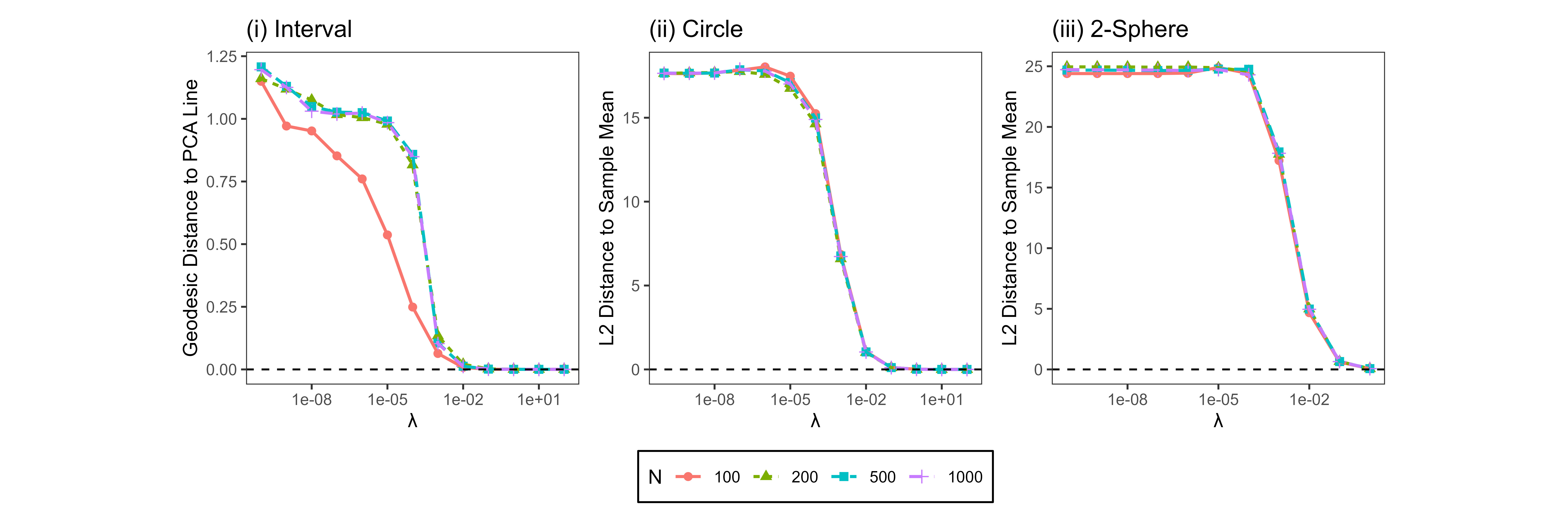
Here, we examine two extremes, λ=0\lambda=0 and λ→∞\lambda\rightarrow\infty. When λ=0\lambda=0, the minimization in (3.1) is essentially equivalent to the framework proposed by hastie1989principal, as indicated by (1.1). duchamp1996extremal demonstrate that the loss function ℒλ​(𝒇)\mathcal{L}_{\lambda}(\boldsymbol{f}) in (3.1) generally does not have a minimizer when λ=0\lambda=0, which explains the overfitting results previously observed by hastie1989principal. The overfitting phenomenon is also evident in Figure 2.1(b,e), where the wiggly green curves correspond to an excessively small λ\lambda. When λ→∞\lambda\rightarrow\infty, the following results establish connections between the proposed PME minimizers in (3.1), linear PCA, and the expected value 𝔼​𝑿\mathbb{E}\boldsymbol{X}.

Theorem 3.2.

Let 𝐟λ∗\boldsymbol{f}^{*}_{\lambda} be a minimizer defined in (3.1). Under Assumption 1, we have

  1. i)

    When ∂𝔐=∅\partial\mathfrak{M}=\emptyset, 𝒇λ∗\boldsymbol{f}_{\lambda}^{*} converges to the constant function 𝒎↦𝔼​𝑿\boldsymbol{m}\mapsto\mathbb{E}\boldsymbol{X} as λ→∞\lambda\to\infty in the supremum-norm topology, i.e., max𝒎∈𝔐⁡‖𝒇λ∗​(𝒎)−𝔼​𝑿‖→0\max_{\boldsymbol{m}\in\mathfrak{M}}\|\boldsymbol{f}^{*}_{\lambda}(\boldsymbol{m})-\mathbb{E}\boldsymbol{X}\|\rightarrow 0.

  2. ii)

    Assume that the dd-th largest eigenvalue of the covariance matrix Cov​(𝑿)\mathrm{Cov}(\boldsymbol{X}) is strictly greater than the (d+1)(d+1)-th largest eigenvalue. If 𝔐\mathfrak{M} is a simply connected flat manifold (i.e., its Riemann curvature tensor vanishes everywhere), then 𝒇λ∗\boldsymbol{f}_{\lambda}^{*} converges, as λ→∞\lambda\to\infty, to a subset 𝒜⊆ℱ​(ℙ)\mathscr{A}\subseteq\mathscr{F}(\mathbb{P}) in the following sense: for every open set 𝒱⊆ℱ​(ℙ)\mathscr{V}\subseteq\mathscr{F}(\mathbb{P}) with respect to the supremum-norm topology such that 𝒜⊆𝒱\mathscr{A}\subseteq\mathscr{V}, there exists Λ>0\Lambda>0 such that 𝒇λ∗∈𝒱\boldsymbol{f}_{\lambda}^{*}\in\mathscr{V} for all λ>Λ\lambda>\Lambda. Moreover, for every 𝒇∞∗∈𝒜\boldsymbol{f}_{\infty}^{*}\in\mathscr{A}, its image {𝒇∞∗​(𝒎):𝒎∈𝔐}⊆{𝔼​𝑿+∑j=1dαj​𝒗j:α1,…,αd∈ℝ}\{\boldsymbol{f}_{\infty}^{*}(\boldsymbol{m}):\boldsymbol{m}\in\mathfrak{M}\}\subseteq\{\mathbb{E}\boldsymbol{X}+\sum_{j=1}^{d}\alpha_{j}\boldsymbol{v}_{j}:\ \alpha_{1},\ldots,\alpha_{d}\in\mathbb{R}\}, where 𝒗1,…,𝒗d\boldsymbol{v}_{1},\ldots,\boldsymbol{v}_{d} are eigenvectors of Cov​(𝑿)\mathrm{Cov}(\boldsymbol{X}) corresponding to its largest dd eigenvalues.

The results of Theorem 3.2 are illustrated in Figures 2.1 and 3.1. In panels (b,e) of Figure 2.1, when the tuning parameter λ\lambda is excessively large, the fitted manifold reduces either to a straight line (corresponding to PCA) or to a point (corresponding to the expectation 𝔼​𝑿\mathbb{E}\boldsymbol{X}). Figure 3.1 shows that the fitted closed surface gradually shrinks to a point—visually, the center of the point cloud—as the tuning parameter λ\lambda increases. Appendix D presents additional numerical experiments that validate the two conclusions of Theorem 3.2. The main idea underlying the proof of Theorem 3.2 (given in Appendix E) is that the topology of the template manifold 𝔐\mathfrak{M} influences the structure of the solutions to the differential equation ∇2𝒇=0\nabla^{2}\boldsymbol{f}=0.

While the extreme case of λ=0\lambda=0 results in overfitting, Theorem 3.2 shows that the opposite extreme, λ→∞\lambda\rightarrow\infty, can lead to underfitting unless the underlying manifold is flat or consists of a single point, in which case the mean or PCA of data 𝑿\boldsymbol{X} is satisfactory to a user. Consequently, selecting an optimal value of λ\lambda between these extremes is necessary, which will be addressed in Section 5. Furthermore, the minimizer 𝒇λ∗\boldsymbol{f}^{*}_{\lambda} varies continuously with λ\lambda, allowing for stability in the estimate as λ\lambda is varied (see Theorem 5.2 in Section 5 for further details).

Refer to caption
Figure 3.1: The star- and cashew-shaped point clouds in the first and second rows are generated via the mechanisms described in Appendices F.3 and F.4, respectively. We apply the PA algorithm to the point clouds. The top row is initialized using only spherical normalization, and the bottom row using ISOMAP followed by spherical normalization (see Appendix C.1 for details). Each column displays the fitting results corresponding to a prespecified value of λ\lambda. This figure shows that a fitted closed surface gradually shrinks to the center of a point cloud as λ\lambda approaches ∞\infty, as stated in Theorem 3.2.

3.2 Projection-Adaptation Algorithm

Computing the minimizer 𝒇λ∗\boldsymbol{f}_{\lambda}^{*} defined in (3.1) is generally nontrivial, except in the extreme case where λ→∞\lambda\rightarrow\infty (see Theorem 3.2). In this section, we develop the theoretical foundation for an iterative algorithm used to numerically approximate the minimizer. This algorithm was first applied to the PME framework by Hastie1984PrincipalCurves and hastie1989principal, referred to as the principal curve algorithm. Despite its widespread use (e.g., banfield1992ice, yue2016parameterization), theoretical guarantees for this algorithm remain limited. As noted by banfield1992ice, “there is no formal proof that the algorithm converges, but hastie1989principal report that they have had no convergence problems with more than 40 real and simulated examples.” smola2001regularized outline a generalization, termed the projection–adaptation (PA) algorithm, which alternates between a projection step (P-step) and an adaptation step (A-step). meng_principal_2021 adopt the PA algorithm within their PME framework and report numerical convergence across extensive numerical experiments. Nevertheless, a precise convergence statement and a rigorous proof are still lacking. Here, we first describe the PA algorithm within the framework introduced in Section 3.1. We then state and prove our main theorem, which establishes uniform convergence of the PA iterations.

To estimate the minimizer 𝒇λ∗\boldsymbol{f}^{*}_{\lambda} described in equation (3.1), we need the following “bivariate” functional defined for all 𝒇,𝒈∈ℱ​(ℙ)\boldsymbol{f},\boldsymbol{g}\in\mathscr{F}(\mathbb{P})

𝒬λ​(𝒇|𝒈):=𝔼​{‖𝑿−𝒇​(𝝅𝒈​(𝑿))‖2}+λ⋅‖∇𝒇2‖L2​(𝔐)2.\displaystyle\mathcal{Q}_{\lambda}(\boldsymbol{f}\,|\,\boldsymbol{g}):=\mathbb{E}\left\{\|\boldsymbol{X}-\boldsymbol{f}\left(\boldsymbol{\pi}_{\boldsymbol{g}}(\boldsymbol{X})\right)\|^{2}\right\}+\lambda\cdot\|\nabla{}^{2}\boldsymbol{f}\|^{2}_{L^{2}(\mathfrak{M})}. (3.2)

In general, 𝒬λ​(𝒇|𝒈)≠𝒬λ​(𝒈|𝒇)\mathcal{Q}_{\lambda}(\boldsymbol{f}\,|\,\boldsymbol{g})\neq\mathcal{Q}_{\lambda}(\boldsymbol{g}\,|\,\boldsymbol{f}). Obviously, ℒλ​(𝒇)=𝒬λ​(𝒇|𝒇)\mathcal{L}_{\lambda}(\boldsymbol{f})=\mathcal{Q}_{\lambda}(\boldsymbol{f}\,|\,\boldsymbol{f}) for all 𝒇∈ℱ​(ℙ)\boldsymbol{f}\in\mathscr{F}(\mathbb{P}). The minimizer 𝒇λ∗\boldsymbol{f}^{*}_{\lambda} defined in (3.1) can be approximated through the following iterative algorithm.

𝒇λ(n+1):=arg⁡min𝒇∈ℱ​(ℙ)⁡𝒬λ​(𝒇|𝒇λ(n))=𝒯λ​(𝒇λ(n)), for ​n=0,1,2,…\displaystyle\boldsymbol{f}_{\lambda}^{(n+1)}:=\operatorname*{\arg\!\min}_{\boldsymbol{f}\in\mathscr{F}(\mathbb{P})}\mathcal{Q}_{\lambda}(\boldsymbol{f}\,|\,\boldsymbol{f}^{(n)}_{\lambda})=\mathcal{T}_{\lambda}(\boldsymbol{f}^{(n)}_{\lambda}),\quad\text{ for }n=0,1,2,\ldots (3.3)

where the updating operator 𝒯λ\mathcal{T}_{\lambda} is defined by 𝒯λ​(𝒈):=arg⁡min𝒇∈ℱ​(ℙ)⁡𝒬λ​(𝒇|𝒈)\mathcal{T}_{\lambda}(\boldsymbol{g}):=\operatorname*{\arg\!\min}_{\boldsymbol{f}\in\mathscr{F}(\mathbb{P})}\mathcal{Q}_{\lambda}(\boldsymbol{f}\,|\,\boldsymbol{g}). We refer to the computation of the projection 𝝅𝒇λ(n)​(𝑿)\boldsymbol{\pi}_{\boldsymbol{f}^{(n)}_{\lambda}}(\boldsymbol{X}) as the P-step; practical methods for this computation are given in Appendix C.2. We refer to the minimization in (3.3) as the A-step, whose minimizer exists and is unique by Lemma E.9. The PA algorithm in (3.3) is equivalent to the principal curve algorithm proposed by hastie1989principal when λ=0\lambda=0 (e.g., meng_principal_2021, Theorem 6).

The minimization in (3.1) is an unsupervised learning task that generalizes PCA (see Theorem 3.2). In contrast, each iteration of the PA algorithm in (3.3) is a supervised learning problem, namely, nonlinear regression. Specifically, at a given iteration, the P-step provides the predictor (i.e., the projection index 𝝅𝒇λ(n)​(𝑿)\boldsymbol{\pi}_{\boldsymbol{f}^{(n)}_{\lambda}}(\boldsymbol{X})), and the data point 𝑿\boldsymbol{X} serves as the response (see the combination of (3.2) and (3.3)). This regression problem is well-studied in the literature (e.g., wahba1990spline) and can be solved efficiently by exploiting the fact that H2​(𝔐)H^{2}(\mathfrak{M}) is an RKHS when dim(𝔐)<4\dim(\mathfrak{M})<4 (see Theorem 2.1). Details of the regression fit are provided in Section 3.3. Theorem 3.3 (presented later) shows that the unsupervised minimization in (3.1) can be carried out by iteratively solving these nonlinear regression subproblems.

ℱ​(ℙ)\mathscr{F}(\mathbb{P})ℒλ​(𝒇)\mathcal{L}_{\lambda}(\boldsymbol{f}) for 𝒇∈ℱ​(ℙ)\boldsymbol{f}\in\mathscr{F}(\mathbb{P})𝒇λ∗\boldsymbol{f}_{\lambda}^{\ast}𝒇λ(0)\boldsymbol{f}_{\lambda}^{(0)}𝒯λ​(𝒇λ(0))=𝒇λ(1)\mathcal{T}_{\lambda}(\boldsymbol{f}_{\lambda}^{(0)})=\boldsymbol{f}_{\lambda}^{(1)}𝒇λ(2)\boldsymbol{f}_{\lambda}^{(2)}𝒇λ(3)=𝒯λ​(𝒇λ(2))\boldsymbol{f}_{\lambda}^{(3)}=\mathcal{T}_{\lambda}(\boldsymbol{f}_{\lambda}^{(2)})𝒰\mathscr{U}
Figure 3.2: Illustration of the PA algorithm and the role of Assumption 3. The vertical axis denotes the objective ℒλ​(f)\mathcal{L}_{\lambda}(f) and the horizontal axis represents the function space ℱ​(ℙ)\mathscr{F}(\mathbb{P}) (illustration only, not to scale). The region 𝒰\mathscr{U} (green bracket; boundaries indicated by dashed vertical lines) is a “basin of attraction” in which the updating operator 𝒯λ\mathcal{T}_{\lambda} is intended to operate. Starting from an initialization 𝒇λ(0)∈𝒰\boldsymbol{f}_{\lambda}^{(0)}\in\mathscr{U}, successive iterations 𝒇λ(n+1)=𝒯λ​(𝒇λ(n))\boldsymbol{f}_{\lambda}^{(n+1)}=\mathcal{T}_{\lambda}(\boldsymbol{f}_{\lambda}^{(n)}) (orange points connected by blue arrows) decrease the objective and move toward the unique global minimizer 𝒇λ∗∈𝒰\boldsymbol{f}_{\lambda}^{\ast}\in\mathscr{U} (red point). The dashed portions of the objective curve indicate behavior outside 𝒰\mathscr{U}, where additional stationary points or irregularities may occur and where the convergence guarantee is not asserted.

Lemma E.6 in Appendix E shows that the scalar-valued sequence {ℒλ​(𝒇λ(n))}n∈ℕ\{\mathcal{L}_{\lambda}(\boldsymbol{f}_{\lambda}^{(n)})\}_{n\in\mathbb{N}} is nonincreasing, illustrated in Figures 3.2 and 2.1(c,f). Hence, the scalar-valued limit limn→∞ℒλ​(𝒇(n))\lim_{n\rightarrow\infty}\mathcal{L}_{\lambda}(\boldsymbol{f}^{(n)}) exists. However, the existence of this limit does not guarantee the convergence of limn→∞𝒇λ(n)\lim_{n\rightarrow\infty}\boldsymbol{f}^{(n)}_{\lambda}. The following assumptions are needed to ensure the uniform convergence of {𝒇λ(n)}n∈ℕ\{\boldsymbol{f}^{(n)}_{\lambda}\}_{n\in\mathbb{N}}.

Assumption 3.

There exists a region 𝒰⊆ℱ​(ℙ)\mathscr{U}\subseteq\mathscr{F}(\mathbb{P}) with the following properties:

  1. i)

    (Closedness.) 𝒰\mathscr{U} is closed in C​(𝔐;ℝD)C(\mathfrak{M};\,\mathbb{R}^{D}) under the supremum norm ∥⋅∥C​(𝔐)\|\cdot\|_{C(\mathfrak{M})}.

  2. ii)

    (Invariance.) 𝒯λ​(𝒈)∈𝒰\mathcal{T}_{\lambda}(\boldsymbol{g})\in\mathscr{U} for all 𝒈∈𝒰\boldsymbol{g}\in\mathscr{U}, i.e., 𝒯λ​(𝒰)⊆𝒰\mathcal{T}_{\lambda}(\mathscr{U})\subseteq\mathscr{U}.

  3. iii)

    (Unique global minimizer.) 𝒰\mathscr{U} contains exactly one global minimizer 𝒇λ∗\boldsymbol{f}^{*}_{\lambda}.

  4. iv)

    (Unique fixed point.) If 𝒈∈𝒰\boldsymbol{g}\in\mathscr{U} satisfies 𝒈=𝒯λ​(𝒈)\boldsymbol{g}=\mathcal{T}_{\lambda}(\boldsymbol{g}), then 𝒈=𝒇λ∗\boldsymbol{g}=\boldsymbol{f}^{*}_{\lambda}. That is, within the region 𝒰\mathscr{U}, a fixed point of 𝒯λ\mathcal{T}_{\lambda} must be the unique minimizer 𝒇λ∗\boldsymbol{f}^{*}_{\lambda} in this region.

Assumption 3 posits the existence of a “good” region 𝒰\mathscr{U} that serves as a basin of attraction around the global minimizer 𝒇λ∗\boldsymbol{f}_{\lambda}^{\ast} (see Figure 3.2). In Theorem 3.3, we will show that, provided the initialization 𝒇λ(0)∈𝒰\boldsymbol{f}_{\lambda}^{(0)}\in\mathscr{U} (i.e., it is sufficiently close to 𝒇λ∗\boldsymbol{f}_{\lambda}^{\ast}), the iterations from the PA algorithm converge to 𝒇λ∗\boldsymbol{f}_{\lambda}^{\ast}. Appendix C.1 presents a detailed discussion on practical methods for obtaining effective initializations. The invariance condition 𝒯λ​(𝒰)⊆𝒰\mathcal{T}_{\lambda}(\mathscr{U})\subseteq\mathscr{U} ensures that once the algorithm enters 𝒰\mathscr{U}, all subsequent iterations remain in the region where the PA algorithm is intended to operate. Moreover, the third item of Assumption 3 guarantees that 𝒰\mathscr{U} contains a unique global minimizer, thereby avoiding ambiguity of the target solution within this region. Finally, the last item of Assumption 3 rules out spurious fixed-point solutions in 𝒰\mathscr{U} by requiring that 𝒇λ∗\boldsymbol{f}_{\lambda}^{\ast} be the only fixed point of the updating operator 𝒯λ\mathcal{T}_{\lambda} in 𝒰\mathscr{U}. Consequently, the algorithm cannot stall at any point in 𝒰\mathscr{U} other than 𝒇λ∗\boldsymbol{f}_{\lambda}^{\ast} (see Figure 3.2 for an illustration). While the existence of the minimizer 𝒇λ∗\boldsymbol{f}_{\lambda}^{\ast} (see Theorem 3.1) depends solely on the compactness of the support of the data-generating distribution ℙ\mathbb{P}, Assumption 3 imposes further requirements on ℙ\mathbb{P} to ensure that the PA algorithm is a valid method for estimating the minimizer 𝒇λ∗\boldsymbol{f}_{\lambda}^{\ast}. In addition to Assumption 3, we need the following assumption regarding the relationship between the shape of the support supp​(ℙ)\mathrm{supp}(\mathbb{P}) and the potential limit limn→∞𝒇λ(n)=𝒇λ∗\lim_{n\rightarrow\infty}\boldsymbol{f}_{\lambda}^{(n)}=\boldsymbol{f}^{*}_{\lambda}.

Assumption 4.

Let {𝐟λ(n)}n∈ℕ\{\boldsymbol{f}_{\lambda}^{(n)}\}_{n\in\mathbb{N}} be a sequence generated by the iterative algorithm in (3.3), and let 𝐟λ(∞)\boldsymbol{f}_{\lambda}^{(\infty)} be an arbitrary accumulation point under the supremum norm, i.e., there exists a subsequence {𝐟λ(n,k)}k∈ℕ\{\boldsymbol{f}_{\lambda}^{(n,k)}\}_{k\in\mathbb{N}} such that limk→∞‖𝐟λ(n,k)−𝐟λ(∞)‖C​(𝔐)=0\lim_{k\rightarrow\infty}\|\boldsymbol{f}_{\lambda}^{(n,k)}-\boldsymbol{f}_{\lambda}^{(\infty)}\|_{C(\mathfrak{M})}=0. We assume that arg⁡min𝐦∈𝔐⁡‖𝐱−𝐟λ(∞)​(𝐦)‖\operatorname*{\arg\!\min}_{\boldsymbol{m}\in\mathfrak{M}}\|\boldsymbol{x}-\boldsymbol{f}_{\lambda}^{(\infty)}(\boldsymbol{m})\| is a singleton for every 𝐱∈supp​(ℙ)\boldsymbol{x}\in\mathrm{supp}(\mathbb{P}).

Assumption 4 is a condition imposed for the potential limit limn→∞𝒇λ(n)=𝒇λ∗\lim_{n\rightarrow\infty}\boldsymbol{f}_{\lambda}^{(n)}=\boldsymbol{f}^{*}_{\lambda} that will be of interest in Theorem 3.3. For the image ℳ^λ:=𝒇λ∗​(𝔐)⊂ℝD\widehat{\mathcal{M}}_{\lambda}:=\boldsymbol{f}^{*}_{\lambda}(\mathfrak{M})\subset\mathbb{R}^{D}, the assumption requires that each 𝒙∈supp⁡(ℙ)\boldsymbol{x}\in\operatorname{supp}(\mathbb{P}) admits a unique nearest point in ℳ^λ\widehat{\mathcal{M}}_{\lambda} (hence, the projection index 𝝅𝒇λ∗​(𝒙)\boldsymbol{\pi}_{\boldsymbol{f}^{*}_{\lambda}}(\boldsymbol{x}) is defined as the unique nearest point). Recall that the medial axis of a compact set 𝒜\mathcal{A} is the collection of all points having more than one closest point in 𝒜\mathcal{A} (e.g., see Figure 2.2; blum1967transformation). Then, Assumption 4 can be read as requiring that supp⁡(ℙ)\operatorname{supp}(\mathbb{P}) avoid the medial axis of ℳ^λ\widehat{\mathcal{M}}_{\lambda}. Under the manifold hypothesis—namely, that the data are generated by a low-dimensional manifold contaminated by noise—this amounts to assuming that the noise level is not so large as to push a non-negligible portion of supp​(ℙ)\mathrm{supp}(\mathbb{P}) into the medial-axis region of ℳ^λ\widehat{\mathcal{M}}_{\lambda} (e.g., see Figure 2.2). Assumption 4 is also naturally interpreted through the “reach” and “tubular-neighborhood” viewpoint. The reach, reach​(𝒜)\mathrm{reach}(\mathcal{A}), of a compact set 𝒜\mathcal{A} is the largest r≥0r\geq 0 such that every point 𝒙\boldsymbol{x} with dist​(𝒙,𝒜)<r\mathrm{dist}(\boldsymbol{x},\mathcal{A})<r has a unique nearest point on 𝒜\mathcal{A}, i.e., the nearest-point projection is well-defined throughout the tubular neighborhood {𝒙:dist​(𝒙,𝒜)<r}\{\boldsymbol{x}:\mathrm{dist}(\boldsymbol{x},\mathcal{A})<r\} (Federer1969Geometric, fefferman2016testing). Then, we have the following sufficient condition: when the data lie in a tubular neighborhood of ℳ^λ\widehat{\mathcal{M}}_{\lambda} with a radius less than reach​(ℳ^λ)\mathrm{reach}(\widehat{\mathcal{M}}_{\lambda}), Assumption 4 is satisfied. In the manifold learning literature, the reach of an underlying manifold is commonly assumed to be reasonably large, e.g., genovese2012minimax, fefferman2016testing, and fefferman2025fitting focus on submanifolds endowed with reaches bounded uniformly from below.

Building on Assumptions 3 and 4, we establish the uniform convergence of the PA algorithm dynamics {𝒇λ(n)}n∈ℕ\{\boldsymbol{f}_{\lambda}^{(n)}\}_{n\in\mathbb{N}} to the minimizer 𝒇λ∗\boldsymbol{f}^{*}_{\lambda} defined in (3.1), as established below.

Theorem 3.3.

Assume that Assumption 3 holds. Let 𝒰⊆ℱ​(ℙ)\mathscr{U}\subseteq\mathscr{F}(\mathbb{P}) be the region specified in Assumption 3, and let 𝐟λ∗\boldsymbol{f}^{*}_{\lambda} be the unique minimizer in 𝒰\mathscr{U}. Let {𝐟λ(n)}n∈ℕ\{\boldsymbol{f}_{\lambda}^{(n)}\}_{n\in\mathbb{N}} denote the sequence generated by (3.3), initialized at 𝐟λ(0)\boldsymbol{f}_{\lambda}^{(0)}. If 𝐟λ(0)∈𝒰\boldsymbol{f}_{\lambda}^{(0)}\in\mathscr{U} and Assumption 4 is satisfied, we have the following convergence results for the sequence {𝐟λ(n)}n∈ℕ\{\boldsymbol{f}_{\lambda}^{(n)}\}_{n\in\mathbb{N}}

limn→∞max𝒎∈𝔐⁡‖𝒇λ(n)​(𝒎)−𝒇λ∗​(𝒎)‖=0 and limn→∞ℒλ​(𝒇λ(n))=ℒλ​(𝒇λ∗)=min𝒇∈ℱ​(ℙ)⁡ℒλ​(𝒇).\displaystyle\lim_{n\rightarrow\infty}\max_{\boldsymbol{m}\in\mathfrak{M}}\|\boldsymbol{f}_{\lambda}^{(n)}(\boldsymbol{m})-\boldsymbol{f}^{*}_{\lambda}(\boldsymbol{m})\|=0\ \ \text{ and }\ \ \lim_{n\rightarrow\infty}\mathcal{L}_{\lambda}(\boldsymbol{f}_{\lambda}^{(n)})=\mathcal{L}_{\lambda}\left(\boldsymbol{f}^{*}_{\lambda}\right)=\min_{\boldsymbol{f}\in\mathscr{F}(\mathbb{P})}\,\mathcal{L}_{\lambda}(\boldsymbol{f}).

3.3 Empirical Version

In practice, the underlying distribution ℙ\mathbb{P} is unknown, and only finitely many observations {𝑿i}i∈[N]\{\boldsymbol{X}_{i}\}_{i\in[N]} in the ambient space ℝD\mathbb{R}^{D} are available, where NN is the sample size. We assume these observations are iid draws from ℙ\mathbb{P}. The population-level framework developed in Sections 3.1 and 3.2 is then specialized by replacing ℙ\mathbb{P} with the empirical distribution ℙN:=1N​∑i=1Nδ𝑿i\mathbb{P}_{N}:=\frac{1}{N}\sum_{i=1}^{N}\delta_{\boldsymbol{X}_{i}}. Accordingly, the population expectation 𝔼​(⋅)=∫(⋅)​𝑑ℙ\mathbb{E}(\cdot)=\int(\cdot)d\mathbb{P} is replaced by the empirical average 𝔼N​(⋅)=∫(⋅)​𝑑ℙN\mathbb{E}_{N}(\cdot)=\int(\cdot)d\mathbb{P}_{N}. Given data {𝑿i}i∈[N]\{\boldsymbol{X}_{i}\}_{i\in[N]}, because ℙN\mathbb{P}_{N} is also a probability measure with compact support, the framework outlined in Sections 3.1 and 3.2 still applies to ℙN\mathbb{P}_{N}.

This section presents two main results. First, it is demonstrated that the minimizer 𝒇N,λ∗\boldsymbol{f}^{*}_{N,\lambda}, defined with respect to the empirical distribution ℙN\mathbb{P}_{N}, converges to its population-level counterpart 𝒇λ∗\boldsymbol{f}^{*}_{\lambda} as the sample size N→∞N\rightarrow\infty. Second, an explicit formula for the PA algorithm for the empirical distribution ℙN\mathbb{P}_{N} is presented, utilizing the RKHS structure of H2​(𝔐)H^{2}(\mathfrak{M}).

3.3.1 Consistency of the Empirical Minimizer

Let 𝒇N,λ∗:=arg⁡min𝒇∈ℱ​(ℙN)⁡ℒN,λ​(𝒇)\boldsymbol{f}^{*}_{N,\lambda}:=\operatorname*{\arg\!\min}_{\boldsymbol{f}\in\mathscr{F}(\mathbb{P}_{N})}\mathcal{L}_{N,\lambda}(\boldsymbol{f}), where ℱ​(ℙN)\mathscr{F}(\mathbb{P}_{N}) is defined by (3.1) and

ℒN,λ​(𝒇):=1N​∑i=1N‖𝑿i−𝒇​(𝝅𝒇​(𝑿i))‖2+λ⋅‖∇𝒇2‖L2​(𝔐)2.\displaystyle\mathcal{L}_{N,\lambda}(\boldsymbol{f}):=\frac{1}{N}\sum_{i=1}^{N}\|\boldsymbol{X}_{i}-\boldsymbol{f}\left(\boldsymbol{\pi}_{\boldsymbol{f}}(\boldsymbol{X}_{i})\right)\|^{2}+\lambda\cdot\|\nabla{}^{2}\boldsymbol{f}\|^{2}_{L^{2}(\mathfrak{M})}. (3.4)

Notably, 𝒇N,λ∗\boldsymbol{f}^{*}_{N,\lambda} is a consistent estimator of 𝒇λ∗\boldsymbol{f}^{*}_{\lambda} in the sense that 𝒇N,λ∗\boldsymbol{f}^{*}_{N,\lambda} converges to 𝒇λ∗\boldsymbol{f}^{*}_{\lambda} in outer probability (van1996weak, Sections 1.2 and 1.9), as stated precisely in the following theorem.

Theorem 3.4.

Let λ>0\lambda>0 and {𝐗i}i∈[N]​∼iid​ℙ\{\boldsymbol{X}_{i}\}_{i\in[N]}\overset{\mathrm{iid}}{\sim}\mathbb{P}. Suppose the global minimizer 𝐟λ∗\boldsymbol{f}^{*}_{\lambda} defined in (3.1) is locally unique in the following sense: ℒλ​(𝐟λ∗)<inf𝐟∉𝒢ℒλ​(𝐟)\mathcal{L}_{\lambda}(\boldsymbol{f}^{*}_{\lambda})<\inf_{\boldsymbol{f}\not\in\mathscr{G}}\mathcal{L}_{\lambda}(\boldsymbol{f}) for every open subset 𝒢⊆C​(𝔐)\mathscr{G}\subseteq C(\mathfrak{M}) containing 𝐟λ∗\boldsymbol{f}^{*}_{\lambda}, where openness is understood in the supremum norm topology on C​(𝔐)C(\mathfrak{M}). Then, ‖𝐟N,λ∗−𝐟λ∗‖C​(𝔐)\|\boldsymbol{f}^{*}_{N,\lambda}-\boldsymbol{f}^{*}_{\lambda}\|_{C(\mathfrak{M})} converges to zero in outer probability as N→∞N\rightarrow\infty.

Figure 3.3 provides a visual illustration of Theorem 3.4. The proof of Theorem 3.4 relies on a corollary of the argmax theorem (van1996weak, Section 3.2), together with the compactness of the embedding ι:H2​(𝔐)→C​(𝔐)\iota:\,H^{2}(\mathfrak{M})\rightarrow C(\mathfrak{M}) stated in Theorem 2.1.

Refer to caption
Figure 3.3: Visual illustration of Theorem 3.4. The red curve represents the manifold underlying a point cloud generated according to the data-generating mechanism described in Appendix F.2. For each sample size NN, we repeat the following procedure 100 times: (i) generate a sample of size NN using the data-generating mechanism described in Appendix F.2; and (ii) apply the PA algorithm and plot the resulting estimate as a blue curve.

3.3.2 The Empirical PA Algorithm

The consistent estimator 𝒇N,λ∗\boldsymbol{f}^{*}_{N,\lambda} can be computed numerically using the PA algorithm outlined in (3.3). Specifically, we replace the underlying distribution ℙ\mathbb{P} in (3.2) with the empirical distribution ℙN\mathbb{P}_{N}. This approach imposes two conditions on the resulting function class ℱ​(ℙN)\mathscr{F}(\mathbb{P}_{N}), i.e., 𝒇∈H2​(𝔐)=H2​(𝔐;ℝD)\boldsymbol{f}\in H^{2}(\mathfrak{M})=H^{2}(\mathfrak{M};\,\mathbb{R}^{D}), and ‖𝒇‖C​(𝔐;ℝD)≤2⋅rad0⁡(supp⁡(ℙN))=2⋅max1≤i≤N⁡‖𝑿i‖\|\boldsymbol{f}\|_{C(\mathfrak{M};\,\mathbb{R}^{D})}\leq 2\cdot\operatorname{rad}_{0}\left(\operatorname{supp}(\mathbb{P}_{N})\right)=2\cdot\max_{1\leq i\leq N}\|\boldsymbol{X}_{i}\|. However, the second condition may impede our direct use of the RKHS structure of the Sobolev space H2​(𝔐)H^{2}(\mathfrak{M}). Therefore, in practice, we ignore the second condition and implement the PA algorithm as follows

𝒇N,λ(n+1):=arg⁡min𝒇∈H2​(𝔐)⁡[1N​∑i=1N{‖𝑿i−𝒇​(𝝅𝒇N,λ(n)​(𝑿i))‖2}+λ⋅‖∇𝒇2‖L2​(𝔐)2].\displaystyle\boldsymbol{f}_{N,\lambda}^{(n+1)}:=\operatorname*{\arg\!\min}_{\boldsymbol{f}\in H^{2}(\mathfrak{M})}\left[\frac{1}{N}\sum_{i=1}^{N}\left\{\left\|\boldsymbol{X}_{i}-\boldsymbol{f}\left(\boldsymbol{\pi}_{\boldsymbol{f}_{N,\lambda}^{(n)}}(\boldsymbol{X}_{i})\right)\right\|^{2}\right\}+\lambda\cdot\|\nabla{}^{2}\boldsymbol{f}\|^{2}_{L^{2}(\mathfrak{M})}\right]. (3.5)

Note that the minimization in (3.5) is performed over the entire RKHS H2​(𝔐)H^{2}(\mathfrak{M}) instead of ℱ​(ℙN)\mathscr{F}(\mathbb{P}_{N}). With a reasonable initialization, the minimizers 𝒇N,λ(n+1)\boldsymbol{f}_{N,\lambda}^{(n+1)} generated in our numerical experiments consistently satisfy ‖𝒇N,λ(n+1)‖C​(𝔐)≤2⋅max1≤i≤N⁡‖𝑿i‖\|\boldsymbol{f}_{N,\lambda}^{(n+1)}\|_{C(\mathfrak{M})}\leq 2\cdot\max_{1\leq i\leq N}\|\boldsymbol{X}_{i}\| at every iteration, i.e., each 𝒇N,λ(n+1)\boldsymbol{f}_{N,\lambda}^{(n+1)} does not deviate too far from data {𝑿i}i∈[N]\{\boldsymbol{X}_{i}\}_{i\in[N]}. Consequently, each 𝒇N,λ(n+1)\boldsymbol{f}_{N,\lambda}^{(n+1)} obtained in (3.5) also serves as a minimizer over the function class ℱ​(ℙN)\mathscr{F}(\mathbb{P}_{N}). This supports the compatibility of the iterative method in (3.5) with the PA algorithm outlined in (3.3). As noted in Section 3.1, the use of the factor 2 in the bound 2⋅max1≤i≤N⁡‖𝑿i‖2\cdot\max_{1\leq i\leq N}\|\boldsymbol{X}_{i}\| is for illustrative purposes and may be replaced with any sufficiently large constant.

Given {𝑿i}i∈[N]\{\boldsymbol{X}_{i}\}_{i\in[N]} and the function 𝒇N,λ(n)\boldsymbol{f}_{N,\lambda}^{(n)} from the nnth step, the updated estimator 𝒇N,λ(n+1)\boldsymbol{f}_{N,\lambda}^{(n+1)} in (3.5) admits a closed-form expression via the representer theorem (wahba1990spline, Theorem 1.3.1). Details of the application of the representer theorem to the PA algorithm are presented in Appendix B. Comprehensive implementation details of the PA algorithm are provided in Appendix C. In particular, Algorithm C.1 in Appendix C presents a summary of the PA algorithm, and Appendix C.3 provides a discussion on efficient methods for solving (3.5).

4 Geometric Interpretation of the Penalty

In this section, we provide a detailed interpretation of the penalty ‖∇2𝒇‖L2​(𝔐)2\|\nabla^{2}\boldsymbol{f}\|^{2}_{L^{2}(\mathfrak{M})} used in (3.1). First, we explain why we use the Hessian ∇2\nabla^{2}, rather than the Laplace-Beltrami operator, in defining the penalty term (see Section 4.1). Second, we describe the relationship between our penalty ‖∇2𝒇‖L2​(𝔐)2\|\nabla^{2}\boldsymbol{f}\|^{2}_{L^{2}(\mathfrak{M})} and the curve-length penalty proposed by kegl2000learning (see Section 4.2). Finally, we show that the penalty ‖∇2𝒇‖L2​(𝔐)2\|\nabla^{2}\boldsymbol{f}\|^{2}_{L^{2}(\mathfrak{M})} penalizes both (i) the curvature of the fitted manifold (see Section 4.4.1) and (ii) the discrepancy between the metrics of the template and fitted manifolds (see Section 4.4.2); this is established through the orthogonal decomposition presented in Section 4.3.

4.1 Hessian Penalty versus Laplace-Beltrami Penalty

Theorem 3.2 provides an initial interpretation of the Hessian-based penalty ‖∇2𝒇‖L2​(𝔐)2\|\nabla^{2}\boldsymbol{f}\|^{2}_{L^{2}(\mathfrak{M})}, showing that a heavily penalized estimator tends to have low complexity (e.g., a hyperplane determined by finitely many parameters or a single point). Generally, the Hessian penalty ‖∇2𝒇‖L2​(𝔐)2\|\nabla^{2}\boldsymbol{f}\|^{2}_{L^{2}(\mathfrak{M})} favors estimators that lie close to the finite-dimensional space 𝒩​(∇2):={𝒇∈H2​(𝔐):‖∇2𝒇‖L2​(𝔐)2=0}\mathcal{N}(\nabla^{2}):=\{\boldsymbol{f}\in H^{2}(\mathfrak{M}):\,\|\nabla^{2}\boldsymbol{f}\|^{2}_{L^{2}(\mathfrak{M})}=0\} (see Remark B.1 in Appendix B). This feature helps reduce overfitting effectively.

By contrast, a penalty defined through the Laplace–Beltrami operator need not favor a finite-dimensional space. For any smooth scalar-valued function ff on 𝔐\mathfrak{M}, the Laplace–Beltrami operator Δ\Delta is defined by

Δ​f​(𝒎):=trg⁡(∇2f)​(𝒎)=∑i=1d∇2f​(ei,ei),\displaystyle\Delta f(\boldsymbol{m}):=\operatorname{tr}_{g}(\nabla^{2}f)(\boldsymbol{m})=\sum_{i=1}^{d}\nabla^{2}f(e_{i},e_{i}), (4.1)

where {ek}k∈[d]\{e_{k}\}_{k\in[d]} is any gg-orthonormal basis of the tangent space T𝒎​𝔐T_{\boldsymbol{m}}\mathfrak{M}. For a vector-valued map 𝒇=(f1,…,fD)\boldsymbol{f}=(f_{1},\ldots,f_{D}), we define Δ​𝒇:=(Δ​f1,…,Δ​fD)\Delta\boldsymbol{f}:=(\Delta f_{1},\ldots,\Delta f_{D}). Accordingly, one may consider the penalty ‖Δ​𝒇‖L2​(𝔐)2=∑j=1D‖Δ​fj‖L2​(𝔐)2\|\Delta\boldsymbol{f}\|^{2}_{L^{2}(\mathfrak{M})}=\sum_{j=1}^{D}\|\Delta f_{j}\|^{2}_{L^{2}(\mathfrak{M})} (e.g., wahba1990spline, Section 2.2). When the boundary ∂𝔐\partial\mathfrak{M} is empty, the Hessian penalty ‖∇2𝒇‖L2​(𝔐)2\|\nabla^{2}\boldsymbol{f}\|^{2}_{L^{2}(\mathfrak{M})} and the Laplace–Beltrami penalty ‖Δ​𝒇‖L2​(𝔐)2\|\Delta\boldsymbol{f}\|^{2}_{L^{2}(\mathfrak{M})} are related through Bochner’s formula (li2012geometric, Chapter 3):

‖Δ​𝒇‖L2​(𝔐)2=‖∇2𝒇‖L2​(𝔐)2+∑j=1D∫𝔐Ric​(∇fj,∇fj)​𝑑volg,\displaystyle\|\Delta\boldsymbol{f}\|^{2}_{L^{2}(\mathfrak{M})}=\|\nabla^{2}\boldsymbol{f}\|^{2}_{L^{2}(\mathfrak{M})}+\sum_{j=1}^{D}\int_{\mathfrak{M}}\mathrm{Ric}(\nabla f_{j},\nabla f_{j})\,d\mathrm{vol}_{g}, (4.2)

where Ric​(⋅,⋅)\mathrm{Ric}(\cdot,\cdot) denotes the Ricci curvature tensor. An estimator that is heavily penalized by ‖Δ​𝒇‖L2​(𝔐)2\|\Delta\boldsymbol{f}\|^{2}_{L^{2}(\mathfrak{M})} tends to lie close to the null space 𝒩​(Δ):={𝒇∈H2​(𝔐):‖Δ​𝒇‖L2​(𝔐)2=0}\mathcal{N}(\Delta):=\{\boldsymbol{f}\in H^{2}(\mathfrak{M}):\|\Delta\boldsymbol{f}\|^{2}_{L^{2}(\mathfrak{M})}=0\}, i.e., the space of harmonic maps. However, unlike the Hessian penalty, the null space 𝒩​(Δ)\mathcal{N}(\Delta) may be infinite-dimensional when the boundary ∂𝔐≠∅\partial\mathfrak{M}\neq\emptyset (see Remark B.1). Consequently, the Laplace-Beltrami penalty may be less effective in controlling overfitting, since the infinitely many dimensions still permit substantial flexibility in manifold estimation. Moreover, unlike the Hessian penalty in Theorem 3.2(ii), the Laplace-Beltrami penalty does not recover linear PCA within the PME framework. For these reasons, we adopt and focus on the Hessian penalty ‖∇2𝒇‖L2​(𝔐)2\|\nabla^{2}\boldsymbol{f}\|^{2}_{L^{2}(\mathfrak{M})}.

4.2 Curve Length Penalty

kegl2000learning propose a principal curve framework that minimizes the loss function in (1.2), where its penalty term is equal to the length of the fitted curve (doCarmo1976DifferentialGeometry, Chapter 1). When the template manifold (𝔐,g)(\mathfrak{M},g) is the unit circle 𝕊1\mathbb{S}^{1} endowed with the metric gg induced from ℝ2\mathbb{R}^{2}, the curve length penalty utilized by kegl2000learning is dominated by our proposed penalty ‖∇𝒇2‖L2​(𝕊1)2\|\nabla{}^{2}\boldsymbol{f}\|^{2}_{L^{2}(\mathbb{S}^{1})}. Specifically, we have that

the length of the curve ​𝒇​(𝕊1)≤(2​π)3/2⋅‖∇2𝒇‖L2​(𝕊1),\displaystyle\text{the length of the curve }\boldsymbol{f}(\mathbb{S}^{1})\leq(2\pi)^{3/2}\cdot\|\nabla^{2}\boldsymbol{f}\|_{L^{2}(\mathbb{S}^{1})}, (4.3)

and the proof of (4.3) is given in Appendix E using Poincaré–Wirtinger’s inequality. Therefore, in this case, our proposed ‖∇2𝒇‖L2​(𝕊1)2\|\nabla^{2}\boldsymbol{f}\|^{2}_{L^{2}(\mathbb{S}^{1})} penalizes the curve length, as in kegl2000learning. In addition, the inequality in (4.3) provides an alternative validation of Theorem 3.2(i).

4.3 An Orthogonal Decomposition of the Penalty

We decompose the proposed penalty ‖∇𝒇2‖L2​(𝔐)2\|\nabla{}^{2}\boldsymbol{f}\|^{2}_{L^{2}(\mathfrak{M})} into two additive terms, each with a geometric interpretation.

Let (𝔐,g)(\mathfrak{M},g) be a template manifold satisfying Assumption 1. Assume henceforth that 𝒇:𝔐→ℝD\boldsymbol{f}:\mathfrak{M}\rightarrow\mathbb{R}^{D} is an embedding (lee2018riemannian, Chapter 2). Precisely, 𝒇\boldsymbol{f} is a homeomorphism onto its image 𝒇​(𝔐)\boldsymbol{f}(\mathfrak{M}) with the subspace topology, and it is an immersion, i.e., d​𝒇:T𝒎​𝔐→T𝒇​(𝒎)​ℝD≅ℝDd\boldsymbol{f}:T_{\boldsymbol{m}}\mathfrak{M}\rightarrow T_{\boldsymbol{f}(\boldsymbol{m})}\mathbb{R}^{D}\cong\mathbb{R}^{D} is injective for any 𝒎∈𝔐\boldsymbol{m}\in\mathfrak{M}. Then, we may define a new metric g𝒇=𝒇∗​δg_{\boldsymbol{f}}=\boldsymbol{f}^{*}\delta on 𝔐\mathfrak{M} by

g𝒇​(u,v):=δ​(d​𝒇​(u),d​𝒇​(v))​ for any ​u,v∈Γ​(T​𝔐),\displaystyle g_{\boldsymbol{f}}(u,v):=\delta\big(\,d\boldsymbol{f}(u),\,d\boldsymbol{f}(v)\,\big)\text{ for any }u,v\in\Gamma(T\mathfrak{M}), (4.4)

where δ\delta is the Euclidean metric on ℝD\mathbb{R}^{D}, and (𝔐,g𝒇)(\mathfrak{M},g_{\boldsymbol{f}}) is a dd-dimensional embedded submanifold of ℝD\mathbb{R}^{D} (lee2018riemannian, Chapter 8). Note that the newly defined metric g𝒇g_{\boldsymbol{f}} in (4.4) may differ from the original metric gg. Since g𝒇g_{\boldsymbol{f}} is induced by the Euclidean metric δ\delta on ℝD\mathbb{R}^{D}, and 𝒇:𝔐→ℝD\boldsymbol{f}:\mathfrak{M}\rightarrow\mathbb{R}^{D} is an embedding, we identify (𝔐,g𝒇)(\mathfrak{M},g_{\boldsymbol{f}}) with its image 𝒇​(𝔐)⊆ℝD\boldsymbol{f}(\mathfrak{M})\subseteq\mathbb{R}^{D}.

Let ∇𝒇\nabla^{\boldsymbol{f}} be the Levi-Civita connection associated with g𝒇g_{\boldsymbol{f}} on 𝔐\mathfrak{M}. Recall that ∇\nabla denotes the Levi-Civita connection associated with gg on 𝔐\mathfrak{M}. We will demonstrate that the difference between connections ∇\nabla and ∇𝒇\nabla^{\boldsymbol{f}} constitutes an orthogonal component of our penalty term.

For each 𝒎∈𝔐\boldsymbol{m}\in\mathfrak{M}, let T𝒇​(𝒎)​𝒇​(𝔐)T_{\boldsymbol{f}(\boldsymbol{m})}\boldsymbol{f}(\mathfrak{M}) be the tangent space and N𝒇​(𝒎)​𝒇​(𝔐)N_{\boldsymbol{f}(\boldsymbol{m})}\boldsymbol{f}(\mathfrak{M}) its normal space in ℝD\mathbb{R}^{D}. Then, we have the following decomposition of the Hessian ∇2𝒇\nabla^{2}\boldsymbol{f},

∇2𝒇​(u,v)=𝐈𝐈​(u,v)+d​𝒇​(∇u𝒇v−∇uv)​ for any ​u,v∈Γ​(T​𝔐),\displaystyle\nabla^{2}\boldsymbol{f}(u,v)=\boldsymbol{\mathrm{II}}(u,v)+d\boldsymbol{f}\big(\nabla^{\boldsymbol{f}}_{u}v-\nabla_{u}v\big)\text{ for any }u,v\in\Gamma(T\mathfrak{M}), (4.5)

whose proof can be found in Appendix E, where 𝐈𝐈​(u,v)∈N𝒇​(𝒎)​𝒇​(𝔐)\boldsymbol{\mathrm{II}}(u,v)\in N_{\boldsymbol{f}(\boldsymbol{m})}\boldsymbol{f}(\mathfrak{M}) is the second fundamental form of the embedded submanifold 𝒇​(𝔐)⊂ℝD\boldsymbol{f}(\mathfrak{M})\subset\mathbb{R}^{D}. Section 4.4 will discuss the relationship between the second fundamental form 𝐈𝐈\boldsymbol{\mathrm{II}} and the curvatures of the manifold 𝒇​(𝔐)\boldsymbol{f}(\mathfrak{M}).

The three terms in (4.5) can be viewed as vectors in ℝD\mathbb{R}^{D}. For each 𝒎∈𝔐\boldsymbol{m}\in\mathfrak{M} and u,v∈Γ​(T𝒎​𝔐)u,v\in\Gamma(T_{\boldsymbol{m}}\mathfrak{M}), we have (∇u𝒇v−∇uv)∈T𝒎​𝔐(\nabla^{\boldsymbol{f}}_{u}v-\nabla_{u}v)\in T_{\boldsymbol{m}}\mathfrak{M}, which implies d​𝒇​(∇u𝒇v−∇uv)∈T𝒇​(𝒎)​𝒇​(𝔐)d\boldsymbol{f}\big(\nabla^{\boldsymbol{f}}_{u}v-\nabla_{u}v\big)\in T_{\boldsymbol{f}(\boldsymbol{m})}\boldsymbol{f}(\mathfrak{M}). Note 𝐈𝐈​(u,v)∈N𝒇​(𝒎)​𝒇​(𝔐)\boldsymbol{\mathrm{II}}(u,v)\in N_{\boldsymbol{f}(\boldsymbol{m})}\boldsymbol{f}(\mathfrak{M}) and that T𝒇​(𝒎)​𝒇​(𝔐)T_{\boldsymbol{f}(\boldsymbol{m})}\boldsymbol{f}(\mathfrak{M}) and N𝒇​(𝒎)​𝒇​(𝔐)N_{\boldsymbol{f}(\boldsymbol{m})}\boldsymbol{f}(\mathfrak{M}) are perpendicular to each other. Then, we have

‖∇2𝒇​(u,v)‖ℝD2=‖𝐈𝐈​(u,v)‖ℝD2+‖d​𝒇​(∇u𝒇v−∇uv)‖ℝD2,\displaystyle\|\nabla^{2}\boldsymbol{f}(u,v)\|^{2}_{\mathbb{R}^{D}}=\|\boldsymbol{\mathrm{II}}(u,v)\|^{2}_{\mathbb{R}^{D}}+\|d\boldsymbol{f}\big(\nabla^{\boldsymbol{f}}_{u}v-\nabla_{u}v\big)\|^{2}_{\mathbb{R}^{D}}, (4.6)

where ∥⋅∥ℝD\|\cdot\|_{\mathbb{R}^{D}} denotes the Euclidean norm in ℝD\mathbb{R}^{D}. The orthogonal decomposition in (4.6) holds at every point 𝒇​(𝒎)∈ℝD\boldsymbol{f}(\boldsymbol{m})\in\mathbb{R}^{D} for 𝒎∈𝔐\boldsymbol{m}\in\mathfrak{M}. Using the pointwise orthogonal decomposition in (4.6), we have the following L2L^{2}-decomposition

‖∇𝒇2‖L2​(𝔐)2=‖𝐈𝐈‖L2​(𝔐)2⏟curvature of ​𝒇​(𝔐)+∑i,k=1d∫𝔐‖d​𝒇​(∇ei𝒇ek−∇eiek)|𝒇​(𝒎)∥ℝD2​d​volg​(𝒎)⏟metric mismatch between ​g​ and ​g𝒇,\displaystyle\begin{aligned} \|\nabla{}^{2}\boldsymbol{f}\|^{2}_{L^{2}(\mathfrak{M})}=\underbrace{\|\boldsymbol{\mathrm{II}}\|_{L^{2}(\mathfrak{M})}^{2}}_{\text{curvature of }\boldsymbol{f}(\mathfrak{M})}\;+\;\underbrace{\sum_{i,k=1}^{d}\int_{\mathfrak{M}}\left\|\,d\boldsymbol{f}\big(\nabla^{\boldsymbol{f}}_{e_{i}}e_{k}-\nabla_{e_{i}}e_{k}\big)\big|_{\boldsymbol{f}(\boldsymbol{m})}\,\right\|^{2}_{\mathbb{R}^{D}}\;d\mathrm{vol}_{g}(\boldsymbol{m})}_{\text{metric mismatch between }g\text{ and }g_{\boldsymbol{f}}},\end{aligned} (4.7)

where {ek}k∈[d]\{e_{k}\}_{k\in[d]} is any gg-orthonormal basis of the tangent space T𝒎​𝔐T_{\boldsymbol{m}}\mathfrak{M} at 𝒎∈𝔐\boldsymbol{m}\in\mathfrak{M}. Appendix E provides the detailed derivation from equation (4.6) to equation (4.7).

4.4 A Riemannian Interpretation

4.4.1 Curvature Penalty

The first term ‖𝐈𝐈‖L2​(𝔐)2\|\boldsymbol{\mathrm{II}}\|_{L^{2}(\mathfrak{M})}^{2} in (4.7) imposes a penalty on the intrinsic curvature of the fitted 𝒇​(𝔐)\boldsymbol{f}(\mathfrak{M}), i.e., (𝔐,g𝒇)(\mathfrak{M},\,g_{\boldsymbol{f}}), through the second fundamental form 𝐈𝐈\boldsymbol{\mathrm{II}}. Specifically, let R𝒇:Γ​(T​𝔐)×Γ​(T​𝔐)→Γ​(T​𝔐)R^{\boldsymbol{f}}:\Gamma(T\mathfrak{M})\times\Gamma(T\mathfrak{M})\rightarrow\Gamma(T\mathfrak{M}) denote the Riemann curvature tensor of the induced metric g𝒇g_{\boldsymbol{f}} on 𝔐\mathfrak{M}, and the Gauss equation (lee2018riemannian, Theorem 8.5) implies that

g𝒇​(R𝒇​(u,v)​w,z)=δ​(𝐈𝐈​(u,z),𝐈𝐈​(v,w))−δ​(𝐈𝐈​(u,w),𝐈𝐈​(v,z))\displaystyle g_{\boldsymbol{f}}\,(\,R^{\boldsymbol{f}}(u,v)w,\,z\,)=\delta\,(\,\boldsymbol{\mathrm{II}}(u,z),\,\boldsymbol{\mathrm{II}}(v,w)\,)-\delta\,(\,\boldsymbol{\mathrm{II}}(u,w),\,\boldsymbol{\mathrm{II}}(v,z)\,)

for all u,v,w,z∈Γ​(T​𝔐)u,v,w,z\in\Gamma(T\mathfrak{M}). The sectional, Ricci, and scalar curvatures of the fitted manifold 𝒇​(𝔐)\boldsymbol{f}(\mathfrak{M}) are penalized by ‖𝐈𝐈‖L2​(𝔐)2\|\boldsymbol{\mathrm{II}}\|_{L^{2}(\mathfrak{M})}^{2} due to their dependence on the Riemann curvature tensor (lee2018riemannian, Chapter 7). In particular, when d=2d=2 and D=3D=3 (so that 𝒇​(𝔐)\boldsymbol{f}(\mathfrak{M}) is a two-dimensional hypersurface in three-dimensional space), Gauss’s Theorema Egregium (lee2018riemannian, Theorem 8.27) implies that the Gaussian curvature of the fitted surface is penalized by the term ‖𝐈𝐈‖L2​(𝔐)2\|\boldsymbol{\mathrm{II}}\|_{L^{2}(\mathfrak{M})}^{2}.

4.4.2 Metric Mismatch Penalty

The second term on the right-hand side of (4.7) quantifies the discrepancy between the Levi–Civita connections ∇\nabla and ∇𝒇\nabla^{\boldsymbol{f}}, associated with the metrics gg and g𝒇g_{\boldsymbol{f}}, respectively. By the fundamental theorem of Riemannian geometry (lee2018riemannian, Theorem 5.10), ∇≠∇𝒇\nabla\neq\nabla^{\boldsymbol{f}} implies g≠g𝒇g\neq g_{\boldsymbol{f}}. Consequently, the second term in (4.7) can be interpreted as measuring the dissimilarity between the metrics gg and g𝒇g_{\boldsymbol{f}} on 𝔐\mathfrak{M}.

5 Tuning Parameter Selection

As discussed in Section 3.1, the manifold estimators 𝒇λ∗\boldsymbol{f}_{\lambda}^{*} corresponding to the two extremes λ=0\lambda=0 and λ→∞\lambda\rightarrow\infty typically lead to overfitting and underfitting, respectively. The selection of a proper tuning parameter λ\lambda between the two extremes remains unaddressed in the preceding sections. In this section, we suggest an approach to selecting the tuning parameter λ\lambda that applies to a latent-variable model.

5.1 Latent-Variable Model

Suppose each ℝD\mathbb{R}^{D}-valued data point 𝑿\boldsymbol{X} is generated through the following latent-variable model

𝑿=𝒇0​(𝑻)+𝜺,\displaystyle\boldsymbol{X}=\boldsymbol{f}_{0}(\boldsymbol{T})+\boldsymbol{\varepsilon}, (5.1)

where 𝒇0:𝔐→ℝD\boldsymbol{f}_{0}:\mathfrak{M}\rightarrow\mathbb{R}^{D} is deterministic, smooth, and an embedding, 𝑻\boldsymbol{T} is an 𝔐\mathfrak{M}-valued latent random variable with a non-degenerate distribution (i.e., having a density bounded away from zero), and 𝜺\boldsymbol{\varepsilon} is mean-zero noise supported in the normal spaces of the submanifold 𝒇0​(𝔐)\boldsymbol{f}_{0}(\mathfrak{M}). Specifically, let 𝜻\boldsymbol{\zeta} be independent of 𝑻\boldsymbol{T}, with mean 𝔼​𝜻=𝟎\mathbb{E}\boldsymbol{\zeta}=\boldsymbol{0} and covariance matrix Cov​(𝜻)=σ2​𝑰D\mathrm{Cov}(\boldsymbol{\zeta})=\sigma^{2}\boldsymbol{I}_{D}; let 𝑷​(𝒎)\boldsymbol{P}(\boldsymbol{m}) denote the orthogonal projection matrix in ℝD\mathbb{R}^{D} onto the normal space N𝒇0​(𝒎)​𝒇0​(𝔐)=(d​𝒇0​(T𝒎​𝔐))⊥N_{\boldsymbol{f}_{0}(\boldsymbol{m})}\boldsymbol{f}_{0}(\mathfrak{M})=\left(d\boldsymbol{f}_{0}(T_{\boldsymbol{m}}\mathfrak{M})\right)^{\bot}, for all 𝒎∈𝔐\boldsymbol{m}\in\mathfrak{M}; the noise 𝜺\boldsymbol{\varepsilon} in (5.1) is defined by 𝜺:=𝑷​(𝑻)​𝜻\boldsymbol{\varepsilon}:=\boldsymbol{P}(\boldsymbol{T})\boldsymbol{\zeta}. Then, the conditional distribution of 𝜺\boldsymbol{\varepsilon} given 𝑻\boldsymbol{T} is supported in the normal space N𝒇0​(𝑻)​𝒇0​(𝔐)N_{\boldsymbol{f}_{0}(\boldsymbol{T})}\boldsymbol{f}_{0}(\mathfrak{M}), with 𝔼​(𝜺|𝑻)=𝟎\mathbb{E}(\boldsymbol{\varepsilon}\,|\,\boldsymbol{T})=\boldsymbol{0} and Cov​(𝜺|𝑻)=σ2​𝑷​(𝑻)\mathrm{Cov}(\boldsymbol{\varepsilon}\,|\,\boldsymbol{T})=\sigma^{2}\boldsymbol{P}(\boldsymbol{T}).

The following assumption specifies what constitutes an appropriate choice of λ\lambda.

Assumption 5.

Let {𝐟λ∗}λ>0\{\boldsymbol{f}_{\lambda}^{*}\}_{\lambda>0} denote the class of functions defined by (3.1), and let 𝐟0\boldsymbol{f}_{0} be the underlying function governing the latent-variable model in (5.1). Then, there exists a unique “oracle” λ0>0\lambda_{0}>0 and a smooth diffeomorphism φ:𝔐→𝔐\varphi:\mathfrak{M}\rightarrow\mathfrak{M} such that 𝐟λ0∗=𝐟0∘φ−1\boldsymbol{f}_{\lambda_{0}}^{*}=\boldsymbol{f}_{0}\circ\varphi^{-1}, i.e., 𝐟λ0∗\boldsymbol{f}_{\lambda_{0}}^{*} and 𝐟0\boldsymbol{f}_{0} are identical up to reparameterization.

5.2 Selection

We propose an approach to estimating the λ0\lambda_{0} in Assumption 5. As pointed out by duchamp1996extremal, the core difficulty in selecting model complexity lies in the fact that the mean squared distance functional defined in (1.1) does not have a minimizer. Therefore, we construct a new objective function for estimating λ0\lambda_{0}.

Denote the projection index 𝑴λ:=𝝅𝒇λ∗​(𝑿)\boldsymbol{M}_{\lambda}:=\boldsymbol{\pi}_{\boldsymbol{f}_{\lambda}^{*}}(\boldsymbol{X}) and the fitted residual 𝑹λ:=𝑿−𝒇λ∗​(𝑴λ)\boldsymbol{R}_{\lambda}:=\boldsymbol{X}-\boldsymbol{f}_{\lambda}^{*}(\boldsymbol{M}_{\lambda}). Note that Lemma 2.1 and Definition 2.1 ensure that 𝑴λ\boldsymbol{M}_{\lambda} is a random variable. We define a function on the product space (0,∞)×𝔐(0,\infty)\times\mathfrak{M} as follows

Φ​(λ,𝒎):=𝔼​(‖𝑹λ‖2|𝑴λ=𝒎).\displaystyle\Phi(\lambda,\boldsymbol{m}):=\mathbb{E}\left(\|\boldsymbol{R}_{\lambda}\|^{2}\,\big|\,\boldsymbol{M}_{\lambda}=\boldsymbol{m}\right). (5.2)

With realizations {𝑿i}i∈[N]\{\boldsymbol{X}_{i}\}_{i\in[N]}, for each fixed λ\lambda, the function 𝒎↦Φ​(λ,𝒎)\boldsymbol{m}\mapsto\Phi(\lambda,\boldsymbol{m}) can be learned by regressing {‖𝑿i−𝒇λ∗​(𝝅𝒇λ∗​(𝑿i))‖2}i∈[N]\{\|\boldsymbol{X}_{i}-\boldsymbol{f}^{*}_{\lambda}\left(\boldsymbol{\pi}_{\boldsymbol{f}_{\lambda}^{*}}(\boldsymbol{X}_{i})\right)\|^{2}\}_{i\in[N]} on {𝝅𝒇λ∗​(𝑿i)}i∈[N]\{\boldsymbol{\pi}_{\boldsymbol{f}_{\lambda}^{*}}(\boldsymbol{X}_{i})\}_{i\in[N]}. Note that the predictors are on the manifold 𝔐\mathfrak{M}; the framework of regression on manifolds is needed (e.g., pelletier2006non, di2009local, cheng2013local). The following theorem relates Φ​(λ,𝒎)\Phi(\lambda,\boldsymbol{m}) to the oracle λ0\lambda_{0} in Assumption 5.

Theorem 5.1.

Under Assumption 5, we have Var​(Φ​(λ0,𝐔))=0\mathrm{Var}\big(\Phi(\lambda_{0},\boldsymbol{U})\big)=0, where 𝐔\boldsymbol{U} is uniformly distributed on 𝔐\mathfrak{M}, i.e., 𝐔∼Unif​(𝔐)\boldsymbol{U}\sim\mathrm{Unif}(\mathfrak{M}).

Theorem 5.1 motivates selecting λ\lambda to minimize the dispersion of Φ​(λ,𝑼)\Phi(\lambda,\boldsymbol{U}). However, a small value of the variance Var​(Φ​(λ,𝑼))\mathrm{Var}\big(\Phi(\lambda,\boldsymbol{U})\big) may simply reflect the small scale of Φ​(λ,𝑼)\Phi(\lambda,\boldsymbol{U}), rather than genuinely low dispersion. To account for scale effects and improve numerical stability, we choose λ\lambda by minimizing the coefficient of variation rather than the variance itself. That is, we adopt the following choice of the tuning parameter

λ∗:=arg⁡minλ∈(0,∞)⁡{Var​(Φ​(λ,𝑼))𝔼​(Φ​(λ,𝑼))},\displaystyle\lambda^{*}:=\operatorname*{\arg\!\min}_{\lambda\in(0,\infty)}\left\{\frac{\sqrt{\mathrm{Var}\big(\Phi(\lambda,\boldsymbol{U})\big)}}{\mathbb{E}\big(\Phi(\lambda,\boldsymbol{U})\big)}\right\}, (5.3)

where 𝑼∼Unif​(𝔐)\boldsymbol{U}\sim\mathrm{Unif}(\mathfrak{M}) can be generated artificially in practice; and Φ\Phi, defined in (5.2), can be estimated using a regression model (e.g., pelletier2006non).

Because λ∗\lambda^{*} in (5.3) is selected based on an estimated regression function Φ^≈Φ\widehat{\Phi}\approx\Phi (see (5.2)), any estimation error in Φ^\widehat{\Phi} induces error in the resulting estimation of λ∗\lambda^{*}. Fortunately, the theorem below establishes a stability property: a small error in the estimation of λ∗\lambda^{*} does not translate to a large error in the estimation of 𝒇λ∗∗\boldsymbol{f}^{*}_{\lambda^{*}}.

Theorem 5.2.

Suppose there exists a closed interval [λ¯,λ¯]⊂(0,∞)[\underline{\lambda},\overline{\lambda}]\subset(0,\infty) such that, for every λ∈[λ¯,λ¯]\lambda\in[\underline{\lambda},\overline{\lambda}], the minimizer 𝐟λ∗\boldsymbol{f}_{\lambda}^{*} defined by (3.1) is unique. Then the mapping

[λ¯,λ¯]⟶C​(𝔐;ℝD),λ⟼𝒇λ∗[\underline{\lambda},\overline{\lambda}]\longrightarrow C(\mathfrak{M};\,\mathbb{R}^{D}),\qquad\lambda\longmapsto\boldsymbol{f}_{\lambda}^{*}

is continuous with respect to the supremum norm topology on C​(𝔐)C(\mathfrak{M}).

Our tuning-parameter selection approach in (5.3) is relatively robust to violations of the latent-variable model described in Section 5.1. In particular, even when the noise 𝜺\boldsymbol{\varepsilon} in (5.1) is not supported in the normal space of 𝒇0​(𝔐)\boldsymbol{f}_{0}(\mathfrak{M}), the selection procedure in (5.3) can still yield a reasonable manifold estimate. As a proof of concept, we illustrate the performance and robustness of the proposed selection approach through the following numerical experiments:

  • •

    Figure 5.1. The flower-shaped point cloud in panel (iv) is generated using the data-generating mechanism described in Appendix F.2. Note that this mechanism is not consistent with the latent-variable model specified in Section 5.1. The PA algorithm is applied to this point cloud for each λ>0\lambda>0. In practice, to prevent underfitting, we upper bound the choice of λ\lambda based on the inflection point of the mean of squared residuals 𝔼​(Φ​(λ,𝑼))\mathbb{E}\big(\Phi(\lambda,\boldsymbol{U})\big) as a function of λ\lambda, as shown in panel (ii). This allows the method to be immune to underfitting. The value of λ∗\lambda^{*} that is optimal under criterion (5.3) is indicated in panel (i).

  • •

    Figure 5.2. The three-dimensional point cloud in each panel of the second row is generated according to the data-generating mechanism described in Appendix F.3 (all panels in the second row present the same point cloud). We use the regression estimation method developed by pelletier2006non to estimate the regression function Φ​(λ,𝒎)\Phi(\lambda,\boldsymbol{m}) defined in (5.2). The value of λ∗\lambda^{*} that is optimal under criterion (5.3) is indicated in panel (i). The elbow point of the mean squared residual plot in panel (ii) demonstrates that routine underfitting occurs after this point, so we only consider λ\lambda to the left of this point. An overfitting surface still captures the overall shape, displayed in panel (vi). However, closer inspection of the gray contour lines reveals a jagged surface. Inspecting the optimal λ∗\lambda^{*} surface demonstrates smooth contour lines. The underfitting λ\lambda demonstrates a completely shrunken surface collapsing to the sample mean, a consequence of Theorem 3.2 for closed manifolds.

In both Figures 5.1 and 5.2, each fitted manifold corresponding to the optimal λ∗\lambda^{*} under criterion (5.3) is visually well aligned with the corresponding true manifold.

Refer to caption
Figure 5.1: (i) The coefficient of variation Var​(Φ​(λ,𝑼))/𝔼​(Φ​(λ,𝑼))\sqrt{\mathrm{Var}\big(\Phi(\lambda,\boldsymbol{U})\big)}\big/\mathbb{E}\big(\Phi(\lambda,\boldsymbol{U})\big) as a function of λ\lambda, where the blue dotted line denotes the optimal λ∗\lambda^{*} defined by (5.1). (ii) The mean squared residual 𝔼​(Φ​(λ,𝑼))\mathbb{E}\big(\Phi(\lambda,\boldsymbol{U})\big) as a function of λ\lambda. The black dotted vertical line denotes an inflection point, where we should upper bound the eligible λ\lambda values. (iii) The standard deviation Var​(Φ​(λ,𝑼))\sqrt{\mathrm{Var}\big(\Phi(\lambda,\boldsymbol{U})\big)}. (iv) The data (gray dots), the estimate associated with the optimal λ∗\lambda^{*} (blue dotted curve), and the true latent manifold (red solid curve)
Refer to caption
Figure 5.2: (i) The coefficient of variation Var​(Φ​(λ,𝑼))/𝔼​(Φ​(λ,𝑼))\sqrt{\mathrm{Var}\big(\Phi(\lambda,\boldsymbol{U})\big)}\big/\mathbb{E}\big(\Phi(\lambda,\boldsymbol{U})\big) as a function of λ\lambda, where the red dotted line denotes the optimal λ∗\lambda^{*} defined by (5.1). (ii) The mean squared residual 𝔼​(Φ​(λ,𝑼))\mathbb{E}\big(\Phi(\lambda,\boldsymbol{U})\big) as a function of λ\lambda. The black dotted vertical line denotes an inflection point, where we should upper bound the eligible λ\lambda values. (iii) The standard deviation Var​(Φ​(λ,𝑼))\sqrt{\mathrm{Var}\big(\Phi(\lambda,\boldsymbol{U})\big)}. (iv) Persistence diagram (fasy2014confidence) of the point cloud, indicating one significant one-dimensional homological feature and one significant two-dimensional homological feature; the pink band is a 99% bootstrap confidence band. (v) Point cloud with the true data generating surface. (vi) through (viii) are plots with an overfitting λ\lambda, the optimal λ\lambda from panel (i), and an underfitting λ\lambda, respectively.

6 Conclusion and Future Research

In this article, we established rigorous theoretical foundations for PME on arbitrary compact template manifolds by extending the classical formulation from Euclidean domains to compact Riemannian manifolds. This generalization enables the framework to accommodate non-Euclidean topological structure and to integrate naturally with tools from TDA. Using Sobolev space theory, we proved the existence of the penalized minimizer, established convergence of the PA algorithm under suitable regularity conditions, and proved consistency of the empirical minimizer. We also provided a geometric interpretation of the Hessian-based penalty in terms of the second fundamental form and metric distortion. Importantly, we also proposed a theoretically justified method for selecting the regularization parameter that avoids the deficiencies of the classical fitting-error criterion. Beyond placing PME on a firmer mathematical footing, these results enhance its value for shape data analysis, where accurate recovery of manifold structure from point clouds is often essential for subsequent analysis, and broaden its applicability across scientific disciplines in which complex high-dimensional data are naturally modeled by latent manifold structure. Taken together, our work provides a comprehensive foundation for PME that is mathematically rigorous and practically useful in modern statistical and scientific applications.

There remains substantial scope for further improving and extending the present work. First, computational challenges arise when applying the PA algorithm to very large sample sizes. Because the representation in (B.8) requires inversion of a potentially large matrix, one natural way to alleviate this difficulty is to use a reduced-basis expansion. By selecting only a subset of the NN basis functions, the matrix inversion can be carried out more efficiently (e.g., ma2015efficient, meng2020more). meng_principal_2021 have proposed a similar approach as well. Other approaches employ alternative basis systems that are not tied to the reproducing-kernel basis generated by the observed data; examples are available in the R function splines and in packages such as mgcv (wood2015package). Further discussion of this topic is provided in Appendix C. We plan to investigate these directions in future work in order to improve the computational efficiency of the PME framework.

Second, we plan to apply our proposed PME framework, particularly the PA algorithm, to more general template manifolds. As our simulations demonstrate, the PA algorithm works well for template manifolds [0,1][0,1], 𝕊1\mathbb{S}^{1}, and 𝕊2\mathbb{S}^{2}, provided that a suitable initialization is used. The main barrier to generalizing to other compact manifolds 𝔐\mathfrak{M} is obtaining a computationally efficient representation of the reproducing kernel for the RKHS H2​(𝔐)H^{2}(\mathfrak{M}). The study of kernels on compact Riemannian manifolds has advanced substantially within the statistics literature (e.g., lindgren2011explicit, li2023inference), which facilitates future research in this direction.

Third, we plan to investigate the asymptotic behavior of a fitted principal manifold near the boundary of the latent manifold. A similar study for locally linear embedding (roweis2000nonlinear) has recently been established in the literature (wu2023locally, kuo2025boundary). We hope to adapt the techniques developed there to the PME framework.

Finally, an interesting direction for future research is to connect our PME framework with recent developments in multiview manifold learning and sensor fusion. Whereas our work focuses on estimating an embedded manifold from a single point cloud, recent studies in multiview diffusion geometry have developed rigorous frameworks for recovering a common latent manifold from multiple sensors, while accounting for sensor-specific deformations, nuisance structure, and heterogeneous high-dimensional noise (talmon2019latent, ding2024kernel, ding2026generalized). These developments suggest the possibility of extending PME to multiview settings.

Code Availability

Code for the algorithm is publicly available in our R package CPME on https://github.com/cmperez024/Compact-Principal-Manifold-Estimation. Simulation code for replication purposes is also available in the repository.

Acknowledgments

We are grateful to Dr. Jonathan Stewart (Florida State University) for helpful discussions and valuable suggestions regarding asymptotic analysis.

Appendix

Contents

Appendix A Notation

Constants and Parameters

DD — The ambient dimension.

dd — The intrinsic dimension of the underlying manifold.

λ\lambda — The regularization parameter/tuning parameter in (3.1).

rad0⁡(supp⁡(ℙ))\operatorname{rad}_{0}(\operatorname{supp}\left(\mathbb{P})\right) — The outer radius of the compact support supp​(ℙ)\mathrm{supp}(\mathbb{P}), i.e.,

rad0⁡(supp⁡(ℙ)):=sup𝒙∈supp⁡(ℙ)‖𝒙‖.\operatorname{rad}_{0}\big(\operatorname{supp}(\mathbb{P})\big):=\sup_{\boldsymbol{x}\in\operatorname{supp}(\mathbb{P})}\,\|\boldsymbol{x}\|.

NN — The sample size.

Optimization

ℒλ\mathcal{L}_{\lambda} — The population-level loss functional; see(3.1).

ℒN,λ\mathcal{L}_{N,\lambda} — The empirical-level loss functional; see (3.4).

𝒇λ(n)\boldsymbol{f}_{\lambda}^{(n)} — The nn-th iteration of the population-level PA algorithm based on regularization parameter λ\lambda; see (3.3); not to be confused with the nn-th derivative.

𝒇N,λ(n)\boldsymbol{f}_{N,\lambda}^{(n)} — The nn-th iteration of the empirical-level PA algorithm based on regularization parameter λ\lambda and sample size NN; see (3.4).

𝒇λ∗\boldsymbol{f}^{*}_{\lambda} — A minimizer of ℒλ​(𝒇)\mathcal{L}_{\lambda}(\boldsymbol{f}); see (3.1).

𝒇N,λ∗\boldsymbol{f}^{*}_{N,\lambda} — A minimizer of the empirical ℒN,λ​(𝒇)\mathcal{L}_{N,\lambda}(\boldsymbol{f}); see (3.4).

𝒬λ​(𝒇|𝒈)\mathcal{Q}_{\lambda}(\boldsymbol{f}\,|\,\boldsymbol{g}) — See (3.2).

𝒯λ\mathcal{T}_{\lambda} — The updating operator defined by 𝒯λ​(𝒈):=arg⁡min𝒇∈ℱ​(ℙ)⁡𝒬λ​(𝒇|𝒈)\mathcal{T}_{\lambda}(\boldsymbol{g}):=\operatorname*{\arg\!\min}_{\boldsymbol{f}\in\mathscr{F}(\mathbb{P})}\mathcal{Q}_{\lambda}(\boldsymbol{f}\,|\,\boldsymbol{g}).

Probability and Measure Theory

𝑿\boldsymbol{X} — An ℝD\mathbb{R}^{D}-valued random variable drawn from ℙ\mathbb{P}.

ϱ​(𝑿,𝒇)\varrho(\boldsymbol{X},\boldsymbol{f}) — See (E.5).

𝔼\mathbb{E} — Expectation.

ℙ\mathbb{P} — Probability measure defined on the Borel σ\sigma-algebra ℬ​(ℝD)\mathcal{B}(\mathbb{R}^{D}).

supp⁡(ℙ)\operatorname{supp}(\mathbb{P}) — The support of a probability measure ℙ\mathbb{P}.

ℙN:=1N​∑i=1Nδ𝑿i\mathbb{P}_{N}:=\frac{1}{N}\sum_{i=1}^{N}\delta_{\boldsymbol{X}_{i}} — Empirical distribution.

Spaces and Manifolds

𝔐\mathfrak{M} — The template manifold with dim𝔐=d\dim\mathfrak{M}=d.

ℳ\mathcal{M} — The latent manifold we wish to estimate.

H2​(𝔐)H^{2}(\mathfrak{M}) — Sobolev space; see Section 2.2.

C​(𝔐)C(\mathfrak{M}) — Collection of continuous functions defined on 𝔐\mathfrak{M}.

ℱ​(ℙ)\mathscr{F}(\mathbb{P}) — See (3.1).

Operators and Functions

∇\nabla — The Levi-Civita connection associated with gg on 𝔐\mathfrak{M}.

∇𝒇\nabla^{\boldsymbol{f}} — The Levi-Civita connection associated with g𝒇g_{\boldsymbol{f}} on 𝔐\mathfrak{M}.

Δ\Delta — Laplace-Beltrami operator on 𝔐\mathfrak{M}; see (4.1).

∇2\nabla^{2} — The Hessian operator; see (2.5).

𝝅𝒇\boldsymbol{\pi}_{\boldsymbol{f}} — Projection index; see Definition 2.1.

∥⋅∥\|\cdot\| and ∥⋅∥ℝD\|\cdot\|_{\mathbb{R}^{D}} — Euclidean norm.

δ\delta — The Euclidean metric.

g𝒇g_{\boldsymbol{f}} — Pullback Riemannian metric associated with 𝒇\boldsymbol{f} and 𝔐\mathfrak{M} (4.4).

𝐈𝐈\boldsymbol{\mathrm{II}} — The second fundamental form.

|⋅|g\lvert\cdot\rvert_{g} — The pointwise norm with respect to gg; see (2.1).

∥⋅∥L2​(𝔐)\|\cdot\|_{L^{2}(\mathfrak{M})} — The L2L^{2} norm of a function or a (0,2)(0,2) tensor; see (2.4) and (2.3).

Appendix B Reproducing Kernel Hilbert Spaces

In order to carry out the PA algorithm detailed in (3.5), it is instructive to consider the case where projection indices {𝝅𝒇N,λ(n)​(𝑿i)}i∈[N]\{\boldsymbol{\pi}_{\boldsymbol{f}_{N,\lambda}^{(n)}}(\boldsymbol{X}_{i})\}_{i\in[N]} are considered fixed. In this case, the solution to minimizing the functional in (3.5) is identical to the framework proposed in the smoothing spline literature. One particular result is the representer theorem (wahba1990spline, Theorem 1.3.1), which uses the RKHS structure of H2​(𝔐)=H2​(𝔐;ℝ1)H^{2}(\mathfrak{M})=H^{2}(\mathfrak{M};\mathbb{R}^{1}) to provide a closed form solution for a spline fit fj∈H2​(𝔐)f_{j}\in H^{2}(\mathfrak{M}) for each j∈[D]j\in[D]. Stacking the results gives us a function in H2​(𝔐;ℝD),H^{2}(\mathfrak{M};\mathbb{R}^{D}), i.e., 𝒇=(f1,…,fD)\boldsymbol{f}=(f_{1},\ldots,f_{D}). We henceforth focus on scalar-valued functions. To apply the representer theorem to H2​(𝔐)H^{2}(\mathfrak{M}), we first establish some mathematical preparations in Sections B.1 and B.2.

B.1 An Orthogonal Decomposition of the Space

Define a linear subspace of H2​(𝔐)H^{2}(\mathfrak{M}) by

ℋ0:={f∈H2​(𝔐):∇2f=0​ almost everywhere on ​𝔐}.\displaystyle\mathcal{H}_{0}\;:=\;\left\{\,f\in H^{2}(\mathfrak{M})\;:\;\nabla^{2}f=0\text{ almost everywhere on }\mathfrak{M}\,\right\}. (B.1)

The following lemma shows that ℋ0\mathcal{H}_{0} is finite-dimensional. Its proof can be found in Appendix E.

Lemma B.1.

Let (𝔐,g)(\mathfrak{M},g) be a Riemannian manifold satisfying Assumption 1. Then, ℋ0\mathcal{H}_{0} is a finite-dimensional linear subspace of H2​(𝔐)H^{2}(\mathfrak{M}). More precisely, dimℋ0≤ 1+dim𝔐\dim\mathcal{H}_{0}\;\leq\;1+\dim\mathfrak{M}.

Remark B.1.
  1. i)

    Lemma B.1 implies that the null space 𝒩​(∇2):={𝒇∈H2​(𝔐):‖∇2𝒇‖L2​(𝔐)2=0}\mathcal{N}(\nabla^{2}):=\{\boldsymbol{f}\in H^{2}(\mathfrak{M}):\,\|\nabla^{2}\boldsymbol{f}\|^{2}_{L^{2}(\mathfrak{M})}=0\}, introduced in Section 4.1, is finite-dimensional.

  2. ii)

    The space of harmonic maps 𝒩​(Δ):={𝒇∈H2​(𝔐):‖Δ​𝒇‖L2​(𝔐)2=0}\mathcal{N}(\Delta):=\{\boldsymbol{f}\in H^{2}(\mathfrak{M}):\|\Delta\boldsymbol{f}\|^{2}_{L^{2}(\mathfrak{M})}=0\}, introduced in Section 4.1, may be infinite-dimensional when ∂𝔐≠∅\partial\mathfrak{M}\neq\emptyset. For example, let 𝔐={(x,y)∈ℝ2:x2+y2≤1}\mathfrak{M}=\{(x,y)\in\mathbb{R}^{2}:x^{2}+y^{2}\leq 1\}, the closed unit disk in ℝ2\mathbb{R}^{2} equipped with the Euclidean metric. Then the Laplace-Beltrami operator reduces to the usual Laplacian Δ=∂2∂x2+∂2∂y2\Delta=\frac{\partial^{2}}{\partial x^{2}}+\frac{\partial^{2}}{\partial y^{2}}. Define a sequence of functions {un}n∈ℕ\{u_{n}\}_{n\in\mathbb{N}} on 𝔐\mathfrak{M} by un​(x,y):=Re​(x+i​y)nu_{n}(x,y):=\mathrm{Re}(x+iy)^{n} for (x,y)∈𝔐(x,y)\in\mathfrak{M}. Since z=x+i​y↦znz=x+iy\mapsto z^{n} is holomorphic on ℂ\mathbb{C}, its real part unu_{n} is harmonic on 𝔐\mathfrak{M}. Hence, {un}n∈ℕ⊆𝒩​(Δ)\{u_{n}\}_{n\in\mathbb{N}}\subseteq\mathcal{N}(\Delta). It is easy to show that the infinitely many functions {un}n∈ℕ\{u_{n}\}_{n\in\mathbb{N}} are linearly independent.

Since ℋ0\mathcal{H}_{0} is finite-dimensional, it is closed in L2​(𝔐)L^{2}(\mathfrak{M}). Hence, its L2L^{2}-orthogonal complement ℋ0⟂L2\mathcal{H}_{0}^{\perp_{L^{2}}} is well-defined. We denote

ℋ1:=ℋ0⟂L2∩H2​(𝔐)={f∈H2​(𝔐):∫𝔐f​(𝒎)​f~​(𝒎)​𝑑volg​(𝒎)=0​ for all ​f~∈ℋ0}.\displaystyle\begin{aligned} \mathcal{H}_{1}:&=\mathcal{H}_{0}^{\perp_{L^{2}}}\cap H^{2}(\mathfrak{M})\\ &=\left\{f\in H^{2}(\mathfrak{M}):\int_{\mathfrak{M}}f(\boldsymbol{m})\tilde{f}(\boldsymbol{m})\,d\mathrm{vol}_{g}(\boldsymbol{m})=0\text{ for all }\tilde{f}\in\mathcal{H}_{0}\right\}.\end{aligned} (B.2)

Then, we have the direct sum decomposition

H2​(𝔐)=ℋ0⊕ℋ1.\displaystyle H^{2}(\mathfrak{M})=\mathcal{H}_{0}\oplus\mathcal{H}_{1}.

That is, for every f∈H2​(𝔐)f\in H^{2}(\mathfrak{M}), there exist unique f0∈ℋ0f_{0}\in\mathcal{H}_{0} and f1∈ℋ1f_{1}\in\mathcal{H}_{1} such that f=f0+f1f=f_{0}+f_{1}.

B.2 Inner Products Associated with Reproducing Kernels

To apply the representer theorem to H2​(𝔐)H^{2}(\mathfrak{M}), we first define an inner product on H2​(𝔐)H^{2}(\mathfrak{M}). Specifically, for any f=f0+f1f=f_{0}+f_{1} and f~=f~0+f~1∈H2​(𝔐)\tilde{f}=\tilde{f}_{0}+\tilde{f}_{1}\in H^{2}(\mathfrak{M}) with {f0,f~0}⊆ℋ0\{f_{0},\tilde{f}_{0}\}\subseteq\mathcal{H}_{0} and {f1,f~1}⊆ℋ1\{f_{1},\tilde{f}_{1}\}\subseteq\mathcal{H}_{1}, we define an inner product by

⟨f,f~⟩R:=∫𝔐f0​(𝒎)⋅f~0​(𝒎)​𝑑volg​(𝒎)+⟨∇2f1,∇2f~1⟩L2​(𝔐),where ​⟨∇2f1,∇2f~1⟩L2​(𝔐):=∫𝔐⟨∇2f1​(𝒎),∇2f~1​(𝒎)⟩g​𝑑volg​(𝒎),\displaystyle\begin{aligned} &\langle f,\tilde{f}\rangle_{R}:=\int_{\mathfrak{M}}f_{0}(\boldsymbol{m})\cdot\tilde{f}_{0}(\boldsymbol{m})\,d\mathrm{vol}_{g}(\boldsymbol{m})+\left\langle\nabla^{2}f_{1},\,\nabla^{2}\tilde{f}_{1}\right\rangle_{L^{2}(\mathfrak{M})},\\ &\text{where }\left\langle\nabla^{2}f_{1},\,\nabla^{2}\tilde{f}_{1}\right\rangle_{L^{2}(\mathfrak{M})}:=\int_{\mathfrak{M}}\left\langle\nabla^{2}f_{1}(\boldsymbol{m}),\nabla^{2}\tilde{f}_{1}(\boldsymbol{m})\right\rangle_{g}\,d\mathrm{vol}_{g}(\boldsymbol{m}),\end{aligned} (B.3)

and ⟨⋅,⋅⟩g\langle\cdot,\cdot\rangle_{g} denotes the pointwise inner product induced by the Riemannian metric gg, i.e., ⟨∇2f,∇2f~⟩g=∑i​j​k​ℓgi​k​gj​ℓ​(∇2f)i​j​(∇2f~)k​ℓ\langle\nabla^{2}f,\nabla^{2}\tilde{f}\rangle_{g}=\sum_{ijk\ell}g^{ik}g^{j\ell}(\nabla^{2}f)_{ij}(\nabla^{2}\tilde{f})_{k\ell} in each coordinate chart, compatible with (2.2).

The inner product ⟨⋅,⋅⟩R\langle\cdot,\cdot\rangle_{R} induces a norm ‖f‖R:=⟨f,f⟩R\|f\|_{R}:=\sqrt{\langle f,f\rangle_{R}}. Importantly, it is equivalent to the following Sobolev norm that we use

‖f‖H2​(𝔐):=(‖f‖L2​(𝔐)2+‖∇2f‖L2​(𝔐)2)1/2.\displaystyle\|f\|_{H^{2}(\mathfrak{M})}:=\left(\|f\|_{L^{2}(\mathfrak{M})}^{2}+\|\nabla^{2}f\|_{L^{2}(\mathfrak{M})}^{2}\right)^{1/2}.

Specifically, there exist constants AA and BB such that

A⋅‖f‖R≤‖f‖H2​(𝔐)≤B⋅‖f‖R for all ​f∈H2​(𝔐).\displaystyle A\cdot\|f\|_{R}\leq\|f\|_{H^{2}(\mathfrak{M})}\leq B\cdot\|f\|_{R}\quad\text{ for all }f\in H^{2}(\mathfrak{M}). (B.4)

The proof of (B.4) can be found in Appendix E. When dim𝔐<4\dim\mathfrak{M}<4, Lemma E.1, together with (B.4), implies

‖f‖C​(𝔐)≤CH⋅‖f‖H2​(𝔐)≤CH⋅B⋅‖f‖R for all ​f∈H2​(𝔐),\displaystyle\|f\|_{C(\mathfrak{M})}\leq C_{H}\cdot\|f\|_{H^{2}(\mathfrak{M})}\leq C_{H}\cdot B\cdot\|f\|_{R}\quad\text{ for all }f\in H^{2}(\mathfrak{M}), (B.5)

which further implies that H2​(𝔐)H^{2}(\mathfrak{M}), equipped with the inner product ⟨⋅,⋅⟩R\langle\cdot,\cdot\rangle_{R}, is an RKHS.

In addition, we define the inner product ⟨⋅,⋅⟩R1\langle\cdot,\cdot\rangle_{R_{1}} on ℋ1\mathcal{H}_{1} by

⟨f,f~⟩R1:=⟨∇2f,∇2f~⟩L2​(𝔐)=∫𝔐⟨∇2f​(𝒎),∇2f~​(𝒎)⟩g​𝑑volg​(𝒎) for all ​f,f~∈ℋ1.\displaystyle\begin{aligned} \langle f,\tilde{f}\rangle_{R_{1}}&:=\left\langle\nabla^{2}f,\,\nabla^{2}\tilde{f}\right\rangle_{L^{2}(\mathfrak{M})}\\ &=\int_{\mathfrak{M}}\left\langle\nabla^{2}f(\boldsymbol{m}),\nabla^{2}\tilde{f}(\boldsymbol{m})\right\rangle_{g}\,d\mathrm{vol}_{g}(\boldsymbol{m})\quad\text{ for all }f,\tilde{f}\in\mathcal{H}_{1}.\end{aligned} (B.6)

It is easy to verify that ‖f‖R1:=⟨f,f⟩R1\|f\|_{R_{1}}:=\sqrt{\langle f,f\rangle_{R_{1}}} defines a norm on ℋ1\mathcal{H}_{1}. Then, (B.5) implies that

‖f‖C​(𝔐)≤CH⋅B⋅‖f‖R=CH⋅B⋅‖f‖R1 for all ​f∈ℋ1,\displaystyle\|f\|_{C(\mathfrak{M})}\leq C_{H}\cdot B\cdot\|f\|_{R}=C_{H}\cdot B\cdot\|f\|_{R_{1}}\quad\text{ for all }f\in\mathcal{H}_{1},

where the equality above follows from the definition in (B.3). Hence, (ℋ1,⟨⋅,⋅⟩R1)(\mathcal{H}_{1},\langle\cdot,\cdot\rangle_{R_{1}}) is an RKHS as well, and we denote its reproducing kernel by R1​(⋅,⋅)R_{1}(\cdot,\cdot). By the definition of a reproducing kernel, together with (B.6), we have

R1​(𝒎,𝒎′)=⟨R1​(⋅,𝒎),R1​(⋅,𝒎′)⟩R1=⟨∇2R1​(⋅,𝒎),∇2R1​(⋅,𝒎′)⟩L2​(𝔐).\displaystyle R_{1}(\boldsymbol{m},\boldsymbol{m}^{\prime})=\langle R_{1}(\cdot,\boldsymbol{m}),\,R_{1}(\cdot,\boldsymbol{m}^{\prime})\rangle_{R_{1}}=\left\langle\nabla^{2}R_{1}(\cdot,\boldsymbol{m}),\,\nabla^{2}R_{1}(\cdot,\boldsymbol{m}^{\prime})\right\rangle_{L^{2}(\mathfrak{M})}. (B.7)

B.3 Representer Theorem and an Equivalence of Norms

Note that ℋ1\mathcal{H}_{1} is also orthogonal to ℋ0\mathcal{H}_{0} with respect to the inner product defined in (B.3). Let P1:H2​(𝔐)→ℋ1P_{1}:H^{2}(\mathfrak{M})\rightarrow\mathcal{H}_{1} denote the corresponding ⟨⋅,⋅⟩R\langle\cdot,\cdot\rangle_{R}-orthogonal projection. Then, for every f=f0+f1f=f_{0}+f_{1} with fj∈ℋjf_{j}\in\mathcal{H}_{j} for j=0,1j=0,1, we have

‖∇2f‖L2​(𝔐)2=‖∇2f1‖L2​(𝔐)2=‖f1‖R12=‖P1​f‖R12=‖P1​f‖R2.\displaystyle\|\nabla^{2}f\|_{L^{2}(\mathfrak{M})}^{2}=\|\nabla^{2}f_{1}\|_{L^{2}(\mathfrak{M})}^{2}=\|f_{1}\|_{R_{1}}^{2}=\|P_{1}f\|_{R_{1}}^{2}=\|P_{1}f\|_{R}^{2}.

In addition, let {ϕj}j∈[d0]\{\phi_{j}\}_{j\in[d_{0}]} be a linear basis of ℋ0\mathcal{H}_{0}, where d0:=dimℋ0d_{0}:=\dim\mathcal{H}_{0}.

Given the preceding preparations, we now present the representer theorem for the minimization problem stated in (3.5).

Theorem B.1.

Suppose we observe a point cloud {𝐗i=(Xi​1,…,Xi​D)⊺}i∈[N]⊆ℝD\{\boldsymbol{X}_{i}=(X_{i1},\ldots,X_{iD})^{\intercal}\}_{i\in[N]}\subseteq\mathbb{R}^{D}, and 𝐟N,λ(n)=(fN,λ,1(n),…,fN,λ,D(n))\boldsymbol{f}_{N,\lambda}^{(n)}=(f_{N,\lambda,1}^{(n)},\ldots,f_{N,\lambda,D}^{(n)}) has been fitted. Denote

𝒎i:=𝝅𝒇λ(n)​(𝑿i) for all ​i∈[N],𝑲:=(Ki​j)1≤i,j≤N∈ℝN×N,where ​Ki​j=R1​(𝒎i,𝒎j), and R1 is the reproducing kernel of ​ℋ1,𝑴:=𝑲+N​λ​𝑰N∈ℝN×N, where ​𝑰N​ denotes the N-by-N identity matrix,𝑻:=(Ti​j)1≤i≤N, 1≤j≤dn∈ℝN×d0,where ​Ti​j=ϕj​(𝒎i), and ​{ϕj}j=1d0​ is a linear basis of ​ℋ0,𝑿:=(𝑿1,…,𝑿N)⊺=(Xi​j)1≤i≤N, 1≤j≤D∈ℝN×D,(θi​j)1≤i≤d0, 1≤j≤D:=(𝑻⊺​𝑴−1​𝑻)−1​𝑻⊺​𝑴−1​𝑿∈ℝd0×D,(αi​j)1≤i≤N, 1≤j≤D:=𝑴−1​(𝑰N−𝑻​(𝑻⊺​𝑴−1​𝑻)−1​𝑻⊺​𝑴−1)​𝑿∈ℝN×D.\displaystyle\begin{aligned} &\boldsymbol{m}_{i}:=\boldsymbol{\pi}_{\boldsymbol{f}_{\lambda}^{(n)}}\left(\boldsymbol{X}_{i}\right)\quad\text{ for all }i\in[N],\\ &\boldsymbol{K}:=(K_{ij})_{1\leq i,j\leq N}\in\mathbb{R}^{N\times N},\\ &\text{where }K_{ij}=R_{1}(\boldsymbol{m}_{i},\boldsymbol{m}_{j}),\text{ and $R_{1}$ is the reproducing kernel of }\mathcal{H}_{1},\\ &\boldsymbol{M}:=\boldsymbol{K}+N\lambda\boldsymbol{I}_{N}\in\mathbb{R}^{N\times N},\text{ where }\boldsymbol{I}_{N}\text{ denotes the $N$-by-$N$ identity matrix},\\ &\boldsymbol{T}:=(T_{ij})_{1\leq i\leq N,\,1\leq j\leq d_{n}}\in\mathbb{R}^{N\times d_{0}},\\ &\text{where }T_{ij}=\phi_{j}(\boldsymbol{m}_{i}),\text{ and }\{\phi_{j}\}_{j=1}^{d_{0}}\text{ is a linear basis of }\mathcal{H}_{0},\\ &\boldsymbol{X}:=(\boldsymbol{X}_{1},\ldots,\boldsymbol{X}_{N})^{\intercal}=(X_{ij})_{1\leq i\leq N,\,1\leq j\leq D}\in\mathbb{R}^{N\times D},\\ &(\theta_{ij})_{1\leq i\leq d_{0},\,1\leq j\leq D}:=(\boldsymbol{T}^{\intercal}\boldsymbol{M}^{-1}\boldsymbol{T})^{-1}\boldsymbol{T}^{\intercal}\boldsymbol{M}^{-1}\boldsymbol{X}\in\mathbb{R}^{d_{0}\times D},\\ &(\alpha_{ij})_{1\leq i\leq N,\,1\leq j\leq D}:=\boldsymbol{M}^{-1}\left(\boldsymbol{I}_{N}-\boldsymbol{T}(\boldsymbol{T}^{\intercal}\boldsymbol{M}^{-1}\boldsymbol{T})^{-1}\boldsymbol{T}^{\intercal}\boldsymbol{M}^{-1}\right)\boldsymbol{X}\in\mathbb{R}^{N\times D}.\end{aligned} (B.8)

Then, the minimizing function 𝐟N,λ(n+1)=(fN,λ,1(n+1),…,fN,λ,D(n+1)):𝔐→ℝD\boldsymbol{f}_{N,\lambda}^{(n+1)}=(f_{N,\lambda,1}^{(n+1)},\ldots,f_{N,\lambda,D}^{(n+1)}):\mathfrak{M}\to\mathbb{R}^{D} is given by

fN,λ,j(n+1)​(𝒎)=∑i=1d0θi​j⋅ϕi​(𝒎)+∑ℓ=1Nαℓ​j⋅R1​(𝒎,𝒎ℓ).\displaystyle f_{N,\lambda,j}^{(n+1)}(\boldsymbol{m})=\sum_{i=1}^{d_{0}}\theta_{ij}\cdot\phi_{i}(\boldsymbol{m})+\sum_{\ell=1}^{N}\alpha_{\ell j}\cdot R_{1}(\boldsymbol{m},\boldsymbol{m}_{\ell}). (B.9)

Theorem B.1 follows directly from an application of the representer theorem (wahba1990spline, Theorem 1.3.1).

To tailor the application of Theorem B.1 to a particular template manifold 𝔐\mathfrak{M}, we must identify the reproducing kernel R1R_{1} of the RKHS ℋ1\mathcal{H}_{1} defined in (B.2). For three particular template manifolds:

  • •

    𝕊1=\mathbb{S}^{1}= unit circle,

  • •

    𝕊2=\mathbb{S}^{2}= unit sphere, and

  • •

    the flat unit interval [0,1][0,1],

the corresponding reproducing kernels are known (e.g., wahbacircle, wahbasphere, wahba1990spline, hsing2015theoretical). The results are restated in the following corollary.

Corollary B.1.

The reproducing kernel R1R_{1} of ℋ1\mathcal{H}_{1}, as defined in (B.6), and the matrix 𝐓\boldsymbol{T} defined in (B.8) will vary based on template manifold 𝔐\mathfrak{M} in accordance to the following:

  1. i)

    When 𝔐=[0,1]⊂ℝ\mathfrak{M}=[0,1]\subset\mathbb{R}, we have that

    R1(s,t)=13min(s,t)3−12min(s,t)2(s+t)+min(s,t)(st), and 𝑻=(1m11m2⋮⋮1mN).\displaystyle R_{1}(s,t)=\frac{1}{3}\min(s,t)^{3}-\frac{1}{2}\min(s,t)^{2}(s+t)+\min(s,t)(st),\quad\text{ and }\quad\boldsymbol{T}=\begin{pmatrix}1&m_{1}\\ 1&m_{2}\\ \vdots&\vdots\\ 1&m_{N}\end{pmatrix}.
  2. ii)

    Let 𝔐=𝕊1\mathfrak{M}=\mathbb{S}^{1} and parameterize it by the interval [0,1).[0,1). For s,t∈[0,1)s,t\in[0,1) we have

    R1​(s,t)=−124​B4​([s−t]), and 𝑻=(1,1,…,1)⊺,R_{1}(s,t)=-\frac{1}{24}B_{4}([s-t]),\quad\text{ and }\quad\boldsymbol{T}=(1,1,\ldots,1)^{\intercal},

    where B4​(t)=t4−2​t3+t2−130B_{4}(t)=t^{4}-2t^{3}+t^{2}-\frac{1}{30} is the fourth Bernoulli polynomial and [t]=t−⌊t⌋[t]=t-\lfloor t\rfloor denotes the fractional part operator.

  3. iii)

    Let 𝔐=𝕊2\mathfrak{M}=\mathbb{S}^{2} and parameterize it by unit vectors 𝒔,𝒕∈ℝ3\boldsymbol{s},\boldsymbol{t}\in\mathbb{R}^{3}. There is a topologically equivalent norm on H2​(𝔐)H^{2}(\mathfrak{M}) under which we have the closed form reproducing kernel

    R1​(s,t)=14​π​(q2​(𝒔⊺​𝒕)−13), and 𝑻=(1,1,…,1)⊺∈ℝN,R_{1}(s,t)=\frac{1}{4\pi}\left(q_{2}(\boldsymbol{s}^{\intercal}\boldsymbol{t})-\frac{1}{3}\right),\quad\text{ and }\quad\boldsymbol{T}=(1,1,\ldots,1)^{\intercal}\in\mathbb{R}^{N},

    where

    q2​(t)={0.5t=10.5​(log⁡(1+21−t)​(1−4​t+3​t2)−3​2​(1−t)3+4−3​t)t<1.q_{2}(t)=\begin{cases}0.5&t=1\\ 0.5\left(\log\left(1+\sqrt{\frac{2}{1-t}}\right)(1-4t+3t^{2})-3\sqrt{2(1-t)^{3}}+4-3t\right)&t<1.\end{cases}

Item (i) of Corollary B.1 is discussed in wahba1990spline but its precise form requires a further derivation (see Appendix E). Items (ii) of Corollary B.1 is directly adapted from wahbacircle. Item (iii) is from wahbasphere but necessitates a discussion on what is meant by “topologically equivalent norm on H2​(𝕊2)H^{2}(\mathbb{S}^{2}).” Accordingly, let gg be the standard Riemannian metric associated with 𝕊2\mathbb{S}^{2}. In wahbasphere, the penalty of interest is technically the Laplace Beltrami operator Δ\Delta, defined in (4.1), on the surface, i.e.,

‖Δ​𝒇‖L2​(𝕊2)2=∑i=1D∫𝕊2|Δ​fi|2​𝑑volg\displaystyle\|\Delta\boldsymbol{f}\|_{L^{2}(\mathbb{S}^{2})}^{2}=\sum_{i=1}^{D}\int_{\mathbb{S}^{2}}\left|\Delta f_{i}\right|^{2}d\mathrm{vol}_{g} (B.10)

where 𝒇=(f1,f2,…,fD)\boldsymbol{f}=(f_{1},f_{2},\ldots,f_{D}) and fi∈H2​(𝕊2)f_{i}\in H^{2}(\mathbb{S}^{2}) for i∈[D]i\in[D]. This is not the same as the penalty operator given by the L2L^{2} norm of the Hessian, ‖∇2𝒇‖L2​(𝕊2)\|\nabla^{2}\boldsymbol{f}\|_{L^{2}(\mathbb{S}^{2})}, as defined in (2.7). We demonstrate a result that bridges these two penalties.

Lemma B.2.

Suppose 𝐟∈H2​(𝕊2)\boldsymbol{f}\in H^{2}(\mathbb{S}^{2}). Then,

‖∇2𝒇‖L2​(𝕊2)≤‖Δ​𝒇‖L2​(𝕊2)≤2​‖∇2𝒇‖L2​(𝕊2).\|\nabla^{2}\boldsymbol{f}\|_{L^{2}(\mathbb{S}^{2})}\leq\|\Delta\boldsymbol{f}\|_{L^{2}(\mathbb{S}^{2})}\leq\sqrt{2}\|\nabla^{2}\boldsymbol{f}\|_{L^{2}(\mathbb{S}^{2})}.

The proof is provided in Appendix E. The result shows that the Laplace-Beltrami-based penalty in wahbasphere, i.e., the one defined in (B.10), is equivalent to the Hessian-based penalty on 𝕊2\mathbb{S}^{2}. This allows us to use the reproducing kernel associated with the Laplace-Beltrami operator-based penalty ‖Δ​𝒇‖L2​(𝕊2)2\|\Delta\boldsymbol{f}\|_{L^{2}(\mathbb{S}^{2})}^{2}. The notion of “topologically equivalent norm” refers to both this equivalence and another equivalence imposed in (wahbasphere, Section 3), allowing for a convenient closed form for the reproducing kernel. This form is the one given in Corollary B.1(iii).

We remark that the above discussion was necessary due to the presence of curvature on the manifold 𝕊2\mathbb{S}^{2} and the desire to leverage reproducing kernels associated with Δ\Delta on the sphere, which is common in the literature. However, a penalty on 𝕊1\mathbb{S}^{1} can also be defined in terms of the Laplace-Beltrami operator. As 𝕊1\mathbb{S}^{1} is a one-dimensional manifold, we can choose local coordinates t∈[0,1)t\in[0,1) in which the Riemannian metric can be expressed as g=d​t⊗d​tg=dt\otimes dt. This implies the Christoffel symbols vanish, so we can express the covariant Hessian and Laplace-Beltrami operator as follows:

(∇2f)i​j=∂i​jf−Γi​jk​∂kf⟹∇2f=f′′​(t)​d​t⊗d​t(\nabla^{2}f)_{ij}=\partial_{ij}f-\Gamma_{ij}^{k}\partial_{k}f\implies\nabla^{2}f=f^{\prime\prime}(t)dt\otimes dt
Δg​f=trg​(∇2f)⟹Δg​f=f′′​(t),\Delta_{g}f=\mathrm{tr}_{g}(\nabla^{2}f)\implies\Delta_{g}f=f^{\prime\prime}(t),

which follows from (lee2018riemannian, Example 4.22) and (4.1). Computing the integrals, we see that

‖∇2f‖L2​(𝕊1)2\displaystyle\|\nabla^{2}f\|^{2}_{L^{2}(\mathbb{S}^{1})} =∫𝕊1|∇2f|g2​𝑑volg\displaystyle=\int_{\mathbb{S}^{1}}|\nabla^{2}f|_{g}^{2}d\mathrm{vol}_{g}
=∫01|f′′​(t)|2​|d​t⊗d​t|g2​𝑑t\displaystyle=\int_{0}^{1}|f^{\prime\prime}(t)|^{2}|dt\otimes dt|_{g}^{2}dt
=∫01|f′′​(t)|2​𝑑t,\displaystyle=\int_{0}^{1}|f^{\prime\prime}(t)|^{2}dt,

and

‖Δg​f‖L2​(𝕊1)2\displaystyle\|\Delta_{g}f\|^{2}_{L^{2}(\mathbb{S}^{1})} =∫𝕊1|Δg​f|2​𝑑volg\displaystyle=\int_{\mathbb{S}^{1}}|\Delta_{g}f|^{2}d\mathrm{vol}_{g}
=∫01|f′′​(t)|2​𝑑t.\displaystyle=\int_{0}^{1}|f^{\prime\prime}(t)|^{2}dt.

Hence, there is no need to distinguish between the Hessian and Laplace-Beltrami penalties in this case.

B.4 Closed Form of the Penalty Term

Computing ‖∇2𝒇N,λ(n+1)‖L2​(𝔐)\|\nabla^{2}\boldsymbol{f}_{N,\lambda}^{(n+1)}\|_{L^{2}(\mathfrak{M})} is helpful for visualizing the value of ℒN,λ​(𝒇N,λ(n+1))\mathcal{L}_{N,\lambda}(\boldsymbol{f}_{N,\lambda}^{(n+1)}) as iterations progress (e.g., Figure 2.1). The following lemma provides a closed form for the penalty term.

Lemma B.3.

Suppose we have data {𝐗i}i∈[N]⊆ℝD\{\boldsymbol{X}_{i}\}_{i\in[N]}\subseteq\mathbb{R}^{D} and {𝐦i:=𝛑𝐟N,λ(n)​(𝐗i)}i∈[N]⊆𝔐\{\boldsymbol{m}_{i}:=\boldsymbol{\pi}_{\boldsymbol{f}_{N,\lambda}^{(n)}}(\boldsymbol{X}_{i})\}_{i\in[N]}\subseteq\mathfrak{M}. Using the notations defined in Theorem B.1, the penalty of the optimal solution is given by

‖∇2𝒇N,λ(n+1)‖L2​(𝔐)2=∑j=1D𝜶j⊺​𝑲​𝜶j,\displaystyle\|\nabla^{2}\boldsymbol{f}_{N,\lambda}^{(n+1)}\|^{2}_{L^{2}(\mathfrak{M})}=\sum_{j=1}^{D}\boldsymbol{\alpha}_{j}^{\intercal}\boldsymbol{K}\boldsymbol{\alpha}_{j}, (B.11)

where 𝛂j=(α1,j,…​αN,j)⊺\boldsymbol{\alpha}_{j}=(\alpha_{1,j},\ldots\alpha_{N,j})^{\intercal}.

The proof of Lemma B.3 is given in Appendix E.

Appendix C Projection–Adaptation Algorithm

Following Theorem B.1 and its ensuing Corollary B.1, we now provide the Projection–Adaptation (PA) algorithm in detail in Algorithm C.1.

Algorithm C.1 Projection–Adaptation (PA) Algorithm
1:(i) a point cloud {𝑿i}i∈[N]\{\boldsymbol{X}_{i}\}_{i\in[N]}; (ii) a choice of λ>0\lambda>0; (iii) a stopping criterion ϵstop>0\epsilon_{\text{stop}}>0; (iv) maximum number of iterations, itr\operatorname{itr}; (v) a choice of template manifold 𝔐\mathfrak{M} satisfying Assumptions 1 and 2.
2:Initialize projection indices 𝒎1,…​𝒎N∈𝔐\boldsymbol{m}_{1},\ldots\boldsymbol{m}_{N}\in\mathfrak{M} (see Section C.1 for details).
3:Fit the initial spline 𝒇N,λ(0)=(fN,λ,1(0),…,fN,λ,D(0))\boldsymbol{f}_{N,\lambda}^{(0)}=(f_{N,\lambda,1}^{(0)},\ldots,f_{N,\lambda,D}^{(0)}) by using 𝑿:=(𝑿1,…,𝑿N)⊺\boldsymbol{X}:=(\boldsymbol{X}_{1},\ldots,\boldsymbol{X}_{N})^{\intercal}, λ\lambda, projection indices 𝒎1,…,𝒎N\boldsymbol{m}_{1},\ldots,\boldsymbol{m}_{N}, and the formula in (B.9).
4:Initialize ϵ←ϵstop+1\epsilon\leftarrow\epsilon_{\text{stop}}+1, n←1n\leftarrow 1, and D​(𝒇N,λ(0))←∑i=1N‖𝑿i−𝒇N,λ(0)​(𝝅𝒇N,λ(0)​(𝑿i))‖2D(\boldsymbol{f}_{N,\lambda}^{(0)})\leftarrow\sum_{i=1}^{N}\|\boldsymbol{X}_{i}-\boldsymbol{f}_{N,\lambda}^{(0)}(\boldsymbol{\pi}_{\boldsymbol{f}_{N,\lambda}^{(0)}}(\boldsymbol{X}_{i}))\|^{2}.
5:while ϵ>ϵstop\epsilon>\epsilon_{\text{stop}} and n<itrn<\operatorname{itr} do
6:  Compute 𝝅𝒇N,λ(n−1)​(𝑿i)=arg⁡min𝒎∈𝔐⁡‖𝑿i−𝒇N,λ(n−1)​(𝒎)‖\boldsymbol{\pi}_{\boldsymbol{f}_{N,\lambda}^{(n-1)}}(\boldsymbol{X}_{i})=\operatorname*{\arg\!\min}_{\boldsymbol{m}\in\mathfrak{M}}\|\boldsymbol{X}_{i}-\boldsymbol{f}_{N,\lambda}^{(n-1)}(\boldsymbol{m})\| for all i∈[N]i\in[N] (see Section C.2 for details).
7:  Compute 𝒇N,λ(n)\boldsymbol{f}_{N,\lambda}^{(n)} based on 𝑿=(𝑿1,…,𝑿N)⊺\boldsymbol{X}=(\boldsymbol{X}_{1},\ldots,\boldsymbol{X}_{N})^{\intercal}, λ>0\lambda>0, and projection indices {𝝅𝒇N,λ(n−1)​(𝑿i)}i∈[N]\{\boldsymbol{\pi}_{\boldsymbol{f}_{N,\lambda}^{(n-1)}}(\boldsymbol{X}_{i})\}_{i\in[N]} (see Theorem B.1 and Section C.3).
8:  Set D​(𝒇N,λ(n))←∑i=1N‖𝑿i−𝒇N,λ(n)​(𝝅𝒇N,λ(n−1)​(𝑿i))‖2D(\boldsymbol{f}_{N,\lambda}^{(n)})\leftarrow\sum_{i=1}^{N}\|\boldsymbol{X}_{i}-\boldsymbol{f}_{N,\lambda}^{(n)}(\boldsymbol{\pi}_{\boldsymbol{f}_{N,\lambda}^{(n-1)}}(\boldsymbol{X}_{i}))\|^{2}
9:  Update ϵ←|D​(𝒇N,λ(n))−D​(𝒇N,λ(n−1))|/D​(𝒇N,λ(n−1))\epsilon\leftarrow|D(\boldsymbol{f}_{N,\lambda}^{(n)})-D(\boldsymbol{f}_{N,\lambda}^{(n-1)})|/D(\boldsymbol{f}_{N,\lambda}^{(n-1)})
10:  Update n←n+1n\leftarrow n+1
11:end whilereturn 𝒇N,λ∗←𝒇N,λ(n)\boldsymbol{f}^{*}_{N,\lambda}\leftarrow\boldsymbol{f}_{N,\lambda}^{(n)}

C.1 Initialization

One aspect of Algorithm C.1 requiring further discussion is the initialization of the projection indices—computing the initial 𝒎1,…​𝒎N∈𝔐\boldsymbol{m}_{1},\ldots\boldsymbol{m}_{N}\in\mathfrak{M} so that can we can compute the initial function 𝒇N,λ(0)\boldsymbol{f}_{N,\lambda}^{(0)} using the formula in (B.9). One should strategize based on the choice of template manifold 𝔐\mathfrak{M} as well as the structure of the observed point cloud {𝑿i}i∈[N]\{\boldsymbol{X}_{i}\}_{i\in[N]}.

C.1.1 Template 𝔐=[0,1]\mathfrak{M}=[0,1]

For the case of 𝔐=[0,1]\mathfrak{M}=[0,1], we find satisfactory results from initialization via ISOMAP (tenenbaum2000global) and then rescaling the ISOMAP coordinates to the interval [0,1][0,1], preserving the original order. Given one-dimensional ISOMAP coordinates y1,…,yN∈ℝy_{1},\ldots,y_{N}\in\mathbb{R} corresponding to a dataset of NN points, the projection indices are given by

mi:=yi−mini∈[N]⁡yimaxi∈[N]⁡yi−mini∈[N]⁡yi.m_{i}:=\frac{y_{i}-\min_{i\in[N]}y_{i}}{\max_{i\in[N]}y_{i}-\min_{i\in[N]}y_{i}}.

C.1.2 Template 𝔐=𝕊1\mathfrak{M}=\mathbb{S}^{1} and Ambient Space ℝ2\mathbb{R}^{2}

For initialization for the template manifold 𝔐=𝕊1\mathfrak{M}=\mathbb{S}^{1}, by Assumption 2 in ambient ℝ2\mathbb{R}^{2}, assuming there is some circular structure, we can project the data onto a circle and find its ordering. This calculation involves centering the data and computing the angle from the origin to the data point relative to the positive xx-axis. This value can then be rescaled to [0,1)[0,1). This works well when the underlying manifold satisfies a star-shape-like property. In the literature, subsets SS of a vector space VV are said to be star-shaped at a point x∈Sx\in S if for every y∈Sy\in S, the line segment from xx to yy is inside SS.

This notion of star-shape will have to be modified for our purposes, since for example, manifolds diffeomorphic to 𝕊1\mathbb{S}^{1} typically have no interior in ℝ2\mathbb{R}^{2}. We hence denote star-shape-like to be the following property. Suppose ℳ\mathcal{M} is a latent manifold in ℝD\mathbb{R}^{D}. Let 𝒙∈ℝD\boldsymbol{x}\in\mathbb{R}^{D} denote the mean value of ℳ⊂ℝD\mathcal{M}\subset\mathbb{R}^{D}. For example, for the case of 𝕊1⊂ℝ2\mathbb{S}^{1}\subset\mathbb{R}^{2} centered at the origin, the mean is 𝟎\boldsymbol{0}. Let 𝒙∈ℝD\boldsymbol{x}\in\mathbb{R}^{D} and choose a point 𝒚∈ℳ\boldsymbol{y}\in\mathcal{M}. Draw an infinitely long ray from 𝒙\boldsymbol{x} to 𝒚\boldsymbol{y}. The line should only intersect the manifold once. When the latent manifold satisfies this property, circular projection suffices. But if it does not, the circular projection does not behave well: to remedy this, we recommend applying ISOMAP to get a two-dimensional representation before applying the circular projection.

An illustration of this property is given by Figure C.1. Suppose the latent manifold ℳ\mathcal{M} is diffeomorphic to 𝔐=𝕊1\mathfrak{M}=\mathbb{S}^{1}. The approximate center of ℳ\mathcal{M} is indicated by the black point. Observe that drawing a vector from the black point to point p2p_{2} crosses the manifold 𝔐\mathfrak{M} twice. When this happens, this will lead to an issue exemplified by the following. Suppose θ\theta denotes the angular distance from the positive xx-axis (grey dotted line). Such values of θ\theta determine the ordering induced by the circular projection. Let θ13\theta_{13} denote the angular distance between p1p_{1} and p3p_{3}, and θ23\theta_{23} for p2p_{2} and p3p_{3}. If one were to use the naive circular projection method, it would say that the distance between points p1p_{1} and p3p_{3} is smaller than that of p1p_{1} and p2p_{2}. Translating the angular values to distances on the manifold, this is incorrect. A consequence of this is that the spline fit may take shortcuts: instead of approximately following the geodesic path between p2p_{2} and p3p_{3} (necessarily passing through p1p_{1}), it will cross through the “interior,” bypassing p1p_{1}.

Refer to caption
Figure C.1: A latent manifold ℳ\mathcal{M} with approximate center at the black point. Taking the ordering counterclockwise along the manifold, we have the ordering (p1,p2,p3)(p_{1},p_{2},p_{3}). Now let θ\theta denote the angle along the horizontal axis to a point on the manifold, and θi​j\theta_{ij} denote the distance between pip_{i} and pjp_{j}. This way, we see that θ13>θ23\theta_{13}>\theta_{23}, implying that the circular projection method believes p2p_{2} and p3p_{3} are closer together than p1p_{1} and p3p_{3} are, which is incorrect.

The reason why ISOMAP can be used to solve this issue is its ability to “unwind” point clouds into one that satisfies a star-shape-like property. In Figure C.2, we display a point cloud along a cashew-shaped closed curve and color the points based on the true ordering. If one were to use the circular projection on the left panel directly, we would encounter the issues as described in the previous paragraph. Under ISOMAP, the true ordering is preserved under the circular projection method (as shown in the right panel), resulting in better initializations.

Refer to caption
Figure C.2: The left figure depicts the original dataset. The right panel shows the point cloud of the corresponding ISOMAP into 22 dimensions. The color of the plot denotes the data’s original ordering. Observe how the ordering along the curve is preserved.

When it comes to using the PA algorithm, Figure C.3 demonstrates the poor initialization when ISOMAP is not used on point clouds failing to satisfy the star property. We use the same dataset as in Figure C.2. The left plot shows the initial manifold estimate, and the right side displays the converged estimate. Observe how the ISOMAP method results in a much better initialization than the naive method. Interestingly, once we let the algorithm run to convergence in both cases, we see similar curves that describe the data well. However, in the converged non-ISOMAP case, small high curvature points are present on the curve. This suggests two things: (1) in some cases, the circular projection method can be robust to data not satisfying the star property, but not without consequences (e.g., high curvature points), and (2) using ISOMAP to initialize can lead to a better fit, despite this robustness.

Refer to caption
Figure C.3: First and Converged estimates of data where the initialization is either through ISOMAP into a circular projection, or just a circular projection on raw data.

One may ask, since ISOMAP can be used to find a dd–dimensional coordinate system to represent the data, why use a two-dimensional representation of the data and then project onto a circle, as opposed to finding a one–dimensional representation through ISOMAP directly? Figure C.4 demonstrates why. In the case of using a one-dimensional representation directly for periodic data, we see extremely poor results on just the initialization step. Using ISOMAP to acquire a 2-dimensional system and then projecting onto a circle leads to a significantly better initialization. This is always the approach we use when dealing with misbehaved point clouds. Similarly for 𝕊2\mathbb{S}^{2} in ℝ3\mathbb{R}^{3}, despite it being a two-dimensional manifold, we do ISOMAP to get three-dimensional coordinates and then project onto 𝕊2\mathbb{S}^{2} by centering and dividing by the norm.

Refer to caption
Figure C.4: (i) Underlying manifold (red solid curve) displayed alongside the first spline fit with projection indices from direct 11d ISOMAP initialization (blue dotted curve). (ii) Here the spline fit is instead procured via projection indices from 22d ISOMAP followed by circular projection.

C.1.3 Template 𝔐=𝕊1\mathfrak{M}=\mathbb{S}^{1} and Ambient Space ℝ3\mathbb{R}^{3}

In this situation, we always recommend using a two–dimensional ISOMAP step followed by a circular projection. In ambient ℝ3\mathbb{R}^{3} space, a non–self–intersecting closed curve can behave erratically, and ISOMAP tends to do a satisfactory job in finding the circular structure and retaining it in a two-dimensional coordinate system.

C.1.4 Template 𝔐=𝕊2\mathfrak{M}=\mathbb{S}^{2} and Ambient Space ℝ3\mathbb{R}^{3}

The approach is similar to that of 𝕊1\mathbb{S}^{1} in ℝ2\mathbb{R}^{2}. Since, in our algorithm, we parameterize by directions in ℝ3\mathbb{R}^{3} instead of spherical coordinates, our initialization approach is to simply center the data and then normalize the vectors by their Euclidean norm to acquire unit vectors that describe their location on the sphere. A three–dimensional ISOMAP step should be used when the point cloud does not satisfy a star-shape-like property. One then normalizes the ISOMAP coordinate vectors in the aforementioned fashion.

C.1.5 ISOMAP Parameters

In all applications of ISOMAP, we must specify the nearest-neighbor parameter kk. There are theoretically justified methods for choosing kk, such as studied by samko2006selection. But for our purposes, we find that taking the smallest possible kk such that the ISOMAP graph is connected usually suffices. It is also possible to perform ISOMAP based on a distance parameter ϵ\epsilon, though this was not explored in our work.

C.2 Computing Projecting Indices

We discuss the computation of projection indices 𝝅𝒇N,λ(n)​(𝑿i)=arg⁡min𝒎∈𝔐⁡‖𝑿i−𝒇N,λ(n)​(𝒎)‖\boldsymbol{\pi}_{\boldsymbol{f}_{N,\lambda}^{(n)}}(\boldsymbol{X}_{i})=\operatorname*{\arg\!\min}_{\boldsymbol{m}\in\mathfrak{M}}\|\boldsymbol{X}_{i}-\boldsymbol{f}_{N,\lambda}^{(n)}(\boldsymbol{m})\| for any n=0,1,2,…n=0,1,2,\ldots and all λ>0\lambda>0. For the template manifolds [0,1][0,1] and 𝕊1\mathbb{S}^{1}, since they are intrinsically of dimension 11 and are bounded, the procedure is simple and tractable. We find the best accuracy and speed from doing a partition of the interval.

Accordingly, let M∈ℕM\in\mathbb{N} be a large positive integer. We denote 𝒫=𝒫​([0,1])={xj}j=0M\mathcal{P}=\mathcal{P}([0,1])=\{x_{j}\}_{j=0}^{M} to be a partition of [0,1][0,1], i.e., 0=x0<x1<…<xM=1.0=x_{0}<x_{1}<\ldots<x_{M}=1. The projection index problem can then be reformulated as

𝝅^𝒇N,λ(n)​(𝑿i)=arg⁡mint∈𝒫⁡‖𝑿i−𝒇N,λ(n)​(t)‖.\hat{\boldsymbol{\pi}}_{\boldsymbol{f}_{N,\lambda}^{(n)}}(\boldsymbol{X}_{i})=\operatorname*{\arg\!\min}_{t\in\mathcal{P}}\|\boldsymbol{X}_{i}-\boldsymbol{f}_{N,\lambda}^{(n)}(t)\|.

Due to the finiteness of 𝒫\mathcal{P}, it suffices to check the value of ‖𝑿i−𝒇N,λ(n)​(t)‖\|\boldsymbol{X}_{i}-\boldsymbol{f}_{N,\lambda}^{(n)}(t)\| for each t∈𝒫t\in\mathcal{P} and pick tt such that the quantity is minimized. For a sufficiently fine partition, it will typically find a good approximation of the global minimizer. This also applies to 𝕊1\mathbb{S}^{1} since we can parameterize it with the interval [0,1)[0,1) and construct a finite partition as above, with the modification that tM=1−ϵt_{M}=1-\epsilon for ϵ>0\epsilon>0 small. This is to account for the fact that the endpoints {0,1}\{0,1\} are identified with each other in 𝕊1\mathbb{S}^{1}.

In the case of the template manifold 𝕊2\mathbb{S}^{2}, the addition of an extra dimension complicates the above approach. It is possible to generate a grid of points on a Fibonacci sphere as a partition of 𝕊2\mathbb{S}^{2} and perform the search as described above. While this can find a global solution, it requires a very fine partition, at which point the method has comparable speed and accuracy to other methods, which we describe next. For 𝕊2\mathbb{S}^{2}, we recommend solving the projection index problem by use of techniques such as non-linear minimization/maximization (NLM). In our case, we use the nlm function in R (nlmschnabel1985modular, nlmdennis1996numerical). While a good balance between accuracy and speed, the NLM method may only find a local minimizer. Due to the curvature of the manifold, one may obtain slightly more accurate results by using manifold optimization routines such as in the ManifoldOptim package martin2020manifoldoptim. However, in our testing, the nlm approach yielded faster computation than that of manifold optimization with a similar degree of accuracy.

C.3 An Approximate Spline Solution for Large Sample Sizes

Suppose we have NN many iid observations {𝑿𝒊}i∈[N]\{\boldsymbol{X_{i}}\}_{i\in[N]} of ℝD\mathbb{R}^{D}-valued random variables associated with some latent manifold ℳ.\mathcal{M}. Given a choice of template manifold 𝔐\mathfrak{M}, we obtain a reproducing kernel R=R0+R1R=R_{0}+R_{1} defined by (B.1) and (B.2). By Theorem B.1, the optimal 𝒇N,λ(n)\boldsymbol{f}_{N,\lambda}^{(n)}, which solves the minimization problem in (3.5), will be in the span of {R​(⋅,𝒎i)}i∈[N]\{R(\cdot,\boldsymbol{m}_{i})\}_{i\in[N]}, where {𝒎i}i∈[N]\{\boldsymbol{m}_{i}\}_{i\in[N]} are the projection indices associated with the data. A necessary step in computing the solution is the evaluation of the matrix of evaluations of the rk R1R_{1}, 𝑲=(R1​(𝒎i,𝒎j))i​j\boldsymbol{K}=\big(R_{1}(\boldsymbol{m}_{i},\boldsymbol{m}_{j})\big)_{ij} and the inversion of a positive-definite 𝑴=𝑲+N​λ​𝑰N∈ℝN×N\boldsymbol{M}=\boldsymbol{K}+N\lambda\boldsymbol{I}_{N}\in\mathbb{R}^{N\times N}. The cost of inverting such a matrix is known to be O​(N3)O(N^{3}), which is extremely costly. As a result, the exact solution making use of the entire span of the reproducing kernel is undesirable for large NN.

Recall that a single step in the PA algorithm (Algorithm C.1) is a standard smoothing spline problem where we penalize the second derivative. We discuss two types of approaches that help reduce computation costs when solving for 𝒇N,λ∗\boldsymbol{f}^{*}_{N,\lambda}: (1) methods that use the same reproducing kernel basis or (2) methods that use alternative bases.

First, we wish to reduce computation cost by taking the solution to be in the span of a subset of {R​(⋅,𝒎i)}i∈[N].\{R(\cdot,\boldsymbol{m}_{i})\}_{i\in[N]}. For an adequately chosen subset size N′⊂NN^{\prime}\subset N corresponding to points {𝒎i1,…​𝒎iN′}⊂{𝒎i}i∈[N]\{\boldsymbol{m}_{i_{1}},\ldots\boldsymbol{m}_{i_{N^{\prime}}}\}\subset\{\boldsymbol{m}_{i}\}_{i\in[N]}, one may achieve a good approximation with a significant reduction in computation costs. This type of strategy is studied by ma2015efficient and meng2020more. A strategy of similar spirit is used by meng_principal_2021, which introduces a density estimation algorithm to obtain a reduced dataset {𝑿i′}i∈N′⊂ℝD\{\boldsymbol{X}^{\prime}_{i}\}_{i\in N^{\prime}}\subset\mathbb{R}^{D}—not necessarily a subset of the original data {𝑿i}i∈[N]\{\boldsymbol{X}_{i}\}_{i\in[N]}—and proceeds with the PA algorithm as usual.

Other methods exist that forgo the reproducing kernel basis. Consider the case of the template manifold [0,1][0,1]. For a fixed iteration, the minimizer coincides exactly to a natural polynomial cubic spline with knots given by the projection indices {𝒎i}i∈[N]\{\boldsymbol{m}_{i}\}_{i\in[N]} (berlinet2011reproducing). In the literature, it is standard to further impose a set of basis functions, a common choice being the cubic B-spline basis functions (qiu1995nonparametric). This provides a great numerical advantage, as evidenced in functions such as smooth.spline in R, which is used in our code to approximate spline fits on the template manifold [0,1][0,1]. For the template 𝕊1\mathbb{S}^{1}, we consider splines on the interval [0,1][0,1] with a periodic boundary condition. These splines are called cyclic cubic splines, and these splines can be expanded in terms of a Cardinal spline basis (wood2017generalized). This is the approach implemented in mgcv (wood2015package).

These are not the only methods available, as there exists a substantial literature on the efficient computation and approximation of smoothing splines. There remains considerable scope for improving the efficiency of solving the minimization problem in (3.5).

Appendix D Additional Simulations

This section presents additional numerical experiments that validate the two conclusions of Theorem 3.2.

D.1 One-Dimensional Templates in Ambient Three-Dimensional Space

D.1.1 Interval Template

We plot the algorithm result on a sinusoidal curve as well as a helix in Figure D.1 using the exact method (inversion of a full N×NN\times N matrix by Theorem B.1). The data are generated by uniform sampling of ti∈[0,1]t_{i}\in[0,1] of the parameterized curves

ti↦𝒪​𝒇​(ti)+ϵi,\displaystyle t_{i}\mapsto\mathcal{O}\boldsymbol{f}(t_{i})+\boldsymbol{\epsilon}_{i},
ti↦𝒪​𝒈​(ti)+ϵi.\displaystyle t_{i}\mapsto\mathcal{O}\boldsymbol{g}(t_{i})+\boldsymbol{\epsilon}_{i}.

where 𝒇​(t)=(t,sin⁡(2​π​t))⊺\boldsymbol{f}(t)=(t,\sin(2\pi t))^{\intercal}, 𝒈​(t)=(cos⁡(2​π​t),sin⁡(2​π​t),3​t)⊺\boldsymbol{g}(t)=(\cos(2\pi t),\sin(2\pi t),3t)^{\intercal}, 𝒪\mathcal{O} is a 3×33\times 3 rotation matrix, and ϵi\boldsymbol{\epsilon}_{i} is a multivariate normal sample with mean 𝝁=(0,0,0)⊺\boldsymbol{\mu}=(0,0,0)^{\intercal} and covariance with diagonal entries 0.040.04.

Observe how very small λ\lambda results in underfitting, a moderate choice provides smoothing, while a large λ\lambda results in a PCA line, a consequence of Theorem 3.2. We also see that λ=10−6\lambda=10^{-6} visually provides a good fit to the data.

Refer to caption
Figure D.1: Fits on rotated sinusoidal and helix datasets in ambient ℝ3\mathbb{R}^{3} space for various values of λ\lambda.

D.1.2 Circle Template

For the case of 𝔐=𝕊1\mathfrak{M}=\mathbb{S}^{1}, we have a similar setup and data-generating method, except from 𝒇\boldsymbol{f} that are closed parameterized curves. In the case of λ\lambda being large, 𝒇N,λ∗\boldsymbol{f}^{*}_{N,\lambda} collapses to a sample mean. The data is generated are generated by uniform sampling of ti∈[0,1]t_{i}\in[0,1] of the parameterized curves

ti↦𝒇​(ti)+ϵi,\displaystyle t_{i}\mapsto\boldsymbol{f}(t_{i})+\boldsymbol{\epsilon}_{i},
ti↦𝒪​𝒈​(ti)+ϵi\displaystyle t_{i}\mapsto\mathcal{O}\boldsymbol{g}(t_{i})+\boldsymbol{\epsilon}_{i}

where 𝒇​(t)=(r​(t)​cos⁡(2​π​t),r​(t)​sin⁡(2​π​t),sin⁡(3​π​t))⊺\boldsymbol{f}(t)=(r(t)\cos(2\pi t),r(t)\sin(2\pi t),\sin(3\pi t))^{\intercal} with r​(t)=1+0.3​sin⁡(10​π​t)r(t)=1+0.3\sin(10\pi t), 𝒪\mathcal{O} is a 3×33\times 3 rotation matrix, and ϵi\boldsymbol{\epsilon}_{i} is a multivariate normal sample with mean 𝝁=(0,0,0)⊺\boldsymbol{\mu}=(0,0,0)^{\intercal} and covariance with diagonal entries 0.040.04. The function 𝒈\boldsymbol{g} corresponding to the moon shape does not have a closed form when generating and details are deferred to the function moon1d3D in our code, but essentially corresponds to creating two half circles alongside each other, and joining their endpoints with smaller half circles.

Refer to caption
Figure D.2: Fits on a star-shaped dataset and a moon-shaped dataset, respectively, for varying levels of λ\lambda

The results in Figure D.2 demonstrate interpolation at λ=10−12\lambda=10^{-12}, smoothing with slight underfitting at λ=10−6\lambda=10^{-6} next λ\lambda, and collapse to the sample mean at λ=1\lambda=1. In particular, the case λ=1\lambda=1 validates Theorem 3.2.

D.2 Asymptotics of the Tuning Parameter

By Theorem 3.2, we know what the true 𝒇N,λ∗\boldsymbol{f}^{*}_{N,\lambda} will be. For the case of [0,1][0,1], it will take the form of a PCA line, and for closed manifolds such as 𝕊1\mathbb{S}^{1} and 𝕊2\mathbb{S}^{2}, it will collapse to the sample mean. We present numerical evidence demonstrating this property as λ\lambda increases.

For the case of the interval template, there may be infinitely many reparameterizations of a line. Therefore, we use the geodesic distance between two planar curves to assess convergence (srivastava2016functional). For 𝕊1\mathbb{S}^{1} and 𝕊2\mathbb{S}^{2}, since 𝒇N,λ∗\boldsymbol{f}^{*}_{N,\lambda}collapses to a point, we use a typical L2L^{2} distance metric for functions. The results are demonstrated in figure D.3. Observe how in all cases, as λ\lambda increases, the distance between 𝒇N,λ∗\boldsymbol{f}^{*}_{N,\lambda} and the PCA line (for the interval) or the sample mean (for 𝕊1\mathbb{S}^{1} and 𝕊2\mathbb{S}^{2}) approaches 0.

Refer to caption
Figure D.3: (i): Plot of geodesic distance in the 𝔐=[0,1]\mathfrak{M}=[0,1] case between 𝒇N,λ∗\boldsymbol{f}^{*}_{N,\lambda} and 𝒇N,∞∗\boldsymbol{f}^{*}_{N,\infty} (PCA-line) as a function of λ\lambda, where each line corresponds to a different NN. (ii) and (iii): L2L^{2} distance between 𝒇N,λ∗\boldsymbol{f}^{*}_{N,\lambda} and 𝒇N,∞∗\boldsymbol{f}^{*}_{N,\infty} (sample mean) as a function of λ\lambda for the 𝔐=𝕊1\mathfrak{M}=\mathbb{S}^{1} and 𝔐=𝕊2\mathfrak{M}=\mathbb{S}^{2} cases, respectively.

Appendix E Mathematical Proofs

In this section, we present the proofs of our proposed theorems and lemmas.

E.1 Proofs of the Results in Section 2

We first review the notion of Hölder spaces on Riemannian manifolds (hebey2000nonlinear, Section 2.6). Given a smooth, compact Riemannian manifold (𝔐,g)(\mathfrak{M},g) and 0<α≤10<\alpha\leq 1, let C0,α​(𝔐)C^{0,\alpha}(\mathfrak{M}) be the set of continuous functions u:𝔐→ℝu:\mathfrak{M}\rightarrow\mathbb{R} for which the norm

‖u‖C0,α​(𝔐)=max𝒎∈𝔐⁡|u​(𝒎)|+max𝒎≠𝒎′⁡|u​(𝒎)−u​(𝒎′)|dg​(𝒎,𝒎′)α\displaystyle\|u\|_{C^{0,\alpha}(\mathfrak{M})}=\max_{\boldsymbol{m}\in\mathfrak{M}}|u(\boldsymbol{m})|+\max_{\boldsymbol{m}\neq\boldsymbol{m}^{\prime}}\frac{|u(\boldsymbol{m})-u(\boldsymbol{m}^{\prime})|}{d_{g}(\boldsymbol{m},\,\boldsymbol{m}^{\prime})^{\alpha}}

is finite, where α\alpha is called the Hölder exponent, and dg​(⋅,⋅)d_{g}(\cdot,\cdot) denotes the distance associated with the Riemannian metric gg. Denote

[u]C0,α​(𝔐):=max𝒎≠𝒎′⁡|u​(𝒎)−u​(𝒎′)|dg​(𝒎,𝒎′)α.\displaystyle[u]_{C^{0,\alpha}(\mathfrak{M})}:=\max_{\boldsymbol{m}\neq\boldsymbol{m}^{\prime}}\frac{|u(\boldsymbol{m})-u(\boldsymbol{m}^{\prime})|}{d_{g}(\boldsymbol{m},\,\boldsymbol{m}^{\prime})^{\alpha}}.

For any two Hölder exponents 0<α<β≤10<\alpha<\beta\leq 1, it is easy to verify that C0,β​(𝔐)⊆C0,α​(𝔐)C^{0,\beta}(\mathfrak{M})\subseteq C^{0,\alpha}(\mathfrak{M}) and [u]C0,α​(𝔐)≤Cα,β⋅[u]C0,β​(𝔐)[u]_{C^{0,\alpha}(\mathfrak{M})}\leq C_{\alpha,\beta}\cdot[u]_{C^{0,\beta}(\mathfrak{M})}, where Cα,βC_{\alpha,\beta} is a constant depending on α\alpha and β\beta. Hereafter, uu denotes a real-valued function, in contrast to the vector-valued function 𝒇=(f1,…,fD)\boldsymbol{f}=(f_{1},\ldots,f_{D}).

We begin with a lemma, which serves as preparation for the proof of Theorem 2.1.

Lemma E.1.

Let (𝔐,g)(\mathfrak{M},g) be a smooth, compact dd-dimensional Riemannian manifold. If d<4d<4, we have H2​(𝔐)⊆C0,13​(𝔐)H^{2}(\mathfrak{M})\subseteq C^{0,\frac{1}{3}}(\mathfrak{M}), and there is CHC_{H} such that ‖u‖C0,13​(𝔐)≤CH​‖u‖H2​(𝔐)\|u\|_{C^{0,\frac{1}{3}}(\mathfrak{M})}\leq C_{H}\|u\|_{H^{2}(\mathfrak{M})} for all u∈H2​(𝔐)u\in H^{2}(\mathfrak{M}).

The Hölder exponent 1/31/3 in Lemma E.1 is not optimal, but it is sufficient for the proof of Theorem 2.1. Lemma E.1 is an analogue of Theorem 2.8 in the monograph by hebey2000nonlinear. For the reader’s convenience, we include a proof of Lemma E.1, following the same strategy as employed in the proof of Theorem 2.8 by hebey2000nonlinear.

Proof of Lemma E.1.

Because the differential manifold 𝔐\mathfrak{M} is compact and smooth, we choose a finite atlas {(Ωs,φs)}s∈[N]\{(\Omega_{s},\varphi_{s})\}_{s\in[N]} such that:

  • •

    Each Us:=φs​(Ωs)⊂ℝdU_{s}:=\varphi_{s}(\Omega_{s})\subset\mathbb{R}^{d} is bounded with C1C^{1} boundary (after shrinking if needed). The definition of the Sobolev space H2​(Us)H^{2}(U_{s}) on UsU_{s} can be found in Section 5.2 of the book by evans1998pde.

  • •

    Metric coefficients {gi​j(s)}1≤i,j≤d\{g_{ij}^{(s)}\}_{1\leq i,j\leq d} are uniformly comparable to Euclidean metric on each chart, i.e., there exist constants c0c_{0} and C0C_{0} such that c0​|ξ|2≤∑i​jgi​j(s)​(x)​ξi​ξj≤C0​|ξ|2c_{0}|\xi|^{2}\leq\sum_{ij}g_{ij}^{(s)}(x)\xi_{i}\xi_{j}\leq C_{0}|\xi|^{2}.

  • •

    Derivatives of gi​j(s)g_{ij}^{(s)}, transition maps, and Jacobians are uniformly bounded (finiteness gives uniform constants).

Take {ηs}s∈[N]⊂C∞​(𝔐)\{\eta_{s}\}_{s\in[N]}\subset C^{\infty}(\mathfrak{M}), a partition of unity subordinate to {Ωs}s∈[N]\{\Omega_{s}\}_{s\in[N]}. For every u∈H2​(𝔐)u\in H^{2}(\mathfrak{M}), set us:=(ηs​u)∘φs−1u_{s}:=(\eta_{s}u)\circ\varphi_{s}^{-1} on UsU_{s}. For each s∈[N]s\in[N], by change-of-variables, there exist constants C1C_{1} and C1′C_{1}^{\prime} such that

‖us‖H2​(Us)≤C1​‖ηs​u‖H2​(𝔐)≤C1′​‖u‖H2​(𝔐) for all ​u∈H2​(𝔐),\displaystyle\|u_{s}\|_{H^{2}(U_{s})}\leq C_{1}\|\eta_{s}u\|_{H^{2}(\mathfrak{M})}\leq C_{1}^{\prime}\|u\|_{H^{2}(\mathfrak{M})}\qquad\text{ for all }u\in H^{2}(\mathfrak{M}), (E.1)

where the second inequality uses the Leibniz rule and smooth bounded ηs\eta_{s}.

Now, we apply the “general Sobolev inequalities” (evans1998pde, Section 5.6.3) to each chart. Specifically, for each s∈[N]s\in[N], we have H2​(Us)⊆C0,13​(Us¯)H^{2}(U_{s})\subseteq C^{0,\frac{1}{3}}(\overline{U_{s}}), and there exists a constant C2C_{2} such that

‖us‖C0,13​(U¯s)≤C2​‖us‖H2​(Us).\displaystyle\|u_{s}\|_{C^{0,\frac{1}{3}}(\overline{U}_{s})}\leq C_{2}\|u_{s}\|_{H^{2}(U_{s})}. (E.2)

We patch the local bounds to derive a global bound. Specifically, since u=∑s=1Nηs​uu=\sum_{s=1}^{N}\eta_{s}u, and N<∞N<\infty, we have

‖u‖C0,13​(𝔐)≤∑s=1N‖ηs​u‖C0,13​(𝔐)≤C3​∑s=1N‖us‖C0,13​(U¯s).\displaystyle\|u\|_{C^{0,\frac{1}{3}}(\mathfrak{M})}\leq\sum_{s=1}^{N}\|\eta_{s}u\|_{C^{0,\frac{1}{3}}(\mathfrak{M})}\leq C_{3}\sum_{s=1}^{N}\|u_{s}\|_{C^{0,\frac{1}{3}}(\overline{U}_{s})}. (E.3)

Hence, u∈C0,13​(𝔐)u\in C^{0,\frac{1}{3}}(\mathfrak{M}). Combined with (E.1) and (E.2), (E.3) implies

‖u‖C0,13​(𝔐)≤C3⋅C2⋅∑s=1N‖us‖H2​(Us)≤C3⋅C2⋅N⋅C1′⋅‖u‖H2​(𝔐).\displaystyle\|u\|_{C^{0,\frac{1}{3}}(\mathfrak{M})}\leq C_{3}\cdot C_{2}\cdot\sum_{s=1}^{N}\|u_{s}\|_{H^{2}(U_{s})}\leq C_{3}\cdot C_{2}\cdot N\cdot C_{1}^{\prime}\cdot\|u\|_{H^{2}(\mathfrak{M})}.

With CH=C3⋅C2⋅N⋅C1′C_{H}=C_{3}\cdot C_{2}\cdot N\cdot C_{1}^{\prime}, we complete the proof of Lemma E.1. ∎

Proof of Theorem 2.1.

Without loss of generality, it suffices to consider the case H2​(𝔐)=H2​(𝔐;ℝ1)H^{2}(\mathfrak{M})=H^{2}(\mathfrak{M};\mathbb{R}^{1}). By the definition of C0,13​(𝔐)C^{0,\frac{1}{3}}(\mathfrak{M}), we have

H2​(𝔐)⊆C0,13​(𝔐)⊆C​(𝔐).\displaystyle H^{2}(\mathfrak{M})\subseteq C^{0,\frac{1}{3}}(\mathfrak{M})\subseteq C(\mathfrak{M}).

Hence, the inclusion map ι:H2​(𝔐)→C​(𝔐)\iota:H^{2}(\mathfrak{M})\to C(\mathfrak{M}) is well defined. To prove the compactness of ι\iota, it suffices to show that every bounded sequence in H2​(𝔐)H^{2}(\mathfrak{M}) admits a subsequence converging in C​(𝔐)C(\mathfrak{M}) (hebey2000nonlinear, Section 2.7).

Let {un}n∈ℕ⊆H2​(𝔐)\{u_{n}\}_{n\in\mathbb{N}}\subseteq H^{2}(\mathfrak{M}) be bounded, i.e., supn∈ℕ∥un∥H2​(𝔐)=:M<∞\sup_{n\in\mathbb{N}}\|u_{n}\|_{H^{2}(\mathfrak{M})}=:M<\infty. Applying Lemma E.1, we have the following bound

supn∈ℕ‖un‖C​(𝔐)≤supn∈ℕ‖un‖C0,13​(𝔐)≤CH​M.\sup_{n\in\mathbb{N}}\|u_{n}\|_{C(\mathfrak{M})}\;\leq\;\sup_{n\in\mathbb{N}}\|u_{n}\|_{C^{0,\frac{1}{3}}(\mathfrak{M})}\;\leq\;C_{H}M.

Hence, the sequence {un}n∈ℕ\{u_{n}\}_{n\in\mathbb{N}} is bounded in C​(𝔐)C(\mathfrak{M}). By the previous inequality and the definitions of [un]C0,13​(𝔐)[u_{n}]_{C^{0,\frac{1}{3}}(\mathfrak{M})} and ‖un‖C0,13​(𝔐)\|u_{n}\|_{C^{0,\frac{1}{3}}(\mathfrak{M})}, we have that

|un​(𝒎)−un​(𝒎′)|≤[un]C0,13​(𝔐)⋅dg​(𝒎,𝒎′)1/3≤CH⋅M⋅dg​(𝒎,𝒎′)1/3\displaystyle|u_{n}(\boldsymbol{m})-u_{n}(\boldsymbol{m}^{\prime})|\leq[u_{n}]_{C^{0,\frac{1}{3}}(\mathfrak{M})}\;\cdot\;d_{g}(\boldsymbol{m},\,\boldsymbol{m}^{\prime})^{1/3}\leq C_{H}\cdot M\,\cdot\,d_{g}(\boldsymbol{m},\,\boldsymbol{m}^{\prime})^{1/3}

for all 𝒎,𝒎′∈𝔐\boldsymbol{m},\boldsymbol{m}^{\prime}\in\mathfrak{M}, which implies that the sequence {un}n∈ℕ\{u_{n}\}_{n\in\mathbb{N}} is uniformly equicontinuous. Then, by the Arzelà–Ascoli theorem (brezis2011functional, Theorem 4.25), the family {un}n∈ℕ⊆C​(𝔐)\{u_{n}\}_{n\in\mathbb{N}}\subseteq C(\mathfrak{M}) is relatively compact in C​(𝔐)C(\mathfrak{M}). Consequently, there exist a subsequence {un,k}k∈ℕ\{u_{n,k}\}_{k\in\mathbb{N}} and some u∗∈C​(𝔐)u^{*}\in C(\mathfrak{M}) such that limk→∞‖unk−u∗‖C​(𝔐)=0\lim_{k\rightarrow\infty}\|u_{n_{k}}-u^{*}\|_{C(\mathfrak{M})}=0. Therefore, the inclusion map ι:H2​(𝔐)→C​(𝔐)\iota:H^{2}(\mathfrak{M})\to C(\mathfrak{M}) is compact. ∎

Proof of Lemma 2.1.

We verify the hypotheses of the Kuratowski–Ryll-Nardzewski measurable selection theorem (kuratowski1965general, srivastava1998course, Theorem 5.2.1) for 𝚿:ℝD→2𝔐\boldsymbol{\Psi}:\mathbb{R}^{D}\rightarrow 2^{\mathfrak{M}}.

Part 1 (notation and basic facts). Let 𝒇​(𝔐):={𝒇​(𝒎):𝒎∈𝔐}⊆ℝD\boldsymbol{f}(\mathfrak{M}):=\{\boldsymbol{f}(\boldsymbol{m}):\boldsymbol{m}\in\mathfrak{M}\}\subseteq\mathbb{R}^{D}. Since 𝒇\boldsymbol{f} is continuous and 𝔐\mathfrak{M} is compact, 𝒇​(𝔐)\boldsymbol{f}(\mathfrak{M}) is compact. For any nonempty compact A⊆ℝDA\subseteq\mathbb{R}^{D} define the distance function

d​(𝒙,A):=min𝒚∈A⁡‖𝒙−𝒚‖ for all ​𝒙∈ℝD.\displaystyle d(\boldsymbol{x},A):=\min_{\boldsymbol{y}\in A}\|\boldsymbol{x}-\boldsymbol{y}\|\ \ \text{ for all }\boldsymbol{x}\in\mathbb{R}^{D}.

It is standard that 𝒙↦d​(𝒙,A)\boldsymbol{x}\mapsto d(\boldsymbol{x},A) is continuous and that if A⊆BA\subseteq B then d​(𝒙,B)≤d​(𝒙,A)d(\boldsymbol{x},B)\leq d(\boldsymbol{x},A) for all 𝒙∈ℝD\boldsymbol{x}\in\mathbb{R}^{D}.

Part 2 (closed, nonempty values). For fixed 𝒙\boldsymbol{x}, the map

φ𝒙:\displaystyle\varphi_{\boldsymbol{x}}:\ 𝔐→ℝ,\displaystyle\mathfrak{M}\to\mathbb{R},
𝒎↦φ𝒙​(𝒎)=‖𝒙−𝒇​(𝒎)‖\displaystyle\boldsymbol{m}\mapsto\varphi_{\boldsymbol{x}}(\boldsymbol{m})=\|\boldsymbol{x}-\boldsymbol{f}(\boldsymbol{m})\|

is continuous on compact 𝔐\mathfrak{M}; hence, it attains its minimum and 𝚿​(𝒙)≠∅\boldsymbol{\Psi}(\boldsymbol{x})\neq\emptyset, where 𝚽\boldsymbol{\Phi} is defined in (2.9). Being an argmin set of a continuous function, 𝚿​(𝒙)=φ𝒙−1​(min𝒎∈𝔐⁡φ𝒙​(𝒎))\boldsymbol{\Psi}(\boldsymbol{x})=\varphi_{\boldsymbol{x}}^{-1}(\min_{\boldsymbol{m}\in\mathfrak{M}}\varphi_{\boldsymbol{x}}(\boldsymbol{m})) is closed in 𝔐\mathfrak{M}; thus, it is compact. Therefore, 𝚿\boldsymbol{\Psi} is nonempty, closed-valued.

Part 3 (a countable base with closed containment). As a manifold, 𝔐\mathfrak{M} is satisfies the second axiom of countability (lee2018riemannian, Appendix A), i.e., 𝔐\mathfrak{M} has a countable topological base {Bj}j∈ℕ\{B_{j}\}_{j\in\mathbb{N}}. In particular, for every open U⊆𝔐U\subseteq\mathfrak{M} and 𝒎∈U\boldsymbol{m}\in U, there exists jj with 𝒎∈Bj⊆Bj¯⊆U\boldsymbol{m}\in B_{j}\subseteq\overline{B_{j}}\subseteq U.

Part 4 (characterization of the hit set). Fix an arbitrary open U⊆𝔐U\subseteq\mathfrak{M}, define the “hit set”

HU:={𝒙∈ℝD:𝚿​(𝒙)∩U≠∅}.H_{U}:=\{\boldsymbol{x}\in\mathbb{R}^{D}:\ \boldsymbol{\Psi}(\boldsymbol{x})\cap U\neq\emptyset\}.

For each jj with Bj⊆Bj¯⊆UB_{j}\subseteq\overline{B_{j}}\subseteq U, set Kj:=𝒇​(Bj¯)K_{j}:=\boldsymbol{f}(\overline{B_{j}}), which is compact. Consider

Ej:={𝒙∈ℝD:d​(𝒙,Kj)=d​(𝒙,𝒇​(𝔐))}.E_{j}:=\left\{\boldsymbol{x}\in\mathbb{R}^{D}:\ d(\boldsymbol{x},K_{j})=d\left(\boldsymbol{x},\boldsymbol{f}(\mathfrak{M})\right)\right\}.

Since 𝒙↦d​(𝒙,Kj)\boldsymbol{x}\mapsto d(\boldsymbol{x},K_{j}) and 𝒙↦d​(𝒙,𝒇​(𝔐))\boldsymbol{x}\mapsto d\left(\boldsymbol{x},\boldsymbol{f}(\mathfrak{M})\right) are continuous, each EjE_{j} is closed. We claim

HU=⋃j:Bj⊆Bj¯⊆UEj.H_{U}=\bigcup_{j:\,B_{j}\,\subseteq\,\overline{B_{j}}\,\subseteq U}E_{j}. (E.4)

Part 4.1 (proof of “⊆\subseteq” in (E.4)). Let an arbitrary 𝒙∈HU\boldsymbol{x}\in H_{U}. Since 𝚿​(𝒙)∩U≠∅\boldsymbol{\Psi}(\boldsymbol{x})\cap U\neq\emptyset, there exists 𝒎∗∈𝚿​(𝒙)∩U\boldsymbol{m}_{\ast}\in\boldsymbol{\Psi}(\boldsymbol{x})\cap U. By Part 3, choose jj with 𝒎∗∈Bj⊆Bj¯⊆U\boldsymbol{m}_{\ast}\in B_{j}\subseteq\overline{B_{j}}\subseteq U, which implies that 𝒇​(𝒎∗)∈Kj\boldsymbol{f}(\boldsymbol{m}_{\ast})\in K_{j}. Then

d​(𝒙,Kj)=min𝒚∈Kj⁡‖𝒙−𝒚‖≤‖𝒙−𝒇​(𝒎∗)‖=min𝒎′∈𝔐⁡‖𝒙−𝒇​(𝒎′)‖=d​(𝒙,𝒇​(𝔐)),d(\boldsymbol{x},K_{j})=\min_{\boldsymbol{y}\in K_{j}}\|\boldsymbol{x}-\boldsymbol{y}\|\leq\|\boldsymbol{x}-\boldsymbol{f}(\boldsymbol{m}_{\ast})\|=\min_{\boldsymbol{m}^{\prime}\in\mathfrak{M}}\|\boldsymbol{x}-\boldsymbol{f}(\boldsymbol{m}^{\prime})\|=d(\boldsymbol{x},\boldsymbol{f}(\mathfrak{M})),

while Kj⊆𝒇​(𝔐)K_{j}\subseteq\boldsymbol{f}(\mathfrak{M}) implies d​(𝒙,𝒇​(𝔐))≤d​(𝒙,Kj)d(\boldsymbol{x},\boldsymbol{f}(\mathfrak{M}))\leq d(\boldsymbol{x},K_{j}). Hence, d​(𝒙,𝒇​(𝔐))=d​(𝒙,Kj)d(\boldsymbol{x},\boldsymbol{f}(\mathfrak{M}))=d(\boldsymbol{x},K_{j}), which implies that 𝒙∈Ej\boldsymbol{x}\in E_{j}. That is, HU⊆⋃j:Bj⊆Bj¯⊆UEjH_{U}\subseteq\bigcup_{j:\,B_{j}\,\subseteq\,\overline{B_{j}}\,\subseteq U}E_{j}.

Part 4.2 (proof of “⊇\supseteq” in (E.4)). Let an arbitrary 𝒙∈⋃j:Bj⊆Bj¯⊆UEj\boldsymbol{x}\in\bigcup_{j:\,B_{j}\,\subseteq\,\overline{B_{j}}\,\subseteq U}E_{j}. There exists a jj such that Bj⊆Bj¯⊆UB_{j}\,\subseteq\,\overline{B_{j}}\,\subseteq U and 𝒙∈Ej\boldsymbol{x}\in E_{j}. By compactness of Bj¯\overline{B_{j}}, choose 𝒎j∈Bj¯⊆U\boldsymbol{m}_{j}\in\overline{B_{j}}\subseteq U such that ‖𝒙−𝒇​(𝒎j)‖=min𝒎∈Bj¯⁡‖𝒙−𝒇​(𝒎)‖=d​(𝒙,Kj)\|\boldsymbol{x}-\boldsymbol{f}(\boldsymbol{m}_{j})\|=\min_{\boldsymbol{m}\in\overline{B_{j}}}\|\boldsymbol{x}-\boldsymbol{f}(\boldsymbol{m})\|=d(\boldsymbol{x},K_{j}). Since 𝒙∈Ej\boldsymbol{x}\in E_{j}, we have

‖𝒙−𝒇​(𝒎j)‖=d​(𝒙,Kj)=d​(𝒙,𝒇​(𝔐))=min𝒎′∈𝔐⁡‖𝒙−𝒇​(𝒎′)‖,\displaystyle\|\boldsymbol{x}-\boldsymbol{f}(\boldsymbol{m}_{j})\|=d(\boldsymbol{x},K_{j})=d(\boldsymbol{x},\boldsymbol{f}(\mathfrak{M}))=\min_{\boldsymbol{m}^{\prime}\in\mathfrak{M}}\|\boldsymbol{x}-\boldsymbol{f}(\boldsymbol{m}^{\prime})\|,

hence, 𝒎j∈𝚿​(𝒙)\boldsymbol{m}_{j}\in\boldsymbol{\Psi}(\boldsymbol{x}). Because 𝒎j∈Bj¯⊆U\boldsymbol{m}_{j}\in\overline{B_{j}}\subseteq U, we have 𝒎j∈𝚿​(𝒙)∩U≠∅\boldsymbol{m}_{j}\in\boldsymbol{\Psi}(\boldsymbol{x})\cap U\neq\emptyset, i.e., 𝒙∈HU\boldsymbol{x}\in H_{U}, which implies that HU⊇⋃j:Bj⊆Bj¯⊆UEjH_{U}\supseteq\bigcup_{j:\,B_{j}\,\subseteq\,\overline{B_{j}}\,\subseteq U}E_{j}. This proves (E.4).

Part 5 (Application of the Kuratowski–Ryll-Nardzewski measurable selection theorem). Note that the compact Riemannian manifold 𝔐\mathfrak{M} is a Polish space. By (E.4), HUH_{U} is a countable union of the closed sets EjE_{j}, hence, HUH_{U} is Borel measurable in ℝD\mathbb{R}^{D}. Since the open set UU was arbitrary, the Kuratowski–Ryll-Nardzewski measurable selection theorem implies that there exists a Borel measurable selection 𝝅𝒇:ℝD→𝔐\boldsymbol{\pi}_{\boldsymbol{f}}:\mathbb{R}^{D}\to\mathfrak{M} with 𝝅𝒇​(𝒙)∈𝚿​(𝒙)\boldsymbol{\pi}_{\boldsymbol{f}}(\boldsymbol{x})\in\boldsymbol{\Psi}(\boldsymbol{x}) for all 𝒙∈ℝD\boldsymbol{x}\in\mathbb{R}^{D}. ∎

E.2 Proofs of the Results in Section 3.1

The following lemma serves as preparation for the proof of Theorem 3.1.

Lemma E.2.

We denote

ϱ​(𝒙,𝒇):=min𝒎∈𝔐⁡‖𝒙−𝒇​(𝒎)‖2=‖𝒙−𝒇​(𝝅𝒇​(𝒙))‖2\displaystyle\varrho(\boldsymbol{x},\boldsymbol{f}):=\min_{\boldsymbol{m}\in\mathfrak{M}}\|\boldsymbol{x}-\boldsymbol{f}(\boldsymbol{m})\|^{2}=\|\boldsymbol{x}-\boldsymbol{f}(\boldsymbol{\pi}_{\boldsymbol{f}}(\boldsymbol{x}))\|^{2} (E.5)

for all 𝐱∈ℝD\boldsymbol{x}\in\mathbb{R}^{D} and 𝐟∈ℱ​(ℙ)\boldsymbol{f}\in\mathscr{F}(\mathbb{P}). Then, we have

|ϱ​(𝒙,𝒇)−ϱ​(𝒙,𝒈)|≤6⋅rad0⁡(supp⁡(ℙ))⋅max𝒎∈𝔐⁡‖𝒇​(𝒎)−𝒈​(𝒎)‖.\displaystyle\left|\varrho(\boldsymbol{x},\boldsymbol{f})-\varrho(\boldsymbol{x},\boldsymbol{g})\right|\leq 6\cdot\operatorname{rad}_{0}(\operatorname{supp}\left(\mathbb{P})\right)\cdot\max_{\boldsymbol{m}\in\mathfrak{M}}\|\boldsymbol{f}(\boldsymbol{m})-\boldsymbol{g}(\boldsymbol{m})\|. (E.6)

for all 𝐱∈supp⁡(ℙ)\boldsymbol{x}\in\operatorname{supp}(\mathbb{P}) and 𝐟,𝐠∈ℱ​(ℙ)\boldsymbol{f},\boldsymbol{g}\in\mathscr{F}(\mathbb{P}).

Proof of Lemma E.2.

By Lemma 2.1, we have the following Borel measurable projection indices of 𝒇\boldsymbol{f} and 𝒈\boldsymbol{g}, respectively.

𝝅𝒇​(𝒙)∈arg⁡min𝒎∈𝔐⁡‖𝒙−𝒇​(𝒎)‖2 and 𝝅𝒈​(𝒙)∈arg⁡min𝒎∈𝔐⁡‖𝒙−𝒈​(𝒎)‖2.\displaystyle\boldsymbol{\pi}_{\boldsymbol{f}}(\boldsymbol{x})\in\operatorname*{\arg\!\min}_{\boldsymbol{m}\in\mathfrak{M}}\|\boldsymbol{x}-\boldsymbol{f}(\boldsymbol{m})\|^{2}\ \ \ \text{ and }\ \ \ \boldsymbol{\pi}_{\boldsymbol{g}}(\boldsymbol{x})\in\operatorname*{\arg\!\min}_{\boldsymbol{m}\in\mathfrak{M}}\|\boldsymbol{x}-\boldsymbol{g}(\boldsymbol{m})\|^{2}.

When ϱ​(𝒙,𝒇)≤ϱ​(𝒙,𝒈)\varrho(\boldsymbol{x},\boldsymbol{f})\leq\varrho(\boldsymbol{x},\boldsymbol{g}), we have

|ϱ​(𝒙,𝒇)−ϱ​(𝒙,𝒈)|=ϱ​(𝒙,𝒈)−ϱ​(𝒙,𝒇)=ϱ​(𝒙,𝒈)−‖𝒙−𝒇​(𝝅𝒇​(𝒙))‖2≤‖𝒙−𝒈​(𝝅𝒇​(𝒙))‖2−‖𝒙−𝒇​(𝝅𝒇​(𝒙))‖2=(‖𝒙−𝒈​(𝝅𝒇​(𝒙))‖+‖𝒙−𝒇​(𝝅𝒇​(𝒙))‖)​(‖𝒙−𝒈​(𝝅𝒇​(𝒙))‖−‖𝒙−𝒇​(𝝅𝒇​(𝒙))‖)≤(‖𝒙−𝒈​(𝝅𝒇​(𝒙))‖+‖𝒙−𝒇​(𝝅𝒇​(𝒙))‖)⋅‖𝒈​(𝝅𝒇​(𝒙))−𝒇​(𝝅𝒇​(𝒙))‖≤(2​‖𝒙‖+‖𝒇​(𝝅𝒈​(𝒙))‖+‖𝒈​(𝝅𝒈​(𝒙))‖)⋅‖𝒈​(𝝅𝒇​(𝒙))−𝒇​(𝝅𝒇​(𝒙))‖\displaystyle\begin{aligned} &\ \ \ \left|\varrho(\boldsymbol{x},\boldsymbol{f})-\varrho(\boldsymbol{x},\boldsymbol{g})\right|\\ &=\varrho(\boldsymbol{x},\boldsymbol{g})-\varrho(\boldsymbol{x},\boldsymbol{f})\\ &=\varrho(\boldsymbol{x},\boldsymbol{g})-\|\boldsymbol{x}-\boldsymbol{f}(\boldsymbol{\pi}_{\boldsymbol{f}}(\boldsymbol{x}))\|^{2}\\ &\leq\|\boldsymbol{x}-\boldsymbol{g}(\boldsymbol{\pi}_{\boldsymbol{f}}(\boldsymbol{x}))\|^{2}-\|\boldsymbol{x}-\boldsymbol{f}(\boldsymbol{\pi}_{\boldsymbol{f}}(\boldsymbol{x}))\|^{2}\\ &=\Big(\|\boldsymbol{x}-\boldsymbol{g}(\boldsymbol{\pi}_{\boldsymbol{f}}(\boldsymbol{x}))\|+\|\boldsymbol{x}-\boldsymbol{f}(\boldsymbol{\pi}_{\boldsymbol{f}}(\boldsymbol{x}))\|\Big)\Big(\|\boldsymbol{x}-\boldsymbol{g}(\boldsymbol{\pi}_{\boldsymbol{f}}(\boldsymbol{x}))\|-\|\boldsymbol{x}-\boldsymbol{f}(\boldsymbol{\pi}_{\boldsymbol{f}}(\boldsymbol{x}))\|\Big)\\ &\leq\Big(\|\boldsymbol{x}-\boldsymbol{g}(\boldsymbol{\pi}_{\boldsymbol{f}}(\boldsymbol{x}))\|+\|\boldsymbol{x}-\boldsymbol{f}(\boldsymbol{\pi}_{\boldsymbol{f}}(\boldsymbol{x}))\|\Big)\cdot\|\boldsymbol{g}(\boldsymbol{\pi}_{\boldsymbol{f}}(\boldsymbol{x}))-\boldsymbol{f}(\boldsymbol{\pi}_{\boldsymbol{f}}(\boldsymbol{x}))\|\\ &\leq\Big(2\|\boldsymbol{x}\|+\|\boldsymbol{f}(\boldsymbol{\pi}_{\boldsymbol{g}}(\boldsymbol{x}))\|+\|\boldsymbol{g}(\boldsymbol{\pi}_{\boldsymbol{g}}(\boldsymbol{x}))\|\Big)\cdot\|\boldsymbol{g}(\boldsymbol{\pi}_{\boldsymbol{f}}(\boldsymbol{x}))-\boldsymbol{f}(\boldsymbol{\pi}_{\boldsymbol{f}}(\boldsymbol{x}))\|\\ \end{aligned}

where the second to last inequality follows from the reverse triangle inequality. Recall from (3.1) that, when defining ℱ​(ℙ)\mathscr{F}(\mathbb{P}) and rad0⁡(supp⁡(ℙ)):=sup𝒙∈supp⁡(ℙ)‖𝒙‖\operatorname{rad}_{0}(\operatorname{supp}\left(\mathbb{P})\right):=\sup_{\boldsymbol{x}\in\operatorname{supp}(\mathbb{P})}\,\|\boldsymbol{x}\|,

max𝒎∈𝔐⁡‖𝒇​(𝒎)‖≤2⋅rad0⁡(supp⁡(ℙ)) and max𝒎∈𝔐⁡‖𝒈​(𝒎)‖≤2⋅rad0⁡(supp⁡(ℙ)).\displaystyle\max_{\boldsymbol{m}\in\mathfrak{M}}\|\boldsymbol{f}(\boldsymbol{m})\|\leq 2\cdot\operatorname{rad}_{0}(\operatorname{supp}\left(\mathbb{P})\right)\ \ \text{ and }\ \ \max_{\boldsymbol{m}\in\mathfrak{M}}\|\boldsymbol{g}(\boldsymbol{m})\|\leq 2\cdot\operatorname{rad}_{0}(\operatorname{supp}\left(\mathbb{P})\right). (E.7)

Then, when 𝒙∈supp⁡(ℙ)\boldsymbol{x}\in\operatorname{supp}(\mathbb{P}), applying (E.7) yields

|ϱ​(𝒙,𝒇)−ϱ​(𝒙,𝒈)|≤6⋅rad0⁡(supp⁡(ℙ))⋅‖𝒈​(𝝅𝒇​(𝒙))−𝒇​(𝝅𝒇​(𝒙))‖.\displaystyle\left|\varrho(\boldsymbol{x},\boldsymbol{f})-\varrho(\boldsymbol{x},\boldsymbol{g})\right|\leq 6\cdot\operatorname{rad}_{0}(\operatorname{supp}\left(\mathbb{P})\right)\cdot\|\boldsymbol{g}(\boldsymbol{\pi}_{\boldsymbol{f}}(\boldsymbol{x}))-\boldsymbol{f}(\boldsymbol{\pi}_{\boldsymbol{f}}(\boldsymbol{x}))\|. (E.8)

When ϱ​(𝒙,𝒇)>ϱ​(𝒙,𝒈)\varrho(\boldsymbol{x},\boldsymbol{f})>\varrho(\boldsymbol{x},\boldsymbol{g}), applying (E.7) once again, we have

|ϱ​(𝒙,𝒇)−ϱ​(𝒙,𝒈)|=ϱ​(𝒙,𝒇)−ϱ​(𝒙,𝒈)=ϱ​(𝒙,𝒇)−‖𝒙−𝒈​(𝝅𝒈​(𝒙))‖2≤‖𝒙−𝒇​(𝝅𝒈​(𝒙))‖2−‖𝒙−𝒈​(𝝅𝒈​(𝒙))‖2=(‖𝒙−𝒇​(𝝅𝒈​(𝒙))‖+‖𝒙−𝒈​(𝝅𝒈​(𝒙))‖)​(‖𝒙−𝒇​(𝝅𝒈​(𝒙))‖−‖𝒙−𝒈​(𝝅𝒈​(𝒙))‖)≤(‖𝒙−𝒇​(𝝅𝒈​(𝒙))‖+‖𝒙−𝒈​(𝝅𝒈​(𝒙))‖)⋅‖𝒇​(𝝅𝒈​(𝒙))−𝒈​(𝝅𝒈​(𝒙))‖≤6⋅rad0⁡(supp⁡(ℙ))⋅‖𝒇​(𝝅𝒈​(𝒙))−𝒈​(𝝅𝒈​(𝒙))‖,\displaystyle\begin{aligned} &\ \ \ \left|\varrho(\boldsymbol{x},\boldsymbol{f})-\varrho(\boldsymbol{x},\boldsymbol{g})\right|\\ &=\varrho(\boldsymbol{x},\boldsymbol{f})-\varrho(\boldsymbol{x},\boldsymbol{g})\\ &=\varrho(\boldsymbol{x},\boldsymbol{f})-\|\boldsymbol{x}-\boldsymbol{g}(\boldsymbol{\pi}_{\boldsymbol{g}}(\boldsymbol{x}))\|^{2}\\ &\leq\|\boldsymbol{x}-\boldsymbol{f}(\boldsymbol{\pi}_{\boldsymbol{g}}(\boldsymbol{x}))\|^{2}-\|\boldsymbol{x}-\boldsymbol{g}(\boldsymbol{\pi}_{\boldsymbol{g}}(\boldsymbol{x}))\|^{2}\\ &=\Big(\|\boldsymbol{x}-\boldsymbol{f}(\boldsymbol{\pi}_{\boldsymbol{g}}(\boldsymbol{x}))\|+\|\boldsymbol{x}-\boldsymbol{g}(\boldsymbol{\pi}_{\boldsymbol{g}}(\boldsymbol{x}))\|\Big)\Big(\|\boldsymbol{x}-\boldsymbol{f}(\boldsymbol{\pi}_{\boldsymbol{g}}(\boldsymbol{x}))\|-\|\boldsymbol{x}-\boldsymbol{g}(\boldsymbol{\pi}_{\boldsymbol{g}}(\boldsymbol{x}))\|\Big)\\ &\leq\Big(\|\boldsymbol{x}-\boldsymbol{f}(\boldsymbol{\pi}_{\boldsymbol{g}}(\boldsymbol{x}))\|+\|\boldsymbol{x}-\boldsymbol{g}(\boldsymbol{\pi}_{\boldsymbol{g}}(\boldsymbol{x}))\|\Big)\cdot\|\boldsymbol{f}(\boldsymbol{\pi}_{\boldsymbol{g}}(\boldsymbol{x}))-\boldsymbol{g}(\boldsymbol{\pi}_{\boldsymbol{g}}(\boldsymbol{x}))\|\\ &\leq 6\cdot\operatorname{rad}_{0}(\operatorname{supp}\left(\mathbb{P})\right)\cdot\|\boldsymbol{f}(\boldsymbol{\pi}_{\boldsymbol{g}}(\boldsymbol{x}))-\boldsymbol{g}(\boldsymbol{\pi}_{\boldsymbol{g}}(\boldsymbol{x}))\|,\end{aligned} (E.9)

Combining (E.8) and (E.9), we have (E.6). ∎

Proof of Theorem 3.1.

We divide the proof into three parts. In Part 1, we show that there exists a (sub)sequence, {𝒇(n,k)}k∈ℕ\{\boldsymbol{f}^{(n,k)}\}_{k\in\mathbb{N}}, that converges strongly in C​(𝔐)C(\mathfrak{M}). In Part 2, we use the result from Part 1 to establish the convergence of the fitting-error term 𝔼​ϱ​(𝑿,𝒇(n,k))\mathbb{E}\varrho(\boldsymbol{X},\boldsymbol{f}^{(n,k)}). In Part 3, we leverage the previous results to demonstrate that the infimum inf𝒇∈ℱ​(ℙ)ℒλ​(𝒇)\inf_{\boldsymbol{f}\in\mathscr{F}(\mathbb{P})}\mathcal{L}_{\lambda}(\boldsymbol{f}) is attained at the limit of the aforementioned subsequence, i.e., inf𝒇∈ℱ​(ℙ)ℒλ​(𝒇)=limk→∞ℒλ​(𝒇(n,k))\inf_{\boldsymbol{f}\in\mathscr{F}(\mathbb{P})}\mathcal{L}_{\lambda}(\boldsymbol{f})=\lim_{k\rightarrow\infty}\mathcal{L}_{\lambda}(\boldsymbol{f}^{(n,k)}).
Part 1. By definition of infimum, there exists a sequence {𝒇(n)=(f1(n),f2(n),…,fD(n))}n∈ℕ⊆ℱ​(ℙ)\{\boldsymbol{f}^{(n)}=(f_{1}^{(n)},f_{2}^{(n)},\ldots,f_{D}^{(n)})\}_{n\in\mathbb{N}}\subseteq\mathscr{F}(\mathbb{P}) such that

limn→∞ℒλ​(𝒇(n))=inf𝒇∈ℱ​(ℙ)ℒλ​(𝒇)=inf𝒇∈ℱ​(ℙ)[𝔼​ϱ​(𝑿,𝒇)+λ⋅‖∇𝒇2‖L2​(𝔐)2]<∞.\displaystyle\lim_{n\rightarrow\infty}\mathcal{L}_{\lambda}(\boldsymbol{f}^{(n)})=\inf_{\boldsymbol{f}\in\mathscr{F}(\mathbb{P})}\mathcal{L}_{\lambda}(\boldsymbol{f})=\inf_{\boldsymbol{f}\in\mathscr{F}(\mathbb{P})}\left[\mathbb{E}\varrho(\boldsymbol{X},\boldsymbol{f})+\lambda\cdot\|\nabla{}^{2}\boldsymbol{f}\|^{2}_{L^{2}(\mathfrak{M})}\right]<\infty.

Since the sequence {ℒλ​(𝒇(n))}n∈ℕ\{\mathcal{L}_{\lambda}(\boldsymbol{f}^{(n)})\}_{n\in\mathbb{N}} converges to a (finite) infimum, and λ>0\lambda>0, we have

supn∈ℕ{∥∇𝒇(n)2∥L2​(𝔐)2}=:C1<∞.\displaystyle\sup_{n\in\mathbb{N}}\left\{\|\nabla{}^{2}\boldsymbol{f}^{(n)}\|^{2}_{L^{2}(\mathfrak{M})}\right\}=:C_{1}<\infty. (E.10)

By the definition of the collection ℱ​(ℙ)\mathscr{F}(\mathbb{P}), we have

supn∈ℕ(max𝒎∈𝔐⁡‖𝒇(n)​(𝒎)‖)≤2⋅rad0⁡(supp⁡(ℙ)),\displaystyle\sup_{n\in\mathbb{N}}\left(\max_{\boldsymbol{m}\in\mathfrak{M}}\|\boldsymbol{f}^{(n)}(\boldsymbol{m})\|\right)\leq 2\cdot\operatorname{rad}_{0}(\operatorname{supp}\left(\mathbb{P})\right), (E.11)

which implies that

supn∈ℕ(∫𝔐∥𝒇(n)(𝒎)∥2dvolg(𝒎))≤volg(𝔐)⋅[2⋅rad0(supp(ℙ))]2=:C2\displaystyle\sup_{n\in\mathbb{N}}\left(\int_{\mathfrak{M}}\|\boldsymbol{f}^{(n)}(\boldsymbol{m})\|^{2}\,d\mathrm{vol}_{g}(\boldsymbol{m})\right)\leq\mathrm{vol}_{g}(\mathfrak{M})\cdot\left[2\cdot\operatorname{rad}_{0}(\operatorname{supp}\left(\mathbb{P})\right)\right]^{2}=:C_{2}

Then, we have the following boundedness in H2​(𝔐)H^{2}(\mathfrak{M})

supn∈ℕ‖𝒇(n)‖H2​(𝔐)2=supn∈ℕ{‖𝒇(n)‖L2​(𝔐)2+‖∇2𝒇(n)‖L2​(𝔐)2}≤C1+C2<+∞.\displaystyle\sup_{n\in\mathbb{N}}\|\boldsymbol{f}^{(n)}\|^{2}_{H^{2}(\mathfrak{M})}=\sup_{n\in\mathbb{N}}\left\{\|\boldsymbol{f}^{(n)}\|_{L^{2}(\mathfrak{M})}^{2}+\|\nabla^{2}\boldsymbol{f}^{(n)}\|_{L^{2}(\mathfrak{M})}^{2}\right\}\leq C_{1}+C_{2}<+\infty. (E.12)

Since H2​(𝔐)H^{2}(\mathfrak{M}) is reflexive (hebey2000nonlinear, Proposition 2.3), Theorem 3.18 of brezis2011functional implies that there exists a subsequence {𝒇(n,k)}k∈ℕ\{\boldsymbol{f}^{(n,k)}\}_{k\in\mathbb{N}} of {𝒇(n)}n∈ℕ\{\boldsymbol{f}^{(n)}\}_{n\in\mathbb{N}} that converges weakly, i.e., for every j∈[D]j\in[D],

fj(n,k)​⇀𝑤​fj∗∈H2​(𝔐) as ​k→∞,\displaystyle f_{j}^{(n,k)}\overset{w}{\rightharpoonup}f^{*}_{j}\in H^{2}(\mathfrak{M})\ \ \text{ as }k\rightarrow\infty, (E.13)

where ⇀𝑤\overset{w}{\rightharpoonup} denotes the weak convergence in the Hilbert space H2​(𝔐)H^{2}(\mathfrak{M}). Define

𝒇∗:=(f1∗,f2∗,…,fD∗)∈H2​(𝔐;ℝD).\displaystyle\boldsymbol{f}^{*}:=(f^{*}_{1},f^{*}_{2},\ldots,f^{*}_{D})\in H^{2}(\mathfrak{M};\,\mathbb{R}^{D}).

Theorem 2.1, together with Remark 2 of Chapter 6 of brezis2011functional, implies that 𝒇∗∈C​(𝔐;ℝD)\boldsymbol{f}^{*}\in C(\mathfrak{M};\,\mathbb{R}^{D}) and

limk→∞‖𝒇(n,k)−𝒇∗‖C​(𝔐;ℝD)=limk→∞max𝒎∈𝔐⁡‖𝒇(n,k)​(𝒎)−𝒇∗​(𝒎)‖=0.\displaystyle\lim_{k\rightarrow\infty}\|\boldsymbol{f}^{(n,k)}-\boldsymbol{f}^{*}\|_{C(\mathfrak{M};\,\mathbb{R}^{D})}=\lim_{k\rightarrow\infty}\max_{\boldsymbol{m}\in\mathfrak{M}}\|\boldsymbol{f}^{(n,k)}(\boldsymbol{m})-\boldsymbol{f}^{*}(\boldsymbol{m})\|=0. (E.14)

Furthermore, combining (E.11) and (E.14), we have

max𝒎∈𝔐⁡‖𝒇∗​(𝒎)‖=limk→∞max𝒎∈𝔐⁡‖𝒇(n,k)​(𝒎)‖≤2⋅rad0⁡(supp⁡(ℙ)).\displaystyle\max_{\boldsymbol{m}\in\mathfrak{M}}\|\boldsymbol{f}^{*}(\boldsymbol{m})\|=\lim_{k\rightarrow\infty}\max_{\boldsymbol{m}\in\mathfrak{M}}\|\boldsymbol{f}^{(n,k)}(\boldsymbol{m})\|\leq 2\cdot\operatorname{rad}_{0}(\operatorname{supp}\left(\mathbb{P})\right). (E.15)

Therefore, 𝒇∗∈ℱ​(ℙ)\boldsymbol{f}^{*}\in\mathscr{F}(\mathbb{P}).

Part 2. We now establish the convergence of the fitting-error term 𝔼​ϱ​(𝑿,𝒇(n,k))\mathbb{E}\varrho(\boldsymbol{X},\boldsymbol{f}^{(n,k)}). Using Lemma E.2 and (E.14), we have

limk→∞𝔼​|ϱ​(𝑿,𝒇∗)−ϱ​(𝑿,𝒇(n,k))|\displaystyle\lim_{k\rightarrow\infty}\mathbb{E}\left|\varrho(\boldsymbol{X},\boldsymbol{f}^{*})-\varrho(\boldsymbol{X},\boldsymbol{f}^{(n,k)})\right| =limk→∞∫ℝD|ϱ​(𝒙,𝒇∗)−ϱ​(𝒙,𝒇(n,k))|​ℙ​(d​𝒙)\displaystyle=\lim_{k\rightarrow\infty}\int_{\mathbb{R}^{D}}\left|\varrho(\boldsymbol{x},\boldsymbol{f}^{*})-\varrho(\boldsymbol{x},\boldsymbol{f}^{(n,k)})\right|\,\mathbb{P}(\mathrm{d}\boldsymbol{x})
≤6⋅rad0⁡(supp⁡(ℙ))⋅limk→∞max𝒎∈𝔐⁡‖𝒇∗​(𝒎)−𝒇(n,k)​(𝒎)‖=0,\displaystyle\leq 6\cdot\operatorname{rad}_{0}(\operatorname{supp}\left(\mathbb{P})\right)\cdot\lim_{k\rightarrow\infty}\max_{\boldsymbol{m}\in\mathfrak{M}}\|\boldsymbol{f}^{*}(\boldsymbol{m})-\boldsymbol{f}^{(n,k)}(\boldsymbol{m})\|=0,

which implies that

limk→∞𝔼​ϱ​(𝑿,𝒇(n,k))=𝔼​ϱ​(𝑿,𝒇∗).\displaystyle\lim_{k\to\infty}\mathbb{E}\varrho(\boldsymbol{X},\boldsymbol{f}^{(n,k)})=\mathbb{E}\varrho(\boldsymbol{X},\boldsymbol{f}^{*}). (E.16)

Part 3. The strong convergence in (E.14) implies that

‖𝒇(n,k)−𝒇∗‖L2​(𝔐)2\displaystyle\|\boldsymbol{f}^{(n,k)}-\boldsymbol{f}^{*}\|^{2}_{L^{2}(\mathfrak{M})} =∫𝔐‖𝒇(n,k)​(𝒎)−𝒇∗​(𝒎)‖2​𝑑volg​(𝒎)\displaystyle=\int_{\mathfrak{M}}\|\boldsymbol{f}^{(n,k)}(\boldsymbol{m})-\boldsymbol{f}^{*}(\boldsymbol{m})\|^{2}\,d\mathrm{vol}_{g}(\boldsymbol{m})
≤volg​(𝔐)⋅max𝒎∈𝔐⁡‖𝒇(n,k)​(𝒎)−𝒇∗​(𝒎)‖2→0, as ​k→∞,\displaystyle\leq\mathrm{vol}_{g}(\mathfrak{M})\cdot\max_{\boldsymbol{m}\in\mathfrak{M}}\|\boldsymbol{f}^{(n,k)}(\boldsymbol{m})-\boldsymbol{f}^{*}(\boldsymbol{m})\|^{2}\rightarrow 0,\ \ \text{ as }k\rightarrow\infty,

which further implies that

limk→∞‖𝒇(n,k)‖L2​(𝔐)=‖𝒇∗‖L2​(𝔐).\displaystyle\lim_{k\rightarrow\infty}\|\boldsymbol{f}^{(n,k)}\|_{L^{2}(\mathfrak{M})}=\|\boldsymbol{f}^{*}\|_{L^{2}(\mathfrak{M})}. (E.17)

The weak convergence in (E.13), together with the weak lower semicontinuity of the norm ∥⋅∥H2​(𝔐)\|\cdot\|_{H^{2}(\mathfrak{M})} (brezis2011functional, Proposition 3.5(iii)), implies that

‖fj∗‖L2​(𝔐)2+‖∇2fj∗‖L2​(𝔐)2\displaystyle\|f_{j}^{*}\|_{L^{2}(\mathfrak{M})}^{2}+\|\nabla^{2}f_{j}^{*}\|_{L^{2}(\mathfrak{M})}^{2} =‖fj∗‖H2​(𝔐)2\displaystyle=\|f_{j}^{*}\|_{H^{2}(\mathfrak{M})}^{2}
≤lim infk→∞‖fj(n,k)‖H2​(𝔐)2\displaystyle\leq\liminf_{k\rightarrow\infty}\|f_{j}^{(n,k)}\|_{H^{2}(\mathfrak{M})}^{2}
=lim infk→∞(‖fj(n,k)‖L2​(𝔐)2+‖∇2fj(n,k)‖L2​(𝔐)2)\displaystyle=\liminf_{k\rightarrow\infty}\left(\|f_{j}^{(n,k)}\|_{L^{2}(\mathfrak{M})}^{2}+\|\nabla^{2}f_{j}^{(n,k)}\|_{L^{2}(\mathfrak{M})}^{2}\right)
=‖fj∗‖L2​(𝔐)2+lim infk→∞‖∇2fj(n,k)‖L2​(𝔐)2,\displaystyle=\|f_{j}^{*}\|_{L^{2}(\mathfrak{M})}^{2}+\liminf_{k\rightarrow\infty}\|\nabla^{2}f_{j}^{(n,k)}\|_{L^{2}(\mathfrak{M})}^{2},

for every j∈[D]j\in[D], where the last equality follows from (E.17). Therefore,

‖∇2fj∗‖L2​(𝔐)2≤lim infk→∞‖∇2fj(n,k)‖L2​(𝔐)2, for every ​j∈[D].\displaystyle\|\nabla^{2}f_{j}^{*}\|_{L^{2}(\mathfrak{M})}^{2}\leq\liminf_{k\rightarrow\infty}\|\nabla^{2}f_{j}^{(n,k)}\|_{L^{2}(\mathfrak{M})}^{2},\ \ \text{ for every }j\in[D]. (E.18)

Return to the functional at the outset of the proof. (E.16) and (E.18) imply that

ℒλ​(𝒇∗)=𝔼​ϱ​(𝑿,𝒇∗)+λ⋅∑j=1D‖∇2fj∗‖L2​(𝔐)2≤limk→∞𝔼​ϱ​(𝑿,𝒇(n,k))+λ⋅∑j=1Dlim infk→∞‖∇2fj(n,k)‖L2​(𝔐)2≤lim infk→∞(𝔼​ϱ​(𝑿,𝒇(n,k))+λ⋅∑j=1D‖∇2fj(n,k)‖L2​(𝔐)2)=lim infk→∞ℒλ​(𝒇(n,k)).\displaystyle\begin{aligned} \mathcal{L}_{\lambda}(\boldsymbol{f}^{*})&=\mathbb{E}\varrho(\boldsymbol{X},\boldsymbol{f}^{*})+\lambda\cdot\sum_{j=1}^{D}\|\nabla^{2}f_{j}^{*}\|_{L^{2}(\mathfrak{M})}^{2}\\ &\leq\lim_{k\to\infty}\mathbb{E}\varrho(\boldsymbol{X},\boldsymbol{f}^{(n,k)})+\lambda\cdot{\sum_{j=1}^{D}\liminf_{k\to\infty}\|\nabla^{2}f_{j}^{(n,k)}\|_{L^{2}(\mathfrak{M})}^{2}}\\ &\leq\liminf_{k\to\infty}\Big(\mathbb{E}\varrho(\boldsymbol{X},\boldsymbol{f}^{(n,k)})+{\lambda\cdot\sum_{j=1}^{D}\|\nabla^{2}f_{j}^{(n,k)}\|_{L^{2}(\mathfrak{M})}^{2}}\Big)\\ &=\liminf_{k\to\infty}\mathcal{L}_{\lambda}(\boldsymbol{f}^{(n,k)}).\end{aligned} (E.19)

Since the sequence 𝒇(n)\boldsymbol{f}^{(n)} is defined such that limn→∞ℒλ​(𝒇(n))=inf𝒇∈ℱ​(ℙ)ℒλ​(𝒇)\lim_{n\to\infty}\mathcal{L}_{\lambda}(\boldsymbol{f}^{(n)})=\inf_{\boldsymbol{f}\in\mathscr{F}(\mathbb{P})}\mathcal{L}_{\lambda}(\boldsymbol{f}), any subsequence will converge to the same limit, and thus,

ℒλ​(𝒇∗)≤lim infk→∞ℒλ​(𝒇(n,k))=limk→∞ℒλ​(𝒇(n,k))=inf𝒇∈ℱ​(ℙ)ℒλ​(𝒇)≤ℒλ​(𝒇∗).\displaystyle\mathcal{L}_{\lambda}(\boldsymbol{f}^{*})\leq\liminf_{k\to\infty}\mathcal{L}_{\lambda}(\boldsymbol{f}^{(n,k)})=\lim_{k\to\infty}\mathcal{L}_{\lambda}(\boldsymbol{f}^{(n,k)})=\inf_{\boldsymbol{f}\in\mathscr{F}(\mathbb{P})}\mathcal{L}_{\lambda}(\boldsymbol{f})\leq\mathcal{L}_{\lambda}(\boldsymbol{f}^{*}).

Therefore, the infimum inf𝒇∈ℱ​(ℙ)ℒλ​(𝒇)=ℒλ​(𝒇∗)\inf_{\boldsymbol{f}\in\mathscr{F}(\mathbb{P})}\mathcal{L}_{\lambda}(\boldsymbol{f})=\mathcal{L}_{\lambda}(\boldsymbol{f}^{*}) is achieved by 𝒇λ∗:=𝒇∗∈ℱ​(ℙ)\boldsymbol{f}^{*}_{\lambda}:=\boldsymbol{f}^{*}\in\mathscr{F}(\mathbb{P}). ∎

The following lemma is a standard result in many textbooks (e.g., durrett2019probability, Theorem 2.3.3).

Lemma E.3.

Let {𝐲n}n∈ℕ\{\boldsymbol{y}_{n}\}_{n\in\mathbb{N}} be a sequence of elements of a topological space. If every subsequence {𝐲n,m}m∈ℕ\{\boldsymbol{y}_{n,m}\}_{m\in\mathbb{N}} has a further subsequence {𝐲n,m,k}k∈ℕ\{\boldsymbol{y}_{n,m,k}\}_{k\in\mathbb{N}} that converges to 𝐲\boldsymbol{y}, then 𝐲n→𝐲\boldsymbol{y}_{n}\to\boldsymbol{y}.

The following lemma is a generalization of Lemma E.3.

Lemma E.4.

Let 𝒳\mathscr{X} be a topological space, and let 𝒜⊆𝒳\mathscr{A}\subseteq\mathscr{X}. Let {𝐲n}n∈ℕ\{\boldsymbol{y}_{n}\}_{n\in\mathbb{N}} be a sequence in 𝒳\mathscr{X}. Assume that every subsequence of {𝐲n}n∈ℕ\{\boldsymbol{y}_{n}\}_{n\in\mathbb{N}} has a further subsequence converging to a point in 𝒜\mathscr{A}. Then, {𝐲n}n∈ℕ\{\boldsymbol{y}_{n}\}_{n\in\mathbb{N}} converges to 𝒜\mathscr{A} in the following sense: for every open set 𝒱⊆𝒳\mathscr{V}\subseteq\mathscr{X} with 𝒜⊆𝒱\mathscr{A}\subseteq\mathscr{V}, there exists N∈ℕN\in\mathbb{N} such that 𝐲n∈𝒱\boldsymbol{y}_{n}\in\mathscr{V} for all n≥Nn\geq N.

Proof of Lemma E.4..

We argue by contradiction. Suppose {𝒚n}n∈ℕ\{\boldsymbol{y}_{n}\}_{n\in\mathbb{N}} does not converge to 𝒜\mathscr{A}. Then, by definition, there exists an open set 𝒱⊆𝒳\mathscr{V}\subseteq\mathscr{X} such that 𝒜⊆𝒱\mathscr{A}\subseteq\mathscr{V}, but {𝒚n}n∈ℕ\{\boldsymbol{y}_{n}\}_{n\in\mathbb{N}} is not eventually contained in 𝒱\mathscr{V}. That is, for every N∈ℕN\in\mathbb{N}, there exists n≥Nn\geq N such that 𝒚n∉𝒱\boldsymbol{y}_{n}\notin\mathscr{V}.

We now construct a subsequence {𝒚nm}m∈ℕ\{\boldsymbol{y}_{n_{m}}\}_{m\in\mathbb{N}} with 𝒚nm∉𝒱\boldsymbol{y}_{n_{m}}\notin\mathscr{V} for all m∈ℕm\in\mathbb{N}. Specifically,

  • •

    there exists n1≥1n_{1}\geq 1 such that 𝒚n1∉𝒱\boldsymbol{y}_{n_{1}}\notin\mathscr{V};

  • •

    having had 𝒚nm\boldsymbol{y}_{n_{m}}, there exists nm+1≥max⁡{m,nm+1}n_{m+1}\geq\max\{m,n_{m}+1\} such that 𝒚nm+1∉𝒱\boldsymbol{y}_{n_{m+1}}\notin\mathscr{V}.

By assumption, the subsequence {𝒚nm}m∈ℕ\{\boldsymbol{y}_{n_{m}}\}_{m\in\mathbb{N}} has a further subsequence {𝒚nmk}k∈ℕ\{\boldsymbol{y}_{n_{m_{k}}}\}_{k\in\mathbb{N}} that converges to some point 𝒚∈𝒜\boldsymbol{y}\in\mathscr{A}. Since 𝒜⊆𝒱\mathscr{A}\subseteq\mathscr{V}, we have 𝒚∈𝒱\boldsymbol{y}\in\mathscr{V}. Because 𝒱\mathscr{V} is an open neighborhood of 𝒚\boldsymbol{y} and 𝒚nmk→𝒚\boldsymbol{y}_{n_{m_{k}}}\to\boldsymbol{y}, there exists K∈ℕK\in\mathbb{N} such that

𝒚nmk∈𝒱for all ​k≥K.\boldsymbol{y}_{n_{m_{k}}}\in\mathscr{V}\qquad\text{for all }k\geq K.

This contradicts the fact that 𝒚nmk∉𝒱\boldsymbol{y}_{n_{m_{k}}}\notin\mathscr{V} for all k∈ℕk\in\mathbb{N}. The contradiction shows that {𝒚n}n∈ℕ\{\boldsymbol{y}_{n}\}_{n\in\mathbb{N}} must converge to 𝒜\mathscr{A}. ∎

Lemma E.5.

Let 𝔐\mathfrak{M} be a compact, connected, dd-dimensional Riemannian manifold, and let 𝐡∈H2​(𝔐;ℝD)\boldsymbol{h}\in H^{2}(\mathfrak{M};\,\mathbb{R}^{D}). Assume ‖∇2𝐡‖L2​(𝔐)2=0\|\nabla^{2}\boldsymbol{h}\|_{L^{2}(\mathfrak{M})}^{2}=0. Then, we have:

  1. i)

    If ∂𝔐=∅\partial\mathfrak{M}=\emptyset, i.e., 𝔐\mathfrak{M} is closed, then 𝒉\boldsymbol{h} is constant on 𝔐\mathfrak{M}.

  2. ii)

    If 𝔐\mathfrak{M} is simply connected and flat (i.e., its Riemann curvature tensor vanishes everywhere) with smooth boundary, then 𝒉\boldsymbol{h} is affine in global flat coordinates; that is, after identifying 𝔐\mathfrak{M} with a domain in ℝd\mathbb{R}^{d} via a global isometry, there exist 𝒂∈ℝD\boldsymbol{a}\in\mathbb{R}^{D} and 𝑩∈ℝD×d\boldsymbol{B}\in\mathbb{R}^{D\times d} such that

    𝒉​(𝒙)=𝒂+𝑩​𝒙.\displaystyle\boldsymbol{h}(\boldsymbol{x})=\boldsymbol{a}+\boldsymbol{B}\boldsymbol{x}. (E.20)
Proof of Lemma E.5.

Write 𝒉=(h1,…,hD)\boldsymbol{h}=(h_{1},\dots,h_{D}), where each component hℓ∈H2​(𝔐;ℝ1)h_{\ell}\in H^{2}(\mathfrak{M};\mathbb{R}^{1}). Because ‖∇2𝒉‖L2​(𝔐)2=∑ℓ=1D∫𝔐|∇2hℓ​(𝒎)|2​𝑑volg​(𝒎)=0\|\nabla^{2}\boldsymbol{h}\|_{L^{2}(\mathfrak{M})}^{2}=\sum_{\ell=1}^{D}\int_{\mathfrak{M}}|\nabla^{2}h_{\ell}(\boldsymbol{m})|^{2}\,d\,\mathrm{vol}_{g}(\boldsymbol{m})=0, we have ∫𝔐|∇2hℓ​(𝒎)|2​𝑑volg​(𝒎)=0\int_{\mathfrak{M}}|\nabla^{2}h_{\ell}(\boldsymbol{m})|^{2}\,d\,\mathrm{vol}_{g}(\boldsymbol{m})=0 for all ℓ∈[D]\ell\in[D]. Thus, it suffices to prove the scalar statement for one component h∈H2​(𝔐)=H2​(𝔐;ℝ1)h\in H^{2}(\mathfrak{M})=H^{2}(\mathfrak{M};\mathbb{R}^{1}) with ∫𝔐|∇2h​(𝒎)|2​𝑑volg​(𝒎)=0\int_{\mathfrak{M}}|\nabla^{2}h(\boldsymbol{m})|^{2}\,d\,\mathrm{vol}_{g}(\boldsymbol{m})=0.

Obviously, ∇2h=0\nabla^{2}h=0 almost everywhere (a.e.) on 𝔐\mathfrak{M}.

Part 1: Closed manifold case (∂𝔐=∅\partial\mathfrak{M}=\emptyset). Assume 𝔐\mathfrak{M} is closed.

The Laplace–Beltrami operator Δ\Delta is the trace of the Hessian, i.e., Δ​h=trg⁡(∇2h)\Delta h=\operatorname{tr}_{g}(\nabla^{2}h), defined in (4.1). Since ∇2h=0\nabla^{2}h=0 a.e., it follows that Δ​h=0\Delta h=0 a.e. on 𝔐\mathfrak{M}. By standard interior elliptic regularity for second-order elliptic equations (evans1998pde, Chapter 6, Theorem 3, “Infinite differentiability in the interior”), weakly harmonic functions are locally smooth (e.g., in each sufficiently small coordinate chart), which implies that h∈C∞​(𝔐)h\in C^{\infty}(\mathfrak{M}). Then, Green’s identity holds on the closed manifold 𝔐\mathfrak{M}, i.e.,

∫𝔐|∇h|2​𝑑volg=−∫𝔐h​Δ​h​𝑑volg.\displaystyle\int_{\mathfrak{M}}|\nabla h|^{2}\,d\mathrm{vol}_{g}=-\int_{\mathfrak{M}}h\,\Delta h\,d\mathrm{vol}_{g}.

Since Δ​h=0\Delta h=0, we have that ∫𝔐|∇h|2​𝑑volg=0\int_{\mathfrak{M}}|\nabla h|^{2}\,d\mathrm{vol}_{g}=0, which implies that ∇h=0\nabla h=0 on 𝔐\mathfrak{M}. Hence, hh is constant on 𝔐\mathfrak{M}. Applying this to each component hℓh_{\ell}, we conclude that 𝒉\boldsymbol{h} is a constant vector-valued function on 𝔐\mathfrak{M}.

Part 2: Simply connected flat manifold with smooth boundary. Assume now that 𝔐\mathfrak{M} is simply connected, flat, and has smooth boundary. Then, there exist global coordinates in which the metric is Euclidean (equivalently, 𝔐\mathfrak{M} is globally isometric to a domain Ω⊆ℝd\Omega\subseteq\mathbb{R}^{d}). In these coordinates, the Levi-Civita connection is the standard derivative, so the covariant Hessian agrees with the usual Hessian. Thus, for each scalar component hℓh_{\ell}, the condition that ∇2hℓ=0\nabla^{2}h_{\ell}=0 a.e. becomes that ∂i​jhℓ=0\partial_{ij}h_{\ell}=0 a.e. on Ω\Omega for 1≤i,j≤d1\leq i,j\leq d. Therefore, for each 1≤ℓ≤D1\leq\ell\leq D, there exist aℓ,bℓ∈ℝa^{\ell},b^{\ell}\in\mathbb{R} such that hℓ​(x)=aℓ+∑i=1dbiℓ​xih_{\ell}(x)=a^{\ell}+\sum_{i=1}^{d}b_{i}^{\ell}x_{i} a.e. on Ω\Omega. Denote 𝒂=(a1,…,aD)∈ℝD\boldsymbol{a}=(a^{1},\dots,a^{D})\in\mathbb{R}^{D} and 𝑩=(biℓ)ℓ,i∈ℝD×d\boldsymbol{B}=(b_{i}^{\ell})_{\ell,i}\in\mathbb{R}^{D\times d}. Then, we have that 𝒉​(x)=𝒂+𝑩​𝒙\boldsymbol{h}(x)=\boldsymbol{a}+\boldsymbol{B}\boldsymbol{x} a.e. on Ω\Omega. Due to the embedding result in Theorem 2.1, i.e., 𝒉∈C​(𝔐;ℝD)\boldsymbol{h}\in C(\mathfrak{M};\mathbb{R}^{D}), we have that 𝒉​(x)=𝒂+𝑩​𝒙\boldsymbol{h}(x)=\boldsymbol{a}+\boldsymbol{B}\boldsymbol{x} exactly everywhere on Ω\Omega ∎

Proof of Theorem 3.2.

Suppose {λn}n∈ℕ\{\lambda_{n}\}_{n\in\mathbb{N}} is an arbitrary sequence of positive real numbers such that limn→∞λn=∞\lim_{n\rightarrow\infty}\lambda_{n}=\infty.
Part A: Preparations. We proceed by applying Lemmas E.3 and E.4. To facilitate this, we provide several necessary preparations first. Let {𝒇λn,k∗}k∈ℕ\{\boldsymbol{f}_{\lambda_{n,k}}^{*}\}_{k\in\mathbb{N}} be an arbitrary subsequence of {𝒇λn∗}n∈ℕ\{\boldsymbol{f}_{\lambda_{n}}^{*}\}_{n\in\mathbb{N}}.

Step 1: Boundedness of the subsequence {𝒇λn,k∗}k∈ℕ\{\boldsymbol{f}_{\lambda_{n,k}}^{*}\}_{k\in\mathbb{N}} in H2​(𝔐)H^{2}(\mathfrak{M}).
Fix any 𝒈∈ℱ​(ℙ)\boldsymbol{g}\in\mathscr{F}(\mathbb{P}). Since 𝒇λn,k∗\boldsymbol{f}_{\lambda_{n,k}}^{*} minimizes ℒλn,k​(𝒇)\mathcal{L}_{\lambda_{n,k}}(\boldsymbol{f}) over ℱ​(ℙ)\mathscr{F}(\mathbb{P}), we have

λn,k⋅‖∇2𝒇λn,k∗‖L2​(𝔐)2≤ℒλn,k​(𝒇λn,k∗)≤ℒλn,k​(𝒈)=𝔼​ϱ​(𝑿,𝒈)+λn,k⋅‖∇2𝒈‖L2​(𝔐)2.\displaystyle\lambda_{n,k}\cdot\|\nabla^{2}\boldsymbol{f}_{\lambda_{n,k}}^{*}\|^{2}_{L^{2}(\mathfrak{M})}\leq\mathcal{L}_{\lambda_{n,k}}(\boldsymbol{f}_{\lambda_{n,k}}^{*})\leq\mathcal{L}_{\lambda_{n,k}}(\boldsymbol{g})=\mathbb{E}\,\varrho(\boldsymbol{X},\boldsymbol{g})+\lambda_{n,k}\cdot\|\nabla^{2}\boldsymbol{g}\|^{2}_{L^{2}(\mathfrak{M})}.

Dividing each side by λn,k\lambda_{n,k} and taking k→∞k\to\infty, we obtain

lim supk→∞‖∇2𝒇λn,k∗‖L2​(𝔐)2\displaystyle\limsup_{k\rightarrow\infty}\|\nabla^{2}\boldsymbol{f}_{\lambda_{n,k}}^{*}\|^{2}_{L^{2}(\mathfrak{M})} ≤limk→∞1λn,k​{𝔼​ϱ​(𝑿,𝒈)+λn,k⋅‖∇2𝒈‖L2​(𝔐)2}\displaystyle\leq\lim_{k\rightarrow\infty}\frac{1}{\lambda_{n,k}}\left\{\mathbb{E}\,\varrho(\boldsymbol{X},\boldsymbol{g})+\lambda_{n,k}\cdot\|\nabla^{2}\boldsymbol{g}\|^{2}_{L^{2}(\mathfrak{M})}\right\}
=limk→∞1λn,k​𝔼​ϱ​(𝑿,𝒈)+‖∇2𝒈‖L2​(𝔐)2\displaystyle=\lim_{k\to\infty}\frac{1}{\lambda_{n,k}}\mathbb{E}\,\varrho(\boldsymbol{X},\boldsymbol{g})+\|\nabla^{2}\boldsymbol{g}\|^{2}_{L^{2}(\mathfrak{M})}
=‖∇2𝒈‖L2​(𝔐)2<+∞.\displaystyle=\|\nabla^{2}\boldsymbol{g}\|^{2}_{L^{2}(\mathfrak{M})}<+\infty.

Therefore, supk∈ℕ‖∇2𝒇λn,k∗‖L2​(𝔐)2<+∞\sup_{k\in\mathbb{N}}\|\nabla^{2}\boldsymbol{f}_{\lambda_{n,k}}^{*}\|^{2}_{L^{2}(\mathfrak{M})}<+\infty. In addition, the definition of ℱ​(ℙ)\mathscr{F}(\mathbb{P}) implies that supk∈ℕ‖𝒇λn,k∗‖L2​(𝔐)<+∞\sup_{k\in\mathbb{N}}\|\boldsymbol{f}_{\lambda_{n,k}}^{*}\|_{L^{2}(\mathfrak{M})}<+\infty. Hence, the sequence {𝒇λn,k∗}k∈ℕ\{\boldsymbol{f}_{\lambda_{n,k}}^{*}\}_{k\in\mathbb{N}} is bounded in H2​(𝔐)H^{2}(\mathfrak{M}).

Step 2: Weak convergence in H2​(𝔐)H^{2}(\mathfrak{M}) and strong convergence in C​(𝔐)C(\mathfrak{M}).
Theorem 3.18 of brezis2011functional, together with the result from Step 1, implies that there exists a further subsequence {𝒇λn,k,l∗}l∈ℕ\{\boldsymbol{f}_{\lambda_{n,k,l}}^{*}\}_{l\in\mathbb{N}} and 𝒇~∈H2​(𝔐)\tilde{\boldsymbol{f}}\in H^{2}(\mathfrak{M}) such that

𝒇λn,k,l∗​⇀𝑤​𝒇~​ in ​H2​(𝔐) as ​l→∞.\displaystyle\boldsymbol{f}_{\lambda_{n,k,l}}^{*}\overset{w}{\rightharpoonup}\tilde{\boldsymbol{f}}\text{ in }H^{2}(\mathfrak{M})\quad\text{ as }l\rightarrow\infty. (E.21)

Theorem 2.1, together with Remark 2 of Chapter 6 of brezis2011functional, implies that 𝒇~∈C​(𝔐)\tilde{\boldsymbol{f}}\in C(\mathfrak{M}) and

liml→∞max𝒎∈𝔐⁡‖𝒇λn,k,l∗​(𝒎)−𝒇~​(𝒎)‖=0.\displaystyle\lim_{l\rightarrow\infty}\max_{\boldsymbol{m}\in\mathfrak{M}}\|\boldsymbol{f}_{\lambda_{n,k,l}}^{*}(\boldsymbol{m})-\tilde{\boldsymbol{f}}(\boldsymbol{m})\|=0. (E.22)

Moreover, since each 𝒇λn,k,l∗∈ℱ​(ℙ)\boldsymbol{f}_{\lambda_{n,k,l}}^{*}\in\mathscr{F}(\mathbb{P}) satisfies the uniform bound max𝒎∈𝔐⁡‖𝒇λn,k,l∗​(𝒎)‖≤2⋅rad0⁡(supp⁡(ℙ))\max_{\boldsymbol{m}\in\mathfrak{M}}\|\boldsymbol{f}_{\lambda_{n,k,l}}^{*}(\boldsymbol{m})\|\leq 2\cdot\operatorname{rad}_{0}(\operatorname{supp}\left(\mathbb{P})\right) defining ℱ​(ℙ)\mathscr{F}(\mathbb{P}), the uniform limit 𝒇~\tilde{\boldsymbol{f}} in (E.22) satisfies the same bound. Thus, 𝒇~∈ℱ​(ℙ)\tilde{\boldsymbol{f}}\in\mathscr{F}(\mathbb{P}).

Step 3: Convergence of the fitting-error term.
Lemma E.2, together with (E.22), implies that

liml→∞𝔼​ϱ​(𝑿,𝒇λn,k,l∗)=𝔼​ϱ​(𝑿,𝒇~).\lim_{l\rightarrow\infty}\mathbb{E}\,\varrho(\boldsymbol{X},\boldsymbol{f}_{\lambda_{n,k,l}}^{*})=\mathbb{E}\,\varrho(\boldsymbol{X},\tilde{\boldsymbol{f}}). (E.23)

Step 4: Lower semicontinuity of the limit function’s penalty
(E.22) implies liml→∞‖𝒇λn,k,l∗−𝒇~‖L2​(𝔐)=0\lim_{l\rightarrow\infty}\|\boldsymbol{f}_{\lambda_{n,k,l}}^{*}-\tilde{\boldsymbol{f}}\|_{L^{2}(\mathfrak{M})}=0. In addition, the weak convergence in (E.21), together with the weak lower semicontinuity of the norm ∥⋅∥H2​(𝔐)\|\cdot\|_{H^{2}(\mathfrak{M})} (brezis2011functional, Proposition 3.5(iii)), implies that

‖𝒇~‖L2​(𝔐)2+‖∇2𝒇~‖L2​(𝔐)2=‖𝒇~‖H2​(𝔐)2\displaystyle\|\tilde{\boldsymbol{f}}\|_{L^{2}(\mathfrak{M})}^{2}+\|\nabla^{2}\tilde{\boldsymbol{f}}\|_{L^{2}(\mathfrak{M})}^{2}=\|\tilde{\boldsymbol{f}}\|_{H^{2}(\mathfrak{M})}^{2} ≤lim infl→∞‖𝒇λn,k,l∗‖H2​(𝔐)2\displaystyle\leq\liminf_{l\rightarrow\infty}\|\boldsymbol{f}_{\lambda_{n,k,l}}^{*}\|_{H^{2}(\mathfrak{M})}^{2}
=‖𝒇~‖L2​(𝔐)2+lim infl→∞‖∇2𝒇λn,k,l∗‖L2​(𝔐)2.\displaystyle=\|\tilde{\boldsymbol{f}}\|_{L^{2}(\mathfrak{M})}^{2}+\liminf_{l\rightarrow\infty}\|\nabla^{2}\boldsymbol{f}_{\lambda_{n,k,l}}^{*}\|_{L^{2}(\mathfrak{M})}^{2}.

Therefore,

‖∇2𝒇~‖L2​(𝔐)2≤lim infl→∞‖∇2𝒇λn,k,l∗‖L2​(𝔐)2.\|\nabla^{2}\tilde{\boldsymbol{f}}\|_{L^{2}(\mathfrak{M})}^{2}\leq\liminf_{l\rightarrow\infty}\|\nabla^{2}\boldsymbol{f}_{\lambda_{n,k,l}}^{*}\|_{L^{2}(\mathfrak{M})}^{2}. (E.24)

Step 5: Controlling the Upper Bound of the Penalty of the Sequence
Fix an arbitrary 𝒉∈ℱ​(ℙ)\boldsymbol{h}\in\mathscr{F}(\mathbb{P}). Optimality of 𝒇λn,k,l∗\boldsymbol{f}_{\lambda_{n,k,l}}^{*} for ℒλn,k,l​(𝒇)\mathcal{L}_{\lambda_{n,k,l}}(\boldsymbol{f}) gives

𝔼​ϱ​(𝑿,𝒇λn,k,l∗)+λn,k,l⋅‖∇2𝒇λn,k,l∗‖L2​(𝔐)2≤𝔼​ϱ​(𝑿,𝒉)+λn,k,l⋅‖∇2𝒉‖L2​(𝔐)2.\mathbb{E}\,\varrho(\boldsymbol{X},\boldsymbol{f}_{\lambda_{n,k,l}}^{*})+\lambda_{n,k,l}\cdot\|\nabla^{2}\boldsymbol{f}_{\lambda_{n,k,l}}^{*}\|^{2}_{L^{2}(\mathfrak{M})}\leq\mathbb{E}\,\varrho(\boldsymbol{X},\boldsymbol{h})+\lambda_{n,k,l}\cdot\|\nabla^{2}\boldsymbol{h}\|^{2}_{L^{2}(\mathfrak{M})}.

Divide by λn,k,l\lambda_{n,k,l} and take lim supl→∞\limsup_{l\to\infty} on the left-hand and right-hand sides. Then,

lim supl→∞{1λn,k,l​𝔼​ϱ​(𝑿,𝒇λn,k,l∗)+‖∇2𝒇λn,k,l∗∥L2​(𝔐)2}\displaystyle\limsup_{l\to\infty}\left\{\frac{1}{\lambda_{n,k,l}}\mathbb{E}\,\varrho(\boldsymbol{X},\boldsymbol{f}_{\lambda_{n,k,l}}^{*})+\|\nabla^{2}\boldsymbol{f}_{\lambda_{n,k,l}}^{*}\|^{2}_{L^{2}(\mathfrak{M})}\right\}
≤\displaystyle\leq lim supl→∞{1λn,k,l​𝔼​ϱ​(𝑿,𝒉)+‖∇2𝒉∥L2​(𝔐)2}.\displaystyle\limsup_{l\to\infty}\left\{\frac{1}{\lambda_{n,k,l}}\mathbb{E}\,\varrho(\boldsymbol{X},\boldsymbol{h})+\|\nabla^{2}\boldsymbol{h}\|^{2}_{L^{2}(\mathfrak{M})}\right\}.

Since λn,k,l→∞\lambda_{n,k,l}\rightarrow\infty as l→∞l\rightarrow\infty, we have that

lim supl→∞‖∇2𝒇λn,k,l∗‖L2​(𝔐)2≤‖∇2𝒉‖L2​(𝔐)2.\limsup_{l\to\infty}\|\nabla^{2}\boldsymbol{f}_{\lambda_{n,k,l}}^{*}\|^{2}_{L^{2}(\mathfrak{M})}\leq\|\nabla^{2}\boldsymbol{h}\|^{2}_{L^{2}(\mathfrak{M})}.

Since this must hold for all 𝒉∈ℱ​(ℙ),\boldsymbol{h}\in\mathscr{F}(\mathbb{P}), this includes 𝒉=0\boldsymbol{h}=0. Thus, we have that

lim supl→∞‖∇2𝒇λn,k,l∗‖L2​(𝔐)2=0.\limsup_{l\to\infty}\|\nabla^{2}\boldsymbol{f}_{\lambda_{n,k,l}}^{*}\|^{2}_{L^{2}(\mathfrak{M})}=0. (E.25)

Step 6: Deducing the limit point.
By (E.24), (E.25), lim sup\limsup bounding lim inf\liminf from above, and non-negativity of the norm, it follows that ‖∇2𝒇~‖L2​(𝔐)2=0\|\nabla^{2}\tilde{\boldsymbol{f}}\|^{2}_{L^{2}(\mathfrak{M})}=0.

Step 7: Subsequential limit as a minimizer of the limiting problem.
Let 𝒉∈ℱ​(ℙ)\boldsymbol{h}\in\mathscr{F}(\mathbb{P}) such that ‖∇2𝒉‖L2​(𝔐)2=0\|\nabla^{2}\boldsymbol{h}\|^{2}_{L^{2}(\mathfrak{M})}=0. Then, by the optimality of 𝒇λn,k,l∗\boldsymbol{f}^{*}_{\lambda_{n,k,l}} for the objective ℒλn,k,l​(𝒇)\mathcal{L}_{\lambda_{n,k,l}}(\boldsymbol{f}), we have that

𝔼​ϱ​(𝑿,𝒇n,k,l∗)≤𝔼​ϱ​(𝑿,𝒇n,k,l∗)+λn,k,l⋅‖∇2𝒇n,k,l∗‖L2​(𝔐)2≤𝔼​ϱ​(𝑿,h).\mathbb{E}\varrho(\boldsymbol{X},\boldsymbol{f}^{*}_{n,k,l})\leq\mathbb{E}\varrho(\boldsymbol{X},\boldsymbol{f}^{*}_{n,k,l})+\lambda_{n,k,l}\cdot\|\nabla^{2}\boldsymbol{f}^{*}_{n,k,l}\|^{2}_{L^{2}(\mathfrak{M})}\leq\mathbb{E}\varrho(\boldsymbol{X},h).

Taking limits on the left- and right-hand sides and using (E.23), we have

𝔼​ϱ​(𝑿,𝒇~)=liml→∞𝔼​ϱ​(𝑿,𝒇n,k,l∗)≤𝔼​ϱ​(𝑿,𝒉).\mathbb{E}\varrho(\boldsymbol{X},\tilde{\boldsymbol{f}})=\lim_{l\to\infty}\mathbb{E}\varrho(\boldsymbol{X},\boldsymbol{f}^{*}_{n,k,l})\leq\mathbb{E}\varrho(\boldsymbol{X},\boldsymbol{h}).

The expression above holds for all 𝒉\boldsymbol{h} such that ‖∇2𝒉‖L2​(𝔐)2=0\|\nabla^{2}\boldsymbol{h}\|^{2}_{L^{2}(\mathfrak{M})}=0. Since‖∇2𝒇~‖L2​(𝔐)2=0\|\nabla^{2}\tilde{\boldsymbol{f}}\|^{2}_{L^{2}(\mathfrak{M})}=0, 𝒇~\tilde{\boldsymbol{f}} must be a minimizer. That is,

𝒇~∈arg⁡min𝒉∈ℱ​(ℙ):‖∇2𝒉‖L2​(𝔐)2=0⁡𝔼​ϱ​(𝑿,𝒉).\tilde{\boldsymbol{f}}\in\operatorname*{\arg\!\min}_{\boldsymbol{h}\in\mathscr{F}(\mathbb{P}):\;\|\nabla^{2}\boldsymbol{h}\|^{2}_{L^{2}(\mathfrak{M})}=0}\mathbb{E}\varrho(\boldsymbol{X},\boldsymbol{h}). (E.26)

Part B: special cases. We now aim to prove the two cases in Theorem 3.2, pertaining to two special cases of manifolds. From Part A, we know the minimizaiton is reduced to the form given by (E.26).

Case 1: Manifold without boundary. Assume 𝔐\mathfrak{M} is closed, i.e., ∂𝔐=∅\partial\mathfrak{M}=\emptyset. Due to Lemma E.5, the minimization in (E.26) is equivalent to

arg⁡min𝒉∈ℱ​(ℙ):𝒉=𝒄​ is a constant function⁡𝔼​‖𝑿−𝒄‖2,\displaystyle\operatorname*{\arg\!\min}_{\boldsymbol{h}\in\mathscr{F}(\mathbb{P}):\,\boldsymbol{h}=\boldsymbol{c}\text{ is a constant function}}\;\mathbb{E}\|\boldsymbol{X}-\boldsymbol{c}\|^{2},

which has a unique minimizer, 𝒉=𝔼​𝑿\boldsymbol{h}=\mathbb{E}\boldsymbol{X}. Then, (E.26) implies that 𝒇~​(𝒎)=𝔼​𝑿\tilde{\boldsymbol{f}}(\boldsymbol{m})=\mathbb{E}\boldsymbol{X} for all 𝒎∈𝔐\boldsymbol{m}\in\mathfrak{M}. Therefore, the argument in Part A shows that every subsequence of {𝒇λn∗}n∈ℕ\{\boldsymbol{f}_{\lambda_{n}}^{*}\}_{n\in\mathbb{N}} admits a further subsequence converging to the constant function 𝒎↦𝔼​𝑿\boldsymbol{m}\mapsto\mathbb{E}\boldsymbol{X} in the supremum-norm topology. The first assertion of Theorem 3.2 then follows from Lemma E.3.

Case 2: Simply Connected Flat Manifold with Smooth Boundary. Assume now that 𝔐\mathfrak{M} is simply connected, flat, and has smooth boundary. Due to Lemma E.5, the minimization in (E.26) is equivalent to

𝒜:=arg⁡min𝒉∈ℱ​(ℙ):𝒉​ is an affine function of the form in (E.20)⁡𝔼​{‖𝑿−𝒉​(𝝅𝒉​(𝑿))‖2}.\displaystyle\mathscr{A}:=\;\operatorname*{\arg\!\min}_{\boldsymbol{h}\in\mathscr{F}(\mathbb{P}):\;\boldsymbol{h}\text{ is an affine function of the form in \eqref{eq: affine functions}}}\;\mathbb{E}\left\{\|\boldsymbol{X}-\boldsymbol{h}\left(\boldsymbol{\pi}_{\boldsymbol{h}}(\boldsymbol{X})\right)\|^{2}\right\}. (E.27)

It is straightforward that the set 𝒜\mathscr{A} of minimizers is not a singleton. Once we restrict to affine functions 𝒉\boldsymbol{h} of the form in (E.20), the image of 𝒉\boldsymbol{h} lies in a dd-dimensional affine subspace of ℝD\mathbb{R}^{D}. Then, the minimization in (E.27) is equivalent to finding the dd-dimensional affine subspace that minimizes the expected squared distance from 𝑿\boldsymbol{X}, which is exactly the population PCA optimization problem (jolliffe2002principal, Chapter 2).

Assume that the dd-th largest eigenvalue of the covariance matrix Cov​(𝑿)\mathrm{Cov}(\boldsymbol{X}) is strictly greater than the (d+1)(d+1)-th largest eigenvalue. By the population PCA optimization, for every 𝒇∞∗∈𝒜\boldsymbol{f}^{*}_{\infty}\in\mathscr{A}, we have that

{𝒇∞∗​(𝒎):𝒎∈𝔐}⊆{𝔼​𝑿+∑j=1dαj​𝒗j:α1,…,αd∈ℝ},\displaystyle\{\boldsymbol{f}_{\infty}^{*}(\boldsymbol{m}):\boldsymbol{m}\in\mathfrak{M}\}\subseteq\left\{\mathbb{E}\boldsymbol{X}+\sum_{j=1}^{d}\alpha_{j}\boldsymbol{v}_{j}:\ \alpha_{1},\ldots,\alpha_{d}\in\mathbb{R}\right\},

where 𝒗1,…,𝒗d\boldsymbol{v}_{1},\ldots,\boldsymbol{v}_{d} are eigenvectors of Cov​(𝑿)\mathrm{Cov}(\boldsymbol{X}) corresponding to its largest dd eigenvalues.

Lastly, the discussion in Part A, together with Lemma E.4, establishes the second assertion of Theorem 3.2. ∎

E.3 Proofs of the Results in Section 3.2

The following lemmas serve as preparation for the proof of Theorem 3.3.

Lemma E.6.
  1. i)

    For any 𝒇\boldsymbol{f} and 𝒈∈ℱ​(ℙ)\boldsymbol{g}\in\mathscr{F}(\mathbb{P}), we have ℒλ​(𝒇)≤𝒬λ​(𝒇|𝒈)\mathcal{L}_{\lambda}(\boldsymbol{f})\leq\mathcal{Q}_{\lambda}(\boldsymbol{f}\,|\,\boldsymbol{g}).

  2. ii)

    Let {𝒇(n)}n∈ℕ\{\boldsymbol{f}^{(n)}\}_{n\in\mathbb{N}} be a sequence generated by the iterative algorithm in (3.3). The scalar-valued sequence {ℒλ​(𝒇λ(n))}n∈ℕ\{\mathcal{L}_{\lambda}(\boldsymbol{f}_{\lambda}^{(n)})\}_{n\in\mathbb{N}} is nonincreasing.

Proof of Lemma E.6.

i) The definition of projection indices implies that

ℒλ​(𝒇)\displaystyle\mathcal{L}_{\lambda}(\boldsymbol{f}) =∫ℝD‖𝒙−𝒇​(𝝅𝒇​(𝒙))‖2​ℙ​(d​𝒙)+λ⋅‖∇𝒇2‖L2​(𝔐)2\displaystyle=\int_{\mathbb{R}^{D}}\|\boldsymbol{x}-\boldsymbol{f}\left(\boldsymbol{\pi}_{\boldsymbol{f}}(\boldsymbol{x})\right)\|^{2}\,\mathbb{P}(\mathrm{d}\boldsymbol{x})+\lambda\cdot\|\nabla{}^{2}\boldsymbol{f}\|^{2}_{L^{2}(\mathfrak{M})}
≤∫ℝD‖𝒙−𝒇​(𝝅𝒈​(𝒙))‖2​ℙ​(d​𝒙)+λ⋅‖∇𝒇2‖L2​(𝔐)2=𝒬​(𝒇|𝒈),\displaystyle\leq\int_{\mathbb{R}^{D}}\|\boldsymbol{x}-\boldsymbol{f}\left(\boldsymbol{\pi}_{\boldsymbol{g}}(\boldsymbol{x})\right)\|^{2}\,\mathbb{P}(\mathrm{d}\boldsymbol{x})+\lambda\cdot\|\nabla{}^{2}\boldsymbol{f}\|^{2}_{L^{2}(\mathfrak{M})}=\mathcal{Q}(\boldsymbol{f}\,|\,\boldsymbol{g}),

for all 𝒇\boldsymbol{f} and 𝒈∈ℱ​(ℙ)\boldsymbol{g}\in\mathscr{F}(\mathbb{P}).

ii) The result from part i) implies that

min𝒇∈ℱ​(ℙ)⁡ℒλ​(𝒇)≤ℒλ​(𝒇λ(n+1))≤𝒬λ​(𝒇λ(n+1)|𝒇λ(n))=𝒬λ​(𝒯λ​(𝒇λ(n))|𝒇λ(n))≤𝒬λ​(𝒇λ(n)|𝒇λ(n))=ℒλ​(𝒇λ(n)).\displaystyle\begin{aligned} \min_{\boldsymbol{f}\in\mathscr{F}(\mathbb{P})}\mathcal{L}_{\lambda}(\boldsymbol{f})&\leq\mathcal{L}_{\lambda}(\boldsymbol{f}_{\lambda}^{(n+1)})\\ &\leq\mathcal{Q}_{\lambda}(\boldsymbol{f}_{\lambda}^{(n+1)}\,|\,\boldsymbol{f}^{(n)}_{\lambda})\\ &=\mathcal{Q}_{\lambda}(\mathcal{T}_{\lambda}(\boldsymbol{f}_{\lambda}^{(n)})\,|\,\boldsymbol{f}^{(n)}_{\lambda})\\ &\leq\mathcal{Q}_{\lambda}(\boldsymbol{f}_{\lambda}^{(n)}\,|\,\boldsymbol{f}^{(n)}_{\lambda})\\ &=\mathcal{L}_{\lambda}(\boldsymbol{f}_{\lambda}^{(n)}).\end{aligned} (E.28)

∎

Lemma E.7.

Let {𝐡(k)}k∈ℕ\{\boldsymbol{h}^{(k)}\}_{k\in\mathbb{N}} be a sequence in ℱ​(ℙ)\mathscr{F}(\mathbb{P}), and 𝐡(∞)∈ℱ​(ℙ)\boldsymbol{h}^{(\infty)}\in\mathscr{F}(\mathbb{P}). Suppose

  1. i)

    limk→∞max𝒎∈𝔐⁡‖𝒉(k)​(𝒎)−𝒉(∞)​(𝒎)‖=0\lim_{k\rightarrow\infty}\max_{\boldsymbol{m}\in\mathfrak{M}}\|\boldsymbol{h}^{(k)}(\boldsymbol{m})-\boldsymbol{h}^{(\infty)}(\boldsymbol{m})\|=0, and

  2. ii)

    for every 𝒙∈supp​(ℙ)\boldsymbol{x}\in\mathrm{supp}(\mathbb{P}), the following set

    arg⁡min𝒎′∈𝔐⁡‖𝒙−𝒉(∞)​(𝒎′)‖:={𝒎∈𝔐:‖𝒙−𝒉(∞)​(𝒎)‖=min𝒎′∈𝔐⁡‖𝒙−𝒉(∞)​(𝒎′)‖}\displaystyle\operatorname*{\arg\!\min}_{\boldsymbol{m}^{\prime}\in\mathfrak{M}}\|\boldsymbol{x}-\boldsymbol{h}^{(\infty)}(\boldsymbol{m}^{\prime})\|:=\left\{\boldsymbol{m}\in\mathfrak{M}:\,\|\boldsymbol{x}-\boldsymbol{h}^{(\infty)}(\boldsymbol{m})\|=\min_{\boldsymbol{m}^{\prime}\in\mathfrak{M}}\|\boldsymbol{x}-\boldsymbol{h}^{(\infty)}(\boldsymbol{m}^{\prime})\|\right\}

    is a singleton, denoted as {𝒎(∞)​(𝒙)}\{\boldsymbol{m}^{(\infty)}(\boldsymbol{x})\}.

Then, for every 𝐱∈supp​(ℙ)\boldsymbol{x}\in\mathrm{supp}(\mathbb{P}),

limk→∞𝒎(k)​(𝒙)=𝒎(∞)​(𝒙),\displaystyle\lim_{k\rightarrow\infty}\boldsymbol{m}^{(k)}(\boldsymbol{x})=\boldsymbol{m}^{(\infty)}(\boldsymbol{x}),

where 𝐦(k)​(𝐱)∈arg⁡min𝐦∈𝔐⁡‖𝐱−𝐡(k)​(𝐦)‖\boldsymbol{m}^{(k)}(\boldsymbol{x})\in\operatorname*{\arg\!\min}_{\boldsymbol{m}\in\mathfrak{M}}\|\boldsymbol{x}-\boldsymbol{h}^{(k)}(\boldsymbol{m})\| is allowed to be any Borel measurable selection.

Proof of Lemma E.7.

Fix 𝒙∈supp​(ℙ)\boldsymbol{x}\in\mathrm{supp}(\mathbb{P}).

ϕk​(𝒎):=‖𝒙−𝒉(k)​(𝒎)‖ and ϕ∞​(𝒎):=‖𝒙−𝒉(∞)​(𝒎)‖.\displaystyle\phi_{k}(\boldsymbol{m}):=\|\boldsymbol{x}-\boldsymbol{h}^{(k)}(\boldsymbol{m})\|\ \ \text{ and }\ \ \phi_{\infty}(\boldsymbol{m}):=\|\boldsymbol{x}-\boldsymbol{h}^{(\infty)}(\boldsymbol{m})\|.

Obviously, ϕk\phi_{k} and ϕ∞\phi_{\infty} are continuous functions. Then, 𝒎(k)∈arg⁡min𝒎∈𝔐⁡ϕk​(𝒎)\boldsymbol{m}^{(k)}\in\operatorname*{\arg\!\min}_{\boldsymbol{m}\in\mathfrak{M}}\phi_{k}(\boldsymbol{m}) for all kk, and 𝒎(∞)\boldsymbol{m}^{(\infty)} is the element in the singleton arg⁡min𝒎∈𝔐⁡ϕ∞​(𝒎)\operatorname*{\arg\!\min}_{\boldsymbol{m}\in\mathfrak{M}}\phi_{\infty}(\boldsymbol{m}). (Throughout this proof, we suppress “(𝒙)(\boldsymbol{x})”, i.e., 𝒎(k)​(𝒙)\boldsymbol{m}^{(k)}(\boldsymbol{x}) and 𝒎(∞)​(𝒙)\boldsymbol{m}^{(\infty)}(\boldsymbol{x}) are denoted as 𝒎(k)\boldsymbol{m}^{(k)} and 𝒎(∞)\boldsymbol{m}^{(\infty)}, respectively.) By assumption,

limk→∞max𝒎∈𝔐⁡|ϕk​(𝒎)−ϕ∞​(𝒎)|≤limk→∞max𝒎∈𝔐⁡‖𝒉(k)​(𝒎)−𝒉(∞)​(𝒎)‖=0\displaystyle\lim_{k\rightarrow\infty}\max_{\boldsymbol{m}\in\mathfrak{M}}|\phi_{k}(\boldsymbol{m})-\phi_{\infty}(\boldsymbol{m})|\leq\lim_{k\rightarrow\infty}\max_{\boldsymbol{m}\in\mathfrak{M}}\|\boldsymbol{h}^{(k)}(\boldsymbol{m})-\boldsymbol{h}^{(\infty)}(\boldsymbol{m})\|=0 (E.29)

For any subsequence {𝒎(k,j)}j∈ℕ\{\boldsymbol{m}^{(k,j)}\}_{j\in\mathbb{N}} of {𝒎(k)}k∈ℕ\{\boldsymbol{m}^{(k)}\}_{k\in\mathbb{N}}, the compactness of 𝔐\mathfrak{M} implies that there exists a further subsequence {𝒎(k,j,l)}l∈ℕ\{\boldsymbol{m}^{(k,j,l)}\}_{l\in\mathbb{N}} that is convergent, i.e., there exists an 𝒎^∈𝔐\widehat{\boldsymbol{m}}\in\mathfrak{M} such that 𝒎(k,j,l)→𝒎^\boldsymbol{m}^{(k,j,l)}\rightarrow\widehat{\boldsymbol{m}} as l→∞l\rightarrow\infty.

By (E.29), for any ϵ>0\epsilon>0, there exists a positive integer KK, independent of 𝒎\boldsymbol{m}, such that for all k≥Kk\geq K,

−ϵ≤ϕk​(𝒎)−ϕ∞​(𝒎)≤ϵ for all ​𝒎∈𝔐.\displaystyle-\epsilon\leq\phi_{k}(\boldsymbol{m})-\phi_{\infty}(\boldsymbol{m})\leq\epsilon\ \ \text{ for all }\boldsymbol{m}\in\mathfrak{M}. (E.30)

Because 𝒎(k)\boldsymbol{m}^{(k)} minimizes ϕk\phi_{k}, we have

ϕk​(𝒎(k))≤ϕk​(𝒎) for all ​𝒎∈𝔐.\displaystyle\phi_{k}(\boldsymbol{m}^{(k)})\leq\phi_{k}(\boldsymbol{m})\ \ \text{ for all }\boldsymbol{m}\in\mathfrak{M}. (E.31)

Use (E.30) twice in (E.31),

ϕ∞​(𝒎(k))−ϵ≤ϕk​(𝒎(k))≤ϕk​(𝒎)≤ϕ∞​(𝒎)+ϵ for all ​k≥K​ and all ​𝒎∈𝔐.\displaystyle\phi_{\infty}(\boldsymbol{m}^{(k)})-\epsilon\leq\phi_{k}(\boldsymbol{m}^{(k)})\leq\phi_{k}(\boldsymbol{m})\leq\phi_{\infty}(\boldsymbol{m})+\epsilon\ \ \text{ for all }k\geq K\text{ and all }\boldsymbol{m}\in\mathfrak{M}.

Taking minimum over 𝒎\boldsymbol{m} on the right gives

ϕ∞​(𝒎(k))≤min𝒎∈𝔐⁡ϕ∞​(𝒎)+2​ϵ for all ​k≥K,\displaystyle\phi_{\infty}(\boldsymbol{m}^{(k)})\leq\min_{\boldsymbol{m}\in\mathfrak{M}}\phi_{\infty}(\boldsymbol{m})+2\epsilon\ \ \text{ for all }k\geq K,

which implies that

ϕ∞​(𝒎^)=liml→∞ϕ∞​(𝒎(k,j,l))≤min𝒎∈𝔐⁡ϕ∞​(𝒎)+2​ϵ,\displaystyle\phi_{\infty}(\widehat{\boldsymbol{m}})=\lim_{l\rightarrow\infty}\phi_{\infty}(\boldsymbol{m}^{(k,j,l)})\leq\min_{\boldsymbol{m}\in\mathfrak{M}}\phi_{\infty}(\boldsymbol{m})+2\epsilon,

where the first equality follows from the continuity of ϕ∞\phi_{\infty}. Since ϵ>0\epsilon>0 is arbitrary, we have

ϕ∞​(𝒎^)≤min𝒎∈𝔐⁡ϕ∞​(𝒎),\displaystyle\phi_{\infty}(\widehat{\boldsymbol{m}})\leq\min_{\boldsymbol{m}\in\mathfrak{M}}\phi_{\infty}(\boldsymbol{m}),

which implies that 𝒎^∈arg⁡min⁡ϕ∞={𝒎(∞)}\widehat{\boldsymbol{m}}\in\operatorname*{\arg\!\min}\phi_{\infty}=\{\boldsymbol{m}^{(\infty)}\}. Hence, 𝒎^=𝒎(∞)\widehat{\boldsymbol{m}}=\boldsymbol{m}^{(\infty)}. That is, every subsequence of {𝒎(k)}k∈ℕ\{\boldsymbol{m}^{(k)}\}_{k\in\mathbb{N}} has a further subsequence converging to 𝒎(∞)\boldsymbol{m}^{(\infty)}. By Lemma E.3, we have limk→∞𝒎(k)=𝒎(∞)\lim_{k\rightarrow\infty}\boldsymbol{m}^{(k)}=\boldsymbol{m}^{(\infty)}. ∎

Lemma E.8.

Under the assumptions of Lemma E.7, for any 𝐠∈ℱ​(ℙ)\boldsymbol{g}\in\mathscr{F}(\mathbb{P}), we have

limk→∞𝔼​{‖𝑿−𝒈​(𝒎(k)​(𝑿))‖2}=𝔼​{‖𝑿−𝒈​(𝒎(∞)​(𝑿))‖2},\displaystyle\lim_{k\rightarrow\infty}\mathbb{E}\left\{\left\|\boldsymbol{X}-\boldsymbol{g}\left(\boldsymbol{m}^{(k)}(\boldsymbol{X})\right)\right\|^{2}\right\}=\mathbb{E}\left\{\left\|\boldsymbol{X}-\boldsymbol{g}\left(\boldsymbol{m}^{(\infty)}(\boldsymbol{X})\right)\right\|^{2}\right\}, (E.32)

which implies the following limit for all 𝐠∈ℱ​(ℙ)\boldsymbol{g}\in\mathscr{F}(\mathbb{P})

limk→∞𝒬λ​(𝒈|𝒉(k))=𝒬λ​(𝒈|𝒉(∞)).\displaystyle\lim_{k\rightarrow\infty}\mathcal{Q}_{\lambda}(\boldsymbol{g}\,|\,\boldsymbol{h}^{(k)})=\mathcal{Q}_{\lambda}(\boldsymbol{g}\,|\,\boldsymbol{h}^{(\infty)}).
Proof of Lemma E.8.

It suffices to show (E.32).

The continuity of 𝒈\boldsymbol{g}, together with Lemma E.7, implies that

limk→∞‖𝒙−𝒈​(𝒎(k)​(𝒙))‖2=‖𝒙−𝒈​(𝒎(∞)​(𝒙))‖2,\displaystyle\lim_{k\rightarrow\infty}\left\|\boldsymbol{x}-\boldsymbol{g}\left(\boldsymbol{m}^{(k)}(\boldsymbol{x})\right)\right\|^{2}=\left\|\boldsymbol{x}-\boldsymbol{g}\left(\boldsymbol{m}^{(\infty)}(\boldsymbol{x})\right)\right\|^{2},

for all 𝒙∈supp​(ℙ)\boldsymbol{x}\in\mathrm{supp}(\mathbb{P}). By the definition of ℱ​(ℙ)\mathscr{F}(\mathbb{P}), we have

‖𝒙−𝒈​(𝒎(k)​(𝒙))‖2≤(‖𝒙‖+‖𝒈​(𝒎(k)​(𝒙))‖)2≤(3⋅rad0⁡(supp⁡(ℙ)))2<∞.\displaystyle\left\|\boldsymbol{x}-\boldsymbol{g}\left(\boldsymbol{m}^{(k)}(\boldsymbol{x})\right)\right\|^{2}\leq\left(\|\boldsymbol{x}\|+\left\|\boldsymbol{g}\left(\boldsymbol{m}^{(k)}(\boldsymbol{x})\right)\right\|\right)^{2}\leq\Big(3\cdot\operatorname{rad}_{0}(\operatorname{supp}\left(\mathbb{P})\right)\Big)^{2}<\infty.

Then, the dominated convergence theorem, together with the compactness of supp​(ℙ)\mathrm{supp}(\mathbb{P}), implies that

𝔼​{‖𝑿−𝒈​(𝒎(∞)​(𝑿))‖2}\displaystyle\mathbb{E}\left\{\left\|\boldsymbol{X}-\boldsymbol{g}\left(\boldsymbol{m}^{(\infty)}(\boldsymbol{X})\right)\right\|^{2}\right\} =∫ℝD‖𝒙−𝒈​(𝒎(∞)​(𝒙))‖2​ℙ​(d​𝒙)\displaystyle=\int_{\mathbb{R}^{D}}\left\|\boldsymbol{x}-\boldsymbol{g}\left(\boldsymbol{m}^{(\infty)}(\boldsymbol{x})\right)\right\|^{2}\,\mathbb{P}(\mathrm{d}\boldsymbol{x})
=∫supp​(ℙ)limk→∞‖𝒙−𝒈​(𝒎(k)​(𝒙))‖2​ℙ​(d​𝒙)\displaystyle=\int_{\mathrm{supp}(\mathbb{P})}\lim_{k\rightarrow\infty}\left\|\boldsymbol{x}-\boldsymbol{g}\left(\boldsymbol{m}^{(k)}(\boldsymbol{x})\right)\right\|^{2}\,\mathbb{P}(\mathrm{d}\boldsymbol{x})
=limk→∞∫supp​(ℙ)‖𝒙−𝒈​(𝒎(k)​(𝒙))‖2​ℙ​(d​𝒙)\displaystyle=\lim_{k\rightarrow\infty}\int_{\mathrm{supp}(\mathbb{P})}\left\|\boldsymbol{x}-\boldsymbol{g}\left(\boldsymbol{m}^{(k)}(\boldsymbol{x})\right)\right\|^{2}\,\mathbb{P}(\mathrm{d}\boldsymbol{x})
=limk→∞𝔼​{‖𝑿−𝒈​(𝒎(k)​(𝑿))‖2}.\displaystyle=\lim_{k\rightarrow\infty}\mathbb{E}\left\{\left\|\boldsymbol{X}-\boldsymbol{g}\left(\boldsymbol{m}^{(k)}(\boldsymbol{X})\right)\right\|^{2}\right\}.

∎

Lemma E.9.

For every fixed 𝐠∈ℱ​(ℙ)\boldsymbol{g}\in\mathscr{F}(\mathbb{P}), we have that arg⁡min𝐟∈ℱ​(ℙ)⁡𝒬λ​(𝐟|𝐠)\operatorname*{\arg\!\min}_{\boldsymbol{f}\in\mathscr{F}(\mathbb{P})}\mathcal{Q}_{\lambda}(\boldsymbol{f}\,|\,\boldsymbol{g}) exists and is unique (i.e., a singleton).

Proof of Lemma E.9.

There exists a sequence {𝒇(n)}n∈ℕ⊆ℱ​(ℙ)\{\boldsymbol{f}^{(n)}\}_{n\in\mathbb{N}}\subseteq\mathscr{F}(\mathbb{P}) such that

limn→∞𝒬λ​(𝒇(n)|𝒈)\displaystyle\lim_{n\rightarrow\infty}\mathcal{Q}_{\lambda}(\boldsymbol{f}^{(n)}\,|\,\boldsymbol{g}) =inf𝒇∈ℱ​(ℙ)𝒬λ​(𝒇|𝒈)\displaystyle=\inf_{\boldsymbol{f}\in\mathscr{F}(\mathbb{P})}\mathcal{Q}_{\lambda}(\boldsymbol{f}\,|\,\boldsymbol{g})
=inf𝒇∈ℱ​(ℙ)[𝔼​{‖𝑿−𝒇​(𝝅𝒈​(𝑿))‖2}+λ⋅‖∇𝒇2‖L2​(𝔐)2]<∞.\displaystyle=\inf_{\boldsymbol{f}\in\mathscr{F}(\mathbb{P})}\left[\mathbb{E}\left\{\|\boldsymbol{X}-\boldsymbol{f}\left(\boldsymbol{\pi}_{\boldsymbol{g}}(\boldsymbol{X})\right)\|^{2}\right\}+\lambda\cdot\|\nabla{}^{2}\boldsymbol{f}\|^{2}_{L^{2}(\mathfrak{M})}\right]<\infty.

Using the same argument in Part 1 of the proof of Theorem 3.1, we have the following: there exists 𝒇∗∈ℱ​(ℙ)\boldsymbol{f}^{*}\in\mathscr{F}(\mathbb{P}) and a subsequence {𝒇(n,k)}k∈ℕ\{\boldsymbol{f}^{(n,k)}\}_{k\in\mathbb{N}} of {𝒇(n)}n∈ℕ\{\boldsymbol{f}^{(n)}\}_{n\in\mathbb{N}} such that

𝒇(n,k)​⇀𝑤​𝒇∗∈H2​(𝔐) as ​k→∞, and\displaystyle\boldsymbol{f}^{(n,k)}\overset{w}{\rightharpoonup}\boldsymbol{f}^{*}\in H^{2}(\mathfrak{M})\quad\text{ as }k\rightarrow\infty,\ \text{ and}
limk→∞‖𝒇(n,k)−𝒇∗‖C​(𝔐)=limk→∞max𝒎∈𝔐⁡‖𝒇(n,k)​(𝒎)−𝒇∗​(𝒎)‖=0.\displaystyle\lim_{k\rightarrow\infty}\|\boldsymbol{f}^{(n,k)}-\boldsymbol{f}^{*}\|_{C(\mathfrak{M})}=\lim_{k\rightarrow\infty}\max_{\boldsymbol{m}\in\mathfrak{M}}\|\boldsymbol{f}^{(n,k)}(\boldsymbol{m})-\boldsymbol{f}^{*}(\boldsymbol{m})\|=0.

For every 𝒙∈supp​(ℙ)\boldsymbol{x}\in\mathrm{supp}(\mathbb{P}), we have the following upper bound for all k∈ℕk\in\mathbb{N}

‖𝒙−𝒇(n,k)​(𝝅𝒇​(𝒙))‖≤‖𝒙‖+max𝒎∈𝔐⁡‖𝒇(n,k)​(𝒎)‖≤3⋅rad0⁡(supp⁡(ℙ)).\displaystyle\|\boldsymbol{x}-\boldsymbol{f}^{(n,k)}\left(\boldsymbol{\pi}_{\boldsymbol{f}}(\boldsymbol{x})\right)\|\leq\|\boldsymbol{x}\|+\max_{\boldsymbol{m}\in\mathfrak{M}}\|\boldsymbol{f}^{(n,k)}(\boldsymbol{m})\|\leq 3\cdot\operatorname{rad}_{0}(\operatorname{supp}\left(\mathbb{P})\right).

Then, the dominated convergence theorem implies that

limk→∞𝔼​{‖𝑿−𝒇(n,k)​(𝝅𝒈​(𝑿))‖2}\displaystyle\lim_{k\rightarrow\infty}\mathbb{E}\left\{\|\boldsymbol{X}-\boldsymbol{f}^{(n,k)}\left(\boldsymbol{\pi}_{\boldsymbol{g}}(\boldsymbol{X})\right)\|^{2}\right\} =limk→∞∫supp​(ℙ)‖𝒙−𝒇(n,k)​(𝝅𝒈​(𝒙))‖2​ℙ​(d​𝒙)\displaystyle=\lim_{k\rightarrow\infty}\int_{\mathrm{supp}(\mathbb{P})}\|\boldsymbol{x}-\boldsymbol{f}^{(n,k)}\left(\boldsymbol{\pi}_{\boldsymbol{g}}(\boldsymbol{x})\right)\|^{2}\,\mathbb{P}(d\boldsymbol{x})
=∫supp​(ℙ)limk→∞‖𝒙−𝒇(n,k)​(𝝅𝒈​(𝒙))‖2​ℙ​(d​𝒙)\displaystyle=\int_{\mathrm{supp}(\mathbb{P})}\lim_{k\rightarrow\infty}\|\boldsymbol{x}-\boldsymbol{f}^{(n,k)}\left(\boldsymbol{\pi}_{\boldsymbol{g}}(\boldsymbol{x})\right)\|^{2}\,\mathbb{P}(d\boldsymbol{x})
=∫supp​(ℙ)‖𝒙−𝒇∗​(𝝅𝒈​(𝒙))‖2​ℙ​(d​𝒙)\displaystyle=\int_{\mathrm{supp}(\mathbb{P})}\|\boldsymbol{x}-\boldsymbol{f}^{*}\left(\boldsymbol{\pi}_{\boldsymbol{g}}(\boldsymbol{x})\right)\|^{2}\,\mathbb{P}(d\boldsymbol{x})
=𝔼​{‖𝑿−𝒇∗​(𝝅𝒈​(𝑿))‖2}.\displaystyle=\mathbb{E}\left\{\|\boldsymbol{X}-\boldsymbol{f}^{*}\left(\boldsymbol{\pi}_{\boldsymbol{g}}(\boldsymbol{X})\right)\|^{2}\right\}.

Using the same argument in Part 3 of the proof of Theorem 3.1, we have ‖∇𝒇∗2‖L2​(𝔐)2≤lim infk→∞‖∇𝒇(n,k)2‖L2​(𝔐)2\|\nabla{}^{2}\boldsymbol{f}^{*}\|^{2}_{L^{2}(\mathfrak{M})}\leq\liminf_{k\rightarrow\infty}\|\nabla{}^{2}\boldsymbol{f}^{(n,k)}\|^{2}_{L^{2}(\mathfrak{M})}. Then,

𝒬λ​(𝒇∗|𝒈)\displaystyle\mathcal{Q}_{\lambda}(\boldsymbol{f}^{*}\,|\,\boldsymbol{g}) =𝔼​{‖𝑿−𝒇∗​(𝝅𝒈​(𝑿))‖2}+λ⋅‖∇𝒇∗2‖L2​(𝔐)2\displaystyle=\mathbb{E}\left\{\|\boldsymbol{X}-\boldsymbol{f}^{*}\left(\boldsymbol{\pi}_{\boldsymbol{g}}(\boldsymbol{X})\right)\|^{2}\right\}+\lambda\cdot\|\nabla{}^{2}\boldsymbol{f}^{*}\|^{2}_{L^{2}(\mathfrak{M})}
≤limk→∞𝔼​{‖𝑿−𝒇(n,k)​(𝝅𝒈​(𝑿))‖2}+λ⋅lim infk→∞‖∇𝒇(n,k)2‖L2​(𝔐)2\displaystyle\leq\lim_{k\rightarrow\infty}\mathbb{E}\left\{\|\boldsymbol{X}-\boldsymbol{f}^{(n,k)}\left(\boldsymbol{\pi}_{\boldsymbol{g}}(\boldsymbol{X})\right)\|^{2}\right\}+\lambda\cdot\liminf_{k\to\infty}\|\nabla{}^{2}\boldsymbol{f}^{(n,k)}\|^{2}_{L^{2}(\mathfrak{M})}
≤lim infk→∞[𝔼​{‖𝑿−𝒇(n,k)​(𝝅𝒈​(𝑿))‖2}+λ⋅‖∇𝒇(n,k)2‖L2​(𝔐)2]\displaystyle\leq\liminf_{k\to\infty}\Big[\mathbb{E}\left\{\|\boldsymbol{X}-\boldsymbol{f}^{(n,k)}\left(\boldsymbol{\pi}_{\boldsymbol{g}}(\boldsymbol{X})\right)\|^{2}\right\}+\lambda\cdot\|\nabla{}^{2}\boldsymbol{f}^{(n,k)}\|^{2}_{L^{2}(\mathfrak{M})}\Big]
=lim infk→∞𝒬λ​(𝒇(n,k)|𝒈)\displaystyle=\liminf_{k\to\infty}\mathcal{Q}_{\lambda}(\boldsymbol{f}^{(n,k)}\,|\,\boldsymbol{g})
=limn→∞𝒬λ​(𝒇(n)|𝒈)\displaystyle=\lim_{n\rightarrow\infty}\mathcal{Q}_{\lambda}(\boldsymbol{f}^{(n)}\,|\,\boldsymbol{g})
=inf𝒇∈ℱ​(ℙ)𝒬λ​(𝒇|𝒈).\displaystyle=\inf_{\boldsymbol{f}\in\mathscr{F}(\mathbb{P})}\mathcal{Q}_{\lambda}(\boldsymbol{f}\,|\,\boldsymbol{g}).

The other inequality direction holds from the definition of infimum. This then implies that 𝒇∗\boldsymbol{f}^{*} is a minimizer. The uniqueness of 𝒇∗\boldsymbol{f}^{*} follows from the convexity of the functional 𝒇↦𝔼​{‖𝑿−𝒇​(𝝅𝒈​(𝑿))‖2}\boldsymbol{f}\mapsto\mathbb{E}\left\{\|\boldsymbol{X}-\boldsymbol{f}\left(\boldsymbol{\pi}_{\boldsymbol{g}}(\boldsymbol{X})\right)\|^{2}\right\}, e.g., see the argument utilized in the proof of Lemma 5.1 in the book by steinwart2008support. ∎

Lemma E.10.

Fix λ>0\lambda>0 and let the operator 𝒯λ\mathcal{T}_{\lambda} be defined as in (3.3). Under the setup and conditions of Lemma E.7, we have

limk→∞‖𝒯λ​(𝒉(k))−𝒯λ​(𝒉(∞))‖C​(𝔐;ℝD)=0,\displaystyle\lim_{k\rightarrow\infty}\|\mathcal{T}_{\lambda}(\boldsymbol{h}^{(k)})-\mathcal{T}_{\lambda}(\boldsymbol{h}^{(\infty)})\|_{C(\mathfrak{M};\,\mathbb{R}^{D})}=0,

which implies that 𝒯λ\mathcal{T}_{\lambda} is continuous at 𝐡(∞)\boldsymbol{h}^{(\infty)} under the supremum norm topology of C​(𝔐;ℝD)C(\mathfrak{M};\,\mathbb{R}^{D}).

Proof of Lemma E.10.

Denote

𝒖(k):=𝒯λ​(𝒉(k)) and 𝒖(∞):=𝒯λ​(𝒉(∞)).\displaystyle\boldsymbol{u}^{(k)}:=\mathcal{T}_{\lambda}(\boldsymbol{h}^{(k)})\ \ \text{ and }\ \ \boldsymbol{u}^{(\infty)}:=\mathcal{T}_{\lambda}(\boldsymbol{h}^{(\infty)}).

We prove that ‖𝒖(k)−𝒖(∞)‖C​(𝔐;ℝD)→0\|\boldsymbol{u}^{(k)}-\boldsymbol{u}^{(\infty)}\|_{C(\mathfrak{M};\,\mathbb{R}^{D})}\to 0 as k→∞k\rightarrow\infty.

By Lemma E.3, it suffices to show that every subsequence of {𝒖(k)}k∈ℕ\{\boldsymbol{u}^{(k)}\}_{k\in\mathbb{N}} has a further subsequence that converges to 𝒖(∞)\boldsymbol{u}^{(\infty)} under the C​(𝔐;ℝD)C(\mathfrak{M};\,\mathbb{R}^{D})-norm.

Let {𝒖(k,l)}l∈ℕ\{\boldsymbol{u}^{(k,l)}\}_{l\in\mathbb{N}} be an arbitrary subsequence of {𝒖(k)}k∈ℕ\{\boldsymbol{u}^{(k)}\}_{k\in\mathbb{N}}. Pick a fixed 𝒗⋆∈ℱ​(ℙ)\boldsymbol{v}_{\star}\in\mathscr{F}(\mathbb{P}). By the optimality of 𝒖(k,l)=𝒯λ​(𝒉(k,l))\boldsymbol{u}^{(k,l)}=\mathcal{T}_{\lambda}(\boldsymbol{h}^{(k,l)}), we have

λ∥∇2𝒖(k,l)∥L2​(𝔐)2≤𝒬λ(𝒖(k,l)∣𝒉(k,l))≤𝒬λ(𝒗⋆∣𝒉(k,l))for all l≤∈ℕ.\lambda\|\nabla^{2}\boldsymbol{u}^{(k,l)}\|^{2}_{L^{2}(\mathfrak{M})}\;\leq\;\mathcal{Q}_{\lambda}(\boldsymbol{u}^{(k,l)}\mid\boldsymbol{h}^{(k,l)})\;\leq\;\mathcal{Q}_{\lambda}(\boldsymbol{v}_{\star}\mid\boldsymbol{h}^{(k,l)})\qquad\text{for all }l\leq\in\mathbb{N}.

Lemma E.8 shows that the limit liml→∞𝒬λ​(𝒗⋆∣𝒉(k,l))=𝒬λ​(𝒗⋆∣𝒉(∞))\lim_{l\rightarrow\infty}\mathcal{Q}_{\lambda}(\boldsymbol{v}_{\star}\mid\boldsymbol{h}^{(k,l)})=\mathcal{Q}_{\lambda}(\boldsymbol{v}_{\star}\mid\boldsymbol{h}^{(\infty)}) exists, which implies that

λ​‖∇2𝒖(k,l)‖L2​(𝔐)2≤supl′∈ℕ𝒬λ​(𝒗⋆∣𝒉(k,l′))<∞ for all ​l∈ℕ.\displaystyle\lambda\|\nabla^{2}\boldsymbol{u}^{(k,l)}\|^{2}_{L^{2}(\mathfrak{M})}\;\leq\;\sup_{l^{\prime}\in\mathbb{N}}\mathcal{Q}_{\lambda}(\boldsymbol{v}_{\star}\mid\boldsymbol{h}^{(k,l^{\prime})})<\infty\ \ \text{ for all }l\in\mathbb{N}.

In addition, by the definition of ℱ​(ℙ)\mathscr{F}(\mathbb{P}), we have

‖𝒖(k,l)‖L(𝔐)2=∫𝔐‖𝒖(k,l)​(𝒎)‖2​𝑑volg​(𝒎)≤[2⋅rad0​(supp​(ℙ))]2⋅volg​(𝔐) for all ​l∈ℕ.\displaystyle\|\boldsymbol{u}^{(k,l)}\|^{2}_{L^{(}\mathfrak{M})}=\int_{\mathfrak{M}}\|\boldsymbol{u}^{(k,l)}(\boldsymbol{m})\|^{2}\,d\mathrm{vol}_{g}(\boldsymbol{m})\leq\left[2\cdot\mathrm{rad}_{0}\left(\mathrm{supp}(\mathbb{P})\right)\right]^{2}\cdot\mathrm{vol}_{g}(\mathfrak{M})\ \ \text{ for all }l\in\mathbb{N}.

Therefore, {𝒖(k,l)}k∈ℕ\{\boldsymbol{u}^{(k,l)}\}_{k\in\mathbb{N}} is bounded in H2​(𝔐;ℝD)H^{2}(\mathfrak{M};\,\mathbb{R}^{D}). Theorem 3.18 of brezis2011functional implies that there exists a further subsequence {𝒖(k,l,m)}m∈ℕ\{\boldsymbol{u}^{(k,l,m)}\}_{m\in\mathbb{N}} and 𝒇¯∈H2​(𝔐;ℝD)\bar{\boldsymbol{f}}\in H^{2}(\mathfrak{M};\,\mathbb{R}^{D}) such that

𝒖(k,l,m)​⇀𝑤​𝒇¯in ​H2​(𝔐;ℝD)​ as ​m→∞.\boldsymbol{u}^{(k,l,m)}\overset{w}{\rightharpoonup}\bar{\boldsymbol{f}}\quad\text{in }H^{2}(\mathfrak{M};\,\mathbb{R}^{D})\text{ as }m\rightarrow\infty.

Theorem 2.1, together with Remark 2 of Chapter 6 of brezis2011functional, implies that

limm→∞‖𝒖(k,l,m)−𝒇¯‖C​(𝔐;ℝD)=limm→∞max𝒎∈𝔐⁡‖𝒖(k,l,m)​(𝒎)−𝒇¯​(𝒎)‖=0.\lim_{m\rightarrow\infty}\|\boldsymbol{u}^{(k,l,m)}-\bar{\boldsymbol{f}}\|_{C(\mathfrak{M};\,\mathbb{R}^{D})}=\lim_{m\rightarrow\infty}\max_{\boldsymbol{m}\in\mathfrak{M}}\|\boldsymbol{u}^{(k,l,m)}(\boldsymbol{m})-\bar{\boldsymbol{f}}(\boldsymbol{m})\|=0. (E.33)

We claim that 𝒇¯\bar{\boldsymbol{f}} minimizes 𝒬λ(⋅∣𝒉(∞))\mathcal{Q}_{\lambda}(\,\cdot\,\mid\boldsymbol{h}^{(\infty)}) over ℱ​(ℙ)\mathscr{F}(\mathbb{P}). Fix any 𝒇∈ℱ​(ℙ)\boldsymbol{f}\in\mathscr{F}(\mathbb{P}), by the optimality of 𝒖(k,l,m)=𝒯λ​(𝒉(k,l,m))\boldsymbol{u}^{(k,l,m)}=\mathcal{T}_{\lambda}(\boldsymbol{h}^{(k,l,m)}), we have

𝒬λ​(𝒖(k,l,m)∣𝒉(k,l,m))≤𝒬λ​(𝒇∣𝒉(k,l,m))for all ​m∈ℕ.\mathcal{Q}_{\lambda}(\boldsymbol{u}^{(k,l,m)}\mid\boldsymbol{h}^{(k,l,m)})\;\leq\;\mathcal{Q}_{\lambda}(\boldsymbol{f}\mid\boldsymbol{h}^{(k,l,m)})\qquad\text{for all }m\in\mathbb{N}.

We first show a lower bound for the left-hand side limit, i.e., the following several steps are for showing (E.36). For 𝒙∈supp​(ℙ)\boldsymbol{x}\in\mathrm{supp}(\mathbb{P}), by Lemma E.7 and (E.33), we have

‖𝒖(k,l,m)​(𝝅𝒉(k,l,m)​(𝒙))−𝒇¯​(𝝅𝒉(∞)​(𝒙))‖\displaystyle\|\boldsymbol{u}^{(k,l,m)}(\boldsymbol{\pi}_{\boldsymbol{h}^{(k,l,m)}}(\boldsymbol{x}))-\bar{\boldsymbol{f}}(\boldsymbol{\pi}_{\boldsymbol{h}^{(\infty)}}(\boldsymbol{x}))\|
≤‖𝒖(k,l,m)​(𝝅𝒉(k,l,m)​(𝒙))−𝒇¯​(𝝅𝒉(k,l,m)​(𝒙))‖+‖𝒇¯​(𝝅𝒉(k,l,m)​(𝒙))−𝒇¯​(𝝅𝒉(∞)​(𝒙))‖\displaystyle\leq\|\boldsymbol{u}^{(k,l,m)}(\boldsymbol{\pi}_{\boldsymbol{h}^{(k,l,m)}}(\boldsymbol{x}))-\bar{\boldsymbol{f}}(\boldsymbol{\pi}_{\boldsymbol{h}^{(k,l,m)}}(\boldsymbol{x}))\|+\|\bar{\boldsymbol{f}}(\boldsymbol{\pi}_{\boldsymbol{h}^{(k,l,m)}}(\boldsymbol{x}))-\bar{\boldsymbol{f}}(\boldsymbol{\pi}_{\boldsymbol{h}^{(\infty)}}(\boldsymbol{x}))\|
≤max𝒎∈𝔐⁡‖𝒖(k,l,m)​(𝒎)−𝒇¯​(𝒎)‖+‖𝒇¯​(𝝅𝒉(k,l,m)​(𝒙))−𝒇¯​(𝝅𝒉(∞)​(𝒙))‖\displaystyle\leq\max_{\boldsymbol{m}\in\mathfrak{M}}\|\boldsymbol{u}^{(k,l,m)}(\boldsymbol{m})-\bar{\boldsymbol{f}}(\boldsymbol{m})\|+\|\bar{\boldsymbol{f}}(\boldsymbol{\pi}_{\boldsymbol{h}^{(k,l,m)}}(\boldsymbol{x}))-\bar{\boldsymbol{f}}(\boldsymbol{\pi}_{\boldsymbol{h}^{(\infty)}}(\boldsymbol{x}))\|
→0, as ​m→∞.\displaystyle\rightarrow 0,\text{ as }m\rightarrow\infty.

Thus, we have the following pointwise convergence

limm→∞‖𝒙−𝒖(k,l,m)​(𝝅𝒉(k,l,m)​(𝒙))‖2=‖𝒙−𝒇¯​(𝝅𝒉(∞)​(𝒙))‖2.\lim_{m\rightarrow\infty}\|\boldsymbol{x}-\boldsymbol{u}^{(k,l,m)}(\boldsymbol{\pi}_{\boldsymbol{h}^{(k,l,m)}}(\boldsymbol{x}))\|^{2}\;=\;\|\boldsymbol{x}-\bar{\boldsymbol{f}}(\boldsymbol{\pi}_{\boldsymbol{h}^{(\infty)}}(\boldsymbol{x}))\|^{2}.

Additionally, the definition of ℱ​(ℙ)\mathscr{F}(\mathbb{P}) implies

‖𝒙−𝒖(k,l,m)​(𝝅𝒉(k,l,m)​(𝒙))‖2≤[3⋅rad0​(supp​(ℙ))]2 for all ​m∈ℕ.\displaystyle\|\boldsymbol{x}-\boldsymbol{u}^{(k,l,m)}(\boldsymbol{\pi}_{\boldsymbol{h}^{(k,l,m)}}(\boldsymbol{x}))\|^{2}\leq\left[3\cdot\mathrm{rad}_{0}\left(\mathrm{supp}(\mathbb{P})\right)\right]^{2}\ \ \text{ for all }m\in\mathbb{N}.

Then, the dominated convergence theorem implies that

limm→∞𝔼​{‖𝑿−𝒖(k,l,m)​(𝝅𝒉(k,l,m)​(𝑿))‖2}=𝔼​{‖𝑿−𝒇¯​(𝝅𝒉(∞)​(𝑿))‖2}.\lim_{m\rightarrow\infty}\mathbb{E}\left\{\|\boldsymbol{X}-\boldsymbol{u}^{(k,l,m)}(\boldsymbol{\pi}_{\boldsymbol{h}^{(k,l,m)}}(\boldsymbol{X}))\|^{2}\right\}\;=\;\mathbb{E}\left\{\|\boldsymbol{X}-\bar{\boldsymbol{f}}(\boldsymbol{\pi}_{\boldsymbol{h}^{(\infty)}}(\boldsymbol{X}))\|^{2}\right\}. (E.34)

For the penalty term, weak lower semicontinuity in H2​(𝔐;ℝD)H^{2}(\mathfrak{M};\,\mathbb{R}^{D}) yields

‖∇2𝒇¯‖L2​(M)2≤lim infm→∞‖∇2𝒖(k,l,m)‖L2​(𝔐)2.\|\nabla^{2}\bar{\boldsymbol{f}}\|^{2}_{L^{2}(M)}\;\leq\;\liminf_{m\to\infty}\|\nabla^{2}\boldsymbol{u}^{(k,l,m)}\|^{2}_{L^{2}(\mathfrak{M})}. (E.35)

Combining (E.34) and (E.35), we obtain

𝒬λ​(𝒇¯∣𝒉(∞))≤lim infm→∞𝒬λ​(𝒖(k,l,m)∣𝒉(k,l,m)).\mathcal{Q}_{\lambda}(\bar{\boldsymbol{f}}\mid\boldsymbol{h}^{(\infty)})\;\leq\;\liminf_{m\to\infty}\mathcal{Q}_{\lambda}(\boldsymbol{u}^{(k,l,m)}\mid\boldsymbol{h}^{(k,l,m)}). (E.36)

Next, we apply Lemma E.8 to get

limm→∞𝒬λ​(𝒖(∞)∣𝒉(k,l,m))=𝒬λ​(𝒖(∞)∣𝒉(∞)).\lim_{m\rightarrow\infty}\mathcal{Q}_{\lambda}(\boldsymbol{u}^{(\infty)}\mid\boldsymbol{h}^{(k,l,m)})\;=\;\mathcal{Q}_{\lambda}(\boldsymbol{u}^{(\infty)}\mid\boldsymbol{h}^{(\infty)}). (E.37)

Since 𝒖(k,l,m)=𝒯λ​(𝒉(k,l,m))\boldsymbol{u}^{(k,l,m)}=\mathcal{T}_{\lambda}(\boldsymbol{h}^{(k,l,m)}) minimizes 𝒬λ(⋅∣𝒉(k,l,m))\mathcal{Q}_{\lambda}(\cdot\mid\boldsymbol{h}^{(k,l,m)}),

𝒬λ​(𝒖(k,l,m)∣𝒉(k,l,m))≤𝒬λ​(𝒖(∞)∣𝒉(k,l,m)).\mathcal{Q}_{\lambda}(\boldsymbol{u}^{(k,l,m)}\mid\boldsymbol{h}^{(k,l,m)})\;\leq\;\mathcal{Q}_{\lambda}(\boldsymbol{u}^{(\infty)}\mid\boldsymbol{h}^{(k,l,m)}). (E.38)

Taking lim sup\limsup in (E.38) and using (E.37) yields

lim supm→∞𝒬λ​(𝒖(k,l,m)∣𝒉(k,l,m))≤𝒬λ​(𝒖(∞)∣𝒉(∞)).\limsup_{m\to\infty}\mathcal{Q}_{\lambda}(\boldsymbol{u}^{(k,l,m)}\mid\boldsymbol{h}^{(k,l,m)})\;\leq\;\mathcal{Q}_{\lambda}(\boldsymbol{u}^{(\infty)}\mid\boldsymbol{h}^{(\infty)}). (E.39)

Combining (E.36) and (E.39) gives

𝒬λ​(𝒇¯∣𝒉(∞))≤𝒬λ​(𝒖(∞)∣𝒉(∞)).\mathcal{Q}_{\lambda}(\bar{\boldsymbol{f}}\mid\boldsymbol{h}^{(\infty)})\;\leq\;\mathcal{Q}_{\lambda}(\boldsymbol{u}^{(\infty)}\mid\boldsymbol{h}^{(\infty)}).

Therefore, 𝒇¯\bar{\boldsymbol{f}} is a minimizer of 𝒬λ(⋅∣𝒉(∞))\mathcal{Q}_{\lambda}(\cdot\mid\boldsymbol{h}^{(\infty)}) over ℱ​(ℙ)\mathscr{F}(\mathbb{P}). Note 𝒖(∞)=𝒯λ​(𝒉(∞))\boldsymbol{u}^{(\infty)}=\mathcal{T}_{\lambda}(\boldsymbol{h}^{(\infty)}) is also a minimizer. By Lemma E.9, this minimizer is unique, hence, 𝒇¯=𝒖(∞)\bar{\boldsymbol{f}}=\boldsymbol{u}^{(\infty)}. Then, (E.33) implies

limm→∞‖𝒖(k,l,m)−𝒖(∞)‖C​(𝔐;ℝD)=limm→∞max𝒎∈𝔐⁡‖𝒖(k,l,m)​(𝒎)−𝒖(∞)​(𝒎)‖=0.\lim_{m\rightarrow\infty}\|\boldsymbol{u}^{(k,l,m)}-\boldsymbol{u}^{(\infty)}\|_{C(\mathfrak{M};\,\mathbb{R}^{D})}=\lim_{m\rightarrow\infty}\max_{\boldsymbol{m}\in\mathfrak{M}}\|\boldsymbol{u}^{(k,l,m)}(\boldsymbol{m})-\boldsymbol{u}^{(\infty)}(\boldsymbol{m})\|=0.

We have shown that every subsequence of {𝒖(k)}k∈ℕ\{\boldsymbol{u}^{(k)}\}_{k\in\mathbb{N}} has a further subsequence that converges to 𝒖(∞)\boldsymbol{u}^{(\infty)} under the C​(𝔐;ℝD)C(\mathfrak{M};\,\mathbb{R}^{D})-norm. It then follows from Lemma E.3 that the desired result holds. ∎

Lemma E.11.

For every λ>0\lambda>0, let {𝐟λ(n)}n∈ℕ\{\boldsymbol{f}^{(n)}_{\lambda}\}_{n\in\mathbb{N}} be a sequence of functions generated by the iterative algorithm in (3.3). If the conditions of Theorem 3.3 hold, we have

  1. i)

    There exists a subsequence {𝒇λ(nk)}n∈ℕ⊆{𝒇λ(n)}n∈ℕ\{\boldsymbol{f}^{(n_{k})}_{\lambda}\}_{n\in\mathbb{N}}\subseteq\{\boldsymbol{f}^{(n)}_{\lambda}\}_{n\in\mathbb{N}} and 𝒇λ(∞)∈𝒰\boldsymbol{f}_{\lambda}^{(\infty)}\in\mathscr{U} such that

    limk→∞max𝒎∈𝔐⁡‖𝒇λ(nk)​(𝒎)−𝒇λ(∞)​(𝒎)‖=0 and ℒλ​(𝒇λ(∞))≤limn→∞ℒλ​(𝒇(n)).\displaystyle\lim_{k\rightarrow\infty}\max_{\boldsymbol{m}\in\mathfrak{M}}\|\boldsymbol{f}^{(n_{k})}_{\lambda}(\boldsymbol{m})-\boldsymbol{f}_{\lambda}^{(\infty)}(\boldsymbol{m})\|=0\ \ \text{ and }\ \ \mathcal{L}_{\lambda}(\boldsymbol{f}_{\lambda}^{(\infty)})\leq\lim_{n\rightarrow\infty}\mathcal{L}_{\lambda}(\boldsymbol{f}^{(n)}). (E.40)
  2. ii)

    If arg⁡min𝒎∈𝔐⁡‖𝒙−𝒇λ(∞)​(𝒎)‖\operatorname*{\arg\!\min}_{\boldsymbol{m}\in\mathfrak{M}}\|\boldsymbol{x}-\boldsymbol{f}_{\lambda}^{(\infty)}(\boldsymbol{m})\| is a singleton for every 𝒙∈supp​(ℙ)\boldsymbol{x}\in\mathrm{supp}(\mathbb{P}), we have

    ℒλ​(𝒇λ(∞))=limn→∞ℒλ​(𝒇(n)).\displaystyle\mathcal{L}_{\lambda}(\boldsymbol{f}_{\lambda}^{(\infty)})=\lim_{n\rightarrow\infty}\mathcal{L}_{\lambda}(\boldsymbol{f}^{(n)}).
Proof of Lemma E.11.

Part i). Lemma E.6 implies

0≤‖∇2𝒇λ(n)‖L2​(𝔐)2≤ℒλ​(𝒇λ(n))≤ℒλ​(𝒇λ(1))for all ​n≥1.\displaystyle 0\leq\|\nabla^{2}\boldsymbol{f}_{\lambda}^{(n)}\|^{2}_{L^{2}(\mathfrak{M})}\leq\mathcal{L}_{\lambda}(\boldsymbol{f}_{\lambda}^{(n)})\leq\mathcal{L}_{\lambda}(\boldsymbol{f}_{\lambda}^{(1)})\quad\text{for all }n\geq 1.

Then, the same argument in Part 1 of the proof of Theorem 3.1 implies that there exists a subsequence {𝒇λ(nk)}n∈ℕ⊆{𝒇λ(n)}n∈ℕ\{\boldsymbol{f}^{(n_{k})}_{\lambda}\}_{n\in\mathbb{N}}\subseteq\{\boldsymbol{f}^{(n)}_{\lambda}\}_{n\in\mathbb{N}} and a function 𝒇λ(∞)∈ℱ​(ℙ)\boldsymbol{f}_{\lambda}^{(\infty)}\in\mathscr{F}(\mathbb{P}) such that

𝒇(nk)​⇀𝑤​𝒇(∞)∈H2​(𝔐) as ​k→∞, and\displaystyle\boldsymbol{f}^{(n_{k})}\overset{w}{\rightharpoonup}\boldsymbol{f}^{(\infty)}\in H^{2}(\mathfrak{M})\ \ \text{ as }k\rightarrow\infty,\text{ and }
limk→∞max𝒎∈𝔐⁡‖𝒇λ(nk)​(𝒎)−𝒇λ(∞)​(𝒎)‖=0.\displaystyle\lim_{k\rightarrow\infty}\max_{\boldsymbol{m}\in\mathfrak{M}}\|\boldsymbol{f}^{(n_{k})}_{\lambda}(\boldsymbol{m})-\boldsymbol{f}_{\lambda}^{(\infty)}(\boldsymbol{m})\|=0.

Due to the closedness of 𝒰\mathscr{U} under the supremum norm, 𝒇λ(∞)∈𝒰\boldsymbol{f}_{\lambda}^{(\infty)}\in\mathscr{U}. Applying the lower semicontinuity argument utilized in (E.18) and (E.19), we have

ℒλ​(𝒇λ(∞))≤lim infk→∞ℒλ​(𝒇λ(nk))=limn→∞ℒλ​(𝒇(n)).\displaystyle\mathcal{L}_{\lambda}(\boldsymbol{f}_{\lambda}^{(\infty)})\leq\liminf_{k\rightarrow\infty}\mathcal{L}_{\lambda}(\boldsymbol{f}^{(n_{k})}_{\lambda})=\lim_{n\rightarrow\infty}\mathcal{L}_{\lambda}(\boldsymbol{f}^{(n)}).

Part ii). Lemma E.8, together with Assumption 4, implies that

limk→∞𝒬λ​(𝒇λ(∞)|𝒇λ(nk))=𝒬λ​(𝒇λ(∞)|𝒇λ(∞))=ℒλ​(𝒇(∞)).\displaystyle\lim_{k\rightarrow\infty}\mathcal{Q}_{\lambda}(\boldsymbol{f}_{\lambda}^{(\infty)}\,|\,\boldsymbol{f}^{(n_{k})}_{\lambda})=\mathcal{Q}_{\lambda}(\boldsymbol{f}_{\lambda}^{(\infty)}\,|\,\boldsymbol{f}_{\lambda}^{(\infty)})=\mathcal{L}_{\lambda}(\boldsymbol{f}^{(\infty)}).

Using Lemma E.6 and the definition of 𝒬λ(⋅|⋅)\mathcal{Q}_{\lambda}(\cdot\,|\,\cdot), we have111Note that the superscript nk+1n_{k}+1 means (nk)+1(n_{k})+1, rather than n(k+1)n_{(k+1)}. This follows from iteration 𝒇(nk+1)=𝒯λ​(𝒇(nk))\boldsymbol{f}^{(n_{k}+1)}=\mathcal{T}_{\lambda}(\boldsymbol{f}^{(n_{k})}).

ℒλ​(𝒇(nk+1))≤𝒬λ​(𝒇(nk+1)|𝒇λ(nk))=min𝒇∈ℱ​(ℙ)⁡𝒬λ​(𝒇|𝒇λ(nk))≤𝒬λ​(𝒇λ(∞)|𝒇λ(nk)).\displaystyle\mathcal{L}_{\lambda}(\boldsymbol{f}^{(n_{k}+1)})\leq\mathcal{Q}_{\lambda}(\boldsymbol{f}^{(n_{k}+1)}\,|\,\boldsymbol{f}^{(n_{k})}_{\lambda})=\min_{\boldsymbol{f}\in\mathscr{F}(\mathbb{P})}\mathcal{Q}_{\lambda}(\boldsymbol{f}\,|\,\boldsymbol{f}^{(n_{k})}_{\lambda})\leq\mathcal{Q}_{\lambda}(\boldsymbol{f}_{\lambda}^{(\infty)}\,|\,\boldsymbol{f}^{(n_{k})}_{\lambda}).

Then, we have

ℒλ​(𝒇λ(∞))≤limn→∞ℒλ​(𝒇(n))=limk→∞ℒλ​(𝒇(nk+1))≤limk→∞𝒬λ​(𝒇λ(∞)|𝒇λ(nk))=ℒλ​(𝒇λ(∞)).\displaystyle\mathcal{L}_{\lambda}(\boldsymbol{f}_{\lambda}^{(\infty)})\leq\lim_{n\rightarrow\infty}\mathcal{L}_{\lambda}(\boldsymbol{f}^{(n)})=\lim_{k\rightarrow\infty}\mathcal{L}_{\lambda}(\boldsymbol{f}^{(n_{k}+1)})\leq\lim_{k\rightarrow\infty}\mathcal{Q}_{\lambda}(\boldsymbol{f}_{\lambda}^{(\infty)}\,|\,\boldsymbol{f}^{(n_{k})}_{\lambda})=\mathcal{L}_{\lambda}(\boldsymbol{f}_{\lambda}^{(\infty)}).

Therefore, limn→∞ℒλ​(𝒇(n))=ℒλ​(𝒇λ(∞))\lim_{n\rightarrow\infty}\mathcal{L}_{\lambda}(\boldsymbol{f}^{(n)})=\mathcal{L}_{\lambda}(\boldsymbol{f}_{\lambda}^{(\infty)}). ∎

Proof of Theorem 3.3.

By Lemma E.6, we have that ℒλ​(𝒇λ(n+1))≤ℒλ​(𝒇λ(n))\mathcal{L}_{\lambda}(\boldsymbol{f}_{\lambda}^{(n+1)})\leq\mathcal{L}_{\lambda}(\boldsymbol{f}_{\lambda}^{(n)}) for all n∈ℕn\in\mathbb{N}, so the sequence {ℒλ​(𝒇λ(n))}n∈ℕ\{\mathcal{L}_{\lambda}(\boldsymbol{f}_{\lambda}^{(n)})\}_{n\in\mathbb{N}} is nonincreasing and bounded below by inf𝒇∈ℱ​(ℙ)ℒλ​(𝒇)\inf_{\boldsymbol{f}\in\mathscr{F}(\mathbb{P})}\mathcal{L}_{\lambda}(\boldsymbol{f}). Hence, there exists a finite limit

ℓ:=limn→∞ℒλ​(𝒇λ(n))∈ℝ.\ell:=\lim_{n\to\infty}\mathcal{L}_{\lambda}(\boldsymbol{f}_{\lambda}^{(n)})\in\mathbb{R}.

By Theorem 3.1, there exists a minimizer 𝒇λ∗∈ℱ​(ℙ)\boldsymbol{f}_{\lambda}^{*}\in\mathscr{F}(\mathbb{P}) of ℒλ\mathcal{L}_{\lambda}; by Assumption 3, this minimizer is unique in the closed region 𝒰\mathscr{U}. Denote

L∗:=ℒλ​(𝒇λ∗)=inff∈ℱ​(ℙ)ℒλ​(f).L^{*}:=\mathcal{L}_{\lambda}(\boldsymbol{f}_{\lambda}^{*})=\inf_{f\in\mathscr{F}(\mathbb{P})}\mathcal{L}_{\lambda}(f).

Clearly, L∗≤ℓL^{*}\leq\ell. By Lemma E.11, there exists a subsequence {𝒇λ(nk)}k∈ℕ⊆{𝒇λ(n)}n∈ℕ\{\boldsymbol{f}_{\lambda}^{(n_{k})}\}_{k\in\mathbb{N}}\subseteq\{\boldsymbol{f}^{(n)}_{\lambda}\}_{n\in\mathbb{N}} and a function 𝒇λ(∞)∈𝒰\boldsymbol{f}_{\lambda}^{(\infty)}\in\mathscr{U} satisfying (E.40). Due to Assumption 4, arg⁡min𝒎∈𝔐⁡‖𝒙−𝒇λ(∞)​(𝒎)‖\operatorname*{\arg\!\min}_{\boldsymbol{m}\in\mathfrak{M}}\|\boldsymbol{x}-\boldsymbol{f}_{\lambda}^{(\infty)}(\boldsymbol{m})\| is a singleton for every 𝒙∈supp​(ℙ)\boldsymbol{x}\in\mathrm{supp}(\mathbb{P}). Lemma E.11 implies

ℒλ​(𝒇λ(∞))=limn→∞ℒλ​(𝒇λ(n))=ℓ.\mathcal{L}_{\lambda}(\boldsymbol{f}_{\lambda}^{(\infty)})=\lim_{n\to\infty}\mathcal{L}_{\lambda}(\boldsymbol{f}_{\lambda}^{(n)})=\ell. (E.41)

Recall the iteration 𝒇λ(n+1)=𝒯λ​(𝒇λ(n))\boldsymbol{f}_{\lambda}^{(n+1)}=\mathcal{T}_{\lambda}(\boldsymbol{f}_{\lambda}^{(n)}) for all n∈ℕn\in\mathbb{N}. Let {𝒇λ(nk)}k∈ℕ\{\boldsymbol{f}_{\lambda}^{(n_{k})}\}_{k\in\mathbb{N}} be the convergent subsequence with limit 𝒇λ(∞)\boldsymbol{f}_{\lambda}^{(\infty)} as above. Consider the shifted subsequence {𝒇λ(nk+1)}={𝒯λ​(𝒇λ(nk))}\{\boldsymbol{f}_{\lambda}^{(n_{k}+1)}\}=\{\mathcal{T}_{\lambda}(\boldsymbol{f}_{\lambda}^{(n_{k})})\}. The sequence ℒλ​(𝒇λ(nk+1))\mathcal{L}_{\lambda}(\boldsymbol{f}_{\lambda}^{(n_{k}+1)}) also converges to ℓ\ell, since it is a subsequence of the same nonincreasing sequence {ℒλ​(𝒇λ(n))}\{\mathcal{L}_{\lambda}(\boldsymbol{f}_{\lambda}^{(n)})\}. Using the same argument as in the proof of Lemma E.11, there exists a further subsequence {𝒇λ(nk,l+1)}l∈ℕ⊆{𝒇λ(nk+1)}k∈ℕ\{\boldsymbol{f}_{\lambda}^{(n_{k,l}+1)}\}_{l\in\mathbb{N}}\subseteq\{\boldsymbol{f}_{\lambda}^{(n_{k}+1)}\}_{k\in\mathbb{N}} and a map 𝒇~λ(∞)∈𝒰\tilde{\boldsymbol{f}}_{\lambda}^{(\infty)}\in\mathscr{U} such that 𝒇λ(nk,l+1)​⇀𝑤​𝒇~λ(∞)\boldsymbol{f}_{\lambda}^{(n_{k,l}+1)}\overset{w}{\rightharpoonup}\tilde{\boldsymbol{f}}_{\lambda}^{(\infty)} in H2​(𝔐)H^{2}(\mathfrak{M}) as l→∞l\rightarrow\infty,

liml→∞max𝒎∈𝔐⁡‖𝒇λ(nk,l+1)​(𝒎)−𝒇~λ(∞)​(𝒎)‖=0.\displaystyle\lim_{l\rightarrow\infty}\max_{\boldsymbol{m}\in\mathfrak{M}}\|\boldsymbol{f}^{(n_{k,l}+1)}_{\lambda}(\boldsymbol{m})-\tilde{\boldsymbol{f}}_{\lambda}^{(\infty)}(\boldsymbol{m})\|=0.

Therefore, 𝒇~λ(∞)\tilde{\boldsymbol{f}}_{\lambda}^{(\infty)} is also an accumulation point under the supremum norm. Assumption 4, together with the same argument as that used in the proof of Lemma E.11, we have

ℒλ​(𝒇~λ(∞))=liml→∞ℒλ​(𝒇λ(nk,l+1))=ℓ.\mathcal{L}_{\lambda}\left(\tilde{\boldsymbol{f}}_{\lambda}^{(\infty)}\right)=\lim_{l\rightarrow\infty}\mathcal{L}_{\lambda}\left(\boldsymbol{f}_{\lambda}^{(n_{k,l}+1)}\right)=\ell. (E.42)

On the other hand, by definition of the iteration,

𝒇λ(nk,l+1)=𝒯λ​(𝒇λ(nk,l)).\displaystyle\boldsymbol{f}_{\lambda}^{(n_{k,l}+1)}=\mathcal{T}_{\lambda}(\boldsymbol{f}_{\lambda}^{(n_{k,l})}).

Lemma E.10 implies the following limits under the C​(𝔐)C(\mathfrak{M})-topology

𝒇~λ(∞)=limk→∞𝒇λ(nk,l+1)=limk→∞𝒯λ​(𝒇λ(nk,l))=𝒯λ​(𝒇λ(∞)).\displaystyle\tilde{\boldsymbol{f}}_{\lambda}^{(\infty)}=\lim_{k\rightarrow\infty}\boldsymbol{f}_{\lambda}^{(n_{k,l}+1)}=\lim_{k\rightarrow\infty}\mathcal{T}_{\lambda}(\boldsymbol{f}_{\lambda}^{(n_{k,l})})=\mathcal{T}_{\lambda}(\boldsymbol{f}_{\lambda}^{(\infty)}). (E.43)

Combining (E.41), (E.42), and (E.43), we obtain

ℒλ​(𝒇λ(∞))=ℓ=ℒλ​(𝒇~(∞))=ℒλ​(𝒯λ​(𝒇λ(∞))).\displaystyle\mathcal{L}_{\lambda}(\boldsymbol{f}_{\lambda}^{(\infty)})=\ell=\mathcal{L}_{\lambda}(\tilde{\boldsymbol{f}}^{(\infty)})=\mathcal{L}_{\lambda}\big(\mathcal{T}_{\lambda}(\boldsymbol{f}_{\lambda}^{(\infty)})\big). (E.44)

Lemma E.6 implies that

ℒλ​(𝒯λ​(𝒇λ(∞)))≤𝒬λ​(𝒯λ​(𝒇λ(∞))∣𝒇λ(∞))≤𝒬λ​(𝒇λ(∞)∣𝒇λ(∞))=ℒλ​(𝒇λ(∞)).\mathcal{L}_{\lambda}\big(\mathcal{T}_{\lambda}(\boldsymbol{f}_{\lambda}^{(\infty)})\big)\leq\mathcal{Q}_{\lambda}\big(\mathcal{T}_{\lambda}(\boldsymbol{f}_{\lambda}^{(\infty)})\mid\boldsymbol{f}_{\lambda}^{(\infty)}\big)\leq\mathcal{Q}_{\lambda}(\boldsymbol{f}_{\lambda}^{(\infty)}\mid\boldsymbol{f}_{\lambda}^{(\infty)})=\mathcal{L}_{\lambda}(\boldsymbol{f}_{\lambda}^{(\infty)}). (E.45)

Together with (E.44), we conclude that both inequalities in (E.45) are equalities, i.e.,

𝒬λ​(𝒯λ​(𝒇λ(∞))∣𝒇λ(∞))=𝒬λ​(𝒇λ(∞)∣𝒇λ(∞)).\mathcal{Q}_{\lambda}\big(\mathcal{T}_{\lambda}(\boldsymbol{f}_{\lambda}^{(\infty)})\mid\boldsymbol{f}_{\lambda}^{(\infty)}\big)=\mathcal{Q}_{\lambda}(\boldsymbol{f}_{\lambda}^{(\infty)}\mid\boldsymbol{f}_{\lambda}^{(\infty)}).

The optimality of 𝒯λ​(𝒇λ(∞))\mathcal{T}_{\lambda}(\boldsymbol{f}_{\lambda}^{(\infty)}) indicates that 𝒇λ(∞)\boldsymbol{f}_{\lambda}^{(\infty)} is a minimizer of 𝒇↦𝒬λ(⋅∣𝒇λ(∞))\boldsymbol{f}\mapsto\mathcal{Q}_{\lambda}(\,\cdot\,\mid\boldsymbol{f}_{\lambda}^{(\infty)}) as well. Lemma E.9 indicates that the minimizer of the functional 𝒇↦𝒬λ(⋅∣𝒇λ(∞))\boldsymbol{f}\mapsto\mathcal{Q}_{\lambda}(\,\cdot\,\mid\boldsymbol{f}_{\lambda}^{(\infty)}) is unique, which implies that

𝒯λ​(𝒇λ(∞))=𝒇λ(∞)∈𝒰.\mathcal{T}_{\lambda}(\boldsymbol{f}_{\lambda}^{(\infty)})=\boldsymbol{f}_{\lambda}^{(\infty)}\in\mathscr{U}.

That is, 𝒇λ(∞)\boldsymbol{f}_{\lambda}^{(\infty)} is a fixed point of 𝒯λ\mathcal{T}_{\lambda}. Assumption 3 implies

limk→∞𝒇λ(nk)=𝒇λ(∞)=𝒇λ∗,\displaystyle\lim_{k\rightarrow\infty}\boldsymbol{f}_{\lambda}^{(n_{k})}=\boldsymbol{f}_{\lambda}^{(\infty)}=\boldsymbol{f}_{\lambda}^{*}, (E.46)

where the limit is understood under the supremum norm of C​(𝔐)C(\mathfrak{M}). Lemma E.11, together with (E.46), implies that

ℒλ​(𝒇λ∗)=limn→∞ℒλ​(𝒇(n)).\displaystyle\mathcal{L}_{\lambda}(\boldsymbol{f}_{\lambda}^{*})=\lim_{n\rightarrow\infty}\mathcal{L}_{\lambda}(\boldsymbol{f}^{(n)}).

However, to apply Lemma E.3 to the sequence {𝒇λ(n)}n∈ℕ\{\boldsymbol{f}_{\lambda}^{(n)}\}_{n\in\mathbb{N}}, we must verify that every subsequence of {𝒇λ(n)}n∈ℕ\{\boldsymbol{f}_{\lambda}^{(n)}\}_{n\in\mathbb{N}} admits a further subsequence converging to 𝒇∗\boldsymbol{f}^{*}. To this end, take an arbitrary subsequence of {𝒇λ(n)}n∈ℕ\{\boldsymbol{f}_{\lambda}^{(n)}\}_{n\in\mathbb{N}} and repeat the preceding argument with this subsequence in place of {𝒇λ(n)}n∈ℕ\{\boldsymbol{f}_{\lambda}^{(n)}\}_{n\in\mathbb{N}} throughout, including in all auxiliary lemmas. The argument continues to hold because any such subsequence remains bounded in H2​(𝔐)H^{2}(\mathfrak{M}). Consequently, we conclude that the arbitrary subsequence of {𝒇λ(n)}n∈ℕ\{\boldsymbol{f}_{\lambda}^{(n)}\}_{n\in\mathbb{N}} possesses a further subsequence that converges to 𝒇∗\boldsymbol{f}^{*} in the supremum norm of C​(𝔐)C(\mathfrak{M}). By Lemma E.3, we have

limn→∞max𝒎∈𝔐⁡‖𝒇λ(n)​(𝒎)−𝒇λ∗​(𝒎)‖=0.\displaystyle\lim_{n\rightarrow\infty}\max_{\boldsymbol{m}\in\mathfrak{M}}\|\boldsymbol{f}_{\lambda}^{(n)}(\boldsymbol{m})-\boldsymbol{f}^{*}_{\lambda}(\boldsymbol{m})\|=0.

This completes the proof. ∎

E.4 Proof of the Results in Section 3.3

Lemma E.12.

For fixed λ>0\lambda>0, let 𝐟λ∗\boldsymbol{f}^{*}_{\lambda} be an optimizer as given in (3.1) and 𝐟N,λ∗\boldsymbol{f}^{*}_{N,\lambda} an empirical version of a sample of size NN as the minimizer of (3.4). Let 𝐠∈ℱ​(ℙ)\boldsymbol{g}\in\mathscr{F}(\mathbb{P}) be arbitrary. Then,

‖𝒇λ∗‖H2​(𝔐)≤R and ‖𝒇N,λ∗‖H2​(𝔐)≤R, whereR=(2⋅rad0⁡(supp⁡(ℙ)))2⋅volg​(𝔐)+1λ​(3⋅rad0⁡(supp⁡(ℙ)))2+‖∇2𝒈‖L2​(𝔐)2.\displaystyle\begin{aligned} &\|\boldsymbol{f}^{*}_{\lambda}\|_{H^{2}(\mathfrak{M})}\leq R\quad\text{ and }\quad\|\boldsymbol{f}^{*}_{N,\lambda}\|_{H^{2}(\mathfrak{M})}\leq R,\quad\text{ where}\\ &R=\sqrt{\Big(2\cdot\operatorname{rad}_{0}(\operatorname{supp}\left(\mathbb{P})\right)\Big)^{2}\cdot\mathrm{vol}_{g}(\mathfrak{M})+\frac{1}{\lambda}\Big(3\cdot\operatorname{rad}_{0}(\operatorname{supp}\left(\mathbb{P})\right)\Big)^{2}+\|\nabla^{2}\boldsymbol{g}\|_{L^{2}(\mathfrak{M})}^{2}}.\end{aligned} (E.47)
Proof of Lemma E.12.

Define C:=rad0⁡(supp⁡(ℙ)).C:=\operatorname{rad}_{0}(\operatorname{supp}\left(\mathbb{P})\right). Observe that for any 𝒙∈ℝD\boldsymbol{x}\in\mathbb{R}^{D} and 𝒈∈ℱ​(ℙ)\boldsymbol{g}\in\mathscr{F}(\mathbb{P}),

‖𝒙−𝒈​(𝝅𝒈​(𝒙))‖≤‖x‖+‖𝒈​(𝝅𝒈​(𝒙))‖≤C+2​C=3​C.\|\boldsymbol{x}-\boldsymbol{g}(\boldsymbol{\pi_{g}}(\boldsymbol{x}))\|\leq\|x\|+\|\boldsymbol{g}(\boldsymbol{\pi_{g}}(\boldsymbol{x}))\|\leq C+2C=3C.

We bound the penalty terms first. Under the assumptions of lemma, observe from the definition of 𝒇λ∗\boldsymbol{f}^{*}_{\lambda} that

λ​‖∇2𝒇λ∗‖L2​(𝔐)2≤ℒλ​(𝒇λ∗)\displaystyle\lambda\|\nabla^{2}\boldsymbol{f}^{*}_{\lambda}\|^{2}_{L^{2}(\mathfrak{M})}\leq\mathcal{L}_{\lambda}(\boldsymbol{f}^{*}_{\lambda}) ≤ℒλ​(𝒈),\displaystyle\leq\mathcal{L}_{\lambda}(\boldsymbol{g}),
=𝔼​{‖𝑿−𝒈​(𝝅𝒈​(𝑿))‖2}+λ​‖∇2𝒈‖L2​(𝔐)2\displaystyle=\mathbb{E}\left\{\|\boldsymbol{X}-\boldsymbol{g}(\boldsymbol{\pi_{g}}(\boldsymbol{X}))\|^{2}\right\}+\lambda\|\nabla^{2}\boldsymbol{g}\|_{L^{2}(\mathfrak{M})}^{2}
≤(3​C)2+λ​‖∇2𝒈‖L2​(𝔐)2,\displaystyle\leq(3C)^{2}+\lambda\|\nabla^{2}\boldsymbol{g}\|_{L^{2}(\mathfrak{M})}^{2},

thus we have

‖∇2𝒇λ∗‖L2​(𝔐)2≤1λ​(3​C)2+‖∇2𝒈‖L2​(𝔐)2.\|\nabla^{2}\boldsymbol{f}^{*}_{\lambda}\|^{2}_{L^{2}(\mathfrak{M})}\leq\frac{1}{\lambda}(3C)^{2}+\|\nabla^{2}\boldsymbol{g}\|_{L^{2}(\mathfrak{M})}^{2}.

For the empirical minimizer, observe that

λ​‖∇2𝒇N,λ∗‖L2​(𝔐)2\displaystyle\lambda\|\nabla^{2}\boldsymbol{f}^{*}_{N,\lambda}\|^{2}_{L^{2}(\mathfrak{M})} ≤ℒN,λ​(𝒇N,λ∗)\displaystyle\leq\mathcal{L}_{N,\lambda}(\boldsymbol{f}^{*}_{N,\lambda})
≤ℒN,λ​(𝒈)\displaystyle\leq\mathcal{L}_{N,\lambda}(\boldsymbol{g})
=1N​∑i=1N‖𝑿i−𝒈​(𝝅𝒈​(𝑿i))‖2+λ​‖∇2𝒈‖L2​(𝔐)2\displaystyle=\frac{1}{N}\sum_{i=1}^{N}\|\boldsymbol{X}_{i}-\boldsymbol{g}(\boldsymbol{\pi_{g}}(\boldsymbol{X}_{i}))\|^{2}+\lambda\|\nabla^{2}\boldsymbol{g}\|_{L^{2}(\mathfrak{M})}^{2}
≤(3​C)2+λ​‖∇2𝒈‖L2​(𝔐)2,\displaystyle\leq(3C)^{2}+\lambda\|\nabla^{2}\boldsymbol{g}\|_{L^{2}(\mathfrak{M})}^{2},

which implies

‖∇2𝒇N,λ∗‖L2​(𝔐)2≤1λ​(3​C)2+‖∇2𝒈‖L2​(𝔐)2.\|\nabla^{2}\boldsymbol{f}^{*}_{N,\lambda}\|^{2}_{L^{2}(\mathfrak{M})}\leq\frac{1}{\lambda}(3C)^{2}+\|\nabla^{2}\boldsymbol{g}\|_{L^{2}(\mathfrak{M})}^{2}.

Now, bounding the L2L^{2} norms of the original functions. We have

‖𝒇λ∗‖L22=∫M‖𝒇λ∗​(𝒎)‖2​𝑑volg​(𝒎)≤‖𝒇λ∗‖C​(𝔐)2⋅volg​(𝔐)≤(2​C)2⋅volg​(𝔐);\|\boldsymbol{f}^{*}_{\lambda}\|_{L^{2}}^{2}=\int_{M}\|\boldsymbol{f}^{*}_{\lambda}(\boldsymbol{m})\|^{2}\,d\mathrm{vol}_{g}(\boldsymbol{m})\leq\|\boldsymbol{f}^{*}_{\lambda}\|_{C(\mathfrak{M})}^{2}\cdot\mathrm{vol}_{g}(\mathfrak{M})\leq(2C)^{2}\cdot\mathrm{vol}_{g}(\mathfrak{M});

by the same steps, we have ‖𝒇N,λ∗‖L22≤(2​C)2⋅volg​(𝔐)\|\boldsymbol{f}^{*}_{N,\lambda}\|_{L^{2}}^{2}\leq(2C)^{2}\cdot\mathrm{vol}_{g}(\mathfrak{M}). Define

R:=(2​C)2⋅volg​(𝔐)+1λ​(3​C)2+‖∇2𝒈‖L2​(𝔐)2.R:=\sqrt{(2C)^{2}\cdot\mathrm{vol}_{g}(\mathfrak{M})+\frac{1}{\lambda}(3C)^{2}+\|\nabla^{2}\boldsymbol{g}\|_{L^{2}(\mathfrak{M})}^{2}}.

It follows that

‖𝒇λ∗‖H2​(𝔐)2=‖𝒇λ∗‖L2​(𝔐)2+‖∇2𝒇λ∗‖L2​(𝔐)≤R2,\displaystyle\|\boldsymbol{f}^{*}_{\lambda}\|_{H^{2}(\mathfrak{M})}^{2}=\|\boldsymbol{f}^{*}_{\lambda}\|_{L^{2}(\mathfrak{M})}^{2}+\|\nabla^{2}\boldsymbol{f}^{*}_{\lambda}\|_{L^{2}(\mathfrak{M})}\leq R^{2},
‖𝒇N,λ∗‖H22=‖𝒇N,λ∗‖L22+‖∇2𝒇N,λ∗‖L2​(𝔐)2≤R2.\displaystyle\|\boldsymbol{f}^{*}_{N,\lambda}\|_{H^{2}}^{2}=\|\boldsymbol{f}^{*}_{N,\lambda}\|_{L^{2}}^{2}+\|\nabla^{2}\boldsymbol{f}^{*}_{N,\lambda}\|_{L^{2}(\mathfrak{M})}^{2}\leq R^{2}.

Taking the square root concludes the proof. ∎

Lemma E.13.

Let U={um}m∈𝔐U=\{u_{m}\}_{m\in\mathfrak{M}} and V={vm}m∈𝔐V=\{v_{m}\}_{m\in\mathfrak{M}} be subsets of ℝ\mathbb{R} indexed by m∈𝔐m\in\mathfrak{M}. Suppose δ>0\delta>0 is some constant. If |um−vm|≤δ|u_{m}-v_{m}|\leq\delta for all m∈𝔐m\in\mathfrak{M}, it follows that

|infm∈𝔐um−infm∈𝔐vm|≤δ.\left|\inf_{m\in\mathfrak{M}}u_{m}-\inf_{m\in\mathfrak{M}}v_{m}\right|\leq\delta.
Proof of Lemma E.13.

By hypothesis, for all m∈𝔐m\in\mathfrak{M},

−δ≤um−vm≤δ.-\delta\leq u_{m}-v_{m}\leq\delta.

Since um−vm≤δu_{m}-v_{m}\leq\delta, it follows that infm′∈𝔐um′≤um≤δ+vm\inf_{m^{\prime}\in\mathfrak{M}}u_{m^{\prime}}\leq u_{m}\leq\delta+v_{m} for all m∈𝔐m\in\mathfrak{M}. This implies that for all m∈𝔐m\in\mathfrak{M}, infm′∈𝔐um′\inf_{m^{\prime}\in\mathfrak{M}}u_{m^{\prime}} is a lower bound for δ+vm\delta+v_{m}. But since the infimum has the property of being the greatest lower bound, it must be that

infm∈𝔐um≤infm∈𝔐(δ+vm)=δ+infm∈𝔐vm,\inf\limits_{m\in\mathfrak{M}}u_{m}\leq\inf\limits_{m\in\mathfrak{M}}(\delta+v_{m})=\delta+\inf\limits_{m\in\mathfrak{M}}v_{m},

implying

infm∈𝔐um−infm∈𝔐vm≤δ.\inf\limits_{m\in\mathfrak{M}}u_{m}-\inf\limits_{m\in\mathfrak{M}}v_{m}\leq\delta.

Since we also have that vm≤um+δv_{m}\leq u_{m}+\delta, an analogous argument swapping the roles of umu_{m} and vmv_{m} yields

infm∈𝔐vm−infm∈𝔐um≤δ.\inf\limits_{m\in\mathfrak{M}}v_{m}-\inf\limits_{m\in\mathfrak{M}}u_{m}\leq\delta.

Combining results, we obtain

|infm∈𝔐um−infm∈𝔐vm|≤δ.\left|\inf_{m\in\mathfrak{M}}u_{m}-\inf_{m\in\mathfrak{M}}v_{m}\right|\leq\delta.

∎

Proof of Theorem 3.4.

We make use of Corollary 3.2.3(i) in van1996weak along with the previous lemmas. To this end, let λ>0\lambda>0 and 𝒈∈ℱ​(ℙ)\boldsymbol{g}\in\mathscr{F}(\mathbb{P}). Define

ℱR:={𝒇∈ℱ​(ℙ):‖𝒇‖H2​(𝔐)≤R},\displaystyle\mathscr{F}_{R}:=\left\{\boldsymbol{f}\in\mathscr{F}(\mathbb{P}):\|\boldsymbol{f}\|_{H^{2}(\mathfrak{M})}\leq R\right\},

where RR is given by (E.47). Lemma E.12 implies that 𝒇λ∗,𝒇N,λ∗∈ℱR\boldsymbol{f}^{*}_{\lambda},\boldsymbol{f}^{*}_{N,\lambda}\in\mathscr{F}_{R} for all N∈ℕN\in\mathbb{N}. Hereafter, we consider the empirical processes {ℒN,λ​(𝒇)}𝒇∈ℱR\{\mathcal{L}_{N,\lambda}(\boldsymbol{f})\}_{\boldsymbol{f}\in\mathscr{F}_{R}} indexed by ℱR\mathscr{F}_{R} and the deterministic functional ℒλ:𝒇↦ℒλ​(𝒇)\mathcal{L}_{\lambda}:\boldsymbol{f}\mapsto\mathcal{L}_{\lambda}(\boldsymbol{f}) defined on ℱR\mathscr{F}_{R}. To apply the corollary from van1996weak, we must prove three items:

  1. i)

    TN:=sup𝒇∈ℱR|ℒN,λ​(𝒇)−ℒλ​(𝒇)|T_{N}:=\sup_{\boldsymbol{f}\in\mathscr{F}_{R}}|\mathcal{L}_{N,\lambda}(\boldsymbol{f})-\mathcal{L}_{\lambda}(\boldsymbol{f})| converges in outer probability to 0 as N→∞N\rightarrow\infty. (Note that, for each NN, the supremum TNT_{N} is not necessarily measurable.)

  2. ii)

    For any open subset 𝒢⊆C​(𝔐)\mathscr{G}\subseteq C(\mathfrak{M}) containing 𝒇λ∗\boldsymbol{f}^{*}_{\lambda},

    ℒλ​(𝒇λ∗)<inf𝒇∉𝒢ℒλ​(𝒇).\mathcal{L}_{\lambda}(\boldsymbol{f}^{*}_{\lambda})<\inf_{\boldsymbol{f}\not\in\mathscr{G}}\mathcal{L}_{\lambda}(\boldsymbol{f}).
  3. iii)

    For any N∈ℕN\in\mathbb{N}, the minimizer 𝒇N,λ∗\boldsymbol{f}^{*}_{N,\lambda} of (3.4) satisfies

    ℒN,λ​(𝒇N∗)≤inf𝒇∈ℱRℒN,λ​(𝒇).\mathcal{L}_{N,\lambda}(\boldsymbol{f}_{N}^{*})\leq\inf_{\boldsymbol{f}\in\mathscr{F}_{R}}\mathcal{L}_{N,\lambda}(\boldsymbol{f}).

Item (ii) is assumed in the statement of the lemma, and item (iii) is immediate. Therefore, it remains only to prove item (i).

As in Lemma E.2, we define For 𝒙∈ℝD,f∈ℱ​(ℙ)\boldsymbol{x}\in\mathbb{R}^{D},f\in\mathscr{F}(\mathbb{P}),

ϱ​(𝒙,𝒇):=min𝒎∈𝔐⁡‖𝒙−𝒇​(𝒎)‖2=‖𝒙−𝒇​(𝝅𝒇​(𝒙))‖2.\varrho(\boldsymbol{x},\boldsymbol{f}):=\min_{\boldsymbol{m}\in\mathfrak{M}}\|\boldsymbol{x}-\boldsymbol{f}(\boldsymbol{m})\|^{2}=\|\boldsymbol{x}-\boldsymbol{f}(\boldsymbol{\pi}_{\boldsymbol{f}}(\boldsymbol{x}))\|^{2}.

Also, let C:=rad0⁡(supp⁡(ℙ))C:=\operatorname{rad}_{0}(\operatorname{supp}\left(\mathbb{P})\right). Furthermore, we adopt the notation standard in the empirical process literature (e.g., van1996weak) and denote

PN​ϱ​(⋅,𝒇):=1N​∑i=1Nϱ​(𝑿i,𝒇),\displaystyle P_{N}\varrho(\cdot,\boldsymbol{f}):=\frac{1}{N}\sum_{i=1}^{N}\varrho(\boldsymbol{X}_{i},\,\boldsymbol{f}),
P​ϱ​(⋅,𝒇):=𝔼​ϱ​(𝑿1,𝒇),\displaystyle P\varrho(\cdot,\boldsymbol{f}):=\mathbb{E}\varrho(\boldsymbol{X}_{1},\,\boldsymbol{f}),
(PN−P)​ϱ​(⋅,𝒇):=PN​ϱ​(⋅,𝒇)−P​ϱ​(⋅,𝒇).\displaystyle(P_{N}-P)\varrho(\cdot,\boldsymbol{f}):=P_{N}\varrho(\cdot,\boldsymbol{f})-P\varrho(\cdot,\boldsymbol{f}).

Thus, we have

TN=sup𝒇∈ℱR|ℒN,λ​(𝒇)−ℒλ​(𝒇)|=sup𝒇∈ℱR|(PN−P)​ϱ​(⋅,𝒇)|.\displaystyle T_{N}=\sup_{\boldsymbol{f}\in\mathscr{F}_{R}}|\mathcal{L}_{N,\lambda}(\boldsymbol{f})-\mathcal{L}_{\lambda}(\boldsymbol{f})|=\sup_{\boldsymbol{f}\in\mathscr{F}_{R}}|(P_{N}-P)\varrho(\cdot,\boldsymbol{f})|.

The main strategy of the proof will be to, given ε>0\varepsilon>0, acquire an ε\varepsilon-net that will assist in providing an upper bound.

Consider our restricted space ℱR\mathscr{F}_{R}. By Theorem 2.1, the inclusion ι:H2​(𝔐)↪C​(𝔐)\iota:H^{2}(\mathfrak{M})\hookrightarrow C(\mathfrak{M}) is a compact operator. Since ℱR\mathscr{F}_{R} is bounded in H2​(𝔐)H^{2}(\mathfrak{M}), this means ℱR\mathscr{F}_{R} is totally bounded in C​(𝔐)C(\mathfrak{M}). By the definition of total-boundedness, for every ε>0\varepsilon>0, there exist finitely many 𝒇(1),…,𝒇(K)∈ℱR\boldsymbol{f}^{(1)},\ldots,\boldsymbol{f}^{(K)}\in\mathscr{F}_{R} such that for all 𝒇∈ℱR\boldsymbol{f}\in\mathscr{F}_{R}, there exists a j∈{1,…,K}j\in\{1,\ldots,K\} such that we have the bound

‖𝒇−𝒇(j)‖C​(𝔐)<ε.\displaystyle\|\boldsymbol{f}-\boldsymbol{f}^{(j)}\|_{C(\mathfrak{M})}<\varepsilon. (E.48)

The compactness of supp​(ℙ)\mathrm{supp}(\mathbb{P}) guarantees P​ϱ​(⋅,𝒇)P{\varrho}(\cdot,\boldsymbol{f}) is finite for all 𝒇∈ℱR\boldsymbol{f}\in\mathscr{F}_{R}. So by the weak law of large numbers (klenke2008probability, Section 5.3), we have

|(PN−P)​ϱ​(⋅,𝒇(j))|​→𝑃​0 as ​N→∞,\displaystyle\left|(P_{N}-P)\varrho(\cdot,\boldsymbol{f}^{(j)})\right|\overset{P}{\rightarrow}0\quad\text{ as }N\rightarrow\infty,

where “→𝑃\overset{P}{\rightarrow}” denotes that the sequence converges in probability. Taking the maximum with respect to jj, we obtain

max1≤j≤K⁡|(PN−P)​ϱ​(⋅,𝒇(j))|​→𝑃​0 as ​N→∞.\displaystyle\max_{1\leq j\leq K}\left|(P_{N}-P)\varrho(\cdot,\boldsymbol{f}^{(j)})\right|\overset{P}{\rightarrow}0\quad\text{ as }N\rightarrow\infty. (E.49)

Before continuing, we demonstrate another upper bound. Given 𝒇,𝒈∈ℱR,𝒙∈ℝD\boldsymbol{f},\boldsymbol{g}\in\mathscr{F}_{R},\boldsymbol{x}\in\mathbb{R}^{D}, and 𝒎∈𝔐\boldsymbol{m}\in\mathfrak{M}, observe that

|‖𝒙−𝒇​(𝒎)‖2−‖𝒙−𝒈​(𝒎)‖2|\displaystyle\Big|\|\boldsymbol{x}-\boldsymbol{f}(\boldsymbol{m})\|^{2}-\|\boldsymbol{x}-\boldsymbol{g}(\boldsymbol{m})\|^{2}\Big| =(‖𝒙−𝒇​(𝒎)‖+‖𝒙−𝒈​(𝒎)‖)​|‖𝒙−𝒇​(𝒎)‖−‖𝒙−𝒈​(𝒎)‖|\displaystyle=\Big(\|\boldsymbol{x}-\boldsymbol{f}(\boldsymbol{m})\|+\|\boldsymbol{x}-\boldsymbol{g}(\boldsymbol{m})\|\Big)\Big|\|\boldsymbol{x}-\boldsymbol{f}(\boldsymbol{m})\|-\|\boldsymbol{x}-\boldsymbol{g}(\boldsymbol{m})\|\Big|
≤(‖𝒙−𝒇​(𝒎)‖+‖𝒙−𝒈​(𝒎)‖)​‖𝒇​(𝒎)−𝒈​(𝒎)‖\displaystyle\leq\Big(\|\boldsymbol{x}-\boldsymbol{f}(\boldsymbol{m})\|+\|\boldsymbol{x}-\boldsymbol{g}(\boldsymbol{m})\|\Big)\|\boldsymbol{f}(\boldsymbol{m})-\boldsymbol{g}(\boldsymbol{m})\|
≤(2​‖𝒙‖+‖𝒇​(𝒎)‖+‖𝒈​(𝒎)‖)​‖𝒇​(𝒎)−𝒈​(𝒎)‖\displaystyle\leq\Big(2\|\boldsymbol{x}\|+\|\boldsymbol{f}(\boldsymbol{m})\|+\|\boldsymbol{g}(\boldsymbol{m})\|\Big)\|\boldsymbol{f}(\boldsymbol{m})-\boldsymbol{g}(\boldsymbol{m})\|
≤6​C​max𝒎∈𝔐⁡‖𝒇​(𝒎)−𝒈​(𝒎)‖.\displaystyle\leq 6C\max_{\boldsymbol{m}\in\mathfrak{M}}\|\boldsymbol{f}(\boldsymbol{m})-\boldsymbol{g}(\boldsymbol{m})\|.

Since 𝒎∈𝔐\boldsymbol{m}\in\mathfrak{M} was arbitrary, it follows from Lemma E.13 that

|ϱ​(𝒙,𝒇)−ϱ​(𝒙,𝒈)|=|inf𝒎∈𝔐‖𝒙−𝒇​(𝒎)‖2−inf𝒎∈𝔐‖𝒙−𝒈​(𝒎)‖2|≤6​C​max𝒎∈𝔐⁡‖𝒇​(𝒎)−𝒈​(𝒎)‖.\displaystyle\begin{aligned} |\varrho(\boldsymbol{x},\boldsymbol{f})-\varrho(\boldsymbol{x},\boldsymbol{g})|&=\Big|\inf_{\boldsymbol{m}\in\mathfrak{M}}\|\boldsymbol{x}-\boldsymbol{f}(\boldsymbol{m})\|^{2}-\inf_{\boldsymbol{m}\in\mathfrak{M}}\|\boldsymbol{x}-\boldsymbol{g}(\boldsymbol{m})\|^{2}\Big|\\ &\leq 6C\max_{\boldsymbol{m}\in\mathfrak{M}}\|\boldsymbol{f}(\boldsymbol{m})-\boldsymbol{g}(\boldsymbol{m})\|.\end{aligned} (E.50)

We return now to (E.49). Choose j∈{1,…​K}j\in\{1,\ldots K\} such that the ε\varepsilon bound in (E.48) for our 𝒇\boldsymbol{f} of interest is satisfied. Then,

|PN​ϱ​(⋅,𝒇)−P​ϱ​(⋅,𝒇)|\displaystyle|P_{N}\varrho(\cdot,\boldsymbol{f})-P\varrho(\cdot,\boldsymbol{f})|
=\displaystyle= |(PN−P)​ϱ​(⋅,𝒇)|\displaystyle|(P_{N}-P)\varrho(\cdot,\boldsymbol{f})|
=\displaystyle= |(PN−P)​(ϱ​(⋅,𝒇)−ϱ​(⋅,𝒇(j))+ϱ​(⋅,𝒇(j)))|\displaystyle\Big|(P_{N}-P)\Big(\varrho(\cdot,\boldsymbol{f})-\varrho(\cdot,\boldsymbol{f}^{(j)})+\varrho(\cdot,\boldsymbol{f}^{(j)})\Big)\Big|
≤\displaystyle\leq |(PN−P)​ϱ​(⋅,𝒇(j))|+PN​|ϱ​(⋅,𝒇)−ϱ​(⋅,𝒇(j))|+P​|ϱ​(⋅,𝒇)−ϱ​(⋅,𝒇(j))|.\displaystyle\Big|(P_{N}-P)\varrho(\cdot,\boldsymbol{f}^{(j)})\Big|+P_{N}\Big|\varrho(\cdot,\boldsymbol{f})-\varrho(\cdot,\boldsymbol{f}^{(j)})\Big|+P\Big|\varrho(\cdot,\boldsymbol{f})-\varrho(\cdot,\boldsymbol{f}^{(j)})\Big|.

Observe that the second and third term in the last inequality are bounded by (E.50) (substituting 𝒇(j)\boldsymbol{f}^{(j)} for 𝒈\boldsymbol{g}). Using this,

|PN​ϱ​(⋅,𝒇)−P​ϱ​(⋅,𝒇)|\displaystyle|P_{N}\varrho(\cdot,\boldsymbol{f})-P\varrho(\cdot,\boldsymbol{f})| ≤|(PN−P)​ϱ​(⋅,𝒇(j))|+12​C​‖𝒇−𝒇(j)‖∞\displaystyle\leq\Big|(P_{N}-P)\varrho(\cdot,\boldsymbol{f}^{(j)})\Big|+12C\|\boldsymbol{f}-\boldsymbol{f}^{(j)}\|_{\infty}
≤|(PN−P)​ϱ​(⋅,𝒇(j))|+12​C​ε.\displaystyle\leq\Big|(P_{N}-P)\varrho(\cdot,\boldsymbol{f}^{(j)})\Big|+12C\varepsilon.

Note that ε\varepsilon is arbitrary and let ε→0\varepsilon\rightarrow 0. Taking supremums and maximums, we have

0≤TN=sup𝒇∈ℱR|PN​ϱ​(⋅,𝒇)−P​ϱ​(⋅,𝒇)|\displaystyle 0\leq T_{N}=\sup_{\boldsymbol{f}\in\mathscr{F}_{R}}|P_{N}\varrho(\cdot,\boldsymbol{f})-P\varrho(\cdot,\boldsymbol{f})| ≤max1≤j≤K⁡|(PN−P)​ϱ​(⋅,𝒇(j))|.\displaystyle\leq\max_{1\leq j\leq K}\Big|(P_{N}-P)\varrho(\cdot,\boldsymbol{f}^{(j)})\Big|.

Let TN∗T^{*}_{N} be the measurable cover function of TNT_{N} (van1996weak, Lemma 1.2.1). Then, Lemma 1.2.1(ii) implies that

TN∗≤max1≤j≤K⁡|(PN−P)​ϱ​(⋅,𝒇(j))|almost surely.\displaystyle T^{*}_{N}\leq\max_{1\leq j\leq K}\Big|(P_{N}-P)\varrho(\cdot,\boldsymbol{f}^{(j)})\Big|\quad\text{almost surely}.

The convergence in probability in (E.49) implies that TN∗​→𝑃​0T^{*}_{N}\overset{P}{\rightarrow}0. By Definition 1.9.1(i) of van1996weak, TNT_{N} convergence in outer probability to 0 as N→∞N\rightarrow\infty, i.e., item (i) is proved.

All three items together, using Corollary 3.2.3(i) in van1996weak, imply Theorem 3.4. ∎

E.5 Proof of the Results in Section 4

The following lemma is about the Sobolev space W1,1​(I)={u∈L1​(I):u′∈L1​(I)}W^{1,1}(I)=\{u\in L^{1}(I):u^{\prime}\in L^{1}(I)\}, where I⊂ℝI\subset\mathbb{R} is a bounded interval, and u′u^{\prime} is the weak derivative of uu (evans1998pde, Section 5.2.1). This lemma is commonly known as Poincaré–Wirtinger’s inequality in the literature on partial differential equations (e.g., brezis2011functional). For the reader’s convenience, we include a brief proof.

Lemma E.14 (Poincaré–Wirtinger’s inequality).

Let I⊂ℝI\subset\mathbb{R} be a bounded interval and let u∈W1,1​(I)u\in W^{1,1}(I). Define the mean value of uu on II by u¯:=1|I|​∫Iu​(x)​𝑑x\bar{u}:=\frac{1}{|I|}\int_{I}u(x)\,dx, where |I||I| denotes the length of II. Then, ‖u−u¯‖L∞​(I)≤‖u′‖L1​(I)\|u-\bar{u}\|_{L^{\infty}(I)}\leq\|u^{\prime}\|_{L^{1}(I)}.

Proof of Lemma E.14.

Write I=(a,b)I=(a,b), and |I|=b−a|I|=b-a. Since u∈W1,1​(a,b)u\in W^{1,1}(a,b), uu admits an absolutely continuous representative, still denoted by uu, such that for all x,y∈(a,b)x,y\in(a,b),

u​(x)−u​(y)=∫yxu′​(t)​𝑑t,u(x)-u(y)=\int_{y}^{x}u^{\prime}(t)\,dt,

where u′u^{\prime} is the weak derivative of uu (brezis2011functional, Theorem 8.2). Fix x∈(a,b)x\in(a,b). By the definition of u¯\bar{u},

u​(x)−u¯=u​(x)−1|I|​∫abu​(y)​𝑑y=1|I|​∫ab(u​(x)−u​(y))​𝑑y.u(x)-\bar{u}=u(x)-\frac{1}{|I|}\int_{a}^{b}u(y)\,dy=\frac{1}{|I|}\int_{a}^{b}\big(u(x)-u(y)\big)\,dy.

Taking absolute values and using the triangle inequality yields

|u​(x)−u¯|≤1|I|​∫ab|u​(x)−u​(y)|​𝑑y.|u(x)-\bar{u}|\leq\frac{1}{|I|}\int_{a}^{b}|u(x)-u(y)|\,dy.

For each y∈(a,b)y\in(a,b), the fundamental theorem of calculus for the absolutely continuous representative gives

|u​(x)−u​(y)|=|∫yxu′​(t)​𝑑t|≤∫min⁡{x,y}max⁡{x,y}|u′​(t)|​𝑑t≤∫ab|u′​(t)|​𝑑t=‖u′‖L1​(I).|u(x)-u(y)|=\left|\int_{y}^{x}u^{\prime}(t)\,dt\right|\leq\int_{\min\{x,y\}}^{\max\{x,y\}}|u^{\prime}(t)|\,dt\leq\int_{a}^{b}|u^{\prime}(t)|\,dt=\|u^{\prime}\|_{L^{1}(I)}.

Substituting this bound into the previous inequality, we obtain

|u​(x)−u¯|≤1|I|​∫ab‖u′‖L1​(I)​𝑑y=‖u′‖L1​(I).|u(x)-\bar{u}|\leq\frac{1}{|I|}\int_{a}^{b}\|u^{\prime}\|_{L^{1}(I)}\,dy=\|u^{\prime}\|_{L^{1}(I)}.

Since x∈(a,b)x\in(a,b) was arbitrary, taking the supremum over xx gives Poincaré–Wirtinger’s inequality, ‖u−u¯‖L∞​(I)≤‖u′‖L1​(I)\|u-\bar{u}\|_{L^{\infty}(I)}\leq\|u^{\prime}\|_{L^{1}(I)}. ∎

Proof of Equation (4.3).

Let γ​(t):=(cos⁡t,sin⁡t)\gamma(t):=(\cos t,\sin t) for t∈[0,2​π)t\in[0,2\pi) and

𝒈​(t)=(g1​(t),…,gD​(t)):=𝒇​(γ​(t))∈ℝD.\displaystyle\boldsymbol{g}(t)=\left(g_{1}(t),\ldots,g_{D}(t)\right):=\boldsymbol{f}(\gamma(t))\in\mathbb{R}^{D}.

Then, t↦𝒈​(t)t\mapsto\boldsymbol{g}(t) is a parametrized differentiable curve (e.g., doCarmo1976DifferentialGeometry, Chapter 1), and

the length of the curve ​𝒇​(𝕊1)\displaystyle\text{the length of the curve }\boldsymbol{f}(\mathbb{S}^{1}) =∫02​π‖𝒈′​(t)‖​𝑑t\displaystyle=\int_{0}^{2\pi}\|\boldsymbol{g}^{\prime}(t)\|\,dt
≤2​π⋅supt∈[0,2​π)‖𝒈′​(t)‖\displaystyle\leq 2\pi\cdot\sup_{t\in[0,2\pi)}\|\boldsymbol{g}^{\prime}(t)\|
=2​π⋅supt∈[0,2​π)(∑j=1D|gj′​(t)|2)1/2\displaystyle=2\pi\cdot\sup_{t\in[0,2\pi)}\left(\sum_{j=1}^{D}\left|g_{j}^{\prime}(t)\right|^{2}\right)^{1/2}
≤2​π⋅(∑j=1Dsupt∈[0,2​π)|gj′​(t)|2)1/2.\displaystyle\leq 2\pi\cdot\left(\sum_{j=1}^{D}\sup_{t\in[0,2\pi)}\left|g_{j}^{\prime}(t)\right|^{2}\right)^{1/2}.

Now, fix j∈{1,…,D}j\in\{1,\dots,D\}. Since gjg_{j} is 2​π2\pi–periodic, we have

gj′¯:=12​π​∫02​πgj′​(t)​𝑑t=gj​(2​π)−gj​(0)2​π=0.\overline{g_{j}^{\prime}}:=\frac{1}{2\pi}\int_{0}^{2\pi}g_{j}^{\prime}(t)\,dt=\frac{g_{j}(2\pi)-g_{j}(0)}{2\pi}=0.

Applying Poincaré–Wirtinger’s inequality (Lemma E.14) to gj′g_{j}^{\prime} yields

supt∈[0,2​π)|gj′​(t)|=‖gj′−gj′¯‖L∞​(0,2​π)≤∫02​π|gj′′​(t)|​𝑑t,\sup_{t\in[0,2\pi)}|g_{j}^{\prime}(t)|=\|g_{j}^{\prime}-\overline{g_{j}^{\prime}}\|_{L^{\infty}(0,2\pi)}\leq\int_{0}^{2\pi}|g_{j}^{\prime\prime}(t)|\,dt,

which implies that

supt∈[0,2​π)|gj′​(t)|2≤(∫02​π|gj′′​(t)|​𝑑t)2.\sup_{t\in[0,2\pi)}|g_{j}^{\prime}(t)|^{2}\leq\left(\int_{0}^{2\pi}|g_{j}^{\prime\prime}(t)|\,dt\right)^{2}.

Therefore, applying the Cauchy–Schwarz inequality, we have

the length of the curve ​𝒇​(𝕊1)\displaystyle\text{the length of the curve }\boldsymbol{f}(\mathbb{S}^{1}) ≤2​π⋅{∑j=1D(∫02​π|gj′′​(t)|​𝑑t)2}1/2\displaystyle\leq 2\pi\cdot\left\{\sum_{j=1}^{D}\left(\int_{0}^{2\pi}\left|g_{j}^{\prime\prime}(t)\right|\,dt\right)^{2}\right\}^{1/2}
≤2​π⋅(∑j=1D2​π⋅∫02​π|gj′′​(t)|2​𝑑t)1/2\displaystyle\leq 2\pi\cdot\left(\sum_{j=1}^{D}2\pi\cdot\int_{0}^{2\pi}\left|g_{j}^{\prime\prime}(t)\right|^{2}\,dt\right)^{1/2}
=(2​π)3/2​(∫02​π‖𝒈′′​(t)‖2​𝑑t)1/2.\displaystyle=(2\pi)^{3/2}\left(\int_{0}^{2\pi}\|\boldsymbol{g}^{\prime\prime}(t)\|^{2}\,dt\right)^{1/2}.

Since 𝕊1\mathbb{S}^{1} is endowed with the metric gg induced from ℝ2\mathbb{R}^{2}, its Riemannian volume form d​volgd\mathrm{vol}_{g} is the arc-length measure. Under the unit-speed parametrization γ​(t)=(cos⁡t,sin⁡t)\gamma(t)=(\cos t,\sin t), we have d​volg=d​td\mathrm{vol}_{g}=dt. Moreover, viewing 𝒇=(f1,…,fD):𝕊1→ℝD\boldsymbol{f}=(f_{1},\dots,f_{D}):\mathbb{S}^{1}\to\mathbb{R}^{D} componentwise, the (scalar) Hessian ∇2fj=∇(d​fj)\nabla^{2}f_{j}=\nabla(df_{j}) is a symmetric (0,2)(0,2)-tensor, and the vector-valued Hessian is ∇2𝒇=(∇2f1,…,∇2fD)=:∇(d𝒇)\nabla^{2}\boldsymbol{f}=(\nabla^{2}f_{1},\dots,\nabla^{2}f_{D})=:\nabla(d\boldsymbol{f}). In the arc-length coordinate tt, the Levi–Civita connection on 𝕊1\mathbb{S}^{1} satisfies ∇∂t​∂t=0\nabla_{\partial_{t}}\partial_{t}=0. Hence, by (2.5), we have that

(∇2fj)​(∂t,∂t)=∂t(∂tfj)−(∇∂t​∂t)⁡fj=d2d​t2​(fj∘γ)​(t)=gj′′​(t), for each ​j.\displaystyle(\nabla^{2}f_{j})(\partial_{t},\partial_{t})=\partial_{t}(\partial_{t}f_{j})-(\nabla_{\partial_{t}}\partial_{t})f_{j}=\frac{d^{2}}{dt^{2}}\big(f_{j}\circ\gamma\big)(t)=g_{j}^{\prime\prime}(t),\ \ \text{ for each }j.

Therefore, ∇2𝒇​(γ​(t))​(∂t,∂t)=𝒈′′​(t)\nabla^{2}\boldsymbol{f}(\gamma(t))(\partial_{t},\partial_{t})=\boldsymbol{g}^{\prime\prime}(t), where 𝒈​(t)=𝒇​(γ​(t))\boldsymbol{g}(t)=\boldsymbol{f}(\gamma(t)). Consequently, using (2.1) and (2.7), we have that

∫02​π‖𝒈′′​(t)‖2​𝑑t\displaystyle\int_{0}^{2\pi}\|\boldsymbol{g}^{\prime\prime}(t)\|^{2}\,dt =∑j=1D∫02​π|(∇2fj)​(∂t,∂t)|2​𝑑t\displaystyle=\sum_{j=1}^{D}\int_{0}^{2\pi}\left|(\nabla^{2}f_{j})(\partial_{t},\partial_{t})\right|^{2}\,dt
=∑j=1D∫𝕊1|∇2fj|g2​𝑑volg\displaystyle=\sum_{j=1}^{D}\int_{\mathbb{S}^{1}}\big|\nabla^{2}f_{j}\big|_{g}^{2}\,d\mathrm{vol}_{g}
=∫𝕊1|∇2𝒇|g2​𝑑volg\displaystyle=\int_{\mathbb{S}^{1}}\big|\nabla^{2}\boldsymbol{f}\big|_{g}^{2}\,d\mathrm{vol}_{g}
=‖∇2𝒇‖L2​(𝕊1)2.\displaystyle=\|\nabla^{2}\boldsymbol{f}\|_{L^{2}(\mathbb{S}^{1})}^{2}.

Consequently, the length of the curve ​𝒇​(𝕊1)≤(2​π)3/2​‖∇2𝒇‖L2​(𝕊1)\text{the length of the curve }\boldsymbol{f}(\mathbb{S}^{1})\leq(2\pi)^{3/2}\,\|\nabla^{2}\boldsymbol{f}\|_{L^{2}(\mathbb{S}^{1})}. ∎

Lemma E.15.

We adopt the notations defined and utilized in Section 4. In addition, ∇¯\overline{\nabla} denotes the Levi–Civita connection induced by the Euclidean metric δ\delta on ℝD\mathbb{R}^{D}. Then, we have

(∇d​𝒇)​(u,v)=∇¯d​𝒇​(u)​(d​𝒇​(v))−d​𝒇​(∇uv).\displaystyle(\nabla d\boldsymbol{f})(u,v)=\bar{\nabla}_{d\boldsymbol{f}(u)}(d\boldsymbol{f}(v))-d\boldsymbol{f}(\nabla_{u}v). (E.51)
Proof of Lemma E.15.

Let (x1,…,xd)(x^{1},\dots,x^{d}) be local coordinates on 𝔐\mathfrak{M}, and let (y1,…,yD)(y^{1},\dots,y^{D}) be the standard coordinates on ℝD\mathbb{R}^{D}. Write vector fields on 𝔐\mathfrak{M} as

u=uj​∂j,v=vi​∂i,u=u^{j}\,\partial_{j},\qquad v=v^{i}\,\partial_{i},

where ∂j:=∂∂xj\partial_{j}:=\frac{\partial}{\partial x^{j}} and we use the Einstein summation convention.

Let 𝒇=(f1,…,fD):𝔐→ℝD\boldsymbol{f}=(f^{1},\dots,f^{D}):\mathfrak{M}\to\mathbb{R}^{D}. In these coordinates, the differential of 𝒇\boldsymbol{f} is

d​𝒇​(∂i)=∂ifα​∂yα,d\boldsymbol{f}(\partial_{i})=\partial_{i}f^{\alpha}\,\partial_{y^{\alpha}},

so for a general vector field v=vi​∂iv=v^{i}\partial_{i}, we have d​𝒇​(v)=vi​∂ifα​∂yαd\boldsymbol{f}(v)=v^{i}\,\partial_{i}f^{\alpha}\,\partial_{y^{\alpha}}. Let Γi​jk\Gamma^{k}_{ij} be the Christoffel symbols of the Levi–Civita connection ∇\nabla on (𝔐,g)(\mathfrak{M},g). The Euclidean connection ∇¯\overline{\nabla} on ℝD\mathbb{R}^{D} is flat, so in the coordinates (yα)(y^{\alpha}) it is simply given by

∇¯W​Z=Wβ​∂yβZα​∂yα\displaystyle\overline{\nabla}_{W}Z=W^{\beta}\,\partial_{y^{\beta}}Z^{\alpha}\,\partial_{y^{\alpha}} (E.52)

for vector fields W=Wβ​∂yβW=W^{\beta}\partial_{y^{\beta}} and Z=Zα​∂yαZ=Z^{\alpha}\partial_{y^{\alpha}} on ℝD\mathbb{R}^{D}.

Part 1: Computing ∇¯d​𝒇​(u)​(d​𝒇​(v))\overline{\nabla}_{d\boldsymbol{f}(u)}(d\boldsymbol{f}(v)). Along the embedded submanifold 𝒇​(𝔐)\boldsymbol{f}(\mathfrak{M}), we have

d​𝒇​(u)=uj​∂jfβ​∂yβ,\displaystyle d\boldsymbol{f}(u)=u^{j}\,\partial_{j}f^{\beta}\,\partial_{y^{\beta}},
d​𝒇​(v)=vi​∂ifα​∂yα.\displaystyle d\boldsymbol{f}(v)=v^{i}\,\partial_{i}f^{\alpha}\,\partial_{y^{\alpha}}.

Hence, using (E.52), we have that

∇¯d​𝒇​(u)​(d​𝒇​(v))\displaystyle\overline{\nabla}_{d\boldsymbol{f}(u)}\big(d\boldsymbol{f}(v)\big) =(uj​∂jfβ)​∂yβ(vi​∂ifα)​∂yα.\displaystyle=\Big(u^{j}\,\partial_{j}f^{\beta}\Big)\partial_{y^{\beta}}\!\Big(v^{i}\,\partial_{i}f^{\alpha}\Big)\,\partial_{y^{\alpha}}.

Now note that the scalar function Φα​(x):=vi​(x)​∂ifα​(x)\Phi^{\alpha}(x):=v^{i}(x)\,\partial_{i}f^{\alpha}(x) is defined on 𝔐\mathfrak{M}, and the vector field d​𝒇​(u)d\boldsymbol{f}(u) is the pushforward of uu. By the chain rule, differentiating Φα\Phi^{\alpha} along d​𝒇​(u)=uj​∂jfβ​∂yβd\boldsymbol{f}(u)=u^{j}\,\partial_{j}f^{\beta}\,\partial_{y^{\beta}} on 𝒇​(𝔐)\boldsymbol{f}(\mathfrak{M}) is the same as differentiating Φα\Phi^{\alpha} along u=uj​∂ju=u^{j}\,\partial_{j} on 𝔐\mathfrak{M}, i.e.

(uj​∂jfβ)​∂yβ(vi​∂ifα)|y=𝒇​(x)=uj​∂j(vi​∂ifα)​(x).\Big(u^{j}\partial_{j}f^{\beta}\Big)\partial_{y^{\beta}}\!\Big(v^{i}\partial_{i}f^{\alpha}\Big)\Big|_{y=\boldsymbol{f}(x)}=u^{j}\,\partial_{j}\big(v^{i}\partial_{i}f^{\alpha}\big)(x).

Therefore, we have that

∇¯d​𝒇​(u)​(d​𝒇​(v))=uj​∂j(vi​∂ifα)​∂yα=uj​((∂jvi)​∂ifα+vi​∂j∂ifα)​∂yα.\displaystyle\overline{\nabla}_{d\boldsymbol{f}(u)}\big(d\boldsymbol{f}(v)\big)=u^{j}\,\partial_{j}\big(v^{i}\,\partial_{i}f^{\alpha}\big)\,\partial_{y^{\alpha}}=u^{j}\Big((\partial_{j}v^{i})\,\partial_{i}f^{\alpha}+v^{i}\,\partial_{j}\partial_{i}f^{\alpha}\Big)\partial_{y^{\alpha}}.

Part 2: Computing d​𝒇​(∇uv)d\boldsymbol{f}(\nabla_{u}v). The covariant derivative of vv has components (∇uv)k=uj​∂jvk+Γj​ℓk​uj​vℓ(\nabla_{u}v)^{k}=u^{j}\,\partial_{j}v^{k}+\Gamma^{k}_{j\ell}u^{j}v^{\ell}. Thus, we have that

d​𝒇​(∇uv)=(∇uv)k​∂kfα​∂yα=(uj​∂jvk+Γj​ℓk​uj​vℓ)​∂kfα​∂yα.\displaystyle d\boldsymbol{f}(\nabla_{u}v)=(\nabla_{u}v)^{k}\,\partial_{k}f^{\alpha}\,\partial_{y^{\alpha}}=\Big(u^{j}\,\partial_{j}v^{k}+\Gamma^{k}_{j\ell}u^{j}v^{\ell}\Big)\partial_{k}f^{\alpha}\,\partial_{y^{\alpha}}.

Part 3: Subtracting. We now compute ∇¯d​𝒇​(u)​(d​𝒇​(v))−d​𝒇​(∇uv)\overline{\nabla}_{d\boldsymbol{f}(u)}\big(d\boldsymbol{f}(v)\big)-d\boldsymbol{f}(\nabla_{u}v). Using the two expressions above, we obtain

∇¯d​𝒇​(u)​(d​𝒇​(v))−d​𝒇​(∇uv)\displaystyle\quad\overline{\nabla}_{d\boldsymbol{f}(u)}\big(d\boldsymbol{f}(v)\big)-d\boldsymbol{f}(\nabla_{u}v)
=uj​((∂jvi)​∂ifα+vi​∂j∂ifα)​∂yα−(uj​∂jvk+Γj​ℓk​uj​vℓ)​∂kfα​∂yα.\displaystyle=u^{j}\Big((\partial_{j}v^{i})\,\partial_{i}f^{\alpha}+v^{i}\,\partial_{j}\partial_{i}f^{\alpha}\Big)\partial_{y^{\alpha}}-\Big(u^{j}\,\partial_{j}v^{k}+\Gamma^{k}_{j\ell}u^{j}v^{\ell}\Big)\partial_{k}f^{\alpha}\,\partial_{y^{\alpha}}.

The terms containing ∂jvi​∂ifα\partial_{j}v^{i}\,\partial_{i}f^{\alpha} cancel, and we are left with

∇¯d​𝒇​(u)​(d​𝒇​(v))−d​𝒇​(∇uv)=uj​vi​(∂j∂ifα−Γj​ik​∂kfα)​∂yα.\overline{\nabla}_{d\boldsymbol{f}(u)}\big(d\boldsymbol{f}(v)\big)-d\boldsymbol{f}(\nabla_{u}v)=u^{j}v^{i}\Big(\partial_{j}\partial_{i}f^{\alpha}-\Gamma^{k}_{ji}\,\partial_{k}f^{\alpha}\Big)\partial_{y^{\alpha}}.

By definition, the covariant derivative ∇d​𝒇\nabla d\boldsymbol{f} is a (0,2)(0,2)-tensor with values in ℝD\mathbb{R}^{D}. In these coordinates, its components are (∇d​𝒇)j​iα=∂j∂ifα−Γj​ik​∂kfα(\nabla d\boldsymbol{f})^{\alpha}_{ji}=\partial_{j}\partial_{i}f^{\alpha}-\Gamma^{k}_{ji}\,\partial_{k}f^{\alpha}. For vector fields u=uj​∂ju=u^{j}\partial_{j} and v=vi​∂iv=v^{i}\partial_{i}, we have

(∇d​𝒇)​(u,v)=uj​vi​(∇d​𝒇)j​iα​∂yα=∇¯d​𝒇​(u)​(d​𝒇​(v))−d​𝒇​(∇uv).(\nabla d\boldsymbol{f})(u,v)=u^{j}v^{i}\,(\nabla d\boldsymbol{f})^{\alpha}_{ji}\,\partial_{y^{\alpha}}=\overline{\nabla}_{d\boldsymbol{f}(u)}\big(d\boldsymbol{f}(v)\big)-d\boldsymbol{f}(\nabla_{u}v).

This proves the identity in (E.51). ∎

Proof of Equation (4.5).

Recall that ∇¯\overline{\nabla} denotes the Levi–Civita connection induced by the Euclidean metric δ\delta on ℝD\mathbb{R}^{D}. For vector fields u,v∈Γ​(T​𝔐)u,v\in\Gamma(T\mathfrak{M}), the Euclidean covariant derivative of d​𝒇​(v)d\boldsymbol{f}(v) along d​𝒇​(u)d\boldsymbol{f}(u) decomposes orthogonally into tangent and normal components:

∇¯d​𝒇​(u)​(d​𝒇​(v))=d​𝒇​(∇u𝒇v)+𝐈𝐈​(u,v),\overline{\nabla}_{d\boldsymbol{f}(u)}\big(d\boldsymbol{f}(v)\big)\;=\;d\boldsymbol{f}\big(\nabla^{\boldsymbol{f}}_{u}v\big)\;+\;\boldsymbol{\mathrm{II}}(u,v), (E.53)

where 𝐈𝐈​(u,v)∈N𝒇​(𝒎)​𝒇​(𝔐)\boldsymbol{\mathrm{II}}(u,v)\in N_{\boldsymbol{f}(\boldsymbol{m})}\boldsymbol{f}(\mathfrak{M}) is the second fundamental form of the embedded submanifold 𝒇​(𝔐)⊂ℝD\boldsymbol{f}(\mathfrak{M})\subset\mathbb{R}^{D}. The decomposition in (E.53) is the Gauss formula in Riemannian geometry (lee2018riemannian, Theorem 8.2).

Combining (E.53) with (E.51), we have

∇2𝒇​(u,v)\displaystyle\nabla^{2}\boldsymbol{f}(u,v) =(∇d​𝒇)​(u,v)\displaystyle=(\nabla d\boldsymbol{f})(u,v)
=∇¯d​𝒇​(u)​(d​𝒇​(v))−d​𝒇​(∇uv)\displaystyle=\bar{\nabla}_{d\boldsymbol{f}(u)}(d\boldsymbol{f}(v))-d\boldsymbol{f}(\nabla_{u}v)
=d​𝒇​(∇u𝒇v)+𝐈𝐈​(u,v)−d​𝒇​(∇uv)\displaystyle=d\boldsymbol{f}(\nabla^{\boldsymbol{f}}_{u}v)+\boldsymbol{\mathrm{II}}(u,v)-d\boldsymbol{f}(\nabla_{u}v)
=𝐈𝐈​(u,v)+d​𝒇​(∇u𝒇v−∇uv).\displaystyle=\boldsymbol{\mathrm{II}}(u,v)+d\boldsymbol{f}\big(\nabla^{\boldsymbol{f}}_{u}v-\nabla_{u}v\big).

This proves the identity in (4.5). ∎

Proof of Equation (4.6).

Fix 𝒎∈𝔐\boldsymbol{m}\in\mathfrak{M} and choose a gg-orthonormal basis {ei}i=1d\{e_{i}\}_{i=1}^{d} of T𝒎​𝔐T_{\boldsymbol{m}}\mathfrak{M}. Then, using (2.1), we have

|∇2𝒇​(𝒎)|g2=∑i,k=1d‖(∇2𝒇)​(ei,ek)‖ℝD2\displaystyle|\nabla^{2}\boldsymbol{f}(\boldsymbol{m})|_{g}^{2}=\sum_{i,k=1}^{d}\|(\nabla^{2}\boldsymbol{f})(e_{i},e_{k})\|_{\mathbb{R}^{D}}^{2} =∑i,k=1d{‖𝐈𝐈​(ei,ej)‖ℝD2+‖d​𝒇​(∇ei𝒇ej−∇eiej)‖ℝD2}\displaystyle=\sum_{i,k=1}^{d}\left\{\|\boldsymbol{\mathrm{II}}(e_{i},e_{j})\|^{2}_{\mathbb{R}^{D}}+\|d\boldsymbol{f}\big(\nabla^{\boldsymbol{f}}_{e_{i}}e_{j}-\nabla_{e_{i}}e_{j}\big)\|^{2}_{\mathbb{R}^{D}}\right\}
=|𝐈𝐈​(𝒎)|g2+∑i,k=1d‖d​𝒇​(∇ei𝒇ej−∇eiej)|𝒇​(𝒎)∥ℝD2\displaystyle=|\boldsymbol{\mathrm{II}}(\boldsymbol{m})|^{2}_{g}+\sum_{i,k=1}^{d}\left\|d\boldsymbol{f}\big(\nabla^{\boldsymbol{f}}_{e_{i}}e_{j}-\nabla_{e_{i}}e_{j}\big)\big|_{\boldsymbol{f}(\boldsymbol{m})}\right\|^{2}_{\mathbb{R}^{D}}

Then, Equation (4.6) is obtained by applying the integral ∫𝔐(⋅)​𝑑volg​(𝒎)\int_{\mathfrak{M}}\;(\cdot)\;d\mathrm{vol}_{g}(\boldsymbol{m}) to the preceding identity. ∎

E.6 Proofs of the Results in Section 5

Proof of Theorem 5.1.

It suffices to show that the map 𝒎↦Φ​(λ0,𝒎)\boldsymbol{m}\mapsto\Phi(\lambda_{0},\boldsymbol{m}) is constant.

For any fixed λ>0\lambda>0, define the conditional mean and the associated “bias” by

𝝁λ​(𝒎):=𝔼​(𝑿∣𝑴λ=𝒎),\displaystyle\boldsymbol{\mu}_{\lambda}(\boldsymbol{m}):=\mathbb{E}(\boldsymbol{X}\mid\boldsymbol{M}_{\lambda}=\boldsymbol{m}),
𝜹λ​(𝒎):=𝝁λ​(𝒎)−𝒇λ∗​(𝒎),\displaystyle\boldsymbol{\delta}_{\lambda}(\boldsymbol{m}):=\boldsymbol{\mu}_{\lambda}(\boldsymbol{m})-\boldsymbol{f}^{*}_{\lambda}(\boldsymbol{m}),

and introduce the mean-zero component

𝜼λ:=𝑿−𝝁λ​(𝑴λ)=𝑿−𝔼​(𝑿∣𝑴λ).\displaystyle\boldsymbol{\eta}_{\lambda}:=\boldsymbol{X}-\boldsymbol{\mu}_{\lambda}(\boldsymbol{M}_{\lambda})=\boldsymbol{X}-\mathbb{E}(\boldsymbol{X}\mid\boldsymbol{M}_{\lambda}).

Then, we have that

𝑹λ=𝑿−𝒇λ∗​(𝑴λ)=[𝑿−𝝁λ​(𝑴λ)]+[𝝁λ​(𝑴λ)−𝒇λ∗​(𝑴λ)]=𝜼λ+𝜹λ​(𝑴λ).\displaystyle\boldsymbol{R}_{\lambda}=\boldsymbol{X}-\boldsymbol{f}^{*}_{\lambda}(\boldsymbol{M}_{\lambda})=\bigl[\boldsymbol{X}-\boldsymbol{\mu}_{\lambda}(\boldsymbol{M}_{\lambda})\bigr]+\bigl[\boldsymbol{\mu}_{\lambda}(\boldsymbol{M}_{\lambda})-\boldsymbol{f}^{*}_{\lambda}(\boldsymbol{M}_{\lambda})\bigr]=\boldsymbol{\eta}_{\lambda}+\boldsymbol{\delta}_{\lambda}(\boldsymbol{M}_{\lambda}).

By construction, we have 𝔼​(𝜼λ∣𝑴λ)=𝟎\mathbb{E}(\boldsymbol{\eta}_{\lambda}\mid\boldsymbol{M}_{\lambda})=\boldsymbol{0}. Then,

Φ​(λ,𝒎)\displaystyle\Phi(\lambda,\boldsymbol{m}) =𝔼​[‖𝑹λ‖2∣𝑴λ=𝒎]\displaystyle=\mathbb{E}\bigl[\|\boldsymbol{R}_{\lambda}\|^{2}\mid\boldsymbol{M}_{\lambda}=\boldsymbol{m}\bigr]
=𝔼​[‖𝜼λ+𝜹λ​(𝑴λ)‖2∣𝑴λ=𝒎]\displaystyle=\mathbb{E}\bigl[\|\boldsymbol{\eta}_{\lambda}+\boldsymbol{\delta}_{\lambda}(\boldsymbol{M}_{\lambda})\|^{2}\mid\boldsymbol{M}_{\lambda}=\boldsymbol{m}\bigr]
=𝔼​[‖𝜼λ‖2∣𝑴λ=𝒎]+‖𝜹λ​(𝒎)‖2+2​𝔼​[𝜼λ⊤​𝜹λ​(𝑴λ)∣𝑴λ=𝒎].\displaystyle=\mathbb{E}\bigl[\|\boldsymbol{\eta}_{\lambda}\|^{2}\mid\boldsymbol{M}_{\lambda}=\boldsymbol{m}\bigr]+\|\boldsymbol{\delta}_{\lambda}(\boldsymbol{m})\|^{2}+2\,\mathbb{E}\bigl[\boldsymbol{\eta}_{\lambda}^{\top}\boldsymbol{\delta}_{\lambda}(\boldsymbol{M}_{\lambda})\mid\boldsymbol{M}_{\lambda}=\boldsymbol{m}\bigr].

Given 𝑴λ=𝒎\boldsymbol{M}_{\lambda}=\boldsymbol{m}, the vector 𝜹λ​(𝑴λ)\boldsymbol{\delta}_{\lambda}(\boldsymbol{M}_{\lambda}) is deterministic and 𝔼​[𝜼λ∣𝑴λ=𝒎]=𝟎\mathbb{E}[\boldsymbol{\eta}_{\lambda}\mid\boldsymbol{M}_{\lambda}=\boldsymbol{m}]=\boldsymbol{0}, so the cross term vanishes. Hence,

Φ​(λ,𝒎)=Vλ​(𝒎)+‖𝜹λ​(𝒎)‖2, whereVλ​(𝒎):=𝔼​[‖𝜼λ‖2∣𝑴λ=𝒎]=tr⁡Cov​(𝑿∣𝑴λ=𝒎).\displaystyle\begin{aligned} &\Phi(\lambda,\boldsymbol{m})=V_{\lambda}(\boldsymbol{m})+\|\boldsymbol{\delta}_{\lambda}(\boldsymbol{m})\|^{2},\quad\text{ where}\\ &V_{\lambda}(\boldsymbol{m}):=\mathbb{E}\bigl[\|\boldsymbol{\eta}_{\lambda}\|^{2}\mid\boldsymbol{M}_{\lambda}=\boldsymbol{m}\bigr]=\operatorname{tr}\,\mathrm{Cov}(\boldsymbol{X}\mid\boldsymbol{M}_{\lambda}=\boldsymbol{m}).\end{aligned} (E.54)

Hereafter, let λ\lambda be fixed at the oracle value λ0\lambda_{0} specified in Assumption 5. Then, we have that

𝑴λ0=𝝅𝒇λ0∗​(𝑿)=𝝅𝒇λ0∗​(𝒇0​(𝑻)+𝑷​(𝑻)​𝜻)=𝝅𝒇λ0∗​(𝒇λ0∗​(φ​(𝑻))+𝑷​(𝑻)​𝜻)=φ​(𝑻),\displaystyle\begin{aligned} \boldsymbol{M}_{\lambda_{0}}=\boldsymbol{\pi}_{\boldsymbol{f}_{\lambda_{0}}^{*}}(\boldsymbol{X})&=\boldsymbol{\pi}_{\boldsymbol{f}_{\lambda_{0}}^{*}}\Big(\boldsymbol{f}_{0}(\boldsymbol{T})+\boldsymbol{P}(\boldsymbol{T})\boldsymbol{\zeta}\Big)\\ &=\boldsymbol{\pi}_{\boldsymbol{f}_{\lambda_{0}}^{*}}\Big(\boldsymbol{f}_{\lambda_{0}}^{*}\left(\varphi(\boldsymbol{T})\right)+\boldsymbol{P}(\boldsymbol{T})\boldsymbol{\zeta}\Big)=\varphi(\boldsymbol{T}),\end{aligned} (E.55)

which follows from that 𝒇λ0∗=𝒇0∘φ−1\boldsymbol{f}_{\lambda_{0}}^{*}=\boldsymbol{f}_{0}\circ\varphi^{-1}. Therefore, (E.55) implies that

𝝁λ0​(𝒎)\displaystyle\boldsymbol{\mu}_{\lambda_{0}}(\boldsymbol{m}) =𝔼​[𝑿∣𝑴λ0=𝒎]\displaystyle=\mathbb{E}[\boldsymbol{X}\mid\boldsymbol{M}_{\lambda_{0}}=\boldsymbol{m}]
=𝔼​[𝒇0​(𝑻)+𝑷​(𝑻)​𝜻∣𝑻=φ−1​(𝒎)]\displaystyle=\mathbb{E}\bigl[\boldsymbol{f}_{0}(\boldsymbol{T})+\boldsymbol{P}(\boldsymbol{T})\boldsymbol{\zeta}\mid\boldsymbol{T}=\varphi^{-1}(\boldsymbol{m})\bigr]
=𝒇0​(φ−1​(𝒎))+𝑷​(φ−1​(𝒎))​𝔼​𝜻\displaystyle=\boldsymbol{f}_{0}\bigl(\varphi^{-1}(\boldsymbol{m})\bigr)+\boldsymbol{P}(\varphi^{-1}(\boldsymbol{m}))\mathbb{E}\boldsymbol{\zeta}
=𝒇0​(φ−1​(𝒎))\displaystyle=\boldsymbol{f}_{0}\bigl(\varphi^{-1}(\boldsymbol{m})\bigr)
=𝒇λ0∗​(𝒎),\displaystyle=\boldsymbol{f}_{\lambda_{0}}^{*}(\boldsymbol{m}),

which implies that 𝜹λ0​(𝒎)=𝟎\boldsymbol{\delta}_{\lambda_{0}}(\boldsymbol{m})=\boldsymbol{0} for all 𝒎∈𝔐\boldsymbol{m}\in\mathfrak{M}. Moreover, applying (E.55) again, we have that

𝑹λ0=𝑿−𝒇λ0∗​(𝑴λ0)\displaystyle\boldsymbol{R}_{\lambda_{0}}=\boldsymbol{X}-\boldsymbol{f}_{\lambda_{0}}^{*}(\boldsymbol{M}_{\lambda_{0}}) =𝒇0​(𝑻)+𝑷​(𝑻)​𝜻−𝒇λ0∗​(φ​(𝑻))\displaystyle=\boldsymbol{f}_{0}(\boldsymbol{T})+\boldsymbol{P}(\boldsymbol{T})\boldsymbol{\zeta}-\boldsymbol{f}_{\lambda_{0}}^{*}\left(\varphi(\boldsymbol{T})\right)
=𝒇0​(𝑻)+𝑷​(𝑻)​𝜻−𝒇0​(𝑻)=𝑷​(𝑻)​𝜻.\displaystyle=\boldsymbol{f}_{0}(\boldsymbol{T})+\boldsymbol{P}(\boldsymbol{T})\boldsymbol{\zeta}-\boldsymbol{f}_{0}\left(\boldsymbol{T}\right)=\boldsymbol{P}(\boldsymbol{T})\boldsymbol{\zeta}.

Thus, conditioning on 𝑴λ0=𝒎\boldsymbol{M}_{\lambda_{0}}=\boldsymbol{m} (equivalently 𝑻=φ−1​(𝒎)\boldsymbol{T}=\varphi^{-1}(\boldsymbol{m})), we have

Cov​(𝑿∣𝑴λ0=m)=Cov​(𝑷​(𝑻)​𝜻|𝑻=φ−1​(𝒎))=σ2​𝑷​(φ−1​(𝒎)).\mathrm{Cov}(\boldsymbol{X}\mid\boldsymbol{M}_{\lambda_{0}}=m)=\mathrm{Cov}\Big(\boldsymbol{P}(\boldsymbol{T})\boldsymbol{\zeta}\,\Big|\,\boldsymbol{T}=\varphi^{-1}(\boldsymbol{m})\Big)=\sigma^{2}\boldsymbol{P}\bigl(\varphi^{-1}(\boldsymbol{\boldsymbol{m}})\bigr).

Hence, (E.54) implies that

Vλ0​(𝒎)=tr⁡Cov​(𝑿∣𝑴λ0=𝒎)=σ2​tr⁡(𝑷​(φ−1​(𝒎)))=(D−d)​σ2,V_{\lambda_{0}}(\boldsymbol{m})=\operatorname{tr}\,\mathrm{Cov}(\boldsymbol{X}\mid\boldsymbol{M}_{\lambda_{0}}=\boldsymbol{m})=\sigma^{2}\operatorname{tr}\Bigl(\boldsymbol{P}\bigl(\varphi^{-1}(\boldsymbol{m})\bigr)\Bigr)=(D-d)\sigma^{2},

which is constant in 𝒎\boldsymbol{m}. Substituting into (E.54) yields

Φ​(λ0,𝒎)=(D−d)​σ2,\Phi(\lambda_{0},\boldsymbol{m})=(D-d)\sigma^{2},

i.e., the map 𝒎↦Φ​(λ0,𝒎)\boldsymbol{m}\mapsto\Phi(\lambda_{0},\boldsymbol{m}) is constant. ∎

Proof of Theorem 5.2.

It suffices to show the following: for any sequence {λn}n∈ℕ⊆[λ¯,λ¯]\{\lambda_{n}\}_{n\in\mathbb{N}}\subseteq[\underline{\lambda},\overline{\lambda}] with limn→∞λn=λ∈[λ¯,λ¯]\lim_{n\rightarrow\infty}\lambda_{n}=\lambda\in[\underline{\lambda},\overline{\lambda}], we have

limn→∞max𝒎∈𝔐⁡‖𝒇λn∗​(𝒎)−𝒇λ∗​(𝒎)‖=0.\displaystyle\lim_{n\rightarrow\infty}\max_{\boldsymbol{m}\in\mathfrak{M}}\|\boldsymbol{f}_{\lambda_{n}}^{*}(\boldsymbol{m})-\boldsymbol{f}_{\lambda}^{*}(\boldsymbol{m})\|=0. (E.56)

Using Lemma E.3, we only need to show that any subsequence {𝒇λn,k∗}k∈ℕ\{\boldsymbol{f}_{\lambda_{n,k}}^{*}\}_{k\in\mathbb{N}} of {𝒇λn∗}n∈ℕ\{\boldsymbol{f}_{\lambda_{n}}^{*}\}_{n\in\mathbb{N}} has a further subsequence that converges to 𝒇λ∗\boldsymbol{f}_{\lambda}^{*} under the supremum norm.

Step 1: Boundedness of the subsequence {𝒇λn,k∗}k∈ℕ\{\boldsymbol{f}_{\lambda_{n,k}}^{*}\}_{k\in\mathbb{N}} in H2​(𝔐)H^{2}(\mathfrak{M}).
Fix any 𝒈∈ℱ​(ℙ)\boldsymbol{g}\in\mathscr{F}(\mathbb{P}). Since 𝒇λn,k∗\boldsymbol{f}_{\lambda_{n,k}}^{*} minimizes ℒλn,k​(𝒇)\mathcal{L}_{\lambda_{n,k}}(\boldsymbol{f}) over ℱ​(ℙ)\mathscr{F}(\mathbb{P}), we have

λn,k⋅‖∇2𝒇λn,k∗‖L2​(𝔐)2≤ℒλn,k​(𝒇λn,k∗)\displaystyle\lambda_{n,k}\cdot\|\nabla^{2}\boldsymbol{f}_{\lambda_{n,k}}^{*}\|^{2}_{L^{2}(\mathfrak{M})}\leq\mathcal{L}_{\lambda_{n,k}}(\boldsymbol{f}_{\lambda_{n,k}}^{*}) ≤ℒλn,k​(𝒈)=𝔼​ϱ​(𝑿,𝒈)+λn,k⋅‖∇2𝒈‖L2​(𝔐)2,\displaystyle\leq\mathcal{L}_{\lambda_{n,k}}(\boldsymbol{g})=\mathbb{E}\,\varrho(\boldsymbol{X},\boldsymbol{g})+\lambda_{n,k}\cdot\left\|\nabla^{2}\boldsymbol{g}\right\|^{2}_{L^{2}(\mathfrak{M})},

which implies that

lim supk→∞‖∇2𝒇λn,k∗‖L2​(𝔐)2\displaystyle\limsup_{k\rightarrow\infty}\|\nabla^{2}\boldsymbol{f}_{\lambda_{n,k}}^{*}\|^{2}_{L^{2}(\mathfrak{M})} ≤limk→∞1λn,k​{𝔼​ϱ​(𝑿,𝒈)+λn,k⋅‖∇2𝒈‖L2​(𝔐)2}=ℒλ​(𝒈)λ<+∞.\displaystyle\leq\lim_{k\rightarrow\infty}\frac{1}{\lambda_{n,k}}\left\{\mathbb{E}\,\varrho(\boldsymbol{X},\boldsymbol{g})+\lambda_{n,k}\cdot\left\|\nabla^{2}\boldsymbol{g}\right\|^{2}_{L^{2}(\mathfrak{M})}\right\}=\frac{\mathcal{L}_{\lambda}(\boldsymbol{g})}{\lambda}<+\infty.

Therefore, supk∈ℕ‖∇2𝒇λn,k∗‖L2​(𝔐)2<∞\sup_{k\in\mathbb{N}}\|\nabla^{2}\boldsymbol{f}_{\lambda_{n,k}}^{*}\|^{2}_{L^{2}(\mathfrak{M})}<\infty. In addition, the definition of ℱ​(ℙ)\mathscr{F}(\mathbb{P}) implies that supk∈ℕ‖𝒇λn,k∗‖L2​(𝔐)<+∞\sup_{k\in\mathbb{N}}\|\boldsymbol{f}_{\lambda_{n,k}}^{*}\|_{L^{2}(\mathfrak{M})}<+\infty. Hence, the sequence {𝒇λn,k∗}k∈ℕ\{\boldsymbol{f}_{\lambda_{n,k}}^{*}\}_{k\in\mathbb{N}} is bounded in H2​(𝔐)H^{2}(\mathfrak{M}).

Step 2: Weak convergence in H2​(𝔐)H^{2}(\mathfrak{M}) and strong convergence in C​(𝔐)C(\mathfrak{M}).
Theorem 3.18 of brezis2011functional, together with the result from Step 1, implies that there exists a further subsequence {𝒇λn,k,l∗}l∈ℕ\{\boldsymbol{f}_{\lambda_{n,k,l}}^{*}\}_{l\in\mathbb{N}} and 𝒇~∈H2​(𝔐)\tilde{\boldsymbol{f}}\in H^{2}(\mathfrak{M}) such that

𝒇λn,k,l∗​⇀𝑤​𝒇~​ in ​H2​(𝔐) as ​l→∞.\displaystyle\boldsymbol{f}_{\lambda_{n,k,l}}^{*}\overset{w}{\rightharpoonup}\tilde{\boldsymbol{f}}\text{ in }H^{2}(\mathfrak{M})\quad\text{ as }l\rightarrow\infty. (E.57)

Theorem 2.1, together with Remark 2 of Chapter 6 of brezis2011functional, implies that 𝒇~∈C​(𝔐)\tilde{\boldsymbol{f}}\in C(\mathfrak{M}) and

liml→∞max𝒎∈𝔐⁡‖𝒇λn,k,l∗​(𝒎)−𝒇~​(𝒎)‖=0.\displaystyle\lim_{l\rightarrow\infty}\max_{\boldsymbol{m}\in\mathfrak{M}}\|\boldsymbol{f}_{\lambda_{n,k,l}}^{*}(\boldsymbol{m})-\tilde{\boldsymbol{f}}(\boldsymbol{m})\|=0. (E.58)

Moreover, since each 𝒇λn,k,l∗∈ℱ​(ℙ)\boldsymbol{f}_{\lambda_{n,k,l}}^{*}\in\mathscr{F}(\mathbb{P}) satisfies the uniform bound max𝒎∈𝔐⁡‖𝒇λn,k,l∗​(𝒎)‖≤2⋅rad0⁡(supp⁡(ℙ))\max_{\boldsymbol{m}\in\mathfrak{M}}\|\boldsymbol{f}_{\lambda_{n,k,l}}^{*}(\boldsymbol{m})\|\leq 2\cdot\operatorname{rad}_{0}(\operatorname{supp}\left(\mathbb{P})\right) defining ℱ​(ℙ)\mathscr{F}(\mathbb{P}), the uniform limit 𝒇~\tilde{\boldsymbol{f}} in (E.58) satisfies the same bound. Thus, 𝒇~∈ℱ​(ℙ)\tilde{\boldsymbol{f}}\in\mathscr{F}(\mathbb{P}).

Step 3: Convergence of the fitting-error term.
Lemma E.2, together with (E.58), implies that

liml→∞𝔼​ϱ​(𝑿,𝒇λn,k,l∗)=𝔼​ϱ​(𝑿,𝒇~).\lim_{l\rightarrow\infty}\mathbb{E}\,\varrho(\boldsymbol{X},\boldsymbol{f}_{\lambda_{n,k,l}}^{*})=\mathbb{E}\,\varrho(\boldsymbol{X},\tilde{\boldsymbol{f}}). (E.59)

Step 4: Lower semicontinuity of the penalty.
(E.58) implies liml→∞‖𝒇λn,k,l∗−𝒇~‖L2​(𝔐)=0\lim_{l\rightarrow\infty}\|\boldsymbol{f}_{\lambda_{n,k,l}}^{*}-\tilde{\boldsymbol{f}}\|_{L^{2}(\mathfrak{M})}=0. In addition, the weak convergence in (E.57), together with the weak lower semicontinuity of the norm ∥⋅∥H2​(𝔐)\|\cdot\|_{H^{2}(\mathfrak{M})} (brezis2011functional, Proposition 3.5(iii)), implies that

‖𝒇~‖L2​(𝔐)2+‖∇2𝒇~‖L2​(𝔐)2\displaystyle\|\tilde{\boldsymbol{f}}\|_{L^{2}(\mathfrak{M})}^{2}+\|\nabla^{2}\tilde{\boldsymbol{f}}\|_{L^{2}(\mathfrak{M})}^{2} =‖𝒇~‖H2​(𝔐)2\displaystyle=\|\tilde{\boldsymbol{f}}\|_{H^{2}(\mathfrak{M})}^{2}
≤lim infl→∞‖𝒇λn,k,l∗‖H2​(𝔐)2\displaystyle\leq\liminf_{l\rightarrow\infty}\|\boldsymbol{f}_{\lambda_{n,k,l}}^{*}\|_{H^{2}(\mathfrak{M})}^{2}
=‖𝒇~‖L2​(𝔐)2+lim infl→∞‖∇2𝒇λn,k,l∗‖L2​(𝔐)2.\displaystyle=\|\tilde{\boldsymbol{f}}\|_{L^{2}(\mathfrak{M})}^{2}+\liminf_{l\rightarrow\infty}\|\nabla^{2}\boldsymbol{f}_{\lambda_{n,k,l}}^{*}\|_{L^{2}(\mathfrak{M})}^{2}.

Therefore, we have that

‖∇2𝒇~‖L2​(𝔐)2≤lim infl→∞‖∇2𝒇λn,k,l∗‖L2​(𝔐)2.\|\nabla^{2}\tilde{\boldsymbol{f}}\|_{L^{2}(\mathfrak{M})}^{2}\leq\liminf_{l\rightarrow\infty}\|\nabla^{2}\boldsymbol{f}_{\lambda_{n,k,l}}^{*}\|_{L^{2}(\mathfrak{M})}^{2}. (E.60)

Step 5: The subsequential limit is a minimizer at λ\lambda. Fix any 𝒉∈ℱ​(ℙ)\boldsymbol{h}\in\mathscr{F}(\mathbb{P}). Optimality of 𝒇λn,k,l∗\boldsymbol{f}_{\lambda_{n,k,l}}^{*} for ℒλn,k,l​(𝒇)\mathcal{L}_{\lambda_{n,k,l}}(\boldsymbol{f}) gives

𝔼​ϱ​(𝑿,𝒇λn,k,l∗)+λn,k,l⋅‖∇2𝒇λn,k,l∗‖L2​(𝔐)2≤𝔼​ϱ​(𝑿,𝒉)+λn,k,l⋅‖∇2𝒉‖L2​(𝔐)2.\mathbb{E}\,\varrho(\boldsymbol{X},\boldsymbol{f}_{\lambda_{n,k,l}}^{*})+\lambda_{n,k,l}\cdot\|\nabla^{2}\boldsymbol{f}_{\lambda_{n,k,l}}^{*}\|^{2}_{L^{2}(\mathfrak{M})}\leq\mathbb{E}\,\varrho(\boldsymbol{X},\boldsymbol{h})+\lambda_{n,k,l}\cdot\|\nabla^{2}\boldsymbol{h}\|^{2}_{L^{2}(\mathfrak{M})}.

Take lim infl→∞\liminf_{l\to\infty} on the left-hand and right-hand sides, use (E.59) and (E.60), and note that liml→∞λn,k,l=λ\lim_{l\rightarrow\infty}\lambda_{n,k,l}=\lambda. Then, we have

ℒλ​(𝒇~)\displaystyle\mathcal{L}_{\lambda}(\tilde{\boldsymbol{f}}) =𝔼​ϱ​(𝑿,𝒇~)+λ⋅‖∇2𝒇~‖L2​(𝔐)2\displaystyle=\mathbb{E}\,\varrho(\boldsymbol{X},\tilde{\boldsymbol{f}})+\lambda\cdot\|\nabla^{2}\tilde{\boldsymbol{f}}\|^{2}_{L^{2}(\mathfrak{M})}
=liml→∞𝔼​ϱ​(𝑿,𝒇λn,k,l∗)+(liml→∞λn,k,l)⋅‖∇2𝒇~‖L2​(𝔐)2\displaystyle=\lim_{l\rightarrow\infty}\mathbb{E}\,\varrho(\boldsymbol{X},\boldsymbol{f}_{\lambda_{n,k,l}}^{*})+\left(\lim_{l\rightarrow\infty}\lambda_{n,k,l}\right)\cdot\|\nabla^{2}\tilde{\boldsymbol{f}}\|^{2}_{L^{2}(\mathfrak{M})}
≤lim infl→∞{𝔼​ϱ​(𝑿,𝒇λn,k,l∗)+λn,k,l⋅‖∇2𝒇λn,k,l∗‖L2​(𝔐)2}\displaystyle\leq\liminf_{l\to\infty}\left\{\mathbb{E}\,\varrho(\boldsymbol{X},\boldsymbol{f}_{\lambda_{n,k,l}}^{*})+\lambda_{n,k,l}\cdot\|\nabla^{2}\boldsymbol{f}_{\lambda_{n,k,l}}^{*}\|^{2}_{L^{2}(\mathfrak{M})}\right\}
≤𝔼​ϱ​(𝑿,𝒉)+λ⋅‖∇2𝒉‖L2​(𝔐)2.\displaystyle\leq\mathbb{E}\,\varrho(\boldsymbol{X},\boldsymbol{h})+\lambda\cdot\|\nabla^{2}\boldsymbol{h}\|^{2}_{L^{2}(\mathfrak{M})}.

That is, ℒλ​(𝒇~)≤ℒλ​(𝒉)\mathcal{L}_{\lambda}(\tilde{\boldsymbol{f}})\leq\mathcal{L}_{\lambda}(\boldsymbol{h}). Since 𝒉∈ℱ​(ℙ)\boldsymbol{h}\in\mathscr{F}(\mathbb{P}) was arbitrary, 𝒇~∈arg⁡min𝒉∈ℱ​(ℙ)⁡ℒλ​(𝒉)\tilde{\boldsymbol{f}}\in\arg\min_{\boldsymbol{h}\in\mathscr{F}(\mathbb{P})}\mathcal{L}_{\lambda}(\boldsymbol{h}).

Step 6: Uniqueness implies full convergence and continuity. Since we have assumed that the minimizer arg⁡min𝒉∈ℱ​(ℙ)⁡ℒλ​(𝒉)\arg\min_{\boldsymbol{h}\in\mathscr{F}(\mathbb{P})}\mathcal{L}_{\lambda}(\boldsymbol{h}) is unique, we have 𝒇~=𝒇λ∗\tilde{\boldsymbol{f}}=\boldsymbol{f}_{\lambda}^{*}. By (E.58), we have shown that every subsequence of {𝒇λn∗}n∈ℕ\{\boldsymbol{f}_{\lambda_{n}}^{*}\}_{n\in\mathbb{N}} admits a further subsequence converging uniformly to 𝒇λ∗\boldsymbol{f}_{\lambda}^{*}. By Lemma E.3, this completes the proof. ∎

E.7 Proofs of Results in Appendix B

Proof of Lemma B.1.

Obviously, ℋ0\mathcal{H}_{0} is a linear subspace of H2​(𝔐)=H2​(𝔐;ℝ1)H^{2}(\mathfrak{M})=H^{2}(\mathfrak{M};\mathbb{R}^{1}).

Part 1: from ∇2f=0\nabla^{2}f=0 to Δ​f=0\Delta f=0 and interior smoothness. Let f∈ℋ0f\in\mathcal{H}_{0}. Since f∈H2​(𝔐)f\in H^{2}(\mathfrak{M}), its Hessian ∇2f\nabla^{2}f is well-defined as an L2L^{2}-tensor (in the weak derivative sense). Taking the trace trg​(⋅)\mathrm{tr}_{g}(\cdot) defined in (4.1), we obtain

Δ​f=trg⁡(∇2f)= 0\Delta f\;=\;\operatorname{tr}_{g}(\nabla^{2}f)\;=\;0

in the weak derivative sense on 𝔐\mathfrak{M}, where Δ\Delta is the Laplace–Beltrami operator.

By standard interior elliptic regularity for second-order elliptic equations (evans1998pde, Chapter 6, Theorem 3, “Infinite differentiability in the interior”), weakly harmonic functions are smooth in the interior. That is, for every open set U⊊𝔐U\subsetneq\mathfrak{M}, we have f∈C∞​(U)f\in C^{\infty}(U). Hence, the identity ∇2f=0\nabla^{2}f=0 holds pointwise on int​(𝔐):=\mathrm{int}(\mathfrak{M}):= the interior of 𝔐\mathfrak{M}.

Part 2: ∇2f=0\nabla^{2}f=0 implies ∇f\nabla f is parallel on int​(𝔐)\mathrm{int}(\mathfrak{M}). Let X,YX,Y be smooth vector fields on int​(𝔐)\mathrm{int}(\mathfrak{M}). Recall:

  • •

    The gradient ∇f\nabla f is characterized by

    d​f​(Y)=Y​(f)=⟨∇f,Y⟩gfor all vector fields ​Y.df(Y)=Y(f)=\langle\nabla f,\,Y\rangle_{g}\qquad\text{for all vector fields }Y.
  • •

    The Hessian is the covariant derivative of the 11-form d​fdf:

    (∇2f)​(X,Y):=(∇d​f)​(X,Y)=X​(d​f​(Y))−d​f​(∇XY).(\nabla^{2}f)(X,Y):=(\nabla df)(X,Y)=X\bigl(df(Y)\bigr)-df(\nabla_{X}Y).

Therefore, (∇2f)​(X,Y)=X​(d​f​(Y))−d​f​(∇XY)=X​(⟨∇f,Y⟩g)−⟨∇f,∇XY⟩g(\nabla^{2}f)(X,Y)=X\bigl(df(Y)\bigr)-df(\nabla_{X}Y)=X\bigl(\langle\nabla f,\,Y\rangle_{g}\bigr)-\langle\nabla f,\,\nabla_{X}Y\rangle_{g}. Use the metric compatibility of the Levi–Civita connection, i.e., ∇g=0\nabla g=0, which yields the product rule X​⟨U,V⟩g=⟨∇XU,V⟩g+⟨U,∇XV⟩gX\langle U,V\rangle_{g}=\langle\nabla_{X}U,\,V\rangle_{g}+\langle U,\,\nabla_{X}V\rangle_{g} for all vector fields UU and VV. Applying this with U=∇fU=\nabla f and V=YV=Y gives X​(⟨∇f,Y⟩g)=⟨∇X(∇f),Y⟩g+⟨∇f,∇XY⟩gX\bigl(\langle\nabla f,\,Y\rangle_{g}\bigr)=\langle\nabla_{X}(\nabla f),\,Y\rangle_{g}+\langle\nabla f,\,\nabla_{X}Y\rangle_{g}. Substituting back, we obtain

(∇2f)​(X,Y)\displaystyle(\nabla^{2}f)(X,Y) =(⟨∇X(∇f),Y⟩g+⟨∇f,∇XY⟩g)−⟨∇f,∇XY⟩g\displaystyle=\Bigl(\langle\nabla_{X}(\nabla f),\,Y\rangle_{g}+\langle\nabla f,\,\nabla_{X}Y\rangle_{g}\Bigr)-\langle\nabla f,\,\nabla_{X}Y\rangle_{g}
=⟨∇X(∇f),Y⟩g.\displaystyle=\langle\nabla_{X}(\nabla f),\,Y\rangle_{g}.

Since ∇2f≡0\nabla^{2}f\equiv 0, it follows that ⟨∇X(∇f),Y⟩g=0\langle\nabla_{X}(\nabla f),\,Y\rangle_{g}=0 for any X,YX,Y. Hence,

∇X(∇f)=0 for all ​X​ on ​int​(𝔐).\displaystyle\nabla_{X}(\nabla f)=0\qquad\text{ for all }\,X\text{ on }\mathrm{int}(\mathfrak{M}). (E.61)

Part 3: injectivity of evaluation at one point. Fix a point p∈int​(𝔐)p\in\mathrm{int}(\mathfrak{M}) and define a map

T:\displaystyle T:\ \ ℋ0⟶ℝ×Tp​𝔐,\displaystyle\mathcal{H}_{0}\longrightarrow\mathbb{R}\times T_{p}\mathfrak{M},
f↦T​(f):=(f​(p),∇f​(p)).\displaystyle f\mapsto T(f):=\bigl(f(p),\,\nabla f(p)\bigr).

Obviously, TT is linear. We claim that TT is injective.

Indeed, suppose f∈ℋ0f\in\mathcal{H}_{0} such that T​(f)=0T(f)=0, i.e., f​(p)=0f(p)=0 and ∇f​(p)=0\nabla f(p)=0. Let q∈int​(𝔐)q\in\mathrm{int}(\mathfrak{M}) be arbitrary. Since 𝔐\mathfrak{M} is connected, there exists a smooth curve γ:[0,1]→int​(M)\gamma:[0,1]\to\mathrm{int}(M) with γ​(0)=p\gamma(0)=p and γ​(1)=q\gamma(1)=q. Along γ\gamma, (E.61) implies

∇γ˙​(t)(∇f)=0,\nabla_{\dot{\gamma}(t)}(\nabla f)=0,

that is, ∇f​(γ​(t))\nabla f(\gamma(t)) is obtained by parallel transport of ∇f​(p)=0\nabla f(p)=0; hence

∇f​(γ​(t))≡0for all ​t∈[0,1].\nabla f(\gamma(t))\equiv 0\quad\text{for all }t\in[0,1].

Therefore, dd​t​f​(γ​(t))=d​fγ​(t)​(γ˙​(t))=⟨∇f​(γ​(t)),γ˙​(t)⟩g=0\frac{d}{dt}f(\gamma(t))=df_{\gamma(t)}(\dot{\gamma}(t))=\langle\nabla f(\gamma(t)),\,\dot{\gamma}(t)\rangle_{g}=0. Thus, f​(γ​(t))f(\gamma(t)) is constant in tt, and since f​(γ​(0))=f​(p)=0f(\gamma(0))=f(p)=0, we conclude f​(q)=0f(q)=0. Because q∈int​(𝔐)q\in\mathrm{int}(\mathfrak{M}) was arbitrary, f≡0f\equiv 0 on int​(M)\mathrm{int}(M). Then, the embedding result in Theorem 2.1 implies that f≡0f\equiv 0 on all of 𝔐\mathfrak{M}. Hence, ker⁡T={0}\ker T=\{0\}, and TT is injective.

Part 4: dimension bound. Since TT is an injective linear map into a finite-dimensional space,

dimℋ0≤dim(ℝ×Tp​𝔐)= 1+dim𝔐.\dim\mathcal{H}_{0}\;\leq\;\dim\bigl(\mathbb{R}\times T_{p}\mathfrak{M}\bigr)\;=\;1+\dim\mathfrak{M}.

In particular, ℋ0\mathcal{H}_{0} is finite-dimensional. ∎

Proof of Equation (B.4).

We first show that there exists C>0C>0 such that

‖u‖L2​(𝔐)≤C​‖∇2u‖L2​(𝔐)for all ​u∈ℋ1.\|u\|_{L^{2}(\mathfrak{M})}\leq C\|\nabla^{2}u\|_{L^{2}(\mathfrak{M})}\qquad\text{for all }u\in\mathcal{H}_{1}. (E.62)

Suppose, by contradiction, that (E.62) fails. Then there exists a sequence {u~n}n∈ℕ⊂ℋ1\{\tilde{u}_{n}\}_{n\in\mathbb{N}}\subset\mathcal{H}_{1} such that ‖u~n‖L2​(𝔐)>n⋅‖∇2u~n‖L2​(𝔐)\|\tilde{u}_{n}\|_{L^{2}(\mathfrak{M})}>n\cdot\|\nabla^{2}\tilde{u}_{n}\|_{L^{2}(\mathfrak{M})}. Define {un:=u~n/‖u~n‖L2​(𝔐)}n∈ℕ\{u_{n}:=\tilde{u}_{n}/\|\tilde{u}_{n}\|_{L^{2}(\mathfrak{M})}\}_{n\in\mathbb{N}}, then

‖un‖L2​(𝔐)=1and‖∇2un‖L2​(𝔐)<1n→0.\displaystyle\|u_{n}\|_{L^{2}(\mathfrak{M})}=1\qquad\text{and}\qquad\|\nabla^{2}u_{n}\|_{L^{2}(\mathfrak{M})}<\frac{1}{n}\to 0. (E.63)

Hence, {un}n∈ℕ\{u_{n}\}_{n\in\mathbb{N}} is bounded in H2​(𝔐)H^{2}(\mathfrak{M}). Theorem 3.18 of brezis2011functional implies that there exist a subsequence {un,k}k∈ℕ\{u_{n,k}\}_{k\in\mathbb{N}} and u∗∈H2​(𝔐)u^{*}\in H^{2}(\mathfrak{M}) such that un,k​⇀𝑤​u∗u_{n,k}\overset{w}{\rightharpoonup}u^{*} in H2​(𝔐)H^{2}(\mathfrak{M}) as k→∞k\rightarrow\infty. Furthermore, Theorem 2.1 implies

limk→∞‖un,k−u∗‖C​(𝔐)=0.\displaystyle\lim_{k\rightarrow\infty}\|u_{n,k}-u^{*}\|_{C(\mathfrak{M})}=0. (E.64)

Then, for any v∈ℋ0v\in\mathcal{H}_{0}, we have

|∫𝔐un,k⋅v−∫𝔐u∗⋅v|\displaystyle\left|\int_{\mathfrak{M}}u_{n,k}\cdot v-\int_{\mathfrak{M}}u^{*}\cdot v\right| ≤∫𝔐|un,k−u∗|⋅|v|≤‖un,k−u∗‖C​(𝔐)⋅∫𝔐|v|→0.\displaystyle\leq\int_{\mathfrak{M}}|u_{n,k}-u^{*}|\cdot|v|\leq\|u_{n,k}-u^{*}\|_{C(\mathfrak{M})}\cdot\int_{\mathfrak{M}}|v|\rightarrow 0.

as k→∞k\rightarrow\infty. Because {un,k}k∈ℕ⊆ℋ1=ℋ0⊥L2\{u_{n,k}\}_{k\in\mathbb{N}}\subseteq\mathcal{H}_{1}=\mathcal{H}_{0}^{\bot_{L^{2}}}, we have

∫𝔐u∗⋅v=limk→∞∫𝔐un,k⋅v=0 for all ​v∈ℋ0.\displaystyle\int_{\mathfrak{M}}u^{*}\cdot v=\lim_{k\rightarrow\infty}\int_{\mathfrak{M}}u_{n,k}\cdot v=0\quad\text{ for all }v\in\mathcal{H}_{0}.

Therefore, u∗∈ℋ1u^{*}\in\mathcal{H}_{1}. (E.64) implies limk→∞‖un,k−u∗‖L2​(𝔐)=0\lim_{k\rightarrow\infty}\|u_{n,k}-u^{*}\|_{L^{2}(\mathfrak{M})}=0. The weak lower semicontinuity of the norm ∥⋅∥H2​(𝔐)\|\cdot\|_{H^{2}(\mathfrak{M})} (brezis2011functional, Proposition 3.5(iii)) implies that

‖u∗‖L2​(𝔐)2+‖∇2u∗‖L2​(𝔐)2=‖u∗‖H2​(𝔐)2\displaystyle\|u^{*}\|_{L^{2}(\mathfrak{M})}^{2}+\|\nabla^{2}u^{*}\|_{L^{2}(\mathfrak{M})}^{2}=\|u^{*}\|_{H^{2}(\mathfrak{M})}^{2} ≤lim infk→∞‖un,k‖H2​(𝔐)2\displaystyle\leq\liminf_{k\rightarrow\infty}\|u_{n,k}\|_{H^{2}(\mathfrak{M})}^{2}
=lim infk→∞(‖un,k‖L2​(𝔐)2+‖∇2un,k‖L2​(𝔐)2)\displaystyle=\liminf_{k\rightarrow\infty}\left(\|u_{n,k}\|_{L^{2}(\mathfrak{M})}^{2}+\|\nabla^{2}u_{n,k}\|_{L^{2}(\mathfrak{M})}^{2}\right)
=‖u∗‖L2​(𝔐)2+lim infk→∞‖∇2un,k‖L2​(𝔐)2.\displaystyle=\|u^{*}\|_{L^{2}(\mathfrak{M})}^{2}+\liminf_{k\rightarrow\infty}\|\nabla^{2}u_{n,k}\|_{L^{2}(\mathfrak{M})}^{2}.

Then, we have ‖∇2u∗‖L2​(𝔐)2≤lim infk→∞‖∇2un,k‖L2​(𝔐)2\|\nabla^{2}u^{*}\|_{L^{2}(\mathfrak{M})}^{2}\leq\liminf_{k\rightarrow\infty}\|\nabla^{2}u_{n,k}\|_{L^{2}(\mathfrak{M})}^{2}. Using (E.63), we have ‖∇2u∗‖L2​(𝔐)=0\|\nabla^{2}u^{*}\|_{L^{2}(\mathfrak{M})}=0, which implies ∇2u∗=0\nabla^{2}u^{*}=0 almost everywhere on 𝔐\mathfrak{M}, i.e., u∗∈ℋ0u^{*}\in\mathcal{H}_{0}. Therefore,

u∗∈ℋ0∩ℋ1={0}.u^{*}\in\mathcal{H}_{0}\cap\mathcal{H}_{1}=\{0\}.

However, (E.63) and (E.64) imply that 0=‖u∗‖L2​(𝔐)=limk→∞‖un,k‖L2​(𝔐)=10=\|u^{*}\|_{L^{2}(\mathfrak{M})}=\lim_{k\rightarrow\infty}\|u_{n,k}\|_{L^{2}(\mathfrak{M})}=1, which is a contradiction. Hence (E.62) holds.

Let f∈H2​(𝔐)f\in H^{2}(\mathfrak{M}). By the direct sum decomposition H2​(𝔐)=ℋ0⊕ℋ1H^{2}(\mathfrak{M})=\mathcal{H}_{0}\oplus\mathcal{H}_{1}, we may write f=f0+f1f=f_{0}+f_{1} with f0∈ℋ0f_{0}\in\mathcal{H}_{0} and f1∈ℋ1f_{1}\in\mathcal{H}_{1}. Since ℋ1=ℋ0⟂L2\mathcal{H}_{1}=\mathcal{H}_{0}^{\perp_{L^{2}}}, we have

‖f‖L2​(𝔐)2=‖f0‖L2​(𝔐)2+‖f1‖L2​(𝔐)2\displaystyle\|f\|_{L^{2}(\mathfrak{M})}^{2}=\|f_{0}\|_{L^{2}(\mathfrak{M})}^{2}+\|f_{1}\|_{L^{2}(\mathfrak{M})}^{2} (E.65)

Moreover, because ∇2f0=0\nabla^{2}f_{0}=0, we have ∇2f=∇2f1\nabla^{2}f=\nabla^{2}f_{1}. Hence,

‖∇2f‖L2​(𝔐)=‖∇2f1‖L2​(𝔐).\displaystyle\|\nabla^{2}f\|_{L^{2}(\mathfrak{M})}=\|\nabla^{2}f_{1}\|_{L^{2}(\mathfrak{M})}. (E.66)

Using (E.62) and (E.65), we get

‖f‖L2​(𝔐)=(‖f0‖L2​(𝔐)2+‖f1‖L2​(𝔐)2)1/2≤(‖f0‖L2​(𝔐)2+C2​‖∇2f1‖L2​(𝔐)2)1/2.\|f\|_{L^{2}(\mathfrak{M})}=\bigl(\|f_{0}\|_{L^{2}(\mathfrak{M})}^{2}+\|f_{1}\|_{L^{2}(\mathfrak{M})}^{2}\bigr)^{1/2}\leq\bigl(\|f_{0}\|_{L^{2}(\mathfrak{M})}^{2}+C^{2}\|\nabla^{2}f_{1}\|_{L^{2}(\mathfrak{M})}^{2}\bigr)^{1/2}.

Then, using (E.66), we have

‖f‖H2​(𝔐)2=‖f‖L2​(𝔐)2+‖∇2f‖L2​(𝔐)2\displaystyle\|f\|_{H^{2}(\mathfrak{M})}^{2}=\|f\|_{L^{2}(\mathfrak{M})}^{2}+\|\nabla^{2}f\|_{L^{2}(\mathfrak{M})}^{2} ≤‖f0‖L2​(𝔐)2+C2​‖∇2f1‖L2​(𝔐)2+‖∇2f1‖L2​(𝔐)2\displaystyle\leq\|f_{0}\|_{L^{2}(\mathfrak{M})}^{2}+C^{2}\|\nabla^{2}f_{1}\|_{L^{2}(\mathfrak{M})}^{2}+\|\nabla^{2}f_{1}\|_{L^{2}(\mathfrak{M})}^{2}
=‖f0‖L2​(𝔐)2+(C2+1)⋅‖∇2f1‖L2​(𝔐)2\displaystyle=\|f_{0}\|_{L^{2}(\mathfrak{M})}^{2}+(C^{2}+1)\cdot\|\nabla^{2}f_{1}\|_{L^{2}(\mathfrak{M})}^{2}

Therefore, there exists B>0B>0 such that

‖f‖H2​(𝔐)≤B​‖f‖R.\|f\|_{H^{2}(\mathfrak{M})}\leq B\|f\|_{R}.

For the reverse inequality, note that

‖f0‖L2​(𝔐)≤‖f‖L2​(𝔐)≤‖f‖H2​(𝔐),\displaystyle\|f_{0}\|_{L^{2}(\mathfrak{M})}\leq\|f\|_{L^{2}(\mathfrak{M})}\leq\|f\|_{H^{2}(\mathfrak{M})},
‖∇2f1‖L2​(𝔐)=‖∇2f‖L2​(𝔐)≤‖f‖H2​(𝔐).\displaystyle\|\nabla^{2}f_{1}\|_{L^{2}(\mathfrak{M})}=\|\nabla^{2}f\|_{L^{2}(\mathfrak{M})}\leq\|f\|_{H^{2}(\mathfrak{M})}.

Hence, ‖f‖R=(‖f0‖L2​(𝔐)2+‖∇2f1‖L2​(𝔐)2)1/2≤2​‖f‖H2​(𝔐)\|f\|_{R}=\bigl(\|f_{0}\|_{L^{2}(\mathfrak{M})}^{2}+\|\nabla^{2}f_{1}\|_{L^{2}(\mathfrak{M})}^{2}\bigr)^{1/2}\leq\sqrt{2}\,\|f\|_{H^{2}(\mathfrak{M})}. Thus,

A⋅‖f‖R≤‖f‖H2​(𝔐),A\cdot\|f\|_{R}\leq\|f\|_{H^{2}(\mathfrak{M})},

where A:=1/2A:=1/\sqrt{2}. The proof is completed. ∎

Proof of Corollary B.1.

Suppose 𝔐=[0,1]\mathfrak{M}=[0,1]. The space H2​(𝔐)H^{2}(\mathfrak{M}) can be decomposed into two orthogonal components, ℋ0\mathcal{H}_{0} and ℋ1\mathcal{H}_{1}, as defined in (B.1) and (B.2). Section 1.2 of wahba1990spline implies the following

  • •

    ℋ0\mathcal{H}_{0} is spanned by the functions ϕ1​(t)=1,ϕ2​(t)=t\phi_{1}(t)=1,\phi_{2}(t)=t.

  • •

    The reproducing kernel R1R_{1} is given by R1​(s,t)=∫01G2​(t,u)​G2​(s,u)​𝑑uR_{1}(s,t)=\int_{0}^{1}G_{2}(t,u)G_{2}(s,u)du, where G2​(t,u)=(t−u)+G_{2}(t,u)=(t-u)_{+} and t+=𝟙​(t≥0)t_{+}=\mathbbm{1}(t\geq 0).

We now compute a closed form of R1R_{1} by evaluating the integral:

R1​(s,t)\displaystyle R_{1}(s,t) =∫01(t−u)+​(s−u)+​𝑑u\displaystyle=\int_{0}^{1}(t-u)_{+}(s-u)_{+}du
=∫0min⁡(s,t)(t−u)​(s−u)​𝑑u\displaystyle=\int_{0}^{\min(s,t)}(t-u)(s-u)du
=∫0min⁡(s,t)(u2−u​(s+t)+s​t)​𝑑u\displaystyle=\int_{0}^{\min(s,t)}(u^{2}-u(s+t)+st)du
=13min(s,t)3−12min(s,t)(s+t)+min(s,t)(st).\displaystyle=\frac{1}{3}\min(s,t)^{3}-\frac{1}{2}\min(s,t)(s+t)+\min(s,t)(st).

∎

Proof of Lemma B.2.

To show

∑j=1D‖∇2fj‖L2​(𝕊2)≤∑j=1D‖Δ​fj‖L2​(𝕊2)≤2​∑j=1D‖∇2fj‖L2​(𝕊2),\displaystyle\sum_{j=1}^{D}\|\nabla^{2}f_{j}\|_{L^{2}(\mathbb{S}^{2})}\leq\sum_{j=1}^{D}\|\Delta f_{j}\|_{L^{2}(\mathbb{S}^{2})}\leq\sqrt{2}\sum_{j=1}^{D}\|\nabla^{2}f_{j}\|_{L^{2}(\mathbb{S}^{2})},

it suffices to establish the inequality for each component of 𝒇=(f1,…,fD)\boldsymbol{f}=(f_{1},\ldots,f_{D}) separately, i.e.,

‖∇2f‖L2​(𝕊2)≤‖Δ​f‖L2​(𝕊2)≤2​‖∇2f‖L2​(𝕊2) for all ​f∈H2​(𝕊2).\displaystyle\|\nabla^{2}f\|_{L^{2}(\mathbb{S}^{2})}\leq\|\Delta f\|_{L^{2}(\mathbb{S}^{2})}\leq\sqrt{2}\|\nabla^{2}f\|_{L^{2}(\mathbb{S}^{2})}\quad\text{ for all }f\in H^{2}(\mathbb{S}^{2}). (E.67)

We first prove the result for smooth functions f∈C∞​(𝕊2)f\in C^{\infty}(\mathbb{S}^{2}) and then show it holds for H2​(𝕊).H^{2}(\mathbb{S}). Let gg be the Riemannian metric associated with 𝕊2\mathbb{S}^{2}, induced by the Euclidean metric on ℝ3\mathbb{R}^{3}. For notational purposes, denote g​(u,v)=⟨u,v⟩gg(u,v)=\left\langle u,v\right\rangle_{g} and |u|g=g​(u,u).\lvert u\rvert_{g}=\sqrt{g(u,u)}.

For any f∈C∞​(𝕊2)f\in C^{\infty}(\mathbb{S}^{2}), Bochner’s formula (li2012geometric, Chapter 3) gives

∫𝕊2(Δ​u)2​𝑑volg=∫𝕊2(|∇2u|2+Ric​(∇u,∇u))​𝑑volg.\displaystyle\int_{\mathbb{S}^{2}}(\Delta u)^{2}\,d\mathrm{vol}_{g}=\int_{\mathbb{S}^{2}}\left(\lvert\nabla^{2}u\rvert^{2}+\mathrm{Ric}(\nabla u,\nabla u)\right)\,d\mathrm{vol}_{g}. (E.68)

On a sphere of radius 11, the Riemannian curvature can be expressed as

R​(X,Y)​Z=(g​(Y,Z)​X−g​(X,Z)​Y)R(X,Y)Z=(g(Y,Z)X-g(X,Z)Y)

for tangent vectors X,Y,Z∈Γ​(T​𝕊2)X,Y,Z\in\Gamma(T\mathbb{S}^{2}) (petersen2006riemannian, Section 4.2.1). Let p∈𝕊2p\in\mathbb{S}^{2} arbitrary. Let u,v∈Tp​𝕊2u,v\in T_{p}\mathbb{S}^{2} be arbitrary tangent vectors and e1,e2∈Tp​𝕊2e_{1},e_{2}\in T_{p}\mathbb{S}^{2} an orthonormal basis. Applying the definition of Ricci curvature (petersen2006riemannian, Section 3.1.4), we have

Ric⁡(v,w)\displaystyle\operatorname{Ric}(v,w) =∑i=12gp​(R​(ei,w)​v,ei)\displaystyle=\sum_{i=1}^{2}g_{p}(R(e_{i},w)v,e_{i})
=∑i=12gp​(gp​(w,v)​ei−gp​(ei,v)​w,ei)\displaystyle=\sum_{i=1}^{2}g_{p}\big(g_{p}(w,v)e_{i}-g_{p}(e_{i},v)w,e_{i}\big)
=∑i=12gp​(w,v)​gp​(ei,ei)−∑i=12gp​(ei,v)​gp​(w,ei)\displaystyle=\sum_{i=1}^{2}g_{p}(w,v)g_{p}(e_{i},e_{i})-\sum_{i=1}^{2}g_{p}(e_{i},v)g_{p}(w,e_{i})
=2​gp​(w,v)−gp​(w,v)\displaystyle=2g_{p}(w,v)-g_{p}(w,v)
=gp​(w,v).\displaystyle=g_{p}(w,v).

This implies Ric⁡(∇f,∇f)=|∇f|g2\operatorname{Ric}(\nabla f,\nabla f)=|\nabla f|_{g}^{2}. Hence, (E.68) implies

∫𝕊2|∇2f|g​𝑑volg=∫𝕊2(Δ​f)2​𝑑volg−∫𝕊2|∇f|g2​𝑑volg,\int_{\mathbb{S}^{2}}|\nabla^{2}f|_{g}d\mathrm{vol}_{g}=\int_{\mathbb{S}^{2}}(\Delta f)^{2}d\mathrm{vol}_{g}-\int_{\mathbb{S}^{2}}|\nabla f|_{g}^{2}d\mathrm{vol}_{g},

and by rewriting in terms of norms,

‖∇2f‖L2​(𝕊2)2=‖Δ​f‖L2​(𝕊2)2−‖∇f‖L2​(𝕊2)2.\displaystyle\|\nabla^{2}f\|_{L^{2}(\mathbb{S}^{2})}^{2}=\|\Delta f\|_{L^{2}(\mathbb{S}^{2})}^{2}-\|\nabla f\|_{L^{2}(\mathbb{S}^{2})}^{2}. (E.69)

It follows immediately that

‖∇2f‖L2​(𝕊2)≤‖Δ​f‖L2​(𝕊2).\displaystyle\|\nabla^{2}f\|_{L^{2}(\mathbb{S}^{2})}\leq\|\Delta f\|_{L^{2}(\mathbb{S}^{2})}. (E.70)

We now show the other direction. We begin with a spectral decomposition of the Laplace-Beltrami operator on 𝕊2\mathbb{S}^{2}. Letting f∈C∞​(𝕊2),f\in C^{\infty}(\mathbb{S}^{2}), the decomposition is

f=∑ℓ≥0∑m=−ℓℓaℓ​m​Yℓ​mf=\sum_{\ell\geq 0}\sum_{m=-\ell}^{\ell}a_{\ell m}Y_{\ell m}

where Yℓ​mY_{\ell m} are the spherical harmonics given by −Δ​Yℓ​m=λℓ​Yℓ​m-\Delta Y_{\ell m}=\lambda_{\ell}Y_{\ell m} for λℓ=ℓ​(ℓ+1)≥2,ℓ≥1\lambda_{\ell}=\ell(\ell+1)\geq 2,\,\,\,\ell\geq 1 (wahba1990spline, Section 2.2). Now, we evaluate the following norm using the eigenbasis expansion:

‖∇f‖L2​(𝕊2)2\displaystyle\|\nabla f\|_{L^{2}(\mathbb{S}^{2})}^{2} =∫𝕊2|∇f|g2​𝑑volg\displaystyle=\int_{\mathbb{S}^{2}}\lvert\nabla f\rvert_{g}^{2}d\mathrm{vol}_{g}
=∫𝕊2|∑ℓ≥1∑m=−ℓℓaℓ​m​∇Yℓ​m|g2​𝑑volg\displaystyle=\int_{\mathbb{S}^{2}}\left\lvert\sum_{\ell\geq 1}\sum_{m=-\ell}^{\ell}a_{\ell m}\nabla Y_{\ell m}\right\rvert_{g}^{2}d\mathrm{vol}_{g}
=∑ℓ≥1∑k≥1∑m=−ℓℓ∑n=−kkaℓ​m​ak​n​∫𝕊2⟨∇Yℓ​m,∇Yk​n⟩g​𝑑volg.\displaystyle=\sum_{\ell\geq 1}\sum_{k\geq 1}\sum_{m=-\ell}^{\ell}\sum_{n=-k}^{k}a_{\ell m}a_{kn}\int_{\mathbb{S}^{2}}\left\langle\nabla Y_{\ell m},\nabla Y_{kn}\right\rangle_{g}d\mathrm{vol}_{g}.

By integration by parts, we furthermore have

‖∇f‖L2​(𝕊2)2\displaystyle\|\nabla f\|_{L^{2}(\mathbb{S}^{2})}^{2} =−∑ℓ≥1∑k≥1∑m=−ℓℓ∑n=−kkaℓ​m​ak​n​∫𝕊2Yℓ​m​Δ​Yk​n​𝑑volg\displaystyle=-\sum_{\ell\geq 1}\sum_{k\geq 1}\sum_{m=-\ell}^{\ell}\sum_{n=-k}^{k}a_{\ell m}a_{kn}\int_{\mathbb{S}^{2}}Y_{\ell m}\Delta Y_{kn}d\mathrm{vol}_{g}
=∑ℓ≥1∑k≥1∑m=−ℓℓ∑n=−kkaℓ​m​ak​n​λk​∫𝕊2Yℓ​m​Yk​n​𝑑volg\displaystyle=\sum_{\ell\geq 1}\sum_{k\geq 1}\sum_{m=-\ell}^{\ell}\sum_{n=-k}^{k}a_{\ell m}a_{kn}\lambda_{k}\int_{\mathbb{S}^{2}}Y_{\ell m}Y_{kn}d\mathrm{vol}_{g}
=∑ℓ≥1∑k≥1∑m=−ℓℓ∑n=−kkaℓ​m​ak​n​λk​δℓ​k​δm​n\displaystyle=\sum_{\ell\geq 1}\sum_{k\geq 1}\sum_{m=-\ell}^{\ell}\sum_{n=-k}^{k}a_{\ell m}a_{kn}\lambda_{k}\delta_{\ell k}\delta_{mn}
=∑ℓ≥1∑m=−ℓℓaℓ​m2​λℓ.\displaystyle=\sum_{\ell\geq 1}\sum_{m=-\ell}^{\ell}a_{\ell m}^{2}\lambda_{\ell}.

We perform a similar calculation on the Laplace-Beltrami term:

‖Δ​f‖L2​(𝕊2)2\displaystyle\|\Delta f\|_{L^{2}(\mathbb{S}^{2})}^{2} =∫𝕊2|Δ​f|g2​𝑑volg\displaystyle=\int_{\mathbb{S}^{2}}\lvert\Delta f\rvert_{g}^{2}d\mathrm{vol}_{g}
=∫𝕊2|∑ℓ≥1∑m=−ℓℓaℓ​m​Δ​Yℓ​m|g2​𝑑volg\displaystyle=\int_{\mathbb{S}^{2}}\left\lvert\sum_{\ell\geq 1}\sum_{m=-\ell}^{\ell}a_{\ell m}\Delta Y_{\ell m}\right\rvert_{g}^{2}d\mathrm{vol}_{g}
=∫𝕊2|−∑ℓ≥1∑m=−ℓℓaℓ​m​λℓ​Yℓ​m|g2​𝑑volg\displaystyle=\int_{\mathbb{S}^{2}}\left\lvert-\sum_{\ell\geq 1}\sum_{m=-\ell}^{\ell}a_{\ell m}\lambda_{\ell}Y_{\ell m}\right\rvert_{g}^{2}d\mathrm{vol}_{g}
=∑ℓ≥1∑k≥1∑m=−ℓℓ∑n=−kkaℓ​m​ak​n​λk​λℓ​∫𝕊2Yℓ​m​Yk​n​𝑑volg\displaystyle=\sum_{\ell\geq 1}\sum_{k\geq 1}\sum_{m=-\ell}^{\ell}\sum_{n=-k}^{k}a_{\ell m}a_{kn}\lambda_{k}\lambda_{\ell}\int_{\mathbb{S}^{2}}Y_{\ell m}Y_{kn}d\mathrm{vol}_{g}
=∑ℓ≥1∑k≥1∑m=−ℓℓ∑n=−kkaℓ​m​ak​n​λk​λℓ​δℓ​k​δm​n\displaystyle=\sum_{\ell\geq 1}\sum_{k\geq 1}\sum_{m=-\ell}^{\ell}\sum_{n=-k}^{k}a_{\ell m}a_{kn}\lambda_{k}\lambda_{\ell}\delta_{\ell k}\delta_{mn}
=∑ℓ≥1∑m=−ℓℓaℓ​m2​λℓ2.\displaystyle=\sum_{\ell\geq 1}\sum_{m=-\ell}^{\ell}a_{\ell m}^{2}\lambda_{\ell}^{2}.

We compare the two norm calculations above. Noting that for all ℓ≥1\ell\geq 1, we have λℓ≥2\lambda_{\ell}\geq 2, and thus

‖∇f‖L2​(𝕊2)2=∑ℓ≥1∑m=−ℓℓaℓ​m2​λℓ≤12​∑ℓ≥1∑m=−ℓℓaℓ​m2​λℓ2=12​‖Δ​f‖L2​(𝕊2)2.\|\nabla f\|_{L^{2}(\mathbb{S}^{2})}^{2}=\sum_{\ell\geq 1}\sum_{m=-\ell}^{\ell}a_{\ell m}^{2}\lambda_{\ell}\leq\frac{1}{2}\sum_{\ell\geq 1}\sum_{m=-\ell}^{\ell}a_{\ell m}^{2}\lambda_{\ell}^{2}=\frac{1}{2}\|\Delta f\|_{L^{2}(\mathbb{S}^{2})}^{2}.

Substituting this back into (E.69),

‖∇2f‖L2​(𝕊2)2=‖Δ​f‖L2​(𝕊2)2−‖∇f‖L2​(𝕊2)2≥12​‖Δ​f‖L2​(𝕊2)2.\|\nabla^{2}f\|_{L^{2}(\mathbb{S}^{2})}^{2}=\|\Delta f\|_{L^{2}(\mathbb{S}^{2})}^{2}-\|\nabla f\|_{L^{2}(\mathbb{S}^{2})}^{2}\geq\frac{1}{2}\|\Delta f\|_{L^{2}(\mathbb{S}^{2})}^{2}.

Then,

‖Δ​f‖L2​(𝕊2)≤2​‖∇2f‖L2​(𝕊2).\displaystyle\|\Delta f\|_{L^{2}(\mathbb{S}^{2})}\leq\sqrt{2}\|\nabla^{2}f\|_{L^{2}(\mathbb{S}^{2})}. (E.71)

Combining (E.70) and (E.71) gives the desired result on functions in C∞​(𝕊2)C^{\infty}(\mathbb{S}^{2}):

‖∇2f‖L2​(𝕊2)≤‖Δ​f‖L2​(𝕊2)≤2​‖∇2f‖L2​(𝕊2).\displaystyle\|\nabla^{2}f\|_{L^{2}(\mathbb{S}^{2})}\leq\|\Delta f\|_{L^{2}(\mathbb{S}^{2})}\leq\sqrt{2}\|\nabla^{2}f\|_{L^{2}(\mathbb{S}^{2})}.

Since C​(𝕊2)C(\mathbb{S}^{2}) is dense in H2​(𝕊2)H^{2}(\mathbb{S}^{2}), (E.67) holds. ∎

Proof of Lemma B.3.

Recall the decomposition H2​(𝔐)=ℋ0⊕ℋ1H_{2}(\mathfrak{M})=\mathcal{H}_{0}\oplus\mathcal{H}_{1} from Section B.1. By the representer theorem (Theorem B.1), the optimal 𝒇N,λ(n+1)=(fN,λ,1(n+1),…,fN,λ,D(n+1))\boldsymbol{f}_{N,\lambda}^{(n+1)}=(f_{N,\lambda,1}^{(n+1)},\ldots,f_{N,\lambda,D}^{(n+1)}) at a given iteration nn can be written as

fN,λ,j(n+1)=qj+∑i=1Nαi​j​R1​(⋅,𝒎i) for all ​j∈[D],f_{N,\lambda,j}^{(n+1)}=q_{j}+\sum_{i=1}^{N}\alpha_{ij}R_{1}(\cdot,\boldsymbol{m}_{i})\quad\text{ for all }j\in[D],

where {qj}j∈[D]⊆ℋ0\{q_{j}\}_{j\in[D]}\subseteq\mathcal{H}_{0} and {αi​j}i∈[N],j∈[D]⊆ℝ.\{\alpha_{ij}\}_{i\in[N],\,j\in[D]}\subseteq\mathbb{R}. Applying the Hessian operator, we have

∇2fN,λ,j(n+1)=∑i=1Nαi​j​∇2R1​(⋅,𝒎i).\nabla^{2}f_{N,\lambda,j}^{(n+1)}=\sum_{i=1}^{N}\alpha_{ij}\nabla^{2}R_{1}(\cdot,\boldsymbol{m}_{i}).

We then compute the norm of this term.

‖∇2fN,λ,j(n+1)‖L2​(𝔐)2\displaystyle\|\nabla^{2}f_{N,\lambda,j}^{(n+1)}\|_{L^{2}(\mathfrak{M})}^{2} =⟨∇2fN,λ,j(n+1),∇2fN,λ,j(n+1)⟩L2​(𝔐)\displaystyle=\left\langle\nabla^{2}f_{N,\lambda,j}^{(n+1)},\nabla^{2}f_{N,\lambda,j}^{(n+1)}\right\rangle_{L^{2}(\mathfrak{M})}
=∑i=1N∑ℓ=1Nαi​j​αℓ,j​⟨∇2R1​(⋅,𝒎i),∇2R1​(⋅,𝒎ℓ)⟩L2​(𝔐)\displaystyle=\sum_{i=1}^{N}\sum_{\ell=1}^{N}\alpha_{ij}\alpha_{\ell,j}\left\langle\nabla^{2}R_{1}(\cdot,\boldsymbol{m}_{i}),\nabla^{2}R_{1}(\cdot,\boldsymbol{m}_{\ell})\right\rangle_{L^{2}(\mathfrak{M})}
=∑i=1N∑ℓ=1Nαi​j​αℓ,j​⟨R1​(⋅,𝒎i),R1​(⋅,𝒎ℓ)⟩R1\displaystyle=\sum_{i=1}^{N}\sum_{\ell=1}^{N}\alpha_{ij}\alpha_{\ell,j}\left\langle R_{1}(\cdot,\boldsymbol{m}_{i}),R_{1}(\cdot,\boldsymbol{m}_{\ell})\right\rangle_{R_{1}}
=∑i=1N∑ℓ=1Nαi​j​αℓ,j​R1​(𝒎i,𝒎ℓ),\displaystyle=\sum_{i=1}^{N}\sum_{\ell=1}^{N}\alpha_{ij}\alpha_{\ell,j}R_{1}(\boldsymbol{m}_{i},\boldsymbol{m}_{\ell}),

where the last equality follows from (B.7). Since (𝑲)i​j=R1​(𝒎i,𝒎j)(\boldsymbol{K})_{ij}=R_{1}(\boldsymbol{m}_{i},\boldsymbol{m}_{j}), we have

‖∇2fN,λ,j(n+1)‖L2​(𝔐)2=𝜶j⊺​𝑲​𝜶j,\displaystyle\|\nabla^{2}f_{N,\lambda,j}^{(n+1)}\|_{L^{2}(\mathfrak{M})}^{2}=\boldsymbol{\alpha}_{j}^{\intercal}\boldsymbol{K}\boldsymbol{\alpha}_{j},

which implies (B.11). ∎

Appendix F Data-Generating Mechanisms for Numerical Experiments

We provide detailed descriptions of the data-generating mechanisms used in the numerical experiments throughout the article. We refer to the point cloud as {𝑿i}i∈[N]\{\boldsymbol{X}_{i}\}_{i\in[N]} where NN is the sample size. When describing the dataset, dd specifies the intrinsic dimension of the manifold, and DD the ambient dimension for ℝD\mathbb{R}^{D}.

F.1 Half Circle Point Cloud (d=1d=1, D=2D=2)

𝑿i=(cos⁡(π​ti),sin⁡(π​ti))+(ϵi,1,ϵi,2), where\displaystyle\boldsymbol{X}_{i}=\big(\cos(\pi t_{i}),\,\sin(\pi t_{i})\big)+(\epsilon_{i,1},\,\epsilon_{i,2}),\quad\text{ where}
  • •

    t1,…,tN​∼i​i​d​Unif​(0,1)t_{1},\ldots,t_{N}\overset{iid}{\sim}\mathrm{Unif}(0,1),

  • •

    ϵ1,1,…,ϵN,1,ϵ1,2,…,ϵN,2​∼i​i​d​𝒩​(0,σ2)\epsilon_{1,1},\ldots,\epsilon_{N,1},\epsilon_{1,2},\ldots,\epsilon_{N,2}\overset{iid}{\sim}\mathcal{N}(0,\sigma^{2}).

In Figure 2.1, N=2500N=2500 and σ2=4×10⁻⁴\sigma^{2}=4\times 10^{-4}.

F.2 Boundary of a Flower/Star (d=1d=1, D=2D=2)

𝑿i=(r​(ti)​cos⁡(2​π​ti),r​(ti)​sin⁡(2​π​ti))+(ϵi,1,ϵi,2), where\displaystyle\boldsymbol{X}_{i}=\big(r(t_{i})\cos(2\pi t_{i}),\,r(t_{i})\sin(2\pi t_{i})\big)+(\epsilon_{i,1},\,\epsilon_{i,2}),\quad\text{ where}
  • •

    t1,…,tN​∼i​i​d​Unif​(0,1)t_{1},\ldots,t_{N}\overset{iid}{\sim}\mathrm{Unif}(0,1),

  • •

    r​(ti)=1+0.3​sin⁡(2​π​p​ti)r(t_{i})=1+0.3\sin(2\pi pt_{i}) for i=1,…,Ni=1,\ldots,N,

  • •

    p=5p=5 is the number of petals,

  • •

    ϵ1,1,…,ϵN,1,ϵ1,2,…,ϵN,2​∼i​i​d​𝒩​(0,σ2)\epsilon_{1,1},\ldots,\epsilon_{N,1},\epsilon_{1,2},\ldots,\epsilon_{N,2}\overset{iid}{\sim}\mathcal{N}(0,\sigma^{2}).

Both figures 2.1 and 5.1 use N=2500N=2500 and σ2=10−4.\sigma^{2}=10^{-4}.

F.3 Surface of a Flower/Star (d=2d=2, D=3D=3)

𝑿i=(r​(θi)​cos⁡(θi)​1−zi2,r​(θi)​sin⁡(θi)​1−zi2, 0.5​zi)+(ϵi,1,ϵi,2,ϵi,3), where\displaystyle\boldsymbol{X}_{i}=\left(r(\theta_{i})\cos(\theta_{i})\sqrt{1-z_{i}^{2}},\,r(\theta_{i})\sin(\theta_{i})\sqrt{1-z_{i}^{2}},\,0.5z_{i}\right)+(\epsilon_{i,1},\,\epsilon_{i,2},\epsilon_{i,3}),\quad\text{ where}
  • •

    θ1,…,θN​∼i​i​d​Unif​(0,2​π)\theta_{1},\ldots,\theta_{N}\overset{iid}{\sim}\mathrm{Unif}(0,2\pi),

  • •

    z1,…,zN​∼i​i​d​Unif​(−1,1)z_{1},\ldots,z_{N}\overset{iid}{\sim}\mathrm{Unif}(-1,1),

  • •

    r​(θi)=(1+0.3​cos⁡(p​θi))r(\theta_{i})=(1+0.3\cos(p\theta_{i})) for i=1,…,Ni=1,\ldots,N,

  • •

    pp is the number of petals.

  • •

    ϵ1,1,…,ϵN,1,ϵ1,2,…,ϵN,2,ϵ1,3,…,ϵN,3​∼i​i​d​𝒩​(0,σ2)\epsilon_{1,1},\ldots,\epsilon_{N,1},\epsilon_{1,2},\ldots,\epsilon_{N,2},\epsilon_{1,3},\ldots,\epsilon_{N,3}\overset{iid}{\sim}\mathcal{N}(0,\sigma^{2}).

Figure 3.1 uses N=300N=300, p=6p=6, and σ2=10−4\sigma^{2}=10^{-4}. In Figure 5.2, we use N=2500N=2500, p=5p=5, and σ2=0.004\sigma^{2}=0.004, but θi\theta_{i} and ziz_{i} are generated differently. Suppose we draw NN points from the Fibonacci sphere in Euclidean coordinates (xi,yi,zi)(x_{i},y_{i},z_{i}). We take θi\theta_{i} as the azimuthal angle of the iith draw and ziz_{i} its Euclidean zz-coordinate.

F.4 Surface of a Moon/Cashew (d=2d=2, D=3D=3)

𝑿i=(cos⁡(b​xi2​R)​(ρ​R+yi),sin⁡(b​xi2​R)​(ρ​R+yi),zi)+(ϵi,1,ϵi,2,ϵi,3), where\displaystyle\boldsymbol{X}_{i}=\Big(\cos\!\left(\frac{b\,x_{i}}{2R}\right)(\rho R+y_{i}),\;\sin\!\left(\frac{b\,x_{i}}{2R}\right)(\rho R+y_{i}),\;z_{i}\Big)+(\epsilon_{i,1},\,\epsilon_{i,2},\,\epsilon_{i,3}),\quad\text{ where}
  • •

    ϕ1,…,ϕN​∼i​i​d​Unif​(0,2​π)\phi_{1},\ldots,\phi_{N}\overset{iid}{\sim}\mathrm{Unif}(0,2\pi),

  • •

    u1,…,uN​∼i​i​d​Unif​(−1,1)u_{1},\ldots,u_{N}\overset{iid}{\sim}\mathrm{Unif}(-1,1),

  • •

    θi=arccos⁡(ui)\theta_{i}=\arccos(u_{i}) for i=1,…,Ni=1,\ldots,N,

  • •

    (xi,yi,zi)=(R​sin⁡(θi)​cos⁡(ϕi),R​sin⁡(θi)​sin⁡(ϕi),R​cos⁡(θi))(x_{i},y_{i},z_{i})=\big(R\sin(\theta_{i})\cos(\phi_{i}),\;R\sin(\theta_{i})\sin(\phi_{i}),\;R\cos(\theta_{i})\big),

  • •

    b=1.2​πb=1.2\pi determines the angle of the bend,

  • •

    ρ=2\rho=2 controls the radius at which the bend occurs,

  • •

    R=1R=1 is the overall radius,

  • •

    ϵ1,1,…,ϵN,1,ϵ1,2,…,ϵN,2,ϵ1,3,…,ϵN,3​∼i​i​d​𝒩​(0,σ2).\epsilon_{1,1},\ldots,\epsilon_{N,1},\epsilon_{1,2},\ldots,\epsilon_{N,2},\epsilon_{1,3},\ldots,\epsilon_{N,3}\overset{iid}{\sim}\mathcal{N}(0,\sigma^{2}).

Figure 3.1 uses N=300N=300 and σ2=10−4\sigma^{2}=10^{-4}.