Frequency-dependent capacitance matrix formulation for Fabry-Pérot resonances. Part I: One-dimensional finite systems

Habib Ammari Note: ETH Zürich, Department of Mathematics, Rämistrasse 101, 8092 Zürich, Switzerland, (habib.ammari@math.ethz.ch). Bowen Li Note: Department of Mathematics, City University of Hong Kong, Kowloon Tong, Hong Kong SAR, (bowen.li@cityu.edu.hk). Ping Liu Institute of Fundamental and Transdisciplinary Research, Zhejiang University, Hangzhou, 310027, China. Note: School of Mathematical Sciences, Zhejiang University, Hangzhou, 310027, China, (pingliu@zju.edu.cn, shaoyingjie323@zju.edu.cn). Yingjie Shao³³footnotemark: 3

Abstract

We study scattering resonances of finite one-dimensional systems of high-contrast resonators beyond the subwavelength regime. Introducing a novel tridiagonal frequency-dependent capacitance matrix, we derive quantitative asymptotic expansions of the hybridized Fabry-Pérot resonant frequencies in terms of the material contrast parameter. The leading-order shifts are governed by the eigenvalues of this matrix, while the corresponding eigenmodes are approximated, to leading order, by trigonometric functions on selected spacings between resonators. Our results extend the use of discrete approximations as a powerful tool for characterizing the resonant properties of a system of high-contrast resonators at arbitrarily high frequencies.

Keywords: Fabry-Pérot scattering resonance, frequency-dependent capacitance matrix, high-contrast resonator, discrete approximation

AMS Subject classifications: 35B34, 35P25, 35C20, 15A18

1 Introduction

The study of scattering resonances of high-contrast resonator systems is fundamental in the design of metamaterials. In the subwavelength regime, it was shown in [ammari.davies.ea2024Functional, cbms, feppon.cheng.ea2023Subwavelength] that a capacitance matrix formulation based on first-principles analysis provides a natural starting point for both theoretical analysis and numerical simulation of wave localization and manipulation. This formulation yields a discrete approximation to the low-frequency part of the spectrum of the continuous Helmholtz model, valid in the high-contrast asymptotic limit, and applies to a wide variety of settings, including finite and infinite systems and Hermitian and non-Hermitian models, enabling the description of a rich array of exotic subwavelength phenomena; see [barandun2023, ammariMathematicalFoundationsNonHermitian2024, ammari.barandun.ea2025Subwavelength, ammari2020exceptional].

In [pm1], using a propagation matrix approach, the scattering resonances of a finite system of resonators beyond the subwavelength regime are characterized as zeros of an explicit trigonometric polynomial. Nevertheless, their asymptotic expansions in terms of the contrast parameter are derived using this characterization only in the subwavelength regime.

In [li2025high], for a single resonator in three dimensions, the existence of a family of infinite resonances near the real axis is established, and first-order asymptotic expansions of these resonances in terms of the material contrast parameter are obtained. The study of such high-frequency modes is motivated by the significant potential of high-contrast resonator systems to realize high-frequency and widely tunable resonant devices [HF1, HF2].

In this paper, we consider a finite system of resonators in which the scattering resonant frequencies hybridize due to inter-resonator interactions. We derive a frequency-dependent capacitance matrix formulation that provides the first-order asymptotic expansions of the hybridized scattering resonances with respect to the contrast parameter, valid beyond the subwavelength regime. The capacitance matrix introduced here is tridiagonal, reflecting the nearest-neighbor interaction structure of one-dimensional systems, and depends on the frequency, as it is designed to capture resonances away from zero. In particular, at zero frequency, it reduces to the classical capacitance matrix of [feppon.cheng.ea2023Subwavelength].

The present paper is the first in a series devoted to scattering resonances of high-contrast resonator systems beyond the subwavelength regime. In Part II, we consider periodic infinite structures, combining the approach developed here with those of [junshan1, barandun2023] to generalize our results and study high-frequency wave localization. In Part III, we generalize the frequency-dependent capacitance matrix formulation to three-dimensional systems with long-range inter-resonator interactions, extending the results of [li2025high] to systems of resonators and enabling efficient computation of their high-frequency hybridized resonances. Part IV treats nonlinear high-contrast resonator systems and elucidates the effect of nonlinearities on their spectral properties. Part V addresses time-modulated systems, extending the scattering and transmission results of [liora1, liora2, liora3] to show, in particular, that nonreciprocal wave propagation is achievable in space-time modulated media beyond the subwavelength regime.

The remainder of this paper is organized as follows. In Section 2, we introduce the model problem and state our main results. In Section 3, we study the spectral properties of the frequency-dependent capacitance matrix, which is of independent interest. Section 4 characterizes the resonant frequencies as zeros of an analytic function via the total transfer matrix. Building on this characterization, Section 5 provides a rigorous derivation of the asymptotic expansions of the resonant frequencies with respect to the contrast parameter. Finally, Section 6 derives approximations of the eigenmodes beyond the subwavelength regime, showing that they can be approximated by trigonometric functions whose amplitudes are determined by the eigenvectors of a certain matrix.

2 Model setting and Main results

In this section, we introduce the mathematical model and summarize the main results of this work. We first formulate the one-dimensional system of high-contrast resonators and the governing wave equation in Section 2.1. Section 2.2 defines the frequency-dependent capacitance matrix, which acts as a fundamental analytic tool to characterize hybridized scattering resonances beyond the subwavelength regime. Lastly, Section 2.3 details our main results, providing the asymptotic expansions for both the resonant frequencies and their corresponding eigenmodes in the high-contrast limit.

2.1 Model setting

We consider a one-dimensional chain of $\displaystyle N$ identical disjoint resonators $\displaystyle D_{i}\coloneqq(x_{2i-1},x_{2i})$ , where $\displaystyle(x_{i})_{1\leq i\leq 2N}\subset\mathbb{R}$ are the $\displaystyle 2N$ boundaries satisfying $\displaystyle x_{1}<x_{2}<\cdots<x_{2N}$ . We also denote by $\displaystyle\ell_{i}=x_{2i}-x_{2i-1}$ the length of each of the resonators and by $\displaystyle s_{i}=x_{2i+1}-x_{2i}$ the spacing between the $\displaystyle i$ ^th and $\displaystyle(i+1)$ ^th resonators. The system is illustrated in Figure 1.

Figure 1: A chain of

\displaystyle N

resonators, with lengths

\displaystyle(\ell_{i})_{1\leq i\leq N}

and spacings

\displaystyle(s_{i})_{1\leq i\leq N-1}

We denote by

\displaystyle\displaystyle D\coloneqq\bigcup_{i=1}^{N}(x_{2i-1},x_{2i})

the set of resonators. In this work, we consider the one-dimensional wave equation propagating in a heterogeneous medium with space-dependent material parameters:

\displaystyle\displaystyle\frac{\omega^{2}}{\kappa(x)}u(x)+\frac{\mathrm{d}}{\mathrm{d}x}\left(\frac{1}{\rho(x)}\frac{\mathrm{d}}{\mathrm{d}x}u(x)\right)=0,\qquad x\in\mathbb{R}.

(2.1)

We assume that the material parameters $\displaystyle\kappa(x)$ and $\displaystyle\rho(x)$ are piecewise constant in the interior and exterior of the resonators

\displaystyle\displaystyle\kappa(x)=\begin{dcases}\kappa_{b},&x\in D,\\ \kappa,&x\in\mathbb{R}\setminus D,\end{dcases}\quad\text{and}\quad\rho(x)=\begin{dcases}\rho_{b},&x\in D,\\ \rho,&x\in\mathbb{R}\setminus D,\end{dcases}

where the constants $\displaystyle\rho_{b},\rho,\kappa,\kappa_{b}\in\mathbb{R}_{>0}$ . We denote the wave speeds inside the set $\displaystyle D$ of resonators and inside the background medium $\displaystyle\mathbb{R}\setminus D$ by $\displaystyle v_{b}$ and $\displaystyle v$ , the wave numbers respectively by $\displaystyle k_{b}$ and $\displaystyle k$ , the contrast between the densities of the resonators and the background medium by $\displaystyle\delta$ , and the ratio between wave speeds $\displaystyle v$ and $\displaystyle v_{b}$ by $\displaystyle r$

\displaystyle\displaystyle v_{b}:=\sqrt{\frac{\kappa_{b}}{\rho_{b}}},\qquad v:=\sqrt{\frac{\kappa}{\rho}},\qquad k_{b}:=\frac{\omega}{v_{b}},\qquad k:=\frac{\omega}{v},\qquad\delta:=\frac{\rho_{b}}{\rho},\qquad r:=\frac{v}{v_{b}}.

(2.2)

Remark 2.1.

It should be noted that while $\displaystyle\delta>0$ in (2.2) has a physical meaning, we will always extend it to the complex domain $\displaystyle\delta\in\mathbb{C}$ . Moreover, we will always consider $\displaystyle r$ as a positive real parameter.

For these step-wise defined material parameters, the wave problem determined by (2.1) reduces to the following system of coupled one-dimensional Helmholtz equations:

\displaystyle\displaystyle\begin{dcases}\frac{\mathrm{d}{{}^{2}}}{\mathrm{d}x^{2}}u(x)+\frac{\omega^{2}}{v^{2}}u(x)=0,&x\in\mathbb{R}\setminus D,\\ \frac{\mathrm{d}{{}^{2}}}{\mathrm{d}x^{2}}u(x)+\frac{\omega^{2}}{v_{b}^{2}}u(x)=0,&x\in D,\\ u|_{+}(x_{{j}})=u|_{-}(x_{{j}}),&1\leq j\leq 2N,\\ \left.\frac{\mathrm{d}u}{\mathrm{d}x}\right|_{+}(x_{{2j-1}})=\delta\left.\frac{\mathrm{d}u}{\mathrm{d}x}\right|_{-}(x_{{2j-1}}),&1\leq j\leq N,\\ \left.\frac{\mathrm{d}u}{\mathrm{d}x}\right|_{-}(x_{{2j}})=\delta\left.\frac{\mathrm{d}u}{\mathrm{d}x}\right|_{+}(x_{{2j}}),&1\leq j\leq N,\\ \big(\frac{\mathrm{d}}{\mathrm{d}|x|}-\mathrm{i}k\big)u=0&\text{for }x\in(-\infty,x_{1})\cup(x_{2N},+\infty),\\ \end{dcases}

(2.3)

where for a function $\displaystyle w$ we denote by

\displaystyle\displaystyle w|_{-}(x)\coloneqq\lim_{\begin{subarray}{c}s\to 0\\ s>0\end{subarray}}w(x-s)\quad\mbox{and}\quad w|_{+}(x)\coloneqq\lim_{\begin{subarray}{c}s\to 0\\ s>0\end{subarray}}w(x+s),

if the limits exist. We call $\displaystyle\omega$ a resonant frequency (or resonance) if (2.3) admits a non-trivial solution $\displaystyle u(x)$ and we call such a solution $\displaystyle u(x)$ an eigenmode.

2.2 Frequency-dependent capacitance matrix and its structure

In this section, we introduce the frequency-dependent capacitance matrix and elucidate its structural property. We let the vector $\displaystyle\bm{t}=(t_{1},\dots,t_{2N-1})^{\top}$ be defined by

\bm{t}:=(r\ell_{1},\ s_{1},\ r\ell_{2},\ s_{2},\ \cdots,\ r\ell_{N-1},\ s_{N-1},\ r\ell_{N})^{\top}\in\mathbb{R}^{2N-1}_{>0}.

(2.4)

We define a wave-number-dependent parameter

\displaystyle\displaystyle t_{j}(k)=\begin{cases}t_{j},&\text{if }\pi\mid t_{j}k,\\ \infty,&\text{otherwise},\end{cases}

(2.5)

with the convention that $\displaystyle 1/\infty=0$ . Based on this definition, we introduce the coupling coefficients

\theta_{j}=\frac{1}{t_{j}t_{j+1}},\quad\theta_{j}(k)=\frac{1}{t_{j}(k)t_{j+1}(k)},\quad k\in\mathbb{R},\ 1\leq j\leq 2N-2.

(2.6)

The frequency-dependent capacitance matrix is defined as the following tridiagonal matrix:

\displaystyle\displaystyle\mathcal{C}(k):=\begin{pmatrix}\theta_{1}(k)&-\theta_{1}(k)&&&\\ -\theta_{2}(k)&\theta_{2}(k)+\theta_{3}(k)&-\theta_{3}(k)&&\\ &-\theta_{4}(k)&\theta_{4}(k)+\theta_{5}(k)&-\theta_{5}(k)&\\ &&\ddots&\ddots&\ddots\\ &&&-\theta_{2N-4}(k)&\theta_{2N-4}(k)+\theta_{2N-3}(k)&-\theta_{2N-3}(k)\\ &&&&-\theta_{2N-2}(k)&\theta_{2N-2}(k)\end{pmatrix}.

(2.7)

To further investigate the structure of $\displaystyle\mathcal{C}(k)$ , we introduce several more notations. Our subsequent analysis focuses on a fixed

k_{0}\in E:=\bigcup_{j=1}^{2N-1}\frac{\pi}{t_{j}}\mathbb{Z}.

(2.8)

since $\displaystyle\mathcal{C}(k_{0})$ is not a zero matrix only if $\displaystyle k_{0}\in E$ . For $\displaystyle k_{0}\in E$ , we define the set of resonant indices

I=I(k_{0}):=\bigl\{j:t_{j}k_{0}\in\pi\mathbb{Z},\ 1\leq j\leq 2N-1\bigr\},\qquad n=n(k_{0}):=\#I.

(2.9)

So $\displaystyle j\in I$ if and only if there exists $\displaystyle m_{j}\in\mathbb{Z}$ such that

t_{j}k_{0}=m_{j}\pi.

(2.10)

For $\displaystyle a,b\in\mathbb{Z}$ , we denote by $\displaystyle\llbracket a,b\rrbracket:=[a,b]\cap\mathbb{Z}$ the corresponding integer interval. We partition $\displaystyle I$ into $\displaystyle p$ maximal disjoint integer intervals

I=\bigcup_{j=1}^{p}\mathcal{I}_{j},\qquad\mathcal{I}_{j}=\llbracket a_{j},b_{j}\rrbracket,

(2.11)

where $\displaystyle b_{j}\prec a_{j+1}$ for $\displaystyle j=1,\ldots,p-1$ , which means $\displaystyle a_{j+1}-b_{j}>1$ . We write, for $\displaystyle 1\leq j\leq p$ ,

n_{j}:=\#\mathcal{I}_{j}=b_{j}-a_{j}+1,

(2.12)

so that $\displaystyle n=\sum_{j=1}^{p}n_{j}$ .

Example.

To illustrate (2.8)–(2.12), we consider a concrete configuration with $\displaystyle N=8$ (so $\displaystyle 2N-1=15$ segments) and take

\bm{t}=(1,\,2,\,1.5,\,2.5,\,2,\,2,\,3,\,1,\,0.5,\,2,\,1,\,1.5,\,1,\,1,\,1)^{\top},\qquad k_{0}=\pi.

Since $\displaystyle k_{0}=\pi$ , an interval index $\displaystyle j$ belongs to the resonant set $\displaystyle I$ precisely when $\displaystyle t_{j}$ is an integer. Hence

I=\{1,2,5,6,7,8,10,11,13,14,15\},\qquad n=\#I=11.

Figure 2 illustrates the partition (2.11) of $\displaystyle I$ .

Figure 2: Resonant intervals (red) and non‑resonant intervals (blue) for the example.

Note that while the frequency-dependent capacitance matrix $\displaystyle\mathcal{C}(k_{0})$ defined in (2.7) does not itself have an exact block-diagonal structure, its symmetrized version $\displaystyle\mathcal{C}^{\mathrm{sym}}(k_{0})$ does (see Figures 3 and 8). This structural property underlies the following spectral result, whose proof is given in Section 3.2.

Theorem 2.2.

Let $\displaystyle C_{j}$ , $\displaystyle 1\leq j\leq p$ , be the principal submatrices of $\displaystyle\mathcal{C}(k_{0})$ defined in Section 3.2. Then the nonzero eigenvalues of $\displaystyle\mathcal{C}(k_{0})$ coincide with the union of the nonzero eigenvalues of $\displaystyle C_{1},\ldots,C_{p}$ , counted with multiplicity.

Figure 3: Illustration of the correspondence between the integer intervals

\displaystyle\mathcal{I}_{j}=\llbracket a_{j},b_{j}\rrbracket

and the principal submatrices

\displaystyle C_{j}

\displaystyle\mathcal{C}(k_{0})

defined in Section 3.2. The large box represents

\displaystyle\mathcal{C}(k_{0})

. Colored blocks indicate the positions of the submatrices

\displaystyle C_{j}

; adjacent gray squares (

\displaystyle 1\times 1

) denote possibly nonzero entries outside the blocks, while all remaining entries are zero. In the chain diagram above, blue segments are non-resonant and red segments are resonant.

2.3 Main results

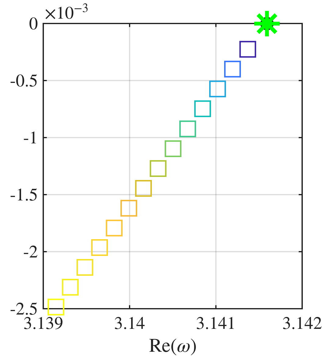
The following results are our main findings in this paper. An illustration of Theorem 2.3 can be found in Figure 4 and Figure 5.

Theorem 2.3.

Let $\displaystyle\delta\in\mathbb{C}$ . Assume that the frequency-dependent capacitance matrix $\displaystyle\mathcal{C}(k_{0})$ has $\displaystyle m$ nonzero eigenvalues, then $\displaystyle m\leq\lfloor n/2\rfloor$ . For cases when $\displaystyle\delta\to 0$ , the scattering problem (2.3) has exactly $\displaystyle n$ (nonzero) resonant frequencies near $\displaystyle k_{0}v$ for $\displaystyle k_{0}\in E$ :

\displaystyle\bullet

The first $\displaystyle 2m$ eigenfrequencies are analytic in $\displaystyle\delta^{1/2}$ and have the following asymptotic expansion:

\omega^{\pm}_{j}(\delta)=k_{0}v\pm v\sqrt{\frac{\lambda_{j}}{r}\delta}+\mathcal{O}(\delta),\quad j=1,2,\cdots,m,

where $\displaystyle\lambda_{1},\cdots,\lambda_{m}$ are the $\displaystyle m$ nonzero eigenvalues of $\displaystyle\mathcal{C}(k_{0})$ .

Moreover, let $\displaystyle\lambda$ be a nonzero eigenvalue of $\displaystyle\mathcal{C}(k_{0})$ with multiplicity $\displaystyle\mathfrak{m}$ . Then $\displaystyle\lambda$ is an eigenvalue of $\displaystyle\mathfrak{m}$ submatrices of $\displaystyle\mathcal{C}(k_{0})$ , denoted by $\displaystyle C_{j_{1}},\cdots,C_{j_{\mathfrak{m}}}$ . The $\displaystyle 2\mathfrak{m}$ branches satisfying $\displaystyle\omega^{\pm}(\delta)=k_{0}v\pm v\sqrt{\lambda\delta/r}+\mathcal{O}(\delta)$ admit the higher-order expansion:

\displaystyle\displaystyle\omega^{i,\pm}(\delta)=k_{0}v\pm v\sqrt{\frac{\lambda}{r}\delta}+\frac{v}{2r}\frac{\bm{\alpha}_{j_{i}}^{\top}B_{j_{i}}\bm{\alpha}_{j_{i}}}{\bm{\alpha}_{j_{i}}^{\top}\mathcal{L}_{j_{i}}\bm{\alpha}_{j_{i}}}\delta+\mathcal{O}(\delta^{3/2}),\quad i=1,2,\cdots,\mathfrak{m},

(2.13)

where $\displaystyle(\lambda,\bm{\alpha}_{j_{i}})$ is an eigenpair of $\displaystyle C_{j_{i}}$ ,

B_{j}=\operatorname{diag}\{\cot(t_{a_{j-1}}k_{0})\chi_{a_{j}},0,\cdots,0,\cot(t_{b_{j+1}}k_{0})\chi_{b_{j}}\},

with the convention that $\displaystyle\cot(t_{j}k_{0}):=-\mathrm{i}$ when $\displaystyle j=0$ or $\displaystyle j=2N$ , and $\displaystyle\mathcal{L}_{j}$ is defined in (3.9). Here, $\displaystyle a_{j},b_{j}$ are the endpoints of $\displaystyle\mathcal{I}_{j}$ in (2.11), and

\chi_{j}=\begin{cases}1,&j\text{ odd},\\ \dfrac{1}{\lambda t_{j}^{2}},&j\text{ even}.\end{cases}

$\displaystyle\bullet$

The remaining $\displaystyle n-2m$ eigenfrequencies have the following asymptotic expansion:

$\omega_{j}(\delta)=k_{0}v+\mathcal{O}(\delta),\qquad j=1,2,\cdots,n-2m.$ (2.14)

Refer to caption — (a) $\displaystyle c_{1}=1,c_{2}=-\textstyle\frac{1+\mathrm{i}}{4}.$

Suppose that $\displaystyle\omega(\delta)=k_{0}v\pm v\sqrt{\lambda_{j}\delta/r}+\mathcal{O}(\delta)$ with $\displaystyle\lambda_{j}$ being a simple nonzero eigenvalue of $\displaystyle\mathcal{C}(k_{0})$ is a resonant frequency for the scattering problem (2.3) and let $\displaystyle u(x)$ be the corresponding non-trivial solution.

For $\displaystyle k_{0}=0$ , we recall from [feppon.cheng.ea2023Subwavelength] that

u(x)=\begin{cases}\alpha_{j}+\mathcal{O}(\delta^{1/2}),&x\in(x_{2j-1},x_{2j}),\qquad j=1,2,\cdots,N,\\ \alpha_{j}+\beta_{j}(x-x_{2j})+\mathcal{O}(\delta^{1/2}),&x\in(x_{2j},x_{2j+1}),\qquad j=1,2,\cdots,N-1,\end{cases}

(2.15)

where $\displaystyle\bm{\alpha}=(\alpha_{1},\alpha_{2},\cdots,\alpha_{N})^{\top}$ is the corresponding eigenvector of the capacitance matrix $\displaystyle\mathcal{C}(0)$ and $\displaystyle\beta_{j}=\tfrac{\alpha_{j+1}-\alpha_{j}}{s_{j}},j=1,2,\cdots,N-1$ .

Beyond the subwavelength regime, that is, for $\displaystyle k_{0}\neq 0$ , deriving an explicit asymptotic expression for the eigenmodes generalizing (2.15) is considerably more involved, as shown in Section 6. For simplicity, we restrict to the case where $\displaystyle\lambda$ is a simple eigenvalue of $\displaystyle\mathcal{C}(k_{0})$ . The multiple eigenvalue case requires additional assumptions and is illustrated through examples in Section 6.2, while a rigorous analysis is deferred to future work.

We now state the precise setup and result. Without loss of generality, we set $\displaystyle r=1$ . We let $\displaystyle\lambda$ be a simple eigenvalue of $\displaystyle\mathcal{C}(k_{0})$ . By Theorem 2.2, there exists a unique index $\displaystyle j^{*}$ such that $\displaystyle\lambda$ is a simple eigenvalue of a submatrix $\displaystyle C_{j^{*}}$ of $\displaystyle\mathcal{C}(k_{0})$ . Let $\displaystyle\mathcal{I}_{j^{*}}=\llbracket a_{j^{*}},b_{j^{*}}\rrbracket$ be the corresponding target resonant interval, and let $\displaystyle s$ be the number of even integers in $\displaystyle\mathcal{I}_{j^{*}}$ , namely $\displaystyle 2\lceil a_{j^{*}}/2\rceil,2\lceil a_{j^{*}}/2\rceil+2,\dots,2\lfloor b_{j^{*}}/2\rfloor$ . Set $\displaystyle j_{0}=2\lceil a_{j^{*}}/2\rceil-2$ . Let $\displaystyle k_{0}\neq 0$ and suppose that $\displaystyle k(\delta)=k_{0}\pm\sqrt{\lambda\delta/r}+\mathcal{O}(\delta)$ is a resonant frequency and $\displaystyle u(x)$ its associated eigenmode.

Theorem 2.4 ((Eigenmodes for a simple resonance)).

Under the above settings, for each $\displaystyle 1\leq j\leq s$ , the eigenmode $\displaystyle u(x)$ has the form

\displaystyle\displaystyle u(x)=\beta_{j_{0}+2j}\sin\bigl(k_{0}(x-x_{a_{j^{*}}})\bigr)+\mathcal{O}(\delta^{1/2}),\quad x\in(x_{j_{0}+2j},x_{j_{0}+2j+1}),

(2.16)

where $\displaystyle(\lambda,\bm{\beta}=(\beta_{j_{0}+2j})_{j=1}^{s})$ is an eigenpair of the matrix $\displaystyle D_{j^{*}}$ defined in (3.3). Moreover, on any interval $\displaystyle(x_{i},x_{i+1})$ with $\displaystyle i\notin\{j_{0}+2j:1\leq j\leq s\}$ , there exists some positive integer $\displaystyle\gamma_{i}$ such that

u(x)=\mathcal{O}(\delta^{\gamma_{i}/2}),\quad x\in(x_{i},x_{i+1}).

For a schematic understanding of Theorem 2.4, see Figure 6; a numerical verification is provided in Figure 7.

Figure 6: Schematic illustration of Theorem 2.4. To leading order, the eigenmode is approximated by a trigonometric function on the spacings within the target block

\displaystyle\mathcal{I}_{j^{*}}

, with amplitudes determined by the eigenvector of

\displaystyle D_{j^{*}}

, and vanishes elsewhere. The green region marks

\displaystyle\mathcal{I}_{j^{*}}

; lighter green segments at the two ends (marked

\displaystyle?

) may or may not belong to

\displaystyle\mathcal{I}_{j^{*}}

depending on the parity of the endpoints

\displaystyle a_{j^{*}}

and

\displaystyle b_{j^{*}}

3 Block partition of the capacitance matrix

In this section, we study the spectral properties of the frequency-dependent capacitance matrix $\displaystyle\mathcal{C}(k_{0}),k_{0}\in E$ . In particular, we give a bound on the number of nonzero eigenvalues of $\displaystyle\mathcal{C}(k_{0})$ and compute a characteristic polynomial of $\displaystyle\mathcal{C}(k_{0})$ (see Theorem 3.5).

3.1 Preliminaries

Let the parameters $\displaystyle t_{1},t_{2},\ldots,t_{2N-1}$ and $\displaystyle\theta_{1},\theta_{2},\ldots,\theta_{2N-2}$ be given in (2.4) and (2.6), respectively. For an integer interval $\displaystyle\mathcal{I}=\llbracket a,b\rrbracket\subset\llbracket 1,2N-1\rrbracket$ , let $\displaystyle s$ and $\displaystyle l$ denote the number of even and odd integers in $\displaystyle\mathcal{I}$ , respectively:

s=\left\lfloor\frac{b}{2}\right\rfloor-\left\lfloor\frac{a-1}{2}\right\rfloor,\qquad l=\left\lceil\frac{b}{2}\right\rceil-\left\lceil\frac{a-1}{2}\right\rceil.

Note that $\displaystyle|s-l|\leq 1$ . We also define the parities of the endpoints by $\displaystyle\xi=a-2\lfloor a/2\rfloor$ and $\displaystyle\eta=b-2\lfloor b/2\rfloor$ , so that $\displaystyle\xi=0$ if $\displaystyle a$ is even and $\displaystyle\xi=1$ if $\displaystyle a$ is odd, and similarly for $\displaystyle\eta$ . The $\displaystyle s\times l$ matrix $\displaystyle A$ is then defined by

\displaystyle\displaystyle A_{i,\,i-1+\xi}=-1,\qquad A_{i,\,i+\xi}=1,

(3.1)

with all other entries equal to zero. We introduce

		$\displaystyle\mathcal{S}=\operatorname{diag}\!\left\{t_{2\lceil a/2\rceil},\,t_{2\lceil a/2\rceil+2},\,\ldots,\,t_{2\lfloor b/2\rfloor}\right\},$		(3.2)
		$\displaystyle\mathcal{L}=\operatorname{diag}\!\left\{t_{2\lfloor a/2\rfloor+1},\,t_{2\lfloor a/2\rfloor+3},\,\ldots,\,t_{2\lceil b/2\rceil-1}\right\},$		(3.2)

so that $\displaystyle\mathcal{S}$ is an $\displaystyle s\times s$ diagonal matrix with even-indexed entries and $\displaystyle\mathcal{L}$ is an $\displaystyle l\times l$ diagonal matrix with odd-indexed entries. We then define the $\displaystyle l\times l$ matrix

C=C^{\xi,\eta}(\theta_{a},\ldots,\theta_{b-1}):=\mathcal{L}^{-1}A^{\top}\mathcal{S}^{-1}A,

which depends only on the coupling coefficients $\displaystyle\theta_{a},\ldots,\theta_{b-1}$ . In the special case $\displaystyle a=1$ , $\displaystyle b=2N-1$ (so that $\displaystyle(\xi,\eta)=(1,1)$ ), $\displaystyle C$ reduces for $\displaystyle k_{0}=0$ to the classical capacitance matrix $\displaystyle\mathcal{C}(0)$ introduced in [feppon.cheng.ea2023Subwavelength]. We will also see in the next subsection that $\displaystyle C$ corresponds to each nonzero block of our frequency-dependent capacitance matrix $\displaystyle\mathcal{C}(k_{0})$ . The explicit forms of $\displaystyle C^{\xi,\eta}$ for each choice of parities are as follows:

C^{1,1}=\begin{pmatrix}\theta_{a}&-\theta_{a}&&\\ -\theta_{a+1}&\theta_{a+1}+\theta_{a+2}&-\theta_{a+2}&\\ &-\theta_{a+3}&\theta_{a+3}+\theta_{a+4}&-\theta_{a+4}&\\ &&\ddots&\ddots&\ddots\\ &&&-\theta_{b-3}&\theta_{b-3}+\theta_{b-2}&-\theta_{b-2}\\ &&&&-\theta_{b-1}&\theta_{b-1}\end{pmatrix},

C^{0,1}=\begin{pmatrix}\theta_{a}+\theta_{a+1}&-\theta_{a+1}&\\ -\theta_{a+2}&\theta_{a+2}+\theta_{a+3}&-\theta_{a+3}&\\ &-\theta_{a+4}&\theta_{a+4}+\theta_{a+5}&-\theta_{a+5}&\\ &&\ddots&\ddots&\ddots&\\ &&&-\theta_{b-3}&\theta_{b-3}+\theta_{b-2}&-\theta_{b-2}\\ &&&&-\theta_{b-1}&\theta_{b-1}\end{pmatrix},

C^{1,0}=\begin{pmatrix}\theta_{a}&-\theta_{a}&\\ -\theta_{a+1}&\theta_{a+1}+\theta_{a+2}&-\theta_{a+2}&\\ &-\theta_{a+3}&\theta_{a+3}+\theta_{a+4}&-\theta_{a+4}&\\ &&\ddots&\ddots&\ddots&\\ &&&-\theta_{b-4}&\theta_{b-4}+\theta_{b-3}&-\theta_{b-3}\\ &&&&-\theta_{b-2}&\theta_{b-2}+\theta_{b-1}\end{pmatrix},

C^{0,0}=\begin{pmatrix}\theta_{a}+\theta_{a+1}&-\theta_{a+1}&\\ -\theta_{a+2}&\theta_{a+2}+\theta_{a+3}&-\theta_{a+3}&\\ &-\theta_{a+4}&\theta_{a+4}+\theta_{a+5}&-\theta_{a+5}&\\ &&\ddots&\ddots&\ddots&\\ &&&-\theta_{b-4}&\theta_{b-4}+\theta_{b-3}&-\theta_{b-3}\\ &&&&-\theta_{b-2}&\theta_{b-2}+\theta_{b-1}\end{pmatrix}.

We also introduce the $\displaystyle s\times s$ matrix $\displaystyle D$ as

\displaystyle\displaystyle D=D^{\xi,\eta}(\theta_{a},\cdots,\theta_{b-1}):=\mathcal{S}^{-1}\cdot A\mathcal{L}^{-1}A^{\top}.

(3.3)

Then a direct computation yields

D^{\xi,\eta}(\theta_{a},\cdots,\theta_{b-1})=C^{1-\xi,1-\eta}(\theta_{a},\cdots,\theta_{b-1}).

Lemma 3.1.

Let $\displaystyle C^{\xi,\eta}$ and $\displaystyle D^{\xi,\eta}$ be defined as above. Let $\displaystyle\mathfrak{n}:=\#I=b-a+1$ . For $\displaystyle 0\leq q\leq\lfloor\mathfrak{n}/2\rfloor$ , define the constants:

c_{a,b,q}=\sum_{a\leq j_{1}\prec j_{2}\prec\cdots\prec j_{q}\leq b-1}\prod_{i=1}^{q}\theta_{j_{i}},\quad q>0.\qquad c_{a,b,0}=1.

It holds that:

(i)

All eigenvalues of $\displaystyle C$ are distinct. If $\displaystyle(\xi,\eta)=(1,1)$ , then $\displaystyle C$ has exactly one zero eigenvalue and all remaining eigenvalues are positive; for all other choices of $\displaystyle(\xi,\eta)$ , every eigenvalue of $\displaystyle C$ is positive.
(ii)

$\displaystyle C$ and $\displaystyle D$ share the same nonzero eigenvalues, and their common nonzero characteristic polynomial is

$P(\lambda)=\sum_{q=0}^{\lfloor\mathfrak{n}/2\rfloor}c_{a,b,q}(-\lambda)^{\lfloor\mathfrak{n}/2\rfloor-q}.$

(iii)

Let $\displaystyle\lambda_{0}$ be a nonzero eigenvalue of $\displaystyle C=C^{\xi,\eta}(\theta_{a},\ldots,\theta_{b-1})$ with corresponding eigenvector $\displaystyle\bm{\alpha}=(\alpha_{1},\ldots,\alpha_{l})^{\top}$ . Let

P_{1}(\lambda)=\sum_{q=0}^{\lfloor(\mathfrak{n}-1)/2\rfloor}c_{a+1,b,q}(-\lambda)^{\lfloor(\mathfrak{n}-1)/2\rfloor-q},\quad P_{2}(\lambda)=\sum_{q=0}^{\lfloor(\mathfrak{n}-1)/2\rfloor}c_{a,b-1,q}(-\lambda)^{\lfloor(\mathfrak{n}-1)/2\rfloor-q},

be the nonzero characteristic polynomials of

\tilde{C}_{1}=C^{1-\xi,\eta}(\theta_{a+1},\cdots,\theta_{b-1}),\quad\tilde{C}_{2}=C^{\xi,1-\eta}(\theta_{a},\cdots,\theta_{b-2}),

(3.4)

respectively. Then

\frac{P_{1}(\lambda_{0})}{P^{\prime}(\lambda_{0})}=(-1)^{\xi+\eta}t_{a}^{2\xi-1}\lambda_{0}^{\eta(2\xi-1)}\frac{\alpha_{1}^{2}}{\bm{\alpha}^{\top}\mathcal{L}\bm{\alpha}},\quad\frac{P_{2}(\lambda_{0})}{P^{\prime}(\lambda_{0})}=(-1)^{\xi+\eta}t_{b}^{2\eta-1}\lambda_{0}^{\xi(2\eta-1)}\frac{\alpha_{l}^{2}}{\bm{\alpha}^{\top}\mathcal{L}\bm{\alpha}};

(iv)

Let $\displaystyle\mu_{1}\mu_{2}=\lambda>0$ , $\displaystyle\bm{\alpha}\in\mathbb{R}^{l}$ , and $\displaystyle\bm{\beta}\in\mathbb{R}^{s}$ . Consider the coupled systems

$\mathrm{(1)}\ A\bm{\alpha}=\mu_{1}\mathcal{S}\bm{\beta},\qquad\mathrm{(2)}\ A^{\top}\bm{\beta}=\mu_{2}\mathcal{L}\bm{\alpha}.$

If all equations in (1) and (2) are satisfied except possibly one specific row, which may be the first or last row of either (1) or (2), then this exceptional row holds if and only if $\displaystyle\lambda$ is an eigenvalue of $\displaystyle C$ (or equivalently, of $\displaystyle D$ ). In that case, $\displaystyle(\lambda,\bm{\alpha})$ is an eigenpair of $\displaystyle C$ and $\displaystyle(\lambda,\bm{\beta})$ is an eigenpair of $\displaystyle D$ .

Proof.

As for item (i), the first statement follows from the fact that $\displaystyle C$ is a tridiagonal matrix with nonzero off-diagonal elements; see [parlett1998symmetric, Lemma 7.7.1]. For the second, we observe that $\displaystyle\mathcal{L}^{1/2}C\mathcal{L}^{-1/2}=\mathcal{L}^{-1/2}A^{\top}\mathcal{S}^{-1}A\mathcal{L}^{-1/2}$ is symmetric and positive semidefinite, since

\bm{x}^{\top}\mathcal{L}^{-1/2}A^{\top}\mathcal{S}^{-1}A\mathcal{L}^{-1/2}\bm{x}\geq 0

for all $\displaystyle\bm{x}$ , with equality if and only if $\displaystyle A\mathcal{L}^{-1/2}\bm{x}=\bm{0}$ . Since $\displaystyle\operatorname{rank}(A\mathcal{L}^{-1/2})=\operatorname{rank}(A)=\min\{s,l\}$ , the equation $\displaystyle A\mathcal{L}^{-1/2}\bm{x}=\bm{0}$ admits a nontrivial solution only when $\displaystyle s<l$ , that is, when $\displaystyle(\xi,\eta)=(1,1)$ , which gives the second statement.

For item (ii), $\displaystyle C=\mathcal{L}^{-1}A^{\top}\cdot\mathcal{S}^{-1}A$ and $\displaystyle D=\mathcal{S}^{-1}A\cdot\mathcal{L}^{-1}A^{\top}$ are products of the same two matrices in reverse order, so they share the same nonzero eigenvalues. For the characteristic polynomial, when $\displaystyle(\xi,\eta)=(1,1)$ , [pm1, Lemma 4.3(2)] gives

|C-\lambda I|=\sum_{q=0}^{(\mathfrak{n}-1)/2}c_{a,b,q}(-\lambda)^{(\mathfrak{n}+1)/2-q},

and the result follows since $\displaystyle C$ has exactly one zero eigenvalue. When $\displaystyle(\xi,\eta)=(0,1)$ , let $\displaystyle Q^{1}$ denote the $\displaystyle(1,1)$ -cofactor of $\displaystyle|C-\lambda I|$ . Expanding along the first column yields

		$\displaystyle\displaystyle\|C-\lambda I\|=\sum_{q=0}^{\mathfrak{n}/2-1}c_{a,b,q}(-\lambda)^{\mathfrak{n}/2-q}+\theta_{a}Q^{1}(\lambda)$
	$\displaystyle\displaystyle=$	$\displaystyle\displaystyle\sum_{q=0}^{\mathfrak{n}/2-1}(-\lambda)^{\mathfrak{n}/2-q}\sum_{a\leq j_{1}\prec j_{2}\prec\cdots\prec j_{q}\leq b-1}\prod_{i=1}^{q}\theta_{j_{i}}+\theta_{a}\sum_{q=1}^{\mathfrak{n}/2}(-\lambda)^{\mathfrak{n}/2-q}\sum_{a+1\leq j_{1}\prec j_{2}\prec\cdots\prec j_{q-1}\leq b-1}\prod_{i=1}^{q-1}\theta_{j_{i}}$
	$\displaystyle\displaystyle=$	$\displaystyle\displaystyle\sum_{q=0}^{\mathfrak{n}/2}(-\lambda)^{\mathfrak{n}/2-q}\sum_{a\leq j_{1}\prec j_{2}\prec\cdots\prec b-1}\prod_{i=1}^{q}\theta_{j_{i}}=\sum_{q=0}^{\mathfrak{n}/2}c_{a,b,q}(-\lambda)^{\mathfrak{n}/2-q},$

and the result follows since $\displaystyle C$ has no zero eigenvalues in this case. The remaining cases $\displaystyle(\xi,\eta)=(1,0)$ and $\displaystyle(\xi,\eta)=(0,0)$ are analogous and omitted.

For item (iii), since $\displaystyle\lambda_{0}$ is simple, $\displaystyle C-\lambda_{0}I$ has rank $\displaystyle l-1$ , so $\displaystyle\operatorname{adj}(C-\lambda_{0}I)$ has rank $\displaystyle 1$ . Hence there exists $\displaystyle c\neq 0$ such that $\displaystyle\operatorname{adj}(C-\lambda_{0}I)=c\bm{\alpha}\widetilde{\bm{\alpha}}$ , where $\displaystyle\bm{\alpha}$ and $\displaystyle\widetilde{\bm{\alpha}}$ are the right and left eigenvectors of $\displaystyle C$ , respectively. Since $\displaystyle\mathcal{L}^{1/2}C\mathcal{L}^{-1/2}$ is symmetric, the left eigenvector satisfies $\displaystyle\widetilde{\bm{\alpha}}=\mathcal{L}\bm{\alpha}$ , and therefore

\left.\frac{\mathrm{d}}{\mathrm{d}\lambda}\right|_{\lambda=\lambda_{0}}|C-\lambda I|=-\operatorname{tr}\!\left(\operatorname{adj}(C-\lambda_{0}I)\right)=-c\,\bm{\alpha}^{\top}\mathcal{L}\bm{\alpha}.

We now compute $\displaystyle P_{1}(\lambda_{0})/P^{\prime}(\lambda_{0})$ for each parity case.

Case $\displaystyle\xi=1$ . Here $\displaystyle\widetilde{C}_{1}$ has no zero eigenvalues, so

P_{1}(\lambda_{0})=|\widetilde{C}_{1}-\lambda_{0}I|=\operatorname{adj}(C-\lambda_{0}I)_{11}=\beta\mathcal{L}_{11}\alpha_{1}^{2}=ct_{a}\alpha_{1}^{2}.

If $\displaystyle(\xi,\eta)=(1,1)$ , then $\displaystyle P^{\prime}(\lambda_{0})=(c/\lambda_{0})\,\bm{\alpha}^{\top}\mathcal{L}\bm{\alpha}$ , giving

\frac{P_{1}(\lambda_{0})}{P^{\prime}(\lambda_{0})}=\lambda_{0}t_{a}\frac{\alpha_{1}^{2}}{\bm{\alpha}^{\top}\mathcal{L}\bm{\alpha}}.

If $\displaystyle(\xi,\eta)=(1,0)$ , $\displaystyle C$ has no zero eigenvalues, and thus the coefficient becomes $\displaystyle-t_{a}$ .

Case $\displaystyle\xi=0$ . Here $\displaystyle C$ has no zero eigenvalues. Letting $\displaystyle E_{11}$ denote the elementary matrix with a $\displaystyle 1$ in position $\displaystyle(1,1)$ and zeros elsewhere,

|\widetilde{C}_{1}-\lambda_{0}I|=|C-\lambda_{0}I-\theta_{a}E_{11}|=|C-\lambda_{0}I|-\theta_{a}\operatorname{adj}(C-\lambda_{0}I)_{11}=-c\theta_{a}t_{a+1}\alpha_{1}^{2}=-c\frac{\alpha_{1}^{2}}{t_{a}}.

If $\displaystyle(\xi,\eta)=(0,1)$ , then $\displaystyle\widetilde{C}_{1}$ has a zero eigenvalue, so

P_{1}(\lambda_{0})=\frac{|\widetilde{C}_{1}-\lambda_{0}I|}{-\lambda_{0}}=\frac{c\alpha_{1}^{2}}{\lambda_{0}t_{a}},\qquad\frac{P_{1}(\lambda_{0})}{P^{\prime}(\lambda_{0})}=-\frac{1}{\lambda_{0}t_{a}}\frac{\alpha_{1}^{2}}{\bm{\alpha}^{\top}\mathcal{L}\bm{\alpha}}.

If $\displaystyle(\xi,\eta)=(0,0)$ , then $\displaystyle\widetilde{C}_{1}$ has no zero eigenvalue and the coefficient becomes $\displaystyle 1/t_{a}$ . The formula for $\displaystyle P_{2}(\lambda_{0})/P^{\prime}(\lambda_{0})$ follows by an analogous argument.

As for item (iv), we only consider the case where the exceptional row is the last row of (2); the other cases are similar. From (1) we have

\displaystyle\displaystyle\bm{\beta}=\mu_{1}^{-1}\mathcal{S}^{-1}A\bm{\alpha}.

(3.5)

Substituting into the first $\displaystyle l-1$ rows of (2) gives, for $\displaystyle i=1,\dots,l-1$ ,

(A^{\top}\bm{\beta})_{i}=\mu_{2}(\mathcal{L}\bm{\alpha})_{i}\Longrightarrow(A^{\top}\mathcal{S}^{-1}A\bm{\alpha})_{i}=\lambda(\mathcal{L}\bm{\alpha})_{i},

and multiplying by $\displaystyle\mathcal{L}^{-1}$ yields

\displaystyle\displaystyle(C\bm{\alpha})_{i}=\lambda\bm{\alpha}_{i},\quad i=1,\cdots,l-1.

(3.6)

The last row of (2) is $\displaystyle(A^{\top}\bm{\beta})_{l}=\mu_{2}(\mathcal{L}\bm{\alpha})_{l}$ , which by (3.5) is equivalent to

\displaystyle\displaystyle(C\bm{\alpha})_{l}=\lambda\bm{\alpha}_{l}.

(3.7)

If the last row holds, then (3.7) gives $\displaystyle C\bm{\alpha}=\lambda\bm{\alpha}$ , and from (3.5) we obtain

D\bm{\beta}=\mathcal{S}^{-1}A\mathcal{L}^{-1}A^{\top}\bm{\beta}=\mathcal{S}^{-1}A\mathcal{L}^{-1}(\mu_{2}\mathcal{L}\bm{\alpha})=\mu_{2}\mathcal{S}^{-1}A\bm{\alpha}=\mu_{2}\mathcal{S}^{-1}(\mu_{1}\mathcal{S}\bm{\beta})=\lambda\bm{\beta}.

Conversely, assume that $\displaystyle\lambda$ is an eigenvalue of $\displaystyle C$ . Let $\displaystyle\tilde{C}$ be the submatrix of $\displaystyle C-\lambda I$ consisting of its first $\displaystyle l-1$ rows. Then (3.6) implies $\displaystyle\bm{\alpha}\in\operatorname{Ker}\tilde{C}$ . Since $\displaystyle C$ is tridiagonal with nonzero off-diagonals, its first $\displaystyle l-1$ rows are linearly independent, so $\displaystyle\operatorname{rank}(\tilde{C})=\operatorname{rank}(C-\lambda I)=l-1$ . The rank–nullity theorem then gives $\displaystyle\dim\operatorname{Ker}\widetilde{C}=\dim\operatorname{Ker}(C-\lambda I)$ , and since $\displaystyle\operatorname{Ker}(C-\lambda I)\subset\operatorname{Ker}\widetilde{C}$ , the two kernels coincide. Hence, $\displaystyle\bm{\alpha}\in\operatorname{Ker}(C-\lambda I)$ , i.e., $\displaystyle C\bm{\alpha}=\lambda\bm{\alpha}$ , and (3.7) holds, so the last row of (2) is satisfied. ∎

Remark 3.2.

Lemma 3.1(iv) can be interpreted as a singular value decomposition of the matrix $\displaystyle K=\mathcal{L}^{-1/2}A^{\top}\mathcal{S}^{-1/2}$ . Indeed, if $\displaystyle\lambda>0$ is an eigenvalue of $\displaystyle C$ (hence of $\displaystyle D$ ) and $\displaystyle\bm{\alpha},\bm{\beta}$ satisfy the equations in the lemma with $\displaystyle\mu_{1}=\mu_{2}:=\mu=\sqrt{\lambda}$ , then setting $\displaystyle\bm{x}=\mathcal{L}^{1/2}\bm{\alpha}$ and $\displaystyle\bm{y}=\mathcal{S}^{1/2}\bm{\beta}$ yields

K\bm{y}=\mu\bm{x},\qquad K^{\top}\bm{x}=\mu\bm{y},

so $\displaystyle\mu$ is a singular value of $\displaystyle K$ with right singular vector $\displaystyle\bm{y}$ and left singular vector $\displaystyle\bm{x}$ . Conversely, any singular value of $\displaystyle K$ gives rise to an eigenpair of $\displaystyle C$ and $\displaystyle D$ via the same transformation.

3.2 Block structures of capacitance matrices

This section elucidates the block structure of capacitance matrix $\displaystyle\mathcal{C}(k_{0})$ and its symmetrized version. We first recall the following standard result from linear algebra.

Lemma 3.3.

Let $\displaystyle X$ and $\displaystyle\widetilde{X}$ be two tridiagonal matrices of the form

X=\begin{pmatrix}a_{1}&c_{1}&&\\ b_{1}&a_{2}&c_{2}&\\ &\ddots&\ddots&c_{n-1}\\ &&b_{n-1}&a_{n}\end{pmatrix},\qquad\widetilde{X}=\begin{pmatrix}a_{1}&\tilde{c}_{1}&&\\ \tilde{b}_{1}&a_{2}&\tilde{c}_{2}&\\ &\ddots&\ddots&\tilde{c}_{n-1}\\ &&\tilde{b}_{n-1}&a_{n}\end{pmatrix}.

If $\displaystyle b_{i}c_{i}=\tilde{b}_{i}\tilde{c}_{i}$ for every $\displaystyle i=1,\dots,n-1$ , then $\displaystyle X$ and $\displaystyle\widetilde{X}$ have the same eigenvalues.

Proof.

Consider the characteristic polynomials of the leading principal submatrices. For $\displaystyle k=1,\dots,n$ , let $\displaystyle P_{k}(\lambda)$ and $\displaystyle\widetilde{P}_{k}(\lambda)$ denote the characteristic polynomials of the $\displaystyle k\times k$ leading principal submatrices of $\displaystyle X$ and $\displaystyle\widetilde{X}$ , respectively. Both satisfy the three-term recurrence

P_{0}(\lambda)=1,\quad P_{1}(\lambda)=\lambda-a_{1},\quad P_{k}(\lambda)=(\lambda-a_{k})P_{k-1}(\lambda)-b_{k-1}c_{k-1}\,P_{k-2}(\lambda),\quad k\geq 2,

and similarly for $\displaystyle\widetilde{P}_{k}$ with $\displaystyle b_{k-1}c_{k-1}$ replaced by $\displaystyle\tilde{b}_{k-1}\tilde{c}_{k-1}$ . Since $\displaystyle b_{k-1}c_{k-1}=\tilde{b}_{k-1}\tilde{c}_{k-1}$ for all $\displaystyle k$ , a straightforward induction gives $\displaystyle P_{k}(\lambda)=\widetilde{P}_{k}(\lambda)$ for all $\displaystyle k$ . In particular, $\displaystyle P_{n}(\lambda)=\widetilde{P}_{n}(\lambda)$ , so $\displaystyle X$ and $\displaystyle\widetilde{X}$ have the same characteristic polynomial and hence the same eigenvalues. ∎

For $\displaystyle k_{0}\in E$ , we introduce the symmetrized version of the frequency-dependent capacitance matrix $\displaystyle\mathcal{C}(k_{0})$ defined in (2.7) by

	$\displaystyle\displaystyle\left(\mathcal{C}^{\mathrm{sym}}(k_{0})\right)_{i,i}$	$\displaystyle\displaystyle:=\left(\mathcal{C}(k_{0})\right)_{i,i},$
	$\displaystyle\displaystyle\left(\mathcal{C}^{\mathrm{sym}}(k_{0})\right)_{i,i+1}=\left(\mathcal{C}^{\mathrm{sym}}(k_{0})\right)_{i+1,i}$	$\displaystyle\displaystyle:=-\sqrt{\left(\mathcal{C}(k_{0})\right)_{i,i+1}\left(\mathcal{C}(k_{0})\right)_{i+1,i}},$

with all remaining entries equal to zero. By Lemma 3.3, $\displaystyle\mathcal{C}(k_{0})$ and $\displaystyle\mathcal{C}^{\mathrm{sym}}(k_{0})$ share the same eigenvalues.

For an integer interval $\displaystyle\mathcal{I}=\llbracket a,b\rrbracket$ , we define

\mathrm{Sta}(\mathcal{I})=\left\lfloor\frac{a}{2}\right\rfloor+1,\qquad\mathrm{End}(\mathcal{I})=\left\lceil\frac{b}{2}\right\rceil.

Let $\displaystyle C_{j}$ (resp. $\displaystyle C_{j}^{\mathrm{sym}}$ ) denote the principal submatrix of $\displaystyle\mathcal{C}(k_{0})$ (resp. $\displaystyle\mathcal{C}^{\mathrm{sym}}(k_{0})$ ) with rows and columns indexed from $\displaystyle\mathrm{Sta}(\mathcal{I}_{j})$ to $\displaystyle\mathrm{End}(\mathcal{I}_{j})$ , where $\displaystyle\{\mathcal{I}_{j}\}$ are defined in (2.11). Similarly, $\displaystyle C_{j}$ and $\displaystyle C_{j}^{\mathrm{sym}}$ share the same eigenvalues. The following proposition, illustrated in Figure 8, describes the block-diagonal structure of $\displaystyle\mathcal{C}^{\mathrm{sym}}(k_{0})$ . Theorem 2.2 follows as a corollary of Proposition 3.4, and will be proved accordingly.

Proposition 3.4 ((Block-diagonal structure)).

$\displaystyle\mathrm{End}(\mathcal{I}_{j})<\mathrm{Sta}(\mathcal{I}_{j+1})$ for $\displaystyle j=1,\ldots,p-1$ . Consequently, the submatrices $\displaystyle\{C_{j}^{\mathrm{sym}}\}_{j=1}^{p}$ are disjoint principal submatrices of $\displaystyle\mathcal{C}^{\mathrm{sym}}(k_{0})$ , with all entries outside these blocks equal to zero. Hence, the nonzero eigenvalues of $\displaystyle\mathcal{C}^{\mathrm{sym}}(k_{0})$ coincide with the union of the nonzero eigenvalues of the $\displaystyle C_{j}^{\mathrm{sym}}$ ’s, counted with their multiplicities.

Proof of Proposition 3.4 and Theorem 2.2.

Since $\displaystyle a_{j+1}-b_{j}\geq 2$ , we have

	$\displaystyle\displaystyle\mathrm{Sta}(\mathcal{I}_{j+1})-\mathrm{End}(\mathcal{I}_{j})$	$\displaystyle\displaystyle=\left\lfloor\frac{a_{j+1}}{2}\right\rfloor-\left\lceil\frac{b_{j}}{2}\right\rceil+1$
		$\displaystyle\displaystyle\geq\left\lfloor\frac{b_{j}+2}{2}\right\rfloor-\left\lceil\frac{b_{j}}{2}\right\rceil+1=\left\lfloor\frac{b_{j}}{2}\right\rfloor-\left\lceil\frac{b_{j}}{2}\right\rceil+2\geq 1.$

It remains to verify that

	$\displaystyle\displaystyle\left(\mathcal{C}^{\mathrm{sym}}(k_{0})\right)_{i,i}$	$\displaystyle\displaystyle=0,\qquad\mathrm{End}(\mathcal{I}_{j})+1\leq i\leq\mathrm{Sta}(\mathcal{I}_{j+1})-1,$
	$\displaystyle\displaystyle\left(\mathcal{C}^{\mathrm{sym}}(k_{0})\right)_{i-1,i}$	$\displaystyle\displaystyle=0,\qquad\mathrm{End}(\mathcal{I}_{j})+1\leq i\leq\mathrm{Sta}(\mathcal{I}_{j+1}).$

By definition of $\displaystyle t_{i}(k_{0})$ and $\displaystyle\mathcal{I}_{j}$ , we have $\displaystyle 1/t_{i}(k_{0})=0$ for $\displaystyle b_{j}<i<a_{j+1}$ .

For the diagonal entries, when $\displaystyle\mathrm{End}(\mathcal{I}_{j})+1\leq i\leq\mathrm{Sta}(\mathcal{I}_{j+1})-1$ , we have

2i-1\in\left[2\left\lceil\frac{b_{j}}{2}\right\rceil+1,\,2\left\lfloor\frac{a_{j+1}}{2}\right\rfloor-1\right]\subset(b_{j},a_{j+1}),

so $\displaystyle 1/t_{2i-1}(k_{0})=0$ and thus $\displaystyle\left(\mathcal{C}^{\mathrm{sym}}(k_{0})\right)_{i,i}=0$ .

For the off-diagonal entries, when $\displaystyle\mathrm{End}(\mathcal{I}_{j})+1\leq i\leq\mathrm{Sta}(\mathcal{I}_{j+1})$ , we have

2i\in\left[2\left\lceil\frac{b_{j}}{2}\right\rceil+2,\,2\left\lfloor\frac{a_{j+1}}{2}\right\rfloor+2\right]\subset(b_{j}+1,a_{j+1}+3),

so at least one of $\displaystyle 2i-3$ , $\displaystyle 2i-2$ , $\displaystyle 2i-1$ lies in $\displaystyle(b_{j},a_{j+1})$ , which forces at least one of $\displaystyle 1/t_{2i-3}(k_{0})$ , $\displaystyle 1/t_{2i-2}(k_{0})$ , $\displaystyle 1/t_{2i-1}(k_{0})$ to vanish, giving $\displaystyle\left(\mathcal{C}^{\mathrm{sym}}(k_{0})\right)_{i-1,i}=0$ . This finally shows that all entries outside $\displaystyle C_{j}^{\text{sym}},1\leq j\leq p$ equal to zero and thus the nonzero eigenvalues of $\displaystyle\mathcal{C}^{\text{sym}}(k_{0})$ coincide with the union of nonzero eigenvalues of the $\displaystyle C^{\text{sym}}_{j}$ ’s counted with their multiplicities. Since $\displaystyle\mathcal{C}(k_{0})$ and $\displaystyle\mathcal{C}^{\text{sym}}(k_{0})$ share the same eigenvalues, and the same holds for $\displaystyle C_{j}$ and $\displaystyle C^{\text{sym}}_{j}$ , Theorem 2.2 follows. ∎

(a) nonzero structure of

\displaystyle\mathcal{C}(k_{0})

(b) nonzero structure of

\displaystyle\mathcal{C}^{\text{sym}}(k_{0})

Figure 8: An example of the nonzero structure of

\displaystyle\mathcal{C}(k_{0})

(left) and its symmetrized version

\displaystyle\mathcal{C}^{\text{sym}}(k_{0})

(right). Colored squares indicate nonzero entries belonging to the submatrices (different colors distinguish different submatrices), while gray squares represent nonzero entries outside these blocks. In accordance with Proposition 3.4,

\displaystyle\mathcal{C}^{\text{sym}}(k_{0})

possesses a block diagonal structure, whereas

\displaystyle\mathcal{C}(k_{0})

does not necessarily.

For each integer interval $\displaystyle\mathcal{I}_{j}=\llbracket a_{j},b_{j}\rrbracket$ , define $\displaystyle\xi_{j}=a_{j}-2\lfloor a_{j}/2\rfloor$ and $\displaystyle\eta_{j}=b_{j}-2\lfloor b_{j}/2\rfloor$ . In the notation of the preceding subsection,

\displaystyle\displaystyle C_{j}=C^{\xi_{j},\eta_{j}}(\theta_{a_{j}},\ldots,\theta_{b_{j}-1}),\qquad j=1,2,\ldots,p,

(3.8)

with the decomposition

\displaystyle\displaystyle C_{j}=\mathcal{L}_{j}^{-1}A_{j}^{\top}\mathcal{S}_{j}^{-1}A_{j},

(3.9)

where $\displaystyle A_{j}$ , $\displaystyle\mathcal{L}_{j}$ , $\displaystyle\mathcal{S}_{j}$ are as defined in (3.1) and (3.2). The associated matrix $\displaystyle D_{j}$ is defined by

\displaystyle\displaystyle D_{j}=\mathcal{S}_{j}^{-1}A_{j}\mathcal{L}_{j}^{-1}A_{j}^{\top}=D^{\xi_{j},\eta_{j}}(\theta_{a_{j}},\ldots,\theta_{b_{j}-1}),

(3.10)

similarly to (3.3). We now summarize the spectral properties of $\displaystyle\mathcal{C}(k_{0})$ .

Theorem 3.5.

Let $\displaystyle m=m(k_{0})$ denote the number of nonzero eigenvalues of $\displaystyle\mathcal{C}(k_{0})$ . Then

m=\sum_{j=1}^{p}\left\lfloor\frac{n_{j}}{2}\right\rfloor\leq\left\lfloor\frac{n}{2}\right\rfloor.

Moreover, a nonzero characteristic polynomial of $\displaystyle\mathcal{C}(k_{0})$ is

P_{I}(\lambda):=\sum_{q=0}^{m}C_{I,q}(-\lambda)^{m-q},

where

\displaystyle\displaystyle C_{I,q}:=\sum_{\begin{subarray}{c}0\leq q_{j}\leq\lfloor n_{j}/2\rfloor\\ q_{1}+\cdots+q_{p}=q\end{subarray}}\prod_{j=1}^{p}c_{a_{j},b_{j},q_{j}}=\sum_{\begin{subarray}{c}j_{1}\prec j_{2}\prec\cdots\prec j_{q}\\ \{j_{i},j_{i}+1\}\subset I\end{subarray}}\prod_{i=1}^{q}\theta_{j_{i}}.

(3.11)

Proof.

By Lemma 3.1(ii), the nonzero characteristic polynomial of $\displaystyle C_{j}$ is

\displaystyle\displaystyle P_{j}(\lambda)=\sum_{q=0}^{\lfloor n_{j}/2\rfloor}c_{a_{j},b_{j},q}(-\lambda)^{\lfloor n_{j}/2\rfloor-q}.

(3.12)

By Theorem 2.2, $\displaystyle P_{I}(\lambda):=\prod_{j=1}^{p}P_{j}(\lambda)$ is then a nonzero characteristic polynomial of $\displaystyle\mathcal{C}(k_{0})$ , and

m=\sum_{j=1}^{p}\left\lfloor\frac{n_{j}}{2}\right\rfloor\leq\left\lfloor\sum_{j=1}^{p}\frac{n_{j}}{2}\right\rfloor=\left\lfloor\frac{n}{2}\right\rfloor.

It remains to verify the second equality in (3.11). Expanding the product over blocks and grouping by the number of selected indices in each block $\displaystyle\mathcal{I}_{j}$ gives

\displaystyle\displaystyle\sum_{\begin{subarray}{c}j_{1}\prec\cdots\prec j_{q}\\ \{j_{i},j_{i}+1\}\subset I\end{subarray}}\prod_{i=1}^{q}\theta_{j_{i}}

\displaystyle\displaystyle=\sum_{\begin{subarray}{c}q_{1}+\cdots+q_{p}=q\\ 0\leq q_{j}\leq\lfloor n_{j}/2\rfloor\end{subarray}}\prod_{l=1}^{p}\left(\sum_{a_{l}\leq j^{(l)}_{1}\prec\cdots\prec j^{(l)}_{q_{l}}\leq b_{l}-1}\prod_{i=1}^{q_{l}}\theta_{j^{(l)}_{i}}\right)=\sum_{\begin{subarray}{c}q_{1}+\cdots+q_{p}=q\\ 0\leq q_{j}\leq\lfloor n_{j}/2\rfloor\end{subarray}}\prod_{j=1}^{p}c_{a_{j},b_{j},q_{j}},

which completes the proof. ∎

4 Propagation matrix approach and asymptotic expansions

In this section, we employ a propagation matrix approach to characterize the scattering resonances of the one-dimensional system. We construct the total transfer matrix for the finite chain of resonators and establish that the resonant frequencies coincide precisely with the zeros of a specific analytic function. This characterization serves as the foundation for the rigorous asymptotic analysis carried out in Section 5.

We introduce the matrices

\displaystyle\displaystyle R(z):=\begin{pmatrix}\dfrac{1+z}{2}&\dfrac{1-z}{2}\\[6.0pt] \dfrac{1-z}{2}&\dfrac{1+z}{2}\end{pmatrix},\qquad L(z):=\begin{pmatrix}\mathrm{e}^{\mathrm{i}z}&0\\ 0&\mathrm{e}^{-\mathrm{i}z}\end{pmatrix}.

(4.1)

We write $\displaystyle L_{j}(k):=L(t_{j}k)$ for the matrix associated with the $\displaystyle j$ ^th component $\displaystyle t_{j}$ of $\displaystyle\bm{t}$ defined in (2.4), and set

\sigma=\frac{\delta}{r}.

The following theorem is a consequence of [pm1, Theorem 3.1 and Lemma 3.5].

Theorem 4.1.

Let $\displaystyle 0\neq\omega=kv$ . Then $\displaystyle\omega$ is a resonant frequency if and only if $\displaystyle k$ is a zero of $\displaystyle f(k;\sigma):=M_{\mathrm{tot}}(k;\sigma)_{2,2}$ , where $\displaystyle M_{\mathrm{tot}}(k;\sigma)$ is the analytic matrix function

M_{tot}(k;\sigma):=\frac{(4\sigma)^{N}}{(1+\sigma)^{2N}}R\left(\frac{1}{\sigma}\right)L_{2N-1}(k)R(\sigma)L_{2N-2}(k)\cdots\\ L_{4}(k)R\left(\frac{1}{\sigma}\right)L_{3}(k)R(\sigma)L_{2}(k)R\left(\frac{1}{\sigma}\right)L_{1}(k)R(\sigma).

(4.2)

As $\displaystyle\sigma\to 0$ , $\displaystyle f(k;\sigma)$ converges uniformly to

f(k;0)=-(2\mathrm{i})^{2N-1}\prod_{j=1}^{2N-1}\sin(t_{j}k)

on every compact set $\displaystyle K\Subset\mathbb{C}$ . A point $\displaystyle k\in\mathbb{C}$ is a zero of $\displaystyle f(\,\cdot\,;0)$ if and only if $\displaystyle k\in E=\cup_{j=1}^{2N-1}(\pi\mathbb{Z}/t_{j})$ , in which case $\displaystyle k$ is a zero of order

n(k):=\#\left\{j:t_{j}k\in\pi\mathbb{Z},\ 1\leq j\leq 2N-1\right\}.

In particular, all zeros of $\displaystyle f(\,\cdot\,;0)$ are real, and $\displaystyle 0$ is a zero of order $\displaystyle 2N-1$ .

Following the notation of [pm1, Section 3.3], we introduce

\nu:=\frac{2\sigma}{1+\sigma}=\frac{2\delta}{\delta+r},\quad R:=\begin{pmatrix}-1&1\\ -1&1\end{pmatrix},\quad R_{\pm}:=\begin{pmatrix}1&\pm 1\\ \pm 1&1\end{pmatrix},\quad S:=\begin{pmatrix}0&-1\\ 1&0\end{pmatrix}.

(4.3)

Define

G(k;\nu):=(R+\nu S)L_{2N-1}(k)(R+\nu S)L_{2N-2}(k)(R+\nu S)\cdots L_{1}(k)(R+\nu S),

(4.4)

and set $\displaystyle g(k;\nu):=G(k;\nu)_{2,2}$ . Then from [pm1] we have

\displaystyle PM_{tot}(k;\sigma)P=G(k;\nu),\quad f(k;\sigma)=g(k;\nu),

(4.5)

with $\displaystyle P=\operatorname{diag}\{-1,1\}$ . Therefore, $\displaystyle\omega=kv$ is a resonant frequency if and only if $\displaystyle k$ is a zero of $\displaystyle g(k;\nu)$ . Since $\displaystyle G(k;\nu)$ is a polynomial in $\displaystyle\nu$ of degree $\displaystyle 2N$ , we expand

G(k;\nu)=\sum_{l=0}^{2N}G_{l}(k)\,\nu^{l},\qquad g(k;\nu)=\sum_{l=0}^{2N}g_{l}(k)\,\nu^{l},

(4.6)

where $\displaystyle g_{l}(k)=G_{l}(k)_{2,2}$ .

Next, extending [pm1, Proposition 4.2], we derive the asymptotic behavior of $\displaystyle G_{l}(k)$ when $\displaystyle k\to k_{0}$ for a fixed $\displaystyle k_{0}\in E$ . The proof is postponed to Appendix A for ease of reading.

Theorem 4.2.

Define the convention that $\displaystyle\cot(t_{0}k_{0})=\cot(t_{2N}k_{0}):=-\mathrm{i}$ . Let $\displaystyle z=k-k_{0}$ , $\displaystyle n$ be the cardinality of set $\displaystyle I$ in (2.9), and $\displaystyle m$ be the number of nonzero eigenvalues of $\displaystyle\mathcal{C}(k_{0})$ . For $\displaystyle 1\leq l\leq m$ , $\displaystyle G_{l}(k_{0}+z)$ admits the following expansions: as $\displaystyle z\to 0$ ,

$\displaystyle G_{l}(k_{0}+z)=$	$\displaystyle C_{1}\cdot 2^{l}(-2\mathrm{i})^{2N-1-2l}z^{n-2l}\left[(1+C_{2}z)\sum_{\begin{subarray}{c}j_{1}\prec j_{2}\prec\cdots\prec j_{l}\\ \{j_{i},j_{i}+1\}\subset I\end{subarray}}\left(\prod_{i=1}^{l}\theta_{j_{i}}\right)\cdot R\right.$	(4.7)
	$\displaystyle+z\sum_{j=1}^{p}\frac{\cot(t_{a_{j}-1}k_{0})}{t_{a_{j}}}\sum_{\begin{subarray}{c}j_{1}\prec j_{2}\prec\cdots\prec j_{l-1}\\ \{j_{i},j_{i}+1\}\subset I\setminus\{a_{j}\}\end{subarray}}\left(\prod_{i=1}^{l-1}\theta_{j_{i}}\right)\cdot R_{a_{j}}$
	$\displaystyle\left.+z\sum_{j=1}^{p}\frac{\cot(t_{b_{j}+1}k_{0})}{t_{b_{j}}}\sum_{\begin{subarray}{c}j_{1}\prec j_{2}\prec\cdots\prec j_{l-1}\\ \{j_{i},j_{i}+1\}\subset I\setminus\{b_{j}\}\end{subarray}}\left(\prod_{i=1}^{l-1}\theta_{j_{i}}\right)\cdot R_{b_{j}}\right]+\mathcal{O}(z^{n-2l+2}),$

where

\displaystyle\displaystyle C_{1}=(-1)^{\sum_{j\in I}m_{j}}\prod_{j\notin I}\sin(t_{j}k_{0})\prod_{j\in I}t_{j},\ C_{2}=\sum_{j\notin I}t_{j}\cot(t_{j}k_{0}),\ R_{j}=\begin{cases}R_{+},&j=1,\\ R_{-},&j=2N-1,\\ R,&1<j<2N-1,\end{cases}

with $\displaystyle m_{j}$ defined by (2.10). Consequently, for $\displaystyle 1\leq l\leq m$ ,

	$\displaystyle g_{l}(k_{0}+z)=$	$\displaystyle C_{1}\cdot 2^{l}(-2\mathrm{i})^{2N-1-2l}z^{n-2l}\left[(1+C_{2}z)\sum_{\begin{subarray}{c}j_{1}\prec j_{2}\prec\cdots\prec j_{l}\\ \{j_{i},j_{i}+1\}\subset I\end{subarray}}\left(\prod_{i=1}^{l}\theta_{j_{i}}\right)\right.$
		$\displaystyle+z\sum_{j=1}^{p}\frac{\cot(t_{a_{j}-1}k_{0})}{t_{a_{j}}}\sum_{\begin{subarray}{c}j_{1}\prec j_{2}\prec\cdots\prec j_{l-1}\\ \{j_{i},j_{i}+1\}\subset I\setminus\{a_{j}\}\end{subarray}}\left(\prod_{i=1}^{l-1}\theta_{j_{i}}\right)$
		$\displaystyle\left.+z\sum_{j=1}^{p}\frac{\cot(t_{b_{j}+1}k_{0})}{t_{b_{j}}}\sum_{\begin{subarray}{c}j_{1}\prec j_{2}\prec\cdots\prec j_{l-1}\\ \{j_{i},j_{i}+1\}\subset I\setminus\{b_{j}\}\end{subarray}}\left(\prod_{i=1}^{l-1}\theta_{j_{i}}\right)\right]+\mathcal{O}(z^{n-2l+2}).$

In addition,

\displaystyle\displaystyle g_{0}(k_{0}+z)=C_{1}\cdot(-2\mathrm{i})^{2N-1}z^{n}\left(1+C_{2}z\right)+\mathcal{O}(z^{n+2}).

(4.8)

5 Newton polygon method and the proof of (2.13)

In this section, we determine the asymptotic behavior of the scattering resonances by analyzing the zeros of the analytic function $\displaystyle g(k;\nu)$ characterized in Section 4. In Section 5.1, we apply the Newton polygon method to classify these zeros into two types according to their asymptotic order in $\displaystyle\nu$ . In Section 5.2, we derive a rigorous and more precise asymptotic expansion for the $\displaystyle 2m$ branches of order $\displaystyle k_{0}+\mathcal{O}(\nu^{1/2})$ , culminating in the proof of Theorem 2.3.

5.1 Newton polygon and asymptotic analysis of resonances

We investigate the asymptotic behavior of the zeros of $\displaystyle g(k;\nu)$ as $\displaystyle\nu\to 0$ . By Theorem 4.1 and (4.5), the limiting function is

g(k;0)=-(2\mathrm{i})^{2N-1}\prod_{j=1}^{2N-1}\sin(t_{j}k).

For $\displaystyle k_{0}\in E$ , Rouché’s theorem guarantees exactly $\displaystyle n=n(k_{0})$ zeros of $\displaystyle g(\,\cdot\,;\nu)$ in a small neighborhood of $\displaystyle k_{0}$ for $\displaystyle\nu$ sufficiently small. We aim to determine the asymptotic order of each of these $\displaystyle n$ zeros. To this end, recall $\displaystyle n_{j}$ in (2.12), and partition $\displaystyle\{1,\ldots,p\}$ into

T^{e}=\{j:n_{j}\text{ is even}\},\qquad T^{o}=\{j:n_{j}\text{ is odd}\},

(5.1)

and define, for each $\displaystyle j$ ,

f_{j}(l)=\begin{cases}n_{j}-2l,&0\leq l\leq\left\lfloor n_{j}/2\right\rfloor,\\[4.0pt] \dfrac{n_{j}+1}{2}-l,&\left\lfloor n_{j}/2\right\rfloor<l\leq\left\lceil n_{j}/2\right\rceil\quad(j\in T^{o}\text{ only}).\end{cases}

(5.2)

The following lemma for the summation of $\displaystyle f_{j}(l_{j})$ ’s will be useful.

Lemma 5.1.

For an integer $\displaystyle 0\leq l\leq n-m$ , consider the optimization problem

S(l):=\min_{\begin{subarray}{c}l_{1},\ldots,l_{p}\in\mathbb{Z}_{\geq 0}\\ l_{1}+\cdots+l_{p}=l\end{subarray}}\sum_{j=1}^{p}f_{j}(l_{j}).

Then

S(l)=\begin{cases}n-2l,&0\leq l\leq m,\\ n-m-l,&m<l\leq n-m.\end{cases}

(5.3)

When $\displaystyle 0\leq l\leq m$ , the minimum is attained if and only if $\displaystyle l_{j}\leq\lfloor n_{j}/2\rfloor$ for all $\displaystyle 1\leq j\leq p$ . When $\displaystyle m<l\leq n-m$ , the minimum is attained if and only if $\displaystyle l_{j}=n_{j}/2$ for $\displaystyle j\in T^{e}$ , exactly $\displaystyle l-m$ indices $\displaystyle j\in T^{o}$ satisfy $\displaystyle l_{j}=(n_{j}+1)/2$ , and the remaining $\displaystyle j\in T^{o}$ satisfy $\displaystyle l_{j}=(n_{j}-1)/2$ .

Proof.

Case $\displaystyle 0\leq l\leq m$ . For each $\displaystyle j$ , $\displaystyle f_{j}(l_{j})\geq n_{j}-2l_{j}$ , with equality if and only if $\displaystyle l_{j}\leq\lfloor n_{j}/2\rfloor$ . Summing over $\displaystyle j$ and using $\displaystyle\sum_{j}l_{j}=l$ ,

\sum_{j=1}^{p}f_{j}(l_{j})\geq\sum_{j=1}^{p}(n_{j}-2l_{j})=n-2l,

with equality if and only if $\displaystyle l_{j}\leq\lfloor n_{j}/2\rfloor$ for all $\displaystyle j$ .

Case $\displaystyle m<l\leq n-m$ . For each $\displaystyle j$ , $\displaystyle f_{j}(l_{j})\geq\lceil n_{j}/2\rceil-l_{j}$ , with equality if and only if $\displaystyle\lfloor n_{j}/2\rfloor\leq l_{j}\leq\lceil n_{j}/2\rceil$ . Similarly, we have

\sum_{j=1}^{p}f_{j}(l_{j})\geq\sum_{j=1}^{p}\left(\left\lceil\frac{n_{j}}{2}\right\rceil-l_{j}\right)=\sum_{j=1}^{p}\left(n_{j}-\left\lfloor\frac{n_{j}}{2}\right\rfloor-l_{j}\right)=n-m-l.

The equality holds if and only if $\displaystyle l_{j}=n_{j}/2$ for $\displaystyle j\in T^{e}$ , exactly $\displaystyle l-m$ indices $\displaystyle j\in T^{o}$ satisfy $\displaystyle l_{j}=(n_{j}+1)/2$ , and the remaining $\displaystyle j\in T^{o}$ satisfy $\displaystyle l_{j}=(n_{j}-1)/2$ . ∎

Our analysis for the asymptotics of resonances is mainly based on the expansion of $\displaystyle G(k,\nu)$ in (4.4) by matrices $\displaystyle L,R,S$ . In particular, the asymptotics of $\displaystyle G(k,\nu)$ in the resonant intervals $\displaystyle\mathcal{I}_{j}=\llbracket a_{j},b_{j}\rrbracket$ ’s (red interval in Figure 3) and the non-resonant intervals $\displaystyle\llbracket b_{j-1}+1,a_{j}-1\rrbracket$ ’s (blue interval in Figure 3) are different. So we will treat them separately in the following discussions. To this end, for resonant intervals $\displaystyle\mathcal{I}_{j}=\llbracket a_{j},b_{j}\rrbracket\subset\llbracket 1,2N-1\rrbracket$ , we define the resonant factor

G_{j}(k;\nu):=(R+\nu S)L_{b_{j}}(k)(R+\nu S)L_{b_{j}-1}(k)(R+\nu S)\cdots L_{a_{j}}(k)(R+\nu S),

(5.4)

and for the non-resonant interval $\displaystyle\llbracket b_{j-1}+1,a_{j}-1\rrbracket$ , we define the non-resonant factors $\displaystyle\widetilde{G}_{j}$ by expansion:

\widetilde{G}_{j}(k;\nu)=L_{a_{j}-1}(k)(R+\nu S)L_{a_{j}-2}(k)\cdots L_{b_{j-1}+2}(k)(R+\nu S)L_{b_{j-1}+1}(k),\ j=2,\ldots,p,

(5.5)

and

	$\displaystyle\displaystyle\widetilde{G}_{1}(k;\nu)$	$\displaystyle\displaystyle=L_{a_{1}-1}(k)(R+\nu S)\cdots L_{1}(k)(R+\nu S),$
	$\displaystyle\displaystyle\widetilde{G}_{p+1}(k;\nu)$	$\displaystyle\displaystyle=(R+\nu S)L_{2N-1}(k)\cdots(R+\nu S)L_{b_{p}+1}(k),$

for the start and end intervals, respectively. If $\displaystyle a_{1}=1$ (resp. $\displaystyle b_{p}=2N-1$ ), then $\displaystyle\widetilde{G}_{1}$ (resp. $\displaystyle\widetilde{G}_{p+1}$ ) is understood as the identity matrix.

We first give the following proposition for the asymptotics of $\displaystyle G_{j}(k,\nu)$ as $\displaystyle k\rightarrow 0$ . Its proof follows the same argument as [pm1, Proposition 4.2]; although [pm1] treats only intervals of odd length, the even-length case is completely analogous and is omitted.

Proposition 5.2.

$\displaystyle G_{j}(k;\nu)$ is a polynomial in $\displaystyle\nu$ of degree $\displaystyle n_{j}+1$ :

G_{j}(k;\nu)=\sum_{l=0}^{n_{j}+1}G_{j,l}(k)\,\nu^{l},

(5.6)

whose coefficients have the following asymptotic behavior as $\displaystyle k\to 0$ :

•

For $\displaystyle l=0$ ,

$G_{j,0}(k)=\prod_{s=a_{j}}^{b_{j}}t_{s}\cdot(-2\mathrm{i}k)^{n_{j}}\cdot R+\mathcal{O}(k^{n_{j}+2}).$

•

For $\displaystyle 1\leq l\leq\lfloor n_{j}/2\rfloor$ ,

G_{j,l}(k)=\left(\prod_{s=a_{j}}^{b_{j}}t_{s}\right)2^{l}(-2\mathrm{i}k)^{n_{j}-2l}c_{a_{j},b_{j},l}\,R+\mathcal{O}(k^{n_{j}-2l+1}).

•

For $\displaystyle l=\lceil n_{j}/2\rceil$ with $\displaystyle n_{j}$ odd,

$G_{j,\lceil n_{j}/2\rceil}(k)=2^{\lceil n_{j}/2\rceil}I+\mathcal{O}(k).$

In particular, $\displaystyle G_{j,l}(k)=\mathcal{O}(k^{f_{j}(l)})$ as $\displaystyle k\to 0$ with $\displaystyle f_{j}(l)$ defined by (5.2), for $\displaystyle 0\leq l\leq\lceil n_{j}/2\rceil$ .

With these tools in place, we establish the following theorem for the resonant frequencies $\displaystyle k(\nu)$ and conclude this subsection. A more precise asymptotic expansion for the $\displaystyle 2m$ branches of $\displaystyle k_{0}+\mathcal{O}(\nu^{1/2})$ is given in Section 5.2.

Theorem 5.3.

Let $\displaystyle m=m(k_{0})$ be the number of nonzero eigenvalues of $\displaystyle\mathcal{C}(k_{0})$ . As $\displaystyle\nu\to 0$ , the $\displaystyle n=n(k_{0})$ zeros of $\displaystyle g(k;\nu)$ near $\displaystyle k_{0}$ split into two types:

$\displaystyle\bullet$

$\displaystyle 2m$ branches of zeros $\displaystyle k(\nu)$ of the form

$k(\nu)=k_{0}+\mathcal{O}(\nu^{1/2});$
$\displaystyle\bullet$

$\displaystyle n-2m$ branches of zeros $\displaystyle k(\nu)$ of the form

$k(\nu)=k_{0}+\mathcal{O}(\nu).$

Proof.

We decompose $\displaystyle G(k;\nu)$ in (4.4) into resonant factors $\displaystyle G_{j}$ and non-resonant factors $\displaystyle\widetilde{G}_{j}$ :

	$\displaystyle\displaystyle G(k;\nu)=$	$\displaystyle\displaystyle\widetilde{G}_{p+1}(k;\nu)\,G_{p}(k;\nu)\cdots\widetilde{G}_{2}(k;\nu)\,G_{1}(k;\nu)\,\widetilde{G}_{1}(k;\nu)$
	$\displaystyle\displaystyle=$	$\displaystyle\displaystyle\widetilde{G}_{p+1}(k_{0}+z;\nu)\,G_{p}(k_{0}+z;\nu)\cdots\widetilde{G}_{2}(k_{0}+z;\nu)\,G_{1}(k_{0}+z;\nu)\,\widetilde{G}_{1}(k_{0}+z;\nu),$		(5.7)

where $\displaystyle z=k-k_{0}$ . We first estimate the resonant factor $\displaystyle G_{j}(k_{0}+z;\nu)$ . By the definition of $\displaystyle L$ in (4.1), we have $\displaystyle L(z_{1}+z_{2})=L(z_{1})L(z_{2})$ and $\displaystyle(-1)^{m_{j}}L_{j}(k_{0})$ is an identity matrix for $\displaystyle m_{j}$ in (2.10), $\displaystyle j\in I$ . This yields

		$\displaystyle\displaystyle G_{j}(k_{0}+z;\nu)$
	$\displaystyle\displaystyle=$	$\displaystyle\displaystyle(R+\nu S)L_{b_{j}}(k_{0}+z)(R+\nu S)L_{b_{j}-1}(k_{0}+z)(R+\nu S)\cdots L_{a_{j}}(k_{0}+z)(R+\nu S)$
	$\displaystyle\displaystyle=$	$\displaystyle\displaystyle(R+\nu S)L_{b_{j}}(k_{0})L_{b_{j}}(z)(R+\nu S)L_{b_{j}-1}(k_{0})L_{b_{j}-1}(z)(R+\nu S)\cdots L_{a_{j}}(k_{0})L_{a_{j}}(z)(R+\nu S)$
	$\displaystyle\displaystyle=$	$\displaystyle\displaystyle(-1)^{\sum_{s=a_{j}}^{b_{j}}m_{s}}(R+\nu S)L_{b_{j}}(z)(R+\nu S)L_{b_{j}-1}(z)(R+\nu S)\cdots L_{a_{j}}(z)(R+\nu S)$
	$\displaystyle\displaystyle=$	$\displaystyle\displaystyle(-1)^{\sum_{s=a_{j}}^{b_{j}}m_{s}}G_{j}(z;\nu).$

According to Proposition 5.2, the factors $\displaystyle G_{j}(z;\nu)$ ’s admit the expansion

G_{j}(z;\nu)=\sum_{l=0}^{n_{j}+1}G_{j,l}(z)\,\nu^{l}

with $\displaystyle G_{j,l}(z)=\mathcal{O}(z^{f_{j}(l)})$ as $\displaystyle z\to 0$ with $\displaystyle f_{j}(l)$ defined by (5.2).

For the non-resonant factor $\displaystyle\widetilde{G}_{j}(k;\nu)$ , by expanding it in $\displaystyle\nu$ , we obtain

\widetilde{G}_{j}(k;\nu)=\sum_{l=0}^{c_{j}}\widetilde{G}_{j,l}(k)\,\nu^{l},

for some integer $\displaystyle c_{j}$ , where

	$\displaystyle\displaystyle\widetilde{G}_{j,0}(k)$	$\displaystyle\displaystyle=L_{a_{j}-1}(k)\,R\,L_{a_{j}-2}(k)\cdots L_{b_{j-1}+2}(k)\,R\,L_{b_{j-1}}(k),\quad j=2,\ldots,p,$
	$\displaystyle\displaystyle\widetilde{G}_{1,0}(k)$	$\displaystyle\displaystyle=L_{a_{1}-1}(k)\,R\cdots L_{1}(k)\,R,$
	$\displaystyle\displaystyle\widetilde{G}_{p+1,0}(k)$	$\displaystyle\displaystyle=R\,L_{2N-1}(k)\cdots R\,L_{b_{p}+1}(k).$

Therefore, expanding $\displaystyle G(k;\nu)$ in (5.7) as $\displaystyle\sum_{l=0}^{2N}G_{l}(k)\nu^{l}$ , we obtain

G_{l}(k)=(-1)^{\sum_{j\in I}m_{j}}\sum_{\tilde{l}_{1}+\cdots+\tilde{l}_{p+1}+l_{1}+\cdots+l_{p}=l}\widetilde{G}_{p+1,\tilde{l}_{p+1}}(k_{0}+z)\,G_{p,l_{p}}(z)\\ \cdots\widetilde{G}_{2,\tilde{l}_{2}}(k_{0}+z)\,G_{1,l_{1}}(z)\,\widetilde{G}_{1,\tilde{l}_{1}}(k_{0}+z).

(5.8)

Based on the expansion above, we employ the Newton polygon method (see Appendix A in [pm1]) to derive the asymptotics of $\displaystyle k(\nu)$ . The key idea is to expand $\displaystyle g(k_{0}+z;\nu)$ as $\displaystyle\sum_{l=0}^{2N}\sum_{q=c(l)}^{\infty}g_{ql}z^{q}\nu^{l}$ , where the summation over $\displaystyle q$ runs over all feasible indices, i.e., those with $\displaystyle g_{q,l}\neq 0$ ; the lower boundary of all feasible $\displaystyle(q,l)$ —the Newton polygon—then determines the asymptotic behavior of $\displaystyle z(\nu)$ .

To proceed, let $\displaystyle\tau_{0}(f)$ denote the order of the leading term in the asymptotic expansion of $\displaystyle f(z)$ as $\displaystyle z\to 0$ . The first identity in (A.1) yields $\displaystyle\tau_{0}(\widetilde{G}_{j,0}(k_{0}+z))=0$ for $\displaystyle j=0,1,\dots,p+1$ . Moreover, by Proposition 5.2, Lemma 5.1, and the fact that $\displaystyle S(l)$ in (5.3) is decreasing, we have

		$\displaystyle\tau_{0}\Bigl(\widetilde{G}_{p+1,\tilde{l}_{p+1}}(k_{0}+z)\,G_{p,l_{p}}(z)\cdots\widetilde{G}_{2,\tilde{l}_{2}}(k_{0}+z)\,G_{1,l_{1}}(z)\,\widetilde{G}_{1,\tilde{l}_{1}}(k_{0}+z)\Bigr)$		(5.9)
		$\displaystyle=\sum_{j=1}^{p+1}\tau_{0}\!\left(\widetilde{G}_{j,\tilde{l}_{j}}\right)+\sum_{j=1}^{p}\tau_{0}\!\left(G_{j,l_{j}}\right)\geq\sum_{j=1}^{p}f_{j}(l_{j})\geq S\!\left(l-\sum_{j=1}^{p+1}\tilde{l}_{j}\right)\geq S(l),$		(5.9)

with equality if and only if $\displaystyle\tilde{l}_{1}=\cdots=\tilde{l}_{p+1}=0$ and $\displaystyle l_{1},\dots,l_{p}$ satisfy the conditions of Lemma 5.1. Consequently, from the expansion (5.8), $\displaystyle G(k_{0}+z;\nu)$ can be further expressed as $\displaystyle\sum_{l=0}^{2N}\sum_{q=S(l)}^{\infty}\widehat{G}_{ql}z^{q}\nu^{l}$ . Since $\displaystyle g(k;\nu)=G(k;\nu)_{2,2}$ and the matrix multiplications involving $\displaystyle L,R,S$ do not cause $\displaystyle(\widehat{G}_{ql})_{2,2}$ to vanish, we obtain the expansion

g(k_{0}+z;\nu)=\sum_{l=0}^{2N}\sum_{q=S(l)}^{\infty}g_{ql}z^{q}\nu^{l},

where the coefficients $\displaystyle g_{ql}$ are non‑zero only if the $\displaystyle q\geq S(l)$ . The expression for $\displaystyle S(l)$ in (5.3) therefore determines the Newton polygon near $\displaystyle(z,\nu)=(0,0)$ , as illustrated in Figure 9.

•

For $\displaystyle m<l\leq n-m$ , we have $\displaystyle S(l)=n-m-l$ . Hence $\displaystyle g(k_{0}+z;\nu)=\sum_{l=0}^{2N}\sum_{q=n-m-l}^{\infty}g_{ql}z^{q}\nu^{l}$ . The corresponding edge $\displaystyle l_{1}$ in Figure 9 (slope $\displaystyle-1$ ) yields $\displaystyle n-2m$ zero branches satisfying $\displaystyle z(\nu)=\mathcal{O}(\nu)$ .
•

For $\displaystyle 0\leq l\leq m$ , we have $\displaystyle S(l)=n-2l$ . Hence $\displaystyle g(k_{0}+z;\nu)=\sum_{l=0}^{2N}\sum_{q=n-2l}^{\infty}g_{ql}z^{q}\nu^{l}$ . The corresponding edge $\displaystyle l_{2}$ in Figure 9 (slope $\displaystyle-1/2$ ) yields $\displaystyle 2m$ zero branches satisfying $\displaystyle z(\nu)=\mathcal{O}(\nu^{1/2})$ .

This completes the proof.

Figure 9: Newton polygon showing the lower boundary of the convex hull near

\displaystyle(z,\nu)=(0,0)

. The edges

\displaystyle l_{1}

and

\displaystyle l_{2}

have slopes

\displaystyle-1

and

\displaystyle-1/2

, respectively.

∎

5.2 Higher-order expansions of $\displaystyle k_{0}+\mathcal{O}(\nu^{1/2})$

We now turn to deriving a more precise asymptotic expansion for the $\displaystyle 2m$ branches of zeros of the form $\displaystyle k(\nu)=k_{0}+\mathcal{O}(\nu^{1/2})$ . In Theorem 4.2, we have derived the asymptotic form of $\displaystyle g_{l}(k),0\leq l\leq m$ . To proceed, we first need to derive the asymptotic form of $\displaystyle g_{m+1}(k)$ . For $\displaystyle j\in T^{o}$ in (5.1), let

T^{o}_{j}:=t_{a_{j}}+t_{a_{j}+2}+t_{a_{j}+4}+\cdots+t_{b_{j}-2}+t_{b_{j}}.

Then we have

Lemma 5.4.

Take the convention $\displaystyle\cot(t_{0}k_{0})=\cot(t_{2N}k_{0}):=-\mathrm{i}$ . Let $\displaystyle z=k-k_{0}$ , $\displaystyle n$ be the cardinality of set $\displaystyle I$ in (2.9), and $\displaystyle m$ be the number of nonzero eigenvalues of $\displaystyle\mathcal{C}(k_{0})$ . If $\displaystyle\#T^{o}=n-2m>0$ , then as $\displaystyle z\to 0$ ,

	$\displaystyle\displaystyle g_{m+1}(k_{0}+z)=$	$\displaystyle\displaystyle(-1)^{\sum_{j\in I}m_{j}}\prod_{j\notin I}\sin(t_{j}k_{0})\prod_{j\in T^{o}}T^{o}_{j}\cdot 2^{m+1}(-2\mathrm{i})^{2N-2m-3}$
		$\displaystyle\displaystyle z^{n-2m-1}\sum_{j\in T^{o}}\frac{1}{T^{o}_{j}}\left[\cot(t_{a_{j}-1}k_{0})+\cot(t_{b_{j}+1}k_{0})\right]+\mathcal{O}(z^{n-2m})$

with $\displaystyle m_{j}$ defined by (2.10).

Proof.

We adopt the notation from the proof of Theorem 5.3. In (5.8) and (5.9), we have shown that $\displaystyle\tau_{0}(G_{m+1}(k_{0}+z))=n-2m+1$ . From the equality condition in Lemma 5.1 and the expansion in Proposition 5.2, we obtain

	$\displaystyle\displaystyle G_{m+1}(k_{0}+z)=$	$\displaystyle\displaystyle(-1)^{\sum_{j\in I}m_{j}}\sum_{j\in T^{o}}\tilde{G}_{p+1,0}(k_{0})G_{p,\left\lfloor n_{p}/2\right\rfloor}(z)\cdots G_{j+1,\left\lfloor n_{j+1}/2\right\rfloor}(z)\tilde{G}_{j+1,0}(k_{0})$
		$\displaystyle\displaystyle G_{j,\left\lceil n_{j}/2\right\rceil}(z)\tilde{G}_{j,0}(k_{0})G_{j-1,\left\lfloor n_{j-1}/2\right\rfloor}(z)\cdots G_{1,\left\lfloor n_{1}/2\right\rfloor}(z)\tilde{G}_{1,0}(k_{0})$
	$\displaystyle\displaystyle=$	$\displaystyle\displaystyle(-1)^{\sum_{j\in I}m_{j}}\prod_{j\notin I}\sin(t_{j}k_{0})\prod_{j\in T^{o}}T^{o}_{j}\cdot 2^{m+1}(-2\mathrm{i})^{2N-2m-3}$
		$\displaystyle\displaystyle z^{n-2m-1}\sum_{j\in T^{o}}\frac{1}{T^{o}_{j}}\left[\cot(t_{a_{j}-1}k_{0}+\cot(t_{b_{j}+1}k_{0})\right]\cdot R_{j}+\mathcal{O}(z^{n-2m}),$

where $\displaystyle R_{j}$ is defined as $\displaystyle R_{+}$ for $\displaystyle j=1$ , $\displaystyle R_{-}$ for $\displaystyle j=p$ , and $\displaystyle R$ for $\displaystyle 1<j<p$ ; see (4.3). The expansion of $\displaystyle g_{m+1}(k_{0}+z)$ is immediately derived using $\displaystyle g_{m+1}(k_{0}+z)=G_{m+1}(k_{0}+z)_{2,2}$ . ∎

The following theorem is the precise version of Theorem 2.3, stated in terms of $\displaystyle\nu$ ; Theorem 2.3 follows immediately via $\displaystyle\nu=2\delta/(\delta+r)$ , $\displaystyle\omega=kv$ , and Theorem 4.1.

Theorem 5.5.

The $\displaystyle 2m$ branches are analytic in $\displaystyle\nu^{1/2}$ and satisfy

k_{j}^{\pm}(\nu)=k_{0}\pm\sqrt{\frac{\lambda_{j}}{2}\,\nu}+\mathcal{O}(\nu),\qquad j=1,2,\ldots,m,

where $\displaystyle\lambda_{1},\ldots,\lambda_{m}$ are the $\displaystyle m$ nonzero eigenvalues of $\displaystyle\mathcal{C}(k_{0})$ . More precisely, let $\displaystyle\lambda$ be a nonzero eigenvalue of $\displaystyle\mathcal{C}(k_{0})$ with multiplicity $\displaystyle\mathfrak{m}$ . By Theorem 2.2, $\displaystyle\lambda$ is an eigenvalue of exactly $\displaystyle\mathfrak{m}$ submatrices of $\displaystyle\mathcal{C}(k_{0})$ , denoted $\displaystyle C_{j_{1}},\ldots,C_{j_{\mathfrak{m}}}$ . The $\displaystyle 2\mathfrak{m}$ branches satisfying $\displaystyle k^{\pm}(\nu)=k_{0}\pm\sqrt{\lambda\nu/2}+\mathcal{O}(\nu)$ admit the refined expansion

\displaystyle\displaystyle k^{i,\pm}(\nu)=k_{0}\pm\sqrt{\frac{\lambda}{2}\,\nu}+\frac{\bm{\alpha}_{j_{i}}^{\top}B_{j_{i}}\bm{\alpha}_{j_{i}}}{4\,\bm{\alpha}_{j_{i}}^{\top}\mathcal{L}_{j_{i}}\bm{\alpha}_{j_{i}}}\,\nu+\mathcal{O}(\nu^{3/2}),\qquad i=1,2,\ldots,\mathfrak{m},

(5.10)

where $\displaystyle(\lambda,\bm{\alpha}_{j_{i}})$ is an eigenpair of $\displaystyle C_{j_{i}}$ ,

B_{j}=\operatorname{diag}\!\left\{\cot(t_{a_{j}-1}k_{0})\,\chi_{a_{j}},\;0,\ldots,0,\;\cot(t_{b_{j}+1}k_{0})\,\chi_{b_{j}}\right\},

with the convention $\displaystyle\cot(t_{j}k_{0}):=-\mathrm{i}$ for $\displaystyle j=0$ or $\displaystyle j=2N$ . Here $\displaystyle\mathcal{L}_{j}$ is defined in (3.9), $\displaystyle a_{j},b_{j}$ are the endpoints of $\displaystyle\mathcal{I}_{j}$ , and

\chi_{j}=\begin{cases}1,&j\text{ odd},\\[4.0pt] \dfrac{1}{\lambda t_{j}^{2}},&j\text{ even}.\end{cases}

Proof.

Expanding

g(k_{0}+z;\nu)=\sum_{j=0}^{\infty}\sum_{l=0}^{2N}c_{jl}\,z^{j}\nu^{l},

the Newton polygon in Figure 9 shows that $\displaystyle c_{jl}=0$ whenever $\displaystyle(j,l)$ lies strictly below the line segments $\displaystyle l_{1}$ and $\displaystyle l_{2}$ . With the notation of Theorem 3.5, Expansion (4.6) and Theorem 4.2 give

c_{n-2l,\,l}=C_{1}\cdot 2^{l}(-2\mathrm{i})^{2N-1-2l}C_{I,l},\quad 0\leq l\leq m,\qquad c_{n+1,\,0}=C_{1}C_{2}(-2\mathrm{i})^{2N-1},

and, for $\displaystyle 1\leq l\leq m$ ,

c_{n-2l+1,\,l}=C_{1}\cdot 2^{l}(-2\mathrm{i})^{2N-1-2l}\bigg[C_{2}C_{I,l}\\ +\sum_{j=1}^{p}\left(\frac{\cot(t_{a_{j}-1}k_{0})}{t_{a_{j}}}C_{I\setminus\{a_{j}\},\,l-1}+\frac{\cot(t_{b_{j}+1}k_{0})}{t_{b_{j}}}C_{I\setminus\{b_{j}\},\,l-1}\right)\bigg],

where $\displaystyle C_{I,l}$ is defined by (3.11). If $\displaystyle\#T^{o}>0$ , Lemma 5.4 yields

c_{n-2m-1,\,m+1}=(-1)^{\sum_{j\in I}m_{j}}\prod_{j\notin I}\sin(t_{j}k_{0})\\ \prod_{j\in T^{o}}T^{o}_{j}\cdot 2^{m+1}(-2\mathrm{i})^{2N-2m-3}\sum_{j\in T^{o}}\frac{\cot(t_{a_{j}-1}k_{0})+\cot(t_{b_{j}+1}k_{0})}{T^{o}_{j}}.

(5.11)

If $\displaystyle\#T^{o}=0$ , the edge $\displaystyle l_{1}$ degenerates and the proof is analogous; we therefore restrict to $\displaystyle\#T^{o}>0$ . The proof will be divided into three steps.

Step 1: Leading-order expansion. The edge $\displaystyle l_{2}$ gives $\displaystyle 2m$ zeros $\displaystyle z\sim c\nu^{1/2}$ with $\displaystyle c\neq 0$ . The balance equation is

\Phi(c):=\sum_{(j,l)\in l_{2}\cap\mathbb{Z}^{2}}c_{jl}\,c^{j}=0.

Recalling $\displaystyle P_{I}(\lambda)$ from Theorem 3.5, a direct computation gives

\Phi(c)=\sum_{l=0}^{m}c_{n-2l,\,l}\,c^{n-2l}=C_{1}\,2^{m}(-2\mathrm{i})^{2N-1-2m}\cdot c^{n-2m}P_{I}(2c^{2}).

(5.12)

The nonzero roots of $\displaystyle\Phi(c)$ are therefore

c_{j}^{\pm}=\pm\sqrt{\frac{\lambda_{j}}{2}},\qquad 1\leq j\leq m,

and the $\displaystyle 2m$ zeros of $\displaystyle g(k;\nu)$ satisfy

k_{j}^{\pm}(\nu)=k_{0}\pm\sqrt{\frac{\lambda_{j}}{2}\,\nu}+o(\nu^{1/2}),\qquad 1\leq j\leq m.

Step 2: Higher-order expansion, simple case $\displaystyle\mathfrak{m}=1$ . Here $\displaystyle\lambda$ is a simple eigenvalue of a unique submatrix $\displaystyle C_{j_{1}}$ of $\displaystyle\mathcal{C}(k_{0})$ . Set

h^{\pm}\!\left(\alpha;\nu^{1/2}\right)=\nu^{-n/2}\,g\!\left(k_{0}+\nu^{1/2}\!\left(\pm\sqrt{\tfrac{\lambda}{2}}+\alpha\right);\nu\right),\qquad\widetilde{\Phi}(c):=\sum_{l=0}^{m+1}c_{n-2l+1,\,l}\,c^{n-2l+1}.

Since $\displaystyle\Phi(\pm\sqrt{\lambda/2})=0$ , expanding $\displaystyle h^{\pm}$ gives

h^{\pm}\!\left(\alpha;\nu^{1/2}\right)=\Phi^{\prime}\!\left(\pm\sqrt{\tfrac{\lambda}{2}}\right)\alpha+\widetilde{\Phi}\!\left(\pm\sqrt{\tfrac{\lambda}{2}}\right)\nu^{1/2}+\sum_{j+l\geq 2}d^{\pm}_{jl}\,\alpha^{j}\nu^{l/2}.

The function $\displaystyle h^{\pm}(\alpha;\nu^{1/2})$ is analytic in $\displaystyle\alpha$ and $\displaystyle\nu^{1/2}$ , with $\displaystyle h^{\pm}(0;0)=0$ . Since $\displaystyle\lambda$ is simple, (5.12) gives

\frac{\partial h^{\pm}}{\partial\alpha}(0;0)=\Phi^{\prime}\!\left(\pm\sqrt{\tfrac{\lambda}{2}}\right)=C_{1}\cdot 2^{m+2}(-2\mathrm{i})^{2N-1-2m}\left(\pm\sqrt{\tfrac{\lambda}{2}}\right)^{n-2m+1}P_{I}^{\prime}(\lambda)\neq 0.

By the implicit function theorem, there exists a unique analytic function $\displaystyle\alpha_{\pm}(\nu^{1/2})$ near $\displaystyle\nu=0$ such that $\displaystyle h^{\pm}(\alpha_{\pm}(\nu^{1/2});\nu^{1/2})=0$ and $\displaystyle\alpha_{\pm}(0)=0$ . To find $\displaystyle\alpha_{\pm}^{\prime}(0)$ , we use the nonzero characteristic polynomials $\displaystyle P_{I\setminus\{a_{j}\}}(\lambda)$ from Theorem 3.5. Their degrees satisfy

\deg P_{I\setminus\{a_{j}\}}=\begin{cases}m-1,&j\in T^{e},\\ m,&j\in T^{o},\end{cases}

and for $\displaystyle j\in T^{o}$ , (3.11) gives

C_{I\setminus\{a_{j}\},\,m}=\frac{t_{a_{j}}}{T^{o}_{j}}\cdot\frac{\prod_{s\in T^{o}}T^{o}_{s}}{\prod_{s\in I}t_{s}},

with an analogous formula for $\displaystyle C_{I\setminus\{b_{j}\},m}$ . Combining with (5.11),

c_{n-2m+1,\,m+1}=C_{1}\cdot 2^{m+1}(-2\mathrm{i})^{2N-2m-3}\sum_{j\in T^{o}}\!\left(\frac{\cot(t_{a_{j}-1}k_{0})}{t_{a_{j}}}C_{I\setminus\{a_{j}\},\,m}+\frac{\cot(t_{b_{j}+1}k_{0})}{t_{b_{j}}}C_{I\setminus\{b_{j}\},\,m}\right).

Collecting all coefficients $\displaystyle c_{n-2l+1,\,l}$ for $\displaystyle 0\leq l\leq m+1$ ,

	$\displaystyle\displaystyle\widetilde{\Phi}(c)$	$\displaystyle\displaystyle=C_{1}C_{2}\cdot c\,\Phi(c)$
		$\displaystyle\displaystyle\quad+C_{1}\,2^{m+1}(-2\mathrm{i})^{2N-3-2m}\cdot c^{n-1-2m}\sum_{j\in T^{o}}\!\left(\frac{\cot(t_{a_{j}-1}k_{0})}{t_{a_{j}}}P_{I\setminus\{a_{j}\}}(2c^{2})+\frac{\cot(t_{b_{j}+1}k_{0})}{t_{b_{j}}}P_{I\setminus\{b_{j}\}}(2c^{2})\right)$
		$\displaystyle\displaystyle\quad+C_{1}\,2^{m}(-2\mathrm{i})^{2N-1-2m}\cdot c^{n+1-2m}\sum_{j\in T^{e}}\!\left(\frac{\cot(t_{a_{j}-1}k_{0})}{t_{a_{j}}}P_{I\setminus\{a_{j}\}}(2c^{2})+\frac{\cot(t_{b_{j}+1}k_{0})}{t_{b_{j}}}P_{I\setminus\{b_{j}\}}(2c^{2})\right).$

Define, for $\displaystyle j=1,\ldots,p$ ,

\widetilde{C}_{j}=C^{1-\xi_{j},\eta_{j}}(\theta_{a_{j}+1},\ldots,\theta_{b_{j}-1}),\qquad\widetilde{\widetilde{C}}_{j}=C^{\xi_{j},1-\eta_{j}}(\theta_{a_{j}},\cdots,\theta_{b_{j}-2}),

and

\widetilde{P}_{j}(\lambda)=\sum_{q=0}^{\lfloor(n_{j}-1)/2\rfloor}c_{a_{j}+1,b_{j},q}(-\lambda)^{\lfloor(n_{j}-1)/2\rfloor-q},\quad\widetilde{\widetilde{P}}_{j}(\lambda)=\sum_{q=0}^{\lfloor(n_{j}-1)/2\rfloor}c_{a_{j},b_{j}-1,q}(-\lambda)^{\lfloor(n_{j}-1)/2\rfloor-q}.

Since $\displaystyle\lambda$ is a simple eigenvalue of $\displaystyle C_{j_{1}}$ and not of $\displaystyle C_{j}$ for $\displaystyle j\neq j_{1}$ ,

P_{I\setminus\{a_{j}\}}(\lambda)=\begin{cases}0,&j\neq j_{1},\\ \prod_{j\neq j_{1}}P_{j}(\lambda)\cdot\widetilde{P}_{j_{1}}(\lambda),&j=j_{1},\end{cases}\qquad P_{I}^{\prime}(\lambda)=\prod_{j\neq j_{1}}P_{j}(\lambda)\cdot P_{j_{1}}^{\prime}(\lambda),

and analogously for $\displaystyle P_{I\setminus\{b_{j}\}}(\lambda)$ . Using $\displaystyle\Phi(\pm\sqrt{\lambda/2})=0$ ,

\widetilde{\Phi}\!\left(\pm\sqrt{\tfrac{\lambda}{2}}\right)=C_{1}\,2^{m+2}(-2\mathrm{i})^{2N-3-2m}\times\\ \left(\pm\sqrt{\tfrac{\lambda}{2}}\right)^{n+1-2m}\widetilde{\chi}_{j_{1}}\left(\frac{\cot(t_{a_{j_{1}}-1}k_{0})}{t_{a_{j_{1}}}}P_{I\setminus\{a_{j_{1}}\}}(\lambda)+\frac{\cot(t_{b_{j_{1}}+1}k_{0})}{t_{b_{j_{1}}}}P_{I\setminus\{b_{j_{1}}\}}(\lambda)\right),

where $\displaystyle\widetilde{\chi}_{j}=1/\lambda$ for $\displaystyle j\in T$ and $\displaystyle\widetilde{\chi}_{j}=-1$ for $\displaystyle j\in S$ . Applying the implicit function theorem together with Lemma 3.1(iii),

	$\displaystyle\displaystyle\alpha_{\pm}^{\prime}(0)$	$\displaystyle\displaystyle=-\frac{\partial_{\nu^{1/2}}h^{\pm}(0;0)}{\partial_{\alpha}h^{\pm}(0;0)}=\frac{\widetilde{\chi}_{j_{1}}}{4P_{I}^{\prime}(\lambda)}\left(\frac{\cot(t_{a_{j_{1}}-1}k_{0})}{t_{a_{j_{1}}}}P_{I\setminus\{a_{j_{1}}\}}(\lambda)+\frac{\cot(t_{b_{j_{1}}+1}k_{0})}{t_{b_{j_{1}}}}P_{I\setminus\{b_{j_{1}}\}}(\lambda)\right)$
		$\displaystyle\displaystyle=\frac{\bm{\alpha}_{j_{1}}^{\top}B_{j_{1}}\bm{\alpha}_{j_{1}}}{4\,\bm{\alpha}_{j_{1}}^{\top}\mathcal{L}_{j_{1}}\bm{\alpha}_{j_{1}}}.$

Hence,

k^{1,\pm}(\nu)=k_{0}\pm\sqrt{\frac{\lambda}{2}\,\nu}+\frac{\bm{\alpha}_{j_{1}}^{\top}B_{j_{1}}\bm{\alpha}_{j_{1}}}{4\,\bm{\alpha}_{j_{1}}^{\top}\mathcal{L}_{j_{1}}\bm{\alpha}_{j_{1}}}\,\nu+\mathcal{O}(\nu^{3/2})

satisfies $\displaystyle g(k^{1,\pm}(\nu);\nu)=0$ near $\displaystyle\nu=0$ and is analytic in $\displaystyle\nu^{1/2}$ .

Step 3: General case $\displaystyle\mathfrak{m}\geq 2$ . By Lemma 3.1(i), $\displaystyle\lambda$ is a simple eigenvalue of exactly $\displaystyle\mathfrak{m}$ submatrices $\displaystyle C_{j_{1}},\ldots,C_{j_{\mathfrak{m}}}$ with $\displaystyle j_{1}<\cdots<j_{\mathfrak{m}}$ . Write $\displaystyle\mathcal{C}(k_{0},\bm{t})$ for $\displaystyle\mathcal{C}(k_{0})$ to make the dependence on $\displaystyle\bm{t}$ explicit. Fix $\displaystyle\mathfrak{m}$ distinct real numbers $\displaystyle\beta_{1},\ldots,\beta_{\mathfrak{m}}$ and define the perturbed vector $\displaystyle\bm{t}(\varepsilon)=(t_{1}(\varepsilon),\ldots,t_{2N-1}(\varepsilon))^{\top}$ by

t_{s}(\varepsilon)=\begin{cases}\dfrac{t_{s}}{1+\varepsilon\beta_{i}},&\text{if }s\in\mathcal{I}_{j_{i}}\text{ for some }1\leq i\leq\mathfrak{m},\\[6.0pt] t_{s},&\text{otherwise},\end{cases}

and set $\displaystyle g(k;\nu,\varepsilon)=G(k;\nu,\varepsilon)_{2,2}$ , where $\displaystyle G(k;\nu,\varepsilon)$ is defined as in (4.4) with $\displaystyle t_{j}$ replaced by $\displaystyle t_{j}(\varepsilon)$ . For $\displaystyle\varepsilon>0$ sufficiently small, $\displaystyle I_{i}(\varepsilon):=\{j:\pi\mid t_{j}(\varepsilon)k_{0}(1+\varepsilon\beta_{i})\}$ equals $\displaystyle\mathcal{I}_{j_{i}}$ for each $\displaystyle i$ . By Theorem 2.2, $\displaystyle\mathcal{C}(k_{0}(1+\varepsilon\beta_{i}),\bm{t}(\varepsilon))$ has the same nonzero eigenvalues as $\displaystyle\widetilde{C}_{j_{i}}(\varepsilon)$ , where $\displaystyle\widetilde{C}_{j_{i}}(\varepsilon)$ denotes the principal submatrix of $\displaystyle\mathcal{C}(k_{0}(1+\varepsilon\beta_{i}),\bm{t}(\varepsilon))$ with rows and columns indexed from $\displaystyle\mathrm{Sta}(\mathcal{I}_{j_{i}})$ to $\displaystyle\mathrm{End}(\mathcal{I}_{j_{i}})$ . A direct calculation gives

\widetilde{C}_{j_{i}}(\varepsilon)=(1+\varepsilon\beta_{i})^{2}C_{j_{i}},\qquad 1\leq i\leq\mathfrak{m}.

Thus, $\displaystyle(1+\varepsilon\beta_{i})^{2}\lambda$ is a simple nonzero eigenvalue of $\displaystyle\widetilde{C}_{j_{i}}(\varepsilon)$ (and also $\displaystyle\mathcal{C}(k_{0}(1+\varepsilon\beta_{i}),\bm{t}(\varepsilon))$ ). Applying Step 2, we have

k^{i,\pm}(\nu,\varepsilon)=(1+\varepsilon\beta_{i})\left[k_{0}\pm\sqrt{\frac{\lambda}{2}\,\nu}+\frac{\bm{\alpha}_{j_{i}}^{\top}B_{j_{i}}(\varepsilon)\bm{\alpha}_{j_{i}}}{4\,\bm{\alpha}_{j_{i}}^{\top}\mathcal{L}_{j_{i}}\bm{\alpha}_{j_{i}}}\,\nu\right]+\mathcal{O}(\nu^{3/2}),\qquad 1\leq i\leq\mathfrak{m},

with $\displaystyle B_{j}(\varepsilon)\to B_{j}$ as $\displaystyle\varepsilon\to 0$ , satisfies $\displaystyle g(k^{i,\pm}(\nu,\varepsilon);\nu,\varepsilon)=0$ near $\displaystyle(\nu,\varepsilon)=(0,0)$ . Since $\displaystyle g(\,\cdot\,;\nu,\varepsilon)\rightrightarrows g(\,\cdot\,;0)$ on compact sets as $\displaystyle(\nu,\varepsilon)\to(0,0)$ , Rouché’s theorem guarantees uniform boundedness of $\displaystyle\{k^{i,\pm}(\nu,\varepsilon)\}_{\varepsilon>0}$ . Montel’s theorem then yields a sequence $\displaystyle\varepsilon_{n}\to 0$ along which $\displaystyle k^{i,\pm}(\nu,\varepsilon_{n})$ converges uniformly to a function $\displaystyle k^{i,\pm}(\nu)$ analytic in $\displaystyle\nu^{1/2}$ . The claim below identifies the coefficients of $\displaystyle k^{i,\pm}(\nu)$ , completing the proof.

Claim: Let $\displaystyle f_{n}(u,v)$ and $\displaystyle f(u,v)$ be continuous on a region in $\displaystyle\mathbb{C}^{2}$ with $\displaystyle f_{n}\rightrightarrows f$ (i.e., uniform convergence). Let $\displaystyle u_{n}(v)$ and $\displaystyle u(v)$ be analytic near $\displaystyle v=0$ with $\displaystyle f_{n}(u_{n}(v),v)\equiv 0$ and $\displaystyle u_{n}(v)\rightrightarrows u(v)$ . Then $\displaystyle f(u(v),v)\equiv 0$ . Moreover, letting

u_{n}(v)=\sum_{m=0}^{\infty}c_{nm}v^{m},\qquad u(v)=\sum_{m=0}^{\infty}c_{m}v^{m},

we have $\displaystyle\lim_{n\to\infty}c_{nm}=c_{m}$ for every $\displaystyle m$ .

Proof of Claim. The first assertion follows from continuity and uniform convergence. For the coefficients, fix $\displaystyle\rho>0$ small enough so that all $\displaystyle u_{n}$ and $\displaystyle u$ are analytic on $\displaystyle\{|\zeta|\leq\rho\}$ ; the conclusion follows from Cauchy’s integral formula and uniform convergence on $\displaystyle|\zeta|=\rho$ . ∎

Remark 5.6.

Theorems 5.3 and 5.5 extend to the case where the wave speeds inside the resonators are not identical. Suppose that the ratio $\displaystyle r_{i}$ between the wave speed outside and inside the $\displaystyle i$ ^th resonator is positive. We replace definition (2.4) by two vectors:

\mathfrak{\bm{t}}=(\mathfrak{t}_{1},\cdots,\mathfrak{t}_{2N-1})^{\top}:=(r_{1}\ell_{1},\ s_{1},\ r_{2}\ell_{2},\ s_{2},\ \cdots,\ r_{N-1}\ell_{N-1},\ s_{N-1},\ r_{N}\ell_{N})^{\top}\in\mathbb{R}^{2N-1}_{>0},

\bm{t}=(t_{1},\cdots,t_{2N-1})^{\top}:=(r_{1}^{2}\ell_{1},\ s_{1},\ r_{2}^{2}\ell_{2},\ s_{2},\ \cdots,\ r_{N-1}^{2}\ell_{N-1},\ s_{N-1},\ r_{N}^{2}\ell_{N})^{\top}\in\mathbb{R}^{2N-1}_{>0}.

and modify the definitions of $\displaystyle t_{j}(k)$ in (2.5) and $\displaystyle E$ in (2.8) to

t_{j}(k)=\begin{cases}t_{j},&\text{if }\pi\mid\mathfrak{t}_{j}k,\\ \infty,&\text{otherwise},\end{cases}\qquad E=\bigcup_{j=1}^{2N-1}\frac{\pi}{\mathfrak{t}_{j}}\mathbb{Z}.

With these modifications, the nonzero eigenvalues $\displaystyle\lambda_{1},\ldots,\lambda_{m}$ of the corresponding frequency-dependent capacitance matrix $\displaystyle\mathcal{C}(k_{0})$ govern the first-order approximations of the resonant frequencies. Specifically, the scattering problem has exactly $\displaystyle n$ resonant frequencies near $\displaystyle k_{0}v$ for $\displaystyle k_{0}\in E$ , of which the first $\displaystyle 2m$ satisfy

\omega_{j}^{\pm}(\delta)=k_{0}v\pm v\sqrt{\delta\lambda_{j}}+\mathcal{O}(\delta),\qquad j=1,\ldots,m,

(5.13)

with a higher-order expansion followed by the same argument as in Theorem 5.5, while the remaining $\displaystyle n-2m$ satisfy

\omega_{j}(\delta)=k_{0}v+\mathcal{O}(\delta),\qquad j=1,\ldots,n-2m.

(5.14)

Since $\displaystyle\mathcal{C}(k_{0})$ can be symmetrized, it is always diagonalizable when the $\displaystyle r_{i}$ are real and positive. If the $\displaystyle r_{i}$ are allowed to be complex, $\displaystyle\mathcal{C}(k_{0})$ need not be diagonalizable; nevertheless, conclusions (5.13) and (5.14) remain valid, with a proof identical to that of Theorems 5.3 and 5.5. We refer to [alex] for a further discussion.

6 Characterization of eigenmodes

In this section, we study the eigenmodes beyond the subwavelength regime, that is, for $\displaystyle k_{0}\neq 0$ ; the subwavelength case has been treated in detail in [feppon.cheng.ea2023Subwavelength, pm1]. Without loss of generality, we set $\displaystyle r=1$ throughout.

Roughly speaking, we will show that the eigenmode $\displaystyle u(x)$ corresponding to a resonant frequency $\displaystyle k(\delta)=k_{0}+\mathcal{O}(\delta^{1/2})$ is approximated, to leading order $\displaystyle\mathcal{O}(\delta^{1/2})$ , by trigonometric functions on specific spacings between resonators and vanishes elsewhere. The amplitudes of these trigonometric functions are determined by the eigenvector of the matrix $\displaystyle D$ (3.3) introduced in Section 3.1. We derive these results using a propagation matrix approach; throughout, we write ^′ in place of $\displaystyle d/dx$ to denote differentiation with respect to $\displaystyle x$ .

Assume that $\displaystyle u(x)$ is a solution to the equation $\displaystyle u^{\prime\prime}+k^{2}u=0$ with $\displaystyle k\neq 0$ , then

\displaystyle\displaystyle\begin{pmatrix}u(x+a)\\ u^{\prime}(x+a)\end{pmatrix}=P(k,a)\begin{pmatrix}u(x)\\ u^{\prime}(x)\end{pmatrix},\forall x,a\in\mathbb{R},\quad P(k,a)=\begin{pmatrix}\cos{ka}&\frac{1}{k}\sin{ka}\\ -k\sin{ka}&\cos{ka}\end{pmatrix}.

(6.1)

Assume that $\displaystyle k(\delta)=k_{0}\pm\sqrt{\lambda\delta}+\mathcal{O}(\delta)$ is a resonant frequency. If $\displaystyle\pi\nmid k_{0}a$ , then

\displaystyle\displaystyle P(k,a)=P(k_{0},a)+\mathcal{O}(\delta^{1/2}).

(6.2)

Otherwise, assume that $\displaystyle k_{0}a=\mathfrak{m}\pi$ for some $\displaystyle\mathfrak{m}\in\mathbb{Z}$ . Then

\displaystyle\displaystyle(-1)^{\mathfrak{m}}P(k,a)=I\pm\sqrt{\lambda}a\begin{pmatrix}&\frac{1}{k_{0}}\\ -k_{0}\end{pmatrix}\delta^{1/2}+\mathcal{O}(\delta).

(6.3)

6.1 Simple eigenvalue case

We investigate the case where $\displaystyle\lambda$ is a simple eigenvalue of $\displaystyle\mathcal{C}(k_{0})$ . Recalling the setup of Theorem 2.4, $\displaystyle\lambda$ is a simple eigenvalue of a unique submatrix $\displaystyle C_{j^{*}}$ and is not an eigenvalue of $\displaystyle C_{j}$ for any $\displaystyle j\neq j^{*}$ . The $\displaystyle s$ even integers in $\displaystyle\mathcal{I}_{j^{*}}$ are $\displaystyle 2\lceil a_{j^{*}}/2\rceil,\,2\lceil a_{j^{*}}/2\rceil+2,\,\ldots,\,2\lfloor b_{j^{*}}/2\rfloor$ . We also recall that $\displaystyle j_{0}=2\lceil a_{j^{*}}/2\rceil-2$ , and $\displaystyle C_{j^{*}}$ , $\displaystyle D_{j^{*}}$ are defined in (3.9) and (3.10), respectively.

We are now ready to prove Theorem 2.4.

Proof of Theorem 2.4..

To avoid a cumbersome case-by-case analysis of endpoint parities of the intervals $\displaystyle\mathcal{I}_{j}=\llbracket a_{j},b_{j}\rrbracket$ , we present the proof for the case where all $\displaystyle(a_{j},b_{j})$ have parity (even, even); the remaining cases follow analogously.

Set $\displaystyle b_{0}=0$ , $\displaystyle a_{p+1}=2N$ , and write $\displaystyle a_{j}=2\hat{a}_{j}$ , $\displaystyle b_{j}=2\hat{b}_{j}$ with integers satisfying

0=\hat{b}_{0}<\hat{a}_{1}<\hat{b}_{1}<\hat{a}_{2}<\hat{b}_{2}<\cdots<\hat{a}_{p}<\hat{b}_{p}<\hat{a}_{p+1}=N.

We use $\displaystyle a_{j},b_{j}$ and $\displaystyle 2\hat{a}_{j},2\hat{b}_{j}$ interchangeably. We analyze $\displaystyle u(x)$ on the intervals $\displaystyle[x_{b_{j}+1},x_{a_{j+1}}]$ ( $\displaystyle 0\leq j\leq p$ ) and $\displaystyle[x_{a_{j}},x_{b_{j}+1}]$ ( $\displaystyle 1\leq j\leq p$ ) by considering the following five regions (see Figure 10):

1.

Non-resonant intervals on the left: $\displaystyle[x_{b_{j}+1},x_{a_{j+1}}]$ , $\displaystyle 0\leq j<j^{*}$ ;
2.

Resonant intervals on the left: $\displaystyle[x_{a_{j}},x_{b_{j}+1}]$ , $\displaystyle 1\leq j<j^{*}$ ;
3.

The target resonant interval: $\displaystyle[x_{a_{j^{*}}},x_{b_{j^{*}}+1}]$ ;
4.

Non-resonant intervals on the right: $\displaystyle[x_{b_{j}+1},x_{a_{j+1}}]$ , $\displaystyle j^{*}\leq j\leq p$ ;
5.

Resonant intervals on the right: $\displaystyle[x_{a_{j}},x_{b_{j}+1}]$ , $\displaystyle j^{*}<j\leq p$ .

Figure 10: Schematic illustration of non-resonant intervals (blue), resonant intervals (red), and the target resonant interval (green), with

\displaystyle j<j^{*}

on the left and

\displaystyle j>j^{*}

on the right.

Throughout Steps 1–6, we work to leading order in $\displaystyle\delta$ and write $\displaystyle a\delta^{\gamma}$ to denote a quantity with asymptotic expansion $\displaystyle a\delta^{\gamma}+\mathcal{O}(\delta^{\gamma+1/2})$ .

Step 1: Non-resonant propagation from $\displaystyle x_{1}$ to $\displaystyle x_{a_{1}}$ . For $\displaystyle x<x_{1}$ , up to a constant factor, $\displaystyle u(x)=\delta^{-1}\mathrm{e}^{-\mathrm{i}kx}$ ; we fix this expression and choose the constant factor later. The initial data at $\displaystyle x_{1}$ are

(u(x_{1}),u^{\prime}_{-}(x_{1}))^{\top}=(\alpha_{1}\delta^{-1},\beta_{1}\delta^{-1})^{\top},\qquad\alpha_{1}=\mathrm{e}^{-\mathrm{i}k_{0}x_{1}},\quad\beta_{1}=-\mathrm{i}k_{0}\mathrm{e}^{-\mathrm{i}k_{0}x_{1}}.

For $\displaystyle 1\leq i<a_{1}$ , we have $\displaystyle\pi\nmid k_{0}t_{i}$ , so (6.2) applies. The jump relation (see the fourth and fifth equations in (2.3)) at $\displaystyle x_{1}$ gives $\displaystyle(u(x_{1}),u^{\prime}_{+}(x_{1}))^{\top}=(\alpha_{1}\delta^{-1},\beta_{1})^{\top}$ , and applying (6.2) yields

\begin{pmatrix}u(x_{2})\\ u^{\prime}_{-}(x_{2})\end{pmatrix}=P(k,t_{1})\begin{pmatrix}u(x_{1})\\ u^{\prime}_{+}(x_{1})\end{pmatrix}=\begin{pmatrix}\alpha_{2}\delta^{-1}\\ \beta_{2}\delta^{-1}\end{pmatrix},\qquad\begin{cases}\alpha_{2}=\alpha_{1}\cos(k_{0}t_{1}),\\ \beta_{2}=-\alpha_{1}k_{0}\sin(k_{0}t_{1}).\end{cases}

Continuing this alternating application of jump relations and (6.2), we obtain the general pattern

\begin{pmatrix}u(x_{2i-1})\\ u^{\prime}_{+}(x_{2i-1})\end{pmatrix}=\begin{pmatrix}\alpha_{2i-1}\delta^{-i}\\ \beta_{2i-1}\delta^{-i+1}\end{pmatrix},\qquad\begin{pmatrix}u(x_{2i})\\ u^{\prime}_{+}(x_{2i})\end{pmatrix}=\begin{pmatrix}\alpha_{2i}\delta^{-i}\\ \beta_{2i}\delta^{-i-1}\end{pmatrix},

where the sequences $\displaystyle(\alpha_{j})_{1\leq j\leq 2\hat{a}_{1}}$ and $\displaystyle(\beta_{j})_{1\leq j\leq 2\hat{a}_{1}}$ satisfy

\begin{cases}\alpha_{2i-1}=\beta_{2i-2}/k_{0}\cdot\sin(k_{0}t_{2i-2}),\\ \beta_{2i-1}=\beta_{2i-2}k_{0}\cos(k_{0}t_{2i-2}),\end{cases}\qquad\begin{cases}\alpha_{2i}=\alpha_{2i-1}\cos(k_{0}t_{2i-1}),\\ \beta_{2i}=-\alpha_{2i-1}k_{0}\sin(k_{0}t_{2i-1}).\end{cases}

In particular,

\begin{pmatrix}u(x_{a_{1}})\\ u^{\prime}_{+}(x_{a_{1}})\end{pmatrix}=\begin{pmatrix}\alpha_{2\hat{a}_{1}}\delta^{-\hat{a}_{1}}\\ \beta_{2\hat{a}_{1}}\delta^{-\hat{a}_{1}-1}\end{pmatrix},\qquad\beta_{2\hat{a}_{1}}=\alpha_{1}k_{0}(-1)^{\hat{a}_{1}}\prod_{i=1}^{2\hat{a}_{1}-1}\sin(k_{0}t_{i})\neq 0.

Step 2: Resonant propagation on $\displaystyle[x_{a_{1}},x_{b_{1}+1}]$ . For $\displaystyle a_{1}\leq i\leq b_{1}$ , we have $\displaystyle k_{0}t_{i}=m_{i}\pi$ with $\displaystyle m_{i}\in\mathbb{Z}$ , so (6.3) applies. Applying it with the jump relation gives

\begin{pmatrix}u(x_{2\hat{a}_{1}+1})\\ u^{\prime}_{+}(x_{2\hat{a}_{1}+1})\end{pmatrix}=(-1)^{m_{2\hat{a}_{1}}}\begin{pmatrix}\alpha_{2\hat{a}_{1}+1}\delta^{-\hat{a}_{1}-1/2}\\ \beta_{2\hat{a}_{1}+1}\delta^{-\hat{a}_{1}}\end{pmatrix},\qquad\begin{cases}\alpha_{2\hat{a}_{1}+1}=\pm\beta_{2\hat{a}_{1}}/k_{0}\cdot\sqrt{\lambda}\,t_{2\hat{a}_{1}},\\ \beta_{2\hat{a}_{1}+1}=\beta_{2\hat{a}_{1}}.\end{cases}

Repeating this procedure gives, for $\displaystyle\hat{a}_{1}+1\leq i\leq\hat{b}_{1}$ ,

\begin{pmatrix}u(x_{2i+1})\\ u^{\prime}_{+}(x_{2i+1})\end{pmatrix}=(-1)^{\sum_{l=a_{1}}^{2i}m_{l}}\begin{pmatrix}\alpha_{2i+1}\delta^{-\hat{a}_{1}-1/2}\\ \beta_{2i+1}\delta^{-\hat{a}_{1}}\end{pmatrix},

where $\displaystyle\alpha_{2i+1}=\alpha_{2i}\pm\beta_{2i}/k_{0}\cdot\sqrt{\lambda}\,t_{2i}$ and $\displaystyle\beta_{2i+1}=\beta_{2i}$ ; and for $\displaystyle\hat{a}_{1}\leq i\leq\hat{b}_{1}-1$ ,

\begin{pmatrix}u(x_{2i+2})\\ u^{\prime}_{+}(x_{2i+2})\end{pmatrix}=(-1)^{\sum_{l=a_{1}}^{2i+1}m_{l}}\begin{pmatrix}\alpha_{2i+2}\delta^{-\hat{a}_{1}-1/2}\\ \beta_{2i+2}\delta^{-\hat{a}_{1}-1}\end{pmatrix},

where $\displaystyle\alpha_{2i+2}=\alpha_{2i+1}$ and $\displaystyle\beta_{2i+2}=\beta_{2i+1}\mp\alpha_{2i+1}k_{0}\sqrt{\lambda}\,t_{2i+1}$ . In particular,

\begin{pmatrix}u(x_{b_{1}+1})\\ u^{\prime}_{+}(x_{b_{1}+1})\end{pmatrix}=(-1)^{\sum_{l=a_{1}}^{b_{1}}m_{l}}\begin{pmatrix}\alpha_{2\hat{b}_{1}+1}\delta^{-\hat{a}_{1}-1/2}\\ \beta_{2\hat{b}_{1}+1}\delta^{-\hat{a}_{1}}\end{pmatrix}.

Set $\displaystyle\bm{\alpha}_{1}=(\alpha_{2\hat{a}_{1}+1},a_{2\hat{a}_{1}+3},\ldots,a_{2\hat{b}_{1}-1})^{\top}$ and $\displaystyle\bm{\beta}_{1}=(\beta_{2\hat{a}_{1}},\beta_{2\hat{a}_{1}+2},\ldots,\beta_{2\hat{b}_{1}})^{\top}$ , and apply Lemma 3.1(iv) with $\displaystyle\mu_{1}=\pm\sqrt{\lambda}/k_{0}$ and $\displaystyle\mu_{2}=\pm\sqrt{\lambda}k_{0}$ . All equations in (1) and (2) are satisfied except the last row of (1). Since $\displaystyle\lambda$ is not an eigenvalue of $\displaystyle C_{1}$ , Lemma 3.1(iv) implies that this row fails, giving

\alpha_{2\hat{b}_{1}+1}=\alpha_{2\hat{b}_{1}-1}\mp\beta_{2\hat{b}_{1}}\sqrt{\lambda}/k_{0}\cdot t_{2\hat{b}_{1}}\neq 0.

Step 3: Propagation across remaining intervals left of $\displaystyle j^{*}$ . For convenience, define

M_{1}=\sum_{l=a_{1}}^{b_{1}}m_{l},\quad A_{1}=\hat{a}_{1},\qquad M_{i}=M_{i-1}+\sum_{l=a_{i}}^{b_{i}}m_{l},A_{i}=A_{i-1}+\left(\hat{a}_{i}-\hat{b}_{i-1}-\tfrac{1}{2}\right),\quad 1<i\leq j^{*}.

Using the same procedures as in Steps 1 and 2, for $\displaystyle 1\leq j<j^{*}$ on the non-resonant intervals $\displaystyle[x_{b_{j}+1},x_{a_{j+1}}]$ ,

\begin{pmatrix}u(x_{2\hat{b}_{j}+2i})\\ u^{\prime}_{+}(x_{2\hat{b}_{j}+2i})\end{pmatrix}=(-1)^{M_{j}}\begin{pmatrix}\alpha_{2\hat{b}_{j}+2i}\delta^{-A_{j}-i+1/2}\\ \beta_{2\hat{b}_{j}+2i}\delta^{-A_{j}-i-1/2}\end{pmatrix},\quad 1\leq i\leq\hat{a}_{j+1}-\hat{b}_{j},

\begin{pmatrix}u(x_{2\hat{b}_{j}+2i+1})\\ u^{\prime}_{+}(x_{2\hat{b}_{j}+2i+1})\end{pmatrix}=(-1)^{M_{j}}\begin{pmatrix}\alpha_{2\hat{b}_{j}+2i+1}\delta^{-A_{j}-i-1/2}\\ \beta_{2\hat{b}_{j}+2i+1}\delta^{-A_{j}-i+1/2}\end{pmatrix},\quad 1\leq i<\hat{a}_{j+1}-\hat{b}_{j},

with recurrences

\begin{cases}\alpha_{2\hat{b}_{j}+2i}=\alpha_{2\hat{b}_{j}+2i-1}\cos(k_{0}t_{2\hat{b}_{j}+2i-1}),\\ \beta_{2\hat{b}_{j}+2i}=-\alpha_{2\hat{b}_{j}+2i-1}k_{0}\sin(k_{0}t_{2\hat{b}_{j}+2i-1}),\end{cases}\quad\begin{cases}\alpha_{2\hat{b}_{j}+2i+1}=\beta_{2\hat{b}_{j}+2i}/k_{0}\cdot\sin(k_{0}t_{2\hat{b}_{j}+2i}),\\ \beta_{2\hat{b}_{j}+2i+1}=\beta_{2\hat{b}_{j}+2i}\cos(k_{0}t_{2\hat{b}_{j}+2i}).\end{cases}

In particular,

\begin{pmatrix}u(x_{a_{j+1}})\\ u^{\prime}_{+}(x_{a_{j+1}})\end{pmatrix}=(-1)^{M_{j}}\begin{pmatrix}\alpha_{2\hat{a}_{j+1}}\delta^{-A_{j+1}}\\ \beta_{2\hat{a}_{j+1}}\delta^{-A_{j+1}-1}\end{pmatrix},

where $\displaystyle\beta_{2\hat{a}_{j+1}}=(-1)^{\hat{a}_{j+1}-\hat{b}_{j}}\alpha_{2\hat{b}_{j}+1}k_{0}\prod_{i=2\hat{b}_{j}+1}^{2\hat{a}_{j+1}-1}\sin(k_{0}t_{i})\neq 0$ .

On the resonant intervals $\displaystyle[x_{a_{j}},x_{b_{j}+1}]$ for $\displaystyle 1<j\leq j^{*}$ , the same procedure as in Step 2 gives

\begin{pmatrix}u(x_{2i+1})\\ u^{\prime}_{+}(x_{2i+1})\end{pmatrix}=(-1)^{M_{j-1}+\sum_{l=a_{j}}^{2i}m_{l}}\begin{pmatrix}\alpha_{2i+1}\delta^{-A_{j}-1/2}\\ \beta_{2i+1}\delta^{-A_{j}}\end{pmatrix},\quad\hat{a}_{j}\leq i\leq\hat{b}_{j},

\displaystyle\displaystyle\begin{pmatrix}u(x_{2i+2})\\ u^{\prime}_{+}(x_{2i+2})\end{pmatrix}=(-1)^{M_{j-1}+\sum_{l=a_{j}}^{2i+1}m_{l}}\begin{pmatrix}\alpha_{2i+2}\delta^{-A_{j}-1/2}\\ \beta_{2i+2}\delta^{-A_{j}-1}\end{pmatrix},\quad\hat{a}_{j}\leq i\leq\hat{b}_{j}-1,

(6.4)

with recurrences $\displaystyle\alpha_{2\hat{a}_{j}+1}=\pm\beta_{2\hat{a}_{j}}/k_{0}\cdot\sqrt{\lambda}\,t_{2\hat{a}_{j}}$ , $\displaystyle\beta_{2\hat{a}_{j}+1}=\beta_{2\hat{a}_{j}}$ , and

\begin{cases}\alpha_{2i}=\alpha_{2i-1},\\ \beta_{2i}=\beta_{2i-1}\mp\alpha_{2i-1}k_{0}\sqrt{\lambda}\,t_{2i-1},\end{cases}\quad\begin{cases}\alpha_{2i+1}=\alpha_{2i}\pm\beta_{2i}/k_{0}\cdot\sqrt{\lambda}\,t_{2i},\\ \beta_{2i+1}=\beta_{2i},\end{cases}\quad\hat{a}_{j}+1\leq i\leq\hat{b}_{j}.

In particular, $\displaystyle\bigl(u(x_{b_{j}+1}),u^{\prime}_{+}(x_{b_{j}+1})\bigr)^{\top}=(-1)^{M_{j}}\bigl(\alpha_{2\hat{b}_{j}+1}\delta^{-A_{j}-1/2},\,\beta_{2\hat{b}_{j}+1}\delta^{-A_{j}}\bigr)^{\top}$ , and by the same reasoning as in Step 2, $\displaystyle\alpha_{2\hat{b}_{j}+1}\neq 0$ for $\displaystyle 1<j<j^{*}$ .

Step 4: Target resonant interval $\displaystyle[x_{a_{j^{*}}},x_{b_{j^{*}}+1}]$ . Since $\displaystyle\lambda$ is a positive eigenvalue of $\displaystyle C_{j^{*}}$ , Lemma 3.1(iv) implies that $\displaystyle\bigl(\lambda,\,\bm{\beta}=(\beta_{2\hat{a}_{j^{*}}},\beta_{2\hat{a}_{j^{*}}+2},\ldots,\beta_{2\hat{b}_{j^{*}}})^{\top}\bigr)$ is an eigenpair of $\displaystyle D_{j^{*}}$ and the last row of (1) holds, giving

\alpha_{2\hat{b}_{j^{*}}+1}=\alpha_{2\hat{b}_{j^{*}}-1}\mp\beta_{2\hat{b}_{j^{*}}}\sqrt{\lambda}/k_{0}\cdot t_{2\hat{b}_{j^{*}}}=0.

Hence there exists $\displaystyle\widetilde{\alpha}_{2\hat{b}_{j^{*}}+1}$ (possibly zero) such that

\displaystyle\displaystyle\begin{pmatrix}u(x_{b_{j^{*}}+1})\\ u^{\prime}_{+}(x_{b_{j^{*}}+1})\end{pmatrix}=(-1)^{M_{j^{*}}}\begin{pmatrix}\widetilde{\alpha}_{2\hat{b}_{j^{*}}+1}\delta^{-A_{j^{*}}}+\mathcal{O}(\delta^{-A_{j^{*}}+1/2})\\ \beta_{2\hat{b}_{j^{*}}+1}\delta^{-A_{j^{*}}}+\mathcal{O}(\delta^{-A_{j^{*}}+1/2})\end{pmatrix}.

(6.5)

Since $\displaystyle\bm{\beta}$ is an eigenvector of a tridiagonal matrix with nonzero off-diagonal entries, all its entries are nonzero (as $\displaystyle\beta_{2\hat{a}_{j^{*}}}\neq 0$ ). In particular, $\displaystyle\beta_{2\hat{b}_{j^{*}}+1}=\beta_{2\hat{b}_{j^{*}}}\neq 0$ .

Step 5: Leftward propagation from $\displaystyle x_{2N}$ to $\displaystyle x_{b_{j^{*}}+1}$ . Since $\displaystyle\widetilde{\alpha}_{2\hat{b}_{j^{*}}+1}$ is undetermined from the rightward propagation, we propagate leftward from $\displaystyle x_{2N}$ and match at $\displaystyle x_{b_{j^{*}}+1}$ . For $\displaystyle x>x_{2N}$ , $\displaystyle u(x)=\mathrm{e}^{\mathrm{i}kx}$ up to a constant factor, so there exists an exponent $\displaystyle B$ such that

\displaystyle\displaystyle(u(x_{2N}),u^{\prime}_{+}(x_{2N}))^{\top}=(\alpha_{2N}\delta^{B-1/2},\beta_{2N}\delta^{B-1/2})^{\top},

(6.6)

with $\displaystyle\alpha_{2N}=\mathrm{e}^{\mathrm{i}k_{0}x_{2N}}$ and $\displaystyle\beta_{2N}=\mathrm{i}k_{0}\mathrm{e}^{\mathrm{i}k_{0}x_{2N}}$ . Proceeding leftward via (6.2) on non-resonant intervals $\displaystyle[x_{b_{j}+1},x_{a_{j+1}}]$ , $\displaystyle j^{*}\leq j\leq p$ , and (6.3) on resonant intervals $\displaystyle[x_{a_{j}},x_{b_{j}}]$ , $\displaystyle j^{*}<j\leq p$ (using $\displaystyle P(k,-t_{i})$ to account for the leftward direction), we record only the resulting orders. Define

B_{p+1}=B,\qquad B_{j}=B_{j+1}-\left(\hat{a}_{j+1}-\hat{b}_{j}-\tfrac{1}{2}\right),\quad j=p,p-1,\ldots,j^{*}.

A straightforward computation gives

\begin{pmatrix}u(x_{2\hat{a}_{j}})\\ u^{\prime}_{+}(x_{2\hat{a}_{j}})\end{pmatrix}=\begin{pmatrix}\mathcal{O}(\delta^{B_{j}-1/2})\\ \mathcal{O}(\delta^{B_{j}-1})\end{pmatrix},\quad j=p,p-1,\ldots,j^{*}+1,

\begin{pmatrix}u(x_{2\hat{b}_{j}+1})\\ u^{\prime}_{+}(x_{2\hat{b}_{j}+1})\end{pmatrix}=\begin{pmatrix}\mathcal{O}(\delta^{B_{j}})\\ \mathcal{O}(\delta^{B_{j}})\end{pmatrix},\quad j=p,p-1,\ldots,j^{*}.

In particular,

\displaystyle\displaystyle\begin{pmatrix}u(x_{b_{j^{*}}+1})\\ u^{\prime}_{+}(x_{b_{j^{*}}+1})\end{pmatrix}=\begin{pmatrix}\mathcal{O}(\delta^{B_{j^{*}}})\\ \mathcal{O}(\delta^{B_{j^{*}}})\end{pmatrix}.

(6.7)

Comparing (6.5) with (6.7) gives $\displaystyle-A_{j^{*}}=B_{j^{*}}$ , and solving for $\displaystyle B$ yields

B=\sum_{j=j^{*}}^{p}\left(\hat{a}_{j+1}-\hat{b}_{j}-\tfrac{1}{2}\right)-\sum_{j=1}^{j^{*}-1}\left(\hat{a}_{j+1}-\hat{b}_{j}-\tfrac{1}{2}\right)-\hat{a}_{1}.

The orders of $\displaystyle(u(x_{i}),u^{\prime}_{+}(x_{i}))^{\top}$ for $\displaystyle b_{j^{*}}+1\leq i\leq 2N$ then follow from the leftward propagation.

Step 6: Eigenmode approximation on each interval. Having determined the orders of $\displaystyle(u(x_{i}),u^{\prime}_{+}(x_{i}))^{\top}$ for $\displaystyle 1\leq i\leq 2N$ , we use (6.1): if $\displaystyle(u(x_{i}),u^{\prime}_{+}(x_{i}))^{\top}=(\mathcal{O}(\delta^{\gamma_{1}}),\mathcal{O}(\delta^{\gamma_{2}}))^{\top}$ , then for $\displaystyle x\in(x_{i},x_{i+1})$ ,

\begin{pmatrix}u(x)\\ u^{\prime}(x)\end{pmatrix}=\begin{pmatrix}\mathcal{O}(\delta^{\min\{\gamma_{1},\gamma_{2}\}})\\ \mathcal{O}(\delta^{\min\{\gamma_{1},\gamma_{2}\}})\end{pmatrix}.

Normalizing by choosing the constant factor so that $\displaystyle u(x)=\delta^{A_{j^{*}}}\mathrm{e}^{-\mathrm{i}kx}$ for $\displaystyle x<x_{1}$ , we find that for $\displaystyle i\notin\{2\hat{a}_{j^{*}},2\hat{a}_{j^{*}}+2,\ldots,2\hat{b}_{j^{*}}\}$ there exists $\displaystyle\gamma_{i}\in\mathbb{Z}_{+}$ such that $\displaystyle u(x)=\mathcal{O}(\delta^{\gamma_{i}/2})$ on $\displaystyle(x_{i},x_{i+1})$ , while for $\displaystyle i\in\{2\hat{a}_{j^{*}},2\hat{a}_{j^{*}}+2,\ldots,2\hat{b}_{j^{*}}\}$ , $\displaystyle u(x)=\mathcal{O}(1)$ . From (6.4), for $\displaystyle i=\hat{a}_{j^{*}},\ldots,\hat{b}_{j^{*}}$ ,

\begin{pmatrix}u(x_{2i})\\ u^{\prime}_{+}(x_{2i})\end{pmatrix}=(-1)^{M_{j^{*}-1}+\sum_{l=a_{j^{*}}}^{2i-1}m_{l}}\begin{pmatrix}\mathcal{O}(\delta^{1/2})\\ \beta_{2i}+\mathcal{O}(\delta^{1/2})\end{pmatrix}.

Applying (6.1) once more, for $\displaystyle x\in(x_{2i},x_{2i+1})$ ,

	$\displaystyle\displaystyle u(x)$	$\displaystyle\displaystyle=(-1)^{M_{j^{}-1}+\sum_{l=a_{j^{}}}^{2i-1}m_{l}}\frac{\beta_{2i}}{k_{0}}\sin(k_{0}(x-x_{2i}))+\mathcal{O}(\delta^{1/2})$
		$\displaystyle\displaystyle=(-1)^{M_{j^{}-1}}\frac{\beta_{2i}}{k_{0}}\sin(k_{0}(x-x_{a_{j^{}}}))+\mathcal{O}(\delta^{1/2}),$

where $\displaystyle\bigl(\lambda,\;(-1)^{M_{j^{*}-1}}\bm{\beta}/k_{0}\bigr)$ with $\displaystyle\bm{\beta}=(\beta_{2\hat{a}_{j^{*}}},\beta_{2\hat{a}_{j^{*}}+2},\ldots,\beta_{2\hat{b}_{j^{*}}})^{\top}$ is an eigenpair of $\displaystyle D_{j^{*}}$ . ∎

Remark 6.1.

In the subwavelength regime (see (2.15)), $\displaystyle(\lambda,\bm{\alpha}=(\alpha_{i})_{i=1}^{N})$ is an eigenpair of $\displaystyle C=\mathcal{C}(0)$ and $\displaystyle(\lambda,\bm{\beta}=((\alpha_{i+1}-\alpha_{i})/s_{i})_{i=1}^{N-1})$ is an eigenpair of $\displaystyle D$ , so that $\displaystyle u(x)$ is approximately constant inside the resonators and linear on the spacings. By contrast, beyond the subwavelength regime, $\displaystyle u(x)$ is approximated by trigonometric functions on specific spacings and vanishes elsewhere to leading order.

This contrast has two sources. First, in the subwavelength regime, $\displaystyle n(0)=2N-1$ and $\displaystyle m=N-1$ [feppon.cheng.ea2023Subwavelength], because $\displaystyle k_{0}=0$ trivially satisfies $\displaystyle t_{j}k_{0}\in\pi\mathbb{Z}$ for every $\displaystyle j$ , so the entire chain forms a single resonant block. Beyond the subwavelength regime, $\displaystyle n(k_{0})\leq 2N-1$ generically, and the index set $\displaystyle I$ splits into several disjoint blocks unless the geometry is specially tuned. This localization of resonance to specific blocks forces the eigenmode to be supported only on those blocks.

Second, the propagation matrix $\displaystyle P(k,a)$ behaves fundamentally differently in the two regimes. For subwavelength frequencies $\displaystyle k(\delta)=\pm\sqrt{\lambda\delta/r}+\mathcal{O}(\delta)$ , a direct expansion gives

P(k,a)=\begin{pmatrix}1&a\\ 0&1\end{pmatrix}+\delta\lambda\begin{pmatrix}-\tfrac{1}{2}a^{2}&-\tfrac{1}{6}a^{3}\\ -a&-\tfrac{1}{2}a^{2}\end{pmatrix}+\mathcal{O}(\delta^{3/2}),

which contrasts sharply with the expansions (6.2) and (6.3) valid for $\displaystyle k_{0}\neq 0$ . Together, these two factors account for the qualitatively different structure of the eigenmodes in the two regimes.

6.2 Multiple eigenvalue case

In this section, we briefly discuss the difficulties for extending Theorem 2.4 to the case where $\displaystyle\lambda$ is a degenerate eigenvalue of $\displaystyle\mathcal{C}(k_{0})$ . Let $\displaystyle k^{\pm}(\delta)=\omega^{\pm}(\delta)/v=k_{0}\pm\sqrt{\lambda\delta}+d\delta+\mathcal{O}(\delta^{3/2})$ be an eigenfrequency with coefficients $\displaystyle\lambda,d$ given by Theorem 2.3. One can verify that $\displaystyle\lambda$ depends only on $\displaystyle\bm{t}|_{\mathcal{I}_{j}}$ for some block $\displaystyle\mathcal{I}_{j}=\llbracket a_{j},b_{j}\rrbracket$ , while $\displaystyle d$ depends only on $\displaystyle\bm{t}|_{\widetilde{\mathcal{I}}_{j}}$ , where $\displaystyle\widetilde{\mathcal{I}}_{j}:=\llbracket a_{j}-1,b_{j}+1\rrbracket$ . In general, neither $\displaystyle\lambda$ nor the pair $\displaystyle(\lambda,d)$ determines $\displaystyle j$ uniquely: multiple blocks may share the same eigenvalue $\displaystyle\lambda$ , or even the same pair $\displaystyle(\lambda,d)$ , as illustrated in the examples below. This non-uniqueness reflects a genuine degeneracy in the eigenmode structure, which we now describe in detail.

1.

When $\displaystyle\lambda$ is an eigenvalue of $\displaystyle\mathfrak{m}\geq 2$ blocks $\displaystyle C_{j_{1}},\ldots,C_{j_{\mathfrak{m}}}$ , the eigenmode $\displaystyle u(x)$ is a superposition of contributions from all blocks sharing $\displaystyle\lambda$ , and the mixing coefficients cannot be determined from the leading-order analysis alone.
2.

The $\displaystyle 2\mathfrak{m}$ branches $\displaystyle k^{i,\pm}(\delta)=k_{0}\pm\sqrt{\lambda\delta}+\mathcal{O}(\delta)$ are indistinguishable at order $\displaystyle\mathcal{O}(\delta^{1/2})$ . Whether and at which order the degeneracy is lifted depends on $\displaystyle\bm{t}$ : if the second-order coefficients $\displaystyle d_{i}$ are distinct, the branches separate at $\displaystyle\mathcal{O}(\delta)$ ; if some $\displaystyle d_{i}$ coincide, one must expand to $\displaystyle\mathcal{O}(\delta^{3/2})$ or beyond. In the worst case, all coefficients agree to every finite order, and the degeneracy is never lifted by a formal asymptotic expansion.
3.

In the simple case, Theorem 2.4 identifies the eigenmode uniquely via a single matching condition in the propagation matrix argument (Step 4 of the proof). In the multiple case, one must instead diagonalise an effective coupling matrix within the degenerate subspace, a procedure whose outcome depends sensitively on the higher-order structure of $\displaystyle\bm{t}$ and does not reduce to a single closed-form expression.

To illustrate, consider the two parameter choices

\displaystyle\displaystyle\bm{t}=(0.3,\ 0.3,\ 1,\ 2,\ 1,\ 1.3,\ 1.3,\ 1,\ 1)^{\top},\qquad k_{0}=\pi,

(6.8)

\displaystyle\displaystyle\bm{t}=(0.3,\ 0.3,\ 1,\ 2,\ 1,\ 1.3,\ 1,\ 1,\ 1.3)^{\top},\qquad k_{0}=\pi

(6.9)

Then,

\mathcal{I}_{1}=\llbracket 3,5\rrbracket,\qquad\mathcal{I}_{2}=\llbracket 8,9\rrbracket\quad\text{or}\quad\mathcal{I}_{2}=\llbracket 7,8\rrbracket,

and both blocks yield $\displaystyle\lambda_{1}=\lambda_{2}=1$ , while the coefficients $\displaystyle d$ determined by $\displaystyle\widetilde{\mathcal{I}}_{1}$ and $\displaystyle\widetilde{\mathcal{I}}_{2}$ differ. Hence $\displaystyle\lambda$ alone does not identify $\displaystyle j$ .

For an example where $\displaystyle(\lambda,d)$ also fails to identify $\displaystyle j$ uniquely, consider

\displaystyle\displaystyle\bm{t}=(0.3,\ 1.3,\ 2,\ 3,\ 1.7,\ 2,\ 2,\ 2,\ 1.7,\ 3,\ 2,\ 2.3,\ 0.3)^{\top},\qquad k_{0}=\pi,

(6.10)

for which $\displaystyle\mathcal{I}_{1}=\llbracket 3,4\rrbracket$ , $\displaystyle\mathcal{I}_{2}=\llbracket 6,8\rrbracket$ , $\displaystyle\mathcal{I}_{3}=\llbracket 10,11\rrbracket$ . The six eigenfrequency branches are

	$\displaystyle\displaystyle k^{1,\pm}(\delta)$	$\displaystyle\displaystyle=\pi\pm\sqrt{\tfrac{1}{6}\,\delta}+\tfrac{1}{12}\cot(0.3\pi)\,\delta+\mathcal{O}(\delta^{3/2}),$
	$\displaystyle\displaystyle k^{2,\pm}(\delta)$	$\displaystyle\displaystyle=\pi\pm\sqrt{\tfrac{1}{2}\delta}-\tfrac{1}{4}\cot(0.3\pi)\,\delta+\mathcal{O}(\delta^{3/2}),$
	$\displaystyle\displaystyle k^{3,\pm}(\delta)$	$\displaystyle\displaystyle=\pi\pm\sqrt{\tfrac{1}{6}\,\delta}+\tfrac{1}{12}\cot(0.3\pi)\,\delta+\mathcal{O}(\delta^{3/2}),$

where $\displaystyle k^{i,\pm}$ is determined by $\displaystyle\widetilde{\mathcal{I}}_{i}$ , $\displaystyle i=1,2,3$ . Here $\displaystyle(\lambda,d)$ for $\displaystyle\widetilde{\mathcal{I}}_{1}$ and $\displaystyle\widetilde{\mathcal{I}}_{3}$ coincide, so $\displaystyle(\lambda,d)$ does not identify $\displaystyle j$ uniquely either.

We now describe the structure of the eigenmodes. Given $\displaystyle(\lambda,d)$ , let $\displaystyle j$ be any index such that $\displaystyle(\lambda,d)$ comes from $\displaystyle\widetilde{\mathcal{I}}_{j}$ . To leading order $\displaystyle\mathcal{O}(\delta^{1/2})$ , the eigenmode $\displaystyle u(x)$ corresponding to $\displaystyle k^{\pm}(\delta)$ is a linear combination of trigonometric functions on the spacings within blocks $\displaystyle\mathcal{I}_{j}$ sharing the same $\displaystyle\lambda$ , with amplitudes determined by the eigenvectors of the corresponding $\displaystyle D_{j}$ in (3.10), and vanishes elsewhere. Moreover, for two blocks $\displaystyle\mathcal{I}_{j_{1}}$ and $\displaystyle\mathcal{I}_{j_{2}}$ sharing the same $\displaystyle\lambda$ (while $\displaystyle d$ can be different): when the gap between them is large, the eigenmode exhibits trigonometric behavior on the spacings of only one block; when the gap is small, it may exhibit trigonometric behavior on the spacings of both blocks. In particular, when the gap is exactly $\displaystyle 1$ , the eigenmode necessarily exhibits trigonometric behavior on the spacings of both $\displaystyle\mathcal{I}_{j_{1}}$ and $\displaystyle\mathcal{I}_{j_{2}}$ . A numerical illustration of the eigenmodes in different settings can be found in Figure 11.

Acknowledgments

This work was partially supported by the National Key R&D Program of China grant number 2024YFA1016000 and the Fundamental Research Funds for the Central Universities grant number 226-2025-00192.

Data Availability Statement

Data and codes supporting the findings of this work are available upon request.

Conflict of interest

The authors have no conflicts of interest to declare.

Appendix A Proof of Theorem 4.2

Proof of Theorem 4.2.

The proof of this expansion relies on (4.4) and the following identities:

$\displaystyle 1.$	$\displaystyle RMR=\eta(M)R;$	(A.1)
$\displaystyle 2.$	$\displaystyle\eta(L_{j})=,\quad\tau_{0}(\eta(L_{j}))=$
$\displaystyle 3.$	$\displaystyle\eta(L_{j+1}SL_{j})=(-1)^{m_{j+1}+m_{j}}2+\mathcal{O}(z^{2}),\tau_{0}(\eta(L_{j+1}SL_{j}))=0,\quad\{j,j+1\}\subset I;$
$\displaystyle 4.$	$\displaystyle\tau_{0}(\eta(L_{j+2}SL_{j+1}SL_{j}))\geq 1,\quad\{j,j+1,j+2\}\subset I;$
$\displaystyle 5.$	$\displaystyle RL_{1}(k)S=(-1)^{m_{1}}R_{+}+\mathcal{O}(z),\quad\text{if }1\in I,$
	$\displaystyle SL_{2N-1}(k)R=(-1)^{m_{2N-1}}R_{-}+\mathcal{O}(z),\quad\text{if }2N-1\in I,$

where $\displaystyle\eta(M)=M_{21}+M_{22}-M_{11}-M_{12}$ for $\displaystyle M\in\mathbb{C}^{2\times 2}$ , and $\displaystyle\tau_{0}(f)$ denotes the order of the first-order term in the asymptotic expansion of $\displaystyle f(z)$ as $\displaystyle z\to 0$ , in particular, $\displaystyle\tau_{0}(0)=+\infty$ .

For $\displaystyle 1\leq l\leq m$ , by (4.4), the expression of $\displaystyle G_{l}(k)$ consists of $\displaystyle\tbinom{2N}{l}$ terms, each corresponding to a selection of $\displaystyle l$ $\displaystyle S$ -matrices (or equivalently, $\displaystyle 2N-l$ $\displaystyle R$ -matrices) from the $\displaystyle 2N$ available matrices $\displaystyle R+\nu S$ . We denote by $\displaystyle Q$ the matrix product corresponding to a specific selection and analyze its order in $\displaystyle z$ as $\displaystyle z\to 0$ .

To this end, we first consider the $\displaystyle 2N-1-l$ gaps formed by the $\displaystyle 2N-l$ $\displaystyle R$ -matrices and denote the product of all matrices within each gap by $\displaystyle M_{1}^{c_{1}},M_{2}^{c_{2}},\ldots,M_{2N-l-1}^{c_{2N-l-1}}$ , where $\displaystyle c_{i}$ denotes the number of $\displaystyle S$ -matrices in the $\displaystyle i$ ^th gap; see Figure 12 for an illustration. Moreover, we denote by $\displaystyle M_{L}^{c_{L}}$ the product of all matrices to the left of the first $\displaystyle R$ -matrix, and by $\displaystyle M_{R}^{c_{R}}$ the product of all matrices to the right of the last $\displaystyle R$ -matrix, where $\displaystyle c_{L}$ and $\displaystyle c_{R}$ denote the corresponding numbers of $\displaystyle S$ -matrices involved. In particular, $\displaystyle M_{L}^{0}$ and $\displaystyle M_{R}^{0}$ are identity matrices.

Figure 12: Structure of

\displaystyle Q

with

\displaystyle c_{L}=1,c_{1}=0,c_{2}=2,\cdots,c_{2N-l-1}=1,c_{R}=2

For a certain gap $\displaystyle M_{i}^{c_{i}}$ , let $\displaystyle\text{Sub}(M_{i}^{c_{i}})$ denote the set of all subscripts $\displaystyle j$ that the term $\displaystyle L_{j}$ appears in $\displaystyle M_{i}^{c_{i}}$ . $\displaystyle\text{Sub}(M_{L}^{c_{L}})$ and $\displaystyle\text{Sub}(M_{L}^{c_{L}})$ can be defined similarly. As an illustration, for the configuration in Figure 12, we have

\text{Sub}(M_{1}^{0})=\{2N-2\},\text{Sub}(M_{2}^{2})=\{2N-3,2N-4,2N-5\},\text{Sub}(M_{2N-1-l}^{1})=\{4,3\},

\text{Sub}(M_{L}^{1})=\{2N-1\},\text{Sub}(M_{R}^{2})=\{2,1\}.

Then, by (A.1)(1), the total matrix product $\displaystyle Q$ can be written as

Q=\left[\prod_{i=1}^{2N-1-l}\eta(M_{i}^{c_{i}})\right]M_{L}^{c_{L}}RM_{R}^{c_{R}}.

(A.2)

Now, we define the index sets

A=\{i:\text{Sub}(M_{i}^{c_{i}})\subset I\},\quad B=\{i:c_{i}=0\}.

Applying (A.1)(2) to (A.2) and using the definition of $\displaystyle\tau_{0}$ , we observe that $\displaystyle\tau_{0}(M_{i}^{c_{i}})=1,i\in A\cap B.$ Note that since $\displaystyle\tau_{0}(M_{L}^{c_{L}}RM_{R}^{c_{R}})$ should always be $\displaystyle 0$ , we have

\displaystyle\displaystyle\tau_{0}(Q)=\sum_{i=1}^{2N-1-l}\tau_{0}(\eta(M_{i}^{c_{i}}))\geq\sum_{i=1}^{2N-1-l}\tau_{0}(\eta(M_{i}^{c_{i}}))\mathbf{1}_{A\cap B}=\#A\cap B.

(A.3)

Furthermore, we introduce the quantities

\tilde{c}_{L}:=\#\left(\text{Sub}(M_{L}^{c_{L}})\cap I\right)\leq\#\text{Sub}(M_{L}^{c_{L}})=c_{L},\quad\tilde{c}_{R}:=\#\left(\text{Sub}(M_{R}^{c_{R}})\cap I\right)\leq\#\text{Sub}(M_{R}^{c_{R}})=c_{R}.

These count the matrices $\displaystyle L_{j}$ within the left and right end segments whose subscripts belong to $\displaystyle I$ . With these definitions, we obtain the lower bound

	$\displaystyle\#A\cap B$	$\displaystyle\geq\#B-[(2N-1-c_{L}-c_{R})-(n-\tilde{c}_{L}-\tilde{c}_{R})]$		(A.4)
		$\displaystyle=\#B-(2N-1-n)+(c_{L}-\tilde{c}_{L})+(c_{R}-\tilde{c}_{R}).$		(A.4)

Since we select exactly $\displaystyle l$ $\displaystyle S$ -matrices, we have $\displaystyle c_{L}+c_{R}+\sum_{i=1}^{2N-1-l}c_{i}=l$ . This forces at least $\displaystyle 2N-1-2l+c_{L}+c_{R}$ of $\displaystyle c_{i}$ ’s to be zero. Therefore,

\displaystyle\displaystyle\#B\geq 2N-1-2l+c_{L}+c_{R}.

(A.5)

Combining this with (A.4) yields

\#A\cap B\geq n-2l+(2c_{L}-\tilde{c}_{L})+(2c_{R}-\tilde{c}_{R})\geq n-2l.

From (A.3) we conclude that $\displaystyle\tau_{0}(Q)\geq n-2l$ . The equality holds if and only if $\displaystyle c_{L}=c_{R}=0$ , $\displaystyle\#B=2N-1-2l$ , exactly $\displaystyle 2N-1-n$ gaps with $\displaystyle c_{i}=0$ satisfy $\displaystyle\text{Sub}(M_{i}^{c_{i}})\cap I=\emptyset$ , the left $\displaystyle n-2l$ gaps with $\displaystyle c_{i}=0$ and the $\displaystyle l$ gaps with $\displaystyle c_{i}=1$ satisfy $\displaystyle\text{Sub}(M_{i}^{c_{i}})\subset I$ . In this case (i.e., $\displaystyle\tau_{0}(Q)=n-2l$ ), the $\displaystyle l$ gaps $\displaystyle M_{i}^{c_{i}}$ with $\displaystyle c_{i}=1$ take the form $\displaystyle L_{j_{i}+1}SL_{j_{i}}$ with $\displaystyle j_{1}\prec j_{2}\prec\cdots\prec j_{l},\{j_{i},j_{i}+1\}\subset I$ . Substituting the asymptotic expansions from (2,3) of (A.1), the leading term of such a product $\displaystyle Q$ becomes

	$\displaystyle\displaystyle Q=$	$\displaystyle\displaystyle\left[\prod_{i=1}^{2N-l-1}\eta(M_{i}^{c_{i}})\right]R=\prod_{j\neq j_{i},j_{i+1}}\eta(L_{j})\prod_{i=1}^{l}\eta(L_{j_{i}+1}SL_{j_{i}})\cdot R$
	$\displaystyle\displaystyle=$	$\displaystyle\displaystyle\prod_{j\notin I}\eta(L_{j})\prod_{I\ni j\neq j_{i},j_{i}+1}\eta(L_{j})\prod_{i=1}^{l}\eta(L_{j_{i}+1}SL_{j_{i}})\cdot R$
	$\displaystyle\displaystyle=$	$\displaystyle\displaystyle C_{1}\cdot 2^{l}(-2\mathrm{i})^{2N-1-2l}z^{n-2l}(1+C_{2}z)\left(\prod_{i=1}^{l}\theta_{j_{i}}\right)\cdot R+\mathcal{O}(z^{n-2l+2}).$

Thus, the expansion of order $\displaystyle\mathcal{O}(z^{n-2l})$ of $\displaystyle G_{l}$ can be given by

G_{l}(k_{0}+z)=C_{1}\cdot 2^{l}(-2\mathrm{i})^{2N-1-2l}z^{n-2l}(1+C_{2}z)\sum_{\begin{subarray}{c}j_{1}\prec j_{2}\prec\cdots\prec j_{l}\\ \{j_{i},j_{i}+1\}\subset I\end{subarray}}\bigl(\prod_{i=1}^{l}\theta_{j_{i}}\bigr)\cdot R+\mathcal{O}(z^{n-2l+2}).

Next, we examine the selections that yield $\displaystyle\tau_{0}(Q)=n-2l+1$ . If $\displaystyle\#B\geq 2N+1-2l$ , (A.4)(A.3) gives $\displaystyle\#A\cap B\geq n-2l+2$ , which implies $\displaystyle\tau_{0}(Q)\geq n-2l+2$ . Thus, $\displaystyle\tau_{0}(Q)=n-2l+1$ cannot be attained in this case. By inequality (A.5), we have $\displaystyle\#B\geq 2N-1-2l$ , so the only possibilities to achieve $\displaystyle\tau_{0}(Q)=n-2l+1$ are when $\displaystyle\#B=2N-2l$ or $\displaystyle\#B=2N-1-2l$ .

Case 1: $\displaystyle\#B=2N-2l$ . Exactly $\displaystyle 2N-2l$ of the $\displaystyle c_{i}$ ’s equal to zero. Since $\displaystyle c_{L}+c_{R}+\sum_{i=1}^{2N-l-1}c_{i}\mathbf{1}_{c_{i}\neq 0}=l$ , we distinguish two subcases:

$\displaystyle\bullet$ $\displaystyle c_{L}=c_{R}=0$ , exactly one $\displaystyle c_{i}$ equals two, and all remaining nonzero $\displaystyle c_{i}$ ’s equal to one. Then (A.4) yields $\displaystyle\#A\cap B\geq n-2l+1$ , with equality holds only if the $\displaystyle 2N-1-n$ gaps with $\displaystyle c_{i}=0$ satisfy $\displaystyle\text{Sub}(M_{i}^{c_{i}})\cap I=\emptyset$ . This forces the unique gap with $\displaystyle c_{i}=2$ to satisfy $\displaystyle\text{Sub}(M_{i}^{c_{i}})\subset I$ . By (A.1)(4), we then have $\displaystyle\tau_{0}(\eta(M_{i}^{c_{i}}))\geq 1$ . Consequently,

	$\displaystyle\displaystyle\tau_{0}(Q)=\sum_{i=1}^{2N-1-l}\tau_{0}(\eta(M_{i}^{c_{i}}))$	$\displaystyle\displaystyle\geq\sum_{i=1}^{2N-1-l}\tau_{0}(\eta(M_{i}^{c_{i}}))(\mathbf{1}_{A\cap B}+\mathbf{1}_{A\cap\{{i:c_{i}=2\}}})$
		$\displaystyle\displaystyle\geq\#A\cap B+1\geq n-2l+2.$

Hence, $\displaystyle\tau_{0}(Q)$ cannot be $\displaystyle n-2l+1$ in this subcase.

$\displaystyle\bullet$ $\displaystyle c_{L}=0,\ c_{R}=1$ or $\displaystyle c_{L}=1,\ c_{R}=0$ , and all nonzero $\displaystyle c_{i}$ equal to one. We first expand $\displaystyle Q$ for the case $\displaystyle c_{L}=0,\ c_{R}=1$ . In this case, (A.4) yields $\displaystyle\#A\cap B\geq n-2l+1+(1-\tilde{c}_{R}),$ and thus $\displaystyle\tau_{0}(Q)=n-2l+1$ occurs only when $\displaystyle\tilde{c}_{R}=1$ , i.e., $\displaystyle 1\in I$ . Assume now that $\displaystyle 1\in I$ , then $\displaystyle\tau_{0}(Q)=n-2l+1$ if and only if exactly $\displaystyle 2N-1-n$ gaps with $\displaystyle c_{i}=0$ satisfy $\displaystyle\text{Sub}(M_{i}^{c_{i}})\cap I=\emptyset$ , the left $\displaystyle n-2l+1$ gaps with $\displaystyle c_{i}=0$ and the $\displaystyle l-1$ gaps with $\displaystyle c_{i}=1$ satisfy $\displaystyle\text{Sub}(M_{i}^{c_{i}})\subset I\setminus\{1\}$ . The $\displaystyle l-1$ matrices $\displaystyle M_{i}^{c_{i}}$ with $\displaystyle c_{i}=1$ have the form $\displaystyle L_{j_{i}+1}SL_{j_{i}}$ , where $\displaystyle j_{1}\prec j_{2}\prec\cdots\prec j_{l-1},\{j_{i},j_{i}+1\}\subset I\setminus\{1\}$ . Then, applying (A.1)(2)(3)(5), we obtain

\displaystyle\displaystyle Q=C_{1}\cdot 2^{l-1}(-2\mathrm{i})^{2N-2l}z^{n-2l+1}\frac{1}{t_{1}}\prod_{i=1}^{l-1}\theta_{j_{i}}\cdot R_{+}+\mathcal{O}(z^{n-2l+2}).

Similarly, we can expand $\displaystyle Q$ for the case where $\displaystyle c_{L}=1,\ c_{R}=0$ . In this circumstance, $\displaystyle\tau_{0}(Q)=n-2l+1$ occurs only when $\displaystyle 2N-1\in I$ . The $\displaystyle l-1$ gaps $\displaystyle M_{i}^{c_{i}}$ with $\displaystyle c_{i}=1$ have the form $\displaystyle L_{j_{i}+1}SL_{j_{i}}$ , where $\displaystyle j_{1}\prec j_{2}\prec\cdots\prec j_{l-1},\{j_{i},j_{i}+1\}\subset I\setminus\{2N-1\}$ . A certain term $\displaystyle Q$ has the form

\displaystyle\displaystyle Q=C_{1}\cdot 2^{l-1}(-2\mathrm{i})^{2N-2l}z^{n-2l+1}\frac{1}{t_{2N-1}}\prod_{i=1}^{l-1}\theta_{j_{i}}\cdot R_{-}+\mathcal{O}(z^{n-2l+2}).

Case 2: $\displaystyle\#B=2N-1-2l$ . Here, the constraint $\displaystyle c_{L}+c_{R}+\sum_{i=1}^{2N-l-1}c_{i}\mathbf{1}_{c_{i}\neq 0}=l$ forces $\displaystyle c_{L}=c_{R}=0$ . Consequently, there are $\displaystyle 2N-1-2l$ gaps with $\displaystyle c_{i}=0$ and $\displaystyle l$ gaps with $\displaystyle c_{i}=1$ . In this situation $\displaystyle\tau_{0}(Q)=\#A\cap B$ . This implies that $\displaystyle\tau_{0}(Q)=n-2l+1$ occurs if and only if $\displaystyle n-2l+1$ gaps with $\displaystyle c_{i}=0$ satisfy $\displaystyle\text{Sub}(M_{i}^{c_{i}})\subset I$ while the left $\displaystyle 2N-2-n$ gaps with $\displaystyle c_{i}=0$ satisfy $\displaystyle\text{Sub}(M_{i}^{c_{i}})\cap I=\emptyset$ . Geometrically, these conditions mean that every position not belonging to $\displaystyle I$ has been occupied, with exactly one position left free. Because each $\displaystyle c_{i}=1$ occupies two positions, the one free position must be adjacent to $\displaystyle I$ . Recall that $\displaystyle I$ is partitioned into $\displaystyle p$ disjoint integer intervals, the one free position can only be of the form $\displaystyle a_{j}-1\text{ or }b_{j}+1,1\leq j\leq p$ . But if $\displaystyle a_{1}=1\text{ or }b_{p}=2N-1$ (equivalently $\displaystyle 1\in I$ or $\displaystyle 2N-1-\in I$ ), position $\displaystyle a_{1}-1\text{ or }b_{p}+1$ does not exist and is disregarded. Suppose that a free position has the form of $\displaystyle a_{j}-1$ , a certain $\displaystyle Q$ should be

	$\displaystyle\displaystyle Q=$	$\displaystyle\displaystyle\prod_{j\notin I\cup\{a_{j}-1\}}\eta(L_{j})\prod_{I\setminus\{a_{j}\}\ni j\neq j_{i},j_{i}+1}\eta(L_{j})\cdot\eta(L_{a_{j}}SL_{a_{j}-1})\cdot\prod_{i=1}^{l-1}\eta(L_{j_{i}+1}SL_{j})\cdot R$
	$\displaystyle\displaystyle=$	$\displaystyle\displaystyle C_{1}\cdot 2^{l}(-2\mathrm{i})^{2N-1-2l}z^{n-2l+1}\frac{\cot(t_{a_{j}-1}k_{0})}{t_{a_{j}}}\prod_{i=1}^{l-1}\theta_{j_{i}}\cdot R+\mathcal{O}(z^{n-2l+2}),$

where the indices $\displaystyle j_{1},j_{2},\cdots,j_{l-1}$ satisfy $\displaystyle j_{1}\prec j_{2}\prec\cdots\prec j_{l-1},\{j_{i},j_{i}+1\}\subset I\setminus\{a_{j}\}$ . If the free position is $\displaystyle b_{j}+1$ , then a similar formula can be derived.

We now combine the two cases $\displaystyle\#B=2N-2l$ and $\displaystyle\#B=2N-1-2l$ . When $\displaystyle 1\in I$ or $\displaystyle 2N-1\in I$ , the terms discussed in case $\displaystyle\#B=2N-2l$ should be taken into account; otherwise, the terms in cases $\displaystyle\#B=2N-1-2l$ should be considered. This finally gives the expansion in (4.7).

Regarding the expansion for $\displaystyle g_{0}(k_{0}+z)$ , Theorem 4.1 yields

g_{0}(k_{0}+z)=g(k_{0}+z;0)=f(k_{0}+z;0)=-(2\mathrm{i})^{2N-1}\prod_{j=1}^{2N-1}\sin[t_{j}(k_{0}+z)].

A direct computation gives (4.8). ∎

Frequency-dependent capacitance matrix formulation for Fabry-Pérot resonances. Part I: One-dimensional finite systems

Abstract

1 Introduction

2 Model setting and Main results

2.1 Model setting

Remark 2.1.

2.2 Frequency-dependent capacitance matrix and its structure

Example.

Theorem 2.2.

2.3 Main results

Theorem 2.3.

Theorem 2.4 ((Eigenmodes for a simple resonance)).

3 Block partition of the capacitance matrix

3.1 Preliminaries

Lemma 3.1.

Proof.

Remark 3.2.

3.2 Block structures of capacitance matrices

Lemma 3.3.

Proof.

Proposition 3.4 ((Block-diagonal structure)).

Proof of Proposition 3.4 and Theorem 2.2.

Theorem 3.5.

Proof.

4 Propagation matrix approach and asymptotic expansions

Theorem 4.1.

Theorem 4.2.

5 Newton polygon method and the proof of (2.13)

5.1 Newton polygon and asymptotic analysis of resonances

Lemma 5.1.

Proof.

Proposition 5.2.

Theorem 5.3.

Proof.

5.2 Higher-order expansions of k0+𝒪​(ν1/2)\displaystyle k_{0}+\mathcal{O}(\nu^{1/2})

Lemma 5.4.

Proof.

Theorem 5.5.

Proof.

Remark 5.6.

6 Characterization of eigenmodes

6.1 Simple eigenvalue case

Proof of Theorem 2.4..

Remark 6.1.

6.2 Multiple eigenvalue case

Acknowledgments

Data Availability Statement

Conflict of interest

Appendix A Proof of Theorem 4.2

Proof of Theorem 4.2.

5.2 Higher-order expansions of $\displaystyle k_{0}+\mathcal{O}(\nu^{1/2})$