Online Learning of Kalman Filtering:
From Output to State Estimation

Lintao Ye School of Artificial Intelligence and Automation at the Huazhong University of Science and Technology, Wuhan, China; {yelintao93,zak,chiming}@hust.edu.cn Ankang Zhang¹¹footnotemark: 1 Ming Chi¹¹footnotemark: 1 Bin Du College of Automation Engineering at Nanjing University of Aeronautics and Astronautics, Nanjing, China; iniesdu@nuaa.edu.cn Jianghai Hu Elmore Family School of Electrical and Computer Engineering at Purdue University, West Lafayette, IN, USA; jianghai@purdue.edu

Abstract

In this paper, we study the problem of learning Kalman filtering with unknown system model in partially observed linear dynamical systems. We propose a unified algorithmic framework based on online optimization that can be used to solve both the output estimation and state estimation scenarios. By exploring the properties of the estimation error cost functions, such as conditionally strong convexity, we show that our algorithm achieves a $\log T$ -regret in the horizon length $T$ for the output estimation scenario. More importantly, we tackle the more challenging scenario of learning Kalman filtering for state estimation, which is an open problem in the literature. We first characterize a fundamental limitation of the problem, demonstrating the impossibility of any algorithm to achieve sublinear regret in $T$ . By further introducing a random query scheme into our algorithm, we show that a $\sqrt{T}$ -regret is achievable when rendering the algorithm limited query access to more informative measurements of the system state in practice. Our algorithm and regret readily capture the trade-off between the number of queries and the achieved regret, and shed light on online learning problems with limited observations. We validate the performance of our algorithms using numerical examples.

1 Introduction

Kalman filtering is a foundational approach to estimation and prediction of time-series data corrupted by stochastic noise [22, 10]. When applied to estimate the state of partially observed linear dynamical systems with Gaussian process and/or measurement noise, the Kalman filter achieves the minimum mean square estimation error among all state estimators of the system [33, 2]. However, constructing the optimal Kalman filter requires complete and exact knowledge of the underlying system model, which is generally absent in many real-world applications [6, 41]. A natural idea is to use the so-called certainty equivalence approach: Identifying the system model from measurement data and then using the identified system model in the Kalman filter design as if it was the true model [52]. Unfortunately, for partially observed linear dynamical system, one can only identify the system model up to some similarity transformation using system data [41, 44, 58]. This makes the approach of learning the Kalman filter using identified system model not applicable [55].

There is a pioneered line of research that takes an alternative approach to learning the Kalman filter with unknown system model [36, 19, 56, 46, 45], which leverages the fact that the Kalman filter constitutes a linear regression from past system outputs to the current state and thus does not need to explicitly identify the system’s internal dynamics. Nonetheless, a caveat in the aforementioned work is that since the system state is not accessible, the regression is instead performed from past system outputs to the current output, which yields an estimate of the system output at the current time step, and the problem thus becomes the output estimation (or prediction) problem with unknown system model [27, 21]. While it has been shown in [19, 56, 46, 45] that least squares methods can be successfully used to obtain the regressed output estimates that are comparable and converging fast to the output estimates returned by the optimal Kalman filter, it does not solve the state estimation problem for which the Kalman filter was originally designed in Kalman’s seminal work [33]. Motivated by this gap in the literature, we aim to answer the following questions in this paper: Can we design a unified algorithmic framework that moves beyond learning Kalman filtering for output estimation to state estimation? Is there any fundamental limitation of learning Kalman filtering for state estimation, and if so, how to resolve it?

As we readily mentioned above, a key challenge for learning Kalman filtering for state estimation is that the state information is absent hence the performance (i.e., state estimation error) of the designed filter cannot be directly evaluated. This creates a paradox in the algorithm design: Optimizing the performance of the learned filter while the performance itself cannot be evaluated. Such a paradox can be bypassed by considering the output estimation problem [27, 56], since the output estimation error can be directly evaluated given the output and the learned output estimate. Hence, we are further motivated to study whether the paradox creates any fundamental limitation in the problem of learning Kalman filtering for state estimation. Meanwhile, following the online learning setup studied in previous work [25, 55, 46], we consider the scenario where the system outputs become available in an online manner (i.e., over time). The filter needs to be designed based on the outputs seen before to produce an estimate of the system output or state at the current time step, and the learning performance is measured by the regret of the online algorithm [26]. The online learning setup is arguably more practical yet more challenging than its offline counterpart, where the learner acts after the whole sequence of data samples becomes available [49]. Our main contributions are summarized below.

•

Unified online optimization framework. We propose a unified online optimization framework that encompasses both output and state estimation setups. Since the Kalman filter in hindsight produces the estimate of the output or state of the system at the current time step as a linear combination of the past outputs, we focus on optimizing over the set of linear filters and show that the estimation error cost is conditionally strongly-convex in the filter parameter. Such strong convexity allows us to show that an online convex optimization algorithm achieves a $\log T$ -regret with respect to the horizon length $T$ for the output estimation problem in the first place, which matches those achieved in [19, 46, 56, 45] using least squares methods. In addition, our proposed online optimization algorithmic framework is conceptually simpler than the least squares methods used, further allowing us to achieve the regret with minimal requirements on prior knowledge of the system model and noise statistics. Nonetheless, the most important advantage of our algorithmic framework is its ability to tackle the more challenging state estimation problem.
•

Fundamental limitation of learning state estimation. Before delving into providing regret upper bounds for learning Kalman filtering for state estimation, we first characterize a fundamental performance limitation of any online learning algorithm applied to the state estimation problem. We demonstrate that for any online learning algorithm that is only given access to the system output history, the state estimates returned by the algorithm must incur a regret that scales at least linearly in the horizon length $T$ , which is no better than, e.g., a naive algorithm that simply returns a bounded state estimate at each time step. Such a regret lower bound result indicates that learning state estimation is provably more difficult than learning output estimation.
•

Achievable performance with informative measurements. As indicated by the above fundamental limitation, to hope for a meaningful regret sublinear in $T$ , an online learning algorithm needs to receive extra information beyond the system output history. To this end, we consider a reasonable and practical scenario where the online algorithm has limited queries to more informative measurements of the underlying system’s state. We show that under the extra queries of the measurements, achieving a $\sqrt{T}$ -regret is possible. We also explicitly characterize the trade-off between the number of extra measurement points and the achievable regret. Such a trade-off is made possible by a novel random query scheme that we introduce into our online algorithm design, which may be of independent interest to the field of online optimization and online learning.

Related Work. The problem of adaptive filtering for output estimation of a linear dynamical system has been studied in the literature for decades [40, 18, 62, 37, 12]. While being able to tackle uncertain or changing system model and noise statistics, this classic line of work mainly focuses on the asymptotic performance guarantees of the proposed methods. Recently, algorithms for learning Kalman filtering for output estimation with finite-time performance guarantees have been proposed with sample complexity analysis [55] or regret bound analysis [36, 19, 46, 55] for stable or marginally stable linear dynamical systems. The algorithm design in these papers is based on least squares methods, and the technical tools are carefully built upon recent advances in finite-sample analysis of control and system identification [57, 44, 14, 47, 32]. While the problem of learning Kalman filtering for state estimation has been considered in [68, 59], they assume that there is an oracle that can directly return the system state or state estimation error for the proposed algorithms.

It is well-known that the Kalman filter for (state) estimation and the Linear Quadratic Regulator (LQR) for control are dual problems, and when the system model is known, they yield the same solution strategy based on solving a set of Riccati equations [2, 3]. The important problem of learning LQR with unknown system model has been well-studied in the literature with an optimal $\sqrt{T}$ -regret [1, 15, 11, 42, 34, 65]. However, when the system model is unknown, learning Kalman filtering and learning LQR are no longer dual of each other, since the learning landscape of the Kalman filter contains an extra set of parameters due to the measurement matrix in partially observed linear dynamical system. This is a common phenomenon identified in the literature on learning in partially observed systems [54, 59] and learning in decentralized systems with limited state information [64, 17, 66].

Notations. The sets of integers and real numbers are denoted as $\mathbb{Z}$ and $\mathbb{R}$ , respectively. For a real number $a$ , let $\lfloor a\rfloor$ be the largest integer that is greater than or equal to $a$ . A positive semidefinite matrix $P$ is denoted by $P\succeq 0$ , and $P\succeq Q$ if and only if $P-Q\succeq 0$ . For a vector $x\in\mathbb{R}^{n}$ , let $\left\|x\right\|$ be its Euclidean norm. For a matrix $P\in\mathbb{R}^{n\times n}$ , let $\rho(P)$ , $\left\|P\right\|$ , and $\left\|P\right\|_{F}$ be its spectral radius, spectral norm, and Frobenius norm, respectively. The Kronecker product is denoted as $\otimes$ . For a matrix $P\succeq 0$ , let $P^{1/2}$ be any matrix $P_{1}$ such that $P_{1}^{\top}P_{1}=P$ , and let $\lambda_{\min}(P)$ (resp., $\lambda_{\max}(P)$ ) be its smallest (resp., greatest) eigenvalue. Let $I_{n}$ be an $n$ -dimensional identity matrix. Given any integer $n\geq 1$ , $[n]\triangleq\{1,\dots,n\}$ . Let $\sigma(\cdot)$ represent the sigma-field generated by the random variables in its argument. Let $\mathcal{N}(0,P)$ be a zero-mean Gaussian distribution with covariance $P\succeq 0$ . Let $[P_{i}]_{i\in[n]}=\begin{bmatrix}P_{1}&\cdots&P_{n}\end{bmatrix}$ be a concatenation of matrices $P_{i}\in\mathbb{R}^{n\times m_{i}}$ .

2 Problem Formulation and Preliminaries

Consider a discrete-time linear time-invariant (LTI) system given by

\begin{split}x_{t+1}&=Ax_{t}+w_{t}\\ y_{t}&=Cx_{t}+v_{t},\end{split}

(1)

where $x_{t}\in\mathbb{R}^{n}$ and $y_{t}\in\mathbb{R}^{p}$ are the state and output of the system, respectively, and $A\in\mathbb{R}^{n\times n}$ and $C\in\mathbb{R}^{p\times n}$ are the system matrices. The noise $w_{t}\overset{i.i.d.}{\sim}\mathcal{N}(0,W)$ and $v_{t}\overset{i.i.d.}{\sim}\mathcal{N}(0,V)$ with $W,V\succeq 0$ are the process noise and measurement noise, respectively, which are assumed to be independent. For simplicity, we assume that the initial state satisfies $x_{0}=0$ . We also make the following assumption throughout the paper.

Assumption 2.1.

The pair $(A,W^{1/2})$ is stabilizable and the pair $(A,C)$ is detectable.

Kalman filter for state estimation. Let $\hat{x}_{t}^{\tt KF}$ be the estimator of the state $x_{t}$ given by the Kalman filter. The standard form of the Kalman filter is given by the following recursion [2]:

\hat{x}_{t+1}^{\tt KF}=(A-L_{t}C)\hat{x}_{t}^{\tt KF}+L_{t}y_{t}

(2)

initialized with $\hat{x}^{\tt KF}_{0}=0$ . The matrix $L_{t}\in\mathbb{R}^{n\times p}$ is known as the Kalman gain given by

L_{t}=A\Sigma_{t}C^{\top}(C\Sigma_{t}C^{\top}+V)^{-1},

(3)

and $\Sigma_{t}$ is given by the following recursion initialized with $\Sigma_{0}=0$ :

\displaystyle\Sigma_{t}=A\Sigma_{t}A^{\top}-A\Sigma_{t-1}C^{\top}(C\Sigma_{t-1}C^{\top}+V)^{-1}C\Sigma_{t-1}A^{\top}+W.

(4)

It is well-known (see, e.g. [2]) that for any $t\geq 0$ , the Kalman filter $\hat{x}_{t}^{\tt KF}$ achieves the minimum mean square estimation error (MSEE), i.e.,

\hat{x}_{t}^{\tt KF}\in\operatorname*{arg\,min}_{\hat{x}_{t}\in\sigma(y_{0},\dots,y_{t-1})}\mathbb{E}\big[\left\|x_{t}-\hat{x}_{t}\right\|^{2}\big].

(5)

Kalman filter for output estimation. Apart from the state estimation problem, Kalman filtering can also be used to construct an estimator (or predictor) for the output $y_{t}$ of system (1) as $\hat{y}_{t}^{\tt KF}=C\hat{x}_{t}^{\tt KF}$ [25, 19, 56], where $\hat{x}_{t}^{\tt KF}$ is given by (2). Note that the output estimator $\hat{y}_{t}^{\tt KF}$ inherits the optimality of the state estimator $\hat{x}_{t}^{\tt KF}$ as we argued above, i.e., for any $t\geq 0$ , $\hat{y}_{t}^{\tt KF}$ achieves the minimum MSEE

\hat{y}_{t}^{\tt KF}\in\operatorname*{arg\,min}_{\hat{y}_{t}\in\sigma(y_{0},\dots,y_{t-1})}\mathbb{E}\Big[\left\|y_{t}-\hat{y}_{t}\right\|^{2}\Big].

(6)

Although the Kalman filter is optimal, its implementation through the steps above relies on the complete knowledge of the system matrices $A,C$ and the noise covariance matrices $W,V$ . To overcome this limitation, the goal of this paper is to propose algorithms leveraging online optimization methods that learn a near-optimal filter without knowing $A,C,W,V$ of the system.

2.1 Steady-State Kalman Filter and Truncated Filters

In this subsection, we introduce the class of filters considered in the online optimization algorithms that will be proposed in later sections. We first observe from (2) and (5) that the idea of Kalman filtering is to compute the current state estimate $\hat{x}_{t}^{\tt KF}$ based on the output history $y_{0},\dots,y_{t-1}$ . Specifically, initialized with $\hat{x}_{0}^{\tt KF}=0$ , we unroll (2) to express $\hat{x}^{\tt KF}$ as

\hat{x}_{t}^{\tt KF}=\sum_{s=1}^{t}\Psi_{t,s}L_{s-1}y_{s-1},

(7)

where for any $k,l\geq\mathbb{Z}_{\geq 0}$ , $\Psi_{k,l}\triangleq(A-L_{k-1}C)(A-L_{k-2}C)\times\cdots\times(A-L_{l}C)$ if $k>l$ and $\Psi_{k,l}\triangleq I_{n}$ if $k\leq l$ . Thus, we may view $\big[\Psi_{t,s}L_{s-1}\big]_{s\in[t]}$ as the (optimal) parameter associated with the Kalman filter $\hat{x}_{t}^{\tt KF}$ . However, the parameter $\big[\Psi_{t,s}L_{s-1}\big]_{s\in[t]}$ is time varying over $t$ and its dimension grows linearly as $t$ . To overcome these drawbacks, we adopt the steady-state version of $\hat{x}_{t}^{\tt KF}$ (see, e.g., [2, Chapter 4]) and truncate it to a fixed-length interval of the past outputs. Formally, denote

M_{s}^{\star}\triangleq(A-LC)^{s-1}L\in\mathbb{R}^{n\times p},\ \forall s\geq 1,

(8)

where

\displaystyle L=A\Sigma C^{\top}(C\Sigma C^{\top}+V)^{-1},

(9)

and $\Sigma$ is the unique positive semidefinite solution to the following discrete algebraic Ricatti equation:¹¹1The existence of a unique positive semidefinite solution to (10) is guaranteed by Assumption 2.1 [2, Chapter 4].

\Sigma=A\Sigma A^{\top}-A\Sigma C^{\top}(C\Sigma C^{\top}+V)^{-1}C\Sigma A^{\top}+W.

(10)

Defining $y_{t}=0$ for all $t<0$ , the steady-state Kalman filter $\hat{x}_{t}^{\tt SK}$ is given by

\displaystyle\hat{x}_{t}^{\tt SK}=\sum_{s=1}^{t}M_{s}^{\star}y_{t-s},\ \forall t\geq 0,

(11)

and a truncated steady-state Kalman filter $\hat{x}_{t}^{\tt TK}$ is given by

\hat{x}_{t}^{\tt TK}=\sum_{s=1}^{h}M_{s}^{\star}y_{t-s},\ \forall t\geq 0,

(12)

where $h\in\mathbb{Z}_{\geq 1}$ will be a tuning parameter in our algorithm that is kept fixed for all $t$ . It follows from (12) that the parameter associated with $\hat{x}_{t}^{\tt TK}$ satisfies that $[M_{s}^{\star}]_{s\in[h]}\in\mathbb{R}^{n\times(ph)}$ and does not change over time $t$ .

In the remainder of this paper, we will assume that there exist known constants $\alpha_{0},\alpha_{1},\psi,\bar{\sigma}\in\mathbb{R}_{>0}$ such that

\displaystyle\alpha_{0}I_{n}\preceq W\preceq\alpha_{1}I_{n},\ \alpha_{0}I_{p}\preceq V\preceq\alpha_{1}I_{p},\ \left\|C\right\|\leq\psi,\ \left\|\Sigma\right\|\leq\bar{\sigma}.

(13)

In addition, we denote

\displaystyle\kappa_{F}=\sqrt{\frac{\bar{\sigma}}{\alpha_{0}}},\ \gamma_{F}=1-\frac{\alpha_{0}}{2\bar{\sigma}},

(14)

where $0<\gamma_{F}<1$ holds by definition (see Lemma E.4 in Appendix E).

We now prove the following properties for the parameter $M^{\star}=[M_{s}^{\star}]_{s\in[h]}$ associated with $\hat{x}_{t}^{\tt TK}$ ; the proof is included in Appendix B.

Lemma 2.1.

For any $s\in\mathbb{Z}_{\geq 1}$ , $\left\|M_{s}^{\star}\right\|\leq\kappa_{F}^{2}\gamma_{F}^{s-1}$ , $\left\|M_{s}^{\star}\right\|_{F}\leq\sqrt{\min\{p,n\}}\kappa_{F}^{2}\gamma_{F}^{s-1}$ and $\left\|M^{\star}\right\|_{F}\leq\sqrt{\min\{p,n\}}\frac{\kappa_{F}^{2}}{1-\gamma_{F}}$ , where $M_{s}^{\star}$ given by (8).

Lemma 2.1 shows that the dependence of $\hat{x}^{\tt TK}_{t}$ on the past information $y_{t-s}$ decays exponentially as $s\in\mathbb{Z}_{\geq 1}$ increases, which will guide our choice of the interval length $h\in\mathbb{Z}_{\geq 1}$ used in $\hat{x}_{t}^{\tt TK}$ . In addition, Lemma 2.1 specifies a set of matrices that the optimal parameter $M^{\star}$ belongs to, i.e., $M^{\star}\in\mathcal{K}_{M}$ with

\mathcal{K}_{M}\triangleq\Big\{M=[M_{s}]_{s\in[h]}:\left\|M\right\|_{F}\leq\sqrt{\min\{p,n\}}\frac{\kappa_{F}^{2}}{1-\gamma_{F}}\Big\}.

(15)

Based on the above arguments, one can show that optimizing over all $M\in\mathcal{K}_{M}$ will give us the parameter $M^{\star}$ in the truncated steady-state Kalman filter $\hat{x}_{t}^{\tt TK}$ ; the specific form of the corresponding optimization problem will be specified later in the next subsection.

The above ideas of using the steady-state version of the Kalman filter and truncating to a fixed interval can also be applied to the output estimation problem. Specifically, similarly to (11)-(12), the steady-state Kalman filter for output estimation and its truncated version are respectively given by

	$\displaystyle\hat{y}_{t}^{\tt SK}=\sum_{s=1}^{t}N_{s}^{\star}y_{t-s},\ \forall t\geq 0,$		(16)
	$\displaystyle\hat{y}_{t}^{\tt TK}=C\hat{x}_{t}^{\tt TK}=\sum_{s=1}^{h}N_{s}^{\star}y_{t-s},\forall t\geq 0,$		(17)

where we also define $y_{t}=0$ for all $t<0$ and

N_{s}^{\star}\triangleq C(A-LC)^{s-1}L\in\mathbb{R}^{p\times p},\ \forall s\geq 1.

(18)

The following result can be proved in a similar way to Lemma 2.1.

Lemma 2.2.

For any $s\in\mathbb{Z}_{\geq 1}$ , $\left\|N_{s}^{\star}\right\|\leq\kappa_{F}^{2}\psi\gamma_{F}^{s-1}$ , $\left\|N_{s}^{\star}\right\|\leq\sqrt{p}\kappa_{F}^{2}\psi\gamma_{F}^{s-1}$ , and $\left\|N^{\star}\right\|\leq\sqrt{p}\psi\frac{\kappa_{F}^{2}}{1-\gamma_{F}}$ , where $N^{\star}=[N_{s}^{\star}]_{s\in[h]}$ with $N_{s}^{\star}$ given by (18).

Finally, similarly to (15), Lemma 2.2 specifies a set of matrices such that the optimal parameter $N^{\star}=[N_{s}^{\star}]_{s\in[h]}$ associated with $\hat{y}_{t}^{\tt TK}$ belongs to, i.e., $N^{\star}\in\mathcal{K}_{N}$ with

\mathcal{K}_{N}\triangleq\Big\{N=[N_{s}]_{s\in[h]}:\left\|N\right\|_{F}\leq\sqrt{p}\psi\frac{\kappa_{F}^{2}}{1-\gamma_{F}^{2}}\Big\}.

(19)

2.2 Online Optimization Framework and Problem Considered

The key to our algorithm design and analysis of learning the Kalman filter is to view the problem as an online (convex) optimization problem [26, 48]. Specifically, the basic framework of online optimization can be viewed as an interaction between a decision-maker and an environment over a time horizon of length $T\in\mathbb{Z}_{\geq 1}$ . At each time step $t\geq 0$ , the decision-maker first chooses $x_{t}\in\mathcal{X}$ from an action set $\mathcal{X}\subseteq\mathbb{R}^{n}$ and incurs a cost given by $f_{t}(x_{t})$ , where $f_{t}(\cdot)$ is a (convex) cost function that only becomes available after the action $x_{t}$ . The goal of the decision maker is to minimize a regret metric defined as ${\tt R}(T)=\sum_{t=0}^{T-1}f_{t}(x_{t})-\sum_{t=0}^{T-1}\min_{x\in\mathcal{X}}f_{t}(x)$ , which compares the cost incurred by the decision-maker and the optimal cost in hindsight, which can be obtained when the functions $f_{0}(\cdot),\dots,f_{T-1}(\cdot)$ are given a priori. If one can show that ${\tt R}(T)=o(T)$ , then ${\tt R}(T)/T\to 0$ as $T\to\infty$ , i.e., $x_{t}$ approaches an optimal solution $x^{\star}\in\operatorname*{arg\,min}_{x\in\mathcal{X}}f_{t}(x)$ as $t\to\infty$ .

Learning Kalman filtering for output estimation. Viewing the above framework in the language of learning Kalman filtering for output estimation, we see that at each time step $t\geq 0$ , the decision-maker first chooses a filter parameter $N_{t}=[N_{t,s}]_{s\in[h]}\in\mathcal{K}_{N}$ with $N_{t,s}\in\mathbb{R}^{p\times p}$ and $\mathcal{K}_{N}$ defined in (19), and incurs the output estimation error $f_{t}(N_{t})=\left\|y_{t}-\hat{y}_{t}(N_{t})\right\|^{2}$ with the output estimate $\hat{y}_{t}(N_{t})=\sum_{s=1}^{h}N_{t,s}y_{t-s}$ .²²2To simplify notations in the paper, we use a single notation $f_{t}(\cdot)$ to denote the objective function in different scenarios; its argument will indicate the underlying scenario that is being considered. Since the decision-maker has access to $y_{t}$ at each time step $t\geq 0$ and $\hat{y}_{t}(N_{t})$ is determined by the decision-maker, the cost function $f_{t}(\cdot)=\left\|y_{t}-\hat{y}_{t}(\cdot)\right\|$ is available to the decision-maker after choosing $N_{t}$ for any $t\geq 0$ . Such a scenario corresponds to the full information setting in online optimization literature [70, 23]. In other words, at each time step $t\geq 0$ , the cost function $f_{t}(\cdot)$ is fully characterized, which also allows the computation of the gradient $\nabla f_{t}(N)$ at any point $N\in\mathcal{K}_{N}$ . As in the general online optimization framework, our goal in the problem of learning Kalman filtering for output estimation is to minimize the following regret:

\displaystyle{\tt R_{y}}(T)=\sum_{t=0}^{T-1}\left\|y_{t}-\hat{y}_{t}(N_{t})\right\|^{2}-\sum_{t=0}^{T-1}\left\|y_{t}-\hat{y}_{t}^{\tt KF}\right\|^{2},

(20)

where $\hat{y}_{t}^{\tt KF}$ is the Kalman filter for output estimation in hindsight given by (6).

Learning Kalman filtering for state estimation. Similarly, we can use the online optimization framework to describe the problem of learning Kalman filtering for state estimation. At each time step $t\geq 0$ , the decision-maker chooses a filter parameter $M_{t}=[M_{t,s}]_{s\in[h]}\in\mathcal{K}_{M}$ with $M_{t,s}\in\mathbb{R}^{n\times p}$ and $\mathcal{K}_{M}$ defined in (15), and incurs the state estimation error $f_{t}(M_{t})=\left\|x_{t}-\hat{x}_{t}(M_{t})\right\|^{2}$ with the state estimate $\hat{x}_{t}(M_{t})=\sum_{s=1}^{h}M_{t,s}y_{t-s}$ . Different from output estimation, we do not have direct access to the state $x_{t}$ at any time step $t\geq 0$ , so that the problem does not correspond to the full information setting in the online optimization framework. Still, the goal in the problem of learning Kalman filtering for state estimation is to minimize the regret defined as

\displaystyle{\tt R_{x}}(T)=\sum_{t=0}^{T-1}\left\|x_{t}-\hat{x}_{t}(M_{t})\right\|^{2}-\sum_{t=0}^{T-1}\left\|x_{t}-\hat{x}_{t}^{\tt KF}\right\|^{2},

(21)

where $\hat{x}_{t}^{\tt KF}$ is the Kalman filter for state estimation in hindsight given by (5). The major challenge here is that the decision-maker does not have direct access to the cost $f_{t}(M_{t})=\left\|x_{t}-\hat{x}_{t}(M_{t})\right\|^{2}$ incurred after choosing $M_{t}$ at each time step $t\geq 0$ . We will provide a remedy for this issue when we study the state estimation problem in Section 5 of the paper.

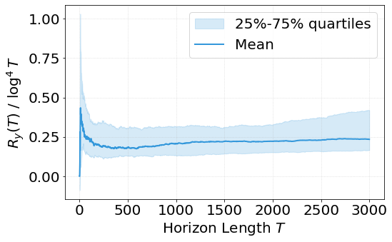
Summary of our main results. In Section 3, we characterize properties of the cost functions $f_{t}(\cdot)$ in both the output and state estimation problems, which will be useful throughout. In Section 4, we propose to use an online gradient descent algorithm for learning Kalman filtering for output estimation and show that it yields an $\mathcal{O}(\log^{4}T)$ regret via the conditionally strong convexity of the cost function. In Section 5.1, we first characterize a fundamental limitation of learning Kalman filtering for state estimation, proving that for any online algorithm given only access to system outputs $y_{0},y_{1},\dots$ , the algorithm inevitably incurs an $\Omega(T)$ regret. In Section 5.2, we consider a scenario where the online algorithm has limited queries to more informative measurements of the system state (besides the original system output history), and propose a novel variant of online gradient descent algorithm based on random queries that achieves an $\tilde{\mathcal{O}}(\tau+\sqrt{T})$ regret for learning Kalman filtering for state estimation, where $\tau$ is the number of queries for informative measurements.

3 Cost Functions of the State and Output Estimation Problems

In this section, we elaborate on the expression of the cost functions in the state and output estimation problems. We begin with the following definitions.

Definition 3.1.

(Strongly-convexity) A differentiable function $f:\mathcal{X}\to\mathbb{R}$ is $\mu$ -strongly convex with $\mu>0$ if

f(y)-f(x)\geq\langle y-x,\nabla f(x)\rangle+\frac{\mu}{2}\left\|y-x\right\|^{2},\forall x,y\in\mathcal{X}.

Definition 3.2.

(Smoothness) A differentiable function $f:\mathcal{X}\to\mathbb{R}$ is $\beta$ -smooth with $\beta>0$ if

\left\|\nabla f(y)-\nabla f(x)\right\|\leq\beta\left\|y-x\right\|,\ \forall x,y\in\mathcal{X}.

Definition 3.3.

(Lipschitzness) A function $f:\mathcal{X}\to\mathbb{R}$ is $l$ -Lipschitz continuous with $l>0$ if

|f(y)-f(x)|\leq l\left\|y-x\right\|,\ \forall x,y\in\mathcal{X}.

Some useful facts are summarized below. For a twice differentiable function $f:\mathcal{X}\to\mathbb{R}$ with $\mathcal{X}\subseteq\mathbb{R}^{d}$ , it is well-known that $\mu$ -strongly convex (resp., $\beta$ -smooth) as per Definition 3.1 (resp., Definition 3.2) is equivalent to $\nabla^{2}f(x)\succeq\mu I_{d}$ (resp., $\nabla^{2}f(x)\preceq\beta I_{d}$ ) for all $x\in\mathcal{X}$ (see, e.g. [7, Chapter 3]), where we also note that $\nabla^{2}f(x)\preceq\left\|\nabla^{2}f(x)\right\|I_{d}$ . Moreover, a direct consequence of $\beta$ -smoothness is that $f(y)-f(x)\leq\nabla f(x)^{\top}(y-x)+\frac{\beta}{2}\left\|y-x\right\|^{2}$ [7, Chapter 3]. For a differentiable function $f:\mathcal{X}\to\mathbb{R}$ , the condition $\left\|\nabla f(x)\right\|\leq l$ for all $x\in\mathcal{X}$ implies that $f(\cdot)$ is $l$ -Lipschitz [7, Chapter 3].

We will make the following assumption, which can also be found in existing work for learning in partially observed LTI systems [38, 44, 47, 64].

Assumption 3.1.

The system matrix $A$ satisfies that $\rho(A)<1$ , i.e., there exist $\kappa_{A}\in\mathbb{R}_{\geq 1}$ and $\gamma_{A}\in\mathbb{R}$ with $\rho(A)<\gamma_{A}<1$ such that $\left\|A^{k}\right\|\leq\kappa_{A}\gamma_{A}^{k}$ for all $k\in\mathbb{Z}_{\geq 0}$ .

Note that the existence of $\kappa_{A}$ and $\gamma_{A}$ in Assumption 3.1 follows from the Gelfand formula [30, Chapter 5].

Cost function of the state estimation problem. Recall that in the problem of learning Kalman filtering for state estimation, the cost function is given by $f_{t}(M)=\left\|x_{t}-\hat{x}_{t}(M)\right\|^{2}$ with $\hat{x}_{t}(M)=\sum_{s=1}^{h}M_{s}y_{t-s}$ and $M=[M_{s}]_{s\in[h]}$ . Note that we may write

	$\displaystyle\hat{x}_{t}(M)=\sum_{s=1}^{h}M_{s}y_{t-s}$	$\displaystyle=[M_{s}]_{s\in[h]}[y_{t-s}^{\top}]_{s\in[h]}^{\top}$
		$\displaystyle=\big(I_{p}\otimes[y_{t-s}^{\top}]_{s\in[h]}\big)\cdot\bm{vec}(M),$

where $\bm{vec}(M)\in\mathbb{R}^{nph}$ concatenates the rows of $M$ into a (column) vector. Further denoting

Y_{t-1:t-h}\triangleq I_{p}\otimes[y_{t-s}^{\top}]_{s\in[h]},

(22)

for a given $M\in\mathbb{R}^{n\times(ph)}$ , we can compactly write

\displaystyle f_{t}(\bm{vec}(M))=(Y_{t-1:t-h}\bm{vec}(M)-x_{t})^{\top}(Y_{t-1:t-h}\bm{vec}(M)-x_{t}),

which yields

	$\displaystyle\nabla f_{t}(\bm{vec}(M))=2Y_{t-1:t-h}^{\top}(Y_{t-1:t-h}\bm{vec}(M)-x_{t}),$		(23)
	$\displaystyle\nabla^{2}f_{t}(\bm{vec}(M))=2Y_{t-1:t-h}^{\top}Y_{t-1:t-h}.$		(24)

To proceed, we introduce the following probabilistic events regarding the noise $w_{t},v_{t}$ in system (1):

\begin{split}&\mathcal{E}_{w}=\Big\{\max_{0\leq t\leq T-1}\left\|w_{t}\right\|\leq\sqrt{5\operatorname{\mathrm{tr}}(W)\log\frac{3T}{\delta}}\Big\},\\ &\mathcal{E}_{v}=\Big\{\max_{0\leq t\leq T-1}\left\|v_{t}\right\|\leq\sqrt{5\operatorname{\mathrm{tr}}(V)\log\frac{3T}{\delta}}\Big\},\end{split}

(25)

where $\delta\in(0,1)$ . It can be shown that the above events hold with high probability; the proof of Lemma 3.1 is given in Appendix B.

Lemma 3.1.

For any $T\geq 1$ , $\mathbb{P}(\mathcal{E}_{w})\geq 1-\delta/3$ , $\mathbb{P}(\mathcal{E}_{v})\geq 1-\delta/3$ and $\mathbb{P}(\mathcal{E}_{w}\cap\mathcal{E}_{v})\geq 1-(2\delta)/3$ .

For notational simplicity in the sequel, let us denote

\begin{split}&R_{x}\triangleq\sqrt{5\operatorname{\mathrm{tr}}(W)\log\frac{3T}{\delta}}\cdot\frac{\kappa_{A}}{1-\gamma_{A}},\\ &R_{y}\triangleq\left\|C\right\|\sqrt{5\operatorname{\mathrm{tr}}(W)\log\frac{3T}{\delta}}\cdot\frac{\kappa_{A}}{1-\gamma_{A}}+\sqrt{5\operatorname{\mathrm{tr}}(V)\log\frac{3T}{\delta}}.\end{split}

(26)

Under the event $\mathcal{E}_{w}\cap\mathcal{E}_{v}$ , we first provide the following bound on the norm of the state $x_{t}$ and output $y_{t}$ of system (1); the proof can be found in Appendix B.

Lemma 3.2.

Under the event $\mathcal{E}_{w}\cap\mathcal{E}_{v}$ and for any $t\in\{0,\dots,T-1\}$ , it holds that $\left\|x_{t}\right\|\leq R_{x}$ , $\left\|y_{t}\right\|\leq R_{y}$ , and $\left\|Y_{t-1:t-h}\right\|\leq\sqrt{h}R_{y}$ .

We then obtain the following properties for the cost function $f_{t}(\cdot)$ in the state estimation problem; the proof can be found in Appendix B.

Lemma 3.3.

For any $M\in\mathcal{K}_{M}$ with $\mathcal{K}_{M}$ defined in (15), $\left\|\bm{vec}(M)\right\|\leq\sqrt{\min\{p,n\}}\frac{\kappa_{F}^{2}}{1-\gamma_{F}}$ . Moreover, under the event $\mathcal{E}_{w}\cap\mathcal{E}_{v}$ , for any $t\in\{0,\dots,T-1\}$ and any $M\in\mathcal{K}_{M}$ ,

	$\displaystyle\left\\|\nabla f_{t}(\bm{vec}(M))\right\\|\leq 2\sqrt{h}R_{y}(\sqrt{\min\{p,n\}}\kappa_{F}^{2}\frac{\sqrt{h}R_{y}}{1-\gamma_{F}}+R_{x}),$		(27)
	$\displaystyle\left\\|\nabla^{2}f_{t}(\bm{vec}(M))\right\\|\leq 2hR_{y}^{2},$		(28)
	$\displaystyle f_{t}(M)\leq 2R_{x}^{2}+2hR_{y}^{2}\min\{p,n\}\kappa_{F}^{4}\frac{1}{(1-\gamma_{F})^{2}}.$		(29)

As we discussed before, the upper bounds in Lemma 3.3 imply that $f_{t}(\cdot)$ is Lipschitz and smooth.

Cost function of output estimation. Recall that in the problem of learning Kalman filtering for output estimation, the cost function is given by $f_{t}(N)=\left\|y_{t}-\hat{y}_{t}(N)\right\|^{2}$ with $\hat{y}_{t}(N)=\sum_{s=1}^{h}N_{s}y_{t-s}$ and $N=[N_{s}]_{s\in[h]}$ . Similarly to the state estimation problem, we have the following results for the cost function $f_{t}(\cdot)$ in the output estimation problem; the proof is similar to that of Lemma 3.4 and is thus omitted for conciseness.

Lemma 3.4.

For any $N\in\mathcal{K}_{N}$ with $\mathcal{K}_{N}$ defined in (19), $\left\|\bm{vec}(N)\right\|\leq\sqrt{p}\psi\frac{\kappa_{F}^{2}}{1-\gamma_{F}}$ and

	$\displaystyle f_{t}(\bm{vec}(N))=(Y_{t-1:t-h}\bm{vec}(N)-y_{t})^{\top}(Y_{t-1:t-h}\bm{vec}(N)-y_{t}),$
	$\displaystyle\nabla f_{t}(\bm{vec}(N))=2Y_{t-1:t-h}^{\top}(Y_{t-1:t-h}\bm{vec}(N)-y_{t}),$
	$\displaystyle\nabla^{2}f_{t}(\bm{vec}(N))=2Y_{t-1:t-h}^{\top}Y_{t-1:t-h}.$

Moreover, under the event $\mathcal{E}_{w}\cap\mathcal{E}_{v}$ , for any $t\in\{0,\dots,T-1\}$ and any $N\in\mathcal{K}_{N}$ ,

	$\displaystyle\left\\|\nabla f_{t}(\bm{vec}(N))\right\\|\leq 2\sqrt{h}R_{y}(\sqrt{p}\kappa_{F}^{2}\psi\frac{\sqrt{h}R_{y}}{1-\gamma_{F}}+R_{y}),$
	$\displaystyle\left\\|\nabla^{2}f_{t}(\bm{vec}(N))\right\\|\leq 2hR_{y}^{2},$
	$\displaystyle f_{t}(N)\leq 2R_{y}^{2}+2hR_{y}^{2}p\kappa_{F}^{4}\psi^{2}\frac{1}{(1-\gamma_{F})^{2}}.$

4 Learning Kalman Filtering for Output Estimation

In this section, we study the output estimation problem, which corresponds to the full information setting in the online optimization framework as we discussed in Section 2.2. Recall that the cost of the output estimation problem is given by $f_{t}(N_{t})=\left\|y_{t}-\hat{y}_{t}(N_{t})\right\|^{2}$ with $\hat{y}_{t}(N_{t})=\sum_{s=1}^{h}N_{t,s}y_{t-s}$ , where the filter parameter $N_{t}=[N_{t,s}]_{s\in[h]}$ is chosen from the set $\mathcal{K}_{N}$ defined in (19).

Input: Step sizes

\{\eta_{t}\}_{t\geq 0}

, truncated filter length

h

1 Initialize

N_{0}=0

2 for $t=0,1,\dots$ do

3 Estimate

\hat{y}_{t}(N_{t})=\sum_{s=1}^{h}N_{t,s}y_{t-s}

4 Obtain

f_{t}(N_{t})=\left\|y_{t}-\hat{y}_{t}(N_{t})\right\|^{2}

5 Update

N_{t+1}=\Pi_{\mathcal{K}_{N}}(N_{t}-\eta_{t}\nabla f_{t}(N_{t}))

Output:

N_{0},N_{1},\dots

Algorithm 1 Online learning for output estimation

4.1 Online Learning Algorithm

We propose using the online learning algorithm (Algorithm 1), which employs the Online Gradient Descent (OGD) method. Specifically, in line 5 of the algorithm, $\Pi_{\mathcal{K}_{N}}(\cdot)$ denotes the projection of a matrix $N\in\mathbb{R}^{p\times(ph)}$ onto the set $\mathcal{K}_{N}$ defined in (19). Noting that $\left\|N\right\|_{F}=\left\|\bm{vec}(N)\right\|$ for any $N\in\mathbb{R}^{p\times(ph)}$ , the projection of $N\in\mathbb{R}^{p\times(ph)}$ onto the set $\mathcal{K}_{N}$ is equivalent to the projection of $\bm{vec}(N)$ onto the $p^{2}h$ -dimensional ball with radius $\sqrt{p}\psi\frac{\kappa_{F}^{2}}{1-\gamma_{F}}$ centered around the origin. Therefore, we see that the projection $\Pi_{\mathcal{K}_{N}}(\cdot)$ in line 5 of Algorithm 1 can be computed as $\Pi_{\mathcal{K}_{N}}(N)=\sqrt{p}\psi\frac{\kappa_{F}^{2}}{1-\gamma_{F}}N/\left\|N\right\|_{F}$ for all $N\in\mathbb{R}^{p\times(ph)}$ .

We now characterize the regret ${\tt R_{y}}(T)$ defined in (20) of Algorithm 1 when applied to solve the problem of learning Kalman filtering for output estimation.

Theorem 4.1.

Let the step sizes be $\eta_{t}=\frac{2}{(\alpha_{0}\log^{2}T)t}$ for all $t\geq 1$ and $\eta_{0}=0$ . Let the length $h$ of the truncated filter $\hat{y}_{t}^{\tt TK}$ given by (17) be $h=\lfloor\log T/\log(1/\gamma_{F})\rfloor$ , where $\gamma_{F}$ is defined in (14). Then, for any $T>1$ and any $\delta\in(0,1)$ , it holds that ${\tt R}_{y}(T)=\mathcal{O}(\log^{4}T)$ , where $\mathcal{O}(\cdot)$ hides polynomial factors in $\log\frac{1}{\delta}$ and problem parameters $p,n,\bar{\sigma},\alpha_{0}^{-1},\alpha_{1},\psi,\frac{\kappa_{A}}{1-\kappa_{A}},\frac{1}{\log(2\bar{\sigma}/(2\bar{\sigma}-\alpha_{0}))}$ .³³3Exact expression of ${\tt R}_{y}(T)$ can be found in the proof of Theorem 4.1.

Challenges in the regret analysis. For the full information setting in online optimization, it has been shown in the literature that for strongly convex cost functions $f_{0}(\cdot),\dots,f_{T-1}(\cdot)$ with $f_{t}:\mathbb{R}^{d}\to\mathbb{R}$ such that $\nabla^{2}f_{t}(N)\succeq\mu I_{d}$ for some $\mu>0$ , the OGD algorithm achieves $\log T$ -regret (e.g., [23]). However, since the output $y_{t}$ of system (1) is random (due to the noise terms $w_{t}$ and $v_{t}$ ), the objective function $f_{t}(N)=\left\|y_{t}-\hat{y}_{t}(N_{t})\right\|^{2}$ is also random given any $N\in\mathcal{K}_{N}$ , which implies that $\nabla^{2}f_{t}(N)\succ 0$ may no longer hold deterministically for any $t$ . Thus, the existing results of OGD for strongly convex functions cannot be applied to our problem. In fact, using only the convexity of $f_{t}(\cdot)$ (that holds deterministically for all $t\geq 0$ ), it was shown in [36] that OGD achieves an $\tilde{\mathcal{O}}(\sqrt{T})$ regret for learning Kalman filtering for output estimation (of scalar linear dynamical system), where $\tilde{\mathcal{O}}(\cdot)$ hides factors in $\log T$ .

Prior knowledge required by Algorithm 1. As mentioned in (13), we assume known constants $\alpha_{0},\psi,\bar{\sigma}$ (i.e., upper bounds on system-related matrices) so that the projection $\Pi_{\mathcal{K}_{N}}(\cdot)$ in line 5 of the algorithm can be implemented. Meanwhile, recalling from (14) that $\gamma_{F}=\sqrt{\bar{\sigma}{\alpha_{0}}}$ , setting the step sizes $\eta_{t}$ for all $t\geq 1$ and truncated filter length $h$ as Theorem 4.1 require $\alpha_{0},\bar{\sigma}$ and the knowledge of the horizon length $T$ . In Appendix C, we argue that using a doubling trick that has been widely used for online algorithms (see, e.g., [39]), one can remove the dependency of $\eta_{t}$ and $h$ on $T$ and achieve the same $\mathcal{O}(\log^{4}T)$ regret as Theorem 4.1 without the knowledge of $T$ . Finally, we note that assuming known constants such as $\alpha_{0},\psi,\bar{\sigma}$ described above is typical in learning to estimate or control of unknown LTI systems [46, 9, 8].

Comparisons to existing work. Compared to the existing work on learning the Kalman filter for output estimation [19, 46, 56, 45] based on least squares methods, our approach has the following advantages: 1) our algorithm design based on OGD method is conceptually simpler, and our regret analysis is also more constructive, achieving comparable regret bounds (e.g., $\mathcal{O}(\log^{4}T)$ in [56] and $\mathcal{O}(\log^{3}T)$ in [45]); 2) we do not require a warm-up period in our algorithm (i.e., the regret holds for any $T>1$ ) or the regularity assumption that the matrix $A-LC$ in the steady-state Kalman filter (see (11)) is diagonalizable [56, 46, 45]; 3) our regret holds against the more general finite-step Kalman filter benchmark (see (20)) as apposed to the steady-state Kalman filter benchmark considered in [19, 46, 56, 45]. While the regret bounds in [19, 46, 56, 45] also hold for open-loop marginally stable system, we argue later in Section 6 that our regret analysis can be extended to handle open-loop unstable system that can be stabilized with closed-loop input. Finally, we stress that the main merit of our algorithmic framework is its ability to handle the state estimation problem that will be studied in Section 5.

4.2 Proof of Theorem 4.1

Notations used in this proof. For notational simplicity in this proof, we assume that any filter parameter $N\in\mathbb{R}^{p\times(ph)}$ has been readily written in its vectorized form $\bm{vec}(N)\in\mathbb{R}^{p^{2}h}$ so that we simply denote $N$ . We also reload the notations and use $\Pi_{\mathcal{K}_{N}}(N)$ to represent the projection of a vector $N\in\mathbb{R}^{p^{2}h}$ onto $\mathcal{K}_{N}=\{N\in\mathbb{R}^{p^{2}h}:\left\|N\right\|\leq\sqrt{p}\psi\frac{\kappa_{F}^{2}}{1-\gamma_{F}}\}$ , i.e., $\Pi_{\mathcal{K}_{N}}(N)=\operatorname*{arg\,min}_{N^{\prime}\in\mathcal{K}_{N}}\left\|N^{\prime}-N\right\|$ . The following notations will also be used in this proof:

\begin{split}&R_{N}\triangleq\sqrt{p}\psi\frac{\kappa_{F}^{2}}{1-\gamma_{F}},\ \beta_{y}\triangleq 2hR_{y}^{2},\\ &l_{y}\triangleq 2\sqrt{h}R_{y}^{2}(\sqrt{p}\psi\kappa_{F}^{2}\frac{\sqrt{h}}{1-\gamma_{F}}+1),\end{split}

(30)

where $R_{y}$ is defined in (26).

In the following, we provide the main steps in the proof and the omitted details are included in Appendix C. We begin by introducing an auxiliary function based on conditional expectation, which will be used throughout this proof.

Definition 4.1.

Let $\{\mathcal{F}_{t}\}_{t\geq 0}$ be a filtration with $\mathcal{F}_{t}\triangleq\sigma(w_{0},\dots,w_{t-1},v_{0},\dots,v_{t-1})$ for $t\geq 1$ and $\mathcal{F}_{0}\triangleq\emptyset$ . For any $N\in\mathbb{R}^{p^{2}h}$ and some $h\in\mathbb{Z}_{\geq 0}$ , define $f_{t;h}(N)=\mathbb{E}[f_{t}(N)|\mathcal{F}_{t-h}]$ for all $t\geq h$ , where the expectation $\mathbb{E}[\cdot]$ is taken with respect to $\{w_{t}\}_{t\geq 0}$ and $\{v_{t}\}_{t\geq 0}$ .

We show that the function $f_{t;h}(\cdot)$ defined above has the following properties.

Lemma 4.1.

For any $t\geq h$ , $f_{t;h}(\cdot)$ is $\alpha_{0}$ -strongly convex. In addition, under the event $\mathcal{E}_{w}\cap\mathcal{E}_{v}$ defined in (25), $f_{t;h}(\cdot)$ is $l_{y}$ -Lipschitz.

Regret decomposition. We decompose the regret ${\tt R}_{y}(T)$ in (20) as

	$\displaystyle{\tt R}_{y}(T)$	$\displaystyle=\sum_{t=0}^{T-1}f_{t}(N_{t})-\sum_{t=0}^{T-1}\left\\|y_{t}-\hat{y}_{t}^{\tt KF}\right\\|^{2}$
		$\displaystyle=\underbrace{\sum_{t=0}^{T-1}\big(f_{t}(N_{t})-f_{t}(N^{\star})\big)}_{\text{online optimization regret}}+\underbrace{\sum_{t=0}^{T-1}\big(f_{t}(N^{\star})-\left\\|y_{t}-\hat{y}_{t}^{\tt KF}\right\\|^{2}\big)}_{\text{truncation \& steady-state regret}},$		(31)

where $f_{t}(N^{\star})=\left\|y_{t}-\hat{y}_{t}^{\tt TK}\right\|^{2}$ and the comparator point $N^{\star}=[N_{s}^{\star}]_{s\in[h]}$ with $N_{s}^{\star}$ defined in (18). In the sequel, we separately analyze the two regret terms in (31) that correspond to the regret incurred by the gradient-based update in Algorithm 1 and the regret incurred by the truncated Kalman filter considered in (17).

Online optimization regret. We first prove the following intermediate result, leveraging the strong convexity of $f_{t;h}(\cdot)$ shown in Lemma 4.1.

Lemma 4.2.

For any $t\geq h$ , let $\varepsilon_{t}^{s}=\nabla f_{t}(N_{t})-\nabla f_{t;h}(N_{t})$ . It holds that

\sum_{t=h}^{T-1}\big(f_{t;h}(N_{t})-f_{t;h}(N^{\star})\big)\leq-\frac{\alpha_{0}\log^{2}T}{4}\sum_{t=h}^{T-1}\left\|N_{t}-N^{\star}\right\|^{2}+\frac{R_{N}\alpha_{0}h\log^{2}T}{2}\\ +\sum_{t=h}^{T-1}\frac{\eta_{t}}{2}\left\|\nabla f_{t}(N_{t})\right\|^{2}-\sum_{t=h}^{T-1}\langle\varepsilon_{t}^{s},N_{t}-N^{\star}\rangle.

Next, we relate $f_{t;h}(\cdot)$ to $f_{t}(\cdot)$ and transform the upper bound in Lemma 4.2 to an upper bound based on $f_{t}(\cdot)$ .

Lemma 4.3.

Under the event $\mathcal{E}_{w}\cap\mathcal{E}_{v}$ , it holds that

\sum_{t=h}^{T-1}\big(f_{t}(N_{t})-f_{t}(N^{\star})\big)\leq-\frac{\alpha_{0}\log^{2}T}{4}\sum_{t=h}^{T-1}\left\|N_{t}-N^{\star}\right\|^{2}+\frac{R_{N}^{2}\alpha_{0}h\log^{2}T}{2}\\ +\sum_{t=h}^{T-1}\frac{\eta_{t}}{2}\left\|\nabla f_{t}(N_{t})\right\|+\frac{8l_{y}h}{\alpha_{0}\log^{2}T}(l_{y}+R_{N}\beta_{y})(1+\log T)+\sum_{t=h}^{T-1}X_{t}(N^{\star}),

where $X_{t}(N^{\star})\triangleq\langle\nabla(f_{t}-f_{t;h})(N_{t-h}),N_{t-h}-N^{\star}\rangle+(f_{t}-f_{t;h})(N_{t-h})+(f_{t;h}-f_{t})(N^{\star})$ . Also, it holds that $\mathbb{E}[X_{t}(N^{\star})|\mathcal{F}_{t-h}]=0$ for all $t\geq h$ .

To proceed, we provide a high probability upper bound on the summation of the stochastic terms $X_{k}(N^{\star}),\dots,X_{T-1}(N^{\star})$ .

Lemma 4.4.

Suppose the event $\mathcal{E}_{w}\cap\mathcal{E}_{v}$ holds. Then, for any $\delta\in(0,1)$ , the following holds with probability at least $1-\delta/3$ :

\displaystyle\sum_{t=h}^{T-1}X_{t}(N^{\star})\leq\frac{32l_{y}^{2}h\log\frac{3h}{\delta}}{\alpha_{0}\log^{2}T}+\frac{\alpha_{0}\log^{2}T}{4}\sum_{t=0}^{T-1}\left\|N_{t}-N^{\star}\right\|^{2}.

Finally, combining Lemmas 4.3-4.4, we see that under the event $\mathcal{E}_{w}\cap\mathcal{E}_{v}$ , the following holds with probability at least $1-\delta/3$ :

	$\displaystyle\sum_{t=0}^{T-1}\big(f_{t}(N_{t})-f_{t}(N^{\star})\big)$
$\displaystyle\leq$	$\displaystyle\sum_{t=0}^{h-1}\big(f_{t}(N_{t})-f_{t}(N^{\star})\big)+\frac{\alpha_{0}\log^{2}T}{4}\sum_{t=0}^{h-1}\left\\|N_{t}-N^{\star}\right\\|^{2}+\frac{R_{N}^{2}\alpha_{0}h\log^{2}T}{2}$
	$\displaystyle\qquad+\sum_{t=h}^{T-1}\frac{\eta_{t}}{2}\left\\|\nabla f_{t}(N_{t})\right\\|^{2}+\frac{8l_{y}h}{\alpha_{0}}(l_{y}+R_{N}\beta_{y})(1+\log T)+\frac{32l_{y}^{2}h\log\frac{3h}{\delta}}{\alpha_{0}}$
$\displaystyle\overset{(a)}{\leq}$	$\displaystyle\frac{3R_{N}^{2}\alpha_{0}h}{2}\log^{2}T+4(R_{y}^{2}+hR_{y}^{2}R_{N}^{2})h+\frac{l_{y}^{2}}{\alpha_{0}\log^{2}T}(1+\log T)$
	$\displaystyle\qquad\qquad\qquad\qquad+\frac{8l_{y}h}{\alpha_{0}\log^{2}T}(l_{y}+R_{N}\beta_{y})(1+\log T)+\frac{32l_{y}^{2}h\log\frac{3h}{\delta}}{\alpha_{0}}$
$\displaystyle\overset{(b)}{=}$	$\displaystyle\mathcal{O}(\log^{4}T),$	(32)

To obtain $(a)$ , we use the upper bound $\left\|N\right\|\leq R_{N}$ for any $N\in\mathcal{K}_{N}$ shown by Lemma 3.4, the upper bound on $f_{t}(N)$ for any $N\in\mathcal{K}_{N}$ given by Lemma 3.4, and the following derivation:

	$\displaystyle\sum_{t=h}^{T-1}\frac{\eta_{t}}{2}\left\\|\nabla f_{t}(N_{t})\right\\|^{2}$	$\displaystyle\leq l_{y}^{2}\sum_{t=h}^{T-1}\frac{1}{(\alpha_{0}\log^{2}T)t}$
		$\displaystyle\leq\frac{l_{y}^{2}}{\alpha_{0}\log^{2}T}(1+\log T),$

where we use the upper bound $\left\|f_{t}(N_{t})\right\|\leq l_{y}$ from Lemma 3.4 and the choice of the step size $\eta_{t}=\frac{2}{(\alpha_{0}\log^{2}T)t}$ for all $t\geq 1$ . To obtain $(b)$ , we first recall the expressions of $\kappa_{F},\gamma_{F}$ in (13) and the choice of $h=\mathcal{O}(\log T)$ , and then deduce from (26) and (30) that $R_{y}=\mathcal{O}(\sqrt{\log T})$ , $\beta_{y}=\mathcal{O}(\log^{2}T)$ , $l_{y}=\mathcal{O}(\log^{2}T)$ and $R_{N}=\mathcal{O}(1)$ , where $\mathcal{O}(\cdot)$ hides the factors stated in Theorem 4.1.

Truncation and steady-state regret. To upper bound the truncation and steady-state regret in (31), we first recall from our discussions in Section 2.1 that $\hat{y}_{t}^{\tt TK}$ in (17) is a truncated steady-state version of the original Kalman filter $\hat{y}_{t}^{\tt KF}=C\hat{x}_{t}^{\tt KF}$ with $\hat{x}_{t}^{\tt KF}$ given by (2). Therefore, the truncation and steady-state regret in (31) consists of two components corresponding to the truncation and the consideration of the steady-state of the Kalman filter. We have

\sum_{t=0}^{T-1}\big(f_{t}(N^{\star})-\left\|y_{t}-\hat{y}_{t}^{\tt KF}\right\|^{2}\big)=\underbrace{\sum_{t=0}^{T-1}\big(\left\|y_{t}-\hat{y}_{t}^{\tt TK}\right\|^{2}-\left\|y_{t}-\hat{y}_{t}^{\tt SK}\right\|^{2}\big)}_{(i)}+\underbrace{\sum_{t=0}^{T-1}\big(\left\|y_{t}-\hat{y}_{t}^{\tt SK}\right\|^{2}-\left\|y_{t}-\hat{y}_{t}^{\tt KF}\right\|^{2}\big)}_{(ii)},

(33)

where $\hat{y}_{t}^{\tt TK}$ and $\hat{y}_{t}^{\tt SK}$ are defined in (16) and (17), respectively. We now prove the following results.

Lemma 4.5.

Under the event $\mathcal{E}_{w}\cap\mathcal{E}_{v}$ , it holds that

\displaystyle\sum_{t=0}^{T-1}\big(\left\|y_{t}-\hat{y}_{t}^{\tt TK}\right\|^{2}-\left\|y_{t}-\hat{y}_{t}^{\tt SK}\right\|^{2}\big)\leq\Big(2+\sqrt{h}R_{N}+\left\|L\right\|\left\|C\right\|\frac{\kappa_{F}}{1-\gamma_{F}}\Big)\frac{R_{y}^{2}\kappa_{F}\left\|L\right\|\left\|C\right\|}{1-\gamma_{F}}.

(34)

Lemma 4.6.

Under the event $\mathcal{E}_{w}\cap\mathcal{E}_{v}$ , it holds that

\displaystyle\sum_{t=0}^{T-1}\big(\left\|y_{t}-\hat{y}_{t}^{\tt SK}\right\|^{2}-\left\|y_{t}-\hat{y}_{t}^{\tt KF}\right\|^{2}\big)=\mathcal{O}(\log^{4}T).

(35)

Overall regret upper bound. Since $\mathbb{P}(\mathcal{E}_{w}\cap\mathcal{E}_{v})\geq 1-(2\delta)/3$ from Lemma 3.1 and the upper bound in (32) holds with probability at least $1-\delta/3$ , we can obtain the overall regret upper bound $\mathcal{O}(\log^{4}T)$ in Theorem 4.1 by combining (32) and (34)-(35) via a union bound, where we also recall the bounds $\left\|C\right\|\leq\psi$ from (13) and $\left\|L\right\|\leq\kappa_{F}$ from Lemma E.4.

5 Learning Kalman Filtering for State Estimation

In this section, we turn our attention to the state estimation problem, which is more challenging as we discussed in Section 2.2. Recall that the cost function of the state estimation problem is given by $f_{t}(M_{t})=\left\|x_{t}-\hat{x}_{t}(M_{t})\right\|^{2}$ with $\hat{x}_{t}(M_{t})=\sum_{s=1}^{h}M_{t,s}y_{t-s}$ , where the filter parameter $M_{t}=[M_{t,s}]_{s\in[h]}$ is chosen from the set $\mathcal{K}_{M}$ defined in (15).

5.1 Lower Bound Results

We first characterize the fundamental limitations of any algorithm for the problem of learning Kalman filtering for state estimation; the proof of Theorem 5.1 is included in Appendix D.

Theorem 5.1.

Consider any (potentially randomized) algorithm for learning the Kalman filter for state estimation that only has access to the outputs $y_{0},\dots,y_{t-1}$ when designing the state estimate $\hat{x}_{t}$ for each time step $t\geq 0$ . Let $\sigma_{w}\in\mathbb{R}_{>0}$ . Then, for any $T\geq 2$ , there exists a scalar and stable LTI system such that ${\tt R_{x}}(T)$ defined in (21) satisfies

\displaystyle\mathbb{E}\big[{\tt R_{x}}(T)\big]\geq 6T\sigma_{w}-\frac{56+50\sigma_{w}}{1875\sigma_{w}},

(36)

where $\mathbb{E}[\cdot]$ is taken with respect to the potential randomness of the algorithm and $\{w_{t}\}_{t\geq 0},\{v_{t}\}_{t\geq 0}$ . Additionally, consider any algorithm that returns $\hat{x}_{t}$ with $\left\|\hat{x}_{t}\right\|\leq c_{\mathcal{A}}$ for all $t\geq 0$ almost surely. Then, for any $T\geq 3$ and any $\delta\in(0,1)$ , it holds with probability at least $1-\delta$ that

\displaystyle{\tt R_{x}}(T)\geq 6T\sigma_{w}-\frac{56+50\sigma_{w}}{1875\sigma_{w}}-{\mathcal{O}}\left(\sqrt{T(c_{\mathcal{A}}+\log^{1.5}T)\log\frac{3}{\delta}}\right).

(37)

Proof idea. The proof hinges on the fact that for partially observed systems, there can be multiple systems with different system matrices $A,C$ that yield the same output history $y_{0},y_{1},\dots$ (given the same realization of the noise sequences $\{w_{t}\}_{t\geq 0}$ and $\{v_{t}\}_{t\geq 0}$ ). Hence, any algorithm (given only access to $y_{0},y_{1},\dots$ ) cannot perform well simultaneously on all such systems, i.e., any algorithm must incur large regret for at least one of such systems.

Theorem 5.1 demonstrates that any algorithm for the problem of learning Kalman filtering for state estimation has to incur a regret at least $\Omega(T)$ , and the lower bound $\Omega(T)$ holds for both expected regret and high probability regret. Thus, we know from Theorem 5.1 that the problem of learning Kalman filtering for state estimation is provably more difficult than the problem of learning output estimation studied in Section 4 and also the problem of learning LQR (with unknown system model). In particular, for the latter problem, it has been shown that an $\tilde{\mathcal{O}}(\sqrt{T})$ regret is achievable [42], matching the $\Omega(\sqrt{T})$ regret lower [50].

5.2 Online Learning Algorithm with Informative Measurements

From the fundamental limitation results given by Theorem 5.1, one cannot hope for sublinear regret in $T$ for the state estimation problem if the online learning algorithm only has access to the outputs $y_{0},y_{1},\dots$ . One natural idea is then to consider that the algorithm has access to limited yet more informative measurements from system (1). In particular, we assume that at certain time steps $t\geq 0$ , the following measurements can potentially be made available to the learner:

\displaystyle\tilde{x}_{t}=x_{t}+\tilde{v}_{t},

(38)

where the measurement noise satisfies that $\tilde{v}_{t}\overset{i.i.d.}{\sim}\mathcal{N}(0,\tilde{V})$ with $\tilde{V}\succeq 0$ and $\{\tilde{v}_{t}\}_{t\geq 0}$ is assumed to be independent of $\{w_{t}\}_{t\geq 0}$ and $\{v_{t}\}_{t\geq 0}$ in system (1). For example, the measurement $\tilde{x}_{t}$ may come from a sensor on system (1) with measurement matrix $C=I_{n}$ or a sensor with a known and full column rank measurement matrix $C\in\mathbb{R}^{p\times n}$ . While being more informative, it can be costly to use such a sensor to collect measurements from system (1). This motivates us to consider the scenario where the learner may only query for the measurements $\tilde{x}_{t}$ at a limited number of time steps, as will be detailed in our algorithm design next. Finally, we note that the measurement model in (38) has been widely adopted in the literature on learning for unknown linear systems [53, 35, 43, 69].

Input: Step sizes

\{\eta_{j}\}_{j\geq 0}

, truncated filter length

h

, parameter

\tau\in\mathbb{Z}_{\geq 1}

1 Initialize

M_{0}=0

and

j=0

2for $i=0,1,\dots$ do

3 Sample

b_{i}\overset{i.i.d.}{\sim}{\tt Unif}(\{0,\dots,\tau-1\})

4 for $t=i\tau,\dots,(i+1)\tau-1$ do

5 Compute

\hat{x}_{t}(M_{t})=\sum_{s=1}^{h}M_{t-s}y_{t-s}

6 if $t\mod\tau=b_{i}$ then

7 Query to obtain

\tilde{x}_{t}=x_{t}+\tilde{v}_{t}

8 Compute

\tilde{f}_{t}(M_{t})=\left\|\tilde{x}_{t}-\hat{x}_{t}(M_{t})\right\|^{2}

9 Update

M_{t+1}=\Pi_{\mathcal{K}_{M}}(M_{t}-\eta_{j}\nabla\tilde{f}_{t}(M_{t}))

j\leftarrow j+1

11 else

M_{t+1}=M_{t}

Output:

M_{0},M_{1},\dots

Algorithm 2 Online learning for state estimation

Description of the online learning algorithm. We now introduce Algorithm 2 for learning the Kalman filter for state estimation under the informative measurement setting introduced above. To respect the limited access to informative measurements in (38), we leverage a randomly sampled $b_{i}\overset{i.i.d.}{\sim}{\tt Unif}(\{0,\dots,\tau-1\})$ in line 3 of Algorithm 2, where ${\tt Unif}(\{0,\dots,\tau-1\})$ denotes a uniform distribution over the integers in $\{0,\dots,\tau-1\}$ and $\tau$ is an input parameter to the algorithm. In a time interval of length $\tau$ , Algorithm 2 then queries to obtain $\tilde{x}_{t}$ once when $t\mod\tau=b_{i}$ , and updates the filter parameter $M_{t}$ accordingly (lines 6-10). Otherwise, Algorithm 2 keeps the same filter parameter $M_{t}$ to the next time step $t+1$ (line 12). Note that the update in line 9 of Algorithm 2 can be viewed as a noisy version of the update in line 5 of Algorithm 1, i.e., a noisy gradient $\nabla\tilde{f}_{t}(M_{t})$ is used rather than the true gradient $\nabla f_{t}(M_{t})$ . Finally, note that the for loop from lines 4 to 12 in Algorithm 2 terminates when $t$ reaches $T-1$ ; moreover, for any horizon length $T\geq 1$ , Algorithm 2 queries to obtain the information measurement in (38) for at most $\lfloor T/\tau\rfloor$ time steps.

We now provide upper bounds on the regret ${\tt R_{x}}(T)$ defined in (21) of Algorithm 2.

Theorem 5.2.

Let the step sizes be $\eta_{j}=\frac{2}{\alpha_{0}j}$ for all $j\geq 1$ and $\eta_{0}=0$ . Let the length $h$ of the truncated filter $\hat{x}_{t}^{\tt TK}$ given by (12) be $h=\lfloor\log T/\log(1/\gamma_{F})\rfloor$ and let $\tau\geq h$ , where $\gamma_{F}$ is defined in (14). Then, for any $T>1$ and any $\delta\in(0,1)$ , with probability at least $1-\delta$ , it holds that ${\tt R_{x}}(T)=\mathcal{O}\big(\tau(\log^{4}T)\log(T/\tau)+\sqrt{T}\log^{2}T\big)$ , where $\mathcal{O}(\cdot)$ hides polynomial factors in $\log\frac{1}{\delta}$ and problem parameters $p,n,\bar{\sigma},\alpha_{0}^{-1},\alpha_{1},\psi,\frac{\kappa_{A}}{1-\kappa_{A}},\frac{1}{\log(2\bar{\sigma}/(2\bar{\sigma}-\alpha_{0}))},\operatorname{\mathrm{tr}}(\tilde{V})$ .⁴⁴4Exact expression of ${\tt R_{x}}(T)$ can be found in the proof of Theorem 5.2.

Trade-off between queries and regret. As can be seen from the results in Theorem 5.2, there is a clear trade-off between the value of the input parameter $\tau$ to Algorithm 2 and the overall regret of the algorithm. In particular, we may write ${\tt R_{x}}(T)=\tilde{\mathcal{O}}(\tau+\sqrt{T})$ , where $\tilde{\mathcal{O}}(\cdot)$ further compresses $\log T$ factors. Recalling that $\lfloor T/\tau\rfloor$ is the number of times that Algorithm 2 queries $\tilde{x}_{t}$ , the algorithm achieves a sublinear regret in $T$ provided that $\lfloor T/\tau\rfloor$ is also sublinear in $T$ . A seemly more straightforward way to reduce the queries of $\tilde{x}_{t}$ in Algorithm 2 is to sample $b_{t}\overset{i.i.d.}{\sim}{\tt Bernoulli}(1/\tau)$ and query for $\hat{x}_{t}$ if and only if $b_{t}=1$ . However, such a sampling scheme only guarantees $\lfloor T/\tau\rfloor$ number of queries for $\tilde{x}_{t}$ in expectation. In contrast, our proposed sampling scheme in line 3 of Algorithm 2 ensures that the number of queries is given by $\lfloor T/\tau\rfloor$ deterministically, which facilitates our regret analysis in Theorem 5.2.

The role of random queries. Algorithm 2 invokes the gradient-based update for the filter parameter $M_{t}$ in line 9 using the queried $\tilde{x}_{t}$ , when the value of the random variable $b_{i}$ sampled in line 3 satisfies the condition in line 6. In our proof of Theorem 5.2 below, we crucially leverage this randomness in the gradient-based update to extend the regret over the steps when $M_{t}$ is updated to the steps over the whole time horizon $t=0,\dots,T-1$ , achieving the desired balance between the number of queries of $\tilde{x}_{t}$ and the regret of Algorithm 2. Such a novel random query (or sampling) scheme also sheds light on online learning problems with costly or limited observations (e.g., [24, 20]).

Prior knowledge required by Algorithm 2. Similarly to our arguments for Algorithm 2, to achieve the regret in Theorem 5.2, Algorithm 2 requires the knowledge of $\alpha_{0},\psi,\bar{\sigma}$ given by (13) and the horizon length $T$ . Again, we argue in Appendix D that one can use a doubling trick to achieve the same regret as Theorem 5.2 without the knowledge of $T$ .

5.3 Proof of Theorem 5.2

Notations used in this proof. Similarly to the proof of Theorem 4.1, we assume that any filter parameter $M\in\mathbb{R}^{n\times(ph)}$ has been readily written in its vectorized form $\bm{vec}(M)\in\mathbb{R}^{nph}$ so that we simply denote $M$ . We also use $\Pi_{\mathcal{K}_{M}}(M)$ to denote the projection of a vector $M\in\mathbb{R}^{nph}$ onto the set $\mathcal{K}_{M}=\{M\in\mathbb{R}^{nph}:\left\|M\right\|\leq\sqrt{\min\{p,n\}}\frac{\kappa_{F}^{2}}{1-\gamma_{F}}\}$ . For our analysis in this proof, we also define the following probabilistic event regarding the noise $\{\tilde{v}_{t}\}_{t\geq 0}$ in (38):

\displaystyle\mathcal{E}_{\tilde{v}}=\Big\{\max_{0\leq t\leq T-1}\left\|\tilde{v}_{t}\right\|\leq\sqrt{5\operatorname{\mathrm{tr}}(\tilde{V})\log\frac{12T}{\delta}}\Big\}.

(39)

Using similar arguments to those for Lemma 3.1, one can show that $\mathbb{P}(\mathcal{E}_{\tilde{v}})=1-\delta/12$ . Noting that Algorithm 2 updates the filter parameter $M_{t}$ in line 9 if and only if $t\mod\tau=b_{i}$ with $b_{i}$ sampled in line 3 of the algorithm, we denote the set of time steps $t$ in $\{0,\dots,T-1\}$ such Algorithm 2 updates $M_{t}$ as $S=\{t\geq 0:t\mod\tau=b_{i}\}=\{t_{0},\dots,t_{H-1}\}$ , where $H=|S|$ and we know from the definition of Algorithm 2 that $t_{i}\in\{i\tau,\dots,(i+1)\tau-1\}$ for all $i\in\{0,\dots,H-1\}$ . Additionally, we denote

\displaystyle S^{\prime}=\{t_{j}:j\in[H],t_{j}\geq\tau\}=\{t_{1},\dots,t_{H-1}\}.

(40)

One can check that $|S|=\lfloor T/\tau\rfloor$ and $|S^{\prime}|=\lfloor T/\tau\rfloor-1$ . Finally, the following notations will also be used in this proof:

\begin{split}&R_{M}\triangleq\sqrt{\min\{p,n\}}\kappa_{F}^{2}\frac{1}{1-\gamma_{F}},\ \beta_{x}\triangleq 2hR_{y}^{2},\\ &l_{x}\triangleq 2\sqrt{h}R_{y}(\sqrt{\min\{p,n\}}\kappa_{F}^{2}\frac{\sqrt{h}R_{y}}{1-\gamma_{F}}+R_{x}),\\ &R_{\tilde{v}}\triangleq\sqrt{5\operatorname{\mathrm{tr}}(\tilde{V})\log\frac{12T}{\delta}},\end{split}

(41)

where $R_{x}$ and $R_{y}$ are defined in (26).

In the following, we provide the main steps in the proof and the omitted details are included in Appendix D.

Regret decomposition. Similarly to (31) in the proof of Theorem 4.1, we decompose the regret ${\tt R_{x}}(T)$ in (21) as

	$\displaystyle{\tt R_{x}}(T)$	$\displaystyle=\sum_{t=0}^{T-1}f_{t}(M_{t})-\sum_{t=0}^{T-1}\left\\|x_{t}-\hat{x}_{t}^{\tt KF}\right\\|$
		$\displaystyle=\underbrace{\sum_{t=0}^{T-1}\big(f_{t}(M_{t})-f_{t}(M^{\star})\big)}_{\text{online optimization regret}}+\underbrace{\sum_{t=0}^{T-1}\big(f_{t}(M^{\star})-\left\\|x_{t}-\hat{x}_{t}^{\tt KF}\right\\|^{2}\big)}_{\text{truncation \& steady-state regret}},$		(42)

where $f_{t}(M^{\star})=\left\|x_{t}-\hat{x}_{t}^{\tt TK}\right\|^{2}$ and the comparator point $M^{\star}=[M_{s}^{\star}]_{s\in[h]}$ with $M_{s}^{\star}$ defined in (8).

Online optimization regret. Similarly to Definition 4.1, we introduce the following auxiliary function.

Definition 5.1.

Let $\{\mathcal{F}_{t}\}_{t\geq 0}$ be a filtration with $\mathcal{F}_{t}\triangleq\sigma(w_{0},\dots,w_{t-1},v_{0},\dots,v_{t-1})$ for $t\geq 1$ and $\mathcal{F}_{0}\triangleq\emptyset$ . For any $N\in\mathbb{R}^{nph}$ and some $h\in\mathbb{Z}_{\geq 0}$ , define $f_{t;h}(M)=\mathbb{E}[f_{t}(M)|\mathcal{F}_{t-h}]$ for all $t\geq h$ , where the expectation $\mathbb{E}[\cdot]$ is taken with respect to $\{w_{t}\}_{t\geq 0}$ and $\{v_{t}\}_{t\geq 0}$ .

Lemma 5.1.

For any $t\geq h$ , $f_{t;h}(\cdot)$ is $\alpha_{0}$ -strongly convex. In addition, under the event $\mathcal{E}_{w}\cap\mathcal{E}_{v}$ , $f_{t;h}(\cdot)$ is $l_{x}$ -Lipschitz.

Similarly to Lemma 4.2, we can leverage the $\alpha_{0}$ -strong convexity of $f_{t;h}(\cdot)$ and prove the following result.

Lemma 5.2.

For any $t\geq h$ , let $\varepsilon_{t}^{s}=\nabla f_{t}(M_{t})-\nabla f_{t;h}(M_{t})$ and $\tilde{\varepsilon}_{t}^{s}=\nabla\tilde{f}_{t}(M_{t})-\nabla f_{t}(M_{t})$ . It holds that

	$\displaystyle\sum_{t_{j}\in S^{\prime}}\big(f_{t;h}(M_{t_{j}}-f_{t;h}(M^{\star}))$	$\displaystyle\leq-\frac{\alpha_{0}}{4}\sum_{t_{j}\in S^{\prime}}\left\\|M_{t_{j}}-M^{\star}\right\\|^{2}+\frac{R_{M}^{2}\alpha_{0}}{2}+\sum_{t_{j}\in S^{\prime}}\frac{\eta_{j}}{2}\left\\|\nabla\tilde{f}_{t_{j}}(M_{t_{j}})\right\\|^{2}$
		$\displaystyle\qquad\qquad-\sum_{t_{j}\in S^{\prime}}\langle\varepsilon_{t_{j}}^{s},M_{t_{j}}-M^{\star}\rangle-\sum_{t_{j}\in S^{\prime}}\langle\tilde{\varepsilon}_{t_{j}}^{s},M_{t_{j}}-M^{\star}\rangle.$

Lemma 5.3.

Under the event $\mathcal{E}_{w}\cap\mathcal{E}_{v}$ , it holds that

	$\displaystyle\sum_{t_{j}\in S^{\prime}}\big(f_{t_{j}}(M_{t_{j}})-f_{t_{j}}(M^{\star})\big)\leq-\frac{\alpha_{0}}{4}\sum_{t_{j}\in S^{\prime}}\left\\|M_{t_{j}}-M^{\star}\right\\|+\frac{R_{M}^{2}\alpha_{0}}{2}+\sum_{t_{j}\in S^{\prime}}\frac{\eta_{j}}{2}\left\\|\nabla\tilde{f}_{t_{j}}(M_{t_{j}})\right\\|^{2}$
	$\displaystyle\quad+4(l_{x}+R_{M}\beta_{x})\sum_{t_{j}\in S^{\prime}}\left\\|M_{t_{j}}-M_{t_{j}-h}\right\\|+\sum_{t_{j}\in S^{\prime}}X_{t_{j}}(M^{\star})-\sum_{t_{j}\in S^{\prime}}\langle\tilde{\varepsilon}_{t_{j}}^{s},M_{t_{j}}-M^{\star}\rangle,$

where $X_{t}(M^{\star})\triangleq\langle\nabla(f_{t}-f_{t;h})(M_{t-h}),M_{t-h}-M^{\star}\rangle+(f_{t}-f_{t;h})(M_{t-h})+(f_{t;h}-f_{t})(M^{\star})$ for all $t\geq h$ . Moreover, it holds that $\mathbb{E}[X_{t}(M^{\star})|\mathcal{F}_{t-h}]=0$ for all $t\geq h$ .

Proof.

The proof follows directly from that of Lemma 4.3 by considering $f_{t}(\cdot)$ and $f_{t;h}(\cdot)$ in the state estimation problem and summing over $t_{j}\in S^{\prime}$ . ∎

As we mentioned before, we now extend the regret over the time steps in $S^{\prime}$ to the expected regret over the steps $t=\tau,\dots,T-1$ .

Lemma 5.4.

Under the event $\mathcal{E}_{w}\cap\mathcal{E}_{v}$ , it holds that

	$\displaystyle\mathbb{E}_{b}\Big[\sum_{t=\tau}^{T-1}\big(f_{t}(M_{t})-f_{t}(M^{\star})\big)\Big]\leq-\frac{\alpha_{0}}{4}\mathbb{E}_{b}\Big[\sum_{t=k}^{T-1}\left\\|M_{t}-M^{\star}\right\\|\Big]+\frac{R_{M}^{2}\alpha_{0}\tau}{2}+\mathbb{E}_{b}\Big[\sum_{t=\tau}^{T-1}X_{t}(M^{\star})\Big]$
	$\displaystyle+\tau\mathbb{E}_{b}\Big[\sum_{t_{j}\in S^{\prime}}\frac{\eta_{j}}{2}\left\\|\nabla\tilde{f}_{t_{j}}(M_{t_{j}})\right\\|^{2}\Big]+4\tau(l_{x}+R_{M}\beta_{x})\mathbb{E}_{b}\Big[\sum_{t_{j}\in S^{\prime}}\left\\|M_{t_{j}}-M_{t_{j}-h}\right\\|\Big]-\mathbb{E}_{b}\Big[\sum_{t=\tau}^{T-1}\langle\tilde{\varepsilon}_{t}^{s},M_{t}-M^{\star}\rangle\Big],$

where $\mathbb{E}_{b}[\cdot]$ denotes the expectation with respect to $b_{0},\dots,b_{\lfloor T/\tau\rfloor}$ sampled in line 3 of Algorithm 2.

We further upper bound various terms on the right-hand side of the inequality in Lemma 5.4.

Lemma 5.5.

Suppose the event $\mathcal{E}_{w}\cap\mathcal{E}_{v}$ holds and consider any $\delta\in(0,1)$ .

(i) It holds with probability at least $1-\delta/12$ that

\displaystyle\mathbb{E}_{b}\Big[\sum_{t=\tau}^{T-1}X_{t}(M^{\star})\Big]\leq\frac{32l_{x}^{2}h\log\frac{12h}{\delta}}{\alpha_{0}}+\frac{\alpha_{0}}{4}\mathbb{E}_{b}\Big[\sum_{t=0}^{T-1}\left\|M_{t}-M^{\star}\right\|\Big].

(ii) Further supposing the event $\mathcal{E}_{\tilde{v}}$ defined in (39) holds,

\displaystyle\mathbb{E}_{b}\Big[\sum_{t_{j}\in S^{\prime}}\frac{\eta_{j}}{2}\left\|\nabla\tilde{f}_{t_{j}}(M_{t_{j}})\right\|^{2}\Big]\leq\frac{(l_{x}+2\sqrt{h}R_{y}R_{\tilde{v}})^{2}}{\alpha_{0}}\big(1+\log\lfloor T/\tau\rfloor\big).

(iii) It holds that

\displaystyle\mathbb{E}_{b}\Big[\sum_{t_{j}\in S^{\prime}}\left\|M_{t_{j}}-M_{t_{j}-h}\right\|\Big]\leq\frac{l_{x}+2\sqrt{h}R_{y}R_{\tilde{v}}}{\alpha_{0}}\big(1+\log\lfloor T/\tau\rfloor\big).

(iv) Further supposing the event $\mathcal{E}_{\tilde{v}}$ holds, the following holds with probability at least $1-\delta/12$ :

\displaystyle-\mathbb{E}_{b}\Big[\sum_{t=\tau}^{T-1}\langle\tilde{\varepsilon}_{t}^{s},M_{t}-M^{\star}\rangle\Big]\leq 4\sqrt{h}R_{y}R_{\tilde{v}}R_{M}\sqrt{T\log\frac{12}{\delta}}.

Finally, we relate the expected regret to high probability regret.

Lemma 5.6.

Under the event $\mathcal{E}_{w}\cap\mathcal{E}_{v}$ , it holds with probability at least $1-\delta/12$ that

\displaystyle\sum_{t=\tau}^{T-1}\Big(f_{t}(M_{t})-f_{t}(M^{\star})-\mathbb{E}_{b}\big[f_{t}(M_{t})-f_{t}(M^{\star})\big]\Big)\leq\big(8R_{x}^{2}+8hR_{y}^{2}R_{M}^{2}\big)\sqrt{2T\log\frac{24}{\delta}}.

(43)

Recalling from Lemma 3.1 that $\mathbb{P}(\mathcal{E}_{w}\cap\mathcal{E}_{v})\geq 1-2\delta/3$ and $\mathbb{P}(\mathcal{E}_{\tilde{v}})\geq 1-\delta/12$ as argued at the beginning of Section 5.3, we can combine Lemmas 5.4-5.6 and obtain from a union bound that under the event $\mathcal{E}_{w}\cap\mathcal{E}_{v}$ , the following holds with probability at least $1-\delta/3$ :

\displaystyle\sum_{t=\tau}^{T-1}\big(f_{t}(M_{t})-f_{t}(M^{\star})\big)=\mathcal{O}\big(\tau(\log^{4}T)\log(T/\tau)+\sqrt{T}\log^{2}T\big),

where we again use the facts deduced from (13)-(14), (26) and (41) that $h=\mathcal{O}(\log T)$ , $l_{x}=\mathcal{O}(\log^{2}T)$ , $R_{y}=\mathcal{O}(\sqrt{\log T})$ , $R_{\tilde{v}}=\mathcal{O}(\sqrt{\log T})$ , $\beta_{x}=\mathcal{O}(\log^{2}T)$ and $R_{M}=\mathcal{O}(1)$ , where $\mathcal{O}(\cdot)$ hides the factors stated in Theorem 5.2. In addition, we get from Lemma 3.3 that under the event $\mathcal{E}_{w}\cap\mathcal{E}_{v}$ ,

\displaystyle\sum_{t=0}^{\tau-1}\big(f_{t}(M_{t})-f_{t}(M^{\star})\big)\leq\tau(R_{x}^{2}+4hR_{y}^{2}R_{M}^{2})=\mathcal{O}(\tau\log^{2}T).

Combining the above two inequalities, we obtain that under the event $\mathcal{E}_{w}\cap\mathcal{E}_{v}$ , the following holds with probability at least $1-\delta/3$ :

\displaystyle\sum_{t=0}^{T-1}\big(f_{t}(M_{t})-f_{t}(M^{\star})\big)=\mathcal{O}\big(\tau(\log^{4}T)\log(T/\tau)+\sqrt{T}\log^{2}T\big),

(44)

which completes upper bounding the online optimization regret in (42).

Truncation and steady-state regret. Investigating the proofs of Lemma 4.5-4.6, one can observe that the proofs also show that under the event $\mathcal{E}_{w}\cap\mathcal{E}_{v}$ ,

\displaystyle\sum_{t=0}^{T-1}\big(f_{t}(M^{\star})-\left\|x_{t}-\hat{x}_{t}^{\tt KF}\right\|^{2}\big)=\mathcal{O}(\log^{4}T).

(45)

Overall regret upper bound. Combining (44)-(45) and noting that $\mathbb{P}(\mathcal{E}_{w}\cap\mathcal{E}_{v})\geq 1-2/(3\delta)$ , we complete the proof of Theorem 5.2.

6 Extensions and Further Comparisons to Existing work

In this section, we extend our algorithmic framework and regret analysis to (open-loop) unstable system and non-Gaussian noise cases.

6.1 Unstable System with Closed-Loop Input

While the Kalman filter can be applied to estimate the state of potentially unstable system [2], the unboundedness of the state of unstable system could make the task of state estimation vacuous, and closed-loop inputs can thus be applied to make the system stable beforehand [3]. Existing work on learning the Kalman filter can only handle open-loop (marginally) stable system without any external inputs [56, 59] or with only open-loop bounded inputs [19, 46, 45]. Note that when there are inputs $u_{t}$ to system (1), the state equation is given by $x_{t+1}=Ax_{t}+Bu_{t}+w_{t}$ . In contrast with the aforementioned work, our algorithm design and regret analysis extend gracefully to open-loop unstable systems that can be stabilized by a static or dynamic output feedback controller [29, 16, 54, 13, 67].⁵⁵5A static output feedback controller is of the form $u_{t}=Ky_{t}$ for some $K\in\mathbb{R}^{m\times p}$ and the closed-loop system is stable if $\rho(A-BKC)<1$ [16]. A dynamic output feedback controller is of the form $u_{t}=C_{K}s_{t}$ , where $s_{t}$ by design is the state of another dynamical system $s_{t+1}=A_{K}s_{t}+B_{K}y_{t}$ , $A_{K}\in\mathbb{R}^{n\times n}$ , $B_{K}\in\mathbb{R}^{n\times p}$ , $C_{K}\in\mathbb{R}^{m\times n}$ and the closed-loop system is stable if an augmented system matrix depending on $A_{K},B_{K},C_{K}$ is stable [54]. Specifically, our current regret analysis for Theorems 4.1 and 5.2 holds under an $\mathcal{O}(\sqrt{\log T})$ bound on the system state norm $\left\|x_{t}\right\|$ for all $t\in\{0,\dots,T-1\}$ , which is a consequence of the assumption that $A$ is stable. One can show that such an $\mathcal{O}(\sqrt{\log T})$ bound on $\left\|x_{t}\right\|$ still holds when the closed-loop system is stable under the output feedback controls described above. Finally, extending to open-loop unstable system with closed-loop input is generally not possible for the existing works that use least squares methods to learn the filter parameter, since the analysis of these methods typically relies on certain persistency excitation conditions that may not hold under closed-loop inputs [56].

6.2 Non-Gaussian Noise and Beyond

Our current regrets in Theorems 4.1 and 5.2 hold when the noise sequences $\{w_{t}\}_{t\geq 0}$ and $\{v_{t}\}_{t\geq 0}$ are i.i.d. Gaussian. To achieve the regret results in Theorems 4.1 and 5.2, we leverage two properties of the Gaussian noise. First, we prove in Lemma 3.1 that $\left\|w_{t}\right\|$ and $\left\|v_{t}\right\|$ are bounded by some $\log T$ -factor (with high probability), which further leads to the $\log T$ -factor bound on $\left\|x_{t}\right\|$ for all $t\in\{0,\dots,T-1\}$ . Second, leveraging the lower bound on the noise covariance $\lambda_{\min}(V)\geq\alpha_{0}>0$ , we show, e.g., in Lemma 4.1 that the output estimation error $f_{t}(\cdot)$ is conditionally strongly-convex. Hence, if other types of noise distributions are considered, as long as the stochastic noise $\{w_{t}\}_{t\geq 0}$ and $\{v_{t}\}_{t\geq 0}$ posses the above two properties (examples include sub-Gaussian noise or bounded stochastic noise [61]), the regret results in Theorems 4.1 and 5.2 continue to hold (with a possibly inflation in the power of the $\log T$ -factor).

Besides stochastic noise, one may also consider potentially adversarially generated non-stochastic noise $\{w_{t}\}_{t\geq 0}$ and $\{v_{t}\}_{t\geq 0}$ with bounded norm [51, 28] (e.g., a constant or a $\log T$ upper bound). Since the non-stochastic noise does not have a covariance matrix, we lose the aforementioned conditional strong convexity of the estimation error cost functions. However, the cost functions in both the output and state estimation problems are always convex (as they are quadratic), one can use this convexity to show $\tilde{\mathcal{O}}(\sqrt{T})$ and $\tilde{\mathcal{O}}(\sqrt{\tau T})$ regret for Algorithms 1 and 2, when applied to solving learning Kalman filtering for output and state estimation, respectively. Note that the regret performance degradation is typical when moving from stochastic noise with positive definite covariance to non-stochastic noise [51, 19]. We leave a formal treatment of non-stochastic noise as future work.

Finally, we remark that when considering non-Gaussian or non-stochastic noise, the Kalman filter in hindsight loses its global optimality in terms of minimizing the MSEE but is optimal within the class of linear state estimators [2, Chapter 5]. In addition, the methods based on least squares proposed in [19, 55, 46] cannot directly handle non-stochastic noise, as the analysis there relies on more subtle properties inherited from the stochastic noise. Existing works that can handle non-stochastic noise only focus on the problem of learning output estimation [27, 36].

7 Numerical Experiments

In this section, we validate the theoretical results provided in Theorems 4.1 and 5.2 for Algorithms 1 and 2, respectively.

7.1 Output Estimation

To validate the regret bound provided in Theorem 4.1, we use randomly generated instances of system (1). Specifically, we generate random system matrices $A\in\mathbb{R}^{4\times 4}$ and $C\in\mathbb{R}^{2\times 4}$ , where the entries of these matrices are drawn uniformly from $(0,1)$ and the matrix $A$ is scaled to have $\rho(A)=0.9$ . The covariance matrices of the Gaussian noise $\{w_{t}\}_{t\geq 0}$ and $\{v_{t}\}_{t\geq 0}$ are set to be $W=0.25I_{4}$ and $V=0.25I_{2}$ , respectively. We test the performance of Algorithm 1 when applied to solve the above problem instances for the problem of learning Kalman filtering for output estimation, where we set the step sizes $\eta_{t}=\frac{1}{(\log^{2}T)t}$ for all $t\geq 1$ with $\eta_{0}=0$ and set the truncated filter length $h=\lfloor\log T\rfloor$ according to Theorem 4.1. We plot curves pertaining to the regret ${\tt R_{y}}(T)$ defined in (20) of Algorithm 1 in Fig. 1, where we vary $T$ from $1$ to $3000$ and conduct $50$ independent experiments. We see from Fig. 1(a)-(b) that ${\tt R_{y}}(T)$ scales as $\log^{4}T$ , as the curve ${\tt R_{y}}(T)/\log^{4}T$ in Fig. 1(b) becomes flat as $T$ increases, which matches our regret bound ${\tt R_{y}}(T)=\mathcal{O}(\log^{4}T)$ provided in Theorem 4.1 and shows that the regret bound ${\tt R_{y}}(T)=\mathcal{O}(\log^{4}T)$ is also tight when Algorithm 1 is applied to solve the problem instances constructed above.

7.2 State Estimation

To validate the regret bound provided in Theorem 5.2, we use the example of longitudinal flight control of Boeing 747 with linearized dynamics given by (see, e.g., [31, 34])

\displaystyle A=\begin{bmatrix}0.99&0.03&-0.02&-0.32\\ 0.01&0.47&4.7&0.0\\ 0.02&-0.06&0.4&0.0\\ 0.01&-0.04&0.72&0.99\end{bmatrix},\ B=\begin{bmatrix}0.01&0.99\\ -3.44&1.66\\ -0.83&0.44\\ -0.47&0.25\end{bmatrix},\ C=\begin{bmatrix}1&0&0&0\\ 0&1&0&0\\ 0&0&1&0\end{bmatrix}.

The system state $x_{t}$ is represented by a four-dimensional vector. Its components correspond to the aircraft’s velocity along the body axis, the velocity perpendicular to the body axis, the pitch angle (defined as the angle between the body axis and the horizontal), and the aircraft’s angular velocity, respectively. Furthermore, the system is driven by a two-dimensional control input consisting of the elevator angle and the engine thrust. We set the covariance matrices of the Gaussian noise $\{w_{t}\}_{t\geq 0}$ and $\{v_{t}\}_{t\geq 0}$ to be $W=0.0025I_{4}$ and $V=0.0025I_{3}$ , respectively.

Given the above system matrices $A,B,C$ , we find an output feedback control $u_{t}=KCy_{t}$ such that the closed-loop system $A+BKC$ is stable, and apply Algorithm 2 to the closed-loop system for the problem of learning Kalman filtering for state estimation (see also our discussions in Section 6). We set the step sizes $\eta_{j}=\frac{1}{j}$ for all $j\geq 1$ with $\eta_{0}=0$ and set the truncated filter length $h=\lfloor\log T\rfloor$ . Additionally, we set $\tau=\lfloor\sqrt{T}\rfloor$ in Algorithm 2 (i.e., the number of queries for the informative measurement $\tilde{x}_{t}$ in (38) is bounded by $\lfloor T/\tau\rfloor=\lfloor\sqrt{T}\rfloor$ ). In Fig 2, we plot curves pertaining to the regret ${\tt R_{x}}(T)$ defined in (21) of Algorithm 2, where we vary $T$ from $1$ to $3000$ and conduct $50$ independent experiments. Noting that the curve ${\tt R_{x}}(T)/\sqrt{T}$ in Fig. 2(b) yields a $\log T$ tendency with respect to $T$ , the results in Fig. 2 again match our regret bound ${\tt R_{x}}(T)=\tilde{\mathcal{O}}(\sqrt{T})$ under the choice of $\tau=\lfloor\sqrt{T}\rfloor$ (with $\tilde{\mathcal{O}}(\cdot)$ hiding $\log T$ -factors) provided in Theorem 5.2 and show that the $\sqrt{T}$ -factor in the regret bound is also tight when Algorithm 2 is applied to the above Boeing 747 example.

8 Conclusion

We provided a unified online learning algorithmic framework that solves both the problems of learning Kalman filtering for output estimation and state estimation in unknown linear dynamical systems. While achieving comparable regret to existing work on learning Kalman filtering for output estimation, our proposed algorithm and regret analysis are conceptually simpler and more constructive in that they rely on certain generic properties of the estimation error cost function such as strongly-convexity that we have shown to hold. Our main contribution is to solve the state estimation scenario, which is also an open problem in the literature. While we showed that achieving a sublinear regret is impossible in general, by introducing an addition query access to more informative measurements of the system state, we showed that a sublinear regret is achievable, successfully balancing queries and performance. Our algorithm and result also shed light on online learning problems with limited or costly observations or feedback. Future work includes moving beyond linear systems to nonlinear systems and considering learning extended Kalman filtering or more general output/state estimators.

References

[1] Y. Abbasi-Yadkori and C. Szepesvári (2011) Regret bounds for the adaptive control of linear quadratic systems. In Proceedings of the 24th Annual Conference on Learning Theory, pp. 1–26. Cited by: §1.
[2] B. D. Anderson and J. B. Moore (2005) Optimal filtering. Courier Corporation. Cited by: §D.1, §D.1, §E.2, §E.2, §E.2, §E.2, §1, §1, §2.1, §2, §2, §6.1, §6.2, footnote 1.
[3] B. D. Anderson and J. B. Moore (2007) Optimal control: linear quadratic methods. Courier Corporation. Cited by: §1, §6.1.
[4] S. Arora and B. Barak (2009) Computational complexity: a modern approach. Cambridge University Press. Cited by: §D.1.
[5] N. Bansal and A. Gupta (2019) Potential-function proofs for gradient methods. Theory of Computing 15 (1), pp. 1–32. Cited by: §C.2, §C.3, §D.5.
[6] S. L. Brunton and J. N. Kutz (2019) Data-driven science and engineering: machine learning, dynamical systems, and control. Cambridge University Press, Cambridge. Cited by: §1.
[7] S. Bubeck et al. (2015) Convex optimization: algorithms and complexity. Foundations and Trends® in Machine Learning 8 (3-4), pp. 231–357. Cited by: §3.
[8] A. B. Cassel and T. Koren (2021) Online policy gradient for model free learning of linear quadratic regulators with $\sqrt{T}$ regret. In International Conference on Machine Learning, pp. 1304–1313. Cited by: Lemma E.1, §4.1.
[9] A. Cohen, T. Koren, and Y. Mansour (2019) Learning linear-quadratic regulators efficiently with only $\sqrt{T}$ regret. In International Conference on Machine Learning, pp. 1300–1309. Cited by: §4.1.
[10] J. J. Commandeur and S. J. Koopman (2007) An introduction to state space time series analysis. Oxford university press. Cited by: §1.
[11] S. Dean, H. Mania, N. Matni, B. Recht, and S. Tu (2020) On the sample complexity of the linear quadratic regulator. Foundations of Computational Mathematics 20 (4), pp. 633–679. Cited by: §1.
[12] F. Ding, Y. Shi, and T. Chen (2006) Performance analysis of estimation algorithms of nonstationary arma processes. IEEE Transactions on Signal Processing 54 (3), pp. 1041–1053. Cited by: §1.
[13] J. Duan, W. Cao, Y. Zheng, and L. Zhao (2023) On the optimization landscape of dynamic output feedback linear quadratic control. IEEE Transactions on Automatic Control 69 (2), pp. 920–935. Cited by: §6.1.
[14] M. K. S. Faradonbeh, A. Tewari, and G. Michailidis (2018) Finite time identification in unstable linear systems. Automatica 96, pp. 342–353. Cited by: §1.
[15] M. K. S. Faradonbeh, A. Tewari, and G. Michailidis (2020) Optimism-based adaptive regulation of linear-quadratic systems. IEEE Transactions on Automatic Control 66 (4), pp. 1802–1808. Cited by: §1.
[16] I. Fatkhullin and B. Polyak (2021) Optimizing static linear feedback: gradient method. SIAM Journal on Control and Optimization 59 (5), pp. 3887–3911. Cited by: §6.1, footnote 5.
[17] S. Fattahi, N. Matni, and S. Sojoudi (2020) Efficient learning of distributed linear-quadratic control policies. SIAM Journal on Control and Optimization 58 (5), pp. 2927–2951. Cited by: §1.
[18] W. A. Fuller and D. P. Hasza (1980) Predictors for the first-order autoregressive process. Journal of Econometrics 13 (2), pp. 139–157. Cited by: §1.
[19] U. Ghai, H. Lee, K. Singh, C. Zhang, and Y. Zhang (2020) No-regret prediction in marginally stable systems. In Conference on Learning Theory, pp. 1714–1757. Cited by: 1st item, §1, §1, §2, §4.1, §6.1, §6.2, §6.2.
[20] S. Ghoorchian, E. Kortukov, and S. Maghsudi (2024) Contextual multi-armed bandit with costly feature observation in non-stationary environments. IEEE Open Journal of Signal Processing 5, pp. 820–830. Cited by: §5.2.
[21] M. Hardt, T. Ma, and B. Recht (2018) Gradient descent learns linear dynamical systems. Journal of Machine Learning Research 19 (29), pp. 1–44. Cited by: §1.
[22] A. C. Harvey (1990) Forecasting, structural time series models and the Kalman filter. Cited by: §1.
[23] E. Hazan, A. Agarwal, and S. Kale (2007) Logarithmic regret algorithms for online convex optimization. Machine Learning 69 (2), pp. 169–192. Cited by: §2.2, §4.1.
[24] E. Hazan and T. Koren (2012) Linear regression with limited observation. In Proceedings of the 29th International Coference on International Conference on Machine Learning, pp. 1865–1872. Cited by: §5.2.
[25] E. Hazan, H. Lee, K. Singh, C. Zhang, and Y. Zhang (2018) Spectral filtering for general linear dynamical systems. Advances in Neural Information Processing Systems 31. Cited by: §1, §2.
[26] E. Hazan et al. (2016) Introduction to online convex optimization. Foundations and Trends® in Optimization 2 (3-4), pp. 157–325. Cited by: §1, §2.2.
[27] E. Hazan, K. Singh, and C. Zhang (2017) Learning linear dynamical systems via spectral filtering. Advances in Neural Information Processing Systems 30. Cited by: §1, §1, §6.2.
[28] E. Hazan and K. Singh (2025) Introduction to online control. Cited by: §6.2.
[29] J. P. Hespanha (2018) Linear systems theory. Princeton university press. Cited by: §6.1.
[30] R. A. Horn and C. R. Johnson (2012) Matrix analysis. Cambridge university press. Cited by: §3.
[31] T. Ishihara, H. Guo, and H. Takeda (1992) A design of discrete-time integral controllers with computation delays via loop transfer recovery. Automatica 28 (3), pp. 599–603. Cited by: §7.2.
[32] Y. Jedra and A. Proutiere (2022) Finite-time identification of linear systems: fundamental limits and optimal algorithms. IEEE Transactions on Automatic Control 68 (5), pp. 2805–2820. Cited by: §1.
[33] R. E. Kalman (1960-03) A new approach to linear filtering and prediction problems. Journal of Basic Engineering 82 (1), pp. 35–45. Cited by: §1, §1.
[34] T. Kargin, S. Lale, K. Azizzadenesheli, A. Anandkumar, and B. Hassibi (2022) Thompson sampling achieves $\tilde{O}(\sqrt{T})$ regret in linear quadratic control. In Conference on Learning Theory, pp. 3235–3284. Cited by: §1, §7.2.
[35] M. M. Khorasani and E. Weyer (2020) Non-asymptotic confidence regions for the parameters of eiv systems. Automatica 115, pp. 108873. Cited by: §5.2.
[36] M. Kozdoba, J. Marecek, T. Tchrakian, and S. Mannor (2019) On-line learning of linear dynamical systems: exponential forgetting in Kalman filters. In Proceedings of the AAAI Conference on Artificial Intelligence, Vol. 33, pp. 4098–4105. Cited by: §1, §1, §4.1, §6.2.
[37] T. L. Lai and Z. Ying (1991) Recursive identification and adaptive prediction in linear stochastic systems. SIAM Journal on Control and Optimization 29 (5), pp. 1061–1090. Cited by: §1.
[38] S. Lale, K. Azizzadenesheli, B. Hassibi, and A. Anandkumar (2020) Logarithmic regret bound in partially observable linear dynamical systems. Advances in Neural Information Processing Systems 33, pp. 20876–20888. Cited by: §3.
[39] T. Lattimore and C. Szepesvári (2020) Bandit algorithms. Cambridge University Press. Cited by: §4.1.
[40] L. Ljung (1978) Convergence of an adaptive filter algorithm. International Journal of Control 27 (5), pp. 673–693. Cited by: §1.
[41] L. Ljung (1999) System identification: theory for the user. 2nd edition, Prentice Hall, Upper Saddle River, NJ. Cited by: §1.
[42] H. Mania, S. Tu, and B. Recht (2019) Certainty equivalence is efficient for linear quadratic control. Advances in Neural Information Processing Systems 32, pp. 10154–10164. Cited by: §E.3, §1, §5.1.
[43] M. Nonhoff, E. Dall’Anese, and M. A. Müller (2024) Online convex optimization for robust control of constrained dynamical systems. arXiv preprint arXiv:2401.04487. Cited by: §5.2.
[44] S. Oymak and N. Ozay (2021) Revisiting Ho–Kalman-based system identification: robustness and finite-sample analysis. IEEE Transactions on Automatic Control 67 (4), pp. 1914–1928. Cited by: §1, §1, §3.
[45] J. Qian and Y. Zheng (2025) Model-free online learning for the Kalman filter: forgetting factor and logarithmic regret. arXiv preprint arXiv:2505.08982. Cited by: 1st item, §1, §4.1, §6.1.
[46] P. Rashidinejad, J. Jiao, and S. Russell (2020) Slip: learning to predict in unknown dynamical systems with long-term memory. Advances in Neural Information Processing Systems 33, pp. 5716–5728. Cited by: 1st item, §1, §1, §1, §4.1, §4.1, §6.1, §6.2.
[47] T. Sarkar, A. Rakhlin, and M. A. Dahleh (2021) Finite time lti system identification. Journal of Machine Learning Research 22 (26), pp. 1–61. Cited by: §1, §3.
[48] S. Shalev-Shwartz et al. (2012) Online learning and online convex optimization. Foundations and Trends® in Machine Learning 4 (2), pp. 107–194. Cited by: §2.2.
[49] S. Shalev-Shwartz (2025) Online learning and online convex optimization. Foundations and Trends® in Machine Learning 4 (2), pp. 107–194. Cited by: §1.
[50] M. Simchowitz and D. Foster (2020) Naive exploration is optimal for online lqr. In International Conference on Machine Learning, pp. 8937–8948. Cited by: §5.1.
[51] M. Simchowitz, K. Singh, and E. Hazan (2020) Improper learning for non-stochastic control. In Conference on Learning Theory, pp. 3320–3436. Cited by: §6.2.
[52] H. A. Simon (1956) Dynamic programming under uncertainty with a quadratic criterion function. Econometrica 24 (1), pp. 74–81. Cited by: §1.
[53] T. Söderström (2007) Errors-in-variables methods in system identification. Automatica 43 (6), pp. 939–958. Cited by: §5.2.
[54] Y. Tang, Y. Zheng, and N. Li (2023) Analysis of the optimization landscape of linear quadratic gaussian (lqg) control. Mathematical Programming 202 (1), pp. 399–444. Cited by: §1, §6.1, footnote 5.
[55] A. Tsiamis, N. Matni, and G. Pappas (2020) Sample complexity of Kalman filtering for unknown systems. In Learning for Dynamics and Control, pp. 435–444. Cited by: §1, §1, §1, §6.2.
[56] A. Tsiamis and G. J. Pappas (2022) Online learning of the Kalman filter with logarithmic regret. IEEE Transactions on Automatic Control 68 (5), pp. 2774–2789. Cited by: 1st item, §1, §1, §2, §4.1, §6.1.
[57] A. Tsiamis, I. Ziemann, N. Matni, and G. J. Pappas (2023) Statistical learning theory for control: a finite-sample perspective. IEEE Control Systems Magazine 43 (6), pp. 67–97. Cited by: §1.
[58] S. Tu, R. Boczar, M. Simchowitz, M. Soltanolkotabi, and B. Recht (2016) Low-rank solutions of linear matrix equations via procrustes flow. In International conference on machine learning, pp. 964–973. Cited by: §1.
[59] J. Umenberger, M. Simchowitz, J. Perdomo, K. Zhang, and R. Tedrake (2022) Globally convergent policy search for output estimation. Advances in Neural Information Processing Systems 35, pp. 22778–22790. Cited by: §1, §1, §6.1.
[60] R. Van Handel (2014) Probability in high dimension. Lecture Notes (Princeton University) 2 (3), pp. 2–3. Cited by: Lemma E.3.
[61] R. Vershynin (2018) High-dimensional probability: an introduction with applications in data science. Vol. 47, Cambridge university press. Cited by: §6.2.
[62] C. Wei (1987) Adaptive prediction by least squares predictors in stochastic regression models with applications to time series. The Annals of Statistics, pp. 1667–1682. Cited by: §1.
[63] A. C. Yao (1977) Probabilistic computations: toward a unified measure of complexity. In 18th Annual Symposium on Foundations of Computer Science (sfcs 1977), pp. 222–227. Cited by: §D.1.
[64] L. Ye, M. Chi, R. Liao, and V. Gupta (2024) Learning decentralized linear quadratic regulators with $\sqrt{T}$ -regret. SIAM Journal on Control and Optimization 62 (6), pp. 3341–3368. Cited by: §1, §3.
[65] L. Ye, M. Chi, Z. Liu, and V. Gupta (2024) Online actuator selection and controller design for linear quadratic regulation with an unknown system model. IEEE Transactions on Automatic Control 70 (1), pp. 18–33. Cited by: §1.
[66] L. Ye, H. Zhu, and V. Gupta (2022) On the sample complexity of decentralized linear quadratic regulator with partially nested information structure. IEEE Transactions on Automatic Control 68 (8), pp. 4841–4856. Cited by: §1.
[67] A. Zhang, M. Chi, X. Wang, and L. Ye (2026) Model-free output feedback stabilization via policy gradient methods. arXiv preprint arXiv:2601.19284. Cited by: §6.1.
[68] X. Zhang, B. Hu, and T. Başar (2023) Learning the Kalman filter with fine-grained sample complexity. In 2023 American Control Conference (ACC), pp. 4549–4554. Cited by: §E.2, §1.
[69] Y. Zhang, X. Zhang, J. Liu, and N. Li (2025) Sample efficient algorithms for linear system identification under noisy observations. arXiv preprint arXiv:2504.09057. Cited by: §5.2.
[70] M. Zinkevich (2003) Online convex programming and generalized infinitesimal gradient ascent. In Proceedings of the 20th international conference on machine learning (icml-03), pp. 928–936. Cited by: §2.2.

Appendix

Appendix A Organization of Appendix and Notations

In Appendix B, we provide the proofs of several preliminary results stated in Sections 2-3, including properties of the truncated steady-state Kalman filter $\hat{x}_{t}^{\tt TK}$ introduced in (12) and properties of estimation error cost function $f_{t}(\cdot)$ . In Appendix C, we provide proofs pertaining to the regret bound of Algorithm 1 when applied to the problem of learning Kalman filtering for output estimation. In Appendix D, we provide the proof of the regret lower bounds for learning Kalman filtering for state estimation and the proofs pertaining to the regret bounds of Algorithm 2 when applied to solve the problem of learning Kalman filtering for state estimation. In Appendix E, we prove some technical lemmas that are used in the proofs of our main results.

Table 1: Notations

Notation	Definition
$\mathcal{K}_{N},\mathcal{K}_{M}$	Sets of candidate filter parameters for output and state estimation, resp.
$R_{N},R_{M}$	Upper bounds on the norm of filter parameters in $\mathcal{K}_{N}$ and $\mathcal{K}_{M}$ , resp.
$\beta_{y},l_{y}$	Smooth and Lipschitz parameters of $f_{t}(N)$ in output estimation, resp.
$R_{x},R_{y}$	Upper bounds on the norm of state and output of system (1), resp.
$R_{\tilde{v}}$	Upper bound on the noise in the informative measurements given by (38)
$\alpha_{0},\alpha_{1},\psi,\bar{\sigma}$	Bounds on system parameters given in (13)
$N^{\star}=[N^{\star}_{s}]_{s\in[h]}$	The optimal filter parameter of $\hat{y}_{t}^{\tt TK}$ given in (17)
$M^{\star}=[M^{\star}_{s}]_{s\in[h]}$	The optimal filter parameter of $\hat{x}_{t}^{\tt TK}$ given in (12)
$\kappa_{A},\gamma_{A}$	Parameters pertaining to matrix $A$ described in Assumption 3.1
$\kappa_{F},\gamma_{F}$	Parameters pertaining to the Kalman filter given in (14)
$\hat{x}_{t}^{\tt SK},\hat{y}_{t}^{\tt SK}$	Steady-state Kalman filter given in (11) and (16), resp.
$Y_{t-1:t-h}$	Matrix form of past output history given in (22)

Appendix B Proofs of Preliminary Results

B.1 Proof of Lemma 2.1

Recalling that $M_{s}^{\star}=(A-LC)^{s-1}L\in\mathbb{R}^{n\times p}$ for all $s\in[h]$ , we have

	$\displaystyle\left\\|M_{s}^{\star}\right\\|$	$\displaystyle=\left\\|(A-LC)^{s-1}L\right\\|$
		$\displaystyle\leq\left\\|(A-LC)^{s-1}\right\\|\left\\|L\right\\|$
		$\displaystyle\leq\kappa_{F}^{2}\gamma_{F}^{s-1},$

where the last relation uses Lemma E.4. Noting the basic inequality $\left\|P\right\|_{F}^{2}\leq\min\{m,n\}\left\|P\right\|^{2}$ for any $P\in\mathbb{R}^{m\times n}$ , we have $\left\|M_{s}^{\star}\right\|_{F}\leq\sqrt{\min\{p,n\}}\kappa_{F}^{2}\gamma_{F}^{s-1}$ for all $s\in[h]$ . Moreover, we have

	$\displaystyle\left\\|M^{\star}\right\\|_{F}$	$\displaystyle=\left\\|[M_{s}^{\star}]_{s\in[h]}\right\\|_{F}$
		$\displaystyle\leq\big(\sum_{s=1}^{h}\left\\|M_{s}^{\star}\right\\|_{F}^{2}\big)^{1/2}$
		$\displaystyle\leq\big(\min\{p,n\}\kappa_{F}^{4}\sum_{s=1}^{h}\gamma_{F}^{2(s-1)}\big)^{1/2}$
		$\displaystyle\leq\sqrt{\min\{p,n\}}\frac{\kappa_{F}^{2}}{1-\gamma_{F}}.$

$\hfill\blacksquare$

B.2 Proof of Lemma 3.1

Recall that the process noise satisfies that $w_{t}\overset{i.i.d.}{\sim}\mathcal{K}_{N}(0,W)$ . For any $t\in\{0,\dots,T-1\}$ , it then follows from Lemma E.1 in Appendix E that $\left\|w_{t}\right\|\leq\sqrt{5\operatorname{\mathrm{tr}}(W)\log\frac{3T}{\delta}}$ with probability at least $1-\delta/(3T)$ . By a union bound over all $t\in\{0,\dots,T-1\}$ , we get that $\mathbb{P}(\mathcal{E}_{w})\geq 1-\delta/3$ . Similarly, we can show $\mathbb{P}(\mathcal{E}_{v})\geq 1-\delta/3$ . Further taking a union bound yields that $\mathbb{P}(\mathcal{E}_{w}\cap\mathcal{E}_{v})\geq 1-(2\delta)/3$ . $\hfill\blacksquare$

B.3 Proof of Lemma 3.2

Unrolling (1) for $t\in\{0,\dots,T-1\}$ and recalling the assumption that $x_{0}=0$ , we get

\displaystyle x_{t}=\sum_{s=0}^{t-1}A^{t-(s+1)}w_{s}.

(B.1)

Suppose the event $\mathcal{E}_{w}\cap\mathcal{E}_{v}$ holds. It follows from (25) and Assumption 3.1 that

	$\displaystyle\left\\|x_{t}\right\\|$	$\displaystyle=\left\\|\sum_{s=0}^{t-1}A^{t-(s+1)}w_{s}\right\\|$
		$\displaystyle\leq\sum_{s=0}^{t-1}\left\\|A^{t-(s+1)}\right\\|\left\\|w_{s}\right\\|$
		$\displaystyle\leq\sqrt{5\operatorname{\mathrm{tr}}(W)\log\frac{3T}{\delta}}\sum_{s=0}^{t-1}\kappa_{A}\gamma_{A}^{t-(s+1)}$
		$\displaystyle\leq\sqrt{5\operatorname{\mathrm{tr}}(W)\log\frac{3T}{\delta}}\cdot\frac{\kappa_{A}}{1-\gamma_{A}}.$

In addition, we have

	$\displaystyle\left\\|y_{t}\right\\|$	$\displaystyle=\left\\|\big(C\sum_{s=0}^{t-1}A^{t-(s+1)}w_{s}\big)+v_{t}\right\\|$
		$\displaystyle\leq\left\\|C\right\\|\sqrt{5\operatorname{\mathrm{tr}}(W)\log\frac{3T}{\delta}}\cdot\frac{\kappa_{A}}{1-\gamma_{A}}+\sqrt{5\operatorname{\mathrm{tr}}(V)\log\frac{3T}{\delta}}.$

Finally, recall from (22) that $Y_{t-1:t-h}=I_{p}\otimes[y_{t-s}^{\top}]_{s\in[h]}^{\top}$ , which yields

\displaystyle Y_{t-1:t-h}^{\top}Y_{t-1:t-h}=I_{p}\otimes([y_{t-s}^{\top}]_{s\in[h]}[y_{t-s}^{\top}]_{s\in[h]}^{\top}).

We then obtain that for any $t\in\{h,\dots,T-1\}$ ,

	$\displaystyle\left\\|Y_{t-1:t-h}\right\\|$	$\displaystyle=\sqrt{\lambda_{\max}(Y_{t-1:t-h}Y_{t-1:t-h}^{\top})}$
		$\displaystyle=\sqrt{[y_{t-s}^{\top}]_{s\in[h]}[y_{t-s}^{\top}]_{s\in[h]}^{\top}}$
		$\displaystyle=\sqrt{\sum_{s=1}^{h}\left\\|y_{t-s}\right\\|^{2}}$
		$\displaystyle\leq\sqrt{h}R_{y},$

which completes the proof of the lemma. $\hfill\blacksquare$

B.4 Proof of Lemma 3.3

First, noting that $\left\|M\right\|_{F}=\left\|\bm{vec}(M)\right\|$ , the upper bound on $\left\|\bm{vec}(M)\right\|$ follows directly from $M\in\mathcal{M}$ and (15).

We then prove (27). Recalling the expression of $\nabla f_{t}(\bm{vec}(M))$ given by (23), we have

	$\displaystyle\left\\|\nabla f_{t}(\bm{vec}(M))\right\\|$	$\displaystyle\leq 2\left\\|Y_{t-1:t-h}\right\\|\left\\|Y_{t-1:t-h}\bm{vec}(M)-x_{t}\right\\|$
		$\displaystyle\leq 2\left\\|Y_{t-1:t-h}\right\\|\big(\left\\|Y_{t-1:t-h}\right\\|\left\\|\bm{vec}(M)\right\\|+\left\\|x_{t}\right\\|\big).$

It then follows from Lemma 3.2 and (15) that

\displaystyle\left\|\nabla f_{t}(\bm{vec}(M))\right\|

\displaystyle\leq 2\sqrt{h}R_{y}(\sqrt{\min\{p,n\}}\kappa_{F}^{2}\frac{\sqrt{h}R_{y}}{1-\gamma_{F}}+R_{x}).

Next, we prove (28). Recalling the expression of $\nabla^{2}f_{t}(\bm{vec}(M))$ given by (24), we have

	$\displaystyle\left\\|\nabla^{2}f_{t}(\bm{vec}(M))\right\\|$	$\displaystyle=2\left\\|Y_{t-1:t-h}^{\top}Y_{t-1:t-h}\right\\|$
		$\displaystyle\leq 2\left\\|Y_{t-1:t-h}\right\\|^{2}$
		$\displaystyle\leq 2hR_{y}^{2},$

where we used the fact that $\left\|Y_{t-1:t-h}^{\top}\right\|=\left\|Y_{t-1:t-h}\right\|$ and Lemma 3.2.

Finally, we prove (29). Recalling that $f_{t}(M)=\left\|x_{t}-\hat{x}_{t}(M)\right\|^{2}$ with $\hat{x}_{t}(M)=\sum_{s=1}^{h}M_{s}y_{t-s}$ for any $M\in\mathcal{M}$ and $Y_{t-1:t-h}$ defined in (22), we have

	$\displaystyle f_{t}(M)$	$\displaystyle\leq 2\left\\|x_{t}\right\\|^{2}+2\left\\|\sum_{s=1}^{h}M_{s}y_{t-s}\right\\|^{2}$
		$\displaystyle\leq 2R_{x}^{2}+2\left\\|Y_{t-1:t-h}\right\\|^{2}\left\\|\bm{vec}(M)\right\\|^{2}$
		$\displaystyle\leq 2R_{x}^{2}+2hR_{y}^{2}\min\{p,n\}\kappa_{F}^{4}\frac{1}{(1-\gamma_{F})^{2}},$

where the last relation follows from the upper bounds on $\left\|Y_{t-1:t-h}\right\|$ and $\left\|\bm{vec}(M)\right\|$ that we have shown above. $\hfill\blacksquare$

Appendix C Omitted Proofs and Discussions in Section 4 for Output Estimation

C.1 Proof of Lemma 4.1

By Definition 4.1, for any $N\in\mathbb{R}^{p\times(ph)}$ , we have $\nabla^{2}f_{t;h}(N)=\nabla^{2}\mathbb{E}[f_{t}(N)|\mathcal{F}_{t-k}]=\mathbb{E}[\nabla^{2}f_{t}(N)|\mathcal{F}_{t-k}]$ , where we swap $\mathbb{E}$ and $\nabla^{2}$ since $\nabla^{2}f_{t}(N)$ is continuous in $N$ . Moreover, since $k=h$ , we get from Lemma 3.4 that for any $t\geq h$ ,

		$\displaystyle\mathbb{E}[\nabla^{2}f_{t}(N)\|\mathcal{F}_{t-h}]$
	$\displaystyle=$	$\displaystyle 2\mathbb{E}[Y_{t-1:t-h}^{\top}Y_{t-1:t-h}\|\mathcal{F}_{t-h}]$
	$\displaystyle=$	$\displaystyle 2I_{p}\otimes\mathbb{E}\big[[y_{t-s}^{\top}]_{s\in[h]}^{\top}[y_{t-s}^{\top}]_{s\in[h]}\|\mathcal{F}_{t-h}\big]$
	$\displaystyle=$	$\displaystyle I_{p}\otimes\mathbb{E}\Big[\Big(\begin{bmatrix}Cx_{t-1}\\ \vdots\\ Cx_{t-h}\end{bmatrix}+\begin{bmatrix}v_{t-1}\\ \vdots\\ v_{t-h}\end{bmatrix}\Big)\Big(\begin{bmatrix}Cx_{t-1}\\ \vdots\\ Cx_{t-h}\end{bmatrix}+\begin{bmatrix}v_{t-1}\\ \vdots\\ v_{t-h}\end{bmatrix}\Big)^{\top}\Big\|\mathcal{F}_{t-h}\Big]$
	$\displaystyle\overset{(a)}{\succeq}$	$\displaystyle I_{p}\otimes\mathbb{E}\Big[\begin{bmatrix}v_{t-1}\\ \vdots\\ v_{t-h}\end{bmatrix}\begin{bmatrix}v_{t-1}^{\top}&\cdots&v_{t-h}^{\top}\end{bmatrix}\Big]+I_{p}\otimes\mathbb{E}\Big[\begin{bmatrix}Cx_{t-1}\\ \vdots\\ Cx_{t-h}\end{bmatrix}\begin{bmatrix}x_{t-1}^{\top}C^{\top}&\cdots x_{t-h}^{\top}C^{\top}\end{bmatrix}\Big\|\mathcal{F}_{t-h}\Big]$
	$\displaystyle\succeq$	$\displaystyle\lambda_{min}(V)I_{p^{2}h}.$

where $(a)$ follows from the fact that the measurement noise $v_{k}$ is independent of the state $x_{k}$ for all $k\geq 0$ , and the definition of the filtration $\mathcal{F}_{t-h}=\sigma(w_{0},\dots,w_{t-h-1},v_{0},\dots,v_{t-h-1})$ . This proves that $f_{t:h}(\cdot)$ is $\alpha_{0}$ -strongly convex for all $t\geq h$ .

Next, we recall from Lemma 3.3 that $f_{t}(\cdot)$ is $l_{y}$ -Lipschitz under the event $\mathcal{E}_{w}\cap\mathcal{E}_{v}$ . Supposing $\mathcal{E}_{w}\cap\mathcal{E}_{v}$ holds, we then get from the definition of $f_{t;h}(\cdot)$ that for any given $N,N^{\prime}\in\mathcal{K}_{N}$ ,

	$\displaystyle\|f_{t;h}(N)-f_{t;h}(N^{\prime})\|$	$\displaystyle=\big\|\mathbb{E}[f_{t}(N)-f_{t}(N^{\prime})\big\|\mathcal{F}_{t-h}]\big\|$
		$\displaystyle\leq\mathbb{E}\big[\|f_{t}(N)-f_{t}(N^{\prime})\|\big\|\mathcal{F}_{t-h}\big]$
		$\displaystyle\leq l_{y}\mathbb{E}\big[\rVert N-N^{\prime}\rVert\big\|\mathcal{F}_{t-h}\big]$
		$\displaystyle\leq l_{y}\lVert N-N^{\prime}\rVert,$

which shows that $f_{t;h}(\cdot)$ is $l_{y}$ -Lipschitzness. $\hfill\blacksquare$

C.2 Proof of Lemma 4.2

Consider any $t\geq h$ . By the $\alpha_{0}$ -strong convexity of $f_{t;h}(\cdot)$ shown in Lemma 4.1, we know from Definition 3.1 that

\displaystyle f_{t;h}(N_{t})-f_{t;h}(N^{\star})\leq\nabla f_{t;h}(N_{t})^{\top}(N_{t}-N^{\star})-\frac{\alpha_{0}}{2}\left\|N_{t}-N^{\star}\right\|^{2}.

(C.1)

Next, we aim to provide an upper bound on $f_{t;h}(N_{t})^{\top}(N_{t}-N^{\star})$ . We first obtain that

	$\displaystyle\left\\|N_{t+1}-N^{\star}\right\\|^{2}$	$\displaystyle\leq\left\\|N_{t}-N^{\star}-\eta_{t}\nabla f_{t}(N_{t})\right\\|$
		$\displaystyle=\left\\|N_{t}-N^{\star}\right\\|^{2}+\eta_{t}^{2}\left\\|\nabla f_{t}(N_{t})\right\\|^{2}-2\eta_{t}\nabla f_{t}(N_{t})^{\top}(N_{t}-N^{\star}),$		(C.2)

where the inequality follows from the fact that $N_{t+1}=\Pi_{\mathcal{K}_{N}}(N_{t}-\eta_{t}\nabla f_{t}(N_{t}))$ and [5, Proposition 2.2]. It then follows from (C.2) that

\displaystyle 2\nabla f_{t}(N_{t})^{\top}(N_{t}-N^{\star})\leq\frac{\left\|N_{t}-N^{\star}\right\|^{2}-\left\|N_{t+1}-N^{\star}\right\|^{2}}{\eta_{t}}+\eta_{t}\left\|\nabla f_{t}(N_{t})\right\|^{2}.

Noting that $\nabla f_{t}(N_{t})=\nabla f_{t;h}(N_{t})+\varepsilon_{t}^{s}$ , we have

\displaystyle\langle\nabla f_{t}(N_{t}),N_{t}-N^{\star}\rangle=\langle\nabla f_{t;h}(N_{t}),N_{t}-N^{\star}\rangle+\langle\varepsilon_{t}^{s},N_{t}-N^{\star}\rangle.

Combining the above two relations, we obtain

\displaystyle\nabla f_{t;h}(N_{t})^{\top}(N_{t}-N^{\star})\leq\frac{\left\|N_{t}-N^{\star}\right\|^{2}-\left\|N_{t+1}-N^{\star}\right\|^{2}}{2\eta_{t}}+\frac{\eta_{t}}{2}\left\|\nabla f_{t}(N_{t})\right\|^{2}-\langle\varepsilon_{t}^{s},N_{t}-N^{\star}\rangle.

(C.3)

Going back to (C.1) and summing over $t\in\{k,\dots,T-1\}$ , we get

		$\displaystyle\sum_{t=h}^{T-1}\big(f_{t;h}(N_{t})-f_{t;h}(N^{\star})\big)$
	$\displaystyle\leq$	$\displaystyle\sum_{t=h}^{T-1}\big(\nabla f_{t;h}(N_{t})^{\top}(N_{t}-N^{\star})-\frac{\alpha_{0}}{2}\left\\|N_{t}-N^{\star}\right\\|^{2}\big)$
	$\displaystyle\leq$	$\displaystyle\frac{1}{2}\sum_{t=h}^{T-1}\Big(\frac{1}{\eta_{t+1}}-\frac{1}{\eta_{t}}-\alpha_{0}\Big)\left\\|N_{t}-N^{\star}\right\\|^{2}+\frac{\left\\|N_{h}-N^{\star}\right\\|^{2}}{2\eta_{h}}+\sum_{t=h}^{T-1}\frac{\eta_{t}}{2}\left\\|\nabla f_{t}(N_{t})\right\\|^{2}-\sum_{t=h}^{T-1}\langle\varepsilon_{t}^{s},N_{t}-N^{\star}\rangle$
	$\displaystyle\leq$	$\displaystyle-\frac{\alpha_{0}\log^{2}T}{4}\sum_{t=h}^{T-1}\left\\|N_{t}-N^{\star}\right\\|^{2}+\frac{R_{N}^{2}\alpha_{0}h}{2}+\sum_{t=h}^{T-1}\frac{\eta_{t}}{2}\left\\|\nabla f_{t}(N_{t})\right\\|^{2}-\sum_{t=h}^{T-1}\langle\varepsilon_{t}^{s},N_{t}-N^{\star}\rangle,$

where the last inequality follows from the choice of the step size $\eta_{t}=\frac{2}{(\alpha_{0}\log^{2}T)t}$ for all $t\geq h$ and the upper bound on the norm of any $N\in\mathcal{K}_{N}$ shown by Lemma 3.4. $\hfill\blacksquare$

C.3 Proof of Lemma 4.3

Throughout this proof, we assume that the event $\mathcal{E}_{w}\cap\mathcal{E}_{v}$ holds. First, relating $f_{t}(\cdot)$ to $f_{t;h}(\cdot)$ , we know from the upper bound $\left\|\nabla f_{t}(N_{t})\right\|\leq l_{y}$ from Lemma 3.4 that

\displaystyle\sum_{t=h}^{T-1}\big(f_{t}(N_{t})-f_{t}(N^{\star})\big)

\displaystyle=\sum_{t=h}^{T-1}\big(f_{t;h}(N_{t})-f_{t;h}(N^{\star})\big)+\sum_{t=h}^{T-1}\big((f_{t}-f_{t;h})(N_{t})+(f_{t;h}-f_{t})(N^{\star})\big),

where we write $(f_{t}-f_{t;h})(N)=f_{t}(N_{t})-f_{t;h}(N)$ for some $N$ to simplify the notations. We then get from Lemma 4.2 that

	$\displaystyle\sum_{t=h}^{T-1}\big(f_{t}(N_{t})-f_{t}(N^{\star})\big)$	$\displaystyle\leq-\frac{\alpha_{0}\log^{2}T}{4}\sum_{t=h}^{T-1}\left\\|N_{t}-N^{\star}\right\\|^{2}+\frac{R_{N}^{2}\alpha_{0}h}{2}+\sum_{t=h}^{T-1}\frac{\eta_{t}}{2}\left\\|\nabla f_{t}(N_{t})\right\\|^{2}$
		$\displaystyle\quad+\underbrace{\sum_{t=h}^{T-1}\langle\varepsilon_{t}^{s},N^{\star}-N_{t}\rangle}_{(i)}+\underbrace{\sum_{t=h}^{T-1}\big((f_{t}-f_{t;h})(N_{t})+(f_{t;h}-f_{t})(N^{\star})\big)}_{(ii)}.$		(C.4)

In the following, we will provide upper bounds on $(i)$ and $(ii)$ on the right-hand side of (C.4).

Upper bound on term $(i)$ in (C.4). We decompose the term $\langle\varepsilon_{t}^{s},N^{\star}-N_{t}\rangle$ to get a term with zero expectation conditioned on the filtration $\mathcal{F}_{t}=\sigma(w_{0},\dots,w_{t-1},v_{0},\dots,v_{t-1})$ , where recall $\varepsilon_{t}^{s}=\nabla f_{t}(N_{t})-\nabla f_{t;h}(N_{t})$ . We have

	$\displaystyle\langle\varepsilon_{t}^{s},N_{t}-N^{\star}\rangle$	$\displaystyle=\langle\nabla(f_{t}-f_{t;h})(N_{t-h}),N_{t-h}-N^{\star}\rangle+\langle\nabla(f_{t}-f_{t;h})(N_{t-h}),N_{t}-N_{t-h}\rangle$
		$\displaystyle\quad+\langle\nabla(f_{t}-f_{t;h})(N_{t})-\nabla(f_{t}-f_{t;h})(N_{t-h}),N_{t}-N^{\star}\rangle.$		(C.5)

Recalling the definition of the filtration $\mathcal{F}_{t-h}=\sigma(w_{0},\dots,w_{t-h-1},v_{0},\dots,v_{t-h-1})$ , we see from Algorithm 1 that $N_{t-h}$ is $\mathcal{F}_{t-h}$ -measurable. It follows that

\displaystyle\mathbb{E}\big[\langle\nabla(f_{t}-f_{t;h})(N_{t-h}),N_{t-h}-N^{\star}\rangle|\mathcal{F}_{t-k}\big]=\langle\mathbb{E}[\nabla(f_{t}-f_{t;h})(N_{t-h})|\mathcal{F}_{t-h}],N_{t-h}-N^{\star}\rangle=0,

where we also recall the definition $f_{t;h}(N_{t-k})=\mathbb{E}[f_{t}(N_{t-h})|\mathcal{F}_{t-k}]$ . We now upper bound the remaining two terms on the right-hand side of (C.5). We have

		$\displaystyle\sum_{t=h}^{T-1}\langle\nabla(f_{t}-f_{t;h})(N_{t-h}),N_{t}-N_{t-k}\rangle+\langle\nabla(f_{t}-f_{t;h})(N_{t})-\nabla(f_{t}-f_{t;h})(N_{t-h}),N_{t}-N^{\star}\rangle$
	$\displaystyle\leq$	$\displaystyle\sum_{t=h}^{T-1}\Big(\left\\|\nabla(f_{t}-f_{t;h})(N_{t-h})\right\\|\left\\|N_{t}-N_{t-h}\right\\|$
		$\displaystyle\qquad+\big(\left\\|\nabla f_{t}(N_{t})-\nabla f_{t}(N_{t-h})\right\\|+\left\\|\nabla f_{t;h}(N_{t-h})-\nabla f_{t;h}(N_{t})\right\\|\big)\left\\|N_{t}-N^{\star}\right\\|\Big)$
	$\displaystyle\overset{(a)}{\leq}$	$\displaystyle\sum_{t=h}^{T-1}\Big(2l_{y}\left\\|N_{t}-N_{t-k}\right\\|+2\beta_{y}\left\\|N_{t}-N_{t-h}\right\\|\left\\|N_{t}-N^{\star}\right\\|\Big)$
	$\displaystyle\overset{(b)}{\leq}$	$\displaystyle 2(l_{y}+2R_{N}\beta_{y})\sum_{t=h}^{T-1}\left\\|N_{t}-N_{t-h}\right\\|,$

where to obtain $(a)$ , we use the upper bound on $\left\|\nabla f_{t}(N_{t-h})\right\|$ shown by Lemma 3.4, which also implies via the definition $f_{t;h}(N_{t-h})=\mathbb{E}[f_{t}(N_{t-h})|\mathcal{F}_{t-h}]$ that $\nabla f_{t;h}(N_{t-k})=\mathbb{E}[\nabla f_{t}(N_{t-k})|\mathcal{F}_{t-k}]$ and thus $\left\|\nabla f_{t;h}(N_{t-h})\right\|\leq l_{y}$ ; to obtain $(b)$ , we use the $\beta_{y}$ -smoothness of $f_{t;h}(\cdot)$ , which is a direct consequence of the $\beta_{y}$ -smoothness of $f_{t}(\cdot)$ shown by Lemma 3.4. It remains to upper bound

$\displaystyle\sum_{t=h}^{T-1}\left\\|N_{t}-N_{t-h}\right\\|$	$\displaystyle\leq\sum_{t=h}^{T-1}\sum_{i=0}^{h-1}\left\\|N_{t-i}-N_{t-i-1}\right\\|$
	$\displaystyle\overset{(a)}{\leq}\sum_{t=h}^{T-1}\sum_{i=0}^{h-1}\left\\|\eta_{t-i-1}\nabla f_{t}(N_{t-i-1})\right\\|$
	$\displaystyle\overset{(b)}{\leq}l_{y}\sum_{t=h}^{T-1}\sum_{i=0}^{h-1}\eta_{t-i-1}$
	$\displaystyle\overset{(c)}{\leq}\frac{2l_{y}h}{\alpha_{0}\log^{2}T}\sum_{t=1}^{T-1}\frac{1}{t}\leq\frac{2l_{y}h}{\alpha_{0}\log^{2}T}(1+\log T),$	(C.6)

where $(a)$ follows from line 5 of Algorithm 1 and [5, Proposition 2.2], $(b)$ uses Lemma 3.4, and $(c)$ follows from the choice of the step size $\eta_{t}=\frac{2}{(\alpha_{0}\log^{2}T)t}$ for $t\geq 1$ and $\eta_{0}=0$ .

Upper bound on term $(ii)$ in (C.4). Similarly, we may decompose each term $(f_{t}-f_{t;h})(N_{t})$ in the summation in $(ii)$ as

\displaystyle f_{t}(N_{t})-f_{t;h}(N_{t})=(f_{t}-f_{t;h})(N_{t-k})+(f_{t}-f_{t;h})(N_{t})-(f_{t}-f_{t;h})(N_{t-k}),

(C.7)

where we notice that $\mathbb{E}[(f_{t}-f_{t;h})(N_{t-h})|\mathcal{F}_{t-h}]=0$ . The remaining two terms in (C.7) can be upper bounded as

		$\displaystyle\sum_{t=h}^{T-1}\big((f_{t}-f_{t;h})(N_{t})-(f_{t}-f_{t;h})(N_{t-h})\big)$
	$\displaystyle\leq$	$\displaystyle\sum_{t=h}^{T-1}\big(f_{t}(N_{t})-f_{t}(N_{t-h})+f_{t;h}(N_{t-h})-f_{t;h}(N_{t})\big)$
	$\displaystyle\leq$	$\displaystyle 2l_{y}\sum_{t=h}^{T-1}\left\\|N_{t}-N_{t-h}\right\\|\overset{(b)}{\leq}\frac{4l_{y}^{2}h}{\alpha_{0}\log^{2}T}(1+\log T),$

where the second inequality follows from the $l_{y}$ -Lipschitzness of $f_{t}(\cdot)$ and $f_{t;h}(\cdot)$ shown by Lemma 3.4 and $(b)$ follows from similar arguments to those for (C.6).

Going back to (C.4) completes the proof of the lemma. $\hfill\blacksquare$

C.4 Proof of Lemma 4.4

We first decompose $X_{h}(N^{\star}),\dots,X_{T-1}(N^{\star})$ into martingale difference (sub)sequences. Defining time indices $t_{i,j}=h+i+(j-1)h$ for all $i\in\{0,\dots,h-1\}$ and all $j\in[T_{i}]$ , where $T_{i}=\max\{j:t_{i,j}\leq T-1\}$ , we may write $\sum_{t=h}^{T-1}X_{t}=\sum_{i=1}^{h}\sum_{j=1}^{T_{i}}X_{t_{i,j}}$ . Since $\mathbb{E}[X_{t}|\mathcal{F}_{t-h}]=0$ as shown by Lemma 4.3 for all $t\geq h$ and $t_{i,j}=t_{i,j-1}+h$ , we have $\mathbb{E}[X_{t_{i,j}}|\mathcal{F}_{t_{i,j}-1}]=0$ . Considering any $i\in\{0,\dots,h-1\}$ and the corresponding filtration $\{\mathcal{F}_{t_{i,j}}\}_{j\geq 1}$ , we see that $\{X_{t_{i,j}}\}_{j\geq 1}$ forms a martingale difference sequence with respect to $\{\mathcal{F}_{t_{i,j}}\}_{j\geq 1}$ . In addition, under the event $\mathcal{E}_{w}\cap\mathcal{E}_{v}$ , we have that for any $t\geq h$ ,

	$\displaystyle\|X_{t}(N^{\star})\|$	$\displaystyle\leq\left\\|\nabla(f_{t}-f_{t;h})(N_{t-h})\right\\|\left\\|N_{t-h}-N^{\star}\right\\|+\|f_{t}(N_{t-h})-f_{t}(N^{\star})\|+\|f_{t;h}(N^{\star})-f_{t;h}(N_{t-h})\|$
		$\displaystyle\overset{(a)}{\leq}2l_{y}\left\\|N_{t-h}-N^{\star}\right\\|+2l_{y}\left\\|N_{t-h}-N^{\star}\right\\|,$

where $(a)$ follows from the fact that both $\left\|\nabla f_{t}(N)\right\|$ and $\left\|\nabla f_{t;h}(N)\right\|$ are upper bounded by $l_{y}$ for all $N\in\mathcal{K}_{N}$ and the fact that both $f_{t}(\cdot)$ and $f_{t;h}(\cdot)$ are $l_{y}$ -Lipschitz continuous, as shown by Lemma 3.4.

Now, for any $i\in\{0,\dots,h-1\}$ , we can apply the Azuma inequality (Lemma E.3) and obtain

\displaystyle\mathbb{P}(\sum_{j=1}^{T_{i}}X_{t_{i,j}}(N^{\star})\geq\epsilon)\leq\exp\Big(-\frac{\epsilon^{2}}{32l_{y}^{2}\sum_{j=1}^{T_{i}}\left\|N_{t_{i,j}-h}-N^{\star}\right\|^{2}}\Big).

(C.8)

Fixing a probability $\delta/(3h)$ for some $\delta\in(0,1)$ and letting

\frac{\delta}{h}=\exp\Big(-\frac{\epsilon^{2}}{32l_{y}^{2}\sum_{j=1}^{T_{i}}\left\|N_{t_{i,j}-h}-N^{\star}\right\|^{2}}\Big),

we compute that

\epsilon=\sqrt{(32l_{y}^{2}\log\frac{3h}{\delta})\sum_{j=1}^{T_{i}}\left\|N_{t_{i,j}-h}-N^{\star}\right\|^{2}}.

It then follows from (C.8) that with probability at least $1-\delta/(3h)$ ,

\displaystyle\sum_{j=1}^{T_{i}}X_{t_{i,j}}(N^{\star})\leq\sqrt{(32l_{y}^{2}\log\frac{3h}{\delta})\sum_{j=1}^{T_{i}}\left\|N_{t_{i,j}-h}-N^{\star}\right\|^{2}}.

Applying a union bound, we further get that with probability at least $1-\delta/3$ ,

	$\displaystyle\sum_{t=h}^{T-1}X_{t}(N^{\star})=\sum_{i=0}^{h-1}\sum_{j=1}^{T_{i}}X_{t_{i,j}}(N^{\star})$	$\displaystyle\leq\sum_{i=0}^{h-1}\sqrt{(32l_{y}^{2}\log\frac{3h}{\delta})\sum_{j=1}^{T_{i}}\left\\|N_{t_{i,j}-h}-N^{\star}\right\\|^{2}}$
		$\displaystyle\overset{(a)}{\leq}\sum_{i=0}^{h-1}\Big(\frac{16l_{y}^{2}\log\frac{3h}{\delta}}{\varrho}+\frac{\varrho}{2}\sum_{j=1}^{T_{i}}\left\\|N_{t_{i,j}-h}-N^{\star}\right\\|^{2}\Big)$
		$\displaystyle\overset{(b)}{=}\frac{16l_{y}^{2}h\log\frac{3h}{\delta}}{\varrho}+\frac{\varrho}{2}\sum_{t=h}^{T-1}\left\\|N_{t-h}-N^{\star}\right\\|^{2}$
		$\displaystyle\leq\frac{16l_{y}^{2}h\log\frac{3h}{\delta}}{\varrho}+\frac{\varrho}{2}\sum_{t=0}^{T-1}\left\\|N_{t}-N^{\star}\right\\|^{2},$

where $(a)$ follows from the inequality $\sqrt{ab}\leq\frac{a}{2\varrho}+\frac{\varrho}{2}b$ that holds for any $a,b,\varrho\in\mathbb{R}_{>0}$ , and $(b)$ follows from the way we set $t_{i,j}$ . Setting $\varrho=(\alpha_{0}\log^{2}T)/2$ gives the result of the lemma. $\hfill\blacksquare$

C.5 Proof of Lemma 4.5

Consider a single term $\left\|y_{t}-\hat{y}_{t}^{\tt TK}\right\|^{2}-\left\|y_{t}-\hat{y}_{t}^{\tt SK}\right\|^{2}$ for any $t\in\{0,\dots,T-1\}$ . We first recall from Lemma 3.2 that $\left\|y_{t}\right\|\leq R_{y}$ (under the event $\mathcal{E}_{w}\cap\mathcal{E}_{v}$ ). We then get from (17) that

	$\displaystyle\left\\|y_{t}^{\tt TK}\right\\|=\left\\|\sum_{s=1}^{h}N_{s}^{\star}y_{t-s}\right\\|$	$\displaystyle\leq\left\\|Y_{t-1:t-h}\right\\|\left\\|N^{\star}\right\\|$
		$\displaystyle\leq\sqrt{h}R_{y}R_{N},$

where we used the upper bounds $\left\|Y_{t-1:t-h}\right\|\leq\sqrt{h}R_{y}$ and $\left\|N^{\star}\right\|\leq R_{N}$ shown in Lemmas 3.2 and 3.4, respectively. Moreover, recalling (16), we also have

\displaystyle\left\|\hat{y}_{t}^{\tt SK}\right\|=\left\|\sum_{s=1}^{t}N_{s}^{\star}y_{t-s}\right\|\leq R_{y}\left\|L\right\|\left\|C\right\|\frac{\kappa_{F}}{1-\gamma_{F}},

(C.9)

where the inequality follows from Lemma 2.2. Furthermore, we obtain that

	$\displaystyle\left\\|\hat{y}_{t}^{\tt SK}-\hat{y}_{t}^{\tt TK}\right\\|$	$\displaystyle=\left\\|\sum_{s=h+1}^{t}N_{s}^{\star}y_{t-s}\right\\|$
		$\displaystyle\leq R_{y}\left\\|L\right\\|\left\\|C\right\\|\frac{\kappa_{F}\gamma_{F}^{h}}{1-\gamma_{F}}.$

Combining the above arguments, we deduce that

	$\displaystyle\left\\|y_{t}-\hat{y}_{t}^{\tt TK}\right\\|^{2}-\left\\|y_{t}-\hat{y}_{t}^{\tt SK}\right\\|^{2}$	$\displaystyle=\big(y_{t}-\hat{y}_{t}^{\tt TK}-y_{t}+\hat{y}_{t}^{\tt SK}\big)^{\top}\big(2y_{t}-\hat{y}_{t}^{\tt TK}-\hat{y}_{t}^{\tt SK}\big)$
		$\displaystyle\leq\left\\|\hat{y}_{t}^{\tt SK}-\hat{y}_{t}^{\tt TK}\right\\|\left\\|2y_{t}-\hat{y}_{t}^{\tt TK}-\hat{y}_{t}^{\tt SK}\right\\|$
		$\displaystyle\leq\Big(2R_{y}+\sqrt{h}R_{y}R_{N}+R_{y}\left\\|L\right\\|\left\\|C\right\\|\frac{\kappa_{F}}{1-\gamma_{F}}\Big)\left\\|\hat{y}_{t}^{\tt SK}-\hat{y}_{t}^{\tt TK}\right\\|$
		$\displaystyle\leq\Big(2+\sqrt{h}R_{N}+\left\\|L\right\\|\left\\|C\right\\|\frac{\kappa_{F}}{1-\gamma_{F}}\Big)\kappa_{F}\left\\|L\right\\|\left\\|C\right\\|\frac{R_{y}^{2}\gamma_{F}^{h}}{1-\gamma_{F}}.$

Now, since we set $h=\lfloor\log T/\log(1/\gamma_{F})\rfloor$ , it holds that $\gamma_{F}^{h}\leq 1/T$ . Summing over $t=0,\dots,T-1$ yields (34). $\hfill\blacksquare$

C.6 Proof of Lemma 4.6

We assume throughout this proof that the event $\mathcal{E}_{w}\cap\mathcal{E}_{v}$ holds. First, consider a single term $\left\|y_{t}-\hat{y}_{t}^{\tt SK}\right\|^{2}-\left\|y_{t}-\hat{y}_{t}^{\tt KF}\right\|^{2}$ for any $t\in\{0,\dots,T-1\}$ , we have

$\displaystyle\left\\|y_{t}-\hat{y}_{t}^{\tt SK}\right\\|^{2}-\left\\|y_{t}-\hat{y}_{t}^{\tt KF}\right\\|^{2}$	$\displaystyle=(\hat{y}_{t}^{\tt KF}-\hat{y}_{t}^{\tt SK})^{\top}(2y_{t}-\hat{y}_{t}^{\tt SK}-\hat{y}_{t}^{\tt KF})$
	$\displaystyle\leq\left\\|\hat{y}_{t}^{\tt KF}-\hat{y}_{t}^{\tt SK}\right\\|\left\\|2y_{t}-\hat{y}_{t}^{\tt SK}-\hat{y}_{t}^{\tt KF}\right\\|$
	$\displaystyle\leq\left\\|\hat{y}_{t}^{\tt KF}-\hat{y}_{t}^{\tt SK}\right\\|\big(2\left\\|y_{t}\right\\|+\left\\|\hat{y}_{t}^{\tt SK}\right\\|+\left\\|\hat{y}_{t}^{\tt KF}\right\\|\big).$	(C.10)

Recall from Lemma 3.2 that $\left\|y_{t}\right\|\leq R_{y}$ holds for all $t\in\{0,\dots,T-1\}$ , and we have shown in the proof of Lemma 4.5 that $\left\|\hat{y}_{t}^{\tt SK}\right\|\leq\sqrt{h}R_{y}R_{N}+R_{y}\kappa_{F}\left\|L\right\|\left\|C\right\|\frac{\gamma_{F}^{h}}{1-\gamma_{F}}$ for all $t\in\{0,\dots,T-1\}$ . Thus, we see that to upper bound (C.10), we need to further upper bound $\left\|\hat{y}_{t}^{\tt KF}-\hat{y}_{t}^{\tt SK}\right\|$ and $\left\|\hat{y}_{t}^{\tt KF}\right\|$ for all $t\in\{0,\dots,T-1\}$ . To this end, we first prove the following intermediate result.

Lemma C.1.

Consider the Kalman filter $\hat{x}_{t}^{\tt KF}$ given by (2) initialized with $\hat{x}_{0}^{\tt KF}=0$ . For any $t\in\{0,\dots,T-1\}$ , it holds that

\displaystyle\left\|\hat{x}_{t}^{\tt KF}\right\|\leq R_{\hat{x}}(t)\triangleq\sqrt{\frac{\left\|W+LVL^{\top}\right\|\kappa_{F}^{2}}{\lambda_{\min}(W)(1-\gamma_{F}^{2})}}R_{y}\left\|L\right\|t+\frac{\kappa_{F}^{4}\left\|W-\Sigma\right\|\left\|C\right\|\left\|W+LVL^{\top}\right\|}{\lambda_{\min}(V)\lambda_{\min}(W)(1-\gamma_{F})^{2}(1+\gamma_{F})}.

(C.11)

In addition, for any $t\in\{0,\dots,T-1\}$ , it holds that

\displaystyle\left\|\hat{x}_{t}^{\tt SK}\right\|\leq\left\|L\right\|R_{y}\frac{\kappa_{F}}{1-\gamma_{F}},

where $\hat{x}_{t}^{\tt SK}$ is given by (11).

Proof.

Recall that we denote

\displaystyle\Psi_{k,l}=(A-L_{k-1}C)(A-L_{k-2}C)\times\cdots\times(A-L_{l}C),

for any $k,l\in\mathbb{Z}_{\geq 0}$ with $k\leq l$ , and let $\Psi_{k,l}=I_{n}$ if $k>l$ . We then get from (2) that

$\displaystyle\left\\|\hat{x}_{t}^{\tt KF}\right\\|$	$\displaystyle=\left\\|\sum_{s=0}^{t-1}\Psi_{t,s+1}L_{s}y_{s}\right\\|$
	$\displaystyle\overset{(a)}{\leq}\sqrt{\frac{\left\\|W+LVL^{\top}\right\\|\kappa_{F}^{2}}{\lambda_{\min}(W)(1-\gamma_{F}^{2})}}R_{y}\sum_{s=0}^{t-1}\left\\|L_{s}\right\\|$
	$\displaystyle\overset{(b)}{\leq}\sqrt{\frac{\left\\|W+LVL^{\top}\right\\|\kappa_{F}^{2}}{\lambda_{\min}(W)(1-\gamma_{F}^{2})}}R_{y}\sum_{s=1}^{t-1}\left(\left\\|L\right\\|+\frac{\kappa_{F}^{3}\gamma_{F}^{s-1}\left\\|W-\Sigma\right\\|\left\\|C\right\\|}{\alpha_{0}}\sqrt{\frac{\left\\|W+LVL^{\top}\right\\|}{{\lambda_{\min}(W)(1-\gamma_{F}^{2})}}}\right)$
	$\displaystyle\leq\sqrt{\frac{\left\\|W+LVL^{\top}\right\\|\kappa_{F}^{2}}{\lambda_{\min}(W)(1-\gamma_{F}^{2})}}R_{y}\left(t\left\\|L\right\\|+\frac{\kappa_{F}^{3}\left\\|W-\Sigma\right\\|\left\\|C\right\\|}{(1-\gamma_{F})\alpha_{0}}\sqrt{\frac{\left\\|W+LVL^{\top}\right\\|}{{\lambda_{\min}(W)(1-\gamma_{F}^{2})}}}\right),$	(C.12)

where $(a)$ follows from (E.2) in Lemma E.5, $(b)$ follows from (E.4) in Lemma E.5 and the fact $L_{0}=0$ since $\Sigma_{0}=0$ .

Next, we get from (11) and Lemma 2.1 that for any $t\in\{0,\dots,T-1\}$ ,

\displaystyle\left\|\hat{x}_{t}^{\tt SK}\right\|=\left\|\sum_{s=1}^{t}M_{s}^{\star}y_{s-1}\right\|\leq\left\|L\right\|R_{y}\frac{\kappa_{F}}{1-\gamma_{F}}.

∎

In the remainder of this proof, we split our arguments into $t\in\{0,\dots,2s_{0}-1\}$ and $t\in\{2s_{0},\dots,T-1\}$ ,⁶⁶6Note that if $T\leq 2s_{0}-1$ , we simply consider $t\in\{0,\dots,2s_{0}-1\}$ in the rest of the proof. where we let

\displaystyle s_{0}=\max\left\{\frac{(1-\gamma_{F})\lambda_{\min}(V)}{2\kappa_{F}^{4}\left\|W-\Sigma\right\|\left\|C\right\|^{2}\log(1/\gamma_{F})}\sqrt{\frac{\lambda_{\min}(W)(1-\gamma_{F}^{2})}{\left\|W+LVL^{\top}\right\|}},\frac{\log T}{\log(1/\gamma_{F})}\right\}+1.

(C.13)

Upper bound on $\left\|\hat{y}_{t}^{\tt KF}-\hat{y}_{t}^{\tt SK}\right\|$ for all $t\in\{2s_{0},\dots,T-1\}$ . First, note that for any $t\in\{2s_{0},\dots,T-1\}$ ,

\displaystyle\hat{x}_{t}^{\tt KF}=\Psi_{t,s_{0}}\hat{x}_{s_{0}}^{\tt KF}+\sum_{s=s_{0}}^{t-1}\Psi_{t,s+1}L_{s}y_{s},

Similarly, note that the (untruncated) steady-state Kalman filter may also be written as

\displaystyle\hat{x}_{t+1}^{\tt SK}=(A-LC)\hat{x}_{t}^{\tt SK}+Ly_{t}

initialized with $\hat{x}_{0}^{\tt SK}=0$ . It follows that for any $t\geq s_{0}$ ,

\displaystyle\hat{x}_{t}^{\tt SK}

\displaystyle=(A-LC)^{t-s_{0}}\hat{x}_{s_{0}}^{\tt SK}+\sum_{s=s_{0}}^{t-1}(A-LC)^{t-(s+1)}Ly_{s}.

Since $\hat{y}_{t}^{\tt KF}=C\hat{x}_{t}^{\tt KF}$ and $\hat{y}_{t}^{\tt SK}=C\hat{x}_{t}^{\tt SK}$ , we compute that for any $t\geq 2s_{0}$ ,

\displaystyle\hat{y}_{t}^{\tt KF}-\hat{y}_{t}^{\tt SK}=\underbrace{C\Psi_{t,s_{0}}\hat{x}_{s_{0}}^{\tt KF}-C(A-LC)^{t-s_{0}}\hat{x}_{s_{0}}^{\tt SK}}_{(i)}+\underbrace{C\sum_{s=s_{0}}^{t-1}\big(\Psi_{t,s+1}L_{s}-(A-LC)^{t-(s+1)}L\big)y_{s}}_{(ii)}.

(C.14)

For term $(i)$ in (C.14), we have

	$\displaystyle\left\\|(i)\right\\|$	$\displaystyle\leq\left\\|C\big(\Psi_{t,s_{0}}-(A-LC)^{t-s_{0}}\big)\hat{x}_{s_{0}}^{\tt KF}\right\\|+\left\\|C(A-LC)^{t-s_{0}}(\hat{x}_{s_{0}}^{\tt KF}-\hat{x}_{s_{0}}^{\tt SK})\right\\|$
		$\displaystyle\leq\left\\|C\right\\|\left\\|\hat{x}_{s_{0}}^{\tt KF}\right\\|\left\\|\Psi_{t,s_{0}}-(A-LC)^{t-s_{0}}\right\\|+\left\\|C\right\\|\left\\|(A-LC)^{t-s_{0}}\right\\|\left\\|\hat{x}_{s_{0}}^{\tt KF}-\hat{x}_{s_{0}}^{\tt SK}\right\\|.$		(C.15)

By the expression of $\Psi_{t,s_{0}}$ , we have

\displaystyle\left\|\Psi_{t,s_{0}}-(A-LC)^{t-s_{0}}\right\|

\displaystyle=\left\|(A-L_{t-1}C)\cdots(A-L_{s_{0}}C)-(A-LC)^{t-s_{0}}\right\|.

Note from Lemma E.5 that for any $s\geq s_{0}$ ,

\displaystyle\left\|A-L_{s}C-(A-LC)\right\|\leq\left\|C\right\|\left\|L_{s}-L\right\|\leq\underbrace{\frac{\kappa_{F}^{3}\gamma_{F}^{s_{0}}\left\|W-\Sigma\right\|\left\|C\right\|^{2}}{\lambda_{\min}(V)}\sqrt{\frac{\left\|W+LVL^{\top}\right\|}{{\lambda_{\min}(W)(1-\gamma_{F}^{2})}}}}_{\varepsilon_{s_{0}}}.

(C.16)

It then follows from Lemma E.7 that for any $t\geq s_{0}$ ,

	$\displaystyle\left\\|\Psi_{t,s_{0}}-(A-LC)^{t-s_{0}}\right\\|$	$\displaystyle\leq(t-s_{0})\kappa_{F}^{2}(\kappa_{F}\varepsilon_{s_{0}}+\gamma_{F})^{t-s_{0}-1}\varepsilon_{s_{0}}$
		$\displaystyle\leq(t-s_{0})\kappa_{F}^{2}\left(\frac{1+\gamma_{F}}{2}\right)^{t-s_{0}-1}\varepsilon_{s_{0}},$		(C.17)

where we also used the fact $\varepsilon_{s_{0}}\leq(1-\gamma_{F})/(2\kappa_{F})$ , i.e., $\kappa_{F}\varepsilon_{s_{0}}+\gamma_{F}\leq(1+\gamma_{F})/2$ , which can be shown via the choice of $s_{0}$ . Going back to (C.15), we obtain that for any $t\geq 2s_{0}$ ,

	$\displaystyle\left\\|(i)\right\\|$	$\displaystyle\leq\left\\|C\right\\|R_{\hat{x}}(s_{0})(t-s_{0})\kappa_{F}^{2}\left(\frac{1+\gamma_{F}}{2}\right)^{t-s_{0}-1}\varepsilon_{s_{0}}+\left\\|C\right\\|\kappa_{F}\gamma_{F}^{t-s_{0}}\left(R_{\hat{x}}(s_{0})+\left\\|L\right\\|R_{y}\frac{\kappa_{F}}{1-\gamma_{F}}\right)$
		$\displaystyle=(t-s_{0})\left(\frac{1+\gamma_{F}}{2}\right)^{t-s_{0}-1}\mathcal{O}\left(\frac{\log^{1.5}T}{T}\right)+\mathcal{O}\left(\frac{\log^{1.5}T}{T}\right).$		(C.18)

To obtain (C.18), we first recall the expressions of $\kappa_{F},\gamma_{F}$ given in (13), the bounds $\alpha_{0},\alpha_{1},\bar{\sigma},\psi$ given in (13), and $\left\|L\right\|\leq\kappa_{F}$ shown by Lemma E.4. One can then show via the choice of $s_{0}$ that $\gamma_{F}^{s_{0}-1}=1/T$ , which also implies $\varepsilon_{s_{0}}=\mathcal{O}(1/T)$ , where $\mathcal{O}(\cdot)$ hides the factors stated in Theorem 4.1. Moreover, we also deduce from Lemma C.1 and the facts $s_{0}=\mathcal{O}(\log T)$ (see (C.13)) and $R_{y}=\mathcal{O}(\sqrt{\log T})$ (see (26)) that $R_{\hat{x}}(s_{0})=\mathcal{O}(\log^{1.5}T)$ .

Similarly, for term $(ii)$ in (C.14), we have

$\displaystyle\left\\|(ii)\right\\|$	$\displaystyle\leq\left\\|C\right\\|R_{y}\sum_{s=s_{0}}^{t-1}\left\\|\Psi_{t,s+1}L_{s}-(A-LC)^{t-(s+1)}L\right\\|$
	$\displaystyle\leq\left\\|C\right\\|R_{y}\sum_{s=s_{0}}^{t-1}\big(\lVert\Psi_{t,s+1}-(A-LC)^{t-(s+1)}\rVert\lVert L_{s}\rVert+\lVert(A-LC)^{t-(s+1)}\rVert\lVert L_{s}-L\rVert\big)$
	$\displaystyle\overset{(a)}{\leq}R_{y}\sum_{s=s_{0}}^{t-1}\left((t-s-1)\kappa_{F}^{2}\left(\frac{1+\gamma_{F}}{2}\right)^{t-s-2}\varepsilon_{s_{0}}(\left\\|C\right\\|\left\\|L\right\\|+\varepsilon_{s_{0}})+\kappa_{F}\gamma_{F}^{t-(s+1)}\varepsilon_{s_{0}}\right)$
	$\displaystyle\overset{(b)}{\leq}\frac{4R_{y}}{(1-\gamma_{F})^{2}}\varepsilon_{s_{0}}(\left\\|C\right\\|\left\\|L\right\\|+\varepsilon_{s_{0}})+\frac{R_{y}\kappa_{F}}{1-\gamma_{F}}\varepsilon_{s_{0}}$
	$\displaystyle\overset{(c)}{=}\mathcal{O}\left(\frac{\sqrt{\log T}}{T}\right),$	(C.19)

where $(a)$ follows from (C.16) and (C.17).⁷⁷7More precisely, one can show that (C.17) still holds if the $s_{0}$ term is replaced by $s+1$ , since $s\geq s_{0}$ in relation $(a)$ . To obtain $(b)$ , we used the relation $\sum_{s=s_{0}}^{t-1}(t-s-1)((1+\kappa_{F})/2)^{t-s-2}\leq 1/(1-\kappa_{F})^{2}$ proved in Lemma E.8. To obtain $(c)$ , we again notice that $R_{y}=O(\sqrt{\log T})$ and $\varepsilon_{0}=O(1/T)$ as we argued above.

Combining (C.15) and (C.19), we obtain from (C.14) that for any $t\in\{2s_{0},\dots,T-1\}$ ,

	$\displaystyle\left\\|\hat{y}_{t}^{\tt KF}-\hat{y}_{t}^{\tt SK}\right\\|$	$\displaystyle\leq(t-s_{0})\left(\frac{1+\gamma_{F}}{2}\right)^{t-s_{0}-1}\mathcal{O}\left(\frac{\log^{1.5}T}{T}\right)+\mathcal{O}\left(\frac{\log^{1.5}T}{T}\right)$
		$\displaystyle=\mathcal{O}\left(\frac{\log^{1.5}T}{T}\right),$		(C.20)

where the equality follows from the fact $((1+\gamma_{F})/2)^{s_{0}-1}\leq 1/T$ which can also be shown via the choice of $s_{0}$ .

Upper bound on $\left\|\hat{y}_{t}^{\tt KF}\right\|$ for all $t\in\{2s_{0},\dots,T-1\}$ . For any $t\in\{2s_{0},\dots,T-1\}$ , we know that

\displaystyle\left\|\hat{y}_{t}^{\tt KF}\right\|\leq\left\|\hat{y}_{t}^{\tt KF}-\hat{y}_{t}^{\tt SK}\right\|+\left\|\hat{y}_{t}^{\tt SK}\right\|.

As we have shown in the proof of Lemma 4.5 that for any $t\in\{2s_{0},\dots,T-1\}$ ,

\displaystyle\left\|\hat{y}_{t}^{\tt SK}\right\|\leq\left\|C\right\|\left\|L\right\|R_{y}\frac{\kappa_{F}}{1-\gamma_{F}}=\mathcal{O}(\sqrt{\log T}).

It follows that for any $t\in\{2s_{0},\dots,T-1\}$ ,

\displaystyle\left\|\hat{y}^{\tt KF}_{t}\right\|=\mathcal{O}\left(\frac{\log^{1.5}T}{T}\right)+\mathcal{O}(\sqrt{\log T}).

(C.21)

Now, going back to (C.10) and using the upper bounds in (C.20) and (C.21), we obtain that for any $t\in\{2s_{0},\dots,T-1\}$ ,

\displaystyle\left\|y_{t}-\hat{y}_{t}^{\tt SK}\right\|^{2}-\left\|y_{t}-\hat{y}_{t}^{\tt KF}\right\|^{2}=\mathcal{O}\left(\frac{\log^{1.5}T}{T}\right)\left(\mathcal{O}(\sqrt{\log T})+\mathcal{O}\left(\frac{\log^{1.5}T}{T}\right)\right),

(C.22)

where we also used $R_{y}=\mathcal{O}(\sqrt{\log T})$ and the above upper bound on $\left\|y_{t}^{\tt SK}\right\|$ . Summing over all $t\in\{2s_{0},\dots,T-1\}$ , we get

\displaystyle\sum_{t=2s_{0}}^{T-1}\big(\left\|y_{t}-\hat{y}_{t}^{\tt SK}\right\|^{2}-\left\|y_{t}-\hat{y}_{t}^{\tt KF}\right\|^{2}\big)

\displaystyle=\mathcal{O}\left(\log^{2}T\right)+\mathcal{O}\left(\frac{\log^{3}T}{T}\right)=\mathcal{O}(\log^{2}T),

(C.23)

where we used the fact $T\geq\log T$ .

Upper bound on the summation of $\left\|y_{t}-\hat{y}_{t}^{\tt SK}\right\|^{2}-\left\|y_{t}-\hat{y}_{t}^{\tt KF}\right\|^{2}$ over $t\in\{0,\dots,2s_{0}-1\}$ . We have

$\displaystyle\sum_{t=0}^{2s_{0}-1}\big(\left\\|y_{t}-\hat{y}_{t}^{\tt SK}\right\\|^{2}-\left\\|y_{t}-\hat{y}_{t}^{\tt KF}\right\\|^{2}\big)$	$\displaystyle\overset{(a)}{\leq}\sum_{t=0}^{2s_{0}-1}\big(4\left\\|y_{t}\right\\|^{2}+2\left\\|y_{t}^{\tt SK}\right\\|^{2}+2\left\\|\hat{y}_{t}^{\tt KF}\right\\|^{2}\big)$
	$\displaystyle\overset{(b)}{\leq}\sum_{t=0}^{2s_{0}-1}\big(4R_{y}+2R_{y}\left\\|L\right\\|\left\\|C\right\\|\frac{\kappa_{F}}{1-\gamma_{F}}+\mathcal{O}(R_{y}^{2}t^{2})\big)$
	$\displaystyle\leq 2s_{0}\big(\mathcal{O}(\sqrt{\log T})+\mathcal{O}((2s_{0}-1)^{2}\log T)\big)$
	$\displaystyle\overset{(c)}{\leq}\mathcal{O}(\log^{4}T),$	(C.24)

where $(a)$ follows from the fact $\left\|a+b\right\|^{2}\leq 2\left\|a\right\|^{2}+2\left\|b\right\|^{2}$ . To obtain $(b)$ , we first recall the upper bounds $\left\|y_{t}\right\|\leq R_{y}$ and the upper bound on $\left\|y_{t}^{\tt SK}\right\|$ given by (C.9) in the proof of Lemma 4.5, for all $t\in\{0,\dots,T-1\}$ . Next, we notice from (C.11) in Lemma C.1 that $\left\|\hat{x}_{t}^{\tt KF}\right\|=\mathcal{O}(R_{y}t)$ , which implies that $\left\|\hat{y}_{t}^{\tt KF}\right\|^{2}\leq\left\|C\right\|^{2}\left\|\hat{y}_{t}^{\tt KF}\right\|^{2}=\mathcal{O}(R_{y}^{2}t^{2})$ for all $t\in\{0,\dots,T-1\}$ . Finally, $(c)$ follows from the choice of $s_{0}=\mathcal{O}(\log T)$ .

Combining (C.23) and (C.24) completes the proof of Lemma 4.6. $\hfill\blacksquare$

C.7 Doubling Trick to Remove the Knowledge of $T$ in Algorithm 1

Theorem 4.1 shows that Algorithm 1 achieves $\mathcal{O}(\log^{4}T)$ regret when the horizon length $T$ is known a priori. We now argue that using a doubling trick, one can achieve the same regret without the knowledge of $T$ . The arguments follow by dividing the total horizon $T$ into $M$ consecutive intervals with length $L_{i}$ for $i\geq 0$ , where $L_{i}=T_{i}-T_{i-1}$ with $T_{i}=2^{2^{i}}$ and $T_{-1}=0$ , and $M=\lceil\log(\frac{\log T}{\log 2})/\log 2\rceil=\mathcal{O}(\log\log T)$ . For each interval of length $L_{i}$ , we apply Algorithm 1 with the horizon length set to be $L_{i}$ , which yields the regret ${\tt R_{y}}(L_{i})=\mathcal{O}(\log^{4}L_{i})$ . Summing over all $i\in\{0,\dots,M\}$ , we obtain

	$\displaystyle{\tt R_{y}}(T)=\sum_{i=0}^{M}{\tt R_{y}}(T_{i}-T_{i-1})$	$\displaystyle\leq\sum_{i=0}^{M}\mathcal{O}(\log^{4}T_{i})$
		$\displaystyle=\sum_{i=0}^{M}\mathcal{O}(2^{4i})$
		$\displaystyle=\mathcal{O}\Big(\frac{1-2^{4(M+1)}}{1-2^{4}}\Big)$
		$\displaystyle=\mathcal{O}(2^{4(M+1)})$
		$\displaystyle=\mathcal{O}\big(2^{4\log\log T}\big)=\mathcal{O}(\log^{4}T).$

Appendix D Omitted Proofs and Discussions in Section 5 for State Estimation

D.1 Proof of Theorem 5.1

By Yao’s principle [63, 4], to establish (36) in the theorem, it is enough to demonstrate a random instance of the state estimation problem and prove that the expected regret of any deterministic algorithm when applied to solve such a random problem instance is large.⁸⁸8Since we consider any algorithm including the optimal Kalman filter that designs the state estimate $\hat{x}_{t}$ for each time step $t\geq 0$ based on the past outputs $y_{0},\dots,y_{t-1}$ . A deterministic algorithm will return a state estimate $\hat{x}_{t}$ that is a deterministic function of $y_{0},\dots,y_{t-1}$ .

First, we describe the random problem instance to be considered. To this end, we define a discrete random variable $r\in\mathbb{R}$ with $\mathbb{P}(r=1)=\mathbb{P}(r=4)=\mathbb{P}(r=-2)=1/3$ , and consider a class of scalar LIT systems (parameterized by the value of $r$ ) given by

\begin{split}x_{t+1}&=ax_{t}+w_{t}\\ y_{t}&=cx_{t}+v_{t}.\end{split}

(D.1)

Here, we let $a=1/5$ , $c=1/r$ , $v_{t}\overset{i.i.d.}{\sim}\mathcal{N}(0,\sigma_{v})$ , $w_{t}=r\tilde{w}_{t}$ with $\tilde{w}_{t}\overset{i.i.d.}{\sim}\mathcal{N}(0,\sigma_{w})$ , $\sigma_{v},\sigma_{w}\in\mathbb{R}_{>0}$ , and $w_{t}$ , $v_{t}$ and $r$ are assumed to be independent of each other for all $t\geq 0$ ; set the initial condition to be $x_{0}=0$ . Conditioned on different values of $r$ , the LTI system in (D.1) takes different forms. Specifically, denoting $r_{1}=1$ , $r_{2}=4$ and $r_{3}=-2$ , we obtain that conditioned on $r=r_{i}$ for any $i\in\{1,2,3\}$ , system (D.1) satisfies that

\begin{split}x_{t+1}^{\tt s(i)}&=\frac{1}{5}x_{t}^{\tt s(i)}+r_{i}\tilde{w}_{t}\\ y_{t}^{\tt s(i)}&=\frac{1}{r_{i}}x_{t}^{\tt s(i)}+v_{t},\end{split}

(D.2)

where we use $x_{t}^{\tt s(i)}$ and $y_{t}^{\tt s(i)}$ to denote the corresponding state and output of the system indexed by ${\tt s(i)}$ , respectively, and note that we also have $x_{t}^{\tt s(i)}=0$ . One can now verify that the LTI systems ${\tt s(1)}$ , ${\tt s(2)}$ and ${\tt s(3)}$ are related to each other by some similarity transformation captured by $r$ . Specifically, one can show the following result.

Lemma D.1.

Given the same initial condition $x_{0}^{\tt s(1)}=x_{0}^{\tt s(2)}=x_{0}^{\tt s(3)}=0$ , it holds that (i) $x_{t}^{\tt s(2)}=r_{2}x_{t}^{\tt s(1)}$ , $x_{t}^{\tt s(3)}=r_{3}x_{t}^{\tt s(1)}$ for all $t\geq 0$ ; and (ii) $y_{t}^{\tt s(1)}=y_{t}^{\tt s(2)}=y_{t}^{\tt s(3)}=y_{t}$ for all $t\geq 0$ , where $y_{t}$ is given by (D.1).

To proceed, recalling the regret ${\tt R_{x}}(T)$ for the state estimation problem defined in (21), we know that the expected regret of any deterministic algorithm satisfies that

\mathbb{E}\big[{\tt R_{x}}(T)\big]=\mathbb{E}\left[\sum_{t=0}^{T-1}\big((\hat{x}_{t}-x_{t})^{2}-(\hat{x}_{t}^{\tt KF}-x_{t})^{2}\big)\right],

(D.3)

where $\mathbb{E}[\cdot]$ denotes the expectation with respect to $\{w_{t}\}_{t\geq 0}$ , $\{v_{t}\}_{t\geq 0}$ and $r$ , $\hat{x}_{t}$ is the state estimate returned by the algorithm, and $\hat{x}_{t}^{\tt KF}$ is the Kalman filter given by (2). For our analysis in the sequel, let $\mathbb{E}_{w,v}[\cdot]$ denote the expectation with respect to $\{w_{t}\}_{t\geq 0}$ and $\{v_{t}\}_{t\geq 0}$ , and let $\mathbb{E}_{r}[\cdot]$ denote the expectation with respect to $r$ . Moreover, let $\hat{x}_{t}^{\tt s(i)}$ and $\hat{x}_{t}^{\tt KF,s(i)}$ respectively denote the state estimate returned by the deterministic algorithm and the Kalman filter, conditioned on $r=r_{i}$ , for all $i\in\{1,2,3\}$ , which are initialized as $\hat{x}_{0}^{\tt KF,s(i)}=\hat{x}_{0}^{\tt s(i)}=0$ . We then deduce that for any $t\in\{0,\dots,T-1\}$ , the corresponding term within the summation in (D.3) satisfies

$\displaystyle\mathbb{E}\big[(\hat{x}_{t}-x_{t})^{2}-(\hat{x}_{t}^{\tt KF}-x_{t})^{2}\big]=$	$\displaystyle\mathbb{E}_{w,v}\Big[\mathbb{E}_{r}\big[(\hat{x}_{t}-x_{t})^{2}-(\hat{x}_{t}^{\tt KF}-x_{t})^{2}\big]\Big]$
$\displaystyle=$	$\displaystyle\mathbb{E}_{w,v}\Big[\sum_{i=1}^{3}\frac{1}{3}\big((\hat{x}_{t}^{\tt s(i)}-x_{t}^{\tt s(i)})^{2}-(\hat{x}_{t}^{\tt KF,s(i)}-x_{t}^{\tt s(i)})^{2}\big)\Big]$
$\displaystyle=$	$\displaystyle\sum_{i=1}^{3}\frac{1}{3}\underbrace{\mathbb{E}_{w,v}\Big[(\hat{x}_{t}^{\tt s(i)}-x_{t}^{\tt s(i)})^{2}-(\hat{x}_{t}^{\tt KF,s(i)}-x_{t}^{\tt s(i)})^{2}\Big]}_{R^{\tt s(i)}_{t}},$	(D.4)

where the first equality follows from the fact that $r$ is independent of $\{w_{t}\}_{t\geq 0}$ and $\{v_{t}\}_{t\geq 0}$ .

Our goal next is to lower bound (D.4) by a positive number. Using the notation $R_{t}^{\tt s(i)}$ introduced in (D.4), our strategy is to first show that $(R_{t}^{\tt s(2)}-R_{t}^{\tt s(1)})+(R_{t}^{\tt s(3)}-R_{t}^{\tt s(1)})$ is lower bounded by a positive number. If we can also show that $R^{\tt s(1)}_{t}\geq 0$ , then we obtain a positive lower bound for (D.4). To this end, for any $i\in\{2,3\}$ and any $t\geq 0$ , we first write

$\displaystyle R^{\tt s(i)}_{t}-R_{t}^{\tt s(1)}$	$\displaystyle=\mathbb{E}_{w,v}\Big[\mathbb{E}_{w,v}\Big[(\hat{x}_{t}^{\tt s(i)}-x_{t}^{\tt s(i)})^{2}-(\hat{x}_{t}^{\tt s(1)}-x_{t}^{\tt s(1)})^{2}\Big]\Big\|y_{0},\dots,y_{t-1}\Big]$
	$\displaystyle\qquad\qquad\qquad\qquad\qquad+\mathbb{E}_{w,v}\Big[(\hat{x}_{t}^{\tt KF,s(1)}-x_{t}^{\tt s(1)})^{2}-(\hat{x}_{t}^{\tt KF,s(i)}-x_{t}^{\tt s(i)})^{2}\Big]$
	$\displaystyle=\mathbb{E}_{w,v}\Big[\mathbb{E}_{w,v}\Big[(\hat{x}_{t}-x_{t}^{\tt s(i)})^{2}-(\hat{x}_{t}-x_{t}^{\tt s(1)})^{2}\Big]\Big\|y_{0},\dots,y_{t-1}\Big]$
	$\displaystyle\qquad\qquad\qquad\qquad\qquad+\mathbb{E}_{w,v}\Big[(\hat{x}_{t}^{\tt KF,s(1)}-x_{t}^{\tt s(1)})^{2}-(\hat{x}_{t}^{\tt KF,s(i)}-x_{t}^{\tt s(i)})^{2}\Big],$	(D.5)

where the first equality uses the total expectation law, and the second equality uses the fact that the state estimate $\hat{x}_{t}$ returned by the deterministic algorithm are determined given $y_{0},\dots,y_{t-1}$ , which allows us to use the same symbol $\hat{x}_{t}$ (resp., $\hat{x}_{t}^{\tt KF}$ ) for the state estimate returned by the deterministic algorithm corresponding to the systems ${\tt s(1)}$ and ${\tt s(2)}$ . The following results provide lower bounds for the two terms on the right-hand side of (D.5).

Lemma D.2.

For any $i\in\{2,3\}$ and any $t\geq 1$ , it holds that

\mathbb{E}_{w,v}\Big[\mathbb{E}_{w,v}\Big[(\hat{x}_{t}-x_{t}^{\tt s(i)})^{2}-(\hat{x}_{t}-x_{t}^{\tt s(1)})^{2}\Big]\Big|y_{0},\dots,y_{t-1}\Big]\\ \geq\mathbb{E}_{w,v}\Big[\mathbb{E}_{w,v}\Big[2(1-r_{i})x_{t}^{\tt s(1)}\hat{x}_{t}\Big|y_{0},\dots,y_{t-1}\Big]\Big]+(r_{i}^{2}-1)\sigma_{w}.

(D.6)

Proof.

For any $i\in\{2,3\}$ and any $t\geq 1$ , we have

		$\displaystyle\mathbb{E}_{w,v}\Big[\mathbb{E}_{w,v}\Big[(\hat{x}_{t}-x_{t}^{\tt s(i)})^{2}-(\hat{x}_{t}-x_{t}^{\tt s(1)})^{2}\Big]\Big\|y_{0},\dots,y_{t-1}\Big]$
	$\displaystyle=$	$\displaystyle\mathbb{E}_{w,v}\Big[\mathbb{E}_{w,v}\Big[(x_{t}^{\tt s(1)}-x_{t}^{\tt s(i)})(2\hat{x}_{t}-x_{t}^{\tt s(i)}-x_{t}^{\tt s(1)})\Big\|y_{0},\dots,y_{t-1}\Big]\Big]$
	$\displaystyle\overset{(a)}{=}$	$\displaystyle\mathbb{E}_{w,v}\Big[\mathbb{E}_{w,v}\Big[(1-r_{i})x_{t}^{\tt s(1)}\big(2\hat{x}_{t}-(r_{i}+1)x_{t}^{\tt s(1)}\big)\Big\|y_{0},\dots,y_{t-1}\Big]\Big]$
	$\displaystyle=$	$\displaystyle\mathbb{E}_{w,v}\Big[\mathbb{E}_{w,v}\Big[2(1-r_{i})x_{t}^{\tt s(1)}\hat{x}_{t}-(1-r_{i}^{2})(x_{t}^{\tt s(1)})^{2}\Big\|y_{0},\dots,y_{t-1}\Big]\Big]$
	$\displaystyle\overset{(b)}{=}$	$\displaystyle\mathbb{E}_{w,v}\Big[\mathbb{E}_{w,v}\Big[2(1-r_{i})x_{t}^{\tt s(1)}\hat{x}_{t}\Big\|y_{0},\dots,y_{t-1}\Big]\Big]-\mathbb{E}_{w,v}\Big[(1-r_{i}^{2})(x_{t}^{\tt s(1)})^{2}\Big],$

where $(a)$ follows from Lemma D.1, and $(b)$ uses again the total expectation law. Additionally, we know that for any $t\geq 1$ ,

	$\displaystyle\mathbb{E}_{w,v}\Big[(r_{i}^{2}-1)(x_{t}^{\tt s(1)})^{2}\Big]$	$\displaystyle=(r_{i}^{2}-1)\mathbb{E}_{w,v}\left[\left(\frac{1}{5}x_{t-1}^{\tt s(1)}+\tilde{w}_{t}\right)^{2}\right]$
		$\displaystyle\overset{(a)}{=}(r_{i}^{2}-1)\mathbb{E}_{w,v}\left[\frac{1}{25}(x_{t-1}^{\tt s(1)})^{2}+\frac{2}{5}x_{t-1}^{\tt s(1)}\tilde{w}_{t}+\tilde{w}_{t}^{2}\right]$
		$\displaystyle\overset{(b)}{\geq}(r_{i}^{2}-1)\mathbb{E}_{w,v}\left[\frac{2}{5}x_{t-1}^{\tt s(1)}\right]\mathbb{E}_{w,v}[\tilde{w}_{t}]+(r_{i}^{2}-1)\mathbb{E}_{w,v}[\tilde{w}_{t}^{2}]$
		$\displaystyle\overset{(c)}{=}(r_{i}^{2}-1)\sigma_{w},$

where $(a)$ uses (D.2), $(b)$ uses the fact $r_{i}^{2}-1>0$ for $r_{2}=4$ and $r_{3}=-2$ , and $(c)$ uses the fact that $\tilde{w}_{t}$ is independent of $\tilde{x}_{t-1}^{\tt s(1)}$ . This completes the proof of the lemma. ∎

Lemma D.3.

For any $i\in\{2,3\}$ and any $t\geq 0$ , it holds that

\displaystyle\mathbb{E}_{w,v}\Big[(\hat{x}_{t}^{\tt KF,s(1)}-x_{t}^{\tt s(1)})^{2}-(\hat{x}_{t}^{\tt KF,s(i)}-x_{t}^{\tt s(i)})^{2}\Big]\geq-\frac{r_{i}^{3}+25r_{i}\sigma_{w}}{625\sigma_{w}T}.

Proof.

Considering any system ${\tt s(i)}$ for $i\in\{1,2,3\}$ , we know from (2) that $\hat{x}_{t}^{\tt KF,s(i)}$ is given by

\hat{x}_{t+1}^{\tt KF,s(i)}=\left(\frac{1}{5}-\frac{l_{t}^{\tt s(i)}}{r_{i}}\right)\hat{x}_{t}^{\tt KF,s(i)}+l_{t}^{\tt s(i)}y_{t},

(D.7)

initialized with $\hat{x}_{t}^{\tt KF,s(1)}=0$ , where

l_{t}^{\tt s(i)}=\frac{\sigma_{t}^{\tt s(i)}}{5r_{i}(\sigma_{t}^{\tt s(i)}/r_{i}^{2}+\sigma_{v})},

and $\sigma_{t}^{\tt s(i)}\geq 0$ is given by the recursion

\sigma_{t}^{\tt s(i)}=\frac{\sigma_{t-1}^{\tt s(i)}}{25}-\frac{(\sigma_{t-1}^{\tt s(i)})^{2}}{25r_{i}^{2}(\sigma_{t-1}^{\tt s(i)}/r_{i}^{2}+\sigma_{v})}+\sigma_{w},

(D.8)

initialized with $\sigma_{0}^{\tt s(i)}=0$ .

Note that the error covariance of the Kalman filter satisfies that $\mathbb{E}_{w,v}\big[(\hat{x}_{t}^{\tt KF,s(i)}-x_{t}^{\tt s(i)})^{2}\big]=\sigma_{t}^{\tt s(i)}$ for all $t\geq 0$ (see, e.g., [2]), which yields

\displaystyle\mathbb{E}_{w,v}\Big[(\hat{x}_{t}^{\tt KF,s(1)}-x_{t}^{\tt s(1)})^{2}-(\hat{x}_{t}^{\tt KF,s(i)}-x_{t}^{\tt s(i)})^{2}\Big]=\sigma_{t}^{\tt s(1)}-\sigma_{t}^{\tt s(i)}.

(D.9)

Moreover, observe from (D.8) that $\sigma_{t}^{\tt s(i)}$ can be viewed as a function of $\sigma_{v}$ for all $t\geq 0$ , and we write $\sigma_{t}^{\tt s(i)}(\sigma_{v})$ accordingly. Also observe from (D.8) that $\sigma_{t}^{\tt s(i)}(0)=\sigma_{w}$ for all $t\geq 0$ and all $i\in\{1,2,3\}$ . Thus, we have $\sigma_{t}^{\tt s(1)}(0)-\sigma_{t}^{\tt s(2)}(0)=0$ for all $t\geq 0$ . Below, we argue by the continuity of $\sigma_{t}^{\tt s(i)}(\sigma_{v})$ in $\sigma_{v}$ that $\sigma_{t}^{\tt s(1)}(\sigma_{v})-\sigma_{t}^{\tt s(2)}(\sigma_{v})$ is also small under our choice of $\sigma_{v}$ (which is close to $0$ ).

Let us consider any system ${\tt s(i)}$ for $i\in\{1,2,3\}$ . For any $t\geq 2$ , we calculate

	$\displaystyle\sigma_{t}^{\tt s(i)}(\sigma_{v})-\sigma_{t}^{\tt s(i)}(0)$	$\displaystyle=\frac{\sigma_{t-1}^{\tt s(i)}}{25}-\frac{(\sigma_{t-1}^{\tt s(i)}(\sigma_{v}))^{2}}{25r_{i}^{2}(\sigma_{t-1}^{\tt s(i)}(\sigma_{v})/r_{i}^{2}+\sigma_{v})}+\sigma_{w}-\sigma_{w}$
		$\displaystyle=\frac{\sigma_{v}r_{i}\sigma_{t-1}^{\tt s(i)}(\sigma_{v})}{25\sigma_{t-1}^{\tt s(i)}(\sigma_{v})+25r_{i}\sigma_{v}}.$		(D.10)

To further upper bound (D.10), we will invoke lower and upper bounds on $\sigma_{t-1}^{\tt s(i)}(\sigma_{v})$ for all $t\geq 2$ . A lower bound can be easily obtained from (D.8) as $\sigma_{t-1}^{\tt s(i)}\geq\sigma_{w}$ for all $t\geq 2$ . To obtain an upper bound, we leverage the optimality of the Kalman filter $\hat{x}_{t}^{\tt s(i)}$ . Specifically, we recall from (5) that the Kalman filter $\hat{x}_{t}^{\tt KF,s(i)}$ with the Kalman gain $l_{t}^{\tt s(i)}$ given by (D.7) achieves the minimum MSEE. Hence, if we replace the optimal Kalman gain $l_{t}^{\tt s(i)}$ in (D.7) with any other gain, e.g., $\frac{r_{i}}{5}$ , we get a suboptimal filter denoted as $\tilde{x}_{t}^{\tt s(i)}$ that satisfies

\tilde{x}_{t+1}^{\tt s(i)}=\frac{r_{i}}{5}y_{t},

initialized with $\tilde{x}_{0}^{\tt s(i)}=0$ . We know from e.g., [2, Chapter 4] that the error covariance of this suboptimal filter satisfies that $\mathbb{E}_{w,v}\big[(\tilde{x}_{t}^{\tt s(i)}-x_{t}^{\tt s(i)})^{2}\big]=\tilde{\sigma}_{t}^{\tt s(i)}$ , where $\tilde{\sigma}_{t}^{\tt s(i)}$ is given by

\tilde{\sigma}_{t}^{\tt s(i)}=\frac{r_{i}^{2}\sigma_{v}}{25}+\sigma_{w},\ \forall t\geq 1

with $\tilde{\sigma}_{t}^{\tt s(i)}=0$ . Since $\tilde{x}_{t}^{\tt s(i)}$ , we have $\sigma_{t}^{\tt s(i)}\leq\tilde{\sigma}_{t}^{\tt s(i)}$ for all $t\geq 1$ .

Using the above lower and upper bounds on $\sigma_{t}^{\tt s(i)}$ for all $t\geq 1$ in (D.10), we obtain that for any $t\geq 2$ ,

$\displaystyle\sigma_{t}^{\tt s(i)}(\sigma_{v})-\sigma_{t}^{\tt s(i)}(0)$	$\displaystyle\leq\frac{\sigma_{v}r_{i}\left(\frac{r_{i}^{2}\sigma_{v}}{25}+\sigma_{w}\right)}{25\sigma_{w}+25r_{i}\sigma_{v}}$
	$\displaystyle=\frac{\frac{r_{i}^{2}}{25T^{2}}+\frac{r_{i}\sigma_{w}}{T}}{25\sigma_{w}+\frac{r_{i}}{25T}}$
	$\displaystyle\leq\frac{\frac{r_{i}^{3}}{25}+r_{i}\sigma_{w}}{25\sigma_{w}}\cdot\frac{1}{T}$
	$\displaystyle=\frac{r_{i}^{3}+25r_{i}\sigma_{w}}{625\sigma_{w}T},$	(D.11)

where we plug in the choice of $\sigma_{v}=1/T$ . Since (D.11) holds for all $i\in\{1,2,3\}$ , and (D.10) directly implies that $\sigma_{t}^{\tt s(i)}(\sigma_{v})-\sigma_{t}^{\tt s(i)}(0)\geq 0$ for all $i\in\{1,2,3\}$ and all $t\geq 2$ , we get from (D.9) that for any $t\geq 2$ ,

	$\displaystyle\mathbb{E}_{w,v}\Big[(\hat{x}_{t}^{\tt KF,s(1)}-x_{t}^{\tt s(1)})^{2}-(\hat{x}_{t}^{\tt KF,s(i)}-x_{t}^{\tt s(i)})^{2}\Big]$	$\displaystyle=\sigma_{t}^{\tt s(1)}(\sigma_{v})-\sigma_{t}^{\tt s(i)}(\sigma_{v})$
		$\displaystyle\geq\sigma_{t}^{\tt s(1)}(0)-\sigma_{t}^{\tt s(i)}(0)-\frac{r_{i}^{3}+25r_{i}\sigma_{w}}{625\sigma_{w}T}$
		$\displaystyle\geq-\frac{r_{i}^{3}+25r_{i}\sigma_{w}}{625\sigma_{w}T},$

where the second inequality uses the relation $\sigma_{t}^{\tt s(1)}(0)=\sigma_{t}^{\tt s(i)}(0)=0$ as we argued above. Finally, we notice from (D.8) that $\sigma_{0}^{\tt s(i)}(\sigma_{v})=0$ and $\sigma_{1}^{\tt s(i)}(\sigma_{v})=\sigma_{w}$ for all $\sigma_{v}\in\mathbb{R}_{\geq 0}$ , which implies that $\sigma_{0}^{\tt s(i)}(\sigma_{v})-\sigma_{0}^{\tt s(i)}(0)=\sigma_{1}^{\tt s(i)}(\sigma_{v})-\sigma_{1}^{\tt s(i)}(0)=0$ , completing the proof of the lemma. ∎

Applying Lemmas D.2-D.3 to (D.5), we obtain that for any $t\geq 1$ ,

	$\displaystyle R_{t}^{\tt s(2)}-R_{t}^{\tt s(1)}+R_{t}^{\tt s(3)}-R_{t}^{\tt s(1)}$	$\displaystyle\geq\mathbb{E}_{w,v}\Big[\mathbb{E}_{w,v}\Big[2(2-r_{2}-r_{3})x_{t}^{\tt s(1)}\hat{x}_{t}\Big\|y_{0},\dots,y_{t-1}\Big]\Big]$
		$\displaystyle\qquad+(r_{2}^{2}+r_{3}^{2}-2)\sigma_{w}-\frac{r_{2}^{3}+r_{3}^{3}+25\sigma_{w}(r_{2}+r_{3})}{625\sigma_{w}T}$
		$\displaystyle=18\sigma_{w}-\frac{56+50\sigma_{w}}{625\sigma_{w}T}.$

Recalling that $R_{t}^{\tt s(1)}=\mathbb{E}_{w,v}\big[(\hat{x}_{t}^{\tt s(i)}-x_{t}^{\tt s(i)})^{2}-(\hat{x}_{t}^{\tt KF,s(i)}-x_{t}^{\tt s(i)})^{2}\big]$ for all $t\geq 0$ , we know by the optimality of the Kalman filter (i.e., (5)) that $R_{t}^{\tt s(1)}\geq 0$ . Going back to (D.4), we now get that for any $t\geq 1$ ,

	$\displaystyle\mathbb{E}\big[(\hat{x}_{t}-x_{t})^{2}-(\hat{x}_{t}^{\tt KF}-x_{t})^{2}\big]$	$\displaystyle=\frac{1}{3}\big(R_{t}^{\tt s(2)}-R_{t}^{\tt s(1)}+R_{t}^{\tt s(3)}-R_{t}^{\tt s(1)}+3R_{t}^{\tt s(1)}\big)$
		$\displaystyle\geq 6\sigma_{w}-\frac{56+50\sigma_{w}}{1875\sigma_{w}T}.$		(D.12)

Finally, noticing that the initial values satisfy $\hat{x}_{0}=\hat{x}_{t}^{\tt s(i)}=x_{0}=0$ and summing (D.12) over all $t\in\{1,\dots,T-1\}$ , we complete the proof of (36) in the theorem.

Notice that we have proved (36) holds for any algorithm that only has access to $y_{0},\dots,y_{t-1}$ when designing $\hat{x}_{t}$ for all $t\geq 0$ , and (36) holds even when the algorithm is applied to the class of stable scalar LTI systems given by (D.1). Thus, to prove (37), we consider any algorithm that returns $\hat{x}_{t}$ such that $\left\|\hat{x}_{t}\right\|\leq c_{\mathcal{A}}$ for all $t\geq 0$ , and also apply the algorithm to the class of systems in (D.1). Moreover, we see that to prove (37), it suffices for us to lower bound ${\tt R_{x}}(T)-\mathbb{E}[{\tt R_{x}}(T)]$ (i.e., upper bound $\mathbb{E}[{\tt R_{x}}(T)]-{\tt R_{x}}(T)$ ) with a high probability. Towards this end, we first prove the following result.

Lemma D.4.

Consider system (D.1), any $T\geq 3$ and any $\delta\in(0,1)$ . Then, under the event $\mathcal{E}_{w}$ defined in (25) for system (D.1), it holds that

\displaystyle|x_{t}|^{2}\leq 125\sigma_{w}\log\frac{T}{\delta},\ \forall t\in\{0,\dots,T-1\}.

In addition, it holds that

\displaystyle\mathbb{E}\big[|x_{t}|^{2}\big]\leq 125\sigma_{w}(1+\log T),\ \forall t\in\{0,\dots,T-1\}.

Proof.

For any $t\geq 0$ , we derive from (D.1) that

	$\displaystyle x_{t}$	$\displaystyle=a^{t}x_{0}+\sum_{s=0}^{t-1}a^{t-(s+1)}w_{t}$
		$\displaystyle=\sum_{s=0}^{t-1}a^{t-(s+1)}r\tilde{w}_{t},$

where we recall that $x_{0}=0$ , and $r\in\{1,4,-2\}$ and $a=1/5$ . It follows that for any $t\in\{0,\dots,T-1\}$ ,

	$\displaystyle\|x_{t}\|$	$\displaystyle\leq\max_{0\leq t\leq T-1}\|\tilde{w}_{t}\|\sum_{s=0}^{t-1}4\left(\frac{1}{5}\right)^{t-(s+1)}$
		$\displaystyle\leq 5\max_{0\leq t\leq T-1}\|\tilde{w}_{t}\|,$

which also implies that

\displaystyle x_{t}^{2}\leq 25\max_{0\leq t\leq T-1}|\tilde{w}_{t}|^{2}.

(D.13)

By the definition of the event $\mathcal{E}_{w}$ defined in (25), we know that under the event $\mathcal{E}_{w}$ ,

|\tilde{w}_{t}|\leq\sqrt{5\sigma_{w}\log\frac{3T}{\delta}},\ \forall t\in\{0,\dots,T-1\}.

It follows from (D.13) that

\displaystyle x_{t}^{2}

\displaystyle\leq 125\sigma_{w}\log\frac{3T}{\delta},\ \forall t\in\{0,\dots,T-1\}.

From (D.13), we also get that

\displaystyle\mathbb{E}\big[x_{t}^{2}\big]\leq 25\mathbb{E}\Big[\max_{0\leq t\leq T-1}|\tilde{w}_{t}|^{2}\Big],

which implies via Lemma E.2 that

\displaystyle\mathbb{E}\big[x_{t}^{2}\big]\leq 125\sigma_{w}(1+\log T),\ \forall t\in\{0,\dots,T-1\}.

∎

Now, considering the term in $\mathbb{E}[{\tt R_{x}}(T)]-{\tt R_{x}}(T)$ corresponding to any $t\in\{0,\dots,T-1\}$ as per (D.3), we have

	$\displaystyle\Big\|\mathbb{E}\big[(\hat{x}_{t}-x_{t})^{2}-(\hat{x}_{t}^{\tt KF}-x_{t})^{2}\big]-\big((\hat{x}_{t}-x_{t})^{2}-(\hat{x}_{t}^{\tt KF}-x_{t})^{2}\big)\Big\|$
$\displaystyle\leq$	$\displaystyle 2\mathbb{E}\big[\hat{x}_{t}^{2}+x_{t}^{2}\big]+2\big(\hat{x}^{\tt KF}\big)^{2}+2x_{t}^{2}$
$\displaystyle\leq$	$\displaystyle 2c_{\mathcal{A}}+2\mathbb{E}\big[x_{t}^{2}\big]+2\big(\hat{x}_{t}^{\tt KF}\big)^{2}+2x_{t}^{2}.$	(D.14)

From Lemma C.1 used in the proof of Lemma 4.6, one can show that $|\hat{x}_{t}^{\tt KF}|=\mathcal{O}(\sqrt{\log T}t)$ for all $t\in\{0,\dots,T-1\}$ , under the event $\mathcal{E}_{w}\cap\mathcal{E}_{v}$ , where $\mathcal{E}_{w}$ and $\mathcal{E}_{v}$ are given by (25) defined for system (D.1). Moreover, using similar arguments to those for (C.21), one can show that $|\hat{x}_{t}^{\tt KF}|=\mathcal{O}(\sqrt{\log T})$ for all $t\in\{2s_{0},\dots,T-1\}$ , under the event $\mathcal{E}_{w}\cap\mathcal{E}_{v}$ , where $s_{0}$ is given by (C.13) and satisfies $s_{0}=\mathcal{O}(\log T)$ . Combining the above arguments, we see that under the event $\mathcal{E}_{w}\cap\mathcal{E}_{v}$ , $|\hat{x}_{t}^{\tt KF}|=\mathcal{O}(\log^{1.5}T)$ holds for all $t\in\{0,\dots,T-1\}$ . Applying Lemma D.4, we then get from (D.14) that under the event $\mathcal{E}_{w}\cap\mathcal{E}_{v}$ ,

		$\displaystyle\Big\|\mathbb{E}\big[(\hat{x}_{t}-x_{t})^{2}-(\hat{x}_{t}^{\tt KF}-x_{t})^{2}\big]-\big((\hat{x}_{t}-x_{t})^{2}-(\hat{x}_{t}^{\tt KF}-x_{t})^{2}\big)\Big\|$
	$\displaystyle\leq$	$\displaystyle 2c_{\mathcal{A}}+250\sigma_{w}\log\frac{3T}{\delta}+250\sigma_{w}(1+\log T)+\mathcal{O}(\log^{1.5}T)$
	$\displaystyle=$	$\displaystyle\mathcal{O}(c_{\mathcal{A}}+\log^{1.5}T).$

One can now apply Lemma E.3 and deduce that under the event $\mathcal{E}_{w}\cap\mathcal{E}_{v}$ , the following holds with probability at least $1-\delta/3$ :

		$\displaystyle\mathbb{E}\big[{\tt R_{x}}(T)\big]-{\tt R_{x}}(T)$
	$\displaystyle=$	$\displaystyle\sum_{t=0}^{T-1}\Big(\mathbb{E}\big[(\hat{x}_{t}-x_{t})^{2}-(\hat{x}_{t}^{\tt KF}-x_{t})^{2}\big]-\big((\hat{x}_{t}-x_{t})^{2}-(\hat{x}_{t}^{\tt KF}-x_{t})^{2}\big)\Big)$
	$\displaystyle\leq$	$\displaystyle\sqrt{2T\mathcal{O}(c_{\mathcal{A}}+\log^{1.5}T)\log\frac{3}{\delta}}.$

We now obtain from a union bound and (36) that the following holds with probability at least $1-\delta$ .

\displaystyle{\tt R_{x}}(T)\geq 6T\sigma_{w}-\frac{56+50\sigma_{w}}{1875\sigma_{w}}-{\mathcal{O}}\left(\sqrt{(c_{\mathcal{A}}+\log^{1.5}T)T\log\frac{3}{\delta}}\right).

$\blacksquare$

D.2 Proof of Lemma 5.1

First, noting that $\nabla^{2}f_{t}(M)$ shares the same expression with $\nabla^{2}f_{t}(N)$ in the output estimation problem for any $M$ and any $N$ (see our discussions in Section 3), we know from our arguments in the proof of Lemma 4.1 that $\nabla^{2}f_{t;h}(N)\succeq\alpha_{0}$ for all $N\in\mathbb{R}^{nph}$ , which proves that $f_{t;h}(\cdot)$ is $\alpha_{0}$ -strongly convex. Moreover, we know from Lemma 3.3 that $f_{t}(\cdot)$ in the state estimation problem is $l_{x}$ -Lipschitz under the event $\mathcal{E}_{w}\cap\mathcal{E}_{v}$ . It follows from our arguments in the proof of Lemma 4.1 that $f_{t;h}(\cdot)$ is $l_{x}$ -Lipschitz under the event $\mathcal{E}_{w}\cap\mathcal{E}_{v}$ . $\blacksquare$

D.3 Proof of Lemma 5.2

Consider the function $f_{t;h}(\cdot)$ defined in Definition 5.1 for the state estimation problem. Note that the update rule in line 9 of Algorithm 2 is based on $\nabla\tilde{f}_{t}(M_{t})$ (rather than the true gradient $\nabla f_{t}(M_{t})$ ). Now, following similar arguments in the proof of Lemma 4.2 leading up to (C.3) (replacing $N$ with $M$ and replacing $\nabla f_{t}(\cdot)$ with $\nabla\tilde{f}_{t}(\cdot)$ ), one can get that

		$\displaystyle\sum_{t_{j}\in S^{\prime}}\big(f_{t_{j};h}(M_{t_{j}})-f_{t_{j};h}(M^{\star})\big)$
	$\displaystyle\leq$	$\displaystyle\sum_{t_{j}\in S^{\prime}}\big(\nabla f_{t_{j};h}(M_{t_{j}})^{\top}(M_{t_{j}}-M^{\star})-\frac{\alpha_{0}}{2}\left\\|M_{t_{j}}-M^{\star}\right\\|\big)$
	$\displaystyle\leq$	$\displaystyle\frac{1}{2}\sum_{t_{j}\in S^{\prime}}\Big(\frac{1}{\eta_{j+1}}-\frac{1}{\eta_{j}}-\alpha_{0}\Big)\left\\|M_{t_{j}}-M^{\star}\right\\|+\frac{\left\\|M_{t_{1}}-M^{\star}\right\\|^{2}}{2\eta_{1}}$
		$\displaystyle\qquad\qquad+\sum_{t_{j}\in S^{\prime}}\frac{\eta_{j}}{2}\left\\|\nabla\tilde{f}_{t_{j}}(M_{t_{j}})\right\\|^{2}-\sum_{t_{j}\in S^{\prime}}\langle\nabla\tilde{f}_{t_{j}}(M_{t_{j}})-\nabla f_{t_{j};h}(M_{t_{j}}),M_{t_{j}}-M^{\star}\rangle$
	$\displaystyle=$	$\displaystyle-\frac{\alpha_{0}}{4}\sum_{t_{j}\in S^{\prime}}\left\\|M_{t_{j}}-M^{\star}\right\\|^{2}+\frac{R_{M}^{2}\alpha_{0}}{2}+\sum_{t_{j}\in S^{\prime}}\frac{\eta_{j}}{2}\left\\|\nabla\tilde{f}_{t_{j}}(M_{t_{j}})\right\\|^{2}$
		$\displaystyle\qquad\qquad\qquad\qquad-\sum_{t_{j}\in S^{\prime}}\langle\varepsilon_{t_{j}}^{s},M_{t_{j}}-M^{\star}\rangle-\sum_{t_{j}\in S^{\prime}}\langle\tilde{\varepsilon}_{t_{j}}^{s},M_{t_{j}}-M^{\star}\rangle,$

where the last inequality follows from the choice of the step size $\eta_{j}=\frac{2}{\alpha_{0}j}$ for all $j\geq 1$ and the upper bound on the norm of any $M\in\mathcal{K}_{M}$ shown by Lemma 3.3. $\blacksquare$

D.4 Proof of Lemma 5.4

First, for $t=0,1,\dots$ in Algorithm 2, let $\theta_{t}=1$ if $t\mod\tau=b_{i}$ (i.e., if Algorithm 1 performs the update in line 9), and let $\theta_{t}=0$ if otherwise. It then follows from the definition of $S^{\prime}$ in (40) that the left-hand side of the inequality shown in Lemma 5.3 can be written as

\displaystyle\sum_{t_{j}\in S^{\prime}}\big(f_{t_{j}}(M_{t_{j}})-f_{t_{j}}(M^{\star})\big)=\sum_{t=\tau}^{T-1}\big(f_{t}(M_{t})-f_{t}(M^{\star})\big)\theta_{t}.

Taking the expectation $\mathbb{E}_{b}[\cdot]$ with respect to $\{b_{i}\}_{i\geq 0}$ sampled in line 3 of Algorithm 2, we obtain that

$\displaystyle\mathbb{E}_{b}\Big[\sum_{t_{j}\in S^{\prime}}\big(f_{t_{j}}(M_{t_{j}})-f_{t_{j}}(M^{\star})\big)\Big]$	$\displaystyle=\mathbb{E}_{b}\Big[\sum_{t=\tau}^{T-1}\big(f_{t}(M_{t})-f_{t}(M^{\star})\big)\theta_{t}\Big]$
	$\displaystyle\overset{(a)}{=}\sum_{t=\tau}^{T-1}\mathbb{E}_{b}\Big[f_{t}(M_{t})-f_{t}(M^{\star})\Big]\mathbb{E}_{b}[\theta_{t}]$
	$\displaystyle\overset{(b)}{=}\mathbb{E}_{b}\Big[\sum_{t=\tau}^{T-1}\big(f_{t}(M_{t})-f_{t}(M^{\star})\big)\Big]\frac{1}{\tau}.$	(D.15)

To obtain $(a)$ , we first recall that $b_{i}\overset{i.i.d.}{\sim}{\tt Unif}(\{0,\dots,\tau-1\})$ (and thus $\{\theta_{t}\}_{t\geq 0}$ ) is assumed to be independent of $\{w_{t}\}_{t\geq 0}$ , $\{v_{t}\}_{t\geq 0}$ and $\{\tilde{v}_{t}\}_{t\geq 0}$ . Since $M_{t}$ is measurable with respect to the sigma-field $\sigma(w_{0},\dots,w_{t-1},v_{0},\dots,v_{t-1},\tilde{v}_{t},\dots,\tilde{v}_{t-1},b_{0},\dots,b_{\lfloor t/\tau\rfloor-1})$ and $\theta_{t}$ is independent of $b_{0},\dots,b_{\lfloor t/\tau\rfloor-1}$ , we conclude that $\theta_{t}$ is independent of $M_{t}$ for all $t\in\{k,\dots,T-1\}$ . To obtain $(b)$ , we use the facts that $\theta_{t}\in\{0,1\}$ and $\mathbb{P}(\theta_{t}=1)=1/\tau$ .

Similarly, we take the expectation $\mathbb{E}_{b}[\cdot]$ on each term on the right-hand side of the inequality shown in Lemma 5.3. Using similar arguments to those for (D.15), one can show that

	$\displaystyle\mathbb{E}_{b}\Big[\sum_{t_{j}\in S^{\prime}}X_{t_{j}}(M^{\star})\Big]$	$\displaystyle=\mathbb{E}_{b}\Big[\sum_{t=\tau}^{T-1}X_{t}(M^{\star})\Big]\frac{1}{\tau}$
	$\displaystyle\mathbb{E}_{b}\Big[\sum_{t_{j}\in S^{\prime}}\langle\tilde{\varepsilon}_{t_{j}}^{s},M_{t_{j}}-M^{\star}\rangle\Big]$	$\displaystyle=\mathbb{E}_{b}\Big[\sum_{t=\tau}^{T-1}\langle\tilde{\varepsilon}_{t}^{s},M_{t}-M^{\star}\rangle\Big]\frac{1}{\tau},$

where we similarly use the independence of $\theta_{t}$ from $X_{t}(M^{\star})$ and $\tilde{\varepsilon}_{t}^{s}$ . $\blacksquare$

D.5 Proof of Lemma 5.5

Suppose throughout this proof that the event $\mathcal{E}_{w}\cap\mathcal{E}_{v}$ holds and consider any $\delta\in(0,1)$ .

Proof of part (i). The proof of part (i) follows directly from that of Lemma 4.4. Specifically, we observe that if we replace $N$ with $M$ , instead define the time indices $t_{i,j}=k+i+(j-1)h$ for all $i\in\{0,\dots,h-1\}$ and all $j\in[T_{i}]$ , where $T_{i}=\max\{j:t_{i,j}\leq T-1\}$ , and replace $\delta$ with $\delta/4$ , the proof of Lemma 4.4 still holds, which yields

\displaystyle\sum_{t=\tau}^{T-1}X_{t}(M^{\star})\leq\frac{32l_{x}^{2}h\log\frac{12h}{\delta}}{\alpha_{0}}+\frac{\alpha_{0}}{4}\sum_{t=0}^{T-1}\left\|M_{t}-M^{\star}\right\|.

Since the above inequality holds for any realization of the random variables $b_{0},\dots,b_{\lfloor T/\tau\rfloor}$ , taking the expectation $\mathbb{E}_{b}[\cdot]$ with respect to $b_{0},\dots,b_{\lfloor T/\tau\rfloor}$ on both sides of the above inequality proves part (i).

Proof of part (ii). First, we get from $\tilde{f}_{t_{j}}(M_{t_{j}})=\left\|x_{t_{j}}+\tilde{v}_{t_{j}}-\hat{x}_{t_{j}}(M_{t_{j}})\right\|^{2}$ that

	$\displaystyle\nabla\tilde{f}_{t_{j}}(M_{t_{j}})$	$\displaystyle=2Y_{t_{j}-1:t_{j}-h}^{\top}(Y_{t_{j}-1:t_{j}-h}M_{t_{j}}-x_{t_{j}}-\tilde{v}_{t_{j}})$
		$\displaystyle=\nabla f_{t_{j}}(M_{t_{j}})-2Y_{t_{j}-1:t_{j}-h}\tilde{v}_{t_{j}},$		(D.16)

where $Y_{t_{j}-1:t_{j}-h}$ is defined in (22) and the second equation follows from (23). Now, under the event $\mathcal{E}_{\tilde{v}}$ defined in (39), we have $\max_{0\leq t\leq T-1}\left\|\tilde{v}_{t}\right\|\leq R_{\tilde{v}}$ , which implies

	$\displaystyle\left\\|\nabla\tilde{f}_{t_{j}}(M_{t_{j}})\right\\|^{2}$	$\displaystyle\leq\big(\left\\|\nabla f_{t_{j}}\right\\|(M_{t_{j}})+2\left\\|Y_{t-1:t-h}\right\\|\left\\|\tilde{v}_{t_{j}}\right\\|\big)^{2}$
		$\displaystyle\leq(l_{x}+2\sqrt{h}R_{y}R_{\tilde{v}})^{2},\ \forall t_{j}\in S,$		(D.17)

where we also use the upper bound $\left\|Y_{t-1:t-h}\right\|\leq\sqrt{h}R_{y}$ shown in Lemma 3.2 and $\left\|\nabla\tilde{f}_{t}(M_{t_{j}})\right\|\leq l_{x}$ shown in Lemma 3.3.

Thus, we get that under the event $\mathcal{E}_{\tilde{v}}$ ,

	$\displaystyle\sum_{t_{j}\in S^{\prime}}\frac{\eta_{j}}{2}\left\\|\nabla\tilde{f}_{t_{j}}(M_{t_{j}})\right\\|^{2}$	$\displaystyle\leq(l_{x}+2\sqrt{h}R_{y})^{2}\sum_{t_{j}\in S^{\prime}}\frac{\eta_{j}}{2}$
		$\displaystyle=\frac{(l_{x}+2\sqrt{h}R_{y}R_{\tilde{v}})^{2}}{\alpha_{0}}\sum_{j=1}^{\lfloor T/\tau\rfloor-1}\frac{1}{j}$
		$\displaystyle\leq\frac{(l_{x}+2\sqrt{h}R_{y}R_{\tilde{v}})^{2}}{\alpha_{0}}(1+\log\lfloor T/\tau\rfloor),$

where the equality follows from the choice of the step size $\eta_{j}=\frac{1}{\alpha_{0}j}$ for all $j\geq 1$ and the fact $|S^{\prime}|=\lfloor T/\tau\rfloor-1$ . Since the above inequality holds for any realization of the random variables $b_{0},\dots,b_{\lfloor T/\tau\rfloor}$ , taking the expectation $\mathbb{E}_{b}[\cdot]$ with respect to $b_{0},\dots,b_{\lfloor T/\tau\rfloor}$ on both sides of the above inequality completes the proof of part (ii).

Proof of part (iii). From the definition of $S^{\prime}$ in (40) and the assumption that $\tau\geq h$ , we see that from $M_{t_{j}-h}$ to $M_{t_{j}}$ for any $t_{j}\in S^{\prime}$ , Algorithm 2 performs the update in line 9 at most once at the step $t_{j-1}$ . Thus, we have

	$\displaystyle\left\\|M_{t_{j}}-M_{t_{j}-h}\right\\|$	$\displaystyle\overset{(a)}{\leq}\left\\|\eta_{j-1}\nabla\tilde{f}_{t_{j-1}}(M_{t_{j-1}})\right\\|$
		$\displaystyle\overset{(b)}{\leq}\frac{1}{\alpha_{0}(j-1)}(l_{x}+2\sqrt{h}R_{y}R_{\tilde{v}}),\ \forall 2\leq j\leq\lfloor T/\tau\rfloor,$

where $(a)$ follows from line 9 of Algorithm 2 and [5, Proposition 2.2]; $(b)$ follows from the choice of the step size $\eta_{j}=\frac{1}{\alpha_{0}j}$ for all $j\geq 1$ and the upper bound shown in (D.17). Also note that $\left\|M_{t_{1}}-M_{t_{1}-h}\right\|\leq\left\|\eta_{0}\nabla\tilde{f}_{t}(M_{t_{1}-h})\right\|=0$ since $\eta_{0}=0$ . Summing over all $t\in S^{\prime}$ , we get

	$\displaystyle\sum_{t_{j}\in S^{\prime}}\left\\|M_{t_{j}}-M_{t_{j}-h}\right\\|$	$\displaystyle\leq\frac{l_{x}+2\sqrt{h}R_{y}R_{\tilde{v}}}{\alpha_{0}}\sum_{j=2}^{\lfloor T/\tau\rfloor-1}\frac{1}{j-1}$
		$\displaystyle\leq\frac{l_{x}+2\sqrt{h}R_{y}R_{\tilde{v}}}{\alpha_{0}}(1+\log\lfloor T/\tau\rfloor).$

Proof of part (iv). We show that $\{-\langle\tilde{\varepsilon}_{t}^{s},M_{t}-M^{\star}\rangle\}_{t\geq\tau}$ form a martingale difference sequence. For any $t\in\{\tau,\dots,T-1\}$ , we have

	$\displaystyle\mathbb{E}_{\tilde{v}}\Big[\mathbb{E}_{b}\Big[-\langle\tilde{\varepsilon}_{t}^{s},M_{t}-M^{\star}\rangle\Big]\Big]$	$\displaystyle=\mathbb{E}_{b}\Big[-\mathbb{E}_{\tilde{v}}\langle\nabla\tilde{f}_{t}(M_{t})-\nabla f_{t}(M_{t}),M_{t}-M^{\star}\rangle\Big]$
		$\displaystyle=\mathbb{E}_{b}\Big[\mathbb{E}_{\tilde{v}}\Big[\langle 2Y_{t-1:t-h}\tilde{v}_{t},M_{t}-M^{\star}\rangle\Big]\Big]$
		$\displaystyle\overset{(a)}{=}\mathbb{E}_{b}\Big[\langle 2Y_{t-1:t-h}\mathbb{E}_{\tilde{v}}[\tilde{v}_{t}],\mathbb{E}_{\tilde{v}}[M_{t}]-M^{\star}\rangle\Big]\overset{(b)}{=}0,$

where $\mathbb{E}_{\tilde{v}}[\cdot]$ denotes the expectation with respect to $\tilde{v}_{0},\dots,\tilde{v}_{T-1}$ . To obtain $(a)$ , we use the fact that $\{\tilde{v}_{t}\}_{t\geq 0}$ is independent of $M_{t}$ and $\{y_{t}\}_{t\geq 0}$ (and thus $Y_{t-1:t-h}$ ); and $(b)$ follows from the fact that $\tilde{v}_{t}\overset{i.i.d.}{\sim}\mathcal{N}(0,\tilde{V})$ . In addition, we have

	$\displaystyle\mathbb{E}_{b}\Big[\big\|-\langle\tilde{\varepsilon}_{t}^{s},M_{t}-M^{\star}\rangle\big\|\Big]$	$\displaystyle\leq\mathbb{E}_{b}\Big[\left\\|\tilde{\varepsilon}_{t}^{s}\right\\|\left\\|M_{t}-M^{\star}\right\\|\Big]$
		$\displaystyle\leq\mathbb{E}_{b}\Big[2\left\\|Y_{t-1:t-h}\right\\|\left\\|\tilde{v}_{t}\right\\|\left\\|M_{t}-M^{\star}\right\\|\Big]$
		$\displaystyle\leq 4\sqrt{h}R_{y}R_{\tilde{v}}R_{M},$

where the last inequality again uses Lemmas 3.2-3.3 and the fact $M_{t},M^{\star}\in\mathcal{K}_{M}$ . Hence, applying Lemma E.3, we conclude that further under the event $\mathcal{E}_{\tilde{v}}$ , it holds with probability at least $1-\delta/12$ that

\displaystyle\sum_{t=\tau}^{T-1}\mathbb{E}_{b}\Big[-\langle\tilde{\varepsilon}_{t}^{s},M_{t}-M^{\star}\rangle\Big]\leq 4\sqrt{h}R_{y}R_{\tilde{v}}R_{M}\sqrt{T\log\frac{24}{\delta}}.

$\blacksquare$

D.6 Proof of Lemma 5.6

First, for any $t\in\{\tau,\dots,T-1\}$ , we get from Lemma 3.3 that under the event $\mathcal{E}_{w}\cap\mathcal{E}_{v}$ ,

	$\displaystyle\big\|f_{t}(M_{t})-f_{t}(M^{\star})-\mathbb{E}_{b}\big[f_{t}(M_{t})-f_{t}(M^{\star})\big]\big\|$	$\displaystyle\leq 8R_{x}^{2}+8hR_{y}^{2}\min\{p,n\}\frac{\kappa_{F}^{2}\left\\|L\right\\|^{2}}{(1-\gamma_{F})^{2}}$
		$\displaystyle=8R_{x}^{2}+8hR_{y}^{2}R_{M}^{2}.$

Applying Lemma E.3, we obtain that under the event $\mathcal{E}_{w}\cap\mathcal{E}_{v}$ , (43) holds with probability at least $1-\delta/12$ . $\blacksquare$

D.7 Doubling Trick to Remove the Knowledge of $T$ in Algorithm 2

Following the same arguments in Appendix C.7, we divide the total horizon $T$ into consecutive intervals with length $L_{i}=T_{i}-T_{i-1}$ , where $T_{i}=2^{2^{i}}$ with $T_{-1}=0$ , apply Algorithm 2 to each interval, and sum the resulting regret over all the intervals. Moreover, we have

	$\displaystyle{\tt R_{x}}(T)$	$\displaystyle=\sum_{i=0}^{M}{\tt R_{x}}(L_{i})$
		$\displaystyle=\sum_{i=0}^{M}\mathcal{O}\big(\tau(\log^{4}L_{i})\log(L_{i}/\tau)+\sqrt{L_{i}}\log^{2}L_{i}\big)$
		$\displaystyle\leq\sum_{i=0}^{M}\Big(\mathcal{O}(\tau\log(T/\tau)\log^{4}L_{i})+\mathcal{O}(\sqrt{T_{i}}\log^{2}T_{i})\Big)$
		$\displaystyle\overset{(a)}{\leq}\mathcal{O}(\tau\log(T/\tau)\log^{4}T)+\mathcal{O}(\sqrt{T})\sum_{i=0}^{M}\mathcal{O}(2^{2i})$
		$\displaystyle=\mathcal{O}(\tau\log(T/\tau)\log^{4}T)+\mathcal{O}(\sqrt{T})\mathcal{O}(2^{2\log\log T})$
		$\displaystyle\overset{(b)}{=}\mathcal{O}\big(\tau\log(T/\tau)\log^{4}T+\sqrt{T}\log^{2}T\big),$

where $(a)$ follows from the arguments in Appendix C.7 and $(b)$ uses the fact $M=\mathcal{O}(\log\log T)$ .

Appendix E Technical Lemmas

E.1 Statistical Inequalities

Lemma E.1.

[8, Lemma 14] Let $w\sim\mathcal{N}(0,\Sigma_{w})$ with $w\in\mathbb{R}^{d}$ and $\Sigma_{w}\succeq 0$ . For any $z\geq 1$ , it holds that

\mathbb{P}(\left\|w\right\|>\sqrt{5\operatorname{\mathrm{tr}}(\Sigma_{w})z})\leq e^{-z}.

Moreover, for any $\delta\in(0,1/e)$ , it holds with probability at least $1-\delta$ that

\left\|w\right\|\leq\sqrt{5\operatorname{\mathrm{tr}}(\Sigma_{w})\log\frac{1}{\delta}}.

Lemma E.2.

Let $w_{t}\overset{i.i.d.}{\sim}\mathcal{N}(0,\Sigma_{w})$ with $w_{t}\in\mathbb{R}^{d}$ and $\Sigma_{w}\succeq 0$ for $t=0,\dots,T-1$ . Then, for any $T\geq 1$ ,

\displaystyle\mathbb{E}\Big[\max_{0\leq t\leq T-1}\left\|w_{t}\right\|^{2}\Big]\leq 5\operatorname{\mathrm{tr}}(\Sigma_{w})(1+\log T).

Proof.

First, we get from Lemma E.1 and a union bound over all $t\in\{0,\dots,T-1\}$ that

\displaystyle\mathbb{P}\Big(\max_{0\leq t\leq T-1}\left\|w_{t}\right\|^{2}>x\Big)\leq T\exp\Big(-\frac{x}{5\operatorname{\mathrm{tr}}(\Sigma_{w})}\Big),

for any $x\geq 5\operatorname{\mathrm{tr}}(\Sigma_{w})\log T$ . It then follows that

	$\displaystyle\mathbb{E}\Big[\max_{0\leq t\leq T-1}\left\\|w_{t}\right\\|^{2}\Big]$	$\displaystyle=\int_{0}^{\infty}\mathbb{P}\Big(\max_{0\leq t\leq T-1}\left\\|w_{t}\right\\|^{2}>x\Big)dx$
		$\displaystyle\leq\int_{0}^{5\operatorname{\mathrm{tr}}(\Sigma_{w})\log T}1dx+\int_{5\operatorname{\mathrm{tr}}(\Sigma_{w})\log T}^{\infty}T\exp\Big(-\frac{x}{5\operatorname{\mathrm{tr}}(\Sigma_{w})}\Big)dx$
		$\displaystyle=5\operatorname{\mathrm{tr}}(\Sigma_{w})\log T+5\operatorname{\mathrm{tr}}(\Sigma_{w})T\int_{\log T}^{\infty}e^{-y}dy\qquad\Big(\text{Let}\ y=\frac{x}{5\operatorname{\mathrm{tr}}(\Sigma_{w})}\Big)$
		$\displaystyle=5\operatorname{\mathrm{tr}}(\Sigma_{w})\log T+5\operatorname{\mathrm{tr}}(\Sigma_{w}).$

∎

Lemma E.3.

[60, Corollary 3.9] Let $\{X_{k}\}_{k\geq 0}$ be a martingale difference sequence adapted to a filtration $\{\mathcal{F}_{k}\}_{k\geq 0}$ . Suppose $|X_{k}|\leq c_{k}$ for all $k\geq 0$ . Then, for any $s\geq 1$ and any $\epsilon\in\mathbb{R}$ , it holds that

\mathbb{P}\Big(\sum_{k=1}^{s}X_{k}>\epsilon\Big)\leq\exp\Big(-\frac{\epsilon^{2}}{2\sum_{k=1}^{s}c_{k}^{2}}\Big).

Equivalently, for any $0<\delta<1$ and any $\varepsilon\in\mathbb{R}$ , it holds with probability at least $1-\delta$ that

\displaystyle\sum_{k=1}^{s}X_{k}\leq\sqrt{\log\frac{1}{\delta}\sum_{k=1}^{s}2c_{k}^{2}}.

E.2 Kalman Filter Properties

Lemma E.4.

Consider system (1) and suppose Assumption 2.1 holds. Let $\kappa_{F}$ and $\gamma_{F}$ be given by (14). Then, it holds that $0<\gamma_{F}<1$ and $\left\|(A-LC)^{k}\right\|\leq\kappa_{F}\gamma_{F}^{k}$ for all $k\in\mathbb{Z}_{\geq 0}$ , where $L$ is given by (3) and satisfies $\left\|L\right\|\leq\kappa_{F}$ .

Proof.

First, we note from (13) that $W\succeq\alpha_{0}I_{n}$ and $\Sigma$ given by (10) satisfies $\Sigma\preceq\bar{\sigma}I_{n}$ , which also implies via (13) that $W\succeq(\alpha_{0}/\bar{\sigma})\Sigma=2(1-\gamma_{F})\Sigma$ . Since we know from [2, Chapter 4] that $\Sigma$ also satisfies the following equation:

\displaystyle\Sigma=(A-LC)\Sigma(A-LC)^{\top}+W+LVL^{\top},

(E.1)

we get

\displaystyle\Sigma\succeq(A-LC)\Sigma(A-LC)^{\top}+2(1-\gamma_{F})\Sigma,

which further implies

\displaystyle\Sigma^{-1/2}(A-LC)\Sigma(A-LC)^{\top}\Sigma^{-1/2}\preceq(2\gamma_{F}-1)I_{n}.

Denoting $H=\Sigma^{1/2}$ and $\Lambda=\Sigma^{-1/2}(A-LC)\Sigma^{1/2}$ , we have $A-LC=H\Lambda H^{-1}$ . In the following, we will provide upper bounds on $\left\|H\right\|$ , $\lVert H^{-1}\rVert$ and $\left\|\Lambda\right\|$ .

Observing that

\displaystyle\Sigma^{-1/2}(A-LC)\Sigma(A-LC)^{\top}\Sigma^{-1/2}=H^{-1}(H\Lambda H^{-1})HH(H\Lambda H^{-1})^{\top}H^{-1}=\Lambda\Lambda^{\top}\preceq(2\gamma_{F}-1)I_{n},

we obtain $\left\|\Lambda\right\|\leq\sqrt{2\gamma_{F}-1}\leq\gamma_{F}$ . Since $H=\Sigma^{1/2}$ , we directly have $\left\|H\right\|=\left\|\Sigma^{1/2}\right\|=\sqrt{\bar{\sigma}}$ . From (E.1), we also know that $\Sigma\succeq W\succeq\alpha_{0}I_{n}$ , which implies that $\Sigma^{-1/2}\preceq\sqrt{1/\alpha_{0}}I_{n}$ and thus $\lVert\Sigma^{-1/2}\rVert\leq\sqrt{1/\alpha_{0}}$ . Since $H^{-1}=\Sigma^{-1/2}$ , we have $\lVert H^{-1}\rVert\leq\sqrt{1/\alpha_{0}}$ . Combining the above arguments, we see that for any $k\in\mathbb{Z}_{\geq 0}$ , $\lVert(A-LC)^{k}\rVert=\lVert H\rVert\lVert H^{-1}\rVert\lVert\Lambda\rVert^{k}\leq\kappa_{F}\gamma_{F}^{k}$ . Moreover, since $V\succeq\alpha_{0}I_{p}$ by (13), we get from (E.1) that $\Sigma\succeq LVL^{\top}\succeq\alpha_{0}LL^{\top}$ which implies $\lVert L\rVert\leq\sqrt{\bar{\sigma}/\alpha_{0}}$ .

Finally, our above arguments readily show that $\bar{\sigma}\geq\alpha_{0}$ , which implies via $\gamma_{F}=1-\alpha_{0}/(2\bar{\sigma})$ by (13) that $0<\gamma_{F}<1$ . ∎

Lemma E.5.

Consider the Kalman filter $\hat{x}_{t}^{\tt KF}$ for state estimation given by (2) initialized with $\hat{x}_{t}^{\tt KF}=0$ . In addition, consider the corresponding recursion of $\Sigma_{t}$ in (4) initialized with $\Sigma_{0}=0$ and the Riccati equation in (10). For any $k,l\in\mathbb{Z}_{\geq 0}$ , let

\displaystyle\Psi_{k,l}=(A-L_{k-1}C)(A-L_{k-2}C)\times\cdots\times(A-L_{l}C),

if $k>l$ , and let $\Psi_{k,l}=I_{n}$ if $k\leq l$ . Then, for any $t\geq 1$ ,

	$\displaystyle\left\\|\Psi_{t,1}\right\\|\leq\sqrt{\frac{\left\\|W+LVL^{\top}\right\\|\kappa_{F}^{2}}{\lambda_{\min}(W)(1-\gamma_{F}^{2})}},$		(E.2)
	$\displaystyle\left\\|\Sigma_{t}-\Sigma\right\\|\leq\kappa_{F}^{2}\gamma_{F}^{t-1}\left\\|W-\Sigma\right\\|\sqrt{\frac{\left\\|W+LVL^{\top}\right\\|}{\lambda_{\min}(W)(1-\gamma_{F}^{2})}},$		(E.3)
	$\displaystyle\left\\|L_{t}-L\right\\|\leq\frac{\kappa_{F}^{3}\gamma_{F}^{t}\left\\|W-\Sigma\right\\|\left\\|C\right\\|}{\lambda_{\min}(V)}\sqrt{\frac{\left\\|W+LVL^{\top}\right\\|}{{\lambda_{\min}(W)(1-\gamma_{F}^{2})}}},$		(E.4)

where $\Sigma$ is the solution to (10) and $L$ is given by (3).

Proof.

We first prove (E.3). It follows from the recursion of $\Sigma_{t}$ in (4) initialized with $\Sigma_{0}=0$ that $\Sigma_{1}=W$ . We then know from [2, Chapter 4] that for any $t\geq 1$ ,

\displaystyle\Sigma_{t}\succeq\Psi_{t,1}\Sigma_{1}\Psi_{t,1}^{\top}\succeq\lambda_{\min}(W)\Psi_{t,1}\Psi_{k,1}^{\top},

which implies via Lemma E.6 that

\displaystyle\lVert\Psi_{t,1}\rVert\lVert\Psi_{t,1}^{\top}\rVert\leq\frac{\left\|\Sigma_{t}\right\|}{\lambda_{\min}(W)}\implies\left\|\Psi_{t,1}\right\|\leq\sqrt{\frac{\left\|\Sigma_{t}\right\|}{\lambda_{\min}(W)}},

(E.5)

where we also used fact $\lVert\Psi_{t,1}\rVert=\lVert\Psi_{t,1}^{\top}\rVert$ .

To get a uniform upper bound on $\left\|\Psi_{t,1}\right\|$ over $t\geq 1$ , we invoke the optimality of Kalman filtering. Specifically, it is well-known (see, e.g., [2]) that $\Sigma_{t}=\mathbb{E}\big[(x_{t}-\hat{x}_{t}^{\tt KF})(x_{t}-\hat{x}_{t}^{\tt KF})^{\top}\big]$ for all $t\geq 0$ . Thus, the filter $\hat{x}_{t}^{\tt SK}$ given by the recursion $\hat{x}_{t+1}^{\tt SK}=(A-LC)\hat{x}_{t}^{\tt SK}+Ly_{t}$ initialized with $\hat{x}_{0}^{\tt SK}=0$ is a suboptimal filter. Denoting the error covariance of $\hat{x}_{t}^{\tt SK}$ as $\tilde{\Sigma}_{t}=\mathbb{E}\big[(x_{t}-\hat{x}_{t}^{\tt SK})(x_{t}-\hat{x}_{t}^{\tt SK})^{\top}\big]$ , we obtain from the suboptimality of $\hat{x}_{t}^{\tt SK}$ that $\Sigma_{t}\preceq\tilde{\Sigma}_{t}$ for all $t\geq 0$ [2, Chapter 4]. Moreover, the error covariance $\tilde{\Sigma}_{t}$ satisfies the following recursion [2, Chapter 4]:

\displaystyle\tilde{\Sigma}_{t+1}=(A-LC)\tilde{\Sigma}_{t}(A-LC)^{\top}+W+LVL^{\top},

initialized with $\tilde{\Sigma}_{0}=0$ . Unrolling this recursion, we get that for any $t\geq 0$ ,

	$\displaystyle\tilde{\Sigma}_{t}=\sum_{k=0}^{t-1}(A-LC)^{k}(W+LVL^{\top})\big((A-LC)^{\top}\big)^{k}$
$\displaystyle\implies$	$\displaystyle\tilde{\Sigma}_{t}\preceq\left\\|W+LVL^{\top}\right\\|\sum_{k=0}^{t-1}\big((A-LC)(A-LC)^{\top}\big)^{k}$
$\displaystyle\implies$	$\displaystyle\lVert\tilde{\Sigma}_{t}\rVert\leq\left\\|W+LVL^{\top}\right\\|\sum_{k=0}^{t-1}\left\\|A-LC\right\\|^{2k}\leq\left\\|W+LVL^{\top}\right\\|\frac{\kappa_{F}^{2}}{1-\gamma_{F}^{2}},$	(E.6)

where the last inequality follows from similar arguments to those for Lemma 2.1. Using (E.6) in (E.5), we obtain that (E.2) holds for all $t\geq 1$ .

Next, we prove (E.3). We adopt the following recursion of $\Sigma_{t}-\Sigma$ (see, e.g., [2, Chapter 4]):

\displaystyle\Sigma_{t}-\Sigma=(A-LC)(\Sigma_{t-1}-\Sigma)(A-L_{t}C)^{\top}.

Unrolling the above recursion from $t=1$ , we further obtain that for any $t\geq 1$ ,

\displaystyle\Sigma_{t}-\Sigma=(A-LC)^{t-1}(\Sigma_{1}-\Sigma)\Psi_{t,1}^{\top}.

It follows from the above arguments that

	$\displaystyle\left\\|\Sigma_{t}-\Sigma\right\\|$	$\displaystyle=\left\\|(A-LC)^{t-1}\right\\|\left\\|W-\Sigma\right\\|\lVert\Psi_{t,1}^{\top}\rVert$
		$\displaystyle\leq\kappa_{F}\gamma_{F}^{t-1}\left\\|W-\Sigma\right\\|\sqrt{\frac{\left\\|W+LVL^{\top}\right\\|\kappa_{F}^{2}}{\lambda_{\min}(W)(1-\gamma_{F}^{2})}},$

which proves (E.3).

Finally, we prove (E.4). From (3) and (9), one can show that (see e.g. [68]) for any $t\geq 0$ ,

	$\displaystyle L_{t}-L$	$\displaystyle=A\Sigma_{t}C^{\top}(C\Sigma_{t}C^{\top}+V)^{-1}-A\Sigma C^{\top}(C\Sigma C^{\top}+V)^{-1}$
		$\displaystyle=A\Sigma C^{\top}\Big((C\Sigma_{t}C^{\top}+V)^{-1}-(C\Sigma C^{\top}+V)^{-1}\Big)+A(\Sigma_{t}-\Sigma)C^{\top}(C\Sigma_{t}C^{\top}+V)^{-1}$
		$\displaystyle=A\Sigma C^{\top}(C\Sigma C^{\top}+V)^{-\top}C(\Sigma-\Sigma_{t})C^{\top}(C\Sigma_{t}C^{\top})^{-1}-A(\Sigma-\Sigma_{t})C^{\top}(C\Sigma C^{\top}+V)^{-1}$
		$\displaystyle=(LC-A)(\Sigma-\Sigma_{t})C^{\top}(C\Sigma_{t}C^{\top}+V)^{-1}.$

It follows from (E.3) and Lemma E.4 that for any $t\geq 1$ ,

	$\displaystyle\left\\|L_{t}-L\right\\|$	$\displaystyle\leq\left\\|A-LC\right\\|\left\\|\Sigma_{t}-\Sigma\right\\|\left\\|C\right\\|\lVert(C\Sigma_{t}C^{\top}+V)^{-1}\rVert$
		$\displaystyle\leq\kappa_{F}^{3}\gamma_{F}^{t}\left\\|W-\Sigma\right\\|\sqrt{\frac{\left\\|W+LVL^{\top}\right\\|}{{\lambda_{\min}(W)(1-\gamma_{F}^{2})}}}\cdot\frac{\left\\|C\right\\|}{\lambda_{\min}(V)},$

which proves (E.4). ∎

E.3 Matrix and Algebra

Lemma E.6.

For any positive semi-definite matrix $P,Q\in\mathbb{R}^{n\times n}$ with $P\preceq Q$ , it holds that $\left\|P\right\|\leq\left\|Q\right\|$ .

Proof.

Since $P$ and $Q$ are symmetric, we know that $\left\|P\right\|=\lambda_{\max}(P)$ and $\left\|Q\right\|=\lambda_{\max}(Q)$ . By the relation $P\preceq Q$ , we have $x^{\top}Px\preceq x^{\top}Qx$ for all $x\in\mathbb{R}^{n}$ . Since $\lambda_{\max}(M)=\max_{x\in\mathbb{R}^{n},\left\|x\right\|=1}x^{\top}Mx$ for any $M\in\mathbb{R}^{n\times n}$ , we obtain that $\lambda_{\max}(P)\leq\lambda_{\max}(Q)$ . ∎

Lemma E.7.

Consider any matrix $M\in\mathbb{R}^{n\times n}$ and any sequence of matrices $\Delta_{0},\Delta_{1},\dots$ , with $\Delta_{k}\in\mathbb{R}^{n\times n}$ for all $k\geq 0$ . Suppose $\left\|\Delta_{k}\right\|\leq\varepsilon$ for all $k\geq 0$ and for some $\varepsilon\in\mathbb{R}_{>0}$ , and suppose exist $\kappa\in\mathbb{R}_{>0}$ and $\gamma\in\mathbb{R}_{>0}$ such that $\left\|M^{k}\right\|\leq\kappa\gamma^{k}$ for all $k\geq 0$ . Then,

\left\|(M+\Delta_{k_{2}-1})(M+\Delta_{k_{2}-2})\cdots\\ \times(M+\Delta_{k_{1}})-M^{k_{2}-k_{1}}\right\|\leq(k_{1}-k_{1})\kappa^{2}(\kappa\varepsilon+\gamma)^{k_{2}-k_{1}-1}\varepsilon,

for all $k_{1},k_{2}\in\mathbb{Z}_{\geq 0}$ with $k_{2}>k_{1}$ .

Proof.

The proof follows from that of [42, Lemma 5]. ∎

Lemma E.8.

For any $\gamma\in(0,1)$ , it holds that

\displaystyle\sum_{k=2s}^{t}(k-s)\gamma^{k-s-1}

\displaystyle\leq\frac{\gamma^{s-1}\big((1-\gamma)s+\gamma\big)}{(1-\gamma)^{2}}.

Proof.

We have

\displaystyle\sum_{k=2s}^{t}(k-s)\gamma^{k-s-1}=\sum_{k=s}^{t-s-1}k\gamma^{k-1}\leq\sum_{k=s}^{\infty}k\gamma^{k-1}.

Similarly, consider the series

\displaystyle\sum_{k=s}^{\infty}\gamma^{k}=\gamma^{s}\sum_{k=0}^{\infty}\gamma^{k}=\frac{\gamma^{s}}{1-\gamma}.

Differentiating both sides of the above equation with respect to $\gamma$ , one can show that

\displaystyle\sum_{k=s}^{\infty}k\gamma^{k-1}=\frac{d}{d\gamma}\left(\frac{\gamma^{s}}{1-\gamma}\right)=\frac{\gamma^{s-1}\big((1-\gamma)s+\gamma\big)}{(1-\gamma)^{2}},

which proves the second inequality of the lemma. ∎

	$\displaystyle\left\\|M_{s}^{\star}\right\\|$	$\displaystyle=\left\\|(A-LC)^{s-1}L\right\\|$
		$\displaystyle\leq\left\\|(A-LC)^{s-1}\right\\|\left\\|L\right\\|$
		$\displaystyle\leq\kappa_{F}^{2}\gamma_{F}^{s-1},$

	$\displaystyle\left\\|M^{\star}\right\\|_{F}$	$\displaystyle=\left\\|[M_{s}^{\star}]_{s\in[h]}\right\\|_{F}$
		$\displaystyle\leq\big(\sum_{s=1}^{h}\left\\|M_{s}^{\star}\right\\|_{F}^{2}\big)^{1/2}$
		$\displaystyle\leq\big(\min\{p,n\}\kappa_{F}^{4}\sum_{s=1}^{h}\gamma_{F}^{2(s-1)}\big)^{1/2}$
		$\displaystyle\leq\sqrt{\min\{p,n\}}\frac{\kappa_{F}^{2}}{1-\gamma_{F}}.$

	$\displaystyle\left\\|x_{t}\right\\|$	$\displaystyle=\left\\|\sum_{s=0}^{t-1}A^{t-(s+1)}w_{s}\right\\|$
		$\displaystyle\leq\sum_{s=0}^{t-1}\left\\|A^{t-(s+1)}\right\\|\left\\|w_{s}\right\\|$
		$\displaystyle\leq\sqrt{5\operatorname{\mathrm{tr}}(W)\log\frac{3T}{\delta}}\sum_{s=0}^{t-1}\kappa_{A}\gamma_{A}^{t-(s+1)}$
		$\displaystyle\leq\sqrt{5\operatorname{\mathrm{tr}}(W)\log\frac{3T}{\delta}}\cdot\frac{\kappa_{A}}{1-\gamma_{A}}.$

	$\displaystyle\left\\|\nabla^{2}f_{t}(\bm{vec}(M))\right\\|$	$\displaystyle=2\left\\|Y_{t-1:t-h}^{\top}Y_{t-1:t-h}\right\\|$
		$\displaystyle\leq 2\left\\|Y_{t-1:t-h}\right\\|^{2}$
		$\displaystyle\leq 2hR_{y}^{2},$

	$\displaystyle\|f_{t;h}(N)-f_{t;h}(N^{\prime})\|$	$\displaystyle=\big\|\mathbb{E}[f_{t}(N)-f_{t}(N^{\prime})\big\|\mathcal{F}_{t-h}]\big\|$
		$\displaystyle\leq\mathbb{E}\big[\|f_{t}(N)-f_{t}(N^{\prime})\|\big\|\mathcal{F}_{t-h}\big]$
		$\displaystyle\leq l_{y}\mathbb{E}\big[\rVert N-N^{\prime}\rVert\big\|\mathcal{F}_{t-h}\big]$
		$\displaystyle\leq l_{y}\lVert N-N^{\prime}\rVert,$

Online Learning of Kalman Filtering: From Output to State Estimation

Abstract

1 Introduction

2 Problem Formulation and Preliminaries

Assumption 2.1.

2.1 Steady-State Kalman Filter and Truncated Filters

Lemma 2.1.

Lemma 2.2.

2.2 Online Optimization Framework and Problem Considered

3 Cost Functions of the State and Output Estimation Problems

Definition 3.1.

Definition 3.2.

Definition 3.3.

Assumption 3.1.

Lemma 3.1.

Lemma 3.2.

Lemma 3.3.

Lemma 3.4.

4 Learning Kalman Filtering for Output Estimation

4.1 Online Learning Algorithm

Theorem 4.1.

4.2 Proof of Theorem 4.1

Definition 4.1.

Lemma 4.1.

Lemma 4.2.

Lemma 4.3.

Lemma 4.4.

Lemma 4.5.

Lemma 4.6.

5 Learning Kalman Filtering for State Estimation

5.1 Lower Bound Results

Theorem 5.1.

5.2 Online Learning Algorithm with Informative Measurements

Theorem 5.2.

5.3 Proof of Theorem 5.2

Definition 5.1.

Lemma 5.1.

Lemma 5.2.

Lemma 5.3.

Proof.

Lemma 5.4.

Lemma 5.5.

Lemma 5.6.

6 Extensions and Further Comparisons to Existing work

6.1 Unstable System with Closed-Loop Input

6.2 Non-Gaussian Noise and Beyond

7 Numerical Experiments

7.1 Output Estimation

7.2 State Estimation

8 Conclusion

References

Appendix

Appendix A Organization of Appendix and Notations

Appendix B Proofs of Preliminary Results

B.1 Proof of Lemma 2.1

B.2 Proof of Lemma 3.1

B.3 Proof of Lemma 3.2

B.4 Proof of Lemma 3.3

Appendix C Omitted Proofs and Discussions in Section 4 for Output Estimation

C.1 Proof of Lemma 4.1

C.2 Proof of Lemma 4.2

C.3 Proof of Lemma 4.3

C.4 Proof of Lemma 4.4

C.5 Proof of Lemma 4.5

C.6 Proof of Lemma 4.6

Lemma C.1.

Proof.

C.7 Doubling Trick to Remove the Knowledge of TT in Algorithm 1

Appendix D Omitted Proofs and Discussions in Section 5 for State Estimation

D.1 Proof of Theorem 5.1

Lemma D.1.

Lemma D.2.

Proof.

Lemma D.3.

Proof.

Lemma D.4.

Proof.

D.2 Proof of Lemma 5.1

D.3 Proof of Lemma 5.2

D.4 Proof of Lemma 5.4

Online Learning of Kalman Filtering:
From Output to State Estimation

C.7 Doubling Trick to Remove the Knowledge of $T$ in Algorithm 1

D.7 Doubling Trick to Remove the Knowledge of $T$ in Algorithm 2