跳到论文正文
W Papers独立论文阅读器 arXiv:2603.24392 论文正文 计算阅读时间 · 0%
引用这篇论文根据当前论文元数据生成,正式投稿前建议核对。


Federated fairness-aware classification under differential privacy

Gengyu Xue Yi Yu
Abstract

Privacy and algorithmic fairness have become two central issues in modern machine learning. Although each has separately emerged as a rapidly growing research area, their joint effect remains comparatively under-explored. In this paper, we systematically study the joint impact of differential privacy and fairness on classification in a federated setting, where data are distributed across multiple servers. Targeting demographic disparity constrained classification under federated differential privacy, we propose a two-step algorithm, namely FDP-Fair. In the special case where there is only one server, we further propose a simple yet powerful algorithm, namely CDP-Fair, serving as a computationally-lightweight alternative. Under mild structural assumptions, theoretical guarantees on privacy, fairness and excess risk control are established. In particular, we disentangle the source of the private fairness-aware excess risk into a) intrinsic cost of classification, b) cost of private classification, c) non-private cost of fairness and d) private cost of fairness. Our theoretical findings are complemented by extensive numerical experiments on both synthetic and real datasets, highlighting the practicality of our designed algorithms.

1 Introduction

Recent advances in modern technology have made it increasingly easier to collect, store, and analyse large volumes of data. While these developments bring substantial benefits, the growing availability of data has also raised significant public concerns. Among these, privacy concerns due to use of sensitive data and ethical challenges caused by algorithmic unfairness have emerged as two central issues, attracting increasing attention from both researchers and the public.

To address privacy concerns, differential privacy (DP; Dwork et al., 2006) has emerged as one of the most principled approaches with wide applications in Google (e.g. Song et al., 2021), Meta (e.g. Yousefpour et al., 2021) and the US Census Bureau (e.g. United States Census Bureau, 2021), to name but a few. From a statistical perspective, substantial analyses have also been carried out in various settings to quantify the cost of privacy constraints on statistical accuracy across a range of problems, such as mean estimation (e.g. Karwa and Vadhan, 2017), density estimation (e.g. Butucea et al., 2020), classification (e.g. Auddy et al., 2025) and non-parametric regression (e.g. Cai et al., 2024).

Alongside privacy, ensuring fairness in algorithmic decision-making has emerged as another key challenge. Empirical studies have shown that algorithms may inherit biases from data, leading to ethical concerns (e.g. Angwin et al., 2022). In response, leading companies such as LinkedIn (e.g. Quiñonero Candela et al., 2023) and Meta (e.g. Bakalar et al., 2021) have proposed practical frameworks to mitigate fairness issues and protect vulnerable groups in practice. From a methodological perspective, existing approaches to algorithmic fairness are often broadly categorised into pre-processing (e.g. Calmon et al., 2017; Johndrow and Lum, 2019), in-processing (e.g. Celis et al., 2019; Cho et al., 2020), and post-processing (e.g. Zeng et al., 2024a; Hou and Zhang, 2024) strategies, depending on the stage at which fairness constraints are incorporated. We refer readers to Pessach and Shmueli (2022) for a comprehensive review of recent developments.

Despite being well studied separately, DP and fairness have received relatively less attention when considered jointly. Prior empirical work indicates that differential privacy can deteriorate fairness in various settings (e.g. Bagdasaryan et al., 2019; Ganev et al., 2022). From a theoretical perspective, Mangold et al. (2023) further study the impact of DP on fairness when fairness measures are pointwise Lipschitz continuous. By incorporating fairness directly into the objective function, Zhou and Bassily (2024) focus on private worst-group risk minimisation under the min-max fairness framework introduced by Martinez et al. (2020). In the context of classification, Jagielski et al. (2019) consider multi-class private fair classification under label-central DP when only sensitive features are protected. Ghoukasian and Asoodeh (2024) design a post-processing method for private group-wise classifiers, targeting demographic disparity. More recently, Say et al. (2025) consider multi-class classification under DP by extending the framework in Denis et al. (2024) using output perturbation and noisy gradient descent. However, to the best of our knowledge, most prior works lack rigorous theoretical guarantees on both fairness and excess risk control, and are typically developed under a single-server data setting, where all data are assumed to be centrally stored and processed by a single trusted entity. Algorithms with theoretical guarantees for distributed fairness-aware classification under privacy constraints are yet to be explored.

1.1 List of contributions

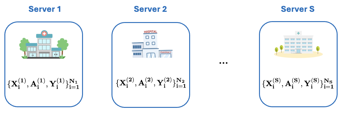
In this paper, we systematically study the problem of classification under demographic disparity (Definition 4) in a distributed learning setup with multiple servers, adhering to federated DP (Definition 2) constraints. This setting is graphically illustrated in Figure 1 and has wide-ranging applications, for instance, analysing data from patients across different hospitals (e.g. Li et al., 2020) and cross-organisation collaborations (e.g. Heyndrickx et al., 2023), among many others.

We summarise the main contributions of the paper as follows.

  • •

    To the best of our knowledge, this is the first work to systematically study private distributed fairness-aware classification. We propose a two-step post-processing algorithm, detailed in Algorithm 1. In the first step, due to the coexistence of scalar and functional outputs, we employ various Gaussian mechanisms, adding univariate Gaussian noise to scalars and Gaussian processes to functional outputs. In the second step, to determine the adjusted decision threshold under federated DP, we introduce a novel private tree-based algorithm that avoids repeated privacy composition arising from summation estimations in the optimisation problem.

  • •

    In the special case when there is only one server, we further show that a new and simpler algorithm, Algorithm 5, is sufficient for fair classification under central DP, in contrast to the more complex tree-based procedure in Algorithm 3. Notably, Algorithm 5 and its theoretical guarantees provide a novel private mechanism for optimising a functional object without incurring functional privacy, and is of independent interest.

  • •

    We further establish finite-sample theoretical guarantees for the proposed algorithms in terms of privacy, fairness and excess risk control. In particular, we show that both Algorithms 1 and 5 satisfy fairness constraints with high probability while maintaining satisfactory classification performance under DP, with the cost of privacy and fairness explicitly quantified. We separate the source of excess risk into decoupled terms, corresponding to the intrinsic hardness of classification, the privacy and fairness constraints. These results provide a rigorous theoretical foundation for the decision makers to understand the trade-offs between privacy, fairness and excess risk.

  • •

    Systematic numerical experiments on both simulated and real datasets are carried out in Section 5. These results further support our theoretical findings in Section 4 and highlight the practicality.

Notation. For a positive integer aa, denote [a]={1,…,a}[a]=\{1,\ldots,a\}. Let ⌈a⌉\lceil a\rceil be the smallest integer greater than or equal to aa and ⌊a⌋\lfloor a\rfloor be the greatest integer less than or equal to aa. For a,b∈ℝa,b\in\mathbb{R}, let a∨b=max⁡{a,b}a\vee b=\max\{a,b\} and a∧b=min⁡{a,b}a\wedge b=\min\{a,b\}. For v∈ℝpv\in\mathbb{R}^{p}, let ‖v‖1\|v\|_{1}, ‖v‖2\|v\|_{2} and ‖v‖∞\|v\|_{\infty} be ℓ1\ell_{1}-, ℓ2\ell_{2}- and ℓ∞\ell_{\infty}-norms. For a sequence of positive numbers {an}\{a_{n}\} and a sequence of random variables {Xn}\{X_{n}\}, denote Xn=Op​(an)X_{n}=O_{\mathrm{p}}(a_{n}) if limM→∞limsupnℙ​(|Xn|≥M​an)=0\lim_{M\rightarrow\infty}\lim\sup_{n}\mathbb{P}(|X_{n}|\geq Ma_{n})=0. We write Xn=O~p​(an)X_{n}=\widetilde{O}_{\mathrm{p}}(a_{n}) if there exists k>0k>0 such that Xn=Op​(an​(log⁡n)k)X_{n}=O_{\mathrm{p}}(a_{n}(\log n)^{k}). For two sequences of positive numbers {an}\{a_{n}\} and {bn}\{b_{n}\}, denote an≲bna_{n}\lesssim b_{n}, an≳bna_{n}\gtrsim b_{n}, and an≍bna_{n}\asymp b_{n}, if there exists some constants c,C>0c,C>0 such that an/bn≤Ca_{n}/b_{n}\leq C, bn/an≤Cb_{n}/a_{n}\leq C and c≤an/bn≤Cc\leq a_{n}/b_{n}\leq C. Write an≲logbna_{n}\lesssim_{\log}b_{n}, an≍logbna_{n}\asymp_{\log}b_{n} and an=logbna_{n}=_{\log}b_{n}, if an≲bna_{n}\lesssim b_{n}, an≍bna_{n}\asymp b_{n} and an=bna_{n}=b_{n} up to poly-logarithmic factors.

For d∈ℕ+d\in\mathbb{N}_{+} and any vector s=(s1,…,sd)⊤∈ℕds=(s_{1},\ldots,s_{d})^{\top}\in\mathbb{N}^{d}, define |s|=∑i=1dsi|s|=\sum_{i=1}^{d}s_{i}, s!=s1!​⋯​sd!s!=s_{1}!\cdots s_{d}! and the associated partial differential operator Ds=∂|s|∂x1s1​⋯​∂xdsdD^{s}=\frac{\partial^{|s|}}{\partial x_{1}^{s_{1}}\cdots\partial x_{d}^{s_{d}}}. For any function f:ℝd→ℝf:\,\mathbb{R}^{d}\to\mathbb{R} that is ⌊β⌋\lfloor\beta\rfloor-times continuously differentiable at point x0x_{0}, denote fx0βf_{x_{0}}^{\beta} the Taylor polynomial of degree ⌊β⌋\lfloor\beta\rfloor at x0x_{0}, defined as fx0β​(x)=∑|s|≤⌊β⌋(x−x0)ss!​Ds​f​(x0)f_{x_{0}}^{\beta}(x)=\sum_{|s|\leq\lfloor\beta\rfloor}\frac{(x-x_{0})^{s}}{s!}D^{s}f(x_{0}). For a constant L>0L>0, let ℋβ​(L)\mathcal{H}^{\beta}(L) be the class of Hölder smooth functions f:ℝp→ℝf:\,\mathbb{R}^{p}\to\mathbb{R} such that ff is ⌊β⌋\lfloor\beta\rfloor-times differentiable for all x∈ℝdx\in\mathbb{R}^{d} and satisfies |f​(x)−fx0β​(x)|≤L​|x−x0|β|f(x)-f_{x_{0}}^{\beta}(x)|\leq L|x-x_{0}|^{\beta}, for all x,x0∈ℝdx,x_{0}\in\mathbb{R}^{d}.

2 Problem formulation

In this section, we formally present the model setup and federated DP in Section 2.1, then introduce fairness constraints and present the framework of distributed fairness-aware classification in Section 2.2.

2.1 Setup and federated differential privacy

Suppose we have NtotalN_{\text{total}} independent and identically distributed samples 𝒟={(Xi,Ai,Yi),i∈[Ntotal]}\mathcal{D}=\{(X_{i},A_{i},Y_{i}),i\in[N_{\text{total}}]\}, where Xi∈[0,1]dX_{i}\in[0,1]^{d} is the standard dd-dimensional feature, Ai∈{0,1}A_{i}\in\{0,1\} is the sensitive feature (e.g. race and gender) and Yi∈{0,1}Y_{i}\in\{0,1\} is the binary label. We further assume that these data are distributed across SS servers, with server s∈[S]s\in[S] holding a dataset 𝒟s={(Xis,Ais,Yis)}i=1Ns\mathcal{D}_{s}=\{(X^{s}_{i},A^{s}_{i},Y^{s}_{i})\}_{i=1}^{N_{s}} of size NsN_{s}, where ∑s=1SNs=Ntotal\sum_{s=1}^{S}N_{s}=N_{\text{total}}.

Refer to caption
Figure 1: An illustration of the framework we consider in the problem of fairness-aware classification in a distributed setting.

With the setup above, we now introduce the federated DP constraints. At a high level, it is a variant of DP tailored to distributed settings, ensuring only private information is shared across servers. To formally define federated DP, we begin with the definition of central DP (Dwork et al., 2006), which is arguably the most fundamental notion of DP and is imposed within each server under our setting. Formally speaking, given a dataset DD, a privacy mechanism Q(⋅|D)Q(\cdot|D) is a conditional distribution of the private information given data DD. Let Z∈𝒵Z\in\mathcal{Z} denote the privatised data and σ​(𝒵)\sigma(\mathcal{Z}) denote the sigma-algebra on 𝒵\mathcal{Z}. We require the privacy mechanism to satisfy the following.

Definition 1 (Central differential privacy, CDP).

For ϵ>0\epsilon>0 and δ≥0\delta\geq 0, the privacy mechanism QQ is said to satisfy (ϵ,δ)(\epsilon,\delta)-CDP if

Q​(Z∈A|D)≤eϵ​Q​(Z∈A|D′)+δ,\displaystyle Q(Z\in A|D)\leq e^{\epsilon}Q(Z\in A|D^{\prime})+\delta,

for all A∈σ​(𝒵)A\in\sigma(\mathcal{Z}) and DD and D′D^{\prime} that differ by at most one data entry, denoted by D∼D′D\sim D^{\prime}.

Motivated by federated learning, Federated DP is introduced and has been applied in various settings under various names, e.g. Li et al. (2024), Cai et al. (2024), Xue et al. (2024), Auddy et al. (2025), and many more. In this paper, we focus on the non-interactive setting, in which no communication or interaction between servers is allowed. Let Zs∈𝒵Z^{s}\in\mathcal{Z} denote the privatised information output by server ss and σ​(𝒵)\sigma(\mathcal{Z}) denote the sigma-algebra on 𝒵\mathcal{Z}.

Definition 2 (Federated differential privacy, FDP).

For S∈ℤ+S\in\mathbb{Z}_{+}, denote (ϵ,𝛅)={(ϵs,δs)}s=1S(\bm{\epsilon},\bm{\delta})=\{(\epsilon_{s},\delta_{s})\}_{s=1}^{S} the collection of privacy parameters where ϵs>0\epsilon_{s}>0 and δs≥0\delta_{s}\geq 0, s∈[S]s\in[S]. We say that a privacy mechanism QQ satisfies (ϵ,𝛅)(\bm{\epsilon},\bm{\delta})-FDP, if for any s∈[S]s\in[S], the transcript Zs∈𝒵Z^{s}\in\mathcal{Z} shared to the central server satisfies an (ϵs,δs)(\epsilon_{s},\delta_{s})-CDP constraint, i.e.

Q​(Zs∈A|𝒟s)≤eϵs​Q​(Zs∈A|𝒟s′)+δs,\displaystyle Q(Z^{s}\in A|\mathcal{D}_{s})\leq e^{\epsilon_{s}}Q(Z^{s}\in A|\mathcal{D}^{\prime}_{s})+\delta_{s},

for all A∈σ​(𝒵)A\in\sigma(\mathcal{Z}) and 𝒟s\mathcal{D}_{s} and 𝒟s′\mathcal{D}_{s}^{\prime} that differ by at most one data entry.

In both Definitions 1 and 2, the strength of the privacy is controlled by (ϵ,δ)(\epsilon,\delta). The parameter ϵ\epsilon controls the strength of the privacy constraint, with smaller values of ϵ\epsilon corresponding to stronger privacy. The parameter δ≥0\delta\geq 0 controls the level of privacy leakage.

2.2 Fairness-aware classification

Having introduced the FDP constraints, we next present the fairness constraints, i.e. demographic disparity (Definition 4), and formulate the fairness-aware classification problem in this subsection.

Definition 3 (Randomised classifier).

For any x∈[0,1]dx\in[0,1]^{d} and a∈{0,1}a\in\{0,1\}, a randomised classifier f∈ℱf\in\mathcal{F} is a measurable function such that f(x,a)=ℙ(Y^f=1|X=x,A=a)f(x,a)=\mathbb{P}(\widehat{Y}_{f}=1|X=x,A=a), where Y^f=Y^f​(x,a)\widehat{Y}_{f}=\widehat{Y}_{f}(x,a) is the predicted label, i.e. Y^f|{X=x,A=a}∼Bernoulli​(f​(x,a))\widehat{Y}_{f}|\{X=x,A=a\}\sim\mathrm{Bernoulli}\;(f(x,a)).

Definition 4 (Demographic disparity).

For a given classifier f∈ℱf\in\mathcal{F}, the demographic disparity (DD\operatorname*{\mathrm{DD}}) is defined as

DD(f)\displaystyle\operatorname*{\mathrm{DD}}(f) =ℙ​{Y^f​(X,1)=1|A=1}−ℙ​{Y^f​(X,0)=1|A=0}.\displaystyle=\mathbb{P}\{\widehat{Y}_{f}(X,1)=1|A=1\}-\mathbb{P}\{\widehat{Y}_{f}(X,0)=1|A=0\}.

Let ℱ\mathcal{F} be the class of measurable functions f:[0,1]d×{0,1}→[0,1]f:[0,1]^{d}\times\{0,1\}\rightarrow[0,1]. For a prespecified α≥0\alpha\geq 0, we define the α\alpha-fair Bayes optimal classifier as the randomised classifier (Definition 3), fDD,α∗f^{*}_{\operatorname*{\mathrm{DD}},\alpha}, which minimises the misclassification error R​(fDD,α∗)=ℙ​(Y^fDD,α∗​(X,A)≠Y)R(f^{*}_{\operatorname*{\mathrm{DD}},\alpha})=\mathbb{P}(\widehat{Y}_{f^{*}_{\operatorname*{\mathrm{DD}},\alpha}}(X,A)\neq Y) while satisfying the α\alpha-demographic disparity , i.e.

fDD,α∗∈arg​minf∈ℱ⁡{R​(f):|DD(f)|≤α}.\displaystyle f^{*}_{\operatorname*{\mathrm{DD}},\alpha}\in\operatorname*{arg\,min}_{f\in\mathcal{F}}\{R(f):|\operatorname*{\mathrm{DD}}(f)|\leq\alpha\}. (1)

The Bayes fairness-aware classifier defined in (1) has been previously studied in Zeng et al. (2024a), where it is shown that the optimal fairness-aware classifier can be obtained by shifting the Bayes decision rule through an adjusted threshold. Specifically,

fDD,α∗​(x,a)={1,ηa​(x)≥12+τDD,α∗​(2​a−1)2​πa,0,ηa​(x)<12+τDD,α∗​(2​a−1)2​πa,\displaystyle f^{*}_{\operatorname*{\mathrm{DD}},\alpha}(x,a)=\begin{cases}\vskip 5.0pt1,&\eta_{a}(x)\geq\frac{1}{2}+\frac{\tau^{*}_{\operatorname*{\mathrm{DD}},\alpha}(2a-1)}{2\pi_{a}},\\ 0,&\eta_{a}(x)<\frac{1}{2}+\frac{\tau^{*}_{\operatorname*{\mathrm{DD}},\alpha}(2a-1)}{2\pi_{a}},\end{cases} (2)

where

τDD,α∗=arg⁡minτ∈ℝ⁡{|τ|:|DD​(τ)|≤α}\tau_{\mathrm{DD},\alpha}^{*}=\arg\min_{\tau\in\mathbb{R}}\big\{|\tau|:\,|\mathrm{DD}(\tau)|\leq\alpha\big\} (3)

is the magnitude of the adjusted threshold, and for any a∈{0,1}a\in\{0,1\} and x∈[0,1]dx\in[0,1]^{d}, ηa(x)=ℙ(Y=1|A=a,X=x)\eta_{a}(x)=\mathbb{P}(Y=1|A=a,X=x), πa,y=ℙ​(A=a,Y=y)\pi_{a,y}=\mathbb{P}(A=a,Y=y) and πa=ℙ​(A=a)\pi_{a}=\mathbb{P}(A=a).

Our goal in this paper is to construct an estimator for fDD,α∗f^{*}_{\operatorname*{\mathrm{DD}},\alpha} under FDP defined in Definition 2.

Remark 1.

In this paper, we focus on classification with demographic disparity, which controls the difference in the probability of predicting the positive label across sensitive groups. We would like to remark that, with minor modifications, our algorithm can be generalised to accommodate other bilinear disparity measures (Definition 6, Definition 3.3 in Zeng et al., 2024a), such as disparity of opportunity (DO) and predictive disparity (PD).

3 Federated differentially private fair classifier under demographic disparity

In this section, we present our two-step plug-in FDP-Fair classifier in Algorithm 1.

Building on the Bayes optimal fairness-aware classifier in (2), the construction of Algorithm 1 relies on estimating three key quantities: regression functions ηa\eta_{a}, class probabilities πa\pi_{a}, and the fairness threshold parameter τDD,α∗\tau^{*}_{\operatorname*{\mathrm{DD}},\alpha}. The algorithm is organised in two steps. S1 produces estimators of ηa\eta_{a} and πa\pi_{a}. In S2, we estimate τDD,α∗\tau^{*}_{\operatorname*{\mathrm{DD}},\alpha} through a private threshold search procedure building upon binary tree constructions in Algorithm 2, which itself relies on the auxiliary procedures given in Algorithms 3 and 4.

For notational clarity, in Algorithm 1, we decompose the data for server s∈[S]s\in[S] as 𝒟s=𝒟0,1s∪𝒟0,0s∪𝒟1,1s∪𝒟1,0s\mathcal{D}^{s}=\mathcal{D}^{s}_{0,1}\cup\mathcal{D}^{s}_{0,0}\cup\mathcal{D}^{s}_{1,1}\cup\mathcal{D}^{s}_{1,0}, where for a,y∈{0,1}a,y\in\{0,1\}, 𝒟a,ys={(Xis,Ais=a,Yis=y)}\mathcal{D}^{s}_{a,y}=\{(X_{i}^{s},A_{i}^{s}=a,Y_{i}^{s}=y)\}. We further denote the ii-th feature in 𝒟a,ys\mathcal{D}^{s}_{a,y} by Xa,ys,iX^{s,i}_{a,y} for i∈[|𝒟a,ys|]i\in[|\mathcal{D}^{s}_{a,y}|]. For any kernel function K:ℝd→ℝ+K:\mathbb{R}^{d}\to\mathbb{R}^{+}, let the scaled kernel function be Kh​(x)=h−d​K​(x/h)K_{h}(x)=h^{-d}K(x/h), for any x∈ℝdx\in\mathbb{R}^{d} and bandwidth 0<h<10<h<1.

The key components of Algorithm 1 are outlined below.

Estimation of class probability πa\pi_{a} and regression function ηa\eta_{a}. In S1. of Algorithm 1, site-wise estimators of πas\pi_{a}^{s} and ηas\eta_{a}^{s} are constructed from the training data using empirical and kernel density estimators, respectively. To preserve FDP, we utilise Gaussian mechanisms for both scalars used in estimating πa\pi_{a}’s and functions in estimating ηa\eta_{a}’s. The resulting privatised site-wise estimators are then aggregated at the central server through weighted sums, yielding global estimators while maintaining FDP constraints.

Binary tree construction. To estimate the private threshold, τ~DD,α\widetilde{\tau}_{\operatorname*{\mathrm{DD}},\alpha}, we approximate the original continuous optimisation problem in (3) using discretisation. For each discretised candidate, we further reduce it to evaluating tail counts utilising binary trees, where counts in dyadic intervals are organised hierarchically, enabling efficient privacy budget allocation across a sufficiently fine evaluation grids.

Specifically, by considering the random variables Zs,a,y=2​(2​a−1)​π~a​{η~a​(Xa,ys)−1/2}Z_{s,a,y}=2(2a-1)\widetilde{\pi}_{a}\{\widetilde{\eta}_{a}(X^{s}_{a,y})-1/2\}, for each evaluated τ∈ℝ\tau\in\mathbb{R}, we can rewrite the empirical plug-in estimator of DD,

DD^​(τ)=\displaystyle\widehat{\mathrm{DD}}(\tau)=\; ∑s=1Sμs​DD^s​(τ)\displaystyle\sum_{s=1}^{S}\mu_{s}\widehat{\mathrm{DD}}_{s}(\tau)
=\displaystyle=\; ∑s=1Sμs[1n˘s,1∑y∈{0,1}∑i=1n˘s,1,y𝟙{2π~1{η~1(X˘1,ys,i)−1/2}≥τ}\displaystyle\sum_{s=1}^{S}\mu_{s}\Bigg[\frac{1}{\breve{n}_{s,1}}\sum_{y\in\{0,1\}}\sum_{i=1}^{\breve{n}_{s,1,y}}\mathds{1}\Big\{2\widetilde{\pi}_{1}\{\widetilde{\eta}_{1}(\breve{X}^{s,i}_{1,y})-1/2\}\geq\tau\Big\}
−1n˘s,0∑y∈{0,1}∑i=1n˘s,0,y𝟙{−2π~0{η~0(X˘0,ys,i)−1/2}≤τ}],\displaystyle\hskip 35.00005pt-\frac{1}{\breve{n}_{s,0}}\sum_{y\in\{0,1\}}\sum_{i=1}^{\breve{n}_{s,0,y}}\mathds{1}\Big\{-2\widetilde{\pi}_{0}\{\widetilde{\eta}_{0}(\breve{X}^{s,i}_{0,y})-1/2\}\leq\tau\Big\}\Bigg], (4)

as

DD^​(τ)=∑s=1Sμs×{∑ycount of ​Zs,1,y​ larger than ​τ∑yTotal count of ​Zs,1,y−∑ycount of ​Zs,0,y​ less than ​τ∑yTotal count of ​Zs,0,y}.\widehat{\operatorname*{\mathrm{DD}}}(\tau)=\sum_{s=1}^{S}\mu_{s}\times\Big\{\frac{\sum_{y}\mbox{count of }Z_{s,1,y}\mbox{ larger than }\tau}{\sum_{y}\mbox{Total count of }Z_{s,1,y}}-\frac{\sum_{y}\mbox{count of }Z_{s,0,y}\mbox{ less than }\tau}{\sum_{y}\mbox{Total count of }Z_{s,0,y}}\Big\}.

Given the fact that |τDD,α∗|≤min⁡{π0,π1}|\tau^{*}_{\operatorname*{\mathrm{DD}},\alpha}|\leq\min\{\pi_{0},\pi_{1}\} in Lemma 11, we partition the interval [−1,1][-1,1] into equal-sized subintervals and arrange them in a multi-layer binary tree. For each server s∈[S]s\in[S] and sensitive group a∈{0,1}a\in\{0,1\}, the count of Zs,a,yZ_{s,a,y} falling into binary subintervals across all layers is computed and privatised using Gaussian mechanisms. The resulting site-wise binary trees are then aggregated at the central server via weighted averaging, where the weights are chosen according to the variances of the corresponding site-level estimators, similar to S1.

Remark 2.

With the binary tree construction in Algorithm 3, changing a single data point affects at most one node per tree-level, resulting in constant-order ℓ2\ell_{2}-sensitivity used in the Gaussian mechanism. Moreover, since the tree depth is logarithmic by selection in Theorem 2, only a logarithmic number of privacy compositions is required. This leads to a substantial improvement in accuracy compared to standard discretisation approaches in private nonparametric estimation, where a polynomial number of compositions is needed. We defer more discussions on tree depth selection until after presenting theoretical results in Theorem 2 in Section 4.

Monotonicity correction. The aggregation of Gaussian noise across different leaves in the binary tree means that the evaluated DD~\widetilde{\operatorname*{\mathrm{DD}}} across grids is no longer guaranteed to be monotonically non-increasing, which is a crucial property of the true DD function underlying the derivation of τDD,α∗\tau^{*}_{\operatorname*{\mathrm{DD}},\alpha} in (3). To preserve this structure, we introduce Algorithm 4, which fits, with high probability, a non-increasing sequence of {DD~​(τj)}\{\widetilde{\operatorname*{\mathrm{DD}}}(\tau_{j})\} while controlling the induced bias.

Algorithm 1 FDP-Fair classifier under demographic disparity.
Data 𝒟\mathcal{D}, disparity level α\alpha, Kernel function KK, bandwidth parameters hh, weights {νs}s∈[S]\{\nu_{s}\}_{s\in[S]} and {μs}s∈[S]\{\mu_{s}\}_{s\in[S]}, constant Cρ,Cω>0C_{\rho},C_{\omega}>0, smallest interval length θ\theta, tolerance η\eta.
For each s∈[S]s\in[S], let ns=⌈Ns/2⌉n_{s}=\lceil N_{s}/2\rceil and n˘s=Ns−ns\breve{n}_{s}=N_{s}-n_{s}. Split the data in each site into training data {(Xis,Ais,Yis)}i=1ns\{(X^{s}_{i},A^{s}_{i},Y^{s}_{i})\}_{i=1}^{n_{s}} and calibration data {(Xis,Ais,Yis)}i=ns+1Ns={X˘is,A˘is,Y˘is}i=1n˘s\{(X^{s}_{i},A^{s}_{i},Y^{s}_{i})\}_{i=n_{s}+1}^{N_{s}}=\{\breve{X}^{s}_{i},\breve{A}^{s}_{i},\breve{Y}^{s}_{i}\}_{i=1}^{\breve{n}_{s}}. We further denote ns,a,y=|{(Xis,Ais=a,Yis=y)}i=1ns|n_{s,a,y}=|\{(X^{s}_{i},A^{s}_{i}=a,Y^{s}_{i}=y)\}_{i=1}^{n_{s}}| and ns,a=|{(Xis,Ais=a,Yis)}i=1ns|n_{s,a}=|\{(X^{s}_{i},A^{s}_{i}=a,Y^{s}_{i})\}_{i=1}^{n_{s}}|.
S1. Estimating regression function ηa\eta_{a} and class probabilities πa\pi_{a} using training data adhering to federated differential privacy constraints.
S1.1 For s∈[S]s\in[S], a∈{0,1}a\in\{0,1\}, generate was∼i.i.d.N​(0,σs2)w^{s}_{a}\mathrel{{\mathop{\sim}\limits^{\mathrm{i.i.d.}}}}N(0,\sigma_{s}^{2}), where σs=4​2​log⁡(5/δs)/(ns​ϵs)\sigma_{s}=4\sqrt{2\log(5/\delta_{s})}/(n_{s}\epsilon_{s}). Calculate
π~a=∑s=1Sνs​π~as,where​π~as=ns,a,0+ns,a,1ns+was.\widetilde{\pi}_{a}=\sum_{s=1}^{S}\nu_{s}\widetilde{\pi}_{a}^{s},\;\text{where}\;\;\widetilde{\pi}_{a}^{s}=\frac{n_{s,a,0}+n_{s,a,1}}{n_{s}}+w_{a}^{s}.
S1.2 Let {Wk,as(⋅)}k,a∈{0,1},s∈[S]}\{W^{s}_{k,a}(\cdot)\}_{k,a\in\{0,1\},s\in[S]}\} be independent mean zero Gaussian processes with covariance kernels Cov(Wk,as​(ℓ),Wk,as​(t))=K​{(ℓ−t)/h},ℓ,t∈[0,1]d\operatorname*{Cov}(W^{s}_{k,a}(\ell),W^{s}_{k,a}(t))=K\{(\ell-t)/h\},\ell,t\in[0,1]^{d}. For any x∈[0,1]dx\in[0,1]^{d} and s∈[S]s\in[S], denote
p~X|A=as​(x|a)=1ns,a​∑y∈{0,1}∑i=1ns,a,yKh​(Xa,ys,i−x)+8​2​CK​log⁡(8/δs)ns,a​ϵs​hd​W1,as​(x),\displaystyle\widetilde{p}^{s}_{X|A=a}(x|a)=\frac{1}{n_{s,a}}\sum_{y\in\{0,1\}}\sum_{i=1}^{n_{s,a,y}}K_{h}(X_{a,y}^{s,i}-x)+\frac{8\sqrt{2C_{K}\log(8/\delta_{s})}}{n_{s,a}\epsilon_{s}h^{d}}W^{s}_{1,a}(x),
and
p~X,Y|A=as​(x,y|a)=1ns,a​∑i=1ns,a,1Kh​(Xa,1s,i−x)+8​2​CK​log⁡(8/δs)ns,a​ϵs​hd​W2,as​(x),\displaystyle\widetilde{p}^{s}_{X,Y|A=a}(x,y|a)=\frac{1}{n_{s,a}}\sum_{i=1}^{n_{s,a,1}}K_{h}(X_{a,1}^{s,i}-x)+\frac{8\sqrt{2C_{K}\log(8/\delta_{s})}}{n_{s,a}\epsilon_{s}h^{d}}W^{s}_{2,a}(x),
Denote p~X|A=a​(x|a)=∑s=1Sνs​p~X|A=as​(x|a)\widetilde{p}_{X|A=a}(x|a)=\sum_{s=1}^{S}\nu_{s}\widetilde{p}^{s}_{X|A=a}(x|a) and η~a​(x)=1p~X|A=a​(x|a)​∑s=1Sνs​p~X,Y|A=as​(x,1|a)\widetilde{\eta}_{a}(x)=\frac{1}{\widetilde{p}_{X|A=a}(x|a)}\sum_{s=1}^{S}\nu_{s}\widetilde{p}^{s}_{X,Y|A=a}(x,1|a).
S2. Estimating the optimal threshold using calibration data.
Set τ~DD,α=FDP.Threshold.Search​({{X˘i,A˘i,Y˘i}i=1n˘s}s=1S,{μs}s∈[S],{η~a,π~a}a∈{0,1},Cρ,Cω,θ,η)\widetilde{\tau}_{\operatorname*{\mathrm{DD}},\alpha}=\textsc{FDP.Threshold.Search}(\{\{\breve{X}_{i},\breve{A}_{i},\breve{Y}_{i}\}_{i=1}^{\breve{n}_{s}}\}_{s=1}^{S},\{\mu_{s}\}_{s\in[S]},\{\widetilde{\eta}_{a},\widetilde{\pi}_{a}\}_{a\in\{0,1\}},C_{\rho},C_{\omega},\theta,\eta). ⊳\triangleright See Algorithm 2.
f~DD,α​(x,a)\widetilde{f}_{\operatorname*{\mathrm{DD}},\alpha}(x,a) with
f~DD,α​(x,a)={1,η~a​(x)≥12+τ~DD,α​(2​a−1)2​π~a,0,η~a​(x)<12+τ~DD,α​(2​a−1)2​πa~.\displaystyle\widetilde{f}_{\operatorname*{\mathrm{DD}},\alpha}(x,a)=\begin{cases}\vskip 5.0pt1,&\widetilde{\eta}_{a}(x)\geq\frac{1}{2}+\frac{\widetilde{\tau}_{\operatorname*{\mathrm{DD}},\alpha}(2a-1)}{2\widetilde{\pi}_{a}},\\ 0,&\widetilde{\eta}_{a}(x)<\frac{1}{2}+\frac{\widetilde{\tau}_{\operatorname*{\mathrm{DD}},\alpha}(2a-1)}{2\widetilde{\pi_{a}}}.\end{cases}
Algorithm 2 FDP.Threshold.Search(𝒟˘,{μs}s∈[S],{η~a,π~a}a∈{0,1},Cρ,Cω,θ,η)(\breve{\mathcal{D}},\{\mu_{s}\}_{s\in[S]},\{\widetilde{\eta}_{a},\widetilde{\pi}_{a}\}_{a\in\{0,1\}},C_{\rho},C_{\omega},\theta,\eta).
Data 𝒟˘\breve{\mathcal{D}}, weight {μs}s∈[S]\{\mu_{s}\}_{s\in[S]} , estimated regression functions and class probabilities {η~a,π~a}a∈{0,1}\{\widetilde{\eta}_{a},\widetilde{\pi}_{a}\}_{a\in\{0,1\}} with bandwidth hh, constant Cρ,Cω>0C_{\rho},C_{\omega}>0, minimum bin length θ\theta, tolerance η\eta.
Set the number of layers at M:=log2⁡(θ−1)+1M:=\log_{2}(\theta^{-1})+1 and tolerance at ρ∗=Cρ​ρ\rho^{*}=C_{\rho}\rho, where ρ\rho is given in (6).
S1 Binary tree construction:
Run FDP.Binary.Tree(𝒟˘,{η~a,π~a}a∈{0,1},M)(\breve{\mathcal{D}},\{\widetilde{\eta}_{a},\widetilde{\pi}_{a}\}_{a\in\{0,1\}},M) detailed in Algorithm 3.
S2 Estimation of disparity value in central server:
Construct evaluation grids 𝒢:={τ1,…,τ2M+1}\mathcal{G}:=\{\tau_{1},\ldots,\tau_{2^{M}+1}\}, where τj=−1+(j−1)​21−M\tau_{j}=-1+(j-1)2^{1-M} for j∈[2M+1]j\in[2^{M}+1].
With the binary tree given in S1, calculate
Ns,1=Ns,1,1,1+Ns,1,1,2,Ns,0=Ns,0,1,1+Ns,0,1,2,N_{s,1}=N_{s,1,1,1}+N_{s,1,1,2},\;\;N_{s,0}=N_{s,0,1,1}+N_{s,0,1,2},
and for any j∈[2M]j\in[2^{M}]
Tails,a​(τj)=∑ℓ=1M∑k=12ℓNs,a,ℓ,k​𝟙​{(k−1)​2M−ℓ+1≥j​ and ​(⌈k/2⌉−1)​2M−ℓ+1+1<j}.\displaystyle\text{Tail}_{s,a}(\tau_{j})=\sum_{\ell=1}^{M}\sum_{k=1}^{2^{\ell}}N_{s,a,\ell,k}\mathds{1}\Big\{(k-1)2^{M-\ell}+1\geq j\text{ and }(\lceil k/2\rceil-1)2^{M-\ell+1}+1<j\Big\}.
Then for any τ∈𝒢\tau\in\mathcal{G}, set DD~​(τ)=∑s=1Sμs​DD~s​(τ)\widetilde{\operatorname*{\mathrm{DD}}}(\tau)=\sum_{s=1}^{S}\mu_{s}\widetilde{\operatorname*{\mathrm{DD}}}^{s}(\tau), where
DD~s​(τ)=Tails,1​(τ)Ns,1−Ns,0−Tails,0​(τ)Ns,0.\displaystyle\widetilde{\operatorname*{\mathrm{DD}}}^{s}(\tau)=\frac{\text{Tail}_{s,1}(\tau)}{N_{s,1}}-\frac{N_{s,0}-\text{Tail}_{s,0}(\tau)}{N_{s,0}}.
Set {DD~↓​(τi)}i∈[2M+1]=Non.increasing​({DD~​(τi)}i∈[2M+1],{μs}s∈[S],Cω,η)\{\widetilde{\operatorname*{\mathrm{DD}}}_{\downarrow}(\tau_{i})\}_{i\in[2^{M}+1]}=\textsc{Non.increasing}(\{\widetilde{\operatorname*{\mathrm{DD}}}(\tau_{i})\}_{i\in[2^{M}+1]},\{\mu_{s}\}_{s\in[S]},C_{\omega},\eta). ⊳\triangleright See Algorithm 4
S3 Threshold selection:
if |DD~↓​(0)|≤α|\widetilde{\operatorname*{\mathrm{DD}}}_{\downarrow}(0)|\leq\alpha then
  Set τ~DD,α=0\widetilde{\tau}_{\operatorname*{\mathrm{DD}},\alpha}=0.
else
  Set τ~DD,α=arg​minτ∈𝒢⁡{|τ|:|DD~↓​(τ)|∈[α−ρ∗,α+ρ∗]}\widetilde{\tau}_{\operatorname*{\mathrm{DD}},\alpha}=\operatorname*{arg\,min}_{\tau\in\mathcal{G}}\{|\tau|:|\widetilde{\operatorname*{\mathrm{DD}}}_{\downarrow}(\tau)|\in[\alpha-\rho^{*},\alpha+\rho^{*}]\}.
end if
τ~DD,α\widetilde{\tau}_{\operatorname*{\mathrm{DD}},\alpha}
Algorithm 3 FDP.Binary.Tree(𝒟˘,{η~a,π~a}a∈{0,1},M)(\breve{\mathcal{D}},\{\widetilde{\eta}_{a},\widetilde{\pi}_{a}\}_{a\in\{0,1\}},M).
Data 𝒟˘\breve{\mathcal{D}}, estimated regression functions and class probabilities {η~a,π~a}a∈{0,1}\{\widetilde{\eta}_{a},\widetilde{\pi}_{a}\}_{a\in\{0,1\}}, number of layers MM.
for s=1,…,S;a=0,1;ℓ=1,…,M​ and ​k=1,…,2ℓs=1,\ldots,S;a=0,1;\ell=1,\ldots,M\text{ and }k=1,\ldots,2^{\ell} do
  Generate independently
w˘s,a,ℓ,k∼N​(0,4​log⁡(1/δs)/ϵs+2ϵs/M).\breve{w}_{s,a,\ell,k}\sim N\Big(0,\frac{4\log(1/\delta_{s})/\epsilon_{s}+2}{\epsilon_{s}/M}\Big).
end for
for s=1,…,Ss=1,\ldots,S do
  for a=0,1a=0,1 do
   For any y∈{0,1}y\in\{0,1\} and i∈[n˘s,a,y]i\in[\breve{n}_{s,a,y}], calculate
Zs,i,a,y:=2​(2​a−1)​π~a​{η~a​(X˘a,ys,i)−1/2}.Z_{s,i,a,y}:=2(2a-1)\widetilde{\pi}_{a}\{\widetilde{\eta}_{a}(\breve{X}^{s,i}_{a,y})-1/2\}.
   for j=1,…,2Mj=1,\ldots,2^{M} do
     Let
counts,a,M,j=∑y∈{0,1}∑i=1n˘s,a,y𝟙​{−1+(j−1)​21−M≤Zs,i,a,y<−1+j​21−M}.\text{count}_{s,a,M,j}=\sum_{y\in\{0,1\}}\sum_{i=1}^{\breve{n}_{s,a,y}}\mathds{1}\Big\{-1+(j-1)2^{1-M}\leq Z_{s,i,a,y}<-1+j2^{1-M}\Big\}.
     for ℓ=M−1,…,1\ell=M-1,\ldots,1 do
      for k=1,…,2ℓk=1,\ldots,2^{\ell} do
        Set
counts,a,ℓ,k=counts,a,l+1,2​k−1+counts,a,l+1,2​k.\text{count}_{s,a,\ell,k}=\text{count}_{s,a,l+1,2k-1}+\text{count}_{s,a,l+1,2k}.
      end for
     end for
   end for
   for ℓ=1,…,M\ell=1,\ldots,M do
     for k=1,…,2ℓk=1,\ldots,2^{\ell} do
      Calculate Ns,a,ℓ,k=counts,a,ℓ,k+w˘s,a,ℓ,k.N_{s,a,\ell,k}=\text{count}_{s,a,\ell,k}+\breve{w}_{s,a,\ell,k}.
     end for
   end for
  end for
end for
Collection of private trees {{Ns,a,ℓ,k}ℓ=1,k=1M,2ℓ}a∈{0,1},s∈[S]\{\{N_{s,a,\ell,k}\}_{\ell=1,k=1}^{M,2^{\ell}}\}_{a\in\{0,1\},s\in[S]}.
Algorithm 4 Non.increasing({gi}i∈[2M+1],{μs}s∈[S],Cω\{g_{i}\}_{i\in[2^{M}+1]},\{\mu_{s}\}_{s\in[S]},C_{\omega}, MM, η\eta)
Sequence of points {gi}i∈[2M+1]\{g_{i}\}_{i\in[2^{M}+1]}, weight {μs}s∈[S]\{\mu_{s}\}_{s\in[S]}, constant CωC_{\omega}, binary tree layers MM, tolerance η\eta.
Set the tolerance level
ω=Cω​∑s=1Sμs2​M4​log⁡(1/δs)​log⁡(M/η)n˘s2​ϵs2.\displaystyle\omega=C_{\omega}\sqrt{\sum_{s=1}^{S}\frac{\mu_{s}^{2}M^{4}\log(1/\delta_{s})\log(M/\eta)}{\breve{n}_{s}^{2}\epsilon_{s}^{2}}}.
if gi≥…≥g2M+1g_{i}\geq\ldots\geq g_{2^{M}+1} then
  Break and return {gi}i∈[2M+1]\{g_{i}\}_{i\in[2^{M}+1]}.
else
  Initialise the algorithm by setting f1=g1+ωf_{1}=g_{1}+\omega.
  for i=2,…,2M+1i=2,\ldots,2^{M}+1 do
   Set fi=min⁡{fi−1,gi+ω}f_{i}=\min\{f_{i-1},g_{i}+\omega\}.
   if fi<gi−ωf_{i}<g_{i}-\omega then
     Break and return NULL.
   else
     Continue
   end if
  end for
end if
Sequence of non-increasing numbers {fi}i∈[2M+1]\{f_{i}\}_{i\in[2^{M}+1]}.

3.1 Special case: Central differential privacy

In the special case when S=1S=1 and N1=NN_{1}=N, Definition 2 reduces to CDP as defined in Definition 1. Rather than implementing Algorithm 1, which targets the general setting when S>1S>1, we present in this subsection a simplified yet powerful algorithm dedicated to the CDP setting, given in Algorithm 5.

Compared with Algorithm 1, the main difference lies in Algorithm 5 S2., which is the estimation of adjusted threshold τDD,α∗\tau^{*}_{\operatorname*{\mathrm{DD}},\alpha}. Instead of using the noisy binary tree based algorithm, we show that shifting the empirical DD vertically by a correctly calibrated Gaussian noise is sufficient. The key idea is illustrated in Figure 2.

Refer to caption
Figure 2: Graphical illustration of S2. of Algorithm 5 when α=0.1\alpha=0.1.

Given the fact that the empirical DD, DD^\widehat{\operatorname*{\mathrm{DD}}} in (4) with S=1S=1, is monotonically non-increasing (Lemma 12), the optimisation problems τ^DD,α=arg​minτ∈ℝ⁡{|τ|:|DD^​(τ)|≤α}\widehat{\tau}_{\operatorname*{\mathrm{DD}},\alpha}=\operatorname*{arg\,min}_{\tau\in\mathbb{R}}\{|\tau|:\,|\widehat{\operatorname*{\mathrm{DD}}}(\tau)|\leq\alpha\} is equivalent to finding the smallest cut-off point in magnitude at which DD^​(τ)\widehat{\operatorname*{\mathrm{DD}}}(\tau) first reaches the fairness threshold α\alpha or −α-\alpha. Therefore, to construct a private cut-off point τ~DD,α\widetilde{\tau}_{\operatorname*{\mathrm{DD}},\alpha}, instead of adding noise directly to the cut-off point, we shift the DD^\widehat{\operatorname*{\mathrm{DD}}} function itself. Geometrically, this corresponds to perturbing the DD^\widehat{\operatorname*{\mathrm{DD}}} curve in the vertical direction (i.e. yy-axis). As a result, the location at which the perturbed DD^\widehat{\operatorname*{\mathrm{DD}}} curve crosses the threshold is shifted horizontally, producing a privacy-preserving cut-off point. By adding correctly calibrated noise and ensuring that each pointwise release of the DD^\widehat{\operatorname*{\mathrm{DD}}} function at any given τ\tau satisfies CDP, we are able to show that the induced release of the cut-off point τ~DD,α\widetilde{\tau}_{\operatorname*{\mathrm{DD}},\alpha} also satisfies CDP. We defer the formal privacy guarantees to Theorem 1 in Section 4.

Algorithm 5 CDP-Fair classifier under demographic disparity.
Data 𝒟\mathcal{D}, disparity level α\alpha, bandwidth parameters hh.
Let n=⌊N/2⌋n=\lfloor N/2\rfloor and n˘=N−n\breve{n}=N-n. Split the data in each site into training data {(Xi,Ai,Yi)}i=1n\{(X_{i},A_{i},Y_{i})\}_{i=1}^{n} and calibration data {(Xi,Ai,Yi)}i=n+1N={X˘i,A˘i,Y˘i}i=1n˘\{(X_{i},A_{i},Y_{i})\}_{i=n+1}^{N}=\{\breve{X}_{i},\breve{A}_{i},\breve{Y}_{i}\}_{i=1}^{\breve{n}}. We further denote n˘a=|{(Xi,Ai=a,Yi)}i=1ns|\breve{n}_{a}=|\{(X_{i},A_{i}=a,Y_{i})\}_{i=1}^{n_{s}}|.
S1. Implement S1 in Algorithm 1 with S=1S=1 to estimate regression function ηa\eta_{a} and class probabilities πa\pi_{a} using training data adhering to central DP constraints.
S2. Estimate the optimal threshold using calibration data.
Generate w˘∼N​(0,σ2)\breve{w}\sim N(0,\sigma^{2}), where σ=2​2​log⁡(1.25/δ)/({n˘0∧n˘1}​ϵ)\sigma=2\sqrt{2\log(1.25/\delta)}/(\{\breve{n}_{0}\wedge\breve{n}_{1}\}\epsilon). Calculate
DD~​(τ)=1n˘1​∑y∈{0,1}∑i=1n˘1,y𝟙​{η~1​(X˘1,yi)≥12+τ2​π~1}−1n˘0​∑y∈{0,1}∑i=1n˘0,y𝟙​{η~0​(X˘0,yi)≥12−τ2​π~0}+w˘.\displaystyle\widetilde{\operatorname*{\mathrm{DD}}}(\tau)=\frac{1}{\breve{n}_{1}}\sum_{y\in\{0,1\}}\sum_{i=1}^{\breve{n}_{1,y}}\mathds{1}\Big\{\widetilde{\eta}_{1}(\breve{X}^{i}_{1,y})\geq\frac{1}{2}+\frac{\tau}{2\widetilde{\pi}_{1}}\Big\}-\frac{1}{\breve{n}_{0}}\sum_{y\in\{0,1\}}\sum_{i=1}^{\breve{n}_{0,y}}\mathds{1}\Big\{\widetilde{\eta}_{0}(\breve{X}^{i}_{0,y})\geq\frac{1}{2}-\frac{\tau}{2\widetilde{\pi}_{0}}\Big\}+\breve{w}.
Set τ~DD,α=arg​minτ∈ℝ⁡{|τ|:|DD~​(τ)|≤α}\widetilde{\tau}_{\operatorname*{\mathrm{DD}},\alpha}=\operatorname*{arg\,min}_{\tau\in\mathbb{R}}\{|\tau|:\,|\widetilde{\operatorname*{\mathrm{DD}}}(\tau)|\leq\alpha\}.
f~DD,α​(x,a)\widetilde{f}_{\operatorname*{\mathrm{DD}},\alpha}(x,a) with
f~DD,α​(x,a)={1,η~a​(x)≥12+τ~DD,α​(2​a−1)2​π~a,0,η~a​(x)<12+τ~DD,α​(2​a−1)2​πa~.\displaystyle\widetilde{f}_{\operatorname*{\mathrm{DD}},\alpha}(x,a)=\begin{cases}\vskip 5.0pt1,&\widetilde{\eta}_{a}(x)\geq\frac{1}{2}+\frac{\widetilde{\tau}_{\operatorname*{\mathrm{DD}},\alpha}(2a-1)}{2\widetilde{\pi}_{a}},\\ 0,&\widetilde{\eta}_{a}(x)<\frac{1}{2}+\frac{\widetilde{\tau}_{\operatorname*{\mathrm{DD}},\alpha}(2a-1)}{2\widetilde{\pi_{a}}}.\end{cases}

4 Theoretical properties

In this section, we provide theoretical guarantees on privacy, fairness, and excess risk control for Algorithms 1 and 5.

4.1 Assumptions

To kick off, we list a few assumptions below.

Assumption 1 (Class and feature probability).

We assume that the following holds for any a∈{0,1}a\in\{0,1\}.

  1. a

    There exists an absolute constant 0<Cπ<10<C_{\pi}<1 such that the class probability πa=ℙ​(A=a)≥Cπ\pi_{a}=\mathbb{P}(A=a)\geq C_{\pi}.

  2. b

    There exists an absolute constant L>0L>0 such that pX|A=a∈ℋβ​(L)p_{X|A=a}\in\mathcal{H}^{\beta}(L). We further assume that infx∈[0,1]dpX|A=a​(x|a)≥Cp\inf_{x\in[0,1]^{d}}p_{X|A=a}(x|a)\geq C_{p} for an absolute constant Cp>0C_{p}>0.

Assumption 2 (Kernel function).

Let the kernel function K:ℝd→ℝ+K:\mathbb{R}^{d}\rightarrow\mathbb{R}^{+} satisfy the following conditions.

  1. a

    There exists an absolute constant CK>0C_{K}>0 such that supx∈ℝdK​(x)≤CK\sup_{x\in\mathbb{R}^{d}}K(x)\leq C_{K}.

  2. b

    We assume that the function KK is Lipschitz, i.e. there exists an absolute constant CLip>0C_{\mathrm{Lip}}>0 such that for any x,y∈ℝdx,y\in\mathbb{R}^{d}, |K​(x)−K​(y)|≤CLip​‖x−y‖2|K(x)-K(y)|\leq C_{\mathrm{Lip}}\|x-y\|_{2}.

  3. c

    The kernel function KK is adaptive to Hölder class ℋβ​(L)\mathcal{H}^{\beta}(L), i.e. for L>0L>0 and any f∈ℋβ​(L)f\in\mathcal{H}^{\beta}(L), it holds that supx∈[0,1]d|∫[0,1]dKh​(x−u)​f​(u)​du−f​(x)|≤Cadp​hβ\sup_{x\in[0,1]^{d}}|\int_{[0,1]^{d}}K_{h}(x-u)f(u)\;\mathrm{d}u-f(x)|\leq C_{\mathrm{adp}}h^{\beta}, where Cadp>0C_{\mathrm{adp}}>0 is an absolute constant only depending on LL.

In 1a, we assume that the class probabilities are bounded away from 0 and 1, essential to ensure that a sufficient number of samples for each group can be observed. In 1b, we further regulate the smoothness and boundedness of the per-sensitive class density of feature distributions. Similar assumptions are commonly seen in the literature of non-parametric statistics (e.g. Madrid Padilla et al., 2023; Auddy et al., 2025).

2 provides standard kernel assumptions in the nonparametric literature (e.g. Kim et al., 2019; Madrid Padilla et al., 2023), holding for various kernels, such as uniform, Epanechnikov and Gaussian. In particular, 2c holds for any β\beta-valid kernel functions.111For a fixed β>0\beta>0, a function K:ℝd→ℝ+K:\mathbb{R}^{d}\rightarrow\mathbb{R}^{+} is a β\beta-valid kernel if ∫ℝdK​(x)​dx=1\int_{\mathbb{R}^{d}}K(x)\;\mathrm{d}x=1, ‖K‖Lp<∞\|K\|_{L_{p}}<\infty for all p≥1p\geq 1, ∫ℝd‖x‖s​K​(x)​dx<∞\int_{\mathbb{R}^{d}}\|x\|^{s}K(x)\;\mathrm{d}x<\infty and ∫ℝdxs​K​(x)​dx=0\int_{\mathbb{R}^{d}}x^{s}K(x)\;\mathrm{d}x=0 for all s=(s1,…,sd)∈ℤds=(s_{1},\dots,s_{d})\in\mathbb{Z}^{d} such that 1≤∑i=1dsi≤⌊β⌋1\leq\sum_{i=1}^{d}s_{i}\leq\lfloor\beta\rfloor, where for x=(x1,…,xd)∈ℝdx=(x_{1},\dots,x_{d})\in\mathbb{R}^{d}, xs=∏i=1dxisix^{s}=\prod_{i=1}^{d}x_{i}^{s_{i}}. See e.g. Definition A.1 in Rigollet and Vert (2009).

Assumption 3 (Regression function).

Recall τDD,α∗\tau^{*}_{\operatorname*{\mathrm{DD}},\alpha}, the optimal magnitude of the adjusted threshold for fairness, defined in (2). Suppose the following holds for any a∈{0,1}a\in\{0,1\}.

  1. a

    The class-wise regression function is Hölder continuous in xx over [0,1]d[0,1]^{d}, i.e. there exists L>0L>0 such that ηa​(x)∈ℋβ​(L)\eta_{a}(x)\in\mathcal{H}^{\beta}(L).

  2. b

    For any τ∈ℝ\tau\in\mathbb{R}, denote Ta​(τ)=1/2+τ​(2​a−1)/(2​πa)T_{a}(\tau)=1/2+\tau(2a-1)/(2\pi_{a}). We assume that the margin condition holds in a small neighbourhood around Ta​(τDD,α∗)T_{a}(\tau^{*}_{\operatorname*{\mathrm{DD}},\alpha}), i.e. for a given small ϖ>0\varpi>0, there exists absolute constants Cm,γ≥0C_{m},\gamma\geq 0 such that for any κ>0\kappa>0, sup|ξ|≤ϖℙ​{|ηa​(X)−Ta​(τDD,α∗+ξ)|≤κ}≤Cm​κγ\sup_{|\xi|\leq\varpi}\mathbb{P}\{|\eta_{a}(X)-T_{a}(\tau^{*}_{\operatorname*{\mathrm{DD}},\alpha}+\xi)|\leq\kappa\}\leq C_{m}\kappa^{\gamma}.

  3. c

    In addition to 3b, in the case when |DD(τDD,α∗)|=α|\operatorname*{\mathrm{DD}}(\tau^{*}_{\operatorname*{\mathrm{DD}},\alpha})|=\alpha, we assume that there exists an absolute constant cm>0c_{m}>0 such that for any small κ\kappa in the neighbourhood of 0, |DD(τDD,α∗+κ)−DD(τDD,α∗)|≥cm​|κ|γ|\operatorname*{\mathrm{DD}}(\tau^{*}_{\operatorname*{\mathrm{DD}},\alpha}+\kappa)-\operatorname*{\mathrm{DD}}(\tau^{*}_{\operatorname*{\mathrm{DD}},\alpha})|\geq c_{m}|\kappa|^{\gamma}.

In 3, we provide assumptions on class-wise regression functions ηa\eta_{a}, a∈{0,1}a\in\{0,1\}, specifically for the task of fairness-aware classification. Similar assumptions can also be found in Zeng et al. (2024b).

3b characterises the decay rate of the regression function within a band of width ϖ\varpi around the decision boundary. This assumption is a mild modification of the margin condition commonly used in the non-parametric classification literature (e.g. Audibert and Tsybakov, 2007; Zeng et al., 2024a). 3b enables us to obtain theoretical guarantees on the estimation error of DD over the critical range relevant for searching the adjusted threshold τ~DD,α\widetilde{\tau}_{\operatorname*{\mathrm{DD}},\alpha}. Theoretically, it suffices for ϖ\varpi to be larger than the order ρ1/γ\rho^{1/\gamma}, where ρ\rho is given in (6).

3c further controls the steepness of DD in a small neighbourhood of τDD,α∗\tau^{*}_{\operatorname*{\mathrm{DD}},\alpha} for the purpose of threshold τDD,α∗\tau^{*}_{\operatorname*{\mathrm{DD}},\alpha} estimation. The smaller the gamma, the steeper the DD near the boundary, the easier the estimation task. At a high level, 3c can also be treated as lower bound counterpart for 3b since by definition we have

cm​|κ|γ≤\displaystyle c_{m}|\kappa|^{\gamma}\leq\; |DD(τDD,α∗)−DD(τDD,α∗+κ)|\displaystyle|\operatorname*{\mathrm{DD}}(\tau^{*}_{\operatorname*{\mathrm{DD}},\alpha})-\operatorname*{\mathrm{DD}}(\tau^{*}_{\operatorname*{\mathrm{DD}},\alpha}+\kappa)|
≤\displaystyle\leq\; ℙ​{|η1​(X)−T1​(τDD,α∗)|<|κ|2​π1}+ℙ​{|η0​(X)−T0​(τDD,α∗)|<κ2​π0}.\displaystyle\mathbb{P}\Big\{|\eta_{1}(X)-T_{1}(\tau^{*}_{\operatorname*{\mathrm{DD}},\alpha})|<\frac{|\kappa|}{2\pi_{1}}\Big\}+\mathbb{P}\Big\{|\eta_{0}(X)-T_{0}(\tau^{*}_{\operatorname*{\mathrm{DD}},\alpha})|<\frac{\kappa}{2\pi_{0}}\Big\}.

4.2 Privacy and fairness control

With the above assumptions, we establish the privacy and fairness guarantee of Algorithms 1 and 5 in this subsection.

Theorem 1.

Denote f~DD,αFDP\widetilde{f}^{\mathrm{FDP}}_{\operatorname*{\mathrm{DD}},\alpha} and f~DD,αCDP\widetilde{f}^{\mathrm{CDP}}_{\operatorname*{\mathrm{DD}},\alpha} the output of Algorithms 1 and 5 respectively. Then under Assumptions 1, 2 and 3, the following holds.

  1. 1.

    Algorithm 1 is (ϵ,𝜹)(\bm{\epsilon},\bm{\delta})-FDP and Algorithm 5 is (ϵ,δ)(\epsilon,\delta)-CDP.

  2. 2.

    It holds that

    |DD(f~DD,αCDP)|≤α+O~p​(1N+1N2​ϵ2),\big|\operatorname*{\mathrm{DD}}(\widetilde{f}^{\mathrm{CDP}}_{\operatorname*{\mathrm{DD}},\alpha})\big|\leq\alpha+\widetilde{O}_{\mathrm{p}}\Big(\sqrt{\frac{1}{N}}+\sqrt{\frac{1}{N^{2}\epsilon^{2}}}\Big), (5)

    where the probability of DD(f~DD,αCDP)\operatorname*{\mathrm{DD}}(\widetilde{f}^{\mathrm{CDP}}_{\operatorname*{\mathrm{DD}},\alpha}) is taken over the test sample conditioning on training data, and p\mathrm{p} in O~p\widetilde{O}_{\mathrm{p}} captures the randomness of training data.

  3. 3.

    For absolute constants C1,C2,C3>0C_{1},C_{2},C_{3}>0, we further assume that mins∈[S]⁡Ns2​ϵs2≥C1\min_{s\in[S]}N_{s}^{2}\epsilon_{s}^{2}\geq C_{1}; ϖ\varpi given in 3b satisfying ϖ≥C2​ρ1/γ\varpi\geq C_{2}\rho^{1/\gamma}; and DD(0)∉[α−ζ,α]∪[−α,−α+ζ]\operatorname*{\mathrm{DD}}(0)\notin[\alpha-\zeta,\alpha]\cup[-\alpha,-\alpha+\zeta] where

    ρ=\displaystyle\rho=\; {∑s=1Sνs2Ns​hd+maxs∈[S]⁡νsNs​hd+hβ+∑s=1Sνs2Ns2​ϵs2​h2​d}γ\displaystyle\Bigg\{\sqrt{\sum_{s=1}^{S}\frac{\nu^{2}_{s}}{N_{s}h^{d}}}+\max_{s\in[S]}\frac{\nu_{s}}{N_{s}h^{d}}+h^{\beta}+\sqrt{\sum_{s=1}^{S}\frac{\nu^{2}_{s}}{N^{2}_{s}\epsilon^{2}_{s}h^{2d}}}\Bigg\}^{\gamma}
    +∑s=1Sμs2Ns+maxs∈[S]⁡μsNs+∑s=1Sμs2Ns2​ϵs2,\displaystyle+\sqrt{\sum_{s=1}^{S}\frac{\mu_{s}^{2}}{N_{s}}}+\max_{s\in[S]}\frac{\mu_{s}}{N_{s}}+\sqrt{\sum_{s=1}^{S}\frac{\mu_{s}^{2}}{N_{s}^{2}\epsilon_{s}^{2}}}, (6)

    and C3​ρ≤ζ<αC_{3}\rho\leq\zeta<\alpha. Then if we initialise Algorithm 1 with the bin width θ=C1​ρ1/γ\theta=C_{1}\rho^{1/\gamma}, it holds that

    |DD(f~DD,αFDP)|≤α+O~p​(ρ),\displaystyle\big|\operatorname*{\mathrm{DD}}(\widetilde{f}^{\mathrm{FDP}}_{\operatorname*{\mathrm{DD}},\alpha})\big|\leq\alpha+\widetilde{O}_{\mathrm{p}}(\rho),

    where the probability of DD(f~DD,αFDP)\operatorname*{\mathrm{DD}}(\widetilde{f}^{\mathrm{FDP}}_{\operatorname*{\mathrm{DD}},\alpha}) is taken over the test sample conditioning on training data, and p\mathrm{p} in O~p\widetilde{O}_{\mathrm{p}} captures the randomness of training data.

Theorem 1 is a direct consequence of Propositions 4, 5, 19, 20 in the Appendix. It demonstrates that both Algorithms 1 and 5 satisfy the privacy constraints, while at the same time only inflate the pre-specified disparity level by a small offset term.

As constructed in S2. of Algorithm 5, the magnitude of the offset term associated to f~DD,αCDP\widetilde{f}^{\mathrm{CDP}}_{\operatorname*{\mathrm{DD}},\alpha}, N−1/2+(N​ϵ)−1N^{-1/2}+(N\epsilon)^{-1}, is determined by the high-probability upper bound on |DD~​(τ~DD,α)−DD(τ~DD,α)||\widetilde{\operatorname*{\mathrm{DD}}}(\widetilde{\tau}_{\operatorname*{\mathrm{DD}},\alpha})-\operatorname*{\mathrm{DD}}(\widetilde{\tau}_{\operatorname*{\mathrm{DD}},\alpha})|, which captures both the deviation of the empirical distribution from its population counterpart, i.e. |DD^​(τ~DD,α)−DD(τ~DD,α)||\widehat{\operatorname*{\mathrm{DD}}}(\widetilde{\tau}_{\operatorname*{\mathrm{DD}},\alpha})-\operatorname*{\mathrm{DD}}(\widetilde{\tau}_{\operatorname*{\mathrm{DD}},\alpha})|, and the variance introduced by the Gaussian noise, i.e. |w˘||\breve{w}|. The parametric rate, N−1/2N^{-1/2}, is commonly observed for plug-in type estimators in the existing literature on fairness-aware classification without privacy constraints (e.g. Hou and Zhang, 2024; Hu et al., 2025). Under additional CDP constraints, as expected, this classical parametric rate is accompanied by a standard additional private parametric rate (e.g. Cai et al., 2021) of order (N​ϵ)−1(N\epsilon)^{-1}. Similar results on disparity control under CDP constraints can also be found in Ghoukasian and Asoodeh (2024).

For f~DD,αFDP\widetilde{f}^{\mathrm{FDP}}_{\operatorname*{\mathrm{DD}},\alpha} output by Algorithm 1, the disparity level will exceed the desired threshold up to the order of ρ\rho, larger than the corresponding excess in (5) for the CDP case when S=1S=1. Unlike CDP, privacy compositions during the communication between servers prohibit infinite pointwise evaluation of DD as discussed in Remark 2, thereby making the construction of a direct plug-in optimisation-based algorithm infeasible. The higher inflation term is primarily driven by the discretisation error introduced by the noisy binary tree construction in Algorithm 3, and corresponds to the estimation error of DD per evaluation.

Remark 3.

We would like to remark that if one instead insists on controlling the population unfairness DD(f~DD,αFDP)\operatorname*{\mathrm{DD}}(\widetilde{f}^{\mathrm{FDP}}_{\operatorname*{\mathrm{DD}},\alpha}) and DD(f~DD,αCDP)\operatorname*{\mathrm{DD}}(\widetilde{f}^{\mathrm{CDP}}_{\operatorname*{\mathrm{DD}},\alpha}) below α\alpha with large probability, then provided that α≳ρ\alpha\gtrsim\rho or α≳N−1/2+(N​ϵ)−1\alpha\gtrsim N^{-1/2}+(N\epsilon)^{-1}, it suffices to adjust the input of Algorithm 1 and Algorithm 5 by α−ρ\alpha-\rho and α−N−1/2+(N​ϵ)−1\alpha-N^{-1/2}+(N\epsilon)^{-1} respectively.

4.3 Excess risk control

We next present the excess risk control of Algorithm 1, with the excess risk control of Algorithm 5 deferred to Theorem 6 in Section B.3.

Note that for any f∈ℱf\in\mathcal{F}, the ordinary excess risk R​(f)−R​(fDD,α∗)R(f)-R(f^{*}_{\operatorname*{\mathrm{DD}},\alpha}), where fDD,α∗f^{*}_{\operatorname*{\mathrm{DD}},\alpha} is the optimal Bayes fairness-aware classifier given in (1), may be negative as fDD,α⋆f_{\operatorname*{\mathrm{DD}},\alpha}^{\star} does not necessarily minimise the excess risk, i.e. fDD,α⋆∉arg​minf∈ℱ⁡R​(f)f_{\operatorname*{\mathrm{DD}},\alpha}^{\star}\notin\operatorname*{arg\,min}_{f\in\mathcal{F}}R(f). To make the excess risk control meaningful, we resort to the quantity |R​(f)−R​(fDD,α∗)||R(f)-R(f^{*}_{\operatorname*{\mathrm{DD}},\alpha})|, which can be further decomposed as the non-negative fairness-aware excess risk dfair​(f,fDD,α⋆)d_{\mathrm{fair}}(f,f^{\star}_{\operatorname*{\mathrm{DD}},\alpha}) (Definition 5) and a disparity cost, namely |R​(f)−R​(fDD,α∗)|≤dfair​(f,fDD,α∗)+|τDD,α∗|⋅|DD(fDD,α∗)−DD(f)||R(f)-R(f^{*}_{\operatorname*{\mathrm{DD}},\alpha})|\leq d_{\mathrm{fair}}(f,f^{*}_{\operatorname*{\mathrm{DD}},\alpha})+|\tau^{*}_{\operatorname*{\mathrm{DD}},\alpha}|\cdot|\operatorname*{\mathrm{DD}}(f^{*}_{\operatorname*{\mathrm{DD}},\alpha})-\operatorname*{\mathrm{DD}}(f)| (e.g. Proposition 4.2 in Zeng et al., 2024b).

Definition 5 (Fairness-aware excess risk under DD, Definition 4.1 in Zeng et al., 2024b).

Let α≥0\alpha\geq 0 and let fDD,α∗f^{*}_{\operatorname*{\mathrm{DD}},\alpha} be an α\alpha-fair Bayes-optimal classifier in (1). For any classifier f:[0,1]d×{0,1}→[0,1]f:[0,1]^{d}\times\{0,1\}\rightarrow[0,1], the fairness-aware excess risk under DD\operatorname*{\mathrm{DD}} is defined as

dfair​(f,fDD,α∗)=2​∑a∈{0,1}πa​[∫{f​(x,a)−fDD,α∗​(x,a)}​{12+τDD,α∗​(2​a−1)2​πa−ηa​(x)}​dℙX∣A=a​(x)].d_{\mathrm{fair}}(f,f^{*}_{\operatorname*{\mathrm{DD}},\alpha})=2\sum_{a\in\{0,1\}}\pi_{a}\Big[\int\big\{f(x,a)-f^{*}_{\operatorname*{\mathrm{DD}},\alpha}(x,a)\big\}\Big\{\frac{1}{2}+\frac{\tau^{*}_{\operatorname*{\mathrm{DD}},\alpha}(2a-1)}{2\pi_{a}}-\eta_{a}(x)\Big\}\;\mathrm{d}\mathbb{P}_{X\mid A=a}(x)\Big].
Remark 4.

An important property of fairness-aware excess risk is that dfair​(f,fDD,α∗)≥0d_{\mathrm{fair}}(f,f^{*}_{\operatorname*{\mathrm{DD}},\alpha})\geq 0 for all f∈ℱf\in\mathcal{F} since it follows from (2) that f​(x,a)−fDD,α∗​(x,a)≤0f(x,a)-f^{*}_{\operatorname*{\mathrm{DD}},\alpha}(x,a)\leq 0 whenever ηa​(x)≥1/2+(τDD,α∗​(2​a−1))/(2​πa)\eta_{a}(x)\geq 1/2+(\tau^{*}_{\operatorname*{\mathrm{DD}},\alpha}(2a-1))/(2\pi_{a}), and vice versa. In the case when fDD,α∗​(x,a)f^{*}_{\operatorname*{\mathrm{DD}},\alpha}(x,a) is automatically fair, dfair​(f,fDD,α∗)d_{\mathrm{fair}}(f,f^{*}_{\operatorname*{\mathrm{DD}},\alpha}) reduces to standard excess risk, and it holds that dfair​(f,fDD,α∗)=R​(f)−R​(fDD,α∗)d_{\mathrm{fair}}(f,f^{*}_{\operatorname*{\mathrm{DD}},\alpha})=R(f)-R(f^{*}_{\operatorname*{\mathrm{DD}},\alpha}).

We are now ready to present the excess risk control for Algorithm 1 in Theorem 2.

Theorem 2.

Let C1>0C_{1}>0 be an absolute constant. Under the same assumptions and notation as in Theorem 1.3, if we initialise Algorithm 1 with the bin width θ=C1​ρ1/γ\theta=C_{1}\rho^{1/\gamma}, then the following holds.

  1. 1.

    The fairness-aware excess risk satisfies

    dfair(f~DD,αFDP,fDD,α∗)=O~p[\displaystyle d_{\mathrm{fair}}(\widetilde{f}^{\mathrm{FDP}}_{\operatorname*{\mathrm{DD}},\alpha},f^{*}_{\operatorname*{\mathrm{DD}},\alpha})=\widetilde{O}_{\mathrm{p}}\Bigg[ {∑s=1Sνs2Ns​hd+maxs∈[S]⁡νsNs​hd+hβ+∑s=1Sνs2Ns2​ϵs2​h2​d}(1+γ)\displaystyle\Bigg\{\sqrt{\sum_{s=1}^{S}\frac{\nu^{2}_{s}}{N_{s}h^{d}}}+\max_{s\in[S]}\frac{\nu_{s}}{N_{s}h^{d}}+h^{\beta}+\sqrt{\sum_{s=1}^{S}\frac{\nu^{2}_{s}}{N^{2}_{s}\epsilon^{2}_{s}h^{2d}}}\Bigg\}^{(1+\gamma)}
    +𝟙{τDD,α∗≠0}{∑s=1Sμs2Ns+maxs∈[S]μsNs+∑s=1Sμs2Ns2​ϵs2}1+γγ].\displaystyle+\mathds{1}\{\tau^{*}_{\operatorname*{\mathrm{DD}},\alpha}\neq 0\}\Bigg\{\sqrt{\sum_{s=1}^{S}\frac{\mu_{s}^{2}}{N_{s}}}+\max_{s\in[S]}\frac{\mu_{s}}{N_{s}}+\sqrt{\sum_{s=1}^{S}\frac{\mu_{s}^{2}}{N_{s}^{2}\epsilon_{s}^{2}}}\Bigg\}^{\frac{1+\gamma}{\gamma}}\Bigg].
  2. 2.

    In the fairness-impacted regime when τDD,α∗≠0\tau^{*}_{\operatorname*{\mathrm{DD}},\alpha}\neq 0, choose the bandwidth hopt∈ℝ+h_{\operatorname*{opt}}\in\mathbb{R}_{+} as the smallest positive real number satisfying

    hopt−2​β≍hoptd​∑s=1S(Ns∧Ns2​ϵs2​hoptd)+{∑s=1S(Ns∧Ns2​ϵs2)}1/γ,\displaystyle h^{-2\beta}_{\operatorname*{opt}}\asymp h^{d}_{\operatorname*{opt}}\sum_{s=1}^{S}(N_{s}\wedge N_{s}^{2}\epsilon_{s}^{2}h^{d}_{\operatorname*{opt}})+\Big\{\sum_{s=1}^{S}(N_{s}\wedge N_{s}^{2}\epsilon_{s}^{2})\Big\}^{1/\gamma}, (7)

    and pick the weights

    νs=us∑j=1Suj, where ​us=Ns∧Ns2​ϵs2​hoptd,\displaystyle\nu_{s}=\frac{u_{s}}{\sum_{j=1}^{S}u_{j}},\text{ where }u_{s}=N_{s}\wedge N_{s}^{2}\epsilon_{s}^{2}h_{\operatorname*{opt}}^{d}, (8)

    and

    μs=us′∑s=1Sus′,where ​us′=Ns∧Ns2​ϵs2.\displaystyle\mu_{s}=\frac{u^{\prime}_{s}}{\sum_{s=1}^{S}u^{\prime}_{s}},\text{where }u_{s}^{\prime}=N_{s}\wedge N_{s}^{2}\epsilon_{s}^{2}. (9)

    Then it holds that

    dfair​(f~DD,αFDP,fDD,α∗)=O~p​(hoptβ​(1+γ)),\displaystyle d_{\mathrm{fair}}(\widetilde{f}^{\mathrm{FDP}}_{\operatorname*{\mathrm{DD}},\alpha},f^{*}_{\operatorname*{\mathrm{DD}},\alpha})=\widetilde{O}_{\mathrm{p}}\Big(h_{\operatorname*{opt}}^{\beta(1+\gamma)}\Big), (10)

    and

    |R​(f~DD,αFDP)−R​(fDD,α∗)|=dfair​(f~DD,αFDP,fDD,α∗)+|τDD,α∗|​O~p​(hoptβ​γ).\displaystyle|R(\widetilde{f}^{\mathrm{FDP}}_{\operatorname*{\mathrm{DD}},\alpha})-R(f^{*}_{\operatorname*{\mathrm{DD}},\alpha})|=d_{\mathrm{fair}}(\widetilde{f}^{\mathrm{FDP}}_{\operatorname*{\mathrm{DD}},\alpha},f^{*}_{\operatorname*{\mathrm{DD}},\alpha})+|\tau^{*}_{\operatorname*{\mathrm{DD}},\alpha}|\widetilde{O}_{\mathrm{p}}(h_{\operatorname*{opt}}^{\beta\gamma}).
  3. 3.

    In the automatically fair regime when τDD,α∗=0\tau^{*}_{\operatorname*{\mathrm{DD}},\alpha}=0, choose the bandwidth hopt∈ℝ+h_{\operatorname*{opt}}\in\mathbb{R}_{+} as the smallest positive real number satisfying

    hopt−2​β≍hoptd​∑s=1S(Ns∧Ns2​ϵs2​hoptd),\displaystyle h^{-2\beta}_{\operatorname*{opt}}\asymp h^{d}_{\operatorname*{opt}}\sum_{s=1}^{S}(N_{s}\wedge N_{s}^{2}\epsilon_{s}^{2}h^{d}_{\operatorname*{opt}}),

    and pick the same weights as (8) and (9). Then it holds that

    dfair​(f~DD,αFDP,fDD,α∗)=O~p​(hoptβ​(1+γ)),\displaystyle d_{\mathrm{fair}}(\widetilde{f}^{\mathrm{FDP}}_{\operatorname*{\mathrm{DD}},\alpha},f^{*}_{\operatorname*{\mathrm{DD}},\alpha})=\widetilde{O}_{\mathrm{p}}\Big(h_{\operatorname*{opt}}^{\beta(1+\gamma)}\Big),

    and

    |R​(f~DD,αFDP)−R​(fDD,α∗)|=dfair​(f~DD,α,fDD,α∗)+|τDD,α∗|​O~p​(hoptβ​γ).\displaystyle|R(\widetilde{f}^{\mathrm{FDP}}_{\operatorname*{\mathrm{DD}},\alpha})-R(f^{*}_{\operatorname*{\mathrm{DD}},\alpha})|=d_{\mathrm{fair}}(\widetilde{f}_{\operatorname*{\mathrm{DD}},\alpha},f^{*}_{\operatorname*{\mathrm{DD}},\alpha})+|\tau^{*}_{\operatorname*{\mathrm{DD}},\alpha}|\widetilde{O}_{\mathrm{p}}(h_{\operatorname*{opt}}^{\beta\gamma}).

We defer the proof of Theorem 2 to Section C.3. Theorem 2 is the first time in literature, providing finite-sample guarantees for excess risk in fairness-aware classification under FDP constraints. To optimise for a heterogeneous distributed setting, we choose the bandwidth hh by balancing the bias and variance trade-offs, and select weights {νs}s\{\nu_{s}\}_{s} and {μs}s\{\mu_{s}\}_{s} that are proportional to the effective sample size at each server.

To better interpret the results of dfair​(f~DD,α,fDD,α∗)d_{\mathrm{fair}}(\widetilde{f}_{\operatorname*{\mathrm{DD}},\alpha},f^{*}_{\operatorname*{\mathrm{DD}},\alpha}) in Theorems 2.2 and 2.3, we present in Corollary 3 the fairness-aware excess risk control for the homogeneous setting.

Corollary 3.

Under the same assumptions as in Theorem 2, in a homogeneous setting when Ns=NN_{s}=N and ϵs=ϵ\epsilon_{s}=\epsilon for all s∈[S]s\in[S], if we pick weights as νs=μs=S−1\nu_{s}=\mu_{s}=S^{-1}, bandwidth as

hopt≍(S​N)−(1+γ)2​β+d+(S​N2​ϵ2)−(1+γ)2​β+2​d+𝟙​{τDD,α∗≠0}⋅{(S​N)−1+γ2​γ​β+(S​N2​ϵ2)−1+γ2​γ​β}h_{\operatorname*{opt}}\asymp(SN)^{-\frac{(1+\gamma)}{2\beta+d}}+(SN^{2}\epsilon^{2})^{-\frac{(1+\gamma)}{2\beta+2d}}+\mathds{1}\big\{\tau^{*}_{\operatorname*{\mathrm{DD}},\alpha}\neq 0\}\cdot\big\{(SN)^{-\frac{1+\gamma}{2\gamma\beta}}+(SN^{2}\epsilon^{2})^{-\frac{1+\gamma}{2\gamma\beta}}\big\}

and the bin width as

θ≍(S​N)−β2​β+d+(S​N2​ϵ2)−β2​β+2​d+(S​N)−12​γ+(S​N2​ϵ2)−12​γ,\theta\asymp(SN)^{-\frac{\beta}{2\beta+d}}+(SN^{2}\epsilon^{2})^{-\frac{\beta}{2\beta+2d}}+(SN)^{-\frac{1}{2\gamma}}+(SN^{2}\epsilon^{2})^{-\frac{1}{2\gamma}},

it holds that

dfair(f~DD,α,fDD,α∗)=O~p(\displaystyle d_{\mathrm{fair}}(\widetilde{f}_{\operatorname*{\mathrm{DD}},\alpha},f^{*}_{\operatorname*{\mathrm{DD}},\alpha})=\widetilde{O}_{\mathrm{p}}\Big( (S​N)−β​(1+γ)2​β+d+(S​N2​ϵ2)−β​(1+γ)2​β+2​d\displaystyle(SN)^{-\frac{\beta(1+\gamma)}{2\beta+d}}+(SN^{2}\epsilon^{2})^{-\frac{\beta(1+\gamma)}{2\beta+2d}}
+𝟙{τDD,α∗≠0}⋅{(SN)−1+γ2​γ+(SN2ϵ2)−1+γ2​γ}).\displaystyle\hskip 60.00009pt+\mathds{1}\big\{\tau^{*}_{\operatorname*{\mathrm{DD}},\alpha}\neq 0\}\cdot\big\{(SN)^{-\frac{1+\gamma}{2\gamma}}+(SN^{2}\epsilon^{2})^{-\frac{1+\gamma}{2\gamma}}\big\}\Big). (11)
Remark 5 (Choice of bandwidth hh).

The choice of bandwidth, hopth_{\mathrm{opt}}, in Corollary 3 is guided by solving equation (7), which matches the bias with four variance terms arising from privacy and fairness constraints. We would like to remark that, in the homogeneous case, it suffices to choose hopt=(S​N)−(1+γ)2​β+d+(S​N2​ϵ2)−(1+γ)2​β+2​dh_{\mathrm{opt}}=(SN)^{-\frac{(1+\gamma)}{2\beta+d}}+(SN^{2}\epsilon^{2})^{-\frac{(1+\gamma)}{2\beta+2d}} without affecting the final rate. The choice of hopth_{\mathrm{opt}} via (7) in Theorem 2 is solely to present the final rate for dfair​(f~DD,αFDP,fDD,α∗)d_{\mathrm{fair}}(\widetilde{f}^{\mathrm{FDP}}_{\operatorname*{\mathrm{DD}},\alpha},f^{*}_{\operatorname*{\mathrm{DD}},\alpha}) in (10) more clearly in the form hoptβ​(1+γ)h_{\operatorname*{opt}}^{\beta(1+\gamma)}.

At a high level, the upper bound in Corollary 3 is of the form

dfair​(f~DD,α,fDD,α∗)≤\displaystyle d_{\mathrm{fair}}(\widetilde{f}_{\operatorname*{\mathrm{DD}},\alpha},f^{*}_{\operatorname*{\mathrm{DD}},\alpha})\leq\; intrinsic cost of classificataion+cost of privacy in classification\displaystyle\mbox{intrinsic cost of classificataion}+\mbox{cost of privacy in classification}
+non-private cost of fairness+private cost of fairness,\displaystyle+\mbox{non-private cost of fairness}+\mbox{private cost of fairness},

where the cost of privacy corresponds to the terms involving ϵ\epsilon, and the cost of fairness corresponds to the terms that are active when τDD,α∗≠0\tau^{*}_{\operatorname*{\mathrm{DD}},\alpha}\neq 0. This result decouples the excess risk into different sources regarding the privacy and fairness constraints.

When τDD,α∗=0\tau^{*}_{\operatorname*{\mathrm{DD}},\alpha}=0, we are in the automatically fair regime and fDD,α∗f^{*}_{\operatorname*{\mathrm{DD}},\alpha} in (2) reduces to the unconstrained groupwise Bayes optimal classifier, indicating that the latter is intrinsically fair. Consequently, imposing fairness constraints incurs no additional excess risk. In this case, our results in (11) recover the excess risk bound, i.e. R​(f~DD,α)−R​(fDD,α∗)R(\widetilde{f}_{\operatorname*{\mathrm{DD}},\alpha})-R(f^{*}_{\operatorname*{\mathrm{DD}},\alpha}), for FDP non-parametric classification without fairness constraints, and match the minimax optimal results in Auddy et al. (2025). The cost of privacy is reflected in a reduction of the effective sample size from S​NSN to S​N2​ϵ2SN^{2}\epsilon^{2} and a loss in the exponent due to an additional dependence on the dimension dd in the denominator.

When fairness constraints are in effect, i.e. τDD,α∗≠0\tau^{*}_{\operatorname*{\mathrm{DD}},\alpha}\neq 0, the two additional terms (S​N)−(1+γ)/(2​γ)(SN)^{-(1+\gamma)/(2\gamma)} and (S​N2​ϵ2)−(1+γ)/(2​γ)(SN^{2}\epsilon^{2})^{-(1+\gamma)/(2\gamma)} in (11) together quantify the cost of fairness, arising from the estimation of τ~DD,α\widetilde{\tau}_{\operatorname*{\mathrm{DD}},\alpha}. The former term represents the non-private cost of fairness and echoes the rate in Zeng et al. (2024b), which studies fairness-aware classification in a single-server setting without privacy constraints. The latter one reflects the additional cost induced by FDP constraints.

Equivalently, the cost of fairness can be rewritten as {(S​N)−1/2+(S​N2​ϵ2)−1/2}(1+γ)/γ\{(SN)^{-1/2}+(SN^{2}\epsilon^{2})^{-1/2}\}^{(1+\gamma)/\gamma}, where the term inside the bracket is the standard parametric rate under FDP (e.g. Li et al., 2024). This parametric term inside the bracket also highlights the importance of the binary tree based construction in Algorithm 1. A naive approach to estimate the adjusted threshold τDD,α∗\tau^{*}_{\operatorname*{\mathrm{DD}},\alpha} might be a plug-in optimisation problem, based on perturbing site-wise empirical DD using Gaussian processes (e.g. Hall et al., 2013) then aggregating. However, due to the non-smoothness of DD^s\widehat{\operatorname*{\mathrm{DD}}}_{s} in (4), additional smoothing is required, which in turn introduces non-parametric rates inside the bracket and leads to strictly weaker guarantees. Moreover, the term (1+γ)(1+\gamma) in the numerator of the exponent in the cost of fairness is linked to the margin assumption in 3b, and similar structures are commonly seen in the existing literature (e.g. Audibert and Tsybakov, 2007). The term γ\gamma in the denominator of the exponent is a consequence of local steepness of DD\operatorname*{\mathrm{DD}} around τDD,α∗\tau^{*}_{\operatorname*{\mathrm{DD}},\alpha} in 3c. The steepness, in turn, implies that |τ~DD,α−τDD,α∗|≤|DD(τ~DD,α)−DD(τDD,α∗)|1/γ|\widetilde{\tau}_{\operatorname*{\mathrm{DD}},\alpha}-\tau^{*}_{\operatorname*{\mathrm{DD}},\alpha}|\leq|\operatorname*{\mathrm{DD}}(\widetilde{\tau}_{\operatorname*{\mathrm{DD}},\alpha})-\operatorname*{\mathrm{DD}}(\tau^{*}_{\operatorname*{\mathrm{DD}},\alpha})|^{1/\gamma} and characterises the 1/γ1/\gamma-type rate in the exponent.

Apart from the choices of bandwidth and site-wise weights, another important ingredient in the analysis is the choice of the bin width θ≍ρ1/γ\theta\asymp\rho^{1/\gamma} in the noisy binary tree construction (Algorithm 3), since discretising the search interval introduces bias into the estimation. The bin width θ\theta is therefore chosen to balance the discretisation bias, i.e. |DD(τ𝒢∗)−DD(τDD,α∗)|≲θγ|\operatorname*{\mathrm{DD}}(\tau^{*}_{\mathcal{G}})-\operatorname*{\mathrm{DD}}(\tau^{*}_{\operatorname*{\mathrm{DD}},\alpha})|\lesssim\theta^{\gamma}, and the error associated with DD estimation, i.e. |DD~↓​(τ𝒢∗)−DD(τ𝒢∗)|≲ρ|\widetilde{\operatorname*{\mathrm{DD}}}_{\downarrow}(\tau^{*}_{\mathcal{G}})-\operatorname*{\mathrm{DD}}(\tau^{*}_{\mathcal{G}})|\lesssim\rho, where τ𝒢∗\tau^{*}_{\mathcal{G}} is the closed point to τDD,α∗\tau^{*}_{\operatorname*{\mathrm{DD}},\alpha} in the searching grids. This choice subsequently ensures that the optimisation problem in S3 of Algorithm 2 admits a feasible solution and, moreover, limits privacy composition across layers to a poly-logarithmic number of times, as the tree depth satisfies M=log2⁡(θ−1)+1≍log2⁡(S​N∧S​N2​ϵ2)M=\log_{2}(\theta^{-1})+1\asymp\log_{2}(SN\wedge SN^{2}\epsilon^{2}). More discussions can be found in Remark 2.

5 Numerical experiments

In this section, we conduct numerical experiments to demonstrate the effectiveness of Algorithms 1 and 5. Experiments with simulated and real datasets are demonstrated in Sections 5.1 and 5.2, respectively. The code for reproducing all experiments can be found at https://github.com/GengyuXue/DP_Fair_classification.

5.1 Simulated data analysis

In this subsection, we carried out independent experiments for Algorithms 1 and 5 on simulated datasets to support our theoretical findings in Section 4.

5.1.1 Numerical experiments for CDP-Fair in Algorithm 5

We consider the case when d=2d=2, where X=(X1,X2)X=(X_{1},X_{2}). We generate the sensitive feature AA according to π1=ℙ​(A=1)=0.3\pi_{1}=\mathbb{P}(A=1)=0.3 and the standard feature (X1,X2)(X_{1},X_{2}) by X1|A=1∼Beta​(4,2)X_{1}|A=1\sim\text{Beta}(4,2), X1|A=0∼Beta​(4.5,2)X_{1}|A=0\sim\text{Beta}(4.5,2) and X2∼Unif​(0,1)X_{2}\sim\text{Unif}(0,1). Given X=(x1,x2)X=(x_{1},x_{2}) and A=aA=a, the label YY is then generated by following

ηa​(x1,x2)=12+1π​arctan​{12​(x1+x2−1)−0.3​(2​a−1)}.\displaystyle\eta_{a}(x_{1},x_{2})=\frac{1}{2}+\frac{1}{\pi}\text{arctan}\Big\{12(x_{1}+x_{2}-1)-0.3(2a-1)\Big\}.

We generate training datasets with size N={5000,7000,9000}N=\{5000,7000,9000\} and evaluate performance on an independently generated test dataset of size 40004000. The privacy parameter is set as ϵ∈{0.75,1,2,3,4}\epsilon\in\{0.75,1,2,3,4\}. The privacy leakage parameter is chosen as δ=(N/2)−2\delta=(N/2)^{-2}.

The kernel KK is chosen to be the Gaussian kernel (CK=1)(C_{K}=1), and the bandwidth hh is selected via a three-fold cross-validation. Specifically, we choose the bandwidth that attains the lowest misclassification error on the training data without incorporating fairness constraints.

To generate the Gaussian process noise added to the regression functions, we perform an eigen-decomposition of the corresponding covariance matrix and retain only the first 3535 leading eigencomponents for computational efficiency. For simplicity, we assume that the class probabilities {πa}a∈{0,1}\{\pi_{a}\}_{a\in\{0,1\}} are known and only use their non-private empirical counterparts during the implementation. During implementation, the training set 𝒟\mathcal{D} is randomly split into two equal-sized subsets, 𝒟1∪𝒟2\mathcal{D}_{1}\cup\mathcal{D}_{2}. One subset is used to estimate η~a\widetilde{\eta}_{a} (S1 in Algorithm 5), while the other is used to estimate the threshold τ~DD,α\widetilde{\tau}_{\operatorname*{\mathrm{DD}},\alpha} (S2 in Algorithm 5). Let f~1\widetilde{f}_{1} denote the classifier estimated using 𝒟1\mathcal{D}_{1} for model estimation and 𝒟2\mathcal{D}_{2} for threshold calibration, and let f~2\widetilde{f}_{2} denote the classifier constructed with the roles of 𝒟1\mathcal{D}_{1} and 𝒟2\mathcal{D}_{2} reversed. To mitigate the randomness caused by random splitting, we adopt a cross-fitting approach and define the final probabilistic classifier as the average f~=(f~1+f~2)/2\widetilde{f}=(\widetilde{f}_{1}+\widetilde{f}_{2})/2.

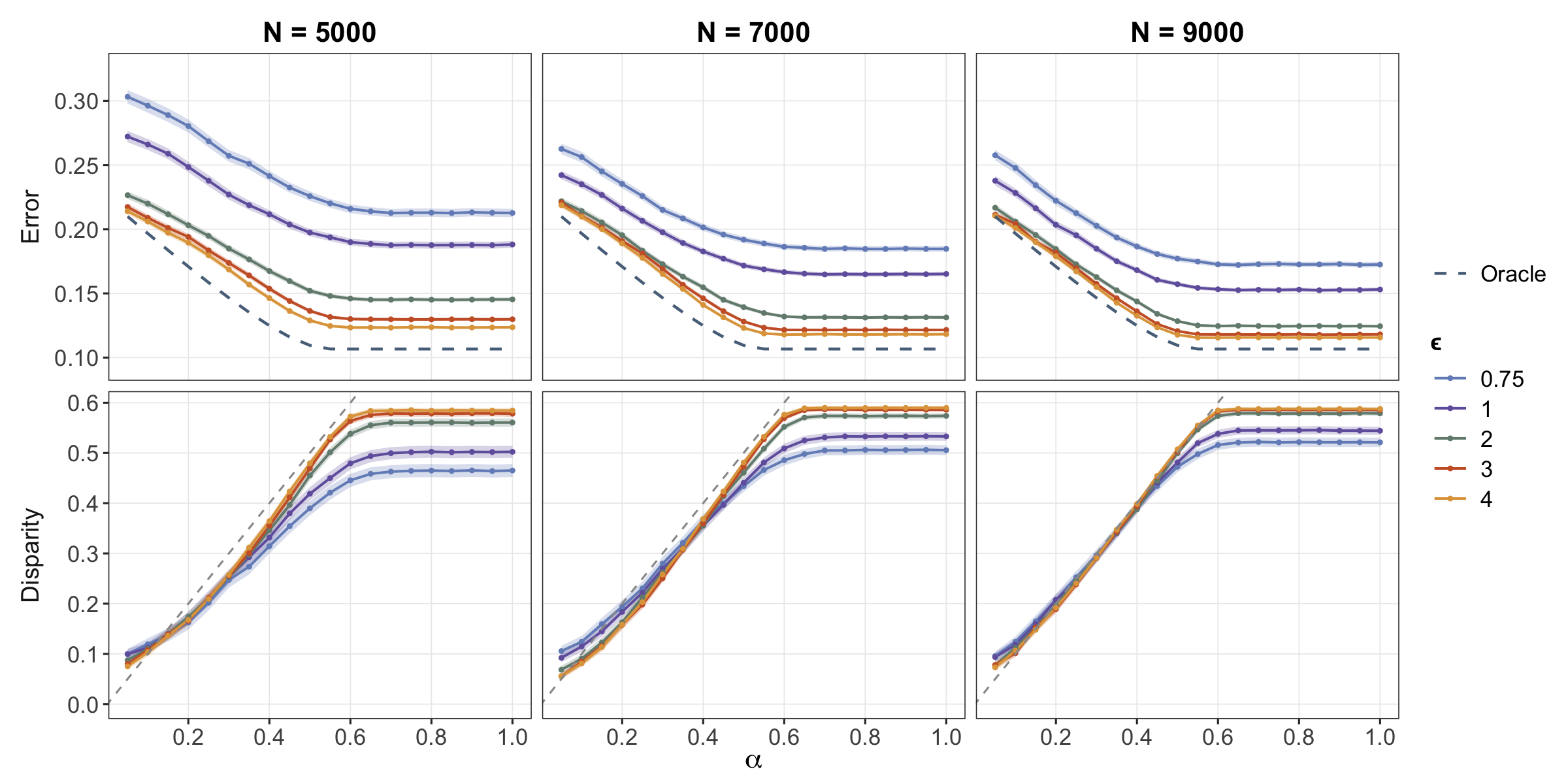
We report the mean misclassification errors and empirical disparities along with their corresponding 95%95\% confidence bands over 200 iterations in Figure 3. For comparisons, we also calculate the oracle misclassification error for group-wise classifiers with and without fairness constraints by simulations on an independent dataset of sample size 200000200000. The simulated Bayes risk for the group-wise classifier without fairness constraint is 0.1060.106, and the intrinsic demographic disparity is 0.5590.559. The simulated Bayes risk for the fairness-aware Bayes classifier is plotted in dashed grey.

Across all sample sizes, Figure 3 exhibits the expected privacy, fairness and accuracy trade-off as shown in Theorem 6 in Section B.3. Our designed classifier CDP-Fair successfully keeps the empirical disparities below the diagonal reference y=xy=x for each α\alpha in the second row of Figure 3, indicating that the target disparity level is respected. In terms of classification accuracy, relaxing the fairness constraint (i.e. increasing α\alpha) yields a noticeable reduction in misclassification error when the fairness constraint is active (i.e. small α\alpha). Once α\alpha exceeds a critical threshold, the fairness constraint becomes inactive and the error curves flatten. Moreover, weakening the privacy constraint (i.e. increasing ϵ\epsilon) reduces the excess risk for each fixed α\alpha, with the performance converging towards the oracle benchmark as ϵ\epsilon grows. Finally, under fixed privacy and fairness parameters (α,ϵ)(\alpha,\epsilon), increasing the sample size NN leads to uniformly smaller misclassification error, and the difference in performance between CDP-Fair and the oracle Bayes fairness-aware classifier becomes less significant when ϵ\epsilon is large.

Refer to caption
Figure 3: Means and 95%95\% confidence bands for misclassification errors and empirical disparities of Algorithm 5 when N∈{5000,7000,9000}N\in\{5000,7000,9000\}. The grey dashed line represents y=xy=x.

5.1.2 Numerical experiments for FDP-Fair in Algorithm 1

To demonstrate the effectiveness of FDP-Fair classifier in Algorithm 1, we generate data following the same mechanism as described in Section 5.1.1, then distribute across various servers. In this subsection, we consider a homogeneous setting where Ns=N=2000N_{s}=N=2000, ϵs=ϵ∈{0.75,1,2,3,4,10}\epsilon_{s}=\epsilon\in\{0.75,1,2,3,4,10\}, δs=δ=(N/2)−2\delta_{s}=\delta=(N/2)^{-2} and vary the number of servers S∈{4,5,6}S\in\{4,5,6\}. We train the classifier using the distributed training data of total size Ntotal=S​NN_{\text{total}}=SN, then test the trained classifier on an independent sample of size 20002000.

In order to implement Algorithm 1, four tuning parameters need to be selected: bandwidth hh, constants CωC_{\omega} and CρC_{\rho} and minimum interval length θ\theta. For all experiments, following the same approach as in Section 5.1.1, we select hh with a three-fold cross-validation on a randomly chosen site. To select θ\theta, we utilise our theoretical results and select θ\theta such that M=max⁡{⌊log2⁡(∑s=1Smin⁡{Ns,Ns2​ϵs2})⌋+1,6}M=\max\{\lfloor\log_{2}\big(\sum_{s=1}^{S}\min\{N_{s},N_{s}^{2}\epsilon_{s}^{2}\}\big)\rfloor+1,6\}. For illustrative purposes, we fix Cω=0.1C_{\omega}=0.1 and ρ=0.03\rho=0.03 throughout the experiments. Sensitivity analysis for CωC_{\omega} and ρ\rho when S=3S=3, Ns=2000N_{s}=2000 and α=0.3\alpha=0.3 are also carried out and defer the results to Section A.2.

To ensure the feasibility of Algorithm 4 in the high privacy regime when the DD~\widetilde{\operatorname*{\mathrm{DD}}} curve fluctuates significantly, we adjust Algorithm 4 to Algorithm 6 detailed in Section A.1 in practice. At a high level, Algorithm 6 outputs a sequence that is as close to non-increasing as possible, subject to bias control.

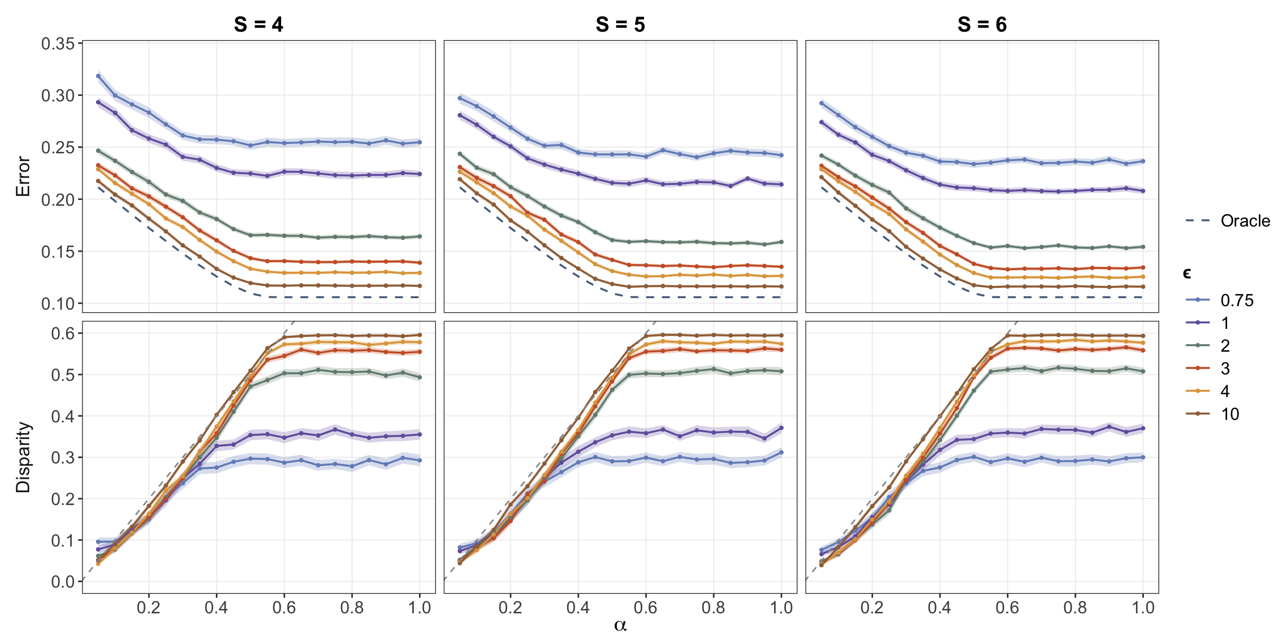
We report the mean misclassification errors and empirical disparities along with their corresponding 95%95\% confidence bands over 200 iterations in Figure 4. Overall, the patterns in Figure 4 closely mirror those observed in Section 5.1.1 and are consistent with our theoretical results detailed in Theorem 2. In particular, as SS increases, the total training sample size S​NSN grows, which leads to uniformly better misclassification error.
Refer to caption
Figure 4: Means and 95%95\% confidence bands for misclassification errors and empirical disparities of Algorithm 1 when Ns=2000N_{s}=2000 and S∈{4,5,6}S\in\{4,5,6\}. The grey dashed line represents y=xy=x.

5.1.3 Effect of the number of servers SS

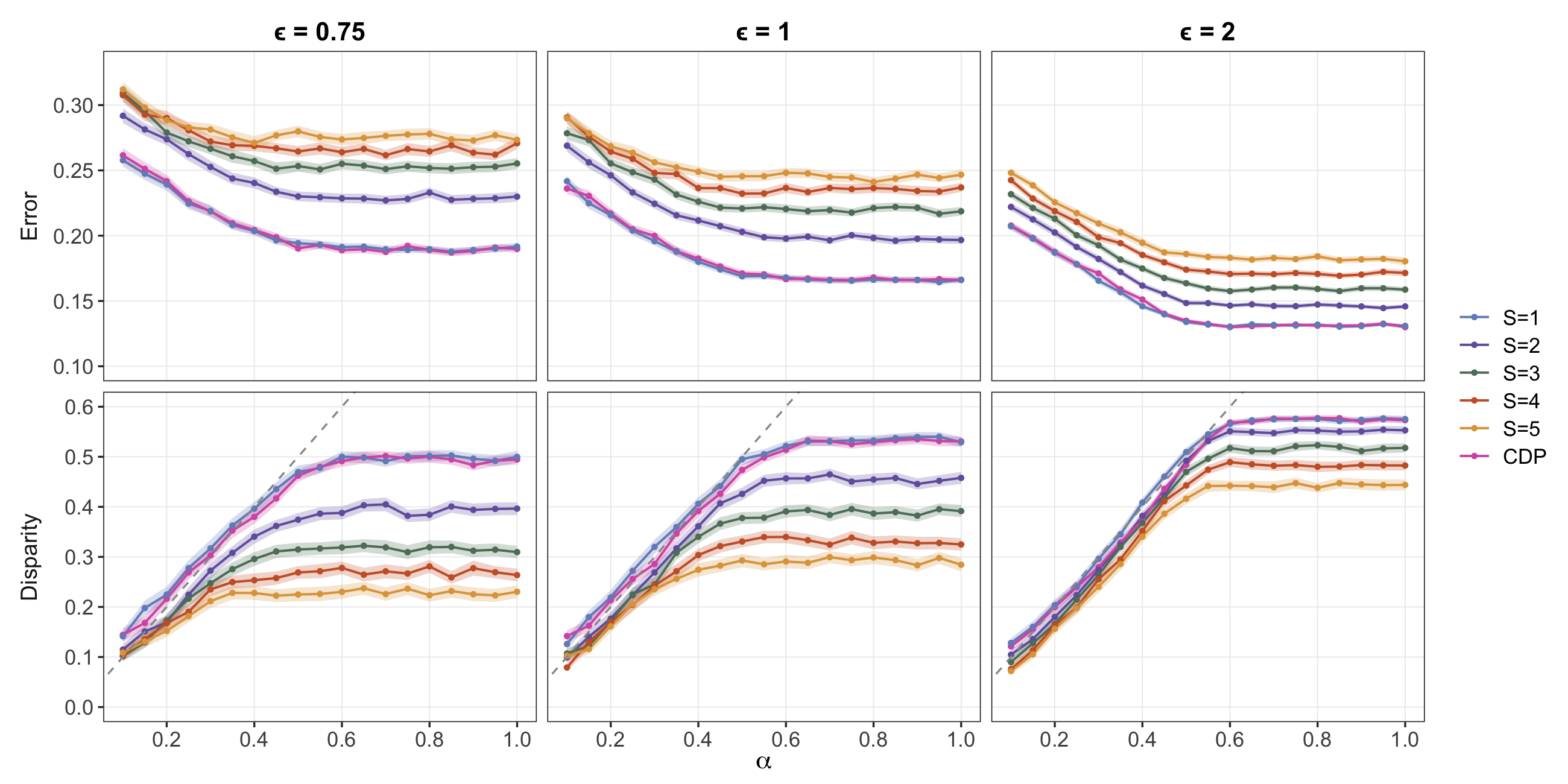
To further study the effect of the distributed nature of data across servers, we consider below the case when a fixed total of Ntotal=7200N_{\text{total}}=7200 data points are equally distributed across S∈{1,2,3,4,5}S\in\{1,2,3,4,5\} servers. In the case when S=1S=1, we further apply CDP-Fair in Algorithm 5. Tuning parameters are selected following the same procedure as described in Section 5.1.2 (Cω=0.1C_{\omega}=0.1, ρ=0.03\rho=0.03). After initial training, we use an independent sample of size 25002500 to test the performance of the trained classifier. The results are collected in Figure 5.

The results in Figure 5 highlight the effect of data decentralisation on both accuracy and disparity control. When S=1S=1, FDP-Fair performs comparably to CDP-Fair, yielding nearly identical misclassification errors and empirical disparities across α\alpha. As SS increases, i.e. when the same amount of data is distributed across more servers, the misclassification error of FDP-Fair deteriorates. Intuitively, distributing a fixed total sample size NtotalN_{\text{total}} across more servers reduces the local sample size per server, which increases estimation error at the server level. Moreover, aggregating output across servers also necessitates additional privacy-preserving communication, introducing extra noise. This phenomenon further echoes our theoretical results in Theorem 2.
Refer to caption
Figure 5: Means and 95%95\% confidence bands for misclassification errors and empirical disparities of Algorithms 1 and 5 when Ntotal=7200N_{\text{total}}=7200 and S∈{1,2,3,4,5}S\in\{1,2,3,4,5\}. The grey dashed line represents y=xy=x.

5.2 Real data analysis

In this section, we compare the performances of CDP-Fair and FDP-Fair with classifiers that satisfy either privacy and fairness constraints or none, on two widely used datasets: AdultCensus and Law school entrance datasets (e.g. Zeng et al., 2024a).

For the privacy-only baseline, we implement CDP-Fair with the fairness step S2 removed. For the fairness-only baseline, we adopt the post-processing approach of Zeng et al. (2024b), using kernel density estimators to obtain the initial regression function estimates. As an unconstrained benchmark, we use a naive plug-in implementation of the group-wise Bayes classifier without privacy or fairness constraints. Finally, we implement CDP-Fair and FDP-Fair with S=1S=1 following the same procedure detailed in Section 5.1, and set Cω=0.1C_{\omega}=0.1 and ρ=0.02\rho=0.02 throughout.

5.2.1 AdultCensus dataset

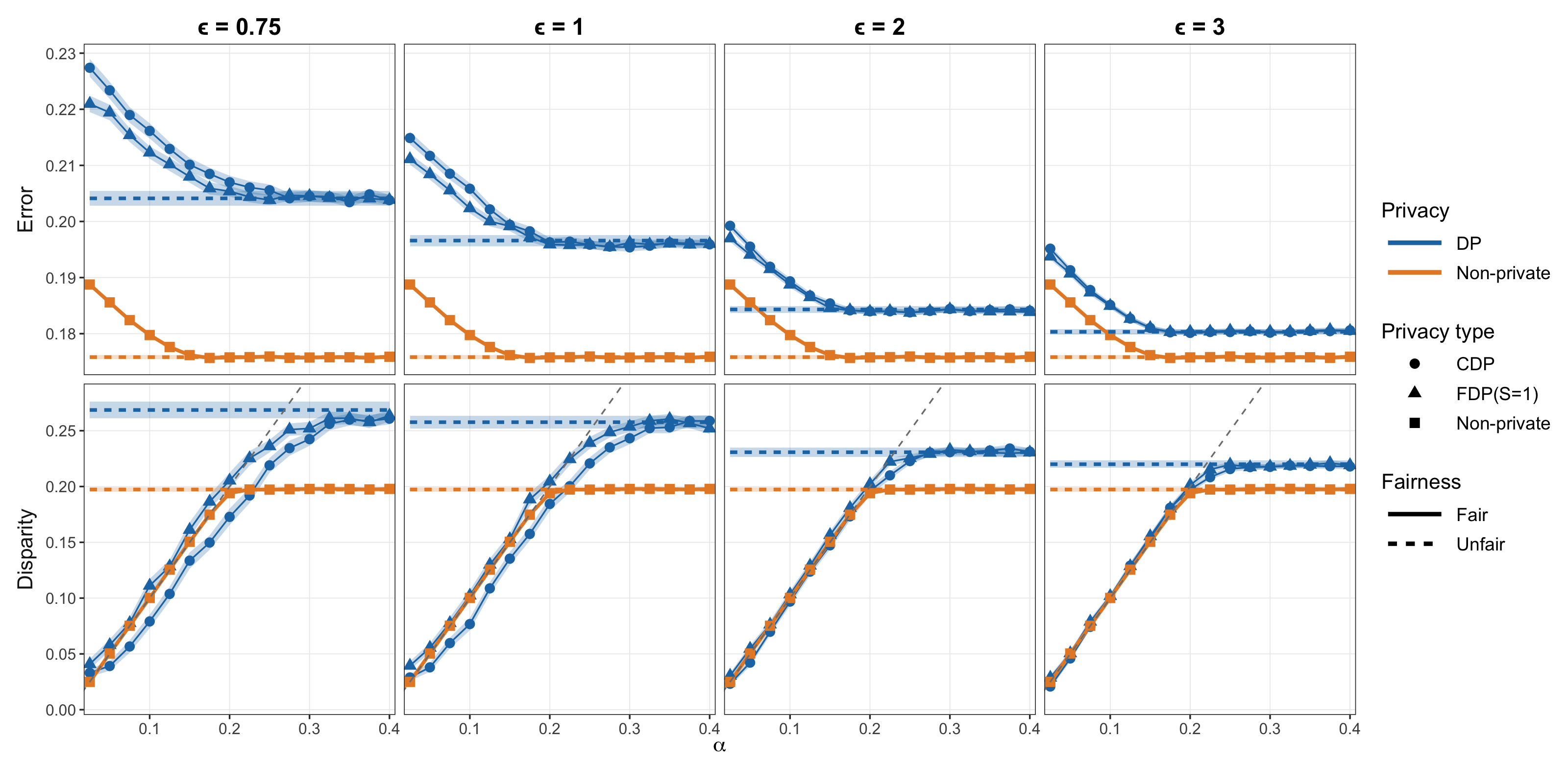
With the AdultCensus dataset, we aim to classify whether an individual’s annual income exceeds $50000. We select age, workclass, and education level as features XX, and take gender as the protected attribute AA. The full dataset contains ntotal=48842n_{\text{total}}=48842 observations. In each experiment, we randomly selected 70%70\% of the data as the training set, and the rest 30%30\% is used as the test dataset. The experiment is repeated for 200200 times, and we report the mean and 95%95\% confidence band in Figure 6. To reflect the post-processing nature of CDP-Fair and FDP-Fair, all unfair classifiers are trained using only half of the available training samples.

As expected, imposing privacy constraints deteriorates classification accuracy. For a fixed fairness level α\alpha, privacy-preserving classifiers incur larger misclassification errors than their non-private counterparts. As ϵ\epsilon increases, the gap steadily narrows, and performance moves towards the non-private regime. In terms of disparity control, classifiers trained without any fairness constraints are substantially unfair, with empirical disparities remaining well above the prescribed tolerance for a wide range of small α\alpha. By contrast, CDP-Fair and FDP-Fair successfully satisfy the fairness requirement, with empirical disparities controlled below the target level α\alpha. Moreover, as ϵ\epsilon increases, CDP-Fair and FDP-Fair converge to the fair non-private benchmark of Zeng et al. (2024a). Finally, the CDP and FDP implementations yield very similar performance, as evidenced by the close overlap of their curves across all panels.

Refer to caption
Figure 6: Means and 95%95\% confidence bands for misclassification errors and empirical disparities on the AdultCensus dataset.

5.2.2 Law school entrance dataset

We further apply our algorithms to a selected subset of the Law school entrance dataset with ntotal=40000n_{\text{total}}=40000. We aim to classify if a student gets admitted to law school using the standard features XX, such as LSAT scores, undergraduate GPA and more. The protected attribute AA is taken as race, i.e. white vs non-white. Numerical results are summarised in Figure 7.

Similar trends as in Section 5.2.1 are observed. One difference compared with Figure 6 is that in the disparity plots of Figure 7, once the fairness constraint becomes inactive for the fair non-private benchmark, the empirical disparities of CDP-Fair and FDP-Fair continue to increase, though they still remain below the prespecified threshold. This gap diminishes as ϵ\epsilon increases. We attribute this behaviour to the bias induced by the data-selection step. In the high-privacy regime, ℙ​(Y~=1∣A=1)\mathbb{P}(\widetilde{Y}=1\mid A=1) can be driven close to 0, while ℙ​(Y~=1∣A=0)\mathbb{P}(\widetilde{Y}=1\mid A=0) becomes comparatively larger than in the non-private case, due to a higher frequency of η~0\widetilde{\eta}_{0} taking values close to 11.

Refer to caption
Figure 7: Means and 95%95\% confidence bands for misclassification errors and empirical disparities on the Law school entrance dataset.

6 Conclusion

In this paper, we study private fairness-aware classification in a distributed setting. To the best of our knowledge, this is the first time seen in the literature. To handle the decentralised nature of data analysis, we propose a two-step plug-in classifier, FDP-fair, which is built upon Gaussian mechanisms and private binary trees. In the special case when there is only one server, we further provide a simplified yet effective algorithm, CDP-Fair. Under appropriate assumptions, theoretical guarantees for privacy, fairness and excess risk controls are provided, which are further supported by extensive numerical experiments on both synthetic and real datasets.

We envisage several potential extensions. Firstly, our algorithms depend on the availability of sensitive features AA, which may be restricted in certain practical settings due to privacy concerns. When sensitive features are available during training but not testing, one possible way is to predict AA using standard feature XX (e.g. Zeng et al., 2024a; Hou and Zhang, 2024). In the case when AA is available but subject to privacy constraints, one may instead adopt a label local DP framework (e.g. Zhao et al., 2025), under which only noisy versions of AA are released for use in the analysis. Secondly, in some scenarios, data from different servers may differ in distribution. Existing literature, e.g. Auddy et al. (2025), attempts to study differentially private transfer learning in non-parametric classifications. It would be interesting to further investigate the effect of data heterogeneity under fairness constraints.

Acknowledgements

Xue is supported by EPSRC programme grant EP/Z531327/1. Yu is partially supported by the Philip Leverhulme Prize and EPSRC programme grant EP/Z531327/1.

References

  • R. J. Adler and J. E. Taylor (2007) Random fields and geometry. Springer. Cited by: §B.3.3, §C.3.1.
  • J. Angwin, J. Larson, S. Mattu, and L. Kirchner (2022) Machine bias. In Ethics of data and analytics, pp. 254–264. Cited by: §1.
  • A. Auddy, T. T. Cai, and A. Chakraborty (2025) Minimax and adaptive transfer learning for nonparametric classification under distributed differential privacy constraints. Journal of the Royal Statistical Society Series B: Statistical Methodology, pp. qkaf070. Cited by: 2nd item, §B.3.3, §1, §2.1, §4.1, §4.3, §6.
  • J. Audibert and A. B. Tsybakov (2007) Fast learning rates for plug-in classifiers. The Annals of Statistics 35 (2), pp. 608 – 633. Cited by: §4.1, §4.3.
  • E. Bagdasaryan, O. Poursaeed, and V. Shmatikov (2019) Differential privacy has disparate impact on model accuracy. Advances in neural information processing systems 32. Cited by: §1.
  • C. Bakalar, R. Barreto, S. Bergman, M. Bogen, B. Chern, S. Corbett-Davies, M. Hall, I. Kloumann, M. Lam, J. Q. Candela, et al. (2021) Fairness on the ground: applying algorithmic fairness approaches to production systems. arXiv preprint arXiv:2103.06172. Cited by: §1.
  • O. Bousquet (2002) A bennett concentration inequality and its application to suprema of empirical processes. Comptes Rendus Mathematique 334 (6), pp. 495–500. Cited by: §C.3.2.
  • C. Butucea, A. Dubois, M. Kroll, and A. Saumard (2020) Local differential privacy: Elbow effect in optimal density estimation and adaptation over Besov ellipsoids. Bernoulli 26 (3), pp. 1727 – 1764. External Links: Document Cited by: §1.
  • T. T. Cai, A. Chakraborty, and L. Vuursteen (2024) Optimal federated learning for nonparametric regression with heterogeneous distributed differential privacy constraints. arXiv preprint arXiv:2406.06755. Cited by: §1, §2.1.
  • T. T. Cai, Y. Wang, and L. Zhang (2021) The cost of privacy: optimal rates of convergence for parameter estimation with differential privacy. The Annals of Statistics 49 (5), pp. 2825–2850. Cited by: §4.2.
  • F. Calmon, D. Wei, B. Vinzamuri, K. Natesan Ramamurthy, and K. R. Varshney (2017) Optimized pre-processing for discrimination prevention. Advances in Neural Information Processing Systems 30. Cited by: §1.
  • L. E. Celis, L. Huang, V. Keswani, and N. K. Vishnoi (2019) Classification with fairness constraints: a meta-algorithm with provable guarantees. In Proceedings of the conference on fairness, accountability, and transparency, pp. 319–328. Cited by: §1.
  • J. Cho, G. Hwang, and C. Suh (2020) A fair classifier using kernel density estimation. Advances in Neural Information Processing Systems 33, pp. 15088–15099. Cited by: §1.
  • C. Denis, R. Elie, M. Hebiri, and F. Hu (2024) Fairness guarantees in multi-class classification with demographic parity. Journal of Machine Learning Research 25 (130), pp. 1–46. Cited by: §1.
  • R. M. Dudley (2016) VN sudakov’s work on expected suprema of gaussian processes. In High Dimensional Probability VII: The Cargèse Volume, pp. 37–43. Cited by: §B.3.3, §C.3.1.
  • R. Durrett (2019) Probability: theory and examples. Vol. 49, Cambridge university press. Cited by: §C.3.2.
  • A. Dvoretzky, J. Kiefer, and J. Wolfowitz (1956) Asymptotic minimax character of the sample distribution function and of the classical multinomial estimator. The Annals of Mathematical Statistics, pp. 642–669. Cited by: §B.2, §B.3.2.
  • C. Dwork, F. McSherry, K. Nissim, and A. Smith (2006) Calibrating noise to sensitivity in private data analysis. In Theory of cryptography conference, pp. 265–284. Cited by: §1, §2.1.
  • C. Dwork, A. Roth, et al. (2014) The algorithmic foundations of differential privacy. Foundations and trends® in theoretical computer science 9 (3–4), pp. 211–407. Cited by: Lemma 38, Lemma 40.
  • G. Ganev, B. Oprisanu, and E. De Cristofaro (2022) Robin hood and matthew effects: differential privacy has disparate impact on synthetic data. In International Conference on Machine Learning, pp. 6944–6959. Cited by: §1.
  • H. Ghoukasian and S. Asoodeh (2024) Differentially private fair binary classifications. In 2024 IEEE International Symposium on Information Theory (ISIT), pp. 611–616. Cited by: §1, §4.2.
  • R. Hall, A. Rinaldo, and L. Wasserman (2013) Differential privacy for functions and functional data. The Journal of Machine Learning Research 14 (1), pp. 703–727. Cited by: §4.3, Lemma 39.
  • W. Heyndrickx, L. Mervin, T. Morawietz, N. Sturm, L. Friedrich, A. Zalewski, A. Pentina, L. Humbeck, M. Oldenhof, R. Niwayama, et al. (2023) Melloddy: cross-pharma federated learning at unprecedented scale unlocks benefits in qsar without compromising proprietary information. Journal of chemical information and modeling 64 (7), pp. 2331–2344. Cited by: §1.1.
  • X. Hou and L. Zhang (2024) Finite-sample and distribution-free fair classification: optimal trade-off between excess risk and fairness, and the cost of group-blindness. arXiv preprint arXiv:2410.16477. Cited by: §1, §4.2, §6.
  • X. Hu, G. Xue, Z. Lin, and Y. Yu (2025) Fairness-aware bayes optimal functional classification. arXiv preprint arXiv:2505.09471. Cited by: §B.3.2, §B.3.2, §4.2.
  • E. K. Hung and Y. Yu (2025) Optimal cox regression under federated differential privacy: coefficients and cumulative hazards. arXiv preprint arXiv:2508.19640. Cited by: §C.1.
  • M. Jagielski, M. Kearns, J. Mao, A. Oprea, A. Roth, S. Sharifi-Malvajerdi, and J. Ullman (2019) Differentially private fair learning. In International Conference on Machine Learning, pp. 3000–3008. Cited by: §1.
  • J. E. Johndrow and K. Lum (2019) An algorithm for removing sensitive information. The Annals of Applied Statistics 13 (1), pp. 189–220. Cited by: §1.
  • V. Karwa and S. Vadhan (2017) Finite sample differentially private confidence intervals. arXiv preprint arXiv:1711.03908. Cited by: §1.
  • J. Kim, J. Shin, A. Rinaldo, and L. Wasserman (2019) Uniform convergence rate of the kernel density estimator adaptive to intrinsic volume dimension. In International Conference on Machine Learning, pp. 3398–3407. Cited by: §4.1.
  • M. Li, Y. Tian, Y. Feng, and Y. Yu (2024) Federated transfer learning with differential privacy. arXiv preprint arXiv:2403.11343. Cited by: §2.1, §4.3.
  • X. Li, Y. Gu, N. Dvornek, L. H. Staib, P. Ventola, and J. S. Duncan (2020) Multi-site fmri analysis using privacy-preserving federated learning and domain adaptation: abide results. Medical image analysis 65, pp. 101765. Cited by: §1.1.
  • C. M. Madrid Padilla, H. Xu, D. Wang, O. H. MADRID PADILLA, and Y. Yu (2023) Change point detection and inference in multivariate non-parametric models under mixing conditions. Advances in Neural Information Processing Systems 36, pp. 21081–21134. Cited by: §4.1, §4.1.
  • P. Mangold, M. Perrot, A. Bellet, and M. Tommasi (2023) Differential privacy has bounded impact on fairness in classification. In International Conference on Machine Learning, pp. 23681–23705. Cited by: §1.
  • N. Martinez, M. Bertran, and G. Sapiro (2020) Minimax pareto fairness: a multi objective perspective. In International conference on machine learning, pp. 6755–6764. Cited by: §1.
  • P. Massart (1990) The tight constant in the dvoretzky-kiefer-wolfowitz inequality. The annals of Probability, pp. 1269–1283. Cited by: §B.2, §B.3.2.
  • D. Pessach and E. Shmueli (2022) A review on fairness in machine learning. ACM Computing Surveys (CSUR) 55 (3), pp. 1–44. Cited by: §1.
  • J. Quiñonero Candela, Y. Wu, B. Hsu, S. Jain, J. Ramos, J. Adams, R. Hallman, and K. Basu (2023) Disentangling and operationalizing ai fairness at linkedin. In Proceedings of the 2023 ACM Conference on Fairness, Accountability, and Transparency, pp. 1213–1228. Cited by: §1.
  • P. Rigollet and R. Vert (2009) Optimal rates for plug-in estimators of density level sets. Bernoulli 15 (4), pp. 1154 – 1178. Cited by: footnote 1.
  • L. Say, C. Denis, and R. Pinot (2025) Fairness meets privacy: integrating differential privacy and demographic parity in multi-class classification. arXiv preprint arXiv:2511.18876. Cited by: §1.
  • J. Smith, H. J. Asghar, G. Gioiosa, S. Mrabet, S. Gaspers, and P. Tyler (2021) Making the most of parallel composition in differential privacy. arXiv preprint arXiv:2109.09078. Cited by: §B.1.
  • S. Song, T. Steinke, O. Thakkar, and A. Thakurta (2021) Evading the curse of dimensionality in unconstrained private glms. In International Conference on Artificial Intelligence and Statistics, pp. 2638–2646. Cited by: §1.
  • United States Census Bureau (2021) Census bureau sets key parameters to protect privacy in 2020 census results. Note: https://www.census.gov/newsroom/press-releases/2021/2020-census-key-parameters.html Cited by: §1.
  • A. W. Van Der Vaart and J. A. Wellner (1996) Weak convergence. In Weak convergence and empirical processes: with applications to statistics, pp. 16–28. Cited by: §C.3.2.
  • R. Vershynin (2018) High-dimensional probability: an introduction with applications in data science. Vol. 47, Cambridge university press. Cited by: §B.2, §B.3.1, §B.3.2, §B.3.3, §B.3.3, §B.3.4, §B.3.4, §B.3.4, §C.3.1, §C.3.2, §C.3.2, §C.3.2, §C.3.2, §C.3.4, §C.3.4.
  • G. Xue, Z. Lin, and Y. Yu (2024) Optimal estimation in private distributed functional data analysis. arXiv preprint arXiv:2412.06582. Cited by: §2.1.
  • A. Yousefpour, I. Shilov, A. Sablayrolles, D. Testuggine, K. Prasad, M. Malek, J. Nguyen, S. Ghosh, A. Bharadwaj, J. Zhao, et al. (2021) Opacus: user-friendly differential privacy library in pytorch. arXiv preprint arXiv:2109.12298. Cited by: §1.
  • X. Zeng, G. Cheng, and E. Dobriban (2024a) Bayes-optimal fair classification with linear disparity constraints via pre-, in-, and post-processing. arXiv preprint arXiv:2402.02817. Cited by: §1, §2.2, §4.1, §5.2.1, §5.2, §6, Definition 6, Remark 1, Proposition 41, Theorem 42, Proposition 43.
  • X. Zeng, G. Cheng, and E. Dobriban (2024b) Minimax optimal fair classification with bounded demographic disparity. arXiv preprint arXiv:2403.18216. Cited by: §4.1, §4.3, §4.3, §5.2, Definition 5.
  • P. Zhao, C. Ma, L. Shen, S. Wang, and R. Fan (2025) On theoretical limits of learning with label differential privacy. arXiv preprint arXiv:2502.14309. Cited by: §6.
  • X. Zhou and R. Bassily (2024) Differentially private worst-group risk minimization. In Forty-first International Conference on Machine Learning, External Links: Link Cited by: §1.

Appendices

All technical details and additional numerical results are collected in the Appendices. Additional numerical experiments are presented in Appendix A. We provide all proofs related to Algorithms 5 and 1 in Appendices B and C, respectively. For completeness, additional background results are provided in Appendix D.

Throughout the appendix, with a slight abuse of notation, unless specifically stated otherwise, let C1,C2,…>0C_{1},C_{2},\ldots>0 denote constants whose values may vary from place to place and depend on dd. Let ⋅^s\widehat{\cdot}_{s} denote standard empirical estimators without privacy constraints for site ss, s∈[S]s\in[S], and ⋅^\widehat{\cdot} the aggregated one. Similarly, let ⋅~s\widetilde{\cdot}_{s} denote the site-wise estimators that satisfy privacy constraints, and let ⋅~\widetilde{\cdot} denote the aggregated one in the central server.

For notational simplicity, throughout the appendix, we write τ~=τ~DD,α\widetilde{\tau}=\widetilde{\tau}_{\operatorname*{\mathrm{DD}},\alpha}.

Appendix A Additional numerical experiments

A.1 Additional algorithm

To ensure the feasibility of the Algorithm 4 in the high privacy regime when the DD curve fluctuates significantly, we adjust Algorithm 4 to Algorithm 6 detailed below in practice.

Algorithm 6 Non.increasing (numerical)({gi}i∈2M+1\{g_{i}\}_{i\in 2^{M}+1}, {μs}s∈[S]\{\mu_{s}\}_{s\in[S]}, CωC_{\omega}, MM, η\eta)
Sequence of number {gi}i∈2M+1\{g_{i}\}_{i\in 2^{M}+1}, weight {μs}s∈[S]\{\mu_{s}\}_{s\in[S]}, constants CωC_{\omega}, binary tree layer MM, tolerance η\eta.
Set the tolerance level
ω=Cω​∑s=1Sμs2​M4​log⁡(1/δs)​log⁡(M/η)n˘s2​ϵs2.\displaystyle\omega=C_{\omega}\sqrt{\sum_{s=1}^{S}\frac{\mu_{s}^{2}M^{4}\log(1/\delta_{s})\log(M/\eta)}{\breve{n}_{s}^{2}\epsilon_{s}^{2}}}.
if gi≥…≥g2M+1g_{i}\geq\ldots\geq g_{2^{M}+1} then
  Break and return {gi}i∈[2M+1]\{g_{i}\}_{i\in[2^{M}+1]}.
else
  Initialize fn=min⁡{gn+ω, 1}f_{n}=\min\{g_{n}+\omega,\,1\}.
  for i=n−1,n−2,…,1i=n-1,n-2,\dots,1 do
   Set fi←min⁡(min⁡{gi+ω, 1},max⁡(max⁡{gi−ω, 0},fi+1))f_{i}\leftarrow\min\bigl(\min\{g_{i}+\omega,\,1\},\;\max(\max\{g_{i}-\omega,\,0\},\;f_{i+1})\bigr).
  end for
end if
{fi}i∈2N+1\{f_{i}\}_{i\in 2^{N}+1}.

A.2 Sensitivity analysis

Under the same setup detailed in Section 5.1.2, we carry out sensitivity analysis for tuning parameters CωC_{\omega} and ρ\rho in a setting where S=3S=3, ns=2000n_{s}=2000, ntest=2000n_{\text{test}}=2000 and α=0.3\alpha=0.3. Numerical experiments are collected in Figures 8 and 9 below.

As detailed in Algorithm 1, ρ\rho determines the tolerance band used in selecting τ~\widetilde{\tau} through the optimisation problem τ~=arg​minτ∈𝒢⁡{|τ|:|DD~↓​(τ)|∈[α−ρ,α+ρ]}\widetilde{\tau}=\operatorname*{arg\,min}_{\tau\in\mathcal{G}}\{|\tau|:|\widetilde{\operatorname*{\mathrm{DD}}}_{\downarrow}(\tau)|\in[\alpha-\rho,\alpha+\rho]\}. Since DD~↓(⋅)\widetilde{\operatorname*{\mathrm{DD}}}{\downarrow}(\cdot) is, with high probability, a monotonically non-increasing function, choosing the feasible τ∈𝒢\tau\in\mathcal{G} with the smallest magnitude tends to pick a threshold for which DD~↓(τ~)\widetilde{\operatorname*{\mathrm{DD}}}{\downarrow}(\widetilde{\tau}) lies near the upper end of the admissible band, i.e. closer to α+ρ\alpha+\rho. Consequently, a larger ρ\rho typically leads to a larger disparity of f~\widetilde{f}, potentially exceeding α\alpha, yet remaining below α+ρ\alpha+\rho. This behaviour is precisely illustrated in Figure 8.

In Algorithm 6, CωC_{\omega} controls the bias incurred when constructing a sequence that is as close to non-increasing as possible. Based on the numerical results in Figure 9, the performance is not particularly sensitive to CωC_{\omega} in terms of either misclassification error or empirical disparity. The slightly upward trend in the disparity plot is mainly because a larger CωC_{\omega} increases the possibilities that the adjusted sequence is non-increasing, which can in turn lead to a slightly more accurate choice of τ~\widetilde{\tau}. However, the corresponding effect on misclassification error is less significant.

Refer to caption
Figure 8: Sensitivity analysis for ρ\rho. The grey dotted lines are y=0.3y=0.3 and y=0.3+ρy=0.3+\rho, respectively.
Refer to caption
Figure 9: Sensitivity analysis for CωC_{\omega}. The grey dotted line represents y=0.3y=0.3.

Appendix B Theoretical guarantee for Algorithm 5

B.1 Privacy guarantee

Proposition 4.

Algorithm 5 is (ϵ,δ)(\epsilon,\delta)-CDP.

Proof.

We divide the proof into two steps, with the first step quantifying the sensitivity parameters used in Lemmas 38 and 39, and the second step involving DP compositions.

Step 1: Upper bound on sensitivity In this step, we upper bound ℓ2\ell_{2} sensitivities for terms of interests in the calculation of π~a\widetilde{\pi}_{a}, p~X|A=a\widetilde{p}_{X|A=a}, η~a\widetilde{\eta}_{a} and DD~\widetilde{\operatorname*{\mathrm{DD}}}. Without loss of generality, we consider the case when A1=a=1A_{1}=a=1 and Y1=1Y_{1}=1. We further assume that only the first data point in the dataset changes i.e. 𝒟={(Xi,Ai,Yi)}i∈[n]\mathcal{D}=\{(X_{i},A_{i},Y_{i})\}_{i\in[n]}, 𝒟′=(X1′,A1′,Y1′)∪{(Xi,Ai,Yi)}i∈[n]\{1}\mathcal{D}^{\prime}=(X_{1}^{\prime},A_{1}^{\prime},Y_{1}^{\prime})\cup\{(X_{i},A_{i},Y_{i})\}_{i\in[n]\backslash\{1\}}. Similar notation is considered for the calibration data 𝒟˘\breve{\mathcal{D}} and 𝒟˘′\breve{\mathcal{D}}^{\prime}. Five general cases are considered below, and other cases can be justified similarly:

  • Case 1: A1=A1′A_{1}=A_{1}^{\prime}, X1=X1′X_{1}=X_{1}^{\prime} and Y1≠Y1′Y_{1}\neq Y_{1}^{\prime};

  • Case 2: A1=A1′A_{1}=A_{1}^{\prime}, X1≠X1′X_{1}\neq X_{1}^{\prime} and Y1=Y1′Y_{1}=Y_{1}^{\prime};

  • Case 3: A1=A1′A_{1}=A_{1}^{\prime}, X1≠X1′X_{1}\neq X_{1}^{\prime} and Y1≠Y1′Y_{1}\neq Y_{1}^{\prime};

  • Case 4: A1≠A1′A_{1}\neq A_{1}^{\prime}, (X1,Y1)=(X1′,Y1′)(X_{1},Y_{1})=(X_{1}^{\prime},Y_{1}^{\prime});

  • Case 5: A1≠A1′A_{1}\neq A_{1}^{\prime}, (X1,Y1)≠(X1′,Y1′)(X_{1},Y_{1})\neq(X_{1}^{\prime},Y_{1}^{\prime}).

  • •

    For π~a\widetilde{\pi}_{a}:

    1. 1.

      Cases 1-3: Since A1=A1′A_{1}=A_{1}^{\prime} in these cases, we have that na,0+na,1=na,0′+na,1′n_{a,0}+n_{a,1}=n^{\prime}_{a,0}+n^{\prime}_{a,1}. Thus,

      Δ=|na,0+na,1n−na,0′+na,1′n|=0.\displaystyle\Delta=\Big|\frac{n_{a,0}+n_{a,1}}{n}-\frac{n^{\prime}_{a,0}+n^{\prime}_{a,1}}{n}\Big|=0.
    2. 2.

      Cases 4 and 5: Since A1≠A1′A_{1}\neq A_{1}^{\prime} in these cases, we have that |na,0+na,1−(na,0′+na,1′)|=1|n_{a,0}+n_{a,1}-(n^{\prime}_{a,0}+n^{\prime}_{a,1})|=1. Thus,

      Δ=|na,0+na,1n−na,0′+na,1′n|=1n.\displaystyle\Delta=\Big|\frac{n_{a,0}+n_{a,1}}{n}-\frac{n^{\prime}_{a,0}+n^{\prime}_{a,1}}{n}\Big|=\frac{1}{n}.
  • •

    For p~X|A=a\widetilde{p}_{X|A=a}: The proof follows from a similar argument as the one on Auddy et al. (2025). Denote ∥⋅∥𝒦\|\cdot\|_{\mathcal{K}} the RKHS norm of the space given by linear combination {∑iθiK{(Xi−⋅)/h}:θi∈ℝ}\{\sum_{i}\theta_{i}K\{(X_{i}-\cdot)/h\}:\theta_{i}\in\mathbb{R}\}. We also rewrite

    1na​∑y∈{0,1}∑i=1na,yKh​(Xa,yi−x)=1na​∑i=1nKh​(Xi−x)​𝟙​{Ai=a}.\frac{1}{n_{a}}\sum_{y\in\{0,1\}}\sum_{i=1}^{n_{a,y}}K_{h}(X_{a,y}^{i}-x)=\frac{1}{n_{a}}\sum_{i=1}^{n}K_{h}(X_{i}-x)\mathds{1}\{A_{i}=a\}.
    1. 1.

      Cases 1-3: Since A1=A1′A_{1}=A_{1}^{\prime} in these cases, we have that

      Δ𝒦=\displaystyle\Delta_{\mathcal{K}}=\; ∥1na∑i=1nKh(Xi−⋅)𝟙{Ai=a}−1na′∑i=1nKh(Xi′−⋅)𝟙{Ai′=a}∥𝒦\displaystyle\Big\|\frac{1}{n_{a}}\sum_{i=1}^{n}K_{h}(X_{i}-\cdot)\mathds{1}\{A_{i}=a\}-\frac{1}{n_{a}^{\prime}}\sum_{i=1}^{n}K_{h}(X^{\prime}_{i}-\cdot)\mathds{1}\{A^{\prime}_{i}=a\}\Big\|_{\mathcal{K}}
      =\displaystyle=\; 1na∥Kh(X1−⋅)−Kh(X1′−⋅)∥𝒦≤2​CKna​hd,\displaystyle\frac{1}{n_{a}}\Big\|K_{h}(X_{1}-\cdot)-K_{h}(X_{1}^{\prime}-\cdot)\Big\|_{\mathcal{K}}\leq\frac{2\sqrt{C_{K}}}{n_{a}h^{d}},

      the last inequality follows from 2a.

    2. 2.

      Cases 4 and 5: Since A1≠A1′A_{1}\neq A_{1}^{\prime} in these two cases, we have that na′=na−1n_{a}^{\prime}=n_{a}-1 and

      Δ𝒦=\displaystyle\Delta_{\mathcal{K}}=\; ∥1na∑i=1nKh(Xi−⋅)𝟙{Ai=a}−1na−1∑i=1nKh(Xi′−⋅)𝟙{Ai′=a}∥𝒦\displaystyle\Big\|\frac{1}{n_{a}}\sum_{i=1}^{n}K_{h}(X_{i}-\cdot)\mathds{1}\{A_{i}=a\}-\frac{1}{n_{a}-1}\sum_{i=1}^{n}K_{h}(X^{\prime}_{i}-\cdot)\mathds{1}\{A^{\prime}_{i}=a\}\Big\|_{\mathcal{K}}
      ≤\displaystyle\leq\; 1na−1(1−na−1na)∥∑i=2nKh(Xi−⋅)𝟙{Ai=a}∥𝒦\displaystyle\frac{1}{n_{a}-1}\Big(1-\frac{n_{a}-1}{n_{a}}\Big)\Big\|\sum_{i=2}^{n}K_{h}(X_{i}-\cdot)\mathds{1}\{A_{i}=a\}\Big\|_{\mathcal{K}}
      +1na∥Kh(X1−⋅)∥𝒦\displaystyle+\frac{1}{n_{a}}\Big\|K_{h}(X_{1}-\cdot)\Big\|_{\mathcal{K}}
      ≤\displaystyle\leq\; 2​CKna​hd.\displaystyle\frac{2\sqrt{C_{K}}}{n_{a}h^{d}}.
  • •

    For η~a\widetilde{\eta}_{a}: The proof is very similar to the proof of p~X|A=a\widetilde{p}_{X|A=a}. Rewrite

    1na​∑i=1na,1Kh​(Xa,1i−x)=1na​∑i=1nYi​Kh​(Xi−x)​𝟙​{Ai=1}.\displaystyle\frac{1}{n_{a}}\sum_{i=1}^{n_{a,1}}K_{h}(X_{a,1}^{i}-x)=\frac{1}{n_{a}}\sum_{i=1}^{n}Y_{i}K_{h}(X_{i}-x)\mathds{1}\{A_{i}=1\}.
    1. 1.

      Cases 1 and 3: In these two cases, we have that A1=A1′=1A_{1}=A_{1}^{\prime}=1 and 1=Y1≠Y1′=01=Y_{1}\neq Y_{1}^{\prime}=0. Thus,

      Δ𝒦=\displaystyle\Delta_{\mathcal{K}}=\; ∥1na∑i=1nYiKh(Xi−⋅)𝟙{Ai=1}−1na∑i=1nYi′Kh(Xi′−⋅)𝟙{Ai′=1}∥𝒦\displaystyle\Big\|\frac{1}{n_{a}}\sum_{i=1}^{n}Y_{i}K_{h}(X_{i}-\cdot)\mathds{1}\{A_{i}=1\}-\frac{1}{n_{a}}\sum_{i=1}^{n}Y^{\prime}_{i}K_{h}(X^{\prime}_{i}-\cdot)\mathds{1}\{A^{\prime}_{i}=1\}\Big\|_{\mathcal{K}}
      =\displaystyle=\; 1na∥Y1Kh(X1−⋅)∥𝒦≤CKna​hd.\displaystyle\frac{1}{n_{a}}\Big\|Y_{1}K_{h}(X_{1}-\cdot)\Big\|_{\mathcal{K}}\leq\frac{\sqrt{C_{K}}}{n_{a}h^{d}}.
    2. 2.

      Case 2: In this case, we have that A1=A1′=1A_{1}=A_{1}^{\prime}=1 and Y1=Y1′=1Y_{1}=Y_{1}^{\prime}=1. Thus,

      Δ𝒦=1na∥Y1Kh(X1−⋅)−Y1′Kh(X1′−⋅)∥𝒦≤2​CKna​hd.\displaystyle\Delta_{\mathcal{K}}=\frac{1}{n_{a}}\Big\|Y_{1}K_{h}(X_{1}-\cdot)-Y^{\prime}_{1}K_{h}(X^{\prime}_{1}-\cdot)\Big\|_{\mathcal{K}}\leq\frac{2\sqrt{C_{K}}}{n_{a}h^{d}}.
    3. 3.

      Cases 4 and 5: we have that 1=A1≠A1′=01=A_{1}\neq A_{1}^{\prime}=0. Thus,

      Δ𝒦=\displaystyle\Delta_{\mathcal{K}}=\; ∥1na∑i=1nYiKh(Xi−⋅)𝟙{Ai=1}−1na−1∑i=1nYi′Kh(Xi′−⋅)𝟙{Ai′=1}∥𝒦\displaystyle\Big\|\frac{1}{n_{a}}\sum_{i=1}^{n}Y_{i}K_{h}(X_{i}-\cdot)\mathds{1}\{A_{i}=1\}-\frac{1}{n_{a}-1}\sum_{i=1}^{n}Y^{\prime}_{i}K_{h}(X^{\prime}_{i}-\cdot)\mathds{1}\{A^{\prime}_{i}=1\}\Big\|_{\mathcal{K}}
      =\displaystyle=\; 1na​(na−1)∥∑i=2nYiKh(Xi−⋅)𝟙{Ai=1}∥𝒦+1na∥Y1Kh(X1−⋅)∥𝒦\displaystyle\frac{1}{n_{a}(n_{a}-1)}\Big\|\sum_{i=2}^{n}Y_{i}K_{h}(X_{i}-\cdot)\mathds{1}\{A_{i}=1\}\Big\|_{\mathcal{K}}+\frac{1}{n_{a}}\Big\|Y_{1}K_{h}(X_{1}-\cdot)\Big\|_{\mathcal{K}}
      ≤\displaystyle\leq\; 2​CKna​hd.\displaystyle\frac{2\sqrt{C_{K}}}{n_{a}h^{d}}.
  • •

    For DD~​(τ)\widetilde{\operatorname*{\mathrm{DD}}}(\tau): Rewrite

    1n˘1​∑y∈{0,1}∑i=1n˘1,y𝟙​{η~1​(X˘1,yi)≥12+τ2​π~1}−1n˘0​∑y∈{0,1}∑i=1n˘0,y𝟙​{η~0​(X˘0,yi)≥12−τ2​π~0}\displaystyle\frac{1}{\breve{n}_{1}}\sum_{y\in\{0,1\}}\sum_{i=1}^{\breve{n}_{1,y}}\mathds{1}\Big\{\widetilde{\eta}_{1}(\breve{X}^{i}_{1,y})\geq\frac{1}{2}+\frac{\tau}{2\widetilde{\pi}_{1}}\Big\}-\frac{1}{\breve{n}_{0}}\sum_{y\in\{0,1\}}\sum_{i=1}^{\breve{n}_{0,y}}\mathds{1}\Big\{\widetilde{\eta}_{0}(\breve{X}^{i}_{0,y})\geq\frac{1}{2}-\frac{\tau}{2\widetilde{\pi}_{0}}\Big\}
    =\displaystyle=\; 1n˘1​∑i=1n˘𝟙​{η~1​(X˘i)≥12+τ2​π~1}​𝟙​{Ai=1}−1n˘0​∑i=1n˘𝟙​{η~0​(X˘i)≥12−τ2​π~0}​𝟙​{Ai=0}.\displaystyle\frac{1}{\breve{n}_{1}}\sum_{i=1}^{\breve{n}}\mathds{1}\Big\{\widetilde{\eta}_{1}(\breve{X}_{i})\geq\frac{1}{2}+\frac{\tau}{2\widetilde{\pi}_{1}}\Big\}\mathds{1}\{A_{i}=1\}-\frac{1}{\breve{n}_{0}}\sum_{i=1}^{\breve{n}}\mathds{1}\Big\{\widetilde{\eta}_{0}(\breve{X}_{i})\geq\frac{1}{2}-\frac{\tau}{2\widetilde{\pi}_{0}}\Big\}\mathds{1}\{A_{i}=0\}.
    1. 1.

      Cases 1-3: In these three cases, we have that A1=A1′=1A_{1}=A_{1}^{\prime}=1, therefore, it holds that

      Δ=1n˘1​|𝟙​{η~1​(X˘1)≥12+τ2​π~1}−𝟙​{η~1​(X˘1′)≥12+τ2​π~1}|≤1n˘1.\displaystyle\Delta=\frac{1}{\breve{n}_{1}}\Big|\mathds{1}\Big\{\widetilde{\eta}_{1}(\breve{X}_{1})\geq\frac{1}{2}+\frac{\tau}{2\widetilde{\pi}_{1}}\Big\}-\mathds{1}\Big\{\widetilde{\eta}_{1}(\breve{X}_{1}^{\prime})\geq\frac{1}{2}+\frac{\tau}{2\widetilde{\pi}_{1}}\Big\}\Big|\leq\frac{1}{\breve{n}_{1}}.
    2. 2.

      Cases 4-6: In these three cases, we have that 1=A1≠A1′=01=A_{1}\neq A_{1}^{\prime}=0. Therefore, we have that n˘1′=n˘1−1\breve{n}_{1}^{\prime}=\breve{n}_{1}-1 and n˘0′=n˘0+1\breve{n}_{0}^{\prime}=\breve{n}_{0}+1. Thus,

      Δ≤\displaystyle\Delta\leq\; |1n˘1​(n˘1−1)∑i=2n𝟙{η~1(X˘i)≥12+τ2​π~1}𝟙{Ai=1}\displaystyle\Big|\frac{1}{\breve{n}_{1}(\breve{n}_{1}-1)}\sum_{i=2}^{n}\mathds{1}\Big\{\widetilde{\eta}_{1}(\breve{X}_{i})\geq\frac{1}{2}+\frac{\tau}{2\widetilde{\pi}_{1}}\Big\}\mathds{1}\{A_{i}=1\}
      −1n˘0​(n˘0+1)​|∑i=2n𝟙​{η~0​(X˘i)≥12−τ2​π~0}​𝟙​{Ai=0}|\displaystyle-\frac{1}{\breve{n}_{0}(\breve{n}_{0}+1)}\Big|\sum_{i=2}^{n}\mathds{1}\Big\{\widetilde{\eta}_{0}(\breve{X}_{i})\geq\frac{1}{2}-\frac{\tau}{2\widetilde{\pi}_{0}}\Big\}\mathds{1}\{A_{i}=0\}\Big|
      +|1n˘1​𝟙​{η~1​(X˘1)≥12+τ2​π~1}−1n˘0+1​𝟙​{η~0​(X˘1′)≥12−τ2​π~0}|\displaystyle+\Big|\frac{1}{\breve{n}_{1}}\mathds{1}\Big\{\widetilde{\eta}_{1}(\breve{X}_{1})\geq\frac{1}{2}+\frac{\tau}{2\widetilde{\pi}_{1}}\Big\}-\frac{1}{\breve{n}_{0}+1}\mathds{1}\Big\{\widetilde{\eta}_{0}(\breve{X}^{\prime}_{1})\geq\frac{1}{2}-\frac{\tau}{2\widetilde{\pi}_{0}}\Big\}\Big|
      ≤\displaystyle\leq\; 1n˘1+1n˘0+1≤2n˘0∧n˘1.\displaystyle\frac{1}{\breve{n}_{1}}+\frac{1}{\breve{n}_{0}+1}\leq\frac{2}{\breve{n}_{0}\wedge\breve{n}_{1}}.

Step 2: DP guarantee. In this step we will show that the final output is (ϵ,δ)(\epsilon,\delta)-DP.

Step 2-1: Privacy guarantee for each estimator. By Step 1 and Lemmas 38 and 39, it holds that π~0\widetilde{\pi}_{0} and π~1\widetilde{\pi}_{1} are (ϵ/4,δ/4)(\epsilon/4,\delta/4)-DP each; p~X|A=0\widetilde{p}_{X|A=0} and p~X|A=1\widetilde{p}_{X|A=1} are (ϵ/4,δ/4)(\epsilon/4,\delta/4)-DP each; η~0\widetilde{\eta}_{0} and η~1\widetilde{\eta}_{1} are (ϵ/4,δ/4)(\epsilon/4,\delta/4)-DP each; and DD~​(τ)\widetilde{\operatorname*{\mathrm{DD}}}(\tau) is (ϵ,δ)(\epsilon,\delta)-DP for a given τ∈ℝ\tau\in\mathbb{R}. To show the privacy guarantee for τ~\widetilde{\tau}, note that for any τ≥0\tau\geq 0, we have that

ℙ​(τ~≤τ|𝒟,𝒟˘)≤ℙ​(DD~​(τ)≤α|𝒟,𝒟˘)≤eϵ​ℙ​(DD~′​(τ)≤α|𝒟,𝒟˘′)+δ,\displaystyle\mathbb{P}(\widetilde{\tau}\leq\tau|\mathcal{D},\breve{\mathcal{D}})\leq\mathbb{P}(\widetilde{\operatorname*{\mathrm{DD}}}(\tau)\leq\alpha|\mathcal{D},\breve{\mathcal{D}})\leq e^{\epsilon}\mathbb{P}(\widetilde{\operatorname*{\mathrm{DD}}}^{\prime}(\tau)\leq\alpha|\mathcal{D},\breve{\mathcal{D}}^{\prime})+\delta,

where the first inequality follows from the fact that DD~​(τ)\widetilde{\operatorname*{\mathrm{DD}}}(\tau) is a non-increasing function as shown in Lemma 12 and DD~​(τ~)≤α\widetilde{\operatorname*{\mathrm{DD}}}(\widetilde{\tau})\leq\alpha, the second inequality follows as DD~​(τ)\widetilde{\operatorname*{\mathrm{DD}}}(\tau) is (ϵ,δ)(\epsilon,\delta)-DP by the Gaussian mechanism. Consider the following set: 𝒜={t≥0:DD~′​(t)≤α}\mathcal{A}=\{t\geq 0:\widetilde{\operatorname*{\mathrm{DD}}}^{\prime}(t)\leq\alpha\}. In the case when DD~′​(τ)≤α\widetilde{\operatorname*{\mathrm{DD}}}^{\prime}(\tau)\leq\alpha, we have τ∈𝒜\tau\in\mathcal{A} and 𝒜\mathcal{A} is non-empty. Define τ𝒜=inf𝒜\tau_{\mathcal{A}}=\inf\mathcal{A} and we have τ𝒜≤τ\tau_{\mathcal{A}}\leq\tau. Recall, by construction, we have that τ~′=arg​mint∈ℝ⁡{|t|:|DD~′​(t)|≤α}\widetilde{\tau}^{\prime}=\operatorname*{arg\,min}_{t\in\mathbb{R}}\{|t|:|\widetilde{\operatorname*{\mathrm{DD}}}^{\prime}(t)|\leq\alpha\}, which is the first time the fairness regime is hit. Consequently, we have that τ~′≤τ𝒜\widetilde{\tau}^{\prime}\leq\tau_{\mathcal{A}}, and further {DD~′​(τ)≤α}⊆{τ~′≤τ}\{\widetilde{\operatorname*{\mathrm{DD}}}^{\prime}(\tau)\leq\alpha\}\subseteq\{\widetilde{\tau}^{\prime}\leq\tau\}. Thus,

ℙ​(τ~≤τ|𝒟,𝒟˘)≤\displaystyle\mathbb{P}(\widetilde{\tau}\leq\tau|\mathcal{D},\breve{\mathcal{D}})\leq\; eϵ​ℙ​(DD~′​(τ)≤α|𝒟,𝒟˘′)+δ\displaystyle e^{\epsilon}\mathbb{P}(\widetilde{\operatorname*{\mathrm{DD}}}^{\prime}(\tau)\leq\alpha|\mathcal{D},\breve{\mathcal{D}}^{\prime})+\delta
≤\displaystyle\leq\; eϵ​ℙ​(τ~′≤τ|𝒟,𝒟˘′)+δ.\displaystyle e^{\epsilon}\mathbb{P}(\widetilde{\tau}^{\prime}\leq\tau|\mathcal{D},\breve{\mathcal{D}}^{\prime})+\delta.

By a similar and even simpler argument, for any τ<0\tau<0, we also have that

ℙ​(τ~≤τ|𝒟,𝒟˘)≤\displaystyle\mathbb{P}(\widetilde{\tau}\leq\tau|\mathcal{D},\breve{\mathcal{D}})\leq\; ℙ​(DD~​(τ)≤−α|𝒟,𝒟˘)\displaystyle\mathbb{P}(\widetilde{\operatorname*{\mathrm{DD}}}(\tau)\leq-\alpha|\mathcal{D},\breve{\mathcal{D}})
≤\displaystyle\leq\; eϵ​ℙ​(DD~′​(τ)≤−α|𝒟,𝒟˘′)+δ\displaystyle e^{\epsilon}\mathbb{P}(\widetilde{\operatorname*{\mathrm{DD}}}^{\prime}(\tau)\leq-\alpha|\mathcal{D},\breve{\mathcal{D}}^{\prime})+\delta
≤\displaystyle\leq\; eϵ​ℙ​(τ~′≤τ|𝒟,𝒟˘′)+δ,\displaystyle e^{\epsilon}\mathbb{P}(\widetilde{\tau}^{\prime}\leq\tau|\mathcal{D},\breve{\mathcal{D}}^{\prime})+\delta,

where the last inequality follows since DD~′\widetilde{\operatorname*{\mathrm{DD}}}^{\prime} is a non-increasing function and the fact that DD~′​(τ)≤−α\widetilde{\operatorname*{\mathrm{DD}}}^{\prime}(\tau)\leq-\alpha implies DD~′​(t)≤−α\widetilde{\operatorname*{\mathrm{DD}}}^{\prime}(t)\leq-\alpha for all t≥τt\geq\tau, hence τ~′≤τ\widetilde{\tau}^{\prime}\leq\tau. Thus, combining both cases together, we show that the release of τ~\widetilde{\tau} is (ϵ,δ)(\epsilon,\delta)-DP.

Step 2-2: DP composition. In S1 of Algorithm 5, since p~X|A=1\widetilde{p}_{X|A=1} and p~X|A=0\widetilde{p}_{X|A=0} are computed using disjoint dataset, by parallel composition, if each of them satisfies (ϵ/4,δ/4)(\epsilon/4,\delta/4)-DP, then both of them together are guaranteed to be (ϵ/4,δ/4)(\epsilon/4,\delta/4)-DP. A similar idea follows for η~1\widetilde{\eta}_{1} and η~0\widetilde{\eta}_{0}. Therefore, together with the fact that π~0\widetilde{\pi}_{0} and π~1\widetilde{\pi}_{1} are each (ϵ/4,δ/4)(\epsilon/4,\delta/4)-DP, by Lemma 40, we can show that S1 is (ϵ,δ)(\epsilon,\delta)-CDP. In S2, we use an independent calibration dataset; thus, by the parallel composition property of DP (e.g. Smith et al., 2021), we have that Algorithm 5 is (ϵ,δ)(\epsilon,\delta)-DP. ∎

B.2 Disparity control

Proposition 5 (Fairness guarantee).

For any α>0\alpha>0, let f~DD,α\widetilde{f}_{\operatorname*{\mathrm{DD}},\alpha} denote the classifier output by Algorithm 5, we have, for any η∈(0,1/2)\eta\in(0,1/2), that

ℙ​{|DD(f~DD,α)|≤α+C1​log⁡(1/η)n˘+C2​log⁡(1/η)​log⁡(1/δ)n˘2​ϵ2}≥1−η,\mathbb{P}\Big\{|\operatorname*{\mathrm{DD}}(\widetilde{f}_{\operatorname*{\mathrm{DD}},\alpha})|\leq\alpha+C_{1}\sqrt{\frac{\log(1/\eta)}{\breve{n}}}+C_{2}\sqrt{\frac{\log(1/\eta)\log(1/\delta)}{\breve{n}^{2}\epsilon^{2}}}\Big\}\geq 1-\eta,

where C1,C2>0C_{1},C_{2}>0 are absolute constants and the probability in DD(f~DD,α)\operatorname*{\mathrm{DD}}(\widetilde{f}_{\operatorname*{\mathrm{DD}},\alpha}) is taken over the test sample conditioning on training data and ℙ\mathbb{P} is taken over the training data.

Proof.

With a slight abuse of notation, in this proof, denote 𝒟={η~0,η~1,π~0,π~1}\mathcal{D}=\{\widetilde{\eta}_{0},\widetilde{\eta}_{1},\widetilde{\pi}_{0},\widetilde{\pi}_{1}\}. Conditioning on 𝒟\mathcal{D}, by the Dvoretzky–Kiefer–Wolfowitz inequality (Dvoretzky et al., 1956; Massart, 1990), we have, for any a∈{0,1}a\in\{0,1\} and t>0t>0,

ℙ[supτ∈ℝ|\displaystyle\mathbb{P}\Big[\sup_{\tau\in\mathbb{R}}\Big| 1n˘a​∑y∈{0,1}∑i=1n˘a,y𝟙​{η~a​(X˘a,yi)≥12+τ​(2​a−1)2​π~a}\displaystyle\frac{1}{\breve{n}_{a}}\sum_{y\in\{0,1\}}\sum_{i=1}^{\breve{n}_{a,y}}\mathds{1}\Big\{\widetilde{\eta}_{a}(\breve{X}^{i}_{a,y})\geq\frac{1}{2}+\frac{\tau(2a-1)}{2\widetilde{\pi}_{a}}\Big\}
−ℙX|A=a{η~a(X)≥12+τ​(2​a−1)2​π~a|𝒟}|≥t|𝒟]≤C1exp(−2n˘at2).\displaystyle-\mathbb{P}_{X|A=a}\Big\{\widetilde{\eta}_{a}(X)\geq\frac{1}{2}+\frac{\tau(2a-1)}{2\widetilde{\pi}_{a}}\Big|\mathcal{D}\Big\}\Big|\geq t\Big|\mathcal{D}\Big]\leq C_{1}\exp(-2\breve{n}_{a}t^{2}).

Taking another expectation over 𝒟\mathcal{D}, we have by the Tower property that

ℙ[supτ∈ℝ|\displaystyle\mathbb{P}\Big[\sup_{\tau\in\mathbb{R}}\Big| 1n˘a​∑y∈{0,1}∑i=1n˘a,y𝟙​{η~a​(X˘a,yi)≥12+τ​(2​a−1)2​π~a}\displaystyle\frac{1}{\breve{n}_{a}}\sum_{y\in\{0,1\}}\sum_{i=1}^{\breve{n}_{a,y}}\mathds{1}\Big\{\widetilde{\eta}_{a}(\breve{X}^{i}_{a,y})\geq\frac{1}{2}+\frac{\tau(2a-1)}{2\widetilde{\pi}_{a}}\Big\}
−ℙX|A=a{η~a(X)≥12+τ​(2​a−1)2​π~a|𝒟}|≥t]≤C1exp(−2n˘at2).\displaystyle-\mathbb{P}_{X|A=a}\Big\{\widetilde{\eta}_{a}(X)\geq\frac{1}{2}+\frac{\tau(2a-1)}{2\widetilde{\pi}_{a}}\Big|\mathcal{D}\Big\}\Big|\geq t\Big]\leq C_{1}\exp(-2\breve{n}_{a}t^{2}). (12)

Additionally, by standard Gaussian tail properties (e.g. Proposition 2.1.2 in Vershynin, 2018), we have with probability at least 1−η/61-\eta/6 that

|w˘|≤C2​log⁡(1/δ)​log⁡(1/η){n˘0∧n˘1}​ϵ.\displaystyle|\breve{w}|\leq\frac{C_{2}\sqrt{\log(1/\delta)\log(1/\eta)}}{\{\breve{n}_{0}\wedge\breve{n}_{1}\}\epsilon}.

Consequently, taking t=C3​log⁡(1/η)/{n˘0∧n˘1}t=C_{3}\sqrt{\log(1/\eta)/\{\breve{n}_{0}\wedge\breve{n}_{1}\}} and by a union bound argument, we have with probability at least 1−η/21-\eta/2 that

|DD(f~DD,α)|\displaystyle|\operatorname*{\mathrm{DD}}(\widetilde{f}_{\operatorname*{\mathrm{DD}},\alpha})|
=\displaystyle=\; |ℙX|A=1​{η~1​(X)≥12+τ~DD,α2​π~1|𝒟}−ℙX|A=0​{η~0​(X)≥12−τ~DD,α2​π~0|𝒟}|\displaystyle\Big|\mathbb{P}_{X|A=1}\Big\{\widetilde{\eta}_{1}(X)\geq\frac{1}{2}+\frac{\widetilde{\tau}_{\operatorname*{\mathrm{DD}},\alpha}}{2\widetilde{\pi}_{1}}\Big|\mathcal{D}\Big\}-\mathbb{P}_{X|A=0}\Big\{\widetilde{\eta}_{0}(X)\geq\frac{1}{2}-\frac{\widetilde{\tau}_{\operatorname*{\mathrm{DD}},\alpha}}{2\widetilde{\pi}_{0}}\Big|\mathcal{D}\Big\}\Big|
≤\displaystyle\leq\; |1n˘1∑y∈{0,1}∑i=1n˘1,y𝟙{η~1(X˘1,yi)≥12+τ~DD,α2​π~1}−1n˘0∑y∈{0,1}∑i=1n˘0,y𝟙{η~0(X˘0,yi≥12−τ~DD,α2​π~0}|\displaystyle\Big|\frac{1}{\breve{n}_{1}}\sum_{y\in\{0,1\}}\sum_{i=1}^{\breve{n}_{1,y}}\mathds{1}\Big\{\widetilde{\eta}_{1}(\breve{X}^{i}_{1,y})\geq\frac{1}{2}+\frac{\widetilde{\tau}_{\operatorname*{\mathrm{DD}},\alpha}}{2\widetilde{\pi}_{1}}\Big\}-\frac{1}{\breve{n}_{0}}\sum_{y\in\{0,1\}}\sum_{i=1}^{\breve{n}_{0,y}}\mathds{1}\Big\{\widetilde{\eta}_{0}(\breve{X}^{i}_{0,y}\geq\frac{1}{2}-\frac{\widetilde{\tau}_{\operatorname*{\mathrm{DD}},\alpha}}{2\widetilde{\pi}_{0}}\Big\}\Big|
+C4​log⁡(1/η)n˘0∧n˘1\displaystyle+C_{4}\sqrt{\frac{\log(1/\eta)}{\breve{n}_{0}\wedge\breve{n}_{1}}}
≤\displaystyle\leq\; |DD~​(τ~DD,α)|+|w˘|+C4​log⁡(1/η)n˘0∧n˘1\displaystyle|\widetilde{\operatorname*{\mathrm{DD}}}(\widetilde{\tau}_{\operatorname*{\mathrm{DD}},\alpha})|+|\breve{w}|+C_{4}\sqrt{\frac{\log(1/\eta)}{\breve{n}_{0}\wedge\breve{n}_{1}}}
≤\displaystyle\leq\; α+C4​log⁡(1/η)n˘0∧n˘1+C2​log⁡(1/δ)​log⁡(1/η){n˘0∧n˘1}​ϵ,\displaystyle\alpha+C_{4}\sqrt{\frac{\log(1/\eta)}{\breve{n}_{0}\wedge\breve{n}_{1}}}+\frac{C_{2}\sqrt{\log(1/\delta)\log(1/\eta)}}{\{\breve{n}_{0}\wedge\breve{n}_{1}\}\epsilon},

where the first inequality follows from the triangle inequality and (12), the second inequality follows from the triangle inequality and the definition of DD~\widetilde{\operatorname*{\mathrm{DD}}}, and the last inequality follows from the construction in S2 of Algorithm 5. The final result holds by a further union bound argument with the event {n˘1≍n˘2≍n˘}\{\breve{n}_{1}\asymp\breve{n}_{2}\asymp\breve{n}\} in Lemma 18.

∎

B.3 Excess risk control

Theorem 6.

Suppose Assumptions 1, 2 and 3 holds. Denote

ρ=C1​[{log⁡{(h−d∨n)/η}n​hd+log⁡(1/δ)​log⁡(1/η)n2​ϵ2​h2​d+hβ}γ+log⁡(1/η)n˘+log⁡(1/δ)​log⁡(1/η)n˘2​ϵ2],\rho=C_{1}\Big[\Big\{\sqrt{\frac{\log\{(h^{-d}\vee n)/\eta\}}{nh^{d}}}+\sqrt{\frac{\log(1/\delta)\log(1/\eta)}{n^{2}\epsilon^{2}h^{2d}}}+h^{\beta}\Big\}^{\gamma}+\sqrt{\frac{\log(1/\eta)}{\breve{n}}}+\sqrt{\frac{\log(1/\delta)\log(1/\eta)}{\breve{n}^{2}\epsilon^{2}}}\Big],

and we further assume that DD(0)∉[α−ζ,α]∪[−α,−α+ζ]\operatorname*{\mathrm{DD}}(0)\notin[\alpha-\zeta,\alpha]\cup[-\alpha,-\alpha+\zeta] where ρ≤ζ<α\rho\leq\zeta<\alpha. Then for any min⁡{n,n˘}≥4​C12​log⁡(1/η)/Cπ2\min\{n,\breve{n}\}\geq 4C_{1}^{2}\log(1/\eta)/C_{\pi}^{2} and absolute constants C1,…,C7>0C_{1},\ldots,C_{7}>0, the following holds.

  1. 1.

    For any η∈(0,1/2)\eta\in(0,1/2) such that

    n​hd≥C2​log⁡{(h−d∨n)/η},n2​ϵ2​h2​d≥C3​log⁡(1/δ)​log⁡(1/η),n˘​ϵ2≥C4​log⁡(1/δ)​log⁡(1/η),nh^{d}\geq C_{2}\log\{(h^{-d}\vee n)/\eta\},\;n^{2}\epsilon^{2}h^{2d}\geq C_{3}\log(1/\delta)\log(1/\eta),\;\breve{n}\epsilon^{2}\geq C_{4}\log(1/\delta)\log(1/\eta),

    then it holds with probability at least 1−η1-\eta that

    dfair​(f~DD,α,fDD,α∗)≤\displaystyle d_{\mathrm{fair}}(\widetilde{f}_{\operatorname*{\mathrm{DD}},\alpha},f^{*}_{\operatorname*{\mathrm{DD}},\alpha})\leq\; C5[log⁡{(h−d∨n)/η}n​hd+log⁡(1/δ)​log⁡(1/η)n2​ϵ2​h2​d+hβ\displaystyle C_{5}\Big[\sqrt{\frac{\log\{(h^{-d}\vee n)/\eta\}}{nh^{d}}}+\sqrt{\frac{\log(1/\delta)\log(1/\eta)}{n^{2}\epsilon^{2}h^{2d}}}+h^{\beta}
    +𝟙{τDD,α∗≠0}⋅{log⁡(1/η)n˘+log⁡(1/δ)​log⁡(1/η)n˘2​ϵ2}1/γ]1+γ.\displaystyle\hskip 14.22636pt+\mathds{1}\{\tau^{*}_{\operatorname*{\mathrm{DD}},\alpha}\neq 0\}\cdot\Big\{\sqrt{\frac{\log(1/\eta)}{\breve{n}}}+\sqrt{\frac{\log(1/\delta)\log(1/\eta)}{\breve{n}^{2}\epsilon^{2}}}\Big\}^{1/\gamma}\Big]^{1+\gamma}.
  2. 2.

    Additionally, if n≍n˘≍Nn\asymp\breve{n}\asymp N up to poly-logarithmic factors, then

    1. (a)

      In the fairness-impacted regime when τDD,α∗≠0\tau^{*}_{\operatorname*{\mathrm{DD}},\alpha}\neq 0, set the bandwidth as

      h=C6​{N−12​β+d∨(N2​ϵ2)−12​β+2​d∨N−12​γ​β∨(N2​ϵ2)−12​γ​β},h=C_{6}\{N^{-\frac{1}{2\beta+d}}\vee(N^{2}\epsilon^{2})^{-\frac{1}{2\beta+2d}}\vee N^{-\frac{1}{2\gamma\beta}}\vee(N^{2}\epsilon^{2})^{-\frac{1}{2\gamma\beta}}\},

      it then holds that

      dfair​(f~DD,α,fDD,α∗)=Op​{N−β​(1+γ)2​β+d∨(N2​ϵ2)−β​(1+γ)2​β+2​d∨N−1+γ2​γ∨(N2​ϵ2)−1+γ2​γ},\displaystyle d_{\mathrm{fair}}(\widetilde{f}_{\operatorname*{\mathrm{DD}},\alpha},f^{*}_{\operatorname*{\mathrm{DD}},\alpha})=O_{\mathrm{p}}\Big\{N^{-\frac{\beta(1+\gamma)}{2\beta+d}}\vee(N^{2}\epsilon^{2})^{-\frac{\beta(1+\gamma)}{2\beta+2d}}\vee N^{-\frac{1+\gamma}{2\gamma}}\vee(N^{2}\epsilon^{2})^{-\frac{1+\gamma}{2\gamma}}\Big\},

      and

      |R​(f~DD,α)−R​(fDD,α∗)|≤dfair​(f~DD,α,fDD,α∗)+|τDD,α∗|⋅Op​{N−12∨(N2​ϵ2)−1}.\displaystyle|R(\widetilde{f}_{\operatorname*{\mathrm{DD}},\alpha})-R(f^{*}_{\operatorname*{\mathrm{DD}},\alpha})|\leq d_{\mathrm{fair}}(\widetilde{f}_{\operatorname*{\mathrm{DD}},\alpha},f^{*}_{\operatorname*{\mathrm{DD}},\alpha})+|\tau^{*}_{\operatorname*{\mathrm{DD}},\alpha}|\cdot O_{\mathrm{p}}\{N^{-\frac{1}{2}}\vee(N^{2}\epsilon^{2})^{-1}\}.
    2. (b)

      In the automatically fair regime when τDD,α∗=0\tau^{*}_{\operatorname*{\mathrm{DD}},\alpha}=0, pick the bandwidth

      h=C7​{N−12​β+d∨(N2​ϵ2)−12​β+2​d},h=C_{7}\{N^{-\frac{1}{2\beta+d}}\vee(N^{2}\epsilon^{2})^{-\frac{1}{2\beta+2d}}\},

      then it holds that

      R​(f~DD,α)−R​(fDD,α∗)=dfair​(f~DD,α,fDD,α∗)=Op​{N−β​(1+γ)2​β+d∨(N2​ϵ2)−β​(1+γ)2​β+2​d}.\displaystyle R(\widetilde{f}_{\operatorname*{\mathrm{DD}},\alpha})-R(f^{*}_{\operatorname*{\mathrm{DD}},\alpha})=d_{\mathrm{fair}}(\widetilde{f}_{\operatorname*{\mathrm{DD}},\alpha},f^{*}_{\operatorname*{\mathrm{DD}},\alpha})=O_{\mathrm{p}}\Big\{N^{-\frac{\beta(1+\gamma)}{2\beta+d}}\vee(N^{2}\epsilon^{2})^{-\frac{\beta(1+\gamma)}{2\beta+2d}}\Big\}.
Proof of Theorem 6.

To prove Theorem 6, it suffices to prove Theorem 6(1), as Theorem 6(2) is a direct consequence.

For notational simplicity, throughout the proof, we write τDD,α∗=τ∗\tau^{*}_{\operatorname*{\mathrm{DD}},\alpha}=\tau^{*} and τ~DD,α=τ~\widetilde{\tau}_{\operatorname*{\mathrm{DD}},\alpha}=\widetilde{\tau}. Denote

Ta∗=12+τ∗​(2​a−1)2​πa,and​T~a=12+τ~​(2​a−1)2​π~aT^{*}_{a}=\frac{1}{2}+\frac{\tau^{*}(2a-1)}{2\pi_{a}},\;\;\text{and}\;\;\widetilde{T}_{a}=\frac{1}{2}+\frac{\widetilde{\tau}(2a-1)}{2\widetilde{\pi}_{a}}

To control the fairness-aware risk, we have

dfair​(f~DD,α,fDD,α∗)\displaystyle d_{\mathrm{fair}}(\widetilde{f}_{\operatorname*{\mathrm{DD}},\alpha},f^{*}_{\operatorname*{\mathrm{DD}},\alpha})
=\displaystyle=\; 2​∑a∈{0,1}πa​[∫{f~DD,α​(x,a)−fDD,α∗​(x,a)}​{Ta∗−ηa​(x)}​dℙX∣A=a​(x)]\displaystyle 2\sum_{a\in\{0,1\}}\pi_{a}\Big[\int\big\{\widetilde{f}_{\operatorname*{\mathrm{DD}},\alpha}(x,a)-f^{*}_{\operatorname*{\mathrm{DD}},\alpha}(x,a)\big\}\big\{T^{*}_{a}-\eta_{a}(x)\big\}\;\mathrm{d}\mathbb{P}_{X\mid A=a}(x)\Big]
=\displaystyle=\; 2​∑a∈{0,1}πa​[∫[𝟙​{η~a​(x)≥T~a}−𝟙​{ηa​(x)≥Ta∗}]​{Ta∗−ηa​(x)}​dℙX∣A=a​(x)]\displaystyle 2\sum_{a\in\{0,1\}}\pi_{a}\Big[\int\big[\mathds{1}\{\widetilde{\eta}_{a}(x)\geq\widetilde{T}_{a}\}-\mathds{1}\{\eta_{a}(x)\geq T^{*}_{a}\}\big]\big\{T^{*}_{a}-\eta_{a}(x)\big\}\;\mathrm{d}\mathbb{P}_{X\mid A=a}(x)\Big]
=\displaystyle=\; 2​∑a∈{0,1}πa​[∫[𝟙​{0>ηa​(x)−Ta∗≥ηa​(x)−η~a​(x)+T~a−Ta∗}]​{Ta∗−ηa​(x)}​dℙX∣A=a​(x)]\displaystyle 2\sum_{a\in\{0,1\}}\pi_{a}\Big[\int\big[\mathds{1}\{0>\eta_{a}(x)-T_{a}^{*}\geq\eta_{a}(x)-\widetilde{\eta}_{a}(x)+\widetilde{T}_{a}-T^{*}_{a}\}\big]\big\{T^{*}_{a}-\eta_{a}(x)\big\}\;\mathrm{d}\mathbb{P}_{X\mid A=a}(x)\Big]
−2​∑a∈{0,1}πa​[∫[𝟙​{0≤ηa​(x)−Ta∗<ηa​(x)−η~a​(x)+T~a−Ta∗}]​{Ta∗−ηa​(x)}​dℙX∣A=a​(x)]\displaystyle-2\sum_{a\in\{0,1\}}\pi_{a}\Big[\int\big[\mathds{1}\{0\leq\eta_{a}(x)-T_{a}^{*}<\eta_{a}(x)-\widetilde{\eta}_{a}(x)+\widetilde{T}_{a}-T^{*}_{a}\}\big]\big\{T^{*}_{a}-\eta_{a}(x)\big\}\;\mathrm{d}\mathbb{P}_{X\mid A=a}(x)\Big]
≤\displaystyle\leq\; 2​∑a∈{0,1}πa​[∫𝟙​{|ηa​(x)−Ta∗|≤‖η~a−ηa‖∞+|T~a−Ta∗|}​|Ta∗−ηa​(x)|​dℙX∣A=a​(x)]\displaystyle 2\sum_{a\in\{0,1\}}\pi_{a}\Big[\int\mathds{1}\big\{|\eta_{a}(x)-T_{a}^{*}|\leq\|\widetilde{\eta}_{a}-\eta_{a}\|_{\infty}+|\widetilde{T}_{a}-T_{a}^{*}|\big\}\big|T^{*}_{a}-\eta_{a}(x)\big|\;\mathrm{d}\mathbb{P}_{X\mid A=a}(x)\Big]
≤\displaystyle\leq\; C1maxa∈{0,1}(∥η~a−ηa∥∞+|T~a−Ta∗|)1+γ,\displaystyle C_{1}\max_{a\in\{0,1\}}(\|\widetilde{\eta}_{a}-\eta_{a}\|_{\infty}+|\widetilde{T}_{a}-T_{a}^{*}|)^{1+\gamma}, (13)

where the last inequality follows from 3. Consider the following two events,

ℰ1={‖η~a−ηa‖∞≤C2​{log⁡{(h−d∨n)/η}n​hd+log⁡(1/δ)​log⁡(1/η)n​ϵ​hd+hβ},a∈{0,1}},\mathcal{E}_{1}=\Big\{\|\widetilde{\eta}_{a}-\eta_{a}\|_{\infty}\leq C_{2}\Big\{\sqrt{\frac{\log\{(h^{-d}\vee n)/\eta\}}{nh^{d}}}+\frac{\sqrt{\log(1/\delta)\log(1/\eta)}}{n\epsilon h^{d}}+h^{\beta}\Big\},\;a\in\{0,1\}\Big\},

and

ℰ2={|T~a−Ta∗|≤εT,a∈{0,1}},\displaystyle\mathcal{E}_{2}=\Big\{|\widetilde{T}_{a}-T_{a}^{*}|\leq\varepsilon_{T},\;a\in\{0,1\}\Big\}, (14)

where

εT=\displaystyle\varepsilon_{T}=\; C3[log⁡(1/η)n+log⁡(1/δ)​log⁡(1/η)n2​ϵ2\displaystyle C_{3}\Big[\sqrt{\frac{\log(1/\eta)}{n}}+\sqrt{\frac{\log(1/\delta)\log(1/\eta)}{n^{2}\epsilon^{2}}}
+𝟙{τ∗≠0}⋅[log⁡{(h−d∨n)/η}n​hd+log⁡(1/δ)​log⁡(1/η)n​ϵ​hd+hβ\displaystyle+\mathds{1}\{\tau^{*}\neq 0\}\cdot\Big[\sqrt{\frac{\log\{(h^{-d}\vee n)/\eta\}}{nh^{d}}}+\frac{\sqrt{\log(1/\delta)\log(1/\eta)}}{n\epsilon h^{d}}+h^{\beta}
+{log⁡(1/η)n˘+log⁡(1/δ)​log⁡(1/η)n˘2​ϵ2}1/γ]].\displaystyle\hskip 79.6678pt+\Big\{\sqrt{\frac{\log(1/\eta)}{\breve{n}}}+\sqrt{\frac{\log(1/\delta)\log(1/\eta)}{\breve{n}^{2}\epsilon^{2}}}\Big\}^{1/\gamma}\Big]\Big].

By Lemmas 7 and 18 and a union bound argument on a∈{0,1}a\in\{0,1\}, we have that ℙ​(ℰ1)≥1−η/2\mathbb{P}(\mathcal{E}_{1})\geq 1-\eta/2. To control the probability of ℰ2\mathcal{E}_{2} happening, note that

|T~a−Ta∗|≤\displaystyle|\widetilde{T}_{a}-T_{a}^{*}|\leq\; |τ~π~a−τ∗πa|≤|τ~|⋅|1π~a−1πa|+1πa​|τ~−τ|=(I)+(I​I).\displaystyle\Big|\frac{\widetilde{\tau}}{\widetilde{\pi}_{a}}-\frac{\tau^{*}}{\pi_{a}}\Big|\leq|\widetilde{\tau}|\cdot\Big|\frac{1}{\widetilde{\pi}_{a}}-\frac{1}{\pi_{a}}\Big|+\frac{1}{\pi_{a}}|\widetilde{\tau}-\tau|=(I)+(II).

To control (I)(I), first note that by Lemmas 9 and 11, we have that with probability at least 1−η/61-\eta/6 that

|τ~|≤\displaystyle|\widetilde{\tau}|\leq\; |τ∗|+C4𝟙{τ∗≠0}⋅[log⁡{(h−d∨n)/η}n​hd+log⁡(1/δ)​log⁡(1/η)n​ϵ​hd+hβ\displaystyle|\tau^{*}|+C_{4}\mathds{1}\{\tau^{*}\neq 0\}\cdot\Big[\sqrt{\frac{\log\{(h^{-d}\vee n)/\eta\}}{nh^{d}}}+\frac{\sqrt{\log(1/\delta)\log(1/\eta)}}{n\epsilon h^{d}}+h^{\beta}
+{log⁡(1/η)n˘+log⁡(1/δ)​log⁡(1/η)n˘2​ϵ2}1/γ]\displaystyle\hskip 142.26378pt+\Big\{\sqrt{\frac{\log(1/\eta)}{\breve{n}}}+\sqrt{\frac{\log(1/\delta)\log(1/\eta)}{\breve{n}^{2}\epsilon^{2}}}\Big\}^{1/\gamma}\Big]
≤\displaystyle\leq\; min⁡{π0,π1}+C5≤C6.\displaystyle\min\{\pi_{0},\pi_{1}\}+C_{5}\leq C_{6}.

Also, by a Lemma 17 and a similar argument leading to (21), it holds with probability at least 1−η/61-\eta/6 that, for a∈{0,1}a\in\{0,1\},

|1π~a−1πa|≤C7​{log⁡(1/η)n+log⁡(1/δ)​log⁡(1/η)n2​ϵ2}.\Big|\frac{1}{\widetilde{\pi}_{a}}-\frac{1}{\pi_{a}}\Big|\leq C_{7}\Big\{\sqrt{\frac{\log(1/\eta)}{n}}+\sqrt{\frac{\log(1/\delta)\log(1/\eta)}{n^{2}\epsilon^{2}}}\Big\}.

To control (I​I)(II), by Lemma 9, we have with probability at least 1−η/61-\eta/6 that

(I​I)≤\displaystyle(II)\leq\; C7Cπ𝟙{τ∗≠0}⋅[log⁡{(h−d∨n)/η}n​hd+log⁡(1/δ)​log⁡(1/η)n​ϵ​hd+hβ\displaystyle\frac{C_{7}}{C_{\pi}}\mathds{1}\{\tau^{*}\neq 0\}\cdot\Big[\sqrt{\frac{\log\{(h^{-d}\vee n)/\eta\}}{nh^{d}}}+\frac{\sqrt{\log(1/\delta)\log(1/\eta)}}{n\epsilon h^{d}}+h^{\beta}
+{log⁡(1/η)n˘+log⁡(1/δ)​log⁡(1/η)n˘2​ϵ2}1/γ].\displaystyle\hskip 22.76228pt+\Big\{\sqrt{\frac{\log(1/\eta)}{\breve{n}}}+\sqrt{\frac{\log(1/\delta)\log(1/\eta)}{\breve{n}^{2}\epsilon^{2}}}\Big\}^{1/\gamma}\Big].

Applying a union bound argument, we thus have that ℙ​(ℰ2)≥1−η/2\mathbb{P}(\mathcal{E}_{2})\geq 1-\eta/2. Hence, a further union bound argument gives ℙ​(ℰ1∩ℰ2)≥1−η\mathbb{P}(\mathcal{E}_{1}\cap\mathcal{E}_{2})\geq 1-\eta and the Lemma thus follows by conditioning on ℰ1∩ℰ2\mathcal{E}_{1}\cap\mathcal{E}_{2} happening.

∎

B.3.1 Upper bound on ‖η~a−ηa‖∞\|\widetilde{\eta}_{a}-\eta_{a}\|_{\infty}

Lemma 7.

Under the same assumptions as in Theorem 6, it holds for any η∈(0,1/2)\eta\in(0,1/2) and a∈{0,1}a\in\{0,1\} that

ℙ​[‖η~a−ηa‖∞≥C1​{log⁡{(h−d∨na)/η}na​hd+log⁡(1/δ)​log⁡(1/η)na​ϵ​hd+hβ}]≤η.\displaystyle\mathbb{P}\Big[\|\widetilde{\eta}_{a}-\eta_{a}\|_{\infty}\geq C_{1}\Big\{\sqrt{\frac{\log\{(h^{-d}\vee n_{a})/\eta\}}{n_{a}h^{d}}}+\frac{\sqrt{\log(1/\delta)\log(1/\eta)}}{n_{a}\epsilon h^{d}}+h^{\beta}\Big\}\Big]\leq\eta.
Proof.

By the triangle inequality, we have that

‖η~a−ηa‖∞≤\displaystyle\|\widetilde{\eta}_{a}-\eta_{a}\|_{\infty}\leq\; ∥1p~X|A=a(⋅|a){1na∑i=1na,1Kh(Xa,1i−⋅)}−ηa(⋅)∥∞+8​2​CK​log⁡(5/δ)na​ϵ​hd∥W2,a​(⋅)p~X|A=a(⋅|a)∥∞\displaystyle\Big\|\frac{1}{\widetilde{p}_{X|A=a}(\cdot|a)}\Big\{\frac{1}{n_{a}}\sum_{i=1}^{n_{a,1}}K_{h}(X_{a,1}^{i}-\cdot)\Big\}-\eta_{a}(\cdot)\Big\|_{\infty}+\frac{8\sqrt{2C_{K}\log(5/\delta)}}{n_{a}\epsilon h^{d}}\Big\|\frac{W_{2,a}(\cdot)}{\widetilde{p}_{X|A=a}(\cdot|a)}\Big\|_{\infty}
=\displaystyle=\; (I)+(I​I).\displaystyle(I)+(II). (15)

Step 1: Upper bound on Term (I)(I). To control (I)(I), note that

(I)=\displaystyle(I)=\; supx∈[0,1]d|1p~X|A=a​(x|a)​{1na​∑i=1na,1Kh​(Xa,1i−x)}−pX,Y|A=a​(x,1|a)pX|A=a​(x|a)|\displaystyle\sup_{x\in[0,1]^{d}}\Big|\frac{1}{\widetilde{p}_{X|A=a}(x|a)}\Big\{\frac{1}{n_{a}}\sum_{i=1}^{n_{a,1}}K_{h}(X_{a,1}^{i}-x)\Big\}-\frac{p_{X,Y|A=a}(x,1|a)}{p_{X|A=a}(x|a)}\Big|
≤\displaystyle\leq\; supx∈[0,1]d|1p~X|A=a​(x|a){1na∑i=1na,1Kh(Xa,1i−x)−∫uKh(u−x)pX,Y|A=a(u,1|a)du}|\displaystyle\sup_{x\in[0,1]^{d}}\Big|\frac{1}{\widetilde{p}_{X|A=a}(x|a)}\Big\{\frac{1}{n_{a}}\sum_{i=1}^{n_{a,1}}K_{h}(X_{a,1}^{i}-x)-\int_{u}K_{h}(u-x)p_{X,Y|A=a}(u,1|a)\;\mathrm{d}u\Big\}\Big|
+supx∈[0,1]d|1p~X|A=a​(x|a){∫uKh(u−x)pX,Y|A=a(u,1|a)du−pX,Y|A=a(x,1|a)}|\displaystyle+\sup_{x\in[0,1]^{d}}\Big|\frac{1}{\widetilde{p}_{X|A=a}(x|a)}\Big\{\int_{u}K_{h}(u-x)p_{X,Y|A=a}(u,1|a)\;\mathrm{d}u-p_{X,Y|A=a}(x,1|a)\Big\}\Big|
+supx∈[0,1]d|pX,Y|A=a​(x,1|a)p~X|A=a​(x|a)−pX,Y|A=a​(x,1|a)pX|A=a​(x|a)|\displaystyle+\sup_{x\in[0,1]^{d}}\Big|\frac{p_{X,Y|A=a}(x,1|a)}{\widetilde{p}_{X|A=a}(x|a)}-\frac{p_{X,Y|A=a}(x,1|a)}{p_{X|A=a}(x|a)}\Big|
=\displaystyle=\; (I)1+(I)2+(I)3.\displaystyle(I)_{1}+(I)_{2}+(I)_{3}.

To control (I)1(I)_{1}, we have that

(I)1≤supx∈[0,1]d1p~X|A=a​(x|a)⋅supx∈[0,1]d|1na∑i=1na,1Kh(Xa,1i−x)−∫uKh(u−x)pX,Y|A=a(u,1|a)du|.\displaystyle(I)_{1}\leq\sup_{x\in[0,1]^{d}}\frac{1}{\widetilde{p}_{X|A=a}(x|a)}\cdot\sup_{x\in[0,1]^{d}}\Big|\frac{1}{n_{a}}\sum_{i=1}^{n_{a,1}}K_{h}(X_{a,1}^{i}-x)-\int_{u}K_{h}(u-x)p_{X,Y|A=a}(u,1|a)\;\mathrm{d}u\Big|.

Therefore, by a union bound argument and Lemmas 8 and 14, it holds that

ℙ​{(I)1≥C1​log⁡{(h−d∨na)/η}na​hd}≤η6.\displaystyle\mathbb{P}\Big\{(I)_{1}\geq C_{1}\sqrt{\frac{\log\{(h^{-d}\vee n_{a})/\eta\}}{n_{a}h^{d}}}\Big\}\leq\frac{\eta}{6}.

To control (I)2(I)_{2}, we have that

(I)2≤\displaystyle(I)_{2}\leq\; supx∈[0,1]d1p~X|A=a​(x|a)\displaystyle\sup_{x\in[0,1]^{d}}\frac{1}{\widetilde{p}_{X|A=a}(x|a)}
⋅supx∈[0,1]d|∫uKh(u−x)pX,Y|A=a(u,1|a)du−pX,Y|A=a(x,1|a)|\displaystyle\hskip 56.9055pt\cdot\sup_{x\in[0,1]^{d}}\Big|\int_{u}K_{h}(u-x)p_{X,Y|A=a}(u,1|a)\;\mathrm{d}u-p_{X,Y|A=a}(x,1|a)\Big|
≤\displaystyle\leq\; Cadp​hβ​supx∈[0,1]d1p~X|A=a​(x|a),\displaystyle C_{\text{adp}}h^{\beta}\sup_{x\in[0,1]^{d}}\frac{1}{\widetilde{p}_{X|A=a}(x|a)},

where the last inequality follows from 2c and the fact that both ηa\eta_{a} and pX|A=ap_{X|A=a} are Hölder over [0,1]d[0,1]^{d} under Assumptions 1b and 3a. Therefore, by Lemma 14, it holds that

ℙ​{(I)2≥C2​hβ}≤η/6.\displaystyle\mathbb{P}\Big\{(I)_{2}\geq C_{2}h^{\beta}\Big\}\leq\eta/6.

To control (I)3(I)_{3}, note that

(I)3≤\displaystyle(I)_{3}\leq\; supx∈[0,1]dpX,Y|A=a​(x,1|a)⋅supx∈[0,1]d|1p~X|A=a​(x|a)−1pX|A=a​(x|a)|\displaystyle\sup_{x\in[0,1]^{d}}p_{X,Y|A=a}(x,1|a)\cdot\sup_{x\in[0,1]^{d}}\Big|\frac{1}{\widetilde{p}_{X|A=a}(x|a)}-\frac{1}{p_{X|A=a}(x|a)}\Big|
≤\displaystyle\leq\; C3​supx∈[0,1]d|p~X|A=a​(x|a)−pX|A=a​(x|a)p~X|A=a​(x|a)​pX|A=a​(x|a)|\displaystyle C_{3}\sup_{x\in[0,1]^{d}}\Big|\frac{\widetilde{p}_{X|A=a}(x|a)-p_{X|A=a}(x|a)}{\widetilde{p}_{X|A=a}(x|a)p_{X|A=a}(x|a)}\Big|
≤\displaystyle\leq\; C3supx∈[0,1]d1p~X|A=a​(x|a)​pX|A=a​(x|a)⋅supx∈[0,1]d|p~X|A=a(x|a)−pX|A=a(x|a)|\displaystyle C_{3}\sup_{x\in[0,1]^{d}}\frac{1}{\widetilde{p}_{X|A=a}(x|a)p_{X|A=a}(x|a)}\cdot\sup_{x\in[0,1]^{d}}\big|\widetilde{p}_{X|A=a}(x|a)-p_{X|A=a}(x|a)\big|
≤\displaystyle\leq\; C3Cpsupx∈[0,1]d1p~X|A=a​(x|a)⋅supx∈[0,1]d|p~X|A=a(x|a)−pX|A=a(x|a)|,\displaystyle\frac{C_{3}}{C_{p}}\sup_{x\in[0,1]^{d}}\frac{1}{\widetilde{p}_{X|A=a}(x|a)}\cdot\sup_{x\in[0,1]^{d}}\big|\widetilde{p}_{X|A=a}(x|a)-p_{X|A=a}(x|a)\big|,

where the second inequality follows from the fact that pX,Y|A=ap_{X,Y|A=a} is continuous over [0,1]d[0,1]^{d}, hence is bounded, and the fourth inequality follows from 1b. Thus, by a union bound argument and Lemmas 13 and 14, it holds that

ℙ​[(I)3≥C4​{log⁡{(h−d∨na)/η}na​hd+log⁡(1/δ)​log⁡(1/η)na​ϵ​hd+hβ}]≤η6.\displaystyle\mathbb{P}\Big[(I)_{3}\geq C_{4}\Big\{\sqrt{\frac{\log\{(h^{-d}\vee n_{a})/\eta\}}{n_{a}h^{d}}}+\frac{\sqrt{\log(1/\delta)\log(1/\eta)}}{n_{a}\epsilon h^{d}}+h^{\beta}\Big\}\Big]\leq\frac{\eta}{6}.

Thus, by another union bound, we have that

ℙ​[(I)≥C5​{log⁡{(h−d∨na)/η}na​hd+log⁡(1/δ)​log⁡(1/η)na​ϵ​hd+hβ}]≤η2.\displaystyle\mathbb{P}\Big[(I)\geq C_{5}\Big\{\sqrt{\frac{\log\{(h^{-d}\vee n_{a})/\eta\}}{n_{a}h^{d}}}+\frac{\sqrt{\log(1/\delta)\log(1/\eta)}}{n_{a}\epsilon h^{d}}+h^{\beta}\Big\}\Big]\leq\frac{\eta}{2}. (16)

Step 2: Upper bound on (I​I)(II). Note that

(I​I)≤8​2​CK​log⁡(8/δ)na​ϵ​hd​supx∈[0,1]d|W2,a​(x)|⋅supx∈[0,1]d1p~X|A=a​(x|a).\displaystyle(II)\leq\frac{8\sqrt{2C_{K}\log(8/\delta)}}{n_{a}\epsilon h^{d}}\sup_{x\in[0,1]^{d}}\Big|W_{2,a}(x)\Big|\cdot\sup_{x\in[0,1]^{d}}\frac{1}{\widetilde{p}_{X|A=a}(x|a)}.

Therefore, by a union bound argument and Lemmas 14 and 16, we have that

ℙ​{(I​I)≥C6​log⁡(1/δ)​log⁡(1/η)na​ϵ​hd}≤η2.\displaystyle\mathbb{P}\Big\{(II)\geq\frac{C_{6}\sqrt{\log(1/\delta)\log(1/\eta)}}{n_{a}\epsilon h^{d}}\Big\}\leq\frac{\eta}{2}. (17)

Step 3: Combine results. The lemma thus follows by substituting the results in (16) and (17) into (15), and a union bound argument.

∎

Lemma 8.

Under the same assumptions as in Theorem 6, it holds for any η∈(0,1/2)\eta\in(0,1/2) and a∈{0,1}a\in\{0,1\} that

ℙ{supx∈[0,1]d|1na∑i=1na,1Kh(Xa,1i−x)−∫uKh(u−x)\displaystyle\mathbb{P}\Big\{\sup_{x\in[0,1]^{d}}\Big|\frac{1}{n_{a}}\sum_{i=1}^{n_{a,1}}K_{h}(X_{a,1}^{i}-x)-\int_{u}K_{h}(u-x) pX,Y|A=a(u,1|a)du|\displaystyle p_{X,Y|A=a}(u,1|a)\;\mathrm{d}u\Big|
≥C1log⁡{(h−d∨na)/η}na​hd}≤η.\displaystyle\geq C_{1}\sqrt{\frac{\log\{(h^{-d}\vee n_{a})/\eta\}}{n_{a}h^{d}}}\Big\}\leq\eta.
Proof.

The proof follows a similar argument to the one in the proof of Lemma 15. Here, we only include the difference. With a slight abuse of notation, we aggregate all data points with Ai=aA_{i}=a together and rewrite

1na​∑i=1na,1Kh​(Xa,1i−x)=1na​∑i=1naYai​Kh​(Xai−x).\frac{1}{n_{a}}\sum_{i=1}^{n_{a,1}}K_{h}(X_{a,1}^{i}-x)=\frac{1}{n_{a}}\sum_{i=1}^{n_{a}}Y^{i}_{a}K_{h}(X_{a}^{i}-x).

Note that for any x∈[0,1]dx\in[0,1]^{d}, under 2a, we have that

|Yai​Kh​(Xai−x)|=|1hd​Yai​K​(Xai−xh)|≤CK​h−d,|Y^{i}_{a}K_{h}(X_{a}^{i}-x)|=\Big|\frac{1}{h^{d}}Y^{i}_{a}K\Big(\frac{X_{a}^{i}-x}{h}\Big)\Big|\leq C_{K}h^{-d},

and also

𝔼​{1na​∑i=1naYai​Kh​(Xai−x)}=\displaystyle\mathbb{E}\Big\{\frac{1}{n_{a}}\sum_{i=1}^{n_{a}}Y^{i}_{a}K_{h}(X_{a}^{i}-x)\Big\}=\; 1na​∑i=1na∑y∈{0,1}∫y​Kh​(u−x)​pX,Y|A=a​(u,y|a)​du\displaystyle\frac{1}{n_{a}}\sum_{i=1}^{n_{a}}\sum_{y\in\{0,1\}}\int yK_{h}(u-x)p_{X,Y|A=a}(u,y|a)\;\mathrm{d}u
=\displaystyle=\; ∫uKh​(u−x)​pX,Y|A=a​(u,1|a)​du.\displaystyle\int_{u}K_{h}(u-x)p_{X,Y|A=a}(u,1|a)\;\mathrm{d}u.

To control the variance, we observe that for any i∈[na]i\in[n_{a}],

Var{Yai​Kh​(Xai−x)}≤\displaystyle\operatorname*{Var}\{Y^{i}_{a}K_{h}(X_{a}^{i}-x)\}\leq\; 𝔼​{1h2​d​(Yai)2​K​(Xai−xh)2}≤1h2​d​𝔼​{K​(Xai−xh)2}\displaystyle\mathbb{E}\Big\{\frac{1}{h^{2d}}(Y^{i}_{a})^{2}K\Big(\frac{X_{a}^{i}-x}{h}\Big)^{2}\Big\}\leq\frac{1}{h^{2d}}\mathbb{E}\Big\{K\Big(\frac{X_{a}^{i}-x}{h}\Big)^{2}\Big\}
≤\displaystyle\leq\; C1h2​d​∫hd​K​(t)2​dt≤C1​CK2​h−d,\displaystyle\frac{C_{1}}{h^{2d}}\int h^{d}K(t)^{2}\;\mathrm{d}t\leq C_{1}C_{K}^{2}h^{-d}, (18)

where the second inequality follows from the fact that |Yai|≤1|Y_{a}^{i}|\leq 1, the third inequality follows from 1b and the last inequality follows from 2a. Therefore, by the Bernstein inequality for bounded distributions (e.g. Theorem 2.8.4 in Vershynin, 2018), it holds that for any 0<t<10<t<1,

ℙ{|1na∑i=1naYaiKh(Xai−x)−∫uKh(u−x)pX,Y|A=a(u,1|a)du|≥t}\displaystyle\mathbb{P}\Big\{\Big|\frac{1}{n_{a}}\sum_{i=1}^{n_{a}}Y^{i}_{a}K_{h}(X_{a}^{i}-x)-\int_{u}K_{h}(u-x)p_{X,Y|A=a}(u,1|a)\;\mathrm{d}u\Big|\geq t\Big\}
≤\displaystyle\leq\; 2​exp⁡(−na​t2C1​CK2​h−d+CK​t​h−d)≤C2​exp⁡(−na​hd​t2).\displaystyle 2\exp\Big(-\frac{n_{a}t^{2}}{C_{1}C_{K}^{2}h^{-d}+C_{K}th^{-d}}\Big)\leq C_{2}\exp(-n_{a}h^{d}t^{2}).

The rest of the proof to control the sup-norm is by a similar argument using the covering lemma as in Step 2 in the proof of Lemma 15, hence is omitted here.

∎

B.3.2 Upper bound on |τ~−τ∗||\widetilde{\tau}-\tau^{*}|

Lemma 9.

Suppose the same assumptions as in Theorem 6 hold. If we additionally assume that

ϖ≥\displaystyle\varpi\geq\; C1[log⁡{(h−d∨n)/η}n​hd+log⁡(1/δ)​log⁡(1/η)n​ϵ​hd+hβ\displaystyle C_{1}\Big[\sqrt{\frac{\log\{(h^{-d}\vee n)/\eta\}}{nh^{d}}}+\frac{\sqrt{\log(1/\delta)\log(1/\eta)}}{n\epsilon h^{d}}+h^{\beta}
+{log⁡(1/η)n˘+log⁡(1/δ)​log⁡(1/η)n˘2​ϵ2}1/γ],\displaystyle\hskip 28.45274pt+\Big\{\sqrt{\frac{\log(1/\eta)}{\breve{n}}}+\sqrt{\frac{\log(1/\delta)\log(1/\eta)}{\breve{n}^{2}\epsilon^{2}}}\Big\}^{1/\gamma}\Big],

where ϖ\varpi is given in 3b, then

ℙ[|τ~−τ∗|≥\displaystyle\mathbb{P}\Big[|\widetilde{\tau}-\tau^{*}|\geq C2𝟙{τ∗≠0}⋅[log⁡{(h−d∨n)/η}n​hd+log⁡(1/δ)​log⁡(1/η)n​ϵ​hd+hβ\displaystyle C_{2}\mathds{1}\{\tau^{*}\neq 0\}\cdot\Big[\sqrt{\frac{\log\{(h^{-d}\vee n)/\eta\}}{nh^{d}}}+\frac{\sqrt{\log(1/\delta)\log(1/\eta)}}{n\epsilon h^{d}}+h^{\beta}
+{log⁡(1/η)n˘+log⁡(1/δ)​log⁡(1/η)n˘2​ϵ2}1/γ]]≤η.\displaystyle\hskip 22.76228pt+\Big\{\sqrt{\frac{\log(1/\eta)}{\breve{n}}}+\sqrt{\frac{\log(1/\delta)\log(1/\eta)}{\breve{n}^{2}\epsilon^{2}}}\Big\}^{1/\gamma}\Big]\Big]\leq\eta.
Proof.

Take

t=\displaystyle t=\; C1[log⁡{(h−d∨n)/η}n​hd+log⁡(1/δ)​log⁡(1/η)n​ϵ​hd+hβ\displaystyle C_{1}\Big[\sqrt{\frac{\log\{(h^{-d}\vee n)/\eta\}}{nh^{d}}}+\frac{\sqrt{\log(1/\delta)\log(1/\eta)}}{n\epsilon h^{d}}+h^{\beta}
+{log⁡(1/η)n˘+log⁡(1/δ)​log⁡(1/η)n˘2​ϵ2}1/γ],\displaystyle\hskip 28.45274pt+\Big\{\sqrt{\frac{\log(1/\eta)}{\breve{n}}}+\sqrt{\frac{\log(1/\delta)\log(1/\eta)}{\breve{n}^{2}\epsilon^{2}}}\Big\}^{1/\gamma}\Big],

by assumption, we have that 0<t≤ϖ0<t\leq\varpi. Consider the event

ℰDD=\displaystyle\mathcal{E}_{\operatorname*{\mathrm{DD}}}=\; {|DD~​(τ∗+t)−DD(τ∗+t)|≤ρDD}∩{|DD~​(τ∗−t)−DD(τ∗−t)|≤ρDD}\displaystyle\{|\widetilde{\operatorname*{\mathrm{DD}}}(\tau^{*}+t)-\operatorname*{\mathrm{DD}}(\tau^{*}+t)|\leq\rho_{\operatorname*{\mathrm{DD}}}\}\cap\{|\widetilde{\operatorname*{\mathrm{DD}}}(\tau^{*}-t)-\operatorname*{\mathrm{DD}}(\tau^{*}-t)|\leq\rho_{\operatorname*{\mathrm{DD}}}\}
∩{|DD~​(τ∗)−DD(τ∗)|≤ρDD},\displaystyle\cap\{|\widetilde{\operatorname*{\mathrm{DD}}}(\tau^{*})-\operatorname*{\mathrm{DD}}(\tau^{*})|\leq\rho_{\operatorname*{\mathrm{DD}}}\},

where

ρDD=\displaystyle\rho_{\operatorname*{\mathrm{DD}}}=\; C2[{log⁡{(h−d∨n)/η}n​hd+log⁡(1/δ)​log⁡(1/η)n​ϵ​hd+hβ}γ\displaystyle C_{2}\Big[\Big\{\sqrt{\frac{\log\{(h^{-d}\vee n)/\eta\}}{nh^{d}}}+\frac{\sqrt{\log(1/\delta)\log(1/\eta)}}{n\epsilon h^{d}}+h^{\beta}\Big\}^{\gamma}
+log⁡(1/η)n˘+log⁡(1/δ)​log⁡(1/η)n˘2​ϵ2].\displaystyle\hskip 20.00003pt+\sqrt{\frac{\log(1/\eta)}{\breve{n}}}+\sqrt{\frac{\log(1/\delta)\log(1/\eta)}{\breve{n}^{2}\epsilon^{2}}}\Big].

We have by Lemma 10 and a union bound argument that ℙ​(ℰDD)≥1−η\mathbb{P}(\mathcal{E}_{\operatorname*{\mathrm{DD}}})\geq 1-\eta. The rest of the proof is constructed conditionally on ℰDD\mathcal{E}_{\operatorname*{\mathrm{DD}}} happening.

Case 1: When |DD(0)|≤α−ρDD|\operatorname*{\mathrm{DD}}(0)|\leq\alpha-\rho_{\operatorname*{\mathrm{DD}}}. In this case, we have τ∗=0\tau^{*}=0. Moreover, on the event ℰDD\mathcal{E}_{\operatorname*{\mathrm{DD}}}, by the triangle inequality, we have |DD~​(0)|≤|DD(0)|+ρDD≤α|\widetilde{\operatorname*{\mathrm{DD}}}(0)|\leq|\operatorname*{\mathrm{DD}}(0)|+\rho_{\operatorname*{\mathrm{DD}}}\leq\alpha. Consequently, ℙ​(|τ~−τ∗|=0)≥ℙ​(ℰDD)\mathbb{P}(|\widetilde{\tau}-\tau^{*}|=0)\geq\mathbb{P}(\mathcal{E}_{\operatorname*{\mathrm{DD}}}).

Case 2: When α−ρDD≤|DD(0)|≤α\alpha-\rho_{\operatorname*{\mathrm{DD}}}\leq|\operatorname*{\mathrm{DD}}(0)|\leq\alpha. Since by the assumption in Theorem 6, we have that DD(0)∉[α−ρDD,α)∪(−α,−α+ρDD]⊆[α−ζ,α)∪(−α,−α+ζ]\operatorname*{\mathrm{DD}}(0)\notin[\alpha-\rho_{\operatorname*{\mathrm{DD}}},\alpha)\cup(-\alpha,-\alpha+\rho_{\operatorname*{\mathrm{DD}}}]\subseteq[\alpha-\zeta,\alpha)\cup(-\alpha,-\alpha+\zeta]. This case will therefore never happen.

Case 3: When τ∗>0\tau^{*}>0 and DD(τ∗)=α\operatorname*{\mathrm{DD}}(\tau^{*})=\alpha. This is similar to Case 3 in the proof of Lemma 13 in Hu et al. (2025). It holds that

ℙ​(τ~>τ∗+t)≤\displaystyle\mathbb{P}(\widetilde{\tau}>\tau^{*}+t)\leq\; ℙ​{DD~​(τ∗+t)>α,ℰDD}+ℙ​(ℰDDc)\displaystyle\mathbb{P}\{\widetilde{\operatorname*{\mathrm{DD}}}(\tau^{*}+t)>\alpha,\mathcal{E}_{\operatorname*{\mathrm{DD}}}\}+\mathbb{P}(\mathcal{E}_{\operatorname*{\mathrm{DD}}}^{c})
=\displaystyle=\; ℙ​{DD~​(τ∗+t)−DD(τ∗+t)>DD(τ∗)−DD(τ∗+t),ℰDD}+ℙ​(ℰDDc)\displaystyle\mathbb{P}\{\widetilde{\operatorname*{\mathrm{DD}}}(\tau^{*}+t)-\operatorname*{\mathrm{DD}}(\tau^{*}+t)>\operatorname*{\mathrm{DD}}(\tau^{*})-\operatorname*{\mathrm{DD}}(\tau^{*}+t),\mathcal{E}_{\operatorname*{\mathrm{DD}}}\}+\mathbb{P}(\mathcal{E}_{\operatorname*{\mathrm{DD}}}^{c})
≤\displaystyle\leq\; ℙ​(ρDD>cm​tγ)+ℙ​(ℰDDc)=ℙ​(ℰDDc),\displaystyle\mathbb{P}(\rho_{\operatorname*{\mathrm{DD}}}>c_{m}t^{\gamma})+\mathbb{P}(\mathcal{E}_{\operatorname*{\mathrm{DD}}}^{c})=\mathbb{P}(\mathcal{E}_{\operatorname*{\mathrm{DD}}}^{c}),

where the first inequality follows from Lemma 12, the second inequality follows from 3c and the last inequality follows as t≥cm−1/γ​ρDD1/γt\geq c_{m}^{-1/\gamma}\rho_{\operatorname*{\mathrm{DD}}}^{1/\gamma}. Similarly, as t≥cm−1/γ​ρDD1/γt\geq c_{m}^{-1/\gamma}\rho_{\operatorname*{\mathrm{DD}}}^{1/\gamma}, it also holds that

ℙ​(τ~<τ∗−t)≤\displaystyle\mathbb{P}(\widetilde{\tau}<\tau^{*}-t)\leq\; ℙ​{DD~​(τ∗−t)<α,ℰDD}+ℙ​(ℰDDc)\displaystyle\mathbb{P}\{\widetilde{\operatorname*{\mathrm{DD}}}(\tau^{*}-t)<\alpha,\mathcal{E}_{\operatorname*{\mathrm{DD}}}\}+\mathbb{P}(\mathcal{E}_{\operatorname*{\mathrm{DD}}}^{c})
≤\displaystyle\leq\; ℙ​{DD(τ∗−t)−DD~​(τ∗−t)>DD(τ∗−t)−DD(τ∗),ℰDD}+ℙ​(ℰDDc)\displaystyle\mathbb{P}\{\operatorname*{\mathrm{DD}}(\tau^{*}-t)-\widetilde{\operatorname*{\mathrm{DD}}}(\tau^{*}-t)>\operatorname*{\mathrm{DD}}(\tau^{*}-t)-\operatorname*{\mathrm{DD}}(\tau^{*}),\mathcal{E}_{\operatorname*{\mathrm{DD}}}\}+\mathbb{P}(\mathcal{E}_{\operatorname*{\mathrm{DD}}}^{c})
≤\displaystyle\leq\; ℙ​(ρDD>cm​tγ,ℰDD)+ℙ​(ℰDDc)=ℙ​(ℰDDc).\displaystyle\mathbb{P}(\rho_{\operatorname*{\mathrm{DD}}}>c_{m}t^{\gamma},\mathcal{E}_{\operatorname*{\mathrm{DD}}})+\mathbb{P}(\mathcal{E}_{\operatorname*{\mathrm{DD}}}^{c})=\mathbb{P}(\mathcal{E}_{\operatorname*{\mathrm{DD}}}^{c}).

Case 4: when τ∗<0\tau^{*}<0 and DD(τ∗)=−α\operatorname*{\mathrm{DD}}(\tau^{*})=-\alpha. This is similar to Case 4 in the proof of Lemma 13 in Hu et al. (2025). Most of the proof follows from a similar idea as the one to the proof of Case 3, and we omit it here.

∎

Lemma 10.

Recall that ϖ\varpi is the parameter given in 3b. Under the same assumptions as in Theorem 6, it holds for any η∈(0,1/2)\eta\in(0,1/2) that

sup|κ|≤ϖℙ[\displaystyle\sup_{|\kappa|\leq\varpi}\mathbb{P}\Big[ |DD~​(τ∗+κ)−DD(τ∗+κ)|\displaystyle|\widetilde{\operatorname*{\mathrm{DD}}}(\tau^{*}+\kappa)-\operatorname*{\mathrm{DD}}(\tau^{*}+\kappa)|
≥C1[{log⁡{(h−d∨n)/η}n​hd+log⁡(1/δ)​log⁡(1/η)n​ϵ​hd+hβ}γ\displaystyle\geq C_{1}\Big[\Big\{\sqrt{\frac{\log\{(h^{-d}\vee n)/\eta\}}{nh^{d}}}+\frac{\sqrt{\log(1/\delta)\log(1/\eta)}}{n\epsilon h^{d}}+h^{\beta}\Big\}^{\gamma}
+log⁡(1/η)n˘+log⁡(1/δ)​log⁡(1/η)n˘2​ϵ2]]≤η.\displaystyle\hskip 28.45274pt+\sqrt{\frac{\log(1/\eta)}{\breve{n}}}+\sqrt{\frac{\log(1/\delta)\log(1/\eta)}{\breve{n}^{2}\epsilon^{2}}}\Big]\Big]\leq\eta.
Proof.

With a slight abuse of notation, in this proof, denote 𝒟={η~0,η~1,π~0,π~1}\mathcal{D}=\{\widetilde{\eta}_{0},\widetilde{\eta}_{1},\widetilde{\pi}_{0},\widetilde{\pi}_{1}\}. By triangle inequality, it holds that

sup|κ|≤ϖ|DD~​(τ∗+κ)−DD(τ∗+κ)|\displaystyle\sup_{|\kappa|\leq\varpi}|\widetilde{\operatorname*{\mathrm{DD}}}(\tau^{*}+\kappa)-\operatorname*{\mathrm{DD}}(\tau^{*}+\kappa)|
≤\displaystyle\leq\; sup|κ|≤ϖ|DD~​(τ)−𝔼​{DD~​(τ)|𝒟}|+sup|κ|≤ϖ|𝔼​{DD~​(τ∗+κ)|𝒟}−DD(τ∗+κ)|\displaystyle\sup_{|\kappa|\leq\varpi}|\widetilde{\operatorname*{\mathrm{DD}}}(\tau)-\mathbb{E}\{\widetilde{\operatorname*{\mathrm{DD}}}(\tau)|\mathcal{D}\}|+\sup_{|\kappa|\leq\varpi}|\mathbb{E}\{\widetilde{\operatorname*{\mathrm{DD}}}(\tau^{*}+\kappa)|\mathcal{D}\}-\operatorname*{\mathrm{DD}}(\tau^{*}+\kappa)|
=\displaystyle=\; (I)+(I​I),\displaystyle(I)+(II),

where 𝔼​{DD~​(τ)|𝒟}\mathbb{E}\{\widetilde{\operatorname*{\mathrm{DD}}}(\tau)|\mathcal{D}\} is given by

𝔼​{DD~​(τ)|𝒟}=\displaystyle\mathbb{E}\{\widetilde{\operatorname*{\mathrm{DD}}}(\tau)|\mathcal{D}\}=\; ℙX|A=1​{η~1​(X)≥12+τ2​π~1|𝒟}−ℙX|A=0​{η~0​(X)≥12−τ2​π~0|𝒟},\displaystyle\mathbb{P}_{X|A=1}\Big\{\widetilde{\eta}_{1}(X)\geq\frac{1}{2}+\frac{\tau}{2\widetilde{\pi}_{1}}\Big|\mathcal{D}\Big\}-\mathbb{P}_{X|A=0}\Big\{\widetilde{\eta}_{0}(X)\geq\frac{1}{2}-\frac{\tau}{2\widetilde{\pi}_{0}}\Big|\mathcal{D}\Big\}, (19)

and DD(τ)\operatorname*{\mathrm{DD}}(\tau) is

DD(τ)=\displaystyle\operatorname*{\mathrm{DD}}(\tau)=\; ℙX|A=1​{η1​(X)≥12+τ2​π1}−ℙX|A=0​{η0​(X)≥12−τ2​π0}.\displaystyle\mathbb{P}_{X|A=1}\Big\{\eta_{1}(X)\geq\frac{1}{2}+\frac{\tau}{2\pi_{1}}\Big\}-\mathbb{P}_{X|A=0}\Big\{\eta_{0}(X)\geq\frac{1}{2}-\frac{\tau}{2\pi_{0}}\Big\}. (20)

Step 1: Upper bound on (I)(I). To control (I)(I), by the Dvoretzky–Kiefer–Wolfowitz inequality (Dvoretzky et al., 1956; Massart, 1990), we have, for any a∈{0,1}a\in\{0,1\} and t1>0t_{1}>0,

ℙ[supτ∈ℝ|\displaystyle\mathbb{P}\Big[\sup_{\tau\in\mathbb{R}}\Big| 1n˘a​∑y∈{0,1}∑i=1n˘a,y𝟙​{η~a​(X˘a,yi)≥12+τ​(2​a−1)2​π~a}\displaystyle\frac{1}{\breve{n}_{a}}\sum_{y\in\{0,1\}}\sum_{i=1}^{\breve{n}_{a,y}}\mathds{1}\Big\{\widetilde{\eta}_{a}(\breve{X}^{i}_{a,y})\geq\frac{1}{2}+\frac{\tau(2a-1)}{2\widetilde{\pi}_{a}}\Big\}
−ℙX|A=a{η~a(X)≥12+τ​(2​a−1)2​π~a|𝒟}|≥t1|𝒟]≤C1exp(−2nat12).\displaystyle-\mathbb{P}_{X|A=a}\Big\{\widetilde{\eta}_{a}(X)\geq\frac{1}{2}+\frac{\tau(2a-1)}{2\widetilde{\pi}_{a}}\Big|\mathcal{D}\Big\}\Big|\geq t_{1}\Big|\mathcal{D}\Big]\leq C_{1}\exp(-2n_{a}t_{1}^{2}).

Moreover, by standard Gaussian tail properties (e.g. Proposition 2.1.2 in Vershynin, 2018), we have that for any t2>0t_{2}>0,

ℙ​(|w˘|≥t2)≤C2​exp⁡(−t22/σ22),\displaystyle\mathbb{P}(|\breve{w}|\geq t_{2})\leq C_{2}\exp(-t_{2}^{2}/\sigma_{2}^{2}),

where σ2=2​2​log⁡(1.25/δ)/({n˘0∧n˘1}​ϵ)\sigma_{2}=2\sqrt{2\log(1.25/\delta)}/(\{\breve{n}_{0}\wedge\breve{n}_{1}\}\epsilon) is given in Algorithm 5. Taking

t1=C3​log⁡(1/η){n˘0∧n˘1},and​t2=C4​log⁡(1/δ)​log⁡(1/η){n˘0∧n˘1}2​ϵ2,t_{1}=C_{3}\sqrt{\frac{\log(1/\eta)}{\{\breve{n}_{0}\wedge\breve{n}_{1}\}}},\;\;\text{and}\;\;t_{2}=C_{4}\sqrt{\frac{\log(1/\delta)\log(1/\eta)}{\{\breve{n}_{0}\wedge\breve{n}_{1}\}^{2}\epsilon^{2}}},

by a union bound argument, it holds with probability at least 1−η/21-\eta/2 that

(I)≤C5​{log⁡(1/η){n˘0∧n˘1}+log⁡(1/δ)​log⁡(1/η){n˘0∧n˘1}2​ϵ2}.\displaystyle(I)\leq C_{5}\Big\{\sqrt{\frac{\log(1/\eta)}{\{\breve{n}_{0}\wedge\breve{n}_{1}\}}}+\sqrt{\frac{\log(1/\delta)\log(1/\eta)}{\{\breve{n}_{0}\wedge\breve{n}_{1}\}^{2}\epsilon^{2}}}\Big\}.

Step 2: Upper bound on (I​I)(II). Denote Ta∗=1/2+τ∗​(2​a−1)/(2​πa)T^{*}_{a}=1/2+\tau^{*}(2a-1)/(2\pi_{a}). We have that

sup|κ|≤ϖ|ℙX|A=1​{η~1​(X)≥12+τ∗+κ2​π~1|𝒟}−ℙX|A=1​{η1​(X)≥12+τ∗+κ2​π1}|\displaystyle\sup_{|\kappa|\leq\varpi}\Big|\mathbb{P}_{X|A=1}\Big\{\widetilde{\eta}_{1}(X)\geq\frac{1}{2}+\frac{\tau^{*}+\kappa}{2\widetilde{\pi}_{1}}\Big|\mathcal{D}\Big\}-\mathbb{P}_{X|A=1}\Big\{\eta_{1}(X)\geq\frac{1}{2}+\frac{\tau^{*}+\kappa}{2\pi_{1}}\Big\}\Big|
≤\displaystyle\leq\; sup|κ|≤ϖ∫|𝟙​{η~1​(x)≥12+τ∗2​π~1+κ2​π~1}−𝟙​{η1​(x)≥T1∗+κ2​π1}|​𝕕ℙX|A=1,𝒟​(x)\displaystyle\sup_{|\kappa|\leq\varpi}\int\Big|\mathds{1}\Big\{\widetilde{\eta}_{1}(x)\geq\frac{1}{2}+\frac{\tau^{*}}{2\widetilde{\pi}_{1}}+\frac{\kappa}{2\widetilde{\pi}_{1}}\Big\}-\mathds{1}\Big\{\eta_{1}(x)\geq T^{*}_{1}+\frac{\kappa}{2\pi_{1}}\Big\}\Big|\;\mathbb{d}\mathbb{P}_{X|A=1,\mathcal{D}}(x)
≤\displaystyle\leq\; sup|κ|≤ϖ∫𝟙​{|η1​(x)−T1∗−κ2​π1|≤‖η~1−η1‖∞+|τ∗+κ|2⋅|1π~1−1π1|}​𝕕ℙX|A=1,𝒟​(x)\displaystyle\sup_{|\kappa|\leq\varpi}\int\mathds{1}\Big\{\Big|\eta_{1}(x)-T^{*}_{1}-\frac{\kappa}{2\pi_{1}}\Big|\leq\|\widetilde{\eta}_{1}-\eta_{1}\|_{\infty}+\frac{|\tau^{*}+\kappa|}{2}\cdot\Big|\frac{1}{\widetilde{\pi}_{1}}-\frac{1}{\pi_{1}}\Big|\Big\}\;\mathbb{d}\mathbb{P}_{X|A=1,\mathcal{D}}(x)
≤\displaystyle\leq\; sup|κ|≤ϖ∫𝟙​{|η1​(x)−T1∗−κ2​π1|≤‖η~1−η1‖∞+|τ∗|+ϖ2⋅|1π~1−1π1|}​𝕕ℙX|A=1,𝒟​(x)\displaystyle\sup_{|\kappa|\leq\varpi}\int\mathds{1}\Big\{\Big|\eta_{1}(x)-T^{*}_{1}-\frac{\kappa}{2\pi_{1}}\Big|\leq\|\widetilde{\eta}_{1}-\eta_{1}\|_{\infty}+\frac{|\tau^{*}|+\varpi}{2}\cdot\Big|\frac{1}{\widetilde{\pi}_{1}}-\frac{1}{\pi_{1}}\Big|\Big\}\;\mathbb{d}\mathbb{P}_{X|A=1,\mathcal{D}}(x)
≤\displaystyle\leq\; Cm​(‖η~1−η1‖∞+|τ∗|+ϖ2⋅|1π~1−1π1|)γ,\displaystyle C_{m}\Big(\|\widetilde{\eta}_{1}-\eta_{1}\|_{\infty}+\frac{|\tau^{*}|+\varpi}{2}\cdot\Big|\frac{1}{\widetilde{\pi}_{1}}-\frac{1}{\pi_{1}}\Big|\Big)^{\gamma},

where the last inequality follows from 3b. Consider the following events:

ℰ1={‖η~a−ηa‖∞≤C6​{log⁡{(h−d∨n)/η}n​hd+log⁡(1/δ)​log⁡(1/η)n​ϵ​hd+hβ},a∈{0,1}}\mathcal{E}_{1}=\Big\{\|\widetilde{\eta}_{a}-\eta_{a}\|_{\infty}\leq C_{6}\Big\{\sqrt{\frac{\log\{(h^{-d}\vee n)/\eta\}}{nh^{d}}}+\frac{\sqrt{\log(1/\delta)\log(1/\eta)}}{n\epsilon h^{d}}+h^{\beta}\Big\},\;a\in\{0,1\}\Big\}
ℰ2={|π~a−πa|≤C7​{log⁡(1/η)n+log⁡(1/δ)​log⁡(1/η)n2​ϵ2},a∈{0,1}}\mathcal{E}_{2}=\Big\{|\widetilde{\pi}_{a}-\pi_{a}|\leq C_{7}\Big\{\sqrt{\frac{\log(1/\eta)}{n}}+\sqrt{\frac{\log(1/\delta)\log(1/\eta)}{n^{2}\epsilon^{2}}}\Big\},\;a\in\{0,1\}\Big\}

and

ℰ3={C8n≤na≤nandC9n˘≤n˘a≤n˘,a∈{0,1}}.\mathcal{E}_{3}=\{C_{8}n\leq n_{a}\leq n\;\;\text{and}\;\;C_{9}\breve{n}\leq\breve{n}_{a}\leq\breve{n},\;a\in\{0,1\}\}.

By Lemmas 7, 17 and 18 and a union bound argument, we have that ℙ​(ℰ1∩ℰ2∩ℰ3)≥1−η/4\mathbb{P}(\mathcal{E}_{1}\cap\mathcal{E}_{2}\cap\mathcal{E}_{3})\geq 1-\eta/4. On the event ℰ2\mathcal{E}_{2}, it holds from the triangle inequality that

π~1≥π1−C7{log⁡(1/η)n+log⁡(1/δ)​log⁡(1/η)n2​ϵ2}}≥Cπ2,\displaystyle\widetilde{\pi}_{1}\geq\pi_{1}-C_{7}\Big\{\sqrt{\frac{\log(1/\eta)}{n}}+\sqrt{\frac{\log(1/\delta)\log(1/\eta)}{n^{2}\epsilon^{2}}}\Big\}\Big\}\geq\frac{C_{\pi}}{2},

where the last inequality follows from 1a. Consequently, we have that

|1π~1−1π1|=|π~1−π1|π~1⋅π1≤2Cπ2​|π~1−π1|.\displaystyle\Big|\frac{1}{\widetilde{\pi}_{1}}-\frac{1}{\pi_{1}}\Big|=\frac{|\widetilde{\pi}_{1}-\pi_{1}|}{\widetilde{\pi}_{1}\cdot\pi_{1}}\leq\frac{2}{C_{\pi}^{2}}|\widetilde{\pi}_{1}-\pi_{1}|. (21)

Thus, we have that

(‖η~1−η1‖∞+|τ∗|+ϖ2⋅|1π~1−1π1|)γ\displaystyle\Big(\|\widetilde{\eta}_{1}-\eta_{1}\|_{\infty}+\frac{|\tau^{*}|+\varpi}{2}\cdot\Big|\frac{1}{\widetilde{\pi}_{1}}-\frac{1}{\pi_{1}}\Big|\Big)^{\gamma}
≤\displaystyle\leq\; C10{log⁡{(h−d∨n)/η}n​hd+log⁡(1/δ)​log⁡(1/η)n​ϵ​hd+hβ\displaystyle C_{10}\Big\{\sqrt{\frac{\log\{(h^{-d}\vee n)/\eta\}}{nh^{d}}}+\frac{\sqrt{\log(1/\delta)\log(1/\eta)}}{n\epsilon h^{d}}+h^{\beta} (22)
+log⁡(1/η)n+log⁡(1/δ)​log⁡(1/η)n2​ϵ2}γ\displaystyle\hskip 85.35826pt+\sqrt{\frac{\log(1/\eta)}{n}}+\sqrt{\frac{\log(1/\delta)\log(1/\eta)}{n^{2}\epsilon^{2}}}\Big\}^{\gamma}
≤\displaystyle\leq\; C11​{log⁡{(h−d∨n)/η}n​hd+log⁡(1/δ)​log⁡(1/η)n​ϵ​hd+hβ}γ,\displaystyle C_{11}\Big\{\sqrt{\frac{\log\{(h^{-d}\vee n)/\eta\}}{nh^{d}}}+\frac{\sqrt{\log(1/\delta)\log(1/\eta)}}{n\epsilon h^{d}}+h^{\beta}\Big\}^{\gamma}, (23)

where the first inequality follows from Lemma 11 and the last inequality follows on the event ℰ3\mathcal{E}_{3}. Similarly, we have that

sup|κ|≤ϖ|ℙX|A=0​{η~0​(X)≥12−τ∗+κ2​π~0|𝒟}−ℙX|A=1​{η0​(X)≥12−τ∗+κ2​π0}|\displaystyle\sup_{|\kappa|\leq\varpi}\Big|\mathbb{P}_{X|A=0}\Big\{\widetilde{\eta}_{0}(X)\geq\frac{1}{2}-\frac{\tau^{*}+\kappa}{2\widetilde{\pi}_{0}}\Big|\mathcal{D}\Big\}-\mathbb{P}_{X|A=1}\Big\{\eta_{0}(X)\geq\frac{1}{2}-\frac{\tau^{*}+\kappa}{2\pi_{0}}\Big\}\Big|
≤\displaystyle\leq\; sup|κ|≤ϖ∫|𝟙​{η~0​(x)≥12−τ∗2​π~0−κ2​π~0}−𝟙​{η0​(x)≥T0∗−κ2​π0}|​𝕕ℙX|A=0,𝒟​(x)\displaystyle\sup_{|\kappa|\leq\varpi}\int\Big|\mathds{1}\Big\{\widetilde{\eta}_{0}(x)\geq\frac{1}{2}-\frac{\tau^{*}}{2\widetilde{\pi}_{0}}-\frac{\kappa}{2\widetilde{\pi}_{0}}\Big\}-\mathds{1}\Big\{\eta_{0}(x)\geq T^{*}_{0}-\frac{\kappa}{2\pi_{0}}\Big\}\Big|\;\mathbb{d}\mathbb{P}_{X|A=0,\mathcal{D}}(x)
≤\displaystyle\leq\; sup|κ|≤ϖ∫𝟙​{|η0​(x)−T0∗+κ2​π0|≤‖η~0−η0‖∞+|τ∗+κ|2⋅|1π~0−1π0|}​𝕕ℙX|A=0,𝒟​(x)\displaystyle\sup_{|\kappa|\leq\varpi}\int\mathds{1}\Big\{\Big|\eta_{0}(x)-T^{*}_{0}+\frac{\kappa}{2\pi_{0}}\Big|\leq\|\widetilde{\eta}_{0}-\eta_{0}\|_{\infty}+\frac{|\tau^{*}+\kappa|}{2}\cdot\Big|\frac{1}{\widetilde{\pi}_{0}}-\frac{1}{\pi_{0}}\Big|\Big\}\;\mathbb{d}\mathbb{P}_{X|A=0,\mathcal{D}}(x)
≤\displaystyle\leq\; Cm​(‖η~0−η0‖∞+|τ∗|+ϖ2⋅|1π~0−1π0|)γ.\displaystyle C_{m}\Big(\|\widetilde{\eta}_{0}-\eta_{0}\|_{\infty}+\frac{|\tau^{*}|+\varpi}{2}\cdot\Big|\frac{1}{\widetilde{\pi}_{0}}-\frac{1}{\pi_{0}}\Big|\Big)^{\gamma}.

By a similar argument leading to (23), we have that with probability at least 1−η/41-\eta/4, we have that

sup|κ|≤ϖ|ℙX|A=0​{η~0​(X)≥12−τ∗+κ2​π~0|𝒟}−ℙX|A=1​{η0​(X)≥12−τ∗+κ2​π0}|\displaystyle\sup_{|\kappa|\leq\varpi}\Big|\mathbb{P}_{X|A=0}\Big\{\widetilde{\eta}_{0}(X)\geq\frac{1}{2}-\frac{\tau^{*}+\kappa}{2\widetilde{\pi}_{0}}\Big|\mathcal{D}\Big\}-\mathbb{P}_{X|A=1}\Big\{\eta_{0}(X)\geq\frac{1}{2}-\frac{\tau^{*}+\kappa}{2\pi_{0}}\Big\}\Big|
≤\displaystyle\leq\; C12​{log⁡{(h−d∨n)/η}n​hd+log⁡(1/δ)​log⁡(1/η)n​ϵ​hd+hβ}γ.\displaystyle C_{12}\Big\{\sqrt{\frac{\log\{(h^{-d}\vee n)/\eta\}}{nh^{d}}}+\frac{\sqrt{\log(1/\delta)\log(1/\eta)}}{n\epsilon h^{d}}+h^{\beta}\Big\}^{\gamma}.

By a union bound argument, we have with probability at least 1−η1-\eta that

(I​I)≤\displaystyle(II)\leq\; C13[{log⁡{(h−d∨n)/η}n​hd+log⁡(1/δ)​log⁡(1/η)n​ϵ​hd+hβ}γ\displaystyle C_{13}\Big[\Big\{\sqrt{\frac{\log\{(h^{-d}\vee n)/\eta\}}{nh^{d}}}+\frac{\sqrt{\log(1/\delta)\log(1/\eta)}}{n\epsilon h^{d}}+h^{\beta}\Big\}^{\gamma}
+log⁡(1/η)n˘+log⁡(1/δ)​log⁡(1/η)n˘2​ϵ2].\displaystyle\hskip 28.45274pt+\sqrt{\frac{\log(1/\eta)}{\breve{n}}}+\sqrt{\frac{\log(1/\delta)\log(1/\eta)}{\breve{n}^{2}\epsilon^{2}}}\Big].

∎

Lemma 11.

It holds that |τDD,α∗|≤min⁡{π0,π1}|\tau^{*}_{\operatorname*{\mathrm{DD}},\alpha}|\leq\min\{\pi_{0},\pi_{1}\}.

Proof.

Recall that gDD,τ​(x,a)=𝟙​{ηa​(x)≥1/2+τ​(2​a−1)/(2​πa)}g_{\operatorname*{\mathrm{DD}},\tau}(x,a)=\mathds{1}\{\eta_{a}(x)\geq 1/2+\tau(2a-1)/(2\pi_{a})\}.

Note that if τ=π1\tau=\pi_{1}, then gDD,τ​(x,1)=0g_{\operatorname*{\mathrm{DD}},\tau}(x,1)=0 for all x∈[0,1]dx\in[0,1]^{d}. Also,

DD(π1)\displaystyle\operatorname*{\mathrm{DD}}(\pi_{1}) =−ℙX|A=0​{η0​(X)≥12−π12​π0}\displaystyle=-\mathbb{P}_{X|A=0}\Big\{\eta_{0}(X)\geq\frac{1}{2}-\frac{\pi_{1}}{2\pi_{0}}\Big\}
{=−1,π1≥π0,≤0,π1<π0.\displaystyle\begin{cases}=-1,\quad&\pi_{1}\geq\pi_{0},\\ \leq 0,&\pi_{1}<\pi_{0}.\end{cases} (24)

If τ=π0\tau=\pi_{0}, then gDD,τ​(x,0)=1g_{\operatorname*{\mathrm{DD}},\tau}(x,0)=1 for all x∈[0,1]dx\in[0,1]^{d}. Then it holds that

DD(π0)\displaystyle\operatorname*{\mathrm{DD}}(\pi_{0}) =ℙX|A=1​{η1​(X)≥12+π02​π1}−1≤0.\displaystyle=\mathbb{P}_{X|A=1}\Big\{\eta_{1}(X)\geq\frac{1}{2}+\frac{\pi_{0}}{2\pi_{1}}\Big\}-1\leq 0. (25)

If τ=−π1\tau=-\pi_{1}, then gDD,τ​(x,1)=1g_{\operatorname*{\mathrm{DD}},\tau}(x,1)=1 for all x∈[0,1]dx\in[0,1]^{d}. Then it holds that

DD(−π1)\displaystyle\operatorname*{\mathrm{DD}}(-\pi_{1}) =1−ℙX|A=0​{η0​(X)≥12+π12​π0}≥0.\displaystyle=1-\mathbb{P}_{X|A=0}\Big\{\eta_{0}(X)\geq\frac{1}{2}+\frac{\pi_{1}}{2\pi_{0}}\Big\}\geq 0.

If τ=−π0\tau=-\pi_{0}, then gDD,τ​(x,0)=0g_{\operatorname*{\mathrm{DD}},\tau}(x,0)=0 for all x∈[0,1]dx\in[0,1]^{d}. Then it holds that

DD(−π0)\displaystyle\operatorname*{\mathrm{DD}}(-\pi_{0}) =ℙX|A=1​{η1​(X)≥12−π02​π1}\displaystyle=\mathbb{P}_{X|A=1}\Big\{\eta_{1}(X)\geq\frac{1}{2}-\frac{\pi_{0}}{2\pi_{1}}\Big\}
{≥0,π1<π0,=1,π1≥π0.\displaystyle\begin{cases}\geq 0,\quad&\pi_{1}<\pi_{0},\\ =1,&\pi_{1}\geq\pi_{0}.\end{cases}

Thus by Proposition 43(i), (24) and (25), if DD(0)>α=DD(τDD,α∗)>0≥{DD(π1)∨DD(π0)}\operatorname*{\mathrm{DD}}(0)>\alpha=\operatorname*{\mathrm{DD}}(\tau^{*}_{\operatorname*{\mathrm{DD}},\alpha})>0\geq\{\operatorname*{\mathrm{DD}}(\pi_{1})\vee\operatorname*{\mathrm{DD}}(\pi_{0})\}, we then have 0<τDD,α∗<min⁡{π0,π1}0<\tau^{*}_{\operatorname*{\mathrm{DD}},\alpha}<\min\{\pi_{0},\pi_{1}\}.

Similarly, if DD(0)<−α=DD(τDD,α∗)<0≤{DD(−π1)∧DD(−π0)}\operatorname*{\mathrm{DD}}(0)<-\alpha=\operatorname*{\mathrm{DD}}(\tau^{*}_{\operatorname*{\mathrm{DD}},\alpha})<0\leq\{\operatorname*{\mathrm{DD}}(-\pi_{1})\wedge\operatorname*{\mathrm{DD}}(-\pi_{0})\}, we then have that max⁡{−π0,−π1}<τDD,α∗<0\max\{-\pi_{0},-\pi_{1}\}<\tau^{*}_{\operatorname*{\mathrm{DD}},\alpha}<0

Furthermore, we have that if |DD(0)|≤α|\operatorname*{\mathrm{DD}}(0)|\leq\alpha, then τDD,α∗=0\tau^{*}_{\operatorname*{\mathrm{DD}},\alpha}=0. Thus, the lemma follows.

∎

Lemma 12.

DD~​(⋅)\widetilde{\operatorname*{\mathrm{DD}}}(\cdot) and DD^​(⋅)\widehat{\operatorname*{\mathrm{DD}}}(\cdot) are non-increasing functions in τ\tau.

Proof.

For any τ1<τ2\tau_{1}<\tau_{2}, we have that

DD~​(τ1)−DD~​(τ2)=DD^​(τ1)−DD^​(τ2)\displaystyle\widetilde{\operatorname*{\mathrm{DD}}}(\tau_{1})-\widetilde{\operatorname*{\mathrm{DD}}}(\tau_{2})=\widehat{\operatorname*{\mathrm{DD}}}(\tau_{1})-\widehat{\operatorname*{\mathrm{DD}}}(\tau_{2})
=\displaystyle=\; 1n˘1​∑y∈{0,1}∑i=1n˘1,y𝟙​{η~1​(X˘1,yi)≥12+τ12​π~1}−1n˘0​∑y∈{0,1}∑i=1n˘0,y𝟙​{η~0​(X˘0,yi)≥12−τ12​π~0}\displaystyle\frac{1}{\breve{n}_{1}}\sum_{y\in\{0,1\}}\sum_{i=1}^{\breve{n}_{1,y}}\mathds{1}\Big\{\widetilde{\eta}_{1}(\breve{X}^{i}_{1,y})\geq\frac{1}{2}+\frac{\tau_{1}}{2\widetilde{\pi}_{1}}\Big\}-\frac{1}{\breve{n}_{0}}\sum_{y\in\{0,1\}}\sum_{i=1}^{\breve{n}_{0,y}}\mathds{1}\Big\{\widetilde{\eta}_{0}(\breve{X}^{i}_{0,y})\geq\frac{1}{2}-\frac{\tau_{1}}{2\widetilde{\pi}_{0}}\Big\}
−1n˘1​∑y∈{0,1}∑i=1n˘1,y𝟙​{η~1​(X˘1,yi)≥12+τ22​π~1}+1n˘0​∑y∈{0,1}∑i=1n˘0,y𝟙​{η~0​(X˘0,yi)≥12−τ22​π~0}\displaystyle-\frac{1}{\breve{n}_{1}}\sum_{y\in\{0,1\}}\sum_{i=1}^{\breve{n}_{1,y}}\mathds{1}\Big\{\widetilde{\eta}_{1}(\breve{X}^{i}_{1,y})\geq\frac{1}{2}+\frac{\tau_{2}}{2\widetilde{\pi}_{1}}\Big\}+\frac{1}{\breve{n}_{0}}\sum_{y\in\{0,1\}}\sum_{i=1}^{\breve{n}_{0,y}}\mathds{1}\Big\{\widetilde{\eta}_{0}(\breve{X}^{i}_{0,y})\geq\frac{1}{2}-\frac{\tau_{2}}{2\widetilde{\pi}_{0}}\Big\}
=\displaystyle=\; 1n˘1​∑y∈{0,1}∑i=1n˘1,y𝟙​{12+τ12​π~1≤η~1​(X˘1,yi)<12+τ22​π~1}\displaystyle\frac{1}{\breve{n}_{1}}\sum_{y\in\{0,1\}}\sum_{i=1}^{\breve{n}_{1,y}}\mathds{1}\Big\{\frac{1}{2}+\frac{\tau_{1}}{2\widetilde{\pi}_{1}}\leq\widetilde{\eta}_{1}(\breve{X}^{i}_{1,y})<\frac{1}{2}+\frac{\tau_{2}}{2\widetilde{\pi}_{1}}\Big\}
+1n˘0​∑y∈{0,1}∑i=1n˘0,y𝟙​{12−τ22​π~0≤η~0​(X˘0,yi)<12−τ12​π~0}\displaystyle+\frac{1}{\breve{n}_{0}}\sum_{y\in\{0,1\}}\sum_{i=1}^{\breve{n}_{0,y}}\mathds{1}\Big\{\frac{1}{2}-\frac{\tau_{2}}{2\widetilde{\pi}_{0}}\leq\widetilde{\eta}_{0}(\breve{X}^{i}_{0,y})<\frac{1}{2}-\frac{\tau_{1}}{2\widetilde{\pi}_{0}}\Big\}
≥\displaystyle\geq\; 0.\displaystyle 0.

Thus, the lemma follows. ∎

B.3.3 Upper bound on ‖p~X|A=a−pX|A=a‖∞\|\widetilde{p}_{X|A=a}-p_{X|A=a}\|_{\infty}

Lemma 13.

Under same assumptions as in Theorem 6, it holds for any η∈(0,1/2)\eta\in(0,1/2) and a∈{0,1}a\in\{0,1\} that

ℙ​[‖p~X|A=a−pX|A=a‖∞≥C1​{log⁡{(h−d∨na)/η}na​hd+log⁡(1/δ)​log⁡(1/η)na​ϵ​hd+hβ}]≤η.\displaystyle\mathbb{P}\Bigg[\|\widetilde{p}_{X|A=a}-p_{X|A=a}\|_{\infty}\geq C_{1}\Bigg\{\sqrt{\frac{\log\{(h^{-d}\vee n_{a})/\eta\}}{n_{a}h^{d}}}+\frac{\sqrt{\log(1/\delta)\log(1/\eta)}}{n_{a}\epsilon h^{d}}+h^{\beta}\Bigg\}\Bigg]\leq\eta.
Proof.

Note that

‖p~X|A=a−pX|A=a‖∞\displaystyle\|\widetilde{p}_{X|A=a}-p_{X|A=a}\|_{\infty}
≤\displaystyle\leq\; supx∈[0,1]d|1na∑y∈{0,1}∑i=1na,yKh(Xa,yi−x)−pX|A=a(x|a)|+8​2​CK​log⁡(5/δ)na​ϵ​hdsupx|W1,a(x)|\displaystyle\sup_{x\in[0,1]^{d}}\Big|\frac{1}{n_{a}}\sum_{y\in\{0,1\}}\sum_{i=1}^{n_{a,y}}K_{h}(X_{a,y}^{i}-x)-p_{X|A=a}(x|a)\Big|+\frac{8\sqrt{2C_{K}\log(5/\delta)}}{n_{a}\epsilon h^{d}}\sup_{x}|W_{1,a}(x)|
≤\displaystyle\leq\; supx∈[0,1]d|1na∑y∈{0,1}∑i=1na,yKh(Xa,yi−x)−∫uKh(u−x)pX|A=a(u|a)du|\displaystyle\sup_{x\in[0,1]^{d}}\Big|\frac{1}{n_{a}}\sum_{y\in\{0,1\}}\sum_{i=1}^{n_{a,y}}K_{h}(X_{a,y}^{i}-x)-\int_{u}K_{h}(u-x)p_{X|A=a}(u|a)\;\mathrm{d}u\Big|
+supx|∫uKh(u−x)pX|A=a(u|a)du−pX|A=a(x|a)|\displaystyle+\sup_{x}\Big|\int_{u}K_{h}(u-x)p_{X|A=a}(u|a)\;\mathrm{d}u-p_{X|A=a}(x|a)\Big|
+8​2​CK​log⁡(5/δ)na​ϵ​hd​supx|W1,a​(x)|\displaystyle+\frac{8\sqrt{2C_{K}\log(5/\delta)}}{n_{a}\epsilon h^{d}}\sup_{x}|W_{1,a}(x)|
=\displaystyle=\; (I)+(I​I)+(I​I​I).\displaystyle(I)+(II)+(III).

To control (I)(I), by Lemma 15, we have that

ℙ​{(I)≥C1​log⁡{(h−d∨na)/η}na​hd}≤η2.\displaystyle\mathbb{P}\Bigg\{(I)\geq C_{1}\sqrt{\frac{\log\{(h^{-d}\vee n_{a})/\eta\}}{n_{a}h^{d}}}\Bigg\}\leq\frac{\eta}{2}.

To control (I​I)(II), by Asssumptions 1b and 2c, it holds that

(I​I)≤Cadp​hβ.\displaystyle(II)\leq C_{\mathrm{adp}}h^{\beta}.

To control (I​I​I)(III), by Lemma 16, it holds that

ℙ​{(I​I​I)≥C2​log⁡(1/δ)​log⁡(1/η)na​ϵ​hd}≤η2.\displaystyle\mathbb{P}\Bigg\{(III)\geq\frac{C_{2}\sqrt{\log(1/\delta)\log(1/\eta)}}{n_{a}\epsilon h^{d}}\Bigg\}\leq\frac{\eta}{2}.

The lemma thus follows by a union bound argument.

∎

Lemma 14.

Under the same assumption as in Theorem 6, it holds for any η∈(0,1/2)\eta\in(0,1/2) and a∈{0,1}a\in\{0,1\} that

ℙ​{C1≤infx∈[0,1]dp~X|A=a​(x)≤supx∈[0,1]dp~X|A=a​(x)≤C2}≥1−η.\displaystyle\mathbb{P}\Big\{C_{1}\leq\inf_{x\in[0,1]^{d}}\widetilde{p}_{X|A=a}(x)\leq\sup_{x\in[0,1]^{d}}\widetilde{p}_{X|A=a}(x)\leq C_{2}\Big\}\geq 1-\eta.
Proof.

Consider the event

ℰ1={‖p~X|A=a−pX|A=a‖∞≤C1​{log⁡{(h−d∨na)/η}na​hd+log⁡(1/δ)​log⁡(1/η)na​ϵ​hd+hβ}}.\displaystyle\mathcal{E}_{1}=\Bigg\{\|\widetilde{p}_{X|A=a}-p_{X|A=a}\|_{\infty}\leq C_{1}\Bigg\{\sqrt{\frac{\log\{(h^{-d}\vee n_{a})/\eta\}}{n_{a}h^{d}}}+\frac{\sqrt{\log(1/\delta)\log(1/\eta)}}{n_{a}\epsilon h^{d}}+h^{\beta}\Bigg\}\Bigg\}.

By Lemma 13, it holds that ℙ​(ℰ1)≥1−η\mathbb{P}(\mathcal{E}_{1})\geq 1-\eta. The rest of the proof is constructed on the event ℰ1\mathcal{E}_{1}. Denote

t=C1​{log⁡{(h−d∨na)/η}na​hd+log⁡(1/δ)​log⁡(1/η)na​ϵ​hd+hβ},\displaystyle t=C_{1}\Bigg\{\sqrt{\frac{\log\{(h^{-d}\vee n_{a})/\eta\}}{n_{a}h^{d}}}+\frac{\sqrt{\log(1/\delta)\log(1/\eta)}}{n_{a}\epsilon h^{d}}+h^{\beta}\Bigg\},

x∗=min​arg​infx∈[0,1]d⁡p~X|A=a​(x)x_{*}=\min\operatorname*{arg\,inf}_{x\in[0,1]^{d}}\widetilde{p}_{X|A=a}(x) and x∗=min​arg​supx∈[0,1]d⁡p~X|A=a​(x)x^{*}=\min\operatorname*{arg\,sup}_{x\in[0,1]^{d}}\widetilde{p}_{X|A=a}(x). By the triangle inequality, we have that

p~X|A=a​(x∗)≤pX|A=a​(x∗)+t≤C3,\displaystyle\widetilde{p}_{X|A=a}(x^{*})\leq p_{X|A=a}(x^{*})+t\leq C_{3},

where the second inequality follows from the fact that pX|A=a​(x|a)p_{X|A=a}(x|a) is Hölder continuous over a compact interval in 1b, hence bounded. Similarly, we have that

p~X|A=a​(x∗)≥pX|A=a​(x∗)−t≥Cp−t≥Cp/2,\displaystyle\widetilde{p}_{X|A=a}(x_{*})\geq p_{X|A=a}(x_{*})-t\geq C_{p}-t\geq C_{p}/2,

where the second inequality follows from 1b. The lemma thus follows.

∎

Lemma 15.

Under the same assumptions as in Theorem 6, it holds for any η∈(0,1/2)\eta\in(0,1/2) and a∈{0,1}a\in\{0,1\} that

ℙ{supx∈[0,1]d|1na∑y∈{0,1}∑i=1na,yKh(Xa,yi−x)−∫uKh(u−x)\displaystyle\mathbb{P}\Big\{\sup_{x\in[0,1]^{d}}\Big|\frac{1}{n_{a}}\sum_{y\in\{0,1\}}\sum_{i=1}^{n_{a,y}}K_{h}(X_{a,y}^{i}-x)-\int_{u}K_{h}(u-x) pX|A=a(u|a)du|\displaystyle p_{X|A=a}(u|a)\;\mathrm{d}u\Big|
≥C1log⁡{(h−d∨na)/η}na​hd}≤η.\displaystyle\geq C_{1}\sqrt{\frac{\log\{(h^{-d}\vee n_{a})/\eta\}}{n_{a}h^{d}}}\Big\}\leq\eta.
Proof.

Step 1: upper bound for any x∈[0,1]dx\in[0,1]^{d}. Note that for any x∈[0,1]dx\in[0,1]^{d}, under 2a, we have that

|Kh​(Xa,yi−x)|=|1hd​K​(Xa,yi−xh)|≤C1​h−d,\displaystyle|K_{h}(X_{a,y}^{i}-x)|=\bigg|\frac{1}{h^{d}}K\bigg(\frac{X_{a,y}^{i}-x}{h}\bigg)\bigg|\leq C_{1}h^{-d},

and also

𝔼​{1na​∑y∈{0,1}∑i=1na,yKh​(Xa,yi−x)}−∫uKh​(u−x)​pX|A=a​(u|a)​du=0\displaystyle\mathbb{E}\Big\{\frac{1}{n_{a}}\sum_{y\in\{0,1\}}\sum_{i=1}^{n_{a,y}}K_{h}(X_{a,y}^{i}-x)\Big\}-\int_{u}K_{h}(u-x)p_{X|A=a}(u|a)\;\mathrm{d}u=0

by construction. To compute the variance, we observe that for each y∈{0,1}y\in\{0,1\} and i∈[na,y]i\in[n_{a,y}],

Var{Kh​(Xa,yi−x)}≤\displaystyle\operatorname*{Var}\big\{K_{h}(X_{a,y}^{i}-x)\big\}\leq\; 𝔼​{1h2​d​K​(Xa,yi−xh)2}≤1h2​d​∫K​(u−xh)2​pX|A=a​(u|a)​du\displaystyle\mathbb{E}\Big\{\frac{1}{h^{2d}}K\Big(\frac{X_{a,y}^{i}-x}{h}\Big)^{2}\Big\}\leq\frac{1}{h^{2d}}\int K\Big(\frac{u-x}{h}\Big)^{2}p_{X|A=a}(u|a)\;\mathrm{d}u
≤\displaystyle\leq\; C2h2​d​∫hd​K​(t)2​dt≤C3​h−d,\displaystyle\frac{C_{2}}{h^{2d}}\int h^{d}K(t)^{2}\;\mathrm{d}t\leq C_{3}h^{-d},

where the third inequality follows from 1b and the last inequality follows from 2a. Therefore, by the Bernstein inequality for bounded distributions (e.g. Theorem 2.8.4 in Vershynin, 2018), it holds that for any 0<t<10<t<1,

ℙ{|1na∑y∈{0,1}∑i=1na,yKh(Xa,yi−x)−∫uKh(u−x)pX|A=a(u|a)du|≥t}\displaystyle\mathbb{P}\Big\{\Big|\frac{1}{n_{a}}\sum_{y\in\{0,1\}}\sum_{i=1}^{n_{a,y}}K_{h}(X_{a,y}^{i}-x)-\int_{u}K_{h}(u-x)p_{X|A=a}(u|a)\;\mathrm{d}u\Big|\geq t\Big\}
≤\displaystyle\leq\; 2​exp⁡(−na​t2/2C3​h−d+C1​h−d​t/3)≤C4​exp⁡(−na​hd​t2).\displaystyle 2\exp\Big(-\frac{n_{a}t^{2}/2}{C_{3}h^{-d}+C_{1}h^{-d}t/3}\Big)\leq C_{4}\exp(-n_{a}h^{d}t^{2}). (26)

Step 2: upper bound on the sup-norm. Denote

𝒯a​(x)=1na​∑y∈{0,1}∑i=1na,yKh​(Xa,yi−x)−∫uKh​(u−x)​pX|A=a​(u|a)​du.\mathcal{T}_{a}(x)=\frac{1}{n_{a}}\sum_{y\in\{0,1\}}\sum_{i=1}^{n_{a,y}}K_{h}(X_{a,y}^{i}-x)-\int_{u}K_{h}(u-x)p_{X|A=a}(u|a)\;\mathrm{d}u.

For any ν∈(0,1)\nu\in(0,1), denote Q=𝒩(ν,∥⋅∥2,[0,1]d)Q=\mathcal{N}(\nu,\|\cdot\|_{2},[0,1]^{d}) the cardinality of an ν\nu-net of [0,1]d[0,1]^{d} with respect to the ℓ2\ell_{2} norm. By standard covering lemma (e.g. Proposition 4.2.12 in Vershynin, 2018), we have that Q≤(C1​d/ν)dQ\leq(C_{1}\sqrt{d}/\nu)^{d}. We further let {z1,…,zQ}\{z_{1},\ldots,z_{Q}\} be a ν\nu-covering of [0,1]d[0,1]^{d} and also let Sj={x∈[0,1]d:‖x−zj‖2≤ν}S_{j}=\{x\in[0,1]^{d}:\|x-z_{j}\|_{2}\leq\nu\}, j∈[Q]j\in[Q]. It then follows that

supx∈[0,1]d|𝒯a​(x)|≤\displaystyle\sup_{x\in[0,1]^{d}}|\mathcal{T}_{a}(x)|\leq\; maxj∈[Q]⁡{|𝒯a​(zj)|+supx∈Sj|𝒯a​(x)−𝒯a​(zj)|}\displaystyle\max_{j\in[Q]}\Big\{|\mathcal{T}_{a}(z_{j})|+\sup_{x\in S_{j}}|\mathcal{T}_{a}(x)-\mathcal{T}_{a}(z_{j})|\Big\}
≤\displaystyle\leq\; maxj∈[Q]⁡|𝒯a​(zj)|+maxj∈[Q]​supx∈Sj|𝒯a​(x)−𝒯a​(zj)|\displaystyle\max_{j\in[Q]}|\mathcal{T}_{a}(z_{j})|+\max_{j\in[Q]}\sup_{x\in S_{j}}|\mathcal{T}_{a}(x)-\mathcal{T}_{a}(z_{j})|
=\displaystyle=\; (I)+(I​I).\displaystyle(I)+(II).

To control (I)(I), by (26) and a union bound argument, we have that

ℙ​{(I)≥t2}≤C5​exp⁡{log⁡(Q)−na​hd​t2}.\displaystyle\mathbb{P}\Big\{(I)\geq\frac{t}{2}\Big\}\leq C_{5}\exp\Big\{\log(Q)-n_{a}h^{d}t^{2}\Big\}. (27)

To control (I​I)(II), note that

(I​I)≤\displaystyle(II)\leq\; maxj∈[Q]​supx∈Sj|1na​∑y∈{0,1}∑i=1na,yKh​(Xa,yi−x)−1na​∑y∈{0,1}∑i=1na,yKh​(Xa,yi−zj)|\displaystyle\max_{j\in[Q]}\sup_{x\in S_{j}}\Big|\frac{1}{n_{a}}\sum_{y\in\{0,1\}}\sum_{i=1}^{n_{a,y}}K_{h}(X_{a,y}^{i}-x)-\frac{1}{n_{a}}\sum_{y\in\{0,1\}}\sum_{i=1}^{n_{a,y}}K_{h}(X_{a,y}^{i}-z_{j})\Big|
+maxj∈[Q]supx∈Sj|∫uKh(u−x)pX|A=a(u|a)du−∫uKh(u−zj)pX|A=a(u|a)du|\displaystyle+\max_{j\in[Q]}\sup_{x\in S_{j}}\Big|\int_{u}K_{h}(u-x)p_{X|A=a}(u|a)\;\mathrm{d}u-\int_{u}K_{h}(u-z_{j})p_{X|A=a}(u|a)\;\mathrm{d}u\Big|
≤\displaystyle\leq\; 2​CLip​h−(d+1)​maxj∈[Q]​supx∈Sj‖x−zj‖2\displaystyle 2C_{\mathrm{Lip}}h^{-(d+1)}\max_{j\in[Q]}\sup_{x\in S_{j}}\|x-z_{j}\|_{2}
≤\displaystyle\leq\; 2​CLip​h−(d+1)​ν=t/2,\displaystyle 2C_{\mathrm{Lip}}h^{-(d+1)}\nu=t/2, (28)

where the second inequality follows from 2b and the last equality follows by setting ν=hd+1​t/(4​CLip)\nu=h^{d+1}t/(4C_{\textrm{Lip}}). Therefore, applying a union bound argument to (27) and (28), we have that

ℙ​{supx∈[0,1]d|𝒯a​(x)|≥t}≤C6​exp⁡{d​log⁡(dhd+1​t)−na​hd​t2}.\displaystyle\mathbb{P}\Big\{\sup_{x\in[0,1]^{d}}|\mathcal{T}_{a}(x)|\geq t\Big\}\leq C_{6}\exp\Big\{d\log\Big(\frac{\sqrt{d}}{h^{d+1}t}\Big)-n_{a}h^{d}t^{2}\Big\}.

The lemma thus follows by taking

t=C7​log⁡{(h−d∨na)/η}na​hd.t=C_{7}\sqrt{\frac{\log\{(h^{-d}\vee n_{a})/\eta\}}{n_{a}h^{d}}}.

∎

Lemma 16.

For any a∈{0,1}a\in\{0,1\}, η∈(0,1/2)\eta\in(0,1/2) and k∈{1,2}k\in\{1,2\}, it holds that

ℙ​{supx∈[0,1]d|Wk,a​(x)|≥C1​log⁡(1/η)}≤η.\displaystyle\mathbb{P}\Big\{\sup_{x\in[0,1]^{d}}|W_{k,a}(x)|\geq C_{1}\sqrt{\log(1/\eta)}\Big\}\leq\eta.
Proof.

The proof follows from a similar argument as the one in the proof of Lemma 3 in Auddy et al. (2025). We first control 𝔼​{supx∈[0,1]dWk,a​(x)}\mathbb{E}\{\sup_{x\in[0,1]^{d}}W_{k,a}(x)\}. By Dudley’s theorem (e.g. Dudley, 2016), we have that

𝔼​{supx∈[0,1]dWk,a​(x)}≤K​(0)+C1​∫01log⁡{(1+2ν)d}​dν≤C2​d=C3.\displaystyle\mathbb{E}\left\{\sup_{x\in[0,1]^{d}}W_{k,a}(x)\right\}\leq K(0)+C_{1}\int_{0}^{1}\sqrt{\log\Big\{\Big(1+\frac{2}{\nu}\Big)^{d}\Big\}}\;\mathrm{d}\nu\leq C_{2}\sqrt{d}=C_{3}.

Also, by the construction of the process Wk,aW_{k,a} in Algorithm 5, we have that

supx∈[0,1]d𝔼​{Wk,a​(x)2}=K​(0)≤CK,\displaystyle\sup_{x\in[0,1]^{d}}\mathbb{E}\{W_{k,a}(x)^{2}\}=K(0)\leq C_{K},

where the inequality follow from 2a. Therefore, by the Borell–TIS inequality (e.g. Theorem 2.1.1 in Adler and Taylor, 2007), it holds that

ℙ​[|supx∈[0,1]dWk,a​(x)−𝔼​{supx∈[0,1]dWk,a​(x)}|≥t]≤2​exp⁡(−t22​CK).\displaystyle\mathbb{P}\Big[\Big|\sup_{x\in[0,1]^{d}}W_{k,a}(x)-\mathbb{E}\big\{\sup_{x\in[0,1]^{d}}W_{k,a}(x)\big\}\Big|\geq t\Big]\leq 2\exp\Big(-\frac{t^{2}}{2C_{K}}\Big).

Therefore, by the triangle inequality, it holds that

ℙ​{|supx∈[0,1]dWk,a​(x)|≥C4​log⁡(1/η)}≤η.\displaystyle\mathbb{P}\Big\{\Big|\sup_{x\in[0,1]^{d}}W_{k,a}(x)\Big|\geq C_{4}\sqrt{\log(1/\eta)}\Big\}\leq\eta.

Similarly, we can also prove a result for the process −Wk,a-W_{k,a}. Thus, the lemma follows by a union bound argument.

∎

B.3.4 Upper bound on |π~a−πa||\widetilde{\pi}_{a}-\pi_{a}|

Lemma 17.

Under the same assumptions as in Theorem 6, it holds for any η∈(0,1/2)\eta\in(0,1/2) and a∈{0,1}a\in\{0,1\} that

ℙ​[|π~a−πa|≥C1​{log⁡(1/η)n+log⁡(1/δ)​log⁡(1/η)n2​ϵ2}]≤η.\displaystyle\mathbb{P}\Big[|\widetilde{\pi}_{a}-\pi_{a}|\geq C_{1}\Big\{\sqrt{\frac{\log(1/\eta)}{n}}+\sqrt{\frac{\log(1/\delta)\log(1/\eta)}{n^{2}\epsilon^{2}}}\Big\}\Big]\leq\eta.
Proof.

For a∈{0,1}a\in\{0,1\}, consider the sequence of bounded random variables {𝟙​{Ai=a}}i=1n\{\mathds{1}\{A_{i}=a\}\}_{i=1}^{n}. We have that

π~a=na,0+na,1n+wa=1n​∑i=1n𝟙​{Ai=a}+wa.\displaystyle\widetilde{\pi}_{a}=\frac{n_{a,0}+n_{a,1}}{n}+w_{a}=\frac{1}{n}\sum_{i=1}^{n}\mathds{1}\{A_{i}=a\}+w_{a}.

By Hoeffding’s inequality for general bounded random variables (e.g. Theorem 2.2.6 in Vershynin, 2018), we have that, for t1>0t_{1}>0,

ℙ​(|1n​∑i=1n𝟙​{Ai=a}−πa|≥t1)≤C1​exp⁡(−t12​n).\displaystyle\mathbb{P}\Big(\Big|\frac{1}{n}\sum_{i=1}^{n}\mathds{1}\{A_{i}=a\}-\pi_{a}\Big|\geq t_{1}\Big)\leq C_{1}\exp(-t_{1}^{2}n).

Moreover, by standard Gaussian tail properties (e.g. Proposition 2.1.2 in Vershynin, 2018), we have that for any t2>0t_{2}>0,

ℙ​(|wa|≥t2)≤C2​exp⁡(−t22/σ12),\displaystyle\mathbb{P}(|w_{a}|\geq t_{2})\leq C_{2}\exp(-t_{2}^{2}/\sigma_{1}^{2}),

where σ1=4​2​log⁡(5/δ)/(n​ϵ)\sigma_{1}=4\sqrt{2\log(5/\delta)}/(n\epsilon) is given in Algorithm 5. Taking

t1=C3​log⁡(1/η)n,and​t2=C4​log⁡(1/δ)​log⁡(1/η)n2​ϵ2,t_{1}=C_{3}\sqrt{\frac{\log(1/\eta)}{n}},\;\;\text{and}\;\;t_{2}=C_{4}\sqrt{\frac{\log(1/\delta)\log(1/\eta)}{n^{2}\epsilon^{2}}},

the lemma thus follows by a union bound argument. ∎

Lemma 18.

For any min⁡{n,n˘}≥4​C12​log⁡(1/η)/Cπ2\min\{n,\breve{n}\}\geq 4C_{1}^{2}\log(1/\eta)/C_{\pi}^{2}, it holds for any η∈(0,1/2)\eta\in(0,1/2) that

ℙ{C2n≤na≤n,andC3n˘≤n˘a≤n˘,a∈{0,1}}≥1−η.\mathbb{P}\Big\{C_{2}n\leq n_{a}\leq n,\;\;\text{and}\;\;C_{3}\breve{n}\leq\breve{n}_{a}\leq\breve{n},\;a\in\{0,1\}\Big\}\geq 1-\eta.
Proof.

For a∈{0,1}a\in\{0,1\}, consider the sequence of indicator random variables {𝟙​{Ai=a}}i=1n\{\mathds{1}\{A_{i}=a\}\}_{i=1}^{n}, then we have that na=∑i=1n𝟙​{Ai=a}n_{a}=\sum_{i=1}^{n}\mathds{1}\{A_{i}=a\} and 𝔼​[∑i=1n𝟙​{Ai=a}]=πa​n\mathbb{E}[\sum_{i=1}^{n}\mathds{1}\{A_{i}=a\}]=\pi_{a}n. Consequently, by Hoeffding’s inequality for general bounded random variables (e.g. Theorem 2.2.6 in Vershynin, 2018), it holds for any t>0t>0 that

ℙ​(|na−πa​n|≥t)≤C1​exp⁡(−t2n).\displaystyle\mathbb{P}(|n_{a}-\pi_{a}n|\geq t)\leq C_{1}\exp\Big(-\frac{t^{2}}{n}\Big).

Taking t=C2​n​log⁡(1/η)t=C_{2}\sqrt{n\log(1/\eta)}, we have that with probability at least 1−η/41-\eta/4 that

na≥πa​n−C2​n​log⁡(1/η)≥Cπ​n−Cπ​n2=Cπ​n2,n_{a}\geq\pi_{a}n-C_{2}\sqrt{n\log(1/\eta)}\geq C_{\pi}n-\frac{C_{\pi}n}{2}=\frac{C_{\pi}n}{2},

where the second inequality follows from 1a for any n≥4​C22​log⁡(1/η)/Cπ2n\geq 4C_{2}^{2}\log(1/\eta)/C_{\pi}^{2}. The proof for the calibration data 𝒟˘\breve{\mathcal{D}} are similar. The lemma thus follows by applying a union bound argument.

∎

Appendix C Theoretical guarantee for Algorithm 1

C.1 Privacy guarantee

Proposition 19.

Algorithm 1 is (ϵ,𝛅)(\bm{\epsilon},\bm{\delta})-FDP.

Proof.

Most of the proof follows from the same argument as the proof of Proposition 4. We only include the difference here.

By a similar argument as the proof of Proposition 4, in Step S1, (ϵ,𝜹)(\bm{\epsilon},\bm{\delta})-FDP is guaranteed because for each site s∈[S]s\in[S], {π~as,p~X|A=as,p~X,Y|A=as}a∈{0,1}\{\widetilde{\pi}^{s}_{a},\widetilde{p}^{s}_{X|A=a},\widetilde{p}^{s}_{X,Y|A=a}\}_{a\in\{0,1\}} together satisfies (ϵ,δ)(\epsilon,\delta)-CDP.

In step S2, namely Algorithm 2, (ϵ,𝜹)(\bm{\epsilon},\bm{\delta})-FDP is also guaranteed. Each level ℓ∈[M]\ell\in[M] of the binary tree from server ss and sensitive attribute aa is given by

bℓ,a​(𝒟s)=(∑y∈{0,1}∑i=1n˘s,a,y𝟙​{τ1≤Zs,i,a,y≤τ2M−ℓ+1},…,∑y∈{0,1}∑i=1n˘s,a,y𝟙​{τ(2ℓ−1)​2M−ℓ+1≤Zs,i,a,y≤1}),\displaystyle b_{\ell,a}(\mathcal{D}^{s})=\Big(\sum_{y\in\{0,1\}}\sum_{i=1}^{\breve{n}_{s,a,y}}\mathds{1}\{\tau_{1}\leq Z_{s,i,a,y}\leq\tau_{2^{M-\ell}+1}\},\ldots,\sum_{y\in\{0,1\}}\sum_{i=1}^{\breve{n}_{s,a,y}}\mathds{1}\{\tau_{(2^{\ell}-1)2^{M-\ell}+1}\leq Z_{s,i,a,y}\leq 1\}\Big),

which is a vector of dimension 2ℓ2^{\ell} containing counts for the bin {[τ(k−1)​2M−ℓ+1\{[\tau_{(k-1)2^{M-\ell}+1}, τk​2M−ℓ+1]}k=12ℓ\tau_{k2^{M-\ell}+1}]\}_{k=1}^{2^{\ell}}. When we append two trees together side by side, then if we change one entry in 𝒟s\mathcal{D}^{s}, only two entries in bℓ​(𝒟s)=(bℓ,1​(𝒟s),bℓ,0​(𝒟s))b_{\ell}(\mathcal{D}^{s})=(b_{\ell,1}(\mathcal{D}^{s}),b_{\ell,0}(\mathcal{D}^{s})) will shift by one. Therefore, we have that sup𝒟s∼𝒟s′‖bℓ​(𝒟s)−bℓ​(𝒟s′)‖22≤2\sup_{\mathcal{D}^{s}\sim\mathcal{D}^{{}^{\prime}s}}\|b_{\ell}(\mathcal{D}^{s})-b_{\ell}(\mathcal{D}^{{}^{\prime}s})\|_{2}^{2}\leq 2. Since this holds for all levels ℓ∈[M]\ell\in[M], by Lemma 30 in Hung and Yu (2025), releasing {{Ns,a,ℓ,k}ℓ=1,k=1M,2ℓ}a∈{0,1}\{\{N_{s,a,\ell,k}\}_{\ell=1,k=1}^{M,2^{\ell}}\}_{a\in\{0,1\}} is therefore (ϵs,δs)(\epsilon_{s},\delta_{s})-CDP for each server. ∎

C.2 Disparity control

Proposition 20.

Under the same assumptions as in Theorem 1.3, we have that

ℙ​{|DD(f~DD,α)|≤α+C1​ρ}≥1−η,\displaystyle\mathbb{P}\big\{|\operatorname*{\mathrm{DD}}(\widetilde{f}_{\operatorname*{\mathrm{DD}},\alpha})|\leq\alpha+C_{1}\rho\big\}\geq 1-\eta,

where ρ\rho is given in (29) and the probability in DD(f~DD,α)\operatorname*{\mathrm{DD}}(\widetilde{f}_{\operatorname*{\mathrm{DD}},\alpha}) is taken over the test sample conditioning on training data and ℙ\mathbb{P} is taken over the training data.

Proof.

By Lemmas 25, 27 and the extra assumption that ϖ≥ρ1/γ\varpi\geq\rho^{1/\gamma}, we have with probability at least 1−η1-\eta that

|DD~↓​(τ~)−DD(τ~)|≤C1​ρ.\displaystyle|\widetilde{\operatorname*{\mathrm{DD}}}_{\downarrow}(\widetilde{\tau})-\operatorname*{\mathrm{DD}}(\widetilde{\tau})|\leq C_{1}\rho.

Thus, by triangle inequality and the design in Algorithm 2, we have that

|DD(τ~)|≤|DD~↓​(τ~)|+C1​ρ≤α+C2​ρ.\displaystyle|\operatorname*{\mathrm{DD}}(\widetilde{\tau})|\leq|\widetilde{\operatorname*{\mathrm{DD}}}_{\downarrow}(\widetilde{\tau})|+C_{1}\rho\leq\alpha+C_{2}\rho.

∎

C.3 Excess risk control

Proof of Theorem 2.

Theorem 2 is a direct consequence of Proposition 21. Note that with the choice of θ=ρ1/γ\theta=\rho^{1/\gamma}, it holds that

M=log2⁡(θ−1)+1=C1​log⁡(∑s=1S{Ns∧Ns2​ϵs}),M=\log_{2}(\theta^{-1})+1=C_{1}\log\Big(\sum_{s=1}^{S}\{N_{s}\wedge N_{s}^{2}\epsilon^{s}\}\Big),

where C1>0C_{1}>0 is a constant depending on γ,d\gamma,d and β\beta. Thus the effect of MM in Proposition 21 are only up to poly-logarithmic factors. ∎

Proposition 21 (Fairness aware excess risk).

Suppose Assumptions 1, 2 and 3 hold. Denote

ρ=\displaystyle\rho=\; C1[{∑s=1Sνs2​log⁡(h−d/η)ns​hd+maxs∈[S]νs​log⁡(h−d/η)ns​hd+hβ+∑s=1Sνs2​log⁡(1/δs)​log⁡(h−1/η)ns2​ϵs2​h2​d}γ\displaystyle C_{1}\Bigg[\Bigg\{\sqrt{\sum_{s=1}^{S}\frac{\nu^{2}_{s}\log(h^{-d}/\eta)}{n_{s}h^{d}}}+\max_{s\in[S]}\frac{\nu_{s}\log(h^{-d}/\eta)}{n_{s}h^{d}}+h^{\beta}+\sqrt{\sum_{s=1}^{S}\frac{\nu^{2}_{s}\log(1/\delta_{s})\log(h^{-1}/\eta)}{n^{2}_{s}\epsilon^{2}_{s}h^{2d}}}\Bigg\}^{\gamma}
+∑s=1Sμs2​log⁡(1/η)n˘s+maxs∈[S]μs​log⁡(1/η)n˘s+∑s=1Sμs2​M4​log⁡(1/δs)​log⁡(M/η)n˘s2​ϵs2].\displaystyle+\sqrt{\sum_{s=1}^{S}\frac{\mu_{s}^{2}\log(1/\eta)}{\breve{n}_{s}}}+\max_{s\in[S]}\frac{\mu_{s}\log(1/\eta)}{\breve{n}_{s}}+\sqrt{\sum_{s=1}^{S}\frac{\mu_{s}^{2}M^{4}\log(1/\delta_{s})\log(M/\eta)}{\breve{n}_{s}^{2}\epsilon_{s}^{2}}}\Bigg]. (29)

and we further assume that DD(0)∉[α−ζ,α]∪[−α,−α+ζ]\operatorname*{\mathrm{DD}}(0)\notin[\alpha-\zeta,\alpha]\cup[-\alpha,-\alpha+\zeta], where ρ≤ζ<α\rho\leq\zeta<\alpha. Then for any min⁡{n,n˘}≳log⁡(S/η)\min\{n,\breve{n}\}\gtrsim\log(S/\eta), mins∈[S]⁡n˘s,a2​ϵs2≥C2​M2​log⁡(1/δs)​log⁡(S/η)\min_{s\in[S]}\breve{n}_{s,a}^{2}\epsilon_{s}^{2}\geq C_{2}M^{2}\log(1/\delta_{s})\log(S/\eta) and η∈(0,1/2)\eta\in(0,1/2), it holds with probability at least 1−η1-\eta that

dfair​(f~DD,α,fDD,α∗)\displaystyle d_{\mathrm{fair}}(\widetilde{f}_{\operatorname*{\mathrm{DD}},\alpha},f^{*}_{\operatorname*{\mathrm{DD}},\alpha})
≲\displaystyle\lesssim\; 𝟙​{τ∗≠0}​[∑s=1Sμs2​log⁡(1/η)n˘s+maxs∈[S]⁡μs​log⁡(1/η)n˘s+∑s=1Sμs2​M4​log⁡(1/δs)​log⁡(M/η)n˘s2​ϵs2]1+γγ\displaystyle\mathds{1}\{\tau^{*}\neq 0\}\Bigg[\sqrt{\sum_{s=1}^{S}\frac{\mu_{s}^{2}\log(1/\eta)}{\breve{n}_{s}}}+\max_{s\in[S]}\frac{\mu_{s}\log(1/\eta)}{\breve{n}_{s}}+\sqrt{\sum_{s=1}^{S}\frac{\mu_{s}^{2}M^{4}\log(1/\delta_{s})\log(M/\eta)}{\breve{n}_{s}^{2}\epsilon_{s}^{2}}}\Bigg]^{\frac{1+\gamma}{\gamma}}
+[∑s=1Sνs2​log⁡(h−d/η)ns​hd+maxs∈[S]⁡νs​log⁡(h−d/η)ns​hd+hβ+∑s=1Sνs2​log⁡(1/δs)​log⁡(h−1/η)ns2​ϵs2​h2​d]1+γ.\displaystyle+\Bigg[\sqrt{\sum_{s=1}^{S}\frac{\nu^{2}_{s}\log(h^{-d}/\eta)}{n_{s}h^{d}}}+\max_{s\in[S]}\frac{\nu_{s}\log(h^{-d}/\eta)}{n_{s}h^{d}}+h^{\beta}+\sqrt{\sum_{s=1}^{S}\frac{\nu^{2}_{s}\log(1/\delta_{s})\log(h^{-1}/\eta)}{n^{2}_{s}\epsilon^{2}_{s}h^{2d}}}\Bigg]^{1+\gamma}.
Proof.

Most of the proof follows from a similar argument used in the proof of Theorem 6. We only include the difference here. To control the fairness-aware excess risk, using a similar argument leading to (13), we have that

dfair(f~DD,α,fDD,α∗)≤C1maxa∈{0,1}(∥η~a−ηa∥∞+|T~a−Ta∗|)1+γ.\displaystyle d_{\mathrm{fair}}(\widetilde{f}_{\operatorname*{\mathrm{DD}},\alpha},f^{*}_{\operatorname*{\mathrm{DD}},\alpha})\leq C_{1}\max_{a\in\{0,1\}}(\|\widetilde{\eta}_{a}-\eta_{a}\|_{\infty}+|\widetilde{T}_{a}-T_{a}^{*}|)^{1+\gamma}.

Consider the following event,

ℰ1={\displaystyle\mathcal{E}_{1}=\Bigg\{ ∥η~a−ηa∥∞≤C2[∑s=1Sνs2​log⁡(h−d/η)ns​hd+maxs∈[S]νs​log⁡(h−d/η)ns​hd\displaystyle\|\widetilde{\eta}_{a}-\eta_{a}\|_{\infty}\leq C_{2}\Bigg[\sqrt{\sum_{s=1}^{S}\frac{\nu^{2}_{s}\log(h^{-d}/\eta)}{n_{s}h^{d}}}+\max_{s\in[S]}\frac{\nu_{s}\log(h^{-d}/\eta)}{n_{s}h^{d}}
+hβ+∑s=1Sνs2​log⁡(1/δs)​log⁡(h−1/η)ns2​ϵs2​h2​d],a∈{0,1}},\displaystyle\hskip 99.58464pt+h^{\beta}+\sqrt{\sum_{s=1}^{S}\frac{\nu^{2}_{s}\log(1/\delta_{s})\log(h^{-1}/\eta)}{n^{2}_{s}\epsilon^{2}_{s}h^{2d}}}\Bigg],a\in\{0,1\}\Bigg\},

and

ℰ2={|T~a−Ta∗|≤C3​ϵT},\displaystyle\mathcal{E}_{2}=\Big\{|\widetilde{T}_{a}-T_{a}^{*}|\leq C_{3}\epsilon_{T}\Big\},

where

ϵT=𝟙​{τ∗≠0}​ρ1/γ+∑s=1Sνs2​log⁡(1/η)ns+∑s=1Sνs2​log⁡(1/δs)​log⁡(1/η)ns2​ϵs2.\epsilon_{T}=\mathds{1}\{\tau^{*}\neq 0\}\rho^{1/\gamma}+\sqrt{\sum_{s=1}^{S}\frac{\nu_{s}^{2}\log(1/\eta)}{n_{s}}}+\sqrt{\sum_{s=1}^{S}\frac{\nu_{s}^{2}\log(1/\delta_{s})\log(1/\eta)}{n_{s}^{2}\epsilon_{s}^{2}}}.

The lemma thus follows by Lemmas 22, 25, 36 and a similar argument as the one in the proof of Theorem 6.

∎

C.3.1 Upper bound on ‖η~a−ηa‖∞\|\widetilde{\eta}_{a}-\eta_{a}\|_{\infty}

Lemma 22.

Under the same assumptions as in Theorem 2, it holds for any η∈(0,1/2)\eta\in(0,1/2) and a∈{0,1}a\in\{0,1\} that

ℙ\displaystyle\mathbb{P} [∥η~a−ηa∥∞\displaystyle\Big[\|\widetilde{\eta}_{a}-\eta_{a}\|_{\infty}
≥C1[∑s=1Sνs2​log⁡(h−d/η)ns,a​hd+maxs∈[S]νs​log⁡(h−d/η)ns,a​hd+hβ+∑s=1Sνs2​log⁡(1/δs)​log⁡(h−1/η)ns,a2​ϵs2​h2​d]}≤η.\displaystyle\hskip-10.00002pt\geq C_{1}\Bigg[\sqrt{\sum_{s=1}^{S}\frac{\nu^{2}_{s}\log(h^{-d}/\eta)}{n_{s,a}h^{d}}}+\max_{s\in[S]}\frac{\nu_{s}\log(h^{-d}/\eta)}{n_{s,a}h^{d}}+h^{\beta}+\sqrt{\sum_{s=1}^{S}\frac{\nu^{2}_{s}\log(1/\delta_{s})\log(h^{-1}/\eta)}{n^{2}_{s,a}\epsilon^{2}_{s}h^{2d}}}\Bigg]\Bigg\}\leq\eta.
Proof.

By the triangle inequality, we have that

‖η~a−ηa‖∞≤\displaystyle\|\widetilde{\eta}_{a}-\eta_{a}\|_{\infty}\leq\; ∥∑s=1Sνsp~X|A=a(⋅|a){1ns,a∑i=1ns,a,1Kh(Xa,1s,i−⋅)}−ηa(⋅)∥∞\displaystyle\Big\|\sum_{s=1}^{S}\frac{\nu_{s}}{\widetilde{p}_{X|A=a}(\cdot|a)}\Big\{\frac{1}{n_{s,a}}\sum_{i=1}^{n_{s,a,1}}K_{h}(X_{a,1}^{s,i}-\cdot)\Big\}-\eta_{a}(\cdot)\Big\|_{\infty}
+‖1p~X|A=a(⋅|a)​∑s=1S8​νs​2​CK​log⁡(8/δs)ns,a​ϵs​hd​W2,as​(⋅)‖∞\displaystyle+\Big\|\frac{1}{\widetilde{p}_{X|A=a}(\cdot|a)}\sum_{s=1}^{S}\frac{8\nu_{s}\sqrt{2C_{K}\log(8/\delta_{s})}}{n_{s,a}\epsilon_{s}h^{d}}W^{s}_{2,a}(\cdot)\Big\|_{\infty}
=\displaystyle=\; (I)+(I​I).\displaystyle(I)+(II).

Step 1: Upper bound on (I)(I). To control (I)(I), note that

(I)=\displaystyle(I)=\; supx∈[0,1]d|∑s=1Sνsp~X|A=a​(x|a)​{1ns,a​∑i=1ns,a,1Kh​(Xa,1s,i−x)}−pX,Y|A=a​(x,1|a)pX|A=a​(x|a)|\displaystyle\sup_{x\in[0,1]^{d}}\Big|\sum_{s=1}^{S}\frac{\nu_{s}}{\widetilde{p}_{X|A=a}(x|a)}\Big\{\frac{1}{n_{s,a}}\sum_{i=1}^{n_{s,a,1}}K_{h}(X_{a,1}^{s,i}-x)\Big\}-\frac{p_{X,Y|A=a}(x,1|a)}{p_{X|A=a}(x|a)}\Big|
≤\displaystyle\leq\; supx∈[0,1]d|1p~X|A=a​(x|a)∑s=1Sνs{1ns,a∑i=1ns,a,1Kh(Xa,1s,i−x)−∫ℓKh(ℓ−x)pX,Y|A=a(ℓ,1|a)dℓ}|\displaystyle\sup_{x\in[0,1]^{d}}\Big|\frac{1}{\widetilde{p}_{X|A=a}(x|a)}\sum_{s=1}^{S}\nu_{s}\Big\{\frac{1}{n_{s,a}}\sum_{i=1}^{n_{s,a,1}}K_{h}(X_{a,1}^{s,i}-x)-\int_{\ell}K_{h}(\ell-x)p_{X,Y|A=a}(\ell,1|a)\;\mathrm{d}\ell\Big\}\Big|
+supx∈[0,1]d|1p~X|A=a​(x|a){∫ℓKh(ℓ−x)pX,Y|A=a(ℓ,1|a)dℓ−pX,Y|A=a(x,1|a)}|\displaystyle+\sup_{x\in[0,1]^{d}}\Big|\frac{1}{\widetilde{p}_{X|A=a}(x|a)}\Big\{\int_{\ell}K_{h}(\ell-x)p_{X,Y|A=a}(\ell,1|a)\;\mathrm{d}\ell-p_{X,Y|A=a}(x,1|a)\Big\}\Big|
+supx∈[0,1]d|pX,Y|A=a​(x,1|a)p~X|A=a​(x|a)−pX,Y|A=a​(x,1|a)pX|A=a​(x|a)|\displaystyle+\sup_{x\in[0,1]^{d}}\Big|\frac{p_{X,Y|A=a}(x,1|a)}{\widetilde{p}_{X|A=a}(x|a)}-\frac{p_{X,Y|A=a}(x,1|a)}{p_{X|A=a}(x|a)}\Big|
=\displaystyle=\; (I)1+(I)2+(I)3.\displaystyle(I)_{1}+(I)_{2}+(I)_{3}.

To control (I)1(I)_{1}, we have that

(I)1\displaystyle(I)_{1}
≤\displaystyle\leq\; supx∈[0,1]d1p~X|A=a​(x|a)⋅supx∈[0,1]d|∑s=1S∑i=1ns,a,1νsns,aKh(Xa,1s,i−x)−∫ℓKh(ℓ−x)pX,Y|A=a(ℓ,1|a)dℓ|.\displaystyle\sup_{x\in[0,1]^{d}}\frac{1}{\widetilde{p}_{X|A=a}(x|a)}\cdot\sup_{x\in[0,1]^{d}}\Big|\sum_{s=1}^{S}\sum_{i=1}^{n_{s,a,1}}\frac{\nu_{s}}{n_{s,a}}K_{h}(X_{a,1}^{s,i}-x)-\int_{\ell}K_{h}(\ell-x)p_{X,Y|A=a}(\ell,1|a)\;\mathrm{d}\ell\Big|.

Therefore, by a union bound argument and Lemma 23 and Corollary 34, it holds that

ℙ​{(I)1≥C1​∑s=1Sνs2​log⁡(h−d/η)ns,a​hd+C2​maxs∈[S]⁡νs​log⁡(h−d/η)ns,a​hd}≤η6.\displaystyle\mathbb{P}\Big\{(I)_{1}\geq C_{1}\sqrt{\sum_{s=1}^{S}\frac{\nu^{2}_{s}\log(h^{-d}/\eta)}{n_{s,a}h^{d}}}+C_{2}\max_{s\in[S]}\frac{\nu_{s}\log(h^{-d}/\eta)}{n_{s,a}h^{d}}\Big\}\leq\frac{\eta}{6}.

To control (I)2(I)_{2}, we have that

(I)2≤\displaystyle(I)_{2}\leq\; supx∈[0,1]d1p~X|A=a​(x|a)⋅supx∈[0,1]d|∫ℓKh(ℓ−x)pX,Y|A=a(ℓ,1|a)dℓ−pX,Y|A=a(x,1|a)|\displaystyle\sup_{x\in[0,1]^{d}}\frac{1}{\widetilde{p}_{X|A=a}(x|a)}\cdot\sup_{x\in[0,1]^{d}}\Big|\int_{\ell}K_{h}(\ell-x)p_{X,Y|A=a}(\ell,1|a)\;\mathrm{d}\ell-p_{X,Y|A=a}(x,1|a)\Big|
≤\displaystyle\leq\; Cadp​hβ​supx∈[0,1]d1p~X|A=a​(x|a),\displaystyle C_{\text{adp}}h^{\beta}\sup_{x\in[0,1]^{d}}\frac{1}{\widetilde{p}_{X|A=a}(x|a)},

where the last inequality follows from 2c and the fact that both ηa\eta_{a} and pX|A=ap_{X|A=a} are Hölder over [0,1]d[0,1]^{d} under Assumptions 1b and 3a. Therefore, by Corollary 34, it holds that

ℙ​{(I)2≥C3​hβ}≤η/6.\displaystyle\mathbb{P}\Big\{(I)_{2}\geq C_{3}h^{\beta}\Big\}\leq\eta/6.

To control (I)3(I)_{3}, note that

(I)3≤\displaystyle(I)_{3}\leq\; supx∈[0,1]dpX,Y|A=a​(x,1|a)⋅supx∈[0,1]d|1p~X|A=a​(x|a)−1pX|A=a​(x|a)|\displaystyle\sup_{x\in[0,1]^{d}}p_{X,Y|A=a}(x,1|a)\cdot\sup_{x\in[0,1]^{d}}\Big|\frac{1}{\widetilde{p}_{X|A=a}(x|a)}-\frac{1}{p_{X|A=a}(x|a)}\Big|
≤\displaystyle\leq\; C4supx∈[0,1]d1p~X|A=a​(x|a)​pX|A=a​(x|a)⋅supx∈[0,1]d|p~X|A=a(x|a)−pX|A=a(x|a)|\displaystyle C_{4}\sup_{x\in[0,1]^{d}}\frac{1}{\widetilde{p}_{X|A=a}(x|a)p_{X|A=a}(x|a)}\cdot\sup_{x\in[0,1]^{d}}\big|\widetilde{p}_{X|A=a}(x|a)-p_{X|A=a}(x|a)\big|
≤\displaystyle\leq\; C4Cpsupx∈[0,1]d1p~X|A=a​(x|a)⋅supx∈[0,1]d|p~X|A=a(x|a)−pX|A=a(x|a)|,\displaystyle\frac{C_{4}}{C_{p}}\sup_{x\in[0,1]^{d}}\frac{1}{\widetilde{p}_{X|A=a}(x|a)}\cdot\sup_{x\in[0,1]^{d}}\big|\widetilde{p}_{X|A=a}(x|a)-p_{X|A=a}(x|a)\big|,

where the first inequality follows from the fact that pX,Y|A=ap_{X,Y|A=a} is continuous over [0,1]d[0,1]^{d}, hence is bounded, and the fourth inequality follows from 1b. Thus, by applying a union bound argument to the events in Lemma 33 and Corollary 34, it holds that

ℙ[(I)3≥C5{∑s=1Sνs2​log⁡(h−d/η)ns,a​hd\displaystyle\mathbb{P}\Bigg[(I)_{3}\geq C_{5}\Bigg\{\sqrt{\sum_{s=1}^{S}\frac{\nu^{2}_{s}\log(h^{-d}/\eta)}{n_{s,a}h^{d}}}
+maxs∈[S]νs​log⁡(h−d/η)ns,a​hd+∑s=1Sνs2​log⁡(1/δs)​log⁡(h−1/η)ns,a2​ϵs2​h2​d}]≤η6.\displaystyle\hskip 100.00015pt+\max_{s\in[S]}\frac{\nu_{s}\log(h^{-d}/\eta)}{n_{s,a}h^{d}}+\sqrt{\sum_{s=1}^{S}\frac{\nu^{2}_{s}\log(1/\delta_{s})\log(h^{-1}/\eta)}{n^{2}_{s,a}\epsilon^{2}_{s}h^{2d}}}\Bigg\}\Bigg]\leq\frac{\eta}{6}.

Thus, by another union bound, we have that

ℙ[(I)≥C6{∑s=1Sνs2​log⁡(h−d/η)ns,a​hd+maxs∈[S]νs​log⁡(h−d/η)ns,a​hd\displaystyle\mathbb{P}\Bigg[(I)\geq C_{6}\Bigg\{\sqrt{\sum_{s=1}^{S}\frac{\nu^{2}_{s}\log(h^{-d}/\eta)}{n_{s,a}h^{d}}}+\max_{s\in[S]}\frac{\nu_{s}\log(h^{-d}/\eta)}{n_{s,a}h^{d}}
+∑s=1Sνs2​log⁡(1/δs)​log⁡(h−1/η)ns,a2​ϵs2​h2​d+hβ}]≤η2.\displaystyle\hskip 100.00015pt+\sqrt{\sum_{s=1}^{S}\frac{\nu^{2}_{s}\log(1/\delta_{s})\log(h^{-1}/\eta)}{n^{2}_{s,a}\epsilon^{2}_{s}h^{2d}}}+h^{\beta}\Bigg\}\Bigg]\leq\frac{\eta}{2}.

Step 2: Upper bound on (I​I)(II). Note that

(I​I)≤supx∈[0,1]d|1p~X|A=a​(x|a)|⋅supx∈[0,1]d|∑s=1S8​νs​2​CK​log⁡(8/δs)ns,a​ϵs​hd​W2,as​(x)|.\displaystyle(II)\leq\sup_{x\in[0,1]^{d}}\Big|\frac{1}{\widetilde{p}_{X|A=a}(x|a)}\Big|\cdot\sup_{x\in[0,1]^{d}}\Big|\sum_{s=1}^{S}\frac{8\nu_{s}\sqrt{2C_{K}\log(8/\delta_{s})}}{n_{s,a}\epsilon_{s}h^{d}}W^{s}_{2,a}(x)\Big|.

Therefore, by applying a union bound argument to Corollary 34 and Lemma 24, it holds that

ℙ​{(I​I)≥C7​∑s=1Sνs2​log⁡(1/δs)​log⁡(h−1/η)ns,a2​ϵs2​h2​d}≤η2.\displaystyle\mathbb{P}\Bigg\{(II)\geq C_{7}\sqrt{\sum_{s=1}^{S}\frac{\nu^{2}_{s}\log(1/\delta_{s})\log(h^{-1}/\eta)}{n^{2}_{s,a}\epsilon^{2}_{s}h^{2d}}}\Bigg\}\leq\frac{\eta}{2}.

Step 3: The lemma thus follows by another union bound argument.

∎

Lemma 23.

Under the same assumptions as in Theorem 2, it holds for any η∈(0,1/2)\eta\in(0,1/2) and a∈{0,1}a\in\{0,1\} that

ℙ{supx∈[0,1]d\displaystyle\mathbb{P}\Big\{\sup_{x\in[0,1]^{d}} |∑s=1S∑i=1ns,a,1νsns,aKh(Xa,1s,i−x)−∫ℓKh(ℓ−x)pX,Y|A=a(ℓ,1|a)dℓ|\displaystyle\Big|\sum_{s=1}^{S}\sum_{i=1}^{n_{s,a,1}}\frac{\nu_{s}}{n_{s,a}}K_{h}(X_{a,1}^{s,i}-x)-\int_{\ell}K_{h}(\ell-x)p_{X,Y|A=a}(\ell,1|a)\;\mathrm{d}\ell\Big|
≥C1∑s=1Sνs2​log⁡(h−d/η)ns,a​hd+C2maxs∈[S]νs​log⁡(h−d/η)ns,a​hd}≤η.\displaystyle\hskip 85.35826pt\geq C_{1}\sqrt{\sum_{s=1}^{S}\frac{\nu^{2}_{s}\log(h^{-d}/\eta)}{n_{s,a}h^{d}}}+C_{2}\max_{s\in[S]}\frac{\nu_{s}\log(h^{-d}/\eta)}{n_{s,a}h^{d}}\Big\}\leq\eta.
Proof.

The proof follows from a similar argument to the one in the proofs of Lemmas 8 and 15; we only include the difference here. With a slight abuse of notation, we aggregate all data points with S=sS=s and Ais=aA^{s}_{i}=a together, and write

∑s=1S∑i=1ns,a,1νsns,a​Kh​(Xa,1s,i−x)=∑s=1S∑i=1ns,aνsns,a​Yas,i​Kh​(Xas,i−x).\displaystyle\sum_{s=1}^{S}\sum_{i=1}^{n_{s,a,1}}\frac{\nu_{s}}{n_{s,a}}K_{h}(X_{a,1}^{s,i}-x)=\sum_{s=1}^{S}\sum_{i=1}^{n_{s,a}}\frac{\nu_{s}}{n_{s,a}}Y_{a}^{s,i}K_{h}(X_{a}^{s,i}-x).

Note that for any x∈[0,1]dx\in[0,1]^{d}, under 2a, we have that

maxs∈[S]⁡maxi∈[ns,a,1]⁡|νsns,a​Yas,i​Kh​(Xas,i−x)|≤maxs∈[S]⁡CK​νsns,a​hd,\displaystyle\max_{s\in[S]}\max_{i\in[n_{s,a,1}]}\Big|\frac{\nu_{s}}{n_{s,a}}Y_{a}^{s,i}K_{h}(X_{a}^{s,i}-x)\Big|\leq\max_{s\in[S]}\frac{C_{K}\nu_{s}}{n_{s,a}h^{d}},

and also

𝔼​{∑s=1S∑i=1ns,aνsns,a​Yas,i​Kh​(Xas,i−x)}=\displaystyle\mathbb{E}\Big\{\sum_{s=1}^{S}\sum_{i=1}^{n_{s,a}}\frac{\nu_{s}}{n_{s,a}}Y_{a}^{s,i}K_{h}(X_{a}^{s,i}-x)\Big\}=\; ∑s=1Sνsns,a​∑i=1ns,a∑y∈{0,1}∫ℓy​Kh​(ℓ−x)​pX,Y|A=a​(ℓ,y|a)​dℓ\displaystyle\sum_{s=1}^{S}\frac{\nu_{s}}{n_{s,a}}\sum_{i=1}^{n_{s,a}}\sum_{y\in\{0,1\}}\int_{\ell}yK_{h}(\ell-x)p_{X,Y|A=a}(\ell,y|a)\;\mathrm{d}\ell
=\displaystyle=\; ∑s=1Sνs​∫ℓKh​(ℓ−x)​pX,Y|A=a​(ℓ,1|a)​dℓ\displaystyle\sum_{s=1}^{S}\nu_{s}\int_{\ell}K_{h}(\ell-x)p_{X,Y|A=a}(\ell,1|a)\;\mathrm{d}\ell
=\displaystyle=\; ∫ℓKh​(ℓ−x)​pX,Y|A=a​(ℓ,1|a)​dℓ.\displaystyle\int_{\ell}K_{h}(\ell-x)p_{X,Y|A=a}(\ell,1|a)\;\mathrm{d}\ell.

To control the variance, we have

Var{∑s=1S∑i=1ns,aνsns,a​Yas,i​Kh​(Xas,i−x)}=\displaystyle\operatorname*{Var}\Big\{\sum_{s=1}^{S}\sum_{i=1}^{n_{s,a}}\frac{\nu_{s}}{n_{s,a}}Y_{a}^{s,i}K_{h}(X_{a}^{s,i}-x)\Big\}=\; ∑s=1S∑i=1ns,aνs2ns,a2​Var{Yas,i​Kh​(Xas,i−x)}\displaystyle\sum_{s=1}^{S}\sum_{i=1}^{n_{s,a}}\frac{\nu^{2}_{s}}{n^{2}_{s,a}}\operatorname*{Var}\big\{Y_{a}^{s,i}K_{h}(X_{a}^{s,i}-x)\big\}
≤\displaystyle\leq\; C1​CK2​∑s=1Sνs2ns,a​hd,\displaystyle C_{1}C_{K}^{2}\sum_{s=1}^{S}\frac{\nu^{2}_{s}}{n_{s,a}h^{d}},

where the first inequality follows from the independence property across and within each server and the second inequality follows from a similar argument leading to (18). Therefore, by the Bernstein inequality for bounded distributions (e.g. Theorem 2.8.4 in Vershynin, 2018), it holds that for any t<1t<1 that

ℙ{|∑s=1S∑i=1ns,aνsns,aYas,iKh(Xas,i−x)−∫ℓKh(ℓ−x)pX,Y|A=a(ℓ,1|a)dℓ|≥t}\displaystyle\mathbb{P}\Big\{\Big|\sum_{s=1}^{S}\sum_{i=1}^{n_{s,a}}\frac{\nu_{s}}{n_{s,a}}Y_{a}^{s,i}K_{h}(X_{a}^{s,i}-x)-\int_{\ell}K_{h}(\ell-x)p_{X,Y|A=a}(\ell,1|a)\;\mathrm{d}\ell\Big|\geq t\Big\}
≤\displaystyle\leq\; C2​exp⁡{−t2​(∑s=1Sνs2ns,a​hd+maxs∈[S]⁡νs​tns,a​hd)−1}.\displaystyle C_{2}\exp\Big\{-t^{2}\Big(\sum_{s=1}^{S}\frac{\nu^{2}_{s}}{n_{s,a}h^{d}}+\max_{s\in[S]}\frac{\nu_{s}t}{n_{s,a}h^{d}}\Big)^{-1}\Big\}.

The rest of the proof to control the sup-norm is similar to the argument in Step 2 in the proof of Lemma 15. With the notation, we can show that

𝒯a​(x)=∑s=1S∑i=1ns,aνsns,a​Yas,i​Kh​(Xas,i−x)−∫ℓKh​(ℓ−x)​pX,Y|A=a​(ℓ,1|a)​dℓ\mathcal{T}_{a}(x)=\sum_{s=1}^{S}\sum_{i=1}^{n_{s,a}}\frac{\nu_{s}}{n_{s,a}}Y_{a}^{s,i}K_{h}(X_{a}^{s,i}-x)-\int_{\ell}K_{h}(\ell-x)p_{X,Y|A=a}(\ell,1|a)\;\mathrm{d}\ell

satisfies that

maxj∈Q⁡maxx∈Sj⁡|𝒯a​(x)−𝒯a​(zj)|\displaystyle\max_{j\in Q}\max_{x\in S_{j}}|\mathcal{T}_{a}(x)-\mathcal{T}_{a}(z_{j})|
≤\displaystyle\leq\; ∑s=1S∑i=1ns,aνsns,a​maxj∈Q⁡maxx∈Sj⁡|Yas,i​Kh​(Xas,i−x)−Yas,i​Kh​(Xas,i−zj)|\displaystyle\sum_{s=1}^{S}\sum_{i=1}^{n_{s,a}}\frac{\nu_{s}}{n_{s,a}}\max_{j\in Q}\max_{x\in S_{j}}\Big|Y_{a}^{s,i}K_{h}(X_{a}^{s,i}-x)-Y_{a}^{s,i}K_{h}(X_{a}^{s,i}-z_{j})\Big|
+maxj∈Qmaxx∈Sj|∫ℓKh(ℓ−x)pX,Y|A=a(ℓ,1|a)dℓ−∫ℓKh(ℓ−zj)pX,Y|A=a(ℓ,1|a)dℓ|\displaystyle+\max_{j\in Q}\max_{x\in S_{j}}\Big|\int_{\ell}K_{h}(\ell-x)p_{X,Y|A=a}(\ell,1|a)\;\mathrm{d}\ell-\int_{\ell}K_{h}(\ell-z_{j})p_{X,Y|A=a}(\ell,1|a)\;\mathrm{d}\ell\Big|
≤\displaystyle\leq\; 2​CLip​h−(d+1)​maxj∈Q⁡maxx∈Sj⁡‖x−zj‖2.\displaystyle 2C_{\text{Lip}}h^{-(d+1)}\max_{j\in Q}\max_{x\in S_{j}}\|x-z_{j}\|_{2}.

The rest of the proof to control the sup norm follows from the same argument using the covering lemma, and we omit it here.

∎

Lemma 24.

Under the same assumptions as in Theorem 2, for any a∈{0,1}a\in\{0,1\}, k∈{1,2}k\in\{1,2\} and η∈(0,1/2)\eta\in(0,1/2), it holds that

ℙ​{supx∈[0,1]d|∑s=1S8​νs​2​CK​log⁡(8/δs)ns,a​ϵs​hd​Wk,as​(x)|≥C1​∑s=1Sνs2​log⁡(1/δs)​log⁡(h−1/η)ns,a2​ϵs2​h2​d}≤η.\displaystyle\mathbb{P}\Bigg\{\sup_{x\in[0,1]^{d}}\Big|\sum_{s=1}^{S}\frac{8\nu_{s}\sqrt{2C_{K}\log(8/\delta_{s})}}{n_{s,a}\epsilon_{s}h^{d}}W^{s}_{k,a}(x)\Big|\geq C_{1}\sqrt{\sum_{s=1}^{S}\frac{\nu^{2}_{s}\log(1/\delta_{s})\log(h^{-1}/\eta)}{n^{2}_{s,a}\epsilon^{2}_{s}h^{2d}}}\Bigg\}\leq\eta.
Proof.

The proof follows from a similar argument to the proof of Lemma 16. Let

Z​(x)=∑s=1S8​νs​2​CK​log⁡(8/δs)ns,a​ϵs​hd​Wk,as​(x).Z(x)=\sum_{s=1}^{S}\frac{8\nu_{s}\sqrt{2C_{K}\log(8/\delta_{s})}}{n_{s,a}\epsilon_{s}h^{d}}W^{s}_{k,a}(x).

Note that by the standard property of Gaussian random variables, it holds that ZZ is a mean-zero Gaussian process, with covariance function

Cov(Z​(ℓ),Z​(t))=C1​∑s=1Sνs2​log⁡(1/δs)ns,a2​ϵs2​h2​d​K​(ℓ−th),\displaystyle\operatorname*{Cov}(Z(\ell),Z(t))=C_{1}\sum_{s=1}^{S}\frac{\nu^{2}_{s}\log(1/\delta_{s})}{n^{2}_{s,a}\epsilon^{2}_{s}h^{2d}}K\Big(\frac{\ell-t}{h}\Big),

for all ℓ,t∈[0,1]d\ell,t\in[0,1]^{d}. Also note that

𝔼​[{Z​(ℓ)−Z​(t)}2]=\displaystyle\mathbb{E}\big[\{Z(\ell)-Z(t)\}^{2}\big]=\; C2​∑s=1Sνs2​log⁡(1/δs)ns,a2​ϵs2​h2​d​{K​(0)−K​(ℓ−th)}\displaystyle C_{2}\sum_{s=1}^{S}\frac{\nu^{2}_{s}\log(1/\delta_{s})}{n^{2}_{s,a}\epsilon^{2}_{s}h^{2d}}\Big\{K(0)-K\Big(\frac{\ell-t}{h}\Big)\Big\}
≤\displaystyle\leq\; C2​∑s=1SCLip​νs2​log⁡(1/δs)ns,a2​ϵs2​h2​d​‖ℓ−t‖2h\displaystyle C_{2}\sum_{s=1}^{S}\frac{C_{\text{Lip}}\nu^{2}_{s}\log(1/\delta_{s})}{n^{2}_{s,a}\epsilon^{2}_{s}h^{2d}}\frac{\|\ell-t\|_{2}}{h}
≤\displaystyle\leq\; C3​∑s=1Sνs2​log⁡(1/δs)ns,a2​ϵs2​h2​d​‖ℓ−t‖2h:=∑s=1SC2​ιs2​‖ℓ−t‖2h.\displaystyle C_{3}\sum_{s=1}^{S}\frac{\nu^{2}_{s}\log(1/\delta_{s})}{n^{2}_{s,a}\epsilon^{2}_{s}h^{2d}}\frac{\|\ell-t\|_{2}}{h}:=\sum_{s=1}^{S}\frac{C_{2}\iota_{s}^{2}\|\ell-t\|_{2}}{h}.

Since 𝒩([0,1]d,∥⋅∥2,κ)≤κ−d\mathcal{N}([0,1]^{d},\|\cdot\|_{2},\kappa)\leq\kappa^{-d}, we have that

𝒩​([0,1]d,dz,κ)≤(∑sιs2κ2​h)d,\mathcal{N}([0,1]^{d},d_{z},\kappa)\leq\Big(\frac{\sum_{s}\iota_{s}^{2}}{\kappa^{2}h}\Big)^{d},

where 𝒩\mathcal{N} is the covering number and dzd_{z} is defined as dz​(ℓ,t)=𝔼​[{Z​(ℓ)−Z​(t)}2]d_{z}(\ell,t)=\sqrt{\mathbb{E}\big[\{Z(\ell)-Z(t)\}^{2}\big]}. By Dudley’s theorem (e.g. Dudley, 2016), it holds that

𝔼​{supx∈[0,1]dZ​(x)}≤\displaystyle\mathbb{E}\big\{\sup_{x\in[0,1]^{d}}Z(x)\big\}\leq\; ∫0∞log⁡{𝒩​([0,1]d,dz,κ)}​dκ\displaystyle\int_{0}^{\infty}\sqrt{\log\{\mathcal{N}([0,1]^{d},d_{z},\kappa)\}}\;\mathrm{d}\kappa
≤\displaystyle\leq\; ∫0CK​∑s=1Sιs2log⁡{𝒩​([0,1]d,dz,κ)}​dκ\displaystyle\int_{0}^{\sqrt{C_{K}\sum_{s=1}^{S}\iota_{s}^{2}}}\sqrt{\log\{\mathcal{N}([0,1]^{d},d_{z},\kappa)\}}\;\mathrm{d}\kappa
≤\displaystyle\leq\; C4​d​∑s=1Sιs2​log⁡(h−1​∑s=1Sιs2)\displaystyle C_{4}\sqrt{d\sum_{s=1}^{S}\iota_{s}^{2}\log\Big(h^{-1}\sum_{s=1}^{S}\iota_{s}^{2}\Big)}
≤\displaystyle\leq\; C5​d​∑s=1Sιs2​log⁡(h−1),\displaystyle C_{5}\sqrt{d\sum_{s=1}^{S}\iota_{s}^{2}\log(h^{-1})},

where the second inequality follows as supx∈[0,1]dVar(Z​(x))=K​(0)​∑s=1Sιs2\sup_{x\in[0,1]^{d}}\operatorname*{Var}(Z(x))=K(0)\sum_{s=1}^{S}\iota_{s}^{2} and the last inequality follows as ∑s=1Sιs2≤1\sum_{s=1}^{S}\iota_{s}^{2}\leq 1. Moreover, by the Borell–TIS inequality (e.g. Theorem 2.1.1 in Adler and Taylor, 2007), it holds that for any t>0t>0,

ℙ​{|supx∈[0,1]dZ​(x)−𝔼​{supx∈[0,1]dZ​(x)}|≥t}≤2​exp⁡{−t2​(2​∑s=1Sνs2​log⁡(1/δs)ns,a2​ϵs2​h2​d)−1}.\displaystyle\mathbb{P}\Big\{\Big|\sup_{x\in[0,1]^{d}}Z(x)-\mathbb{E}\big\{\sup_{x\in[0,1]^{d}}Z(x)\big\}\Big|\geq t\Big\}\leq 2\exp\Big\{-t^{2}\Big(2\sum_{s=1}^{S}\frac{\nu^{2}_{s}\log(1/\delta_{s})}{n^{2}_{s,a}\epsilon^{2}_{s}h^{2d}}\Big)^{-1}\Big\}.

Therefore, by the triangle inequality, it holds that

ℙ​{|supx∈[0,1]dZ​(x)|≥C6​∑s=1Sνs2​log⁡(1/δs)​log⁡(h−1/η)ns,a2​ϵs2​h2​d}≤η.\displaystyle\mathbb{P}\Bigg\{\Big|\sup_{x\in[0,1]^{d}}Z(x)|\geq C_{6}\sqrt{\sum_{s=1}^{S}\frac{\nu^{2}_{s}\log(1/\delta_{s})\log(h^{-1}/\eta)}{n^{2}_{s,a}\epsilon^{2}_{s}h^{2d}}}\Bigg\}\leq\eta.

Similarly, we can also provide the results for the process −Z​(x)-Z(x). The lemma thus follows. ∎

C.3.2 Upper bound on |τ~−τ∗||\widetilde{\tau}-\tau^{*}|

Lemma 25.

Let τ~\widetilde{\tau} be the output of Algorithm 2 and denote

ρ=\displaystyle\rho=\; C1[{∑s=1Sνs2​log⁡(h−d/η)ns​hd+maxs∈[S]νs​log⁡(h−d/η)ns​hd+hβ+∑s=1Sνs2​log⁡(1/δs)​log⁡(h−1/η)ns2​ϵs2​h2​d}γ\displaystyle C_{1}\Bigg[\Bigg\{\sqrt{\sum_{s=1}^{S}\frac{\nu^{2}_{s}\log(h^{-d}/\eta)}{n_{s}h^{d}}}+\max_{s\in[S]}\frac{\nu_{s}\log(h^{-d}/\eta)}{n_{s}h^{d}}+h^{\beta}+\sqrt{\sum_{s=1}^{S}\frac{\nu^{2}_{s}\log(1/\delta_{s})\log(h^{-1}/\eta)}{n^{2}_{s}\epsilon^{2}_{s}h^{2d}}}\Bigg\}^{\gamma}
+∑s=1Sμs2​log⁡(1/η)n˘s+maxs∈[S]μs​log⁡(1/η)n˘s+∑s=1Sμs2​M4​log⁡(1/δs)​log⁡(M/η)n˘s2​ϵs2].\displaystyle+\sqrt{\sum_{s=1}^{S}\frac{\mu_{s}^{2}\log(1/\eta)}{\breve{n}_{s}}}+\max_{s\in[S]}\frac{\mu_{s}\log(1/\eta)}{\breve{n}_{s}}+\sqrt{\sum_{s=1}^{S}\frac{\mu_{s}^{2}M^{4}\log(1/\delta_{s})\log(M/\eta)}{\breve{n}_{s}^{2}\epsilon_{s}^{2}}}\Bigg]. (30)

Suppose Assumptions 1, 2 and 3 hold. We further assume that DD(0)∉[α−ζ,α]∪[−α,−α+ζ]\operatorname*{\mathrm{DD}}(0)\notin[\alpha-\zeta,\alpha]\cup[-\alpha,-\alpha+\zeta], where ρ≤ζ<α\rho\leq\zeta<\alpha.

Take θ=ρ1/γ\theta=\rho^{1/\gamma}, we have that

ℙ​(|τ~−τ∗|≥C2​ρ1/γ​𝟙​{τ∗≠0})≤η,\displaystyle\mathbb{P}\Big(|\widetilde{\tau}-\tau^{*}|\geq C_{2}\rho^{1/\gamma}\mathds{1}\{\tau^{*}\neq 0\}\Big)\leq\eta,

whenever ϖ≥ρ1/γ\varpi\geq\rho^{1/\gamma}.

Proof.

The proof is a consequence of Proposition 26. Denote τ𝒢∗∈𝒢\tau^{*}_{\mathcal{G}}\in\mathcal{G} as the smallest point among the closest points to τ∗\tau^{*} in the grid. We will consider three cases below. Denote

ℰ=\displaystyle\mathcal{E}=\; {|DD~↓​(τ𝒢∗+κ)−DD(τ𝒢∗+κ)|≤ρ}∩{|DD~↓​(τ𝒢∗−κ)−DD(τ𝒢∗−κ)|≤ρ}\displaystyle\big\{|\widetilde{\operatorname*{\mathrm{DD}}}_{\downarrow}(\tau^{*}_{\mathcal{G}}+\kappa)-\operatorname*{\mathrm{DD}}(\tau^{*}_{\mathcal{G}}+\kappa)|\leq\rho\big\}\cap\big\{|\widetilde{\operatorname*{\mathrm{DD}}}_{\downarrow}(\tau^{*}_{\mathcal{G}}-\kappa)-\operatorname*{\mathrm{DD}}(\tau^{*}_{\mathcal{G}}-\kappa)|\leq\rho\big\}
∩{|DD~↓​(τ∗)−DD(τ∗)|≤ρ}∩{Output of Algorithm 4 is valid and non-increasing}\displaystyle\cap\big\{|\widetilde{\operatorname*{\mathrm{DD}}}_{\downarrow}(\tau^{*})-\operatorname*{\mathrm{DD}}(\tau^{*})|\leq\rho\big\}\cap\{\text{Output of }\lx@cref{creftypecap~refnum}{alg_non_increasing}\text{ is valid and non-increasing}\}
∩{(i),(i​i),(i​i​i)​ in Proposition 26},\displaystyle\cap\big\{(i),(ii),(iii)\text{ in }\lx@cref{creftypecap~refnum}{prop_fdp_tau_est}\big\},

where κ>0\kappa>0 (to be specified) is a scalar multiplicative of θ\theta, i.e. τ𝒢∗+κ,τ𝒢∗−κ∈𝒢\tau^{*}_{\mathcal{G}}+\kappa,\tau^{*}_{\mathcal{G}}-\kappa\in\mathcal{G} and τ𝒢∗−κ<τ∗<τ𝒢∗+κ\tau^{*}_{\mathcal{G}}-\kappa<\tau^{*}<\tau^{*}_{\mathcal{G}}+\kappa. By Lemmas 27, 28 and Proposition 26, we have that ℙ​(ℰc)≤η\mathbb{P}(\mathcal{E}^{c})\leq\eta when κ\kappa is chosen such that |κ|+θ≤ϖ|\kappa|+\theta\leq\varpi.

Case 1: τ∗=0\tau^{*}=0. In this case, by Proposition 26, we have that τ~=0\widetilde{\tau}=0. Hence, ℙ​(τ~=τ∗)≥ℙ​(ℰ)\mathbb{P}(\widetilde{\tau}=\tau^{*})\geq\mathbb{P}(\mathcal{E}).

Case 2: τ∗>0\tau^{*}>0. In the case when τ∗>0\tau^{*}>0, we have that DD(τ∗)=α\operatorname*{\mathrm{DD}}(\tau^{*})=\alpha and

ℙ​(τ~>τ𝒢∗+κ)≤\displaystyle\mathbb{P}(\widetilde{\tau}>\tau^{*}_{\mathcal{G}}+\kappa)\leq\; ℙ​{DD~↓​(τ𝒢∗+κ)>DD~↓​(τ~),ℰ}+ℙ​(ℰc)\displaystyle\mathbb{P}\{\widetilde{\operatorname*{\mathrm{DD}}}_{\downarrow}(\tau^{*}_{\mathcal{G}}+\kappa)>\widetilde{\operatorname*{\mathrm{DD}}}_{\downarrow}(\widetilde{\tau}),\mathcal{E}\}+\mathbb{P}(\mathcal{E}^{c})
=\displaystyle=\; ℙ​{DD~↓​(τ𝒢∗+κ)−DD(τ𝒢∗+κ)>DD~↓​(τ~)−DD(τ𝒢∗+κ),ℰ}+ℙ​(ℰc)\displaystyle\mathbb{P}\{\widetilde{\operatorname*{\mathrm{DD}}}_{\downarrow}(\tau^{*}_{\mathcal{G}}+\kappa)-\operatorname*{\mathrm{DD}}(\tau^{*}_{\mathcal{G}}+\kappa)>\widetilde{\operatorname*{\mathrm{DD}}}_{\downarrow}(\widetilde{\tau})-\operatorname*{\mathrm{DD}}(\tau^{*}_{\mathcal{G}}+\kappa),\mathcal{E}\}+\mathbb{P}(\mathcal{E}^{c})
≤\displaystyle\leq\; ℙ​{DD~↓​(τ𝒢∗+κ)−DD(τ𝒢∗+κ)>α−ρ−DD(τ𝒢∗+κ),ℰ}+ℙ​(ℰc)\displaystyle\mathbb{P}\{\widetilde{\operatorname*{\mathrm{DD}}}_{\downarrow}(\tau^{*}_{\mathcal{G}}+\kappa)-\operatorname*{\mathrm{DD}}(\tau^{*}_{\mathcal{G}}+\kappa)>\alpha-\rho-\operatorname*{\mathrm{DD}}(\tau^{*}_{\mathcal{G}}+\kappa),\mathcal{E}\}+\mathbb{P}(\mathcal{E}^{c})
=\displaystyle=\; ℙ​{DD~↓​(τ𝒢∗+κ)−DD(τ𝒢∗+κ)>DD(τ∗)−ρ−DD(τ𝒢∗+κ),ℰ}+ℙ​(ℰc)\displaystyle\mathbb{P}\{\widetilde{\operatorname*{\mathrm{DD}}}_{\downarrow}(\tau^{*}_{\mathcal{G}}+\kappa)-\operatorname*{\mathrm{DD}}(\tau^{*}_{\mathcal{G}}+\kappa)>\operatorname*{\mathrm{DD}}(\tau^{*})-\rho-\operatorname*{\mathrm{DD}}(\tau^{*}_{\mathcal{G}}+\kappa),\mathcal{E}\}+\mathbb{P}(\mathcal{E}^{c})
≤\displaystyle\leq\; ℙ​(2​ρ>(κ−θ)γ)+ℙ​(ℰc)=ℙ​(ℰc),\displaystyle\mathbb{P}(2\rho>(\kappa-\theta)^{\gamma})+\mathbb{P}(\mathcal{E}^{c})=\mathbb{P}(\mathcal{E}^{c}),

where the first inequality follows from the construction of Algorithm 4 and τ~\widetilde{\tau} is the one with the minimum absolute value; the second inequality follows from the fact that DD~↓​(τ~)≥α−ρ\widetilde{\operatorname*{\mathrm{DD}}}_{\downarrow}(\widetilde{\tau})\geq\alpha-\rho as shown in Proposition 26 (i​i​i)(iii); the third inequality follows by 3c, DD(τ∗)>DD(τ𝒢∗+κ)\operatorname*{\mathrm{DD}}(\tau^{*})>\operatorname*{\mathrm{DD}}(\tau^{*}_{\mathcal{G}}+\kappa), |τ∗−τ𝒢∗−κ|=τ𝒢∗+κ−τ∗≥κ−θ|\tau^{*}-\tau^{*}_{\mathcal{G}}-\kappa|=\tau^{*}_{\mathcal{G}}+\kappa-\tau^{*}\geq\kappa-\theta and ℰ\mathcal{E}; and the last equality follows by taking κ=(21/γ+1)​ρ1/γ\kappa=(2^{1/\gamma}+1)\rho^{1/\gamma}. Similarly, by taking κ=2​(21/γ+1)​ρ1/γ\kappa=2(2^{1/\gamma}+1)\rho^{1/\gamma}, we have that

ℙ​(τ~<τ𝒢∗−κ)≤\displaystyle\mathbb{P}(\widetilde{\tau}<\tau^{*}_{\mathcal{G}}-\kappa)\leq\; ℙ​{DD~↓​(τ𝒢∗−κ)≤DD~↓​(τ~),ℰ}+ℙ​(ℰc)\displaystyle\mathbb{P}\{\widetilde{\operatorname*{\mathrm{DD}}}_{\downarrow}(\tau^{*}_{\mathcal{G}}-\kappa)\leq\widetilde{\operatorname*{\mathrm{DD}}}_{\downarrow}(\widetilde{\tau}),\mathcal{E}\}+\mathbb{P}(\mathcal{E}^{c})
=\displaystyle=\; ℙ​{DD(τ𝒢∗−κ)−DD~↓​(τ𝒢∗−κ)≥DD(τ𝒢∗−κ)−DD~↓​(τ~),ℰ}+ℙ​(ℰc)\displaystyle\mathbb{P}\{\operatorname*{\mathrm{DD}}(\tau^{*}_{\mathcal{G}}-\kappa)-\widetilde{\operatorname*{\mathrm{DD}}}_{\downarrow}(\tau^{*}_{\mathcal{G}}-\kappa)\geq\operatorname*{\mathrm{DD}}(\tau^{*}_{\mathcal{G}}-\kappa)-\widetilde{\operatorname*{\mathrm{DD}}}_{\downarrow}(\widetilde{\tau}),\mathcal{E}\}+\mathbb{P}(\mathcal{E}^{c})
≤\displaystyle\leq\; ℙ​{DD(τ𝒢∗−κ)−DD~↓​(τ𝒢∗−κ)≥DD(τ𝒢∗−κ)−α−ρ,ℰ}+ℙ​(ℰc)\displaystyle\mathbb{P}\{\operatorname*{\mathrm{DD}}(\tau^{*}_{\mathcal{G}}-\kappa)-\widetilde{\operatorname*{\mathrm{DD}}}_{\downarrow}(\tau^{*}_{\mathcal{G}}-\kappa)\geq\operatorname*{\mathrm{DD}}(\tau^{*}_{\mathcal{G}}-\kappa)-\alpha-\rho,\mathcal{E}\}+\mathbb{P}(\mathcal{E}^{c})
=\displaystyle=\; ℙ​{DD(τ𝒢∗−κ)−DD~↓​(τ𝒢∗−κ)≥DD(τ𝒢∗−κ)−DD(τ∗)−ρ,ℰ}+ℙ​(ℰc)\displaystyle\mathbb{P}\{\operatorname*{\mathrm{DD}}(\tau^{*}_{\mathcal{G}}-\kappa)-\widetilde{\operatorname*{\mathrm{DD}}}_{\downarrow}(\tau^{*}_{\mathcal{G}}-\kappa)\geq\operatorname*{\mathrm{DD}}(\tau^{*}_{\mathcal{G}}-\kappa)-\operatorname*{\mathrm{DD}}(\tau^{*})-\rho,\mathcal{E}\}+\mathbb{P}(\mathcal{E}^{c})
≤\displaystyle\leq\; ℙ​(2​ρ≥(κ−θ)γ)+ℙ​(ℰc)=ℙ​(ℰc),\displaystyle\mathbb{P}(2\rho\geq(\kappa-\theta)^{\gamma})+\mathbb{P}(\mathcal{E}^{c})=\mathbb{P}(\mathcal{E}^{c}),

where the second inequality follows from the fact that DD~↓​(τ~)≤α+ρ\widetilde{\operatorname*{\mathrm{DD}}}_{\downarrow}(\widetilde{\tau})\leq\alpha+\rho.

Case 3: τ∗<0\tau^{*}<0. The proof of Case 3 is similar to the proof of Case 2. We include the difference here for completeness. In the case when τ∗<0\tau^{*}<0, we have DD(τ∗)=−α\operatorname*{\mathrm{DD}}(\tau^{*})=-\alpha and by taking κ=2​(21/γ+1)​ρ1/γ\kappa=2(2^{1/\gamma}+1)\rho^{1/\gamma}, we have

ℙ​(τ~>τ𝒢∗+κ)≤\displaystyle\mathbb{P}(\widetilde{\tau}>\tau^{*}_{\mathcal{G}}+\kappa)\leq\; ℙ​{DD~↓​(τ𝒢∗+κ)≥DD~↓​(τ~),ℰ}+ℙ​(ℰc)\displaystyle\mathbb{P}\{\widetilde{\operatorname*{\mathrm{DD}}}_{\downarrow}(\tau^{*}_{\mathcal{G}}+\kappa)\geq\widetilde{\operatorname*{\mathrm{DD}}}_{\downarrow}(\widetilde{\tau}),\mathcal{E}\}+\mathbb{P}(\mathcal{E}^{c})
≤\displaystyle\leq\; ℙ{DD~↓(τ𝒢∗+κ)−DD(τ𝒢∗+κ)≥DD(τ∗)−DD(τ𝒢∗+κ)−ρ,ℰ)+ℙ(ℰc)\displaystyle\mathbb{P}\{\widetilde{\operatorname*{\mathrm{DD}}}_{\downarrow}(\tau^{*}_{\mathcal{G}}+\kappa)-\operatorname*{\mathrm{DD}}(\tau^{*}_{\mathcal{G}}+\kappa)\geq\operatorname*{\mathrm{DD}}(\tau^{*})-\operatorname*{\mathrm{DD}}(\tau^{*}_{\mathcal{G}}+\kappa)-\rho,\mathcal{E})+\mathbb{P}(\mathcal{E}^{c})
≤\displaystyle\leq\; ℙ{2ρ≥DD(τ∗)−DD(τ𝒢∗+κ),ℰ)+ℙ(ℰc)\displaystyle\mathbb{P}\{2\rho\geq\operatorname*{\mathrm{DD}}(\tau^{*})-\operatorname*{\mathrm{DD}}(\tau^{*}_{\mathcal{G}}+\kappa),\mathcal{E})+\mathbb{P}(\mathcal{E}^{c})
≤\displaystyle\leq\; ℙ​(2​ρ≥(κ−θ)γ)+ℙ​(ℰc)=ℙ​(ℰc).\displaystyle\mathbb{P}(2\rho\geq(\kappa-\theta)^{\gamma})+\mathbb{P}(\mathcal{E}^{c})=\mathbb{P}(\mathcal{E}^{c}).

Similarly,

ℙ​(τ~<τ𝒢∗−κ)≤\displaystyle\mathbb{P}(\widetilde{\tau}<\tau^{*}_{\mathcal{G}}-\kappa)\leq\; ℙ​{DD~↓​(τ𝒢∗−κ)<DD~↓​(τ~),ℰ}+ℙ​(ℰc)\displaystyle\mathbb{P}\{\widetilde{\operatorname*{\mathrm{DD}}}_{\downarrow}(\tau^{*}_{\mathcal{G}}-\kappa)<\widetilde{\operatorname*{\mathrm{DD}}}_{\downarrow}(\widetilde{\tau}),\mathcal{E}\}+\mathbb{P}(\mathcal{E}^{c})
=\displaystyle=\; ℙ​{DD(τ𝒢∗−κ)−DD~↓​(τ𝒢∗−κ)>DD(τ𝒢∗−κ)−DD~↓​(τ~),ℰ}+ℙ​(ℰc)\displaystyle\mathbb{P}\{\operatorname*{\mathrm{DD}}(\tau^{*}_{\mathcal{G}}-\kappa)-\widetilde{\operatorname*{\mathrm{DD}}}_{\downarrow}(\tau^{*}_{\mathcal{G}}-\kappa)>\operatorname*{\mathrm{DD}}(\tau^{*}_{\mathcal{G}}-\kappa)-\widetilde{\operatorname*{\mathrm{DD}}}_{\downarrow}(\widetilde{\tau}),\mathcal{E}\}+\mathbb{P}(\mathcal{E}^{c})
≤\displaystyle\leq\; ℙ​{DD(τ𝒢∗−κ)−DD~↓​(τ𝒢∗−κ)>DD(τ𝒢∗−κ)−(−α+ρ),ℰ}+ℙ​(ℰc)\displaystyle\mathbb{P}\{\operatorname*{\mathrm{DD}}(\tau^{*}_{\mathcal{G}}-\kappa)-\widetilde{\operatorname*{\mathrm{DD}}}_{\downarrow}(\tau^{*}_{\mathcal{G}}-\kappa)>\operatorname*{\mathrm{DD}}(\tau^{*}_{\mathcal{G}}-\kappa)-(-\alpha+\rho),\mathcal{E}\}+\mathbb{P}(\mathcal{E}^{c})
=\displaystyle=\; ℙ​{DD(τ𝒢∗−κ)−DD~↓​(τ𝒢∗−κ)>DD(τ𝒢∗−κ)−DD(τ∗)−ρ,ℰ}+ℙ​(ℰc)\displaystyle\mathbb{P}\{\operatorname*{\mathrm{DD}}(\tau^{*}_{\mathcal{G}}-\kappa)-\widetilde{\operatorname*{\mathrm{DD}}}_{\downarrow}(\tau^{*}_{\mathcal{G}}-\kappa)>\operatorname*{\mathrm{DD}}(\tau^{*}_{\mathcal{G}}-\kappa)-\operatorname*{\mathrm{DD}}(\tau^{*})-\rho,\mathcal{E}\}+\mathbb{P}(\mathcal{E}^{c})
≤\displaystyle\leq\; ℙ​(2​ρ≥(κ−θ)γ)+ℙ​(ℰc)=ℙ​(ℰc),\displaystyle\mathbb{P}(2\rho\geq(\kappa-\theta)^{\gamma})+\mathbb{P}(\mathcal{E}^{c})=\mathbb{P}(\mathcal{E}^{c}),

where the last inequality follows by choosing κ=(21/γ+1)​ρ1/γ\kappa=(2^{1/\gamma}+1)\rho^{1/\gamma}.

Combine three cases together, we have that with probability at least 1−η1-\eta that |τ~−τ𝒢∗|≤2​(21/γ+1)​ρ1/γ|\widetilde{\tau}-\tau^{*}_{\mathcal{G}}|\leq 2(2^{1/\gamma}+1)\rho^{1/\gamma}. Therefore, the lemma follows by the triangle inequality with the fact that |τ𝒢∗−τ∗|≤θ≤ρ1/γ|\tau^{*}_{\mathcal{G}}-\tau^{*}|\leq\theta\leq\rho^{1/\gamma}.

∎

Proposition 26.

Let τ~\widetilde{\tau} be the output of Algorithm 2 and denote

ρ=\displaystyle\rho=\; C1​[∑s=1Sνs2​M​log⁡(h−d/η)ns​hd+maxs∈[S]⁡νs​M​log⁡(h−d/η)ns​hd+hβ+∑s=1Sνs2​M​log⁡(1/δs)​log⁡(h−1/η)ns2​ϵs2​h2​d]γ\displaystyle C_{1}\Bigg[\sqrt{\sum_{s=1}^{S}\frac{\nu^{2}_{s}M\log(h^{-d}/\eta)}{n_{s}h^{d}}}+\max_{s\in[S]}\frac{\nu_{s}M\log(h^{-d}/\eta)}{n_{s}h^{d}}+h^{\beta}+\sqrt{\sum_{s=1}^{S}\frac{\nu^{2}_{s}M\log(1/\delta_{s})\log(h^{-1}/\eta)}{n^{2}_{s}\epsilon^{2}_{s}h^{2d}}}\Bigg]^{\gamma}
+∑s=1Sμs2​M​log⁡(1/η)n˘s+maxs∈[S]⁡μs​M​log⁡(1/η)n˘s+∑s=1Sμs2​M4​log⁡(1/δs)​log⁡(M/η)n˘s2​ϵs2.\displaystyle+\sqrt{\sum_{s=1}^{S}\frac{\mu_{s}^{2}M\log(1/\eta)}{\breve{n}_{s}}}+\max_{s\in[S]}\frac{\mu_{s}M\log(1/\eta)}{\breve{n}_{s}}+\sqrt{\sum_{s=1}^{S}\frac{\mu_{s}^{2}M^{4}\log(1/\delta_{s})\log(M/\eta)}{\breve{n}_{s}^{2}\epsilon_{s}^{2}}}.

Suppose Assumptions 1, 2 and 3 hold. We further assume that ϖ≥(ρ)1/γ\varpi\geq(\rho)^{1/\gamma} and DD(0)∉[α−ζ,α]∪[−α,−α+ζ]\operatorname*{\mathrm{DD}}(0)\notin[\alpha-\zeta,\alpha]\cup[-\alpha,-\alpha+\zeta], where ρ≤ζ<α\rho\leq\zeta<\alpha. Then the following events uniformly hold with probability at least 1−η1-\eta.

  • (i)

    If τ∗=0\tau^{*}=0, then we have τ~=0\widetilde{\tau}=0.

  • (ii)

    In the case when τ∗≠0\tau^{*}\neq 0, by choosing θ=C2​ρ1/γ\theta=C_{2}\rho^{1/\gamma}, the solution of the optimisation problem in Algorithm 2

    arg​minτ∈𝒢⁡{|τ|:|DD~↓​(τ)|∈[α−C3​ρ,α+C3​ρ]}\operatorname*{arg\,min}_{\tau\in\mathcal{G}}\{|\tau|:|\widetilde{\operatorname*{\mathrm{DD}}}_{\downarrow}(\tau)|\in[\alpha-C_{3}\rho,\alpha+C_{3}\rho]\}

    exists.

  • (iii)

    In the case when τ∗>0\tau^{*}>0, it holds that |DD~↓​(τ~)−α|≤C3​ρ|\widetilde{\operatorname*{\mathrm{DD}}}_{\downarrow}(\widetilde{\tau})-\alpha|\leq C_{3}\rho. Also, in the case when τ∗<0\tau^{*}<0, it holds that |DD~↓​(τ~)+α|≤C3​ρ|\widetilde{\operatorname*{\mathrm{DD}}}_{\downarrow}(\widetilde{\tau})+\alpha|\leq C_{3}\rho.

Proof.

By choosing θ=C2​ρ1/γ\theta=C_{2}\rho^{1/\gamma}, we can always find |κ|≤θ≤ϖ|\kappa|\leq\theta\leq\varpi such that the closest points to τ∗\tau^{*} in the grid is τ𝒢∗=τ∗+κ∈𝒢\tau^{*}_{\mathcal{G}}=\tau^{*}+\kappa\in\mathcal{G}. With such κ\kappa, consider the following event

ℰ=\displaystyle\mathcal{E}=\; {|DD~↓​(τ𝒢∗)−DD(τ𝒢∗)|≤ρ}∩{|DD~↓​(τ∗)−DD(τ∗)|≤ρ}\displaystyle\big\{|\widetilde{\operatorname*{\mathrm{DD}}}_{\downarrow}(\tau^{*}_{\mathcal{G}})-\operatorname*{\mathrm{DD}}(\tau^{*}_{\mathcal{G}})|\leq\rho\big\}\cap\big\{|\widetilde{\operatorname*{\mathrm{DD}}}_{\downarrow}(\tau^{*})-\operatorname*{\mathrm{DD}}(\tau^{*})|\leq\rho\big\}
∩{Output of Algorithm 4 is valid and non-increasing}.\displaystyle\cap\{\text{Output of }\lx@cref{creftypecap~refnum}{alg_non_increasing}\text{ is valid and non-increasing}\}.

By Lemmas 27 and 28 and a union bound argument, we have that ℙ​{ℰ}≥1−η\mathbb{P}\{\mathcal{E}\}\geq 1-\eta.

Proof for (i)(i). In the case when τ∗=0\tau^{*}=0, we have that τ𝒢∗=0\tau^{*}_{\mathcal{G}}=0 and |DD(0)|≤α−ζ≤α−ρ|\operatorname*{\mathrm{DD}}(0)|\leq\alpha-\zeta\leq\alpha-\rho. Conditioning on ℰ\mathcal{E}, we have with probability at least 1−η1-\eta that

|DD~↓​(0)|≤|DD(0)|+ρ≤α.|\widetilde{\operatorname*{\mathrm{DD}}}_{\downarrow}(0)|\leq|\operatorname*{\mathrm{DD}}(0)|+\rho\leq\alpha.

Therefore, S3 in Algorithm 2 will give us τ~=0\widetilde{\tau}=0.

Proof for (i​i)(ii). To show the solution exists, we will divide the proof into 2 cases.

  • •

    In the case when τ∗>0\tau^{*}>0, we have that DD(τ∗)=α\operatorname*{\mathrm{DD}}(\tau^{*})=\alpha. Note that by choosing θ=(ρ∗)1/γ\theta=(\rho^{*})^{1/\gamma}, we have |τ∗−τ𝒢∗|≤θ≤ϖ|\tau^{*}-\tau^{*}_{\mathcal{G}}|\leq\theta\leq\varpi and it holds with probability at least 1−η1-\eta that

    |DD~↓​(τ𝒢∗)−α|≤\displaystyle|\widetilde{\operatorname*{\mathrm{DD}}}_{\downarrow}(\tau^{*}_{\mathcal{G}})-\alpha|\leq\; |DD~↓​(τ𝒢∗)−DD(τ𝒢∗)|+|DD(τ𝒢∗)−DD(τ∗)|\displaystyle|\widetilde{\operatorname*{\mathrm{DD}}}_{\downarrow}(\tau^{*}_{\mathcal{G}})-\operatorname*{\mathrm{DD}}(\tau^{*}_{\mathcal{G}})|+|\operatorname*{\mathrm{DD}}(\tau^{*}_{\mathcal{G}})-\operatorname*{\mathrm{DD}}(\tau^{*})|
    ≤\displaystyle\leq\; ρ+(2​Cm)/(2​Cπ)γ​|τ𝒢∗−τ∗|γ\displaystyle\rho+(2C_{m})/(2C_{\pi})^{\gamma}|\tau^{*}_{\mathcal{G}}-\tau^{*}|^{\gamma}
    ≤\displaystyle\leq\; {1+(2​Cm​C2γ)/(2​Cπ)γ}​ρ,\displaystyle\{1+(2C_{m}C_{2}^{\gamma})/(2C_{\pi})^{\gamma}\}\rho,

    where the first inequality follows from the triangle inequality, the second inequality follows from ℰ\mathcal{E} and Lemma 32 and the third inequality follows since |τ𝒢∗−τ∗|≤θ|\tau^{*}_{\mathcal{G}}-\tau^{*}|\leq\theta.

  • •

    In the case when τ∗<0\tau^{*}<0, we have that DD(τ∗)=−α\operatorname*{\mathrm{DD}}(\tau^{*})=-\alpha. Similarly, with probability at least 1−η1-\eta that

    |DD~↓​(τ𝒢∗)+α|≤\displaystyle|\widetilde{\operatorname*{\mathrm{DD}}}_{\downarrow}(\tau^{*}_{\mathcal{G}})+\alpha|\leq\; |DD~↓​(τ𝒢∗)−DD(τ𝒢∗)|+|DD(τ𝒢∗)−DD(τ∗)|≤C3​ρ.\displaystyle|\widetilde{\operatorname*{\mathrm{DD}}}_{\downarrow}(\tau^{*}_{\mathcal{G}})-\operatorname*{\mathrm{DD}}(\tau^{*}_{\mathcal{G}})|+|\operatorname*{\mathrm{DD}}(\tau^{*}_{\mathcal{G}})-\operatorname*{\mathrm{DD}}(\tau^{*})|\leq C_{3}\rho.

    Hence τ𝒢∗\tau^{*}_{\mathcal{G}} is one solution to the optimisation problem in S3.

Proof for (i​i​i)(iii). Similar to the proof of (i​i)(ii), we will show this by considering two cases seperately.

  • •

    When τ∗>0\tau^{*}>0, in this case, by the proof of (i​i)(ii), we have that τ𝒢∗≥0\tau^{*}_{\mathcal{G}}\geq 0 is one solution satisfying |DD~↓​(τ𝒢∗)−α|≤C3​ρ|\widetilde{\operatorname*{\mathrm{DD}}}_{\downarrow}(\tau^{*}_{\mathcal{G}})-\alpha|\leq C_{3}\rho. Since τ~\widetilde{\tau} is the one with the minimum absolute value while satisfying the fairness constraint, it suffices for us to show there does not exists any τ′∈𝒢\tau^{\prime}\in\mathcal{G}, |τ′|≤τ𝒢∗|\tau^{\prime}|\leq\tau^{*}_{\mathcal{G}} such that |DD~↓​(τ′)+α|≤C3​ρ|\widetilde{\operatorname*{\mathrm{DD}}}_{\downarrow}(\tau^{\prime})+\alpha|\leq C_{3}\rho. This can be easily verified by the fact that {DD~↓​(τ)}τ∈𝒢\{\widetilde{\operatorname*{\mathrm{DD}}}_{\downarrow}(\tau)\}_{\tau\in\mathcal{G}} is a non-increasing sequence of points, hence we must have DD~↓​(τ′)≥DD~↓​(τ𝒢∗)≥0\widetilde{\operatorname*{\mathrm{DD}}}_{\downarrow}(\tau^{\prime})\geq\widetilde{\operatorname*{\mathrm{DD}}}_{\downarrow}(\tau^{*}_{\mathcal{G}})\geq 0 whenever τ′≤τ𝒢∗\tau^{\prime}\leq\tau^{*}_{\mathcal{G}}.

  • •

    When τ∗<0\tau^{*}<0, we have τ𝒢∗≤0\tau^{*}_{\mathcal{G}}\leq 0 and |DD~↓​(τ𝒢∗)+α|≤C3​ρ|\widetilde{\operatorname*{\mathrm{DD}}}_{\downarrow}(\tau^{*}_{\mathcal{G}})+\alpha|\leq C_{3}\rho. Similar to the previous case, using Lemma 28, it can be easily show that there does not exist any τ′∈𝒢\tau^{\prime}\in\mathcal{G}, τ′>τ𝒢∗\tau^{\prime}>\tau^{*}_{\mathcal{G}} such that |DD~↓​(τ′)−α|≤C3​ρ|\widetilde{\operatorname*{\mathrm{DD}}}_{\downarrow}(\tau^{\prime})-\alpha|\leq C_{3}\rho.

∎

Lemma 27.

Suppose the same assumptions as in Theorem 1 hold. For any η∈[0,1/2]\eta\in[0,1/2], denote

ρ=\displaystyle\rho=\; [∑s=1Sνs2​log⁡(h−d/η)ns​hd+maxs∈[S]⁡νs​log⁡(h−d/η)ns​hd+hβ+∑s=1Sνs2​log⁡(1/δs)​log⁡(h−1/η)ns2​ϵs2​h2​d]γ\displaystyle\Bigg[\sqrt{\sum_{s=1}^{S}\frac{\nu^{2}_{s}\log(h^{-d}/\eta)}{n_{s}h^{d}}}+\max_{s\in[S]}\frac{\nu_{s}\log(h^{-d}/\eta)}{n_{s}h^{d}}+h^{\beta}+\sqrt{\sum_{s=1}^{S}\frac{\nu^{2}_{s}\log(1/\delta_{s})\log(h^{-1}/\eta)}{n^{2}_{s}\epsilon^{2}_{s}h^{2d}}}\Bigg]^{\gamma}
+∑s=1Sμs2​log⁡(1/η)n˘s+maxs∈[S]⁡μs​log⁡(1/η)n˘s+∑s=1Sμs2​M4​log⁡(1/δs)​log⁡(M/η)n˘s2​ϵs2.\displaystyle+\sqrt{\sum_{s=1}^{S}\frac{\mu_{s}^{2}\log(1/\eta)}{\breve{n}_{s}}}+\max_{s\in[S]}\frac{\mu_{s}\log(1/\eta)}{\breve{n}_{s}}+\sqrt{\sum_{s=1}^{S}\frac{\mu_{s}^{2}M^{4}\log(1/\delta_{s})\log(M/\eta)}{\breve{n}_{s}^{2}\epsilon_{s}^{2}}}.

Then we have that

ℙ​{supτ∈𝒢:|τ−τ∗|≤ϖ|DD~↓​(τ)−DD(τ)|≥C1​ρ}≤η,\displaystyle\mathbb{P}\Big\{\sup_{\tau\in\mathcal{G}:|\tau-\tau^{*}|\leq\varpi}|\widetilde{\operatorname*{\mathrm{DD}}}_{\downarrow}(\tau)-\operatorname*{\mathrm{DD}}(\tau)|\geq C_{1}\rho\Big\}\leq\eta,

where ϖ\varpi is given in 3b.

Proof.

With a slight abuse of notation, in this proof, denote 𝒟={η~0,η~1,π~0,π~1}\mathcal{D}=\{\widetilde{\eta}_{0},\widetilde{\eta}_{1},\widetilde{\pi}_{0},\widetilde{\pi}_{1}\}. By the triangle inequality, it holds that

supτ∈𝒢:|τ−τ∗|≤ϖ|DD~↓​(τ)−DD(τ)|\displaystyle\sup_{\tau\in\mathcal{G}:|\tau-\tau^{*}|\leq\varpi}|\widetilde{\operatorname*{\mathrm{DD}}}_{\downarrow}(\tau)-\operatorname*{\mathrm{DD}}(\tau)|
≤\displaystyle\leq\; supτ∈𝒢|DD~​(τ)−𝔼​{DD~​(τ)|𝒟}|+supτ∈𝒢:|τ−τ∗|≤ϖ|𝔼​{DD~​(τ)|𝒟}−DD(τ)|\displaystyle\sup_{\tau\in\mathcal{G}}|\widetilde{\operatorname*{\mathrm{DD}}}(\tau)-\mathbb{E}\{\widetilde{\operatorname*{\mathrm{DD}}}(\tau)|\mathcal{D}\}|+\sup_{\tau\in\mathcal{G}:|\tau-\tau^{*}|\leq\varpi}|\mathbb{E}\{\widetilde{\operatorname*{\mathrm{DD}}}(\tau)|\mathcal{D}\}-\operatorname*{\mathrm{DD}}(\tau)|
+supτ∈𝒢|DD~↓​(τ)−DD~​(τ)|\displaystyle+\sup_{\tau\in\mathcal{G}}|\widetilde{\operatorname*{\mathrm{DD}}}_{\downarrow}(\tau)-\widetilde{\operatorname*{\mathrm{DD}}}(\tau)|
=\displaystyle=\; (I)+(I​I)+(I​I​I),\displaystyle(I)+(II)+(III), (31)

where 𝔼​{DD~​(τ)|𝒟}\mathbb{E}\{\widetilde{\operatorname*{\mathrm{DD}}}(\tau)|\mathcal{D}\} is given by

𝔼​{DD~​(τ)|𝒟}=\displaystyle\mathbb{E}\{\widetilde{\operatorname*{\mathrm{DD}}}(\tau)|\mathcal{D}\}=\; ℙX|A=1​{η~1​(X)≥12+τ2​π~1|𝒟}−ℙX|A=0​{η~0​(X)≥12−τ2​π~0|𝒟},\displaystyle\mathbb{P}_{X|A=1}\Big\{\widetilde{\eta}_{1}(X)\geq\frac{1}{2}+\frac{\tau}{2\widetilde{\pi}_{1}}\Big|\mathcal{D}\Big\}-\mathbb{P}_{X|A=0}\Big\{\widetilde{\eta}_{0}(X)\geq\frac{1}{2}-\frac{\tau}{2\widetilde{\pi}_{0}}\Big|\mathcal{D}\Big\},

and DD(τ)\operatorname*{\mathrm{DD}}(\tau) is

DD(τ)=\displaystyle\operatorname*{\mathrm{DD}}(\tau)=\; ℙX|A=1​{η1​(X)≥12+τ2​π1}−ℙX|A=0​{η0​(X)≥12−τ2​π0}.\displaystyle\mathbb{P}_{X|A=1}\Big\{\eta_{1}(X)\geq\frac{1}{2}+\frac{\tau}{2\pi_{1}}\Big\}-\mathbb{P}_{X|A=0}\Big\{\eta_{0}(X)\geq\frac{1}{2}-\frac{\tau}{2\pi_{0}}\Big\}.

Step 1: Upper bound on (I)(I). For any τ∈𝒢\tau\in\mathcal{G},

DD^s​(τ)=1n˘s,1​∑y∈{0,1}∑i=1n˘s,1,y𝟙​{η~1​(X˘1,ys,i)≥12+τ2​π~1}−1n˘s,0​∑y∈{0,1}∑i=1n˘s,0,y𝟙​{η~0​(X˘0,ys,i)≥12−τ2​π~0}.\displaystyle\widehat{\operatorname*{\mathrm{DD}}}^{s}(\tau)=\frac{1}{\breve{n}_{s,1}}\sum_{y\in\{0,1\}}\sum_{i=1}^{\breve{n}_{s,1,y}}\mathds{1}\Big\{\widetilde{\eta}_{1}(\breve{X}^{s,i}_{1,y})\geq\frac{1}{2}+\frac{\tau}{2\widetilde{\pi}_{1}}\Big\}-\frac{1}{\breve{n}_{s,0}}\sum_{y\in\{0,1\}}\sum_{i=1}^{\breve{n}_{s,0,y}}\mathds{1}\Big\{\widetilde{\eta}_{0}(\breve{X}^{s,i}_{0,y})\geq\frac{1}{2}-\frac{\tau}{2\widetilde{\pi}_{0}}\Big\}.

Then we have that for τj∈𝒢\tau_{j}\in\mathcal{G},

DD~s​(τj)=\displaystyle\widetilde{\operatorname*{\mathrm{DD}}}^{s}(\tau_{j})=\; DD^s​(τj)+(n˘s,1Ns,1−1)​1n˘s,1​∑y∈{0,1}∑i=1n˘s,1,y𝟙​{η~1​(X˘1,ys,i)≥12+τj2​π~1}\displaystyle\widehat{\operatorname*{\mathrm{DD}}}^{s}(\tau_{j})+\Big(\frac{\breve{n}_{s,1}}{N_{s,1}}-1\Big)\frac{1}{\breve{n}_{s,1}}\sum_{y\in\{0,1\}}\sum_{i=1}^{\breve{n}_{s,1,y}}\mathds{1}\Big\{\widetilde{\eta}_{1}(\breve{X}^{s,i}_{1,y})\geq\frac{1}{2}+\frac{\tau_{j}}{2\widetilde{\pi}_{1}}\Big\}
−(n˘s,0Ns,0−1)​1n˘s,0​∑y∈{0,1}∑i=1n˘s,0,y𝟙​{η~0​(X˘0,ys,i)≥12−τj2​π~0}\displaystyle-\Big(\frac{\breve{n}_{s,0}}{N_{s,0}}-1\Big)\frac{1}{\breve{n}_{s,0}}\sum_{y\in\{0,1\}}\sum_{i=1}^{\breve{n}_{s,0,y}}\mathds{1}\Big\{\widetilde{\eta}_{0}(\breve{X}^{s,i}_{0,y})\geq\frac{1}{2}-\frac{\tau_{j}}{2\widetilde{\pi}_{0}}\Big\}
+1Ns,1​∑ℓ=1M∑k=12ℓw˘s,1,ℓ,k​𝟙​{(k−1)​2M−ℓ+1≥j​ and ​(⌈k/2⌉−1)​2M−ℓ+1+1<j}\displaystyle+\frac{1}{N_{s,1}}\sum_{\ell=1}^{M}\sum_{k=1}^{2^{\ell}}\breve{w}_{s,1,\ell,k}\mathds{1}\Big\{(k-1)2^{M-\ell}+1\geq j\text{ and }(\lceil k/2\rceil-1)2^{M-\ell+1}+1<j\Big\}
−1Ns,0​∑ℓ=1M∑k=12ℓw˘s,0,ℓ,k​𝟙​{(k−1)​2M−ℓ+1≥j​ and ​(⌈k/2⌉−1)​2M−ℓ+1+1<j}.\displaystyle-\frac{1}{N_{s,0}}\sum_{\ell=1}^{M}\sum_{k=1}^{2^{\ell}}\breve{w}_{s,0,\ell,k}\mathds{1}\Big\{(k-1)2^{M-\ell}+1\geq j\text{ and }(\lceil k/2\rceil-1)2^{M-\ell+1}+1<j\Big\}.

Consequently,

supτ∈𝒢|DD~​(τ)−𝔼​{DD~​(τ)|𝒟}|\displaystyle\sup_{\tau\in\mathcal{G}}|\widetilde{\operatorname*{\mathrm{DD}}}(\tau)-\mathbb{E}\{\widetilde{\operatorname*{\mathrm{DD}}}(\tau)|\mathcal{D}\}|
=\displaystyle=\; supτ∈𝒢|∑s=1Sμs​DD~s​(τ)−∑s=1Sμs​𝔼​{DD~​(τ)|𝒟}|\displaystyle\sup_{\tau\in\mathcal{G}}\Big|\sum_{s=1}^{S}\mu_{s}\widetilde{\operatorname*{\mathrm{DD}}}^{s}(\tau)-\sum_{s=1}^{S}\mu_{s}\mathbb{E}\{\widetilde{\operatorname*{\mathrm{DD}}}(\tau)|\mathcal{D}\}\Big|
≤\displaystyle\leq\; supτ∈𝒢|∑s=1Sμs​{DD^s​(τ)−𝔼​{DD~​(τ)|𝒟}}|\displaystyle\sup_{\tau\in\mathcal{G}}\Big|\sum_{s=1}^{S}\mu_{s}\big\{\widehat{\operatorname*{\mathrm{DD}}}^{s}(\tau)-\mathbb{E}\{\widetilde{\operatorname*{\mathrm{DD}}}(\tau)|\mathcal{D}\big\}\big\}\Big|
+2​supτ∈𝒢maxa∈{0,1}⁡|∑s=1Sμs​(n˘s,aNs,a−1)​1n˘s,a​∑y∈{0,1}∑i=1n˘s,a,y𝟙​{η~a​(X˘a,ys,i)≥12+(2​a−1)​τj2​π~a}|\displaystyle+2\sup_{\tau\in\mathcal{G}}\max_{a\in\{0,1\}}\Big|\sum_{s=1}^{S}\mu_{s}\Big(\frac{\breve{n}_{s,a}}{N_{s,a}}-1\Big)\frac{1}{\breve{n}_{s,a}}\sum_{y\in\{0,1\}}\sum_{i=1}^{\breve{n}_{s,a,y}}\mathds{1}\Big\{\widetilde{\eta}_{a}(\breve{X}^{s,i}_{a,y})\geq\frac{1}{2}+\frac{(2a-1)\tau_{j}}{2\widetilde{\pi}_{a}}\Big\}\Big|
+2​M​supℓ,k,a|∑s=1Sμs​w˘s,a,ℓ,kNs,1∧Ns,0|\displaystyle+2M\sup_{\ell,k,a}\Big|\sum_{s=1}^{S}\frac{\mu_{s}\breve{w}_{s,a,\ell,k}}{N_{s,1}\wedge N_{s,0}}\Big|
=\displaystyle=\; (I)1+(I)2+(I)3,\displaystyle(I)_{1}+(I)_{2}+(I)_{3},

where the second inequality follows from the fact that

∑ℓ=1M∑k=12ℓ𝟙​{(k−1)​2M−ℓ+1≥j​ and ​(⌈k/2⌉−1)​2M−ℓ+1+1<j}≤M, for all ​j.\sum_{\ell=1}^{M}\sum_{k=1}^{2^{\ell}}\mathds{1}\{(k-1)2^{M-\ell}+1\geq j\text{ and }(\lceil k/2\rceil-1)2^{M-\ell+1}+1<j\}\leq M,\text{ for all }j.

Step 1-1: Upper bound on (I)1(I)_{1}. To control (I)1(I)_{1}, denote

F^s,a​(τ)=1n˘s,a​∑y∈{0,1}∑i=1n˘s,a,y𝟙​{η~a​(X˘a,ys,i)≥12+(2​a−1)​τ2​π~a}=1n˘s,a​∑y∈{0,1}∑i=1n˘s,a,yfτ,a​(X˘a,ys,i),\widehat{F}_{s,a}(\tau)=\frac{1}{\breve{n}_{s,a}}\sum_{y\in\{0,1\}}\sum_{i=1}^{\breve{n}_{s,a,y}}\mathds{1}\Big\{\widetilde{\eta}_{a}(\breve{X}^{s,i}_{a,y})\geq\frac{1}{2}+\frac{(2a-1)\tau}{2\widetilde{\pi}_{a}}\Big\}=\frac{1}{\breve{n}_{s,a}}\sum_{y\in\{0,1\}}\sum_{i=1}^{\breve{n}_{s,a,y}}f_{\tau,a}(\breve{X}^{s,i}_{a,y}),

and

Fs,a​(τ)=ℙX|A=a​{η~a​(X)≥12+(2​a−1)​τ2​π~a|𝒟}=𝔼​{fτ,a​(X)|𝒟,A=a}.F_{s,a}(\tau)=\mathbb{P}_{X|A=a}\Big\{\widetilde{\eta}_{a}(X)\geq\frac{1}{2}+\frac{(2a-1)\tau}{2\widetilde{\pi}_{a}}\Big|\mathcal{D}\Big\}=\mathbb{E}\Big\{f_{\tau,a}(X)\Big|\mathcal{D},A=a\Big\}.

Then by the triangle inequality, we have that

(I)1≤\displaystyle(I)_{1}\leq\; supτ∈𝒢|∑s=1Sμs​{F^s,1​(τ)−Fs,1​(τ)}|+supτ∈𝒢|∑s=1Sμs​{F^s,0​(τ)−Fs,0​(τ)}|\displaystyle\sup_{\tau\in\mathcal{G}}\Big|\sum_{s=1}^{S}\mu_{s}\big\{\widehat{F}_{s,1}(\tau)-F_{s,1}(\tau)\big\}\Big|+\sup_{\tau\in\mathcal{G}}\Big|\sum_{s=1}^{S}\mu_{s}\big\{\widehat{F}_{s,0}(\tau)-F_{s,0}(\tau)\big\}\Big|
≤\displaystyle\leq\; ∑a∈{0,1}supτ∈𝒢|∑s=1S∑i=1n˘s,a,y∑y∈{0,1}μsn˘s,a​[fτ,a​(X˘a,ys,i)−𝔼​{fτ,a​(X˘a,ys,i)|𝒟,A=a}]|\displaystyle\sum_{a\in\{0,1\}}\sup_{\tau\in\mathcal{G}}\Big|\sum_{s=1}^{S}\sum_{i=1}^{\breve{n}_{s,a,y}}\sum_{y\in\{0,1\}}\frac{\mu_{s}}{\breve{n}_{s,a}}\big[f_{\tau,a}(\breve{X}^{s,i}_{a,y})-\mathbb{E}\{f_{\tau,a}(\breve{X}^{s,i}_{a,y})|\mathcal{D},A=a\}\big]\Big|

When a=1a=1, note that

maxs∈[S]maxy∈{0,1}maxi∈[n˘s,1,y]|μsns,1[fτ,1(X˘1,ys,i)−𝔼{fτ,1(X˘1,ys,i)|𝒟,A=1}|≤maxs∈[S]μsn˘s,1,\displaystyle\max_{s\in[S]}\max_{y\in\{0,1\}}\max_{i\in[\breve{n}_{s,1,y}]}\Big|\frac{\mu_{s}}{n_{s,1}}\big[f_{\tau,1}(\breve{X}^{s,i}_{1,y})-\mathbb{E}\{f_{\tau,1}(\breve{X}^{s,i}_{1,y})|\mathcal{D},A=1\}\Big|\leq\max_{s\in[S]}\frac{\mu_{s}}{\breve{n}_{s,1}},

and

supτ∈𝒢Var{∑s=1Sμs​{F^s,1​(τ)−Fs,1​(τ)}|𝒟}≤∑s=1Sμs2n˘s,1,\displaystyle\sup_{\tau\in\mathcal{G}}\operatorname*{Var}\Big\{\sum_{s=1}^{S}\mu_{s}\big\{\widehat{F}_{s,1}(\tau)-F_{s,1}(\tau)\big\}\Big|\mathcal{D}\Big\}\leq\sum_{s=1}^{S}\frac{\mu_{s}^{2}}{\breve{n}_{s,1}},

where the last inequality follows from the independence between samples within and across SS servers conditional on 𝒟\mathcal{D}. Therefore, by the Bennett concentration inequality for empirical processes (e.g. Theorem 2.3 in Bousquet, 2002), it holds that

ℙ[\displaystyle\mathbb{P}\Bigg[ supτ∈𝒢|∑s=1Sμs​{F^s,1​(τ)−Fs,1​(τ)}|\displaystyle\sup_{\tau\in\mathcal{G}}\Big|\sum_{s=1}^{S}\mu_{s}\big\{\widehat{F}_{s,1}(\tau)-F_{s,1}(\tau)\big\}\Big|
≥𝔼{supτ∈𝒢|∑s=1Sμs{F^s,1(τ)−Fs,1(τ)}||𝒟}+2​t​∑s=1Sμs2n˘s,1+t3maxs∈[S]μsn˘s,1|𝒟]≤exp(−t).\displaystyle\geq\mathbb{E}\Big\{\sup_{\tau\in\mathcal{G}}\big|\sum_{s=1}^{S}\mu_{s}\big\{\widehat{F}_{s,1}(\tau)-F_{s,1}(\tau)\big\}\big|\Big|\mathcal{D}\Big\}+\sqrt{2t\sum_{s=1}^{S}\frac{\mu_{s}^{2}}{\breve{n}_{s,1}}}+\frac{t}{3}\max_{s\in[S]}\frac{\mu_{s}}{\breve{n}_{s,1}}\Big|\mathcal{D}\Bigg]\leq\exp(-t).

To control the expectation term, by the symmetrisation lemma (e.g. Lemma 2.3.1 in Van Der Vaart and Wellner, 1996), it holds that

𝔼​[supτ∈𝒢|∑s=1Sμs​{F^s,1​(τ)−Fs,1​(τ)}||𝒟]\displaystyle\mathbb{E}\Big[\sup_{\tau\in\mathcal{G}}\big|\sum_{s=1}^{S}\mu_{s}\big\{\widehat{F}_{s,1}(\tau)-F_{s,1}(\tau)\big\}\big|\Big|\mathcal{D}\Big]
≤\displaystyle\leq\; 𝔼​[supτ:|τ|≤1|∑s=1Sμs​{F^s,1​(τ)−Fs,1​(τ)}||𝒟]\displaystyle\mathbb{E}\Big[\sup_{\tau:|\tau|\leq 1}\big|\sum_{s=1}^{S}\mu_{s}\big\{\widehat{F}_{s,1}(\tau)-F_{s,1}(\tau)\big\}\big|\Big|\mathcal{D}\Big]
≤\displaystyle\leq\; 2​𝔼​[supτ:|τ|≤1|∑s=1S∑y∈{0,1}∑i=1n˘s,1,yμsn˘s,1​ξs,i,y​fτ,1​(X˘1,ys,i)||𝒟],\displaystyle 2\mathbb{E}\Big[\sup_{\tau:|\tau|\leq 1}\big|\sum_{s=1}^{S}\sum_{y\in\{0,1\}}\sum_{i=1}^{\breve{n}_{s,1,y}}\frac{\mu_{s}}{\breve{n}_{s,1}}\xi_{s,i,y}f_{\tau,1}(\breve{X}^{s,i}_{1,y})\big|\Big|\mathcal{D}\Big],

where {ξs,i,y}\{\xi_{s,i,y}\} is a sequence of i.i.d. Rademacher random variables. Conditioning on the samples {X˘1,ys,i}\{\breve{X}^{s,i}_{1,y}\} and pooling the data together, we can sort the values of {η~a​(X˘a,ys,i)}\{\widetilde{\eta}_{a}(\breve{X}^{s,i}_{a,y})\} in descending order and rewrite

supτ:|τ|≤1|∑s=1S∑y∈{0,1}∑i=1n˘s,1,yμsn˘s,1​ξs,i,y​fτ,1​(X˘1,ys,i)|=supτ:|τ|≤1|∑j=1Nμs​(j)n˘s​(j),1​ξj​fτ,1​(X˘j)|,\sup_{\tau:|\tau|\leq 1}\big|\sum_{s=1}^{S}\sum_{y\in\{0,1\}}\sum_{i=1}^{\breve{n}_{s,1,y}}\frac{\mu_{s}}{\breve{n}_{s,1}}\xi_{s,i,y}f_{\tau,1}(\breve{X}^{s,i}_{1,y})\big|=\sup_{\tau:|\tau|\leq 1}\big|\sum_{j=1}^{N}\frac{\mu_{s(j)}}{\breve{n}_{s(j),1}}\xi_{j}f_{\tau,1}(\breve{X}_{j})\big|,

where N=∑s=1S∑y∈{0,1}n˘s,1,yN=\sum_{s=1}^{S}\sum_{y\in\{0,1\}}\breve{n}_{s,1,y} and s​(j)s(j) gives the server label of the rank jj value of {η~a​(X˘a,ys,i)}\{\widetilde{\eta}_{a}(\breve{X}^{s,i}_{a,y})\}. Since fτ,1​(⋅)f_{\tau,1}(\cdot) is an indicator function to test if the value of η1​(⋅)\eta_{1}(\cdot) exceeds the threshold 1/2+τ/(2​π~1)1/2+\tau/(2\widetilde{\pi}_{1}), finding the τ∗\tau_{*}, which gives the sup of the sum, is equivalent to finding the r∗r^{*}-th value of sorted η1​(X˘1,ys,i)\eta_{1}(\breve{X}^{s,i}_{1,y}) such that the sum |∑j=1r∗μs​(j)​ξj/n˘s​(j),1||\sum_{j=1}^{r^{*}}\mu_{s(j)}\xi_{j}/\breve{n}_{s(j),1}| is maximised. Thus, we have that

supτ:|τ|≤1|∑j=1Nμs​(j)n˘s​(j),1​ξj​fτ,1​(X˘j)|=maxr∗∈[N]⁡|∑j=1r∗μs​(j)n˘s​(j),1​ξj|.\displaystyle\sup_{\tau:|\tau|\leq 1}\big|\sum_{j=1}^{N}\frac{\mu_{s(j)}}{\breve{n}_{s(j),1}}\xi_{j}f_{\tau,1}(\breve{X}_{j})\big|=\max_{r^{*}\in[N]}\big|\sum_{j=1}^{r^{*}}\frac{\mu_{s(j)}}{\breve{n}_{s(j),1}}\xi_{j}\big|.

Since {Sr=∑j=1rμs​(j)​ξj/n˘s​(j),1}\{S_{r}=\sum_{j=1}^{r}\mu_{s(j)}\xi_{j}/\breve{n}_{s(j),1}\} is a martingale sequence, by Doob’s maximal inequality (e.g. Theorem 4.4.4 in Durrett, 2019), we have that

𝔼ξ[maxr∗∈[N](∑j=1r∗μs​(j)n˘s​(j),1ξj)2|𝒟]≤4𝔼ξ[(∑j=1Nμs​(j)n˘s​(j),1ξj)2|𝒟]=4∑j=1Nμs​(j)2n˘s​(j),12=4∑s=1Sμs2n˘s,1.\displaystyle\mathbb{E}_{\xi}\Big[\max_{r^{*}\in[N]}\Big(\sum_{j=1}^{r^{*}}\frac{\mu_{s(j)}}{\breve{n}_{s(j),1}}\xi_{j}\Big)^{2}\Big|\mathcal{D}\Big]\leq 4\mathbb{E}_{\xi}\Big[\Big(\sum_{j=1}^{N}\frac{\mu_{s(j)}}{\breve{n}_{s(j),1}}\xi_{j}\Big)^{2}\Big|\mathcal{D}\Big]=4\sum_{j=1}^{N}\frac{\mu^{2}_{s(j)}}{\breve{n}^{2}_{s(j),1}}=4\sum_{s=1}^{S}\frac{\mu_{s}^{2}}{\breve{n}_{s,1}}.

Taking another expectation over {η~a​(X˘a,ys,i)}\{\widetilde{\eta}_{a}(\breve{X}^{s,i}_{a,y})\} and applying Jensen’s inequality lead to

𝔼​[supτ:|τ|≤1|∑s=1S∑y∈{0,1}∑i=1n˘s,1,yμsn˘s,1​ξs,i,y​fτ,1​(X˘1,ys,i)||𝒟]=𝔼​[maxr∗∈[N]⁡|∑j=1r∗μs​(j)n˘s​(j),1​ξj||𝒟]≤2​∑s=1Sμs2n˘s,1.\displaystyle\mathbb{E}\Big[\sup_{\tau:|\tau|\leq 1}\big|\sum_{s=1}^{S}\sum_{y\in\{0,1\}}\sum_{i=1}^{\breve{n}_{s,1,y}}\frac{\mu_{s}}{\breve{n}_{s,1}}\xi_{s,i,y}f_{\tau,1}(\breve{X}^{s,i}_{1,y})\big|\Big|\mathcal{D}\Big]=\mathbb{E}\Big[\max_{r^{*}\in[N]}\big|\sum_{j=1}^{r^{*}}\frac{\mu_{s(j)}}{\breve{n}_{s(j),1}}\xi_{j}\big|\Big|\mathcal{D}\Big]\leq 2\sqrt{\sum_{s=1}^{S}\frac{\mu_{s}^{2}}{\breve{n}_{s,1}}}.

A similar justification can also be applied to the case when a=0a=0. Therefore, by a union bound argument and tower property, we have that

ℙ​[(I)1≥C1​{∑s=1Sμs2​log⁡(1/η)n˘s,1∧n˘s,0+maxs∈[S]⁡μs​log⁡(1/η)n˘s,1∧n˘s,0}]≤η9.\displaystyle\mathbb{P}\Big[(I)_{1}\geq C_{1}\Big\{\sqrt{\sum_{s=1}^{S}\frac{\mu_{s}^{2}\log(1/\eta)}{\breve{n}_{s,1}\wedge\breve{n}_{s,0}}}+\max_{s\in[S]}\frac{\mu_{s}\log(1/\eta)}{\breve{n}_{s,1}\wedge\breve{n}_{s,0}}\Big\}\Big]\leq\frac{\eta}{9}. (32)

Step 1-2: Upper bound on (I)2(I)_{2}. Denote

ιa,s,τ=1n˘s,a​∑y∈{0,1}∑i=1n˘s,a,y𝟙​{η~a​(X˘a,ys,i)≥12+(2​a−1)​τ2​π~a},\iota_{a,s,\tau}=\frac{1}{\breve{n}_{s,a}}\sum_{y\in\{0,1\}}\sum_{i=1}^{\breve{n}_{s,a,y}}\mathds{1}\Big\{\widetilde{\eta}_{a}(\breve{X}^{s,i}_{a,y})\geq\frac{1}{2}+\frac{(2a-1)\tau}{2\widetilde{\pi}_{a}}\Big\},

and by construction, we have that supτ,a,sιa,s,τ2≤1\sup_{\tau,a,s}\iota_{a,s,\tau}^{2}\leq 1. Also, by Lemma 31, we have with probability at least 1−η/181-\eta/18 that

(I)2=\displaystyle(I)_{2}=\; 2​supτ∈𝒢maxa∈{0,1}⁡|∑s=1Sμs​ιa,s,τNs,a​(w˘s,a,1,1+w˘s,a,1,2)|\displaystyle 2\sup_{\tau\in\mathcal{G}}\max_{a\in\{0,1\}}\Big|\sum_{s=1}^{S}\frac{\mu_{s}\iota_{a,s,\tau}}{N_{s,a}}\big(\breve{w}_{s,a,1,1}+\breve{w}_{s,a,1,2}\big)\Big|
≤\displaystyle\leq\; C2​supτ∈𝒢maxa∈{0,1}⁡|∑s=1Sμs​ιa,s,τn˘s,a​(w˘s,a,1,1+w˘s,a,1,2)|.\displaystyle C_{2}\sup_{\tau\in\mathcal{G}}\max_{a\in\{0,1\}}\Big|\sum_{s=1}^{S}\frac{\mu_{s}\iota_{a,s,\tau}}{\breve{n}_{s,a}}\big(\breve{w}_{s,a,1,1}+\breve{w}_{s,a,1,2}\big)\Big|.

Moreover, using the independence property between {w˘}s,a,ℓ,k\{\breve{w}\}_{s,a,\ell,k} and conditioning on {ιa,s,τ}s=1S\{\iota_{a,s,\tau}\}_{s=1}^{S}, we the have that

∑s=1Sμs​ιa,s,τn˘s,a​(w˘s,a,1,1+w˘s,a,1,2)∼N​(0,∑s=1S8​μs2​ιa,s2​M​log⁡(1/δs)n˘s,a2​ϵs2).\displaystyle\sum_{s=1}^{S}\frac{\mu_{s}\iota_{a,s,\tau}}{\breve{n}_{s,a}}\big(\breve{w}_{s,a,1,1}+\breve{w}_{s,a,1,2}\big)\sim N\Big(0,\sum_{s=1}^{S}\frac{8\mu^{2}_{s}\iota^{2}_{a,s}M\log(1/\delta_{s})}{\breve{n}^{2}_{s,a}\epsilon_{s}^{2}}\Big).

Consequently, the standard Gaussian tail properties (e.g. Proposition 2.1.2 in Vershynin, 2018) gives us

ℙ​{|∑s=1Sμs​ιa,s,τn˘s,a​(w˘s,a,1,1+w˘s,a,1,2)|≥C3​∑s=1Sμs2​M​log⁡(1/δs)​log⁡(1/η)n˘s,a2​ϵs2|{ιa,s,τ}s∈[S]}\displaystyle\mathbb{P}\Big\{\Big|\sum_{s=1}^{S}\frac{\mu_{s}\iota_{a,s,\tau}}{\breve{n}_{s,a}}\big(\breve{w}_{s,a,1,1}+\breve{w}_{s,a,1,2}\big)\Big|\geq\sqrt{C_{3}\sum_{s=1}^{S}\frac{\mu^{2}_{s}M\log(1/\delta_{s})\log(1/\eta)}{\breve{n}^{2}_{s,a}\epsilon_{s}^{2}}}\Big|\{\iota_{a,s,\tau}\}_{s\in[S]}\Big\}
≤\displaystyle\leq\; ℙ​{|∑s=1Sμs​ιa,s,τn˘s,a​(w˘s,a,1,1+w˘s,a,1,2)|≥C3​∑s=1Sμs2​ιa,s2​M​log⁡(1/δs)​log⁡(1/η)n˘s,a2​ϵs2|{ιa,s,τ}s∈[S]}≤η18.\displaystyle\mathbb{P}\Big\{\Big|\sum_{s=1}^{S}\frac{\mu_{s}\iota_{a,s,\tau}}{\breve{n}_{s,a}}\big(\breve{w}_{s,a,1,1}+\breve{w}_{s,a,1,2}\big)\Big|\geq C_{3}\sqrt{\sum_{s=1}^{S}\frac{\mu^{2}_{s}\iota^{2}_{a,s}M\log(1/\delta_{s})\log(1/\eta)}{\breve{n}^{2}_{s,a}\epsilon_{s}^{2}}}\Big|\{\iota_{a,s,\tau}\}_{s\in[S]}\Big\}\leq\frac{\eta}{18}.

Thus, by the tower property and a union bound argument, we have that

ℙ​[(I)2≥C15​∑s=1Sμs2​M2​log⁡(1/δs)​log⁡(1/η){n˘s,1∧n˘s,0}2​ϵs2]≤η9.\displaystyle\mathbb{P}\Bigg[(I)_{2}\geq C_{15}\sqrt{\sum_{s=1}^{S}\frac{\mu^{2}_{s}M^{2}\log(1/\delta_{s})\log(1/\eta)}{\{\breve{n}_{s,1}\wedge\breve{n}_{s,0}\}^{2}\epsilon_{s}^{2}}}\Bigg]\leq\frac{\eta}{9}. (33)

Step 1-3: Upper bound on (I)3(I)_{3}. On the event in Lemma 31, we have with probability at least 1−η/101-\eta/10 that

(I)3≤2​M​supℓ,k,a|∑s=1Sμs​w˘s,a,ℓ,kn˘s,1∧n˘s,0|.\displaystyle(I)_{3}\leq 2M\sup_{\ell,k,a}\Big|\sum_{s=1}^{S}\frac{\mu_{s}\breve{w}_{s,a,\ell,k}}{\breve{n}_{s,1}\wedge\breve{n}_{s,0}}\Big|.

Note that the standard Gaussian tail properties (e.g. Proposition 2.1.2 in Vershynin, 2018) gives

∑s=1Sμs​w˘s,a,ℓ,kn˘s,1∧n˘s,0∼N​(0,∑s=1S4​μs2​M​log⁡(1/δs){n˘s,1∧n˘s,0}2​ϵs2).\sum_{s=1}^{S}\frac{\mu_{s}\breve{w}_{s,a,\ell,k}}{\breve{n}_{s,1}\wedge\breve{n}_{s,0}}\sim N\Big(0,\sum_{s=1}^{S}\frac{4\mu_{s}^{2}M\log(1/\delta_{s})}{\{\breve{n}_{s,1}\wedge\breve{n}_{s,0}\}^{2}\epsilon_{s}^{2}}\Big).

Therefore, by the standard Gaussian tail properties (e.g. Proposition 2.1.2 in Vershynin, 2018) and a union bound argument, we have

ℙ​[(I)3≥C4​∑s=1Sμs2​M4​log⁡(1/δs)​log⁡(M/η){n˘s,1∧n˘s,0}2​ϵs2]≤η9.\displaystyle\mathbb{P}\Bigg[(I)_{3}\geq C_{4}\sqrt{\sum_{s=1}^{S}\frac{\mu_{s}^{2}M^{4}\log(1/\delta_{s})\log(M/\eta)}{\{\breve{n}_{s,1}\wedge\breve{n}_{s,0}\}^{2}\epsilon_{s}^{2}}}\Bigg]\leq\frac{\eta}{9}. (34)

Step 2: Upper bound on (I​I)(II). This is very similar to Step 2 in the proof of Lemma 10. We only include the difference here. Denote Ta∗=1/2+τ∗​(2​a−1)/(2​πa)T^{*}_{a}=1/2+\tau^{*}(2a-1)/(2\pi_{a}) and write τ=τ∗+κ\tau=\tau^{*}+\kappa. It holds that

supκ:|κ|≤ϖ|ℙX|A=1​{η~1​(X)≥12+τ∗+κ2​π~1|𝒟}−ℙX|A=1​{η1​(X)≥12+τ∗+κ2​π1}|\displaystyle\sup_{\kappa:|\kappa|\leq\varpi}\Big|\mathbb{P}_{X|A=1}\Big\{\widetilde{\eta}_{1}(X)\geq\frac{1}{2}+\frac{\tau^{*}+\kappa}{2\widetilde{\pi}_{1}}\Big|\mathcal{D}\Big\}-\mathbb{P}_{X|A=1}\Big\{\eta_{1}(X)\geq\frac{1}{2}+\frac{\tau^{*}+\kappa}{2\pi_{1}}\Big\}\Big|
=\displaystyle=\; supκ:|κ|≤ϖ∫|𝟙​{η~1​(x)≥12+τ∗2​π~1+κ2​π~1}−𝟙​{η1​(x)≥T1∗+κ2​π1}|​𝕕ℙX|A=1,𝒟​(x)\displaystyle\sup_{\kappa:|\kappa|\leq\varpi}\int\Big|\mathds{1}\Big\{\widetilde{\eta}_{1}(x)\geq\frac{1}{2}+\frac{\tau^{*}}{2\widetilde{\pi}_{1}}+\frac{\kappa}{2\widetilde{\pi}_{1}}\Big\}-\mathds{1}\Big\{\eta_{1}(x)\geq T^{*}_{1}+\frac{\kappa}{2\pi_{1}}\Big\}\Big|\;\mathbb{d}\mathbb{P}_{X|A=1,\mathcal{D}}(x)
≤\displaystyle\leq\; supκ:|κ|≤ϖ∫𝟙​{|η1​(x)−T1∗−κ2​π1|≤‖η~1−η1‖∞+|τ∗+κ|2⋅|1π~1−1π1|}​𝕕ℙX|A=1,𝒟​(x)\displaystyle\sup_{\kappa:|\kappa|\leq\varpi}\int\mathds{1}\Big\{\Big|\eta_{1}(x)-T^{*}_{1}-\frac{\kappa}{2\pi_{1}}\Big|\leq\|\widetilde{\eta}_{1}-\eta_{1}\|_{\infty}+\frac{|\tau^{*}+\kappa|}{2}\cdot\Big|\frac{1}{\widetilde{\pi}_{1}}-\frac{1}{\pi_{1}}\Big|\Big\}\;\mathbb{d}\mathbb{P}_{X|A=1,\mathcal{D}}(x)
≤\displaystyle\leq\; supκ:|κ|≤ϖ∫𝟙​{|η1​(x)−T1∗−κ2​π1|≤‖η~1−η1‖∞+|τ∗|+ϖ2⋅|1π~1−1π1|}​𝕕ℙX|A=1,𝒟​(x)\displaystyle\sup_{\kappa:|\kappa|\leq\varpi}\int\mathds{1}\Big\{\Big|\eta_{1}(x)-T^{*}_{1}-\frac{\kappa}{2\pi_{1}}\Big|\leq\|\widetilde{\eta}_{1}-\eta_{1}\|_{\infty}+\frac{|\tau^{*}|+\varpi}{2}\cdot\Big|\frac{1}{\widetilde{\pi}_{1}}-\frac{1}{\pi_{1}}\Big|\Big\}\;\mathbb{d}\mathbb{P}_{X|A=1,\mathcal{D}}(x)
≤\displaystyle\leq\; Cm​(‖η~1−η1‖∞+|τ∗|+ϖ2⋅|1π~1−1π1|)γ,\displaystyle C_{m}\Big(\|\widetilde{\eta}_{1}-\eta_{1}\|_{\infty}+\frac{|\tau^{*}|+\varpi}{2}\cdot\Big|\frac{1}{\widetilde{\pi}_{1}}-\frac{1}{\pi_{1}}\Big|\Big)^{\gamma},

where the last inequality follows from 3b. Consider the following events:

ℰ1={\displaystyle\mathcal{E}_{1}=\Bigg\{ ∥η~a−ηa∥∞≤C5[∑s=1Sνs2​log⁡(h−d/η)ns​hd+maxs∈[S]νs​log⁡(h−d/η)ns​hd\displaystyle\|\widetilde{\eta}_{a}-\eta_{a}\|_{\infty}\leq C_{5}\Bigg[\sqrt{\sum_{s=1}^{S}\frac{\nu^{2}_{s}\log(h^{-d}/\eta)}{n_{s}h^{d}}}+\max_{s\in[S]}\frac{\nu_{s}\log(h^{-d}/\eta)}{n_{s}h^{d}}
+hβ+∑s=1Sνs2​log⁡(1/δs)​log⁡(h−1/η)ns2​ϵs2​h2​d],a∈{0,1}},\displaystyle\hskip 99.58464pt+h^{\beta}+\sqrt{\sum_{s=1}^{S}\frac{\nu^{2}_{s}\log(1/\delta_{s})\log(h^{-1}/\eta)}{n^{2}_{s}\epsilon^{2}_{s}h^{2d}}}\Bigg],a\in\{0,1\}\Bigg\},
ℰ2={|π~a−πa|≤C6​{∑s=1Sνs2​log⁡(1/η)ns+∑s=1Sνs2​log⁡(1/δs)​log⁡(1/η)ns2​ϵs2},a∈{0,1}},\mathcal{E}_{2}=\Bigg\{|\widetilde{\pi}_{a}-\pi_{a}|\leq C_{6}\Bigg\{\sqrt{\sum_{s=1}^{S}\frac{\nu_{s}^{2}\log(1/\eta)}{n_{s}}}+\sqrt{\sum_{s=1}^{S}\frac{\nu_{s}^{2}\log(1/\delta_{s})\log(1/\eta)}{n_{s}^{2}\epsilon_{s}^{2}}}\Bigg\},\;a\in\{0,1\}\Bigg\},

and

ℰ3={C7ns≤ns,a≤nsandC8n˘s≤n˘s,a≤n˘s,a∈{0,1},s∈[S]}.\mathcal{E}_{3}=\{C_{7}n_{s}\leq n_{s,a}\leq n_{s}\;\;\text{and}\;\;C_{8}\breve{n}_{s}\leq\breve{n}_{s,a}\leq\breve{n}_{s},\;a\in\{0,1\},s\in[S]\}.

By Lemmas 22, 36 and Corollary 37 and a union bound argument, we have that ℙ​(ℰ1∩ℰ2∩ℰ3)≥1−η/3\mathbb{P}(\mathcal{E}_{1}\cap\mathcal{E}_{2}\cap\mathcal{E}_{3})\geq 1-\eta/3. Under ℰ2\mathcal{E}_{2}, it holds from the triangle inequality that

π~1≥π1−C9​{∑s=1Sνs2​log⁡(1/η)ns+∑s=1Sνs2​log⁡(1/δs)​log⁡(1/η)ns2​ϵs2}≥Cπ2,\displaystyle\widetilde{\pi}_{1}\geq\pi_{1}-C_{9}\Bigg\{\sqrt{\sum_{s=1}^{S}\frac{\nu_{s}^{2}\log(1/\eta)}{n_{s}}}+\sqrt{\sum_{s=1}^{S}\frac{\nu_{s}^{2}\log(1/\delta_{s})\log(1/\eta)}{n_{s}^{2}\epsilon_{s}^{2}}}\Bigg\}\geq\frac{C_{\pi}}{2},

where the last inequality follows from 1a. Consequently, we have that

|1π~1−1π1|=|π~1−π1|π~1⋅π1≤2Cπ2​|π~1−π1|.\displaystyle\Big|\frac{1}{\widetilde{\pi}_{1}}-\frac{1}{\pi_{1}}\Big|=\frac{|\widetilde{\pi}_{1}-\pi_{1}|}{\widetilde{\pi}_{1}\cdot\pi_{1}}\leq\frac{2}{C_{\pi}^{2}}|\widetilde{\pi}_{1}-\pi_{1}|.

Thus, we have with probability at least 1−η/61-\eta/6 that

(‖η~1−η1‖∞+|τ∗|+ϖ2⋅|1π~1−1π1|)γ\displaystyle\Big(\|\widetilde{\eta}_{1}-\eta_{1}\|_{\infty}+\frac{|\tau^{*}|+\varpi}{2}\cdot\Big|\frac{1}{\widetilde{\pi}_{1}}-\frac{1}{\pi_{1}}\Big|\Big)^{\gamma}
≤\displaystyle\leq\; C10[∑s=1Sνs2​log⁡(h−d/η)ns​hd+maxs∈[S]νs​log⁡(h−d/η)ns​hd+hβ+∑s=1Sνs2​log⁡(1/δs)​log⁡(h−1/η)ns2​ϵs2​h2​d\displaystyle C_{10}\Bigg[\sqrt{\sum_{s=1}^{S}\frac{\nu^{2}_{s}\log(h^{-d}/\eta)}{n_{s}h^{d}}}+\max_{s\in[S]}\frac{\nu_{s}\log(h^{-d}/\eta)}{n_{s}h^{d}}+h^{\beta}+\sqrt{\sum_{s=1}^{S}\frac{\nu^{2}_{s}\log(1/\delta_{s})\log(h^{-1}/\eta)}{n^{2}_{s}\epsilon^{2}_{s}h^{2d}}}
+∑s=1Sνs2​log⁡(1/η)ns+∑s=1Sνs2​log⁡(1/δs)​log⁡(1/η)ns2​ϵs2]γ\displaystyle\hskip 28.45274pt+\sqrt{\sum_{s=1}^{S}\frac{\nu_{s}^{2}\log(1/\eta)}{n_{s}}}+\sqrt{\sum_{s=1}^{S}\frac{\nu_{s}^{2}\log(1/\delta_{s})\log(1/\eta)}{n_{s}^{2}\epsilon_{s}^{2}}}\Bigg]^{\gamma}
≤\displaystyle\leq\; C11​[∑s=1Sνs2​log⁡(h−d/η)ns​hd+maxs∈[S]⁡νs​log⁡(h−d/η)ns​hd+hβ+∑s=1Sνs2​log⁡(1/δs)​log⁡(h−1/η)ns,12​ϵs2​h2​d]γ,\displaystyle C_{11}\Bigg[\sqrt{\sum_{s=1}^{S}\frac{\nu^{2}_{s}\log(h^{-d}/\eta)}{n_{s}h^{d}}}+\max_{s\in[S]}\frac{\nu_{s}\log(h^{-d}/\eta)}{n_{s}h^{d}}+h^{\beta}+\sqrt{\sum_{s=1}^{S}\frac{\nu^{2}_{s}\log(1/\delta_{s})\log(h^{-1}/\eta)}{n^{2}_{s,1}\epsilon^{2}_{s}h^{2d}}}\Bigg]^{\gamma}, (35)

where the first inequality follows from Lemma 11 and the last inequality follows under ℰ3\mathcal{E}_{3}. Similarly, we have that

supκ:|κ|≤ϖ|ℙX|A=0​{η~0​(X)≥12−τ∗+κ2​π~0|𝒟}−ℙX|A=1​{η0​(X)≥12−τ∗+κ2​π0}|\displaystyle\sup_{\kappa:|\kappa|\leq\varpi}\Big|\mathbb{P}_{X|A=0}\Big\{\widetilde{\eta}_{0}(X)\geq\frac{1}{2}-\frac{\tau^{*}+\kappa}{2\widetilde{\pi}_{0}}\Big|\mathcal{D}\Big\}-\mathbb{P}_{X|A=1}\Big\{\eta_{0}(X)\geq\frac{1}{2}-\frac{\tau^{*}+\kappa}{2\pi_{0}}\Big\}\Big|
≤\displaystyle\leq\; supκ:|κ|≤ϖ∫𝟙​{|η0​(x)−T0∗+κ2​π0|≤‖η~0−η0‖∞+|τ∗+κ|2⋅|1π~0−1π0|}​𝕕ℙX|A=0,𝒟​(x)\displaystyle\sup_{\kappa:|\kappa|\leq\varpi}\int\mathds{1}\Big\{\Big|\eta_{0}(x)-T^{*}_{0}+\frac{\kappa}{2\pi_{0}}\Big|\leq\|\widetilde{\eta}_{0}-\eta_{0}\|_{\infty}+\frac{|\tau^{*}+\kappa|}{2}\cdot\Big|\frac{1}{\widetilde{\pi}_{0}}-\frac{1}{\pi_{0}}\Big|\Big\}\;\mathbb{d}\mathbb{P}_{X|A=0,\mathcal{D}}(x)
≤\displaystyle\leq\; Cm​(‖η~0−η0‖∞+|τ∗|+ϖ2⋅|1π~0−1π0|)γ.\displaystyle C_{m}\Big(\|\widetilde{\eta}_{0}-\eta_{0}\|_{\infty}+\frac{|\tau^{*}|+\varpi}{2}\cdot\Big|\frac{1}{\widetilde{\pi}_{0}}-\frac{1}{\pi_{0}}\Big|\Big)^{\gamma}.

By a similar argument leading to (35), we have that with probability at least 1−η/61-\eta/6, we have that

supκ:|κ|≤ϖ|ℙX|A=0​{η~0​(X)≥12−τ∗+κ2​π~0|𝒟}−ℙX|A=1​{η0​(X)≥12−τ∗+κ2​π0}|\displaystyle\sup_{\kappa:|\kappa|\leq\varpi}\Big|\mathbb{P}_{X|A=0}\Big\{\widetilde{\eta}_{0}(X)\geq\frac{1}{2}-\frac{\tau^{*}+\kappa}{2\widetilde{\pi}_{0}}\Big|\mathcal{D}\Big\}-\mathbb{P}_{X|A=1}\Big\{\eta_{0}(X)\geq\frac{1}{2}-\frac{\tau^{*}+\kappa}{2\pi_{0}}\Big\}\Big|
≤\displaystyle\leq\; C12​[∑s=1Sνs2​log⁡(h−d/η)ns​hd+maxs∈[S]⁡νs​log⁡(h−d/η)ns​hd+hβ+∑s=1Sνs2​log⁡(1/δs)​log⁡(h−1/η)ns2​ϵs2​h2​d]γ.\displaystyle C_{12}\Bigg[\sqrt{\sum_{s=1}^{S}\frac{\nu^{2}_{s}\log(h^{-d}/\eta)}{n_{s}h^{d}}}+\max_{s\in[S]}\frac{\nu_{s}\log(h^{-d}/\eta)}{n_{s}h^{d}}+h^{\beta}+\sqrt{\sum_{s=1}^{S}\frac{\nu^{2}_{s}\log(1/\delta_{s})\log(h^{-1}/\eta)}{n^{2}_{s}\epsilon^{2}_{s}h^{2d}}}\Bigg]^{\gamma}.

By a union bound argument, we have with probability at least 1−η/31-\eta/3 that

(I​I)\displaystyle(II)
≤\displaystyle\leq\; C13​[∑s=1Sνs2​log⁡(h−d/η)ns​hd+maxs∈[S]⁡νs​log⁡(h−d/η)ns​hd+hβ+∑s=1Sνs2​log⁡(1/δs)​log⁡(h−1/η)ns2​ϵs2​h2​d]γ.\displaystyle C_{13}\Bigg[\sqrt{\sum_{s=1}^{S}\frac{\nu^{2}_{s}\log(h^{-d}/\eta)}{n_{s}h^{d}}}+\max_{s\in[S]}\frac{\nu_{s}\log(h^{-d}/\eta)}{n_{s}h^{d}}+h^{\beta}+\sqrt{\sum_{s=1}^{S}\frac{\nu^{2}_{s}\log(1/\delta_{s})\log(h^{-1}/\eta)}{n^{2}_{s}\epsilon^{2}_{s}h^{2d}}}\Bigg]^{\gamma}. (36)

Step 3: Upper bound on (I​I​I)(III). By Lemma 28, we have with probability at least 1−η/31-\eta/3 that

(I​I​I)≤ω=C14​∑s=1Sμs2​M4​log⁡(1/δs)​log⁡(M/η)n˘s2​ϵs2\displaystyle(III)\leq\omega=C_{14}\sqrt{\sum_{s=1}^{S}\frac{\mu_{s}^{2}M^{4}\log(1/\delta_{s})\log(M/\eta)}{\breve{n}_{s}^{2}\epsilon_{s}^{2}}} (37)

Step 4: The lemma thus follows by applying a union bound argument, Corollary 37, and substituting the results in (32), (33), (34), (36) and (37) into (31).

∎

Lemma 28.

Denote {fi}i∈[2M+1]\{f_{i}\}_{i\in[2^{M}+1]} the output of Algorithm 4 with input sequence {DD~​(τi)}i∈[2M+1]\{\widetilde{\operatorname*{\mathrm{DD}}}(\tau_{i})\}_{i\in[2^{M}+1]}. It holds with probability at least 1−η1-\eta that Algorithm 4 will output a non-increasing sequence f1,…,f2M+1f_{1},\ldots,f_{2^{M}+1} satisfying supi∈[2M+1]|fi−DD~​(τi)|≤ω\sup_{i\in[2^{M}+1]}|f_{i}-\widetilde{\operatorname*{\mathrm{DD}}}(\tau_{i})|\leq\omega.

Proof.

By construction, if Algorithm 4 does not output NULL, then the lemma follows. Therefore, in the rest of the proof, it suffices for us to show that for all i∈[2M+1]i\in[2^{M}+1], with large probability, fi=min⁡{fi−1,DD~​(τi)+ω}≥DD~​(τi)−ωf_{i}=\min\{f_{i-1},\widetilde{\operatorname*{\mathrm{DD}}}(\tau_{i})+\omega\}\geq\widetilde{\operatorname*{\mathrm{DD}}}(\tau_{i})-\omega. We will show this by an induction argument.

Denote

ℰ={DD~​(τ1)≥DD~​(τ2)−ω, for all ​τ1,τ2∈𝒢,τ1≤τ2}.\displaystyle\mathcal{E}=\Bigg\{\widetilde{\operatorname*{\mathrm{DD}}}(\tau_{1})\geq\widetilde{\operatorname*{\mathrm{DD}}}(\tau_{2})-\omega,\text{ for all }\tau_{1},\tau_{2}\in\mathcal{G},\tau_{1}\leq\tau_{2}\Bigg\}.

By Lemma 29, we have that ℙ​(ℰ)≥1−η\mathbb{P}(\mathcal{E})\geq 1-\eta. The rest of the proof is constructed conditioning on ℰ\mathcal{E} happening.

Consider another sequence {hi}i∈[2M+1]\{h_{i}\}_{i\in[2^{M}+1]}, where hi=supj≥iDD~​(τj)−ωh_{i}=\sup_{j\geq i}\widetilde{\operatorname*{\mathrm{DD}}}(\tau_{j})-\omega. By construction, we have that {hi}\{h_{i}\} is non-increasing. Moreover, since for all j≥ij\geq i, we have that DD~​(τi)≥DD~​(τj)−ω\widetilde{\operatorname*{\mathrm{DD}}}(\tau_{i})\geq\widetilde{\operatorname*{\mathrm{DD}}}(\tau_{j})-\omega. It holds that

DD~​(τi)≥supj≥iDD~​(τj)−ω=hi≥DD~​(τi)−ω.\displaystyle\widetilde{\operatorname*{\mathrm{DD}}}(\tau_{i})\geq\sup_{j\geq i}\;\widetilde{\operatorname*{\mathrm{DD}}}(\tau_{j})-\omega=h_{i}\geq\widetilde{\operatorname*{\mathrm{DD}}}(\tau_{i})-\omega. (38)

With the newly defined sequence {hi}\{h_{i}\}, we prove the lemma by induction.

For the base case when i=1i=1, we have that f1=DD~​(τ1)+ω≥DD~​(τ1)−ωf_{1}=\widetilde{\operatorname*{\mathrm{DD}}}(\tau_{1})+\omega\geq\widetilde{\operatorname*{\mathrm{DD}}}(\tau_{1})-\omega. Also, f1≥DD~​(τ1)≥h1f_{1}\geq\widetilde{\operatorname*{\mathrm{DD}}}(\tau_{1})\geq h_{1} by construction.

Next, suppose that min⁡{fl−1,DD~​(τl)+ω}≥DD~​(τl)−ω\min\{f_{l-1},\widetilde{\operatorname*{\mathrm{DD}}}(\tau_{l})+\omega\}\geq\widetilde{\operatorname*{\mathrm{DD}}}(\tau_{l})-\omega and fl≥hlf_{l}\geq h_{l} for l∈[2M+1]\{1}l\in[2^{M}+1]\backslash\{1\}. We want to show min⁡{fl,DD~​(τl+1)+ω}≥DD~​(τl+1)−ω\min\{f_{l},\widetilde{\operatorname*{\mathrm{DD}}}(\tau_{l+1})+\omega\}\geq\widetilde{\operatorname*{\mathrm{DD}}}(\tau_{l+1})-\omega and fl+1≥hl+1f_{l+1}\geq h_{l+1}.

By construction, we have that hl+1≤DD~​(τℓ+1)≤DD~​(τℓ+1)+ωh_{l+1}\leq\widetilde{\operatorname*{\mathrm{DD}}}(\tau_{\ell+1})\leq\widetilde{\operatorname*{\mathrm{DD}}}(\tau_{\ell+1})+\omega. Also, since {hl}\{h_{l}\} is non-increasing, we have that hℓ+1≤hℓ≤fℓh_{\ell+1}\leq h_{\ell}\leq f_{\ell}. Combine the two bounds together, we have that hℓ+1≤min⁡{fℓ,DD~​(τℓ+1)+ω}=fℓ+1h_{\ell+1}\leq\min\{f_{\ell},\widetilde{\operatorname*{\mathrm{DD}}}(\tau_{\ell+1})+\omega\}=f_{\ell+1}. In addition, since hℓ+1≥DD~​(τℓ+1)−ωh_{\ell+1}\geq\widetilde{\operatorname*{\mathrm{DD}}}(\tau_{\ell+1})-\omega by (38). We have shown that DD~​(τℓ+1)−ω≤hℓ+1≤fℓ+1\widetilde{\operatorname*{\mathrm{DD}}}(\tau_{\ell+1})-\omega\leq h_{\ell+1}\leq f_{\ell+1}. Thus, the induction step holds and the condition fi<DD~​(τi)−ωf_{i}<\widetilde{\operatorname*{\mathrm{DD}}}(\tau_{i})-\omega is never satisfied under ℰ\mathcal{E}.

∎

Lemma 29.

Suppose the same assumptions as in Theorem 2 hold. For any η∈(0,1/2)\eta\in(0,1/2), it holds that

ℙ​[DD~​(τ1)≥DD~​(τ2)−C1​∑s=1Sμs2​M4​log⁡(1/δs)​log⁡(M/η)n˘s2​ϵs2, for all ​τ1,τ2∈𝒢,τ1≤τ2]≥1−η.\displaystyle\mathbb{P}\Bigg[\widetilde{\operatorname*{\mathrm{DD}}}(\tau_{1})\geq\widetilde{\operatorname*{\mathrm{DD}}}(\tau_{2})-C_{1}\sqrt{\sum_{s=1}^{S}\frac{\mu_{s}^{2}M^{4}\log(1/\delta_{s})\log(M/\eta)}{\breve{n}_{s}^{2}\epsilon_{s}^{2}}},\text{ for all }\tau_{1},\tau_{2}\in\mathcal{G},\tau_{1}\leq\tau_{2}\Bigg]\geq 1-\eta.
Proof.

Note we can rewrite

DD~​(τ)=\displaystyle\widetilde{\operatorname*{\mathrm{DD}}}(\tau)=\; DD^​(τ)+ε0​(τ),\displaystyle\widehat{\operatorname*{\mathrm{DD}}}(\tau)+\varepsilon_{0}(\tau),

where for any τ=τj∈𝒢\tau=\tau_{j}\in\mathcal{G},

ε0​(τ)\displaystyle\varepsilon_{0}(\tau)
=\displaystyle=\; ∑s=1Sμs[(n˘s,1Ns,1−1)1n˘s,1∑y∈{0,1}∑i=1n˘s,1,y𝟙{η~1(X˘1,ys,i)≥12+τ2​π~1}\displaystyle\sum_{s=1}^{S}\mu_{s}\Bigg[\Big(\frac{\breve{n}_{s,1}}{N_{s,1}}-1\Big)\frac{1}{\breve{n}_{s,1}}\sum_{y\in\{0,1\}}\sum_{i=1}^{\breve{n}_{s,1,y}}\mathds{1}\Big\{\widetilde{\eta}_{1}(\breve{X}^{s,i}_{1,y})\geq\frac{1}{2}+\frac{\tau}{2\widetilde{\pi}_{1}}\Big\}
−(n˘s,0Ns,0−1)​1n˘s,0​∑y∈{0,1}∑i=1n˘s,0,y𝟙​{η~0​(X˘0,ys,i)≥12−τ2​π~0}\displaystyle\hskip 28.45274pt-\Big(\frac{\breve{n}_{s,0}}{N_{s,0}}-1\Big)\frac{1}{\breve{n}_{s,0}}\sum_{y\in\{0,1\}}\sum_{i=1}^{\breve{n}_{s,0,y}}\mathds{1}\Big\{\widetilde{\eta}_{0}(\breve{X}^{s,i}_{0,y})\geq\frac{1}{2}-\frac{\tau}{2\widetilde{\pi}_{0}}\Big\}
+1Ns,1​∑ℓ=1M∑k=12ℓw˘s,1,ℓ,k​𝟙​{(k−1)​2M−ℓ+1≥j​ and ​(⌈k/2⌉−1)​2M−ℓ+1+1<j}\displaystyle\hskip 28.45274pt+\frac{1}{N_{s,1}}\sum_{\ell=1}^{M}\sum_{k=1}^{2^{\ell}}\breve{w}_{s,1,\ell,k}\mathds{1}\Big\{(k-1)2^{M-\ell}+1\geq j\text{ and }(\lceil k/2\rceil-1)2^{M-\ell+1}+1<j\Big\}
−1Ns,0∑ℓ=1M∑k=12ℓw˘s,0,ℓ,k𝟙{(k−1)2M−ℓ+1≥j and (⌈k/2⌉−1)2M−ℓ+1+1<j}],\displaystyle\hskip 28.45274pt-\frac{1}{N_{s,0}}\sum_{\ell=1}^{M}\sum_{k=1}^{2^{\ell}}\breve{w}_{s,0,\ell,k}\mathds{1}\Big\{(k-1)2^{M-\ell}+1\geq j\text{ and }(\lceil k/2\rceil-1)2^{M-\ell+1}+1<j\Big\}\Bigg],

and DD^​(⋅)\widehat{\operatorname*{\mathrm{DD}}}(\cdot) is defined in Corollary 30. By a similar argument to control (I)2(I)_{2} and (I)3(I)_{3} in Step 1-3 in the proof of Lemma 27, we have with probability at least 1−η1-\eta that

supτ∈𝒢|ε0​(τ)|≤C1​∑s=1Sμs2​M4​log⁡(1/δs)​log⁡(M/η)n˘s2​ϵs2.\displaystyle\sup_{\tau\in\mathcal{G}}|\varepsilon_{0}(\tau)|\leq C_{1}\sqrt{\sum_{s=1}^{S}\frac{\mu_{s}^{2}M^{4}\log(1/\delta_{s})\log(M/\eta)}{\breve{n}_{s}^{2}\epsilon_{s}^{2}}}.

Consequently, the lemma follows by the fact that DD^\widehat{\operatorname*{\mathrm{DD}}} is non-increasing as shown in Corollary 30 and a union bound argument over all possible choices of τ1,τ2∈𝒢\tau_{1},\tau_{2}\in\mathcal{G}. ∎

Corollary 30.

For any τ∈𝒢\tau\in\mathcal{G}, denote DD^​(τ)=∑s=1Sνs​DD^s​(τ)\widehat{\operatorname*{\mathrm{DD}}}(\tau)=\sum_{s=1}^{S}\nu_{s}\widehat{\operatorname*{\mathrm{DD}}}^{s}(\tau), where

DD^s​(τ)=1Ns,1​∑y∈{0,1}∑i=1n˘s,1,y𝟙​{η~1​(X˘1,ys,i)≥12+τ2​π~1}−1Ns,0​∑y∈{0,1}∑i=1n˘s,0,y𝟙​{η~0​(X˘0,ys,i)≥12−τ2​π~0}.\widehat{\operatorname*{\mathrm{DD}}}^{s}(\tau)=\frac{1}{N_{s,1}}\sum_{y\in\{0,1\}}\sum_{i=1}^{\breve{n}_{s,1,y}}\mathds{1}\Big\{\widetilde{\eta}_{1}(\breve{X}^{s,i}_{1,y})\geq\frac{1}{2}+\frac{\tau}{2\widetilde{\pi}_{1}}\Big\}-\frac{1}{N_{s,0}}\sum_{y\in\{0,1\}}\sum_{i=1}^{\breve{n}_{s,0,y}}\mathds{1}\Big\{\widetilde{\eta}_{0}(\breve{X}^{s,i}_{0,y})\geq\frac{1}{2}-\frac{\tau}{2\widetilde{\pi}_{0}}\Big\}.

Then we have that DD^​(⋅)\widehat{\operatorname*{\mathrm{DD}}}(\cdot) is a non-increasing function.

Proof.

Corollary 30 follows from a similar argument as Lemma 12. We omit the proof here. ∎

Lemma 31.

If we additionally assume that mins∈[S]⁡n˘s,a2​ϵs2≥C1​M​log⁡(1/δs)​log⁡(S/η)\min_{s\in[S]}\breve{n}_{s,a}^{2}\epsilon_{s}^{2}\geq C_{1}M\log(1/\delta_{s})\log(S/\eta), then

ℙ{C1n˘s,a≤Ns,a≤C2n˘s,a, for all s∈[S],a∈{0,1}}≥1−η.\displaystyle\mathbb{P}\Big\{C_{1}\breve{n}_{s,a}\leq N_{s,a}\leq C_{2}\breve{n}_{s,a},\text{ for all }s\in[S],a\in\{0,1\}\Big\}\geq 1-\eta.
Proof.

By construction in Algorithm 2, since for any s,i,a,ys,i,a,y, we have π~a∈[0,1],η~∈[0,1]\widetilde{\pi}_{a}\in[0,1],\;\;\widetilde{\eta}\in[0,1], hence Zs,i,a,y∈[−1,1]Z_{s,i,a,y}\in[-1,1], and we have that for any a∈{0,1}a\in\{0,1\},

Ns,a=n˘s,a+w˘s,a,1,1+w˘s,a,1,2.\displaystyle N_{s,a}=\breve{n}_{s,a}+\breve{w}_{s,a,1,1}+\breve{w}_{s,a,1,2}.

By standard Gaussian tail properties (e.g. Proposition 2.1.2 in Vershynin, 2018) and a union bound argument, we have that with probability at least 1−η1-\eta that for all s∈[S]s\in[S] and a∈{0,1}a\in\{0,1\},

|Ns,a−n˘s,a|≤C1​M​log⁡(1/δs)​log⁡(S/η)ϵs2.\displaystyle|N_{s,a}-\breve{n}_{s,a}|\leq C_{1}\sqrt{\frac{M\log(1/\delta_{s})\log(S/\eta)}{\epsilon_{s}^{2}}}.

Hence, by using a similar argument as the one used in the proof of Lemma 18, the lemma holds whenever mins∈[S]⁡n˘s,a2​ϵs2≥C2​M​log⁡(1/δs)​log⁡(S/η)\min_{s\in[S]}\breve{n}_{s,a}^{2}\epsilon_{s}^{2}\geq C_{2}M\log(1/\delta_{s})\log(S/\eta). ∎

Lemma 32.

Under 3b, we have for any small ρ\rho in the neighbourhood of 0,

|DD(τ∗+ρ)−DD(τ∗)|≤(2​Cm)/(2​Cπ)​|ρ|γ.|\operatorname*{\mathrm{DD}}(\tau^{*}+\rho)-\operatorname*{\mathrm{DD}}(\tau^{*})|\leq(2C_{m})/(2C_{\pi})|\rho|^{\gamma}.
Proof.

By definition, we have that for any ρ>0\rho>0, we have

0<\displaystyle 0<\; DD(τ∗)−DD(τ∗+ρ)\displaystyle\operatorname*{\mathrm{DD}}(\tau^{*})-\operatorname*{\mathrm{DD}}(\tau^{*}+\rho)
=\displaystyle=\; ℙ​{12+τ∗2​π1≤η1​(X)<12+τ∗+ρ2​π1}+ℙ​{12−τ∗+ρ2​π0≤η0​(X)<12−τ∗2​π0}\displaystyle\mathbb{P}\Big\{\frac{1}{2}+\frac{\tau^{*}}{2\pi_{1}}\leq\eta_{1}(X)<\frac{1}{2}+\frac{\tau^{*}+\rho}{2\pi_{1}}\Big\}+\mathbb{P}\Big\{\frac{1}{2}-\frac{\tau^{*}+\rho}{2\pi_{0}}\leq\eta_{0}(X)<\frac{1}{2}-\frac{\tau^{*}}{2\pi_{0}}\Big\}
=\displaystyle=\; ℙ​{0≤η1​(X)−T1∗<ρ2​π1}+ℙ​{−ρ2​π0≤η0​(X)−T0∗<0}\displaystyle\mathbb{P}\Big\{0\leq\eta_{1}(X)-T_{1}^{*}<\frac{\rho}{2\pi_{1}}\Big\}+\mathbb{P}\Big\{-\frac{\rho}{2\pi_{0}}\leq\eta_{0}(X)-T_{0}^{*}<0\Big\}
≤\displaystyle\leq\; ℙ​{|η1​(X)−T1∗|<ρ2​π1}+ℙ​{|η0​(X)−T0∗|<ρ2​π0}≤2​Cm(2​Cπ)γ​ργ,\displaystyle\mathbb{P}\Big\{|\eta_{1}(X)-T_{1}^{*}|<\frac{\rho}{2\pi_{1}}\Big\}+\mathbb{P}\Big\{|\eta_{0}(X)-T_{0}^{*}|<\frac{\rho}{2\pi_{0}}\Big\}\leq\frac{2C_{m}}{(2C_{\pi})^{\gamma}}\rho^{\gamma},

where the last inequality follows from 3b. Similarly, when ρ<0\rho<0, we have that

0<\displaystyle 0<\; DD(τ∗+ρ)−DD(τ∗)\displaystyle\operatorname*{\mathrm{DD}}(\tau^{*}+\rho)-\operatorname*{\mathrm{DD}}(\tau^{*})
=\displaystyle=\; ℙ​{ρ2​π1≤η1​(X)−T1∗<0}+ℙ​{0≤η0​(X)−T0∗<−ρ2​π0}\displaystyle\mathbb{P}\Big\{\frac{\rho}{2\pi_{1}}\leq\eta_{1}(X)-T_{1}^{*}<0\Big\}+\mathbb{P}\Big\{0\leq\eta_{0}(X)-T_{0}^{*}<-\frac{\rho}{2\pi_{0}}\Big\}
≤\displaystyle\leq\; ℙ​{|η1​(X)−T1∗|<−ρ2​π1}+ℙ​{|η0​(X)−T0∗|<−ρ2​π0}≤2​Cm(2​Cπ)γ​(−ρ)γ.\displaystyle\mathbb{P}\Big\{|\eta_{1}(X)-T_{1}^{*}|<-\frac{\rho}{2\pi_{1}}\Big\}+\mathbb{P}\Big\{|\eta_{0}(X)-T_{0}^{*}|<-\frac{\rho}{2\pi_{0}}\Big\}\leq\frac{2C_{m}}{(2C_{\pi})^{\gamma}}(-\rho)^{\gamma}.

Therefore, we have that for any small ρ\rho in the neighbourhood of 0,

|DD(τ∗+ρ)−DD(τ∗)|≤C2​|ρ|γ.|\operatorname*{\mathrm{DD}}(\tau^{*}+\rho)-\operatorname*{\mathrm{DD}}(\tau^{*})|\leq C_{2}|\rho|^{\gamma}.

∎

C.3.3 Upper bound on ‖p~X|A=a−pX|A=a‖∞\|\widetilde{p}_{X|A=a}-p_{X|A=a}\|_{\infty}

Lemma 33.

Under the same assumptions as in Theorem 2, it holds for any η∈(0,1/2)\eta\in(0,1/2) and a∈{0,1}a\in\{0,1\} that

ℙ\displaystyle\mathbb{P} {∥p~X|A=a−pX|A=a∥∞\displaystyle\Bigg\{\|\widetilde{p}_{X|A=a}-p_{X|A=a}\|_{\infty}
≥C1[∑s=1Sνs2​log⁡(h−d/η)ns,a​hd+maxs∈[S]νs​log⁡(h−d/η)ns,a​hd+hβ+∑s=1Sνs2​log⁡(1/δs)​log⁡(h−1/η)ns,a2​ϵs2​h2​d]}≤η.\displaystyle\hskip-10.00002pt\geq C_{1}\Bigg[\sqrt{\sum_{s=1}^{S}\frac{\nu^{2}_{s}\log(h^{-d}/\eta)}{n_{s,a}h^{d}}}+\max_{s\in[S]}\frac{\nu_{s}\log(h^{-d}/\eta)}{n_{s,a}h^{d}}+h^{\beta}+\sqrt{\sum_{s=1}^{S}\frac{\nu^{2}_{s}\log(1/\delta_{s})\log(h^{-1}/\eta)}{n^{2}_{s,a}\epsilon^{2}_{s}h^{2d}}}\Bigg]\Bigg\}\leq\eta.
Proof.

The proof is similar to the argument used in the proof of Lemma 13. By the triangle inequality, we have that

‖p~X|A=a−pX|A=a‖∞\displaystyle\|\widetilde{p}_{X|A=a}-p_{X|A=a}\|_{\infty}
≤\displaystyle\leq\; supx∈[0,1]d|∑s=1Sνsns,a∑y∈{0,1}∑i=1ns,a,yKh(Xa,ys,i−x)−pX|A=a(x|a)|\displaystyle\sup_{x\in[0,1]^{d}}\Big|\sum_{s=1}^{S}\frac{\nu_{s}}{n_{s,a}}\sum_{y\in\{0,1\}}\sum_{i=1}^{n_{s,a,y}}K_{h}(X_{a,y}^{s,i}-x)-p_{X|A=a}(x|a)\Big|
+supx∈[0,1]d|∑s=1S8​νs​2​CK​log⁡(8/δs)ns,a​ϵs​hd​W1,as​(x)|\displaystyle+\sup_{x\in[0,1]^{d}}\Big|\sum_{s=1}^{S}\frac{8\nu_{s}\sqrt{2C_{K}\log(8/\delta_{s})}}{n_{s,a}\epsilon_{s}h^{d}}W^{s}_{1,a}(x)\Big|
≤\displaystyle\leq\; supx∈[0,1]d|∑s=1Sνsns,a∑y∈{0,1}∑i=1ns,a,yKh(Xa,ys,i−x)−∫xKh(u−1)pX|A=a(u|a)du|\displaystyle\sup_{x\in[0,1]^{d}}\Big|\sum_{s=1}^{S}\frac{\nu_{s}}{n_{s,a}}\sum_{y\in\{0,1\}}\sum_{i=1}^{n_{s,a,y}}K_{h}(X_{a,y}^{s,i}-x)-\int_{x}K_{h}(u-1)p_{X|A=a}(u|a)\;\mathrm{d}u\Big|
+supx∈[0,1]d|∫xKh(u−1)pX|A=a(u|a)du−pX|A=a(x|a)|\displaystyle+\sup_{x\in[0,1]^{d}}\Big|\int_{x}K_{h}(u-1)p_{X|A=a}(u|a)\;\mathrm{d}u-p_{X|A=a}(x|a)\Big|
+supx∈[0,1]d|∑s=1S8​νs​2​CK​log⁡(8/δs)ns,a​ϵs​hd​W1,as​(x)|\displaystyle+\sup_{x\in[0,1]^{d}}\Big|\sum_{s=1}^{S}\frac{8\nu_{s}\sqrt{2C_{K}\log(8/\delta_{s})}}{n_{s,a}\epsilon_{s}h^{d}}W^{s}_{1,a}(x)\Big|
=\displaystyle=\; (I)+(I​I)+(I​I​I).\displaystyle(I)+(II)+(III).

To control (I)(I), by Corollary 35, we have that

ℙ​{(I)≥C1​∑s=1Sνs2​log⁡(h−d/η)ns,a​hd+C2​maxs∈[S]⁡νs​log⁡(h−d/η)ns,a​hd}≤η2.\displaystyle\mathbb{P}\Big\{(I)\geq C_{1}\sqrt{\sum_{s=1}^{S}\frac{\nu^{2}_{s}\log(h^{-d}/\eta)}{n_{s,a}h^{d}}}+C_{2}\max_{s\in[S]}\frac{\nu_{s}\log(h^{-d}/\eta)}{n_{s,a}h^{d}}\Big\}\leq\frac{\eta}{2}.

To control (I​I)(II), by Assumptions 1b and 2c, we have that

(I​I)≤Cadp​hβ.\displaystyle(II)\leq C_{\text{adp}}h^{\beta}.

To control (I​I​I)(III), by Lemma 24, we have that

ℙ​{(I​I​I)≥C3​∑s=1Sνs2​log⁡(1/δs)​log⁡(h−1/η)ns,a2​ϵs2​h2​d}≤η2.\displaystyle\mathbb{P}\Big\{(III)\geq C_{3}\sqrt{\sum_{s=1}^{S}\frac{\nu^{2}_{s}\log(1/\delta_{s})\log(h^{-1}/\eta)}{n^{2}_{s,a}\epsilon^{2}_{s}h^{2d}}}\Big\}\leq\frac{\eta}{2}.

The lemma thus follows from a union bound argument.

∎

Corollary 34.

Under the same assumption of Theorem 2, it holds for any η∈(0,1/2)\eta\in(0,1/2) and a∈{0,1}a\in\{0,1\} that

ℙ​{C1≤infx∈[0,1]dp~X|A=a​(x)≤supx∈[0,1]dp~X|A=a​(x)≤C2}≥1−η.\displaystyle\mathbb{P}\Big\{C_{1}\leq\inf_{x\in[0,1]^{d}}\widetilde{p}_{X|A=a}(x)\leq\sup_{x\in[0,1]^{d}}\widetilde{p}_{X|A=a}(x)\leq C_{2}\Big\}\geq 1-\eta.
Proof.

The proof follows from Lemma 33 and a similar argument used in the proof of Lemma 14. We omit the proof here. ∎

Corollary 35.

Under the same assumption of Theorem 2, it holds for any η∈(0,1/2)\eta\in(0,1/2) and a∈{0,1}a\in\{0,1\} that

ℙ{supx∈[0,1]d|∑s=1S\displaystyle\mathbb{P}\Big\{\sup_{x\in[0,1]^{d}}\Big|\sum_{s=1}^{S} νsns,a∑y∈{0,1}∑i=1ns,a,yKh(Xa,ys,i−x)−∫xKh(u−1)pX|A=a(u|a)du|\displaystyle\frac{\nu_{s}}{n_{s,a}}\sum_{y\in\{0,1\}}\sum_{i=1}^{n_{s,a,y}}K_{h}(X_{a,y}^{s,i}-x)-\int_{x}K_{h}(u-1)p_{X|A=a}(u|a)\;\mathrm{d}u\Big|
≥C1∑s=1Sνs2​log⁡(h−d/η)ns,a​hd+C2maxs∈[S]νs​log⁡(h−d/η)ns,a​hd}≤η.\displaystyle\hskip 85.35826pt\geq C_{1}\sqrt{\sum_{s=1}^{S}\frac{\nu^{2}_{s}\log(h^{-d}/\eta)}{n_{s,a}h^{d}}}+C_{2}\max_{s\in[S]}\frac{\nu_{s}\log(h^{-d}/\eta)}{n_{s,a}h^{d}}\Big\}\leq\eta.
Proof.

The proof follows from similar arguments to the proofs of Lemmas 15 and 23. We omit it here. ∎

C.3.4 Upper bound on |π~a−πa||\widetilde{\pi}_{a}-\pi_{a}|

Lemma 36.

Under the same assumptions as in Theorem 2, it holds for any η∈(0,1/2)\eta\in(0,1/2) and a∈{0,1}a\in\{0,1\} that

ℙ​[|π~a−πa|≥C1​{∑s=1Sνs2​log⁡(1/η)ns+∑s=1Sνs2​log⁡(1/δs)​log⁡(1/η)ns2​ϵs2}]≤η.\displaystyle\mathbb{P}\Bigg[|\widetilde{\pi}_{a}-\pi_{a}|\geq C_{1}\Bigg\{\sqrt{\sum_{s=1}^{S}\frac{\nu_{s}^{2}\log(1/\eta)}{n_{s}}}+\sqrt{\sum_{s=1}^{S}\frac{\nu_{s}^{2}\log(1/\delta_{s})\log(1/\eta)}{n_{s}^{2}\epsilon_{s}^{2}}}\Bigg\}\Bigg]\leq\eta.
Proof.

Consider the sequence of bounded random variables 𝟙​{Ais=a}i=1Na\mathds{1}\{A^{s}_{i}=a\}_{i=1}^{N_{a}}, and we have that

π~a=∑s=1Sνs​(ns,a,0+ns,a,1ns+was)=∑s=1S∑i=1nsνs​𝟙​{Ais=a}ns+∑s=1Sνs​was.\displaystyle\widetilde{\pi}_{a}=\sum_{s=1}^{S}\nu_{s}\Big(\frac{n_{s,a,0}+n_{s,a,1}}{n_{s}}+w^{s}_{a}\Big)=\sum_{s=1}^{S}\sum_{i=1}^{n_{s}}\frac{\nu_{s}\mathds{1}\{A^{s}_{i}=a\}}{n_{s}}+\sum_{s=1}^{S}\nu_{s}w^{s}_{a}.

By general Hoeffding’s inequality (e.g. Theorem 2.6.2 in Vershynin, 2018), we have that for any t1>0t_{1}>0,

ℙ​(|∑s=1S∑i=1nsνs​𝟙​{Ais=a}ns−πa|≥t1)≤C1​exp⁡(−t12∑s=1Sνs2ns).\displaystyle\mathbb{P}\Big(\Big|\sum_{s=1}^{S}\sum_{i=1}^{n_{s}}\frac{\nu_{s}\mathds{1}\{A^{s}_{i}=a\}}{n_{s}}-\pi_{a}\Big|\geq t_{1}\Big)\leq C_{1}\exp\Bigg(-\frac{t_{1}^{2}}{\sum_{s=1}^{S}\frac{\nu_{s}^{2}}{n_{s}}}\Bigg).

Moreover, by standard properties of Gaussian random variables, we have that

∑s=1Sνs​was∼N​(0,∑s=1Sνs2​σs2),\displaystyle\sum_{s=1}^{S}\nu_{s}w^{s}_{a}\sim N\Big(0,\sum_{s=1}^{S}\nu_{s}^{2}\sigma_{s}^{2}\Big),

where σ=4​2​log⁡(5/δs)/(ns​ϵs)\sigma=4\sqrt{2\log(5/\delta_{s})}/(n_{s}\epsilon_{s}). Thus standard Gaussian tail properties (e.g. Proposition 2.1.2 in Vershynin, 2018) gives for any t2>0t_{2}>0,

ℙ​(|∑s=1Sνs​was|≥t2)≤C2​exp⁡(−t22∑s=1Sνs2​log⁡(1/δs)ns2​ϵs2).\displaystyle\mathbb{P}\Big(\Big|\sum_{s=1}^{S}\nu_{s}w^{s}_{a}\Big|\geq t_{2}\Big)\leq C_{2}\exp\Bigg(-\frac{t_{2}^{2}}{\sum_{s=1}^{S}\frac{\nu_{s}^{2}\log(1/\delta_{s})}{n_{s}^{2}\epsilon_{s}^{2}}}\Bigg).

Taking

t1=C3​∑s=1Sνs2​log⁡(1/η)ns,and​t2=C4​∑s=1Sνs2​log⁡(1/δs)​log⁡(1/η)ns2​ϵs2,t_{1}=C_{3}\sqrt{\sum_{s=1}^{S}\frac{\nu_{s}^{2}\log(1/\eta)}{n_{s}}},\;\;\text{and}\;\;t_{2}=C_{4}\sqrt{\sum_{s=1}^{S}\frac{\nu_{s}^{2}\log(1/\delta_{s})\log(1/\eta)}{n_{s}^{2}\epsilon_{s}^{2}}},

the lemma thus follows by a union bound argument. ∎

Corollary 37.

For any min⁡{ns,n˘s}≥4​C12​log⁡(S/η)/Cπ2\min\{n_{s},\breve{n}_{s}\}\geq 4C_{1}^{2}\log(S/\eta)/C_{\pi}^{2}, it holds that

ℙ{C2ns≤ns,a≤ns,andC3n˘s≤n˘s,a≤n˘s,a∈{0,1},s∈[S]}≥1−η.\mathbb{P}\Big\{C_{2}n_{s}\leq n_{s,a}\leq n_{s},\;\;\text{and}\;\;C_{3}\breve{n}_{s}\leq\breve{n}_{s,a}\leq\breve{n}_{s},\;a\in\{0,1\},s\in[S]\Big\}\geq 1-\eta.
Proof.

The proof follows from Lemma 36 and a similar argument used in the proof of Lemma 18. We omit it here. ∎

Appendix D Additional background

We collect some background results that are used throughout the paper.

D.1 Additional background related to DP

Lemma 38 (Gaussian mechanism for univariate output, Theorem 3.22 in Dwork et al., 2014).

Let ff be a function f:𝒟→ℝf:\mathcal{D}\rightarrow\mathbb{R} such that Δ​(f)=supD∼D′|f​(D)−f​(D′)|\Delta(f)=\sup_{D\sim D^{\prime}}|f(D)-f(D^{\prime})| is finite. Then for any ϵ,δ>0\epsilon,\delta>0, the mechanism M​(D)=f​(D)+2​log⁡(1.25/δ)​Δ​(f)​Z/ϵM(D)=f(D)+\sqrt{2\log(1.25/\delta)}\Delta(f)Z/\epsilon is (ϵ,δ)(\epsilon,\delta)-CDP, where Z∼N​(0,1)Z\sim N(0,1).

Lemma 39 (Gaussian mechanism for functional output, Corollary 9 in Hall et al., 2013).

Let GG be a Gaussian process with mean zero and covariance function KK. We further denote 𝒦\mathcal{K} the RKHS space associated with kernel KK with RKHS norm ∥⋅∥𝒦\|\cdot\|_{\mathcal{K}}. Then for any function f:𝒟→𝒦f:\mathcal{D}\rightarrow\mathcal{K}, the point-wise release of

fD​(⋅)+2​log⁡(2/δ)​Δ𝒦​(f)ϵ​G​(⋅)\displaystyle f_{D}(\cdot)+\frac{\sqrt{2\log(2/\delta)}\Delta_{\mathcal{K}}(f)}{\epsilon}G(\cdot)

is (ϵ,δ)(\epsilon,\delta)-CDP, where Δ𝒦​(f)=supD∼D′‖fD−fD′‖𝒦\Delta_{\mathcal{K}}(f)=\sup_{D\sim D^{\prime}}\|f_{D}-f_{D^{\prime}}\|_{\mathcal{K}} and fD​(⋅)f_{D}(\cdot) is a shorthand notion for f​(D)​(⋅)f(D)(\cdot).

Lemma 40 (Composition of DP, e.g. Theorem 3.16 in Dwork et al. (2014)).

For ϵ1,ϵ2>0\epsilon_{1},\epsilon_{2}>0 and δ1,δ2≥0\delta_{1},\delta_{2}\geq 0. Suppose that algorithms M1M_{1} and M2M_{2} are (ϵ1,δ1)(\epsilon_{1},\delta_{1})-DP and (ϵ2,δ2)(\epsilon_{2},\delta_{2})-DP respectively. It then holds that the composition M1∘M2M_{1}\circ M_{2} is (ϵ1+ϵ2,δ1+δ2)(\epsilon_{1}+\epsilon_{2},\delta_{1}+\delta_{2})-DP.

D.2 Additional background related to Fairness

Definition 6 (Definitions 3.2 and 3.3 in Zeng et al., 2024a).

We call a disparity measure D:ℱ→[0,1]\operatorname*{\mathrm{D}}:\mathcal{F}\to[0,1] linear if for all ℙ\mathbb{P}, there is a weighting function wD,ℙ:[0,1]d×{0,1}→ℝw_{\operatorname*{\mathrm{D}},\mathbb{P}}:[0,1]^{d}\times\{0,1\}\to\mathbb{R} such that for all f∈ℱf\in\mathcal{F},

D(f)=∑a∈{0,1}∫[0,1]df​(x,a)​wD​(x,a)​dℙX,A​(x,a).\operatorname*{\mathrm{D}}(f)=\sum_{a\in\{0,1\}}\int_{[0,1]^{d}}f(x,a)\,w_{\operatorname*{\mathrm{D}}}(x,a)\,\mathrm{d}\mathbb{P}_{X,A}(x,a).

We further call the disparity measure D bilinear if for all ℙ\mathbb{P}, there is sD,as_{\operatorname*{\mathrm{D}},a} and bD,ab_{\operatorname*{\mathrm{D}},a} depending on a∈{0,1}a\in\{0,1\} such that for all x∈[0,1]dx\in[0,1]^{d}, wD​(x,a)=sD,a⋅ηa​(x)+bD,aw_{\operatorname*{\mathrm{D}}}(x,a)=s_{\operatorname*{\mathrm{D}},a}\cdot\eta_{a}(x)+b_{\operatorname*{\mathrm{D}},a}.

Proposition 41 (Proposition 3.4 in Zeng et al., 2024a).

The disparity measure DD in Definition 4 is bilinear with weighting functions defined for all x,ax,a by wDD​(x,a)=(2​a−1)πaw_{\operatorname*{\mathrm{DD}}}(x,a)=\frac{(2a-1)}{\pi_{a}}. Thus we have sDD,a=0s_{\operatorname*{\mathrm{DD}},a}=0 and bDD,a=(2​a−1)/πab_{\operatorname*{\mathrm{DD}},a}=(2a-1)/\pi_{a}.

Theorem 42 (Theorem 4.2 in Zeng et al., 2024a).

Assume that ηa​(X)\eta_{a}(X) is a continuous random variable for a∈{0,1}a\in\{0,1\}. For any τ∈ℝ\tau\in\mathbb{R} and a given bilinear disparity measure D\operatorname*{\mathrm{D}} in Definition 6, denote the classifier

gD,τ​(x,a)={1,(2−τ​sD,a)​ηa​(x)≥1+τ​bD,a,0,(2−τ​sD,a)​ηa​(x)<1+τ​bD,a,\displaystyle g_{\operatorname*{\mathrm{D}},\tau}(x,a)=\begin{cases}\vskip 5.0pt1,&(2-\tau s_{\operatorname*{\mathrm{D}},a})\eta_{a}(x)\geq 1+\tau b_{\operatorname*{\mathrm{D}},a},\\ 0,&(2-\tau s_{\operatorname*{\mathrm{D}},a})\eta_{a}(x)<1+\tau b_{\operatorname*{\mathrm{D}},a},\end{cases}

and let D​(τ)=D​(gD,τ)\mathrm{D}(\tau)=\mathrm{D}(g_{\mathrm{D},\tau}). Then, for any α≥0\alpha\geq 0, the α\alpha-fair Bayes optimal classifier is fD,α∗=gD,τD,α∗f_{\mathrm{D},\alpha}^{*}=g_{\mathrm{D},\tau_{\mathrm{D},\alpha}^{*}}, where

τD,α∗=arg​minτ∈ℝ⁡{|τ|:|D​(τ)|≤α}.\displaystyle\tau_{\mathrm{D},\alpha}^{*}=\operatorname*{arg\,min}_{\tau\in\mathbb{R}}\big\{|\tau|:\,|\mathrm{D}(\tau)|\leq\alpha\big\}.
Proposition 43 (Proposition 4.1 in Zeng et al., 2024a).

Recall that D​(τ)=D​(gD,τ)D(\tau)=D(g_{D,\tau}), where gD,τg_{D,\tau} is defined in Theorem 42. Then, under the assumptions in Theorem 42, the following properties hold.

  1. (i)

    The disparity D​(τ)D(\tau) is continuous and non-increasing.

  2. (ii)

    The misclassification R​(gD,τ)R(g_{D,\tau}) is non-increasing with respect to τ\tau on (−∞,0)(-\infty,0) and non-decreasing with respect to τ\tau on (0,+∞)(0,+\infty).