[1]\fnmBennet \surGebken
1]\orgdivDepartment of Mathematics, \orgnameTechnical University of Munich, \orgaddress\streetBoltzmannstr. 3, \cityGarching b. München, \postcode85748, \countryGermany
Superlinear convergence in nonsmooth optimization via higher-order cutting-plane models
Abstract
A cutting-plane model for a nonsmooth function is the maximum of several first-order expansions centered at different points. Using such a model in a bundle method leads to linear convergence (of serious steps) to a minimum. In smooth optimization, superlinear convergence can be achieved by using higher-order models. We show that the same is true for the nonsmooth case, i.e., we show that cutting-plane models involving higher-order expansions can be used to achieve superlinear convergence in nonsmooth optimization. We first formally define higher-order cutting-plane models for lower- functions and derive an error estimate. Afterwards, we construct a trust-region bundle method based on these models that achieves local superlinear convergence of serious steps, and overall superlinear convergence for certain finite max-type functions. Finally, we verify the superlinear convergence in numerical experiments.
keywords:
nonsmooth optimization, nonconvex optimization, convergence rates, superlinear convergence, bundle method, trust-region method, lower-pacs:
[MSC Classification]90C30, 90C26, 65K10, 49J52
1 Introduction
Given a function and a point , a fundamental strategy for finding a point with is to generate a simple local model of around and then minimize the model. If this is done iteratively and the decrease per iteration is sufficient, then a sequence is obtained that converges to a local minimum of , with a speed that depends on the accuracy of the model. When is smooth, Taylor expansion can be used for building the model. For example, first-order Taylor expansion leads to the steepest descent method, converging linearly under certain assumptions ([NW2006], Thm. 3.4), and a more accurate second-order Taylor expansion leads to Newton’s method, typically converging (locally) quadratically ([NW2006], Thm. 3.5). When is nonsmooth, Taylor expansion fails to yield a useful model (cf. [L1989], Sec. 3). In this case, a standard approach is to use a cutting-plane model, which is the piecewise linear maximum of several first-order Taylor expansions (potentially using subgradients instead of gradients) at points close to the current point. In accordance with the first-order model in the smooth case, bundle methods using this model achieve linear convergence of so-called serious steps (when assuming a subdifferential error bound, cf. [ASS2023]). This analogy for first-order models naturally raises the question whether the maximum of higher-order Taylor expansions, i.e., a higher-order cutting-plane model, can be used as a model to achieve higher orders of convergence. We show that for lower- functions [RW1998] satisfying a polynomial growth assumption, this is indeed the case, yielding local R-superlinear convergence of serious steps, with an order that depends on the order of the model and the order of growth. Furthermore, stepwise R-superlinear convergence of the overall sequence is shown for finite max-type functions.
While methods with superlinear convergence, like quasi-Newton methods, have been the state of the art in smooth optimization for a long time, this speed is significantly more difficult to (provably) achieve in nonsmooth optimization (and was even described as a “wondrous grail” in [MS2012]). Note that we consider convergence rates in the sense of Q- or R-convergence (see, e.g., [NW2006], Appendix A.2) with respect to oracle calls, which differ from non-asymptotic convergence rates, like the ones considered in [ZLJ2020, DG2023]. Furthermore, we emphasize that we are concerned with black-box optimization, in the sense that we can evaluate the objective value and its (generalized) derivatives, but do not have access to any potential nonsmooth structure of the objective like a DC [TD2018] or a composite structure [KL2020]. To the best of the authors’ knowledge, there are only few methods that are able to achieve superlinear convergence for such a general case:
-
•
The -algorithm [MS2005, LS2020] is based on the observation that locally around the minimum of a nonsmooth function , the variable space can often be decomposed into a -space, in which grows linearly, and a -space, in which behaves smoothly. If these spaces are known, then Newton-like steps can be performed along to inherit the fast convergence of Newton’s method. However, automatically identifying these spaces in a black-box setting is difficult and has, to the authors’ knowledge, only been achieved for certain convex, piecewise differentiable functions when an active index is available [DSS2009].
-
•
The method SuperPolyak [CD2024] is a modification of the bundle method by Polyak [P1969]. It achieves superlinear convergence for functions with a sharp minimum (around which grows linearly) when the optimal value is available.
-
•
The bundle-Newton method [LV1998] is based on using (convexified) second-order cutting-plane models together with ideas from sequential quadratic programming (SQP), but superlinear convergence can only be proven under a certain smoothness assumption on .
-
•
Finally, the -bundle Newton method from [LW2019] also combines second-order models with SQP, resulting in a method that achieves local stepwise quadratic convergence on a certain class of well-behaved, strongly convex, piecewise differentiable functions. However, the correct choice of the (fixed) bundle size requires some additional knowledge of .
(We mention that the unpublished preprint [G2025] can be seen as a predecessor to the current work. It used the maximum of second-order Taylor expansions as a model, but a different algorithmic setting and a different function class meant that no results on the speed of convergence could be given.)
The idea of this work is to use the maximum of Taylor expansions of arbitrary order with centers (with being the “bundle” in the language of bundle methods) as models for nonsmooth functions . Fig. 1 shows a visualization of this idea.


Due to the max-type nature of these models, they only work well when itself has a max-type structure. As such, we restrict ourselves to the case where is a lower- function, which means that it can locally be represented as the maximum of infinitely many (or even ) functions. (This class of functions is closely related to the class of weakly convex and the class of prox-regular functions, cf. [DM2005], Rem. 1.1.) In particular, the higher-order derivatives of these underlying smooth functions act as the “higher-order generalized derivatives” of at points where it is not differentiable. Since our models may be nonconvex in case is nonconvex, we only minimize them over a closed -ball around the current iterate, so that the resulting method can be seen as a higher-order version of a trust-region bundle method (see, e.g., [HUL1993b], Sec. 2.1). In each iteration, it first generates a finite subset of the -ball around the current iterate (via “null steps”) for which the resulting model approximates sufficiently well, which can be measured using a Taylor-like error estimate. Afterwards, the minimum of this model is computed, yielding the next iterate (the “serious step”). In terms of convergence, we prove that if satisfies a growth assumption, the initial trust-region radius is small enough, and the initial trust region contains the minimum of , then the sequence converges R-superlinearly to the minimum. However, while this shows that our method is efficient in terms of oracle calls, we point out that the subproblem of minimizing the model is a non-quadratic, nonconvex (but smooth) optimization problem itself, which may be significantly more expensive to solve than the linear or quadratic subproblems in other methods.
It is important to note that the requirements of our local convergence result demand significantly more than just the initial being close to , as we also have to explicitly know a small enough upper bound such that the initial trust region, i.e., the -ball around , contains . As such, the question of how this initial data can be provided, or, in other words, how our method can be globalized, is crucial. To not overload the current work, we only give a sketch of the globalization here, and refer to [GU2026b] (which was written in parallel) for the details. The idea is to use a global trust-region bundle method as a wrapper for the local method, by attempting the local method whenever the trust region in the global method is decreased. Using this idea, we can prove global convergence with transition to local R-superlinear convergence for certain finite max-type functions (cf. [GU2026b], Cor. 3.1).
The remainder of this work is structured as follows: In Sec. 2 we introduce the notation and the basic concepts that we use. Sec. 3 introduces the higher-order cutting-plane models and derives error estimates for the distance of the model minima to the actual minimum under a polynomial growth assumption. In Sec. 4 we use these models to construct the trust-region bundle method and prove local R-superlinear convergence. The globalization of this method from [GU2026b] is summarized in Sec. 5. In Sec. 6 the R-superlinear convergence is verified in numerical experiments. Finally, in Sec. 7, we discuss future work.
A Matlab implementation of our method (and the globalization from [GU2026b]), including scripts for the reproduction of all experiments shown in this work, is available at https://github.com/b-gebken/higher-order-trust-region-bundle-method.
2 Preliminaries
In this section, we introduce our notation and the class of objective functions that we consider. Let be the Euclidean norm on . For let . The closure and the convex hull of a set are denoted by and , respectively. The sum of two sets is defined as .
Since there is no standard notation for higher-order derivatives, we introduce the notation that we use here (from [B1964], Chapter V) for completeness. To this end, let be open and . For we say that is if it is -times continuously differentiable at every . For and , denote and
| (2.1) | ||||
Note that and . If is convex and is for , then by Taylor’s theorem (see, e.g., [B1964], Thm. 20.16), for any there is some such that for
| (2.2) |
An important observation for our results will be that continuity of the partial derivatives of up to order implies that for any bounded, convex set , there is some such that
The objective functions we consider in this work belong to the class of lower- functions [RW1998], which can be defined as follows:
Definition 2.1.
A function is called lower- for , if, for every , there are an open neighborhood of , a compact topological space , and functions , , such that
| (2.3) |
and and all its partial derivatives up to order depend continuously on .
We refer to (2.3) as a representation of around , with an index set . We call the active set of at . The functions , , are called the selection functions, and we say that a selection function is active at if . If is finite, then we say that is a finite max-type function on . By [RW1998], Thm. 10.31, lower- functions are locally Lipschitz continuous and their Clarke subdifferential [C1990] is given by . By [RW1998], Cor. 10.34, every lower- function is automatically lower-. For a general locally Lipschitz continuous functions and a point , we say that is critical if . For a lower- function, this means that there is a convex combination of gradients of active selection functions at that is zero.
3 Higher-order cutting-plane models and error estimates
In this section, we first introduce higher-order cutting-plane models for the local approximation of lower- functions. Afterwards, we derive an upper bound for the pointwise distance of these models to the original function. Combined with a growth assumption, this allows us to derive an estimate for the distance of the model minima to the actual minima. Finally, we discuss how these results can be used to construct solution methods with local R-superlinear convergence.
Before introducing the models, we first have to discuss the oracle information that we assume to be available. For first-order information, the standard oracle assumption for a locally Lipschitz continuous function is that for each , we have access to and a subgradient (see, e.g., [L1989], (1.10)). If is lower-, then any representation around yields the same first-order information , so the subgradients are the convex combinations of gradients of active selection functions in any representation. In particular, if is a point where is , then , so for any representation around , all gradients of selection functions that are active at must equal . Unfortunately, for higher-order information, this relationship does not persist: for example, consider the function , , which has the representation with and . Then for any we have , but for all . More generally, by [RW1998], Thm. 10.33, for each lower- function, there are representations with quadratic selection functions, such that no derivative information of of order or higher can be obtained from such selection functions. This means that the higher-order derivative information we obtain from selection functions heavily depends on the representation of , and that it may not even correspond to higher-order derivatives of at smooth points.
For the above reasons, we do not just assume to be a lower- function on an open set , but also fix a single, global representation on . By [RW1998], Prop. 10.54, if is bounded and can be extended to a lower- function on an open superset of the closure , then such a global representation always exists. In particular, if is a lower- function on , then there is a global representation on any bounded set . Since the method we derive in this work always generates bounded sequences (cf. Lem. 5.1), assuming a large enough avoids any practical restrictions of this assumption. (Later on, in the local convergence results, can be thought of as a small open neighborhood of the minimum of .) Furthermore, to be able to use the remainder formula (2.2), we assume that is convex and that the selection functions are . More formally, for , consider the following assumption:
Assumption (A1).
The set is open and convex. For there are a compact topological space and functions , , such that
and and all its partial derivatives up to order depend continuously on .
Clearly, (A1) implies that is lower- on , and, since , it is even lower-. We assume that we have access to the following oracle information for functions satisfying (A1):
Oracle 1.
For a function satisfying (A1) and for each , we have access to the objective value and the maps for some and all .
We emphasize that the oracle only implies that we have access to the derivatives of at up to order , but not to the index itself or other information about the function . In particular, when evaluating or its derivatives in two different points , we do not know whether . (In a numerical setting, one typically does not encounter points at which is not unless specific initial data is chosen. As such, for the numerical experiments in Sec. 6, we simply use the derivatives of itself. The discrepancy of this “practical oracle” to Oracle 1 is discussed in Sec. 7.)
Using the information provided by Oracle 1, the -order cutting-plane model can be defined as follows: Let and assume that satisfies (A1). For , with , a nonempty, finite set , and , let
| (3.1) |
Since is finite and is for all , the function is lower- and, in particular, locally Lipschitz continuous. Fig. 1 shows the graph of (red) for .
In the following, we derive an error estimate for these models. To this end, denote and
Clearly, if . In a sense, is the best approximation of we can hope to achieve when only using the oracle information at points from . By applying Taylor’s theorem to each selection function, we obtain the following upper bound for the error of the model in :
Lemma 3.1.
Let and assume that satisfies (A1). Then for every bounded set and every with , there is some such that
for all , , and finite, nonempty sets .
Proof 3.2.
Assume w.l.o.g. that is convex. (Recall that is convex by assumption.)
Part 1: Let and . Taylor’s theorem (cf. Sec. 2) applied to shows that for any , there is some such that
Continuity of partial derivatives of up to order with respect to , compactness of , and compactness of imply that there is an upper bound for the derivative on the right-hand side of this inequality that does not depend on or (but on , , and ). More formally, there is some such that
| (3.2) |
Part 2: Let and . Since for all , (3.2) shows that
| (3.3) |
for .
Part 3: Let , , and . Let be such that and be such that . If , then (3.3) and imply that
If instead , then (3.3) and imply that
completing the proof.
The idea of our minimization algorithm is to approximate the minimum of by minimizing . Since may be nonconvex and since the error estimate in Lem. 3.1 only holds on , we constrain the minimization of to . As such, our approach can be seen as a type of trust-region method. More formally, let and assume that satisfies (A1). For , with , and a nonempty, finite set , let
| (3.4) |
which is well-defined by continuity of . For the sake of brevity, we write whenever the context allows. While the optimization problem on the right-hand side of (3.4) is again a nonsmooth problem, it has the following epigraph reformulation as a smooth, constrained problem:
| (3.5) | ||||
| s.t. | ||||
Note that for this problem is neither quadratic nor convex. As such, it may be significantly more expensive to solve than the subproblems that appear in common bundle methods.
Assume that has a minimum in . In the following, we derive an upper bound for when , i.e., when lies inside the trust region . By Lem. 3.1, in the ideal case where , the model approximates on up to an error of . As such, if for , then the error bound in Lem. 3.1 cannot be used to show that the point is in any way more favorable than the original point . To circumvent this issue, we have to make sure that does not become too “flat” around its minimum, which we do via the following growth assumption:
Assumption 1.
The function satisfies (A1) for . Furthermore, for and , there is some such that
for all . The value is referred to as the order of growth of around .
Note that 1 implies that is the unique global minimum of in , and that for bounded , a minimum of order is also a minimum of any order . (Typically, growth assumptions only have to hold on an open neighborhood of a point. However, since can be thought of a small open neighborhood of the minimum in all our local convergence results, the global growth on in 1 is no practical restriction.) If and , then 1 avoids the issues discussed above. For , an additional bound for has to be assumed. In general, we obtain the following lemma:
Lemma 3.3.
Assume that satisfies 1 for . Denote . Then for every with there is some such that for every , , and finite, nonempty set , it holds
| (3.6) | ||||
In particular:
-
(a)
If then
-
(b)
If and
(3.7) then
(3.8)
Proof 3.4.
Let so that . Let , , and be finite and nonempty. Then and
| (3.9) |
Since , the growth assumption 1 yields
Applying Lem. 3.1 to (for ) yields some (which does not depend on , , or ) such that
which shows the first inequality in (3.6). The second inequality follows by
If then , so , which is equivalent to the estimate in (a). If then
which is equivalent to the estimate in (b), completing the proof.
Lem. 3.3 shows that if we know that the distance of to the minimum is at most and one of the prerequisites of (a) or (b) holds, then the distance is at most for and some which does not depend on , , or (since in the first factor on the right-hand side of (3.8)). In other words, and the estimate for differ by a factor of . If and is small enough, then this factor is less than , such that the distance is less than the estimate for the distance . Starting with some and such that , this motivates a method for approximating by iterating for suitable sequences and with and for all . Since the factor decreases when decreases, can be chosen as Q-superlinearly vanishing, such that converges R-superlinearly to . To obtain an implementable method from this idea, there are three challenges that have to be overcome:
-
(C1)
Every iteration requires a compact set such that the prerequisites of (a) or (b) in Lem. 3.3 are satisfied. The prerequisite of (a) is satisfied trivially if is finite and , i.e., if for each , contains a point with . However, recall that our oracle does not give us access to any information about the active indices of , which makes it impossible to work with prerequisite of (a) explicitly. Fortunately, no knowledge about active indices is required when working with the prerequisite of (b), and the left-hand side of (3.7) can be evaluated in practice.
-
(C2)
A vanishing sequence with Q-superlinear convergence has to be found such that for all . In theory, we could simply define as . However, since the constant depends on (from Lem. 3.1) and (from 1), and since we do not assume that these two constants are known, we cannot do this in practice. Instead, has to be an upper bound that is tight enough for to be Q-superlinearly vanishing.
-
(C3)
The method requires an initial point that is already close enough to the minimum . Additionally, a sufficiently small with has to be known.
We will refer to the items in the above list as Challenges (C1), (C2), and (C3). In the following section, we show how (C1) and (C2) can be overcome to obtain an implementable, locally convergent method. Challenge (C3) is concerned with the globalization of the local method. We only give a summary of how this can be achieved in Sec. 5 and refer to the accompanying paper [GU2026b] for the details.
4 Trust-region bundle method with R-superlinear convergence
In this section, we turn the theoretical method described at the end of the previous section into a practical method with local R-superlinear convergence by resolving the Challenges (C1) and (C2). First of all, for (C1), we present a subroutine that computes a set satisfying the prerequisite (3.7) of Lem. 3.3(b) by iteratively solving (3.5). Afterwards, for (C2), we construct an explicit sequence that has the required properties if the initial is small enough.
To this end, let , with , and let be finite and nonempty. By definition of (cf. (3.1)), for all we have
so
In particular, if (3.7) is violated, then . Thus, adding to leads to an augmented model. This is the motivation for Alg. 4.1.
The following lemma shows that this algorithm always terminates, which means that a set satisfying (3.7) for a given is found:
Lemma 4.1.
Proof 4.2.
(a) Assume that Alg. 4.1 does not terminate, i.e., that the inequality in Step 4 is violated for all . Then is an infinite sequence, which, by compactness of , has an accumulation point. Let be a converging subsequence of and let be the corresponding subsequence of . Then by definition of (cf. (3.1)) and since , it holds
By continuity of and , and by compactness of , the right-hand of this inequality vanishes for . In particular, the inequality in Step 4 has to hold after finitely many iterations, which is a contradiction.
(b) If holds in iteration of Alg. 4.1, then . By construction of the algorithm, this means that . Since and , this can only happen in at most iterations. In particular, there must be some with .
Let so that . Let . Then and Lem. 3.1 (with ) implies that there is some (which does not depend on or ) such that
so
Assuming w.l.o.g. that implies , causing the algorithm to stop in Step 4 in iteration . (If then this follows trivially.)
We discuss further properties of Alg. 4.1 in the following remark:
Remark 4.3.
-
(a)
A simple choice for the initial is . However, if Alg. 4.1 is used as a subroutine in a larger algorithm, then points from in which the oracle was already evaluated can be included in . In this way, a bundle-like behavior with a memory of oracle information can be induced. Alternatively, one could randomly sample points from for the initial as in random gradient sampling [BLO2005, BCL2020].
- (b)
Alg. 4.1 resolves Challenge (C1), since it allows us to compute finite sets for which the estimate (3.8) in Lem. 3.3(b) holds. To resolve Challenge (C2), we have to find an upper bound for this estimate that we can actually compute in practice and that is tight enough to obtain fast convergence. To this end, for and , consider the sequence defined by
| (4.1) |
The following, purely arithmetic lemma shows that if , then for any choice of and , this sequence has the desired properties if is small enough:
Lemma 4.4.
Let with , , and . Let be defined as in (4.1).
-
(a)
The sequence monotonically decreases and vanishes Q-superlinearly with order .
-
(b)
Let . Then there is some such that for all , it holds
Proof 4.5.
For ease of notation let , so . Since and it holds .
(a) Let and . Then
For , the right-hand side of this equation is less than for all and vanishes for , since and . Thus, is monotonically decreasing and vanishes Q-superlinearly. Furthermore, for , the right-hand side does not depend on and is therefore bounded, such that converges with order .
(b) It holds
Since , we can choose small enough so that for all , it holds
| (4.2) |
In particular, the first inequality in (4.4) holds. For the second inequality, for , we have
Since is monotonically decreasing, this shows that we can choose small enough so that for all , the second inequality in (4.4) holds.
By construction of Alg. 4.1, in Step 5 was already computed in Step 4. While knowledge about the order of growth is required, it suffices if is an upper estimate for the actual order when considering the local convergence (cf. 1). Note that there is no mechanism in Alg. 4.2 that enforces that , and the numerical experiments in Sec. 6 (cf. Fig. 5(b)) will indeed show that it is not a descent method. The following theorem shows that if and is small enough, then Alg. 4.2 is well-defined (i.e., Oracle 1 is never called outside ) and the sequence generated by this method converges to with an R-superlinear rate:
Theorem 4.6.
Proof 4.7.
Let small enough so that . Let and . By construction of Alg. 4.1, satisfies (3.7) (with ) for all . Thus, Lem. 3.3(b) shows that there is some with
By Lem. 4.4(b) (for ), we can assume w.l.o.g. that is small enough to have , i.e., . Since only depends on (cf. Lem. 3.1), induction shows that for all , proving the first inequality in (4.3) (and showing that for all ). For the second inequality, let . Then
| (4.4) | ||||
By the second inequality in Lem. 4.4(b), we can assume w.l.o.g. that is small enough so that the right-hand side of (4.4) is less than . Finally, the order of convergence of follows from combination of the first inequality in (4.3) with Lem. 4.4(a), completing the proof.
The second inequality in (4.3) shows that the -ball constraint in the subproblem (3.5) becomes inactive after the first iteration of Alg. 4.2 if is small enough and . This behavior is analogous to the local convergence of the trust-region Newton method, where the trust region eventually becomes inactive when the method is close enough to the minimum (see, e.g., [NW2006], Thm. 4.9). This property will be crucial for the globalization of the local method in Sec. 5 (and [GU2026b]).
Note that Thm. 4.6 provides a rate of convergence with respect to the index in Alg. 4.2 (which can be interpreted as the “serious steps”, yielding a result as in [ASS2023]), but not with respect to the number of oracle calls. Since all oracle calls in Alg. 4.2 are performed during the execution of Alg. 4.1 in Step 4, a rate with respect to oracle calls can be obtained when the number of iterations in Alg. 4.1 is bounded:
Corollary 4.8.
In the setting of Thm. 4.6, let be the index of the iteration of Alg. 4.2 in which the -th oracle call occurs (within Alg. 4.1). Assume that the number of oracle calls performed during each execution of Alg. 4.1 is bounded by . Then converges -step R-superlinearly (cf. [NW2006], (5.51)) to with order . Furthermore, converges R-superlinearly with order .
Proof 4.9.
Part 1: By construction, it holds and for all . For this implies
As in the proof of Lem. 4.4(a), the -step Q-superlinear convergence of with order follows. In particular, converges -step R-superlinearly with the same order.
Part 2: To see that also converges R-superlinearly, note that by assumption, we have
With a slight abuse of notation, consider the function , . Analogous to the proof of Lem. 4.4(a), it can be shown that the function decreases monotonically, which implies that for all , and that vanishes Q-superlinearly with order , which completes the proof.
Combined with Lem. 4.1(b), the previous corollary shows that if is finite (i.e., if is finite max-type function) and is small enough, then Alg. 4.2 generates a sequence that converges to at an R-superlinear rate with respect to oracle calls. (However, note that due to taking the -th root, the order may be close to .) The proof of Lem. 4.1(b) requires that in Alg. 4.1, so we cannot provably achieve an order of convergence of for while having bounded oracle calls in Alg. 4.1. In particular, for and smooth , we cannot recover the order of local convergence of the trust-region Newton method. (The difference is that the models in our method may be centered at any point in the trust region, not just its midpoint. This is also the reason why the trust-region radius must vanish in our method.)
5 Globalization
In the previous section, we have resolved the Challenges (C1) and (C2). To overcome Challenge (C3), Alg. 4.2 has to be globalized. To do so, the idea is to construct an auxiliary trust-region method that generates sequences and with and for infinitely many , while applying Alg. 4.2 with and for each . By Thm. 4.6, this will eventually lead to a run of Alg. 4.2 being successful, in the sense that it generates a sequence converging R-superlinearly to . To make this idea implementable, we have to provide a method that is able to generate and with the above properties, and a way to check whether an application of Alg. 4.2 will be successful (since Alg. 4.2 has no stopping criterion). In this work, we only provide the latter, in Subsec. 5.1. Since the method that provides and must be a globally convergent solution method for nonsmooth optimization problems in its own right, its construction and the verification of the stated properties require their own theory. As such, we only give a brief summary of this method in Subsec. 5.2, and refer to the accompanying paper [GU2026b] for the details.
5.1 Detecting superlinear convergence
To obtain a criterion for a successful application of Alg. 4.2, we exploit the second inequality in (4.3). It states that from the second iteration onward, the trust-region constraint in the subproblem (3.5) that yields the next iterate is always inactive. As such, if this constraint is active for any iteration after the first one, we can immediately stop the algorithm. What remains is the question whether the trust-region constraint being inactive is sufficient for R-superlinear convergence to . While we cannot prove that it is sufficient for convergence to , it turns out that it is indeed sufficient for R-superlinear convergence to some critical point of , which we prove in the following two lemmas. The first lemma shows that any sequence with for all and as in (4.1) converges R-superlinearly to some point .
Lemma 5.1.
For , , , and , consider the sequence from (4.1), i.e., for . If is a sequence with for all , then there are and such that
In particular, converges R-superlinearly with order .
Proof 5.2.
For ease of notation let , so . Since and it holds .
Part 1: For consider the sequence defined by .
Since , there is some such that for all . This means that eventually decreases faster than a geometric sequence, which implies that is finite for all and that .
Part 2: For , , the triangle inequality implies
Since vanishes, this shows that is a Cauchy sequence, which implies that it has a limit . In particular, letting yields for all .
Part 3: For all it holds
where finiteness of follows from eventually decreasing faster than . Combined with Part 2 we obtain
Finally, the order of convergence of follows from Lem. 4.4(a).
The second lemma shows that if the trust-region constraint in Alg. 4.2 is inactive for all larger than some , then converges R-superlinearly to a point that is at least critical.
Lemma 5.3.
Proof 5.4.
Part 1: We first consider the optimality conditions of the epigraph formulation (3.5) for general , , and . To this end, let and with and let be finite and nonempty. Denote . It is easy to see that the constraints in (3.5) satisfy the MFCQ (see, e.g., [NW2006], Def. 12.6). Assume that the trust-region constraint is inactive. Then the first-order necessary optimality conditions imply that there are , , such that
with if . The second line of this equation yields and the first line yields
| (5.1) | ||||
Part 2: For consider (5.1) with , , and (cf. Step 4 in Alg. 4.2). Note that for each and , each summand in contains a factor , (cf. (2.1)). Since and the partial derivatives are bounded above, this implies that the term (b) in (5.1) vanishes for . In particular, since the left-hand side in (5.1) is zero, the term (a) vanishes as well.
Part 3: By Lem. 5.1 the sequence converges to some (R-superlinearly with order ). Note that for all . (The set is known as the Goldstein -subdifferential [G1977] of at .) Part 2 showed that the element with the smallest norm in vanishes for . Upper semicontinuity of the Clarke subdifferential implies that is critical (see, e.g., [G2022], Def. 4.4.1 and Lem. 4.4.4 for details), completing the proof.
5.2 Computing the initial data
In this subsection we briefly summarize the method from [GU2026b] which, given a sequence with , is able to compute a sequence with for infinitely many . Its derivation is based around the theoretical quantity
, , and with . The idea is to show that for a function satisfying 1 for order , there is a constant such that if is close to but , then . In words, this means that as long as is not in the trust region , the value of can be decreased by at least . For example, consider the function , for . Let such that (i.e., ). Then and, since , we have
In [GU2026b], for general functions satisfying 1, it is shown that for , the above property holds when is finite (cf. [GU2026b], Sec. 4.1), and for , it holds when is finite and the vanishing convex combination of gradients at is unique and “stable” (cf. [GU2026b], Sec. 4.2).
Now consider a sequence with . From a theoretical point of view, the above property of allows for the conceptual Alg. 5.1 for computing a corresponding sequence .
For each , it decreases the objective value by as long as possible. When this is no longer possible, the trust-region radius is changed and Alg. 4.2 is attempted. A proof by contradiction shows that this eventually leads to a successful run of Alg. 4.2: If Alg. 5.1 remains in Step 12 infinitely, then Alg. 4.2 is successful by Lem. 5.1 and Lem. 5.3. Assume that this never happens. If is bounded below, then the -loops must always be finite, such that is an infinite sequence. In particular, for . Using the Goldstein -subdifferential [G1977], one can show that this implies that all accumulation points of must be critical points of (cf. [GU2026b], Sec. 2.1). If satisfies 1 for being one of these accumulation points, then the above property of assures that for all with , which are infinitely many since . Thus, for some , the requirements of Thm. 4.6 must hold, such that the algorithm remains in Step 12 infinitely, leading to a contradiction.
Clearly Alg. 5.1 is purely conceptual since (and therefore ) cannot be computed in practice. However, it can be turned into an implementable algorithm by replacing in Step 4 and Step 7 by from (3.5) (for a set from Alg. 4.1). While the resulting method uses the same model and the same subproblem as Alg. 4.2, the key difference is that Alg. 5.1 enforces sufficient decrease in every iteration via Step 4 and does not attempt to achieve fast convergence via Lem. 3.3. In particular, the sequence does not have to be chosen as in Challenge (C2), and can instead be any vanishing sequence (like a linearly vanishing sequence as in standard trust-region methods). Fortunately, for , this modified version of Alg. 5.1 still retains all convergence properties discussed above (cf. [GU2026b], Cor. 3.1), such that it eventually executes a successful run of Alg. 4.2 with R-superlinear convergence in Step 12. Numerical experiments with the resulting method are shown in [GU2026b], Sec. 5.
6 Numerical experiments
In this section, we show the behavior of an implementation of Alg. 4.2 in numerical experiments. We first consider a univariate toy example that allows us to verify the order of R-convergence from Thm. 4.6 for different model orders . Afterwards, we analyze the behavior on a nonconvex finite max-type function and on a convex lower- function which is not of finite max-type. Finally, we compare it to the superlinear solvers VUbundle111https://github.com/GillesBareilles/NonSmoothSolvers.jl (Retrieved Mar. 24, 2026) and SuperPolyak222https://github.com/COR-OPT/SuperPolyak.jl (Retrieved Mar. 24, 2026). Matlab code for the reproduction of all experiments shown in this section is available at https://github.com/b-gebken/higher-order-trust-region-bundle-method.
In all experiments, we assume that is sufficiently smooth at every point where Oracle 1 is called, and use the exact analytic formulas of for the derivatives. For the parameters of Alg. 4.2, we always use and . As a stopping criterion, we check whether lies below a certain threshold value . (This value varies in our experiments due to the different accuracies with which the subproblem (3.5) is solved for different .) For the initialization of Alg. 4.1 (in Step 4 of Alg. 4.2), except for Ex. 6.1, we reuse all points in the current trust region at which the oracle was already evaluated in previous iterations (cf. Rem. 4.3(a)). (For Ex. 6.1, we simply use in Alg. 4.1.) While Thm. 4.6 only guarantees local convergence of Alg. 4.2, we deliberately do not choose the initial points particularly close to the respective minima to highlight the surprising robustness of Alg. 4.2 when it comes to the initial data. In particular, as suggested by Lem. 5.3, we will see that the first few iterates lying outside may not cause any convergence issues. For the comparison to other solvers, we mainly focus on the number of oracle calls as a performance metric. For Alg. 4.2, all derivatives are evaluated the same number of times (during the construction of the subproblem (3.5) in Step 3 of Alg. 4.1). The number of objective evaluations is larger by one, since the objective value of the final iterate is evaluated in Step 4 of Alg. 4.1 before the algorithm stops. To show the impact of the effort of solving subproblem (3.5), we also state the actual runtimes for the comparison333Hardware used for the experiments: Intel(R) Core(TM) i7-8565 CPU@1.80GHz, Intel(R) UHD Graphics 620, 16GB RAM.. However, since the methods are implemented in different programming languages, and oracle calls are cheap in our examples, comparing these runtimes has limited significance.
Clearly, Alg. 4.2 can only approximate the minimum of a function up to the accuracy with which the subproblem (3.5) is solved. This introduces unwanted artifacts into Alg. 4.2 when becomes lower than that accuracy. In particular, may not lie below machine precision (which, in Matlab, is ). While this is unlikely to be an issue in practice, it does become a hindrance when analyzing high orders of convergence. As such, to first show the “clean” behavior of Alg. 4.2, we consider an example with and highly accurate solutions of (3.5). For , the solution of (3.5) is a critical point of one of the Taylor expansions, a point where two expansions have the same value, or one of the two boundary points of . Since these are (typically) finitely many points, we can simply check their objective values to find the solution. To achieve high accuracy, we use Matlab’s variable precision arithmetic (vpa).
Example 6.1.
For consider the nonconvex function
It is easy to see that is a finite max-type function with . The unique global minimum is , for which the growth assumption 1 holds for . Now consider the case . Fig. 2(a) shows, in black, the distances for sequences generated by Alg. 4.2 for , , , and .

(a)

(b)
The subproblems were solved with digits of accuracy via Matlab’s vpa. For each run, it holds in every iteration. As expected due to Thm. 4.6, the distance is bounded above by the corresponding sequence , shown as red, dotted lines. In particular, since , the order of R-convergence is quadratic (order ) for , cubic (order ) for , quartic (order ) for , and quintic (order ) for .
Due to the simplicity of the nonsmoothness of the function in Ex. 6.1 for , Alg. 4.1 (with initialization ) only required two oracle calls in every iteration of Alg. 4.2. The next example shows a more realistic case with a more complex nonsmooth structure. From now on, we always we use the bundling technique described in Rem. 4.3(a) for initializing Alg. 4.1. We consider the quadratically growing, nonconvex function (8.5) from [LW2019], and use second-order models for Alg. 4.2. The subproblem (3.5) is solved via IPOPT [WB2005] (using the Matlab interface mexIPOPT444https://github.com/ebertolazzi/mexIPOPT (Retrieved Mar. 24, 2026)). Since IPOPT failed to converge when , we use the threshold for stopping.
Example 6.2.
For , , and , consider the nonconvex function
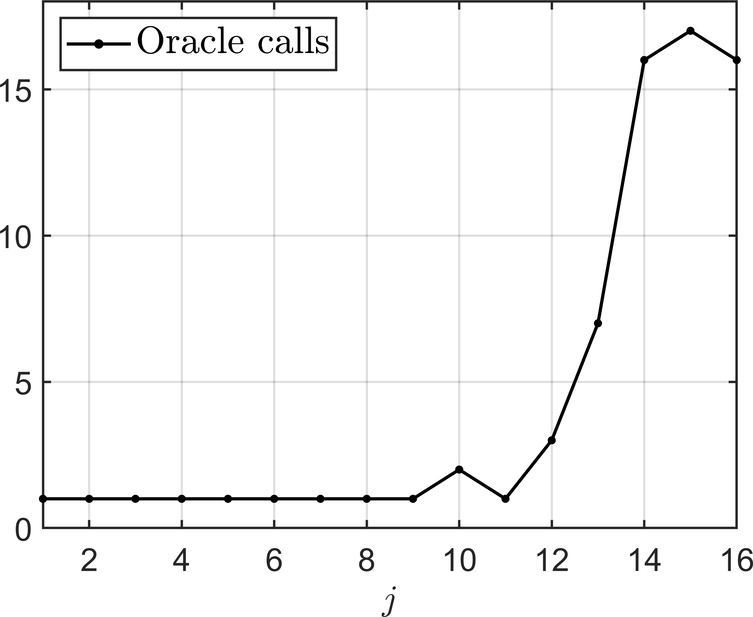
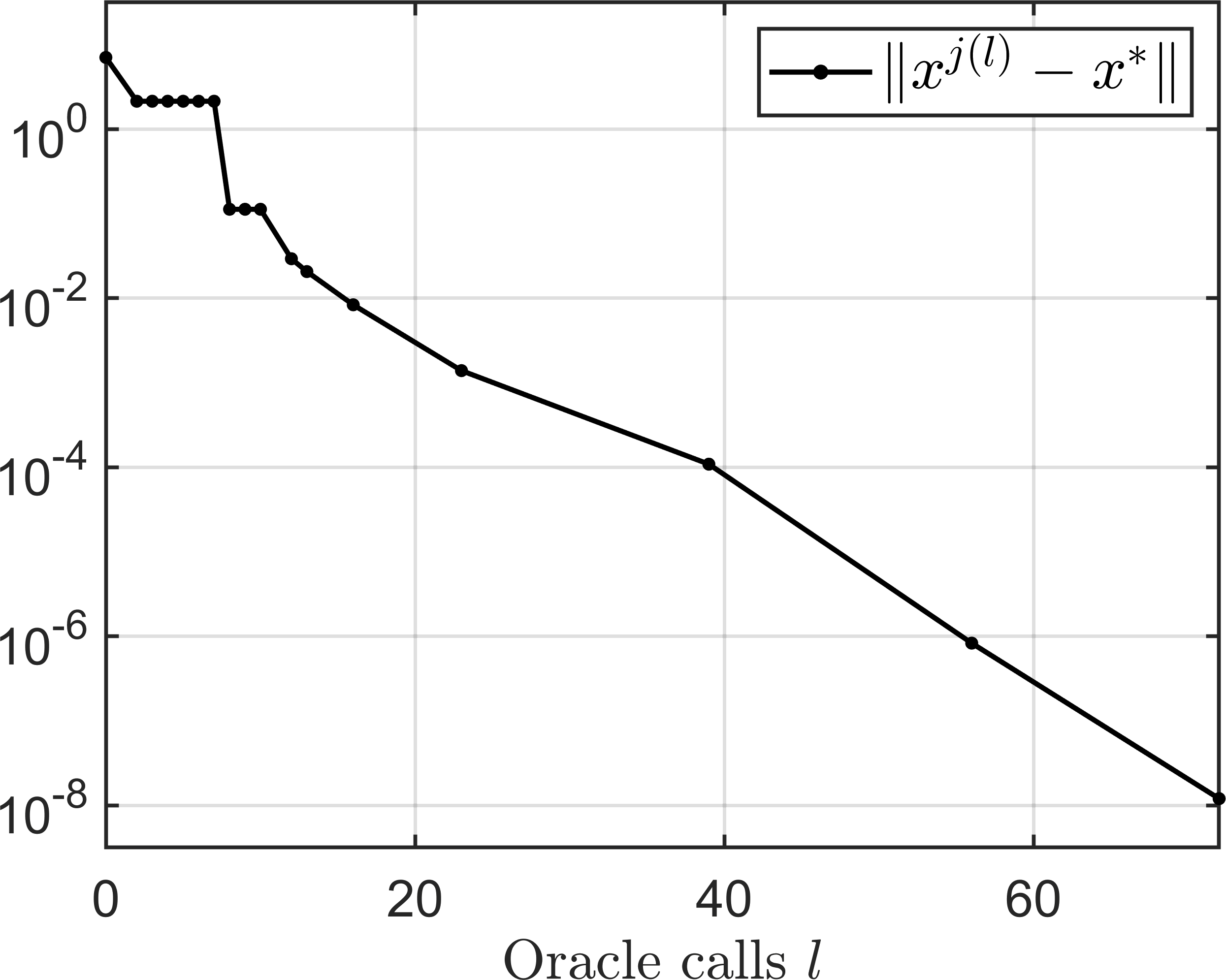
from [LW2019], where for all , is symmetric, pos. definite for all , and the vectors , , are affinely independent with for some with . It is easy to see that is a finite max-type function with . The global minimum of this function is , for which the growth assumption 1 holds with (since all are pos. definite). We generate a random instance of this problem for and and apply Alg. 4.2 with , , , and . (For details on the random generation, see the corresponding code.) Fig. 2(b) shows the distance of the resulting sequence and the upper bound , confirming the R-superlinear convergence (with order ). Fig. 3(a) shows the number of oracle calls that were required by Alg. 4.1 in each iteration of Alg. 4.2.
(a)
(b)
We see that the closer is to the minimum, the more oracle calls are required, i.e., the larger the set . Finally, Fig. 3(b) shows the speed of convergence with respect to oracle calls, i.e., it shows the distance for the sequence from Cor. 4.8, where is the iteration of Alg. 4.2 in which the -th oracle call occurred. (For simplicity, only the oracle calls where changes are plotted.) Since we stop the algorithm already when (due to the accuracy of IPOPT), the R-superlinear convergence is not (yet) visible here.
In both examples considered so far, the objective was a finite max-type function. To show the behavior of Alg. 4.2 for lower- functions that are not of finite max-type and for which no representation as in (2.3) is practically available, we consider an example from the area of eigenvalue optimization [O1992, FN1995, LW2019], where the largest eigenvalue of an affine combination of matrices is minimized. Since is infinite in this case, we cannot use Lem. 4.1(b) to guarantee boundedness of the oracle calls in Alg. 4.1 in Step 4 of Alg. 4.2. Here, we also show a comparison to the HANSO555https://cs.nyu.edu/~overton/software/hanso/ (Retrieved Mar. 24, 2026) software package.
Example 6.3.
For and symmetric matrices , consider the function
where denotes the largest eigenvalue of a matrix . This function is convex, and thus lower- (cf. [RW1998], Thm. 10.33), but in general not of finite max-type (see [O1992], p. 89). It is bounded below if and only if there is no for which is positive definite (cf. [FN1995], p. 227). We are not aware of results about the growth of around its minimum (if existing), and we blindly assume that it grows at least quadratically, i.e., with . We generate a random instance of this problem for and and apply Alg. 4.2 with , , , and . (For details on the random generation, see the corresponding code.) The subproblem (3.5) is solved via IPOPT. Since an explicit expression for the minimum is not available for this example, we use HANSO (with starting point and default parameters) to compute a reference solution . Fig. 4(a) shows the distance for the sequence generated by Alg. 4.2.

(a)

(b)
Note that the expected convergence behavior can be observed despite the initial not being contained in . Fig. 4(b) shows, in black, the distance for as in Cor. 4.8. Despite Lem. 4.1(b) not being applicable, we still observe fast convergence in terms of oracle calls, with Alg. 4.1 needing at most oracle calls in every iteration of Alg. 4.2. The blue, dashed line shows the objective value for all oracle calls performed by HANSO (cut off at for better comparison). HANSO required oracle calls to obtain its final point . Alg. 4.2 required oracle calls for the final point , which satisfies . To reach a point with an objective value less than , HANSO required oracle calls. In terms of runtime, Alg. 4.2 required s and HANSO required s. So while Alg. 4.2 needed far fewer oracle calls than HANSO, the time required for solving the subproblem (3.5) evens out the comparison here. Furthermore, one should keep in mind that Alg. 4.2 requires the Hessian matrix for its oracle (when ), whereas HANSO only requires the objective value and the gradient.
For the final two experiments, we compare Alg. 4.2 to other superlinear solvers for nonsmooth optimization problems. The first one is VUbundle, which is a Julia implementation of the -bundle method from [MS2005], and only requires objective values and (sub)gradients as oracle information. As a test problem, we use the convex function from [LO2008], Sec. 5.5 (named Half-and-half in [MS2012]), which is again not a finite max-type function.
Example 6.4.
Consider the convex function
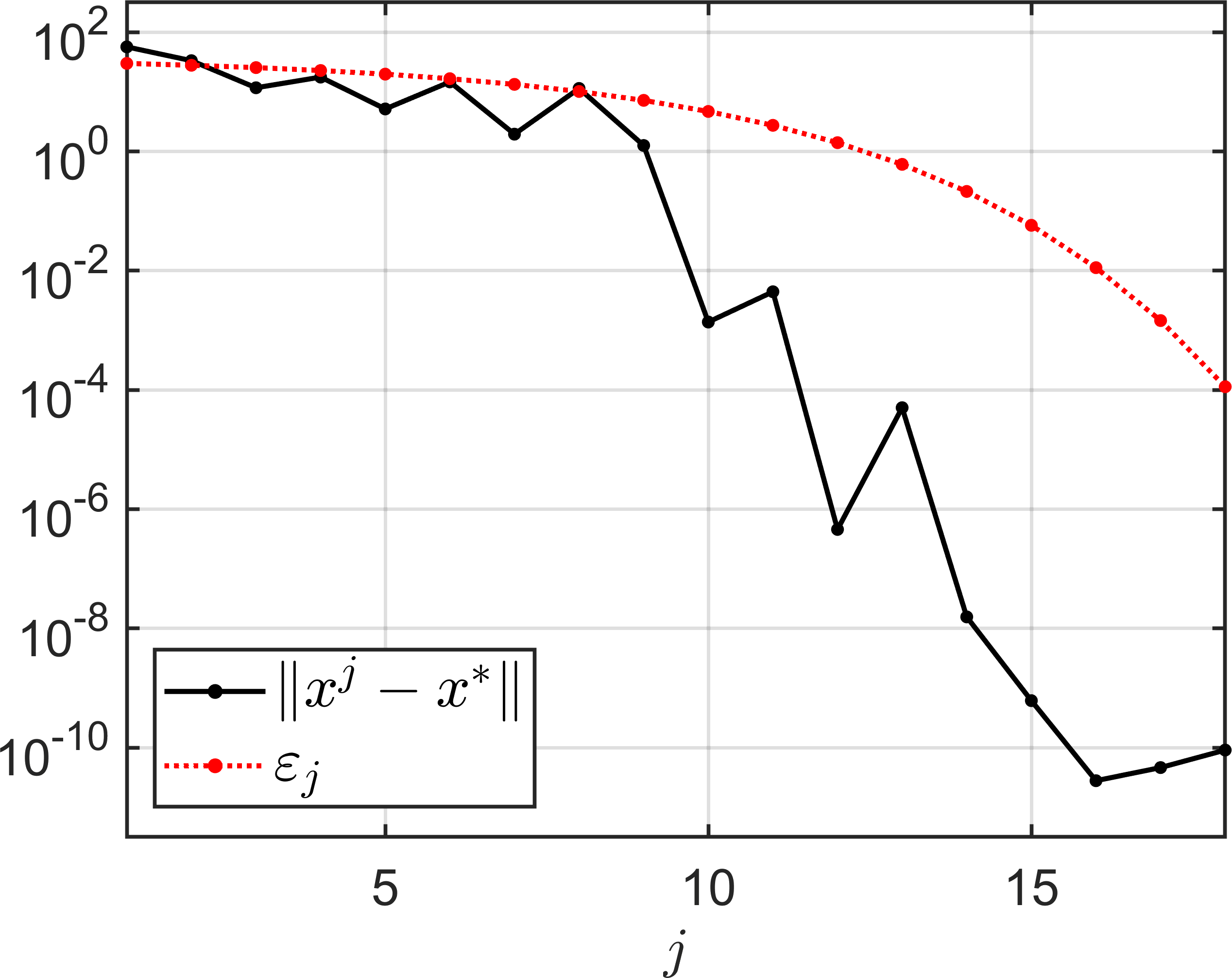
The global minimum is , around which grows with order . We apply Alg. 4.2 with , (as in [MS2012], p. 298), , and . The subproblem (3.5) is solved via IPOPT. For VUbundle we use the default parameters and the same starting point . Fig. 5(a) shows the distance for the sequence generated by Alg. 4.2.
(a)
(b)
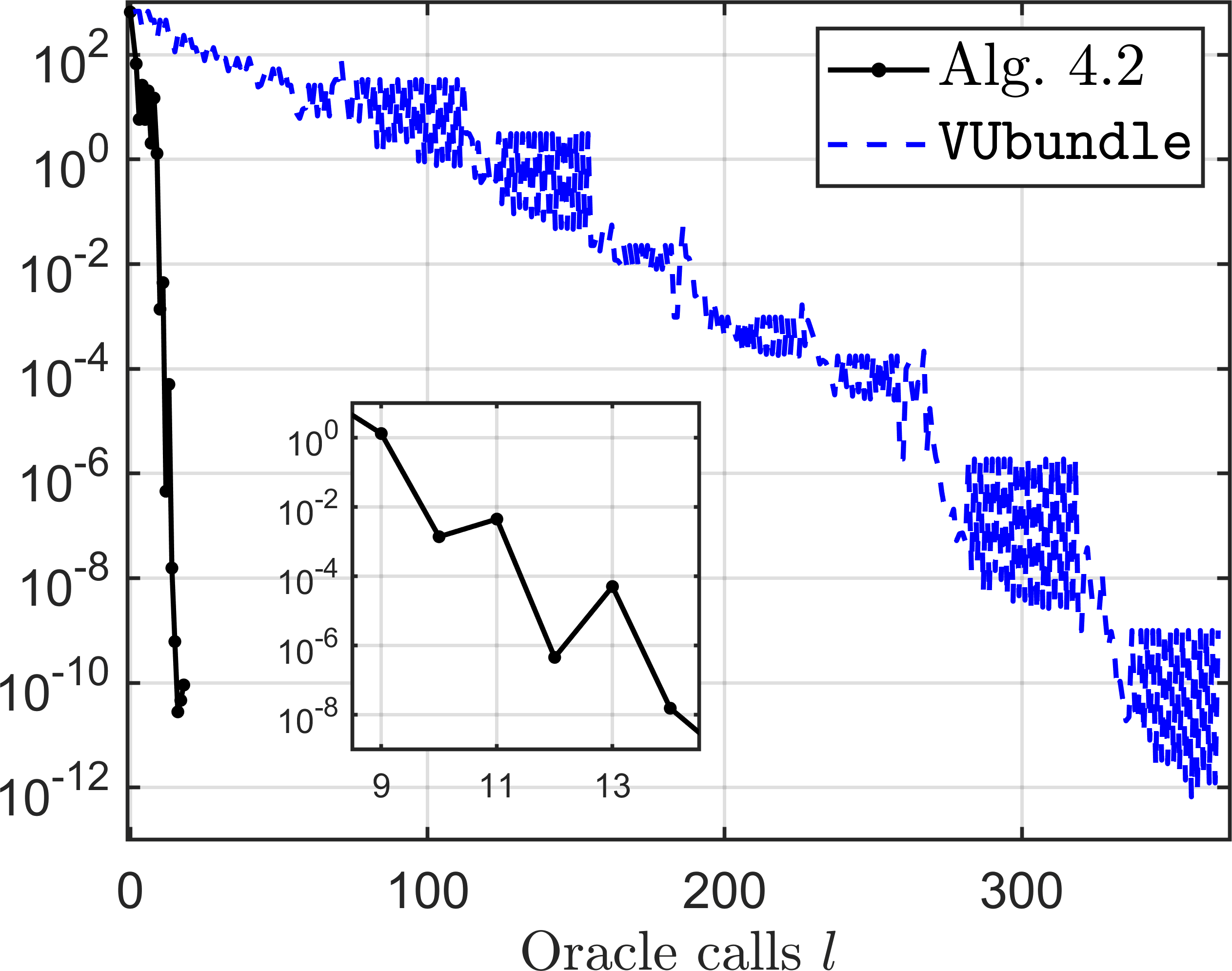
We see (roughly) R-superlinear convergence despite multiple of the early iterates not being contained in the corresponding . (The lack of improvement once the distance lies below is due to the accuracy of IPOPT.) Fig. 5(b) shows, in black, the distance for as in Cor. 4.8. (Due to the bundling in Alg. 4.1 (cf. Rem. 4.3(a)), every iteration of Alg. 4.2 only requires a single oracle call for this example.) Since the numbers of oracle calls for objective values and for gradients in VUbundle are not equal, and since gradients are typically more costly to compute than objective values, we use the number of gradient evaluations for VUbundle in our comparison, shown as the blue, dotted line. While it suggests that for this function, Alg. 4.2 is more efficient than VUbundle in terms of oracle calls, the fact that oracle calls are cheap means that the overall runtime is far slower, with our implementation of Alg. 4.2 requiring s and VUbundle only requiring s.
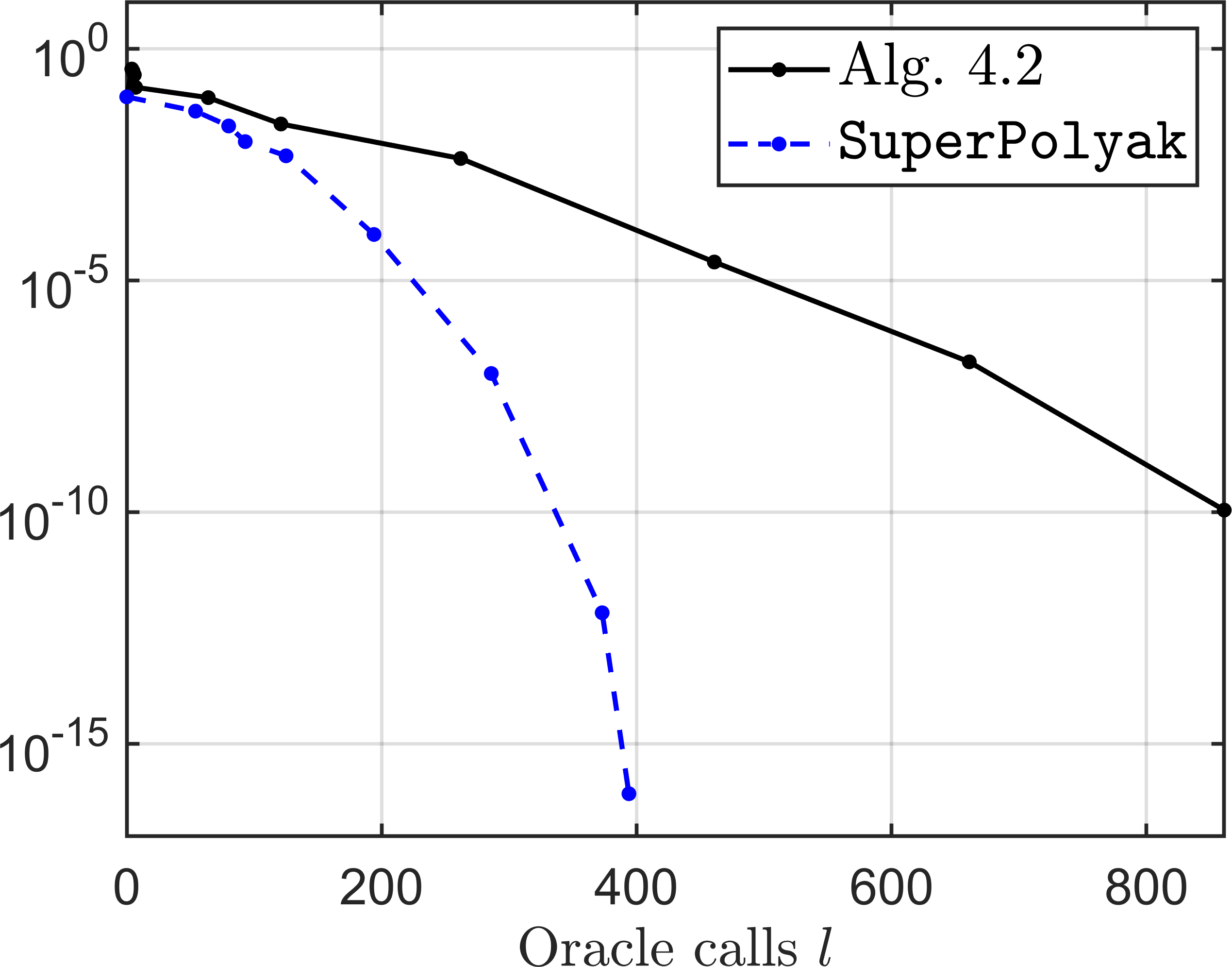
For the second comparison, we consider the Julia implementation of SuperPolyak from [CD2024], which converges superlinearly for functions with a sharp minimum (i.e., 1 holds with ). It requires the objective values and (sub)gradients as oracle information. Additionally, it requires the optimal value to be known. As a test problem, we again consider the nonconvex function from Ex. 6.1. Since in this case, it suffices to choose for Alg. 4.2, which means that the model is a standard cutting-plane model. By choosing the maximum norm for the trust region (and omitting the exponent in the constraint), the subproblem (3.5) then becomes a linear problem, which we can solve using Matlab’s linprog solver.
Example 6.5.
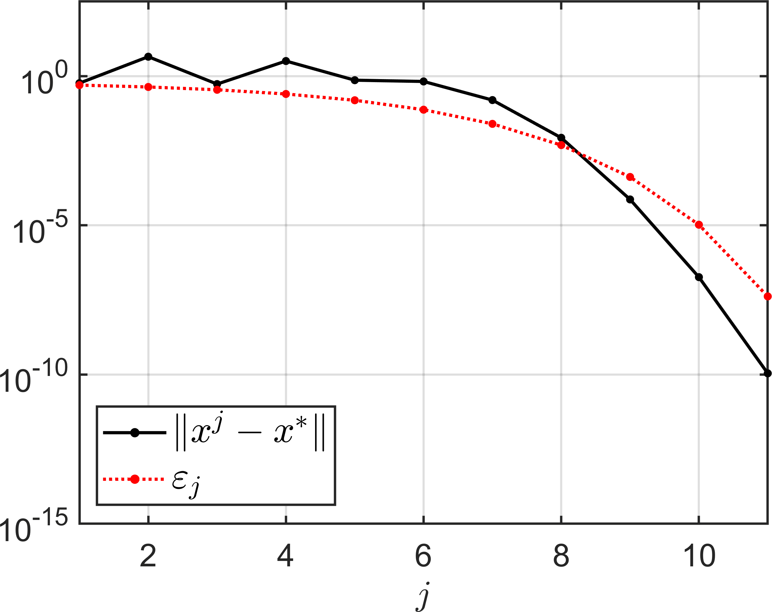
Consider the function from Ex. 6.1 with . We apply Alg. 4.2 with , , , and . The subproblem (3.5) is solved as discussed above. For SuperPolyak we use the default parameters and the same starting point . Fig. 6(a) shows the distance for the sequence generated by Alg. 4.2, suggesting R-superlinear convergence (despite again violating the first inequality in (4.3)).
(a)
(b)
Fig. 6(b) shows, in black, the distance for as in Cor. 4.8. For , Alg. 4.1 required the full iterations (cf. Lem. 4.1(b)), which explains the relatively slow convergence of . The blue, dotted line shows the number of oracle calls for SuperPolyak. We see that SuperPolyak converges significantly faster than Alg. 4.2, only needing about half the number of oracle calls. The difference in runtime is even larger, with Alg. 4.2 requiring s (due to the many iterations of Alg. 4.1) and SuperPolyak only s.
7 Discussion and outlook
We defined higher-order cutting-plane models for lower- functions and showed how they can be used to construct a trust-region bundle method with local R-superlinear convergence. There are multiple directions for future research:
-
•
In the numerical experiments, we used the derivatives of itself as our oracle information. For , this yields an oracle as in Oracle 1 (cf. the discussion at the beginning of Sec. 3). However, for , this may not be the case. For example, for in Ex. 6.4, the Hessian matrix is unbounded for . Since the selection functions in Def. 2.1 are continuous in , there cannot be a representation with for infinitely many arbitrarily close to . Thus, the practical oracle differs from Oracle 1 for this function. Nonetheless, this was no issue in any of our numerical experiments. Resolving this gap from theory to practice likely requires more theoretical analysis of the meaning of derivatives of selection functions in local representations of lower- functions. For example, we expect that for finite max-type functions, it is possible to show that there is a local representation of for which the practical oracle equals the theoretical oracle. Analyzing how well lower- functions can be approximated by finite max-type functions may then close the above gap.
-
•
The numerical experiments showed that if functions evaluations are cheap, then in terms of runtime, the current implementation of Alg. 4.2 is significantly slower than other solvers (on their respective problem classes). In Ex. 6.5, roughly of the runtime is taken up by the solution of the subproblem (3.5), so a faster implementation can only be obtained by employing a different approach for solving this subproblem. For , it might be possible to exploit the fact that (3.5) is a quadratically constrained quadratic program (QCQP), for which specialized solvers exist (see, e.g., [L2005]). Alternatively, one could consider approximate solutions, since intuitively, exact solutions should only be necessary “in the limit” as the sequence approaches the minimum. For example, it may be possible to use ideas from SQP methods to first estimate the Lagrange multipliers in (3.5) and then compute an approximate solution based on the estimated multipliers, similar to the approach of [LW2019], Sec. 3.6.
-
•
Our convergence theory for Alg. 4.2 technically requires global solutions of the subproblem (3.5) (for the inequality (3.9) in the proof of Lem. 3.3). While we did not encounter any convergence issues in our numerical experiments when using non-global solvers, the effect of local solutions of (3.5) on the convergence still has to be properly analyzed.
-
•
Clearly, derivatives of an order larger than may be cumbersome to provide and to work with. Considering the derivation of quasi-Newton methods from Newton’s method in smooth optimization, it should be analyzed whether there is a quasi-Newton version of Alg. 4.2 that only requires first-order information and approximates the Hessian matrix.
- •
Acknowledgements. This research was funded by Deutsche Forschungsgemeinschaft (DFG, German Research Foundation) – Projektnummer 545166481.