Acoustic limit of Boltzmann equations for gas mixture

Gaofeng Wang, Tianfang Wu and Linjie Xiong G.F. Wang. School of Mathematics and Statistics, Nantong University, Nantong 226019, P. R. China. gfwang@ntu.edu.cn T.F. Wu. (corresponding author). Wenzhou Business College, Wenzhou 325000, P. R. China. 20249237@wzbc.edu.cn L.J.Xiong. School of Mathematical Sciences, Hunan University, Changsha, 410082, P.R.China. xlj@hnu.edu.cn

Abstract.

In this paper, we study the hydrodynamic and acoustic limit from Boltzmann equations for two species gas mixture with potential $\gamma\in\left(-3,1\right]$ . Here the particle masses are different which derives to the loss of symmetry to the linearized collision operator. We construct the hydrodynamic limit for two species based on the Hilbert expansion method when the Knudsen number is small. The key observation is the precise properties of the linearized collision operators, including the extra operators due to the different particle masses $(m^{A}\neq m^{B})$ . In additional, the acoustic limit of the Boltzmann equations for gas mixtures is rigorously justified by assuming the strength of the initial data depends on the Knudsen number.

Keywords. Compressible Euler equations; Acoustic system; Boltzmann equations of gas mixture; Different particle masses.

AMS subject classifications: 35B38, 35J47

1. Introduction and main result

1.1. Introduction

We consider the Boltzmann equations for two species particles $A,B$ as follows

\left\{\begin{gathered}\partial_{t}F^{A}+v\cdot\nabla_{x}F^{A}=\frac{1}{\varepsilon}\Big[Q^{AA}(F^{A},F^{A})+Q^{AB}(F^{A},F^{B})\Big],\\ \partial_{t}F^{B}+v\cdot\nabla_{x}F^{B}=\frac{1}{\varepsilon}\Big[Q^{BA}(F^{B},F^{A})+Q^{BB}(F^{B},F^{B})\Big].\end{gathered}\right.

(1.1)

In the following, the particle species is denoted by the Greek letters $\alpha$ and $\beta$ ( $\alpha,\beta\in\{A,B\}$ ). The density distribution function for species $\alpha$ is given by $F^{\alpha}(t,x,v)$ , which is defined at time $t>0$ , position $x=(x_{1},x_{2},x_{3})$ with the velocity $v=(v_{1},v_{2},v_{3})$ . Particle mass of species $\alpha$ is denoted by $m^{\alpha}$ . The parameter $\varepsilon$ is called Knudsen number, which is proportional to the mean free path. The collision operator for $\alpha$ - $\beta$ particle pairs takes the form

Q^{\alpha\beta}(F^{\alpha},F^{\beta})=\int_{\mathbb{R}^{3}}\int_{\mathbb{S}^{2}}B^{\alpha\beta}(|v-v_{*}|,\theta)\Big[F^{\alpha}(v^{\prime})F^{\beta}(v^{\prime}_{*})-F^{\alpha}(v)F^{\beta}(v_{*})\Big]d\omega dv_{*}.

Here $v,v_{*}$ and $v^{\prime},v^{\prime}_{*}$ are the velocities before and after the collision corresponding to the species $\alpha$ and $\beta$ , which obey the laws of momentum conservation and energy conservation:

m^{\alpha}v^{\prime}+m^{\beta}v_{*}^{\prime}=m^{\alpha}v+m^{\beta}v_{*},\quad m^{\alpha}|v^{\prime}|^{2}+m^{\beta}|v_{*}^{\prime}|^{2}=m^{\alpha}|v|^{2}+m^{\beta}|v_{*}|^{2}.

Let $\omega\in\mathbb{S}^{2}$ and $\cos\theta=\frac{\omega\cdot(v-v_{*})}{|v-v_{*}|}$ . The velocity $v^{\prime},v^{\prime}_{*}$ after the collision are expressed as

v^{\prime}=v-\frac{2m^{\beta}}{m^{\alpha}+m^{\beta}}[(v-v_{*})\cdot\omega]\omega,\quad v^{\prime}_{*}=v_{*}+\frac{2m^{\alpha}}{m^{\alpha}+m^{\beta}}[(v-v_{*})\cdot\omega]\omega.

The collision kernels $B^{\alpha\beta}(|v-v_{*}|,\theta)$ is assumed to satisfy the following assumptions:

(1) The symmetry of collision kernels

B^{\alpha\beta}(|v-v_{*}|,\theta)=B^{\beta\alpha}(|v_{*}-v|,\theta)\,\quad\alpha,\beta\in\{A,B\}.

(2) The collision kernels are decomposed into

B^{\alpha\beta}(|v-v_{*}|,\theta)=\Phi^{\alpha\beta}(|v-v_{*}|)b^{\alpha\beta}(\cos\theta)\,\quad\alpha,\beta\in\{A,B\}.

Here the kinetic part takes

\Phi^{\alpha\beta}(|v-v_{*}|)=C_{\alpha\beta}^{\Phi}|v-v_{*}|^{\gamma},\,C_{\alpha\beta}^{\Phi}>0,\,\gamma\in(-3,1],

where $\gamma=$ and there exist a constant $C_{b}>0$ , for $\forall\alpha,\beta\in\{A,B\}$ and $\theta\in[0,\pi]$ , such that

0\leq b^{\alpha\beta}(\cos\theta)\leq C_{b}|\cos\theta|.

It means that the angular part satisfies Grad’s angular cutoff assumption [10].

The derivation of the fluid dynamical equations from kinetic theory can be traced back to the seminal contributions of Maxwell [26] and Boltzmann [5]. Although the formal derivations [2] have been established at various conceptual levels, a comprehensive mathematical justification remains challengeable which aligns with the objective of Hilbert’s sixth problem [19]: to construct a unified mathematical framework for gas dynamics across different descriptive scales.

Over the past four decades, substantial research has addressed the well-posedness and fluid limits of the Boltzmann equation. There exist two main methodologies in the classical solutions framework: one involves the spectral analysis of the semigroup generated by the linearized Boltzmann equation, refer to [3], [24], [25], [27], while the other lies in developing a framework for $L^{2}$ energy estimates, see [7], [11], [14], [15]. Guo developed the $L^{2}-L^{\infty}$ method [17], [18], which employs Hilbert expansion and reduce to the system of remainder terms. It is sufficient to establish the uniform of the remainders via $L^{2}$ energy and $L^{\infty}$ characteristic line procedures with weighting techniques. Within this framework, Guo, Huang, and Wang [16] studied the fluid limit of the single Boltzmann equation for the hard-sphere model in a half-space with specular reflection. Later, the hydrodynamic limit of the same equation with the Maxwell or complete diffuse reflection were examined in [20], [21]. Both the kinetic boundary layer and the fluid boundary layer appeared to match the boundary conditions and the compressible Euler equation in the interior.

Compared with the extensive study of single-gas Boltzmann equations, the study on the Boltzmann equation of gas mixtures has also attracted attention. These studies focus on the case of the same particle mass, that is $m^{A}=m^{B}$ . Wang [28] investigated diffusive limits in VPB systems with periodic boundaries, later quantifying decay rates in such systems [29]. Aoki, Bardos, and Takata [1] studied Knudsen layer existence for Boltzmann equations with zero macroscopic flow, later generalized by Bardos and Yang [4] for arbitrary flow velocities. Guo’s foundational work [12] established the Euler-Maxwell limit for hard-sphere VMB systems. Duan and Liu [8] examined one-dimensional Euler-Poisson limits from Boltzmann system of mixtures, while Jiang, Lei, and Zhao [22] explored Euler-Maxwell limits for $-3<\gamma\leq 1$ , $(m_{\pm}=e_{\pm}=1)$ . It is worthwhile to mention Fang and Qi’s recent study [9] on the hydrodynamic limit from Boltzmann equations for gas mixtures to a two-fluid macroscopic system. There are relatively few results on the fluid limits of the Boltzmann equation system for gas mixtures of particles with unequal masses.

Refer to caption — Figure 1. The collision between nitrogen and oxygen molecules

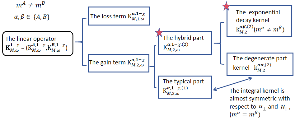
However, it is nature to study the combined system with different mass particles $m^{A}\neq m^{B}$ . In [6], Briant and Daus studied the stability and the time decay rate of the solution around the equilibrium of the multi-species Boltzmann system. Although the compressible Euler system for gas mixture has been established in reference [32], the estimates of the linear operators were brought from those of single-species Boltzmann equation without proof. To study the hydrodynamic limit of the system 1.1, one should give some more precise analysis of the linear operators. In particular, the main observation here is the estimation of the operator $K_{M,2,w}^{\alpha,1-\chi}$ for the Boltzmann system of unequal-mass mixtures, (see Lemma 2.4), which reveals that it can be divided into two parts

K_{M,2,w}^{\alpha,1-\chi}=\underbrace{K_{M,2,w}^{\alpha,1-\chi,(1)}}_{\text{Typical part}}+\underbrace{K_{M,2,w}^{\alpha,1-\chi,(2)}}_{\text{Hybrid part}},

(1.2)

where “Typical part” shares the properties analogous to that of the Boltzmann equations in the case of identical gas molecules $(m_{A}=m_{B})$ . “Hybrid part” consists of a degenerate part $(m^{\alpha}=m^{\beta})$ and a part that exhibit exponential decay $(m^{\alpha}\neq m^{\beta})$ . The exponential decay part is the main difference arising from the different mass particles $m^{A}\neq m^{B}$ . The estimate of $K_{M,2,w}^{\alpha,1-\chi}$ provides critical theoretical results for spectral analysis of the linearized Boltzmann operator in multi-component gas systems with mass disparity. This precise structural analysis offers the fundamental estimates of the linear operator in the unequal mass case, we believed that these estimates are helpful to get the pointwise estimates of classical solutions to the Boltzmann equation for the mixed gases. This will be studied in the forthcoming paper.

1.2. The properties of the collision operator.

For $\mathbf{F}=(F^{A},F^{B})^{\top}$ , we introduce the bilinear Boltzmann collision operator $\mathscr{C}$ in vector form as follows:

\mathscr{C}\mathbf{F}=\left(\begin{array}[]{cccc}Q^{AA}(F^{A},F^{A})+Q^{AB}(F^{A},F^{B})\vskip 3.0pt\\ Q^{BA}(F^{B},F^{A})+Q^{BB}(F^{B},F^{B})\end{array}\right).

(1.3)

The operator $\mathscr{C}$ has the following properties [6]:
Collision invariant A function $\mathbf{\Psi}=(\Psi^{A},\Psi^{B})^{\top}$ is called a collision invariant of the operator $\mathscr{C}$ with respect to the inner product in $(L^{2}_{v}(\mathbb{R}^{3}))^{2}$ if it satisfies

\langle\mathscr{C}\mathbf{F},\mathbf{\Psi}\rangle_{(L_{v}^{2}(\mathbb{R}^{3}))^{2}}=\sum_{\alpha,\beta\in{A,B}}\left\langle Q^{\alpha\beta}(F^{\alpha},F^{\beta}),\Psi^{\alpha}\right\rangle_{L_{v}^{2}}=0\quad\text{for any vector }\mathbf{F}.

(1.4)

It derives to

\mathbf{\Psi}\in\text{Span}\{\mathbf{e}_{1},\mathbf{e}_{2},v_{1}\mathbf{m},v_{2}\mathbf{m},v_{3}\mathbf{m},|v|^{2}\mathbf{m}\},

(1.5)

where $\mathbf{m}=(m^{A},m^{B})^{T}$ and $\mathbf{e}_{j}$ is the $j^{\text{th}}$ unit vector in $\mathbb{R}^{2}$ .
H-theorem The entropy function of the two-species Boltzmann equations satisfies

\left\langle\mathscr{C}\mathbf{F},\log\mathbf{F}\right\rangle_{(L_{v}^{2}(\mathbb{R}^{3}))^{2}}=\sum_{\alpha,\beta\in\{A,B\}}\left\langle Q^{\alpha\beta}(F^{\alpha},F^{\beta}),~~\log F^{\alpha}\right\rangle_{L_{v}^{2}(\mathbb{R}^{3})}\leq 0,

(1.6)

and this equality holds if and only if

\mathbf{F}=\left(\begin{array}[]{cccc}\frac{n^{A}(m^{A})^{3/2}}{(2\pi\theta)^{3/2}}e^{-\frac{m^{A}|v-\mathbf{u}|^{2}}{2\theta}}\vskip 3.0pt\\ \frac{n^{B}(m^{B})^{3/2}}{(2\pi\theta)^{3/2}}e^{-\frac{m^{B}|v-\mathbf{u}|^{2}}{2\theta}}\end{array}\right)=:\left(\begin{array}[]{cccc}\mu^{A}\\ \mu^{B}\end{array}\right),

(1.7)

where $n^{\alpha}(\alpha=A,B)$ are the number density of particle $\alpha$ , $u,\theta$ are the bulk velocity and temperature of the system.

For later use, we also denote that $F=(F^{A},F^{B})^{\top}$ with $F^{\alpha}=\mu^{\alpha}+\sqrt{\mu^{\alpha}}f^{\alpha}$ . Thus, for $\mathbf{f}=(f^{A},f^{B})^{\top}$ , we yield the following linear operator

\displaystyle\mathbf{L}\mathbf{f}=\left(\begin{array}[]{lll}\mathbf{L}^{A}\mathbf{f}\\ \mathbf{L}^{B}\mathbf{f}\end{array}\right)=:-\left(\begin{array}[]{lll}\frac{1}{\sqrt{\mu^{A}}}\displaystyle{\sum_{\beta=A,B}}\left[Q^{A\beta}(\mu^{A},\sqrt{\mu^{\beta}}f^{\beta})+Q^{A\beta}(\sqrt{\mu^{A}}f^{A},\mu^{\beta})\right]\\ \frac{1}{\sqrt{\mu^{B}}}\displaystyle{\sum_{\beta=A,B}}\left[Q^{B\beta}(\mu^{B},\sqrt{\mu^{\beta}}f^{\beta})+Q^{B\beta}(\sqrt{\mu^{B}}f^{B},\mu^{\beta})\right]\end{array}\right).

(1.12)

From the H-theorem, it is well known that $\mathbf{L}$ is a self-adjoint operator in $(L^{2}_{v}(\mathbb{R})^{3})^{2}$ , and the kernel of $\mathbf{L}$ is spanned by the following six dimensional vector functions (see [6])

{\rm Ker}\mathbf{L}={\rm span}\{\mathbf{X}_{0},\mathbf{X}_{1},\cdots,\mathbf{X}_{5}\},

(1.13)

with

\begin{split}&\mathbf{X}_{0}=\sqrt{\frac{\mu^{A}}{n^{A}}}\mathbf{e}_{1},\,\,\,\mathbf{X}_{1}=\sqrt{\frac{\mu^{B}}{n^{B}}}\mathbf{e}_{2},\,\,\,\mathbf{X}_{j}=\frac{v_{j-1}-u^{j-1}}{\sqrt{\theta n}}\left(\begin{array}[]{ccc}m^{A}\sqrt{\mu^{A}}\\[5.69054pt] m^{B}\sqrt{\mu^{B}}\end{array}\right)~(j=2,3,4),\\ &\mathbf{X}_{5}=\frac{1}{\sqrt{6n}}\left(\begin{array}[]{ccc}(\frac{m^{A}|v-\mathbf{u}|^{2}}{\theta}-3)\sqrt{\mu^{A}}\\[5.69054pt] (\frac{m^{B}|v-\mathbf{u}|^{2}}{\theta}-3)\sqrt{\mu^{B}}\end{array}\right)~~~~{\rm where}~n=n^{A}+n^{B}.\end{split}

(1.14)

One can check that $\langle\mathbf{X}_{i},\mathbf{X}_{j}\rangle=\delta_{ij},\,0\leq i,j\leq 5$ , where $\delta_{ij}$ is the Kronecker symbol. The space $(L^{2}_{v}(\mathbb{R}^{3}))^{2}$ can be decomposed as ${\rm Ker}\mathbf{L}\oplus\mathcal{N}(\mathbf{L})^{\bot}$ , where $\mathcal{N}(\mathbf{L})^{\bot}$ is the orthogonal set of ${\rm Ker}\mathbf{L}$ . Then, for any $\mathbf{f}=(f^{A},f^{B})^{\top}\in(L^{2}_{v}(\mathbb{R}^{3}))^{2}$ , it can be decomposed as

\displaystyle\mathbf{f}=\mathcal{P}\mathbf{f}+(\mathbf{I}-\mathcal{P})\mathbf{f},\quad{\rm with}\quad\mathcal{P}\mathbf{f}=\sum_{i=0}^{5}\langle\mathbf{f},\mathbf{X}_{i}\rangle\mathbf{X}_{i},

(1.15)

where $\mathcal{P}\mathbf{f}$ and $(\mathbf{I}-\mathcal{P})\mathbf{f}=\mathbf{f}-\mathcal{P}\mathbf{f}$ are the macro-micro parts of $\mathbf{f}$ respectively. The main properties of the operator $\mathbf{L}$ is list in the following.

(The solvability of $\mathbf{L}$ ). For any $\mathbf{R}=(R^{A},R^{B})^{\top}\in(L^{2}_{v}(\mathbb{R}^{3})^{2})^{2}$ , there exists a unique solution for $\mathbf{L}\mathbf{f}=\mathbf{R}$ , if and only if $\mathbf{R}\in\mathcal{N}(\mathbf{L})^{\bot}$ , that is,

\displaystyle\langle\mathbf{R},\mathbf{X}_{i}\rangle_{(L^{2}_{v}(\mathbb{R})^{3})^{2}}=0,\quad{\rm for~all}\quad i=0,\cdots,5.

(1.16)

Moreover, the solution $\mathbf{f}$ could be formulated as

\displaystyle\mathbf{f}=\mathbf{L}^{-1}\mathbf{R}\in\mathcal{N}(\mathbf{L})^{\bot}.

(1.17)

(The coercivity of $\mathbf{L}$ ). There exists a positive number $c_{0}>0$ , for any $\mathbf{f}=(f^{A},f^{B})^{\top}\in(L^{2}_{v}(\mathbf{R}^{3}))^{2}$ , it holds

\left\langle\mathbf{L}\mathbf{f},\mathbf{f}\right\rangle_{v}\geq c_{0}|(\mathbf{I}-\mathcal{P})\mathbf{f}|_{\nu}^{2}.

(1.18)

The proof of (1.18) for hard potential case is in [6], and [31], and for soft potential case one can refer [30].

1.3. The main results

Following the ideas in [13], the compressible Euler system for mixtures is derived by the Hilbert expansion of the Boltzmann equation for gas mixture. The life-span of the fluid limit system together with the truncation of the Hilbert expansion is obtained when the strength of the perturbation of the initial data is sufficiently small but independent of the Knudsen number. The hydrodynamic limit of the Boltzmann equation of gas mixture is established by study the uniform estimates of the remainder term. Later, the acoustic limit is yielded when the strength of the perturbation of the initial data is dependent on the Kundsen number. It is proved that the rigorous justification of the acoustic limit of 1.1 is valid for any time interval when the Knudsen number is small enough. More precisely, we firstly assume the solutions of (1.1) have the following Hilbert expansion form

F_{\varepsilon}^{\alpha}=F^{\alpha}_{0}+\sum_{k=1}^{5}\varepsilon^{k}F^{\alpha}_{k}+\varepsilon^{3}F_{R}^{\alpha},\quad{\rm for}\quad\alpha\in\{A,B\}.

(1.19)

Substituting it into (1.1), and compare the coefficients about order of $\varepsilon$ , we can obtain that

		$\displaystyle\text{Order ~$O(\varepsilon^{-1})$:}\qquad\quad~~\qquad\qquad~\,~~0={\sum_{\beta=A,B}}Q^{\alpha\beta}(F_{0}^{\alpha},F_{0}^{\beta}),$		(1.20)
		$\displaystyle\text{Order ~$O(1)$:}\qquad\quad~~~~(\partial_{t}+v\cdot\nabla_{x})F_{0}^{\alpha}={\sum_{i^{\prime}+i^{\prime\prime}=1}\sum_{\beta=A,B}}Q^{\alpha\beta}(F_{i^{\prime}}^{\alpha},F_{i^{\prime\prime}}^{\beta}),$
		$\displaystyle\text{Order ~$O(\varepsilon)$:}\quad\quad\qquad~~~~(\partial_{t}+v\cdot\nabla_{x})F_{1}^{\alpha}={\sum_{i^{\prime}+i^{\prime\prime}=2}\sum_{\beta=A,B}}Q^{\alpha\beta}(F_{i^{\prime}}^{\alpha},F_{i^{\prime\prime}}^{\beta}),$
		$\displaystyle.\,.\,.$
		$\displaystyle\text{Order ~$O(\varepsilon^{i})$:}\,\quad\quad~~~~~~(\partial_{t}+v\cdot\nabla_{x})F_{i}^{\alpha}={\mathop{\sum}_{i^{\prime}+i^{\prime\prime}=i+1\atop i^{\prime},i^{\prime\prime}\geq 0}\sum_{\beta=A,B}}Q^{\alpha\beta}(F_{i^{\prime}}^{\alpha},F_{i^{\prime\prime}}^{\beta}),\quad{i}\in\mathbf{Z}^{+},\quad{i}\geq 2.$

The remainder term satisfies

\begin{gathered}(\partial_{t}+v\cdot\nabla_{x})F_{R}^{\alpha}-\frac{1}{\varepsilon}\displaystyle{\sum_{\beta=A,B}}(Q^{\alpha\beta}(F_{0}^{\alpha},F_{R}^{\beta})+Q^{\alpha\beta}(F_{R}^{\alpha},F_{0}^{\beta}))=\varepsilon^{2}\displaystyle{\sum_{\beta=A,B}}Q^{\alpha\beta}(F_{R}^{\alpha},F_{R}^{\beta})\\ \hskip 113.81102pt+\displaystyle{\sum^{5}_{i=1}}\displaystyle{\sum_{\beta=A,B}}\varepsilon^{i-1}(Q^{\alpha\beta}(F_{i}^{\alpha},F_{R}^{\beta})+Q^{\alpha\beta}(F_{R}^{\alpha},F_{i}^{\beta}))+\varepsilon^{2}E^{\alpha},\end{gathered}

(1.21)

where

\displaystyle E^{\alpha}=

\displaystyle-(\partial_{t}+v\cdot\nabla_{x})F_{5}^{\alpha}+\mathop{\sum}_{i^{\prime}+i^{\prime\prime}\geq 6\atop i^{\prime},i^{\prime\prime}\geq 1}{\sum_{\beta=A,B}}\varepsilon^{i^{\prime}+i^{\prime\prime}-6}Q^{\alpha\beta}(F_{i^{\prime}}^{\alpha},F_{i^{\prime\prime}}^{\beta}).

(1.22)

Step 1. From $\eqref{ORDERZONG}_{1}$ and H-theorem, we know that $\mathbf{F}_{0}=(F_{0}^{A},F_{0}^{B})^{\top}$ is a local bi-Maxwellian as

\mathbf{F}_{0}=\left(\begin{array}[]{cccc}\frac{n^{A}_{\delta}(m^{A})^{3/2}}{(2\pi\theta_{\delta})^{3/2}}e^{-\frac{m^{A}|v-\mathbf{u}_{\delta}|^{2}}{2\theta_{\delta}}}\vskip 3.0pt\\ \frac{n^{B}_{\delta}(m^{B})^{3/2}}{(2\pi\theta_{\delta})^{3/2}}e^{-\frac{m^{B}|v-\mathbf{u}_{\delta}|^{2}}{2\theta_{\delta}}}\end{array}\right)=:\left(\begin{array}[]{cccc}\mu^{A}_{\delta}\\ \mu^{B}_{\delta}\end{array}\right).

(1.23)

By imposing the initial data (2.2), one has $\mathbf{F}_{0}(0)=(\mu^{A,\rm in}_{\delta},\mu^{B,\rm in}_{\delta})^{\top}$ . The densities $n^{A}_{\delta},n^{B}_{\delta}$ , the bulk velocity $\mathbf{u}_{\delta}$ and the bulk temperature $\theta_{\delta}$ will be determined later with this initial data.

Step 2. From $\eqref{ORDERZONG}_{2}$ , one could derives that

\displaystyle\mathbf{L}_{\delta}\mathbf{f}_{1}=\mathbf{R}_{0},

(1.24)

where the operator $\mathbf{L}_{\delta}$ is defined in (1.12) by replacing $\mu^{\alpha}$ by $\mu^{\alpha}_{\delta}$ and $\mathbf{R}_{0}=(-\frac{1}{\sqrt{\mu^{A}_{\delta}}}(\partial_{t}+v\cdot\nabla_{x})\mu^{A}_{\delta},-\frac{1}{\sqrt{\mu^{B}_{\delta}}}(\partial_{t}+v\cdot\nabla_{x})\mu^{B}_{\delta})^{\top}$ . From the solvability of $\mathbf{L}_{\delta}$ , one could derive the compressible Euler equations (2.4) and get $n^{A}_{\delta},n^{B}_{\delta},\mathbf{u}_{\delta},\theta_{\delta}$ in the time interval $[0,\tau^{\delta}]$ for $\tau^{\delta}=O(\frac{1}{\delta})$ with the initial data (2.2).

Step 2. To solve $\eqref{dyjhlibsxF}_{k}$ , we set $F_{k}^{\alpha}=f_{k}^{\alpha}\sqrt{\mu^{\alpha}_{\delta}}$ and $\mathbf{f}_{k}=(f_{k}^{A},f_{k}^{B})^{\top}$ for $k=1,2,\cdots,5$ . Here $\mathbf{f}_{k}$ will be decomposed to the macroscopic and microscopic parts as

\mathbf{f}_{k}=\mathcal{P}\mathbf{f}_{k}+(\mathbf{I}-\mathcal{P})\mathbf{f}_{k},

with

\displaystyle\mathcal{P}\mathbf{f}_{k}=\frac{n^{A}_{k}}{\sqrt{n^{A}_{\delta}}}\mathbf{X}_{0}^{\delta}+\frac{n^{B}_{k}}{\sqrt{n^{B}_{\delta}}}\mathbf{X}_{1}^{\delta}+\sum_{j=2,3,4}\sqrt{\frac{n_{\delta}}{\theta_{\delta}}}u_{k}^{j-1}\mathbf{X}_{j}^{\delta}+\sqrt{\frac{n_{\delta}}{6}}\frac{\theta_{k}}{\theta_{\delta}}\mathbf{X}_{5}^{\delta}.

(1.25)

Here $\mathbf{X}_{k}^{\delta}(k=0,\cdots,5)$ comes from (1.14) by replacing $\mu^{\alpha}$ with $\mu^{\alpha}_{\delta}$ .

On the one hand, from the solvability of $\mathbf{L}_{\delta}$ , (1.17) and (1.24) give

\displaystyle(\mathbf{I}-\mathcal{P}){f}_{1}=\mathbf{L}_{\delta}^{-1}\mathbf{R}_{0}\in\mathcal{N}(\mathbf{L}_{\delta})^{\bot}.

(1.26)

On the other hand, the equation of the macroscopic part $(n^{A}_{1},n^{B}_{1},\mathbf{u}_{1},\theta_{1})$ in (1.25) could be derived from the solvability of the next order $\eqref{ORDERZONG}_{3}$ , which is the linear compressible Euler equation (2.8). The existence and the uniform estimates of this part is established when the initial data $(n^{A,\rm in}_{1},n^{B,\rm in}_{1},\mathbf{u}^{\rm in}_{1},\theta^{\rm in}_{1})$ is specified. Thus, one could get the vector $\mathbf{f}_{1}$ as well as $\mathbf{F}_{1}$ .

Following the same process, we can get the terms $\mathbf{F}_{k}(k=1,\cdots,5)$ together with the uniform estimates in the interval $[0,\tau^{\delta}]$ when the initial data $(n^{A,\rm in}_{k},n^{B,\rm in}_{k},\mathbf{u}^{\rm in}_{k},\theta^{\rm in}_{k})$ are given. Thus, one could get the vector $\mathbf{f}_{k}$ and $\mathbf{F}_{k}$ for $k=2,\cdots,5$ . We omit the details here.

With these in hand, we derive the uniform estimates of the remainder $\mathbf{F}_{R}$ from the equation (1.21). The hydrodynamic limit of the (1.1) could be established as follows.

Theorem 1.1.

Let $(n_{\delta}^{A,\rm in},n_{\delta}^{B,\rm in},\mathbf{u}^{\rm in}_{\delta},\theta^{\rm in}_{\delta})$ is given as (2.2). Suppose that there exists a series of integers $s_{0}>s_{1}>\cdots>s_{4}>s_{5}>3,$ such that the initial data satisfy

\mathcal{E}^{\rm in}_{s_{0}}=:\|(\sigma^{A,\rm in},\sigma^{B,\rm in},\mathbf{u}^{\rm in},\theta^{\rm in})\|_{H^{s_{0}}}<+\infty

(1.27)

and

\mathcal{E}^{\rm in}_{s_{k}}=:\|(n^{A,\rm in}_{k},n^{B,\rm in}_{k},\mathbf{u}^{\rm in}_{k},\theta_{k}^{\rm in})\|_{H^{s_{k}}}<+\infty,\,\,{\rm for}\,\,k=1,2\cdots,5.

(1.28)

Then, there exists some constant $\delta_{0}>0$ independent of $\varepsilon$ such that, for any $0<\delta<\delta_{0}$ , (1.20) admit $\mathbf{F}_{k}$ for all $0\leq t\leq\tau^{\delta}=O(\frac{1}{\delta})$ with $n^{A}_{k},n^{B}_{k},\mathbf{u}_{k},\theta_{k}\in C([0,\tau^{\delta}),H^{s_{k}})$ for $k=0,\cdots,5$ . Let the initial data $\mathbf{F}_{\varepsilon}^{\rm in}=(F_{\varepsilon}^{A,{\rm in}},F_{\varepsilon}^{B,{\rm in}})^{\top}$ of (1.1) is imposed as

\mathbf{F}_{\varepsilon}|_{t=0}=\mathbf{F}_{\varepsilon}^{\rm in}=:\mathbf{F}_{0}(0)+\sum_{k=1}^{5}\varepsilon^{k}\mathbf{F}_{k}(0)+\varepsilon^{3}\mathbf{F}_{R}(0),

(1.29)

with $F_{\varepsilon}^{A,{\rm in}},F_{\varepsilon}^{B,{\rm in}}\geq 0$ , where $\mathbf{F}_{k}(0)(k=0,\cdots,5)$ are the initial value of $\mathbf{F}_{k}$ from Step 1-Step 3. Let the global bi-Maxwellian $\mu_{M}$ is defined in (2.22) with (2.23) and the initial value of the remainder term $\mathbf{F}_{R}(0)=(F_{R}^{A}(0),F_{R}^{B}(0))^{\top}$ is assumed to satisfy

\mathcal{E}^{\rm in}_{R}=:\sum_{\alpha=A,B}\left\{\left\|\frac{F_{R}^{\rm\alpha}(0)}{\sqrt{\mu^{\alpha,\rm in}_{\delta}}}\right\|_{L^{2}_{x,v}}+\left\|\left\langle v\right\rangle^{2l}\frac{F_{R}^{\rm\alpha}(0)}{\sqrt{\mu^{\alpha}_{M}}}\right\|_{L^{\infty}_{x,v}}\right\}<\infty,\quad{\rm for}\quad l\geq\frac{25}{4}.

(1.30)

Then, there exists some constant $\varepsilon_{0}>0$ such that, for $0<\varepsilon\leq\varepsilon_{0}$ , the initial value problem (1.1) with (1.29) admits a unique solution

\mathbf{F}_{\varepsilon}(t)=\mathbf{F}_{0}(t)+\sum_{k=1}^{5}\varepsilon^{k}\mathbf{F}_{k}(t)+\varepsilon^{3}\mathbf{F}_{R}(t),

(1.31)

for all $0\leq t\leq\tau^{\delta}$ , where the remainder term satisfies

\sup_{0\leq t\leq\tau^{\delta}}\sum_{\alpha=A,B}\left\{\sqrt{\varepsilon}\left\|\frac{F_{R}^{\rm\alpha}}{\sqrt{\mu^{\alpha}_{\delta}}}(t)\right\|_{L^{2}_{x,v}}+\varepsilon^{2}\left\|\left\langle v\right\rangle^{2l}\frac{F_{R}^{\rm\alpha}(t)}{\sqrt{\mu^{\alpha}_{M}}}\right\|_{L^{\infty}_{x,v}}\right\}\leq C.

(1.32)

Furthermore, it implies that

\sup_{0\leq t\leq\tau^{\delta}}\sum_{\alpha=A,B}\left\{\left\|\frac{F_{\varepsilon}^{\rm\alpha}-\mu^{\alpha}_{\delta}}{\sqrt{\mu^{\alpha}_{\delta}}}(t)\right\|_{L^{2}_{x,v}}+\left\|\left\langle v\right\rangle^{2l}\frac{F_{\varepsilon}^{\rm\alpha}(t)-\mu^{\alpha}_{\delta}(t)}{\sqrt{\mu^{\alpha}_{M}}}\right\|_{L^{\infty}_{x,v}}\right\}\leq C\varepsilon\rightarrow 0,\,\,{\rm as}\,\,\varepsilon\rightarrow 0.

(1.33)

It should be pointed out that the compressible Euler limit could be derived in the time interval $[0,\tau^{\delta}]$ with $\tau^{\delta}=O(\frac{1}{\delta})$ regardless of the strength $\delta$ . It is interesting to derive the acoustic system when the fluctuation amplitude $\delta$ satisfies $\delta\to 0$ as $\varepsilon\to 0$ . Throughout the paper, we assume that

\displaystyle\frac{\varepsilon}{\delta}\rightarrow 0,\quad{\rm as}\quad\varepsilon\rightarrow 0.

(1.34)

For instance, one can take

\delta=\varepsilon^{\tilde{m}}\quad{\rm for\,\,some}\quad 0<\tilde{m}<1.

Similar to [18], we suppose that the Boltzmann equations for gas mixture (1.1) is defined as

\mathbf{F}_{\varepsilon}=\bm{\mu}_{0}+\delta\mathbf{G}_{\varepsilon},

(1.35)

where $\mathbf{G}_{\varepsilon}=(G^{A}_{\varepsilon},G^{B}_{\varepsilon})^{\top}$ and the scaled standard global bi-Maxwellian is denoted as

\bm{\mu}_{0}=\left(\begin{array}[]{ccc}\mu^{A}_{0}\\[5.69054pt] \mu^{B}_{0}\end{array}\right)=\left(\begin{array}[]{ccc}(\frac{m^{A}}{2\pi})^{\frac{3}{2}}\exp\left(-\frac{m^{A}|v|^{2}}{2}\right)\\[5.69054pt] (\frac{m^{B}}{2\pi})^{\frac{3}{2}}\exp\left(-\frac{m^{B}|v|^{2}}{2}\right)\end{array}\right).

(1.36)

On one hand, combing with (1.31), it could be shown that

\displaystyle\mathbf{G}_{\varepsilon}=\frac{1}{\delta}\left(\mathbf{F}_{0}(t)-\bm{\mu}_{0}(t)\right)+\frac{\varepsilon}{\delta}\Big\{\sum_{k=1}^{5}\varepsilon^{k-1}\mathbf{F}_{k}(t)+\varepsilon^{2}\mathbf{F}_{R}(t)\Big\}.

Thus, from (1.23) and (1.32), one gets $\mathbf{G}_{\varepsilon}$ in the interval $[0,\tau^{\delta})$ as in Theorem 1.1.

On the other hand, one derives that $\mathbf{G}_{\varepsilon}=(G^{A}_{\varepsilon},G^{B}_{\varepsilon})^{\top}$ satisfies

\displaystyle\begin{aligned} \partial_{t}G^{\alpha}_{\varepsilon}+v\cdot\nabla_{x}G^{\alpha}_{\varepsilon}-\frac{1}{\varepsilon}\sum_{\beta=A,B}\Big[Q^{\alpha\beta}(\mu^{\alpha}_{0},G^{\beta}_{\varepsilon})+Q^{\alpha\beta}(G^{\alpha}_{\varepsilon},\mu^{\beta}_{0})\Big]=\frac{\delta}{\varepsilon}\sum_{\beta=A,B}Q^{\alpha\beta}(G^{\alpha}_{\varepsilon},G^{\beta}_{\varepsilon}).\end{aligned}

(1.37)

Formally, one gets that

\left(\begin{array}[]{lll}Q^{AA}(\mu^{A}_{0},G^{A}_{\varepsilon})+Q^{AA}(G^{A}_{\varepsilon},\mu^{A}_{0})+Q^{AB}(\mu^{A}_{0},G^{B}_{\varepsilon})+Q^{AB}(G^{A}_{\varepsilon},\mu^{B}_{0})\vskip 5.69054pt\\ Q^{BA}(\mu^{B}_{0},G^{A}_{\varepsilon})+Q^{BA}(G^{B}_{\varepsilon},\mu^{A}_{0})+Q^{BB}(\mu^{B}_{0},G^{B}_{\varepsilon})+Q^{BB}(G^{B}_{\varepsilon},\mu^{B}_{0})\end{array}\right)\rightarrow 0~~{\rm as}~~\varepsilon\to 0.

It means that, for $\alpha=A,B$ , one has

\displaystyle G^{\alpha}_{\varepsilon}\rightarrow G^{\alpha}=\left\{\sigma^{\alpha}+m^{\alpha}\mathbf{u}\cdot\mathbf{v}+\Big(\frac{m^{\alpha}|v|^{2}-3}{2}\Big)\theta\right\}\mu^{\alpha}_{0},~~{\rm as}~~\varepsilon\rightarrow 0.

(1.38)

From the solvability of (1.37), one derives that $\sigma^{A},\sigma^{B},\mathbf{u},\theta$ satisfy the acoustic system (3.1). Let the initial data of $\sigma^{A},\sigma^{B},\mathbf{u},\theta$ is given as (2.2), the acoustic limit of (1.1) is stated as follows.

Theorem 1.2.

Let $\mathbf{F}_{\varepsilon}$ is the solution of (1.1) established in Theorem 1.1. Suppose that the relation (1.34) holds and $\mathbf{F}_{\varepsilon}$ is denoted as (1.35). Then, for any $\tau>0$ , there exist $\varepsilon_{0}>0$ and $C>0$ such that, for each $0<\varepsilon\leq\varepsilon_{0}$ , it holds

\sup_{0\leq t\leq\tau}\sum_{\alpha=A,B}\left(\|G^{\alpha}_{\varepsilon}-G^{\alpha}\|_{L^{2}_{x,v}}+\|G^{\alpha}_{\varepsilon}-G^{\alpha}\|_{L^{\infty}_{x,v}}\right)\leq C\left(\frac{\varepsilon}{\delta}+\delta\right),

where $G^{\alpha}_{\varepsilon}$ and $G^{\alpha}$ are defined in (1.35) and (1.38). Particularly, it can be observed that the optimal result is achieved when $\delta=\sqrt{\varepsilon}$ .

Notations: We use notation $\|\cdot\|_{L^{p}_{x,v}}$ to denote the norm of $L^{p}$ space with respect to the variables $(x,v)\in\mathbb{R}^{3}\times\mathbb{R}^{3}$ , and $|\cdot|_{L^{p}_{v}}$ , $|\cdot|_{L^{p}_{x}}$ are the $L^{p}$ norms w.r.t. the variable $v$ or $x$ ( $1\leq p\leq\infty$ ). For vector functions $\mathbf{f}(t,x,v)=(f^{A},f^{B})^{\top}$ , its $L^{p}$ norms are denoted by

\|\mathbf{f}\|_{L^{p}_{x,v}}=\|f^{A}\|_{L^{p}_{x,v}}+\|f^{B}\|_{L^{p}_{x,v}},\qquad|\mathbf{f}|_{L^{p}_{v}}=|f^{A}|_{L^{p}_{v}}+|f^{B}|_{L^{p}_{v}}.

The notations $\left\langle\cdot,\cdot\right\rangle_{x,v}$ and $\left\langle\cdot,\cdot\right\rangle_{v}$ are the inner product of the function space $L^{2}_{x,v}$ and $L^{2}_{v}$ respectively. For vector functions $\mathbf{f}$ and $\mathbf{g}$ , their inner product in $L^{2}_{v}$ and $L^{2}_{x,v}$ are denoted as

	$\displaystyle\left\langle\mathbf{f},\mathbf{g}\right\rangle_{v}=\left\langle f^{A},g^{A}\right\rangle_{v}+\left\langle f^{B},g^{B}\right\rangle_{v},$
	$\displaystyle\left\langle\mathbf{f},\mathbf{g}\right\rangle_{x,v}=\left\langle f^{A},g^{A}\right\rangle_{x,v}+\left\langle f^{B},g^{B}\right\rangle_{x,v}.$

Let $\ell=(\ell_{1},\ell_{2},\ell_{3})$ be a multi-index, its $s-$ th order derivatives are $\partial_{x}^{\ell}=\partial_{x_{1}}^{\ell_{1}}\partial_{x_{2}}^{\ell_{2}}\partial_{x_{3}}^{\ell_{3}}$ with $|\ell|=s$ . $W_{x}^{s,p}$ denotes the standard Sobolev space with corresponding norm $\|\cdot\|_{W_{x}^{s,p}}$ . Moreover, we write $W_{x}^{s,2}$ as $H_{x}^{s}$ . We also define $\left\langle v\right\rangle=1+|v|$ , and the collision frequency function

\upsilon^{\alpha}=\sum_{\beta=A,B}\int_{\mathbb{R}^{3}\times\mathbb{S}^{2}}B^{\alpha\beta}(|v-v_{*}|,\cos\theta)\mu^{\beta}(v_{*})d\sigma dv_{*}.

(1.39)

For $-3<\gamma\leq 1$ , it can be proved that $\upsilon^{\alpha}\thicksim\left\langle v\right\rangle^{\gamma}$ , we introduce the following weighted $L^{2}$ norm

\displaystyle\|f\|_{\nu}^{2}=\iint_{\mathbb{R}^{3}\times\mathbb{R}^{3}}|f|^{2}\left\langle v\right\rangle^{\gamma}dxdv,\qquad|f|_{\nu}^{2}=\int_{\mathbb{R}^{3}}|f|^{2}\left\langle v\right\rangle^{\gamma}dv.

The letter $C$ is a constant, which may vary from line to line. $J\lesssim K$ means $J\leq CK$ . If both hold $J\lesssim K$ and $K\lesssim J$ , then we use the notation $J\thicksim K$ .

This paper is structured as follows: Section 2 establishes the properties of solutions to the compressible Euler system (2.4) and linear hyperbolic systems (2.8). Combining this with residual estimates, Theorem 1.1 is proven. We firstly derive equations the expansion, including the existence of the solution for the compressible Euler limit-Theorem 1.1 as well as the existence and bound of the terms in the expansion. Then, we prove Theorem 1.1 by establishing the estimates of the remainder terms by $L^{2}-L^{\infty}$ estimates Notably, it analyzes the velocity decay of the $K_{M,2,w}^{\alpha,c}$ operator under mass inequality conditions and provides a rigorous justification. We establish the acoustic limit results under the framework of small perturbations in Section 3. It derives the acoustic system by linearizing the compressible Euler equations in the vicinity of small perturbations around the equilibrium state (1,1,0,1), and establishes the existence and boundedness estimates of the perturbations. We further expands the solution of the compressible Euler equations to the second-order in small perturbations, deriving the linear equation satisfied by the second-order perturbation coefficients, and establishes the existence and boundedness estimates of the solution. Then we provide an error estimate between $\bf{\mu}_{\delta}$ and its first-order expansion with respect to small perturbations using the Taylor expansion method. Finally, we yield the acoustic limit for a mixture of two particle species with unequal masses by the above discussion.

2. The compressible Euler limit

2.1. The determination of $\mathbf{F}_{k}~~(k=0,1,\cdots,5)$ .

We firstly determine $\mathbf{F}_{0}$ as following

\mathbf{F}_{0}=\left(\begin{array}[]{cccc}F_{0}^{A}\\ F_{0}^{B}\end{array}\right)=\left(\begin{array}[]{cccc}\frac{n_{\delta}^{A}(m^{A})^{3/2}}{(2\pi\theta_{\delta})^{3/2}}e^{-\frac{m^{A}|v-\mathbf{u}_{\delta}|^{2}}{2\theta_{\delta}}}\vskip 3.0pt\\ \frac{n^{B}_{\delta}(m^{B})^{3/2}}{(2\pi\theta_{\delta})^{3/2}}e^{-\frac{m^{B}|v-\mathbf{u}_{\delta}|^{2}}{2\theta_{\delta}}}\end{array}\right)=:\left(\begin{array}[]{cccc}\mu^{A}_{\delta}\\ \mu^{B}_{\delta}\end{array}\right)

(2.1)

with the initial data $\mathbf{F}_{0}(0)=(\mu^{A,\rm in}_{\delta},\mu^{B,\rm in}_{\delta})^{\top}$ . Here the initial value is imposed as

\begin{split}(n^{A}_{\delta},n^{B}_{\delta},\mathbf{u}_{\delta},\theta_{\delta})|_{t=0}&=(n^{A,\rm{in}}_{\delta},n^{B,\rm{in}}_{\delta},\mathbf{u}^{\rm{in}}_{\delta},\theta^{\rm{in}}_{\delta}).\end{split}

(2.2)

which is given as

(n^{A,\rm{in}}_{\delta},n^{B,\rm{in}}_{\delta},\mathbf{u}^{\rm{in}}_{\delta},\theta^{\rm{in}}_{\delta})=(1+\delta\sigma^{A,\rm in},1+\delta\sigma^{B,\rm in},\delta\mathbf{u}^{\rm in},1+\delta\theta^{\rm in}),

where the strength of the initial perturbation is denoted as $\delta$ and

\mathcal{E}^{\rm in}_{s_{0}}=:\|(\sigma^{A,\rm in},\sigma^{B,\rm in},\mathbf{u}^{\rm in},\theta^{\rm in})\|_{H^{s_{0}}}<+\infty,\quad\quad s_{0}\geq 9.

(2.3)

It is necessary to get the equations of $n^{A}_{\delta},n_{\delta}^{B},\mathbf{u}_{\delta},\theta_{\delta}$ . From the solvability of $\mathbf{L}_{\delta}$ , the equation (1.24) gives $\mathbf{R}_{0}\in\mathcal{N}^{\bot}$ , that is $\langle\mathbf{R}_{0},\mathbf{X}_{i}^{\delta}\rangle_{v}=0$ . It derives to

\left\{\begin{array}[]{lll}\partial_{t}n^{A}_{\delta}+{\rm div}(n^{A}_{\delta}\mathbf{u}_{\delta})=0,\\[5.69054pt] \partial_{t}n^{B}_{\delta}+{\rm div}(n^{B}_{\delta}\mathbf{u}_{\delta})=0,\\[5.69054pt] \partial_{t}\mathbf{u}_{\delta}+(\mathbf{u}_{\delta}\cdot\nabla\mathbf{u}_{\delta})+\frac{n_{\delta}\nabla\theta_{\delta}}{\rho_{\delta}}+\frac{\theta_{\delta}\nabla n_{\delta}}{\rho_{\delta}}=0,\\[5.69054pt] \partial_{t}\theta_{\delta}+\mathbf{u}_{\delta}\cdot\nabla\theta_{\delta}+\frac{2}{3}\theta_{\delta}\nabla\cdot\mathbf{u}_{\delta}=0,\end{array}\right.

(2.4)

where

\rho_{\delta}=m^{A}n^{A}_{\delta}+m^{B}n^{B}_{\delta},\quad\qquad n_{\delta}=n^{A}_{\delta}+n^{B}_{\delta}.\\

The classical theory of symmetric hyperbolic systems shows that (2.4) with (2.2) admits smooth solution at least in the time interval $O(\frac{1}{\delta})$ . The result is summarized in the following lemma.

Lemma 2.1.

Let $\delta_{1}>0$ be sufficiently small such that $(n^{A,\rm in}_{\delta},n^{B,\rm in}_{\delta},\theta^{\rm in}_{\delta})>0$ for all $0<\delta<\delta_{1}$ . Then, there are constants $C_{0},C_{1}>0$ such that (2.4)-(2.2) admits a family of classical solutions

(n^{A}_{\delta},n^{B}_{\delta},\mathbf{u}_{\delta},\theta_{\delta})=(1+\delta\sigma^{A},1+\delta\sigma^{B},\delta\mathbf{u},1+\delta\theta)

with

(\sigma^{A},\sigma^{B},\mathbf{u},\theta)\in C([0,\tau^{\delta}];H^{s})\cap C^{1}([0,\tau^{\delta}];H^{s-1}),

for some $\tau^{\delta}\geq\frac{C_{0}}{\delta}.$ Moreover, it satisfy $n^{A}_{\delta},n^{B}_{\delta},\theta_{\delta}>0$ and

\|(n^{A}_{\delta},n^{B}_{\delta},\mathbf{u}_{\delta},\theta_{\delta})-(1,1,0,1)\|_{C([0,\tau^{\delta}];H^{s})\cap C^{1}([0,\tau^{\delta}];H^{s-1})}\leq C_{1}\delta.

(2.5)

The proof of this lemma is in [32] page 427. $\hfill{\square}$

Next, we determine the terms $\mathbf{F}_{k}$ , or $\mathbf{f}_{k}=(f^{A}_{k},f^{B}_{k})^{\top}(k=1,2,\cdots,5)$ in the following.

Suppose that one has $(f_{l}^{A},f_{l}^{B})^{\top}$ for $k\leq k$ in hand, from $\eqref{ORDERZONG}_{3}$ , we obtain

\displaystyle\begin{aligned} \mathbf{L}_{\delta}\mathbf{f}_{k}=\mathbf{R}_{k-1},\quad\mathbf{L}_{\delta}\mathbf{f}_{k+1}=\mathbf{R}_{k}.\end{aligned}

(2.6)

On one hand, one could get the micro-part of $\mathbf{f}_{k}$ is expressed as

\displaystyle(\mathbf{I}-\mathcal{P})\mathbf{f}_{k}=\mathbf{L}_{\delta}^{-1}\mathbf{R}_{k-1}.

(2.7)

On the other hand, the solvability condition of (2.6)₂ means that $\left\langle\mathbf{R}_{k},\mathbf{X}_{j}^{\delta}\right\rangle_{v}=0$ for all $j=0,\cdots,5.$ It derives to the following equations

\left\{\begin{array}[]{lllll}\partial_{t}n^{A}_{k}+{\rm div}_{x}(n^{A}_{k}\mathbf{u}_{\delta}+n^{A}_{\delta}\mathbf{u}_{k})=0,\vskip 3.0pt\\ \partial_{t}n^{B}_{k}+{\rm div}_{x}(n^{B}_{k}\mathbf{u}_{\delta}+n^{B}_{\delta}\mathbf{u}_{k})=0,\\ \rho_{\delta}(\partial_{t}\mathbf{u}_{k}+\mathbf{u}_{k}\cdot\nabla_{x}\mathbf{u}_{\delta}+\mathbf{u}_{\delta}\cdot\nabla_{x}\mathbf{u}_{k})-\Big[\frac{n^{A}_{k}}{n^{A}_{\delta}}\nabla_{x}(n^{A}_{\delta}\theta_{\delta})+\frac{n^{B}_{k}}{n^{B}_{\delta}}\nabla_{x}(n^{B}_{\delta}\theta_{\delta})\Big]\vskip 3.0pt\\ \hskip 85.35826pt+\nabla\Big(\frac{n^{A}_{\delta}\theta_{k}+3\theta_{\delta}n_{k}^{A}}{3}\Big)+\nabla\Big(\frac{n^{B}_{\delta}\theta_{k}+3\theta_{\delta}n_{k}^{B}}{3}\Big)=\mathbf{H}_{k-1},\vskip 3.0pt\\ n_{\delta}\Big(\partial_{t}\theta_{k}+\frac{2}{3}(\theta_{k}{\rm div}\mathbf{u}_{\delta}+3\theta_{\delta}{\rm div}\mathbf{u}_{k})+\mathbf{u}_{\delta}\cdot\nabla_{x}\theta_{k}+3\mathbf{u}_{k}\cdot\nabla_{x}\theta_{\delta}\Big)={\rm g}_{k-1},\end{array}\right.

(2.8)

where

\displaystyle\begin{aligned} (\mathbf{H}_{k-1})_{i}=&-\sum_{\alpha=A,B}m^{\alpha}\sum_{j=1}^{3}\partial_{x_{j}}\Big(\frac{\theta_{\delta}}{m^{\alpha}}\int_{\mathbb{R}^{3}}\mathbf{A}^{\alpha}_{i,j}f_{k}^{\alpha}dv\Big),\\ {\rm g}_{k-1}=&-2\sum_{\alpha=A,B}m^{\alpha}\sum_{i=1}^{3}\partial_{x_{i}}\Big((\frac{\theta_{\delta}}{m^{\alpha}})^{\frac{3}{2}}\int_{\mathbb{R}^{3}}\mathbf{B}^{\alpha}_{i}f_{k}^{\alpha}dv+\sum_{j=1}^{3}u_{\delta,j}\frac{\theta_{\delta}}{m^{\alpha}}\int_{\mathbb{R}^{3}}\mathbf{A}^{\alpha}_{i,j}f_{k}^{\alpha}dv\Big)\\ &-2\mathbf{u}_{k}\cdot\mathbf{H}_{k-1}.\end{aligned}

(2.9)

The Burnett functions $\mathbf{A}^{\alpha}_{i,j},\mathbf{B}^{\alpha}_{i}(\alpha=A,B)$ are defined as follows

\begin{split}\mathbf{A}^{\alpha}_{i,j}:=&\Big(\frac{m^{\alpha}(v_{i}-\mathbf{u}_{\delta,i})(v_{j}-\mathbf{u}_{\delta,j})}{\theta_{\delta}}-\delta_{ij}\frac{m^{\alpha}|v-\mathbf{u}_{\delta}|^{2}}{3\theta_{\delta}}\Big)\sqrt{\mu_{\delta}^{\alpha}},\\ \mathbf{B}^{\alpha}_{i}:=&\frac{v_{i}-\mathbf{u}_{\delta,i}}{2}\sqrt{\frac{m^{\alpha}}{\theta_{\delta}}}(\frac{m^{\alpha}|v-\mathbf{u}_{\delta}|^{2}}{\theta_{\delta}}-5)\sqrt{\mu_{\delta}^{\alpha}}.\end{split}

Since $\mathbf{A}^{\alpha}_{i,j}\in\mathcal{N}^{\bot}$ and $\mathbf{B}^{\alpha}_{i}\in\mathcal{N}^{\bot}$ , the source term $\mathbf{H}_{k-1}$ and $\rm{g}_{k-1}$ in (2.9) depend only on the microscopic part of $(f_{k}^{A},f_{k}^{B})^{\top}$ . With the imposed initial data

(n^{A}_{k},n^{B}_{k},\mathbf{u}_{k},\theta_{k})(0,x,v)=(n^{A,\rm in}_{k},n^{B,\rm in}_{k},\mathbf{u}^{\rm in}_{k},\theta_{k}^{\rm in}),

(2.10)

one could yield the solution $(n_{k}^{A},n_{k}^{B},\mathbf{u}_{k},\theta_{k})$ of (2.8) in the time interval $[0,\tau^{\delta})$ . Thus, one yield the macroscopic part of $\mathcal{P}\mathbf{f}_{k}$ as

\displaystyle\begin{split}\mathcal{P}\mathbf{f}_{k}=&\frac{n^{A}_{k}}{\sqrt{n^{A}_{\delta}}}\mathbf{X}_{0}^{\delta}+\frac{n^{B}_{k}}{\sqrt{n^{B}_{\delta}}}\mathbf{X}_{1}^{\delta}+\sum_{j=2,3,4}\sqrt{\frac{n_{\delta}}{\theta_{\delta}}}u_{k}^{j-1}\mathbf{X}_{j}^{\delta}+\sqrt{\frac{n_{\delta}}{6}}\frac{\theta_{k}}{\theta_{\delta}}\mathbf{X}_{5}^{\delta}\\ =&\left(\begin{array}[]{lll}\Big(\frac{n^{A}_{k}}{n^{A}_{\delta}}+\mathbf{u}_{k}\cdot\frac{m^{A}(v-\mathbf{u}_{\delta})}{\theta_{\delta}}+\frac{\theta_{k}}{6\theta_{\delta}}(\frac{m^{A}|v-\mathbf{u}_{\delta}|^{2}}{\theta_{\delta}}-3)\Big)\sqrt{\mu^{A}_{\delta}}\vskip 3.0pt\\ \Big(\frac{n^{B}_{k}}{n^{B}_{\delta}}+\mathbf{u}_{k}\cdot\frac{m^{B}(v-\mathbf{u}_{\delta})}{\theta_{\delta}}+\frac{\theta_{k}}{6\theta_{\delta}}(\frac{m^{B}|v-\mathbf{u}_{\delta}|^{2}}{\theta_{\delta}}-3)\Big)\sqrt{\mu^{B}_{\delta}}\end{array}\right),\end{split}

(2.11)

where

\displaystyle\begin{split}&n_{k}=n_{k}^{A}+n_{k}^{B},\quad n_{k}^{\alpha}=\int_{\mathbb{R}^{3}}F_{k}^{\alpha}dv=\int_{\mathbb{R}^{3}}f_{k}^{\alpha}\sqrt{\mu_{\delta}^{\alpha}}dv,\\ &\rho_{k}=m^{A}n_{k}^{A}+m^{B}n_{k}^{B},\,\,n_{k}^{\alpha}u^{j}+n^{\alpha}_{\delta}u^{j}_{k}=\int_{\mathbb{R}^{3}}v_{j}F_{k}^{\alpha}dv=\int_{\mathbb{R}^{3}}v_{j}f_{k}^{\alpha}\sqrt{\mu_{\delta}^{\alpha}}dv,\\ &n_{\delta}^{\alpha}\theta_{k}+3\theta_{\delta}n^{\alpha}_{k}=\int_{\mathbb{R}^{3}}m^{\alpha}|v-\mathbf{u}_{\delta}|^{2}F_{k}^{\alpha}dv=\int_{\mathbb{R}^{3}}m^{\alpha}|v-\mathbf{u}_{\delta}|^{2}f_{k}^{\alpha}\sqrt{\mu_{\delta}^{\alpha}}dv.\end{split}

(2.12)

We suppose $m^{s}=\min\{m^{A},m^{B}\}$ , for $s\in\{A,B\}$ . The result is concluded in the following lemma.

Lemma 2.1.

Let $(n^{A}_{\delta},n^{B}_{\delta},\mathbf{u}_{\delta},\theta_{\delta})$ be the smooth solution of established in Lemma 2.1. Suppose that there exists a series of integers $s_{0}>s_{1}>\cdots>s_{4}>s_{5}>3,$ such that initial data satisfy

\mathcal{E}^{\rm in}_{s_{k}}=:\|(n^{A,\rm in}_{k},n^{B,\rm in}_{k},\mathbf{u}^{\rm in}_{k},\theta_{k}^{\rm in})\|_{H^{s_{k}}}<+\infty,\quad for\quad k=1,2\cdots 5.

(2.13)

Then, $F_{k}^{\alpha}=\sqrt{\mu^{\alpha}_{\delta}}f_{k}^{\alpha}$ $(\alpha=A,B,k=1,2,\cdots,5)$ of (1.19) can be constructed from (2.7)-(2.12) for $t\in[0,\tau^{\delta}]$ . Moreover, there are series $p_{0}>p_{1}>\cdots>p_{5}\geq 4$ and $\frac{\max\{m^{A},m^{B}\}}{2(m^{A}+m^{B})}<b<\frac{1}{2}$ such that

\displaystyle\begin{split}{\displaystyle\sup_{t\in[0,\tau^{\delta}]}\sum_{k=1}^{5}\sum_{\alpha=A,B}\sum_{\delta_{k}+|\delta_{k}^{\prime}|\leq s_{k}}\|(1+|v|)^{p_{k}}[\mu^{s}_{\delta}]^{-b}\partial^{\delta_{k}}_{t}\partial_{x}^{\delta^{\prime}_{k}}f^{\alpha}_{k}\|_{L^{2}_{x}L^{\infty}_{v}}}\leq C(\tau,m^{A},m^{B},\mathcal{E}^{\rm in}),\end{split}

(2.14)

where $\mu^{s}_{\delta}=\frac{n_{\delta}^{s}(m^{s})^{3/2}}{(2\pi\theta_{\delta})^{3/2}}e^{-\frac{m^{s}|v-\mathbf{u}_{\delta}|^{2}}{2\theta_{\delta}}}$ and $\mathcal{E}^{\rm in}=\sum_{k=0}^{5}\mathcal{E}_{s_{k}}^{\rm in}$ .

2.2. The estimates of the remainder

To prove this theorem, we need to establish a uniform estimate of the remainder, which is divided into two parts ( $L^{2}$ estimate and $L^{\infty}$ estimate). We first rewrite the remainder as

F_{R}^{\alpha}=\sqrt{\mu^{\alpha}_{\delta}}f^{\alpha}_{R},\quad{\rm for}~\alpha=A,B.

(2.15)

From (1.21), we derive $\mathbf{f}_{R}=(f_{R}^{A},f_{R}^{B})^{\top}$ satisfies the following equation

\begin{split}\partial_{t}\mathbf{f}_{R}&+v\cdot\nabla_{x}\mathbf{f}_{R}+\frac{1}{\varepsilon}\mathbf{L}_{\delta}\mathbf{f}_{R}=\mathbf{E}_{1}+\mathbf{E}_{2}+\mathbf{E}_{3}+\mathbf{E}_{4}.\end{split}

(2.16)

Here $\mathbf{E}_{i}=(E_{i}^{A},E_{i}^{B})^{\top}(i=1,2,3,4)$ , and

\begin{split}E_{1}^{\alpha}=&\frac{(\partial_{t}+v\cdot\nabla_{x})\sqrt{\mu^{\alpha}_{\delta}}}{\sqrt{\mu^{\alpha}_{\delta}}}f_{R}^{\alpha},\quad E_{2}^{\alpha}=\varepsilon^{2}\displaystyle{\sum_{\beta=A,B}\Gamma^{\alpha\beta}(f_{R}^{\alpha},f_{R}^{\beta})},\\ E_{3}^{\alpha}=&\sum_{i=1}^{5}\sum_{\beta=A,B}\varepsilon^{i-1}\Big[\Gamma^{\alpha\beta}(f^{\alpha}_{i},f^{\beta}_{R})+\Gamma^{\alpha\beta}(f^{\alpha}_{R},f^{\beta}_{i})\Big],\\ E_{4}^{\alpha}=&-\frac{(\partial_{t}+v\cdot\nabla_{x})}{\sqrt{\mu^{\alpha}_{\delta}}}(\sqrt{\mu^{\alpha}_{\delta}}f_{5}^{\alpha})+{\small\sum_{i,j\leq 5,i+j\geq 6}\sum_{\beta=A,B}\frac{\varepsilon^{i+j-6}}{\sqrt{\mu^{\beta}_{\delta}}}\Big[\Gamma^{\alpha\beta}(f^{\alpha}_{i},f^{\beta}_{j})+\Gamma^{\alpha\beta}(f^{\alpha}_{j},f^{\beta}_{i})\Big]}.\end{split}

Here the (non-symmetric) bilinear form $\Gamma^{\alpha\beta}$ is given by

\displaystyle\begin{split}\Gamma^{\alpha\beta}(g_{1},g_{2})\triangleq&\frac{1}{\sqrt{\mu^{\alpha}_{\delta}}}Q^{\alpha\beta}(\sqrt{\mu^{\alpha}_{\delta}}g_{1},\sqrt{\mu^{\beta}_{\delta}}g_{2})\\ =&\frac{1}{\sqrt{\mu^{\alpha}_{\delta}}}\int_{\mathbb{R}^{3}\times\mathbb{S}^{2}}|v-v_{*}|^{\gamma}b^{\alpha\beta}(\theta)\\ &\times\left(\sqrt{\mu^{\alpha}_{\delta}(v^{\prime})\mu^{\beta}_{\delta}(v_{*}^{\prime})}g_{1}(v^{\prime})g_{2}(v_{*}^{\prime})-\sqrt{\mu^{\alpha}_{\delta}(v)\mu^{\beta}_{\delta}(v_{*})}g_{1}(v)g_{2}(v_{*})\right)d\sigma dv_{*}\\ =:&J_{\rm gain}^{\alpha\beta}-J_{\rm loss}^{\alpha\beta}.\end{split}

(2.17)

For the $L^{2}$ estimates of $\mathbf{f}_{R}$ , we introduce the following global bi-Maxwellian

\displaystyle\mu_{M}=\left(\begin{array}[]{cccc}\mu_{M}^{A}\\ \mu_{M}^{B}\end{array}\right)=\left(\begin{array}[]{cccc}\frac{({m^{A}})^{3/2}}{(2\pi\theta_{M})^{3/2}}e^{-\frac{m_{A}|v|^{2}}{2\theta_{M}}}\\ \frac{({m^{B}})^{3/2}}{(2\pi\theta_{M})^{3/2}}e^{-\frac{m_{B}|v|^{2}}{2\theta_{M}}}\end{array}\right),

(2.22)

From (2.5), there exists some sufficiently small $\delta_{2}>0$ such that, for all $0<\delta\leq\delta_{2}$ , one can choose $\theta_{M}$ satisfies

\theta_{M}\leq\mathop{\rm min}_{(t,x)\in[0,\tau^{\delta}]\times\mathbb{R}^{3}}\theta_{\delta}(t,x)\leq\mathop{\rm max}_{(t,x)\in[0,\tau^{\delta}]\times\mathbb{R}^{3}}\theta_{\delta}(t,x)\leq\frac{m^{A}+m^{B}}{\max\{m^{A},m^{B}\}}\theta_{M}.

(2.23)

Thus, from (2.5), there exist constants $C$ and $\frac{m^{A}}{m^{A}+m^{B}}<\tilde{q}<1$ such that

C^{-1}\mu^{\alpha}_{M}\leq\mu^{\alpha}_{\delta}\leq C(\mu^{\alpha}_{M})^{\tilde{q}},\quad{\rm for}\quad\alpha=A,B.

(2.24)

Furthermore, we define

h^{\alpha}_{R}=\frac{(1+|v|^{2})^{l}}{\sqrt{\mu^{\alpha}_{M}}}F_{R}^{\alpha}=\frac{w}{\sqrt{\mu^{\alpha}_{M}}}F_{R}^{\alpha}\quad{\rm for}~~\alpha=A,B

(2.25)

where $w(v)=\left\langle v\right\rangle^{l}$ with $l>\frac{21}{4}-\gamma$ . The $L^{2}$ estimate for the remainder is list in the following proposition.

Proposition 2.2.

Let $(n^{A}_{\delta},n^{B}_{\delta},\mathbf{u}_{\delta},\theta_{\delta})\in L^{\infty}([0,\tau^{\delta}),H^{s_{0}})$ be the solution of the hyperbolic system (2.4) obtained in Lemma 2.1. Let $\mathbf{f}_{R}=(f^{A}_{R},f^{B}_{R})^{\top}$ satisfies (2.16) and $\mathbf{h}_{R}=(h^{A}_{R},h^{B}_{R})^{\top}$ is defined as (2.25). Then, there exist constants $\varepsilon_{0}>0$ and $C$ such that for all $0<\varepsilon<\varepsilon_{0}$ , it holds

\begin{split}\frac{d}{dt}\|\mathbf{f}_{R}\|_{L^{2}_{x,v}}^{2}+\frac{c_{0}}{2\varepsilon}\|(\mathbf{I}-\mathcal{P})\mathbf{f}_{R}\|_{\nu}^{2}\leq C\left(\sqrt{\varepsilon}\|\varepsilon^{\frac{3}{2}}\mathbf{h}_{R}\|_{L^{\infty}_{x,v}}+1\right)(\|\mathbf{f}_{R}\|_{L^{2}_{x,v}}^{2}+\|\mathbf{f}_{R}\|_{L^{2}_{x,v}}).\end{split}

(2.26)

The proof of (2.26) is presented in [32] page 438-441.

We now consider the $L^{\infty}$ estimates of the remainder. Recall the global Maxwellian defined in (2.22), for the vector function $\mathbf{g}=(g^{A},g^{B})^{T}$ , we introduce the linear operator $\mathbf{L}_{M}=(\mathbf{L}_{M}^{A},\mathbf{L}_{M}^{B})^{T}$ as following:

\displaystyle\begin{split}\mathbf{L}^{\alpha}_{M}\mathbf{g}&=-\frac{1}{\sqrt{\mu^{\alpha}_{M}}}\sum_{\beta=A,B}\left[Q^{\alpha\beta}(\mu^{\alpha}_{\delta},\sqrt{\mu^{\beta}_{M}}g^{\beta})+Q^{\alpha\beta}(\sqrt{\mu^{\alpha}_{M}}g^{\alpha},\mu^{\beta}_{\delta})\right].\vskip 3.0pt\\ &=:\upsilon^{\alpha}g^{\alpha}+K_{M}^{\alpha}\mathbf{g}.\end{split}

(2.27)

Here, the collision frequency is defined as

\upsilon^{\alpha}=\sum_{\beta=A,B}\int_{\mathbb{R}^{3}\times\mathbb{S}^{2}}B^{\alpha\beta}(|v-v_{*}|,\cos\theta)\mu^{\beta}(v_{*})d\omega dv_{*},

(2.28)

and the operator is decoupled into

K_{M}^{\alpha}\mathbf{g}=K_{M,1}^{\alpha}\mathbf{g}+K_{M,2}^{\alpha}\mathbf{g},

(2.29)

with

\begin{split}&K_{M,1}^{\alpha}\mathbf{g}=\frac{1}{\sqrt{\mu_{M}^{\alpha}}}\sum_{\beta=A,B}\int_{\mathbb{R}^{3}\times\mathbb{S}^{2}}B^{\alpha\beta}(|v-v_{*}|,\cos\theta)\mu^{\alpha}_{\delta}(v)\sqrt{\mu_{M}^{\beta}(v_{*})}g^{\beta}(v_{*})d\omega dv_{*},\\ &K_{M,2}^{\alpha}\mathbf{g}=-\frac{1}{\sqrt{\mu_{M}^{\alpha}}}\sum_{\beta=A,B}\int_{\mathbb{R}^{3}\times\mathbb{S}^{2}}B^{\alpha\beta}(|v-v_{*}|,\cos\theta)\Big[\mu^{\alpha}_{\delta}(v^{\prime})\sqrt{\mu_{M}^{\beta}(v_{*}^{\prime})}g^{\beta}(v_{*}^{\prime})\\ &\hskip 193.47882pt+\mu^{\beta}_{\delta}(v_{*}^{\prime})\sqrt{\mu_{M}^{\alpha}(v^{\prime})}\,g^{\alpha}(v^{\prime})\Big]d\omega dv_{*}.\end{split}

Firstly, there exists some constant $C$ depends on $\delta$ such that

\displaystyle C^{-1}\left\langle v\right\rangle^{\gamma}\leq\upsilon^{\alpha}\leq C\left\langle v\right\rangle^{\gamma},\quad{\rm for}\quad\alpha=A,B.

Secondly, we introduce a smooth cut off function $0\leq\chi_{m}\leq 1$ to cancel the singular part in the operators of $K^{\alpha\beta}_{M}$ , for any small $\delta>0$ , such that

\chi_{m}(s)\equiv 1\quad\textnormal{for}\,s\leq m,\quad{\rm and}\quad\chi_{m}(s)\equiv 0,\quad\textnormal{for}\,s\geq 2m.

(2.30)

Let $B^{\alpha\beta}_{\chi}(|v-v_{*}|,\cos\theta)=:B^{\alpha\beta}(|v-v_{*}|,\cos\theta)\chi_{m}(|v-v_{*}|)$ , define the singular parts of the operators as

\displaystyle K_{M}^{\alpha,\chi}\mathbf{g}=K_{M,1}^{\alpha,\chi}\mathbf{g}+K_{M,2}^{\alpha,\chi}\mathbf{g},

with

\displaystyle\begin{split}&K_{M,1}^{\alpha,\chi}\mathbf{g}=\frac{1}{\sqrt{\mu_{M}^{\alpha}}}\sum_{\beta=A,B}\int_{\mathbb{R}^{3}\times\mathbb{S}^{2}}B_{\chi}^{\alpha\beta}(|v-v_{*}|,\cos\theta)\mu^{\alpha}_{\delta}(v)\sqrt{\mu_{M}^{\beta}(v_{*})}g^{\beta}(v_{*})d\omega dv_{*},\\ &K_{M,2}^{\alpha,\chi}\mathbf{g}=-\frac{1}{\sqrt{\mu_{M}^{\alpha}}}\sum_{\beta=A,B}\int_{\mathbb{R}^{3}\times\mathbb{S}^{2}}B_{\chi}^{\alpha\beta}(|v-v_{*}|,\cos\theta)\Big[\mu^{\alpha}_{\delta}(v^{\prime})\sqrt{\mu_{M}^{\beta}(v_{*}^{\prime})}g^{\beta}(v_{*}^{\prime})\\ &\hskip 193.47882pt+\mu^{\beta}_{\delta}(v_{*}^{\prime})\sqrt{\mu_{M}^{\alpha}(v^{\prime})}\,g^{\alpha}(v^{\prime})\Big]d\omega dv_{*}.\end{split}

(2.31)

Further, the remainder operator is defined as

\displaystyle K_{M}^{\alpha,1-\chi}\mathbf{g}=K_{M,1}^{\alpha,1-\chi}\mathbf{g}+K_{M,2}^{\alpha,1-\chi}\mathbf{g},

with

\displaystyle K_{M,1}^{\alpha,1-\chi}\mathbf{g}=(K_{M,1}^{\alpha}-K_{M,1}^{\alpha,\chi})\mathbf{g},\qquad K_{M,2}^{\alpha,1-\chi}\mathbf{g}=(K_{M,2}^{\alpha}-K_{M,2}^{\alpha,\chi})\mathbf{g}.

(2.32)

Thus, one has

\displaystyle K_{M}^{\alpha}\mathbf{g}=K_{M}^{\alpha,\chi}\mathbf{g}+K_{M}^{\alpha,1-\chi}\mathbf{g}.

We denote

\displaystyle\begin{split}K_{M,w}^{\alpha}(\mathbf{g})=K_{M,w}^{\alpha,\chi}(\mathbf{g})+K_{M,w}^{\alpha,1-\chi}(\mathbf{g}),\end{split}

with

\displaystyle\begin{split}&K_{M,w}^{\alpha,\chi}(\mathbf{g})=K_{M,1,w}^{\alpha,\chi}(\mathbf{g})+K_{M,2,w}^{\alpha,\chi}(\mathbf{g})~{\rm where}~K_{M,i,w}^{\alpha,\chi}(\mathbf{g})=wK_{M,i}^{\alpha,\chi}(\frac{\mathbf{g}}{w})\quad(i=1,2),\\ &K_{M,w}^{\alpha,1-\chi}(\mathbf{g})=K_{M,1,w}^{\alpha,1-\chi}(\mathbf{g})+K_{M,2,w}^{\alpha,1-\chi}(\mathbf{g})~{\rm where}~K_{M,i,w}^{\alpha,1-\chi}(\mathbf{g})=wK_{M,i}^{\alpha,1-\chi}(\frac{\mathbf{g}}{w})\quad(i=1,2).\end{split}

(2.33)

The following lemma gives the $L^{\infty}_{v}$ estimates of the singular parts $K_{M,1,w}^{\alpha,\chi},K_{M,2,w}^{\alpha,\chi}$ .

Lemma 2.3.

Let $-3<\gamma\leq 1$ and $0<m<1$ are given. Then, there exists some constant $C$ independent of $m$ such that

\displaystyle|K_{M,w}^{\alpha,1-\chi}\mathbf{g}|\leq Cm^{3+\gamma}\left\langle v\right\rangle^{\gamma}|\mathbf{g}|_{L^{\infty}_{v}}.

(2.34)

Proof.

By (2.24), c.f [18], we have

c_{1}\mu_{M}^{\alpha}\leq\mu^{\alpha}_{\delta}\leq c_{2}(\mu_{M}^{\alpha})^{\tilde{q}},\quad{\rm for\,\,some}\quad\tilde{q}>\frac{\max\{m^{A},m^{B}\}}{m^{A}+m^{B}}.

From the conservation law $m^{\alpha}|v^{\prime}|^{2}+m^{\beta}|v_{*}^{\prime}|^{2}=m^{\alpha}|v|^{2}+m^{\beta}|v_{*}|^{2}$ for $\alpha,\beta\in\{A,B\}$ , we obtain

\displaystyle\begin{split}\mu^{\alpha}_{\delta}(v^{\prime})\frac{\sqrt{\mu_{M}^{\beta}(v_{*}^{\prime})}}{\sqrt{\mu_{M}^{\alpha}(v)}}\leq&c_{2}[\mu_{M}^{\alpha}(v^{\prime})]^{\tilde{q}}\frac{\sqrt{\mu_{M}^{\beta}(v_{*}^{\prime})}}{\sqrt{\mu_{M}^{\alpha}(v)}}\leq C[\mu_{M}^{\alpha}(v^{\prime})]^{\tilde{q}-\frac{1}{2}}\sqrt{\mu_{M}^{\beta}(v_{*})},\\ \mu^{\beta}_{\delta}(v_{*}^{\prime})\frac{\sqrt{\mu_{M}^{\alpha}(v^{\prime})}}{\sqrt{\mu_{M}^{\alpha}(v)}}\leq&c_{2}[\mu_{M}^{\beta}(v_{*}^{\prime})]^{\tilde{q}}\frac{\sqrt{\mu_{M}^{\alpha}(v^{\prime})}}{\sqrt{\mu_{M}^{\alpha}(v)}}\leq C[\mu_{M}^{\beta}(v_{*}^{\prime})]^{\tilde{q}-\frac{1}{2}}\sqrt{\mu_{M}^{\beta}(v_{*})},\\ \mu^{\alpha}_{\delta}(v)\frac{\sqrt{\mu_{M}^{\beta}(v_{*})}}{\sqrt{\mu_{M}^{\alpha}(v)}}\leq&c_{2}[\mu_{M}^{\alpha}(v)]^{\tilde{q}-\frac{1}{2}}\sqrt{\mu_{M}^{\beta}(v_{*})}.\end{split}

(2.35)

Since $|v-v_{*}|\leq 2m<2$ , then one has

	$\displaystyle\mu_{M}^{\beta}(v_{})=(2\pi\theta_{M})^{-\frac{3}{2}}e^{-\frac{m^{\beta}\|v_{}\|^{2}}{2\theta_{M}}}\leq(2\pi\theta_{M})^{-\frac{3}{2}}e^{-\frac{m^{\beta}\{\|v\|^{2}-\|v-v_{*}\|^{2}\}}{2\theta_{M}}}\leq C\mu_{M}^{\beta}(v),$
	$\displaystyle\frac{w(v)}{w(v_{*})}\big[\mu_{M}^{\beta}(v)\big]^{1/4}\leq C\left\langle v\right\rangle^{\gamma}.$

Thus, for all $-3<\gamma\leq 1$ , one has

	$\displaystyle\|K_{M,w}^{\alpha,1-\chi}\mathbf{g}\|$	$\displaystyle\leq C\sum_{\beta=A,B}\int_{\mathbb{R}^{3}\times\mathbb{S}^{2}}\|v-v_{}\|^{\gamma}\frac{w(v)}{w(v_{})}\chi_{m}(\|v-v_{}\|)b^{\alpha\beta}(\theta)d\omega dv_{}\sqrt{\mu_{M}^{\beta}(v)}\,\|\mathbf{g}\|_{L^{\infty}_{v}}$
		$\displaystyle\leq Cm^{3+\gamma}\left\langle v\right\rangle^{\gamma}\|\mathbf{g}\|_{L^{\infty}_{v}}.$

This completes the proof of Lemma 2.3. ∎

The following lemma provide detailed estimates for $K_{M}^{\alpha,c}$ operators, which plays an important role in $L^{\infty}$ estimates.

Lemma 2.4.

For $-3<\gamma\leq 1$ , by the notations in (2.29)-(2.33), the regular part is expressed as $K_{M,w}^{\alpha,1-\chi}=K_{M,1,w}^{\alpha,1-\chi}+K_{M,2,w}^{\alpha,1-\chi}$ . Further, $K_{M,1,w}^{\alpha,\chi},K_{M,2,w}^{\alpha,\chi}$ can be expressed in the following form of the integral

\displaystyle\begin{split}K_{M,1,w}^{\alpha,1-\chi}\mathbf{g}(v)=\sum_{\beta=A,B}\int_{\mathbb{R}^{3}}k_{M,1}^{\alpha\beta}(v,v_{*})\frac{w(v)}{w(v_{*})}g^{\beta}(v_{*})dv_{*},\end{split}

(2.36)

and

K_{M,2,w}^{\alpha,1-\chi}\mathbf{g}(v)=\underbrace{K_{M,2,w}^{\alpha,1-\chi,(1)}\mathbf{g}(v)}_{\text{Typical part}}+\underbrace{K_{M,2,w}^{\alpha,1-\chi,(2)}\mathbf{g}(v)}_{\text{Hybrid part}}.

(2.37)

where the “Typical part” is expressed as

\displaystyle\begin{split}K_{M,2,w}^{\alpha,1-\chi,(1)}\mathbf{g}(v)&=\sum_{\beta=A,B}\int_{\mathbb{R}^{3}}\frac{w(v)}{w(v+\frac{2m^{\beta}}{m^{\alpha}+m^{\beta}}u_{\parallel})}k_{M,2}^{\alpha\beta(1)}(v,u_{\parallel})g^{\alpha}(v+\frac{2m^{\beta}}{m^{\alpha}+m^{\beta}}u_{\parallel})du_{\parallel},\end{split}

(2.38)

and the “Hybrid part” is expressed as

\displaystyle\begin{split}K_{M,2,w}^{\alpha,1-\chi,(2)}\mathbf{g}(v)&=\prescript{(\alpha\neq\beta)}{}{K}_{M,2,w}^{\alpha,1-\chi,(2)}\mathbf{g}(v)+\prescript{(\alpha=\beta)}{}{K}_{M,2,w}^{\alpha,1-\chi,(2)}\mathbf{g}(v)\\ &=:\int_{\mathbb{R}^{3}}\int_{\mathbb{R}^{2}}\frac{w(v)}{w(v+u_{\perp}+\frac{m^{\beta}-m^{\alpha}}{m^{\alpha}+m^{\beta}}u_{\parallel})}k_{M,2}^{\alpha\beta(2)}(v,u_{\perp},u_{\parallel})\\ &\hskip 142.26378pt\times g^{\beta}(v+u_{\perp}+\frac{m^{\beta}-m^{\alpha}}{m^{\alpha}+m^{\beta}}u_{\parallel})du_{\perp}du_{\parallel}\qquad\alpha\neq\beta\\ &\hskip 17.07182pt+\int_{\mathbb{R}^{3}}\frac{w(v)}{w(v+u_{\perp})}k_{M,2}^{\alpha\alpha(2)}(v,u_{\perp})g^{\alpha}(v+u_{\perp})du_{\perp}.\end{split}

(2.39)

There exists a small constant $c>0$ such that

\displaystyle\begin{split}\frac{w(v)}{w(v_{*})}|k_{M,1}^{\alpha\beta}(v,v_{*})|&\leq C\,e^{-c(|v|^{2}+|v_{*}|^{2})},\\ \frac{w(v)}{w(v+\frac{2m^{\beta}}{m^{\alpha}+m^{\beta}}u_{\parallel})}|k_{M,2}^{\alpha\beta(1)}(v,u_{\parallel})|&\leq C_{m}\frac{(1+|v|+|u_{\parallel}|)^{\gamma-1}}{|u_{\parallel}|}\,e^{-c(|u_{\parallel}|^{2}+|v_{\parallel}|^{2})}.\end{split}

(2.40)

If $\alpha\neq\beta$ ,

\displaystyle\begin{split}\frac{w(v)}{w(v+u_{\perp}+\frac{m^{\beta}-m^{\alpha}}{m^{\alpha}+m^{\beta}}u_{\parallel})}|k_{M,2}^{\alpha\beta(2)}(v,u_{\perp},u_{\parallel})|\leq C_{m}\,e^{-c(|v|^{2}+|u_{\parallel}|^{2}+|u_{\perp}|^{2})}.\end{split}

(2.41)

If $\alpha=\beta$ ,

\displaystyle\begin{split}\frac{w(v)}{w(v+u_{\perp})}|k_{M,2}^{\alpha\alpha(2)}(v,u_{\perp})|&\leq C_{m}\,\frac{(1+|v|+|u_{\perp}|)^{\gamma-1}}{|u_{\perp}|}\,e^{-c(|u_{\perp}|^{2}+|v_{\parallel}|^{2})}.\end{split}

(2.42)

Moreover, they satisfy

\displaystyle\begin{split}&\int_{\mathbb{R}^{3}}\big|k_{M,2}^{\alpha\beta(1)}(v,u_{\parallel})\big|\frac{w(v)}{w(v+\frac{2m^{\beta}}{m^{\alpha}+m^{\beta}}u_{\parallel})}du_{\parallel}+\int_{\mathbb{R}^{3}}\big|k_{M,2}^{\alpha\alpha(2)}(v,u_{\perp})\big|\frac{w(v)}{w(v+u_{\perp})}du_{\perp}\leq C_{m}\left\langle v\right\rangle^{\gamma-2}.\end{split}

(2.43)

The above lemma provides the decay estimates for the linear $\mathbf{K}$ -operator. Although applying it to prove the $L^{\infty}$ -estimate is not difficult, it would consume approximately 8–10 pages. For the sake of conciseness in the article, we demonstrate its relationship with a single particle through the following two remarks. This connection allows its integral kernel form to be transformed into the form of the integral kernel satisfied by [18], thus enabling us to apply its proof.

Remark 2.5.

‌The kernel $k_{M,2}^{\alpha\beta(1)}(v,u_{\parallel})$ has similar properties to the Boltzmann equation kernel for a single particle species. Although it contains the more parameters $m^{A},m^{B}$ , in fact, through a change of variable:

v+\frac{2m^{\beta}}{m^{\alpha}+m^{\beta}}u_{\parallel}\rightarrow v^{*},

(2.44)

yields

\int_{\mathbb{R}^{3}}k_{M,2}^{\alpha\beta(1)}(v,u_{\parallel})\frac{w(v)}{w(v+\frac{2m^{\beta}}{m^{\alpha}+m^{\beta}}u_{\parallel})}g^{\alpha}(v+\frac{2m^{\beta}}{m^{\alpha}+m^{\beta}}u_{\parallel})du_{\parallel}=\int_{\mathbb{R}^{3}}\tilde{k}_{M,2}^{\alpha\beta(1)}(v,v^{*})\frac{w(v)}{w(v^{*})}g^{\alpha}(v^{*})dv^{*},

which satisfies

\displaystyle\begin{split}\frac{w(v)}{w(v^{*})}|\tilde{k}_{M,2}^{\alpha\beta(1)}(v,v^{*})|\leq C_{m}\frac{(1+|v|+|v^{*}|)^{\gamma-1}}{|v-v^{*}|}\,e^{-c\{|v-v^{*}|^{2}+\frac{||v|^{2}-|v^{*}|^{2}|^{2}}{|v-v^{*}|^{2}}\}}.\end{split}

(2.45)

The above estimate is identical to that for the single-particle kernel. Hence, $K_{M,2,w}^{\alpha,1-\chi,(1)}\mathbf{g}(v)$ is called “Typical part”. While, “Hybrid part” consists of two terms exhibiting different decay characteristics. One term has exponentially decaying integral kernels $k_{M,2}^{\alpha\beta(2)}(v,u_{\perp},u_{\parallel})$ $(\alpha\neq\beta)$ . The other term’s integral kernel $k_{M,2}^{\alpha\alpha(2)}(v,u_{\perp})$ shares similar properties with the $k_{M,2}^{\alpha\alpha(1)}(v,u_{\parallel})$ , since they are almost symetric $(u_{\parallel}\leftrightarrow u_{\perp})$ .

Remark 2.6.

‌By (2.39), the infinitesimal elements of integral kernel are on $u_{\perp}$ and $u_{\parallel}$ , and the independent variable in $g^{\beta}(\cdot)$ is $v+u_{\perp}+\frac{m^{\beta}-m^{\alpha}}{m^{\alpha}+m^{\beta}}u_{\parallel}$ . This makes it impossible to perform a translation transformation as (2.44) to satisfy the integral kernel form in [18]. However, noting that the integral kernel $k_{M,2}^{\alpha\beta(2)}(v,u_{\perp},u_{\parallel})$ satisfies the estimate (2.41), it can be indirectly deformed formally through control functions. So, we perform the variable substitution

u_{\perp}+\frac{m^{\beta}-m^{\alpha}}{m^{\alpha}+m^{\beta}}u_{\parallel}\rightarrow u^{*}.

There exists an integral kernel $\hat{k}_{M,2}^{\alpha\beta(2)}(v,u^{*})$ such that:

\displaystyle\begin{split}&\big|\prescript{(\alpha\neq\beta)}{}{K}_{M,2,w}^{\alpha,1-\chi,(2)}\mathbf{g}(v)\big|\leq\int_{\mathbb{R}^{3}}\hat{k}_{M,2}^{\alpha\beta(2)}(v,u^{*})g^{\beta}(v+u^{*})\,du^{*}\qquad\alpha\neq\beta,\end{split}

(2.46)

which satisfies

\displaystyle\begin{split}|\hat{k}_{M,2}^{\alpha\beta(2)}(v,u^{*})|\leq Ce^{-c(|v|^{2}+|u^{*}|^{2})}.\end{split}

(2.47)

The proofs of Remark 2.5 and Remark 2.6 will be given after the proof of Lemma (2.4).

Proof of Lemma (2.4):

Proof.

We take the weight function $w(v)=(1+|v|)^{l},\,l\geq 0$ to give the proof, by (2.28) and (2.32), we have

K_{M,1}^{\alpha,1-\chi}\mathbf{g}=\frac{\mu^{\alpha}_{\delta}(v)}{\sqrt{\mu_{M}^{\alpha}}}\sum_{\beta=A,B}\int_{\mathbb{R}^{3}\times\mathbb{S}^{2}}\{1-\chi_{m}(|v-v_{*}|)\}B^{\alpha\beta}(|v-v_{*}|,\cos\theta)\sqrt{\mu_{M}^{\beta}(v_{*})}g^{\beta}(v_{*})d\omega dv_{*}.

So we take

k_{M,1}^{\alpha\beta}(v,v_{*})=\{1-\chi_{m}(|v-v_{*}|)\}B^{\alpha\beta}(|v-v_{*}|,\cos\theta)\frac{\mu^{\alpha}_{\delta}(v)}{\sqrt{\mu_{M}^{\alpha}}}\sqrt{\mu_{M}^{\beta}(v_{*})}.

We can choose $c$ small enough, such that

\frac{\mu^{\alpha}_{\delta}(v)}{\sqrt{\mu_{M}^{\alpha}}}\sqrt{\mu_{M}^{\beta}(v_{*})}\leq Ce^{-2c\{|v|^{2}+|v_{*}|^{2}\}}.

Since $\kappa_{0}$ is small enough, and $B^{\alpha\beta}(|v-v_{*}|,\cos\theta)\leq C|v-v_{*}|^{\gamma}$ , it yields that

\frac{w(v)}{w(v_{*})}|k_{M,1}^{\alpha\beta}(v,v_{*})|\leq C\,e^{-c\{|v|^{2}+|v_{*}|^{2}\}}.

This complete the proof of $\eqref{a1a4main236}_{1}$ .

$\mathbf{Step1}$ . Analysis of the expression for operator $K_{M,2}^{\alpha,1-\chi}$ .

We perform a variable substitution:

\displaystyle u=v_{*}-v,\quad u_{\parallel}=(u\cdot\omega)\omega,\quad u_{\perp}=u-(u\cdot\omega)\omega,

(2.48)

where $u\in\mathbb{R}^{3}$ , $\omega\in\mathbb{S}^{2}$ , $u_{\parallel}\in\mathbb{R}^{3}$ , $u_{\perp}\in\mathbb{R}^{2}$ , and

|u_{\parallel}|^{2}(|u_{\parallel}|^{-1}d|u_{\parallel}|)d\omega=du_{\parallel},\qquad du={du}^{+}+{du}^{-}=2(|u_{\parallel}|^{-1}d|u_{\parallel}|)du_{\perp}.

The expression $(|u_{\parallel}|^{-1}d|u_{\parallel}|)$ can be identified with the radial differential $``dr^{\prime\prime}$ in spherical coordinates, as its directional variation is confined to the axis defined by $\omega$ or $-\omega$ . It yields

{du}^{+}=\mathbf{1}_{\{u\cdot\omega\geq 0\}}du=(|u_{\parallel}|^{-1}d|u_{\parallel}|)du_{\perp},\hskip 14.22636pt{du}^{-}=\mathbf{1}_{\{u\cdot\omega<0\}}du=(|u_{\parallel}|^{-1}d|u_{\parallel}|)du_{\perp}.

So, we get

dud\omega=2|u_{\parallel}|^{-2}du_{\perp}du_{\parallel}.

(2.49)

If $m^{\alpha}>m^{\beta}$ , we perform variable substitution $-u\rightarrow u$ . Therefore, we only needs to consider $m^{\beta}>m^{\alpha}$ , for $\beta\neq\alpha$ .

Then $K_{M,2}^{\alpha,1-\chi}\mathbf{g}$ in (2.32) can be expressed by

$\displaystyle\sum_{\beta=A,B}$	$\displaystyle\Bigg(\int_{\mathbb{R}^{3}\times\mathbb{S}^{2}}\|u\|^{\gamma}[\mu_{M}^{\beta}(u+v)]^{\frac{1}{2}}\{1-\chi_{m}\}(\|u\|)[\mu_{M}^{\beta}(v+u_{\perp}+\frac{m^{\beta}-m^{\alpha}}{m^{\alpha}+m^{\beta}}u_{\parallel})]^{\tilde{q}-\frac{1}{2}}$
	$\displaystyle\hskip 142.26378pt\times g^{\alpha}(v+\frac{2m^{\beta}}{m^{\alpha}+m^{\beta}}u_{\parallel})b^{\alpha\beta}(\theta)\,du\,d\omega\Bigg)$	(2.50)
$\displaystyle+$	$\displaystyle\int_{\mathbb{R}^{3}\times\mathbb{S}^{2}}\|u\|^{\gamma}[\mu_{M}^{\beta}(u+v)]^{\frac{1}{2}}\{1-\chi_{m}\}(\|u\|)[\mu_{M}^{\alpha}(v+\frac{2m^{\beta}}{m^{\alpha}+m^{\beta}}u_{\parallel})]^{\tilde{q}-\frac{1}{2}}\hskip 28.45274pt(\alpha\neq\beta)$
	$\displaystyle\hskip 159.3356pt\times g^{\beta}(v+u_{\perp}+\frac{m^{\beta}-m^{\alpha}}{m^{\alpha}+m^{\beta}}u_{\parallel})b^{\alpha\beta}(\theta)\,du\,d\omega$	(2.51)
$\displaystyle+$	$\displaystyle\int_{\mathbb{R}^{3}\times\mathbb{S}^{2}}\|u\|^{\gamma}[\mu_{M}^{\alpha}(u+v)]^{\frac{1}{2}}\{1-\chi_{m}\}(\|u\|)[\mu_{M}^{\alpha}(v+u_{\parallel})]^{\tilde{q}-\frac{1}{2}}g^{\alpha}(v+u_{\perp})b^{\alpha\alpha}(\theta)\,du\,d\omega.$	(2.52)

where $\alpha\neq\beta$ in (2.51). Let $\bar{c}=(2\tilde{q}-1)$ , $0<\bar{c}<1$ , and

\displaystyle\begin{split}\zeta_{\parallel}+\zeta_{\perp}&=\frac{1+\sqrt{\bar{c}}}{2}v+(\frac{1}{2}+\frac{\sqrt{\bar{c}}(m^{\beta}-m^{\alpha})}{2(m^{\alpha}+m^{\beta})})u_{\parallel}+\frac{1+\sqrt{\bar{c}}}{2}u_{\perp},\\ \psi_{\parallel}+\psi_{\perp}&=\frac{1-\sqrt{\bar{c}}}{2}v+(\frac{1}{2}-\frac{\sqrt{\bar{c}}(m^{\beta}-m^{\alpha})}{2(m^{\alpha}+m^{\beta})})u_{\parallel}+\frac{1-\sqrt{\bar{c}}}{2}u_{\perp}.\end{split}

where $\zeta_{\parallel}\parallel u_{\parallel},\quad\zeta_{\perp}\parallel u_{\perp}$ . Then, we change variables

\displaystyle\begin{split}\zeta_{\parallel}&=\frac{1+\sqrt{\bar{c}}}{2}v_{\parallel}+(\frac{1}{2}+\frac{\sqrt{\bar{c}}(m^{\beta}-m^{\alpha})}{2(m^{\alpha}+m^{\beta})})u_{\parallel}\\ \zeta_{\perp}&=\frac{1+\sqrt{\bar{c}}}{2}v_{\perp}+\frac{1+\sqrt{\bar{c}}}{2}u_{\perp},\end{split}

(2.53)

and

\displaystyle\begin{split}\psi_{\parallel}&=\frac{1-\sqrt{\bar{c}}}{2}v_{\parallel}+(\frac{1}{2}-\frac{\sqrt{\bar{c}}(m^{\beta}-m^{\alpha})}{2(m^{\alpha}+m^{\beta})})u_{\parallel}\\ \psi_{\perp}&=\frac{1-\sqrt{\bar{c}}}{2}v_{\perp}+\frac{1-\sqrt{\bar{c}}}{2}u_{\perp},\end{split}

(2.54)

where $v=v_{\parallel}+v_{\perp},u=u_{\parallel}+u_{\perp}$ , and $|v|^{2}=|v_{\parallel}|^{2}+|v_{\perp}|^{2},|u|^{2}=|u_{\parallel}|^{2}+|u_{\perp}|^{2}$ .

Therefore, it yields that

	$\displaystyle u+v$	$\displaystyle=[\zeta_{\parallel}+\zeta_{\perp}]+[\psi_{\parallel}+\psi_{\perp}],$
	$\displaystyle\sqrt{\bar{c}}(v+u_{\perp}$	$\displaystyle+\frac{m^{\beta}-m^{\alpha}}{m^{\alpha}+m^{\beta}}u_{\parallel})=[\zeta_{\parallel}+\zeta_{\perp}]-[\psi_{\parallel}+\psi_{\perp}].$

Obviously, the exponent in (2.50) is $-\frac{m^{\beta}}{4\theta_{M}}\Big[|\zeta_{\perp}|^{2}+|\zeta_{\parallel}|^{2}+|\psi_{\parallel}|^{2}+|\psi_{\perp}|^{2}\Big]$ .
Notice that

|u_{\parallel}|=|u\cos\theta|=\sqrt{|u_{\parallel}|^{2}+|u_{\perp}|^{2}}\,|\cos\theta|.

Hence, (2.50) can be written as

	$\displaystyle\int_{\mathbb{R}^{3}}\frac{1}{\|u_{\parallel}\|^{2}}e^{-\frac{m^{\beta}}{4\theta_{M}}\big[\|\zeta_{\parallel}\|^{2}+\|\psi_{\parallel}\|^{2}\big]}g^{\alpha}(v+\frac{2m^{\beta}}{m^{\alpha}+m^{\beta}}u_{\parallel})$
	$\displaystyle\quad\times\int_{\mathbb{R}^{2}}e^{-\frac{m^{\beta}}{4\theta_{M}}\big[\|\zeta_{\perp}\|^{2}+\|\psi_{\perp}\|^{2}\big]}\left[\|u_{\parallel}\|^{2}+\|u_{\perp}\|^{2}\right]^{\frac{\gamma}{2}}\{1-\chi_{m}\}\big(\sqrt{\|u_{\parallel}\|^{2}+\|u_{\perp}\|^{2}}\big)b^{\alpha\beta}(\theta)\,du_{\perp}du_{\parallel}$
$\displaystyle=$	$\displaystyle\int_{\mathbb{R}^{3}}\frac{1}{\|u_{\parallel}\|}e^{-\frac{m^{\beta}}{4\theta_{M}}\big[\|\zeta_{\parallel}\|^{2}+\|\psi_{\parallel}\|^{2}\big]}g^{\alpha}(v+\frac{2m^{\beta}}{m^{\alpha}+m^{\beta}}u_{\parallel})$
	$\displaystyle\quad\times\int_{\mathbb{R}^{2}}e^{-\frac{m^{\beta}}{4\theta_{M}}\big[\|\zeta_{\perp}\|^{2}+\|\psi_{\perp}\|^{2}\big]}\left[\|u_{\parallel}\|^{2}+\|u_{\perp}\|^{2}\right]^{\frac{\gamma-1}{2}}\{1-\chi_{m}\}\big(\sqrt{\|u_{\parallel}\|^{2}+\|u_{\perp}\|^{2}}\big)\frac{b^{\alpha\beta}(\theta)}{\|\cos\theta\|}\,du_{\perp}du_{\parallel}.$	(2.55)

We introduce the integral kernel $k_{M,2}^{\alpha\beta(1)}(v,u_{\parallel})$ :

	$\displaystyle k_{M,2}^{\alpha\beta(1)}(v,u_{\parallel})$	$\displaystyle=:\frac{1}{\|u_{\parallel}\|}e^{-\frac{m^{\beta}}{4\theta_{M}}\big[\|\zeta_{\parallel}\|^{2}+\|\psi_{\parallel}\|^{2}\big]}\int_{\mathbb{R}^{2}}e^{-\frac{m^{\beta}}{4\theta_{M}}[\|\zeta_{\perp}\|^{2}+\|\psi_{\perp}\|^{2}]}$
		$\displaystyle\hskip 79.6678pt\times\left[\|u_{\parallel}\|^{2}+\|u_{\perp}\|^{2}\right]^{\frac{\gamma-1}{2}}\chi\big(\sqrt{\|u_{\parallel}\|^{2}+\|u_{\perp}\|^{2}}\big)\frac{b^{\alpha\beta}(\theta)}{\|\cos\theta\|}\,du_{\perp}.$		(2.56)

Then (2.50) can be further expressed as

\sum_{\beta=A,B}\int_{\mathbb{R}^{3}}k_{M,2}^{\alpha\beta(1)}(v,u_{\parallel})\,g^{\alpha}(v+\frac{2m^{\beta}}{m^{\alpha}+m^{\beta}}u_{\parallel})\,du_{\parallel},

and (2.38) is expressed as

\displaystyle\begin{split}\sum_{\beta=A,B}\int_{\mathbb{R}^{3}}\frac{w(v)}{w(v+\frac{2m^{\beta}}{m^{\alpha}+m^{\beta}}u_{\parallel})}k_{M,2}^{\alpha\beta(1)}(v,u_{\parallel})g^{\alpha}(v+\frac{2m^{\beta}}{m^{\alpha}+m^{\beta}}u_{\parallel})du_{\parallel}.\end{split}

We denote $\hat{c}=\frac{m^{\beta}}{4\theta_{M}}[(\frac{1+\sqrt{\bar{c}}}{2})^{2}+(\frac{1-\sqrt{\bar{c}}}{2})^{2}]$ , since $(\frac{1+\sqrt{\bar{c}}}{2}):(\frac{1+\sqrt{\bar{c}}}{2})=(\frac{1-\sqrt{\bar{c}}}{2}):(\frac{1-\sqrt{\bar{c}}}{2})$ , we can write the exponents as

e^{-\frac{m^{\beta}}{4\theta_{M}}[|\zeta_{\perp}|^{2}+|\psi_{\perp}|^{2}]}=e^{-\hat{c}|v_{\perp}+u_{\perp}|^{2}}.

By a direct calculation, it shows that

(\frac{1+\sqrt{\bar{c}}}{2}):(\frac{1}{2}+\frac{\sqrt{\bar{c}}(m^{\beta}-m^{\alpha})}{2(m^{\alpha}+m^{\beta})})>(\frac{1-\sqrt{\bar{c}}}{2}):(\frac{1}{2}-\frac{\sqrt{\bar{c}}(m^{\beta}-m^{\alpha})}{2(m^{\alpha}+m^{\beta})}).

(2.57)

This indicates that if we regard $v_{\parallel}$ and $u_{\parallel}$ as a set of basis, the two vectors $\zeta_{\parallel}$ and $\psi_{\parallel}$ are linearly independent. But, vectors $\zeta_{\perp}$ and $\psi_{\perp}$ are not linearly independent which means there is no decay about $u_{\perp}$ and $v_{\perp}$ .

By comparing the expressions for $\zeta_{\parallel}$ and $\psi_{\parallel}$ in (2.53) and (2.54), one can see that there exist constants $0<c_{v_{\parallel}},c_{u_{\parallel}}<1$ such that

\begin{split}c_{v_{\parallel}}(\frac{1+\sqrt{\bar{c}}}{2})=&(\frac{1-\sqrt{\bar{c}}}{2}),\\ c_{u_{\parallel}}(\frac{1}{2}+\frac{\sqrt{\bar{c}}(m^{\beta}-m^{\alpha})}{2(m^{\alpha}+m^{\beta})})=&(\frac{1}{2}-\frac{\sqrt{\bar{c}}(m^{\beta}-m^{\alpha})}{2(m^{\alpha}+m^{\beta})}).\end{split}

(2.58)

From (2.58), it can be obtained that

\begin{split}c_{u,-}:=&c_{v_{\parallel}}(\frac{1}{2}+\frac{\sqrt{\bar{c}}(m^{\beta}-m^{\alpha})}{2(m^{\alpha}+m^{\beta})})-(\frac{1}{2}-\frac{\sqrt{\bar{c}}(m^{\beta}-m^{\alpha})}{2(m^{\alpha}+m^{\beta})})<0,\\ c_{v,-}:=&(\frac{1-\sqrt{\bar{c}}}{2})-c_{u_{\parallel}}(\frac{1+\sqrt{\bar{c}}}{2})<0.\end{split}

We denote

\begin{split}\mathbf{c}_{u,+}=\frac{1}{\sqrt{2}}(c_{v_{\parallel}}\zeta_{\parallel}+\psi_{\parallel}),\qquad\mathbf{c}_{u,-}=\frac{1}{\sqrt{2}}(c_{v_{\parallel}}\zeta_{\parallel}-\psi_{\parallel})=\frac{c_{u,-}}{\sqrt{2}}u_{\parallel},\\ \mathbf{c}_{v,+}=\frac{1}{\sqrt{2}}(c_{u_{\parallel}}\zeta_{\parallel}+\psi_{\parallel}),\qquad\mathbf{c}_{v,-}=\frac{1}{\sqrt{2}}(\psi_{\parallel}-c_{u_{\parallel}}\zeta_{\parallel})=\frac{c_{v,-}}{\sqrt{2}}v_{\parallel},\end{split}

which gives the equality that

\begin{split}(c_{v_{\parallel}})^{2}|\zeta_{\parallel}|^{2}+|\psi_{\parallel}|^{2}=|\mathbf{c}_{u,+}|^{2}+|\mathbf{c}_{u,-}|^{2}=|\mathbf{c}_{u,+}|^{2}+\frac{(c_{u,-})^{2}}{2}|u_{\parallel}|^{2},\\ (c_{u_{\parallel}})^{2}|\zeta_{\parallel}|^{2}+|\psi_{\parallel}|^{2}=|\mathbf{c}_{v,+}|^{2}+|\mathbf{c}_{v,-}|^{2}=|\mathbf{c}_{v,+}|^{2}+\frac{(c_{v,-})^{2}}{2}|v_{\parallel}|^{2}.\end{split}

The exponential term about $|\zeta_{\parallel}|,|\zeta_{\parallel}|,|\psi_{\perp}|,|\psi_{\perp}|$ , in (2.55) can be bounded as follows:

e^{-\frac{1}{4}\Big[|\psi_{\parallel}|^{2}+|\zeta_{\parallel}|^{2}+|\psi_{\perp}|^{2}+|\zeta_{\perp}|^{2}\Big]}\leq e^{-\bar{c}\Big[|v_{\parallel}|^{2}+|u_{\parallel}|^{2}+|u_{\perp}+v_{\perp}|^{2}\Big]}.

Therefore, (2.50) can be finally bounded by

	$\displaystyle\int_{\mathbb{R}^{3}}\frac{1}{\|u_{\parallel}\|}e^{-\bar{c}_{1}\big[\|v_{\parallel}\|^{2}+\|u_{\parallel}\|^{2}\big]}g^{\alpha}(v+\frac{2m^{\beta}}{m^{\alpha}+m^{\beta}}u_{\parallel})$
	$\displaystyle\quad\times\int_{\mathbb{R}^{2}}e^{-\hat{c}\|u_{\perp}+v_{\perp}\|^{2}}\left[\|u_{\parallel}\|^{2}+\|u_{\perp}\|^{2}\right]^{\frac{\gamma-1}{2}}\{1-\chi_{m}\}\big(\sqrt{\|u_{\parallel}\|^{2}+\|u_{\perp}\|^{2}}\big)\frac{b^{\alpha\beta}(\theta)}{\|\cos\theta\|}\,du_{\perp}du_{\parallel},$		(2.59)

where

\bar{c}_{1}=\frac{m^{\beta}}{64\theta_{M}}\min\{(c_{u,-})^{2},(c_{v,-})^{2},(\tilde{c}_{u,-})^{2},(\tilde{c}_{v,-})^{2}\}>0,\quad\quad\hat{c}=\frac{m^{\beta}(1+\bar{c})}{8\theta_{M}}>0.

Therefore, $k_{M,2}^{\alpha\beta(1)}(v,u_{\parallel})$ is bounded by

	$\displaystyle\big\|k_{M,2}^{\alpha\beta(1)}(v,u_{\parallel})\big\|$	$\displaystyle\leq\frac{C}{\|u_{\parallel}\|}e^{-\bar{c}_{1}\big[\|v_{\parallel}\|^{2}+\|u_{\parallel}\|^{2}\big]}\int_{\mathbb{R}^{2}}e^{-\hat{c}\|u_{\perp}+v_{\perp}\|^{2}}\left[\|u_{\parallel}\|^{2}+\|u_{\perp}\|^{2}\right]^{\frac{\gamma-1}{2}}$
		$\displaystyle\hskip 85.35826pt\times\{1-\chi_{m}\}\big(\sqrt{\|u_{\parallel}\|^{2}+\|u_{\perp}\|^{2}}\big)\frac{b^{\alpha\beta}(\theta)}{\|\cos\theta\|}\,du_{\perp}.$		(2.60)

Next, we consider integral for $k_{M,2}^{\alpha\beta(2)}(v,u_{\perp},u_{\parallel})$ , $(\alpha\neq\beta)$ . Note that in (2.51), the exponents are different. To clearly characterize their exponential decay, we let

\displaystyle\begin{split}\xi_{\parallel}+\xi_{\perp}&=\frac{\sqrt{\bar{c}m^{\alpha}}+\sqrt{m^{\beta}}}{2}v+(\frac{\sqrt{m^{\beta}}}{2}+\frac{\sqrt{\bar{c}m^{\alpha}}m^{\beta}}{m^{\alpha}+m^{\beta}})u_{\parallel}+\frac{\sqrt{m^{\beta}}}{2}u_{\perp},\quad\xi_{\parallel}\parallel u_{\parallel},\quad\xi_{\perp}\parallel u_{\perp},\\ \eta_{\parallel}+\eta_{\perp}&=\frac{\sqrt{m^{\beta}}-\sqrt{\bar{c}m^{\alpha}}}{2}v+(\frac{\sqrt{m^{\beta}}}{2}-\frac{\sqrt{\bar{c}m^{\alpha}}m^{\beta}}{m^{\alpha}+m^{\beta}})u_{\parallel}+\frac{\sqrt{m^{\beta}}}{2}u_{\perp},\quad\eta_{\parallel}\parallel u_{\parallel},\quad\eta_{\perp}\parallel u_{\perp}.\end{split}

It follows that

	$\displaystyle\sqrt{\bar{c}m^{\alpha}}(v+\frac{2m^{\beta}}{m^{\alpha}+m^{\beta}}u_{\parallel})$	$\displaystyle=\xi_{\parallel}+\xi_{\perp}-\big[\eta_{\parallel}+\eta_{\perp}\big],$
	$\displaystyle\sqrt{m^{\beta}}(v+u_{\parallel}+u_{\perp})$	$\displaystyle=\xi_{\parallel}+\xi_{\perp}+\big[\eta_{\parallel}+\eta_{\perp}\big].$

To keep the notation concise, we make the following variable substitution

\displaystyle\begin{split}\eta_{\parallel}&=\frac{\sqrt{m^{\beta}}-\sqrt{\bar{c}m^{\alpha}}}{2}v_{\parallel}+(\frac{\sqrt{m^{\beta}}}{2}-\frac{\sqrt{\bar{c}m^{\alpha}}m^{\beta}}{m^{\alpha}+m^{\beta}})u_{\parallel},\\ \eta_{\perp}&=\frac{\sqrt{m^{\beta}}-\sqrt{\bar{c}m^{\alpha}}}{2}v_{\perp}+\frac{\sqrt{m^{\beta}}}{2}u_{\perp},\end{split}

(2.61)

and

\displaystyle\begin{split}\xi_{\parallel}&=\frac{\sqrt{m^{\beta}}+\sqrt{\bar{c}m^{\alpha}}}{2}v_{\parallel}+(\frac{\sqrt{m^{\beta}}}{2}+\frac{\sqrt{\bar{c}m^{\alpha}}m^{\beta}}{m^{\alpha}+m^{\beta}})u_{\parallel},\\ \xi_{\perp}&=\frac{\sqrt{m^{\beta}}+\sqrt{\bar{c}m^{\alpha}}}{2}v_{\perp}+\frac{\sqrt{m^{\beta}}}{2}u_{\perp},\end{split}

(2.62)

where $v=v_{\parallel}+v_{\perp},v_{\parallel}\parallel u_{\parallel},v_{\perp}\parallel u_{\perp}$ . Then, we deduce that the exponents in (2.51) are

-\frac{1}{4\theta_{M}}\Big[|\xi_{\parallel}|^{2}+|\xi_{\perp}|^{2}+|\eta_{\parallel}|^{2}+|\eta_{\perp}|^{2}\Big].

Therefore, (2.51) can be written as

	$\displaystyle\int_{\mathbb{R}^{3}}\frac{1}{\|u_{\parallel}\|^{2}}e^{-\frac{1}{4\theta_{M}}\big[\|\xi_{\parallel}\|^{2}+\|\eta_{\parallel}\|^{2}\big]}\int_{\mathbb{R}^{2}}b^{\alpha\beta}(\theta)\chi_{m}\big(\sqrt{\|u_{\parallel}\|^{2}+\|u_{\perp}\|^{2}}\big)$
	$\displaystyle\quad\times e^{-\frac{1}{4\theta_{M}}\big[\|\xi_{\perp}\|^{2}+\|\eta_{\perp}\|^{2}\big]}\left[\|u_{\parallel}\|^{2}+\|u_{\perp}\|^{2}\right]^{\frac{\gamma}{2}}g^{\beta}(v+u_{\perp}+\frac{m^{\beta}-m^{\alpha}}{m^{\alpha}+m^{\beta}}u_{\parallel})\,du_{\perp}du_{\parallel}$
$\displaystyle=$	$\displaystyle\int_{\mathbb{R}^{3}}\frac{1}{\|u_{\parallel}\|}e^{-\frac{1}{4\theta_{M}}\big[\|\xi_{\parallel}\|^{2}+\|\eta_{\parallel}\|^{2}\big]}\int_{\mathbb{R}^{2}}\frac{b^{\alpha\beta}(\theta)}{\|\cos\theta\|}\chi_{m}\big(\sqrt{\|u_{\parallel}\|^{2}+\|u_{\perp}\|^{2}}\big)$
	$\displaystyle\quad\times e^{-\frac{1}{4\theta_{M}}\big[\|\xi_{\perp}\|^{2}+\|\eta_{\perp}\|^{2}\big]}\left[\|u_{\parallel}\|^{2}+\|u_{\perp}\|^{2}\right]^{\frac{\gamma-1}{2}}g^{\beta}(v+u_{\perp}+\frac{m^{\beta}-m^{\alpha}}{m^{\alpha}+m^{\beta}}u_{\parallel})\,du_{\perp}du_{\parallel}.$	(2.63)

We define the integral kernel $k_{M,2}^{\alpha\beta(2)}(v,u_{\perp},u_{\parallel})$ , $(\alpha\neq\beta)$ :

	$\displaystyle k_{M,2}^{\alpha\beta(2)}(v,u_{\perp},u_{\parallel})=:$	$\displaystyle\frac{1}{\|u_{\parallel}\|}e^{-\frac{1}{4\theta_{M}}\big[\|\eta_{\parallel}\|^{2}+\|\xi_{\parallel}\|^{2}+\|\eta_{\perp}\|^{2}+\|\xi_{\perp}\|^{2}\big]}\chi_{m}\big(\sqrt{\|u_{\parallel}\|^{2}+\|u_{\perp}\|^{2}}\big)$
		$\displaystyle\hskip 113.81102pt\times\left[\|u_{\parallel}\|^{2}+\|u_{\perp}\|^{2}\right]^{\frac{\gamma-1}{2}}\frac{b^{\alpha\beta}(\theta)}{\|\cos\theta\|}.$		(2.64)

Then (2.51) is expressed as

\int_{\mathbb{R}^{3}\times\mathbb{R}^{2}}k_{M,2}^{\alpha\beta(2)}(v,u_{\perp},u_{\parallel})\,g^{\beta}(v+u_{\perp}+\frac{m^{\beta}-m^{\alpha}}{m^{\alpha}+m^{\beta}}u_{\parallel})\,du_{\perp}\,du_{\parallel},

and $\eqref{lem431123512}_{1}$ is expressed as

\displaystyle\begin{split}\int_{\mathbb{R}^{3}\times\mathbb{R}^{2}}\frac{w(v)}{w(v+u_{\perp}+\frac{m^{\beta}-m^{\alpha}}{m^{\alpha}+m^{\beta}}u_{\parallel})}k_{M,2}^{\alpha\beta(2)}(v,u_{\perp},u_{\parallel})g^{\beta}(v+u_{\perp}+\frac{m^{\beta}-m^{\alpha}}{m^{\alpha}+m^{\beta}}u_{\parallel})\,du_{\perp}\,du_{\parallel}.\end{split}

(2.65)

By direct calculation, it shows that $(\frac{\sqrt{m^{\beta}}}{2}-\frac{\sqrt{\bar{c}m^{\alpha}}m^{\beta}}{m^{\alpha}+m^{\beta}})>0$ , and

(\frac{\sqrt{m^{\beta}}-\sqrt{\bar{c}m^{\alpha}}}{2}):(\frac{\sqrt{m^{\beta}}}{2}-\frac{\sqrt{\bar{c}m^{\alpha}}m^{\beta}}{m^{\alpha}+m^{\beta}})>(\frac{\sqrt{m^{\beta}}+\sqrt{\bar{c}m^{\alpha}}}{2}):(\frac{\sqrt{m^{\beta}}}{2}+\frac{\sqrt{\bar{c}m^{\alpha}}m^{\beta}}{m^{\alpha}+m^{\beta}}).

(2.66)

This indicates that if we regard $u_{\parallel}$ and $v_{\parallel}$ as a set of basis, the two vectors $\xi_{\parallel}$ and $\eta_{\parallel}$ are linearly independent. Similarly, we can infer that under the basis $u_{\perp}$ and $v_{\perp}$ , vectors $\xi_{\perp}$ and $\eta_{\perp}$ are also linearly independent.

By comparing the expressions for $\xi_{\parallel}$ and $\eta_{\parallel}$ in (2.61) and (2.62), one can see that there exist constants $0<d_{v_{\parallel}},d_{u_{\parallel}}<1$ such that

\begin{split}d_{v_{\parallel}}(\frac{\sqrt{m^{\beta}}+\sqrt{\bar{c}m^{\alpha}}}{2})=&\frac{\sqrt{m^{\beta}}-\sqrt{\bar{c}m^{\alpha}}}{2},\\ d_{u_{\parallel}}(\frac{\sqrt{m^{\beta}}}{2}+\frac{\sqrt{\bar{c}m^{\alpha}}m^{\beta}}{m^{\alpha}+m^{\beta}})=&\frac{\sqrt{m^{\beta}}}{2}-\frac{\sqrt{\bar{c}m^{\alpha}}m^{\beta}}{m^{\alpha}+m^{\beta}}.\end{split}

(2.67)

From (2.66), it can be obtained that

\begin{split}d_{u,-}:=&d_{v_{\parallel}}(\frac{\sqrt{m^{\beta}}}{2}+\frac{\sqrt{\bar{c}m^{\alpha}}m^{\beta}}{m^{\alpha}+m^{\beta}})-(\frac{\sqrt{m^{\beta}}}{2}-\frac{\sqrt{\bar{c}m^{\alpha}}m^{\beta}}{m^{\alpha}+m^{\beta}})>0,\\ d_{v,-}:=&(\frac{\sqrt{m^{\beta}}-\sqrt{\bar{c}m^{\alpha}}}{2})-d_{u_{\parallel}}(\frac{\sqrt{m^{\beta}}+\sqrt{\bar{c}m^{\alpha}}}{2})>0.\end{split}

We denote

\begin{split}\mathbf{d}_{u,+}=\frac{1}{\sqrt{2}}(d_{v_{\parallel}}\xi_{\parallel}+\eta_{\parallel}),\qquad\mathbf{d}_{u,-}=\frac{1}{\sqrt{2}}(d_{v_{\parallel}}\xi_{\parallel}-\eta_{\parallel})=\frac{d_{u,-}}{\sqrt{2}}u_{\parallel},\\ \mathbf{d}_{v,+}=\frac{1}{\sqrt{2}}(d_{u_{\parallel}}\xi_{\parallel}+\eta_{\parallel}),\qquad\mathbf{d}_{v,-}=\frac{1}{\sqrt{2}}(\eta_{\parallel}-d_{u_{\parallel}}\xi_{\parallel})=\frac{d_{v,-}}{\sqrt{2}}v_{\parallel},\end{split}

which gives the equality that

\begin{split}(d_{v_{\parallel}})^{2}|\xi_{\parallel}|^{2}+|\eta_{\parallel}|^{2}=|\mathbf{d}_{u,+}|^{2}+|\mathbf{d}_{u,-}|^{2}=|\mathbf{d}_{u,+}|^{2}+\frac{(d_{u,-})^{2}}{2}|u_{\parallel}|^{2},\\ (d_{u_{\parallel}})^{2}|\xi_{\parallel}|^{2}+|\eta_{\parallel}|^{2}=|\mathbf{d}_{v,+}|^{2}+|\mathbf{d}_{v,-}|^{2}=|\mathbf{d}_{v,+}|^{2}+\frac{(d_{v,-})^{2}}{2}|v_{\parallel}|^{2}.\end{split}

Similarly, it can be observed that

(\frac{\sqrt{m^{\beta}}-\sqrt{\bar{c}m^{\alpha}}}{2}):\frac{\sqrt{m^{\beta}}}{2}<(\frac{\sqrt{m^{\beta}}+\sqrt{\bar{c}m^{\alpha}}}{2}):\frac{\sqrt{m^{\beta}}}{2}.

Through a process analogous to the above that there exist constants $0<d_{v_{\perp}}<1$ and $\tilde{d}_{u,-},\tilde{d}_{v,-}>0$ , as well as vectors $\tilde{\mathbf{d}}_{u,+},\tilde{\mathbf{d}}_{v,+}$ , such that

\begin{split}(d_{v_{\perp}})^{2}|\xi_{\perp}|^{2}+|\eta_{\perp}|^{2}&=|\mathbf{d}_{u,+}|^{2}+|\mathbf{d}_{u,-}|^{2}=|\mathbf{d}_{u,+}|^{2}+\frac{(d_{u,-})^{2}}{2}|u_{\perp}|^{2},\\ |\xi_{\perp}|^{2}+|\eta_{\perp}|^{2}&=|\mathbf{d}_{v,+}|^{2}+|\mathbf{d}_{v,-}|^{2}=|\mathbf{d}_{v,+}|^{2}+\frac{(d_{v,-})^{2}}{2}|v_{\perp}|^{2}.\end{split}

The exponential term about $\xi_{\parallel},\xi_{\perp},\eta_{\parallel},\eta_{\perp}$ , in (2.63) can be bounded as follows:

e^{-\frac{1}{4}\Big[|\xi_{\parallel}|^{2}+|\xi_{\perp}|^{2}+|\eta_{\parallel}|^{2}+|\eta_{\perp}|^{2}\Big]}<e^{-\bar{c}_{2}\Big[|v_{\parallel}|^{2}+|v_{\perp}|^{2}+|u_{\parallel}|^{2}+|u_{\perp}|^{2}\Big]},

where

\bar{c}_{2}=\frac{1}{64\theta_{M}}\min\{(d_{u,-})^{2},(d_{v,-})^{2},(\tilde{d}_{u,-})^{2},(\tilde{d}_{v,-})^{2}\}>0.

Therefore, (2.51) is bounded by

	$\displaystyle\int_{\mathbb{R}^{3}}\frac{1}{\|u_{\parallel}\|}e^{-\bar{c}_{2}\big[\|v_{\parallel}\|^{2}+\|u_{\parallel}\|^{2}\big]}\int_{\mathbb{R}^{2}}\frac{b^{\alpha\beta}(\theta)}{\|\cos\theta\|}\chi_{m}\big(\sqrt{\|u_{\parallel}\|^{2}+\|u_{\perp}\|^{2}}\big)$
	$\displaystyle\quad\times e^{-\bar{c}_{2}\big[\|v_{\perp}\|^{2}+\|u_{\perp}\|^{2}\big]}\left[\|u_{\parallel}\|^{2}+\|u_{\perp}\|^{2}\right]^{\frac{\gamma-1}{2}}f^{\beta}(v+u_{\perp}+\frac{m^{\beta}-m^{\alpha}}{m^{\alpha}+m^{\beta}}u_{\parallel})\,du_{\perp}du_{\parallel}.$

The second integral kernel $k_{M,2}^{\alpha\beta(2)}(v,u_{\perp},u_{\parallel})$ is bounded by

$\displaystyle\big\|k_{M,2}^{\alpha\beta(2)}(v,u_{\perp},u_{\parallel})\big\|$	$\displaystyle\leq\frac{C}{\|u_{\parallel}\|}e^{-\bar{c}_{2}\big[\|v\|^{2}+\|u_{\parallel}\|^{2}+\|u_{\perp}\|^{2}\big]}\left[\|u_{\parallel}\|^{2}+\|u_{\perp}\|^{2}\right]^{\frac{\gamma-1}{2}}$
	$\displaystyle\hskip 99.58464pt\times\frac{b^{\alpha\beta}(\theta)}{\|\cos\theta\|}\{1-\chi_{m}\}\big(\sqrt{\|u_{\parallel}\|^{2}+\|u_{\perp}\|^{2}}\big)$
	$\displaystyle\leq\frac{C_{m}}{\|u_{\parallel}\|}e^{-\bar{c}_{2}\big[\|v\|^{2}+\|u\|^{2}\big]}.$	(2.68)

The degenerate part*. Finally, we turn to the degenerate $(\alpha=\beta)$ term in the “Hybrid part”.

The integration kernel‌ $k_{M,2}^{\alpha\alpha(2)}$ no longer adheres to exponential decay (2.68), but instead satisfies the decay analogous to $k_{M,2}^{\alpha\beta(1)}$ .

Proof.

Notice by (2.61) and (2.62), when $\alpha=\beta$ , we have

\displaystyle\begin{split}\xi_{\parallel}&=\sqrt{m^{\alpha}}\frac{(1+\sqrt{\bar{c}})}{2}(v_{\parallel}+u_{\parallel}),\hskip 31.2982pt\eta_{\parallel}=\sqrt{m^{\alpha}}\frac{(1-\sqrt{\bar{c}})}{2}(v_{\parallel}+u_{\parallel})\\ \xi_{\perp}&=\sqrt{m^{\alpha}}\frac{(1+\sqrt{\bar{c}})}{2}v_{\perp}+\frac{\sqrt{m^{\alpha}}}{2}u_{\perp},\hskip 14.22636pt\eta_{\perp}=\sqrt{m^{\alpha}}\frac{(1-\sqrt{\bar{c}})}{2}v_{\perp}+\frac{\sqrt{m^{\alpha}}}{2}u_{\perp}\end{split}

Notice that $\xi_{\parallel}$ and $\eta_{\parallel}$ are directly proportional. Therefore, they are not linearly independent. There is not exponential decay for $v_{\parallel}$ and $u_{\parallel}$ individually. But only exhibits exponential decay with respect to $(v_{\parallel}+u_{\parallel})$ . This results in $k_{M,2}^{\alpha\alpha(2)}$ no longer having exponential decay with respect to $v$ .

Comparing (2.52) and (2.50), ̵‌we note that the independent variables are $v+\frac{2m^{\beta}}{m^{\alpha}+m^{\beta}}u_{\parallel}$ and $v+u_{\perp}$ in these two cases, respectively. Since “ $du\,d\omega$ ” has five degrees of freedom, when the independent variable involves $\frac{2m^{\beta}}{m^{\alpha}+m^{\beta}}u_{\parallel}$ , we can assign $u_{\parallel}$ to have three degrees of freedom, while $u_{\perp}$ retains two degrees of freedom. When the independent variable involves $u_{\perp}$ , we must assign $u_{\perp}$ to have three degrees of freedom while $u_{\parallel}$ retains two degrees of freedom.

Recall that in (2.50), we assign $u_{\parallel}$ to have three degrees of freedom, $u\in\mathbb{R}^{3}$ , $\omega\in\mathbb{S}^{2}$ , $u_{\parallel}\in\mathbb{R}^{3}$ , $u_{\perp}\in\mathbb{R}^{2}$ , and

|u_{\parallel}|^{2}(|u_{\parallel}|^{-1}d|u_{\parallel}|)d\omega=du_{\parallel},\qquad du=2(|u_{\parallel}|^{-1}d|u_{\parallel}|)du_{\perp}.

But in (2.52), we assign $u_{\perp}$ to have three degrees of freedom, $u\in\mathbb{R}^{3}$ , $\omega^{\prime}\in\mathbb{S}^{2}$ , $u_{\perp}\in\mathbb{R}^{3}$ , $u_{\parallel}\in\mathbb{R}^{2}$ , and

|u_{\perp}|^{2}(|u_{\perp}|^{-1}d|u_{\perp}|)d\omega^{\prime}=du_{\perp},\qquad du=2(|u_{\perp}|^{-1}d|u_{\perp}|)du_{\parallel}.

(2.69)

Let the three coordinates of the spherical coordinate transformation be $(\tilde{r},\tilde{\theta},\tilde{\phi})$ , where $\tilde{r}\geq 0$ is radial distance, $0\leq\tilde{\theta}\leq\pi$ is polar angle and $0\leq\tilde{\phi}\leq 2\pi$ is azimuthal angle.

In (2.50), we take $(|u_{\parallel}|,\theta,\tilde{\phi})\rightarrow(\tilde{r},\tilde{\theta},\tilde{\phi})$ .

The differential area element on the unit sphere is $d\omega=\sin\theta d\theta d\tilde{\phi}$ .

In (2.52), we take $(|u_{\perp}|,\varphi,\tilde{\phi})\rightarrow(\tilde{r},\tilde{\theta},\tilde{\phi})$ .

The differential area element on the unit sphere is $d\omega^{\prime}=\sin\varphi d\varphi d\tilde{\phi}$ .

From the picture (Figure 2), we have $|u_{\parallel}|=|u\cos\theta|$ , $|u_{\perp}|=|u\cos\varphi|$ , and $\varphi+\theta=\frac{\pi}{2}$ . Therefore, it yields

du_{\perp}=|u_{\perp}|^{2}(|u_{\perp}|^{-1}d|u_{\perp}|)d\omega^{\prime}=|u_{\perp}||u_{\parallel}|(|u_{\perp}|^{-1}d|u_{\perp}|)d\omega

Together with (2.69), for , we have

dud\omega=2|u_{\parallel}|^{-1}|u_{\perp}|^{-1}du_{\perp}du_{\parallel}

(2.70)

Through a process analogous to (2.57)-(2.60), we show that (2.52) can be expressed as

\sum_{\beta=A,B}\int_{\mathbb{R}^{3}}k_{M,2}^{\alpha\alpha(2)}(v,u_{\perp})\,g^{\alpha}(v+u_{\perp})\,du_{\perp},

and the integral kernel is

	$\displaystyle k_{M,2}^{\alpha\alpha(2)}(v,u_{\perp})$	$\displaystyle=:\frac{1}{\|u_{\perp}\|}e^{-\frac{1}{4\theta_{M}}[\|\xi_{\perp}\|^{2}+\|\eta_{\perp}\|^{2}]}\int_{\mathbb{R}^{2}}e^{-\frac{1}{4\theta_{M}}[\|\xi_{\parallel}\|^{2}+\|\eta_{\parallel}\|^{2}]}$
		$\displaystyle\hskip 71.13188pt\times\left[\|u_{\parallel}\|^{2}+\|u_{\perp}\|^{2}\right]^{\frac{\gamma-1}{2}}\chi_{m}\big(\sqrt{\|u_{\parallel}\|^{2}+\|u_{\perp}\|^{2}}\big)\frac{b^{\alpha\beta}(\theta)}{\|\cos\theta\|}\,du_{\parallel}.$		(2.71)

where $u_{\perp}\in\mathbb{R}^{3},u_{\parallel}\in\mathbb{R}^{2}$ . It is further bounded by

	$\displaystyle\|k_{M,2}^{\alpha\alpha(2)}(v,u_{\perp})\|$	$\displaystyle\leq\frac{C}{\|u_{\perp}\|}e^{-c\big[\|v_{\perp}\|^{2}+\|u_{\perp}\|^{2}\big]}\int_{\mathbb{R}^{2}}e^{-c\|u_{\parallel}+v_{\parallel}\|^{2}}$
		$\displaystyle\hskip 71.13188pt\times\left[\|u_{\parallel}\|^{2}+\|u_{\perp}\|^{2}\right]^{\frac{\gamma-1}{2}}\chi_{m}\big(\sqrt{\|u_{\parallel}\|^{2}+\|u_{\perp}\|^{2}}\big)\frac{b^{\alpha\beta}(\theta)}{\|\cos\theta\|}\,du_{\parallel}.$		(2.72)

Therefore, when $m^{\alpha}=m^{\beta}$ , the integral kernel $k_{\alpha\beta}^{(2),r}(v,u_{\perp},u_{\parallel})$ degenerates into the integral kernel $k_{\alpha\alpha}^{(2),r}(v,u_{\perp})$ , which is almost equal to $k_{\alpha\alpha}^{(1),r}(v,u_{\parallel})$ in the symmetric sense. ∎

$\mathbf{Step2}$ . The decay estimate for $K_{M,2,w}^{\alpha,1-\chi}$ .
First, we prove the decay estimate for the part of $k_{M,2}^{\alpha\beta(1)}(v,u_{\parallel})$ . The integration domain $D$ can be devided as follows:

	$\displaystyle D=\{(v,u)\in\mathbb{R}^{3}\times\mathbb{R}^{3}\}=$	$\displaystyle\Biggl\{\Big[(\|u_{\parallel}\|\geq\frac{\|u\|}{\sqrt{2}})\cap(\|u_{\parallel}\|\geq\frac{\|v\|}{8})\Big]\bigcup\Big[(\|u_{\perp}\|\geq\frac{\|u\|}{\sqrt{2}})\cap(\|u_{\parallel}\|\geq\frac{\|v\|}{8})\Big]$
		$\displaystyle\hskip 11.38092pt\bigcup\Big[(\|u_{\parallel}\|\geq\frac{\|u\|}{\sqrt{2}})\cap(\|u_{\perp}\|\geq\frac{\|v\|}{8})\Big]\bigcup\Big[(\|u_{\perp}\|\geq\frac{\|u\|}{2})\cap(\|u_{\perp}\|\geq\frac{\|v\|}{8})\Big]$
		$\displaystyle\hskip 11.38092pt\bigcup\Big[(\|v_{\parallel}\|\geq\frac{\|v\|}{\sqrt{2}})\cap(\|u_{\parallel}\|\leq\frac{\|v\|}{8})\cap(\|u_{\perp}\|\leq\frac{\|v\|}{8})\Big]$
		$\displaystyle\hskip 11.38092pt\bigcup\Big[(\|v_{\perp}\|\geq\frac{\|v\|}{\sqrt{2}})\cap(\|u_{\parallel}\|\leq\frac{\|v\|}{8})\cap(\|u_{\perp}\|\leq\frac{\|v\|}{8})\Big]\Biggr\}.$

Note that the above integral domains satisfy

	$\displaystyle\Big[(\|u_{\parallel}\|\geq\frac{\|u\|}{\sqrt{2}})\cap(\|u_{\parallel}\|\geq\frac{\|v\|}{8})\Big]\supseteq\Big[(\|u_{\parallel}\|\geq\frac{\|u\|}{\sqrt{2}})\cap(\|u_{\perp}\|\geq\frac{\|v\|}{8})\Big],$
	$\displaystyle\Big[(\|u_{\perp}\|\geq\frac{\|u\|}{\sqrt{2}})\cap(\|u_{\perp}\|\geq\frac{\|v\|}{8})\Big]\supseteq\Big[(\|u_{\perp}\|\geq\frac{\|u\|}{\sqrt{2}})\cap(\|u_{\parallel}\|\geq\frac{\|v\|}{8})\Big].$

By the cutoff function, we have $|v-v_{*}|=|u|\geq 2m$ . Without loss of generality, we assume $|v|\geq 1$ .

The proof of $\eqref{a1a4main236}_{2}$ . It can be divided into the following four cases for discussion.

Case A1. $\Big(|u_{\parallel}|\geq\frac{|u|}{\sqrt{2}}\Big)\cap\Big(|u_{\parallel}|\geq\frac{|v|}{8}\Big)$ .

Since $\{1-\chi_{m}\}(\sqrt{|u_{\parallel}|^{2}+|u_{\perp}|^{2}})=1-\chi_{m}$ vanishes near the origin and $|B(\theta)|\leq C|\cos\theta|$ , for the chosen small $1>m>0$ , we get

\begin{split}&\int_{\mathbb{R}^{2}}e^{-\hat{c}|u_{\perp}+v_{\perp}|^{2}}\left[|u_{\parallel}|^{2}+|u_{\perp}|^{2}\right]^{\frac{\gamma-1}{2}}\chi_{m}\big(\sqrt{|u_{\parallel}|^{2}+|u_{\perp}|^{2}}\big)\frac{b^{\alpha\beta}(\theta)}{|\cos\theta|}\,du_{\perp}\\ &\hskip 14.22636pt\leq C_{m}\int_{\mathbb{R}^{2}}e^{-\hat{c}|u_{\perp}+v_{\perp}|^{2}}du_{\perp}<\infty.\end{split}

(2.73)

Since

w(v)\leq Cw(v+\frac{2m^{\beta}}{m^{\alpha}+m^{\beta}}u_{\parallel})w(\frac{2m^{\beta}}{m^{\alpha}+m^{\beta}}u_{\parallel}),

we deduce that

\frac{w(v)}{w(v+\frac{2m^{\beta}}{m^{\alpha}+m^{\beta}}u_{\parallel})}\leq Cw(\frac{2m^{\beta}}{m^{\alpha}+m^{\beta}}u_{\parallel})\leq Ce^{\frac{\bar{c}_{1}}{8}|u_{\parallel}|^{2}}.

(2.74)

Notice that $|u_{\parallel}|\geq\frac{|v|}{8}\geq\frac{1}{8}$ , it yields that

\frac{w(v)}{w(v+\frac{2m^{\beta}}{m^{\alpha}+m^{\beta}}u_{\parallel})}(1+|v|+|u_{\parallel}|)^{1-\gamma}\leq Ce^{\frac{\bar{c}_{1}}{4}|u_{\parallel}|^{2}}.

Then, $\frac{w(v)}{w(v+\frac{2m^{\beta}}{m^{\alpha}+m^{\beta}}u_{\parallel})}|k_{M,2}^{\alpha\beta(1)}(v,u_{\parallel})|$ is bounded by

		$\displaystyle\frac{w(v)}{w(v+\frac{2m^{\beta}}{m^{\alpha}+m^{\beta}}u_{\parallel})}\frac{1}{\|u_{\parallel}\|}e^{-\bar{c}_{1}[\|v_{\parallel}\|^{2}+\|u_{\parallel}\|^{2}]}\int_{\mathbb{R}^{2}}e^{-\hat{c}\|u_{\perp}+v_{\perp}\|^{2}}\left[\|u_{\parallel}\|^{2}+\|u_{\perp}\|^{2}\right]^{\frac{\gamma-1}{2}}$
		$\displaystyle\hskip 142.26378pt\times\{1-\chi_{m}\}\big(\sqrt{\|u_{\parallel}\|^{2}+\|u_{\perp}\|^{2}}\big)\frac{b^{\alpha\beta}(\theta)}{\|\cos\theta\|}\,du_{\perp}$
	$\displaystyle\leq C$	$\displaystyle\frac{1}{\|u_{\parallel}\|}e^{-\frac{\bar{c}_{1}}{2}[\|v_{\parallel}\|^{2}+\|u_{\parallel}\|^{2}]}(1+\|v\|+\|u_{\parallel}\|)^{\gamma-1}.$

Therefore, we have completed the proof of $\eqref{a1a4main236}_{2}$ in case A1.

Case A2. $\Big(|u_{\perp}|\geq\frac{|u|}{\sqrt{2}}\Big)\cap\Big(|u_{\perp}|\geq\frac{|v|}{8}\Big)$ .

In this case $|u_{\perp}|\geq\frac{|v|}{8}\geq\frac{1}{8}$ , it holds that

	$\displaystyle\int_{\mathbb{R}^{2}}e^{-\hat{c}\|u_{\perp}+v_{\perp}\|^{2}}\left[\|u_{\parallel}\|^{2}+\|u_{\perp}\|^{2}\right]^{\frac{\gamma-1}{2}}\chi_{m}\big(\sqrt{\|u_{\parallel}\|^{2}+\|u_{\perp}\|^{2}}\big)\frac{b^{\alpha\beta}(\theta)}{\|\cos\theta\|}\,du_{\perp}$
	$\displaystyle\hskip 11.38092pt\leq C_{m}\int_{\mathbb{R}^{2}}e^{-\hat{c}\|u_{\perp}+v_{\perp}\|^{2}}\|u_{\perp}\|^{\gamma-1}du_{\perp}$
	$\displaystyle\hskip 11.38092pt\leq C_{m}(1+\|v\|)^{\gamma-1}\int_{\mathbb{R}^{2}}e^{-\hat{c}\|u_{\perp}+v_{\perp}\|^{2}}du_{\perp}$
	$\displaystyle\hskip 11.38092pt\leq C_{m}(1+\|v\|)^{\gamma-1},$

and if $|u_{\parallel}|>1$ ,

\frac{w(v)}{w(v+\frac{2m^{\beta}}{m^{\alpha}+m^{\beta}}u_{\parallel})}(1+|u_{\parallel}|)^{1-\gamma}\leq Cw(\frac{2m^{\beta}}{m^{\alpha}+m^{\beta}}u_{\parallel})(1+|u_{\parallel}|)^{1-\gamma}\leq Ce^{\frac{\bar{c}_{1}}{4}|u_{\parallel}|^{2}}.

if $|u_{\parallel}|\leq 1$ ,

\frac{w(v)}{w(v+\frac{2m^{\beta}}{m^{\alpha}+m^{\beta}}u_{\parallel})}(1+|u_{\parallel}|)^{1-\gamma}\leq Cw(\frac{2m^{\beta}}{m^{\alpha}+m^{\beta}}u_{\parallel})(1+|u_{\parallel}|)^{1-\gamma}\leq C.

Then, we can bound $\frac{w(v)}{w(v+\frac{2m^{\beta}}{m^{\alpha}+m^{\beta}}u_{\parallel})}|k_{M,2}^{\alpha\beta(1)}(v,u_{\parallel})|$ by

	$\displaystyle\frac{w(v)}{w(v+\frac{2m^{\beta}}{m^{\alpha}+m^{\beta}}u_{\parallel})}\frac{1}{\|u_{\parallel}\|}e^{-\bar{c}_{1}[\|v_{\parallel}\|^{2}+\|u_{\parallel}\|^{2}]}\int_{\mathbb{R}^{2}}e^{-\hat{c}\|u_{\perp}+v_{\perp}\|^{2}}\left[\|u_{\parallel}\|^{2}+\|u_{\perp}\|^{2}\right]^{\frac{\gamma-1}{2}}$
	$\displaystyle\hskip 142.26378pt\times\{1-\chi_{m}\}\left(\sqrt{\|u_{\parallel}\|^{2}+\|u_{\perp}\|^{2}}\right)\frac{b^{\alpha\beta}(\theta)}{\|\cos\theta\|}\,du_{\perp}$
	$\displaystyle\hskip 11.38092pt\leq C_{m}\frac{1}{\|u_{\parallel}\|}e^{-\frac{\bar{c}_{1}}{2}[\|v_{\parallel}\|^{2}+\|u_{\parallel}\|^{2}]}(1+\|v\|)^{\gamma-1}(1+\|u_{\parallel}\|)^{\gamma-1}$
	$\displaystyle\hskip 11.38092pt\leq C_{m}\frac{1}{\|u_{\parallel}\|}e^{-\frac{\bar{c}_{1}}{2}[\|v_{\parallel}\|^{2}+\|u_{\parallel}\|^{2}]}(1+\|v\|+\|u_{\parallel}\|)^{\gamma-1}.$

Therefore, we have completed the proof of $\eqref{a1a4main236}_{2}$ in case A2.

Case A3. $\Big(|v_{\parallel}|\geq\frac{|v|}{\sqrt{2}}\Big)\cap\Big(|u_{\parallel}|\leq\frac{|v|}{8}\Big)\cap\Big(|u_{\perp}|\leq\frac{|v|}{8}\Big)$ .

Since

v=v_{\parallel}+v_{\perp},u=u_{\parallel}+u_{\perp},\quad and\quad|v|^{2}=|v_{\parallel}|^{2}+|v_{\perp}|^{2},|u|^{2}=|u_{\parallel}|^{2}+|u_{\perp}|^{2},

in this case we have $|v_{\parallel}|\geq\frac{|v|}{\sqrt{2}}\geq|u|$ and

\frac{w(v)}{w(v+\frac{2m^{\beta}}{m^{\alpha}+m^{\beta}}u_{\parallel})}(1+|u_{\parallel}|+|v|)^{1-\gamma}\leq Cw(\frac{2m^{\beta}}{m^{\alpha}+m^{\beta}}u_{\parallel})(1+|u_{\parallel}|+|v|)^{1-\gamma}\leq Ce^{\frac{\bar{c}_{1}}{4}|v_{\parallel}|^{2}}.

By (2.73), $\frac{w(v)}{w(v+\frac{2m^{\beta}}{m^{\alpha}+m^{\beta}}u_{\parallel})}|k_{M,2}^{\alpha\beta(1)}(v,u_{\parallel})|$ is bounded by

	$\displaystyle\frac{w(v)}{w(v+\frac{2m^{\beta}}{m^{\alpha}+m^{\beta}}u_{\parallel})}\frac{1}{\|u_{\parallel}\|}e^{-\bar{c}_{1}[\|v_{\parallel}\|^{2}+\|u_{\parallel}\|^{2}]}\int_{\mathbb{R}^{2}}e^{-\hat{c}\|u_{\perp}+v_{\perp}\|^{2}}\left[\|u_{\parallel}\|^{2}+\|u_{\perp}\|^{2}\right]^{\frac{\gamma-1}{2}}$
	$\displaystyle\hskip 170.71652pt\times\{1-\chi_{m}\}\left(\sqrt{\|u_{\parallel}\|^{2}+\|u_{\perp}\|^{2}}\right)\frac{b^{\alpha\beta}(\theta)}{\|\cos\theta\|}\,du_{\perp}$
	$\displaystyle\hskip 11.38092pt\leq C_{m}\frac{1}{\|u_{\parallel}\|}e^{-\frac{\bar{c}_{1}}{2}[\|v_{\parallel}\|^{2}+\|u_{\parallel}\|^{2}]}(1+\|v\|+\|u_{\parallel}\|)^{\gamma-1}.$

Therefore, we have completed the proof of $\eqref{a1a4main236}_{2}$ in case A3.

Case A4. $\Big(|v_{\perp}|\geq\frac{|v|}{\sqrt{2}}\Big)\cap\Big(|u_{\parallel}|\leq\frac{|v|}{8}\Big)\cap\Big(|u_{\perp}|\leq\frac{|v|}{8}\Big)$ .

In this case it yields that

|u_{\perp}+v_{\perp}|\geq\frac{|v|}{4}\geq|u|.

Then, we get

	$\displaystyle\frac{w(v)}{w(v+\frac{2m^{\beta}}{m^{\alpha}+m^{\beta}}u_{\parallel})}(1+\|u_{\parallel}\|+\|v\|)^{1-\gamma}$
	$\displaystyle\hskip 8.5359pt\leq Cw(\frac{2m^{\beta}}{m^{\alpha}+m^{\beta}}u_{\parallel})(1+\|u_{\parallel}\|+\|v\|)^{1-\gamma}$
	$\displaystyle\hskip 8.5359pt\leq Ce^{\frac{\bar{c}_{1}}{4}\|u_{\perp}+v_{\perp}\|^{2}}.$

Hence, $\frac{w(v)}{w(v+\frac{2m^{\beta}}{m^{\alpha}+m^{\beta}}u_{\parallel})}|k_{M,2}^{\alpha\beta(1)}(v,u_{\parallel})|$ can be bounded by

	$\displaystyle\frac{w(v)}{w(v+\frac{2m^{\beta}}{m^{\alpha}+m^{\beta}}u_{\parallel})}\frac{1}{\|u_{\parallel}\|}e^{-\bar{c}_{1}[\|v_{\parallel}\|^{2}+\|u_{\parallel}\|^{2}]}\int_{\mathbb{R}^{2}}e^{-\hat{c}\|u_{\perp}+v_{\perp}\|^{2}}\left[\|u_{\parallel}\|^{2}+\|u_{\perp}\|^{2}\right]^{\frac{\gamma-1}{2}}$
	$\displaystyle\hskip 184.9429pt\times\{1-\chi_{m}\}\left(\sqrt{\|u_{\parallel}\|^{2}+\|u_{\perp}\|^{2}}\right)\frac{b^{\alpha\beta}(\theta)}{\|\cos\theta\|}\,du_{\perp}$
	$\displaystyle\hskip 14.22636pt\leq C_{m}\frac{(1+\|v\|+\|u_{\parallel}\|)^{\gamma-1}}{\|u_{\parallel}\|}e^{-\bar{c}_{1}[\|v_{\parallel}\|^{2}+\|u_{\parallel}\|^{2}]}\int_{\mathbb{R}^{2}}e^{-\frac{\hat{c}}{2}\|u_{\perp}+v_{\perp}\|^{2}}\left[\|u_{\parallel}\|^{2}+\|u_{\perp}\|^{2}\right]^{\frac{\gamma-1}{2}}$
	$\displaystyle\hskip 184.9429pt\times\{1-\chi_{m}\}\left(\sqrt{\|u_{\parallel}\|^{2}+\|u_{\perp}\|^{2}}\right)\frac{b^{\alpha\beta}(\theta)}{\|\cos\theta\|}\,du_{\perp}$
	$\displaystyle\hskip 14.22636pt\leq C_{m}\frac{1}{\|u_{\parallel}\|}e^{-\bar{c}_{1}[\|v_{\parallel}\|^{2}+\|u_{\parallel}\|^{2}]}(1+\|v\|+\|u_{\parallel}\|)^{\gamma-1}.$

Therefore, we have completed the proof of $\eqref{a1a4main236}_{2}$ in Case A4.

The proof of (2.41). By the estimate of $k_{M,2}^{\alpha\beta(2)}(v,u_{\perp},u_{\parallel})$ in (2.68) $(\alpha\neq\beta)$ , and

\frac{w(v)}{w(v+u_{\perp}+\frac{m^{\beta}-m^{\alpha}}{m^{\alpha}+m^{\beta}}u_{\parallel})}\leq Cw(u_{\perp})w(\frac{m^{\beta}-m^{\alpha}}{m^{\alpha}+m^{\beta}}u_{\parallel})\leq Ce^{\frac{\bar{c}_{2}}{2}[|u_{\parallel}|^{2}+|u_{\perp}|^{2}]},

we immediately get

\displaystyle\begin{split}\frac{w(v)}{w(v+u_{\perp}+\frac{m^{\beta}-m^{\alpha}}{m^{\alpha}+m^{\beta}}u_{\parallel})}|k_{M,2}^{\alpha\beta(2)}(v,u_{\perp},u_{\parallel})|\leq C_{m}\,e^{-c(|v|^{2}+|u_{\parallel}|^{2}+|u_{\perp}|^{2})}.\end{split}

The proof of (2.42). Comparing the two expressions (2.71) and (2.56) for $\alpha=\beta$ , we observe that they become identical if we interchange the symbols “ $\parallel$ ” and “ $\perp$ ” in one of the expressions. Thus, the analysis of $CaseA_{1}-CaseA_{4}$ for $k_{M,2}^{\alpha\beta(1)}(v,u_{\parallel})$ is applicable to that of $k_{M,2}^{\alpha\alpha(2)}(v,u_{\perp})$ . We therefore obtain

\displaystyle\begin{split}\frac{w(v)}{w(v+u_{\perp})}|k_{M,2}^{\alpha\alpha(2)}(v,u_{\perp})|&\leq C_{m}\,\frac{(1+|v|+|u_{\perp}|)^{\gamma-1}}{|u_{\perp}|}\,e^{-c(|u_{\perp}|^{2}+|v_{\parallel}|^{2})}.\end{split}

(2.75)

The proof of (2.43). By $\eqref{a1a4main236}_{2}$ , it follows that

\displaystyle\int_{\mathbb{R}^{3}}|k_{M,2}^{\alpha\beta(1)}(v,u_{\parallel})|\frac{w(v)}{w(v+\frac{2m^{\beta}}{m^{\alpha}+m^{\beta}}u_{\parallel})}du_{\parallel}\leq C_{m}\int_{\mathbb{R}^{3}}\frac{(1+|v|+|u_{\parallel}|)^{\gamma-1}}{|u_{\parallel}|}\,e^{-c\{|u_{\parallel}|^{2}+|v_{\parallel}|^{2}\}}du_{\parallel}.

(2.76)

Notice that $|u_{\parallel}|^{2}+|v_{\parallel}|^{2}\geq\frac{1}{2}(|u_{\parallel}|^{2}+|u_{\parallel}|\cdot|v_{\parallel}|)$ , then (2.76) is bounded by

C_{m}\int_{\mathbb{R}^{3}}\frac{(1+|v|+|u_{\parallel}|)^{\gamma-1}}{|u_{\parallel}|}\,e^{-c\{|u_{\parallel}|^{2}+|u_{\parallel}|\cdot|v_{\parallel}|\}}du_{\parallel}.

Since $|u_{\parallel}|\cdot|v_{\parallel}|=|v\cdot u_{\parallel}|$ , and $u_{\parallel}\in\mathbb{R}^{3}$ , we decompose $u_{\parallel}$ by

u_{\parallel}=u^{0}_{\parallel}+u^{1}_{\parallel},\qquad u^{0}_{\parallel}\parallel v,\qquad u^{1}_{\parallel}\perp v,

where $u^{0}_{\parallel}\in\mathbb{R}^{1}$ , $u^{1}_{\parallel}\in\mathbb{R}^{2}$ . So, it yields that

	$\displaystyle C_{m}\int_{\mathbb{R}^{1}}\frac{(1+\|v\|+\|u_{\parallel}\|)^{\gamma-1}}{\|u_{\parallel}\|}\,e^{-c\{\|u_{\parallel}\|^{2}+\|u_{\parallel}\|\cdot\|v_{\parallel}\|\}}du_{\parallel}$
	$\displaystyle\hskip 11.38092pt\leq C_{m}(1+\|v\|)^{\gamma-1}\int_{\mathbb{R}^{1}}\,e^{-c\|v\cdot u_{\parallel}\|}du^{0}_{\parallel}\int_{\mathbb{R}^{2}}\frac{1}{\|u^{1}_{\parallel}\|}e^{-c\|u^{1}_{\parallel}\|^{2}}du^{1}_{\parallel}$
	$\displaystyle\hskip 11.38092pt\leq C_{m}(1+\|v\|)^{\gamma-1}\int_{\mathbb{R}^{1}}\,e^{-c\{\|v\|u^{0}_{\parallel}\}}du^{0}_{\parallel}$
	$\displaystyle\hskip 11.38092pt\leq C_{m}(1+\|v\|)^{\gamma-2}\int_{\mathbb{R}^{1}}\,e^{-c\{\|v\|u^{0}_{\parallel}\}}d\{\|v\|u^{0}_{\parallel}\}$
	$\displaystyle\hskip 11.38092pt\leq C_{m}(1+\|v\|)^{\gamma-2}.$		(2.77)

Therefore, we complete the proof of $\eqref{sec4inL1decayK12}_{1}$ . By (2.75), applying‌ an analogous procedure to (2.76)-(2.77) ̵‌with $u_{\parallel}$ and $u_{\perp}$ interchanged‌, we can prove

\displaystyle\begin{split}\int_{\mathbb{R}^{3}}\big|k_{M,2}^{\alpha\alpha(2)}(v,u_{\perp})\big|\frac{w(v)}{w(v+u_{\perp})}du_{\perp}\leq C_{m}\left\langle v\right\rangle^{\gamma-2}.\end{split}

In summary, this completes the proof of Lemma 2.4.

The proof of remark 2.5.

We change the variable $v+\frac{2m^{\beta}}{m^{\alpha}+m^{\beta}}u_{\parallel}\rightarrow v^{*}$ to get

\int_{\mathbb{R}^{3}}k_{M,2}^{\alpha\beta(1)}(v,u_{\parallel})\frac{w(v)}{w(v+\frac{2m^{\beta}}{m^{\alpha}+m^{\beta}}u_{\parallel})}g^{\alpha}(v+\frac{2m^{\beta}}{m^{\alpha}+m^{\beta}}u_{\parallel})du_{\parallel}=\int_{\mathbb{R}^{3}}\tilde{k}_{M,2}^{\alpha\beta(1)}(v,v^{*})\frac{w(v)}{w(v^{*})}g^{\alpha}(v^{*})dv^{*}.

Then, by (2.60) and (2.74), adjusting the constant $c$ , it holds that

\displaystyle\begin{split}\frac{w(v)}{w(v_{*})}|\tilde{k}_{M,2}^{\alpha\beta(1)}(v,v_{*})|\leq C_{m}\frac{(1+|v|+|v_{*}-v|)^{\gamma-1}}{|v-v_{*}|}\,e^{-c\{|v-v_{*}|^{2}+|v_{\parallel}|^{2}\}}.\end{split}

(2.78)

Since

v+v_{*}=2v+\frac{2m^{\beta}}{m^{\alpha}+m^{\beta}}u_{\parallel},\qquad(|v_{\parallel}|^{2}+|u_{\parallel}|^{2})\thicksim(|2v_{\parallel}+\frac{2m^{\beta}}{m^{\alpha}+m^{\beta}}u_{\parallel}|^{2}+|u_{\parallel}|^{2}),

Adjusting the constant $c$ , the exponential in (2.78) can be replaced by

e^{-c\{|v-v_{*}|^{2}+|2v_{\parallel}+\frac{2m^{\beta}}{m^{\alpha}+m^{\beta}}u_{\parallel}|^{2}\}}.

Furthermore, we write $2v_{\parallel}+\frac{2m^{\beta}}{m^{\alpha}+m^{\beta}}u_{\parallel}$ as

\big|2v_{\parallel}+\frac{2m^{\beta}}{m^{\alpha}+m^{\beta}}u_{\parallel}\big|=\frac{\big|\left\langle 2v+\frac{2m^{\beta}}{m^{\alpha}+m^{\beta}}u_{\parallel},\frac{2m^{\beta}}{m^{\alpha}+m^{\beta}}u_{\parallel}\right\rangle_{v}\big|}{|\frac{2m^{\beta}}{m^{\alpha}+m^{\beta}}u_{\parallel}|}=\frac{|\left\langle v+v_{*},v-v_{*}\right\rangle_{v}|}{|v-v_{*}|}=\frac{||v|^{2}-|v_{*}|^{2}|}{|v-v_{*}|}.

So we get

e^{-c\{|v-v_{*}|^{2}+|v_{\parallel}|^{2}\}}\thicksim e^{-c\{|v-v_{*}|^{2}+\frac{||v|^{2}-|v_{*}|^{2}|^{2}}{|v-v_{*}|^{2}}\}}.

Combine with

(1+|v|+|v_{*}-v|)\thicksim(1+|v|+|v_{*}|),

thus we complete the proof of remark 2.5 . ∎

The proof of remark 2.6.

Proof.

By (2.39),

\displaystyle\begin{split}\prescript{(\alpha\neq\beta)}{}{K}_{M,2,w}^{\alpha,1-\chi,(2)}\mathbf{g}(v)&=:\int_{\mathbb{R}^{3}}\int_{\mathbb{R}^{2}}\frac{w(v)}{w(v+u_{\perp}+\frac{m^{\beta}-m^{\alpha}}{m^{\alpha}+m^{\beta}}u_{\parallel})}k_{M,2}^{\alpha\beta(2)}(v,u_{\perp},u_{\parallel})\\ &\hskip 142.26378pt\times g^{\beta}(v+u_{\perp}+\frac{m^{\beta}-m^{\alpha}}{m^{\alpha}+m^{\beta}}u_{\parallel})du_{\perp}du_{\parallel},\qquad\alpha\neq\beta.\end{split}

(2.79)

From (2.49), (2.48), it yields

2|u_{\parallel}|^{-2}du_{\perp}du_{\parallel}=dud\omega=dv_{*}d\omega.

Note that

v_{*}^{\prime}=v+u_{\perp}+\frac{m^{\beta}-m^{\alpha}}{m^{\alpha}+m^{\beta}}u_{\parallel},

we need to calculate the Jacobian determinant for the change of variables $v_{*}\rightarrow v_{*}^{\prime}$ . The Jacobian matrix is

\mathbf{J}=\Big(\frac{\partial v^{\prime}_{*}}{\partial v_{*}}\Big)_{3\times 3}=\Big(\mathbf{I}-\frac{2m^{\alpha}}{m^{\alpha}+m^{\beta}}\omega\omega^{\rm{T}}\Big)_{3\times 3},

where $\mathbf{I}$ is a $3\times 3$ identity matrix, and $\omega=(\omega_{1},\omega_{2},\omega_{3})^{\rm{T}}\in\mathbb{S}^{2}$ is a column vector. Its Jacobian determinant is

	$\displaystyle\det\mathbf{J}=$	$\displaystyle\det\Big(\mathbf{I}-\frac{2m^{\alpha}}{m^{\alpha}+m^{\beta}}\omega\omega^{\rm{T}}\Big)$
	$\displaystyle=$	$\displaystyle\left\|\begin{array}[]{ccc}1-\frac{2m^{\alpha}}{m^{\alpha}+m^{\beta}}\omega_{1}^{2}&-\frac{2m^{\alpha}}{m^{\alpha}+m^{\beta}}\omega_{1}\omega_{2}&-\frac{2m^{\alpha}}{m^{\alpha}+m^{\beta}}\omega_{1}\omega_{3}\\ -\frac{2m^{\alpha}}{m^{\alpha}+m^{\beta}}\omega_{2}\omega_{1}&1-\frac{2m^{\alpha}}{m^{\alpha}+m^{\beta}}\omega_{2}\omega_{2}&-\frac{2m^{\alpha}}{m^{\alpha}+m^{\beta}}\omega_{2}\omega_{3}\\ -\frac{2m^{\alpha}}{m^{\alpha}+m^{\beta}}\omega_{3}\omega_{1}&-\frac{2m^{\alpha}}{m^{\alpha}+m^{\beta}}\omega_{3}\omega_{2}&1-\frac{2m^{\alpha}}{m^{\alpha}+m^{\beta}}\omega_{3}\omega_{3}\end{array}\right\|$
	$\displaystyle=$	$\displaystyle(1-\frac{2m^{\alpha}}{m^{\alpha}+m^{\beta}}\omega_{1}^{2})\Big[(1-\frac{2m^{\alpha}}{m^{\alpha}+m^{\beta}}\omega_{2}^{2})(1-\frac{2m^{\alpha}}{m^{\alpha}+m^{\beta}}\omega_{3}^{2})-(\frac{2m^{\alpha}}{m^{\alpha}+m^{\beta}})^{2}\omega_{2}^{2}\omega_{3}^{2}\Big]$
		$\displaystyle+\frac{2m^{\alpha}}{m^{\alpha}+m^{\beta}}\omega_{1}\omega_{2}\Big[-\frac{2m^{\alpha}}{m^{\alpha}+m^{\beta}}\omega_{1}\omega_{2}(1-\frac{2m^{\alpha}}{m^{\alpha}+m^{\beta}}\omega^{2}_{3})-(\frac{2m^{\alpha}}{m^{\alpha}+m^{\beta}})^{2}\omega_{1}\omega_{2}\omega^{2}_{3}\Big]$
		$\displaystyle-\frac{2m^{\alpha}}{m^{\alpha}+m^{\beta}}\omega_{1}\omega_{3}\big[(\frac{2m^{\alpha}}{m^{\alpha}+m^{\beta}})^{2}\omega_{1}\omega^{2}_{2}\omega_{3}+\frac{2m^{\alpha}}{m^{\alpha}+m^{\beta}}\omega_{1}\omega_{3}(1-\frac{2m^{\alpha}}{m^{\alpha}+m^{\beta}}\omega_{2}^{2})\big]$
	$\displaystyle=$	$\displaystyle 1-\frac{2m^{\alpha}}{m^{\alpha}+m^{\beta}}\omega^{2}_{1}-\frac{2m^{\alpha}}{m^{\alpha}+m^{\beta}}\omega^{2}_{2}-\frac{2m^{\alpha}}{m^{\alpha}+m^{\beta}}\omega^{2}_{3},$
	$\displaystyle=$	$\displaystyle\frac{m^{\beta}-m^{\alpha}}{m^{\alpha}+m^{\beta}}\neq 0.$

We denote $u^{*}=v_{*}^{\prime}-v$ , then we write (2.79) as

\displaystyle\begin{split}\prescript{(\alpha\neq\beta)}{}{K}_{M,2,w}^{\alpha,1-\chi,(2)}\mathbf{g}(v)&=:\int_{\mathbb{R}^{3}}\int_{\mathbb{R}^{2}}\frac{\frac{1}{2}|u_{\parallel}|^{2}w(v)}{w(v+u^{*})}k_{M,2}^{\alpha\beta(2)}(v,u_{\perp},u_{\parallel})g^{\beta}(v+u^{*})du^{*}d\omega,\qquad\alpha\neq\beta.\end{split}

(2.80)

According to the energy conservation equality

|v|^{2}+|v_{*}|^{2}=|v^{\prime}|^{2}+|v_{*}^{\prime}|^{2},

and the fact that

(1+|v|+|u_{*}-v|)\thicksim(1+|v|+|u_{*}|),\quad(1+|v|+|v_{*}-v|)\thicksim(1+|v|+|v_{*}|),

we have

(|v|^{2}+|u|^{2})\geq c(|v^{\prime}|^{2}+|v_{*}^{\prime}|^{2}+|v|^{2})\geq c(|v|^{2}+|u^{*}|^{2}).

(2.81)

Let

\hat{k}_{M,2}^{\alpha\beta(2)}(v,u^{*})=Ce^{-\frac{c}{2}(|v|^{2}+|u^{*}|^{2})},

we note that

\frac{|u_{\parallel}|^{2}w(v)}{w(v+u^{*})}\leq Ce^{\frac{c}{2}(|v|^{2}+|u^{*}|^{2})},

by (2.41) and (2.81), it yields

|k_{M,2}^{\alpha\beta(2)}(v,u_{\perp},u_{\parallel})|\leq Ce^{-c(|v|^{2}+|u^{*}|^{2})}.

Therefore

\frac{w(v)}{w(v+u^{*})}|k_{M,2}^{\alpha\beta(2)}(v,u_{\perp},u_{\parallel})|\leq\hat{k}_{M,2}^{\alpha\beta(2)}(v,u^{*}).

Then, (2.80) is bounded by

\displaystyle\begin{split}\big|\prescript{(\alpha\neq\beta)}{}{K}_{M,2,w}^{\alpha,1-\chi,(2)}\mathbf{g}(v)\big|&\leq\int_{\mathbb{R}^{3}}\int_{\mathbb{R}^{2}}\hat{k}_{M,2}^{\alpha\beta(2)}(v,u^{*})g^{\beta}(v+u^{*})du^{*}d\omega\\ &\leq 4\pi\int_{\mathbb{R}^{3}}\hat{k}_{M,2}^{\alpha\beta(2)}(v,u^{*})g^{\beta}(v+u^{*})du^{*}.\end{split}

This completed the proof of remark 2.6 . ∎

We have now completed the proof of the key Lemma 2.4, and proceed to present the $L^{\infty}_{x,v}$ -estimates.

Let $\mathbf{h}_{R}$ is defined in (2.25) and $\upsilon^{\alpha}(t,x,v)$ is defined in (1.39). We could derive to

\displaystyle\begin{split}\partial_{t}h^{\alpha}_{R}&+v\cdot\nabla_{x}h^{\alpha}_{R}+\frac{1}{\varepsilon}\upsilon^{\alpha}h^{\alpha}_{R}=\mathcal{R}^{\alpha}_{1}+\mathcal{R}^{\alpha}_{2}+\mathcal{R}^{\alpha}_{3}+\frac{1}{\varepsilon}(K_{\chi}^{\alpha,w}+K_{1-\chi}^{\alpha,w})\mathbf{h}_{R},\end{split}

(2.82)

where

\displaystyle\begin{split}\mathcal{R}^{\alpha}_{1}=&\varepsilon^{2}\frac{w}{\sqrt{\mu^{\alpha}_{M}}}\sum_{\beta=A,B}Q^{\alpha\beta}(\frac{\sqrt{\mu^{\alpha}_{M}}}{w}h^{\alpha}_{R},\frac{\sqrt{\mu^{\beta}_{M}}}{w}h^{\beta}_{R}),\\ \mathcal{R}_{2}^{\alpha}=&\frac{w}{\sqrt{\mu^{\alpha}_{M}}}\sum_{\beta=A,B}\sum_{i=1}^{5}\varepsilon^{i-1}\Big[Q^{\alpha\beta}(F_{i}^{\alpha},\frac{\sqrt{\mu^{\beta}_{M}}}{w}h^{\beta}_{R})+Q^{\alpha\beta}(\frac{\sqrt{\mu^{\alpha}_{M}}}{w}h^{\alpha}_{R},F_{i}^{\beta})\Big],\\ \mathcal{R}^{\alpha}_{3}=&\varepsilon^{2}\frac{w}{\sqrt{\mu^{\alpha}_{M}}}\Big\{-(\partial_{t}+v\cdot\nabla_{x})F^{\alpha}_{5}\\ &\vskip 5.0pt+\sum_{\beta=A,B}\sum_{i,j\leq 5;i+j\geq 6}\varepsilon^{i+j-6}\Big[Q^{\alpha\beta}(F_{i}^{\alpha},F_{j}^{\beta})+Q^{\alpha\beta}(F_{j}^{\alpha},F_{i}^{\beta})\Big]\Big\},\end{split}

The characteristic curve of (2.82) through $(t,x)$ is defined as the solution of the equation

\displaystyle\frac{d}{ds}X(s)=v,\quad X|_{s=t}=x,\quad{\rm i.e.}~~X(s)=x-v(t-s).

Along this characteristics, the equation (2.82) gives the expression of $h^{\alpha}_{R}$ as

\displaystyle\begin{split}h^{\alpha}_{R}(t,x,v)=&\exp\left(-\frac{1}{\varepsilon}\int_{0}^{t}\upsilon^{\alpha}(\tau,X(\tau),v)d\tau\right)h^{\alpha}_{R}(0,X(0),v)\\ &+\int_{0}^{t}\exp\left(-\frac{1}{\varepsilon}\int_{s}^{t}\upsilon^{\alpha}(\tau,X(\tau),v)d\tau\right)\sum_{j=1}^{3}\mathcal{R}^{\alpha}_{j}(s,X(s),v)ds\\ &+\frac{1}{\varepsilon}\int_{0}^{t}\exp\left(-\frac{1}{\varepsilon}\int_{s}^{t}\upsilon^{\alpha}(\tau,X(\tau),v)d\tau\right)K_{M,w}^{\alpha,\chi}\mathbf{h}_{R}(s,X(s),v)ds\\ &+\frac{1}{\varepsilon}\int_{0}^{t}\exp\left(-\frac{1}{\varepsilon}\int_{s}^{t}\upsilon^{\alpha}(\tau,X(\tau),v)d\tau\right)K_{M,w}^{\alpha,1-\chi}\mathbf{h}_{R}(s,X(s),v)ds.\end{split}

(2.83)

Proposition 2.7.

Let $(n^{A}_{\delta},n^{B}_{\delta},\mathbf{u}_{\delta},\theta_{\delta})\in C([0,\tau];H^{s_{0}}(\mathbb{{R}}^{3}))\cap C^{1}([0,\tau];H^{s_{0}-1}(\mathbb{{R}}^{3}))$ be the solution of (2.4) which is established in Lemma 2.1. Let $\mathbf{F}=(F^{A}_{R},F^{B}_{R})^{\top}$ is the remainder term defined in (1.21), and $\mathbf{f}_{R},\,\mathbf{h}_{R}$ are defined in (2.15) and (2.25). Then there exist $\varepsilon_{0}>0$ and $C_{\tau}>0$ such that for all $0<\varepsilon<\varepsilon_{0}$ , it holds

\begin{split}\mathop{sup}_{0\leq t\leq\tau}(\varepsilon^{\frac{3}{2}}\|\mathbf{h}_{R}(t)\|_{L^{\infty}_{x,v}})\leq C_{\tau}\left(\varepsilon^{\frac{3}{2}}\|\mathbf{h}^{in}_{R}\|_{L^{\infty}_{x,v}}+\sup_{0\leq t\leq\tau}\|\mathbf{f}_{R}(t)\|_{L^{2}_{x,v}}+\varepsilon^{\frac{7}{2}}\right),\end{split}

(2.84)

where the initial data is given by $\mathbf{h}_{R}(0)=\mathbf{h}^{in}_{R}$ .

By Lemma (2.4), Remark 2.5 and Remark 2.6, we can use the proof in [32] page 446-454.

∎

2.3. The hydrodynamic limit

We now proceed to the proof of Theorem 1.1.

Proof.

Proposition 2.2 and Proposition 2.7 give us that

	$\displaystyle\frac{d}{dt}\\|\mathbf{f}_{R}\\|_{L^{2}_{x,v}}^{2}+\frac{c_{0}}{2\varepsilon}\\|(\mathbf{I}-\mathcal{P}\}\mathbf{f}_{R}\\|_{\nu}^{2}$
	$\displaystyle\hskip 14.22636pt\leq C\left(\sqrt{\varepsilon}\Big[\sup_{0\leq s\leq t}\\|\mathbf{f}_{R}(s)\\|_{L^{2}_{x,v}}+\\|\varepsilon^{\frac{3}{2}}\mathbf{h}_{R}^{\rm in}\\|_{L^{\infty}_{x,v}}+\varepsilon^{\frac{7}{2}}\Big]+1\right)(\\|\mathbf{f}_{R}\\|_{L^{2}_{x,v}}^{2}+\\|\mathbf{f}_{R}\\|_{L^{2}_{x,v}}).$

Gronwall inequality yields

\|\mathbf{f}_{R}\|_{L^{2}_{x,v}}+1\leq(\|\mathbf{f}^{\rm in}_{R}\|_{L^{2}_{x,v}}+1)\exp\Big\{Ct\{2+\sqrt{\varepsilon}(\sup_{0\leq s\leq t}\|\mathbf{f}_{R}(s)\|_{L^{2}_{x,v}}+\|\varepsilon^{\frac{3}{2}}\mathbf{h}_{R}^{\rm in}\|_{L^{\infty}_{x,v}})\}\Big\}.

For bounded $\sup_{0\leq s\leq t}\|\mathbf{f}_{R}(s)\|_{L^{2}_{x,v}}$ , and for $\varepsilon$ small, using the Taylor expansion of the exponential function in the above inequality, we obtain

\|\mathbf{f}_{R}\|_{L^{2}_{x,v}}\leq C(\|\mathbf{f}^{\rm in}_{R}\|_{L^{2}_{x,v}}+1)\{1+\sqrt{\varepsilon}(\sup_{0\leq s\leq t}\|\mathbf{f}_{R}(s)\|_{L^{2}_{x,v}}+\|\varepsilon^{\frac{3}{2}}\mathbf{h}_{R}^{\rm in}\|_{L^{\infty}_{x,v}})\}

For $0<t\leq\tau$ and small enough $\varepsilon$ , it yields that

\sup_{0\leq t\leq\tau}\|\mathbf{f}_{R}(s)\|_{L^{2}_{x,v}}\leq C_{\tau}\{1+\|\mathbf{f}^{\rm in}_{R}\|_{L^{2}_{x,v}}+\|\varepsilon^{\frac{3}{2}}\mathbf{h}_{R}^{\rm in}\|_{L^{\infty}_{x,v}}\}

This completed the proof of Theorem 1.1. ∎

3. Acoustic Limit

The acoustic system is the linearization around the uniform equilibrium (1,1,0,1) of this compressible Euler system for mixed fluids. Its fluid fluctuations $(\sigma^{A},\sigma^{B},\mathbf{u},\theta)$ satisfy the following linear system

\left\{\begin{array}[]{lll}\partial_{t}\sigma^{A}+\nabla_{x}\cdot\mathbf{u}=0,\\[5.69054pt] \partial_{t}\sigma^{B}+\nabla_{x}\cdot\mathbf{u}=0,\\[5.69054pt] \partial_{t}\mathbf{u}+\frac{2\nabla\theta}{m^{A}+m^{B}}+\frac{\nabla n}{m^{A}+m^{B}}=0,\\[5.69054pt] \partial_{t}\theta+\frac{2}{3}\nabla_{x}\cdot\mathbf{u}=0,\end{array}\right.

(3.1)

where $n=\sigma^{A}+\sigma^{B}$ , with initial data

(\sigma^{A},\sigma^{B},\mathbf{u},\theta)(0,\mathbf{x})=(\sigma^{A,\rm in},\sigma^{B,\rm in},\mathbf{u}^{\rm in},\theta^{\rm in}).

(3.2)

3.1. The Acoustic System for gas mixture

We let $w=\nabla\times\mathbf{u}$ , and apply operator $\partial_{t}$ to $\eqref{EQF0EPSIONline}_{3}$ , it holds that

\displaystyle\partial_{t}w=0.

(3.3)

We deduce that

\displaystyle w=\nabla\times\mathbf{u}^{\rm{in}}=:w^{\rm{in}}.

(3.4)

According to the curl identity

\nabla(\nabla\cdot\mathbf{u})=\Delta\mathbf{u}+\nabla\times(\nabla\times\mathbf{u}).

(3.5)

We apply operator $\partial_{t}$ to $\eqref{EQF0EPSIONline}_{3}$ , and substituting $\eqref{EQF0EPSIONline}_{1},\eqref{EQF0EPSIONline}_{2}$ , $\eqref{EQF0EPSIONline}_{4}$ into it, we obtain:

\partial^{2}_{tt}\mathbf{u}-\frac{10}{3(m^{A}+m^{B})}\Delta\mathbf{u}=\frac{10}{3(m^{A}+m^{B})}(\nabla\times w^{\rm{in}}).

(3.6)

Since the source term on the right-hand side is known, the equation above can be solved either by the Fourier transform method or by Poisson’s formula. The solution is then substituted into $\eqref{EQF0EPSIONline}_{1},\eqref{EQF0EPSIONline}_{2}$ and $\eqref{EQF0EPSIONline}_{4}$ to obtain $\sigma^{A},\sigma^{B}$ and $\theta$ .

Next, we consider its energy estimate by applying operator $\partial^{\tilde{\alpha}}_{x}$ to (3.1), we have

\left\{\begin{array}[]{lll}\partial_{t}\partial^{\tilde{\alpha}}_{x}\sigma^{A}+\nabla_{x}\cdot\partial^{\tilde{\alpha}}_{x}\mathbf{u}=0,\\[5.69054pt] \partial_{t}\partial^{\tilde{\alpha}}_{x}\sigma^{B}+\nabla_{x}\cdot\partial^{\tilde{\alpha}}_{x}\mathbf{u}=0,\\[5.69054pt] \partial_{t}\partial^{\tilde{\alpha}}_{x}\mathbf{u}+\frac{2\nabla\partial^{\tilde{\alpha}}_{x}\theta}{m^{A}+m^{B}}+\frac{\nabla\partial^{\tilde{\alpha}}_{x}n}{m^{A}+m^{B}}=0,\\[5.69054pt] \partial_{t}\partial^{\tilde{\alpha}}_{x}\theta+\frac{2}{3}\nabla_{x}\cdot\partial^{\tilde{\alpha}}_{x}\mathbf{u}=0.\end{array}\right.

(3.7)

Multiply $\eqref{partialDXACOU1}_{1}$ by $\partial^{\tilde{\alpha}}_{x}\mathbf{u}$ and integrate with respect to $x$ , yielding:

\int_{\mathbb{R}^{3}}(\partial_{t}\partial^{\tilde{\alpha}}_{x}\mathbf{u}+\frac{2\nabla\partial^{\tilde{\alpha}}_{x}\theta}{m^{A}+m^{B}}+\frac{\nabla\partial^{\tilde{\alpha}}_{x}n}{m^{A}+m^{B}})\partial^{\tilde{\alpha}}_{x}\mathbf{u}dx=0.

(3.8)

We perform integration by parts on the product of $n$ and $\theta$ , followed by substituting $\eqref{partialDXACOU1}_{1}$ , $\eqref{partialDXACOU1}_{2}$ , and $\eqref{partialDXACOU1}_{4}$ into (3.8) to derive

\partial_{t}\int_{\mathbb{R}^{3}}|\partial^{\tilde{\alpha}}_{x}\mathbf{u}|^{2}+\frac{3|\partial^{\tilde{\alpha}}_{x}\theta|^{2}}{(m^{A}+m^{B})}+\frac{|\partial^{\tilde{\alpha}}_{x}n|^{2}}{2(m^{A}+m^{B})}dx=0.

(3.9)

On the other hand, classical solutions to compressible Euler equations exist for only finite time. For any given $\tau>0$ and given acoustic initial data $(\sigma^{A,\rm in},\sigma^{B,\rm in},\mathbf{u}^{\rm in},\theta^{\rm in})$ , we define

\delta_{1}=\frac{C_{1}}{\tau}.

(3.10)

Then, the lifespan of the solutions for the compressible Euler equations have a uniform lower bound

\tau^{\delta}\geq\frac{C_{1}}{\delta}>\frac{C_{1}}{\delta_{1}}=\tau.

Therefore, we can consider the solutions of the compressible Euler system on an arbitrary finite time interval $[0,\tau]$ , for fixed $\delta_{1}$ in (3.9).

Next, in order to establish $\frac{\mu^{\alpha}_{\delta}}{\delta}$ as an effective intermediary, we therefore examine its second-order variation with respect to $\delta$ .

3.2. The second-order perturbation in $\delta$ of Euler solutions

We introduce the variables $(\sigma^{A}_{\delta,d},\sigma^{B}_{\delta,d},\mathbf{u}_{\delta,d},\theta_{\delta,d})$ , such that

\delta^{2}\sigma^{\alpha}_{\delta,d}=n^{\alpha}_{\delta}-1-\delta\sigma^{\alpha},\quad\delta^{2}\mathbf{u}_{\delta,d}=\mathbf{u}_{\delta}-\delta\mathbf{u},\quad\delta^{2}\theta_{\delta,d}=\theta_{\delta}-1-\delta\theta.

(3.11)

Lemma 3.1.

For any given $\tau>0$ . Let $(n^{A}_{\delta},n^{B}_{\delta},\mathbf{u}_{\delta},\theta_{\delta})$ be the Euler solutions of (2.4) with the initial data (2.2) and $(\sigma^{A},\sigma^{B},\mathbf{u},\theta)$ be the acoustic solution of (3.1) with initial data (3.2). Then for all $0<\delta\leq\delta_{0}$ and $s\geq 3$ , there exists a constant $C_{2}>0$ depending only on time $\tau$ and the $H^{s+1}$ norm of $(\sigma^{A,\rm in},\sigma^{B,\rm in},\mathbf{u}^{\rm in},\theta^{\rm in})$ such that

\|(\sigma^{A}_{\delta,d},\sigma^{B}_{\delta,d},\mathbf{u}_{\delta,d},\theta_{\delta,d})\|_{H^{s}}\leq C_{2},

(3.12)

which means the acoustic system is the linearization near the constant state $(1,1,0,1)$ of the compressible Euler system:

\sup_{0\leq t\leq\tau}\|(n^{A}_{\delta}-1-\delta\sigma^{A},n^{B}_{\delta}-1-\delta\sigma^{B},\mathbf{u}_{\delta}-\delta\mathbf{u},\theta_{\delta}-1-\delta\theta)\|_{H^{s}}\leq C_{s}\delta^{2}.

(3.13)

Moreover, for $s\geq 3$ , the Sobolev embedding theorem implies the uniform pointwise estimates of $(\sigma^{A}_{\delta,d},\sigma^{B}_{\delta,d},\mathbf{u}_{\delta,d},\theta_{\delta,d})$ .

Proof.

We rewrite (3.11) as

n^{\alpha}_{\delta}=1+\delta\sigma^{\alpha}+\delta^{2}\sigma^{\alpha}_{\delta,d},\quad\mathbf{u}_{\delta}=\delta\mathbf{u}+\delta^{2}\mathbf{u}_{\delta,d},\quad\theta_{\delta}=1+\delta\theta+\delta^{2}\theta_{\delta,d},

and plug it into (2.4) to get

	$\displaystyle\partial_{t}\left(\delta\sigma^{A}+\delta^{2}\sigma^{A}_{\delta,d}\right)+\left(\delta\mathbf{u}+\delta^{2}\mathbf{u}_{\delta,d}\right)\cdot\nabla\left(\delta\sigma^{A}+\delta^{2}\sigma^{A}_{\delta,d}\right)$
	$\displaystyle\hskip 156.49014pt+\left(1+\delta\sigma^{A}+\delta^{2}\sigma^{A}_{\delta,d}\right)\nabla\cdot\left(\delta\mathbf{u}+\delta^{2}\mathbf{u}_{\delta,d}\right)=0,$
	$\displaystyle\partial_{t}\left(\delta\sigma^{B}+\delta^{2}\sigma^{B}_{\delta,d}\right)+\left(\delta\mathbf{u}+\delta^{2}\mathbf{u}_{\delta,d}\right)\cdot\nabla\left(\delta\sigma^{B}+\delta^{2}\sigma^{B}_{\delta,d}\right)$
	$\displaystyle\hskip 156.49014pt+\left(1+\delta\sigma^{B}+\delta^{2}\sigma^{B}_{\delta,d}\right)\nabla\cdot\left(\delta\mathbf{u}+\delta^{2}\mathbf{u}_{\delta,d}\right)=0,$
	$\displaystyle\sum_{\alpha=A,B}\left[m^{\alpha}(1+\delta\sigma^{\alpha}+\delta^{2}\sigma^{\alpha}_{\delta,d})\right]\partial_{t}\left(\delta\mathbf{u}+\delta^{2}\mathbf{u}_{\delta,d}\right)$
	$\displaystyle\hskip 56.9055pt+\sum_{\alpha=A,B}\left[m^{\alpha}(1+\delta\sigma^{\alpha}+\delta^{2}\sigma^{\alpha}_{\delta,d})\right]\left[(\delta\mathbf{u}+\delta^{2}\mathbf{u}_{\delta,d})\cdot\nabla\right]\left(\delta\mathbf{u}+\delta^{2}\mathbf{u}_{\delta,d}\right)$
	$\displaystyle\hskip 142.26378pt+\sum_{\alpha=A,B}\left(1+\delta\sigma^{\alpha}+\delta^{2}\sigma^{\alpha}_{\delta,d}\right)\nabla\left(\delta\theta+\delta^{2}\theta_{\delta,d}\right)$
	$\displaystyle\hskip 142.26378pt+\sum_{\alpha=A,B}\left(1+\delta\theta+\delta^{2}\theta_{\delta,d}\right)\nabla\left(\delta\sigma^{\alpha}+\delta^{2}\sigma^{\alpha}_{\delta,d}\right)=0,$
	$\displaystyle\partial_{t}\left(\delta\theta+\delta^{2}\theta_{\delta,d}\right)+\left(\delta\mathbf{u}+\delta^{2}\mathbf{u}_{\delta,d}\right)\cdot\nabla\left(\delta\theta+\delta^{2}\theta_{\delta,d}\right)$
	$\displaystyle\hskip 159.3356pt+\frac{2}{3}\left(1+\delta\theta+\delta^{2}\theta_{\delta,d}\right)\nabla\cdot\left(\delta\mathbf{u}+\delta^{2}\mathbf{u}_{\delta,d}\right)=0.$

The coefficients of $(\sigma^{A},\sigma^{B},\mathbf{u},\theta)$ in the above equations satisfy the acoustic system (3.1), which can be used to simplify the expression. Consequently, residual terms are at least of order $O(\delta^{2})$ . For example, the continuity equation simplifies to

	$\displaystyle\delta^{2}\Big[\partial_{t}\sigma^{\alpha}_{\delta,d}+(\mathbf{u}+\delta\mathbf{u}_{\delta,d})\cdot\nabla\sigma^{\alpha}+(\delta\mathbf{u}+\delta^{2}\mathbf{u}_{\delta,d})\cdot\nabla\sigma^{\alpha}_{\delta,d}$
	$\displaystyle\hskip 85.35826pt+(\sigma^{\alpha}+\delta\sigma^{\alpha}_{\delta,d})\nabla\cdot\mathbf{u}+(1+\delta\sigma^{\alpha}+\delta^{2}\sigma^{\alpha}_{\delta,d})\nabla\cdot\mathbf{u}_{\delta,d}\Big]=0.$

Using (3.11), the above equation can be written as

\partial_{t}\sigma^{\alpha}_{\delta,d}+(\mathbf{u}_{\delta}\cdot\nabla)\sigma^{\alpha}_{\delta,d}+n^{\alpha}_{\delta}\nabla\cdot\mathbf{u}_{\delta,d}+\delta[\nabla\sigma^{\alpha}\cdot\mathbf{u}_{\delta,d}+(\nabla\cdot\mathbf{u})\sigma^{\alpha}_{\delta,d}]+\nabla\cdot(\sigma^{\alpha}\mathbf{u})=0.

We can also deduce that $(\sigma^{A}_{\delta,d},\sigma^{B}_{\delta,d},\mathbf{u}_{\delta,d},\theta_{\delta,d})$ satisfies the following linear system:

	$\displaystyle\partial_{t}\sigma^{A}_{\delta,d}+(\mathbf{u}_{\delta}\cdot\nabla)\sigma^{A}_{\delta,d}+n^{A}_{\delta}\nabla\cdot\mathbf{u}_{\delta,d}+\delta[\nabla\sigma^{A}\cdot\mathbf{u}_{\delta,d}+(\nabla\cdot\mathbf{u})\sigma^{A}_{\delta,d}]=-\nabla\cdot(\sigma^{A}\mathbf{u}),$
	$\displaystyle\partial_{t}\sigma^{B}_{\delta,d}+(\mathbf{u}_{\delta}\cdot\nabla)\sigma^{B}_{\delta,d}+n^{B}_{\delta}\nabla\cdot\mathbf{u}_{\delta,d}+\delta[\nabla\sigma^{B}\cdot\mathbf{u}_{\delta,d}+(\nabla\cdot\mathbf{u})\sigma^{B}_{\delta,d}]=-\nabla\cdot(\sigma^{B}\mathbf{u}),$
	$\displaystyle\rho_{\delta}\partial_{t}\mathbf{u}_{\delta,d}+\rho_{\delta}(\mathbf{u}_{\delta}\cdot\nabla)\mathbf{u}_{\delta,d}+n_{\delta}\nabla\theta_{\delta,d}+\theta_{\delta}\nabla(\sigma^{A}_{\delta,d}+\sigma^{B}_{\delta,d})$		(3.14)
	$\displaystyle\hskip 42.67912pt+\delta[(\partial_{t}\mathbf{u})(m^{A}\sigma^{A}_{\delta,d}+m^{B}\sigma^{B}_{\delta,d})+\rho_{\delta}(\mathbf{u}_{\delta}\cdot\nabla)\mathbf{u}+\theta_{\delta,d}\nabla n+(\sigma^{A}_{\delta,d}+\sigma^{B}_{\delta,d})\nabla\theta]$
	$\displaystyle\hskip 142.26378pt=-(m^{A}\sigma^{A}+m^{B}\sigma^{B})\partial_{t}\mathbf{u}-\rho_{\delta}(\mathbf{u}\cdot\nabla)\mathbf{u}-\nabla(n\theta),$
	$\displaystyle\partial_{t}\theta_{\delta,d}+(\mathbf{u}_{\delta}\cdot\nabla)\theta_{\delta,d}+\frac{2}{3}\theta_{\delta}\nabla\cdot\mathbf{u}_{\delta,d}+\delta[\nabla\theta\cdot\mathbf{u}_{\delta,d}+\frac{2}{3}(\nabla\cdot\mathbf{u})\theta_{\delta,d}]$
	$\displaystyle\hskip 227.62204pt=-\mathbf{u}\cdot\nabla\theta-\frac{2}{3}\theta\nabla\cdot\mathbf{u}.$

The above system is a linear system about the unknown $(\sigma^{A}_{\delta,d},\sigma^{B}_{\delta,d},\mathbf{u}_{\delta,d},\theta_{\delta,d})$ . Its coefficients depend on $(n^{A}_{\delta},n^{B}_{\delta},\mathbf{u}_{\delta},\theta_{\delta})$ and $(\sigma^{A},\sigma^{B},\mathbf{u},\theta)$ , which are the solutions of the compressible Euler system (2.4) and the acoustic system (3.1). These coefficients are also smooth functions with $H^{s}$ bounds. We denote $\mathbf{W}_{d}=(\sigma^{A}_{\delta,d},\sigma^{B}_{\delta,d},\mathbf{u}_{\delta,d},\theta_{\delta,d})$ , the system can be written into the following vector form

\partial_{t}\mathbf{W}_{d}+\sum_{i=1}^{3}\mathbf{A}_{i}\partial_{i}\mathbf{W}_{d}+\mathbf{B}\mathbf{W}_{d}=\mathbf{G}.

(3.15)

According to classical hyperbolic equation theory, it is required to find a symmetric positive-definite matrix $\mathbf{A}_{0}$ that symmetrizes the coefficient matrices preceding the spatial derivatives.

\mathbf{A}_{0}(\mathbf{U}_{0})=\begin{pmatrix}\frac{\theta_{\delta}}{n^{A}_{\delta}}&0&0&0\\ 0&\frac{\theta_{\delta}}{n^{B}_{\delta}}&0&0\\ 0&0&\rho_{\delta}\mathbf{I}_{3}&0\\ 0&0&0&\frac{3}{2}\frac{n_{\delta}}{\theta}\end{pmatrix},

(3.16)

such that

\begin{gathered}\mathbf{A}_{0}(\mathbf{U}_{0})\mathbf{A}_{j}(\mathbf{U}_{0})=\begin{pmatrix}\frac{u^{j}_{\delta}\theta_{\delta}}{n^{A}_{\delta}}&0&\theta_{\delta}\mathbf{e}_{j}^{T}&0\\ 0&\frac{u^{j}_{\delta}\theta_{\delta}}{n^{B}_{\delta}}&\theta_{\delta}\mathbf{e}_{j}^{T}&0\\ \theta_{\delta}\mathbf{e}_{j}&\theta_{\delta}\mathbf{e}_{j}&\rho_{\delta}u^{j}_{\delta}\mathbf{I}_{3}&n_{\delta}\mathbf{e}_{j}\\ 0&0&n_{\delta}\mathbf{e}_{j}^{T}&\frac{3}{2}\frac{n_{\delta}}{\theta_{\delta}}u^{j}_{\delta}\\ \end{pmatrix}\end{gathered}\quad j=1,2,3.

(3.17)

Here $\mathbf{B}$ is a $3\times 3$ matrix and $\mathbf{G}$ is a $3\times 1$ column vector, they are consist of $(n^{A}_{\delta},n^{B}_{\delta},\mathbf{u}_{\delta},\theta_{\delta})$ and $(\sigma^{A},\sigma^{B},\mathbf{u},\theta)$ and their first derivatives. Since $(n^{A}_{\delta},n^{B}_{\delta},\mathbf{u}_{\delta},\theta_{\delta})$ have positive upper and lower bounds for $t\in[0,\tau]$ , we can apply the standard energy method of the linear symmetric hyperbolic system to obtain the following energy estimate

\frac{d}{dt}\|U_{d}\|^{2}_{H^{s}}\leq C_{3}\|U_{d}\|^{2}_{H^{s}}+C_{4}\|U_{d}\|_{H^{s}},

where the constants $C_{3},C_{4}$ depend on $\|(n^{A}_{\delta},n^{B}_{\delta},\mathbf{u}_{\delta},\theta_{\delta})\|^{2}_{H^{s+1}}$ and $\|(\sigma^{A},\sigma^{B},\mathbf{u},\theta)\|^{2}_{H^{s+1}}$ . By the Gronwall inequality, we conclude that $(\sigma^{A}_{\delta,d},\sigma^{B}_{\delta,d},\mathbf{u}_{\delta,d},\theta_{\delta,d})$ is bounded by a constant depending on time $\tau$ and the initial data $(\sigma^{A,\rm in},\sigma^{B,\rm in},\mathbf{u}^{\rm in},\theta^{\rm in})$ . Therefore, the proof of Lemma 3.1 is completed. ∎

3.3. Second-order expansion approximation of the local Maxwellian $\mu^{\alpha}_{\delta}$ .

By estimate (3.13), we can choose $\delta_{2}$ sufficiently small such that for each $0<\delta\leq\delta_{2}$ , $\theta_{\delta}$ satisfies

\theta_{M}<\theta_{\delta}<2\theta_{M}

(3.18)

where $\theta_{M}$ is a constant depending on $\delta$ . We take

\delta_{0}=\min\{\delta_{1},\delta_{2}\}

(3.19)

For each $\varepsilon>0$ , we choose $0<\delta\leq\delta_{0}$ and take the Hilbert expansion of the Boltzmann equation (LABEL:Meqeps) around the local Maxwellian of the form

\left(\begin{array}[]{ccc}F_{\varepsilon}^{A}\\[5.69054pt] F_{\varepsilon}^{B}\end{array}\right)=\sum_{k=0}^{5}\varepsilon^{k}\left(\begin{array}[]{ccc}F_{k}^{A}\\[5.69054pt] F_{k}^{B}\end{array}\right)+\varepsilon^{3}\left(\begin{array}[]{ccc}F_{R}^{A}\\[5.69054pt] F_{R}^{B}\end{array}\right).

(3.20)

where we have set $F^{\alpha}_{0}=\mu^{\alpha}_{\delta}$ and $F_{0}\cdots F_{5}$ are the first six terms of the Hilbert expansion. $(n^{A}_{\delta},n^{B}_{\delta},\mathbf{u}_{\delta},\theta_{\delta})$ is the smooth solution to the compressible Euler system satisfying condition (2.23), By Theorem 1.1 for sufficiently small $0<\varepsilon\leq\varepsilon_{0}$ , (1.33) yields.

Next, we need to show that $\mu^{\alpha}_{\delta}$ is close to $\mu^{\alpha}_{0}+\delta G^{\alpha}$ , where $\mu^{\alpha}_{0}$ is the a global Maxwellian defined in (1.36), $G^{\alpha}$ is a acoustic perturbation defined in (1.38).

Lemma 3.2.

Let $\mu^{\alpha}_{\delta}$ be given in (2.1), and $G^{\alpha}$ be defined as (1.38). The solutions $(n^{A}_{\delta},n^{B}_{\delta},\mathbf{u}_{\delta},\theta_{\delta})$ and $(\sigma^{A},\sigma^{B},\mathbf{u},\theta)$ guarantee that $(\sigma^{A}_{\delta,d},\sigma^{B}_{\delta,d},\mathbf{u}_{\delta,d},\theta_{\delta,d})$ is a smooth solution of (3.14). Then there exists a small $\delta_{0}>0$ , and a constant $C_{\tau}$ depending on time $\tau$ and initial data $(\sigma^{A,\rm in},\sigma^{B,\rm in},\mathbf{u}^{\rm in},\theta^{\rm in})$ , such that for all $0<\delta\leq\delta_{0}$ , we have

\sup_{0\leq t\leq\tau}\{\|\mu^{\alpha}_{\delta}-\mu^{\alpha}_{0}-\delta G^{\alpha}\|_{L^{2}_{x,v}}+\|\mu^{\alpha}_{\delta}-\mu^{\alpha}_{0}-\delta G^{\alpha}\|_{L^{\infty}_{x,v}}\}\leq C_{\tau}\delta^{2}.

(3.21)

Proof.

We define the following functions

n^{\alpha,z}_{\delta}=1+z\sigma^{\alpha}+z^{2}\sigma^{\alpha}_{\delta,d},\quad\mathbf{u}^{z}_{\delta}=z\mathbf{u}+z^{2}\mathbf{u}_{\delta,d},\quad\theta^{z}_{\delta}=1+z\theta+z^{2}\theta_{\delta,d},

(3.22)

and introduce auxiliary local bi-Maxwellians

\mu^{\alpha}(z)=\mu^{\alpha,z}_{\delta}=\frac{n^{\alpha,z}_{\delta}}{[2\pi\theta^{z}_{\delta}]^{\frac{3}{2}}}\exp\Big\{-\frac{m^{\alpha}|v-\mathbf{u}_{\delta}^{z}|^{2}}{2\theta^{z}_{\delta}}\Big\}.

(3.23)

By (3.11) and (3.22), we observe that $n^{\alpha,\delta}_{\delta}=n^{\alpha}_{\delta},\,\mathbf{u}_{\delta}^{\delta}=\mathbf{u}_{\delta},\,\theta^{\delta}_{\delta}=\theta_{\delta}$ . So, $\mu^{\alpha}(\delta)=\mu^{\alpha}_{\delta}$ and it can be expanded by Taylor’s formula as a function of $z$ :

\mu^{\alpha}(z)=\mu^{\alpha}(0)+\{\mu^{\alpha}\}^{\prime}(0)z+\{\mu^{\alpha}\}^{\prime\prime}(z_{*})\frac{z^{2}}{2},

(3.24)

here $0\leq z_{*}\leq z$ , depending on $(t,x,v)$ and $\delta$ . Direct computation shows that

	$\displaystyle\{\mu^{\alpha}\}^{\prime}(z)=$	$\displaystyle\Big\{\frac{(n^{\alpha,z}_{\delta})^{\prime}}{n^{\alpha,z}_{\delta}}-\frac{3(\theta^{z}_{\delta})^{\prime}}{2\theta^{z}_{\delta}}+m^{\alpha}(v-\mathbf{u}_{\delta}^{z})\cdot\frac{(\mathbf{u}_{\delta}^{z})^{\prime}}{\theta^{z}_{\delta}}+\frac{m^{\alpha}\|v-\mathbf{u}_{\delta}^{z}\|^{2}(\theta^{z}_{\delta})^{\prime}}{2(\theta^{z}_{\delta})^{2}}\Big\}\mu^{\alpha,z}_{\delta}$
	$\displaystyle:=$	$\displaystyle D^{\alpha,z}_{\delta}\mu^{\alpha,z}_{\delta},$

where

(n^{\alpha,z}_{\delta})^{\prime}=\sigma^{\alpha}+2z\sigma^{\alpha}_{\delta,d},\quad(\mathbf{u}^{z}_{\delta})^{\prime}=\mathbf{u}+2z\mathbf{u}_{\delta,d},\quad(\theta^{z}_{\delta})^{\prime}=\theta+2z\theta_{\delta,d}.

Let $z=0$ , we have $[(n^{\alpha,z}_{\delta})^{\prime},(\mathbf{u}^{z}_{\delta})^{\prime},(\theta^{z}_{\delta})^{\prime}](0)=[\sigma^{\alpha},\mathbf{u},\theta]$ , which gives that

\{\mu^{\alpha}\}^{\prime}(0)=\{\sigma^{\alpha}+v\cdot\mathbf{u}+(\frac{m^{\alpha}|v|^{2}-3}{2})\theta\}\mu^{\alpha}_{0}=G^{\alpha}(t,x,v).

(3.25)

Take the second derivative with respect to z, we have

	$\displaystyle(D^{\alpha,z}_{\delta})^{\prime}=$	$\displaystyle\frac{(n^{\alpha,z}_{\delta})^{\prime\prime}}{n^{\alpha,z}_{\delta}}-\frac{((n^{\alpha,z}_{\delta})^{\prime})^{2}}{(n^{\alpha,z}_{\delta})^{2}}-\frac{3(\theta^{z}_{\delta})^{\prime\prime}}{2\theta^{z}_{\delta}}+\frac{3((\theta^{z}_{\delta})^{\prime})^{2}}{2(\theta^{z}_{\delta})^{2}}-m^{\alpha}\frac{\|(\mathbf{u}_{\delta}^{z})^{\prime}\|^{2}}{\theta^{z}_{\delta}}$
		$\displaystyle+m^{\alpha}(v-\mathbf{u}_{\delta}^{z})\cdot\Big\{\frac{(\mathbf{u}_{\delta}^{z})^{\prime\prime}}{\theta^{z}_{\delta}}-2\frac{(\mathbf{u}_{\delta}^{z})^{\prime}(\theta^{z}_{\delta})^{\prime}}{(\theta^{z}_{\delta})^{2}}\Big\}$
		$\displaystyle+m^{\alpha}\|v-\mathbf{u}_{\delta}^{z}\|^{2}\Big\{\frac{(\theta^{z}_{\delta})^{\prime\prime}}{2(\theta^{z}_{\delta})^{2}}-\frac{((\theta^{z}_{\delta})^{\prime})^{2}}{(\theta^{z}_{\delta})^{3}}\Big\}.$

By (3.22), $(n^{\alpha,z}_{\delta})^{\prime\prime},(\mathbf{u}_{\delta}^{z})^{\prime\prime},(\theta^{z}_{\delta})^{\prime\prime}$ can be written as

(n^{\alpha,z}_{\delta})^{\prime\prime}=2\sigma^{\alpha}_{\delta,d},(\mathbf{u}_{\delta}^{z})^{\prime\prime}=2\mathbf{u}_{\delta,d},(\theta^{z}_{\delta})^{\prime\prime}=2\theta_{\delta,d}

We take $z=\delta$ in (3.24) to get

\mu^{\alpha}_{\delta}=\mu^{\alpha}_{0}+\delta G^{\alpha}+\{\mu^{\alpha}\}^{\prime\prime}(\delta_{*})\frac{\delta^{2}}{2},\qquad 0\leq\delta_{*}\leq\delta.

By Lemma 3.1, $(\sigma^{A}_{\delta,d},\sigma^{B}_{\delta,d},\mathbf{u}_{\delta,d},\theta_{\delta,d})$ are uniformly bounded, which gives the uniform pointwise estimates of $(n^{\alpha,z}_{\delta},n^{\alpha,z}_{\delta},\mathbf{u}^{z}_{\delta},\theta^{z}_{\delta})$ and their first and second order derivatives. Furthermore, for $\delta\leq\delta_{0}$ small enough, $n^{\alpha,z}_{\delta},n^{\alpha,z}_{\delta},\theta^{z}_{\delta}$ have uniform lower bounds. Thus we complete the proof of Lemma 3.2 . ∎

At the end of this paper, we prove Theorem 1.2.

Proof.

From (1.35), we deduce that

	$\displaystyle\sum_{\alpha=A,B}\sup_{0\leq t\leq\tau}\{\\|G^{\alpha}_{\varepsilon}-G^{\alpha}\\|_{L^{2}_{x,v}}+\\|G^{\alpha}_{\varepsilon}-G^{\alpha}\\|_{L^{\infty}_{x,v}}\}$
	$\displaystyle\hskip 28.45274pt=\sum_{\alpha=A,B}\sup_{0\leq t\leq\tau}\{\\|\frac{F^{\alpha}_{\varepsilon}-\mu^{\alpha}_{0}}{\delta}-G^{\alpha}\\|_{L^{2}_{x,v}}+\\|\frac{F^{\alpha}_{\varepsilon}-\mu^{\alpha}_{0}}{\delta}-G^{\alpha}\\|_{L^{\infty}_{x,v}}\}$

where

\frac{F^{\alpha}_{\varepsilon}-\mu^{\alpha}_{0}}{\delta}-G^{\alpha}=\frac{F^{\alpha}_{\varepsilon}-\mu^{\alpha}_{\delta}}{\delta}+\frac{\mu^{\alpha}_{\delta}-\mu^{\alpha}_{0}-\delta G^{\alpha}}{\delta}

Therefore, by Lemma 3.2, it yields that

	$\displaystyle\sum_{\alpha=A,B}\sup_{0\leq t\leq\tau}\{\\|G^{\alpha}_{\varepsilon}-G^{\alpha}\\|_{L^{2}_{x,v}}+\\|G^{\alpha}_{\varepsilon}-G^{\alpha}\\|_{L^{\infty}_{x,v}}\}$
	$\displaystyle\hskip 14.22636pt=\sum_{\alpha=A,B}\sup_{0\leq t\leq\tau}\Big\{\\|\frac{F^{\alpha}_{\varepsilon}-\mu^{\alpha}_{\delta}}{\delta}\\|_{L^{2}_{x,v}}+\\|\frac{F^{\alpha}_{\varepsilon}-\mu^{\alpha}_{\delta}}{\delta}\\|_{L^{\infty}_{x,v}}$
	$\displaystyle\hskip 42.67912pt+\\|\frac{\mu^{\alpha}_{\delta}-\mu^{\alpha}_{0}-\delta G^{\alpha}}{\delta}\\|_{L^{2}_{x,v}}+\\|\frac{\mu^{\alpha}_{\delta}-\mu^{\alpha}_{0}-\delta G^{\alpha}}{\delta}\\|_{L^{\infty}_{x,v}}\Big\}$
	$\displaystyle\hskip 14.22636pt\leq C\{\frac{\varepsilon}{\delta}+\delta\}.$

This completes the proof of the acoustic limit result. ∎

Acknowledgements

The authors are grateful for the valuable comments made by the referees. This research was supported by the National Natural Science Foundation of China (Grant 12271356 and 12526581).

References

[1] K. Aoki, C. Bardos and C. Takata, Knudsen layer for gas mixture. J. Stat. Phys. 112 (2003), 629-655.
[2] C. Bardos, F. Golse and F, C.D. Levermore, Fluid dynamic limits of kinetic equations. I. Formal derivations. J. Statist. Phys. 63 (1991) no. 1-2, 323-344.
[3] C. Bardos and S. Ukai, The classical incompressible Navier-Stokes limit of the Boltzmann equation. Math. Models Methods Appl. Sci, 1 (1991), 235-257.
[4] C. Bardos and X.F. Yang, The Classification of well-posed kinetic boundary layer for hard sphere gas mixtures. Comm. Partial Diff. Eqs. 37 (2012), 1286-1314.
[5] L. Boltzmann, Weitere Studien über das Wärmegleichgewicht unter Gasmolekülen. Sitzungs Akad.Wiss. Wien 66 (1872), 275-370; translated as: Further studies on the thermal equilibrium of gas molecules. Kinetic theory, vol. 2, 88-174. Pergamon, London, 1966.
[6] M. Briant, E.S. Daus, The Boltzmann equation for a multi-species mixture close to global equilibrium. Arch. Rational Mech. Anal. 222 (2016) 1367-1443
[7] R.J.Duan, T.Yang and H.J.Zhao, The Vlasov-Poisson-Boltzmann system in the whole space: The hard potential case, J. Differential Equations, 252 (2012), pp. 6356–6386.
[8] R.J.Duan and S.Q. Liu, The Vlasov-Poisson-Boltzmann system for a disparate mass binary mixture. J Stat Phys (2017) 169:614–684.
[9] Z.D. FANG and K.L. QI, From the Boltzmann equation for gas mixture to the two-fluid incompressible hydrodynamic system. arxiv:2408.03570vl [math.AP].
[10] H. Grad, Principles of the kinetic theory of gases.. In: Handbuch der Physik Bd. 12, Thermodynamik der Gase, pp. 205-249. Springer Verlag, Berlin, 1958.
[11] Y. Guo The Vlasov-Poisson-Boltzmann system near Maxwellians. Comm. Pure Appl. Math. 55 (2002), no. 9, 1104-1135.
[12] Y. Guo, The Vlasov-Maxwell-Boltzmann system near Maxwellians. Invent. math. 153 (2003), 593-630.
[13] Y. Guo and J. Jang, Global Hilbert expansion for the Vlasov-Poisson-Boltzmann system. Comm. Math. Phys. 299 (2010), 469-501.
[14] Y. Guo, Boltzmann diffusive limit beyond the Navier-Stokes approximation. Comm. Pure Appl. Math, 59 (2006), 626-687.
[15] Y. Guo, Decay and continuity of the Boltzmann equation in bounded domains. Arch. Rational Mech. Anal. 197 (2010), 713-809
[16] Y. Guo, F.M. Huang and Y. Wang, Hilbert expansion of the Boltzmann equation with specular boundary condition in half-space. Arch. Rational Mech. Anal. 241 (2021), 231-309.
[17] Y. Guo, J. Jang and N. Jiang, Local Hilbert expansion for the Boltzmann equation. Kinet. Relat. Models. 2 (2009) no. 1, 205-214.
[18] Y. Guo, J. Jang and N. Jiang, Acoustic limit for the Boltzmann equation in optimal scaling. Comm. Pure Appl. Math. 63 (2010) no. 3, 337-361.
[19] D. Hilbert, Mathematical problems. Bull. Amer. Math. Soc. (N.S.) 37 (2000) no. 4, 407-436.
[20] N. Jiang, Y.L. Luo and S.J. Tang, Compressible Euler limit from Boltzmann equation with complete diffusive boundary condition in half-space, arxiv:3714535 [math.AP]
[21] N. Jiang, Y.L. Luo and S.J. Tang, Compressible Euler limit from Boltzmann equation with Maxwell reflection boundary condition in half-space, arxiv:2101.11199 [math.AP]
[22] N. Jiang, Y.J. Lei and H.J. Zhao, On the Vlasov-Poisson-Boltzmann limit of the Vlasov-Maxwell-Boltzmann system, J. Func. Anal. 287 (2024) 110529.
[23] F.C. Li and Y.C. Wang, Global Euler-Poisson limit to the Vlasov–Poisson–Boltzmann system with soft potential. SIAM J. Math. Anal. Vol 55, no. 4, 2887-2916.
[24] T.P. Liu and S.H.Yu, The Green’s function and large-time behavior of solutions for one-dimensional Boltzmann equation. Comm. Pure Appl. Math 57 (2004), 1543-1608.
[25] T.P. Liu and S.H.Yu, The Green’s function of Boltzmann equation, 3D waves. Bull. Inst. Math. Acad. Sin 1 (2006), 1-78.
[26] J.C. Maxwell, On the dynamical theory of gases. Philos. Trans. Roy. Soc. London Ser. A 157 (1867), 49-88. Reprinted in The scientific letters and papers of James Clerk Maxwell, vol. II, 1862-1873. Dover, New York, 1965.
[27] A. Sotirov and S.H.Yu, On the Solution of a Boltzmann System for a Gas Mixtures. Arch. Ration. Mech. Anal, 195 (2010), 675-700.
[28] Y.J. Wang, The diffusive limit of the Vlasov-Boltzmann system for binary fluids. SIAM J. Math. Anal. 43, No. 1(2011), pp. 253-301.
[29] Y.J. Wang, Decay of the two-species Vlasov-Poisson-Boltzmann system. J. Differential Equations 254 (2013) no. 5, 2304-2340.
[30] G.F.Wang, W.K.Wang and T.F. Wu, Classical solutions to the Boltzmann equations for gas mixture with unequal molecular masses. preprint.
[31] Y.C.Wang, T.F. Wu and X.F. Yang, Diffusive limit of the Boltzmann equations for gas mixture. preprint.
[32] T.F. Wu and X.F. Yang, Hydrodynamic limit of Boltzmann equations for gas mixture. J. Differential Equations 377 (2023) 418-468.

	$\displaystyle\int_{\mathbb{R}^{3}}\frac{1}{\|u_{\parallel}\|^{2}}e^{-\frac{m^{\beta}}{4\theta_{M}}\big[\|\zeta_{\parallel}\|^{2}+\|\psi_{\parallel}\|^{2}\big]}g^{\alpha}(v+\frac{2m^{\beta}}{m^{\alpha}+m^{\beta}}u_{\parallel})$
	$\displaystyle\quad\times\int_{\mathbb{R}^{2}}e^{-\frac{m^{\beta}}{4\theta_{M}}\big[\|\zeta_{\perp}\|^{2}+\|\psi_{\perp}\|^{2}\big]}\left[\|u_{\parallel}\|^{2}+\|u_{\perp}\|^{2}\right]^{\frac{\gamma}{2}}\{1-\chi_{m}\}\big(\sqrt{\|u_{\parallel}\|^{2}+\|u_{\perp}\|^{2}}\big)b^{\alpha\beta}(\theta)\,du_{\perp}du_{\parallel}$
$\displaystyle=$	$\displaystyle\int_{\mathbb{R}^{3}}\frac{1}{\|u_{\parallel}\|}e^{-\frac{m^{\beta}}{4\theta_{M}}\big[\|\zeta_{\parallel}\|^{2}+\|\psi_{\parallel}\|^{2}\big]}g^{\alpha}(v+\frac{2m^{\beta}}{m^{\alpha}+m^{\beta}}u_{\parallel})$
	$\displaystyle\quad\times\int_{\mathbb{R}^{2}}e^{-\frac{m^{\beta}}{4\theta_{M}}\big[\|\zeta_{\perp}\|^{2}+\|\psi_{\perp}\|^{2}\big]}\left[\|u_{\parallel}\|^{2}+\|u_{\perp}\|^{2}\right]^{\frac{\gamma-1}{2}}\{1-\chi_{m}\}\big(\sqrt{\|u_{\parallel}\|^{2}+\|u_{\perp}\|^{2}}\big)\frac{b^{\alpha\beta}(\theta)}{\|\cos\theta\|}\,du_{\perp}du_{\parallel}.$	(2.55)

	$\displaystyle\big\|k_{M,2}^{\alpha\beta(1)}(v,u_{\parallel})\big\|$	$\displaystyle\leq\frac{C}{\|u_{\parallel}\|}e^{-\bar{c}_{1}\big[\|v_{\parallel}\|^{2}+\|u_{\parallel}\|^{2}\big]}\int_{\mathbb{R}^{2}}e^{-\hat{c}\|u_{\perp}+v_{\perp}\|^{2}}\left[\|u_{\parallel}\|^{2}+\|u_{\perp}\|^{2}\right]^{\frac{\gamma-1}{2}}$
		$\displaystyle\hskip 85.35826pt\times\{1-\chi_{m}\}\big(\sqrt{\|u_{\parallel}\|^{2}+\|u_{\perp}\|^{2}}\big)\frac{b^{\alpha\beta}(\theta)}{\|\cos\theta\|}\,du_{\perp}.$		(2.60)

	$\displaystyle\int_{\mathbb{R}^{3}}\frac{1}{\|u_{\parallel}\|^{2}}e^{-\frac{1}{4\theta_{M}}\big[\|\xi_{\parallel}\|^{2}+\|\eta_{\parallel}\|^{2}\big]}\int_{\mathbb{R}^{2}}b^{\alpha\beta}(\theta)\chi_{m}\big(\sqrt{\|u_{\parallel}\|^{2}+\|u_{\perp}\|^{2}}\big)$
	$\displaystyle\quad\times e^{-\frac{1}{4\theta_{M}}\big[\|\xi_{\perp}\|^{2}+\|\eta_{\perp}\|^{2}\big]}\left[\|u_{\parallel}\|^{2}+\|u_{\perp}\|^{2}\right]^{\frac{\gamma}{2}}g^{\beta}(v+u_{\perp}+\frac{m^{\beta}-m^{\alpha}}{m^{\alpha}+m^{\beta}}u_{\parallel})\,du_{\perp}du_{\parallel}$
$\displaystyle=$	$\displaystyle\int_{\mathbb{R}^{3}}\frac{1}{\|u_{\parallel}\|}e^{-\frac{1}{4\theta_{M}}\big[\|\xi_{\parallel}\|^{2}+\|\eta_{\parallel}\|^{2}\big]}\int_{\mathbb{R}^{2}}\frac{b^{\alpha\beta}(\theta)}{\|\cos\theta\|}\chi_{m}\big(\sqrt{\|u_{\parallel}\|^{2}+\|u_{\perp}\|^{2}}\big)$
	$\displaystyle\quad\times e^{-\frac{1}{4\theta_{M}}\big[\|\xi_{\perp}\|^{2}+\|\eta_{\perp}\|^{2}\big]}\left[\|u_{\parallel}\|^{2}+\|u_{\perp}\|^{2}\right]^{\frac{\gamma-1}{2}}g^{\beta}(v+u_{\perp}+\frac{m^{\beta}-m^{\alpha}}{m^{\alpha}+m^{\beta}}u_{\parallel})\,du_{\perp}du_{\parallel}.$	(2.63)

$\displaystyle\big\|k_{M,2}^{\alpha\beta(2)}(v,u_{\perp},u_{\parallel})\big\|$	$\displaystyle\leq\frac{C}{\|u_{\parallel}\|}e^{-\bar{c}_{2}\big[\|v\|^{2}+\|u_{\parallel}\|^{2}+\|u_{\perp}\|^{2}\big]}\left[\|u_{\parallel}\|^{2}+\|u_{\perp}\|^{2}\right]^{\frac{\gamma-1}{2}}$
	$\displaystyle\hskip 99.58464pt\times\frac{b^{\alpha\beta}(\theta)}{\|\cos\theta\|}\{1-\chi_{m}\}\big(\sqrt{\|u_{\parallel}\|^{2}+\|u_{\perp}\|^{2}}\big)$
	$\displaystyle\leq\frac{C_{m}}{\|u_{\parallel}\|}e^{-\bar{c}_{2}\big[\|v\|^{2}+\|u\|^{2}\big]}.$	(2.68)

	$\displaystyle\|k_{M,2}^{\alpha\alpha(2)}(v,u_{\perp})\|$	$\displaystyle\leq\frac{C}{\|u_{\perp}\|}e^{-c\big[\|v_{\perp}\|^{2}+\|u_{\perp}\|^{2}\big]}\int_{\mathbb{R}^{2}}e^{-c\|u_{\parallel}+v_{\parallel}\|^{2}}$
		$\displaystyle\hskip 71.13188pt\times\left[\|u_{\parallel}\|^{2}+\|u_{\perp}\|^{2}\right]^{\frac{\gamma-1}{2}}\chi_{m}\big(\sqrt{\|u_{\parallel}\|^{2}+\|u_{\perp}\|^{2}}\big)\frac{b^{\alpha\beta}(\theta)}{\|\cos\theta\|}\,du_{\parallel}.$		(2.72)

Acoustic limit of Boltzmann equations for gas mixture

Abstract.

1. Introduction and main result

1.1. Introduction

1.2. The properties of the collision operator.

1.3. The main results

Theorem 1.1.

Theorem 1.2.

2. The compressible Euler limit

2.1. The determination of 𝐅k​(k=0,1,⋯,5)\mathbf{F}_{k}~~(k=0,1,\cdots,5).

Lemma 2.1.

Lemma 2.1.

2.2. The estimates of the remainder

Proposition 2.2.

Lemma 2.3.

Proof.

Lemma 2.4.

Remark 2.5.

Remark 2.6.

Proof.

Proof.

Proof.

Proposition 2.7.

2.3. The hydrodynamic limit

Proof.

3. Acoustic Limit

3.1. The Acoustic System for gas mixture

3.2. The second-order perturbation in δ\delta of Euler solutions

Lemma 3.1.

Proof.

3.3. Second-order expansion approximation of the local Maxwellian μδα\mu^{\alpha}_{\delta}.

Lemma 3.2.

Proof.

Proof.

Acknowledgements

References

2.1. The determination of $\mathbf{F}_{k}~~(k=0,1,\cdots,5)$ .

3.2. The second-order perturbation in $\delta$ of Euler solutions

3.3. Second-order expansion approximation of the local Maxwellian $\mu^{\alpha}_{\delta}$ .