Parallel adaptive reweighting importance sampling for Bayesian astrophysics
Abstract
Efficiently sampling from high-dimensional, multi-modal posteriors is a central challenge in Bayesian inference for astrophysics, especially gravitational-wave astronomy. Popular families of methods like Markov-chain Monte Carlo, nested sampling, and importance sampling all rely on proposal distributions to guide exploration. Because prior knowledge of the target is often limited, practitioners can adopt adaptive proposals that iteratively refine themselves using information gained from previously drawn samples. Traditional adaptive strategies, however, struggle in high-dimensional multi-modal settings: complex, non-linear correlations are hard to capture, and hyperparameters typically require tedious, problem-specific tuning. To address these issues, we introduce Parallel Adaptive Reweighting Importance Sampling (PARIS). PARIS models its proposal as a Gaussian mixture whose component centers are the existing samples and whose component weights match the current importance weights. New draws from the proposal therefore concentrate around high-weight regions, while candidate points in unexplored areas receive intentionally inflated weights. As the algorithm continuously reweights all samples up to the latest proposal, any initial over-weighting self-corrects once additional neighbor samples are collected. To enable rapid reweighting, we present an efficient update scheme and evaluate PARIS on illustrative toy problems and more realistic gravitational-wave parameter estimation tasks. PARIS achieves accurate posterior reconstruction and evidence estimation with substantially fewer function evaluations than competing approaches, highlighting its promise for widespread use in astrophysical data analysis.
I Introduction
Since LIGO’s first gravitational-wave (GW) detection in 2015 [3], characterizing the sources from noisy data has been a central challenge in GW astronomy [25]. This naturally leads to Bayesian inference, which provides a rigorous statistical framework for parameter estimation and uncertainty quantification [98]. Bayesian inference relies on updating prior beliefs based on observed data, with the Bayesian evidence acting as a normalization factor to ensure a proper probability distribution. This framework enables posterior estimation for GW source parameters as well as model selection for competing hypotheses, which is useful in resolving debates such as the nature of GW190521 [5] and in testing general relativity.
The advancement of GW detection and modeling has led to increasingly multi-modal posteriors. Next-generation detectors (LISA [11, 10], Tianqin [73, 66], Taiji [53], Einstein Telescope [74, 85], Cosmic Explorer [45, 4]), with their enhanced sensitivity and frequency coverage, will increase the likelihood of overlapping signals and thus require the simultaneous detection of multiple sources. Comparing a single-source template to multi-source data naturally results in a multi-modal likelihood, as different parameter regions can partially explain the data [80]. Additionally, complex waveforms like extreme mass-ratio inspiral signals contain multitudinous secondary peaks, further complicating sampling by obscuring the primary peak [28, 26].
At the same time, GW parameter inference remains a high-dimensional problem. The dimensionality for a single source typically ranges from 10 to 20 [25], while LISA global fitting requires simultaneously estimating thousands of overlapping sources plus noise parameters, creating joint parameter spaces with tens to hundreds of thousands of dimensions that necessitate global rather than sequential analysis approaches [29, 68]. In pulsar timing array studies, the parameter space dimensionality is also inflated due to the need to simultaneously infer detailed noise models for each individual pulsar [12, 104].
Current sampling methods, such as Markov Chain Monte Carlo (MCMC) and nested sampling, provide practical solutions for Bayesian inference but still face limitations when applied to realistic likelihood distributions. MCMC methods are widely used in GW astronomy due to their ability to explore high-dimensional spaces efficiently [13], and can provide evidence estimation via techniques such as thermodynamic integration. However, they rely on local moves and suffer from poor mixing when likelihood distributions are highly multi-modal, leading to slow convergence [latuszyński2025mcmcmultimodaldistributions]. To improve mixing, parallel tempering MCMC (PTMCMC) is typically employed, where multiple parallel chains with different temperatures interact during exploration [55, 97, 1, 100], but this significantly increases computational costs and the required degree of fine-tuning.
Nested sampling, though powerful for evidence estimation [20, 93, 52, 46, 8, 19], can also struggle with the multi-modal and heavy-tailed posteriors in GW analysis [39]. In multi-modal settings, the fundamental idea of shrinking the sampling region breaks down, as the region cannot be smaller than the separation between distinct modes [14]. Accurate mode identification requires clustering of live points, but this is hindered by their limited number and noisy updates at each iteration, often resulting in unstable cluster assignments and unreliable allocation of live points [23, 47, 92]. If the live point allocation is suboptimal, entire modes may be underestimated or completely missed, compromising both standard and dynamic nested sampling [95]. While increasing resolution and adopting tuning strategies (e.g., more live points, better clustering) can mitigate some of these issues, they come with a significant computational cost and require careful hyperparameter tuning, which limits the practical efficiency of nested sampling in high-dimensional GW problems.
Importance sampling (IS) provides a general approach for posterior evaluation and evidence estimation [62, 89, 103, 79, 36, 60]. Recent applications in GW analysis include using IS to approximate high-fidelity posteriors from low-fidelity likelihood samples [89], to leverage metric-based likelihood tiling [79], and to incorporate neural networks for proposal adaptation [36], among others. Sequential Monte Carlo (an extension of IS) with temperature annealing has also been validated for GW inference, demonstrating robust performance through adaptive exploration of complex posterior landscapes [101].
Traditional IS methods are most effective when the structure of the target distribution is well understood or hyperparameters are optimized, which is challenging for distributions where prior knowledge is limited. Adaptive importance sampling (AIS) improves IS by iteratively refining proposal distributions, which is particularly crucial in complex cases to reduce estimator variance [22, 81, 82, 44, 41, 31, 21, 81, 33, 67, 42, 76]. However, AIS typically assumes a fixed proposal form, limiting its adaptability to complex likelihoods; it also struggles with large variance in importance weights [64], especially in noisy likelihoods. Some methods incorporate MCMC-assisted adaptation [78], but this increases computational cost. Overcoming these challenges requires a more adaptive and efficient approach to proposal refinement.
In this paper, we propose Parallel Adaptive Reweighting Importance Sampling (PARIS), a novel scheme that integrates global exploration with local adaptation to achieve efficient sampling in complex target distributions. The algorithm begins by employing global Latin hypercube sampling (LHS) to identify high-probability points across the entire parameter space, which then serve as seeds to initialize independent Adaptive Reweighting Importance Sampling (ARIS) processes. Crucially, each ARIS process constructs its own mixture proposal (we adopt Gaussian mixtures in this paper), where the individual proposal components are defined by the samples generated within that process. Specifically, each component is centered on an individual sample, with its scale estimated from the weighted sample set, and its weight determined by the corresponding importance weight. As new samples are drawn from the updated proposal, they are incorporated into the process’ sample set, triggering a global reweighting of all samples (both new and old) according to the composite proposal; this weight update follows the standard multi-proposal IS framework by summing over all past proposals, thereby ensuring unbiased estimation across iterations [44, 43, 51]. Moreover, by facilitating interactions among the independent AIS processes through merging those in close proximity based on a covariance-adjusted distance metric, the algorithm effectively avoids redundant exploration and enhances efficiency in multi-modal settings.
PARIS holds significant potential for astrophysical applications, offering several advantages over traditional approaches. 1) By leveraging LHS for initial space exploration, we ensure systematic and uniform coverage of the parameter space, reducing the risk of clumping in high-dimensional spaces. 2) Incorporating previous samples as component centers of a mixture proposal distribution allows it to flexibly adapt to complex, multimodal distributions without assuming a fixed distribution family. 3) PARIS dynamically adjusts importance weights: if a sample receives an excessively high weight, new samples are drawn around it, increasing the local proposal density. This reweighting mechanism automatically adjusts the level of exploration across different regions of parameter space, while a practical scheme is designed to make weight evaluation computationally efficient. 4) Each local adaptive process maintains its own sample set and mixture proposal, naturally forming clusters corresponding to distinct modes. When two processes become sufficiently close in distribution, they are merged to prevent redundant exploration. 5) Finally, method parameters are intuitively linked to prior knowledge, facilitating effective tuning. Mode scales estimate the density of LHS points, the number of modes guides the number of initial processes, and the merging threshold reflects mode separation assumptions.
The remainder of this paper is organized as follows: Sec.II provides background on IS and adaptive methods, laying the foundation for understanding the proposed approach. Sec.III introduces the base implementation of the PARIS algorithm, detailing its adaptive strategy and parallel processing framework. Sec.IV presents the practical implementation of PARIS, incorporating optimizations for computational efficiency. Sec.V evaluates PARIS on both toy models and GW parameter estimation tasks, comparing it to other modern samplers and demonstrating its effectiveness across diverse applications. Finally, Sec.VI discusses our results and suggests directions for future research. A summary of notation used throughout the paper is provided in Table 7 in Appendix A. An open-source Python implementation of the PARIS algorithm is publicly available at https://github.com/mx-Liu123/parismc.
II Background
Given observational data , which is a vector in , and a model , the goal is to infer the unknown parameters , which form a vector in . The parameters describe properties of the model , such as masses and spins in a binary black hole system. The posterior distribution of is given by Bayes’ theorem [49]:
| (1) | ||||
Here, the likelihood measures data fit, and the prior encodes prior beliefs about the parameters. The evidence normalizes the posterior but is typically intractable to compute because it requires integration over the high-dimensional parameter space. Consequently, we perform inference by sampling from the unnormalized posterior to approximate the posterior and its expectations without computing . Hence, the purpose of this paper is to develop a method for efficiently sampling in proportion to the unnormalized posterior , although the method is applicable to arbitrary target distributions. For brevity, we refer to as and as throughout the rest of the paper.
II.1 Importance Sampling
IS is a Monte Carlo technique that allows us to estimate the posterior using samples drawn from a proposal distribution [86]. Given a proposal distribution , a sample is drawn from at every iteration. We introduce importance weights to correct for the discrepancy between and the target posterior . The importance weight associated with sample at iteration is defined as
| (2) |
Using these weights, after iterations, the IS estimate of the normalized posterior distribution is given by
| (3) |
where also represents the total number of samples drawn from the proposal distribution , and is the Dirac delta function centered at sample [31, 75]. The term is the estimated Bayesian evidence, computed as
| (4) |
This formulation shows that IS provides a weighted empirical approximation of the posterior, where the samples are assigned weights to correct for the mismatch between the proposal and target distributions. Additionally, since the evidence is the integral of the unnormalized posterior over the parameter space, it can be directly estimated via the average importance weight.
II.2 Multiple Proposal and Reweighting Strategy
In cases where the proposal distribution varies across iterations, such that at each iteration , a sample is drawn from a different proposal distribution , the importance weights must be adjusted accordingly because the standard IS assumption—that all samples are drawn from a single fixed proposal distribution—no longer holds. Hence a “deterministic-mixture” reweighting strategy is employed, where previously drawn samples are retained and their weights are updated dynamically as new proposals are introduced [31].
Under this strategy, the proposal distribution is treated as a mixture over all , and the accumulated samples are treated as being drawn from this mixture. Specifically, instead of a single proposal distribution , we maintain a cumulative mixture of proposal distributions across iterations. The importance weight of each sample in sample set is therefore given by
| (5) |
where the denominator represents the averaged mixture of all proposal distributions up to the current iteration, thus ensuring normalization. As a new sample is added, all existing sample weights are recomputed based on the updated mixture of proposals. By applying the reweighting strategy, previously drawn samples remain useful throughout the process, preventing the loss of valuable information.
II.3 Adaptive Multiple Importance Sampling
Adaptive Multiple Importance Sampling (AMIS) incorporates the sample reweighting strategy to improve efficiency [31, 21]. In AMIS, the proposal itself is updated from previous samples. At iteration , a sample is drawn from a parametric proposal distribution with parameters , and all existing samples are reweighted; the importance weight for each sample in the full sample set is thus given by Eq. (5) with .
The parameters are updated iteratively from past weighted samples using some strategy : either (i) a chosen parametric family updated by moment matching (e.g., fit a Student’s -distribution by weighted mean and covariance) or by Kullback–Leibler (KL) divergence minimization (equivalently, weighted maximum likelihood within the family); or (ii) Gaussian mixture models (GMMs) refined by a weighted expectation-maximization (EM) update of mixture weights, means, and covariances.
Algorithm 1
Adaptive Multiple Importance Sampling (AMIS)
Notation: Given an unnormalized target density . Let .
Input: Initial proposal parameters .
Iteration
-
1)
Draw a new sample . Let the accumulated sample set be .
-
2)
Reweight all samples (deterministic–mixture weights):
-
3)
(Optional) Compute estimated evidence and posterior:
-
4)
Update proposal parameters:
Output: Weighted samples , evidence , and the empirically recovered posterior .
Remark. This paper presents and uses the case ; classical AMIS allows drawing samples per iteration and employs the general deterministic–mixture weight formulation [31].
The core of AMIS lies in the proper selection of an adaptive parametric proposal and an update strategy for its parameters. If chosen appropriately, AMIS can balance exploration and exploitation by dynamically refining the proposal distribution to better fit the target posterior. For AMIS and related methods such as population Monte Carlo [82, 42], the overall efficiency of sampling is influenced by the flexibility (or degrees of freedom) of the proposal, which allows it to better adapt to complex or multi-modal target distributions.
Standard AMIS proposal families and update rules have practical limitations: -families are unimodal with elliptical symmetry; KL-based weighted MLE fits can be sensitive to misspecification; and GMMs require choosing the number of components while incurring extra cost from evaluating many components per sample per iteration. Moreover, naïve deterministic–mixture reweighting yields cost per process (each of the stored samples is evaluated under all proposals). Our proposed algorithm PARIS is a variant of AMIS that mitigates both issues by adopting a sample-centered mixture proposal together with a sliding-window, rolling-denominator scheme whose cost scales linearly with the window size while preserving estimator quality.
III PROPOSED ALGORITHM: PARIS (Base Implementation)
In this section, we present an idealized “base” version of the PARIS algorithm to illustrate the core ideas behind it. This version is designed to clearly demonstrate the adaptive strategy and parallel structure, while keeping the implementation minimal and transparent. A more numerically stable and computationally efficient version of the algorithm will be introduced in Sec. IV. The asymptotic consistency of the estimator constructed from the PARIS algorithm is addressed in Appendix B.
III.1 Adaptive Reweighting Strategy
We adopt a sample-centered mixture as the proposal: each stored sample serves as a Gaussian component whose mean is fixed at that sample; all components share a covariance estimated from the current weighted set and updated periodically; and component weights are the normalized importance weights. This differs from a conventional EM-fitted finite Gaussian mixture: we do not run EM, we do not preselect a fixed number of components, and we avoid per-component covariance estimation. The mixture size increases automatically with the number of stored samples, removing model-order selection and reducing sensitivity to initialization.
We now define the construction of an ARIS process that utilizes such an adaptive proposal. Suppose the current iteration is . Given the sample set
| (6) |
with corresponding importance weights
| (7) |
we define the normalization
| (8) |
as well as the weighted covariance (using samples up to iteration ),
| (9) |
where the weighted mean vector is
| (10) |
A Gaussian mixture proposal at iteration can then be explicitly defined as:
| (11) |
where serves as a normalization factor. To draw a new sample from this adaptive proposal: 1) Choose a sample according to their normalized weights; 2) Sample .
Over iterations, the cumulative proposal distribution (i.e., the mixture over all previous proposals) will be updated as:
| (12) |
where the factor ensures normalization across iterations. Thus, the importance weights of all collected samples can be updated as:
| (13) |
where is the target posterior density.
The adaptive behavior of the proposal distribution arises directly from the cumulative reweighting process: as the overall proposal evolves with each iteration, samples drawn from regions where it remains small naturally receive higher importance weights. Subsequent proposals—constructed from the weighted sample set—therefore allocate more probability mass near these regions. As increases locally with continued sampling, the corresponding weights shrink, producing a self-stabilizing adaptation that automatically balances exploration and exploitation without any manual tuning or heuristic correction.
III.2 Parallel Processes
One of the key advantages of PARIS lies in its inherent parallel structure, which enables multiple sampling processes to run concurrently and almost independently. A notable computational benefit of this approximate independence is that the importance weight for each sample need not account for the mixture proposals of all processes. With as the process index, we have in principle:
| (14) |
where is the current number of processes. However, if different processes explore non-overlapping or only weakly overlapping regions (maintained via the merging criterion described below), we may safely approximate
| (15) |
effectively treating each process as locally self-contained. The validity of this approximation for any given process relies on the assumption that in the denominator of Eq. (14), the contributions from other processes are negligible compared to the self-term; that is, . To enforce this condition, we introduce a merging criterion based directly on the relative magnitude of these proposal densities.
For any two active processes and at iteration , we assess whether process has significantly encroached upon the region explored by process . A conflict arises if the “foreign” proposal density exceeds the “local” proposal density at any of ’s historical samples. Formally, this occurs when:
| (16) |
When this condition is met, the term becomes a dominant component in the global mixture denominator for sample , violating the independence assumption. Consequently, the two processes are identified as exploring the same mode and must be merged.
In practice, at each iteration, we collect any pairs of processes that satisfy the above condition into clusters. Within each cluster, we retain only the process with the highest posterior peak found so far and terminate the others. This ensures that the remaining active processes are sufficiently distinct, justifying the use of the computationally efficient local weight approximation (15). Such a density-based clustering scheme effectively identifies and eliminates redundant processes exploring the same posterior mode, thereby preventing the overcounting of local evidence contributions.
Finally, a suitable initialization scheme is needed to seed a set of parallel processes for effective global exploration. In PARIS, the initial locations of processes are determined using LHS, a type of quasi-Monte Carlo (QMC) method designed to ensure better coverage of the parameter space than purely random sampling [54, 90, 18]. LHS stratifies each dimension of the space into equally probable intervals and samples within each interval, promoting space-filling properties and reducing sample clustering. Depending on the task, LHS might also be replaced by other QMC methods [38].
Algorithm 2
PARIS (Base Implementation)
Input:
-
•
Distribute LHS points over the prior and select points with the highest posterior as seeds .
-
•
Initialize the set of active processes and the initial proposal covariance .
Iteration
-
1)
Parallel Sampling & Weighting: For each active process :
-
1.1)
Construct Proposal :
-
*
If : Set .
-
*
If : Compute weighted covariance from past samples . Define the mixture:
-
*
-
1.2)
Draw Sample: Draw (by first selecting a component index proportional to , then sampling from that Gaussian).
-
1.3)
AMIS Weight Update: Update weights for all samples :
-
1.4)
Storage: Update trajectory data
.
-
1.5)
Local Evidence Update:
-
1.1)
-
2)
Process Interaction (Merging):
-
2.1)
Check Dominance: For every pair of active processes and , check if dominates at any sample point:
-
2.2)
Clustering: Construct a directed graph where an edge exists if the above is true. Identify weakly connected components as clusters.
-
2.3)
Selection: In each cluster, retain the process with the highest posterior peak. Terminate others and update the active set .
-
2.1)
IV PROPOSED ALGORITHM: PARIS (Practical Implementation)
In this section, we present the practical implementation of the PARIS algorithm, which incorporates additional strategies for improved computational efficiency and numerical stability. This is the version used in the experiments reported in the following section. To standardize the sampling space, all priors of the target distribution’s parameters are normalized (re-scaled) to lie within the interval.
IV.1 Covariance Update Strategy
In our adaptive strategy, the covariance matrix is updated only once every iterations. Thus, the notation for the process covariance at iteration becomes , where denotes the ceiling operator. This design choice significantly reduces memory usage by avoiding the need to store the full collection of historical covariances. More importantly, it allows us to employ more robust yet computationally expensive covariance estimation methods without introducing excessive overhead. For example, details on how we estimate the covariance matrix from samples truncated by the prior region—as well as how we apply conservative corrections when the number of samples is small—are provided in Appendix C. The parameter also controls the initial iterations where the initial covariance is used, ensuring sufficient data accumulation before updating. If is too small, the new covariance, estimated from a limited sample size, may be unreliable and ad-hoc.
IV.2 Modified Gaussian for Proposal Regularization
In high dimensions, a -dimensional Gaussian places most of its probability mass on a thin typical set at squared Mahalanobis radius approximately (see Fig. 1). However, for a kernel , where denotes the Mahalanobis distance, the pointwise density at the mean exceeds the typical pointwise density (at ) by a “peak-to-typical” factor
In other words, most samples from high-dimensional Gaussians will lie far from the mean, even though the probability density at their locations is much lower.

Under deterministic–mixture reweighting, when a new sample is also used as the next component center , the denominator at includes a self-term evaluated at its own mean, . This self-term can dominate the mixture denominator, causing the importance weight to be artificially small even when reveals a new mode. To correct for this bias, which we term “self-density inflation”, we calibrate the self-term down to the density value on the typical shell. We define a modified Gaussian function, denoted by , whose peak value at the mean is rescaled. Specifically, instead of the usual value at the mean
| (17) |
we define
| (18) |
The factor cancels out the peak-to-typical factor of a -dimensional Gaussian, thereby calibrating the self-term to the desired value. In our implementation, the modified function is used consistently both during exploration and in the final deterministic–mixture weights, because the self-term otherwise dominates the mixture denominator even at convergence. The adjustment effectively restores balance between local self-density and cross-component contributions, and leads to more robust performance overall.
IV.3 Various Approximations for Weight Evaluation
The computational burden of weight evaluation in the base implementation is substantial. At iteration , for a generic sample , the cost of evaluating the cumulative proposal density up to that iteration,
| (19) |
is (since there are Gaussian components in the sum). Consequently, evaluating this density across all samples incurs a total cost of . To maintain scalability, we introduce two key approximations for the deterministic-mixture denominator:
| (20) |
The first approximation is justified by the convergence of the cumulative weight sum to a stable evidence value , which is both observed empirically and implied by the asymptotic consistency argued in Appendix B. In other words, the individual new weights satisfy as , which also means that the sequence of proposals becomes stationary. This allows the latest proposal to effectively represent the cumulative average of all previous proposals. Such an assumption is also made in, e.g., El-Laham et al. [41].
For the second approximation, we substitute the weighted mixture with an unweighted empirical sum, i.e.,
| (21) |
where due to the convergence of the sample covariance estimator. This substitution is valid since , and the law of large numbers implies that for any test function :
| (22) |
Building on these approximations, we introduce a sliding window over the most recent iterations. These latest samples are considered “live” samples, and only their importance weights are updated using:
| (23) |
Earlier samples are treated as “dead” samples, and their weights are no longer updated. The hyperparameter controls the approximation precision.
Now, if we define the unnormalized denominator of importance weights:
| (24) |
then Eq. (23) becomes
| (25) |
At iteration , the values of for each of the samples can then be computed efficiently:
-
•
For the new sample , compute:
(26) -
•
For existing samples , where , update:
(27)
This rolling update efficiently incorporates the latest proposal while removing the oldest (now outside the live window), and avoids recomputing the full sum from scratch. As a result, the computational complexity per iteration is rather than . Furthermore, discarding early proposals enhances the stability of importance weights within the live window. During the initial adaptive phase, the proposals evolve rapidly; removing these outdated components prevents the estimator from being biased or destabilized by high-variance weights associated with suboptimal early explorations.
While population Monte Carlo methods also utilize Gaussian mixture proposals, the number of mixture components (essentially in our method) is typically limited to less than 100 due to computational constraints [42, 76]. In contrast, our approach (selecting previous samples as component centers and leveraging a scalable weight update) enables the use of components without prohibitive computational cost. This scalability allows the mixture to more closely approximate complex target distributions. In this work, we set the hyperparameter to be 1000 for all of the experiments.
IV.4 Efficient Process Interaction
The merging criterion introduced in the base implementation requires evaluating the full cumulative mixture densities for all historical samples. Specifically, evaluating the proposal density at a single point involves summing over past iterations, where the proposal at each iteration is itself a mixture of up to components. This results in a computational cost of per point evaluation. Since the original merging criterion requires verifying this condition across all historical samples for every pair of processes, the total complexity scales as . As increases, this cubic scaling becomes computationally prohibitive.
To maintain scalability, we propose a practical merging criterion that leverages the sliding window approximation in Sec. IV.3, and further restricts the check to the most recent sample from each process. Recall that for each process , the unnormalized proposal density at is approximated by Eq. (26):
| (28) |
To test if a foreign process overlaps with process , we evaluate the unnormalized proposal density for at :
| (29) |
As in the base implementation, a merger is triggered if the foreign process provides a higher density contribution than the local process, but here the check is weakened to only the current sample point:
| (30) |
In practice, this means that 1) ARIS processes will not merge as quickly as in the base implementation, and 2) the weight approximation (15) is less valid during the exploration phase, but the impact of this is transitory and largely negligible in an adaptive algorithm. More crucially, the cost of the merging criterion now also scales linearly with the window size rather than cubically with the iteration count , ensuring the algorithm remains efficient over long runs.
Algorithm 3
PARIS (Practical Implementation)
Input:
-
•
Distribute LHS points over the prior and select points with the highest posterior as seeds .
-
•
Parameters: Initial covariance , sliding window size , covariance update interval .
-
•
Initialize active processes set .
Iteration
-
1)
Proposal Adaptation & Sampling: For each :
-
1.1)
Construct Proposal :
-
*
If : .
-
*
If :
-
1.
Covariance Update: If , estimate new covariance using past weighted samples (see Appendix C); otherwise, maintain the previous covariance.
-
2.
Mixture Construction: Define the proposal as a mixture over the sliding window :
-
1.
-
*
-
1.2)
Draw Sample: Repeat steps (a)–(b) until acceptance:
-
(a)
Draw (by first selecting a component index proportional to , then sampling from that Gaussian.
-
(b)
If is within the prior region or reach maximum number (set to 1000 in this work) of trail , set and record trial number .
-
(a)
-
1.1)
-
2)
Sliding Window Weight Update: For each :
-
2.1)
Update Past Denominators: For samples in the window :
If , remove the leaving component:
-
2.2)
Initialize New Denominator: Compute for the new sample :
-
2.3)
Compute Weights: For all active samples :
-
2.4)
Storage: Update trajectory data
.
-
2.5)
Local Evidence Update:
-
2.1)
-
3)
Process Interaction (Merging):
-
3.1)
Check Dominance: For every pair of active processes and , check if dominates at the current sample:
Identify if covers using the condition:
-
3.2)
Clustering: Construct a directed graph where an edge exists if the above is true. Identify weakly connected components as clusters.
-
3.3)
Selection: In each cluster, retain the process with the highest posterior peak. Terminate others and update the active set .
-
3.1)
V Application to Toy Models and GW Analysis
In this section, we apply PARIS to various numerical experiments, and compare its performance to two other modern samplers that are commonly used in GW analysis: PTMCMC and dynamic nested sampling (DNS). We begin with toy models to demonstrate PARIS’s ability to sample complex patterns, high-dimensional multimodal distributions, and heavy-tailed distributions. Subsequently, we investigate PARIS’s effectiveness and robustness in GW analysis by testing it on two representative cases: searching for Galactic binaries (GBs) in LISA data [70, 71] and performing parameter estimation for the GW150914 event [2].
PARIS has several hyperparameters (see Table 7 in App. A), of which three should be loosely tuned to the problem at hand. First, the global exploration parameter depends on the ratio between the size of the modes and the volume of the prior region, and so different estimates are used for the experiments in this section. Second, as a process is exploiting a mode locally, the number of seeds is empirically set to approximately 10 times the expected mode number, but this number must also be estimated for each experiment. Finally, we use a diagonal initial covariance with conservatively small scales (and in most cases , where is the identity matrix), to ensure stable early-stage exploration by minimizing mode jumping. In future GW analyses, the Fisher information matrix [99] could provide a more tailored .
In our experiments, we focus on the number of function evaluations, since it dominates the sampling cost in GW scenarios. For clarity, the initial LHS evaluations () are fully integrated into the reported function evaluations. For fair comparisons in toy model experiments, we run all compared samplers until they produce the same specified number of posterior samples. In contrast, for the GW cases, we allow different posterior sample numbers because PARIS generates a sample per iteration, and terminating with a small posterior sample number could lead to the insufficient sampling of complex, high-dimensional patterns. For the GB search, we run PARIS until the cluster number becomes stable. For GW150914 parameter estimation, we run PARIS until the evidence estimation becomes stable.
When estimating the evidence, PARIS uses the latest half of the samples in Eq. (4) to ensure a stable estimate based on well-converged samples. Evidence estimation is already a defining feature of nested sampling, and is thus provided in the particular implementation of DNS that we use (the Dynesty package [94, 63]). In the case of PTMCMC, we employ the implementation in the Eryn package [55, 56, 48], which estimates the evidence using thermodynamic integration.
V.1 NUS Model

To evaluate the sampling performance on complex posterior landscapes, we consider a 2D toy distribution whose support traces out the letters “NUS”—a structured yet irregular pattern composed of disconnected regions, curved boundaries, and sharp edges. This example serves as a controlled testbed for assessing the sampler’s ability to resolve non-Gaussian, multi-modal distributions with minimal assumptions.
This test challenges the core assumptions of many standard methods. For instance, DNS relies on an exponential contraction of the prior volume, which becomes inefficient when the modes are not nested in a simple hierarchical structure. PTMCMC, while capable of escaping local modes through temperature ladders, often requires a large number of function evaluations to sufficiently mix across modes—especially when the posterior has narrow bridges or disconnected components.
The sampling efficiency and performance of the three methods on the 2D “NUS” toy model are summarized in Table 1. PARIS successfully reconstructs the complex geometry of the target density using significantly fewer function evaluations, with hyperparameters set to , , and . In contrast, DNS requires a much higher computational budget to achieve similar resolution, configured with 500 live points and a stopping criterion of . Similarly, the PTMCMC run, utilizing 10 walkers across 5 temperatures with a 1000-step burn-in period, also exhibits lower efficiency compared to the PARIS framework.
| Method | Posterior Samples | Function Evaluations | Log Evidence |
|---|---|---|---|
| DNS | 10000 | 1500000 | -2.40 |
| PTMCMC | 10000 | 87000 | -14.2 |
| PARIS | 10000 | 10100 | -2.45 |
V.2 10D GMM
We further evaluate the performance of PARIS in a higher-dimensional () setting involving a GMM with equally weighted modes. This example is designed to test the algorithm’s scalability and robustness in higher-dimensional and strongly multi-modal spaces. The centers of the 10D GMM are generated using LHS, which ensures that the modes are well separated across all dimensions. This placement strategy creates a challenging target distribution for samplers: although some modes appear close in the one-dimensional marginals, they are in fact separated by large low-likelihood regions in the full 10D space. As a result, mode identification and exploration become non-trivial for DNS, which relies on clustering in live-point space, as well as for PTMCMC, which requires efficient mixing across modes.
In our tests, the PARIS hyperparameters are , , and . DNS is configured with 5,000 initial live points and a stopping criterion of . PTMCMC uses 100 walkers, 5 temperatures, and 1,000 burn-in steps. From Figure 3, we observe that the modes in the target distribution are all of equal weight, and PARIS yields consistent results across them. In contrast, both DNS and PTMCMC exhibit significant biases among modes. Table 2 compares the posterior evaluation for samplers and their evidence estimation. Both PARIS and DNS give accurate evidence estimation, though DNS uses many more posterior evaluations. In Figure 3, DNS exhibits a peak height bias in the 1D marginalized likelihood distributions. Despite this local discrepancy, DNS provides accurate evidence estimates. This accuracy arises because, in high-dimensional Gaussian distributions, the majority of the probability mass is concentrated in a shell at a radius not near the center where the bias is most apparent. Consequently, DNS effectively captures the dominant contribution to the evidence integral from the outer regions of each GMM component. PARIS not only achieves accurate sampling but also does so with substantially fewer function evaluations than DNS and PTMCMC.

| Method | Posterior Samples | Function Evaluations | Log Evidence |
|---|---|---|---|
| DNS | 145423 | 8587847 | 2.30 |
| PTMCMC | 145400 | 822352 | 1.91 |
| PARIS | 145420 | 160050 | 2.30 |
V.3 Toy Overlapping GW Signal
To evaluate the robustness of PARIS in the presence of long tails and multiple modes, we construct a toy GW inference problem inspired by the slowly evolving, low-eccentricity GB signals that LISA will observe [88]. The waveform is modeled as a sinusoidal chirp of the form:
| (31) |
where defines the signal parameters. Despite its simplicity, this model captures essential features of real waveforms (such as frequency evolution) while also inducing complex likelihood structures.
In this 4-dimensional example, we take the superposition of two signals as the data stream , each with distinct parameters but within the same prior volume (re-scaled to the unit hypercube ). This construction creates a controlled multi-modal posterior with two well-separated peaks. Crucially, the posterior exhibits long tails and multiple local maxima, as is the case in more realistic GW posteriors. These arise from the fact that small changes in frequency or phase can yield partially aligned waveforms, producing aliased peaks and ridges in the likelihood. These structures pose challenges to traditional samplers—the movement of PTMCMC is hindered by multiple local maxima, while DNS needs more live points to sample the tail regions correctly.
In the context of GW astronomy, the strain data (representing the general data in Sec. II) collected by an interferometer is modeled as a combination of a deterministic signal and stochastic noise :
| (32) |
Assuming the detector noise is additive, stationary, and Gaussian, the probability of observing data given the source parameters is described by the Whittle likelihood [9]:
| (33) |
where is a noise-weighted inner product [9]:
| (34) |
Here, is the Fourier transform of , and is the one-sided noise power spectral density (PSD) of the detector. If we assume a flat prior over the relevant search region, the unnormalized log-posterior simplifies to the quadratic form:
| (35) |
This assumption is used for both the simplified toy GW model and the more realistic parameter estimation tasks presented in later sections. In this toy model, we adopt a constant PSD, setting for all frequencies, which simplifies the calculation while preserving the essential behavior of the likelihood. The simulated data stream has a duration of , sampled at .

We run PARIS with hyperparameters , and . For comparison, DNS is configured with multi-bound sampling, the rslice sampler, 500 live points, and a stopping criterion of . PTMCMC is configured with 10 walkers, 1 temperatures, and 100 burn-in steps as an intuitive configuration for this experiment. Figure 4 and Table 3 present the comparative results. The grey contour in Figure 4 represents a reference solution from a long-running PTMCMC run with 6.5 million function evaluations. PARIS recovers the full structure of the posterior more accurately than DNS and the short PTMCMC run, as evidenced by the 1D and 2D marginal posteriors. It also achieves better sampling efficiency, requiring fewer function evaluations than both other methods. PARIS shows similar evidence estimation results to DNS.
| Method | Posterior Samples | Function Evaluations | Log Evidence |
|---|---|---|---|
| DNS | 15213 | 510089 | -18.40 |
| PTMCMC | 15200 | 106688 | -19.93 |
| PARIS | 15200 | 26297 | -18.49 |
V.4 Searching for GB Signals in LISA Data
The Laser Interferometer Space Antenna (LISA) is a planned space-based GW observatory with arm lengths significantly longer than those of ground-based detectors, enabling high sensitivity in the millihertz frequency band [11, 10]. In this band, the dominant sources are expected to be stellar-mass binaries in the Milky Way (primarily white-dwarf binaries) which emit nearly monochromatic GWs throughout the mission duration. Due to their abundance, LISA is expected to observe millions of such GB systems [16, 91]. However, only about of these binaries will be individually resolvable. The remaining unresolved sources will form a confusion foreground, resulting in overlapping signals in both the time and frequency domains. Disentangling tens of thousands of overlapping signals over the mission lifetime presents a substantial data analysis challenge.
Resolving individual sources generally involves two main phases: searching and parameter estimation. During the search phase, we aim to identify the maximum a posteriori (MAP) point in parameter space for each source. Parameter estimation then refines the posterior distribution once the signals have been localized in that space. In this experiment, we focus on the search task to demonstrate the performance of PARIS on optimization, as the posterior landscape contains numerous secondary modes that can trap traditional samplers in their search for the primary mode.
Existing search methods in GW data analysis include coordinate descent [96], swarm-based algorithms [105, 17] and extensively used MCMC [32, 70, 71, 69]. Recently, a versatile MCMC sampler called Eryn was introduced [55], designed to unify many modern Bayesian inference strategies (such as trans-dimensional MCMC) into a single framework. Eryn has emerged as a significant tool for tackling complex inference tasks, such as the LISA global fit problem, making it a key point of comparison in this experiment. However, the search phase still poses distinct challenges due to the high degree of multi-modality in the problem. To address these challenges, we leverage the intrinsic adaptive mechanism of PARIS, as detailed in Sec. III.1. This property enables the algorithm to navigate complex, multi-modal landscapes effectively, and to locate the MAP estimates as a direct byproduct of the sampling process.
A GB signal can be described by eight parameters [57]:
| (36) |
where is the characteristic amplitude, and the frequency evolution is modeled via a Taylor expansion as , where and represent the GW frequency and its first derivative at the reference time , respectively. The initial phase is denoted by . The spatial location and orientation of the binary relative to the ecliptic coordinate system are encoded by the ecliptic longitude and latitude , the inclination angle , and the polarization angle [88].
We choose the waveform duration to be 4 years and focus on a narrow frequency window between 3.997 and 4 mHz, where multiple overlapping sources are present in the LDC2 catalog [65], providing a sufficiently representative test case for our search algorithm. Our synthetic data set is the sum of five noiseless waveform templates:
| (37) |
whose parameters are selected and adapted from the LDC2 catalog in this frequency range, except that the waveform amplitudes are adjusted to yield an optimal signal-to-noise ratio (SNR) of . This choice is a simplifying assumption to improve the performance of samplers (not just PARIS) on this illustrative example. A more realistic setup with significantly different SNRs would likely necessitate the joint analysis of all signals’ parameters using a multi-source (either fixed or trans-dimensional) model; but see also the discussion in Sec. VI.
We define the unnormalized log-“posterior” for the search problem as
| (38) |
where the inner product is taken over the A and E data channels and the PSD obtained from [87]. This log density is a standard GW statistic called the detection SNR; in the presence of a signal and Gaussian noise, it is normally distributed with a mean equal to the optimal SNR and unit variance [9]. Under this definition, the overall amplitude no longer appears in the posterior, and we additionally maximize over the phase [84]. Consequently, the model has six free parameters; the search ranges for these are given in Table 4. All GB waveforms used here are generated with the GBGPU package [59, 30, 88, 58].
| Parameter | Prior |
|---|---|
| Frequency | |
| Log10 Frequency dot | |
| Inclination in Radian | |
| Polarization angle in Radian | |
| Ecliptic longitude in Radian | |
| Ecliptic latitude in Radian |
The PARIS hyperparameters are and ; the initial covariance matrix is diagonal, with diagonal elements corresponding to frequency, ecliptic longitude, and ecliptic latitude set to , and all others set to . This larger scale is chosen for parameters that are expected to be weakly constrained by the data, ensuring the initial proposal sufficiently covers their broad posterior support. During the sampling process, the 50 initial processes merged into 10. The entire search yielded 100,000 posterior samples with just under 200,000 function evaluations. To identify distinct GW sources from the 10 remaining processes, we re-clustered them using the overlap between their waveforms corresponding to their MAP parameters:
| (39) |
The hierarchical clustering result is shown in Figure 5. The dendrogram reveals that for a broad range of thresholds (including the chosen threshold of 0.6), there are five clusters corresponding exactly to the five true signals.
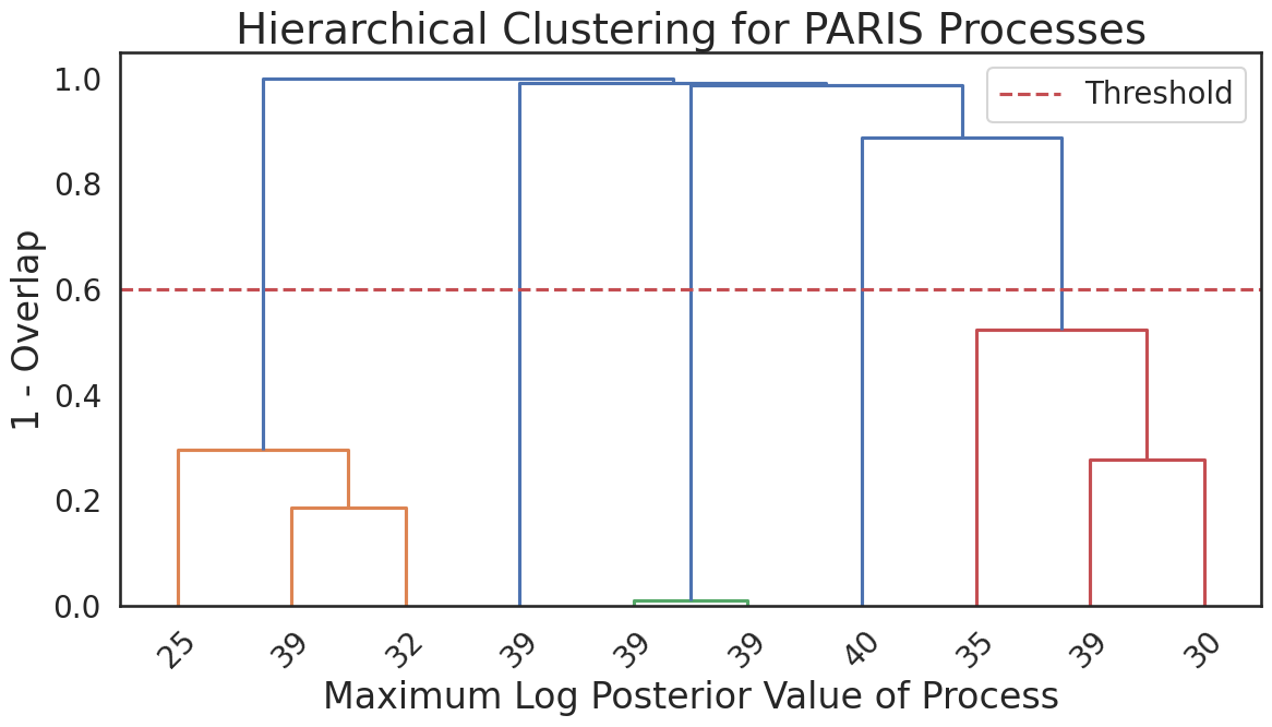

Using this clustering information, we analyze the parameter estimation performance for each identified source. As shown in Figure 6, the injection parameters are well-recovered within their respective confidence regions for all five true sources (Clusters 0-4). The posterior distributions show clear peaks at the injected parameter values, with the found MAP estimates approximately equal to the true parameters for each source (summarized in Table 5).
For comparison, we post-processed the PTMCMC and DNS results by assigning their samples to the nearest injected signal parameters. This procedure is equivalent to a single-iteration K-means clustering with centroids fixed at the true values, allowing us to explicitly count how many distinct modes each sampler successfully recovered. PTMCMC with 50 walkers (starting from the same seed points as PARIS) and 5 temperatures spent 210,000 function evaluations to obtain 64,350 posterior samples, but failed to find the signals corresponding to modes 2 and 3 in Figure 6. DNS, with 1,000 initial live points and a stopping criterion of , required 1.7 million function evaluations to converge with 21,725 posterior samples, but missed modes 1, 2 and 4.
| Mode 0 | Mode 1 | Mode 2 | Mode 3 | Mode 4 | |
|---|---|---|---|---|---|
| DNS | 40.0 | 36.4 | 23.9 | 40.0 | 32.2 |
| PTMCMC | 40.0 | 40.0 | 26.9 | 37.3 | 39.2 |
| PARIS | 40.0 | 40.0 | 39.9 | 39.9 | 39.5 |
V.5 GW150914: The First Observed Binary Black Hole Merger

GW150914 was the historic first direct detection of GWs by the LIGO detectors [3], originating from the inspiral and coalescence of two stellar-mass black holes [2]. Owing to its high SNR and relatively simple structure as a quasi-circular binary black hole merger, GW150914 provides a classical example for assessing the performance of sampling algorithms in GW parameter estimation [102, 50, 35]. Despite being a single-mode distribution in the full parameter space, the posterior exhibits nontrivial internal structure and non-Gaussianity in certain parameters such as declination (dec), right ascension (ra), and inclination angle ().
In analyzing GW150914-like events, waveforms typically incorporate the inspiral, merger, and ringdown phases of compact binary coalescences. In our study, waveform generation is performed using the bilby package [15], which provides interfaces to various phenomenological and numerical-relativity-based waveforms. For computational efficiency, we employ an aligned-spin waveform model IMRPhenomPv2 [61] which captures the essential physics of black hole mergers and is designed for robust use in data analysis.
In our parameter-estimation study of GW150914, we adopt the Hanford (H1) and Livingston (L1) strain data within a frequency band of Hz. The noise power spectral density (PSD) is estimated using the Welch method with a median average and a 0.4s roll-off Tukey window. Following the framework in Sec. II, and assuming broad uniform priors in the sampling space, the unnormalized log-posterior is equivalent to the log-likelihood defined in Eq. (33) :
| (40) |
To improve sampling efficiency, we analytically marginalize over the coalescence time, phase, and luminosity distance. The 13 remaining model parameters are:
-
•
Intrinsic parameters: (primary and secondary masses); (spin magnitudes); (spin tilt angles); (azimuthal angle between spin vectors); and (angle between total and orbital angular momentum).
-
•
Extrinsic parameters: (sky location); (inclination angle); (polarization angle); and (coalescence time uncertainty).
We then applied the PARIS sampler, configured with:
In this analysis, we initialize PARIS with a single seed at the outset, as the target posterior distribution of GW150914 exhibits a single-mode structure. PARIS completed the parameter estimation in 100 thousand function evaluations. In contrast, PTMCMC—configured with 10 walkers and a single temperature (since the distribution is effectively single-mode)—required 3 million function evaluations with greater sampling error (see Figure 7). DNS, initialized with 2000 live points and using a stopping criterion of , also totaled 3 million function evaluations. Table 6 compares the number of posterior samples, function evaluations and log evidence for each method, with PARIS having a similar evidence estimate to DNS.
| Method | Posterior Samples | Function Evaluations | Log Evidence |
|---|---|---|---|
| DNS | 40,567 | 3,109,912 | -32108.26 |
| PTMCMC | 30,000 | 3,202,895 | - |
| PARIS | 100,000 | 100,000 | -32108.43 |
As seen in Figure 7 and Table 6, PARIS and DNS yield largely consistent posterior structures and matching log-evidence estimates. Since these are two independent sampling frameworks, their agreement indicates a converged and reliable estimation of the true posterior. With this baseline established, we observe that PTMCMC overestimates the probability density in low-posterior regions, as evidenced by its wider and more uneven contours (particularly in sky location and inclination). While DNS accurately reproduces the posterior, it requires millions of function evaluations to achieve such fidelity. In contrast, PARIS effectively captures the landscape with significantly fewer evaluations, but at the cost of more uneven (under-resolved) sampling in some 1D marginals; nevertheless, these do not have a big impact on the evidence estimation.
VI Analysis and Discussion
In a series of experiments with a range of dimensionality and posterior morphology, PARIS consistently delivers accurate parameter estimation and evidence estimation, while using significantly fewer function evaluations than standard implementations of DNS and PTMCMC. This efficiency highlights its potential as a computationally effective tool for Bayesian inference, particularly in GW analysis where function evaluations are costly. Each experiment in Sec. V showcases a unique strength of PARIS: the NUS model demonstrates its ability to resolve complex, disconnected patterns; the 10D GMM illustrates balanced mode exploitation in higher-dimensional spaces; the toy GW example emphasizes its effectiveness with long-tailed, multi-modal posteriors; the GB signal search underscores its utility for the exploration and optimization of large, complex landscapes; and the GW150914 example validates its precision in estimating a noisy and non-Gaussian single-mode posterior. These diverse challenges collectively affirm PARIS’s versatility and robustness across varied inference tasks.
By using previous samples as Gaussian mixture centers weighted by their importance, PARIS focuses sampling on high-posterior regions while exploring under-sampled areas, balancing exploitation and exploration effectively. The parallel processes, initialized via LHS and refined through merging, ensure thorough coverage and reduce redundancy, while the reweighting scheme provides accurate evidence estimates. The adaptive strategy underpinning PARIS is also notably insensitive to initial conditions and hyperparameters—a feature evident across all experiments. We employed a simple diagonal initial covariance matrix with roughly scaled diagonal elements and a fixed sliding window size , yet PARIS consistently adapted to the target distribution without requiring fine-tuning.
However, PARIS has several potential limitations that can arise due to improper hyperparameter settings. 1) The presence of extremely localized modes (relative to the prior) may require more initial LHS samples or more initial processes for them to be detected reliably. 2) An excessively large may cause processes to drift erratically away from high-probability regions, whereas a value that is too small can lead to numerical singularities (i.e., ill-conditioned covariance matrices) during early iterations. 3) When a single process attempts to bridge multiple adjacent modes, an insufficient sliding window size may fail to construct a proposal capable of enveloping the multi-peaked landscape.
To improve the PARIS algorithm, several future directions are promising. First, incorporating location-dependent information—where the proposal geometry adapts as a function of its position (e.g., via analytical kernels or neural networks)—would enable a single process to more effectively bridge and envelope multiple adjacent modes in complex landscapes [36]. Second, to improve proposal efficiency, past samples could be used to train predictive models like Gaussian processes [27, 77, 72, 40] to identify and reject low-density regions. Last, the extension of PARIS to deal with significantly varying SNRs in the GB search can be explored by switching to a traditional trans-dimensional approach [70, 71], but another possibility could be to introduce modifications to the base algorithm that prioritize the local exploitation of individual processes, such as reverse annealing or an overlap-based merging criterion.
Code Availability
The source code for the PARIS algorithm, along with instructions and examples used to generate the results presented in this work, are publicly available on GitHub at https://github.com/mx-Liu123/parismc.
Acknowledgements.
ML would like to express his sincere gratitude to Kate Lee, Nandini Sahu, Joshua Speagle, and Peter Pang for their invaluable insights and constructive feedback on this work. He also thanks several colleagues at NUS for their support and stimulating discussions throughout the development of the PARIS framework, especially Soichiro Isoyama, Josh Mathews, Shubham Kejriwal, Davendra Hassan, and Rishav Agrawal. ML is supported by the NUS Research Scholarship for his PhD.| Symbol | Description |
|---|---|
| Dimensionality of the samples | |
| Unnormalized target density | |
| The total number of iterations and the current iteration index, respectively. | |
| The true Bayesian evidence and its empirical estimate, respectively. (Subscript , e.g., or , denotes the estimate or cumulative weight sum at iteration ) | |
| The sample at -th iteration of the -th process | |
| Importance weight of sample | |
| Proposal distribution at iteration in -th process | |
| Covariance matrix of weighted sample set evaluated at iteration in the -th process. In the practical version, updated every iterations and denoted as | |
| Proposal center for generating | |
| The cumulative proposal distribution for the -th process, used as the importance weight denominator. | |
| The set of currently active sampling processes during the dynamic merging and splitting phases. | |
| Modified Gaussian distribution with a rescaled peak value, introduced to prevent density inflation in high-dimensional spaces. | |
| Denominator of the importance weight for at iteration | |
| Cross-density contribution from external process evaluated at the current sample position of process . | |
| Method hyperparameters | |
| Number of initial Latin hypercube samples covering the prior region | |
| Number of processes in initialization | |
| The scale of initial proposal | |
| Iteration count to update the proposal covariance, fixed as 100 for all experiments in this work | |
| Truncation parameter, considering only the latest iterations’ samples, fixed as 1000 for all experiments in this work | |
Appendix A Notation
Table 7 summarizes the notation used throughout the paper for convenience of reference.
Appendix B Consistency of the PARIS Estimator
The base PARIS estimator for some test function at iteration is defined as
| (41) |
where all historical samples are used and reweighted according to the entire sequence of proposal distributions up to iteration . This is an example of deterministic-mixture reweighting in AMIS, which was popularized by Cornuet et al. [31] and formally established to have the lowest variance lower bound in Elvira et al. [44]. However, while AMIS algorithms (such as PARIS) yield estimators with asymptotic variance reduction, proving their strong consistency remains difficult. The most robust attempt strictly requires the per-iteration sample size to grow rapidly (i.e., ) [75]. This approach is not taken in PARIS (where ; see remark in Algorithm 1), as it is computationally unfeasible for expensive target densities such as astrophysical posteriors.
Conversely, a parallel branch of literature has successfully proven asymptotic consistency for AIS (not AMIS) with a fixed sample size per iteration, without relying on the variance reduction of deterministic-mixture reweighting. By evaluating a sample solely against the single proposal that generated it (thus preserving the martingale property), Portier et al. [83] and Delyon et al. [37] established uniform convergence rates for fixed sample sizes. Optimization-based perspectives further proved fixed-sample convergence by formulating parametric AIS as a stochastic gradient descent problem [6, 7]. However, these fixed-sample AIS results expose the difficulty of establishing asymptotic consistency for target densities with non-compact support. In such cases, if the proposal’s tails decay faster than the target’s, the variance of the importance weights explodes to infinity. To counteract this, algorithms are often forced to incorporate artificial, heavy-tailed “defensive” mixtures, drastically complicating the methodology [37].
In PARIS, the support of the target density is explicitly required to be compact, as it is mapped onto a unit hypercube . This design constraint (along with the Gaussian-mixture proposals) ensures that the importance weights remain bounded (i.e., ), and effectively removes the risk of variance explosion in a fixed-sample approach. As also noted in Appendix B of Delyon et al. [37], operating within a compact support drastically relaxes convergence requirements. Taken in combination, all of these results indicate that deterministic-mixture AMIS with a fixed sample size per iteration but a compact support will generally achieve strong consistency, although we are unable to prove it for PARIS at this point.
Appendix C Covariance Estimation
Standard sample covariance estimates can be biased near boundaries. To address this, we model the samples as being drawn from a multivariate Gaussian distribution truncated to the prior region . We propose a covariance estimation scheme that minimizes the negative log-likelihood of this truncated distribution [34].
C.1 Truncated Gaussian Formulation
Let the normalization constant (partition function) over the prior region be defined as:
| (42) |
Given a set of weighted samples , the negative log-likelihood function for the truncated Gaussian is:
| (43) |
Minimizing with respect to allows us to recover the underlying covariance structure. The integral is approximated as:
| (44) |
where is the volume fraction of the Gaussian distribution falling within . In this work, is estimated via Monte Carlo simulation using samples drawn from the untruncated . Note that in the practical implementation (Algorithm 3), the recorded trial count serves as a trigger for this expensive correction, as it provides a rough historical estimate of leakage.
C.2 Estimation Procedure
The optimization determines a scaling vector to define a rescaled covariance , where . The procedure is summarized in Algorithm 4.
Algorithm 4
Covariance Estimation
Input: Weighted samples , Recorded trial counts , Prior region , Previous mean .
1) Initial Estimate
-
•
Compute raw weighted covariance using Eq. (9).
2) Boundary Check & Branching
-
•
Compute average trials per sample: .
-
•
Estimate fraction outside : .
-
•
If :
-
•
Else (): Proceed to Step 3.
3) Optimization (Truncation Correction)
-
•
Estimate precision ratio using Monte Carlo samples from .
-
•
Initialize scaling vector and define .
-
•
Construct objective covariance: .
-
•
Solve for optimal scaling:
-
•
Update: .
4) Stabilization
-
•
Apply Oracle Approximating Shrinkage (OAS):
To address ill-conditioning, particularly with small sample sizes, we apply OAS to , producing the OAS estimate , which minimizes the mean-squared error in covariance estimation [24]:
Output: Estimated covariance .
References
- [1] (1996) Exchange monte carlo method and application to spin glass simulations. Journal of the Physical Society of Japan 65 (6), pp. 1604–1608. External Links: Document, Link, https://doi.org/10.1143/JPSJ.65.1604 Cited by: §I.
- [2] (2016) GW150914: First results from the search for binary black hole coalescence with Advanced LIGO. Phys. Rev. D 93 (12), pp. 122003. External Links: 1602.03839, Document Cited by: §V.5, §V.
- [3] (2016) Observation of Gravitational Waves from a Binary Black Hole Merger. Phys. Rev. Lett. 116 (6), pp. 061102. External Links: 1602.03837, Document Cited by: §I, §V.5.
- [4] (2017) Exploring the Sensitivity of Next Generation Gravitational Wave Detectors. Class. Quant. Grav. 34 (4), pp. 044001. External Links: 1607.08697, Document Cited by: §I.
- [5] (2020) Properties and Astrophysical Implications of the 150 M⊙ Binary Black Hole Merger GW190521. Astrophys. J. Lett. 900 (1), pp. L13. External Links: 2009.01190, Document Cited by: §I.
- [6] (2021) Convergence rates for optimised adaptive importance samplers. Statistics and Computing 31 (2), pp. 12. Cited by: Appendix B.
- [7] (2022) Global convergence of optimized adaptive importance samplers. arXiv preprint arXiv:2201.00409. Cited by: Appendix B.
- [8] (2024-09) A comparison of Bayesian sampling algorithms for high-dimensional particle physics and cosmology applications. External Links: 2409.18464 Cited by: §I.
- [9] (2012) FINDCHIRP: an algorithm for detection of gravitational waves¡? format?¿ from inspiraling compact binaries. Physical Review D—Particles, Fields, Gravitation, and Cosmology 85 (12), pp. 122006. Cited by: §V.3, §V.3, §V.4.
- [10] (2012) Low-frequency gravitational-wave science with eLISA/NGO. Class. Quant. Grav. 29, pp. 124016. External Links: 1202.0839, Document Cited by: §I, §V.4.
- [11] (2017-02) Laser Interferometer Space Antenna. External Links: 1702.00786 Cited by: §I, §V.4.
- [12] (2022-01) The international pulsar timing array second data release: search for an isotropic gravitational wave background. Monthly Notices of the Royal Astronomical Society 510 (4), pp. 4873–4887. External Links: ISSN 1365-2966, Link, Document Cited by: §I.
- [13] (2021-08) ¡Scp¿bilby¡/scp¿-mcmc: an mcmc sampler for gravitational-wave inference. Monthly Notices of the Royal Astronomical Society 507 (2), pp. 2037–2051. External Links: ISSN 1365-2966, Link, Document Cited by: §I.
- [14] (2022) Nested sampling for physical scientists. Nature 2. External Links: 2205.15570, Document Cited by: §I.
- [15] (2019) BILBY: A user-friendly Bayesian inference library for gravitational-wave astronomy. Astrophys. J. Suppl. 241 (2), pp. 27. External Links: 1811.02042, Document Cited by: §V.5.
- [16] (2023) Cosmology with the Laser Interferometer Space Antenna. Living Rev. Rel. 26 (1), pp. 5. External Links: 2204.05434, Document Cited by: §V.4.
- [17] (2016) Detecting compact galactic binaries using a hybrid swarm-based algorithm. Phys. Rev. D 93 (6), pp. 064020. External Links: 1509.08867, Document Cited by: §V.4.
- [18] (2019) A python surrogate modeling framework with derivatives. Advances in Engineering Software, pp. 102662. External Links: ISSN 0965-9978, Document Cited by: §III.2.
- [19] (2021-01) UltraNest – a robust, general purpose Bayesian inference engine. External Links: 2101.09604 Cited by: §I.
- [20] (2023-01) Nested sampling methods. Statistics Surveys 17 (none). External Links: ISSN 1935-7516, Link, Document Cited by: §I.
- [21] (2017-07) Adaptive importance sampling: the past, the present, and the future. IEEE Signal Processing Magazine 34 (4), pp. 60–79. External Links: Document Cited by: §I, §II.3.
- [22] (2017-07) Adaptive importance sampling: the past, the present, and the future. IEEE Signal Processing Magazine 34 (4), pp. 60–79. External Links: Document, ISSN 1053-5888, Link Cited by: §I.
- [23] (2022-10) Proximal nested sampling for high-dimensional bayesian model selection. Statistics and Computing 32 (5). External Links: ISSN 1573-1375, Link, Document Cited by: §I.
- [24] (2010-10) Shrinkage algorithms for mmse covariance estimation. IEEE Transactions on Signal Processing 58 (10), pp. 5016–5029. External Links: ISSN 1941-0476, Link, Document Cited by: 1st item.
- [25] (2022) Parameter estimation with gravitational waves. Rev. Mod. Phys. 94 (2), pp. 025001. External Links: 2204.04449, Document Cited by: §I, §I.
- [26] (2022) Nonlocal parameter degeneracy in the intrinsic space of gravitational-wave signals from extreme-mass-ratio inspirals. Phys. Rev. D 106 (12), pp. 124046. External Links: 2109.14254, Document Cited by: §I.
- [27] (2020) Gaussian processes for the interpolation and marginalization of waveform error in extreme-mass-ratio-inspiral parameter estimation. Phys. Rev. D 101 (4), pp. 044027. External Links: 1912.11543, Document Cited by: §VI.
- [28] (2022) One-stop function for gravitational-wave detection, identification, and inference. Phys. Rev. D 106 (10), pp. 104051. External Links: 2205.08702, Document Cited by: §I.
- [29] (2005-08) LISA data analysis using markov chain monte carlo methods. Physical Review D 72 (4). External Links: ISSN 1550-2368, Link, Document Cited by: §I.
- [30] (2007-10) Tests of bayesian model selection techniques for gravitational wave astronomy. Physical Review D 76 (8). External Links: ISSN 1550-2368, Link, Document Cited by: §V.4.
- [31] (2012) Adaptive multiple importance sampling. Scandinavian Journal of Statistics 39 (4), pp. 798–812. Cited by: Appendix B, §I, §II.1, §II.2, §II.3, Algorithm 1.
- [32] (2007) A Solution to the Galactic Foreground Problem for LISA. Phys. Rev. D 75, pp. 043008. External Links: astro-ph/0611546, Document Cited by: §V.4.
- [33] (2014) Gaussian process adaptive importance sampling. International Journal for Uncertainty Quantification 4 (2), pp. 133–149. External Links: Document, Link Cited by: §I.
- [34] (2018) Efficient statistics, in high dimensions, from truncated samples. In 2018 IEEE 59th Annual Symposium on Foundations of Computer Science (FOCS), pp. 639–649. Cited by: Appendix C.
- [35] (2021) Real-Time Gravitational Wave Science with Neural Posterior Estimation. Phys. Rev. Lett. 127 (24), pp. 241103. External Links: 2106.12594, Document Cited by: §V.5.
- [36] (2023) Neural Importance Sampling for Rapid and Reliable Gravitational-Wave Inference. Phys. Rev. Lett. 130 (17), pp. 171403. External Links: 2210.05686, Document Cited by: §I, §VI.
- [37] (2021) Safe adaptive importance sampling. The Annals of Statistics 49 (2), pp. 885–917. Cited by: Appendix B, Appendix B.
- [38] (2013) High-dimensional integration: the quasi-monte carlo way. Acta Numerica 22, pp. 133–288. External Links: Document Cited by: §III.2.
- [39] (2024-09) Notes on the practical application of nested sampling: multinest, (non)convergence, and rectification. The Open Journal of Astrophysics 7. External Links: ISSN 2565-6120, Link, Document Cited by: §I.
- [40] (2025-03) Accelerating LISA inference with Gaussian processes. External Links: 2503.21871 Cited by: §VI.
- [41] (2019-09) Efficient adaptive multiple importance sampling. In 2019 27th European Signal Processing Conference (EUSIPCO), A Coruna, Spain, pp. 1–5. External Links: Document, ISSN 2076-1465, ISBN 978-9-0827-9703-9, Link Cited by: §I, §IV.3.
- [42] (2022) Optimized population monte carlo. IEEE Transactions on Signal Processing 70, pp. 2489–2501. External Links: ISSN 1941-0476, Link, Document Cited by: §I, §II.3, §IV.3.
- [43] (2015-10) Efficient multiple importance sampling estimators. IEEE Signal Processing Letters 22 (10), pp. 1757–1761. External Links: ISSN 1558-2361, Link, Document Cited by: §I.
- [44] (2019-02) Generalized multiple importance sampling. Statistical Science 34 (1). External Links: ISSN 0883-4237, Link, Document Cited by: Appendix B, §I, §I.
- [45] (2021-09) A Horizon Study for Cosmic Explorer: Science, Observatories, and Community. External Links: 2109.09882 Cited by: §I.
- [46] (2009) Use of the MultiNest algorithm for gravitational wave data analysis. Class. Quant. Grav. 26, pp. 215003. External Links: 0904.1544, Document Cited by: §I.
- [47] (2008) Multimodal nested sampling: an efficient and robust alternative to MCMC methods for astronomical data analysis. Mon. Not. Roy. Astron. Soc. 384, pp. 449. External Links: 0704.3704, Document Cited by: §I.
- [48] (2013-03) emcee: The MCMC Hammer. Publications of the Astronomical Society of the Pacific 125 (925), pp. 306. External Links: Document, 1202.3665 Cited by: §V.
- [49] (2013) Bayesian data analysis. 3rd edition, Chapman and Hall/CRC, Boca Raton, FL. Note: With errors fixed as of 20 February 2025 External Links: ISBN 9781439840955 Cited by: §II.
- [50] (2021) Complete parameter inference for GW150914 using deep learning. Mach. Learn. Sci. Tech. 2 (3), pp. 03LT01. External Links: 2008.03312, Document Cited by: §V.5.
- [51] (2014) Optimal mixture weights in multiple importance sampling. External Links: 1411.3954, Link Cited by: §I.
- [52] (2018-09) Sampling errors in nested sampling parameter estimation. Bayesian Analysis 13 (3). External Links: ISSN 1936-0975, Link, Document Cited by: §I.
- [53] (2017) The Taiji Program in Space for gravitational wave physics and the nature of gravity. Natl. Sci. Rev. 4 (5), pp. 685–686. External Links: Document Cited by: §I.
- [54] (2005-09) An efficient algorithm for constructing optimal design of computer experiments. Journal of Statistical Planning and Inference 134 (1), pp. 268–287. External Links: Document Cited by: §III.2.
- [55] (2023-03) Eryn : A multi-purpose sampler for Bayesian inference. External Links: 2303.02164 Cited by: §I, §V.4, §V.
- [56] Mikekatz04/eryn: first full release External Links: Document, Link Cited by: §V.
- [57] (2022-09) Bayesian characterization of circumbinary sub-stellar objects with lisa. Monthly Notices of the Royal Astronomical Society 517 (1), pp. 697–711. External Links: ISSN 1365-2966, Link, Document Cited by: §V.4.
- [58] (2022) Bayesian characterization of circumbinary sub-stellar objects with LISA. Mon. Not. Roy. Astron. Soc. 517 (1), pp. 697–711. External Links: 2205.03461, Document Cited by: §V.4.
- [59] Mikekatz04/gbgpu: first official public release! External Links: Document, Link Cited by: §V.4.
- [60] (2025-03) Bias-Corrected Importance Sampling for Inferring Beyond Vacuum-GR Effects in Gravitational Wave Sources. External Links: 2503.01120 Cited by: §I.
- [61] (2019) Phenomenological model for the gravitational-wave signal from precessing binary black holes with two-spin effects. Phys. Rev. D 100 (2), pp. 024059. External Links: 1809.10113, Document Cited by: §V.5.
- [62] (2022) Fast sky localization of gravitational waves using deep learning seeded importance sampling. Phys. Rev. D 106 (2), pp. 023032. External Links: 2111.00833, Document Cited by: §I.
- [63] Joshspeagle/dynesty: v2.1.4 External Links: Document, Link Cited by: §V.
- [64] (2021) Adaptive importance sampling meets mirror descent: a bias-variance tradeoff. External Links: 2110.15590, Link Cited by: §I.
- [65] Cited by: §V.4.
- [66] (2024-09) Gravitational Wave Astronomy With TianQin. External Links: 2409.19665 Cited by: §I.
- [67] (2015-08) An adaptive importance sampling algorithm for bayesian inversion with multimodal distributions. Journal of Computational Physics 294, pp. 173–190. External Links: Document, Link Cited by: §I.
- [68] (2023-03) Prototype global analysis of lisa data with multiple source types. Physical Review D 107 (6). External Links: ISSN 2470-0029, Link, Document Cited by: §I.
- [69] (2023) Prototype global analysis of LISA data with multiple source types. Phys. Rev. D 107 (6), pp. 063004. External Links: 2301.03673, Document Cited by: §V.4.
- [70] (2011) A detection pipeline for galactic binaries in LISA data. Phys. Rev. D 84, pp. 063009. External Links: 1106.6355, Document Cited by: §V.4, §V, §VI.
- [71] (2020) Global Analysis of the Gravitational Wave Signal from Galactic Binaries. Phys. Rev. D 101 (12), pp. 123021. External Links: 2004.08464, Document Cited by: §V.4, §V, §VI.
- [72] (2023) Improving the scalability of the Gaussian-process error marginalization in gravitational-wave inference. Phys. Rev. D 108 (10), pp. 103027. External Links: 2307.07233, Document Cited by: §VI.
- [73] (2016) TianQin: a space-borne gravitational wave detector. Class. Quant. Grav. 33 (3), pp. 035010. External Links: 1512.02076, Document Cited by: §I.
- [74] (2020) Science Case for the Einstein Telescope. JCAP 03, pp. 050. External Links: 1912.02622, Document Cited by: §I.
- [75] (2017-03) Consistency of adaptive importance sampling and recycling schemes. Bernoulli 25 (3), pp. 1987–2016. External Links: Document, Link Cited by: Appendix B, §II.1.
- [76] (2015-08) An adaptive population importance sampler: learning from uncertainty. IEEE Transactions on Signal Processing 63 (16), pp. 4422–4437. External Links: Document, ISSN 1053-587X, Link Cited by: §I, §IV.3.
- [77] (2016) Improving gravitational-wave parameter estimation using Gaussian process regression. Phys. Rev. D 93 (6), pp. 064001. External Links: 1509.04066, Document Cited by: §VI.
- [78] (2021) Hamiltonian adaptive importance sampling. IEEE Signal Processing Letters 28, pp. 713–717. External Links: ISSN 1558-2361, Link, Document Cited by: §I.
- [79] (2024-10) Robust, Rapid, and Simple Gravitational-wave Parameter Estimation. External Links: 2410.05190 Cited by: §I.
- [80] (2017) An architecture for efficient gravitational wave parameter estimation with multimodal linear surrogate models. Class. Quant. Grav. 34 (14), pp. 144002. External Links: 1701.01137, Document Cited by: §I.
- [81] (2021-02) Implicitly adaptive importance sampling. Statistics and Computing 31 (2). External Links: ISSN 1573-1375, Link, Document Cited by: §I.
- [82] (2023) Population monte carlo with normalizing flow. External Links: 2312.03857, Link Cited by: §I, §II.3.
- [83] (2018) Asymptotic optimality of adaptive importance sampling. Advances in neural information processing systems 31. Cited by: Appendix B.
- [84] (2007) -Statistic search for white-dwarf binaries in the first mock lisa data challenge. Classical and Quantum Gravity 24 (19), pp. S565–S574. Cited by: §V.4.
- [85] (2010) The Einstein Telescope: A third-generation gravitational wave observatory. Class. Quant. Grav. 27, pp. 194002. External Links: Document Cited by: §I.
- [86] (2004) Monte carlo statistical methods. 2nd edition, Springer, New York, NY. External Links: ISBN 9780387212395 Cited by: §II.1.
- [87] (2019-04) The construction and use of lisa sensitivity curves. Classical and Quantum Gravity 36 (10), pp. 105011. External Links: ISSN 1361-6382, Link, Document Cited by: §V.4.
- [88] (2018-09) Detecting hierarchical stellar systems with lisa. Physical Review D 98 (6). External Links: ISSN 2470-0029, Link, Document Cited by: §V.3, §V.4, §V.4.
- [89] (2024) Tempered multifidelity importance sampling for gravitational wave parameter estimation. Phys. Rev. D 110 (10), pp. 104037. External Links: 2405.19407, Document Cited by: §I.
- [90] (2024) SMT 2.0: A surrogate modeling toolbox with a focus on hierarchical and mixed variables gaussian processes. Advances in Engineering Sofware 188, pp. 103571. External Links: Document Cited by: §III.2.
- [91] (2023) Astrophysics with the Laser Interferometer Space Antenna. Living Rev. Rel. 26 (1), pp. 2. External Links: 2203.06016, Document Cited by: §V.4.
- [92] (2007) Clustered nested sampling: Efficient Bayesian inference for cosmology. Mon. Not. Roy. Astron. Soc. 378, pp. 1365–1370. External Links: astro-ph/0701867, Document Cited by: §I.
- [93] (2006) Nested sampling for general bayesian computation. Bayesian Analysis 1, pp. 833–859. External Links: Link Cited by: §I.
- [94] (2020-02) Dynesty: a dynamic nested sampling package for estimating bayesian posteriors and evidences. Monthly Notices of the Royal Astronomical Society 493 (3), pp. 3132–3158. External Links: ISSN 1365-2966, Link, Document Cited by: §V.
- [95] (2023) dynesty: Dynamic Nested Sampling in Python. Note: https://dynesty.readthedocs.io/en/latest/quickstart.htmlAccessed: 2025-05-01 Cited by: §I.
- [96] (2022-09) Bayesian parameter estimation of galactic binaries in lisa data with gaussian process regression. Physical Review D 106 (6). External Links: ISSN 2470-0029, Link, Document Cited by: §V.4.
- [97] (1986-11) Replica monte carlo simulation of spin-glasses. Phys. Rev. Lett. 57, pp. 2607–2609. External Links: Document, Link Cited by: §I.
- [98] (2019) An introduction to Bayesian inference in gravitational-wave astronomy: parameter estimation, model selection, and hierarchical models. Publ. Astron. Soc. Austral. 36, pp. e010. Note: [Erratum: Publ.Astron.Soc.Austral. 37, e036 (2020)] External Links: 1809.02293, Document Cited by: §I.
- [99] (2008) Use and abuse of the fisher information matrix in the assessment of gravitational-wave parameter-estimation prospects. Physical Review D—Particles, Fields, Gravitation, and Cosmology 77 (4), pp. 042001. Cited by: §V.
- [100] (2015-11) Dynamic temperature selection for parallel tempering in markov chain monte carlo simulations. Monthly Notices of the Royal Astronomical Society 455 (2), pp. 1919–1937. External Links: ISSN 0035-8711, Document, Link, https://academic.oup.com/mnras/article-pdf/455/2/1919/18514064/stv2422.pdf Cited by: §I.
- [101] (2025) Validating sequential monte carlo for gravitational-wave inference. External Links: 2506.18977, Link Cited by: §I.
- [102] (2023) Fast Gravitational-wave Parameter Estimation without Compromises. Astrophys. J. 958 (2), pp. 129. External Links: 2302.05333, Document Cited by: §V.5.
- [103] (2009) Estimation of cosmological parameters using adaptive importance sampling. Phys. Rev. D 80, pp. 023507. External Links: 0903.0837, Document Cited by: §I.
- [104] (2023) Searching for the nano-hertz stochastic gravitational wave background with the chinese pulsar timing array data release i. Research in Astronomy and Astrophysics 23. External Links: Link Cited by: §I.
- [105] (2021) Resolving Galactic binaries in LISA data using particle swarm optimization and cross-validation. Phys. Rev. D 104, pp. 024023. External Links: 2103.09391, Document Cited by: §V.4.