Finite Sample Smeariness on Spheres and Modulation-aware Tests
Abstract.
Directional and shape data often live on manifolds, where standard central limit theorems (CLT) and the associated Wald-type -tests require curvature-dependent recalibration: the limiting normal covariance is modified by the Hessian of the Fréchet function. On spheres, under the positive-Hessian assumptions considered here, this curvature correction yields Type I finite sample smeariness (FSS), meaning that the asymptotic modulation exceeds . This paper studies FSS on and develops modulation-aware tests.
We first show that, for absolutely continuous distributions on with positive definite Hessians, Type I FSS is unavoidable under the stated classical CLT and moment assumptions. The geometric mechanism is that, for the absolutely continuous spherical distributions considered here, positive curvature of the sphere gives the strict spectral bound , so that the limiting modulation is strictly larger than one.
We then prove a curse-of-dimensionality result for dimensionally comparable rotationally symmetric families: their asymptotic modulation is monotone increasing with dimension and can become arbitrarily large as the support approaches a hemisphere. Motivated by these results, we derive explicit consistent plug-in estimators of the Fréchet-function Hessian and use them to construct one-sample and two-sample Hessian-corrected Hotelling-type statistics with limits. Numerical experiments on low- and high-dimensional spheres show that the proposed modulation-aware tests have rejection behavior comparable to bootstrap-based FSS corrections, while being substantially faster due to the explicit Hessian formulas.
Susovan Pal
Department of Mathematics and Data Science, Vrije Universiteit Brussel (VUB)
Pleinlaan 2, B-1050 Elsene/Ixelles, Belgium
susovan.pal@vub.be, susovan97@gmail.com
Keywords: Fréchet means, finite sample smeariness, variance modulation, spheres, Hessian-corrected inference, geometric statistics
2020 Mathematics Subject Classification: Primary: 62H11; Secondary: 60F05, 60D05, 53C22.
1. Introduction
1.1. Fréchet means and Wald-type tests
Directional and shape data often take values in nonlinear spaces, such as spheres, shape spaces, and more general Riemannian manifolds. In such settings the Fréchet mean plays the role of the Euclidean expectation. If is a random variable on a Riemannian manifold , with law and Riemannian distance , its Fréchet function is
A minimizer of is called a population Fréchet mean. Given i.i.d. observations , the empirical Fréchet function is , and a measurable minimizer is called a sample Fréchet mean.
Central limit theorems for sample Fréchet means are by now classical in statistics on manifolds; see, for instance, Hendriks and Landsman (1998); Bhattacharya and Patrangenaru (2005); Bhattacharya and Lin (2017); Hotz and Huckemann (2015a); Huckemann (2011). The important point for inference is that, even in the ordinary -rate regime, the limiting covariance is not generally the covariance of the tangent data alone. If is the unique population Fréchet mean, , , and , then, under the usual smoothness, uniqueness, and nondegeneracy hypotheses, the non-smeary manifold CLT has the form
Thus the Hessian of the Fréchet function enters directly into the covariance of the limiting Gaussian distribution, and hence into Wald-type -tests based on this distribution. In Euclidean space , so the correction disappears and the limiting covariance reduces to the usual covariance . On curved spaces, however, ignoring the Hessian correction can produce systematically miscalibrated tests. This paper studies this effect on , and develops explicit Hessian-corrected, modulation-aware tests.
1.2. Variance modulation and finite sample smeariness
Following Hundrieser et al. (2020); Huckemann et al. (2021); Eltzner et al. (2021), we use the following formulation.
Definition 1.1 (Variance modulation and finite sample smeariness).
Let be a unique Fréchet mean of a random variable on a Riemannian manifold , and let be a measurable sequence of sample Fréchet means based on an i.i.d. sample of size . Define
and, whenever , define the finite-sample variance modulation
We say that the Fréchet mean is finite sample smeary (FSS for short) if
More specifically, it is called
-
(i)
Type I FSS if ;
-
(ii)
Type II FSS if .
Remark 1.2.
Unlike in the previous literature stated here, we use and in Definition 1.1, rather than assuming that the modulation sequence converges. In the standard examples where the limit exists, this formulation agrees with the usual Type I/Type II distinction.
The Euclidean benchmark is . Thus FSS means that there exists a finite sample size for which the modulation exceeds unlike in the Euclidean setting. Type I FSS implies that, asymptotically, the modulation stays bounded away from . Type II FSS means that the modulation may exceed at finite sample sizes, but returns asymptotically to its Euclidean value. It is noteworthy that on circles, both Type I and Type II FSS are present; see Hundrieser et al. (2020), Theorem 3.1 and Corollary 3.2.
For later use, we also record the corresponding limiting or asymptotic modulation in the non-smeary CLT regime (cf. Definition 1.4).
Definition 1.3 (Asymptotic modulation).
Let be a unique Fréchet mean of on , and let be sample Fréchet means. Set , , and for . If is non-smeary and exists, we call the asymptotic modulation.
In the setting of Lemma 5.1 and Assumption 5.2, the non-smeary CLT and the required moment bound imply
This formula demonstrates that a suitable Hessian correction needs to be applied to the Euclidean setting, and thus the Wald-type tests in the spherical setting also need to be modified accordingly.
1.3. Finite sample smeariness as an intermediate regime between Euclidean and smeary regimes
The present paper is about finite sample smeariness in the non-smeary regime. Nevertheless, it is useful to recall how this differs from smeariness. Smeariness occurs when the Fréchet function is flatter than quadratic at the population Fréchet mean, leading to slower-than- asymptotics; see Hotz and Huckemann (2015b); Huckemann and Eltzner (2019); Eltzner (2022). The degeneracy may occur in all tangent directions, or only along a proper subspace. We use the following definition, adapted from the subspace formulation of Eltzner (2022).
Definition 1.4 (Smeariness and directional smeariness).
Let be a Fréchet mean of a random variable on a Riemannian manifold , and let be the lifted Fréchet function in exponential coordinates at , viewed on . Let be a linear subspace.
In the smooth finite-order setting considered here, we say that , or equivalently , is smeary along if for all sufficiently small , the quadratic term of vanishes at , and the first nonzero term in the Taylor expansion of has order and is positive on . We call the smeariness exponent along . If , we say that is smeary; if is a proper nonzero subspace, we say that is directionally smeary along .
Finite sample smeariness is different. It is not the regime of slower asymptotic rate. Rather, it is the intermediate regime in which the usual -rate CLT (also called BP-CLT, after Bhattacharya and Patrangenaru (2003)) still holds, but the Euclidean variance calibration is still wrong.
This distinction can be made precise under the upgrade from convergence in distribution to convergence of second moments, under Assumption 5.2. Suppose, for example, that in some nonzero tangent direction , a smeary CLT gives , where and . Under Assumption 5.2, the squares are uniformly integrable and
Since whenever lies in the normal neighborhood of , the variance modulation diverges. Thus, in the smeary or directionally smeary regimes covered by such CLTs, the modulation is not merely larger than one; it becomes unbounded. Finite sample smeariness is therefore a bounded, non-smeary analogue: worse than the Euclidean case, but less singular than full or directional smeariness.
1.4. Main results and contribution
The first main result is that Type I FSS is unavoidable on spheres in the positive-Hessian, non-smeary CLT regime. More precisely, Theorem 5.4 shows that if is absolutely continuous on , , has a unique Fréchet mean, positive definite Hessian, satisfies the non-smeary CLT, and satisfies the moment condition in Assumption 5.2, then the asymptotic modulation exists and is strictly larger than one.
The second main result is a curse of dimensionality effect on modulation. For dimensionally comparable rotationally symmetric families, introduced in Definition 6.1, Theorem 6.3 proves that the asymptotic modulation is strictly increasing with the sphere dimension. It also gives an explicit high-dimensional limit of the asymptotic modulation . In particular, when the support approaches a hemisphere, the limiting modulation can be made arbitrarily large.
The third contribution is inferential. The explicit Hessian formulas in Proposition 3.2 in the general-density and rotationally symmetric cases lead to consistent plug-in Hessian estimators. Proposition 7.3 proves consistency in both the general-density and rotationally symmetric settings. These estimators are then used to construct Hessian-corrected quadratic statistics. Proposition 7.4 and Theorem 7.5 give the one-sample version, while Theorem 7.7 gives the corresponding two-sample Hotelling-type statistic. The point is that the naive tangent covariance is replaced by the curvature-corrected covariance .
Section 8 compares three procedures: a naive tangent-space -test, a bootstrap-based finite-sample-smeariness correction, and the proposed Hessian-corrected modulation-aware test. The low-dimensional experiment on shows that the two corrected procedures behave similarly near the null. The high-dimensional experiment on shows a much sharper effect: the naive test severely over-rejects, while the bootstrap-based and modulation-aware tests both correct the level. The runtime comparison in Table 3 shows that, in the reported high-dimensional experiment, the modulation-aware test is about times faster per test call.
Finally, Section 9 applies the two-sample procedure to Microtus lower first molar preshape data on . The data are highly concentrated around their Fréchet mean, so the empirical Hessian is nearly and the modulation-aware statistic is numerically almost identical to the naive Hotelling statistic, providing a real-data local-Euclidean sanity check.
The sharp support-threshold theory for full and directional smeariness on spheres is treated separately in Pal (2026). The present paper uses that viewpoint only as background and as a source of clean non-smeary regimes. Its main focus is finite sample smeariness, dimension-dependent modulation, and Hessian-corrected inference.
1.5. Organization of the paper
Section 2 derives the second-order Taylor expansion of the squared Riemannian distance on in normal coordinates. Section 3 uses this expansion to obtain the Hessian formula for the Fréchet function, first for general densities and then under rotational symmetry; see Proposition 3.2. Section 4 records the radial function and its unique zero , which control the rotationally symmetric Hessian; see Proposition 4.1.
Section 5 proves the Type I finite sample smeariness theorem. Lemma 5.1 gives the required moment-convergence step, Lemma 5.3 proves the strict spectral bound for the Hessian, and Theorem 5.4 combines these ingredients to obtain . Section 6 proves the curse-of-dimensionality theorem for modulation, Theorem 6.3, and Section 6.1 gives a numerical illustration of this dimension effect.
Section 7 develops the statistical procedures. Proposition 7.3 proves consistency of the plug-in Hessian estimators, Proposition 7.4 gives the basic quadratic-form limit, Theorem 7.5 gives the one-sample modulation-aware test, and Theorem 7.7 gives the two-sample Hessian-corrected Hotelling statistic. Section 8 presents the simulation study comparing naive, bootstrap-based, and modulation-aware tests. The symbolic computation used for the Taylor expansion is recorded in Appendix A.
1.6. Acknowledgements and funding.
This research was supported by funding from Research Foundation–Flanders (FWO) via the Odysseus II programme no. G0DBZ23N. The author acknowledges technical discussions with Stephan Huckemann from the University of Göttingen, Germany, and also encouragement by David Tewodrose at Vrije Universiteit Brussel.
2. Taylor expansion of the Riemannian squared distance on through order
This section records the Taylor expansion, in normal coordinates at the north pole, of the squared Riemannian distance on the sphere through order two. This second-order expansion is the local computational input used later to derive the Hessian of the Fréchet function. Throughout, the expansion is taken in the first variable while the second variable is fixed away from the cut locus.
2.1. Taylor expansion of the Riemannian squared distance function in the tangent space using the exponential map
Let be the unit sphere, let be the north pole, and identify with the Euclidean inner product and norm . Fix with , and define the pulled-back squared distance function on by
| (1) |
For with , set and . Thus is the line restriction of along . By the spherical cosine law in normal coordinates,
| (2) |
Equivalently, if , then , where . Expanding at gives , with
| (3) |
The symbolic calculation of these Taylor coefficients is recorded in Appendix A. For , whenever is times differentiable at , the line-restriction identity gives .
Now write as , with and . Then , and . Hence, for fixed , the expansion through degree is
| (4) |
2.2. Explicit formula for the Hessian of the squared distance
We next extract from (4) the second derivative of at . Fix , where and . The derivatives below are always taken with respect to the -variable, with fixed.
In the Euclidean vector space , one has and . Therefore (4) gives, for every ,
| (5) |
3. Setup and Hessian formulas
This section records the common setup and the Hessian formulas for the population Fréchet function on . We first treat an arbitrary absolutely continuous density, not assumed to be rotationally symmetric, and then obtain the rotationally symmetric formula as a reduction. The pointwise expansion of the squared Riemannian distance is the one derived in Section 2.
3.1. General densities and rotational symmetry
Let be an absolutely continuous probability measure on . After applying an isometry, we take a population Fréchet mean to be the north pole , and write . Since and is absolutely continuous, . Thus is defined -a.s., and we write , with and . In these coordinates, .
Assume that has density in polar coordinates, so that
| (6) |
The lifted Fréchet function in these coordinates is
| (7) |
The rotationally symmetric case is the specialization , giving
| (8) |
Assumption 3.1 (Cut-locus avoidance).
We assume that there exists such that for a.e. with . In the rotationally symmetric case this means for sufficiently close to . Under this assumption, the integrand is smooth in for near and is uniformly separated from the cut locus. Hence differentiation under the integral sign at , in particular up to second order, is justified; compare Tran (2020), Proposition 3.2.1.
3.2. Formula for the Hessian of the Fréchet function and its rotationally symmetric reduction
Proposition 3.2 (Formula for the Hessian of the Fréchet function).
Assume Assumption 3.1. Let denote the Hessian of the lifted Fréchet function at , equivalently the Hessian of at . Then
| (9) |
Equivalently, for every ,
| (10) |
In the rotationally symmetric case, define
| (11) |
Then
| (12) |
Thus, under rotational symmetry, the Hessian is singular if and only if it vanishes, equivalently if and only if the scalar integral in (12) vanishes.
Proof.
By (7), Assumption 3.1, and the pointwise Hessian formula (5), differentiating under the integral sign gives (10), hence (9). If , then the Funk–Hecke formula gives
see, for example, Chafaï (2021). Therefore (12) follows. The final assertion follows because the Hessian is then a scalar multiple of . ∎
4. Radial threshold function and its zero
Under rotational symmetry, the Hessian formula (12) shows that the lifted Fréchet function is governed, at second order, by the radial function defined in (11). We record here the elementary sign structure of . Its unique zero marks the Hessian threshold used below for the rotationally symmetric non-smeary regime.
4.1. Analysis of
Proposition 4.1 (The Hessian threshold).
Let , and following (11), let be defined by . Then is strictly decreasing on , has a unique zero
| (13) |
and satisfies for and for .
Proof.
Set . Then
The numerator satisfies and on . Hence , so is strictly decreasing. Moreover, as , while as . Thus has a unique zero. Since , this zero lies in , and the stated signs follow from strict monotonicity. ∎
5. Finite sample smeariness in the non-smeary regime
This section proves that, on spheres of dimension , the ordinary non-smeary central limit regime is still finite-sample smeary of Type I whenever the Hessian is positive definite and the corresponding second moments converge. The mechanism is second-order: the Hessian correction in the Fréchet mean CLT inflates the limiting trace because of positive curvature.
We start with a technical lemma used to upgrade convergence in distribution to convergence of second moments.
Lemma 5.1 (Convergence of second moments under a uniform bound).
Let be a sequence of -valued random variables. Assume that and that there exists such that
Then .
Proof.
The moment bound implies uniform integrability of . The conclusion is the standard consequence of convergence in distribution together with uniform integrability; see Billingsley (1999). ∎
We shall use the following moment assumption for sample Fréchet means.
Assumption 5.2 (Uniform moment bound).
Let be a measurable sequence of intrinsic sample Fréchet means and set . We assume that there exists such that
Lemma 5.3 (Strict spectral upper bound for the Hessian).
Proof.
Let . As in the proof of Proposition 4.1, for . For , the Hessian formula (10) gives
| (14) | ||||
Since is a density with respect to , the equality set has -measure zero. Hence on a set of full -measure, and the inequality in (14) is strict for every unit . By continuity of and compactness of the unit sphere in , the supremum over is also strictly smaller than . Thus . ∎
Theorem 5.4 (Type I finite-sample smeariness in the non-smeary regime).
Let , and let be absolutely continuous on with unique Fréchet mean . Assume that satisfies the setup of Section 3.1 and Assumption 3.1. Let be a measurable sequence of intrinsic sample Fréchet means, set , and let
Assume that is positive definite and that the non-smeary Fréchet mean CLT holds:
Assume also Assumption 5.2. Then is Type I finite sample smeary. More precisely, the asymptotic modulation exists and satisfies .
Proof.
Remark 5.5 (Special case of hemispherical support).
Hemispherical support provides a natural non-smeary regime on spheres, so that the previous theorem can be applied to deduce Type-I FSS; see Pal (2026) for the corresponding support-threshold picture.
Remark 5.6 (Previous Type-I FSS results).
The theorem generalizes Theorem 6 of Eltzner et al. (2021) in the case of densities: no rotational symmetry has been assumed here.
Remark 5.7 (On the necessity of the moment condition).
The next remark shows that, even in the non-smeary rotationally symmetric regime, the limiting modulation can be made arbitrarily large, similar to the construction with a measure carrying a point mass in Eltzner (2022, Theorem 4.3).
Remark 5.8 (Arbitrarily high modulation under rotational symmetry).
Fix , and let denote the unique zero of . Let . Then, at the level of the rotationally symmetric Hessian formula, one can choose a smooth rotationally symmetric density on , with radial support contained in a small interval , for some sufficiently close to , such that is positive definite and satisfies .
Indeed, by (12), under rotational symmetry one has
Since on and as , choosing supported in a sufficiently small neighborhood of , with , yields . Consequently, in the rotationally symmetric scalar-Hessian case, whenever the corresponding limiting modulation is defined, can be made arbitrarily large.
6. Curse of dimensionality for modulation of non-smeary random variables
This section shows that, for dimensionally comparable rotationally symmetric densities supported in a closed sub-hemispherical cap around the unique Fréchet mean, the asymptotic modulation increases with dimension. The effect is purely second-order: under rotational symmetry, the Hessian is a scalar multiple of the identity, and the scalar Hessian eigenvalue decreases with dimension.
Definition 6.1 (Dimensionally comparable rotationally symmetric family).
Let denote the north pole. Fix and set . For each , let be a probability measure on , rotationally symmetric about , with
We say that is a dimensionally comparable rotationally symmetric family if there exists a measurable function such that, for every ,
and, in normal polar coordinates , the density of with respect to polar volume measure has the form
where is the uniform probability density on . Equivalently, the induced radial probability measure on is
Thus the family is generated by a single dimension-independent unnormalized radial weight , while the dependence on enters only through the Jacobian factor and the normalizing constant .
Example 6.2 (Dimensionally comparable distributions).
The following are dimensionally comparable rotationally symmetric families.
-
(1)
Uniform law on the truncated geodesic ball. Take . Then
-
(2)
Truncated von Mises–Fisher family with fixed concentration parameter . Since the von Mises–Fisher density is proportional to and , take . Then
See Jupp et al. (2016). By rotational symmetry, is a critical point of the Fréchet function.
- (3)
-
(4)
General truncated zonal family with fixed profile. More generally, if is measurable, then defines a dimensionally comparable rotationally symmetric family. See Jupp et al. (2016).
The following theorem proves that, for the families in Definition 6.1, the asymptotic modulation is strictly increasing with dimension.
Theorem 6.3 (Dimension monotonicity of asymptotic modulation for dimensionally comparable rotationally symmetric families).
Fix and set . For each integer , let be an absolutely continuous probability measure on with unique intrinsic Fréchet mean , and assume that is a dimensionally comparable rotationally symmetric family about , supported in , in the sense of Definition 6.1. Assume further that the moment condition 5.2 holds for each . Let , set , and let . Define the dimension-indexed asymptotic modulations, cf. Definition 1.3, by
Then:
-
(1)
The sequence is strictly increasing with dimension:
-
(2)
If the common radial weight from Definition 6.1 satisfies, for every ,
then, in the extended real line,
Proof.
Proof of (1). By Definition 6.1, there exists a measurable function such that , , and , where is the uniform probability density on . Rotational symmetry gives
Using the Hessian formula (9) with this normalized angular density, equivalently the rotationally symmetric reduction (12) with the angular volume factor cancelled by , we obtain
Since , this becomes , where
Since on and , we have . Hence , so is positive definite. The trace formula in Definition 1.3 therefore gives
Thus is equivalent to .
We next prove that . Define the probability measure on by
Let . Then
Therefore
Subtracting , and using the standard covariance symmetrization identity, gives
The map is strictly decreasing on , while is strictly increasing on . Hence the integrand is everywhere nonpositive. Since is absolutely continuous with respect to Lebesgue measure and is not supported on a single point, the inequality is strict. Thus .
Finally,
Since and , this inequality holds. Therefore , and hence .
Proof of (2). Assume that for every , . Fix and write and . Then
while
Since , it follows that
As is continuous on , we obtain
Therefore , and consequently
∎
6.1. Numerical simulation of curse of dimensionality for modulation
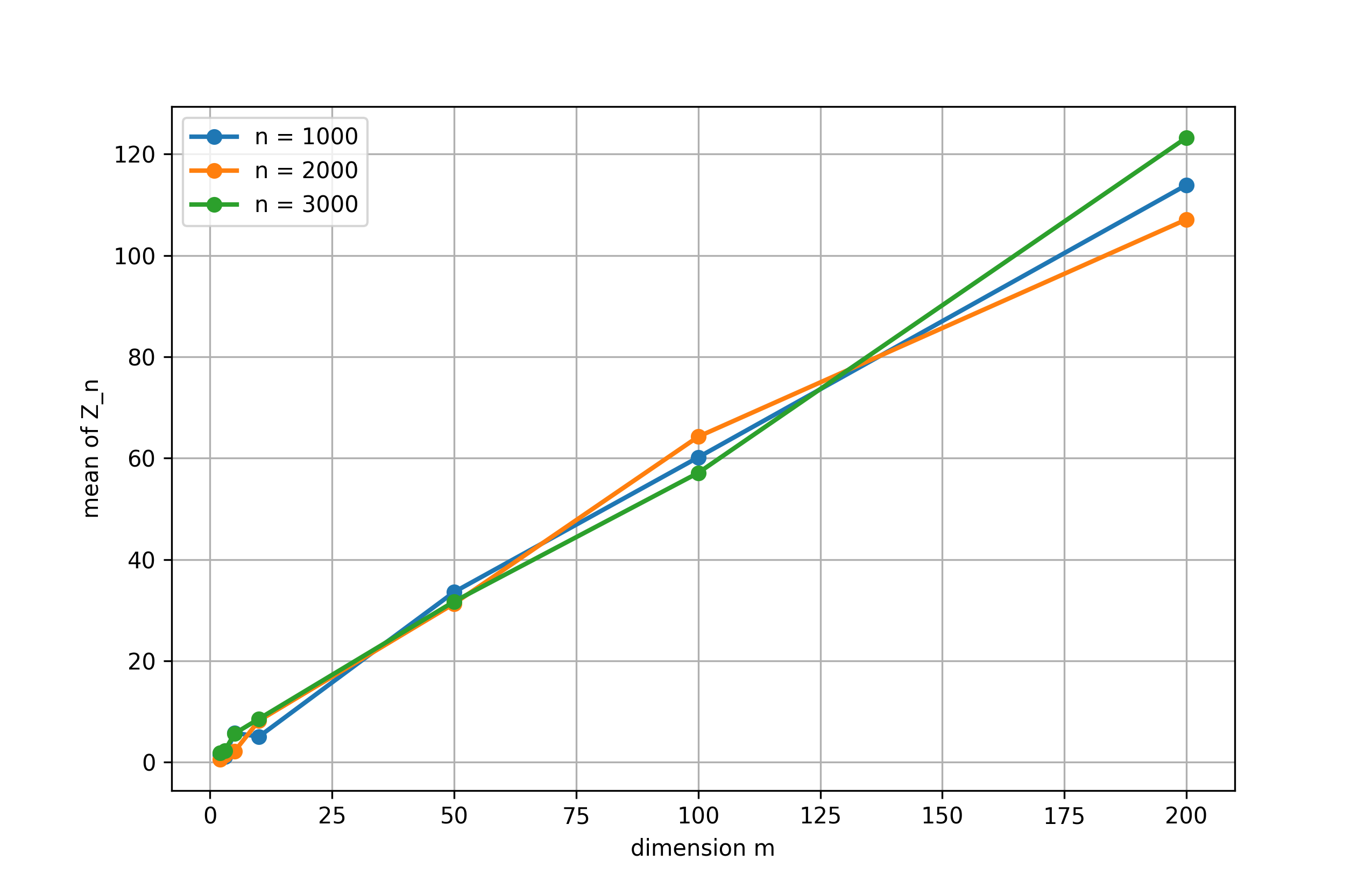
We carried out a numerical experiment for the uniform distribution supported on a sub-hemispherical cap in . More precisely, for each , we considered the uniform distribution on the geodesic cap , with , centered at the north pole . For each sample size , we generated independent samples from this cap-uniform distribution, computed the sample intrinsic Fréchet mean by Riemannian gradient descent on , and then evaluated the finite-sample quantity
For each pair , the experiment was repeated three times and we recorded the empirical mean of , shown in Figure 1.
7. Application to Geometric Statistics: Hessian Estimation and modulation-aware tests
Throughout this section, assume that the random variable , or equivalently its induced measure , has a unique population Fréchet mean . We shall use one of the following two support assumptions. In the general case, assume that there exists such that
Assumption 7.1.
.
In the rotationally symmetric case, we allow the weaker condition that there exists , where is the first zero of (cf. Equation 11), such that
Assumption 7.2.
and is rotationally symmetric about .
Under Assumption 7.1, the Hessian of the Fréchet function at is positive definite by Theorem 6.1 of Pal (2026). Under Assumption 7.2, this also follows from Theorem 5.1 of the same paper. Let denote the Hessian of the lifted Fréchet function in normal coordinates at .
Recall from Section 3.1 that, when has density in the polar coordinates around , the general Hessian formula is
In the rotationally symmetric case this reduces to (cf. Equation (12))
7.1. Plug-in Hessian estimators in the general and rotationally symmetric cases
Let be i.i.d. copies of , and let be a measurable selection of sample Fréchet means. Define the plug-in tangent vectors and radii
For , set , with all tangent vectors represented in a smooth local orthonormal frame. In the general case, the plug-in Hessian estimator is obtained by replacing the population integral in the general Hessian formula, Equation (9), by the empirical average:
| (15) |
with the convention that the th summand is when .
In the rotationally symmetric case, one may instead use the simpler radial plug-in estimator, obtained from Equation (12),
| (16) |
Below, denotes (Equation (15)) in the general case and in the rotationally symmetric case (Equation (16)) .
In the remainder of this section, denotes under Assumption 7.1, and under Assumption 7.2. The next result shows that is indeed a consistent estimator of the Hessian of the Fréchet function.
Proposition 7.3 (Consistency of the plug-in Hessian estimators).
Under the corresponding support assumption,
Proof.
We prove the general case, where . The rotationally symmetric case follows from the same argument applied to the scalar radial formula involving .
By the consistency results in Ziezold (1977) for Fréchet sample mean sets, together with uniqueness of the population Fréchet mean , any measurable selection of sample Fréchet means satisfies in probability.
Choose such that , and set On , for every ,
Hence the logarithm map and the pointwise Hessian of squared distance are smooth on the compact set
Let denote, in the chosen smooth local orthonormal frame, the pointwise Hessian contribution
with the convention . By smoothness on the compact set above, there exists such that, on ,
for every . Define
By the weak law of large numbers applied entrywise,
Moreover, on ,
Since and in probability, it follows that in probability. Combining this with proves in probability.
For , the same proof applies with the matrix-valued map replaced by the scalar Lipschitz function on . This proves the rotationally symmetric case as well. ∎
7.2. A Hessian-corrected quadratic form
Let
Let be a symmetric estimator of such that in probability.
Proposition 7.4 (Quadratic form limit).
Assume that is positive definite, and assume that the non-smeary central limit theorem holds:
Assume moreover that is positive definite and that in probability. Define
Set
| (17) |
Then
Proof.
By Proposition 7.3, in probability. Since is positive definite and therefore invertible, so
Similarly, since in probability and is positive definite, Hence Since
and since the map is continuous at on the cone of positive definite matrices, it follows that Since is positive definite, continuity of inversion and matrix square root on the cone of positive definite matrices yields By Slutsky’s theorem, Since , the continuous mapping theorem applied to gives Finally, for every ,
because on the two quantities coincide. Therefore
∎
Theorem 7.5 (Consistent estimator of tangential covariance above, and a modulation-aware one-sample test statistic).
Assume the corresponding support assumption stated at the beginning of this section, namely Assumption 7.1 in the general case or Assumption 7.2 in the rotationally symmetric case. Assume that and are positive definite, and that the non-smeary CLT where . Fix a smooth local orthonormal frame on a neighborhood of , and represent all tangent vectors in this frame. Define
and set the tangential sample covariance matrix
Then
Consequently, in Equation (17), we have
Proof.
Set
Since with , we may choose such that Then, for every and every , Hence stays away from the cut locus of , and therefore the map is smooth on the compact set In particular, there exists such that on the event , one has
for every .
Since in probability by the consistency theorem in Ziezold (1977), and uniqueness of the population Fréchet mean, we have
Using the definitions
we obtain, on ,
Next, since on , using the Lipschitz continuity on bounded sets of , there exists such that
for every . Therefore, on ,
Using the identity
it follows that
On the other hand, by the strong law of large numbers, Hence
Remark 7.6 (Relation with earlier FSS corrections and novelty of the present approach).
The statistic in Theorem 7.5, (cf. Equation (17)) provides a direct Hessian-corrected quadratic form for asymptotic inference in the non-smeary regime. This should be contrasted with the finite sample smeariness literature, where correction of quantile-based inference was carried out via bootstrap procedures; see, for example, Section 4 of Eltzner et al. (2021) and also Hundrieser et al. (2020). The reason is that in that line of work one does not build an explicit plug-in estimator for the Hessian correction entering the covariance term , and so bootstrap-based calibration is used instead.
In the present sphere setting, by contrast, the Hessian is explicit for measures with a density in both rotationally symmetric (Equation (12)) as well as general cases (Equation (9)); in the rotationally symmetric case it reduces to the particularly simple scalar form used above. This makes it straightforward to construct a consistent plug-in estimator and hence a consistent estimator
Accordingly, the resulting quadratic form yields an explicit modulation-aware testing procedure based on a directly estimated Hessian correction, rather than on bootstrap calibration. We now use this estimator for inference in the next Section 8.
7.3. Modulation-aware, Hessian-corrected, two-sample Hotelling statistic
We now record the two-sample analogue of Theorem 7.5. This is the version used for testing equality of two Fréchet means.
Theorem 7.7 (Two-sample Hessian-corrected Hotelling statistic with possibly unequal covariance where pooled covariance is invertible (Behrens-Fisher problem)).
Let and be two independent samples on , with laws and unique population Fréchet means . Consider the null hypothesis . For , let , and define, under ,
Assume that, group-wise under , the corresponding support condition from Assumption 7.1 or Assumption 7.2 holds. Assume also that and are positive definite, and that the non-smeary CLT holds for each group:
where is a measurable sample Fréchet mean of the -th sample. Let , and assume , hence .
Define the group-wise sample Fréchet functions by , , and let be a measurable pooled sample Fréchet mean, that is,
Represent all tangent vectors below in a smooth local orthonormal frame near . For and , set , , and when . Define by the group-wise version of the plug-in Hessian estimator given by (15) in the general case, or by (16) in the rotationally symmetric case, using as base point. Define
and, whenever the inverses exist, set
Finally define
On the event
define
| (18) |
On , set . Then, under ,
Thus the asymptotic level- test rejects whenever .
Proof.
Under , the two population Fréchet means coincide at . We take the measurable selections and to be group-wise, that is, each depends only on its own sample. Hence, by independence of the two samples, the two group-wise sample Fréchet means are independent. Therefore the group-wise non-smeary CLTs, independence, and imply
We first note that in probability. Indeed, by definition,
Since the sphere is compact, the group-wise empirical Fréchet functions converge uniformly in probability to , . Together with , this gives uniform convergence of to
Under , both and have the same unique minimizer ; hence the positive weighted sum also has unique minimizer . The argmin consistency argument (see e.g. van der Vaart (1998), Theorem 5.7, and apply this to ) therefore gives in probability.
We next justify replacing the fixed base point by . By the support assumptions, all relevant points lie, with probability tending to one, in a common compact neighborhood on which the logarithm map is smooth away from the cut locus. Work in a smooth local orthonormal frame near , and write , . In this frame set
The map is smooth near , and . Hence, by the fundamental theorem of calculus,
Since is smooth, the last display is , hence, equivalently, for sufficiently close to ,
Apply this with and . Since in probability and the group-wise CLTs imply (this is immediate once we use the fact that a sequence of random variable converging in distribution to a random variable is tight), we obtain
Consequently,
The consistency proof of Proposition 7.3 is local and uniform for base points in a sufficiently small neighborhood of . Since in probability, the same group-wise argument with the random base point gives
Similarly, the argument of Theorem 7.5, again used locally uniformly in the base point, gives
Hence in probability for . Since and ,
The matrix is positive definite because are positive definite and . Therefore, by continuity of the smallest eigenvalue,
Since multiplication by the positive scalar does not affect invertibility, it follows that
Together with and positive definite, which imply
we obtain .
On , the statistic can be written as
Since and in probability, Slutsky’s theorem and the continuous mapping theorem give
Thus . Since , the convention on does not affect the limiting distribution. This proves the claim. ∎
8. Numerical experiments on synthetic data: bootstrap-based versus Hessian-corrected tests
8.1. Experiments with synthetic dataset
This section reports numerical experiments comparing three one-sample tests for the Fréchet mean on spheres, given the iid sample that will be generated in a way to be made precise.
The first test is the naive quantile-based test. In the numerical experiments below, the null hypothesis is . We therefore measure the displacement of the sample Fréchet mean from the null mean , and set
The naive quantile-based statistic is
where is the empirical covariance matrix of the tangent vectors . The test rejects for large values of , using the quantile as critical value. This is the direct Euclidean tangent-space calibration: it would be -calibrated if the Hessian correction were absent, as in the Euclidean case, where . In the non-smeary curved setting, however, the limiting covariance contains the Hessian correction ; see Section 7.
The second test is the bootstrap-based test. It keeps the same testing problem, but replaces the direct -quantile calibration by bootstrap calibration. This is the type of correction used in the finite sample smeariness literature to address the poor finite-sample behavior of the naive quantile approximation; see Section 4 of Eltzner et al. (2021) and also Hundrieser et al. (2020).
The third test is the novel modulation-aware Hessian-corrected test developed in Section 7. It uses the tangent vector from the hypothesized mean to the sample Fréchet mean,
and the statistic
where is the plug-in Hessian estimator from Proposition 7.3, and is the empirical tangential covariance estimator from Theorem 7.5. In the rotationally symmetric simulations below, is the estimator in Equation (16) in the rotationally symmetric regime. By Proposition 7.4 and Theorem 7.5, under and in the non-smeary regime,
Thus this third test also uses a critical value, but with the estimated Hessian correction (pre-multiplying by and post-multiplying by ) included through . The comparison below is therefore between
-
(1)
ignoring the Hessian correction,
-
(2)
calibrating by bootstrap,
-
(3)
and taking into account the Hessian correction directly.
8.2. Truncated von Mises–Fisher (tvMF) distribution as a hemisphrically supported, non-smeary distribution
We use the term truncated von Mises–Fisher distribution for the von Mises–Fisher density restricted and renormalized to a geodesic ball. More precisely, for center , concentration , and truncation radius , the density with respect to Riemannian volume is
Thus, in geodesic polar coordinates (N.B. is the Riemannian exponential at ), the radial density is proportional to
Note that when the above distribution reduces to the von Mises Fisher distribution.
8.2.1. Local angular displacement and simulation design
For each experiment, the null hypothesis is
where is the north pole. The true population mean is shifted along a fixed geodesic by a scalar angular parameter , namely
where is a fixed unit vector. Thus corresponds to the null hypothesis, while corresponds to a local alternative. In the ambient representation, this is equivalently
Samples were generated from a non-smeary, rotationally symmetric, truncated von Mises–Fisher type distribution centered at , with concentration parameter and support in the closed geodesic ball around . Since rotations of are isometries, rotating to the north pole preserves the support radius and rotational symmetry. Hence the support-threshold results cited below apply after this rotation and show that the generated law has unique population Fréchet mean ; consequently is the null case , while gives local alternatives.
In radial coordinates around , the radial density is proportional to (see Section 8.2 above)
In all experiments below we used
Since in the dimensions considered below, the experiments are in the non-smeary regime (cf. Theorems 5.1 and 6.1 from Pal (2026) that guarantee non-smeariness when the support is contained in a ball of radius in both the rotationally symmetric and general cases) covered by the Hessian estimator in Section 7, Equation (16) for rotationally symmetric case.
The naive quantile-based statistic uses the empirical covariance of tangent vectors at the null mean and compares the resulting quadratic form with the quantile. The bootstrap-based test uses resampling under the null calibration, following the finite-sample-smeariness correction philosophy in Eltzner et al. (2021); Hundrieser et al. (2020). The modulation-aware test uses the statistic from Equation (17), with the plug-in Hessian estimator and the tangential covariance estimator from Theorem 7.5.
8.2.2. Low-dimensional experiment on
We first tested the behavior on . The parameters were
Here denotes the number of bootstrap resamples per simulated dataset. The angular grid was
The empirical rejection probabilities are reported in Table 1 and plotted in Figure 2.
| Naive quantile-based | Bootstrap-based | Modulation-aware | |
|---|---|---|---|

In this low-dimensional experiment, all three tests behave reasonably near the null. At , the naive test rejects with probability , while the bootstrap-based and modulation-aware tests reject with probabilities and , respectively. Thus the bootstrap and modulation-aware tests are slightly closer to the nominal level. For the local alternatives and , the bootstrap-based and modulation-aware rejection probabilities are very close. In this regime, the main observation is therefore not a clear statistical separation between the two corrected tests, but rather that the Hessian-corrected statistic behaves comparably to bootstrap calibration.
8.3. High-dimensional experiment on
We next tested the same procedure on . The parameters were
The angular grid was concentrated near the null:
The empirical rejection probabilities are reported in Table 2 and plotted in Figure 3.
| Naive quantile-based | Bootstrap-based | Modulation-aware | |
|---|---|---|---|

The high-dimensional behavior is substantially different from the case. The naive quantile-based test is severely miscalibrated: at the null , it rejects with probability , although the nominal level is . This is consistent with the curse of dimensionality for modulation studied in Theorem 6.3.
Both corrected procedures substantially reduce this over-rejection. At , the bootstrap-based test rejects with probability , and the modulation-aware test rejects with probability . Thus, in this run, the modulation-aware test is exactly at the nominal level, while the bootstrap-based test is slightly above it. For , both corrected tests remain close to the nominal level. For , both tests begin to show local power, with rejection probabilities of the same order. The modulation-aware test is slightly lower in power at , and higher at .
These numerical values should not be interpreted as proving that one corrected test uniformly dominates the other. The Monte Carlo standard error is non-negligible with repetitions, especially for probabilities close to . The robust conclusion is that, in this high-dimensional experiment, the naive quantile-based test fails badly, whereas the bootstrap-based and modulation-aware tests both give a substantial correction. The modulation-aware test is comparable to bootstrap calibration in rejection behavior.
8.3.1. Runtime comparison for the high-dimensional experiments
Finally, we measured the runtime cost of the bootstrap-based and modulation-aware tests in the same high-dimensional setting. This timing experiment was performed separately from the rejection-probability simulation. It measures the average cost of one test call, not the runtime of the full simulation producing the curves above.
| Modulation-aware | Bootstrap-based | |
|---|---|---|
| Mean time per test call | s | s |
| Median time per test call | s | s |
| Total time over 60 calls | s | s |
The ratio of mean runtimes was
Thus, in this implementation and hardware environment, the bootstrap-based test was approximately times slower per test call, even with only bootstrap resamples.

These timings are implementation- and hardware-dependent. Nevertheless, the qualitative computational difference is expected. The bootstrap-based test repeatedly recomputes bootstrap Fréchet means and bootstrap test statistics, rendering it computationally expensive, see Hundrieser et al. (2020), Section 5.2. By contrast, the modulation-aware statistic uses one sample Fréchet mean together with the plug-in Hessian estimator and tangential covariance estimator . Therefore the modulation-aware procedure avoids bootstrap calibration while retaining, in these experiments, rejection behavior comparable to the bootstrap-based correction.
8.3.2. Summary of the numerical findings from synthetic dataset
The experiments support the following conclusions.
First, in low dimension, specifically on , the bootstrap-based and modulation-aware tests have very similar rejection behavior. The naive test is only mildly more liberal near the null.
Second, in high dimension, specifically on , the naive quantile-based test can be severely miscalibrated. In the experiment above, it rejects of the time under the null. Both the bootstrap-based and modulation-aware tests substantially correct this behavior.
Third, the modulation-aware test gives bootstrap-comparable rejection probabilities in the tested regimes, while being much faster per test call. The numerical evidence therefore supports the practical value of the explicit Hessian correction: it provides a direct non-bootstrap calibration of the quadratic form using the plug-in estimator developed in Section 7.
9. A real-data local-Euclidean diagnostic on
In this section, we finally report a real-data diagnostic using landmark data from the Microtus lower first molar dataset of Fox et al. (2020a) and its accompanying Dryad archive (Fox et al., 2020b). The dataset was designed to study measurement error in geometric morphometrics. It contains two-dimensional landmark configurations of the lower first molar from five North American Microtus species, with planar landmarks per specimen. The Dryad archive provides several repeated landmark datasets, corresponding to different image-acquisition and digitization conditions.
Our goal in this subsection is not to demonstrate superiority of the modulation-aware statistic. Instead, the aim is to check what the proposed Hessian correction does on a real preshape-sphere dataset which turns out to be highly concentrated around its Fréchet mean. This gives a useful “local-Euclidean” sanity check: if the data occupy a small neighborhood of the sphere, then the sphere should behave almost like its tangent space, the empirical Hessian should be close to , and the Hessian-corrected statistic should reduce, up to a very small numerical difference, to the usual Hotelling statistic.
We used the file
| ProcANOVA/Nikon_NoTilt_EO_T2.TPS |
from the Dryad archive. This gives configurations, each consisting of two-dimensional landmarks. Each configuration was centered by subtracting its landmark centroid and then scaled to unit centroid size. Thus each specimen was represented as a preshape point on since raw coordinates are reduced by the two centering constraints and then normalized to have unit norm. We do not quotient by rotations here; the purpose of this diagnostic is to work directly on the preshape sphere, where the results of the preceding sections apply. This is the standard preshape-sphere representation used in landmark shape analysis; see, for example, Dryden and Mardia (2016).
We then repeated the following random splitting procedure times. In each repetition, we randomly divided the observations into two disjoint groups with group sizes and . Since the partition is independent of the observed configurations, the artificial group labels introduce no systematic difference between the two groups. Thus this random-split experiment represents a null comparison within the pooled dataset.
Let and be the two groupwise sample Fréchet means, and let be the pooled sample Fréchet mean. We formed the tangent-space difference
Writing for the empirical tangent covariance matrix of in group , an estimator of the covariance of the difference between the two sample mean vectors, namely is
The corresponding naive two-sample Hotelling statistic is
where denotes the Moore–Penrose inverse. In the present experiment all reported covariance ranks were , so the use of the pseudoinverse is only a numerical safeguard.
For the modulation-aware statistic, we used the groupwise plug-in Hessian estimators and at the pooled base point . The Hessian-corrected covariance estimator is
The modulation-aware statistic is then
This is the two-sample analogue of the Hessian-corrected statistic from Theorem 7.7.
There is one additional finite-sample point which is important in this real-data experiment. The tangent dimension is , while the total sample size is only . Therefore the crude large-sample calibration is not expected to be accurate for an ordinary Hotelling statistic, because the covariance matrix is estimated from the data. To avoid confusing this classical finite-sample Hotelling effect with the geometric Hessian correction, we also used the usual Hotelling-style -calibration
where is the numerical rank of the covariance matrix. Thus here is compared with an distribution. For the naive statistic this is the standard finite-sample Hotelling calibration in the Euclidean model. For the Hessian-corrected statistic we use the same calibration only as a finite-sample diagnostic; the asymptotic result proved in Theorem 7.7 remains the calibration.
For a nominal level , let and denote the upper-tail -values obtained in the -th random split from the -calibrations of the naive and modulation-aware statistics, respectively; explicitly, , and analogously for with . Likewise, let and denote the corresponding -values obtained from the -calibrations. The four empirical rejection rates are
The results are given in Table 4. The -calibrated rejection rates are close to their nominal levels for both statistics. By contrast, the large-sample calibration is much too liberal in this finite-sample setting.
Nominal level
We next explain why the naive and modulation-aware columns are almost identical. Let
denote the tangent vectors at the full-sample Fréchet mean. The average geodesic radius of the data cloud is small:
and even the largest observed radius is only
The total tangent variance is also small:
Thus the observed landmark configurations occupy a small region of the preshape sphere. In such a local region, the sphere is well approximated by its tangent space.
This concentration is also visible directly in the Hessian. The full-sample empirical Hessian satisfies
Hence is extremely close to :
This is exactly the local-Euclidean behavior predicted by the general plug-in Hessian estimator in Equation (15), which is used here. Applied to the full sample at the base point , that formula has , , and . Since as , the difference between the th bracketed term in Equation (15) and is . Consequently, as , . The small observed radii therefore directly explain why is close to the Euclidean value .
The numerical effect on the covariance estimator is consequently very small. Across the random splits,
Thus the Hessian-corrected covariance differs from the naive covariance by only about in relative Frobenius norm. The main local-Euclidean diagnostics are summarized in Table 5.
Diagnostic quantity Value Mean geodesic radius rad Median geodesic radius rad Maximum geodesic radius rad Mean squared geodesic radius Trace of tangent covariance Smallest covariance eigenvalue Largest covariance eigenvalue Smallest Hessian eigenvalue Mean Hessian eigenvalue Largest Hessian eigenvalue Relative Hessian deviation Median relative covariance change
The conclusion is therefore deliberately modest. This real-data experiment does not show a practical separation between the naive and modulation-aware statistics. Rather, it shows that on this Microtus measurement condition the data are so concentrated near the Fréchet mean that the preshape sphere is effectively locally Euclidean. In this regime,
and hence the Hessian-corrected statistic reduces numerically to the usual Hotelling statistic. This is consistent with the geometric interpretation of the modulation correction: it matters when curvature changes the covariance of the Fréchet mean, and it disappears when the data lie in a small region where the manifold behaves almost Euclidean.
Appendix A Symbolic Computation Code
The following Python (SymPy) code was used to compute the Taylor coefficients:
import sympy as sp

# Symbols
t, a, R, alpha = sp.symbols(’t a R alpha’, real=True)
r = t*a

X = (sp.cos(r)*sp.cos(R)
     + (sp.sin(r)/r)*(sp.sin(R)/R)*(t*alpha))

f = sp.acos(X)**2

series_f = sp.series(f, t, 0, 5)
series_noO = sp.expand(series_f.removeO())

# Extract coefficients
coeffs = {}
for k in range(5):
    ck = sp.simplify(series_noO.coeff(t, k))
    coeffs[k] = ck
    print(f"C{k} =", ck)
References
- Omnibus clts for fréchet means and nonparametric inference on non-euclidean spaces. Proceedings of the American Mathematical Society 145 (1), pp. 413–428. Cited by: §1.1.
- Large sample theory of intrinsic and extrinsic sample means on manifolds. i. Annals of Statistics 31 (1), pp. 1–29. External Links: Document Cited by: §1.3.
- Large sample theory of intrinsic and extrinsic sample means on manifolds ii. The Annals of Statistics 33 (3), pp. 1225–1259. Cited by: §1.1.
- Convergence of probability measures. 2nd edition, Wiley Series in Probability and Statistics, John Wiley & Sons, New York. Cited by: §5.
- The funk–hecke formula. Note: https://djalil.chafai.net/blog/2021/05/22/the-funk-hecke-formula/Accessed January 2026 Cited by: §3.2.
- Statistical shape analysis: with applications in R. Second edition, Wiley. Cited by: §9.
- Finite sample smeariness on spheres. In Geometric Science of Information, F. Nielsen and F. Barbaresco (Eds.), Lecture Notes in Computer Science, Vol. 12829, pp. 12–19. External Links: Document Cited by: §1.2, Remark 5.6, Remark 7.6, §8.1, §8.2.1.
- Geometrical smeariness – a new phenomenon of fréchet means. Bernoulli 28 (1), pp. 580–602. External Links: Document Cited by: §1.3, §5.
- Are geometric morphometric analyses replicable? evaluating landmark measurement error and its impact on extant and fossil Microtus classification. Ecology and Evolution 10, pp. 3260–3275. External Links: Document Cited by: §9.
- Are geometric morphometric analyses replicable? evaluating landmark measurement error and its impact on extant and fossil Microtus classification. Dryad. Note: Dataset External Links: Document Cited by: §9.
- Asymptotic distribution of sample means on manifolds: the extrinsic approach. Annals of Statistics 26 (1), pp. 226–237. External Links: Document Cited by: §1.1.
- Intrinsic means on the circle: uniqueness, locus and asymptotics. Annals of the Institute of Statistical Mathematics 67 (1), pp. 177–193. Cited by: §1.1.
- Intrinsic means on the circle: uniqueness, locus, and asymptotics. Annals of the Institute of Statistical Mathematics 67 (1), pp. 177–193. External Links: Document Cited by: §1.3.
- A smeary central limit theorem for manifolds with application to high dimensional spheres. The Annals of Statistics 47 (6), pp. 3360–3381. External Links: Document Cited by: §1.3.
- Smeariness begets finite sample smeariness. Bernoulli 27 (4), pp. 2540–2566. External Links: Document Cited by: §1.2.
- Inference on 3D Procrustes means: tree boles growth, rank-deficient diffusion tensors and perturbation models. Scandinavian Journal of Statistics 38 (3), pp. 424–446. Cited by: §1.1.
- Finite sample smeariness of fréchet means and application to climate. arXiv preprint. External Links: 2005.02321 Cited by: §1.2, §1.2, Remark 7.6, §8.1, §8.2.1, §8.3.1.
- A general setting for symmetric distributions and their relationship to general distributions. Journal of Multivariate Analysis 148, pp. 107–119. External Links: Document Cited by: item 2, item 4.
- Statistics of directional data (with discussion). Journal of the Royal Statistical Society: Series B (Methodological) 37 (3), pp. 349–393. External Links: Document Cited by: item 3.
- Sharp support thresholds for smeariness of absolutely continuous measures on spheres. Note: arXiv preprint External Links: 2606.02144, Document Cited by: §1.4, Remark 5.5, §7, §8.2.1.
- Sampling from stratified spaces. Ph.D. Thesis, Duke University, Durham, NC. Cited by: Assumption 3.1.
- Asymptotic statistics. Cambridge Series in Statistical and Probabilistic Mathematics, Cambridge University Press, Cambridge. External Links: ISBN 0-521-49603-9 Cited by: §7.3.
- Equatorial distributions on a sphere. Biometrika 52 (1/2), pp. 193–201. External Links: Document Cited by: item 3.
- On expected figures and a strong law of large numbers for random elements in quasi-metric spaces. In Transactions of the Seventh Prague Conference on Information Theory, Statistical Decision Functions, Random Processes and of the 1974 European Meeting of Statisticians, pp. 591–602. External Links: Document Cited by: §7.1, §7.2.