Homotopy lattice gauge fields 1:
The fields and their properties
Abstract
We introduce homotopy lattice gauge fields (HLGFs), a version of gauge fields over a discretized base, based on a notion of higher parallel transport that enriches the usual parallel transport along paths on a lattice to also consider higher dimensional paths.
Higher dimensional data keeps information about the parallel transport along homotopies of curves. With this data, a HLGF on a base space of dimension two or three determines a principal bundle over the base manifold. This data is also responsible for our formulas for the topological charge on two-dimensional bases.
Our framework is an application of a nonabelian algebraic topology framework developed to solve the local to global problem in higher dimensional homotopy.
No previous knowledge of higher category theory is assumed.
The second part will be devoted to the space of fields as an arena for doing Quantum Field Theory, and to give the first examples of how our framework refines standard lattice gauge theory.
1 Introduction: The lattice homotopy cutoff, a better cutoff for gauge fields
In this series of two papers, we introduce a new discretization of gauge fields. In this first part we define our gauge fields over a discrete base space, and describe their properties. The second part (work in progress) is devoted to the space of fields, and to show that it is a good arena for doing Quantum Field Theory.
Gauge fields are ubiquitous in fundamental physics. They are used to describe the so-called Standard Model of high energy physics, some systems in condensed matter physics and some approaches to quantum gravity.
Quantum field theory requires a cutoff. Cutoffs are not considered to provide simplified frameworks; they are a necessary ingredient in the Wilsonian construction of interacting quantum field theories. As far as quantum physics is concerned, we could say that frameworks involving a cutoff are more fundamental than frameworks based on the smooth category, which is well motivated by classical considerations.
Lattice gauge theory (LGT) is a framework for working with quantum gauge fields based on a lattice discretization of the base space. The usual lattice cutoff of gauge theories avoids the difficulties in producing a gauge independent procedure faced by perturbative approaches. The focus is on parallel transport, and the cutoff consists of selecting a finitely generated subgroupoid of the path groupoid selected by an embedded lattice . LGT is a tremendously successful framework: Its predictions about the masses of elementary particles have been verified with accuracies higher than 99%.
It is, however, known that lattice gauge fields do not keep track of the topological information present in a -gauge field in the continuum. For example, the gauge field in the continuum determines a principal -bundle over the base space, and this property does not hold for lattice gauge fields (LGFs); see Section 2. A symptom is that a formula for the topological charge that is free of ambiguities cannot be given before a continuum limit is reached.
Now we briefly describe the contributions of this work. We introduce a version of gauge fields on a discretized base space endowed with a special structure designed to keep track of homotopies of curves, they are called homotopy lattice gauge fields (HLGFs). They can be seen as a particular type of “higher gauge fields” on a discrete base space describing a “higher parallel transport operation”. We can say that the difference between HLGFs and standard lattice gauge fields is that the focus is on higher parallel transport, which includes ordinary parallel transport and keeps more information about the gauge field in the continuum associated to parallel transport along homotopies of paths. HLGFs give a (higher) algebraic structure to previous version of homotopy aware lattice gauge fields proposed by one of the authors in collaboration with Claudio Meneses [8, 9]. This algebraic structure provides the geometrical clarity that lets uncover the parallel transport operation natural to HLGFs, and provide a coarse graining map (that we will introduce in the second article of this series). On a separate note, the restriction of HLGFs to dimension 2 reproduces a previous notion of higher gauge field on a discretized base proposed by Pfeiffer [12]. We will see that, for base spaces of dimensions 2 or 3, a HLGF determines a -bundle over the base space. We also give a simple formula to calculate the topological charge in dimension 2.
Reading this paper does not require previous knowledge of category theory. We develop the necessary algebraic tools providing geometrical motivation. The reader will learn the essence and basic tools of a “non abelian algebraic topology” framework developed by Brown, Higgins and collaborators [3]. This language is also used to introduce a higher version of the gauge groupoid (or Atiyah groupoid) that gives a rich algebraic context to our higher parallel transport operation.
There is a profound reason behind the “coincidence” of finding that our mathematical needs demanded by physical requirements had already been developed. Researchers in algebraic topology had big hopes for using higher homotopy groups to study spaces. They then realized that for any the groups are abelian. Another problem they faced was the local to global problem: understanding the homotopy type of a space that is decomposed into a collection of pieces in terms of homotopy properties of its pieces, is a difficult awkward problem. Whitehead [14] was the first to realize that extending the study of homotopy to the study of relative homotopy leads to nonabelian structures. Later Brown, Higgins and collaborators after working for decades solved the local to global problem for relative homotopy on filtered spaces [4]; see [3] for a pedagogical account of nonabelian algebraic topology. Filtered spaces add structure to topological spaces (or to based topological spaces) that make it natural to replace groups with groupoids. This change was crucial for solving the local to global problem. Additionally, filtered spaces facilitate the goal of talking about relative homotopy. In physics, we are interested in local descriptions of systems, as well as in considering relative observables, and we need a cutoff (at least as an intermediate step). In this work and in [11], we import the setting and tools of nonabelian algebraic topology to lattice gauge theory and harvest the first fruits.
In the second part of the series, we define and give structure to the space of fields. We show that it is a good arena for QFT at a given cutoff. We provide examples, and show that our framework refines standard LGT in the sense that its predictions regarding observables living in the standard lattice is the same, but we have access to higher dimensional observables that let us keep track of homotopy data dismissed by LGT. Among the new observables that we have at our disposal is the topological charge for two-dimensional bases. We also introduce coarse-graining maps linking different cutoffs in such a way that an inverse limit lets us “get rid of the cutoff”.
The organization of this paper is as follows: In Section 2 we geometrically motivate the main ideas and show how the homotopy lattice cutoff brings a field in the continuum to a HLGF. Section 3 introduces higher algebraic structures in a pedagogical way relying on the motivation given in the previous section. Section 4 contains all the topological aspects of this work. We show that in dimensions 2 or 3 a HLGF determines a -bundle over the base manifold, and give a formula for the topological charge in dimension two. The final section contains a summary and discussion.
2 Preparing gauge fields in the continuum for the homotopy lattice cutoff
We will describe how an ordinary gauge field in the continuum induces a higher homotopy parallel transport map. This is no more than an observation, but it is the cornerstone of the homotopy lattice cutoff and its ability to locally store information regarding the bundle structure induced by a gauge field in the continuum for base spaces of dimension 3 or 2.
2.1 Parallel transport
We assume that the reader is familiar with the differential geometric notion of principal bundles, connections and the induced parallel transport map. We describe it briefly to set up our notation in a familiar context. Then we talk about parallel transport from an alternative point of view.
Consider a smooth -dimensional manifold with a smooth triangulation and a Lie group. The term curve will be used for elements of a groupoid. From now on a piecewise smooth map444In Section 3 we introduce formally cubical and globular shapes that let us compose in higher dimensions. To relate the two shapes it is easier to parametrize curves with domain instead of the traditional domain . will be called a singular curve on 555In the smooth category, it is more common to consider lazy paths [13] as singular curves instead of piecewise smooth curves. These paths are smooth everywhere, but they are allowed to have points where their velocity vector vanishes. Our treatment of the smooth category is heuristic, and at this level we can describe things easier by following our conventions.. Singular curves have a source and a target , .
A principal bundle with a connection. There may be inequivalent -principal bundles over . For the moment we will choose one of them. A connection on determines a lift for any singular curve in once an initial condition is specified in the fiber over . Consider a singular curve in ; the lift from any initial condition induces a map that commutes with the right action on . We say that a connection determines a parallel transport map [7]. A visual summary is given in Figure 1.

Parallel transport from a connection on a bundle.
, the space of singular curves in , has two important structures:
(i) It has a smooth structure that will let us talk about smooth maps with that space as domain. The idea is to consider as a parametrized space in which a special set of parametrizations are defined to be smooth with the objective of defining a map
to be smooth if and only if precomposition with any of the smooth parametrizations results in a smooth map. One realization of such a smooth structure is the concept of a diffeological space [6], which we will use when we deal with the space of fields in the second part of this series.
This notion of a smooth space extends the notion of a smooth manifold: All smooth manifolds are diffeological spaces. Importantly, that structure descends to quotient spaces and certain limits that we will use in the second part of this series.
(ii) becomes a groupoid after taking a quotient by the equivalence relation of thin homotopy relative to vertices. It has a set of operations (source, target, composition, inverse and identities) that descend to the quotient and give it the structure of a groupoid.
The source and target maps were introduced earlier. Composition corresponds to singular curve concatenation; when it makes sense, is another singular curve corresponding to following first and later . The inverse corresponds to inverting the direction in which the singular curve is traversed . A constant curve on is called an identity and it is denoted by .
Thin equivalence is an equivalence relation among singular curves such that .
For gauge fields the definition has a clear motivation: If we can go from one singular curve to another one without sweeping any area, an appropriately defined integrated curvature would vanish.
It is a very nice equivalence relation because in some sense it is the weakest equivalence relation that makes the quotient a groupoid and because it has natural generalizations for the higher dimensional analogs of singular curves666In the next section, we will define thin equivalence precisely within a special context in which the concept is simply stated..
The elements of will be called curves or paths.
A parallel transport map is defined on but descends to . Given , the induced transport map transports the fiber over the source to the fiber over the target in a -equivariant way. Additionally, given composable singular curves, , and . These are the algebraic properties of parallel transport maps.
We would like to describe as a field with the smooth groupoid as domain. would be a groupoid homomorphism that after evaluation keeps tract of the evaluation point as it happens for any field modeled as a section. This would provide an elegant summary of what we described above. The question is what is the appropriate groupoid that is the target of . Now we heuristically describe this idea. For any curve , ’s outcome is a -equivariant transport map , and we also know that the map depends on . Thus, the target groupoid should have objects that can be interpreted as fibers over points of the base (for ), and its morphisms should have the interpretation of -equivariant maps , while remembering that they are associated to curves (with and ). It turns out that these clues are sufficient to define the Atiyah groupoid .
Let us describe with slightly more detail; a more formal introduction will be given in the following section. Objects are where initial conditions for parallel transport can live. There is one object for each point ; it will be convenient to denote objects as pairs . Morphisms will dictate the parallel transport of initial conditions along paths on the base. It will be convenient to denote morphisms by pairs of the form where is the source of and is the target of and commutes with the global right action on the fibers of . The source and target maps of these morphisms are obvious. Identity morphisms are of the form for all . Composition of morphisms, when defined, is also clear. Inversion reverses the direction of the curve and inverts the map.
Forgetting the second entry provides a projection . Forgetting the first entry provides a projection to the following groupoid: Its set of objects is the set of fibers of ; that is, objects are of the form for some . Its morphisms are maps that commute with the global right -action on . The operations on this groupoid are obvious.
In this context, a parallel transport map is a smooth groupoid homomorphism
which is a section of the mentioned projection .
The presentation given above starts with a connection on a bundle and constructs . A trivial, but interesting, observation is that determines a distribution of horizontal spaces on ; that is, determines .
Parallel transport on . The following observation is the origin of important decisions that shaped the work presented in this article. It suggests working on a more economical space of singular curves in . Parallel transport on the restricted space of paths still determines the connection , while leading to simpler gauge transformations and a conceptually simpler framework.
Let be the space of piecewise smooth curves with source and target points, , , restricted to lie in the set of vertices of the triangulation . is a subgroupoid of . See Figure 2.

The restricted parallel transport map also descends to the quotient . This groupoid has a discrete set of objects . On the other hand, the set of paths (morphisms) has not acquired extra restrictions apart from having restricted endpoints.
A question arises: Does determine ?
Geometric intuition tells us that it should be enough to distinguish between any two different connections: If the two connections have different curvature, there must be a point on the base space and a neighborhood of that point where parallel transport along small loops would detect the difference in curvature. The mentioned small loop can be extended to have a base points in ; this path would be able to distinguish the two connections under consideration.
Before proceeding or giving any details notice that since is a discrete set, information about the fibers over cannot encode the structure of a bundle over . Thus, parallel transport along paths in is an operation that does not rely on a preexisting bundle structure. Then parallel transport on lets us distinguish between any two connections on a given bundle and, at the same time, permits a framework in which connections on any possible bundle over are treated at once. It is natural to conjecture that can also distinguish between different bundles.
The heuristic argument of the previous paragraph was transformed into a rigorous construction by Barrett [1] following a comment from Kobayashi [7]. An explicit construction of the bundle and the connection from the parallel transport map is in [1] (considering a base with a single selected base point ). A “groupoid version” that is more directly related to our exposition can be found in [9]777The construction given in [9] uses a triangulation arising from baricentric subdivision, but it is easily adapted to any triangulation with a triangulation associated with a simplicial set. The main difference with a simplicial complex is that k-simplices are identified with a totally ordered set of (k+1) elements, and the induced partial order of vertices permeates the whole structure. .
In summary, the Barrett-Kobayashi construction tells us that the map
is invertible.
2.2 Higher homotopy parallel transport in the continuum
Here we heuristically describe how an ordinary gauge field acts on homotopies of curves on a base space. We call the resulting notion “higher homotopy parallel transport”. A single curve lets the gauge field parallel transport initial conditions on the fiber over its source point, to final conditions on the fiber over its target point. Homotopies of curves let the gauge field transport homotopies of initial conditions, and yield homotopies of final conditions. If we assign globular shapes to the homotopies of initial conditions and of curves and of final conditions, the resulting higher homotopy parallel transport operation has powerful gluing and composition properties. The transport of globular homotopies of initial conditions of dimensions 1 captures non trivial information about the gauge field. In Section 4 we will see that there is no interesting information to capture from the transport of 2 dimensional homotopies of initial conditions, and that the transport of k dimensional homotopies of initial conditions may contain interesting information about the gauge field, but the globular machinery that we use does not capture it for .
Consider a smooth parallel transport map on . A homotopy of curves sharing their source and target points in will be called a singular 2-globe. Now consider an initial condition in the fiber over . The parallel transport along the singular 2-globe leads to a homotopy in interpolating between and . Notice that this transport operation started with an object of one type (a single initial condition) and ended up with an object of another type. On the other hand, a homotopy of points in the initial fiber is transported along the singular 2-globe to a homotopy of points in the final fiber
In summary, is a homotopy interpolating between and taking homotopies of initial conditions on and transporting them to homotopies of final conditions on . Our objective is to interpret as a transport map in itself acting on the appropriate type of initial conditions. See Figure 3.

Now that we know what kind of objects can be transported by a singular 2-globe to objects of the same type, let us see if the possible compositions of singular 2-globes get along with parallel transport.
Singular 2-globes can be composed in two directions. See Figure 16 in the next section for a self explanatory picture. Notice that singular 2-globes have 0-dimensional source and target points, and they also have 1-dimensional source and target singular curves. First, singular 2-globes such that the 0-dimensional target of coincides with the 0-dimensional source of can be composed . Parallel transport along the resulting 2-globe is, clearly, the composition of the parallel transport operations along the original 2-globes. Second, composition of and is possible when the 1-dimensional target of coincides with the 1-dimensional source of (i.e. if ); we write for the concatenation of homotopies relative to fixed endpoints by lifting the condition of being fixed of the middle point (and redefining the parameter ). Parallel transport along acting on homotopies in the initial fiber of the type (where denotes the class of a curve in resulting from composing representatives of ) is a distributive operation as stated below. In summary, these two composition operations of singular 2-globes are compatible with parallel transport. Since the parallel transport map in the continuum is assumed to be smooth, in particular it is continuous leading to compatibility as stated by the simple algebraic rules
Analogously, acts on higher homotopies of curves leading to maps parallel transporting higher homotopies of initial conditions. To have convenient algebraic gluing rules, we must choose a shape; we will continue to use globes.888A cubical structure is another choice; the resulting formalism is transparent and powerful [11]. The globular choice is more economical, and the notion of gauge transformations is simpler. Higher homotopies of curves in the base will be higher dimensional globes, and initial conditions on the fiber over the source point will be globes of the corresponding dimension.
To sharpen the presented ideas, we introduce a higher homotopy extension of the Atiyah groupoid. Here we will not be rigorous yet; what we present here is a prelude to what we will introduce formally in the following section.
We want a higher dimensional extension of describing homotopies of paths in . In the globular structure: The objects would be points in , the 1-morphisms would be paths in , the 2-morphisms would be 2-globes interpolating between 1-morphisms, etc. After taking a quotient by thin homotopy, singular k-globes become elements of a k-groupoid, and are called k-globes. The collection of k-globes for all get organized into the structure of an strict infinity groupoid [5]. A singular (k+1)-globe can be regarded as a homotopy of k-globes sharing their source and target (k-1)-globes; in the next section, we give a formal definition in a restricted context. Clearly, the task of making this construction rigorous in the smooth category is nontrivial; see [13]. We will define the appropriate notion of thin homotopy in our context in the next section. For our heuristic description, let us use the notation and for the infinity groupoid of globes on (to be constructed in the next section) and for the fundamental homotopy infinity groupoid of the fiber [5] respectively. We would like to enrich for describing the higher homotopy parallel transport described above, where the initial conditions that may be transported are higher homotopies in the fibers over . Thus, there should be one object per vertex , but they should be thought of as , and the morphisms should have the interpretation of describing globular higher homotopies of parallel transport maps, which means commuting with the right action on the set of objects . Let us call the resulting structure .
In this language, we have heuristically described that a smooth parallel transport map in the continuum induces a higher homotopy parallel transport map
which is a section of the projection . This picture will be described with some detail in the following section.
Physical motivations call for a cutoff in quantum field theories. The homotopy lattice cutoff sketched below leads to a context of parallel transport along restricted path homotopies. That reduced context will let us give precise and simple definitions of the notions heuristically described above.
2.3 The homotopy lattice cutoff: Essential ingredients
The cutoff. Cutoffs are not considered to provide simplified frameworks; they are a necessary ingredient in the Wilsonian construction of interacting quantum field theories. We could say that as far as quantum physics is concerned, cutoff frameworks for field theory are more fundamental than a formalism in the smooth category, which is well motivated by classical considerations. The usual lattice cutoff of gauge theories avoids the difficulties in producing a gauge independent procedure faced by perturbative approaches. The focus is on parallel transport, and the cutoff consists of selecting a finitely generated subgroupoid of the path groupoid selected by an embedded lattice . This determines a space of gauge fields in the lattice and a cutoff map
Our goal in this section is to describe the homotopy lattice cutoff of gauge theories, which refines the standard lattice cutoff as we explain later on. The focus is on higher parallel transport along path homotopies selected by a cellular decomposition of . This determines a space of gauge fields in the homotopy lattice and a cutoff map
The fundamental higher homotopy groupoid of a filtered space. It is an appropriate finitely generated subinfinity-groupoid of that will lets us extend the cutoff leading to standard lattice gauge fields. A truncation should lead to a rigorous, powerful and simple formalism. It may look like a lot to ask, but it turns out that we are looking for a structure that already exists: It is the infinity fundamental groupoid of the filtered space . A filtered space is a topological space together with a collection of nested subsets such that their union equals the space . We are interested in skeletal filtrations; that is, the space is assumed to have cellular decomposition , and the subset of the filtration is the k-th skeleton of . A cubical version was developed by Brown and Higgins starting in the early 80s [2] (see also the book [3]), and [5] gives a globular version that will be essential in this paper. We will describe a minimal version of it in the next section. The truncation consists of not allowing singular globes to roam everywhere in : Singular k-globes are restricted to have image in the k-skeleton. The enormous simplification, as compared with the construction of in the smooth category, comes from using the skeletal structure to define thin equivalence: Two singular k-globes are thin equivalent if there is a homotopy interpolating between them with image contained in . Figure 4 shows two singular curves sharing endpoints that are thin equivalent.

The higher homotopy Atiyah groupoid of a filtered space. Recall the heuristic description of given in Section 2.1. Now we present a variant of that provides a framework for describing our higher homotopy parallel transport with internal group . Let us call it . There are three important changes: The first is that we reduced the set of allowed base points to be . As discussed earlier, this implies that the set of fibers over the base points does not know the bundle structure. The second is the cutoff induced by , which carries a simple definition of thin equivalence. The third is that the goal of the structure is to parallel transport homotopies of elements of the fibers along appropriate homotopies of paths. The resulting structure has objects and morphisms denoted by pairs. The second entry of the objects , where the initial conditions to be parallel transported live, is appropriate for describing -dimensional globular homotopies in (for some ). The first entry of the morphisms is a globe with 0-dimensional source and 0-dimensional target ; the second entry is a map commuting with the right action. The first entry of those morphisms models a homotopy of curves, and the second one models the corresponding homotopy of transport maps appropriate for acting on homotopies of initial conditions.
Importantly, the homotopy structures of the objects and that of the morphisms are coordinated precisely as needed for us to describe homotopy parallel transport. The conditions are stated at a technical level, but the idea is simple. Now we describe an instance of these conditions through an example depicted in the Figure 5: Consider a situation in which we have initial conditions at , and they are a homotopy (relative to fixed endpoints) written as the composition . The initial condition is transported along a 2-globe that is also expressed as a composition . The morphisms of the groupoid that we are constructing are associated with pairs; in the described situation we have three different pairs , and . The compatibility condition says that we can transport the glued initial condition using , or we can transport the unglued pieces using respectively and then glue them, obtaining the same result

Similar conditions ensure that if we have initial conditions at corresponding to a homotopy that are transported along a 2-globe . Then we can calculate the initial point (or source) of the transported homotopy in two equivalent ways: We can calculate the source of and transport it using the 1-dimensional source of , or we can first transport using and then calculate its source. Etc.
2.4 The homotopy lattice cutoff: A preliminary example
As a preliminary example, consider the case where we consider and . See Figure 6. The truncation is induced by a triangulation . The triangulation has a set of vertices denoted by , a 1-dimensional skeleton consisting of edges and vertices and denoted by and a two-dimensional skeleton consisting of faces, edges and vertices denoted by . The skeletal filtration induced by the triangulation is . As shown in Figure 6, our triangulation has five vertices; two of them located on the North and South Poles and other three vertices on the Equator located at equidistant points. The Greenwich meridian lies on . As mentioned earlier, we need a triangulation associated with an underlying simplicial set. To provide this structure we number the vertices: The vertex in the intersection of the Greenwich meridian and the equator will be . Vertices and lie on the equator with the line running from west to east. Finally, and correspond to the north and south poles, respectively. This completes the description of . The set of edges is , . Notice that we have written 1-simplices, edges, as a pair of vertices respecting the order of vertices.

A set of generators of the path groupoid in is with , where represents a singular curve with image and running in the opposite direction. That is, and . This convention is compatible with the conventions followed in [9], as explained in Section 3. If we want to refer to a singular curve running in the opposite direction we write . The set of faces is (where triplets of vertices are written respecting their order). A set of generators of the 2-groupoid of 2-globes in is with , where represents a singular 2-globe going from the singular curve to the singular curve . The specific homotopy of singular curves is shown in Figure 13 (in Section 3.1). Additionally, a concrete formula is given in [11]; again, we adopt this convention to be compatible with [9].
If we want to refer to a singular 2-globe with source and target singular curves running in the opposite direction, or what is the same with 0-dimensional source and target interchanged, we write , and denotes the singular 2-globe where 1-dimensional source and target have exchanged places. This completes the description of the triangulation , the induced skeletal filtration and our conventions for associating generating singular globes to simplices.
The infinity groupoid has three nontrivial levels the objects (or vertices), the path groupoid and the 2-groupoid of 2-globes.
Now we will undertake the task of describing one given parallel transport map using the example of the parallel transport of unit vectors over points in resulting from the Levi-Civita connection associated with the metric of round unit sphere .
The situation is geometrically clear, but to describe the action of we need the reference provided by a trivialization on the fibers over . Parallel transport along a curve will correspond to an element of , and parallel transport along a singular 2-globe will correspond to a homotopy of parallel transport maps (considered up to relative homotopy) described by a curve in considered up to homotopy relative to having fixed endpoints. We will choose an arbitrary trivialization over the north pole . In order to help us give a simple description, the trivialization on the fibers over the other vertices will be chosen using . The trivializations over and are chosen transporting the trivialization from using along the link that joins them. The local trivialization over is chosen transporting the trivialization on with along the Greenwich meridian.
According to the convention described above, parallel transport on paths corresponding to edges is
| (1) |
and the numbers shown in Figure 7. When the arrow in the figure is opposite to , we invert the sign of the integer shown in the figure to compute .

Homotopy parallel transport along singular 2-globes, as mentioned above, is described by curves in considered up to homotopy relative to having fixed endpoints. In our notation, such classes of curves in are denoted by a triple satisfying . The triple determines the singular curve , and denotes the homotopy class of the curve relative to having fixed endpoints.
In our example, homotopy parallel transport along singular 2-globes associated with faces is
| (2) |
with , , , , , .
A visual representation of homotopy parallel transport on 2-globes is shown in Figure 8.

Parallel transport along any singular curve contained in is calculated by composing parallel transport along the edges. Similarly, as we will show in Section 3, homotopy parallel transport along any singular 2-globe fitting in can be calculated composing homotopy parallel transport along singular 2-globes associated with faces and along degenerate singular 2-globes with image contained on the edges. As an example, consider singular 2-globes interpolating between the Greenwich meridian and meridians at longitude , and ; see Figure 7. Let us call the described singular 2-globes with . Because the metric on the unit round sphere has constant curvature, we know that
Notice that for any parallel transport map the last entry of the above evaluations must have the structure
, and this requires that
is an integer. This integer is called the topological charge of ; in the case of the connection induced by the round metric on , we obtain . In Section 4, we give more details about the calculation of the topological charge and the characterization of the bundle class in two or three dimensions. We also explain why a generalization to four dimensions requires extra ingredients.
The homotopy cutoff takes the gauge field induced by restricting the parallel transport of the Levi-Civita connection on the round sphere to act on unit vectors and forgets all the information in it except for (1) and (2). This is an example of the evaluation of the homotopy cutoff map
from the space of smooth connections over to the space of gauge fields on the homotopy lattice. , defines a homotopy lattice for , that considers paths on and homotopies among those paths restricted to (considered only up to homotopy), and in general homotopies among k-homotopies of paths restricted to .
3 HLGFs as higher parallel transport maps on the homotopy lattice
Firstly in this section, we define Homotopy Lattice Gauge Fields (HLGFs) at an abstract level. Secondly, we use a trivialization on the fibers over points in the discrete set to provide a useful description of HLGFs. Finally, we give a set of generators of k-globes that provide a set of elementary building blocks for HLGFs. Since generating 1-globes are links in , we will see that elementary data associated with 1-dimensional objects by an HLGF is exactly standard lattice gauge field data.
3.1 Prelude to nonabelian algebraic topology
Remark 1.
It turns out that the conventions used in differential geometry and in physics follow the convention of composing curves from right to left. This forces us to adhere to this convention in our short introduction to the tools of nonabelian algebraic topology. Standard conventions in that field use category theory conventions composing from left to right. In [11] we used standard category theory conventions but arrived at awkward conventions in which -bundles had a global left action and (after local trivialization) parallel transport along composite curves could be described by right multiplication in the group.
Filtered spaces and filtered maps. Consider a space. Here our focus is on finite dimensional manifolds possibly with boundary and corners, which are equipped with a nested collection of subsets such that is the union of the subsets. Such a space is called a filtered space and is denoted as ; the collection of nested subsets is called a filtration. A concrete example was given in Section 2.4. Filtered spaces together with maps among them, which preserve each level of their filtrations ( for all ), are organized into the category FTOP.
**** Here I stopped adding corrections from Mary (until the end) ****
We will use two kinds of filtrations: Skeletal filtrations, where is the k-dimensional skeleton of a cellular decomposition, and trivial filtrations, where for all . Filtered homotopy relative to vertices in the case of a skeletal filtration becomes thin homotopy rel. vertices, which we need to use in the base space, and in the case of a trivial filtration it becomes standard homotopy rel. vertices, which we use for the gauge group.
Skeletal filtrations. First we briefly describe the homotopy theory resulting from skeletal filtrations. Our space will have a triangulation or a cellular decomposition (by a CW complex, as would be the case of a cubiculation of the n-torus by a “Cartesian cubiculation” with periodic boundary conditions), and will denote its k-skeleton. Then .
An example of a space with a skeletal filtration is the standard n-cube . The filtration comes from the cellular decomposition in which the k-cells are the closed k-dimensional faces of . See Figure 9 for standard 1 and 2 cubes with our convention for how to picture their standard parametrization.

Another family of examples that we will use is the family of standard n-globes. Our conventions are based on those of [5]; the difference is motivated by agreeing with the conventions of differential geometry as stated in Remark 1. In this paragraph, the difference will show up only in the picture. The standard n-globe is the n-dimensional disc with the skeletal filtration inherited from the cellular decomposition with one n-cell and for two k-dimensional cells contained in the intersection of and the k-dimensional subspace determined by for every . Cell satisfies . See Figure 10.

Now we give examples of filtered maps. They will be relevant in the algebraic structures defined below (see Figure 11)

In [5] a collection of filtered maps
for all are defined inductively. They satisfy: (1) . (2) If we write then . (3) . (4) sends the dimensional face of transversal to direction in and with to the dimensional cell . See Figure 12 for .

A singular 1-globe (which is the same as a singular 1-cube) in a filtered space is a parametrized curve in ; at a more precise level, it is a filtered map . Thus, it sends to and to . Notice that this is not the same as sending vertices to vertices and edges to edges because the image of needs to lie in , but is not restricted to be a single edge. In Section 2.4 each edge is a singular 1-globe, and also the Greenwich meridian running from north to south and the equator running from west to east and starting at longitude are singular 1-globes (see Figure 6). The space of 1-globes in is denoted by ; previously we had called it .
Similarly, a k-globe in is a filtered map , and a k-cube in is a filtered map . The spaces of k-globes and k-cubes in are denoted by and respectively. Each face in the example of Section 2.4 is a singular 2-globe. In [11] we give an explicit map from to a triangulation with the images of and equal respectively to the highest and second highest vertices of a face, as shown in Figure 6. (That map must be adapted to the conventions that we are now using with .) It is easy to see that this type of degenerate singular 2-cubes can also be seen as singular 2-globes.
k-Globes and k-cubes are parametrized k-dimensional subspaces of (possibly with singular image) fitting into the skeletal filtration. Their special shape (globes or cubes) will let us talk about homotopies among them, and precisely describe the gluing of those homotopies.
Cubical sets with “connections”. Now we will introduce algebraic operations in that will let us talk about homotopies among cubes.
Face maps: Given , we define (for any and ) as . As its name suggests, is the -face in direction of . In our preliminary example of Section 2.4, we see that , . Also, at the pictorial level999The example can be completely precise following the definition of as a singular 2-cube given in the Appendix 6., we can see that . In order to describe we need notation for degenerate cubes that we will give in a moment, and in order to describe we need notation for gluing that we will see in a few paragraphs.
Degeneracy maps: Given , we define by
. As its name suggests, is a dimensional cube with the same image as which is degenerate in direction . Notice that we can compose degeneracy maps to construct cubes with a higher degree of degeneracy. We see from Figure 13 that in our preliminary example of Section 2.4 , .
Connection maps: Given , we define by
. This map produces degenerate cubes, but the degeneracy is associated with the pair of directions . It is because we have these maps that cubical gluing rules do not have a cartesian flavor; see Figure 15 below.
It is not difficult to verify that the defined operations defined on satisfy the relations of a “cubical set with connections” listed in the appendix 6; here are some of mentioned relations: if , if , if .
Globular sets. The set of globes admits an algebraic structure for talking about homotopies among globes. Below we will introduce operations on satisfying the appropriate set of relations, giving it the structure of a globular set.
The collection of maps send globes to cubes by pullback
Clearly, this map trivially sends 0-globes into 0-cubes and 1-globes into 1-cubes. Notice that for the map is not surjective: its image is the set of cubes such that for .
It is simple to verify that the operations preserve . Using those operations we will define globular operations in that make it into a globular set. Recall that has two -dimensional cells for ; one is called the source cell of that dimension, and the other one is called the target cell of that dimension.
Our preliminary example of Section 2.4 can be made precise in a simple way using globes. The 0-globes are the vertices in . The 1-globes shown in Figure 6 are continuous maps with and . The 2-globes are the continuous maps shown in Figure 13.

Face maps: Given , for we define as , or equivalently as . They are the -dimensional source and target faces of the globe. We will use again the preliminary example of Section 2.4, but this time we will use the notation for globes. , , (see Figure 13). will be given below.
Degeneracy maps: Given , for we define as . The idea is simple, we need to extend from being defined in dimension to a higher dimension, and we do it one step at a time: Recall that . Consider the natural embedding of into at the subspace; using that embedding we can extend maps from to as maps that are independent of the coordinate. In order to bring from to , the described extension has to be performed times.
These maps follow the “globular relations”:
Higher dimensional groupoid structures. Now we are ready to glue homotopy maps. Here is where our convention differs from the usual convention followed in category theory treatments. The reason for our choice is given in Remark 1. We describe the structure first for cubical homotopies. The operations on are defined extending the usual definitions of concatenation of curves and direction reversal of curves to higher dimensions. Consider such that , then we define by a simple adjustment that makes the -th coordinate of the parameter space run twice as fast and use followed by . Figure 14 illustrates gluing in two different directions for and the all important “interchange rule”.

The operation is defined by following the the th coordinate of parameter space in reversed direction.
These operations together with the cubical operations and the connection, let us compose (or glue) homotopies among cubes in a flexible manner. As an example, Figure 15 shows the diagram corresponding to the building instructions for a cellular decomposition of as the boundary of a 3-dimensional cube.

At this point, we do not yet have a higher dimensional groupoid structure. This structure will emerge after taking a quotient by thin homotopy.
Relation shows us that we can consider singular globes as particular cases of singular cubes. The gluing and direction changing operations preserve the subset , inducing corresponding gluing operations for globes. The picture for gluing globes is shown in Figure 16.

It could appear that gluing singular globes along higher codimensional cells would necessarily lead to new singular globes in which the gluing region is special. We will show, with an example, that after taking thin homotopy equivalence into account, this is not the case.
Thin homotopy. In gauge theories, talking about equivalence of curves by thin homotopy is essential. Parallel transport as described in the previous section acting on two curves sharing their source and target points may differ even if and are homotopic rel. endpoints. Only in the case of flat connections parallel transport is a function of homotopy classes of curves relative to having fixed endpoints. On the other hand, consider the case of the constant curve with , and the curve for any curve with ; this pair of curves are related by a homotopy retracting the curve to within the image of curve. This is an example of a pair of curves related by thin homotopy. It turns out that for any -connection in , we have . In general, for any connection and any two curves with the same endpoints and related by thin homotopy relative to their endpoints we have . A clearly related phenomenon is that the space of singular curves modulo thin homotopy relative to endpoints becomes a groupoid.
In the context of a filtered space with a skeletal filtration, two singular k-cubes such that are declared to be thin homotopic relative to vertices if and only if there is a continuous map with for all such that and , .
The set of classes of singular cubes by thin homotopy
inherits the set of operations , following the set of relations listed in The Appendix 6, that make it into an -groupoid. Its elements, singular cubes up to thin homotopy, are called cubes.
Apart from the advantage of using a shorter name, considering cubes is motivated by parallel transport. Additionally, the gluing of cubes has a better behavior than gluing before considering equivalence classes by thin homotopy rel. vertices. Recall the preliminary example of Section 2.4; it is not difficult to see that, using cubical conventions, , where all the elements of the equation are defined in Section 2.4.
The resulting category of -groupoids is complete and cocomplete. This property is inherited by the category of infinity groupoids, that we will present below, and this will be crucial when we deal with the space of fields in the second part of this series.
We return to globes. Again we can consider the preliminary example of Section 2.4. Recall that we showed explicitly how the 1-simplices of paths are singular 2-globes; that now we consider up to thin homotopy and call them just 2-globes. We can use globular notation to see that . This shows that gluing globes along higher codimensional cells (e.g. using ) does not always lead to glued regions showing their seams; in other words, having distinguishable points associated with the place where the gluing took place as it could appear from Figure 16.
As another example of how globes can be glued, consider the boundary of the 3-cube can be built using globes. We first assign 2-globes to the squares in the boundary as shown in Figure 17. Degenerate 2-globes are also necessary.

A globe covering once can be constructed gluing three globular pieces, named for Right-Front, Back-Bottom and Left-Top respectively,
The set of classes of singular globes by thin homotopy
inherits the set of operations , following the globular relations stated above and relations stating compatibility with the gluing operations (stated below), making it into a strict -groupoid. Its elements, singular globes up to thin homotopy, are called globes. The relations stating compatibility of the gluing operations with the globular operations and internal compatibility of the gluing operations are
whenever the expressions are defined.
Trivial filtrations. Our physical motivation needs a cutoff for quantum field theory, making the space of histories (also called the space of field configurations) finite dimensional. We achieve this goal introducing a filtration in spacetime’s path groupoid and considering paths up to filtered homotopy rel. vertices. On the other hand, the gauge group playing the central role in the target space of our HLGFs cannot have a filtration where . The reason is that our mathematical structure only works when is a group, and in general there is only a finite collection of nonabelian subgroups of a Lie group . We could work with a filtration using a discrete subgroup , but we would have to live with that structure without the possibility of getting rid of that cutoff by using “finer and finer discrete subgroups”. In the 80s discrete subgroups were used in simulations within lattice gauge theory, but as soon as the computer power allowed them to abandon that drastic simplification the use of discrete subgroups became a historical curiosity.
A filtration in with a discrete subgroup and for could be interesting for the calculation of topological invariants; we do not pursue this route in this work.
Below we briefly describe the fundamental higher homotopy groupoid in the case where the filtration in the space is the trivial filtration; i.e., for all . We omit the subscript to show in the notation that the trivial filtration is used.
It is unfortunate that the standard notation uses for the gauge group and the standard globular shape for k-globes is also denoted using the same letter. We will keep the standard notation. The context should help the reader avoid confusion; also the standard k-dimensional globular shape has a superscript and the gauge group doesn’t.
k-globes in are equivalence classes of filtered maps from to relative to vertices. The set of vertices in the domain has two elements and . Their images are arbitrary points in . Thus, k-globes are filtered homotopy clases of maps relative to having the points fixed during the homotopy. Since we are using the trivial filtration, filtered homotopy rel. vertices becomes usual homotopy rel. vertices.
In the case of 1-globes with , homotopy rel. vertices becomes the standard notion of homotopy of closed based curves rel. their base point. In other words, has subgroups of the type for being any point in .
For the moment forget that our is a Lie group. Could we capture the information about the second homotopy group of a space from truncated at level two? The candidate singular globes containing that information are 2-singular globes with and . We add a tilde to remind us that they are not 2-globes because we have not considered their equivalence class up to filtered homotopy rel. vertices. could be considered as a based map from to , and we could consider its homotopy class among such maps. We remark that is not the same kind of equivalence class as . The big difference is that during the homotopies defining the image of and can be different from the constant curve . On the other hand, the definition of as the equivalence class of maps from requires that during the homotopy the image of the complete boundary of remains to be the base point.
The same phenomenon happens for higher dimensional globes: is the same type of equivalence class as only for 1-globes.
Since is trivial for all Lie groups, working with fails to give us information about the homotopy type of starting at the third fundamental group. In Section 4 we will see that this is the reason that a HLGF determines a bundle for base spaces of dimension two and three, but in general not for higher dimensional base spaces.
The category of -groupoids turns out to be equivalent to the category of -groupoids.
3.2 Abstract HLGFs and the higher homotopy Atiyah groupoid
In section 2 we described gauge fields in the continuum as smooth parallel transport maps. In order to state the properties of parallel transport maps in convenient algebraic terms, we presented the Atiyah groupoid: Parallel transport maps are sections of the canonical projection from the Atiyah groupoid to the path groupoid. Later, we motivated that HLGFs should be parallel transport maps along globes transporting relative homotopies (of initial conditions) in the fiber over the source point to relative homotopies (of final conditions) in the fiber over the target point. Here we will formalize these ideas.
We will start describing in detail what the Atiyah groupoid over is. This is the appropriate groupoid to talk about parallel transport on . Such parallel transport maps correspond to standard lattice gauge fields. In section 3.6 we will describe these fields in terms of generators; the resulting picture will be recognizable as a standard gauge field, where a gauge field is given in terms of data associated with the links of .
Consider a torsor for the Lie group ; that is, it is a smooth manifold with a transitive and free action of . Left and right actions will both pay different roles below. will be the typical fiber of the -bundles that we will construct.
The pair groupoid has as set of objects and its set of morphisms is the set of ordered pairs of objects. Source and target maps are obvious, and composition of composable morphisms is also clear.
the Atiyah groupoid over is a modification of with set of objects and set of morphisms corresponding to fibers over points in and equivariant maps among them. In detail, it is convenient to define objects to be pairs for some , and morphisms to be pairs where the first entry is an ordered pair of points in and the second one is a -equivariant map . The source map is and the target map is . Composition of equivariant maps is another equivariant map; the composition of morphisms in is a new pair where the first entry is a composition of pairs and the second one a composition of equivariant maps. Finally, notice that the set of equivariant maps is conveniently described by its 1 to 1 correspondence with the set , where the quotient is by the diagonal right action. We will summarize the construction by writing
the Atiyah groupoid over is the enrichment of , the path groupoid of , needed for considering its morphisms as parallel transport maps. Thus, it is defined by the following pullback diagram (Figure 18)

The meaning of the previous definition “by pullback” is the following: We know all the corners of the diagram except for the top left corner. We also know all the arrows except for the ones starting in the top left corner. Consider the problem of finding a groupoid in the top left corner together with its arrows which make the diagram into a commuting square. We would like to find a solution to the problem which is minimal and sufficient. A solution of this problem is considered minimal and sufficient if and only if any other solution (together with the corresponding arrows) can be obtained from it (by means of a map labeled by ) as shown below (Figure 19)
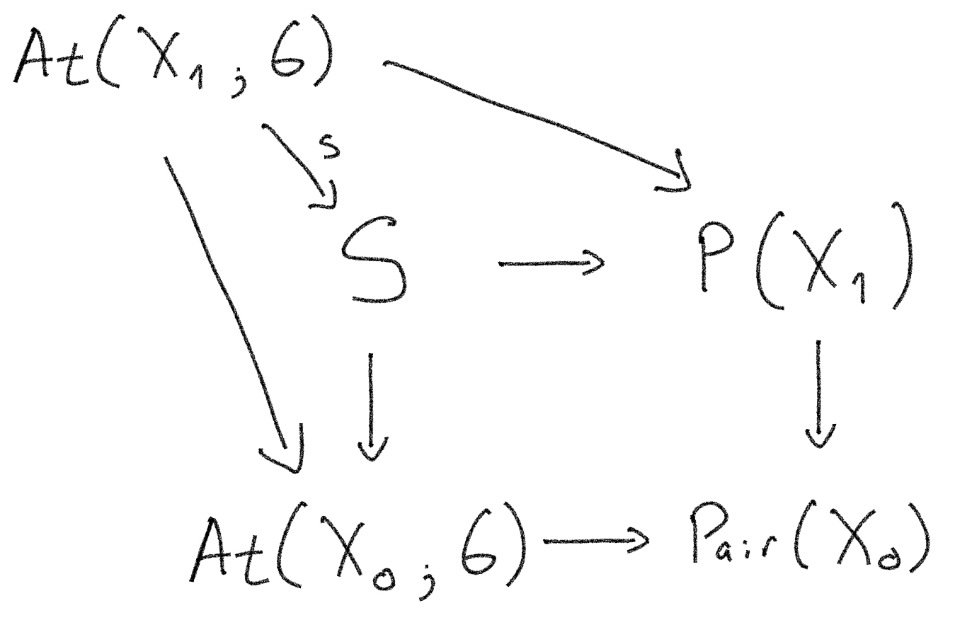
This procedure is considered a definition because, in the context of a complete and cocomplete category like the one we are using, it is known that the problem has an answer, and it is unique.
An explicit description of at a heuristic level was given in section 2.1. That description is easily adapted to describe . The reader is invited to verify that the resulting description does satisfy the definition given above.
Before proceeding, let us clarify a point where our language and the previous technical definitions do not exactly match. We repeatedly mentioned the parallel transport of initial conditions on the fiber over the source of a curve in the base space; we referred to the initial conditions as “the objects” being parallel transported. Due to the required equivariance of the parallel transport map and the property of the right action being transitive, the information contained in a map transporting one initial condition along a curve is the same as that contained in a map transporting another initial condition along the same curve . Because of this, we may consider that the objects being transported along a curve are entire fibers . The technical terminology used above calls entire fibers the objects. The parallel transport map associated with a curve is a map from one fiber to another one; using that map we can transport individual initial conditions. This is the picture portrayed when we define parallel transport maps as sections
of the projection .
This is the picture that will be extended to construct homotopy parallel transport. Parallel transport maps associated with paths are maps from the source fiber to the target fiber. Transport along 2-globes should be thought of as homotopies of parallel transport maps relative to having their endpoints fixed; as such, they are maps from a source fiber with the interpretation of being possible homotopies of initial conditions to a target fiber with the interpretation of being the resulting homotopies of final conditions. Using these parallel transport maps associated with 2-globes, from the source fiber (hosting relative homotopies of initial conditions), we can transport a particular homotopy initial conditions.
Now we proceed to construct the appropriate structure to describe homotopy parallel transport in the homotopy lattice.
The construction requires a groupoid covering such that its objects have elements corresponding to higher homotopies in (of different dimensions) of initial conditions, and morphisms correspond to homotopies of equivariant maps . Thus, we will consider pairs with and as objects. Morphisms among these objects are pairs where the first entry is a pair of points in and the second entry is a -equivariant map for SOME ??????
. The construction mirrors precisely that of , and it is summarized as
At a closer level, we notice an important difference:
The objects over a given point are of the form
for any given ; this set of objects may be denoted by and has the structure of an infinity groupoid. Similarly, the set of morphisms over a given pair of points organizes into an infinity groupoid that may be denoted by .
Notice that, as is clear from the definition, the source and target maps intertwine with at each level.
This internal structure is responsible for the superscript in .
– JUAN: Check if this structure is the same as groupoids internal to infinity groupoids. –
Since we gave the structure of an infinity groupoid internal to groupoids, and we need it to somehow cover , we will need to trivially promote to an infinity groupoid internal to groupoids. By construction, there is a surjective morphism
Now we need to tell the structure that parallel transport happens along globes of arbitrary dimension modeling homotopies of paths in the base.
** We need to reinterpret (slightly modify) the structure over the underlying set of to make it an infinity groupoid internal to a groupoid. **
The set of objects is just but seen as a trivial infinity groupoid.
k-Morphisms in for any project onto morphisms of the groupoid ; the projection given by the 0-dimensional source and target maps . We will use this projection to make into a groupoid.
Morphisms over a given pair are associated with ()-globes (for SOME ????
) such that and . This set of morphisms over is itself an infinity groupoid, but notice that its zeroth level starts with 1-globes. This infinity groupoid describes higher homotopies of paths from to in the cutoff provided by the skeletal filtration. A morphism will be called a k-globe of paths if . Source and target maps are , . The identity elements are degenerate k-globes with image for some and some . The inverse map is . Composition in the groupoid is . The shift in the level by one in the morphisms plays an important role in gauge fields, as we will see below. Let us call this structure
where the superscript helps us distinguish it from the infinity groupoid and it reminds us of the level shift in the infinity groupoid structure described above. Clearly, there is a projection map (surjective morphism)
is defined by the following pullback diagram of infinity groupoids internal to groupoids

To gain a more concrete understanding, let us explicitly describe the structure of . Its objects are of the form for some and any given . Notice that the set of such objects for a given is organized into the infinity groupoid .
The set of morphisms is in correspondence with morphisms in and in . Given a pair , morphisms are of the form where is a k-globe of paths with and (for any given ) is a -equivariant map. The set of morphisms covering in organizes into an infinity groupoid.
Source and target maps in are obvious; for example, . Our final observation regarding the structure of is that as a cover of , the preimages of the projection have the structure of an infinity groupoid, and at the lowest level, we find ; all the different levels will be denoted by .
Parallel transport maps in the homotopy lattice, abbreviated as HLGFs, correspond to sections of the projection in the top row of the diagram
| (3) |
Let us see how, given a k-globe of paths with , such section induces a parallel transport map taking any initial condition to a resulting final condition . The section yields , a morphism in at level . According to the preceding description of , this is a pair consisting of the globe of paths itself and a -equivariant map
Clearly, the second entry is a map that can transport a k-dimensional relative homotopy in modeled as a k-globe to a resulting k-globe in . This is the parallel transport map associated with by .
We invite the reader to work out in detail how is that for paths induces the parallel transport map associated with standard lattice gauge fields.
Like with ordinary fields, our gauge fields are now seen as sections. Since the non trivial information is all contained in the second entry of the image, a short hand notation, similar to the one used for ordinary fields writing instead of , is
3.3 HLGFs after a trivialization over vertices
In the differential geometric treatment of bundles and connections, a local trivialization is used to describe any particular connection with respect to the trivialization. The result is a concrete description. Concreteness comes at the price of having to take care of relating descriptions that differ only by the use of different local trivializations. In this subsection we will present a concrete description of HLGFs relying on the choice of a trivialization on the fibers over .
It is very important to realize that because is a discrete set, we can choose a trivialization on the fibers over without the need to work locally and leading with compatibility at chart intersection that is unavoidable when allowing a continuum set of fibers101010In [11] we presented two equivalent descriptions of HLGFs working with trivializations, one uses globes as we have done here. The other one is based on cubes instead of globes, and it was very useful for proving key properties, but it has the inconvenience that it needs local trivializations with non trivial intersections as in the usual approach in the continuum. In that context, a HLGF is a consistent collection of local HLGFs relative to local trivializations..
A trivialization is a set of identifications compatible with the right and left actions of . Consequently, a equivariant map translates into a group homomorphism from to commuting with the right multiplication. All such maps can be obtained by left multiplication . Recall that the composition of two equivariant maps is described by the corresponding group elements multiplied in a left-wise order. Similarly, a equivariant map translates into an automorphism of commuting with the right multiplication, and all such automorphisms can be obtained by left multiplication. Thus, relative to the trivialization, a HLGF acting on a k-globe of paths is encoded by an element
acting by left multiplication on . We have a collection of these assignments for every level of globes of paths. They are summarized by an assignment from to , where the assignment sends k-globes of paths (which is the same as globes in ) to k-globes in .
That is a morphism must translate into some property of . The clue to understanding this property is the mismatch between the structures in the expression that we want to understand: On one side we have that has the structure of an infinity groupoid internal to a groupoid as described in the previous subsection. On the other side, we have that we are using for two reasons, its group structure (inherited from the group structure of ) and an infinity groupoid structure whose stratification into levels lets us encode equivariant map by left multiplication on . Since we may consider groups as groupoids with a single object, we see that can be given the structure of an infinity groupoid internal to a groupoid (the groupoid structure inherited from that of , and the infinity groupoid structure following from higher homotopy). We will denote te corresponding structure by .
By construction, we see that a trivialization transforms into a morphism of infinity groupoids internal to groupoids where the composition and inverse -1 of the groupoid is in correspondence with the multiplication and multiplicative inverse in , and the internal infinity groupoid structure in is in correspondence with the higher fundamental groupoid structure of . In summary, a trivialization transforms into a morphism
| (4) |
Conversely, one such morphism of infinity groupoids internal to groupoids induces a HLGF.
In [11] we had defined HLGFs as morphisms of infinity groupoids
| (5) |
We will not give the definition of here, but a simple comparison makes it obvious that the definitions agree.
A change to a different trivialization of the fibers over results in a morphism related to by conjugation. First, changing from trivialization to trivialization is accomplished by left multiplication by the left action of the transition functions on as follows: . Then for any k-globe of paths we have
3.4 Gauge transformations
In the differential geometric picture, gauge transformations are induced by bundle automorphisms. A bundle automorphism transforms a given connection to another one. At a local level with respect to a given local trivialization, these transformations act by conjugation as in the last formula of the previous subsection (but within the given local trivialization). For each given bundle, these transformations form a group defining gauge equivalence classes in the space of connections on that bundle. If all -bundles over a bases space are treated at once in the standard continuum treatment, gauge transformations form a groupoid that is a disjoin union of the automorphism groups of each separate bundle (two bundle automorphisms can be composed only if they act on the same bundle). From the algebraic point of view in the continuum picture heuristically described in Subsection 2.2, considering a groupoid of paths in with a discrete collection of base points, we described gauge fields on all possible -bundles over a given base as a groupoid homomorphisms (the heuristic counterpart in the continuum of definition (3) in our discrete setting). Notice however, that HLGFs are only sensitive to the restriction of bundle automorphisms to the restriction of the bundle over the discrete set , and that the resulting automorphisms over the bundle over do form a group.
An automorphism of the bundle over is characterized by a map . The induced gauge transformation acting on HLGFs is described using a trivialization over yields
Considering the abstract definition of a HLGF of equation (3), , the gauge transformation is a natural transformation . Let us recall that both and are sections of the projection , and as such they send objects in to objects (for any given ) in and morphisms in to morphisms in . At a given level , the component of the natural transformation over is the morphism acting on by left multiplication by . Given any morphism in at level with , the following diagram in commutes
Notice that the definition of homotopy parallel transport maps as commuting with the right action of on fibers over objects forces all natural transformations connecting HLGFs to be determined by left multiplication by some . Also notice that this type of natural transformations form a group acting on HLGFs.
3.5 The homotopy lattice cutoff
Now that HLGFs have been formally introduced, it is clear that a cellular decomposition of the base space induces a cutoff map sending any gauge field in the continuum to its corresponding HLGF constructed evaluating the higher parallel transport of on higher dimensional globes fitting in the skeleton of the appropriate dimension
We will describe the space of HLGFs in detail in the second part of this series.
3.6 A set of generators for HLGFs: ELGFs
In this section, except where we explicitly say otherwise, we assume that the cellular decomposition is a triangulation by a simplicial set.
Extended Lattice Gauge Fields (ELGFs) were introduced by Claudio Meneses in collaboration with one of the authors of this paper [8, 9]. The motivation and the main result was to refine the lattice cutoff for gauge fields in such a way that the resulting extended lattice gauge fields retain the ability of characterizing a -bundle (up to bundle equivalence) after the cutoff111111Article [8] proposes two notions of extended lattice gauge fields. The fields in the first of them tautologically characterize a bundle, and the second turns out to characterize the first for two and three dimensional base spaces, but not in the general case . The second notion is the one further developed in [9], and it is what we call ELGFs in this paper.. In this subsection we describe how the version of ELGFs given in [9] can be understood as HLGFs evaluated on a set of generators of ; thus providing a 1-1 relationship between HLGFs and ELGFs. The original work on ELGFs did not provide a notion of higher homotopy parallel transport, nor the complete algebraic toolbox for gluing simplices of paths. The mentioned relationship will let us import the topological results of ELGFs to algebraically superior structure of HLGFs.
Simplices of paths
Simplices of paths were described in Section 2.4. The 0-simplex of paths is a path (i.e. 1-globe) whose image is contained in the 1-simplex of with ordered vertex set . It has as source and as target.
The 1-simplex of paths is a 2-globe whose image is contained in the 2-simplex of with ordered vertex set . It represents a 1-homotopy of paths, all of them with as source and as target. The homotopy uses the geometric 1-simplex as parameter space: Every determines a path passing by in its way from to .
The globular structure of was explicitly given in Section 3.1 (see Figure 13).
Similarly, the 2-simplex of paths has image in the 3-simplex with ordered set of vertices , and it represents a homotopy of paths using the geometric 2-simplex as parameter space (which has the structure of a 2-globe).
The general construction directly extends the one shown in Figure 13, making it the case .
Write where is a homeomorphism from the standard (k+1)-globe to a closed (k+1)-ball presented as the union of two (k+1)-simplices with vertices and .
The choice of must be compatible with the choice of . Our choice satisfies (where we have identified with the union of the two k-simplices in the boundary of as suggested by the vertex numbering) and .
On the other hand, is an injective simplicial map, and is the simplicial map determined by and .
The original construction presented in [9] uses a triangulation by a simplicial set constructed as the baricentric subdivision of a simplicial complex. In that reference a k-simplex of paths contained in simplex of is denoted by where is the k-simplex serving as parameter space for the homotopy; the 2-simplex of paths would have been written as with and . In [11] we use a similar notation (reversing the roles of the Greek letters), with and the parameter space for the homotopy being .
Simplices of paths generate
In [11] we proved that simplices of paths are generators for when is a triangulation by a simplicial set.
A sketch of the proof is the following:
(i) The HHSvK theorem [5] (solving the local to global problem in higher homotopy) tells us that a solution of the problem at a local level yields a solution of the general problem. More precisely, an open cover with elements that are inflated top dimensional simplices of satisfies the condition that let us construct from the set of its restrictions to the open sets . Thus, if simplices of paths generate for each element of the cover they also generate the whole .
(ii) It is proven that every globe of paths with image contained in a single k-simplex of is generated using r-simplices of paths with . This proof relies in the simplicial approximation theorem allowing us to construct any desired filtered map up to homotopy as a composition of simplicial maps (after refining the domain of the map).
The evaluation of HLGFs on simplices of paths
Let us define
for every . This is our notation for the evaluation of on all the simplices of paths in . The set of evaluations is an ELGF. Because the set of simplices of paths is a generating set for globes in we know that an ELGF determines a HLGF.
The set of evaluations is not independent, however. Algebraic relations that connect all the different simplices of paths as elements of imply relations among the evaluations.
Evaluation on -globes of paths are independent of each other. Evaluations on k-globes of paths need to be compatible with the evaluations on lower dimensional globes of paths on their boundary. Additionally, the set of evaluations of a HLGF on simplices of paths that bind a higher dimensional simplex of paths are subject to an extendibility condition. It states that there is an HLGF compatible with them that can also be evaluated on the bounded higher dimensional simplex of paths.
The ELGF as a set of consistent data
ELGFs were introduced before HLGFs. When they were defined they could have been though of as consistent evaluations for gauge fields in the continuum. We saw that a gauge field in the continuum can be evaluated on homotopies of paths. Thus the simplices of paths in determined a set of evaluations resulting from the parallel transport along the homotopies of paths corresponding to path simplices. The set of such evaluations was not an independent set for the same reasons as the ones given above. An ELGF could have been defined as a set of consistent data for the evaluation of some gauge field in the continuum. Thus, in this paragraph we think of as the evaluation of a homotopy of parallel transport maps on the simplex of paths calculated using a gauge field in the continuum.
An ELGF is a set of consistent evaluations specified following a particular order: We first specify the evaluations on 0-simplices of paths (i.e. give standard lattice gauge field data by evaluation on lattice links). This is free data. After prescribing consistent evaluations on k-simplices of paths for , characterizing the evaluation on any k-globe of paths with , the next step is prescribing compatible evaluations on (m+1)-simplices of paths. A set of evaluations on (m+1)-simplices of paths is consistent if it satisfies two types of conditions:
-
1.
and are compatible with the evaluations on -globes of paths (known from the evaluations on lower dimensional simplices of paths.
(6) -
2.
For each , (m+3)-simplex of , there is a consistency condition implying that a gauge field in the continuum with the prescribed evaluation can be extended from to the interior of .
Consider the (m+1)-globe of paths
; it can be seen as the image of with base point winding around once. ThenFor the condition may be written as
(7)
3.7 General higher gauge fields on the homotopy lattice
In this article, our main objective is to describe ordinary gauge fields within a cutoff as explained previously. In this subsection we deviate from this goal to consider “higher gauge fields” not necessarily associated with relative higher homotopy classes of ordinary parallel transport.
Considering our definition (3) of a HLGF as a section of a groupoid with higher homotopy internal structure,
we see that a route for generalizing our higher gauge fields is to find infinity groupoids , replacing and respectively, and with the additional internal group structure in and the transitive and free right action of on .
From the construction given here, we see that the resulting higher gauge fields would come with a notion of higher parallel transport along globes of paths: The gluing map of would be in correspondence with the internal multiplication in the replacement of .
This generalization exercise was studied, using definition (5), in [11]; we found agreement with an existing notion of higher gauge fields (using 2-groups) in the lattice [12]. Additionally, we found in [11] that any such generalization can be realized by an appropriate filtered group . That is, given with the specified structure, there is a filtered group such that and where is a torsor for .
4 The topological charge and other topological considerations
The topological charge is a functional of the gauge field that is a topological invariant of the -bundle. Since it happens that the evaluations of the functional can only achieve values in a discrete set, the functional may carry non trivial information only if the space of gauge fields has more than one connected component; in other words, the topological charge is relevant only if there is more than one -bundle class over the given base space. A physical situation of interest takes place in the base space , which represents spacetime, and there are “fall-off conditions” for the gauge field ensuring at at infinity the field is trivial up to gauge. In Euclidian quantum field theory the fall-off conditions are naturally implemented considering a compactification of the base space to . In the continuum, the topological charge can be evaluated in several ways. The most common one is as an integral of a polynomial function of the curvature; we could try to regularize the curvature and the mentioned polynomial function in terms of HLGFs. The alternative way, which we review below, is to calculate the topological charge in as the winding number of a map from to representing the transition function between the local trivializations (constructed using the gauge field) over the two hemispheres. The equivalence of these two ways to calculate the topological charge is proven in [7]. At the end of Section 3.1 we saw that the homotopy lattice cutoff leading to HLGFs keeps homotopical information of the gauge field for base spaces of dimension 2 and 3. This will let us give a simple formula for the topological charge calculated as a winding number for bases of dimension 2.
4.1 The topological charge of gauge fields over
We start with the example of HLGFs on with the triangulation described in Section 2.4.
The main idea of the calculation of the topological charge as a winding number in the continuum [7] has the following ingredients:
(i) Separate the base into two charts , with the topology of the disc intersecting in a neighborhood with the topology of .
(ii) Use the gauge field and a path system to setup a trivialization over . The path system is the assignment of a path to every point from the base point (the South Pole) to . Then the gauge field parallel transports any to . Moreover, since the parallel transport map is 1 to 1, any point in can be parametrized using . This procedure determines a trivialization over ; the analogous procedure yields a trivialization over .
(iii) The transition function restricted to is a continuous map determined by the gauge field characterizing the bundle
where in this formula we see each factor in the righthand side as valued in . A crucial property is that a homotopy between two such transition functions determines a bundle map between the corresponding bundles, making them equivalent. Homotopy classes are classified by their winding number, and the topological charge is defined to be winding number
| (8) |
For the HLGF the important principle is that the homotopy lattice cutoff keeps the exact homotopical information when it is casted in a format that is compatible with their algebraic structure. Thus, the regularization of (8) for HLGFs follows three steps:
-
1.
Choose a triangulation with one vertex in , another vertex in and such that the Equator is contained in .
-
2.
Realize as the evaluation of the gauge field on the singular 1-globe of paths (the family of meridians) with source in , target in and paramertized by a singular 1-globe winding once around the Equator
-
3.
Then the evaluation of the HLGF on the 1-globe of paths in (up to thin homotopy) is precisely the relative homotopy class of
-
4.
Since the evaluation is a 1-globe in with its source equal to its target, and its homotopy class relative to endpoints is characterized by its winding number
This result captures the essence of what HLGFs can do that standard lattice gauge fields can’t.
Below we present a more abstract version of the same idea, which shows the power and versatility of the algebraic machinery presented in this article.
A simple observation lets us change the perspective of the calculation to base it on higher parallel transport. determines parallel transport along 1-globes of paths transporting 1-globes of initial conditions on the 0-source of the globe of paths. Thus, a constant initial condition is transported along from the South Pole to the North Pole. The result is a 1-globe with equal source and target; its homotopy class is determined by its winding number, and this calculation coincides with the topological charge
in the sense that if then .
In a more abstract view, notice that is a subgroup for any vertex . Then the restriction of any HLGF induces a group morphism
| (9) |
which in this case is characterized by the multiplication by an integer. For other gauge groups, like , this definition has a clear extension. The relation between this definition and the previous paragraphs, for which the 1-globe of paths is not an element of for any is a simple exercise in globular algebra left to the reader.
Notice that our definition of implies a collection of equivalent formulas to evaluate the topological charge in terms of local data. An ELGF is local data characterizing a HLGF , and the globular algebra gives us precise formulas to evaluate . In Section 2.4 we worked out the example of the gauge field induced by the Levi-Civita connection on restricted to parallel transport unit vectors. We found that .
It is easy to show that for any given there are HLGFs with .
4.2 The bundle induced by a HLGF over 2 or 3 dimensional base spaces
The bundle induced by a HLGF
We saw that a HLGF determines an extended lattice gauge field simply by evaluating on simplices of paths.
On the other hand, on triangulated base space of dimension 2 or 3
an extended lattice gauge field with gauge group induces a -bundle [9, 8] . Therefore, for base space of dimension 2 or 3, a HLGF induces a -bundle
The proof given in [9] explicitly constructs local trivializations and transition functions. The transition functions are determined by the parallel transport map induced by the gauge field in the continuum; then, as shown in Section 3.1, for base spaces of dimension 2 or 3 the HLGF captures the information of the parallel transport up to homotopy rel. vertices.
Here we sketch its basic idea:
Consider triangulated by a simplicial set . Each simplex of the triangulation may be considered as a chart, and with the aid of a gauge field in the continuum, a local trivialization is constructed: A path system on connects the maximal vertex of to each point by a path . Then, once an initial condition in the fiber over the maximal vertex is chosen, transports to a fiber over defining the local trivialization.
For points that lie in the boundary of a simplex (with not containing the maximal vertex of ) the parallel transport maps tell us how to glue the two local trivializations. In that way, a bundle over is determined by gluing the trivial bundles over the simplices of .
The standard lattice cutoff tells us how to glue the mentioned trivial bundles over simplices at the vertices only. The homotopy lattice cutoff refines the standard lattice cutoff in that (for base spaces of dimension 2 o 3) keeps the homotopy class of the gluing maps relative to the evaluation at vertices (see Figure 21), and this information is enough to determine the bundle (up to a bundle equivalence maps determined by the homotopies). Thus, for base spaces of dimension 2 or 3, induces a -bundle; the same -bundle that induces.

5 Summary and discussion
In this article we introduced HLGFs providing a geometrical motivation and a precise algebraic definition. We also pedagogically presented the necessary algebraic framework backing up our proposal. We showed that, for base spaces of dimension 2 or 3, a HLGF determines a principal bundle. We also gave exact explicit formulas for the topological charge of a HLGF in dimension 2.
In a base space triangulated by a simplicial set, HLGFs evaluated on simplices of paths determine a set of generators for HLGFs. In previous work of one of the authors in collaboration with Claudio Meneses, these generators were called extended lattice gauge fields [8, 9]. This work is the direct precursor of what we presented here. We saw that in dimension 2 HLGFs reproduce a previous proposal given by Pfeiffer [12].
Let us briefly mention the reason making our claim of characterizing a principal bundle over the base manifold be valid only for bases of dimension 2 or 3. The obstacle for a stronger result comes from our use of a trivial filtration in the gauge group . the mathematical framework mixing homotopy with the group structure in requires that the first level of the filtration be a subgroup of . Mathematically speaking we could work with a discrete subgroup , but physics prefers the choice , and we stick with it. Questions regarding involve maps . At the algebraic level, the framework that we used to talk about higher homotopy is based on maps whose domain is the standard k-globe, which has the topology of a disk, instead of the sphere. Since the maps are considered up to hopmotopy relative to vertices in the case when the image of the two vertices of coincide, we obtain the information about the fundamental group. For higher dimensional globes, if the whole boundary of where fixed during the homotopy, we could capture the information about . This happens when we restrict to filtered maps and the filtration in does not allow homotopies unwinding . This is what fails due to our use of a trivial filtration in . Then we only see for . Fortunately for any Lie group is trivial.
A detailed explanation will be included in Ivan Sanchez’ PhD thesis (in preparation).
For purely mathematical interests, we could use a variant of our HLGFs using a nontrivial filtration in the gauge group to calculate characteristic classes.
In the paper describing second part of this work we will give structure to the space of fields that let us define measures and amplitudes. We apply the ideas behind the mentioned results solving the local to global problem in higher dimensional homotopy [3] to construct the space of fields (and the Hilbert space associated to such spaces) from the space of fields associated to elementary blocks. We also use general theorems in higher algebra to justify our definition of the spaces corresponding to the continuum limit as the appropriate inverse limits. All these results announced in the conference 17th Marcel Grossmann Meeting, and the proceedings paper [10] has ben accepted for publication. We also show that our framework refines standard lattice gauge theory in the sense that it agrees in its predictions regarding observables following from their 1-dimensional parallel transport, but we have access to a wider algebra of observables following from our higher dimensional parallel transport. In the case of 2d Yang-Mills theory, for example, we have a lattice version based on the heat kernel measure that is quantum perfect. Since we can also calculate the topological charge exactly, we can calculate the topological susceptibility exactly [10].
6 Appendix
Here we write the structural relations of -groupoids. The original reference is [2], but the notation follows [5], which is compatible with their notation for -goupoids that we use here. We have added an extra subindex to the degeneracy operator because that “extended notation” makes our formula for gauge transformations more explicit.
is a cellular decomposition of , and is the filtered topological space determined by the skeleta of the cellular decomposition.
para
| (10) |
| (11) |
| (12) |
| (13) |
| (14) |
| (15) |
| (16) |
If , then is defined if and only if and then
| (17) |
| (18) |
The interchange laws. If then
| (19) |
| (20) |
| (21) |
Supported by grant PAPITT-UNAM IN114723
References
- [1] (1991) Holonomy and path structures in general relativity and Yang-Mills theory. Int. J. Theor. Phys. 30, pp. 1171–1215. External Links: Document Cited by: §2.1.
- [2] (1981) On the algebra of cubes. Journal of Pure and Applied Algebra 21, pp. 133–260. Cited by: §2.3, §6.
- [3] (2012) Nonabelian algebraic topology: filtered spaces, crossed complexes, cubical homotopy groupoids. Vol. 15, Elementary Tracts in Mathematics, EMS Press. Cited by: §1, §1, §2.3, §5.
- [4] (1979) Colimit theorems for relative homotopy groups. University of Wales. School of Mathematics and Computer Science. Cited by: §1.
- [5] (2007) A new higher homotopy groupoid: the fundamental globular omega-groupoid of a filtered space. arXiv preprint math/0702677. Cited by: §2.2, §2.3, §3.1, §3.1, §3.6, §6.
- [6] (2013) Diffeology. Vol. 185, American Mathematical Soc.. Cited by: §2.1.
- [7] (1996) Foundations of differential geometry, volume 1. Vol. 61, John Wiley & Sons. Cited by: §2.1, §2.1, §4.1, §4.
- [8] (2019) Homotopy classes of gauge fields and the lattice. Adv. Theor. Math. Phys. 23 (8), pp. 2207–2254. External Links: 1701.00775, Document Cited by: §1, §3.6, §3.6, §3.6, §4.2, §5, footnote 11.
- [9] (2019) Macroscopic observables from the comparison of local reference systems. Class. Quant. Grav. 36 (23), pp. 235011. External Links: 1905.04797, Document Cited by: §1, §2.1, §2.4, §3.6, §3.6, §3.6, §3.6, §4.2, §4.2, §5, footnote 11, footnote 7.
- [10] (2024-07) A better space of generalized connections. External Links: 2407.17400 Cited by: §5.
- [11] (2023-11) Higher homotopy and lattice gauge fields. External Links: 2311.02363 Cited by: §1, §2.4, §3.1, §3.3, §3.6, §3.6, §3.7, Remark 1, footnote 10, footnote 8.
- [12] (2003) Higher gauge theory and a nonAbelian generalization of 2-form electrodynamics. Annals Phys. 308, pp. 447–477. External Links: hep-th/0304074, Document Cited by: §1, §3.7, §5.
- [13] (2007) Parallel transport and functors. arXiv preprint arXiv:0705.0452. Cited by: §2.2, footnote 5.
- [14] (1948) On operators in relative homotopy groups. Annals of Mathematics 49 (3), pp. 610–640. Cited by: §1.