Hierarchical Latent Structure Learning through Online Inference
Abstract
Learning systems must balance generalization across experiences with discrimination of task-relevant details. Effective learning therefore requires representations that support both. Online latent-cause models support incremental inference but assume flat partitions, whereas hierarchical Bayesian models capture multilevel structure but typically require offline inference. We introduce the Hierarchical Online Learning of Multiscale Experience Structure (HOLMES) model, a computational framework for hierarchical latent structure learning through online inference. HOLMES combines a variation on the nested Chinese Restaurant Process prior with sequential Monte Carlo inference to perform tractable trial-by-trial inference over hierarchical latent representations without explicit supervision over the latent structure. In simulations, HOLMES matched the predictive performance of flat models while learning more compact representations that supported one-shot transfer to higher-level latent categories. In a context-dependent task with nested temporal structure, HOLMES also improved outcome prediction relative to flat models. These results provide a tractable computational framework for discovering hierarchical structure in sequential data.
Introduction
A central challenge in learning is balancing generalization and discrimination. Generalization allows agents to apply prior knowledge to novel situations, whereas discrimination enables sensitivity to subtle but meaningful differences in observations Tenenbaum and Griffiths (2001); Tenenbaum et al. (2011); Barak et al. (2013); Lake2015. Effective learning therefore requires representations that capture shared structure across multiple levels of abstraction while preserving task-relevant distinctions among observations.
One influential approach is latent structure inference, in which an agent partitions observations into hidden causes that generate the data. Bayesian nonparametric models provide a principled framework for this process by allowing the number of latent causes to grow with experience Anderson (1991); Mansinghka et al. (2006); Gershman et al. (2010); Gershman and Niv (2012). However, most existing models assume flat partitions in which all latent causes exist at a single level of abstraction.
Many environments are instead inherently hierarchicalO’Doherty et al. (2021), where observations share intermediate categories and broader contextual regularities. Hierarchical Bayesian models Teh et al. (2006) such as the nested Chinese Restaurant Process (nCRP) Griffiths et al. (2003); Blei et al. (2010) capture such structure, but typically rely on offline batch inference. Conversely, online latent cause models based on sequential Monte Carlo methods support incremental trial-by-trial inference but typically assume flat latent spacesGershman and Blei (2012). Bridging this gap requires a model that combines hierarchical representation with online inference.
Here, we introduce Hierarchical Online Learning of Multiscale Experience Structure (HOLMES), a framework that combines hierarchical nonparametric structure with online sequential inference. Our model performs trial-by-trial inference over dynamically expanding latent trees, enabling hierarchical representations to be discovered directly from sequential experience.
We evaluate the model in two classes of synthetic tasks. In compositional environments, hierarchical inference preserves predictive performance while learning more compact representations that support one-shot transfer across latent categories. In a context-dependent decision-making task with nested temporal structure, hierarchical inference additionally improves outcome prediction by capturing latent rule structure across contexts and timescales.
Methods
We formalize HOLMES as a Bayesian nonparametric model in which observations are assigned to paths through a latent tree. The model combines a hierarchical prior over tree structure with sequential Monte Carlo inference, allowing latent representations to be constructed and updated online from sequential observations. We first describe the standard flat latent-cause model Gershman et al. (2010); Gershman and Niv (2012), then introduce our hierarchical model and its online inference procedure.

Formal problem definition
We consider a task in which an agent observes a sequential dataset
| (1) |
where each observation is an -dimensional binary vector indicating the presence (1) or absence (0) of each feature at time . In classical conditioning, for example, this vector may encode the presence of a cue and an outcome. The agent’s goal is to infer, at each time step , a latent assignment sequence
| (2) |
where indexes the cluster associated with observation . Critically, both the number of clusters and their assignments are unknown and must be inferred from data.
Because the number of possible partitions grows super-exponentially, exact inference is intractable Hjort et al. (2010). We therefore combine a Bayesian nonparametric prior Aldous (1985) and sequential Monte Carlo method (particle filtering) Speekenbrink (2016); Martino2018-st to approximate posterior beliefs online.
Flat latent-cause model
In the flat latent cause model, observations are grouped using a Bayesian nonparametric clustering formalism, with clusters commonly interpreted as “latent causes” that generate the observations. Gershman et al. (2010). On each trial, the model evaluates whether the current observation is better explained by an existing cluster or by introducing a new one.
Prior over cluster assignments
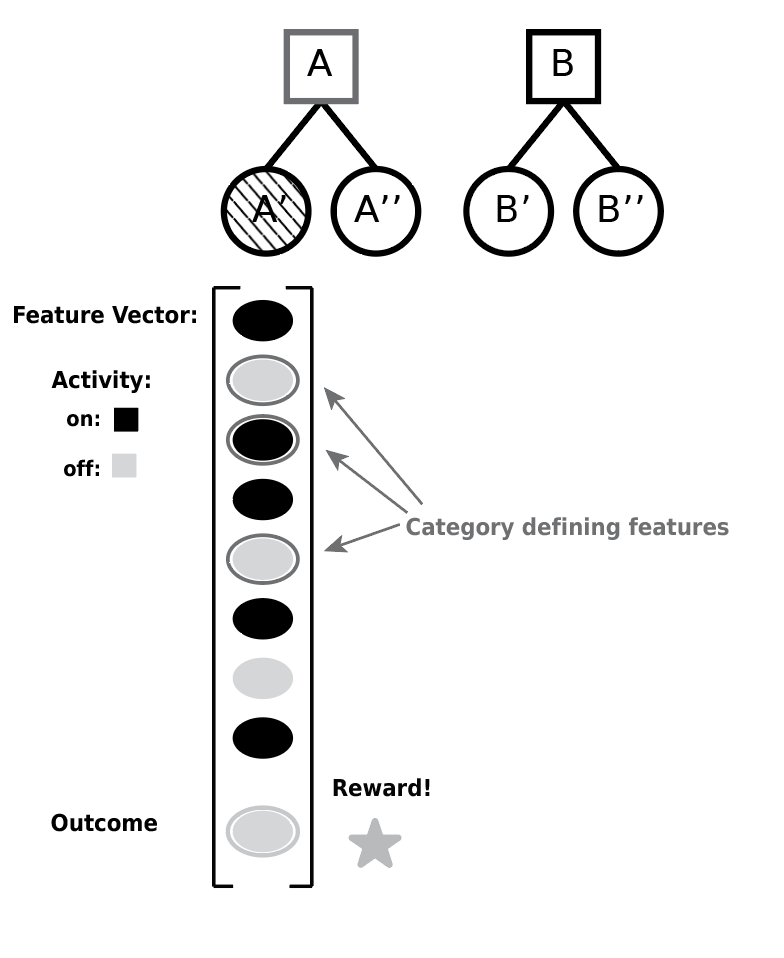
The prior over latent assignments is specified using the Chinese Restaurant Process (CRP) (Fig.1A). This allows the number of clusters (tables in a restaurant) to grow with experience while favoring reuse of previously inferred clusters Aldous (1985).
Under the CRP, the probability that observation is assigned to an existing cluster or a new cluster is:
| (3) |
where is the number of previous observations assigned to cause , and is a concentration parameter. Larger favors finer partitions with more clusters, whereas smaller favors reuse of existing clusters and broader generalization.
Likelihood and online updates
Observations are modeled independently across features within each cluster using a factorized likelihood. For each cluster and feature , the model maintains sufficient statistics:
-
•
: number of times feature has been observed as present in cluster
-
•
: number of times feature has been observed as absent in cluster
All feature counts are initialized with a symmetric pseudocount :
| (4) |
This observation bias regularizes inference when data are sparse and encodes prior uncertainty about feature distributions.
At each observation , the agent observes a binary feature vector
| (5) |
and updates sufficient statistics for the assigned cluster :
| (6) | ||||
| (7) |
These recursive updates allow learning to proceed fully online.
Likelihood computation
Given current feature counts, the likelihood of observation under cluster follows a Beta–Bernoulli distribution:
| (8) |
where counts are initialized with pseudocount (Eq. 4) and include all observations up to observation .
The parameter controls the influence of new evidence: larger values promote slower updating and greater generalization, whereas smaller values allow more rapid context differentiation at the cost of increased sensitivity to noise and risk of overfitting.
Sequential Monte Carlo inference
Exact posterior inference over latent assignments is intractable. We therefore approximate the posterior using particle filtering. The particle filter maintains an ensemble of particles, each representing a hypothesis about the current clustering state, including cluster assignments and feature statistics.
At observation , particles sample assignments from the CRP prior and are weighted by the likelihood of the current observation:
| (9) |
Weights are normalized and particles are resampled at each observation to prevent particle degeneracy.
The model’s predictions are computed as posterior expectations over the particle ensemble, naturally reflecting uncertainty when particles disagree.
HOLMES: online hierarchical latent structure learning
We extend the flat latent-cause model by assigning observations to paths through a hierarchical tree of latent causes. Unlike standard flat formulations, this extension organizes latent structure across multiple levels of abstraction, allowing higher-level nodes to capture shared regularities and lower-level nodes to capture more detailed distinctions.
Hierarchical prior over latent paths
We define the prior over tree structures using a depth-decayed, sticky nested Chinese Restaurant Process (nCRP)Blei et al. (2010); Griffiths et al. (2003). Unlike a standard CRP, where observations are assigned to a single partition, the nCRP recursively partitions data at multiple levels (Fig.1B). At each trial , each particle samples a sequence of latent assignments
where indexes the node at level , and the depth may vary across trials.
Depth-decayed concentration and stopping.
We define depth-adjusted concentration as
| (10) |
which implements a depth budget constraint: the exponential decay rate is directly tied to the base concentration, such that models with higher (favoring proliferation of clusters) deplete their capacity for deep branching more rapidly. This coupling ensures that the model cannot simultaneously maintain high branching factors and deep hierarchies—a form of implicit model capacity control. Under this parameterization, is non-monotone in for fixed (maximized at ), reflecting the tradeoff between local branching propensity and global depth budget. We interpret as controlling overall model capacity rather than concentration at any single level Dasgupta2022; Piray2021.
At level , given parent node , the probability of assigning an observation to an existing child branch or creating a new branch follows the standard CRP form with the described depth-adjusted concentration:
| (11) |
where is the number of previous assignments to child at level within particle , and is the total count at level within particle . We impose a maximum branching factor of 20 children per node for computational tractability, as a weak limit approximation.
In addition to depth-dependent branching, the model includes a stochastic stopping mechanism that allows path traversal to terminate at any levelGhahramani et al. (2010). After selecting a branch at level , traversal stops with probability:
| (12) |
Stopping is not permitted at level , ensuring at least one representational level exists. Together, depth-dependent concentration and stochastic stopping define a flexible prior over hierarchical depth without requiring an explicit depth limit.
Persistence and node reuse
To capture temporal persistence in latent structure, we include a stickiness bias Fox et al. (2007) that increases the probability of reusing the previously inferred latent configuration at each level and allows reuse of global node identities across particles. When different particles discover identical substructures, they share the same global node rather than maintaining redundant local copies Blei et al. (2010) (see Supplementary Methods for full implementation).
Hierarchical inference procedure
Inference used the same particle filtering framework as in the flat model. At each trial, each particle samples a path through the hierarchical prior, evaluates the likelihood of the observation at the leaf node, and updates its weight accordingly. We normalized particles and resampled to approximate the posterior distribution. As in the flat model, likelihoods are evaluated only at the leaf nodes of the inferred hierarchy based on the observation statistics (see Supplementary Methods). This allows the inference space to remain constrained even as the hypothesis space grows.
Simulation environment
Compositional task environment
We first evaluated the models in synthetic compositional tasks (Fig. 2A). These tasks contained two to five levels, where each level represented a binary latent category that determined observable feature values. Observations were binary feature vectors (Fig. S2) generated by level-specific rules. The top levels were encoded as single binary features, the next lower identity was encoded with two binary features, and the lower levels were encoded as a one-hot vector across four random features. Observations were generated by sampling a latent category value at each hierarchical level, then deterministically encoding the resulting configuration as features. Outcomes were determined by a conjunctive rule over the latent category assignments at the two highest levels (Fig. 2A).
Context-dependent task with nested temporal structure
We next evaluated the models in a synthetic context-dependent task with nested temporal structure Mante et al. (2013); Bernardi et al. (2020). On each trial, the model observed one of four stimuli defined by the combination of two binary feature dimensions (e.g., color and shape), and reward depended on the current task context. The task alternated between two slowly changing rule contexts, each specifying which feature dimension determined reward. In one context, the first feature dimension was predictive of reward while the second was irrelevant; in the other context, the second feature dimension was predictive while the first was irrelevant. Within each slow context, the rewarded feature value also switched, creating nested temporal structure across timescales (Fig. 4A,B).
Evaluation metrics
Outcome prediction accuracy
The outcome prediction accuracy was defined as the proportion of trials in which the model correctly predicted whether an outcome occurred.
Representational efficiency
To quantify representational efficiency, we measured the entropy of cluster assignments within each ground truth category: , where is the proportion of category- trials assigned to cluster . Lower entropy indicates that trials from a category concentrated in fewer clusters. In the transfer task, categories corresponded to ground truth labels at a given hierarchical level. For the temporal task, categories were the four latent states formed by crossing contexts (shape-rule vs. texture-rule) with rewarded values (e.g., shape-circle, texture-stripes). For hierarchical models, we report results from the highest non-root tree level created. We averaged entropy across categories, weighted by trial frequency (see Supplementary Methods for details).
One-shot transfer
To assess generalization, we evaluated one-shot transfer after training. A single higher level labeled exemplar was presented and models were required to generalize that label to previously observed stimuli belonging to the same latent category. Transfer performance was quantified using recall: the proportion of true same-category trials correctly identified Buckland and Gey . We focus on recall as the primary metric because (1) category membership is balanced across trials, making recall directly interpretable as generalization success, and (2) the scientific question concerns the model’s ability to recognize same-category instances across contexts, which recall measures directly. This is highly correlated with F1 score across all task complexities (for additional metrics, see Supplementary Table 2).
Results
Hierarchical inference preserves outcome prediction while improving representational efficiency
We first examined whether hierarchical inference improves the efficiency with which compositional structure is represented during learning. In many environments, observable features combine to form higher-level latent categories that determine outcomes. Learning in such settings requires discovering how observations compose into reusable abstractions. We therefore asked whether hierarchical clustering produces more efficient internal representations than flat clustering when learning compositional tasks.
To test this, we constructed synthetic categorization environments in which observations were generated from latent factors organized in a nested hierarchy (Fig. 2A). In the simplest 2-level version, observable binary features combine to define a latent category, which in turn determines the binary outcome (reward/no reward; Fig. 2A). More complex versions add additional latent factors in the hierarchy above this category, creating deeper hierarchical structures.
These tasks allow a direct comparison between two representational strategies. A flat model represents each feature combination independently, whereas a hierarchical model can reuse latent structure across observations by organizing them into a tree of shared causes. Fig. 2B illustrates the difference in the 2-level task: the flat model creates separate clusters for each observation-outcome combination at the observation level, while HOLMES compresses this information into a tree with category-level groups. This organization allows multiple observations to inherit shared latent structure rather than being encoded independently.
Despite their architectural differences, both models achieved equivalent performance on the primary learning objective. We quantified learning performance as outcome prediction accuracy—the proportion of trials on which models correctly predicted binary outcomes (reward vs. no reward) from observable features. At 2-level complexity, flat and hierarchical models showed statistically indistinguishable accuracy (Fig. 2C). Thus hierarchical organization does not impair predictive learning.
However, the models differed markedly in representational efficiency. To quantify, we measured the entropy of cluster assignments within each true category: a metric capturing how consistently trials from the same category mapped to the same cluster. Lower entropy indicates more organized, efficient representations. HOLMES showed significantly lower entropy than flat models at the 2-level task (Fig. 2D), indicating more consistent category-to-cluster mappings despite equivalent outcome prediction.

We next examined how these effects scale with task complexity. We generated tasks with up to 5 hierarchical levels, training both models to predict the same binary outcome across increasing structural complexity. Across all complexity levels, both models achieved comparable accuracy in predicting outcomes (Fig. 2E). However, HOLMES showed significantly lower entropy than flat models at all complexity levels (Fig. 2F), indicating more consistent category-to-cluster mappings regardless of task depth.
We further quantified compression efficiency by measuring the number of clusters learned relative to the true number of latent categories. HOLMES maintained near-optimal compression across task complexities, using approximately as many clusters as true category labels (Fig. 2G, light). In contrast, flat models showed increasing redundancy with complexity, requiring progressively more clusters than necessary (Fig. 2G, dark). Together, these results demonstrate that hierarchical clustering preserves predictive performance while learning substantially more efficient internal representations of compositional structure.
Hierarchical representations enable one-shot transfer across latent categories

If hierarchical inference discovers latent compositional structure during learning, the resulting representations should support rapid generalization across observations sharing the same latent category. We therefore next asked whether the hierarchical model’s more efficient representations enable one-shot transfer across latent categories.
To test this prediction, we implemented a one-shot transfer paradigm (Fig. 3A). Models were first trained on outcome prediction exactly as before, learning to predict reward outcomes without ever receiving explicit category labels (e.g., ”category A”). After training, we introduced a teaching phase consisting of a single labeled example—showing the model one previously-observed stimulus and labeling it as belonging to a particular latent category. In the transfer test, models had to generalize this label to identify which other previously-observed stimuli belonged to the same category, despite having only seen a single labeled example and never being trained on categorization directly.
This paradigm requires models to have spontaneously discovered the latent category structure during outcome prediction learning. A model that only learned observation-level associations must treat each stimulus independently and therefore cannot reliably generalize categories. In contrast, a model that learned abstract category-level representations should readily transfer the label across different colored instances of the same latent structure.
Consistent with this prediction, HOLMES showed stronger transfer performance than the flat model as task complexity increased (Fig. 3B). While both models performed similarly in the simplest 2-level task, HOLMES substantially outperformed the flat model as the tasks became deeper (Fig. 3B). The hierarchical advantage increased systematically with task complexity (Fig. 3C), indicating that the benefit of hierarchical representations becomes more pronounced as latent structure deepens.
To examine generalization across different abstraction levels, we tested both models on all hierarchical levels in the most complex (5-level) task. The hierarchical model outperformed the flat model across all tested levels, with the advantage being most pronounced at deeper levels of the hierarchy (Fig. 3D).
We next examined the relationship between outcome prediction accuracy and one-shot transfer performance across parameter regimes. Both model architectures exhibited a negative correlation between these objectives, suggesting a fundamental tradeoff between fine-grained discrimination and broad generalization. Parameter regimes that optimize outcome prediction create many fine-grained observation-level clusters, which can impair generalization. However, at matched levels of outcome prediction accuracy, hierarchical models consistently achieved superior transfer performance, suggesting a Pareto improvement rather than a simple parameter-dependent tradeoff (Fig. 3E). This advantage likely reflects the hierarchical model’s ability to simultaneously maintain task-relevant fine-grained distinctions at lower tree levels while building reusable abstractions at higher levels—a form of representational specialization unavailable to flat architectures.
To assess whether these advantages depended on specific parameter choices, we evaluated model performance across a broad range of concentration and bias parameters. Across 200 sampled parameter combinations, HOLMES consistently produced more efficient representations (Supplementary Fig. S4 A,B) and higher transfer accuracy than the flat latent-cause model (Supplementary Fig. S4 C,D). These results indicate that the hierarchical advantage reflects architectural properties of the model rather than parameter tuning.
Together, these findings show that hierarchical structure learning enables agents to organize experience into reusable abstractions that support both accurate prediction and rapid transfer from minimal supervision.
Hierarchical inference improves outcome prediction in a context-dependent task with nested temporal structure
So far we examined compositional environments, in which latent structure is embedded in combinations of observable features. However, many environments are structural: the relevant regularities are rules that govern how features map to outcomes across contexts and time. We therefore asked whether hierarchical inference also improves learning when the relevant structure unfolds across multiple timescales.
To test this, we constructed a synthetic context-dependent task with nested temporal structure. In this task, models had to infer both a slowly changing rule context and faster switches in the rewarded feature value within each context. On each trial, the model observed one of four stimuli defined by two binary feature dimensions. The rewarded feature dimension depended on a slowly changing rule context. In one context, the first feature dimension predicted reward, whereas in the other context, the second dimension was predictive. Within each rule context, the rewarded feature value also switched periodically, creating nested temporal structure across timescales (Fig. 4A,B).
Unlike the compositional tasks, we found that the hierarchical model showed a clear advantage in outcome prediction. The flat model treats each stimulus–outcome contingency independently and therefore operates near chance performance. In contrast, HOLMES can capture the latent rule structure linking contexts, feature dimensions, and rewarded feature values (Fig. 4C).
Representational efficiency mirrored the pattern observed in the compositional tasks. HOLMES produced substantially more specialized representations, with trials from each latent state concentrated in fewer clusters. This resulted in significantly lower within-state entropy than the flat model (Fig. 4D) and fewer clusters used per latent state (Fig. 4E).
These results show that the hierarchical model discovers compact representations aligned with the latent rule structure across contexts and timescales, improving both predictive performance and representational efficiency.

Discussion
We introduced HOLMES, an online hierarchical latent-cause model for sequential structure learning. The model combines hierarchical nonparametric structure with tractable sequential inference, allowing latent causes to be organized across multiple levels of abstraction during online learning. Across compositional tasks, the hierarchical model matched the predictive performance of flat latent-cause models while learning more compact representations and enabling improved one-shot transfer. In a context-dependent task with nested temporal structure, hierarchical inference additionally improved outcome prediction by capturing latent rule structure across contexts and timescales. These results demonstrate how hierarchical latent structure can support both efficient representation and flexible generalization in sequential learning.
Our model bridges two previously separate approaches. Hierarchical Bayesian models, such as the nested Chinese Restaurant Process (nCRP) Griffiths et al. (2003); Blei et al. (2010), originally developed for hierarchical topic modeling, can represent rich multi-level structure but typically rely on batch inference. Online latent-cause inference models Gershman et al. (2010) perform sequential inference but operate over flat latent spaces. By combining a modified nCRP prior with particle filtering, our model supports trial-by-trial inference over hierarchical latent structure. Unlike other hierarchical models that rely on batch inference, fixed hierarchies Wang et al. (2011), or Bayesian model selection over candidate structures (e.g., the COIN model Heald2021), HOLMES performs fully online inference of arbitrary depth, enabling dynamic construction of hierarchical representations during sequential experience.
Our simulations illustrate two functional consequences of hierarchical inference. In compositional environments, hierarchical structure learning produced substantially more efficient representations while preserving outcome prediction performance. These compressed representations aligned with the latent generative structure of the task and enabled rapid generalization across observations sharing higher-level categories. The flat latent cause model, in contrast, required multiple independent clusters to represent the same structure, limiting their ability to support transfer across related observations. This result highlights how representational organization, rather than predictive accuracy alone, can determine the range of generalization operations supported by a learned model.
Prior work has shown that one-shot generalization can arise from richly structured generative priors (e.g., Lake2015). The open question, however, is how reusable abstractions that support one-shot generalization can be discovered incrementally from sequential experience without explicit supervision over the latent structure. Our contribution is therefore not one-shot learning per se, but a tractable online framework for inferring hierarchical latent representations that make one-shot transfer possible. Unlike standard one-shot concept-learning benchmarks, the task studied here requires category structure to be inferred from unlabeled sequential experience rather than specified in advance by a richly structured concept prior.
In a context-dependent task with nested temporal structure, hierarchical inference provided an additional advantage by enabling discovery of latent rule structure across contexts and timescales. Because stimulus–outcome associations alone were insufficient to solve the task, successful learning required identifying the rule governing which feature dimension predicted reward. The hierarchical model could capture this structure by organizing contexts and value states into a nested representation, whereas the flat model treated each contingency independently. This result highlights how hierarchical inference can support rule learning in environments where relevant structure unfolds across multiple temporal scales.
An important refinement of our model is that decays with tree depth. This can be interpreted as a bounded-rational Bhui2021 prior over structure: agents cannot “over-carve” the world at every scale but must allocate a limited segmentation budget. This constraint is consistent with the idea that abstraction is economical—higher levels of representation are sparse and conservative, while finer distinctions emerge only when prediction errors justify additional complexity. This depth-dependent attenuation implements a soft penalty on hierarchical elaboration, capturing the trade-off between expressive capacity and representational simplicity. More broadly, the model connects to theories of approximate Bayesian inference under resource constraints Simon1957; Gershman et al. (2015); Bhui2021. Particle filtering approximates the Bayesian posterior using limited computational resources, introducing a trade-off between accuracy and computational cost: the number of particles determines how well the filter can represent multimodal hierarchical beliefs.
Several limitations remain. Our analysis focused on synthetic tasks with discrete binary features and known generative trees. In real-world environments, hierarchical structure may be ambiguous or partially overlapping.
The model also currently lacks a forgetting or pruning mechanismHuys et al. (2012), which may be important in non-stationary environments. Incorporating structural pruning or recency-weighted updates may allow the model to adapt more flexibly to changing environments.
Despite these limitations, our work provides a tractable computational framework for online hierarchical latent-cause inference, offering a foundation for studying compositional reasoning, rule discovery, continual learning, and structured generalization in both biological and artificial learning systems.
Code availability.
All model and simulation code will be made available at https://github.com/Iigaya-Lab/HOLMES-2026.
All simulations were implemented in Python using NumPy for numerical operations, Scipy and Sklearn for statistics, and figures were generated using Matplotlib and Seaborn.
Acknowledgments
The authors would like to thank Kim Stachenfeld, Adithya Gungi, Deniz Yagmur Urey, Sashank Pisupati. Research reported in this publication was supported by the National Institute of Mental Health (R01MH136214; KI), the Brain & Behavior Research Foundation Young Investigator Grant (KI), and the National Institute of Neurological Disorders and Stroke (T32NS064929; IA).
References
- [1] (1985) Exchangeability and related topics. In École d’Été de Probabilités de Saint-Flour XIII — 1983, pp. 1–198. External Links: ISBN 9783540393160, ISSN 1617-9692, Link, Document Cited by: Formal problem definition, Prior over cluster assignments.
- [2] (1991) The adaptive nature of human categorization.. 98 (3), pp. 409. Cited by: Introduction.
- [3] (2013-02) The sparseness of mixed selectivity neurons controls the generalization–discrimination trade-off. 33 (9), pp. 3844–3856. External Links: ISSN 1529-2401, Link, Document Cited by: Introduction.
- [4] (2020-11) The geometry of abstraction in the hippocampus and prefrontal cortex. Cell 183 (4), pp. 954–967.e21. External Links: ISSN 0092-8674, Link, Document Cited by: Context-dependent task with nested temporal structure.
- [5] (2010) The nested chinese restaurant process and bayesian nonparametric inference of topic hierarchies. 57 (2), pp. 1–30. Cited by: Introduction, Hierarchical prior over latent paths, Persistence and node reuse, Discussion, Canonical node reuse..
- [6] The relationship between recall and precision. Journal of the American Society for Information ScienceIEEE Transactions on signal processingAdvances in neural information processing systemsJournal of the ACM (JACM)sciencePsychological reviewThe Journal of NeuroscienceArxiv preprintThe Annals of Applied StatisticsNature NeuroscienceCurrent Opinion in Behavioral SciencesCoRRSciencePLoS computational biologyIFAC Proceedings VolumesTrends in Cognitive SciencesJournal of the American Statistical AssociationCognitive ScienceDevelopmental ScienceHarvard Review of PsychiatryJournal of Quality TechnologyLanguage, Cognition and NeuroscienceJournal of Affective DisordersPsychiatry ResearchAmerican Journal of PsychiatryPsychiatry ResearchPsychological MedicineJournal of Mathematical PsychologyLearning & BehaviorCurrent Opinion in NeurobiologyLearning & BehaviorPsychological ReviewCognitionSchizophrenia ResearchBehavioral and Brain SciencesJournal of Mathematical PsychologyPsychological ReviewSchizophrenia BulletinIndian Journal of Psychological MedicinePsychological ReviewAddiction NeuroscienceBiological PsychiatryLearning & BehaviorTrends in Cognitive SciencesSchizophrenia ResearchPsychological MedicineScientific ReportsArchives of General PsychiatryWorld PsychiatrySchizophrenia BulletinConsciousness and CognitionConsciousness and CognitionSchizophrenia ResearchJournal of Abnormal PsychologyIEEE Transactions on Pattern Analysis and Machine IntelligenceNeuropsychopharmacologyBehavioural Brain ResearchMolecular PsychiatryPsychiatry and Clinical NeurosciencesBiological PsychiatrySchizophrenia BulletinSchizophrenia Bulletin OpenCognitive NeuropsychiatryFrontiers in Artificial IntelligenceProceedings of the Royal Society of London. Series B: Biological SciencesJournal of Computational and Graphical StatisticsMind & LanguageWorld PsychiatryNeurobiology of Learning and MemoryPsychophysiologyBorderline Personality Disorder and Emotion DysregulationAmerican Journal of PsychotherapyScientific ReportsCommunications PsychologyThe Journal of NeuroscienceApplied SciencesTrends in Cognitive SciencesNeuronPsychological ScienceProceedings of the National Academy of SciencesNeuronPLOS Computational BiologyAutism Research 45 (1), pp. 12–19. External Links: Document, Link, https://asistdl.onlinelibrary.wiley.com/doi/pdf/10.1002/Abstract Empirical studies of retrieval performance have shown a tendency for Precision to decline as Recall increases. This article examines the nature of the relationship between Precision and Recall. The relationships between Recall and the number of documents retrieved, between Precision and the number of documents retrieved, and between Precision and Recall are described in the context of different assumptions about retrieval performance. It is demonstrated that a tradeoff between Recall and Precision is unavoidable whenever retrieval performance is consistently better than retrieval at random. More generally, for the Precision–Recall trade-off to be avoided as the total number of documents retrieved increases, retrieval performance must be equal to or better than overall retrieval performance up to that point. Examination of the mathematical relationship between Precision and Recall shows that a quadratic Recall curve can resemble empirical Recall–Precision behavior if transformed into a tangent parabola. With very large databases and/or systems with limited retrieval capabilities there can be advantages to retrieval in two stages: Initial retrieval emphasizing high Recall, followed by more detailed searching of the initially retrieved set, can be used to improve both Recall and Precision simultaneously. Even so, a tradeoff between Precision and Recall remains. © 1994 John Wiley & Sons, Inc. 1994 @article{precision, author = {Buckland, Michael and Gey, Fredric}, title = {The relationship between Recall and Precision}, journal = {Journal of the American Society for Information Science}, volume = {45}, number = {1}, pages = {12-19}, doi = {https://doi.org/10.1002/(SICI)1097-4571(199401)45:1<12::AID-ASI2>3.0.CO;2-L}, url = {https://asistdl.onlinelibrary.wiley.com/doi/abs/10.1002/%28SICI%291097-4571%28199401%2945%3A1%3C12%3A%3AAID-ASI2%3E3.0.CO%3B2-L}, eprint = {https://asistdl.onlinelibrary.wiley.com/doi/pdf/10.1002/%28SICI%291097-4571%28199401%2945%3A1%3C12%3A%3AAID-ASI2%3E3.0.CO%3B2-L}, abstract = {Abstract Empirical studies of retrieval performance have shown a tendency for Precision to decline as Recall increases. This article examines the nature of the relationship between Precision and Recall. The relationships between Recall and the number of documents retrieved, between Precision and the number of documents retrieved, and between Precision and Recall are described in the context of different assumptions about retrieval performance. It is demonstrated that a tradeoff between Recall and Precision is unavoidable whenever retrieval performance is consistently better than retrieval at random. More generally, for the Precision–Recall trade-off to be avoided as the total number of documents retrieved increases, retrieval performance must be equal to or better than overall retrieval performance up to that point. Examination of the mathematical relationship between Precision and Recall shows that a quadratic Recall curve can resemble empirical Recall–Precision behavior if transformed into a tangent parabola. With very large databases and/or systems with limited retrieval capabilities there can be advantages to retrieval in two stages: Initial retrieval emphasizing high Recall, followed by more detailed searching of the initially retrieved set, can be used to improve both Recall and Precision simultaneously. Even so, a tradeoff between Precision and Recall remains. © 1994 John Wiley \& Sons, Inc.}, year = {1994}} Cited by: One-shot transfer.
- [7] (2007) The sticky hdp-hmm: bayesian nonparametric hidden markov models with persistent states. 2. Cited by: Persistence and node reuse.
- [8] (2011-06) A sticky hdp-hmm with application to speaker diarization. 5 (2A). External Links: ISSN 1932-6157, Link, Document Cited by: Stickiness.
- [9] (2010-01) Context, learning, and extinction. 117 (1), pp. 197–209 (eng). External Links: ISSN 1939-1471, Document Cited by: Introduction, Flat latent-cause model, Methods, Discussion.
- [10] (2012-02) A tutorial on Bayesian nonparametric models. 56 (1), pp. 1–12. External Links: ISSN 0022-2496, Link, Document Cited by: Introduction.
- [11] (2015-07) Computational rationality: a converging paradigm for intelligence in brains, minds, and machines. 349 (6245), pp. 273–278. External Links: ISSN 1095-9203, Link, Document Cited by: Discussion.
- [12] (2012-09) Exploring a latent cause theory of classical conditioning. 40 (3), pp. 255–268 (en). External Links: ISSN 1543-4508, Link, Document Cited by: Introduction, Methods.
- [13] (2010) Tree-structured stick breaking for hierarchical data. Advances in neural information processing systems 23. Cited by: Depth-decayed concentration and stopping..
- [14] (2003) Hierarchical topic models and the nested chinese restaurant process. 16. Cited by: Introduction, Hierarchical prior over latent paths, Discussion.
- [15] (2010) An invitation to bayesian nonparametrics. In Bayesian Nonparametrics, N. L. Hjort, C. Holmes, P. Müller, and S. G. Walker (Eds.), Cambridge Series in Statistical and Probabilistic Mathematics, pp. 1–21. Cited by: Formal problem definition.
- [16] (2012) Bonsai trees in your head: how the pavlovian system sculpts goal-directed choices by pruning decision trees. PLoS computational biology 8 (3), pp. e1002410. Cited by: Discussion.
- [17] (2009) An overview of sequential monte carlo methods for parameter estimation in general state-space models. 42 (10), pp. 774–785. External Links: ISSN 1474-6670, Link, Document Cited by: Particle Filter.
- [18] (2006) Structured priors for structure learning. In Proceedings of the Twenty-Second Conference on Uncertainty in Artificial Intelligence, pp. 324–331. Cited by: Introduction.
- [19] (2013-11) Context-dependent computation by recurrent dynamics in prefrontal cortex. Nature 503 (7474), pp. 78–84. External Links: ISSN 1476-4687, Link, Document Cited by: Context-dependent task with nested temporal structure.
- [20] (2021-10) The hierarchical construction of value. 41, pp. 71–77. External Links: ISSN 2352-1546, Link, Document Cited by: Introduction.
- [21] (2016-08) A tutorial on particle filters. 73, pp. 140–152 (en). External Links: ISSN 0022-2496, Link, Document Cited by: Formal problem definition.
- [22] (2006-12) Hierarchical dirichlet processes. 101 (476), pp. 1566–1581. External Links: ISSN 1537-274X, Link, Document Cited by: Introduction.
- [23] (2011) How to grow a mind: statistics, structure, and abstraction. 331 (6022), pp. 1279–1285. Cited by: Introduction.
- [24] (2001) Generalization, similarity, and Bayesian inference. 24 (4), pp. 629–640. Note: Edition: 2002/08/20 Publisher: Cambridge University Press External Links: ISSN 0140-525X, Link, Document Cited by: Introduction.
- [25] (2011) Online variational inference for the hierarchical dirichlet process. In Proceedings of the fourteenth international conference on artificial intelligence and statistics, pp. 752–760. Cited by: Discussion.
Supplemental Materials
Extended Methods
Particle Filter
Exact posterior inference over latent assignments is intractable in both the flat and hierarchical models. We therefore approximate the posterior using a particle filter with particles, which we found to provide stable estimates without unnecessary computational cost. Each particle maintains a cluster assignment sampled from the CRP prior, together with feature count statistics for each cluster discovered by that particle. Each particle’s weight represents how well that hypothesis explains the observed data. Since particles are sampled directly from the CRP prior rather than from a separate proposal distribution, the weight reduces to the data likelihood under that particle’s cluster assignment:
| (13) |
Weights are normalized so that , forming a discrete approximation to the posterior. Particles are resampled at each time step with probability proportional to their weights, concentrating computational resources on high-likelihood hypotheses and pruning implausible ones, thereby preventing particle degeneracy [17]. Hypotheses that predict data well proliferate, while poor hypotheses are eliminated. The model’s predictions are computed as posterior expectations over the particle ensemble, naturally reflecting uncertainty when particles disagree about cluster assignments: when particles are distributed across different cluster assignments, the prediction is a mixture of different cluster statistics.
We consider particle filtering to be particularly well-suited to modeling cognition because it operates in a single forward pass through the data stream, maintaining a running posterior approximation that can generate predictions at any time step. This mirrors the constraints faced by biological agents processing temporal sequences of experience, in contrast to batch sampling methods such as Gibbs sampling that require multiple passes over the full dataset.

Depth-decay interpretation.
The exponential decay schedule in Eq. 10 has a natural bounded-rationality interpretation: it implements a fixed segmentation budget that must be allocated across levels of the hierarchy. Higher exhausts this budget quickly, producing shallow trees; lower preserves budget for deeper levels, encouraging finer-grained distinctions when evidence warrants them. This adaptive depth control emerges automatically from the concentration schedule without requiring an explicit depth limit. The combination of depth decay and stochastic stopping (Eq. 12) provides two complementary mechanisms for controlling tree complexity: depth decay exponentially reduces the prior probability of branching at deeper levels, while stochastic stopping allows the model to terminate paths early even when branches exist. Together, they implement a flexible prior over hierarchical depth that adapts to environmental structure.
Likelihood computation.
Likelihoods are evaluated only at the leaf nodes of the inferred hierarchy. Each leaf maintains Beta-Bernoulli feature statistics , initialized with pseudocount , exactly as in the flat model. After observing feedback, feature counts for the active leaf are updated incrementally. For numerical stability, all likelihood computations are performed in log-space.
Canonical node reuse.
When different particles discover identical substructures during inference, they share the same global node identity rather than maintaining redundant local copies. This canonical node reuse [5] supports hierarchical abstraction by ensuring that the inferred tree represents shared latent structure across the particle ensemble, rather than a collection of particle-specific local trees. Global node identities are assigned at the time a new branch is first created and are preserved across all particles that subsequently visit the same branch.
Stickiness
To encourage temporal persistence, we add ’stickiness’ to states [8]. This sticky parameter augments the Chinese Restaurant Process by adding extra weight to self-transitions:
| (14) |
where serves dual roles as both the outcome prior pseudocount and the stickiness parameter (denoted in Fox et al.). This coupling maintains consistent prior strength across model components: strong prior beliefs ( large) simultaneously bias toward fewer clusters (via the outcome prior) and persistent assignments (via stickiness), naturally linking representational parsimony with temporal stability.
Simulations
We instantiate the hierarchical latent-cause model parameterized by the concentration parameter (and depth limiter) and the observation pseudocount (and stickiness) as described above.
We ran simulations using 200 particles for all main analyses, providing stable estimates without unnecessary computational cost.
For hierarchical modeling, we set a maximum tree depth of 20 levels and a maximum of 20 children per node to limit runaway growth while retaining substantial representational capacity.
To systematically assess the representational efficiency of hierarchical versus flat structure, we generated synthetic tasks with controlled hierarchical ground truth and varying complexity.
Scalable Task structure.
We constructed a scalable synthetic categorization task in which the number of hierarchical levels was varied parametrically from 2 to 5. Each level introduced an additional binary latent variable, producing task environments of increasing structural complexity.
The observation feature space consisted of three types of binary features. First, observation-level features (4 dimensions): a one-hot encoding representing the lowest level of the hierarchy, with the feature at index set to 1. Second, first latent features (2 dimensions, present for ): both dimensions were assigned the same binary value , encoding the first latent category level. Third, higher latent features (1 dimension per level above 2, present for ): each additional hierarchical level contributed one binary feature encoding that level’s latent value.
For a task with levels, the total number of observable features was , giving for . The outcome label was appended as a final feature, yielding a feature matrix with dimensions , where is the total number of trials.
Context enumeration.
All possible contexts were enumerated recursively. At the base level (), four contexts corresponded to the four observation-level values. At each additional level, the context set doubled by pairing all existing sub-contexts with each of two binary values for the new latent level. This yielded contexts for a task of levels:
| Hierarchical Levels () | Number of Contexts | Trials per Level (10 per context) |
| 2 | 8 | 80 |
| 3 | 16 | 160 |
| 4 | 32 | 320 |
| 5 | 64 | 640 |
Outcome rule.
Outcomes were binary () and were determined by a conjunctive rule defined over the two highest latent levels of the hierarchy. For , the outcome was if the first latent level value (level 2) , and otherwise. For , the outcome was if and only if both the top latent level value (level ) and the second-highest latent level value (level ) ; otherwise .
This conjunction rule ensured that no single observation-level feature was sufficient to predict the outcome: models were required to identify and represent the relevant higher-order latent structure to achieve high outcome prediction accuracy.
Observation generation and noise.
For each context, a prototype feature vector was constructed according to the encoding rules above. On each trial, a copy of the prototype was presented with a small probability of perceptual noise: with probability 0.02, one randomly selected observation-level feature dimension was bit-flipped ( or ). All trials across all contexts were shuffled uniformly at random prior to presentation using a seeded random number generator, ensuring independent trial orderings across seeds.
Both the flat and hierarchical models received the full feature matrix as input and were evaluated on the same task instance per seed.
Outcome prediction accuracy.
The primary learning metric was outcome prediction accuracy, computed as the proportion of trials on which the model’s binarized outcome estimate matched the true outcome:
| (15) |
where is the model’s posterior mean outcome estimate at trial and is the true outcome. This was computed separately for the flat model () and the hierarchical model ().
To characterize the representational efficiency of each model, we computed two key metrics relating the model’s learned cluster structure to the ground-truth categorical labels at each hierarchical level. For each trial, the cluster assignment was determined by majority vote across particles. Trials with no valid assignment (cluster id ) were excluded, with analyses requiring at least 10% valid coverage and a minimum of 5 valid trials.
-
•
Number of clusters (): the total number of distinct cluster identities present in the valid trial assignments.
-
•
Average within-label entropy: for each ground-truth label , the Shannon entropy of the cluster assignment distribution over trials with that label, , where is the proportion of label- trials assigned to cluster . Entropy was normalized by where is the number of distinct clusters used for label (set to 0 if ). The weighted average across labels (weighted by label frequency) was reported.
For the flat model, representational efficiency metrics were computed directly from the particle filter’s cluster assignments. For the hierarchical model, representational efficiency metrics were computed using the same tree level that was selected for transfer, ensuring consistency between the generalization and representational efficiency assessments.
Parameter selection.
Scaling task analyses were performed across 200 randomly sampled parameter combinations (, ), with each combination evaluated over 6 independent random seeds. For each parameter combination, we computed mean performance across its 6 seeds. Reported statistics (confidence intervals, effect sizes) were computed across these 200 parameter combinations, capturing variability across the parameter space rather than seed-to-seed variability alone. The asymptotic outcome prediction accuracy was computed from the final 70% of trials. Error bars represent 95% confidence intervals unless otherwise noted.
Compression efficiency is robust
Hierarchical models showed superior compression efficiency (lower entropy) across 100% of tested parameter combinations (mean entropy advantage: , range: ; Figure S4, panels A-B). The negative values indicate that hierarchical models consistently achieved lower entropy than flat models, demonstrating more efficient category-to-cluster mappings regardless of parameter settings. This universal advantage indicates that hierarchical compression reflects an architectural property rather than parameter-specific tuning.
One-shot transfer generalization.
To assess whether each model had learned a representation that supported generalization, we evaluated one-shot categorization transfer after task completion. For each hierarchical level , the true factor at that level partitioned trials into two categories (factor value 0 or 1). A single labeled exemplar was selected as the first trial in the sequence for which the factor value was 0. The model’s cluster assignment at that trial was taken as the anchor cluster. All remaining trials were then classified as belonging to the same category as the anchor (predicted category 0) if assigned to the same cluster, or to a different category (predicted category 1) otherwise.
Transfer performance was quantified using three metrics that characterize different aspects of generalization. Recall measures the proportion of true same-category trials correctly identified as such:
| (16) |
where is the set of trials belonging to true category 0 at level , is the majority-voted cluster assignment of trial across particles, is the majority-voted assignment of the labeled exemplar trial, TP denotes true positives (correct same-category identifications), and FN denotes false negatives (same-category trials misclassified as different). Precision quantifies the specificity of same-category predictions: Precision = TP/(TP + FP), where FP denotes false positives (different-category trials misclassified as same). F1 score is the harmonic mean of precision and recall, balancing both aspects: F1 = 2 (Precision Recall)/(Precision + Recall).
We report recall as the primary metric because it directly quantifies the model’s generalization ability—the capacity to recognize same-category instances across contexts—independent of overgeneralization tendencies. Category membership is balanced in our task design, making recall directly interpretable. Critically, recall is highly correlated with F1 score across all parameter combinations (Table 2 note), confirming that conclusions are robust to metric choice. Precision and F1 provide complementary information about the precision-recall tradeoff.
For the hierarchical model, cluster assignments were extracted from the tree path at a target depth corresponding to the level being evaluated (). A fallback procedure was applied: if fewer than 10% of trials had valid (non-negative) node assignments at the target depth, the model fell back to the next shallower level, continuing until a sufficient level was found or no valid level remained.
Table 2 presents transfer performance across all metrics and task complexities.
| Level | Model | Recall | Precision | F1 |
|---|---|---|---|---|
| 2 | Flat | 0.897 (0.147) | 0.995 (0.025) | 0.918 (0.117) |
| Hierarchical | 0.893 (0.128) | 0.656 (0.097) | 0.707 (0.106) | |
| 3 | Flat | 0.445 (0.064) | 0.661 (0.132) | 0.507 (0.064) |
| Hierarchical | 0.655 (0.137) | 0.579 (0.091) | 0.541 (0.080) | |
| 4 | Flat | 0.329 (0.098) | 0.517 (0.076) | 0.368 (0.080) |
| Hierarchical | 0.576 (0.186) | 0.601 (0.077) | 0.468 (0.114) | |
| 5 | Flat | 0.355 (0.085) | 0.533 (0.077) | 0.397 (0.068) |
| Hierarchical | 0.621 (0.186) | 0.590 (0.076) | 0.507 (0.110) |
-
•
Mean (SD) across 200 parameter combinations (6 seeds each). At 3–5 levels, hierarchical models achieve substantially higher recall and F1 scores, indicating superior generalization with balanced precision-recall tradeoff. Recall and F1 are highly correlated across parameter combinations (3-level: ; 4-level: ; 5-level: ).

Transfer advantage holds across most parameter space
Hierarchical models achieved superior transfer performance across 94% of parameter combinations (Supplementary Figure S4, panels C-D). These results confirm that the hierarchical transfer advantage is robust across nearly all reasonable parameter settings.

Switching Task structure.
We constructed a nested temporal task requiring discovery of structure across two timescales. The task environment alternated between two rule contexts every 100 trials (slow timescale), with each rule context further subdivided into alternating value contexts every 12 trials (fast timescale).
The observation feature space consisted of two binary dimensions. First, shape feature (1 dimension): encoding whether the stimulus was a circle () or triangle (). Second, texture feature (1 dimension): encoding whether the stimulus had stripes () or dots (). The outcome label was appended as a final feature, yielding a feature matrix with dimensions , where is the total number of trials.
Context structure.
The task comprised four slow rule contexts (two shape-rule, two texture-rule) that alternated every 50 trials. In shape-rule contexts, outcomes depended on the shape feature while texture was irrelevant. In texture-rule contexts, outcomes depended on the texture feature while shape was irrelevant. Within each slow context, the rewarded feature value alternated every 12 trials: in shape-rule contexts, circles were rewarded, then triangles, then circles again; in texture-rule contexts, stripes were rewarded, then dots, then stripes again.
All four stimulus combinations (circle+stripes, circle+dots, triangle+stripes, triangle+dots) were presented in every 12-trial block with equal frequency. This design ensured that individual stimulus combinations carried no predictive information: for example, circle+dots was rewarded 50% of the time overall, with outcomes determined by the current position in the nested temporal structure.
Outcome rule.
Outcomes were binary () and were determined by a conjunction of the current slow context (which dimension matters) and fast context (which value is rewarded). In shape-rule contexts with circles rewarded, if , otherwise . In shape-rule contexts with triangles rewarded, if , otherwise .
Observation generation and noise.
Within each fast context block, one trial of each of the four stimulus combinations was presented in random order. With probability 0.02, the outcome on any trial was bit-flipped ( or ), introducing stochastic noise. The full sequence of 200 trials (4 slow contexts 50 trials each) was generated using a seeded random number generator.
Both the flat and hierarchical models received the same feature matrix as input and were evaluated on identical task instances per seed.
Outcome prediction accuracy.
The primary learning metric was outcome prediction accuracy, computed as the proportion of trials on which the model’s binarized outcome estimate matched the true outcome:
| (17) |
where is the model’s posterior mean outcome estimate at trial and is the true outcome.

Main text figures were generated by running 150 random runs using the best found parameters for average total accuracy in a sweep of 50 parameters run with 6 seeds each.
Efficiency
To quantify representational efficiency, we measured within-state cluster entropy: how concentrated trials from each of the 4 true latent state were across clusters.
For each latent state , we computed the entropy of cluster assignments:
| (18) |
where is the proportion of state- trials assigned to cluster by majority vote across particles. Lower entropy indicates more specialized representations: trials from a given state concentrate in fewer clusters. We then averaged across states, weighted by the number of trials in each state:
| (19) |
where is the number of trials in state and is the total number of trials.
For the hierarchical model, we analyzed the deepest tree level with substantial posterior mass—defined as the deepest level where at least 1% of trials were assigned by the particle filter. This threshold ensures we measure the most refined compositional structure the model actively uses rather than shallower or unused levels. We also quantified representational complexity as the average number of clusters (or nodes) used per latent state.
