Local Knots, $\nu^{+}$-Sharp Knots, and Rational Slice Genus

Our main motivation for this article is to understand the rational slice genus of local knots in rational homology $3$-spheres. A knot $K$ in a $3$-manifold $Y$ is called local if it is contained in a $3$-ball in $Y$. By definition, for a local knot in a rational homology $3$-sphere $Y$, and more generally for a knot $K$ that is null-homologous in $Y$, we have

where the minimum is taken over all compact, oriented, connected surfaces $F$ that are smoothly and properly embedded in $Y\times I$ and satisfy $\partial F=K\subset Y\times\{1\}$.

Note that each local knot $K\subset Y$ is induced by a knot $K\subset S^{3}$. When there is no ambiguity, we will abuse notation and use the same symbol for both. With this convention, we clearly have

for any local knot $K\subset Y$. An interesting open question is whether $g_{Y\times I}(K)=g_{4}(K)$ for all local knots (see, e.g., [KR21, Section 2]). If true, this would mean that allowing a larger ambient $3$-manifold does not permit a more efficient choice of bounding surface, which is perhaps somewhat counterintuitive. Note that this question is not restricted to knots in rational homology $3$-spheres. More generally, for any local knot $K$ in an arbitrary $3$-manifold $Y$, we may define $g_{Y\times I}(K)$ analogously.

There are several known cases in which

In [NOP+19, Proposition 2.9] (see also [KR21, Proposition 2.2]), the authors show that this equality always holds when $g_{4}(K)\leq 1$. In particular, if there exists an example for which the inequality is strict, then it must satisfy $g_{4}(K)>1$. Moreover, [DNP+18, Theorem 2.5] proves that the equality holds for every local knot in $S^{1}\times S^{2}$, and [KR21, Proposition 2.4] proves that it also holds for every local knot in a $3$-manifold that smoothly embeds in $S^{4}$.

We extend these results by showing that $\nu^{+}$-sharp knots provide a broad new class of local knots for which the two genera agree.

More generally, we show that the same phenomenon holds for $\nu^{+}$-sharp knots in arbitrary rational homology $3$-spheres.

The two theorems above are consequences of a more general result concerning the additivity of the rational slice genus.

Let $K$ and $K^{\prime}$ be knots in rational homology $3$–spheres $Y$ and $Y^{\prime}$, respectively. For the rational slice genus, we have the usual subadditivity (see Lemma 4.1):

This inequality can be strict, while the $3$–dimensional analogue is additive; see [NV19, Lemma 5.1].

We prove that if $K$ is $\nu^{+}$-sharp and $K^{\prime}$ satisfies a suitable condition, then additivity holds for the rational slice genus. Roughly speaking, the condition on $K^{\prime}$ is that, for each $\rm Spin^{c}$ structure, its knot Floer complex splits, up to acyclic summands, as a shifted copy of the unknot complex. We call such knots totally locally trivial; see Definition 3.3.

We note that some hypothesis on $K^{\prime}$ is necessary: if $K\subset S^{3}$ has positive slice genus and we take $K^{\prime}=-K\subset S^{3}$, then additivity fails. Moreover, requiring $K^{\prime}$ to be merely $\nu^{+}$-sharp is still not sufficient. Indeed, there are $\nu^{+}$-sharp knots $K\subset S^{3}$, arising as connected sums of two torus knots [BCG17, FP21], for which both $K$ and $-K$ are $\nu^{+}$-sharp.

In Lemma 4.3, we prove that the unknot in a rational homology $3$-sphere is totally locally trivial and $\nu^{+}$-sharp. Thus, Theorems 1.1 and 1.2 follow directly by taking $K^{\prime}=U$ in Theorem 1.3.

Using Theorem 1.3, we can also consider another common class of totally locally trivial knots, namely Floer simple knots. Simple knots were introduced by Berge in his study of lens space surgeries [BER90]. Recall that a lens space is a closed, oriented $3$-manifold other than $S^{3}$ and $S^{1}\times S^{2}$ admitting a genus $1$ Heegaard splitting. A pair of compressing disks, one in each Heegaard solid torus, is called standard if their boundary circles are in minimal position on the Heegaard torus. A simple knot in a lens space is then obtained by taking the union of two properly embedded arcs, one in each of these standard compressing disks. Moreover, for each homology class in a lens space, one can explicitly construct a simple knot representing it.

Heegaard Floer theory associates to each closed $3$-manifold $Y$ the group $\widehat{HF}(Y)$, and to a knot $K\subset Y$ the group $\widehat{HFK}(K)$. When $Y$ is a rational homology $3$-sphere, their ranks satisfy

We say that $Y$ is an $L$-space if the second inequality is an equality. A knot in an $L$-space is called Floer simple if, furthermore, the first inequality is an equality. In particular, lens spaces are $L$-spaces, and simple knots in lens spaces provide fundamental examples of Floer simple knots. More examples of Floer simple knots are given in Section 5.3.

For Floer simple knots, $\nu^{+}$ detects an analogue of the Seifert genus for knots in rational homology $3$-spheres, namely the rational Seifert genus. More precisely, the rational Seifert genus of $K$ is defined as

where the minimum is taken over all rational Seifert surfaces $S$ for $K$ (see Section 2.1 for the precise definition).²²2We normalize the rational Seifert genus in [NW14, WY23] by adding $\frac{1}{2}$ so that this definition agrees with the Seifert genus when $K$ is a knot in $S^{3}$. For a Floer simple knot $K$ in $Y$, we have

See [NW14, Proposition 5.1] and [WY23, Theorems 1.1, 1.3, and 1.4].

Taking $K^{\prime}$ to be a Floer simple knot in Theorem 1.3, we immediately obtain the following:

With this corollary, it is possible to compute the rational slice genera of various knots. For instance, the rational slice genus of the knot in Figure 1 can be determined, where we perform $n$-surgery along an $L$-space knot $J\subset S^{3}$ for sufficiently large $n$, and $K$ is a $\nu^{+}$-sharp knot in $S^{3}$.

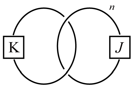
Note that when $n>2g(J)-1$, $n$-surgery on $J$ yields an $L$-space, and the meridian of $J$ in the resulting $L$-space is Floer simple [GRE15, RAS07, HED11], where $g(J)$ denotes the Seifert genus of $J$. More examples will be presented in Section 5, including explicit families of $\nu^{+}$-sharp knots and Floer simple knots.

The proof of Theorem 1.3 is based on Proposition 3.6, which establishes an additivity result for the $\nu^{+}$-invariant. In general, as in the case of knots in $S^{3}$, the $\nu^{+}$-invariant is only subadditive; see Theorem 3.2. In Proposition 3.6, we give a necessary and sufficient condition for a knot to satisfy $\nu^{+}$-additivity when taking connected sums with arbitrary knots. Both the additivity and subadditivity results for $\nu^{+}$ may be of independent interest.

The paper is organized as follows. In Section 2, we review some preliminaries, including the definition of the rational slice genus and background on knot Floer homology. In Section 3, we prove the subadditivity and additivity results for the $\nu^{+}$-invariant. In Section 4, we prove our main results. Section 5 presents examples of $\nu^{+}$-sharp knots. Throughout, we work over $\mathbb{F}=\mathbb{Z}/2\mathbb{Z}$.

We would like to thank Zhechi Chen, Stefan Friedl, Matthew Hedden, and Jennifer Hom for helpful discussions and suggestions. The first author is partially supported by the Samsung Science and Technology Foundation (SSTF-BA2102-02) and by the NRF grant RS-2025-00542968. The second author is partially supported by a grant from the Research Grants Council of Hong Kong Special Administrative Region, China (Project No. 14301825). The third author is supported by the National Natural Science Foundation of China (Project No. 12301087), Fujian Provincial Natural Science Foundation of China (Project No. 2024J08012), and Fundamental Research Funds for the Central Universities (Project No. 20720230026).

We recently learned that Stefan Friedl, Tejas Kalelkar, José Pedro Quintanilha, and Tanushree Shah have an upcoming paper on an analogous problem. Whereas our paper focuses on the slice genus of local knots, theirs investigates the unknotting number and the Gordian distance [FKQ+26].

We first recall the definitions related to the rational longitude; see [WY23, Section 1] for a more detailed discussion. Let $K\subset Y$ be a knot in a rational homology $3$-sphere, and set

where $N(K)$ denotes a tubular neighborhood of $K$ and $N^{\circ}(K)$ its interior. Note that the inclusion map

has kernel isomorphic to $\mathbb{Z}$. Thus there exists a primitive class $\lambda_{r}\in H_{1}(\partial M;\mathbb{Z})$ and a positive integer $k$ such that

The class $\lambda_{r}$ determines a well-defined slope on $\partial M$, called the rational longitude of $K$.

A rational Seifert surface for $K$ is a properly embedded, compact, connected, oriented surface $S\subset M$ such that

A Seifert framed rational slice surface for $K$ is a compact, connected, oriented surface $F$ smoothly embedded in

such that $\partial F=F\cap\partial N(K)$ and

where $N(K)$ denotes a solid torus neighborhood of $K$ in $Y\times\{1\}$. We call $F$ Seifert framed because its boundary has the same slope as a rational Seifert surface for $K$.

Let $K$ be a knot in a rational homology $3$-sphere $Y$. Fix a doubly pointed Heegaard diagram $(\Sigma,\alpha,\beta,w,z)$ for $(Y,K)$ and a $\rm Spin^{c}$ structure $\mathfrak{s}$ on $Y$. The knot Floer complex $C_{\mathfrak{s}}=CFK^{\infty}(Y,K,\mathfrak{s})$ is generated by triples $[x,i,j]$, where $x\in\mathbb{T}_{\alpha}\cap\mathbb{T}_{\beta}$ satisfies $\mathfrak{s}_{w}(x)=\mathfrak{s}$, $i\in\mathbb{Z}$, and

Here $A_{Y,K}\colon\underline{\rm Spin^{c}}(Y,K)\to\mathbb{Q}$ denotes the Alexander grading on relative ${\rm Spin^{c}}$ structures associated to $(Y,K)$. The differential is the usual one defined by counting holomorphic disks. See [HL24, Section 2.4] for more details.

Let $\underline{\rm Spin^{c}}(Y,K,\mathfrak{s})$ denote the set of relative $\rm Spin^{c}$ structures with underlying ${\rm Spin^{c}}$ structure $\mathfrak{s}$, that is, those $\xi$ with $G_{Y,K}(\xi)=\mathfrak{s}$. For $\xi\in\underline{\rm Spin^{c}}(Y,K,\mathfrak{s})$, define

In particular,

and $A^{-}_{\xi}(K)$ is quasi-isomorphic to the complex $CF^{-}$ of a sufficiently large surgery along $K$ in a suitable ${\rm Spin^{c}}$ structure.

For a knot $K\subset S^{3}$, Ni and the second author defined a family of $\mathbb{Z}_{\geq 0}$-valued invariants $\{V_{k}(K)\}_{k\in\mathbb{Z}}$ in [NW15]. The analogous $V$-invariants for a knot $K$ in a rational homology $3$-sphere $Y$ can be defined in a similar manner as follows; see [WY23, Section 5.1].

Let $v^{-}_{\xi}\colon A^{-}_{\xi}(K)\to B^{-}_{\xi}(K)$ be the inclusion map. It induces

Both $H_{\ast}(A^{-}_{\xi}(K))$ and $H_{\ast}(B^{-}_{\xi}(K))$ are isomorphic to the direct sum of $\mathbb{F}[U]$ and a finite-dimensional $U$-torsion module. The map $v^{-}_{\xi,\ast}$ induces a homogeneous, non-zero map between the free parts $\mathbb{F}[U]$, which is necessarily multiplication by $U^{N}$ for some non-negative integer $N$. We define

The correction term $d(Y,\mathfrak{s})$ is defined as the maximum Maslov grading of any non-torsion element in $HF^{-}(Y,\mathfrak{s})$. Since $U$ decreases the Maslov grading by two, we can reformulate the definition of $V$-invariants as follows:

where ${\rm gr}$ denotes the Maslov grading and $\mathfrak{s}=G_{Y,K}(\xi)$.

The $\nu^{+}$-invariant of a knot $K\subset S^{3}$ is defined by

We define the $\nu^{+}$-invariants of knots in rational homology $3$-spheres similarly.

The $\nu^{+}$-invariant gives a lower bound on the rational slice genus.

In this subsection, we record several key facts in knot Floer homology that will be used frequently in the subsequent sections.

Let $K$ be a knot in a rational homology $3$-sphere $Y$. Reversing the orientations of both $Y$ and $K$ yields the reverse of the mirror, denoted $-K\subset-Y$. Given any ${\rm Spin^{c}}$ structure $\mathfrak{s}\in{\rm Spin^{c}}(Y)\cong{\rm Spin^{c}}(-Y)$, there is a filtered chain homotopy equivalence

where $CFK^{\infty}(Y,K,\mathfrak{s})^{\ast}$ denotes the dual complex

and $J$ is the conjugation action on ${\rm Spin^{c}}(Y)$. See [OS04a, Section 3.5].

In [WY23, Section 2.2], the middle relative ${\rm Spin^{c}}$ structure was introduced for each $\mathfrak{s}\in{\rm Spin^{c}}(Y)$, defined as the unique relative ${\rm Spin^{c}}$ structure $\xi^{0}_{\mathfrak{s}}\in\underline{{\rm Spin^{c}}}(Y,K,\mathfrak{s})$ such that

where $H$ is a family of invariants defined similarly to $V$; see [WY23, Section 5.1] for the precise definition. Several useful properties of the middle relative ${\rm Spin^{c}}$ structure were also established there.

A simple computation yields the following symmetry in the Alexander gradings of the middle relative ${\rm Spin^{c}}$ structures.

The $\nu^{+}$ and $V$-invariants for knots in rational homology $3$-spheres satisfy subadditivity properties, analogous to the case of knots in $S^{3}$.

We begin by introducing a simple class of full knot Floer complexes $CFK^{\infty}$ that behaves well under tensor products (equivalently, under connected sum of knots).

The following proposition gives a necessary and sufficient condition for $\nu^{+}_{\mathfrak{s}}$ to be additive under connected sum with an arbitrary knot.

References

- [BM18] (2018) Montesinos knots, Hopf plumbings, and L-space surgeries. J. Math. Soc. Japan 70 (1), pp. 95–110. External Links: ISSN 0025-5645,1881-1167, Document, Link, MathReview (Masakazu Teragaito) Cited by: item (a).
- [BER90] (1990) Some knots with surgeries yielding lens spaces. preprint arXiv:1802.09722. Cited by: §1, item (a).
- [BCG17] (2017) A note on cobordisms of algebraic knots. Algebr. Geom. Topol. 17 (4), pp. 2543–2564. External Links: ISSN 1472-2747,1472-2739, Document, Link, MathReview (Yuanan Diao) Cited by: §1.
- [CZZ25] (2025) Applications of the L-space satellite formula. preprint arXiv:2509.20288. Cited by: item (f).
- [DNP+18] (2018) Concordance of knots in . J. Lond. Math. Soc. (2) 98 (1), pp. 59–84. External Links: ISSN 0024-6107,1469-7750, Document, Link, MathReview (Allison N. Miller) Cited by: §1.
- [FLL25] (2025) Squeezed knots. Quantum Topol. 16 (4), pp. 831–865. External Links: ISSN 1663-487X,1664-073X, Document, Link, MathReview Entry Cited by: item (d).
- [FP21] (2021) Genus one cobordisms between torus knots. Int. Math. Res. Not. IMRN (1), pp. 523–550. External Links: ISSN 1073-7928,1687-0247, Document, Link, MathReview (Christopher William Davis) Cited by: §1.
- [FKQ+26] (2026) Gordian distance between local knots in 3-manifolds. Cited by: §1.
- [GAB90] (1990) -bridge braids in solid tori. Topology Appl. 37 (3), pp. 221–235. External Links: ISSN 0166-8641,1879-3207, Document, Link, MathReview (Cameron McA. Gordon) Cited by: item (a).
- [GN16] (2016) Links of plane curve singularities are -space links. Algebr. Geom. Topol. 16 (4), pp. 1905–1912. External Links: ISSN 1472-2747,1472-2739, Document, Link, MathReview (Meirav Amram) Cited by: item (a).
- [GLV18] (2018) L-space knots. Compos. Math. 154 (5), pp. 918–933. External Links: ISSN 0010-437X,1570-5846, Document, Link, MathReview (Kazuhiro Ichihara) Cited by: item (a), item (b), item (c).
- [GRE15] (2015) L-space surgeries, genus bounds, and the cabling conjecture. J. Differential Geom. 100 (3), pp. 491–506. External Links: ISSN 0022-040X,1945-743X, Link, MathReview (Daniel Ruberman) Cited by: §1, item (c).
- [HRW24] (2024) Bordered Floer homology for manifolds with torus boundary via immersed curves. J. Amer. Math. Soc. 37 (2), pp. 391–498. External Links: ISSN 0894-0347,1088-6834, Document, Link, MathReview (Francesco Lin) Cited by: item (a).
- [HL24] (2024) A surgery formula for knot Floer homology. Quantum Topol. 15 (2), pp. 229–336. External Links: ISSN 1663-487X,1664-073X, Document, Link, MathReview Entry Cited by: §2.2, §4.
- [HR23a] (2023) A 4-dimensional rational genus bound. preprint arXiv:2308.16853. Cited by: footnote 1.
- [HR23b] (2023) Knot Floer homology and relative adjunction inequalities. Selecta Math. (N.S.) 29 (1), pp. Paper No. 7, 48. External Links: ISSN 1022-1824,1420-9020, Document, Link, MathReview (Tye Lidman) Cited by: §3.2.
- [HED09] (2009) On knot Floer homology and cabling. II. Int. Math. Res. Not. IMRN (12), pp. 2248–2274. External Links: ISSN 1073-7928,1687-0247, Document, Link, MathReview Entry Cited by: item (c).
- [HED10] (2010) Notions of positivity and the Ozsváth-Szabó concordance invariant. J. Knot Theory Ramifications 19 (5), pp. 617–629. External Links: ISSN 0218-2165,1793-6527, Document, Link, MathReview Entry Cited by: item (b).
- [HED11] (2011) On Floer homology and the Berge conjecture on knots admitting lens space surgeries. Trans. Amer. Math. Soc. 363 (2), pp. 949–968. External Links: ISSN 0002-9947,1088-6850, Document, Link, MathReview (Adam M. Lowrance) Cited by: §1, item (c).
- [HH19] (2019) A note on knot concordance and involutive knot Floer homology. In Breadth in contemporary topology, Proc. Sympos. Pure Math., Vol. 102, pp. 113–118. External Links: ISBN 978-1-4704-4249-1, Document, Link, MathReview (Allison N. Miller) Cited by: §3.2.
- [HLV14] (2014) Berge-Gabai knots and L-space satellite operations. Algebr. Geom. Topol. 14 (6), pp. 3745–3763. External Links: ISSN 1472-2747,1472-2739, Document, Link, MathReview (Kimihiko Motegi) Cited by: item (a).
- [HW16] (2016) Four-ball genus bounds and a refinement of the Ozsváth-Szabó tau invariant. J. Symplectic Geom. 14 (1), pp. 305–323. External Links: ISSN 1527-5256,1540-2347, Document, Link, MathReview (Nikolai N. Saveliev) Cited by: §1, §3.2, §5.1.1, §5.1.2.
- [HOM11] (2011) A note on cabling and -space surgeries. Algebr. Geom. Topol. 11 (1), pp. 219–223. External Links: ISSN 1472-2747,1472-2739, Document, Link, MathReview Entry Cited by: item (a).
- [HOM14] (2014) Bordered Heegaard Floer homology and the tau-invariant of cable knots. J. Topol. 7 (2), pp. 287–326. External Links: ISSN 1753-8416,1753-8424, Document, Link, MathReview (Arunima Ray) Cited by: §5.1.2.
- [HOM17] (2017) A survey on Heegaard Floer homology and concordance. J. Knot Theory Ramifications 26 (2), pp. 1740015, 24. External Links: ISSN 0218-2165,1793-6527, Document, Link, MathReview (Se-Goo Kim) Cited by: §3.2, §4.
- [KR21] (2021) Deep and shallow slice knots in 4-manifolds. Proc. Amer. Math. Soc. Ser. B 8, pp. 204–218. External Links: ISSN 2330-1511, Document, Link, MathReview (Allison N. Miller) Cited by: §1, §1.
- [KM93] (1993) Gauge theory for embedded surfaces. I. Topology 32 (4), pp. 773–826. External Links: ISSN 0040-9383, Document, Link, MathReview (Ronald J. Stern) Cited by: §1.
- [LM16] (2016) Pretzel knots with -space surgeries. Michigan Math. J. 65 (1), pp. 105–130. External Links: ISSN 0026-2285,1945-2365, Link, MathReview (Arunima Ray) Cited by: item (a).
- [LV18] (2018) The four-genus of connected sums of torus knots. Math. Proc. Cambridge Philos. Soc. 164 (3), pp. 531–550. External Links: ISSN 0305-0041,1469-8064, Document, Link, MathReview (Makoto Ozawa) Cited by: item (e), §5.1.2.
- [MUR65] (1965) On a certain numerical invariant of link types. Trans. Amer. Math. Soc. 117, pp. 387–422. External Links: ISSN 0002-9947,1088-6850, Document, Link, MathReview (R. H. Fox) Cited by: §1.
- [NOP+19] (2019) Smooth and topological almost concordance. Int. Math. Res. Not. IMRN (23), pp. 7324–7355. External Links: ISSN 1073-7928,1687-0247, Document, Link, MathReview (Daniel Silver) Cited by: §1.
- [NV19] (2019) Null surgery on knots in L-spaces. Trans. Amer. Math. Soc. 372 (12), pp. 8279–8306. External Links: ISSN 0002-9947,1088-6850, Document, Link, MathReview (Duncan McCoy) Cited by: §1, §4.
- [NW14] (2014) Heegaard Floer correction terms and rational genus bounds. Adv. Math. 267, pp. 360–380. External Links: ISSN 0001-8708,1090-2082, Document, Link, MathReview (Tye Lidman) Cited by: §1, §4, §5.2, footnote 2.
- [NW15] (2015) Cosmetic surgeries on knots in . J. Reine Angew. Math. 706, pp. 1–17. External Links: ISSN 0075-4102,1435-5345, Document, Link, MathReview (Bruno P. Zimmermann) Cited by: §2.3.
- [NI09] (2009) Link Floer homology detects the Thurston norm. Geom. Topol. 13 (5), pp. 2991–3019. External Links: ISSN 1465-3060,1364-0380, Document, Link, MathReview Entry Cited by: §4, §5.2.
- [OS03a] (2003) Absolutely graded Floer homologies and intersection forms for four-manifolds with boundary. Adv. Math. 173 (2), pp. 179–261. External Links: ISSN 0001-8708,1090-2082, Document, Link, MathReview (Jacob Andrew Rasmussen) Cited by: §3.1.
- [OS03b] (2003) Knot Floer homology and the four-ball genus. Geom. Topol. 7, pp. 615–639. External Links: ISSN 1465-3060,1364-0380, Document, Link, MathReview (Stanislav Jabuka) Cited by: §1, §5.1.1.
- [OS04a] (2004) Holomorphic disks and knot invariants. Adv. Math. 186 (1), pp. 58–116. External Links: ISSN 0001-8708,1090-2082, Document, Link, MathReview (Stanislav Jabuka) Cited by: §1, §2.5.
- [OS04b] (2004) Holomorphic disks and three-manifold invariants: properties and applications. Ann. of Math. (2) 159 (3), pp. 1159–1245. External Links: ISSN 0003-486X,1939-8980, Document, Link, MathReview (Thomas E. Mark) Cited by: §3.1, §3.1.
- [OS04c] (2004) Holomorphic disks and topological invariants for closed three-manifolds. Ann. of Math. (2) 159 (3), pp. 1027–1158. External Links: ISSN 0003-486X,1939-8980, Document, Link, MathReview (Thomas E. Mark) Cited by: §1.
- [OS11] (2011) Knot Floer homology and rational surgeries. Algebr. Geom. Topol. 11 (1), pp. 1–68. External Links: ISSN 1472-2747,1472-2739, Document, Link, MathReview (Hans U. Boden) Cited by: §3.2.
- [PLA04] (2004) Bounds for the Thurston-Bennequin number from Floer homology. Algebr. Geom. Topol. 4, pp. 399–406. External Links: ISSN 1472-2747,1472-2739, Document, Link, MathReview (Stanislav Jabuka) Cited by: item (b).
- [RAO20] (2020) -invariants for knots in rational homology spheres. Algebr. Geom. Topol. 20 (4), pp. 1601–1640. External Links: ISSN 1472-2747,1472-2739, Document, Link, MathReview (Christopher William Davis) Cited by: §3.1, §3.2, §3.2.
- [RAS03] (2003) Floer homology and knot complements. ProQuest LLC, Ann Arbor, MI. Note: Thesis (Ph.D.)–Harvard University External Links: ISBN 978-0496-39374-9, Link, MathReview Entry Cited by: §1.
- [RR17] (2017) Floer simple manifolds and L-space intervals. Adv. Math. 322, pp. 738–805. External Links: ISSN 0001-8708,1090-2082, Document, Link, MathReview (Matthew Stoffregen) Cited by: item (c), §5.2.
- [RAS07] (2007) Lens space surgeries and l-space homology spheres. preprint arXiv:arXiv:0710.2531. Cited by: §1, item (b), item (c).
- [RAS10] (2010) Khovanov homology and the slice genus. Invent. Math. 182 (2), pp. 419–447. External Links: ISSN 0020-9910,1432-1297, Document, Link, MathReview (William D. Gillam) Cited by: §1.
- [SAT18] (2018) A full-twist inequality for the -invariant. Topology Appl. 245, pp. 113–130. External Links: ISSN 0166-8641,1879-3207, Document, Link, MathReview (Shida Wang) Cited by: Theorem 5.1.
- [VAF15] (2015) On the knot Floer homology of twisted torus knots. Int. Math. Res. Not. IMRN (15), pp. 6516–6537. External Links: ISSN 1073-7928,1687-0247, Document, Link, MathReview (Fatemeh Douroudian) Cited by: item (a).
- [WY23] (2023) Rational genus and Heegaard Floer homology. preprint arXiv:2307.06807. Cited by: §1, §1, §2.1, §2.3, §2.5, §2.5, Definition 2.1, Theorem 2.2, Lemma 2.4, Lemma 2.5, §3.2, §4, §4, footnote 1, footnote 2.
- [WU16] (2016) A cabling formula for the invariant. Proc. Amer. Math. Soc. 144 (9), pp. 4089–4098. External Links: ISSN 0002-9939,1088-6826, Document, Link, MathReview (William W. Menasco) Cited by: §5.1.2.
- [ZEM19] (2019) Connected sums and involutive knot Floer homology. Proc. Lond. Math. Soc. (3) 119 (1), pp. 214–265. External Links: ISSN 0024-6115,1460-244X, Document, Link, MathReview (Sergiy Koshkin) Cited by: §3.2.