Grounding the Score: Explicit Visual Premise Verification for Reliable VLM Process Reward Models
Abstract
Vision-language process reward models (VL-PRMs) score intermediate reasoning steps and rerank candidates under test-time scaling, yet their step scores are often hard to interpret: a low reward may indicate a genuine reasoning mistake, or simply unreliable visual grounding by the policy or the verifier. This entanglement yields systematic false positives (rewarding hallucinated visual premises) and false negatives (penalizing correct grounded statements), degrading both reranking and error localization.
We propose Explicit Visual Premise Verification (EVPV), a lightweight, test-time framework that decouples visual premise reliability from step correctness. EVPV prompts the policy to emit a step-wise visual checklist and independently extracts structured visual constraints from the image. By matching checklist claims against constraints, EVPV computes a scalar visual reliability signal and uses it to gate rewards for visually dependent steps, avoiding per-step tool calls. To fully realize this framework, we train EVPV-PRM, a Qwen2.5-VL-Instruct-7B-based step verifier that provides probabilistic base rewards and can be calibrated by EVPV at inference time. Across VisualProcessBench and six downstream benchmarks, EVPV improves step-level verification and yields overall Best-of- reranking gains, while our EVPV-PRM achieves strong performance as a deployable reranker. Under controlled constraint corruption, performance degrades monotonically, providing interventional evidence that the gains are driven by constraint fidelity.
1 Introduction
Multimodal mathematical reasoning couples two error-prone components: visual perception (e.g., diagrams, tables/OCR, geometric relations) and symbolic reasoning (derivation and computation). Although modern MLLMs can generate fluent multi-step solutions, a single perceptual misread can derail the whole chain while keeping later steps locally coherent, making process-level verification and selection crucial under test-time scaling such as Best-of- and search-based decoding (zheng2025survey; ma2023let; zhang2024rest).
Process reward models (PRMs) implement process supervision by scoring each step, and are widely used for Best-of- reranking, guided search, and post-training (zheng2025survey; ma2023let; zhang2024rest). In vision-language reasoning, VisualPRM and VisualProcessBench show that step-aware critics improve performance under test-time scaling (wang2025visualprm), and data-efficient training can further reduce verifier cost (wang2025athena). However, current VL-PRMs often behave as black-box judges: a low step score is ambiguous—it may reflect a true reasoning error or unreliable visual grounding by the policy/verifier—echoing broader concerns on PRM reliability and calibration (ye2025uncertainty; park2025know).

This ambiguity is a systematic source of verification errors. Under uncertain grounding, a PRM may penalize correct visual statements (false negatives) or reward hallucinated premises (false positives), harming reranking and error localization. Figure 1A shows such a case: VisualPRM rewards a fluent step that assumes a nonexistent “cylindrical hole.” Visual misinterpretation also constitutes a major fraction of step errors on VisualProcessBench (wang2025visualprm). Tool-integrated verification can reduce confirmation bias by querying evidence independently (kuang2025tim), but per-step tool calls are often too costly for long traces at Best-of- scale (ma2023let; zhang2024rest).
We propose Explicit Visual Premise Verification (EVPV) as a lightweight, test-time framework that decouples premise reliability from step correctness. EVPV prompts the policy to state a step-wise visual checklist of explicit premises and uses a constraint extractor to predict structured visual facts (numeric readings, relations, and compositional structure) once per instance. EVPV matches checklist claims against constraints to compute a visual reliability signal, and uses it to gate rewards for visually dependent steps: when premises are unreliable, rewards are attenuated toward neutrality; when premises are reliable, base rewards are preserved.
To maximize the effectiveness of this framework in a deployable setting, we train EVPV-PRM, a Qwen2.5-VL-Instruct-7B-based probabilistic step verifier that provides base step rewards and can be calibrated by EVPV at inference time. We evaluate EVPV on VisualProcessBench and six multimodal reasoning benchmarks under Best-of- reranking. EVPV improves step-level verification and yields overall reranking gains across InternVL2.5 policy scales (Figure 1C–D). Finally, controlled corruption of the extracted constraints induces monotonic performance degradation, providing interventional evidence that verification quality is driven by constraint fidelity rather than incidental prompt effects.
2 Related Work
Process reward models (PRMs).
PRMs provide step-level supervision and are widely used for test-time scaling (e.g., Best-of- reranking), guided decoding, and post-training (zheng2025survey; ma2023let; zhang2024rest). Recent work explores stronger verification procedures, including verifiers that generate intermediate analyses or perform generative verification (she2025r; zhao2025genprm; khalifa2025process; jia2025writing), as well as improved learning objectives and supervision pipelines (yin2025dynamic; zhang2024entropy; zhang2025bidirectional; duan2025efficient; tan2025aurora; zhang2025openprm). Our work is orthogonal to these directions: rather than changing the verifier architecture or training signal, we provide a test-time calibration interface that conditions step rewards on the reliability of the visual premises they depend on.
Visual perception reliability and verification.
MLLMs often struggle with fine-grained perception such as counting, geometry, and structured reading (fu2024blink; schulze2025visual), motivating improved vision encoders and perception-centric modeling/training (jain2024vcoder; yu2024texthawk; huang2023language; wu2024visionllm; huang2025visual; tang2024chain; yu2025introducing). These findings support our motivation: in multimodal reasoning, verification should account for uncertainty in visual premises rather than treating all image-conditioned statements as equally reliable.
Multimodal PRMs and grounded verification.
VisualPRM introduces VisualPRM400K and VisualProcessBench, establishing a standard training/evaluation pipeline for multimodal step verification (wang2025visualprm). ATHENA improves data efficiency for training multimodal PRMs (wang2025athena), and broader analyses study training design choices and perception-focused supervision for VL-PRMs (ong2025training; luo2025unlocking; cao2025dreamprm). EVPV builds on this line by adding a grounding-aware calibration layer on top of a step judge: it makes visual premises explicit (a checklist), verifies them against structured visual constraints extracted once per instance, and gates rewards accordingly. This is complementary to training better PRMs (e.g., VisualPRM/ATHENA): EVPV can be used with our trained EVPV-PRM or attached to an external judge at inference time.
Tool-integrated verifiers such as TIM-PRM query visual evidence via tools to reduce confirmation bias (kuang2025tim). EVPV targets a different cost–reliability trade-off: it avoids per-step tool calls by extracting structured evidence once and reusing it across steps and candidates, making it suitable for Best-of- reranking at scale. Recent works also strengthen multimodal judges via richer reasoning, diagnosis, or correction (e.g., VRPRM and GM-PRM) (chen2025vrprm; zhang2025gm); these approaches improve “how the judge reasons,” whereas EVPV focuses on whether the visual premise is trustworthy, which is complementary when deep reasoning is performed on unreliable premises. Finally, VLRMBench expands evaluation for vision-language reward modeling beyond step verification (ruan2025vlrmbench); we primarily use VisualProcessBench and downstream reranking benchmarks, and view broader evaluation as future work.
3 Methodology
3.1 Problem Setup
Each instance consists of an image and a question . A multimodal policy samples a step-by-step solution with a final answer . Our goal is premise-aware process verification: assign a reward to each step such that (i) step-level judgments are robust to visual misperception, and (ii) aggregated trajectory scores support reliable Best-of- reranking.
A key challenge in multimodal reasoning is that failures arise from two distinct sources: visual grounding errors (misread values, incorrect relations/structure) and symbolic reasoning errors (invalid deductions, arithmetic mistakes). Standard VL-PRMs entangle the two by directly scoring steps as if the underlying visual premises were reliable. We instead explicitly verify the visual premises a trace relies on and use this signal to calibrate step rewards at inference time.
3.2 EVPV: Explicit Visual Premise Verification
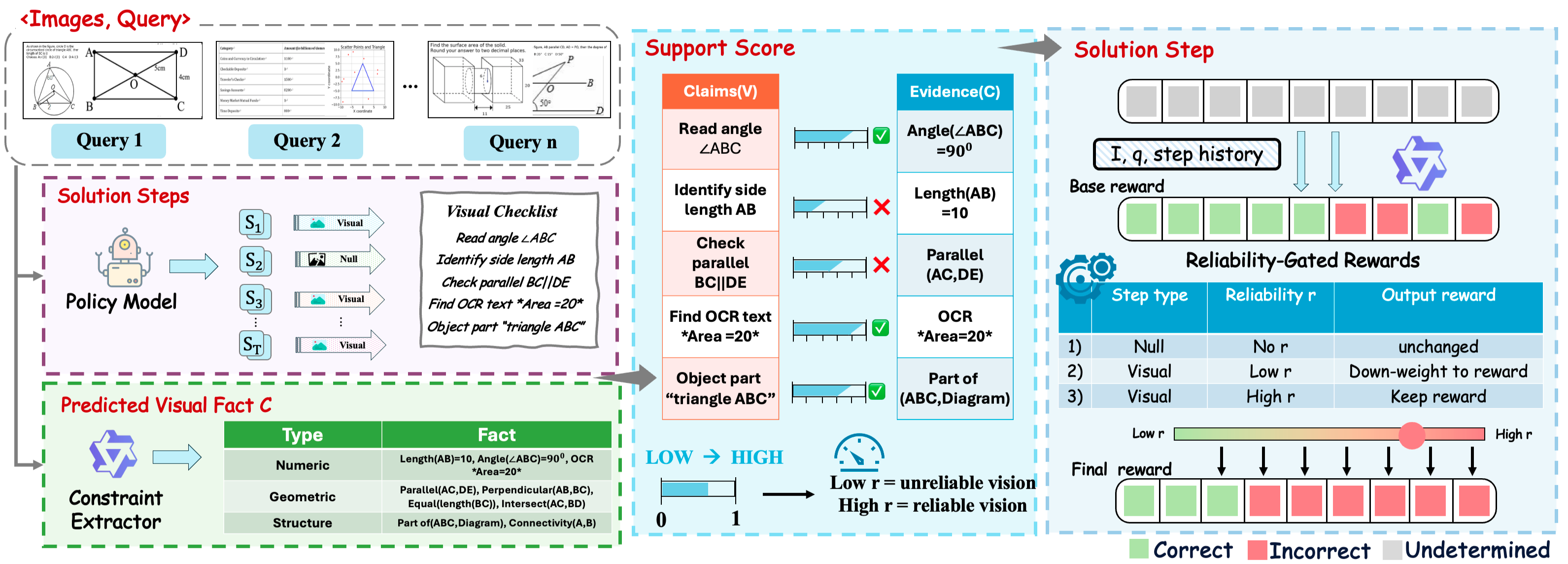
EVPV is a lightweight, judge-agnostic calibration interface for multimodal process reward modeling. It operates in three stages: (1) make each step’s visual premises explicit (a checklist), (2) extract structured visual evidence once per instance, and (3) convert checklist–evidence consistency into a scalar visual reliability used to calibrate step rewards. Figure 2 illustrates the pipeline.
3.2.1 Step-wise Visual Checklist
We prompt the policy to accompany each reasoning step with a minimal declaration of the visual premise it depends on:
| (1) |
If , the step asserts dependence on a concrete visual fact (e.g., “the radius is ”, “”, “a cone is attached on top of a cylinder”). We define the visual-dependency indicator:
| (2) |
Collecting all non-null declarations yields a visual checklist . This checklist is the interface EVPV needs: it turns implicit visual assumptions into explicit claims that can be verified independently from later algebra. We empirically audit the completeness of this policy-reported visual dependency signal (i.e., omission vs. over-reporting) on a human-verified subset; see Appendix F and Table 10.
3.2.2 Structured Visual Evidence (Constraints)
To verify the checklist, we extract structured visual evidence once per instance using a constraint extractor :
| (3) |
Each constraint follows a unified JSON schema (Appendix A) covering (i) numeric readings (lengths, angles, table entries), (ii) relations (parallel/perpendicular/equality/incidence/containment), and (iii) compositional structure (part–whole, attachments, adjacency). At test time, EVPV relies only on predicted ; no gold facts are used. Crucially, is computed once and reused across all steps and all candidates for the same , enabling scalable Best-of- reranking. We evaluate the fidelity of these predicted constraints with a human-annotated study, reporting precision/recall/F1 by category; see Appendix G and Table 11.
3.2.3 Consistency-to-Reliability
EVPV converts checklist–evidence consistency into a scalar visual reliability score. Let be a type-aware matching function that measures whether a checklist claim is supported by the extracted constraints :
| (4) |
where is high when the claim is entailed by (with numeric tolerance and entity/relation alignment; Appendix B).
We then aggregate per-claim support scores into a single candidate-level reliability score using a smoothed geometric mean:
| (5) |
where is a small constant for numerical stability. This aggregation is intentionally sensitive to catastrophic premise failures: if any claim is strongly unsupported (), drops sharply, reflecting that a single misread visual premise can invalidate the entire reasoning trace.
3.3 Judge-Agnostic Step Rewards with Reliability Gating
3.3.1 A unified judge interface
EVPV does not assume a particular step judge. Instead, it takes as input a base step reward from an arbitrary judge module :
| (6) |
This abstraction lets EVPV act as a plug-in calibration layer on top of both trained PRMs and prompted black-box judges.
Instantiation 1: EVPV-PRM (our trained verifier).
In our main system, the judge is a trained step verifier that outputs a correctness probability:
| (7) |
mapped to a signed reward:
| (8) |
Instantiation 2: EVPV as a plug-in for external VLM/LLM judges.
EVPV can also be applied to an external prompted judge (e.g., GPT/Gemini) that outputs a binary step decision, yielding . All subsequent EVPV computations (reliability, gating, aggregation) remain unchanged.
3.3.2 Reliability gating
A base step reward alone is ambiguous in multimodal settings: a low score may reflect a true reasoning error, or simply that the step rests on an unreliable visual premise. EVPV resolves this ambiguity by calibrating rewards for visually dependent steps using .
We convert reliability into a smooth gating factor:
| (9) |
where is a reliability threshold, controls sharpness, and is the logistic function. The final step reward is
| (10) |
Intuitively, when is low, and visually grounded steps are pushed toward a neutral score, preventing unreliable visual premises from producing overly confident positive/negative signals. When is high, and the judge behaves like a conventional PRM.
3.4 Trajectory Scoring for Best-of- Reranking
Given a candidate solution , we compute gated step rewards and aggregate them into a trajectory score for reranking. Since reliability gating rescales reward magnitudes, we use a magnitude-sensitive aggregation so that gating can influence candidate ranking. We first map to positive values:
| (11) |
and compute a geometric-mean trajectory score:
| (12) |
We select the candidate with the highest . Alternative aggregations are reported in Appendix E.

3.5 Training and Inference
EVPV introduces two trainable modules: the constraint extractor and the step verifier (used in the EVPV-PRM instantiation). The policy is not trained in this work; it is only prompted to output steps and checklist items at inference time (Figure 3).
Training data and evaluation boundary.
To avoid any training–test contamination, we do not use VisualProcessBench (wang2025visualprm) for training. All training data are sampled from VisualPRM400K (wang2025visualprm), restricted to geometry- and table-centric subsets (Geo170K, GeometryData, GeomVerse, GEOS, MAVIS-Geometry, TabMWP, UniGeo). VisualProcessBench is used only for step-level evaluation (Section 4.2; Table 1).
Training the constraint extractor.
We distill pseudo-gold structured constraints using a strong teacher Qwen3-vl-235b-a22b-instruct. Specifically, we construct an SFT corpus of 26,454 image–question pairs from the above VisualPRM400K subsets; for each pair, the teacher is prompted with our JSON schema (Appendix A) and the correct solution steps to produce a solution-critical constraint set . We fine-tune by maximizing :
| (13) |
To further improve fidelity, we run a DPO stage on an additional 5,832 instances where the teacher rewrites constraints to form preference pairs (Appendix C).
| Model | EVPV | DynaMath | MMMU | MathVerse | MathVision | WeMath | Overall |
|---|---|---|---|---|---|---|---|
| Proprietary Models | |||||||
| gpt-4o-mini | ✗ | ||||||
| ✓ | |||||||
| +1.56 | -0.88 | +1.56 | +0.65 | -2.12 | +0.72 | ||
| doubao-seed-1.6-vision | ✗ | ||||||
| ✓ | |||||||
| +2.47 | +2.39 | +2.45 | +1.44 | +1.88 | +2.14 | ||
| Gemini 2.5 Pro | ✗ | ||||||
| ✓ | |||||||
| +2.85 | +1.08 | +1.52 | +0.11 | +2.95 | +1.51 | ||
| Open-source Models | |||||||
| qwen2.5-vl-72b-instruct | ✗ | ||||||
| ✓ | |||||||
| +4.44 | +0.82 | +3.42 | +1.03 | +4.00 | +2.80 | ||
| Qwen3-VL-30B-A3B-instruct | ✗ | ||||||
| ✓ | |||||||
| +3.32 | -2.29 | +2.31 | -1.00 | +0.74 | +1.04 | ||
| Qwen3-VL-235B-A22B-instruct | ✗ | ||||||
| ✓ | |||||||
| +10.80 | +2.81 | +7.89 | +4.95 | +5.40 | +6.94 | ||
| Process Reward Models | |||||||
| QWEN-VL-PRM-7B (ong2025training) | |||||||
| TIM-PRM-8B (kuang2025tim) | |||||||
| VisualPRM-8B (wang2025visualprm) | |||||||
| EVPV-PRM | |||||||
Training the step verifier (EVPV-PRM).
We train as a probabilistic step verifier using 19,490 supervised step-labeled trajectories sampled from VisualPRM400K. Each training trajectory provides step-level correctness labels derived from its reference solution trace, yielding binary targets . We optimize binary cross-entropy:
| (14) |
where . Reliability gating is applied only at inference time (Eq. 10), keeping verifier training unchanged and allowing EVPV to be attached to other judges.
Inference.
For each , we first predict constraints once. For each candidate solution , we (i) parse the policy-produced checklist to obtain and , (ii) compute reliability by matching against , (iii) obtain base step rewards from a judge (our trained or an external prompted judge), (iv) apply reliability gating to produce , and (v) aggregate using Eq. 12 for reranking. This yields premise-aware verification without per-step tool calls.
4 Experiments
4.1 Benchmarks, Protocol, and Baselines
We evaluate EVPV from two angles: (i) step-level verification on annotated reasoning traces, and (ii) deployable test-time gains under Best-of- reranking. For step-level evaluation we use VisualProcessBench (wang2025visualprm). For downstream evaluation we use six multimodal reasoning benchmarks: LogicVista (xiao2024logicvista), MMMU (yue2024mmmu), MathVerse-VO (zhang2024mathverse), MathVision (wang2024measuring), MathVista (lu2023mathvista), and WeMath (qiao2025we).
Evaluation protocol (what is fixed vs. what changes).
All experiments follow the EVPV pipeline in Section 3: (i) a policy produces step traces with per-step visualdependency (our visual checklist), (ii) a constraint extractor predicts structured constraints once per instance, (iii) checklist–constraint matching yields a candidate-level reliability , and (iv) reliability gating calibrates base step rewards for visually dependent steps. What differs across settings is how the base step reward is produced:
-
•
EVPV-PRM (ours). Base rewards are produced by our trained probabilistic step verifier (Eq. 8), then gated by EVPV.
-
•
EVPV plug-in for external judges. For a black-box VLM/LLM judge (e.g., GPT/Gemini/Qwen) that outputs a binary step judgment , we can attach EVPV as a plug-in calibration layer. In Table 1, No means using the external judge alone, while Yes means using the same external judge with EVPV enabled (i.e., computing from structured constraints and applying reliability gating to the judge’s step rewards).111In the Yes setting, the judge additionally receives our predicted structured constraints as evidence (Appendix D), and EVPV uses the same constraints to compute ; this keeps the plug-in setting self-contained and fully inference-time.
Metrics.
On VisualProcessBench we report step-level Macro-F1 (primary) and accuracy. On downstream benchmarks we report Pass@1 (policy accuracy without reranking), BoN@k (accuracy after reranking samples), and the practical gain . We also report Std Pass@k, the oracle upper bound of the candidate set, to separate candidate quality from selection quality.
| Model | MathVista | MathVision | MathVerse-VO | WeMath | LogicVista | MMMU | Overall |
|---|---|---|---|---|---|---|---|
| Proprietary Models | |||||||
| GPT-4o | 60.00 | 31.20 | 40.60 | 45.80 | 52.80 | 70.70 | 47.90 |
| Gemini-2.0-Flash | 70.40 | 43.60 | 47.80 | 47.40 | 52.30 | 69.90 | 53.40 |
| Claude-3.5-Sonnet | 65.30 | 35.60 | 46.30 | 44.00 | 60.40 | 66.40 | 50.50 |
| Open-source Models | |||||||
| InternVL2.5-8B | 64.50 | 17.00 | 22.80 | 23.50 | 36.38 | 56.20 | 32.84 |
| +VisualPRM | 68.50 | 25.70 | 35.80 | 36.50 | 43.80 | 60.20 | 41.40 |
| +4.00 | +8.70 | +13.00 | +13.00 | +7.80 | +4.00 | +8.40 | |
| +EVPV-PRM | 76.30 | 22.07 | 29.47 | 37.45 | 45.33 | 67.75 | 41.67 |
| +11.80 | +5.07 | +6.67 | +13.95 | +8.95 | +11.55 | +8.83 | |
| InternVL2.5-26B | 68.20 | 23.40 | 24.00 | 30.90 | 39.64 | 60.70 | 37.23 |
| +VisualPRM | 73.10 | 29.60 | 39.10 | 40.80 | 51.00 | 63.90 | 45.80 |
| +4.90 | +6.20 | +15.10 | +9.90 | +11.40 | +3.20 | +8.90 | |
| +EVPV-PRM | 79.60 | 28.11 | 32.47 | 42.14 | 51.72 | 69.25 | 46.75 |
| +11.40 | +4.71 | +8.47 | +11.24 | +12.08 | +8.55 | +9.52 | |
| InternVL2.5-38B | 71.90 | 32.20 | 36.90 | 38.30 | 47.90 | 63.90 | 45.44 |
| +VisualPRM | 73.90 | 35.20 | 46.70 | 46.20 | 53.70 | 69.00 | 50.70 |
| +2.00 | +3.00 | +9.80 | +7.90 | +5.80 | +5.10 | +6.30 | |
| +EVPV-PRM | 83.50 | 37.59 | 47.67 | 50.00 | 58.74 | 72.33 | 55.22 |
| +11.60 | +5.39 | +10.77 | +11.70 | +10.84 | +8.43 | +9.78 | |
Trajectory scoring for reranking.
Unless stated otherwise, we use the geometric-mean aggregation in Eq. 12 for Best-of- reranking (Appendix E reports alternatives). This magnitude-sensitive aggregation ensures that reliability gating can affect candidate ranking.
Baselines.
We compare against multimodal PRMs including VisualPRM (wang2025visualprm), QWEN-VL-PRM-7B (ong2025training) and the tool-integrated verifier TIM-PRM (kuang2025tim). We also evaluate several strong MLLMs as step judges under a standardized prompt, with two conditions: No (judge alone) and Yes (judge + EVPV plug-in). Finally, we include component ablations of EVPV (checklist, constraints, matching, gating). We also report an efficiency comparison with tool-integrated verification: Table 12 (Appendix G) summarizes the per-question inference cost in terms of model/tool calls and a unified token/latency accounting for EVPV and TIM-PRM.
4.2 Exp-1: Step Verification on VisualProcessBench
We evaluate step-level verification directly on VisualProcessBench (wang2025visualprm). Table 1 compares our method with prior multimodal PRMs and a set of judge models.
Protocol.
For each annotated trace, we evaluate each step given and obtain a binary correctness prediction. For PRM-style verifiers (including ours), we threshold the predicted probability at (equivalently, ). For external judge models, we use their prompted binary output in . Macro-F1 is computed over all steps and then macro-averaged across subsets as in wang2025visualprm.
Judge models: No vs. Yes.
For judge models in Table 1, No uses the external judge directly to label each step. Yes attaches EVPV as a plug-in: for each instance we predict structured constraints once, compute reliability by matching the policy-produced checklist against (Section 3.2.3), and apply reliability gating to calibrate the judge’s step rewards before thresholding. This evaluates whether premise-aware calibration improves step discrimination for black-box judges under real visual uncertainty.
Two observations stand out in Table 1. First, our method achieves the best overall Macro-F1 among the compared PRMs, indicating stronger step discrimination under real visual uncertainty. Second, many judge models improve under Yes, suggesting that EVPV-style premise verification and reliability calibration is broadly reusable as an inference-time plug-in—even without retraining the judge—and that a non-trivial part of verification error comes from missing or unreliable grounding.
| Variant | DynaMath | MMMU | MathVerse | MathVision | WeMath | Overall | |
| Full Method | |||||||
| Full (EVPV + gating) | +0.00 | ||||||
| Evidence / structure ablations | |||||||
| w/o structured facts (caption-only) | -4.08 | ||||||
| w/o constraints (facts = ) | -5.35 | ||||||
| w/ shuffled facts (structure corrupted) | -7.64 | ||||||
| Remove modalities / severe corruption | |||||||
| w/o vision (text-only judge, keep JSON) | -12.53 | ||||||
| w/o vision & w/o JSON (text-only) | -19.23 | ||||||
| w/ drop-facts corruption | -31.69 | ||||||
4.3 Exp-2: Best-of- Reranking in Downstream Benchmarks
We next test whether premise-aware verification translates into deployable test-time gains. We rerank candidates generated by InternVL2.5 policy models at three scales (8B/26B/38B). For each question, the policy samples candidate solutions; we rerank them using step rewards and report BoN@8.
Protocol.
For each question, we first predict structured constraints once. For each candidate solution, the policy provides steps with per-step visualdependency. We compute candidate-level reliability via checklist–constraint matching, obtain base step rewards from the reranker PRM (VisualPRM or our EVPV-PRM), apply EVPV gating when applicable, and aggregate gated rewards using the geometric-mean trajectory score (Eq. 12) to rank the candidates.
Table 2 summarizes the results. Across all three policy sizes, our PRM yields consistent gains over the base policy and improves upon VisualPRM (wang2025visualprm) in overall performance (e.g., +8.83, +9.52, and +9.78 points over Pass@1 for 8B/26B/38B, respectively). The improvements are especially pronounced on visually intensive benchmarks such as MathVista, WeMath, and LogicVista, which matches EVPV’s intent: when early visual premises are the dominant failure mode, reliability-aware step scoring reduces selection errors without incurring the per-step tool overhead of TIM-PRM (kuang2025tim).

| Variant | DynaMath | MMMU | MathVerse | MathVision | WeMath | Overall | |
| Full Method | |||||||
| Full (EVPV + gating) | +0.00 | ||||||
| Evidence / structure ablations | |||||||
| w/o structured facts (caption-only) | -4.08 | ||||||
| w/o constraints (facts = ) | -5.35 | ||||||
| w/ shuffled facts (structure corrupted) | -7.64 | ||||||
| Remove modalities / severe corruption | |||||||
| w/o vision (text-only judge, keep JSON) | -12.53 | ||||||
| w/o vision & w/o JSON (text-only) | -19.23 | ||||||
| w/ drop-facts corruption | -31.69 | ||||||
4.4 Exp-3: Perception Evidence Quality and Its Causal Impact on Verification
EVPV is motivated by a single principle: reliable visual evidence is a prerequisite for meaningful process verification. We therefore examine this principle from two complementary angles—(i) intervention on the policy’s perceived evidence and (ii) controlled degradation of the verifier’s extracted constraints—to quantify both the sensitivity of multimodal reasoning to perception and the causal role of constraint fidelity in step verification.
(A) Perception interventions for the policy.
To measure how strongly multimodal reasoning depends on perception quality, we evaluate the same questions under four controlled settings: (I) Normal (image+), (II) Oracle perception (image+ plus an oracle structured description), (III) Noisy perception (image+ plus a corrupted description), and (IV) Text-only (remove the image). We run a fixed policy model for all settings and report answer accuracy and PRM trajectory scores (Eq. 12). Table LABEL:tab:attrib shows two consistent patterns: providing oracle perception substantially improves accuracy, while text-only performance drops sharply, indicating that perception is a dominant bottleneck; moreover, our PRM yields a monotonic ordering of trajectory scores aligned with perception quality: (II)(III)(I)(IV), matching EVPV’s intent that weakened visual evidence should not produce a strong “correct process” signal.
(B) Causal curve via constraint corruption.
EVPV further attributes its gains to the fidelity of the extracted structured constraints used to validate checklist claims. To test this causally, we inject controlled noise into the constraint set by randomly flipping a fraction of constraint fields (flip ratio), while keeping the policy, verifier/judge, and scoring procedure fixed. As shown in Figure 4, VisualProcessBench Macro-F1 decreases monotonically as the flip ratio increases across all evaluated judges, providing interventional evidence that verification quality is driven by constraint fidelity and premise verification rather than incidental prompt effects. The mild drop under low noise also indicates that reliability gating is not overly brittle: small constraint errors do not immediately collapse step judgments.
4.5 Exp-4: Ablation Studies
We ablate core components of EVPV to identify which parts are responsible for the verification and reranking gains. Table 4 reports representative variants on VisualProcessBench (Macro-F1).
The trends closely match the EVPV design. First, premise verification requires usable structured evidence. Replacing structured constraints with caption-only descriptions reduces overall Macro-F1 by 4.08 points, and completely removing constraints (facts = ) further degrades performance (-5.35). This shows that simply having additional text context is insufficient; the verifier benefits from structured, matchable facts that can support checklist claims.When we keep the same facts but shuffle them to corrupt the relational structure, Macro-F1 drops more sharply (-7.64). This indicates that EVPV is not merely exploiting the presence of extra tokens, but relies on faithful entity/relation alignment between checklist items and evidence to compute reliability and gate rewards appropriately.
EVPV still benefits from direct visual input. Making the judge text-only while keeping JSON constraints reduces Macro-F1 by 12.53, and removing both vision and JSON drops it by 19.23. Severe evidence loss (drop-facts) collapses performance by 31.69, indicating that calibration fails when constraints are too incomplete.
5 Discussion
EVPV helps by separating two failure sources that standard VL-PRMs often mix: bad premises (misread or hallucinated visual facts) versus bad reasoning. We prompt the policy to state a step-wise visual checklist, verify those claims against independently extracted structured constraints, and use the resulting reliability to gate rewards. This premise-first design fits the broader lesson that grounded reasoning depends on faithful perception (zhang2025mm) and echoes “generate, then verify” style faithfulness checks (wu2025generate). It is also complementary to stronger/generative verifiers (she2025r; zhao2025genprm; khalifa2025process): deeper deliberation does not fix reasoning built on a wrong visual premise, whereas EVPV explicitly down-weights rewards when the premise is unreliable.
Viewed another way, EVPV is a visual-specific calibration layer: it tempers overconfident step rewards under uncertain perception (ye2025uncertainty; park2025know). Empirically, it improves step verification on VisualProcessBench (Table 1) and yields stronger Best-of- reranking across InternVL2.5 policy sizes (Table 2), with larger gains on perception-heavy benchmarks. Compared with tool-based approaches such as TIM-PRM (kuang2025tim), EVPV trades some evidence granularity for efficiency by extracting evidence once and reusing it across steps and candidates.
Finally, our corruption and ablation results show that evidence quality matters: performance drops smoothly as constraints are corrupted (Figure 4) and falls when structured evidence is removed (Table 4). In the larger landscape of grounded verification and process alignment (e.g., MJ1/PaLMR-style verified multimodal reasoning), EVPV should be read as a PRM-focused component: a lightweight test-time calibration layer, not a full grounded reasoning pipeline.
6 Conclusion
We introduced Explicit Visual Premise Verification (EVPV), a test-time framework that calibrates multimodal step rewards using premise reliability. EVPV makes visual premises explicit via a checklist, verifies them against structured constraints extracted once per instance, and gates rewards for visually dependent steps. To make this practical in deployment, we trained EVPV-PRM, a Qwen2.5-VL-Instruct-7B based probabilistic step verifier whose rewards can be calibrated by EVPV. Across VisualProcessBench and six downstream benchmarks, EVPV improves step verification and yields overall Best-of- reranking gains; controlled constraint corruption leads to monotonic degradation, supporting the role of evidence fidelity.
Limitations and future work.
EVPV depends on constraint coverage/accuracy and on checklist completeness. We currently use a candidate-level (global) reliability signal, which may propagate a local visual misread to the whole trajectory; step-local reliability is an important next step. The visual checklist is self-reported by the policy, so it can under-report visual dependency (e.g., outputting null when a step actually relies on the image); an external dependency detector/auditor would improve robustness. Finally, the constraint extractor is trained on teacher-generated pseudo-gold constraints, so fidelity should be validated with human-annotated subsets (precision/recall), not only internal matching signals.
References
Appendix A Structured Visual Constraint Schema
The constraint extractor maps an image–question pair to a structured set . Each belongs to one of three categories: numeric, relation, or structure. The schema is serialized as a JSON array and is used as the direct supervision target during SFT (Appendix C).
A.1 Complete Example
The following JSON shows a representative constraint set for a geometry problem whose image depicts a combined cone-and-cylinder solid with labeled dimensions.
At test time, predicts from directly; no gold constraints are used. During training (Appendix C), the teacher model provides as supervision targets.
A.2 Schema Specification
| Category | Key fields | Description |
|---|---|---|
| numeric | entity, attribute, value, unit, confidence* | A measurable fact associated with a named visual entity. entity is a label or description of the object (e.g., "segment AB"); attribute names the quantity (e.g., "length", "angle", "count"); value is a numeric literal; unit is optional (e.g., "cm", "degrees"). |
| relation | type, entities, direction, confidence | A geometric or logical relationship between two or more entities. type encodes one of {parallel, perpendicular, equal, subset, incident, adjacent, greater, less}. entities is an ordered list of participants; direction is optional (e.g., "ABCD"). |
| structure | type, parts, attachment, adjacency, confidence | Compositional or topological description of a multi-part figure. type is one of {composite, graph, table, sequence}. parts lists sub-components; attachment and adjacency are optional relational lists specifying how parts connect. |
Appendix B Checklist–Constraint Matching Function
We describe the type-aware matching function that maps a single checklist claim to a support score . This matching is used to compute the candidate-level visual reliability in Eq. 5 of the main paper.
B.1 Claim Parsing
Each checklist item (produced by the policy’s visualdependency field) is a short natural-language assertion. We classify it into one of three claim types—numeric, relational, or structural—using a lightweight classifier trained on the schema vocabulary.
Unclassifiable claims.
If a claim cannot be reliably parsed into the schema (e.g., too vague or out-of-domain), we assign a neutral support score . This represents uncertainty rather than contradiction and prevents the reliability score from collapsing due to parser limitations.
B.2 Type-Specific Matching
Preliminaries (tokenization and similarity).
We normalize strings by lowercasing, removing punctuation, and splitting on whitespace. For any string , let be its token set. We use Jaccard similarity between token sets:
We treat two entity strings as approximately matched if .
Numeric matching.
For a numeric claim asserting “entity has attribute equal to value (unit )”, we search for numeric constraints with attribute and entity. Among all matched constraints, we choose the one with highest confidence and compute
| (15) |
with tolerance .
No match for a well-formed claim.
If the claim is parsed successfully as numeric but no numeric constraint matches its entity/attribute, we set . This corresponds to “unsupported by extracted evidence” and is intended to penalize hallucinated or misread premises under the geometric-mean aggregation (Eq. 5).
Relation matching.
For a relational claim asserting a relation type over entities , we search for relation constraints with type. For each candidate constraint , we compute entity-set overlap by comparing the union of tokens:
We define
| (16) |
where is the subset of constraints with type. Synonym groups are used to handle equivalent relation labels (e.g., perpendicular orthogonal).
Relation no-match.
If the claim is parsed as a relation but is empty or the maximum overlap is , we set .
Structural matching.
For a structural claim specifying a set of parts , we search for structure constraints of compatible type (e.g., composite, graph, table, sequence). Let and similarly for . We compute:
| (17) |
If no structure constraint exists or overlap is , we set .
B.3 Final Per-Claim Score
The per-claim score is the type-specific score from the matched routine:
Note that “no match” for a well-formed claim yields , while “cannot parse” yields a neutral .
B.4 Reliability Score
Given checklist claims with support scores , we compute the candidate-level visual reliability score using the smoothed geometric mean (same as Eq. 5 in the main paper):
| (18) |
This aggregation is deliberately sensitive to catastrophic premise failures: if any well-formed claim is clearly unsupported (), then drops sharply and reliability gating attenuates the rewards for visually dependent steps.
Appendix C Training Details
C.1 Dataset Construction and Leakage Control
Train/eval boundary.
We use VisualProcessBench (wang2025visualprm) only for evaluation. No VisualProcessBench instances (images or questions) are used in training either or . All training data are sampled from VisualPRM400K (wang2025visualprm). We further restrict training to geometry- and table-focused sources within VisualPRM400K: Geo170K, GeometryData, GeomVerse, GEOS, MAVIS-Geometry, TabMWP, and UniGeo. This design prevents overlap with VisualProcessBench by construction and keeps the benchmark as a held-out testbed.
Constraint distillation corpus (for ).
We construct an SFT corpus of 26,454 image–question pairs from the above VisualPRM400K subsets. For each instance, we use qwen3-vl-235b-a22b-instruct as a teacher to produce a pseudo-gold constraint set . The teacher is prompted with (i) the schema in Appendix A and (ii) the reference solution steps for the problem, and is instructed to output a JSON array of constraints that are directly supported by the image and solution-critical. Responses that fail schema validation are filtered. These pairs form the SFT dataset for .
Preference data for DPO (for ).
To improve fidelity on hard cases, we additionally sample 5,832 instances and ask the same teacher to generate rewritten constraint variants that form a preferred/rejected pair . These preference pairs are used in a DPO stage after SFT (details below).
Step verifier training corpus (for ).
We train on 19,490 step-labeled trajectories sampled from VisualPRM400K. Each trajectory provides step-level supervision derived from its reference trace, producing binary labels . We emphasize that these labels are not taken from VisualProcessBench; VisualProcessBench labels are used only for evaluation.
C.2 Constraint Extractor
Architecture.
is initialized from a pre-trained multimodal VLM backbone (Qwen2.5-VL-Instruct-7B) and fine-tuned to generate structured constraint JSON conditioned on .
SFT stage.
We minimize the next-token prediction loss on the JSON serialization of :
| (19) |
We train on 26,454 instances using AdamW with learning rate , linear warmup over the first 3% of steps, cosine decay, batch size 16, and 3 epochs. Maximum sequence length is 4096 tokens.
DPO stage.
After SFT, we apply DPO using 5,832 preference pairs. For each instance, we optimize:
| (20) |
with and preference-pair weight . DPO runs for 1 epoch with learning rate . Preferred/rejected pairs are produced by the teacher via schema-preserving rewrites; the selection criterion is a schema-aware distance to the teacher’s pseudo-gold constraints (Appendix B).
C.3 Step Verifier
is fine-tuned from the same Qwen2.5-VL-Instruct-7B backbone using binary cross-entropy on step-level correctness labels from the VisualPRM400K-derived training corpus (19,490 trajectories):
| (21) |
where . Training uses AdamW with learning rate , batch size 8, 3 epochs, and maximum sequence length 8,192 tokens. Reliability gating is applied only at inference time as a calibration layer; the verifier is trained on raw step labels without gating.
C.4 Reliability Gating Hyperparameters
The gating factor (Eq. (9) of the main paper) is controlled by two hyperparameters:
-
•
: reliability threshold below which rewards are attenuated. A claim-set where every claim is half-supported yields , which maps to under our sigmoid.
-
•
: sigmoid sharpness. At the transition from near-zero attenuation () to near-full attenuation () spans roughly 0.4 units of , providing a smooth but decisive gate.
Sensitivity analysis.
Table 6 reports VisualProcessBench overall Macro-F1 under five choices of (with fixed). Performance is relatively stable for .
| 0.3 | 0.4 | 0.5 | 0.6 | 0.7 | |
|---|---|---|---|---|---|
| Macro-F1 | 66.91 | 67.23 | 67.46 | 67.18 | 66.74 |
Appendix D Complete Prompt Templates
We provide the verbatim prompts used in our pipeline. Placeholders are shown in angle brackets ({...}). Importantly, EVPV relies on structured constraints (Appendix A) and a type-aware matching function (Appendix B) to compute visual reliability; it does not require natural-language “gold image descriptions” or an LLM-based checklist auditor at test time.
For clarity, we separate prompts by module: (i) the policy prompt (producing steps and the visual checklist), (ii) the teacher prompt used only for distilling structured constraints for training the constraint extractor, and (iii) an optional external step-judge prompt used when EVPV is plugged into black-box VLM/LLM judges. Our main EVPV-PRM results use the trained step verifier (probabilistic output) and therefore do not require (iii).
D.1 Policy Inference Prompt (Steps + Visual Checklist)
Used to elicit structured, step-by-step solutions with per-step visualdependency annotations (our visual checklist) from the policy. A unique nonce and variant_id are injected per candidate to promote diversity across the samples.
D.2 Teacher Prompt for Constraint Distillation (Training Only)
This prompt is used only during data construction to distill pseudo-gold structured constraints for training the constraint extractor . At test time, EVPV uses the constraints predicted by and does not use any natural-language “gold description”.
D.3 Constraint Extractor Inference Prompt (If Using Prompted Decoding)
In our main system, is a fine-tuned model trained to directly generate constraints in the JSON format (Appendix A). If one instantiates via prompted decoding (e.g., for ablations), we use the following prompt.
D.4 Optional External Step-Judge Prompt (EVPV Plug-in)
EVPV is judge-agnostic: it can calibrate rewards from an external black-box judge that outputs binary step decisions. This prompt is used only for plug-in experiments where the base reward is provided by an external VLM/LLM (e.g., GPT/Gemini). Our main EVPV-PRM results use a trained step verifier (probabilistic output) and thus do not require this prompt.
D.5 Step Error Attribution in VisualProcessBench
Step-level evaluation labels (VisualProcessBench).
We use the process-level correctness annotations from VisualProcessBench (wang2025visualprm), which provides per-step labels () for each solution trace. These labels are used only for evaluation of step verification (e.g., Macro-F1 in Table 1) and for the error analysis below. The step verifier is trained on VisualPRM400K-derived step-labeled trajectories as described in Appendix C, not on VisualProcessBench.
Step-level error-type attribution in VisualProcessBench.
VisualProcessBench provides step-level correctness labels ( = correct, = incorrect) for each solution trace. To understand why incorrect steps fail and to support the error-distribution statistics reported in the main paper (e.g., the pie charts), we performed error-type classification on all steps marked incorrect ().
The taxonomy is two-level. Top-level categories: Visual Misinterpretation (misreading or misusing the image), Logical Error (invalid deduction or reasoning chain), Calculation Error (arithmetic or algebraic mistake), Knowledge Error (wrong formula or domain fact), and Incompleteness (step is underspecified or missing key detail). Visual Misinterpretation is further split into sub-types: Structural Misunderstanding (wrong spatial or geometric structure), Value Misreading (wrong number or measure from the figure), and Object Misidentification (wrong object, label, or correspondence).
We used a dedicated prompt (below) with Gemini-2.5-Pro to assign, for each incorrect step, one top-level category and, when applicable, one visual sub-type. The model was given the problem text, the image, the full solution, and the index of the incorrect step. Human annotators then reviewed a subset of model-predicted labels, correcting misclassifications. Disagreements were resolved by discussion or a third annotator. Statistics reported in the main paper are computed from the final, human-verified distribution over all incorrect steps.
Appendix E Alternative Score Aggregation Strategies
The main paper uses the geometric-mean trajectory score in Eq. 12 for Best-of- reranking. This choice is deliberate: reliability gating (Eq. 10) rescales step-reward magnitudes, and a magnitude-sensitive aggregation ensures that gating can affect candidate ranking. Here we report results under five aggregation strategies implemented in our evaluation pipeline.
Aggregation strategies.
Let denote the (gated) step rewards for a candidate solution, where for our probabilistic PRM judge and for binary external judges. We consider:
-
1.
Geometric Mean (main paper). We first map rewards to positive values and compute
which is identical to Eq. 12. This aggregation is sensitive to any low-scoring step, matching the intuition that a single catastrophic premise failure can invalidate an entire trace.
-
2.
Correctness Rate (alternative).
This sign-based aggregation is simple but largely insensitive to magnitude rescaling, and thus can under-utilize reliability gating.
-
3.
Streak Score (alternative). We reward consecutive correct-step runs: the score is incremented by the current streak length on each correct step and decremented by 1 on each incorrect step, then normalized to .
-
4.
Weighted Correctness (alternative). Later steps receive linearly higher weight. Let and compute
where are the maximum/minimum achievable weighted sums.
-
5.
First-Error Position (alternative).
where is the index of the first step with ; it equals if no error occurs.
Tables 7–9 report Pass@1 and BoN@8 accuracy (%) for each strategy across three InternVL2.5 policy scales, where .
Overall, the geometric mean achieves the best or near-best BoN@8 across scales and benchmarks while remaining simple to compute. Weighted Correctness is the most conservative, often over-penalizing candidates with a single minor error. Correctness Rate and First-Error Position generally track the geometric mean, indicating that reranking gains are robust to the choice of aggregation, though magnitude-sensitive aggregations tend to better reflect reliability gating.
| MathVista | MathVision | MathVerse-VO | WeMath | LogicVista | Overall | |||||||||||||
|---|---|---|---|---|---|---|---|---|---|---|---|---|---|---|---|---|---|---|
| Strategy | P@1 | B@8 | P@1 | B@8 | P@1 | B@8 | P@1 | B@8 | P@1 | B@8 | P@1 | B@8 | ||||||
| Geometric Mean | 64.5 | 76.3 | +11.8 | 17.0 | 22.1 | +5.1 | 22.8 | 29.5 | +6.7 | 23.5 | 37.5 | +14.0 | 36.4 | 45.3 | +8.9 | 32.8 | 41.7 | +8.9 |
| Correctness Rate | 64.5 | 75.1 | +10.6 | 17.0 | 21.4 | +4.4 | 22.8 | 28.9 | +6.1 | 23.5 | 36.8 | +13.3 | 36.4 | 44.6 | +8.2 | 32.8 | 41.0 | +8.2 |
| Streak Score | 64.5 | 74.8 | +10.3 | 17.0 | 21.9 | +4.9 | 22.8 | 28.6 | +5.8 | 23.5 | 36.5 | +13.0 | 36.4 | 44.3 | +7.9 | 32.8 | 40.7 | +7.9 |
| Weighted Correctness | 64.5 | 73.2 | +8.7 | 17.0 | 20.5 | +3.5 | 22.8 | 27.4 | +4.6 | 23.5 | 35.1 | +11.6 | 36.4 | 43.1 | +6.7 | 32.8 | 39.5 | +6.7 |
| First-Error Position | 64.5 | 75.7 | +11.2 | 17.0 | 22.0 | +5.0 | 22.8 | 29.0 | +6.2 | 23.5 | 37.1 | +13.6 | 36.4 | 44.9 | +8.5 | 32.8 | 41.3 | +8.5 |
| MathVista | MathVision | MathVerse-VO | WeMath | LogicVista | Overall | |||||||||||||
|---|---|---|---|---|---|---|---|---|---|---|---|---|---|---|---|---|---|---|
| Strategy | P@1 | B@8 | P@1 | B@8 | P@1 | B@8 | P@1 | B@8 | P@1 | B@8 | P@1 | B@8 | ||||||
| Geometric Mean | 68.2 | 79.6 | +11.4 | 23.4 | 28.1 | +4.7 | 24.0 | 32.5 | +8.5 | 30.9 | 42.1 | +11.2 | 39.6 | 51.7 | +12.1 | 37.2 | 46.8 | +9.6 |
| Correctness Rate | 68.2 | 78.4 | +10.2 | 23.4 | 27.5 | +4.1 | 24.0 | 31.8 | +7.8 | 30.9 | 41.3 | +10.4 | 39.6 | 50.9 | +11.3 | 37.2 | 45.8 | +8.6 |
| Streak Score | 68.2 | 78.0 | +9.8 | 23.4 | 27.2 | +3.8 | 24.0 | 31.4 | +7.4 | 30.9 | 41.0 | +10.1 | 39.6 | 50.5 | +10.9 | 37.2 | 45.4 | +8.2 |
| Weighted Correctness | 68.2 | 76.5 | +8.3 | 23.4 | 26.0 | +2.6 | 24.0 | 30.1 | +6.1 | 30.9 | 39.6 | +8.7 | 39.6 | 49.1 | +9.5 | 37.2 | 44.0 | +6.8 |
| First-Error Position | 68.2 | 79.0 | +10.8 | 23.4 | 27.9 | +4.5 | 24.0 | 32.2 | +8.2 | 30.9 | 41.7 | +10.8 | 39.6 | 51.2 | +11.6 | 37.2 | 46.3 | +9.1 |
| MathVista | MathVision | MathVerse-VO | WeMath | LogicVista | Overall | |||||||||||||
|---|---|---|---|---|---|---|---|---|---|---|---|---|---|---|---|---|---|---|
| Strategy | P@1 | B@8 | P@1 | B@8 | P@1 | B@8 | P@1 | B@8 | P@1 | B@8 | P@1 | B@8 | ||||||
| Geometric Mean | 71.9 | 83.5 | +11.6 | 32.2 | 37.6 | +5.4 | 36.9 | 47.7 | +10.8 | 38.3 | 50.0 | +11.7 | 47.9 | 58.7 | +10.8 | 45.4 | 55.2 | +9.8 |
| Correctness Rate | 71.9 | 82.3 | +10.4 | 32.2 | 36.8 | +4.6 | 36.9 | 46.8 | +9.9 | 38.3 | 49.1 | +10.8 | 47.9 | 57.8 | +9.9 | 45.4 | 54.3 | +8.9 |
| Streak Score | 71.9 | 81.9 | +10.0 | 32.2 | 36.4 | +4.2 | 36.9 | 46.5 | +9.6 | 38.3 | 48.8 | +10.5 | 47.9 | 57.5 | +9.6 | 45.4 | 54.0 | +8.6 |
| Weighted Correctness | 71.9 | 80.4 | +8.5 | 32.2 | 35.0 | +2.8 | 36.9 | 45.1 | +8.2 | 38.3 | 47.4 | +9.1 | 47.9 | 56.1 | +8.2 | 45.4 | 52.5 | +7.1 |
| First-Error Position | 71.9 | 83.0 | +11.1 | 32.2 | 37.3 | +5.1 | 36.9 | 47.3 | +10.4 | 38.3 | 49.6 | +11.3 | 47.9 | 58.3 | +10.4 | 45.4 | 54.7 | +9.3 |
| Split | #Units | #Steps | #ShouldVis | #ModelVis | #Omit | OmissionRate | Completeness |
| Overall | |||||||
| TOTAL | 415 | 1780 | 1305 | 1314 | 77 | 0.0590 | 0.9410 |
| By policy file | |||||||
| InternVL2.5-8B | 153 | 689 | 453 | 419 | 48 | 0.1060 | 0.8940 |
| InternVL2.5-26B | 159 | 666 | 507 | 518 | 25 | 0.0493 | 0.9507 |
| InternVL2.5-38B | 103 | 425 | 345 | 377 | 4 | 0.0116 | 0.9884 |
| By dataset | |||||||
| MathVerse-VO | 196 | 858 | 591 | 616 | 26 | 0.0440 | 0.9560 |
| MathVision | 96 | 442 | 340 | 322 | 36 | 0.1059 | 0.8941 |
| WeMath | 66 | 279 | 203 | 203 | 13 | 0.0640 | 0.9360 |
| MathVista | 34 | 110 | 91 | 92 | 0 | 0.0000 | 1.0000 |
| LogicVista | 23 | 91 | 80 | 81 | 2 | 0.0250 | 0.9750 |
Appendix F Checklist Completeness Audit for visualdependency
EVPV uses the policy-provided visualdependency field as a step-wise visual checklist (Section 3.2.1), which determines whether a step is treated as visually dependent () and thus subject to reliability gating (Eq. 10). A natural concern is whether a policy could under-report visual dependency (e.g., outputting null) for steps that in fact rely on the image.
Audit protocol.
We perform a human-verified audit on 415 sampled solution traces (1,780 total steps) drawn from the same benchmark family used in our downstream evaluation. For each step, we compare the policy flag with an independent annotation indicating whether the step should require visual information. The annotation follows a lenient policy that favors recall: if a step plausibly depends on reading values, identifying objects/labels, or using diagram/table/plot relations, we mark ; only clearly image-independent steps are marked .
Metrics.
We count omissions (under-reporting) and false positives (over-reporting):
We report:
Results and discussion.
Table 10 shows that omissions are limited in practice. Overall, we observe an omission rate of 5.9% (completeness 94.1%) and a false-positive rate of 7.1%. The omission rate decreases with stronger policies (e.g., 38B has 1.2% omission), suggesting that visual dependency declaration behaves primarily as an instruction-following task rather than an adversarial objective. Importantly, EVPV separates the checklist from reward prediction: the base step rewards are produced by an independent judge/verifier, while visualdependency only controls whether reliability gating is applied. This decoupling reduces incentives for reward hacking via systematically misreporting visual dependency, and the audit confirms that large-scale under-reporting is not observed.
| Type | TP | FP | FN | Prec | Rec | F1 |
| LogicVista | ||||||
| numeric | 19 | 6 | 3 | 0.7600 | 0.8636 | 0.8085 |
| relation | 23 | 11 | 12 | 0.6765 | 0.6571 | 0.6667 |
| structure | 40 | 4 | 4 | 0.9091 | 0.9091 | 0.9091 |
| OVERALL | 82 | 21 | 19 | 0.7961 | 0.8119 | 0.8039 |
| MMMU | ||||||
| numeric | 107 | 19 | 12 | 0.8492 | 0.8992 | 0.8735 |
| relation | 77 | 20 | 8 | 0.7938 | 0.9059 | 0.8462 |
| structure | 114 | 8 | 7 | 0.9344 | 0.9421 | 0.9383 |
| OVERALL | 298 | 47 | 27 | 0.8638 | 0.9169 | 0.8896 |
| MathVerse-VO | ||||||
| numeric | 421 | 91 | 35 | 0.8223 | 0.9232 | 0.8698 |
| relation | 423 | 152 | 54 | 0.7357 | 0.8868 | 0.8042 |
| structure | 536 | 77 | 21 | 0.8744 | 0.9623 | 0.9162 |
| OVERALL | 1380 | 320 | 110 | 0.8118 | 0.9262 | 0.8652 |
| MathVision | ||||||
| numeric | 193 | 43 | 23 | 0.8178 | 0.8935 | 0.8540 |
| relation | 211 | 90 | 29 | 0.7010 | 0.8792 | 0.7800 |
| structure | 331 | 43 | 23 | 0.8850 | 0.9350 | 0.9093 |
| OVERALL | 735 | 176 | 75 | 0.8068 | 0.9074 | 0.8542 |
| MathVista | ||||||
| numeric | 125 | 7 | 12 | 0.9470 | 0.9124 | 0.9294 |
| relation | 86 | 19 | 11 | 0.8190 | 0.8866 | 0.8515 |
| structure | 132 | 10 | 7 | 0.9296 | 0.9496 | 0.9395 |
| OVERALL | 343 | 36 | 30 | 0.9050 | 0.9196 | 0.9122 |
| WeMath | ||||||
| numeric | 102 | 29 | 18 | 0.7786 | 0.8500 | 0.8127 |
| relation | 134 | 47 | 13 | 0.7403 | 0.9116 | 0.8171 |
| structure | 160 | 26 | 8 | 0.8602 | 0.9524 | 0.9040 |
| OVERALL | 396 | 102 | 39 | 0.7952 | 0.9103 | 0.8489 |
| TOTAL | ||||||
| numeric | 967 | 195 | 103 | 0.8322 | 0.9037 | 0.8665 |
| relation | 954 | 339 | 127 | 0.7378 | 0.8825 | 0.8037 |
| structure | 1313 | 168 | 70 | 0.8866 | 0.9494 | 0.9169 |
| OVERALL | 3234 | 702 | 300 | 0.8216 | 0.9151 | 0.8659 |
Appendix G Fidelity of the Structured Visual Constraints
EVPV relies on a constraint extractor to produce a reusable set of structured visual facts (Appendix A). While these constraints are trained via teacher distillation, it is important to verify their faithfulness to the underlying images with a direct, human-annotated evaluation.
Protocol.
We randomly sample 600 instances from six multimodal reasoning benchmarks and evaluate the predicted constraints against the images. After filtering instances with missing/invalid outputs, 534 instances remain. For each instance, annotators assess predicted constraints by type (numeric, relation, structure): a constraint supported by the image is counted as a true positive (TP); an unsupported or contradictory constraint as a false positive (FP); and a solution-critical visual fact missing from the predicted set as a false negative (FN). We report Precision/Recall/F1: , , and .
Results.
Table 11 shows that the extractor achieves strong overall fidelity: 0.8216 precision, 0.9151 recall, and 0.8659 F1. By category, structure facts are the most reliable (0.9169 F1), followed by numeric (0.8665 F1), while relation remains the most challenging (0.8037 F1) due to fine-grained entity alignment (e.g., segment labels) and subtle geometric relations. Importantly, recall is high across all categories, indicating broad coverage of solution-critical premises.
Discussion.
Perfect constraint extraction is inherently difficult in visual math settings (e.g., small text/OCR ambiguity, occlusion, and implicit or visually subtle relations), and thus 100% agreement is not expected. The results above nevertheless indicate that produces high-quality, largely faithful structured evidence suitable for EVPV: it provides both strong precision (to avoid spurious support for hallucinated premises) and high recall (to cover the facts required to validate grounded reasoning).
Appendix H Efficiency and Cost
We compare EVPV with tool-integrated verification (TIM-PRM) from a deployment-cost perspective. Table 12 summarizes the per-question inference cost in terms of (i) the number of extractor/judge/tool calls and (ii) a unified token/latency accounting. EVPV performs a single constraint extraction per instance and reuses the resulting structured evidence across all steps (and candidates), thereby avoiding the per-step tool-execution loop used by TIM-PRM. For TIM-PRM, we estimate the expected number of tool calls as using the tool-call frequency reported in the original paper, and highlight the resulting cost trade-off in the row.
| Method | Calls per question | Expected cost formula | vs. Baseline |
|---|---|---|---|
| Call breakdown (Extractor / Judge / Tool) | |||
| EVPV (ours) | extractor + judge + tool | Baseline | |
| TIM-PRM kuang2025tim | + + | + tool calls | |
| EVPV TIM-PRM () | extractor, tools | Saves tools | |
Notation. : reasoning steps; : per-step tool probability (0.21 from TIM-PRM paper); : latency per call; EVPV extracts constraints once per instance and reuses across all steps/candidates.
Appendix I Complete Ablation Results
Table 13 extends Table 4 of the main paper to include all 27 ablation configurations executed in Exp4. Configurations are organized by the component being varied; the Full Method row (EVPV + reliability gating) is repeated at the top for reference. All scores are VisualProcessBench Macro-F1 (%); is relative to the full method.
Several additional observations emerge from Table 13. First, history length shows a consistent monotonic trend: longer history is better, but the marginal gain diminishes quickly beyond 4 steps, suggesting a memory saturation effect. Second, vision sampling temperature has negligible impact (), indicating robust constraint extraction under moderate decoding variation. Third, parse-failure policy matters modestly (): defaulting to (conservative) slightly outperforms defaulting to or random.
| Group | Variant | DynaMath | MMMU | MathVerse | MathVision | WeMath | Overall | |
| Full Method (Reference) | ||||||||
| Full Method | Full (EVPV + gating) | 69.57 | 68.86 | 67.09 | 65.27 | 69.11 | 67.46 | +0.00 |
| Evidence type | ||||||||
| Evidence type | w/o structured facts (caption-only) | 67.75 | 58.09 | 63.48 | 60.68 | 67.10 | 63.38 | 4.08 |
| Evidence type | w/o constraints (facts = ) | 66.66 | 55.80 | 62.61 | 59.13 | 65.81 | 62.11 | 5.35 |
| Evidence type | w/ shuffled facts (structure corrupted) | 62.86 | 52.57 | 59.81 | 58.52 | 64.77 | 59.82 | 7.64 |
| Evidence type | w/ noise caption only | 64.41 | 56.22 | 61.05 | 59.80 | 65.33 | 61.18 | 6.28 |
| Evidence type | Short vision prompt | 68.02 | 66.14 | 65.73 | 63.91 | 67.44 | 66.05 | 1.41 |
| Evidence type | w/ drop-facts corruption | 34.90 | 34.40 | 36.29 | 36.14 | 35.96 | 35.77 | 31.69 |
| Modality | ||||||||
| Modality | w/o vision (text-only judge, keep JSON) | 58.44 | 49.44 | 53.59 | 54.07 | 61.02 | 54.93 | 12.53 |
| Modality | w/o vision & w/o JSON (text-only) | 54.49 | 43.93 | 42.78 | 50.84 | 53.78 | 48.23 | 19.23 |
| Modality | w/o vision JSON (keep image) | 65.83 | 62.19 | 63.72 | 62.44 | 66.07 | 64.14 | 3.32 |
| Judge prompt | ||||||||
| Judge prompt | Lenient judge prefix | 66.91 | 65.28 | 64.02 | 62.75 | 67.09 | 65.13 | 2.33 |
| Judge prompt | No-vision judge prefix | 57.22 | 48.71 | 52.84 | 53.30 | 60.14 | 54.21 | 13.25 |
| Judge prompt | Judge temperature 0.2 | 68.44 | 67.50 | 66.11 | 64.38 | 68.22 | 66.58 | 0.88 |
| Judge prompt | Judge temperature 0.5 | 67.83 | 66.97 | 65.44 | 63.76 | 67.81 | 66.02 | 1.44 |
| History length | ||||||||
| History length | History: none | 65.74 | 63.21 | 62.80 | 61.45 | 65.53 | 63.49 | 3.97 |
| History length | History: last 1 step | 66.88 | 65.42 | 64.55 | 63.02 | 66.91 | 65.22 | 2.24 |
| History length | History: last 2 steps | 67.51 | 66.09 | 65.18 | 63.74 | 67.60 | 65.90 | 1.56 |
| History length | History: last 4 steps | 68.31 | 67.44 | 65.93 | 64.56 | 68.40 | 66.73 | 0.73 |
| History length | History: last 8 steps | 68.94 | 68.21 | 66.58 | 64.97 | 68.82 | 67.14 | 0.32 |
| Vision decoding | ||||||||
| Vision decoding | Vision temperature 0.0 | 68.75 | 67.91 | 66.43 | 64.81 | 68.51 | 67.01 | 0.45 |
| Vision decoding | Vision temperature 0.5 | 69.02 | 68.27 | 66.76 | 65.01 | 68.79 | 67.18 | 0.28 |
| Vision decoding | Vision top-p 0.7 | 68.83 | 68.44 | 66.91 | 65.10 | 68.93 | 67.25 | 0.21 |
| Parse-failure policy | ||||||||
| Parse-failure | Parse fail | 67.44 | 66.31 | 65.02 | 63.19 | 67.25 | 65.68 | 1.78 |
| Parse-failure | Parse fail random | 67.89 | 66.74 | 65.47 | 63.67 | 67.72 | 66.12 | 1.34 |
| Parse-failure | Parse fail (default) | 69.57 | 68.86 | 67.09 | 65.27 | 69.11 | 67.46 | +0.00 |
| Compound ablations | ||||||||
| Compound | No vision JSON + text-only judge | 53.11 | 42.87 | 41.64 | 49.72 | 52.45 | 47.07 | 20.39 |
| Compound | Caption-only + no image in judge | 56.72 | 47.39 | 49.81 | 52.14 | 57.03 | 52.49 | 14.97 |
| Compound | Shuffled facts + lenient judge | 61.45 | 50.88 | 57.93 | 56.71 | 62.24 | 57.94 | 9.52 |
Appendix J Qualitative Case Studies
We present three cases from VisualProcessBench. In each, process_correctness denotes the ground-truth step-level labels ( = correct, = incorrect). We show that EVPV-PRM’s step-wise judgments align with these labels by verifying the policy’s visual claims against extracted constraints .