Tractable bank capital structure: optimal control under Basel III constraints

Erhan Bayraktar ¹¹1Department of Mathematics, University of Michigan, USA, erhan@umich.edu . Supported in part by the National Science Foundation and the Susan M. Smith Chair. Etienne Chevalier²²2LaMME, Universite d’Evry, France, etienne.chevalier@univ-evry.fr. Vathana Ly Vath³³3LaMME, ENSIIE, France, lyvath@ensiie.fr. Yuqiong Wang⁴⁴4Department of Mathematics, University of Michigan, USA, yuqw@umich.edu.

Abstract

Banks must optimize risky investments, dividend payouts, and capital structure under tight Basel III solvency and liquidity constraints, while costly equity issuance serves as a distress-recovery tool. We formulate this as a stochastic control problem that reduces the high-dimensional balance-sheet dynamics to a tractable one-dimensional process in the leverage ratio, with state-dependent investment limits.

The resulting policy is simple and interpretable: pay dividends at an upper reflection barrier and, when needed, recapitalize only at the distress boundary, jumping to a unique target level. We characterize these thresholds analytically and show their sensitivity to regulatory parameters.

From a regulatory viewpoint, we solve an outer optimization problem that maps the efficient frontier between shareholder value and survival probability (via Monte Carlo), with and without leverage caps. Results highlight that tightening solvency requirements often yields the best safety-profitability trade-off.

Key words : bank capital optimization, Basel III, optimal dividends, impulse and singular control, regulatory constraints, leverage ratio, profitability-safety frontier.

1 Introduction

Banks continuously balance three competing objectives: paying dividends to shareholders, taking on risky investments to generate returns, and maintaining sufficient capital and liquidity buffers to satisfy regulators. Dividends are attractive to shareholders but reduce equity; Risky investments can raise profitability but also increase the probability of distress; recapitalization through new equity issuance can restore solvency, but it is typically costly due to flotation costs, dilution, and market frictions. These trade-offs are amplified by regulatory requirements, such as Basel III’s Tier-1 capital ratio and Liquidity Coverage Ratio (LCR), which impose hard constraints on leverage and liquid-asset holdings.

In this paper, we develop a tractable continuous-time model of a bank’s optimal capital structure, dividend policy, and investment strategy under these two regulatory constraints. The bank collects deposits (paying interest rate $r_{L}$ ) and invests in risk-free and risky assets financed by deposits and shareholders’ equity. The manager controls the fraction $\pi_{t}$ invested in the risky asset, cumulative dividends, and the timing and size of equity issuance, where issuance carries proportional costs $\kappa$ and $\kappa^{\prime}$ . Solvency and LCR requirements translate into a state-dependent upper bound $\overline{\pi}(y)$ on risky exposure, where $y=X/L$ is the leverage ratio (total assets over deposits). The objective is to maximize shareholders’ value — expected discounted dividends net of issuance costs — subject to bankruptcy when equity hits zero. These regulatory constraints actively shape the bank’s feasible strategies. As capital or liquidity buffers deteriorate, the bank may be forced to reduce risk taking, retain earnings, recapitalize at a cost, or liquidate. Issuance costs create a tension between immediate penalties and the value of avoiding distress.

Dynamic models of bank capital structure with costly recapitalization form a growing literature. [18] study optimal equity choice under delayed issuance. The effect of capital regulation on banks’ portfolio choices is studied in [19]; [14] and [4] examine how liquidity and leverage rules jointly drive capital structure, default risk, and refinancing. [4] in particular derive a two-sided boundary for dividends and issuance in a setting without hard regulatory distress triggers. Liquidity is often treated as an exogenous buffer [9] or via runoff/haircut assumptions [2, 5, 10]; [10] argue that while the LCR reduces reliance on short-term funding, its optimal design remains open. Early works on singular dividend control include [6] and [15], while combined singular-impulse and switching problems are studied in [21] and others.

From a mathematical perspective, the problem is a combined singular-impulse control problem for diffusions: singular control for dividends (reflection barriers, [13]; [15]) and impulse control for recapitalization (jump structure, [12, 17]; [1]). A related corporate finance model is studied in [7]. Extensions incorporating investment/growth appear in [8], [16], [11], and others. Our contribution advances this line in three key ways, with direct relevance to stochastic optimization in OR.

First, we embed Tier-1 solvency and LCR constraints (with haircuts and runoff) into the admissible set $\overline{\pi}(y)$ . Exploiting homogeneity, the two-dimensional $(X,L)$ problem reduces to a one-dimensional impulse-singular problem in leverage ratio $Y_{t}=X_{t}/L_{t}$ . Prior banking models typically remain two-dimensional, as they do not leverage the fact that both regulatory ratios depend solely on $y$ . This reduction makes the problem analytically tractable.

Second, we fully characterize the value function analytically. It is the unique continuous viscosity solution to the variational inequality, satisfies linear growth, and—crucially—is concave in $y$ . Concavity, a staple of unconstrained dividend problems, survives despite state-dependent investment caps and forces a clean threshold geometry: dividends via reflection at a single upper barrier $y^{*}$ , and (when optimal) recapitalization only at the distress boundary $y=1$ jumping to a unique target, see Theorem 3.1, which states the paper’s main analytical result. This contrasts sharply with two-sided boundaries in less-constrained settings (e.g., [4]) and extends classical reflection results (e.g., [15]) as well as combined singular-impulse frameworks (e.g., [1]) to regulated investment environments with dual state-dependent constraints.

Third, we obtain quantitative insights that are directly relevant for regulation. We explicitly characterize $y^{*}$ and the post-issuance target, trace sensitivities to regulatory parameters $a_{1}$ (solvency), $a_{2}$ (runoff), $a_{3}$ (haircut), and quantify the recapitalization option’s value. We then formulate and solve a regulator’s problem—maximize bank value subject to a survival-probability constraint over a finite horizon—with and without a no-leverage restriction ( $\pi\leq 1$ ). Monte Carlo evaluation of the resulting Pareto frontier shows $a_{1}$ dominates in both regimes, implying capital-requirement tightening is often the most efficient safety tool, see Section 4.3. This regulator-facing optimization fills a gap in the stochastic-control banking literature and aligns with OR’s emphasis on computationally grounded policy analysis.

The paper proceeds as follows. Section 2 details balance-sheet dynamics, constraints, and the one-dimensional reduction. In Section 3, we first prove the viscosity characterization and concavity of the value function, using which we derive the explicit thresholds for issuance and dividends. Section 4 presents numerical results on value/policy sensitivities and the regulator’s frontier. Proofs appear in the Appendix 5.

2 Balance-sheet dynamics, regulatory constraints, and the bank’s optimization problem

Let $(\Omega,\mathbb{F},\mathbb{P})$ be a probability space equipped with a filtration $\mathbb{F}=({\cal F}_{t})_{t\geq 0}$ satisfying the usual conditions. All random variables and stochastic processes are defined on this probability space. Let $W$ and $B$ be two correlated $\mathbb{F}$ -Brownian motions, with correlation coefficient $c$ , i.e. $d[W,B]_{t}=cdt$ for all $t$ . We consider a bank whose liabilities consist of customer deposits, denoted by $L_{t}$ at time $t$ . We assume that the process $L$ is governed by the following stochastic differential equation

\displaystyle dL_{t}=L_{t}\left(\mu_{{}_{L}}dt+\sigma_{{}_{L}}dW_{t}\right),\>L_{0}=\ell,

(1)

where $\sigma_{{}_{L}}$ is a positive constant and $\mu_{{}_{L}}:=\gamma+r_{{}_{L}}$ , with $\gamma\in\mathbb{R}$ being the exogenous growth rate of the deposit and $r_{L}\geq 0$ the interest rate paid by the bank to its clients. The bank may invest in a risk-free asset with a constant interest rate $r>0$ or in a risky asset whose value process $S$ solves the following stochastic differential equation

\displaystyle dS_{t}=S_{t}\left(\mu dt+\sigma dB_{t}\right),\>S_{0}=s,

(2)

where $\mu\in\mathbb{R}$ , $\sigma>0$ . Let $X_{t}$ denote the bank’s total assets at time $t$ , and let $\pi_{t}$ denote the fraction invested in the risky asset. Accordingly, $(1-\pi_{t})X_{t}$ is invested in the risk-free asset and $\pi_{t}X_{t}$ is invested in the risky asset by the bank at time $t$ . By the balance-sheet identity, we have

X_{t}=F_{t}+L_{t}\quad\forall t\geq 0,

where $F_{t}$ corresponds to shareholders’ equity at time $t$ . The manager of the bank controls both the assets allocation between the risk-free and risky assets and the bank’s capital through equity issuance and dividend payments. We then consider a control strategy ${\widehat{\alpha}}=((\tau_{n})_{n\in\mathbb{N}^{*}},(\widehat{\xi}_{n})_{n\in\mathbb{N}^{*}},\widehat{Z},\pi)$ , where the $\mathbb{F}$ -adapted cádlág nondecreasing process $\widehat{Z}$ represents the total amount of dividend distributed, with $\widehat{Z}_{0^{-}}=0$ . The non-decreasing sequence of stopping times $(\tau_{n})_{n\in\mathbb{N}^{*}}$ represents the decision times at which the manager decides to issue new capital, and $\widehat{\xi}_{n}\in(0,+\infty)$ which is ${\cal F}_{\tau_{n}^{-}}$ -measurable, represents amount of capital issue at $\tau_{n}$ . The process $\pi$ is the proportion of the bank’s wealth invested in the risky asset. The equity process associated with a control ${\widehat{\alpha}}$ then has the following dynamics:

\left\{\begin{array}[]{lllr}dF_{t}&=&-r_{{}_{L}}L_{t}dt-d\widehat{Z}_{t}+(1-\pi_{t})X_{t}rdt+\pi_{t}X_{t}\left(\mu dt+\sigma dB_{t}\right)&\textrm{ for }\tau_{i}<t<\tau_{i+1}\\ F_{\tau_{i}}&=&(1-\kappa)F_{\tau^{-}_{i}}+(1-\kappa^{\prime})\widehat{\xi}_{i}&\end{array}\right.

where $\kappa^{\prime}$ , $\kappa>0$ are issuance cost parameters. More precisely, when issuing capital at time $t$ , we assume that one has to pay a cost proportional to the capital issued and $\kappa F_{t^{-}}$ is the cost due to compensation for existing (prior to the issue of capital) shareholders (against dilution). We also assume that $\widehat{\xi}_{i}$ is large enough to ensure that $F_{\tau_{i}}>F_{\tau_{i}^{-}}$ i.e. $\widehat{\xi}_{i}>\frac{\kappa}{1-\kappa^{\prime}}F_{\tau^{-}_{i}}$ . Otherwise, the manager would be better off avoiding issuance and distributing dividends instead. The corresponding wealth process $X$ then solves

\displaystyle\left\{\begin{array}[]{lrl}dX_{t}&=&\left((1-\pi_{t})rX_{t}+\pi_{t}\mu X_{t}+\gamma L_{t}\right)dt+\pi_{t}\sigma X_{t}dB_{t}+\sigma_{L}L_{t}dW_{t}-d\widehat{Z}_{t},\\ &&\textrm{ for }\tau_{i}<t<\tau_{i+1},\\ X_{\tau_{i}}&=&X_{\tau^{-}_{i}}+(1-\kappa^{\prime})\widehat{\xi}_{i}-\kappa F_{\tau^{-}_{i}}\end{array}\right.

(6)

We first define the bankruptcy time as the first time when the equity becomes negative:

T^{{\widehat{\alpha}}}=\inf\{t\geq 0:\ {F_{t}}<0\}

We assume that when the bankruptcy time is reached, the bank is liquidated immediately and ceases operations. We fix a constant shareholder’s discount rate $\rho>0$ . The shareholders receive cumulative dividends $\widehat{Z}$ until bankruptcy. At capital issuance time $\tau_{n}$ , a total amount of $(1-\kappa^{\prime})\widehat{\xi}_{n}$ is added to the equity, while the dilution cost $\kappa F_{\tau_{n}^{-}}$ is extracted at issuance. Accordingly, the next issuance cashflow to the shareholders at $\tau_{n}$ is $\widehat{\xi}_{n}-\kappa F_{\tau_{n}^{-}}$ . Given initial liability $\ell>0$ and initial wealth $x>0$ , the shareholders’ present value under the policy ${\widehat{\alpha}}$ is defined by

J^{{\widehat{\alpha}}}(\ell,x)=\mathbb{E}_{l,x}\Big[\int_{0}^{T^{\widehat{\alpha}}}e^{-\rho t}d\widehat{Z}_{t}-\sum_{n=1}^{+\infty}e^{-\rho\tau_{n}}(\widehat{\xi}_{n}-\kappa F_{\tau_{n}^{-}})\mbox{1\hskip-2.5ptl}_{\{\tau_{n}\leq T^{\widehat{\alpha}}\}}\Big].

We now introduce the regulatory constraints that reflects the institutional features of banking. The first constraint is a solvency requirement, which reflects the ability of the bank to absorb losses without default. In our setting, the solvency ratio is the ratio of equity to risky asset holdings. In our problem, it corresponds to the ratio between shareholders’ equity and its risky investments $\frac{F_{t}}{\pi_{t}X_{t}}\geq a_{1}$ for some $a_{1}\in(0,1)$ . Equivalently, by introducing the leverage ratio $Y_{t}:=\frac{X_{t}}{L_{t}}$ , this condition can be rewritten as

1-\frac{1}{Y_{t}}\geq a_{1}\pi_{t}.

The second constraint is the Liquidity Coverage Ratio (LCR), defined as the ratio between High Quality Liquid Assets (HQLA) and cash outflow during 30 days. The main cash outflows we consider are the potential run-off of proportion of retail deposits, and we model the $30-$ day net outflow as a fixed fraction $a_{2}\in(0,1)$ of liabilities, i.e., $a_{2}L_{t}$ . We assume that risk-free assets qualify fully as HQLA. In addition, we allow risky assets to contribute to HQLA only after applying a regulatory haircut as indicated in the Basel III LCR framework [3]. In other words, a fraction $a_{3}\in(0,1)$ is excluded from HQLA. Hence, when the bank invests a fraction $\pi_{t}$ in risky assets, the HQLA level is $(1-\pi_{t})X_{t}+(1-a_{3})\pi_{t}X_{t}=X_{t}-a_{3}\pi_{t}X_{t}$ . The liquidity constraints can therefore be expressed as $\frac{X_{t}-a_{3}\pi_{t}X_{t}}{a_{2}L_{t}}\geq 1\textrm{ for all }t\geq 0,$ or in terms of the leverage ratio $Y$ ,

1-\frac{a_{2}}{Y_{t}}\geq a_{3}\pi_{t}.

This leads us to introduce the function $\overline{\pi}$ defined on $[1,+\infty)$ by

\overline{\pi}(y)=\min\left(\frac{1}{a_{1}}(1-\frac{1}{y});\ \frac{1}{a_{3}}(1-\frac{a_{2}}{y})\right).

(7)

The function $\overline{\pi}$ gives the regulatory upper bound on the proportion of investment in risky assets. The set of admissible controls, denoted by $\widehat{{\cal A}}$ , is defined by

\widehat{\mathcal{A}}=\{{\widehat{\alpha}}=((\tau_{n})_{n\in\mathbb{N}^{*}},(\widehat{\xi}_{n})_{n\in\mathbb{N}^{*}},\widehat{Z},\pi):\forall 0\leq t\leq T^{\widehat{\alpha}},0\leq\pi_{t}\leq\overline{\pi}(\frac{X_{t}}{L_{t}}),\ \forall n\geq 1:\widehat{\xi}_{n}>\frac{\kappa}{1-\kappa^{\prime}}F_{\tau_{n}^{-}}\}.

Hence, our value function is defined by

\displaystyle\widehat{v}(\ell,x)=\sup_{{\widehat{\alpha}}\in\widehat{\mathcal{A}}}J^{\widehat{\alpha}}(\ell,x)\quad\textrm{for }(\ell,x)\in\mathcal{S}:=\{(\ell,x)\in[0,+\infty)^{2}:x\geq{\ell}\}.

(8)

We now state a result that transforms our initial two-dimensional problem into a one-dimensional control problem in terms of the leverage ratio $Y$ , which is also a natural state variable from a regulatory perspective.

Proposition 2.1 (Reduction to the leverage ratio).

Let $\alpha:=((\tau_{n})_{n\in\mathbb{N}^{*}},({\xi}_{n})_{n\in\mathbb{N}^{*}},{Z},\pi)$ where $(\tau_{n})_{n\in\mathbb{N}^{*}}$ is an increasing sequence of stopping times, $({\xi}_{n})_{n\in\mathbb{N}^{*}}$ a sequence of positive $\mathcal{F}_{\tau_{n}^{-}}$ -measurable random variables, and $Z$ an increasing process. Define the process $Y^{\alpha}$ as a solution of the following stochastic differential equation

\begin{cases}dY^{\alpha}_{t}=&\left(Y^{\alpha}_{t}\left[\mu(\pi_{t})-\mu_{L}\right]+\gamma\right)dt\\ &+\pi_{t}Y^{\alpha}_{t}\sigma dB_{t}+\sigma_{L}(1-Y^{\alpha}_{t})dW_{t}-d{Z}_{t}\textrm{ for }\tau_{n}<t<\tau_{n+1}\\ Y_{\tau_{n}}=&(1-\kappa)Y_{\tau_{n}^{-}}+(1-\kappa^{\prime})\xi_{n}+\kappa,\end{cases}

where $\mu(\pi)=(1-\pi)r+\pi\mu$ . Define the stopping time $T^{\alpha}=\inf\{t\geq 0:\ Y^{\alpha}_{t}<1\}$ . We have $\widehat{v}(\ell,x)=lv(\frac{x}{\ell})$ , for all $\ell>0$ and $x\geq\ell$ , where $v:[1,\infty)\to\mathbb{R}$ is given by

v(y)=\sup_{{{\alpha}}\in\mathcal{A}}\mathbb{E}_{y}\Big[\int_{0}^{T^{{\alpha}}}e^{-\rho_{L}t}d{Z}_{t}-\sum_{n=1}^{+\infty}e^{-\rho_{L}\tau_{n}}({\xi}_{n}-\kappa(Y^{\alpha}_{\tau_{n}^{-}}-1))\mbox{1\hskip-2.55554ptl}_{\{\tau_{n}\leq T^{\alpha}\}}\Big]

with $\rho_{L}:=\rho-\mu_{L}$ .

3 Characterization of the optimal strategies

In this section, we study the value function and establish its analytical properties, and later use them to characterize the optimal strategies.

3.1 Analytical properties of the value function

This subsection establishes the analytical properties of the value function, which underpin the structure of the optimal strategies later. Its main result is the $v$ is the unique viscosity solution of the following variational inequality:

\begin{cases}0=\min\{\rho_{L}v(y)-\displaystyle\sup_{0\leq\pi\leq\overline{\pi}(y)}{\cal L}^{\pi}v(y);v^{\prime}(y)-1;v(y)-\mathcal{H}v(y)\},\\ v(1)=\max\left(0,\ \mathcal{H}v(1)\right).\end{cases}

(9)

where the impulse operator $\mathcal{H}$ is defined by

\displaystyle\mathcal{H}\varphi(y)

\displaystyle=

\displaystyle\sup_{\xi>\frac{\kappa}{1-\kappa^{\prime}}(y-1)}\Big[\varphi((1-\kappa)y+(1-\kappa^{\prime})\xi+\kappa)-\xi+\kappa(y-1)\Big],

and the operator ${\cal L}^{\pi}$ is defined by

\displaystyle{\cal L}^{\pi}\varphi(y)

\displaystyle=

\displaystyle\frac{1}{2}\left(\pi^{2}\sigma^{2}y^{2}+2\pi c\sigma\sigma_{L}y(1-y)+\sigma_{L}^{2}(1-y)^{2}\right)\varphi^{\prime\prime}+\left(y\left[\mu(\pi)-\mu_{L}\right]+\gamma\right)\varphi^{\prime}.

with $\mu(\pi)=(1-\pi)r+\pi\mu$ . We first observe that for any bounded stopping time $\theta$ , the value function $v$ satisfies the following dynamic programming principle (DPP):

v(y)=\sup_{{{\alpha}}\in\mathcal{A}}\mathbb{E}_{y}\Big[\int_{0}^{\theta}e^{-\rho_{L}t}d{Z}_{t}-\sum_{\tau_{n}\leq\theta}e^{-\rho_{L}\tau_{n}}({\xi}_{n}-\kappa(Y^{\alpha}_{\tau_{n}^{-}}-1))+e^{-\rho_{L}\theta}v(Y^{\alpha}_{\theta})\Big].

(10)

3.1.1 Lower and upper bounds for the value function

We introduce notation that will be useful in the analysis. Recall that the bank allocates a fraction $\pi_{t}$ of its assets to the risky asset, and the instantaneous expected return is $\mu(\pi_{t})=r+(\mu-r)\pi_{t}$ . Since $\mu$ is affine in $\pi_{t}$ and the regulatory constraints tell us $0\leq\pi_{t}\leq\overline{\pi}(y)$ . $\mu(\pi)$ is thus maximized at an endpoint. We define the drift-maximizing strategy by $\pi^{*}(y)=\overline{\pi}(y)\mbox{1\hskip-2.5ptl}_{\{\mu\geq r\}}$ , and the corresponding maximized instantaneous expected return by $\mu^{*}(y):=r+\pi^{*}(y)(\mu-r)=\max\{(1-\pi)r+\pi\mu:0\leq\pi\leq\overline{\pi}(y)\}$ . We emphasize here that $\pi^{*}$ is not necessarily optimal for the full control problem, since optimality also depends on the correlation and volatility parameters, as well as the issuance and dividend strategies through the variational inequality. We refer to $\pi^{*}$ as the myopic strategy for the rest of the paper. Recall that the upper bound $\overline{\pi}(y)=\min\left(\frac{1}{a_{1}}(1-\frac{1}{y});\ \frac{1}{a_{3}}(1-\frac{a_{2}}{y})\right)$ increases in $y$ , and it converges as $y\to\infty$ to $\lim_{y\to\infty}\overline{\pi}(y)=\frac{1}{\max(a_{1},a_{3})}=:\frac{1}{\bar{a}}$ . It follows that

\displaystyle\sup_{y\geq 1}\mu^{*}(y)=\begin{cases}r,\quad\mu\leq r,\\ \frac{\mu+(1-\bar{a})r}{\bar{a}},\quad\mu>r.\end{cases}

In particular, $\overline{\pi}(1)=0$ , so at $y=1$ the bank can only invest in risk-free assets. Therefore, we assume $r>r_{L}$ , so that the ratio process has a positive drift at $y=1$ and the problem remains economically meaningful. We now impose a parameter restriction ensuring that the discounting dominates the maximal growth permitted by regulation, which guarantees the well-posedness of the problem.

Proposition 3.1.

If $\rho<\max(\mu_{L},r+\frac{(\mu-r)^{+}}{\bar{a}})$ , we have $v(y)=+\infty$ on $[1,+\infty)$ .

For any initial state $y\geq 1$ , the bank can liquidate immediately by paying dividends up to bankruptcy. This immediately yields the lower bound:

v(y)\geq y-1,\quad\textrm{for }y\geq 1.

(11)

We next construct an upper bound for $v$ , showing that the value grows at most linearly. This relies on the following two results.

Proposition 3.2.

Let $\varphi\in\mathcal{C}^{2}([1,+\infty))$ such that $\min(\varphi(1),\ \varphi(1)-\mathcal{H}\varphi(1))\geq 0$ and

\displaystyle\min\left[\ \rho_{L}\varphi(y)-\displaystyle\sup_{\pi\in[0,\overline{\pi}(y)]}{\cal L}^{\pi}\varphi(y);\varphi^{\prime}(y)-1;\varphi(y)-\mathcal{H}\varphi(y)\ \right]\geq 0,\quad\textrm{for any }y>1

(12)

then $v\leq\varphi$ on $[1,+\infty).$

Corollary 3.1.

Let $y\in[1,+\infty)$ . We have

y-1\leq v(y)\leq y+\frac{1}{\rho_{L}}\textrm{max}\left(-\rho_{L},A+\gamma,B+\gamma\right),

where the parameters $A$ and $B$ are given by

	$\displaystyle A$	$\displaystyle:=$	$\displaystyle\left(r+\frac{(\mu-r)^{+}}{a_{3}}-\rho\right)\hat{y}-\frac{a_{2}(\mu-r)^{+}}{a_{3}}$
	$\displaystyle B$	$\displaystyle:=$	$\displaystyle\left(r+\frac{(\mu-r)^{+}}{a_{1}}-\rho\right)^{+}\hat{y}-\left(r+\frac{(\mu-r)^{+}}{a_{1}}-\rho\right)^{-}-\frac{(\mu-r)^{+}}{a_{1}},$

with the regime switching point $\hat{y}=\frac{a_{3}-a_{1}a_{2}}{a_{3}-a_{1}}$ . In particular, if $-\rho_{L}\geq max(A,B)+\gamma$ , $v(y)=y-1$ , the optimal policy is to immediately distribute dividends up to bankruptcy.

By Proposition 3.2 and Corollary 3.1, we exclude both cases where the value function blow up, and the degenerate case where immediate liquidation is always optimal. Accordingly, throughout the rest of the paper we assume that the parameters satisfy:

\displaystyle\rho>\max(\mu_{L},r+\frac{(\mu-r)^{+}}{\bar{a}})\quad\textrm{and}\quad-\rho_{L}<\max(A,B)+\gamma.

(13)

3.1.2 Viscosity characterization of the value function

We first state the continuity of $v$ , which is needed for both the viscosity framework and the stable characterization of the free boundaries. We then show in Proposition 3.3 that the value function is uniquely characterized as the solution of the variational inequality.

Proposition 3.3 (Viscosity characterization of the value function).

The value function $v$ is the unique continuous function on $[1,+\infty)$ that satisfies a linear growth condition and is a viscosity solution of (9).

The key structural property of the value function is concavity, because it shapes the geometry of the optimal control regions. Economically, concavity of $v$ indicates diminishing marginal value of capital: an additional unit of $y$ is most valuable near bankruptcy, which leads to a single-threshold type of dividend structure.

Proposition 3.4 (Concavity of the value function).

The value function $v$ is concave on $[1,\infty)$ .

Finally, we define the continuation, dividend, and issuance regions, and establish interior regularity of $v$ , which yields a classical solution in the continuation region. This is not merely technical: it provides the smooth-fit conditions used to compute the dividend barrier, and it supports the numerical analysis.

Corollary 3.2.

The value function $v$ is $C^{1}$ on $\{y>1:v(y)>\mathcal{H}v(y)\}$ . Define the issuance region ${\cal K}$ , dividend region ${\cal D}$ , and the continuation region ${\cal C}$ by

$\displaystyle\mathcal{K}$	$\displaystyle:=$	$\displaystyle\left\{y\geq 1~,v(y)\;=\;\mathcal{H}v(y)\right\}$	(14)
$\displaystyle{\cal D}$	$\displaystyle=$	$\displaystyle\overline{{\rm int}\left(\left\{y\geq 1~,v^{\prime}(y)=1\right\}\right)},$	(15)
$\displaystyle{\cal C}$	$\displaystyle=$	$\displaystyle\{y>1:v(y)>\mathcal{H}v(y),\enskip D^{+}v(y)>1\}.$	(16)

We have ${\cal C}$ open and ${\cal K}\cap{\cal D}=\emptyset$ . Furthermore, $v$ is $C^{2}$ on the open set ${\cal C}\cup{\rm int}({\cal D})$ , and the HJB equation $\rho_{L}v(y)-\displaystyle\sup_{0\leq\pi\leq\overline{\pi}(y)}{\cal L}^{\pi}v(y)=0$ , $y\in{\cal C}$ holds in the classical sense.

3.2 Optimal dividend and capital issuance strategies

In this section, we translate the variational inequality into explicit characterizations of the optimal strategies, which constitutes the paper’s main structural result. First, dividends are optimal when retaining one more unit of capital is no more valuable than paying it out. The concavity of the value function means that once paying dividends is optimal, it remains optimal for all larger $y$ , which implies a single barrier structure. The same concavity argument also governs capital issuance. Theorem 3.1 shows that the optimal strategy has a simple two-sided structure: dividends are paid at an upper barrier, while recapitalization, when optimal, is triggered at the distress boundary and jumps to a unique post-issuance target.

Theorem 3.1.

Optimal dividend and capital issuance strategy. The optimal strategy is characterized as follows.

(i)

The equation $\rho_{L}v(y)=\gamma-(\mu_{L}-\mu^{*}(y))y$ admits a unique solution $y^{*}$ on $[1,+\infty)$ . In addition, $y^{*}$ satisfies $1\leq y^{*}<\frac{\rho_{L}+\gamma}{\rho-\mu^{*}(y^{*})}$ , and the dividend region is of the form ${\cal D}=[y^{*},+\infty).$
(ii)

${\cal K}\subset\{1\}$ . Moreover, if ${\cal K}\not=\emptyset$ , then $v^{\prime}(1^{+})>\frac{1}{1-\kappa^{\prime}}$ , and there exists a unique post-issuance target $y_{post}^{*}$ such that $v^{\prime}(y_{post}^{*})=\frac{1}{1-\kappa^{\prime}}$ . The corresponding optimal issuance amount is $\xi^{*}=\frac{y_{post}^{*}-1}{1-\kappa^{\prime}}$ . Finally, the value function at $y=1$ satisfies $v(1)=v({y_{post}^{*}})-\frac{1}{1-\kappa^{\prime}}\left(y_{post}^{*}-1\right)$ .

4 Sensitivity analysis and safety-profitability frontiers under regulation

4.1 Value function and optimal strategies

⁵⁵5The numerical results in this section were generated using scripts available on GitHub at https://github.com/yuqiongwang/bank_capital_structure

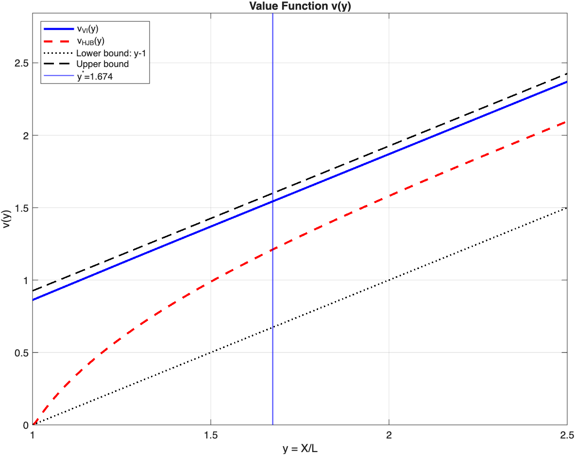
We begin by plotting the value function $v$ and comparing it with the benchmark case where equity issuance is not allowed, denoted by $v^{HJB}$ . The function $v^{HJB}$ represents the value function without the possibility of issuing capital, and it solves the following singular control problem:

0=\min\{\rho_{L}v(y)-\displaystyle\sup_{0\leq\pi\leq\overline{\pi}(y)}{\cal L}^{\pi}v(y);v^{\prime}(y)-1\},\quad v(1)=0.

In the numerical experiments, we use the following baseline parameters:

r=0.01,\enskip\mu=0.04,\enskip\mu_{L}=0.03,\enskip\rho=0.12,\enskip\sigma=0.08,\enskip\sigma_{L}=0.03,\enskip c=0.20,\enskip\gamma=0.01

together with issuance costs $\kappa=0.01$ and $\kappa^{\prime}=0.02$ . Figure 1 shows that the incremental value generated by the option of issuing is largest at $y=1$ and decreases monotonically with $y$ . In other words, the flexibility to recapitalize is most useful when the bank is close to bankruptcy and becomes less relevant when the bank is well-capitalized. For completeness, we also plot the value function expressed in the original $(x,l)-$ coordinate.

Refer to caption — (a) The value function $v(y)$

We illustrate the strategy in Figure 2 by simulating a single sample path starting from $y_{0}=1.2$ , with a dividend barrier $y^{*}=1.674$ and a post-issuance target $y_{post}^{*}=1.228$ , over a horizon of $50$ years. The path shows the expected two-sided control structure: each time the state hits the issuance boundary $y=1$ , it jumps upward by a fixed size into the interior of the continuation region. Each time the state reaches the dividend region at $y^{*}$ it is reflected back into the continuation region. In this simulation, the cumulative issuance is $1.63$ and the cumulative dividend payout is $4.78$ , as shown in Figure 3.

4.2 Sensitivity to regulatory parameters

We next study how the optimal dividend boundary $y^{*}$ and the relative value of issuance respond to changes in the regulatory parameters $a_{1},a_{2}$ and $a_{3}$ . From the model’s perspective, $(a_{1},a_{2},a_{3})$ only enter through the state-dependent investment cap $\overline{\pi}(y)$ . Changing these parameters affects the drift and volatility of the underlying process $Y$ by altering the admissible investment cap, and hence the feasible values of $\pi(y)\leq\overline{\pi}(y)$ . The dividend barrier $y^{*}$ reflects the balance between current dividend payouts and maintaining a future buffer under the constraint dynamics. The issuance value $\Delta v/v$ increases when the constraint makes it more likely to hit bankruptcy, and it decreases when the process tends to avoid hitting the lower boundary, thus making recapitalization less attractive.

The key structure is the minimum operator that has a switching point $\hat{y}>1$ , which induces a two-regime investment cap. With our current baseline parameters $(a_{1},a_{2},a_{3})=(0.045,0.05,0.3)$ , we have $\hat{y}=1.168$ . When $1<y\leq\hat{y}$ , the investment cap $\overline{\pi}(y)=\frac{1}{a_{1}}(1-\frac{1}{y})$ (solvency-dominated), and when $y>\hat{y}$ we have $\overline{\pi}(y)=\frac{1}{a_{3}}(1-\frac{a_{2}}{y})$ (liquidity-dominated). In addition, every issuance event moves the bank directly to the post issuance state $y_{post}^{*}=1.228$ in the liquidity-dominated region. Thus, an issuing event not only raises capital but may also move the bank into a different regulatory regime through the risky investment cap. The numerical results are reported in Table 1. Keeping all other parameters fixed, we evaluate the model at the reference level $y_{0}=1.2$ and vary one regulatory parameter at a time. We report $(i)$ the dividend threshold $y^{*}$ and $(ii)$ the relative value of issuance:

\frac{\Delta v}{v}(y_{0}):=\frac{v-v^{HJB}}{v}(y_{0}),

(17)

which measures the fraction of the value function due to the possibility of issuance. It reflects both the likelihood of hitting the bankruptcy boundary and the continuation value generated near the post-issuance target $y_{post}^{*}$ .

Table 1: Sensitivity to

(a_{1},a_{2},a_{3})

y_{0}=1.2

$a_{1}$

$a_{1}$	$y^{*}$	$\frac{\Delta v}{v}(1.2)$
0.045	1.674	0.5229
0.05	1.699	0.5235
0.06	1.753	0.5245
0.07	1.814	0.5256
0.08	1.882	0.5276
0.09	1.957	0.5304
0.1	2.041	0.5357
0.11	2.134	0.5438
0.12	2.236	0.5545

$a_{2}$

$a_{2}$	$y^{*}$	$\frac{\Delta v}{v}(1.2)$
0.05	1.674	0.5229
0.06	1.667	0.5198
0.08	1.653	0.5136
0.09	1.646	0.5105
0.1	1.639	0.5073
0.12	1.625	0.5008
0.15	1.604	0.4909
0.18	1.583	0.4806
0.2	1.569	0.4735

$a_{3}$

$a_{3}$	$y^{*}$	$\frac{\Delta v}{v}(1.2)$
0.15	1.895	0.8074
0.2	1.885	0.7144
0.25	1.710	0.6089
0.3	1.674	0.5229
0.35	1.414	0.4882
0.4	1.316	0.4659
0.45	1.259	0.4443
0.5	1.221	0.4243
0.55	1.193	0.4060

First, we observe that increasing $a_{1}$ from the baseline value $0.045$ to $0.12$ leads to a large increase in $y^{*}$ from $1.674$ to $2.236$ . At the same time, the relative gain rises moderately. $a_{1}$ enters only through the first regime $\frac{1}{a_{1}}(1-\frac{1}{y})$ and increasing $a_{1}$ lowers this cap for all $y$ , shrinks the feasible set in size throughout that regime. Consequently, the bank is motivated to adopt a more conservative strategy by retaining earnings and building a larger capital buffer before paying dividends, and thus the free boundary $y^{*}$ shifts upward. Similarly, solvency tightening makes it more likely to hit the bankruptcy boundary, and recapitalization becomes more attractive, so the relative value of issuance also increases. However, the relative issuance value increases only moderately compared to the large shift in $y^{*}$ as $a_{1}$ has no influence in the liquidity-dominated region.

As $a_{2}$ rises from $0.05$ to $0.2$ , $y^{*}$ falls from $1.674$ to $1.569$ , and $\frac{\Delta v}{v}(1.2)$ falls from $0.5229$ to $0.4735$ . The parameter $a_{2}$ reduces the continuation value at $y_{post}^{*}$ , and thus issuance is less attractive, though still feasible. Similarly, the continuation value is less sensitive to extra capital buffers. And thus $v^{\prime}$ drops sooner towards $1$ and $y^{*}$ decreases. In addition, the volatility decreases for admissible values of $\pi$ in the region of interest. It is then less likely to hit $y=1$ , which again supports a smaller $y^{*}$ . Increasing $a_{3}$ from $0.15$ to $0.55$ has a similar effect: the dividend boundary falls from $1.895$ to $1.193$ , and $\frac{\Delta v}{v}(1.2)$ changes from $0.8074$ to $0.4060$ . This is because $a_{3}$ works similarly to $a_{2}$ on the investment cap in the liquidity-dominated region, which scales the whole cap uniformly.

4.3 Regulatory parameter optimization

From a regulatory perspective, it is natural to push the parameters $a_{1},a_{2},a_{3}$ as high as possible to increase resilience. Doing so, however, comes at the cost of reduced profitability for the bank. The overall health of a financial institution cannot be assessed solely through solvency considerations: it must balance the interests of regulators, shareholders, and depositors. Motivated by this trade-off, we introduce a metric to quantify the overall health of the bank. First, the bank should operate with low default risk, or at least with limited exposure to financial stress. Since equity issuance is triggered only at the solvency boundary, we interpret a boundary hit as a stress event and define the associated hitting time:

\tau:=\inf\{t\geq 0:Y_{t}<1\}

and require the probability of avoiding such a stress event over a reference horizon to be sufficiently high. On the other hand, for any fixed regulatory triple $(a_{1},a_{2},a_{3})$ , the bank responds optimally by solving the variational inequality (9). This leads to the following optimization problem with restrictions:

\max_{\{(a_{1},a_{2},a_{3})\}}v(y_{0})\quad s.t.\quad\mathbb{P}(\tau\geq T)\geq\eta

for some probability threshold $\eta$ and reference time $T$ . In this numerical illustration, we set $T=5$ . We numerically approximate the solution of this problem by evaluating all combinations in the following parameter grids:

	$\displaystyle a_{1}\in\{0.045,0.05,0.06,0.07,0.08,0.09,0.10,0.11,0.12\},$
	$\displaystyle a_{2}\in\{0.05,0.06,0.08,0.09,0.10,0.12,0.15,0.18,0.2\},$
	$\displaystyle a_{3}\in\{0.15,0.20,0.25,0.3,0.35,0.4,0.45,0.5,0.55\},$

excluding parameter combinations that violate the feasibility conditions (13). For each parameter triple, We evaluate the model at $y_{0}=1.2$ , using $1,000$ Monte Carlo simulations.

In our model, $\pi$ is the proportion invested in risky assets, $\pi>1$ corresponds to a leveraged position, and $\pi\in[0,1]$ corresponds to a no-borrowing long position. Although allowing $\pi>1$ is natural in theoretical investment optimization problems, it makes more sense for real-world banks to have leverage constraints. For this reason, and as a robustness check, we study two cases: one without any additional restriction on $\pi$ , and one with the leverage constraint $\pi\leq 1$ .

4.3.1 Case without a leverage restriction

In this case, we have $486$ parameter triples in total that are feasible. We first plot the pairs $(\mathbb{P}(\tau\geq 5),v(y_{0}))$ generated by all the feasible parameter triples, and illustrate the trade-off between profit and safety. We call a triple $(a_{1},a_{2},a_{3})$ efficient if no other triple yields both a higher value $v(y_{0})$ and a higher survival probability $\mathbb{P}(\tau\geq 5)$ . We indicate these points in the plot in Figure 4 and say that they lie on the Pareto efficient frontier, and we further report these points in Table 2. On the frontier, any attempt to increase the survival probability must come at a cost in the value function, and vice versa. For any target survival probability $\eta$ , the optimal regulatory choice must lie on this frontier.

[Uncaptioned image] — Table 2: Pareto frontier without restriction

The Pareto frontier contains $11$ points, and interestingly, the frontier is primarily driven by $a_{1}$ and almost always selects the same pair of liquidity parameters $(a_{2},a_{3})=(0.05,0.3)$ , and it seems to be most sensitive to the solvency parameter $a_{1}$ . Along those frontier points, increasing $a_{1}$ raises the dividend barrier substantially from $1.674$ to $2.236$ , and this, in turn, affects the survival probability: $\mathbb{P}(\tau\geq T)$ rises from $0.336$ to $0.923$ as $a_{1}$ increases over the curve, while $v(y_{0})$ decreases only slightly. In other words, tightening the solvency parameter $a_{1}$ is the most efficient way to increase safety while not losing too much value in our optimization, whereas altering $a_{2},a_{2}$ generally leads to dominated outcomes.

In addition, the frontier reveals some drastic behavior at high safety levels. To push beyond $\mathbb{P}(\tau\geq T)\approx 0.923$ one needs to increase $a_{2}$ sharply from $0.05$ to $0.18$ , but reducing $v(y_{0})$ to $0.8711$ . The gain in safety at this point thus becomes very expensive and requires very restrictive liquidity regulations, whereas most of the improvement in probability can be achieved by increasing $a_{1}$ only. Within our model, tightening requirements beyond this point appears inefficient, as it yields only a marginal safety gain at a substantial cost in value.

Table 3: Optimal regulatory parameters without restriction

$\eta$	$a_{1}^{*}$	$a_{2}^{*}$	$a_{3}^{*}$	$y^{*}$	$v(y_{0})$	$\mathbb{P}(\tau\geq T)$
0.8	0.1	0.05	0.3	2.041	1.0198	0.848
0.9	0.12	0.05	0.3	2.236	0.9948	0.923

Fix $\eta\in(0,1)$ . Maximizing $v(y_{0})$ under the constraint $\mathbb{P}(\tau\geq T)\geq\eta$ selects an optimal point on the Pareto frontier, and typical choices of $\eta$ could be $0.8,0.9$ , reported in Table 3. In this subsection we take $\eta=0.8$ . Using the resulting optimized parameters, we simulate six representative banks with different starting points $y_{0}$ ’s over a $50-$ year horizon. For each initial condition, we run $1,000$ Monte Carlo trajectories and compute the average cumulative issuance and average cumulative dividends over the full horizon. In addition, we report the Sharpe ratio of the net profit, $\mathbb{E}[\text{net payoff}]/\sigma(\text{net payoff})$ , to examine the risk-adjusted profitability of the bank. Here, $\sigma(\cdot)$ is the standard deviation.

We see a clear monotonic pattern in the initial health $y_{0}$ : as the bank is better capitalized, the expected accumulated dividends increase (from about $5.05$ at $y_{0}=1.05$ to about $5.32$ at $y_{0}=1.30$ ), and the Sharpe ratio also increases modestly (from $1.87$ to $1.95$ ). This is consistent with the fact that a well-capitalized bank reaches the dividend region sooner, and the increase in the Sharpe ratio indicates that the higher net payoff is not driven solely by greater risk exposure. In contrast, the expected cumulative issuance decreases with $y_{0}$ (from $1.41$ to $1.14$ ), with the marginal reduction becoming smaller once $y_{0}$ is sufficiently high.

Table 4: Monte Carlo simulation for

6

banks over

50

years without restriction

$y_{0}$	$\mathbb{E}[\text{Total issuance}]$	$\mathbb{E}[\text{Total dividend}]$	Sharpe ratio
1.05	1.4077	5.0537	1.8698
1.1	1.2853	5.0502	1.8965
1.15	1.2311	5.0812	1.8757
1.2	1.1917	5.1485	1.8991
1.25	1.1598	5.2062	1.9138
1.3	1.1376	5.3152	1.9477

4.3.2 Case with the leverage restriction $\pi\leq 1$

Under the restriction $\pi\leq 1$ , there are $729$ feasible parameter triples. We report the points on the Pareto frontier in Table 5 and plot all pairs of $(\mathbb{P}(\tau\geq 5),v(y_{0}))$ in Figure 5. We observe that the value functions is substantially lower compared to the unrestricted case, and the Pareto frontier is mainly affected by the parameter $a_{1}$ . However, the optimization problem becomes degenerate in the sense that there are only $9$ points on the Pareto frontier in Figure 5, generated by $9$ values of $a_{1}$ . In effect, the value function is insensitive to the liquidity parameters over this range. However, increasing $a_{1}$ pushes the dividend boundary higher and reduces the value function from $0.3357$ to $0.2664$ , while delivering a large improvement in survival probability. For our choice of $a_{2}\leq 0.2,a_{3}\leq 0.55$ , the liquidity cap satisfies $\frac{1}{a_{3}}(1-\frac{a_{2}}{y})\geq 1.455>1$ for all $y\geq 1$ . Thus, throughout the entire liquidity-dominated region, $\overline{\pi}\geq 1$ . Under the additional restriction $\pi\leq 1$ , the liquidity constraints never bind. This shows our earlier conclusion — that the parameter optimization problem is most sensitive to the solvency constraint parameter $a_{1}$ — is robust. Different $a_{2},a_{3}$ parameters produce small differences in the estimated survival probability, although they should not affect the control problem in this regime. Since these differences show no systematic monotonicity, they are most likely due to Monte Carlo noise.

In contrast to the unrestricted case, there is no feasible parameter set achieving $\eta\geq 0.9$ anymore. We therefore select the parameters that give $\eta=0.8$ , as shown in Table 6.

Table 6: Optimal regulatory parameters with

\pi\leq 1

$\eta$	$a_{1}^{*}$	$a_{2}^{*}$	$a_{3}^{*}$	$y^{*}$	$v(y_{0})$	$\mathbb{P}(\tau\geq T)$
0.8	0.12	0.05	0.25	1.175	0.2664	0.86

As in the unconstrained case, we simulate the profitability of $6$ banks restricted to $\pi\leq 1$ with $1,000$ Monte Carlo trajectories. The same monotonic relationship between profitability and the initial capitalization ratio is preserved. Compared to the unrestricted case, the leverage cap substantially reduces profitability: the accumulated dividends drop from $5.05$ – $5.32$ to $1.05$ – $1.28$ , a reduction of roughly $75\%$ – $80\%$ reduction, but the total issuance also falls by around $45\%$ – $53\%$ . Interestingly, the Sharpe ratios of the net gain are higher under the restriction: around $2.45$ to $2.97$ compared to $1.87$ – $1.95$ without restriction. Economically, imposing the leverage tightens the distribution of the net profits, and it reduces the variance more than it reduces the mean. Thus, risk-adjusted profitability improves even though the absolute net payoffs are lower.

Table 7: Monte Carlo simulation for

6

banks over

50

years with

\pi\leq 1

$y_{0}$	$\mathbb{E}[\text{Total issuance}]$	$\mathbb{E}[\text{Total dividend}]$	Sharpe ratio
1.05	0.6765	1.0465	2.4530
1.1	0.6425	1.0855	2.5124
1.15	0.6307	1.1365	2.6160
1.2	0.6261	1.1822	2.7263
1.25	0.6257	1.2318	2.8472
1.3	0.6257	1.2818	2.9684

5 Appendix

Proof of Proposition 2.1

Proof.

Let $(l,x)\in\mathcal{S}\setminus\{0\}$ and ${\widehat{\alpha}}=((\tau_{n})_{n\in\mathbb{N}^{*}},(\widehat{\xi}_{n})_{n\in\mathbb{N}^{*}},\widehat{Z},\pi)\in\mathcal{A}.$ We define an increasing and càdlàg process by

Z_{t}=\int_{0}^{t}L_{u}^{-1}\,d\widehat{Z}_{t}

for $t\geq 0$ . Define a sequence of $\mathcal{F}_{\tau_{n}}$ -measurable random variables by

\xi_{n}=\frac{\widehat{\xi}_{n}}{L_{\tau_{n}}}\quad\textrm{ for }n\in\mathbb{N}^{*}.

Using the identities $F_{\tau_{n}^{-}}=X_{\tau_{n}^{-}}-L_{\tau_{n}}=(Y_{\tau_{n}^{-}}-1)L_{\tau_{n}}$ , $d\hat{Z}_{t}=L_{t}dZ_{t}$ , we can write

\widehat{J}^{\widehat{\alpha}}(l,x)=\mathbb{E}_{l,x}\Big[\int_{0}^{{T}^{\widehat{\alpha}}}e^{-\rho t}L_{t}d{Z}_{t}-\sum_{n=1}^{\infty}e^{-\rho\tau_{n}}L_{\tau_{n}}({\xi}_{n}-\kappa(Y_{\tau_{n}^{-}}-1))\mbox{1\hskip-2.5ptl}_{\{\tau_{n}\leq T^{\widehat{\alpha}}\}}\Big].

Since the process $L$ is a geometric Brownian motion, it admits the representation $L_{t}=l\exp\left(\left(\mu_{L}-\frac{1}{2}\sigma_{L}^{2}\right)t+\sigma_{L}W_{t}\right)$ . Define a process $M$ by $M_{t}:=\frac{L_{t}}{l}e^{-\mu_{L}t}=\exp(\sigma_{L}W_{t}-\frac{1}{2}\sigma_{L}^{2}t)$ , then $M$ is a positive martingale. Substituting $L_{t}=le^{\mu_{L}t}M_{t}$ into the expression of $\widehat{J}$ , we obtain

\widehat{J}^{\widehat{\alpha}}(l,x)=l\mathbb{E}_{l,x}\Big[\int_{0}^{{T}^{\widehat{\alpha}}}e^{-\rho_{L}t}M_{t}d{Z}_{t}-\sum_{n=1}^{\infty}e^{-\rho_{L}\tau_{n}}M_{\tau_{n}}({\xi}_{n}-\kappa(Y_{\tau_{n}^{-}}-1))\mbox{1\hskip-2.5ptl}_{\{\tau_{n}\leq T^{\widehat{\alpha}}\}}\Big].

Moreover, by integration by parts applied to the martingale $M$ and the finite-variation process $\int_{0}^{t}e^{-\rho_{L}s}dZ_{s}$ , we obtain

\mathbb{E}_{l,x}[\int_{0}^{{T}^{\widehat{\alpha}}}e^{-\rho_{L}t}M_{t}dZ_{t}=\mathbb{E}[M_{{T}^{\widehat{\alpha}}}\int_{0}^{{T}^{\widehat{\alpha}}}e^{-\rho_{L}t}dZ_{t}].

For each impulse term, the martingale property of $M$ yields

		$\displaystyle\mathbb{E}\Big[e^{-\rho_{L}\tau_{n}}M_{\tau_{n}}({\xi}_{n}-\kappa(Y_{\tau_{n}^{-}}-1))\mbox{1\hskip-2.5ptl}_{\{\tau_{n}\leq T^{\widehat{\alpha}}\}}\Big]$
	$\displaystyle=$	$\displaystyle\mathbb{E}\Big[e^{-\rho_{L}\tau_{n}}\mathbb{E}[M_{{T}^{\widehat{\alpha}}}\|\mathcal{F}_{\tau_{n}}]({\xi}_{n}-\kappa(Y_{\tau_{n}^{-}}-1))\mbox{1\hskip-2.5ptl}_{\{\tau_{n}\leq T^{\widehat{\alpha}}\}}]\Big]$
	$\displaystyle=$	$\displaystyle\mathbb{E}\Big[e^{-\rho_{L}\tau_{n}}M_{{T}^{\widehat{\alpha}}}({\xi}_{n}-\kappa(Y_{\tau_{n}^{-}}-1))\mbox{1\hskip-2.5ptl}_{\{\tau_{n}\leq T^{\widehat{\alpha}}\}}\Big]$

Consequently, we can write the payoff as

\displaystyle\widehat{J}^{\widehat{\alpha}}(l,x)

\displaystyle=

\displaystyle l\mathbb{E}_{l,x}\Big[M_{T}\left(\int_{0}^{{T}^{\widehat{\alpha}}}e^{-\rho_{L}t}d{Z}_{t}-\sum_{n=1}^{\infty}e^{-\rho_{L}\tau_{n}}({\xi}_{n}-\kappa(\frac{X^{\widehat{\alpha}}_{\tau_{n}^{-}}}{L_{\tau_{n}^{-}}}-1))\mbox{1\hskip-2.5ptl}_{\{\tau_{n}\leq T^{\widehat{\alpha}}\}}\right)\Big].

We now introduce a new probability measure $\mathbb{P}^{*}$ on $\mathcal{F}_{t}$ by ${\left.\frac{d\mathbb{P}^{*}}{d\mathbb{P}}\right|}_{\mathcal{F}_{t}}=M_{t}$ . Under $\mathbb{P}^{*}$ , the processes $W^{*}$ and $B^{*}$ defined by

W_{t}^{*}:=W_{t}-\sigma_{L}t,\quad B_{t}^{*}:=B_{t}-c\sigma_{L}t

are standard Brownian motions with correlation coefficient $c$ . We may therefore express the dynamics in terms of $(W^{*},B^{*})$ . Let $Y^{\widehat{\alpha}}$ denote the leverage ratio defined by $Y^{\widehat{\alpha}}_{t}:=\frac{X^{\widehat{\alpha}}_{t}}{L_{t}}$ . For $\tau_{n}<t<\tau_{n+1}$ , Itô’s formula gives,

$\displaystyle dY^{\widehat{\alpha}}_{t}$	$\displaystyle=$	$\displaystyle\frac{dX^{\widehat{\alpha}}_{t}}{L_{t}}-\frac{X^{\widehat{\alpha}}_{t}dL_{t}}{(L_{t})^{2}}+\frac{X^{\widehat{\alpha}}_{t}d\langle L\rangle_{t}}{(L_{t})^{3}}+d\langle X^{\widehat{\alpha}},L^{-1}\rangle_{t}$
	$\displaystyle=$	$\displaystyle\left(Y^{\widehat{\alpha}}_{t}\left[(1-\pi_{t})r+\pi_{t}\mu\right]+\gamma\right)dt+\pi_{t}\sigma Y^{\widehat{\alpha}}_{t}+\sigma_{L}dW_{t}-dZ_{t}$
		$\displaystyle-Y^{\widehat{\alpha}}_{t}\mu_{L}dt-\sigma_{L}Y^{\widehat{\alpha}}_{t}dW_{t}+\sigma_{L}^{2}Y^{\widehat{\alpha}}_{t}dt-c\pi_{t}c\sigma\sigma_{L}Y^{\widehat{\alpha}}_{t}dt-\sigma_{L}^{2}dt$
	$\displaystyle=$	$\displaystyle\left(Y^{\widehat{\alpha}}_{t}\left[(1-\pi_{t})r+\pi_{t}\mu-\mu_{L}+\sigma_{L}^{2}-c\pi_{t}\sigma\sigma_{L}\right]+\gamma-\sigma_{L}^{2}\right)dt$
		$\displaystyle+\pi_{t}Y^{\widehat{\alpha}}_{t}\sigma dB_{t}+\sigma_{L}(1-Y^{\widehat{\alpha}}_{t})dW_{t}-dZ_{t}.$

By Girsanov’s Theorem, under the measure $\mathbb{P}^{*}$ , the process $Y^{\widehat{\alpha}}_{t}$ satisfies

$\displaystyle dY^{\widehat{\alpha}}_{t}$	$\displaystyle=$	$\displaystyle\left(Y^{\alpha}_{t}\left[(1-\pi_{t})r+\pi_{t}\mu-\mu_{L}\right]+\gamma\right)dt$
		$\displaystyle+\pi_{t}Y^{\widehat{\alpha}}_{t}\sigma d(B_{t}-c\sigma_{L}t)+\sigma_{L}(1-Y^{\widehat{\alpha}}_{t})d(W_{t}-\sigma_{L}t)-d{Z}_{t}$
	$\displaystyle=$	$\displaystyle\left(Y^{\widehat{\alpha}}_{t}\left[(1-\pi_{t})r+\pi_{t}\mu-\mu_{L}\right]+\gamma\right)dt$
		$\displaystyle+\pi_{t}Y^{\widehat{\alpha}}_{t}\sigma d(B_{t}^{})+\sigma_{L}(1-Y^{\widehat{\alpha}}_{t})d(W_{t}^{})-d{Z}_{t}$

for $\tau_{n}<t<\tau_{n+1}$ . Moreover, at issuance times $\tau_{n}$ , we have $X_{\tau_{n}}=X_{\tau_{n}^{-}}+(1-\kappa^{\prime})\widehat{\xi}_{\tau_{n}}-\kappa F_{\tau^{-}_{\tau_{n}}}$ . Using $F_{\tau_{n}^{-}}=(Y^{\widehat{\alpha}}_{\tau_{n}^{-}}-1)L_{\tau_{n}}$ and $\widehat{\xi}_{\tau_{n}}={\xi}_{\tau_{n}}L_{\tau_{n}}$ , this becomes

X_{\tau_{n}}=Y^{\widehat{\alpha}}_{\tau_{n}^{-}}L_{\tau_{n}}+(1-\kappa^{\prime}){\xi}_{\tau_{n}}L_{\tau_{n}}-\kappa(Y^{\widehat{\alpha}}_{\tau_{n}^{-}}-1)L_{\tau_{n}}.

Equivalently, $Y^{\widehat{\alpha}}_{\tau_{n}}=(1-\kappa)Y^{\widehat{\alpha}}_{\tau_{n}^{-}}+(1-\kappa^{\prime}){\xi}_{\tau_{n}}+\kappa$ . We define the control set by $\mathcal{A}$ :

{\small{\mathcal{A}}=\{{{\alpha}}:=((\tau_{n})_{n\in\mathbb{N}^{*}},({\xi}_{n})_{n\in\mathbb{N}^{*}},{Z},\pi):\ \forall t\geq 0:\ 0\leq\pi_{t}<\overline{\pi}(Y_{t}^{\alpha}),\ \forall n\geq 0:\ {\xi}_{n}>\frac{\kappa}{1-\kappa^{\prime}}(Y^{\alpha}_{\tau_{n}^{-}}-1)\}.}

For each $\widehat{\alpha}\in\widehat{{\mathcal{A}}}$ , there exists an $\alpha\in{\mathcal{A}}$ such that $Y^{\widehat{\alpha}}=Y^{\alpha}$ . Finally, we observe that the admissibility condition on $\widehat{\xi}_{n}$ is equivalent to the corresponding condition on ${\xi}_{n}$ :

\{\widehat{\xi}_{n}>\frac{\kappa}{1-\kappa^{\prime}}F_{\tau_{n}^{-}}\}=\{{\xi}_{n}>\frac{\kappa}{1-\kappa^{\prime}}(Y^{\widehat{\alpha}}_{\tau_{n}^{-}}-1)\}.

Moreover, the bankruptcy times coincide: $T^{\alpha}:=\inf\{t\geq 0:Y^{\alpha}_{t}<1\}=\inf\{t\geq 0:F_{t}<0\}=T^{\widehat{\alpha}}$ . Under the new measure $\mathbb{P}^{*}$ , we can write

\widehat{J}^{\widehat{\alpha}}(l,x)=l\mathbb{E}^{*}_{y}\Big[\int_{0}^{{T}^{\alpha}}e^{-\rho_{L}t}d{Z}_{t}-\sum_{n=1}^{\infty}e^{-\rho_{L}\tau_{n}}({\xi}_{n}-\kappa(Y^{\alpha}_{\tau_{n}^{-}}-1))\mbox{1\hskip-2.5ptl}_{\{\tau_{n}\leq T^{\alpha}\}}\Big].

Taking the supremum over the set ${\mathcal{A}}$ on both sides yields

\widehat{v}(l,x)=l\sup_{\alpha\in{\mathcal{A}}}\mathbb{E}^{*}_{y}\Big[\int_{0}^{{T}^{\alpha}}e^{-\rho_{L}t}d{Z}_{t}-\sum_{n=1}^{\infty}e^{-\rho_{L}\tau_{n}}({\xi}_{n}-\kappa(Y^{\alpha}_{\tau_{n}^{-}}-1))\mbox{1\hskip-2.5ptl}_{\{\tau_{n}\leq T^{\alpha}\}}\Big]=:lv(y)=lv(\frac{x}{l}).

Since $(B^{*},W^{*})$ under $\mathbb{P}^{*}$ has the same law as the process $(B,W)$ under $\mathbb{P}$ , passing to the canonical space does not change the distribution of the relevant objects. To simplify notation, we therefore write $(B,W)$ instead of $(B^{*},W^{*})$ and understand all subsequent probabilities as taken under $\mathbb{P}^{*}$ . ∎

Proof of Proposition 3.1

Proof.

We discuss three parameter regimes and construct admissible strategies showing that $v(y)=\infty$ .

Case 1 ( $\rho<\mu_{L}$ ). Consider the strategy with no issuance and no investment in the risky asset: $\pi_{t}\equiv 0$ . Since $r>r_{L}$ , the drift of $Y$ is positive. By continuity, there exists $\epsilon>0$ such that the drift remains positive on $y\in[1,1+\epsilon]$ . Define the lower bound

m:=\inf_{y\in[1,1+\epsilon]}(r-\mu_{L})y+\gamma>0.

We choose a dividend region to be $[1+\epsilon,\infty)$ , that is, any excess above $1+\epsilon$ is immediately paid out as dividends. Fix an initial state $Y_{0}=y>1$ . Under this strategy, the controlled dynamics of $Y$ are $dY_{t}=((r-\mu_{L})Y_{t}+\gamma)dt+\sigma_{L}(1-Y_{t})dW_{t}-dZ_{t}$ . Taking expectations up to time $t$ :

1+\epsilon\geq\mathbb{E}[Y_{t}]=y+\int_{0}^{t}\mathbb{E}[(r-\mu_{L})Y_{s}+\gamma]ds-\mathbb{E}[Z_{t}]\geq y+mt-\mathbb{E}[Z_{t}].

This implies $\mathbb{E}[Z_{t}]\geq mt+y-(1+\epsilon)$ for $t\geq t_{0}=\frac{1+\epsilon-y}{m}$ . Thus $\mathbb{E}[Z_{t}]$ grows at least linearly with $t$ . Since $\rho_{L}<0$ , the value function satisfies

v(y)\geq\mathbb{E}[\int_{0}^{\infty}e^{-\rho_{L}s}dZ_{s}]=\int_{0}^{\infty}e^{-\rho_{L}s}d\mathbb{E}[Z_{s}]\geq\int_{t_{0}}^{\infty}e^{-\rho_{L}s}mds=\infty.

If the initial state is $1$ , the agent can first issue a small amount of capital and then follow the above strategy.

Case $2$ : $\mu_{L}\leq\rho<r=\max(r,\frac{\mu+(1-\bar{a})r}{\bar{a}})$ . In this regime, $\mu<r$ , so the drift-maximizing strategy satisfies $\mu^{*}(y)=r$ on $[1,\infty)$ . Fix $y_{0}>1$ and let $y\geq y_{0}>1$ . Fix $t>0$ , consider the strategy with constant control $\pi^{*}_{s}=0$ for $0\leq s<t$ . At time $t$ , provided bankruptcy has not occurred, the agent distributes dividends to brings the state to $1$ . Let $Y^{0}$ denote the ratio process under the strategy $\pi_{t}=0$ , stopped at bankruptcy. $Y^{0}$ is the solution of

dY^{0}_{t}=\left((r-\mu_{L})Y^{0}_{t}+\gamma\right)dt+\sigma_{L}(1-Y^{0}_{t})dW_{t},\quad Y_{0}=y.

A direct computation yields

\displaystyle e^{-\rho_{L}t}Y^{0}_{t}=\mathcal{E}_{t}\left(Y_{0}+b\int_{0}^{t}\mathcal{E}_{u}^{-1}\,du+\sigma_{L}\int_{0}^{t}\mathcal{E}_{u}^{-1}\,dW_{u}\right),

(18)

where $b=\gamma+\sigma_{L}^{2}$ and the process $\mathcal{E}$ is solution of $d\mathcal{E}_{t}=\mathcal{E}_{t}\left((r-\rho)dt-\sigma_{L}dW_{t}\right)$ with $\mathcal{E}_{0}=1$ . The value function therefore satisfies

v(y)\geq\mathbb{E}\Big[e^{-\rho_{L}t}(Y^{0}_{t}-1)\mbox{1\hskip-2.5ptl}_{\{t<T(y)\}}\Big],

where $T(y)=\inf\{t\geq 0:\ Y^{0}_{t}<1\}$ is the time of bankruptcy. Applying Itô’s formula to $e^{-\rho_{L}t}Y^{0}_{t}$ up to time $t\wedge T(y)$ and taking expectation,

	$\displaystyle\mathbb{E}\Big[e^{-\rho_{L}t}Y^{0}_{t}\mbox{1\hskip-2.5ptl}_{\{t<T(y)\}}\Big]$	$\displaystyle=$	$\displaystyle y-\mathbb{E}\Big[e^{-\rho_{L}T(y)}\mbox{1\hskip-2.5ptl}_{\{T(y)\leq t\}}\Big]$
			$\displaystyle+\mathbb{E}\Big[\int_{0}^{t\wedge T(y)}e^{-\rho_{L}u}((r-\rho)Y^{0}_{u})\,du\Big]+\gamma\mathbb{E}\Big[\int_{0}^{t\wedge T(y)}e^{-\rho_{L}u}\,du\Big].$

Since $r>\rho$ , the integrand in the second term is nonnegative. Moreover, the bankruptcy time is increasing in the initial condition: for all $y\geq y_{0}$ , $T(y)\geq T(y_{0}),\enskip a.s.$ . Hence, for $y\geq y_{0}$ ,

\int_{0}^{t\wedge T(y)}e^{-\rho_{L}u}Y^{0}_{u}\,du\geq\int_{0}^{t\wedge T(y_{0})}e^{-\rho_{L}u}Y^{0}_{u}\,du.

Using this monotonicity, we obtain

\mathbb{E}\Big[e^{-\rho_{L}t}Y^{0}_{t}\mbox{1\hskip-2.5ptl}_{\{t<T(y)\}}\Big]\geq y+(r-\rho)\mathbb{E}\Big[\int_{0}^{t\wedge T(y_{0})}e^{-\rho_{L}u}Y^{0}_{u}\,du\Big]-1-\frac{\mid\gamma\mid}{\rho_{L}}.

Plugging in the representation in 18, we deduce that

	$\displaystyle v(y)$	$\displaystyle\geq$	$\displaystyle y\left(1+(r-\rho)\mathbb{E}\Big[\int_{0}^{T(y_{0})\wedge t}\mathcal{E}_{u}\,du\Big]\right)-1-\frac{\mid\gamma\mid}{\rho_{L}}$
			$\displaystyle+(r-\rho)\mathbb{E}\Big[\int_{0}^{T(y_{0})\wedge t}\mathcal{E}_{u}\left(b\int_{0}^{u}\mathcal{E}_{s}^{-1}\,ds+\sigma_{L}\int_{0}^{u}\mathcal{E}_{s}^{-1}\,dW_{s}\right)\,du\Big].$

Define $c_{1}(t,y_{0}):=(r-\rho)\mathbb{E}\Big[\int_{0}^{T(y_{0})\wedge t}\mathcal{E}_{u}\,du\Big]>0$ , which is finite and independent of $y$ . There exists $c_{2}\geq 0$ such that $v(y)\geq(1+c_{1})y-c_{2}$ for all $y\geq y_{0}$ . For $1\leq y\leq y_{0}$ , we obtain:

v(y)\geq y-1\geq(1+c_{1}(t,y_{0}))y-1-c_{1}(t,y_{0})y_{0}.

Thus there exists $c_{1},$ $c_{2}>0$ such that for all $y\geq 1$ , $v(y)\geq(1+c_{1})y-c_{2}$ . Suppose that for some $n\in\mathbb{N}^{*}\setminus\{0\}$ such that

v(y)\geq(1+c_{1})^{n}y-c_{2}\sum_{i=0}^{n-1}(1+c_{1})^{i},\quad\forall y\in(1,\infty).

Consider the strategy where the agent does nothing until time $t\wedge T(y)$ and then follows an optimal strategy, we get

$\displaystyle v(y)$	$\displaystyle\geq$	$\displaystyle\mathbb{E}\Big[e^{-\rho_{L}t}v(Y_{t})\mbox{1\hskip-2.5ptl}_{\{t<T(y)\}}\Big]$
	$\displaystyle\geq$	$\displaystyle(1+c_{1})^{n}\mathbb{E}\Big[e^{-\rho_{L}t}Y_{t}\mbox{1\hskip-2.5ptl}_{\{t<T(y)\}}\Big]-c_{2}\sum_{i=0}^{n-1}(1+c_{1})^{i}$
	$\displaystyle\geq$	$\displaystyle(1+c_{1})^{n+1}y-c_{2}\sum_{i=0}^{n}(1+c_{1})^{i}.$

Thus, by induction, for all $(y,n)\in[1,\infty)\times\mathbb{N}^{*}\setminus\{0\}$ , $v(y)\geq(1+c_{1})^{n}(y-\frac{c_{2}}{c_{1}})$ . For $y>\frac{c_{2}}{c_{1}}$ we then obtain $v(y)=\infty$ letting $n\to\infty$ . For $y\leq\frac{c_{2}}{c_{1}}$ , define $\theta(z):=\inf\{s\geq 0:\ Y^{0}_{s}=z\}$ , for $z>\frac{c_{2}}{c_{1}}$ . By the strong Markov property,

v(y)\geq v(z)\mathbb{E}\Big[e^{-\rho_{L}\theta_{z}}\mbox{1\hskip-2.5ptl}_{\{\theta_{z}<T(y)\}}\Big].

Since the diffusion is nondegenerate, $\mathbb{P}(\theta_{z}<T(y))>0$ , and thus the right hand side equals $\infty$ . Therefore, $v(y)=\infty$ for all $y\geq 1$ , which concludes the proof.

Case $3$ : $\mu_{L}\leq\rho<\frac{\mu+(1-\bar{a})r}{\bar{a}}=\max(r,\frac{\mu+(1-\bar{a})r}{\bar{a}})$ . In that case, we have $r\leq\mu$ , and it is optimal to invest as much as possible in the risky asset, subject to the capital constraint. Consider the maximal-investment strategy $\overline{\pi}$ defined in (7), then $\mu^{*}(y)=r+\overline{\pi}(y)(\mu-r),\quad y\in[1,\infty)$ . Under this strategy, the ratio process $Y^{*}$ satisfies

	$\displaystyle dY^{*}_{t}$	$\displaystyle=$	$\displaystyle\left((\mu^{}(Y^{}_{t})-\mu_{L})Y^{}_{t}+\gamma\right)dt+\overline{\pi}(Y^{}_{t})Y^{}_{t}\sigma dB_{t}+\sigma_{L}(1-Y^{}_{t})dW_{t},$
		$\displaystyle=$	$\displaystyle\left((r-\mu_{L})Y^{}_{t}+(\mu-r)\overline{\pi}(Y^{}_{t})Y^{}_{t}+\gamma\right)dt+\overline{\pi}(Y^{}_{t})Y^{}_{t}\sigma dB_{t}+\sigma_{L}(1-Y^{}_{t})dW_{t}$

with $Y^{*}_{0}=y$ . If $a_{3}\leq a_{1}$ , then $y\overline{\pi}(y)=\frac{1}{a_{1}}(y-1)$ for any $y\geq 1$ . The SDE becomes

\displaystyle dY^{*}_{t}

\displaystyle=

\displaystyle\left((r-\mu_{L}+\frac{\mu-r}{a_{1}})Y^{*}_{t}+\gamma-(\mu-r)\frac{1}{a_{1}}\right)dt+\frac{\sigma}{a_{1}}(Y^{*}_{t}-1)dB_{t}+\sigma_{L}(1-Y^{*}_{t})dW_{t}.

The above SDE is in the same affine form as in Case 2, with $(r-\mu_{L}+\frac{\mu-r}{a_{1}})>\rho_{L}$ . Using teh same argument as in Case 2, there exists some $c_{1},c_{2}>0$ such that $v(y)\geq(1+c_{1})y-c_{2}$ and thus the value function $v(y)=\infty$ . We now turn to the case where $a_{3}>a_{1}$ . Define the threshold $\hat{y}:=\frac{a_{3}-a_{1}a_{2}}{a_{3}-a_{1}}\geq 1$ and we observe that, for $y\geq\hat{y}$ we have $y\overline{\pi}(y)=\frac{1}{a_{3}}(y-a_{2})$ . Define $T_{\hat{y}}:=\inf\{t\geq 0:\ Y^{*}_{t}<\hat{y}\}$ , then for $0\leq t\leq T_{\hat{y}},$ the dynamics of the $Y^{*}$ process becomes

dY^{*}_{t}=\left((r-\mu_{L}+\frac{\mu-r}{a_{3}})Y^{*}_{t}-(\mu-r)\frac{a_{2}}{a_{3}}+\gamma\right)dt+\frac{\sigma}{a_{3}}(Y^{*}_{t}-a_{2})dB_{t}+\sigma_{L}(1-Y^{*}_{t})dW_{t}.

Since $r-\mu_{L}+\frac{\mu-r}{a_{3}}>\rho_{L}$ , the same argument as in Case 2 applied up to time $t\wedge T(y)\wedge T_{\hat{y}}$ shows that $v(y)=\infty$ . ∎

Proof of Proposition 3.2

Proof.

Fix $y>1$ and an arbitrary admissible control $\alpha\in{\cal A}$ . Let $T^{\alpha}$ denote the corresponding bankruptcy time. Let $\tau_{0}=0$ and first assume $\tau_{1}>0$ . Fix $n\in\mathbb{N}$ and work on the event $\{\tau_{n}<T^{\alpha}\}$ . Note that $\{\tau_{n}=T^{\alpha}\}=\emptyset$ since $\xi_{n}>\frac{\kappa}{1-\kappa^{\prime}}(Y_{\tau_{n}^{-}}-1).$ For each integer $m\geq 2$ , let $\theta_{m,n}$ be the first exit time from $(1+1/m,m)$ after $\tau_{n}$ :

\theta_{m,n}:=\inf\{t\geq\tau_{n}:Y_{t}^{y,\alpha}\geq m\;\mbox{ or }\;Y_{t}^{y,\alpha}\leq 1+1/m\}.

On the event $\{\tau_{n}<T^{\alpha}\}\in\mathcal{F}_{\tau_{n}}$ , one can choose $m$ large enough so that $\tau_{n}<\theta_{m,n}$ . Moreover, $\theta_{m,n}$ $\nearrow$ $T^{\alpha}$ almost surely as $m\to\infty$ . Define $\eta:=\theta_{m,n}\wedge\tau_{n+1}$ . We now apply Itô’s formula to the process $\left(e^{-\rho_{L}t}\varphi(Y_{t}^{y,\alpha})\right)$ on the time interval $[\tau_{n},\eta]$ :

$\displaystyle e^{-\rho_{L}\eta}\varphi(Y_{(\eta)^{-}}^{y,\alpha})$	$\displaystyle=$	$\displaystyle e^{-\rho_{L}\tau_{n}}\varphi(Y^{y,\alpha}_{\tau_{n}})+\int_{\tau_{n}}^{\eta}e^{-\rho_{L}t}({\cal L}^{\pi}\varphi-\rho_{L}\varphi)(Y_{t}^{y,\alpha})dt$
		$\displaystyle-\int_{\tau_{n}}^{\eta}e^{-\rho_{L}t}\varphi^{\prime}(Y_{t}^{y,\alpha})dZ^{c}_{t}+\sum_{\tau_{n}\leq t<\eta}e^{-\rho_{L}t}\left[\varphi(Y_{t}^{y,\alpha})-\varphi(Y_{t^{-}}^{y,\alpha})\right]$
		$\displaystyle+\int_{\tau_{n}}^{\eta}e^{-\rho_{L}t}\sigma\pi_{t}Y_{t}^{y,\alpha}\varphi^{\prime}(Y_{t}^{y,\alpha})dB_{t}+\int_{\tau_{n}}^{\eta}e^{-\rho_{L}t}\sigma_{L}(1-Y_{t}^{y,\alpha})\varphi^{\prime}(Y_{t}^{y,\alpha})dW_{t},$

where $Z^{c}$ is the continuous part of the dividend process $Z$ . For any jump time $t\in[\tau_{n},\eta)$ , it holds that $Y_{t}^{y,\alpha}-Y_{t^{-}}^{y,\alpha}=-(Z_{t}-Z_{t^{-}})$ . Since $\varphi^{\prime}$ $\geq$ $1$ , the mean-value theorem implies that

\varphi(Y_{t}^{y,\alpha})-\varphi(Y_{t^{-}}^{y,\alpha})\leq Y_{t}^{y,\alpha}-Y_{t^{-}}^{y,\alpha}=-(Z_{t}-Z_{t^{-}})

for $\tau_{n}$ $\leq$ $t$ $<$ $\eta$ . Since $\varphi$ is a supersolution, we also have ${\cal L}^{\pi}\varphi(y)-\rho_{L}\varphi(y)\leq 0$ with any admissible $\pi$ . Taking conditional expectations with respect to $\mathcal{F}_{\tau_{n}}$ , and using that the integrands in the stochastic integral terms are bounded by a constant depending on $m$ , we obtain, on $\{\tau_{n}\leq T^{\alpha}\}$ ,

	$\displaystyle\mathbb{E}\left[e^{-\rho_{L}\eta}\varphi(Y_{(\eta)^{-}}^{y,\alpha})\|\mathcal{F}_{\tau_{n}}\right]$	$\displaystyle\leq$	$\displaystyle e^{-\rho_{L}\tau_{n}}\varphi(Y^{y,\alpha}_{\tau_{n}})-\mathbb{E}\left[\int_{\tau_{n}}^{\eta}e^{-\rho_{L}t}dZ_{t}^{c}\|\mathcal{F}_{\tau_{n}}\right]$
			$\displaystyle\;-\;\mathbb{E}\left[\sum_{\tau_{n}\leq t<\eta}e^{-\rho_{L}t}(Z_{t}-Z_{t^{-}})\|\mathcal{F}_{\tau_{n}}\right].$

Consequently, $e^{-\rho_{L}\tau_{n}}\varphi(Y^{y,\alpha}_{\tau_{n}})\geq\mathbb{E}\left[\int_{\tau_{n}}^{\eta}e^{-\rho_{L}t}dZ_{t}+e^{-\rho_{L}\eta}\varphi(Y_{(\eta)^{-}}^{y,\alpha})|\mathcal{F}_{\tau_{n}}\right]$ . Since $\varphi(y)\geq 0$ , after sending $m$ to infinity, Fatou’s lemma yields

e^{-\rho_{L}\tau_{n}}\varphi(Y^{y,\alpha}_{\tau_{n}})\geq\mathbb{E}\left[\int_{\tau_{n}}^{\tau_{n+1}\wedge T^{\alpha}}e^{-\rho_{L}t}dZ_{t}+e^{-\rho_{L}\tau_{n+1}\wedge T^{\alpha}}\varphi(Y_{(\tau_{n+1}\wedge T^{\alpha})^{-}}^{y,\alpha})|\mathcal{F}_{\tau_{n}}\right].

On the event $\{\tau_{n+1}\leq T^{\alpha}\}$ , we have

	$\displaystyle\varphi(Y_{\tau_{n+1}^{-}}^{y,\alpha})\geq\mathcal{H}\varphi(Y_{\tau_{n+1}^{-}}^{y,\alpha})$	$\displaystyle\geq$	$\displaystyle\varphi((1-\kappa)Y_{\tau_{n+1}^{-}}^{y,\alpha}+(1-\kappa^{\prime})\xi_{n+1}+\kappa)-\xi_{n+1}+\kappa(Y_{\tau_{n+1}^{-}}^{y,\alpha}-1)$
		$\displaystyle=$	$\displaystyle\varphi(Y_{\tau_{n+1}}^{y,\alpha})-\xi_{n+1}+\kappa(Y_{\tau_{n+1}^{-}}^{y,\alpha}-1).$

On the complementary event $\{T^{\alpha}<\tau_{n+1}\}$ , we have $Y_{(T^{\alpha})^{-}}^{y,\alpha}\geq 1$ . Therefore, $\varphi(Y_{(\tau_{n+1}\wedge T^{\alpha})^{-}}^{y,\alpha})\geq 0$ . then we obtain

	$\displaystyle e^{-\rho_{L}\tau_{n}}\varphi(Y^{y,\alpha}_{\tau_{n}})$	$\displaystyle\geq$	$\displaystyle\mathbb{E}\left[\int_{\tau_{n}}^{\tau_{n+1}\wedge T^{\alpha}}e^{-\rho_{L}t}dZ_{t}\|\mathcal{F}_{\tau_{n}}\right]$
			$\displaystyle+\mathbb{E}\left[e^{-\rho_{L}\tau_{n+1}}\left(\varphi(Y_{\tau_{n+1}}^{y,\alpha})-\xi_{n+1}+\kappa(Y_{\tau_{n+1}^{-}}^{y,\alpha}-1)\right)\mbox{1\hskip-2.5ptl}_{\{\tau_{n+1}\leq T^{\alpha}\}}\|\mathcal{F}_{\tau_{n}}\right]\ .$

Now fix $N\geq 0$ ,

		$\displaystyle\varphi(Y^{y,\alpha}_{0})-\mathbb{E}\left[e^{-\rho_{L}\tau_{N+1}}\varphi(Y^{y,\alpha}_{\tau_{N+1}})\mbox{1\hskip-2.5ptl}_{\{\tau_{N+1}\leq T^{\alpha}\}}\right]$
	$\displaystyle=$	$\displaystyle\sum_{n=0}^{N}\left(\mathbb{E}\left[e^{-\rho_{L}\tau_{n}}\varphi(Y^{y,\alpha}_{\tau_{n}})\mbox{1\hskip-2.5ptl}_{\{\tau_{n}\leq T^{\alpha}\}}-e^{-\rho_{L}\tau_{n+1}}\varphi(Y^{y,\alpha}_{\tau_{n+1}})\mbox{1\hskip-2.5ptl}_{\{\tau_{n+1}\leq T^{\alpha}\}}\right]\right)$
	$\displaystyle\geq$	$\displaystyle\sum_{n=0}^{N}\left(\mathbb{E}\left[\int_{\tau_{n}}^{{\tau_{n+1}}\wedge T^{\alpha}}e^{-\rho_{L}t}dZ_{t}-e^{-\rho_{L}\tau_{n+1}}\left(\xi_{n+1}-\kappa(Y_{\tau_{n+1}^{-}}^{y,\alpha}-1)\right)\mbox{1\hskip-2.5ptl}_{\{\tau_{n+1}\leq T^{\alpha}\}}\right]\right).$

We now distinguish two cases. First assume first that $\tau_{1}>0$ . Letting $N\to\infty$ , and using the tower property together with the previous inequalities, we obtain

\displaystyle\varphi(y)

\displaystyle\geq

\displaystyle\mathbb{E}\left[\int_{0}^{T^{\alpha}}e^{-\rho_{L}t}dZ_{t}-\sum_{n=1}^{\infty}e^{-\rho_{L}\tau_{n}}\left(\xi_{n}-\kappa(Y_{\tau_{n}^{-}}^{y,\alpha}-1)\right)\mbox{1\hskip-2.5ptl}_{\{\tau_{n}\leq T^{\alpha}\}}\right]\ .

As $\lim_{n\to\infty}\tau_{n}=\infty$ and $\rho_{L}>0$ , we have

\mathbb{E}\left[e^{-\rho_{L}T^{\alpha}}\sum_{n=0}^{\infty}\mbox{1\hskip-2.5ptl}_{\{\tau_{n}<T^{\alpha}<\tau_{n+1}\}}\right]=\mathbb{E}\left[e^{-\rho_{L}T^{\alpha}}\mbox{1\hskip-2.5ptl}_{\{T^{\alpha}<\infty\}}\right]=\mathbb{E}\left[e^{-\rho_{L}T^{\alpha}}\right].

Now assume that $\tau_{1}=0$ . The same arguments as before yields

\displaystyle\varphi(y)

\displaystyle\geq

\displaystyle\mathbb{E}\left[\int_{0}^{T^{\alpha}}e^{-\rho_{L}t}dZ_{t}-\sum_{n=2}^{\infty}e^{-\rho_{L}\tau_{n}}\left(\xi_{n}-\kappa(Y_{\tau_{n}^{-}}^{y,\alpha}-1)\right)\mbox{1\hskip-2.5ptl}_{\{\tau_{n}\leq T^{\alpha}\}}\right].

Since $\varphi(y)\geq\mathcal{H}\varphi(y)\geq\varphi(Y_{0}^{y,\alpha})-\xi_{1}+\kappa(y-1)$ , we obtain

\displaystyle\varphi(y)

\displaystyle\geq

\displaystyle\mathbb{E}\left[\int_{0}^{T^{\alpha}}e^{-\rho_{L}t}dZ_{t}-\sum_{n=1}^{\infty}e^{-\rho_{L}\tau_{n}}\left(\xi_{n}-\kappa(Y_{\tau_{n}^{-}}^{y,\alpha}-1)\right)\mbox{1\hskip-2.5ptl}_{\{\tau_{n}\leq T^{\alpha}\}}\right],

for all arbitrary control $\alpha$ . Taking the supremum over all controls on both sides yields $\varphi(y)\geq v(y)$ for all $y>1$ . It follows that $\mathcal{H}v(1)\leq\mathcal{H}\varphi(1)$ , and thus

v(1)=\max\left(0,\ \mathcal{H}v(1)\right)\leq\max\left(0,\ \mathcal{H}\varphi(1)\right)\leq\varphi(1).

∎

Proof of Corollary 3.1

Proof.

The lower bound follows by considering the strategy that pays an immediate lump-sum dividend of size $Z_{0}-Z_{0-}=y-1$ . For the upper bound, we set $K=\frac{1}{\rho_{L}}\textrm{max}\left(-\rho_{L},A+\gamma,B+\gamma\right)$ , and introduce the function $\varphi(y)=y+K$ . By Proposition 3.2, it suffices to prove that $\varphi$ is a super solution of equation 9. Since $\varphi$ is affine, we have

\sup_{0\leq\pi\leq\overline{\pi}(y)}\mathcal{L}^{\pi}\varphi(y)=\sup_{0\leq\pi\leq\overline{\pi}(y)}y\left[\mu(\pi)-\mu_{L}\right]+\gamma=y\left[\mu^{*}(y)-\mu_{L}\right]+\gamma.

Using the identity

y\overline{\pi}(y)=\left\{\begin{array}[]{lll}\frac{1}{a_{3}}(y-a_{2})&\quad\textrm{ if }a_{3}>a_{1}\textrm{ and }y\geq\hat{y},\\ \frac{1}{a_{1}}(y-1)&\quad\textrm{ else,}\end{array}\right.

with $\hat{y}=\frac{a_{3}-a_{1}a_{2}}{a_{3}-a_{1}}$ , we can compute $\sup_{0\leq\pi\leq\overline{\pi}(y)}\mathcal{L}^{\pi}\varphi(y)$ and it follows that

\sup_{0\leq\pi\leq\overline{\pi}(y)}\mathcal{L}^{\pi}\varphi(y)=\left\{\begin{array}[]{lll}\left(r+\frac{(\mu-r)^{+}}{a_{3}}-\mu_{L}\right)y+\gamma-\frac{a_{2}(\mu-r)^{+}}{a_{3}}&\quad&\textrm{ if }y\overline{\pi}(y)=\frac{1}{a_{3}}(y-a_{2})\\ \left(r+\frac{(\mu-r)^{+}}{a_{1}}-\mu_{L}\right)y+\gamma-\frac{(\mu-r)^{+}}{a_{1}}&\quad&\textrm{ if }y\overline{\pi}(y)=\frac{1}{a_{1}}(y-1)\end{array}\right.

Therefore, we have

\rho_{L}\varphi(y)-\sup_{0\leq\pi\leq\overline{\pi}(y)}\mathcal{L}^{\pi}\varphi(y)=\left\{\begin{array}[]{ll}\left(\rho-r-\frac{(\mu-r)^{+}}{a_{3}}\right)y-\gamma+\frac{a_{2}(\mu-r)^{+}}{a_{3}}+\rho_{L}K&\textrm{ if }y\overline{\pi}(y)=\frac{y-a_{2}}{a_{3}}\\ \left(\rho-r-\frac{(\mu-r)^{+}}{a_{1}}\right)y-\gamma+\frac{(\mu-r)^{+}}{a_{1}}+\rho_{L}K&\textrm{ if }y\overline{\pi}(y)=\frac{y-1}{a_{1}}\end{array}\right.

Since the right-hand sides are affine in $y$ , their minima are attained at the endpoints. The constant $K$ was chosen that $\rho_{L}\varphi(y)-\sup_{0\leq\pi\leq\overline{\pi}(y)}\mathcal{L}^{\pi}\varphi(y)\geq 0$ . Moreover, we have

\mathcal{H}\varphi(y)=\sup_{\xi>\frac{\kappa}{1-\kappa^{\prime}}(y-1)}\left(y+K-\kappa^{\prime}\xi\right)<\varphi(y).

Finally, since $K\geq-1$ , we have $\lim_{y\downarrow 1}\varphi(y)\geq 0$ , and therefore $\varphi$ satisfies assumptions of Proposition 3.2, which implies $v\leq\varphi$ . In particular, if $-\rho_{L}\geq max(A,B)+\gamma$ , then $\max(-\rho_{L},A+\gamma,B+\gamma)=-\rho_{K}$ , so $K=-1$ . Combining this with the lower bound yields $v(y)=y-1$ . ∎

Proof of Proposition 3.3

To prove Proposition 3.3, we first state and prove the following Lemma.

Lemma 5.1.

The value function $v$ is non-decreasing and continuous on $[1,+\infty)$ .

Proof of Lemma 5.1.

We first show that $v$ is continuous on $(1,\infty)$ . Fix $y>1$ . For $\varepsilon>0$ , define the hitting times $T_{\varepsilon}\;=\;\inf\{t\geq 0;\>Y_{t}^{y}=y+\varepsilon\}$ and $T_{1}\;=\;\inf\{t\geq 0;\>Y_{t}^{y}=1.\}$ . Consider a control $\alpha$ $=$ $((\tau_{n})_{n\in\mathbb{N}^{*}},({\xi}_{n})_{n\in\mathbb{N}^{*}},{Z},\pi^{*})$ $\in$ ${\cal A}$ such that $Z\equiv 0$ and $\tau_{1}>T_{\varepsilon}$ . In other words, no dividends are paid and no capital is issued before $T_{\varepsilon}$ . Then $Y_{t}=Y^{*}_{t}$ for all $t<\tau_{1}$ . On $T_{\varepsilon}<T_{1}$ , we have $Y_{T_{\varepsilon}\wedge T_{1}}=y+\epsilon$ ; on $T_{\varepsilon}\geq T_{1}$ , we have $Y_{T_{\varepsilon}\wedge T_{1}}=1$ . Applying the dynamic programming principle (DPP) up to time $T_{1}\wedge T_{\varepsilon}$ , we obtain

v(y)\geq\mathbb{E}\left[e^{-\rho_{L}T_{\varepsilon}\wedge T_{1}}v(Y_{T_{\varepsilon}\wedge T_{1}})\right]=\mathbb{E}\left[e^{-\rho_{L}T_{\varepsilon}}v(y+\varepsilon)\mbox{1\hskip-2.5ptl}_{T_{\varepsilon}<T_{1}}\right]+\mathbb{E}\left[e^{-\rho_{L}T_{\varepsilon}}v(1)\mbox{1\hskip-2.5ptl}_{T_{\varepsilon}\geq T_{1}}\right].

Since the value function $v$ is non-decreasing, we have

	$\displaystyle 0\leq v(y+\varepsilon)-v(y)$	$\displaystyle\leq$	$\displaystyle\mathbb{E}\left[(1-e^{-\rho_{L}T_{\varepsilon}})v(y+\varepsilon)\mbox{1\hskip-2.5ptl}_{T_{\varepsilon}<T_{1}}+(v(y+\varepsilon)-v(1))\mbox{1\hskip-2.5ptl}_{T_{\varepsilon}\geq T_{1}}\right]$
		$\displaystyle\leq$	$\displaystyle v(y+\varepsilon)\left(1-\mathbb{E}[e^{-\rho_{L}T_{\varepsilon}}]\right)+(v(y+\varepsilon)-v(1))\mathbb{P}(T_{\varepsilon}\geq T_{1}).$

Now fix $\varepsilon_{0}>0$ , and restrict to $\varepsilon<\varepsilon_{0}$ . Then

\displaystyle v(y+\varepsilon)-v(y)\leq

\displaystyle v(y+\varepsilon_{0})\left(1-\mathbb{E}[e^{-\rho_{L}T_{\varepsilon}}]\right)+(v(y+\varepsilon_{0})-v(1))\mathbb{P}(T_{\varepsilon}\geq T_{1}).

(19)

Now take $\varepsilon\downarrow 0$ . Because $Y$ has continuous paths, $T_{\varepsilon}\longrightarrow 0$ almost surely, and by dominated convergence, $\mathbb{E}[e^{-\rho_{L}T_{\varepsilon}}]\longrightarrow 1$ , as $\varepsilon\downarrow 0$ . In addition, the continuity of scale functions of $Y^{*}$ implies that $\mathbb{P}(T_{\varepsilon}\geq T_{1})\longrightarrow 0$ , as $\varepsilon\downarrow 0$ . Since $v$ is finite by Corollary 3.1, we obtain that the right-hand side of equation (19) goes to zero as $\varepsilon\downarrow 0$ . This proves the right-continuity of $v$ . An analogous argument, starting from $y-\epsilon$ and consider the first hitting time of $\{1,y\}$ , proves the left-continuity of the value function. We now turn to the right-continuity of $v$ at $1$ . Let $\varepsilon>0$ . By immediately paying dividends down to the bankruptcy level, we obtain $v(1+\varepsilon)\geq v(1)+\varepsilon$ . Let $\eta>0$ . By (10), there exists $\alpha\in\mathcal{A}$ such that

	$\displaystyle v(1+\varepsilon)$	$\displaystyle\leq$	$\displaystyle\mathbb{E}\Big[\int_{0}^{T_{1}\wedge\tau_{1}}e^{-\rho_{L}t}d{Z}_{t}\Big]$
		$\displaystyle+$	$\displaystyle\mathbb{E}\Big[e^{-\rho_{L}\tau_{1}}\Big[v\left((1-\kappa)Y_{\tau_{1}^{-}}+(1-\kappa^{\prime})\xi+\kappa\right)-\xi+\kappa(Y_{\tau_{1}^{-}}-1)\Big]\mbox{1\hskip-2.5ptl}_{\{\tau_{1}\leq T_{1}\}}\Big]+\eta,$

where the hitting time $T_{1}=\inf\{t\geq 0:\ Y_{t}=1\}$ . On the other hand, on the set $\{\tau_{1}\leq T_{1}\}$ , we have

v(1)\geq\mathcal{H}v(1)\geq v\left(Y_{\tau_{1}}\right)-\tilde{\xi}=v\left((1-\kappa)Y_{\tau_{1}^{-}}+(1-\kappa^{\prime}){\xi}+\kappa\right)-\tilde{\xi},

with $\tilde{\xi}=\xi+\frac{1-\kappa}{1-\kappa^{\prime}}(Y_{\tau_{1}^{-}}-1)$ . Since $\rho_{L}>0$ and $v\geq 0$ , combining the previous two inequalities yields

$\displaystyle v(1+\varepsilon)-v(1)$	$\displaystyle\leq$	$\displaystyle\mathbb{E}\Big[\int_{0}^{(T_{1}\wedge\tau_{1})^{-}}e^{-\rho_{L}t}d{Z}_{t}\Big]$
	$\displaystyle+$	$\displaystyle\mathbb{E}\Big[(e^{-\rho_{L}\tau_{1}}-1)\Big[v\left((1-\kappa)Y_{\tau_{1}^{-}}+(1-\kappa^{\prime})\xi+\kappa\right)\Big]\mbox{1\hskip-2.5ptl}_{\{\tau_{1}\leq T_{1}\}}\Big]$
	$\displaystyle+$	$\displaystyle\mathbb{E}\Big[e^{-\rho_{L}\tau_{1}}\left(\tilde{\xi}-\xi+\kappa(Y_{\tau_{1}^{-}}-1)\right)\mbox{1\hskip-2.5ptl}_{\{\tau_{1}\leq T_{1}\}}\Big]+\eta$
	$\displaystyle\leq$	$\displaystyle\mathbb{E}\Big[\int_{0}^{(T_{1}\wedge\tau_{1})^{-}}e^{-\rho_{L}t}d{Z}_{t}\Big]+\frac{1-\kappa\kappa^{\prime}}{1-\kappa^{\prime}}\mathbb{E}\Big[e^{-\rho_{L}\tau_{1}}\left(Y_{\tau_{1}^{-}}-1\right)\mbox{1\hskip-2.5ptl}_{\{\tau_{1}\leq T_{1}\}}\Big]+\eta$
	$\displaystyle\leq$	$\displaystyle\frac{1-\kappa\kappa^{\prime}}{1-\kappa^{\prime}}\mathbb{E}\Big[e^{-\rho_{L}T_{1}\wedge\tau_{1}}\left(Y_{(T_{1}\wedge\tau_{1})^{-}}-1\right)+\int_{0}^{(T_{1}\wedge\tau_{1})^{-}}e^{-\rho_{L}t}d{Z}_{t}\Big]+\eta$

Applying Itô’s formula to the process $e^{-\rho_{L}t}\left(Y_{t}-1\right)$ on the interval $[0,(T_{1}\wedge\tau_{1})^{-}]$ , we get

d\left(e^{-\rho_{L}t}\left(Y_{t}-1\right)\right)=e^{-\rho_{L}t}\left(Y_{t}(\mu(\pi_{t})-\rho)+\gamma+\rho_{L}\right)dt+e^{-\rho_{L}t}\left(\sigma\Pi_{t}Y_{t}dB_{t}+\sigma_{L}(1-Y_{t})dW_{t}.\right)

Substituting this identity into the previous inequality yields

\displaystyle v(1+\varepsilon)-v(1)

\displaystyle\leq

\displaystyle\frac{1-\kappa\kappa^{\prime}}{1-\kappa^{\prime}}\mathbb{E}\Big[\varepsilon+\int_{0}^{(T_{1}\wedge\tau_{1})^{-}}e^{-\rho_{L}t}\left(Y_{t}(\mu(\pi_{t})-\rho)+\gamma+\rho_{L}\right)\,dt\Big]+\eta.

By the standing assumption on $\rho$ , we have $\mu(\pi_{t})\leq\rho$ and thus $Y_{t}(\mu(\pi_{t})-\rho)\leq 0$ . Therefore,

v(1+\varepsilon)-v(1)\leq\frac{1-\kappa\kappa^{\prime}}{1-\kappa^{\prime}}\left(\varepsilon+\frac{(\gamma+\rho_{L})^{+}}{\rho_{L}}\left(1-\mathbb{E}[e^{-\rho_{L}T}]\right)\right)+\eta

where $T=\inf\{t\geq 0:\ \tilde{Y}_{t}<1\}$ , and $\tilde{Y}$ solves

\left\{\begin{array}[]{lll}d\tilde{Y}_{t}&=&\left((\mu(\pi_{t})-\mu_{L})\tilde{Y}_{t}+\gamma\right)dt+\sigma\pi_{t}\tilde{Y}_{t}dB_{t}+\sigma_{L}(1-\tilde{Y}_{t})dW_{t}\\ \tilde{Y}_{0}&=&1+\varepsilon.\end{array}\right.

Since the drift and diffusion coefficients are bounded, there exists $\delta>0$ that is small compared to $\epsilon$ , $\mathbb{P}(T\leq\delta)\to 0$ . Since $\mathbb{E}[e^{-\rho_{L}T}]\geq\mathbb{E}[e^{-\rho_{L}T}1_{T>\delta}]\geq e^{-\rho_{L}\delta}\mathbb{P}(T>\delta)$ , letting $\delta\downarrow 0$ proves the right-continuity of $v$ at $1$ . ∎

Proof of Proposition 3.3.

We first show that $v$ is a viscosity supersolution. Take $y_{0}\in(1,\infty)$ , and let $\phi\in C^{2}(1,\infty)$ be such that $v(y_{0})=\phi(y_{0})$ and $v-\phi$ attains its local minimum at $y_{0}$ . We must show that

\min\{\rho_{L}\phi(y_{0})-\displaystyle\sup_{0\leq\pi\leq\overline{\pi}(y_{0})}{\cal L}^{\pi}\phi(y_{0});\phi^{\prime}(y_{0})-1;v(y_{0})-\mathcal{H}v(y_{0})\}\geq 0.

The inequality $v(y_{0})\geq\mathcal{H}v(y_{0})$ follows by considering immediate issuance. To prove $\phi^{\prime}(y_{0})\geq 1$ , fix $\epsilon\in(0,y_{0}-1)$ . Then $v(y_{0})\geq v(y_{0}-\epsilon)+\epsilon$ . Locally, we have $\phi(y_{0})-\phi(y_{0}-\epsilon)\geq v(y_{0})-v(y_{0}-\epsilon)\geq\epsilon$ , which implies $\phi^{\prime}(y_{0})\geq 1$ . It remains to show that $\rho_{L}\phi(y_{0})-\displaystyle\sup_{0\leq\pi\leq\overline{\pi}(y)}{\cal L}^{\pi}\phi(y_{0})\geq 0$ . Suppose, for contradiction, that

\rho_{L}\phi(y_{0})-\displaystyle\sup_{0\leq\pi\leq\overline{\pi}(y)}{\cal L}^{\pi}\phi(y_{0})<0.

Choose a strategy $\pi^{*}$ under which ${\cal L}^{\pi}\phi(y_{0})$ attains its maximum, and consider the strategy with no dividends or issuance. Then there exists $\delta>0$ such that ${\cal L}^{\pi^{*}}\phi-\rho_{L}\phi>\delta$ in a neighborhood $U$ of $y_{0}$ . For small $h>0$ , define $\tau:=\inf\{t\geq 0:Y_{t}^{\pi^{*}}\notin U\}\wedge h$ . By the dynamic programming principle 10, $v(y_{0})\geq\mathbb{E}[e^{-\rho_{L}\tau}v(Y^{\pi^{*}}_{\tau})]\geq\mathbb{E}[e^{-\rho_{L}\tau}\phi(Y^{\pi^{*}}_{\tau})]$ . Applying Itô’s formula shows that the right-hand side satisfies

\mathbb{E}[e^{-\rho_{L}\tau}\phi(Y^{\pi^{*}}_{\tau})]>\phi(y_{0})+\delta\mathbb{E}[\int_{0}^{\tau}e^{-\rho_{L}t}dt]>\phi(y_{0})=v(y_{0}).

This contradiction shows that $\rho_{L}\phi(y_{0})-\displaystyle\sup_{0\leq\pi\leq\overline{\pi}(y)}{\cal L}^{\pi}\phi(y_{0})\geq 0$ . We next show that $v$ is a viscosity subsolution. Let $\phi\in C^{2}(1,\infty)$ such that $v-\phi$ attains a local maximum at $y_{0}$ and $v(y_{0})=\phi(y_{0})$ . We must show that

\min\{\rho_{L}\phi(y_{0})-\displaystyle\sup_{0\leq\pi\leq\overline{\pi}(y_{0})}{\cal L}^{\pi}\phi(y_{0});\phi^{\prime}(y_{0})-1;v(y_{0})-\mathcal{H}v(y_{0})\}\leq 0.

Suppose, for contradiction, that

\rho_{L}\phi(y_{0})-\displaystyle\sup_{0\leq\pi\leq\overline{\pi}(y_{0})}{\cal L}^{\pi}\phi(y_{0})>0,\enskip\phi^{\prime}(y_{0})-1>0,\enskip v(y_{0})-\mathcal{H}v(y_{0})>0.

Then there exists $\delta>0$ and a neighborhood $U$ of $y_{0}$ such that $\rho_{L}\phi(y_{0})-\displaystyle\sup_{0\leq\pi\leq\overline{\pi}(y_{0})}{\cal L}^{\pi}\phi(y_{0})\geq\delta$ , $\phi^{\prime}(y_{0})-1\geq\delta$ and $v(y_{0})-\mathcal{H}v(y_{0})\geq\delta$ . For $h>0$ small, define $\tau:=\inf\{t\geq 0:Y_{t}^{\pi^{*}}\notin U\}\wedge h$ . Consider an $\epsilon-$ optimal strategy. Then, by the dynamic programming principle,

	$\displaystyle v(y_{0})\leq$	$\displaystyle\epsilon+\mathbb{E}\Big[\int_{0}^{\tau}e^{-\rho_{L}t}d{Z}_{t}-\sum_{\tau_{n}\leq\tau}e^{-\rho_{L}\tau_{n}}({\xi}_{n}-\kappa(Y_{\tau_{n}^{-}}-1))+e^{-\rho_{L}\tau}\phi(Y_{\tau})\Big]$
	$\displaystyle=$	$\displaystyle\epsilon+\phi(y_{0})+\mathbb{E}\Big[\int_{0}^{\tau}e^{-\rho_{L}t}({\cal L}^{\pi}-\rho_{L})\phi(Y_{t})dt+\int_{0}^{\tau}e^{-\rho_{L}t}(1-\phi^{\prime}(Y_{t}))d{Z}_{t}\Big]$
		$\displaystyle+\sum_{\tau_{n}\leq\tau}e^{-\rho_{L}\tau_{n}}({\xi}_{n}-\kappa(Y_{\tau_{n}^{-}}-1)+\phi(Y_{\tau_{n}})-\phi(Y_{\tau_{n}^{-}}))\Big]$
	$\displaystyle\leq$	$\displaystyle\epsilon+\phi(y_{0})-2\delta\mathbb{E}\Big[\int_{0}^{\tau}e^{-\rho_{L}t}dt\Big]+\mathbb{E}\Big[\sum_{\tau_{n}\leq\tau}e^{-\rho_{L}\tau_{n}}(\phi-v)(Y_{\tau_{n}})-\delta\Big]$
	$\displaystyle<$	$\displaystyle\epsilon+\phi(y_{0})=\epsilon+v(y_{0}).$

Letting $\epsilon\downarrow 0$ yields a contradiction. Hence $v$ is a viscosity subsolution. Consequently, $v$ is a viscosity solution to the variational inequality (9). To show uniqueness, let $u$ be an upper semicontinuous viscosity subsolution and $w$ a viscosity supersolution of the variational inequality. It suffices to show that $u\leq w$ . Suppose, for contradiction, $M:=\sup_{y\geq 1}(u-w)(y)>0$ . Fix small $\epsilon,\delta>0$ , and for $\alpha>0$ , define

\Phi_{\alpha}(y,z):=u(y)-w(z)-\frac{(y-z)^{2}}{2\alpha}+\epsilon(y-1)-\delta(y^{2}+z^{2}),\quad y,z\geq 1,

and let $(y_{\alpha},z_{\alpha})$ be its maximizer on $[1,\infty)^{2}$ . Define $k_{\alpha}:=\frac{y_{\alpha}-z_{\alpha}}{\alpha}$ and two test functions

	$\displaystyle\psi^{1}_{\alpha}(y):$	$\displaystyle=w(z_{\alpha})+\frac{(y-z_{\alpha})^{2}}{2\alpha}-\epsilon(y-1)+\delta(y^{2}+z_{\alpha}^{2}),$
	$\displaystyle\psi^{2}_{\alpha}(z):$	$\displaystyle=u(y_{\alpha})-\frac{(y_{\alpha}-z)^{2}}{2\alpha}+\epsilon(y_{\alpha}-1)-\delta(y_{\alpha}^{2}+z^{2}).$

Then $u-\psi^{1}$ attains a local maximum at $y_{\alpha}$ and $w-\psi^{2}$ attains a local minimum at $z_{\alpha}$ . A direct computation gives

(\psi^{1}_{\alpha})^{\prime}(y_{\alpha})=k_{\alpha}-\epsilon+2\delta y_{\alpha}=:q_{\alpha},\quad(\psi^{2}_{\alpha})^{\prime}(z_{\alpha})=k_{\alpha}-2\delta z_{\alpha}=:r_{\alpha}.

Since $w$ is a viscosity supersolution and $w-\psi^{2}$ has a minimum at $z_{\alpha}$ , we have $(\psi^{2}_{\alpha})^{\prime}(z_{\alpha})-1\geq 0$ , i.e., $k_{\alpha}-2\delta z_{\alpha}\geq 1$ . Hence, $(\psi^{1}_{\alpha})^{\prime}(y_{\alpha})\geq 1-\epsilon+2\delta(y_{\alpha}+z_{\alpha})$ . Choosing $\epsilon$ sufficiently small, we obtain $(\psi^{2}_{\alpha})^{\prime}(y_{\alpha})>1$ for all small $\alpha$ . So the derivative condition in the variational inequality cannot be active for $u$ . For the impulse control term, we next show that $u(y_{\alpha})>\mathcal{H}u(y_{\alpha})$ . Write $I(y,\xi)=(1-\kappa)y+(1-\kappa^{\prime})\xi+\kappa$ . Suppose for contradiction that $u(y_{\alpha})\leq\mathcal{H}u(y_{\alpha})$ . Let $\xi_{\alpha}$ be $\eta-$ optimal in the definition of $\mathcal{H}u(y_{\alpha})$ , so that

u(y_{\alpha})\leq u(I(y_{\alpha},\xi_{\alpha}))-\xi_{\alpha}+\kappa(y_{\alpha}-1)+\eta.

And $w$ satisfies

w(z_{\alpha})\geq w(I(z_{\alpha},\xi_{\alpha}))-\xi_{\alpha}+\kappa(z_{\alpha}-1).

Taking the difference, we have

u(y_{\alpha})-w(z_{\alpha})\leq u(I(y_{\alpha},\xi_{\alpha}))-w(I(z_{\alpha},\xi_{\alpha}))+\kappa(y_{\alpha}-z_{\alpha})+\eta.

By maximality of $(y_{\alpha},z_{\alpha})$ , $\Phi_{\alpha}(I(y_{\alpha},\xi_{\alpha}),I(z_{\alpha},\xi_{\alpha}))\leq\Phi_{\alpha}(y_{\alpha},z_{\alpha})$ . We thus have

		$\displaystyle u\left(I(y_{\alpha},\xi_{\alpha})\right)-w\left(I(z_{\alpha},\xi_{\alpha})\right)$
	$\displaystyle\leq$	$\displaystyle u(y_{\alpha})-w(z_{\alpha})+\epsilon(y_{\alpha}-I(y_{\alpha},\xi_{\alpha}))+\frac{1}{2\alpha}\left((I(y_{\alpha},\xi_{\alpha})-I(z_{\alpha},\xi_{\alpha}))^{2}-(y_{\alpha}-z_{\alpha})^{2}\right)$
		$\displaystyle+\delta\left(I^{2}(y_{\alpha},\xi_{\alpha})+I^{2}(z_{\alpha},\xi_{\alpha})-y_{\alpha}^{2}-z_{\alpha}^{2}\right).$

Combining the previous two inequalities, we obtain

	$\displaystyle 0$	$\displaystyle\leq\epsilon(y_{\alpha}-I(y_{\alpha},\xi_{\alpha}))+\kappa(y_{\alpha}-z_{\alpha})+\eta$
		$\displaystyle+\delta\left(I^{2}(y_{\alpha},\xi_{\alpha})+I^{2}(z_{\alpha},\xi_{\alpha})-y_{\alpha}^{2}-z_{\alpha}^{2}\right)+\frac{1}{2\alpha}\left((I(y_{\alpha},\xi_{\alpha})-I(z_{\alpha},\xi_{\alpha}))^{2}-(y_{\alpha}-z_{\alpha})^{2}\right).$

Since $I$ is affine, the last term tends to $0$ as $\alpha\downarrow 0$ , while the penultimate term is bounded by $C\delta$ for some $C>0$ . Therefore, $0\leq\epsilon(y_{\alpha}-I(y_{\alpha},\xi_{\alpha}))+C\delta+\eta$ . Letting $\delta,\eta\downarrow 0$ yields a contradiction. Hence $u(y_{\alpha})>\mathcal{H}u(y_{\alpha})$ , so the subsolution inequality implies that

\rho_{L}u(y_{\alpha})-\sup_{0\leq\pi\leq\overline{\pi}(y_{\alpha})}\mathcal{L}^{\pi}\psi^{1}_{\alpha}(y_{\alpha})\leq 0.

Similarly, since $w$ is a supersolution,

\rho_{L}w(y_{\alpha})-\sup_{0\leq\pi\leq\overline{\pi}(z_{\alpha})}\mathcal{L}^{\pi}\psi^{2}_{\alpha}(z_{\alpha})\geq 0.

Define $a(\pi,y)=\frac{1}{2}\left(\pi^{2}\sigma^{2}y^{2}+\pi c\sigma\sigma_{L}y(1-y)+\sigma_{L}^{2}(1-y)^{2}\right)$ and $b(\pi,y)=y\left[\mu(\pi)-\mu_{L}\right]+\gamma$ . Then

\rho_{L}\left(u(y_{\alpha})-w(y_{\alpha})\right)\leq\sup_{\pi}\left(a(\pi,y_{\alpha})X_{\alpha}-a(\pi,z_{\alpha})Y_{\alpha}+b(\pi,y_{\alpha})q_{\alpha}-b(\pi,z_{\alpha})r_{\alpha}\right),

where $(q_{\alpha},X_{\alpha})\in J^{2,+}u(y_{\alpha})$ , $(r_{\alpha},Y_{\alpha})\in J^{2,+}w(z_{\alpha})$ are given by Ishii’s lemma, and

\begin{pmatrix}X_{\alpha}&0\\ 0&-Y_{\alpha}\end{pmatrix}\leq\frac{1}{\alpha}\begin{pmatrix}1&-1\\ -1&1\end{pmatrix}+(2\delta+\eta)I.

The matrix inequality above yields the estimates

	$\displaystyle a(\pi,y_{\alpha})X_{\alpha}-a(\pi,z_{\alpha})Y_{\alpha}\leq C\frac{\|y_{\alpha}-z_{\alpha}\|^{2}}{\alpha}+C(\delta+\eta),$
	$\displaystyle b(\pi,y_{\alpha})q_{\alpha}-b(\pi,z_{\alpha})r_{\alpha}\leq C\frac{\|y_{\alpha}-z_{\alpha}\|^{2}}{\alpha}+C(\delta+\epsilon).$

Substituting these estimates and letting $\alpha\downarrow 0$ yields $\sup_{y\geq 1}\left(u(y)-w(y)+\epsilon(y-1)-2\delta y^{2}\right)$ . Finally, letting $\epsilon,\delta\downarrow 0$ down to $0$ gives $\sup_{y\geq 1}(u(y)-w(y))\leq 0$ . The uniqueness of $v$ then follows. ∎

Proof of Proposition 3.4

Proof.

We will show the concavity of $v$ in three steps. First, define $v^{0}$ as the value function when capital issuance is not allowed. In other words, $v^{0}(y)=\sup_{{{\alpha}}\in\mathcal{A}}\mathbb{E}_{y}\Big[\int_{0}^{T^{{\alpha}}}e^{-\rho_{L}t}d{Z}_{t}\Big]$ . Here the control set is ${\mathcal{A}}=\{{{\alpha}}:=({Z},\pi):\ \forall t\geq 0:\ 0\leq\pi_{t}<\overline{\pi}(Y_{t})\}$ . Under such a control, the state process $Y$ satisfies

dY^{\alpha}_{t}=\left(Y_{t}\left[\mu\pi_{t}+r(1-\pi_{t})-\mu_{L}\right]+\gamma\right)dt+\sigma\pi_{t}Y_{t}dB_{t}+\sigma_{L}(1-Y_{t})dW_{t}-dZ_{t},

with $0\leq\pi_{t}\leq\overline{\pi}(Y_{t})=\min\left(\frac{1}{a_{1}}(1-\frac{1}{Y_{t}});\ \frac{1}{a_{3}}(1-\frac{a_{2}}{Y_{t}})\right)$ . Introduce the new control process $U_{t}:=\pi_{t}Y_{t}$ for all $t\geq 0$ . Then the dynamics can be written as

dY^{\alpha}_{t}=\left((r-\mu_{L})Y_{t}+(\mu-r)U_{t}+\gamma\right)dt+\sigma U_{t}dB_{t}+\sigma_{L}(1-Y_{t})dW_{t}-dZ_{t},

and the admissible control set becomes

{\mathcal{A}}(y)=\{{{\alpha}}:=({Z},U):\ \forall t\geq 0:\ 0\leq U_{t}<\overline{u}(Y_{t}),Y_{0}=y\}

with $\overline{u}(y)=\min\left(\frac{y-1}{a_{1}};\ \frac{y-a_{2}}{a_{3}}\right)$ , which is concave in $y$ . Let $Y^{(1)},Y^{(2)}$ be controlled processes starting from $y_{1},y_{2}\in[1,\infty)$ , with control pairs $(Z^{1},U^{1})\in\mathcal{A}(y_{1})$ , $(Z^{2},U^{2})\in\mathcal{A}(y_{2})$ , respectively. Let $\lambda\in[0,1]$ and define

Y^{\lambda}=\lambda Y^{(1)}+(1-\lambda)Y^{(2)},\quad U^{\lambda}=\lambda U^{1}+(1-\lambda)U^{2},\quad Z^{\lambda}=\lambda Z^{1}+(1-\lambda)Z^{2}.

Because the coefficients are affine in $(Y,U)$ , the convex combination $Y^{\lambda}$ satisfies the same dynamics under the control $(Z^{\lambda},U^{\lambda})$ , starting from $y_{\lambda}:=\lambda y_{1}+(1-\lambda)y_{2}$ . Moreover, for $t\geq 0$ , we have

\displaystyle 0\leq U_{t}^{\lambda}\leq\lambda\overline{u}(Y_{t}^{(1)})+(1-\lambda)\overline{u}(Y_{t}^{(2)})\leq\overline{u}(\lambda Y_{t}^{(1)}+(1-\lambda)Y_{t}^{(2)})=\overline{u}(Y_{t}^{\lambda}).

Hence, $(Z^{\lambda},U^{\lambda})\in\mathcal{A}(y_{\lambda})$ . Moreover, the payoff functional is linear in $Z$ . Writing $v^{0}(y)=\sup_{{{\alpha}}\in\mathcal{A(y)}}J^{0}(y,U,Z)$ , we obtain

J^{0}(y_{\lambda},U^{\lambda},Z^{\lambda})=\lambda J^{0}(y_{1},U^{(1))},Z^{(1))})+(1-\lambda)J^{0}(y_{2},U^{(2))},Z^{(2))}).

Taking $\epsilon-$ optimal strategy on the right-hand side and letting $\epsilon\downarrow 0$ , we conclude that $v^{0}(y_{\lambda})\geq\lambda v^{0}(y_{1})+(1-\lambda)v^{0}(y_{2})$ . Next, we show that the operator

\mathcal{H}\varphi(y)=\sup_{\xi>\frac{\kappa}{1-\kappa^{\prime}}(y-1)}\Big[\varphi((1-\kappa)y+(1-\kappa^{\prime})\xi+\kappa)-\xi+\kappa(y-1)\Big]

preserves concavity, that is, $\mathcal{H}\varphi$ is concave whenever $\varphi$ is concave. Let $\xi_{\lambda}:=\lambda\xi_{1}+(1-\lambda)\xi_{2}$ , where $\xi_{i}>\frac{\kappa}{1-\kappa^{\prime}}(y_{i}-1)$ , $i=1,2$ . Then $\xi_{\lambda}$ is feasible for $y_{\lambda}$ . Define $F(y,\xi):=(1-\kappa)y+(1-\kappa^{\prime})\xi+\kappa$ . Since $F$ is affine in $(y,\xi)$ ,

	$\displaystyle\mathcal{H}\varphi(y_{\lambda})$	$\displaystyle\geq\varphi(F(y_{\lambda},\xi_{\lambda}))-\xi_{\lambda}+\kappa(y_{\lambda}-1)$
		$\displaystyle=\varphi(\lambda F(y_{1},\xi_{1})+(1-\lambda)F(y_{2},\xi_{2}))-\xi_{\lambda}+\kappa(y_{\lambda}-1)$
		$\displaystyle\geq\lambda\varphi(F(y_{1},\xi_{1}))+(1-\lambda)\varphi(F(y_{2},\xi_{2}))-\xi_{\lambda}+\kappa(y_{\lambda}-1)$
		$\displaystyle=\lambda\left(\varphi(F(y_{1},\xi_{1}))-\xi_{1}+\kappa(y_{1}-1)\right)+(1-\lambda)\left(\varphi(F(y_{2},\xi_{2}))-\xi_{2}+\kappa(y_{2}-1)\right).$

Taking the supremum over $\xi_{1}$ and $\xi_{2}$ on the right-hand side yields $\mathcal{H}\varphi(y_{\lambda})\geq\lambda\mathcal{H}\varphi(y_{1})+(1-\lambda)\mathcal{H}\varphi(y_{2})$ . In other words, $\mathcal{H}$ preserves concavity. We now define a sequence of functions $\{v^{(n)}\}_{n\geq 0}:[1,\infty)\to[0,\infty)$ by setting

v^{(0)}=v^{0},\quad v^{(n+1)}=T(\mathcal{H}v^{(n)}),\quad n\geq 0,

where the continuation operator $T$ is defined by

(Tf)(y):=\sup_{(Z,U,\tau)}\mathbb{E}_{y}\left[\int_{0}^{\tau}e^{-\rho_{L}t}dZ_{t}+e^{-\rho_{L}\tau}f(Y_{\tau})\right].

Moreover, $v^{(0)}$ is a fixed point of $T$ . Both $T$ and $\mathcal{H}$ are monotone operators. Furthermore, $T$ preserves concavity, that is, $Tf$ is concave whenever $f$ is concave. The proof is analogous to that for $\mathcal{H}$ . We have $v^{(0)}=Tv^{(0)}\leq T(\mathcal{H}v^{(0)})=v^{(1)}$ . It follows by induction that $v^{(n)}\leq v^{(n+1)}$ for all $n\geq 0$ . In addition, $v^{(n)}$ is concave for all $n$ since $v^{(0)}$ is concave. Each element $v^{(n)}$ in the sequence has a natural interpretation as the value function when there are at most $n$ capital issuance events allowed. Consequently, $v^{(n)}$ converges pointwise to $v$ , and thus $v$ is concave in $y$ on $[1,\infty)$ . ∎

Proof of Corollary 3.2

Proof.

Since $v$ is concave on $[1,\infty)$ , its right and left derivatives exist for every $y>1$ . Define

D^{+}v(y):=\lim_{h\downarrow 0}\frac{v(y+h)-v(y)}{h},\quad D^{-}v(y):=\lim_{h\uparrow 0}\frac{v(y+h)-v(y)}{h}.

These derivatives are finite and nonincreasing in $y$ . The continuation set can be written as ${\cal C}=\{y>1:v(y)>\mathcal{H}v(y),\enskip D^{+}v(y)>1\}=(1,\infty)\setminus({\cal K}\cup{\cal D})$ . Recall that $D^{+}$ is right-continuous and $D^{-}$ is left-continuous. In particular, since $v(1)\geq\mathcal{H}v(1)\geq v(1+(1-\kappa^{\prime})\xi)-\xi$ for every $\xi>0$ , we have $D^{+}v(1)\leq\frac{1}{1-\kappa^{\prime}}$ . Concavity then yields the upper bound that

v(y)\leq v(1)+\frac{y-1}{1-\kappa^{\prime}}.

This growth condition implies that $y\mapsto\mathcal{H}v(y)$ is upper semicontinuous, and that the set $\{y>1:v(y)>\mathcal{H}v(y)\}$ is open. Combined with the right continuity of $D^{+}$ , this implies that ${\cal C}$ is open. On the set ${\cal C}$ , the variational inequality reduces to the HJB equation $\rho_{L}v=\sup_{\pi}{\cal L}^{\pi}v$ . Since this equation is uniformly elliptic on ${\cal C}$ , the value function $v\in C^{2}({\cal C})$ and the HJB equation holds there in the classical sense, by arguments in [20]. We next turn to the issuance set ${\cal K}$ . Fix $y\in{\cal D}$ , since $D^{+}v(y)=1$ , we have $v(z)\leq v(y)+(z-y)$ for all $z>y$ . Let $z=(1-\kappa)y+(1-\kappa^{\prime})\xi+\kappa$ . Then

v((1-\kappa)y+(1-\kappa^{\prime})\xi+\kappa)-\xi+\kappa(y-1)\leq v(y)-\kappa^{\prime}\xi.

Taking the supremum over admissible $\xi$ on both sides yields

\mathcal{H}v(y)\leq v(y)-\kappa^{\prime}\inf_{\xi>\frac{\kappa}{1-\kappa^{\prime}}(y-1)}\xi=v(y)-\frac{\kappa\kappa^{\prime}}{1-\kappa^{\prime}}(y-1)<v(y)

since $\kappa,\kappa^{\prime}>0$ and $y>1$ on ${\cal D}$ . This implies that ${\cal K}\cap{\cal D}=\emptyset$ . Finally, concavity implies that the set ${\cal D}$ is of the form ${\cal D}=[y^{*},\infty)$ with $y^{*}=\inf\{y\geq 1:D^{+}v(y)=1\}$ . Thus, it remains to show that $D^{-}v(y^{*})\leq 1$ , which would imply that $v$ is $C^{1}$ across the boundary at $y^{*}$ . Since ${\cal K}\cap{\cal D}=\emptyset$ , a standard argument applied at the first hitting time of ${\cal K}$ yields $D^{-}v(y^{*})\leq 1$ . Therefore $v$ satisfies the smooth-fit condition at $y=y^{*}$ , and thus $v$ is $C^{1}$ across the dividend boundary. ∎

Proof of Theorem 3.1

Proof.

(i). By Proposition 3.4 and Corollary 3.2, the dividend region is a ray: there exists $\overline{y}\geq 1$ such that ${\cal D}=[\overline{y},\infty)$ . Moreover, smooth-fit holds at $y=\overline{y}$ . Consequently, $v$ is affine with slope $1$ on the entire dividend region:

v(y)=v(\overline{y})+(y-\overline{y}),\quad y\geq\overline{y}.

For $y>1$ , we set $\psi(y)=\rho_{L}v(y)+(\mu_{L}-\mu^{*}(y))y-\gamma$ . We have

\psi(y)=\left\{\begin{array}[]{ccc}\rho_{L}v(y)+\left(\mu_{L}-r-\frac{(\mu-r)^{+}}{a_{1}}\right)y+\frac{(\mu-r)^{+}}{a_{1}}-\gamma&\textrm{ if }&y\overline{\pi}(y)=\frac{y-1}{a_{1}}\\ \rho_{L}v(y)+\left(\mu_{L}-r-\frac{(\mu-r)^{+}}{a_{3}}\right)y+\frac{a_{2}(\mu-r)^{+}}{a_{3}}-\gamma&\textrm{ if }&y\overline{\pi}(y)=\frac{y-a_{2}}{a_{3}}\end{array}\right.

Since $v^{\prime}\geq 1$ , it follows that

\psi^{\prime}(y)\geq\left\{\begin{array}[]{ccc}\rho-r-\frac{(\mu-r)^{+}}{a_{1}}&\textrm{ if }&y\overline{\pi}(y)=\frac{y-1}{a_{1}}\\ \rho-r-\frac{(\mu-r)^{+}}{a_{3}}&\textrm{ if }&y\overline{\pi}(y)=\frac{y-a_{2}}{a_{3}}\end{array}\right.

By the well-posedness assumption 13, we have $\psi^{\prime}\geq 0$ for all $y\geq 1$ . Moreover, Corollary 3.1 implies that

$\displaystyle\lim_{y\downarrow 1}\psi(y)$	$\displaystyle=$	$\displaystyle\lim_{y\downarrow 1}\left(\rho_{L}(v(y)-y)+(\rho-\mu^{*}(y))y-\gamma\right)$
	$\displaystyle\leq$	$\displaystyle\rho_{L}\lim_{y\downarrow 1}(v(y)-y)+\rho-r-\gamma$
	$\displaystyle\leq$	$\displaystyle-\rho_{L}+\rho-r-\gamma$
	$\displaystyle=$	$\displaystyle r_{L}-r<0.$

Here the second inequality uses lower bound $v(y)\geq y-1$ . Therefore, the equation $\psi(y)=0$ admits a unique solution on $[1,\infty)$ denoted by $y^{*}$ . Finally, we show that $\overline{y}=y^{*}$ . For $y\geq\overline{y}$ , substituting the affine function $v$ into the HJB equation yields

\rho_{L}v(y)-\sup_{0\leq\pi\leq\overline{\pi}(y)}{\cal L}^{\pi}v(y)=(\rho-\mu^{*}(y)(y-\overline{y})+(\rho-\mu^{*}(y)\overline{y}+\rho_{L}(v({\overline{y}})-\overline{y})-\gamma\geq 0.

Using continuity of $v$ and smooth-fit at $\overline{y}$ , we may let $y\downarrow\overline{y}$ and obtain $\psi(\overline{y})=0$ . Since $y^{*}$ is the unique root of $\psi$ , it follows that $\overline{y}=y^{*}$ and thus ${\cal D}=[y^{*},\infty)$ .

(ii). Fix $y\in[1,y^{*})$ such that $1<D^{+}v(y)\leq\frac{1}{1-\kappa^{\prime}}$ . For $\xi>\frac{\kappa}{1-\kappa^{\prime}}(y-1)$ , it follows from the concavity of $v$ that

			$\displaystyle v\left((1-\kappa)y+(1-\kappa^{\prime})\xi+\kappa\right)-\xi+\kappa(y-1)$
		$\displaystyle\leq$	$\displaystyle v(y)+\Big[-\kappa y+(1-\kappa^{\prime})\xi+\kappa\Big]D^{+}v(y)-\xi+\kappa(y-1)$
		$\displaystyle=$	$\displaystyle v(y)+\xi\Big[(1-\kappa^{\prime})D^{+}v(y)-1\Big]+\kappa(y-1)\Big[1-D^{+}v(y)\Big]$
		$\displaystyle<$	$\displaystyle v(y)-\frac{\kappa\kappa^{\prime}}{1-\kappa^{\prime}}(y-1)\leq v(y),$

where the strict inequality follows from the constraint $\xi>\frac{\kappa}{1-\kappa^{\prime}}(y-1)$ . Hence, for every $y\in[1,y^{*})$ satisfying $1<D^{+}v(y)\leq\frac{1}{1-\kappa^{\prime}}$ , we have $\mathcal{H}v(y)\leq v(y)$ . Therefore, ${\cal K}\subset\{y\geq 1:\ D^{+}v(y)>\frac{1}{1-\kappa^{\prime}}\}$ . Now suppose that ${\cal K}\not=\emptyset$ and $\sup{\cal K}>1$ . Let $y_{K}\in(1,y^{*}]\cap{\cal K}$ . There exists $\xi_{K}\in(\frac{\kappa}{1-\kappa^{\prime}}(y_{K}-1),\infty)$ such that $v\left(\overline{y}_{K}\right)-\xi_{K}+\kappa(y_{K}-1)=v(y_{K})$ , where $\overline{y}_{K}=(1-\kappa)y_{K}+(1-\kappa^{\prime})\xi_{K}+\kappa$ . Fix $y\in(1,y_{K})$ , and choose $\xi=\frac{1}{1-\kappa^{\prime}}\left(\overline{y}_{K}-(1-\kappa)y-\kappa\right).$ With this choice of $\xi$ , we obtain

$\displaystyle{\cal H}v(y)$	$\displaystyle\geq$	$\displaystyle v\Big[(1-\kappa)y+(1-\kappa^{\prime})\xi+\kappa\Big]-\xi+\kappa(y-1)$
	$\displaystyle=$	$\displaystyle v(\overline{y}_{K})-\xi+\kappa(y-1)$
	$\displaystyle=$	$\displaystyle v(y_{K})+\xi_{K}-\xi-\kappa(y_{K}-y)$
	$\displaystyle=$	$\displaystyle v(y_{K})-\frac{1-\kappa\kappa^{\prime}}{1-\kappa^{\prime}}(y_{K}-y).$

On the other hand, the concavity of $v$ implies that

v(y)\leq v(y_{K})-(y_{K}-y)D^{-}v(y_{K})<v(y_{K})-\frac{1-\kappa\kappa^{\prime}}{1-\kappa^{\prime}}(y_{K}-y),

since $D^{-}v(y_{K})\geq D^{+}v(y_{K})>\frac{1}{1-\kappa^{\prime}}$ . We obtain a contradiction as we have shown that $v(y)\geq{\cal H}v(y)>v(y)$ . Hence, whenever ${\cal K}\neq\emptyset$ , it must be that ${\cal K}=\{1\}$ . Finally, define $\psi(\xi)=v\Big[1+(1-\kappa^{\prime})\xi\Big]-\xi$ for $\xi>0$ . Since $v$ is concave, $\psi$ is concave. Moreover, $D^{+}v(1)>\frac{1}{1-\kappa^{\prime}}$ , so $\psi$ initially increases. The upper bound of $v$ implies that $\psi(\xi)\to-\infty$ as $\xi\to\infty$ . Hence, $\psi$ has a unique positive maximizer. Let $\xi^{*}$ be its maximizer and define $y^{*}_{post}:=1+(1-\kappa^{\prime})\xi^{*}$ . By Corollary 3.2, $v\in C^{1}$ at $y^{*}_{post}$ . The first order condition for maximizing $\psi$ yields $v^{\prime}(y^{*}_{post})=\frac{1}{1-\kappa^{\prime}}$ . It follows that $y^{*}_{post}\in{\cal C}$ and $v(1)=\mathcal{H}v(1)=v({y_{post}^{*}})-\frac{1}{1-\kappa^{\prime}}\left(y_{post}^{*}-1\right)$ . ∎

References

[1] L. H. R. Alvarez (2008) A class of singular stochastic control problems with optimal stopping and impulse control. Stochastic Processes and their Applications 118 (8), pp. 1423–1452. Note: Classic reference on combined singular-impulse problems with stopping/impulse features relevant to dividend + recapitalization setups External Links: Document Cited by: §1, §1.
[2] L. Balasubramanyan and D. D. VanHoose (2013) Bank balance sheet dynamics under a regulatory liquidity-coverage-ratio constraint. Journal of Macroeconomics 37, pp. 53–67. Cited by: §1.
[3] Basel Committee on Banking Supervision (2013-01) Basel III: The Liquidity Coverage Ratio and liquidity risk monitoring tools. Technical report Technical Report BCBS 238, Bank for International Settlements. External Links: Link Cited by: §2.
[4] P. Bolton, Y. Li, N. Wang, and J. Yang (2025) Dynamic banking and the value of deposits. The Journal of Finance 80 (4), pp. 2063–2105. Cited by: §1, §1.
[5] J. Cetina and K. Gleason (2015) The difficult business of measuring banks’ liquidity: understanding the liquidity coverage ratio. Office of Financial Research Working Paper (15-20). Cited by: §1.
[6] T. Choulli, M. Taksar, and X. Zhou (2003) A diffusion model for optimal dividend distribution for a company with constraints on risk control. SIAM Journal on Control and Optimization 41 (6), pp. 1946–1979. External Links: Document Cited by: §1.
[7] J. Décamps, T. Mariotti, J. Rochet, and S. Villeneuve (2011) Free cash flow, issuance costs, and stock prices. The Journal of Finance 66 (5), pp. 1501–1544. Cited by: §1.
[8] J. Décamps and S. Villeneuve (2007) Optimal dividend policy and growth option. Finance and Stochastics 11 (1), pp. 3–27. External Links: Document Cited by: §1.
[9] D. W. Diamond and P. H. Dybvig (1983) Bank runs, deposit insurance, and liquidity. Journal of political economy 91 (3), pp. 401–419. Cited by: §1.
[10] S. Doerr and M. Drehmann (2025) The liquidity coverage ratio a decade on: a stocktake of the literature. Available at SSRN 5758225. Cited by: §1.
[11] X. Guo and P. Tomecek (2008) Connections between singular control and optimal switching. SIAM Journal on Control and Optimization 47 (1), pp. 421–443. External Links: Document Cited by: §1.
[12] J. M. Harrison, T. M. Sellke, and A. J. Taylor (1983) Impulse control of brownian motion. Mathematics of Operations Research 8 (3), pp. 454–466. Cited by: §1.
[13] J. M. Harrison and M. I. Taksar (1983) Instantaneous control of brownian motion. Mathematics of Operations research 8 (3), pp. 439–453. Cited by: §1.
[14] J. Hugonnier and E. Morellec (2017) Bank capital, liquid reserves, and insolvency risk. Journal of Financial Economics 125 (2), pp. 266–285. Cited by: §1.
[15] M. Jeanblanc-Picqué and A. N. Shiryaev (1995) Optimization of the flow of dividends. Russian Mathematical Surveys 50 (2), pp. 257–277. External Links: Document Cited by: §1, §1, §1.
[16] V. Ly Vath, H. Pham, and S. Villeneuve (2008) A mixed singular/switching control problem for a dividend policy with reversible technology investment. The Annals of Applied Probability 18 (3), pp. 1164–1200. External Links: Document Cited by: §1.
[17] M. Ormeci, J. G. Dai, and J. V. Vate (2008) Impulse control of brownian motion: the constrained average cost case. Operations Research 56 (3), pp. 618–629. Cited by: §1.
[18] S. Peura and J. Keppo (2006-07) Optimal bank capital with costly recapitalization. The Journal of Business 79 (4), pp. 2163–2202. External Links: Document Cited by: §1.
[19] J. Rochet (1992) Capital requirements and the behaviour of commercial banks. European economic review 36 (5), pp. 1137–1170. Cited by: §1.
[20] S. E. Shreve and H. M. Soner (1994) Optimal investment and consumption with transaction costs. The Annals of Applied Probability 4 (3), pp. 609–692. External Links: Document Cited by: §5.
[21] L. R. Sotomayor and A. Cadenillas (2011) Classical, singular, and impulse stochastic control for the optimal dividend policy when there is regime switching. Insurance: Mathematics and Economics 48 (3), pp. 344–354. External Links: Document Cited by: §1.

	$\displaystyle\mathbb{E}\left[e^{-\rho_{L}\eta}\varphi(Y_{(\eta)^{-}}^{y,\alpha})\|\mathcal{F}_{\tau_{n}}\right]$	$\displaystyle\leq$	$\displaystyle e^{-\rho_{L}\tau_{n}}\varphi(Y^{y,\alpha}_{\tau_{n}})-\mathbb{E}\left[\int_{\tau_{n}}^{\eta}e^{-\rho_{L}t}dZ_{t}^{c}\|\mathcal{F}_{\tau_{n}}\right]$
			$\displaystyle\;-\;\mathbb{E}\left[\sum_{\tau_{n}\leq t<\eta}e^{-\rho_{L}t}(Z_{t}-Z_{t^{-}})\|\mathcal{F}_{\tau_{n}}\right].$

Tractable bank capital structure: optimal control under Basel III constraints

Abstract

1 Introduction

2 Balance-sheet dynamics, regulatory constraints, and the bank’s optimization problem

Proposition 2.1 (Reduction to the leverage ratio).

3 Characterization of the optimal strategies

3.1 Analytical properties of the value function

3.1.1 Lower and upper bounds for the value function

Proposition 3.1.

Proposition 3.2.

Corollary 3.1.

3.1.2 Viscosity characterization of the value function

Proposition 3.3 (Viscosity characterization of the value function).

Proposition 3.4 (Concavity of the value function).

Corollary 3.2.

3.2 Optimal dividend and capital issuance strategies

Theorem 3.1.

4 Sensitivity analysis and safety-profitability frontiers under regulation

4.1 Value function and optimal strategies

4.2 Sensitivity to regulatory parameters

4.3 Regulatory parameter optimization

4.3.1 Case without a leverage restriction

4.3.2 Case with the leverage restriction π≤1\pi\leq 1

5 Appendix

Proof of Proposition 2.1

Proof.

Proof of Proposition 3.1

Proof.

Proof of Proposition 3.2

Proof.

Proof of Corollary 3.1

Proof.

Proof of Proposition 3.3

Lemma 5.1.

Proof of Lemma 5.1.

Proof of Proposition 3.3.

Proof of Proposition 3.4

Proof.

Proof of Corollary 3.2

Proof.

Proof of Theorem 3.1

Proof.

References

4.3.2 Case with the leverage restriction $\pi\leq 1$