Fast Single Nitrogen-Vacancy Center Ramsey Characterization using a Physics-Informed Neural Network
Abstract
Precise characterization of the local spin environment of single diamond nitrogen-vacancy (NV) centers is crucial for advancing quantum sensing, quantum networking, and the optimization of quantum materials. However, single NV center fluorescence measurements requires long averaging times to obtain clean data that is suitable for conventional model fitting, and that constitutes a key experimental bottleneck for high-throughput characterization. To address this, we introduce NVRNet, a physics-informed simulation-to-reality machine learning pipeline that maps minimal-sweep, noisy Ramsey data to a denoised waveform while directly estimating the hyperfine coupling to proximal nuclear spins. The pipeline’s denoiser utilizes a two-stage time–frequency U-Net and an attention-augmented time-domain U-Net, pretrained on Hamiltonian-based spin-dynamics simulations with experimentally calibrated noise. To effectively bridge the simulation-to-reality gap, parameter-efficient adapters are attached to the backbone and fine-tuned on targeted experimental data. Across three distinct NV centers, this experimentally fine-tuned model reduces the median reconstruction error on held-out, few-sweep traces to of the raw experimental noise level. Subsequently, a transformer-based estimator extracts the underlying hyperfine parameters. Forward reconstructions derived from these inferred parameters faithfully reproduce the dominant experimental time- and frequency-domain features, yielding representative normalized fast Fourier transform (FFT) reconstruction errors of . By reducing both the required data volume and acquisition time, NVRNet enables up to acceleration of the measurement process, establishing a fast, hardware-compatible pathway for robust hyperfine inference and autonomous qubit characterization.
I Introduction
Nitrogen-vacancy (NV) centers in diamond are a solid-state spin qubit system with room-temperature optical initialization and readout, microwave manipulation, and long spin coherence, making them a versatile platform for quantum sensing and quantum information science [17, 34, 5, 15]. Applications span nanoscale vector magnetometry (single-NV scanning probes and wide-field ensembles) [43, 56, 42, 22, 48, 58], biosensing with fluorescent nanodiamonds [51, 44], rotation sensing via geometric-phase protocols [53, 36, 33, 63, 4], and nuclear-spin–assisted quantum registers, with strain and electromechanical coupling providing routes to hybrid transduction [14, 55, 54, 41, 46, 57].
A practical bottleneck is the rapid and reliable characterization of individual NV centers and their local nuclear spin environments [29, 5]. Standard workflows include pulsed measurement protocols (e.g. Rabi, Ramsey, spin echo) to extract photoluminescence (PL) contrast, , and , and information about the local spin environment such as the hyperfine coupling to proximal spins [17, 48, 55, 54]. In the short data acquisition time regime, where the signal amplitude is near the shot-noise limit, weak hyperfine beating is difficult to resolve and least-squares model fitting often fails to disambiguate the start of beating from real dephasing. Therefore, one typically requires long time averaging or longer dynamical-decoupling protocols which reduces the throughput for screening [15, 48, 29]. Spectral crowding from small couplings can lead to overlapping signatures that are easily masked by the experimental artifacts like drift and sampling misalignment [55, 54, 17]. Fitting-based analysis is tricky when there are multiple environmental spins interacting with the NV center, thus requiring significant decision-making by the experimentalist to establish the details of the model [29].
These challenges motivate an exploitation of machine-learning methods tailored to NV center-related time-series data. In broader signal-processing domains—such as speech enhancement, audio denoising, and general nonstationary time-series regression: 1D UNet encoder–decoder architectures are effective because they combine multiscale feature extraction with skip connections that preserve localized structure while suppressing baseline drift and broadband noise [49, 27, 65, 19, 6]. Attention-based models provide a complementary mechanism: by allowing global interactions across a sequence, self-attention can disentangle multiple, simultaneously present spectral components and track long-range correlations that are difficult to represent with purely local convolutions [62, 8, 52, 6].
Recent work on deep learning in NV spectroscopy has primarily adopted CNN-based encoder–decoder designs and focused on multi-pulse “fingerprint” sequences[61, 35, 66]. While these architectures perform well for signals dominated by repetitive motifs, such as a sequence of dips with similar morphology. However,they are less well suited to the more intricate, multi-frequency oscillatory structure typical of Ramsey traces in complex hyperfine environments. Moreover, much of the reported parameter-estimation capability has been demonstrated predominantly on simulated datasets, leaving two practical gaps for deployment: 1. Incomplete coverage of real laboratory noise mechanisms, such as laser intensity drift or slow mechanical drift of the objective/sample relative position. 2. Limited explicit treatment of measurement uncertainty. As a result, models trained on idealized simulations can generalize poorly to experimental data, motivating approaches that reduce pulse complexity and acquisition time while explicitly addressing long-range structure and simulation-to-reality mismatch [61, 35].
This work addresses these challenges by targeting the minimal averaging regime: a few sweeps of noisy Ramsey traces (with photons collected for each free-induction-decay period measurement) that still contain hyperfine information in weak beating components. We introduce NVRNet, a physics-informed machine-learning pipeline that converts noisy Ramsey PL contrast time series data into (i) a denoised trace suitable for conventional fitting and (ii) a direct estimate of the hyperfine parameters, including the count (up to ) and parallel couplings. The workflow is shown in Fig. 1. The central advance is a principled simulation-to-reality strategy that combines large-scale simulation pretraining with lightweight experimental adaptation. A two-stage time–frequency denoiser is pretrained on synthetic Ramsey signals generated from a realistic NV Hamiltonian model with randomized nuclear configurations and experimentally calibrated noise statistics. Although this simulation pipeline is explicitly tuned to reproduce the experimentally observed residual structure, it cannot perfectly capture all laboratory-specific, nonstationary noise processes and, crucially, does not intrinsically encode how the mapping should adapt as the input uncertainty level changes. To address this, we adopt a pretraining–post-training strategy in the same spirit as modern large-language-model pipelines: we freeze the pretrained backbone and fine-tune only uncertainty-aware adapter layers on a small set of experimental traces, providing a low-parameter mechanism to learn experimental artifacts without catastrophic overfitting [45, 23]. The denoised output is then fed to a dedicated parameter-estimation network trained on simulation, which predicts the hyperfine content and is validated experimentally by forward reconstruction: inferred parameters are mapped back through the physical model to reproduce the observed time- and frequency-domain features.
By explicitly separating (i) a robust, transferable denoising stage optimized for the few-sweep regime and (ii) a physics-constrained parameter estimator trained with deterministic labels, NVRNet tackles two long-standing obstacles in automated NV characterization: the sensitivity of inference to realistic experimental noise and the human time spent initializing and stabilizing hyperfine fits. We demonstrate that adapter fine-tuning consistently improves denoising accuracy and robustness on held-out experimental traces, and that the parameter estimator recovers hyperfine-relevant spectral structure sufficient to provide reliable initialization for downstream refinement. This enables a substantially faster path from raw Ramsey data to actionable hyperfine information, supporting high-throughput screening and more scalable calibration of NV-based quantum devices.

II Physical Modeling and Data Generation
We construct a physics-grounded synthetic dataset by first generating stochastic realizations of an NV center’s local nuclear-spin environment from explicit diamond lattice geometry, extracting hyperfine parameters directly from the resulting spatial configuration. Using these parameters, we simulate Ramsey free-induction signals from a reduced rotating-frame NV Hamiltonian and subsequently apply an experimentally calibrated noise model to produce realistic noisy training data.
II.1 Lattice Structure Generation
For each realization, we generate a finite diamond supercell, form an NV center via a vacancy–nitrogen substitution, and stochastically dope at natural abundance, retaining only spins within a cutoff radius to form a compact bath. Hyperfine couplings are assigned using the secular dipolar scaling ; full construction details, cutoff justification, and statistics are provided in Appendix B.1.
II.2 Ramsey Signal Simulation
For each lattice configuration, we simulate Ramsey free induction in the manifold using a rotating-frame model in which perpendicular hyperfine terms are neglected to leading order under . We simulate the Ramsey protocol using a semi-quantum dynamical method implemented in the Qutip Package [37]. We average over quasi-static nuclear spin projections, apply an empirical Gaussian envelope, and map the resulting population to photoluminescence contrast via a linear readout model. Simulation details, approximated Hamiltonian derivation, and averaging details are provided in Appendix B.2.
II.3 Noise Modeling
To calibrate the noise model used for large-scale synthetic pretraining, we analyze experimental Ramsey traces. Throughout this work, the measured photoluminescence observable is reported as a normalized readout rather than as raw photon counts:
| (1) |
where and denote the signal-window and normalization-window photon counts, respectively. Thus, values reported in PL(%) correspond to percentage-scaled normalized PL readout, while differences between traces are reported in percentage points of normalized PL.
For each NV center, we construct a high-SNR reference trace from repeated measurements under nominally identical conditions and use it as a practical proxy for the underlying mean Ramsey response. Experimental acquisition, reference-trace construction, and uncertainty-propagation details are provided in Appendix C. For an individual experimental sweep , with sampled evolution times , we define the residual sequence pointwise as
| (2) |
Across the dataset, the residuals are well described by two dominant contributions: (i) fast fluctuations consistent with shot-noise-limited detection and (ii) slow sweep-to-sweep drift that appears primarily as a baseline offset. Accordingly, we model an experimental trace as
| (3) |
where denotes the clean reference sequence with entries , is the all-ones vector, is a trace-level baseline offset, and is the fast pointwise noise. The corresponding residual sequence is therefore
| (4) |
Fast heteroscedastic component. Conditioned on the clean sequence, we assume independent Gaussian fluctuations at each time point with a variance set by the local PL level,
| (5) |
and estimate the noise scale function from data by binning residual entries versus their corresponding reference levels and fitting the empirical standard deviation with a low-order polynomial. In this work we use a quadratic parameterization,
| (6) |
with fitted coefficients (in PL units)
| (7) |
and we clip to remain positive when sampling synthetic noise.
Trace-level drift component. To capture sweep-to-sweep PL-strength drift, we include a single random baseline offset for each synthetic trace (held constant across the 200 time points within that trace). We model this offset as a zero-mean Gaussian variable with variance , is drawn from , (PL units).
The scale is estimated empirically from the distribution of per-sweep residual means,
| (8) |
computed over the experimental sweep ensemble for each NV center.
Full noise synthesis.
Given any clean simulated PL sequence produced by the physical model, we synthesize a noisy realization by (i) drawing a trace-level baseline offset and (ii) drawing a zero-mean fluctuation sequence whose pointwise variance is set by the local PL level through Eq. \eqrefeq:hetero_eps. We then form the noisy trace as
| (9) |
where is the length-200 all-ones vector. Conditional on , each entry is modeled as a zero-mean Gaussian fluctuation with variance , so the noise amplitude follows the local signal level across the sequence. This vector-valued construction captures both the PL-dependent fast fluctuations and the dominant sweep-to-sweep baseline drift observed in the experimental residual sequences, while remaining simple enough to scale to synthetic traces.
Principal component analysis validation in the time domain.
To assess whether the simulated dataset reproduces the dominant structure of experimentally observed noise and trace-to-trace variability, we perform principal component analysis (PCA) on Ramsey traces that are resampled onto a common time grid and mean-centered [47, 30]. Denoting the centered data matrix by (with traces and time samples), PCA yields orthonormal temporal modes and scalar scores such that an individual trace can be approximated as
| (10) |
where is the empirical mean trace and is the number of retained components [47]. In our setting each trace contains time samples, so PCA produces up to 200 principal components(PCs); we find that the first two components already capture the majority of the variance, with and explaining and respectively (cumulatively ).
We first compare the marginal distributions of pointwise residuals (experimental and simulated) in Fig. 2(a), showing that the simulation reproduces the overall width and shape of the experimental noise distribution in normalized PL. We next compare the low-dimensional geometry of the two datasets using principal component analysis. Figure 2(b) shows that the simulated traces span the region occupied by the experimental traces in the plane, indicating that the simulation captures the dominant trace-to-trace variability observed in experiment.
Taken together, these results provide a time-domain validation that the synthetic dataset reproduces the principal low-dimensional structure of the experimental measurements, while the remaining mismatch motivates the subsequent adapter-based fine-tuning on experimental traces. The physical interpretation of PC1 and PC2 is discused in Appendix D.

III NVRNet
This section presents NVRNet, a physics-informed learning pipeline that converts few sweep Ramsey PL traces into physically interpretable hyperfine parameters. The workflow is end-to-end: a raw experimental time trace is first denoised to recover the underlying Ramsey oscillation while retaining weak, phase-coherent beating; the denoised output is then encoded jointly in the time and frequency domains and mapped to an estimate of the coupled 13C count and the corresponding parallel hyperfine couplings, which are finally validated by forward reconstruction of the Ramsey response using the same physical model class. We begin by introducing the denoising module, optimized to suppress realistic laboratory noise (shot noise, drift, and contrast fluctuations) without hallucinating oscillatory structure, and we report quantitative and qualitative denoising performance within the same subsection (Sec. III.1). We then describe the supervised hyperfine-parameter estimator trained on labeled simulations, which combines auxiliary “oscillation-pattern” regressors with a time–frequency Transformer head, and we evaluate both simulated accuracy and experimental reconstruction fidelity in Sec. III.2.
III.1 Denoising Network
III.1.1 Model structure
The denoising network reconstructs the latent Ramsey waveform from noisy measurements while preserving the weak beating features that encode hyperfine-induced detunings. To address this, we use the two-stage architecture shown in Fig. 3, in which an initial frequency-domain denoising step is followed by a time-domain refinement step.
Two-stage denoising: frequency-domain coarse pass and time-domain refinement.
For each noisy Ramsey trace, the first stage applies a real Fourier transform and performs a coarse denoising pass in the spectral domain using a compact 1D CNN–UNet. Operating in frequency space allows the model to attenuate broadband noise while retaining the narrowband beating structure associated with the underlying spin dynamics. The resulting coarse reconstruction is then transformed back to the time domain and passed to a second refinement network, which suppresses residual local artifacts and restores the correct oscillatory envelope. The details of the model structure is shown in Appendix F.1.
Self-attention at the UNet bottlenecks.
To complement convolutional locality with global context, we augment the bottleneck of both UNets with multi-head self-attention [62, 64, 10] within the standard encoder–decoder design [49]. Functionally, this attention module allows the network to relate distant time points (or frequency bins) when forming its denoised representation, rather than relying purely on finite receptive fields [64, 62, 10]. This is particularly important for Ramsey traces, where the hyperfine-induced beating is expressed through distributed phase relationships and weak oscillatory components that can span the entire acquisition window. The full mathematical definition of the attention operator and our implementation details are given in Appendix F.2.

III.1.2 Training objective and optimization
Normalization. During training, each noisy/clean pair is min–max normalized using the minimum and maximum of the corresponding clean trace. This removes trivial amplitude scaling differences across synthetic configurations and focuses learning on waveform structure.
Loss function. The core is pretrained on the synthetic dataset (Sec. II.3) using paired noisy and clean traces. We minimize a time-domain mean-squared error together with a short-time Fourier transform (STFT) term that encourages preservation of local spectral content [67]:
| (11) |
where is the denoised output and is the corresponding clean target. The first term is a mean-squared error (MSE) in the time domain, which penalizes pointwise deviations between the predicted and clean traces. The second term is a short-time Fourier transform (STFT) consistency penalty: After mean-centering each trace to remove trivial DC offsets (the DC component corresponds to the signal mean), we compute the STFT of the prediction and target and minimize their elementwise difference to encourage agreement of local time–frequency structure [60, 20, 67]. We set the weighting factor to in all experiments reported here.
III.1.3 Uncertainty adapters for simulation-to-reality fine-tuning
To bridge the residual domain gap between synthetic and experimental noise—including correlated drift, contrast fluctuations, and uncertainty miscalibration not fully captured by the analytic noise model—we adopted lightweight uncertainty adapters that are fine-tuned on experimental traces while freezing the simulation-pretrained core network (Fig. 4). Concretely, a front adapter ingests the raw experimental PL trace together with a per-time-point uncertainty channel and maps this two-channel input into the feature space expected by the core. A back adapter then maps the core output back into the experimental trace representation. This design concentrates the simulation-to-reality correction into a small number of trainable parameters, enabling stable adaptation without catastrophic forgetting of the physics-informed structure learned during large-scale simulation pretraining.

III.1.4 Denoising Result

We evaluate denoising on experimental Ramsey PL time traces using two model variants: a core-only network trained exclusively on simulated data with artificially added Gaussian noise, and a core+adapter model in which the same simulation-pretrained core is augmented with lightweight adapter modules that are fine-tuned on experimental training traces. The experimental test set is strictly held out from all data used for adapter fine-tuning. This comparison directly tests the central hypothesis of this work: modest experimental adaptation on top of simulation pretraining produces a denoiser that is more robust to laboratory noise processes than a simulation-only model trained with Gaussian noise augmentation.
Denoising performance is quantified using the root-mean-square error (RMSE) between the denoised trace and a high-SNR reference trace , reported in percentage points of normalized PL. For discretely sampled evolution times , we compute
| (12) |
which summarizes the typical pointwise deviation of the denoised waveform from the best available experimental estimate of the underlying Ramsey response. As the reference , we use the least-squares fit to a dedicated high-averaging acquisition for each measurement (orange curve in Fig. 5), which provides a consistent high-SNR target across datasets. Lower RMSE, therefore, corresponds to smaller residual mismatch to the experimental reference trace and, in practice, to improved stability for downstream fitting of quantities such as , detuning, and hyperfine beating components. Further discussion of the relation between this metric and residual-based fitting diagnostics is provided in Appendix E.
Figure 5(a)–(c) shows representative single-trace examples from three NV centers. For visual clarity only, the reference and the core-only output are plotted with a constant vertical offset; this offset is not applied when computing RMSE. In each case, the raw experimental input (black) exhibits substantial point-to-point fluctuations that obscure the Ramsey envelope. The core+adapter output (blue) suppresses these fluctuations while preserving the qualitative features of the trace, yielding a lower RMSE than the raw baseline in all three examples: for NV 1 the RMSE decreases from to PL(%), for NV 2 from to PL(%), and for NV 3 from to PL(%). In contrast, the simulation-only core model (green dashed) is consistently worse than the core+adapter model on these experimental examples, most notably for NV 2 where it incurs a large error ( PL(%) ). These qualitative examples already indicate that the dominant failure mode is not the network capacity per se, but rather the simulation-to-experiment domain gap: Gaussian noise injection captures part of the stochastic variance but does not reproduce common experimental nuisances such as correlated readout fluctuations, slow drift, contrast variations, and other device-specific artifacts. Adapter fine-tuning provides a lightweight mechanism to absorb these non-idealities without retraining the full model.
The dataset-level behavior in the few sweep setting (inputs formed by averaging only experimental sweeps) is summarized in Fig. 5(d), which compares RMSE distributions over all held-out traces for each NV. In this noise-dominated regime, the core+adapter model improves upon the experimental baseline for all three NVs, indicating that adapter fine-tuning learns experimentally relevant noise statistics that are not captured by simulation-only pretraining. We refer to the “experimental baseline” as the no-denoising reference in which the raw experimental input trace is directly compared to the clean reference when computing RMSE. Qualitatively, Table 1 shows that the adapter-fine-tuned model consistently reduces denoising error relative to the raw experimental baseline for all three NV centers. The improvement is most pronounced for NV 1 and NV 2, where the error distributions shift substantially toward lower RMSE after adaptation, indicating that the adapters effectively absorb NV-specific experimental noise processes. For NV 3 the gain is more modest, but the median behavior still favors the adapted model, suggesting that the core already captures a larger fraction of the dominant noise structure for this dataset and that only limited additional correction is required. This few-sweep regime is operationally central for rapid NV characterization, where parameter inference must be performed with minimal acquisition overhead; reducing typical denoising error therefore directly stabilizes downstream fits (e.g., and detuning) and suppresses rare large-error excursions that can otherwise dominate least-squares estimates.
By contrast, the simulation-trained core-only model is not a reliable deployment strategy under conditions. While it improves relative to baseline for NV 1, it fails markedly for NV 2 (median PL(%)), and it remains worse than baseline for NV 3. Beyond median performance, Fig. 5(d) highlights a qualitative limitation of simulation-only training: the core-only RMSE distributions are comparatively narrow and weakly dependent on the NV, suggesting that the model does not strongly respond to changes in experimental noise conditions. In effect, a network trained only on simulated noise tends to produce outputs with a more uniform error profile even when the true experimental noisiness varies across NVs and traces. Adapter fine-tuning mitigates this domain mismatch by incorporating experimental noise statistics into the mapping, yielding both lower typical error in the few sweep regime and an error distribution that more faithfully reflects the heterogeneity of real measurements.
Figure 5(e) probes robustness as a function of measurement SNR by varying the number of averaged experimental sweeps used to form each input trace prior to inference. From an experimental perspective, this analysis is operationally important: it delineates the regime in which the ML denoiser provides a genuine reduction in acquisition overhead (i.e., achieving a target reconstruction error with substantially fewer sweeps) versus the regime in which conventional averaging already yields high-SNR traces and the denoiser offers little additional benefit. Consistent with statistical averaging, the experimental baseline error decreases monotonically with . The core+adapter model exhibits its strongest advantage in the low- (noise-dominated) regime that is most relevant for rapid characterization, and it continues to improve as increases, indicating that the learned mapping does not saturate at a fixed denoising strength but can exploit higher-quality inputs. This behavior is especially significant because the adapters are conditioned on a per-time-point uncertainty channel: as the effective uncertainty decreases with increasing , the model can adaptively reduce the degree of correction, whereas at higher uncertainty it applies a stronger suppression of stochastic fluctuations while preserving coherent beating structure. In contrast, the simulation-only core model shows only weak dependence on , suggesting limited sensitivity to the true experimental noise level and, correspondingly, limited ability to capitalize on additional averaging. At sufficiently large , where stochastic noise is already strongly suppressed, the residual discrepancy can become dominated by small systematic effects (e.g., mild over-smoothing or a subtle amplitude/offset bias), so the marginal advantage of the core+adapter model may diminish and can even slightly reverse. Taken together, panels (d) and (e) identify the practical “assist” window for ML-based denoising and highlight that uncertainty-conditioned adapter fine-tuning restores a physically reasonable dependence of reconstruction performance on measurement SNR, which is largely absent under simulation-only training with Gaussian augmentation.
| NV | Base med. | Core med. | Core+Adapt med. | |
|---|---|---|---|---|
| NV 1 | 40000 | 2.255 | 1.570 | 0.984 |
| NV 2 | 40000 | 1.864 | 3.392 | 1.248 |
| NV 3 | 40000 | 1.897 | 2.021 | 1.856 |
III.2 Hyperfine Parameter Estimator
III.2.1 Model structure and training
After denoising, the remaining task is to infer the hyperfine content that produces the observed beating pattern in Ramsey signals. We cast this as a supervised parameter-estimation problem trained entirely on simulation data, where the ground-truth hyperfine configuration is known. The estimator is modular (Fig. 6): three “oscillation pattern encoders” extract scalars that set the gross shape of the trace (overall contrast level, inhomogeneous dephasing time, and an experimental offset detuning), and a final Transformer-based predictor converts these summaries together with the waveform features into hyperfine parameters.

Oscillation pattern encoders (auxiliary regressors).
These encoders provide physically interpretable scalars that strongly affect the Ramsey waveform, and they are trained on simulation metadata.
(i) Inhomogeneous dephasing time encoder (). We use a one-dimensional convolutional neural network (1D CNN) followed by a Transformer encoder layer and a small multilayer perceptron (MLP). A 1D CNN applies the same short filter along the time axis, so it is well matched to local oscillatory features while remaining insensitive to absolute time shifts. In our implementation each convolution stage is followed by a BatchNorm layer[32] and Gaussian Error Linear Unit (GELU) [26]. A single Transformer encoder layer then aggregates information over the entire trace before mean pooling and regression to .
The model is trained using a mean-squared error in log space,
| (13) |
which reduces sensitivity to the wide dynamic range of values and makes relative errors more uniform across the dataset[11].
(ii) Overall amplitude (contrast) encoder. The PL/contrast level is inferred by a compact 1D CNN with global average pooling and an MLP head. The network concatenates a normalized time channel (time rescaled to per trace) so it can learn consistent temporal priors. This encoder is trained with standard mean-squared error:
| (14) |
(iii) Experimental offset detuning encoder ( estimator). In experiments we apply an artificial detuning near MHz to simplify Fourier-domain analysis (see Appendix. C and Fig. 12); however, microwave drift and timing imperfections can shift the apparent central peak by up to MHz. We explicitly model this by training a dedicated estimator on simulated data where the detuning is randomized within this range. The model computes an internal real Fourier transform, converts the spectrum to a log-magnitude representation (to compress dynamic range), and then uses a small 1D CNN and an MLP to regress the offset frequency (in MHz). We train with a robust regression loss (SmoothL1):
| (15) |
Defining the residual , the SmoothL1 penalty is
| (16) |
where sets the transition between quadratic and linear behavior. Thus the loss is locally quadratic for small errors (encouraging precise fits) and becomes linear for large errors (reducing sensitivity to outliers) [39, 21, 31]. In our implementation we use the default (in MHz units).
Hyperfine frequency predictor (Transformer head).
As shown in Fig. 6, the hyperfine frequency predictor maps a denoised Ramsey trace to (i) the discrete number of coupled 13C spins and (ii) a fixed-length vector of hyperfine parameters (zero-padded when fewer spins are present). We evaluate traces in mini-batches; here batchsize denotes the number of traces processed in parallel.
Tokenization and Transformer predictor.
The Transformer head operates on a joint time–frequency representation of each denoised Ramsey trace, augmented with the physically interpretable scalars produced by the auxiliary encoders (Fig. 6). Concretely, we first normalize each trace to remove trivial amplitude and offset variation, then represent it using two complementary views: (i) the normalized time-domain samples, which preserve phase evolution and envelope shape, and (ii) a compact frequency-domain summary derived from the real Fourier transform, which highlights narrowband beating components associated with hyperfine-induced detunings. We concatenate these waveform tokens with a learnable classification summary token and a small set of metadata tokens encoding the estimated global factors (contrast/PL, , and the offset detuning ) [16, 18]. A Transformer encoder [62] then performs self-attention over the full token sequence, enabling the model to relate distributed phase information in the time domain to localized spectral structure in the frequency domain. The final classification embedding is used as a pooled sequence representation [16, 18, 59] and is passed to two heads that predict (i) the discrete 13C count and (ii) a fixed-length, zero-padded vector of parallel hyperfine couplings. The precise token construction, embedding maps, and the attention equations are provided in Appendix F.3.
Count head and cross-entropy. The count head treats the number as a discrete label . For each trace in a mini-batch, it outputs an 11-element score vector (logits) , where indexes the -th sample (trace) in the mini-batch. We convert these scores into class probabilities with a softmax [12],
| (17) |
and train the head using the cross-entropy loss [3, 28, 9, 38],
| (18) |
where is the ground-truth count label for the -th trace.
Physically, this objective encourages the model to place high probability on the correct nuclear-spin count class for each denoised Ramsey trace. Different counts correspond to different levels of beating complexity in the Ramsey free-induction signal: low-count environments typically yield sparser modulation components, while higher counts produce denser multi-frequency structure that is more ambiguous in few-shot data. Cross-entropy penalizes the network when it assigns low probability to the true count, promoting discriminative features that separate these regimes while allowing uncertainty to be expressed through probability mass distributed across neighboring count classes when the waveform is intrinsically ambiguous.
Hyperfine head and masked regression. The hyperfine head outputs (kHz). Because the target vector is zero-padded when fewer spins are present, we apply a masked regression loss. For a sample with true count , define a mask
| (19) |
and use a masked SmoothL1 objective[39, 31, 21]
| (20) |
Total loss. The total multi-task loss is
| (21) |
so that (i) the count head learns a categorical distribution over via (Eq. 18), and (ii) only the first hyperfine entries contribute to for a sample with coupled spins.
III.2.2 Parameter Estimation Results

Simulation results We first quantify hyperfine-parameter inference on a fully independent simulated noise-free test set. The evaluation comprises Ramsey traces, spanning distinct doping configurations with a maximum count of . The model produces (i) a discrete estimate of the number and (ii) a continuous estimate of the parallel hyperfine couplings , reported in kHz. For regression we use the per-trace mean absolute error (MAE)[50],
| (22) |
where the sum runs over the nuclei in the ground-truth configuration and hats denote predictions.
Figure 7(a) reports the confusion matrix for -count prediction on this held-out test set. The network achieves its best performance at intermediate counts, with strong diagonal entries (e.g., for , for , for , and for ). Misclassifications are predominantly near-diagonal, indicating that the dominant failure mode is confusion between neighboring counts rather than arbitrary errors. In contrast, performance degrades toward the distribution edges: low counts are frequently overestimated (e.g., is often mapped to ), while higher counts exhibit systematic under-resolution, with notably reduced diagonal fractions for (e.g., for and for ). This trend is consistent with the increased spectral congestion of the Ramsey beating pattern as additional nuclei contribute, which makes distinct configurations less identifiable. The continuous regression behavior is summarized in Fig. 7(b), which shows the distribution of hyperfine MAE versus the true count. The MAE is concentrated at low values for and broadens substantially for larger , consistent with the growing parameter degeneracy and reduced identifiability at high nuclear density. Taken together, panels (a) and (b) demonstrate that the model captures physically meaningful structure in the simulated Ramsey response: regimes with accurate count classification also exhibit tight hyperfine-error distributions, whereas high- regimes suffer both increased count ambiguity and heavier MAE tails.
Experimental results

| NV | ||||||
|---|---|---|---|---|---|---|
| (MHz) | (s) | (s) | ||||
| NV 1 | 5 | 3 | 0.18 | 1.13 | ||
| NV 2 | 5 | 2 | 0.18 | 1.57 | ||
| NV 3 | 5 | 1 | 0.10 | 1.74 |
The experimental performance of the hyperfine-parameter estimator is summarized in Fig. 8 and Table 2. For each NV center, we input a denoised Ramsey trace to the network to obtain a predicted count and a set of parallel hyperfine couplings . To validate these predictions, we perform a forward reconstruction: the inferred parameters are inserted into the same reduced NV Hamiltonian model used in simulation, generating a synthetic Ramsey response under the experimental timing grid. In Fig. 8(a–c), this reconstructed curve is compared directly to the high-SNR experimental reference defined by a least-squares fit to the 200-sweep averaged measurement on the same NV (Sec. II.3). The close agreement in the time domain, both in the overall decay envelope and in the early-time oscillatory pattern, indicates that the inferred hyperfine parameters capture the dominant coherent components of the experimental signal, rather than simply producing a smoothed waveform.
The frequency-domain comparison provides a more direct diagnostic of hyperfine content: the normalized FFT magnitudes [Fig. 8(d–f)] show substantial overlap of the principal hyperfine bands across all three NV centers, with small values (Table 2) that quantitatively support the visual agreement. In particular, the dominant spectral features and their approximate locations are preserved, consistent with the estimator recovering physically meaningful hyperfine-parallel couplings that explain the observed modulation frequencies.
Operationally, this result is significant because hyperfine-assisted Ramsey fitting in real experiments often requires extensive manual initialization and iterative “guess-and-check” of discrete 13C configurations and coupling parameters to avoid local minima and unphysical solutions. The predictor provides a principled, data-driven initialization: it outputs a plausible and a ranked set of values that can be used directly as starting points (or priors) for conventional nonlinear least-squares refinement. Because the network is trained on a carefully constructed physics-based simulation set spanning hundreds of distinct 13C configurations, these estimates are constrained to lie within a physically consistent manifold, which helps regularize the inference problem and reduces the human overhead in parameter tuning. The representative examples in Table 2 further illustrate that the model produces interpretable outputs at low averaging (), including nontrivial multi-carbon solutions (e.g., for NV 1 and NV 2) and a lower-count case (NV 3), while still maintaining strong FFT agreement.
III.2.3 Evaluation on Auxiliary Encoders

| PL (%) | 75 | 80 | 85 | ||
|---|---|---|---|---|---|
| RMSE (PL) | 0.02964 | 0.10810 | 0.03391 | ||
| (MHz) | 4.0 | 4.5 | 5.0 | 5.5 | 6.0 |
| RMSE (MHz) | 0.08138 | 0.04827 | 0.03648 | 0.05016 | 0.08127 |
| (s) | 0.5 | 1.0 | 1.5 | 2.0 | 2.5 |
| RMSE (s) | 0.0311 | 0.0857 | 0.203 | 0.274 | 0.282 |
| (s) | 3.0 | 3.5 | 4.0 | 4.5 | 5.0 |
| RMSE (s) | 0.300 | 0.310 | 0.380 | 0.502 | 0.678 |
| (s) | 5.5 | 6.0 | 6.5 | 7.0 | 7.5 |
| RMSE (s) | 0.908 | 1.15 | 1.35 | 1.48 | 1.54 |
| (s) | 8.0 | 8.5 | 9.0 | 9.5 | 10.0 |
| RMSE (s) | 1.57 | 1.62 | 1.68 | 1.78 | 1.93 |
Simulation Results Figure 9 and Table 3 summarize simulation-only generalization of the three auxiliary “oscillation-pattern” encoders on the simulation test set. Across all three tasks, the prediction-error distributions are tightly centered near zero at each discrete label value, indicating that the encoders learn largely unbiased mappings under the same physical simulator and noise statistics used to generate the training corpus.
For the PL spin contrast encoder [Fig. 9(a)], the errors remain narrowly concentrated at all representative operating points, with RMSEs at the few-– PL(%) level (Table 3). This is consistent with contrast acting as a dominant, low-dimensional degree of freedom in the simulated traces: it primarily rescales the overall Ramsey response and is therefore strongly constrained by coarse waveform statistics, even when fast fluctuations are present. In the context of simulation-based hyperfine inference (Sec. III.2), providing an accurate contrast summary helps separate global amplitude variation from the weaker, phase-coherent beating signatures that carry hyperfine information.
The artificial detuning encoder [Fig. 9(b)] achieves sub- MHz RMSE throughout the 4–6 MHz range used in the simulator, with distributions concentrated near zero for each label. Within the synthetic pipeline, this accuracy directly supports the behavior seen in Fig. 7: because the hyperfine predictor must distinguish beating patterns rather than absorb global frequency shifts, an explicit detuning estimate reduces the effective nuisance variability in the time–frequency representation and makes the remaining classification ambiguity more clearly attributable to intrinsic spectral congestion at larger .
The encoder [Fig. 9(c)] tracks inhomogeneous dephasing with small errors at short-to-intermediate , while the spread grows toward longer values (Table 3). This trend is expected within the fixed simulation window: as increases, the envelope becomes progressively flatter over the sampled evolution times and is therefore less identifiable from the trace alone. Importantly, the error remains centered near zero across the full range, indicating that the encoder captures the correct monotonic relationship between envelope curvature and dephasing time. This behavior aligns with the hyperfine results in Fig. 7(b), where regression errors broaden primarily in regimes that are intrinsically less identifiable (large and congested spectra), rather than from systematic bias in these auxiliary summaries.
Experimental Results

Figure 10 evaluates the auxiliary encoders on held-out experimental Ramsey traces and exposes a clear limitation of the predictor in its current sim-only form. In Fig. 10(a), the globally trained model (synthetic –; orange) performs poorly on these measurements, frequently producing multi-microsecond values that disagree with the independent multi-sweep fits, whereas training the same architecture on a narrow-range dataset (–; blue) substantially improves agreement and keeps predictions within the experimentally relevant regime (with residual bias remaining, most clearly for NV1 and NV3).We attribute this primarily to data-distribution mismatch: under the present laboratory conditions the fitted values are concentrated in –, so the experimental test set effectively constitutes a narrow-regime operating point that is marginal relative to the global-range training objective, leading to poor calibration in the region of interest.
Secondarily, the remaining discrepancies are consistent with a feature-extraction mismatch between simulation and experiment. Because the predictors operate on denoiser outputs rather than raw sweeps, small systematic distortions of the recovered envelope (amplitude, baseline, or normalization) can bias the scalar summaries extracted from the trace. This mechanism naturally affects not only but also the PL-contrast encoder, and is consistent with the slight but systematic offsets in Fig. 10(b) between the predicted distributions and the experimental fit markers. Notably, the contrast predictions exhibit substantially lower variance than across repeated few-shot traces, suggesting that contrast is an easier and more stable target for the encoder, but also making small systematic calibration errors easier to detect. In this sense, Fig. 10(b) serves as a complementary diagnostic: it indicates that the learned features capture the correct relative contrast ordering across different NV centers, while still requiring modest experimental calibration for absolute accuracy.
In practice, these observations motivate a range-conditioned deployment strategy: maintain a small library of checkpoints trained on different ranges and select (or ensemble) the checkpoint matched to the expected experimental regime, thereby preserving global coverage while improving local accuracy. To further reduce feature-level bias, one can introduce lightweight experimental adaptation (e.g., a small adapter layer or calibration head) trained on high-SNR experimental fits; however, obtaining sufficiently large, high-quality labeled experimental datasets is costly, motivating data-efficient adaptation schemes and careful prioritization of calibration measurements.
IV Conclusion and Outlook
In this work, we introduced NVRNet, a physics-informed deep-learning pipeline for rapid NV characterization in the few-sweep Ramsey regime. The method couples (i) a dual-path time–frequency denoising network pretrained on large-scale Hamiltonian-based simulations with experimentally calibrated noise statistics and (ii) lightweight, uncertainty-aware adapter modules fine-tuned on experimental traces to close the simulation-to-reality gap without retraining the full core. The denoised output is then fed to a hyperfine-parameter estimator trained on simulation labels, enabling direct prediction of the count (up to ) and parallel hyperfine couplings. Across held-out experimental data restricted to low averaging (), the core+adapter model consistently improves over the raw baseline for three distinct NV centers, with substantial median RMSE reductions for NV 1 and NV 2 and a positive, albeit smaller, improvement for NV 3. Importantly, the simulation-only core model is not a reliable deployment strategy in this regime: it degrades severely for certain NVs and exhibits weak sensitivity to changes in experimental noise level, highlighting the practical necessity of targeted experimental adaptation. For hyperfine inference, forward reconstruction from predicted parameters reproduces the dominant time- and frequency-domain features of experimental traces, indicating that the estimator recovers physically meaningful spectral content that can serve as a principled initialization for conventional fitting workflows.
These results establish two practical conclusions. First, simulation pretraining alone is insufficient for robust few sweep denoising on experimental NV data even when synthetic noise is carefully engineered; lightweight adapter fine-tuning provides a high-leverage and parameter-efficient correction that materially improves the results. Second, physics-trained parameter prediction can reduce the human overhead of hyperfine model initialization by producing consistent, interpretable candidate parameters whose forward reconstructions agree with experimental FFT features, thereby accelerating the path from a short Ramsey acquisition to actionable hyperfine information.
Several extensions could further strengthen NVRNet. Simulation-to-reality robustness may be improved by incorporating additional experimental nonidealities—such as time-base jitter, pulse-area errors, slow frequency drift, and correlated readout fluctuations—either directly in the simulator or through learned noise models, and by making the denoiser more calibration-aware via uncertainty-aware training or explicit uncertainty prediction. For hyperfine estimation, spectral congestion at high density motivates permutation-invariant or probabilistic outputs that represent ambiguity rather than single point estimates; performance may also improve as larger, well-curated experimental databases become available for training and benchmarking. More broadly, integrating the pipeline into closed-loop experiments could enable adaptive selection of Ramsey sampling grids and averaging strategies, while the same physics-pretraining–plus–adapter framework should transfer naturally to richer NV characterization tasks, including dynamical-decoupling fingerprints, multi-axis sensing, and register calibration.
V Acknowledgments
This work was supported by Q-NEXT through the U.S. Department of Energy, Office of Science, National Quantum Information Science Research Centers. This work was performed in part at the Cornell NanoScale Facility, an NNCI member supported by NSF Grant NNCI-2025233.
Appendix A Models Training Details
We optimize all networks with AdamW [40]. For the UNet denoiser backbone, we use an initial learning rate of on the full simulated dataset using a (train/validation) split. We employ a reduce-on-plateau learning-rate schedule: if the validation loss does not improve for five consecutive validation evaluations, the learning rate is decreased. We also use early stopping under the same patience criterion and retain the checkpoint with the lowest validation loss for all downstream experiments. Unless otherwise noted, core pretraining is run for 215 epochs (wall clock time h). For UNet Adapter fine-tuning, we minimizes the same composite objective used for core pretraining, evaluated on experimentally augmented batches (Appendix C). Training is performed for up to 50 epochs (wall clock time min). All auxiliary encoders (, overall contrast/PL, and detuning offset) and the hyperfine predictor are trained on the same fully simulated dataset used for denoiser backbone pretraining, for which the simulator can provides deterministic ground-truth labels (, PL, detuning , 13C spin count, and hyperfine parameters). We report the checkpoint with the lowest validation loss. In our runs, the predictor converged after 35 epochs, the PL predictor after 22 epochs, the detuning-offset predictor after 56 epochs, and the hyperfine predictor after 50 epochs. All training is performed on a single NVIDIA RTX 5090 GPU.
Appendix B Details on lattice simulation and physical modeling
B.1 Lattice construction, cutoff, and statistics
Diamond supercell enumeration.
We generate a finite diamond simulation lattice by explicitly enumerating a conventional-cell basis over an supercell. Using the lattice constant , atomic coordinates are constructed from integer “mod-4” basis points (eight sites per conventional cell) and an FCC supercell index as
| (23) |
After enumeration, we recenter the coordinates by subtracting the geometric center of the bounding box, such that the simulation volume is symmetric about the origin. For the parameters used here (), the integer coordinates span along each axis, so the resulting cubic box has side length
| (24) |
which we refer to as a –-scale “large box” used to seed dopant generation.
NV placement and exclusion of first-shell carbons.
An NV center is instantiated by selecting the lattice site closest to the origin as the vacancy and removing it from the coordinate list; the nearest neighbor to the vacancy is labeled as substitutional nitrogen. We then shift all coordinates so that the vacancy is at . To avoid unphysical perturbations of the defect core, carbon sites in the first coordination shell of the vacancy are excluded from substitution. In practice we identify this shell via a nearest-neighbor distance threshold
| (25) |
and disallow substitution at sites with (up to a small numerical tolerance).
Stochastic substitution and dopant cap.
To model the nuclear bath, each eligible carbon site is independently converted to with probability (natural abundance), i.e.,
| (26) |
with independent draws across sites. To prevent rare high-density realizations from dominating memory and runtime, we also enforce a hard cap on the total number of doped sites generated in the large box (here in the generator).
Spherical cutoff and coupling-based justification.
To bound the effective bath size while retaining only couplings that measurably modulate the Ramsey free-induction signal, we keep only spins within a spherical cutoff radius from the NV center (here ) and discard more distant dopants. For a nucleus at position (NV axis ), the lattice generator uses the secular dipolar scaling
| (27) |
where , is the polar angle relative to the NV axis, and collects constants and gyromagnetic ratios [1]. Using and [1], the code conversion yields
| (28) |
At the cutoff boundary , the characteristic scale is
| (29) |
and since , the boundary couplings satisfy
| (30) |
In our Ramsey acquisitions, spectral components far below this – scale produce oscillation periods comparable to (or longer than) the accessible evolution window and are further attenuated by the envelope, making them difficult to distinguish from slow baseline drift in few sweep traces. Because , increasing the cutoff rapidly admits many additional spins whose couplings fall below the experimentally resolvable bandwidth (e.g., at the same scale drops to ), increasing computational cost without commensurate gain in identifiable beating structure. We therefore adopt together with the dopant cap to control worst-case bath size. The resulting distribution of retained counts in the training set is shown in Fig. 11.

B.2 Rotating-wave approximation for the NV center: elimination of perpendicular hyperfine terms and rotating-frame reduction
This appendix derives the effective two-level rotating-frame Hamiltonian used in the Ramsey simulator and justifies neglecting perpendicular (spin-flip) hyperfine terms under our experimental conditions. In the following derivation, we treat for convinience. We begin from the ground-state NV Hamiltonian (NV axis ) including nearby nuclear spins,
| (31) |
with
{align}
H_NV = D S_z^2 + γ_e B_0 S_z,
H_nuc = ∑_jγ_n,j B_0 I_z,j,
H_hf = ∑_jS⋅A_j ⋅I_j,
where , is the static bias field aligned to , and is the hyperfine tensor for nucleus (the intrinsic 14N and retained 13C spins). The microwave drive is modeled as a near-resonant transverse field,
| (32) |
where is the Rabi frequency set by the applied microwave amplitude.
Projection to the manifold.
In the bias-field regime of this work, the level is far detuned from the addressed transition and is not appreciably populated. We therefore restrict the electronic Hilbert space to the two-dimensional subspace . Within , one may define Pauli operators , , and . Up to an irrelevant energy shift, the bare electronic Hamiltonian in this subspace is
| (33) |
where denotes projection onto . (The sign convention for depends on the choice of ; only frequency differences matter below.)
Parallel/perpendicular hyperfine decomposition.
In the NV principal-axis frame, the hyperfine interaction for each nucleus can be decomposed into longitudinal (secular) and transverse (nonsecular) parts,
| (34) |
with and [14, 17, 5]. The term preserves the electronic spin projection and produces a state-dependent energy shift, while induces electron–nuclear flip-flops.
Interaction picture with respect to the fast electronic splitting.
To make the time-scale separation explicit, we move to the interaction picture generated by the dominant electronic term of Eq. \eqrefeq:app_omega0. For any operator , define . Because , the longitudinal term is stationary,
| (35) |
By contrast, the transverse electronic ladder operators rotate at ,
| (36) |
so the transverse hyperfine interaction becomes
| (37) |
where we have neglected the much slower nuclear Larmor rotation (typically MHz) relative to the GHz electronic splitting, since it does not change the averaging argument below.
For Ramsey evolution times satisfying and couplings (our regime), the oscillatory terms in Eq. \eqrefeq:app_Hperp_I average to (near) zero at leading order. Formally, the first Magnus term for scales as
| (38) |
so that does not contribute to the effective Hamiltonian to leading order [2]. The resulting secular hyperfine Hamiltonian is therefore
| (39) |
Residual effects of enter at higher order as small energy shifts scaling as and are neglected in this work.
Rotating frame at the microwave frequency (RWA for the drive).
During the Ramsey pulses we apply the standard rotating-wave approximation to the microwave drive of Eq. \eqrefeq:app_drive by transforming to a frame rotating at in the manifold. After discarding counter-rotating terms at , the driven two-level Hamiltonian takes the usual form
| (40) |
where is the detuning between the applied microwave and the (hyperfine-shifted) transition. In the Ramsey free-precession interval the drive is off (), so only the detuning term remains.
Effective detuning from quasi-static nuclear projections.
Under the secular approximation of Eq. \eqrefeq:app_secular, the nuclei contribute additively as a longitudinal frequency shift of the electronic transition. Treating the nuclear bath as quasi-static over a single Ramsey shot, we replace each nuclear operator by its eigenvalue . In our notation, for 14N and for each retained 13C. The resulting detuning used in simulation is
| (41) |
where is the offset detuning used to match experimental operating conditions and facilitate FFT-based parameter extraction (see Appendix C). Equation \eqrefeq:app_detuning is the effective Hamiltonian input to our Ramsey simulator: during free evolution, the state accumulates a relative phase in the manifold, generating the multi-frequency beating patterns later exploited for hyperfine-parameter estimation.
Ramsey signal, ensemble averaging, and envelope.
For a fixed quasi-static detuning and ideal –– sequence, the population in after the second pulse takes the standard form
| (42) |
up to an overall phase convention set by pulse axes. We model inhomogeneous dephasing by multiplying the oscillatory term by an empirical Gaussian envelope, , and then ensemble-average over the relevant nuclear-spin projection combinations (all and ) to obtain the simulated Ramsey fringe used for training and evaluation. For the global training dataset, is sampled from to in increments of , while for the narrowed dataset it is limited to –. In addition, to improve robustness against modest electronic noise and slow experimental drift, we simulate artificial detunings , where , where , even though the nominal experimental value is .
Appendix C Experimental Data Acquisition, Augmentation and Uncertainty Propagation Methods
Experimental Acquisition and normalized-PL construction.

For each NV center, Ramsey measurements are acquired as repeated single-sweep experiments under nominally identical laboratory conditions. Each sweep uses the Ramsey microwave sequence shown in Fig. 12, in which two pulses are separated by a variable free-precession interval and the artificial detuning () is introduced via a phase ramp on the second pulse. In a single sweep, the Ramsey sequence is evaluated on a discrete grid of 200 free-precession times . At each time point , the optical readout is integrated over two fixed temporal windows: a normalization window of width and a signal window of width . Let denote the photon counts collected in the normalization window and the photon counts collected in the signal window. The normalized photoluminescence observable used throughout this work is then defined as
| (43) |
The factor of 100 expresses the readout on a percentage-scaled normalized-PL axis; it should therefore be interpreted as normalized PL readout rather than as a relative percent change.
To construct the high-SNR reference trace for a given NV, we acquire 200 such sweeps on the same time grid and under the same control settings. Each sweep produces a length-200 normalized PL trace. These traces are averaged pointwise across sweeps, and the resulting averaged curve is further fit by least squares to produce the reference trace . This fitted reference is used in the main text as the clean target for residual analysis and noise-model calibration.
The same acquisition convention is used for all experimental traces entering the dataset. In particular, the single-sweep traces are used to characterize residual noise statistics, while subsets of repeated sweeps are combined to emulate lower- or higher-averaging conditions for denoiser evaluation. Because both the signal and normalization channels are retained at the acquisition stage, the normalized PL observable and its associated uncertainty can be recomputed consistently for different sweep averages during downstream analysis.
K-sweep averaging by random subset selection.
Given the set of single-sweep traces, we form a synthetic -sweep input by selecting, without replacement, a subset of indices
| (44) |
and combining the corresponding sweeps into an averaged measurement. For each , we generate up to resampled realizations by drawing unique index sets using a fix ed random seed (for reproducibility). This procedure emulates the experimental practice of averaging multiple sweeps to improve signal-to-noise ratio (SNR), while producing a large, labeled test corpus for systematic evaluation.
Photon-count aggregation and PL ratio.
For each resampled realization and time sample , we aggregate the photon counts from the normalization and signal windows,
| (45) |
where and denote the per-sweep normalization and signal counts (converted to raw counts from the stored kcounts units). The corresponding PL ratio trace is then computed from the sample means,
| (46) |
In addition, we retain the simple summed PL channel for bookkeeping and sanity checks, although all quantitative evaluations in this work use the ratio-based PL representation.
Uncertainty propagation.
To propagate measurement uncertainty under finite , we estimate the variance of the ratio-of-means using a first-order (delta-method) approximation that includes the empirical covariance between the signal and normalization channels across the selected sweeps. Let and be the sample variances of and , and let be the sample covariance. The variance of is estimated as
| (47) |
and we report the per-point standard uncertainty . This uncertainty is stored alongside each resampled trace and is used for downstream diagnostics and consistency checks.
Appendix D Interpretation of the Leading Principal Components
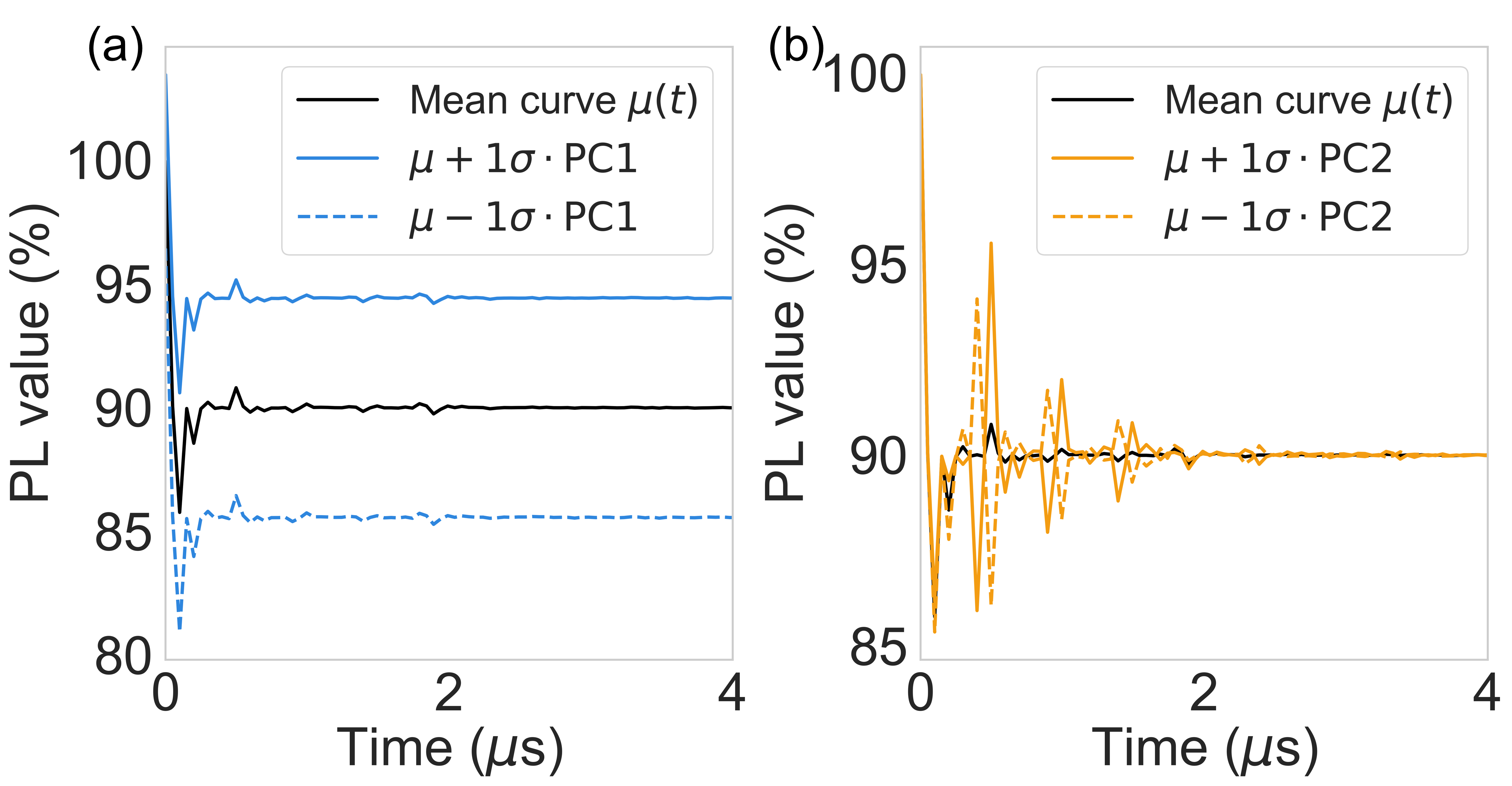
To interpret the leading principal components physically, we reconstruct time-domain modes around the empirical mean trace using
| (48) |
where is the th principal component and is the standard deviation of its score distribution. The corresponding reconstructions for the first two components are shown in Fig. 13(a,b).
Figure 13(a) indicates that predominantly captures a global normalized-PL contrast or baseline variation: varying the score along this mode mainly shifts the overall level of the Ramsey trace while preserving its gross oscillatory structure. This is consistent with the experimentally observed spread in readout contrast, where the reference level lies near 100 in normalized-PL units and the readout level typically falls in the – range, corresponding to an overall contrast span of roughly 10–25 percentage points of normalized PL.
By contrast, Fig. 13(b) shows that primarily modulates the oscillatory structure of the trace rather than its global offset. In particular, motion along this component changes the relative beating pattern and local oscillation content, consistent with variations in hyperfine-induced frequency components arising from different nearby configurations. In this sense, the first two principal components separate two experimentally relevant forms of variability: a dominant contrast/baseline degree of freedom (PC1) and a leading oscillatory-structure degree of freedom (PC2).
Appendix E Relation of RMSE to Residual-based Fitting Metrics
The denoising metric used in the main text is the root-mean-square error (RMSE) between the denoised trace and the high-SNR reference trace . Writing the pointwise residuals as
| (49) |
one has
| (50) |
so the metric is simply the mean squared residual expressed in percentage points of normalized PL.
This quantity is the unweighted analogue of the residual measures that enter standard least-squares diagnostics. In a weighted analysis, one instead defines
| (51) |
with the experimental uncertainty at time point and the number of degrees of freedom. Our use of RMSE avoids imposing a specific uncertainty model during denoiser evaluation, while preserving a direct interpretation as the typical residual mismatch to the experimental reference trace. Lower RMSE therefore implies improved compatibility with downstream residual-based fitting of , detuning, and hyperfine-structure parameters.
Appendix F Deep Learning Model Structure details
F.1 Detailed architecture of the denoising network
Input representation.
Each Ramsey trace consists of 200 uniformly sampled time points and is treated as a single-channel one-dimensional signal. During training and inference, traces are processed in mini-batches. For a batch of input traces, the time-domain input to the denoiser is therefore represented as a tensor of shape .
Stage 1: frequency-domain coarse denoising.
In the first stage, each input trace is transformed to the spectral domain using a real fast Fourier transform (rFFT). For a length-200 real-valued signal, this produces 101 complex frequency bins. We represent this complex spectrum using two real-valued channels corresponding to the real and imaginary parts, yielding an input tensor of shape .
The spectral tensor is then passed through a compact 1D UNet that performs coarse denoising directly in frequency space. The network outputs a denoised spectral representation with the same shape as the input. An inverse real Fourier transform maps this output back to the time domain, producing a coarse waveform reconstruction of shape . This stage is designed primarily to suppress broadband noise while retaining the narrowband spectral content associated with Ramsey beating.
Stage 2: time-domain refinement.
The coarse time-domain reconstruction from Stage 1 is then used as the input to a second denoising network operating directly in the time domain. This stage performs waveform-to-waveform refinement, removing residual local artifacts that remain after the spectral pass and improving recovery of the oscillatory envelope. In particular, this refinement stage helps preserve weak phase-coherent modulations that may be partially distorted by frequency-domain denoising alone.
F.2 Multi-head self-attention used at the UNet bottlenecks
At the bottleneck of each 1D UNet we apply standard multi-head self-attention (MHA) [62]. Let denote the bottleneck representation written as a length- sequence of -dimensional tokens. MHA with heads computes queries, keys, and values by learned linear projections
| (52) |
and evaluates scaled dot-product attention per head,
| (53) |
where and the softmax is applied row-wise [62]. Head outputs are concatenated and projected,
| (54) |
followed by a residual connection and layer normalization [25, 7],
| (55) |
In our implementation we place this block only at the bottleneck (rather than at full resolution), which preserves the UNet inductive bias while enabling efficient non-local interactions; related design choices have been explored in attention-augmented UNet variants [13, 24].
F.3 Token construction, embeddings, and Transformer self-attention for the hyperfine predictor
This appendix specifies the exact tokenization and Transformer operations used by the hyperfine frequency predictor (Transformer head) in Sec. III.2.
Per-trace normalization.
For a single trace we compute
| (56) |
with a small for numerical stability.
Time and frequency tokens.
The time tokens are the scalar samples . The frequency tokens are derived from the real FFT of the normalized trace. Let
| (57) |
so that provides a log-magnitude summary of the 101 real-FFT bins for a length-200 sequence.
Metadata tokens and embedding dimension.
We prepend (i) a learnable classification token and (ii) scalar metadata tokens encoding global waveform factors (contrast/PL, , and optionally the offset detuning if used as an input token). Scalars are rescaled to comparable numeric ranges, e.g.
| (58) |
(and similarly for if included). Each scalar token is embedded into the common model dimension via a learned linear map. The full token sequence length is
| (59) |
where is the number of scalar metadata tokens used (typically for PL and , or if is also included). The embedded input is then
| (60) |
We add learned token-type embeddings (to distinguish classification, metadata, time, and frequency tokens) and learned positional embeddings along the sequence.
Transformer encoder and self-attention.
The embedded sequence is processed by a Transformer encoder [62]. For a layer input , multi-head self-attention forms queries, keys, and values by learned projections
| (61) |
and computes (for each head) scaled dot-product attention followed by head concatenation and an output projection:
| (62) |
We use the standard pre-normalization encoder form (LayerNorm before attention and before the feed-forward sublayer), which improves optimization stability for moderate depth. The sequence-level representation is taken as the final classification embedding [16, 18, 59],
| (63) |
and is fed to the count and hyperfine regression heads described in Sec. III.2.
Appendix G Supplementary Results
G.1 False-Positive Test on the denoised result
To verify that the denoiser does not hallucinate Ramsey-like structure when no physical signal is present, we perform a false-positive control using pure-noise inputs. Specifically, we generate random traces with the same length and scale as the experimental PL readout and provide an uncertainty channel set pointwise as , mirroring the shot-noise scaling used elsewhere in our pipeline. These noise-only traces are then passed through the full denoising model (core+adapters). Figure 14 shows that most of the network outputs the noise signals, rather than producing oscillatory envelopes or beating patterns that could be misinterpreted as hyperfine signatures. The corresponding frequency-domain check further supports this conclusion: the rFFT magnitudes of the model outputs exhibit strong suppression of broadband components without introducing narrowband peaks. Together, these results indicate that the denoiser is not simply a generic oscillation generator; instead, it remains conservative on unstructured inputs and preferentially preserves oscillatory content only when it is supported by coherent structure in the input data.

G.2 More result on Experimental Hyperfine Prediction and reconstruction
To complement the representative examples shown in the main text (Fig. 8), we provide additional qualitative results illustrating the consistency of the hyperfine-parameter estimator across the held-out experimental test set. Figure 15 shows multiple randomly selected reconstructions for each NV center, where predicted hyperfine parameters (obtained from the denoised traces) are used to forward reconstruct the Ramsey response. Across these examples, the reconstructions reproduce the dominant oscillatory content and the main frequency-band structure observed in the reference traces, supporting the conclusion that the estimator recovers physically meaningful hyperfine information.

References
- [1] (2019) Atomic-scale imaging of a 27-nuclear-spin cluster using a quantum sensor. Nature 576 (7787), pp. 411–415. Cited by: §B.1.
- [2] (1961) The principles of nuclear magnetism. Clarendon Press. External Links: ISBN 9780198520146 Cited by: §B.2.
- [3] (1985) A learning algorithm for boltzmann machines. Cognitive science 9 (1), pp. 147–169. Cited by: §III.2.1.
- [4] (2012) Stable three-axis nuclear-spin gyroscope in diamond. Physical Review A—Atomic, Molecular, and Optical Physics 86 (6), pp. 062104. Cited by: §I.
- [5] (2018) Quantum technologies with optically interfaced solid-state spins. Nat. Photonics 12 (9), pp. 516–527. External Links: Document, Link Cited by: §B.2, §I, §I.
- [6] (2022) Contextual attention network: transformer meets u-net. In International workshop on machine learning in medical imaging, pp. 377–386. Cited by: §I.
- [7] (2016) Layer normalization. In NIPS 2016 Deep Learning Workshop, Cited by: §F.2.
- [8] (2015) Neural machine translation by jointly learning to align and translate. In 3rd International Conference on Learning Representations, ICLR 2015, San Diego, CA, USA, May 7-9, 2015, Conference Track Proceedings, Y. Bengio and Y. LeCun (Eds.), External Links: Link Cited by: §I.
- [9] (1987) Supervised learning of probability distributions by neural networks. In Neural information processing systems, Cited by: §III.2.1.
- [10] (2019) Attention augmented convolutional networks. In 2019 IEEE/CVF International Conference on Computer Vision (ICCV), External Links: Document, Link Cited by: §III.1.1.
- [11] (1964) An analysis of transformations. Journal of the Royal Statistical Society: Series B (Methodological) 26 (2), pp. 211–252. External Links: Document, Link Cited by: §III.2.1.
- [12] (1989) Training stochastic model recognition algorithms as networks can lead to maximum mutual information estimation of parameters. Advances in neural information processing systems 2. Cited by: §III.2.1.
- [13] (2021) TransUNet: transformers make strong encoders for medical image segmentation. arXiv. External Links: Document, Link Cited by: §F.2.
- [14] (2006) Coherent dynamics of coupled electron and nuclear spin qubits in diamond. Science 314 (5797), pp. 281–285. External Links: Document, Link Cited by: §B.2, §I.
- [15] (2017) Quantum sensing. Rev. Mod. Phys. 89, pp. 035002. External Links: Document, Link Cited by: §I, §I.
- [16] (2019) BERT: pre-training of deep bidirectional transformers for language understanding. In Proceedings of the 2019 Conference of the North American Chapter of the Association for Computational Linguistics: Human Language Technologies (NAACL-HLT), Volume 1, pp. 4171–4186. External Links: Document, Link Cited by: §F.3, §III.2.1.
- [17] (2013) The nitrogen-vacancy colour centre in diamond. Phys. Rep. 528 (1), pp. 1–45. External Links: Document, Link Cited by: §B.2, §I, §I.
- [18] (2021) An image is worth 16x16 words: transformers for image recognition at scale. In International Conference on Learning Representations (ICLR), External Links: Document, Link Cited by: §F.3, §III.2.1.
- [19] (2016) The importance of skip connections in biomedical image segmentation. In International workshop on deep learning in medical image analysis, pp. 179–187. Cited by: §I.
- [20] (2020) DDSP: differentiable digital signal processing. In International Conference on Learning Representations (ICLR), External Links: Link Cited by: §III.1.2.
- [21] (2015) Fast r-cnn. In Proceedings of the IEEE international conference on computer vision, pp. 1440–1448. Cited by: §III.2.1, §III.2.1.
- [22] (2013) Nanoscale magnetic imaging of a single electron spin under ambient conditions. Nat. Phys. 9 (4), pp. 215–219. External Links: Document, Link Cited by: §I.
- [23] (2025-09) DeepSeek-r1 incentivizes reasoning in llms through reinforcement learning. Nature 645 (8081), pp. 633–638. External Links: ISSN 1476-4687, Link, Document Cited by: §I.
- [24] (2022) UNETR: transformers for 3d medical image segmentation. In 2022 IEEE/CVF Winter Conference on Applications of Computer Vision (WACV), pp. 1748–1758. External Links: Document, Link Cited by: §F.2.
- [25] (2016) Deep residual learning for image recognition. In 2016 IEEE Conference on Computer Vision and Pattern Recognition (CVPR), External Links: Document, Link Cited by: §F.2.
- [26] (2016) Gaussian error linear units (gelus). arXiv:1606.08415. Cited by: §III.2.1.
- [27] (2020) Denoising diffusion probabilistic models. Advances in neural information processing systems 33, pp. 6840–6851. Cited by: §I.
- [28] (1987) Learning algorithms and probability distributions in feed-forward and feed-back networks. Proceedings of the national academy of sciences 84 (23), pp. 8429–8433. Cited by: §III.2.1.
- [29] (2018) Spin readout techniques of the nitrogen-vacancy center in diamond. Micromachines 9 (9), pp. 437. External Links: Document, Link Cited by: §I.
- [30] (1933) Analysis of a complex of statistical variables into principal components. Journal of Educational Psychology 24, pp. 417–441. External Links: Document, Link Cited by: §II.3.
- [31] (1992) Robust estimation of a location parameter. In Breakthroughs in statistics: Methodology and distribution, pp. 492–518. Cited by: §III.2.1, §III.2.1.
- [32] (2015) Batch normalization: accelerating deep network training by reducing internal covariate shift. In Proceedings of the 32nd International Conference on Machine Learning (ICML), Proceedings of Machine Learning Research, Vol. 37, pp. 448–456. External Links: Link Cited by: §III.2.1.
- [33] (2021) Demonstration of diamond nuclear spin gyroscope. Science advances 7 (43), pp. eabl3840. Cited by: §I.
- [34] (2006) Single defect centres in diamond: a review. Phys. Status Solidi A 203 (13), pp. 3207–3225. External Links: Document, Link Cited by: §I.
- [35] (2021) Deep learning enhanced individual nuclear-spin detection. npj Quantum Information 7 (1), pp. 41. Cited by: §I.
- [36] (2025-12) Optical readout of coherent nuclear spins in diamond coupled to electronic spins in a thermal state. Phys. Rev. Appl. 24, pp. 064059. External Links: Document, Link Cited by: §I.
- [37] (2026) QuTiP 5: the quantum toolbox in Python. Physics Reports 1153, pp. 1–62. External Links: ISSN 0370-1573, Document, Link Cited by: §II.2.
- [38] (1988) Accelerated learning in layered neural networks. Complex systems 2 (625-640), pp. 3. Cited by: §III.2.1.
- [39] (2016) Ssd: single shot multibox detector. In European conference on computer vision, pp. 21–37. Cited by: §III.2.1, §III.2.1.
- [40] (2019) Decoupled weight decay regularization. External Links: 1711.05101, Link Cited by: Appendix A.
- [41] (2015) Coherent control of a nitrogen-vacancy center spin ensemble with a diamond mechanical resonator. Optica 2 (3), pp. 233–238. External Links: Document, Link Cited by: §I.
- [42] (2012) A robust scanning diamond sensor for nanoscale imaging with single nitrogen-vacancy centres. Nat. Nanotechnol. 7 (5), pp. 320–324. External Links: Document, Link Cited by: §I.
- [43] (2008) Nanoscale magnetic sensing with an individual electronic spin in diamond. Nature 455 (7213), pp. 644–647. External Links: Document, Link Cited by: §I.
- [44] (2011) Quantum measurement and orientation tracking of fluorescent nanodiamonds inside living cells. Nat. Nanotechnol. 6 (6), pp. 358–363. External Links: Document, Link Cited by: §I.
- [45] (2022) Training language models to follow instructions with human feedback. External Links: 2203.02155, Link Cited by: §I.
- [46] (2014) Dynamic strain-mediated coupling of a single diamond spin to a mechanical resonator. Nat. Commun. 5, pp. 4429. External Links: Document, Link Cited by: §I.
- [47] (1901) LIII. on lines and planes of closest fit to systems of points in space. The London, Edinburgh, and Dublin Philosophical Magazine and Journal of Science 2 (11), pp. 559–572. External Links: Document, Link Cited by: §II.3, §II.3.
- [48] (2014) Magnetometry with nitrogen-vacancy defects in diamond. Rep. Prog. Phys. 77 (5), pp. 056503. External Links: Document, Link Cited by: §I, §I.
- [49] (2015) U-net: convolutional networks for biomedical image segmentation. In International Conference on Medical image computing and computer-assisted intervention, pp. 234–241. Cited by: §I, §III.1.1.
- [50] (1986) Learning representations by back-propagating errors. nature 323 (6088), pp. 533–536. Cited by: §III.2.2.
- [51] (2014) Nitrogen-vacancy centers in diamond: nanoscale sensors for physics and biology. Annu. Rev. Phys. Chem. 65, pp. 83–105. External Links: Document, Link Cited by: §I.
- [52] (2019) Temporal pattern attention for multivariate time series forecasting. Machine Learning 108 (8), pp. 1421–1441. Cited by: §I.
- [53] (2021) Nuclear spin gyroscope based on the nitrogen vacancy center in diamond. Physical Review Letters 126 (19), pp. 197702. Cited by: §I.
- [54] (2014) Universal control and error correction in multi-qubit spin registers in diamond. Nat. Nanotechnol. 9 (3), pp. 171–176. External Links: Document, Link Cited by: §I, §I.
- [55] (2012) Detection and control of individual nuclear spins using a weakly coupled electron spin. Phys. Rev. Lett. 109, pp. 137602. External Links: Document, Link Cited by: §I, §I.
- [56] (2008) High-sensitivity diamond magnetometer with nanoscale resolution. Nat. Phys. 4 (10), pp. 810–816. External Links: Document, Link Cited by: §I.
- [57] (2014) Strain coupling of a nitrogen-vacancy center spin to a diamond mechanical oscillator. Phys. Rev. Lett. 113, pp. 020503. External Links: Document, Link Cited by: §I.
- [58] (2018) Spin properties of dense near-surface ensembles of nitrogen-vacancy centers in diamond. Phys. Rev. B 97, pp. 085402. External Links: Document, Link Cited by: §I.
- [59] (2021) Training data-efficient image transformers & distillation through attention. In Proceedings of the 38th International Conference on Machine Learning (ICML), Proceedings of Machine Learning Research, Vol. 139, pp. 10347–10357. External Links: Link Cited by: §F.3, §III.2.1.
- [60] (2024) Digital signal processing (lecture slides). Note: See slide section defining DC component as the mean and AC component as signal minus mean External Links: Link Cited by: §III.1.2.
- [61] (2024) Automatic detection of nuclear spins at arbitrary magnetic fields via signal-to-image ai model. Physical Review Letters 132 (15), pp. 150801. Cited by: §I.
- [62] (2017) Attention is all you need. Advances in neural information processing systems 30. Cited by: §F.2, §F.2, §F.3, §I, §III.1.1, §III.2.1.
- [63] (2024-10) Hyperfine-enhanced gyroscope based on solid-state spins. Phys. Rev. Lett. 133, pp. 150801. External Links: Document, Link Cited by: §I.
- [64] (2018) Non-local neural networks. In 2018 IEEE/CVF Conference on Computer Vision and Pattern Recognition (CVPR), pp. 7794–7803. External Links: Document, Link Cited by: §III.1.1.
- [65] (2023) META-unet: multi-scale efficient transformer attention unet for fast and high-accuracy polyp segmentation. IEEE Transactions on Automation Science and Engineering 21 (3), pp. 4117–4128. Cited by: §I.
- [66] (2023) Noise prediction and reduction of single electron spin by deep-learning-enhanced feedforward control. Nano Letters 23 (7), pp. 2460–2466. Cited by: §I.
- [67] (2020) Parallel WaveGAN: a fast waveform generation model based on generative adversarial networks with multi-resolution spectrogram. In Proceedings of the 2020 IEEE International Conference on Acoustics, Speech and Signal Processing (ICASSP), pp. 6199–6203. External Links: Document, Link Cited by: §III.1.2, §III.1.2.