Neural Field Thermal Tomography: A Differentiable Physics Framework for Non-Destructive Evaluation

Tao Zhong¹, Yixun Hu¹, Dongzhe Zheng¹, Aditya Sood¹, Christine Allen-Blanchette¹
¹Princeton University
{tzhong, ca15}@princeton.edu

Abstract

Inverse problems for stiff parabolic partial differential equations (PDEs), such as the inverse heat conduction problem (IHCP), are severely ill-posed: the forward map rapidly damps high-frequency interior structure before it reaches the boundary. Soft-constrained physics-informed neural networks (PINNs), which embed the PDE as a residual penalty, suffer from gradient pathology in this regime and tend to fit boundary measurements while leaving the interior field essentially untouched. We propose Neural Field Thermal Tomography (NeFTY), a hard-constrained neural field framework for label-free three-dimensional inverse heat conduction. NeFTY represents the unknown diffusivity as a continuous coordinate-based neural network, and at every optimization step passes the candidate field through a differentiable implicit-Euler heat solver with harmonic-mean interface flux, so that the governing PDE holds exactly on the discretization rather than as a soft penalty. Adjoint gradients propagate the surface reconstruction error back to the network weights at solver-level memory cost, making test-time inversion tractable on a single GPU. Across synthetic 3D benchmarks, NeFTY substantially outperforms soft-constrained PINN variants and a voxel-grid baseline on label-free volumetric recovery, and it transfers to real thermography data, surpassing classical signal-processing baselines in both defect segmentation and depth estimation. Additional details at cab-lab-princeton.github.io/nefty.

1 Introduction

Inverse problems for stiff parabolic partial differential equations (PDEs) are central to scientific machine learning, yet they remain among the hardest to solve from observations alone. The forward heat operator is compact and strongly smoothing: high spatial frequencies in the interior are damped before they reach the boundary, so the map from internal material properties to surface measurements destroys much of the information needed to invert it [19, 16]. Soft physics-informed losses can fit boundary data without recovering the underlying field, because their gradients become poorly conditioned and dominated by the surface signal in this stiff regime [44, 55]. A complementary line of work in differentiable physics builds the discretized solver directly into the optimization loop, so that the governing equations hold as a hard constraint at every step rather than as a residual penalty in the objective [37, 24, 23, 11]. We apply this paradigm to the canonical case of the three-dimensional inverse heat conduction problem (IHCP).

Non-destructive testing (NDT) by pulsed thermography is the working example throughout (Figure 1). A pulsed laser deposits energy on the specimen surface, and a high-speed camera records the subsequent surface temperature decay; subsurface delaminations, voids, and inclusions perturb the diffusive flux and leave faint thermal contrast on the boundary [28, 46, 41]. Reconstructing the volumetric thermal diffusivity field $\alpha(x,y,z)$ from these surface signals is the inverse heat conduction problem. Unlike hyperbolic ultrasonic or radar imaging [4, 54], the parabolic forward map damps

Refer to caption — Figure 1: IHCP setup. A high-speed camera measures the transient surface temperature following pulsed laser heating; NeFTY reconstructs the 3D subsurface diffusivity field from these measurements.

internal features rapidly with depth, so small surface perturbations can correspond to large interior variations and the inverse map becomes severely ill-posed [29, 43].

Existing approaches do not address this volumetric inversion well. Classical thermography pipelines, including Thermographic Signal Reconstruction (TSR) [50, 49], Pulsed Phase Thermography (PPT) [32], and the Virtual Wave Concept (VWC) [3, 1], transform the temporal data into domains where defect contrast is enhanced, but they reduce to 1D pixel-wise inversions that ignore lateral diffusion and bias estimates for shallow or low-aspect-ratio defects [42]. Soft-constrained physics-informed neural networks (PINNs) target the volumetric problem in principle, yet they inherit the gradient pathology that limits these methods in stiff transient diffusion: the PDE residual is high and rugged, so the optimizer makes progress on the surface-data term while the diffusivity network saturates at a near-trivial field that explains the boundary measurements without recovering the bulk [55]. Supervised volumetric learning sidesteps these issues but requires 3D ground-truth labels that are unavailable in real NDT.

To this end, we introduce Neural Field Thermal Tomography (NeFTY), a hard-constrained neural field framework for label-free 3D inverse heat conduction. NeFTY represents the unknown diffusivity as a continuous coordinate-based neural network [52, 34] with positional encoding, frequency annealing, and a bounded output. At every optimization step, the candidate field is passed through a differentiable implicit-Euler heat solver with harmonic-mean interface flux, so the heat equation holds exactly on the discretization rather than as a soft penalty. Adjoint gradients propagate the surface reconstruction error back to the network weights at solver-level memory cost, making test-time inversion tractable on a single GPU. On synthetic homogeneous and layered settings, NeFTY reaches volumetric IoU of $0.45$ and $0.37$ , while soft-constrained PINN variants and a voxel-grid baseline remain at or near zero, and it outperforms classical thermography baselines on real PVC thermal data in both 2D defect segmentation and 2.5D depth recovery.

We summarize our contributions as follows:

•

We propose a hard-constrained neural field formulation for label-free 3D inverse heat conduction from surface-only thermal sequences, combining a continuous coordinate-based prior with a differentiable implicit heat solver and adjoint gradients.
•

We give an empirical and theoretical account of why soft-constrained PINNs fail on stiff parabolic inverse problems, demonstrating across several modern PINN variants that low surface error does not imply correct volumetric recovery.
•

We carry out a comprehensive evaluation that pairs synthetic 3D label-free reconstruction with real PVC thermal data, soft-constrained PINN baselines, frequency- and edge-domain diagnostics, component ablations, and a wall-clock and memory analysis of the adjoint solver.

2 Related Work

Thermographic Non-Destructive Testing traditionally extracts subsurface defect information through signal-processing transforms applied to surface temperature decays. Thermographic Signal Reconstruction (TSR) [50, 49] fits log-time polynomials to enhance defect contrast, Pulsed Phase Thermography (PPT) [32, 9] maps the decays into a frequency phase domain that suppresses noise and emissivity variations, and the Virtual Wave Concept (VWC) [3, 48, 1] deconvolves the diffusive forward map into a pseudo-wave for depth estimation. Quantitative-thermography refinements push these heuristics further with calibrated depth correlations [31, 42], but the underlying inverse mappings remain pixel-wise and amplify high-frequency measurement noise. In parallel, supervised convolutional pipelines based on U-Net [45, 36, 51, 15] learn defect masks directly from thermal sequences, and several recent surveys [41, 28, 46] catalogue this growing detection-only literature. Both lines stop short of the volumetric inverse problem: signal-processing transforms ignore lateral heat flux, and supervised models require 3D diffusivity labels that are unavailable in real NDT. NeFTY recovers a full 3D diffusivity field directly from the surface sequence, without volumetric labels and without 1D pixel-wise approximations.

Physics-Informed Neural Networks embed governing equations as soft penalties alongside data terms in scientific machine learning. Standard PINNs [44, 5, 29] jointly minimize boundary fit and a PDE residual, and a series of variants attack the resulting optimization pathologies: separable architectures in SPINN [8] scale up collocation throughput, temporal-causality weighting in Causal-PINN [56] stabilizes long-horizon transients, and dual-cone gradient descent in DCGD [25] resolves residual-versus-data gradient conflicts. Diagnostic studies [55, 20] nonetheless trace recurring failures to the soft-penalty formulation itself, where stiff PDE residuals dominate the data signal and induce spectral bias against deep high-frequency features even with adaptive loss balancing such as GradNorm [7]. A complementary line replaces the penalty with a differentiable solver: discretize-then-optimize [37], differentiable PDE engines [24, 23, 2], and end-to-end differentiable physics for control and robotics [11, 12, 53, 61] all enforce the governing equations exactly at every optimization step. This solver-in-the-loop paradigm has yet to be applied to thermal IHCP. NeFTY closes the gap by composing a coordinate-based diffusivity field with a differentiable implicit-Euler heat solver, so the heat equation holds as a hard constraint at every iteration and gradients propagate through a numerically stable adjoint.

Coordinate-based Neural Fields parameterize a continuous signal as a multilayer perceptron (MLP) over spatial coordinates, typically combined with positional encoding or sinusoidal activations. SIREN [52] and NeRF [34] established neural fields as a high-frequency representation prior for visual signals, and deformable extensions such as Nerfies [38] broadened the class of recoverable scenes. Scientific imaging has begun to adopt the same representation for tomographic and field-reconstruction problems, including X-ray computed tomography [60, 62], dynamic medical imaging via ProxNF [30], and fluid scalar fields with FluidNeRF [27]. These works contribute a continuous, mesh-free function space, but the representation alone is agnostic to physics: nothing in the parameterization enforces that the reconstructed field obeys a governing PDE. NeFTY treats the neural field strictly as the diffusivity prior and couples it with a differentiable heat solver, so the scientific contribution rests on hard physics constraints rather than on the representation itself.

3 Forward Model, Ill-Posedness, and Soft-Constraint Pathology

3.1 Forward model and effective-diffusivity parameterization

The conservation form of transient heat conduction in an isotropic medium is posed on a bounded Lipschitz domain $\Omega\subset\mathbb{R}^{3}$ , with boundary $\partial\Omega$ and observation window $\Gamma_{\mathrm{obs}}\subseteq\partial\Omega$ , as follows:

\rho(\mathbf{x})C_{p}(\mathbf{x})\,\partial_{t}T\;=\;\nabla\cdot\big(k(\mathbf{x})\,\nabla T\big)+Q(\mathbf{x},t),\qquad\mathbf{x}\in\Omega,\;t\in(0,t_{\mathrm{end}}],

(1)

with mass density $\rho$ , specific heat capacity $C_{p}$ , thermal conductivity $k$ , and source $Q$ ( $Q\equiv 0$ post flash). Dividing (1) by $\rho C_{p}$ and applying the product rule gives the equivalent diffusivity form

\partial_{t}T\;=\;\nabla\cdot\big(\alpha(\mathbf{x})\nabla T\big)\;-\;k(\mathbf{x})\,\nabla T\cdot\nabla\!\big(\tfrac{1}{\rho C_{p}}\big),\qquad\alpha(\mathbf{x}):=\frac{k(\mathbf{x})}{\rho(\mathbf{x})C_{p}(\mathbf{x})},

(2)

valid when $\rho,C_{p}\in C^{1}(\Omega)$ are strictly positive (Appendix A.1). When $\rho C_{p}$ is piecewise-constant with bulk and defect phases separated by an interface set $\Sigma$ , the second term in (2) vanishes a.e. on $\Omega\setminus\Sigma$ and concentrates as a singular flux jump on $\Sigma$ that a finite-volume grid cannot represent [40]. NeFTY therefore parameterizes a single effective field $\alpha(\mathbf{x})$ obeying $\partial_{t}T=\nabla\cdot(\alpha\nabla T)$ on $\Omega\setminus\Sigma$ and recovers continuity of the reduced $\alpha$ -flux at cell faces through the harmonic mean.

Proposition 1 (Harmonic mean as discrete interface continuity for the effective- $\alpha$ flux).

For a one-dimensional cell pair with constant cell-centered diffusivities $\alpha_{i},\alpha_{i+1}$ , cell spacing $\Delta x$ , cell-centered temperatures $T_{i},T_{i+1}$ , and effective $\alpha$ -flux $j_{\alpha}:=-\alpha\partial_{x}T$ , the unique flux satisfying continuity across the cell face $x_{i+1/2}$ is $j_{\alpha}=-\bar{\alpha}_{i+1/2}(T_{i+1}-T_{i})/\Delta x$ with $\bar{\alpha}_{i+1/2}=2\alpha_{i}\alpha_{i+1}/(\alpha_{i}+\alpha_{i+1})$ .

The proof, multi-dimensional consequence, and high-contrast behavior are in Appendix A; synthetic and real-PVC initial and boundary condition settings are specified in Appendix A.5.

3.2 The inverse problem and its ill-posedness

The IHCP recovers $\alpha$ from noisy surface measurements $\hat{T}(\mathbf{x},t_{i})$ , $\mathbf{x}\in\Gamma_{\mathrm{obs}}$ , $t_{i}\in\{t_{1},\dots,t_{M}\}\subset(0,t_{\mathrm{end}}]$ . Let $\mathcal{K}(\alpha):=T_{\alpha}|_{\Gamma_{\mathrm{obs}}\times(0,t_{\mathrm{end}})}$ denote the parameter-to-observation operator (with $T_{\alpha}$ the

solution of (2) under fixed initial and lateral boundary conditions) acting on the admissible set $\mathcal{A}\subset H^{1}(\Omega)\cap L^{\infty}(\Omega)$ . The reconstruction objective is

	$\displaystyle\alpha^{*}$	$\displaystyle=\;\arg\min_{\alpha\in\mathcal{A}}\,\mathcal{J}(\alpha),$		(3)
	$\displaystyle\mathcal{J}(\alpha)$	$\displaystyle=\;\sum_{i=1}^{M}\big\\|\mathcal{K}(\alpha)(\cdot,t_{i})-\hat{T}(\cdot,t_{i})\big\\|_{\Gamma_{\mathrm{obs}}}^{2}+\lambda\mathcal{R}(\alpha),$		(3)

with $\|\cdot\|_{\Gamma_{\mathrm{obs}}}$ the $L^{2}$ norm over $\Gamma_{\mathrm{obs}}$ , $\mathcal{R}$ a regularization functional, and $\lambda>0$ . The IHCP is widely recognized as one of the most severely ill-posed problems in mathematical physics [19, 33, 14]; we make the failure quantitative.

Proposition 2 (Compactness and algebraic singular-value decay).

Let $\alpha_{0}>0$ be a constant background diffusivity with $\nabla T_{\alpha_{0}}\in L^{\infty}(\Omega\times(0,t_{\mathrm{end}}))$ . The Fréchet derivative $d\mathcal{K}_{\alpha_{0}}:H^{1}(\Omega)\to L^{2}(\Gamma_{\mathrm{obs}}\times(0,t_{\mathrm{end}}))$ is bounded and compact, with singular values $\sigma_{n}\leq C\,(1+\lambda_{n})^{-1/2}$ , where $\{\lambda_{j}\}_{j\geq 0}$ are the Laplacian eigenvalues on $\Omega$ under the imposed boundary conditions; on the slab, Weyl’s law gives $\sigma_{n}\lesssim n^{-1/3}$ .

Corollary 1 (Hadamard ill-posedness).

The pseudo-inverse $d\mathcal{K}_{\alpha_{0}}^{\dagger}$ is unbounded, with $\sigma_{n}^{-1}\geq C^{-1}(1+\lambda_{n})^{1/2}$ amplifying noise along the $n$ -th left singular vector.

Proof in Appendix B; Figure 2 visualizes the smoothing. NeFTY counters this with a neural-field prior plus frequency annealing (Section 4) and a total-variation penalty $\mathcal{R}(\alpha)$ .

3.3 Soft-constraint pathology in stiff parabolic inversion

A standard PINN approximates the inverse map by jointly optimizing two networks: a temperature surrogate $T_{\phi}(\mathbf{x},t)$ with parameters $\phi$ and a diffusivity surrogate $\alpha_{\theta}(\mathbf{x})$ with parameters $\theta$ , against

\mathcal{L}_{\mathrm{PINN}}\;=\;\underbrace{\|T_{\phi}-\hat{T}\|^{2}_{\Gamma_{\mathrm{obs}}}}_{\mathcal{L}_{\mathrm{data}}}+\lambda_{\mathrm{PDE}}\underbrace{\|\partial_{t}T_{\phi}-\nabla\cdot(\alpha_{\theta}\nabla T_{\phi})\|^{2}_{\Omega}}_{\mathcal{L}_{\mathrm{PDE}}}+\lambda_{\mathrm{IC}}\underbrace{\|T_{\phi}(\cdot,0)-T_{0}\|^{2}_{\Omega}}_{\mathcal{L}_{\mathrm{IC}}},

(4)

with weights $\lambda_{\mathrm{PDE}},\lambda_{\mathrm{IC}}>0$ and $T_{0}$ the prescribed initial temperature field. Because $T_{\phi}$ is parameterized by $\phi$ alone, $\nabla_{\theta}\mathcal{L}_{\mathrm{data}}=\nabla_{\theta}\mathcal{L}_{\mathrm{IC}}=0$ , so the diffusivity update reduces to $\nabla_{\theta}\mathcal{L}_{\mathrm{PINN}}=\lambda_{\mathrm{PDE}}\nabla_{\theta}\mathcal{L}_{\mathrm{PDE}}$ , with magnitude controlled pointwise by the Laplacian $\Delta T_{\phi}$ of the under-fitted temperature surrogate. Appendix C gives the full derivation and shows that adaptive loss balancing (GradNorm), separable temperature parameterizations (SPINN), causal weighting (Causal-PINN), and gradient-conflict resolution (DCGD) all preserve this decoupling.

The decoupling is structural: surface observations cannot reach $\theta$ except indirectly through the residual penalty. Combined with the unbounded amplification in Corollary 1, this gives a plausible mechanism for the well-documented PINN training pathology in which $\mathcal{L}_{\mathrm{PDE}}$ shrinks while $\alpha_{\theta}$ remains near a trivial constant [55, 20], which we confirm empirically across all four PINN variants in Section 5. NeFTY removes the soft constraint at its source, so surface data propagates to $\alpha_{\theta}$ through the adjoint of the discretized heat operator.

4 Method

NeFTY recovers the diffusivity field by directly minimizing the reconstruction objective $\mathcal{J}$ of equation (3), with the heat equation enforced as a hard constraint at every optimization step rather than as a soft residual penalty. The framework couples three components, illustrated in Figure 3: (i) a continuous coordinate-based parameterization $\alpha_{\theta}(\mathbf{x})$ that supplies a low-dimensional differentiable prior, (ii) a finite-volume implicit-Euler discretization of the bulk equation (2) whose interface flux is restored by the harmonic-mean stencil of Proposition 1, and (iii) a discrete adjoint that propagates the surface-fidelity gradient back to $\theta$ through the same sparse system used in the forward pass. By construction, the discrete temperature at each step is the solution of the discretized PDE driven by $\alpha_{\theta}$ , so the gradient decoupling of Section 3.3 cannot occur.

4.1 Neural diffusivity field

NeFTY parameterizes the unknown effective diffusivity $\alpha_{\theta}:\Omega\to\mathbb{R}_{>0}$ as a coordinate multilayer perceptron (MLP) $f_{\theta}:\mathbb{R}^{d_{\gamma}}\to\mathbb{R}$ whose input is lifted through a Fourier feature map $\gamma:\mathbb{R}^{3}\to\mathbb{R}^{d_{\gamma}}$ :

\gamma(\mathbf{x})\;=\;\big(\sin(2^{0}\pi\mathbf{x}),\cos(2^{0}\pi\mathbf{x}),\dots,\sin(2^{N-1}\pi\mathbf{x}),\cos(2^{N-1}\pi\mathbf{x})\big),

(5)

of bandwidth $N$ . The encoding combats the spectral bias of plain MLPs and lets the network represent the sharp interfaces characteristic of subsurface defects [34, 52]. To stabilize the high-frequency components against the algebraic noise amplification of Corollary 1, we adopt the cosine frequency-annealing schedule of Park et al. [38], gradually unmasking encoding bands during training. The network output is hard-bracketed to the physically admissible range

\alpha_{\theta}(\mathbf{x})\;=\;\alpha_{\min}+(\alpha_{\max}-\alpha_{\min})\,\sigma\!\big(f_{\theta}(\gamma(\mathbf{x}))\big),

(6)

with $\sigma(\cdot)$ the logistic sigmoid; the bounds $\alpha_{\min},\alpha_{\max}>0$ are chosen to span the bulk-to-defect contrast of the application without inducing ill-conditioning in the discrete system below. We instantiate the regularizer in (3) as the isotropic total variation $\mathcal{R}(\alpha_{\theta})=\int_{\Omega}\|\nabla\alpha_{\theta}\|$ [47], consistent with the piecewise-constant defect structure of the effective-diffusivity model in Appendix A. The full architecture, the cosine annealing schedule, and the discrete TV form are given in Appendix D.1.

4.2 Hard-constrained differentiable physics

We discretize the bulk equation $\partial_{t}T=\nabla\cdot(\alpha\nabla T)$ on a uniform Cartesian grid covering $\Omega$ with spacings $\Delta x,\Delta y,\Delta z$ along the three axes and $N_{t}$ time steps of size $\Delta t$ aligned with the camera frame rate. Let $\mathbf{T}^{n}\in\mathbb{R}^{N_{g}}$ denote the discrete temperature at step $n$ on the $N_{g}$ grid nodes, and let $\bar{\alpha}_{i+1/2}$ denote the harmonic-mean face-centered diffusivity from Proposition 1. The second-order finite-volume diffusion operator $\mathbf{L}(\alpha_{\theta})\in\mathbb{R}^{N_{g}\times N_{g}}$ acts at an interior node by

{[\mathbf{L}(\alpha_{\theta})\mathbf{T}]}_{i,j,k}\;=\;\frac{1}{\Delta x^{2}}\!\left[\bar{\alpha}_{i+1/2}(T_{i+1,j,k}-T_{i,j,k})-\bar{\alpha}_{i-1/2}(T_{i,j,k}-T_{i-1,j,k})\right]+(\text{$y$-, $z$-terms}),

(7)

with lateral periodic and through-thickness adiabatic conditions (Appendix A.5) closing the stencil at the boundary. The harmonic-mean coefficient is the unique discrete realization of effective-flux continuity at interior faces for the single- $\alpha$ model (Proposition 1); an arithmetic mean would spuriously allow heat to leak across the interface [40]. All discrete temperatures here are interpreted as deviations from the ambient temperature (Appendix A.5), so the implicit-Euler step is affine-free.

To decouple the time step from the diffusivity contrast, we integrate in time with the unconditionally stable implicit Euler scheme [10], advancing $\mathbf{T}^{n}$ to $\mathbf{T}^{n+1}$ through the sparse linear system

\mathbf{A}(\alpha_{\theta})\,\mathbf{T}^{n+1}\;=\;\mathbf{T}^{n},\qquad\mathbf{A}(\alpha_{\theta})\;:=\;\mathbf{I}-\Delta t\,\mathbf{L}(\alpha_{\theta}).

(8)

The matrix $\mathbf{A}(\alpha_{\theta})$ is sparse, symmetric positive-definite for our boundary conditions, and depends on $\theta$ only through $\alpha_{\theta}$ . We solve (8) on the GPU through a fixed number $K$ of unrolled Jacobi iterations [22], expressed as stencil convolutions to fit seamlessly into autodiff frameworks [39]. The full discretization, choice of $K$ , and Jacobi update rule are given in Appendix D.2. At every optimization iteration, the temperature $\mathbf{T}^{n+1}$ produced by (8) satisfies the discrete heat equation up to the iterative solver tolerance.

4.3 Adjoint optimization

Composing the implicit Euler recurrence (8) from $\mathbf{T}^{0}$ defines $\mathbf{T}^{n}=\mathbf{T}^{n}(\alpha_{\theta})$ implicitly, hence the discrete analogue $\mathcal{K}_{\mathrm{disc}}$ of the parameter-to-observation map. Let $n_{i}\in\{1,\dots,N_{t}\}$ be chosen so that $t_{n_{i}}=t_{i}$ for each measurement time $t_{i}$ , and let $\boldsymbol{\Pi}_{\Gamma}:\mathbb{R}^{N_{g}}\to\mathbb{R}^{N_{\Gamma}}$ denote the row-selector matrix that extracts the $N_{\Gamma}$ surface samples on $\Gamma_{\mathrm{obs}}$ . NeFTY minimizes the discrete reconstruction objective

\min_{\theta}\;\;\mathcal{J}_{\mathrm{disc}}(\theta)\;=\;\sum_{i=1}^{M}\big\|\boldsymbol{\Pi}_{\Gamma}\mathbf{T}^{n_{i}}(\alpha_{\theta})-\hat{\mathbf{T}}_{i}\big\|^{2}\;+\;\lambda\,\mathcal{R}(\alpha_{\theta}),

(9)

the discretization of (3) with $\|\cdot\|$ the standard Euclidean norm on $\mathbb{R}^{N_{\Gamma}}$ (equal to the discrete $L^{2}(\Gamma_{\mathrm{obs}})$ norm up to the lateral quadrature weight $\Delta x\Delta y$ , which we absorb into the regularization weight $\lambda>0$ ), and $\mathcal{R}$ instantiated as the discrete total-variation regularizer of Appendix D.1; we keep the symbol $\lambda$ from (3) now in its TV-weight role. Because $\mathbf{T}^{n}$ is defined implicitly by the state equation (8), gradients $d\mathcal{J}_{\mathrm{disc}}/d\theta$ obtained by storing the full forward trajectory and applying backpropagation through time cost $\mathcal{O}(N_{g}N_{t})$ memory, which is prohibitive for the $N_{g}\approx 10^{5}$ , $N_{t}\approx 10^{2}$ regime of pulsed thermography. We use the discrete adjoint method instead [6, 37].

Treat (8) as the constraint $\mathbf{F}^{n}(\mathbf{T}^{n},\mathbf{T}^{n-1},\alpha_{\theta}):=\mathbf{A}(\alpha_{\theta})\mathbf{T}^{n}-\mathbf{T}^{n-1}=\mathbf{0}$ for $n=1,\dots,N_{t}$ , and introduce adjoint variables $\boldsymbol{\mu}^{n}$ as Lagrange multipliers for each step. Setting the total derivative of the augmented Lagrangian with respect to $\mathbf{T}^{n}$ to zero yields the backward-in-time recurrence

\mathbf{A}(\alpha_{\theta})^{\top}\boldsymbol{\mu}^{n}\;=\;\boldsymbol{\mu}^{n+1}+\big(\partial\ell^{n}/\partial\mathbf{T}^{n}\big)^{\top},\qquad\boldsymbol{\mu}^{N_{t}+1}\;=\;\mathbf{0},

(10)

where $\ell^{n}$ collects the data-fidelity terms in (9) that depend on $\mathbf{T}^{n}$ (nonzero only at measurement frames $n\in\{n_{1},\dots,n_{M}\}$ ). The adjoint at step $n$ uses the transpose of the same sparse $\mathbf{A}$ that drives the forward solve, so a single backward sweep with the same Jacobi inner loop yields all $\boldsymbol{\mu}^{n}$ at the cost of one forward pass. The parameter gradient is then assembled by

\frac{d\mathcal{J}_{\mathrm{disc}}}{d\theta}\;=\;\frac{\partial(\lambda\mathcal{R})}{\partial\theta}\;+\;\Delta t\,\sum_{n=1}^{N_{t}}(\boldsymbol{\mu}^{n})^{\top}\,\frac{\partial\!\left(\mathbf{L}(\alpha_{\theta})\mathbf{T}^{n}\right)}{\partial\alpha_{\theta}}\,\frac{\partial\alpha_{\theta}}{\partial\theta},

(11)

where $\partial\alpha_{\theta}/\partial\theta$ is the standard MLP Jacobian. Because (10) requires only $\boldsymbol{\mu}^{n+1}$ and $\mathbf{T}^{n}$ , the backward sweep has constant memory in $N_{t}$ . The full Lagrangian construction, the derivation of (10)–(11), and the consistency with the continuous adjoint of the bulk equation are given in Appendix D.3; the implementation hyperparameters (depth, width, encoding bandwidth $N$ , grid resolution, Jacobi count $K$ , and optimizer schedule) are catalogued in Appendix D.4. Crucially, the data-side gradient on $\theta$ is non-vanishing precisely because $\boldsymbol{\Pi}_{\Gamma}\mathbf{T}^{n_{i}}$ is now a function of $\theta$ , restoring the dependency chain $\theta\to\alpha_{\theta}\to\mathbf{T}^{n}\to\mathcal{J}_{\mathrm{disc}}$ that the soft-PINN formulation of Section 3.3 broke.

5 Experiments

5.1 Setup

Datasets. Synthetic data are generated with PhiFlow [23], a finite-volume engine independent of the implicit-Euler Jacobi solver of Section 4.2, so reconstruction is not subject to inverse crime; the real PVC datasets [59, 58] provide only 2D defect masks and discrete defect depths from CAD, so real-world evaluation uses projected 2D masks and 2.5D depth annotations rather than 3D volumetric labels. The synthetic benchmark contains $1{,}000$ samples on the unitless slab $\Omega=[0,10]^{2}\times[0,1]$ at $64\times 64\times 16$ resolution, $100$ frames at $\Delta t=0.05$ , and one to four subsurface defects per sample, split into a homogeneous and a layered configuration. Full data-generation procedure, dimensional analysis, and compute resources are in Appendix E.

Baselines. On synthetic data we compare to direct grid optimization (Grid Opt.), PINN [44] with GradNorm [7], SPINN [8], Causal-PINN [56], DCGD [25], and a Sound-Only U-Net [45] that trains on only defect-free samples and probes data-driven generalization to out-of-distribution defects. On real PVC data we additionally compare to the classical thermography heuristics PPT [32, 26] and TSR [50, 49] and to a Swin-UNETR [21] trained on the synthetic benchmark and transferred zero-shot. Implementation details for every baseline are in Appendix F.

Metrics. Synthetic 3D reconstruction is evaluated by Mean Squared Error (MSE), Peak Signal-to-Noise Ratio (PSNR), Structural Similarity (SSIM) [57], and volumetric Intersection over Union (IoU; defect mask $\alpha_{\theta}<0.03$ ). Real PVC results are evaluated by 2D IoU and Dice for defect segmentation and by Absolute Relative error (Abs Rel), Root Mean Squared Error (RMSE), and the standard depth thresholds $\delta<1.25^{k}$ ( $k=1,2,3$ ) [13]. Defect Edge F1 and the radial power spectrum of the recovered field, both targeting frequency-domain fidelity, are reported as diagnostics in Appendix G. Precise definitions for all metrics are catalogued in Appendix E.

5.2 Synthetic 3D reconstruction

Table 1: Label-free 3D thermal diffusivity reconstruction on synthetic

1{,}000

-sample benchmark (mean

\pm

95% CI).

\uparrow

higher is better,

\downarrow

lower is better. Best label-free entry per metric in bold. PINN [44], Causal-PINN [56], and DCGD [25]

\alpha_{\theta}

rows coincide because all three collapse to the same near-trivial constant; see Section 5.2 and Appendix C.

	Homogeneous				Layered
Method	MSE ( $10^{-4}$ ) $\downarrow$	PSNR $\uparrow$	SSIM $\uparrow$	IoU $\uparrow$	MSE ( $10^{-4}$ ) $\downarrow$	PSNR $\uparrow$	SSIM $\uparrow$	IoU $\uparrow$
Data-driven (zero-shot)
U-Net (Sound-Only) [45]	$14.73\pm 3.83$	$14.83\pm 0.71$	$0.83\pm 0.02$	$0.00\pm 0.00$	$10.17\pm 2.21$	$15.42\pm 0.98$	$0.88\pm 0.02$	$0.00\pm 0.00$
Label-free
PINN [44, 7]	$208.4\pm 26.2$	$-0.24\pm 0.06$	$0.04\pm 0.00$	$0.015\pm 0.003$	$200.4\pm 17.8$	$1.42\pm 0.27$	$0.04\pm 0.00$	$0.018\pm 0.004$
SPINN [8]	$32.71\pm 10.02$	$9.12\pm 0.93$	$0.45\pm 0.06$	$0.001\pm 0.001$	$33.84\pm 8.57$	$9.71\pm 0.77$	$0.53\pm 0.07$	$0.000\pm 0.000$
Causal-PINN [56]	$208.4\pm 26.2$	$-0.24\pm 0.06$	$0.04\pm 0.00$	$0.015\pm 0.003$	$200.4\pm 17.8$	$1.42\pm 0.27$	$0.04\pm 0.00$	$0.018\pm 0.004$
DCGD [25]	$208.4\pm 26.2$	$-0.24\pm 0.06$	$0.04\pm 0.00$	$0.015\pm 0.003$	$200.4\pm 17.8$	$1.42\pm 0.27$	$0.04\pm 0.00$	$0.018\pm 0.004$
Grid Opt.	$12.61\pm 4.20$	$13.99\pm 1.18$	$0.56\pm 0.04$	$0.04\pm 0.02$	$15.01\pm 2.97$	$13.27\pm 0.88$	$0.57\pm 0.04$	$0.03\pm 0.01$
NeFTY (Ours)	$\mathbf{3.66\pm 1.31}$	$\mathbf{18.48\pm 0.53}$	$\mathbf{0.77\pm 0.02}$	$\mathbf{0.45\pm 0.04}$	$\mathbf{9.26\pm 2.81}$	$\mathbf{15.88\pm 0.79}$	$\mathbf{0.74\pm 0.03}$	$\mathbf{0.37\pm 0.06}$

Table 1 reports the full benchmark; Figures 4 and 5 show representative qualitative reconstructions in the homogeneous and layered settings (per-defect-count and per-layer breakdowns are in Appendix G). Grid Opt. inverts the same hard PDE constraint as NeFTY but lacks a coordinate-based regularizer: it lowers the diffusivity MSE by an order of magnitude relative to the PINN family yet caps IoU at $0.04$ / $0.03$ with ringing artifacts at defect interfaces. The four soft-constrained PINN variants of Section 3.3 fit the surface temperature observations through their $T_{\phi}$ network but fail volumetrically: their $\alpha_{\theta}$ networks all saturate to a near-trivial constant with IoU $\leq 0.018$ , in line with the structural decoupling $\nabla_{\theta}\mathcal{L}_{\mathrm{data}}=0$ proven in Appendix C (the bit-identical PINN, Causal-PINN, and DCGD $\alpha_{\theta}$ rows in Table 1 reflect this same collapse despite differing $T_{\phi}$ surrogates). NeFTY balances the physical consistency of the hard solver with the prior of a continuous neural field, reaching IoU $0.45$ / $0.37$ and PSNR $18.48$ / $15.88$ dB.

Data-fit paradox. The PINN failures co-exist with surface-data fits that are only modestly worse than NeFTY’s: vanilla PINN attains a surface PSNR of $\sim 63$ dB on $T_{\phi}$ while its volumetric IoU is $0.01$ , SPINN reaches $\sim 61$ dB at IoU $0.000$ , and NeFTY $\sim 82$ dB at IoU $0.45$ . Under the soft-constraint formulation of Eq. (4), low surface error does not translate into correct volumetric structure because surface fitting and diffusivity recovery are not coupled through the residual term in the stiff parabolic regime (Appendix C.2). Frequency-domain diagnostics in Appendix G (Edge F1 $0.470\pm 0.137$ for NeFTY versus $0.000$ for every PINN variant; full radial power spectrum) confirm that NeFTY is the only label-free method whose recovered field carries detectable defect-scale gradients.

5.3 Real-world PVC validation

The same NeFTY solver is applied to the PVC datasets after the three physical adaptations of Appendix A.5 (near-uniform front-face flash initial condition, centimeter and second-scale Fourier-number rescaling, convective Robin back-face boundary), with the projection from $\hat{\alpha}_{\theta}$ to 2D masks and 2.5D depth documented in Appendix H. As reported in Table 2, NeFTY is the best label-free method on every metric, with $0.431$ IoU and $0.597$ Dice for 2D segmentation and $0.465$ Abs Rel and $0.385$ $\delta<1.25$ accuracy for 2.5D depth. The classical heuristics PPT and TSR are competitive on segmentation but degrade sharply on depth, since their inversion formulas assume a semi-infinite one-dimensional geometry that does not hold on the finite PVC slab (Appendix F.4). The supervised Swin-UNETR collapses under the synthetic-to-real domain shift, in contrast to NeFTY’s per-specimen test-time optimization which adapts to the observed data without training labels (Figure 6; full depth-metric breakdown in Appendix H.4).

Table 3: Ablation of NeFTY: each row adds one component (H/L = homogeneous/Layered).

Variant	PSNR (H/L) $\uparrow$	IoU (H/L) $\uparrow$
Base	$\phantom{0}0.47$ / $\phantom{0}2.89$	$0.03$ / $0.02$
+ PE	$\phantom{0}4.17$ / $\phantom{0}6.15$	$0.09$ / $0.09$
+ PE, FA	$\phantom{0}8.33$ / $\phantom{0}8.81$	$0.14$ / $0.14$
+ PE, FA, $\sigma$	$\phantom{0}9.19$ / $\phantom{0}9.27$	$0.18$ / $0.14$
+ PE, FA, $\sigma$ , HM	$10.95$ / $11.26$	$0.24$ / $0.22$
Full ( + TV)	$\mathbf{18.48}$ / $\mathbf{15.88}$	$\mathbf{0.45}$ / $\mathbf{0.37}$

Table 4: Solver-level efficiency benchmark: our discrete adjoint method (AM) matches the simulation accuracy of autograd (AD) while reducing peak GPU memory by orders of magnitude on a single

64\!\times\!64\!\times\!16

sample over

50

time steps.

Method	Fwd Time (s) $\downarrow$	Bwd Time (s) $\downarrow$	Peak Mem $\downarrow$	Sim. Error $\downarrow$
PhiFlow (Ex)	$26.36\pm 0.10$	$0.87\pm 0.01$	$3.26$ GB	$7.91\times 10^{-4}$
PhiFlow (Im)	$\phantom{0}3.26\pm 0.40$	$0.76\pm 0.01$	$275.5$ MB	$8.47\times 10^{-4}$
Ours (AD)	$\phantom{0}1.43\pm 0.04$	$1.30\pm 0.02$	$18.63$ GB	$\mathbf{3.73\times 10^{-8}}$
Ours (AM)	$\mathbf{0.46\pm 0.00}$	$\mathbf{0.50\pm 0.00}$	$\mathbf{21.9}$ MB	$\mathbf{3.73\times 10^{-8}}$

5.4 Ablations

Table 3 traces the contribution of each NeFTY component: positional encoding (PE) and frequency annealing (FA) push IoU from $0.03$ to $0.14$ by stabilizing high-frequency optimization against the noise amplification of Corollary 1; the bounded sigmoid output ( $\sigma$ ) prevents drift into the ill-conditioned regime $\alpha_{\theta}\to 0$ ; the harmonic-mean coefficient (HM, Proposition 1) restores effective-flux continuity at high-contrast interfaces; and the TV regularizer doubles IoU again to $0.45$ / $0.37$ by aligning the prior with the piecewise-constant defect structure of the effective-diffusivity model. The full ablation with $95\%$ CIs and a per-difficulty breakdown is in Appendix G.

5.5 Computational efficiency

Table 4 reports a per-step solver benchmark on a single specimen. The discrete adjoint method (AM) of Section 4.3 matches the simulation accuracy of standard Autograd (AD) bit-for-bit while reducing peak GPU memory by three orders of magnitude (from $18.63$ GB to $21.9$ MB) and halving the backward time, in agreement with the $\mathcal{O}(N_{g})$ versus $\mathcal{O}(KN_{g}N_{t})$ analysis of Appendix D.3. The same AM forward pass is also $\sim\!7\times$ faster than PhiFlow’s implicit solver. The training-level wall-clock comparison across all baselines (NeFTY converges in $9.6$ min versus $18.2$ - $58.3$ min for the soft-PINN family on the same hardware) is in Table 9 of Appendix G.

6 Conclusion

We presented NeFTY, a hard-constrained neural field framework for three-dimensional inverse heat conduction. NeFTY parameterizes the unknown thermal diffusivity as a continuous coordinate-based field, enforces the governing PDE through a differentiable implicit-Euler solver with harmonic-mean interface flux, and inverts the resulting forward map with adjoint gradients at solver-level memory cost. On synthetic homogeneous and layered settings it reaches IoU $0.45$ and $0.37$ , while four modern soft-constrained PINN variants and a voxel-grid baseline remain at or near zero, and on real PVC pulsed-thermography data it segments defects at IoU $0.431$ and recovers depth at Abs Rel $0.465$ from surface measurements alone. More broadly, our findings are consistent with a recurring pattern in scientific machine learning: when the forward operator is strongly smoothing, embedding the discretized physics as a hard constraint inside the optimization loop tends to be more reliable than penalizing its residual in the loss.

Limitations and Broader Impact. NeFTY shares the limitations common to test-time inverse-problem solvers: per-specimen optimization at higher latency than supervised feedforward inversion, attenuated quantitative recovery inside very high-contrast voids, and evaluation against projected 2D and 2.5D supervision because public NDT benchmarks do not yet provide 3D volumetric ground truth. Each is addressable with established tooling, including amortized initialization through meta-learning or hypernetworks, preconditioned solvers in the differentiable loop, and paired computed-tomography labels for full volumetric evaluation; we discuss them in detail in Appendix J. The intended use of NeFTY is non-destructive evaluation, where it can support safer infrastructure inspection and earlier defect detection without destructive testing or ionizing X-ray exposure. As with any automated inspection pipeline, its outputs are best treated as decision support rather than a substitute for human qualification of safety-critical components, and reconstructions in regions of low surface sensitivity should be reported with uncertainty alongside the recovered field.

References

Ali et al. [2025] Zain Ali, Sri Addepalli, and Yifan Zhao. Effective thermal diffusivity measurement using through-transmission pulsed thermography: Extending the current practice by incorporating multi-parameter optimisation. Sensors, 25(4):1139, 2025.
Bouziani et al. [2024] Nacime Bouziani, David A Ham, and Ado Farsi. Differentiable programming across the pde and machine learning barrier. arXiv preprint arXiv:2409.06085, 2024.
Burgholzer et al. [2017] Peter Burgholzer, Michael Thor, Jürgen Gruber, and Günther Mayr. Three-dimensional thermographic imaging using a virtual wave concept. Journal of Applied Physics, 121(10), 2017.
Burgholzer et al. [2018] Peter Burgholzer, Gregor Stockner, and Guenther Mayr. Acoustic reconstruction for photothermal imaging. Bioengineering, 5(3):70, 2018.
Cai et al. [2021] Shengze Cai, Zhicheng Wang, Sifan Wang, Paris Perdikaris, and George Em Karniadakis. Physics-informed neural networks for heat transfer problems. Journal of Heat Transfer, 143(6):060801, 2021.
Céa [1986] Jean Céa. Conception optimale ou identification de formes, calcul rapide de la dérivée directionnelle de la fonction coût. ESAIM: Modélisation mathématique et analyse numérique, 20(3):371–402, 1986.
Chen et al. [2018] Zhao Chen, Vijay Badrinarayanan, Chen-Yu Lee, and Andrew Rabinovich. Gradnorm: Gradient normalization for adaptive loss balancing in deep multitask networks. In International conference on machine learning, pages 794–803. PMLR, 2018.
Cho et al. [2023] Junwoo Cho, Seungtae Nam, Hyunmo Yang, Seok-Bae Yun, Youngjoon Hong, and Eunbyung Park. Separable physics-informed neural networks. Advances in Neural Information Processing Systems, 36:23761–23788, 2023.
Chung et al. [2021] Yoonjae Chung, Seungju Lee, and Wontae Kim. Latest advances in common signal processing of pulsed thermography for enhanced detectability: A review. Applied Sciences, 11(24):12168, 2021.
Courant et al. [1928] Richard Courant, Kurt Friedrichs, and Hans Lewy. Über die partiellen differenzengleichungen der mathematischen physik. Mathematische annalen, 100(1):32–74, 1928.
de Avila Belbute-Peres et al. [2018] Filipe de Avila Belbute-Peres, Kevin Smith, Kelsey Allen, Josh Tenenbaum, and J Zico Kolter. End-to-end differentiable physics for learning and control. Advances in neural information processing systems, 31, 2018.
Degrave et al. [2019] Jonas Degrave, Michiel Hermans, Joni Dambre, and Francis Wyffels. A differentiable physics engine for deep learning in robotics. Frontiers in neurorobotics, 13:6, 2019.
Eigen et al. [2014] David Eigen, Christian Puhrsch, and Rob Fergus. Depth map prediction from a single image using a multi-scale deep network. Advances in neural information processing systems, 27, 2014.
Engl et al. [1996] Heinz Werner Engl, Martin Hanke, and Andreas Neubauer. Regularization of inverse problems, volume 375. Springer Science & Business Media, 1996.
Fang et al. [2023] Qiang Fang, Clemente Ibarra-Castanedo, Iván Garrido, Yuxia Duan, and Xavier Maldague. Automatic detection and identification of defects by deep learning algorithms from pulsed thermography data. Sensors, 23(9):4444, 2023.
Gahleitner et al. [2024] Lukas Gahleitner, Gregor Thummerer, Bernhard Plank, Johannes Wiedemann, Günther Mayr, Christian Hühne, Peter Burgholzer, and Umut Cakmak. Photothermal defect imaging in hybrid fiber metal laminates using the virtual wave concept. Journal of Applied Physics, 135(7), 2024.
Garcea et al. [2018] Serafina C Garcea, Ying Wang, and Philip J Withers. X-ray computed tomography of polymer composites. Composites Science and Technology, 156:305–319, 2018.
Glorot and Bengio [2010] Xavier Glorot and Yoshua Bengio. Understanding the difficulty of training deep feedforward neural networks. In Proceedings of the thirteenth international conference on artificial intelligence and statistics, pages 249–256. JMLR Workshop and Conference Proceedings, 2010.
Hadamard [1902] Jacques Hadamard. Sur les problèmes aux dérivées partielles et leur signification physique. Princeton university bulletin, pages 49–52, 1902.
Hao et al. [2024] Baoli Hao, Ulisses Braga-Neto, Chun Liu, Lifan Wang, and Ming Zhong. Training pinns with hard constraints and adaptive weights: An ablation study. arXiv preprint arXiv:2404.16189, 2024.
Hatamizadeh et al. [2021] Ali Hatamizadeh, Vishwesh Nath, Yucheng Tang, Dong Yang, Holger R Roth, and Daguang Xu. Swin unetr: Swin transformers for semantic segmentation of brain tumors in mri images. In International MICCAI brainlesion workshop, pages 272–284. Springer, 2021.
Hestenes et al. [1952] Magnus R Hestenes, Eduard Stiefel, et al. Methods of conjugate gradients for solving linear systems. Journal of research of the National Bureau of Standards, 49(6):409–436, 1952.
Holl and Thuerey [2024] Philipp Holl and Nils Thuerey. $\phi$ -flow: Differentiable simulations for pytorch, tensorflow and jax. In Proceedings of the Forty-first International Conference on Machine Learning, 2024.
Holl et al. [2020] Philipp Holl, Vladlen Koltun, and Nils Thuerey. Learning to control pdes with differentiable physics. arXiv preprint arXiv:2001.07457, 2020.
Hwang and Lim [2024] Youngsik Hwang and Dong-Young Lim. Dual cone gradient descent for training physics-informed neural networks. Advances in Neural Information Processing Systems, 37:98563–98595, 2024.
Ibarra-Castanedo and Maldague [2004] Clemente Ibarra-Castanedo and Xavier Maldague. Pulsed phase thermography reviewed. Quantitative Infrared Thermography Journal, 1(1):47–70, 2004.
Kelly and Thurow [2023] Dustin L Kelly and Brian S Thurow. Fluidnerf: A scalar-field reconstruction technique for flow diagnostics using neural radiance fields. In AIAA SciTech 2023 Forum, page 0412, 2023.
Kovács et al. [2020] Péter Kovács, Bernhard Lehner, Gregor Thummerer, Günther Mayr, Peter Burgholzer, and Mario Huemer. Deep learning approaches for thermographic imaging. Journal of Applied Physics, 128(15), 2020.
Leontiou et al. [2024] Theodoros Leontiou, Anna Frixou, Marios Charalambides, Efstathios Stiliaris, Costas N Papanicolas, Sofia Nikolaidou, and Antonis Papadakis. Three-dimensional thermal tomography with physics-informed neural networks. Tomography, 10(12):1930, 2024.
Lozenski et al. [2024] Luke Lozenski, Refik Mert Cam, Mark D Pagel, Mark A Anastasio, and Umberto Villa. Proxnf: neural field proximal training for high-resolution 4d dynamic image reconstruction. IEEE Transactions on Computational Imaging, 2024.
Ma et al. [2025] Botao Ma, Shupeng Sun, and Lin Zhang. Quantitative depth estimation in lock-in thermography: Modeling and correction of lateral heat conduction effects. Materials, 18(22):5247, 2025.
Maldague et al. [2002] Xavier Maldague, François Galmiche, and Adel Ziadi. Advances in pulsed phase thermography. Infrared physics & technology, 43(3-5):175–181, 2002.
Martinez Mundarain [2024] Andrea Carolina Martinez Mundarain. Artificial neural networks as the solution of inverse heat conduction problems in multidimensional domains. 2024.
Mildenhall et al. [2021] Ben Mildenhall, Pratul P Srinivasan, Matthew Tancik, Jonathan T Barron, Ravi Ramamoorthi, and Ren Ng. Nerf: Representing scenes as neural radiance fields for view synthesis. Communications of the ACM, 65(1):99–106, 2021.
Nair and Hinton [2010] Vinod Nair and Geoffrey E Hinton. Rectified linear units improve restricted boltzmann machines. In Proceedings of the 27th international conference on machine learning (ICML-10), pages 807–814, 2010.
Oliveira et al. [2021] BCF Oliveira, AA Seibert, VK Borges, A Albertazzi, and RH Schmitt. Employing a u-net convolutional neural network for segmenting impact damages in optical lock-in thermography images of cfrp plates. Nondestructive Testing and Evaluation, 36(4):440–458, 2021.
Onken and Ruthotto [2020] Derek Onken and Lars Ruthotto. Discretize-optimize vs. optimize-discretize for time-series regression and continuous normalizing flows. arXiv preprint arXiv:2005.13420, 2020.
Park et al. [2021] Keunhong Park, Utkarsh Sinha, Jonathan T Barron, Sofien Bouaziz, Dan B Goldman, Steven M Seitz, and Ricardo Martin-Brualla. Nerfies: Deformable neural radiance fields. In Proceedings of the IEEE/CVF international conference on computer vision, pages 5865–5874, 2021.
Paszke et al. [2019] Adam Paszke, Sam Gross, Francisco Massa, Adam Lerer, James Bradbury, Gregory Chanan, Trevor Killeen, Zeming Lin, Natalia Gimelshein, Luca Antiga, et al. Pytorch: An imperative style, high-performance deep learning library. Advances in neural information processing systems, 32, 2019.
Patankar [1980] S. Patankar. Numerical Heat Transfer and Fluid Flow. Series in computational methods in mechanics and thermal sciences. Taylor & Francis, 1980. ISBN 9780891165224.
Peng et al. [2025] Shaoyang Peng, Sri Addepalli, and Maryam Farsi. Machine learning in thermography non-destructive testing: a systematic review. Applied Sciences, 15(17):9624, 2025.
Pérez et al. [2025] Eduardo Pérez, Cemil Emre Ardıç, Ozan Çakıroğlu, Kevin Jacob, Sayako Kodera, Luca Pompa, Mohamad Rachid, Han Wang, Yiming Zhou, Cyril Zimmer, et al. Integrating ai in nde: techniques, trends, and further directions. NDT & E International, 156:103442, 2025.
Qian et al. [2023] Weijia Qian, Xin Hui, Bosen Wang, Zongwei Zhang, Yuzhen Lin, and Siheng Yang. Physics-informed neural network for inverse heat conduction problem. Heat Transfer Research, 54(4), 2023.
Raissi et al. [2019] Maziar Raissi, Paris Perdikaris, and George E Karniadakis. Physics-informed neural networks: A deep learning framework for solving forward and inverse problems involving nonlinear partial differential equations. Journal of Computational physics, 378:686–707, 2019.
Ronneberger et al. [2015] Olaf Ronneberger, Philipp Fischer, and Thomas Brox. U-net: Convolutional networks for biomedical image segmentation. In International Conference on Medical image computing and computer-assisted intervention, pages 234–241. Springer, 2015.
Rosa et al. [2025] Renan Garcia Rosa, Bruno Pereira Barella, Iago Garcia Vargas, José Ricardo Tarpani, Hans-Georg Herrmann, and Henrique Fernandes. Advanced thermal imaging processing and deep learning integration for enhanced defect detection in carbon fiber-reinforced polymer laminates. Materials, 18(7):1448, 2025.
Rudin et al. [1992] Leonid I Rudin, Stanley Osher, and Emad Fatemi. Nonlinear total variation based noise removal algorithms. Physica D: nonlinear phenomena, 60(1-4):259–268, 1992.
Schager et al. [2020] Alexander Schager, Gerald Zauner, Günther Mayr, and Peter Burgholzer. Extension of the thermographic signal reconstruction technique for an automated segmentation and depth estimation of subsurface defects. Journal of Imaging, 6(9):96, 2020.
Shepard and Beemer [2015] Steven M Shepard and Maria Frendberg Beemer. Advances in thermographic signal reconstruction. In Thermosense: thermal infrared applications XXXVII, volume 9485, pages 204–210. SPIE, 2015.
Shepard et al. [2002] Steven M Shepard, D Wang, James R Lhota, Bruce A Rubadeux, and Tasdiq Ahmed. Reconstruction and enhancement of thermographic sequence data. In Nondestructive evaluation and health monitoring of aerospace materials and civil infrastructures, volume 4704, pages 74–77. SPIE, 2002.
Shi and Hsieh [2021] Xijin Shi and Sheng-Jen Hsieh. Infrared imaging and machine learning techniques for plant root location and depth prediction. In Thermosense: Thermal Infrared Applications XLIII, volume 11743, page 1174303. SPIE, 2021.
Sitzmann et al. [2020] Vincent Sitzmann, Julien Martel, Alexander Bergman, David Lindell, and Gordon Wetzstein. Implicit neural representations with periodic activation functions. Advances in neural information processing systems, 33:7462–7473, 2020.
Turpin et al. [2023] Dylan Turpin, Tao Zhong, Shutong Zhang, Guanglei Zhu, Eric Heiden, Miles Macklin, Stavros Tsogkas, Sven Dickinson, and Animesh Garg. Fast-grasp’d: Dexterous multi-finger grasp generation through differentiable simulation. In 2023 IEEE International Conference on Robotics and Automation (ICRA), 2023.
Vavilov et al. [1992] V Vavilov, Xavier Maldague, J Picard, RL Thomas, and LD Favro. Dynamic thermal tomography: new nde technique to reconstruct inner solids structure using multiple ir image processing. In Review of progress in quantitative nondestructive evaluation, pages 425–432. Springer, 1992.
Wang et al. [2022] Sifan Wang, Xinling Yu, and Paris Perdikaris. When and why pinns fail to train: A neural tangent kernel perspective. Journal of Computational Physics, 449:110768, 2022.
Wang et al. [2024] Sifan Wang, Shyam Sankaran, and Paris Perdikaris. Respecting causality for training physics-informed neural networks. Computer Methods in Applied Mechanics and Engineering, 421:116813, 2024.
Wang et al. [2004] Zhou Wang, Alan C Bovik, Hamid R Sheikh, and Eero P Simoncelli. Image quality assessment: from error visibility to structural similarity. IEEE transactions on image processing, 13(4):600–612, 2004.
Wei et al. [2023a] Ziang Wei, Ahmad Osman, Bernd Valeske, and Xavier Maldague. A dataset of pulsed thermography for automated defect depth estimation. Applied Sciences, 13(24):13093, 2023a.
Wei et al. [2023b] Ziang Wei, Ahmad Osman, Bernd Valeske, and Xavier Maldague. Pulsed thermography dataset for training deep learning models. Applied Sciences, 13(5):2901, 2023b.
Xu et al. [2025] Di Xu, Yang Yang, Hengjie Liu, Qihui Lyu, Martina Descovich, Dan Ruan, and Ke Sheng. Tomograf: An x-ray physics-driven generative radiance field framework for extremely sparse view ct reconstruction. Plos one, 20(8):e0330463, 2025.
Zhong and Allen-Blanchette [2025] Tao Zhong and Christine Allen-Blanchette. Gagrasp: Geometric algebra diffusion for dexterous grasping. In 2025 IEEE International Conference on Robotics and Automation (ICRA), pages 6771–6778, 2025. doi: 10.1109/ICRA55743.2025.11127957.
Zhou et al. [2025] Li Zhou, Changsheng Fang, Bahareh Morovati, Yongtong Liu, Shuo Han, Yongshun Xu, and Hengyong Yu. $\rho$ -nerf: leveraging attenuation priors in neural radiance field for 3d computed tomography reconstruction. In 2025 IEEE International Conference on Image Processing (ICIP), pages 1636–1641. IEEE, 2025.

Appendix

Appendix A Effective Diffusivity Model and Interface Flux

A.1 Derivation of the diffusivity form

Let $\rho,C_{p}\in C^{1}(\Omega)$ with $\rho C_{p}>0$ on $\bar{\Omega}$ , and let $T\in C^{2,1}(\Omega\times(0,t_{\mathrm{end}}])$ satisfy the conservation form (1) with $Q\equiv 0$ :

\rho C_{p}\,\partial_{t}T\;=\;\nabla\cdot(k\nabla T).

Dividing both sides by the strictly positive function $\rho C_{p}$ and applying the product rule $\nabla\cdot(\gamma\mathbf{v})=\gamma\nabla\cdot\mathbf{v}+\nabla\gamma\cdot\mathbf{v}$ with $\gamma=1/(\rho C_{p})$ and $\mathbf{v}=k\nabla T$ gives

	$\displaystyle\partial_{t}T\;$	$\displaystyle=\;\frac{1}{\rho C_{p}}\,\nabla\cdot(k\nabla T)\;=\;\nabla\cdot\!\left(\frac{k}{\rho C_{p}}\nabla T\right)\;-\;\nabla\!\left(\frac{1}{\rho C_{p}}\right)\cdot(k\nabla T)$
		$\displaystyle=\;\nabla\cdot(\alpha\nabla T)\;-\;k\nabla T\cdot\nabla\!\left(\frac{1}{\rho C_{p}}\right),$

with $\alpha:=k/(\rho C_{p})$ . The reduction is reversible by multiplying through by $\rho C_{p}$ , so the conservation form (1) (under $Q\equiv 0$ ) and the diffusivity form (2) are equivalent on $\Omega\times(0,t_{\mathrm{end}}]$ whenever $\rho C_{p}\in C^{1}$ .

A.2 Distributional treatment of the heat-capacity correction

When $\rho C_{p}$ is piecewise-constant with values $c_{b}>0$ on a bulk subdomain $\Omega_{b}$ and $c_{d}>0$ on a defect subdomain $\Omega_{d}$ , separated by a smooth interface $\Sigma=\partial\Omega_{b}\cap\partial\Omega_{d}$ , the gradient $\nabla(1/(\rho C_{p}))$ is a vector-valued distribution supported on $\Sigma$ :

\nabla\!\left(\frac{1}{\rho C_{p}}\right)\;=\;\left(\frac{1}{c_{d}}-\frac{1}{c_{b}}\right)\mathbf{n}_{\Sigma}\,\delta_{\Sigma},

(12)

where $\mathbf{n}_{\Sigma}$ is the unit normal to $\Sigma$ pointing from $\Omega_{b}$ to $\Omega_{d}$ and $\delta_{\Sigma}$ is the surface measure on $\Sigma$ . The correction term in (2) reads

-\,k\nabla T\cdot\nabla\!\left(\frac{1}{\rho C_{p}}\right)\;=\;-\!\left(\frac{1}{c_{d}}-\frac{1}{c_{b}}\right)(k\nabla T\cdot\mathbf{n}_{\Sigma})\,\delta_{\Sigma},

which is identically zero on $\Omega\setminus\Sigma$ and concentrates as a jump in the normal physical Fourier flux $q:=-k\,\partial_{n}T$ across $\Sigma$ . A finite-volume discretization on a uniform Cartesian grid of spacing $\Delta x$ cannot resolve a Dirac measure on a measure-zero interface [40]; dropping this distributional term yields the bulk equation $\partial_{t}T=\nabla\cdot(\alpha\nabla T)$ on $\Omega\setminus\Sigma$ , which is the model NeFTY actually solves.

The single- $\alpha$ effective model has its own interface conservation law: across a face where $\alpha$ jumps, the effective $\alpha$ -flux $j_{\alpha}:=-\alpha\partial_{n}T$ must be continuous, since otherwise temperature would lose mass at that face. The remainder of this appendix shows that the harmonic-mean stencil enforces this $j_{\alpha}$ -continuity exactly. We do not claim that the harmonic mean reproduces the dropped distributional term of the full $\rho C_{p}$ model; rather, the harmonic-mean stencil is the unique discrete analogue of the jump condition appropriate to the single- $\alpha$ model that NeFTY parameterizes.

A.3 Proof of Proposition 1 (Harmonic mean as discrete interface continuity)

Consider two adjacent one-dimensional cells with center coordinates $x_{i}$ and $x_{i+1}=x_{i}+\Delta x$ , cell-centered diffusivities $\alpha_{i}$ and $\alpha_{i+1}$ , and cell-centered temperatures $T_{i}$ and $T_{i+1}$ . Assume each cell has constant diffusivity, with the discontinuity located at the cell face $x_{i+1/2}=x_{i}+\Delta x/2$ . Let $T_{i+1/2}$ denote the (a priori unknown) face temperature.

Within the left half-cell $[x_{i},x_{i+1/2}]$ , Fourier’s law for the effective $\alpha$ -flux $j_{\alpha}=-\alpha\partial_{x}T$ gives a constant flux and a linear temperature profile, so

j_{\alpha}\;=\;-\alpha_{i}\cdot\frac{T_{i+1/2}-T_{i}}{\Delta x/2}.

(13)

Within the right half-cell $[x_{i+1/2},x_{i+1}]$ , by the same argument,

j_{\alpha}\;=\;-\alpha_{i+1}\cdot\frac{T_{i+1}-T_{i+1/2}}{\Delta x/2}.

(14)

Continuity of the effective flux at $x_{i+1/2}$ in the single- $\alpha$ model imposes the same value of $j_{\alpha}$ in (13) and (14). From (13), $T_{i+1/2}=T_{i}-j_{\alpha}\Delta x/(2\alpha_{i})$ . From (14), $T_{i+1/2}=T_{i+1}+j_{\alpha}\Delta x/(2\alpha_{i+1})$ . Equating and rearranging,

T_{i}-T_{i+1}\;=\;j_{\alpha}\,\frac{\Delta x}{2}\!\left(\frac{1}{\alpha_{i}}+\frac{1}{\alpha_{i+1}}\right)\;=\;j_{\alpha}\,\frac{\Delta x\,(\alpha_{i}+\alpha_{i+1})}{2\alpha_{i}\alpha_{i+1}}.

Solving for $j_{\alpha}$ ,

j_{\alpha}\;=\;-\frac{2\alpha_{i}\alpha_{i+1}}{\alpha_{i}+\alpha_{i+1}}\cdot\frac{T_{i+1}-T_{i}}{\Delta x}\;=:\;-\bar{\alpha}_{i+1/2}\cdot\frac{T_{i+1}-T_{i}}{\Delta x}.

The expression $\bar{\alpha}_{i+1/2}=2\alpha_{i}\alpha_{i+1}/(\alpha_{i}+\alpha_{i+1})$ is the harmonic mean. Uniqueness follows from the linearity of the two-equation system in $(j_{\alpha},T_{i+1/2})$ with non-degenerate coefficient matrix. $\square$

A.4 Multi-dimensional consequence and physical interpretation

In ambient spatial dimension $D\in\{2,3\}$ on a uniform Cartesian grid, the same argument applied along each principal direction gives the second-order finite-volume diffusion operator $\mathbf{L}(\alpha)$ used by NeFTY, defined by its action on a discrete temperature field $\mathbf{T}$ at grid node $(i,j,k)$ :

{[\mathbf{L}(\alpha)\mathbf{T}]}_{i,j,k}\;:=\;\frac{1}{\Delta x^{2}}\!\left[\bar{\alpha}_{i+1/2}(T_{i+1,j,k}-T_{i,j,k})-\bar{\alpha}_{i-1/2}(T_{i,j,k}-T_{i-1,j,k})\right]\;+\;(\text{$y$-, $z$-terms}).

The harmonic mean has two physically important properties for thermal NDT. First, $\bar{\alpha}_{i+1/2}$ is dominated by the smaller of $\alpha_{i},\alpha_{i+1}$ when the two are well separated, so an insulating defect cell $\alpha_{i+1}\ll\alpha_{i}$ throttles flux at its boundary as physical thermal resistance does. Second, $\bar{\alpha}$ is exact for piecewise-constant $\alpha$ at cell faces and second-order accurate for smooth $\alpha$ ; using the arithmetic mean instead is first-order accurate and overestimates flux across high-contrast interfaces, leading to systematic underestimation of defect depth in inverse reconstruction [40]. NeFTY’s adoption of the harmonic mean is therefore the unique discrete analogue of the effective-flux continuity condition for the single- $\alpha$ bulk equation in (2).

A.5 Initial and boundary conditions: synthetic and real PVC datasets

The bulk diffusivity equation $\partial_{t}T=\nabla\cdot(\alpha\nabla T)$ is closed by an initial condition and by lateral and through-thickness boundary conditions. The synthetic dataset and the real PVC datasets [59, 58] require different choices, all consistent with the same underlying physics but adapted to the specimen scale, the heating modality, and the dominant non-dimensional groups.

Synthetic dataset. The synthetic data are generated on a unitless slab $\Omega=[0,L]^{2}\times[0,H]$ with $L=10$ , $H=1$ , grid resolution $64\times 64\times 16$ and 100 transient frames, on micron-scale specimens at microsecond timescales for which the Biot number is small and convective dissipation is negligible. We accordingly impose:

•

Initial condition. A spatially Gaussian post-flash temperature distribution localized near the front face,

T_{0}(\mathbf{x})\;=\;T_{\mathrm{amb}}+A\exp\!\big(-((x-x_{c})^{2}+(y-y_{c})^{2})/(2w_{xy}^{2})\big)\exp\!\big(-z^{2}/(2w_{z}^{2})\big),

where $T_{\mathrm{amb}}$ is the ambient temperature, $A$ is the deposited pulse amplitude, $(x_{c},y_{c})$ is the lateral footprint center, $w_{xy}$ is the lateral pulse width, and $w_{z}\ll H$ is the absorption depth set by the focused-laser pulse profile.

•

Lateral boundaries ( $\partial\Omega_{xy}$ ). Periodic conditions on $\partial\Omega_{xy}:=[0,L]^{2}\times\{0,L\}_{x}\times\{0,L\}_{y}$ (the $x=0/L$ and $y=0/L$ faces), modeling a semi-infinite slab and removing reflections from the truncated simulation grid.
•

Through-thickness boundaries ( $\partial\Omega_{z}$ ). Adiabatic conditions $\mathbf{n}\cdot(\alpha\nabla T)=0$ on $\partial\Omega_{z}$ (the front $z=0$ and back $z=H$ faces), modeling negligible convective loss during the short inspection window.

Real PVC dataset. The PVC-Infrared [59] and PVC-Depth [58] benchmarks consist of pulsed thermography sequences on $100\times 100\times 5$ mm PVC specimens with cylindrical flat-bottom holes of varying size and depth, recorded over second-scale dynamics. Three physical adaptations are required so that the same NeFTY solver applies without retraining the ground-truth simulator:

•

Initial condition. The Gaussian pulse is replaced by a near-uniform front-face flash $T_{0}(\mathbf{x})=T_{\mathrm{amb}}+A\exp(-z^{2}/(2w_{z}^{2}))$ , matching the broad flash-lamp excitation used in the benchmark setups (lateral profile uniform over the inspection footprint, absorption depth $w_{z}$ small relative to specimen thickness).
•

Centimeter and second-scale Fourier-number rescaling. The PVC specimens are centimeter-scale at second-scale dynamics rather than the synthetic micron / microsecond regime; the unitless solver is rescaled through the Fourier number $\mathrm{Fo}=\alpha_{\mathrm{phys}}\,t_{\mathrm{total}}/L_{0}^{2}$ (full scaling below).
•

Convective Robin back-face boundary. The centimeter-scale specimen and second-scale dynamics make convective dissipation non-negligible; on the back face we therefore impose a Robin condition $\mathbf{n}\cdot(\alpha\nabla T)=-h\,(T-T_{\mathrm{amb}})$ with $h>0$ a calibrated convective coefficient, recovering the asymptotic Biot regime appropriate for the PVC scale. The front face retains the adiabatic Neumann condition; lateral conditions remain periodic on interior crops or are replaced by adiabatic Neumann depending on the recording.

The unitless and dimensional scales are aligned through the Fourier number $\mathrm{Fo}=\alpha_{\mathrm{phys}}\,t_{\mathrm{total}}/L_{0}^{2}$ , with $\alpha_{\mathrm{phys}}$ the physical diffusivity (in $\mathrm{m}^{2}/\mathrm{s}$ ), $t_{\mathrm{total}}$ the physical experiment duration (in $\mathrm{s}$ ), and $L_{0}$ a characteristic specimen length scale (in $\mathrm{m}$ ); the unitless solver evolves in $(t/t_{\mathrm{total}},\mathbf{x}/L_{0})$ coordinates with effective diffusivity $\alpha=\alpha_{\mathrm{phys}}\,t_{\mathrm{total}}/L_{0}^{2}$ . A single set of unitless solver parameters represents widely different material classes by reinterpreting $L_{0}$ and $t_{\mathrm{total}}$ , so the synthetic and real PVC settings differ in their initial-condition shape and back-face Robin coefficient but share the same forward operator $\mathcal{K}$ and the same harmonic-mean stencil derived above. Full physical scaling, calibrated $h$ values, and projection from a reconstructed 3D $\alpha$ field to the 2D defect masks and 2.5D depth labels supplied by the benchmarks are documented in Appendix H.

Appendix B Ill-Posedness of the Inverse Heat Conduction Problem

This appendix establishes the compactness and algebraic singular-value decay claimed in Proposition 2. The argument is consistent with the standard treatment of parameter identification in parabolic inverse problems [19, 33, 14]; we present a self-contained derivation on the slab geometry used in our experiments. The proof factorizes $d\mathcal{K}_{\alpha_{0}}=B\circ J$ , where $B:L^{2}(\Omega)\to L^{2}(\Gamma_{\mathrm{obs}}\times(0,t_{\mathrm{end}}))$ is bounded by an energy estimate plus a parabolic boundary trace, and $J:H^{1}(\Omega)\hookrightarrow L^{2}(\Omega)$ is the compact Rellich–Kondrachov embedding whose approximation numbers along the Laplacian eigenbasis decay as $(1+\lambda_{n})^{-1/2}$ . Truncating the parameter side via $J$ rather than the source side avoids the mode-mixing introduced by multiplication with $\nabla T_{\alpha_{0}}$ .

B.1 Linearization of the parameter-to-observation map

Let $\alpha_{0}>0$ be a constant background diffusivity and let $T_{\alpha_{0}}(\mathbf{x},t)$ solve the bulk heat equation $\partial_{t}T=\alpha_{0}\Delta T$ with the prescribed initial condition $T_{0}$ and boundary conditions on the slab $\Omega=[0,L]^{2}\times[0,H]$ . Throughout the proof we assume the background satisfies $\nabla T_{\alpha_{0}}\in L^{\infty}(Q)$ with $Q:=\Omega\times(0,t_{\mathrm{end}})$ . Consider a perturbation $\alpha=\alpha_{0}+\varepsilon\,\delta\alpha$ with $\delta\alpha\in H^{1}(\Omega)$ and $\varepsilon>0$ small. To first order in $\varepsilon$ , the perturbation $\delta T=(T_{\alpha}-T_{\alpha_{0}})/\varepsilon$ solves the linearized PDE in the weak sense

\langle\partial_{t}(\delta T),v\rangle+\alpha_{0}\big(\nabla(\delta T),\nabla v\big)_{L^{2}(\Omega)}\;=\;-\!\int_{\Omega}\delta\alpha\,\nabla T_{\alpha_{0}}(\cdot,t)\cdot\nabla v\,d\mathbf{x},

(15)

for all $v\in H^{1}(\Omega)$ compatible with the imposed boundary conditions, with vanishing initial condition $\delta T(\cdot,0)=0$ . We define the source distribution $F_{\delta\alpha}(t)\in H^{-1}(\Omega)$ by $\langle F_{\delta\alpha}(t),v\rangle=-\!\int_{\Omega}\delta\alpha\,\nabla T_{\alpha_{0}}(\cdot,t)\cdot\nabla v\,d\mathbf{x}$ , satisfying

\|F_{\delta\alpha}(t)\|_{H^{-1}(\Omega)}\;\leq\;\|\nabla T_{\alpha_{0}}(\cdot,t)\|_{L^{\infty}(\Omega)}\,\|\delta\alpha\|_{L^{2}(\Omega)}.

(16)

The Fréchet derivative is the linear map $d\mathcal{K}_{\alpha_{0}}:H^{1}(\Omega)\to L^{2}(\Gamma_{\mathrm{obs}}\times(0,t_{\mathrm{end}}))$ defined by $d\mathcal{K}_{\alpha_{0}}(\delta\alpha)=\delta T|_{\Gamma_{\mathrm{obs}}\times(0,t_{\mathrm{end}})}$ .

B.2 Proof of Proposition 2 (Compactness and algebraic singular-value decay)

The proof has four steps: (i) an energy estimate in $L^{2}(0,t_{\mathrm{end}};H^{1}(\Omega))$ for $\delta T$ ; (ii) a parabolic trace inequality giving boundedness of the auxiliary map $B$ ; (iii) a finite-rank approximation through the Rellich–Kondrachov embedding $J$ ; (iv) Weyl asymptotics on the slab.

Step 1: energy estimate. Existence and uniqueness of a weak solution $\delta T\in L^{2}(0,t_{\mathrm{end}};H^{1}(\Omega))\cap H^{1}(0,t_{\mathrm{end}};H^{-1}(\Omega))$ to (15) with vanishing initial data and source $F_{\delta\alpha}\in L^{2}(0,t_{\mathrm{end}};H^{-1}(\Omega))$ follow from standard Galerkin / Lions–Magenes parabolic theory [14]. With this regularity, testing (15) with $v=\delta T(\cdot,t)$ is permissible and gives

\tfrac{1}{2}\tfrac{d}{dt}\|\delta T(\cdot,t)\|_{L^{2}(\Omega)}^{2}+\alpha_{0}\|\nabla\delta T(\cdot,t)\|_{L^{2}(\Omega)}^{2}\;=\;-\!\int_{\Omega}\delta\alpha\,\nabla T_{\alpha_{0}}(\cdot,t)\cdot\nabla(\delta T)(\cdot,t)\,d\mathbf{x}.

Applying Young’s inequality $|ab|\leq\tfrac{1}{2\alpha_{0}}a^{2}+\tfrac{\alpha_{0}}{2}b^{2}$ to the right-hand side and integrating over $(0,t_{\mathrm{end}})$ with the vanishing initial condition,

\tfrac{1}{2}\|\delta T(\cdot,t_{\mathrm{end}})\|_{L^{2}(\Omega)}^{2}+\tfrac{\alpha_{0}}{2}\int_{0}^{t_{\mathrm{end}}}\|\nabla\delta T\|_{L^{2}(\Omega)}^{2}\,dt\;\leq\;\tfrac{1}{2\alpha_{0}}\int_{0}^{t_{\mathrm{end}}}\|\delta\alpha\,\nabla T_{\alpha_{0}}(\cdot,t)\|_{L^{2}(\Omega)}^{2}\,dt.

With $\|\delta\alpha\,\nabla T_{\alpha_{0}}(\cdot,t)\|_{L^{2}(\Omega)}\leq\|\nabla T_{\alpha_{0}}(\cdot,t)\|_{L^{\infty}(\Omega)}\,\|\delta\alpha\|_{L^{2}(\Omega)}$ , this yields

\|\delta T\|_{L^{2}(0,t_{\mathrm{end}};H^{1}(\Omega))}\;\leq\;C_{E}(\Omega,t_{\mathrm{end}},\alpha_{0})\,\|\nabla T_{\alpha_{0}}\|_{L^{\infty}(Q)}\,\|\delta\alpha\|_{L^{2}(\Omega)},

(17)

with $C_{E}$ an absolute constant depending only on $\Omega$ , $t_{\mathrm{end}}$ , $\alpha_{0}$ (a Poincaré-type constant absorbed into the bound).

Step 2: boundary trace and the auxiliary operator $B$ . The Sobolev trace inequality $\|u|_{\partial\Omega}\|_{L^{2}(\partial\Omega)}\leq C_{\Gamma}\|u\|_{H^{1}(\Omega)}$ on a Lipschitz domain combined with (17) gives

\|\delta T|_{\Gamma_{\mathrm{obs}}\times(0,t_{\mathrm{end}})}\|_{L^{2}(\Gamma_{\mathrm{obs}}\times(0,t_{\mathrm{end}}))}^{2}\;\leq\;C_{\Gamma}^{2}\,\|\delta T\|_{L^{2}(0,t_{\mathrm{end}};H^{1}(\Omega))}^{2}\;\leq\;C_{B}^{2}\,\|\delta\alpha\|_{L^{2}(\Omega)}^{2},

with $C_{B}:=C_{\Gamma}\,C_{E}\,\|\nabla T_{\alpha_{0}}\|_{L^{\infty}(Q)}$ . The map

B\,:\,L^{2}(\Omega)\,\to\,L^{2}(\Gamma_{\mathrm{obs}}\times(0,t_{\mathrm{end}})),\qquad B(\delta\alpha)\,=\,\delta T|_{\Gamma_{\mathrm{obs}}\times(0,t_{\mathrm{end}})},

is therefore bounded, $\|B\|_{\mathrm{op}}\leq C_{B}$ . The Fréchet derivative is $d\mathcal{K}_{\alpha_{0}}=B\circ J$ , where $J:H^{1}(\Omega)\hookrightarrow L^{2}(\Omega)$ is the inclusion.

Step 3: compactness and singular-value decay via Rellich–Kondrachov. The embedding $J$ is compact by the Rellich–Kondrachov theorem on bounded Lipschitz domains. Equipping $H^{1}(\Omega)$ with the spectral norm $\|\delta\alpha\|_{H^{1}}^{2}=\sum_{j\geq 0}(1+\lambda_{j})|a_{j}|^{2}$ where $\delta\alpha=\sum_{j}a_{j}\phi_{j}$ , the approximation numbers of $J$ along the Laplacian eigenbasis are exactly $(1+\lambda_{n})^{-1/2}$ : for the $L^{2}$ -orthogonal projector $P_{N}$ onto $\mathrm{span}(\phi_{0},\dots,\phi_{N-1})$ ,

\|(I-P_{N})\delta\alpha\|_{L^{2}(\Omega)}^{2}\;=\;\sum_{j\geq N}a_{j}^{2}\;\leq\;(1+\lambda_{N})^{-1}\sum_{j\geq N}(1+\lambda_{j})a_{j}^{2}\;\leq\;(1+\lambda_{N})^{-1}\,\|\delta\alpha\|_{H^{1}(\Omega)}^{2}.

Define the rank- $N$ operator $A_{N}:=B\circ P_{N}\circ J$ . For $\|\delta\alpha\|_{H^{1}}\leq 1$ ,

\|(d\mathcal{K}_{\alpha_{0}}-A_{N})(\delta\alpha)\|_{L^{2}(\Gamma_{\mathrm{obs}}\times(0,t_{\mathrm{end}}))}\;\leq\;\|B\|_{\mathrm{op}}\,\|(I-P_{N})(J\delta\alpha)\|_{L^{2}(\Omega)}\;\leq\;C_{B}\,(1+\lambda_{N})^{-1/2}.

Since approximation numbers and singular values coincide for compact operators between Hilbert spaces [14], this yields

\sigma_{N+1}(d\mathcal{K}_{\alpha_{0}})\;\leq\;C_{B}\,(1+\lambda_{N})^{-1/2},\qquad N\geq 0.

(18)

Compactness of $d\mathcal{K}_{\alpha_{0}}$ follows from $\sigma_{n}\to 0$ , equivalently the convergence $A_{N}\to d\mathcal{K}_{\alpha_{0}}$ in operator norm. The mode-mixing introduced by multiplication with $\nabla T_{\alpha_{0}}$ in the source $F_{\delta\alpha}$ does not affect this argument: the truncation $P_{N}$ acts on the parameter $\delta\alpha$ before it enters the linearized PDE, and the small- $L^{2}$ -tail of $\delta\alpha$ for $\delta\alpha\in H^{1}$ -unit-ball produces a small output in $L^{2}(\Gamma_{\mathrm{obs}}\times(0,t_{\mathrm{end}}))$ via the $L^{2}$ -bounded map $B$ .

Step 4: slab Weyl asymptotics. For $\Omega=[0,L]^{2}\times[0,H]$ with periodic conditions on the lateral faces and Neumann conditions on the top/bottom, the eigenfunctions are tensor products $\phi_{m,\ell,p}(x,y,z)=e^{2\pi i(mx/L+\ell y/L)}\cos(p\pi z/H)$ with eigenvalues $\lambda_{m,\ell,p}=(2\pi m/L)^{2}+(2\pi\ell/L)^{2}+(p\pi/H)^{2}$ , indexed by $(m,\ell,p)\in\mathbb{Z}^{2}\times\mathbb{Z}_{\geq 0}$ . By Weyl’s law in three dimensions, enumerated in increasing order $\lambda_{n}\asymp n^{2/3}$ , so (18) reads $\sigma_{n}\lesssim n^{-1/3}$ on the slab. $\square$

Remark 1.

The constant Laplacian eigenmode $\phi_{0}\equiv|\Omega|^{-1/2}$ has $\lambda_{0}=0$ , and adding a constant to $\alpha$ only rescales time without changing the inverse problem. Restricting to mean-zero perturbations $\delta\alpha\in\{a\in H^{1}(\Omega):\int_{\Omega}a\,d\mathbf{x}=0\}$ with norm $\|\nabla\delta\alpha\|_{L^{2}}$ replaces the bound by $\sigma_{n}\leq C\,\lambda_{n}^{-1/2}$ for $n\geq 1$ , recovering exactly the algebraic rate $\nu=1/2$ .

B.3 Proof of Corollary 1 (Hadamard ill-posedness)

By Proposition 2, the singular values of $d\mathcal{K}_{\alpha_{0}}$ tend to zero, so the Moore–Penrose pseudo-inverse $d\mathcal{K}_{\alpha_{0}}^{\dagger}$ is unbounded on the closure of the range. Concretely, the singular value decomposition $d\mathcal{K}_{\alpha_{0}}(\delta\alpha)=\sum_{n:\sigma_{n}>0}\sigma_{n}\langle\delta\alpha,v_{n}\rangle u_{n}$ has right singular vectors $v_{n}\in H^{1}(\Omega)$ in the parameter space and left singular vectors $u_{n}\in L^{2}(\Gamma_{\mathrm{obs}}\times(0,t_{\mathrm{end}}))$ in the data space, with $d\mathcal{K}_{\alpha_{0}}^{\dagger}u_{n}=\sigma_{n}^{-1}v_{n}$ for the indices $n$ with $\sigma_{n}>0$ and $d\mathcal{K}_{\alpha_{0}}^{\dagger}u_{n}=0$ on the kernel of $d\mathcal{K}_{\alpha_{0}}^{*}$ . A measurement perturbation aligned with a non-degenerate $n$ -th left singular vector $u_{n}$ therefore produces an $H^{1}$ -norm perturbation in the recovered diffusivity of magnitude $\sigma_{n}^{-1}\geq C_{B}^{-1}(1+\lambda_{n})^{1/2}$ . The forward problem is well-posed (existence, uniqueness, continuous dependence in the forward direction follow from standard parabolic theory), but inversion fails the continuous-dependence criterion in the sense of Hadamard. $\square$

B.4 Discussion: pointwise damping versus operator decay

Two distinct smoothing rates appear in this analysis and should not be conflated. Pointwise in time, the free-space heat kernel $G_{t}(\mathbf{x})=(4\pi\alpha_{0}t)^{-3/2}\exp(-|\mathbf{x}|^{2}/(4\alpha_{0}t))$ governs the impulse response: a localized defect at depth $z$ contributes a surface temperature signal whose amplitude decays Gaussian-fast in $z$ , suppressed by $\exp(-z^{2}/(4\alpha_{0}t))$ at observation time $t>0$ . Equivalently in the spectral picture, the heat semigroup $S(t)=e^{\alpha_{0}\Delta t}$ damps the $j$ -th Laplacian eigenmode by $e^{-\alpha_{0}\lambda_{j}t}$ , so a defect supported at frequency $\lambda_{j}$ is exponentially attenuated at any fixed time. These pointwise statements are the depth- and frequency-decay heuristics that motivate the original ill-posedness intuition for IHCP.

The operator decay of $d\mathcal{K}_{\alpha_{0}}$ , in contrast, integrates the boundary trace against the entire time interval $(0,t_{\mathrm{end}})$ , and the bound (18) is only algebraic in $\lambda_{n}$ . The two rates coincide in the degenerate observation model where the trace is taken at a single final time $t=t_{\mathrm{end}}$ , in which case $\sigma_{n}(S(t_{\mathrm{end}}))=e^{-\alpha_{0}\lambda_{n}t_{\mathrm{end}}}$ recovers the exponential rate; integrating over $(0,t_{\mathrm{end}})$ averages out this exponential factor and yields the algebraic bound proven above.

The practical consequences for IHCP follow from the algebraic operator-rate. Longer observation windows $t_{\mathrm{end}}$ and higher-conductivity bulk materials improve early-time signal-to-noise ratio but preserve the algebraic singular-value rate; regularization remains mandatory at any rate, since any consistent reconstruction method must implicitly or explicitly bound the high-frequency content of admissible $\alpha$ . NeFTY combines two such regularizers, namely a continuous neural-field prior with frequency annealing (Section 4) and an isotropic total-variation penalty $\mathcal{R}(\alpha)=\int_{\Omega}\|\nabla\alpha\|$ aligned with the piecewise-constant defect structure assumed by the effective-diffusivity model of Section 3.1.

Appendix C Soft-Constraint Gradient Pathology in PINNs

C.1 Derivation of the gradient decoupling

Write $\mathcal{L}_{\mathrm{PINN}}=\mathcal{L}_{\mathrm{data}}(T_{\phi})+\lambda_{\mathrm{PDE}}\mathcal{L}_{\mathrm{PDE}}(T_{\phi},\alpha_{\theta})+\lambda_{\mathrm{IC}}\mathcal{L}_{\mathrm{IC}}(T_{\phi})$ as in equation (4). The data term $\mathcal{L}_{\mathrm{data}}(T_{\phi})=\|T_{\phi}-\hat{T}\|^{2}_{\Gamma_{\mathrm{obs}}}$ depends on $\theta$ only if $T_{\phi}$ does. Because $T_{\phi}$ is parameterized by $\phi$ alone, $\partial T_{\phi}/\partial\theta\equiv 0$ , hence $\nabla_{\theta}\mathcal{L}_{\mathrm{data}}=0$ . The same argument applied to $\mathcal{L}_{\mathrm{IC}}(T_{\phi})$ gives $\nabla_{\theta}\mathcal{L}_{\mathrm{IC}}=0$ . Therefore

\nabla_{\theta}\mathcal{L}_{\mathrm{PINN}}\;=\;\lambda_{\mathrm{PDE}}\,\nabla_{\theta}\mathcal{L}_{\mathrm{PDE}}(T_{\phi},\alpha_{\theta}),

which establishes the gradient decoupling. To bound the residual-gradient magnitude, expand $\mathcal{L}_{\mathrm{PDE}}$ pointwise:

\mathcal{L}_{\mathrm{PDE}}(T_{\phi},\alpha_{\theta})\;=\;\frac{1}{N_{c}}\sum_{i=1}^{N_{c}}\big(r_{i}(T_{\phi},\alpha_{\theta})\big)^{2},\qquad r_{i}\;=\;\partial_{t}T_{\phi}(\mathbf{x}_{i},\tau_{i})-\nabla\cdot(\alpha_{\theta}\nabla T_{\phi})(\mathbf{x}_{i},\tau_{i}),

where $\{(\mathbf{x}_{i},\tau_{i})\}_{i=1}^{N_{c}}$ are the PINN collocation points (using $\tau_{i}$ for collocation times to distinguish them from the measurement times $t_{i}$ of Section 3.2). Differentiating with respect to $\theta$ and applying the product rule to the divergence,

\nabla\cdot(\alpha_{\theta}\nabla T_{\phi})\;=\;\alpha_{\theta}\,\Delta T_{\phi}\;+\;\nabla\alpha_{\theta}\cdot\nabla T_{\phi},

\nabla_{\theta}r_{i}\;=\;-\Delta T_{\phi}(\mathbf{x}_{i},\tau_{i})\,\nabla_{\theta}\alpha_{\theta}(\mathbf{x}_{i})\;-\;\nabla T_{\phi}(\mathbf{x}_{i},\tau_{i})\cdot\nabla_{\theta}\nabla\alpha_{\theta}(\mathbf{x}_{i}).

(19)

The Cauchy–Schwarz bound $\|\nabla_{\theta}\mathcal{L}_{\mathrm{PDE}}\|\leq\frac{2}{N_{c}}\sum_{i}|r_{i}|\,\|\nabla_{\theta}r_{i}\|$ combined with (19) gives a residual-gradient magnitude controlled by the spatial derivatives $\Delta T_{\phi}$ and $\nabla T_{\phi}$ of the temperature surrogate at the collocation points, dominated by $\|\Delta T_{\phi}\|$ when $\nabla\alpha_{\theta}$ is bounded. Empirically and analytically, $\|\Delta T_{\phi}\|$ is large whenever $T_{\phi}$ has not yet converged, because second-order spatial derivatives of an under-fitted neural temperature field are noisy and large in magnitude.

The decoupling does not by itself prove that $\alpha_{\theta}$ collapses to a constant. It does prove that surface observations cannot reach $\theta$ except indirectly through the residual term, so the only avenue for $\hat{T}$ to influence $\alpha_{\theta}$ is via residual gradients that scale with the under-fitted Laplacian of $T_{\phi}$ . The empirical PINN failure mode reported in Section 5 and observed across PINN training analyses [55, 20] is consistent with this structural channel and is the experimental complement to the present derivation.

C.2 Coupling with the ill-posedness of Section 3.2

Even if the gradient decoupling derived in Appendix C.1 were absent, recovering $\alpha_{\theta}$ through any chain that begins at the surface data would require inverting the parameter-to-observation map $\mathcal{K}$ . By Corollary 1, this inverse algebraically amplifies the $n$ -th left singular vector by $\sigma_{n}^{-1}\geq C_{B}^{-1}(1+\lambda_{n})^{1/2}$ . In the soft-PINN, the surface data influences $\alpha_{\theta}$ only second-hand, by first updating $T_{\phi}$ through $\mathcal{L}_{\mathrm{data}}$ and then propagating to $\alpha_{\theta}$ through the residual term: the high-frequency information needed to localize defects is already attenuated by the smoothing of the forward map before the residual gradient sees it, and must then be re-amplified by an unbounded pseudo-inverse. The result is the experimentally observed pattern in which $\mathcal{L}_{\mathrm{data}}$ converges (the temperature net fits the surface) but $\alpha_{\theta}$ remains near a trivial constant; this is the soft-constraint analogue of the data-fit paradox documented in our experimental study (Section 5) and in independent analyses of PINN training [55, 20].

C.3 Why standard remedies do not resolve the decoupling

Several SciML methods have been proposed to address PINN training pathologies. We argue that none of them creates a path from $\hat{T}$ to $\theta$ that bypasses the residual term, so the gradient decoupling continues to apply.

GradNorm [7]. GradNorm rescales the loss weights $\lambda_{\mathrm{PDE}},\lambda_{\mathrm{IC}}$ to balance gradient magnitudes during training. Because the rescaling acts on $\lambda_{\mathrm{PDE}}$ and not on the parameterization, the identity $\nabla_{\theta}\mathcal{L}_{\mathrm{PINN}}=\lambda_{\mathrm{PDE}}\nabla_{\theta}\mathcal{L}_{\mathrm{PDE}}$ is unchanged. GradNorm changes the relative size of the residual gradient but cannot manufacture a data-side gradient on $\theta$ .

SPINN [8]. SPINN replaces the joint $T_{\phi}(\mathbf{x},t)$ network with a separable product $T_{\phi}(\mathbf{x},t)=\sum_{k}T_{\phi}^{(1)}(x)\,T_{\phi}^{(2)}(y)\,T_{\phi}^{(3)}(z)\,T_{\phi}^{(4)}(t)$ , accelerating collocation and reducing the variance of the residual term. The diffusivity network $\alpha_{\theta}$ remains independent of $\phi$ ; the gradient decoupling is unchanged.

Causal-PINN [56]. Causal-PINN reweights the residual integrand by a causal weight that emphasizes early times before late times. The weight enters $\mathcal{L}_{\mathrm{PDE}}$ through a non-negative pointwise factor and again does not change the parameterization. The decoupling result holds.

DCGD [25]. Dual-cone gradient descent projects the data and residual gradients onto a common acceptable cone to avoid destructive interference. By construction it operates on already-computed gradients of $\mathcal{L}_{\mathrm{data}}$ and $\mathcal{L}_{\mathrm{PDE}}$ separately. Because $\nabla_{\theta}\mathcal{L}_{\mathrm{data}}=0$ identically, the only gradient applied to $\theta$ remains the (projected) residual gradient.

In each case, the structural decoupling persists. NeFTY removes it at the source: the temperature is no longer an independent neural surrogate, but the implicit solution of a discretized PDE driven by $\alpha_{\theta}$ , so the chain of dependencies is $\theta\to\alpha_{\theta}\to T\to\mathcal{L}_{\mathrm{data}}$ and the surface data provides a non-vanishing gradient on $\theta$ through the adjoint of the discrete heat operator (Section 4).

Appendix D Method Details: Neural-Field Architecture, Forward Solver, and Adjoint Gradients

This appendix records the implementation of the three components introduced in Section 4: the neural diffusivity field of Section 4.1, the discrete forward solver of Section 4.2, and the discrete adjoint of Section 4.3. The harmonic-mean stencil derived in Appendix A (Proposition 1) and the boundary conditions described in Appendix A.5 are reused without further comment. Notation matches Section 4 throughout: $\theta$ denotes the MLP parameter set, $\boldsymbol{\mu}^{n}$ the discrete adjoint variable at step $n$ (kept distinct from the Laplacian eigenvalues $\lambda_{n}$ of Proposition 2 and from the regularization weight $\lambda$ in (9)), $\boldsymbol{\Pi}_{\Gamma}$ the observation projector onto $\Gamma_{\mathrm{obs}}$ , and $\mathbf{A}(\alpha_{\theta}):=\mathbf{I}-\Delta t\,\mathbf{L}(\alpha_{\theta})$ the implicit-Euler system matrix. The boldface discrete diffusion operator $\mathbf{L}(\alpha_{\theta})$ is distinct from the italic lateral side length $L$ of Appendix A.5, the boldface Jacobi diagonal $\mathbf{D}$ and off-diagonal $\mathbf{R}$ of Appendix D.2 are distinct from the italic spatial dimension $D$ and the calligraphic regularizer $\mathcal{R}$ of (9), and the boldface state residual $\mathbf{F}^{n}$ is distinct from the italic source $F_{\delta\alpha}$ of Appendix B.1.

D.1 Neural diffusivity-field architecture

Coordinate MLP. The diffusivity field is modeled as a fully connected network $f_{\theta}:\mathbb{R}^{d_{\gamma}}\to\mathbb{R}$ with depth $L_{\mathrm{MLP}}$ , hidden width $W_{\mathrm{MLP}}$ , ReLU activations [35], and a single skip connection that re-injects the encoded coordinate $\gamma(\mathbf{x})$ at the middle layer to preserve gradient flow [34]. Weights are initialized with Xavier scaling [18]. Concrete values for $L_{\mathrm{MLP}},W_{\mathrm{MLP}}$ , and the skip-layer index are tabulated in Appendix D.4.

Positional encoding. Each input coordinate $\mathbf{x}\in\Omega\subset\mathbb{R}^{D}$ is normalized to $[-1,1]^{D}$ and mapped to

\gamma(\mathbf{x})\;=\;\big(\sin(2^{0}\pi\mathbf{x}),\cos(2^{0}\pi\mathbf{x}),\dots,\sin(2^{N-1}\pi\mathbf{x}),\cos(2^{N-1}\pi\mathbf{x})\big)\;\in\;\mathbb{R}^{2DN},

(20)

yielding $d_{\gamma}=2DN$ . The bandwidth $N$ controls the maximum spatial frequency the network can express; raising $N$ improves the network’s ability to resolve sharp interfaces but exposes it to the algebraic noise amplification of Corollary 1 along high-eigenmode left singular vectors.

Frequency annealing. To suppress this amplification during the early phase of optimization, we apply the cosine schedule of Park et al. [38] to the encoding bands. Let $\beta(t)\in[0,N]$ be a training-step-dependent annealing parameter; the $k$ -th band ( $k=0,\dots,N-1$ ) of $\gamma(\mathbf{x})$ is multiplied by

w_{k}(\beta)\;=\;\tfrac{1}{2}\!\left[1-\cos\!\big(\pi\,\mathrm{clamp}(\beta-k,0,1)\big)\right],

(21)

so that $w_{k}=0$ before the schedule reaches band $k$ , ramps smoothly to $w_{k}=1$ over a unit-width interval in $\beta$ , and remains at one thereafter. We linearly increase $\beta$ from $0$ to $N$ over the first $T_{\mathrm{FA}}$ optimization steps (frequency-annealing horizon, value in Appendix D.4), after which all bands are fully unmasked. Compared with binary masking, the cosine schedule avoids abrupt gradient bursts when a new band becomes active and lets the network grow high-frequency detail only after the low-frequency reconstruction has stabilized.

Bounded output. The MLP output is hard-bracketed to a physically admissible range,

\alpha_{\theta}(\mathbf{x})\;=\;\alpha_{\min}+(\alpha_{\max}-\alpha_{\min})\,\sigma\!\big(f_{\theta}(\gamma(\mathbf{x}))\big),

with $\sigma(\cdot)$ the logistic sigmoid and bounds $0<\alpha_{\min}<\alpha_{\max}$ . The bracketing serves three purposes: (i) it enforces $\alpha_{\theta}(\mathbf{x})>0$ identically, satisfying the positivity required by the diffusivity form (2); (ii) it bounds the diffusivity contrast so that the system matrix $\mathbf{A}(\alpha_{\theta})$ remains well-conditioned for the Jacobi inner solver of Appendix D.2; (iii) it prevents the early-training optimizer from probing extreme values that would yield zero gradients through the saturation of the sigmoid or through stiff numerical regimes. Concrete numerical values for $\alpha_{\min},\alpha_{\max}$ are calibrated once per dataset using the bulk-to-defect contrast described in Appendix A.5, and are reported in Appendix D.4.

Discrete total-variation regularizer. The continuous regularizer $\mathcal{R}(\alpha_{\theta})=\int_{\Omega}\|\nabla\alpha_{\theta}(\mathbf{x})\|\,d\mathbf{x}$ is implemented on the same Cartesian grid used by the forward solver, with per-axis dimensions $N_{x},N_{y},N_{z}$ and spacings $\Delta x,\Delta y,\Delta z$ formally defined in Appendix D.2. With $\alpha_{i,j,k}:=\alpha_{\theta}(\mathbf{x}_{i,j,k})$ at grid node $(i,j,k)$ , we use the isotropic forward-difference discretization

\mathcal{R}(\alpha_{\theta})\;=\;\Delta x\,\Delta y\,\Delta z\!\!\sum_{i,j,k=0}^{N_{x}-1,\,N_{y}-1,\,N_{z}-1}\!\!\Bigg[\big(\delta_{x}\alpha_{i,j,k}/\Delta x\big)^{\!2}\\ +\big(\delta_{y}\alpha_{i,j,k}/\Delta y\big)^{\!2}+\big(\delta_{z}\alpha_{i,j,k}/\Delta z\big)^{\!2}+\epsilon_{\mathrm{TV}}^{\,2}\Bigg]^{1/2},

(22)

where the per-axis forward differences are $\delta_{x}\alpha_{i,j,k}:=\alpha_{(i+1)\bmod N_{x},j,k}-\alpha_{i,j,k}$ , $\delta_{y}\alpha_{i,j,k}:=\alpha_{i,(j+1)\bmod N_{y},k}-\alpha_{i,j,k}$ (lateral periodic wrap, matching the lateral periodic BCs of Appendix A.5), and $\delta_{z}\alpha_{i,j,k}:=\alpha_{i,j,k+1}-\alpha_{i,j,k}$ for $k<N_{z}-1$ with $\delta_{z}\alpha_{i,j,N_{z}-1}:=0$ (the adiabatic and Robin BCs do not constrain $\alpha$ at the front/back faces, so the through-thickness forward difference at the top slice vanishes; the lateral $\delta_{x},\delta_{y}$ contributions on that slice are retained). The smoothing constant $\epsilon_{\mathrm{TV}}>0$ has dimension $[\alpha]/[\mathrm{length}]$ and ensures differentiability at vanishing gradients (concrete value in Appendix D.4, distinct from the perturbation parameter $\varepsilon$ used in Appendix B.1). The penalty promotes piecewise-constant $\alpha_{\theta}$ aligned with the model assumed in Appendix A.2 and supplements the high-eigenmode suppression provided by frequency annealing.

D.2 Discrete forward solver

Ambient shift. Throughout this appendix and Section 4, the discrete temperature field $\mathbf{T}^{n}$ denotes the deviation from the ambient temperature $T_{\mathrm{amb}}$ defined in Appendix A.5. Under this convention the synthetic post-flash and PVC near-uniform initial conditions of Appendix A.5 have ambient floor zero and the convective Robin condition $\mathbf{n}\cdot(\alpha\nabla T)=-h(T-T_{\mathrm{amb}})$ becomes the homogeneous form $\mathbf{n}\cdot(\alpha\nabla\mathbf{T})=-h\,\mathbf{T}$ . All measured frames $\hat{\mathbf{T}}_{i}$ in Section 4.3 are likewise interpreted as ambient-shifted observations $\hat{T}_{i}-T_{\mathrm{amb}}$ . The state equation (8) therefore retains the homogeneous form $\mathbf{A}(\alpha_{\theta})\mathbf{T}^{n+1}=\mathbf{T}^{n}$ across both datasets, with no affine right-hand side.

Spatial discretization. The bulk equation $\partial_{t}T=\nabla\cdot(\alpha\nabla T)$ on the slab $\Omega=[0,L]^{2}\times[0,H]$ is discretized on a uniform Cartesian grid with $N_{x}\times N_{y}\times N_{z}$ nodes and spacings $\Delta x,\Delta y,\Delta z$ aligned with the lateral and through-thickness axes. Continuing the one-dimensional argument of Proposition 1, the second-order finite-volume diffusion operator $\mathbf{L}(\alpha_{\theta})\in\mathbb{R}^{N_{g}\times N_{g}}$ acts at an interior node $(i,j,k)$ by

	$\displaystyle{[\mathbf{L}(\alpha_{\theta})\mathbf{T}]}_{i,j,k}\;=$	$\displaystyle\tfrac{1}{\Delta x^{2}}\!\left[\bar{\alpha}_{i+1/2,j,k}(T_{i+1,j,k}-T_{i,j,k})-\bar{\alpha}_{i-1/2,j,k}(T_{i,j,k}-T_{i-1,j,k})\right]$
	$\displaystyle\;+$	$\displaystyle\tfrac{1}{\Delta y^{2}}\!\left[\bar{\alpha}_{i,j+1/2,k}(T_{i,j+1,k}-T_{i,j,k})-\bar{\alpha}_{i,j-1/2,k}(T_{i,j,k}-T_{i,j-1,k})\right]$
	$\displaystyle\;+$	$\displaystyle\tfrac{1}{\Delta z^{2}}\!\left[\bar{\alpha}_{i,j,k+1/2}(T_{i,j,k+1}-T_{i,j,k})-\bar{\alpha}_{i,j,k-1/2}(T_{i,j,k}-T_{i,j,k-1})\right],$

with each face-centered coefficient $\bar{\alpha}$ computed as the harmonic mean of its two neighbouring cell-centered values. By Proposition 1 this is the unique discrete realization of effective-flux continuity for the single- $\alpha$ model.

Boundary conditions. Lateral periodicity is implemented by circular padding so that the stencil at $i=0$ wraps to $i=N_{x}-1$ and similarly for $j$ . Through-thickness adiabatic conditions (zero-flux Neumann) are implemented by replicate padding on the front $z=0$ and back $z=H$ faces, which enforces $\bar{\alpha}_{i,j,-1/2}(T_{i,j,0}-T_{i,j,-1})=0$ at the boundary face by zeroing the cross-face temperature increment. The PVC convective Robin condition described in Appendix A.5 replaces the back-face replicate padding by a ghost-cell update consistent with $\mathbf{n}\cdot(\alpha\nabla T)=-h(T-T_{\mathrm{amb}})$ .

Implicit-Euler step. The state at frame $n+1$ is the solution of the sparse linear system

\mathbf{A}(\alpha_{\theta})\,\mathbf{T}^{n+1}\;=\;\mathbf{T}^{n},\qquad\mathbf{A}(\alpha_{\theta})\;:=\;\mathbf{I}-\Delta t\,\mathbf{L}(\alpha_{\theta}),

(23)

which is unconditionally stable [10] so that $\Delta t$ is set by the camera frame rate rather than the CFL bound $\Delta t\leq\Delta x^{2}/(2D\,\alpha_{\max})$ .

Symmetry, sign, and diagonal dominance. Under the homogeneous boundary conditions enforced by the ambient shift above (lateral periodic, adiabatic through-thickness, and the homogeneous Robin form $\mathbf{n}\cdot(\alpha\nabla\mathbf{T})=-h\,\mathbf{T}$ on the PVC back face), the harmonic-mean construction makes $\mathbf{L}(\alpha_{\theta})$ symmetric: each interior face conductance $a_{pq}:=\bar{\alpha}_{pq}/\Delta x_{d}^{2}$ ( $d\in\{x,y,z\}$ the axis joining grid nodes $p,q$ ) appears symmetrically in row $p$ and row $q$ , lateral periodic wrapping preserves this symmetry, and a finite-volume back-face flux balance $\mathbf{n}\cdot(\alpha\nabla\mathbf{T})\cdot\Delta x\Delta y=-h\,T_{p}\cdot\Delta x\Delta y$ divided by the nodal volume $\Delta x\Delta y\Delta z$ yields a strictly positive diagonal sink $\beta_{p}:=h/\Delta z$ on each back-face Robin row. Writing $q\sim p$ for the set of interior-face neighbours of node $p$ and $\beta_{p}\geq 0$ for the per-row Robin sink (zero for non-Robin rows), the entries of $\mathbf{L}(\alpha_{\theta})$ are

	$\displaystyle{[\mathbf{L}(\alpha_{\theta})]}_{pp}$	$\displaystyle=\;-\beta_{p}-\!\!\sum_{q\sim p}a_{pq},$	$\displaystyle{[\mathbf{L}(\alpha_{\theta})]}_{pq}$	$\displaystyle=\;a_{pq}\geq 0\;\;\text{for}\;\;q\sim p,$
	$\displaystyle\sum_{q}{[\mathbf{L}(\alpha_{\theta})]}_{pq}$	$\displaystyle=\;-\beta_{p}\;\leq 0,$

so the constant-temperature mode is annihilated on rows without a Robin sink and damped at rate $\beta_{p}$ on Robin boundary rows. Therefore $\mathbf{L}(\alpha_{\theta})$ is symmetric and negative semi-definite under purely periodic/adiabatic BCs, and negative definite once at least one $\beta_{p}>0$ . Strict diagonal dominance of $\mathbf{A}(\alpha_{\theta})$ follows from the identity term and the (non-negative) Robin sink:

{[\mathbf{A}(\alpha_{\theta})]}_{pp}-\!\!\sum_{q\neq p}\big|{[\mathbf{A}(\alpha_{\theta})]}_{pq}\big|\;=\;\big(1+\Delta t\beta_{p}+\Delta t\!\!\sum_{q\sim p}a_{pq}\big)-\Delta t\!\!\sum_{q\sim p}a_{pq}\;=\;1+\Delta t\beta_{p}\;\geq\;1\;>\;0,

holding strictly on every row independently of the conductance pattern, so $\mathbf{A}(\alpha_{\theta})$ is symmetric positive-definite and the Jacobi iteration below converges geometrically.

Jacobi inner solver. For autodiff compatibility on the GPU we avoid sparse-matrix factorizations and solve (23) by a fixed unrolled number $K$ of Jacobi iterations. With the splitting $\mathbf{A}(\alpha_{\theta})=\mathbf{D}+\mathbf{R}$ where $\mathbf{D}$ is the diagonal of $\mathbf{A}$ and $\mathbf{R}$ the off-diagonal remainder, the iteration with right-hand side $\mathbf{b}:=\mathbf{T}^{n}$ is

\mathbf{T}^{(\kappa+1)}\;=\;\mathbf{D}^{-1}\!\left(\mathbf{b}-\mathbf{R}\,\mathbf{T}^{(\kappa)}\right),\qquad\kappa=0,1,\dots,K-1,

(24)

initialized from $\mathbf{T}^{(0)}:=\mathbf{T}^{n}$ (warm-started by the previous frame’s solution). Equation (24) reduces to a 7-point stencil convolution, expressible as a single fused kernel in standard autodiff frameworks [39] and accelerated with torch.compile just-in-time autotuning. The iteration count $K$ is chosen large enough that the residual $\|\mathbf{A}\mathbf{T}^{(K)}-\mathbf{b}\|$ falls below the noise floor of the camera measurements (Appendix D.4); empirically $K=50$ suffices for our grid resolution and $\Delta t$ . Because the Jacobi iteration converges to the unique exact solution of (23) under the strict diagonal dominance established above, we treat $\mathbf{T}^{(K)}$ as the (numerical) exact state $\mathbf{T}^{n+1}$ , and the discrete adjoint of Appendix D.3 below is derived for this exact linear solve. The resulting parameter gradients are exact for the converged objective up to the same iterative tolerance.

D.3 Adjoint recurrence and gradient assembly

Constraint and augmented Lagrangian. Set $\mathbf{T}^{0}$ from the prescribed initial condition (Appendix A.5) and define the state residual at step $n$ by

\mathbf{F}^{n}(\mathbf{T}^{n},\mathbf{T}^{n-1},\alpha_{\theta})\;:=\;\mathbf{A}(\alpha_{\theta})\,\mathbf{T}^{n}-\mathbf{T}^{n-1}\;=\;\mathbf{0},\qquad n=1,\dots,N_{t}.

(25)

Define the per-step data term

\ell^{n}(\mathbf{T}^{n})\;:=\;\begin{cases}\big\|\boldsymbol{\Pi}_{\Gamma}\mathbf{T}^{n}-\hat{\mathbf{T}}_{i}\big\|^{2}&\text{if }n=n_{i}\in\{n_{1},\dots,n_{M}\},\\[2.0pt] 0&\text{otherwise,}\end{cases}

so the data part of the objective is $\sum_{n=1}^{N_{t}}\ell^{n}(\mathbf{T}^{n})$ and matches the data-fidelity sum in (9). We introduce adjoint variables $\boldsymbol{\mu}^{n}\in\mathbb{R}^{N_{g}}$ for $n=1,\dots,N_{t}$ as Lagrange multipliers of the state residuals, giving the augmented functional

\widetilde{\mathcal{L}}(\theta;\{\mathbf{T}^{n}\},\{\boldsymbol{\mu}^{n}\})\;=\;\sum_{n=1}^{N_{t}}\ell^{n}(\mathbf{T}^{n})+\lambda\mathcal{R}(\alpha_{\theta})-\sum_{n=1}^{N_{t}}(\boldsymbol{\mu}^{n})^{\top}\mathbf{F}^{n}(\mathbf{T}^{n},\mathbf{T}^{n-1},\alpha_{\theta}).

For any $\{\mathbf{T}^{n}\}$ that satisfy the state equation (25), $\widetilde{\mathcal{L}}=\mathcal{J}_{\mathrm{disc}}(\theta)$ regardless of the multipliers $\boldsymbol{\mu}^{n}$ .

Stationarity and adjoint recurrence. Computing $d\mathcal{J}_{\mathrm{disc}}/d\theta$ via the chain rule and discarding terms that are eliminated by the state equation, it suffices to compute $d\widetilde{\mathcal{L}}/d\theta$ in the way that does not require the implicit derivatives $d\mathbf{T}^{n}/d\theta$ . To eliminate them, we choose the multipliers so that the partial derivative of $\widetilde{\mathcal{L}}$ with respect to each $\mathbf{T}^{n}$ vanishes. Differentiating,

\frac{\partial\widetilde{\mathcal{L}}}{\partial\mathbf{T}^{n}}\;=\;\frac{\partial\ell^{n}}{\partial\mathbf{T}^{n}}-(\boldsymbol{\mu}^{n})^{\top}\,\frac{\partial\mathbf{F}^{n}}{\partial\mathbf{T}^{n}}-(\boldsymbol{\mu}^{n+1})^{\top}\,\frac{\partial\mathbf{F}^{n+1}}{\partial\mathbf{T}^{n}}\;=\;0,

where we set $\boldsymbol{\mu}^{N_{t}+1}=\mathbf{0}$ because no constraint $\mathbf{F}^{N_{t}+1}$ exists. Reading off the partials from (25),

\frac{\partial\mathbf{F}^{n}}{\partial\mathbf{T}^{n}}\;=\;\mathbf{A}(\alpha_{\theta}),\qquad\frac{\partial\mathbf{F}^{n+1}}{\partial\mathbf{T}^{n}}\;=\;-\mathbf{I},

the stationarity condition becomes

\mathbf{A}(\alpha_{\theta})^{\top}\boldsymbol{\mu}^{n}\;=\;\big(\partial\ell^{n}/\partial\mathbf{T}^{n}\big)^{\top}+\boldsymbol{\mu}^{n+1},\qquad\boldsymbol{\mu}^{N_{t}+1}\;=\;\mathbf{0},

(26)

which is (10). The recurrence is integrated backwards in time from $n=N_{t}$ down to $n=1$ . The same Jacobi inner solver of Appendix D.2 applies because the finite-volume discretization with diagonal Robin sink $\beta_{p}:=h/\Delta z$ makes $\mathbf{A}(\alpha_{\theta})^{\top}=\mathbf{A}(\alpha_{\theta})$ on every dataset (lateral periodic, adiabatic through-thickness, and homogeneous Robin), so the forward and backward sweeps share the same SPD system matrix.

Gradient assembly. With $\boldsymbol{\mu}^{n}$ chosen so that $\partial\widetilde{\mathcal{L}}/\partial\mathbf{T}^{n}=0$ for $n=1,\dots,N_{t}$ , the total derivative of $\mathcal{J}_{\mathrm{disc}}$ with respect to $\theta$ is the partial derivative of $\widetilde{\mathcal{L}}$ with respect to $\theta$ at fixed $\{\mathbf{T}^{n}\}$ :

\frac{d\mathcal{J}_{\mathrm{disc}}}{d\theta}\;=\;\frac{\partial\widetilde{\mathcal{L}}}{\partial\theta}\;=\;\frac{\partial(\lambda\mathcal{R})}{\partial\theta}-\sum_{n=1}^{N_{t}}(\boldsymbol{\mu}^{n})^{\top}\,\frac{\partial\mathbf{F}^{n}}{\partial\alpha_{\theta}}\,\frac{\partial\alpha_{\theta}}{\partial\theta}.

Because $\mathbf{F}^{n}=\mathbf{A}(\alpha_{\theta})\mathbf{T}^{n}-\mathbf{T}^{n-1}$ and $\mathbf{A}(\alpha_{\theta})=\mathbf{I}-\Delta t\,\mathbf{L}(\alpha_{\theta})$ depends on $\alpha_{\theta}$ only through the diffusion operator,

\frac{\partial\mathbf{F}^{n}}{\partial\alpha_{\theta}}\;=\;-\Delta t\,\frac{\partial\!\left(\mathbf{L}(\alpha_{\theta})\mathbf{T}^{n}\right)}{\partial\alpha_{\theta}},

so the assembled gradient becomes

\frac{d\mathcal{J}_{\mathrm{disc}}}{d\theta}\;=\;\frac{\partial(\lambda\mathcal{R})}{\partial\theta}\;+\;\Delta t\,\sum_{n=1}^{N_{t}}(\boldsymbol{\mu}^{n})^{\top}\,\frac{\partial\!\left(\mathbf{L}(\alpha_{\theta})\mathbf{T}^{n}\right)}{\partial\alpha_{\theta}}\,\frac{\partial\alpha_{\theta}}{\partial\theta},

(27)

which is (11). The Jacobian $\partial\alpha_{\theta}/\partial\theta$ is obtained by ordinary backpropagation through the MLP at each grid node, and the term $\partial(\mathbf{L}(\alpha_{\theta})\mathbf{T}^{n})/\partial\alpha_{\theta}$ is a sparse local stencil whose nonzeros are determined by the harmonic-mean derivatives $\partial\bar{\alpha}_{i+1/2}/\partial\alpha_{i}=2\alpha_{i+1}^{2}/(\alpha_{i}+\alpha_{i+1})^{2}$ and similarly for $\partial/\partial\alpha_{i+1}$ .

Memory cost. The forward sweep produces $\mathbf{T}^{1},\dots,\mathbf{T}^{N_{t}}$ , which the gradient assembly (27) consumes one frame at a time during the backward sweep that produces $\boldsymbol{\mu}^{n}$ . Because (26) requires only $\boldsymbol{\mu}^{n+1}$ and $\mathbf{T}^{n}$ at any given step, only one current and one trailing temperature slice plus the running gradient accumulator need to reside in memory beyond the cost of a single forward solve. The naive backpropagation-through-time alternative would store the entire computational graph of the $K$ unrolled Jacobi iterations at every one of the $N_{t}$ time steps, with peak memory scaling as $\mathcal{O}(KN_{g}N_{t})$ ; the adjoint replaces this with $\mathcal{O}(N_{g})$ at the cost of one backward solve, an exact restatement of the implicit-function-theorem trick in a sequential setting [6].

Sensitivity to initial conditions. If the initial temperature $\mathbf{T}^{0}$ is itself uncertain or learnable, the same calculation under the augmented Lagrangian above (which carries a $-\sum_{n}(\boldsymbol{\mu}^{n})^{\top}\mathbf{F}^{n}$ term) gives

\frac{d\mathcal{J}_{\mathrm{disc}}}{d\mathbf{T}^{0}}\;=\;-\,(\boldsymbol{\mu}^{1})^{\top}\,\frac{\partial\mathbf{F}^{1}}{\partial\mathbf{T}^{0}}\;=\;-\,(\boldsymbol{\mu}^{1})^{\top}(-\mathbf{I})\;=\;+\,\boldsymbol{\mu}^{1},

where only $\mathbf{F}^{1}=\mathbf{A}\mathbf{T}^{1}-\mathbf{T}^{0}$ depends on $\mathbf{T}^{0}$ . The sign is consistent with the adjoint recurrence (26) and the gradient assembly (27) under the same Lagrangian convention. We do not exercise this option in the experiments of Section 5, where the post-flash initial profile is calibrated externally per Appendix A.5.

Consistency with the continuous adjoint. The recurrence (26) is the implicit-Euler discretization, applied backwards in time, of the continuous adjoint problem associated with the bulk equation $\partial_{t}T=\nabla\cdot(\alpha\nabla T)$ and the cumulative observation functional $\sum_{i}\|\boldsymbol{\Pi}_{\Gamma}T(\cdot,t_{i})-\hat{T}_{i}\|^{2}$ : namely, $-\partial_{t}p=\nabla\cdot(\alpha\nabla p)+\sum_{i}2\boldsymbol{\Pi}_{\Gamma}^{*}(\boldsymbol{\Pi}_{\Gamma}T(\cdot,t_{i})-\hat{T}_{i})\,\delta(t-t_{i})$ with terminal condition $p(\cdot,t_{\mathrm{end}})=0$ . The discretize-then-optimize formulation we use thus inherits the same backward-parabolic structure as the continuous setting [37], while delivering exact gradients of the discrete objective $\mathcal{J}_{\mathrm{disc}}$ rather than discretized gradients of the continuous one.

D.4 Implementation hyperparameters

The hyperparameters used in the synthetic experiments of Section 5 are listed in Table 5. Adam is used with the listed learning rate and step decay; gradients are accumulated through a single forward and a single backward solver sweep per iteration. Compute resources, including the GPUs used for benchmarking, are documented in Appendix E.

Table 5: Hyperparameter configuration for NeFTY on the synthetic benchmark.

Category	Parameter	Value
Network architecture	MLP depth $L_{\mathrm{MLP}}$	10
	MLP hidden width $W_{\mathrm{MLP}}$	512
	Encoding bandwidth $N$	12
	Skip-connection layer	4
	Output activation	scaled sigmoid
Domain and grid	Domain size $(L,L,H)$	$10.0\times 10.0\times 1.0$
	Grid resolution $(N_{x},N_{y},N_{z})$	$64\times 64\times 16$
	Lateral spacing $\Delta x=\Delta y$	$0.156$
	Through-thickness spacing $\Delta z$	$0.0625$
Forward solver	Time step $\Delta t$	$0.05$
	Number of frames $N_{t}$	$100$
	Time integrator	implicit Euler
	Inner solver	Jacobi unrolling
	Jacobi iterations $K$	$50$
	Face coefficient	harmonic mean (Prop. 1)
	Diffusivity bounds $(\alpha_{\min},\alpha_{\max})$	$(0.003,\,0.25)$
Optimization	Optimizer	Adam
	Learning rate	$5\times 10^{-5}$
	Step decay $\gamma$	$0.1$ per $1000$ steps
	Total iterations	$10{,}000$
	Frequency-annealing horizon $T_{\mathrm{FA}}$	$2{,}500$
Regularization	TV weight $\lambda$	$1\times 10^{-3}$
	TV smoothing $\epsilon$	$1\times 10^{-6}$

Appendix E Experimental Details

E.1 Synthetic dataset generation

Inverse-crime mitigation. To avoid evaluating the reconstruction against data generated by its own discretization, we use PhiFlow [23], an independent finite-volume engine, for ground-truth generation. PhiFlow integrates the bulk equation (2) with an explicit scheme; to overcome the explicit stability constraint at fine grid resolution, we apply an adaptive substepping routine. The maximum stable step size is

\Delta t_{\mathrm{stable}}\;\approx\;\frac{\Delta x^{2}}{2D\,\alpha_{\max}},

with $D\in\{2,3\}$ the spatial dimension and $\alpha_{\max}$ the per-batch maximum diffusivity, and the number of solver substeps per recorded frame is set to

N_{\mathrm{sub}}\;=\;\max\!\left(10,\;\left\lceil\frac{\Delta t}{\Delta t_{\mathrm{stable}}}\times 2.0\right\rceil\right),

so that the forward simulation often executes dozens of substeps per recorded frame.

Simulation configuration. All synthetic samples are generated on the unitless slab $\Omega=[0,10]^{2}\times[0,1]$ at $64\times 64\times 16$ grid resolution. The lateral $(x,y)$ faces use periodic boundary conditions and the through-thickness $(z)$ faces use adiabatic Neumann conditions, both consistent with Appendix A.5. The transient is recorded over $100$ frames with $\Delta t=0.05$ . Material properties are sampled from uniform distributions: bulk diffusivity $\alpha_{\mathrm{base}}\sim\mathcal{U}(0.1,0.2)$ , defect diffusivity $\alpha_{\mathrm{defect}}\sim\mathcal{U}(0.005,0.015)$ . Each sample contains one to four ellipsoidal, cylindrical, or box-shaped subsurface defects buried at varying depth. The dataset of $1{,}000$ samples is split into a homogeneous configuration (constant $\alpha_{\mathrm{base}}$ ) and a layered configuration (three to four bulk strata along $z$ ), and we evaluate every method on the full $1{,}000$ -sample benchmark per configuration.

Dimensional analysis. The unitless solver evolves in $(t/t_{\mathrm{total}},\mathbf{x}/L_{0})$ coordinates with effective diffusivity $\alpha_{\mathrm{sim}}=\alpha_{\mathrm{phys}}\,t_{\mathrm{total}}/L_{0}^{2}$ , the Fourier-number scaling of Appendix A.5. A simulation with $\alpha_{\mathrm{sim}}\approx 0.1$ corresponds to highly conductive silicon ( $\alpha_{\mathrm{phys}}\approx 10^{-4}\,\mathrm{m}^{2}/\mathrm{s}$ ) on a microsecond timescale at $L_{0}=10\,\mu\mathrm{m}$ , or to a resistive polymer ( $\alpha_{\mathrm{phys}}\approx 10^{-7}\,\mathrm{m}^{2}/\mathrm{s}$ ) on a millisecond timescale at the same length scale; a single set of unitless parameters thus represents widely different material classes by reinterpreting $L_{0}$ and $t_{\mathrm{total}}$ .

Defect contrast scaling. The defect-to-bulk diffusivity ratio is set to roughly $1\!:\!20$ . We choose this contrast over the realistic air-to-solid ratio of $>1\!:\!1000$ for numerical stability: at $1\!:\!1000$ the linear system $\mathbf{A}(\alpha_{\theta})=\mathbf{I}-\Delta t\,\mathbf{L}(\alpha_{\theta})$ becomes severely ill-conditioned and the iterative solver stalls. At $1\!:\!20$ the surface-temperature signature already saturates against the perfect-insulator limit (further reductions in $\alpha_{\mathrm{defect}}$ leave the boundary thermograms unchanged), while the condition number remains compatible with efficient gradient-based optimization.

E.2 Metrics

Synthetic 3D reconstruction. For each test sample, let $\alpha^{\star}$ denote the ground-truth diffusivity field on the $N_{g}=N_{x}N_{y}N_{z}$ grid and $\hat{\alpha}$ the recovered field. We report:

•

MSE $=\frac{1}{N_{g}}\|\hat{\alpha}-\alpha^{\star}\|_{2}^{2}$ .
•

PSNR $=10\log_{10}\!\big((\alpha_{\max}-\alpha_{\min})^{2}/\mathrm{MSE}\big)$ .
•

SSIM [57] computed slice-by-slice along $z$ and averaged.
•

IoU $=|\,(\hat{\alpha}<\tau)\cap(\alpha^{\star}<\tau)\,|/|\,(\hat{\alpha}<\tau)\cup(\alpha^{\star}<\tau)\,|$ with defect threshold $\tau=0.03$ , chosen as twice the upper end of the defect distribution to provide a clean binary defect mask.

The metrics are computed per sample and averaged over the full $1{,}000$ -sample benchmark per configuration.

Real PVC: 2D segmentation. Following the convention of the PVC-Infrared benchmark [59], the recovered 3D $\hat{\alpha}_{\theta}$ is projected onto a 2D defect mask through the depth-averaged anomaly contrast described in Appendix H, and IoU and Dice are computed against the 2D ground-truth annotation.

Real PVC: 2.5D depth. For each pixel $p$ assigned to a defect, let $d^{\star}_{p}$ denote the ground-truth depth (in mm) supplied by the PVC-Depth benchmark [58] and $\hat{d}_{p}$ the predicted depth from the spatial-median anomaly contrast along $z$ (Appendix H). Let $P$ denote the set of pixels assigned to a defect by the 2D mask above and $\delta_{p}:=\max(\hat{d}_{p}/d^{\star}_{p},d^{\star}_{p}/\hat{d}_{p})$ the per-pixel depth ratio. We report the standard depth metrics of Eigen et al. [13]: Absolute Relative error $\mathrm{Abs\,Rel}=\frac{1}{|P|}\sum_{p\in P}|\hat{d}_{p}-d^{\star}_{p}|/d^{\star}_{p}$ , RMSE $=\big(\frac{1}{|P|}\sum_{p\in P}(\hat{d}_{p}-d^{\star}_{p})^{2}\big)^{1/2}$ , and the threshold accuracies $\delta<1.25^{k}:=\frac{1}{|P|}|\{p\in P:\delta_{p}<1.25^{k}\}|$ for $k\in\{1,2,3\}$ .

Frequency-domain diagnostics. Defect Edge F1 thresholds the gradient magnitude $\|\nabla\alpha\|$ at $50\%$ of the ground-truth maximum, restricts to a dilated defect-boundary mask, and reports the harmonic mean of precision and recall. Radial power spectrum extracts a tight $16\times 16\times 8$ crop centered on the defect cluster, computes the 3D Fourier transform, and radially averages the power, with frequencies normalized so that the through-thickness Nyquist limit equals $\sim 8$ cycles per unit length.

E.3 Hyperparameters and compute resources

The full NeFTY hyperparameter table (architecture, solver, optimization, regularization) is given in Table 5 of Appendix D.4. Our experimental framework was executed on a hybrid infrastructure comprising local workstations for controlled benchmarking and a high-performance computing (HPC) cluster for large-scale training. The local development environment consists of servers equipped with a 32-core CPU and two NVIDIA RTX PRO 6000 Blackwell GPUs (96 GB VRAM each). To ensure rigorous consistency in our efficiency analysis, all hardware-sensitive metrics, specifically the wall-clock times and peak GPU memory usage detailed in Table 4 of the main body and Table 9 of this appendix, were benchmarked exclusively on this local server with reconstruction confined to a single GPU per specimen. For the large-scale synthetic dataset generation under PhiFlow, we utilized a compute cluster where each node is provisioned with dual 26-core CPUs and eight NVIDIA L40 GPUs.

Appendix F Baseline Implementations

This appendix gives the configuration of every baseline used in Section 5. Unless otherwise stated, all baselines are tuned with the same compute budget as NeFTY on the same hardware (Appendix E.3).

F.1 Soft-constrained PINN family

PINN with GradNorm. The vanilla PINN baseline instantiates two networks, a temperature surrogate $T_{\phi}(\mathbf{x},t)$ and a diffusivity surrogate $\alpha_{\theta}(\mathbf{x})$ , and minimizes the composite loss of equation (4). The PDE residual is evaluated through automatic differentiation at $N_{c}$ space-time collocation points sampled uniformly per iteration, and the initial-condition penalty matches $T_{\phi}(\mathbf{x},0)$ to the prescribed Gaussian post-flash profile of Appendix A.5. The two physics weights $\lambda_{\mathrm{PDE}}$ and $\lambda_{\mathrm{IC}}$ are dynamically balanced through GradNorm [7], which normalizes per-loss gradient magnitudes to a common scale. We use $T_{\phi}$ depth $5$ and width $128$ (4.91 M total parameters across both networks), $N_{c}=24{,}576$ collocation points per iteration, Adam with learning rate $10^{-3}$ , and $22{,}000$ iterations: $2.2\times$ more iterations and $2\times$ more parameters than NeFTY. Despite this advantage, the recovered $\alpha_{\theta}$ saturates at a near-trivial constant (Section 5.2), in line with the structural decoupling proven in Appendix C.

SPINN, Causal-PINN, DCGD. For the three modern PINN variants we follow the official implementations and hyperparameter settings released by the original authors [8, 56, 25], paired with the same diffusivity-network $\alpha_{\theta}$ and the same $24{,}576$ collocation points and $22{,}000$ iterations as the vanilla PINN above so that compute is matched across the family.

F.2 Voxel-grid optimization

The Grid Opt. baseline replaces the neural diffusivity field $\alpha_{\theta}$ of Section 4.1 by a learnable tensor $\boldsymbol{\alpha}\in\mathbb{R}^{N_{x}\times N_{y}\times N_{z}}$ (initialized at the bulk mean) and optimizes it through the same differentiable solver and adjoint of Section 4. This isolates the contribution of the continuous coordinate-based prior. Grid Opt. uses the same Adam learning-rate schedule, the same number of iterations ( $10{,}000$ ), and the same TV regularizer as NeFTY; without the neural prior it converges to a noisy field with ringing artifacts (Section 5.2).

F.3 Supervised U-Net baselines

U-Net (Full). A 3D U-Net [45] adapted for spatiotemporal regression. The input temperature sequence of shape $(B,1,100,64,64)$ is interpolated along the temporal axis from $100$ to $16$ depth slices and treated as a $(B,1,16,64,64)$ volume. The architecture follows a four-level encoder-decoder with channel sizes $\{32,64,128,256\}$ , double 3D convolutions and max-pooling on the contracting path, and trilinear upsampling with skip connections on the expansive path; the output passes through a sigmoid scaled to $[\alpha_{\min},\alpha_{\max}]$ . Training uses MSE between predicted and ground-truth $\alpha$ on the full synthetic dataset (defects included), which represents an upper bound consuming the volumetric labels that the label-free baselines never see.

U-Net (Sound-Only). The same architecture trained exclusively on defect-free samples. This baseline probes the susceptibility of purely data-driven inversion to out-of-distribution defects, and is included in the main Table 1 as a data-driven zero-shot reference.

F.4 Classical thermography heuristics

PPT. Pulsed Phase Thermography [32, 26] computes the per-pixel discrete Fourier transform of the surface-temperature decay, identifies the dominant phase peak at frequency $f_{\mathrm{peak}}$ , and inverts depth through the diffusion-length formula $d=1.82\,\sqrt{\alpha_{\mathrm{phys}}/(\pi f_{\mathrm{peak}})}$ . We use the implementation of the original authors with six target frequencies spanning $0.01$ - $0.5$ Hz, matching the PVC-Depth recording rate.

TSR. Thermographic Signal Reconstruction [50, 49] fits a polynomial in $\log t$ to each pixel’s temperature decay, identifies the time $t_{\mathrm{peak}}$ at which the second log-derivative peaks, and inverts depth as $d=1.8\,\sqrt{\alpha_{\mathrm{phys}}\,t_{\mathrm{peak}}}$ . We use the standard fifth-order polynomial fit and the per-pixel $t_{\mathrm{peak}}$ extraction.

F.5 Swin-UNETR (real PVC, zero-shot transfer)

The supervised Swin-UNETR baseline of Hatamizadeh et al. [21] is trained on the synthetic dataset of Appendix E.1 for $500$ epochs under MSE supervision (loss converges to $4\times 10^{-6}$ ) and transferred zero-shot to the real PVC datasets. Inputs are temporally resampled from the PVC frame rate to the synthetic $100$ -frame format and amplitude-normalized to the synthetic peak-temperature scale; the predicted 3D $\hat{\alpha}$ is projected to 2D masks and 2.5D depth through the same procedure used for NeFTY (Appendix H).

Appendix G Additional Results

This appendix collects the supporting evidence referenced from Section 5: the per-difficulty robustness breakdown including the supervised U-Net (Full) upper bound (Table 6), the surface-fidelity decomposition that quantifies the data-fit paradox of Section 5.2 (Table 7 and Figure 7), the cumulative ablation in full (Table 8), the training-level wall-clock comparison referenced from Section 5.5 (Table 9), the frequency-domain diagnostics (Edge F1 and radial power spectrum), additional per-defect-count and per-layer-count qualitative reconstructions (Figures 10–13), and a representative failure mode (Figure 14).

G.1 Robustness across defect count and layer count

Table 6: Robustness breakdown of Table 1. PSNR

\uparrow

and IoU

\uparrow

stratified by defect count (Homogeneous,

1

4

defects) and layer count (Layered Composite,

3

and

4

layers, each with

1

4

defects). The supervised U-Net (Full) upper bound is included here, as it consumes the volumetric labels the label-free baselines never see. Best label-free entry per column in bold.

	Homogeneous								Layered Composite
	$1$ Defect		$2$ Defects		$3$ Defects		$4$ Defects		$3$ Layers		$4$ Layers
Method	PSNR	IoU	PSNR	IoU	PSNR	IoU	PSNR	IoU	PSNR	IoU	PSNR	IoU
Supervised
U-Net (Full)	$27.98$	$0.72$	$24.99$	$0.72$	$22.97$	$0.69$	$20.84$	$0.66$	$20.81$	$0.67$	$19.26$	$0.68$
U-Net (Sound-Only)	$18.96$	$0.00$	$15.95$	$0.00$	$13.19$	$0.00$	$11.23$	$0.00$	$15.62$	$0.00$	$15.22$	$0.00$
Label-free
Grid Opt.	$17.41$	$0.03$	$14.01$	$0.01$	$13.04$	$0.06$	$11.51$	$0.07$	$13.15$	$0.04$	$13.40$	$0.02$
PINN	$-0.37$	$0.01$	$-0.30$	$0.01$	$-0.18$	$0.02$	$-0.13$	$0.02$	$1.19$	$0.02$	$1.64$	$0.02$
SPINN	$10.48$	$0.000$	$\phantom{0}9.42$	$0.000$	$\phantom{0}9.53$	$0.000$	$\phantom{0}7.04$	$0.004$	$\phantom{0}9.59$	$0.000$	$\phantom{0}9.84$	$0.000$
NeFTY (Ours)	$\mathbf{19.99}$	$\mathbf{0.40}$	$\mathbf{19.36}$	$\mathbf{0.51}$	$\mathbf{17.55}$	$\mathbf{0.43}$	$\mathbf{17.04}$	$\mathbf{0.44}$	$\mathbf{16.69}$	$\mathbf{0.41}$	$\mathbf{15.07}$	$\mathbf{0.34}$

NeFTY’s IoU stays in the $0.34$ - $0.51$ band across defect-count and layer-count slices, while Grid Opt. collapses below $0.07$ and PINN stays at $\sim 0.02$ . SPINN, the strongest of the four PINN variants on the aggregate SSIM (Table 1), still recovers IoU $\leq 0.004$ in every slice and its PSNR drifts down with defect density (from $10.48$ at one defect to $7.04$ at four defects), confirming that the soft-PINN pathology is invariant to scene complexity. The supervised U-Net (Full) peaks at IoU $0.72$ on the simplest setting and degrades only mildly with complexity, providing the upper bound referenced from Section 5.2. NeFTY closes a substantial portion of the gap between unsupervised baselines and the supervised upper bound while requiring no labels.

G.2 Surface fidelity and the data-fit paradox

Table 7: Surface-temperature reconstruction error. For each method we re-simulate the temperature with the recovered

\alpha_{\theta}

(or directly read off

T_{\phi}

for the soft-PINN family) and compare to the ground-truth surface frames. Comparing with the volumetric IoU of Table 6 surfaces the data-fit paradox of Section 5.2: PINN attains a surface PSNR above

62

dB while its IoU stays at

\sim 0.01

. MSE is scaled by

10^{-4}

	Homogeneous								Layered Composite
	$1$ Defect		$2$ Defects		$3$ Defects		$4$ Defects		$3$ Layers		$4$ Layers
Method	MSE $\downarrow$	PSNR $\uparrow$	MSE $\downarrow$	PSNR $\uparrow$	MSE $\downarrow$	PSNR $\uparrow$	MSE $\downarrow$	PSNR $\uparrow$	MSE $\downarrow$	PSNR $\uparrow$	MSE $\downarrow$	PSNR $\uparrow$
Grid Opt.	$4.82$	$75.51$	$7.02$	$71.56$	$9.14$	$71.03$	$29.84$	$67.36$	$15.94$	$71.14$	$6.61$	$71.95$
PINN	$43.89$	$63.04$	$45.10$	$62.82$	$52.12$	$62.20$	$52.65$	$62.19$	$54.28$	$62.05$	$55.39$	$61.95$
NeFTY (Ours)	$\mathbf{0.50}$	$\mathbf{82.33}$	$\mathbf{0.52}$	$\mathbf{82.26}$	$\mathbf{0.73}$	$\mathbf{81.34}$	$\mathbf{0.56}$	$\mathbf{82.17}$	$\mathbf{0.54}$	$\mathbf{82.10}$	$\mathbf{0.50}$	$\mathbf{82.42}$

The PINN baseline attains a surface MSE of $43.89\times 10^{-4}$ and a PSNR of $63.04$ dB on the single-defect setting yet a volumetric IoU of $0.01$ , the data-fit paradox anticipated by Appendix C.2: the soft-constraint formulation can fit the boundary thermograms with a non-physical interior. NeFTY is forced through the hard solver to keep its interior consistent with the boundary, and consequently attains the lowest surface MSE ( $0.50\times 10^{-4}$ ) and the highest PSNR ( $82.33$ dB) while also recovering the correct internal structure.

G.3 Cumulative ablation, complete

Table 8: Cumulative ablation in full. Each row adds one component to the previous configuration, mean

\pm

95\%

CI across the

1{,}000

-sample synthetic benchmark. The compact summary version is Table 3 in the main body.

	Homogeneous				Layered
Variant	MSE ( $10^{-4}$ ) $\downarrow$	PSNR $\uparrow$	SSIM $\uparrow$	IoU $\uparrow$	MSE ( $10^{-4}$ ) $\downarrow$	PSNR $\uparrow$	SSIM $\uparrow$	IoU $\uparrow$
Base	$127.4\pm 92.2$	$0.47\pm 3.17$	$0.28\pm 0.05$	$0.03\pm 0.02$	$221.6\pm 130.5$	$2.89\pm 1.88$	$0.24\pm 0.05$	$0.02\pm 0.02$
+ PE	$126.1\pm 59.4$	$4.17\pm 1.36$	$0.12\pm 0.02$	$0.09\pm 0.03$	$87.16\pm 29.71$	$6.15\pm 1.11$	$0.13\pm 0.02$	$0.09\pm 0.03$
+ PE, FA	$29.80\pm 4.78$	$8.33\pm 0.59$	$0.16\pm 0.02$	$0.14\pm 0.03$	$44.33\pm 15.94$	$8.81\pm 0.87$	$0.18\pm 0.03$	$0.14\pm 0.03$
+ PE, FA, $\sigma$	$31.43\pm 8.58$	$9.19\pm 0.94$	$0.26\pm 0.03$	$0.18\pm 0.04$	$35.60\pm 6.07$	$9.27\pm 0.82$	$0.24\pm 0.04$	$0.14\pm 0.04$
+ PE, FA, $\sigma$ , HM	$21.01\pm 5.67$	$10.95\pm 0.94$	$0.36\pm 0.03$	$0.24\pm 0.05$	$23.09\pm 4.77$	$11.26\pm 0.84$	$0.33\pm 0.05$	$0.22\pm 0.06$
Full ( + TV)	$\mathbf{3.66\pm 1.31}$	$\mathbf{18.48\pm 0.53}$	$\mathbf{0.77\pm 0.02}$	$\mathbf{0.45\pm 0.04}$	$\mathbf{9.26\pm 2.81}$	$\mathbf{15.88\pm 0.79}$	$\mathbf{0.74\pm 0.03}$	$\mathbf{0.37\pm 0.06}$

Table 8 expands the compact ablation of Table 3: each row reports MSE, PSNR, SSIM, and IoU as mean $\pm$ $95\%$ CI across the $1{,}000$ -sample synthetic benchmark, separately for the homogeneous and layered configurations. The variance is highest at the Base and ${+}$ PE configurations, where the optimizer regularly converges to qualitatively different fields across samples; subsequent additions (FA, $\sigma$ , HM, TV) progressively tighten the CI as they constrain the optimization landscape. The single largest jump is the final TV regularizer, which more than halves the diffusivity MSE and nearly doubles IoU on both configurations by suppressing the residual high-frequency noise that the previous ablation rows still admit.

G.4 Training-level efficiency benchmark

Table 9: Training-level wall-clock and memory per specimen on a single NVIDIA RTX PRO 6000 (96 GB), the training-level companion to the solver-level Table 4 in the main body. Wall-clock includes the one-time torch.compile overhead (Grid Opt.

\sim 6

s, NeFTY

\sim 11

s). Iterations are reported at convergence or at the saturation plateau; collocation columns apply only to the PINN family.

Method	Params	Colloc.	Iters	ms/iter	Wall-clock	Peak GPU
PINN [44]	$4.91$ M	$24{,}576$	$22{,}000$	$128$	$47.0$ min	$10.4$ GB
Causal-PINN [56]	$4.91$ M	$24{,}576$	$22{,}000$	$144$	$52.7$ min	$10.4$ GB
DCGD [25]	$4.91$ M	$24{,}576$	$22{,}000$	$159$	$58.3$ min	$11.7$ GB
SPINN [8]	$2.64$ M	$24{,}576$	$22{,}000$	$49.5$	$18.2$ min	$\phantom{0}3.9$ GB
Grid Opt.	$0.07$ M	—	$10{,}000$	$47.8$	$\phantom{0}8.0$ min	$\phantom{0}1.2$ GB
NeFTY (Ours)	$\mathbf{2.44}$ M	—	$\mathbf{10{,}000}$	$57.5$	$\mathbf{9.6}$ min	$\phantom{0}\mathbf{4.3}$ GB

NeFTY converges in $9.6$ minutes per specimen, comparable to Grid Opt. ( $8.0$ minutes) and $1.9\times$ to $6.1\times$ faster than the four PINN variants ( $18.2$ - $58.3$ minutes), even though the PINN baselines were given $2.2\times$ more iterations and $2\times$ the parameter count. The peak GPU memory of NeFTY ( $4.3$ GB) is dominated by the unrolled Jacobi iterations of the forward solve; the discrete adjoint of Section 4.3 keeps the backward sweep at constant memory in $N_{t}$ , in contrast to the $\mathcal{O}(KN_{g}N_{t})$ of standard backpropagation through time (Table 4).

G.5 Frequency-domain diagnostics: Edge F1 and radial power spectrum

To quantify whether each method recovers sharp defect boundaries (Section 5.2), we threshold the gradient magnitude $\|\nabla\alpha\|$ at $50\%$ of the ground-truth maximum, restrict to a dilated boundary mask, and compute Edge F1. Averaged across the $1{,}000$ -sample homogeneous benchmark we obtain $0.470\pm 0.137$ for NeFTY, $0.029\pm 0.036$ for Grid Opt., and $0.000$ for vanilla PINN, SPINN, Causal-PINN, and DCGD. NeFTY is the only label-free method whose recovered field carries detectable defect-scale gradients; the four PINN variants produce featureless interiors. Figure 9 plots the radial power spectrum, computed over a $16\times 16\times 8$ defect crop and radially averaged across the same $1{,}000$ -sample benchmark. NeFTY tracks the ground-truth spectrum from the lowest wavenumbers up to the Nyquist limit ( $\sim 8$ cycles per unit length in the $z$ -direction), while all four PINN variants collapse to near-zero power across the spectrum and Grid Opt. falls off above the mid frequencies. This is the operator-theoretic counterpart of Corollary 1: a method must inject high-frequency content actively to recover the volumetric structure that the parameter-to-observation map filters away.

G.6 Additional qualitative reconstructions

To complement the headline qualitative reconstructions of Figures 4 and 5 in the main body, we provide a stratified qualitative comparison across defect density and layer count. Figures 10–12 show single-, two-, and four-defect reconstructions in the homogeneous setting, illustrating that NeFTY’s defect-localization quality is preserved as the number of subsurface scatterers grows from one to four; in particular, NeFTY separates two laterally adjacent defects (Figure 11) without merging their thermal signatures, a regime in which the unregularized voxel grid blurs both defects together. Figure 13 extends the comparison to a four-layer composite where the bulk diffusivity steps with depth (visible as changing background intensity in the ground-truth row); NeFTY isolates the embedded defects against the layered background, confirming the layered-setting trend of Table 1 at the per-specimen level.

G.7 Failure mode

We identify one consistent failure mode of NeFTY: when defects are placed shallow and close to the laser-illuminated front surface, the surface-only data become weakly sensitive to the back-face diffusivity, and the optimizer occasionally introduces a spurious low- $\alpha$ artifact along the back boundary that is consistent with the surface decay but not with the ground truth (Figure 14). The defect itself is still recovered at the correct lateral position, so the artifact does not affect 2D segmentation, but it propagates into the depth metric of Table 2 for shallow defects. Stronger back-face priors, a multi-side acquisition that adds back-face thermograms, or a depth-adaptive TV weight that suppresses high-curvature solutions far from observed pixels would all reduce this failure mode; we leave a quantitative ablation of these remedies to future work.

Appendix H Real PVC Data Details

H.1 Datasets

The PVC-Infrared [59] and PVC-Depth [58] benchmarks consist of $19$ and $38$ pulsed-thermography sequences respectively on $100\times 100\times 5$ mm PVC specimens with cylindrical flat-bottom holes of varying diameter and depth, recorded with a long-wave-infrared camera at second-scale dynamics under flash-lamp excitation. PVC-Infrared annotates each specimen with a 2D binary defect mask derived from CAD drawings and bottom-view inspection; PVC-Depth additionally annotates discrete defect depths. Neither benchmark provides a 3D volumetric diffusivity ground truth, since obtaining such labels requires destructive sectioning or X-ray CT (5-96 hours per specimen [17]). Thermal sequences are temporally resampled and amplitude-normalized as documented in Appendix F.5 for compatibility across baselines.

H.2 Physical adaptations

The synthetic benchmark of Appendix E.1 is set on micron-scale specimens at microsecond timescales with negligible convective dissipation, while the PVC specimens are centimeter-scale at second-scale dynamics; three physical adaptations of Appendix A.5 are required for NeFTY to apply without re-training the ground-truth simulator.

Initial condition. The Gaussian post-flash profile is replaced by a near-uniform front-face flash $T_{0}(\mathbf{x})=T_{\mathrm{amb}}+A\exp(-z^{2}/(2w_{z}^{2}))$ , with $w_{z}$ the absorption depth and $A$ calibrated against the first measured frame; this matches the broad flash-lamp excitation used by Wei et al. [59, 58].

Convective Robin boundary. On the back face we replace the synthetic adiabatic Neumann boundary by a Robin condition $\mathbf{n}\cdot(\alpha\nabla T)=-h\,(T-T_{\mathrm{amb}})$ , with $h>0$ a calibrated convective coefficient. The unitless $h$ is set to match the asymptotic Biot regime of natural convection on PVC over the relevant second-scale window. After the ambient shift of Section 4.2, this becomes $\mathbf{n}\cdot(\alpha\nabla T)=-h\,T$ , so the discrete implicit-Euler step remains affine-free and the diagonal-dominance argument of Appendix D.2 carries over without change.

Dimensional rescaling. The unitless solver evolves in $(t/t_{\mathrm{total}},\mathbf{x}/L_{0})$ coordinates with effective diffusivity $\alpha_{\mathrm{sim}}=\alpha_{\mathrm{phys}}\,t_{\mathrm{total}}/L_{0}^{2}$ (Appendix A.5). For PVC we set $L_{0}=100$ mm (lateral specimen size) and $t_{\mathrm{total}}$ to the recording window of the benchmark, so the unitless diffusivity ranges of the synthetic benchmark map onto the physical PVC diffusivity range. Lateral boundaries remain periodic when the camera footprint is far from the specimen edge; on cropped specimens we replace lateral periodicity by adiabatic Neumann boundaries.

H.3 Projection from 3D diffusivity to 2D and 2.5D labels

The reconstructed 3D field $\hat{\alpha}_{\theta}(x,y,z)$ is reduced to the labels supplied by the benchmarks through two complementary projections.

2D defect mask. For each lateral pixel $(x,y)$ , we compute the depth-averaged diffusivity $\bar{\alpha}(x,y)=N_{z}^{-1}\sum_{z}\hat{\alpha}_{\theta}(x,y,z)$ and the normalized one-sided diffusivity deficit $d(x,y)=\left[1-\bar{\alpha}(x,y)/\alpha_{\mathrm{base}}\right]_{+}$ . Because sound pixels should have $\bar{\alpha}(x,y)\approx\alpha_{\mathrm{base}}$ , we estimate the reconstruction noise floor by $\hat{\sigma}=1.4826\,\mathrm{MAD}\{d(x,y)\}_{(x,y)}$ and define the mask to be $\mathbf{1}\{d(x,y)>2\hat{\sigma}\}$ . The same fixed post-processing rule is applied to NeFTY, Grid Opt., Swin-UNETR, and SPINN; PPT/TSR follow their publication-default segmentation rules.

2.5D defect depth. For each pixel $p$ inside the predicted 2D mask we extract the through-thickness depth $\hat{d}_{p}$ as the spatial median of the depths of the $z$ -voxels whose $\hat{\alpha}_{\theta}$ falls below the bulk by more than the noise floor of the defect-free region. PPT and TSR use their published depth formulas with the calibrated PVC diffusivity; Swin-UNETR uses the same spatial-median rule applied to its supervised prediction.

H.4 Real PVC depth, full metric breakdown

We provide the full table and an additional qualitative example in Table 10 and Figure 15.

Table 10: Real PVC 2.5D depth recovery, full metric breakdown. Companion to Table 2 in the main body, reporting RMSE in millimetres and the full

\delta<1.25^{k}

threshold accuracies for

k\in\{1,2,3\}

alongside Abs Rel. NeFTY is best label-free on every metric.

Method	Abs Rel $\downarrow$	RMSE (mm) $\downarrow$	$\delta<1.25$ $\uparrow$	$\delta<1.25^{2}$ $\uparrow$	$\delta<1.25^{3}$ $\uparrow$
Swin-UNETR [21]	$3.131$	$1.983$	$0.052$	$0.126$	$0.190$
PPT [32]	$3.416$	$2.075$	$0.005$	$0.006$	$0.073$
TSR [50]	$13.366$	$7.655$	$0.002$	$0.002$	$0.002$
SPINN [8]	$6.737$	$3.913$	$0.002$	$0.002$	$0.004$
Grid Opt.	$0.941$	$0.983$	$0.104$	$0.399$	$0.614$
NeFTY (Ours)	$\mathbf{0.465}$	$\mathbf{0.541}$	$\mathbf{0.385}$	$\mathbf{0.621}$	$\mathbf{0.743}$

Appendix I Validation of the Differentiable Heat Diffusion Simulator

We validate the correctness of our differentiable heat diffusion simulator, implemented using an implicit Euler time discretization solved via a Jacobi iterative scheme, through both analytical consistency checks and numerical experiments.

I.1 Governing Equation and Analytical Behavior

To validate our simulator, we fix $\alpha$ as a constant, set the source term $Q$ in Eq. (1) to zero, and prescribe a Gaussian initial temperature distribution. Under these settings the simulator reduces to

\frac{\partial T(\mathbf{x},t)}{\partial t}=\alpha\nabla^{2}T(\mathbf{x},t),

(28)

where $T(\mathbf{x},t)$ denotes temperature and $\alpha$ is a constant, isotropic thermal diffusivity.

For an initial Gaussian temperature distribution

T(\mathbf{x},0)=A\exp\left(-\frac{\|\mathbf{x}-\mathbf{x}_{0}\|^{2}}{2\sigma_{0}^{2}}\right),

(29)

where $A>0$ is the peak amplitude, $\mathbf{x}_{0}\in\mathbb{R}^{3}$ the source center, and $\sigma_{0}>0$ the initial standard deviation along each axis. The analytical solution of Eq. (28) remains Gaussian for all $t>0$ . In particular, the variance along each spatial dimension evolves as

\sigma^{2}(t)=\sigma_{0}^{2}+2\alpha t,

(30)

which implies a linear growth rate

\frac{d\sigma^{2}}{dt}=2\alpha.

(31)

This property provides a quantitative criterion for validating the physical fidelity of a numerical diffusion solver.

I.2 Numerical Setup

We discretize the spatial domain using a uniform Cartesian grid and advance Eq. (28) in time using an implicit Euler scheme. The resulting linear system at each time step is solved using a fixed number of Jacobi iterations, yielding a fully differentiable simulation pipeline.

Periodic boundary conditions are used in the $x$ and $y$ directions, and zero-flux (Neumann) boundary conditions are applied along the $z$ axis. Temperature observations are taken from the top surface of the domain to match the sensing configuration used in thermal imaging.

I.3 Gaussian Diffusion Rate Verification

To verify the analytical variance growth in Eq. (30), we simulate the diffusion of a 3D Gaussian heat source with constant diffusivity $\alpha=0.1$ in a large domain. At each time step, we compute the temperature-weighted second moments on the surface,

\sigma_{x}^{2}(t)=\frac{\sum(x-\bar{x})^{2}T(x,y,t)}{\sum T(x,y,t)},\quad\sigma_{y}^{2}(t)=\frac{\sum(y-\bar{y})^{2}T(x,y,t)}{\sum T(x,y,t)},

(32)

with $\bar{x}=\sum x\,T(x,y,t)/\sum T(x,y,t)$ and $\bar{y}$ defined analogously, the temperature-weighted lateral centroids on the observed top surface.

Linear regression is performed on $\sigma_{x}^{2}(t)$ and $\sigma_{y}^{2}(t)$ after an initial transient period. As shown in Fig. 16, both measured variances exhibit a linear increase over time, with an average slope of $0.1997$ , compared to the theoretical value $2\alpha=0.2000$ . The resulting relative error is $0.16\%$ , demonstrating excellent agreement with the analytical solution.

I.4 Qualitative Validation: Constant and Variable Diffusivity

We further validate the simulator through qualitative visualization of the temperature evolution.

Constant diffusivity.

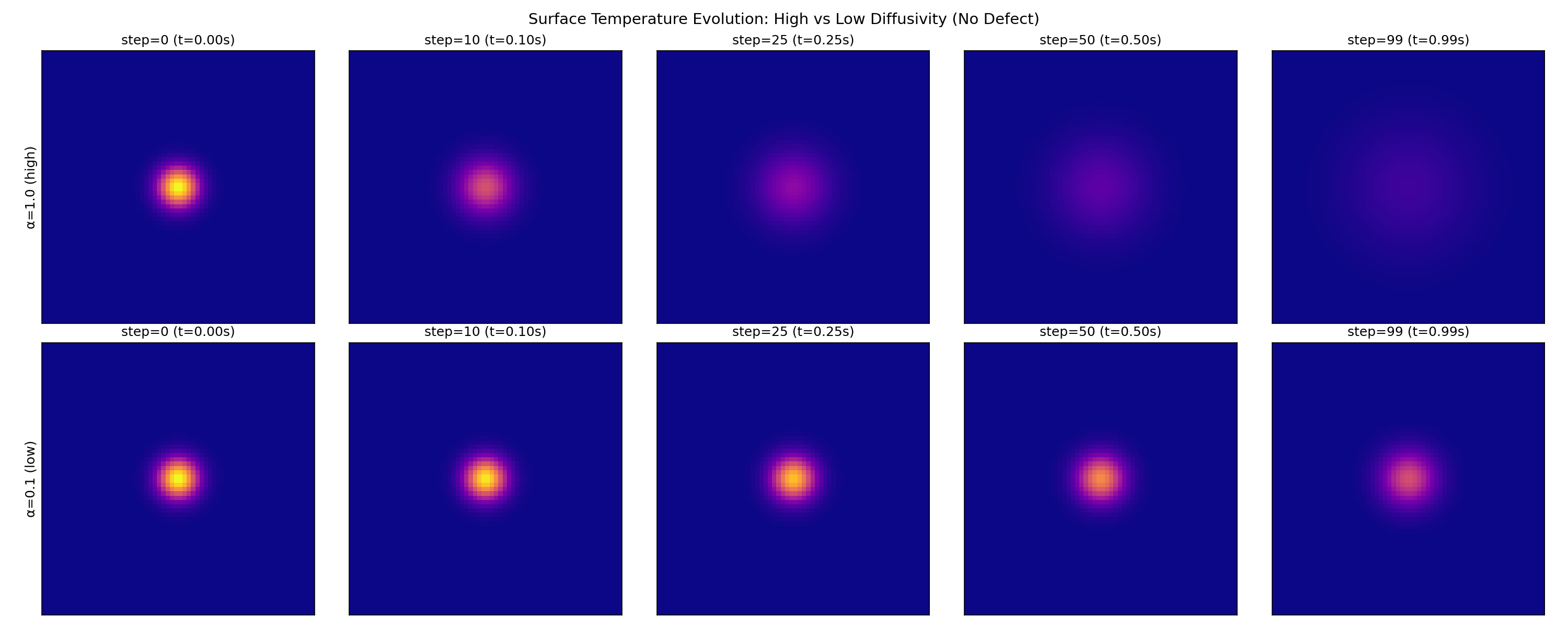
Figure 17 shows the surface temperature evolution under uniform diffusivity ( $\alpha=0.1$ and $\alpha=1.0$ ). The initially localized heat source spreads isotropically over time, preserving Gaussian symmetry as expected from Eq. (28).

Variable diffusivity with defect.

To test spatially varying material properties, we introduce a low-diffusivity spherical defect embedded in a homogeneous background. As illustrated in Fig. 18 (bottom row), the heat propagation is locally impeded near the defect region, resulting in a clearly asymmetric temperature field. This behavior is consistent with the physical interpretation of reduced thermal diffusivity.

I.5 Effect of Diffusivity Magnitude

We also compare diffusion dynamics under different diffusivity values in a defect-free setting. Figure 19 contrasts $\alpha=1.0$ (high diffusivity) with $\alpha=0.1$ (low diffusivity) using identical spatial and temporal resolutions. As expected, higher diffusivity leads to significantly faster spreading and lower peak temperatures, while preserving the overall Gaussian structure.

Appendix J Limitations and Future Work

Test-time optimization cost. Unlike supervised feedforward inversion (e.g., U-Net) that runs in milliseconds, NeFTY relies on per-specimen test-time optimization. Recovering one specimen takes $\sim 10$ minutes on a single high-end GPU (Table 9). This cost is acceptable for offline NDE inspection where accuracy is paramount but limits applicability in high-throughput manufacturing lines. Amortized-inference strategies, for example meta-learning or hypernetworks that predict a good initialization for the neural field, could substantially reduce the number of optimization steps and are a natural follow-up.

Quantitative diffusivity under high contrast. As discussed in Appendix E.1, we operate at a defect-to-bulk diffusivity contrast of $\sim 1\!:\!20$ . At realistic air-to-solid ratios ( $>1\!:\!1000$ ), the linear system $\mathbf{A}(\alpha_{\theta})$ becomes severely ill-conditioned and the iterative solver stalls. NeFTY recovers defect geometry reliably in this regime (Section 5.2, Section 5.3) but recovering the precise quantitative magnitude of $\alpha$ inside high-contrast voids remains hard because the diffusion time inside an insulator scales as $L^{2}/\alpha$ and saturates for $\alpha\to 0$ . Preconditioned or multi-grid solvers within the differentiable loop could extend NeFTY to the regime of stiff air voids.

Lack of 3D real labels. The real PVC datasets used in Section 5.3 provide only 2D defect masks and discrete defect depths from CAD; full 3D volumetric diffusivity ground truth is not available for any public NDT dataset, and obtaining it requires destructive testing or X-ray CT [17]. We therefore evaluate real-world performance through projected 2D and 2.5D labels rather than direct volumetric error. Building a benchmark that pairs surface thermograms with volumetric diffusivity ground truth would constitute a significant standalone materials-science contribution and remains a future direction.

	2D segm.		2.5D depth
Method	IoU $\uparrow$	Dice $\uparrow$	Abs Rel $\downarrow$	$\delta<1.25$ $\uparrow$
Swin-UNETR [21]	0.085	0.151	3.131	0.052
PPT [32]	0.419	0.563	3.416	0.005
TSR [50]	0.346	0.464	13.366	0.002
SPINN [8]	0.050	0.086	6.737	0.002
Grid Opt.	0.395	0.557	0.941	0.104
NeFTY (Ours)	0.431	0.597	0.465	0.385