Two-grid Penalty Approximation Scheme for Doubly Reflected BSDEs

Wonjae Lee Department of Mathematical Sciences, Seoul National University, Seoul 08826, South Korea. phwjlee117@gmail.com Hyungbin Park Research Institute of Mathematics and Department of Mathematical Sciences, Seoul National University, Seoul 08826, South Korea. hyungbin@snu.ac.kr

Abstract

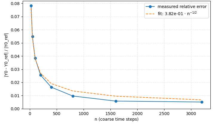
We study penalization coupled with time discretization for decoupled Markovian doubly reflected BSDEs with obstacles $p_{b}(t,X_{t})\leq Y_{t}\leq p_{w}(t,X_{t})$ . The DRBSDE is approximated by a penalized BSDE with parameter $\lambda$ and discretized by an implicit Euler scheme with step $\Delta t$ . A key difficulty is that the forward approximation used to evaluate the obstacles generates an error term that is amplified by $\lambda$ . In the single-obstacle case this amplification can be removed by the shift $Y-p_{b}(t,X)$ , but no analogous transformation eliminates both obstacles simultaneously; this motivates simulating the forward SDE on a finer grid $\tilde{\Delta t}$ and projecting onto the backward grid (two-grid scheme). Under structural assumptions motivated by financial barriers we sharpen penalization rates and obtain a uniform $O(\lambda^{-1})$ bound for the value process. We derive an explicit error bound in $(\Delta t,\tilde{\Delta t},\lambda)$ and tuning rules; for $Z$ -independent drivers, $\lambda\asymp\Delta t^{-1/2}$ with $\tilde{\Delta t}=O(\Delta t/\lambda^{2})$ yields the target $O(\Delta t^{1/2})$ rate. Nonsmooth barriers/payoffs are handled via a multivariate Itô–Tanaka and local-time-on-surfaces argument. We also provide numerical experiments for a one-dimensional game put under the Black–Scholes model. The observed grid-refinement errors are consistent with the predicted $O(n^{-1/2})$ behavior, while the penalty sweep indicates that the tested regime remains pre-asymptotic with respect to the penalty parameter.

Keywords: doubly reflected BSDEs, Dynkin games, penalization, time discretization, implicit Euler scheme, two-grid scheme, local time on surfaces, game options

1 Introduction

Backward stochastic differential equations (BSDEs) with reflection arise naturally in stochastic control, mathematical finance, and game theory. Reflected BSDEs with a single barrier provide probabilistic representations for optimal stopping problems and obstacle partial differential equations. Doubly reflected BSDEs (DRBSDEs), which are subject to two barriers, are closely connected to Dynkin games, variational inequalities with two obstacles, and the valuation of game-type contingent claims such as callable, putable, and convertible securities; see, for example, [1, 3, 4].

This paper studies an approximation method for DRBSDEs. We consider the decoupled Markovian DRBSDE

\left\{\quad\begin{aligned} &dX_{t}=b(t,X_{t})\,dt+\sigma(t,X_{t})\,dW_{t}\,,\\ &Y_{t}=g(X_{T})+\int_{t}^{T}f(s,X_{s},Y_{s},Z_{s})\,ds\\ &\qquad\qquad+(A_{T}-A_{t})-(K_{T}-K_{t})-\int_{t}^{T}Z_{s}\,dW_{s}\,,\;\;0\leq t\leq T\end{aligned}\right.

(1.1)

subject to the double obstacle constraint

p_{b}(t,X_{t})\leq Y_{t}\leq p_{w}(t,X_{t})\,,\;t\in[0,T]\,.

A classical approach to approximating reflected BSDEs is the penalization method, in which the reflection terms are replaced by large penalty terms whenever the solution exits the admissible region. In this setting, the DRBSDE (1.1) is approximated by the penalized BSDE

Y_{t}^{\lambda}=g(X_{T})+\int_{t}^{T}f_{\lambda}(s,X_{s},Y_{s}^{\lambda},Z_{s}^{\lambda})\,ds-\int_{t}^{T}Z_{s}^{\lambda}\,dW_{s},

(1.2)

where

f_{\lambda}(t,x,y,z):=f(t,x,y,z)+\lambda\,(y-p_{b}(t,x))^{-}-\lambda\,(p_{w}(t,x)-y)^{-},\quad\lambda>0\,.

It was shown in [16] that the penalized solutions converge to the solution of the original DRBSDE, with penalization error of order $\lambda^{-1/2}$ as $\lambda\to\infty$ .

In practice, the penalized BSDE is numerically solved by time discretization. Unlike the standard discretization schemes, which is based on a single partition of $[0,T]$ , we employ two nested partitions

\pi=\{t_{i}\}_{i=0}^{n}\subseteq\tilde{\pi}=\{\tilde{t}_{j}\}_{j=0}^{mn}

of $[0,T]$ , with coarse and fine step sizes

\Delta t:=T/n,\qquad\tilde{\Delta t}:=T/(mn),

respectively. More precisely, we discretize the penalized DRBSDE (1.2) on the coarse grid $\pi$ , while the forward process $X$ is simulated on the finer grid $\tilde{\pi}$ by the Euler–Maruyama scheme and then evaluated at the coarse-grid times. With $\Delta W_{i+1}=W_{t_{i+1}}-W_{t_{i}}$ , the scheme is given by

\begin{cases}\mathcal{Y}^{\lambda,\pi}_{t_{i+1}}:=\mathcal{Y}^{\lambda,\pi}_{t_{i}}-f_{\lambda}\left(t_{i},X^{\tilde{\pi}}_{t_{i}},\mathcal{Y}^{\lambda,\pi}_{t_{i}},\mathcal{Z}^{\lambda,\pi}_{t_{i}}\right)\Delta t+\mathcal{Z}^{\lambda,\pi}_{t_{i}}\Delta W_{i+1},\\ \mathcal{Y}^{\lambda,\pi}_{t_{n}}=g(X^{\tilde{\pi}}_{t_{n}}),\end{cases}

for $i=n-1,\dots,0$ .

However, several issues arise naturally in implementing this procedure: (i) how the penalty parameter $\lambda$ interacts with the time discretization, (ii) which choice of $\lambda$ and $\tilde{\Delta t}$ leads to an efficient implementation, and (iii) what convergence rate is achieved by the resulting approximation. This paper addresses these questions.

Contributions. The main contributions of this paper can be summarized as follows.

1.

Improved penalization error under structural assumptions. Building on a PDE comparison/viscosity argument in the spirit of [13] and under additional assumptions tailored to financial barriers, we improve the pure penalization bound and obtain

$|Y_{t}-Y_{t}^{\lambda}|\leq\frac{C}{\lambda}$

uniformly in $t$ , improving the $\lambda^{-1/2}$ bound in [16]. This sharper penalization rate is essential for balancing the total approximation error in Corollary 4.7.
2.

Two-grid forward simulation for double barriers. We propose a two-grid discretization that restores the standard $O(\Delta t^{1/2})$ convergence behavior of the value approximation with respect to the backward time step, without requiring the backward scheme itself to be run on a fine grid. The method simulates the forward SDE on a finer grid $\tilde{\pi}$ and discretizes the penalized backward equation on a coarser grid $\pi\subset\tilde{\pi}$ . This separation is essential in the double-barrier case, because the error incurred in evaluating the barriers $p_{b}(t,X_{t})$ and $p_{w}(t,X_{t})$ along the forward approximation appears multiplied by the penalty parameter $\lambda$ . By refining only the forward simulation, the scheme controls this amplified error at relatively low cost, while preserving a cheaper coarse-grid backward recursion.

Explicit error rates with parameter coupling. We derive quantitative error bounds for the full penalization–discretization approximation $(X^{\tilde{\pi}},\mathcal{Y}^{\lambda,\pi},\mathcal{Z}^{\lambda,\pi})$ , with explicit dependence on the coarse and fine step sizes $\Delta t$ and $\tilde{\Delta t}$ , and on the penalty parameter $\lambda$ . In the general Lipschitz case, allowing $Z$ -dependence in the driver, we prove the mean-square estimate

\Big(\max_{0\leq i\leq n-1}\mathbb{E}|Y_{t_{i}}-\mathcal{Y}^{\lambda,\pi}_{t_{i}}|^{2}\Big)^{1/2}\leq C\Big(\lambda\Delta t^{1/2}+\lambda^{-1}\Big),

under the natural terminal approximation, so that the balancing choice $\lambda\asymp\Delta t^{-1/2}$ yields the rate $O(\Delta t^{1/4})$ for the value process. When the driver is independent of $Z$ , we further obtain the absolute-error bound

\max_{0\leq i\leq n-1}\mathbb{E}|Y_{t_{i}}-\mathcal{Y}^{\lambda,\pi}_{t_{i}}|\leq C\Big(\Delta t^{1/2}+\lambda\tilde{\Delta t}^{1/2}+\lambda\Delta t+\lambda^{-1}\Big),

which exhibits the two-grid coupling explicitly. In particular, choosing $\lambda\asymp\Delta t^{-1/2}$ together with $\tilde{\Delta t}=O(\Delta t/\lambda^{2})$ recovers the target rate

\max_{0\leq i\leq n-1}\mathbb{E}|Y_{t_{i}}-Y^{\lambda,\pi}_{t_{i}}|=O(\Delta t^{1/2}).

These results extend the single-obstacle analysis of [13] to the double-barrier setting. In contrast to [13], which treats drivers linear in $Y$ and independent of $Z$ , our framework allows drivers that are Lipschitz in both $Y$ and $Z$ .

4.

Nonsmooth payoffs and barriers via multivariate Itô–Tanaka. Financial barriers such as basket calls and puts are typically not globally $C^{1,2}$ . We allow barrier functions that are $C^{1,2}$ away from a finite union of $C^{2}$ hypersurfaces. The analysis uses Tanaka-type arguments together with the change-of-variable formula with local time on surfaces (Peskir, 2007), which allows us to handle kink-type singularities while still deriving quantitative bounds compatible with penalization and discretization.
5.

Numerical validation and finite-sample behavior. We complement the theoretical analysis with numerical experiments for a one-dimensional game put under the Black–Scholes model. The grid-refinement experiment, performed under the theoretically motivated coupling $\lambda\asymp n^{1/2}$ , exhibits relative errors consistent with an $n^{-1/2}$ decay. A second penalty sweep at fixed $n$ shows that, over the tested range, the error continues to decrease as $\lambda$ increases, indicating that the computations remain in a pre-asymptotic regime in which the asymptotic balancing effect is not yet sharply resolved.

Organization. Section 2 introduces the DRBSDE framework and basic assumptions, together with existence and uniqueness results. Section 3 establishes the penalization error and the improved $O(\lambda^{-1})$ bound. Section 4 presents the two-grid numerical scheme and derives explicit discretization error bounds, together with parameter couplings that yield the $O(\Delta t^{1/2})$ rate. Section 5 reports numerical experiments for a game put example under the Black–Scholes model. Section 6 concludes.

2 Doubly reflected BSDEs: setting and preliminaries

We now describe the framework and introduce Markovian doubly reflected BSDEs under suitable assumptions. Let us fix a time horizon $T>0$ and consider a filtered probability space

(\Omega,\mathcal{F}_{T},\mathbb{F}=(\mathcal{F}_{t})_{t\in[0,T]},\mathbb{P}).

Let $W=(W_{t})_{t\in[0,T]}$ be a standard $\mathbb{R}^{d}$ -valued Brownian motion defined on the above probability space.

For $m\in\mathbb{N}$ and $p\geq 2$ , we use the following notations.

•

$L^{p}_{\mathcal{F}_{T}}(\mathbb{R}^{m})$ is the space of all $\mathcal{F}_{T}$ -measurable $\mathbb{R}^{m}$ -valued random variables $X$ such that

$\|X\|^{p}:=\mathbb{E}\left[|X|^{p}\right]<\infty.$
•

$\mathbb{H}^{p}(\mathbb{R}^{m})$ is the space of all $\mathbb{R}^{m}$ -valued progressively measurable processes $\phi$ such that

$\|\phi\|^{p}_{\mathbb{H}^{p}}:=\mathbb{E}\left[\left(\int^{T}_{0}|\phi_{t}|^{2}\,dt\right)^{\frac{p}{2}}\right]<\infty.$
•

$\mathbb{S}^{p}(\mathbb{R}^{m})$ is the space of all adapted continuous processes $\phi$ such that

$\|\phi\|^{p}_{\mathbb{S}^{p}}:=\mathbb{E}\left[\sup_{t\in[0,T]}|\phi_{t}|^{p}\right]<\infty.$
•

$\mathcal{A}$ is the space of real-valued non-decreasing continuous predictable processes $A$ with $A_{0}=0$ . We also define

$\mathcal{A}^{2}:=\{A\in\mathcal{A}\mid\mathbb{E}\left[A^{2}_{T}\right]<\infty\}.$

We are now ready to define doubly reflected BSDEs along with our assumptions. For $X_{0}\in L^{2}(\Omega)$ , we study BSDEs of the form

\begin{cases}\text{(i)}\ X_{t}=X_{0}+\int^{t}_{0}b(s,X_{s})\,ds+\int^{t}_{0}\sigma(s,X_{s})^{\top}\,dW_{s},\quad t\in[0,T],\\ \text{(ii)}\ Y_{t}=g(X_{T})+\int^{T}_{t}f\left(s,X_{s},Y_{s},Z_{s}\right)\,ds+(A_{T}-A_{t})\\ \ \ \ \ \ \ \ \ \ \ -(K_{T}-K_{t})-\int^{T}_{t}(Z_{s})^{\top}\,dW_{s},\quad t\in[0,T],\\ \text{(iii)}\ \forall t\in[0,T],\ \xi_{t}:=p_{b}(t,X_{t})\leq Y_{t}\leq\zeta_{t}:=p_{w}(t,X_{t})\ a.s.\\ \text{(iv)}\ \int^{T}_{0}(Y_{t}-\xi_{t})dA_{t}=0\ a.s.\ \text{and}\int^{T}_{0}(\zeta_{t}-Y_{t})dK_{t}=0\ a.s.\end{cases}

(2.1)

under the following assumptions on coefficients.

Assumption 2.1.

(i)

The maps $b:[0,T]\times\mathbb{R}^{d}\to\mathbb{R}^{d}$ , $\sigma:[0,T]\times\mathbb{R}^{d}\to\mathbb{R}^{d\times d}$ are $\frac{1}{2}$ -Hölder continuous in the first argument. That is, there exist constants $K_{b,\frac{1}{2}},K_{\sigma,\frac{1}{2}},$ such that

\displaystyle|b(t,x)-b(t^{\prime},x)|\leq K_{b,\frac{1}{2}}|t-t^{\prime}|^{\frac{1}{2}},\quad|\sigma(t,x)-\sigma(t^{\prime},x)|\leq K_{\sigma,\frac{1}{2}}|t-t^{\prime}|^{\frac{1}{2}}

for all $t,t^{\prime}\in[0,T]$ and $x\in\mathbb{R}^{d}$ . Also, $b$ and $\sigma$ are Lipschitz continuous in the second argument, i.e., there exist constants $K_{b},K_{\sigma}>0$ such that

\displaystyle|b(t,x)-b(t,y)|\leq K_{b}|x-y|,\quad|\sigma(t,x)-\sigma(t,y)|\leq K_{\sigma}|x-y|

for all $t\in[0,T]$ and $x,y\in\mathbb{R}^{d}$ .

(ii)

There exists a constant $\kappa>0$ such that, for all $(t,x)\in[0,T]\times\mathbb{R}^{d}$ and all $\xi\in\mathbb{R}^{d}$ ,

$\xi^{\top}\big(\sigma(t,x)\sigma(t,x)^{\top}\big)\,\xi\;\geq\;\kappa\,|\xi|^{2}.$
(iii)

The function $g:\mathbb{R}^{d}\to\mathbb{R}$ is Lipschitz continuous, i.e., there exists a constant $K_{g}$ such that

$|g(x)-g(y)|\leq K_{g}|x-y|$

for all $x,y\in\mathbb{R}^{d}$

(iv)

There exist constants $K_{x},K_{y},K_{z}>0$ such that the function $f:[0,T]\times\mathbb{R}^{d}\times\mathbb{R}\times\mathbb{R}^{d}\to\mathbb{R}$ satisfies

|f(t,x,y,z)-f(t,x^{\prime},y^{\prime},z^{\prime})|\leq K_{x}|x-x^{\prime}|+K_{y}|y-y^{\prime}|+K_{z}|z-z^{\prime}|

for all $(t,x,y,z),(t,x^{\prime},y^{\prime},z^{\prime})\in[0,T]\times\mathbb{R}^{d}\times\mathbb{R}\times\mathbb{R}^{d}$ . Also,

\|f(0,\cdot,0,0)\|_{\infty}<\infty

and there exists a constant $K_{f,\frac{1}{2}}$ such that

|f(t,x,y,z)-f(t^{\prime},x,y,z)|\leq K_{f,\frac{1}{2}}|t-t^{\prime}|^{\frac{1}{2}}

for all $(t,x,y,z),(t^{\prime},x^{\prime},y^{\prime},z^{\prime})\in[0,T]\times\mathbb{R}^{d}\times\mathbb{R}\times\mathbb{R}^{d}$ .

(v)

The functions $p_{w},p_{b}:[0,T]\times\mathbb{R}^{d}\to\mathbb{R}$ are $\frac{1}{2}$ -Hölder continuous in the first argument with Hölder constants $K_{w,\frac{1}{2}},K_{b,\frac{1}{2}}$ , respectively, and Lipschitz-continuous in the second arguments with Lipschitz constants $K_{w},K_{b}$ , respectively.
(vi)

We have $p_{b}(t,x)<p_{w}(t,x)$ and $p_{b}(T,x)\leq g(x)\leq p_{w}(T,x)$ for all $t\in[0,T)$ and $x\in\mathbb{R}^{d}$ .

With Assumption 2.1, we can establish the following theorem of uniqueness and existence of solution to (2.1) as a straightforward corollary to Theorem 3.7 of [8].

Theorem 2.2.

Under Assumption 2.1, there exists a unique solution $(X,Y,Z,A,K)\in\mathbb{S}^{2}(\mathbb{R}^{d})\times\mathbb{S}^{2}(\mathbb{R})\times\mathbb{H}^{2}(\mathbb{R}^{d})\times\mathcal{A}^{2}\times\mathcal{A}^{2}$ to the BSDE (2.1).

Furthermore, it is well known that (2.1) has a connection to the free-boundary PDE for $V:[0,T]\times\mathbb{R}^{d}\to\mathbb{R}$ given by

\begin{cases}\max\left(\min(-\mathcal{L}V-f(\cdot,\cdot,V,\sigma\nabla_{x}V),V-p_{b}),V-p_{w}\right)=0\text{ on }[0,T)\times\mathbb{R}^{d}\\ p_{b}(t,x)\leq V(t,x)\leq p_{w}(t,x),\\ V(T,x)=g(x),\end{cases}

(2.2)

where

\displaystyle\mathcal{L}V(t,x)=\partial_{t}V(t,x)+

\displaystyle b(t,x)^{\top}\nabla_{x}V(t,x)+\frac{1}{2}\sigma(t,x)^{\top}\nabla_{x}^{2}V(t,x)\sigma(t,x).

Specifically, we have the following well known result, as can be checked in [5].

Theorem 2.3.

Suppose Assumption 2.1 holds. Let $(X,Y,Z,A,K)$ be a solution to (2.1). The PDE (2.2) has a unique viscosity solution $V$ and we have

Y_{t}=V(t,X_{t})

almost surely for all $t\in[0,T]$ .

For our method, we also consider the following penalized BSDE which approximates (2.1) as $\lambda\to\infty$ :

\begin{cases}\text{(i)}\ X_{t}=X_{0}+\int^{t}_{0}b(s,X_{s})\,ds+\int^{t}_{0}\sigma(s,X_{s})^{\top}\,dW_{s},\quad t\in[0,T],\\ \text{(ii)}\ Y^{\lambda}_{t}=g(X_{T})+\int^{T}_{t}f_{\lambda}\left(s,X_{s},Y^{\lambda}_{s},Z^{\lambda}_{s}\right)\,ds-\int^{T}_{t}(Z^{\lambda}_{s})^{\top}\,dW_{s},\quad t\in[0,T].\end{cases}

(2.3)

Here, $\lambda>0$ and $f_{\lambda}:[0,T]\times\mathbb{R}^{d}\times\mathbb{R}\to\mathbb{R}$ is defined by

f_{\lambda}(t,x,y,z):=f(t,x,y,z)+\lambda\left(y-p_{b}(t,x)\right)^{-}-\lambda\left(p_{w}(t,x)-y\right)^{-}

We aim to calculate the error bound of the discretization scheme for the penalized BSDE (2.3). Again, if Assumption 2.1 holds, we have the following uniqueness and existence result. (See, e.g., [10]).

Theorem 2.4.

Under Assumption 2.1, there exists a unique solution $(X,Y^{\lambda},Z^{\lambda})\in\mathbb{S}^{2}(\mathbb{R}^{d})\times\mathbb{S}^{2}(\mathbb{R})\times\mathbb{H}^{2}(\mathbb{R}^{d})$ to the BSDE (2.3).

Let us now discuss the partial differential equation (PDE) corresponding to (2.3). Specifically, for $V:[0,T]\times\mathbb{R}^{d}\to\mathbb{R}$ , we consider the PDE

	$\displaystyle\mathcal{L}V^{\lambda}(t,x)+f_{\lambda}\left(t,x,V^{\lambda}(t,x),\sigma(t,x)\nabla_{x}V^{\lambda}(t,x)\right)$	$\displaystyle=0,\quad(t,x)\in[0,T)\times\mathbb{R}^{d}$		(2.4)
	$\displaystyle V^{\lambda}(T,x)$	$\displaystyle=g(x),\quad x\in\mathbb{R}^{d}.$		(2.4)

It is well known that, under suitable conditions, the solution to the BSDE (2.3) can be expressed in terms of the solution $V$ to the PDE (2.4). Specifically, we have the following result (See, e.g., [11].)

Assumption 2.5.

(i)

$\sigma$ is uniformly elliptic on $[0,T]\times\mathbb{R}^{d}$ .
(ii)

$b$ and $\sigma$ are $C^{1}_{b}$ in the second argument.

Theorem 2.6.

Under Assumption 2.1 and 2.5, the PDE (2.4) has a unique viscosity solution $V^{\lambda}$ in $C^{0,1}_{b}([0,T)\times\mathbb{R}^{d},\mathbb{R})$ . Furthermore, let $X$ be the solution to the forward SDE of (2.3). Then, $(X,Y^{\lambda},Z^{\lambda})$ , with $Y^{\lambda}$ and $Z^{\lambda}$ defined by

	$\displaystyle Y^{\lambda}_{t}$	$\displaystyle=V^{\lambda}(t,X_{t}),\quad t\in[0,T],$
	$\displaystyle Z^{\lambda}_{t}$	$\displaystyle=\sigma(t,X_{t})\nabla_{x}V^{\lambda}(t,X_{t}),\quad t\in[0,T],$

is the unique solution to the BSDE (2.3).

3 Penalty error

For analyzing error from penalization, we first make the following additional assumptions on the payoff functions and the initial condition of the forward process.

Assumption 3.1.

There exist $C^{2}$ hypersurfaces $\Gamma_{1},\dots,\Gamma_{q}\subset\mathbb{R}^{d}$ such that $\Gamma_{k}=\{x\in\mathbb{R}^{d}:\varphi_{k}(x)=0\}$ for some $\varphi_{k}\in C^{2}(\mathbb{R}^{d})$ with $\inf_{x\in\Gamma_{k}}|\nabla\varphi_{k}(x)|>0$ , satisfying the following conditions. We set $\Gamma:=\bigcup_{k=1}^{q}\Gamma_{k}$ and $U:=\mathbb{R}^{d}\setminus\Gamma$ .

(i)

We have $p_{b},p_{w}\in C^{1,2}\big([0,T)\times U\big)$ and $\mathbb{P}(X_{0}\in\Gamma)=0$ . Moreover, for each $k$ and each of $p\in\{p_{b},p_{w}\}$ , the one-sided normal derivatives $\nabla_{n_{k}}p(t,x\pm)$ exist for $(t,x)\in[0,T)\times\Gamma_{k}$ , where $n_{k}(x):=\nabla\varphi_{k}(x)/|\nabla\varphi_{k}(x)|$ .

(ii)

There exists $J>0$ such that for each $k$ and each $p\in\{p_{b},p_{w}\}$ ,

\sup_{(t,x)\in[0,T)\times\Gamma_{k}}\Big|\big[\nabla_{n_{k}}p\big](t,x)\Big|\leq J,

where

\sup_{(t,x)\in[0,T)\times\Gamma_{k}}\Big|\big[\nabla_{n_{k}}p\big](t,x)\Big|\;:=\;\sup_{(t,x)\in[0,T)\times\Gamma_{k}}\Big|\nabla_{n_{k}}p(t,x+)-\nabla_{n_{k}}p(t,x-)\Big|.

(iii)

There exist $P>0$ and $r\geq 0$ such that for each $p\in\{p_{b},p_{w}\}$ ,

$|\mathcal{L}p(t,x)|\leq P(1+|x|^{r}),\qquad(t,x)\in[0,T)\times U.$

(iv)

We have $D_{b}>-\infty$ and $D_{w}<\infty$ , where

D_{b}:=\inf_{(t,x)\in[0,T)\times(\mathbb{R}^{d}\setminus\Gamma)}\mathcal{L}p_{b}(t,x)+f\left(t,x,p_{b}(t,x),\sigma(t,x)\nabla_{x}p_{b}(t,x)\right)

and

D_{w}:=\sup_{(t,x)\in[0,T)\times(\mathbb{R}^{d}\setminus\Gamma)}\mathcal{L}p_{w}(t,x)+f\left(t,x,p_{w}(t,x),\sigma(t,x)\nabla_{x}p_{w}(t,x)\right.

Example 3.2.

Consider a put option where the holder may exercise early while the writer may also cancel early by paying an additional penalty. The underlying consists of $d$ assets. Under a risk-neutral measure, the asset dynamics are given by the Black–Scholes SDE

dX_{t}^{i}=rX_{t}^{i}\,dt+\sigma X_{t}^{i}\,dW_{t}^{i}.

(3.1)

The holder’s exercise payoff $p_{b}:[0,T]\times\mathbb{R}^{d}\to\mathbb{R}$ is the arithmetic-basket put

p_{b}(t,x)=\min\left(\Bigl(K-\frac{1}{d}\sum_{i=1}^{d}x^{i}\Bigr)^{+},K\right),

and the writer’s cancellation payoff $p_{w}:[0,T]\times\mathbb{R}^{d}\to\mathbb{R}$ is defined by adding a time-dependent penalty

p_{w}(t,x):=p_{b}(t,x)+\delta(T-t),

(3.2)

so that $p_{b}(t,x)\leq p_{w}(t,x)$ for all $(t,x)$ and $p_{w}(T,x)=p_{b}(T,x)$ .

By the standard Dynkin-game representation and its characterization via doubly reflected BSDEs (see, e.g., [3]), the undiscounted value process $Y$ is characterized as the $Y$ -component of the DRBSDE (2.1) with coefficients

b(s,x)=r\,x,\qquad\sigma(s,x)=\sigma\,\mathrm{diag}(x^{1},\dots,x^{d}),\qquad f(s,x,y,z)=-r\,y.

and terminal payoff $g(x)=p_{b}(T,x)=p_{w}(T,x)$ and obstacles $\xi_{t}=p_{b}(t,X_{t})$ , $\zeta_{t}=p_{w}(t,X_{t})$ .

Then, it is straightforward to check that Assumptions 2.1 and 2.5 hold. Furthermore, with $\Gamma_{1}=\{x\in\mathbb{R}^{d}\mid K-\frac{1}{d}\sum^{d}_{i=1}x^{i}=0\}$ and $\Gamma_{2}=\{x\in\mathbb{R}^{d}\mid\sum^{d}_{i=1}x^{i}=0\}$ as the hypersurfaces of singularity, it is clear that Assumption 3.1 holds as well.

The following proposition is analogous to Proposition 1 of [13].

Proposition 3.3.

Let $\lambda>K_{y}$ . Suppose Assumptions 2.1,2.5 and 3.1 hold. Let us denote by $V^{\lambda}$ the solution to the PDE (2.4). Then,

(\lambda-K_{y})(V^{\lambda}(t,x)-p_{b}(t,x))^{-}\leq D_{b}^{-}

and

(\lambda-K_{y})(p_{w}(t,x)-V^{\lambda}(t,x))^{-}\leq D_{w}^{+}

for all $(t,x)\in[0,T]\times\mathbb{R}^{d}$

Proof.

We prove the first inequality. The second one is proved analogously.

Let $Q(x):=(1+|x|^{2})^{m}$ and choose $m,a>0$ large enough to satisfy

\mathcal{L}Q(x)-aQ(x)+K_{y}|Q(x)|+K_{z}|\sigma(t,x)\nabla Q(x)|\leq 0

(3.3)

for all $(t,x)\in[0,T]\times\mathbb{R}^{d}$ .

Also, for $\varepsilon>0$ , we define

\ell(t,x):=p_{b}(t,x)-V^{\lambda}(t,x)-\varepsilon e^{-at}Q(x).

Since $p_{b}$ and $V^{\lambda}$ have at most linear growth whereas $Q$ has superlinear growth, there exists a compact set

K=[0,T]\times[-M,M]^{d}

such that $\ell<0$ on $([0,T]\times\mathbb{R}^{d})\setminus K$ .

If $\ell\leq 0$ on $[0,T]\times\mathbb{R}^{d}$ , then

(V^{\lambda}(t,x)-p_{b}(t,x))^{-}\leq\varepsilon e^{-at}Q(x),

and letting $\varepsilon\downarrow 0$ yields the conclusion. We may therefore assume that $\ell$ is positive somewhere, and hence attains a maximum on $K$ .

We now distinguish two cases.

Case 1. We assume that $\ell$ attains a positive maximum at some

(t_{0},x_{0})\in[0,T)\times(\mathbb{R}^{d}\setminus\Gamma).

Since $x_{0}\notin\Gamma$ , the function $p_{b}$ is $C^{1,2}$ in a neighborhood of $(t_{0},x_{0})$ .

We set

\phi(t,x):=p_{b}(t,x)-\varepsilon e^{-at}Q(x)-\ell(t_{0},x_{0}).

Then

V^{\lambda}(t_{0},x_{0})=\phi(t_{0},x_{0}),

and the maximality of $\ell$ at $(t_{0},x_{0})$ gives

V^{\lambda}(t,x)\geq\phi(t,x)

for $(t,x)$ near $(t_{0},x_{0})$ . Thus $V^{\lambda}-\phi$ has a local minimum $0$ at $(t_{0},x_{0})$ , and the viscosity supersolution property of $V^{\lambda}$ yields

\mathcal{L}\phi(t_{0},x_{0})+f_{\lambda}\bigl(t_{0},x_{0},\phi(t_{0},x_{0}),\sigma(t_{0},x_{0})\nabla\phi(t_{0},x_{0})\bigr)\geq 0.

(3.4)

From

p_{b}(t_{0},x_{0})-\phi(t_{0},x_{0})=\ell(t_{0},x_{0})+\varepsilon e^{-at_{0}}Q(x_{0})>0,

we obtain

(\phi(t_{0},x_{0})-p_{b}(t_{0},x_{0}))^{-}=\ell(t_{0},x_{0})+\varepsilon e^{-at_{0}}Q(x_{0}).

Since $\phi(t_{0},x_{0})<p_{b}(t_{0},x_{0})\leq p_{w}(t_{0},x_{0})$ , we also have

(p_{w}(t_{0},x_{0})-\phi(t_{0},x_{0}))^{-}=0.

Substituting these relations into (3.4), we obtain

$\displaystyle 0$	$\displaystyle\leq\mathcal{L}\phi(t_{0},x_{0})+f\bigl(t_{0},x_{0},\phi(t_{0},x_{0}),\sigma(t_{0},x_{0})\nabla\phi(t_{0},x_{0})\bigr)$	(3.5)
	$\displaystyle\qquad+\lambda\bigl(\phi(t_{0},x_{0})-p_{b}(t_{0},x_{0})\bigr)^{-}$
	$\displaystyle=\mathcal{L}p_{b}(t_{0},x_{0})-\varepsilon e^{-at_{0}}\bigl(\mathcal{L}Q(x_{0})-aQ(x_{0})\bigr)$
	$\displaystyle\qquad+f\bigl(t_{0},x_{0},\phi(t_{0},x_{0}),\sigma(t_{0},x_{0})\nabla\phi(t_{0},x_{0})\bigr)$
	$\displaystyle\qquad\qquad+\lambda\bigl(\ell(t_{0},x_{0})+\varepsilon e^{-at_{0}}Q(x_{0})\bigr).$

Furthermore, the Lipschitz continuity of $f$ in $(y,z)$ gives

	$\displaystyle f\bigl(t_{0},x_{0},\phi(t_{0},x_{0}),\sigma(t_{0},x_{0})\nabla\phi(t_{0},x_{0})\bigr)$
	$\displaystyle\geq f\bigl(t_{0},x_{0},p_{b}(t_{0},x_{0}),\sigma(t_{0},x_{0})\nabla p_{b}(t_{0},x_{0})\bigr)$
	$\displaystyle\qquad-K_{y}\bigl(\ell(t_{0},x_{0})+\varepsilon e^{-at_{0}}Q(x_{0})\bigr)-\varepsilon e^{-at_{0}}K_{z}\|\sigma(t_{0},x_{0})\nabla Q(x_{0})\|.$

Substituting this into (3.5), we arrive at

		$\displaystyle(\lambda-K_{y})\ell(t_{0},x_{0})$
	$\displaystyle\leq\;$	$\displaystyle-\Bigl(\mathcal{L}p_{b}(t_{0},x_{0})+f\bigl(t_{0},x_{0},p_{b}(t_{0},x_{0}),\sigma(t_{0},x_{0})\nabla p_{b}(t_{0},x_{0})\bigr)\Bigr)$
		$\displaystyle\quad+\varepsilon e^{-at_{0}}\Bigl(\mathcal{L}Q(x_{0})-aQ(x_{0})+K_{y}\|Q(x_{0})\|+K_{z}\|\sigma(t_{0},x_{0})\nabla Q(x_{0})\|\Bigr).$

By (3.3) and the definition of $D_{b}$ , this yields

(\lambda-K_{y})\ell(t_{0},x_{0})\leq D_{b}^{-}.

Since $\ell(t,x)\leq\ell(t_{0},x_{0})$ for all $(t,x)\in[0,T]\times\mathbb{R}^{d}$ , we obtain

(\lambda-K_{y})\Bigl((V^{\lambda}(t,x)-p_{b}(t,x))^{-}-\varepsilon e^{-at}Q(x)\Bigr)\leq D_{b}^{-},\qquad\forall(t,x)\in[0,T]\times\mathbb{R}^{d}.

By letting $\varepsilon\downarrow 0$ , we conclude that

(\lambda-K_{y})(V^{\lambda}(t,x)-p_{b}(t,x))^{-}\leq D_{b}^{-}.

Case 2. We now assume that every maximizer of $\ell$ lies on $[0,T]\times(\Gamma\cap K)$ .

Since $\Gamma$ has empty interior and $\ell$ is continuous, there exists $(\bar{t},\bar{x})\in K$ with $\bar{x}\notin\Gamma$ such that

\ell(\bar{t},\bar{x})\geq\sup_{(t,x)\in K}\ell(t,x)-\eta.

for any $\eta>0$ .

Applying Ekeland’s variational principle [6] to the continuous function $-\ell$ on the complete metric space $K$ , we conclude that for every $\delta>0$ , there exists $(t_{\eta},x_{\eta})\in K$ such that

\ell(t_{\eta},x_{\eta})\geq\ell(\bar{t},\bar{x}),\qquad|(t_{\eta},x_{\eta})-(\bar{t},\bar{x})|\leq\delta,

and such that

\ell_{\eta}(t,x):=\ell(t,x)-\frac{\eta}{\delta}\bigl(|t-t_{\eta}|^{2}+|x-x_{\eta}|^{2}\bigr)

attains its maximum over $K$ at $(t_{\eta},x_{\eta})$ .

Choosing $\delta<\mathrm{dist}(\bar{x},\Gamma)$ , we have $x_{\eta}\notin\Gamma$ , and hence $p_{b}$ is $C^{1,2}$ in a neighborhood of $(t_{\eta},x_{\eta})$ .

Let

\rho_{\eta}(t,x):=\frac{\eta}{\delta}\bigl(|t-t_{\eta}|^{2}+|x-x_{\eta}|^{2}\bigr),

and

\phi_{\eta}(t,x):=p_{b}(t,x)-\varepsilon e^{-at}Q(x)-\rho_{\eta}(t,x)-\ell_{\eta}(t_{\eta},x_{\eta}),

then since

V^{\lambda}(t_{\eta},x_{\eta})=\phi_{\eta}(t_{\eta},x_{\eta}),

and $V^{\lambda}-\phi_{\eta}$ has a local minimum $0$ at $(t_{\eta},x_{\eta})$ , the viscosity supersolution property yields

\mathcal{L}\phi_{\eta}(t_{\eta},x_{\eta})+f_{\lambda}\bigl(t_{\eta},x_{\eta},\phi_{\eta}(t_{\eta},x_{\eta}),\sigma(t_{\eta},x_{\eta})\nabla\phi_{\eta}(t_{\eta},x_{\eta})\bigr)\geq 0.

Since

\nabla\rho_{\eta}(t_{\eta},x_{\eta})=0,\quad\text{and}\quad\mathcal{L}\rho_{\eta}(t_{\eta},x_{\eta})\geq 0,

similar calculations as in Case 1 yield

		$\displaystyle(\lambda-K_{y})\ell_{\eta}(t_{\eta},x_{\eta})$
	$\displaystyle\leq\;$	$\displaystyle-\Bigl(\mathcal{L}p_{b}(t_{\eta},x_{\eta})+f\bigl(t_{\eta},x_{\eta},p_{b}(t_{\eta},x_{\eta}),\sigma(t_{\eta},x_{\eta})\nabla p_{b}(t_{\eta},x_{\eta})\bigr)\Bigr)$
		$\displaystyle\quad+\varepsilon e^{-at_{\eta}}\Bigl(\mathcal{L}Q(x_{\eta})-aQ(x_{\eta})+K_{y}\|Q(x_{\eta})\|+K_{z}\|\sigma(t_{\eta},x_{\eta})\nabla Q(x_{\eta})\|\Bigr).$

Again, by (3.3), we obtain

(\lambda-K_{y})\ell_{\eta}(t_{\eta},x_{\eta})\leq D_{b}^{-}.

Since $\rho_{\eta}(t_{\eta},x_{\eta})=0$ , we have $\ell_{\eta}(t_{\eta},x_{\eta})=\ell(t_{\eta},x_{\eta})$ , and thus

	$\displaystyle(\lambda-K_{y})\sup_{K}\ell\leq$	$\displaystyle(\lambda-K_{y})\ell(\bar{t},\bar{x})+(\lambda-K_{y})\eta$
	$\displaystyle\leq$	$\displaystyle(\lambda-K_{y})\ell(t_{\eta},x_{\eta})+(\lambda-K_{y})\eta$
	$\displaystyle=$	$\displaystyle(\lambda-K_{y})\ell_{\eta}(t_{\eta},x_{\eta})+(\lambda-K_{y})\eta$
	$\displaystyle\leq$	$\displaystyle D_{b}^{-}+(\lambda-K_{y})\eta.$

Letting $\eta\downarrow 0$ yields

(\lambda-K_{y})\sup_{K}\ell\leq D_{b}^{-}.

Since we assumed $\ell$ attains it’s global maximum on $K$ , we conclude

(\lambda-K_{y})\Bigl((V^{\lambda}(t,x)-p_{b}(t,x))^{-}-\varepsilon e^{-at}Q(x)\Bigr)\leq D_{b}^{-},\qquad\forall(t,x)\in[0,T]\times\mathbb{R}^{d}.

Again, letting $\varepsilon\downarrow 0$ yields

(\lambda-K_{y})(V^{\lambda}(t,x)-p_{b}(t,x))^{-}\leq D_{b}^{-}.

This proves the first inequality.

For the second inequality, one argues in the same way with

\hat{\ell}(t,x):=V^{\lambda}(t,x)-p_{w}(t,x)-\varepsilon e^{-at}Q(x),

replacing positive maxima by negative minima throughout. This completes the proof. ∎∎

Corollary 3.4.

Suppose Assumptions 2.1,2.5 and 3.1 hold. Let $(X,Y,Z)$ be the solution to (2.3) and choose $\lambda>2K_{y}$ . Then, we have

\lambda(Y_{t}-p_{b}(t,X_{t}))^{-}\leq 2D_{b}^{-}

and

\lambda(p_{w}(t,X_{t})-Y_{t})^{-}\leq 2D_{w}^{+}

almost surely for all $t\in[0,T]$ .

Proof.

The result follows directly from Theorem 2.6 and Proposition 3.3. ∎∎

Theorem 3.5.

Let $V$ and $V^{\lambda}$ each denote the solutions to (2.2) and (2.4), respectively. If we choose $\lambda>2K_{y}$ , we have

-e^{K_{y}T}\frac{2D^{+}_{w}}{\lambda}\leq V(t,x)-V^{\lambda}(t,x)\leq e^{K_{y}T}\frac{2D_{b}^{-}}{\lambda}

for all $(t,x)\in[0,T]\times\mathbb{R}^{d}$ . Thus, if we denote by $(X,Y,Z,A,K)$ the solution to (2.1) and by $(X,Y^{\lambda},Z^{\lambda})$ the solution to (2.3), then we have

|Y_{t}-Y_{t}^{\lambda}|\leq e^{K_{y}T}\frac{2\max(D^{+}_{w},D^{-}_{b})}{\lambda}

(3.6)

almost surely for all $t\in[0,T]$ .

Proof.

For brevity, we write

C_{b}:=\frac{D_{b}^{-}}{\lambda-K_{y}},\qquad C_{w}:=\frac{D_{w}^{+}}{\lambda-K_{y}}.

Note that for $\lambda>2K_{y}$ , we have $C_{b}\leq e^{K_{y}T}\frac{2D_{b}^{-}}{\lambda}$ and $C_{w}\geq-e^{K_{y}T}\frac{2D^{+}_{w}}{\lambda}$ .

We first prove the upper bound inequality

V(t,x)-V^{\lambda}(t,x)\leq e^{K_{y}(T-t)}C_{b}.

Let

c_{b}(t):=e^{K_{y}(T-t)}C_{b},\qquad\overline{V}^{\lambda}(t,x):=V^{\lambda}(t,x)+c_{b}(t),

then, it is sufficient to show that $\overline{V}^{\lambda}$ is a viscosity supersolution of

\max\Bigl(\min\bigl(-\mathcal{L}u-f(t,x,u,\sigma(t,x)\nabla_{x}u),\,u-p_{b}(t,x)\bigr),\,u-p_{w}(t,x)\Bigr)=0.

(3.7)

Let $\varphi\in C^{1,2}$ be such that $\overline{V}^{\lambda}-\varphi$ attains a local minimum $0$ at $(t_{0},x_{0})$ , and set

\psi(t,x):=\varphi(t,x)-c_{b}(t).

Then $V^{\lambda}-\psi$ attains a local minimum $0$ at $(t_{0},x_{0})$ .

We consider the following two cases.

Case 1. If $\overline{V}^{\lambda}(t_{0},x_{0})\geq p_{w}(t_{0},x_{0})$ , then the supersolution condition for (3.7) is immediate since the second entry in the outer maximum is nonnegative.

Case 2. Assume that $\overline{V}^{\lambda}(t_{0},x_{0})<p_{w}(t_{0},x_{0})$ . The estimate of Proposition 3.3,

(\lambda-K_{y})(V^{\lambda}-p_{b})^{-}\leq D_{b}^{-},

implies that

(V^{\lambda}-p_{b})^{-}\leq C_{b},

or equivalently,

V^{\lambda}(t,x)+C_{b}\geq p_{b}(t,x)\qquad\forall(t,x)\in[0,T]\times\mathbb{R}^{d}.

Since $c_{b}(t)\geq C_{b}$ , one has

\overline{V}^{\lambda}(t_{0},x_{0})\geq p_{b}(t_{0},x_{0}).

In this case, verifying the supersolution condition reduces to proving

-\mathcal{L}\varphi(t_{0},x_{0})-f\bigl(t_{0},x_{0},\varphi(t_{0},x_{0}),\sigma(t_{0},x_{0})\nabla_{x}\varphi(t_{0},x_{0})\bigr)\geq 0.

Since $V^{\lambda}$ is a viscosity supersolution of the penalized PDE, we have

-\mathcal{L}\psi(t_{0},x_{0})-f_{\lambda}\bigl(t_{0},x_{0},\psi(t_{0},x_{0}),\sigma(t_{0},x_{0})\nabla_{x}\psi(t_{0},x_{0})\bigr)\geq 0.

(3.8)

Also, since $\varphi=\psi+c_{b}$ and $c_{b}$ depends only on $t$ , it follows that

-\mathcal{L}\varphi(t_{0},x_{0})=-\mathcal{L}\psi(t_{0},x_{0})-c_{b}^{\prime}(t_{0}).

(3.9)

Furthermore, the inequality $\overline{V}^{\lambda}(t_{0},x_{0})<p_{w}(t_{0},x_{0})$ gives us

\psi(t_{0},x_{0})=V^{\lambda}(t_{0},x_{0})<p_{w}(t_{0},x_{0})-c_{b}(t_{0})<p_{w}(t_{0},x_{0}),

and hence

(p_{w}(t_{0},x_{0})-\psi(t_{0},x_{0}))^{-}=0.

Thus, we arrive at

f_{\lambda}\bigl(t_{0},x_{0},\psi,\sigma\nabla\psi\bigr)=f\bigl(t_{0},x_{0},\psi,\sigma\nabla\psi\bigr)+\lambda(\psi-p_{b})^{-}(t_{0},x_{0})\geq f\bigl(t_{0},x_{0},\psi,\sigma\nabla\psi\bigr).

(3.10)

Combining (3.8), (3.9), and (3.10), we obtain

	$\displaystyle-\mathcal{L}\varphi(t_{0},x_{0})-f\bigl(t_{0},x_{0},\varphi(t_{0},x_{0}),\sigma\nabla\varphi(t_{0},x_{0})\bigr)$
	$\displaystyle\geq-c_{b}^{\prime}(t_{0})+f\bigl(t_{0},x_{0},\psi(t_{0},x_{0}),\sigma\nabla\psi(t_{0},x_{0})\bigr)-f\bigl(t_{0},x_{0},\varphi(t_{0},x_{0}),\sigma\nabla\varphi(t_{0},x_{0})\bigr).$

Because $\nabla\varphi=\nabla\psi$ and $\varphi=\psi+c_{b})$ , the Lipschitz continuity of $f$ in the $y$ -variable gives

f\bigl(t_{0},x_{0},\psi,\sigma\nabla\psi\bigr)-f\bigl(t_{0},x_{0},\varphi,\sigma\nabla\varphi\bigr)\geq-K_{y}c_{b}(t_{0}).

Hence

-\mathcal{L}\varphi(t_{0},x_{0})-f\bigl(t_{0},x_{0},\varphi(t_{0},x_{0}),\sigma\nabla\varphi(t_{0},x_{0})\bigr)\geq-c_{b}^{\prime}(t_{0})-K_{y}c_{b}(t_{0}).

Since $c_{b}^{\prime}(t)=-K_{y}c_{b}(t)$ , the right-hand side is equal to $0$ . This proves that $\overline{V}^{\lambda}$ is a viscosity supersolution of (3.7).

The terminal condition satisfies

\overline{V}^{\lambda}(T,x)=V^{\lambda}(T,x)+C_{b}=g(x)+C_{b}\geq g(x)=V(T,x),

and hence applying the comparison principle gives us

V(t,x)\leq\overline{V}^{\lambda}(t,x)=V^{\lambda}(t,x)+e^{K_{y}(T-t)}C_{b},

which implies the desired conclusion.

The lower bound can also be proven similarly. ∎∎

For the total penalty error, we define increasing finite variation processes $A^{\lambda}$ and $K^{\lambda}$ by

A^{\lambda}_{t}:=\lambda\int^{t}_{0}(Y^{\lambda}_{s}-p_{b}(s,X_{s}))^{-}\,ds,\quad K^{\lambda}_{t}:=\lambda\int^{t}_{0}(p_{w}(s,X_{s})-Y^{\lambda}_{s})^{-}\,ds.

Then the backward equation of penalized BSDE (2.3) can be rewritten as

-dY^{\lambda}_{t}=f(t,X_{t},Y^{\lambda}_{t},Z^{\lambda}_{t})\,dt+dA^{\lambda}_{t}-dK^{\lambda}_{t}-(Z^{\lambda}_{t})^{\top}\,dW_{t}

in differential form.

Theorem 3.6.

Let us denote by $(X,Y,Z,A,K)$ and $(X,Y^{\lambda},Z^{\lambda})$ the solutions to (2.1) and (2.3), respectively. Suppose Assumptions 2.1,2.5, and 3.1 hold and choose $\lambda>2K_{y}$ . Then, we have

\mathbb{E}\left[\sup_{0\leq t\leq T}|Y_{t}-Y^{\lambda}_{t}|^{2}\right]<\frac{C_{2}}{\lambda^{2}}\quad\text{ and }\quad\int^{T}_{0}\mathbb{E}|Z_{s}-Z^{\lambda}_{s}|^{2}\,ds<\frac{C_{2}}{\lambda}.

Proof.

First, we have

\mathbb{E}\left[\sup_{0\leq t\leq T}|Y_{t}-Y^{\lambda}_{t}|^{2}\right]<\frac{C_{2}}{\lambda^{2}}

from Theorem 3.5. Now, let us denote $\delta Y^{\lambda}:=Y^{\lambda}-Y$ and $\delta Z^{\lambda}:=Z^{\lambda}-Z$ . Then, we have

	$\displaystyle-\delta Y^{\lambda}_{t}=$	$\displaystyle\left(f(t,X_{t},Y^{\lambda}_{t},Z^{\lambda}_{t})-f(t,X_{t},Y_{t},Z_{t})\right)\,dt$
		$\displaystyle+(dA^{\lambda}_{t}-dA_{t})-(dK^{\lambda}_{t}-dK_{t})-(\delta Z^{\lambda}_{t})^{\top}\,dW_{t}.$

Thus, applying the Itô formula to $|\delta Y^{\lambda}_{t}|^{2}$ , we obtain

$\displaystyle\|\delta Y^{\lambda}_{0}\|^{2}$	$\displaystyle\;+\;\int^{T}_{0}\|\delta Z^{\lambda}_{s}\|^{2}\,ds$	(3.11)
	$\displaystyle=\|\delta Y^{\lambda}_{T}\|^{2}+2\int^{T}_{0}\delta Y^{\lambda}_{s}\,\left(f(s,X_{s},Y^{\lambda}_{s},Z^{\lambda}_{s})-f(s,X_{s},Y_{s},Z_{s})\right)\,ds$
	$\displaystyle\quad+2\int^{T}_{0}\delta Y^{\lambda}_{s}\,dA^{\lambda}_{s}-2\int^{T}_{0}\delta Y^{\lambda}_{s}\,dA_{s}$
	$\displaystyle\quad-2\int^{T}_{0}\delta Y^{\lambda}_{s}\,dK^{\lambda}_{s}+2\int^{T}_{0}\delta Y^{\lambda}_{s}\,dK_{s}-2\int^{T}_{0}\delta Y^{\lambda}_{s}\,\Delta Z_{s}\,dW_{s}.$

By Young’ inequality and the Lipschitz property of $f$ , we have

	$\displaystyle 2\int^{T}_{0}\delta Y^{\lambda}_{s}\,\left(f(s,X_{s},Y^{\lambda}_{s},Z^{\lambda}_{s})-f(s,X_{s},Y_{s},Z_{s})\right)\,ds$	(3.12)
$\displaystyle\leq$	$\displaystyle 4K^{2}_{z}\int^{T}_{0}\|\delta Y^{\lambda}_{s}\|^{2}\,ds+\frac{1}{4K^{2}_{z}}\int^{T}_{0}\left(f(s,X_{s},Y^{\lambda}_{s},Z^{\lambda}_{s})-f(s,X_{s},Y_{s},Z_{s})\right)^{2}\,ds$
$\displaystyle\leq$	$\displaystyle 4K^{2}_{z}\int^{T}_{0}\|\delta Y^{\lambda}_{s}\|^{2}\,ds+\frac{1}{4K^{2}_{z}}\int^{T}_{0}2K^{2}_{y}\|\delta Y^{\lambda}_{s}\|^{2}+2K^{2}_{Z}\|\delta Z^{\lambda}_{s}\|^{2}\,ds$
$\displaystyle\leq$	$\displaystyle\frac{C_{2}}{\lambda^{2}}+\frac{1}{2}\int^{T}_{0}\|\delta Z^{\lambda}_{s}\|^{2}\,ds.$

Next, note that

$\displaystyle 2\int^{T}_{0}\delta Y^{\lambda}_{s}dA^{\lambda}_{s}=$	$\displaystyle 2\int^{T}_{0}(Y^{\lambda}_{s}-p_{b}(s,X_{s}))dA^{\lambda}_{s}-2\int^{T}_{0}(Y_{s}-p_{b}(s,X_{s}))dA^{\lambda}_{s}$	(3.13)
$\displaystyle\leq$	$\displaystyle 2\int^{T}_{0}(Y^{\lambda}_{s}-p_{b}(s,X_{s}))(Y^{\lambda}_{s}-p_{b}(s,X_{s}))^{-}ds$
$\displaystyle\leq$	$\displaystyle 0$

and

$\displaystyle 2\int^{T}_{0}\delta Y^{\lambda}_{s}dK^{\lambda}_{s}=$	$\displaystyle 2\int^{T}_{0}(Y^{\lambda}_{s}-p_{w}(s,X_{s}))dK^{\lambda}_{s}-2\int^{T}_{0}(Y_{s}-p_{w}(s,X_{s}))dK^{\lambda}_{s}$	(3.14)
$\displaystyle\geq$	$\displaystyle-2\int^{T}_{0}(p_{w}(s,X_{s})-Y^{\lambda}_{s})(p_{w}(s,X_{s})-Y^{\lambda}_{s})^{-}ds$
$\displaystyle\geq$	$\displaystyle 0.$

Plugging in (3.12), (3.13), and (3.14) into (3.11), and then taking expectaion of absolute values of both sides, we arrive at

	$\displaystyle\mathbb{E}\|\delta Y^{\lambda}_{0}\|^{2}$	$\displaystyle\;+\;\frac{1}{2}\int^{T}_{0}\mathbb{E}\|\delta Z^{\lambda}_{s}\|^{2}\,ds$		(3.15)
		$\displaystyle\leq\frac{C_{2}}{\lambda^{2}}+2\mathbb{E}\left[\int^{T}_{0}\|\delta Y^{\lambda}_{s}\|\,dA_{s}\right]+2\mathbb{E}\left[\int^{T}_{0}\|\delta Y^{\lambda}_{s}\|\,dK_{s}\right].$		(3.15)

Also, since $A,K\in A^{2}$ we have $\mathbb{E}[A_{T}^{2}]+\mathbb{E}[K_{T}^{2}]<\infty$ . Thus, applying the Cauchy–Schwarz inequality yields

	$\displaystyle\mathbb{E}\int_{0}^{T}\|\delta Y_{s}^{\lambda}\|\,dA_{s}$	$\displaystyle\leq\left(\mathbb{E}\left[\sup_{0\leq s\leq T}\|\delta Y_{s}^{\lambda}\|^{2}\right]\right)^{1/2}\left(\mathbb{E}[A_{T}^{2}]\right)^{1/2}\leq\frac{C_{2}}{\lambda},$
	$\displaystyle\mathbb{E}\int_{0}^{T}\|\delta Y_{s}^{\lambda}\|\,dK_{s}$	$\displaystyle\leq\left(\mathbb{E}\left[\sup_{0\leq s\leq T}\|\delta Y_{s}^{\lambda}\|^{2}\right]\right)^{1/2}\left(\mathbb{E}[K_{T}^{2}]\right)^{1/2}\leq\frac{C_{2}}{\lambda}.$

Plugging these estimates into (3.15), we conclude that

\int_{0}^{T}\mathbb{E}|\delta Z_{s}^{\lambda}|^{2}\,ds\leq\frac{C_{2}}{\lambda}.

∎∎

4 Numerical scheme and error analysis

We describe the numerical scheme and derive an error bound of our method. From here on, we denote by $C_{2}$ any constant depending only on the data of the BSDE (2.1): $T$ , $X_{0}$ , $b$ , $\sigma$ , $g$ , $f$ , $p_{b}$ , and $p_{w}$ . Note that the constant does not depend on the penalty parameter $\lambda$ .

4.1 Numerical scheme

We describe the numerical scheme of our approximation method. First, we fix two time grids $\pi:=\{t_{i}:=iT/n,i=0,...,n\}$ and $\tilde{\pi}:=\{t_{i}:=iT/(mn),i=0,...,mn\}$ $(n,m\in\mathbb{N})$ on $[0,T]$ and write $\Delta t:=T/n$ and $\Delta\tilde{t}:=T/(mn)$ . Note that $\pi\subset\tilde{\pi}$ , $\Delta t\geq\Delta\tilde{t}$ , and the generic constant $C_{2}$ does not depend on the resolution $n$ nor on $m$ .

The solution $X$ to the forward equation is approximated by the Euler–Maruyama scheme $X^{\pi}$ , with values on the finer grid $\tilde{\pi}$ given inductively as

\begin{cases}X^{\tilde{\pi}}_{0}=X_{0}\\ X^{\tilde{\pi}}_{\tilde{t}_{i+1}}=X^{\tilde{\pi}}_{\tilde{t}_{i}}+b(\tilde{t}_{i},X^{\tilde{\pi}}_{\tilde{t}_{i}})\Delta\tilde{t}+\sigma(\tilde{t}_{i},X^{\tilde{\pi}}_{\tilde{t}_{i}})\left(W_{\tilde{t}_{i+1}}-W_{\tilde{t}_{i}}\right).\end{cases}

(4.1)

for $i=0,...,mn-1$ .

Then, on the coarser grid $\pi$ , we consider the discretization scheme

\mathcal{Y}^{\lambda,\pi}_{t_{i+1}}:=\mathcal{Y}^{\lambda,\pi}_{t_{i}}-f_{\lambda}\left(t_{i},X^{\tilde{\pi}}_{t_{i}},\mathcal{Y}^{\lambda,\pi}_{t_{i}},\mathcal{Z}^{\lambda,\pi}_{t_{i}}\right)\Delta t+\mathcal{Z}^{\lambda,\pi}_{t_{i}}\Delta W_{i+1},

(4.2)

with terminal condition

\mathcal{Y}^{\lambda,\pi}_{t_{n}}=g(X^{\tilde{\pi}}_{t_{n}}),

(4.3)

where $\Delta W_{i+1}:=W_{t_{i+1}}-W_{t_{i}}$ , to approximate the penalized BSDE solution $(Y^{\lambda},Z^{\lambda})$ associated with the forward Euler approximation $X^{\tilde{\pi}}$ of $X$ .

It is easy to see that (4.2) implies the implicit discretization scheme

\begin{cases}\mathcal{Y}^{\lambda,\pi}_{t_{i}}:=\mathbb{E}\left[\mathcal{Y}^{\lambda,\pi}_{t_{i+1}}\mid\mathcal{F}_{t_{i}}\right]+f_{\lambda}\left(t_{i},X^{\tilde{\pi}}_{t_{i}},\mathcal{Y}^{\lambda,\pi}_{t_{i}},\mathcal{Z}^{\lambda,\pi}_{t_{i}}\right)\Delta t,\\[5.0pt] \mathcal{Z}^{\lambda,\pi}_{t_{i}}:=\frac{1}{\Delta t}\mathbb{E}\left[\mathcal{Y}^{\lambda,\pi}_{t_{i+1}}\Delta W_{i+1}\mid\mathcal{F}_{t_{i}}\right],\end{cases}

(4.4)

for $i=0,\ldots,n-1$ , as introduced for instance in [2].

It is well known that under our assumptions,

\max_{i\in\{0,\cdots,mn\}}\mathbb{E}\left[\sup_{t\in[\tilde{t}_{i},\tilde{t}_{i+1})}\left|X_{t}-X^{\tilde{\pi}}_{\tilde{t}_{i}}\right|^{p}\right]\leq C_{2}\,\Delta\tilde{t}^{\frac{p}{2}},

(4.5)

\max_{i\in\{0,\cdots,n\}}\mathbb{E}\left|X^{\tilde{\pi}}_{t_{i}}\right|^{p}\leq C_{2},

(4.6)

\|X\|^{p}_{\mathbb{S}^{p}}<C_{2},

(4.7)

and

\mathbb{E}\left|X_{s}-X_{t_{i}}\right|^{p}\leq C_{2}\,\Delta t^{\frac{p}{2}}\quad(s\in[t_{i},t_{i+1}),i=0,\cdots,n-1)

(4.8)

hold for any $p\geq 2$ [12, 9].

4.2 A priori estimates

Before obtaining error bounds, we derive a priori estimates. The following bound on the norms of the solutions to (2.3) can be obtained by applying previous results to alter proofs of well known results, such as Lemmata 1.5.1 and 1.5.2 of Part II of [7].

Proposition 4.1.

Suppose Assumptions 2.1, 2.5, and 3.1 hold. Let $(X,Y^{\lambda},Z^{\lambda})$ denote the solution to (2.3) and choose $\lambda>2K_{y}$ . Then, we have

\|Y^{\lambda}\|^{p}_{\mathbb{S}^{p}}+\|Z^{\lambda}\|^{p}_{\mathbb{H}^{p}}\leq C_{2}

for any $p\geq 2$ .

Proof.

We first divide $[0,T]$ into $N$ intervals $[\tau_{i},\tau_{i+1}]$ with $\tau_{i+1}-\tau_{i}=1/N\,(i=0,\cdots,N-1)$ . For any $\tau_{i}\leq r\leq\tau_{i+1}$ , we have

Y^{\lambda}_{r}=Y^{\lambda}_{\tau_{i+1}}+\int^{\tau_{i+1}}_{r}f_{\lambda}(s,X_{s},Y^{\lambda}_{s},Z^{\lambda})\,ds-\int^{\tau_{i+1}}_{r}(Z^{\lambda}_{s})^{\top}\,dW_{s}.

Taking conditional expectations on both sides leads to

Y^{\lambda}_{r}=\mathbb{E}\left[Y^{\lambda}_{\tau_{i+1}}+\int^{\tau_{i+1}}_{r}f_{\lambda}(s,X_{s},Y^{\lambda}_{s},Z^{\lambda}_{s})\,ds\mid\mathcal{F}_{r}\right].

Thus, for $\tau_{i}\leq t\leq r\leq\tau_{i+1},$ we obtain

\left|Y^{\lambda}_{r}\right|\leq\mathbb{E}\left[\left|Y^{\lambda}_{\tau_{i+1}}\right|+\int^{\tau_{i+1}}_{t}\left|f_{\lambda}(s,X_{s},Y^{\lambda}_{s},Z^{\lambda}_{s})\right|\,ds\mid\mathcal{F}_{r}\right].

Thus, by Doob and Jensen’s inequality, we obtain

		$\displaystyle\\|Y^{\lambda}\\|^{p}_{\mathbb{S^{p}}[t,\tau_{i+1}]}=\mathbb{E}\left[\sup_{t\leq r\leq\tau_{i+1}}\left\|Y^{\lambda}_{r}\right\|^{p}\right]$		(4.9)
	$\displaystyle\leq$	$\displaystyle C_{2}\,\mathbb{E}\left[\left\|Y^{\lambda}_{\tau_{i+1}}\right\|^{p}+\left(\int^{\tau_{i+1}}_{t}\left\|f_{\lambda}(s,X_{s},Y^{\lambda}_{s},Z^{\lambda}_{s})\right\|\,ds\right)^{p}\right].$		(4.9)

Next, we apply the Burkholder–Davis–Gundy inequality to the martingale

M_{u}:=\int^{u}_{t}(Z^{\lambda}_{s})^{\top}\,dW_{s}=Y^{\lambda}_{u}-Y^{\lambda}_{t}+\int^{u}_{t}f_{\lambda}\left(s,X_{s},Y^{\lambda}_{s},Z^{\lambda}_{s}\right)\,ds\quad(t\leq u\leq\tau_{i+1})

to obtain

	$\displaystyle\\|Z\\|^{p}_{\mathbb{H}^{p}[t,\tau_{i+1}]}=\mathbb{E}\left[\left(\int^{\tau_{i+1}}_{t}(Z^{\lambda}_{s})^{2}\,ds\right)^{\frac{p}{2}}\right]$	(4.10)
$\displaystyle=$	$\displaystyle\mathbb{E}\left[[M]^{\frac{p}{2}}_{\tau_{i+1}}\right]\leq C_{2}\,\mathbb{E}\left[\left(\sup_{t\leq r\leq\tau_{i+1}}\|M_{r}\|\right)^{p}\right]$
$\displaystyle\leq$	$\displaystyle C_{2}\,\mathbb{E}\left[\sup_{t\leq r\leq\tau_{i+1}}\left\|Y^{\lambda}_{r}\right\|^{p}+\left\|Y^{\lambda}_{t}\right\|^{p}+\int^{\tau_{i+1}}_{t}\left\|f_{\lambda}\left(s,X_{s},Y^{\lambda}_{s},Z^{\lambda}_{s}\right)\right\|^{p}\,ds\right]$
$\displaystyle\leq$	$\displaystyle C_{2}\left(\\|Y^{\lambda}\\|^{p}_{\mathbb{S}^{p}[t,\tau_{i+1}]}+\,\mathbb{E}\left[\int^{\tau_{i+1}}_{t}\left\|f_{\lambda}\left(s,X_{s},Y^{\lambda}_{s},Z^{\lambda}_{s}\right)\right\|^{p}\,ds\right]\right).$

Thus, putting together (4.9) and (4.10) yields

		$\displaystyle\\|Y^{\lambda}\\|^{p}_{\mathbb{S}^{p}[t,\tau_{i+1}]}+\\|Z^{\lambda}\\|^{p}_{\mathbb{H}^{p}[t,\tau_{i+1}]}$
	$\displaystyle\leq$	$\displaystyle C_{2}\,\mathbb{E}\left[\left\|Y^{\lambda}_{\tau_{i+1}}\right\|^{p}+\left(\int^{\tau_{i+1}}_{t}\left\|f_{\lambda}(s,X_{s},Y^{\lambda}_{s},Z^{\lambda}_{s})\right\|\,ds\right)^{p}\right].$

We then apply the continuity properties of $f$ , inequality (4.7), and Corollary 3.4 to obtain

		$\displaystyle\\|Y^{\lambda}\\|^{p}_{\mathbb{S}^{p}[t,\tau_{i+1}]}+\\|Z^{\lambda}\\|^{p}_{\mathbb{H}^{p}[t,\tau_{i+1}]}$
	$\displaystyle\leq$	$\displaystyle C_{2}\,\mathbb{E}\left[\|Y^{\lambda}_{\tau_{i+1}}\|^{p}+\left(\int^{\tau_{i+1}}_{t}\left\|f_{\lambda}(s,X_{s},Y^{\lambda}_{s},Z^{\lambda}_{s})\right\|\,ds\right)^{p}\right]$
	$\displaystyle\leq$	$\displaystyle C_{2}\mathbb{E}\Bigg[\|Y^{\lambda}_{\tau_{i+1}}\|^{p}+\Big(\int^{\tau_{i+1}}_{t}\left\|f(s,X_{s},Y^{\lambda}_{s},Z^{\lambda}_{s})\right\|+$
		$\displaystyle\qquad\left\|\lambda\left((Y^{\lambda}_{s}-p_{b}(s,X_{s}))^{-}-(p_{w}(s,X_{s})-Y^{\lambda}_{s})^{-}\right)\right\|\,ds\Big)^{p}\Bigg]$
	$\displaystyle\leq$	$\displaystyle C_{2}\mathbb{E}\left[\|Y^{\lambda}_{\tau_{i+1}}\|^{p}+\left(\int^{\tau_{i+1}}_{t}\left\|f(s,X_{s},Y^{\lambda}_{s},Z^{\lambda}_{s})\right\|\,ds\right)^{p}\right]$
	$\displaystyle\leq$	$\displaystyle C_{2}\mathbb{E}\left(\|Y^{\lambda}_{\tau_{i+1}}\|^{p}+\int^{\tau_{i+1}}_{t}\|f(0,0,0,0)\|^{p}+\mathbb{E}\|Y^{\lambda}_{s}\|^{p}+\mathbb{E}\|Z^{\lambda}_{s}\|^{p}\,ds\right)$
		$\displaystyle+C_{2}\mathbb{E}\left[\int^{\tau_{i+1}}_{t}s^{\frac{p}{2}}+\|X_{s}\|^{p}\,ds\right]$
	$\displaystyle\leq$	$\displaystyle C_{2}\left(\mathbb{E}\|Y^{\lambda}_{\tau_{i+1}}\|^{p}+\int^{\tau_{i+1}}_{t}\\|Y^{\lambda}\\|^{p}_{\mathbb{S}^{p}[t,\tau_{i+1}]}\,ds+\frac{1}{N}\\|Z^{\lambda}\\|^{p}_{\mathbb{H}^{p}{[t,\tau_{i+1}]}}\right).$

Choosing $N>2C_{2}$ , we arrive at

	$\displaystyle\\|Y^{\lambda}\\|^{p}_{\mathbb{S}^{p}[t,\tau_{i+1}]}\leq$	$\displaystyle\\|Y^{\lambda}\\|^{p}_{\mathbb{S}^{p}[t,\tau_{i+1}]}+\\|Z^{\lambda}\\|^{p}_{\mathbb{H}^{p}[t,\tau_{i+1}]}$		(4.11)
	$\displaystyle\leq$	$\displaystyle C_{2}\left(\mathbb{E}\|Y^{\lambda}_{\tau_{i+1}}\|^{p}+\int^{\tau_{i+1}}_{t}\\|Y^{\lambda}\\|^{p}_{\mathbb{S}^{p}[t,\tau_{i+1}]}\,ds\right),$		(4.11)

Therefore, applying Grönwall’s lemma yields

\|Y^{\lambda}\|^{p}_{\mathcal{S}^{p}[\tau_{i},\tau_{i+1}]}\leq C_{2}\mathbb{E}|Y^{\lambda}_{\tau_{i+1}}|^{p}\leq C_{2}\|Y^{\lambda}\|^{p}_{\mathcal{S}^{p}[\tau_{i+1},\tau_{i+2}]}\quad(i=0,\cdots,N-2).

Thus, $\|Y^{\lambda}\|^{p}_{\mathbb{S}^{p}}<C_{2}$ follows from induction, the Lipschitz property of $\bar{g}$ , and (4.7). Plugging this into (4.11) and using induction yields $\|Z^{\lambda}\|^{p}_{\mathbb{H}^{p}}<C_{2}$ as well, and the desired conclusion follows. ∎∎

Remark 4.2.

The intervals $[\tau_{i},\tau_{i+1}]$ introduced in the proof of Proposition 4.1 is irrelevant to the partition $\pi$ of the discretization scheme of our method.

Corollary 4.3.

Suppose Assumptions 2.1, 2.5, and 3.1 hold. Let $(X,Y^{\lambda},Z^{\lambda})$ denote the solution to (2.3) and choose $\lambda>2K_{y}$ . Then,

\sum^{n-1}_{i=0}\int^{t_{i+1}}_{t_{i}}\mathbb{E}\left|Y^{\lambda}_{s}-Y^{\lambda}_{t_{i}}\right|^{2}\,ds\leq C_{2}\Delta t.

Proof.

From (2.3), we calculate

		$\displaystyle\mathbb{E}\left\|Y^{\lambda}_{s}-Y^{\lambda}_{t_{i}}\right\|^{2}$
	$\displaystyle\leq$	$\displaystyle C_{2}\,\mathbb{E}\left[\int^{s}_{t_{i}}\left\|f_{\lambda}\left(r,X_{r},Y^{\lambda}_{r},Z^{\lambda}_{r}\right)\right\|^{2}\,dr+\left(\int^{s}_{t_{i}}(Z^{\lambda}_{r})^{\top}\,dW_{r}\right)^{2}\right]$
	$\displaystyle\leq$	$\displaystyle C_{2}\,\Bigg(\int^{s}_{t_{i}}\mathbb{E}\left[\left\|f\left(r,X_{r},Y^{\lambda}_{r},Z^{\lambda}_{r}\right)\right\|^{2}+(Z^{\lambda}_{r})^{2}\right]\,dr$
		$\displaystyle\quad+\int^{s}_{t_{i}}\mathbb{E}\left\|\lambda\left((Y^{\lambda}_{r}-p_{b}(r,X_{r}))^{-}-(p_{w}(r,X_{r})-Y^{\lambda}_{r})^{-}\right)\right\|^{2}\,dr\Bigg)$
	$\displaystyle\leq$	$\displaystyle C_{2}\,\int^{s}_{t_{i}}\left\|f(0,0,0,0)\right\|^{2}+r+\mathbb{E}\|X_{r}\|^{2}+\mathbb{E}\|Y^{\lambda}_{r}\|^{2}+\mathbb{E}\|Z^{\lambda}_{r}\|^{2}\,dr$
	$\displaystyle=$	$\displaystyle C_{2}\left((s-t_{i})+\int^{s}_{t_{i}}\mathbb{E}\|Z^{\lambda}_{r}\|^{2}\,dr\right),$

for $t_{i}\leq s\leq t_{i+1}$ , where we have used Itô isometry in the second inequality and Corollary 3.4, the continuity property of $f$ , and Proposition 4.1 in the last inequality. Thus, using Fubini’s theorem and Proposition 4.1 again, we obtain

		$\displaystyle\sum^{n-1}_{i=0}\int^{t_{i+1}}_{t_{i}}\mathbb{E}\left\|Y^{\lambda}_{s}-Y^{\lambda}_{t_{i}}\right\|^{2}\,ds$
		$\displaystyle\leq C_{2}\sum^{n-1}_{i=0}\int^{t_{i+1}}_{t_{i}}\left((s-t_{i})+\int^{s}_{t_{i}}\mathbb{E}\|Z^{\lambda}_{r}\|^{2}\,dr\right)\,ds$
		$\displaystyle\leq C_{2}\sum^{n-1}_{i=0}\frac{1}{2}(t_{i+1}-t_{i})^{2}+\sum^{n-1}_{i=0}\int^{t_{i+1}}_{t_{i}}\int^{s}_{t_{i}}\mathbb{E}\|Z^{\lambda}_{r}\|^{2}\,dr\,ds$
		$\displaystyle\leq C_{2}\Delta t+\sum^{n-1}_{i=0}\int^{t_{i+1}}_{t_{i}}(t_{i+1}-s)\mathbb{E}\|Z^{\lambda}_{s}\|^{2}\,ds$
		$\displaystyle\leq C_{2}\Delta t+\Delta t\sum^{n-1}_{i=0}\int^{t_{i+1}}_{t_{i}}\mathbb{E}\|Z^{\lambda}_{s}\|^{2}\,ds$
		$\displaystyle=C_{2}\Delta t+\Delta t\\|Z^{\lambda}\\|^{2}_{\mathbb{H}^{2}}$
		$\displaystyle\leq C_{2}\Delta t.$

∎∎

4.3 Square error bound

We now derive the total square error bound of our scheme.

Theorem 4.4.

Suppose Assumptions 2.1,2.5 and 3.1 hold. Let $(X,Y^{\lambda},Z^{\lambda})$ denote the solution to (2.3) and choose $\lambda>2K_{y}$ and $\Delta t<1/(16K^{2}_{z})$ . Then, for $(X^{\tilde{\pi}},\mathcal{Y}^{\lambda,\pi},\mathcal{Z}^{\lambda,\pi})$ satisfying (4.1) and (4.2), we have

	$\displaystyle\max_{i\in\{0,\cdots,n-1\}}\mathbb{E}\left\|Y^{\lambda}_{t_{i}}-\mathcal{Y}^{\lambda,\pi}_{t_{i}}\right\|^{2}+\sum^{n-1}_{i=0}\mathbb{E}\left[\int^{t_{i+1}}_{t_{i}}\|Z^{\lambda}_{s}-\mathcal{Z}^{\lambda,\pi}_{t_{i}}\|^{2}\,ds\right]$
	$\displaystyle\leq C_{2}\left(\mathbb{E}\left\|g(X_{T})-\mathcal{Y}^{\lambda,\pi}_{T}\right\|^{2}+\lambda^{2}\Delta t\right).$

Furthermore, if $(X^{\tilde{\pi}},\mathcal{Y}^{\lambda,\pi},\mathcal{Z}^{\lambda,\pi})$ also satisfies (4.3), then

\max_{i\in\{0,\cdots,n-1\}}\mathbb{E}\left|Y^{\lambda}_{t_{i}}-\mathcal{Y}^{\lambda,\pi}_{t_{i}}\right|^{2}+\sum^{n-1}_{i=0}\mathbb{E}\left[\int^{t_{i+1}}_{t_{i}}|Z^{\lambda}_{s}-\mathcal{Z}^{\lambda,\pi}_{t_{i}}|^{2}\,ds\right]\\ \leq C_{2}\lambda^{2}\Delta t.

Proof.

We use the notations $\delta Y^{\lambda}_{t_{i}}:=Y^{\lambda}_{t_{i}}-\mathcal{Y}^{\lambda,\pi}_{t_{i}}$ , $\delta X_{t_{i}}:=X_{t_{i}}-X^{\tilde{\pi}}_{t_{i}}$ and

\delta f_{t_{i}}(s):=f\left(t_{i},X_{t_{i}},Y^{\lambda}_{t_{i}},Z^{\lambda}_{s}\right)-f\left(t_{i},X^{\tilde{\pi}}_{t_{i}},\mathcal{Y}^{\lambda,\pi}_{t_{i}},\mathcal{Z}^{\lambda,\pi}_{t_{i}}\right).

From (2.3), we have

$\displaystyle Y^{\lambda}_{t_{i}}=$	$\displaystyle Y^{\lambda}_{t_{i+1}}+\int^{t_{i+1}}_{t_{i}}f_{\lambda}\left(s,X_{s},Y^{\lambda}_{s},Z^{\lambda}_{s}\right)\,ds-\int^{t_{i+1}}_{t_{i}}(Z^{\lambda}_{s})^{\top}\,dW_{s}$	(4.12)
$\displaystyle=$	$\displaystyle Y^{\lambda}_{t_{i+1}}+\int^{t_{i+1}}_{t_{i}}f_{\lambda}\left(t_{i},X_{t_{i}},Y^{\lambda}_{t_{i}},Z^{\lambda}_{s}\right)\,ds$
	$\displaystyle+\int^{t_{i+1}}_{t_{i}}f_{\lambda}\left(s,X_{s},Y^{\lambda}_{s},Z^{\lambda}_{s}\right)-f_{\lambda}\left(t_{i},X_{t_{i}},Y^{\lambda}_{t_{i}},Z^{\lambda}_{s}\right)\,ds-\int^{t_{i+1}}_{t_{i}}(Z^{\lambda}_{s})^{\top}\,dW_{s}$
$\displaystyle=$	$\displaystyle Y^{\lambda}_{t_{i+1}}+\int^{t_{i+1}}_{t_{i}}f\left(t_{i},X_{t_{i}},Y^{\lambda}_{t_{i}},Z^{\lambda}_{s}\right)\,ds$
	$\displaystyle+\lambda\left((Y^{\lambda}_{t_{i}}-p_{b}(t_{i},X_{t_{i}}))^{-}-(p_{w}(t_{i},X_{t_{i}})-Y^{\lambda}_{t_{i}})^{-}\right)\Delta t-\int^{t_{i+1}}_{t_{i}}(Z^{\lambda}_{s})^{\top}\,dW_{s}+r_{i},$

where

r_{i}:=\int^{t_{i+1}}_{t_{i}}f_{\lambda}\left(s,X_{s},Y^{\lambda}_{s},Z^{\lambda}_{s}\right)-f_{\lambda}\left(t_{i},X_{t_{i}},Y^{\lambda}_{t_{i}},Z^{\lambda}_{s}\right)\,ds.

Thus, combining (4.2) and (4.12) yields

		$\displaystyle\delta Y^{\lambda}_{t_{i}}$
	$\displaystyle=$	$\displaystyle\delta Y^{\lambda}_{t_{i+1}}+\int^{t_{i+1}}_{t_{i}}\delta f_{t_{i}}(s)\,ds+\lambda\left((Y^{\lambda}_{t_{i}}-p_{b}(t_{i},X_{t_{i}}))^{-}-(\mathcal{Y}^{\lambda,\pi}_{t_{i}}-p_{b}(t_{i},X^{\tilde{\pi}}_{t_{i}}))^{-}\right)\Delta t$
		$\displaystyle+\lambda\left((p_{w}(t_{i},X_{t_{i}})-Y^{\lambda}_{t_{i}})^{-}-(p_{w}(t_{i},X^{\tilde{\pi}}_{t_{i}})-\mathcal{Y}^{\lambda,\pi}_{t_{i}})^{-}\right)\Delta t-\int^{t_{i+1}}_{t_{i}}(Z^{\lambda}_{s}-\mathcal{Z}^{\lambda,\pi}_{t_{i}})^{\top}\,dW_{s}+r_{i}.$

Let

\eta_{1}:=-\lambda\Delta t\frac{\left(Y^{\lambda}_{t_{i}}-p_{b}(t_{i},X_{t_{i}})\right)^{-}-\left(\mathcal{Y}^{\lambda,\pi}_{t_{i}}-p_{b}(t_{i},X_{t_{i}})\right)^{-}}{\delta Y^{\lambda}_{t_{i}}}\mathbf{1}_{\delta Y^{\lambda}_{t_{i}}\neq 0}\geq 0,

\eta_{2}:=\lambda\Delta t\frac{\left(p_{w}(t_{i},X_{t_{i}})-Y^{\lambda}_{t_{i}}\right)^{-}-\left(p_{w}(t_{i},X_{t_{i}})-\mathcal{Y}^{\lambda,\pi}_{t_{i}}\right)^{-}}{\delta Y^{\lambda}_{t_{i}}}\mathbf{1}_{\delta Y^{\lambda}_{t_{i}}\neq 0}\geq 0,

and $\eta=\eta_{3}+\eta_{4}$ , where

\eta_{3}:=(\mathcal{Y}^{\lambda,\pi}_{t_{i}}-p_{b}(t_{i},X_{t_{i}}))^{-}-(\mathcal{Y}^{\lambda,\pi}_{t_{i}}-p_{b}(t_{i},X^{\tilde{\pi}}_{t_{i}}))^{-}

and

\eta_{4}:=(p_{w}(t_{i},X_{t_{i}})-\mathcal{Y}^{\lambda,\pi}_{t_{i}})^{-}-(p_{w}(t_{i},X^{\tilde{\pi}}_{t_{i}})-\mathcal{Y}^{\lambda,\pi}_{t_{i}})^{-}.

Then, $|\eta|<C_{2}|\delta X_{t_{i}}|$ by Lipschitz continuity, and we obtain

	$\displaystyle(1+\eta_{1}+\eta_{2})\delta Y^{\lambda}_{t_{i}}+\int^{t_{i+1}}_{t_{i}}(Z^{\lambda}_{s}-\mathcal{Z}^{\lambda,\pi}_{t_{i}})^{\top}\,dW_{s}$		(4.13)
	$\displaystyle=\delta Y^{\lambda}_{t_{i+1}}+\int^{t_{i+1}}_{t_{i}}\delta f_{t_{i}}(s)\,ds+r_{i}+\lambda\Delta t\,\eta.$		(4.13)

Thus, squaring both side of (4.13) and taking expectation, and then using Itô isometry yields

		$\displaystyle\mathbb{E}\left[(1+\eta_{1}+\eta_{2})^{2}(\delta Y^{\lambda}_{t_{i}})^{2}\right]+\mathbb{E}\left[\int^{t_{i+1}}_{t_{i}}\left\|Z^{\lambda}_{s}-\mathcal{Z}^{\lambda,\pi}_{t_{i}}\right\|^{2}\,ds\right]$		(4.14)
	$\displaystyle=$	$\displaystyle\mathbb{E}\left[\left(\delta Y^{\lambda}_{t_{i+1}}+\int^{t_{i+1}}_{t_{i}}\delta f_{t_{i}}(s)\,ds+r_{i}+\eta\lambda\Delta t\right)^{2}\right].$		(4.14)

Since $1+\eta_{1}+\eta_{2}>1$ , applying Young’s inequality to the right hand side of (4.14) gives us

	$\displaystyle\mathbb{E}\left\|\delta Y^{\lambda}_{t_{i}}\right\|^{2}+\mathbb{E}\left[\int^{t_{i+1}}_{t_{i}}\left\|Z^{\lambda}_{s}-\mathcal{Z}^{\lambda,\pi}_{t_{i}}\right\|^{2}\,ds\right]$	(4.15)
$\displaystyle\leq$	$\displaystyle(1+6K^{2}_{z}\Delta t)\mathbb{E}\left\|\delta Y^{\lambda}_{t_{i+1}}\right\|^{2}$
	$\displaystyle+3\left(1+\frac{1}{16K^{2}_{z}\Delta t}\right)\mathbb{E}\left[\left(\int^{t_{i+1}}_{t_{i}}\delta f_{t_{i}}(s)\,ds\right)^{2}+\|r_{i}\|^{2}+\lambda^{2}\Delta t^{2}\eta^{2}\right]$

By the continuity property of $f$ and Young’s inequality, we have

	$\displaystyle\mathbb{E}\left[\left(\int^{t_{i+1}}_{t_{i}}\delta f_{t_{i}}(s)\,ds\right)^{2}\right]$	(4.16)
$\displaystyle\leq$	$\displaystyle\mathbb{E}\left[\left(\int^{t_{i+1}}_{t_{i}}\left\|\delta f_{t_{i}}(s)\right\|\,ds\right)^{2}\right]$
$\displaystyle\leq$	$\displaystyle\mathbb{E}\Bigg[\Big(\int^{t_{i+1}}_{t_{i}}K_{x}\|\delta X_{t_{i}}\|+\int^{t_{i+1}}_{t_{i}}K_{y}\left\|\delta Y^{\lambda}_{t_{i}}\right\|+K_{z}\int^{t_{i+1}}_{t_{i}}\|Z^{\lambda}_{s}-\mathcal{Z}^{\lambda,\pi}_{t_{i}}\|\,ds\Big)^{2}\Bigg]$
$\displaystyle\leq$	$\displaystyle 4\mathbb{E}\Big\|\int^{t_{i+1}}_{t_{i}}K_{x}\|\delta X_{t_{i}}\|\,ds\Big\|^{2}+4\mathbb{E}\left\|\int^{t_{i+1}}_{t_{i}}K_{y}\left\|\delta Y^{\lambda}_{t_{i}}\right\|\,ds\right\|^{2}+2K^{2}_{z}\,\mathbb{E}\left\|\int^{t_{i+1}}_{t_{i}}\|Z^{\lambda}_{s}-\mathcal{Z}^{\lambda,\pi}_{t_{i}}\|\,ds\right\|^{2}$

We now bound each terms on the righthand side of (4.16). First, applying the Cauchy–Schwartz inequality, Young’s inequality, and (4.5), we have

	$\displaystyle 4\mathbb{E}\Big\|\int^{t_{i+1}}_{t_{i}}K_{x}\|\delta X_{t_{i}}\|\,ds\Big\|^{2}$	(4.17)
$\displaystyle\leq$	$\displaystyle 4K^{2}_{x}\mathbb{E}\left[\left(\int^{t_{i+1}}_{t_{i}}1\,ds\right)\left(\int^{t_{i+1}}_{t_{i}}\|\delta X_{t_{i}}\|^{2}\,ds\right)\right]$
$\displaystyle\leq$	$\displaystyle C_{2}\Delta t\left(\left\|\int^{t_{i+1}}_{t_{i}}\mathbb{E}\|\delta X_{t_{i}}\|^{2}\,ds\right\|\right)$
$\displaystyle\leq$	$\displaystyle C_{2}\Delta t^{2}\Delta\tilde{t}$
$\displaystyle\leq$	$\displaystyle C_{2}\Delta t^{3}$

For the second term, we find

\displaystyle 4\mathbb{E}\left|\int^{t_{i+1}}_{t_{i}}K_{y}\left|\delta Y^{\lambda}_{t_{i}}\right|\,ds\right|^{2}=4\mathbb{E}\left|K_{y}\left|\delta Y^{\lambda}_{t_{i}}\right|\int^{t_{i+1}}_{t_{i}}\,ds\right|^{2}=4K^{2}_{y}\Delta t^{2}\mathbb{E}\left|\delta Y^{\lambda}_{t_{i}}\right|^{2}.

(4.18)

We apply the Cauchy–Schwartz inequality to the third term to obtain

	$\displaystyle 2K^{2}_{z}\,\mathbb{E}\left\|\int^{t_{i+1}}_{t_{i}}\|Z^{\lambda}_{s}-\mathcal{Z}^{\lambda,\pi}_{t_{i}}\|\,ds\right\|^{2}\leq$	$\displaystyle 2K^{2}_{z}\,\mathbb{E}\left[\left(\int^{t_{i+1}}_{t_{i}}1^{2}\,ds\right)\left(\int^{t_{i+1}}_{t_{i}}\|Z^{\lambda}_{s}-\mathcal{Z}^{\lambda,\pi}_{t_{i}}\|^{2}\,ds\right)\right]$		(4.19)
	$\displaystyle=$	$\displaystyle 2K^{2}_{z}\,\Delta t\,\mathbb{E}\left[\int^{t_{i+1}}_{t_{i}}\|Z^{\lambda}_{s}-\mathcal{Z}^{\lambda,\pi}_{t_{i}}\|^{2}\,ds\right].$		(4.19)

Plugging in (4.17), (4.18), and (4.19) into (4.16) yields

	$\displaystyle\mathbb{E}\left[\left(\int^{t_{i+1}}_{t_{i}}\delta f_{t_{i}}(s)\,ds\right)^{2}\right]\leq$	$\displaystyle C_{2}\Delta t^{3}+4K^{2}_{y}\Delta t^{2}\mathbb{E}\left\|\delta Y^{\lambda}_{t_{i}}\right\|$		(4.20)
		$\displaystyle+2K^{2}_{z}\,\Delta t\,\mathbb{E}\left[\int^{t_{i+1}}_{t_{i}}\|Z^{\lambda}_{s}-\mathcal{Z}^{\lambda,\pi}_{t_{i}}\|^{2}\,ds\right].$		(4.20)

Thus, (4.20), (4.15), and $\mathbb{E}[\eta^{2}]\leq\mathbb{E}[\delta X^{2}_{t_{i}}]<C_{2}\Delta\tilde{t}$ gives us

	$\displaystyle\mathbb{E}\left\|\delta Y^{\lambda}_{t_{i}}\right\|^{2}+\frac{1}{2}\mathbb{E}\left[\int^{t_{i+1}}_{t_{i}}\left\|Z^{\lambda}_{s}-\mathcal{Z}^{\lambda,\pi}_{t_{i}}\right\|^{2}\,ds\right]$	(4.21)
$\displaystyle\leq$	$\displaystyle(1+6K^{2}_{z}\Delta t)\mathbb{E}\left\|\delta Y^{\lambda}_{t_{i+1}}\right\|^{2}$
	$\displaystyle+C_{2}\Delta t^{2}+\left(\frac{K_{y}}{K_{z}}\right)^{2}\Delta t\,\mathbb{E}\left\|\delta Y^{\lambda}_{t_{i}}\right\|^{2}$
	$\displaystyle\quad+\frac{C_{2}}{\Delta t}\,\mathbb{E}\left\|r_{i}\right\|^{2}+C_{2}\lambda^{2}\Delta t\,\Delta\tilde{t}.$

Since $(1+16K^{2}_{z}\Delta t)^{k}<e^{16K^{2}_{z}T}$ for $k\leq n$ , induction on (4.21) gives us

	$\displaystyle\mathbb{E}\left\|\delta Y^{\lambda}_{t_{i}}\right\|^{2}+\frac{1}{2}\mathbb{E}\left[\int^{t_{i+1}}_{t_{i}}\|Z^{\lambda}_{s}-\mathcal{Z}^{\lambda,\pi}_{t_{i}}\|^{2}\,ds\right]$	(4.22)
$\displaystyle\leq$	$\displaystyle e^{16K^{2}_{z}T}\,\mathbb{E}\left\|\delta Y^{\lambda}_{T}\right\|^{2}$
	$\displaystyle+C_{2}\left(\Delta t+\frac{1}{\Delta t}\,\sum^{n-1}_{j=i}\mathbb{E}\|r_{j}\|^{2}\right)$
	$\displaystyle+C_{2}\lambda^{2}\Delta\tilde{t}+2e^{16K^{2}_{z}T}\left(\frac{K_{y}}{K_{z}}\right)^{2}\,\sum^{n-1}_{j=i}\Delta t\,\mathbb{E}\left\|\delta Y^{\lambda}_{t_{j+1}}\right\|^{2}.$

Therefore, applying Proposition 4.1 and Grönwall’s inequality to (4.22) yields

		$\displaystyle\mathbb{E}\left\|\delta Y^{\lambda}_{t_{i}}\right\|^{2}+\mathbb{E}\left[\int^{t_{i+1}}_{t_{i}}\|Z^{\lambda}_{s}-\mathcal{Z}^{\lambda,\pi}_{t_{i}}\|^{2}\,ds\right]$		(4.23)
	$\displaystyle\leq$	$\displaystyle C_{2}\left(\mathbb{E}\left\|\delta Y^{\lambda}_{T}\right\|^{2}+\Delta t+\frac{1}{\Delta t}\,\sum^{n-1}_{j=i}\mathbb{E}\|r_{j}\|^{2}\right)+C_{2}\lambda^{2}\Delta\tilde{t}$		(4.23)

Also, applying Young’s inequality, continuity properties of $f$ , Proposition 4.1, and Corollary 4.3, we calculate

	$\displaystyle\sum^{n-1}_{j=i}\mathbb{E}\|r_{j}\|^{2}$	(4.24)
$\displaystyle\leq$	$\displaystyle\sum^{n-1}_{i=0}\mathbb{E}\Bigg\|\int^{t_{i+1}}_{t_{i}}f\left(s,X_{s},Y^{\lambda}_{s},Z^{\lambda}_{s}\right)-f\left(t_{i},X_{t_{i}},Y^{\lambda}_{t_{i}},Z^{\lambda}_{s}\right)\,ds$
	$\displaystyle+\int^{t_{i+1}}_{t_{i}}\lambda\left(\left(Y^{\lambda}_{s}-p_{b}(s,X_{s})\right)^{-}-\left(Y^{\lambda}_{t_{i}}-p_{b}(t_{i},X_{t_{i}})\right)^{-}\right)\,ds$
	$\displaystyle+\int^{t_{i+1}}_{t_{i}}\lambda\left(\left(p_{w}(s,X_{s})-Y^{\lambda}_{s}\right)^{-}-\left(p_{w}(t_{i},X_{t_{i}})-Y^{\lambda}_{t_{i}})\right)^{-}\right)\,ds\Bigg\|^{2}$
$\displaystyle\leq$	$\displaystyle 3\,\sum^{n-1}_{i=0}\mathbb{E}\Bigg\|\int^{t_{i+1}}_{t_{i}}f\left(s,X_{s},Y^{\lambda}_{s},Z^{\lambda}_{s}\right)-f\left(t_{i},X_{t_{i}},Y^{\lambda}_{t_{i}},Z^{\lambda}_{s}\right)\,ds\Bigg\|^{2}$
	$\displaystyle+3\,\sum^{n-1}_{i=0}\mathbb{E}\left\|\int^{t_{i+1}}_{t_{i}}\lambda\left(\left(Y^{\lambda}_{s}-p_{b}(s,X_{s})\right)^{-}-\left(Y^{\lambda}_{t_{i}}-p_{b}(t_{i},X_{t_{i}})\right)^{-}\right)\,ds\right\|^{2}$
	$\displaystyle+3\,\sum^{n-1}_{i=0}\mathbb{E}\left\|\int^{t_{i+1}}_{t_{i}}\lambda\left(\left(p_{w}(s,X_{s})-Y^{\lambda}_{s}\right)^{-}-\left(p_{w}(t_{i},X_{t_{i}})-Y^{\lambda}_{t_{i}})\right)^{-}\right)\,ds\right\|^{2}$

Using (4.8) and applying Young’s inequality, Cauchy–Schwartz inequality, and Corollary 4.3, we have

	$\displaystyle 3\,\sum^{n-1}_{i=0}\mathbb{E}\Bigg\|\int^{t_{i+1}}_{t_{i}}f\left(s,X_{s},Y^{\lambda}_{s},Z^{\lambda}_{s}\right)-f\left(t_{i},X_{t_{i}},Y^{\lambda}_{t_{i}},Z^{\lambda}_{s}\right)\,ds\Bigg\|^{2}$	(4.25)
$\displaystyle\leq$	$\displaystyle 3\,\sum^{n-1}_{i=0}\mathbb{E}\Bigg\|\int^{t_{i+1}}_{t_{i}}K_{f,\frac{1}{2}}\sqrt{s-t_{i}}+K_{x}\|X_{s}-X_{t_{i}}\|+K_{y}\|Y^{\lambda}_{s}-Y^{\lambda}_{t_{i}}\|\,ds\Bigg\|^{2}$
$\displaystyle\leq$	$\displaystyle C_{2}\sum^{n-1}_{i=0}\mathbb{E}\Bigg\|\int^{t_{i+1}}_{t_{i}}K_{f,\frac{1}{2}}\sqrt{s-t_{i}}+K_{x}\|X_{s}-X_{t_{i}}\|\,ds\Bigg\|^{2}$
	$\displaystyle+C_{2}\sum^{n-1}_{i=0}\mathbb{E}\Bigg\|\int^{t_{i+1}}_{t_{i}}K_{y}\|Y^{\lambda}_{s}-Y^{\lambda}_{t_{i}}\|\,ds\Bigg\|^{2}$
$\displaystyle\leq$	$\displaystyle C_{2}\sum^{n-1}_{i=0}\Delta t^{3}+C_{2}\Delta t\sum^{n-1}_{i=0}\int^{t_{i+1}}_{t_{i}}\mathbb{E}\left\|Y^{\lambda}_{s}-Y^{\lambda}_{t_{i}}\right\|^{2}\,ds$
$\displaystyle\leq$	$\displaystyle C_{2}\Delta t^{2}.$

Also, by Proposition 4.3 and the Cauchy–Schwartz inequality, we find that

	$\displaystyle 3\,\sum^{n-1}_{i=0}\mathbb{E}\left\|\int^{t_{i+1}}_{t_{i}}\lambda\left(\left(Y^{\lambda}_{s}-p_{b}(s,X_{s})\right)^{-}-\left(Y^{\lambda}_{t_{i}}-p_{b}(t_{i},X_{t_{i}}))\right)^{-}\right)\,ds\right\|^{2}$	(4.26)
$\displaystyle\leq$	$\displaystyle C_{2}\lambda^{2}\,\sum^{n-1}_{i=0}\mathbb{E}\left\|\Delta t\,\int^{t_{i+1}}_{t_{i}}\left\|Y^{\lambda}_{s}-Y^{\lambda}_{t_{i}}\right\|^{2}+K^{2}_{b,\frac{1}{2}}\|s-t_{i}\|+K^{2}_{b}\|X_{s}-X_{t_{i}}\|^{2}\,ds\right\|$
$\displaystyle\leq$	$\displaystyle C_{2}\lambda^{2}\Delta t\sum^{n-1}_{i=0}\left(\int^{t_{i+1}}_{t_{i}}\mathbb{E}\left\|Y^{\lambda}_{s}-Y^{\lambda}_{t_{i}}\right\|^{2}\,ds+\Delta t^{2}+\int^{t_{i+1}}_{t_{i}}\mathbb{E}\left\|X_{s}-X_{t_{i}}\right\|^{2}\,ds\right)$
$\displaystyle\leq$	$\displaystyle C_{2}\lambda^{2}\Delta t\sum^{n-1}_{i=0}\left(\int^{t_{i+1}}_{t_{i}}\mathbb{E}\left\|Y^{\lambda}_{s}-Y^{\lambda}_{t_{i}}\right\|^{2}\,ds+\Delta t^{2}\right)$
$\displaystyle\leq$	$\displaystyle C_{2}\lambda^{2}\,\Delta t^{2}.$

By the same argument, we also have

\displaystyle 3\,\sum^{n-1}_{i=0}\mathbb{E}\left|\int^{t_{i+1}}_{t_{i}}\lambda\left(\left(p_{w}(s,X_{s})-Y^{\lambda}_{s}\right)^{-}-\left(p_{w}(t_{i},X_{t_{i}})-Y^{\lambda}_{t_{i}})\right)^{-}\right)\,ds\right|^{2}\leq C_{2}\lambda^{2}\,\Delta t^{2}.

(4.27)

Thus, plugging in (4.25), (4.26), and (4.27) into (4.24), we arrive at

\sum^{n-1}_{j=i}\mathbb{E}|r_{j}|^{2}\leq C_{2}\,\lambda^{2}\Delta t^{2}.

(4.28)

Finally, plugging in (4.28) into (4.23), we obtain

\mathbb{E}|\delta Y^{\lambda}_{t_{i}}|^{2}<C_{2}(\mathbb{E}|\delta Y^{\lambda}_{T}|^{2}+\lambda^{2}\Delta t).

Plugging this into (4.21), we obtain

		$\displaystyle\mathbb{E}\left\|\delta Y^{\lambda}_{t_{i}}\right\|^{2}+\frac{1}{2}\mathbb{E}\left[\int^{t_{i+1}}_{t_{i}}\left\|Z^{\lambda}_{s}-\mathcal{Z}^{\lambda,\pi}_{t_{i}}\right\|^{2}\,ds\right]$
	$\displaystyle\leq$	$\displaystyle\mathbb{E}\left\|\delta Y^{\lambda}_{t_{i+1}}\right\|^{2}+C_{2}(\mathbb{E}\|\delta Y^{\lambda}_{T}\|^{2}+\lambda^{2}\Delta t)\Delta t$
		$\displaystyle+C_{2}\lambda\Delta t^{2}+\left(\frac{K_{y}}{K_{z}}\right)^{2}\Delta t\,\mathbb{E}\left\|\delta Y^{\lambda}_{t_{i}}\right\|^{2}+\frac{C_{2}}{\Delta t}\,\mathbb{E}\left\|r_{i}\right\|^{2}+C_{2}\lambda^{2}\Delta t^{2}.$

Summing up , we arrive at

		$\displaystyle\sum^{n-1}_{j=i}\left(\mathbb{E}\left\|\delta Y^{\lambda}_{t_{j}}\right\|^{2}+\frac{1}{2}\mathbb{E}\left[\int^{t_{j+1}}_{t_{j}}\left\|Z^{\lambda}_{s}-\mathcal{Z}^{\lambda,\pi}_{t_{j}}\right\|^{2}\,ds\right]\right)$
	$\displaystyle\leq$	$\displaystyle\sum^{n-1}_{j=i}\mathbb{E}\left\|\delta Y^{\lambda}_{t_{j+1}}\right\|^{2}+C_{2}(\mathbb{E}\|\delta Y^{\lambda}_{T}\|^{2}+\lambda^{2}\Delta t)$
		$\displaystyle+C_{2}\lambda\Delta t+\sum^{n-1}_{j=i}\left(\frac{K_{y}}{K_{z}}\right)^{2}\Delta t\,\mathbb{E}\left\|\delta Y^{\lambda}_{t_{j}}\right\|^{2}+\frac{C_{2}}{\Delta t}\,\sum^{n-1}_{j=i}\mathbb{E}\left\|r_{j}\right\|^{2}+C_{2}\lambda^{2}\Delta t.$

Plugging in (4.24) again, we find

		$\displaystyle\mathbb{E}\left\|\delta Y^{\lambda}_{t_{i}}\right\|^{2}+\frac{1}{2}\sum^{n-1}_{i=j}\mathbb{E}\left[\int^{t_{j+1}}_{t_{j}}\left\|Z^{\lambda}_{s}-\mathcal{Z}^{\lambda,\pi}_{t_{j}}\right\|^{2}\,ds\right]$
	$\displaystyle\leq$	$\displaystyle C_{2}\mathbb{E}\left\|\delta Y^{\lambda}_{T}\right\|^{2}$
		$\displaystyle+C_{2}\lambda^{2}\Delta t+\sum^{n-1}_{j=i}\left(\frac{K_{y}}{K_{z}}\right)^{2}\Delta t\,\mathbb{E}\left\|\delta Y^{\lambda}_{t_{j}}\right\|^{2}+\frac{C_{2}}{\Delta t}\,\sum^{n-1}_{j=i}\mathbb{E}\left\|r_{j}\right\|^{2}+C_{2}\lambda^{2}\Delta t$
	$\displaystyle\leq$	$\displaystyle C_{2}\left(\mathbb{E}\|\delta Y^{\lambda}_{T}\|^{2}+\lambda^{2}\Delta t+\sum^{n-1}_{j=i}\Delta t\mathbb{E}\left\|\delta Y^{\lambda}_{t_{i}}\right\|^{2}\right).$

Applying the discrete Grönwall inequality again, we obtain the first desired inquality.

Furthermore, if (4.3) holds, then by the Lipschitz property of $\bar{g}$ and (4.5), it is clear that

\mathbb{E}\left|\delta Y^{\lambda}_{T}\right|^{2}\leq C_{2}\Delta t.

(4.29)

Plugging (4.29) into the first inequality yields the second desired inequality. ∎∎

Combining the penalty error from Theorem 3.6 and discretization error from Theorem 4.4, we obtain the total error as follows.

Corollary 4.5.

Suppose Assumptions 2.1, 2.5, and 3.1 hold and let $(X^{\tilde{\pi}},\mathcal{Y}^{\lambda,\pi},\mathcal{Z}^{\lambda,\pi})$ satisfy (4.1) and (4.2). Let $(X,Y,Z,A,K)$ denote the solution to (2.1) and choose $\lambda>2K_{y}$ and $\Delta t<1/(16K^{2}_{z})$ . Then, we have

\left(\max_{i\in\{0,\cdots,n-1\}}\mathbb{E}\left|Y_{t_{i}}-\mathcal{Y}^{\lambda,\pi}_{t_{i}}\right|^{2}\right)^{\frac{1}{2}}\leq C_{2}\left((\mathbb{E}|g(X_{T})-\mathcal{Y}^{\lambda,\pi}_{T}|^{2})^{\frac{1}{2}}+\lambda\Delta t^{\frac{1}{2}}+\frac{1}{\lambda}\right)

and

		$\displaystyle\left(\sum^{n-1}_{i=0}\mathbb{E}\left[\int^{t_{i+1}}_{t_{i}}\|Z_{s}-\mathcal{Z}^{\lambda,\pi}_{t_{i}}\|^{2}\,ds\right]\right)^{\frac{1}{2}}$
	$\displaystyle\leq$	$\displaystyle C_{2}\left((\mathbb{E}\|g(X_{T})-\mathcal{Y}^{\lambda,\pi}_{T}\|^{2})^{\frac{1}{2}}+\lambda\Delta t^{\frac{1}{2}}+\frac{1}{\sqrt{\lambda}}\right)$

Furthermore, if $(X^{\tilde{\pi}},\mathcal{Y}^{\lambda,\pi},\mathcal{Z}^{\lambda,\pi})$ also satisfies (4.3), we have

\left(\max_{i\in\{0,\cdots,n-1\}}\mathbb{E}\left|Y_{t_{i}}-\mathcal{Y}^{\lambda,\pi}_{t_{i}}\right|^{2}\right)^{\frac{1}{2}}\leq C_{2}\left(\lambda\Delta t^{\frac{1}{2}}+\frac{1}{\lambda}\right)

and

\displaystyle\left(\sum^{n-1}_{i=0}\mathbb{E}\left[\int^{t_{i+1}}_{t_{i}}|Z_{s}-\mathcal{Z}^{\lambda,\pi}_{t_{i}}|^{2}\,ds\right]\right)^{\frac{1}{2}}\leq C_{2}\left(\lambda\Delta t^{\frac{1}{2}}+\frac{1}{\sqrt{\lambda}}\right)

In particular, if $\lambda=\Delta t^{-\frac{1}{2}}$ , we obtain the minimal error rate

\left(\max_{i\in\{0,\cdots,n-1\}}\mathbb{E}\left|Y_{t_{i}}-\mathcal{Y}^{\lambda,\pi}_{t_{i}}\right|^{2}\right)^{\frac{1}{2}}\leq C_{2}\Delta t^{\frac{1}{4}}

for the value process. This is suboptimal compared to the error rate of $O(\Delta t^{\frac{1}{2}})$ for conventional approximation schemes.

4.4 Absolute error bound for Z-independent driver

We consider the case in which the driver $f$ is not dependent on $Z$ , and obtain the absolute error bound for the value process. It follows that optimal error rate of $O(\Delta t^{\frac{1}{2}})$ can be obtained with choices $\lambda=\Delta t^{\frac{1}{2}}$ and $\Delta\tilde{t}=\Delta t/m$ for $m\geq\lambda^{2},m\in\mathbb{N}$ .

As before, we work under Assumptions 2.1,2.5, and 3.1. For each $k=1,\cdots,q$ , let $\delta_{k}$ be the signed distance to $\Gamma_{k}$ on a tubular neighborhood and define

L_{t}^{k}:=L_{t}^{0}\big(\delta_{k}(X)\big),\qquad t\in[0,T],

where $L^{0}(\cdot)$ denotes the symmetric semimartingale local time at $0$ . For $j\in\{b,w\}$ define

A_{j,t}^{\Gamma}:=\frac{1}{2}\sum_{k=1}^{q}\int_{0}^{t}\big[\partial_{n_{k}}p_{j}\big](s,X_{s})\,dL_{s}^{k},\qquad t\in[0,T],

with $[\partial_{n_{k}}p_{j}](t,x):=\partial_{n_{k}}p_{j}(t,x+)-\partial_{n_{k}}p_{j}(t,x-)$ . It is standard that we have

\mathbb{E}[L^{k}_{t}]<C_{2},\quad\forall t\in[0,T],\ \forall k=1,\cdots,q.

(4.30)

The following is the extended version of Theorem 2 of [13].

Theorem 4.6.

Suppose $f(t,x,y,z)=f(t,x,y,0)$ for all $(t,x,y,z)\in[0,T]\times\mathbb{R}^{d}\times\mathbb{R}\times\mathbb{R}^{d}$ . Let Assumptions 2.1,2.5 and 3.1 hold. We denote by $(X,Y^{\lambda},Z^{\lambda})$ the solution to (2.3) and choose $\lambda>2K_{y}$ and $\Delta t<\frac{1}{16K^{2}_{z}}$ . Then, for $(X^{\tilde{\pi}},\mathcal{Y}^{\lambda,\pi},\mathcal{Z}^{\lambda,\pi})$ satisfying (4.1) and (4.2), we have

\max_{i\in\{0,\cdots,n\}}\mathbb{E}\left|Y^{\lambda}_{t_{i}}-\mathcal{Y}^{\lambda,\pi}_{t_{i}}\right|\leq C_{2}\left(\mathbb{E}|g(X_{T})-\mathcal{Y}^{\lambda,\pi}_{T}|+\Delta t^{\frac{1}{2}}+\lambda\Delta\tilde{t}^{\frac{1}{2}}+\lambda\Delta t\right).

Furthermore, if $(X^{\tilde{\pi}},\mathcal{Y}^{\lambda,\pi},\mathcal{Z}^{\lambda,\pi})$ also satisfies (4.3), we obtain

\max_{i\in\{0,\cdots,n\}}\mathbb{E}\left|Y^{\lambda}_{t_{i}}-\mathcal{Y}^{\lambda,\pi}_{t_{i}}\right|\leq C_{2}\left(\Delta t^{\frac{1}{2}}+\lambda\Delta\tilde{t}^{\frac{1}{2}}+\lambda\Delta t\right).

Proof.

We use the same notations as in the proof of Theorem 4.4. Taking conditional expectation of both sides of (4.13) and then taking absolute values, we obtain

(1+\eta_{1}+\eta_{2})\left|\delta Y^{\lambda}_{t_{i}}\right|=\left|\mathbb{E}\left[\delta Y^{\lambda}_{t_{i+1}}+\delta f_{t_{i}}\Delta t+r_{i}+\lambda\Delta t\,\eta\Big|\mathcal{F}_{t_{i}}\right]\right|.

(4.31)

Since $1+\eta_{1}+\eta_{2}>1$ , we find that

\mathbb{E}\left|\delta Y^{\lambda}_{t_{i}}\right|\leq\mathbb{E}\left|\delta Y^{\lambda}_{t_{i+1}}\right|+\mathbb{E}\left|\delta f_{t_{i}}\right|\Delta t+\mathbb{E}\left|\mathbb{E}[r_{i}\mid\mathcal{F}_{t_{i}}]|\right|+C_{2}\lambda\Delta t\Delta\tilde{t}^{\frac{1}{2}}.

(4.32)

Using the Cauchy–Schwartz inequality, Proposition 4.1, and (4.5), we calculate

$\displaystyle\mathbb{E}\|\delta f_{t_{i}}\|$	$\displaystyle\leq\mathbb{E}\left\|K_{x}\|X_{t_{i}}-X^{\tilde{\pi}}_{t_{i}}\|+K_{y}\left\|\delta Y^{\lambda}_{t_{i}}\right\|\right\|$	(4.33)
	$\displaystyle\leq C_{2}\left([\mathbb{E}[\|X_{t_{i}}-X^{\tilde{\pi}}_{t_{i}}\|^{2}]^{\frac{1}{2}}+\mathbb{E}\left\|\delta Y^{\lambda}_{t_{i}}\right\|\right)$
	$\displaystyle\leq C_{2}\left(\Delta t^{\frac{1}{2}}+\mathbb{E}\left\|\delta Y^{\lambda}_{t_{i}}\right\|\right).$

Now, note that

	$\displaystyle\mathbb{E}[\|\mathbb{E}[r_{j}\mid\mathcal{F}_{t_{i}}]\|]$	(4.34)
$\displaystyle\leq$	$\displaystyle\mathbb{E}\Bigg\|\int^{t_{i+1}}_{t_{i}}f\left(s,X_{s},Y^{\lambda}_{s},0\right)-f\left(t_{i},X_{t_{i}},Y^{\lambda}_{t_{i}},0\right)\,ds\Bigg\|$
	$\displaystyle+\mathbb{E}\Bigg\|\int^{t_{i+1}}_{t_{i}}\lambda\,\mathbb{E}\left[\left(Y^{\lambda}_{s}-p_{b}(s,X_{s})\right)^{-}-\left(Y^{\lambda}_{t_{i}}-p_{b}(t_{i},X_{t_{i}})\right)^{-}\Big\|\mathcal{F}_{t_{i}}\right]\,ds\Bigg\|$
	$\displaystyle+\mathbb{E}\Bigg\|\int^{t_{i+1}}_{t_{i}}\lambda\mathbb{E}\left[\left(p_{w}(s,X_{s})-Y^{\lambda}_{s}\right)^{-}-\left(p_{w}(t_{i},X_{t_{i}})-Y^{\lambda}_{t_{i}})\right)^{-}\Big\|\mathcal{F}_{t_{i}}\right]\,ds\Bigg\|.$

Then, we have

	$\displaystyle\mathbb{E}\Bigg\|\int^{t_{i+1}}_{t_{i}}f\left(s,X_{s},Y^{\lambda}_{s},0\right)-f\left(t_{i},X_{t_{i}},Y^{\lambda}_{t_{i}},0\right)\,ds\Bigg\|$	(4.35)
$\displaystyle\leq$	$\displaystyle C_{2}\int^{t_{i+1}}_{t_{i}}\left(\sqrt{s-t_{i}}+\mathbb{E}[\|X_{s}-X_{t_{i}}\|^{2}]^{\frac{1}{2}}+\mathbb{E}\|Y^{\lambda}_{s}-Y^{\lambda}_{t_{i}}\|\right)\,ds$
$\displaystyle\leq$	$\displaystyle C_{2}\left(\Delta t^{\frac{3}{2}}+\int^{t_{i+1}}_{t_{i}}\mathbb{E}\|Y^{\lambda}_{s}-Y^{\lambda}_{t_{i}}\|\,ds\right).$

Also, applying Tanaka’s formula together with the change-of-variable formula with local time on surfaces [15, 14], we calculate that for $t_{i}\leq s\leq t_{i+1}$ ,

		$\displaystyle\mathbb{E}\left[\left(Y^{\lambda}_{s}-p_{b}(s,X_{s})\right)^{-}-\left(Y^{\lambda}_{t_{i}}-p_{b}(t_{i},X_{t_{i}})\right)^{-}\Big\|\mathcal{F}_{t_{i}}\right]$
	$\displaystyle=$	$\displaystyle\mathbb{E}\Bigg[-\int_{t_{i}}^{s}\mathbf{1}_{\{Y^{\lambda}_{u}-p_{b}(u,X_{u})\leq 0\}}\,d\left(Y^{\lambda}_{u}-p_{b}(u,X_{u})\right)+\frac{1}{2}\left(L^{b}_{s}-L^{b}_{t_{i}}\right)\Big\|\mathcal{F}_{t_{i}}\Bigg],$

where $L^{b}:=L^{0}(Y^{\lambda}_{\cdot}-p_{b}(\cdot,X_{\cdot}))$ . Moreover, by Peskir’s formula we have

dp_{b}(u,X_{u})=\mathcal{L}p_{b}(u,X_{u})\,du+(\nabla_{x}p_{b}\,\sigma)(u,X_{u})\,dW_{u}+dA^{\Gamma}_{b,u}.

Thus, using $dY^{\lambda}_{u}=-f_{\lambda}(u,X_{u},Y^{\lambda}_{u},Z^{\lambda}_{u})\,du+Z^{\lambda}_{u}\,dW_{u}$ , we obtain

		$\displaystyle\mathbb{E}\left[\left(Y^{\lambda}_{s}-p_{b}(s,X_{s})\right)^{-}-\left(Y^{\lambda}_{t_{i}}-p_{b}(t_{i},X_{t_{i}})\right)^{-}\Big\|\mathcal{F}_{t_{i}}\right]$
	$\displaystyle=$	$\displaystyle\mathbb{E}\Bigg[\int_{t_{i}}^{s}\mathbf{1}_{\{Y^{\lambda}_{u}-p_{b}(u,X_{u})\leq 0\}}\Big(f_{\lambda}(u,X_{u},Y^{\lambda}_{u},Z^{\lambda}_{u})+\mathcal{L}p_{b}(u,X_{u})\Big)\,du$
		$\displaystyle\qquad\quad+\int_{t_{i}}^{s}\mathbf{1}_{\{Y^{\lambda}_{u}-p_{b}(u,X_{u})\leq 0\}}\,dA^{\Gamma}_{b,u}-\int_{t_{i}}^{s}\mathbf{1}_{\{Y^{\lambda}_{u}-p_{b}(u,X_{u})\leq 0\}}\Big(Z^{\lambda}_{u}-(\nabla_{x}p_{b}\,\sigma)(u,X_{u})\Big)\,dW_{u}$
		$\displaystyle\qquad\quad+\frac{1}{2}\left(L^{b}_{s}-L^{b}_{t_{i}}\right)\Bigg\|\mathcal{F}_{t_{i}}\Bigg].$

Taking conditional expectations eliminates the stochastic integral, hence

		$\displaystyle\mathbb{E}\left[\left(Y^{\lambda}_{s}-p_{b}(s,X_{s})\right)^{-}-\left(Y^{\lambda}_{t_{i}}-p_{b}(t_{i},X_{t_{i}})\right)^{-}\Big\|\mathcal{F}_{t_{i}}\right]$
	$\displaystyle=$	$\displaystyle\mathbb{E}\Bigg[\int_{t_{i}}^{s}\mathbf{1}_{\{Y^{\lambda}_{u}-p_{b}(u,X_{u})\leq 0\}}\Big(f_{\lambda}(u,X_{u},Y^{\lambda}_{u},Z^{\lambda}_{u})+\mathcal{L}p_{b}(u,X_{u})\Big)\,du+\int_{t_{i}}^{s}\mathbf{1}_{\{Y^{\lambda}_{u}-p_{b}(u,X_{u})\leq 0\}}\,dA^{\Gamma}_{b,u}$
		$\displaystyle\qquad\quad+\frac{1}{2}\left(L^{b}_{s}-L^{b}_{t_{i}}\right)\Bigg\|\mathcal{F}_{t_{i}}\Bigg].$

Thus, by Proposition 4.1, continuity properties of $f$ , polynomial growth of $\mathcal{L}p_{b}$ , Corollary 3.4, and (4.7), we have

	$\displaystyle\mathbb{E}\left\|\int^{t_{i+1}}_{t_{i}}\mathbb{E}\left[\left(Y^{\lambda}_{s}-p_{b}(s,X_{s})\right)^{-}-\left(Y^{\lambda}_{t_{i}}-p_{b}(t_{i},X_{t_{i}})\right)^{-}\Big\|\mathcal{F}_{t_{i}}\right]\,ds\right\|$	(4.36)
$\displaystyle\leq$	$\displaystyle\mathbb{E}\left\|\int^{t_{i+1}}_{t_{i}}\int^{s}_{t_{i}}\left\|f\left(u,X_{u},Y^{\lambda}_{u},0\right)\right\|\,du\,ds\right\|$
	$\displaystyle+\mathbb{E}\left\|\int^{t_{i+1}}_{t_{i}}\int^{s}_{t_{i}}\left\|\lambda\left((Y^{\lambda}_{u}-p_{b}(u,X_{u}))^{-}-(p_{w}(u,X_{u})-Y^{\lambda}_{u})^{-}\right)\right\|\,du\,ds\right\|$
	$\displaystyle+\mathbb{E}\left\|\int^{t_{i+1}}_{t_{i}}\int^{s}_{t_{i}}\left\|\mathcal{L}p_{b}(u,X_{u})\right\|\,du\,ds\right\|$
	$\displaystyle+\mathbb{E}\left\|\int^{t_{i+1}}_{t_{i}}\int^{s}_{t_{i}}d\big\|A^{\Gamma}_{b}\big\|_{u}\,ds\right\|+\mathbb{E}\left\|\int^{t_{i+1}}_{t_{i}}\frac{1}{2}\left(L^{b}_{s}-L^{b}_{t_{i}}\right)\,ds\right\|$
$\displaystyle\leq$	$\displaystyle C_{2}\Big(\Delta t^{2}+\Delta t\,\mathbb{E}\left[L^{b}_{t_{i+1}}-L^{b}_{t_{i}}\right]+\Delta t\,\sum_{k=1}^{q}\mathbb{E}\left[L^{k}_{t_{i+1}}-L^{k}_{t_{i}}\right]\Big).$

Here $|A^{\Gamma}_{b}|$ denotes the total variation process of $A^{\Gamma}_{b}$ , and we used that $d|A^{\Gamma}_{b}|_{u}\leq C_{2}\sum_{k=1}^{q}dL_{u}^{k}$ by the bounded jump condition (Assumption 3.1(ii)) on $[\partial_{n_{k}}p_{b}]$ .

By the same argument, we also have

		$\displaystyle\mathbb{E}\left\|\int^{t_{i+1}}_{t_{i}}\mathbb{E}\left[\left(p_{w}(s,X_{s})-Y^{\lambda}_{s}\right)^{-}-\left(p_{w}(t_{i},X_{t_{i}})-Y^{\lambda}_{t_{i}}\right)^{-}\Big\|\mathcal{F}_{t_{i}}\right]\,ds\right\|$		(4.37)
	$\displaystyle\leq$	$\displaystyle\;C_{2}\left(\Delta t^{2}+\Delta t\,\mathbb{E}\left[L^{w}_{t_{i+1}}-L^{w}_{t_{i}}\right]+\Delta t\,\sum_{k=1}^{q}\mathbb{E}\left[L^{k}_{t_{i+1}}-L^{k}_{t_{i}}\right]\right),$		(4.37)

where $L^{w}_{\cdot}:=L^{0}\big(p_{w}(\cdot,X_{\cdot})-Y^{\lambda}_{\cdot}\big)$ and $|A^{\Gamma}_{w}|$ denotes the total variation process of $A^{\Gamma}_{w}$ .

Thus, plugging in (4.35), (4.36), and (4.37) into (4.34), we obtain

	$\displaystyle\mathbb{E}\Big[\big\|\mathbb{E}[r_{j}\mid\mathcal{F}_{t_{i}}]\big\|\Big]\leq C_{2}\Big($	$\displaystyle\Delta t^{\frac{3}{2}}+\lambda\Delta t^{2}+\lambda\Delta t\,\mathbb{E}\big[L^{b,w}_{t_{i+1}}-L^{b,w}_{t_{i}}\big]$		(4.38)
		$\displaystyle+\lambda\Delta t\,\sum_{k=1}^{q}\mathbb{E}\left[L^{k}_{t_{i+1}}-L^{k}_{t_{i}}\right]\Big),$		(4.38)

where $L^{b,w}:=L^{b}+L^{w}$ .

In turn, plugging in (4.33) and (4.38) into (4.32), we obtain

	$\displaystyle\mathbb{E}\left\|\delta Y^{\lambda}_{t_{i}}\right\|\leq$	$\displaystyle\mathbb{E}\left\|\delta Y^{\lambda}_{t_{i+1}}\right\|+C_{2}\Big(\Delta t^{\frac{3}{2}}+\lambda\Delta t^{2}+\lambda\Delta t\,\mathbb{E}\big[L^{b,w}_{t_{i+1}}-L^{b,w}_{t_{i}}\big]\Big)$		(4.39)
		$\displaystyle+C_{2}\lambda\Delta t\sum_{k=1}^{q}\mathbb{E}\left[L^{k}_{t_{i+1}}-L^{k}_{t_{i}}\right]+C_{2}\Delta t\,\mathbb{E}\left\|\delta Y^{\lambda}_{t_{i}}\right\|+C_{2}\lambda\Delta t\,\Delta\tilde{t}^{\frac{1}{2}}.$		(4.39)

Summing up, we obtain

$\displaystyle\sum_{j=i}^{n-1}\mathbb{E}\left\|\delta Y^{\lambda}_{t_{j}}\right\|\leq$	$\displaystyle\sum_{j=i}^{n-1}\mathbb{E}\left\|\delta Y^{\lambda}_{t_{j+1}}\right\|+C_{2}\sum_{j=i}^{n-1}\Big(\Delta t^{\frac{3}{2}}+\lambda\Delta t^{2}+\lambda\Delta t\,\Delta\tilde{t}^{\frac{1}{2}}\Big)$	(4.40)
	$\displaystyle+C_{2}\lambda\Delta t\sum_{j=i}^{n-1}\mathbb{E}\big[L^{b,w}_{t_{j+1}}-L^{b,w}_{t_{j}}\big]+C_{2}\lambda\Delta t\sum_{j=i}^{n-1}\sum_{k=1}^{q}\mathbb{E}\big[L^{k}_{t_{j+1}}-L^{k}_{t_{j}}\big]$
	$\displaystyle+C_{2}\sum_{j=i}^{n-1}\Delta t\,\mathbb{E}\left\|\delta Y^{\lambda}_{t_{j}}\right\|$
$\displaystyle\leq$	$\displaystyle\sum_{j=i}^{n-1}\mathbb{E}\left\|\delta Y^{\lambda}_{t_{j+1}}\right\|+C_{2}\Big(\Delta t^{\frac{1}{2}}+\lambda\Delta t+\lambda\Delta\tilde{t}^{\frac{1}{2}}\Big)$
	$\displaystyle+C_{2}\lambda\Delta t\,\mathbb{E}\big[L^{b,w}_{T}-L^{b,w}_{0}\big]+C_{2}\lambda\Delta t\sum_{k=1}^{q}\mathbb{E}\left[L^{k}_{T}-L^{k}_{0}\right]$
	$\displaystyle+C_{2}\sum_{j=i}^{n-1}\Delta t\,\mathbb{E}\left\|\delta Y^{\lambda}_{t_{j}}\right\|.$

Note that, by Tanaka’s formula and Peskir’s change-of-variable formula,

	$\displaystyle\mathbb{E}\big[L^{b}_{T}-L^{b}_{0}\big]=$	$\displaystyle\,\mathbb{E}\Big[\|Y^{\lambda}_{T}-p_{b}(T,X_{T})\|-\|Y^{\lambda}_{0}-p_{b}(0,X_{0})\|\Big]$
		$\displaystyle+\mathbb{E}\Bigg[\int_{0}^{T}\mathrm{sgn}\big(Y^{\lambda}_{u}-p_{b}(u,X_{u})\big)\Big(f_{\lambda}(u,X_{u},Y^{\lambda}_{u},Z^{\lambda}_{u})+\mathcal{L}p_{b}(u,X_{u})\Big)\,du\Bigg]$
		$\displaystyle+\mathbb{E}\Bigg[\int_{0}^{T}\mathrm{sgn}\big(Y^{\lambda}_{u}-p_{b}(u,X_{u})\big)\,dA^{\Gamma}_{b,u}\Bigg].$

Thus,

	$\displaystyle\mathbb{E}\big[L^{b}_{T}-L^{b}_{0}\big]\leq$	$\displaystyle\;\mathbb{E}\|Y^{\lambda}_{T}\|+\mathbb{E}\|p_{b}(T,X_{T})\|+\mathbb{E}\|Y^{\lambda}_{0}\|+\mathbb{E}\|p_{b}(0,X_{0})\|$
		$\displaystyle+\int_{0}^{T}\mathbb{E}\big\|f(u,X_{u},Y^{\lambda}_{u},0)\big\|\,du+\int_{0}^{T}\mathbb{E}\big\|\mathcal{L}p_{b}(u,X_{u})\big\|\,du$
		$\displaystyle+\int_{0}^{T}\mathbb{E}\big\|\lambda(Y^{\lambda}_{u}-p_{b}(u,X_{u}))^{-}\big\|\,du+\int_{0}^{T}\mathbb{E}\big\|\lambda(p_{w}(u,X_{u})-Y^{\lambda}_{u})^{-}\big\|\,du$
		$\displaystyle+\mathbb{E}\big[\|A^{\Gamma}_{b}\|_{T}-\|A^{\Gamma}_{b}\|_{0}\big]$
	$\displaystyle\leq$	$\displaystyle\;C_{2}\left(1+\sum_{k=1}^{q}\mathbb{E}\left[L^{k}_{T}-L^{k}_{0}\right]\right),$

where we used Proposition 4.1, and Corollary 3.4. Similarly, $\mathbb{E}\big[L^{w}_{T}-L^{w}_{0}\big]\leq C_{2}\left(1+\sum_{k=1}^{q}\mathbb{E}\left[L^{k}_{T}-L^{k}_{0}\right]\right)$ , and hence

\mathbb{E}\big[L^{b,w}_{T}-L^{b,w}_{0}\big]\leq C_{2}\left(1+\sum_{k=1}^{q}\mathbb{E}\left[L^{k}_{T}-L^{k}_{0}\right]\right).

(4.41)

Moreover, it follows from (4.30) that

\sum_{k=1}^{q}\mathbb{E}\left[L^{k}_{T}-L^{k}_{0}\right]\leq C_{2}.

(4.42)

Therefore, putting in (4.41) and (4.42) into (4.40), we arrive at

\displaystyle\mathbb{E}\left|\delta Y^{\lambda}_{t_{i}}\right|\leq

\displaystyle\mathbb{E}\left|\delta Y^{\lambda}_{T}\right|+C_{2}\left(\Delta t^{\frac{1}{2}}+\lambda\Delta\tilde{t}^{\frac{1}{2}}+\lambda\Delta t+\sum^{n-1}_{j=i}\Delta t\mathbb{E}\left|\delta Y^{\lambda}_{t_{j}}\right|\right).

Finally, applying the discrete Gröwall inequality yields the first desired inequality.

Also, if (4.3) holds, then the Lipschitz property of $g$ and (4.5) implies $\mathbb{E}|\delta Y^{\lambda}_{T}|<C_{2}\Delta t^{\frac{1}{2}}$ , yielding the second desired inquality. ∎∎

Combining Theorem 4.6 and Theorem 3.6, we obtain the total absolute error bound as follows.

Corollary 4.7.

Suppose Assumptions 2.1, 2.5, and 3.1 hold and let $(X^{\tilde{\pi}},\mathcal{Y}^{\lambda,\pi},\mathcal{Z}^{\lambda,\pi})$ satisfy (4.1) and (4.4). Let $(X,Y,Z,A,K)$ denote the solution to (2.1) and choose $\lambda>2K_{y}$ and $\Delta t<1/(16K^{2}_{z})$ . If $f(t,x,y,z)=f(t,x,y,0)$ for all $(t,x,y,z)\in[0,T]\times\mathbb{R}^{d}\times\mathbb{R}\times\mathbb{R}^{d}$ , then we have

		$\displaystyle\max_{i\in\{0,\cdots,n-1\}}\mathbb{E}\left\|Y_{t_{i}}-\mathcal{Y}^{\lambda,\pi}_{t_{i}}\right\|$
	$\displaystyle\leq$	$\displaystyle C_{2}\Big((\mathbb{E}\|g(X_{T})-\mathcal{Y}^{\lambda,\pi}_{T}\|+\Delta t^{\frac{1}{2}}+\lambda\Delta\tilde{t}^{\frac{1}{2}}+\lambda\Delta t+\frac{1}{\lambda}\Big).$

Furthermore, if $(X^{\tilde{\pi}},\mathcal{Y}^{\lambda,\pi},\mathcal{Z}^{\lambda,\pi})$ also satisfies (4.3), we have

\max_{i\in\{0,\cdots,n-1\}}\mathbb{E}\left|Y_{t_{i}}-\mathcal{Y}^{\lambda,\pi}_{t_{i}}\right|\leq C_{2}\left(\Delta t^{\frac{1}{2}}+\lambda\Delta\tilde{t}^{\frac{1}{2}}+\lambda\Delta t+\frac{1}{\lambda}\right).

It is easy to see that the optimal error rate of $O(\Delta t^{\frac{1}{2}})$ is achieved with $\lambda=\Delta t^{-\frac{1}{2}}$ and $\Delta\tilde{t}=\Delta t/m$ for $m>\lambda^{2},m\in\mathbb{N}$ .

Remark 4.8.

In the bound of Corollary 4.7, the leading terms are

\Delta t^{\frac{1}{2}}\;+\;\lambda\,\Delta t\;+\;\lambda\,\Delta\tilde{t}^{\frac{1}{2}}\;+\;\frac{1}{\lambda}.

To obtain the target rate $O(\Delta t^{1/2})$ , the auxiliary time step $\Delta\tilde{t}$ must be chosen so that

\lambda\,\Delta\tilde{t}^{\frac{1}{2}}=O(\Delta t^{\frac{1}{2}}),\qquad\text{equivalently}\qquad\Delta\tilde{t}=O\!\left(\frac{\Delta t}{\lambda^{2}}\right).

Under this coupling, choosing $\lambda\asymp\Delta t^{-1/2}$ yields

\max_{i\in\{0,\dots,n-1\}}\mathbb{E}\bigl|Y_{t_{i}}-\mathcal{Y}^{\lambda,\pi}_{t_{i}}\bigr|\;=\;O(\Delta t^{1/2}).

5 Experimental results

Problem setup and DRBSDE.

We work under the risk-neutral Black–Scholes model

dX_{t}=rX_{t}\,dt+\sigma X_{t}\,dW_{t},\qquad X_{0}=24,\qquad t\in[0,T],\qquad T=1,

with parameters $r=0.02$ and $\sigma=0.2$ . We consider a one-dimensional Dynkin game (Israeli/game put): the holder may exercise to receive the put payoff, while the writer may cancel by paying an additional time-dependent premium. In the DRBSDE formulation, we solve for adapted processes $(Y,Z,A,K)$ such that

Y_{t}=g(X_{T})+\int_{t}^{T}(-rY_{s})\,ds+\bigl(A_{T}-A_{t}\bigr)-\bigl(K_{T}-K_{t}\bigr)-\int_{t}^{T}Z_{s}\,dW_{s},\qquad t\in[0,T],

where $A$ and $K$ are nondecreasing processes with $A_{0}=K_{0}=0$ , together with the obstacle condition

p_{b}(t,X_{t})\leq Y_{t}\leq p_{w}(t,X_{t}),\qquad t\in[0,T],

and the Skorokhod reflection conditions

\int_{0}^{T}\bigl(Y_{t}-p_{b}(t,X_{t})\bigr)\,dA_{t}=0,\qquad\int_{0}^{T}\bigl(p_{w}(t,X_{t})-Y_{t}\bigr)\,dK_{t}=0.

Here

g(x)=(K-x)^{+},\qquad p_{b}(t,x)=(K-x)^{+},\qquad p_{w}(t,x)=p_{b}(t,x)+\delta(T-t),

with strike $K=25$ and $\delta=1$ . The quantity of interest is the initial value $Y_{0}$ .

Experimental procedure and parameter sweeps.

We compare our penalized implicit discretization, implemented with LSMC regression for conditional expectations, against a penalty-free reference computed by a CRR binomial Dynkin-game recursion. The CRR baseline uses a recombining tree with a large number of steps, here $N_{\mathrm{tree}}=10{,}000$ , yielding the reference value

Y_{0}^{\mathrm{ref}}=1.626263795927.

For our method, we simulate $N=60{,}000$ sample paths of $S$ , repeat the experiment over three random seeds, and report the mean estimate of $Y_{0}$ together with the absolute and relative errors

\mathrm{abs\_err}=|Y_{0}-Y_{0}^{\mathrm{ref}}|,\qquad\mathrm{rel\_err}=\frac{|Y_{0}-Y_{0}^{\mathrm{ref}}|}{|Y_{0}^{\mathrm{ref}}|}.

Since the forward process is sampled exactly under the Black–Scholes model, no additional fine-grid approximation is needed in the forward simulation, and hence the auxiliary parameter $m$ does not appear in the experiments.

We perform two parameter sweeps.

1.

Time-step sweep. We vary the number of backward time steps

$n\in\{25,50,100,200,400,800,1600,3200\},\qquad\Delta t=T/n,$

and choose the penalty parameter according to the theoretically motivated scaling

$\lambda=\lambda_{0}n^{1/2},\qquad\lambda_{0}=2000.$

Since Corollary 4.7 predicts an $O(\Delta t^{1/2})$ convergence rate in the $Z$ -independent case under the coupling $\lambda\asymp\Delta t^{-1/2}$ , this experiment tests whether the observed error behaves like $n^{-1/2}$ . In addition to the measured errors, we fit a curve of the form $Cn^{-1/2}$ to the observed relative errors.
2.

Penalty sweep at fixed $n$ . Fixing $n=200$ , we vary the penalty parameter according to

$\lambda=\lambda_{\mathrm{scale}}\,n^{a},\qquad\lambda_{\mathrm{scale}}=2000,$

for several values of $a$ . Although the asymptotic error analysis suggests $a=1/2$ as the natural balancing choice, this second experiment is intended to assess the finite-resolution sensitivity of the method to the penalty level and to determine whether the asymptotic balancing regime is already visible at the tested resolutions.

Results.

Table 1 and Figure 1 summarize the time-step sweep with

\lambda=2000\,n^{1/2}.

The observed relative error decreases steadily as $n$ increases. Moreover, the graph closely follows the fitted profile

Cn^{-1/2},\qquad C=3.82\times 10^{-1},

over the first four grid levels, and for the finer grid levels the measured error falls slightly below the fitted curve. This behavior is fully consistent with the theoretical $O(n^{-1/2})$ prediction.

Table 2 and Figure 2 display the penalty sweep at fixed $n=200$ . Over the tested range, the relative error decreases monotonically as $\lambda$ increases. This behavior does not contradict the theory. Rather, it indicates that the experiment remains in a pre-asymptotic regime in which stronger penalization continues to improve the approximation, while the balancing effect underlying the asymptotically optimal scaling $\lambda\asymp n^{1/2}$ is not yet sharply visible at the present resolution. Accordingly, the penalty sweep should be interpreted as a finite-sample sensitivity study rather than as a direct numerical identification of the asymptotic balancing point.

$n$	$\Delta t$	$\lambda$	$Y_{0}$	abs. error	rel. error
25	$4.000\times 10^{-2}$	$1.000\times 10^{4}$	1.7534011957	$1.271\times 10^{-1}$	$7.818\times 10^{-2}$
50	$2.000\times 10^{-2}$	$1.414\times 10^{4}$	1.7153466906	$8.908\times 10^{-2}$	$5.478\times 10^{-2}$
100	$1.000\times 10^{-2}$	$2.000\times 10^{4}$	1.6886314368	$6.237\times 10^{-2}$	$3.835\times 10^{-2}$
200	$5.000\times 10^{-3}$	$2.828\times 10^{4}$	1.6679777902	$4.171\times 10^{-2}$	$2.565\times 10^{-2}$
400	$2.500\times 10^{-3}$	$4.000\times 10^{4}$	1.6529172189	$2.665\times 10^{-2}$	$1.639\times 10^{-2}$
800	$1.250\times 10^{-3}$	$5.657\times 10^{4}$	1.6420117424	$1.575\times 10^{-2}$	$9.684\times 10^{-3}$
1600	$6.250\times 10^{-4}$	$8.000\times 10^{4}$	1.6357353240	$9.472\times 10^{-3}$	$5.824\times 10^{-3}$
3200	$3.125\times 10^{-4}$	$1.131\times 10^{5}$	1.6346008394	$8.337\times 10^{-3}$	$5.127\times 10^{-3}$

Table 1: Grid-refinement sweep with

\lambda=2000\,n^{1/2}

. The table reports the penalized-LSMC estimate

Y_{0}

and the corresponding absolute and relative errors with respect to the CRR reference value

Y_{0}^{\mathrm{ref}}=1.626263795927

Refer to caption — Figure 1: Relative error as a function of the coarse grid size $n$ under the theoretically motivated choice $\lambda=2000\,n^{1/2}$ . The dashed curve represents the fitted profile $Cn^{-1/2}$ with $C=3.82\times 10^{-1}$ . The measured error closely follows the fitted $n^{-1/2}$ trend for the first four grid levels and then falls slightly below it, in agreement with the theoretical prediction. The plot is generated from the values reported in Table 1.

$a$	$\lambda$	$Y_{0}$	abs. error	rel. error
0	$2.000\times 10^{3}$	1.6708014595	$4.454\times 10^{-2}$	$2.739\times 10^{-2}$
0.25	$7.52121\times 10^{3}$	1.6685825388	$4.232\times 10^{-2}$	$2.602\times 10^{-2}$
0.5	$2.82843\times 10^{4}$	1.6679777902	$4.171\times 10^{-2}$	$2.565\times 10^{-2}$
0.75	$1.06366\times 10^{5}$	1.6678159132	$4.155\times 10^{-2}$	$2.555\times 10^{-2}$
1	$4.000\times 10^{5}$	1.6677727926	$4.151\times 10^{-2}$	$2.552\times 10^{-2}$
1.5	$5.65685\times 10^{6}$	1.6677582704	$4.149\times 10^{-2}$	$2.552\times 10^{-2}$
2	$8.000\times 10^{7}$	1.6677572434	$4.149\times 10^{-2}$	$2.551\times 10^{-2}$
4	$3.200\times 10^{12}$	1.6677571652	$4.149\times 10^{-2}$	$2.551\times 10^{-2}$

Table 2: Penalty-parameter sweep at fixed

n=200

, with

\lambda=2000\,n^{a}

. The table reports the penalized-LSMC estimate

Y_{0}

and the corresponding absolute and relative errors with respect to the CRR reference value

Y_{0}^{\mathrm{ref}}=1.626263795927

6 Conclusion

We analyzed a penalty approximation of a decoupled Markovian doubly reflected BSDE in the computational regime where penalization is coupled with time discretization. The central difficulty in the two-barrier setting is that the error produced by evaluating the obstacles along an approximated forward process enters multiplied by the penalty parameter $\lambda$ , and unlike in the single-barrier case, no simple transformation removes this amplification for both obstacles simultaneously. This motivates the two-grid construction, in which the forward process is resolved separately from the backward discretization.

Under additional structural assumptions motivated by typical financial barriers, we sharpened the penalization error and obtained a uniform $O(\lambda^{-1})$ bound for the value process. Combining this with the fully discrete scheme yields explicit error bounds in $(\Delta t,\tilde{\Delta t},\lambda)$ and transparent parameter-coupling rules. In particular, in the $Z$ -independent case, choosing

\lambda\asymp\Delta t^{-1/2},\qquad\tilde{\Delta t}=O\!\left(\frac{\Delta t}{\lambda^{2}}\right)

recovers the target $O(\Delta t^{1/2})$ rate for the value process.

The numerical experiments support this picture. In the grid-refinement experiment, performed under the theoretically motivated scaling $\lambda=2000\,n^{1/2}$ , the observed relative error follows the predicted $n^{-1/2}$ behavior closely. In the penalty sweep at fixed resolution, the error continues to decrease as $\lambda$ increases over the tested range, suggesting that the computations remain in a pre-asymptotic regime in which stronger penalization still improves the approximation and the asymptotic balancing effect is not yet sharply visible.

Several directions remain open. On the theoretical side, it would be natural to extend the analysis beyond the decoupled Markovian setting, and to investigate whether comparable quantitative results can be obtained for more general obstacle geometries or less regular coefficients. On the numerical side, it would be interesting to combine the present error analysis with more flexible regression or deep-learning-based solvers in higher dimensions.

Acknowledgments

Hyungbin Park was supported by the National Research Foundation of Korea (NRF) grants funded by the Ministry of Science and ICT (Nos. 2021R1C1C1011675 and 2022R1A5A6000840). Financial support from the Institute for Research in Finance and Economics of Seoul National University is gratefully acknowledged.

References

[1] T. R. Bielecki, S. Crépey, M. Jeanblanc, and M. Rutkowski (2009) Valuation and hedging of defaultable game options in a hazard process model. Journal of Applied Mathematics and Stochastic Analysis 2009, pp. 695798. External Links: Document Cited by: §1.
[2] B. Bouchard and R. Elie (2008) Discrete-time approximation of decoupled forward-backward SDEs with jumps. Stochastic Processes and their Applications 118 (1), pp. 53–75. External Links: Document Cited by: §4.1.
[3] J. Cvitanić and I. Karatzas (1996) Backward stochastic differential equations with reflection and Dynkin games. The Annals of Probability 24 (4), pp. 2024–2056. External Links: Document Cited by: §1, Example 3.2.
[4] R. Dumitrescu and C. Labart (2016) Numerical approximation of doubly reflected BSDEs with jumps and RCLL obstacles. Journal of Mathematical Analysis and Applications 442 (1), pp. 206–243. External Links: Document Cited by: §1.
[5] R. Dumitrescu, M. Quenez, and A. Sulem (2016) Generalized Dynkin games and doubly reflected BSDEs with jumps. Electronic Journal of Probability 21, pp. 1–32. External Links: Document Cited by: §2.
[6] I. Ekeland (1974) On the variational principle. Journal of Mathematical Analysis and Applications 47 (2), pp. 324–353. External Links: Document Cited by: §3.
[7] R. Elie (2006) Contrôle stochastique et méthodes numériques en finance mathématique. Ph.D. Thesis, Université Paris-Dauphine. Cited by: §4.2.
[8] S. Hamadène and M. Hassani (2005) BSDEs with two reflecting barriers: the general result. Probability Theory and Related Fields 132 (2), pp. 237–264. External Links: Document Cited by: §2.
[9] P. E. Kloeden and E. Platen (1992) Numerical solution of stochastic differential equations. Applications of Mathematics, Vol. 23, Springer, Berlin. Cited by: §4.1.
[10] J. Ma and J. Yong (1999) Forward-backward stochastic differential equations and their applications. Springer. Cited by: §2.
[11] J. Ma and J. Zhang (2002) Representation theorems for backward stochastic differential equations. The Annals of Applied Probability 12 (4), pp. 1390–1418. External Links: Document Cited by: §2.
[12] B. Øksendal (2003) Stochastic differential equations: an introduction with applications. 6 edition, Universitext, Springer, Berlin. Cited by: §4.1.
[13] Y. Peng, P. Wei, and W. Wei (2024) Deep penalty methods: a class of deep learning algorithms for solving high dimensional optimal stopping problems. External Links: 2405.11392, Document Cited by: item 1, item 3, §3, §4.4.
[14] G. Peskir (2007) A change-of-variable formula with local time on surfaces. In Séminaire de Probabilités XL, Lecture Notes in Mathematics, Vol. 1899, pp. 69–96. External Links: Document Cited by: §4.4.
[15] D. Revuz and M. Yor (1999) Continuous martingales and brownian motion. Grundlehren der mathematischen Wissenschaften, Vol. 293, Springer, Berlin, Heidelberg. External Links: Document Cited by: §4.4.
[16] M. Xu (2011) Numerical algorithms and simulations for reflected backward stochastic differential equations with two continuous barriers. Journal of Computational and Applied Mathematics 236 (5), pp. 1137–1154. External Links: Document Cited by: item 1, §1.

	$\displaystyle\mathbb{E}\|\delta Y^{\lambda}_{0}\|^{2}$	$\displaystyle\;+\;\frac{1}{2}\int^{T}_{0}\mathbb{E}\|\delta Z^{\lambda}_{s}\|^{2}\,ds$		(3.15)
		$\displaystyle\leq\frac{C_{2}}{\lambda^{2}}+2\mathbb{E}\left[\int^{T}_{0}\|\delta Y^{\lambda}_{s}\|\,dA_{s}\right]+2\mathbb{E}\left[\int^{T}_{0}\|\delta Y^{\lambda}_{s}\|\,dK_{s}\right].$		(3.15)

	$\displaystyle\mathbb{E}\int_{0}^{T}\|\delta Y_{s}^{\lambda}\|\,dA_{s}$	$\displaystyle\leq\left(\mathbb{E}\left[\sup_{0\leq s\leq T}\|\delta Y_{s}^{\lambda}\|^{2}\right]\right)^{1/2}\left(\mathbb{E}[A_{T}^{2}]\right)^{1/2}\leq\frac{C_{2}}{\lambda},$
	$\displaystyle\mathbb{E}\int_{0}^{T}\|\delta Y_{s}^{\lambda}\|\,dK_{s}$	$\displaystyle\leq\left(\mathbb{E}\left[\sup_{0\leq s\leq T}\|\delta Y_{s}^{\lambda}\|^{2}\right]\right)^{1/2}\left(\mathbb{E}[K_{T}^{2}]\right)^{1/2}\leq\frac{C_{2}}{\lambda}.$

		$\displaystyle\\|Y^{\lambda}\\|^{p}_{\mathbb{S}^{p}[t,\tau_{i+1}]}+\\|Z^{\lambda}\\|^{p}_{\mathbb{H}^{p}[t,\tau_{i+1}]}$
	$\displaystyle\leq$	$\displaystyle C_{2}\,\mathbb{E}\left[\|Y^{\lambda}_{\tau_{i+1}}\|^{p}+\left(\int^{\tau_{i+1}}_{t}\left\|f_{\lambda}(s,X_{s},Y^{\lambda}_{s},Z^{\lambda}_{s})\right\|\,ds\right)^{p}\right]$
	$\displaystyle\leq$	$\displaystyle C_{2}\mathbb{E}\Bigg[\|Y^{\lambda}_{\tau_{i+1}}\|^{p}+\Big(\int^{\tau_{i+1}}_{t}\left\|f(s,X_{s},Y^{\lambda}_{s},Z^{\lambda}_{s})\right\|+$
		$\displaystyle\qquad\left\|\lambda\left((Y^{\lambda}_{s}-p_{b}(s,X_{s}))^{-}-(p_{w}(s,X_{s})-Y^{\lambda}_{s})^{-}\right)\right\|\,ds\Big)^{p}\Bigg]$
	$\displaystyle\leq$	$\displaystyle C_{2}\mathbb{E}\left[\|Y^{\lambda}_{\tau_{i+1}}\|^{p}+\left(\int^{\tau_{i+1}}_{t}\left\|f(s,X_{s},Y^{\lambda}_{s},Z^{\lambda}_{s})\right\|\,ds\right)^{p}\right]$
	$\displaystyle\leq$	$\displaystyle C_{2}\mathbb{E}\left(\|Y^{\lambda}_{\tau_{i+1}}\|^{p}+\int^{\tau_{i+1}}_{t}\|f(0,0,0,0)\|^{p}+\mathbb{E}\|Y^{\lambda}_{s}\|^{p}+\mathbb{E}\|Z^{\lambda}_{s}\|^{p}\,ds\right)$
		$\displaystyle+C_{2}\mathbb{E}\left[\int^{\tau_{i+1}}_{t}s^{\frac{p}{2}}+\|X_{s}\|^{p}\,ds\right]$
	$\displaystyle\leq$	$\displaystyle C_{2}\left(\mathbb{E}\|Y^{\lambda}_{\tau_{i+1}}\|^{p}+\int^{\tau_{i+1}}_{t}\\|Y^{\lambda}\\|^{p}_{\mathbb{S}^{p}[t,\tau_{i+1}]}\,ds+\frac{1}{N}\\|Z^{\lambda}\\|^{p}_{\mathbb{H}^{p}{[t,\tau_{i+1}]}}\right).$

		$\displaystyle\mathbb{E}\left\|Y^{\lambda}_{s}-Y^{\lambda}_{t_{i}}\right\|^{2}$
	$\displaystyle\leq$	$\displaystyle C_{2}\,\mathbb{E}\left[\int^{s}_{t_{i}}\left\|f_{\lambda}\left(r,X_{r},Y^{\lambda}_{r},Z^{\lambda}_{r}\right)\right\|^{2}\,dr+\left(\int^{s}_{t_{i}}(Z^{\lambda}_{r})^{\top}\,dW_{r}\right)^{2}\right]$
	$\displaystyle\leq$	$\displaystyle C_{2}\,\Bigg(\int^{s}_{t_{i}}\mathbb{E}\left[\left\|f\left(r,X_{r},Y^{\lambda}_{r},Z^{\lambda}_{r}\right)\right\|^{2}+(Z^{\lambda}_{r})^{2}\right]\,dr$
		$\displaystyle\quad+\int^{s}_{t_{i}}\mathbb{E}\left\|\lambda\left((Y^{\lambda}_{r}-p_{b}(r,X_{r}))^{-}-(p_{w}(r,X_{r})-Y^{\lambda}_{r})^{-}\right)\right\|^{2}\,dr\Bigg)$
	$\displaystyle\leq$	$\displaystyle C_{2}\,\int^{s}_{t_{i}}\left\|f(0,0,0,0)\right\|^{2}+r+\mathbb{E}\|X_{r}\|^{2}+\mathbb{E}\|Y^{\lambda}_{r}\|^{2}+\mathbb{E}\|Z^{\lambda}_{r}\|^{2}\,dr$
	$\displaystyle=$	$\displaystyle C_{2}\left((s-t_{i})+\int^{s}_{t_{i}}\mathbb{E}\|Z^{\lambda}_{r}\|^{2}\,dr\right),$

		$\displaystyle\sum^{n-1}_{i=0}\int^{t_{i+1}}_{t_{i}}\mathbb{E}\left\|Y^{\lambda}_{s}-Y^{\lambda}_{t_{i}}\right\|^{2}\,ds$
		$\displaystyle\leq C_{2}\sum^{n-1}_{i=0}\int^{t_{i+1}}_{t_{i}}\left((s-t_{i})+\int^{s}_{t_{i}}\mathbb{E}\|Z^{\lambda}_{r}\|^{2}\,dr\right)\,ds$
		$\displaystyle\leq C_{2}\sum^{n-1}_{i=0}\frac{1}{2}(t_{i+1}-t_{i})^{2}+\sum^{n-1}_{i=0}\int^{t_{i+1}}_{t_{i}}\int^{s}_{t_{i}}\mathbb{E}\|Z^{\lambda}_{r}\|^{2}\,dr\,ds$
		$\displaystyle\leq C_{2}\Delta t+\sum^{n-1}_{i=0}\int^{t_{i+1}}_{t_{i}}(t_{i+1}-s)\mathbb{E}\|Z^{\lambda}_{s}\|^{2}\,ds$
		$\displaystyle\leq C_{2}\Delta t+\Delta t\sum^{n-1}_{i=0}\int^{t_{i+1}}_{t_{i}}\mathbb{E}\|Z^{\lambda}_{s}\|^{2}\,ds$
		$\displaystyle=C_{2}\Delta t+\Delta t\\|Z^{\lambda}\\|^{2}_{\mathbb{H}^{2}}$
		$\displaystyle\leq C_{2}\Delta t.$