跳到论文正文
W Papers独立论文阅读器 arXiv:2603.09462 论文正文 计算阅读时间 · 0%
引用这篇论文根据当前论文元数据生成,正式投稿前建议核对。


Mollified Christoffel-Darboux Kernels and Density Recovery on Varieties111This work was partially supported by the French-Uruguayan Laboratory of Mathematics IFUMI-CNRS IRL 2030. M. Velasco was partially supported by Fondo Clemente Estable grant FCE-1-2023-1-176172 (ANII). L. Bentancur acknowledges support from a PhD fellowship from the Comisión Académica de Posgrado, Universidad de la República, Uruguay.

Leandro Bentancur222Facultad de Ciencias, Universidad de la República, Montevideo, Uruguay. Email: leandrob@cmat.edu.uy    Didier Henrion333LAAS-CNRS, University of Toulouse, France and Faculty of Electrical Engineering, Czech Technical University in Prague, Czechia. Email: henrion@laas.fr    Mauricio Velasco444Facultad de Ciencias, Universidad de la República, Montevideo, Uruguay. Email: mvelasco@cmat.edu.uy
Abstract

We introduce mollified Christoffel-Darboux (CD) kernels on varieties, a systematic regularization of the classical CD kernel associated with a probability measure on a compact domain. The main motivations are twofold: first, to sharpen the classical on/off-support dichotomy of the CD polynomial by replacing linear growth on the support by a uniform bound; second, to obtain consistent and quantitatively controlled recovery of densities from moment data, without the need to know the equilibrium measure of the underlying domain.

Our contributions are the following: (i) We introduce families of mollifiers on algebraic varieties. For each measure and degree on such a variety we define a mollified CD kernel, which can be computed from the moments of the underlying measure by linear algebra. (ii) We prove, by elementary arguments, that an improved dichotomy property holds: on the interior of the support the mollified CD polynomial is uniformly bounded in the degree, while outside the support it grows exponentially with the degree. (iii) Assuming Sobolev regularity of the density with respect to a reference measure, we derive explicit convergence rates for density recovery for measures in Euclidean space via mollified CD kernel. (iv) On the unit sphere, we show that suitably chosen algebraic mollifiers, constructed from zonal polynomials, lead to kernels with improved rates, building on classical constructive approximation results.

2020 Mathematics Subject Classification. Primary 41A10, 44A60; Secondary 41A25, 62G07.

Keywords. Christoffel–Darboux kernel, mollifiers, density estimation, support estimation.

1 Introduction

Let X⊂ℝnX\subset\mathbb{R}^{n} be a compact set with nonempty interior, and let μ\mu be a Borel probability measure supported on XX. The Christoffel-Darboux (CD) kernel associated with μ\mu and a finite-dimensional subspace Vd⊂ℒ2​(μ)V_{d}\subset{\mathscr{L}}^{2}(\mu) (typically the space of polynomials of degree at most dd) plays a central role in approximation theory, potential theory and numerical analysis. In particular, the diagonal of the kernel - the CD polynomial or its reciprocal the Christoffel function - encodes fine geometric information about the support of μ\mu and have found many applications in convex optimization and data science. For example, in the context of the moment-SOS hierarchy, the CD polynomial is used to quantify the convergence rates for solving non-convex polynomial optimization problems [15], or to approximate the transport map when solving optimal transport problems [11]. It is a powerful tool in data analysis and machine learning [5, 14, 2]. The Christoffel function is fundamental in approximation theory when studying least squares sampling [4, 1]. For an overview see [7] and references therein.

The classical CD polynomial enjoys a striking dichotomy property used to recover the support of the measure μ\mu from moments. Denote by nd=dimVdn_{d}=\dim V_{d} the dimension of the finite-dimensional space. Under mild regularity assumptions on μ\mu and XX, one has, as d→∞d\to\infty:

  • •

    On the interior of the support of μ\mu, the CD polynomial grows linearly in ndn_{d}.

  • •

    Outside the support of μ\mu, the CD polynomial grows exponentially fast in dd, with a growth rate that depends on the distance to the support of μ\mu.

The CD polynomial is the squared norm in VdV_{d} of the evaluation functional at xx. As the dimension ndn_{d} grows, point evaluation becomes increasingly expensive in norm on the support, while outside the support the norm must blow up exponentially.

When μ\mu admits a density ff with respect to a reference measure λ\lambda (for instance the Lebesgue measure on XX with suitable regularity assumptions), the classical CD polynomial does not directly recover ff. Rather, under appropriate assumptions and scaling, it converges to ff multiplied by the density of the equilibrium measure of the domain XX (this measure is intrinsic, determined by the pluripotential theory of the set XX). In particular, density recovery from the classical CD kernel requires explicit knowledge of the equilibrium measure, which is available only in special cases (such as boxes, balls, or other highly symmetric domains).

A modified Christoffel function was recently proposed by Lasserre [8] to address this limitation. The key idea is to relax the point-evaluation constraint in the variational characterization of the Christoffel function and replace it by a weaker constraint that yields a bounded ℒ2{\mathscr{L}}^{2} norm of the corresponding linear functional as the dimension ndn_{d} grows. This yields an estimator that converges directly to the density without requiring the knowledge of the equilibrium measure of the support.

The purpose of the present paper is to generalize and systematize this idea along three axes:

  1. 1.

    We introduce the notion of variety with mollifiers and the ensuing mollified Christoffel-Darboux (MCD) kernels, defined by replacing the point evaluation with the smoothing operators associated to a given family of mollifiers at a smoothing scale ϵ\epsilon. This yields a family of regularized CD kernels parametrized by the choice of mollifier. Our definition contains as a special case the modified CD kernel of [8].

  2. 2.

    We prove an improved dichotomy property: for fixed ε>0\varepsilon>0, the MCD polynomial is uniformly bounded on the interior of the support of μ\mu as d→∞d\to\infty, while it grows exponentially fast off the support. The proof of exponential growth uses an elementary polynomial of tensor-product type, much simpler than the Kroó-Lubinsky needle polynomial based on Chebyshev polynomials used in earlier works [7, Section 4.4].

  3. 3.

    Assuming Sobolev regularity of the density ff we give several quantitative recovery guarantees obtained by balancing a projection error (due to finite-dimensional approximation) and an approximation error (due to mollification). More specifically, (i) We derive explicit convergence rates for density recovery from the MCD kernel for measures supported on a regular compact domain in ℝn\mathbb{R}^{n} (i​i)(ii) When XX is the sphere, we construct algebraic mollifiers from zonal polynomials and use Ragozin’s constructive approximation results [13] to obtain rates that strictly improve on the current estimates known for spheres [7, Corollary 5.3.5].

The paper is organized as follows: In Section 2 we introduce the MCD kernel on varieties and discuss its basic properties. In Section 3 we introduce our two main uses for MCD kernels: as support locators and as density estimators, we prove the improved dichotomy property and we establish the desired asymptotic behavior. In Section 4 we derive density recovery results and convergence rates. More specifically, Section 4.1 focuses on quantitative rate estimates for density recovery in ℝn\mathbb{R}^{n} whereas Section 4.2 is devoted to the spherical case, where algebraic mollifiers lead to improved approximation rates. Finally, Section 5 contains a numerical illustration of our methods.

2 Mollified Christoffel-Darboux kernels

In this Section we introduce MCD kernels on varieties. By an algebraic variety in ℝn\mathbb{R}^{n} we mean any set consisting of the common real zeroes of a finite collection of polynomials in x1,…,xnx_{1},\dots,x_{n} with real coefficients.

Definition 1.

A real algebraic variety 𝒵⊆ℝn\mathcal{Z}\subseteq\mathbb{R}^{n} with a reference Borel measure λ\lambda is endowed with ℒ2{\mathscr{L}}^{2}-mollifiers if there exists a set ℰ⊆(0,∞){\mathcal{E}}\subseteq(0,\infty) with 0∈ℰ¯0\in\overline{{\mathcal{E}}} and a collection of functions ϕz,ϵ:𝒵→ℝ\phi_{z,\epsilon}:\mathcal{Z}\rightarrow\mathbb{R} for z∈𝒵z\in\mathcal{Z}, ϵ∈ℰ\epsilon\in{\mathcal{E}} called mollifiers satisfying:

  1. 1.

    Every mollifier ϕz,ϵ\phi_{z,\epsilon} is a probability density with respect to λ\lambda, that is: ∀y∈𝒵,ϕz,ϵ​(y)≥0\forall y\in\mathcal{Z},\phi_{z,\epsilon}(y)\geq 0 and ∫𝒵ϕz,ϵ​(y)​𝑑λ​(y)=1\int_{\mathcal{Z}}\phi_{z,\epsilon}(y)d\lambda(y)=1.

  2. 2.

    The mollifiers lie in ℒ2​(λ){\mathscr{L}}^{2}(\lambda) uniformly in 𝒵\mathcal{Z}. More precisely ‖ϕz,ϵ‖ℒ2​(λ)<∞\|\phi_{z,\epsilon}\|_{{\mathscr{L}}^{2}(\lambda)}<\infty and for every ϵ∈ℰ\epsilon\in{\mathcal{E}} there exist positive constants cϵ,Cϵc_{\epsilon},C_{\epsilon} such that

    ∀z∈𝒵,cϵ<‖ϕz,ϵ‖ℒ2​(λ)<Cϵ.\forall z\in\mathcal{Z},c_{\epsilon}<\|\phi_{z,\epsilon}\|_{{\mathscr{L}}^{2}(\lambda)}<C_{\epsilon}.
  3. 3.

    The mollifiers ϕz,ϵ\phi_{z,\epsilon} reproduce the evaluation at zz as ϵ∈ℰ\epsilon\in{\mathcal{E}} approaches zero:

    ∀z∈𝒵,∀p∈C0​(𝒵),limϵ→0∫𝒵ϕz,ϵ​(t)​p​(y)​𝑑λ​(y)=p​(x).\forall z\in\mathcal{Z},\;\forall p\in C^{0}(\mathcal{Z}),\;\lim_{\epsilon\rightarrow 0}\int_{\mathcal{Z}}\phi_{z,\epsilon}(t)p(y)d\lambda(y)=p(x).
  4. 4.

    The mollifiers ϕz,ϵ\phi_{z,\epsilon} concentrate their energy around zz as ϵ∈ℰ\epsilon\in{\mathcal{E}} approaches zero:

    ∀δ>0,limϵ→0∫𝒵∩{y:|y−x|>δ}ϕz,ϵ​(y)2​𝑑λ​(y)‖ϕz,ϵ‖ℒ2​(λ)2=0.\forall\delta>0,\;\lim_{\epsilon\rightarrow 0}\frac{\int_{\mathcal{Z}\cap\{y:|y-x|>\delta\}}\phi_{z,\epsilon}(y)^{2}d\lambda(y)}{\|\phi_{z,\epsilon}\|^{2}_{{\mathscr{L}}^{2}(\lambda)}}=0.

Henceforth assume 𝒵\mathcal{Z} is a variety endowed with ℒ2{\mathscr{L}}^{2}-mollifiers. For a positive integer dd, let VdV_{d} be the vector space of functions on 𝒵\mathcal{Z} that arise as restriction to 𝒵\mathcal{Z} of some polynomial with real coefficients of degree at most dd in ℝn\mathbb{R}^{n}.

Definition 2.

Assume μ\mu is a Borel measure with support X:=spt⁡μ⊆𝒵X:=\operatorname{spt}\mu\subseteq\mathcal{Z} and A⊆𝒵A\subseteq\mathcal{Z} is any Borel set. For ϵ∈ℰ\epsilon\in{\mathcal{E}} and a positive integer dd the mollified Christoffel-Darboux (MCD) kernel of degree dd and resolution ϵ\epsilon determined by μ\mu and AA is the function M​C​Dd,ϵμ,A:𝒵×𝒵→ℝMCD_{d,\epsilon}^{\mu,A}:\mathcal{Z}\times\mathcal{Z}\rightarrow\mathbb{R} given by

M​C​Dd,ϵμ,A​(x,y)=⟨φx,φy⟩ℒ2​(μ)MCD_{d,\epsilon}^{\mu,A}(x,y)=\langle\varphi_{x},\varphi_{y}\rangle_{{\mathscr{L}}^{2}(\mu)}

where, for each z∈𝒵z\in\mathcal{Z}, the function φz∈Vd\varphi_{z}\in V_{d} is the Riesz representative of the mollification centered at zz with resolution ϵ\epsilon on Vd⊆ℒ2​(μ)V_{d}\subseteq{\mathscr{L}}^{2}(\mu). More precisely, for each z∈𝒵z\in\mathcal{Z}, φz\varphi_{z} is the element of VdV_{d} satisfying

∀p∈Vd,∫Aϕz,ϵ​(y)​p​(y)​𝑑λ​(y)=∫Xφz​(y)​p​(y)​𝑑μ​(y).\forall p\in V_{d},\;\int_{A}\phi_{z,\epsilon}(y)p(y)d\lambda(y)=\int_{X}\varphi_{z}(y)p(y)d\mu(y).

Note that although φz\varphi_{z} depends not only on zz but also on μ,A,d\mu,A,d and ϵ\epsilon, we omit those dependencies for notational simplicity.

The following Lemma summarizes the basic properties of MCD kernels, analogous to well-known properties of the standard CD kernel. Since we will use them freely we include short and simple proofs for the reader’s benefit. Furthermore we introduce the following notation: for any function p∈C0​(𝒵)p\in C^{0}(\mathcal{Z}) let

ℓz,ϵA​(p):=∫Aϕz,ϵ​(y)​p​(y)​𝑑λ​(y).\ell^{A}_{z,\epsilon}(p):=\int_{A}\phi_{z,\epsilon}(y)p(y)d\lambda(y).

Finally, recall that a set A⊆𝒵A\subseteq\mathcal{Z} is Zariski-dense in 𝒵\mathcal{Z} if every polynomial vanishing identically on AA vanishes identically on 𝒵\mathcal{Z}. In subsequent sections, we specialize AA to be 𝒵\mathcal{Z} or XX in order to achieve support detection and density recovery, respectively.

Lemma 1.

If XX is compact and Zariski dense in 𝒵\mathcal{Z} then the following statements hold for any ϵ∈ℰ\epsilon\in{\mathcal{E}} and any positive integer dd,

  1. 1.

    The MCD kernel M​C​Dd,ϵμ,A​(x,y)MCD_{d,\epsilon}^{\mu,A}(x,y) is well-defined.

  2. 2.

    The function M​C​Dd,ϵμ,A​(x,y)MCD_{d,\epsilon}^{\mu,A}(x,y) can be computed via either of the following two formulas:

    1. (a)

      If q1,…,qNq_{1},\dots,q_{N} are a μ\mu-orthonormal basis for VdV_{d} then

      M​C​Dd,ϵμ,A​(x,y)=∑j=1Nℓx,ϵA​(qj)​ℓy,ϵA​(qj)MCD_{d,\epsilon}^{\mu,A}(x,y)=\sum_{j=1}^{N}\ell^{A}_{x,\epsilon}(q_{j})\ell^{A}_{y,\epsilon}(q_{j})
    2. (b)

      If b1,…,bNb_{1},\dots,b_{N} are any basis for VdV_{d} then

      M​C​Dd,ϵμ,A​(x,y)=ℓx,ϵA​(b)⊤​M−1​ℓy,ϵA​(b)MCD_{d,\epsilon}^{\mu,A}(x,y)=\ell^{A}_{x,\epsilon}(b)^{\top}M^{-1}\ell^{A}_{y,\epsilon}(b)

      where ℓz,ϵA​(b)\ell^{A}_{z,\epsilon}(b) is the column vector with components ℓz,ϵA​(bj)\ell^{A}_{z,\epsilon}(b_{j}) and MM is the symmetric moment matrix with entries Mi​j:=∫Xbi​(y)​bj​(y)​𝑑μ​(y)M_{ij}:=\int_{X}b_{i}(y)b_{j}(y)d\mu(y).

  3. 3.

    The diagonal of the mollified CD kernel M​C​Dd,ϵμ,A​(x,x)MCD_{d,\epsilon}^{\mu,A}(x,x) and its multiplicative inverse, known as the mollified Christoffel function, admit the following variational characterizations:

    1. (a)
      M​C​Dd,ϵμ,A​(x,x)=max⁡{ℓx,ϵA​(p)2:p∈Vd​ , ​‖p‖ℒ2​(μ)=1}MCD_{d,\epsilon}^{\mu,A}(x,x)=\max\left\{\ell_{x,\epsilon}^{A}(p)^{2}:p\in V_{d}\text{ , }\|p\|_{{\mathscr{L}}^{2}(\mu)}=1\right\}
    2. (b)
      1M​C​Dd,ϵμ,A​(x,x)=min⁡{‖p‖ℒ2​(μ)2:p∈Vd​ , ​ℓx,ϵA​(p)=1}\frac{1}{MCD_{d,\epsilon}^{\mu,A}(x,x)}=\min\left\{\|p\|_{{\mathscr{L}}^{2}(\mu)}^{2}:p\in V_{d}\text{ , }\ell_{x,\epsilon}^{A}(p)=1\right\}
Proof.

(1)(1) Since XX is compact the function ⟨p,q⟩ℒ2​(μ):=∫Xp​(y)​q​(y)​𝑑μ​(y)\langle p,q\rangle_{{\mathscr{L}}^{2}(\mu)}:=\int_{X}p(y)q(y)d\mu(y) is a bilinear symmetric form on VdV_{d}. If ⟨p,p⟩ℒ2​(μ)=0\langle p,p\rangle_{{\mathscr{L}}^{2}(\mu)}=0 for some p∈Vdp\in V_{d} then, by continuity, pp it is identical to zero on XX and thus on 𝒵\mathcal{Z} by Zariski density. It follows that VdV_{d} is a Hilbert space with the inner product ⟨p,q⟩ℒ2​(μ)\langle p,q\rangle_{{\mathscr{L}}^{2}(\mu)} and thus any linear functional, and in particular those coming from mollified CD-kernels, have unique Riesz representatives proving that the function M​C​Dd,ϵμ,A​(x,y)MCD_{d,\epsilon}^{\mu,A}(x,y) is well defined. (2​a)(2a) If q1,…,qNq_{1},\dots,q_{N} is a μ\mu-orthonormal basis and z∈𝒵z\in\mathcal{Z} then φz:=∑j=1Nℓz,ϵA​(qj)​qj\varphi_{z}:=\sum_{j=1}^{N}\ell_{z,\epsilon}^{A}(q_{j})q_{j} so by orthonormality of the qjq_{j}, M​C​Dd,ϵμ,A​(x,y)=⟨φx,φy⟩ℒ2​(μ)MCD^{\mu,A}_{d,\epsilon}(x,y)=\langle\varphi_{x},\varphi_{y}\rangle_{{\mathscr{L}}^{2}(\mu)} is given by the formula in (2​a)(2a).(2​b)(2b) Since qq is an orthonormal basis the column vectors bb and qq containing the bases are related by the matrix product b=U​qb=Uq where Ui​j=⟨bi,qj⟩ℒ2​(μ)U_{ij}=\langle b_{i},q_{j}\rangle_{{\mathscr{L}}^{2}(\mu)}. Integrating entry by entry the resulting relation b​b⊤=U​q​q⊤​U⊤bb^{\top}=Uqq^{\top}U^{\top} we conclude that the moment matrix satisfies M=U​U⊤M=UU^{\top}. It follows that

ℓx,ϵA​(b)⊤​M−1​ℓy,ϵA​(b)=(U​ℓx,ϵA​(q))⊤​(U​U⊤)−1​U​ℓy,ϵA​(q)=ℓx,ϵA​(q)⊤​ℓy,ϵA​(q)=M​C​Dd,ϵμ,A​(x,y)\ell^{A}_{x,\epsilon}(b)^{\top}M^{-1}\ell^{A}_{y,\epsilon}(b)=(U\ell^{A}_{x,\epsilon}(q))^{\top}(UU^{\top})^{-1}U\ell^{A}_{y,\epsilon}(q)=\ell^{A}_{x,\epsilon}(q)^{\top}\ell^{A}_{y,\epsilon}(q)=MCD^{\mu,A}_{d,\epsilon}(x,y)

where the last equality follows from (2​a)(2a). (3​a)(3a) By definition, we know that M​C​Dd,ϵμ,A​(x,x)=‖φx‖ℒ2​(μ)2MCD_{d,\epsilon}^{\mu,A}(x,x)=\|\varphi_{x}\|^{2}_{{\mathscr{L}}^{2}(\mu)} so the variational characterization of every norm in a Hilbert space

‖φx‖ℒ2​(μ)=max⁡{⟨φx,p⟩ℒ2​(μ):p∈Vd​ , ​‖p‖ℒ2​(μ)=1}\|\varphi_{x}\|_{{\mathscr{L}}^{2}(\mu)}=\max\left\{\langle\varphi_{x},p\rangle_{{\mathscr{L}}^{2}(\mu)}:p\in V_{d}\text{ , }\|p\|_{{\mathscr{L}}^{2}(\mu)}=1\right\}

immediately implies the validity of the formula (3​a)(3a). For (3​b)(3b) note that if 1=ℓx,ϵA​(p)=⟨φx,p⟩1=\ell_{x,\epsilon}^{A}(p)=\langle\varphi_{x},p\rangle then the Cauchy-Schwartz inequality implies 1≤‖φx‖ℒ2​(μ)2​‖p‖ℒ2​(μ)21\leq\|\varphi_{x}\|^{2}_{{\mathscr{L}}^{2}(\mu)}\|p\|^{2}_{{\mathscr{L}}^{2}(\mu)} so

1M​C​Dd,ϵμ,A​(x,x)≤min⁡{‖p‖ℒ2​(μ)2:p∈Vd​ , ​ℓx,ϵA​(p)=1}.\frac{1}{MCD_{d,\epsilon}^{\mu,A}(x,x)}\leq\min\left\{\|p\|_{{\mathscr{L}}^{2}(\mu)}^{2}:p\in V_{d}\text{ , }\ell_{x,\epsilon}^{A}(p)=1\right\}.

If p∗p^{*} is a witness for the norm of φx\varphi_{x} in the sense that ‖p∗‖ℒ2​(μ)=1\|p^{*}\|_{{\mathscr{L}}^{2}(\mu)}=1 and ⟨φx,p∗⟩=‖φx‖\langle\varphi_{x},p^{*}\rangle=\|\varphi_{x}\| then p:=p∗/ℓx,ϵA​(p∗)p:=p^{*}/\ell_{x,\epsilon}^{A}(p^{*}) verifies that the inequality above is in fact an equality. ∎

2.1 Examples of varieties with mollifiers

The reader should keep in mind the following examples while reading the general theory. They are the simplest examples where the theory can be applied. We will revisit them later on to prove detailed quantitative estimates on their mollified CD kernels. Let ℬ​(x,r)\mathscr{B}(x,r) denote the Euclidean ball of radius rr centered around xx.

Example 1.

(Euclidean space with local support mollifiers) Let 𝒵=ℝn\mathcal{Z}=\mathbb{R}^{n} and let λ\lambda be the Lebesgue measure on 𝒵\mathcal{Z}. Let ϕ:𝒵→ℝ\phi:\mathcal{Z}\rightarrow\mathbb{R} be a nonnegative function with ∫𝒵ϕ​(y)​𝑑λ​(y)=1\int_{\mathcal{Z}}\phi(y)d\lambda(y)=1 and spt⁡ϕ⊆ℬ​(0,1)\operatorname{spt}\phi\subseteq\mathscr{B}(0,1). For z∈𝒵z\in\mathcal{Z} and ϵ>0\epsilon>0 define

ϕz,ϵ​(y):=1ϵn​ϕ​(x−yϵ).\phi_{z,\epsilon}(y):=\frac{1}{\epsilon^{n}}\phi\left(\frac{x-y}{\epsilon}\right).

These functions have local support in the sense that spt⁡ϕz,ϵ⊆ℬ​(z,ϵ)\operatorname{spt}\phi_{z,\epsilon}\subseteq\mathscr{B}(z,\epsilon) and integrate to one by the chosen scaling. It follows easily that the {ϕz,ϵ}\{\phi_{z,\epsilon}\} are mollifiers for 𝒵\mathcal{Z} with ℰ:=(0,+∞){\mathcal{E}}:=(0,+\infty).

Two special choices of ϕ\phi will play an important role in the article:

  1. 1.

    Lasserre’s modified mollifiers [8] obtained by setting

    ϕ​(y):=(n2)n​𝟏{‖y‖∞<1n}​(y).\phi(y):=\left(\frac{\sqrt{n}}{2}\right)^{n}\mathbf{1}_{\left\{\|y\|_{\infty}<\frac{1}{\sqrt{n}}\right\}}(y).
  2. 2.

    C∞C^{\infty} mollifiers, obtained by setting

    ϕ​(y):={exp⁡(−11−‖y‖2)​c−1​, if ‖y‖<10​ , otherwise\phi(y):=\begin{cases}\exp\left(\frac{-1}{1-\|y\|^{2}}\right)c^{-1}\text{, if $\|y\|<1$}\\ 0\text{ , otherwise}\end{cases}

    where c:=∫‖y‖<1exp⁡(−11−‖y‖2)​𝑑λ​(y)c:=\displaystyle\int_{\|y\|<1}\exp\left(\frac{-1}{1-\|y\|^{2}}\right)d\lambda(y) is the normalizing constant.

Example 2.

(Algebraic mollifiers on the sphere) Let 𝒵:=𝒮\mathcal{Z}:=\mathcal{S} be the standard unit sphere in ℝn\mathbb{R}^{n} and let λ\lambda be its normalized surface area measure (i.e. the unique rotation-invariant probability measure). Following Ragozin [13] one can construct a sequence of nonnegative univariate functions ψk:[−1,1]→ℝ\psi_{k}:[-1,1]\rightarrow\mathbb{R}, k∈ℕk\in\mathbb{N} such that the zonal functions gx,k​(y):=ψk​(⟨x,y⟩)g_{x,k}(y):=\psi_{k}(\langle x,y\rangle) form an approximate identity on the sphere, in the sense that

∀h∈C0​(𝒵),limk→∞∫𝒵gx,k​(y)​h​(y)​𝑑λ​(y)∫𝒵gx,k​(y)​𝑑λ​(y)=h​(x).\forall h\in C^{0}(\mathcal{Z}),\;\lim_{k\rightarrow\infty}\frac{\int_{\mathcal{Z}}g_{x,k}(y)h(y)d\lambda(y)}{\int_{\mathcal{Z}}g_{x,k}(y)d\lambda(y)}=h(x).

Moreover, one can arrange that the squares gx,k​(y)2g_{x,k}(y)^{2} also form an approximate identity. It follows that the quantity

ϵk:=∫𝒵gx,k​(y)​‖x−y‖2​𝑑λ​(y)∫𝒵gx,k​(y)​𝑑λ​(y)\epsilon_{k}:=\frac{\int_{\mathcal{Z}}g_{x,k}(y)\|x-y\|^{2}d\lambda(y)}{\int_{\mathcal{Z}}g_{x,k}(y)d\lambda(y)}

is independent of xx and converges to zero as k→∞k\rightarrow\infty.

Letting ℰ:={ϵk:k∈ℕ}{\mathcal{E}}:=\{\epsilon_{k}:k\in\mathbb{N}\} and defining, for ϵ∈ℰ\epsilon\in{\mathcal{E}} and x∈𝒵x\in\mathcal{Z} the function

ϕx,ϵ​(y):=gx,ϵ​(y)∫𝒵gx,ϵ​(y)​ , if ϵ=ϵk\phi_{x,\epsilon}(y):=\frac{g_{x,\epsilon}(y)}{\int_{\mathcal{Z}}g_{x,\epsilon}(y)}\text{ , if $\epsilon=\epsilon_{k}$}

we endow the sphere 𝒵\mathcal{Z} with a collection of ℒ2{\mathscr{L}}^{2}-mollifiers which satisfy the conditions of Definition 1. We call the mollifiers gx,kg_{x,k} algebraic if the functions ψk​(t)\psi_{k}(t) are univariate polynomials.

Remark 1.

The previous two examples illustrate the diversity of situations that a satisfactory theory for mollifiers on varieties needs to account for. It must admit both continuous and discrete families of mollifiers and it must allow for mollifiers with local support and for mollifiers supported in all of 𝒵\mathcal{Z} (the latter is necessary if one wishes to consider algebraic mollifiers because no nonzero regular function on an irreducible variety can be supported inside a small euclidean ball).

3 Mollified kernels for support location and density estimation

Motivated by applications, we will focus on two main special cases of the MCD kernel defined previously: the Support locator MCD kernel, defined as

S​M​C​Dd,ϵμ​(x,y):=M​C​Dd,ϵμ,𝒵​(x,y),SMCD^{\mu}_{d,\epsilon}(x,y):=MCD^{\mu,\mathcal{Z}}_{d,\epsilon}(x,y),

and the Density estimator MCD kernel, defined as

D​M​C​Dd,ϵμ​(x,y):=M​C​Dd,ϵμ,X​(x,y).DMCD^{\mu}_{d,\epsilon}(x,y):=MCD^{\mu,X}_{d,\epsilon}(x,y).

The main results of this Section are two Theorems proving that under rather general assumptions the Support locator MCD satisfies an on-support/off support dichotomy property which allows us to locate the support of the measure μ\mu and that a suitably normalized limit of the Density estimator MCD converges to the Radon-Nikodym density d​μd​λ\frac{d\mu}{d\lambda} at interior points of XX. These results hold under the following basic assumptions which we make throughout.

Assumptions. Let 𝒵⊆ℝn\mathcal{Z}\subseteq\mathbb{R}^{n} be a variety with ℒ2{\mathscr{L}}^{2}-mollifiers ϕz,ϵ\phi_{z,\epsilon} with respect to a reference measure λ\lambda. Let μ\mu be a finite Borel measure on 𝒵\mathcal{Z} and let X⊆𝒵X\subseteq\mathcal{Z} be its support. We assume that XX is a compact subset with nonempty euclidean interior relative to 𝒵\mathcal{Z}, that XX is Zariski dense on 𝒵\mathcal{Z} and that μ\mu admits a continuous and strictly positive density ff with respect to the measure λ\lambda on XX.

Remark 2.

Since XX has nonempty Euclidean interior relative to 𝒵\mathcal{Z} it is automatically Zariski dense whenever the interior of XX intersects every irreducible component of 𝒵\mathcal{Z}. In particular, Zariski density holds automatically when the variety 𝒵\mathcal{Z} is irreducible.

Theorem 1.

(Improved support dichotomy). If the mollifiers on 𝒵\mathcal{Z} have local support, in the sense that ∀z∈𝒵,∀ϵ∈ℰ,spt⁡ϕz,ϵ⊆ℬ​(z,ϵ)\forall z\in\mathcal{Z},\;\forall\epsilon\in{\mathcal{E}},\;\operatorname{spt}\phi_{z,\epsilon}\subseteq\mathscr{B}(z,\epsilon), then the following statements hold:

  1. 1.

    If z∉Xz\not\in X then S​M​C​Dd,ϵμ​(z,z)SMCD^{\mu}_{d,\epsilon}(z,z) grows exponentially in dd for every sufficiently small ϵ∈ℰ\epsilon\in{\mathcal{E}}. More precisely, the following inequality holds

    S​M​C​Dd,ϵμ​(z,z)≥(1+3​δ​(z)24​(ρ​(z)2−δ​(z)2))2​⌈d2⌉​(∫ℬ​(z,δ​(z)/2)ϕz,ϵ​(y)​𝑑λ​(y))2μ​(X).SMCD^{\mu}_{d,\epsilon}(z,z)\geq\left(1+\frac{3\delta(z)^{2}}{4\left(\rho(z)^{2}-\delta(z)^{2}\right)}\right)^{2\lceil\frac{d}{2}\rceil}\frac{\left(\int_{\mathscr{B}(z,\delta(z)/2)}\phi_{z,\epsilon}(y)d\lambda(y)\right)^{2}}{\mu(X)}.

    where δ​(z):=min⁡{‖z−y‖:y∈X}\delta(z):=\min\{\|z-y\|:y\in X\} is the distance, ρ​(z):=max⁡{‖z−y‖:y∈X}\rho(z):=\max\{\|z-y\|:y\in X\} is the eccentricity and ϵ<δ​(z)/2\epsilon<\delta(z)/2.

  2. 2.

    If zz is interior to XX then S​M​C​Dd,ϵμ​(z,z)SMCD^{\mu}_{d,\epsilon}(z,z) is bounded in dd for every sufficiently small ϵ∈ℰ\epsilon\in{\mathcal{E}}. More precisely, if ℬ​(z,ϵ)∩X=ℬ​(z,ϵ)∩𝒵\mathscr{B}(z,\epsilon)\cap X=\mathscr{B}(z,\epsilon)\cap\mathcal{Z} for some ϵ∈ℰ\epsilon\in{\mathcal{E}} then the function S​M​C​Dd,ϵμ​(z,z)SMCD^{\mu}_{d,\epsilon}(z,z) is a bounded function of dd with a uniform upper bound over all such zz.

Proof.

(1)(1) To prove the lower bound in (1)(1) we will use the variational characterization from Lemma 1 part (3​a)(3a). For z∉Xz\not\in X let

pz​(y):=(1−‖z−y‖2ρ​(z)2)d.p_{z}(y):=\left(1-\frac{\|z-y\|^{2}}{\rho(z)^{2}}\right)^{d}.

Since z∉Xz\not\in X, for every y∈Xy\in X we have

δ​(z)≤‖z−y‖≤ρ​(z)\delta(z)\leq\|z-y\|\leq\rho(z)

and therefore

(1−(δ​(z)ρ​(z))2)d≥pz​(y)≥0\left(1-\left(\frac{\delta(z)}{\rho(z)}\right)^{2}\right)^{d}\geq p_{z}(y)\geq 0

so in particular ‖pz‖ℒ2​(μ)2≤(1−(δ​(z)ρ​(z))2)2​d​μ​(X)\|p_{z}\|^{2}_{{\mathscr{L}}^{2}(\mu)}\leq\left(1-\left(\frac{\delta(z)}{\rho(z)}\right)^{2}\right)^{2d}\mu(X). Dividing by the right-hand side we conclude that the normalized polynomial

pz^​(y):=pz​(y)(1−(δ​(z)ρ​(z))2)d​μ​(X)\widehat{p_{z}}(y):=\frac{p_{z}(y)}{\left(1-\left(\frac{\delta(z)}{\rho(z)}\right)^{2}\right)^{d}\sqrt{\mu(X)}}

lies in the unit ball in ℒ2​(μ){\mathscr{L}}^{2}(\mu) and therefore Lemma 1 part (3​a)(3a) implies that S​M​C​Dd,ϵμ​(z,z)≥ℓz𝒵​(pz^​(y))2SMCD^{\mu}_{d,\epsilon}(z,z)\geq\ell_{z}^{\mathcal{Z}}(\widehat{p_{z}}(y))^{2}, where

ℓz𝒵​(pz^​(y))=∫𝒵ϕz,ϵ​(y)​pz^​(y)​𝑑λ​(y).\ell_{z}^{\mathcal{Z}}(\widehat{p_{z}}(y))=\int_{\mathcal{Z}}\phi_{z,\epsilon}(y)\widehat{p_{z}}(y)d\lambda(y).

If ϵ<δ​(z)/2\epsilon<\delta(z)/2 then the function ϕz,ϵ​(y)​pz^​(y)\phi_{z,\epsilon}(y)\widehat{p_{z}}(y) is supported in ℬ​(z,δ​(z)/2)\mathscr{B}(z,\delta(z)/2). At all points yy of this ball ‖z−y‖≤δ​(z)/2\|z-y\|\leq\delta(z)/2 and therefore pz​(y)≥(1−(δ​(z)2​ρ​(z))2)dp_{z}(y)\geq\left(1-\left(\frac{\delta(z)}{2\rho(z)}\right)^{2}\right)^{d}. It follows that

ℓz𝒵​(pz^​(y))2≥(1−(δ​(z)2​ρ​(z))21−(δ​(z)ρ​(z))2)2​d​(∫ℬ​(z,δ​(z)/2)ϕz,ϵ​(y)​𝑑λ​(y))2μ​(X)\ell_{z}^{\mathcal{Z}}(\widehat{p_{z}}(y))^{2}\geq\left(\frac{1-\left(\frac{\delta(z)}{2\rho(z)}\right)^{2}}{1-\left(\frac{\delta(z)}{\rho(z)}\right)^{2}}\right)^{2d}\frac{\left(\int_{\mathscr{B}(z,\delta(z)/2)}\phi_{z,\epsilon}(y)d\lambda(y)\right)^{2}}{\mu(X)}

which yields the inequality in part (1)(1) for even dd by elementary algebraic manipulation. Since Vd⊆Vd+1V_{d}\subseteq V_{d+1} function S​M​C​Dd,ϵμ​(z,z)SMCD^{\mu}_{d,\epsilon}(z,z) is monotonic in dd proving the claimed inequality for odd dd.

(2)(2) If ℬ​(z,ϵ)∩X=ℬ​(z,ϵ)∩𝒵\mathscr{B}(z,\epsilon)\cap X=\mathscr{B}(z,\epsilon)\cap\mathcal{Z} for some ϵ∈ℰ\epsilon\in{\mathcal{E}} then by the local support assumption of mollifiers we have

∫𝒵ϕz,ϵ​(y)​p​(y)​𝑑λ​(y)=∫Xϕz,ϵ​(y)​p​(y)​𝑑λ​(y).\int_{\mathcal{Z}}\phi_{z,\epsilon}(y)p(y)d\lambda(y)=\int_{X}\phi_{z,\epsilon}(y)p(y)d\lambda(y).

The strict positivity of the density ff of μ\mu with respect to λ\lambda in XX implies that for every p∈C0​(X)p\in C^{0}(X)

∫Xϕz,ϵ​(y)​p​(y)​𝑑λ​(y)=∫Xϕz,ϵ​(y)f​(y)​p​(y)​𝑑μ​(y)\int_{X}\phi_{z,\epsilon}(y)p(y)d\lambda(y)=\int_{X}\frac{\phi_{z,\epsilon}(y)}{f(y)}p(y)d\mu(y)

and in particular the Riesz representative in Vd⊆ℒ2​(μ)V_{d}\subseteq{\mathscr{L}}^{2}(\mu) of the linear function defined by the left-hand side is given by the orthogonal projection Πdμ​(ϕz,ϵ​(y)f​(y))\Pi^{\mu}_{d}\left(\frac{\phi_{z,\epsilon}(y)}{f(y)}\right). It follows that

S​M​C​Dd,ϵμ​(z,z)=‖Πdμ​(ϕz,ϵ​(y)f​(y))‖ℒ2​(μ)2≤‖ϕz,ϵ​(y)f​(y)‖ℒ2​(μ)2=∫Xϕz,ϵ​(y)2f​(y)​𝑑λ​(y)≤M​CϵSMCD^{\mu}_{d,\epsilon}(z,z)=\left\|\Pi^{\mu}_{d}\left(\frac{\phi_{z,\epsilon}(y)}{f(y)}\right)\right\|_{{\mathscr{L}}^{2}(\mu)}^{2}\leq\left\|\frac{\phi_{z,\epsilon}(y)}{f(y)}\right\|_{{\mathscr{L}}^{2}(\mu)}^{2}=\int_{X}\frac{\phi_{z,\epsilon}(y)^{2}}{f(y)}d\lambda(y)\leq MC_{\epsilon}

where M=1/min⁡{|f​(x)|:x∈X}>0M=1/\min\{|f(x)|:x\in X\}>0 and CϵC_{\epsilon} is the constant appearing in part (2)(2) of the definition of space with mollifiers and is therefore uniformly bounded as claimed.

∎

Theorem 2.

(Density recovery). The following identity holds:

limϵ→0(limd→∞D​M​C​Dd,ϵμ​(x,x)‖ϕx,ϵ‖ℒ2​(λ)2)={1f​(x)​ , if x∈X∘0​ , if x∉X.\lim_{\epsilon\rightarrow 0}\left(\lim_{d\rightarrow\infty}\frac{DMCD^{\mu}_{d,\epsilon}(x,x)}{\|\phi_{x,\epsilon}\|^{2}_{{\mathscr{L}}^{2}(\lambda)}}\right)=\begin{cases}\frac{1}{f(x)}\text{ , if $x\in X^{\circ}$}\\ 0\text{ , if $x\not\in X$.}\\ \end{cases}
Proof.

Since XX is Zariski dense in 𝒵\mathcal{Z}, the DMCD kernel is well defined by Lemma 1 part (1)(1). If z∈𝒵z\in\mathcal{Z} then the strict positivity of the density ff of μ\mu with respect to λ\lambda in XX implies that for every p∈C0​(X)p\in C^{0}(X)

∫Xϕz,ϵ​(y)​p​(y)​𝑑λ​(y)=∫Xϕz,ϵ​(y)f​(y)​p​(y)​𝑑μ​(y)\int_{X}\phi_{z,\epsilon}(y)p(y)d\lambda(y)=\int_{X}\frac{\phi_{z,\epsilon}(y)}{f(y)}p(y)d\mu(y)

and in particular the Riesz representative in Vd⊆ℒ2​(μ)V_{d}\subseteq{\mathscr{L}}^{2}(\mu) of the linear function defined by the left-hand side is given by the orthogonal projection Πdμ​(ϕz,ϵ​(y)f​(y))\Pi^{\mu}_{d}\left(\frac{\phi_{z,\epsilon}(y)}{f(y)}\right). As a result the following equality holds for any z∈𝒵z\in\mathcal{Z},

D​M​C​Dd,ϵμ​(z,z)=‖Πdμ​(ϕz,ϵ​(y)f​(y))‖ℒ2​(μ)2.DMCD_{d,\epsilon}^{\mu}(z,z)=\left\|\Pi^{\mu}_{d}\left(\frac{\phi_{z,\epsilon}(y)}{f(y)}\right)\right\|_{{\mathscr{L}}^{2}(\mu)}^{2}.

Since ϕz,ϵ​(y)f​(y)∈ℒ2​(μ)\frac{\phi_{z,\epsilon}(y)}{f(y)}\in{\mathscr{L}}^{2}(\mu) it follows that

limd→∞D​M​C​Dd,ϵμ​(z,z)=‖ϕz,ϵ​(y)f​(y)‖ℒ2​(μ)2=∫X(ϕz,ϵ​(y)f​(y))2​𝑑μ​(y)=∫Xϕz,ϵ​(y)2f​(y)​𝑑λ​(y)\lim_{d\rightarrow\infty}DMCD_{d,\epsilon}^{\mu}(z,z)=\left\|\frac{\phi_{z,\epsilon}(y)}{f(y)}\right\|^{2}_{{\mathscr{L}}^{2}(\mu)}=\int_{X}\left(\frac{\phi_{z,\epsilon}(y)}{f(y)}\right)^{2}d\mu(y)=\int_{X}\frac{\phi_{z,\epsilon}(y)^{2}}{f(y)}d\lambda(y)

and we conclude that

limϵ→0limd→∞D​M​C​Dd,ϵμ​(z,z)‖ϕz,ϵ‖ℒ2​(λ)2=limϵ→0∫X1f​(y)​ϕz,ϵ​(y)2​𝑑λ​(y)∫𝒵ϕz,ϵ​(y)2​𝑑λ​(y).\lim_{\epsilon\rightarrow 0}\frac{\lim_{d\rightarrow\infty}DMCD_{d,\epsilon}^{\mu}(z,z)}{\|\phi_{z,\epsilon}\|^{2}_{{\mathscr{L}}^{2}(\lambda)}}=\lim_{\epsilon\rightarrow 0}\frac{\int_{X}\frac{1}{f(y)}\phi_{z,\epsilon}(y)^{2}d\lambda(y)}{\int_{\mathcal{Z}}\phi_{z,\epsilon}(y)^{2}d\lambda(y)}.

If xx is any point interior to XX, then there exists a δ0>0\delta_{0}>0 such that ℬ​(x,δ0)∩𝒵=ℬ​(x,δ0)∩X\mathscr{B}(x,\delta_{0})\cap\mathcal{Z}=\mathscr{B}(x,\delta_{0})\cap X. For any η>0\eta>0 the continuity of 1/f​(y)1/f(y) on XX implies that there exists δ1<δ0\delta_{1}<\delta_{0} such that |1/f​(y)−1/f​(x)|<η|1/f(y)-1/f(x)|<\eta whenever |y−x|<δ1|y-x|<\delta_{1} and y∈𝒵y\in\mathcal{Z}. Letting hx​(y):=1/f​(y)−1/f​(x)h_{x}(y):=1/f(y)-1/f(x) for y∈Xy\in X we conclude that

|∫X1f​(y)​ϕx,ϵ​(y)2​𝑑λ​(y)∫𝒵ϕx,ϵ​(y)2​𝑑λ​(y)−1f​(x)|=|∫Xhx​(y)​ϕx,ϵ​(y)2​𝑑λ​(y)∫𝒵ϕx,ϵ​(y)2​𝑑λ​(y)|≤\left|\frac{\int_{X}\frac{1}{f(y)}\phi_{x,\epsilon}(y)^{2}d\lambda(y)}{\int_{\mathcal{Z}}\phi_{x,\epsilon}(y)^{2}d\lambda(y)}-\frac{1}{f(x)}\right|=\left|\frac{\int_{X}h_{x}(y)\phi_{x,\epsilon}(y)^{2}d\lambda(y)}{\int_{\mathcal{Z}}\phi_{x,\epsilon}(y)^{2}d\lambda(y)}\right|\leq
|∫X∩{y:|y−z|<δ1}hx​(y)​ϕx,ϵ​(y)2​𝑑λ​(y)+∫X∩{y:|y−z|>δ1}hx​(y)​ϕx,ϵ​(y)2​𝑑λ​(y)∫𝒵ϕx,ϵ​(y)2​𝑑λ​(y)|≤\left|\frac{\int_{X\cap\left\{y:|y-z|<\delta_{1}\right\}}h_{x}(y)\phi_{x,\epsilon}(y)^{2}d\lambda(y)+\int_{X\cap\left\{y:|y-z|>\delta_{1}\right\}}h_{x}(y)\phi_{x,\epsilon}(y)^{2}d\lambda(y)}{\int_{\mathcal{Z}}\phi_{x,\epsilon}(y)^{2}d\lambda(y)}\right|\leq
≤∫𝒵∩{y:|y−z|<δ1}|hx​(y)|​ϕx,ϵ​(y)2​𝑑λ​(y)∫𝒵ϕx,ϵ​(y)2​𝑑λ​(y)+∫X∩{y:|y−z|>δ1}|hx​(y)|​ϕx,ϵ​(y)2​𝑑λ​(y)∫𝒵ϕx,ϵ​(y)2​𝑑λ​(y)\leq\frac{\int_{\mathcal{Z}\cap\left\{y:|y-z|<\delta_{1}\right\}}|h_{x}(y)|\phi_{x,\epsilon}(y)^{2}d\lambda(y)}{\int_{\mathcal{Z}}\phi_{x,\epsilon}(y)^{2}d\lambda(y)}+\frac{\int_{X\cap\left\{y:|y-z|>\delta_{1}\right\}}\left|h_{x}(y)\right|\phi_{x,\epsilon}(y)^{2}d\lambda(y)}{\int_{\mathcal{Z}}\phi_{x,\epsilon}(y)^{2}d\lambda(y)}
≤η+2​M​∫𝒵∩{y:|y−z|>δ1}ϕx,ϵ​(y)2​𝑑λ​(y)∫𝒵ϕx,ϵ​(y)2​𝑑λ​(y)\leq\eta+2M\frac{\int_{\mathcal{Z}\cap\left\{y:|y-z|>\delta_{1}\right\}}\phi_{x,\epsilon}(y)^{2}d\lambda(y)}{\int_{\mathcal{Z}}\phi_{x,\epsilon}(y)^{2}d\lambda(y)}

where MM denotes the maximum value of the continuous function 1/f​(y)1/f(y) for yy in the compact set XX. Since |hx​(y)|≤2​M|h_{x}(y)|\leq 2M and the mollifiers ϕx,ϵ\phi_{x,\epsilon} concentrate their energy around xx as ϵ→0\epsilon\rightarrow 0 (see property (4)(4) of Definition 1 of the space with ℒ2{\mathscr{L}}^{2} mollifiers 𝒵\mathcal{Z}) the limit as ϵ→0\epsilon\rightarrow 0 of the last upper bound above converges to η\eta. Since η>0\eta>0 was arbitrary we conclude that

limϵ→0|∫X1f​(y)​ϕx,ϵ​(y)2​𝑑λ​(y)∫𝒵ϕx,ϵ​(y)2​𝑑λ​(y)−1f​(x)|=0\lim_{\epsilon\rightarrow 0}\left|\frac{\int_{X}\frac{1}{f(y)}\phi_{x,\epsilon}(y)^{2}d\lambda(y)}{\int_{\mathcal{Z}}\phi_{x,\epsilon}(y)^{2}d\lambda(y)}-\frac{1}{f(x)}\right|=0

proving the claimed equality for points interior to XX.

If z∉Xz\not\in X then for any d>0d>0 the following inequality holds,

D​M​C​Dd,ϵμ​(z,z)=‖Πdμ​(ϕz,ϵ​(y)f​(y))‖ℒ2​(μ)2≤‖ϕz,ϵ​(y)f​(y)‖ℒ2​(μ)2=∫X1f​(y)​ϕz,ϵ​(y)2​𝑑λ​(y)DMCD_{d,\epsilon}^{\mu}(z,z)=\left\|\Pi^{\mu}_{d}\left(\frac{\phi_{z,\epsilon}(y)}{f(y)}\right)\right\|_{{\mathscr{L}}^{2}(\mu)}^{2}\leq\left\|\frac{\phi_{z,\epsilon}(y)}{f(y)}\right\|_{{\mathscr{L}}^{2}(\mu)}^{2}=\int_{X}\frac{1}{f(y)}\phi_{z,\epsilon}(y)^{2}d\lambda(y)

we conclude that if MM denotes the maximum value of the continuous function 1/f​(y)1/f(y) for yy in the compact set XX then

D​M​C​Dd,ϵμ​(z,z)‖ϕz,ϵ​(y)‖ℒ2​(λ)2≤∫X1f​(y)​ϕz,ϵ​(y)2​𝑑λ​(y)‖ϕz,ϵ​(y)‖ℒ2​(λ)2≤M​∫Xϕz,ϵ​(y)2​𝑑λ​(y)‖ϕz,ϵ​(y)‖ℒ2​(λ)2≤M​∫𝒵∩{y:|y−z|≥dist​(z,X)}ϕz,ϵ​(y)2​𝑑λ​(y)‖ϕz,ϵ​(y)‖ℒ2​(λ)2\frac{DMCD_{d,\epsilon}^{\mu}(z,z)}{\|\phi_{z,\epsilon}(y)\|^{2}_{{\mathscr{L}}^{2}(\lambda)}}\leq\frac{\int_{X}\frac{1}{f(y)}\phi_{z,\epsilon}(y)^{2}d\lambda(y)}{\|\phi_{z,\epsilon}(y)\|^{2}_{{\mathscr{L}}^{2}(\lambda)}}\leq M\frac{\int_{X}\phi_{z,\epsilon}(y)^{2}d\lambda(y)}{\|\phi_{z,\epsilon}(y)\|^{2}_{{\mathscr{L}}^{2}(\lambda)}}\leq M\frac{\int_{\mathcal{Z}\cap\left\{y:|y-z|\geq{\rm dist}(z,X)\right\}}\phi_{z,\epsilon}(y)^{2}d\lambda(y)}{\|\phi_{z,\epsilon}(y)\|^{2}_{{\mathscr{L}}^{2}(\lambda)}}

where the last inequality holds because z∉Xz\not\in X and thus X⊆𝒵∩{y:|y−z|≥dist​(z,X)}X\subseteq\mathcal{Z}\cap\left\{y:|y-z|\geq{\rm dist}(z,X)\right\}. The rightmost quantity goes to zero as ϵ→0\epsilon\rightarrow 0 because the mollifiers ϕz,ϵ\phi_{z,\epsilon} concentrate their energy around zz as ϵ→0\epsilon\rightarrow 0 (by property (4)(4) of the space with ℒ2{\mathscr{L}}^{2} mollifiers 𝒵\mathcal{Z}).∎

4 Quantitative estimates for density recovery via MCD kernels

As shown in Theorem 2 the density estimator MCD kernel converges pointwise to 1/f​(x)1/f(x) at points xx interior to XX. In this section we show that under Sobolev regularity assumptions on the density f​(x)f(x), the convergence is in fact uniform if ϵ\epsilon and dd are coupled appropriately. More precisely, in the next two sections we derive quantitative estimates on the rate of convergence in two cases of much interest to applications:

  1. 1.

    Recovery of densities on regular compact domains in Euclidean space using local support mollifiers (see Theorem 4) and

  2. 2.

    Recovery of densities via algebraic mollifiers on spheres (see Theorem 5).

While the details of the estimations depend on the chosen space, both proofs share a fundamental structural similarity which we now emphasize.

For each x∈int⁡Xx\in\operatorname{int}X and ε>0\varepsilon>0, we have seen that if

hx,ε​(y):=ϕx,ε​(y)f​(y)∈ℒ2​(μ)h_{x,\varepsilon}(y):=\frac{\phi_{x,\varepsilon}(y)}{f(y)}\in{\mathscr{L}}^{2}(\mu)

then the Density estimator mollified CD polynomial is given by

DMCDd,ϵμ​(x,x)=∥Πd​hx,ε∥ℒ2​(μ)2.{\rm DMCD}^{\mu}_{d,\epsilon}(x,x)=\lVert\Pi_{d}h_{x,\varepsilon}\rVert_{{\mathscr{L}}^{2}(\mu)}^{2}.

The key observation, originally made in [8], is that in the limit of infinite-dimensional approximation, the quantity

∥hx,ε∥ℒ2​(μ)2‖ϕx,ε‖ℒ2​(λ)2=∫Xϕx,ε​(y)2f​(y)​𝑑μ​(y)∫Xϕx,ε​(y)2​𝑑λ​(y)\frac{\lVert h_{x,\varepsilon}\rVert_{{\mathscr{L}}^{2}(\mu)}^{2}}{\|\phi_{x,\varepsilon}\|_{{\mathscr{L}}^{2}(\lambda)}^{2}}=\frac{\displaystyle\int_{X}\frac{\phi_{x,\varepsilon}(y)^{2}}{f(y)}\,d\mu(y)}{\displaystyle\int_{X}\phi_{x,\varepsilon}(y)^{2}\,d\lambda(y)}

converges to 1/f​(x)1/f(x) as ε→0\varepsilon\to 0. Thus our estimator of 1/f​(x)1/f(x) is

g^d,ε​(x):=pd,εμ​(x)‖ϕx,ε‖ℒ2​(λ)2=∥Πd​hx,ε∥ℒ2​(μ)2‖ϕx,ε‖ℒ2​(λ)2,g​(x):=1f​(x).\widehat{g}_{d,\varepsilon}(x):=\frac{p_{d,\varepsilon}^{\mu}(x)}{\|\phi_{x,\varepsilon}\|_{{\mathscr{L}}^{2}(\lambda)}^{2}}=\frac{\lVert\Pi_{d}h_{x,\varepsilon}\rVert_{{\mathscr{L}}^{2}(\mu)}^{2}}{\|\phi_{x,\varepsilon}\|_{{\mathscr{L}}^{2}(\lambda)}^{2}},\qquad g(x):=\frac{1}{f(x)}. (4.1)

We decompose the error as

|g^d,ε​(x)−g​(x)|≤|∥Πd​hx,ε∥ℒ2​(μ)2−∥hx,ε∥ℒ2​(μ)2|‖ϕx,ε‖ℒ2​(λ)2⏟projection error+|∥hx,ε∥ℒ2​(μ)2‖ϕx,ε‖ℒ2​(λ)2−g​(x)|⏟approximation error.\left|\widehat{g}_{d,\varepsilon}(x)-g(x)\right|\leq\underbrace{\frac{\left|\lVert\Pi_{d}h_{x,\varepsilon}\rVert_{{\mathscr{L}}^{2}(\mu)}^{2}-\lVert h_{x,\varepsilon}\rVert_{{\mathscr{L}}^{2}(\mu)}^{2}\right|}{\|\phi_{x,\varepsilon}\|_{{\mathscr{L}}^{2}(\lambda)}^{2}}}_{\text{projection error}}+\underbrace{\left|\frac{\lVert h_{x,\varepsilon}\rVert_{{\mathscr{L}}^{2}(\mu)}^{2}}{\|\phi_{x,\varepsilon}\|_{{\mathscr{L}}^{2}(\lambda)}^{2}}-g(x)\right|}_{\text{approximation error}}. (4.2)

The projection error is due to finite-dimensional approximation (VdV_{d} versus the full ℒ2​(μ){\mathscr{L}}^{2}(\mu)), while the approximation error is due to mollification (ε>0\varepsilon>0 versus ε→0\varepsilon\to 0). Our quantitative estimates bound each of these sources of error independently.

4.1 Density recovery in Euclidean space using mollifiers with local support

We now turn to quantitative estimates on density recovery in Euclidean space ℝn\mathbb{R}^{n} using mollifiers with local support as in Example 1. More precisely, our Theorems will hold under the following set of mild assumptions:

Assumption 1.

The following statements hold:

  1. 1.

    The chosen mollifiers are given by

    ϕz,ϵ​(y)=1ϵn​ϕ​(z−yϵ)\phi_{z,\epsilon}(y)=\frac{1}{\epsilon^{n}}\phi\left(\frac{z-y}{\epsilon}\right)

    where ϕ:ℝn→ℝ\phi:\mathbb{R}^{n}\rightarrow\mathbb{R} is a nonnegative, C∞C^{\infty} function with ∫ℝnϕ​(y)​𝑑λ​(y)=1\int_{\mathbb{R}^{n}}\phi(y)d\lambda(y)=1 and spt⁡ϕ⊆B​(0,1)\;\operatorname{spt}\phi\subseteq B(0,1). These mollifiers have local support in the sense that ∀z∈ℝn,∀ϵ∈ℰ,spt⁡ϕz,ϵ⊆ℬ​(z,ϵ).\forall z\in\mathbb{R}^{n},\;\forall\epsilon\in{\mathcal{E}},\;\operatorname{spt}\phi_{z,\epsilon}\subseteq\mathscr{B}(z,\epsilon).

  2. 2.

    The chosen mollifiers ϕz,ϵ\phi_{z,\epsilon} are symmetric around zz in the sense that if ℬ​(z,ϵ)⊆X\mathscr{B}(z,\epsilon)\subseteq X then

    0=∫Xϕz,ϵ2​(y)​η​(y)​𝑑λ​(y)0=\int_{X}\phi_{z,\epsilon}^{2}(y)\eta(y)d\lambda(y)

    holds for every linear form η​(y)=∑ci​(yi−zi)\eta(y)=\sum c_{i}(y_{i}-z_{i}) vanishing at zz. This assumption holds whenever ϕ​(−y)=ϕ​(y)\phi(-y)=\phi(y) for every y∈ℝny\in\mathbb{R}^{n}.

  3. 3.

    The compact set XX which supports the measure μ\mu is a regular Lipschitz domain. This means that it is equal to the closure of its interior and that its boundary is given locally by the graph of a Lipschitz function.

  4. 4.

    The density is bounded and strictly positive. More precisely we assume 0<m≤f≤M<∞0<m\leq f\leq M<\infty on XX for given constants mm and MM.

Parts (1)(1) and (2)(2) of the previous assumption set hold for the mollifiers in Example 1 and do so for any set of mollifiers for which the basic function ϕ\phi is radially symmetric. Part (3)(3) holds quite generally, for instance it holds for any compact set with 𝒞1\mathscr{C}^{1} boundary.

4.1.1 Approximation error

We first control the approximation error, which depends only on the local regularity of the density.

Lemma 2 (Approximation error).

Assume f∈𝒞2​(X)f\in\mathscr{C}^{2}(X). If Assumption 1 holds, then for each compact set K⊂int⁡XK\subset\operatorname{int}X there exist constants C>0C>0 and ε0>0\varepsilon_{0}>0 such that for all x∈Kx\in K and all 0<ε<ε00<\varepsilon<\varepsilon_{0},

|‖hx,ε‖ℒ2​(μ)2‖ϕx,ε‖ℒ2​(λ)2−1f​(x)|≤C​ε2.\left|\frac{\|h_{x,\varepsilon}\|_{{\mathscr{L}}^{2}(\mu)}^{2}}{\|\phi_{x,\varepsilon}\|_{{\mathscr{L}}^{2}(\lambda)}^{2}}-\frac{1}{f(x)}\right|\leq C\,\varepsilon^{2}.

In particular, the convergence is uniform on KK.

Proof.

By definition,

‖hx,ε‖ℒ2​(μ)2‖ϕx,ε‖ℒ2​(λ)2=∫Xϕx,ε​(y)2​g​(y)​𝑑λ​(y)∫Xϕx,ε​(y)2​𝑑λ​(y).\frac{\|h_{x,\varepsilon}\|_{{\mathscr{L}}^{2}(\mu)}^{2}}{\|\phi_{x,\varepsilon}\|_{{\mathscr{L}}^{2}(\lambda)}^{2}}=\frac{\displaystyle\int_{X}\phi_{x,\varepsilon}(y)^{2}g(y)\,d\lambda(y)}{\displaystyle\int_{X}\phi_{x,\varepsilon}(y)^{2}\,d\lambda(y)}.

Fix a compact set K⊂int⁡XK\subset\operatorname{int}X. Because g∈𝒞2​(X)g\in\mathscr{C}^{2}(X), for each x∈Kx\in K there is a quadratic Taylor expansion

g​(y)=g​(x)+(y−x)T​∇g​(x)+12​(y−x)T​∇2g​(x)​(y−x)+rx​(y),g(y)=g(x)+(y-x)^{T}\nabla g(x)+\frac{1}{2}(y-x)^{T}\nabla^{2}g(x)(y-x)+r_{x}(y),

where ∇g​(x)\nabla g(x) is the gradient and ∇2g​(x)\nabla^{2}g(x) is the Hessian of gg at xx. For yy close to xx,

|rx​(y)|≤C1​‖y−x‖2,|r_{x}(y)|\leq C_{1}\|y-x\|^{2},

with a constant C1C_{1} independent of x∈Kx\in K (by compactness).

Since K⊂int⁡XK\subset\operatorname{int}X and ϕx,ε\phi_{x,\varepsilon} has compact support, we can choose ε0>0\varepsilon_{0}>0 such that, for all x∈Kx\in K and 0<ε<ε00<\varepsilon<\varepsilon_{0}, the support of y↦ϕx,ε​(y)y\mapsto\phi_{x,\varepsilon}(y) is contained in a ball ℬ​(x,ε)⊂X\mathscr{B}(x,\varepsilon)\subset X where the Taylor estimate above holds. Substituting the Taylor expansion into the ratio gives

‖hx,ε‖ℒ2​(μ)2‖ϕx,ε‖ℒ2​(λ)2\displaystyle\frac{\|h_{x,\varepsilon}\|_{{\mathscr{L}}^{2}(\mu)}^{2}}{\|\phi_{x,\varepsilon}\|_{{\mathscr{L}}^{2}(\lambda)}^{2}} =g​(x)+∫Xϕx,ε​(y)2​[(y−x)T​∇g​(x)]​𝑑λ​(y)∫Xϕx,ε​(y)2​𝑑λ​(y)\displaystyle=g(x)+\frac{\displaystyle\int_{X}\phi_{x,\varepsilon}(y)^{2}\bigl[(y-x)^{T}\nabla g(x)\bigr]\,d\lambda(y)}{\displaystyle\int_{X}\phi_{x,\varepsilon}(y)^{2}\,d\lambda(y)}
+12​∫Xϕx,ε​(y)2​[(y−x)T​∇2g​(x)​(y−x)+ex​(y)]​𝑑λ​(y)∫Xϕx,ε​(y)2​𝑑λ​(y).\displaystyle\quad+\frac{1}{2}\frac{\displaystyle\int_{X}\phi_{x,\varepsilon}(y)^{2}\bigl[(y-x)^{T}\nabla^{2}g(x)(y-x)+e_{x}(y)\bigr]\,d\lambda(y)}{\displaystyle\int_{X}\phi_{x,\varepsilon}(y)^{2}\,d\lambda(y)}.

The first correction term vanishes by symmetry (part (2)(2) of Assumption 1), yielding

∫Xϕx,ε​(y)2​[(y−x)T​∇g​(x)]​𝑑λ​(y)=0.\int_{X}\phi_{x,\varepsilon}(y)^{2}\bigl[(y-x)^{T}\nabla g(x)\bigr]\,d\lambda(y)=0.

For the quadratic term, let

Λ:=supx∈K,z|z⊤​∇2g​(x)​zz⊤​z|∈(0,∞)\Lambda:=\sup_{x\in K,z}\left|\frac{z^{\top}\nabla^{2}g(x)z}{z^{\top}z}\right|\in(0,\infty)

so that

|(y−x)T​∇2g​(x)​(y−x)|≤Λ​‖y−x‖2.\bigl|(y-x)^{T}\nabla^{2}g(x)(y-x)\bigr|\leq\Lambda\|y-x\|^{2}.

Using also |rx​(y)|≤C1​‖y−x‖2|r_{x}(y)|\leq C_{1}\|y-x\|^{2}, we get the uniform bound

|(y−x)T​∇2g​(x)​(y−x)+rx​(y)|≤(Λ+C1)​‖y−x‖2.\bigl|(y-x)^{T}\nabla^{2}g(x)(y-x)+r_{x}(y)\bigr|\leq(\Lambda+C_{1})\,\|y-x\|^{2}.

By part (1)(1) of Assumption 1, ϕx,ε\phi_{x,\varepsilon} is supported in ℬ​(x,ε)\mathscr{B}(x,\varepsilon) so we have ‖y−x‖≤ε\|y-x\|\leq\varepsilon on the support, and therefore

|∫Xϕx,ε​(y)2​[(y−x)T​∇2g​(x)​(y−x)+rx​(y)]​𝑑λ​(y)∫Xϕx,ε​(y)2​𝑑λ​(y)|≤(Λ+C1)​ε2.\left|\frac{\displaystyle\int_{X}\phi_{x,\varepsilon}(y)^{2}\bigl[(y-x)^{T}\nabla^{2}g(x)(y-x)+r_{x}(y)\bigr]\,d\lambda(y)}{\displaystyle\int_{X}\phi_{x,\varepsilon}(y)^{2}\,d\lambda(y)}\right|\leq(\Lambda+C_{1})\,\varepsilon^{2}.

Combining the above estimates yields

|‖hx,ε‖ℒ2​(μ)2‖ϕx,ε‖ℒ2​(λ)2−g​(x)|≤C​ε2\left|\frac{\|h_{x,\varepsilon}\|_{{\mathscr{L}}^{2}(\mu)}^{2}}{\|\phi_{x,\varepsilon}\|_{{\mathscr{L}}^{2}(\lambda)}^{2}}-g(x)\right|\leq C\,\varepsilon^{2}

for all x∈Kx\in K and 0<ε<ε00<\varepsilon<\varepsilon_{0}, with C:=12​(Λ+C1)C:=\frac{1}{2}(\Lambda+C_{1}) independent of xx and ε\varepsilon. This proves the claim and shows that the convergence is uniform on KK. ∎

Remark 3.

The previous proof shows that the approximation error is controlled by the variance

∫Xϕx,ε​(y)2​‖y−x‖2​𝑑λ​(y)∫Xϕx,ε​(y)2​𝑑λ​(y).\frac{\displaystyle\int_{X}\phi_{x,\varepsilon}(y)^{2}\|y-x\|^{2}\,d\lambda(y)}{\displaystyle\int_{X}\phi_{x,\varepsilon}(y)^{2}\,d\lambda(y)}.

For standard scaled radial mollifiers this quantity behaves like c​ε2c\,\varepsilon^{2}, so the rate 𝒪​(ε2)\mathcal{O}(\varepsilon^{2}) cannot be improved uniformly over all 𝒞2\mathscr{C}^{2} densities ff. Faster rates are in principle possible only if one allows signed, higher-order kernels with additional vanishing-moment conditions, which are no longer positive mollifiers of the usual type.

4.1.2 Projection error and Sobolev approximation

The projection error involves the approximation of hx,εh_{x,\varepsilon} by its orthogonal projection onto VdV_{d}. We now quantify this error using polynomial approximation in Sobolev spaces, following [10].

We first recall the relevant Sobolev estimate on the ball. Let ℬ⊂ℝn{\mathscr{B}}\subset\mathbb{R}^{n} denote a closed ball, and for an integer k≥0k\geq 0 let ℋk​(ℬ)\mathscr{H}^{k}(\mathscr{B}) be the Sobolev space of functions h:ℬ→ℝh:{\mathscr{B}}\to\mathbb{R} whose weak derivatives ∂αh\partial^{\alpha}h belong to ℒ2​(ℬ){\mathscr{L}}^{2}({\mathscr{B}}) for all multi-indices α\alpha with |α|≤k|\alpha|\leq k. The Sobolev norm is

‖h‖ℋk​(ℬ):=∑|α|≤k‖∂αh‖ℒ2​(ℬ)2.\|h\|_{\mathscr{H}^{k}({\mathscr{B}})}:=\sqrt{\sum_{|\alpha|\leq k}\|\partial^{\alpha}h\|_{{\mathscr{L}}^{2}({\mathscr{B}})}^{2}}.
Theorem 3.

[10, Theorem 1.1] For each integer k≥1k\geq 1 there exists a constant ck>0c_{k}>0 such that for every h∈ℋk​(ℬ)h\in\mathscr{H}^{k}({\mathscr{B}}) and every integer d≥1d\geq 1 there exists a polynomial pdp_{d} of degree at most dd satisfying

‖h−pd‖ℒ2​(ℬ)≤ck​d−k​‖h‖ℋk​(ℬ).\|h-p_{d}\|_{{\mathscr{L}}^{2}({\mathscr{B}})}\leq c_{k}\,d^{-k}\,\|h\|_{\mathscr{H}^{k}({\mathscr{B}})}.

In particular, the best ℒ2{\mathscr{L}}^{2} approximation error by degree-dd polynomials is bounded by the right-hand side.

Remark 4.

The statement is a specialization of [10, Theorem 1.1] with p=2p=2, k=0k=0 in their notation and our kk playing the role of their smoothness index ss. Their parameter nn corresponds to the polynomial degree dd.

We now translate this into a bound on the projection error which will depend on the Sobolev regularity of the density,

Assumption 2.

Assume that ff and 1/f1/f belong to ℋs​(X)\mathscr{H}^{s}(X) for some s>n/2s>n/2.

Lemma 3 (Projection error).

Under Assumption 1 and Assumption 2, fix an integer kk with 1≤k≤s1\leq k\leq s and k>n/2k>n/2. For every compact set K⊆int⁡XK\subseteq\operatorname{int}X there exists positive constants ε0,C\varepsilon_{0},C such that the following equality holds for every x∈Kx\in K, ϵ≤ϵ0\epsilon\leq\epsilon_{0} and positive integer dd,

‖hx,ε−Πd​hx,ε‖ℒ2​(μ)2≤C​(ϕ,f,k,n)​ε−n​(ε​d)−2​k.\big\|h_{x,\varepsilon}-\Pi_{d}h_{x,\varepsilon}\big\|_{{\mathscr{L}}^{2}(\mu)}^{2}\;\leq\;C(\phi,f,k,n)\,\varepsilon^{-n}(\varepsilon d)^{-2k}. (4.3)

Consequently, the difference of squared norms satisfies

0≤‖hx,ε‖ℒ2​(μ)2−‖Πd​hx,ε‖ℒ2​(μ)2=‖hx,ε−Πd​hx,ε‖ℒ2​(μ)2≤C​(ϕ,f,k,n)​ε−n​(ε​d)−2​k.0\leq\big\|h_{x,\varepsilon}\big\|_{{\mathscr{L}}^{2}(\mu)}^{2}-\big\|\Pi_{d}h_{x,\varepsilon}\big\|_{{\mathscr{L}}^{2}(\mu)}^{2}=\big\|h_{x,\varepsilon}-\Pi_{d}h_{x,\varepsilon}\big\|_{{\mathscr{L}}^{2}(\mu)}^{2}\;\leq\;C(\phi,f,k,n)\,\varepsilon^{-n}(\varepsilon d)^{-2k}. (4.4)
Proof.

Step 1: Localization and extension to a ball. Since XX is bounded, there exists a closed ball ℬ⊂ℝn{\mathscr{B}}\subset\mathbb{R}^{n} such that X⊂ℬX\subset{\mathscr{B}}. since XX is a Lipschitz Domain, a Sobolev extension Theorem [9, Theorem 12.15] guarantees the existence of an extension g~∈ℋs​(ℬ)\tilde{g}\in\mathscr{H}^{s}({\mathscr{B}}) which agrees with gg on XX.

Because KK is compact there exists a positive real number ε0\varepsilon_{0} such that ℬ​(x,ε0)⊂int⁡X⊂ℬ\mathscr{B}(x,\varepsilon_{0})\subset\operatorname{int}X\subset{\mathscr{B}} for every x∈Kx\in K. If 0<ε<ε00<\varepsilon<\varepsilon_{0} then the support of y↦ϕx,ε​(y)y\mapsto\phi_{x,\varepsilon}(y) is contained in the ball ℬ​(x,ε)⊆int⁡X\mathscr{B}(x,\varepsilon)\subseteq\operatorname{int}X and therefore ϕx,ϵ\phi_{x,\epsilon} or more precisely its extension by zero lies in Hs​(ℬ)H^{s}({\mathscr{B}}).

Step 2: Sobolev regularity and scaling of the Riesz representer. Since k>n2k>\frac{n}{2} the spaces Hk​(ℬ)H^{k}({\mathscr{B}}) are Banach algebras so they are closed under product

hx,ε​(⋅)=ϕx,ε​(⋅)​g~​(⋅)∈ℋk​(ℬ),h_{x,\varepsilon}(\cdot)=\phi_{x,\varepsilon}(\cdot)\,\tilde{g}(\cdot)\in\mathscr{H}^{k}({\mathscr{B}}),

and there exists a constant C′​(k,n)C^{\prime}(k,n) such that ‖hx,ε‖ℋk​(ℬ)≤C′​‖ϕx,ε‖ℋk​(ℬ)​‖g‖ℋk​(ℬ)\|h_{x,\varepsilon}\|_{\mathscr{H}^{k}({\mathscr{B}})}\leq C^{\prime}\|\phi_{x,\varepsilon}\|_{\mathscr{H}^{k}({\mathscr{B}})}\|g\|_{\mathscr{H}^{k}({\mathscr{B}})}.

We now estimate the Sobolev norm of ϕx,ε\phi_{x,\varepsilon}. For any multi-index α\alpha with |α|≤k|\alpha|\leq k, the chain rule gives

∂αϕx,ε​(y)=ε−n−|α|​(∂αϕ)​(x−yε).\partial^{\alpha}\phi_{x,\varepsilon}(y)=\varepsilon^{-n-|\alpha|}\,(\partial^{\alpha}\phi)\!\left(\frac{x-y}{\varepsilon}\right).

Hence

‖∂αϕx,ε‖ℒ2​(ℬ)2≤ε−2​n−2​|α|​∫ℝn|∂αϕ​(x−yε)|2​𝑑y=ε−2​n−2​|α|​εn​∫ℝn|∂αϕ​(z)|2​𝑑z=Cα​ε−n−2​|α|,\|\partial^{\alpha}\phi_{x,\varepsilon}\|_{{\mathscr{L}}^{2}({\mathscr{B}})}^{2}\leq\varepsilon^{-2n-2|\alpha|}\int_{\mathbb{R}^{n}}\left|\partial^{\alpha}\phi\!\left(\frac{x-y}{\varepsilon}\right)\right|^{2}\,dy=\varepsilon^{-2n-2|\alpha|}\,\varepsilon^{n}\int_{\mathbb{R}^{n}}|\partial^{\alpha}\phi(z)|^{2}\,dz=C_{\alpha}\,\varepsilon^{-n-2|\alpha|},

with Cα:=‖∂αφ‖ℒ2​(ℝn)2C_{\alpha}:=\|\partial^{\alpha}\varphi\|_{{\mathscr{L}}^{2}(\mathbb{R}^{n})}^{2} independent of xx and ε\varepsilon. Summing over |α|≤k|\alpha|\leq k yields

‖ϕx,ε‖ℋk​(ℬ)2=∑|α|≤k‖∂αϕx,ε‖ℒ2​(ℬ)2≤C1​(ϕ,k,n)​ε−n−2​k,\|\phi_{x,\varepsilon}\|_{\mathscr{H}^{k}({\mathscr{B}})}^{2}=\sum_{|\alpha|\leq k}\|\partial^{\alpha}\phi_{x,\varepsilon}\|_{{\mathscr{L}}^{2}({\mathscr{B}})}^{2}\leq C_{1}(\phi,k,n)\,\varepsilon^{-n-2k},

for some constant C1C_{1} and therefore

‖ϕx,ε‖ℋk​(ℬ)≤C1​(ϕ,k,n)1/2​ε−n/2−k.\|\phi_{x,\varepsilon}\|_{\mathscr{H}^{k}({\mathscr{B}})}\leq C_{1}(\phi,k,n)^{1/2}\,\varepsilon^{-n/2-k}.

Combining this with the product estimate above yields,

‖hx,ε‖ℋk​(ℬ)≤C2​(ϕ,f,k,n)​ε−n/2−k,\|h_{x,\varepsilon}\|_{\mathscr{H}^{k}({\mathscr{B}})}\;\leq\;C_{2}(\phi,f,k,n)\,\varepsilon^{-n/2-k}, (4.5)

with C2C_{2} independent of x∈Kx\in K and ε≤ε0\varepsilon\leq\varepsilon_{0}.

Step 3: Polynomial approximation on the ball. By Theorem 3, applied on ℬ{\mathscr{B}}, there exists a polynomial pdp_{d} of degree at most dd such that

‖hx,ε−pd‖ℒ2​(ℬ)≤ck​d−k​‖hx,ε‖ℋk​(ℬ).\|h_{x,\varepsilon}-p_{d}\|_{{\mathscr{L}}^{2}({\mathscr{B}})}\leq c_{k}\,d^{-k}\,\|h_{x,\varepsilon}\|_{\mathscr{H}^{k}({\mathscr{B}})}.

Using (4.5), we obtain

‖hx,ε−pd‖ℒ2​(ℬ)≤C3​(ϕ,f,k,n)​d−k​ε−n/2−k,\|h_{x,\varepsilon}-p_{d}\|_{{\mathscr{L}}^{2}({\mathscr{B}})}\leq C_{3}(\phi,f,k,n)\,d^{-k}\,\varepsilon^{-n/2-k}, (4.6)

for some constant C3C_{3} independent of x∈Kx\in K, ε≤ε0\varepsilon\leq\varepsilon_{0} and dd.

Step 4: From ℒ2​(ℬ){\mathscr{L}}^{2}({\mathscr{B}}) to ℒ2​(μ){\mathscr{L}}^{2}(\mu) and best approximation. Since 0<m≤f≤M<∞0<m\leq f\leq M<\infty on XX, the norms ∥⋅∥ℒ2​(μ)\|\cdot\|_{{\mathscr{L}}^{2}(\mu)} and ∥⋅∥ℒ2​(λ)\|\cdot\|_{{\mathscr{L}}^{2}(\lambda)} are equivalent on XX:

‖u‖ℒ2​(μ)2=∫Xu2​f​𝑑λ≤M​∫Xu2​𝑑λ≤M​∫ℬu2​𝑑λ=M​‖u‖ℒ2​(ℬ)2.\|u\|_{{\mathscr{L}}^{2}(\mu)}^{2}=\int_{X}u^{2}f\,d\lambda\leq M\int_{X}u^{2}\,d\lambda\leq M\int_{{\mathscr{B}}}u^{2}\,d\lambda=M\|u\|_{{\mathscr{L}}^{2}({\mathscr{B}})}^{2}.

Applying this to u=hx,ε−pdu=h_{x,\varepsilon}-p_{d} yields

‖hx,ε−pd‖ℒ2​(μ)≤M​‖hx,ε−pd‖ℒ2​(ℬ)≤C4​(ϕ,f,k,n)​d−k​ε−n/2−k.\|h_{x,\varepsilon}-p_{d}\|_{{\mathscr{L}}^{2}(\mu)}\leq\sqrt{M}\,\|h_{x,\varepsilon}-p_{d}\|_{{\mathscr{L}}^{2}({\mathscr{B}})}\leq C_{4}(\phi,f,k,n)\,d^{-k}\,\varepsilon^{-n/2-k}.

Now, Πd​hx,ε\Pi_{d}h_{x,\varepsilon} is the orthogonal projection of hx,εh_{x,\varepsilon} onto VdV_{d} in ℒ2​(μ){\mathscr{L}}^{2}(\mu), hence the best ℒ2​(μ){\mathscr{L}}^{2}(\mu) approximation of hx,εh_{x,\varepsilon} by degree-dd polynomials. Therefore

‖hx,ε−Πd​hx,ε‖ℒ2​(μ)≤‖hx,ε−pd‖ℒ2​(μ)≤C4​(ϕ,f,k,n)​d−k​ε−n/2−k.\big\|h_{x,\varepsilon}-\Pi_{d}h_{x,\varepsilon}\big\|_{{\mathscr{L}}^{2}(\mu)}\leq\big\|h_{x,\varepsilon}-p_{d}\big\|_{{\mathscr{L}}^{2}(\mu)}\leq C_{4}(\phi,f,k,n)\,d^{-k}\,\varepsilon^{-n/2-k}.

Rewriting this bound yields

‖hx,ε−Πd​hx,ε‖ℒ2​(μ)≤C4​(ϕ,f,k,n)​ε−n/2​(ε​d)−k,\big\|h_{x,\varepsilon}-\Pi_{d}h_{x,\varepsilon}\big\|_{{\mathscr{L}}^{2}(\mu)}\leq C_{4}(\phi,f,k,n)\,\varepsilon^{-n/2}(\varepsilon d)^{-k},

and squaring gives (4.3) with C​(ϕ,f,k,n):=C4​(ϕ,f,k,n)2C(\phi,f,k,n):=C_{4}(\phi,f,k,n)^{2}.

Finally, since Πd\Pi_{d} is an orthogonal projection in ℒ2​(μ){\mathscr{L}}^{2}(\mu),

‖hx,ε‖ℒ2​(μ)2=‖Πd​hx,ε‖ℒ2​(μ)2+‖hx,ε−Πd​hx,ε‖ℒ2​(μ)2,\|h_{x,\varepsilon}\|_{{\mathscr{L}}^{2}(\mu)}^{2}=\|\Pi_{d}h_{x,\varepsilon}\|_{{\mathscr{L}}^{2}(\mu)}^{2}+\|h_{x,\varepsilon}-\Pi_{d}h_{x,\varepsilon}\|_{{\mathscr{L}}^{2}(\mu)}^{2},

so the difference of squared norms is exactly the squared projection error, and (4.4) follows. ∎

Remark 5 (Normalized projection error).

Recall that

‖ϕx,ε‖ℒ2​(λ)2=∫X(1ϵn​ϕ​(x−yϵ))2​𝑑λ​(y)=ε−n​‖ϕ‖ℒ2​(ℝn)2\|\phi_{x,\varepsilon}\|_{{\mathscr{L}}^{2}(\lambda)}^{2}=\int_{X}\left(\frac{1}{\epsilon^{n}}\phi\left(\frac{x-y}{\epsilon}\right)\right)^{2}\,d\lambda(y)=\varepsilon^{-n}\|\phi\|_{{\mathscr{L}}^{2}(\mathbb{R}^{n})}^{2}

whenever ℬ​(z,ϵ)⊆X\mathscr{B}(z,\epsilon)\subseteq X. Thus, when we consider the normalized projection error appearing in (4.2),

|‖hx,ε‖ℒ2​(μ)2−‖Πd​hx,ε‖ℒ2​(μ)2|‖ϕx,ε‖ℒ2​(λ)2≤C′′​(ϕ,f,k,n)​(ε​d)−2​k,\frac{\big|\|h_{x,\varepsilon}\|_{{\mathscr{L}}^{2}(\mu)}^{2}-\|\Pi_{d}h_{x,\varepsilon}\|_{{\mathscr{L}}^{2}(\mu)}^{2}\big|}{\|\phi_{x,\varepsilon}\|_{{\mathscr{L}}^{2}(\lambda)}^{2}}\;\leq\;C^{\prime\prime}(\phi,f,k,n)\,(\varepsilon d)^{-2k},

for some constant C′′C^{\prime\prime} independent of x∈Kx\in K, ε≤ε0\varepsilon\leq\varepsilon_{0} and dd. This is the form that enters directly in the density estimator error analysis.

4.1.3 Convergence rates with local support mollifiers

Combining the approximation error (Lemma 2) and the projection error (Lemma 3) with the error decomposition (4.2), we obtain the following quantitative density recovery result.

Theorem 4 (Density recovery with explicit rate).

If Assumption 1 and Assumption 2 hold with a density f=1/g∈𝒞2​(X)f=1/g\in\mathscr{C}^{2}(X) and kk is an integer with 1≤k≤s1\leq k\leq s and k>n/2k>n/2 as in Lemma 3 then for every compact set K⊂int⁡XK\subset\operatorname{int}X there exist constants A,B>0A,B>0 and ε0>0\varepsilon_{0}>0 such that for every x∈Kx\in K, every d∈ℕd\in\mathbb{N} and every 0<ε<ε00<\varepsilon<\varepsilon_{0},

|g^d,ε​(x)−g​(x)|≤A​(ε​d)−2​k+B​ε2,\bigl|\widehat{g}_{d,\varepsilon}(x)-g(x)\bigr|\;\leq\;A\,(\varepsilon d)^{-2k}\;+\;B\,\varepsilon^{2}, (4.7)

where g^d,ε\widehat{g}_{d,\varepsilon} is defined in (4.1). In particular, choosing ε=d−kk+1\varepsilon=d^{-\frac{k}{k+1}} yields

|g^d,εd​(x)−g​(x)|=O​(d−2​kk+1)\bigl|\widehat{g}_{d,\varepsilon_{d}}(x)-g(x)\bigr|=O\bigl(d^{-\frac{2k}{k+1}}\bigr)

uniformly on compact subsets of int⁡X\operatorname{int}X.

Proof.

Fix a compact set K⊂int⁡XK\subset\operatorname{int}X. For each x∈Kx\in K, d∈ℕd\in\mathbb{N} and 0<ε<ε00<\varepsilon<\varepsilon_{0}, the error decomposition (4.2) gives

|g^d,ε​(x)−g​(x)|≤eproj​(x,d,ε)+eapprox​(x,ε),\bigl|\widehat{g}_{d,\varepsilon}(x)-g(x)\bigr|\;\leq\;e_{\mathrm{proj}}(x,d,\varepsilon)+e_{\mathrm{approx}}(x,\varepsilon),

where

eproj​(x,d,ε):=|‖Πd​hx,ε‖ℒ2​(μ)2−‖hx,ε‖ℒ2​(μ)2|‖ϕx,ε‖ℒ2​(λ)2,eapprox​(x,ε):=|‖hx,ε‖ℒ2​(μ)2‖ϕx,ε‖ℒ2​(λ)2−g​(x)|.e_{\mathrm{proj}}(x,d,\varepsilon):=\frac{\bigl|\|\Pi_{d}h_{x,\varepsilon}\|_{{\mathscr{L}}^{2}(\mu)}^{2}-\|h_{x,\varepsilon}\|_{{\mathscr{L}}^{2}(\mu)}^{2}\bigr|}{\|\phi_{x,\varepsilon}\|_{{\mathscr{L}}^{2}(\lambda)}^{2}},\qquad e_{\mathrm{approx}}(x,\varepsilon):=\left|\frac{\|h_{x,\varepsilon}\|_{{\mathscr{L}}^{2}(\mu)}^{2}}{\|\phi_{x,\varepsilon}\|_{{\mathscr{L}}^{2}(\lambda)}^{2}}-g(x)\right|.

Step 1: Approximation error. By Lemma 2 (approximation error), since f∈𝒞2​(X)f\in\mathscr{C}^{2}(X) and K⊂int⁡XK\subset\operatorname{int}X, there exist constants B>0B>0 and ε0>0\varepsilon_{0}>0 such that, for all x∈Kx\in K and all 0<ε<ε00<\varepsilon<\varepsilon_{0},

eapprox​(x,ε)≤B​ε2.e_{\mathrm{approx}}(x,\varepsilon)\;\leq\;B\,\varepsilon^{2}. (4.8)

The constants depend only on ff, ϕ\phi and KK, and not on dd.

Step 2: Projection error. By Lemma 3 (projection error), under Assumption 2 we have that there exists ε0\varepsilon_{0} such that ℬ​(x,ε0)⊂int⁡X⊂ℬ\mathscr{B}(x,\varepsilon_{0})\subset\operatorname{int}X\subset{\mathscr{B}} for every x∈Kx\in K and such that for all ϵ<ε0\epsilon<\varepsilon_{0},

0≤‖hx,ε‖ℒ2​(μ)2−‖Πd​hx,ε‖ℒ2​(μ)2=‖hx,ε−Πd​hx,ε‖ℒ2​(μ)2≤C1​(ϕ,f,k,n)​ε−n​(ε​d)−2​k.0\leq\|h_{x,\varepsilon}\|_{{\mathscr{L}}^{2}(\mu)}^{2}-\|\Pi_{d}h_{x,\varepsilon}\|_{{\mathscr{L}}^{2}(\mu)}^{2}=\|h_{x,\varepsilon}-\Pi_{d}h_{x,\varepsilon}\|_{{\mathscr{L}}^{2}(\mu)}^{2}\;\leq\;C_{1}(\phi,f,k,n)\,\varepsilon^{-n}(\varepsilon d)^{-2k}. (4.9)

On the other hand, by the direct computation of Remark 5, the denominator satisfies

∥ϕx,ε∥ℒ2​(λ)2=ε−n∥φ∥ℒ2​(ℝn)2=:Cφε−n,\|\phi_{x,\varepsilon}\|_{{\mathscr{L}}^{2}(\lambda)}^{2}=\varepsilon^{-n}\|\varphi\|_{{\mathscr{L}}^{2}(\mathbb{R}^{n})}^{2}=:C_{\varphi}\,\varepsilon^{-n},

independently of x∈Kx\in K and dd whenever ε<ε0\varepsilon<\varepsilon_{0}. Therefore

eproj​(x,d,ε)=|‖Πd​hx,ε‖ℒ2​(μ)2−‖hx,ε‖ℒ2​(μ)2|‖ϕx,ε‖ℒ2​(λ)2≤C1​(φ,f,k,n)​ε−n​(ε​d)−2​kCφ​ε−n=A​(ε​d)−2​k,e_{\mathrm{proj}}(x,d,\varepsilon)=\frac{\bigl|\|\Pi_{d}h_{x,\varepsilon}\|_{{\mathscr{L}}^{2}(\mu)}^{2}-\|h_{x,\varepsilon}\|_{{\mathscr{L}}^{2}(\mu)}^{2}\bigr|}{\|\phi_{x,\varepsilon}\|_{{\mathscr{L}}^{2}(\lambda)}^{2}}\leq\frac{C_{1}(\varphi,f,k,n)\,\varepsilon^{-n}(\varepsilon d)^{-2k}}{C_{\varphi}\,\varepsilon^{-n}}=A\,(\varepsilon d)^{-2k},

with A:=C1​(φ,f,k,n)/CφA:=C_{1}(\varphi,f,k,n)/C_{\varphi} independent of xx, dd and ε\varepsilon.

Thus, for all x∈Kx\in K, all d∈ℕd\in\mathbb{N} and all 0<ε<ε00<\varepsilon<\varepsilon_{0},

|g^d,ε​(x)−g​(x)|≤A​(ε​d)−2​k+B​ε2,\bigl|\widehat{g}_{d,\varepsilon}(x)-g(x)\bigr|\;\leq\;A\,(\varepsilon d)^{-2k}\;+\;B\,\varepsilon^{2}, (4.10)

which is exactly (4.7).

Step 3: Choice of εd\varepsilon_{d} and optimization. Letting εd:=d−γ\varepsilon_{d}:=d^{-\gamma} for some γ∈(0,1)\gamma\in(0,1). and substituting εd\varepsilon_{d} into (4.10) yields

|g^d,εd​(x)−g​(x)|≤A​(εd​d)−2​k+B​εd2=A​d−2​k​(1−γ)+B​d−2​γ.\bigl|\widehat{g}_{d,\varepsilon_{d}}(x)-g(x)\bigr|\leq A\,(\varepsilon_{d}d)^{-2k}+B\,\varepsilon_{d}^{2}=A\,d^{-2k(1-\gamma)}+B\,d^{-2\gamma}.

Hence there exists a constant C>0C>0, independent of x∈Kx\in K and dd, such that

|g^d,εd​(x)−g​(x)|≤C​d−θ,\bigl|\widehat{g}_{d,\varepsilon_{d}}(x)-g(x)\bigr|\leq C\,d^{-\theta},

where

θ=min⁡{2​k​(1−γ), 2​γ}.\theta=\min\bigl\{2k(1-\gamma),\,2\gamma\bigr\}.

To maximize θ\theta over γ∈(0,1)\gamma\in(0,1), we balance the two exponents:

2​k​(1−γ)=2​γ⟺k​(1−γ)=γ⟺k=γ​(k+1)⟺γ=kk+1.2k(1-\gamma)=2\gamma\quad\Longleftrightarrow\quad k(1-\gamma)=\gamma\quad\Longleftrightarrow\quad k=\gamma(k+1)\quad\Longleftrightarrow\quad\gamma=\frac{k}{k+1}.

With this choice,

2​γ=2​kk+1,2​k​(1−γ)=2​k​(1−kk+1)=2​kk+1,2\gamma=\frac{2k}{k+1},\qquad 2k(1-\gamma)=2k\Bigl(1-\frac{k}{k+1}\Bigr)=\frac{2k}{k+1},

so both terms decay like d−2​k/(k+1)d^{-2k/(k+1)} and

θ=2​kk+1.\theta=\frac{2k}{k+1}.

This shows that

|g^d,εd​(x)−g​(x)|=O​(d−2​k/(k+1)),\bigl|\widehat{g}_{d,\varepsilon_{d}}(x)-g(x)\bigr|=O\bigl(d^{-2k/(k+1)}\bigr),

uniformly for x∈Kx\in K. Since K⊂int⁡XK\subset\operatorname{int}X was arbitrary, the convergence is uniform on compact subsets of int⁡X\operatorname{int}X. ∎

Remark 6.

The integer kk can be chosen as any integer satisfying n/2<k≤sn/2<k\leq s, where ss is the Sobolev regularity exponent in Assumption 2. Increasing ss allows one to choose larger kk, which improves the rate 2​k/(k+1)2k/(k+1) towards 22. This is consistent with classical spectral approximation results for polynomial approximation in Sobolev spaces; see, e.g., [10] and references therein.

4.2 Density recovery with algebraic mollifiers on the sphere

Let S:=Sn−1⊂ℝnS:=S^{n-1}\subset\mathbb{R}^{n} be the unit sphere and let λ\lambda denote the rotation-invariant probability measure on SS. In this section we develop quantitative estimates for density recovery on the sphere using algebraic mollifiers as in Example 2.

More precisely, for positive integers kk, let us define the family of mollifiers,

gk​(t):=(t+12)k,ϕx,k​(y):=gk​(⟨x,y⟩),x,y∈S.g_{k}(t):=\left(\frac{t+1}{2}\right)^{k},\qquad\phi_{x,k}(y):=g_{k}(\langle x,y\rangle),\qquad x,y\in S. (4.11)

We assume throughout that the density d​μ​(y)=f​(y)​d​λ​(y)d\mu(y)=f(y)d\lambda(y) satisfies 0<m≤f≤M<∞0<m\leq f\leq M<\infty for given constants mm and MM and y∈Sy\in S. In particular, it follows that the support of the unknown measure is the whole sphere and that the support location and density estimator MCD kernels coincide. We denote both with the symbol Kdμ​(x,y)K_{d}^{\mu}(x,y) defined by

Kd,kμ​(x,y):=⟨Πd​hx,k,Πd​hy,k⟩ℒ2​(μ),K_{d,k}^{\mu}(x,y):=\langle\Pi_{d}h_{x,k},\Pi_{d}h_{y,k}\rangle_{{\mathscr{L}}^{2}(\mu)},

where hx,k​(y):=ϕx,k​(y)f​(y)h_{x,k}(y):=\frac{\phi_{x,k}(y)}{f(y)} and the projection is taken onto the space VdV_{d} of spherical polynomials of degree ≤d\leq d. As previously, we consider the estimator

g^d​(x):=pdμ​(x)‖ϕx,k‖ℒ2​(λ)2,g​(x):=1f​(x).\widehat{g}_{d}(x):=\frac{p_{d}^{\mu}(x)}{\|\phi_{x,k}\|_{{\mathscr{L}}^{2}(\lambda)}^{2}},\qquad g(x):=\frac{1}{f(x)}.

and study the projection and approximation errors independently. Note that the degree kk of the polynomial gkg_{k} plays the role of the chosen mollifier resolution ϵ\epsilon whereas dd measures the degree up to which we know the moments of the measure μ\mu. At the end of the section we will select kk as a function of dd in a way which leads to optimal error estimates depending only on dd.

4.2.1 Approximation error

For each fixed x∈Sx\in S, let νx,k\nu_{x,k} be the probability measure on SS with density proportional to ϕx,k​(y)2\phi_{x,k}(y)^{2}:

d​νx,k​(y):=ϕx,k​(y)2∫Sϕx,k​(z)2​𝑑λ​(z)​d​λ​(y).d\nu_{x,k}(y):=\frac{\phi_{x,k}(y)^{2}}{\displaystyle\int_{S}\phi_{x,k}(z)^{2}\,d\lambda(z)}\,d\lambda(y).

Then the approximation error at xx is given by

∫Sϕx,k​(y)2​g​(y)​𝑑λ​(y)∫Sϕx,k​(y)2​𝑑λ​(y)−g​(x)=∫S(g​(y)−g​(x))​𝑑νx,k​(y).\frac{\displaystyle\int_{S}\phi_{x,k}(y)^{2}g(y)\,d\lambda(y)}{\displaystyle\int_{S}\phi_{x,k}(y)^{2}\,d\lambda(y)}-g(x)=\int_{S}\bigl(g(y)-g(x)\bigr)\,d\nu_{x,k}(y).

We first treat the Lipschitz case and then the 𝒞2\mathscr{C}^{2} case.

Lemma 4 (Approximation error on the sphere, Lipschitz case).

Assume that g=1/fg=1/f is Lipschitz on SS with Lipschitz constant KK with respect to the geodesic distance dS​(x,y)d_{S}(x,y). Then for all x∈Sx\in S and all k∈ℕk\in\mathbb{N},

|∫Sϕx,k​(y)2​g​(y)​𝑑λ​(y)∫Sϕx,k​(y)2​𝑑λ​(y)−g​(x)|≤K​π2​n−12​k+n−1=O​(k−12).\left|\frac{\displaystyle\int_{S}\phi_{x,k}(y)^{2}g(y)\,d\lambda(y)}{\displaystyle\int_{S}\phi_{x,k}(y)^{2}\,d\lambda(y)}-g(x)\right|\leq\,\frac{K\pi}{\sqrt{2}}\sqrt{\frac{n-1}{2k+n-1}}\,=\,O(k^{-\frac{1}{2}}).
Proof.

Fix x∈Sx\in S and k∈ℕk\in\mathbb{N}. By Lipschitz continuity of gg,

|g​(y)−g​(x)|≤K​dS​(x,y),∀y∈S.|g(y)-g(x)|\leq K\,d_{S}(x,y),\qquad\forall y\in S.

Hence

|∫Sϕx,k​(y)2​g​(y)​𝑑λ​(y)∫Sϕx,k​(y)2​𝑑λ​(y)−g​(x)|\displaystyle\left|\frac{\displaystyle\int_{S}\phi_{x,k}(y)^{2}g(y)\,d\lambda(y)}{\displaystyle\int_{S}\phi_{x,k}(y)^{2}\,d\lambda(y)}-g(x)\right| =|∫S(g​(y)−g​(x))​𝑑νx,k​(y)|\displaystyle=\left|\int_{S}\bigl(g(y)-g(x)\bigr)\,d\nu_{x,k}(y)\right|
≤K​∫SdS​(x,y)​𝑑νx,k​(y).\displaystyle\leq K\int_{S}d_{S}(x,y)\,d\nu_{x,k}(y).

Applying Jensen’s inequality to the nonnegative random variable Y↦dS​(x,Y)Y\mapsto d_{S}(x,Y) under νx,k\nu_{x,k} yields

∫SdS​(x,y)​𝑑νx,k​(y)≤∫SdS​(x,y)2​𝑑νx,k​(y).\int_{S}d_{S}(x,y)\,d\nu_{x,k}(y)\leq\sqrt{\int_{S}d_{S}(x,y)^{2}\,d\nu_{x,k}(y)}.

On the sphere, the geodesic distance can be expressed as dS​(x,y)=arccos⁡⟨x,y⟩d_{S}(x,y)=\arccos\langle x,y\rangle; moreover, for t∈[−1,1]t\in[-1,1] one has the inequality

arccos⁡(t)≤π2​1−t,\arccos(t)\leq\frac{\pi}{\sqrt{2}}\,\sqrt{1-t},

see Appendix A for a proof. Therefore

dS​(x,y)2≤π22​(1−⟨x,y⟩),d_{S}(x,y)^{2}\leq\frac{\pi^{2}}{2}\,(1-\langle x,y\rangle),

and we obtain

∫SdS​(x,y)2​𝑑νx,k​(y)\displaystyle\int_{S}d_{S}(x,y)^{2}\,d\nu_{x,k}(y) ≤π22​∫S(1−⟨x,y⟩)​𝑑νx,k​(y)\displaystyle\leq\frac{\pi^{2}}{2}\int_{S}(1-\langle x,y\rangle)\,d\nu_{x,k}(y)
=π22​∫S(1−⟨x,y⟩)​ϕx,k​(y)2​𝑑λ​(y)∫Sϕx,k​(y)2​𝑑λ​(y).\displaystyle=\frac{\pi^{2}}{2}\,\frac{\displaystyle\int_{S}(1-\langle x,y\rangle)\phi_{x,k}(y)^{2}\,d\lambda(y)}{\displaystyle\int_{S}\phi_{x,k}(y)^{2}\,d\lambda(y)}.

Combining the above estimates, we arrive at

|∫Sϕx,k​(y)2​g​(y)​𝑑λ​(y)∫Sϕx,k​(y)2​𝑑λ​(y)−g​(x)|≤K​π2​∫S(1−⟨x,y⟩)​ϕx,k​(y)2​𝑑λ​(y)∫Sϕx,k​(y)2​𝑑λ​(y).\left|\frac{\displaystyle\int_{S}\phi_{x,k}(y)^{2}g(y)\,d\lambda(y)}{\displaystyle\int_{S}\phi_{x,k}(y)^{2}\,d\lambda(y)}-g(x)\right|\leq\frac{K\pi}{\sqrt{2}}\,\sqrt{\frac{\displaystyle\int_{S}(1-\langle x,y\rangle)\phi_{x,k}(y)^{2}\,d\lambda(y)}{\displaystyle\int_{S}\phi_{x,k}(y)^{2}\,d\lambda(y)}}. (4.12)

We now reduce the ratio of integrals to a univariate expression using the Funk-Hecke formula, see Appendix B. Since ϕx,k​(y)2\phi_{x,k}(y)^{2} depends only on t:=⟨x,y⟩t:=\langle x,y\rangle, we can write

Rk:=∫S(1−⟨x,y⟩)​ϕx,k​(y)2​𝑑λ​(y)∫Sϕx,k​(y)2​𝑑λ​(y)=cα​∫−11(1−t)​gk​(t)2​w​(t)​𝑑tcα​∫−11gk​(t)2​w​(t)​𝑑t.R_{k}:=\frac{\displaystyle\int_{S}(1-\langle x,y\rangle)\phi_{x,k}(y)^{2}\,d\lambda(y)}{\displaystyle\int_{S}\phi_{x,k}(y)^{2}\,d\lambda(y)}=\frac{c_{\alpha}\displaystyle\int_{-1}^{1}(1-t)\,g_{k}(t)^{2}\,w(t)\,dt}{c_{\alpha}\displaystyle\int_{-1}^{1}g_{k}(t)^{2}\,w(t)\,dt}.

where α=n−22\alpha=\frac{n-2}{2}, w​(t):=(1−t2)α−1/2w(t):=(1-t^{2})^{\alpha-1/2} is the Gegenbauer weight and cα>0c_{\alpha}>0 is a normalization constant (independent of kk). The constant cαc_{\alpha} cancels in the ratio.

We can use the change of variables r=1+t2r=\frac{1+t}{2} in order to compute those integrals. Then

t=2​r−1,d​t=2​d​r.t=2r-1,\quad dt=2dr.

This implies that

1−t=2​(1−r),1+t=2​r,1−t2=(1−t)​(1+t)=4​r​(1−r).1-t=2(1-r),\quad 1+t=2r,\quad 1-t^{2}=(1-t)(1+t)=4r(1-r).

Now, the ratio RkR_{k} can be computed as

Rk=∫012​(1−r)​r2​k​(4​r​(1−r))α−12​𝑑r∫01r2​k​(4​r​(1−r))α−12​ 2​𝑑r=2​∫01r2​k+α−12​(1−r)α+12​𝑑r∫01r2​k+α−12​(1−r)α−12​𝑑r.R_{k}=\frac{\int_{0}^{1}2(1-r)\,r^{2k}\,(4r(1-r))^{\alpha-\frac{1}{2}}dr}{\int_{0}^{1}r^{2k}\,(4r(1-r))^{\alpha-\frac{1}{2}}\,2dr}=2\frac{\int_{0}^{1}r^{2k+\alpha-\frac{1}{2}}(1-r)^{\alpha+\frac{1}{2}}dr}{\int_{0}^{1}r^{2k+\alpha-\frac{1}{2}}(1-r)^{\alpha-\frac{1}{2}}dr}.

Let us express this integral as Beta functions. Recall

∫01rp−1​(1−r)q−1​𝑑r=B​(p,q)=Γ​(p)​Γ​(q)Γ​(p+q),\int_{0}^{1}r^{p-1}(1-r)^{q-1}dr=B(p,q)=\frac{\Gamma(p)\Gamma(q)}{\Gamma(p+q)},

and that Γ\Gamma satisfies

Γ​(z+1)=z​Γ​(z).\Gamma(z+1)=z\Gamma(z).

So we have that

Rk\displaystyle R_{k} =2​B​(2​k+α+12,α+32)B​(2​k+α+12,α+12)\displaystyle=2\frac{B(2k+\alpha+\frac{1}{2},\alpha+\frac{3}{2})}{B(2k+\alpha+\frac{1}{2},\alpha+\frac{1}{2})}
=2​Γ​(2​k+α+12)​Γ​(α+32)Γ​(2​k+2​α+2)​Γ​(2​k+2​α+1)Γ​(2​k+α+12)​Γ​(α+12)\displaystyle=2\frac{\Gamma(2k+\alpha+\frac{1}{2})\Gamma(\alpha+\frac{3}{2})}{\Gamma(2k+2\alpha+2)}\frac{\Gamma(2k+2\alpha+1)}{\Gamma(2k+\alpha+\frac{1}{2})\Gamma(\alpha+\frac{1}{2})}
=2​α+12​k+2​α+1.\displaystyle=\frac{2\alpha+1}{2k+2\alpha+1}.

Finally, if we substitute α\alpha by n−22\frac{n-2}{2}, we obtain

Rk=n−12​k+n−1.R_{k}=\frac{n-1}{2k+n-1}.

∎

We now study the case under 𝒞2\mathscr{C}^{2} regularity for the density.

Lemma 5 (Approximation error on the sphere, 𝒞2\mathscr{C}^{2} case).

Assume that g=1/fg=1/f is strictly positive and belongs to 𝒞2​(S)\mathscr{C}^{2}(S). Let

Λ:=supx∈S,z|z⊤​∇2g​(x)​zz⊤​z|∈(0,∞),\Lambda:=\sup_{x\in S,z}\left|\frac{z^{\top}\nabla^{2}g(x)z}{z^{\top}z}\right|\in(0,\infty),

where ∇2g​(x)\nabla^{2}g(x) is the Riemannian Hessian of gg at xx on SS. Then, for all x∈Sx\in S and all k∈ℕk\in\mathbb{N},

|∫Sϕx,k​(y)2​g​(y)​𝑑λ​(y)∫Sϕx,k​(y)2​𝑑λ​(y)−g​(x)|≤π2​Λ4​n−12​k+n−1=O​(k−1).\left|\frac{\displaystyle\int_{S}\phi_{x,k}(y)^{2}g(y)\,d\lambda(y)}{\displaystyle\int_{S}\phi_{x,k}(y)^{2}\,d\lambda(y)}-g(x)\right|\leq\frac{\pi^{2}\Lambda}{4}\,\frac{n-1}{2k+n-1}=O(k^{-1}).
Proof.

Fix x∈Sx\in S and let expx:Tx​S→S\exp_{x}:T_{x}S\to S be the Riemannian exponential map at xx. For any v∈Tx​Sv\in T_{x}S, the Riemannian Taylor expansion of gg reads

g​(expx⁡(v))=g​(x)+∇g​(x)​[v]+∫01(1−s)​∇2g​(expx⁡(s​v))​[v,v]​𝑑s,g(\exp_{x}(v))=g(x)+\nabla g(x)[v]+\int_{0}^{1}(1-s)\,\nabla^{2}g(\exp_{x}(sv))[v,v]\,ds,

where ∇g​(x)∈Tx​S\nabla g(x)\in T_{x}S is the linear form (gradient) and ∇2g​(x)\nabla^{2}g(x) is the symmetric bilinear form (Hessian).

By the definition of Λ\Lambda, we obtain

|∫01(1−s)​∇2g​(expx⁡(s​v))​[v,v]​𝑑s|≤Λ​‖v‖2​∫01(1−s)​𝑑s=Λ2​‖v‖2.\left|\int_{0}^{1}(1-s)\,\nabla^{2}g(\exp_{x}(sv))[v,v]\,ds\right|\leq\Lambda\|v\|^{2}\int_{0}^{1}(1-s)\,ds=\frac{\Lambda}{2}\|v\|^{2}.

Any point y∈Sy\in S can be written as y=expx⁡(v)y=\exp_{x}(v) with v=expx−1⁡(y)∈Tx​Sv=\exp_{x}^{-1}(y)\in T_{x}S and ‖v‖=dS​(x,y)\|v\|=d_{S}(x,y). On the unit sphere, one has the explicit formula

v=expx−1⁡(y)=arccos⁡(⟨x,y⟩)​uy,v=\exp_{x}^{-1}(y)=\arccos(\langle x,y\rangle)\,u_{y},

where uy∈Tx​Su_{y}\in T_{x}S is a unit tangent vector orthogonal to xx. Thus ‖v‖=dS​(x,y)=arccos⁡(⟨x,y⟩)\|v\|=d_{S}(x,y)=\arccos(\langle x,y\rangle), and

g​(y)=g​(x)+arccos⁡(⟨x,y⟩)​∇g​(x)​[uy]+Rx​(y),g(y)=g(x)+\arccos(\langle x,y\rangle)\,\nabla g(x)[u_{y}]+R_{x}(y),

where the remainder satisfies

|Rx(y)|≤Λ2arccos(⟨x,y⟩)2.|R_{x}(y)|\leq\frac{\Lambda}{2}\,\arccos(\langle x,y\rangle)^{2}.

Integrating against νx,k\nu_{x,k} as before, we obtain

∫Sϕx,k​(y)2​g​(y)​𝑑λ​(y)∫Sϕx,k​(y)2​𝑑λ​(y)=g​(x)+T1+T2,\frac{\displaystyle\int_{S}\phi_{x,k}(y)^{2}g(y)\,d\lambda(y)}{\displaystyle\int_{S}\phi_{x,k}(y)^{2}\,d\lambda(y)}=g(x)+T_{1}+T_{2},

where

T1\displaystyle T_{1} :=∫Sarccos⁡(⟨x,y⟩)​∇g​(x)​[uy]​𝑑νx,k​(y),\displaystyle:=\int_{S}\arccos(\langle x,y\rangle)\,\nabla g(x)[u_{y}]\,d\nu_{x,k}(y),
T2\displaystyle T_{2} :=∫SRx​(y)​𝑑νx,k​(y).\displaystyle:=\int_{S}R_{x}(y)\,d\nu_{x,k}(y).

Because ϕx,k2\phi_{x,k}^{2} depends only on the inner product ⟨x,y⟩\langle x,y\rangle, the measure νx,k\nu_{x,k} is invariant under rotations around the axis through xx. In particular, the distribution of the tangent direction uyu_{y} is symmetric and has zero mean. This implies

∫Sarccos⁡(⟨x,y⟩)​uy​𝑑νx,k​(y)=0,\int_{S}\arccos(\langle x,y\rangle)\,u_{y}\,d\nu_{x,k}(y)=0,

and hence T1=0T_{1}=0. Thus the linear term vanishes by symmetry, exactly as in the Euclidean radial-mollifier case.

For the quadratic term, we get

|T2|≤Λ2∫Sarccos(⟨x,y⟩)2dνx,k(y).|T_{2}|\leq\frac{\Lambda}{2}\int_{S}\arccos(\langle x,y\rangle)^{2}\,d\nu_{x,k}(y).

As before, we use the inequality

arccos⁡(t)≤π2​1−t,t∈[−1,1],\arccos(t)\leq\frac{\pi}{\sqrt{2}}\sqrt{1-t},\qquad t\in[-1,1],

of Appendix A. Therefore,

|T2|≤π2​Λ4​∫S(1−⟨x,y⟩)​𝑑νx,k​(y).|T_{2}|\leq\frac{\pi^{2}\Lambda}{4}\,\int_{S}(1-\langle x,y\rangle)\,d\nu_{x,k}(y).

As in the Lipschitz case, by the Funk-Hecke reduction of Appendix B,

∫S(1−⟨x,y⟩)​𝑑νx,k​(y)=∫−11(1−t)​gk​(t)2​w​(t)​𝑑t∫−11gk​(t)2​w​(t)​𝑑t=n−12​k+n−1,\int_{S}(1-\langle x,y\rangle)\,d\nu_{x,k}(y)=\frac{\int_{-1}^{1}(1-t)\,g_{k}(t)^{2}\,w(t)\,dt}{\int_{-1}^{1}\,g_{k}(t)^{2}\,w(t)\,dt}=\frac{n-1}{2k+n-1},

by the same argument as above. This concludes the proof. ∎

4.2.2 Projection error

The projection error on the sphere involves approximating the localized functions

hx,k​(y)=ϕx,k​(y)f​(y),x,y∈S,h_{x,k}(y)=\frac{\phi_{x,k}(y)}{f(y)},\qquad x,y\in S,

by spherical polynomials of degree at most dd in ℒ2​(μ){\mathscr{L}}^{2}(\mu). We control this error using spectral approximation results for spherical harmonics.

Let ℋs​(S){\mathscr{H}}^{s}(S) denote the Sobolev space on the sphere of order s>0s>0, defined via the Laplace–Beltrami operator, see e.g. [3]. For s>(n−1)/2s>(n-1)/2, the space ℋs​(S){\mathscr{H}}^{s}(S) embeds continuously into 𝒞0​(S){\mathscr{C}}^{0}(S).

A standard Jackson-type inequality for spherical harmonics, see, e.g., [3, Cor. 4.5.6], states that for any s>0s>0 there exists a constant Cs>0C_{s}>0 such that for every h∈ℋs​(S)h\in{\mathscr{H}}^{s}(S) and every integer d≥1d\geq 1,

ed​(h)ℒ2​(λ):=infp∈𝒱d‖h−p‖ℒ2​(λ)≤Cs​d−s​‖h‖ℋs​(S),e_{d}(h)_{{\mathscr{L}}^{2}(\lambda)}:=\inf_{p\in{\mathscr{V}}_{d}}\|h-p\|_{{\mathscr{L}}^{2}(\lambda)}\leq C_{s}\,d^{-s}\,\|h\|_{{\mathscr{H}}^{s}(S)}, (4.13)

where 𝒱d{\mathscr{V}}_{d} denotes the space of spherical polynomials of degree at most dd.

In our setting hx,k=ϕx,k​gh_{x,k}=\phi_{x,k}\,g with g=1/fg=1/f and ϕx,k\phi_{x,k} a zonal polynomial of degree kk.

Lemma 6 (Normalized projection error on the sphere).

Assume that ff is a strictly positive density on SS with respect to λ\lambda, with 0<m≤f≤M<∞0<m\leq f\leq M<\infty. Let ϕx,k\phi_{x,k} be the family of algebraic mollifiers as in (4.11). Fix s∈{1,2}s\in\{1,2\}. Assume that g∈ℋs​(S)g\in\mathscr{H}^{s}(S) and ∂βg∈L∞​(S)\partial^{\beta}g\in L^{\infty}(S) for every |β|≤s|\beta|\leq s.

Then:

  1. 1.

    If s=1s=1, the normalized projection error satisfies

    |‖hx,k‖ℒ2​(μ)2−‖Πd​hx,k‖ℒ2​(μ)2|‖ϕx,k‖ℒ2​(λ)2=O​(kd2).\frac{\big|\|h_{x,k}\|_{{\mathscr{L}}^{2}(\mu)}^{2}-\|\Pi_{d}h_{x,k}\|_{{\mathscr{L}}^{2}(\mu)}^{2}\big|}{\|\phi_{x,k}\|_{{\mathscr{L}}^{2}(\lambda)}^{2}}=O\left(\frac{k}{d^{2}}\right).
  2. 2.

    If s=2s=2, the normalized projection error satisfies

    |‖hx,k‖ℒ2​(μ)2−‖Πd​hx,k‖ℒ2​(μ)2|‖ϕx,k‖ℒ2​(λ)2=O​(k2d4).\frac{\big|\|h_{x,k}\|_{{\mathscr{L}}^{2}(\mu)}^{2}-\|\Pi_{d}h_{x,k}\|_{{\mathscr{L}}^{2}(\mu)}^{2}\big|}{\|\phi_{x,k}\|_{{\mathscr{L}}^{2}(\lambda)}^{2}}=O\left(\frac{k^{2}}{d^{4}}\right).
Proof.

First, because of the Pythagorean Theorem, we know that:

0≤‖hx,k‖ℒ2​(μ)2−‖Πd​hx,k‖ℒ2​(μ)2=‖hx,k−Πd​hx,k‖ℒ2​(μ)2.0\leq\big\|h_{x,k}\big\|_{{\mathscr{L}}^{2}(\mu)}^{2}-\big\|\Pi_{d}h_{x,k}\big\|_{{\mathscr{L}}^{2}(\mu)}^{2}=\big\|h_{x,k}-\Pi_{d}h_{x,k}\big\|_{{\mathscr{L}}^{2}(\mu)}^{2}. (4.14)

We first work in ℒ2​(λ){\mathscr{L}}^{2}(\lambda). Since 0<m≤f≤M<∞0<m\leq f\leq M<\infty on SS, the norms ∥⋅∥ℒ2​(μ)\|\cdot\|_{{\mathscr{L}}^{2}(\mu)} and ∥⋅∥ℒ2​(λ)\|\cdot\|_{{\mathscr{L}}^{2}(\lambda)} are equivalent:

m1/2​‖u‖ℒ2​(λ)≤‖u‖ℒ2​(μ)≤M1/2​‖u‖ℒ2​(λ),∀u.m^{1/2}\|u\|_{{\mathscr{L}}^{2}(\lambda)}\leq\|u\|_{{\mathscr{L}}^{2}(\mu)}\leq M^{1/2}\|u\|_{{\mathscr{L}}^{2}(\lambda)},\qquad\forall u.

In particular,

‖hx,k−Πd​hx,k‖ℒ2​(μ)≤M1/2​‖hx,k−Πd​hx,k‖ℒ2​(λ).\big\|h_{x,k}-\Pi_{d}h_{x,k}\big\|_{{\mathscr{L}}^{2}(\mu)}\leq M^{1/2}\,\big\|h_{x,k}-\Pi_{d}h_{x,k}\big\|_{{\mathscr{L}}^{2}(\lambda)}.

Using that Πd​hx,k∈𝒱d\Pi_{d}h_{x,k}\in{\mathscr{V}}_{d}, we have

‖hx,k−Πd​hx,k‖ℒ2​(λ)≤infp∈𝒱d∥hx,k−p∥ℒ2​(λ).\big\|h_{x,k}-\Pi_{d}h_{x,k}\big\|_{{\mathscr{L}}^{2}(\lambda)}\leq\inf_{p\in\mathscr{V}_{d}}\lVert h_{x,k}-p\rVert_{{\mathscr{L}}^{2}(\lambda)}.

By assumption g∈ℋs​(S)g\in\mathscr{H}^{s}(S) and ∂βg\partial^{\beta}g is bounded for every |β|≤s|\beta|\leq s. The Sobolev space defined via the Laplace–Beltrami operator admits an equivalent characterization in terms of angular derivatives Di,jD_{i,j}, see [3, Chap. 4, Sec. 1.8]. Since these operators are linear combinations of Euclidean derivatives, the Sobolev norm is equivalent to a norm involving Euclidean derivatives restricted to the sphere. Now apply the Jackson inequality (4.13) to h=hx,kh=h_{x,k}:

infp∈𝒱d∥hx,k−p∥ℒ2​(λ)≤Cs​d−s​‖hx,k‖ℋs​(S)≤Cs′​d−s​∑|α|≤s‖∂αhx,k‖ℒ2​(λ)2,\inf_{p\in\mathscr{V}_{d}}\lVert h_{x,k}-p\rVert_{{\mathscr{L}}^{2}(\lambda)}\leq C_{s}\,d^{-s}\,\|h_{x,k}\|_{{\mathscr{H}}^{s}(S)}\leq C^{\prime}_{s}\,d^{-s}\,\sqrt{\sum_{|\alpha|\leq s}\|\partial^{\alpha}h_{x,k}\|_{{\mathscr{L}}^{2}({\lambda})}^{2}},

for some constants Cs,Cs′>0C_{s},C^{\prime}_{s}>0.

Using the Leibniz rule, we can bound ‖∂βhx,k‖ℒ2​(λ)\|\partial^{\beta}h_{x,k}\|_{{\mathscr{L}}^{2}({\lambda})} by ‖∂βϕx,k‖ℒ2​(λ)\|\partial^{\beta}\phi_{x,k}\|_{{\mathscr{L}}^{2}({\lambda})} times a constant that depends on the bound of ∂βg\partial^{\beta}g. Then, there exists a constant C>0C>0 depending only on ss and gg such that

‖hx,k−Πd​hx,k‖ℒ2​(λ)2‖ϕx,k‖ℒ2​(λ)2≤C​d−2​s​∑|α|≤s‖∂αϕx,k‖ℒ2​(λ)2‖ϕx,k‖ℒ2​(λ)2.\frac{\|h_{x,k}-\Pi_{d}h_{x,k}\|_{{\mathscr{L}}^{2}(\lambda)}^{2}}{\|\phi_{x,k}\|_{{\mathscr{L}}^{2}(\lambda)}^{2}}\leq C\,d^{-2s}\frac{\sum_{|\alpha|\leq s}\|\partial^{\alpha}\phi_{x,k}\|_{{\mathscr{L}}^{2}({\lambda})}^{2}}{\|\phi_{x,k}\|_{{\mathscr{L}}^{2}(\lambda)}^{2}}.

Case s=𝟏\bm{s=1}. In this case, the previous bound reduces to

‖hx,k−Πd​hx,k‖ℒ2​(λ)2‖ϕx,k‖ℒ2​(λ)2≤C​d−2​(1+‖∇ϕx,k‖ℒ2​(λ)2‖ϕx,k‖ℒ2​(λ)2).\frac{\|h_{x,k}-\Pi_{d}h_{x,k}\|_{{\mathscr{L}}^{2}(\lambda)}^{2}}{\|\phi_{x,k}\|_{{\mathscr{L}}^{2}(\lambda)}^{2}}\leq C\,d^{-2}\left(1+\frac{\|\nabla\phi_{x,k}\|_{{\mathscr{L}}^{2}({\lambda})}^{2}}{\|\phi_{x,k}\|_{{\mathscr{L}}^{2}(\lambda)}^{2}}\right).

We want to study the behavior of

R1​(k):=‖∇ϕx,k‖ℒ2​(λ)2‖ϕx,k‖ℒ2​(λ)2R_{1}(k):=\frac{\|\nabla\phi_{x,k}\|_{{\mathscr{L}}^{2}({\lambda})}^{2}}{\|\phi_{x,k}\|_{{\mathscr{L}}^{2}(\lambda)}^{2}}

Observe that

|∇Sn−1ϕx,k​(y)|2=(1−t2)​|gk′​(t)|2,|\nabla_{S^{n-1}}\phi_{x,k}(y)|^{2}=(1-t^{2})|g_{k}^{\prime}(t)|^{2},

and

gk′​(t)=k2​(t+12)k−1.g_{k}^{\prime}(t)=\frac{k}{2}\Big(\frac{t+1}{2}\Big)^{k-1}.

and for a zonal function,

Thus, again by the Funk-Hecke reduction of Appendix B and the change of variables r=(t+1)/2r=(t+1)/2,

R1​(k)=cαk24∫−11(t+12)2​k−2(1−t2)α+12dt.cα∫−11(t+12)2​k(1−t2)α−12dt.=k2∫01r 2​k+α−32(1−r)α+12dr.∫01r2​k+α−12​(1−r)α−12​𝑑rR_{1}(k)=\frac{c_{\alpha}\frac{k^{2}}{4}\int_{-1}^{1}\Big(\frac{t+1}{2}\Big)^{2k-2}(1-t^{2})^{\alpha+\frac{1}{2}}\,dt.}{c_{\alpha}\int_{-1}^{1}\Big(\frac{t+1}{2}\Big)^{2k}(1-t^{2})^{\alpha-\frac{1}{2}}\,dt.}=\frac{k^{2}\,\int_{0}^{1}r^{\,2k+\alpha-\frac{3}{2}}(1-r)^{\alpha+\frac{1}{2}}\,dr.}{\int_{0}^{1}r^{2k+\alpha-\frac{1}{2}}(1-r)^{\alpha-\frac{1}{2}}\,dr}

If we express this in term of Beta function,

R1​(k)=k2​B​( 2​k+α−12,α+32)B​(2​k+α+12,α+12)=k2​Γ​(2​k+α−12)​Γ​(α+32)Γ​(2​k+2​α+1)​Γ​(2​k+2​α+1)Γ​(2​k+α+12)​Γ​(α+12)R_{1}(k)=k^{2}\frac{B(\,2k+\alpha-\frac{1}{2},\alpha+\frac{3}{2})}{B(2k+\alpha+\frac{1}{2},\alpha+\frac{1}{2})}=k^{2}\frac{\Gamma\left(2k+\alpha-\frac{1}{2}\right)\Gamma\left(\alpha+\frac{3}{2}\right)}{\Gamma(2k+2\alpha+1)}\frac{\Gamma(2k+2\alpha+1)}{\Gamma\left(2k+\alpha+\frac{1}{2}\right)\Gamma\left(\alpha+\frac{1}{2}\right)}

Recall that Γ​(z+1)=z​Γ​(z)\Gamma(z+1)=z\Gamma(z). Then

R1​(k)=k2​α+122​k+α−12=k2​n−14​k+n−3,R_{1}(k)=k^{2}\frac{\alpha+\frac{1}{2}}{2k+\alpha-\frac{1}{2}}=k^{2}\frac{n-1}{4k+n-3},

and the first statement holds.

Case s=𝟐\bm{s=2}. Assume now that g∈ℋ2​(S)g\in\mathscr{H}^{2}(S) and that all derivatives of order ≤2\leq 2 are bounded. Applying Jackson’s inequality with s=2s=2,

‖hx,k−Πd​hx,k‖ℒ2​(λ)2‖ϕx,k‖ℒ2​(λ)2≤C​d−4​(1+R1​(k)+R2​(k)),\frac{\|h_{x,k}-\Pi_{d}h_{x,k}\|_{{\mathscr{L}}^{2}(\lambda)}^{2}}{\|\phi_{x,k}\|_{{\mathscr{L}}^{2}(\lambda)}^{2}}\leq C\,d^{-4}\left(1+R_{1}(k)+R_{2}(k)\right),

where

R2​(k):=‖D2​ϕx,k‖ℒ2​(λ)2‖ϕx,k‖ℒ2​(λ)2.R_{2}(k):=\frac{\|D^{2}\phi_{x,k}\|_{{\mathscr{L}}^{2}(\lambda)}^{2}}{\|\phi_{x,k}\|_{{\mathscr{L}}^{2}(\lambda)}^{2}}.

Again, since ϕx,k\phi_{x,k} is zonal with respect to xx, direct computation gives

|DSn−12​ϕx,k​(y)|2=(1−t2)2​|gk′′​(t)|2+(n−1)​(1−t2)​|gk′​(t)|2,|D^{2}_{S^{n-1}}\phi_{x,k}(y)|^{2}=(1-t^{2})^{2}|g_{k}^{\prime\prime}(t)|^{2}+(n-1)(1-t^{2})|g_{k}^{\prime}(t)|^{2},

where gk′′​(t)=k​(k−1)4​(t+12)k−2g_{k}^{\prime\prime}(t)=\frac{k(k-1)}{4}\Big(\frac{t+1}{2}\Big)^{k-2}.

Therefore, by the Funk–Hecke reduction,

‖D2​ϕx,k‖ℒ2​(λ)2=cα​∫−11[(1−t2)2​|gk′′​(t)|2+(n−1)​(1−t2)​|gk′​(t)|2]​(1−t2)α−12​𝑑t.\|D^{2}\phi_{x,k}\|_{{\mathscr{L}}^{2}(\lambda)}^{2}=c_{\alpha}\int_{-1}^{1}\Big[(1-t^{2})^{2}|g_{k}^{\prime\prime}(t)|^{2}+(n-1)(1-t^{2})|g_{k}^{\prime}(t)|^{2}\Big](1-t^{2})^{\alpha-\frac{1}{2}}\,dt.

Splitting the two contributions,

‖D2​ϕx,k‖ℒ2​(λ)2=Ak+Bk,\|D^{2}\phi_{x,k}\|_{{\mathscr{L}}^{2}(\lambda)}^{2}=A_{k}+B_{k},

where

Ak=cα​k2​(k−1)216​∫−11(t+12)2​k−4​(1−t2)α+32​𝑑t,A_{k}=c_{\alpha}\frac{k^{2}(k-1)^{2}}{16}\int_{-1}^{1}\Big(\frac{t+1}{2}\Big)^{2k-4}(1-t^{2})^{\alpha+\frac{3}{2}}\,dt,

and

Bk=cα​(n−1)​k24​∫−11(t+12)2​k−2​(1−t2)α+12​𝑑t.B_{k}=c_{\alpha}(n-1)\frac{k^{2}}{4}\int_{-1}^{1}\Big(\frac{t+1}{2}\Big)^{2k-2}(1-t^{2})^{\alpha+\frac{1}{2}}\,dt.

The term BkB_{k} is of the same type as in R1​(k)R_{1}(k) and therefore contributes O​(k)O(k) after normalization.

Using again the change of variables r=(t+1)/2r=(t+1)/2, we obtain

Ak=k2​(k−1)2​∫01r 2​k+α−52​(1−r)α+32​𝑑r∫01r 2​k+α−12​(1−r)α−12​𝑑rA_{k}=k^{2}(k-1)^{2}\frac{\int_{0}^{1}r^{\,2k+\alpha-\frac{5}{2}}(1-r)^{\alpha+\frac{3}{2}}\,dr}{\int_{0}^{1}r^{\,2k+\alpha-\frac{1}{2}}(1-r)^{\alpha-\frac{1}{2}}\,dr}

Repeating the same arguments with the Beta function and the Stirling’s formula, it holds

Ak=O​(k2).A_{k}=O(k^{2}).

Since R1​(k)=O​(k)R_{1}(k)=O(k) and Bk=O​(k)B_{k}=O(k), the dominant contribution is AkA_{k} and this completes the proof. ∎

4.2.3 Convergence rates

We can now combine the approximation and projection error bounds into a convergence Theorem for density recovery on the sphere.

Theorem 5 (Improved density recovery on the sphere).

Let S⊂ℝnS\subset\mathbb{R}^{n} be the unit sphere and λ\lambda the normalized surface measure. Let μ\mu be a probability measure on SS with strictly positive density ff with respect to λ\lambda. Assume that:

  • (i)

    0<m≤f≤M<∞0<m\leq f\leq M<\infty on SS;

  • (ii)

    the algebraic mollifiers ϕx,d\phi_{x,d} are constructed as in (4.11), choosing k=⌊d4/3⌋.k=\lfloor d^{4/3}\rfloor.

Then, the estimator g^d​(x)\widehat{g}_{d}(x) satisfies:

  • •

    if g∈𝒞1​(S)g\in\mathscr{C}^{1}(S), |g^d​(x)−g​(x)|=O​(d−2/3)\big|\widehat{g}_{d}(x)-g(x)\big|=O\!\left(d^{-2/3}\right);

  • •

    if g∈𝒞2​(S)g\in\mathscr{C}^{2}(S), |g^d​(x)−g​(x)|=O​(d−4/3)\big|\widehat{g}_{d}(x)-g(x)\big|=O\!\left(d^{-4/3}\right);

uniformly in x∈Sx\in S. The implicit constants depend only on nn, m,Mm,M, and the Sobolev/bounded-derivative constants of gg.

Proof.

Recall hx,k=ϕx,k/fh_{x,k}=\phi_{x,k}/f, and let Πd\Pi_{d} denote the orthogonal projection onto spherical polynomials of degree ≤d\leq d in ℒ2​(μ){\mathscr{L}}^{2}(\mu). The error decomposition is

|g^d​(x)−g​(x)|≤|‖hx,k‖ℒ2​(μ)2−‖Πd​hx,k‖ℒ2​(μ)2|‖ϕx,k‖ℒ2​(λ)2⏟projection error+|‖hx,k‖ℒ2​(μ)2‖ϕx,k‖ℒ2​(λ)2−g​(x)|⏟approximation error.\big|\widehat{g}_{d}(x)-g(x)\big|\leq\underbrace{\frac{\big|\|h_{x,k}\|_{{\mathscr{L}}^{2}(\mu)}^{2}-\|\Pi_{d}h_{x,k}\|_{{\mathscr{L}}^{2}(\mu)}^{2}\big|}{\|\phi_{x,k}\|_{{\mathscr{L}}^{2}(\lambda)}^{2}}}_{\text{projection error}}+\underbrace{\left|\frac{\|h_{x,k}\|_{{\mathscr{L}}^{2}(\mu)}^{2}}{\|\phi_{x,k}\|_{{\mathscr{L}}^{2}(\lambda)}^{2}}-g(x)\right|}_{\text{approximation error}}.

For the case of regularity s=1s=1, from Lemma 4 we know that the approximation error is O​(k−1/2)O\left(k^{-1/2}\right), and from Lemma 6 that the projection error is O​(k​d−2)O\left(kd^{-2}\right). Setting k=dγk=d^{\gamma} and equating exponents, we obtain

−γ2=γ−2⟹γ=43.-\frac{\gamma}{2}=\gamma-2\quad\Longrightarrow\quad\gamma=\frac{4}{3}.

Thus both terms are O​(d−2/3)O(d^{-2/3}).

In the case g∈𝒞2​(S)g\in\mathscr{C}^{2}(S), applying Lemmas 5 and 6, the approximation error is O​(k−1)O(k^{-1}) and the projection error is O​(k2​d−4)O(k^{2}d^{-4}). Setting again k=dγk=d^{\gamma} and equating exponents, we obtain

−γ=2​γ−4⟹γ=43.-\gamma=2\gamma-4\quad\Longrightarrow\quad\gamma=\frac{4}{3}.

Thus both terms are O​(d−4/3)O(d^{-4/3}). ∎

Remark 7.

The regularity assumption in the first part can be weakened. It is sufficient to assume that g∈ℋ1​(S)g\in\mathscr{H}^{1}(S) and that gg is Lipschitz, which are the hypotheses required in Lemmas 4 and 6.

5 Numerical experiments

In this section we report some numerical experiments illustrating the performance of the density estimator based on the mollified Christoffel–Darboux (MCD) kernel on the sphere. The Python code used to produce these examples and additional numerical details are available via GitHub at https://github.com/LeandroBentancur/mollifiedcdkernel.

First, we build an orthonormal basis of spherical harmonics b={b1,…,bN}b=\{b_{1},\ldots,b_{N}\} and the family of algebraic mollifiers constructed from Gegenbauer polynomials introduced in Subsection 4.2.1. Then, Lemma 1 gives us an explicit representation

D​M​C​Dd,ϵμ​(x,x)=[Πd​(ϕx,d)]b⊤​M−1​(μ)​[Πd​(ϕx,d)]b,DMCD_{d,\epsilon}^{\mu}(x,x)=[\Pi_{d}(\phi_{x,d})]_{b}^{\top}M^{-1}(\mu)[\Pi_{d}(\phi_{x,d})]_{b},

where [Πd​(ϕx,d)]b[\Pi_{d}(\phi_{x,d})]_{b} are the coefficients of Πd​(ϕx,d)\Pi_{d}(\phi_{x,d}) in the basis bb. As bb is an orthonormal basis of spherical harmonics, we can obtain these coefficients using the Funk-Hecke formula (Theorem 6) just as a projection of gdg_{d} to VdV_{d}. All integrals are approximated using quadrature rules on S2S^{2}.

The computational bottleneck of the method is solving the linear systems associated with the moment matrix, whose dimension is of order (n+dn,d)\binom{n+d}{n,d}. In our implementation this is handled via a Cholesky factorization. In addition, for very concentrated mollifiers, numerical instabilities may arise.

The von Mises-Fisher distribution in the sphere with mean direction μ\mu and concentration parameter κ\kappa is defined by the density function f​(x;μ,κ)=C​(κ)​exp⁡(κ​μ⊤​x)f(x;\mu,\kappa)=C(\kappa)\exp(\kappa\mu^{\top}x), where κ>0\kappa>0, ∥μ∥=1\lVert\mu\rVert=1 and C​(κ)C(\kappa) is a normalization constant. We denote by fκf_{\kappa} the equally weighted mixture of three von Mises-Fisher distributions with means on the three canonical basis vectors of ℝ3\mathbb{R}^{3} and common concentration parameter κ\kappa. Specifically, we analyze the case where κ=3\kappa=3 (denoted as f3f_{3}) to evaluate the behavior of the MCD kernel density estimator over S2S^{2} using the family of algebraic mollifiers.
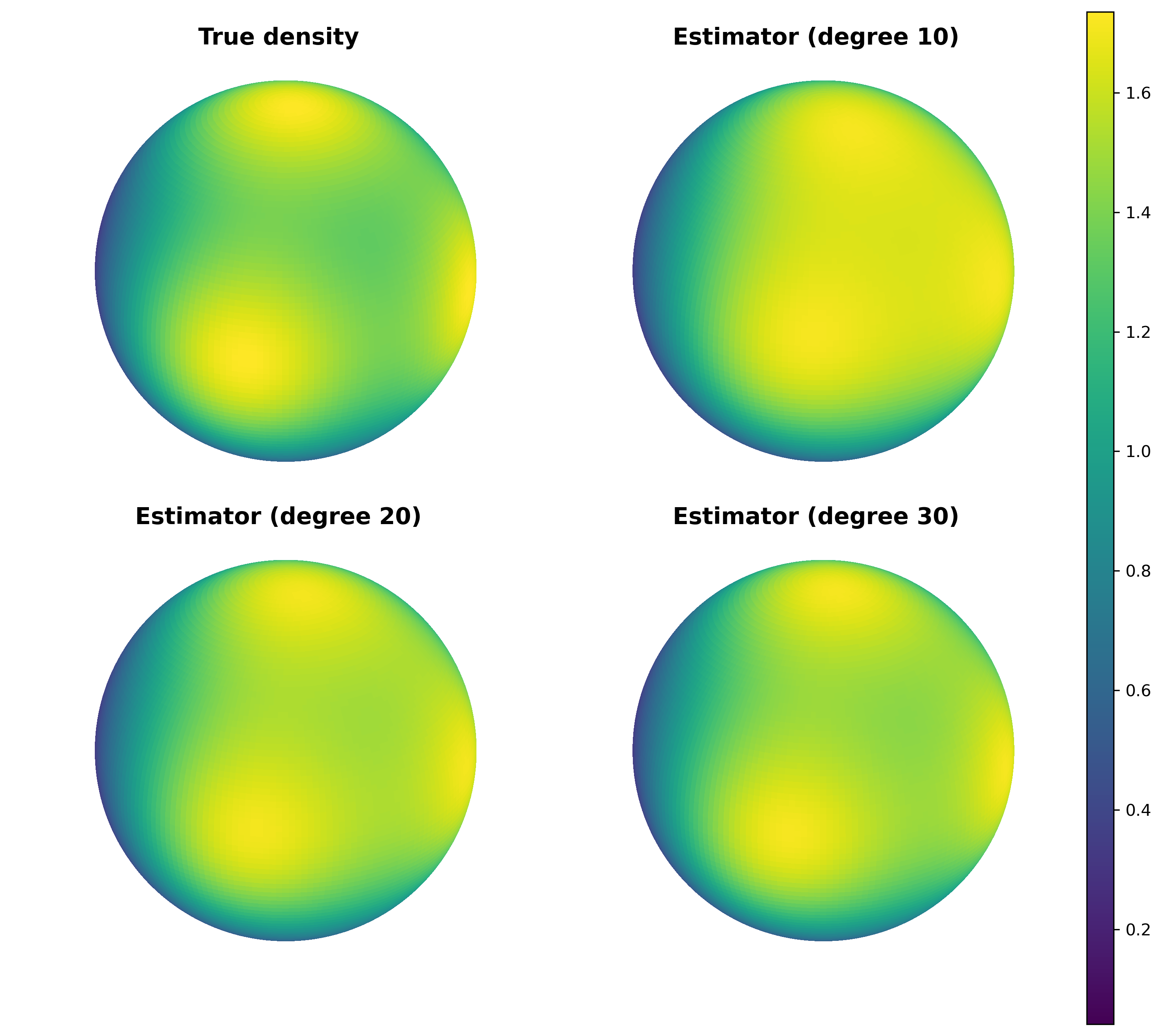
Refer to caption
Figure 1: Plot of the f3f_{3} density alongside its approximations using the MCD kernel density estimator for degrees 1010, 2020, and 3030.

Figure 1 illustrates the true f3f_{3} density and its MCD kernel approximations for various degrees. As shown in Figure 2, the approximation error exhibits a decay of 𝒪​(d−4/3)\mathcal{O}(d^{-4/3}), which dominates the total error. These experiments demonstrate that the MCD kernel reproduces the theoretically predicted error decomposition in a nontrivial example on S2S^{2}.

Refer to caption
Figure 2: ℒ2{\mathscr{L}}^{2} errors for the recovery of the f3f_{3} density as a function of the degree dd.

Appendix A Trigonometric inequality

Lemma 7.

For every θ∈[0,π]\theta\in[0,\pi] one has

1−cos⁡θ≥2π2​θ2.1-\cos\theta\;\geq\;\frac{2}{\pi^{2}}\,\theta^{2}. (A.1)

Equivalently, for every t∈[−1,1]t\in[-1,1],

arccos⁡(t)≤π2​1−t.\arccos(t)\;\leq\;\frac{\pi}{\sqrt{2}}\,\sqrt{1-t}. (A.2)
Proof.

Define

h​(θ):=1−cos⁡θθ2,θ∈(0,π].h(\theta):=\frac{1-\cos\theta}{\theta^{2}},\qquad\theta\in(0,\pi].

If we can show that hh is decreasing on (0,π](0,\pi], then

h​(θ)≥h​(π)=1−cos⁡ππ2=2π2,h(\theta)\;\geq\;h(\pi)=\frac{1-\cos\pi}{\pi^{2}}=\frac{2}{\pi^{2}},

which is exactly (A.1).

Differentiating,

h′​(θ)=θ2​sin⁡θ−2​θ​(1−cos⁡θ)θ4=k​(θ)θ3,h^{\prime}(\theta)=\frac{\theta^{2}\sin\theta-2\theta(1-\cos\theta)}{\theta^{4}}=\frac{k(\theta)}{\theta^{3}},

where

k​(θ):=θ​sin⁡θ−2​(1−cos⁡θ).k(\theta):=\theta\sin\theta-2(1-\cos\theta).

Thus sign⁡(h′​(θ))=sign⁡(k​(θ))\operatorname{sign}(h^{\prime}(\theta))=\operatorname{sign}(k(\theta)) for θ>0\theta>0. Differentiate kk:

k′​(θ)=θ​cos⁡θ−sin⁡θ,k′′​(θ)=−θ​sin⁡θ.k^{\prime}(\theta)=\theta\cos\theta-\sin\theta,\qquad k^{\prime\prime}(\theta)=-\theta\sin\theta.

For θ∈[0,π]\theta\in[0,\pi] we have sin⁡θ≥0\sin\theta\geq 0, hence k′′​(θ)≤0k^{\prime\prime}(\theta)\leq 0, so k′k^{\prime} is decreasing on [0,π][0,\pi]. Using the Taylor expansions sin⁡θ=θ+O​(θ3)\sin\theta=\theta+O(\theta^{3}), cos⁡θ=1+O​(θ2)\cos\theta=1+O(\theta^{2}) as θ→0\theta\to 0, one checks that k′​(0)=0k^{\prime}(0)=0. Since k′k^{\prime} is decreasing and k′​(0)=0k^{\prime}(0)=0, it follows that k′​(θ)≤0k^{\prime}(\theta)\leq 0 for θ∈[0,π]\theta\in[0,\pi], so kk is decreasing on [0,π][0,\pi]. Again using Taylor expansion, k​(0)=0k(0)=0, hence k​(θ)≤0k(\theta)\leq 0 for all θ∈[0,π]\theta\in[0,\pi]. Therefore h′​(θ)≤0h^{\prime}(\theta)\leq 0 on (0,π](0,\pi], so hh is decreasing and (A.1) holds.

To obtain (A.2), let t∈[−1,1]t\in[-1,1] and set θ:=arccos⁡(t)∈[0,π]\theta:=\arccos(t)\in[0,\pi]. Then t=cos⁡θt=\cos\theta and 1−t=1−cos⁡θ1-t=1-\cos\theta, so (A.1) gives

1−t=1−cos⁡θ≥2π2​θ2,1-t=1-\cos\theta\;\geq\;\frac{2}{\pi^{2}}\,\theta^{2},

that is

θ≤π2​1−t.\theta\;\leq\;\frac{\pi}{\sqrt{2}}\sqrt{1-t}.

Since θ=arccos⁡(t)\theta=\arccos(t), this is exactly (A.2). ∎

Appendix B The Funk-Hecke formula

In this appendix we recall the Funk-Hecke formula, which allows one to reduce integrals of zonal functions against spherical harmonics to one-dimensional integrals on [−1,1][-1,1].

Let S:=Sn−1⊂ℝnS:=S^{n-1}\subset\mathbb{R}^{n} denote the unit sphere, and let λ\lambda be the normalized surface measure on SS. For each integer ℓ≥0\ell\geq 0, let ℋℓ\mathcal{H}_{\ell} denote the space of spherical harmonics of degree ℓ\ell, i.e., the restrictions to SS of homogeneous harmonic polynomials of degree ℓ\ell in ℝn\mathbb{R}^{n}. It is well known that

ℒ2​(S,λ)=⨁ℓ=0∞ℋℓ,\mathscr{\mathscr{L}}^{2}(S,\lambda)=\bigoplus_{\ell=0}^{\infty}\mathcal{H}_{\ell},

and that each ℋℓ\mathcal{H}_{\ell} is finite-dimensional. We fix once and for all an orthonormal basis {Yℓ,k}k=1Nℓ\{Y_{\ell,k}\}_{k=1}^{N_{\ell}} of ℋℓ\mathcal{H}_{\ell} in ℒ2​(S,λ){\mathscr{L}}^{2}(S,\lambda).

A function K:S×S→ℝK:S\times S\to\mathbb{R} is called zonal (or rotationally invariant) if it depends only on the inner product:

K​(x,y)=F​(⟨x,y⟩),x,y∈S,K(x,y)=F(\langle x,y\rangle),\qquad x,y\in S,

for some function F:[−1,1]→ℝF:[-1,1]\to\mathbb{R}. In this case we will also write KF​(x,y)K_{F}(x,y) for the kernel associated with FF.

Let α:=(n−1)/2\alpha:=(n-1)/2 and denote by Cℓ(α)C_{\ell}^{(\alpha)} the Gegenbauer polynomial of degree ℓ\ell. Let wα​(t):=(1−t2)α−1/2w_{\alpha}(t):=(1-t^{2})^{\alpha-1/2} be the associated weight function on [−1,1][-1,1].

Theorem 6 (Funk-Hecke formula).

Let F:[−1,1]→ℂF:[-1,1]\to\mathbb{C} be such that

∫−11|F​(t)|​wα​(t)​𝑑t<∞.\int_{-1}^{1}|F(t)|\,w_{\alpha}(t)\,dt<\infty.

Fix x∈Sx\in S and define the zonal kernel

KF​(x,y):=F​(⟨x,y⟩),y∈S.K_{F}(x,y):=F(\langle x,y\rangle),\qquad y\in S.

Then for every spherical harmonic Yℓ,k∈ℋℓY_{\ell,k}\in\mathcal{H}_{\ell} one has

∫SKF​(x,y)​Yℓ,k​(y)​𝑑λ​(y)=λℓ​(F)​Yℓ,k​(x),\int_{S}K_{F}(x,y)\,Y_{\ell,k}(y)\,d\lambda(y)=\lambda_{\ell}(F)\,Y_{\ell,k}(x),

where the scalar coefficient λℓ​(F)\lambda_{\ell}(F) depends only on ℓ\ell and FF and is given explicitly by

λℓ​(F)=ωn−2ωn−1​Cℓ(α)​(1)​∫−11F​(t)​Cℓ(α)​(t)​wα​(t)​𝑑t.\lambda_{\ell}(F)=\frac{\omega_{n-2}}{\omega_{n-1}C_{\ell}^{(\alpha)}(1)}\int_{-1}^{1}F(t)\,C_{\ell}^{(\alpha)}(t)\,w_{\alpha}(t)\,dt.

Here ωn−1\omega_{n-1} and ωn−2\omega_{n-2} denotes the surface area of Sn−1S^{n-1} and Sn−2S^{n-2}, respectively. In particular, the integral on the left-hand side is a multiple of Yℓ,k​(x)Y_{\ell,k}(x), and the multiple is the same for all k=1,…,Nℓk=1,\dots,N_{\ell}.

In the special case ℓ=0\ell=0, C0(α)​(t)≡1C_{0}^{(\alpha)}(t)\equiv 1 and Y0,1Y_{0,1} is constant, so the formula reduces to

∫SF​(⟨x,y⟩)​𝑑λ​(y)=ωn−2ωn−1​∫−11F​(t)​wα​(t)​𝑑t,\int_{S}F(\langle x,y\rangle)\,d\lambda(y)=\frac{\omega_{n-2}}{\omega_{n-1}}\int_{-1}^{1}F(t)\,w_{\alpha}(t)\,dt,

which shows that such zonal integrals are independent of xx and can be reduced to a univariate integral on [−1,1][-1,1].

For more details, we refer to standard texts on spherical harmonics, e.g. [12].

References

  • [1] B. Adcock, Optimal sampling for least-squares approximation, Found. Comput. Math. 25 (2025), 1975–2034.
  • [2] B. Adcock, J. M. Cardenas, and N. Dexter, CS4ML: a general framework for active learning with arbitrary data based on Christoffel functions, Proc. 37th Int. Conf. Neural Information Processing Systems (NeurIPS), 2023, pp. 19990–20037.
  • [3] F. Dai and Y. Xu, Approximation theory and harmonic analysis on spheres and balls, Springer, 2013.
  • [4] M. Dolbeault and A. Cohen, Optimal sampling and Christoffel functions on general domains, Constr. Approx. 56 (2021), 121–163.
  • [5] M. Fanuel, J. Schreurs, and J. A. K. Suykens, Nyström landmark sampling and regularized Christoffel functions, Mach. Learn. 111 (2022), 2213–2254.
  • [6] W. Gautschi, Orthogonal polynomials: computation and approximation, Oxford Univ. Press, 2004.
  • [7] J. B. Lasserre, E. Pauwels, and M. Putinar, The Christoffel-Darboux kernel for data analysis, Cambridge Univ. Press, 2022.
  • [8] J. B. Lasserre, A modified Christoffel function and its asymptotic properties, J. Approx. Theory 295 (2023), 105955.
  • [9] G. Leoni, A first course in Sobolev spaces, Amer. Math. Soc., 2009.
  • [10] H. Li and Y. Xu, Spectral approximation on the unit ball, SIAM J. Numer. Anal. 52 (2014), 2647–2675.
  • [11] O. Mula and A. Nouy, Moment-SoS methods for optimal transport problems, Numer. Math. 156 (2024), 1541–1578.
  • [12] C. Müller, Spherical harmonics, Springer, 1966.
  • [13] D. L. Ragozin, Constructive polynomial approximation on the sphere, Trans. Amer. Math. Soc. 162 (1971), 157–170.
  • [14] P. Roos Hoefgeest and L. Slot, The Christoffel-Darboux kernel for topological data analysis, Proc. 39th Int. Symp. Comput. Geometry (SoCG), 2023.
  • [15] L. Slot, Sum-of-squares hierarchies for polynomial optimization and the Christoffel-Darboux kernel, SIAM J. Optim. 32 (2022), 2612–2635.
  • [16] G. Szegő, Orthogonal polynomials, 4th ed., Amer. Math. Soc., 1975.