跳到论文正文
W Papers独立论文阅读器 arXiv:2603.07479 论文正文 计算阅读时间 · 0%
引用这篇论文根据当前论文元数据生成,正式投稿前建议核对。


License: arXiv.org perpetual non-exclusive license
arXiv:2603.07479v1 [stat.ME] 08 Mar 2026

Mixed Effects Mixture of Experts: Modeling Double Heterogeneous Trajectories

Xinkai Yue, Xiaodong Yan, Haohui Han and Liya Fu
School of Mathematics and Statistics, Xi’an Jiaotong University
The authors gratefully acknowledge the National Natural Science Foundation of China (No. 12371295, 12371292) and the Shaanxi Fundamental Science Research Project for Mathematics and Physics (No. 22JSY002)Email: fuliya@mail.xjtu.edu.cn
Abstract

Linear mixed-effects model (LMM) is a cornerstone of longitudinal data analysis, but is limited to adeptly make heterogeneous analyses predictable under both group-specific fixed effects and subject-specific random effects. To address this challenge, we propose a novel statistical framework by using a large model prototype: a mixed effects mixture of experts model (MEMoE). This framework integrates the ‘divide-and-conquer’ paradigm of Mixture of Experts Models with classical mixed-effect modeling. In the proposed MEMoE, each ‘expert’ is a full LMM dedicated to capturing the longitudinal trajectory of a specific latent subpopulation, while another model “gating function” learns to route subjects to the most appropriate expert in a data-driven manner based on baseline covariates. We develop a robust inferential procedure for parameter estimation based on the Laplace Expectation-Maximization algorithm, with standard errors calibrated using robust sandwich estimators to account for potential model misspecification. Extensive simulation studies and an empirical application demonstrate that MEMoE outperforms both traditional single-population LMM and conventional Mixture of Experts models in terms of parameter recovery, classification accuracy, and overall model fit.

Keywords: Large Model Prototype; Mixture of Experts; Mixed Effects; Prediction Set.

1 Introduction

Longitudinal data provides substantial information on dynamic processes, including disease progression, cognitive development, and behavioral changes (Diggle et al. 2002, Fitzmaurice et al. 2011). The linear mixed-effects model (LMM) accounts for subject-level correlations in longitudinal data by adding random effects, avoids the underestimation of standard errors, and thus ensures the validity of hypothesis testing for correlated data (Hedeker and Gibbons 2006) by separating variance into fixed (population-level) and random (subject-level) components (Laird and Ware 1982, Verbeke and Molenberghs 2000, Pinheiro and Bates 2000, Little and Rubin 2019). To address the limitations of the homogeneous population assumption in longitudinal data analysis, mixture linear mixed models (Verbeke and Lesaffre 1996, Muthén 2004) or subgroup analysis approaches (Yang et al. 2019, Yan et al. 2021, Huang et al. 2023) have been developed to accommodate non-Gaussian random-effect distributions and enable clustering of subjects with distinct trajectories. Nonetheless, LMM and its extensions have limited capacity to accurately predict under heterogeneous model structures that simultaneously incorporate group-specific fixed effects and subject-specific random effects.

The large model prototype “mixture of experts” (MoE) paradigm is a foundational technique that leverages a gating function to route inputs to appropriate specialized submodels, thereby facilitating the adaptive assignment of expert-specific (i.e., group-specific) effects (Jacobs et al. 1991). In this framework, each expert focuses on a distinct region of the input space and is accountable for a specific data subset. This methodology has demonstrated efficacy across various domains, enabling flexible capture and discovery of latent subgroups in regression data (Yuksel et al. 2012, Bishop 2006). In large-scale data contexts, MoE enhances scalability—a key reason for its adoption in modern deep learning—by efficiently managing complex, multimodal distributions without imposing uniformity assumptions (Shazeer et al. 2017). Recent applications to longitudinal trajectories further illustrate MoE’s capacity to identify latent classes while accounting for heterogeneity, as in growth curve analysis (Gao et al. 2002, Quiroz and Villani 2013). The adaptive gating mechanism weights expert contributions differentially across individuals or time points, thereby effectively accommodating population heterogeneity (He et al. 2025). Consequently, MoE is particularly advantageous for longitudinal applications involving divergent subgroup patterns, such as varying treatment responses in patient cohorts or differential growth curves in educational studies, where it can uncover time-dependent latent classes, such as heterogeneous brain activity trajectories in infant emotional reactivity research (Che et al. 2023).

However, standard MoE models lack an explicit mechanism to account for within correlation, simply treating all observations as independent, which can lead to biased estimates in longitudinal settings (Jordan and Jacobs 1994). Hierarchical extensions of MoE have been proposed, but they typically fail to incorporate random effects within the experts, thereby limiting their ability to capture unobserved subject-level heterogeneity (Xu and Jordan 1996). In contrast, existing mixed-effects extensions of regression models, such as mixtures of linear mixed models, effectively capture correlations yet fail to leverage the gating-expert architecture of MoE. Recent research has sought to bridge this gap. Fung and Tseung (2022) proposed a mixed MoE for multilevel data, demonstrating that such models can approximate arbitrary mixed-effects distributions. Similarly, Kock et al. (2025) developed a deep mixture of linear mixed models to handle irregular longitudinal data with complex temporal dynamics, incorporating deep latent factors to model high-dimensional random effects. These pioneering studies underscore the promise of combining mixtures and random effects. However, practical parameter estimation remains difficult, stemming not only from the presence of hidden variables but also from the substantial computational burden associated with integrating over random effects.

To address the challenges of classical LMMs and MoE models, we propose a Mixed-Effects Mixture of Experts (MEMoE) model, which unifies the MoE framework with subject-specific random effects. In MEMoE, each expert comprises a linear mixed-effects model with its own random intercepts and slopes, governed by a multivariate normal prior; the gating function then probabilistically assigns observations to the respective experts. This approach captures heterogeneity between-subjects through mixture components while simultaneously accounting for within correlations through random effects, thereby bridging multilevel data structures with MoE architecture. The key contributions are listed as follows:

(i) For methodology, the proposed MEMoE model advances the synergy between MoE and LMMs, because it flexibly models double heterogeneous longitudinal trajectories, accommodating subject-specific variability. Relative to mixtures of linear mixed models, MEMoE employs explicit gating for subgroup discovery; in contrast to standard MoE models, it formally incorporates within correlations.

(ii) In computation, we develop a new Laplace-EM algorithm to address the challenge of intractable marginal likelihood, which integrates over the latent random effects.

(iii) Practically, MEMoE is especially appropriate for applications such as patient trajectory modeling in healthcare, where latent subgroups may exhibit distinct progression patterns (e.g., heterogeneous epidemic disease progression, (Cui et al. 2022)); educational growth curves accounting for student-specific differences; or socioeconomic trends with subgroup-specific dynamics.

The remainder of this paper is organized as follows. In Section 2, we present the MEMoE models and the Laplace-EM algorithm. Section 3 provides a set of constructions for response prediction. In Section 4, we establish the theoretical properties of the proposed estimator, including the consistency of the Laplace-EM estimator and the asymptotic normality of the predictor. Section 5 evaluates the performance of the proposed method through extensive simulation studies and real-data analysis. Section 6 gives some concluding remarks.

2 Methods

This section introduces the MEMoE framework, which demonstrates the primary advantage of making both observation- and subgroup-specific heterogeneous analyses predictable when the subgroup structure is unknown.

2.1 The Mixed Effects Mixture of Experts Models

Consider the data collected from NN subjects. Let yi​jy_{ij} denote the jj-th outcome for subject ii, and xi​j=(1,xi​j​1,…,xi​j​(p−1))⊤∈ℝp{x}_{ij}=(1,x_{ij1},\dots,x_{ij(p-1)})^{\top}\in\mathbb{R}^{p} be the fixed-effect covariates and zi​j∈ℝq{z}_{ij}\in\mathbb{R}^{q} be the random-effect covariates, where i=1,…​Ni=1,\ldots N and j=1,…,nij=1,\dots,n_{i}. We posit KK latent subgroups and assign to each observation a latent label vi​j∈{1,…,K}v_{ij}\in\{1,\dots,K\} indicating its subgroup membership. Given the expert label vi​j=kv_{ij}=k, the response follows an expert-specific mixed effects model:

yi​j=xi​j⊤​βk+zi​j⊤​ui+εi​jk,y_{ij}\;=\;x_{ij}^{\top}\beta_{k}\;+\;z_{ij}^{\top}u_{i}\;+\;\varepsilon_{ij}^{k},

where βk∈ℝp{\beta}_{k}\in\mathbb{R}^{p} is an expert-specific fixed effect, ui∈ℝq{u}_{i}\in\mathbb{R}^{q} is a subject-level random effect shared between experts, and the random error εi​jk∼𝒩​(0,σk2)\varepsilon_{ij}^{k}\sim\mathcal{N}(0,\sigma_{k}^{2}). Then

yi​j∣xi​j,zi​j,ui,vi​j=k∼𝒩​(xi​j⊤​βk+zi​j⊤​ui,σk2).y_{ij}\mid x_{ij},z_{ij},u_{i},v_{ij}=k\;\sim\;\mathcal{N}\!\big(x_{ij}^{\top}\beta_{k}+z_{ij}^{\top}u_{i},\ \sigma_{k}^{2}\big). (1)

To identify which expert a subject belongs to, we assume that the gating function depends only on the covariates at the subject-level:

vi​j∣xi​j,zi​j∼Multinomial​(π1​(xi​j,zi​j;α),…,πK​(xi​j,zi​j;α)),v_{ij}\mid{x}_{ij},{z}_{ij}\ \sim\ \mathrm{Multinomial}\big(\,\pi_{1}({x}_{ij},{z}_{ij};\alpha),\ldots,\pi_{K}({x}_{ij},{z}_{ij};\alpha)\big),

where α\alpha is an unknown parameter vector. The covariate-dependent weight πk​(xi​j,zi​j;α)\pi_{k}({x}_{ij},{z}_{ij};\alpha) can be interpreted as the probability that the (i,j)(i,j)-th observation comes from the kkth expert model and serves to automatically discover latent subgroups and regime changes.

To provide a more explanatory and predictive structure for subject-level random effects uiu_{i}, we construct the following covariate-dependent model:

ui∣wi∼𝒩​(κ​wi,Σ),u_{i}\mid w_{i}\sim\mathcal{N}(\kappa w_{i},\Sigma), (2)

where wiw_{i} collects subject-level covariates (e.g., demographics, baseline measures), κ∈ℝq×d\kappa\in\mathbb{R}^{q\times d}, and Σ\Sigma is a q×qq\times q covariance matrix. This specification encodes explainable between-subject variation through wiw_{i}; setting κ=0\kappa=0 recovers the commonly used random-effects ui∼𝒩​(0,Σ)u_{i}\sim\mathcal{N}(0,\Sigma). In this zero-mean random-effects case, we refer to the resulting expert model as the random-effects mixture-of-experts (ReMoE) specification. Figure 1 shows the workflow framework of the proposed MEMoE model.

Refer to caption
Figure 1: Structure of the MEMoE. Pink blocks represent data inputs, yellow blocks denote the created model framework, and the green block signifies the model output.

The proposed MEMoE specification is a unifying formulation that nests several widely used expert models. In particular, when each subject has a single observation (ni=1n_{i}=1 for all ii) or the random effects vanish (i.e., Σ=0\Sigma=0, such that ui≡0u_{i}\equiv 0), the model coincides with the classical MoE regression, dedicating an expert model to each partitioned observation. When the gating function is degenerate with only one expert, i.e., β1=⋯=βK\beta_{1}=\cdots=\beta_{K} and σ12=⋯=σK2\sigma_{1}^{2}=\cdots=\sigma_{K}^{2}, MEMoE reduces to a single homoscedastic linear mixed effects model.

2.2 Laplace-EM Algorithm

In this subsection, we construct a Laplace EM algorithm to estimate the parameters in the MEMoE. The E-step relies on a Laplace approximation to compute the approximate modes of the random effects (Breslow and Clayton 1993, Skaug and Fournier 2006). The M-step updates model parameters via block-wise optimizations. To ensure stable and monotonic convergence, particularly for non-convex components, we integrate a majorize-minimize strategy (Hunter and Lange 2004).

Conditional on the random effect uiu_{i} and covariates xi​jx_{ij} and zi​jz_{ij}, the conditional density of yi​jy_{ij} is

f​(yi​j∣ui,xi​j,zi​j;Ψ)=∑k=1Kπk​(xi​j,zi​j;α)​φ​(yi​j;xi​j⊤​βk+zi​j⊤​ui,σk2),f\!\left(y_{ij}\mid u_{i},x_{ij},z_{ij};\Psi\right)=\sum_{k=1}^{K}\pi_{k}(x_{ij},z_{ij};\alpha)\;\varphi\!\left(y_{ij};\,x_{ij}^{\top}\beta_{k}+z_{ij}^{\top}u_{i},\ \sigma_{k}^{2}\right),

where φ​(⋅)\varphi(\cdot) is a normal density

φ​(yi​j;xi​j⊤​βk+zi​j⊤​ui,σk2)=12​π​σk2​exp⁡{−(yi​j−(xi​j⊤​βk+zi​j⊤​ui))22​σk2},\varphi\!\left(y_{ij};\,x_{ij}^{\top}\beta_{k}+z_{ij}^{\top}u_{i},\ \sigma_{k}^{2}\right)=\frac{1}{\sqrt{2\pi\sigma_{k}^{2}}}\exp\left\{-\frac{\left(y_{ij}-(x_{ij}^{\top}\beta_{k}+z_{ij}^{\top}u_{i})\right)^{2}}{2\sigma_{k}^{2}}\right\},

and Ψ\Psi represents the set of all model parameters and belongs to a parameter space Θ\Theta. Under the assumption that {yi​j}j=1ni\{y_{ij}\}_{j=1}^{n_{i}} are conditionally independent given uiu_{i}, the likelihood function for the repeated measurements takes the following form:

L​(Ψ)\displaystyle L(\Psi) =∏i=1Nf​(yi​1,yi​2,…,yi​ni∣{xi​j,zi​j}j=1ni;Ψ)\displaystyle=\prod_{i=1}^{N}f(y_{i1},y_{i2},\ldots,y_{in_{i}}\mid\{x_{ij},z_{ij}\}_{j=1}^{n_{i}};\Psi)
=∏i=1N∫∏j=1nif​(yi​j∣ui,xi​j,zi​j;Ψ)​φ​(ui;κ​wi,Σ)​d​ui\displaystyle=\prod_{i=1}^{N}\int\prod_{j=1}^{n_{i}}f(y_{ij}\mid u_{i},x_{ij},z_{ij};\Psi)\,\varphi(u_{i};\kappa w_{i},\Sigma)\,du_{i}
=∏i=1N∫[∏j=1ni∑k=1Kπk​(xi​j,zi​j;α)​φ​(yi​j;xi​j⊤​βk+zi​j⊤​ui,σk2)]​φ​(ui;κ​wi,Σ)​𝑑ui.\displaystyle=\prod_{i=1}^{N}\int\left[\prod_{j=1}^{n_{i}}\sum_{k=1}^{K}\pi_{k}(x_{ij},z_{ij};\alpha)\,\varphi\big(y_{ij};x_{ij}^{\top}\beta_{k}+z_{ij}^{\top}u_{i},\sigma_{k}^{2}\big)\right]\varphi\big(u_{i};\kappa w_{i},\Sigma\big)\,du_{i}. (3)

This integral has no closed-form in general because the subject-level mixture is embedded within the product over jj, and all measurements share the same random effect uiu_{i}. Expanding the product of sums leads to a mixture of KniK^{n_{i}} multivariate Gaussians. We therefore approximate the integral in (2.2) using the Laplace method (Breslow and Clayton 1993, Tierney and Kadane 1986). Let hi​(ui;Ψ)h_{i}(u_{i};\Psi) denote the logarithm of the integrand:

hi​(ui;Ψ)=log⁡φ​(ui;κ​wi,Σ)+∑j=1nilog⁡[∑k=1Kπk​(xi​j,zi​j;α)​φ​(yi​j;xi​j⊤​βk+zi​j⊤​ui,σk2)].h_{i}(u_{i};\Psi)=\log\varphi(u_{i};\kappa w_{i},\Sigma)+\sum_{j=1}^{n_{i}}\log\left[\sum_{k=1}^{K}\pi_{k}(x_{ij},z_{ij};\alpha)\varphi\left(y_{ij};x_{ij}^{\top}\beta_{k}+z_{ij}^{\top}u_{i},\sigma_{k}^{2}\right)\right].

The Laplace method approximates the integral by forming a second-order Taylor expansion of hi​(ui;Ψ)h_{i}(u_{i};\Psi) around its mode, u^i=arg⁡maxui⁡hi​(ui;Ψ)\hat{u}_{i}=\arg\max_{u_{i}}h_{i}(u_{i};\Psi). Let Hi=Hi​(u^i;Ψ)=−∇ui2hi​(ui;Ψ)|ui=u^i{H}_{i}={H}_{i}(\hat{u}_{i};\Psi)=-\nabla^{2}_{u_{i}}h_{i}(u_{i};\Psi)\big|_{u_{i}=\hat{u}_{i}} be the negative Hessian matrix evaluated in the mode, then

Hi\displaystyle H_{i} =Σ−1−∑j=1ni∑k=1Kπk​(xi​j,zi​j;α)​φi​j​k​(u^i)∑ℓ=1Kπℓ​(xi​j,zi​j;α)​φi​j​ℓ​(u^i)​(ei​j​k​(u^i)2σk4−1σk2)​zi​j​zi​j⊤\displaystyle=\Sigma^{-1}-\sum_{j=1}^{n_{i}}\sum_{k=1}^{K}\frac{\pi_{k}(x_{ij},z_{ij};\alpha)\varphi_{ijk}(\hat{u}_{i})}{\sum_{\ell=1}^{K}\pi_{\ell}(x_{ij},z_{ij};\alpha)\varphi_{ij\ell}(\hat{u}_{i})}\left(\frac{e_{ijk}(\hat{u}_{i})^{2}}{\sigma_{k}^{4}}-\frac{1}{\sigma_{k}^{2}}\right)z_{ij}z_{ij}^{\top}
+∑j=1ni(∑k=1Kπk​(xi​j,zi​j;α)​φi​j​k​(u^i)∑ℓ=1Kπℓ​(xi​j,zi​j;α)​φi​j​ℓ​(u^i)​ei​j​k​(u^i)σk2​zi​j)​(∑k=1Kπk​(xi​j,zi​j;α)​φi​j​k​(u^i)∑ℓ=1Kπℓ​(xi​j,zi​j;α)​φi​j​ℓ​(u^i)​ei​j​k​(u^i)σk2​zi​j⊤),\displaystyle+\sum_{j=1}^{n_{i}}\left(\sum_{k=1}^{K}\frac{\pi_{k}(x_{ij},z_{ij};\alpha)\varphi_{ijk}(\hat{u}_{i})}{\sum_{\ell=1}^{K}\pi_{\ell}(x_{ij},z_{ij};\alpha)\varphi_{ij\ell}(\hat{u}_{i})}\frac{e_{ijk}(\hat{u}_{i})}{\sigma_{k}^{2}}z_{ij}\right)\left(\sum_{k=1}^{K}\frac{\pi_{k}(x_{ij},z_{ij};\alpha)\varphi_{ijk}(\hat{u}_{i})}{\sum_{\ell=1}^{K}\pi_{\ell}(x_{ij},z_{ij};\alpha)\varphi_{ij\ell}(\hat{u}_{i})}\frac{e_{ijk}(\hat{u}_{i})}{\sigma_{k}^{2}}z_{ij}^{\top}\right),

where ei​j​k​(u^i)=yi​j−xi​j⊤​βk−zi​j⊤​u^ie_{ijk}(\hat{u}_{i})=y_{ij}-x_{ij}^{\top}\beta_{k}-z_{ij}^{\top}\hat{u}_{i}. Therefore,

Hi\displaystyle H_{i} ≃\displaystyle\simeq Σ−1+∑j=1ni∑k=1Kπk​(xi​j,zi​j;α)​φi​j​k​(u^i)∑ℓ=1Kπℓ​(xi​j,zi​j;α)​φi​j​ℓ​(u^i)​1σk2​zi​j​zi​j⊤\displaystyle\Sigma^{-1}+\sum_{j=1}^{n_{i}}\sum_{k=1}^{K}\frac{\pi_{k}(x_{ij},z_{ij};\alpha)\varphi_{ijk}(\hat{u}_{i})}{\sum_{\ell=1}^{K}\pi_{\ell}(x_{ij},z_{ij};\alpha)\varphi_{ij\ell}(\hat{u}_{i})}\frac{1}{\sigma_{k}^{2}}z_{ij}z_{ij}^{\top}

is positive definite. The Laplace approximation to the likelihood function is then given by:

L​(Ψ)≈∏i=1N[(2​π)q/2​|Hi|−1/2​exp⁡{hi​(u^i;Ψ)}].L(\Psi)\approx\prod_{i=1}^{N}\left[(2\pi)^{q/2}|{H}_{i}|^{-1/2}\exp\left\{h_{i}(\hat{u}_{i};\Psi)\right\}\right].

Taking the logarithms yields the approximated log-likelihood for the parameter set Ψ\Psi:

ℓLA​(Ψ)=N​q2​log⁡(2​π)+∑i=1N[hi​(u^i;Ψ)−12​log⁡|Hi|].\ell_{\rm LA}(\Psi)=\frac{Nq}{2}\log(2\pi)+\sum_{i=1}^{N}\left[h_{i}(\hat{u}_{i};\Psi)-\frac{1}{2}\log|{H}_{i}|\right].

Optimizing the Laplace-approximated log-likelihood ℓLA​(Ψ)\ell_{{\rm LA}}(\Psi) poses significant challenges. In this context, we implement an EM-inspired minorize-maximize algorithm that iteratively builds and maximizes a lower-bound surrogate of ℓLA​(Ψ)\ell_{\rm LA}(\Psi), thereby ensuring steady progress toward a local optimum. Given the current iterate Ψ(t)\Psi^{(t)}, we construct a surrogate lower bound QLA​(Ψ∣Ψ(t))Q_{{\rm LA}}\big(\Psi\mid\Psi^{(t)}\big) for ℓLA​(Ψ)\ell_{{\rm LA}}(\Psi) and maximize it over Ψ\Psi, thereby increasing ℓLA​(Ψ)−ℓLA​(Ψ(t))\ell_{{\rm LA}}(\Psi)-\ell_{{\rm LA}}(\Psi^{(t)}). Concretely, QLAQ_{{\rm LA}} is obtained by a Laplace expansion of the subject-level integral at the posterior mode u^i\hat{u}_{i} computed by the negative Hessian HiH_{i}.

E-step (random effects mode and responsibilities).

Let u^i(t)=arg⁡maxui⁡hi​(ui;Ψ(t)).\hat{u}_{i}^{(t)}=\arg\max_{u_{i}}\,h_{i}(u_{i};\Psi^{(t)}). Denote γi​j​k(t)\gamma_{ijk}^{(t)} as the probability that observation is generated by expert kk, conditional on the latent random effect:

γi​j​k(t)=πk​(xi​j,zi​j;α(t))​φ​(yi​j;xi​j⊤​βk(t)+zi​j⊤​u^i(t),(σk2)(t))∑ℓ=1Kπℓ​(xi​j,zi​j;α(t))​φ​(yi​j;xi​j⊤​βℓ(t)+zi​j⊤​u^i(t),(σℓ2)(t)).\gamma_{ijk}^{(t)}=\frac{\pi_{k}(x_{ij},z_{ij};\alpha^{(t)})\,\varphi\!\big(y_{ij};\,x_{ij}^{\top}\beta_{k}^{(t)}+z_{ij}^{\top}\hat{u}_{i}^{(t)},\,(\sigma^{2}_{k})^{(t)}\big)}{\displaystyle\sum_{\ell=1}^{K}\pi_{\ell}(x_{ij},z_{ij};\alpha^{(t)})\,\varphi\!\big(y_{ij};\,x_{ij}^{\top}\beta_{\ell}^{(t)}+z_{ij}^{\top}\hat{u}_{i}^{(t)},\,(\sigma^{2}_{\ell})^{(t)}\big)}. (4)

It is called the responsibility, as it quantifies how ‘responsibility’ expert kk is for yi​jy_{ij} at the current conditional state.

Form a touching lower limit QLA​(Ψ∣Ψ(t))Q_{{\rm LA}}(\Psi\mid\Psi^{(t)}) for ℓLA​(Ψ)\ell_{{\rm LA}}(\Psi) using Jensen’s inequality to the subject-level term log⁡[∑k=1Kπk​(xi​j,zi​j;α)​φ​(yi​j;xi​j⊤​βk+zi​j⊤​ui,σk2)]\log\left[\sum_{k=1}^{K}\pi_{k}(x_{ij},z_{ij};\alpha)\varphi\left(y_{ij};x_{ij}^{\top}\beta_{k}+z_{ij}^{\top}u_{i},\sigma_{k}^{2}\right)\right] evaluated at u^i(t)\hat{u}_{i}^{(t)}, and linearize −log⁡|Hi|-\log|H_{i}| at the current estimate Hi(t)H_{i}^{(t)}, with −log⁡|Hi|≥−log⁡|Hi(t)|−tr​{(Hi(t))−1​(Hi−Hi(t))}-\log|H_{i}|\;\geq\;-\log|H_{i}^{(t)}|-\,\mathrm{tr}\Big\{\big(H_{i}^{(t)}\big)^{-1}\big(H_{i}-H_{i}^{(t)}\big)\Big\}. Then the QLA​(Ψ∣Ψ(t))Q_{{\rm LA}}\big(\Psi\mid\Psi^{(t)}\big) is

QLA​(Ψ∣Ψ(t))\displaystyle Q_{{\rm LA}}\big(\Psi\mid\Psi^{(t)}\big) =\displaystyle= ∑i=1N{logφ(u^i(t);κwi,Σ)+∑j=1ni∑k=1Kγi​j​k(t)[logπk(xi​j,zi​j;α)\displaystyle\sum_{i=1}^{N}\Bigg\{\log\varphi\big(\hat{u}_{i}^{(t)};\kappa w_{i},\Sigma\big)+\sum_{j=1}^{n_{i}}\sum_{k=1}^{K}\gamma_{ijk}^{(t)}\Big[\log\pi_{k}(x_{ij},z_{ij};\alpha) (5)
+\displaystyle+ logφ(yi​j;xi​j⊤βk+zi​j⊤u^i(t),σk2)−logγi​j​k(t)]}−12∑i=1Ntr((Hi(t))−1Hi).\displaystyle\log\varphi\big(y_{ij};x_{ij}^{\top}\beta_{k}+z_{ij}^{\top}\hat{u}_{i}^{(t)},\sigma_{k}^{2}\big)-\log\gamma_{ijk}^{(t)}\Big]\Bigg\}{-\frac{1}{2}\sum_{i=1}^{N}\mathrm{tr}\big((H_{i}^{(t)})^{-1}H_{i}\big)}.

M-step: parameter updates to maximize the objective function in (5).

Gating parameter vector α\alpha is updated by the following formula:

α(t+1)=arg⁡maxα​∑i=1N∑j=1ni∑k=1Kγi​j​k(t)​log⁡πk​(xi​j,zi​j;α).\alpha^{(t+1)}=\arg\max_{\alpha}\ \sum_{i=1}^{N}\sum_{j=1}^{n_{i}}\sum_{k=1}^{K}\gamma_{ijk}^{(t)}\,\log\pi_{k}(x_{ij},z_{ij};\alpha).

Expert’s coefficients {βk}k=1K\{\beta_{k}\}_{k=1}^{K}:

β^k(t+1)=(∑i,jγi​j​k(t)σ^k2,(t)​xi​j​xi​j⊤)−1​(∑i,jγi​j​k(t)σ^k2,(t)​xi​j​(yi​j−zi​j⊤​u^i(t))).\hat{\beta}_{k}^{(t+1)}=\Big(\sum_{i,j}\tfrac{\gamma_{ijk}^{(t)}}{\hat{\sigma}_{k}^{2,(t)}}x_{ij}x_{ij}^{\top}\Big)^{-1}\Big(\sum_{i,j}\tfrac{\gamma_{ijk}^{(t)}}{\hat{\sigma}_{k}^{2,(t)}}x_{ij}(y_{ij}-z_{ij}^{\top}\hat{u}_{i}^{(t)})\Big).

Noise variances {σk2}k=1K\{\sigma_{k}^{2}\}_{k=1}^{K}:

(σk2)(t+1)=∑i=1N∑j=1niγi​j​k(t)​[(yi​j−xi​j⊤​βk(t+1)−zi​j⊤​u^i(t))2+zi​j⊤​(Hi(t))−1​zi​j]∑i=1N∑j=1niγi​j​k(t).(\sigma^{2}_{k})^{(t+1)}=\frac{\displaystyle\sum_{i=1}^{N}\sum_{j=1}^{n_{i}}\gamma_{ijk}^{(t)}\Big[\big(y_{ij}-x_{ij}^{\top}\beta_{k}^{(t+1)}-z_{ij}^{\top}\hat{u}_{i}^{(t)}\big)^{2}+z_{ij}^{\top}(H_{i}^{(t)})^{-1}z_{ij}\Big]}{\displaystyle\sum_{i=1}^{N}\sum_{j=1}^{n_{i}}\gamma_{ijk}^{(t)}}.

Random-effect mean parameter matrix κ\kappa:

κ(t+1)=(∑i=1Nu^i(t)​wi⊤)​(∑i=1Nwi​wi⊤)−1.\kappa^{(t+1)}=\Big(\sum_{i=1}^{N}\hat{u}_{i}^{(t)}w_{i}^{\top}\Big)\Big(\sum_{i=1}^{N}w_{i}w_{i}^{\top}\Big)^{-1}.

Random-effect covariance matrix Σ\Sigma:

Σ(t+1)=1N​∑i=1N[(u^i(t)−κ(t+1)​wi)​(u^i(t)−κ(t+1)​wi)⊤+(Hi(t))−1].\Sigma^{(t+1)}=\frac{1}{N}\sum_{i=1}^{N}\Big[\big(\hat{u}_{i}^{(t)}-\kappa^{(t+1)}w_{i}\big)\big(\hat{u}_{i}^{(t)}-\kappa^{(t+1)}w_{i}\big)^{\top}+(H_{i}^{(t)})^{-1}\Big].

The algorithm alternates between computing subject-level membership probabilities and updating the model parameters. At iteration tt, the E-step computes the responsibilities γi​j​k(t){\gamma_{ijk}^{(t)}}, u^i(t)\hat{u}_{i}^{(t)}, and Hi(t)H_{i}^{(t)}, using the current parameter vector Ψ(t)\Psi^{(t)}. Subsequently, the M-step updates the elements of Ψ\Psi via the specified iterative formulas.

3 Prediction Sets

Quantifying predictive uncertainty is essential for reliable inference in longitudinal studies that exhibit both population heterogeneity and within-subject dependence. We develop prediction sets for the MEMoE model — a covariate-gated mixture framework that captures the latent subgroup structures while accounting for subject-specific random effects. Given a fitted model based on NN subjects, a target confidence level 1−q∈(0,1)1-q\in(0,1), and a tuple of new covariates (xnew,znew,wnew)(x_{\text{new}},z_{\text{new}},w_{\text{new}}), our aim is to construct a conditionally valid prediction set Ω​(xnew,znew,wnew)\Omega(x_{\text{new}},z_{\text{new}},w_{\text{new}}) for a future response ynewy_{\text{new}}, such that:

Pr⁡(ynew∈Ω​(xnew,znew,wnew)∣xnew,znew,wnew)≥1−q,\Pr\left(y_{\text{new}}\in\Omega(x_{\text{new}},z_{\text{new}},w_{\text{new}})\mid x_{\text{new}},z_{\text{new}},w_{\text{new}}\right)\geq 1-q, (6)

a guaranty targeted at fixed covariates rather than averaged over their distribution (cf. conditional versus marginal coverage in predictive inference). In words, a prediction set is a range — possibly a union of disjoint intervals — within which a future response is expected to fall with a probability of at least 1−q1-q; shorter prediction sets are preferred for informativeness, whereas the trivial set (−∞,∞)(-\infty,\infty) achieves 100%100\% coverage yet conveys no meaningful information. This conditional coverage target mirrors recent developments in predictive inference for MoE models and highlights the advantage of parametric modeling of the conditional law when per-covariate guarantees are required.

Given the new input, the density of the response ynewy_{\text{new}} can be obtained via

f​(ynew∣xnew,znew,wnew;Ψ)\displaystyle f(y_{\text{new}}\mid x_{\text{new}},z_{\text{new}},w_{\text{new}};\Psi) =∫f​(ynew∣unew,xnew,znew;Ψ)​φ​(unew;κ​wnew,Σ)​𝑑u\displaystyle=\int f(y_{\text{new}}\mid u_{\text{new}},x_{\text{new}},z_{\text{new}};\Psi)\,\varphi(u_{\text{new}};\kappa w_{\text{new}},\Sigma)\,du
=∑k=1Kπk​(xnew,znew;α)​𝒩​(ynew;xnew⊤​βk+znew⊤​κ​wnew,σk2+znew⊤​Σ​znew).\displaystyle=\sum_{k=1}^{K}\pi_{k}(x_{\text{new}},z_{\text{new}};\alpha)\mathcal{N}\left(y_{\text{new}};x_{\text{new}}^{\top}\beta_{k}+z_{\text{new}}^{\top}\kappa w_{\text{new}},\,\sigma_{k}^{2}+z_{\text{new}}^{\top}\Sigma z_{\text{new}}\right).

If vnew=kv_{\text{new}}=k, we obtain the predictor Γ^k=xnew⊤​β^k+znew⊤​κ^​wnew\hat{\Gamma}_{k}=x_{\text{new}}^{\top}\hat{\beta}_{k}+z_{\text{new}}^{\top}\hat{\kappa}w_{\text{new}} based on Laplace-EM estimates and approximate the variance of Γ^k\hat{\Gamma}_{k} by a working variance matrix V^k=V^k(β)+V^k(κ)\hat{V}_{k}=\hat{V}_{k}^{(\beta)}+\hat{V}_{k}^{(\kappa)}, where V^k(β)=xnew⊤​(∑i,jγi​j​kσ^k2​xi​j​xi​j⊤)−1​xnew\hat{V}_{k}^{(\beta)}=x_{\text{new}}^{\top}\left(\sum_{i,j}\frac{\gamma_{ijk}}{\hat{\sigma}_{k}^{2}}x_{ij}x_{ij}^{\top}\right)^{-1}x_{\text{new}} and V^k(κ)=(wnew⊗znew)⊤​(Σ^⊗(∑i=1Nwi​wi⊤)−1)​(wnew⊗znew).\hat{V}_{k}^{(\kappa)}=(w_{\text{new}}\otimes z_{\text{new}})^{\top}\left(\hat{\Sigma}\otimes\left(\sum_{i=1}^{N}w_{i}w_{i}^{\top}\right)^{-1}\right)(w_{\text{new}}\otimes z_{\text{new}}). Then the variance estimate of the predicted response is

b^k2=znew⊤​Σ^​znew+σ^k2+V^k.\hat{b}_{k}^{2}=z_{\text{new}}^{\top}\hat{\Sigma}z_{\text{new}}+\hat{\sigma}_{k}^{2}+\hat{V}_{k}. (7)

Recall that our goal is to construct a 100​(1−q)%100(1-q)\% prediction set Ωq​(xnew,znew,wnew)\Omega_{q}(x_{\mathrm{new}},z_{\mathrm{new}},w_{\mathrm{new}}) satisfying (6). In MEMoE, the predictive distribution for ynewy_{\mathrm{new}} given covariates (xnew,znew,wnew)(x_{\mathrm{new}},z_{\mathrm{new}},w_{\mathrm{new}}) is a finite mixture of Gaussian, with each component corresponding to an expert indexed by k=1,…,Kk=1,\dots,K. Motivated by the mixture structure, we establish a prediction set given as follows:

Ωq​(xnew,znew,wnew)=⋃k=1K[ℓk,uk],\Omega_{q}(x_{\mathrm{new}},z_{\mathrm{new}},w_{\mathrm{new}})\;=\;\bigcup_{k=1}^{K}[\ell_{k},u_{k}],

where each [ℓk,uk][\ell_{k},u_{k}] is a estimator Γ^k\hat{\Gamma}_{k}. Treating the length of Ωq​(xnew,znew,wnew)\Omega_{q}(x_{\mathrm{new}},z_{\mathrm{new}},w_{\mathrm{new}}) as our budget, it is intuitive that we should allocate more of this budget to the mixture components to which the new predictor is more likely to be assigned–that is, to those groups kk with larger value of π​(xnew,znew){\pi}(x_{\mathrm{new}},z_{\mathrm{new}}). To this end, we construct the marginal predictive density f^​(y)\hat{f}(y) using a weighted mixture of Gaussian mixture densities:

f^​(y)=∑k=1Kπ^k​1b^k​φ​(y−Γ^kb^k),\hat{f}(y)=\sum_{k=1}^{K}\hat{\pi}_{k}\frac{1}{\hat{b}_{k}}\varphi\left(\frac{y-\hat{\Gamma}_{k}}{\hat{b}_{k}}\right),

where φ​(⋅)\varphi(\cdot) denotes the density function of the standard normal distribution, and π^k=πk​(xnew,znew;α^)\hat{\pi}_{k}=\pi_{k}(x_{\mathrm{new}},z_{\mathrm{new}};\hat{\alpha}).

Our objective is to construct the shortest set Ωq⊂ℝ\Omega_{q}\subset\mathbb{R} such that ∫Ωqf^​(y)​𝑑y≥1−q\int_{\Omega_{q}}\hat{f}(y)dy\geq 1-q. To ensure that the numerical search is limited to a finite and relevant region, we first define a conservative bounding interval 𝒬\mathcal{Q} guaranteed to contain the target set. Let cq=Φ−1​(1−q/2)c_{q}=\Phi^{-1}(1-q/2) and define

𝒬=[mink⁡{Γ^k−cq​b^k},maxk⁡{Γ^k+cq​b^k}],\mathcal{Q}=\Big[\min_{k}\{\hat{\Gamma}_{k}-c_{q}\hat{b}_{k}\},\ \max_{k}\{\hat{\Gamma}_{k}+c_{q}\hat{b}_{k}\}\Big],

which has a probability of at least 1−q1-q. Next, we partition 𝒬\mathcal{Q} into MM equal width subintervals Qr=[ar,er)Q_{r}=[a_{r},e_{r}) with length δ=\delta= Len(𝒬)/M(\mathcal{Q})/M, where ar=mink⁡{Γ^k−cq​b^k}+(r−1)​δa_{r}=\min_{k}\{\hat{\Gamma}_{k}-c_{q}\hat{b}_{k}\}+(r-1)\delta and er=mink⁡{Γ^k−cq​b^k}+r​δe_{r}=\min_{k}\{\hat{\Gamma}_{k}-c_{q}\hat{b}_{k}\}+r\delta, for r=1,⋯,Mr=1,\cdots,M. Let yr=(ar+er)/2y_{r}=(a_{r}+e_{r})/2 be the midpoint. For each cell, we compute the exact probability under the estimated predictive density f^​(⋅)\hat{f}(\cdot)

mr=∫Qrf^​(y)​𝑑y=∑k=1Kπ^k​[Φ​(er−Γ^kb^k)−Φ​(ar−Γ^kb^k)],m_{r}=\int_{Q_{r}}\hat{f}(y)\,dy=\sum_{k=1}^{K}\hat{\pi}_{k}\!\left[\Phi\!\Big(\tfrac{e_{r}-\hat{\Gamma}_{k}}{\hat{b}_{k}}\Big)-\Phi\!\Big(\tfrac{a_{r}-\hat{\Gamma}_{k}}{\hat{b}_{k}}\Big)\right],

and record the midpoint value hr=f^​(yr)h_{r}=\hat{f}(y_{r}). By sorting {hr}\{h_{r}\} in decreasing order: h(1)≥⋯≥h(M)h_{(1)}\geq\cdots\geq h_{(M)} and applying the same permutation to {mr}\{m_{r}\}, we choose the smallest n⋆n^{\star} such that:

n⋆=min⁡{n:∑i=1nm(i)≥ 1−q}.n^{\star}=\min\left\{n:\sum_{i=1}^{n}m_{(i)}\ \geq\ 1-q\right\}.

Define the selected set 𝒮={(1),(2),…,(n⋆)}.\mathcal{S}=\{(1),(2),\dots,(n^{\star})\}. Form the discrete region on this grid by taking the union of the selected cells

Ω^q:=⋃r∈𝒮Qr=⋃i=1n⋆Q(i).\widehat{\Omega}_{q}\;:=\;\bigcup_{r\in\mathcal{S}}Q_{r}\;=\;\bigcup_{i=1}^{n^{\star}}Q_{(i)}.

By construction, ∫Ω^qf^​(y)​𝑑y=∑i=1n⋆m(i)≥ 1−q\int_{\widehat{\Omega}_{q}}\hat{f}(y)\,dy=\sum_{i=1}^{n^{\star}}m_{(i)}\;\geq\;1-q, and thus Ω^q\widehat{\Omega}_{q} is a finite grid approximation to the shortest set Ωq\Omega_{q} with f^\hat{f}–mass at least 1−q1-q. Algorithm 1 presents the detailed steps for constructing a (1−q)(1\!-\!q) prediction set for MEMoE.

Algorithm 1 Constructing a (1−q)(1\!-\!q) Prediction Set for MEMoE
1: Inputs: Confidence level 1−q1-q; discretization scale δ\delta, fitted value Ψ^\hat{\Psi}; covariates (xnew,znew,wnew)(x_{\mathrm{new}},z_{\mathrm{new}},w_{\mathrm{new}}).
2: Form a weighted mixture of Gaussian densities:
f^​(y)=∑k=1Kπ^k​(xnew,znew;α^)​1b^k​φ​(y−Γ^kb^k).\hat{f}(y)=\sum_{k=1}^{K}\hat{\pi}_{k}(x_{\mathrm{new}},z_{\mathrm{new}};\hat{\alpha})\frac{1}{\hat{b}_{k}}\varphi\left(\frac{y-\hat{\Gamma}_{k}}{\hat{b}_{k}}\right).
3: Coverage-safe truncation: Let cq=Φ−1​(1−q/2)c_{q}=\Phi^{-1}(1-q/2) and set 𝒬\mathcal{Q} that ∫𝒬f^​(y)​𝑑y≥1−q\int_{\mathcal{Q}}\hat{f}(y)dy\geq 1-q, i.e.
𝒬=[mink⁡(Γ^k−cq​b^k),maxk⁡(Γ^k+cq​b^k)].\mathcal{Q}=[\min_{k}(\hat{\Gamma}_{k}-c_{q}\hat{b}_{k}),\max_{k}(\hat{\Gamma}_{k}+c_{q}\hat{b}_{k})].
4: Grid by density threshold: Divide 𝒬\mathcal{Q} into mesh QrQ_{r} of size δ\delta with midpoints yry_{r} and
mr=∫Qrf^​(y)​𝑑y=∑k=1Kπ^k​[Φ​(er−Γ^kb^k)−Φ​(ar−Γ^kb^k)].m_{r}=\int_{Q_{r}}\hat{f}(y)\,dy=\sum_{k=1}^{K}\hat{\pi}_{k}\!\left[\Phi\!\Big(\frac{e_{r}-\hat{\Gamma}_{k}}{\hat{b}_{k}}\Big)-\Phi\!\Big(\frac{a_{r}-\hat{\Gamma}_{k}}{\hat{b}_{k}}\Big)\right].
Sort hr=f^​(yr)h_{r}=\hat{f}(y_{r}) decreasing and find the smallest n⋆n^{\star} such that
∑i=1n⋆m(i)≥1−q.\sum_{i=1}^{n^{\star}}m_{(i)}\geq 1-q.
Set the prediction set as:
Ω^q​(xnew,znew,wnew)=⋃i=1n⋆Q(i).\hat{\Omega}_{q}(x_{\mathrm{new}},z_{\mathrm{new}},w_{\mathrm{new}})=\bigcup_{i=1}^{n^{\star}}Q_{(i)}.
5: Output: Ωq​(xnew,znew,wnew){\Omega}_{q}(x_{\mathrm{new}},z_{\mathrm{new}},w_{\mathrm{new}})

4 Asymptotical Properties

In this section, we will prove the consistency of the Laplace-EM estimator Ψ^\hat{\Psi} and asymptotic normality of the regression parameter estimator β^k\hat{\beta}_{k}. Before giving the consistency of the estimator Ψ^\hat{\Psi}, the following regularity conditions are required.

  • (A1)

    For covariates, 𝔼​(‖xi​j‖6)<∞\mathbb{E}(\|x_{ij}\|^{6})<\infty, 𝔼​(‖zi​j‖6)<∞\mathbb{E}(\|z_{ij}\|^{6})<\infty, and 𝔼​(‖wi‖6)<∞\mathbb{E}(\|w_{i}\|^{6})<\infty, where ∥⋅∥\|\cdot\| denotes L2L_{2} norm.

  • (A2)

    The parameter space Θ\Theta is a compact set.

  • (A3)

    There exist constants 0<c1≤c2<∞0<c_{1}\leq c_{2}<\infty such that the eigenvalues of Σ\Sigma satisfy c1≤λmin​(Σ)≤λmax​(Σ)≤c2c_{1}\leq\lambda_{\min}(\Sigma)\leq\lambda_{\max}(\Sigma)\leq c_{2}.

  • (A4)

    𝔼​(ℓLA​(Ψ))\mathbb{E}(\ell_{{\rm LA}}(\Psi)) is uniquely maximized at the true parameter value Ψ\Psi.

  • (A5)

    Let [K][K] denotes the set {1,⋯,k}\{1,\cdots,k\}. Assume that {αk+c:k∈[K]}\{\alpha_{k}+c:k\in[K]\} corresponds to the same πk​(xi​j,zi​j)\pi_{k}(x_{ij},z_{ij}) as {αk:k∈[K]}\{\alpha_{k}:k\in[K]\} for a constant cc.

Conditions (A1)–(A4) are standard regularity assumptions in the literature on mixture models and linear mixed effect models (Kiefer 1959, Hennig 2000). Condition (A5) ensures that the parameters in the gating function are identifiable. Based on these regularity conditions, we establish the consistency of the parameter estimators.

Theorem 1.

Let Ψ^\hat{\Psi} denote the estimator obtained by maximizing ℓLA​(Ψ)\ell_{{\rm LA}}(\Psi) over the parameter space. Under the regularity conditions (A1)–(A5), Ψ^\hat{\Psi} is a consistent estimator of Ψ\Psi as N→∞N\to\infty; that is: Ψ^→𝑝Ψ.\hat{\Psi}\xrightarrow{p}\Psi.

Theorem 1 establishes the consistency of the global parameter estimator Ψ^\hat{\Psi} as N→∞N\to\infty. To establish the asymptotic normality of the regression estimator, we require the following additional regularity conditions.

  • (B1)

    There exists a constant cz>0c_{z}>0 such that the second moment of the random-effect covariates zi​jz_{ij} satisfies cz≤𝔼​[zi​j​zi​j⊤]<∞c_{z}\leq\mathbb{E}[z_{ij}z_{ij}^{\top}]<\infty.

  • (B2)

    The information matrix is positive definite:

    0≺𝔼​[−∂2ℓLA∂βk​∂βk⊤]≺∞.0\prec\mathbb{E}\left[-\frac{\partial^{2}\ell_{\rm LA}}{\partial\beta_{k}\partial\beta_{k}^{\top}}\right]\prec\infty.
  • (B3)

    The function hi​(ui;Ψ)h_{i}(u_{i};\Psi) is strictly concave in a neighborhood of the true random effect uiu_{i}. Furthermore, the negative Hessian matrix Hi​(ui,Ψ)=−∇ui2hi​(ui;Ψ){H}_{i}(u_{i},\Psi)=-\nabla^{2}_{u_{i}}h_{i}(u_{i};\Psi) is positive definite. The smallest eigenvalue of −∇ui2hi​(u^i;Ψ)-\nabla^{2}_{u_{i}}h_{i}(\hat{u}_{i};\Psi) satisfies a linear growth condition:

    λmin​(−∇ui2hi​(u^i;Ψ))≥λ0+c1​ni,\lambda_{\min}\left(-\nabla^{2}_{u_{i}}h_{i}(\hat{u}_{i};\Psi)\right)\geq\lambda_{0}+c_{1}n_{i},

    where λ0>0\lambda_{0}>0 depends on the variance of the random effects and c1>0c_{1}>0 depends on the error variance lower bound.

  • (B4)

    There exists a constant L>0L>0 such that for subjects ii, all indices j,k,l∈{1,…,q}j,k,l\in\{1,\ldots,q\},

    |∂3hi​(ui;Ψ)∂uj​∂uk​∂ul|≤L⋅ni.\left|\frac{\partial^{3}h_{i}(u_{i};\Psi)}{\partial u_{j}\partial u_{k}\partial u_{l}}\right|\leq L\cdot n_{i}.

Condition (B1) ensures that the asymptotic variance of the estimators is well-defined and finite. Condition (B2) guarantees the uniqueness of u^i\hat{u}_{i}, as stated in Pinheiro and Bates (2000). Condition (B3) serves as a regularity condition for deriving the convergence rate of the Taylor expansion, while also ensuring the existence of a unique mode u^i\hat{u}_{i} in a neighborhood of uiu_{i}. Condition (B4) assumes that the norm of the third derivative of hi​(ui;Ψ)h_{i}(u_{i};\Psi) is bounded by a term linear in nin_{i}.

Theorem 2.

Suppose that the regularity conditions (A1)–(A5) and (B1)–(B3) hold. For any fixed expert component k∈[K]k\in[K], the estimator converges in distribution to a normal distribution as N→∞N\to\infty:

N​(β^k−βk)→𝑑𝒩​(0,Vβk),Vβk=Jβk−1​Kβk​Jβk−1,\sqrt{N}\,(\hat{\beta}_{k}-\beta_{k})\ \xrightarrow{d}\ \mathcal{N}\big(0,\ V_{\beta_{k}}\big),\qquad V_{\beta_{k}}=J_{\beta_{k}}^{-1}K_{\beta_{k}}J_{\beta_{k}}^{-1},

where

Jβk:=𝔼​[−∂2ℓLA∂βk​∂βk⊤],Kβk:=𝔼​[(∂ℓLA∂βk)​(∂ℓLA∂βk)⊤].J_{\beta_{k}}:=\mathbb{E}\left[-\frac{\partial^{2}\ell_{\rm LA}}{\partial\beta_{k}\partial\beta_{k}^{\top}}\right],\qquad K_{\beta_{k}}:=\mathbb{E}\left[\left(\frac{\partial\ell_{\rm LA}}{\partial\beta_{k}}\right)\left(\frac{\partial\ell_{\rm LA}}{\partial\beta_{k}}\right)^{\top}\right].

Theorem 2 explicitly characterizes the asymptotic behavior of the estimator of regression coefficients βk\beta_{k}. This result plays a pivotal role in quantifying predictive uncertainty and ensuring the validity of the constructed prediction sets. The proofs of Theorems 1 and 2 are provided in the supplementary materials.

5 Numerical studies

In this section, we conduct three simulation experiments to investigate the finite-sample performance of the proposed MEMoE across a sequence of mixture-of-experts designs. We compare MEMoE against three methods: (1) The linear mixed model (LMM), which incorporates random effects to account for within correlations but assumes a uniform model structure across all subjects (i.e., it lacks the mixture-of-experts framework to capture group-level heterogeneity); (2) The classical mixture-of-experts (MoE) model, which captures group heterogeneity through latent components but treats repeated measurements as statistically independent (i.e., it ignores within correlations); (3) The random effects mixture-of-experts (REMoE) model, which incorporates both the mixture-of-experts structure and random effects, with the random effects distribution specified as zero-mean. In the three simulation experiments, the generated data are randomly split into two datasets: 80%80\% allocated to the training set and the remaining 20%20\% to the test set. The entire simulation procedure is replicated 500500 times for each case. Additionally, we apply the proposed method to a real-data case study.

5.1 Simulation studies

Example 1: We generate the data from a two-component mixture-of-experts model without a random-effect term. The latent expert label

vi∼Muitinomial​(π1​(xi),π2​(xi)),πk​(xi)=exp⁡(xi⊤​αk)∑ℓ=12exp⁡(xi⊤​αℓ),k=1,2,v_{i}\sim\mathrm{Muitinomial}\bigl(\pi_{1}(x_{i}),\pi_{2}(x_{i})\bigr),\quad\pi_{k}(x_{i})=\frac{\exp(x_{i}^{\top}\alpha_{k})}{\sum_{\ell=1}^{2}\exp(x_{i}^{\top}\alpha_{\ell})},~~k=1,2,

where the gating‐network parameters α1=(6,−5,3,2,1)⊤\alpha_{1}=(6,-5,3,2,1)^{\top} and α2=(−4,2,−7,5,−3)⊤\alpha_{2}=(-4,2,-7,5,-3)^{\top}. Conditional on vi=kv_{i}=k, the response variable is generated via the following model:

yi=xi⊤​βk+ϵi,y_{i}=x_{i}^{\top}\beta_{k}+\epsilon_{i},

with regression coefficients vectors β1=(3,−3,1,−1,0)⊤\beta_{1}=(3,-3,1,-1,0)^{\top} and β2=(−5,5,0,2,−2)⊤\beta_{2}=(-5,5,0,2,-2)^{\top}. The covariate vector xix_{i} is independently generated from 𝒩​(𝟎,I5)\mathcal{N}(\mathbf{0},I_{5}), and the random error ϵi\epsilon_{i} is generated from 𝒩​(0,1)\mathcal{N}(0,1). A total of 15001500 independent observations are sampled. The average biases and mean squared errors (MSEs) of regression parameters and gating-network parameters for MoE, ReMoE, and MEMoE are presented in Table 1. The prediction errors are exhibited in the left panel of Figure 2.

Table 1: Average biases and MSEs of parameter estimators in Example 1 and MEMoE attains the performance of oracle estimators.
Parameter Method
MoE ReMoE MEMoE
Bias MSE Bias MSE Bias MSE
Expert 1 β1\beta_{1} 0.0025 (0.0015) 0.0026 (0.0015) 0.0024 (0.0015)
α1\alpha_{1} 0.0661 (0.0085) 0.0793 (0.0106) 0.0726 (0.0094)
Expert 2 β2\beta_{2} 0.0049 (0.0013) 0.0049 (0.0012) 0.0048 (0.0013)
α2\alpha_{2} 0.0628 (0.0076) 0.0575 (0.0051) 0.0542 (0.0047)

As expected, the standard MoE estimator exhibits negligible bias and small variance for both expert-specific regression coefficients and gating parameters (Table 1). The estimates of the expert coefficients βk\beta_{k} and gating parameters αk\alpha_{k} obtained from the proposed MEMoE and ReMoE are unbiased and have variances comparable to those of the correctly specified MoE. The simulation results demonstrate that, when the data-generating process is a standard MoE without random effects, introducing a mixed-effects layer into the MoE framework does not result in significant efficiency loss in either parameter estimation or predictive performance.

Example 2: We generate the data from a classical linear mixed‐effects model:

yi​j=xi​j⊤​β+ui+ϵi​j,i=1,⋯,100,j=1,⋯,15,y_{ij}=x_{ij}^{\top}\beta+u_{i}+\epsilon_{ij},~~i=1,\cdots,100,~~j=1,\cdots,15, (8)

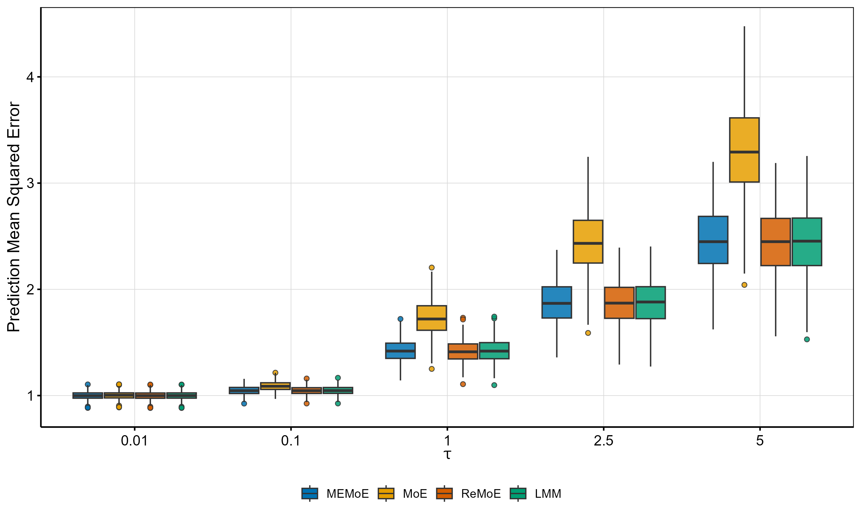
where β=(3,−3, 1,−1, 0)⊤\beta=(3,\ -3,\ 1,\ -1,\ 0)^{\top}, and the covariate vector xi​jx_{ij} is independently sampled from 𝒩​(𝟎,I5)\mathcal{N}({\bf 0},I_{5}), in which I5I_{5} denotes the five-dimensional identity matrix. The random effect uiu_{i} is generated from a normal distribution 𝒩​(0,τ)\mathcal{N}(0,\tau), where the variance parameter τ\tau takes a value of 0.010.01, 0.10.1, 11, 2.52.5, and 55. The random error ϵi​j\epsilon_{ij} is drawn from 𝒩​(0,1)\mathcal{N}(0,1). The average biases and mean squared errors (MSEs) of regression parameters and gating network parameters for the MoE, ReMoE, and MEMoE are presented in the top panel of Table 2. The prediction errors are exhibited in the right panel of Figure 2.

When τ\tau is less than 11, the performance of the four methods is comparable. As τ\tau increases, the bias and variance of MoE increase and are larger than those of the other three methods; in contrast, the biases and variances of MEMoE and ReMoE exhibit slight fluctuations and remain stable, yielding results comparable to those of the classical LMM approach. The boxplots (Figure 2) show prediction mean squared errors (PMSE) of the four methods. The PMSE of MoE increases with τ\tau. In contrast, the PMSEs of MEMoE, ReMoE, and LMM have no significant change as τ\tau increases.

Example 2 serves as a key validation: when the data conform to a classical LMM framework, the MEMoE procedures closely align with the LMM benchmark in terms of both estimation and prediction accuracy. However, it is worth noting that the performance of the MoE approach declines as variability between subjects increases. When considered alongside the findings from Example 2, these results demonstrate that MEMoE adapts well to both the presence and absence of subject-level random effects. In contrast, models that neglect either the random effects (the standard MoE) or expert heterogeneity (LMM) exhibit severe bias when deployed in misspecified modeling scenarios.

Refer to caption
(a)
Refer to caption
(b)
Figure 2: Prediction mean square error under MEMoE, MoE, ReMoE and LMM for Examples 1 and 2. LMM is deleted in Examples 1 because it shows larger PMSE and all results imply that MEMoE attains oracle estimation performance.

Example 3: We consider a linear mixed model mixture-of-experts framework with a Gaussian response. The observed data consist of n=100n=100 subjects, with each subject contributing ni=15n_{i}=15 repeated measurements; this yields a total of N=∑i=1nni=1500N=\sum_{i=1}^{n}n_{i}=1500 observations. The covariate vector xi​j=(xi​j​1,xi​j​2,…,xi​j​5)⊤x_{ij}=(x_{ij1},x_{ij2},\dots,x_{ij5})^{\top} is independently drawn from a multivariate normal distribution 𝒩​(𝟎,𝐈5)\mathcal{N}(\mathbf{0},\mathbf{I}_{5}). Expert membership for each observation is determined by a multinomial gating mechanism, where a softmax function governs class assignment probabilities:

πk​(xi​j,zi​j,α)=exp⁡(xi​j⊤​αk)∑ℓ=1Kexp⁡(xi​j⊤​αℓ),k=1,⋯,K.\pi_{k}(x_{ij},z_{ij},\alpha)=\frac{\exp(x_{ij}^{\top}\alpha_{k})}{\sum_{\ell=1}^{K}\exp(x_{ij}^{\top}\alpha_{\ell})},\quad k=1,\cdots,K.

For each observation with assigned latent expert kk, the Gaussian response yi​jy_{ij} is generated according to a linear mixed-effects model:

yi​j=xi​j⊤​𝜷k+ui+ϵi​j.y_{ij}={x}_{ij}^{\top}\boldsymbol{\beta}_{k}+u_{i}+\epsilon_{ij}.

We consider the following three cases for the number of experts KK, the random effect uiu_{i}, the random error ϵi​j\epsilon_{ij}, the regression coefficients 𝜷k\boldsymbol{\beta}_{k}, and the gating-network parameters αk\alpha_{k} for k=1,⋯,Kk=1,\cdots,K.

Case 1: For K=2K=2. Expert-specific fixed effects and the gating-network parameters are given by:

𝜷1\displaystyle\boldsymbol{\beta}_{1} =(3,−3, 1,−1, 0)⊤,\displaystyle=(3,\ -3,\ 1,\ -1,\ 0)^{\top},\quad 𝜶1\displaystyle\boldsymbol{\alpha}_{1} =(6,−5, 3, 2, 1)⊤,\displaystyle=(6,\ -5,\ 3,\ 2,\ 1)^{\top},
𝜷2\displaystyle\boldsymbol{\beta}_{2} =(−5, 5, 0, 2,−2)⊤,\displaystyle=(-5,\ 5,\ 0,\ 2,\ -2)^{\top},\quad 𝜶2\displaystyle\boldsymbol{\alpha}_{2} =(−4, 2,−7, 5,−3)⊤.\displaystyle=(-4,\ 2,\ -7,\ 5,\ -3)^{\top}.

The random error ϵi​j\epsilon_{ij} is independently sampled from 𝒩​(0,1)\mathcal{N}(0,1), and the random effect uiu_{i} is generated from 𝒩​(0,τ)\mathcal{N}(0,\tau).

Case 2: The settings of the number of experts, the random error, the expert-specific fixed effects, and the gating-network parameters are the same as those in Case 1. The random effect uiu_{i} is generated from 𝒩​(κ​wi,τ)\mathcal{N}(\kappa w_{i},\tau), where ωi=(1,ωi​2,ωi​3,ωi​4)⊤\omega_{i}=(1,\omega_{i2},\omega_{i3},\omega_{i4})^{\top} with ωi​j∼i.i.d.𝒩​(0,1)\omega_{ij}\stackrel{{\scriptstyle i.i.d.}}{{\sim}}\mathcal{N}(0,1) for j=2,3,4j=2,3,4, and κ=(2,5,−1,5)⊤\kappa=(2,5,-1,5)^{\top}.

Case 3: For K=3K=3. Expert-specific fixed effects and the gating-network parameters are given by

𝜷1\displaystyle\boldsymbol{\beta}_{1} =(3,−3, 1,−1, 0)⊤,\displaystyle=(3,\ -3,\ 1,\ -1,\ 0)^{\top},\quad 𝜶1\displaystyle\boldsymbol{\alpha}_{1} =(6,−5, 3, 2, 1)⊤,\displaystyle=(6,\ -5,\ 3,\ 2,\ 1)^{\top},
𝜷2\displaystyle\boldsymbol{\beta}_{2} =(−5, 5, 0, 2,−2)⊤,\displaystyle=(-5,\ 5,\ 0,\ 2,\ -2)^{\top},\quad 𝜶2\displaystyle\boldsymbol{\alpha}_{2} =(−4, 2,−7, 5,−3)⊤,\displaystyle=(-4,\ 2,\ -7,\ 5,\ -3)^{\top},
𝜷3\displaystyle\boldsymbol{\beta}_{3} =(1,−2, 3, 1,−4)⊤,\displaystyle=(1,\ -2,\ 3,\ 1,\ -4)^{\top},\quad 𝜶3\displaystyle\boldsymbol{\alpha}_{3} =(2,−1, 4,−3, 6)⊤.\displaystyle=(2,\ -1,\ 4,\ -3,\ 6)^{\top}.

The random effect uiu_{i} is generated from 𝒩​(κ​wi,τ)\mathcal{N}(\kappa w_{i},\tau), where κ=(5,−3,2,1)\kappa=(5,-3,2,1) and ωi=(1,ωi​2,ωi​3,ωi​4)⊤\omega_{i}=(1,\omega_{i2},\omega_{i3},\omega_{i4})^{\top} with ωi​j∼i.i.d.𝒩​(0,1)\omega_{ij}\stackrel{{\scriptstyle i.i.d.}}{{\sim}}\mathcal{N}(0,1). Conditional on the kkth expert, the random error ϵi​j∼𝒩​(0,σk2)\epsilon_{ij}\sim\mathcal{N}(0,\sigma_{k}^{2}). The standard deviations for three experts are σ1=1.0\sigma_{1}=1.0, σ2=1.2\sigma_{2}=1.2, and σ3=0.8\sigma_{3}=0.8, respectively.

The average biases and mean squared errors of the parameter estimators for fixed effects in three cases are presented in Table 2. The prediction mean squared errors for three cases are displayed in panels (a), (c), and (e) of Figure 3. The empirical coverage probabilities for three cases are shown in panels (b), (d), and (f) of Figure 3.

For the expert-specific regression coefficients βk\beta_{k}, both MEMoE and ReMoE yield essentially unbiased estimates with small variance across all values of τ\tau. In contrast, the LMM estimator, which ignores the underlying expert structure, exhibits substantial bias, reflecting its inability to recover expert-specific effects. The standard MoE performs well when τ\tau is near zero but shows a marked increase in both bias and variance as τ\tau grows, confirming the severe impact of ignoring subject-level random effects.

Across all three cases, MEMoE and ReMoE achieve the lowest and most stable prediction mean squared errors, while the performance of the standard MoE deteriorates sharply with larger τ\tau, and LMM yields intermediate but consistently inferior performance. Overall, Simulation 3 confirms the theoretical advantages of correctly specifying both the expert structure and the random-effects distribution, and highlights that MEMoE provides the most reliable parameter and prediction inference in heterogeneous mixed-effects settings.

Across all three simulation settings, the prediction sets of the proposed MEMoE maintain empirical 95%95\% coverage probabilities closely aligned with the nominal level across a wide range of random-effect variances. The mean interval lengths increase as τ\tau grows. The simulation results provide strong finite-sample evidence for the validity of the proposed prediction-set construction.

Table 2: Biases and MSEs of parameter estimates of β\beta in Examples 2 and 3 across different variances of random effects. MEMoE shows robust and best estimation performance except for the oracle estimators.
τ=0.01\tau=0.01 τ=0.1\tau=0.1 τ=1\tau=1 τ=2.5\tau=2.5 τ=5\tau=5
Scenario Parameter Model Bias MSE Bias MSE Bias MSE Bias MSE Bias MSE
Example 2 β\beta LMM (oracle) 0.015 0.005 0.015 0.005 0.016 0.005 0.016 0.005 0.017 0.005
MoE 0.025 0.015 0.026 0.015 0.027 0.017 0.038 0.019 0.044 0.025
ReMoE (oracle) 0.017 0.005 0.018 0.005 0.020 0.005 0.025 0.005 0.025 0.005
MEMoE 0.025 0.007 0.025 0.005 0.026 0.006 0.026 0.005 0.026 0.007
Example 3: (Cases 1–3)
τ=0.01\tau=0.01 τ=0.1\tau=0.1 τ=1\tau=1 τ=2.5\tau=2.5 τ=5\tau=5
Case 1 Expert 1 β1\beta_{1} LMM 1.997 4.020 1.997 4.019 1.997 4.020 1.997 4.022 1.998 4.024
MoE 0.020 0.001 0.020 0.001 0.035 0.002 0.048 0.002 0.066 0.010
ReMoE (oracle) 0.012 0.001 0.018 0.001 0.012 0.001 0.010 0.001 0.010 0.001
MEMoE 0.015 0.003 0.014 0.004 0.019 0.003 0.020 0.003 0.021 0.003
Expert 2 β2\beta_{2} MoE 0.021 0.001 0.024 0.005 0.041 0.003 0.063 0.007 0.084 0.013
ReMoE 0.021 0.001 0.019 0.001 0.016 0.001 0.017 0.001 0.017 0.001
MEMoE 0.018 0.003 0.019 0.004 0.019 0.004 0.021 0.004 0.022 0.004
Case 2 Expert 1 β1\beta_{1} LMM 5.955 2.210 5.938 2.205 5.954 2.210 5.945 2.205 5.958 2.210
MoE 0.097 0.403 0.071 0.411 0.099 0.421 0.108 0.406 0.109 0.415
ReMoE 0.013 0.044 0.018 0.047 0.014 0.047 0.010 0.046 0.006 0.048
MEMoE 0.003 0.016 0.006 0.017 0.004 0.016 0.003 0.016 0.008 0.018
Expert 2 β2\beta_{2} MoE 0.092 0.403 0.096 0.399 0.118 0.418 0.104 0.415 0.102 0.430
ReMoE 0.011 0.045 0.019 0.047 0.013 0.047 0.011 0.047 0.003 0.046
MEMoE 0.003 0.016 0.003 0.017 0.004 0.017 0.004 0.017 0.009 0.016
Case 3 Expert 1 β1\beta_{1} LMM 2.641 8.557 2.641 8.557 2.641 8.557 2.642 8.557 2.642 8.557
MoE 1.380 2.483 1.381 2.489 1.385 2.510 1.387 2.533 1.389 2.561
ReMoE 0.015 0.014 0.015 0.014 0.015 0.014 0.015 0.014 0.015 0.014
MEMoE 0.007 0.004 0.007 0.004 0.007 0.004 0.007 0.004 0.006 0.004
Expert 2 β2\beta_{2} MoE 1.679 3.079 1.681 3.086 1.685 3.108 1.689 3.129 1.693 3.155
ReMoE 0.014 0.013 0.017 0.014 0.016 0.014 0.016 0.014 0.016 0.014
MEMoE 0.003 0.004 0.003 0.004 0.002 0.004 0.002 0.004 0.001 0.004
Expert 3 β3\beta_{3} MoE 1.396 2.643 1.397 2.645 1.398 2.654 1.400 2.666 1.400 2.681
ReMoE 0.015 0.012 0.014 0.012 0.015 0.012 0.015 0.012 0.015 0.012
MEMoE 0.003 0.002 0.003 0.002 0.003 0.002 0.003 0.002 0.004 0.002
Refer to caption
(a)
Refer to caption
(b)
Refer to caption
(c)
Refer to caption
(d)
Refer to caption
(e)
Refer to caption
(f)
Figure 3: Prediction mean square error (a),(c) and (e) under MEMoE, MoE, ReMoE and LMM for Cases 1-3 of Example 3 and MEMoE shows the best prediction performance. MEMoE is also robust about the random effect variance in (b), (d) and (f).
Table 3: Coverage probabilities (CP) and mean interval lengths of 95%95\% confidence intervals across τ\tau values in Cases 1, 2, and 3.
τ\tau Case 1 Case 2 Case 3
CP Interval Length CP Interval Length CP Interval Length
0.01 0.9521 4.4463 0.9509 4.4592 0.9560 4.7725
0.10 0.9432 4.4730 0.9458 4.4891 0.9452 4.7818
0.25 0.9427 4.7090 0.9443 4.7204 0.9401 5.0306
1.00 0.9425 5.9020 0.9416 5.9086 0.9381 6.2112
2.50 0.9338 7.6414 0.9417 7.7088 0.9409 8.0411
5.00 0.9173 9.7118 0.9239 9.7735 0.9275 10.0818

5.2 Real Data Analysis

Primary Biliary Cirrhosis (PBC) is a chronic, progressive autoimmune liver disease characterized by the destruction of intrahepatic bile ducts, leading to cholestasis, cirrhosis, and eventually liver failure. The data used in this section are from a randomized clinical trial conducted at the Mayo Clinic between January 1974 and May 1984 that compared D-penicillamine with a placebo (Murtaugh et al. 1994). The randomized sample comprises 312312 patients with 1,9451,945 measurements. The number of visits per patient varies from 11 to 1616 during a follow-up period of up to 14.114.1 years. The dataset is available in the survival R package (named pbcseq).

Among the collected longitudinal biomarkers, serum bilirubin is widely recognized as the most powerful prognostic indicator of disease progression and survival. To mitigate skewness and stabilize variance, a natural logarithm transformation is applied to serum bilirubin (log⁡(bili)\log(\text{bili})) as the response variable yi​jy_{ij} for subsequent analyses. To model the longitudinal disease progression while accounting for patient differences, we specify three design components: (i) observation-level covariates xi​jx_{ij} for the expert mean functions; (ii) random-effects design vector zi​j=(1,ti​j)⊤z_{ij}=(1,t_{ij})^{\top} for representing random intercepts and slopes and capturing within correlations, where ti​jt_{ij} denotes the follow-up time in years; (iii) and subject-level covariates wi=(1,Stagei)⊤w_{i}=(1,\text{Stage}_{i})^{\top} for modeling the distribution of the random effects. The covariates maily include demographic factors: Agei\text{Age}_{i} and Sexi\text{Sex}_{i} (coded as 1 for females); key biochemical markers of liver function: serum cholesterol (Choli​0\text{Chol}_{i0}), baseline serum bilirubin (Bilii​0\text{Bili}_{i0}), albumin (Albi​0\text{Alb}_{i0}), and prothrombin time (Protimei​0\text{Protime}_{i0}); and clinical signs of disease severity: presence of edema (Edemai​0\text{Edema}_{i0}), spiders angiomata (Spidersi​0\text{Spiders}_{i0}), and ascites (Ascitesi​j\text{Ascites}_{ij}). Note that while Ascitesi​j\text{Ascites}_{ij} is modeled as a time-varying covariate to capture disease progression, other clinical and biochemical markers are fixed at their baseline values (denoted by the subscript “0”) to serve as baseline prognostic stratification factors. Trti\text{Trt}_{i} indicates the treatment group (1 for D-penicillamine, 0 for placebo). The observation-level design vector xi​jx_{ij} is constructed using a comprehensive set of feature factors. Specifically:

xi​j=(1,ti​j,Agei,Choli​0,Sexi,Ascitesi​j,Edemai​0,Trti,Bilii​0,Albi​0,Protimei​0,Spidersi​0)⊤.x_{ij}=(1,t_{ij},\text{Age}_{i},\text{Chol}_{i0},\text{Sex}_{i},\text{Ascites}_{ij},\text{Edema}_{i0},\text{Trt}_{i},\text{Bili}_{i0},\text{Alb}_{i0},\text{Protime}_{i0},\text{Spiders}_{i0})^{\top}.

Excluding time variable ti​jt_{ij}, all predictors are fixed at enrollment. This approach ensures temporal precedence and reduces endogeneity bias caused by biomarkers that change with disease activity (Hernán et al. 2004). Specifically, all continuous covariates are standardized.

The histogram (Figure 4) of the residuals from the LMM exhibits a clear bimodal pattern, with two local peaks around the zero line and a noticeable dip in the middle. This deviation from unimodality indicates the presence of unobserved heterogeneity within the patient population. Therefore, given the implication of potential latent subgroups, we adopt the MEMoE framework to model this hidden heterogeneity.

Refer to caption
Figure 4: The histogram of residuals from the LMM.

The data are randomly partitioned into 80%80\% for training and 20%20\% for testing. The five-fold cross-validation is conducted on the training set to select the optimal number of experts, with the training set split into four folds for model training and one for validation in each iteration. For each candidate number of experts KK ranging from 1 to 5, model parameters are estimated using the four training folds, and the corresponding predictive error is computed on the validation fold. Let π^k​(xi​j,zi​j)\hat{\pi}_{k}({x}_{ij},z_{ij}) and β^k\hat{{\beta}}_{k} denote the estimates of the gating probabilities and the expert-specific regression coefficients, respectively. We use

y^=(xnew)⊤​β^k^+(𝒛new)⊤​κ^​wnew\hat{y}=({x}_{\mathrm{new}})^{\top}\hat{{\beta}}_{\hat{k}}+(\boldsymbol{z}_{\mathrm{new}})^{\top}\hat{{\kappa}}{w}_{\mathrm{new}}

to make predictions at a given xnew{x}_{\mathrm{new}}, znew{z}_{\mathrm{new}}, wnew{w}_{\mathrm{new}}, where k^=arg​maxk∈{1,…,K}⁡π^k​(xnew,znew)\hat{k}=\operatorname*{arg\,max}_{k\in\{1,\dots,K\}}\;\hat{\pi}_{k}({x}_{\mathrm{new}},{z}_{\mathrm{new}}) is the class with highest estimated probability. The cross-validated root mean squared error indicates that K=3K=3 yields the lowest predictive error. Subsequently, the full training set is used to re-estimate the model parameters using the selected optimal KK. Table 4 presents the expert-specific estimates of parameters in the three-expert MEMoE model.

Table 4: Parameter estimates for the MEMoE model (K=3K=3) on PBC data, and ∗ indicates pp-value is less than 0.050.05.
Parameter Expert 1 Expert 2 Expert 3
Fixed Effects (βk\beta_{k})
Intercept 0.393∗ −-2.375∗ 1.308∗
Time (ti​jt_{ij}) −-0.030∗ −-0.098∗ −-0.041∗
Baseline Age −-0.048∗ −-0.486∗ −-0.096∗
Baseline Albumin −-0.093∗ −-0.573∗ −-0.242∗
Baseline Bilirubin 1.496∗ 0.673∗ 0.698∗
Baseline Cholesterol 0.100∗ 0.411∗ 0.042∗
Baseline Prothrombin Time 0.021∗ 0.467∗ −-0.030∗
Sex (Female) −-0.276∗ 0.228∗ −-0.593∗
Ascites −-0.149∗ 1.556∗ 0.010
Edema score 0.066∗ −-2.497∗ −-0.018
Spiders 0.123∗ −-0.522∗ 0.212∗
Treatment 0.022 −-0.197∗ 0.141∗
σk2\sigma_{k}^{2} 0.090 0.041 0.058

The results indicate the existence of three distinct latent progression patterns, each characterized by specific factor drivers. Expert 1 represents a “Biochemical Instability” phenotype, exhibiting the strongest positive association with Baseline Bilirubin (1.496) among the experts. This group also demonstrates the largest variance (σk2=0.090\sigma_{k}^{2}=0.090), reflecting a high degree of clinical unpredictability driven by biochemical derangement rather than physical signs. Expert 2 characterizes a “Clinical Decompensation” phenotype. This component is dominated by severe clinical manifestations, showing the most significant coefficients for Ascites (1.5561.556) and Edema (−2.497-2.497), as well as the strongest negative association with Baseline Albumin (−0.573-0.573). The substantial impact of these markers suggests this subgroup represents patients with advanced structural damage and synthetic failure. Notably, this is the only subgroup where Treatment shows a significant negative association (−0.197-0.197), suggesting a potential differential response. Expert 3 captures a “Demographic-Driven” phenotype. Unlike the other groups, this pattern shows strong sensitivity to Sex (−0.593-0.593) and a high baseline intercept. In contrast to Expert 2, clinical signs of fluid retention (Ascites, Edema) contribute minimally (0.010 and −-0.018, respectively) and are not statistically significant. This suggests a subgroup in which disease trajectory is influenced more by demographic factors and baseline metabolic state (Bilirubin 0.698) than by overt clinical decompensation.

The proposed MEMoE achieved the lowest predictive error (RMSE = 0.7560.756), outperforming both the standard MoE (RMSE = 0.8350.835) and the single-component LMM (RMSE = 0.9900.990). This sequential reduction in RMSE shows that accounting for within correlations via random effects—beyond merely capturing population heterogeneity—is essential for accurate PBC progression modeling.

Furthermore, we construct the 95%95\% predictive sets (Ω0.05​(xnew))(\Omega_{0.05}(x_{\text{new}})) and record whether ynew∈Ω0.05​(xnew)y_{\text{new}}\in\Omega_{0.05}(x_{\text{new}}) for 100100 randomly selected test observations (see Figure 5). The overall cover probability is 94.76%. Most prediction sets are contiguous, while the MEMoE adaptively produces disjoint intervals (visible as gaps in the red lines) in regions where the predictive distribution is highly skewed or exhibits multiple modes. This flexibility reflects genuine ambiguity about future log⁡(bilirubin)\log(\text{bilirubin}) levels, yet even in these complex cases, the vast majority of observations are correctly covered by the prediction sets.

Refer to caption
Figure 5: Plot of MEMoE 95% prediction sets for the PBCseq bilirubin. The red bars are prediction sets for each observation. The dark and light blue points correspond to the covered and missed log⁡(bilirubin)\log(\text{bilirubin}) values by the prediction sets, respectively.

6 Conclusions

In this paper, we propose a MEMoE model that combines subject-level random effects with a flexible expert structure and a gating function. The MEMoE framework provides a unified approach that simultaneously addresses between-subject heterogeneity and within correlations by integrating a covariate-dependent gating function with expert-specific linear mixed-effects models. To overcome the computational intractability of the likelihood function, we develop a robust estimation scheme that combines a Laplace approximation for latent-variable integration with a generalized EM algorithm augmented by a majorize-minimize strategy. This method ensures numerical stability and the accuracy of the model parameter estimates. Simulation studies and the real data application show that MEMoE can effectively identify hidden dynamic regimes and significantly improve predictive accuracy for new samples compared to LMMs and standard MoE. A key innovation in our framework is the construction of prediction sets. Unlike traditional interval estimates, the proposed method can easily handle multimodal predictive distributions, which commonly arise in heterogeneous populations, thereby facilitating more comprehensive uncertainty quantification. Despite these positive aspects, the current model has some limitations. The Laplace approximation can introduce bias when the number of longitudinal observations per subject is small, and the non-convexity of the objective function poses challenges for avoiding local optima. In summary, MEMoE bridges the gap between the interpretability of mixed-effects models and the flexibility of finite mixture models, providing a valuable and principled tool for complex longitudinal data analysis.

7 Disclosure statement

The authors report there are no competing interests to declare.

8 Data Availability Statement

The data used in this study are available in the [survival] R package.

SUPPLEMENTARY MATERIAL

Detailed mathematical proofs for Theorems 1 and 2 are provided in the supplementary material.

References

  • C. M. Bishop (2006) Pattern recognition and machine learning. Information Science and Statistics, Springer. External Links: ISBN 978-0-387-31073-2, Document Cited by: §1.
  • N. E. Breslow and D. G. Clayton (1993) Approximate inference in generalized linear mixed models. Journal of the American Statistical Association 88 (421), pp. 9–25. Cited by: §2.2, §2.2.
  • C. Che, S. Li, C. Zhang, and H. Li (2023) Covariate-guided bayesian mixture of spline experts for the analysis of multivariate high-density longitudinal data. Biometrics 79 (2), pp. 1239–1252. Cited by: §1.
  • S. Cui, E. C. Yoo, D. Li, K. Laudanski, and B. E. Engelhardt (2022) Hierarchical Gaussian processes and mixtures of experts to model COVID-19 patient trajectories. Pacific Symposium on Biocomputing 27, pp. 266–277. External Links: Document Cited by: §1.
  • P. J. Diggle, P. J. Heagerty, Kung-Yee. Liang, and S. L. Zeger (2002) Analysis of longitudinal data. 2nd edition, Oxford University Press, Oxford. External Links: ISBN 9780198524847, Document Cited by: §1.
  • G. M. Fitzmaurice, N. M. Laird, and J. H. Ware (2011) Applied longitudinal analysis. 2 edition, Wiley. External Links: Document Cited by: §1.
  • T. C. Fung and S. C. Tseung (2022) Mixture of experts models for multilevel data: modelling framework and approximation theory. Neural Networks 154, pp. 287–302. External Links: Document Cited by: §1.
  • J. Gao, S. Gunn, and J. Kandola (2002) Adapting kernels by variational approach in svm. In AI 2002: Advances in Artificial Intelligence, B. McKay and J. Slaney (Eds.), Berlin, Heidelberg, pp. 395–406. External Links: ISBN 978-3-540-36187-9 Cited by: §1.
  • T. He, K. Jiang, A. Zhao, A. Schroder, E. Thompson, S. Soskic, F. Barkhof, and D. C. Alexander (2025) A stage-aware mixture of experts framework for neurodegenerative disease progression modelling. arXiv preprint arXiv:2508.07032. External Links: Link Cited by: §1.
  • D. Hedeker and R. D. Gibbons (2006) Longitudinal data analysis. Wiley Series in Probability and Statistics, John Wiley & Sons, Hoboken. External Links: ISBN 9780470036471 Cited by: §1.
  • C. Hennig (2000) Identifiablity of models for clusterwise linear regression. Journal of Classification 17 (2), pp. 273–296. External Links: Document Cited by: §4.
  • M. A. Hernán, S. Hernández-Díaz, and J. M. Robins (2004) A structural approach to selection bias. Epidemiology 15 (5), pp. 615–625. External Links: Document Cited by: §5.2.
  • J. Huang, Y. Jiao, W. Wang, X. Yan, and L. Zhu (2023) Integrative analysis for high-dimensional stratified models. Statistica Sinica 33, pp. 1533–1553. Cited by: §1.
  • D. R. Hunter and K. Lange (2004) A tutorial on mm algorithms. The American Statistician 58 (1), pp. 30–37. External Links: Document Cited by: §2.2.
  • R. A. Jacobs, M. I. Jordan, S. J. Nowlan, and G. E. Hinton (1991) Adaptive mixtures of local experts. Neural Computation 3 (1), pp. 79–87. External Links: Document Cited by: §1.
  • M. I. Jordan and R. A. Jacobs (1994) Hierarchical mixtures of experts and the em algorithm. Neural Computation 6 (2), pp. 181–214. External Links: Document Cited by: §1.
  • J. Kiefer (1959) Optimum experimental designs. Journal of the Royal Statistical Society. Series B (Methodological) 21 (2), pp. 272–319. External Links: ISSN 0035-9246 Cited by: §4.
  • L. Kock, N. Klein, and D. J. Nott (2025) Deep mixture of linear mixed models for complex longitudinal data. Statistics in Medicine 44 (23-24), pp. e70288. External Links: Document Cited by: §1.
  • N. M. Laird and J. H. Ware (1982) Random-effects models for longitudinal data. Biometrics 38 (4), pp. 963–974. External Links: Document Cited by: §1.
  • R. J. A. Little and D. B. Rubin (2019) Statistical analysis with missing data. 3rd edition, Wiley Series in Probability and Statistics, John Wiley & Sons, Hoboken, NJ. External Links: Document Cited by: §1.
  • P. A. Murtaugh, E. R. Dickson, G. Van Dam, M. Malinchoc, P. Grambsch, A. Langworthy, and C. Gips (1994) Primary biliary cirrhosis: prediction of short-term survival based on repeated patient visits. Hepatology 20 (1), pp. 126–134. External Links: Document Cited by: §5.2.
  • B. Muthén (2004) Latent variable analysis: growth mixture modeling and related techniques for longitudinal data. In Handbook of Quantitative Methodology for the Social Sciences, D. Kaplan (Ed.), pp. 345–369. External Links: Document Cited by: §1.
  • J. C. Pinheiro and D. M. Bates (2000) Mixed-effects models in s and s-plus. Statistics and Computing, Springer. External Links: Document, ISBN 978-0-387-98957-0 Cited by: §1, §4.
  • M. Quiroz and M. Villani (2013) Dynamic mixture-of-experts models for longitudinal and discrete-time survival data. Working Paper Series Technical Report 268, Sveriges Riksbank. External Links: Document Cited by: §1.
  • N. Shazeer, A. Mirhoseini, K. Maziarz, A. Davis, Q. Le, G. Hinton, and J. Dean (2017) OUTRAGEOUSLY large neural networks: the sparsely-gated mixture-of-experts layer. In International Conference on Learning Representations, External Links: Document Cited by: §1.
  • H. J. Skaug and D. A. Fournier (2006) Automatic approximation of the marginal likelihood in Non-Gaussian hierarchical models. Computational Statistics & Data Analysis 51 (2), pp. 699–709. External Links: Document Cited by: §2.2.
  • L. Tierney and J. B. Kadane (1986) Accurate approximations for posterior moments and marginal densities. Journal of the American Statistical Association 81 (393), pp. 82–86. External Links: Document Cited by: §2.2.
  • G. Verbeke and E. Lesaffre (1996) A linear mixed-effects model with heterogeneity in the random-effects population. Journal of the American Statistical Association 91 (433), pp. 217–221. External Links: Document Cited by: §1.
  • G. Verbeke and G. Molenberghs (2000) Linear mixed models for longitudinal data. Springer. External Links: Document Cited by: §1.
  • L. Xu and M. I. Jordan (1996) On convergence properties of the em algorithm for Gaussian mixtures. Neural Computation 8 (1), pp. 129–151. External Links: Document Cited by: §1.
  • X. Yan, G. Yin, and X. Zhao (2021) Subgroup analysis in censored linear regression. Statistica Sinica 31, pp. 1027–1054. Cited by: §1.
  • X. Yang, X. Yan, and J. Huang (2019) High-dimensional integrative analysis with homogeneity and sparsity recovery. Journal of Multivariate Analysis 174, pp. 104529. Cited by: §1.
  • S. E. Yuksel, J. N. Wilson, and P. D. Gader (2012) Twenty years of mixture of experts. IEEE Transactions on Neural Networks and Learning Systems 23 (8), pp. 1177–1193. External Links: Document Cited by: §1.

Proof Theorem 1

We define the population objective function as the expected Laplace-approximated log-likelihood for a representative subject:

M​(Ψ):=𝔼​[1N​∑i=1NℓLA,i​(Ψ)],M(\Psi):=\mathbb{E}\left[\frac{1}{N}\sum_{i=1}^{N}\ell_{\text{LA},i}(\Psi)\right],

where

ℓLA,i​(Ψ)=hi​(u^i​(Ψ);Ψ)+q2​log⁡(2​π)−12​log⁡|Hi​(Ψ)|.\ell_{\text{LA},i}(\Psi)=h_{i}(\hat{u}_{i}(\Psi);\Psi)+\frac{q}{2}\log(2\pi)-\frac{1}{2}\log|H_{i}(\Psi)|.

Correspondingly, the sample objective function is:

MN​(Ψ):=1N​∑i=1NℓLA,i​(Ψ).M_{N}(\Psi):=\frac{1}{N}\sum_{i=1}^{N}\ell_{\text{LA},i}(\Psi).

The norm ∥⋅∥\|\cdot\| in these supplementary materials is defined as the L2L_{2} norm. For a vector v∈ℝdv\in\mathbb{R}^{d}, ‖v‖=v⊤​v=(∑k=1dvk2)1/2\|v\|=\sqrt{v^{\top}v}=(\sum_{k=1}^{d}v_{k}^{2})^{1/2}; for a matrix A∈ℝm×dA\in\mathbb{R}^{m\times d}, ‖A‖:=sup‖v‖=1‖A​v‖=λmax​(A⊤​A)\|A\|:=\sup_{\|v\|=1}\|Av\|=\sqrt{\lambda_{\max}(A^{\top}A)}, where λmax\lambda_{\max} is the largest eigenvalue. To prove Theorem 1, we give the following Propositions 1 and 2.

8.0.0.1 Proposition 1

Under conditions (A1)– (A4), the class of functions {ℓLA,i​(Ψ):Ψ∈Θ}\{\ell_{\text{LA},i}(\Psi):\Psi\in\Theta\}, as N→∞N\to\infty:

supΨ∈Θ|MN​(Ψ)−M​(Ψ)|→𝑝0.\sup_{\Psi\in\Theta}\left|M_{N}(\Psi)-M(\Psi)\right|\xrightarrow{p}0.

Remark: By the Glivenko-Cantelli theorem, it suffices to verify that the function class ℱ={ℓLA,i​(Ψ):Ψ∈Θ}\mathcal{F}=\{\ell_{\text{LA},i}(\Psi):\Psi\in\Theta\} satisfies: each function Ψ↦ℓLA,i​(Ψ)\Psi\mapsto\ell_{\text{LA},i}(\Psi) is continuous on the compact set Θ\Theta; there exists a random variable GiG_{i} with supΨ∈Θ|ℓLA,i​(Ψ)|≤Gi\sup_{\Psi\in\Theta}|\ell_{\text{LA},i}(\Psi)|\leq G_{i} and 𝔼​[Gi]<∞\mathbb{E}[G_{i}]<\infty.

Proof.

We first construct an integrable envelope function that does not depend on Ψ\Psi. By the eigenvalue bounds in Condition (A3) and the compactness of the parameter space Θ\Theta in Condition (A2), all parameter components (α,β,σ2,κ,Σ)(\alpha,\beta,\sigma^{2},\kappa,\Sigma) are uniformly bounded over Ψ∈Θ\Psi\in\Theta. The eigenvalues of Σ\Sigma are uniformly bounded away from zero and infinity.

Condition (A2) imposes uniform bounds on all model parameters, and Condition (A1) ensures finite second moments for the covariates. Therefore, the unconditional second moment of the response

𝔼​[yi​j2]≤C′​(1+𝔼​‖xi​j‖2+𝔼​‖zi​j‖2+𝔼​‖wi‖2)<∞.\mathbb{E}[y_{ij}^{2}]\;\leq\;C^{\prime}\left(1+\mathbb{E}\|x_{ij}\|^{2}+\mathbb{E}\|z_{ij}\|^{2}+\mathbb{E}\|w_{i}\|^{2}\right)\;<\;\infty.

We will prove that ℓLA,i​(Ψ)\ell_{\mathrm{LA},i}(\Psi) is continuous on the parameter space Θ\Theta. Recall that

ℓLA,i​(Ψ)=hi​(u^i​(Ψ);Ψ)+q2​log⁡(2​π)−12​log⁡|Hi​(Ψ)|,\ell_{\text{LA},i}(\Psi)=h_{i}(\hat{u}_{i}(\Psi);\Psi)+\frac{q}{2}\log(2\pi)-\frac{1}{2}\log|H_{i}(\Psi)|,

where u^i​(Ψ)=arg⁡maxu⁡hi​(u;Ψ)\hat{u}_{i}(\Psi)=\arg\max_{u}h_{i}(u;\Psi) and Hi​(Ψ)=−∇u2hi​(u^i​(Ψ);Ψ)H_{i}(\Psi)=-\nabla_{u}^{2}h_{i}(\hat{u}_{i}(\Psi);\Psi).

We first establish the continuity of the mapping Ψ↦u^i​(Ψ)\Psi\mapsto\hat{u}_{i}(\Psi). Specifically, u^i​(Ψ)\hat{u}_{i}(\Psi) denotes the unique solution to the first-order condition ∇uhi​(u,Ψ)=0\nabla_{u}h_{i}(u,\Psi)=0. Under the smoothness conditions imposed by the model, the function F​(u,Ψ):=∇uhi​(u,Ψ)F(u,\Psi):=\nabla_{u}h_{i}(u,\Psi) is continuously differentiable. For an arbitrary fixed Ψ0∈Θ\Psi_{0}\in\Theta, let u0=u^i​(Ψ0)u_{0}=\hat{u}_{i}(\Psi_{0}). The partial derivative of F​(u,Ψ)F(u,\Psi) with respect to uu, evaluated at (u0,Ψ0)(u_{0},\Psi_{0}), is the Hessian matrix of the joint log-likelihood function hi​(⋅,⋅)h_{i}(\cdot,\cdot):

∂∂u​F​(u,Ψ)|(u0,Ψ0)=∇u2hi​(u0,Ψ0)=−Hi​(Ψ0).\frac{\partial}{\partial u}F(u,\Psi)|_{(u_{0},\Psi_{0})}=\nabla_{u}^{2}h_{i}(u_{0},\Psi_{0})=-H_{i}(\Psi_{0}).

Hi​(Ψ0)H_{i}(\Psi_{0}) is positive definite, and hence ∇u2hi​(u0;Ψ0)=−Hi​(Ψ0)\nabla_{u}^{2}h_{i}(u_{0};\Psi_{0})=-H_{i}(\Psi_{0}) is negative definite and thus invertible. By the Implicit Function Theorem, there exists a neighborhood UU of Ψ0\Psi_{0} and a unique continuously differentiable function g:U→ℝqg:U\to\mathbb{R}^{q} such that F​(g​(Ψ),Ψ)=0F(g(\Psi),\Psi)=0 for all Ψ∈U\Psi\in U. Given the global uniqueness of the maximizer u^i​(Ψ)\hat{u}_{i}(\Psi), we identify u^i​(Ψ)=g​(Ψ)\hat{u}_{i}(\Psi)=g(\Psi) on UU. Since Ψ0\Psi_{0} is chosen arbitrarily, the mapping Ψ↦u^i​(Ψ)\Psi\mapsto\hat{u}_{i}(\Psi) is continuous over the entire compact set Θ\Theta.

The function hi​(u;Ψ)h_{i}(u;\Psi) is differentiable with respect to uu and Ψ\Psi, and the mapping (u,Ψ)↦hi​(u;Ψ)(u,\Psi)\mapsto h_{i}(u;\Psi) is jointly continuous. Since the mapping Ψ↦u^i​(Ψ)\Psi\mapsto\hat{u}_{i}(\Psi) is continuous, Ψ↦hi​(u^i​(Ψ);Ψ)\Psi\mapsto h_{i}(\hat{u}_{i}(\Psi);\Psi) is continuous on Θ\Theta. The Hessian (u,Ψ)↦∇u2hi​(u;Ψ)(u,\Psi)\mapsto\nabla_{u}^{2}h_{i}(u;\Psi) is continuous (as the second derivative of a three-times differentiable function). Since Hi​(Ψ)=−∇u2hi​(u^i​(Ψ);Ψ)H_{i}(\Psi)=-\nabla_{u}^{2}h_{i}(\hat{u}_{i}(\Psi);\Psi), similarly, the mapping Ψ↦Hi​(Ψ)\Psi\mapsto H_{i}(\Psi) is continuous on Θ\Theta.

Since Hi​(Ψ)H_{i}(\Psi) is positive definite, all its eigenvalues are strictly positive. Since Ψ↦Hi​(Ψ)\Psi\mapsto H_{i}(\Psi) is continuous, and Θ\Theta is compact, the eigenvalue function Ψ↦λmin​(Hi​(Ψ))\Psi\mapsto\lambda_{\min}(H_{i}(\Psi)) is continuous on the compact set. By the extreme value theorem,

c:=infΨ∈Θλmin​(Hi​(Ψ))=minΨ∈Θ⁡λmin​(Hi​(Ψ))>0.c:=\inf_{\Psi\in\Theta}\lambda_{\min}(H_{i}(\Psi))=\min_{\Psi\in\Theta}\lambda_{\min}(H_{i}(\Psi))>0.

Therefore, for all Ψ∈Θ\Psi\in\Theta:

|Hi​(Ψ)|=∏j=1qλj​(Hi​(Ψ))≥λmin​(Hi​(Ψ))q≥cq>0.|H_{i}(\Psi)|=\prod_{j=1}^{q}\lambda_{j}(H_{i}(\Psi))\geq\lambda_{\min}(H_{i}(\Psi))^{q}\geq c^{q}>0.

Since |Hi​(Ψ)||H_{i}(\Psi)| is strictly positive and continuous on Θ\Theta, and the logarithm function is continuous on (0,∞)(0,\infty), the mapping

Ψ↦log⁡|Hi​(Ψ)|\Psi\mapsto\log|H_{i}(\Psi)|

is continuous on Θ\Theta.

Finally, the function ℓLA,i​(Ψ)\ell_{\text{LA},i}(\Psi) is a linear combination of continuous functions:

ℓLA,i​(Ψ)=hi​(u^i​(Ψ);Ψ)⏟continuous+q2​log⁡(2​π)⏟constant−12​log⁡|Hi​(Ψ)|⏟continuous.\ell_{\text{LA},i}(\Psi)=\underbrace{h_{i}(\hat{u}_{i}(\Psi);\Psi)}_{\text{continuous}}+\underbrace{\frac{q}{2}\log(2\pi)}_{\text{constant}}-\frac{1}{2}\underbrace{\log|H_{i}(\Psi)|}_{\text{continuous}}.

Therefore, ℓLA,i​(Ψ)\ell_{\text{LA},i}(\Psi) is continuous on Θ\Theta.

We now prove that there exists a random variable GiG_{i} such that

supΨ∈Θ|ℓLA,i​(Ψ)|≤Gi,and𝔼​[Gi]<∞.\sup_{\Psi\in\Theta}|\ell_{\mathrm{LA},i}(\Psi)|\leq G_{i},\quad\text{and}\quad\mathbb{E}[G_{i}]<\infty.

The maximizer u^i​(Ψ)=arg⁡maxui⁡hi​(ui;Ψ)\hat{u}_{i}(\Psi)=\arg\max_{u_{i}}h_{i}(u_{i};\Psi) satisfies the first-order condition

∇uihi​(ui;Ψ)=−Σ−1​(ui−κ​wi)+∑j=1ni∑k=1Kγi​j​k​(Ψ)​zi​j​(yi​j−xi​j⊤​βk−zi​j⊤​ui)σk2=0,\nabla_{u_{i}}h_{i}(u_{i};\Psi)=-\Sigma^{-1}\left(u_{i}-\kappa w_{i}\right)+\sum_{j=1}^{n_{i}}\sum_{k=1}^{K}\gamma_{ijk}(\Psi)\frac{z_{ij}\left(y_{ij}-x_{ij}^{\top}\beta_{k}-z_{ij}^{\top}u_{i}\right)}{\sigma_{k}^{2}}=0,

where γi​j​k​(Ψ)∈(0,1)\gamma_{ijk}(\Psi)\in(0,1) and ∑k=1Kγi​j​k=1\sum_{k=1}^{K}\gamma_{ijk}=1. Rearrange the first-order condition, and we obtain

Σ−1​u^i+∑j,kγi​j​k​(Ψ)​zi​j​zi​j⊤σk2​u^i=Σ−1​κ​wi+∑j,kγj​k​(Ψ)​zi​j​(yi​j−xi​j⊤​βk)σk2.\Sigma^{-1}\hat{u}_{i}+\sum_{j,k}\gamma_{ijk}(\Psi)\frac{z_{ij}z_{ij}^{\top}}{\sigma_{k}^{2}}\hat{u}_{i}=\Sigma^{-1}\kappa w_{i}+\sum_{j,k}\gamma_{jk}(\Psi)\frac{z_{ij}\left(y_{ij}-x_{ij}^{\top}\beta_{k}\right)}{\sigma_{k}^{2}}. (9)

According to

Hi​(Ψ)=Σ−1+∑j=1ni∑k=1Kπk​(xi​j,zi​j;α)​φi​j​k​(u^i)∑ℓ=1Kπℓ​(xi​j,zi​j;α)​φi​j​ℓ​(u^i)​1σk2​zi​j​zi​j⊤,H_{i}(\Psi)=\Sigma^{-1}+\sum_{j=1}^{n_{i}}\sum_{k=1}^{K}\frac{\pi_{k}(x_{ij},z_{ij};\alpha)\varphi_{ijk}(\hat{u}_{i})}{\sum_{\ell=1}^{K}\pi_{\ell}(x_{ij},z_{ij};\alpha)\varphi_{ij\ell}(\hat{u}_{i})}\frac{1}{\sigma_{k}^{2}}z_{ij}z_{ij}^{\top},

the equation (9) becomes

Hi​(Ψ)​u^i=Σ−1​κ​wi+∑j,kγj​k​(Ψ)​zi​j​(yi​j−xi​j⊤​βk)σk2.H_{i}(\Psi)\hat{u}_{i}=\Sigma^{-1}\kappa w_{i}+\sum_{j,k}\gamma_{jk}(\Psi)\frac{z_{ij}\left(y_{ij}-x_{ij}^{\top}\beta_{k}\right)}{\sigma_{k}^{2}}.

Under Condition (A3), the eigenvalues of Σ\Sigma are bounded as c1≤λmin​(Σ)≤λmax​(Σ)≤c2c_{1}\leq\lambda_{\min}(\Sigma)\leq\lambda_{\max}(\Sigma)\leq c_{2}. According to Condition (A2), the variances satisfy 0<σmin2≤σk2≤σmax2<∞0<\sigma_{\min}^{2}\leq\sigma_{k}^{2}\leq\sigma_{\max}^{2}<\infty for all kk. It follows that

Hi​(Ψ)⪰Σ−1⟹λmin​(Hi​(Ψ))≥λmin​(Σ−1)=1λmax​(Σ)≥1c2,H_{i}(\Psi)\succeq\Sigma^{-1}\quad\Longrightarrow\quad\lambda_{\min}(H_{i}(\Psi))\geq\lambda_{\min}(\Sigma^{-1})=\frac{1}{\lambda_{\max}(\Sigma)}\geq\frac{1}{c_{2}},

and hence

‖Hi​(Ψ)−1‖=1λmin​(Hi​(Ψ))≤c2\|H_{i}(\Psi)^{-1}\|=\frac{1}{\lambda_{\min}(H_{i}(\Psi))}\leq c_{2}

uniformly over Ψ∈Θ\Psi\in\Theta.

Taking norms on both sides of the normal equation and using the triangle inequality, we obtain

‖u^i​(Ψ)‖≤‖Hi​(Ψ)−1‖​(‖Σ−1​κ​wi‖+‖∑j,kγj​k​(Ψ)​zi​j​(yi​j−xi​j⊤​βk)σk2‖),\|\hat{u}_{i}(\Psi)\|\leq\left\|H_{i}(\Psi)^{-1}\right\|\left(\|\Sigma^{-1}\kappa w_{i}\|+\left\|\sum_{j,k}\gamma_{jk}(\Psi)\frac{z_{ij}\left(y_{ij}-x_{ij}^{\top}\beta_{k}\right)}{\sigma_{k}^{2}}\right\|\right),

Under Conditions (A2) and (A3), there exists a constant Cκ>0C_{\kappa}>0 such that ‖κ‖≤Cκ\|\kappa\|\leq C_{\kappa}, and similarly ‖βk‖≤B\|\beta_{k}\|\leq B for all kk, where B:=supk‖βk‖<∞B:=\sup_{k}\left\|\beta_{k}\right\|<\infty. Moreover, ‖Σ−1‖≤c1−1\|\Sigma^{-1}\|\leq c_{1}^{-1} and σk2≥σmin2\sigma_{k}^{2}\geq\sigma_{\min}^{2}. Hence

‖Σ−1​κ​wi‖≤‖Σ−1‖​‖κ‖​‖wi‖≤c1−1​Cκ​‖wi‖,\left\|\Sigma^{-1}\kappa w_{i}\right\|\leq\left\|\Sigma^{-1}\right\|\|\kappa\|\|w_{i}\|\leq c_{1}^{-1}C_{\kappa}\|w_{i}\|,

we can obtain

‖∑j,kγj​k​(Ψ)​zi​j​(yi​j−xi​j⊤​βk)σk2‖≤1σmin2​∑j=1ni‖zi​j‖​(|yi​j|+maxk⁡|xi​j⊤​βk|)≤1σmin2​∑j=1ni‖zi​j‖​(|yi​j|+B​‖xi​j‖),\left\|\sum_{j,k}\gamma_{jk}(\Psi)\frac{z_{ij}\left(y_{ij}-x_{ij}^{\top}\beta_{k}\right)}{\sigma_{k}^{2}}\right\|\leq\frac{1}{\sigma_{\min}^{2}}\sum_{j=1}^{n_{i}}\left\|z_{ij}\right\|\left(\left|y_{ij}\right|+\max_{k}\left|x_{ij}^{\top}\beta_{k}\right|\right)\leq\frac{1}{\sigma_{\min}^{2}}\sum_{j=1}^{n_{i}}\|z_{ij}\|\bigl(|y_{ij}|+B\|x_{ij}\|\bigr),

where σmin 2>0\sigma_{\text{min }}^{2}>0 is the lower bound of the variances, and |xi​j⊤​βk|≤‖xi​j‖​‖βk‖≤B​‖xi​j‖\left|x_{ij}^{\top}\beta_{k}\right|\leq\left\|x_{ij}\right\|\left\|\beta_{k}\right\|\leq B\left\|x_{ij}\right\|. Altogether,

‖u^i​(Ψ)‖≤c2​(c1−1​Cκ​‖wi‖+1σmin2​∑j=1ni‖zi​j‖​(|yi​j|+B​‖xi​j‖)),\|\hat{u}_{i}(\Psi)\|\leq c_{2}\left(c_{1}^{-1}C_{\kappa}\|w_{i}\|+\frac{1}{\sigma_{\min}^{2}}\sum_{j=1}^{n_{i}}\left\|z_{ij}\right\|\left(\left|y_{ij}\right|+B\left\|x_{ij}\right\|\right)\right),

Using (a+b)2≤2​(a2+b2)(a+b)^{2}\leq 2(a^{2}+b^{2}):

‖u^i​(Ψ)‖2≤2​c22​[Cκ2c12​‖wi‖2+1σmin4​(∑j=1ni‖zi​j‖​(|yi​j|+B​‖xi​j‖))2].\|\hat{u}_{i}(\Psi)\|^{2}\leq 2c_{2}^{2}\left[\frac{C_{\kappa}^{2}}{c_{1}^{2}}\|w_{i}\|^{2}+\frac{1}{\sigma_{\min}^{4}}\left(\sum_{j=1}^{n_{i}}\|z_{ij}\|(|y_{ij}|+B\|x_{ij}\|)\right)^{2}\right].

For the second term, using the Cauchy-Schwarz inequality:

(∑j=1ni‖zi​j‖​(|yi​j|+B​‖xi​j‖))2\displaystyle\left(\sum_{j=1}^{n_{i}}\|z_{ij}\|(|y_{ij}|+B\|x_{ij}\|)\right)^{2} ≤∑j=1ni‖zi​j‖2⋅∑j=1ni(|yi​j|+B​‖xi​j‖)2\displaystyle\leq\sum_{j=1}^{n_{i}}\|z_{ij}\|^{2}\cdot\sum_{j=1}^{n_{i}}\left(|y_{ij}|+B\|x_{ij}\|\right)^{2}
≤∑j=1ni‖zi​j‖2⋅∑j=1ni2​(yi​j2+B2​‖xi​j‖2)\displaystyle\leq\sum_{j=1}^{n_{i}}\|z_{ij}\|^{2}\cdot\sum_{j=1}^{n_{i}}2(y_{ij}^{2}+B^{2}\|x_{ij}\|^{2})
=2​∑j=1ni‖zi​j‖2⋅∑j=1ni(yi​j2+B2​‖xi​j‖2).\displaystyle=2\sum_{j=1}^{n_{i}}\|z_{ij}\|^{2}\cdot\sum_{j=1}^{n_{i}}(y_{ij}^{2}+B^{2}\|x_{ij}\|^{2}).

Substituting:

‖u^i​(Ψ)‖2\displaystyle\|\hat{u}_{i}(\Psi)\|^{2} ≤2​c22​[Cκ2c12​‖wi‖2+2σmin4​(∑j=1ni‖zi​j‖2)​(∑j=1ni(yi​j2+B2​‖xi​j‖2))]\displaystyle\leq 2c_{2}^{2}\left[\frac{C_{\kappa}^{2}}{c_{1}^{2}}\|w_{i}\|^{2}+\frac{2}{\sigma_{\min}^{4}}\left(\sum_{j=1}^{n_{i}}\|z_{ij}\|^{2}\right)\left(\sum_{j=1}^{n_{i}}(y_{ij}^{2}+B^{2}\|x_{ij}\|^{2})\right)\right]
≤C1′​[‖wi‖2+(∑j=1ni‖zi​j‖2)​(∑j=1ni(yi​j2+‖xi​j‖2))],\displaystyle\leq C_{1}^{\prime}\left[\|w_{i}\|^{2}+\left(\sum_{j=1}^{n_{i}}\|z_{ij}\|^{2}\right)\left(\sum_{j=1}^{n_{i}}(y_{ij}^{2}+\|x_{ij}\|^{2})\right)\right],

where C1′:=max⁡{2​c22​Cκ2/c12,4​c22​B2/σmin4,4​c22/σmin4}C_{1}^{\prime}:=\max\{2c_{2}^{2}C_{\kappa}^{2}/c_{1}^{2},4c_{2}^{2}B^{2}/\sigma_{\min}^{4},4c_{2}^{2}/\sigma_{\min}^{4}\}.

Consequently, we define a random variable:

Wi(1):=1+‖wi‖2+∑j=1ni(|yi​j|2+‖xi​j‖2+‖zi​j‖2).W_{i}^{(1)}:=1+\|w_{i}\|^{2}+\sum_{j=1}^{n_{i}}(|y_{ij}|^{2}+\|x_{ij}\|^{2}+\|z_{ij}\|^{2}).

Since all terms are non-negative, the individual components are bounded by the envelope:

‖wi‖2≤Wi(1),∑j=1ni‖zi​j‖2≤Wi(1),and∑j=1ni(|yi​j|2+‖xi​j‖2)≤Wi(1).\|w_{i}\|^{2}\leq W_{i}^{(1)},\quad\sum_{j=1}^{n_{i}}\|z_{ij}\|^{2}\leq W_{i}^{(1)},\quad\text{and}\quad\sum_{j=1}^{n_{i}}(|y_{ij}|^{2}+\|x_{ij}\|^{2})\leq W_{i}^{(1)}.

Applying these bounds to the inequality derived above:

‖u^i​(Ψ)‖2\displaystyle\|\hat{u}_{i}(\Psi)\|^{2} ≤C1′​[‖wi‖2+∑j=1ni‖zi​j‖2⋅∑j=1ni(|yi​j|2+‖xi​j‖2)]\displaystyle\leq C_{1}^{\prime}\left[\|w_{i}\|^{2}+\sum_{j=1}^{n_{i}}\|z_{ij}\|^{2}\cdot\sum_{j=1}^{n_{i}}(|y_{ij}|^{2}+\|x_{ij}\|^{2})\right]
≤C1′​[Wi(1)+Wi(1)⋅Wi(1)]\displaystyle\leq C_{1}^{\prime}\left[W_{i}^{(1)}+W_{i}^{(1)}\cdot W_{i}^{(1)}\right]
=C1′​[Wi(1)+(Wi(1))2].\displaystyle=C_{1}^{\prime}\left[W_{i}^{(1)}+(W_{i}^{(1)})^{2}\right].

Since Wi(1)≥1W_{i}^{(1)}\geq 1, we have Wi(1)≤(Wi(1))2W_{i}^{(1)}\leq(W_{i}^{(1)})^{2}. Therefore,

‖u^i​(Ψ)‖2≤C1′​[(Wi(1))2+(Wi(1))2]=2​C1′​(Wi(1))2.\|\hat{u}_{i}(\Psi)\|^{2}\leq C_{1}^{\prime}\left[(W_{i}^{(1)})^{2}+(W_{i}^{(1)})^{2}\right]=2C_{1}^{\prime}(W_{i}^{(1)})^{2}.

Let C1:=2​C1′C_{1}:=2C_{1}^{\prime}. We conclude that

supΨ∈Θ‖u^i​(Ψ)‖2≤C1​(Wi(1))2.\sup_{\Psi\in\Theta}\|\hat{u}_{i}(\Psi)\|^{2}\leq C_{1}(W_{i}^{(1)})^{2}.

Regarding integrability, since Wi(1)W_{i}^{(1)} consists of linear terms of the data, its square (Wi(1))2(W_{i}^{(1)})^{2} consists of squared terms (e.g., ‖wi‖4,yi​j4,‖xi​j‖4\|w_{i}\|^{4},y_{ij}^{4},\|x_{ij}\|^{4}) and cross-products. Condition (A1) guarantees finite second moments for the response and covariates, and by the Generalized Hölder’s Inequality, the expectation of the cross-products is finite provided the individual fourth moments are finite. Thus, 𝔼​[(Wi(1))2]<∞\mathbb{E}[(W_{i}^{(1)})^{2}]<\infty.

In summary, under Conditions (A1), (A2) and (A3), there exists a constant C1>0C_{1}>0 such that

supΨ∈Θ‖u^i​(Ψ)‖2≤C1​(Wi(1))2,\sup_{\Psi\in\Theta}\|\hat{u}_{i}(\Psi)\|^{2}\leq C_{1}(W_{i}^{(1)})^{2}, (10)

where Wi(1)W_{i}^{(1)} is a random variable defined by linear terms, satisfying 𝔼​(Wi(1))<∞\mathbb{E}(W_{i}^{(1)})<\infty. Recall that

hi​(ui;Ψ)=log⁡φ​(ui;κ​wi,Σ)+∑j=1nilog⁡[∑k=1Kπk​(xi​j,zi​j;α)​φ​(yi​j;xi​j⊤​βk+zi​j⊤​ui,σk2)].h_{i}(u_{i};\Psi)=\log\varphi(u_{i};\kappa w_{i},\Sigma)+\sum_{j=1}^{n_{i}}\log\left[\sum_{k=1}^{K}\pi_{k}(x_{ij},z_{ij};\alpha)\varphi(y_{ij};x_{ij}^{\top}\beta_{k}+z_{ij}^{\top}u_{i},\sigma_{k}^{2})\right].

We bound the random effects term and the likelihood term separately. Recall the expression for the log-density of the Gaussian random effects:

log⁡φ​(ui;κ​wi,Σ)=−q2​log⁡(2​π)−12​log⁡|Σ|−12​(ui−κ​wi)⊤​Σ−1​(ui−κ​wi).\log\varphi(u_{i};\kappa w_{i},\Sigma)=-\frac{q}{2}\log(2\pi)-\frac{1}{2}\log|\Sigma|-\frac{1}{2}(u_{i}-\kappa w_{i})^{\top}\Sigma^{-1}(u_{i}-\kappa w_{i}).

We bound the three terms on the right-hand side uniformly over Θ\Theta, using the eigenvalue bounds from Condition (A3), λmax​(Σ−1)=1/λmin​(Σ)≤1/c1\lambda_{\max}(\Sigma^{-1})=1/\lambda_{\min}(\Sigma)\leq 1/c_{1},

(ui−κ​wi)⊤​Σ−1​(ui−κ​wi)≤λmax​(Σ−1)​‖u−κ​wi‖2≤c1−1​(‖u‖+‖κ‖​‖w‖)2≤2​c1−1​(‖u‖2+Cκ2​‖w‖2).(u_{i}-\kappa w_{i})^{\top}\Sigma^{-1}(u_{i}-\kappa w_{i})\leq\lambda_{\max}\left(\Sigma^{-1}\right)\|u-\kappa w_{i}\|^{2}\leq c_{1}^{-1}\left(\|u\|+\|\kappa\|\|w\|\right)^{2}\leq 2c_{1}^{-1}\left(\|u\|^{2}+C_{\kappa}^{2}\|w\|^{2}\right).

Therefore,

|log⁡φ​(ui;κ​wi,Σ)|≤q2​log⁡(2​π)+12​|log⁡|Σ||+12⋅2c1​(‖u‖2+Cκ2​‖wi‖2)≤C2​(1+‖ui‖2+‖wi‖2),|\log\varphi(u_{i};\kappa w_{i},\Sigma)|\leq\frac{q}{2}\log(2\pi)+\frac{1}{2}|\log|\Sigma||+\frac{1}{2}\cdot\frac{2}{c_{1}}(\|u\|^{2}+C_{\kappa}^{2}\|w_{i}\|^{2})\leq C_{2}(1+\|u_{i}\|^{2}+\|w_{i}\|^{2}),

where C2:=max⁡{q​log⁡(2​π)/2,1/2​log⁡(c2q),1/c1,Cκ2/c1}C_{2}:=\max\{q\log(2\pi)/2,{1}/{2}\log(c_{2}^{q}),{1}/{c_{1}},{C_{\kappa}^{2}}/{c_{1}}\}. Substituting ui=u^i​(Ψ)u_{i}=\hat{u}_{i}(\Psi) and using equation (10)

supΨ⊂Θ|log⁡φ​(u^i​(Ψ);κ​wi,Σ)|≤C2​(1+(C1​Wi(1))2+‖wi‖2)≤C3​(1+(Wi(1))2+‖wi‖2).\sup_{\Psi\subset\Theta}|\log\varphi(\hat{u}_{i}(\Psi);\kappa w_{i},\Sigma)|\leq C_{2}\left(1+\left(C_{1}W_{i}^{(1)}\right)^{2}+\|w_{i}\|^{2}\right)\leq C_{3}\left(1+\left(W_{i}^{(1)}\right)^{2}+\|w_{i}\|^{2}\right).

For the jj-th observation of the ii-th subject (j=1,…,nij=1,\dots,n_{i}), define the contribution to the likelihood as:

ℓi​j​(Ψ):=log⁡[∑k=1Kπk​(xi​j,zi​j;α)​φ​(yi​j;xi​j⊤​βk+zi​j⊤​u^i​(Ψ),σk2)].\ell_{ij}(\Psi):=\log\left[\sum_{k=1}^{K}\pi_{k}(x_{ij},z_{ij};\alpha)\varphi\left(y_{ij};x_{ij}^{\top}\beta_{k}+z_{ij}^{\top}\hat{u}_{i}(\Psi),\sigma_{k}^{2}\right)\right].

Since ∑k=1Kπk=1\sum_{k=1}^{K}\pi_{k}=1 and φ​(⋅;⋅,⋅)\varphi(\cdot;\cdot,\cdot) is a density function, we have ∑k=1Kπk​φ​(yi​j;xi​j⊤​βk+zi​j⊤​u^i​(Ψ),σk2)≤maxk⁡φ​(yi​j;xi​j⊤​βk+zi​j⊤​u^i​(Ψ),σk2).\sum_{k=1}^{K}\pi_{k}\varphi(y_{ij};x_{ij}^{\top}\beta_{k}+z_{ij}^{\top}\hat{u}_{i}(\Psi),\sigma_{k}^{2})\leq\max_{k}\varphi(y_{ij};x_{ij}^{\top}\beta_{k}+z_{ij}^{\top}\hat{u}_{i}(\Psi),\sigma_{k}^{2}). The Gaussian density is bounded by (2​π​σmin 2)−1/2\left(2\pi\sigma_{\text{min }}^{2}\right)^{-1/2}. Hence

ℓi​j(Ψ)≤log(Kmaxkφ(yi​j;xi​j⊤βk+zi​j⊤u^i(Ψ),σk2))≤logK−12log(2πσmin2)=:C+,\ell_{ij}(\Psi)\leq\log\left(K\max_{k}\varphi(y_{ij};x_{ij}^{\top}\beta_{k}+z_{ij}^{\top}\hat{u}_{i}(\Psi),\sigma_{k}^{2})\right)\leq\log K-\frac{1}{2}\log\left(2\pi\sigma_{\min}^{2}\right)=:C^{+},

a deterministic constant.

For any fixed component kk,

φ​(yi​j;xi​j⊤​βk+zi​j⊤​u^i​(Ψ),σk2)=12​π​σk2​exp⁡(−(yi​j−xi​j⊤​βk+zi​j⊤​u^i​(Ψ))22​σk2).\varphi\left(y_{ij};x_{ij}^{\top}\beta_{k}+z_{ij}^{\top}\hat{u}_{i}(\Psi),\sigma_{k}^{2}\right)=\frac{1}{\sqrt{2\pi\sigma_{k}^{2}}}\exp\left(-\frac{\left(y_{ij}-x_{ij}^{\top}\beta_{k}+z_{ij}^{\top}\hat{u}_{i}(\Psi)\right)^{2}}{2\sigma_{k}^{2}}\right).

Thus

log⁡φ​(yi​j;xi​j⊤​βk+zi​j⊤​u^i​(Ψ),σk2)=−12​log⁡(2​π​σk2)−(yi​j−xi​j⊤​βk+zi​j⊤​u^i​(Ψ))22​σk2.\log\varphi\left(y_{ij};x_{ij}^{\top}\beta_{k}+z_{ij}^{\top}\hat{u}_{i}(\Psi),\sigma_{k}^{2}\right)=-\frac{1}{2}\log\left(2\pi\sigma_{k}^{2}\right)-\frac{\left(y_{ij}-x_{ij}^{\top}\beta_{k}+z_{ij}^{\top}\hat{u}_{i}(\Psi)\right)^{2}}{2\sigma_{k}^{2}}.

Due to σmin2≤σk2≤σmax2\sigma_{\min}^{2}\leq\sigma_{k}^{2}\leq\sigma_{\max}^{2}, (yi​j−xi​j⊤​βk−zi​j⊤​u^i​(Ψ))2≤2​yi​j2+2​(xi​j⊤​βk−zi​j⊤​u^i​(Ψ))2(y_{ij}-x_{ij}^{\top}\beta_{k}-z_{ij}^{\top}\hat{u}_{i}(\Psi))^{2}\leq 2y_{ij}^{2}+2(x_{ij}^{\top}\beta_{k}-z_{ij}^{\top}\hat{u}_{i}(\Psi))^{2}, then

log⁡φ​(yi​j;xi​j⊤​βk+zi​j⊤​u^i​(Ψ),σk2)≥−12​log⁡(2​π​σmax2)−1σmin2​(yi​j2+(xi​j⊤​βk−zi​j⊤​u^i​(Ψ))2).\log\varphi\left(y_{ij};x_{ij}^{\top}\beta_{k}+z_{ij}^{\top}\hat{u}_{i}(\Psi),\sigma_{k}^{2}\right)\geq-\frac{1}{2}\log(2\pi\sigma_{\max}^{2})-\frac{1}{\sigma_{\min}^{2}}\left(y_{ij}^{2}+(x_{ij}^{\top}\beta_{k}-z_{ij}^{\top}\hat{u}_{i}(\Psi))^{2}\right).

Using the inequality (a+b+c)2≤3​(a2+b2+c2)(a+b+c)^{2}\leq 3(a^{2}+b^{2}+c^{2}):

(yi​j−xi​j⊤​βk−zi​j⊤​u^i​(Ψ))2≤3​|yi​j|2+3​‖xi​j‖2​‖βk‖2+3​‖zi​j‖2​‖u^i​(Ψ)‖2.(y_{ij}-x_{ij}^{\top}\beta_{k}-z_{ij}^{\top}\hat{u}_{i}(\Psi))^{2}\leq 3|y_{ij}|^{2}+3\|x_{ij}\|^{2}\|\beta_{k}\|^{2}+3\|z_{ij}\|^{2}\|\hat{u}_{i}(\Psi)\|^{2}.

Substituting the bound for ‖u^i​(Ψ)‖\|\hat{u}_{i}(\Psi)\| derived in equation 10, i.e., ‖u^i​(Ψ)‖2≤C1​(Wi(1))2\|\hat{u}_{i}(\Psi)\|^{2}\leq C_{1}(W_{i}^{(1)})^{2}:

(yi​j−xi​j⊤​βk−zi​j⊤​u^i​(Ψ))2≤3​[|yi​j|2+B2​‖xi​j‖2+‖zi​j‖2​‖u^i​(Ψ)‖2],(y_{ij}-x_{ij}^{\top}\beta_{k}-z_{ij}^{\top}\hat{u}_{i}(\Psi))^{2}\leq 3[|y_{ij}|^{2}+B^{2}\|x_{ij}\|^{2}+\|z_{ij}\|^{2}\|\hat{u}_{i}(\Psi)\|^{2}],

Therefore,

log⁡φ​(yi​j;xi​j⊤​βk+zi​j⊤​u^i​(Ψ),σk2)≥−12​log⁡(2​π​σmax2)−32​σmin2​[|yi​j|2+B2​‖xi​j‖2+‖zi​j‖2​‖u^i​(Ψ)‖2].\log\varphi\left(y_{ij};x_{ij}^{\top}\beta_{k}+z_{ij}^{\top}\hat{u}_{i}(\Psi),\sigma_{k}^{2}\right)\geq-\frac{1}{2}\log(2\pi\sigma_{\max}^{2})-\frac{3}{2\sigma_{\min}^{2}}[|y_{ij}|^{2}+B^{2}\|x_{ij}\|^{2}+\|z_{ij}\|^{2}\|\hat{u}_{i}(\Psi)\|^{2}].

Since the mixture includes at least one component with a positive weight

ℓi​j​(Ψ)\displaystyle\ell_{ij}(\Psi) =log​∑k=1Kπk​φk≥log⁡(mink⁡πk⋅maxk⁡φk)=log⁡πmin+maxk⁡log⁡φ​(yi​j;xi​j⊤​βk+zi​j⊤​u^i​(Ψ),σk2)\displaystyle=\log\sum_{k=1}^{K}\pi_{k}\varphi_{k}\geq\log\left(\min_{k}\pi_{k}\cdot\max_{k}\varphi_{k}\right)=\log\pi_{\min}+\max_{k}\log\varphi(y_{ij};x_{ij}^{\top}\beta_{k}+z_{ij}^{\top}\hat{u}_{i}(\Psi),\sigma_{k}^{2})
≥−C3−32​σmin2​[|yi​j|2+B2​‖xi​j‖2+‖zi​j‖2​‖u^i​(Ψ)‖2],\displaystyle\geq-C_{3}-\frac{3}{2\sigma_{\min}^{2}}[|y_{ij}|^{2}+B^{2}\|x_{ij}\|^{2}+\|z_{ij}\|^{2}\|\hat{u}_{i}(\Psi)\|^{2}],

where C3:=1/2​log⁡(2​π​σmax2)+|log⁡πmin|C_{3}:={1}/{2}\log(2\pi\sigma_{\max}^{2})+|\log\pi_{\min}|.

The mixture is at least one component times its weight, and the weights are positive and uniformly bounded below on a compact set Θ\Theta for fixed data. Combining constants, we derive

|ℓi​j​(Ψ)|≤C4​(1+|yi​j|2+‖xi​j‖2+‖zi​j‖2​‖u^i​(Ψ)‖2),|\ell_{ij}(\Psi)|\leq C_{4}\left(1+|y_{ij}|^{2}+\left\|x_{ij}\right\|^{2}+\left\|z_{ij}\right\|^{2}\|\hat{u}_{i}(\Psi)\|^{2}\right),

where C4:=max⁡{C+,C3,3​B2/2​σmin2,3/2​σmin2}C_{4}:=\max\{C^{+},C_{3},{3B^{2}}/{2\sigma_{\min}^{2}},{3}/{2\sigma_{\min}^{2}}\}.

Summing over all nin_{i} observations:

|∑j=1niℓi​j​(Ψ)|\displaystyle\left|\sum_{j=1}^{n_{i}}\ell_{ij}(\Psi)\right| ≤∑j=1ni|ℓi​j​(Ψ)|≤C4​∑j=1ni(1+|yi​j|2+‖xi​j‖2+‖zi​j‖2​‖u^i​(Ψ)‖2)\displaystyle\leq\sum_{j=1}^{n_{i}}|\ell_{ij}(\Psi)|\leq C_{4}\sum_{j=1}^{n_{i}}(1+|y_{ij}|^{2}+\|x_{ij}\|^{2}+\|z_{ij}\|^{2}\|\hat{u}_{i}(\Psi)\|^{2})
=C4​[ni+∑j=1ni(|yi​j|2+‖xi​j‖2)+‖u^i​(Ψ)‖2​∑j=1ni‖zi​j‖2],\displaystyle=C_{4}\left[n_{i}+\sum_{j=1}^{n_{i}}(|y_{ij}|^{2}+\|x_{ij}\|^{2})+\|\hat{u}_{i}(\Psi)\|^{2}\sum_{j=1}^{n_{i}}\|z_{ij}\|^{2}\right],

thus

supΨ∈Θ|∑j=1niℓi​j​(u^i​(Ψ);Ψ)|≤C4​[ni+∑j=1ni(|yi​j|2+‖xi​j‖2)+C1​(Wi(1))2​∑j=1ni‖zi​j‖2].\sup_{\Psi\in\Theta}\left|\sum_{j=1}^{n_{i}}\ell_{ij}(\hat{u}_{i}(\Psi);\Psi)\right|\leq C_{4}\left[n_{i}+\sum_{j=1}^{n_{i}}(|y_{ij}|^{2}+\|x_{ij}\|^{2})+C_{1}(W_{i}^{(1)})^{2}\sum_{j=1}^{n_{i}}\|z_{ij}\|^{2}\right].

Combining the bounds

supΨ∈Θ|hi​(u^i​(Ψ);Ψ)|\displaystyle\sup_{\Psi\in\Theta}|h_{i}(\hat{u}_{i}(\Psi);\Psi)| ≤supΨ|log⁡φ​(u^i​(Ψ);κ​wi,Σ)|+supΨ|∑j=1niℓi​j​(u^i​(Ψ);Ψ)|\displaystyle\leq\sup_{\Psi}|\log\varphi(\hat{u}_{i}(\Psi);\kappa w_{i},\Sigma)|+\sup_{\Psi}\left|\sum_{j=1}^{n_{i}}\ell_{ij}(\hat{u}_{i}(\Psi);\Psi)\right|
≤C2​(1+C12​(Wi(1))2+‖wi‖2)\displaystyle\leq C_{2}(1+C_{1}^{2}(W_{i}^{(1)})^{2}+\|w_{i}\|^{2})
+C4​[ni+∑j=1ni(|yi​j|2+‖xi​j‖2)+C1​(Wi(1))2​∑j=1ni‖zi​j‖2].\displaystyle\quad+C_{4}\left[n_{i}+\sum_{j=1}^{n_{i}}(|y_{ij}|^{2}+\|x_{ij}\|^{2})+C_{1}(W_{i}^{(1)})^{2}\sum_{j=1}^{n_{i}}\|z_{ij}\|^{2}\right].

The term C1​(Wi(1))2​∑j‖zi​j‖2C_{1}(W_{i}^{(1)})^{2}\sum_{j}\|z_{ij}\|^{2} can be bounded using

C1​(Wi(1))2​∑j=1ni‖zi​j‖2≤C1​(Wi(1))2⋅Wi(1)=C1​(Wi(1))3.C_{1}(W_{i}^{(1)})^{2}\sum_{j=1}^{n_{i}}\|z_{ij}\|^{2}\leq C_{1}(W_{i}^{(1)})^{2}\cdot W_{i}^{(1)}=C_{1}(W_{i}^{(1)})^{3}.

Since Wi(1)≥1W_{i}^{(1)}\geq 1, we have

1≤Wi(1)≤(Wi(1))2≤(Wi(1))3.1\leq W_{i}^{(1)}\leq(W_{i}^{(1)})^{2}\leq(W_{i}^{(1)})^{3}.

We now simplify the bound by defining an appropriate random variable Wi(2)W_{i}^{(2)}. Define

Wi(2):=ni+(Wi(1))3+∑j=1ni(|yi​j|2+‖xi​j‖2+‖zi​j‖2)+‖wi‖2.W_{i}^{(2)}:=n_{i}+\left(W_{i}^{(1)}\right)^{3}+\sum_{j=1}^{n_{i}}\left(|y_{ij}|^{2}+\left\|x_{ij}\right\|^{2}+\left\|z_{ij}\right\|^{2}\right)+\|w_{i}\|^{2}.

Note that by the definition of Wi(1)W_{i}^{(1)},

Wi(2)=ni+(Wi(1))3+[Wi(1)−1].W_{i}^{(2)}=n_{i}+(W_{i}^{(1)})^{3}+[W_{i}^{(1)}-1].

Therefore:

supΨ|hi​(u^i​(Ψ);Ψ)|\displaystyle\sup_{\Psi}|h_{i}(\hat{u}_{i}(\Psi);\Psi)| ≤C2​(1+C1​(Wi(1))2+‖wi‖2)+C4​(ni+Wi(1)+C1​(Wi(1))3)\displaystyle\leq C_{2}(1+C_{1}(W_{i}^{(1)})^{2}+\|w_{i}\|^{2})+C_{4}(n_{i}+W_{i}^{(1)}+C_{1}(W_{i}^{(1)})^{3})
≤[C2+C4]​Wi(2)+[C2​C1+C4​C1]​Wi(2)=C5⋅Wi(2),\displaystyle\leq[C_{2}+C_{4}]W_{i}^{(2)}+[C_{2}C_{1}+C_{4}C_{1}]W_{i}^{(2)}=C_{5}\cdot W_{i}^{(2)},

where C5:=(C2+C4)​(2+C1).C_{5}:=(C_{2}+C_{4})(2+C_{1}).

To establish that the envelope is integrable, i.e., 𝔼​[Wi(2)]<∞\mathbb{E}[W_{i}^{(2)}]<\infty, we must examine the moments of the dominating terms. Since ui∼𝒩​(κ​wi,Σ)u_{i}\sim\mathcal{N}(\kappa w_{i},\Sigma) and ‖a+b‖6≤25​(‖a‖6+‖b‖6)\|a+b\|^{6}\leq 2^{5}(\|a\|^{6}+\|b\|^{6}),

𝔼​[‖ui‖6]≤32​‖κ‖6​𝔼​[‖wi‖6]+32​𝔼​[‖u~i‖6],\mathbb{E}[\|u_{i}\|^{6}]\leq 32\|\kappa\|^{6}\mathbb{E}[\|w_{i}\|^{6}]+32\mathbb{E}[\|\tilde{u}_{i}\|^{6}],

where u~i∼𝒩​(0,Σ)\tilde{u}_{i}\sim\mathcal{N}(0,\Sigma). Since u~i\tilde{u}_{i} is zero-mean Gaussian, all its moments are finite. Under Condition (A1), we have 𝔼​[‖ui‖6]<∞\mathbb{E}[\|u_{i}\|^{6}]<\infty.

Conditionally on covariates and random effects,

yi​j=xi​j⊤​βk+zi​j⊤​ui+ϵi​j,y_{ij}=x_{ij}^{\top}\beta_{k}+z_{ij}^{\top}u_{i}+\epsilon_{ij},

we have

𝔼​[|yi​j|6]≤C​(𝔼​[‖xi​j‖6​‖βk‖6]+𝔼​[‖zi​j‖6​‖ui‖6]+𝔼​[ϵi​j6])<+∞.\mathbb{E}[|y_{ij}|^{6}]\leq C\left(\mathbb{E}[\|x_{ij}\|^{6}\|\beta_{k}\|^{6}]+\mathbb{E}[\|z_{ij}\|^{6}\|u_{i}\|^{6}]+\mathbb{E}[\epsilon_{ij}^{6}]\right)<+\infty.

All cross-product terms can be bounded using Hölder’s inequality,

𝔼​[‖wi‖4​|yi​j|2]≤𝔼​[‖wi‖8]⋅𝔼​[|yi​j|4]≤𝔼​[‖wi‖6]2/3⋅𝔼​[|yi​j|6]1/3<∞.\mathbb{E}[\|w_{i}\|^{4}|y_{ij}|^{2}]\leq\sqrt{\mathbb{E}[\|w_{i}\|^{8}]}\cdot\sqrt{\mathbb{E}[|y_{ij}|^{4}]}\leq\mathbb{E}[\|w_{i}\|^{6}]^{2/3}\cdot\mathbb{E}[|y_{ij}|^{6}]^{1/3}<\infty.

Therefore, (Wi(1))3(W_{i}^{(1)})^{3} has a finite expectation under the strengthened moment conditions, which implies

𝔼​[Wi(2)]<∞.\mathbb{E}[W_{i}^{(2)}]<\infty.

Thus, there exists a constant C6>0C_{6}>0 and a random variable Wi(2)W_{i}^{(2)} such that

supΨ∈Θ|hi​(u^i,Ψ)|≤C6​Wi(2)\sup_{\Psi\in\Theta}|h_{i}(\hat{u}_{i},\Psi)|\leq C_{6}W_{i}^{(2)}

with E​[Wi(2)]<∞.E[W_{i}^{(2)}]<\infty. The Hessian is given by Hi​(Ψ)=Σ−1+∑j=1n∑k=1Kγj​k​(Ψ)​zi​j​zi​j⊤/σk2,H_{i}(\Psi)=\Sigma^{-1}+\sum_{j=1}^{n}\sum_{k=1}^{K}\gamma_{jk}(\Psi){z_{ij}z_{ij}^{\top}}/{\sigma_{k}^{2}}, where γi​j​k​(Ψ)∈(0,1)\gamma_{ijk}(\Psi)\in(0,1) and ∑k=1Kγi​j​k​(Ψ)=1\sum_{k=1}^{K}\gamma_{ijk}(\Psi)=1. Since Hi​(Ψ)H_{i}(\Psi) is positive definite, by Condition (A3), the eigenvalues are bounded by

λmin​(Hi​(Ψ))≥λmin​(Σ−1)=1/λmax​(Σ)≥1c2:=λ¯>0.\lambda_{\min}\left(H_{i}(\Psi)\right)\geq\lambda_{\min}\left(\Sigma^{-1}\right)=1/\lambda_{\max}(\Sigma)\geq\frac{1}{c_{2}}:=\underline{\lambda}>0.

By the sub-additivity of the maximum eigenvalue for positive definite matrices:

λmax​(Hi​(Ψ))\displaystyle\lambda_{\max}(H_{i}(\Psi)) ≤λmax​(Σ−1)+λmax​(∑j=1ni∑k=1Kγi​j​k​(Ψ)​zi​j​zi​j⊤σk2)\displaystyle\leq\lambda_{\max}(\Sigma^{-1})+\lambda_{\max}\left(\sum_{j=1}^{n_{i}}\sum_{k=1}^{K}\gamma_{ijk}(\Psi)\frac{z_{ij}z_{ij}^{\top}}{\sigma_{k}^{2}}\right)
≤λmax​(Σ−1)+∑j=1ni∑k=1Kγi​j​k​(Ψ)​λmax​(zi​j​zi​j⊤)σk2\displaystyle\leq\lambda_{\max}(\Sigma^{-1})+\sum_{j=1}^{n_{i}}\sum_{k=1}^{K}\gamma_{ijk}(\Psi)\frac{\lambda_{\max}(z_{ij}z_{ij}^{\top})}{\sigma_{k}^{2}}
=λmax​(Σ−1)+∑j=1ni∑k=1Kγi​j​k​(Ψ)​‖zi​j‖2σk2.\displaystyle=\lambda_{\max}(\Sigma^{-1})+\sum_{j=1}^{n_{i}}\sum_{k=1}^{K}\gamma_{ijk}(\Psi)\frac{\|z_{ij}\|^{2}}{\sigma_{k}^{2}}.

Since ∑k=1Kγi​j​k​(Ψ)=1\sum_{k=1}^{K}\gamma_{ijk}(\Psi)=1 and σk2≥σmin2\sigma_{k}^{2}\geq\sigma_{\min}^{2},

λmax​(Hi​(Ψ))≤λmax​(Σ−1)+∑j,kγj​k​(Ψ)​λmax​(zi​j​zi​j⊤)σk2≤c1−1+σmin2​∑j=1ni‖zi​j‖2:=λ¯i\lambda_{\max}\left(H_{i}(\Psi)\right)\leq\lambda_{\max}\left(\Sigma^{-1}\right)+\sum_{j,k}\gamma_{jk}(\Psi)\frac{\lambda_{\max}\left(z_{ij}z_{ij}^{\top}\right)}{\sigma_{k}^{2}}\leq c_{1}^{-1}+\sigma_{\min}^{2}\sum_{j=1}^{n_{i}}\left\|z_{ij}\right\|^{2}:=\bar{\lambda}_{i}

Thus, the eigenvalues of Hi​(Ψ)H_{i}(\Psi) satisfy

λ¯≤λr​(Hi​(Ψ))≤λ¯i,r=1,⋯,q.\underline{\lambda}\leq\lambda_{r}\left(H_{i}(\Psi)\right)\leq\bar{\lambda}_{i},\quad r=1,\cdots,q.

Consequently, since the determinant is the product of eigenvalues,

|Hi​(Ψ)|=∏r=1qλr​(Hi​(Ψ))∈[λ¯q,λ¯iq].\left|H_{i}(\Psi)\right|=\prod_{r=1}^{q}\lambda_{r}\left(H_{i}(\Psi)\right)\in\left[\underline{\lambda}^{q},\bar{\lambda}_{i}^{q}\right].

Since |Hi​(Ψ)|>0|H_{i}(\Psi)|>0, we have

|log|Hi(Ψ)∥≤max{q|logλ¯|,q|logλ¯i|}.|\log|H_{i}(\Psi)\|\leq\max\left\{q|\log\underline{\lambda}|,q\left|\log\bar{\lambda}_{i}\right|\right\}.

For the upper bound term,

λ¯i=1c1+1σmin2​∑j=1ni‖zi​j‖2=1c1​(1+c1σmin2​∑j=1ni‖zi​j‖2).\bar{\lambda}_{i}=\frac{1}{c_{1}}+\frac{1}{\sigma_{\min}^{2}}\sum_{j=1}^{n_{i}}\|z_{ij}\|^{2}=\frac{1}{c_{1}}\left(1+\frac{c_{1}}{\sigma_{\min}^{2}}\sum_{j=1}^{n_{i}}\|z_{ij}\|^{2}\right).

Therefore,

q​log⁡λ¯i=q​log⁡[1c1​(1+c1σmin2​∑j=1ni‖zi​j‖2)]=−q​log⁡c1+q​log⁡(1+c1σmin2​∑j=1ni‖zi​j‖2).q\log\bar{\lambda}_{i}=q\log\left[\frac{1}{c_{1}}\left(1+\frac{c_{1}}{\sigma_{\min}^{2}}\sum_{j=1}^{n_{i}}\|z_{ij}\|^{2}\right)\right]=-q\log c_{1}+q\log\left(1+\frac{c_{1}}{\sigma_{\min}^{2}}\sum_{j=1}^{n_{i}}\|z_{ij}\|^{2}\right).

Using the elementary inequality log⁡(1+t)≤t\log(1+t)\leq t for t≥0t\geq 0,

q​log⁡λ¯i≤q​|log⁡c1|+q⋅c1σmin2​∑j=1ni‖zi​j‖2.q\log\bar{\lambda}_{i}\leq q|\log c_{1}|+q\cdot\frac{c_{1}}{\sigma_{\min}^{2}}\sum_{j=1}^{n_{i}}\|z_{ij}\|^{2}.

Thus,

|log⁡|Hi​(Ψ)||≤max⁡{q​log⁡c2,q​|log⁡c1​|+q​c1σmin2​∑j=1ni‖​zi​j‖2}≤C6​(1+∑j=1ni‖zi​j‖2),|\log|H_{i}(\Psi)||\leq\max\left\{q\log c_{2},q|\log c_{1}|+\frac{qc_{1}}{\sigma_{\min}^{2}}\sum_{j=1}^{n_{i}}\|z_{ij}\|^{2}\right\}\leq C_{6}\left(1+\sum_{j=1}^{n_{i}}\|z_{ij}\|^{2}\right),

where C6:=max⁡{q​log⁡c2,q​|log⁡c1|,q​c1/σmin2}.C_{6}:=\max\left\{q\log c_{2},q|\log c_{1}|,{qc_{1}}/{\sigma_{\min}^{2}}\right\}.

Define Wi(3):=1+∑j=1ni‖zi​j‖2W_{i}^{(3)}:=1+\sum_{j=1}^{n_{i}}\|z_{ij}\|^{2}. We can derive

supΨ∈Θ|log⁡|Hi​(Ψ)||≤C6​Wi(3).\sup_{\Psi\in\Theta}|\log|H_{i}(\Psi)||\leq C_{6}W_{i}^{(3)}.

By Condition (A1),

𝔼​[Wi(3)]=1+𝔼​[∑j=1ni‖zi​j‖2]<∞.\mathbb{E}[W_{i}^{(3)}]=1+\mathbb{E}[\sum_{j=1}^{n_{i}}\|z_{ij}\|^{2}]<\infty.

There exists a constant C6>0C_{6}>0 such that

supΨ∈Θ|log⁡|Hi​(Ψ)||≤C6​Wi(3),\sup_{\Psi\in\Theta}|\log|H_{i}(\Psi)||\leq C_{6}W_{i}^{(3)},

with 𝔼​[Wi(3)]<∞\mathbb{E}[W_{i}^{(3)}]<\infty.

Combine the bounds from the above proof to construct an integrable envelope for {ℓLA,i​(Ψ):Ψ∈Θ}\{\ell_{\text{LA},i}(\Psi):\Psi\in\Theta\}. Recall the Laplace-approximated log-likelihood

ℓLA,i​(Ψ)=hi​(u^​(Ψ),Ψ)+q2​log⁡(2​π)−12​log⁡|Hi​(Ψ)|.\ell_{\text{LA},i}(\Psi)=h_{i}(\hat{u}(\Psi),\Psi)+\frac{q}{2}\log(2\pi)-\frac{1}{2}\log|H_{i}(\Psi)|.

Using the triangle inequality,

|ℓLA,i​(Ψ)|≤|hi​(u^i​(Ψ);Ψ)​|+q2|​log⁡(2​π)​|+12|​log⁡|Hi​(Ψ)||.|\ell_{\text{LA},i}(\Psi)|\leq|h_{i}(\hat{u}_{i}(\Psi);\Psi)|+\frac{q}{2}|\log(2\pi)|+\frac{1}{2}|\log|H_{i}(\Psi)||.

Taking supremum over Ψ∈Θ\Psi\in\Theta,

supΨ∈Θ|ℓLA,i(Ψ)|≤supΨ|hi(u^(Ψ),Ψ)|+q2log(2π)+12|supΨ|log|Hi(Ψ)||.\sup_{\Psi\in\Theta}|\ell_{\text{LA},i}(\Psi)|\leq\sup_{\Psi}|h_{i}(\hat{u}(\Psi),\Psi)|+\frac{q}{2}\log(2\pi)+\frac{1}{2}|\sup_{\Psi}|\log|H_{i}(\Psi)||.

According to supΨ∈Θ|hi​(u^i​(Ψ);Ψ)|≤C6​Wi(2)\sup_{\Psi\in\Theta}|h_{i}(\hat{u}_{i}(\Psi);\Psi)|\leq C_{6}W_{i}^{(2)} and supΨ∈Θ|log⁡|Hi​(Ψ)||≤C7​Wi(3)\sup_{\Psi\in\Theta}|\log|H_{i}(\Psi)||\leq C_{7}W_{i}^{(3)}, we obtain

supΨ∈Θ|ℓLA,i​(Ψ)|≤C6​Wi(2)+q2​log⁡(2​π)+12​C7​Wi(3).\sup_{\Psi\in\Theta}|\ell_{\text{LA},i}(\Psi)|\leq C_{6}W_{i}^{(2)}+\frac{q}{2}\log(2\pi)+\frac{1}{2}C_{7}W_{i}^{(3)}.

Define the integrable envelope

Gi:=C6​Wi(2)+12​C7​Wi(3)+q2​|log⁡(2​π)|.G_{i}:=C_{6}W_{i}^{(2)}+\frac{1}{2}C_{7}W_{i}^{(3)}+\frac{q}{2}|\log(2\pi)|.

Then for all Ψ∈Θ\Psi\in\Theta, |ℓLA,i​(Ψ)|≤supΨ∈Θ|ℓLA,i​(Ψ)|≤Gi|\ell_{\text{LA},i}(\Psi)|\leq\sup_{\Psi\in\Theta}|\ell_{\text{LA},i}(\Psi)|\leq G_{i}. Because Wi(2)W_{i}^{(2)} and Wi(3)W_{i}^{(3)} have finite expectations,

𝔼​[Gi]≤C6​𝔼​[Wi(2)]+12​C7​𝔼​[Wi(3)]+q2​|log⁡(2​π)|<∞.\mathbb{E}[G_{i}]\leq C_{6}\mathbb{E}[W_{i}^{(2)}]+\frac{1}{2}C_{7}\mathbb{E}[W_{i}^{(3)}]+\frac{q}{2}|\log(2\pi)|<\infty.

This establishes that GiG_{i} is an integrable envelope for the class {ℓLA,i​(Ψ):Ψ∈Θ}\{\ell_{\text{LA},i}(\Psi):\Psi\in\Theta\}.

Since the parameter space Θ\Theta is compact, and ℓLA,i​(Ψ)\ell_{\mathrm{LA},i}(\Psi) are continuous in Ψ\Psi and dominated by an integrable envelope GiG_{i}, the Glivenko–Cantelli property holds. By the Glivenko-Cantelli theorem for continuous functions on compact spaces,

supΨ∈Θ|1N​∑i=1NℓLA,i​(Ψ)−𝔼​[1N​∑i=1NℓLA,i​(Ψ)]|→𝑝0as ​N→∞.\sup_{\Psi\in\Theta}\left|\frac{1}{N}\sum_{i=1}^{N}\ell_{\text{LA},i}(\Psi)-\mathbb{E}[\frac{1}{N}\sum_{i=1}^{N}\ell_{\text{LA},i}(\Psi)]\right|\xrightarrow{p}0\quad\text{as }N\to\infty.

Equivalently, in terms of the objective functions,

supΨ∈Θ|MN​(Ψ)−M​(Ψ)|→𝑝0as ​N→∞.\sup_{\Psi\in\Theta}|M_{N}(\Psi)-M(\Psi)|\xrightarrow{p}0\quad\text{as }N\to\infty.

This completes the proof of uniform convergence. ∎

8.0.0.2 Proposition 2

Under Conditions (A2) and (A4), the true parameter Ψ0\Psi_{0} is the unique maximizer of the limiting objective function M​(Ψ)M(\Psi). Specifically, for any ϵ>0\epsilon>0, there exists a constant Δ​(ϵ)>0\Delta(\epsilon)>0 such that:

sup‖Ψ−Ψ0‖≥ϵM​(Ψ)≤M​(Ψ0)−Δ​(ϵ).\sup_{\|\Psi-\Psi_{0}\|\geq\epsilon}M(\Psi)\leq M(\Psi_{0})-\Delta(\epsilon).

This means the peak of the population objective function at Ψ0\Psi_{0} is strictly higher than its value anywhere outside an ϵ\epsilon-neighborhood of Ψ0\Psi_{0}

Proof.

Let Ψ^\hat{\Psi} be any value that maximizes MN​(Ψ)M_{N}(\Psi). By definition, MN​(Ψ^)≥MN​(Ψ)M_{N}(\hat{\Psi})\geq M_{N}(\Psi) for all Ψ∈Θ\Psi\in\Theta. In particular, MN​(Ψ^)≥MN​(Ψ0)M_{N}(\hat{\Psi})\geq M_{N}(\Psi_{0}).

Fix an arbitrary ϵ>0\epsilon>0. According to Proposition 1, the well-separated maximum condition guarantees the existence of a constant Δ​(ϵ)>0\Delta(\epsilon)>0 such that M​(Ψ)≤M​(Ψ0)−Δ​(ϵ)M(\Psi)\leq M(\Psi_{0})-\Delta(\epsilon) whenever ‖Ψ−Ψ0‖≥ϵ\|\Psi-\Psi_{0}\|\geq\epsilon. The Uniform Law of Large Numbers states that for any δ>0\delta>0, we can find a sample size NδN_{\delta} such that for all N≥NδN\geq N_{\delta}, the event MN={supΨ∈Θ|MN​(Ψ)−M​(Ψ)|<Δ​(ϵ)/2}{M}_{N}=\{\sup_{\Psi\in\Theta}|M_{N}(\Psi)-M(\Psi)|<\Delta(\epsilon)/2\} occurs with a probability of at least 1−δ1-\delta.

First, by applying the triangle inequality at the true parameter Ψ0\Psi_{0}, we have MN​(Ψ0)>M​(Ψ0)−Δ​(ϵ)/2M_{N}(\Psi_{0})>M(\Psi_{0})-\Delta(\epsilon)/2. Second, for any parameter value Ψ\Psi outside the ϵ\epsilon-ball around Ψ0\Psi_{0} (i.e., where ‖Ψ−Ψ0‖≥ϵ\|\Psi-\Psi_{0}\|\geq\epsilon), we have MN​(Ψ)<M​(Ψ)+Δ​(ϵ)/2M_{N}(\Psi)<M(\Psi)+\Delta(\epsilon)/2. Using the separation property, this becomes

MN​(Ψ)<(M​(Ψ0)−Δ​(ϵ))+Δ​(ϵ)/2=M​(Ψ0)−Δ​(ϵ)/2.M_{N}(\Psi)<(M(\Psi_{0})-\Delta(\epsilon))+\Delta(\epsilon)/2=M(\Psi_{0})-\Delta(\epsilon)/2.

Combining these two inequalities on the event ℰN\mathcal{E}_{N} reveals a crucial relationship:

sup‖Ψ−Ψ0‖≥ϵMN​(Ψ)<M​(Ψ0)−Δ​(ϵ)2<MN​(Ψ0).\sup_{\|\Psi-\Psi_{0}\|\geq\epsilon}M_{N}(\Psi)<M(\Psi_{0})-\frac{\Delta(\epsilon)}{2}<M_{N}(\Psi_{0}).

This chain of inequalities shows that the value of the sample objective function anywhere outside the ϵ\epsilon-ball around Ψ0\Psi_{0} is strictly less than its value at Ψ0\Psi_{0}. Since Ψ^\hat{\Psi} is the maximizer of MN​(Ψ)M_{N}(\Psi), it must achieve a value at least as large as MN​(Ψ0)M_{N}(\Psi_{0}). Therefore, Ψ^\hat{\Psi} cannot possibly lie outside the ϵ\epsilon-ball. This means that on the event ℰN\mathcal{E}_{N}, the estimator Ψ^\hat{\Psi} must be within a distance ϵ\epsilon of Ψ0\Psi_{0}. ∎

From Proposition 1 and Proposition 2, this implies that {‖Ψ^−Ψ0‖≥ϵ}\{\|\hat{\Psi}-\Psi_{0}\|\geq\epsilon\} is a subset of the complement of ℰN\mathcal{E}_{N}, such {‖Ψ^N−Ψ0‖≥ϵ}⊆ℰNc\{\|\hat{\Psi}_{N}-\Psi_{0}\|\geq\epsilon\}\subseteq\mathcal{E}_{N}^{c}. Consequently, for all N≥NδN\geq N_{\delta}, its probability is bounded:

P​(‖Ψ^−Ψ0‖≥ϵ)≤P​(ℰNc)<δ.P(\|\hat{\Psi}-\Psi_{0}\|\geq\epsilon)\leq P(\mathcal{E}_{N}^{c})<\delta.

Since δ\delta can be made arbitrarily small by choosing a large enough NN, we have shown that for any ϵ>0\epsilon>0, limN→∞P​(‖Ψ^−Ψ0‖≥ϵ)=0\lim_{N\to\infty}P(\|\hat{\Psi}-\Psi_{0}\|\geq\epsilon)=0.

This is the definition of convergence in probability, which completes the proof of consistency.

Proof of Theorem 2

8.1 Proof of Lemma 1

To prove Theorem 2, we provide the following Lemma.

Lemma 1.

For subject ii, let the random effects mode be u^i:=arg⁡maxu⁡ℓi​(u)\hat{u}_{i}:=\arg\max_{u}\ell_{i}(u). Under the conditions (B1)-(B3), When the number of observations ni→∞n_{i}\to\infty, for subject ii,

‖u^i−ui‖=Op​(ni−1/2).\|\hat{u}_{i}-u_{i}\|=O_{p}(n_{i}^{-1/2}).
Proof.

Let u^i\hat{u}_{i} be the maximizer of hi​(u)h_{i}(u):

u^i=arg⁡maxu∈ℝq⁡hi​(u).\hat{u}_{i}=\arg\max_{u\in\mathbb{R}^{q}}h_{i}(u).

By definition, the mode u^i\hat{u}_{i} is a stationary point of the log-posterior function; it must satisfy the first-order optimality condition:∇uhi​(u^i)=0.\nabla_{u}h_{i}(\hat{u}_{i})=0. The second-order Taylor expansion of this score vector around the true value uiu_{i}:

0=∇uℓi​(u^i)=∇uℓi​(ui)+∇u2ℓi​(u¯i)​(u^i−ui),0=\nabla_{u}\ell_{i}(\hat{u}_{i})=\nabla_{u}\ell_{i}(u_{i})+\nabla_{u}^{2}\ell_{i}(\bar{u}_{i})(\hat{u}_{i}-u_{i}),

where u¯i\bar{u}_{i} is a point on the line segment between u^i\hat{u}_{i} and uiu_{i}. Let si​(ui):=∇uℓi​(ui)s_{i}(u_{i}):=\nabla_{u}\ell_{i}(u_{i}) denote the score vector evaluated at the true value, and let Hi​(u):=−∇u2ℓi​(u)H_{i}(u):=-\nabla_{u}^{2}\ell_{i}(u) be the negative Hessian matrix. The expansion can be rewritten as:

0=si​(ui)−Hi​(u¯i)​(u^i−ui).0=s_{i}(u_{i})-H_{i}(\bar{u}_{i})(\hat{u}_{i}-u_{i}).

Rearranging this equation gives a fundamental expression for the estimation error:

u^i−ui=Hi​(u¯i)−1​si​(ui).\hat{u}_{i}-u_{i}=H_{i}(\bar{u}_{i})^{-1}s_{i}(u_{i}).

Under the assumption of a correctly specified model, the conditional expectation of the score, given the true random effect uiu_{i} and covariates, is zero. The variance of the score, being a sum of approximately independent, mean-zero terms, scales linearly with the number of observations. Thus, we have:

𝔼​[si​(ui)|ui,xi​j,zi​j]=0andVar​(si​(ui))=O​(ni).\mathbb{E}[s_{i}(u_{i})|u_{i},x_{ij},z_{ij}]=0\quad\text{and}\quad\text{Var}(s_{i}(u_{i}))=O(n_{i}).

According to Chebyshev’s inequality, a mean-zero random vector with variance of order O​(ni)O(n_{i}) has a stochastic magnitude of order Op​(ni)O_{p}(\sqrt{n_{i}}). Therefore, ‖si​(ui)‖=Op​(ni1/2).\|s_{i}(u_{i})\|=O_{p}(n_{i}^{1/2}).

First, Condition (B1) directly provides the key property of the Hessian: its eigenvalues grow linearly with nin_{i}. The norm of the inverse of a symmetric matrix is the reciprocal of its smallest eigenvalue. There exists a constantch>0c_{h}>0 such thatλmin​{Hi​(u)}≥ch​ni\lambda_{\min}\{H_{i}(u)\}\geq c_{h}n_{i}, so we have: ‖Hi​(u)−1‖≤1ch​ni.\|H_{i}(u)^{-1}\|\leq\frac{1}{c_{h}n_{i}}. So the inverse Hessian shrinks at a rate of O​(ni−1)O(n_{i}^{-1}) for any uu in the specified neighborhood.

Assuming for a moment that u¯i\bar{u}_{i} is in the neighborhood, we can bound the error:

‖u^i−ui‖=‖Hi​(u¯i)−1​si​(ui)‖≤‖Hi​(u¯i)−1‖⋅‖si​(ui)‖=Op​(ni−1)⋅Op​(ni1/2)=Op​(ni−1/2).\|\hat{u}_{i}-u_{i}\|=\|H_{i}(\bar{u}_{i})^{-1}s_{i}(u_{i})\|\leq\|H_{i}(\bar{u}_{i})^{-1}\|\cdot\|s_{i}(u_{i})\|=O_{p}(n_{i}^{-1})\cdot O_{p}(n_{i}^{1/2})=O_{p}(n_{i}^{-1/2}).

This preliminary result shows that the error ‖u^i−ui‖\|\hat{u}_{i}-u_{i}\| converges to zero in probability as ni→∞n_{i}\to\infty. Since u¯i\bar{u}_{i} lies between u^i\hat{u}_{i} and uiu_{i}, it must also converge to uiu_{i}. Therefore, for any fixed neighborhood around uiu_{i}, u¯i\bar{u}_{i} will eventually lie within it with probability approaching one. This validates the use of the Hessian bound at the point u¯i\bar{u}_{i}. ∎

8.2 Proof of Theorem 2

Proof.

Suppose Conditions (A1)–(A5) and (B1)–(B4) hold, and let Ψ0=(β0⊤,θ0⊤)⊤\Psi_{0}=(\beta_{0}^{\top},\theta_{0}^{\top})^{\top} denote the true parameter, where β0=(β1,0⊤,…,βK,0⊤)⊤\beta_{0}=(\beta_{1,0}^{\top},\dots,\beta_{K,0}^{\top})^{\top}. By Lemma 1, we can replace u^i​(Ψ0)\hat{u}_{i}(\Psi_{0}) with uiu_{i} in the score, enabling application of the central limit theorem.

For a fixed k∈{1,…,K}k\in\{1,\dots,K\}, define the subject-level score and Hessian blocks

Ui,βk​(Ψ):=∂ℓLA,i​(Ψ)∂βk,Hi,βk​(Ψ):=−∂2ℓLA,i​(Ψ)∂βk​∂βk⊤.U_{i,\beta_{k}}(\Psi):=\frac{\partial\ell_{{\rm LA},i}(\Psi)}{\partial\beta_{k}},\qquad H_{i,\beta_{k}}(\Psi):=-\,\frac{\partial^{2}\ell_{{\rm LA},i}(\Psi)}{\partial\beta_{k}\partial\beta_{k}^{\top}}.

Then 𝔼​[Hi,βk​(Ψ0)]−1\mathbb{E}\big[H_{i,\beta_{k}}(\Psi_{0})\big]^{-1} is positive definite and the Laplace–MLE β^k\hat{\beta}_{k} satisfies

N​(β^k−βk,0)→𝑑𝒩​(0,Vβk),\sqrt{N}\,(\hat{\beta}_{k}-\beta_{k,0})\ \xrightarrow{d}\ \mathcal{N}\big(0,\ V_{\beta_{k}}\big),

where

Vβk=𝔼​[Hi,βk​(Ψ0)]−1​𝔼​[Ui,βk​(Ψ0)​Ui,βk​(Ψ0)⊤]​𝔼​[Hi,βk​(Ψ0)]−1.V_{\beta_{k}}=\mathbb{E}\big[H_{i,\beta_{k}}(\Psi_{0})\big]^{-1}\mathbb{E}\big[U_{i,\beta_{k}}(\Psi_{0})\,U_{i,\beta_{k}}(\Psi_{0})^{\top}\big]\mathbb{E}\big[H_{i,\beta_{k}}(\Psi_{0})\big]^{-1}.

Our model’s Laplace log likelihood is

ℓLA​(Ψ)=∑i=1N{hi​(u^i;Ψ)+q2​log⁡(2​π)−12​log⁡|Hi|},\ell_{\rm LA}(\Psi)=\sum_{i=1}^{N}\left\{h_{i}(\hat{u}_{i};\Psi)+\frac{q}{2}\log(2\pi)-\frac{1}{2}\log|{H}_{i}|\right\},

where

hi​(u^i;Ψ)=log⁡φ​(u^i;κ​ωi,Σ)+∑j=1nilog⁡[∑k=1Kπk​(xi​j,zi​j;α)​φ​(yi​j;xi​j⊤​βk+zi​j⊤​u^i,σk2)].h_{i}(\hat{u}_{i};\Psi)=\log\varphi(\hat{u}_{i};\kappa\omega_{i},\Sigma)+\sum_{j=1}^{n_{i}}\log\left[\sum_{k=1}^{K}\pi_{k}(x_{ij},z_{ij};\alpha)\varphi\left(y_{ij};x_{ij}^{\top}\beta_{k}+z_{ij}^{\top}\hat{u}_{i},\sigma_{k}^{2}\right)\right].

Define

γi​j,k​(Ψ,u^i)=πk​(xi​j,zi​j;α)​φi​j,k∑m=1Kπm​(xi​j,zi​j;α)​φi​j,m.\gamma_{ij,k}(\Psi,\hat{u}_{i})=\frac{\pi_{k}(x_{ij},z_{ij};\alpha)\varphi_{ij,k}}{\sum_{m=1}^{K}\pi_{m}(x_{ij},z_{ij};\alpha)\varphi_{ij,m}}.

We obtain

∂ℓLA∂βk|u=u^\displaystyle\left.\frac{\partial\ell_{\rm LA}}{\partial\beta_{k}}\right|_{u=\hat{u}} =∑i=1N∂hi∂βk|u=u^=∑i=1N(∑j=1niπk​(xi​j,zi​j;α)​φi​j,k∑m=1Kπm​(xi​j,zi​j;α)​φi​j,m​yi​j−xi​j⊤​βk+zi​j⊤​u^iσk2​xi​j)\displaystyle=\sum_{i=1}^{N}\left.\frac{\partial h_{i}}{\partial\beta_{k}}\right|_{u=\hat{u}}=\sum_{i=1}^{N}\left(\sum_{j=1}^{n_{i}}\frac{\pi_{k}(x_{ij},z_{ij};\alpha)\varphi_{ij,k}}{\sum_{m=1}^{K}\pi_{m}(x_{ij},z_{ij};\alpha)\varphi_{ij,m}}\frac{y_{ij}-x_{ij}^{\top}\beta_{k}+z_{ij}^{\top}\hat{u}_{i}}{\sigma_{k}^{2}}x_{ij}\right)
=∑i=1N∑j=1niγi​j,k​yi​j−xi​j⊤​βk+zi​j⊤​u^iσk2​xi​j.\displaystyle=\sum_{i=1}^{N}\sum_{j=1}^{n_{i}}\gamma_{ij,k}\frac{y_{ij}-x_{ij}^{\top}\beta_{k}+z_{ij}^{\top}\hat{u}_{i}}{\sigma_{k}^{2}}x_{ij}.

According to

∂2ℒ∂β​∂β=∂2h∂β​∂β−∂2h∂β​∂u^​(∂2h∂u^​∂u^T)−1​∂2h∂u^​∂β,\frac{\partial^{2}\mathcal{L}}{\partial\beta\partial\beta}=\frac{\partial^{2}h}{\partial\beta\partial\beta}-\frac{\partial^{2}h}{\partial\beta\partial\hat{u}}\left(\frac{\partial^{2}h}{\partial\hat{u}\partial\hat{u}^{T}}\right)^{-1}\frac{\partial^{2}h}{\partial\hat{u}\partial\beta},

the second derivative of ℓLA\ell_{\rm LA} is

∂2ℓLA∂βk​∂βk⊤\displaystyle\frac{\partial^{2}\ell_{\rm LA}}{\partial\beta_{k}\partial\beta_{k}^{\top}} =∑i=1N∑j=1ni[−γi​j​kσk2xi​jxi​j⊤+γi​j​k​(1−γi​j​k)σk4(yi​j−xi​j⊤βk−zi​j⊤u^i)2xi​jxi​j⊤\displaystyle=\sum_{i=1}^{N}\sum_{j=1}^{n_{i}}\Biggl[-\frac{\gamma_{ijk}}{\sigma_{k}^{2}}\,x_{ij}x_{ij}^{\top}+\frac{\gamma_{ijk}(1-\gamma_{ijk})}{\sigma_{k}^{4}}\Bigl(y_{ij}-x_{ij}^{\top}\beta_{k}-z_{ij}^{\top}\hat{u}_{i}\Bigr)^{2}\,x_{ij}x_{ij}^{\top}
−γi​j​kσk2xi​jzi​j⊤[Hi]−1∑j′=1niγi​j′​kσk2zi​j′xi​j′⊤],\displaystyle\qquad\qquad-\frac{\gamma_{ijk}}{\sigma_{k}^{2}}\,x_{ij}z_{ij}^{\top}[H_{i}]^{-1}\sum_{j^{\prime}=1}^{n_{i}}\frac{\gamma_{ij^{\prime}k}}{\sigma_{k}^{2}}\,z_{ij^{\prime}}x_{ij^{\prime}}^{\top}\Biggr],

where

∂2hi∂βk​∂βk⊤\displaystyle\frac{\partial^{2}h_{i}}{\partial\beta_{k}\partial\beta_{k}^{\top}} =−∑j=1nixi​j​xi​j⊤σk2​[γi​j​k−γi​j​k​(1−γi​j​k)​(yi​j−xi​j⊤​βk−zi​j⊤​u^i)2σk2],\displaystyle=-\sum_{j=1}^{n_{i}}\frac{x_{ij}x_{ij}^{\top}}{\sigma_{k}^{2}}\Biggl[\gamma_{ijk}-\gamma_{ijk}(1-\gamma_{ijk})\frac{\bigl(y_{ij}-x_{ij}^{\top}\beta_{k}-z_{ij}^{\top}\hat{u}_{i}\bigr)^{2}}{\sigma_{k}^{2}}\Biggr],
∂2hi∂ui​∂ui⊤\displaystyle\frac{\partial^{2}h_{i}}{\partial u_{i}\partial u_{i}^{\top}} =−Σ−1+∑j=1nizi​jzi​j⊤{[∑k=1Kγi​j​k(yi​j−xi​j⊤​βk−zi​j⊤​u^iσk2)2\displaystyle=-\Sigma^{-1}+\sum_{j=1}^{n_{i}}z_{ij}z_{ij}^{\top}\Biggl\{\Biggl[\sum_{k=1}^{K}\gamma_{ijk}\left(\frac{y_{ij}-x_{ij}^{\top}\beta_{k}-z_{ij}^{\top}\hat{u}_{i}}{\sigma_{k}^{2}}\right)^{\!2}
−(∑k=1Kγi​j​kyi​j−xi​j⊤​βk−zi​j⊤​u^iσk2)2]−∑k=1Kγi​j​kσk2},\displaystyle\qquad\qquad-\left(\sum_{k=1}^{K}\gamma_{ijk}\frac{y_{ij}-x_{ij}^{\top}\beta_{k}-z_{ij}^{\top}\hat{u}_{i}}{\sigma_{k}^{2}}\right)^{\!2}\Biggr]-\sum_{k=1}^{K}\frac{\gamma_{ijk}}{\sigma_{k}^{2}}\Biggr\},
∂2hi∂βk​∂ui⊤\displaystyle\frac{\partial^{2}h_{i}}{\partial\beta_{k}\partial u_{i}^{\top}} =∑j=1niγi​j​kσk2[(yi​j−xi​j⊤​βk−zi​j⊤​u^i)2σk2\displaystyle=\sum_{j=1}^{n_{i}}\frac{\gamma_{ijk}}{\sigma_{k}^{2}}\Biggl[\frac{\bigl(y_{ij}-x_{ij}^{\top}\beta_{k}-z_{ij}^{\top}\hat{u}_{i}\bigr)^{2}}{\sigma_{k}^{2}}
−(yi​j−xi​j⊤βk−zi​j⊤u^i)(∑ℓ=1Kγi​j​ℓ​(yi​j−xi​j⊤​βℓ−zi​j⊤​u^i)σℓ2)−1]xi​jzi​j⊤,\displaystyle\qquad-\bigl(y_{ij}-x_{ij}^{\top}\beta_{k}-z_{ij}^{\top}\hat{u}_{i}\bigr)\left(\sum_{\ell=1}^{K}\frac{\gamma_{ij\ell}\bigl(y_{ij}-x_{ij}^{\top}\beta_{\ell}-z_{ij}^{\top}\hat{u}_{i}\bigr)}{\sigma_{\ell}^{2}}\right)-1\Biggr]\,x_{ij}z_{ij}^{\top},
∂2hi∂ui​∂βk⊤\displaystyle\frac{\partial^{2}h_{i}}{\partial u_{i}\partial\beta_{k}^{\top}} =∑j=1niγi​j​kσk2[(yi​j−xi​j⊤​βk−zi​j⊤​u^i)2σk2\displaystyle=\sum_{j=1}^{n_{i}}\frac{\gamma_{ijk}}{\sigma_{k}^{2}}\Biggl[\frac{\bigl(y_{ij}-x_{ij}^{\top}\beta_{k}-z_{ij}^{\top}\hat{u}_{i}\bigr)^{2}}{\sigma_{k}^{2}}
−(yi​j−xi​j⊤βk−zi​j⊤u^i)(∑ℓ=1Kγi​j​ℓ​(yi​j−xi​j⊤​βℓ−zi​j⊤​u^i)σℓ2)−1]zi​jxi​j⊤.\displaystyle\qquad-\bigl(y_{ij}-x_{ij}^{\top}\beta_{k}-z_{ij}^{\top}\hat{u}_{i}\bigr)\left(\sum_{\ell=1}^{K}\frac{\gamma_{ij\ell}\bigl(y_{ij}-x_{ij}^{\top}\beta_{\ell}-z_{ij}^{\top}\hat{u}_{i}\bigr)}{\sigma_{\ell}^{2}}\right)-1\Biggr]\,z_{ij}x_{ij}^{\top}.

We assume that

si​j​k:=γi​j​k−γi​j​k​(yi​j−xi​j⊤​βk−zi​j⊤​u^i)2σk2+γi​j​k​(yi​j−xi​j⊤​βk−zi​j⊤​u^i)​(∑k=1Kγi​j​k​(yi​j−xi​j⊤​βk−zi​j⊤​u^i)σk2),s_{ijk}:=\gamma_{ijk}-\gamma_{ijk}\frac{(y_{ij}-x_{ij}^{\top}\beta_{k}-z_{ij}^{\top}\hat{u}_{i})^{2}}{\sigma_{k}^{2}}+\gamma_{ijk}(y_{ij}-x_{ij}^{\top}\beta_{k}-z_{ij}^{\top}\hat{u}_{i})\left(\sum_{k=1}^{K}\frac{\gamma_{ijk}(y_{ij}-x_{ij}^{\top}\beta_{k}-z_{ij}^{\top}\hat{u}_{i})}{\sigma_{k}^{2}}\right),
ti​j​k:=∑k=1K∑l=1Kγi​j​k​γi​j​l​[(yi​j−xi​j⊤​βk−zi​j⊤​u^iσk2)−(yi​j−xi​j⊤​βl−zi​j⊤​u^iσl2)]2,t_{ijk}:=\sum_{k=1}^{K}\sum_{l=1}^{K}\gamma_{ijk}\gamma_{ijl}\left[\left(\frac{{y_{ij}-x_{ij}^{\top}\beta_{k}-z_{ij}^{\top}\hat{u}_{i}}}{\sigma_{k}^{2}}\right)-\left(\frac{{y_{ij}-x_{ij}^{\top}\beta_{l}-z_{ij}^{\top}\hat{u}_{i}}}{\sigma_{l}^{2}}\right)\right]^{2},
qi​j​k:=γi​j​k−γi​j​k​(1−γi​j​k)​(yi​j−xi​j⊤​βk−zi​j⊤​u^i)2σk2.q_{ijk}:=\gamma_{ijk}-\gamma_{ijk}(1-\gamma_{ijk})\frac{({y_{ij}-x_{ij}^{\top}\beta_{k}-z_{ij}^{\top}\hat{u}_{i}})^{2}}{\sigma_{k}^{2}}.

Therefore, we can rewrite them as follows:

∂2hi∂βk​∂βk⊤\displaystyle\frac{\partial^{2}h_{i}}{\partial\beta_{k}\partial\beta_{k}^{\top}} =\displaystyle= −∑j=1niqi​j​k​xi​j​xi​j⊤σk2,∂2hi∂ui​∂ui⊤=−∑j=1ni∑k=1Kti​j​k​zi​j​zi​j⊤σk2,\displaystyle-\sum_{j=1}^{n_{i}}q_{ijk}\frac{x_{ij}x_{ij}^{\top}}{\sigma_{k}^{2}},\quad\frac{\partial^{2}h_{i}}{\partial u_{i}\partial u_{i}^{\top}}=-\sum_{j=1}^{n_{i}}\sum_{k=1}^{K}t_{ijk}\frac{z_{ij}z_{ij}^{\top}}{\sigma_{k}^{2}},
∂2hi∂βk​∂ui⊤\displaystyle\frac{\partial^{2}h_{i}}{\partial\beta_{k}\partial u_{i}^{\top}} =\displaystyle= −∑j=1ni∑k=1Ksi​j​k​xi​j​zi​j⊤σk2,∂2hi∂ui​∂βk⊤=−∑j=1ni∑k=1Ksi​j​k​zi​j​xi​j⊤σk2.\displaystyle-\sum_{j=1}^{n_{i}}\sum_{k=1}^{K}s_{ijk}\frac{x_{ij}z_{ij}^{\top}}{\sigma_{k}^{2}},\quad\frac{\partial^{2}h_{i}}{\partial u_{i}\partial\beta_{k}^{\top}}=-\sum_{j=1}^{n_{i}}\sum_{k=1}^{K}s_{ijk}\frac{z_{ij}x_{ij}^{\top}}{\sigma_{k}^{2}}.

Apply the uniform law of large numbers, for any compact neighborhood 𝒩​(Ψ0)⊂Θ\mathcal{N}(\Psi_{0})\subset\Theta:

supΨ∈𝒩​(Ψ0)‖1N​∑i=1NHi,βk​(Ψ)−E​[Hi,βk​(Ψ0)]‖→𝑝0.\sup_{\Psi\in\mathcal{N}(\Psi_{0})}\left\|\frac{1}{N}\sum_{i=1}^{N}H_{i,\beta_{k}}(\Psi)-E[H_{i,\beta_{k}}(\Psi_{0})]\right\|\xrightarrow{p}0.

We assume ri​j​k=yi​j−xi​j⊤​βk−zi​j⊤​u^ir_{ijk}=y_{ij}-x_{ij}^{\top}\beta_{k}-z_{ij}^{\top}\hat{u}_{i}. Differentiate qi​j​kq_{ijk} with respect to βk\beta_{k}:

∂qi​j​k∂βk\displaystyle\frac{\partial q_{ijk}}{\partial\beta_{k}} =∂γi​j​k∂βk−∂γi​j​k∂βk​(1−γi​j​k)​ri​j​k2σk2−γi​j​k​∂(1−γi​j​k)∂βk​ri​j​k2σk2−γi​j​k​(1−γi​j​k)​∂∂βk​ri​j​k2σk2\displaystyle=\frac{\partial\gamma_{ijk}}{\partial\beta_{k}}-\frac{\partial\gamma_{ijk}}{\partial\beta_{k}}(1-\gamma_{ijk})\frac{{r_{ijk}}^{2}}{\sigma_{k}^{2}}-\gamma_{ijk}\frac{\partial(1-\gamma_{ijk})}{\partial\beta_{k}}\frac{{r_{ijk}}^{2}}{\sigma_{k}^{2}}-\gamma_{ijk}(1-\gamma_{ijk})\frac{\partial}{\partial\beta_{k}}\frac{{r_{ijk}}^{2}}{\sigma_{k}^{2}}
=∂γi​j​k∂βk​[1−(1−γi​j​k)​ri​j​k2σk2]+γi​j​k​∂γi​j​k∂βk​ri​j​k2σk2−2​γi​j​k​(1−γi​j​k)​ri​j​kσk2​xi​j\displaystyle=\frac{\partial\gamma_{ijk}}{\partial\beta_{k}}\left[1-\frac{(1-\gamma_{ijk}){r_{ijk}}^{2}}{\sigma_{k}^{2}}\right]+\gamma_{ijk}\frac{\partial\gamma_{ijk}}{\partial\beta_{k}}\frac{{r_{ijk}}^{2}}{\sigma_{k}^{2}}-\frac{2\gamma_{ijk}(1-\gamma_{ijk})r_{ijk}}{\sigma_{k}^{2}}x_{ij}
=∂γi​j​k∂βk​[1−(1−2​γi​j​k)​ri​j​k2σk2]−2​γi​j​k​(1−γi​j​k)​ri​j​kσk2​xi​j,\displaystyle=\frac{\partial\gamma_{ijk}}{\partial\beta_{k}}\left[1-\frac{(1-2\gamma_{ijk})r_{ijk}^{2}}{\sigma_{k}^{2}}\right]-\frac{2\gamma_{ijk}(1-\gamma_{ijk})r_{ijk}}{\sigma_{k}^{2}}x_{ij},

and hence we can contribute

‖∂qi​j​k∂βk‖\displaystyle\left\|\frac{\partial q_{ijk}}{\partial\beta_{k}}\right\| ≤‖∂γi​j​k∂βk‖⋅|1−(1−2​γi​j​k)​ri​j​k2σk2|+‖2​γi​j​k​(1−γi​j​k)​ri​j​kσk2​xi​j‖\displaystyle\leq\left\|\frac{\partial\gamma_{ijk}}{\partial\beta_{k}}\right\|\cdot\left|1-\frac{(1-2\gamma_{ijk})r_{ijk}^{2}}{\sigma_{k}^{2}}\right|+\left\|\frac{2\gamma_{ijk}(1-\gamma_{ijk})r_{ijk}}{\sigma_{k}^{2}}x_{ij}\right\|
≤‖∂γi​j​k∂βk‖⋅[1+1σk2​(|ϵi​j​k|+‖xi​j‖​‖βk‖+‖zi​j‖​‖u^i‖)2]\displaystyle\leq\left\|\frac{\partial\gamma_{ijk}}{\partial\beta_{k}}\right\|\cdot\left[1+\frac{1}{\sigma_{k}^{2}}\left(|\epsilon_{ijk}|+\|x_{ij}\|\|\beta_{k}\|+\|z_{ij}\|\|\hat{u}_{i}\|\right)^{2}\right]
+12​σk2​(|ϵi​j​k|+‖xi​j‖​‖βk‖+‖zi​j‖​‖u^i‖)​‖xi​j‖.\displaystyle+\frac{1}{2\sigma_{k}^{2}}\left(|\epsilon_{ijk}|+\|x_{ij}\|\|\beta_{k}\|+\|z_{ij}\|\|\hat{u}_{i}\|\right)\|x_{ij}\|.

Using the derivative property of Softmax,

∂γi​j​k∂βk\displaystyle\frac{\partial\gamma_{ijk}}{\partial\beta_{k}} =\displaystyle= γi​j​k​xi​j​ri​j​kσk2−γi​j​k​∑ℓ=1Kγi​j​ℓ​xi​j​ri​j​ℓσℓ2,\displaystyle\gamma_{ijk}\frac{x_{ij}r_{ijk}}{\sigma_{k}^{2}}-\gamma_{ijk}\sum_{\ell=1}^{K}\gamma_{ij\ell}\frac{x_{ij}r_{ij\ell}}{\sigma_{\ell}^{2}},
‖∂γi​j​k∂βk‖\displaystyle\left\|\frac{\partial\gamma_{ijk}}{\partial\beta_{k}}\right\| ≤\displaystyle\leq γi​j​k​(‖xi​j​ri​j​kσk2‖+∑ℓ=1Kγi​j​ℓ​‖xi​j​ri​j​ℓσℓ2‖).\displaystyle\gamma_{ijk}\left(\left\|\frac{x_{ij}r_{ijk}}{\sigma_{k}^{2}}\right\|+\sum_{\ell=1}^{K}\gamma_{ij\ell}\left\|\frac{x_{ij}r_{ij\ell}}{\sigma_{\ell}^{2}}\right\|\right).

Due to γi​j​k≤1\gamma_{ijk}\leq 1 and σk2≥σmin2\sigma_{k}^{2}\geq\sigma_{\min}^{2},

‖∂γi​j​k∂βk‖≤1⋅(‖xi​j‖​maxℓ⁡|ri​j​ℓ|σmin2+(∑ℓγi​j​ℓ)​‖xi​j‖​maxℓ⁡|ri​j​ℓ|σmin2)=2​‖xi​j‖​maxℓ⁡|ri​j​ℓ|σmin2,\left\|\frac{\partial\gamma_{ijk}}{\partial\beta_{k}}\right\|\leq 1\cdot\left(\frac{\|x_{ij}\|\max_{\ell}|r_{ij\ell}|}{\sigma_{\min}^{2}}+\left(\sum_{\ell}\gamma_{ij\ell}\right)\frac{\|x_{ij}\|\max_{\ell}|r_{ij\ell}|}{\sigma_{\min}^{2}}\right)=\frac{2\|x_{ij}\|\max_{\ell}|r_{ij\ell}|}{\sigma_{\min}^{2}},

and then we derive

‖∂γi​j​k∂βk‖≤2​‖xi​j‖σmin2​[maxk⁡|ϵi​j​k|+‖xi​j‖​‖βk‖+‖zi​j‖​‖u^i‖].\left\|\frac{\partial\gamma_{ijk}}{\partial\beta_{k}}\right\|\leq\frac{2\|x_{ij}\|}{\sigma_{\min}^{2}}[\max_{k}|\epsilon_{ijk}|+\|x_{ij}\|\|\beta_{k}\|+\|z_{ij}\|\|\hat{u}_{i}\|].

Assume that Mi​j:=|maxk|ϵi​j​k|+∥xi​j∥∥βk∥+∥zi​j∥∥u^i∥M_{ij}:=|\max_{k}|\epsilon_{ijk}|+\|x_{ij}\|\|\beta_{k}\|+\|z_{ij}\|\|\hat{u}_{i}\|,

‖∂qi​j​k∂βk‖\displaystyle\left\|\frac{\partial q_{ijk}}{\partial\beta_{k}}\right\| ≤‖∂qi​j​k∂βk‖⋅[1+1σk2​Mi​j2]+12​σk2​Mi​j​‖xi​j‖\displaystyle\leq\left\|\frac{\partial q_{ijk}}{\partial\beta_{k}}\right\|\cdot[1+\frac{1}{\sigma_{k}^{2}}M_{ij}^{2}]+\frac{1}{2\sigma_{k}^{2}}M_{ij}\|x_{ij}\|
≤2​‖xi​j‖σmin2​Mi​j+2​‖xi​j‖σmin2​σk2​Mi​j3+12​σk2​Mi​j​‖xi​j‖≤12​σmin2​B2​‖xi​j‖4.\displaystyle\leq\frac{2\|x_{ij}\|}{\sigma_{\min}^{2}}M_{ij}+\frac{2\|x_{ij}\|}{\sigma_{\min}^{2}\sigma_{k}^{2}}M_{ij}^{3}+\frac{1}{2\sigma_{k}^{2}}M_{ij}\|x_{ij}\|\leq\frac{1}{2\sigma_{\min}^{2}}B^{2}\|x_{ij}\|^{4}.

Under the stated assumptions, together with the normality of the noise and the finiteness of KK, the expectation of the preceding quantity is finite. This bounded gradient implies that qi​j​kq_{ijk} is Lipschitz continuous with respect to βk\beta_{k}. Similarly, we can conclude that si​j​ks_{ijk} and ti​j​kt_{ijk} is also Lipschitz continuous, with Lipschitz constant O​(2​Mi​j3​‖xi​j‖/σmin4)O(2M_{ij}^{3}{\|x_{ij}\|}/{\sigma_{\min}^{4}}).

Next, we consider the second-order derivative term

Hi,βk​(Ψ)=∂2hi​(u^i,Ψ)∂βk​∂βk⊤+∂2hi​(u^i,Ψ)∂βk​∂ui⊤⋅[Hi​(u^i,Ψ)]−1⋅∂2hi​(u^i,Ψ)∂ui​∂βk⊤.H_{i,\beta_{k}}(\Psi)=\frac{\partial^{2}h_{i}(\hat{u}_{i},\Psi)}{\partial\beta_{k}\partial\beta_{k}^{\top}}+\frac{\partial^{2}h_{i}(\hat{u}_{i},\Psi)}{\partial\beta_{k}\partial u_{i}^{\top}}\cdot[H_{i}(\hat{u}_{i},\Psi)]^{-1}\cdot\frac{\partial^{2}h_{i}(\hat{u}_{i},\Psi)}{\partial u_{i}\partial\beta_{k}^{\top}}.

The difference between Hi,βk​(Ψ)H_{i,\beta_{k}}(\Psi) at Ψ\Psi and Ψ~\tilde{\Psi} can be decomposed into four terms:

Hi,βk​(Ψ)−Hi,βk​(Ψ~)=Δ1+Δ2+Δ3+Δ4.H_{i,\beta_{k}}(\Psi)-H_{i,\beta_{k}}(\tilde{\Psi})=\Delta_{1}+\Delta_{2}+\Delta_{3}+\Delta_{4}.

The first term represents the difference in the direct second derivatives with respect to βk\beta_{k}:

Δ1=[∂2hi​(u^i,Ψ)∂βk​∂βk⊤−∂2hi​(u^i,Ψ~)∂βk​∂βk⊤].\Delta_{1}=\left[\frac{\partial^{2}h_{i}(\hat{u}_{i},\Psi)}{\partial\beta_{k}\partial\beta_{k}^{\top}}-\frac{\partial^{2}h_{i}(\hat{u}_{i},\tilde{\Psi})}{\partial\beta_{k}\partial\beta_{k}^{\top}}\right].

The remaining terms arise from the expansion of the product involving the inverse random-effect Hessian matrix [Hi]−1[H_{i}]^{-1}. By adding and subtracting intermediate terms, we obtain

Δ2\displaystyle\Delta_{2} =[∂2hi​(u^i,Ψ)∂βk​∂ui⊤−∂2hi​(u^i,Ψ~)∂βk​∂ui⊤]​[Hi​(u^i,Ψ~)]−1​∂2hi​(u^i,Ψ~)∂ui​∂βk,\displaystyle=\left[\frac{\partial^{2}h_{i}(\hat{u}_{i},\Psi)}{\partial\beta_{k}\partial u_{i}^{\top}}-\frac{\partial^{2}h_{i}(\hat{u}_{i},\tilde{\Psi})}{\partial\beta_{k}\partial u_{i}^{\top}}\right][H_{i}(\hat{u}_{i},\tilde{\Psi})]^{-1}\frac{\partial^{2}h_{i}(\hat{u}_{i},\tilde{\Psi})}{\partial u_{i}\partial\beta_{k}},
Δ3\displaystyle\Delta_{3} =∂2hi​(u^i,Ψ)∂βk​∂ui⊤​[Hi​(u^i,Ψ~)]−1​[∂2hi​(u^i,Ψ)∂ui​∂βk−∂2hi​(u^i,Ψ~)∂ui​∂βk],\displaystyle=\frac{\partial^{2}h_{i}(\hat{u}_{i},\Psi)}{\partial\beta_{k}\partial u_{i}^{\top}}[H_{i}(\hat{u}_{i},\tilde{\Psi})]^{-1}\left[\frac{\partial^{2}h_{i}(\hat{u}_{i},\Psi)}{\partial u_{i}\partial\beta_{k}}-\frac{\partial^{2}h_{i}(\hat{u}_{i},\tilde{\Psi})}{\partial u_{i}\partial\beta_{k}}\right],
Δ4\displaystyle\Delta_{4} =∂2hi​(u^i,Ψ)∂βk​∂ui⊤​([Hi​(u^i,Ψ)]−1−[Hi​(u^i,Ψ~)]−1)​∂2hi​(u^i,Ψ)∂ui​∂βk.\displaystyle=\frac{\partial^{2}h_{i}(\hat{u}_{i},\Psi)}{\partial\beta_{k}\partial u_{i}^{\top}}\left([H_{i}(\hat{u}_{i},\Psi)]^{-1}-[H_{i}(\hat{u}_{i},\tilde{\Psi})]^{-1}\right)\frac{\partial^{2}h_{i}(\hat{u}_{i},\Psi)}{\partial u_{i}\partial\beta_{k}}.

Bound for Δ1\Delta_{1}: Recall that the Hessian (or its principal part) is given by

∂2hi​(u^i;Ψ)∂βk​∂βk⊤=−∑j=1niqi​j​kσk2​xi​j​xi​j⊤.\frac{\partial^{2}h_{i}(\hat{u}_{i};\Psi)}{\partial\beta_{k}\partial\beta_{k}^{\top}}=-\sum_{j=1}^{n_{i}}\frac{q_{ijk}}{\sigma_{k}^{2}}x_{ij}x_{ij}^{\top}.

Using the Mean Value Theorem to the scalar weights qi​j​kq_{ijk}, we have

|qi​j​k​(Ψ)−qi​j​k​(Ψ~)|≤‖∇βqi​j​k‖​‖βk−βk~‖.|q_{ijk}(\Psi)-q_{ijk}(\tilde{\Psi})|\leq\|\nabla_{\beta}q_{ijk}\|\|\beta_{k}-\tilde{\beta_{k}}\|. (11)

Substituting the previously derived bound for ‖∇qi​j​k‖\|\nabla q_{ijk}\|, we obtain

‖Δ1‖\displaystyle\|\Delta_{1}\| ≤1σmin2​∑j=1ni(B2σmin2​‖xi​j‖4​‖βk−βk~‖)​‖xi​j‖2\displaystyle\leq\frac{1}{\sigma_{\min}^{2}}\sum_{j=1}^{n_{i}}\left(\frac{B^{2}}{\sigma_{\min}^{2}}\|x_{ij}\|^{4}\|\beta_{k}-\tilde{\beta_{k}}\|\right)\|x_{ij}\|^{2}
=(B2σmin2​∑j=1ni‖xi​j‖6)​‖βk−βk~‖.\displaystyle=\left(\frac{B^{2}}{\sigma_{\min}^{2}}\sum_{j=1}^{n_{i}}\|x_{ij}\|^{6}\right)\|\beta_{k}-\tilde{\beta_{k}}\|.

This confirms that Δ1\Delta_{1} scales linearly with the subject size nin_{i}. Define

Bi​(Ψ):=‖∂2hi​(u^i,Ψ)∂βk​∂ui⊤‖=‖∑j=1niqi​j​kσk2​xi​j​zi​j⊤‖,B_{i}(\Psi):=\|\frac{\partial^{2}h_{i}(\hat{u}_{i},\Psi)}{\partial\beta_{k}\partial u_{i}^{\top}}\|=\left\|\sum_{j=1}^{n_{i}}\frac{q_{ijk}}{\sigma_{k}^{2}}x_{ij}z_{ij}^{\top}\right\|,

we can get

‖∑j=1niqi​j​k​(Ψ~)σk2​xi​j​zi​j⊤‖\displaystyle\left\|\sum_{j=1}^{n_{i}}\frac{q_{ijk}(\tilde{\Psi})}{\sigma_{k}^{2}}x_{ij}z_{ij}^{\top}\right\| ≤\displaystyle\leq ∑j=1ni|qi​j​k|σmin2​‖xi​j‖​‖zi​j‖≤CB​∑j=1ni‖xi​j‖​‖zi​j‖,\displaystyle\sum_{j=1}^{n_{i}}\frac{|q_{ijk}|}{\sigma_{\min}^{2}}\|x_{ij}\|\|z_{ij}\|\leq C_{B}\sum_{j=1}^{n_{i}}\|x_{ij}\|\|z_{ij}\|,
Bi​(Ψ)−Bi​(Ψ~)\displaystyle B_{i}(\Psi)-B_{i}(\tilde{\Psi}) =\displaystyle= −∑j=1ni1σk2​(qi​j​k​(Ψ)−qi​j​k​(Ψ~))​xi​j​zi​j⊤.\displaystyle-\sum_{j=1}^{n_{i}}\frac{1}{\sigma_{k}^{2}}\left(q_{ijk}(\Psi)-q_{ijk}(\tilde{\Psi})\right)x_{ij}z_{ij}^{\top}.

By the Mean Value Theorem applied to the scalar function qi​j​k​(Ψ)q_{ijk}(\Psi), with the bound derived in equation (11), and using the gradient bound derived earlier, substituting this back:

‖Bi​(Ψ)−Bi​(Ψ~)‖\displaystyle\|B_{i}(\Psi)-B_{i}(\tilde{\Psi})\| ≤∑j=1ni1σmin2​(12​σmin2​B2​‖xi​j‖4​‖Ψ−Ψ~‖)​‖xi​j‖​‖zi​j‖\displaystyle\leq\sum_{j=1}^{n_{i}}\frac{1}{\sigma_{\min}^{2}}\left(\frac{1}{2\sigma_{\min}^{2}}B^{2}\|x_{ij}\|^{4}\|\Psi-\tilde{\Psi}\|\right)\|x_{ij}\|\|z_{ij}\|
≤(CB′​∑j=1ni‖xi​j‖5​‖zi​j‖)​‖Ψ−Ψ~‖.\displaystyle\leq\left(C_{B}^{\prime}\sum_{j=1}^{n_{i}}\|x_{ij}\|^{5}\|z_{ij}\|\right)\|\Psi-\tilde{\Psi}\|.

Decompose Δ2\Delta_{2} into three components

‖Δ2‖≤‖Bi​(Ψ)−Bi​(Ψ~)‖⋅‖[Hi​(Ψ~)]−1‖⋅‖Bi​(Ψ~)‖,\|\Delta_{2}\|\leq\|B_{i}(\Psi)-B_{i}(\tilde{\Psi})\|\cdot\|[H_{i}(\tilde{\Psi})]^{-1}\|\cdot\|B_{i}(\tilde{\Psi})\|,

and

Δ3≤‖Bi​(Ψ)‖⋅‖[Hi​(Ψ~)]−1‖⋅‖Bi​(Ψ)⊤−Bi​(Ψ~)⊤‖.\Delta_{3}\leq\|{B_{i}(\Psi)}\|\cdot\|[H_{i}(\tilde{\Psi})]^{-1}\|\cdot\|B_{i}(\Psi)^{\top}-B_{i}(\tilde{\Psi})^{\top}\|.

Bound for Δ4\Delta_{4}: According to A−1−B−1=−A−1​(A−B)​B−1A^{-1}-B^{-1}=-A^{-1}(A-B)B^{-1}, we expand the difference of inverses,

[Hi​(u^i,Ψ)​(Ψ)]−1−[Hi​(u^i,Ψ~)]−1=−[Hi​(u^i,Ψ)]−1​(Hi​(u^i,Ψ)−Hi​(u^i,Ψ~))​[Hi​(u^i,Ψ~)]−1,\left[H_{i}(\hat{u}_{i},\Psi)(\Psi)\right]^{-1}-\left[H_{i}(\hat{u}_{i},\tilde{\Psi})\right]^{-1}=-\left[H_{i}(\hat{u}_{i},\Psi)\right]^{-1}\left(H_{i}(\hat{u}_{i},\Psi)-H_{i}(\hat{u}_{i},\tilde{\Psi})\right)\left[H_{i}(\hat{u}_{i},\tilde{\Psi})\right]^{-1},

and hence

Δ4=−∂2hi​(u^i,Ψ)∂βk​∂ui⊤​([Hi​(u^i,Ψ)]−1​(Hi​(u^i,Ψ)−Hi​(u^i,Ψ~))​[Hi​(u^i,Ψ~)]−1)​∂2hi​(u^i,Ψ)∂ui​∂βk.\Delta_{4}=-\frac{\partial^{2}h_{i}(\hat{u}_{i},\Psi)}{\partial\beta_{k}\partial u_{i}^{\top}}\left(\left[H_{i}(\hat{u}_{i},\Psi)\right]^{-1}\left(H_{i}(\hat{u}_{i},\Psi)-H_{i}(\hat{u}_{i},\tilde{\Psi})\right)\left[H_{i}(\hat{u}_{i},\tilde{\Psi})\right]^{-1}\right)\frac{\partial^{2}h_{i}(\hat{u}_{i},\Psi)}{\partial u_{i}\partial\beta_{k}}.

Because

Hi​(u^i,Ψ)=∂2h∂u^​∂u^⊤=−Σ−1−∑j=1ni∑k=1Kqi​j​k​zi​j​zi​j⊤,H_{i}(\hat{u}_{i},\Psi)=\frac{\partial^{2}h}{\partial\hat{u}\partial\hat{u}^{\top}}=-\Sigma^{-1}-\sum_{j=1}^{n_{i}}\sum_{k=1}^{K}q_{ijk}z_{ij}z_{ij}^{\top},

we can derive

𝔼​(∂2h∂u^​∂u^⊤)\displaystyle\mathbb{E}\left(\frac{\partial^{2}h}{\partial\hat{u}\partial\hat{u}^{\top}}\right) =𝔼(∑k=1Kqi​j​kzi​jzi​j⊤)≥𝔼(2(k−1)⋅mink((xi​j⊤βk+zi​j⊤ui−yi​j)2+1)⋅zi​jzi​j⊤))\displaystyle=\mathbb{E}\left(\sum_{k=1}^{K}q_{ijk}z_{ij}z_{ij}^{\top}\right)\geq\mathbb{E}\left(2(k-1)\cdot\min_{k}((x_{ij}^{\top}\beta_{k}+z_{ij}^{\top}u_{i}-y_{ij})^{2}+1)\cdot z_{ij}z_{ij}^{\top})\right)
≥[(K−1)min(βk−βl)24​σm​a​x2+1]​𝔼​(zi​j​zi​j⊤)≥c​Iq,\displaystyle\geq\left[\frac{(K-1)\min(\beta_{k}-\beta_{l})^{2}}{4\sigma_{max}^{2}}+1\right]\mathbb{E}(z_{ij}z_{ij}^{\top})\geq cI_{q},

where IqI_{q} is a q×qq\times q dimensional identity matrix. According to the Law of Large Numbers, when the sample size nin_{i}is sufficiently large, Hi​(u^i,Ψ)H_{i}(\hat{u}_{i},\Psi) converges in probability to its expectation. Thus, for sufficiently large nin_{i}, we have

λmin​(Hi​(u^i,Ψ))≥C2=λ1,‖[Hi​(u^i,Ψ)]−1‖≤1λ1.\lambda_{\min}(H_{i}(\hat{u}_{i},\Psi))\geq\frac{C}{2}=\lambda_{1},\quad\|[H_{i}(\hat{u}_{i},\Psi)]^{-1}\|\leq\frac{1}{\lambda_{1}}.

Therefore,

‖[Hi​(u^i,Ψ)]−1​(Hi​(u^i,Ψ)−Hi​(u^i,Ψ~))​[Hi​(u^i,Ψ~)]−1‖≤1λ12​‖Hi​(u^i,Ψ)−Hi​(u^i,Ψ~)‖.\left\|\left[H_{i}(\hat{u}_{i},\Psi)\right]^{-1}\left(H_{i}(\hat{u}_{i},\Psi)-H_{i}(\hat{u}_{i},\tilde{\Psi})\right)\left[H_{i}(\hat{u}_{i},\tilde{\Psi})\right]^{-1}\right\|\leq\frac{1}{\lambda_{1}^{2}}\left\|H_{i}(\hat{u}_{i},\Psi)-H_{i}(\hat{u}_{i},\tilde{\Psi})\right\|.

Recall the structure of the Hessian matrix with respect to uiu_{i}, and the difference is driven entirely by the weights qi​j​kq_{ijk}:

Hi​(Ψ)−Hi​(Ψ~)=∑j=1ni∑k=1K(qi​j​k​(Ψ)−qi​j​k​(Ψ~))​zi​j​zi​j⊤.H_{i}(\Psi)-H_{i}(\tilde{\Psi})=\sum_{j=1}^{n_{i}}\sum_{k=1}^{K}(q_{ijk}(\Psi)-q_{ijk}(\tilde{\Psi}))z_{ij}z_{ij}^{\top}.

Applying the gradient bound derived previously:

|qi​j​k​(Ψ)−qi​j​k​(Ψ~)|≤‖∇βqi​j​k‖​‖Ψ−Ψ~‖≤(B2σmin2​‖xi​j‖4)​‖Ψ−Ψ~‖.|q_{ijk}(\Psi)-q_{ijk}(\tilde{\Psi})|\leq\|\nabla_{\beta}q_{ijk}\|\|\Psi-\tilde{\Psi}\|\leq\left(\frac{B^{2}}{\sigma_{\min}^{2}}\|x_{ij}\|^{4}\right)\|\Psi-\tilde{\Psi}\|.

Substituting this back:

‖Hi​(Ψ)−Hi​(Ψ~)‖\displaystyle\|H_{i}(\Psi)-H_{i}(\tilde{\Psi})\| ≤∑j=1ni∑k=1K|qi​j​k​(Ψ)−qi​j​k​(Ψ~)|⋅‖zi​j​zi​j⊤‖\displaystyle\leq\sum_{j=1}^{n_{i}}\sum_{k=1}^{K}|q_{ijk}(\Psi)-q_{ijk}(\tilde{\Psi})|\cdot\|z_{ij}z_{ij}^{\top}\|
≤(∑j=1niK​B2σmin2​‖xi​j‖4​‖zi​j‖2)​‖Ψ−Ψ~‖≤∑j=1niK​B2σmin2​‖xi​j‖4​‖zi​j‖2​‖β−β~‖.\displaystyle\leq\left(\sum_{j=1}^{n_{i}}\frac{KB^{2}}{\sigma_{\min}^{2}}\|x_{ij}\|^{4}\|z_{ij}\|^{2}\right)\|\Psi-\tilde{\Psi}\|\leq\sum_{j=1}^{n_{i}}\frac{KB^{2}}{\sigma_{\min}^{2}}\|x_{ij}\|^{4}\|z_{ij}\|^{2}\|\beta-\tilde{\beta}\|.

The term ∂2hi∂βk​∂ui⊤\frac{\partial^{2}h_{i}}{\partial\beta_{k}\partial u_{i}^{\top}} is bounded by

‖∑j=1ni∂ℓi​j∂βk​∂ui⊤‖≤CB​∑j=1ni‖xi​j‖​‖zi​j‖.\left\|\sum_{j=1}^{n_{i}}\frac{\partial\ell_{ij}}{\partial\beta_{k}\partial u_{i}^{\top}}\right\|\leq C_{B}\sum_{j=1}^{n_{i}}\|x_{ij}\|\|z_{ij}\|.

Now, assemble the bounds,

‖Δ4‖\displaystyle\|\Delta_{4}\| ≤‖∂ℓi​j∂βk​∂ui⊤‖⋅‖[Hi​(Ψ)]−1−[Hi​(Ψ~)]−1‖⋅‖∂ℓi​j∂βk​∂ui⊤‖\displaystyle\leq\|\frac{\partial\ell_{ij}}{\partial\beta_{k}\partial u_{i}^{\top}}\|\cdot\left\|[H_{i}(\Psi)]^{-1}-[H_{i}(\tilde{\Psi})]^{-1}\right\|\cdot\|\frac{\partial\ell_{ij}}{\partial\beta_{k}\partial u_{i}^{\top}}\|
≤‖∂ℓi​j∂βk​∂ui⊤‖2⋅1λ12⋅‖Hi​(Ψ)−Hi​(Ψ~)‖​‖β−β~‖\displaystyle\leq\|\frac{\partial\ell_{ij}}{\partial\beta_{k}\partial u_{i}^{\top}}\|^{2}\cdot\frac{1}{\lambda_{1}^{2}}\cdot\|H_{i}(\Psi)-H_{i}(\tilde{\Psi})\|\|\beta-\tilde{\beta}\|
≤(CB​∑j=1ni‖xi​j‖​‖zi​j‖)2⋅1λ12⋅(K​B2σmin2​∑j=1ni‖xi​j‖4​‖zi​j‖2)\displaystyle\leq\left(C_{B}\sum_{j=1}^{n_{i}}\|x_{ij}\|\|z_{ij}\|\right)^{2}\cdot\frac{1}{\lambda_{1}^{2}}\cdot\left(\frac{KB^{2}}{\sigma_{\min}^{2}}\sum_{j=1}^{n_{i}}\|x_{ij}\|^{4}\|z_{ij}\|^{2}\right)
=CBλ12​(∑j=1ni‖xi​j‖​‖zi​j‖)2​(∑j=1ni‖xi​j‖4​‖zi​j‖2)​‖β−β~‖.\displaystyle=\frac{C_{B}}{\lambda_{1}^{2}}\left(\sum_{j=1}^{n_{i}}\|x_{ij}\|\|z_{ij}\|\right)^{2}\left(\sum_{j=1}^{n_{i}}\|x_{ij}\|^{4}\|z_{ij}\|^{2}\right)\|\beta-\tilde{\beta}\|.

Bound for Δ2\Delta_{2} and Δ3\Delta_{3}:

‖Δ3‖≈‖Δ2‖≤Cb′λ1​(∑j=1ni‖xi​j‖5​‖zi​j‖)​(∑j=1ni‖xi​j‖​‖zi​j‖)​‖β−β~‖.\displaystyle\|\Delta_{3}\|\approx\|\Delta_{2}\|\leq\frac{C_{b}^{\prime}}{\lambda_{1}}\left(\sum_{j=1}^{n_{i}}\|x_{ij}\|^{5}\|z_{ij}\|\right)\left(\sum_{j=1}^{n_{i}}\|x_{ij}\|\|z_{ij}\|\right)\|\beta-\tilde{\beta}\|.

According to Theorem 1, βk^→𝑝βk\hat{\beta_{k}}\xrightarrow{p}\beta_{k}; additionally, since the preceding term is bounded, Δ1+Δ2+Δ3+Δ4→𝑝0\Delta_{1}+\Delta_{2}+\Delta_{3}+\Delta_{4}\xrightarrow{p}0. Finally, regarding the first-order derivative part, the results hold because the mixed normal distribution density function is continuously twice differentiable, and the samples are independent. Further, by Condition (B4) and Slutsky’s theorem, we have

N​(β^k−βk)⇒𝑑𝒩​(0,Vβ),\sqrt{N}(\hat{\beta}_{k}-\beta_{k})\xRightarrow{d}\mathcal{N}\left(0,V_{\beta}\right),

where

Vβ=(𝔼​[∂2ℓ∂βk​∂βk⊤]β0)−1​(𝔼​[∂ℓ∂βk​(∂ℓ∂βk)⊤]β0)​(𝔼​[∂2ℓ∂βk​∂βk⊤]β0)−1.V_{\beta}=\bigg(\mathbb{E}\bigg[\frac{\partial^{2}\ell}{\partial\beta_{k}\partial\beta_{k}^{\top}}\bigg]_{\beta_{0}}\bigg)^{-1}\bigg(\mathbb{E}\bigg[\frac{\partial\ell}{\partial\beta_{k}}\bigg(\frac{\partial\ell}{\partial\beta_{k}}\bigg)^{\top}\bigg]_{\beta_{0}}\bigg)\bigg(\mathbb{E}\bigg[\frac{\partial^{2}\ell}{\partial\beta_{k}\partial\beta_{k}^{\top}}\bigg]_{\beta_{0}}\bigg)^{-1}.

∎