From debt crises to financial crashes (and back): a stock–flow consistent model for stock price bubbles

Denote real economic output, measured in goods per year, by $Y$ and assume that it is related to the stock of real capital $K$ held by firms, measured in units of goods, through a constant capital-to-output ratio $\bar{\nu}$ according to

$$Y=\frac{K}{\bar{\nu}}\;,$$

(5)

so that $\bar{\nu}$ has units of time. Assumption (5) can be relaxed to incorporate a variable rate of capacity utilization as in [GrasselliNguyenHuu2018], but this generalization is not needed for the purposes of this paper. Capital is then assumed to evolve according to the dynamics

$$\dot{K}=I-\bar{\delta}K\;,$$

(6)

where $I$ denotes gross investment by firms and $\bar{\delta}$, which has units of inverse of time, is a constant depreciation rate. Firms obtain funds for investment both internally and externally. Following the current account column in Table 1, we define profits before dividends as¹¹1Observe that we deviate slightly from equation (51) in [GrasselliNguyenHuu2015] by accounting for the cost of depreciation in the definition profits, in line with equation (3) in [BovariGiraudMcIsaac2018], which we use as our main reference for the empirical estimates of the parameters in the model.

$$\Pi=pY-W-p\bar{\delta}K+\bar{r}_{M}M_{f}-rL,$$

(7)

where $p$ denotes the price level for a basket of goods, measured in units of currency per good, $\bar{r}_{M}$ is the instantaneous interest rate received by firms on deposits $M_{f}$, and $r$ is the instantaneous interest rate paid by firms on loans $L$.

The deposit rate $\bar{r}_{M}$ represents the return on liquid money holdings of households. It is the benchmark monetary rate in the real-economy block. By contrast, $r$ (and later $\bar{r}_{L}$) denotes the baseline funding rate at which firms and financial market participants can borrow in the absence of transaction costs or endogenous risk premia.

Observe that each quantity appearing in (7) has units of currency per time (e.g., USD/year), and consequently so does $\Pi$. Accordingly, we define the profit ratio before dividends as the dimensionless quantity

$$\pi=\frac{\Pi}{pY}=1-\omega-\bar{\delta}\bar{\nu}+\bar{r}_{M}m_{f}-r\ell,$$

(8)

where

$$\omega=\frac{W}{pY},\qquad m_{f}=\frac{M_{f}}{pY},\qquad\ell=\frac{L}{pY},$$

(9)

denote, respectively, the wage share, the deposit ratio for firms, and the loan ratio. Observe that, similar to $\pi$, the wage share $\omega$ is also dimensionless, whereas the ratios $m_{f}$ and $\ell$ are measured in units of time, since the numerator in each case has units of currency (e.g., $M_{f}$ is measured in USD) whereas the denominator $pY$ has units of currency per time (e.g., USD/year). The profit ratio $\pi$ is used as the main behavioral variable for the firms, as we assume that gross investment is given by

$$I=\kappa(\pi)Y$$

(10)

where $\kappa(\cdot)$ is an increasing function, which for concreteness we assume to have the form

$$\kappa(\pi)=\min\big(\bar{\kappa}_{max},\max\left(\bar{\kappa}_{\min},\bar{\kappa}_{0}+\bar{\kappa}_{1}\pi\right)\big),$$

(11)

as adopted in [BovariGiraudMcIsaac2018], where the constants $\bar{\kappa}_{\cdot}$ are all dimensionless.

Next we assume that firms distribute dividends to households according to²²2This is also a departure from the baseline model in [GrasselliNguyenHuu2018], which we adopt in order to be able to use the parameters estimated in [BovariGiraudMcIsaac2018].

$$\Pi_{d}=\Delta(\pi)pY,$$

(12)

where, for concreteness, we take

$$\Delta(\pi)=\min\left(\bar{\Delta}_{max},\max\left(\bar{\Delta}_{min},\bar{\Delta}_{0}+\bar{\Delta}_{1}\pi\right)\right),$$

(13)

as proposed in [BovariGiraudMcIsaac2018], where the constants $\bar{\Delta}_{\cdot}$ are all dimensionless. Accordingly, internal funds for firms are given by the retained profits

$$\Pi_{r}=\Pi-\Pi_{d}.$$

(14)

We further assume that the external funds available to firms in this model consist solely of loans from the banking sector. As can be seen in Table 1, whenever nominal net investment $p(I-\bar{\delta}K)$ differs from retained profits $\Pi_{r}$, firms change their net borrowing, that is,

$$\dot{L}-\dot{M}_{f}=p(I-\bar{\delta}K)-\Pi_{r}.$$

(15)

The exact partition of the difference between net investment and retained profits among a change in loans $\dot{L}$ and a change in deposits $\dot{M}_{f}$ depends on the liquidity preferences of the firms. We adopt here the following generalization of the formulation in [GrasselliNguyenHuu2015]:

	$\displaystyle\dot{M}_{f}$	$\displaystyle=pY-W-p\bar{\delta}K+\bar{r}_{M}M_{f}-(1-\bar{\zeta})p(I-\bar{\delta}K)-\bar{\kappa}_{L}L-\Pi_{d}+F$		(16)
	$\displaystyle\dot{L}$	$\displaystyle=\bar{\zeta}p(I-\bar{\delta}K)+rL-\bar{\kappa}_{L}L+F$		(17)

where $\bar{\zeta}\in[0,1]$ is the proportion of net investment that is financed by new loans, $\bar{\kappa}_{L}\in[0,1]$ is the instantaneous rate of loan repayment, and $F$ is a speculative flow. In the absence of $F$, the rationale for this formulation is straightforward: proceeds from sales $pY$ first increase deposits $M_{f}$, which are then used to pay wages $W$ to workers and to transfer the depreciation amount $p\bar{\delta}K$ to the capital account. The remainder, with the addition of earned interest $\bar{r}_{M}M_{f}$, is then used to pay for a fraction $(1-\bar{\zeta})$ of net investment $p(I-\bar{\delta}K)$, as well as to repay an amount $\bar{\kappa}_{L}L$ of outstanding loans $L$ and dividends to households. Accordingly, the loan amount $L$ increases by the remaining portion of net investment $\bar{\zeta}p(I-\bar{\delta}K)$ and the interest charges $rL$, minus the repayment amount $\bar{\kappa}_{L}L$.

The term $F$ in (16)-(17) is one of the main modeling innovations in [GrasselliNguyenHuu2015], which we explore further in this paper. It corresponds to additional borrowing by firms with the purpose of purchasing existing assets (e.g., real estate, financial instruments, art work) from other firms. Accordingly, being transactions within a sector, these purchases are not represented in the matrix shown in Table 1, which only records transactions between sectors (or, in the case of investment, between the current and capital accounts of the firms’ sector). Moreover, these debt-financed purchases increase the loans of the buying firm by exactly the same amount as the deposits of the selling firms, as expressed in (16) and (17). In [GrasselliNguyenHuu2015] the dynamics of $F$ follows what had been proposed originally in [Keen1995], namely with instantaneous increments $\dot{F}$ given as a varying fraction of nominal output, where here we adopt the simpler formulation

$$F=\Psi(g(\pi)+i(\omega))pY,$$

(18)

where $\Psi(\cdot)$ is an increasing function of the observed growth rate $g(\pi)+i(\omega)$ of nominal economic output $pY$, to be defined in (30) and (25) below. For concreteness, we take

$$\Psi(x)=\min\left(\bar{\Psi}_{\max},\max\left(\bar{\Psi}_{\min},\bar{\Psi}_{0}+\bar{\Psi}_{1}x\right)\right),$$

(19)

by analogy with the investment and dividend functions in (11) and (13). Observe that, unlike in (11) and (13) where all constants are dimensionless, the constants $\Psi_{1}$ in (19) have units of time, since the growth rate $g+i$ has units of inverse of time.

We assume that firms follow a minimally rational behaviour by hiring the required amount of labour $E$ at full capacity, that is

$$E=\frac{Y}{a}=\frac{K}{a\bar{\nu}}$$

(20)

where $a$ represents average labour productivity, measured in units of goods per year per worker and assumed to grow at a constant rate

$$\bar{\alpha}=\frac{\dot{a}}{a}.$$

(21)

Accordingly, we define the endogenously determined employment rate as the dimensionless quantity

$$e=\frac{E}{N}$$

(22)

for a total workforce $N$, which is also assumed to grow at a constant rate

$$\bar{\beta}=\frac{\dot{N}}{N}.$$

(23)

Notice that both (21) and (23) can be relaxed, for example by adopting a logistic growth for population as in [BovariGiraudMcIsaac2018], but we will not pursue these generalizations here.

Next we follow [Desai1973] and [Keen2013] and consider a price-wage dynamics of the form

	$\displaystyle\frac{\dot{\mathrm{w}}}{\mathrm{w}}$	$\displaystyle=\Phi(e)+\bar{\gamma}i(\omega)\;,$		(24)
	$\displaystyle i(\omega)$	$\displaystyle:=\frac{\dot{p}}{p}=-\bar{\eta}_{p}\left[1-\bar{\xi}\frac{\mathrm{w}}{ap}\right]=\bar{\eta}_{p}(\bar{\xi}\omega-1)$		(25)

for constants $\bar{\gamma}\in[0,1]$, $\bar{\eta}_{p}>0$ and $\bar{\xi}\geq 1$. The first equation states that workers bargain for wages based on the current state of the labour market through a Philips curve $\Phi(\cdot)$ while also take into account the observed inflation rate. The dimensionless constant $\bar{\gamma}$ represents the degree of money illusion, with $\bar{\gamma}=1$ corresponding to the case where workers fully incorporate inflation in their bargaining, which is equivalent to the wage bargaining in real terms as assumed in [Keen1995]. The second equation assumes that the long-run equilibrium price is given by a dimensionless markup $\bar{\xi}$ times unit labor cost $\mathrm{w}/a$, whereas observe prices converge to this through a lagged adjustment of exponential form with a relaxation time $1/\bar{\eta}_{p}$. For concreteness, we adopt the linear Philips curve specification in [BovariGiraudMcIsaac2018]:

$$\Phi(e)=\bar{\Phi}_{0}+\bar{\Phi}_{1}e,$$

(26)

for constants $\bar{\Phi}_{0}$ and $\bar{\Phi}_{1}$ with units of inverse of time.

We assume that banks satisfy the demands of firms for loans according to (17), while adjusting the effective interest rate on loans $r$ as described in the Section 3. Furthermore, bank profits of the form

$$\Pi_{b}=rL-\bar{r}_{M}M$$

(27)

are fully transferred to households, so that bank equity ${\mathcal{E}}_{b}$ remains constant. This assumption can be modified, for example by considering a constant equity ratio instead as in [GrasselliLipton2019a], but this is not needed for the purposes of this paper.

Finally, household consumption plays the role of an accommodating variable in the model, in the sense that it must satisfy

$$C_{h}=C=Y-I=(1-\kappa(\pi))Y,$$

(28)

since there are no inventories in the model, which means that total output is implicitly assumed to be sold either as investment or consumption. In other words, consumption is fully determined by the investment decisions of firms. This shortcoming of the model is highlighted in NguyenHuuPottier2017 and addressed in [GrasselliNguyenHuu2018], where inventories are included in the model and consumption and investment are independently specified. For this paper, however, we adopt the original specification (28).

The overall stock–flow consistency of the model can now be verified by checking that the financial balances of all sectors add up to zero as shown in Table 1, namely

	$\displaystyle S_{h}+\Pi_{r}-p(I-\bar{\delta}K)=$	$\displaystyle\,\,W+\bar{r}_{M}M+\Pi_{d}+\Pi_{b}-pC_{h}+pC+pI$
		$\displaystyle-W-p\bar{\delta}K+\bar{r}_{M}M_{f}-rL-\Pi_{d}-pI+p\bar{\delta}K$
		$\displaystyle+rL-\bar{r}_{M}M-\Pi_{b}=0$

Before introducing stochasticity, one can already analyze the determinisic extended model with $\bar{\sigma}=\bar{\lambda}^{\pm}=0$. In this case, the stock price process becomes the growing exponential $S_{t}=S_{0}e^{\bar{r}_{L}t}$ and the trend indicator satisfies

$$\lim_{t\to+\infty}\mu_{t}=\bar{r}_{L}$$

and, as a consequence, $\lim_{t\to+\infty}r_{t}=\bar{r}_{L}+\bar{\rho}_{1}$.

In this case, the stochastic differential equation (34) has a solution given by

$$S_{t}=S_{0}e^{\left(\bar{r}_{L}-\frac{1}{2}\bar{\sigma}^{2}\right)t+\bar{\sigma}W_{t}}\;,\quad t\geq 0\;,$$

(42)

whereas the trend indicator satisfies

$$d\mu_{t}=\bar{\eta}_{\mu}\left(\bar{r}_{L}-\frac{1}{2}\bar{\sigma}^{2}-\mu_{t}\right)dt+\bar{\sigma}dW_{t},$$

(43)

which defines an Ornstein–Uhlenbeck (OU) process with long-term mean

$$\bar{\mu}_{0}=\bar{r}_{L}-\frac{1}{2}\bar{\sigma}^{2},$$

(44)

mean-reversion speed $\bar{\eta}_{\mu}$ and volatility $\bar{\sigma}$. Consequently, in this case, the trend indicator is asymptotically stationary with a Gaussian distribution with mean $\bar{\mu}_{0}$ and variance $\frac{\bar{\sigma}^{2}}{2\bar{\eta}_{\mu}}$. Accordingly, the premium process $X_{t}$ defined in (40) is asymptotically log-normal with parameters $\left(\frac{\bar{\rho}_{2}\bar{\sigma}^{2}}{2},\frac{\bar{\rho}_{2}^{2}\bar{\sigma}^{2}}{2\bar{\eta}_{\mu}}\right)$, so that its asymptotic mean is equal to

$$\bar{X}_{0}=\bar{\rho}_{1}e^{\frac{\bar{\rho}_{2}\bar{\sigma}^{2}}{2}+\frac{\bar{\rho}_{2}^{2}\bar{\sigma}^{2}}{4\bar{\eta}_{\mu}}}>\bar{\rho}_{1},$$

(45)

meaning that, on average, the asymptotic effective rate $r_{t}$ remains above the base level $\bar{r}_{L}+\bar{\rho}_{1}$ obtained when $\bar{\sigma}=0$, and this difference is increasing in $\bar{\rho}_{2}$ and $\bar{\sigma}$, but decreasing in $\bar{\eta}_{\mu}$.

In this case $f^{-}=0$ and the trend indicator $\mu_{t}$ defined in (38) becomes an extended Ornstein–Uhlenbeck (OU) proces with Poisson jumps of constant size $\log(1-\bar{J}^{+})$ and constant intensity $\bar{\lambda}^{+}\bar{f}>0$, which has an asymptotic stationary distribution (see, for example, [Applebaum04]) consisting of the convolution of a Gaussian and compound Poisson distributions whose characteristic function $\phi(u)$ is given by

$$\log\phi(u)=iu\bar{\mu}^{+}-\frac{\bar{\sigma}^{2}u^{2}}{4\bar{\eta}_{m}u}+\bar{\lambda}^{+}\bar{f}\int_{0}^{\infty}\left(e^{iu\tilde{J}^{+}e^{-\bar{\eta}_{u}s}}-1-iu\tilde{J}^{+}e^{-\bar{\eta}_{\mu}s}\right)ds,$$

(46)

where

$$\bar{\mu}^{+}=\bar{r}_{L}-\frac{1}{2}\bar{\sigma}^{2}+\left(\tilde{J}^{+}+\bar{J}^{+}\right)\bar{\lambda}^{+}\bar{f},$$

(47)

and

$$\tilde{J}^{+}=\log(1-\bar{J}^{+}).$$

(48)

From it, one can deduce that the mean of the stationary distribution is given by $\bar{\mu}^{+}$, whereas its variance is given by

$$\text{Var}(\mu)_{\infty}=\frac{\bar{\sigma}^{2}}{2\bar{\eta}_{\mu}}+\frac{\bar{\lambda}^{+}\bar{f}(\tilde{J}^{+})^{2}}{2\bar{\eta}_{\mu}}.$$

(49)

That is to say, compared to the previous case with $\bar{\lambda}^{\pm}=0$, the case with constant intensity for downward jumps reduces the mean of the stationary distribution of the trend indicator to $\bar{\mu}^{+}<\bar{\mu}_{0}$, since $\left(\log(1-\bar{J}^{+})+\bar{J}\right)\bar{\lambda}^{+}\bar{f}<0$, and increases its variance. Moreover, the skewness of the stationary distribution of the trend indicator is

$$\text{Skewness}(\mu)_{\infty}=-\frac{2^{3/2}\bar{\lambda}^{+}\bar{f}(\tilde{J}^{+})^{3}}{3\left(\bar{\sigma}^{2}+\bar{\lambda}^{+}\bar{f}(\tilde{J}^{+})^{2}\right)^{3/2}}>0,$$

(50)

as the jumps of size $\log(1-\bar{J}^{+})<0$ make it spend more time below its mean. Finally, its kurtosis is given by

$$\text{Kurtosis}(\mu)_{\infty}=3+\frac{4\bar{\eta}_{\mu}\bar{\lambda}^{+}\bar{f}(\tilde{J}^{+})^{4}}{\left(\bar{\sigma}^{2}+\bar{\lambda}^{+}\bar{f}(\tilde{J}^{+})^{2}\right)^{2}}>3,$$

(51)

meaning that the jumps cause it to be fat-tailed. All of these properties translate easily to the asymptotic stationary distribution of the process $\log X_{t}$ in (41) and, with the necessary adjustment, to the corresponding lending rate in (39).

In this case $f^{+}=0$ and the trend indicator $\mu_{t}$ defined in (38) becomes an extended Ornstein–Uhlenbeck (OU) process with Poisson jumps of constant size $\log(1+\bar{J}^{-})$ and constant intensity $\bar{\lambda}^{-}\bar{f}>0$. The same calculations as before lead to an asymptotic stationary distribution with mean

$$\bar{\mu}^{-}=\bar{r}_{L}-\frac{1}{2}\bar{\sigma}^{2}+\left(\tilde{J}^{-}-\bar{J}^{-}\right)\bar{\lambda}^{-}\bar{f},$$

(52)

where

$$\tilde{J}^{-}=\log(1+\bar{J}^{-}).$$

(53)

The variance, skewness and kurtosis of the asymptotic stationary distribution are given by the same expressions as in (49), (50) and (51), but with $\bar{\lambda}^{+}$ replaced with $\bar{\lambda}^{-}$ and $\tilde{J}^{+}$ replaced with $\tilde{J}^{-}$.

Compared to the case with $\bar{\lambda}^{\pm}=0$, we see that the case with constant intensity for upward jumps also reduces the mean of the stationary distribution of the trend indicator to $\bar{\mu}^{-}<\bar{\mu}_{0}$, since $\left(\log(1+\bar{J}^{-})-\bar{J}^{-}\right)\bar{\lambda}^{-}\bar{f}<0$, and increases its variance. Moreover, the skewness is now negative, as the jumps of size $\log(1+\bar{J}^{+})>0$ make the trend indicator spend more time above its mean, whereas the distribution is also fat-tailed, as the kurtosis is greater than 3.

We start with the fully decoupled case when $\bar{\rho}_{1}=\bar{\lambda}^{\pm}=0$. In this case, the real economy system (29) exhibits behaviour similar to that in [GrasselliNguyenHuu2015], with convergence to an interior equilibrium for the baseline parameters and divergence to an explosive regime when the cost of borrowing, here represented by the difference $(\bar{r}_{L}-\bar{r}_{M})$, increases, as shown in Figure 1. As expected, in both cases the stock price behaves as a geometric Brownian motion, regardless of the state of the economy, with the trend indicator mean-reverting to the long-term value $\bar{\mu}_{0}$ defined in (44)

Next we consider the same two regimes, namely low and high cost of borrowing, but with nonzero jump intensities $\bar{\lambda}^{+}$ and $\bar{\lambda}^{-}$, while keeping $\rho_{1}=0$, so that the real economy affects the stock market but not the other way around. As expected, the real economy behaves in exactly the same way as in the previous case, but now has an effect on the stock price, as shown in Figure 2. In the convergent case, we see that the speculative flow is asymptotically constant at a positive value $f^{+}=\bar{f}\approx 0.0566$, so that we are in the situation described in Section 3.1.3, with downward jumps in the stock price and a positive drift, leading to the long-term average $\bar{\mu}^{+}<\bar{\mu}_{0}$ defined in (47) for the trend indicator. Conversely, in the divergent case we see that the speculative flow is asymptotically constant at a negative value with $f^{-}=\bar{f}\approx 0.15$, so that we are in the situation described in Section 3.1.4, with upwardd jumps in the stock price and a negative drift, leading to the long-term average $\bar{\mu}^{-}<\bar{\mu}_{0}$ for the trend indicator.

As a final experiment in this section we revert to the case of jump intensities $\bar{\lambda}^{\pm}=0$ but allow the stock market to influence the economy through the interest rate by setting $\bar{\rho}_{1}=0.01$ in (39). In this case, even in the absence of jumps, we see that the stock market influence through the effective interest rate $r_{t}$ can have the effect of causing the real economy to collapse even in the case of a low baseline interest rate $\bar{r}_{L}=0.02$, essentially by raising the effective lending rate during periods of market downturn.

We now consider the full model, where the economy affects the stock market through nonzero jump intensities that depend on the speculative flow $f$ and the stock market affect the economy through the stochastic interest $r$. We consider first the baseline parameters in Table 1, which corresponds to adding a stochastic interest rate to the case previously considered in the left panel of Figure 2 or, alternatively, adding stock price jumps to the case previously considered in the left panel of Figure 3. What we observe is that the economy fluctuates between periods of high and low speculative flows and eventually collapses when interest rates remain high for extended periods, as shown in the left panel of Figure 4. The right panel shows similar behaviour, only exacerbated by a higher stock price volatility $\bar{\sigma}=0.25$, instead of the base value $\bar{\sigma}=0.1$ from Table 2.

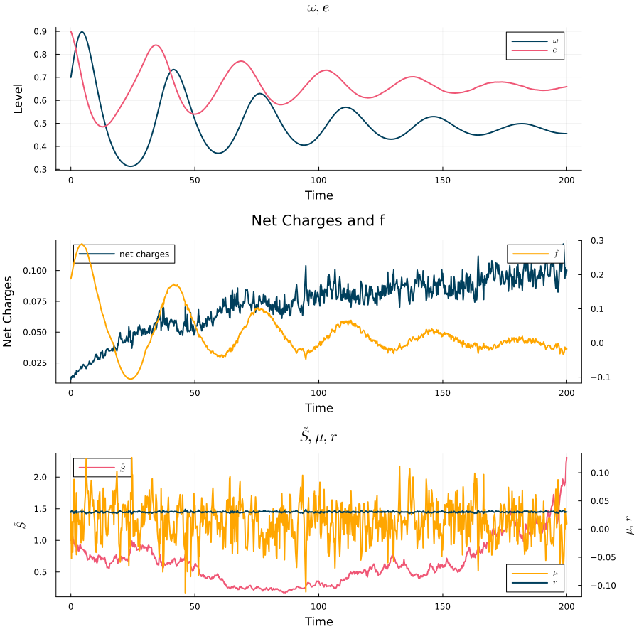
Next in Figure 5, we explore the effect of the speed of mean reversion of the trend indicator $\mu$. Instead of the base value $\bar{\eta}_{\mu}=0.5$ from Table 2, the left panel shows the results for a faster mean reversion $\bar{\eta}_{\mu}=5$, where we see that the economy experiences prolonged periods without a major crash, whereas the right panel shows that a slower mean reversion $\bar{\eta}_{\mu}=0.2$ leads to a crash sooner.

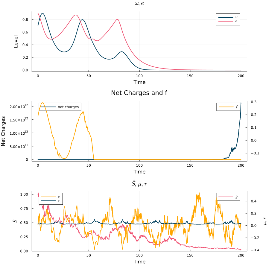
As a final experiment in this section, in Figure 6 we repeat the conditions of faster and slower mean reversion of the trend indicator, but with $\bar{\rho}_{2}=3$ instead of the base value $\bar{\rho}_{2}=5$ from Table 2, meaning that the response of the interest rate to a drop in the trend indicator is less pronounced, with corresponding improvements in the economic outcomes.

References

- [1] (2017) Julia: a fresh approach to numerical computing. SIAM Review 59 (1), pp. 65–98. Cited by: §4.
- [2] (2014) Shifting martingale measures and the birth of a bubble as a submartingale. Finance and Stochastics 18 (2), pp. 297–326. External Links: Document Cited by: §1.
- [3] (1982) Bubbles, rational expectations and financial markets. In Crises in the Economic and Financial Structure, P. Wachtel (Ed.), pp. 295–316. Note: NBER Working Paper No. 945, doi:10.3386/w0945 External Links: Link Cited by: §1.
- [4] (2022) The inelastic market hypothesis: a microstructural interpretation. Quantitative Finance 22 (10), pp. 1785–1795. Cited by: §1, §3.
- [5] (2018) Debt and damages: what are the chances of staying under the 2 c warming threshold?. International Economics 155, pp. 92–108. Cited by: §4.
- [6] (2014) Follow the money: the monetary roots of bubbles and crashes. International Review of Financial Analysis 32, pp. 47–59. Cited by: §3.
- [7] (2005) Local martingales, bubbles and option prices. Finance and Stochastics 9 (4), pp. 477–492. External Links: Document Cited by: §1.
- [8] (1970) Efficient capital markets: a review of theory and empirical work. The journal of Finance 25 (2), pp. 383–417. Cited by: §3.
- [9] (2021) In search of the origins of financial fluctuations: the inelastic markets hypothesis. Technical report National Bureau of Economic Research. Cited by: §1, §3.
- [10] (2007) Options and bubbles. Review of Financial Studies 20 (2), pp. 359–390. External Links: Document Cited by: §1.
- [11] (2010) Asset price bubbles in incomplete markets. Mathematical Finance 20 (2), pp. 145–185. External Links: Document Cited by: §1.
- [12] (2015) Strict local martingales and bubbles. The Annals of Applied Probability 25 (4), pp. 1827–1867. External Links: Document Cited by: §1.
- [13] (2000) Local martingales, arbitrage, and viability: free snacks and cheap thrills. Economic Theory 16 (1), pp. 135–161. External Links: Document Cited by: §1.
- [14] (2000) Rational equilibrium asset-pricing bubbles in continuous trading models. Journal of Economic Theory 91 (1), pp. 17–58. External Links: Document Cited by: §1.
- [15] (1978) Asset prices in an exchange economy. Econometrica: journal of the Econometric Society, pp. 1429–1445. Cited by: §3.
- [16] (2020) Co-existence of trend and value in financial markets: estimating an extended chiarella model. Journal of Economic Dynamics and Control 112, pp. 103791. Cited by: §3.
- [17] (2014) Money creation in the modern economy. Bank of England Quarterly Bulletin 54 (1), pp. 14–27. External Links: Link Cited by: §1.
- [18] (2017) DifferentialEquations.jl–a performant and feature-rich ecosystem for solving differential equations in julia. Journal of Open Research Software 5 (1). Cited by: §4.
- [19] (2021) Stochastic differential equations in julia. Journal of Statistical Software 96 (6). Cited by: §4.
- [20] (2011) From financial crash to debt crisis. American Economic Review 101 (5), pp. 1676–1706. External Links: Document Cited by: §1.
- [21] (1985) Asset bubbles and overlapping generations. Econometrica 53 (6), pp. 1499–1528. External Links: Link Cited by: §1.
- [22] (2014) Can banks individually create money out of nothing? — the theories and the empirical evidence. International Review of Financial Analysis 36, pp. 1–19. External Links: Document Cited by: §1, §1.
- [23] (2012) Towards a new research programme on ’banking and the economy’-implications of the quantity theory of credit for the prevention and resolution of banking and debt crises. International Review of Financial Analysis 25, pp. 1–17. Cited by: §1, §1, §3.