跳到论文正文
W Papers独立论文阅读器 arXiv:2603.05491 论文正文 计算阅读时间 · 0%
引用这篇论文根据当前论文元数据生成,正式投稿前建议核对。


License: arXiv.org perpetual non-exclusive license
arXiv:2603.05491v1 [math.PR] 05 Mar 2026

Local limits of uniform triangulations with boundaries in high genus

Tanguy Lions111ENS Lyon, tanguy.lions@ens-lyon.fr
Abstract

We study the local limits of uniform random triangulations with boundaries in the regime where the genus is proportional to the number of faces. Budzinski and Louf proved in [15] that when there are no boundaries, the local limits exist and are the Planar Stochastic Hyperbolic Triangulation (PSHT) introduced in [23].

We show that when the triangulations considered have size nn and boundaries with total length p→+∞p\to+\infty and p=o​(n)p=o(n), the local limits around a typical boundary edge are the half-plane hyperbolic triangulations defined by Angel and Ray in [4]. This provides, for the first time, a construction of these hyperbolic half-plane triangulations as local limits of large genus triangulations.

We also prove that under the condition p=o​(n)p=o(n), the local limit when rooted on a uniformly chosen oriented edge is given by the PSHT. Contrary to [15], the latter does not rely on the Goulden-Jackson recurrence relation, but only on coarse combinatorial estimates. Thus, we expect that the proof can be adapted to local limits in similar models.

[Uncaptioned image]

1 Introduction

Enumeration of maps.

Since the enumeration of planar maps by Tutte in the 1960s [42], maps have attracted a lot of interest from different communities within mathematics and theoretical physics. The enumeration of maps in terms of their size nn and their genus gg is linked to the topological recursion [27] and to solutions of several integrable hierarchies such as the KdV, the KP and 22-Toda hierarchies [39, 38, 29]. These methods provide asymptotics for the enumeration of maps when gg is fixed and n→+∞n\to+\infty [8]. When both n,g→+∞n,g\to+\infty, these methods have been less successful so far, but the work of Budzinski and Louf [15] provides asymptotics for the number of triangulations in large genus up to sub-exponential factors.

Random maps.

Simultaneously, probabilists have also been studying geometric properties of random maps chosen uniformly among a certain class. They particularly focused on certain regimes where the size nn becomes large. The planar case g=0g=0 is now very well understood in terms of local and scaling limits. Various classes of models have been proved to converge locally to infinite random planar maps such as the UIPT [5] (see also [41] for type-I UIPT), the UIPQ [32, 20] or infinite Boltzmann planar maps [11]. On the other hand, the Brownian sphere [34, 36] appears as the scaling limit of many models of random planar maps [35, 1, 2]. For g≥0g\geq 0, the Brownian sphere has analogues called Brownian surfaces [10] which have been recently proven in [9] to be the scaling limit of large quadrangulations of fixed genus g≥0g\geq 0 as n→+∞n\to+\infty. The Brownian sphere is also linked to the Liouville quantum gravity (see [26]) approach to random planar geometry.

Another regime that is well understood is when the genus is unconstrained and the map is a random uniform gluing of polygons. In this case, the number of vertices is typically very small, the mean degree of vertices goes to infinity and the genus concentrates close to the maximal possible value ([21, 13, 28]). Thus, there is no hope for a proper local or scaling limit result in this regime.

Random maps in large genus.

The investigation of the regimes where g→+∞g\to+\infty was started much more recently. In the case of unicellular maps (i.e. maps with one face) many results are now known, such as the local convergence to a supercritical random tree [3], the calculation of the diameter [40] and the convergence of the length spectrum [30, 31]. Note that this last result seems to indicate a connection between large genus random maps and large genus random hyperbolic surfaces since the same limit for the length spectrum is obtained in both models [31, 37, 7].

Beyond the unicellular case, Budzinski and Louf proved in [15] that large genus triangulations with a size proportional to the genus locally converge to the Planar Stochastic Hyperbolic Triangulations (PSHT) defined in [23]222Actually, in [15], the authors consider type-I triangulations while the PSHT defined in [23] are type-II triangulations. Type-I refers to triangulations where loops are allowed and type-II to the case where loops are not allowed. The type-I analogue of [23] is defined in [16].. A similar local convergence result has been obtained in the case of arbitrary (even) face degrees in [14]. More recently, the paper [12] shows that as soon as gn→θ∈(0,12)\frac{g}{n}\to\theta\in(0,\frac{1}{2}), the typical graph distances and the diameter are of logarithmic order with high probability. The present paper again focuses on the same regime gn→θ∈[0,12)\frac{g}{n}\to\theta\in[0,\frac{1}{2}) but where now, the triangulations have boundaries with perimeters p1n,⋯,pℓnp_{1}^{n},\cdots,p_{\ell}^{n} such that ∑i=1ℓpin​⟶n→+∞+∞\sum_{i=1}^{\ell}p^{n}_{i}\underset{n\to+\infty}{\longrightarrow}+\infty. The local limit of these triangulations with boundaries is expected to be the half-plane analogue of the PSHT.

Planar/half-planar stochastic hyperbolic triangulations.

Angel and Ray introduced in [4] a one-parameter family of triangulations of the half-plane. This family splits into two subfamilies, one being subcritical and the other supercritical. In this paper, we will be interested in the supercritical models. The PSHT introduced in [23] were motivated as the plane analogue of these supercritical half-plane triangulations.
Here, we consider the type-I version of the half-plane triangulations of [4]. They form a one-parameter family of triangulations of the half-plane (ℍλ)0<λ≤λc(\mathbb{H}_{\lambda})_{0<\lambda\leq\lambda_{c}} introduced in [17], where λc=(12​3)−1\lambda_{c}=(12\sqrt{3})^{-1}. For 0<λ≤λc0<\lambda\leq\lambda_{c}, let us introduce h∈(0,14]h\in(0,\frac{1}{4}] such that λ=h(1+8​h)32\lambda=\frac{h}{(1+8h)^{\frac{3}{2}}}. The triangulations ℍλ\mathbb{H}_{\lambda} are characterized by the probabilities of the events of the form t⊂ℍλt\subset\mathbb{H}_{\lambda} where tt are maps of a certain form. More precisely, the maps tt considered are those with a finite number of triangles (the grey faces in Figure 1), one infinite boundary (the dark grey face in Figure 1) and one infinite hole (the white infinite face in Figure 1). For such a triangulation tt, we denote by |tin||t_{\mathrm{in}}| the number of vertices of tt not on the infinite boundary (the green vertices in Figure 1) and by |∂∗t|−|∂t||\partial^{*}t|-|\partial t| the length of the red segment minus the length of the blue segment in Figure 1. Finally, we write t⊂ℍλt\subset\mathbb{H}_{\lambda} if ℍλ\mathbb{H}_{\lambda} can be obtained from tt by filling the infinite hole with a triangulation of the half-plane. The half-plane triangulations (ℍλ)0<λ≤λc(\mathbb{H}_{\lambda})_{0<\lambda\leq\lambda_{c}} are characterized by the spatial Markov property: for any such triangulation tt, we have

ℙ​(t⊂ℍλ)=(8+1h)|∂∗t|−|∂t|​λ|tin|.\displaystyle\mathbb{P}(t\subset\mathbb{H}_{\lambda})=\bigg(8+\frac{1}{h}\bigg)^{|\partial^{*}t|-|\partial t|}\lambda^{|t_{\mathrm{in}}|}.
Refer to caption
Figure 1: On the left: a realisation of ℍλ\mathbb{H}_{\lambda}. On the right, a triangulation tt with one infinite boundary (dark grey face) and one infinite hole (white face) such that t⊂ℍλt\subset\mathbb{H}_{\lambda}. On this example, |tin|=17|t_{\mathrm{in}}|=17 denotes the number of green vertices and |∂∗t|−|∂t|=8−5=3|\partial^{*}t|-|\partial t|=8-5=3 denotes the number of red edges minus the number of blue edges.

We also introduce the type-I PSHT (𝕋λ)0≤λ≤λc(\mathbb{T}_{\lambda})_{0\leq\lambda\leq\lambda_{c}} as the full-plane analogue of the half-plane family (ℍλ)0<λ≤λc(\mathbb{H}_{\lambda})_{0<\lambda\leq\lambda_{c}}. The family (𝕋λ)0≤λ≤λc(\mathbb{T}_{\lambda})_{0\leq\lambda\leq\lambda_{c}} was introduced in [16] and is characterized by the spatial Markov property: for any triangulation tt with |t||t| vertices and one hole of perimeter pp, we have

ℙ​(t⊂𝕋λ)=Cp​(λ)​λ|t|,\displaystyle\mathbb{P}(t\subset\mathbb{T}_{\lambda})=C_{p}(\lambda)\lambda^{|t|},

where Cp​(λ)C_{p}(\lambda) is explicit (see Section 2.4). For every p≥1p\geq 1, we will also need to consider a version 𝕋λ(p)\mathbb{T}^{(p)}_{\lambda} of 𝕋λ\mathbb{T}_{\lambda} with a boundary of perimeter pp. In that case, the spatial Markov property can be written as follows: for any triangulation tt with boundary of perimeter pp, with |tin||t_{\mathrm{in}}| vertices not on the boundary and with one hole of perimeter qq, we have

ℙ​(t⊂𝕋λ(p))=Cq​(λ)Cp​(λ)​λ|tin|.\displaystyle\mathbb{P}(t\subset\mathbb{T}^{(p)}_{\lambda})=\frac{C_{q}(\lambda)}{C_{p}(\lambda)}\lambda^{|t_{\mathrm{in}}|}.
Uniform triangulations with boundaries.

We now define the finite models we will be interested in. Fix integers g,ℓ≥0g,\ell\geq 0, n≥2​g−1n\geq 2g-1 and 𝐩=(p1,…,pℓ)∈ℕℓ\mathbf{p}=(p_{1},\dots,p_{\ell})\in\mathbb{N}^{\ell}. We write |𝐩|=p1+⋯+pℓ|\mathbf{p}|=p_{1}+\cdots+p_{\ell}. We introduce the set of triangulations 𝒯𝐩​(n,g)\mathcal{T}_{\mathbf{p}}(n,g) defined as the set of maps tt such that:

  • ∙\bullet

    tt has genus gg and n+2−2​gn+2-2g vertices.

  • ∙\bullet

    tt has ℓ\ell distinguished faces ∂1,⋯,∂ℓ\partial_{1},\cdots,\partial_{\ell} of perimeters p1,⋯,pℓp_{1},\cdots,p_{\ell} called the boundaries, which are simple and vertex-disjoint, and each face ∂i\partial_{i} is equipped with a distinguished oriented edge eie_{i} such that ∂i\partial_{i} lies to the right of eie_{i}.

  • ∙\bullet

    The faces of tt that are not boundaries have degree 33.

For t∈𝒯𝐩​(n,g)t\in\mathcal{T}_{\mathbf{p}}(n,g) and ee an oriented edge of tt, the pair (t,e)(t,e) is viewed as the triangulation tt rooted at ee. For a sequence (tn,en)n≥0(t_{n},e^{n})_{n\geq 0} of rooted triangulations, we say that the sequence converges locally to a rooted triangulation (t,e)(t,e) if, for any r≥0r\geq 0, the ball of radius rr around ene^{n} seen as a map is eventually equal to the ball of radius rr around ee in tt. See Section 2 for more precise definitions. We denote by Tn,g,𝐩T_{n,g,\mathbf{p}} an element of 𝒯𝐩​(n,g)\mathcal{T}_{\mathbf{p}}(n,g) chosen uniformly at random. For any λ∈(0,λc]\lambda\in(0,\lambda_{c}], let h=h​(λ)h=h(\lambda) be the unique h∈(0,14]h\in(0,\frac{1}{4}] such that λ=h(1+8​h)32\lambda=\frac{h}{(1+8h)^{\frac{3}{2}}} and let

d​(λ)=h​log⁡(1+1−4​h1−1−4​h)(1+8​h)​1−4​h.\displaystyle d(\lambda)=\frac{h\log\Big(\frac{1+\sqrt{1-4h}}{1-\sqrt{1-4h}}\bigg)}{(1+8h)\sqrt{1-4h}}.

It is shown in [15] that d​(λ)d(\lambda) is increasing with d​(λc)=16d(\lambda_{c})=\frac{1}{6} and limλ→0d​(λ)=0\lim_{\lambda\to 0}d(\lambda)=0, and that the quantity d​(λ)d(\lambda) denotes the expectation of the inverse of the root degree in 𝕋λ\mathbb{T}_{\lambda}. Our main theorems are local convergence results, both around a typical oriented edge and around a typical oriented edge chosen on a boundary. The main new result is the following theorem.

Theorem 1.1.

Fix θ∈[0,12)\theta\in[0,\frac{1}{2}), gnn​⟶n→+∞​θ\displaystyle\frac{g_{n}}{n}\underset{n\to+\infty}{\longrightarrow}\theta and 𝐩n=(p1n,⋯,pℓnn)\mathbf{p}^{n}=(p^{n}_{1},\cdots,p^{n}_{\ell_{n}}) such that |𝐩n|=o​(n)|\mathbf{p}^{n}|=o(n) and |𝐩n|ℓn​⟶n→+∞+∞\displaystyle\frac{|\mathbf{p}^{n}|}{\ell_{n}}\underset{n\to+\infty}{\longrightarrow}+\infty. Denote by ene^{n} a uniformly chosen oriented edge on the union ∂1∪⋯∪∂ℓn\partial_{1}\cup\cdots\cup\partial_{\ell_{n}} of the boundaries of Tn,gn,𝐩nT_{n,g_{n},\mathbf{p}^{n}}. Then, the following convergence holds for the local topology

(Tn,gn,𝐩n,en)​→(d)​ℍλ​(θ),\displaystyle(T_{n,g_{n},\mathbf{p}^{n}},e^{n})\overset{(d)}{\to}\mathbb{H}_{\lambda(\theta)},

where λ​(θ)\lambda(\theta) is the unique solution to the equation

d​(λ​(θ))=1−2​θ6.\displaystyle d(\lambda(\theta))=\frac{1-2\theta}{6}. (1)

The extra hypothesis |𝐩n|ℓn​→n→+∞+∞\displaystyle\frac{|\mathbf{p}^{n}|}{\ell_{n}}\underset{n\to+\infty}{\to}+\infty ensures that a typical boundary has a size that tends to +∞+\infty (in probability). This theorem answers in the affirmative conjectures in [4][24, open question 8.2] stating that the hyperbolic triangulations ℍλ\mathbb{H}_{\lambda} of the half-plane can be obtained as local limits of large genus triangulations with a boundary length that also tends to infinity. We expect that the result should hold if we choose our root edge to be the distinguished edge e1ne^{n}_{1} on the boundary ∂1\partial_{1} and we only assume p1n​⟶n→+∞+∞p^{n}_{1}\underset{n\to+\infty}{\longrightarrow}+\infty.

In the regime where |𝐩n|∼α​n|\mathbf{p}^{n}|\sim\alpha n with α>0\alpha>0, we still expect to see a local convergence result. However, in that case, we conjecture that the limit should be a triangulation with infinitely many infinite faces. No canonical such model has yet been studied in the literature. We will investigate this problem in a future work.

Now we give another local convergence result when ene^{n} is chosen uniformly at random among all edges of Tn,gn,𝐩nT_{n,g_{n},\mathbf{p}^{n}}. In [15, Theorem 1.11.1], the authors treat the case 𝐩n=∅\mathbf{p}^{n}=\emptyset, here we generalize the result to the case |𝐩n|=o​(n)|\mathbf{p}^{n}|=o(n).

Theorem 1.2.

Fix θ∈[0,12)\theta\in[0,\frac{1}{2}), gnn→θ\displaystyle\frac{g_{n}}{n}\to\theta and 𝐩n=(p1n,⋯,pℓnn)\mathbf{p}^{n}=(p^{n}_{1},\cdots,p^{n}_{\ell_{n}}) such that |𝐩n|=o​(n)|\mathbf{p}^{n}|=o(n). Let ene^{n} denote an oriented edge chosen uniformly at random in Tn,gn,𝐩nT_{n,g_{n},\mathbf{p}^{n}}. Then the following convergence holds for the local topology

(Tn,gn,𝐩n,en)​→(d)​𝕋λ​(θ),\displaystyle(T_{n,g_{n},\mathbf{p}^{n}},e^{n})\overset{(d)}{\to}\mathbb{T}_{\lambda(\theta)},

where λ​(θ)\lambda(\theta) is the unique solution to the equation

d​(λ​(θ))=1−2​θ6.\displaystyle d(\lambda(\theta))=\frac{1-2\theta}{6}.

Moreover, let us also fix p≥1p\geq 1. Consider Tn,gn,(p,𝐩n)T_{n,g_{n},(p,\mathbf{p}^{n})} and let e1ne^{n}_{1} denote the distinguished edge on the first boundary of Tn,gn,(p,𝐩n)T_{n,g_{n},(p,\mathbf{p}^{n})}. Then the following convergence holds for the local topology

(Tn,gn,(p,𝐩n),e1n)​→(d)​𝕋λ​(θ)(p).\displaystyle(T_{n,g_{n},(p,\mathbf{p}^{n})},e^{n}_{1})\overset{(d)}{\to}\mathbb{T}^{(p)}_{\lambda(\theta)}.
Motivation: long-term exploration of uniform triangulations.

Let us give a potential application of our theorems. First, one can discover Tn,gnT_{n,g_{n}} triangle by triangle in a Markovian fashion. This yields a growing sequence of triangulations t1⊂⋯​tk⊂⋯t_{1}\subset\cdots t_{k}\subset\cdots, called the peeling exploration of Tn,gnT_{n,g_{n}}. Depending on the order in which the triangles are discovered, we can keep track of different geometric information. However, the transition probabilities appearing in the exploration are very hard to understand, which makes the process hard to study. Using [15, Theorem 1.11.1] or equivalently Theorem 1.2, we have Tn,gn→𝕋λ​(θ)T_{n,g_{n}}\to\mathbb{T}_{\lambda(\theta)}. Thus, as long as we restrict to studying a bounded number of peeling steps, the transition probabilities converge to the ones of 𝕋λ​(θ)\mathbb{T}_{\lambda(\theta)} which are explicit. Still, understanding the exploration for an unbounded number of steps is out of reach using only [15]. Using Theorem 1.1, one can understand more steps in the peeling exploration. Indeed, for k→+∞k\to+\infty and k=o​(n)k=o(n) assuming that Tn,gn\tkT_{n,g_{n}}\backslash t_{k} is connected, then Tn,gn\tk​=(d)​Tn−o​(n),gn−o​(n),𝐩knT_{n,g_{n}}\backslash t_{k}\overset{(d)}{=}T_{n-o(n),g_{n}-o(n),\mathbf{p}^{n}_{k}} for some random 𝐩kn\mathbf{p}^{n}_{k} that represents the perimeters of the holes of tkt_{k}. Moreover, Theorem 1.1 gives (Tn−o​(n),gn−o​(n),𝐩kn,en)→ℍλ​(θ)(T_{n-o(n),g_{n}-o(n),\mathbf{p}^{n}_{k}},e^{n})\to\mathbb{H}_{\lambda(\theta)} when rooted on a typical edge on the boundary, which ensures that we can understand the peeling transitions for an unbounded number of steps, provided k=o​(n)k=o(n).

In a future work, we plan to use this to study the typical distances in Tn,gn,𝐩nT_{n,g_{n},\mathbf{p}^{n}} by discovering the balls of radius rr with such a Markovian exploration. We hope this will make more precise some results obtained in [12] on the logarithmic order of magnitude of these distances.

Finally, note that as in [15], our results provide some combinatorial estimates (see Proposition 4.9), which we hope can be of independent interest.

Strategy of the proof.

The proofs of Theorem 1.1 and Theorem 1.2 are quite robust and rely mainly on coarse combinatorial estimates that hold for many classes of large genus random maps. In particular, the proof of Theorem 1.2 does not rely on the Goulden-Jackson recursion formula obtained in [29].

In Section 4, we prove Theorem 1.2. The main new argument is the proof that the limit is planar. The rest of the proof is standard and follows the same strategy as in [15], so we do not describe it here. To prove the planarity, one roughly needs to prove that the probability ℙ​(t⊂(Tn,gn,𝐩n,en))\mathbb{P}(t\subset(T_{n,g_{n},\mathbf{p}^{n}},e^{n})), where tt is a finite triangulation of genus 11, goes to 0 as n→+∞n\to+\infty. Let us explain how to prove that. One can write this probability in terms of combinatorial estimates and gets a quantity that roughly looks like:

τ𝐩n​(n−m,gn−1)τ𝐩n​(n,gn)\displaystyle\frac{\tau_{\mathbf{p}^{n}}(n-m,g_{n}-1)}{\tau_{\mathbf{p}^{n}}(n,g_{n})}, for some fixed m≥0m\geq 0.

By standard estimates, there is an absolute constant C>0C>0 such that the following crude estimate holds:

exp⁡(−C​n)​n2​gn≤τ𝐩n​(n,gn)≤exp⁡(C​n)​n2​gn.\displaystyle\exp(-Cn)n^{2g_{n}}\leq\tau_{\mathbf{p}^{n}}(n,g_{n})\leq\exp(Cn)n^{2g_{n}}. (2)

Thus, we find

τ𝐩n​(n−m,gn−1)τ𝐩n​(n,gn)≤exp⁡(2​C​n)​n−2\displaystyle\frac{\tau_{\mathbf{p}^{n}}(n-m,g_{n}-1)}{\tau_{\mathbf{p}^{n}}(n,g_{n})}\leq\exp(2Cn)n^{-2}.

Unfortunately, the right-hand side does not tend to 0. We now describe one of the main new ideas of the paper, which solves this issue. Let us fix ε>0\varepsilon>0 and assume that ℙ​(t⊂(Tn,gn,𝐩n,en))≥ε>0\mathbb{P}(t\subset(T_{n,g_{n},\mathbf{p}^{n}},e^{n}))\geq\varepsilon>0 for nn large enough. Since ene^{n} is uniform, there is a probability at least ε/2\varepsilon/2 that Tn,gn,𝐩nT_{n,g_{n},\mathbf{p}^{n}} contains η​n\eta n copies of tt called t1,⋯,tη​nt^{1},\cdots,t^{\eta n}, with η>0\eta>0 a small constant. Moreover, up to choosing η\eta smaller, we may assume that these copies are disjoint. We can rewrite the probability to have the copies t1,⋯,tη​nt^{1},\cdots,t^{\eta n} contained in Tn,gn,𝐩nT_{n,g_{n},\mathbf{p}^{n}} in terms of combinatorics and obtain a quantity that looks like

τ𝐩n​(n−η​n​m,gn−η​n)τ𝐩n​(n,gn)\displaystyle\frac{\tau_{\mathbf{p}^{n}}(n-\eta nm,g_{n}-\eta n)}{\tau_{\mathbf{p}^{n}}(n,g_{n})}.

By the above estimates (2) we have the bound

τ𝐩n​(n−η​n​m,gn−η​n)τ𝐩n​(n,gn)≤exp⁡(2​C​n)​n−2​η​n.\displaystyle\displaystyle\frac{\tau_{\mathbf{p}^{n}}(n-\eta nm,g_{n}-\eta n)}{\tau_{\mathbf{p}^{n}}(n,g_{n})}\leq\exp(2Cn)n^{-2\eta n}.

Taking into account all the possible locations for the copies t1,⋯,tη​nt^{1},\cdots,t^{\eta n} multiplies this quantity by a factor nη​nn^{\eta n}. We conclude using the fact that exp⁡(2​C​n)​n−η​n→0\exp(2Cn)n^{-\eta n}\to 0. This proves ℙ​(t⊂(Tn,gn,𝐩n,en))≤ε\mathbb{P}(t\subset(T_{n,g_{n},\mathbf{p}^{n}},e^{n}))\leq\varepsilon and thus the local planarity. In words, taking many copies of tt makes the error factor exp⁡(C​n)\exp(Cn) negligible compared to the reduction of the genus by η​n\eta n which divides the volume by n2​η​nn^{2\eta n}. This argument still works if we replace (Tn,gn,𝐩n)n≥1(T_{n,g_{n},\mathbf{p}^{n}})_{n\geq 1} with any model of triangulations (T~n)n≥0(\tilde{T}_{n})_{n\geq 0} that is invariant under rerooting and such that T~n\tilde{T}_{n} is absolutely continuous with respect to Tn,gn,𝐩nT_{n,g_{n},\mathbf{p}^{n}} and such that d​T~nd​Tn,gn,𝐩n≤exp⁡(C​n)\displaystyle\frac{\mathrm{d}\tilde{T}_{n}}{\mathrm{d}T_{n,g_{n},\mathbf{p}^{n}}}\leq\exp(Cn) for some absolute constant C>0C>0. In particular, one would expect this argument to apply to high genus triangulations equipped with a decoration such as an Ising model.

In Section 5, we prove Theorem 1.1. The proof is very technical here, and the difficulties are very different from those encountered in Theorem 1.2. Indeed, the planarity comes for free, since the planarity in Theorem 1.2 gives the estimate

τ𝐩n​(n,gn−1)τ𝐩n​(n,gn)→0\displaystyle\frac{\tau_{\mathbf{p}^{n}}(n,g_{n}-1)}{\tau_{\mathbf{p}^{n}}(n,g_{n})}\to 0.

We also easily get the one-endedness, again by using combinatorial estimates that follow from Theorem 1.2. Let us write ∂i\partial_{i} for the boundary such that en∈∂ie^{n}\in\partial_{i}. The main difficulty here is to exclude the following two pathological cases that are closely related to the geometry of the boundaries (see Figure 2):

  1. 1.

    A small neighbourhood of ene^{n} intersects another boundary ∂j\partial_{j} for i≠ji\neq j.

  2. 2.

    A small neighbourhood of ene^{n} sees a part of ∂i\partial_{i} that is far from ene^{n} along ∂i\partial_{i}, i.e. the boundary ∂i\partial_{i} folds onto itself near ene^{n}.

Refer to caption
Figure 2: The red neighbourhood of the edge ene^{n} touches another boundary and the opposite side of the boundary ∂i\partial_{i}. These are the two pathological cases to exclude.

These cases cannot be ruled out using Theorem 1.2, since when ene^{n} is chosen uniformly at random on Tn,gn,𝐩nT_{n,g_{n},\mathbf{p}^{n}}, it typically lies far from the boundaries. These two cases are excluded in Section 5.2 which is the most technical part of this work. Finally, there remains to identify the limit. In [4], the authors show that the random triangulations of the half-plane that satisfy a nice Markov property form a one-parameter family333Their work is done in the type I​III case. In the type-II case the family obtained with their work is much larger. However, with a stronger Markov property that we use here (see Definition 2.5) we recover a one-parameter family. (Hα)0<α<1(H_{\alpha})_{0<\alpha<1}. This family splits into two subfamilies that behave very differently, one being subcritical and one supercritical:

  • ∙\bullet

    The elements of the family (Hα)α<13(H_{\alpha})_{\alpha<\frac{1}{\sqrt{3}}} are subcritical, i.e. the half-plane triangulations look like critical Galton-Watson trees.

  • ∙\bullet

    The elements of the family (Hα)α>13(H_{\alpha})_{\alpha>\frac{1}{\sqrt{3}}} are supercritical. They share many properties with hyperbolic graphs such as exponential volume growth, positive anchored expansion…

Using structural results on half-plane triangulations satisfying a Markov property, we can show that any subsequential limit in Theorem 1.1 is a mixture of the half-plane triangulations (Hα)0<α<1(H_{\alpha})_{0<\alpha<1}. Then, using Theorem 1.2, we obtain

τ𝐩n​(n−1,gn)τ𝐩n​(n,gn)→λ​(θ),\displaystyle\frac{\tau_{\mathbf{p}^{n}}(n-1,g_{n})}{\tau_{\mathbf{p}^{n}}(n,g_{n})}\to\lambda(\theta),

and deduce that any subsequential limit is a mixture of Hα1H_{\alpha_{1}} and Hα2H_{\alpha_{2}}, where Hα1H_{\alpha_{1}} is subcritical and Hα2​=(d)​ℍλ​(θ)H_{\alpha_{2}}\overset{(d)}{=}\mathbb{H}_{\lambda(\theta)} is the expected limit. To exclude Hα1H_{\alpha_{1}}, we use surgery operations on the peeling diagram of Tn,gn,𝐩nT_{n,g_{n},\mathbf{p}^{n}} inspired by [22].

Acknowledgements.

I am grateful to Thomas Budzinski for his crucial help at various stages of this project. I also thank Grégory Miermont for stimulating discussions.

2 Preliminaries

2.1 Definitions

We begin by recalling the main definitions used throughout the paper.

A (finite or infinite) map mm is obtained by gluing together a collection of oriented polygons along their edges, with matching orientations, so that the resulting surface is connected. If finitely many polygons are glued, the resulting surface is orientable, and we can define its genus. We say that a map mm is rooted if it is equipped with a distinguished oriented edge called the root edge. The face on the right of the root edge is called the root face, and the vertex at its origin is called the root vertex. We denote by m∗m^{*} the dual of mm, defined as the map where the vertices correspond to the faces of mm and two vertices of m∗m^{*} are connected by an edge if the corresponding faces are connected by an edge in mm.

A triangulation is a map all of whose faces have degree 33. We focus on type-I triangulations, that is, triangulations that may contain multiple edges and loops. For n≥1n\geq 1 and g≥0g\geq 0, we denote by 𝒯​(n,g)\mathcal{T}(n,g) the set of rooted triangulations of genus gg with 2​n2n faces. By Euler’s formula, a triangulation in 𝒯​(n,g)\mathcal{T}(n,g) has 3​n3n edges and n+2−2​gn+2-2g vertices. In particular, the set 𝒯​(n,g)\mathcal{T}(n,g) is non-empty if and only if n≥2​g−1n\geq 2g-1. We denote by τ​(n,g)\tau(n,g) the cardinality of 𝒯​(n,g)\mathcal{T}(n,g), and we write Tn,gT_{n,g} for a uniform random triangulation in 𝒯​(n,g)\mathcal{T}(n,g).

In this paper, we will consider maps with boundaries. We introduce two notions, the first including the second.

Definition 2.1.

A triangulation with holes is a finite map tt with:

  • ∙\bullet

    A set of distinguished faces, called the boundaries (or external faces) ∂1,…,∂ℓ\partial_{1},\dots,\partial_{\ell}, of degrees p1,…,pℓ≥1p_{1},\dots,p_{\ell}\geq 1, which are vertex-simple (that is, all vertices of ∂i\partial_{i} are distinct) and share no vertices. Each boundary ∂i\partial_{i} is equipped with a distinguished edge eie_{i} such that ∂i\partial_{i} lies to the right of eie_{i}.

  • ∙\bullet

    A set of distinguished faces h1,…,hrh_{1},\dots,h_{r} of degrees q1,…,qr≥1q_{1},\dots,q_{r}\geq 1, called the holes, which are edge-simple (each hih_{i} is composed of qiq_{i} edges) and share no edges.

  • ∙\bullet

    Faces that are neither boundaries nor holes have degree 33.

  • ∙\bullet

    The dual t∗t^{*} remains connected when removing the boundaries.

The perimeter of tt is the tuple 𝐩=(p1,…,pℓ)\mathbf{p}=(p_{1},\dots,p_{\ell}), and the boundary length or total perimeter is |𝐩|=p1+⋯+pℓ|\mathbf{p}|=p_{1}+\cdots+p_{\ell}. Note that in the above definition, boundaries and holes may share vertices and edges. The internal faces of tt are the faces that are not boundaries. In particular, holes are internal faces. Similarly, the internal vertices (resp. edges) are the vertices (resp. edges) that do not lie on a boundary.

This definition extends naturally to infinite triangulations and also to the case where pi=+∞p_{i}=+\infty. For a triangulation with holes tt, we write ∂∗t\partial^{*}t for the union of holes and ∂t\partial t for the union of boundaries.

Definition 2.2.

For ℓ≥0\ell\geq 0 and p1,…,pℓ≥1p_{1},\dots,p_{\ell}\geq 1, a triangulation of the 𝐩\mathbf{p} multi-polygon (or of the 𝐩\mathbf{p}-gon) is a triangulation with holes that has perimeter 𝐩\mathbf{p} and has no holes.

One can think of a triangulation with holes as a neighborhood of the root in a triangulation of the 𝐩\mathbf{p}-gon (see Figure 3). The holes are faces that can be filled by other triangulations of multi-polygons.

Refer to caption
Figure 3: Left: a triangulation of the (6,8,9,14)(6,8,9,14)-gon of genus 55 with nn vertices. Right: a triangulation with holes t0⊂tt_{0}\subset t, which has 11 boundary and 55 holes. Triangulations of multi-polygons t1t_{1} and t2t_{2} are the connected components of t\t0t\backslash t_{0}. The triangulation t1t_{1} (resp. t2t_{2}) is a triangulation of the (6,8,5,13)(6,8,5,13)-gon (resp. (14,2,4,7)(14,2,4,7)-gon).

For 𝐩=(p1,…,pℓ)∈ℕℓ\mathbf{p}=(p_{1},\dots,p_{\ell})\in\mathbb{N}^{\ell}, we denote by 𝒯𝐩​(n,g)\mathcal{T}_{\mathbf{p}}(n,g) the set of triangulations of the 𝐩\mathbf{p}-gon of genus gg with 2​n−∑i=1ℓ(pi−2)2n-\sum_{i=1}^{\ell}(p_{i}-2) triangles, and by τ𝐩​(n,g)\tau_{\mathbf{p}}(n,g) its cardinality. One can verify that a triangulation of the 𝐩\mathbf{p}-gon has n+2−2​gn+2-2g vertices.

In the following, we shall introduce a notion of local distance between maps. It is therefore convenient to work with maps having a single root edge, unlike elements of 𝒯𝐩​(n,g)\mathcal{T}_{\mathbf{p}}(n,g). For t∈𝒯𝐩​(n,g)t\in\mathcal{T}_{\mathbf{p}}(n,g) and ee an oriented edge of tt, we write (t,e)(t,e) for the map obtained by forgetting the distinguished edges of tt and taking ee as the root. We denote by 𝒯𝐩1​(n,g)\mathcal{T}^{1}_{\mathbf{p}}(n,g) the set of all such rooted maps, and we define

𝒯1=⨆g,n,ℓ≥0p1,…,pℓ≥1𝒯p1,…,pℓ1​(n,g),\mathcal{T}^{1}=\bigsqcup_{\begin{subarray}{c}g,n,\ell\geq 0\\ p_{1},\dots,p_{\ell}\geq 1\end{subarray}}\mathcal{T}^{1}_{p_{1},\dots,p_{\ell}}(n,g),

the disjoint union over all parameters.

If (t0,e0)(t_{0},e_{0}) is a rooted triangulation with holes and (t,e)(t,e) a rooted triangulation of the 𝐩\mathbf{p}-gon, we write (t0,e0)⊂(t,e)(t_{0},e_{0})\subset(t,e) if (t,e)(t,e) can be obtained444Note that by the last item in Definition 2.1, if (t0,e0)⊂(t,e)(t_{0},e_{0})\subset(t,e), there is a unique way to obtain (t,e)(t,e) by filling the holes of (t0,e0)(t_{0},e_{0}) from (t0,e0)(t_{0},e_{0}) by gluing one or several triangulations t1,…,tkt_{1},\dots,t_{k} of multi-polygons to the holes of t0t_{0} (see Figure 3). We write (t,e)\(t0,e0)(t,e)\backslash(t_{0},e_{0}) for the collection of triangulations of multi-polygons that have to be glued to t0t_{0} to obtain (t,e)(t,e). If (t,e)(t,e) is an infinite rooted triangulation of the 𝐩\mathbf{p}-gon, we say that it is one-ended if, for every (t0,e0)⊂(t,e)(t_{0},e_{0})\subset(t,e) with a finite number of internal faces, only one connected component of (t,e)\(t0,e0)(t,e)\backslash(t_{0},e_{0}) is infinite. We say that (t,e)(t,e) is planar if, for every (t0,e0)⊂(t,e)(t_{0},e_{0})\subset(t,e) with a finite number of internal faces, the triangulation with holes (t0,e0)(t_{0},e_{0}) is planar. For two vertices x,yx,y in a triangulation with holes tt, we write dt​(x,y)d_{t}(x,y) for the graph distance between xx and yy in tt.

If tt is a triangulation of a multi-polygon, it is more convenient to adopt the convention that the external faces of tt do not belong to t∗t^{*}. Since the external faces of a triangulation of a multi-polygon are simple and disjoint, the dual map t∗t^{*} is connected. We denote by d∗d^{*} the graph distance on the internal faces of tt. We extend dt∗d^{*}_{t} to the set of edges by writing for e,e′e,e^{\prime} two distinct edges

dt∗​(e,e′)=minf,f′⁡dt∗​(f,f′)+1,d^{*}_{t}(e,e^{\prime})=\min_{f,f^{\prime}}d^{*}_{t}(f,f^{\prime})+1,

where f,f′f,f^{\prime} run over all internal faces incident to ee and e′e^{\prime}. We also extend dt∗d^{*}_{t} to the set of vertices by writing, for v,v′v,v^{\prime} two distinct vertices

dt∗​(v,v′)=minf,f′⁡dt∗​(f,f′)+1,d^{*}_{t}(v,v^{\prime})=\min_{f,f^{\prime}}d^{*}_{t}(f,f^{\prime})+1,

where f,f′f,f^{\prime} run over all internal faces incident to vv and v′v^{\prime}.

2.2 Combinatorics

In this section, we recall some combinatorial estimates in the planar case. For p≥1p\geq 1 and n≥p−2n\geq p-2, a formula is given in [33] for the volumes τp​(n,0)\tau_{p}(n,0):

τp​(n,0)=p​(2​p)!(p!)2​4n−p+1​(3​n−p+1)!!(n−p+2)!​(n+p+1)!!​∼n→+∞​c​(p)​λc−n​n−52,\displaystyle\tau_{p}(n,0)=\frac{p(2p)!}{(p!)^{2}}\frac{4^{n-p+1}(3n-p+1)!!}{(n-p+2)!(n+p+1)!!}\underset{n\to+\infty}{\sim}c(p)\lambda_{c}^{-n}n^{-\frac{5}{2}},

where λc=112​3\lambda_{c}=\frac{1}{12\sqrt{3}}, and

c​(p)=λc2−p​3p−2​p​(2​p)!4​2​π​(p!)2​∼p→+∞​136​π​2​12p​p.\displaystyle c(p)=\lambda_{c}^{2-p}\frac{3^{p-2}p(2p)!}{4\sqrt{2\pi}(p!)^{2}}\underset{p\to+\infty}{\sim}\frac{1}{36\pi\sqrt{2}}12^{p}\sqrt{p}.

Note that τp​(n−2+p,0)\tau_{p}(n-2+p,0) denotes the number of triangulations of the pp-gon with nn internal vertices. For p≥1p\geq 1 and λ>0\lambda>0, we define

wλ​(p)=∑n≥0τp​(n−2+p,0)​λn.w_{\lambda}(p)=\sum_{n\geq 0}\tau_{p}(n-2+p,0)\lambda^{n}.

This quantity is finite if and only if λ≤λc\lambda\leq\lambda_{c}. We also define

Wλ​(x)=∑p≥1wλ​(p)​xp.W_{\lambda}(x)=\sum_{p\geq 1}w_{\lambda}(p)x^{p}.

Then, from Equation (4) in [33], we obtain the explicit formula:

Wλ​(x)=λ2​((1−1+8​hh​x)​1−4​(1+8​h)​x−1+xλ),\displaystyle W_{\lambda}(x)=\frac{\lambda}{2}\left(\left(1-\frac{1+8h}{h}x\right)\sqrt{1-4(1+8h)x}-1+\frac{x}{\lambda}\right), (3)

where h∈(0,14]h\in(0,\frac{1}{4}] is given by λ=h(1+8​h)3/2\lambda=\frac{h}{(1+8h)^{3/2}}. From this expression, one can derive the formula

wλ​(1)=12−1+2​h2​1+8​h,w_{\lambda}(1)=\frac{1}{2}-\frac{1+2h}{2\sqrt{1+8h}},

and for p≥2p\geq 2,

wλ​(p)=(2+16​h)p​(2​p−5)!!p!​((1−4​h)​p+6​h)4​(1+8​h)3/2.\displaystyle w_{\lambda}(p)=(2+16h)^{p}\frac{(2p-5)!!}{p!}\frac{((1-4h)p+6h)}{4(1+8h)^{3/2}}. (4)

We then define the Boltzmann triangulation of the pp-gon (with parameter λ\lambda) as the random planar triangulation Tλ(p)T^{(p)}_{\lambda} that takes the value tt with probability λ|tin|wλ​(p)\frac{\lambda^{|t_{\mathrm{in}}|}}{w_{\lambda}(p)}, where |tin||t_{\mathrm{in}}| denotes the number of vertices of tt that do not lie on the boundary face.

2.3 Local convergence and dual local convergence

In this section, we introduce two notions of local distance between maps in 𝒯1\mathcal{T}^{1}. The first one is the most important, since Theorems 1.1 and 1.2 are stated for this distance. However, in Section 4, it is sometimes more convenient to use an alternative notion of distance.

Local distance.

For r≥0r\geq 0 and (t,e)∈𝒯1(t,e)\in\mathcal{T}^{1}, we define the ball of radius rr, denoted Br​(t,e)B_{r}(t,e), as the submap consisting of the edges having at least one endpoint at graph distance at most r−1r-1 from the origin of ee (see Figure 4). We then introduce the local distance on 𝒯1\mathcal{T}^{1} by

dloc​((t,e),(t′,e′))=(1+max⁡{r≥0:Br​(t,e)=Br​(t′,e′)})−1.\displaystyle d_{\mathrm{loc}}((t,e),(t^{\prime},e^{\prime}))=(1+\max\{r\geq 0:B_{r}(t,e)=B_{r}(t^{\prime},e^{\prime})\})^{-1}. (5)

The definition used for Br​(t,e)B_{r}(t,e) here is not the usual one. Indeed, the most natural definition would be to take all faces incident to a vertex at distance at most r−1r-1 from the origin of ee. However, with this choice, if the root edge ee lies on the boundary ∂1\partial_{1}, then we would have ∂1⊂B1​(t,e)\partial_{1}\subset B_{1}(t,e). Consequently, as soon as p1n​⟶n→+∞+∞p^{n}_{1}\underset{n\to+\infty}{\longrightarrow}+\infty, one cannot expect any local convergence result.

A drawback of this definition is that, in general, we do not have Br​(t,e)⊂(t,e)B_{r}(t,e)\subset(t,e), since the ball Br​(t,e)B_{r}(t,e) might not be a triangulation with holes. Its completion, denoted 𝒯1¯\overline{\mathcal{T}^{1}}, is a Polish space that can be viewed as the set of rooted (finite or infinite) triangulations of a multi-polygon (with a finite or infinite number of boundaries) in which all vertices have finite degree. Note that pp can be infinite, and this space is not compact.

Dual local distance.

For r≥0r\geq 0 and (t,e)∈𝒯1(t,e)\in\mathcal{T}^{1}, we define the dual ball of radius rr, denoted Br∗​(t,e)B_{r}^{*}(t,e). We define Br∗​(t,e)B_{r}^{*}(t,e) as the triangulation with holes rooted at ee, obtained as follows (see Figure 4):

  • ∙\bullet

    Take all internal faces f′f^{\prime} at dual distance at most rr from an internal face incident to ee.

  • ∙\bullet

    Add the boundaries sharing a vertex with one of the faces already included.

For any r≥0r\geq 0, we always have Br∗​(t,e)⊂tB^{*}_{r}(t,e)\subset t. We then define the local dual distance on 𝒯1\mathcal{T}^{1} by

dloc∗​((t,e),(t′,e′))=(1+max⁡{r≥0:Br∗​(t,e)=Br∗​(t′,e′)})−1.\displaystyle d^{*}_{\mathrm{loc}}((t,e),(t^{\prime},e^{\prime}))=(1+\max\{r\geq 0:B^{*}_{r}(t,e)=B^{*}_{r}(t^{\prime},e^{\prime})\})^{-1}. (6)

Let 𝒯1¯∗\overline{\mathcal{T}^{1}}^{*} denote the completion of 𝒯1\mathcal{T}^{1} under dloc∗d^{*}_{\mathrm{loc}}. The set 𝒯1¯∗\overline{\mathcal{T}^{1}}^{*} is not compact under dloc∗d^{*}_{\mathrm{loc}}, since Br∗​(t,e)B^{*}_{r}(t,e) may touch boundaries and thus may contain arbitrarily large faces.

However, consider a sequence (Tn,en)n≥0(T_{n},e_{n})_{n\geq 0} of random rooted triangulations of a multi-polygon, and let ρn\rho_{n} be the origin of ene_{n}. Suppose that for any r≥0r\geq 0, we have ℙ​(dTn∗​(ρn,∂Tn)≤r)→0\mathbb{P}(d_{T_{n}}^{*}(\rho_{n},\partial T_{n})\leq r)\to 0, i.e., the root edge typically lies far from the boundaries. Then, under the event {dTn​(ρn,∂Tn)>r}\{d_{T_{n}}(\rho_{n},\partial T_{n})>r\}, the dual ball Br∗​(tn,en)B^{*}_{r}(t_{n},e_{n}) of radius rr, has at most 3⋅2r3\cdot 2^{r} triangles so it can take only finitely many values. We deduce that the sequence (Tn,en)(T_{n},e_{n}) is tight for dloc∗d^{*}_{\mathrm{loc}}. This argument will later be used in Section 4 to establish tightness easily. Indeed, in Section 4, we consider Tn=Tn,gn,𝐩nT_{n}=T_{n,g_{n},\mathbf{p}^{n}} with |𝐩n|=o​(n)|\mathbf{p}^{n}|=o(n) and ene^{n} a uniformly chosen oriented edge on TnT_{n}. Hence, the edge ene^{n} typically lies far from the boundaries. In the regime studied in [15], the authors consider the case ∂Tn=∅\partial T_{n}=\emptyset, so the condition is always satisfied, and tightness follows automatically under this topology.

Refer to caption
Figure 4: We represent a triangulation tt of the 𝐩\mathbf{p}-gon. On the left, we show the ball of radius 22 centered at e1e_{1}, which lies on a boundary, and at e2e_{2}, which lies far from the boundaries. On the right, we show the dual local ball of radius 22 centered at e1e_{1}, e2e_{2}, and e3e_{3}. Note that B2∗​(t,e1)B_{2}^{*}(t,e_{1}) contains the boundary on which e1e_{1} lies. Moreover, in B1∗​(t,e3)B^{*}_{1}(t,e_{3}), one of the green internal faces shares a vertex with a boundary face, and thus, this boundary face also belongs to B2∗​(t,e)B^{*}_{2}(t,e).

2.4 Triangulations of the plane

In this section, we recall the definition of type-I Planar Stochastic Hyperbolic Triangulations (PSHT). They were first defined in [23] for type-II triangulations, and later extended to the type-I setting in [16]. The interested reader may read [24, Section 8] for a construction of these random maps in a general setting. The PSHT form a one-parameter family (𝕋λ)0<λ≤λc(\mathbb{T}_{\lambda})_{0<\lambda\leq\lambda_{c}}, where λc=112​3\lambda_{c}=\frac{1}{12\sqrt{3}}. They are random triangulations of the plane characterized by a Markov property. For any triangulation tt with one hole of perimeter pp and vv vertices in total, we have

ℙ​(t⊂𝕋λ)=Cp​(λ)​λv.\displaystyle\mathbb{P}(t\subset\mathbb{T}_{\lambda})=C_{p}(\lambda)\lambda^{v}.

Note that 𝕋λc\mathbb{T}_{\lambda_{c}} has the law of the Uniform Infinite Planar Triangulation (UIPT). For λ∈(0,λc)\lambda\in(0,\lambda_{c}), let us define h∈(0,14]h\in(0,\frac{1}{4}] as the unique solution of the equation

λ=h(1+8​h)32.\displaystyle\lambda=\frac{h}{(1+8h)^{\frac{3}{2}}}.

We have

Cp​(λ)=1λ​(8+1h)p−1​∑q=0p−1(2​qq)​hq.\displaystyle C_{p}(\lambda)=\frac{1}{\lambda}\bigg(8+\frac{1}{h}\bigg)^{p-1}\sum_{q=0}^{p-1}\binom{2q}{q}h^{q}.

For any p≥0p\geq 0, we introduce the extension 𝕋λ(p)\mathbb{T}_{\lambda}^{(p)} of 𝕋λ\mathbb{T}_{\lambda} to the finite boundary case. Indeed, 𝕋λ(p)\mathbb{T}_{\lambda}^{(p)} is a random infinite, one-ended, planar triangulation of the pp-gon characterized by the probabilities

ℙ​(t⊂𝕋λ(p))=Cq​(λ)Cp​(λ)​λv,\displaystyle\mathbb{P}(t\subset\mathbb{T}_{\lambda}^{(p)})=\frac{C_{q}(\lambda)}{C_{p}(\lambda)}\lambda^{v},

for any triangulation tt with a boundary of perimeter pp and one hole of perimeter qq, where vv denotes the total number of vertices of tt that do not lie on the boundary. Note that 𝕋λ\mathbb{T}_{\lambda} can be identified with 𝕋λ(1)\mathbb{T}^{(1)}_{\lambda}. Indeed, given an infinite triangulation of the plane TT, one can split the root edge into a digon and add a loop inside. Then, rerooting on the loop, one obtains a triangulation T′T^{\prime} of the plane with boundary of perimeter 11. This procedure can be reversed, yielding a bijection between triangulations of the plane and those with a boundary of perimeter 11.
Note that the triangulations 𝕋λ(p)\mathbb{T}_{\lambda}^{(p)} have a nice spatial Markov property since 𝕋λ(p)\t\mathbb{T}_{\lambda}^{(p)}\backslash t has the law of 𝕋λ(q)\mathbb{T}_{\lambda}^{(q)}. This allows one to explore 𝕋λ(p)\mathbb{T}_{\lambda}^{(p)} in a Markovian way and motivates the question of what happens when p→+∞p\to+\infty.

We finally introduce two degenerate infinite planar triangulations. These are deterministic infinite planar triangulations with infinite vertex degrees. The planar triangulation 𝕋0\mathbb{T}_{0} is obtained by gluing the edges of triangles along the structure of an infinite binary tree. We also define 𝕋⋆\mathbb{T}_{\star}, the planar triangulation obtained by starting with a triangle consisting of three loops and then recursively adding two loops in each loop (see Figure 5).

Refer to caption
Figure 5: On the left, the triangulation 𝕋0\mathbb{T}_{0}. On the right, the triangulation 𝕋⋆\mathbb{T}_{\star}.

These two degenerate definitions are motivated by [18, Theorem 1], which states that any infinite random planar triangulation of the plane satisfying a "reasonable" Markov property is a mixture of (𝕋λ)0<λ<λc(\mathbb{T}_{\lambda})_{0<\lambda<\lambda_{c}}, 𝕋0\mathbb{T}_{0}, and 𝕋⋆\mathbb{T}_{\star}.

Definition 2.3.

Let TT be a random infinite planar triangulation. We say that TT is weakly Markovian if there exist numbers avp1,…,pka_{v}^{p_{1},\dots,p_{k}} for k≥1k\geq 1 and p1,…,pk≥1p_{1},\dots,p_{k}\geq 1, v≥0v\geq 0, such that for any triangulation tt with kk holes of perimeters p1,…,pkp_{1},\dots,p_{k} and vv internal vertices,

ℙ​(t⊂T)=avp1,…,pk.\displaystyle\mathbb{P}(t\subset T)=a_{v}^{p_{1},\dots,p_{k}}.

Then, we state [18, Theorem 11] . Note that we do not assume the triangulations to be one-ended here.

Theorem 2.4.

Let TT be a random infinite planar triangulation that is weakly Markovian. Then, TT is of the form 𝕋Λ\mathbb{T}_{\Lambda} where Λ\Lambda is a random variable taking values in [0,λc]∪{⋆}[0,\lambda_{c}]\cup\{\star\}.

2.5 Triangulations of the half-plane

A triangulation of the half-plane is a planar triangulation of the ∞\infty-gon that is one-ended and has vertices of finite degree. For a triangulation with holes tt with exactly one infinite boundary ∂t\partial t and one infinite hole ∂∗t\partial^{*}t (see Figure 1), we use the shorthand notation

|∂∗t|−|∂t|:=|∂∗t\∂t|−|∂t\∂∗t|.|\partial^{*}t|-|\partial t|:=|\partial^{*}t\backslash\partial t|-|\partial t\backslash\partial^{*}t|.

We also denote by |tin||t_{\mathrm{in}}| the number of vertices of tt that do not lie on ∂t\partial t.

Definition 2.5.

A random triangulation of the half-plane HH is said to satisfy a weak spatial Markov property if there exists a function aa such that, for any tt, we have

ℙ​(t⊂H)=a​(|∂∗t|−|∂t|,|tin|).\mathbb{P}(t\subset H)=a(|\partial^{*}t|-|\partial t|,|t_{\mathrm{in}}|).

We say that HH is strongly Markovian if there exist constants β,λ>0\beta,\lambda>0 such that, for any tt, we have

ℙ​(t⊂H)=β|∂∗t|−|∂t|​λ|tin|.\mathbb{P}(t\subset H)=\beta^{|\partial^{*}t|-|\partial t|}\lambda^{|t_{\mathrm{in}}|}.

For 0<λ≤λc0<\lambda\leq\lambda_{c}, we introduce the type-I random triangulation of the half-plane, denoted by ℍλ\mathbb{H}_{\lambda}, introduced in [17]. These triangulations are characterized by

ℙ​(t⊂ℍλ)=(8+1h)|∂∗t|−|∂t|​λvin.\displaystyle\mathbb{P}(t\subset\mathbb{H}_{\lambda})=\bigg(8+\frac{1}{h}\bigg)^{|\partial^{*}t|-|\partial t|}\lambda^{v_{\mathrm{in}}}. (7)

In particular, the half-plane triangulation ℍλ\mathbb{H}_{\lambda} is strongly Markovian. Note that for any tt we have ℍλ\t​=(d)​ℍλ\mathbb{H}_{\lambda}\backslash t\overset{(d)}{=}\mathbb{H}_{\lambda}, which corresponds to the Markov property considered in [4]. Moreover, the triangulation of the half-plane ℍλ\mathbb{H}_{\lambda} is characterized by the local limit

𝕋λ(p)​⟶p→+∞​ℍλ.\displaystyle\mathbb{T}_{\lambda}^{(p)}\underset{p\to+\infty}{\longrightarrow}\mathbb{H}_{\lambda}. (8)

In [4], the authors introduced a one-parameter family (Hα)0≤α<1(H_{\alpha})_{0\leq\alpha<1} of type-I​III triangulations of the half-plane that describes all translation-invariant random triangulations of the half-plane satisfying a spatial Markov property. The Markov property considered there states that for any tt, conditionally on t⊂Hαt\subset H_{\alpha}, we have Hα\t​=(d)​HαH_{\alpha}\backslash t\overset{(d)}{=}H_{\alpha}. This result holds for type-II triangulations. Since we work in the type-I setting, there exists a larger class of triangulations satisfying such a Markov property. However, the formula (7) defining ℍλ\mathbb{H}_{\lambda} above is a stronger assumption. Thus, we recover a one-parameter family of triangulations of the half-plane satisfying this condition (see Proposition 2.6 below).

Let us now give a complete description of half-plane triangulations that are weakly or strongly Markovian. This Proposition is the analogue of [15, Proposition 15]

Proposition 2.6.
  1. 1.

    For any 0≤λ≤λc0\leq\lambda\leq\lambda_{c}, there exists a unique random triangulation of the half-plane555Here ℍ~λ\widetilde{\mathbb{H}}_{\lambda} is the analogue of HαH_{\alpha} for α≤23\alpha\leq\frac{2}{3}, and ℍλ\mathbb{H}_{\lambda} is the analogue of HαH_{\alpha} for α≥23\alpha\geq\frac{2}{3}. ℍ~λ\widetilde{\mathbb{H}}_{\lambda} characterized by the probabilities

    ℙ​(t⊂ℍ~λ)=(32​h+4)|∂∗t|−|∂t|​λvin.\mathbb{P}(t\subset\widetilde{\mathbb{H}}_{\lambda})=\big(32h+4\big)^{|\partial^{*}t|-|\partial t|}\lambda^{v_{\mathrm{in}}}.

    In particular, we have ℍ~λc=ℍλc\widetilde{\mathbb{H}}_{\lambda_{c}}=\mathbb{H}_{\lambda_{c}}.

  2. 2.

    Let HH be a strongly Markovian random triangulation of the half-plane. Then HH is either of the form ℍλ\mathbb{H}_{\lambda} for some 0<λ≤λc0<\lambda\leq\lambda_{c} or ℍ~λ\widetilde{\mathbb{H}}_{\lambda} for some 0≤λ≤λc0\leq\lambda\leq\lambda_{c}.

  3. 3.

    Let HH be a weakly Markovian random triangulation of the half-plane. Then HH is a mixture of {ℍλ}0<λ≤λc∪{ℍ~λ}0≤λ≤λc\{\mathbb{H}_{\lambda}\}_{0<\lambda\leq\lambda_{c}}\cup\{\widetilde{\mathbb{H}}_{\lambda}\}_{0\leq\lambda\leq\lambda_{c}}.

Proof.

Let us start by proving Item 1. The proof is standard and follows the lines of [4]. We define ℍ~λ\widetilde{\mathbb{H}}_{\lambda} using a peeling procedure. Indeed, if ℍ~λ\widetilde{\mathbb{H}}_{\lambda} exists, let f0f_{0} be the triangle incident to the root edge of ℍ~λ\widetilde{\mathbb{H}}_{\lambda}. If the third vertex of f0f_{0} does not lie on the boundary, we say that Case I occurs. For i≥0i\geq 0, if the third vertex lies ii vertices to the left (resp. i+1i+1 to the right) of the root vertex, we say that Case IIi\text{II}_{i} occurs (resp. Case IIIi\text{III}_{i}). Note that in Cases IIi\text{II}_{i} and IIIi\text{III}_{i}, a hole of perimeter i+1i+1 is created, which is filled with an independent Boltzmann triangulation of the (i+1)(i+1)-gon with parameter λ\lambda.

Refer to caption
Figure 6: The three possible cases.

We can write

ℙ​(Case I occurs)=(32​h+4)​λ.\mathbb{P}(\text{Case I occurs})=(32h+4)\lambda.

For i≥0i\geq 0, we also have

ℙ​(Case IIi​ occurs)=ℙ​(Case IIIi​ occurs)=(32​h+4)−i​wλ​(i+1).\mathbb{P}(\text{Case II}_{i}\text{ occurs})=\mathbb{P}(\text{Case III}_{i}\text{ occurs})=(32h+4)^{-i}w_{\lambda}(i+1).

Summing these probabilities gives

(32​h+4)​λ+2​∑i≥0(32​h+4)−i​wλ​(i+1)=(32​h+4)​λ+2​(32​h+4)​Wλ​((32​h+4)−1)=1.(32h+4)\lambda+2\sum_{i\geq 0}(32h+4)^{-i}w_{\lambda}(i+1)=(32h+4)\lambda+2(32h+4)W_{\lambda}\big((32h+4)^{-1}\big)=1.

by (3). Since these probabilities sum to 11, we can construct ℍ~λ\widetilde{\mathbb{H}}_{\lambda} by peeling with these transitions. When a peeling step of type IIi\text{II}_{i} or IIIi\text{III}_{i} occurs, we fill the newly created hole with a Boltzmann triangulation of the (i+1)(i+1)-gon with parameter λ\lambda. See [4, 23] for similar constructions.

We now prove Item 3. Fix a weakly Markovian triangulation of the half-plane HH. Let X={(p,v)∈ℤ2:v≥max⁡(0,p)}X=\{(p,v)\in\mathbb{Z}^{2}:v\geq\max(0,p)\}. For (p,v)∈X(p,v)\in X, let tp,vt_{p,v} be a triangulation with one infinite boundary, one infinite hole such that |∂∗tp,v|−|∂tp,v|=p|\partial^{*}t_{p,v}|-|\partial t_{p,v}|=p and exactly vv vertices not lying on the boundary. Since HH is weakly Markovian, define

ap,v=ℙ​(tp,v⊂H).a_{p,v}=\mathbb{P}(t_{p,v}\subset H).

We also introduce

bp,v=ℙ​(tp,v⊂ℍλc)=12−p​(112​3)v,b_{p,v}=\mathbb{P}(t_{p,v}\subset\mathbb{H}_{\lambda_{c}})=12^{-p}\bigg(\frac{1}{12\sqrt{3}}\bigg)^{v},

and define

h​(p,v)=ap,vbp,v.h(p,v)=\frac{a_{p,v}}{b_{p,v}}.

Let (Tk)k≥0(T_{k})_{k\geq 0} be a peeling exploration of ℍλc\mathbb{H}_{\lambda_{c}} for an arbitrary peeling algorithm 𝒜\mathcal{A} (see Section 2.6). Let (Pk,Vk)k≥0(P_{k},V_{k})_{k\geq 0} denote the process where Pk:=|∂∗Tk|−|∂Tk|P_{k}:=|\partial^{*}T_{k}|-|\partial T_{k}| and VkV_{k} is the number of vertices of TkT_{k} not on the boundary. Since we consider the evolution of the volume and perimeter of (Tk)k≥0(T_{k})_{k\geq 0}, the distribution of this process is independent of the choice of 𝒜\mathcal{A}. Since ℍλc\Tk\mathbb{H}_{\lambda_{c}}\backslash T_{k} is distributed as ℍλc\mathbb{H}_{\lambda_{c}}, the process (Pk,Vk)k≥0(P_{k},V_{k})_{k\geq 0} is a random walk starting from (0,0)(0,0) with i.i.d. increments in ℤ×ℕ\mathbb{Z}\times\mathbb{N}. The transition probabilities are given by

{Q​((p,v),(p+1,v+1))=13,Q​((p,v),(p−k,v+m))=2⋅12k​(112​3)m,∀(k,m)∈ℕ×ℕ.\begin{cases}Q\big((p,v),(p+1,v+1)\big)=\frac{1}{\sqrt{3}},\\[4.0pt] Q\big((p,v),(p-k,v+m)\big)=2\cdot 12^{k}\bigg(\frac{1}{12\sqrt{3}}\bigg)^{m},\quad\forall(k,m)\in\mathbb{N}\times\mathbb{N}.\end{cases}

Thus, one can verify that (Pk,Vk)(P_{k},V_{k}) takes values in XX. We claim that hh is QQ-harmonic. Indeed, conditionally on tp,v⊂Ht_{p,v}\subset H, we can fix an edge on the hole of tp,vt_{p,v} and reveal the triangle incident to this edge. Filling any finite hole created yields

ap,v=ap+1,v+1+2​∑m,k≥0ap−k,v+m​τk+1​(k+m−1,0).\displaystyle a_{p,v}=a_{p+1,v+1}+2\sum_{m,k\geq 0}a_{p-k,v+m}\tau_{k+1}(k+m-1,0). (9)

Dividing by bp,vb_{p,v} gives

h​(p,v)=h​(p+1,v+1)​Q​((p,v),(p+1,v+1))+∑m,k≥0Q​((p,v),(p−k,v+m))​h​(p−k,v+m),h(p,v)=h(p+1,v+1)Q\big((p,v),(p+1,v+1)\big)+\sum_{m,k\geq 0}Q\big((p,v),(p-k,v+m)\big)h(p-k,v+m),

showing that hh is QQ-harmonic.

Our main tool is the classification of QQ-harmonic functions obtained in Corollary A.2. Let h0h_{0} be the function on XX defined by h0​(p,v)=𝟏{p=v}​Q​((0,0),(1,1))−vh_{0}(p,v)=\mathbf{1}_{\{p=v\}}Q((0,0),(1,1))^{-v}. By Corollary A.2, there exists a measure Λ0\Lambda_{0} on (ℝ+)2(\mathbb{R}_{+})^{2} and γ≥0\gamma\geq 0 such that for all (p,v)∈X(p,v)\in X,

h​(p,v)=∫(ℝ+)2ηp​αv​Λ0​(d​η,d​α)+γ​h0​(p,v).h(p,v)=\int_{(\mathbb{R}_{+})^{2}}\eta^{p}\alpha^{v}\,\Lambda_{0}(d\eta,d\alpha)+\gamma\,h_{0}(p,v).

Multiplying by bp,vb_{p,v} gives

ap,v=∫(ℝ+)2(η12)p​(α12​3)v​Λ0​(d​η,d​α)+γ​bp,v​h0​(p,v).a_{p,v}=\int_{(\mathbb{R}_{+})^{2}}\bigg(\frac{\eta}{12}\bigg)^{p}\bigg(\frac{\alpha}{12\sqrt{3}}\bigg)^{v}\Lambda_{0}(d\eta,d\alpha)+\gamma\,b_{p,v}h_{0}(p,v).

Letting Λ\Lambda be the pushforward of Λ0\Lambda_{0} by (η,α)↦(η12,α12​3)(\eta,\alpha)\mapsto(\frac{\eta}{12},\frac{\alpha}{12\sqrt{3}}), we have

ap,v=∫(ℝ+)2βp​λv​Λ​(d​β,d​λ)+γ​bp,v​h0​(p,v).a_{p,v}=\int_{(\mathbb{R}_{+})^{2}}\beta^{p}\lambda^{v}\,\Lambda(d\beta,d\lambda)+\gamma\,b_{p,v}h_{0}(p,v).

We now show that γ=0\gamma=0. First note that

bp,v​h0​(p,v)=𝟏{p=v}​Q​(1,1)−v​Q​(1,1)v=𝟏{p=v}.b_{p,v}h_{0}(p,v)=\mathbf{1}_{\{p=v\}}Q(1,1)^{-v}Q(1,1)^{v}=\mathbf{1}_{\{p=v\}}.

Choosing tv,vt_{v,v} a triangulation with a hole in which the root vertex has degree 2+v2+v, we deduce from the fact that the root edge of HH almost surely has finite degree that

0≤γ≤ℙ​(tv,v⊂H)→v→∞0,0\leq\gamma\leq\mathbb{P}(t_{v,v}\subset H)\xrightarrow[v\to\infty]{}0,

and hence γ=0\gamma=0.

Rewriting (9) with p=v=0p=v=0, we find that Λ\Lambda is a probability measure satisfying

1=a0,0=∫(ℝ+)2(β​λ+2​∑m,k≥0λm​β−k​τk+1​(k+m−1,0))​Λ​(d​β,d​λ).1=a_{0,0}=\int_{(\mathbb{R}_{+})^{2}}\bigg(\beta\lambda+2\sum_{m,k\geq 0}\lambda^{m}\beta^{-k}\tau_{k+1}(k+m-1,0)\bigg)\Lambda(d\beta,d\lambda).

Using (3), the term in parentheses can be rewritten as β​λ+2​β​Wλ​(β−1)\beta\lambda+2\beta W_{\lambda}(\beta^{-1}). The function Wλ​(β−1)W_{\lambda}(\beta^{-1}) is finite if and only if λ≤λc\lambda\leq\lambda_{c} and β∈[32​h+4,8+1h]\beta\in[32h+4,8+\frac{1}{h}]. For 0≤λ≤λc0\leq\lambda\leq\lambda_{c} and β∈[32​h+4,8+1h]\beta\in[32h+4,8+\frac{1}{h}] (if λ=0\lambda=0, then β∈[4,+∞)\beta\in[4,+\infty)), we have

β​λ+2​β​Wλ​(β−1)=1+λ​β​(1−1+8​hh​β−1)​1−4​(1+8​h)​β−1.\displaystyle\beta\lambda+2\beta W_{\lambda}(\beta^{-1})=1+\lambda\beta\bigg(1-\frac{1+8h}{h}\beta^{-1}\bigg)\sqrt{1-4(1+8h)\beta^{-1}}. (10)

Since the right-hand side is negative, we deduce that Λ\Lambda is supported on

{(λ,β):0<λ≤λc,β∈{32​h+4,(1+8​h)/h}}∪{(0,4)}.\{(\lambda,\beta):0<\lambda\leq\lambda_{c},\,\beta\in\{32h+4,(1+8h)/h\}\}\cup\{(0,4)\}.

This concludes the proof of Item 3.

Item 2 follows from Item 3. Indeed, fix a strongly Markovian triangulation HH of the half-plane. Then, there exist λ1,β1≥0\lambda_{1},\beta_{1}\geq 0 such that for any (p,v)∈X(p,v)\in X,

ℙ​(tp,v⊂H)=λ1v​β1p.\mathbb{P}(t_{p,v}\subset H)=\lambda_{1}^{v}\beta_{1}^{p}.

Assuming λ1>0\lambda_{1}>0 (the case λ1=0\lambda_{1}=0 being analogous), applying (9) with p=v=0p=v=0 gives

1=β1​λ1+2​β1​Wλ1​(β1−1).1=\beta_{1}\lambda_{1}+2\beta_{1}W_{\lambda_{1}}(\beta_{1}^{-1}).

The right-hand side is finite if and only if λ1≤λc\lambda_{1}\leq\lambda_{c} and β1∈[32​h+4,(1+8​h)/h]\beta_{1}\in[32h+4,(1+8h)/h]. In that case,

1=1+λ1​β1​(1−1+8​hh​β1−1)​1−4​(1+8​h)​β1−1,1=1+\lambda_{1}\beta_{1}\bigg(1-\frac{1+8h}{h}\beta_{1}^{-1}\bigg)\sqrt{1-4(1+8h)\beta_{1}^{-1}},

which implies β1∈{32​h+4,(1+8​h)/h}\beta_{1}\in\{32h+4,(1+8h)/h\}. This concludes the proof. ∎

2.6 Peeling explorations and peeling diagrams

In this section, we define peeling explorations. This method allows discovering a triangulation, triangle by triangle, in a Markovian fashion. We also introduce the peeling diagram associated with such an exploration. It provides a convenient graphical representation of the peeling process. This notion is strongly inspired by [22], which we extend to a general genus setting.

Definition 2.7.

A peeling algorithm 𝒜\mathcal{A} is a function that, given a triangulation with holes tt, associates one edge 𝒜​(t)\mathcal{A}(t) on one of the holes of tt.

Fix n,g≥0n,g\geq 0 and 𝐩=(p1,…,pℓ)∈ℕℓ\mathbf{p}=(p_{1},\dots,p_{\ell})\in\mathbb{N}^{\ell}. Also fix t∈𝒯(p1,…,pℓ)​(n,g)t\in\mathcal{T}_{(p_{1},\dots,p_{\ell})}(n,g) and a peeling algorithm 𝒜\mathcal{A}. We define by induction a sequence (ℰk𝒜​(t))k≥0(\mathcal{E}_{k}^{\mathcal{A}}(t))_{k\geq 0} of triangulations with holes and an increasing sequence (𝒟k𝒜​(t))k≥0(\mathcal{D}_{k}^{\mathcal{A}}(t))_{k\geq 0} of diagrams. We define ℰ0𝒜​(t)\mathcal{E}_{0}^{\mathcal{A}}(t) as the map consisting of a single p1p_{1}-gon, and 𝒟0𝒜​(t)\mathcal{D}_{0}^{\mathcal{A}}(t) as the graph with one vertex labelled p1p_{1}.

For k≥0k\geq 0, suppose we have already constructed the triangulation with holes ℰk𝒜​(t)\mathcal{E}_{k}^{\mathcal{A}}(t) and the decorated graph 𝒟k𝒜​(t)\mathcal{D}_{k}^{\mathcal{A}}(t). If ℰk𝒜​(t)=t\mathcal{E}_{k}^{\mathcal{A}}(t)=t, we set ℰk+1𝒜​(t)=ℰk𝒜​(t)\mathcal{E}_{k+1}^{\mathcal{A}}(t)=\mathcal{E}_{k}^{\mathcal{A}}(t) and 𝒟k+1𝒜​(t)=𝒟k𝒜​(t)\mathcal{D}_{k+1}^{\mathcal{A}}(t)=\mathcal{D}_{k}^{\mathcal{A}}(t).

Let h1,…,hdh_{1},\dots,h_{d} be the holes of ℰk𝒜​(t)\mathcal{E}_{k}^{\mathcal{A}}(t), and let ℓ1,…,ℓd\ell_{1},\dots,\ell_{d} be their lengths. We assume that the holes h1,…,hdh_{1},\dots,h_{d} are represented in 𝒟k𝒜​(t)\mathcal{D}_{k}^{\mathcal{A}}(t) by vertices x1,…,xdx_{1},\dots,x_{d} labelled ℓ1,…,ℓd\ell_{1},\dots,\ell_{d}. We denote by hih_{i} the hole containing the edge 𝒜​(ℰk𝒜​(t))\mathcal{A}(\mathcal{E}_{k}^{\mathcal{A}}(t)). We then define ℰk+1𝒜​(t)\mathcal{E}_{k+1}^{\mathcal{A}}(t) and 𝒟k+1𝒜​(t)\mathcal{D}_{k+1}^{\mathcal{A}}(t) according to the type of triangle revealed incident to this edge.

Type I. The hole hih_{i} has length 22 (ℓi=2\ell_{i}=2) and is filled with the empty map. Then ℰk+1𝒜​(t)\mathcal{E}_{k+1}^{\mathcal{A}}(t) is obtained by identifying the two edges of hih_{i}. The decorated graph 𝒟k+1𝒜​(t)\mathcal{D}_{k+1}^{\mathcal{A}}(t) is obtained by adding a vertex labelled 0 and an oriented edge from xix_{i} to this new vertex.

[Uncaptioned image]

Type II. The discovered triangle has its third vertex not lying on any hole nor on any boundary ∂j\partial_{j} of tt. Then ℰk+1𝒜​(t)\mathcal{E}_{k+1}^{\mathcal{A}}(t) is obtained by gluing this triangle along 𝒜​(ℰk𝒜​(t))\mathcal{A}(\mathcal{E}_{k}^{\mathcal{A}}(t)). The decorated graph 𝒟k+1𝒜​(t)\mathcal{D}_{k+1}^{\mathcal{A}}(t) is obtained by adding a vertex labelled ℓi+1\ell_{i}+1 and an oriented edge from xix_{i} to this new vertex.

[Uncaptioned image]

Type III. The discovered triangle has its third vertex vv lying on a boundary ∂j\partial_{j} of tt not yet revealed in ℰk𝒜​(t)\mathcal{E}_{k}^{\mathcal{A}}(t). Then ℰk+1𝒜​(t)\mathcal{E}_{k+1}^{\mathcal{A}}(t) is obtained by gluing this triangle to the boundary ∂j\partial_{j} along 𝒜​(ℰk𝒜​(t))\mathcal{A}(\mathcal{E}_{k}^{\mathcal{A}}(t)). The decorated graph 𝒟k+1𝒜​(t)\mathcal{D}_{k+1}^{\mathcal{A}}(t) is obtained by adding one vertex labelled ℓi+pj+1\ell_{i}+p_{j}+1 and an oriented edge from xix_{i} to this new vertex. We label the added edge (j,b)(j,b), where bb is such that vv is the bthb^{\mathrm{th}} vertex to the right of the root of ∂j\partial_{j}.

[Uncaptioned image]

Type IV. The discovered triangle has its third vertex lying on hih_{i}, splitting it into two holes. The left one has length aa and the right one has length bb, with a+b=ℓi+1a+b=\ell_{i}+1. Then ℰk+1𝒜​(t)\mathcal{E}_{k+1}^{\mathcal{A}}(t) is obtained by gluing this trianglealong 𝒜​(ℰk𝒜​(t))\mathcal{A}(\mathcal{E}_{k}^{\mathcal{A}}(t)). The decorated graph 𝒟k+1𝒜​(t)\mathcal{D}_{k+1}^{\mathcal{A}}(t) is obtained by adding two vertices: one labelled aa and one labelled bb. We add an oriented edge labelled ←\leftarrow (resp. →\rightarrow) from xix_{i} to the vertex labelled aa (resp. bb).

[Uncaptioned image]

Type V. The discovered triangle has its third vertex vv lying on another hole hjh_{j} with j≠ij\neq i. Thus it merges the two holes hih_{i} and hjh_{j}. Then ℰk+1𝒜​(t)\mathcal{E}_{k+1}^{\mathcal{A}}(t) is obtained by gluing this triangle along 𝒜​(ℰk𝒜​(t))\mathcal{A}(\mathcal{E}_{k}^{\mathcal{A}}(t)). The decorated graph 𝒟k+1𝒜​(t)\mathcal{D}_{k+1}^{\mathcal{A}}(t) is obtained by adding a vertex xx labelled ℓi+ℓj+1\ell_{i}+\ell_{j}+1. We add two oriented edges: one going from xix_{i} to xx and one going from xjx_{j} to xx. The edge from xix_{i} to xx is labelled by the integer bb such that vv is the bthb^{\mathrm{th}} vertex to the right of the leftmost vertex of hjh_{j} at minimal distance from the root ρ\rho.

[Uncaptioned image]

This defines two eventually constant families (ℰk𝒜​(t))k≥0(\mathcal{E}_{k}^{\mathcal{A}}(t))_{k\geq 0} and (𝒟k𝒜​(t))k≥0(\mathcal{D}_{k}^{\mathcal{A}}(t))_{k\geq 0}. Let 𝒟𝒜​(t)\mathcal{D}^{\mathcal{A}}(t) denote the limit value of (𝒟k𝒜​(t))k≥0(\mathcal{D}_{k}^{\mathcal{A}}(t))_{k\geq 0}. We call 𝒟𝒜​(t)\mathcal{D}^{\mathcal{A}}(t) the peeling diagram of tt associated with the algorithm 𝒜\mathcal{A}. It is a decorated graph that encodes the complete genealogy of the peeling exploration. In other words, given 𝒜\mathcal{A} and 𝒟𝒜​(t)\mathcal{D}^{\mathcal{A}}(t), one can reconstruct the entire peeling exploration (ℰk𝒜​(t))k≥0(\mathcal{E}_{k}^{\mathcal{A}}(t))_{k\geq 0} by following the transitions encoded in the diagram.

We denote by 𝒟𝒜​(n,g,𝐩):=𝒟𝒜​(𝒯𝐩​(n,g))\mathcal{D}^{\mathcal{A}}(n,g,\mathbf{p}):=\mathcal{D}^{\mathcal{A}}(\mathcal{T}_{\mathbf{p}}(n,g)) the set of all possible peeling diagrams obtained with algorithm 𝒜\mathcal{A}. It is important to note that this set depends on the chosen algorithm 𝒜\mathcal{A}.

The vertex labels encode the sizes of the holes during the exploration. The edge labels (j,b)(j,b) in Type III steps indicate which boundary of TT is being revealed and which vertex is being touched by the triangle. The arrows ←\leftarrow and →\rightarrow in Type IV steps specify which hole was created on the left and which one on the right. Finally, in Type V steps, the label bb on an edge indicates where the third vertex of the discovered triangle lies on hjh_{j}.

Note that in the planar case (g=0g=0), peeling diagrams are trees, since Type V steps cannot occur. Each Type V step increases the genus of ℰk𝒜​(T)\mathcal{E}_{k}^{\mathcal{A}}(T) by exactly one, so there are precisely gg such steps. In the planar case (g=0g=0), the set of all possible peeling diagrams does not depend on 𝒜\mathcal{A}. Moreover, each Type II step corresponds to the discovery of one internal vertex, so the number of internal vertices n+2−2​g−∑i=1ℓpin+2-2g-\sum_{i=1}^{\ell}p_{i} equals the number of Type II steps. In [22], a similar construction is used for planar triangulations, though the definitions differ slightly since the peeling procedures are not identical: our boundaries are simple, whereas in [22] they are not. Nevertheless, the two constructions remain closely related.

Refer to caption
Figure 7: Left: a triangulation t∈𝒯4​(7,1)t\in\mathcal{T}_{4}(7,1). Right: its peeling diagram associated with an algorithm 𝒜\mathcal{A}. The peeling order is indicated by the numbers. Starting from a polygon of length 44, one can reconstruct the entire peeling exploration of the triangulation on the left using the peeling diagram on the right.

3 Combinatorial estimates

This section collects the coarse combinatorial estimates used throughout the paper. We begin with a crude bound on the volume τ​(n,g)\tau(n,g). A sharper asymptotic, valid in the regime gn→θ\frac{g}{n}\to\theta, can be found in [15, Theorem 3]. Here we only require the following weaker estimate, which also holds for various other models of random maps of large genus.

Lemma 3.1.

There exists a constant C>0C>0 such that for all n,g≥0n,g\geq 0 with n≥2​g−1n\geq 2g-1,

e−C​n​n2​g≤τ​(n,g)≤eC​n​n2​g.\displaystyle e^{-Cn}n^{2g}\leq\tau(n,g)\leq e^{Cn}n^{2g}.
Proof.

Let 𝒯~​(n,g)\widetilde{\mathcal{T}}(n,g) denote the set of triangulations t∈𝒯​(n,g)t\in\mathcal{T}(n,g) endowed with a spanning tree SS. Since tt has n+2−2​gn+2-2g vertices, the tree SS has n+1−2​gn+1-2g edges. Write τ~​(n,g)\tilde{\tau}(n,g) for the cardinality of this set. For each t∈𝒯​(n,g)t\in\mathcal{T}(n,g), since tt has exactly 3​n3n edges, the number of spanning trees of tt is at most (3​nn+1−2​g)≤8n\binom{3n}{n+1-2g}\leq 8^{n}. Hence

8−n​τ~​(n,g)≤τ​(n,g)≤τ~​(n,g).\displaystyle 8^{-n}\tilde{\tau}(n,g)\leq\tau(n,g)\leq\tilde{\tau}(n,g).

We now estimate τ~​(n,g)\tilde{\tau}(n,g). Given tt and a spanning tree SS of tt, consider U​(t,S)U(t,S), the unicellular map of genus gg obtained by cutting the dual map t∗t^{*} along all edges dual to those of SS. The resulting map is precubic (each vertex has degree 11 or 33). This cutting operation defines a non-crossing matching ℳ\mathcal{M} of the leaves on the boundary face of U​(t,S)U(t,S). The map U​(t,S)U(t,S) has 4​n+1−2​g4n+1-2g edges. For such a unicellular map, the number of possible matchings equals the Catalan number C​a​t​(n+1−2​g)≤4nCat(n+1-2g)\leq 4^{n}. Setting φ​(t,S)=(U​(t,S),ℳ)\varphi(t,S)=(U(t,S),\mathcal{M}), we obtain an injective map from 𝒯~​(n,g)\widetilde{\mathcal{T}}(n,g) to the set of precubic unicellular maps of genus gg with 4​n+1−2​g4n+1-2g edges and a matching. In fact, this mapping is a bijection.

The number of such precubic unicellular maps is given explicitly in [19, Corollary 7] as

(8​n−4​g+2)​(4​n−2​g)!12g​g!​(2​n−4​g+2)!​(2​n−g)!.\displaystyle\frac{(8n-4g+2)(4n-2g)!}{12^{g}g!\,(2n-4g+2)!(2n-g)!}.

Consequently,

τ~​(n,g)=C​a​t​(n+1−2​g)⋅(8​n−4​g+2)​(4​n−2​g)!12g​g!​(2​n−4​g+2)!​(2​n−g)!.\displaystyle\tilde{\tau}(n,g)=Cat(n+1-2g)\cdot\frac{(8n-4g+2)(4n-2g)!}{12^{g}g!\,(2n-4g+2)!(2n-g)!}. (11)

A direct estimate yields

12−n​(4​n−4​g+2)2​g−2≤τ~​(n,g)≤4n+1​(8​n+2)​(4​n)2​g−2.\displaystyle 12^{-n}(4n-4g+2)^{2g-2}\leq\tilde{\tau}(n,g)\leq 4^{n+1}(8n+2)(4n)^{2g-2}.

Using n≥2​g−1n\geq 2g-1, we obtain

n−2​12−n​n2​g≤τ~​(n,g)≤(8​n+2)​n−2​64n+1​n2​g.\displaystyle n^{-2}12^{-n}n^{2g}\leq\tilde{\tau}(n,g)\leq(8n+2)n^{-2}64^{n+1}n^{2g}.

This proves the claim by choosing C>0C>0 large enough so that (8​n+2)​n−2​64n+1≤eC​n(8n+2)n^{-2}64^{n+1}\leq e^{Cn} and e−C​n≤n−2​12−ne^{-Cn}\leq n^{-2}12^{-n}. ∎

Lemma 3.2.

For all n,g≥0n,g\geq 0 such that n≥2​g−1n\geq 2g-1, we have

∑n1+n2=ng1+g2=gτ​(n1,g1)​τ​(n2,g2)≤τ​(n+1,g).\displaystyle\sum_{\begin{subarray}{c}n_{1}+n_{2}=n\\ g_{1}+g_{2}=g\end{subarray}}\tau(n_{1},g_{1})\tau(n_{2},g_{2})\leq\tau(n+1,g).
Proof.

For each (t1,t2)∈⨆n1+n2=ng1+g2=g𝒯​(n1,g1)×𝒯​(n2,g2)(t_{1},t_{2})\in\displaystyle\bigsqcup_{\begin{subarray}{c}n_{1}+n_{2}=n\\ g_{1}+g_{2}=g\end{subarray}}\mathcal{T}(n_{1},g_{1})\times\mathcal{T}(n_{2},g_{2}), let φ​(t1,t2)\varphi(t_{1},t_{2}) be the map obtained as follows: in each tit_{i}, split the root edge eie_{i} into a digon, fill the digon with a loop based at the origin of eie_{i}, and glue the two resulting maps along the loops, rooting the resulting map on this loop. This produces φ​(t1,t2)∈𝒯​(n+1,g)\varphi(t_{1},t_{2})\in\mathcal{T}(n+1,g). The construction is clearly injective, completing the proof. ∎

We now state a version of the bounded-ratio lemma [15, Lemma 4] adapted to our setting.666There is a minor inaccuracy in the proof of [15, Lemma 4]: the gluing operation described there does not necessarily yield a map in 𝒯p​(n−1,g)\mathcal{T}_{p}(n-1,g) when one of the two GOOD vertices lies on a boundary. The conclusion remains correct since the authors only consider the regime |𝐩|=𝒪​(1)|\mathbf{p}|=\mathcal{O}(1). Since in our work we consider boundaries of perimeters 𝐩n=(p1n,…,pℓnn)\mathbf{p}^{n}=(p^{n}_{1},\dots,p^{n}_{\ell_{n}}) satisfying |𝐩n|=o​(n)|\mathbf{p}^{n}|=o(n), we also require an estimate showing that changing the total perimeter by a constant only modifies the volume by a constant factor.

Lemma 3.3.

Let ε>0\varepsilon>0. There exists a constant Cε>0C_{\varepsilon}>0 such that for all g≥0g\geq 0 and n≥2​g−1n\geq 2g-1 with gn≤12−4​ε\frac{g}{n}\leq\frac{1}{2}-4\varepsilon and for all p1,…,pℓ≥1p_{1},\dots,p_{\ell}\geq 1 with |𝐩|≤ε​n|\mathbf{p}|\leq\varepsilon n,

1≤τ𝐩​(n+1,g)τ𝐩​(n,g)≤Cε,\displaystyle 1\leq\frac{\tau_{\mathbf{p}}(n+1,g)}{\tau_{\mathbf{p}}(n,g)}\leq C_{\varepsilon},

and

Cε−1≤τ(p1+1,p2,…,pℓ)​(n,g)τ(p1,p2,…,pℓ)​(n,g)≤1.\displaystyle C_{\varepsilon}^{-1}\leq\frac{\tau_{(p_{1}+1,p_{2},\dots,p_{\ell})}(n,g)}{\tau_{(p_{1},p_{2},\dots,p_{\ell})}(n,g)}\leq 1.
Proof.

For the first inequality, we follow the argument of [15, Lemma 4]. For t∈𝒯𝐩​(n,g)t\in\mathcal{T}_{\mathbf{p}}(n,g), we call a pair of vertices (v,v′)(v,v^{\prime}) GOOD if deg⁡(v)+deg⁡(v′)≤6ε\deg(v)+\deg(v^{\prime})\leq\frac{6}{\varepsilon}, d∗​(v,v′)≤12εd^{*}(v,v^{\prime})\leq\frac{12}{\varepsilon}, and neither vertex lies on a boundary777Our definition slightly differs from that in [15, Lemma 5], where boundary vertices were allowed..

As in [15, Lemma 5], one shows that there are at least ε12​n\frac{\varepsilon}{12}n such pairs in tt. Indeed, the average degree mm satisfies

m=2​(3​n+∑i=1ℓ(3−pi))n+2−2​g≤32​ε,m=\frac{2(3n+\sum_{i=1}^{\ell}(3-p_{i}))}{n+2-2g}\leq\frac{3}{2\varepsilon},

and since n+2−2​g≥8​ε​nn+2-2g\geq 8\varepsilon n, there are at least ε​n\varepsilon n vertices of degree less than 3ε\frac{3}{\varepsilon} (excluding boundary vertices).

Following the proof of [15, Lemma 4], to each (t,v,v′)(t,v,v^{\prime}) with t∈𝒯𝐩​(n+1,g)t\in\mathcal{T}_{\mathbf{p}}(n+1,g) and (v,v′)(v,v^{\prime}) a GOOD pair, associate a triangulation φ​(t,v,v′)\varphi(t,v,v^{\prime}) in 𝒯𝐩​(n,g)\mathcal{T}_{\mathbf{p}}(n,g) with a marked vertex vv of degree at most 36ε\frac{36}{\varepsilon} and two marked edges incident to vv. The number of possible outputs is bounded by n​(36/ε)24/ε+2​τ𝐩​(n,g)n(36/\varepsilon)^{24/\varepsilon+2}\tau_{\mathbf{p}}(n,g). Since φ\varphi is injective, we deduce

ε12​n​τ𝐩​(n+1,g)≤(36ε)24/ε+2​n​τ𝐩​(n,g).\displaystyle\frac{\varepsilon}{12}n\tau_{\mathbf{p}}(n+1,g)\leq\Big(\frac{36}{\varepsilon}\Big)^{24/\varepsilon+2}n\tau_{\mathbf{p}}(n,g).

For the second inequality, the right-hand side follows from the injection 𝒯(p1+1,p2,…,pℓ)​(n,g)↪𝒯(p1,p2,…,pℓ)​(n,g)\mathcal{T}_{(p_{1}+1,p_{2},\dots,p_{\ell})}(n,g)\hookrightarrow\mathcal{T}_{(p_{1},p_{2},\dots,p_{\ell})}(n,g) obtained by adding an edge inside the first external boundary between the root edge and the second vertex to its right. The left-hand side follows from the injection 𝒯(p1,p2,…,pℓ)​(n,g)↪𝒯(p1+1,p2,…,pℓ)​(n+1,g)\mathcal{T}_{(p_{1},p_{2},\dots,p_{\ell})}(n,g)\hookrightarrow\mathcal{T}_{(p_{1}+1,p_{2},\dots,p_{\ell})}(n+1,g) constructed by gluing a triangle along the distinguished edge e1e_{1} inside the first boundary, and applying the first inequality. ∎

Lemma 3.4.

Let ε>0\varepsilon>0. There exists Cε>0C_{\varepsilon}>0 such that for all g≥0g\geq 0 and n≥2​g−1n\geq 2g-1 with gn≤12−4​ε\frac{g}{n}\leq\frac{1}{2}-4\varepsilon and all p1,…,pℓ≥1p_{1},\dots,p_{\ell}\geq 1 with |𝐩|≤ε​n|\mathbf{p}|\leq\varepsilon n,

τ(p1,…,pℓ)​(n,g)≤(6​n)ℓ−1​τ​(n,g),\displaystyle\tau_{(p_{1},\dots,p_{\ell})}(n,g)\leq(6n)^{\ell-1}\tau(n,g),

and

(Cε)−1​n≤τ(1,p1,…,pℓ)​(n,g)τ(p1,…,pℓ)​(n,g).\displaystyle(C_{\varepsilon})^{-1}n\leq\frac{\tau_{(1,p_{1},\dots,p_{\ell})}(n,g)}{\tau_{(p_{1},\dots,p_{\ell})}(n,g)}.
Proof.

The first inequality follows from [15, Lemma 1]. For the second, fix t∈𝒯(p1,…,pℓ)​(n,g)t\in\mathcal{T}_{(p_{1},\dots,p_{\ell})}(n,g) and an oriented edge ee with endpoints xx and yy (possibly x=yx=y). Perform the following operations (see Figure 8):

  1. 1.

    Split ee into a digon.

  2. 2.

    Add a loop based at xx inside the digon.

  3. 3.

    Add a digon inside that loop and denote by zz the new vertex.

  4. 4.

    Add a loop inside the new digon starting at zz.

Refer to caption
Figure 8: Left: the distinguished edge. Right: the resulting map after the sequence of operations.

This operation preserves the boundary lengths and adds one vertex and one boundary (the last loop) of length 11. Moreover, the operation is injective. We deduce

2​(3​n+∑i=1ℓ(3−pi))​τ(p1,…,pℓ)​(n,g)≤τ(1,p1,…,pℓ)​(n+1,g),\displaystyle 2\Big(3n+\sum_{i=1}^{\ell}(3-p_{i})\Big)\tau_{(p_{1},\dots,p_{\ell})}(n,g)\leq\tau_{(1,p_{1},\dots,p_{\ell})}(n+1,g),

where the factor on the left-hand side counts the number of oriented edges. Combining this with Lemma 3.3 gives

τ(1,p1,…,pℓ)​(n,g)τ(p1,…,pℓ)​(n,g)≥(Cε)−1​(6−2​ε)​n.\displaystyle\frac{\tau_{(1,p_{1},\dots,p_{\ell})}(n,g)}{\tau_{(p_{1},\dots,p_{\ell})}(n,g)}\geq(C_{\varepsilon})^{-1}(6-2\varepsilon)n.

∎

Proposition 3.5.

Let ε>0\varepsilon>0. There exists Cε>0C_{\varepsilon}>0 such that for all g≥0g\geq 0 and n≥2​g−1n\geq 2g-1 with gn≤12−ε\frac{g}{n}\leq\frac{1}{2}-\varepsilon, any k≥0k\geq 0, and sequences 𝐩1,…,𝐩k\mathbf{p}_{1},\dots,\mathbf{p}_{k} with 𝐩i=(p1,i,…,pℓi,i)\mathbf{p}_{i}=(p_{1,i},\dots,p_{\ell_{i},i}), we have

∑n1+⋯+nk=nh1+⋯+hk=g∏i=1kτ𝐩i​(ni,hi)≤exp⁡(Cε​(n+k))​n2​g+∑i=1k(ℓi−1).\displaystyle\sum_{\begin{subarray}{c}n_{1}+\cdots+n_{k}=n\\ h_{1}+\cdots+h_{k}=g\end{subarray}}\prod_{i=1}^{k}\tau_{\mathbf{p}_{i}}(n_{i},h_{i})\leq\exp(C_{\varepsilon}(n+k))n^{2g+\sum_{i=1}^{k}(\ell_{i}-1)}.
Proof.

Using Lemma 3.4 and Lemma 3.2 and the fact that ni≤nn_{i}\leq n for all ii, we obtain

∑n1+⋯+nk=nh1+⋯+hk=g∏i=1kτ𝐩i​(ni,hi)\displaystyle\sum_{\begin{subarray}{c}n_{1}+\cdots+n_{k}=n\\ h_{1}+\cdots+h_{k}=g\end{subarray}}\prod_{i=1}^{k}\tau_{\mathbf{p}_{i}}(n_{i},h_{i}) ≤(6​n)∑i=1k(ℓi−1)​∑n1+⋯+nk=nh1+⋯+hk=g∏i=1kτ​(ni,hi)\displaystyle\leq(6n)^{\sum_{i=1}^{k}(\ell_{i}-1)}\sum_{\begin{subarray}{c}n_{1}+\cdots+n_{k}=n\\ h_{1}+\cdots+h_{k}=g\end{subarray}}\prod_{i=1}^{k}\tau(n_{i},h_{i})
≤(6​n)∑i=1k(ℓi−1)​τ​(n+k−1,g).\displaystyle\leq(6n)^{\sum_{i=1}^{k}(\ell_{i}-1)}\tau(n+k-1,g).

Since gn+k−1≤gn≤12−ε\frac{g}{n+k-1}\leq\frac{g}{n}\leq\frac{1}{2}-\varepsilon, using Lemma 3.3 and Lemma 3.1 yields

τ​(n+k−1,g)≤Cεk​exp⁡(Cε​n)​n2​g,\tau(n+k-1,g)\leq C_{\varepsilon}^{k}\exp(C_{\varepsilon}n)n^{2g},

and the result follows. ∎

We conclude this section with an estimate on planar triangulations that will be useful later.

Lemma 3.6.

For any α,ε>0\alpha,\varepsilon>0, there exists a constant Cα,ε>0C_{\alpha,\varepsilon}>0 such that for any n,p≥1n,p\geq 1 such that n+2≥pn+2\geq p we have

∑n1+n2=n−1p1+p2=p+1α​p≤p1≤p2τp1​(n1,0)​τp2​(n2,0)τp​(n,0)≤Cα,ε​p−14+ε.\displaystyle\sum_{\begin{subarray}{c}n_{1}+n_{2}=n-1\\ p_{1}+p_{2}=p+1\\ \alpha p\leq p_{1}\leq\frac{p}{2}\end{subarray}}\frac{\tau_{p_{1}}(n_{1},0)\tau_{p_{2}}(n_{2},0)}{\tau_{p}(n,0)}\leq C_{\alpha,\varepsilon}p^{-\frac{1}{4}+\varepsilon}.
Remark 3.7.

This last estimate is expected to be non-optimal. In the regime where pn→(0,1)\frac{p}{n}\to(0,1) the decay should be of order p−12p^{-\frac{1}{2}} while in the regime p=𝒪​(n)p=\mathcal{O}(\sqrt{n}) it should be of order p−32p^{-\frac{3}{2}}. Here, we obtain the bound p−14+εp^{-\frac{1}{4}+\varepsilon} in all regimes. We did not attempt to optimize, as it is sufficient for the rest of the paper.

Proof.

Let us fix α,ε>0\alpha,\varepsilon>0. In this proof, we use the notation f​(n,p)=Θ​(g​(n,p))f(n,p)=\Theta(g(n,p)) when c​g​(n,p)≤f​(n,p)≤C​g​(n,p)cg(n,p)\leq f(n,p)\leq Cg(n,p) for some absolute constants c,C>0c,C>0.

For p≥1p\geq 1 and n≥p−2n\geq p-2, we recall the formula obtained in [33] for the volumes τp​(n,0)\tau_{p}(n,0):

τp​(n,0)=p​(2​p)!(p!)2​4n−p+1​(3​n−p+1)!!(n−p+2)!​(n+p+1)!!.\displaystyle\tau_{p}(n,0)=\frac{p(2p)!}{(p!)^{2}}\frac{4^{n-p+1}(3n-p+1)!!}{(n-p+2)!(n+p+1)!!}.

Using Stirling’s formula, we obtain the following uniform estimate:

τp​(n,0)\displaystyle\tau_{p}(n,0) =Θ​(p​3​n−p+1n+3−p​(n+p+1)52​4n​(3​n−p+1)3​n−p+12(n+2−p)n+2−p​(n+p+1)n+p−32)\displaystyle=\Theta\left(\frac{\sqrt{p}\sqrt{3n-p+1}}{\sqrt{n+3-p}(n+p+1)^{\frac{5}{2}}}\frac{4^{n}(3n-p+1)^{\frac{3n-p+1}{2}}}{(n+2-p)^{n+2-p}(n+p+1)^{\frac{n+p-3}{2}}}\right)
=Θ​(p​3​n−p+1n+3−p​(n+p+1)52​(12​3)n​3−p2​φ​(n,p)),\displaystyle=\Theta\left(\frac{\sqrt{p}\sqrt{3n-p+1}}{\sqrt{n+3-p}(n+p+1)^{\frac{5}{2}}}(12\sqrt{3})^{n}3^{-\frac{p}{2}}\varphi(n,p)\right),

where

φ​(n,p)=exp⁡(n​h​(pn+2)),\displaystyle\varphi(n,p)=\exp\left(nh\left(\frac{p}{n+2}\right)\right),

where for any u∈[0,1]u\in[0,1],

h​(u)=3−u2​log⁡(1−u3)−(1−u)​log⁡(1−u)−1+u2​log⁡(1+u).\displaystyle h(u)=\frac{3-u}{2}\log\left(1-\frac{u}{3}\right)-(1-u)\log(1-u)-\frac{1+u}{2}\log(1+u).

Consequently, for any n1+n2=n−1n_{1}+n_{2}=n-1 and p1+p2=p+1p_{1}+p_{2}=p+1 such that α​p≤p1≤p2\alpha p\leq p_{1}\leq\frac{p}{2}, we can write

τp1​(n1,0)​τp2​(n2,0)τp​(n,0)=𝒪(\displaystyle\frac{\tau_{p_{1}}(n_{1},0)\tau_{p_{2}}(n_{2},0)}{\tau_{p}(n,0)}=\mathcal{O}\bigg( p1​p2p​3​n1−p1+1​3​n2−p2+13​n−p+1\displaystyle\frac{\sqrt{p_{1}p_{2}}}{\sqrt{p}}\frac{\sqrt{3n_{1}-p_{1}+1}\sqrt{3n_{2}-p_{2}+1}}{\sqrt{3n-p+1}}
×n+3−pn1+3−p1​n2+3−p2\displaystyle\times\frac{\sqrt{n+3-p}}{\sqrt{n_{1}+3-p_{1}}\sqrt{n_{2}+3-p_{2}}}
×(n+p+1)52(n1+p1+1)52​(n2+p2+1)52\displaystyle\times\frac{(n+p+1)^{\frac{5}{2}}}{(n_{1}+p_{1}+1)^{\frac{5}{2}}(n_{2}+p_{2}+1)^{\frac{5}{2}}}
×φ​(n1,p1)​φ​(n2,p2)φ​(n,p)).\displaystyle\times\frac{\varphi(n_{1},p_{1})\varphi(n_{2},p_{2})}{\varphi(n,p)}\bigg). (12)

Now, we observe that

φ​(n1,p1)​φ​(n2,p2)φ​(n,p)=𝒪​(exp⁡(−n​(h​(pn+2)−n1n​h​(p1n1+2)−n2n​h​(p2n2+2)))).\displaystyle\frac{\varphi(n_{1},p_{1})\varphi(n_{2},p_{2})}{\varphi(n,p)}=\mathcal{O}\bigg(\exp\left(-n\left(h\left(\frac{p}{n+2}\right)-\frac{n_{1}}{n}h\left(\frac{p_{1}}{n_{1}+2}\right)-\frac{n_{2}}{n}h\left(\frac{p_{2}}{n_{2}+2}\right)\right)\right)\bigg). (13)

It can be verified that hh is strictly concave with h′′​(0)<0h^{\prime\prime}(0)<0. Therefore, there exists a constant cα>0c_{\alpha}>0 such that

φ​(n1,p1)​φ​(n2,p2)φ​(n,p)≤exp⁡(−cα​n​|n1n−p1p|2).\displaystyle\frac{\varphi(n_{1},p_{1})\varphi(n_{2},p_{2})}{\varphi(n,p)}\leq\exp\left(-c_{\alpha}n\left|\frac{n_{1}}{n}-\frac{p_{1}}{p}\right|^{2}\right). (14)

Then, for p1+p2=p+1p_{1}+p_{2}=p+1 fixed, we write

∑n1+n2=n−1τp1​(n1,0)​τp2​(n2,0)τp​(n,0)=𝒪​(𝒜n​(p,p1,p2)+ℬn​(p,p1,p2)),\displaystyle\sum_{n_{1}+n_{2}=n-1}\frac{\tau_{p_{1}}(n_{1},0)\tau_{p_{2}}(n_{2},0)}{\tau_{p}(n,0)}=\mathcal{O}\bigg(\mathcal{A}_{n}(p,p_{1},p_{2})+\mathcal{B}_{n}(p,p_{1},p_{2})\bigg), (15)

where 𝒜n​(p,p1,p2)\mathcal{A}_{n}(p,p_{1},p_{2}) contains the terms in the sum such that |n1−p1​np|>n12+ε\bigg|n_{1}-p_{1}\frac{n}{p}\bigg|>n^{\frac{1}{2}+\varepsilon} and ℬn​(p,p1,p2)\mathcal{B}_{n}(p,p_{1},p_{2}) contains the terms in the sum such that |n1−p1​np|≤n12+ε\bigg|n_{1}-p_{1}\frac{n}{p}\bigg|\leq n^{\frac{1}{2}+\varepsilon}. Using (3) and (14), it follows that

𝒜n​(p,p1,p2)=𝒪​(n×n5​exp⁡(−cα​nε)).\displaystyle\mathcal{A}_{n}(p,p_{1},p_{2})=\mathcal{O}\bigg(n\times n^{5}\exp(-c_{\alpha}n^{\varepsilon})\bigg). (16)

The factor n5n^{5} is a crude bound for the factors in (3) (except the last factor). The factor nn bounds the number of terms appearing in the sum 𝒜n​(p,p1,p2)\mathcal{A}_{n}(p,p_{1},p_{2}).

Now let us bound ℬn​(p,p1,p2)\mathcal{B}_{n}(p,p_{1},p_{2}). Since (n1+3−p1)+(n2+3−p2)=n+6−p>n+3−p(n_{1}+3-p_{1})+(n_{2}+3-p_{2})=n+6-p>n+3-p we deduce that

mini=1,2⁡n+3−pni+3−pi≤2.\displaystyle\min_{i=1,2}\frac{\sqrt{n+3-p}}{\sqrt{n_{i}+3-p_{i}}}\leq\sqrt{2}.

Moreover we also have

maxi=1,2⁡3​ni−pi+13​n−p+1≤32.\displaystyle\max_{i=1,2}\frac{\sqrt{3n_{i}-p_{i}+1}}{\sqrt{3n-p+1}}\leq\frac{\sqrt{3}}{\sqrt{2}}.

For n1n_{1} such that |n1−p1​np|≤n12+ε\bigg|n_{1}-p_{1}\frac{n}{p}\bigg|\leq n^{\frac{1}{2}+\varepsilon}, we have n1≥α​n−n12+εn_{1}\geq\alpha n-n^{\frac{1}{2}+\varepsilon} and n2=n−1−n1≥n2−1−n12+εn_{2}=n-1-n_{1}\geq\frac{n}{2}-1-n^{\frac{1}{2}+\varepsilon}. We deduce the following bounds

τp1​(n1,0)​τp2​(n2,0)τp​(n,0)\displaystyle\frac{\tau_{p_{1}}(n_{1},0)\tau_{p_{2}}(n_{2},0)}{\tau_{p}(n,0)} =𝒪α​(p​n−52​maxi=1,2⁡3​ni−pi+1ni+3−pi)\displaystyle=\mathcal{O}_{\alpha}\bigg(\sqrt{p}n^{-\frac{5}{2}}\max_{i=1,2}\frac{\sqrt{3n_{i}-p_{i}+1}}{\sqrt{n_{i}+3-p_{i}}}\bigg)
=𝒪α​(p​n−2​(1n1+3−p1+1n2+3−p2)).\displaystyle=\mathcal{O}_{\alpha}\bigg(\sqrt{p}n^{-2}\bigg(\frac{1}{\sqrt{n_{1}+3-p_{1}}}+\frac{1}{\sqrt{n_{2}+3-p_{2}}}\bigg)\bigg).

Finally summing over n1n_{1}, we obtain the bound

ℬn​(p,p1,p2)=𝒪α​(p​n−2​∑k=12​n12+ε+11k)=𝒪α​(n−54+2​ε),\displaystyle\mathcal{B}_{n}(p,p_{1},p_{2})=\mathcal{O}_{\alpha}\bigg(\sqrt{p}n^{-2}\sum_{k=1}^{2n^{\frac{1}{2}+\varepsilon}+1}\frac{1}{\sqrt{k}}\bigg)=\mathcal{O}_{\alpha}\bigg(n^{-\frac{5}{4}+2\varepsilon}\bigg), (17)

where the first bound follows from the fact there are at most 2​n12+ε+12n^{\frac{1}{2}+\varepsilon}+1 terms appearing in ℬn​(p,p1,p2)\mathcal{B}_{n}(p,p_{1},p_{2}) and the sum of the terms 1n1+3−p1+1n2+3−p2\frac{1}{\sqrt{n_{1}+3-p_{1}}}+\frac{1}{\sqrt{n_{2}+3-p_{2}}} is at most888This inequality is very crude. This is why we obtain p−54+εp^{-\frac{5}{4}+\varepsilon} and not p−32p^{-\frac{3}{2}}. 2​∑k=12​n12+ε+11k2\sum_{k=1}^{2n^{\frac{1}{2}+\varepsilon}+1}\frac{1}{\sqrt{k}}.

Putting together (16) and (17) in (15), we obtain

∑n1+n2=n−1τp1​(n1,0)​τp2​(n2,0)τp​(n,0)=𝒪α,ε​(n−54+ε2).\displaystyle\sum_{n_{1}+n_{2}=n-1}\frac{\tau_{p_{1}}(n_{1},0)\tau_{p_{2}}(n_{2},0)}{\tau_{p}(n,0)}=\mathcal{O}_{\alpha,\varepsilon}\bigg(n^{-\frac{5}{4}+\frac{\varepsilon}{2}}\bigg).

Then summing over p1∈{c​p,⋯,p2}p_{1}\in\{cp,\cdots,\frac{p}{2}\} and using the fact that there are at most nn terms gives

∑n1+n2=n−1p1+p2=p+1α​p≤p1≤p2τp1​(n1,0)​τp2​(n2,0)τp​(n,0)=𝒪α,ε​(p−14+ε2).\displaystyle\sum_{\begin{subarray}{c}n_{1}+n_{2}=n-1\\ p_{1}+p_{2}=p+1\\ \alpha p\leq p_{1}\leq\frac{p}{2}\end{subarray}}\frac{\tau_{p_{1}}(n_{1},0)\tau_{p_{2}}(n_{2},0)}{\tau_{p}(n,0)}=\mathcal{O}_{\alpha,\varepsilon}\bigg(p^{-\frac{1}{4}+\frac{\varepsilon}{2}}\bigg).

This concludes the proof. ∎

4 Local limit from a uniform point in Tn,gn,𝐩nT_{n,g_{n},\mathbf{p}^{n}}

In this section, let θ∈[0,12)\theta\in[0,\frac{1}{2}), assume that gnn→θ\displaystyle\frac{g_{n}}{n}\to\theta, and let 𝐩n=(p1n,…,pℓnn)\mathbf{p}^{n}=(p^{n}_{1},\dots,p^{n}_{\ell_{n}}) be such that |𝐩n|=o​(n)|\mathbf{p}^{n}|=o(n). Let ene^{n} denote an oriented edge chosen uniformly at random in Tn,gn,𝐩nT_{n,g_{n},\mathbf{p}^{n}} and ρn\rho^{n} its starting point. The goal of this section is to show that the local limit of (Tn,gn,𝐩n,en)(T_{n,g_{n},\mathbf{p}^{n}},e^{n}) with respect to the topology dlocd_{\mathrm{loc}} is 𝕋λ​(θ)\mathbb{T}_{\lambda(\theta)}, where λ​(θ)\lambda(\theta) is defined in (1).

Following the approach of [15], we first obtain estimates ensuring that any subsequential limit is planar and one-ended. We then conclude that every subsequential limit must be 𝕋λ​(θ)\mathbb{T}_{\lambda(\theta)}.

The main new idea of this section lies in the proof of Lemma 4.5, which establishes the planarity of any subsequential limit. We refer the reader to Section 1 for an overview of the proof strategy.

4.1 Planarity when rooted in the middle

In this section, we focus on planarity. We begin by showing that a uniformly chosen oriented edge is, with high probability, at graph distance greater than rr from the boundaries.

Lemma 4.1.

Recall that ene^{n} denotes a uniformly chosen oriented edge in Tn,gn,𝐩nT_{n,g_{n},\mathbf{p}^{n}} and ρn\rho^{n} its starting point. For any r>0r>0, we have

ℙ​(d​(ρn,∂Tn,gn,𝐩n)≤r)​→n→+∞​0.\mathbb{P}\big(d(\rho^{n},\partial T_{n,g_{n},\mathbf{p}^{n}})\leq r\big)\underset{n\to+\infty}{\to}0.
Proof.

The argument is similar to the proof of the lower bound in [12, Theorem 1].

Fix (t,e)(t,e) where t∈𝒯𝐩n​(n,gn)t\in\mathcal{T}_{\mathbf{p}^{n}}(n,g_{n}) and ee is an oriented edge on tt starting from a vertex ρ\rho. Suppose that there exists a vertex x∈⋃i=1ℓn∂itx\in\bigcup_{i=1}^{\ell_{n}}\partial_{i}t such that d​(x,ρ)≤rd(x,\rho)\leq r, where ρ\rho denotes the starting point of ee. We distinguish three cases.

Case 1. Assume first that e∈∂te\in\partial t. The number of such pairs (t,e)(t,e) equals 2​|𝐩n|​τ𝐩n​(n,gn)2|\mathbf{p}^{n}|\tau_{\mathbf{p}^{n}}(n,g_{n}).

Case 2. Assume now that ρ∈∂t\rho\in\partial t but e∉∂te\notin\partial t. Fix 1≤i≤ℓn1\leq i\leq\ell_{n} such that ρ∈∂i\rho\in\partial_{i}. Consider the triangulation obtained by splitting ee into a digon and then splitting ρ\rho into two vertices xx and yy joined by a boundary edge. This produces a triangulation t′∈𝒯(p1n,…,pin+1,…,pℓnn)​(n,gn)t^{\prime}\in\mathcal{T}_{(p^{n}_{1},\dots,p^{n}_{i}+1,\dots,p^{n}_{\ell_{n}})}(n,g_{n}). Let e′e^{\prime} denote the oriented edge corresponding to the new edge created on the ithi^{\mathrm{th}} boundary, oriented so that ∂i\partial_{i} lies to its right (see Figure 9). We define φ​(t,e)=(t′,e′)\varphi(t,e)=(t^{\prime},e^{\prime}). This map is injective, since (t,e)(t,e) can be recovered by identifying the endpoints of e′e^{\prime}, removing e′e^{\prime}, and merging the two edges of the resulting digon. This procedure applies even when ee is a loop. Hence, the number of such pairs (t,e)(t,e) is bounded by

∑i=1ℓnτ(p1n,…,pin+1,…,pℓnn)​(n,gn)​(pin+1)≤Cθ​|𝐩n|​τ𝐩n​(n,gn),\displaystyle\sum_{i=1}^{\ell_{n}}\tau_{(p^{n}_{1},\dots,p^{n}_{i}+1,\dots,p^{n}_{\ell_{n}})}(n,g_{n})(p^{n}_{i}+1)\leq C_{\theta}|\mathbf{p}^{n}|\tau_{\mathbf{p}^{n}}(n,g_{n}), (18)

where the inequality follows from Lemma 3.3.

Refer to caption
Figure 9: Left: the distinguished edge ee with starting point ρ\rho on ∂i\partial_{i}. Right: the map obtained after the operation.

Case 3. Assume finally that ρ∉⋃i=1ℓn∂i\rho\notin\bigcup_{i=1}^{\ell_{n}}\partial_{i}. Choose a simple path γ=(γ0,…,γs)\gamma=(\gamma_{0},\dots,\gamma_{s}) such that the first edge (γ0,γ1)(\gamma_{0},\gamma_{1}) is ee (or its reverse −e-e) and the endpoint γs\gamma_{s} lies on some ∂i\partial_{i} with 1≤i≤ℓn1\leq i\leq\ell_{n}. Assume moreover that γj∉∂t\gamma_{j}\notin\partial t for all j<sj<s and that s≤r+1s\leq r+1. Cutting along γ\gamma produces a triangulation t′∈𝒯p1n,…,pin+2​s,…,pℓnn​(n+s,gn)t^{\prime}\in\mathcal{T}_{p^{n}_{1},\dots,p^{n}_{i}+2s,\dots,p^{n}_{\ell_{n}}}(n+s,g_{n}). We equip the ithi^{\mathrm{th}} boundary of t′t^{\prime} with a distinguished oriented edge e′e^{\prime} corresponding to ee after the cutting, oriented so that ∂i\partial_{i} lies to its right. We also distinguish the segment γ′\gamma^{\prime} on ∂i\partial_{i} arising from the cut. This defines φ​(t,e)=(t′,e′,γ′)\varphi(t,e)=(t^{\prime},e^{\prime},\gamma^{\prime}). The map is injective since (t,e)(t,e) can be recovered from (t′,e′,γ′)(t^{\prime},e^{\prime},\gamma^{\prime}) by gluing the edges along γ′\gamma^{\prime}. Hence, the number of inputs is bounded by

∑i=1ℓn∑s=0r+12​(pin+2​s)​τp1n,…,pin+2​s,…,pℓnn​(n+s,gn)≤Cθ,r​|𝐩n|​τ𝐩n​(n,gn),\displaystyle\sum_{i=1}^{\ell_{n}}\sum_{s=0}^{r+1}2(p^{n}_{i}+2s)\tau_{p^{n}_{1},\dots,p^{n}_{i}+2s,\dots,p^{n}_{\ell_{n}}}(n+s,g_{n})\leq C_{\theta,r}|\mathbf{p}^{n}|\tau_{\mathbf{p}^{n}}(n,g_{n}), (19)

where the inequality again follows from Lemma 3.3. Here, the extra factor pin+2​sp_{i}^{n}+2s accounts for the number of choices for e′e^{\prime} on ∂i\partial_{i}, and the factor 22 bounds the number of possible segments γ′\gamma^{\prime}.

Refer to caption
Figure 10: Left: the distinguished edge ee and a path γ\gamma from ee to ∂i\partial_{i}. Right: the resulting map after cutting along γ\gamma.

Combining (18) and (19), we obtain

ℙ​(d​(ρn,∂Tn,gn,𝐩n)≤r)≤Cθ,r​|𝐩n|6​n−2​∑i=1ℓn(3−pin).\mathbb{P}\big(d(\rho^{n},\partial T_{n,g_{n},\mathbf{p}^{n}})\leq r\big)\leq C_{\theta,r}\frac{|\mathbf{p}^{n}|}{6n-2\sum_{i=1}^{\ell_{n}}(3-p^{n}_{i})}.

Since |𝐩n|=o​(n)|\mathbf{p}^{n}|=o(n), the result follows. ∎

Corollary 4.2.

The sequence (Tn,gn,𝐩n,en)(T_{n,g_{n},\mathbf{p}^{n}},e^{n}) is tight with respect to the topology dloc∗d^{*}_{\mathrm{loc}}, and any subsequential limit is a weakly Markovian triangulation.

Proof.

The tightness, and the fact that any subsequential limit is a triangulation, follow from the discussion in Section 2.3 together with Proposition 4.1. Fix TT a subsequential limit. Fix a finite rooted triangulation with holes tt having no boundary. Writing ℙ​(t⊂(Tn,gn,𝐩n,en))\mathbb{P}(t\subset(T_{n,g_{n},\mathbf{p}^{n}},e^{n})) as a ratio of two combinatorial quantities, there are functions φn\varphi_{n} such that

ℙ​(t⊂(Tn,gn,𝐩n,en))=φn​(v,p1,…,pk),\mathbb{P}(t\subset(T_{n,g_{n},\mathbf{p}^{n}},e^{n}))=\varphi_{n}(v,p_{1},\dots,p_{k}),

where vv denotes the number of vertices of tt and p1,…,pkp_{1},\dots,p_{k} are the perimeters of its holes. Hence ℙ​(t⊂T)=limnφn​(v,p1,…,pk)\mathbb{P}(t\subset T)=\lim_{n}\varphi_{n}(v,p_{1},\dots,p_{k}), which shows that TT is weakly Markovian. ∎

For the rest of this section, we introduce a family (ein)i≥0(e^{n}_{i})_{i\geq 0} of independent uniformly chosen oriented edges on Tn,gn,𝐩nT_{n,g_{n},\mathbf{p}^{n}}. For i≥0i\geq 0, we write ρin\rho^{n}_{i} for the starting point of eine^{n}_{i}. For any r≥0r\geq 0 and i,j∈ℕi,j\in\mathbb{N} such that i≠ji\neq j, we define the events

𝒜n​(i,j,r)={d​(ρin,ρjn)>2​r},\displaystyle\mathcal{A}_{n}(i,j,r)=\big\{d(\rho^{n}_{i},\rho^{n}_{j})>2r\big\}, (20)
ℬn​(i,r)={d​(ρin,∂Tn,gn,𝐩n)>3​r}.\displaystyle\mathcal{B}_{n}(i,r)=\big\{d(\rho^{n}_{i},\partial T_{n,g_{n},\mathbf{p}^{n}})>3r\big\}. (21)

Using Proposition 4.1, we obtain that for any i≥0i\geq 0,

ℙ​(ℬn​(i,r))→n→∞1.\mathbb{P}(\mathcal{B}_{n}(i,r))\xrightarrow[n\to\infty]{}1.

The next proposition shows that, conditionally on ℬn​(i,r)\mathcal{B}_{n}(i,r), the event 𝒜n​(i,j,r)\mathcal{A}_{n}(i,j,r) holds with high probability.

Remark 4.3.

The probability of the event 𝒜n​(i,j,r)\mathcal{A}_{n}(i,j,r) does not depend on the choice of ii and jj.

Proposition 4.4.

For any r≥0r\geq 0, there exists a constant Cr,θ>0C_{r,\theta}>0 such that for nn large enough

ℙ​(ℬn​(1,r)∩𝒜n​(1,2,r)c)≤Cr,θn.\mathbb{P}\big(\mathcal{B}_{n}(1,r)\cap\mathcal{A}_{n}(1,2,r)^{c}\big)\leq\frac{C_{r,\theta}}{n}.
Proof.

The proof follows the same general strategy as that of Proposition 4.1. Fix r≥0r\geq 0, and consider t∈𝒯𝐩n​(n,gn)t\in\mathcal{T}_{\mathbf{p}^{n}}(n,g_{n}) together with two oriented edges ee and e′e^{\prime}. We introduce the starting points ρ\rho and ρ′\rho^{\prime} of ee and e′e^{\prime}. Suppose that d​(ρ,ρ′)≤2​rd(\rho,\rho^{\prime})\leq 2r and d​(ρ,∂t)>3​rd(\rho,\partial t)>3r. Choose a vertex-injective path γ=(γ0,…,γs)\gamma=(\gamma_{0},\dots,\gamma_{s}) of length at most 2​r+22r+2, whose first edge is either ee or its reverse −e-e, and whose last edge is either e′e^{\prime} or −e′-e^{\prime}. Since d​(ρ,∂t)>3​rd(\rho,\partial t)>3r, this path is vertex-disjoint from all boundaries of tt.

Cutting along γ\gamma produces a triangulation t′∈𝒯(2​s,p1n,…,pℓnn)​(n+s−1,gn)t^{\prime}\in\mathcal{T}_{(2s,p_{1}^{n},\dots,p^{n}_{\ell_{n}})}(n+s-1,g_{n}) and an additional oriented edge e∗e^{*} lying on ∂1\partial_{1}. Intuitively, the distinguished boundary of length 2​s2s encodes the path γ\gamma, the root edge of this boundary encodes ee and e∗e^{*} encodes e′e^{\prime}. This construction defines an injective mapping. Hence,

ℙ​(ℬn​(1,r)∩𝒜n​(1,2,r)c)\displaystyle\mathbb{P}\big(\mathcal{B}_{n}(1,r)\cap\mathcal{A}_{n}(1,2,r)^{c}\big) ≤∑s=12​r+22​s​τ(2​s,𝐩n)​(n,gn)(6​n−2​∑i=1ℓn(3−pin))2​τ𝐩n​(n,gn)\displaystyle\leq\frac{\sum_{s=1}^{2r+2}2s\,\tau_{(2s,\mathbf{p}^{n})}(n,g_{n})}{(6n-2\sum_{i=1}^{\ell_{n}}(3-p^{n}_{i}))^{2}\,\tau_{\mathbf{p}^{n}}(n,g_{n})}
≤Cr,θ​n(6​n−2​∑i=1ℓn(3−pin))2\displaystyle\leq\frac{C_{r,\theta}n}{(6n-2\sum_{i=1}^{\ell_{n}}(3-p^{n}_{i}))^{2}}
≤Cr,θn,\displaystyle\leq\frac{C_{r,\theta}}{n},

where the second inequality follows from Lemma 3.3 and Lemma 3.4, and the last one from the fact that |𝐩n|=o​(n)|\mathbf{p}^{n}|=o(n). ∎

In the next lemma, we use the main new idea of this section (see the strategy of proof in the Section 1). We now show that any subsequential limit is planar.

Lemma 4.5.

Every subsequential limit (T,e)(T,e) of the sequence (Tn,gn,𝐩n,en)n≥0(T_{n,g_{n},\mathbf{p}^{n}},e^{n})_{n\geq 0} with respect to the topology dloc∗d^{*}_{\mathrm{loc}} is almost surely planar.

Proof.

Fix a subsequential limit (T,e)(T,e). We reason by contradiction. Assume that there exist ε>0\varepsilon>0 and a finite rooted triangulation with holes tt of genus g′≥1g^{\prime}\geq 1 such that

ℙ​(t⊂(T,e))≥3​ε>0.\mathbb{P}(t\subset(T,e))\geq 3\varepsilon>0.

Then, for nn large enough

ℙ​(t⊂(Tn,gn,𝐩n,en))>2​ε>0.\mathbb{P}(t\subset(T_{n,g_{n},\mathbf{p}^{n}},e^{n}))>2\varepsilon>0.

Let r≥0r\geq 0 be such that tt has diameter at most rr. Recall the definitions of 𝒜n​(i,j,r)\mathcal{A}_{n}(i,j,r) and ℬn​(i,r)\mathcal{B}_{n}(i,r) from (20). Let c:=cε,r,θ≤Cr,θ−1​ε2c:=c_{\varepsilon,r,\theta}\leq C_{r,\theta}^{-1}\displaystyle\frac{\varepsilon}{2}, where Cr,θC_{r,\theta} is the constant from Proposition 4.4. For 1≤i≤c​n1\leq i\leq cn, we define

𝒞n​(i,t)={t⊂(Tn,gn,𝐩n,ein)}∩ℬn​(i,r)∩⋂j=1j≠ic​n𝒜n​(i,j,r).\displaystyle\mathcal{C}_{n}(i,t)=\{t\subset(T_{n,g_{n},\mathbf{p}^{n}},e^{n}_{i})\}\cap\mathcal{B}_{n}(i,r)\cap\bigcap_{\begin{subarray}{c}j=1\\ j\neq i\end{subarray}}^{cn}\mathcal{A}_{n}(i,j,r). (22)

Since the family (Tn,gn,𝐩n,ein)i≥0\big(T_{n,g_{n},\mathbf{p}^{n}},e^{n}_{i}\big)_{i\geq 0} is exchangeable, the probabilities ℙ​(𝒞n​(i,t))\mathbb{P}(\mathcal{C}_{n}(i,t)) are identical for all 1≤i≤c​n1\leq i\leq cn. By Lemma 4.1 and Proposition 4.4, we have ℙ​(𝒞n​(i,t))≥ε\mathbb{P}(\mathcal{C}_{n}(i,t))\geq\varepsilon for nn large enough. Hence,

∑i=1c​n𝟏𝒞n​(i,t)\sum_{i=1}^{cn}\mathbf{1}_{\mathcal{C}_{n}(i,t)}

is a random variable taking values in {1,…,c​n}\{1,\dots,cn\} with expectation at least c​n​εcn\varepsilon. Therefore,

ℙ​(⋃I⊂{1,…,c​n}|I|=ε2​c​n⋂i∈I𝒞n​(i,t))=ℙ​(∑i=1c​n𝟏𝒞n​(i,t)≥ε2​c​n)≥ε2.\displaystyle\mathbb{P}\!\left(\bigcup_{\begin{subarray}{c}I\subset\{1,\dots,cn\}\\ |I|=\frac{\varepsilon}{2}cn\end{subarray}}\bigcap_{i\in I}\mathcal{C}_{n}(i,t)\right)=\mathbb{P}\!\left(\sum_{i=1}^{cn}\mathbf{1}_{\mathcal{C}_{n}(i,t)}\geq\frac{\varepsilon}{2}cn\right)\geq\frac{\varepsilon}{2}. (23)

On the other hand,

ℙ​(⋃I⊂{1,…,c​n}|I|=ε2​c​n⋂i∈I𝒞n​(i,t))≤2c​n​ℙ​(⋂i=1ε2​c​n𝒞n​(i,t)),\displaystyle\mathbb{P}\!\left(\bigcup_{\begin{subarray}{c}I\subset\{1,\dots,cn\}\\ |I|=\frac{\varepsilon}{2}cn\end{subarray}}\bigcap_{i\in I}\mathcal{C}_{n}(i,t)\right)\leq 2^{cn}\,\mathbb{P}\!\left(\bigcap_{i=1}^{\frac{\varepsilon}{2}cn}\mathcal{C}_{n}(i,t)\right), (24)

where 2c​n2^{cn} crudely bounds the number of subsets II, and all intersections ⋂i∈I𝒞n​(i,t)\bigcap_{i\in I}\mathcal{C}_{n}(i,t) have the same probability. We now estimate ℙ​(⋂i=1ε2​c​n𝒞n​(i,t))\mathbb{P}\!\left(\bigcap_{i=1}^{\frac{\varepsilon}{2}cn}\mathcal{C}_{n}(i,t)\right).

We denote by h1,…,hsh_{1},\dots,h_{s} the holes of tt and by q1,…,qsq_{1},\dots,q_{s} their respective perimeters. Under the event ⋂i=1ε2​c​n𝒞n​(i,t)\bigcap_{i=1}^{\frac{\varepsilon}{2}cn}\mathcal{C}_{n}(i,t), for each 1≤i≤ε2​c​n1\leq i\leq\frac{\varepsilon}{2}cn, let tit_{i} be the copy of tt around eine_{i}^{n} and write h1i,…,hsih^{i}_{1},\dots,h^{i}_{s} for its holes. Note that the copies t1,⋯,tε2​c​nt_{1},\cdots,t_{\frac{\varepsilon}{2}cn} are vertex-disjoint. Let T1,…,TkT_{1},\dots,T_{k} be the connected components of Tn,gn,𝐩n∖{t1,…,tε2​c​n}T_{n,g_{n},\mathbf{p}^{n}}\setminus\{t_{1},\dots,t_{\frac{\varepsilon}{2}cn}\}. This induces a partition π={X1,…,Xk}\pi=\{X_{1},\dots,X_{k}\} of the set ⨆i=1ε2​c​n{h1i,…,hsi}\bigsqcup_{i=1}^{\frac{\varepsilon}{2}cn}\{h^{i}_{1},\dots,h^{i}_{s}\}, where each XjX_{j} consists of the holes glued to the same component TjT_{j}. Similarly, we obtain a partition π′\pi^{\prime} of the boundary components {∂1,…,∂ℓn}\{\partial_{1},\dots,\partial_{\ell_{n}}\} (see Figure 11).

Let αj\alpha_{j} denote the number of holes glued to TjT_{j}, and βj\beta_{j} the number of boundaries ∂i\partial_{i} contained in TjT_{j}. Write (𝐪j,𝐩j)(\mathbf{q}_{j},\mathbf{p}_{j}) for the boundary sizes of TjT_{j}, where 𝐪j\mathbf{q}_{j} corresponds to the glued holes and 𝐩j\mathbf{p}_{j} to the original boundaries. Let nj,bj≥0n_{j},b_{j}\geq 0 be such that Tj∈𝒯(𝐪j,𝐩j)​(nj,bj)T_{j}\in\mathcal{T}_{(\mathbf{q}_{j},\mathbf{p}_{j})}(n_{j},b_{j}). Then, a direct computation yields

∑j=1kbj=gn−ε2​c​n​g′−(ε2​c​n​(s−1)−k+1),\displaystyle\sum_{j=1}^{k}b_{j}=g_{n}-\frac{\varepsilon}{2}cng^{\prime}-\bigg(\frac{\varepsilon}{2}cn(s-1)-k+1\bigg),
∑j=1knj=n+ε2​c​n​m,\displaystyle\sum_{j=1}^{k}n_{j}=n+\frac{\varepsilon}{2}cnm,

where

m=12​(−|F​(t)|+∑i=1r(qi−2)).m=\frac{1}{2}\left(-|F(t)|+\sum_{i=1}^{r}(q_{i}-2)\right).
Refer to caption
Figure 11: A triangulation T∈𝒯(9,8,9,9)​(n,21)T\in\mathcal{T}_{(9,8,9,9)}(n,21) and nine copies of tt, where tt is a triangulation with holes of genus 11 with two holes of sizes 44 and 22. The copies t1,…,t9t_{1},\dots,t_{9} split TT into two components T1,T2T_{1},T_{2}. The corresponding partitions are π={{h11,h21,h12,h22,h13,h23,h14,h15},{h24,h25,h16,h26,h17,h27,h18,h28,h19,h29}}\pi=\{\{h^{1}_{1},h^{1}_{2},h^{2}_{1},h^{2}_{2},h^{3}_{1},h^{3}_{2},h^{4}_{1},h^{5}_{1}\},\{h^{4}_{2},h^{5}_{2},h^{6}_{1},h^{6}_{2},h^{7}_{1},h^{7}_{2},h^{8}_{1},h^{8}_{2},h^{9}_{1},h^{9}_{2}\}\} and π′={{∂1},{∂2,∂3,∂4}}\pi^{\prime}=\{\{\partial_{1}\},\{\partial_{2},\partial_{3},\partial_{4}\}\}.

This yields the bound

ℙ​(⋂i=1ε2​c​n𝒞n​(i,t))≤∑π,π′∑n1+⋯+nk=n+ε2​c​n​mb1+⋯+bk=gn−ε2​c​n​g′−(ε2​c​n​(s−1)−k+1)∏j=1kτ(𝐪j,𝐩j)​(nj,bj)(6​n−2​∑i=1ℓn(3−pin))ε2​c​n​τ𝐩n​(n,gn).\displaystyle\mathbb{P}\!\left(\bigcap_{i=1}^{\frac{\varepsilon}{2}cn}\mathcal{C}_{n}(i,t)\right)\leq\sum_{\pi,\pi^{\prime}}\sum_{\begin{subarray}{c}n_{1}+\cdots+n_{k}=n+\frac{\varepsilon}{2}cnm\\ b_{1}+\cdots+b_{k}=g_{n}-\frac{\varepsilon}{2}cng^{\prime}-(\frac{\varepsilon}{2}cn(s-1)-k+1)\end{subarray}}\frac{\prod_{j=1}^{k}\tau_{(\mathbf{q}_{j},\mathbf{p}_{j})}(n_{j},b_{j})}{(6n-2\sum_{i=1}^{\ell_{n}}(3-p^{n}_{i}))^{\frac{\varepsilon}{2}cn}\tau_{\mathbf{p}^{n}}(n,g_{n})}. (25)

The factor (6​n−2​∑i=1ℓn(3−pin))ε2​c​n(6n-2\sum_{i=1}^{\ell_{n}}(3-p^{n}_{i}))^{\frac{\varepsilon}{2}cn} in the denominator counts the number of choices for e1n,…,eε2​c​nne^{n}_{1},\dots,e^{n}_{\frac{\varepsilon}{2}cn}.

Fix π,π′\pi,\pi^{\prime} in the first sum. Choosing c>0c>0 small enough, we have for nn large enough

gn−ε2​c​n​g′−(ε2​c​n​s−k)n+ε2​c​n​m≤gnn​(1+ε2​c​m)−1≤θ2+14<12.\frac{g_{n}-\frac{\varepsilon}{2}cng^{\prime}-\bigg(\frac{\varepsilon}{2}cns-k\bigg)}{n+\frac{\varepsilon}{2}cnm}\leq\frac{g_{n}}{n}\Big(1+\frac{\varepsilon}{2}cm\Big)^{-1}\leq\frac{\theta}{2}+\frac{1}{4}<\frac{1}{2}.

Thus, by Proposition 3.5, the contribution of (π,π′)(\pi,\pi^{\prime}) to (25) is bounded by

(6​n−2​∑i=1ℓn(3−pin))−ε2​c​n​τ𝐩n​(n,gn)−1​exp⁡(Cθ​n)​n2​(gn−ε2​c​n​g′−(ε2​c​n​(s−1)−k+1))+∑j=1k(αj+βj−1).(6n-2\sum_{i=1}^{\ell_{n}}(3-p^{n}_{i}))^{-\frac{\varepsilon}{2}cn}\tau_{\mathbf{p}^{n}}(n,g_{n})^{-1}\exp(C_{\theta}n)\,n^{2(g_{n}-\frac{\varepsilon}{2}cng^{\prime}-(\frac{\varepsilon}{2}cn(s-1)-k+1))+\sum_{j=1}^{k}(\alpha_{j}+\beta_{j}-1)}.

By repeatedly applying Lemma 3.3, Lemma 3.4 and Lemma 3.1, we obtain the lower bound

τ𝐩n​(n,gn)≥exp⁡(−cθ​n)​n2​gn+(ℓn−1).\tau_{\mathbf{p}^{n}}(n,g_{n})\geq\exp(-c_{\theta}n)\,n^{2g_{n}+(\ell_{n}-1)}.

Combining these inequalities, noting that ∑j=1kβj=ℓn\sum_{j=1}^{k}\beta_{j}=\ell_{n}, ∑j=1kαj=ε2​c​n​s\sum_{j=1}^{k}\alpha_{j}=\frac{\varepsilon}{2}cns and ℓn=o​(n)\ell_{n}=o(n), we deduce that the contribution of (π,π′)(\pi,\pi^{\prime}) in (25) is bounded by

n−ε​c​n​g′−ε2​c​n​(s−1)+k​exp⁡(Cθ′​n).n^{-\varepsilon cng^{\prime}-\frac{\varepsilon}{2}cn(s-1)+k}\exp(C^{\prime}_{\theta}n).

Now we bound the number of such partitions. The number of partitions of a set of pp elements into qq subsets is at most qpq!\frac{q^{p}}{q!}. Here π\pi partitions the ε2​c​n​s\frac{\varepsilon}{2}cns holes of ⨆i=1ε2​c​n{h1i,…,hsi}\bigsqcup_{i=1}^{\frac{\varepsilon}{2}cn}\{h^{i}_{1},\dots,h^{i}_{s}\}. Summing the last bound over all π\pi (the number of subsets), we obtain that the contribution of π′\pi^{\prime} to (25) is bounded by

n−ε​c​n​g′−ε2​c​n​(s−1)​exp⁡(Cθ′​n)​kε2​c​s​nk!​nk.n^{-\varepsilon cng^{\prime}-\frac{\varepsilon}{2}cn(s-1)}\exp(C^{\prime}_{\theta}n)\frac{k^{\frac{\varepsilon}{2}csn}}{k!}n^{k}.

Using kε2​c​s​n≤nε2​c​s​nk^{\frac{\varepsilon}{2}csn}\leq n^{\frac{\varepsilon}{2}csn} and nkk!≤exp⁡(n)\frac{n^{k}}{k!}\leq\exp(n), we finally get the bound

n−ε​c​n​g′+ε2​c​n​exp⁡((Cθ′+1)​n).n^{-\varepsilon cng^{\prime}+\frac{\varepsilon}{2}cn}\exp((C^{\prime}_{\theta}+1)n).

Finally, the number of partitions π′\pi^{\prime} is at most ℓnℓn≤|𝐩n||𝐩n|\ell_{n}^{\ell_{n}}\leq|\mathbf{p}^{n}|^{|\mathbf{p}^{n}|}. Therefore, the right-hand side of (24) is bounded by

2c​n​|𝐩n||𝐩n|​n−ε​c​n​g′+ε2​c​n​exp⁡((Cθ′+1)​n)→n→∞0,2^{cn}|\mathbf{p}^{n}|^{|\mathbf{p}^{n}|}\,n^{-\varepsilon cng^{\prime}+\frac{\varepsilon}{2}cn}\exp((C^{\prime}_{\theta}+1)n)\xrightarrow[n\to\infty]{}0,

since |𝐩n|=o​(n)|\mathbf{p}^{n}|=o(n) and g′≥1g^{\prime}\geq 1. This contradicts (23) and completes the proof. ∎

4.2 One-endedness and finite degrees when rooted in the middle

By Corollary 4.2 and Lemma 4.5, any subsequential limit of (Tn,gn,𝐩n,en)(T_{n,g_{n},\mathbf{p}^{n}},e^{n}) for dloc∗d^{*}_{\mathrm{loc}} is a weakly Markovian infinite planar triangulation. By Theorem 2.4, it is therefore of the form 𝕋Λ\mathbb{T}_{\Lambda}, where Λ\Lambda is a random variable taking values in [0,λc]∪{⋆}[0,\lambda_{c}]\cup\{\star\}.

Proposition 4.6.

Let TT be any subsequential limit of (Tn,gn,𝐩n,en)(T_{n,g_{n},\mathbf{p}^{n}},e^{n}). Writing T=𝕋ΛT=\mathbb{T}_{\Lambda}, we have

ℙ​(Λ∈{0,⋆})=0.\mathbb{P}(\Lambda\in\{0,\star\})=0.

In particular, TT is almost surely one-ended and has finite vertex degrees.

Proof.

First, note that proving ℙ​(Λ∈{0,⋆})=0\mathbb{P}(\Lambda\in\{0,\star\})=0 implies that TT has almost surely finite vertex degrees and is one-ended. Indeed, for every λ∈(0,λc]\lambda\in(0,\lambda_{c}], the triangulation 𝕋λ\mathbb{T}_{\lambda} almost surely has finite degrees and is one-ended. Thus, we only prove the first part of the proposition.

The argument used here follows the classical tightness argument of [5]. For any r≥0r\geq 0, write 𝕋0,r=Br∗​(𝕋0)\mathbb{T}_{0,r}=B^{*}_{r}(\mathbb{T}_{0}) for the dual ball of radius rr in 𝕋0\mathbb{T}_{0}. It follows that, for nn large enough,

ℙ​(Br∗​(Tn,gn,𝐩n,en)=𝕋0,r)≥ℙ​(Λ=0)2>0.\mathbb{P}\big(B^{*}_{r}(T_{n,g_{n},\mathbf{p}^{n}},e^{n})=\mathbb{T}_{0,r}\big)\geq\frac{\mathbb{P}(\Lambda=0)}{2}>0.

Recall the definition of the peeling exploration from Section 2.6. Fix any peeling algorithm 𝒜\mathcal{A} and consider the peeling process (ℰn𝒜​(k))k≥0(\mathcal{E}^{\mathcal{A}}_{n}(k))_{k\geq 0} applied to (Tn,gn,𝐩n,en)(T_{n,g_{n},\mathbf{p}^{n}},e^{n}). Under the event Br∗​(Tn,gn,𝐩n,en)=𝕋0,rB^{*}_{r}(T_{n,g_{n},\mathbf{p}^{n}},e^{n})=\mathbb{T}_{0,r}, for any k∈{0,…,r−1}k\in\{0,\dots,r-1\}, the triangulation with a hole ℰn𝒜​(k)\mathcal{E}^{\mathcal{A}}_{n}(k) is planar with a single boundary of perimeter 3+k3+k. Moreover, at each step ℰn𝒜​(k)⊂ℰn𝒜​(k+1)\mathcal{E}^{\mathcal{A}}_{n}(k)\subset\mathcal{E}^{\mathcal{A}}_{n}(k+1), the third vertex of the discovered triangle does not belong to the current boundary of ℰn𝒜​(k)\mathcal{E}^{\mathcal{A}}_{n}(k).

Let ℒn​(k)\mathcal{L}_{n}(k) denote the event that the triangle discovered behind the peeled edge 𝒜​(ℰn𝒜​(k))\mathcal{A}(\mathcal{E}^{\mathcal{A}}_{n}(k)) creates a loop at the left endpoint of that edge, and that this loop is immediately filled by an edge. The probability of this event satisfies

ℙ​(ℒn​(k)|ℰn𝒜​(k)⊂𝕋0,r)=τ(3+k,p1n,…,pℓnn)​(n−1,gn)τ(3+k,p1n,…,pℓnn)​(n,gn)≥cθ>0,\mathbb{P}\big(\mathcal{L}_{n}(k)\,\big|\,\mathcal{E}^{\mathcal{A}}_{n}(k)\subset\mathbb{T}_{0,r}\big)=\frac{\tau_{(3+k,p^{n}_{1},\dots,p^{n}_{\ell_{n}})}(n-1,g_{n})}{\tau_{(3+k,p^{n}_{1},\dots,p^{n}_{\ell_{n}})}(n,g_{n})}\geq c_{\theta}>0,

where the inequality follows from Lemma 3.3. Consequently,

ℙ​(ℰn𝒜​(r)⊂B∗​(𝕋0,r))≤(1−cθ)r.\mathbb{P}\big(\mathcal{E}^{\mathcal{A}}_{n}(r)\subset B^{*}(\mathbb{T}_{0},r)\big)\leq(1-c_{\theta})^{r}.

We deduce that for any r≥0r\geq 0, we have (1−cθ)r≥ℙ​(Λ=0)2(1-c_{\theta})^{r}\geq\frac{\mathbb{P}(\Lambda=0)}{2}. Thus ℙ​(Λ=0)=0\mathbb{P}(\Lambda=0)=0.

The proof that ℙ​(Λ=⋆)=0\mathbb{P}(\Lambda=\star)=0 proceeds analogously, replacing the event ℒn​(k)\mathcal{L}_{n}(k) by 𝒞n​(k)\mathcal{C}_{n}(k), which denotes the event that the triangle revealed behind the peeled edge has its third vertex lying outside ℰn𝒜​(k)\mathcal{E}^{\mathcal{A}}_{n}(k). ∎

4.3 𝕋λ\mathbb{T}_{\lambda} as the limit of (Tn,gn,𝐩n,en)(T_{n,g_{n},\mathbf{p}^{n}},e^{n})

Let TT be a subsequential limit of (Tn,gn,𝐩n,en)(T_{n,g_{n},\mathbf{p}^{n}},e^{n}) with respect to dloc∗d^{*}_{\mathrm{loc}}, where ene^{n} is an oriented edge chosen uniformly at random in Tn,gn,𝐩nT_{n,g_{n},\mathbf{p}^{n}}. By Proposition 4.6, we can write T=𝕋ΛT=\mathbb{T}_{\Lambda} where Λ\Lambda is a random variable taking values in (0,λc](0,\lambda_{c}]. Since the vertices of 𝕋Λ\mathbb{T}_{\Lambda} have almost surely finite degrees, it follows from [15, Lemma 3] that the convergence in distribution also holds for dlocd_{\mathrm{loc}}. The next proposition shows that Λ\Lambda is deterministic, thereby proving the first convergence stated in Theorem 1.2. We recall that λ​(θ)\lambda(\theta) is defined in (1).

Proposition 4.7.

Almost surely, Λ=λ​(θ)\Lambda=\lambda(\theta).

Proof.

We do not provide all the details of the proof since they are the same as in [15]. Let e1ne^{n}_{1} and e2ne^{n}_{2} be two independent uniformly chosen oriented edges in Tn,gn,𝐩nT_{n,g_{n},\mathbf{p}^{n}}. Since both triangulations (Tn,gn,𝐩n,e1n)(T_{n,g_{n},\mathbf{p}^{n}},e^{n}_{1}) and (Tn,gn,𝐩n,e2n)(T_{n,g_{n},\mathbf{p}^{n}},e^{n}_{2}) converge in distribution with respect to dlocd_{\mathrm{loc}}, their joint distribution

((Tn,gn,𝐩n,e1n),(Tn,gn,𝐩n,e2n))((T_{n,g_{n},\mathbf{p}^{n}},e^{n}_{1}),(T_{n,g_{n},\mathbf{p}^{n}},e^{n}_{2}))

is tight. Fix a subsequential limit (𝕋Λ1,𝕋Λ2)(\mathbb{T}_{\Lambda^{1}},\mathbb{T}_{\Lambda^{2}}). By the Skorokhod representation theorem, we may assume that the convergence holds almost surely. Then, using Lemma 4.1 and Proposition 4.4, the same proof as in [15, Proposition 18] applies, yielding Λ1=Λ2\Lambda^{1}=\Lambda^{2} almost surely. Moreover, by [15, Lemma 20], there exists a measurable function

ℓ:⋃n≥1𝒯𝐩n​(n,gn)⟶(0,λc]\ell:\bigcup_{n\geq 1}\mathcal{T}_{\mathbf{p}^{n}}(n,g_{n})\longrightarrow(0,\lambda_{c}]

such that

((Tn,gn,𝐩n,en),ℓ​(Tn,gn,𝐩n,en))→n→∞(d)(𝕋Λ,Λ).\big((T_{n,g_{n},\mathbf{p}^{n}},e^{n}),\ell(T_{n,g_{n},\mathbf{p}^{n}},e^{n})\big)\;\xrightarrow[n\to\infty]{(d)}\;(\mathbb{T}_{\Lambda},\Lambda).

In words, this means that asymptotically the value of Λ\Lambda can be read directly from (Tn,gn,𝐩n,en)(T_{n,g_{n},\mathbf{p}^{n}},e^{n}). It follows that

(ℓ​(Tn,gn,𝐩n,e1n),ℓ​(Tn,gn,𝐩n,e2n))→n→∞(d)(Λ,Λ).\big(\ell(T_{n,g_{n},\mathbf{p}^{n}},e^{n}_{1}),\ell(T_{n,g_{n},\mathbf{p}^{n}},e^{n}_{2})\big)\xrightarrow[n\to\infty]{(d)}(\Lambda,\Lambda).

Let ff be any bounded continuous function on (0,λc](0,\lambda_{c}]. Then,

f​(ℓ​(Tn,gn,𝐩n,e1n))−f​(ℓ​(Tn,gn,𝐩n,e2n))→n→∞L10.f\!\left(\ell(T_{n,g_{n},\mathbf{p}^{n}},e^{n}_{1})\right)-f\!\left(\ell(T_{n,g_{n},\mathbf{p}^{n}},e^{n}_{2})\right)\xrightarrow[n\to\infty]{L^{1}}0.

Let d​(λ):=𝔼​[1deg𝕋λ⁡(ρ)]d(\lambda):=\mathbb{E}\!\left[\frac{1}{\deg_{\mathbb{T}_{\lambda}}(\rho)}\right] denote the mean inverse degree of the root in 𝕋λ\mathbb{T}_{\lambda}. From [15, Proposition 20], the function dd is strictly increasing on [0,λc][0,\lambda_{c}]. We can then write

𝔼​[1degTn,gn,𝐩n⁡(ρ1n)​f​(ℓ​(Tn,gn,𝐩n,e1n))]=𝔼​[1degTn,gn,𝐩n⁡(ρ1n)​f​(ℓ​(Tn,gn,𝐩n,e2n))]+o​(1).\mathbb{E}\!\left[\frac{1}{\deg_{T_{n,g_{n},\mathbf{p}^{n}}}(\rho^{n}_{1})}f\!\left(\ell(T_{n,g_{n},\mathbf{p}^{n}},e^{n}_{1})\right)\right]=\mathbb{E}\!\left[\frac{1}{\deg_{T_{n,g_{n},\mathbf{p}^{n}}}(\rho^{n}_{1})}f\!\left(\ell(T_{n,g_{n},\mathbf{p}^{n}},e^{n}_{2})\right)\right]+o(1).

The left-hand side converges to 𝔼​[d​(Λ)​f​(Λ)]\mathbb{E}[d(\Lambda)f(\Lambda)]. Conditionally on (Tn,gn,𝐩n,en2)(T_{n,g_{n},\mathbf{p}^{n}},e^{2}_{n}), the expectation of 1degTn,gn,𝐩n⁡(ρ1n)\frac{1}{\deg_{T_{n,g_{n},\mathbf{p}^{n}}}(\rho^{n}_{1})} equals

#​V​(Tn,gn,𝐩n)2​#​E​(Tn,gn,𝐩n)⟶1−2​θ6.\frac{\#V(T_{n,g_{n},\mathbf{p}^{n}})}{2\,\#E(T_{n,g_{n},\mathbf{p}^{n}})}\;\longrightarrow\;\frac{1-2\theta}{6}.

Hence,

𝔼​[d​(Λ)​f​(Λ)]=1−2​θ6​𝔼​[f​(Λ)].\mathbb{E}[d(\Lambda)f(\Lambda)]=\frac{1-2\theta}{6}\,\mathbb{E}[f(\Lambda)].

We therefore conclude that d​(Λ)=1−2​θ6d(\Lambda)=\frac{1-2\theta}{6} almost surely, and by injectivity of dd, this implies that Λ\Lambda is almost surely constant, equal to λ​(θ)\lambda(\theta). ∎

We can now complete the proof of Theorem 1.2.

Proof.

The convergence (Tn,gn,𝐩n,en)→𝕋λ(T_{n,g_{n},\mathbf{p}^{n}},e^{n})\to\mathbb{T}_{\lambda} follows directly from Proposition 4.7. We briefly explain the proof of

(Tn,gn,(p,𝐩n),e1n)→𝕋λ(p).(T_{n,g_{n},(p,\mathbf{p}^{n})},e^{n}_{1})\to\mathbb{T}_{\lambda}^{(p)}.

For a fixed p≥1p\geq 1, let tt be a rooted planar triangulation with one hole of perimeter pp and mm vertices. The value of mm is arbitrary but chosen so that such a triangulation tt exists. The first part of the theorem gives the convergence

(Tn+m−p,gn,𝐩n,en)→𝕋λ.(T_{n+m-p,g_{n},\mathbf{p}^{n}},e^{n})\to\mathbb{T}_{\lambda}.

On the other hand, conditionally on t⊂(Tn+m−p,gn,𝐩n,en)t\subset(T_{n+m-p,g_{n},\mathbf{p}^{n}},e^{n}), we have

(Tn+m−p,gn,𝐩n,en)∖t​=(d)​Tn,gn,(p,𝐩n).(T_{n+m-p,g_{n},\mathbf{p}^{n}},e^{n})\setminus t\;\overset{(d)}{=}\;T_{n,g_{n},(p,\mathbf{p}^{n})}.

Combining these two facts, we deduce that

Tn,gn,(p,𝐩n)→T,T_{n,g_{n},(p,\mathbf{p}^{n})}\to T,

where TT has the same distribution as 𝕋λ∖t\mathbb{T}_{\lambda}\setminus t conditionally on the event {t⊂𝕋λ}\{t\subset\mathbb{T}_{\lambda}\}. This is precisely the law of 𝕋λ(p)\mathbb{T}_{\lambda}^{(p)}. This completes the proof. ∎

4.4 Combinatorial consequences

The fact that T=𝕋ΛT=\mathbb{T}_{\Lambda} with Λ∈(0,λc]\Lambda\in(0,\lambda_{c}] is non-trivial and relies on the results of [18]. In particular, the one-endedness of TT follows directly from Proposition 4.6. This property can be rephrased combinatorially, leading to non-trivial combinatorial estimates that will be useful throughout the rest of the paper. In particular, for a triangulation tt with two holes h1h_{1} and h2h_{2}, under the event t⊂(Tn,gn,𝐩n,en)t\subset(T_{n,g_{n},\mathbf{p}^{n}},e^{n}), it is very unlikely that (Tn,gn,𝐩n,en)∖t(T_{n,g_{n},\mathbf{p}^{n}},e^{n})\setminus t remains connected. Moreover, if (Tn,gn,𝐩n,en)∖t(T_{n,g_{n},\mathbf{p}^{n}},e^{n})\setminus t has two connected components, then with high probability one of them contains all the genus, all the boundaries ∂1,…,∂ℓn\partial_{1},\dots,\partial_{\ell_{n}}, and almost all the vertices (see Proposition 4.9). We begin with a simpler estimate that captures part of this phenomenon.

Proposition 4.8.

Fix θ∈[0,12)\theta\in[0,\frac{1}{2}), gnn→θ\displaystyle\frac{g_{n}}{n}\to\theta and 𝐩n=(p1n,⋯,pℓnn)\mathbf{p}^{n}=(p^{n}_{1},\cdots,p^{n}_{\ell_{n}}) such that |𝐩n|=o​(n)|\mathbf{p}^{n}|=o(n). We have the convergence

τ𝐩n​(n,gn−1)τ𝐩n​(n,gn)⟶0.\frac{\tau_{\mathbf{p}^{n}}(n,g_{n}-1)}{\tau_{\mathbf{p}^{n}}(n,g_{n})}\longrightarrow 0.
Proof.

Fix a triangulation tt of genus 11 with one hole of perimeter 11 and 77 vertices in total (the choice of 77 is arbitrary and ensures that such a triangulation exists). By Theorem 1.2, we have

ℙ​(t⊂(Tn,gn,𝐩n,en))⟶0.\mathbb{P}(t\subset(T_{n,g_{n},\mathbf{p}^{n}},e^{n}))\longrightarrow 0.

On the other hand, combining Lemmas 3.3 and 3.4, there exists a constant Cθ>0C_{\theta}>0 such that, for nn large enough,

ℙ​(t⊂(Tn,gn,𝐩n,en))=τ1,𝐩n​(n−9,gn−1)(6​n−2​∑i=1ℓn(3−pin))​τ𝐩n​(n,gn)≥Cθ​τ𝐩n​(n,gn−1)τ𝐩n​(n,gn)⟶0.\mathbb{P}(t\subset(T_{n,g_{n},\mathbf{p}^{n}},e^{n}))=\frac{\tau_{1,\mathbf{p}^{n}}(n-9,g_{n}-1)}{(6n-2\sum_{i=1}^{\ell_{n}}(3-p^{n}_{i}))\,\tau_{\mathbf{p}^{n}}(n,g_{n})}\geq C_{\theta}\frac{\tau_{\mathbf{p}^{n}}(n,g_{n}-1)}{\tau_{\mathbf{p}^{n}}(n,g_{n})}\longrightarrow 0.

This concludes the proof. ∎

For a>0a>0, define ℳ​(n,a)\mathcal{M}(n,a) as the set of all pairs ((n1,g1,I),(n2,g2,J))((n_{1},g_{1},I),(n_{2},g_{2},J)) satisfying

{n1+n2=n,g1+g2=gn,I⊔J={1,…,ℓn},n1+2−2​g1≥n+2−2​gn2,n2≥a​or​g2≥1​or​J≠∅.\displaystyle\begin{cases}n_{1}+n_{2}=n,\\ g_{1}+g_{2}=g_{n},\\ I\sqcup J=\{1,\dots,\ell_{n}\},\\ n_{1}+2-2g_{1}\geq\dfrac{n+2-2g_{n}}{2},\\ n_{2}\geq a\ \text{or}\ g_{2}\geq 1\ \text{or}\ J\neq\emptyset.\end{cases} (26)
Proposition 4.9.

Fix θ∈[0,12)\theta\in[0,\frac{1}{2}), gnn→θ\displaystyle\frac{g_{n}}{n}\to\theta and 𝐩n=(p1n,⋯,pℓnn)\mathbf{p}^{n}=(p^{n}_{1},\cdots,p^{n}_{\ell_{n}}) such that |𝐩n|=o​(n)|\mathbf{p}^{n}|=o(n). For any r1,r2≥0r_{1},r_{2}\geq 0 and any ε>0\varepsilon>0, there exists a>0a>0 such that, for all sufficiently large nn,

(n​τ𝐩n​(n,gn))−1​∑((n1,g1,I),(n2,g2,J))∈ℳ​(n,a)τ(r1,𝐩In)​(n1,g1)​τ(r2,𝐩Jn)​(n2,g2)≤ε.(n\tau_{\mathbf{p}^{n}}(n,g_{n}))^{-1}\sum_{((n_{1},g_{1},I),(n_{2},g_{2},J))\in\mathcal{M}(n,a)}\tau_{(r_{1},\mathbf{p}_{I}^{n})}(n_{1},g_{1})\,\tau_{(r_{2},\mathbf{p}_{J}^{n})}(n_{2},g_{2})\leq\varepsilon.

Moreover,

τr1,r2,𝐩n​(n,gn−1)n​τ𝐩n​(n,gn)⟶0.\frac{\tau_{r_{1},r_{2},\mathbf{p}^{n}}(n,g_{n}-1)}{n\tau_{\mathbf{p}^{n}}(n,g_{n})}\longrightarrow 0.

In particular,

τ𝐩n​(n,gn−1)τ𝐩n​(n,gn)=o​(n−1).\frac{\tau_{\mathbf{p}^{n}}(n,g_{n}-1)}{\tau_{\mathbf{p}^{n}}(n,g_{n})}=o(n^{-1}).
Proof.

The last statement follows from the second one by setting r1=r2=1r_{1}=r_{2}=1 and using Lemma 3.4.

Fix r1,r2r_{1},r_{2} and ε>0\varepsilon>0. We start by proving the first inequality. Consider a triangulation tt with two holes h1h_{1} and h2h_{2} of perimeters r1r_{1} and r2r_{2}, respectively. Let

m=12​(−|F​(t)|+r1−2+r2−2).m=\frac{1}{2}\big(-|F(t)|+r_{1}-2+r_{2}-2\big).

By Theorem 1.2, the rooted triangulation (Tn−m,gn,𝐩n,en)(T_{n-m,g_{n},\mathbf{p}^{n}},e^{n}) converges in distribution to 𝕋λ\mathbb{T}_{\lambda}. Under the event t⊂𝕋Λt\subset\mathbb{T}_{\Lambda}, let 𝔱1\mathfrak{t}_{1} and 𝔱2\mathfrak{t}_{2} denote the triangulations filling the holes h1h_{1} and h2h_{2}. Since 𝕋Λ\mathbb{T}_{\Lambda} is almost surely one-ended, we have

ℙ​(t⊂𝕋λ,#​V​(𝔱1)=+∞,𝔱2∉⋃k=0a𝒯r2​(k,0))​⟶a→∞​0.\displaystyle\mathbb{P}\!\left(t\subset\mathbb{T}_{\lambda},\,\#V(\mathfrak{t}_{1})=+\infty,\,\mathfrak{t}_{2}\notin\bigcup_{k=0}^{a}\mathcal{T}_{r_{2}}(k,0)\right)\underset{a\to\infty}{\longrightarrow}0. (27)

Now, define the event 𝒟n\mathcal{D}_{n} on which t⊂(Tn−m,gn,𝐩n,en)t\subset(T_{n-m,g_{n},\mathbf{p}^{n}},e^{n}) and Tn−m,gn,𝐩n∖tT_{n-m,g_{n},\mathbf{p}^{n}}\setminus t is disconnected. Under 𝒟n\mathcal{D}_{n}, write T1T_{1} and T2T_{2} for the triangulations filling h1h_{1} and h2h_{2}, respectively, and denote

(T1,T2)∈𝒯(r1,𝐩In)​(n1,g1)×𝒯(r2,𝐩Jn)​(n2,g2),(T_{1},T_{2})\in\mathcal{T}_{(r_{1},\mathbf{p}^{n}_{I})}(n_{1},g_{1})\times\mathcal{T}_{(r_{2},\mathbf{p}^{n}_{J})}(n_{2},g_{2}),

with n1+n2=nn_{1}+n_{2}=n, g1+g2=gng_{1}+g_{2}=g_{n}, and I⊔J={1,…,ℓn}I\sqcup J=\{1,\dots,\ell_{n}\}. Under 𝒟n\mathcal{D}_{n}, the pair ((n1,g1,I),(n2,g2,J))((n_{1},g_{1},I),(n_{2},g_{2},J)) is random. For any a≥0a\geq 0, the event

#​V​(T1)≥n+2−2​gn2andT2∉⋃k=0a𝒯r2​(k,0)\#V(T_{1})\geq\frac{n+2-2g_{n}}{2}\quad\text{and}\quad T_{2}\notin\bigcup_{k=0}^{a}\mathcal{T}_{r_{2}}(k,0)

is equivalent to ((n1,g1,I),(n2,g2,J))∉ℳ​(n,a)((n_{1},g_{1},I),(n_{2},g_{2},J))\notin\mathcal{M}(n,a). Moreover, by Theorem 1.2,

lim supnℙ(𝒟n,#V(T1)≥n+2−gn2,T2∉⋃k=0a𝒯r2(k,0))≤ℙ(t⊂𝕋λ,#𝔱1=+∞,𝔱2∉⋃k=0a𝒯r2(k,0)).\displaystyle\limsup_{n}\mathbb{P}\!\left(\mathcal{D}_{n},\,\#V(T_{1})\geq\frac{n+2-g_{n}}{2},\,T_{2}\notin\bigcup_{k=0}^{a}\mathcal{T}_{r_{2}}(k,0)\right)\leq\mathbb{P}\!\left(t\subset\mathbb{T}_{\lambda},\,\#\mathfrak{t}_{1}=+\infty,\,\mathfrak{t}_{2}\notin\bigcup_{k=0}^{a}\mathcal{T}_{r_{2}}(k,0)\right).

Then, by (27), there exists a>0a>0 such that, for nn large enough

ℙ(𝒟n,#V(T1)≥n+2−gn2,T2∉⋃k=0a𝒯r2(k,0))≤ε.\mathbb{P}\!\left(\mathcal{D}_{n},\,\#V(T_{1})\geq\frac{n+2-g_{n}}{2},\,T_{2}\notin\bigcup_{k=0}^{a}\mathcal{T}_{r_{2}}(k,0)\right)\leq\varepsilon.

Rewriting the left-hand side gives the bound

((6​n−2​∑i=1ℓn(3−pin))​τ𝐩n​(n−m,gn))−1​∑(n1,g1,I),(n2,g2,J)∈ℳ​(n,a)τ(r1,𝐩In)​(n1,g1)​τ(r2,𝐩Jn)​(n2,g2)≤ε.\big((6n-2\sum_{i=1}^{\ell_{n}}(3-p^{n}_{i}))\,\tau_{\mathbf{p}^{n}}(n-m,g_{n})\big)^{-1}\sum_{\begin{subarray}{c}(n_{1},g_{1},I),(n_{2},g_{2},J)\in\mathcal{M}(n,a)\end{subarray}}\tau_{(r_{1},\mathbf{p}_{I}^{n})}(n_{1},g_{1})\,\tau_{(r_{2},\mathbf{p}_{J}^{n})}(n_{2},g_{2})\leq\varepsilon.

Finally, using Lemma 3.3 and the fact that |𝐩n|=o​(n)|\mathbf{p}^{n}|=o(n), there exists Cθ,r1,r2>0C_{\theta,r_{1},r_{2}}>0 such that, for nn large enough,

(n​τ𝐩n​(n,gn))−1​∑(n1,g1,I),(n2,g2,J)∈ℳ​(n,a)τ(r1,𝐩In)​(n1,g1)​τ(r2,𝐩Jn)​(n2,g2)≤Cθ,r1,r2​ε.(n\tau_{\mathbf{p}^{n}}(n,g_{n}))^{-1}\sum_{\begin{subarray}{c}(n_{1},g_{1},I),(n_{2},g_{2},J)\in\mathcal{M}(n,a)\end{subarray}}\tau_{(r_{1},\mathbf{p}_{I}^{n})}(n_{1},g_{1})\,\tau_{(r_{2},\mathbf{p}_{J}^{n})}(n_{2},g_{2})\leq C_{\theta,r_{1},r_{2}}\,\varepsilon.

Since this holds for any ε>0\varepsilon>0, the first inequality follows. The proof of the second estimate is similar, considering instead the event 𝒞n\mathcal{C}_{n} on which t⊂Tn,gnt\subset T_{n,g_{n}} and Tn,gn∖tT_{n,g_{n}}\setminus t is connected. ∎

In the case 𝐩n=∅\mathbf{p}^{n}=\emptyset, Proposition 4.9 yields

τ​(n,gn−1)τ​(n,gn)=o​(n−1).\frac{\tau(n,g_{n}-1)}{\tau(n,g_{n})}=o(n^{-1}).

This is weaker than the estimate obtained from the Goulden–Jackson recursion formula [29], which gives τ​(n,gn−1)τ​(n,gn)=𝒪​(n−2)\frac{\tau(n,g_{n}-1)}{\tau(n,g_{n})}=\mathcal{O}(n^{-2}). However, our combinatorial estimate is quantitative and derived solely from coarse combinatorial bounds and probabilistic arguments. We thus expect that similar bounds can be obtained for related models using the same approach. Moreover, our result holds in the more general regime |𝐩n|=o​(n)|\mathbf{p}^{n}|=o(n).

Theorem 1.2 also allows us to compute the asymptotic ratio τ𝐩n​(n−1,gn)τ𝐩n​(n,gn)\frac{\tau_{\mathbf{p}^{n}}(n-1,g_{n})}{\tau_{\mathbf{p}^{n}}(n,g_{n})}.

Proposition 4.10.

Fix θ∈[0,12)\theta\in[0,\frac{1}{2}), gnn→θ\displaystyle\frac{g_{n}}{n}\to\theta and 𝐩n=(p1n,⋯,pℓnn)\mathbf{p}^{n}=(p^{n}_{1},\cdots,p^{n}_{\ell_{n}}) such that |𝐩n|=o​(n)|\mathbf{p}^{n}|=o(n). We have the limits

τ(1,𝐩n)​(n,gn)6​n​τ𝐩n​(n,gn)​→n→+∞​1,τ𝐩n​(n−1,gn)τ𝐩n​(n,gn)​→n→+∞​λ​(θ).\frac{\tau_{(1,\mathbf{p}^{n})}(n,g_{n})}{6n\,\tau_{\mathbf{p}^{n}}(n,g_{n})}\underset{n\to+\infty}{\to}1,\qquad\frac{\tau_{\mathbf{p}^{n}}(n-1,g_{n})}{\tau_{\mathbf{p}^{n}}(n,g_{n})}\underset{n\to+\infty}{\to}\lambda(\theta).
Proof.

By Lemma 4.1,

ℙ​(d​(ρn,∂Tn,gn,𝐩n)≤1)​→n→+∞​0.\displaystyle\mathbb{P}\!\big(d(\rho^{n},\partial T_{n,g_{n},\mathbf{p}^{n}})\leq 1\big)\underset{n\to+\infty}{\to}0. (28)

Given t∈𝒯𝐩n​(n,gn)t\in\mathcal{T}_{\mathbf{p}^{n}}(n,g_{n}) and an oriented edge ee whose starting vertex xx does not lie on a boundary, define φ​(t,e)∈𝒯(1,𝐩n)​(n,gn)\varphi(t,e)\in\mathcal{T}_{(1,\mathbf{p}^{n})}(n,g_{n}) as the triangulation obtained by splitting ee into a digon filled with a loop at xx. It is straightforward to verify that φ\varphi defines a bijection. Combining (28) with this observation yields

τ(1,𝐩n)​(n,gn)(6​n+2​∑i=1ℓn(3−pin))​τ𝐩n​(n,gn)​→n→+∞​1.\frac{\tau_{(1,\mathbf{p}^{n})}(n,g_{n})}{(6n+2\sum_{i=1}^{\ell_{n}}(3-p^{n}_{i}))\,\tau_{\mathbf{p}^{n}}(n,g_{n})}\underset{n\to+\infty}{\to}1.

The first convergence follows from the fact that 6​n+2​∑i=1ℓn(3−pin)=6​n+o​(n)6n+2\sum_{i=1}^{\ell_{n}}(3-p^{n}_{i})=6n+o(n) since |𝐩n|=o​(n)|\mathbf{p}^{n}|=o(n).

For the second estimate, fix a triangulation tt with one hole of perimeter 11 and exactly two vertices. By Theorem 1.2,

τ(1,𝐩n)​(n−1,gn)6​n​τ𝐩n​(n,gn)=ℙ​(t⊂𝕋n,gn,𝐩n)​→n→+∞​ℙ​(t⊂𝕋λ)=λ​(θ).\frac{\tau_{(1,\mathbf{p}^{n})}(n-1,g_{n})}{6n\,\tau_{\mathbf{p}^{n}}(n,g_{n})}=\mathbb{P}(t\subset\mathbb{T}_{n,g_{n},\mathbf{p}^{n}})\underset{n\to+\infty}{\to}\mathbb{P}(t\subset\mathbb{T}_{\lambda})=\lambda(\theta).

Using the first part of the proposition, we then have

τ(1,𝐩n)​(n−1,gn)6​n​τ𝐩n​(n−1,gn)​→n→+∞​1,\frac{\tau_{(1,\mathbf{p}^{n})}(n-1,g_{n})}{6n\,\tau_{\mathbf{p}^{n}}(n-1,g_{n})}\underset{n\to+\infty}{\to}1,

which completes the proof. ∎

5 Local limit from the boundaries of Tn,gn,𝐩nT_{n,g_{n},\mathbf{p}^{n}}

In this section, let θ∈[0,12)\theta\in[0,\frac{1}{2}) and let n,gn≥0n,g_{n}\geq 0 be such that n+2−2​gn>0n+2-2g_{n}>0 and gnn→θ\displaystyle\frac{g_{n}}{n}\to\theta. We also introduce 𝐩n=(p1n,…,pℓnn)\mathbf{p}^{n}=(p^{n}_{1},\dots,p^{n}_{\ell_{n}}) satisfying |𝐩n|=o​(n)|\mathbf{p}^{n}|=o(n) and ℓn|𝐩n|→0\frac{\ell_{n}}{|\mathbf{p}^{n}|}\to 0.

Throughout the rest of the paper, the notation ene^{n} refers to a uniformly chosen oriented edge on ∂Tn,gn,𝐩n\partial T_{n,g_{n},\mathbf{p}^{n}}, oriented so that a boundary face lies to the right of ene^{n}. We denote by ρn\rho^{n} the starting vertex of ene^{n}. For each 1≤i≤ℓn1\leq i\leq\ell_{n}, we also denote by eine^{n}_{i} the distinguished oriented edge on the ithi^{\mathrm{th}} boundary and by ρin\rho^{n}_{i} its starting vertex.

The goal of this section is to prove Theorem 1.1. Namely, we aim to show that, for the topology dlocd_{\mathrm{loc}}, the local limit of (Tn,gn,𝐩n,en)(T_{n,g_{n},\mathbf{p}^{n}},e^{n}) is ℍλ​(θ)\mathbb{H}_{\lambda(\theta)}, where λ​(θ)\lambda(\theta) is defined in (1).

The condition |𝐩n|=o​(n)|\mathbf{p}^{n}|=o(n) and ℓn|𝐩n|→0\frac{\ell_{n}}{|\mathbf{p}^{n}|}\to 0 can be interpreted as follows: for any fixed A>0A>0, the probability that ene^{n} lies on a boundary of perimeter less than AA tends to 0 as n→∞n\to\infty. More precisely, we introduce the event

𝒫n:={en​ lies on a boundary with perimeter at least ​(|𝐩n|ℓn)1/2}.\displaystyle\mathcal{P}_{n}:=\Big\{e^{n}\text{ lies on a boundary with perimeter at least }\Big(\frac{|\mathbf{p}^{n}|}{\ell_{n}}\Big)^{1/2}\Big\}. (29)
Proposition 5.1.

We have

ℙ​(𝒫n)→n→∞1.\mathbb{P}(\mathcal{P}_{n})\xrightarrow[n\to\infty]{}1.
Proof.

We can write

ℙ​(𝒫nc)\displaystyle\mathbb{P}(\mathcal{P}_{n}^{c}) =ℙ(∃i∈{1,…,ℓn}:en∈∂i and pin<(|𝐩n|ℓn)1/2)\displaystyle=\mathbb{P}\Big(\exists\,i\in\{1,\dots,\ell_{n}\}:e^{n}\in\partial_{i}\text{ and }p^{n}_{i}<\Big(\frac{|\mathbf{p}^{n}|}{\ell_{n}}\Big)^{1/2}\Big)
=|𝐩n|−1​∑i=1pin≤(|𝐩n|ℓn)1/2ℓnpin\displaystyle=|\mathbf{p}^{n}|^{-1}\sum_{\begin{subarray}{c}i=1\\ p^{n}_{i}\leq(\frac{|\mathbf{p}^{n}|}{\ell_{n}})^{1/2}\end{subarray}}^{\ell_{n}}p^{n}_{i}
≤|𝐩n|−1​ℓn​(|𝐩n|ℓn)1/2=(ℓn|𝐩n|)1/2→n→∞0.\displaystyle\leq|\mathbf{p}^{n}|^{-1}\,\ell_{n}\Big(\frac{|\mathbf{p}^{n}|}{\ell_{n}}\Big)^{1/2}=\Big(\frac{\ell_{n}}{|\mathbf{p}^{n}|}\Big)^{1/2}\xrightarrow[n\to\infty]{}0.

∎

We now outline the strategy used to prove the local limit result. In Sections 5.1, 5.2 and 5.3, we establish the tightness of the sequence (Tn,gn,𝐩n,en)(T_{n,g_{n},\mathbf{p}^{n}},e^{n}) for the topology dlocd_{\mathrm{loc}} (see Proposition 5.15). We also prove that any subsequential limit is a triangulation of the half-plane. This is the most technical part of the paper. Then, in Section 5.4, we will show that the only possible limit is ℍλ​(θ)\mathbb{H}_{\lambda(\theta)}. This last step will be relatively easy because we already have Proposition 4.10.

Peeling cases to avoid.

To prove tightness, we use an appropriate peeling exploration to reveal the local neighbourhood of ene^{n}. However, we must ensure that the triangles revealed during the exploration do not fall into certain pathological cases, which we now describe. Let tt be the triangle adjacent to ene^{n}, and let zz be its third vertex. Assume that en∈∂ie^{n}\in\partial_{i} for some 1≤i≤ℓn1\leq i\leq\ell_{n}. The pathological situations are the following:

  1. 1.

    The vertex zz is the kthk^{\mathrm{th}} vertex to the left (resp. right) of ρn\rho^{n} on ∂i\partial_{i} and Tn,gn,𝐩n∖tT_{n,g_{n},\mathbf{p}^{n}}\setminus t is connected. This case is handled in Proposition 5.3.

  2. 2.

    The vertex zz is the kthk^{\mathrm{th}} vertex to the left (resp. right) of ρn\rho^{n} on ∂i\partial_{i}, and Tn,gn,𝐩n∖tT_{n,g_{n},\mathbf{p}^{n}}\setminus t is disconnected, but the triangulation filling the left (resp. right) created hole of perimeter k+1k+1 is either non-planar, contains other boundaries {∂1,…,∂ℓn}∖{∂i}\{\partial_{1},\dots,\partial_{\ell_{n}}\}\setminus\{\partial_{i}\}, or has a number of vertices much larger than 11. This is also treated in Proposition 5.3.

  3. 3.

    The discovered triangle tt splits ∂i\partial_{i} into two holes of perimeter much larger than 11. This case is treated in Proposition 5.4.

  4. 4.

    The vertex zz lies on another boundary ∂j\partial_{j} with j≠ij\neq i. This is handled in Proposition 5.4.

Excluding these cases ensures that a typical local neighbourhood of (Tn,gn,𝐩n,en)(T_{n,g_{n},\mathbf{p}^{n}},e^{n}) resembles that of a triangulation of the half-plane. Items 3 and 4 are the most delicate to rule out. To deal with them, we crucially use the fact that ene^{n} is chosen uniformly among all boundary edges. If ene^{n} were conditioned to lie on a specific boundary, say ∂1\partial_{1}, we could not complete the proof.

Fix n,g≥0n,g\geq 0 such that n+2−2​g>0n+2-2g>0, and let 𝐩∈ℕℓ\mathbf{p}\in\mathbb{N}^{\ell}, t∈𝒯𝐩​(n,g)t\in\mathcal{T}_{\mathbf{p}}(n,g), and e∈∂ie\in\partial_{i} for some 1≤i≤ℓ1\leq i\leq\ell. Let ρ\rho denote the starting vertex of ee and zz the third vertex of the triangle t0t_{0} adjacent to ee. For k∈{0,…,pi}k\in\{0,\dots,p_{i}\}:

  • ∙\bullet

    We say that (t,e)(t,e) satisfies ℒk\mathcal{L}_{k} (resp. ℛk\mathcal{R}_{k}) if zz is the kthk^{\mathrm{th}} vertex to the left (resp. to the right) of ρ\rho on ∂i\partial_{i}. This operation creates two holes: one of perimeter k+1k+1 on the left (resp. right) of ee, and another of perimeter pi−kp_{i}-k on the right (resp. the left) of ee. If t∖t0t\setminus t_{0} is connected, we say that (t,e)(t,e) satisfies ℒknsep\mathcal{L}_{k}^{\mathrm{nsep}} (resp. ℛknsep\mathcal{R}_{k}^{\mathrm{nsep}}), and in this case

    t∖t0∈𝒯(p1,…,k+1,pi−k,…,pℓ)​(n−1,g−1).t\setminus t_{0}\in\mathcal{T}_{(p_{1},\dots,k+1,p_{i}-k,\dots,p_{\ell})}(n-1,g-1).

    Otherwise, we say that (t,e)(t,e) satisfies ℒksep\mathcal{L}_{k}^{\mathrm{sep}} (resp. ℛksep\mathcal{R}_{k}^{\mathrm{sep}}). In that case, writing t∖t0=t1∪t2t\setminus t_{0}=t_{1}\cup t_{2}, we have

    (t1,t2)∈⨆n1+n2=n−1g1+g2=gI⊔J={1,…,ℓ}∖{i}𝒯(k+1,𝐩I)​(n1,g1)×𝒯(pi−k,𝐩J)​(n2,g2).(t_{1},t_{2})\in\bigsqcup_{\begin{subarray}{c}n_{1}+n_{2}=n-1\\ g_{1}+g_{2}=g\\ I\sqcup J=\{1,\dots,\ell\}\setminus\{i\}\end{subarray}}\mathcal{T}_{(k+1,\mathbf{p}_{I})}(n_{1},g_{1})\times\mathcal{T}_{(p_{i}-k,\mathbf{p}_{J})}(n_{2},g_{2}).
  • ∙\bullet

    We say that (t,e)(t,e) satisfies (ℋk)(\mathcal{H}_{k}) if z∈∂iz\in\partial_{i} and both resulting holes have perimeter at least kk.

  • ∙\bullet

    We say that (t,e)(t,e) satisfies (𝒪)(\mathcal{O}) if z∈∂jz\in\partial_{j} for some j≠ij\neq i.

Note that the events (ℋk)(\mathcal{H}_{k}) and (𝒪)(\mathcal{O}) are disjoint, since different boundaries are vertex-disjoint.

For any n,k≥0n,k\geq 0 and any random oriented edge ene_{n} on ∂Tn,gn,𝐩n\partial T_{n,g_{n},\mathbf{p}^{n}}, we denote by ℒn,k​(en)\mathcal{L}_{n,k}(e_{n}) the event that (Tn,gn,𝐩n,en)(T_{n,g_{n},\mathbf{p}^{n}},e_{n}) satisfies ℒk\mathcal{L}_{k}. We define analogously the events ℒn,ksep​(en)\mathcal{L}^{\mathrm{sep}}_{n,k}(e_{n}), ℒn,knsep​(en)\mathcal{L}^{\mathrm{nsep}}_{n,k}(e_{n}), ℛn,k​(en)\mathcal{R}_{n,k}(e_{n}), ℛn,ksep​(en)\mathcal{R}^{\mathrm{sep}}_{n,k}(e_{n}), ℛn,knsep​(en)\mathcal{R}^{\mathrm{nsep}}_{n,k}(e_{n}), ℋk​(en)\mathcal{H}_{k}(e_{n}), and 𝒪n​(en)\mathcal{O}_{n}(e_{n}).

5.1 Small holes are filled by small planar triangulations

This section is devoted to ruling out the first two pathological cases (1) and (2). Under the event ℒn,k​(en)\mathcal{L}_{n,k}(e^{n}), we denote by T1​(en)T^{1}(e^{n}) the triangulation filling the left hole of perimeter k+1k+1 (see Figure 12). Note that denoting by tt the triangle incident to ene^{n}, under the event ℒn,k​(en)\mathcal{L}_{n,k}(e^{n}), we might have Tn,gn,𝐩n\tT_{n,g_{n},\mathbf{p}^{n}}\backslash t connected. In that case, we have T1​(en)=Tn,gn,𝐩n\tT^{1}(e^{n})=T_{n,g_{n},\mathbf{p}^{n}}\backslash t. We will show that, conditionally on ℒn,k​(en)\mathcal{L}_{n,k}(e^{n}), the event ℒn,ksep​(en)\mathcal{L}_{n,k}^{\mathrm{sep}}(e^{n}) occurs with high probability and that T1​(en)T^{1}(e^{n}) is a planar triangulation of the (k+1)(k+1)-gon. Fortunately, this is almost a corollary of Proposition 4.9.

We first prove that it is unlikely that ℒn,ksep​(en)\mathcal{L}_{n,k}^{\mathrm{sep}}(e^{n}) occurs and that the triangulation T1​(en)T^{1}(e^{n}) contains a positive proportion of all faces.

Proposition 5.2.

For any k,δ>0k,\delta>0, we have

ℙ​(ℒn,ksep​(en),#​F​(T1​(en))≥δ​n)→n→∞0.\mathbb{P}\big(\mathcal{L}_{n,k}^{\mathrm{sep}}(e^{n}),\,\#F(T^{1}(e^{n}))\geq\delta n\big)\xrightarrow[n\to\infty]{}0.
Proof.

Fix k,δ>0k,\delta>0 and ε>0\varepsilon>0. By Proposition 5.1, it suffices to show that for all nn large enough and for any 1≤i≤ℓn1\leq i\leq\ell_{n} with pin≥12​(k+1)δ​εp^{n}_{i}\geq\frac{12(k+1)}{\delta\varepsilon}, we have

ℙ​(ℒn,ksep​(en),#​F​(T1​(en))≥δ​n|en∈∂i)≤ε2.\displaystyle\mathbb{P}\big(\mathcal{L}_{n,k}^{\mathrm{sep}}(e^{n}),\,\#F(T^{1}(e^{n}))\geq\delta n\,\big|\,e^{n}\in\partial_{i}\big)\leq\frac{\varepsilon}{2}. (30)

The left-hand side of (30) can be rewritten as

ℙ​(ℒn,ksep​(ein),#​F​(T1​(ein))≥δ​n).\mathbb{P}\big(\mathcal{L}_{n,k}^{\mathrm{sep}}(e^{n}_{i}),\,\#F(T^{1}(e^{n}_{i}))\geq\delta n\big).

Since the order of the boundaries plays no role, we may assume p1n≥12​(k+1)δ​εp^{n}_{1}\geq\frac{12(k+1)}{\delta\varepsilon} and prove

ℙ​(ℒn,ksep​(e1n),#​F​(T1​(e1n))≥δ​n)≤ε2.\mathbb{P}\big(\mathcal{L}_{n,k}^{\mathrm{sep}}(e^{n}_{1}),\,\#F(T^{1}(e^{n}_{1}))\geq\delta n\big)\leq\frac{\varepsilon}{2}.

For 0≤i<p1n0\leq i<p^{n}_{1}, let uiu_{i} denote the ithi^{\mathrm{th}} edge to the right of e1ne^{n}_{1}. Define the event ℬn,i\mathcal{B}_{n,i} where ℒn,ksep​(ui)\mathcal{L}_{n,k}^{\mathrm{sep}}(u_{i}) occurs and #​F​(T1​(ui))≥δ​n\#F(T^{1}(u_{i}))\geq\delta n. We claim that

#​{i∈{0,…,p1n−1}:ℬn,i​ occurs}≤6​(k+1)δ.\displaystyle\#\{\,i\in\{0,\dots,p^{n}_{1}-1\}:\mathcal{B}_{n,i}\text{ occurs}\,\}\leq\frac{6(k+1)}{\delta}. (31)

Indeed, suppose that

#​{i∈{0,…,p1n−1}:ℬn,i​ occurs}>6​(k+1)δ.\#\{\,i\in\{0,\dots,p^{n}_{1}-1\}:\mathcal{B}_{n,i}\text{ occurs}\,\}>\frac{6(k+1)}{\delta}.

Then there exist distinct edges ui1,…,ui3δu_{i_{1}},\dots,u_{i_{\frac{3}{\delta}}}, each two of them separated by at least k+1k+1 edges along ∂1\partial_{1}, such that each ℬn,ij\mathcal{B}_{n,i_{j}} occurs. Consequently, for 1≤j<j′≤3δ1\leq j<j^{\prime}\leq\frac{3}{\delta}, the corresponding triangulations are disjoint: F​(T1​(uij))∩F​(T1​(uij′))=∅F(T^{1}(u_{i_{j}}))\cap F(T^{1}(u_{i_{j^{\prime}}}))=\emptyset. Hence,

2​n−∑i=1ℓn(pin−2)=#​F​(Tn,gn,𝐩n)≥3δ​δ​n=3​n.2n-\sum_{i=1}^{\ell_{n}}(p^{n}_{i}-2)=\#F(T_{n,g_{n},\mathbf{p}^{n}})\geq\tfrac{3}{\delta}\,\delta n=3n.

That is a contradiction for nn large enough (see Figure 12).

Refer to caption
Figure 12: We represent in blue the edges ui1,…,ui3δu_{i_{1}},\dots,u_{i_{\frac{3}{\delta}}}. The triangles behind the edges are represented in red. The components T1​(ui1),…,T1​(ui3δ)T^{1}(u_{i_{1}}),\dots,T^{1}(u_{i_{\frac{3}{\delta}}}) are represented in orange. Each orange component has at least δ​n\delta n triangles, thus Tn,gn,𝐩nT_{n,g_{n},\mathbf{p}^{n}} has at least 3​n3n internal faces.

Using the translation invariance of (Tn,gn,𝐩n,e1n)(T_{n,g_{n},\mathbf{p}^{n}},e^{n}_{1}) along ∂1\partial_{1}, we have

𝔼​[#​{i∈{0,…,p1n−1}:ℬn,i​ occurs}]=p1n​ℙ​(ℒn,ksep​(e1n),#​F​(T1​(e1n))≥δ​n).\mathbb{E}\Big[\#\{\,i\in\{0,\dots,p^{n}_{1}-1\}:\mathcal{B}_{n,i}\text{ occurs}\,\}\Big]=p^{n}_{1}\,\mathbb{P}\big(\mathcal{L}_{n,k}^{\mathrm{sep}}(e^{n}_{1}),\,\#F(T^{1}(e^{n}_{1}))\geq\delta n\big).

Combining this with (31) yields

ℙ​(ℒn,ksep​(e1n),#​F​(T1​(e1n))≥δ​n)≤6​(k+1)δ​p1n≤ε2.\mathbb{P}\big(\mathcal{L}_{n,k}^{\mathrm{sep}}(e^{n}_{1}),\,\#F(T^{1}(e^{n}_{1}))\geq\delta n\big)\leq\frac{6(k+1)}{\delta p^{n}_{1}}\leq\frac{\varepsilon}{2}.

This concludes the proof.

∎

We now prove that for fixed k≥0k\geq 0, if ℒn,k​(en)\mathcal{L}_{n,k}(e^{n}) occurs, then with high probability T1​(en)T^{1}(e^{n}) is a small planar triangulation of the (k+1)(k+1)-gon.

Proposition 5.3.

For any k,ε>0k,\varepsilon>0, there exists a>0a>0 such that for nn large enough,

ℙ​(ℒn,k​(en),T1​(en)∉⨆j=0a𝒯k+1​(j,0))≤ε.\mathbb{P}\big(\mathcal{L}_{n,k}(e^{n}),\,T^{1}(e^{n})\notin\bigsqcup_{j=0}^{a}\mathcal{T}_{k+1}(j,0)\big)\leq\varepsilon.
Proof.

Fix ε>0\varepsilon>0. Let δ>0\delta>0 be small enough so that, for nn sufficiently large,

gnn≤(1−4​δ)​(θ2+14).\frac{g_{n}}{n}\leq(1-4\delta)\Big(\frac{\theta}{2}+\frac{1}{4}\Big).

By Proposition 5.2, it suffices to prove that there exists a>0a>0 such that for nn large enough,

ℙ(ℒn,k(en),T1(en)∉⨆j=0a𝒯k+1(j,0),(ℒn,ksep∩{#F(T1(en))≥δn})c)≤ε.\mathbb{P}\!\left(\mathcal{L}_{n,k}(e^{n}),T^{1}(e^{n})\notin\bigsqcup_{j=0}^{a}\mathcal{T}_{k+1}(j,0),\big(\mathcal{L}^{\mathrm{sep}}_{n,k}\cap\{\#F(T^{1}(e^{n}))\geq\delta n\}\big)^{c}\right)\leq\varepsilon.

As in the proof of Proposition 5.2, we may assume p1n≥kp^{n}_{1}\geq k and show that there exists a>0a>0 such that, for nn large enough,

ℙ(ℒn,k(e1n),T1(e1n)∉⨆j=0a𝒯k+1(j,0),(ℒn,ksep∩{#F(T1(e1n))≥δn})c)≤ε.\mathbb{P}\!\left(\mathcal{L}_{n,k}(e^{n}_{1}),T^{1}(e^{n}_{1})\notin\bigsqcup_{j=0}^{a}\mathcal{T}_{k+1}(j,0),\big(\mathcal{L}^{\mathrm{sep}}_{n,k}\cap\{\#F(T^{1}(e^{n}_{1}))\geq\delta n\}\big)^{c}\right)\leq\varepsilon.

We can express this probability as

τ𝐩n(n,gn)−1(\displaystyle\tau_{\mathbf{p}^{n}}(n,g_{n})^{-1}\!\Big( τk+1,p1n−k,p2n,…,pℓnn​(n,gn−1)\displaystyle\tau_{k+1,p^{n}_{1}-k,p^{n}_{2},\dots,p^{n}_{\ell_{n}}}(n,g_{n}-1) (32)
+∑(n1,g1,I),(n2,g2,J)τ(k+1,𝐩In)(n1,g1)τ(p1n−k,𝐩Jn)(n2,g2)),\displaystyle\quad+\sum_{(n_{1},g_{1},I),(n_{2},g_{2},J)}\tau_{(k+1,\mathbf{p}^{n}_{I})}(n_{1},g_{1})\tau_{(p^{n}_{1}-k,\mathbf{p}^{n}_{J})}(n_{2},g_{2})\Big),

where the sum is taken over indices satisfying

{n1+n2=n−1,g1+g2=gn,I⊔J={2,…,ℓn},2​n1−∑i∈I(pin−2)≤δ​n,n1≥a​ or ​g1≥1​ or ​I≠∅.\left\{\begin{array}[]{l}n_{1}+n_{2}=n-1,\\ g_{1}+g_{2}=g_{n},\\ I\sqcup J=\{2,\dots,\ell_{n}\},\\ 2n_{1}-\sum_{i\in I}(p^{n}_{i}-2)\leq\delta n,\\ n_{1}\geq a\text{ or }g_{1}\geq 1\text{ or }I\neq\emptyset.\end{array}\right.

The condition 2​n1−∑i∈I(pin−2)≤δ​n2n_{1}-\sum_{i\in I}(p^{n}_{i}-2)\leq\delta n follows from #​F​(T1​(e1n))≤δ​n\#F(T^{1}(e^{n}_{1}))\leq\delta n, and the last condition expresses that T1​(e1n)∉⨆j=0a𝒯k+1​(j,0)T^{1}(e^{n}_{1})\notin\bigsqcup_{j=0}^{a}\mathcal{T}_{k+1}(j,0). We have n1≤δ​n+|𝐩n|≤2​δ​nn_{1}\leq\delta n+|\mathbf{p}^{n}|\leq 2\delta n for nn large enough, hence n2≥n−4​δ​nn_{2}\geq n-4\delta n. In particular,

g2n2≤gn(1−4​δ)​n≤θ2+14∈[0,12)\frac{g_{2}}{n_{2}}\leq\frac{g_{n}}{(1-4\delta)n}\leq\frac{\theta}{2}+\frac{1}{4}\in[0,\tfrac{1}{2})

by the choice of δ\delta. Combining this with |𝐩Jn|+p1n−k≤|𝐩n|=o​(n)|\mathbf{p}^{n}_{J}|+p^{n}_{1}-k\leq|\mathbf{p}^{n}|=o(n) and using Lemmas 3.3 and 3.4, we obtain for nn large enough,

τp1n−k,𝐩Jn​(n2,g2)≤Cθ,k​n−1​τ1,p1n,𝐩Jn​(n2,g2).\tau_{p^{n}_{1}-k,\mathbf{p}^{n}_{J}}(n_{2},g_{2})\leq C_{\theta,k}\,n^{-1}\,\tau_{1,p^{n}_{1},\mathbf{p}^{n}_{J}}(n_{2},g_{2}).

Applying both parts of Proposition 4.9 with r1=k+1r_{1}=k+1 and r2=1r_{2}=1, and using that the indices in (32) satisfy ((n1,g1,I),(n2,g2,J))∈ℳ​(n,a)((n_{1},g_{1},I),(n_{2},g_{2},J))\in\mathcal{M}(n,a), we deduce that there exists a>0a>0 such that, for nn large enough, the quantity in (32) is bounded by Cθ,k​εC_{\theta,k}\varepsilon. This concludes the proof, since this holds for any ε>0\varepsilon>0. ∎

5.2 Boundaries do not touch each other or fold on themselves

In this section, we rule out the last two pathological cases, namely (3) and (4). Pathological case (3) occurs when the boundary containing ene^{n} folds back onto itself at ene^{n}, whereas pathological case (4) arises when the boundary containing ene^{n} comes too close to another boundary at ene^{n} (see Figure 13).

Refer to caption
Figure 13: We represent a triangulation of the multi-polygon with many edges e∈∂te\in\partial t such that (t,e)(t,e) satisfies (ℋk)​ or ​(𝒪)(\mathcal{H}_{k})\text{ or }(\mathcal{O}) with k≫1k\gg 1. The green edges ee are such that (t,e)(t,e) satisfies (𝒪)(\mathcal{O}). The blue edges ee are such that (t,e)(t,e) satisfies (ℋk)(\mathcal{H}_{k}).

The main result of this section is the following.

Proposition 5.4.

For any ε>0\varepsilon>0, there exists k≥0k\geq 0 such that for all sufficiently large nn,

ℙ​((Tn,gn,𝐩n,en)​ satisfies ​(ℋk)​ or ​(𝒪))≤ε.\mathbb{P}\big((T_{n,g_{n},\mathbf{p}^{n}},e^{n})\text{ satisfies }(\mathcal{H}_{k})\text{ or }(\mathcal{O})\big)\leq\varepsilon.
Heuristic idea.

We first give some intuition for why Proposition 5.4 holds. Suppose, for the sake of contradiction, that there exists ε>0\varepsilon>0 and arbitrarily large k,nk,n such that

ℙ​((Tn,gn,𝐩n,en)​ satisfies ​(ℋk)​ or ​(𝒪))≥ε.\mathbb{P}\big((T_{n,g_{n},\mathbf{p}^{n}},e^{n})\text{ satisfies }(\mathcal{H}_{k})\text{ or }(\mathcal{O})\big)\geq\varepsilon.

Then, at least a proportion ε/2\varepsilon/2 of triangulations t∈𝒯𝐩n​(n,gn)t\in\mathcal{T}_{\mathbf{p}^{n}}(n,g_{n}) would contain at least e1,…,eε2​|𝐩n|e_{1},\dots,e_{\frac{\varepsilon}{2}|\mathbf{p}^{n}|} distinct boundary edges such that each pair (t,ej)(t,e_{j}) satisfies (ℋk)(\mathcal{H}_{k}) or (𝒪)(\mathcal{O}). Let fjf_{j} denote the triangle incident to eje_{j}. We claim that only two possible scenarios (see Proposition 5.9) can occur:

  • ∙\bullet

    The triangles f1,…,fε2​|𝐩n|f_{1},\dots,f_{\frac{\varepsilon}{2}|\mathbf{p}^{n}|} cross each other a lot, which significantly reduces the genus of t∖{f1∪⋯∪fε2​|𝐩n|}t\setminus\{f_{1}\cup\cdots\cup f_{\frac{\varepsilon}{2}|\mathbf{p}^{n}|}\} (see the right of Figure 14).

  • ∙\bullet

    A positive proportion of the edges eje_{j} have large neighbourhoods that resemble a collection of planar triangulations glued together in a “linear” fashion (see left of Figure 14).

This section decomposes as follows:

  • ∙\bullet

    In Section 5.2.1 we show that the second scenario is very unlikely as nn tends to +∞+\infty. This is Proposition 5.7.

  • ∙\bullet

    In Section 5.2.2 we prove that we fall in one of the two scenarios. This is Proposition 5.9.

  • ∙\bullet

    In Section 5.2.3 we exclude the first scenario and thus prove Proposition 5.4.

The first situation can be controlled using genus-reduction estimates as in the proof of Lemma 4.5. The second one is more delicate: a uniform planar triangulation of a polygon is very unlikely to display a “linear” structure (see Proposition 5.8). Moreover, since Tn,gn,𝐩nT_{n,g_{n},\mathbf{p}^{n}} is chosen uniformly at random, any planar neighbourhood of (Tn,gn,𝐩n,en)(T_{n,g_{n},\mathbf{p}^{n}},e^{n}) should itself be uniformly distributed, conditionally on its size. Thus, the left pattern of Figure 14 should be atypical.
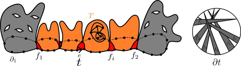
Refer to caption
Figure 14: On the left: a triangulation (t,e)(t,e) satisfying (𝒞L,p)(\mathcal{C}_{L,p}). The red triangles fif_{i} correspond to triangles discovered behind edges e′e^{\prime} lying on ∂1\partial_{1} such that (t,e′)(t,e^{\prime}) satisfies (ℋp​L)(\mathcal{H}_{pL}). Each of them is p​LpL-close to the triangle tt behind ene^{n}. The planar triangulation TT in orange between f1f_{1} and f2f_{2} is non-typical because the red triangles disconnect TT into a collection of planar triangulations arranged in a line. On the right: the boundary of a triangulation tt where the faces f1,⋯,f6f_{1},\cdots,f_{6} cross each other a lot.

Let us now formalize this intuition. Fix n,gn,g, 𝐩=(p1,…,pℓ)\mathbf{p}=(p_{1},\dots,p_{\ell}), and t∈𝒯𝐩​(n,g)t\in\mathcal{T}_{\mathbf{p}}(n,g). Let e1,e2e_{1},e_{2} be two edges on ∂t\partial t, and let f1,f2f_{1},f_{2} denote the triangles behind them. Denote by x1,x2x_{1},x_{2} the vertices of e1e_{1}, by x3x_{3} the third vertex of f1f_{1}, and symmetrically by y1,y2,y3y_{1},y_{2},y_{3} the vertices of f2f_{2}. Assume that both x3x_{3} and y3y_{3} lie on ∂t\partial t.

Definition 5.5.

For L>0L>0, we say that f1f_{1} and f2f_{2} (see Figure 15) are LL-close if:

  • •

    each vertex x1,x2,x3x_{1},x_{2},x_{3} is at distance at most LL from {y1,y2,y3}\{y_{1},y_{2},y_{3}\} along ∂t\partial t,

  • •

    each vertex y1,y2,y3y_{1},y_{2},y_{3} is at distance at most LL from {x1,x2,x3}\{x_{1},x_{2},x_{3}\} along ∂t\partial t.

Refer to caption
Figure 15: Example where the triangles f1f_{1} and f2f_{2} are LL-close. Note that it is possible that i=ji=j.

In particular, if f1f_{1} and f2f_{2} are LL-close for some L≥0L\geq 0, then there exist boundaries ∂i\partial_{i} and ∂j\partial_{j} such that all six vertices x1,x2,x3,y1,y2,y3x_{1},x_{2},x_{3},y_{1},y_{2},y_{3} belong to ∂i∪∂j\partial_{i}\cup\partial_{j}.

Definition 5.6.

Fix L,p≥0L,p\geq 0, a triangulation tt of the (p1,…,pℓ)(p_{1},\dots,p_{\ell})-gon, and an oriented edge ee that lies on ∂i\partial_{i} for 1≤i≤ℓ1\leq i\leq\ell. We denote by ff the triangle that lies behind ee. We say that (t,e)(t,e) satisfies (𝒞L,p)(\mathcal{C}_{L,p}) (see Figure 16) if (t,e)(t,e) satisfies (ℋ2​p​L)(\mathcal{H}_{2pL}) or (𝒪)(\mathcal{O}) and if there exist pp distinct edges e1,…,epe_{1},\dots,e_{p} (different from ee) on ∂T\partial T such that, for each 1≤i≤p1\leq i\leq p, writing fif_{i} for the triangle behind eie_{i}, we have that fif_{i} and ff are p​LpL-close.

Refer to caption
Figure 16: Examples of (t,e)(t,e) and (t,e′)(t,e^{\prime}) satisfying (𝒞L,p)(\mathcal{C}_{L,p}). On the left: an edge e∈∂ie\in\partial_{i} such that (t,e)(t,e) satisfies (ℋp)(\mathcal{H}_{p}) and (𝒞L,p)(\mathcal{C}_{L,p}). On the right: an edge e′∈∂ke^{\prime}\in\partial_{k} such that (t,e′)(t,e^{\prime}) satisfies (𝒪)(\mathcal{O}) and (𝒞L,q)(\mathcal{C}_{L,q}).

5.2.1 (Tn,gn,𝐩n,en)(T_{n,g_{n},\mathbf{p}^{n}},e^{n}) is unlikely to satisfy (𝒞L,p)(\mathcal{C}_{L,p})

We now show that (Tn,gn,𝐩n,en)(T_{n,g_{n},\mathbf{p}^{n}},e^{n}) is unlikely to satisfy (𝒞L,p)(\mathcal{C}_{L,p}) for any fixed LL when pp is large enough.

Proposition 5.7.

For any ε>0\varepsilon>0 and any L≥0L\geq 0, there exists p≥0p\geq 0 such that, for nn large enough

ℙ​((Tn,gn,𝐩n,en)​ satisfies ​(𝒞L,p))≤ε.\mathbb{P}\big((T_{n,g_{n},\mathbf{p}^{n}},e^{n})\text{ satisfies }(\mathcal{C}_{L,p})\big)\leq\varepsilon.

We first prove that the “linear pattern” illustrated in Figure 14 is unlikely to occur in a uniform planar triangulation. For any m,p≥0m,p\geq 0 and α>0\alpha>0, define

Nm,p,α:=#​{e∈∂Tm,0,p:(Tm,0,p,e)​ satisfies ​(ℋα​p)}.\displaystyle N_{m,p,\alpha}:=\#\big\{e\in\partial T_{m,0,p}:(T_{m,0,p},e)\text{ satisfies }(\mathcal{H}_{\alpha p})\big\}. (33)
Lemma 5.8.

Fix α1,α2>0\alpha_{1},\alpha_{2}>0. There exists a constant Cα1,α2>0C_{\alpha_{1},\alpha_{2}}>0 such that for any m,p≥0m,p\geq 0 we have

ℙ​(Nm,p,α1≥α2​p)≤Cα1,α2​p−65.\displaystyle\mathbb{P}(N_{m,p,\alpha_{1}}\geq\alpha_{2}p)\leq C_{\alpha_{1},\alpha_{2}}p^{-\frac{6}{5}}.
Proof.

Let (ei)1≤i≤5(e^{i})_{1\leq i\leq 5} be five distinct edges chosen uniformly at random on ∂Tm,0,p\partial T_{m,0,p}. We define c=min⁡(α2100,α1)c=\min(\frac{\alpha_{2}}{100},\alpha_{1}). Let AA be the event that the triangles (fi)1≤i≤5(f_{i})_{1\leq i\leq 5} incident to the edges (ei)1≤i≤5(e^{i})_{1\leq i\leq 5} have all their vertices on ∂Tm,0,p\partial T_{m,0,p}, and such that the six planar triangulations composing Tm,0,p\(f1∪⋯∪f5)T_{m,0,p}\backslash(f_{1}\cup\cdots\cup f_{5}) have perimeters at least c​pcp. The probability of this event satisfies

ℙ​(A)≤120​τp​(m,0)−1​∑m1+⋯+m6=m−5p1+⋯+p6=p+5p1,⋯,p6≥c​p∏i=16τpi​(mi,0),\displaystyle\mathbb{P}(A)\leq 120\tau_{p}(m,0)^{-1}\sum_{\begin{subarray}{c}m_{1}+\cdots+m_{6}=m-5\\ p_{1}+\cdots+p_{6}=p+5\\ p_{1},\cdots,p_{6}\geq cp\end{subarray}}\prod_{i=1}^{6}\tau_{p_{i}}(m_{i},0), (34)

where the factor 120=5!120=5! counts the order in which the edges e1​⋯,e5e^{1}\cdots,e^{5} appear on the boundary. Using Proposition 3.6 with α=c\alpha=c and ε>0\varepsilon>0 such that −54+5​ε≤−65-\frac{5}{4}+5\varepsilon\leq-\frac{6}{5}, it follows that for any m′≥1m^{\prime}\geq 1 and 1≤p′≤m′+21\leq p^{\prime}\leq m^{\prime}+2 we have

∑m1+m2=m′−1p1+p2=p′+1p1,p2≥c​p′τp1​(m1,0)​τp2​(m2,0)≤Cα1,α2​(p′)−14+ε​τp′​(m′,0).\displaystyle\sum_{\begin{subarray}{c}m_{1}+m_{2}=m^{\prime}-1\\ p_{1}+p_{2}=p^{\prime}+1\\ p_{1},p_{2}\geq cp^{\prime}\end{subarray}}\tau_{p_{1}}(m_{1},0)\tau_{p_{2}}(m_{2},0)\leq C_{\alpha_{1},\alpha_{2}}(p^{\prime})^{-\frac{1}{4}+\varepsilon}\tau_{p^{\prime}}(m^{\prime},0).

Fix m1,⋯,m4m_{1},\cdots,m_{4} and p1,⋯,p4p_{1},\cdots,p_{4} in (34) and let us write m′=m−m1−⋯−m4m^{\prime}=m-m_{1}-\cdots-m_{4} and p′=p+4−p1−⋯−p4p^{\prime}=p+4-p_{1}-\cdots-p_{4}. Note that we have p′≥c​pp^{\prime}\geq cp. Then, summing over m5m_{5} and p5p_{5} in (34) leads to the sum

∑m5+m6=m′p5+p6=p′+1p5,p6≥c​pτp5​(m5,0)​τp6​(m6,0)\displaystyle\sum_{\begin{subarray}{c}m_{5}+m_{6}=m^{\prime}\\ p_{5}+p_{6}=p^{\prime}+1\\ p_{5},p_{6}\geq cp\end{subarray}}\tau_{p_{5}}(m_{5},0)\tau_{p_{6}}(m_{6},0) ≤Cα1,α2​c−14+ε​p−14+ε​τp′​(m′,0).\displaystyle\leq C_{\alpha_{1},\alpha_{2}}c^{-\frac{1}{4}+\varepsilon}p^{-\frac{1}{4}+\varepsilon}\tau_{p^{\prime}}(m^{\prime},0).

We deduce

∑m1+⋯+m6=m−5p1+⋯+p6=p+5p1,⋯,p6≥c​p∏i=16τpi​(mi,0)≤Cα1,α2​c−14+ε​p−14+ε​∑m1+⋯+m5=m−4p1+⋯+p5=p+4p1,⋯,p5≥c​p∏i=15τpi​(mi,0).\displaystyle\sum_{\begin{subarray}{c}m_{1}+\cdots+m_{6}=m-5\\ p_{1}+\cdots+p_{6}=p+5\\ p_{1},\cdots,p_{6}\geq cp\end{subarray}}\prod_{i=1}^{6}\tau_{p_{i}}(m_{i},0)\leq C_{\alpha_{1},\alpha_{2}}c^{-\frac{1}{4}+\varepsilon}p^{-\frac{1}{4}+\varepsilon}\sum_{\begin{subarray}{c}m_{1}+\cdots+m_{5}=m-4\\ p_{1}+\cdots+p_{5}=p+4\\ p_{1},\cdots,p_{5}\geq cp\end{subarray}}\prod_{i=1}^{5}\tau_{p_{i}}(m_{i},0).

Iterating this argument leads to the bound

ℙ​(A)\displaystyle\mathbb{P}(A) ≤Cα1,α2′​p−54+5​ε≤Cα1,α2′​p−65,\displaystyle\leq C_{\alpha_{1},\alpha_{2}}^{\prime}p^{-\frac{5}{4}+5\varepsilon}\leq C_{\alpha_{1},\alpha_{2}}^{\prime}p^{-\frac{6}{5}}, (35)

for some Cα1,α2′>0C_{\alpha_{1},\alpha_{2}}^{\prime}>0. Let II denote the set of edges ee on the boundary ∂Tm,0,p\partial T_{m,0,p} such that (Tm,0,p,e)(T_{m,0,p},e) satisfies (ℋα1​p)(\mathcal{H}_{\alpha_{1}p}). Let v1,⋯,v5v^{1},\cdots,v^{5} denote the third vertices of the faces f1,⋯,f5f_{1},\cdots,f_{5}. Let CC denote the event that for each i∈{1,⋯,5}i\in\{1,\cdots,5\} the edge eie^{i} lies in II and is at distance at least α2100​p\frac{\alpha_{2}}{100}p from {ej,vj}j≠i−1\{e^{j},v^{j}\}_{j\neq i-1} along ∂Tm,0,p\partial T_{m,0,p}. We claim that

ℙ​(C∣Nm,p,α1≥α2​p)≥(α2)525.\displaystyle\mathbb{P}(C\mid N_{m,p,\alpha_{1}}\geq\alpha_{2}p)\geq\frac{(\alpha_{2})^{5}}{2^{5}}. (36)

Indeed, this follows from the fact that {Nm,p,α1≥α2​p}={#​I≥α2​p}\{N_{m,p,\alpha_{1}}\geq\alpha_{2}p\}=\{\#I\geq\alpha_{2}p\} and that e1,⋯,e5e^{1},\cdots,e^{5} are chosen uniformly at random on ∂Tm,0,p\partial T_{m,0,p}. Thus, for each 1≤i≤51\leq i\leq 5, conditionally on e1,…,ei−1e^{1},\dots,e^{i-1}, the probability that eie^{i} lies in II and is at distance at least α2100​p\frac{\alpha_{2}}{100}p from {ej,vj}j≤i\{e^{j},v^{j}\}_{j\leq i} is at least α2−4​i100​α2≥α22\alpha_{2}-\frac{4i}{100}\alpha_{2}\geq\frac{\alpha_{2}}{2}.

Finally, under the event {Nm,p,α1≥α2​p}∩C\{N_{m,p,\alpha_{1}}\geq\alpha_{2}p\}\cap C, the event AA occurs. Combining (35) and (36), we deduce the result:

ℙ​(Nm,p,α1≥α2​p)≤((α2)525)−1​Cα1,α2′​p−65.\displaystyle\mathbb{P}(N_{m,p,\alpha_{1}}\geq\alpha_{2}p)\leq\left(\frac{(\alpha_{2})^{5}}{2^{5}}\right)^{-1}C_{\alpha_{1},\alpha_{2}}^{\prime}p^{-\frac{6}{5}}.

∎

We now prove Proposition 5.7.

Proof.

Fix ε,L>0\varepsilon,L>0. As in the proof of Proposition 5.2, using Proposition 5.1, it suffices to assume that p1n→+∞p^{n}_{1}\to+\infty and to prove that there exists p≥0p\geq 0 such that, for nn large enough

ℙ​((Tn,gn,𝐩n,e1n)​ satisfies ​(𝒞L,p))≤ε.\displaystyle\mathbb{P}\big((T_{n,g_{n},\mathbf{p}^{n}},e^{n}_{1})\text{ satisfies }(\mathcal{C}_{L,p})\big)\leq\varepsilon. (37)

If (Tn,gn,𝐩n,e1n)(T_{n,g_{n},\mathbf{p}^{n}},e^{n}_{1}) satisfies (𝒞L,p)(\mathcal{C}_{L,p}), then it satisfies either (ℋ2​p​L)(\mathcal{H}_{2pL}) or (𝒪)(\mathcal{O}). We first handle the case of (ℋ2​p​L)(\mathcal{H}_{2pL}) and prove that there exists p≥0p\geq 0 such that, for nn large enough,

ℙ​((Tn,gn,𝐩n,e1n)​ satisfies ​(𝒞L,p)​ and ​(ℋ2​p​L))≤ε.\displaystyle\mathbb{P}\big((T_{n,g_{n},\mathbf{p}^{n}},e^{n}_{1})\text{ satisfies }(\mathcal{C}_{L,p})\text{ and }(\mathcal{H}_{2pL})\big)\leq\varepsilon. (38)

Assume that (Tn,gn,𝐩n,e1n)(T_{n,g_{n},\mathbf{p}^{n}},e^{n}_{1}) satisfies both (𝒞L,p)(\mathcal{C}_{L,p}) and (ℋ2​p​L)(\mathcal{H}_{2pL}). Let ff be the triangle behind e1ne^{n}_{1} and let zz be its third vertex. Let I1I_{1} (resp. I2I_{2}) be the segment of p​LpL edges immediately to the left (resp. right) of e1ne^{n}_{1} on ∂1\partial_{1}, and let I3I_{3} (resp. I4I_{4}) be the segment of p​LpL edges to the left (resp. right) of zz on ∂1\partial_{1}. We have p1n≥4​p​Lp^{n}_{1}\geq 4pL, so the segments I1,I2,I3,I4I_{1},I_{2},I_{3},I_{4} are pairwise disjoint (see Figure 17).

For 1≤j≤41\leq j\leq 4, let AjA_{j} be the event that there exist at least p4\frac{p}{4} edges e′e^{\prime} in IjI_{j} such that the corresponding triangles f′f^{\prime} behind e′e^{\prime} are p​LpL-close to tt. Since (Tn,gn,𝐩n,e)(T_{n,g_{n},\mathbf{p}^{n}},e) satisfies (𝒞L,p)(\mathcal{C}_{L,p}), at least one of the events AjA_{j} must occur.

Refer to caption
Figure 17: Left: the triangle ff and the four disjoint segments I1,I2,I3,I4I_{1},I_{2},I_{3},I_{4} on ∂1\partial_{1}. Right: illustration of the case where A1A_{1} and B1,kB_{1,k} occur.

Thus,

ℙ​((Tn,gn,𝐩n,e1n)​ satisfies ​(𝒞L,p)​ and ​(ℋp))≤ℙ​(⋃i=14Ai)≤∑i=14ℙ​(Ai).\displaystyle\mathbb{P}\big((T_{n,g_{n},\mathbf{p}^{n}},e^{n}_{1})\text{ satisfies }(\mathcal{C}_{L,p})\text{ and }(\mathcal{H}_{p})\big)\leq\mathbb{P}\Big(\bigcup_{i=1}^{4}A_{i}\Big)\leq\sum_{i=1}^{4}\mathbb{P}(A_{i}). (39)

By symmetry, it suffices to bound ℙ​(A1)\mathbb{P}(A_{1}). The same argument applies to the other AiA_{i}.

Under A1A_{1}, let e′e^{\prime} be the leftmost edge in I1I_{1} such that f′f^{\prime} (the triangle behind e′e^{\prime}) is p​LpL-close to ff, and let z′z^{\prime} be the third vertex of f′f^{\prime} (see Figure 17). Then z′z^{\prime} must lie in I3∪I4I_{3}\cup I_{4}: otherwise, the vertex zz would be at distance at least p​L+1pL+1 from any vertex of f′f^{\prime} on ∂Tn,gn,𝐩n\partial T_{n,g_{n},\mathbf{p}^{n}}.

Let B1B_{1} (resp. C1C_{1}) denote the event that A1A_{1} occurs and that z′z^{\prime} is (resp. is not) incident to an edge in I3I_{3}. Thus,

A1=B1⊔C1.A_{1}=B_{1}\sqcup C_{1}.

We first check that the event C1C_{1} is very unlikely. Under C1C_{1}, the vertex z′z^{\prime} is incident to an edge in I4I_{4}, so the triangles ff and f′f^{\prime} cross each other, implying

Tn,gn∖{f∪f′}∈𝒯(p1+2,…,pℓn)​(n,gn−1).T_{n,g_{n}}\setminus\{f\cup f^{\prime}\}\in\mathcal{T}_{(p_{1}+2,\dots,p_{\ell_{n}})}(n,g_{n}-1).

Since there are at most p​LpL choices for e′e^{\prime} and at most p​L+1pL+1 choices for zz (since I4I_{4} contains p​LpL edges, i.e. p​L+1pL+1 vertices), we get

ℙ​(C1)≤(p​L+1)​p​L​τ(p1n+2,…,pℓnn)​(n,gn−1)τ𝐩n​(n,gn)→n→∞0,\displaystyle\mathbb{P}(C_{1})\leq(pL+1)pL\,\frac{\tau_{(p^{n}_{1}+2,\dots,p^{n}_{\ell_{n}})}(n,g_{n}-1)}{\tau_{\mathbf{p}^{n}}(n,g_{n})}\xrightarrow[n\to\infty]{}0, (40)

where the limit follows from Lemma 3.3 and Proposition 4.8, since p,Lp,L are fixed.

Now, for p4−1≤k≤p​L\frac{p}{4}-1\leq k\leq pL, let us denote by B1,kB_{1,k} the event that B1B_{1} occurs and that the segment between e1ne^{n}_{1} and e′e^{\prime} contains exactly kk edges. Then B1=⨆k=p4−1p​LB1,kB_{1}=\bigsqcup_{k=\frac{p}{4}-1}^{pL}B_{1,k}. Fix such a k∈{p4−1,…,p​L}k\in\{\frac{p}{4}-1,\dots,pL\}. Let us show that

ℙ​(B1,k)≤CL​p−65.\displaystyle\mathbb{P}(B_{1,k})\leq C_{L}\,p^{-\frac{6}{5}}. (41)

Under B1,kB_{1,k}, the vertex z′z^{\prime} lies on I3I_{3}, so the union f∪f′f\cup f^{\prime} splits ∂1t\partial_{1}t into three holes, denoted by h1,h2,h3h_{1},h_{2},h_{3} from left to right, with random perimeters r1,r2,r3r_{1},r_{2},r_{3}. Let TT be the component of Tn,gn,𝐩n∖{f∪f′}T_{n,g_{n},\mathbf{p}^{n}}\setminus\{f\cup f^{\prime}\} that contains h2h_{2}. Note that TT might also contain h1h_{1} or h3h_{3}. We decompose

ℙ​(B1,k)\displaystyle\mathbb{P}(B_{1,k}) =ℙ​(B1,k​ and ​T∉⋃m≥0𝒯r2​(m,0))+ℙ​(B1,k​ and ​T∈⋃m≥0𝒯r2​(m,0)).\displaystyle=\mathbb{P}\big(B_{1,k}\text{ and }T\notin\bigcup_{m\geq 0}\mathcal{T}_{r_{2}}(m,0)\big)+\mathbb{P}\big(B_{1,k}\text{ and }T\in\bigcup_{m\geq 0}\mathcal{T}_{r_{2}}(m,0)\big). (42)

We first show that

ℙ​(B1,k​ and ​T∉⋃m≥0𝒯r2​(m,0))→n→∞0.\displaystyle\mathbb{P}\big(B_{1,k}\text{ and }T\notin\bigcup_{m\geq 0}\mathcal{T}_{r_{2}}(m,0)\big)\xrightarrow[n\to\infty]{}0. (43)

Let us recall the notations ℒn,k​(e)\mathcal{L}_{n,k}(e) and ℛn,k​(e)\mathcal{R}_{n,k}(e) defined in the introduction of Section 5. Let uiu_{i} (resp. viv_{i}) be the ithi^{\mathrm{th}} edge to the left (resp. right) of e1ne^{n}_{1} on ∂1\partial_{1}. Under B1,kB_{1,k}, the events ℒn,r1−1​(uk+1)\mathcal{L}_{n,r_{1}-1}(u_{k+1}) and ℛn,r3−1​(e1n)\mathcal{R}_{n,r_{3}-1}(e^{n}_{1}) occur (see Figure 18). Hence,

ℙ​(B1,k,T∉⋃m≥0𝒯r2​(m,0))≤∑r1,r2,r3ℙ​(ℒn,r1−1​(uk+1),ℛn,r3−1​(e1n),T∉⋃m≥0𝒯r2​(m,0)).\displaystyle\mathbb{P}\big(B_{1,k},T\notin\bigcup_{m\geq 0}\mathcal{T}_{r_{2}}(m,0)\big)\leq\sum_{r_{1},r_{2},r_{3}}\mathbb{P}\big(\mathcal{L}_{n,r_{1}-1}(u_{k+1}),\mathcal{R}_{n,r_{3}-1}(e^{n}_{1}),T\notin\bigcup_{m\geq 0}\mathcal{T}_{r_{2}}(m,0)\big). (44)

For fixed r1,r2,r3r_{1},r_{2},r_{3}, we claim that:

  • •

    ℙ​(ℒn,r1−1​(uk+1)∩ℛn,r3−1​(e1n))=ℙ​(ℒn,r2−1​(e1n)∩ℛn,r3−1​(v1))\mathbb{P}(\mathcal{L}_{n,r_{1}-1}(u_{k+1})\cap\mathcal{R}_{n,r_{3}-1}(e^{n}_{1}))=\mathbb{P}(\mathcal{L}_{n,r_{2}-1}(e^{n}_{1})\cap\mathcal{R}_{n,r_{3}-1}(v_{1})).

  • •

    the law of Tn,gn,𝐩n∖{f∪f′}T_{n,g_{n},\mathbf{p}^{n}}\setminus\{f\cup f^{\prime}\} under ℒn,r1−1​(uk+1)\mathcal{L}_{n,r_{1}-1}(u_{k+1}) and ℛn,r3−1​(e1n)\mathcal{R}_{n,r_{3}-1}(e^{n}_{1}) is identical to that of Tn,gn,𝐩n∖{f∪f∗}T_{n,g_{n},\mathbf{p}^{n}}\setminus\{f\cup f^{*}\} under ℒn,r2−1​(e1n)\mathcal{L}_{n,r_{2}-1}(e^{n}_{1}) and ℛn,r3−1​(v1)\mathcal{R}_{n,r_{3}-1}(v_{1}), where f∗f^{*} is the triangle behind v1v_{1}.

Indeed, in both configurations, the two triangles do not cross each other and create holes of perimeters (r1,r2,r3)(r_{1},r_{2},r_{3}) or (r2,r1,r3)(r_{2},r_{1},r_{3}) respectively (see Figure 18). Thus, the two items above hold since for each identities considered, both sides of the equation writes as the same ratio of combinatorial quantities.

Under ℒn,r2−1​(e1n)\mathcal{L}_{n,r_{2}-1}(e^{n}_{1}) and ℛn,r3−1​(v1)\mathcal{R}_{n,r_{3}-1}(v_{1}), let T′T^{\prime} be the component of Tn,gn,𝐩n∖{f,f∗}T_{n,g_{n},\mathbf{p}^{n}}\setminus\{f,f^{*}\} filling the hole of perimeter r2r_{2}. Then, the right-hand side of (44) can be rewritten

∑r1,r2,r3ℙ​(ℒn,r2−1​(e1n),ℛn,r3−1​(v1),T′∉⋃m≥0𝒯r2​(m,0))\displaystyle\sum_{r_{1},r_{2},r_{3}}\mathbb{P}(\mathcal{L}_{n,r_{2}-1}(e^{n}_{1}),\mathcal{R}_{n,r_{3}-1}(v_{1}),T^{\prime}\notin\bigcup_{m\geq 0}\mathcal{T}_{r_{2}}(m,0)) (45)
≤∑r2ℙ​(ℒn,r2−1​(e1n),T′∉⋃m≥0𝒯r2​(m,0))→n→∞0,\displaystyle\leq\sum_{r_{2}}\mathbb{P}(\mathcal{L}_{n,r_{2}-1}(e^{n}_{1}),T^{\prime}\notin\bigcup_{m\geq 0}\mathcal{T}_{r_{2}}(m,0))\xrightarrow[n\to\infty]{}0, (46)

by Proposition 5.3, since r2∈{p4,…,2​p​L+2}r_{2}\in\{\frac{p}{4},\dots,2pL+2\}. This proves (43).

Refer to caption
Figure 18: Left: the events ℒn,r1−1​(uk+1)\mathcal{L}_{n,r_{1}-1}(u_{k+1}) and ℛn,r3−1​(e1n)\mathcal{R}_{n,r_{3}-1}(e^{n}_{1}) occur. Right: the events ℒn,r2−1​(e1n)\mathcal{L}_{n,r_{2}-1}(e^{n}_{1}) and ℛn,r3−1​(v1)\mathcal{R}_{n,r_{3}-1}(v_{1}) occur.

Next, we bound the second term in (42). Under B1,kB_{1,k}, there exist at least p30\frac{p}{30} edges ee on ∂T\partial T such that (T,e)(T,e) satisfies (ℋp/10)(\mathcal{H}_{p/10}). Indeed, from the definition of A1A_{1}, there are at least p4−1\frac{p}{4}-1 edges ee on I1I_{1} such that tt and t​(e)t(e) (the triangle behind ee) are p​LpL-close. Discarding the p10\frac{p}{10} leftmost and rightmost such edges leaves at least p30\frac{p}{30} edges. For each ee, by planarity of TT, the third vertex of the triangle t​(e)t(e) lies on I3I_{3}. Hence (T,e)(T,e) satisfies (ℋp/10)(\mathcal{H}_{p/10}).

Since TT has perimeter r2r_{2} with p8≤r2≤4​p​L\frac{p}{8}\leq r_{2}\leq 4pL and the fact that TT is uniform conditionally on its perimeter m2m_{2} and its volume mm, we can apply Lemma 5.8 with α1=1/40​L,α2=1/120​L\alpha_{1}=1/40L,\alpha_{2}=1/120L and we obtain the bound

ℙ​(B1,k​ and ​T∈⋃m≥0𝒯r2​(m,0))≤CL​p−65.\mathbb{P}\big(B_{1,k}\text{ and }T\in\bigcup_{m\geq 0}\mathcal{T}_{r_{2}}(m,0)\big)\leq C_{L}\,p^{-\frac{6}{5}}.

Combining this with (43) we find that for nn large enough we have

ℙ​(B1,k)≤CL​p−65.\displaystyle\mathbb{P}\big(B_{1,k})\leq C_{L}p^{-\frac{6}{5}}.

Summing over kk and taking pp large enough such that CL​L​p−16≤ε/2C_{L}Lp^{-\frac{1}{6}}\leq\varepsilon/2, we get for nn large enough,

ℙ​(B1)≤∑k=p4p​Lℙ​(B1,k)≤ε,ℙ​(A1)≤ℙ​(B1)+ℙ​(C1)≤2​ε.\mathbb{P}(B_{1})\leq\sum_{k=\frac{p}{4}}^{pL}\mathbb{P}(B_{1,k})\leq\varepsilon,\qquad\mathbb{P}(A_{1})\leq\mathbb{P}(B_{1})+\mathbb{P}(C_{1})\leq 2\varepsilon.

The same bound holds for each ℙ​(Ai)\mathbb{P}(A_{i}), completing the proof of (39).

Finally, to bound

ℙ​((Tn,gn,𝐩n,e1n)​ satisfies ​(𝒞L,p)​ and ​(𝒪)),\displaystyle\mathbb{P}\big((T_{n,g_{n},\mathbf{p}^{n}},e^{n}_{1})\text{ satisfies }(\mathcal{C}_{L,p})\text{ and }(\mathcal{O})\big), (47)

we reduce to the case already handled. If (Tn,gn,𝐩n,e1n)(T_{n,g_{n},\mathbf{p}^{n}},e^{n}_{1}) satisfies (𝒞L,p)(\mathcal{C}_{L,p}) and (𝒪)(\mathcal{O}), let z∈∂jz\in\partial_{j} with 2≤j≤ℓn2\leq j\leq\ell_{n} be the third vertex of the triangle behind e1ne^{n}_{1}. Then

Tn,gn,𝐩n∖f∈𝒯(p1n+pjn+1,p2n,…,pj−1n,pj+1n,…,pℓnn)​(n+1,gn).T_{n,g_{n},\mathbf{p}^{n}}\setminus f\in\mathcal{T}_{(p^{n}_{1}+p^{n}_{j}+1,p^{n}_{2},\dots,p^{n}_{j-1},p^{n}_{j+1},\dots,p^{n}_{\ell_{n}})}(n+1,g_{n}).

Moreover, conditionally on z∈∂jz\in\partial_{j}, the triangulation Tn,gn,𝐩n∖fT_{n,g_{n},\mathbf{p}^{n}}\setminus f is uniformly distributed in 𝒯(p1n+pjn+1,p2n,…,pj−1n,pj+1n,…,pℓnn)​(n+1,gn)\mathcal{T}_{(p^{n}_{1}+p^{n}_{j}+1,p^{n}_{2},\dots,p^{n}_{j-1},p^{n}_{j+1},\dots,p^{n}_{\ell_{n}})}(n+1,g_{n}). Thus it suffices to bound

ℙ​((Tn,gn,𝐩n,e1n)​ satisfies ​(𝒞L,p)​ and ​(𝒪)|z∈∂j),\mathbb{P}\big((T_{n,g_{n},\mathbf{p}^{n}},e^{n}_{1})\text{ satisfies }(\mathcal{C}_{L,p})\text{ and }(\mathcal{O})|z\in\partial_{j}\big),

uniformly on j∈{2,⋯,ℓn}j\in\{2,\cdots,\ell_{n}\} for nn large enough. For j∈{2,⋯,ℓn}j\in\{2,\cdots,\ell_{n}\}, let XjX_{j} be the set of edges in ∂1∪∂j\partial_{1}\cup\partial_{j} whose incident vertices are within distance p​LpL from either e1ne^{n}_{1} or zz along ∂1∪∂j\partial_{1}\cup\partial_{j}. Then #​Xj≤4​p​L\#X_{j}\leq 4pL. Moreover, discarding the edges having an incident vertex at distance at most p/8p/8 from ee or e1ne^{n}_{1} in ∂1∪∂j\partial_{1}\cup\partial_{j} (see the right part of Figure 16), we find

#​{e∈Xj:(Tn,gn,𝐩n∖f,e)​ satisfies ​(𝒞L,p/16​L)​ and ​(ℋp/8)}≥p/32.\#\{e\in X_{j}:(T_{n,g_{n},\mathbf{p}^{n}}\setminus f,e)\text{ satisfies }(\mathcal{C}_{L,p/16L})\text{ and }(\mathcal{H}_{p/8})\}\geq p/32.

By (38), if pp is chosen large enough, for nn large enough, for all jj we have

ℙ​((Tn,gn,(p1n+pjn+1,p2n,…,pℓnn),e1n)​ satisfies ​(𝒞L,p/16​L)​ and ​(ℋp/8​L))≤ε128​L.\mathbb{P}\big((T_{n,g_{n},(p^{n}_{1}+p^{n}_{j}+1,p^{n}_{2},\dots,p^{n}_{\ell_{n}})},e^{n}_{1})\text{ satisfies }(\mathcal{C}_{L,p/16L})\text{ and }(\mathcal{H}_{p/8L})\big)\leq\frac{\varepsilon}{128L}.

Then using the translation invariance of (Tn,gn,(p1n+pjn+1,p2n,…,pℓnn),e1n)(T_{n,g_{n},(p^{n}_{1}+p^{n}_{j}+1,p^{n}_{2},\dots,p^{n}_{\ell_{n}})},e^{n}_{1}) along ∂1\partial_{1}, the Markov inequality yields

ℙ​(#​{e∈Xj:(Tn,gn,𝐩n∖f,e)​ satisfies ​(𝒞L,p/16​L)​ and ​(ℋp/8)}≥p/32)≤(4​p​L)​32p​ε128​L≤ε.\mathbb{P}\bigg(\#\{e\in X_{j}:(T_{n,g_{n},\mathbf{p}^{n}}\setminus f,e)\text{ satisfies }(\mathcal{C}_{L,p/16L})\text{ and }(\mathcal{H}_{p/8})\}\geq p/32\bigg)\leq(4pL)\frac{32}{p}\frac{\varepsilon}{128L}\leq\varepsilon.

Thus, for nn large enough, we have

∀j∈{2,⋯,ℓn}, ​ℙ​((Tn,gn,𝐩n,e1n)​ satisfies ​(𝒞L,p)​ and ​(𝒪)|z∈∂j).\forall j\in\{2,\cdots,\ell_{n}\},\text{ }\mathbb{P}\big((T_{n,g_{n},\mathbf{p}^{n}},e^{n}_{1})\text{ satisfies }(\mathcal{C}_{L,p})\text{ and }(\mathcal{O})|z\in\partial_{j}\big).

This concludes the proof. ∎

5.2.2 Deterministic discovery of triangles

We start by mentioning that this section is entirely deterministic. It is dedicated to showing that if (Tn,gn,𝐩n,e)(T_{n,g_{n},\mathbf{p}^{n}},e) satisfies (ℋk)(\mathcal{H}_{k}) or (𝒪)(\mathcal{O}) for many choices of e∈∂Tn,gn,𝐩ne\in\partial T_{n,g_{n},\mathbf{p}^{n}}, we fall into one of the two cases below:

  • ∙\bullet

    There is a positive proportion of edges e∈∂Tn,gn,𝐩ne\in\partial T_{n,g_{n},\mathbf{p}^{n}} such that the triangles lying behind these edges cross each other significantly.

  • ∙\bullet

    There is a positive proportion of edges e∈∂Tn,gn,𝐩ne\in\partial T_{n,g_{n},\mathbf{p}^{n}} such that (Tn,gn,𝐩n,e)(T_{n,g_{n},\mathbf{p}^{n}},e) satisfies (𝒞L,p)(\mathcal{C}_{L,p}) for an appropriate choice of LL and pp.

See the proposition below.

Proposition 5.9.

Fix n,g,ℓ≥0n,g,\ell\geq 0 and (p1,⋯,pℓ)∈(ℕ∗)ℓ(p_{1},\cdots,p_{\ell})\in(\mathbb{N}^{*})^{\ell}. We also fix t∈𝒯𝐩​(n,g)t\in\mathcal{T}_{\mathbf{p}}(n,g) and ε>0,p≥4\varepsilon>0,p\geq 4. Suppose that there exist distinct edges e1,⋯,e1000​ε​|𝐩|e_{1},\cdots,e_{1000\varepsilon|\mathbf{p}|} on ∂1∪⋯∪∂ℓ\partial_{1}\cup\cdots\cup\partial_{\ell} such that for all 1≤j≤1000​ε​|𝐩|1\leq j\leq 1000\varepsilon|\mathbf{p}|:

(t,ej)(t,e_{j}) satisfies (𝒪)(\mathcal{O}) or (ℋ2​ε−1​p)(\mathcal{H}_{2\varepsilon^{-1}p}).

Then one of the following two statements holds:

  1. 1.

    There exists I⊂{1,⋯,1000​ε​|𝐩|}I\subset\{1,\cdots,1000\varepsilon|\mathbf{p}|\} such that r:=|I|≥ε​p−1​|𝐩|r:=|I|\geq\varepsilon p^{-1}|\mathbf{p}| and denoting by fif_{i} for the triangle that lies behind the edge eie_{i}, we have t\(⨆i∈Ifi)∈𝒯𝐪​(n′,g′)t\backslash\bigg(\bigsqcup_{i\in I}f_{i}\bigg)\in\mathcal{T}_{\mathbf{q}}(n^{\prime},g^{\prime}) for some 𝐪=(q1,⋯,qℓ′)\mathbf{q}=(q_{1},\cdots,q_{\ell^{\prime}}), where (ℓ−ℓ′)+2​(g−g′)=r(\ell-\ell^{\prime})+2(g-g^{\prime})=r and n′≤n+|𝐩|n^{\prime}\leq n+|\mathbf{p}|.

  2. 2.

    There are more than ε​|𝐩|\varepsilon|\mathbf{p}| edges e∈∂te\in\partial t such that (t,e)(t,e) satisfies (𝒞ε−1,p)(\mathcal{C}_{\varepsilon^{-1},p}).

Refer to caption
Figure 19: We represent here the boundaries of a triangulation tt with 77 boundaries and the triangles behind the edges ee on the boundaries such that (t,e)(t,e) satisfies (𝒪)(\mathcal{O}) or (ℋε−1​p)(\mathcal{H}_{\varepsilon^{-1}p}).

We fix n,g,ℓ>0n,g,\ell>0, 𝐩∈(ℕ∗)ℓ\mathbf{p}\in(\mathbb{N}^{*})^{\ell}, t∈𝒯𝐩​(n,g)t\in\mathcal{T}_{\mathbf{p}}(n,g), 0<ε<110000<\varepsilon<\frac{1}{1000}, p≥4p\geq 4 and (e1,⋯,e1000​ε​|𝐩|)(e_{1},\cdots,e_{1000\varepsilon|\mathbf{p}|}) as in the statement of the proposition. For 1≤i≤1000​ε​|𝐩|1\leq i\leq 1000\varepsilon|\mathbf{p}|, we denote by fif_{i} the triangle that lies behind eie_{i} in tt. We assume throughout the whole section that Case 11 of Proposition 5.9 does not hold. Thus, we aim to prove that Case 2 occurs. Let us explain intuitively why this proposition is true and why it is not obvious. In words, the fact that (1) does not hold means that the triangles f1,⋯,f1000​ε​|𝐩|f_{1},\cdots,f_{1000\varepsilon|\mathbf{p}|} do not “cross each other” much. Thus, the triangles fjf_{j} must be “aligned” (see Figure 14). In other words, there exists a positive proportion of edges e∈∂te\in\partial t such that (t,e)(t,e) satisfies (𝒞ε−1,p)(\mathcal{C}_{\varepsilon^{-1},p}). However, making this idea precise is not straightforward. In particular, we must be careful when discussing triangles that “cross each other”. Although this notion might seem intuitive (see Figure 19), it is quite technical to make it rigorous. Indeed, we might have four triangles f1,f2,f3,f4f_{1},f_{2},f_{3},f_{4} such that f1,f2f_{1},f_{2} cross each other and so do f3,f4f_{3},f_{4}. However, f3f_{3} and f4f_{4} may no longer cross each other in t\(f1∪f2)t\backslash(f_{1}\cup f_{2}) (see Figure 20). To deal with this, we will discover the triangles in a well-chosen order (see Proposition 5.13).

Refer to caption
Figure 20: On the left, we represent the boundary ∂1\partial_{1} of a triangulation tt and four triangles f1,f2,f3,f4f_{1},f_{2},f_{3},f_{4} such that f1,f3f_{1},f_{3} cross each other, and so do f2,f4f_{2},f_{4}. The red path is the hole of ∂t∪f1∪f3\partial t\cup f_{1}\cup f_{3}. On the right, we represent t\(f1∪f3)t\backslash(f_{1}\cup f_{3}). The triangles f2,f4f_{2},f_{4} no longer cross each other in t\(f1∪f3)t\backslash(f_{1}\cup f_{3}). More precisely, in both orders (1,3,2,4)(1,3,2,4) and (2,4,1,3)(2,4,1,3), step 11 is SEP and step 22 is NSEP. However, for the order (1,3,2,4)(1,3,2,4), both steps 33 and 44 are SEP.

To prove this result, we discover the triangles f1,⋯,f1000​ε​|𝐩|f_{1},\cdots,f_{1000\varepsilon|\mathbf{p}|} one by one according to a well-chosen order.

Definition 5.10.

An order is a bijection from {1,⋯,1000​ε​|𝐩|}\{1,\cdots,1000\varepsilon|\mathbf{p}|\} to itself. We write i1,⋯,i1000​ε​|𝐩|i_{1},\cdots,i_{1000\varepsilon|\mathbf{p}|} for an order. A partial order is an injection from {1,⋯,m}\{1,\cdots,m\} to {1,⋯,1000​ε​|𝐩|}\{1,\cdots,1000\varepsilon|\mathbf{p}|\} with m≤1000​ε​|𝐩|m\leq 1000\varepsilon|\mathbf{p}|. We write i1,⋯,imi_{1},\cdots,i_{m} for a partial order.

For any 1≤j≤1000​ε​|𝐩|1\leq j\leq 1000\varepsilon|\mathbf{p}|, we denote by ℬj={α1j,⋯,αℓjj}\mathcal{B}_{j}=\{\alpha^{j}_{1},\cdots,\alpha^{j}_{\ell_{j}}\} the set of boundaries of t\(fi1∪⋯∪fij)t\backslash(f_{i_{1}}\cup\cdots\cup f_{i_{j}}). The elements of ℬj\mathcal{B}_{j} are vertex-injective cycles that are vertex-disjoint from each other. The edges of the boundaries αij\alpha^{j}_{i} consist of edges of the initial boundaries of tt, plus potential edges coming from the already discovered triangles fi1,⋯,fijf_{i_{1}},\cdots,f_{i_{j}}. We refer to the discovery of the triangle fijf_{i_{j}} as step jj. After discovering fi1,⋯,fijf_{i_{1}},\cdots,f_{i_{j}}, we say that we are at time jj. The step jj is completely determined by the edge eije_{i_{j}}, which lies on one of the boundaries {α1j,⋯,αℓjj}\{\alpha^{j}_{1},\cdots,\alpha^{j}_{\ell_{j}}\}, and by the vertex vijv_{i_{j}}, which lies on one of these boundaries and corresponds to the third vertex of the triangle fijf_{i_{j}}.

Definition 5.11.

For any order (ij)(i_{j}) and any 1≤j≤1000​ε​|𝐩|1\leq j\leq 1000\varepsilon|\mathbf{p}|, step jj is said to be SEP if eij∈αsje_{i_{j}}\in\alpha^{j}_{s} and vij∈αsjv_{i_{j}}\in\alpha^{j}_{s} for some s∈{1,⋯,ℓj}s\in\{1,\cdots,\ell_{j}\}. Otherwise, it is said to be NSEP. Thus, a SEP step splits the boundary αsj\alpha_{s}^{j} containing eije_{i_{j}} into two boundaries. The NSEP occurs when fijf_{i_{j}} connects two distinct boundaries.

Remark 5.12.

Note that the type of a step jj depends on i1,⋯,ij−1i_{1},\cdots,i_{j-1}. Therefore, the type of step jj is not determined by iji_{j} alone. See Figure 20.

Let us explain, in words, the order in which we will discover the triangles. We start by choosing NSEP steps as long as possible. When this is no longer possible, we consider pairs of consecutive steps such that the first is SEP and the second NSEP. The pairs (SEP,NSEP) have the effect of reducing the genus of t\(fi1∪⋯∪fij)t\backslash(f_{i_{1}}\cup\cdots\cup f_{i_{j}}). When this is no longer possible either, we will show that regardless of the order in which we discover the remaining triangles, all subsequent steps will be SEP.

Refer to caption
Figure 21: Starting from the example in Figure 19, we first discover i1,i2,i3,i4,i5i_{1},i_{2},i_{3},i_{4},i_{5} since each of these steps is NSEP. Then we discover i6,i7,i8,i9,i10,i11i_{6},i_{7},i_{8},i_{9},i_{10},i_{11} as these alternate between SEP and NSEP steps. By Proposition 5.13, for any ordering of the grey triangles, all remaining steps after step 1111 are SEP.
Proposition 5.13.

There exist m1,m2≥0m_{1},m_{2}\geq 0 and a partial order i1,⋯,im1+2​m2i_{1},\cdots,i_{m_{1}+2m_{2}} with m:=m1+2​m2≤ε​p−1​|𝐩|m:=m_{1}+2m_{2}\leq\varepsilon p^{-1}|\mathbf{p}| such that:

  1. 1.

    For any j∈{1,⋯,m1}j\in\{1,\cdots,m_{1}\}, step jj is 𝐍𝐒𝐄𝐏\mathbf{NSEP}.

  2. 2.

    For any j∈{1,⋯,m2}j\in\{1,\cdots,m_{2}\}, step m1+2​j−1m_{1}+2j-1 is 𝐒𝐄𝐏\mathbf{SEP} and step m1+2​jm_{1}+2j is 𝐍𝐒𝐄𝐏\mathbf{NSEP}.

  3. 3.

    For any im+1,⋯,i1000​ε​|𝐩|i_{m+1},\cdots,i_{1000\varepsilon|\mathbf{p}|} completing the partial order i1,⋯,imi_{1},\cdots,i_{m} to a full order i1,⋯,i1000​ε​|𝐩|i_{1},\cdots,i_{1000\varepsilon|\mathbf{p}|} and for any j∈{m+1,⋯,1000​ε​|𝐩|}j\in\{m+1,\cdots,1000\varepsilon|\mathbf{p}|\}, step jj is 𝐒𝐄𝐏\mathbf{SEP}.

Here we emphasize that our proof is entirely deterministic and depends only on tt.

Proof.

We first construct m1,m2≥0m_{1},m_{2}\geq 0 and i1,⋯,imi_{1},\cdots,i_{m}, and then verify that items (1), (2), and (3) are satisfied. To do so, let us introduce a partial order (i1,⋯,im1)(i_{1},\cdots,i_{m_{1}}) of maximal size such that for 1≤j≤m11\leq j\leq m_{1}, step jj is NSEP. Thus, for any j∈{1,⋯,m1}j\in\{1,\cdots,m_{1}\}, the triangulation t\(f1∪⋯∪fj)t\backslash(f_{1}\cup\cdots\cup f_{j}) has exactly one less boundary component than t\(f1∪⋯∪fj−1)t\backslash(f_{1}\cup\cdots\cup f_{j-1}) and the same genus. We deduce that

t\(f1∪⋯∪fm1)∈𝒯(q1,⋯,qℓ−m1)​(n+m1,g)t\backslash(f_{1}\cup\cdots\cup f_{m_{1}})\in\mathcal{T}_{(q_{1},\cdots,q_{\ell-m_{1}})}(n+m_{1},g),

for some (q1,⋯,qℓ−m1)(q_{1},\cdots,q_{\ell-m_{1}}).

Now, let us construct im1+1,⋯,im1+2​m2i_{m_{1}+1},\cdots,i_{m_{1}+2m_{2}}. We denote by ZZ the set of tuples (im1+1,⋯,im1+2​j)(i_{m_{1}+1},\cdots,i_{m_{1}+2j}) with j≥0j\geq 0 satisfying the following conditions:

  1. 1.

    (i1,⋯,im1+2​j)(i_{1},\cdots,i_{m_{1}+2j}) is a partial order.

  2. 2.

    For any s∈{1,⋯,j}s\in\{1,\cdots,j\}, step m1+2​s−1m_{1}+2s-1 is SEP.

  3. 3.

    For any s∈{1,⋯,j}s\in\{1,\cdots,j\}, step m1+2​sm_{1}+2s is NSEP.

We first claim that for any (im1+1,⋯,im1+2​j)∈Z(i_{m_{1}+1},\cdots,i_{m_{1}+2j})\in Z:

  • a)

    We have t\(f1∪⋯∪fm1+2​j)∈𝒯(q1,⋯,qℓ−m1)​(n+m1,g−j)t\backslash(f_{1}\cup\cdots\cup f_{m_{1}+2j})\in\mathcal{T}_{(q_{1},\cdots,q_{\ell-m_{1}})}(n+m_{1},g-j) where (q1,⋯,qℓ−m1)∈(ℕ∗)ℓ−m1(q_{1},\cdots,q_{\ell-m_{1}})\in(\mathbb{N}^{*})^{\ell-m_{1}}.

  • b)

    For any im1+2​j+1∈{1,⋯,1000​ε​|𝐩|}\{i1,⋯,im1+2​j}i_{m_{1}+2j+1}\in\{1,\cdots,1000\varepsilon|\mathbf{p}|\}\backslash\{i_{1},\cdots,i_{m_{1}+2j}\}, in the partial order (i1,⋯,im1+2​j,im1+2​j+1)(i_{1},\cdots,i_{m_{1}+2j},i_{m_{1}+2j+1}), step m1+2​j+1m_{1}+2j+1 is SEP.

We prove this claim by induction on j≥0j\geq 0.

  • ∙\bullet

    For j=0j=0, we have t\(f1∪⋯∪fm1)=t∈𝒯(q1,⋯,qℓ−m1)​(n+m1,g)t\backslash(f_{1}\cup\cdots\cup f_{m_{1}})=t\in\mathcal{T}_{(q_{1},\cdots,q_{\ell-m_{1}})}(n+m_{1},g), so item (a) holds. Item (b) follows from the definition of m1m_{1}.

  • ∙\bullet

    Suppose the result holds for some j≥0j\geq 0. Let us fix (im1+1,⋯,im1+2​j+2)∈Z(i_{m_{1}+1},\cdots,i_{m_{1}+2j+2})\in Z. Then (im1+1,⋯,im1+2​j)∈Z(i_{m_{1}+1},\cdots,i_{m_{1}+2j})\in Z, so

    t\(f1∪⋯∪fm1+2​j)∈𝒯(q1,⋯,qℓ−m1)​(n+m1,g−j)t\backslash(f_{1}\cup\cdots\cup f_{m_{1}+2j})\in\mathcal{T}_{(q_{1},\cdots,q_{\ell-m_{1}})}(n+m_{1},g-j).

    Moreover, by item (2), step m1+2​j+1m_{1}+2j+1 is SEP. Thus, the triangle fim1+2​j+1f_{i_{m_{1}+2j+1}} splits a boundary α∈ℬm1+2​j\alpha\in\mathcal{B}_{m_{1}+2j} into two boundaries β,γ∈ℬm1+2​j+1\beta,\gamma\in\mathcal{B}_{m_{1}+2j+1}. We claim that

    fim1+2​j+2​ connects ​β​ and ​γ​ in ​t\(f1∪⋯∪fm1+2​j∪fm1+2​j+1).\displaystyle f_{i_{m_{1}+2j+2}}\text{ connects }\beta\text{ and }\gamma\text{ in }t\backslash(f_{1}\cup\cdots\cup f_{m_{1}+2j}\cup f_{m_{1}+2j+1}). (48)

    Otherwise, in the partial order (i1,⋯,im1+2​j,im1+2​j+2)(i_{1},\cdots,i_{m_{1}+2j},i_{m_{1}+2j+2}) (removing im1+2​j+1i_{m_{1}+2j+1}), step m1+2​j+1m_{1}+2j+1 would be NSEP (see Figure 22), contradicting item (b) of the induction hypothesis.

    Refer to caption
    Figure 22: On the left, step m1+2​j+2m_{1}+2j+2 is NSEP and connects two boundaries δ,η∈ℬm1+2​j+1\{β,γ}\delta,\eta\in\mathcal{B}_{m_{1}+2j+1}\backslash\{\beta,\gamma\}. On the right, step m1+2​j+2m_{1}+2j+2 is NSEP and connects boundary γ\gamma with a boundary δ∈ℬm1+2​j+1\{β,γ}\delta\in\mathcal{B}_{m_{1}+2j+1}\backslash\{\beta,\gamma\}. In both cases, in the partial order (i1,⋯,im1+2​j,im1+2​j+2)(i_{1},\cdots,i_{m_{1}+2j},i_{m_{1}+2j+2}), step m1+2​j+1m_{1}+2j+1 becomes NSEP.

    Hence,

    t\(f1∪⋯∪fm1+2​j∪fm1+2​j+1∪fm1+2​j+2)∈𝒯(q1,⋯,qℓ−m1)​(n+m1,g−j−1)t\backslash(f_{1}\cup\cdots\cup f_{m_{1}+2j}\cup f_{m_{1}+2j+1}\cup f_{m_{1}+2j+2})\in\mathcal{T}_{(q_{1},\cdots,q_{\ell-m_{1}})}(n+m_{1},g-j-1),

    so item (a) is proved. Item (b) also follows. Indeed, suppose that there exists im1+2​j+3∈{1,⋯,1000​ε​|𝐩|}\{i1,⋯,im1+2​j+2}i_{m_{1}+2j+3}\in\{1,\cdots,1000\varepsilon|\mathbf{p}|\}\backslash\{i_{1},\cdots,i_{m_{1}+2j+2}\} such that in the partial order (i1,⋯,im1+2​j+2,im1+2​j+3)(i_{1},\cdots,i_{m_{1}+2j+2},i_{m_{1}+2j+3}), step m1+2​j+3m_{1}+2j+3 is NSEP. Then, removing im1+2​j+1i_{m_{1}+2j+1} and im1+2​j+2i_{m_{1}+2j+2} would make step m1+2​j+1m_{1}+2j+1 discovering fim1+2​j+3f_{i_{m_{1}+2j+3}}, thus it would connect two boundaries and thus be of type NSEP, contradicting item (b) of the induction hypothesis.

We have ∅∈Z\emptyset\in Z, hence we can define m2m_{2} as the maximal size of an element of ZZ. Let us fix (im1+1,⋯,im1+2​m2)∈Z(i_{m_{1}+1},\cdots,i_{m_{1}+2m_{2}})\in Z (potentially empty). By item (a) we have

t\(f1∪⋯∪fm1+2​m2)∈𝒯(q1,⋯,qℓ−m1)​(n+m1,g−m2)t\backslash(f_{1}\cup\cdots\cup f_{m_{1}+2m_{2}})\in\mathcal{T}_{(q_{1},\cdots,q_{\ell-m_{1}})}(n+m_{1},g-m_{2}).

Since Item 1 of Proposition 5.9 does not hold, it follows that (ℓ−(ℓ−m1))+2​(g−(g−m2))≤ε​p−1​|𝐩|(\ell-(\ell-m_{1}))+2(g-(g-m_{2}))\leq\varepsilon p^{-1}|\mathbf{p}|, i.e.

m1+2​m2≤ε​p−1​|𝐩|.m_{1}+2m_{2}\leq\varepsilon p^{-1}|\mathbf{p}|.

Items (1) and (2) of Proposition 5.13 follow from the construction of m1m_{1} and m2m_{2}. Finally, we prove item (3). We prove this result by induction. For any j∈{m+1,⋯,1000​ε​|𝐩|}j\in\{m+1,\cdots,1000\varepsilon|\mathbf{p}|\}, define:

𝒫j\mathcal{P}_{j} := For any (im+1,⋯,ij)(i_{m+1},\cdots,i_{j}) such that (i1,⋯,im,⋯,ij)(i_{1},\cdots,i_{m},\cdots,i_{j}) is a partial order, and for any s∈{m+1,⋯,j}s\in\{m+1,\cdots,j\}, step ss is SEP.

We prove this property by induction on jj.

  • ∙\bullet

    Statement 𝒫m+1\mathcal{P}_{m+1} holds by item (b). Statement 𝒫m+2\mathcal{P}_{m+2} holds by definition of m2m_{2}.

  • ∙\bullet

    Suppose 𝒫j\mathcal{P}_{j} holds for some j≥m+2j\geq m+2. Let us prove 𝒫j+1\mathcal{P}_{j+1}. Fix im+1,⋯,ij,ij+1i_{m+1},\cdots,i_{j},i_{j+1} such that (i1,⋯,im,⋯,ij+1)(i_{1},\cdots,i_{m},\cdots,i_{j+1}) is a partial order. By induction, for any s∈{m+1,⋯,j}s\in\{m+1,\cdots,j\}, step ss is SEP. Suppose that step j+1j+1 is NSEP. Since step jj is SEP, the triangle fijf_{i_{j}} splits a boundary α\alpha into two boundaries β\beta and γ\gamma. Then fij+1f_{i_{j+1}} must connect β\beta and γ\gamma, as in (48). But then, in the partial order (i1,⋯,ij−2,ij,ij+1)(i_{1},\cdots,i_{j-2},i_{j},i_{j+1}) (removing ij−1i_{j-1}), step jj would be NSEP, contradicting 𝒫j\mathcal{P}_{j}.

This concludes the induction. Item (3) of Proposition 5.13 is precisely 𝒫1000​ε​|𝐩|\mathcal{P}_{1000\varepsilon|\mathbf{p}|}, which concludes the proof. ∎

For the rest of this section, we fix (i1,⋯,im)(i_{1},\cdots,i_{m}) given by Proposition 5.13. We write t′=t\(fi1∪⋯∪fim)t^{\prime}=t\backslash(f_{i_{1}}\cup\cdots\cup f_{i_{m}}). Let us write t′∈𝒯(q1,⋯,qℓ′)​(n′,g′)t^{\prime}\in\mathcal{T}_{(q_{1},\cdots,q_{\ell^{\prime}})}(n^{\prime},g^{\prime}). We denote by {f1′,⋯,f1000​ε​|𝐩|−m′}:={f1,⋯,f1000​ε​|𝐩|}\{fi1,⋯,fim}\{f^{\prime}_{1},\cdots,f^{\prime}_{1000\varepsilon|\mathbf{p}|-m}\}:=\{f_{1},\cdots,f_{1000\varepsilon|\mathbf{p}|}\}\backslash\{f_{i_{1}},\cdots,f_{i_{m}}\} the set of triangles that remain to be discovered.

Although we are now working in t′t^{\prime}, the notion of being L−c​l​o​s​eL-close is still defined with respect to tt.

We introduce ℰ\mathcal{E} as the set of edges lying on the boundaries of t′t^{\prime} that are incident to one of the already discovered triangles fi1,⋯,fimf_{i_{1}},\cdots,f_{i_{m}}. Item 3 of Proposition 5.13 ensures that the triangles {f1′,⋯,f1000​ε​|𝐩|−m′}\{f_{1}^{\prime},\cdots,f_{1000\varepsilon|\mathbf{p}|-m}^{\prime}\} are embedded in a planar way on ∂t′\partial t^{\prime} (see Figure 23).

We introduce ℋ\mathcal{H} as the set of holes hh of ∂t′∪f1′∪⋯∪f1000​ε​|𝐩|−m′\partial t^{\prime}\cup f_{1}^{\prime}\cup\cdots\cup f_{1000\varepsilon|\mathbf{p}|-m}^{\prime} that are incident to one of the triangles in {f1′,⋯,f1000​ε​|𝐩|−m′}\{f_{1}^{\prime},\cdots,f_{1000\varepsilon|\mathbf{p}|-m}^{\prime}\}.

We can now define a forest structure ℱ\mathcal{F} (see Figure 23) as follows:

  • ∙\bullet

    The set of vertices VV consists of the edges e∈ℰe\in\mathcal{E} and the holes h∈ℋh\in\mathcal{H}.

  • ∙\bullet

    The set of edges EE consists of:

    • ∙\bullet

      Edges u={h,e}u=\{h,e\} where h∈ℋh\in\mathcal{H}, e∈ℰe\in\mathcal{E}, and ee lies on hh.

    • ∙\bullet

      Edges u={h,h′}u=\{h,h^{\prime}\} where h,h′∈ℋh,h^{\prime}\in\mathcal{H} and h,h′h,h^{\prime} are separated by a single triangle fi′f_{i}^{\prime}.

Refer to caption
Figure 23: We represent the triangles {f1′,⋯,f1000​ε​|𝐩|−m′}\{f_{1}^{\prime},\cdots,f_{1000\varepsilon|\mathbf{p}|-m}^{\prime}\} that remain to be discovered, embedded in the boundaries of t′t^{\prime}. The edges in red correspond to ℰ\mathcal{E}. The forest ℱ\mathcal{F} is also represented.

This forest encapsulates, in a more concise way, how the triangles fi′f_{i}^{\prime} embed on ∂t′\partial t^{\prime}. In the next proposition, we aim to show that most of the vertices of the forest ℱ\mathcal{F} have degree 22. Thus, when choosing a uniform vertex x∈ℱx\in\mathcal{F}, its neighbourhood typically looks like a “line.” We relate this structure to the pattern observed in Figure 14 and the event (𝒞L,p)(\mathcal{C}_{L,p}).

The number of vertices in the forest ℱ\mathcal{F} is at least 2​m+(1000​ε​|𝐩|−m+1)=1000​ε​|𝐩|+m+12m+(1000\varepsilon|\mathbf{p}|-m+1)=1000\varepsilon|\mathbf{p}|+m+1, where 2​m2m accounts for the number of edges in ℰ\mathcal{E} and 1000​ε​|𝐩|−m+11000\varepsilon|\mathbf{p}|-m+1 is a crude lower bound for the number of holes hh in ∂t′∪(f1′∪⋯∪f1000​ε​|𝐩|−m′)\partial t^{\prime}\cup(f_{1}^{\prime}\cup\cdots\cup f_{1000\varepsilon|\mathbf{p}|-m}^{\prime}) that are incident to one of the triangles in {f1′,⋯,f1000​ε​|𝐩|−m′}\{f_{1}^{\prime},\cdots,f_{1000\varepsilon|\mathbf{p}|-m}^{\prime}\}.

This is made more precise in the next proposition. For any h∈ℋh\in\mathcal{H}, we write ϕ​(h)\phi(h) for the perimeter of hh.

Proposition 5.14.

The forest ℱ\mathcal{F} satisfies the following properties:

  1. 1.

    We have the bound ∑h∈ℋϕ​(h)≤2​|𝐩|\displaystyle\sum_{h\in\mathcal{H}}\phi(h)\leq 2|\mathbf{p}|.

  2. 2.

    The number of leaves plus isolated vertices is bounded by 3​ε​p−1​|𝐩|3\varepsilon p^{-1}|\mathbf{p}|. There are more than 1000​ε​|𝐩|1000\varepsilon|\mathbf{p}| vertices in ℱ\mathcal{F} and more than 999​ε​|𝐩|999\varepsilon|\mathbf{p}| edges.

  3. 3.

    We have the bound ∑v∈ℱdeg⁡(v)≥3degℱ⁡(v)≤18​ε​p−1​|𝐩|\displaystyle\sum_{\begin{subarray}{c}v\in\mathcal{F}\\ \deg(v)\geq 3\end{subarray}}\deg_{\mathcal{F}}(v)\leq 18\varepsilon p^{-1}|\mathbf{p}|.

  4. 4.

    Let hh be a vertex in ℱ\mathcal{F} with degree 22. Then h∈ℋh\in\mathcal{H}. Moreover, suppose that the neighbours of hh are h1,h2∈ℋh_{1},h_{2}\in\mathcal{H}. Write f1f_{1} for the triangle separating h1h_{1} and hh, and f2f_{2} for the triangle separating h2h_{2} and hh. Then f1f_{1} and f2f_{2} are ϕ​(h)\phi(h)-close in tt.

Proof.

Let us prove item 1. This follows from the fact that each discovered triangle increases the total perimeter by at most 11. Since we have discovered 1000​ε​|𝐩|<|𝐩|1000\varepsilon|\mathbf{p}|<|\mathbf{p}| triangles, we obtain

∑h∈ℋϕ​(h)≤|𝐩|+1000​ε​|𝐩|≤2​|𝐩|.\sum_{h\in\mathcal{H}}\phi(h)\leq|\mathbf{p}|+1000\varepsilon|\mathbf{p}|\leq 2|\mathbf{p}|.

Now we prove item 2. The union of the leaves and isolated vertices of ℱ\mathcal{F} is given by the vertices e∈ℰe\in\mathcal{E} and the holes h∈ℋh\in\mathcal{H} having degree 11 in ℱ\mathcal{F}. We have #​ℰ≤2​m≤2​ε​p−1​|𝐩|\#\mathcal{E}\leq 2m\leq 2\varepsilon p^{-1}|\mathbf{p}|. Fix h∈ℋh\in\mathcal{H} with exactly one neighbour in ℱ\mathcal{F}. Then, we claim that

ϕ​(h)≥2​ε−1​p.\displaystyle\phi(h)\geq 2\varepsilon^{-1}p. (49)

Indeed, let f0′f_{0}^{\prime} be the unique triangle to which hh is incident, and e0e_{0} the edge of ∂t′\partial t^{\prime} behind which f0′f_{0}^{\prime} lies. Let e1e_{1} be the edge of f0′f_{0}^{\prime} lying in hh. Denote by a,ba,b the two endpoints of e1e_{1}. Then h\e1h\backslash e_{1} defines a path γ\gamma between aa and bb. Since no edge of ℰ\mathcal{E} lies on hh, the path γ\gamma is composed entirely of edges of ∂t\partial t (see Figure 24).

By the hypothesis of Proposition 5.9, (t,e0)(t,e_{0}) satisfies either (ℋε−1​p)(\mathcal{H}_{\varepsilon^{-1}p}) or (𝒪)(\mathcal{O}). It cannot satisfy (𝒪)(\mathcal{O}), since aa and bb lie on the same boundary of ∂t\partial t. Thus, (t,e0)(t,e_{0}) satisfies (ℋ2​ε−1​p)(\mathcal{H}_{2\varepsilon^{-1}p}), and hence d∂t​(a,b)≥2​ε−1​p−1d_{\partial t}(a,b)\geq 2\varepsilon^{-1}p-1. In particular, the path γ\gamma has length at least 2​ε−1​p−12\varepsilon^{-1}p-1, which implies ϕ​(h)≥2​ε−1​p\phi(h)\geq 2\varepsilon^{-1}p.

Combining this with item 1, we find that the number of leaves plus isolated vertices is bounded by

2​ε​p−1​|𝐩|+(2​ε−1​p)−1​2​|𝐩|=3​ε​p−1​|𝐩|.2\varepsilon p^{-1}|\mathbf{p}|+(2\varepsilon^{-1}p)^{-1}2|\mathbf{p}|=3\varepsilon p^{-1}|\mathbf{p}|.

The total number of vertices in ℱ\mathcal{F} is at least 1000​ε​|𝐩|+m+1≥1000​ε​|𝐩|1000\varepsilon|\mathbf{p}|+m+1\geq 1000\varepsilon|\mathbf{p}|. In a forest, the total number of edges equals #​V−C\#V-C, where CC denotes the number of connected components. Since the number of connected components is bounded by the number of leaves, the total number of edges is bounded below by

1000​ε​|𝐩|−4​ε​p−1​|𝐩|≥999​ε​|𝐩|.1000\varepsilon|\mathbf{p}|-4\varepsilon p^{-1}|\mathbf{p}|\geq 999\varepsilon|\mathbf{p}|.

Now we prove item 3. Since ℱ\mathcal{F} is a forest, we have ∑v∈ℱ(degℱ⁡(v)−2)≤0\sum_{v\in\mathcal{F}}(\deg_{\mathcal{F}}(v)-2)\leq 0. Thus,

∑v∈ℱdegℱ⁡(v)≥3degℱ⁡(v)\displaystyle\sum_{\begin{subarray}{c}v\in\mathcal{F}\\ \deg_{\mathcal{F}}(v)\geq 3\end{subarray}}\deg_{\mathcal{F}}(v) ≤3​∑v∈ℱdegℱ⁡(v)≥3(degℱ⁡(v)−2)≤3​∑v∈ℱdegℱ⁡(v)∈{0,1}(2−degℱ⁡(v))​≤Item​2​18​ε​p−1​|𝐩|.\displaystyle\leq 3\sum_{\begin{subarray}{c}v\in\mathcal{F}\\ \deg_{\mathcal{F}}(v)\geq 3\end{subarray}}(\deg_{\mathcal{F}}(v)-2)\leq 3\sum_{\begin{subarray}{c}v\in\mathcal{F}\\ \deg_{\mathcal{F}}(v)\in\{0,1\}\end{subarray}}(2-\deg_{\mathcal{F}}(v))\underset{\mathrm{Item}\penalty 10000\ \ref{it2forest}}{\leq}18\varepsilon p^{-1}|\mathbf{p}|.
Refer to caption
Figure 24: Left: the hole hh has degree 11 in ℱ\mathcal{F}. The edges e∈ℰe\in\mathcal{E} are shown in red. The path γ\gamma does not use any red edge since hh has degree 11; thus, it only uses edges of ∂t\partial t. Right: the hole hh has degree 22 in ℱ\mathcal{F} and its two neighbours are holes h1h_{1} and h2h_{2}. Since hh has degree 22, the paths γ1\gamma_{1} and γ2\gamma_{2} only use edges of ∂t\partial t. Hence d∂t​(a1,a2)≤ϕ​(h)−1d_{\partial t}(a_{1},a_{2})\leq\phi(h)-1 and d∂t​(b1,b2)≤ϕ​(h)−1d_{\partial t}(b_{1},b_{2})\leq\phi(h)-1, so f1f_{1} and f2f_{2} are ϕ​(h)\phi(h)-close in tt.

Finally, we prove item 4. Let hh be a vertex in ℱ\mathcal{F} with degree 22. Since the vertices in ℰ\mathcal{E} are leaves, we deduce that h∈ℋh\in\mathcal{H}. Suppose the two neighbours h1,h2h_{1},h_{2} of hh in ℱ\mathcal{F} are elements of ℋ\mathcal{H}. Write f1f_{1} for the triangle separating h1h_{1} and hh, and f2f_{2} for the triangle separating h2h_{2} and hh. Let e1e_{1} (resp. e2e_{2}) be the edge of f1f_{1} (resp. f2f_{2}) that lies in hh. Denote by a1,b1a_{1},b_{1} (resp. a2,b2a_{2},b_{2}) the two endpoints of e1e_{1} (resp. e2e_{2}). Then h\{e1,e2}h\backslash\{e_{1},e_{2}\} consists of two paths γ1\gamma_{1} and γ2\gamma_{2} connecting a1,a2a_{1},a_{2} and b1,b2b_{1},b_{2}.

These paths are composed of edges of ∂t\partial t, since hh has degree 22 (there is no edge of ℰ\mathcal{E} lying on hh). They have length at most ϕ​(h)−1\phi(h)-1. This proves that f1f_{1} and f2f_{2} are ϕ​(h)\phi(h)-close in tt (see Figure 24). ∎

Now we can prove Proposition 5.9.

Proof.

For any edge uu of ℱ\mathcal{F} such that both endpoints aa and bb of uu have degree 22 in ℱ\mathcal{F}, the endpoints a,ba,b are holes in ℋ\mathcal{H}, and we can associate to uu the triangle f​(u)f(u) that separates aa and bb. We also define e​(u)e(u) as the edge on ∂t\partial t such that f​(u)f(u) lies behind e​(u)e(u).

Let X⊂ℱX\subset\mathcal{F} be the subset of edges u∈ℱu\in\mathcal{F} such that the endpoints x,yx,y of uu are at graph distance (in ℱ\mathcal{F}) at least pp from any vertex of degree different from 22 in ℱ\mathcal{F}. In words, around uu, the forest ℱ\mathcal{F} looks like a line segment of length at least 2​p2p (see Figure 25).

Refer to caption
Figure 25: We represent an edge u∈Xu\in X. Thus around uu, the forest ℱ\mathcal{F} looks like a line of length at least 2​p2p. In particular, for any u′∈ℰ​(u)u^{\prime}\in\mathcal{E}(u), the triangles t​(u)t(u) and t​(u′)t(u^{\prime}) are ∑h∈𝒱​(u)ϕ​(h)\sum_{h\in\mathcal{V}(u)}\phi(h)-close.

We denote by 𝒱​(u)\mathcal{V}(u) the set of vertices of ℱ\mathcal{F} at distance at most pp from an endpoint of uu, and by ℰ​(u)\mathcal{E}(u) the set of edges of ℱ\mathcal{F} whose two endpoints both belong to 𝒱​(u)\mathcal{V}(u). Hence, for any u∈Xu\in X and any v∈𝒱​(u)v\in\mathcal{V}(u), we have degℱ⁡(v)=2\deg_{\mathcal{F}}(v)=2.

By item (4) of Proposition 5.14, for any u′∈ℰ​(u)u^{\prime}\in\mathcal{E}(u), the triangles f​(u)f(u) and f​(u′)f(u^{\prime}) are ∑h∈𝒱​(u)ϕ​(h)\sum_{h\in\mathcal{V}(u)}\phi(h)-close (see Figure 25). It follows that if

∑h∈𝒱​(u)ϕ​(h)≤ε−1​p,\sum_{h\in\mathcal{V}(u)}\phi(h)\leq\varepsilon^{-1}p,

then (t,e​(u))(t,e(u)) satisfies (𝒞ε−1,p)(\mathcal{C}_{\varepsilon^{-1},p}) (see Definition 5.6).

Let us therefore define

X′={u∈X:∑h∈𝒱​(u)ϕ​(h)≤ε−1​p}.X^{\prime}=\bigg\{u\in X:\sum_{h\in\mathcal{V}(u)}\phi(h)\leq\varepsilon^{-1}p\bigg\}.

To prove Proposition 5.9, it suffices to show that #​E​(X′)≥ε​|𝐩|\#E(X^{\prime})\geq\varepsilon|\mathbf{p}|.

Let BB denote the set of vertices in ℱ\mathcal{F} with degree different from 22. For any r≥0r\geq 0, let CrC_{r} be the set of edges in ℱ\mathcal{F} having at least one endpoint at graph distance at most r−1r-1 from BB. From items (2) and (3) of Proposition 5.14, we obtain

#​E​(C1)≤18​ε​p−1​|𝐩|.\#E(C_{1})\leq 18\varepsilon p^{-1}|\mathbf{p}|.

By induction, it follows that for any r≥1r\geq 1, we have

#​E​(Cr+1\Cr)≤18​ε​p−1​|𝐩|.\#E(C_{r+1}\backslash C_{r})\leq 18\varepsilon p^{-1}|\mathbf{p}|.

It follows that for any r≥1r\geq 1 we have

#​E​(Cr)≤18​r​ε​p−1​|𝐩|.\#E(C_{r})\leq 18r\varepsilon p^{-1}|\mathbf{p}|.

Note that E​(ℱ)\E​(C2​p)⊂E​(X)E(\mathcal{F})\backslash E(C_{2p})\subset E(X). Using again item (2) of Proposition 5.14, we deduce that

#​E​(X)≥963​ε​|𝐩|.\#E(X)\geq 963\varepsilon|\mathbf{p}|.

Now, we estimate the total contribution of the perimeters:

∑u∈X∑h∈𝒱​(u)ϕ​(h)≤2​p​∑h∈ℋϕ​(h)​≤Item​1​4​p​|𝐩|,\sum_{u\in X}\sum_{h\in\mathcal{V}(u)}\phi(h)\leq 2p\sum_{h\in\mathcal{H}}\phi(h)\underset{\mathrm{Item}\penalty 10000\ \ref{it1forest}}{\leq}4p|\mathbf{p}|,

where we used the fact that a hole h∈ℋh\in\mathcal{H} can belong to at most 2​p2p subsets 𝒱​(u)\mathcal{V}(u) with u∈Xu\in X.

It follows that there are at most 4​ε​|𝐩|4\varepsilon|\mathbf{p}| edges u∈Xu\in X such that ∑h∈𝒱​(u)ϕ​(h)≥ε−1​p\sum_{h\in\mathcal{V}(u)}\phi(h)\geq\varepsilon^{-1}p. Therefore,

#​X′≥#​X−4​ε​|𝐩|≥959​ε​|𝐩|≥ε​|𝐩|.\#X^{\prime}\geq\#X-4\varepsilon|\mathbf{p}|\geq 959\varepsilon|\mathbf{p}|\geq\varepsilon|\mathbf{p}|.

This concludes the proof. ∎

5.2.3 Proof of Proposition 5.4

This section concludes the proof of Proposition 5.4. The proof consists in adapting the argument of Section 4.1.

Proof.

In this proof, we will treat Case 11 of Proposition 5.9. Case 22 is handled by Proposition 5.7. Fix ε>0\varepsilon>0. By Proposition 5.7, fix a constant p>0p>0 such that, for nn large enough, we have

ℙ​((Tn,gn,𝐩n,en)​ satisfies ​(𝒞ε−1,p))≤ε220000.\displaystyle\mathbb{P}\Big((T_{n,g_{n},\mathbf{p}^{n}},e^{n})\text{ satisfies }(\mathcal{C}_{\varepsilon^{-1},p})\Big)\leq\frac{\varepsilon^{2}}{20000}. (50)

We reason by contradiction. Suppose that there exist arbitrarily large values of nn such that

ℙ​((Tn,gn,𝐩n,en)​ satisfies ​(ℋ2​ε−1​p)​ or ​(𝒪))≥ε>0.\mathbb{P}\Big((T_{n,g_{n},\mathbf{p}^{n}},e^{n})\text{ satisfies }(\mathcal{H}_{2\varepsilon^{-1}p})\text{ or }(\mathcal{O})\Big)\geq\varepsilon>0.

Since ene^{n} is chosen uniformly at random on ∂Tn,gn,𝐩n\partial T_{n,g_{n},\mathbf{p}^{n}}, there is a proportion at least ε2\frac{\varepsilon}{2} of triangulations t∈𝒯𝐩n​(n,gn)t\in\mathcal{T}_{\mathbf{p}^{n}}(n,g_{n}) such that there exist distinct edges (e1,⋯,eε2​|𝐩n|)(e_{1},\cdots,e_{\frac{\varepsilon}{2}|\mathbf{p}^{n}|}) on the boundaries of tt with

(t,ei)(t,e_{i}) satisfying (ℋ2​ε−1​p)(\mathcal{H}_{2\varepsilon^{-1}p}) or (𝒪)(\mathcal{O}).

By (50), there is a proportion at most ε4\frac{\varepsilon}{4} of triangulations t∈𝒯𝐩n​(n,gn)t\in\mathcal{T}_{\mathbf{p}^{n}}(n,g_{n}) such that there exist distinct edges (e1′,⋯,eε4000​|𝐩n|′)(e_{1}^{\prime},\cdots,e_{\frac{\varepsilon}{4000}|\mathbf{p}^{n}|}^{\prime}) on ∂t\partial t for which (t,ej′)(t,e^{\prime}_{j}) satisfies (𝒞ε−1,p)(\mathcal{C}_{\varepsilon^{-1},p}). Combining this with Proposition 5.9, we deduce that there is a proportion at least ε4\frac{\varepsilon}{4} of triangulations t∈𝒯𝐩n​(n,gn)t\in\mathcal{T}_{\mathbf{p}^{n}}(n,g_{n}) satisfying the following property: there exist distinct edges e1,⋯,ere_{1},\cdots,e_{r} with ε​p−1​|𝐩n|≤r≤|𝐩n|\varepsilon p^{-1}|\mathbf{p}^{n}|\leq r\leq|\mathbf{p}^{n}| on ∂t\partial t such that, writing f1,⋯,frf_{1},\cdots,f_{r} for the triangles behind e1,⋯,ere_{1},\cdots,e_{r}, we have

t\(f1∪⋯∪fr)∈𝒯(q1,⋯,qℓ′)​(n′,g′)t\backslash(f^{1}\cup\cdots\cup f^{r})\in\mathcal{T}_{(q_{1},\cdots,q_{\ell^{\prime}})}(n^{\prime},g^{\prime})

for some (q1,⋯,qℓ′)(q_{1},\cdots,q_{\ell^{\prime}}), where (ℓn−ℓ′)+2​(gn−g′)=r(\ell_{n}-\ell^{\prime})+2(g_{n}-g^{\prime})=r. We also have n′≤n+r≤n+|𝐩n|n^{\prime}\leq n+r\leq n+|\mathbf{p}^{n}|.

For such triangulations tt, define the pair of triangulations with holes

φ​(t)=(t\(f1∪⋯∪fr),∂t∪f1∪⋯∪fr).\varphi(t)=\big(t\backslash(f^{1}\cup\cdots\cup f^{r}),\partial t\cup f^{1}\cup\cdots\cup f^{r}\big).

The function φ\varphi is injective since one can recover tt by gluing t\(f1∪⋯∪fr)t\backslash(f^{1}\cup\cdots\cup f^{r}) back to ∂t∪f1∪⋯∪fr\partial t\cup f^{1}\cup\cdots\cup f^{r}.

Using Lemma 3.3 and Lemma 3.4 (whose assumptions can be verified directly), the number of inputs is at least

exp⁡(−Cθ​|𝐩n|)​nℓn−1​ε4​τ​(n,gn).\displaystyle\exp(-C_{\theta}|\mathbf{p}^{n}|)\,n^{\ell_{n}-1}\,\frac{\varepsilon}{4}\,\tau(n,g_{n}). (51)

On the other hand, the number of outputs is bounded by

∑r,f1,⋯,frτ𝐪​(n′,g′),\sum_{\begin{subarray}{c}r,f^{1},\cdots,f^{r}\end{subarray}}\tau_{\mathbf{q}}(n^{\prime},g^{\prime}),

where 𝐪=(q1,⋯,qℓ′),n′,g′\mathbf{q}=(q_{1},\cdots,q_{\ell^{\prime}}),n^{\prime},g^{\prime} depend on r,f1,⋯,frr,f^{1},\cdots,f^{r}.

Fix r,f1,⋯,frr,f^{1},\cdots,f^{r} in the sum. Applying first Lemma 3.3 using n′≤n+r≤n+|𝐩n|n^{\prime}\leq n+r\leq n+|\mathbf{p}^{n}|, and then Lemma 3.4, we deduce the sequence of inequalities

τ𝐪​(n′,g′)\displaystyle\tau_{\mathbf{q}}(n^{\prime},g^{\prime}) ≤τ𝐪​(n+|𝐩n|,g′)≤(6​n)ℓ′−1​τ​(n+|𝐩n|,g′).\displaystyle\leq\tau_{\mathbf{q}}(n+|\mathbf{p}^{n}|,g^{\prime})\leq(6n)^{\ell^{\prime}-1}\tau(n+|\mathbf{p}^{n}|,g^{\prime}). (52)

The Goulden–Jackson recursion formula [29, Theorem 4] reads:

τ​(n,g)=4n+1​(n​(3​n−2)​(3​n−4)​τ​(n−2,g−1)+∑i+j=n−2h+k=g(3​i+2)​(3​j+2)​τ​(i,h)​τ​(j,k)).\displaystyle\tau(n,g)=\frac{4}{n+1}\Big(n(3n-2)(3n-4)\tau(n-2,g-1)+\sum_{\begin{subarray}{c}i+j=n-2\\ h+k=g\end{subarray}}(3i+2)(3j+2)\tau(i,h)\tau(j,k)\Big).

For n≥2n\geq 2, this implies

τ​(n,g)≥n2​τ​(n−2,g−1).\displaystyle\tau(n,g)\geq n^{2}\tau(n-2,g-1).

Hence, the right-hand side of (52) is bounded by

C​(6​n)ℓ′−1​n−2​(gn−g′)​τ​(n+|𝐩n|+2​(gn−g′),gn),\displaystyle C(6n)^{\ell^{\prime}-1}n^{-2(g_{n}-g^{\prime})}\tau(n+|\mathbf{p}^{n}|+2(g_{n}-g^{\prime}),g_{n}), (53)

where C>0C>0 is a constant. Note that this is the only place in the paper where we use the Goulden–Jackson recursion formula.

Iterating Lemma 3.3 and using the fact that gn−g′≤|𝐩n|g_{n}-g^{\prime}\leq|\mathbf{p}^{n}|, we further bound the last term by

C​exp⁡(Cθ​|𝐩n|)​nℓ′−2​(gn−g′)−1​τ​(n,gn).\displaystyle C\exp(C_{\theta}|\mathbf{p}^{n}|)n^{\ell^{\prime}-2(g_{n}-g^{\prime})-1}\tau(n,g_{n}). (54)

Since the number of inputs of φ\varphi is bounded above by the number of outputs, we obtain

exp⁡(−Cθ​|𝐩n|)​nℓn−1​ε4​τ​(n,gn)≤∑r,f1,⋯,frC​exp⁡(Cθ​|𝐩n|)​nℓ′−2​(gn−g′)−1​τ​(n,gn),\displaystyle\exp(-C_{\theta}|\mathbf{p}^{n}|)n^{\ell_{n}-1}\frac{\varepsilon}{4}\tau(n,g_{n})\leq\sum_{\begin{subarray}{c}r,f^{1},\cdots,f^{r}\end{subarray}}C\exp(C_{\theta}|\mathbf{p}^{n}|)n^{\ell^{\prime}-2(g_{n}-g^{\prime})-1}\tau(n,g_{n}),

or equivalently,

1≤4​Cε​∑r,f1,⋯,frexp⁡(Cθ​|𝐩n|)​n−r,\displaystyle 1\leq\frac{4C}{\varepsilon}\sum_{\begin{subarray}{c}r,f^{1},\cdots,f^{r}\end{subarray}}\exp(C_{\theta}|\mathbf{p}^{n}|)n^{-r}, (55)

where we recall that (ℓn−ℓ′)+2​(gn−g′)=r(\ell_{n}-\ell^{\prime})+2(g_{n}-g^{\prime})=r.

For a fixed rr satisfying ε​p−1​|𝐩n|≤r≤|𝐩n|\varepsilon p^{-1}|\mathbf{p}^{n}|\leq r\leq|\mathbf{p}^{n}|, the number of possible choices for {f1,⋯,fr}\{f^{1},\cdots,f^{r}\} is bounded by

2|𝐩n|​∏i=0r−1(|𝐩n|+i).\displaystyle 2^{|\mathbf{p}^{n}|}\prod_{i=0}^{r-1}(|\mathbf{p}^{n}|+i). (56)

Indeed, the factor 2|𝐩n|2^{|\mathbf{p}^{n}|} accounts for the number of possible sets of edges {e1,⋯,er}\{e^{1},\cdots,e^{r}\}. Then, for f1f^{1} we must choose a third vertex, given |𝐩n||\mathbf{p}^{n}| choices. For each subsequent fi+1f^{i+1}, we must choose a third vertex among the vertices on the boundaries of t\(f1∪⋯∪fi)t\backslash(f^{1}\cup\cdots\cup f^{i}), whose total perimeter is at most |𝐩n|+i|\mathbf{p}^{n}|+i. This gives the factor ∏i=0r−1(|𝐩n|+i)\prod_{i=0}^{r-1}(|\mathbf{p}^{n}|+i). Using |𝐩n|+i≤2​|𝐩n||\mathbf{p}^{n}|+i\leq 2|\mathbf{p}^{n}|, we deduce that the right-hand side of (55) is bounded by

4​Cε​exp⁡(Cθ′​|𝐩n|)​∑r=ε​p−1​|𝐩n||𝐩n|(|𝐩n|n)r≤2​C​exp⁡(Cθ′​|𝐩n|)​(|𝐩n|n)ε​p−1​|𝐩n|.\displaystyle\frac{4C}{\varepsilon}\exp(C_{\theta}^{\prime}|\mathbf{p}^{n}|)\sum_{r=\varepsilon p^{-1}|\mathbf{p}^{n}|}^{|\mathbf{p}^{n}|}\Big(\frac{|\mathbf{p}^{n}|}{n}\Big)^{r}\leq 2C\exp(C_{\theta}^{\prime}|\mathbf{p}^{n}|)\Big(\frac{|\mathbf{p}^{n}|}{n}\Big)^{\varepsilon p^{-1}|\mathbf{p}^{n}|}. (57)

Since |𝐩n|=o​(n)|\mathbf{p}^{n}|=o(n), the right-hand side tends to 0 as n→+∞n\to+\infty. This leads to a contradiction in (55). This completes the proof. ∎

5.3 Subsequential limits are triangulations of the half-plane

This section is devoted to proving the following Proposition. We recall that weak Markov triangulations are defined in Definition 2.5.

Proposition 5.15.

The sequence (Tn,gn,𝐩n,en)n≥0(T_{n,g_{n},\mathbf{p}^{n}},e^{n})_{n\geq 0} is tight for dlocd_{\mathrm{loc}}. Moreover, any subsequential limit is an infinite half-plane triangulation that is weakly Markovian.

To prove this result, we explore the neighbourhood of ene^{n} using a suitably chosen peeling exploration. See Section 2.6 for the definition of the peeling exploration. Here, we consider the filled-in peeling, which we now define. For a peeling algorithm 𝒜\mathcal{A}, t∈𝒯𝐩n​(n,gn)t\in\mathcal{T}_{\mathbf{p}^{n}}(n,g_{n}), and e∈∂te\in\partial t, we define ℰ¯0𝒜​(t,e)\bar{\mathcal{E}}^{\mathcal{A}}_{0}(t,e) as the polygon ∂i\partial_{i} on which ee lies, rooted at ee. For j≥0j\geq 0, we define ℰ^j+1𝒜​(t,e)\widehat{\mathcal{E}}^{\mathcal{A}}_{j+1}(t,e) as the triangulation with holes obtained from ℰ¯j𝒜​(t,e)\bar{\mathcal{E}}^{\mathcal{A}}_{j}(t,e) by revealing the triangle behind 𝒜​(ℰ¯j𝒜​(t,e))\mathcal{A}(\bar{\mathcal{E}}^{\mathcal{A}}_{j}(t,e)) in tt. Then, we define ℰ¯j+1𝒜​(t,e)\bar{\mathcal{E}}^{\mathcal{A}}_{j+1}(t,e) as the map obtained by gluing to ℰ^j+1𝒜​(t,e)\widehat{\mathcal{E}}^{\mathcal{A}}_{j+1}(t,e) the components of (t,e)\ℰj+1𝒜​(t,e)(t,e)\backslash\mathcal{E}^{\mathcal{A}}_{j+1}(t,e) that are planar triangulations. The discovery of the jt​hj^{th} triangle is referred to as step jj.

We recall the definitions of ℒk,ℛk,(ℋk),(𝒪)\mathcal{L}_{k},\mathcal{R}_{k},(\mathcal{H}_{k}),(\mathcal{O}) introduced in the introduction of Section 5. Propositions 5.3 and 5.4 ensure that for any peeling algorithm 𝒜\mathcal{A} with high probability the pathological cases (1), (2), (3), and (4) do not occur at the first step of the peeling exploration started from the root edge ene^{n}, chosen uniformly at random on ∂Tn,gn,𝐩n\partial T_{n,g_{n},\mathbf{p}^{n}}. We prove that with high probability, these pathological cases still do not occur as long as we consider only a constant number of peeling steps. Let us make this more precise

Definition 5.16.

Fix A,a>0A,a>0 and t∈𝒯𝐩n​(n,gn)t\in\mathcal{T}_{\mathbf{p}^{n}}(n,g_{n}). Let i∈{1,⋯,ℓn}i\in\{1,\cdots,\ell_{n}\} and e∈∂ite\in\partial_{i}t. Fix a peeling algorithm 𝒜\mathcal{A}. Fix j≥0j\geq 0 and assume that ℰ¯j𝒜​(t,e)\bar{\mathcal{E}}^{\mathcal{A}}_{j}(t,e) is a planar triangulation with one hole. We say that step j+1j+1 is 𝐁𝐀𝐃𝒜​(A,a)\mathbf{BAD}^{\mathcal{A}}(A,a) (see Figure 26) if it satisfies one of the conditions below:

  1. 1.

    The triangulation ((t,e)\ℰ¯j𝒜​(t,e),𝒜​(ℰ¯j𝒜​(t,e)))\bigg((t,e)\backslash\bar{\mathcal{E}}^{\mathcal{A}}_{j}(t,e),\mathcal{A}(\bar{\mathcal{E}}^{\mathcal{A}}_{j}(t,e))\bigg) satisfies ℒknsep\mathcal{L}_{k}^{\mathrm{nsep}} or ℛknsep\mathcal{R}_{k}^{\mathrm{nsep}} with k∈{0,⋯,A−1}k\in\{0,\cdots,A-1\}.

  2. 2.

    The triangulation ((t,e)\ℰ¯j𝒜​(t,e),𝒜​(ℰ¯j𝒜​(t,e)))\bigg((t,e)\backslash\bar{\mathcal{E}}^{\mathcal{A}}_{j}(t,e),\mathcal{A}(\bar{\mathcal{E}}^{\mathcal{A}}_{j}(t,e))\bigg) satisfies ℒksep\mathcal{L}_{k}^{\mathrm{sep}} (resp. ℛksep\mathcal{R}_{k}^{\mathrm{sep}}) with k∈{0,⋯,A−1}k\in\{0,\cdots,A-1\}, and writing t1t_{1} for the component filling the left hole (resp. the right hole), we have t1∉⨆i=0a𝒯k+1​(i,0)t_{1}\notin\bigsqcup_{i=0}^{a}\mathcal{T}_{k+1}(i,0).

  3. 3.

    The triangulation ((t,e)\ℰ¯j𝒜​(t,e),𝒜​(ℰ¯j𝒜​(t,e)))\bigg((t,e)\backslash\bar{\mathcal{E}}^{\mathcal{A}}_{j}(t,e),\mathcal{A}(\bar{\mathcal{E}}^{\mathcal{A}}_{j}(t,e))\bigg) satisfies (ℋA+1)(\mathcal{H}_{A+1}).

  4. 4.

    The triangulation ((t,e)\ℰ¯j𝒜​(t,e),𝒜​(ℰ¯j𝒜​(t,e)))\bigg((t,e)\backslash\bar{\mathcal{E}}^{\mathcal{A}}_{j}(t,e),\mathcal{A}(\bar{\mathcal{E}}^{\mathcal{A}}_{j}(t,e))\bigg) satisfies (𝒪)(\mathcal{O}).

Otherwise, it is said to be 𝐆𝐎𝐎𝐃𝒜​(A,a)\mathbf{GOOD}^{\mathcal{A}}(A,a). Note that if step j+1j+1 is 𝐆𝐎𝐎𝐃𝒜​(A,a)\mathbf{GOOD}^{\mathcal{A}}(A,a), then ℰ¯j+1𝒜​(t,e)\bar{\mathcal{E}}^{\mathcal{A}}_{j+1}(t,e) is again a planar triangulation with one hole.

Refer to caption
Figure 26: Illustration of Definition 5.16.

We define the event 𝐆𝐎𝐎𝐃n𝒜​(A,a,k)\mathbf{GOOD}^{\mathcal{A}}_{n}(A,a,k) as the event that the first kk steps of the peeling exploration (ℰ¯j𝒜​(Tn,gn,𝐩n,en))j≥0(\bar{\mathcal{E}}^{\mathcal{A}}_{j}(T_{n,g_{n},\mathbf{p}^{n}},e^{n}))_{j\geq 0} are 𝐆𝐎𝐎𝐃𝒜​(A,a)\mathbf{GOOD}^{\mathcal{A}}(A,a). We write 𝐁𝐀𝐃n𝒜​(A,a,k)=𝐆𝐎𝐎𝐃n𝒜​(A,a,k)c\mathbf{BAD}^{\mathcal{A}}_{n}(A,a,k)=\mathbf{GOOD}^{\mathcal{A}}_{n}(A,a,k)^{c}. The next proposition shows that for any fixed k≥1k\geq 1, for suitably chosen values of A,a≥0A,a\geq 0, and for nn large enough, the event 𝐆𝐎𝐎𝐃n𝒜​(A,a,k)\mathbf{GOOD}^{\mathcal{A}}_{n}(A,a,k) occurs with high probability.

Proposition 5.17.

For any k≥1k\geq 1 and any ε>0\varepsilon>0, there exist A,a>0A,a>0 such that, for nn large enough and for any peeling algorithm 𝒜\mathcal{A}, we have

ℙ​(𝐆𝐎𝐎𝐃n𝒜​(A,a,k))≥1−ε.\displaystyle\mathbb{P}\bigg(\mathbf{GOOD}^{\mathcal{A}}_{n}(A,a,k)\bigg)\geq 1-\varepsilon.
Proof.

Observe that, due to the invariance under translation along the boundary, the probability of the event considered is independent of the peeling algorithm 𝒜\mathcal{A}. We proceed by induction on k≥1k\geq 1. The base case k=1k=1 follows directly from Proposition 5.4 and Proposition 5.3.

Assume that the result holds for all 1≤j≤k1\leq j\leq k. We now prove it for k+1k+1. Fix ε>0\varepsilon>0. By the induction hypothesis, there exist A,a>0A,a>0 such that, for any peeling algorithm 𝒜\mathcal{A} and for sufficiently large nn, we have

ℙ​(𝐆𝐎𝐎𝐃n𝒜​(A,a,k))≥1−ε3andℙ​(𝐆𝐎𝐎𝐃n𝒜​(A,a,1))≥1−ε3.\displaystyle\mathbb{P}\left(\mathbf{GOOD}^{\mathcal{A}}_{n}(A,a,k)\right)\geq 1-\frac{\varepsilon}{3}\quad\text{and}\quad\mathbb{P}\left(\mathbf{GOOD}^{\mathcal{A}}_{n}(A,a,1)\right)\geq 1-\frac{\varepsilon}{3}. (58)

We now introduce a specifically constructed peeling algorithm. For any oriented edge e∈∂Tn,gn,𝐩ne\in\partial T_{n,g_{n},\mathbf{p}^{n}}, let θ​(e)\theta(e) denote the oriented edge obtained by shifting ee by one position to the right along the boundary ∂Tn,gn,𝐩n\partial T_{n,g_{n},\mathbf{p}^{n}}. For each j≥0j\geq 0, we define a peeling algorithm 𝒜j\mathcal{A}_{j} as follows. For a triangulation with holes tt rooted at an oriented boundary edge e0e_{0}, we define:999If the root edge e0e_{0} does not lie on a boundary, we define 𝒜​(t)\mathcal{A}(t) arbitrarily.

  1. 1.

    If the edge θ3​j​A​(e0)\theta^{3jA}(e_{0}) lies on the boundary of a hole in tt, we set 𝒜j​(t)=θ3​j​A​(e0)\mathcal{A}_{j}(t)=\theta^{3jA}(e_{0}).

  2. 2.

    Otherwise, the edge 𝒜j​(t)\mathcal{A}_{j}(t) is chosen arbitrarily.

We now define a peeling algorithm 𝒜\mathcal{A} which, intuitively, applies 𝒜k\mathcal{A}_{k} at the kk-th step of the exploration. More precisely, for a triangulation with holes tt:

  • •

    If t=ℰ¯j𝒜​(t0,e0)t=\bar{\mathcal{E}}^{\mathcal{A}}_{j}(t_{0},e_{0}) for some j≥0j\geq 0, then we define 𝒜​(t)=𝒜j​(t)\mathcal{A}(t)=\mathcal{A}_{j}(t).

  • •

    Otherwise, we define 𝒜​(t)\mathcal{A}(t) arbitrarily.

Observe that, by induction on i∈{0,…,j}i\in\{0,\dots,j\}, the triangulation with holes ℰ¯j𝒜​(t0,e0)\bar{\mathcal{E}}^{\mathcal{A}}_{j}(t_{0},e_{0}) uniquely determines the sequence (ℰ¯0𝒜​(t0,e0),…,ℰ¯i𝒜​(t0,e0))(\bar{\mathcal{E}}^{\mathcal{A}}_{0}(t_{0},e_{0}),\dots,\bar{\mathcal{E}}^{\mathcal{A}}_{i}(t_{0},e_{0})). Consequently, a triangulation with holes tt cannot satisfy t=ℰ¯i𝒜​(t0,e0)=ℰ¯j𝒜​(t0,e0)t=\bar{\mathcal{E}}^{\mathcal{A}}_{i}(t_{0},e_{0})=\bar{\mathcal{E}}^{\mathcal{A}}_{j}(t_{0},e_{0}) with j≠ij\neq i. This uniqueness of the step index ensures that 𝒜\mathcal{A} is well-defined.

We now seek to bound

ℙ​(𝐆𝐎𝐎𝐃n𝒜​(A,a,k)∩𝐁𝐀𝐃n𝒜​(A,a,k+1)).\displaystyle\mathbb{P}\left(\mathbf{GOOD}^{\mathcal{A}}_{n}(A,a,k)\cap\mathbf{BAD}^{\mathcal{A}}_{n}(A,a,k+1)\right).

Let I∈{1,…,ℓn}I\in\{1,\dots,\ell_{n}\} be the random index such that en∈∂Ie^{n}\in\partial_{I}. Note that if pIn>6​A​kp^{n}_{I}>6Ak and the event 𝐆𝐎𝐎𝐃n𝒜​(A,a,k)\mathbf{GOOD}^{\mathcal{A}}_{n}(A,a,k) occurs, then the edge θ3​k​A​(en)\theta^{3kA}(e^{n}) belongs to the boundary of a hole of ℰ¯k𝒜​(Tn,gn,𝐩n,en)\bar{\mathcal{E}}^{\mathcal{A}}_{k}(T_{n,g_{n},\mathbf{p}^{n}},e^{n}). Moreover, if the event 𝐁𝐀𝐃n𝒜​(A,a,k+1)\mathbf{BAD}^{\mathcal{A}}_{n}(A,a,k+1) also occurs, then it implies the occurrence of 𝐁𝐀𝐃n𝒜k​(A,a,1)\mathbf{BAD}^{\mathcal{A}_{k}}_{n}(A,a,1) (see Figure 27).

Refer to caption
Figure 27: In this example, we depict a triangulation (t,e0)(t,e_{0}) and the first k+1k+1 steps of its peeling exploration using algorithm 𝒜\mathcal{A}. The orange components represent planar triangulations filling the holes. The first kk steps satisfy 𝐆𝐎𝐎𝐃𝒜​(A,a)\mathbf{GOOD}^{\mathcal{A}}(A,a), whereas the (k+1)(k+1)-th step is 𝐁𝐀𝐃𝒜​(A,a)\mathbf{BAD^{\mathcal{A}}}(A,a). Indeed, the (k+1)(k+1)-th discovered triangle encloses more than AA edges to its right, which satisfies condition 3 in Definition 5.16. Step 11 is also 𝐁𝐀𝐃𝒜k​(A,a)\mathbf{BAD}^{\mathcal{A}_{k}}(A,a) since the first kk triangles do not touch any edge at distance at most AA from θ3​k​A​(e0)\theta^{3kA}(e_{0}).

Recall the event 𝒫n:={en​ belongs to a boundary component with perimeter at least ​(|𝐩n|ℓn)1/2}\mathcal{P}_{n}:=\left\{e^{n}\text{ belongs to a boundary component with perimeter at least }\left(\frac{|\mathbf{p}^{n}|}{\ell_{n}}\right)^{1/2}\right\}. Using Proposition 5.1, we deduce that for sufficiently large nn,

ℙ​(𝐆𝐎𝐎𝐃n𝒜​(A,a,k)∩𝐁𝐀𝐃n𝒜​(A,a,k+1))≤ℙ​(𝐁𝐀𝐃n𝒜k​(A,a,1))+ℙ​(𝒫nc).\displaystyle\mathbb{P}\left(\mathbf{GOOD}^{\mathcal{A}}_{n}(A,a,k)\cap\mathbf{BAD}^{\mathcal{A}}_{n}(A,a,k+1)\right)\leq\mathbb{P}\left(\mathbf{BAD}^{\mathcal{A}_{k}}_{n}(A,a,1)\right)+\mathbb{P}(\mathcal{P}_{n}^{c}).

Using the induction hypothesis and the fact that the second term tends to 0 as n→+∞n\to+\infty, we conclude that for nn large enough,

ℙ​(𝐆𝐎𝐎𝐃n𝒜​(A,a,k)∩𝐁𝐀𝐃n𝒜​(A,a,k+1))≤ε2.\displaystyle\mathbb{P}\left(\mathbf{GOOD}^{\mathcal{A}}_{n}(A,a,k)\cap\mathbf{BAD}^{\mathcal{A}}_{n}(A,a,k+1)\right)\leq\frac{\varepsilon}{2}.

Finally, for sufficiently large nn,

ℙ​(𝐆𝐎𝐎𝐃n𝒜​(A,a,k+1))\displaystyle\mathbb{P}\left(\mathbf{GOOD}^{\mathcal{A}}_{n}(A,a,k+1)\right) ≥ℙ​(𝐆𝐎𝐎𝐃n𝒜​(A,a,k))−ℙ​(𝐆𝐎𝐎𝐃n𝒜​(A,a,k)∩𝐁𝐀𝐃n𝒜​(A,a,k+1))\displaystyle\geq\mathbb{P}\left(\mathbf{GOOD}^{\mathcal{A}}_{n}(A,a,k)\right)-\mathbb{P}\left(\mathbf{GOOD}^{\mathcal{A}}_{n}(A,a,k)\cap\mathbf{BAD}^{\mathcal{A}}_{n}(A,a,k+1)\right)
≥1−ε.\displaystyle\geq 1-\varepsilon.

This concludes the proof. ∎

Now we move on to the proof of Proposition 5.15. To do so, we will apply Proposition 5.17 to a peeling algorithm that discovers the balls around the root edge. Fix tt a planar triangulation with one hole101010If tt does not satisfy this assumption, we define 𝒜metric​(t,e)\mathcal{A}_{\mathrm{metric}}(t,e) arbitrarily. and ee an oriented edge of tt. Let ρ\rho denote the origin of ee. We define 𝒜metric​(t,e)\mathcal{A}_{\mathrm{metric}}(t,e) as follows:

  • ∙\bullet

    Choose v∈∂∗tv\in\partial^{*}t such that dt​(ρ,v)d_{t}(\rho,v) is minimal, taking vv having the leftmost geodesic from ρ\rho to vv in case of equality.

  • ∙\bullet

    Define 𝒜metric​(t,e)\mathcal{A}_{\mathrm{metric}}(t,e) as the edge immediately to the right of vv on the hole.

For any n,k≥0n,k\geq 0, we set

tkn:=ℰ¯k𝒜metric​(Tn,gn,𝐩n,en),t_{k}^{n}:=\bar{\mathcal{E}}^{\mathcal{A}_{\mathrm{metric}}}_{k}(T_{n,g_{n},\mathbf{p}^{n}},e^{n}),

the rooted triangulation with holes obtained after kk steps of the peeling exploration with the algorithm 𝒜metric\mathcal{A}_{\mathrm{metric}}. We also denote by vknv^{n}_{k} the left vertex of the peeled edge 𝒜metric​(tkn)\mathcal{A}_{\mathrm{metric}}(t^{n}_{k}). For any n,k≥0n,k\geq 0, we define

σn​(k):=minx∈∂∗tkn⁡dtkn​(x,ρn)=dtkn​(vkn,ρn).\displaystyle\sigma_{n}(k):=\min_{x\in\partial^{*}t_{k}^{n}}d_{t_{k}^{n}}(x,\rho^{n})=d_{t^{n}_{k}}(v^{n}_{k},\rho^{n}). (59)

We aim to prove that, for any r≥0r\geq 0, with high probability and for n,kn,k large enough, σn​(k)≥r\sigma_{n}(k)\geq r (see Proposition 5.18). The argument is now classical and goes back all the way to the study of the UIPT in [6]. Nevertheless, we provide a detailed proof since we are working with non-planar triangulations and must ensure that the argument applies in this context. This will be guaranteed by Proposition 5.17.

Refer to caption
Figure 28: On the left, an instance of t7nt_{7}^{n}. The labels inside the white vertices indicate the distances to the origin in t7nt_{7}^{n}. The blue edge represents the one to be peeled, 𝒜metric​(t7n)\mathcal{A}_{\mathrm{metric}}(t_{7}^{n}). On the right, we show the triangulation with holes t8nt_{8}^{n} obtained after peeling this edge. Note that the vertex v7nv^{n}_{7} to the right of the peeled edge becomes internal in t8nt_{8}^{n}. In this example, the event 𝒞8\mathcal{C}_{8} occurs.
Proposition 5.18.

For any r≥0r\geq 0 and any ε>0\varepsilon>0, there exists k>0k>0 such that, for nn large enough,

ℙ​(σn​(k)≥r)≥1−ε.\displaystyle\mathbb{P}(\sigma_{n}(k)\geq r)\geq 1-\varepsilon.
Proof.

We proceed by induction on rr. The case r=0r=0 is trivial. Suppose the result holds for some r≥0r\geq 0. Fix ε>0\varepsilon>0 and choose j≥0j\geq 0 given by the induction hypothesis such that, for nn large enough,

ℙ​(σn​(j)≥r)≥1−ε3.\displaystyle\mathbb{P}(\sigma_{n}(j)\geq r)\geq 1-\frac{\varepsilon}{3}. (60)

Fix j≤kj\leq k. We aim to bound ℙ​(σn​(k)<r+1)\mathbb{P}(\sigma_{n}(k)<r+1) for nn large enough. By Proposition 5.17, there exist A,a>0A,a>0 such that, for nn large enough,

ℙ​(𝐆𝐎𝐎𝐃n𝒜metric​(A,a,k))≥1−ε3.\displaystyle\mathbb{P}\big(\mathbf{GOOD}_{n}^{\mathcal{A}_{\mathrm{metric}}}(A,a,k)\big)\geq 1-\frac{\varepsilon}{3}. (61)

Let us recall 𝒫n:={en​ lies on a boundary with perimeter at least ​(|𝐩n|ℓn)1/2}\mathcal{P}_{n}:=\Big\{e^{n}\text{ lies on a boundary with perimeter at least }\Big(\frac{|\mathbf{p}^{n}|}{\ell_{n}}\Big)^{1/2}\Big\}. For j≤ij\leq i, define the event Fn​(j,i,A,a)F_{n}(j,i,A,a) as the event where 𝐆𝐎𝐎𝐃n𝒜metric​(A,a,i)\mathbf{GOOD}_{n}^{\mathcal{A}_{\mathrm{metric}}}(A,a,i) holds, σn​(j)≥r\sigma_{n}(j)\geq r and 𝒫n\mathcal{P}_{n} occurs. The family of events (Fn​(j,i,A,a))j≤i(F_{n}(j,i,A,a))_{j\leq i} is decreasing in ii. Moreover, each Fn​(j,i,A,a)F_{n}(j,i,A,a) is measurable with respect to tint^{n}_{i}. By Proposition 5.1, (60) and (61), for nn large enough we have

ℙ​(Fn​(j,k,A,a))≥1−ε.\displaystyle\mathbb{P}(F_{n}(j,k,A,a))\geq 1-\varepsilon. (62)

For j≤ij\leq i, we introduce the set of vertices on the holes that are exactly at graph distance rr from ρn\rho^{n} in tint^{n}_{i}:

Bn​(i,r)={x∈∂∗tin:dtin​(x,ρn)=r}.\displaystyle B_{n}(i,r)=\{x\in\partial^{*}t_{i}^{n}:d_{t_{i}^{n}}(x,\rho^{n})=r\}. (63)

We first check that

#​Bn​(0,r)≤2and#​(Bn​(i+1,r)∖Bn​(i,r))≤1​ , ​∀i≥0.\#B_{n}(0,r)\leq 2\quad\text{and}\quad\#(B_{n}(i+1,r)\setminus B_{n}(i,r))\leq 1\text{ , }\forall i\geq 0.

The first statement is obvious, and the second follows because at each peeling step we add at most one new vertex to the hole and we peel to the right of a vertex at minimal distance from the root. In particular, j+2≤#​Bn​(j,r)j+2\leq\#B_{n}(j,r). Moreover, under Fn​(j,i,A,a)F_{n}(j,i,A,a), we have

Bn​(i+1,r)⊂Bn​(i,r),B_{n}(i+1,r)\subset B_{n}(i,r),

which follows from the fact that the algorithm 𝒜metric\mathcal{A}_{\mathrm{metric}} peels the edge to the left of a vertex minimizing the distance to ρn\rho^{n}. Now we write

ℙ​(σn​(k)≤r)≤ℙ​(Fn​(j,k,A,a)c)+ℙ​(Fn​(j,k,A,a),Bn​(k,r)≠∅).\displaystyle\mathbb{P}(\sigma_{n}(k)\leq r)\leq\mathbb{P}(F_{n}(j,k,A,a)^{c})+\mathbb{P}(F_{n}(j,k,A,a),\,B_{n}(k,r)\neq\emptyset). (64)

For j+1≤i≤kj+1\leq i\leq k, let CiC_{i} be the event that the ithi^{\mathrm{th}} peeling step creates a hole of size 22 to the left of the peeled edge and that this hole is filled by an empty map (see Figure 28). Then, under CiC_{i} and if #​Bn​(i,r)>0\#B_{n}(i,r)>0, we have #​Bn​(i,r)−#​Bn​(i−1,r)≤−1\#B_{n}(i,r)-\#B_{n}(i-1,r)\leq-1.

We now note that, conditionally on tint^{n}_{i} such that Fn​(j,i,A,a)F_{n}(j,i,A,a) holds, the triangulation (Tn,gn,𝐩n,en)\tin(T_{n,g_{n},\mathbf{p}^{n}},e^{n})\backslash t^{n}_{i} is uniformly distributed in 𝒯(p1n,⋯,psn+q,⋯,pℓnn)​(n+m,gn)\mathcal{T}_{(p^{n}_{1},\cdots,p^{n}_{s}+q,\cdots,p^{n}_{\ell_{n}})}(n+m,g_{n}), where s,q,m∈ℤs,q,m\in\mathbb{Z} are tint^{n}_{i}-measurable. Moreover, q∈{−A​i,⋯,i}q\in\{-Ai,\cdots,i\} and m∈{−a​i,⋯,0}m\in\{-ai,\cdots,0\} and s∈{1,⋯,ℓn}s\in\{1,\cdots,\ell_{n}\} is such that psn≥(|𝐩n|ℓn)12p^{n}_{s}\geq(\frac{|\mathbf{p}^{n}|}{\ell_{n}})^{\frac{1}{2}}.

Using Lemma 3.3, we obtain, for nn large enough,

ℙ​(Ci∣ti)=τ(p1n,⋯,psn+q−1,⋯,pℓnn)​(n+m−1,gn)τ(p1n,⋯,psn+q,⋯,pℓnn)​(n+m,gn)≥cθ>0.\mathbb{P}(C_{i}\mid t_{i})=\frac{\tau_{(p^{n}_{1},\cdots,p^{n}_{s}+q-1,\cdots,p^{n}_{\ell_{n}})}(n+m-1,g_{n})}{\tau_{(p^{n}_{1},\cdots,p^{n}_{s}+q,\cdots,p^{n}_{\ell_{n}})}(n+m,g_{n})}\geq c_{\theta}>0.

From this, we can construct, for nn large enough, a family of i.i.d. Bernoulli random variables (Zi)i≥0(Z_{i})_{i\geq 0} with parameter cθc_{\theta} such that, for any j+1≤i≤kj+1\leq i\leq k, under Fn​(j,i,A,a)F_{n}(j,i,A,a), we have 𝟏Ci≥Zi\mathbf{1}_{C_{i}}\geq Z_{i}. It follows that the second term in (64) is bounded by

ℙ​(∑i=j+1kZi≤j−2)=ℙ​(Bin​(k−j,cθ)≤j+2).\mathbb{P}\Bigg(\sum_{i=j+1}^{k}Z_{i}\leq j-2\Bigg)=\mathbb{P}(\mathrm{Bin}(k-j,c_{\theta})\leq j+2).

Finally, for nn large enough, we can write

ℙ​(σn​(k)≤r)≤ℙ​(Fn​(j,k,A,a)c)+ℙ​(Bin​(k−j,cθ)≤j+2).\mathbb{P}(\sigma_{n}(k)\leq r)\leq\mathbb{P}(F_{n}(j,k,A,a)^{c})+\mathbb{P}(\mathrm{Bin}(k-j,c_{\theta})\leq j+2).

Choosing kk large enough so that ℙ​(Bin​(k−j,cθ)≤j+2)≤ε\mathbb{P}(\mathrm{Bin}(k-j,c_{\theta})\leq j+2)\leq\varepsilon and using (62) concludes the proof. ∎

We can now complete the proof of Proposition 5.15.

Proof.

Fix r≥0r\geq 0 and ε>0\varepsilon>0. Let us recall

𝒫n:={en​ lies on a boundary with perimeter at least ​(|𝐩n|ℓn)1/2}\mathcal{P}_{n}:=\Big\{e^{n}\text{ lies on a boundary with perimeter at least }\Big(\frac{|\mathbf{p}^{n}|}{\ell_{n}}\Big)^{1/2}\Big\}.

Using Proposition 5.18, choose k>0k>0 such that, for nn large enough,

ℙ​(σn​(k)≥r)≥1−ε3.\mathbb{P}(\sigma_{n}(k)\geq r)\geq 1-\frac{\varepsilon}{3}.

Using Proposition 5.17, choose A,a≥0A,a\geq 0 such that, for nn large enough,

ℙ​(𝐆𝐎𝐎𝐃n𝒜metric​(A,a,k))≥1−ε3.\mathbb{P}\big(\mathbf{GOOD}^{\mathcal{A}_{\mathrm{metric}}}_{n}(A,a,k)\big)\geq 1-\frac{\varepsilon}{3}.

Define ℱn​(A,a,k,r)\mathcal{F}_{n}(A,a,k,r) as the event on which 𝐆𝐎𝐎𝐃n𝒜metric​(A,a,k)\mathbf{GOOD}_{n}^{\mathcal{A}_{\mathrm{metric}}}(A,a,k) holds, σn​(k)≥r\sigma_{n}(k)\geq r, and the event 𝒫n\mathcal{P}_{n} occurs. Combining these facts with Proposition 5.1, we obtain, for nn large enough,

ℙ​(ℱn​(A,a,k,r))≥1−ε.\displaystyle\mathbb{P}(\mathcal{F}_{n}(A,a,k,r))\geq 1-\varepsilon. (65)

Under ℱn​(A,a,k,r)\mathcal{F}_{n}(A,a,k,r) and for nn large enough, define t~kn\widetilde{t}_{k}^{n} as the triangulation with holes tknt_{k}^{n} where we remove the edges e∈∂tkn∩∂∗tkne\in\partial t_{k}^{n}\cap\partial^{*}t_{k}^{n}. In t~kn\widetilde{t}_{k}^{n}, the boundary consists of a segment colored in blue (coming from the boundary of tknt_{k}^{n}) and a segment colored in green (coming from the hole of tknt_{k}^{n}). Then the ball Br​(Tn,gn,𝐩n,en)B_{r}(T_{n,g_{n},\mathbf{p}^{n}},e^{n}) is contained in t~kn\widetilde{t}_{k}^{n} (see Figure 29).

Since the first kk steps are 𝐆𝐎𝐎𝐃𝒜metric​(A,a)\mathbf{GOOD}^{\mathcal{A}_{\mathrm{metric}}}(A,a), the triangulation t~kn\widetilde{t}_{k}^{n} contains at most k​(A+a)k(A+a) vertices, ensuring that under ℱn​(A,a,k,r)\mathcal{F}_{n}(A,a,k,r), the ball Br​(Tn,gn,𝐩n,en)B_{r}(T_{n,g_{n},\mathbf{p}^{n}},e^{n}) can take only finitely many possible values. This establishes tightness.

Refer to caption
Figure 29: Left: the triangulation with holes tknt_{k}^{n}. Under Bn​(A,a,k,r)B_{n}(A,a,k,r), it contains the ball of radius rr. Right: the triangulation t~kn\widetilde{t}_{k}^{n} obtained after removing edges e∈∂tkn∩∂∗tkne\in\partial t_{k}^{n}\cap\partial^{*}t_{k}^{n}.

Now fix (H,e)(H,e) a subsequential limit of (Tn,gn,𝐩n,en)(T_{n,g_{n},\mathbf{p}^{n}},e^{n}). On Bn​(A,a,k,r)B_{n}(A,a,k,r), the blue part of the boundary of t~kn\widetilde{t}_{k}^{n} has size greater than kk, ensuring that HH has an infinite boundary. Moreover, since t~kn\widetilde{t}_{k}^{n} is planar, the limit is also planar. Finally, t~kn\widetilde{t}_{k}^{n} contains the ball of radius rr and Tn,gn,𝐩n\tknT_{n,g_{n},\mathbf{p}^{n}}\backslash t^{n}_{k} is connected, which implies that HH is one-ended.

Since (Tn,gn,𝐩n,en)(T_{n,g_{n},\mathbf{p}^{n}},e^{n}) is weakly Markovian, the limit (H,e)(H,e) is also weakly Markovian. This completes the proof. ∎

5.4 ℍλ​(θ)\mathbb{H}_{\lambda(\theta)} is the limit of (Tn,gn,𝐩n,en)(T_{n,g_{n},\mathbf{p}^{n}},e^{n})

The goal of this section is to prove Theorem 1.1.

We recall the definitions of ℍλ\mathbb{H}_{\lambda} and ℍ~λ\widetilde{\mathbb{H}}_{\lambda} from Section 2.5. We recall that the triangulations ℍ~λ\widetilde{\mathbb{H}}_{\lambda} are subcritical while the triangulations ℍλ\mathbb{H}_{\lambda} are hyperbolic. We also recall that for 0<λ≤λc0<\lambda\leq\lambda_{c}, the value h​(λ)h(\lambda) is defined by the equation λ=h(1+8​h)3/2\lambda=\frac{h}{(1+8h)^{3/2}}.

For the remainder of this section, by Proposition 5.15, we fix a subsequential limit HH of (Tn,gn,𝐩n,en)(T_{n,g_{n},\mathbf{p}^{n}},e^{n}). Using Proposition 2.6, we fix Λ\Lambda, a probability measure on ℝ+2\mathbb{R}_{+}^{2}, supported on

{(λ,β):0<λ≤λc​ and ​β∈{32​h+4, 8+1h}}∪{(0,4)},\displaystyle\big\{(\lambda,\beta):0<\lambda\leq\lambda_{c}\text{ and }\beta\in\{32h+4,\,8+\tfrac{1}{h}\}\big\}\cup\{(0,4)\},

such that for any triangulation with holes tt having an infinite boundary and one infinite hole, we can write

ℙ​(t⊂H)=∫ℝ+2β|∂∗t|−|∂t|​λ|tin|​Λ​(d​β,d​λ).\displaystyle\mathbb{P}(t\subset H)=\int_{\mathbb{R}_{+}^{2}}\beta^{|\partial^{*}t|-|\partial t|}\lambda^{|t_{\mathrm{in}}|}\,\Lambda(\mathrm{d}\beta,\mathrm{d}\lambda).

We recall the definition

d​(λ)=h​log⁡(1+1−4​h1−1−4​h)(1+8​h)​1−4​h,\displaystyle d(\lambda)=\frac{h\log\!\big(\frac{1+\sqrt{1-4h}}{1-\sqrt{1-4h}}\big)}{(1+8h)\sqrt{1-4h}},

and that λ​(θ)\lambda(\theta) is the unique solution to

d​(λ​(θ))=1−2​θ6.\displaystyle d(\lambda(\theta))=\frac{1-2\theta}{6}.

It remains to show that, Λ\Lambda-almost surely,

λ=λ​(θ)\lambda=\lambda(\theta) and β=8+1h​(λ​(θ))\beta=8+\dfrac{1}{h(\lambda(\theta))}.

We begin by proving that λ=λ​(θ)\lambda=\lambda(\theta) almost surely.

Lemma 5.19.

Λ\Lambda-almost surely, λ=λ​(θ)\lambda=\lambda(\theta).

Proof.

For r≥0r\geq 0, let tt be a triangulation with holes having one infinite boundary, one infinite hole, exactly rr internal vertices and such that |∂∗t|=|∂t||\partial^{*}t|=|\partial t|. Then

ℙ​(t⊂H)=∫ℝ+2λr​Λ​(d​β,d​λ).\displaystyle\mathbb{P}(t\subset H)=\int_{\mathbb{R}_{+}^{2}}\lambda^{r}\,\Lambda(\mathrm{d}\beta,\mathrm{d}\lambda).

On the other hand, since HH is a local limit of (Tn,gn,𝐩n,en)(T_{n,g_{n},\mathbf{p}^{n}},e^{n}) along a subsequence (nk)k≥0(n_{k})_{k\geq 0}, and using Proposition 4.10, we can write

ℙ​(t⊂H)=limk→+∞τ𝐩nk​(nk−r,gnk)τ𝐩nk​(nk,gnk)=λ​(θ)r.\displaystyle\mathbb{P}(t\subset H)=\lim_{k\to+\infty}\frac{\tau_{\mathbf{p}_{n_{k}}}(n_{k}-r,g_{n_{k}})}{\tau_{\mathbf{p}_{n_{k}}}(n_{k},g_{n_{k}})}=\lambda(\theta)^{r}.

Thus, the marginal distribution of λ\lambda under Λ\Lambda has the same moments (of all orders) as δλ​(θ)\delta_{\lambda(\theta)}. Since δλ​(θ)\delta_{\lambda(\theta)} has compact support, the two measures coincide. This proves the lemma. ∎

Finally, we prove that β=8+1h​(λ​(θ))\beta=8+\frac{1}{h(\lambda(\theta))} almost surely. By Lemma 5.19, we can write H=x​ℍ~λ​(θ)+(1−x)​ℍλ​(θ)H=x\,\widetilde{\mathbb{H}}_{\lambda(\theta)}+(1-x)\,\mathbb{H}_{\lambda(\theta)} for some 0≤x≤10\leq x\leq 1, i.e. HH is a mixture of ℍ~λ​(θ)\widetilde{\mathbb{H}}_{\lambda(\theta)} and ℍλ​(θ)\mathbb{H}_{\lambda(\theta)}. If θ=0\theta=0, using the first Item of Proposition 2.6, we have ℍ~λ​(θ)=ℍλ​(θ)\widetilde{\mathbb{H}}_{\lambda(\theta)}=\mathbb{H}_{\lambda(\theta)}, which immediately yields Theorem 1.1. Hence, we now assume θ>0\theta>0 and reason by contradiction, assuming x>0x>0.

Our main tool will be a surgery operation on the peeling diagrams inspired from [22]. In words, the peeling diagram associated to a peeling exploration is a decorated diagram that encapsulates the genealogy of the peeling steps. See Section 2.6 for the formal definitions.

We now define a suitable peeling algorithm, denoted by 𝒜left\mathcal{A}_{\mathrm{left}}. Informally, this algorithm always peels on the “leftmost” boundary. We now make this notion precise. The definition of 𝒜left\mathcal{A}_{\mathrm{left}} is recursive. Fix t∈𝒯𝐩n​(n,gn)t\in\mathcal{T}_{\mathbf{p}^{n}}(n,g_{n}) and an oriented edge ee lying on ∂1\partial_{1}. Then ℰ0𝒜left​(t,e)\mathcal{E}^{\mathcal{A}_{\mathrm{left}}}_{0}(t,e) is the polygon ∂1\partial_{1} rooted at ee. We define 𝒜left​(ℰ0𝒜left​(t,e))\mathcal{A}_{\mathrm{left}}(\mathcal{E}^{\mathcal{A}_{\mathrm{left}}}_{0}(t,e)) as any edge chosen arbitrarily on ∂1\partial_{1}. Suppose that for k≥0k\geq 0, we have constructed ℰk𝒜left​(t,e)\mathcal{E}^{\mathcal{A}_{\mathrm{left}}}_{k}(t,e). Then, consider the peeling diagram 𝒟k𝒜left​(t,e)\mathcal{D}^{\mathcal{A}_{\mathrm{left}}}_{k}(t,e). For each hole hh of ℰk𝒜left​(t,e)\mathcal{E}^{\mathcal{A}_{\mathrm{left}}}_{k}(t,e), denote by γ​(h)\gamma(h) the leftmost oriented path in 𝒟k𝒜left​(t,e)\mathcal{D}^{\mathcal{A}_{\mathrm{left}}}_{k}(t,e) from the root to hh. The notion of “leftmost” is well-defined via the labelling ←\leftarrow and →\rightarrow of the edges in 𝒟k𝒜left​(t,e)\mathcal{D}^{\mathcal{A}_{\mathrm{left}}}_{k}(t,e). Let h0h_{0} denote the hole whose associated path γ​(h0)\gamma(h_{0}) is the leftmost among {γ​(h)}h\{\gamma(h)\}_{h}. We then define 𝒜left​(ℰk𝒜left​(t,e))\mathcal{A}^{\mathrm{left}}(\mathcal{E}^{\mathcal{A}_{\mathrm{left}}}_{k}(t,e)) by choosing an arbitrary edge on h0h_{0}. As will be seen later, the use of this specific peeling algorithm is crucial.

The main idea behind the argument will be that the half-plane triangulation ℍ~λ​(θ)\widetilde{\mathbb{H}}_{\lambda(\theta)} has a boundary that “folds into itself”. Indeed, in ℍ~λ​(θ)\widetilde{\mathbb{H}}_{\lambda(\theta)} the probability to have the first peeling step that swallows at least kk edges on the boundary is of order r−12r^{-\frac{1}{2}}, while in ℍλ\mathbb{H}_{\lambda} it is of order exp⁡(−C​k)\exp(-Ck) for some constant C>0C>0. Then, with probability of order r−12r^{-\frac{1}{2}}, the peeling diagram of ℍ~λ​(θ)\widetilde{\mathbb{H}}_{\lambda(\theta)} might split into two disconnected components of size more than rr. We show in Proposition 5.21 that the decay of this event is at least r−1r^{-1} in Tn,gn,𝐩nT_{n,g_{n},\mathbf{p}^{n}} which will exclude ℍ~λ​(θ)\widetilde{\mathbb{H}}_{\lambda(\theta)}.

We now formalize this notion.

Definition 5.20.

Fix t∈𝒯𝐩n​(n,gn)t\in\mathcal{T}_{\mathbf{p}^{n}}(n,g_{n}) and an oriented edge ee lying on ∂1\partial_{1}. Fix a peeling algorithm 𝒜\mathcal{A}. For any r≥0r\geq 0, we say that 𝒟𝒜​(t,e)\mathcal{D}^{\mathcal{A}}(t,e) satisfies (𝒮r)(\mathcal{S}_{r}) if the following conditions hold:

  1. 1.

    The first step of the peeling exploration is of type IV (the discovered triangle splits a boundary into two holes) and disconnects the peeling diagram 𝒟𝒜​(t,e)\mathcal{D}^{\mathcal{A}}(t,e) into two connected components.

  2. 2.

    The right component (the one induced by the edge labelled →\rightarrow) is a tree with more than rr vertices in total.

We recall that e1ne^{n}_{1} denotes the distinguished edge on ∂1\partial_{1}. We now show that for large rr, there are few t∈𝒯𝐩n​(n,gn)t\in\mathcal{T}_{\mathbf{p}^{n}}(n,g_{n}) satisfying the above condition.

Lemma 5.21.

For θ>0\theta>0, there exists a constant Cθ>0C_{\theta}>0 such that for any r≥0r\geq 0, we have

#​{t∈𝒯𝐩n​(n,gn):𝒟𝒜left​(t,e1n)​ satisfies ​(𝒮r)}≤Cθ​r−1​τ𝐩n​(n,gn).\displaystyle\#\{t\in\mathcal{T}_{\mathbf{p}^{n}}(n,g_{n}):\mathcal{D}^{\mathcal{A}_{\mathrm{left}}}(t,e^{n}_{1})\text{ satisfies }(\mathcal{S}_{r})\}\leq C_{\theta}r^{-1}\tau_{\mathbf{p}^{n}}(n,g_{n}).
Proof.

Fix r≥0r\geq 0 and t∈𝒯𝐩n​(n,gn)t\in\mathcal{T}_{\mathbf{p}^{n}}(n,g_{n}) such that 𝒟𝒜left​(t,e1n)\mathcal{D}^{\mathcal{A}_{\mathrm{left}}}(t,e^{n}_{1}) satisfies (𝒮r)(\mathcal{S}_{r}). The root of 𝒟𝒜left​(t,e1n)\mathcal{D}^{\mathcal{A}_{\mathrm{left}}}(t,e^{n}_{1}) has two children: one labelled p1n−kp_{1}^{n}-k (connected by the edge labelled ←\leftarrow) and one labelled k+1k+1 (connected by the edge labelled →\rightarrow). Let ℒ\mathcal{L} (resp. ℛ\mathcal{R}) denote the descendants of the left child (resp. right child) of 𝒟𝒜left​(t,e1n)\mathcal{D}^{\mathcal{A}_{\mathrm{left}}}(t,e^{n}_{1}) at the root. We also choose:

  • ∙\bullet

    a vertex x∈ℛx\in\mathcal{R}.

  • ∙\bullet

    a vertex y∈ℒy\in\mathcal{L} labelled a∈ℕ∗a\in\mathbb{N}^{*} such that the edge outgoing from yy is labelled by a number ss, i.e. the corresponding peeling step is of type V (the discovered triangles connect two distinct holes). Let zz denote the child of yy and ee the oriented edge from yy to zz.

Let γ\gamma be the leftmost oriented path from the root of the diagram to yy (see the orange path in Figure 30). We now define a new peeling diagram obtained by a surgery operation, denoted 𝒟~𝒜left​(t)\widetilde{\mathcal{D}}^{\mathcal{A}_{\mathrm{left}}}(t). Care must be taken to preserve the correct labelling (see Figure 30):

  1. 1.

    remove the root vertex and the edges emanating from it.

  2. 2.

    along the oriented path γ\gamma, increase the labels of the encountered vertices by kk.

  3. 3.

    add an oriented edge labelled ←\leftarrow starting at yy and connecting to ℛ\mathcal{R}. Split ee into two consecutive oriented edges: the first labelled →\rightarrow, the second labelled ss, with an intermediate vertex labelled aa.

Refer to caption
Figure 30: Left: the peeling diagram 𝒟𝒜left​(t,e1n)\mathcal{D}^{\mathcal{A}_{\mathrm{left}}}(t,e^{n}_{1}) with distinguished vertices xx (blue) and yy (red). The oriented path γ\gamma is shown in orange. Right: the new peeling diagram 𝒟~𝒜left​(t,e1n)\widetilde{\mathcal{D}}^{\mathcal{A}_{\mathrm{left}}}(t,e^{n}_{1}) obtained after surgery. Note that the labels along γ\gamma are all increased by kk.

We claim that this new diagram is of the form 𝒟𝒜left​(t~,e1n)\mathcal{D}^{\mathcal{A}_{\mathrm{left}}}(\widetilde{t},e^{n}_{1}) for some t~∈𝒯𝐩n​(n,gn)\widetilde{t}\in\mathcal{T}_{\mathbf{p}^{n}}(n,g_{n}). Indeed, given 𝒟~𝒜left​(t,e)\widetilde{\mathcal{D}}^{\mathcal{A}_{\mathrm{left}}}(t,e), one can reconstruct all peeling steps of a peeling exploration with algorithm 𝒜left\mathcal{A}_{\mathrm{left}}. Note that it is crucial that we are working with algorithm 𝒜left\mathcal{A}_{\mathrm{left}}. Indeed if one uses another peeling algorithm 𝒜′\mathcal{A}^{\prime} and copy the argument, it could turn out that the diagram obtained after the surgery operation is no longer a peeling diagram with algorithm 𝒜′\mathcal{A}^{\prime}.

Define φ​(t,x,y)=(t~,x)\varphi(t,x,y)=(\widetilde{t},x). We claim that φ\varphi is injective. Indeed, given φ​(t,x,y)\varphi(t,x,y), and since ℛ\mathcal{R} is a tree, one can start from xx and backtrack until reaching the first vertex vv that has a descendant that is a type V step. This vertex is yy. From yy, one can then recover the modified region and reconstruct (t,x,y)(t,x,y).

Next, we compare the number of inputs and outputs of this injection. For any t∈𝒯𝐩n​(n,gn)t\in\mathcal{T}_{\mathbf{p}^{n}}(n,g_{n}) such that 𝒟𝒜left​(t,e1n)\mathcal{D}^{\mathcal{A}_{\mathrm{left}}}(t,e^{n}_{1}) satisfies (𝒮r)(\mathcal{S}_{r}), the component ℛ\mathcal{R} has more than rr vertices, giving at least rr choices for xx. Moreover, since there are gng_{n} steps of type V in 𝒟𝒜left​(t,e1n)\mathcal{D}^{\mathcal{A}_{\mathrm{left}}}(t,e^{n}_{1}), there are gng_{n} choices for yy. Thus, the number of inputs is at least

gn​r​#​{t∈𝒯𝐩n​(n,gn):𝒟𝒜left​(t,e1n)​ satisfies ​(𝒮r)}.\displaystyle g_{n}r\#\{t\in\mathcal{T}_{\mathbf{p}^{n}}(n,g_{n}):\mathcal{D}^{\mathcal{A}_{\mathrm{left}}}(t,e^{n}_{1})\text{ satisfies }(\mathcal{S}_{r})\}.

For any t~\widetilde{t}, the number of possible xx is bounded by the number of vertices in 𝒟𝒜left​(t~)\mathcal{D}^{\mathcal{A}_{\mathrm{left}}}(\widetilde{t}). Each internal vertex (except the root) in 𝒟𝒜left​(t~)\mathcal{D}^{\mathcal{A}_{\mathrm{left}}}(\widetilde{t}) corresponds to a peeling step that introduced it: this mapping is at most two-to-one since type IV steps introduce two new vertices in 𝒟𝒜left​(t~)\mathcal{D}^{\mathcal{A}_{\mathrm{left}}}(\widetilde{t}). Thus, the number of internal vertices in 𝒟𝒜left​(t~)\mathcal{D}^{\mathcal{A}_{\mathrm{left}}}(\widetilde{t}) is bounded by the number of internal faces in tt. Each leaf corresponds to an edge in the triangulation. Hence, the number of vertices in the diagram is bounded by 2​#​F​(t~)+#​E​(t~)+12\#F(\widetilde{t})+\#E(\widetilde{t})+1, where #​E​(t~)=3​n−∑i=1ℓ(pin−3)\#E(\widetilde{t})=3n-\sum_{i=1}^{\ell}(p^{n}_{i}-3) and #​F​(t~)=2​n−∑i=1ℓ(pin−2)\#F(\widetilde{t})=2n-\sum_{i=1}^{\ell}(p^{n}_{i}-2). Therefore, the number of outputs of φ\varphi is bounded by 10​n​τ𝐩n​(n,gn)10n\tau_{\mathbf{p}^{n}}(n,g_{n}). Using the injectivity of φ\varphi and Lemma 3.3, we obtain

gn​r​#​{t∈𝒯𝐩n​(n,gn):𝒟𝒜left​(t)​ satisfies ​(𝒮r)}≤10​n​τ𝐩n​(n,gn).\displaystyle g_{n}r\#\{t\in\mathcal{T}_{\mathbf{p}^{n}}(n,g_{n}):\mathcal{D}^{\mathcal{A}_{\mathrm{left}}}(t)\text{ satisfies }(\mathcal{S}_{r})\}\leq 10n\tau_{\mathbf{p}^{n}}(n,g_{n}).

Dividing by gn​rg_{n}r and noting that for nn large enough gn≥θ2​ng_{n}\geq\frac{\theta}{2}n completes the proof. ∎

We can now conclude the proof of Theorem 1.1.

Proof.

We have

(Tn,gn,𝐩n,en)​⟶n→+∞(d)​x​ℍ~λ​(θ)+(1−x)​ℍλ​(θ).(T_{n,g_{n},\mathbf{p}^{n}},e^{n})\underset{n\to+\infty}{\overset{(d)}{\longrightarrow}}x\,\widetilde{\mathbb{H}}_{\lambda(\theta)}+(1-x)\,\mathbb{H}_{\lambda(\theta)}.

Let us assume x>0x>0. For j≥0j\geq 0, t∈𝒯𝐩n​(n,gn)t\in\mathcal{T}_{\mathbf{p}^{n}}(n,g_{n}) and ee an edge that lies on a boundary of tt, we recall that (t,e)(t,e) satisfies ℛjsep\mathcal{R}^{\mathrm{sep}}_{j} if the triangle behind ee in tt has its third vertex that lies on the same boundary as ee and the right hole created has perimeter j+1j+1 and disconnects tt in two disconnected components. For any k∈{1,⋯,ℓn}k\in\{1,\cdots,\ell_{n}\}, recalling that ekne^{n}_{k} denotes the distringuished edge on ∂k\partial_{k}, let 𝒜n​(r,k)\mathcal{A}_{n}(r,k) denote the event that (Tn,gn,𝐩n,ekn)(T_{n,g_{n},\mathbf{p}^{n}},e^{n}_{k}) satisfies ℛjsep\mathcal{R}^{\mathrm{sep}}_{j} for some j≥rj\geq r, and that the triangulation T2T^{2} filling the hole of perimeter j+1j+1 to the right is planar. Let 𝒜​(r)\mathcal{A}(r) be the event that (ℍ~λ​(θ),e)(\widetilde{\mathbb{H}}_{\lambda(\theta)},e) satisfies ℛjsep\mathcal{R}^{\mathrm{sep}}_{j} with j≥rj\geq r, where ee is the root edge of ℍ~λ​(θ)\widetilde{\mathbb{H}}_{\lambda(\theta)}.

we get, for nn large enough,

∑k=1ℓnpkn|𝐩n|​ℙ​(𝒜n​(r,k))≥x2​ℙ​(𝒜​(r)).\displaystyle\sum_{k=1}^{\ell_{n}}\frac{p^{n}_{k}}{|\mathbf{p}^{n}|}\mathbb{P}(\mathcal{A}_{n}(r,k))\geq\frac{x}{2}\mathbb{P}(\mathcal{A}(r)). (66)

Using (4), we have

ℙ​(𝒜​(r))=(32​h+4)−r​wλ​(θ)​(r+1)​∼r→+∞​Cλ​(θ)​r−1/2.\displaystyle\mathbb{P}(\mathcal{A}(r))=(32h+4)^{-r}w_{\lambda(\theta)}(r+1)\underset{r\to+\infty}{\sim}C_{\lambda(\theta)}r^{-1/2}.

Hence, for rr and nn large enough, there exists k∈{1,⋯,ℓn}k\in\{1,\cdots,\ell_{n}\} such that

ℙ​(𝒜n​(r,k))≥x2​Cλ​(θ)​r−1/2.\mathbb{P}(\mathcal{A}_{n}(r,k))\geq\frac{x}{2}C_{\lambda(\theta)}r^{-1/2}.

Now, we claim that on 𝒜n​(r,k)\mathcal{A}_{n}(r,k), the peeling diagram 𝒟𝒜left​(Tn,gn,𝐩n,ekn)\mathcal{D}^{\mathcal{A}_{\mathrm{left}}}\big(T_{n,g_{n},\mathbf{p}^{n}},e^{n}_{k}\big) satisfies (𝒮r)(\mathcal{S}_{r}).

Indeed, the first peeling step is of type IV. Moreover, since the right hole has perimeter r+1r+1 and is filled by a planar triangulation of the (r+1)(r+1)-gon, the component ℛ\mathcal{R} induced by the edge →\rightarrow at the root of 𝒟𝒜left​(Tn,gn,𝐩n,ekn)\mathcal{D}^{\mathcal{A}_{\mathrm{left}}}\big(T_{n,g_{n},\mathbf{p}^{n}},e_{k}^{n}\big) is a tree with at least r+1r+1 vertices. However, by Lemma 5.21, we also have

ℙ​(𝒟𝒜left​(Tn,gn,𝐩n,ekn)​ satisfies ​(𝒮r))≤Cθ​r−1.\mathbb{P}\big(\mathcal{D}^{\mathcal{A}_{\mathrm{left}}}(T_{n,g_{n},\mathbf{p}^{n}},e^{n}_{k})\text{ satisfies }(\mathcal{S}_{r})\big)\leq C_{\theta}r^{-1}.

We therefore deduce

x4​Cλ​(θ)​r−1/2≤Cθ​r−1,\frac{x}{4}C_{\lambda(\theta)}r^{-1/2}\leq C_{\theta}r^{-1},

which leads to a contradiction for large rr. This concludes the proof. ∎

Appendix A Martin boundaries and harmonic functions

In this appendix, we provide a classification of harmonic functions for a specific class of Markov chains. The arguments used in this part are probably standard. However, we did not find a reference that works in our context. We fix a probability measure μ\mu on

S={(1,1)}∪{(−k,m):(k,m)∈ℕ2}.S=\{(1,1)\}\cup\{(-k,m):(k,m)\in\mathbb{N}^{2}\}.

We write

X={(p,v)∈ℤ2:v≥max⁡(0,p)}.X=\{(p,v)\in\mathbb{Z}^{2}:v\geq\max(0,p)\}.

Let us introduce the vectors e1=(−1,0)e_{1}=(-1,0) and e2=(1,1)e_{2}=(1,1). In this way, any element (x,y)∈X(x,y)\in X can be uniquely decomposed as (x,y)=k1​e1+k2​e2(x,y)=k_{1}e_{1}+k_{2}e_{2} with k1,k2≥0k_{1},k_{2}\geq 0. The set XX is stable under addition by an element of SS. We assume that μ​(e1)>0\mu(e_{1})>0 and μ​(e2)>0\mu(e_{2})>0. For any x∈Xx\in X, the random walk starting from xx with i.i.d. increments distributed according to μ\mu takes its values in XX.

A function hh on XX is said to be μ\mu-harmonic if

∀x∈X,h​(x)=∑y∈Sμ​(y)​h​(x+y).\displaystyle\forall x\in X,\quad h(x)=\sum_{y\in S}\mu(y)\,h(x+y). (67)

A nonnegative function hh on XX is said to be minimal μ\mu-harmonic if it is μ\mu-harmonic and if, for any other nonnegative μ\mu-harmonic function ww such that 0≤w≤h0\leq w\leq h, there exists C≥0C\geq 0 with w=C​hw=Ch.

Following the construction of [25, Section 4], there exists a metric space ∂mXM\partial_{m}X_{M}, called the minimal Martin boundary, with the following properties:

  1. 1.

    For any α∈∂mXM\alpha\in\partial_{m}X_{M}, there exists a minimal μ\mu-harmonic function K​(⋅,α)≥0K(\cdot,\alpha)\geq 0.

  2. 2.

    For any positive μ\mu-harmonic function hh, there exists a unique measure νh\nu_{h} on ∂mXM\partial_{m}X_{M} such that, for any x∈Sx\in S,

    h​(x)=∫α∈∂mXMK​(x,α)​νh​(d​α).h(x)=\int_{\alpha\in\partial_{m}X_{M}}K(x,\alpha)\,\nu_{h}(\mathrm{d}\alpha).

We leave it to the reader to verify that the function defined by

h0​(p,v)=μ​(e2)−v​𝟏{p=v}h_{0}(p,v)=\mu(e_{2})^{-v}\mathbf{1}_{\{p=v\}}

is a minimal μ\mu-harmonic function on XX. The next lemma classifies all minimal μ\mu-harmonic functions.

Lemma A.1.

Let hh be a minimal μ\mu-harmonic function on SS such that h​(0,0)=1h(0,0)=1, distinct from h0h_{0}. Then, there exist constants η,α≥0\eta,\alpha\geq 0 such that

∀(x,y)∈X,h​(x,y)=ηx​αy.\forall(x,y)\in X,\quad h(x,y)=\eta^{x}\alpha^{y}.
Proof.

Fix a minimal μ\mu-harmonic function hh on SS with h​(0,0)=1h(0,0)=1 and h≠h0h\neq h_{0}. For any (p,v)∈X(p,v)\in X, define the shifted function h(p,v)h_{(p,v)} by h(p,v)​(a,b)=h​(p+a,v+b)h_{(p,v)}(a,b)=h(p+a,v+b). Fix n≥0n\geq 0 such that

cp,v:=μn​((0,0),(p,v))>0,c_{p,v}:=\mu^{n}((0,0),(p,v))>0,

which is always possible. By harmonicity, we have

0≤h(p,v)​(a,b)​cp,v≤h​(a,b).0\leq h_{(p,v)}(a,b)c_{p,v}\leq h(a,b).

By minimality, there exists a constant dp,v≥0d_{p,v}\geq 0 such that h(p,v)=dp,v​hh_{(p,v)}=d_{p,v}h. Evaluating at (0,0)(0,0) gives dp,v=h​(p,v)d_{p,v}=h(p,v), hence

h​(p+a,v+b)=h​(p,v)​h​(a,b).h(p+a,v+b)=h(p,v)h(a,b).

We may therefore write

h​(p,v)=h​(e1)v−p​h​(e2)v.h(p,v)=h(e_{1})^{v-p}h(e_{2})^{v}.

Since h≠h0h\neq h_{0}, we must have h​(e1)>0h(e_{1})>0. The result follows by setting η=h​(e1)−1\eta=h(e_{1})^{-1} and α=h​(e1)​h​(e2)\alpha=h(e_{1})h(e_{2}). ∎

As a consequence, we obtain the following corollary.

Corollary A.2.

For any μ\mu-harmonic function hh, there exist a measure Λ0\Lambda_{0} on (ℝ+)2(\mathbb{R}_{+})^{2} and a constant λ≥0\lambda\geq 0 such that, for any (x,y)∈X(x,y)\in X,

h​(x,y)=∫(η,α)∈(ℝ+)2ηx​αy​Λ0​(d​η,d​α)+λ​h0​(x,y).h(x,y)=\int_{(\eta,\alpha)\in(\mathbb{R}_{+})^{2}}\eta^{x}\alpha^{y}\,\Lambda_{0}(\mathrm{d}\eta,\mathrm{d}\alpha)+\lambda\,h_{0}(x,y).

References

  • [1] L. Addario-Berry and M. Albenque (2017) The scaling limit of random simple triangulations and random simple quadrangulations. Annals of Probability. Cited by: §1.
  • [2] L. Addario-Berry and M. Albenque (2021) Convergence of non-bipartite maps via symmetrization of labeled trees. Annales Henri Lebesgue. Cited by: §1.
  • [3] O. Angel, G. Chapuy, N. Curien, and G. Ray (2013) The local limit of unicellular maps in high genus. Electronic Communications in Probability. Cited by: §1.
  • [4] O. Angel and G. Ray (2015) Classification of half-planar maps. Annals of Probability. Cited by: §1, §1, §1, §2.5, §2.5, §2.5, §2.5.
  • [5] O. Angel and O. Schramm (2003) Uniform infinite planar triangulations. Communications in Mathematical Physics. Cited by: §1, §4.2.
  • [6] O. Angel (2003) Growth and percolation on the uniform infinite planar triangulation. Geometric and Functional Analysis. Cited by: §5.3.
  • [7] S. Barazer, A. Giacchetto, and M. Liu (2025) Length spectrum of large genus random metric maps. Forum of Mathematics, Sigma. Cited by: §1.
  • [8] E. A. Bender and E. R. Canfield (1986) The asymptotic number of rooted maps on a surface. Journal of Combinatorial Theory, Series A. Cited by: §1.
  • [9] J. Bettinelli and G. Miermont (2022) Compact brownian surfaces ii. orientable surfaces. Memoirs of the European Mathematical Society. Cited by: §1.
  • [10] J. Bettinelli (2016) Geodesics in brownian surfaces. Annales de l’Institut Henri Poincaré, Probabilités et Statistiques. Cited by: §1.
  • [11] T. Budd (2016) The peeling process of infinite boltzmann planar maps. Electronic Journal of Combinatorics. Cited by: §1.
  • [12] T. Budzinski, G. Chapuy, and B. Louf (2025) Distances and isoperimetric inequalities in random triangulations of high genus. Annals of Probability. Cited by: §1, §1, §4.1.
  • [13] T. Budzinski, N. Curien, and B. Petri (2019) Universality for random surfaces in unconstrained genus. Electronic Journal of Combinatorics. Cited by: §1.
  • [14] T. Budzinski and B. Louf (2020) Local limits of bipartite maps with prescribed face degrees in high genus. Annals of Probability. Cited by: §1.
  • [15] T. Budzinski and B. Louf (2020) Local limits of uniform triangulations in high genus. Inventiones Mathematicae. Cited by: §1, §1, §1, §1, §1, §1, §1, §2.3, §2.5, §3, §3, §3, §3, §3, §3, §4.3, §4.3, §4.3, §4.3, §4, footnote 2, footnote 6, footnote 7.
  • [16] T. Budzinski (2018) The hyperbolic brownian plane. Probability Theory and Related Fields. Cited by: §1, §2.4, footnote 2.
  • [17] T. Budzinski (2020) Infinite geodesics in hyperbolic random triangulations. Annales de l’Institut Henri Poincaré, Probabilités et Statistiques. Cited by: §1, §2.5.
  • [18] T. Budzinski (2022) Multi-ended markovian triangulations and robust convergence to the uipt. Annales Henri Lebesgue. Cited by: §2.4, §2.4, §4.4.
  • [19] G. Chapuy (2011) A new combinatorial identity for unicellular maps, via a direct bijective approach. Advances in Applied Mathematics. Cited by: §3.
  • [20] P. Chassaing and B. Durhuus (2006) Local limit of labeled trees and expected volume growth in a random quadrangulation. Annals of Probability. Cited by: §1.
  • [21] S. Chmutov and P. Boris (2016) On a surface formed by randomly gluing together polygonal discs. Advances in Applied Mathematics. Cited by: §1.
  • [22] A. Contat (2022) Last car decomposition of planar maps. Annales de l’Institut Henri Poincaré D. Cited by: §1, §2.6, §2.6, §5.4.
  • [23] N. Curien (2016) Planar stochastic hyperbolic triangulations. Probability Theory and Related Fields. Cited by: §1, §1, §2.4, §2.5, footnote 2.
  • [24] N. Curien (2019) Peeling on random planar maps. Springer. Cited by: §1, §2.4.
  • [25] J. L. Doob, J. L. Snell, and R. E. Williamson (1960) Application of boundary theory to sums of independent random variables. Stanford University Press. Cited by: Appendix A.
  • [26] B. Duplantier, J. Miller, and S. Sheffield (2021) Liouville quantum gravity as a mating of trees. Astérisque. Cited by: §1.
  • [27] B. Eynard (2016) Counting surfaces. Springer. Cited by: §1.
  • [28] A. Gamburd (2005) Poisson–dirichlet distribution for random belyi surfaces. Annals of Probability. Cited by: §1.
  • [29] I. P. Goulden and D. M. Jackson (2008) The kp hierarchy, branched covers, and triangulations. Advances in Mathematics. Cited by: §1, §1, §4.4, §5.2.3.
  • [30] S. Janson and B. Louf (2022) Short cycles in high genus unicellular maps. Annales de l’Institut Henri Poincaré, Probabilités et Statistiques. Cited by: §1.
  • [31] S. Janson and B. Louf (2023) Unicellular maps vs. hyperbolic surfaces in large genus: simple closed curves. Annals of Probability. Cited by: §1.
  • [32] M. Krikun (2006) Local structure of random quadrangulations. External Links: arXiv:0512304 Cited by: §1.
  • [33] M. Krikun (2007) Explicit enumeration of triangulations with multiple boundaries. Electronic Journal of Combinatorics. Cited by: §2.2, §2.2, §3.
  • [34] J. Le Gall (2013) Uniqueness and universality of the brownian map. Annals of Probability. Cited by: §1.
  • [35] C. Marzouk (2024) Scaling limits of random looptrees and bipartite plane maps with prescribed large faces. Annales de l’Institut Henri Poincaré, Probabilités et Statistiques. Cited by: §1.
  • [36] G. Miermont (2013) The brownian map is the scaling limit of uniform random plane quadrangulations. Acta Mathematica. Cited by: §1.
  • [37] M. Mirzakhani and B. Petri (2019) Lengths of closed geodesics on random surfaces of large genus. Commentarii Mathematici Helvetici. Cited by: §1.
  • [38] T. Miwa, M. Jimbo, and E. Date (2000) Solitons. Cambridge University Press. Cited by: §1.
  • [39] A. Okounkov (2000) Toda equations for hurwitz numbers. Mathematical Research Letters. Cited by: §1.
  • [40] G. Ray (2015) Large unicellular maps in high genus. Annales de l’Institut Henri Poincaré, Probabilités et Statistiques. Cited by: §1.
  • [41] R. Stephenson (2018) Local convergence of large critical multi-type galton–watson trees and applications to random maps. Journal of Theoretical Probability. Cited by: §1.
  • [42] W. T. Tutte (1963) A census of planar maps. Journal Canadien de Mathématiques. Cited by: §1.