跳到论文正文
W Papers独立论文阅读器 arXiv:2603.02069 论文正文 计算阅读时间 · 0%
引用这篇论文根据当前论文元数据生成,正式投稿前建议核对。


Scaling Laws of SignSGD in Linear
Regression: When Does It Outperform SGD?

Jihwan Kim
Seoul National University & KAIST InnoCORE LLM
aqua4689@snu.ac.kr &Dogyoon Song
University of California, Davis
dgsong@ucdavis.edu &Chulhee Yun
KAIST
chulhee.yun@kaist.ac.kr
Abstract

We study scaling laws of signSGD under a power-law random features (PLRF) model that accounts for both feature and target decay. We analyze the population risk of a linear model trained with one-pass signSGD on Gaussian-sketched features. We express the risk as a function of model size, training steps, learning rate, and the feature and target decay parameters. Comparing against the SGD risk analyzed by Paquette et al. (2024), we identify a drift-normalization effect and a noise-reshaping effect unique to signSGD. We then obtain compute-optimal scaling laws under the optimal choice of learning rate. Our analysis shows that the noise-reshaping effect can make the compute-optimal slope of signSGD steeper than that of SGD in regimes where noise is dominant. Finally, we observe that the widely used warmup-stable-decay (WSD) schedule further reduces the noise term and sharpens the compute-optimal slope, when feature decay is fast but target decay is slow.

1 Introduction

In large-scale language model training, neural scaling laws are a well-documented empirical regularity: performance tends to improve predictably as data, parameters, and compute increase. Kaplan et al. (2020) observe that the language model cross-entropy loss scales as a power-law of model size MM and number of steps NN in terms of the risk formula R​(M,N)≂M−τ1+N−τ2R(M,N)\eqsim M^{-\tau_{1}}+N^{-\tau_{2}} for some τ1,τ2>0\tau_{1},\tau_{2}>0.111We use ≂\eqsim to denote equality up to a multiplicative constant, i.e., f​(x)≂g​(x)f(x)\eqsim g(x) means c1​g​(x)≤f​(x)≤c2​g​(x)c_{1}g(x)\leq f(x)\leq c_{2}g(x) for some constants c1,c2>0c_{1},c_{2}>0. Also, they observe that loss scales as the power of training compute, under optimal allocation of compute between model size and number of steps.

A growing body of theory has sought to explain this phenomenon, most prominently by analyzing the stochastic gradient descent (SGD) optimizer under the power-law random features (PLRF) model (Paquette et al., 2024; Lin et al., 2024; 2025). Yet, in practice, SGD is not the optimizer that powers today’s state-of-the-art LLMs. Instead, their training is dominated by Adam (Kingma and Ba, 2015) and its variants. While Adam is considerably more difficult to analyze theoretically, it is often approximated in theory by the simpler signSGD (Bernstein et al., 2018), which captures Adam’s coordinate-wise adaptivity. This gap between practice and theory motivates a natural question: how do scaling laws change when we replace SGD with signSGD? Addressing this question can help align theory with optimizer choices used in practice, and clarify how adaptive updates could reshape compute‑optimal scaling regimes in the PLRF setting.

Refer to caption
Refer to caption
Figure 1: Left: SGD vs. signSGD; Right: signSGD with constant vs. warmup-stable-decay schedules. Colored lines represent the training trajectories of each algorithm, and black lines denote the compute-optimal curves. The upper right legend in each panel shows the theoretical value of the compute-optimal slope. SignSGD achieves a steeper compute-optimal slope than SGD (left panel), and warmup-stable-decay scheduling sharpens the compute-optimal slope relative to a constant schedule (right panel), for some parameter configurations. See Appendix C for parameters used in the experiment.

1.1 Our Contribution

We study the scaling law of signSGD in the power-law random features (PLRF) model, and our contributions are as follows.

  1. 1.

    We derive a scaling law of signSGD with constant learning rates involving three variables (model size MM, training steps NN, learning rate γ0\gamma_{0}) and two PLRF model parameters (feature decay α\alpha, target decay β\beta); see (12). By comparing with the SGD scaling laws of Paquette et al. (2024) and Lin et al. (2024), we observe two effects of signSGD: a drift-normalization effect and a noise-reshaping effect, inside the scaling law (see Section 4.1).

  2. 2.

    Under the fixed compute budget, we balance model size MM and training steps NN, and optimize over learning rate γ0\gamma_{0}. This allows us to characterize the compute-optimal loss decay rate and optimal model size with respect to the compute budget (see Table 1). Comparing against the compute-optimal scaling laws of SGD from Paquette et al. (2024) across regimes of the (α,β)(\alpha,\beta)-parameter plane, we find that signSGD can achieve better exponents in the SGD noise bottleneck regimes, due to the noise-reshaping effect (see Figure 1).

  3. 3.

    We show that learning rate scheduling can further reduce the stochastic noise of signSGD. We analyze a warmup-stable-decay (WSD) schedule (Hu et al., 2024) widely used in large language model training. By maintaining drift velocity during the stable interval and reducing stochastic noise by the polynomially decaying interval, this schedule increases the compute-optimal slope in the PLRF setting for large α\alpha and small β\beta (see Section 4.3 and Figure 1).

  4. 4.

    We empirically validate our theory; see Figure 1 and Appendix C for details.

1.2 Related Work

Here we discuss directly relevant results; additional related work is deferred to Appendix B.

Empirical Scaling Laws.

Modern empirical work shows that performance improves with scale across data, parameters, and compute, following power laws across many domains (Hestness et al., 2017). In language modeling, Kaplan et al. (2020) document power-law loss trends over multiple orders of magnitude and simple budgeting rules linking model size, data, and compute. Henighan et al. (2020) extend these curves to images, video, and multimodal settings. Building on this, Hoffmann et al. (2022) argue that many LMs were under-trained on tokens and propose data-optimal scaling that substantially improves accuracy at fixed compute. Tissue et al. (2025) investigate the empirical scaling law with learning rate annealing.

Scaling Law Theory.

Our work starts from the SGD scaling law in the PLRF model in Paquette et al. (2024) and Lin et al. (2024). In particular, Paquette et al. (2024) derive a scaling-law formula for one-pass SGD, where MM, NN, and γ0\gamma_{0} denote the model size, number of training steps, and learning rate, respectively, and α\alpha and β\beta are the feature- and target-decay parameters.

R​(M,N,γ0)≂M−2​α+max⁡(0, 1−2​β)⏟=⁣:𝒜​(M)+(N​γ0)−2​α+2​β−12​α⏟=⁣:𝒟alSGD​(N,γ0)+M−1​(N​γ0)−2​α−12​α⏟=⁣:𝒟disSGD​(M,N,γ0)+γ0​(N​γ0)−4​α−12​α⏟=⁣:𝒩SGD​(N,γ0).R(M,N,\gamma_{0})\;\eqsim\;\underbrace{M^{-2\alpha+\max(0,\,1-2\beta)}}_{=:\mathcal{A}(M)}+\underbrace{(N\gamma_{0})^{-\tfrac{2\alpha+2\beta-1}{2\alpha}}}_{=:\mathcal{D}_{\mathrm{al}}^{\mathrm{SGD}}(N,\gamma_{0})}+\underbrace{M^{-1}(N\gamma_{0})^{-\tfrac{2\alpha-1}{2\alpha}}}_{=:\mathcal{D}_{\mathrm{dis}}^{\mathrm{SGD}}(M,N,\gamma_{0})}+\underbrace{\gamma_{0}(N\gamma_{0})^{-\tfrac{4\alpha-1}{2\alpha}}}_{=:\mathcal{N}^{\mathrm{SGD}}(N,\gamma_{0})}. (1)

The 𝒜​(M)\mathcal{A}(M) term corresponds to the approximation error, i.e., the loss as N→∞N\to\infty. Paquette et al. (2024) explain that 𝒟alSGD​(N,γ0)\mathcal{D}_{\mathrm{al}}^{\mathrm{SGD}}(N,\gamma_{0}) represents the aligned feature loss, as it coincides with the loss for a diagonal sketch matrix 𝑺{\bm{S}} (see Section 2.2 for a formal description). They also explain that 𝒟disSGD​(M,N,γ0)\mathcal{D}_{\mathrm{dis}}^{\mathrm{SGD}}(M,N,\gamma_{0}) corresponds to the distorted feature loss, arising from projection with a random matrix 𝑺{\bm{S}}, and it decays more slowly than the aligned feature loss. Finally, 𝒩SGD​(N,γ0)\mathcal{N}^{\mathrm{SGD}}(N,\gamma_{0}) captures the SGD noise, stemming from the quadratic term in the Taylor expansion of the SGD update.

Several subsequent papers extend this baseline along two axes: (i) optimizer changes and (ii) model/training‑protocol variations. On the optimizer side, Ferbach et al. (2025) investigate dimension-adapted Nesterov acceleration in the PLRF model and argue that it gives a better scaling law for 2​α>12\alpha>1 regime. Kunstner and Bach (2025) compare the gradient descent and sign descent scaling law in the linear bigram model. Comparison with their work is in Appendix B.1. Lin et al. (2025) cover the multi-pass SGD scaling law and identify the effect of data reuse for the scaling law. Discussion of the model/training-protocol changes is deferred to Appendix B.

Scaling Behavior of Linear Models in the Context of Kernel Methods.

The power-law settings for data and targets adopted in our work are deeply rooted in the literature on kernel methods and their finite-width approximations. In this context, the power-law decays of the covariance spectrum and target coefficients are analogous to the classical capacity and source conditions, respectively. These spectral assumptions have been extensively investigated in kernel ridge regression (Caponnetto and De Vito, 2007; Cui et al., 2021) and random-features ridge regression (Rudi and Rosasco, 2017; Bach, 2017; Defilippis et al., 2024). Furthermore, similar conditions are fundamental to prior theoretical works on SGD that are closely related to our setting, including studies on one-pass SGD (Yao et al., 2007; Ying and Pontil, 2008; Carratino et al., 2018; Berthier et al., 2020) and multi-pass SGD (Pillaud-Vivien et al., 2018). Detailed comparison with these works is in Appendix B.3.

SignSGD Dynamics.

Bernstein et al. (2018) give the non-convex convergence rate of signSGD. Xiao et al. (2025) derive the SDE and ODE for one-pass signSGD in the linear regression setting with squared loss. The ODE we derive matches theirs in final form; however, we obtain it in an alternative route that does not require a spectral lower bound on the covariance matrix that they imposed. Detailed comparison with Xiao et al. (2025) is in Appendix B.2. Compagnoni et al. (2025) derive SDEs for adaptive methods, including signSGD.

2 Problem Setup

2.1 Notation

We use bold lowercase letters (e.g., 𝒖{\bm{u}}) to denote vectors and bold uppercase letters (e.g., 𝑨{\bm{A}}) to denote matrices. For vectors 𝒖{\bm{u}} and 𝒗{\bm{v}}, we denote the outer product by 𝒖⊗𝒗:=𝒖​𝒗𝖳{\bm{u}}\otimes{\bm{v}}:={\bm{u}}{\bm{v}}^{\mathsf{T}}. λi​(𝑨)\lambda_{i}({\bm{A}}) denotes the i-th eigenvalue of the matrix 𝑨{\bm{A}}. For positive-valued functions f​(x)f(x) and g​(x)g(x), we use f​(x)≲g​(x)f(x)\lesssim g(x) if there exists C>0C>0 such that f​(x)≤C​g​(x)f(x)\leq Cg(x) for sufficiently large xx, and we use f​(x)≂g​(x)f(x)\eqsim g(x) if there exist c,C>0c,C>0 such that c​g​(x)≤f​(x)≤C​g​(x)cg(x)\leq f(x)\leq Cg(x) for sufficiently large xx.

2.2 Model

We consider the power-law random features (PLRF) model, parameterized by 𝜽∈ℝM{\bm{\theta}}\in\mathbb{R}^{M}. Given a feature-label pair (𝒙,y)∈ℝd×ℝ({\bm{x}},y)\in\mathbb{R}^{d}\times\mathbb{R}, the parameter 𝜽{\bm{\theta}} plays the role of a linear regression coefficient vector on the sketched features 𝑺​𝒙{\bm{S}}{\bm{x}} (for some 𝑺∈ℝM×d{\bm{S}}\in\mathbb{R}^{M\times d}), and the population risk function is

L​(𝜽)=𝔼𝒙​[(⟨𝑺​𝒙,𝜽⟩−y)2].L({\bm{\theta}})=\mathbb{E}_{{\bm{x}}}\big[(\langle{\bm{S}}{\bm{x}},{\bm{\theta}}\rangle-y)^{2}\big].

The data are generated as follows: the feature vector 𝒙∈ℝd{\bm{x}}\in\mathbb{R}^{d} is drawn from 𝒩​(0,𝑯){\mathcal{N}}(0,{\bm{H}}) where 𝑯{\bm{H}} has eigenvalues 1−2​α,…,d−2​α1^{-2\alpha},\dots,d^{-2\alpha}, and the label is y=⟨𝒙,𝒘∗⟩y=\langle{\bm{x}},{\bm{w}}^{*}\rangle with ⟨𝒗i,𝒘∗⟩=i−β\langle{\bm{v}}_{i},{\bm{w}}^{*}\rangle=i^{-\beta}, where 𝒗i{\bm{v}}_{i} is an eigenvector of 𝑯{\bm{H}} corresponding to eigenvalue i−2​αi^{-2\alpha} for i=1,…,di=1,\dots,d; we call α\alpha and β\beta feature‑decay and target‑decay parameters, respectively. The sketch matrix 𝑺∈ℝM×d{\bm{S}}\in\mathbb{R}^{M\times d} is a random matrix that has i.i.d. entries 𝒩​(0,1/M){\mathcal{N}}(0,1/M), is drawn once and then held fixed throughout training; we refer to MM (with M≤dM\leq d) as the model size. Under these model assumptions,

L​(𝜽)=∥𝑯1/2​(𝑺𝖳​𝜽−𝒘∗)∥2.L({\bm{\theta}})=\lVert{\bm{H}}^{1/2}({\bm{S}}^{\mathsf{T}}{\bm{\theta}}-{\bm{w}}^{*})\rVert^{2}.

We assume d≥r0​Md\geq r_{0}M for some r0>1r_{0}>1, and let d/M→r∈[r0,∞]d/M\to r\in[r_{0},\infty] as d,M→∞d,M\to\infty when 2​α>12\alpha>1, and d/M→r∈[r0,∞)d/M\to r\in[r_{0},\infty) when 2​α<12\alpha<1. The projected optimal parameter is

𝜽∗=(𝑺​𝑯​𝑺𝖳)−1​𝑺​𝑯​𝒘∗.{\bm{\theta}}^{*}=({\bm{S}}{\bm{H}}{\bm{S}}^{\mathsf{T}})^{-1}{\bm{S}}{\bm{H}}{\bm{w}}^{*}. (2)

Define 𝒘⟂=𝒘∗−𝑺𝖳​𝜽∗{\bm{w}}_{\perp}={\bm{w}}^{*}-{\bm{S}}^{\mathsf{T}}{\bm{\theta}}^{*} so that 𝒘∗=𝑺𝖳​𝜽∗+𝒘⟂{\bm{w}}^{*}={\bm{S}}^{\mathsf{T}}{\bm{\theta}}^{*}+{\bm{w}}_{\perp} and 𝑺​𝑯​𝒘⟂=0{\bm{S}}{\bm{H}}{\bm{w}}_{\perp}=0. The loss decomposes as

L​(𝜽)=∥𝑯1/2​𝑺𝖳​(𝜽−𝜽∗)∥2+∥𝑯1/2​𝒘⟂∥2,L({\bm{\theta}})=\lVert{\bm{H}}^{1/2}{\bm{S}}^{\mathsf{T}}({\bm{\theta}}-{\bm{\theta}}^{*})\rVert^{2}+\lVert{\bm{H}}^{1/2}{\bm{w}}_{\perp}\rVert^{2},

where the second term represents the approximation error.

SignSGD.

We estimate the minimizer of the population risk via empirical risk minimization using signSGD. At step kk, we draw a fresh sample (𝒙k,yk)({\bm{x}}_{k},y_{k}) from our data model and form the stochastic gradient

𝒈k=2​(⟨𝑺​𝒙k,𝜽k⟩−yk)​𝑺​𝒙k.{\bm{g}}_{k}=2\big(\langle{\bm{S}}{\bm{x}}_{k},{\bm{\theta}}_{k}\rangle-y_{k}\big){\bm{S}}{\bm{x}}_{k}. (3)

The signSGD update rule is

𝜽k+1\displaystyle{\bm{\theta}}_{k+1} =𝜽k−γk​sign⁡(𝒈k)\displaystyle={\bm{\theta}}_{k}-\gamma_{k}\operatorname{sign}({\bm{g}}_{k})
=𝜽k−γk​sign⁡(⟨𝑺​𝒙k,𝜽k⟩−yk)​sign⁡(𝑺​𝒙k).\displaystyle={\bm{\theta}}_{k}-\gamma_{k}\operatorname{sign}\big(\langle{\bm{S}}{\bm{x}}_{k},{\bm{\theta}}_{k}\rangle-y_{k}\big)\operatorname{sign}({\bm{S}}{\bm{x}}_{k}).

2.3 Representation of the Result

Let R​(M,N,γ0)R(M,N,\gamma_{0}) denote the loss L​(𝜽N)L({\bm{\theta}}_{N}) under learning rate γ0\gamma_{0} and fixed model size MM. We define the computational budget in terms of FLOPS222floating point operations per second as 𝔣=M​N\mathfrak{f}=MN, and consider the optimal model size M⋆M^{\star} under fixed 𝔣\mathfrak{f}, and optimal scaling of learning rate in the form γ0⋆=(M⋆)−e∗\gamma_{0}^{\star}=(M^{\star})^{-e^{*}}. For SGD, Paquette et al. (2024) derive compute-optimal scaling laws of the following form:

M⋆≂𝔣ξ,R​(M⋆,𝔣M⋆,γ0⋆)≂𝔣−η.M^{\star}\eqsim\mathfrak{f}^{\xi},\qquad R\left(M^{\star},\tfrac{\mathfrak{f}}{M^{\star}},\gamma_{0}^{\star}\right)\eqsim\mathfrak{f}^{-\eta}.

Our objective is to derive analogous formulas for signSGD, namely, R​(M,N,γ0)R(M,N,\gamma_{0}) and R​(M⋆,𝔣M⋆,γ0⋆)R\bigl(M^{\star},\tfrac{\mathfrak{f}}{M^{\star}},\gamma_{0}^{\star}\bigr), and to compare them with the corresponding results for SGD.

3 Analyzing the SignSGD

In this section, we formulate the implicit integral equation for signSGD. We define

𝑲=𝑺𝑯𝑺𝖳,𝑲¯=diag(𝑲)−1/2𝑲,𝑲σ=arcsin(diag(𝑲)−1/2𝑲diag(𝑲)−1/2),{\bm{K}}={\bm{S}}{\bm{H}}{\bm{S}}^{\mathsf{T}},\quad\overline{{\bm{K}}}=\operatorname{diag}({\bm{K}})^{-1/2}{\bm{K}},\quad{\bm{K}}_{\sigma}=\arcsin\!\big(\operatorname{diag}({\bm{K}})^{-1/2}{\bm{K}}\operatorname{diag}({\bm{K}})^{-1/2}\big), (4)

where arcsin\arcsin is applied entry-wise; we use these matrices and notation throughout the paper. We decompose the loss via

ri​(N)≔(𝜽N−𝜽∗)𝖳​(𝑲​𝒖i⊗𝒘i)​(𝜽N−𝜽∗),r_{i}(N)\coloneqq({\bm{\theta}}_{N}-{\bm{\theta}}^{*})^{\mathsf{T}}({\bm{K}}{\bm{u}}_{i}\otimes{\bm{w}}_{i})({\bm{\theta}}_{N}-{\bm{\theta}}^{*}),

where 𝒖i,𝒘i{\bm{u}}_{i},{\bm{w}}_{i} are the right/left eigenvectors of 𝑲¯\overline{{\bm{K}}} corresponding to the iith eigenvalue λi​(𝑲¯)\lambda_{i}(\overline{{\bm{K}}}). This modal decomposition matches that of Xiao et al. (2025). For brevity we write L​(N)≔L​(𝜽N)L(N)\coloneqq L({\bm{\theta}}_{N}).

L​(N)=∑i=1Mri​(N)+∥𝑯1/2​𝒘⟂∥2.L(N)=\sum_{i=1}^{M}r_{i}(N)+\lVert{\bm{H}}^{1/2}{\bm{w}}_{\perp}\rVert^{2}. (5)

In Appendix E.1, we derive the one-step update formula for signSGD on a quadratic objective, using a second-order Taylor expansion and sign–Gaussian identities. Applying this to rir_{i} yields

𝔼[ri(k+1)−ri(k)|ℱk]=−4​γkπ​L​(k)​λi​(𝑲¯)⏟driftri(k)+2​γk2π​𝒘i𝖳​𝑲σ​𝑲​𝒖i⏟quadratic noise.\mathbb{E}\!\left[r_{i}(k+1)-r_{i}(k)\,\middle|\,\mathcal{F}_{k}\right]=-\underbrace{\frac{4\gamma_{k}}{\pi\sqrt{L(k)}}\,\lambda_{i}(\overline{{\bm{K}}})}_{\textbf{drift}}\,r_{i}(k)+\underbrace{\frac{2\gamma_{k}^{2}}{\pi}\,{\bm{w}}_{i}^{\mathsf{T}}{\bm{K}}_{\sigma}{\bm{K}}{\bm{u}}_{i}}_{\textbf{quadratic noise}}. (6)
  1. 1.

    Drift. The first term in (6) yields a systematic decrease of mode ii: it is proportional to the curvature λi​(𝑲¯)\lambda_{i}(\overline{{\bm{K}}}) and the learning rate γk\gamma_{k}, while the factor 1/L​(k)1/\sqrt{L(k)} self–normalizes the step. Note that the directions corresponding to larger eigenvalues contract faster.

  2. 2.

    Quadratic noise. The second term in (6) is an O​(γk2)O(\gamma_{k}^{2}) variance injection shaped by curvature and the sign–noise covariance. It is independent of ri​(k)r_{i}(k) and may set a noise floor of rir_{i}, unless γk\gamma_{k} decays.

Overall, one‑step progress reflects a balance between drift and quadratic noise: when ri​(k)r_{i}(k) is large, the drift decreases ri​(k)r_{i}(k); near the optimum, quadratic noise can dominate and cause ri​(k)r_{i}(k) to plateau.

Converting the one-step update formula to the continuous-time ODE, we obtain 333We treat LL, rir_{i}, and the learning-rate γk\gamma_{k} as continuous extensions, so γt/γ0\gamma_{t/\gamma_{0}} is well-defined for any t>0t>0.

d​rid​t=−4​γt/γ0π​γ0​L​(t)​λi​(𝑲¯)⏟=⁣:Φidrift​(t)​ri​(t)+2​γt/γ02π​γ0​𝒘i𝖳​𝑲σ​𝑲​𝒖i⏟=⁣:Φinoise​(t).\frac{dr_{i}}{dt}=-\underbrace{\frac{4\gamma_{t/\gamma_{0}}}{\pi\gamma_{0}\sqrt{L(t)}}\,\lambda_{i}(\overline{{\bm{K}}})}_{=:\Phi^{\textbf{drift}}_{i}(t)}\,r_{i}(t)+\underbrace{\frac{2\gamma_{t/\gamma_{0}}^{2}}{\pi\gamma_{0}}\,{\bm{w}}_{i}^{\mathsf{T}}{\bm{K}}_{\sigma}{\bm{K}}{\bm{u}}_{i}}_{=:\Phi^{\textbf{noise}}_{i}(t)}. (7)

Compared to SGD, the drift is self-normalized by 1/L​(t)1/\sqrt{L(t)} and the quadratic noise term does not carry the extra L​(t)L(t) factor present in SGD. So, for the constant learning rate, the quadratic noise does not decrease over time. The variation‑of‑constants formula gives the implicit integral representation

ri​(N)=ri​(0)​exp⁡{−∫0NΦidrift​(u)​𝑑u}+∫0Nexp⁡{−∫zNΦidrift​(u)​𝑑u}×Φinoise​(z)​𝑑z.r_{i}(N)=r_{i}(0)\,\exp\!\left\{-\int_{0}^{N}\Phi^{\textbf{drift}}_{i}(u)\,du\right\}\;+\;\int_{0}^{N}\exp\!\left\{-\int_{z}^{N}\Phi^{\textbf{drift}}_{i}(u)\,du\right\}\times\Phi^{\textbf{noise}}_{i}(z)\,dz. (8)

Summing over modes, we define

Ldrift​(N)=∑i=1Mri​(0)​exp⁡{−∫0NΦidrift​(u)​𝑑u},\displaystyle L^{\text{drift}}(N)=\sum_{i=1}^{M}r_{i}(0)\,\exp\!\left\{-\int_{0}^{N}\Phi^{\textbf{drift}}_{i}(u)\,du\right\}, (9)
Lnoise​(N)=∑i=1M∫0Nexp⁡{−∫zNΦidrift​(u)​𝑑u}×Φinoise​(z)​𝑑z.\displaystyle L^{\text{noise}}(N)=\sum_{i=1}^{M}\int_{0}^{N}\exp\!\left\{-\int_{z}^{N}\Phi^{\textbf{drift}}_{i}(u)\,du\right\}\times\Phi^{\textbf{noise}}_{i}(z)\,dz. (10)

Exact formulation of Ldrift​(N)L^{\text{drift}}(N) and Lnoise​(N)L^{\text{noise}}(N) can be found in (27) of Appendix E.2. Then by (5) our risk is decomposed as

L​(N)=Ldrift​(N)+Lnoise​(N)+∥𝑯1/2​𝒘⟂∥2⏟approx.L(N)=L^{\text{drift}}(N)+L^{\text{noise}}(N)+\underbrace{\lVert{\bm{H}}^{1/2}{\bm{w}}_{\perp}\rVert^{2}}_{\text{approx}}. (11)

4 Main Results

4.1 Loss Formula for Constant Learning Rate

We now analyze (11) to express it in the form of R​(M,N,γ0)R(M,N,\gamma_{0}), the loss after NN steps with constant learning rate γ0\gamma_{0} and model size MM; time-varying schedules are discussed later.

  • •

    For Ldrift​(N)L^{\text{drift}}(N), we use a deterministic approximation (Appendix E.2.2) similar to Paquette et al. (2024), and obtain the asymptotic self-consistent equation: with ΓM=Mmin⁡(α,0.5)​γ0\Gamma_{M}=M^{\min(\alpha,0.5)}\gamma_{0},

    Ldrift​(N)≂(ΓM​∫0NLdrift​(u)−1/2​𝑑u)−2​α+2​β−12​α+M−1​(ΓM​∫0NLdrift​(u)−1/2​𝑑u)−2​α−12​α.\displaystyle L^{\text{drift}}(N)\eqsim\left(\Gamma_{M}\!\int_{0}^{N}L^{\text{drift}}(u)^{-1/2}\,du\right)^{-\tfrac{2\alpha+2\beta-1}{2\alpha}}+M^{-1}\left(\Gamma_{M}\!\int_{0}^{N}L^{\text{drift}}(u)^{-1/2}\,du\right)^{-\tfrac{2\alpha-1}{2\alpha}}.

    Solving this yields signSGD counterparts of the aligned- and distorted- feature loss terms in (1), denoted by 𝒟alsign​(M,N,γ0)\mathcal{D}_{\mathrm{al}}^{\mathrm{sign}}(M,N,\gamma_{0}) and 𝒟dissign​(M,N,γ0)\mathcal{D}_{\mathrm{dis}}^{\mathrm{sign}}(M,N,\gamma_{0}); see (12) below for their precise forms.

  • •

    For Lnoise​(N)L^{\text{noise}}(N) and approximation term, we calculate the limit loss L∞L_{\infty} and get

    L∞≂max⁡{γ02​M2−min⁡(1,2​α),∥𝑯1/2​𝒘⟂∥2}L_{\infty}\eqsim\max\Bigl\{\gamma_{0}^{2}\,M^{2-\min(1,2\alpha)},\ \lVert{\bm{H}}^{1/2}{\bm{w}}_{\perp}\rVert^{2}\Bigr\}

    Lastly we use approximation error result from Paquette et al. (2024); Lin et al. (2024),

    ∥𝑯1/2​𝒘⟂∥2≂M−2​α+max⁡(0,1−2​β).\lVert{\bm{H}}^{1/2}{\bm{w}}_{\perp}\rVert^{2}\eqsim M^{-2\alpha+\max(0,1-2\beta)}.

Combining two parts yields a proxy for the loss formula, and we prove that it satisfies the implicit integral equation (11) in Appendix E.3.4 and E.4.4. Finally, we get the following four-term scaling law formula for one-pass signSGD in the regime −α+0.5<β<α+0.5-\alpha+0.5<\beta<\alpha+0.5: 444For the case β>α+0.5\beta>\alpha+0.5, 𝒟alsign​(M,N,γ0)\mathcal{D}_{\mathrm{al}}^{\mathrm{sign}}(M,N,\gamma_{0}) takes form of (1−κ​Mmin⁡(α,0.5)​N​γ0)−2​(2​α+2​β−1)2​α−2​β+1\bigl(1-\kappa M^{\min(\alpha,0.5)}N\gamma_{0}\bigr)^{-\tfrac{2(2\alpha+2\beta-1)}{2\alpha-2\beta+1}}. See Appendix E.5 for more details.

R​(M,N,γ0)≂M−2​α+max⁡(0, 1−2​β)⏟=⁣:𝒜​(M)+(Mmin⁡(α,0.5)​N​γ0)−2​(2​α+2​β−1)2​α−2​β+1⏟=⁣:𝒟alsign​(M,N,γ0)\displaystyle R(M,N,\gamma_{0})\;\eqsim\;\underbrace{M^{-2\alpha+\max(0,\,1-2\beta)}}_{=:\mathcal{A}(M)}+\underbrace{\bigl(M^{\min(\alpha,0.5)}N\gamma_{0}\bigr)^{-\tfrac{2(2\alpha+2\beta-1)}{2\alpha-2\beta+1}}}_{=:\mathcal{D}_{\mathrm{al}}^{\mathrm{sign}}(M,N,\gamma_{0})} (12)
+M−6​α−12​α+1​(N​γ0)−2​(2​α−1)2​α+1⏟=⁣:𝒟dissign​(M,N,γ0)+γ02​M2−min⁡(1,2​α)⏟=⁣:𝒩sign​(M,γ0).\displaystyle+\underbrace{M^{-\tfrac{6\alpha-1}{2\alpha+1}}(N\gamma_{0})^{-\tfrac{2(2\alpha-1)}{2\alpha+1}}}_{=:\mathcal{D}_{\mathrm{dis}}^{\mathrm{sign}}(M,N,\gamma_{0})}+\underbrace{\gamma_{0}^{2}\,M^{2-\min(1,2\alpha)}}_{=:\mathcal{N}^{\mathrm{sign}}(M,\gamma_{0})}.

Interpretation.  The term 𝒜​(M)\mathcal{A}(M) is the approximation error. The terms 𝒟alsign​(M,N,γ0)\mathcal{D}_{\mathrm{al}}^{\mathrm{sign}}(M,N,\gamma_{0}) and 𝒟dissign​(M,N,γ0)\mathcal{D}_{\mathrm{dis}}^{\mathrm{sign}}(M,N,\gamma_{0}) arise from the drift’s exponential damping ri​(0)​exp⁡{−∫0NΦidrift​(u)​𝑑u}r_{i}(0)\,\exp\!\left\{-\int_{0}^{N}\Phi^{\textbf{drift}}_{i}(u)\,du\right\} and correspond to the aligned and distorted feature losses of SGD scaling law in Paquette et al. (2024). The term 𝒩sign​(M,γ0)\mathcal{N}^{\mathrm{sign}}(M,\gamma_{0}) captures the quadratic noise from the one-step Taylor expansion, specific to one-pass signSGD.

Comparison.

We compare our signSGD scaling law formula with the SGD formula (1) of Paquette et al. (2024). Since the approximation error is optimizer-independent, the term 𝒜​(M)\mathcal{A}(M) remains unchanged. For the NN-exponent in 𝒟al\mathcal{D}_{\mathrm{al}} and 𝒟dis\mathcal{D}_{\mathrm{dis}}, when the absolute value of the exponent is xx for SGD, then it changes to 22−x​x\frac{2}{2-x}x in signSGD, which is strictly larger than xx. Therefore, 𝒟alsign​(M,N,γ0)\mathcal{D}_{\mathrm{al}}^{\mathrm{sign}}(M,N,\gamma_{0}) and 𝒟dissign​(M,N,γ0)\mathcal{D}_{\mathrm{dis}}^{\mathrm{sign}}(M,N,\gamma_{0}) decrease faster in the number of steps NN under signSGD. By contrast, the signSGD noise term 𝒩sign​(M,γ0)\mathcal{N}^{\mathrm{sign}}(M,\gamma_{0}) does not decay with NN, whereas the SGD noise 𝒩SGD​(N,γ0)\mathcal{N}^{\mathrm{SGD}}(N,\gamma_{0}) does.555Decay with respect to MM depends on the choice of γ0\gamma_{0}; in the subsequent sections, we set γ0\gamma_{0} as M−eM^{-e}.

We discuss the underlying mechanism that modifies the drift terms 𝒟al\mathcal{D}_{\mathrm{al}}, 𝒟dis\mathcal{D}_{\mathrm{dis}}, and the noise term 𝒩\mathcal{N}.

  • •

    Drift terms (Drift-normalization effect): In signSGD, the drift in (6) is 4​γkπ​L​(k)​λi​(𝑲¯)\frac{4\gamma_{k}}{\pi\sqrt{L(k)}}\,\lambda_{i}(\overline{{\bm{K}}}), whereas for SGD it is 2​γk​λi​(𝑲)2\gamma_{k}\,\lambda_{i}({\bm{K}}); see (4) for the definition of 𝑲{\bm{K}} and 𝑲¯\overline{{\bm{K}}}. The diagonal preconditioning embedded in 𝑲¯\overline{{\bm{K}}} contributes an extra factor Mmin⁡(α,1/2)M^{\min(\alpha,1/2)}, since the scale of the matrix diag(𝑲)−1/2\operatorname{diag}({\bm{K}})^{-1/2}, which is multiplied in 𝑲¯\overline{{\bm{K}}}, is Mmin⁡(α,1/2)M^{\min(\alpha,1/2)}. The normalization by L​(k)\sqrt{L(k)} replaces the effective flow time N​γ0N\gamma_{0} with γ0​∫0NL​(u)−1/2​𝑑u\gamma_{0}\int_{0}^{N}L(u)^{-1/2}\,du, which accelerates progress in training whenever L​(u)≲1L(u)\lesssim 1. Thus, in the aligned/distorted drift terms, N​γ0N\gamma_{0} is replaced by Mmin⁡(α,1/2)​γ0​∫0NL​(u)−1/2​𝑑uM^{\min(\alpha,1/2)}\gamma_{0}\int_{0}^{N}L(u)^{-1/2}\,du. It leads to the self-consistent equation, which does not occur in SGD, and the solution of the self-consistent equation includes powers of Mmin⁡(α,1/2)​N​γ0M^{\min(\alpha,1/2)}N\gamma_{0}. The absolute value of the exponent increases compared to SGD due to the acceleration in the regime L​(u)≲1L(u)\lesssim 1.

  • •

    Noise term (Noise-reshaping effect): The signSGD noise in (6) is 2​γk2π​𝒘i⊤​𝑲σ​𝑲​𝒖i\frac{2\gamma_{k}^{2}}{\pi}\,{\bm{w}}_{i}^{\top}{\bm{K}}_{\sigma}{\bm{K}}{\bm{u}}_{i}, while for SGD it is γk2​(𝒗i⊤​𝑲​𝒗i)​L​(k)\gamma_{k}^{2}\,({\bm{v}}_{i}^{\top}{\bm{K}}{\bm{v}}_{i})\,L(k) with 𝒗i{\bm{v}}_{i} an eigenvector of 𝑲{\bm{K}}. The normalization removes the multiplicative L​(k)L(k) in signSGD, eliminating the Volterra structure present in Paquette et al. (2024). This difference is crucial: the lack of L​(k)L(k) in the quadratic term ultimately yields a noise term that does not decay in NN. In the final formula, it removes the (N​γ0)−4​α−12​α(N\gamma_{0})^{-\frac{4\alpha-1}{2\alpha}} factor which appears in the SGD noise term, and therefore the noise term of signSGD increases as the learning rate γ0\gamma_{0} grows for all (α,β)(\alpha,\beta). In contrast, when the learning rate γ0\gamma_{0} grows, the noise term of SGD decreases for α>0.5\alpha>0.5 and increases for α<0.5\alpha<0.5. Meanwhile, an additional MM‑dependence arises from working in the 𝑲¯\overline{{\bm{K}}}‑eigenbasis (rather than 𝑲{\bm{K}}‑eigenbasis) due to the sign operation.

4.2 Compute-Optimal Result under Optimal Constant Learning Rate

In the constant learning-rate schedule, we allow γ0\gamma_{0} to scale with the model size via γ0=M−e\gamma_{0}=M^{-e}. The hyperparameter ee directly influences the compute-optimal scaling law.666One may wonder why we do not parameterize by NN. Setting γ0=M−e\gamma_{0}=M^{-e} is without loss of generality, since in the compute-optimal case both MM and NN are expressed as powers of the total compute 𝔣\mathfrak{f}.

Following Paquette et al. (2024), we distinguish the maximal and optimal learning rates for SGD. The maximal rate is the largest step that yields a stable (non-exploding) recursion; for signSGD, it leads to a zero compute-optimal slope (see Appendix F.1). We therefore focus on the optimal learning rate γ0⋆\gamma_{0}^{\star}, which maximizes the decay exponent η\eta in

R​(M⋆,𝔣/M⋆,γ0⋆)≂𝔣−η,R(M^{\star},\mathfrak{f}/M^{\star},\gamma_{0}^{\star})\eqsim\mathfrak{f}^{-\eta},

where M⋆M^{\star} denotes the model size minimizing R​(⋅)R(\cdot) at fixed compute budget 𝔣\mathfrak{f}.

To characterize the compute‑optimal scaling, set γ0=M−e\gamma_{0}=M^{-e}, M=𝔣xM=\mathfrak{f}^{x}, and N=𝔣 1−xN=\mathfrak{f}^{\,1-x} (with x∈[0,1]x\in[0,1]), and solve

(e∗,x∗)∈arg​mine,x⁡R​(M,N,γ0)=arg​mine,x⁡R​(𝔣x,𝔣 1−x,𝔣−e​x).(e^{*},x^{*})\in\operatorname*{arg\,min}_{e,x}R\bigl(M,N,\gamma_{0}\bigr)=\operatorname*{arg\,min}_{e,x}R\bigl(\mathfrak{f}^{x},\mathfrak{f}^{\,1-x},\mathfrak{f}^{-ex}\bigr). (13)

Then M⋆=𝔣x∗M^{\star}=\mathfrak{f}^{x^{*}}, N⋆=𝔣 1−x∗N^{\star}=\mathfrak{f}^{\,1-x^{*}}, and γ0⋆=(M⋆)−e∗\gamma_{0}^{\star}=(M^{\star})^{-e^{*}}, and at the optimum

R​(M⋆,𝔣/M⋆,γ0⋆)≂𝔣−η​(α,β),R\big(M^{\star},\mathfrak{f}/M^{\star},\gamma_{0}^{\star}\big)\eqsim\mathfrak{f}^{-\eta(\alpha,\beta)},

for some η​(α,β)>0\eta(\alpha,\beta)>0, which we refer to as the compute‑optimal slope.

In problem (13), each of the four terms in (12) scales as 𝔣−ℓi​(e,x)\mathfrak{f}^{-\ell_{i}(e,x)}, so minimizing RR is equivalent to maximizing min⁡{ℓ1,ℓ2,ℓ3,ℓ4}\min\{\ell_{1},\ell_{2},\ell_{3},\ell_{4}\}. The optimal value (e∗,x∗)(e^{*},x^{*}) is obtained by balancing three active exponents. The resulting formulas and dominant and balancing terms are summarized in Table 1; see Appendix F.2 for details.

Refer to caption
Refer to caption
Figure 2: Left: Phase plane for signSGD; Right: Phase plane for SGD. The white region indicates parameter values with no power-law scaling. The dark blue area represents the region where warmup-stable-decay scheduling (Section 4.3) yields a better compute-optimal exponent.

We follow Paquette et al. (2024) in defining phases by dominant terms; to avoid confusion with their SGD phases, we label our signSGD phases by uppercase letters. Accordingly, any reference to Phase I–IV hereafter refers exclusively to the SGD phases of Paquette et al. (2024). For signSGD, the phase plane is simpler: when α>0.5\alpha>0.5 and β>0.5\beta>0.5 (Phase B) all four terms are dominant; otherwise (Phase A) the dominant terms are 𝒜​(M)\mathcal{A}(M), 𝒟alsign​(M,N,γ0)\mathcal{D}_{\mathrm{al}}^{\mathrm{sign}}(M,N,\gamma_{0}), and 𝒩sign​(M,γ0)\mathcal{N}^{\mathrm{sign}}(M,\gamma_{0}). We declare subphases whenever the formula of at least one of γ0=M−e∗\gamma_{0}=M^{-e^{*}}, M⋆M^{\star}, or R​(M⋆,𝔣/M⋆,γ0⋆)R(M^{\star},\mathfrak{f}/M^{\star},\gamma_{0}^{\star}) changes. These changes occur across the boundaries α=0.5\alpha=0.5, β=0.5\beta=0.5, and β=α+0.5\beta=\alpha+0.5, yielding six subphases in total (Phase A split into four, Phase B into two). We provide a formula of approximation, drift, and noise term for each subphase in Table 2. For context, Paquette et al. (2024) partition the (α,β)(\alpha,\beta)-plane into four phases with six subphases for optimal learning rate (and seven for the maximal learning rate).

Table 1: Dominant and balancing terms, optimal learning rate, compute-optimal model size, and risk across different (α,β)(\alpha,\beta) phases. Refer to (12) for the definitions of the terms 𝒜\mathcal{A}, 𝒟al\mathcal{D}_{\mathrm{al}},𝒟dis\mathcal{D}_{\mathrm{dis}}, 𝒩\mathcal{N}. See Figures 8 to 12 in the Appendix for empirical validation of the theoretical exponents.
Term structure Compute–optimal
Phase Dominant terms Balancing terms 𝜸𝟎⋆\bm{\gamma_{0}^{\star}} 𝑴⋆\bm{M^{\star}} 𝑹​(𝑴⋆,𝖋𝑴⋆,𝜸𝟎⋆)\bm{R\left(M^{\star},\frac{\mathfrak{f}}{M^{\star}},\gamma_{0}^{\star}\right)}
Phase A 𝒜\mathcal{A}, 𝒟al\mathcal{D}_{\mathrm{al}}, 𝒩\mathcal{N} 𝒜\mathcal{A}, 𝒟al\mathcal{D}_{\mathrm{al}}, 𝒩\mathcal{N} Aa M−(α+β)M^{-(\alpha+\beta)} 𝔣12​α+1\mathfrak{f}^{\frac{1}{2\alpha+1}} 𝔣−2​α+2​β−12​α+1\mathfrak{f}^{-\frac{2\alpha+2\beta-1}{2\alpha+1}}
Ab M−2​β+12M^{-\frac{2\beta+1}{2}} 𝔣12\mathfrak{f}^{\frac{1}{2}} 𝔣−2​α+2​β−12\mathfrak{f}^{-\frac{2\alpha+2\beta-1}{2}}
Ac M−1M^{-1} 𝔣2​α+2​β−12​(2​β−α​(2​β−3)−1)\mathfrak{f}^{\frac{2\alpha+2\beta-1}{2(2\beta-\alpha(2\beta-3)-1)}} 𝔣−α​(2​α+2​β−1)2​β−α​(2​β−3)−1\mathfrak{f}^{-\frac{\alpha(2\alpha+2\beta-1)}{2\beta-\alpha(2\beta-3)-1}}
Ad M−1M^{-1} 𝔣12−α\mathfrak{f}^{\frac{1}{2-\alpha}} 𝔣−2​α2−α\mathfrak{f}^{-\frac{2\alpha}{2-\alpha}}
Phase B 𝒜\mathcal{A}, 𝒟al\mathcal{D}_{\mathrm{al}},𝒟dis\mathcal{D}_{\mathrm{dis}}, 𝒩\mathcal{N} 𝒟al\mathcal{D}_{\mathrm{al}},𝒟dis\mathcal{D}_{\mathrm{dis}}, 𝒩\mathcal{N} Ba M−2​α+4​β−14​βM^{-\frac{2\alpha+4\beta-1}{4\beta}} 𝔣βα+β\mathfrak{f}^{\frac{\beta}{\alpha+\beta}} 𝔣−2​α+2​β−12​α+2​β\mathfrak{f}^{-\frac{2\alpha+2\beta-1}{2\alpha+2\beta}}
Bb M−6​α+14​α+2M^{-\frac{6\alpha+1}{4\alpha+2}} 𝔣2​α+14​α+1\mathfrak{f}^{\frac{2\alpha+1}{4\alpha+1}} 𝔣−4​α4​α+1\mathfrak{f}^{-\frac{4\alpha}{4\alpha+1}}
Remark 1 (Dominant vs. balancing terms).

Dominant terms refer to those that dominate the risk for some (γ0,M,N)(\gamma_{0},M,N). Balancing terms are the ones that tie (hence “balancing”) at the compute‑optimal choice (γ0⋆,M⋆,N⋆)(\gamma_{0}^{\star},M^{\star},N^{\star}) and therefore determine the slope; they form a subset of the dominant terms.

Comparison of Compute-optimal Results.

For the intersection of Phase Aa, Ab, Ac, Ba and Phase I, II, the compute-optimal slope η​(α,β)\eta(\alpha,\beta) and optimal model size M⋆M^{\star} are the same for signSGD and SGD. In contrast, for the area of Phase III, IV excluding the case 0.25<α<1/30.25<\alpha<1/3, β>(1−α)​(1−2​α)/(2​(1−3​α))\beta>(1-\alpha)(1-2\alpha)/(2(1-3\alpha)) (See Figure 4 in the Appendix for the visualization of this area), the compute-optimal slope η​(α,β)\eta(\alpha,\beta) for signSGD is steeper than that for SGD, and the optimal model size is bigger in signSGD. We refer to this region as the Area III-IVsub\text{III-IV}_{\text{sub}}. Finally, for the optimal learning rate γ0=M−e∗\gamma_{0}=M^{-e^{*}}, the exponent e∗e^{*} is always bigger than SGD in signSGD, which means signSGD always has a smaller optimal learning rate.

4.3 Effect of Warmup-stable-decay Scheduling

We next study the widely used warmup-stable-decay schedule (Hu et al., 2024), which reduces late-stage noise via the decay interval while maintaining the drift rate over the stable interval.

For the warmup-stable-decay schedule, we set the learning rate to γk=γ0​f​(k)\gamma_{k}=\gamma_{0}f(k) with

f​(k)={k/(w​N),k≤w​N,1,w​N≤k≤p​N,(1+τ​(k−p​N))−c,k>p​N,f(k)=\begin{cases}k/(wN),&k\leq wN,\\ 1,&wN\leq k\leq pN,\\ \bigl(1+\tau(k-pN)\bigr)^{-c},&k>pN,\end{cases} (14)

where w,p,c∈(0,1)w,p,c\in(0,1) and τ>0\tau>0. In other words, the learning rate increases linearly for the first w​NwN steps, stays constant for the next (p−w)​N(p-w)N steps, and finally decays as a polynomial of exponent cc for the remaining (1−p)​N(1-p)N steps. Throughout, we additionally assume w<p/2w<p/2.

In Phase Aa, the ff-scheduled noise bound can improve over constant LR:

Lnoise​(N)≲γ0​M12​N−c​L​(N)+γ012​α​M14​α​N−(1−c)​(1−12​α).L^{\text{noise}}(N)\;\lesssim\;\gamma_{0}M^{\frac{1}{2}}N^{-c}\sqrt{L(N)}+\gamma_{0}^{\frac{1}{2\alpha}}M^{\frac{1}{4\alpha}}N^{-(1-c)(1-\frac{1}{2\alpha})}.

Combining this with the drift and approximation terms, and then optimizing over ee of γ0=M−e\gamma_{0}=M^{-e}, the decay parameter cc, and the model size MM, yields the ff-scheduled risk bound 777The loss bound (15) also holds for stable-decay scheduling without a warmup stage, as well as for cosine and linear scheduling. Refer to Appendices G and H.

Rf​(M⋆,𝔣/M⋆,(M⋆)−e∗)≲𝔣−2​(4​α−1)​(2​α+2​β−1)16​α2+8​α​β+2​α−2​β−1.R_{f}(M^{\star},\mathfrak{f}/M^{\star},(M^{\star})^{-e^{*}})\;\lesssim\;\mathfrak{f}^{-\tfrac{2(4\alpha-1)(2\alpha+2\beta-1)}{16\alpha^{2}+8\alpha\beta+2\alpha-2\beta-1}}. (15)

The absolute value of the exponent in (15) exceeds the compute-optimal slope under constant learning rate when α>0.5\alpha>0.5 and 0.5−α<β<2​α−12​(4​α−1)0.5-\alpha<\beta<\tfrac{2\alpha-1}{2(4\alpha-1)}. Thus, warmup-stable-decay scheduling yields a strictly larger compute-optimal slope in the upper left region of Phase Aa (marked with dark blue in Figure 2). We will refer to this region as Area Aa⋆\text{Aa}^{\star} throughout the paper.

Scheduling does not improve the SGD compute-optimal exponent in Phases I–II (see Appendix G.5). Thus, with scheduling, signSGD achieves a larger compute-optimal exponent compared to SGD in Area Aa⋆\text{Aa}^{\star}. 888Whether scheduling benefits other regions of signSGD or other phases of SGD remains open, since for both methods the scheduled noise upper and lower bounds do not match tightly, even up to constant factors.

5 Discussion: Where and Why SignSGD Provides Benefits?

With a constant learning rate γ0=M−e\gamma_{0}=M^{-e}, signSGD yields improvements over SGD in Area III-IVsub\text{III-IV}_{\text{sub}}. Under warmup-stable-decay scheduling, we find signSGD also provides benefits in Area Aa⋆\text{Aa}^{\star}.

Mechanisms.

These gains can be explained by noise‑reshaping, together with drift‑normalization. In Paquette et al. (2024), Phases III–IV are the SGD noise‑bottleneck regimes. By contrast, noise‑reshaping in signSGD can alleviate this bottleneck with a suitable learning‑rate choice, yielding improved compute‑optimal slopes.

Role of Learning‑rate Scaling.

The signSGD noise term with constant LR is 𝒩sign​(M,γ0)=γ02​M2−min⁡(1,2​α)\mathcal{N}^{\mathrm{sign}}(M,\gamma_{0})=\gamma_{0}^{2}\,M^{2-\min(1,2\alpha)}, whereas for SGD it is 𝒩SGD​(N,γ0)=γ0​(N​γ0)−(4​α−1)/(2​α)\mathcal{N}^{\mathrm{SGD}}(N,\gamma_{0})=\gamma_{0}(N\gamma_{0})^{-(4\alpha-1)/(2\alpha)}. If γ0≂1\gamma_{0}\eqsim 1, 𝒩sign​(M,γ0)\mathcal{N}^{\mathrm{sign}}(M,\gamma_{0}) is much larger than 𝒩SGD​(N,γ0)\mathcal{N}^{\mathrm{SGD}}(N,\gamma_{0}), making the compute‑optimal slope asymptotically zero. Hence, we set γ0=M−e\gamma_{0}=M^{-e} and optimize ee to balance terms and obtain a steep compute-optimal curve: decreasing γ0\gamma_{0} lowers 𝒩sign​(M,γ0)\mathcal{N}^{\mathrm{sign}}(M,\gamma_{0}) while increasing the drift terms 𝒟alsign​(M,N,γ0)\mathcal{D}_{\mathrm{al}}^{\mathrm{sign}}(M,N,\gamma_{0}) and 𝒟dissign​(M,N,γ0)\mathcal{D}_{\mathrm{dis}}^{\mathrm{sign}}(M,N,\gamma_{0}), and the optimal ee strikes the balance.

Why Gains Arise in Area III-IVsub\text{III-IV}_{\text{sub}}.

For SGD, the shape of 𝒩SGD​(N,γ0)\mathcal{N}^{\mathrm{SGD}}(N,\gamma_{0}) makes it dominate 𝒟alSGD​(N,γ0)\mathcal{D}_{\mathrm{al}}^{\mathrm{SGD}}(N,\gamma_{0}) at the compute‑optimal point in Phases III–IV. It is because the absolute value of exponent in 𝒩SGD​(N,γ0)=γ0​(N​γ0)−4​α−12​α\mathcal{N}^{\mathrm{SGD}}(N,\gamma_{0})=\gamma_{0}(N\gamma_{0})^{-\frac{4\alpha-1}{2\alpha}} is smaller than that of 𝒟alSGD​(N,γ0)=(N​γ0)−2​α+2​β−12​α\mathcal{D}_{\mathrm{al}}^{\mathrm{SGD}}(N,\gamma_{0})=(N\gamma_{0})^{-\frac{2\alpha+2\beta-1}{2\alpha}} in Area III-IVsub\text{III-IV}_{\text{sub}}. For signSGD, noise‑reshaping alters 𝒩sign​(M,γ0)\mathcal{N}^{\mathrm{sign}}(M,\gamma_{0}) so it can balance against 𝒟alsign​(M,N,γ0)\mathcal{D}_{\mathrm{al}}^{\mathrm{sign}}(M,N,\gamma_{0}). Note that the noise term takes a completely different form: 𝒩sign​(M,γ0)=γ02​M2−min⁡(1,2​α)\mathcal{N}^{\mathrm{sign}}(M,\gamma_{0})=\gamma_{0}^{2}\,M^{2-\min(1,2\alpha)}, therefore dominance against the aligned drift term disappears. On the other hand, drift‑normalization steepens the decay of 𝒟alsign​(M,N,γ0)\mathcal{D}_{\mathrm{al}}^{\mathrm{sign}}(M,N,\gamma_{0}) by increasing the absolute value of the exponent with respect to NN. This creates room for a balance in which both terms are smaller than the SGD noise 𝒩SGD​(N,γ0)\mathcal{N}^{\mathrm{SGD}}(N,\gamma_{0}) at optimum, explaining the improvements in Area III-IVsub\text{III-IV}_{\text{sub}}. For example, in the intersection between Phase Ba and Phase III, balancing 𝒩sign​(M,γ0)\mathcal{N}^{\mathrm{sign}}(M,\gamma_{0}) and 𝒟alsign​(M,N,γ0)\mathcal{D}_{\mathrm{al}}^{\mathrm{sign}}(M,N,\gamma_{0}) leads to 𝔣−2​α+2​β−12​α+2​β\mathfrak{f}^{-\frac{2\alpha+2\beta-1}{2\alpha+2\beta}}, whereas 𝒩SGD​(N,γ0)\mathcal{N}^{\mathrm{SGD}}(N,\gamma_{0}) takes bigger value 𝔣−4​α−14​α\mathfrak{f}^{-\frac{4\alpha-1}{4\alpha}}.

Why Warmup-stable-decay Scheduling Helps.

For a learning-rate schedule γk=γ0​f​(k)\gamma_{k}=\gamma_{0}f(k) with general ff, the drift‑only self‑consistent solution in Phase Aa takes the form

(M1/2​γ0​F​(N))−2​(2​α+2​β−1)2​α−2​β+1,whereF​(N):=∫0Nf​(u)​𝑑u.\big(M^{1/2}\,\gamma_{0}\,F(N)\big)^{-\frac{2(2\alpha+2\beta-1)}{2\alpha-2\beta+1}},\qquad\text{where}\qquad F(N):=\int_{0}^{N}f(u)\,du.

This can be viewed as 𝒟alsign​(M,N,γ0)\mathcal{D}_{\mathrm{al}}^{\mathrm{sign}}(M,N,\gamma_{0}) with NN replaced by F​(N)F(N). This aligns with empirical observations that a loss term can decay polynomially with the area under the learning‑rate curve (Tissue et al., 2025).

In contrast, the noise term depends most heavily on the learning rate near the end of training, since earlier noise can be damped by later drift; see (8). Warmup-stable-decay preserves the total area F​(N)F(N) asymptotically while shrinking the late‑stage learning rate, thereby reducing noise without sacrificing drift. As a result, warmup-stable-decay scheduling yields a larger compute‑optimal slope in Area Aa⋆\text{Aa}^{\star} (upper‑left Phase Aa; see Section 5.1 for intuition). More broadly, we conjecture that appropriate scheduling can further reduce the signSGD noise term, enabling improvements beyond Area III-IVsub\text{III-IV}_{\text{sub}} and Area Aa⋆\text{Aa}^{\star}.

5.1 Hypothesis for the Position of the Beneficial Area

Here, we hypothesize why the areas with improved scaling law lie near the left edge (small β\beta) and the right side (β>α\beta>\alpha) of the phase plane.

Heuristic Criterion.

Let “target decay” denote the coordinate-wise decay of 𝜽∗{\bm{\theta}}^{*} in (2), and let “stochastic-gradient decay” denote that of the stochastic gradient in (3). SignSGD is advantageous when the target decays more slowly than the stochastic gradient. Under SGD, coordinates with smaller gradients take smaller updates; if the target does not decay much, those coordinates still require learning targets of comparable magnitude, so more iterations are needed—an inefficiency that signSGD mitigates by normalizing per‑coordinate updates via the sign operation.

When Does This Occur? Observations and Conjecture

Let 𝑺​𝑯​𝑺⊤=𝑼​𝚲​𝑼⊤{\bm{S}}{\bm{H}}{\bm{S}}^{\top}={\bm{U}}{\bm{\Lambda}}{\bm{U}}^{\top} be the eigendecomposition. Then the expected stochastic-gradient expressed in the 𝑼{\bm{U}}-eigenbasis has iith coordinate magnitude that decays as i−2​αi^{-2\alpha}. See Appendix I for details of analysis.

Next, we examine how the target decays in the basis of the columns of 𝑼{\bm{U}}. For that, we have to consider 𝑼𝖳​𝜽∗{\bm{U}}^{\mathsf{T}}{\bm{\theta}}^{*}. Since 𝔼​[𝑺𝖳​𝑺]=𝑰\mathbb{E}[{\bm{S}}^{\mathsf{T}}{\bm{S}}]={\bm{I}}, we decompose

𝑺𝖳​𝑺=𝑰+𝑬,𝑬:=𝑺𝖳​𝑺−𝑰,{\bm{S}}^{\mathsf{T}}{\bm{S}}={\bm{I}}+{\bm{E}},\qquad{\bm{E}}:={\bm{S}}^{\mathsf{T}}{\bm{S}}-{\bm{I}},

so that 𝑬{\bm{E}} represents the zero-mean fluctuation around the identity. Then we have

𝑼𝖳​𝜽∗\displaystyle{\bm{U}}^{\mathsf{T}}{\bm{\theta}}^{*} =𝑼𝖳​(𝑺​𝑯​𝑺𝖳)−1​𝑺​𝑯​𝒘∗\displaystyle={\bm{U}}^{\mathsf{T}}({\bm{S}}{\bm{H}}{\bm{S}}^{\mathsf{T}})^{-1}{\bm{S}}{\bm{H}}{\bm{w}}^{*}
=𝑼𝖳​(𝑺​𝑯​𝑺𝖳)−1​𝑺​𝑯​(𝑺𝖳​𝑺−𝑬)​𝒘∗\displaystyle={\bm{U}}^{\mathsf{T}}({\bm{S}}{\bm{H}}{\bm{S}}^{\mathsf{T}})^{-1}{\bm{S}}{\bm{H}}({\bm{S}}^{\mathsf{T}}{\bm{S}}-{\bm{E}}){\bm{w}}^{*}
=𝑼𝖳​𝑺​𝒘∗−𝑼𝖳​(𝑺​𝑯​𝑺𝖳)−1​𝑺​𝑯​𝑬​𝒘∗.\displaystyle={\bm{U}}^{\mathsf{T}}{\bm{S}}{\bm{w}}^{*}-{\bm{U}}^{\mathsf{T}}({\bm{S}}{\bm{H}}{\bm{S}}^{\mathsf{T}})^{-1}{\bm{S}}{\bm{H}}{\bm{E}}{\bm{w}}^{*}.

Since 𝑺​𝑯​𝑺⊤=𝑼​𝚲​𝑼⊤{\bm{S}}{\bm{H}}{\bm{S}}^{\top}={\bm{U}}{\bm{\Lambda}}{\bm{U}}^{\top} and the columns of 𝑼{\bm{U}} and 𝑺{\bm{S}} are well aligned, we expect that 𝑼⊤​𝑺​𝒘∗{\bm{U}}^{\top}{\bm{S}}{\bm{w}}^{*} would exhibit a decay pattern similar to 𝒘∗{\bm{w}}^{*}. The second term 𝑼𝖳​(𝑺​𝑯​𝑺𝖳)−1​𝑺​𝑯​𝑬​𝒘∗{\bm{U}}^{\mathsf{T}}({\bm{S}}{\bm{H}}{\bm{S}}^{\mathsf{T}})^{-1}{\bm{S}}{\bm{H}}{\bm{E}}{\bm{w}}^{*} could be thought of as a stochastic error which hinders the decay. For small β\beta, as the decay of 𝒘∗{\bm{w}}^{*} is slow, the decay of 𝑼𝖳​𝑺​𝒘∗{\bm{U}}^{\mathsf{T}}{\bm{S}}{\bm{w}}^{*} is expected to be slow, and therefore the overall decay of 𝑼𝖳​𝜽∗{\bm{U}}^{\mathsf{T}}{\bm{\theta}}^{*} will be slow as well. If we increase the β\beta, the decay of 𝑼𝖳​𝑺​𝒘∗{\bm{U}}^{\mathsf{T}}{\bm{S}}{\bm{w}}^{*} will become faster, which also drives a faster decay of 𝑼𝖳​𝜽∗{\bm{U}}^{\mathsf{T}}{\bm{\theta}}^{*}. However, when β\beta becomes too big, as the first term 𝑼𝖳​𝑺​𝒘∗{\bm{U}}^{\mathsf{T}}{\bm{S}}{\bm{w}}^{*} decays rapidly, the second term 𝑼𝖳​(𝑺​𝑯​𝑺𝖳)−1​𝑺​𝑯​𝑬​𝒘∗{\bm{U}}^{\mathsf{T}}({\bm{S}}{\bm{H}}{\bm{S}}^{\mathsf{T}})^{-1}{\bm{S}}{\bm{H}}{\bm{E}}{\bm{w}}^{*} dominates quickly, and therefore 𝑼𝖳​𝜽∗{\bm{U}}^{\mathsf{T}}{\bm{\theta}}^{*} will plateau quickly after some steep decay.

Refer to caption
Figure 3: Decay of θ∗{\bm{\theta}}^{*} in the basis of columns of U{\bm{U}} compared to w∗{\bm{w}}^{*}.  The legend on the top shows (α,β,fitted slope of​𝑼𝖳​𝜽∗)(\alpha,\beta,\text{fitted slope of}\ {\bm{U}}^{\mathsf{T}}{\bm{\theta}}^{*}).

Figure 22 empirically validates our intuition for the decay of 𝑼𝖳​𝜽∗{\bm{U}}^{\mathsf{T}}{\bm{\theta}}^{*}. For (α,β)=(0.7,1.1)(\alpha,\beta)=(0.7,1.1), 𝑼⊤​𝜽∗{\bm{U}}^{\top}{\bm{\theta}}^{*} plateaus quickly; for (0.7,0.6)(0.7,0.6) it decays longer; and for (0.7,0.1)(0.7,0.1), since 𝒘∗{\bm{w}}^{*} hardly decays, the target also shows little decay.

These observations suggest that in the left region (small β\beta) and the right region (β>α\beta>\alpha), the targets decay more slowly than the stochastic gradient, whereas in the middle band (0.5<β<α0.5<\beta<\alpha) they do not. This could potentially explain why the signSGD‑beneficial area appears near the left edge and the right side of the phase plane.

5.2 Conjecture for Adam

We conjecture that Adam with β2\beta_{2} parameter sufficiently close to 11 follows the same scaling law with signSGD, based on the heuristic analysis in Appendix J. In detail, we expect Adam to follow the same asymptotic loss formula (12) with signSGD, and therefore to follow the same compute-optimal scaling law with respect to FLOPS 𝔣\mathfrak{f} in the Table 1. We also conducted an experiment on Adam and checked that the exponents in the Table 1 and the measured compute-optimal loss exponents and optimal model size exponents for Adam match well (see Figure 24).

6 Conclusion

We derived the scaling law of signSGD under the PLRF model and identified two distinctive effects—drift-normalization and noise-reshaping—relative to SGD. Analyzing compute-optimal tradeoffs, we showed that signSGD achieves steeper slopes than SGD in the noise-bottleneck regimes, and that the warmup-stable-decay schedule further improves performance in the Area Aa⋆\text{Aa}^{\star}. Additionally, in Appendix J, we analyze Adam using the heuristic of Xiao et al. (2025) and observe the same scaling law as signSGD. Deriving Adam’s scaling law without heuristic assumptions is a compelling direction. We defer the discussion of limitations and additional future work to Appendix A.

Acknowledgments

Jihwan Kim thanks Junghyun Lee for helpful discussions and insightful feedback. This work was supported in part by an Institute of Information & communications Technology Planning & Evaluation (IITP) grant (No. RS-2024-00457882, National AI Research Lab Project) funded by the Korean government (MSIT) and the InnoCORE program of the Ministry of Science and ICT (No. N10250156).

References

  • F. Bach (2017) On the equivalence between kernel quadrature rules and random feature expansions. Journal of Machine Learning Research 18 (21), pp. 1–38. Cited by: §B.3, §1.2.
  • Y. Bahri, E. Dyer, J. Kaplan, J. Lee, and U. Sharma (2024) Explaining neural scaling laws. Proceedings of the National Academy of Sciences 121 (27), pp. e2311878121. Cited by: Appendix B.
  • L. Balles, F. Pedregosa, and N. L. Roux (2020) The geometry of sign gradient descent. arXiv preprint arXiv:2002.08056. Cited by: Appendix B.
  • J. Bernstein, Y. Wang, K. Azizzadenesheli, and A. Anandkumar (2018) SignSGD: compressed optimisation for non-convex problems. In International Conference on Machine Learning, pp. 560–569. Cited by: §1.2, §1.
  • J. Bernstein, J. Zhao, K. Azizzadenesheli, and A. Anandkumar (2019) SignSGD with majority vote is communication efficient and fault tolerant. In International Conference on Learning Representations, Vol. 2019. Cited by: Appendix B.
  • R. Berthier, F. Bach, and P. Gaillard (2020) Tight nonparametric convergence rates for stochastic gradient descent under the noiseless linear model. Advances in Neural Information Processing Systems 33, pp. 2576–2586. Cited by: §B.3, §B.3, §1.2.
  • B. Bordelon, A. Atanasov, and C. Pehlevan (2024) A dynamical model of neural scaling laws. In International Conference on Machine Learning, pp. 4345–4382. Cited by: Appendix B.
  • B. Bordelon, A. Atanasov, and C. Pehlevan (2025) How feature learning can improve neural scaling laws. Journal of Statistical Mechanics: Theory and Experiment 2025 (8), pp. 084002. Cited by: Appendix B, §C.6.
  • A. Caponnetto and E. De Vito (2007) Optimal rates for the regularized least-squares algorithm. Foundations of Computational Mathematics 7 (3), pp. 331–368. Cited by: §B.3, §B.3, §1.2.
  • L. Carratino, A. Rudi, and L. Rosasco (2018) Learning with sgd and random features. Advances in Neural Information Processing Systems 31, pp. 10213–10224. Cited by: §B.3, §1.2.
  • E. M. Compagnoni, T. Liu, R. Islamov, F. Proske, A. Orvieto, and A. Lucchi (2025) Adaptive methods through the lens of sdes: theoretical insights on the role of noise. In International Conference on Learning Representations, Vol. 2025, pp. 95500–95557. Cited by: §1.2.
  • H. Cui, B. Loureiro, F. Krzakala, and L. Zdeborová (2021) Generalization error rates in kernel regression: the crossover from the noiseless to noisy regime. Advances in Neural Information Processing Systems 34, pp. 10131–10143. Cited by: §B.3, §1.2.
  • L. Defilippis, B. Loureiro, and T. Misiakiewicz (2024) Dimension-free deterministic equivalents and scaling laws for random feature regression. Advances in Neural Information Processing Systems 37, pp. 104630–104693. Cited by: §B.3, §1.2.
  • S. Ding, H. Zhang, H. Zhao, and C. Fang (2025) Scaling law for stochastic gradient descent in quadratically parameterized linear regression. arXiv preprint arXiv:2502.09106. Cited by: Appendix B.
  • EleutherAI (2024) OpenWebText2: an enhanced webtext-style corpus of reddit outbound links. Note: https://openwebtext2.readthedocs.io/en/latest/Accessed: 2025-11-17 Cited by: §C.5.1.
  • D. Ferbach, K. Everett, G. Gidel, E. Paquette, and C. Paquette (2025) Dimension-adapted momentum outscales sgd. Advances in Neural Information Processing Systems 38. Cited by: Appendix A, Appendix J, Figure 5, Figure 5, Figure 5, §B.5, §C.3, §G.5, §1.2.
  • T. Henighan, J. Kaplan, M. Katz, M. Chen, C. Hesse, J. Jackson, H. Jun, T. B. Brown, P. Dhariwal, S. Gray, et al. (2020) Scaling laws for autoregressive generative modeling. arXiv preprint arXiv:2010.14701. Cited by: §1.2.
  • J. Hestness, S. Narang, N. Ardalani, G. Diamos, H. Jun, H. Kianinejad, M. M. A. Patwary, Y. Yang, and Y. Zhou (2017) Deep learning scaling is predictable, empirically. arXiv preprint arXiv:1712.00409. Cited by: §1.2.
  • J. Hoffmann, S. Borgeaud, A. Mensch, E. Buchatskaya, T. Cai, E. Rutherford, D. de Las Casas, L. A. Hendricks, J. Welbl, A. Clark, et al. (2022) Training compute-optimal large language models. Advances in Neural Information Processing Systems 35, pp. 30016–30030. Cited by: Appendix B, §1.2.
  • S. Hu, Y. Tu, X. Han, G. Cui, C. He, W. Zhao, X. Long, Z. Zheng, Y. Fang, Y. Huang, et al. (2024) MiniCPM: unveiling the potential of small language models with scalable training strategies. In First Conference on Language Modeling, Vol. 2024. Cited by: item 3, §4.3.
  • M. Hutter (2021) Learning curve theory. arXiv preprint arXiv:2102.04074. Cited by: Appendix B.
  • J. Kaplan, S. McCandlish, T. Henighan, T. B. Brown, B. Chess, R. Child, S. Gray, A. Radford, J. Wu, and D. Amodei (2020) Scaling laws for neural language models. arXiv preprint arXiv:2001.08361. Cited by: Appendix B, §1.2, §1.
  • S. P. Karimireddy, Q. Rebjock, S. Stich, and M. Jaggi (2019) Error feedback fixes signsgd and other gradient compression schemes. In International Conference on Machine Learning, pp. 3252–3261. Cited by: Appendix B.
  • D. P. Kingma and J. Ba (2015) Adam: a method for stochastic optimization. In International Conference on Learning Representations, Vol. 2015. Cited by: Appendix J, §1.
  • T. Kumar, Z. Ankner, B. Spector, B. Bordelon, N. Muennighoff, M. Paul, C. Pehlevan, C. Re, and A. Raghunathan (2025) Scaling laws for precision. In International Conference on Learning Representations, Vol. 2025, pp. 71833–71864. Cited by: Appendix B.
  • F. Kunstner and F. Bach (2025) Scaling laws for gradient descent and sign descent for linear bigram models under zipf’s law. Advances in Neural Information Processing Systems 38. Cited by: §B.1, §1.2.
  • F. Kunstner, J. Chen, J. W. Lavington, and M. Schmidt (2023) Noise is not the main factor behind the gap between sgd and adam on transformers, but sign descent might be. In International Conference on Learning Representations, Vol. 2023. Cited by: Appendix B.
  • L. Lin, J. Wu, and P. Bartlett (2025) Improved scaling laws in linear regression via data reuse. Advances in Neural Information Processing Systems 38. Cited by: §1.2, §1.
  • L. Lin, J. Wu, S. M. Kakade, P. L. Bartlett, and J. D. Lee (2024) Scaling laws in linear regression: compute, parameters, and data. Advances in Neural Information Processing Systems 37, pp. 60556–60606. Cited by: §L.3, Appendix L, Appendix L, §E.3.2, §E.4.2, Appendix I, item 1, §1.2, §1, 2nd item.
  • I. Loshchilov and F. Hutter (2019) Decoupled weight decay regularization. In International Conference on Learning Representations, Vol. 2019. Cited by: §C.5.1.
  • B. Lyu, D. Wang, and Z. Zhu (2025) A solvable attention for neural scaling laws. In International Conference on Learning Representations, Vol. 2025, pp. 53372–53411. Cited by: Appendix B.
  • E. Paquette, C. Paquette, L. Xiao, and J. Pennington (2024) 4+ 3 phases of compute-optimal neural scaling laws. Advances in Neural Information Processing Systems 37, pp. 16459–16537. Cited by: §K.1, §K.1, §K.1, §K.1, §K.1, §K.1, §K.1, §K.3, §K.3, §L.3, §B.3, §B.3, §C.3, §E.2.1, §E.2.2, §E.2.3, §E.3.2, §E.4.2, §F.1, §G.1, item 1, item 2, §1.2, §1.2, §1, §2.3, 1st item, 2nd item, 2nd item, §4.1, §4.1, §4.2, §4.2, §5.
  • L. Pillaud-Vivien, A. Rudi, and F. Bach (2018) Statistical optimality of stochastic gradient descent on hard learning problems through multiple passes. Advances in Neural Information Processing Systems 31, pp. 8125–8135. Cited by: §B.3, §1.2.
  • T. Porian, M. Wortsman, J. Jitsev, L. Schmidt, and Y. Carmon (2024) Resolving discrepancies in compute-optimal scaling of language models. Advances in Neural Information Processing Systems 37, pp. 100535–100570. Cited by: Appendix B.
  • A. Rudi and L. Rosasco (2017) Generalization properties of learning with random features. Advances in Neural Information Processing Systems 30, pp. 3218–3228. Cited by: §B.3, §1.2.
  • U. Sharma and J. Kaplan (2020) A neural scaling law from the dimension of the data manifold. arXiv preprint arXiv:2004.10802. Cited by: Appendix B.
  • Shehper (2025) Scaling_laws: an open-source implementation of scaling laws for neural language models using nanogpt. Note: https://github.com/shehper/scaling_lawsGitHub repository, accessed 2025-11-17 Cited by: §C.5.1.
  • H. Tissue, V. Wang, and L. Wang (2025) Scaling law with learning rate annealing. Advances in Neural Information Processing Systems 38. Cited by: §1.2, §5.
  • A. Vaswani, N. Shazeer, N. Parmar, J. Uszkoreit, L. Jones, A. N. Gomez, Ł. Kaiser, and I. Polosukhin (2017) Attention is all you need. Advances in Neural Information Processing Systems 30, pp. 6000–6010. Cited by: §C.5.1.
  • K. L. Xiao, N. Marshall, A. Agarwala, and E. Paquette (2025) Exact risk curves of signsgd in high-dimensions: quantifying preconditioning and noise-compression effects. In International Conference on Machine Learning, pp. 68391–68439. Cited by: Appendix J, Appendix J, §B.2, §B.2, §E.1, item (10), §1.2, §3, §6.
  • Y. Yao, L. Rosasco, and A. Caponnetto (2007) On early stopping in gradient descent learning. Constructive Approximation 26 (2), pp. 289–315. Cited by: §B.3, §B.3, §1.2.
  • Y. Ying and M. Pontil (2008) Online gradient descent learning algorithms. Foundations of Computational Mathematics 8 (5), pp. 561–596. Cited by: §B.3, §1.2.

Supplementary Materials for
“Scaling Laws of SignSGD in Linear Regression:
When Does It Outperform SGD?”

Usage of LLM

We primarily used LLMs to polish the English writing throughout the paper. They were also employed to help us identify additional related work beyond those we were already familiar with. When preparing well-formatted tables, we relied on LLMs for assistance. We also used LLMs to refine LaTeX code so that complicated formulas appeared clean and readable in the manuscript. Finally, we sought LLM support for debugging code used in our experiments.

Overview of Appendix

  1. (1)

    In Appendix A we discuss limitations and future work.

  2. (2)

    In Appendix B we discuss more related works beyond those discussed in Section 1.2, and provide a detailed comparison with closely related works.

  3. (3)

    In Appendix C we present experimental results which support our theory.

  4. (4)

    In Appendix D, we prove that the general setting with a feature covariance HH can be reduced to the diagonal covariance case without loss of generality.

  5. (5)

    In Appendix E we derive the scaling law formula (12) of R​(M,N,γ0)R(M,N,\gamma_{0}) under constant learning rate. We first derive a one-step update formula and convert it to an ODE to get an integral equation. We use a deterministic approximation for the integral equation with experimental results. Then we set a proxy of the loss function and verify that it satisfies the integral equation.

  6. (6)

    In Appendix F we discuss the maximal learning rate deferred from the main text, and derive the optimal learning rate, compute-optimal loss, and optimal model size in Table 1.

  7. (7)

    In Appendix G we derive the result for the warmup-stable-decay learning rate in Section 4.3.

  8. (8)

    In Appendix H, we provide an analysis for the linear decaying scheduling and the cosine scheduling.

  9. (9)

    In Appendix I we provide analysis for stochastic gradient decay deferred from Section 5.1.

  10. (10)

    In Appendix J we derive scaling law of Adam under heuristic proposed by Xiao et al. (2025), and verify our results with experiment.

  11. (11)

    In Appendix K we provide omitted analysis from Appendix E.

  12. (12)

    In Appendix L, we provide an analysis for the case with noisy labels.

Appendix A Limitation and Future Work

Limitation.

Our analysis assumes batch size 11 and focuses on the PLRF setting; we leave theoretical extensions to minibatches for future work and provide only empirical evidence in Section C.4.

We also use a deterministic approximation whose accuracy we verify empirically; tightening constants and extending the formal guarantees are left for future work.

Future Work.

Combining signSGD with dimension‑adapted acceleration (Ferbach et al., 2025) and extending the framework to more complex architectures (e.g., two‑layer linear networks or self‑attention) are promising avenues.

Appendix B Additional Related Work

More Related Works on Empirical Scaling Laws.

Porian et al. (2024) resolve discrepancy between Kaplan et al. (2020) and Hoffmann et al. (2022). Kumar et al. (2025) investigate precision-aware scaling law.

More Related Works on Scaling Law Theory.

There are lines of work analyzing more complex models compared to the power-law random features (PLRF) model. Bordelon et al. (2025) investigate the scaling law of a two-layer linear neural network with projected gradient descent, and argue the benefit compared to the PLRF model, which is one-layer. Ding et al. (2025) cover the scaling law of quadratically parameterized linear regression with SGD. Lyu et al. (2025) cover the scaling law of linear self-attention under gradient flow.

Sharma and Kaplan (2020) show that test loss scales as a power-law of model size in regression problems. Hutter (2021) investigates binary classification using a tabulation learning algorithm, deriving a power-law scaling with respect to dataset size. Bahri et al. (2024) analyze a linear random features model with SGD, showing a power-law decay in test loss with respect to sample size (or model size, when the other is infinite). Bordelon et al. (2024) derive a power law over model size, dataset size, and time for the linear random features model under gradient flow dynamics.

More Related Works about signSGD and sign descent.

Balles et al. (2020) investigate the geometry of sign gradient descent. Kunstner et al. (2023) discover that sign descent could be the key factor making the gap between SGD and Adam on Transformers. Bernstein et al. (2019) propose signSGD with majority vote, which is communication efficient and fault-tolerant. Karimireddy et al. (2019) prove that error-feedback can make the rate of convergence of signSGD better.

B.1 Comparison with Kunstner and Bach (2025)

First, their work compares the scaling laws of sign descent and gradient descent, whereas our work compares the scaling laws of signSGD and SGD. Second, they analyze a Linear Bigram Model, while we analyze for the power-law random features (PLRF) model. The advantage of the PLRF model is that it models two parameters each for feature vector decay and target decay, while the Linear Bigram Model has one parameter for data frequency decay. Lastly, they derived a scaling law where the model size goes to infinity; in contrast, our scaling law covers both finite model size and infinite limit by representing the loss as a function of model size, number of steps, and learning rate. This makes it possible for us to analyze the compute-optimal scaling law.

B.2 Comparison with Xiao et al. (2025)

ODE for signSGD in Xiao et al. (2025) is equivalent to the ODE that occurs during our analysis. The reason that we were not able to directly use their ODE is that they derived it under the spectrum lower bound assumption for the covariance matrix. In our case, the spectrum of the covariance matrix 𝑺​𝑯​𝑺𝖳{\bm{S}}{\bm{H}}{\bm{S}}^{\mathsf{T}} decays asymptotically as i−2​αi^{-2\alpha}, so their assumption does not hold for our setup. So we re-derived the ODE without the spectrum lower bound assumption. Due to the spectrum lower bound assumption, they led to an exponential decay to limit risk, which is completely different from the polynomial neural scaling law derived from our paper. They discussed the noise-reshaping effect on the level of SDE. In contrast, we observed noise reshaping on the level of scaling law and investigated its effect on compute-optimal scaling.

B.3 Comparison with the Works in the Context of Kernel Methods

Yao et al. (2007) study deterministic Gradient Descent and SGD under the reproducing kernel Hilbert space (RKHS) model. Their setup captures the infinite-dimensional case, while our paper handles model size MM as a tunable parameter to achieve optimal risk. They analyze the Early Stopping and that concept is closely related to the number of optimal steps N=𝔣/M⋆N=\mathfrak{f}/M^{\star} under fixed compute in our paper. Both imply that stopping the algorithm before the convergence can be helpful. The strength of our paper compared to theirs is that we provide an asymptotic loss function with model size and number of steps (which is the same as sample count in one-pass setting), while they provide an upper bound of loss by a polynomial of the sample count. They use the source parameter rr and relation r=(2​α+2​β−1)/(4​α)r=(2\alpha+2\beta-1)/(4\alpha) was indicated in Paquette et al. (2024). The authors derive m−(α+β−0.5)/(6​α+2​β−1)m^{-(\alpha+\beta-0.5)/(6\alpha+2\beta-1)} rate under condition α+β>0.5\alpha+\beta>0.5, where mm is sample count. Our signSGD rate with respect to NN for noisy labels in Section L is better than their rate. Their strength compared to our paper is that they also cover the classification setting, not only the regression setting. We leave the classification setting as future work.

Ying and Pontil (2008) study online gradient descent without regularization under the reproducing kernel Hilbert space (RKHS) model. They represent the expected loss as a function of the number of online steps TT. They derive loss formula T−(2​α+2​β−1)/(4​α+2​β−1)​ln⁡TT^{-(2\alpha+2\beta-1)/(4\alpha+2\beta-1)}\ln T. Similar to Yao et al. (2007), our signSGD rate with respect to NN for noisy labels in Section L is better than their rate. Their source parameter β\beta is related to the target decay parameter β\beta in our paper. Note that they use the same Greek letter but have different meanings. They focus on the number of online steps TT, while we handle two variables: model size MM and number of steps NN. Their paper investigates the universal polynomially decaying step size and constant step size depending on the number of online steps TT. The first one is similar to the polynomially decaying part of the warmup-stable-decay scheduling. One major difference is that we tune the learning rate based on model size MM.

Carratino et al. (2018) study both multiple and single pass SGD under a random feature model with a connection to the RKHS setting. In their random feature model, non-linearity is included by the continuous map ψ\psi, we leave the analysis of signSGD under the nonlinear model for future work. They provide a bound of risk with high probability, while we focus on the average asymptotic behavior of signSGD. They handle both model size MM and number of iterations tt, and it is the same as our setting. Their strength compared to our paper is that they cover minibatching, while we focus on batch size 1. For the signSGD batch size bigger than 1 makes the problem significantly complicated to solve compared to the case of SGD, so we leave minibatching for future work. Their rate with sample count nn is n−(2​α+2​β−1)/(2​(α+β))n^{-(2\alpha+2\beta-1)/(2(\alpha+\beta))}. Our signSGD rate with respect to NN for noisy labels in Section L is better than their rate for the case β>0\beta>0, and theirs is better for the case β<0\beta<0.

Berthier et al. (2020) has a closer setting to our paper. They study linear regression with SGD and assume a noiseless label. Their upper bound of loss is n−min⁡((2​α+2​β−1)/(2​α),1−1/(2​α))n^{-\min((2\alpha+2\beta-1)/(2\alpha),1-1/(2\alpha))} where nn is number of samples. Later work Paquette et al. (2024) has the same exponents for drift terms, as they also use SGD and assume a noiseless label.

The difference between exponents in Berthier et al. (2020) and the exponents of the drift term in our work stems from the drift-normalization effect of signSGD. Also note that our work is different in several other aspects: (i) we consider a model size parameter MM; (ii) we cover the regime 2​α<12\alpha<1; (iii) we derive the asymptotic loss formula rather than an upper bound; (iv) we consider the compute-optimal aspect.

Pillaud-Vivien et al. (2018) investigate multi-pass SGD in least-squares regression with bounded label noise. They got a rate n−(2​α+2​β−1)/(2​α+2​β)n^{-(2\alpha+2\beta-1)/(2\alpha+2\beta)} where nn is the number of samples, and it is better than single-pass SGD in the regime β<0\beta<0. Compared to the signSGD rate with respect to NN for noisy labels in Section L, our signSGD rate is better when β>0\beta>0 and worse for regime β<0\beta<0 than the single-pass SGD. Investigating multi-pass signSGD for β<0\beta<0 will be an interesting future direction.

Much earlier work Caponnetto and De Vito (2007) study kernel ridge regression in the RKHS model. Their rate is l−2​α+2​β−12​α+2​βl^{-\frac{2\alpha+2\beta-1}{2\alpha+2\beta}} where ll is number of samples. Their rate is better than our signSGD rate with respect to NN for noisy labels in Section L for the case β<0\beta<0, and worse for the case β>0\beta>0.

Later work Cui et al. (2021) also investigate kernel ridge regression in the RKHS model. Different from Caponnetto and De Vito (2007), they also consider a noiseless target and get a rate of n−(2​α+2​β−1)n^{-(2\alpha+2\beta-1)} for that case, where nn is the number of samples. Our noiseless drift exponent −2​(2​α+2​β−1)2​α−2​β+1-\frac{2(2\alpha+2\beta-1)}{2\alpha-2\beta+1} is better when α>β+0.5\alpha>\beta+0.5, and worse otherwise.

Rudi and Rosasco (2017) consider random-features ridge regression under the RKHS model. They give a rate of n−(2​α+2​β)/(2​α+2​β+1)n^{-(2\alpha+2\beta)/(2\alpha+2\beta+1)} where nn is the number of samples. Compared to our signSGD rate with respect to NN for noisy labels in Section L, ours is better when β>0\beta>0, α>1/(4​β)−β\alpha>1/(4\beta)-\beta holds, and worse otherwise.

Bach (2017) also considers random-features ridge regression under the RKHS model, and gives a different upper bound rate n−αn^{-\alpha} where nn is the number of samples. Compared to our signSGD rate with respect to NN for noisy labels in Section L, ours is better when β>α2−α+0.5\beta>\alpha^{2}-\alpha+0.5, and worse otherwise.

Defilippis et al. (2024) derive a deterministic equivalent for random-features ridge regression under the RKHS model. Their rate is n−(2​β−1)/(2​β)n^{-(2\beta-1)/(2\beta)} for β≤0.5+2​α\beta\leq 0.5+2\alpha and n−(4​α)/(4​α+1)n^{-(4\alpha)/(4\alpha+1)} for β≥0.5+2​α\beta\geq 0.5+2\alpha. Compared to our signSGD rate with respect to NN for noisy labels in Section L, ours is better when α>−2​β2+β\alpha>-2\beta^{2}+\beta, β≤0.5+2​α\beta\leq 0.5+2\alpha or β>(2​α+1)/(8​α+2)\beta>(2\alpha+1)/(8\alpha+2), β≥0.5+2​α\beta\geq 0.5+2\alpha holds, and worse otherwise.

B.4 Table of Asymptotic forms of Approximation, Drift, and Noise Term for SignSGD and SGD

We added Table 2 and Table 3, which show asymptotic forms of approximation, drift, and noise term for signSGD and SGD, for comparison.

Table 2: Asymptotic forms of approximation, drift, and noise term for signSGD in different (α,β)(\alpha,\beta) phases. In this table, we provide a formula of approximation, drift, and noise term for 6 subphases.
Phase Approx Drift Noise
Phase Aa M−(2​α+2​β−1)M^{-(2\alpha+2\beta-1)} (M1/2​N​γ0)−2​(2​α+2​β−1)2​α−2​β+1(M^{1/2}N\gamma_{0})^{-\tfrac{2(2\alpha+2\beta-1)}{2\alpha-2\beta+1}} γ02​M\gamma_{0}^{2}M
Phase Ab M−(2​α+2​β−1)M^{-(2\alpha+2\beta-1)} (Mα​N​γ0)−2​(2​α+2​β−1)2​α−2​β+1(M^{\alpha}N\gamma_{0})^{-\tfrac{2(2\alpha+2\beta-1)}{2\alpha-2\beta+1}} γ02​M2−2​α\gamma_{0}^{2}M^{2-2\alpha}
Phase Ac M−2​αM^{-2\alpha} (Mα​N​γ0)−2​(2​α+2​β−1)2​α−2​β+1(M^{\alpha}N\gamma_{0})^{-\tfrac{2(2\alpha+2\beta-1)}{2\alpha-2\beta+1}} γ02​M2−2​α\gamma_{0}^{2}M^{2-2\alpha}
Phase Ad M−2​αM^{-2\alpha} (max⁡(1−Mα​N​γ0,0))2​(2​α+2​β−1)−2​α+2​β−1(\max(1-M^{\alpha}N\gamma_{0},0))^{\tfrac{2(2\alpha+2\beta-1)}{-2\alpha+2\beta-1}} γ02​M2−2​α\gamma_{0}^{2}M^{2-2\alpha}
Phase Ba M−2​αM^{-2\alpha} (M1/2​N​γ0)−2​(2​α+2​β−1)2​α−2​β+1+M−6​α−12​α+1​(N​γ0)−2​(2​α−1)2​α+1(M^{1/2}N\gamma_{0})^{-\tfrac{2(2\alpha+2\beta-1)}{2\alpha-2\beta+1}}\;+\;M^{-\tfrac{6\alpha-1}{2\alpha+1}}(N\gamma_{0})^{-\tfrac{2(2\alpha-1)}{2\alpha+1}} γ02​M\gamma_{0}^{2}M
Phase Bb M−2​αM^{-2\alpha} (max⁡(1−M1/2​N​γ0,0))2​(2​α+2​β−1)−2​α+2​β−1+M−6​α−12​α+1​(N​γ0)−2​(2​α−1)2​α+1(\max(1-M^{1/2}N\gamma_{0},0))^{\tfrac{2(2\alpha+2\beta-1)}{-2\alpha+2\beta-1}}\;+\;M^{-\tfrac{6\alpha-1}{2\alpha+1}}(N\gamma_{0})^{-\tfrac{2(2\alpha-1)}{2\alpha+1}} γ02​M\gamma_{0}^{2}M
Table 3: Asymptotic forms of approximation, drift, and noise term for SGD in different (α,β)(\alpha,\beta) phases. In this table, we provide a formula of approximation, drift, and noise term for 6 subphases.
Phase Approx Drift Noise
Phase Ia M−(2​α+2​β−1)M^{-(2\alpha+2\beta-1)} (N​γ0)−2​α+2​β−12​α(N\gamma_{0})^{-\tfrac{2\alpha+2\beta-1}{2\alpha}} γ0​(N​γ0)−4​α−12​α\gamma_{0}(N\gamma_{0})^{-\tfrac{4\alpha-1}{2\alpha}}
Phase Ib M−(2​α+2​β−1)M^{-(2\alpha+2\beta-1)} (N​γ0)−2​α+2​β−12​α(N\gamma_{0})^{-\tfrac{2\alpha+2\beta-1}{2\alpha}} γ0​(N​γ0)−4​α−12​α\gamma_{0}(N\gamma_{0})^{-\tfrac{4\alpha-1}{2\alpha}}
Phase Ic M−2​αM^{-2\alpha} (N​γ0)−2​α+2​β−12​α(N\gamma_{0})^{-\tfrac{2\alpha+2\beta-1}{2\alpha}} γ0​(N​γ0)−4​α−12​α\gamma_{0}(N\gamma_{0})^{-\tfrac{4\alpha-1}{2\alpha}}
Phase II M−2​αM^{-2\alpha} (N​γ0)−2​α+2​β−12​α+M−1​(N​γ0)−2​α−12​α(N\gamma_{0})^{-\tfrac{2\alpha+2\beta-1}{2\alpha}}\;+\;M^{-1}(N\gamma_{0})^{-\tfrac{2\alpha-1}{2\alpha}} γ0​(N​γ0)−4​α−12​α\gamma_{0}(N\gamma_{0})^{-\tfrac{4\alpha-1}{2\alpha}}
Phase III M−2​αM^{-2\alpha} (N​γ0)−2​α+2​β−12​α+M−1​(N​γ0)−2​α−12​α(N\gamma_{0})^{-\tfrac{2\alpha+2\beta-1}{2\alpha}}\;+\;M^{-1}(N\gamma_{0})^{-\tfrac{2\alpha-1}{2\alpha}} γ0​(N​γ0)−4​α−12​α\gamma_{0}(N\gamma_{0})^{-\tfrac{4\alpha-1}{2\alpha}}
Phase IV M−2​αM^{-2\alpha} (N​γ0)−2​α+2​β−12​α(N\gamma_{0})^{-\tfrac{2\alpha+2\beta-1}{2\alpha}} γ0​(N​γ0)−4​α−12​α\gamma_{0}(N\gamma_{0})^{-\tfrac{4\alpha-1}{2\alpha}}

B.5 Additional Phase Plane Plots to Compare with Prior Work

Figure 4 indicates the area where signSGD has a steeper compute-optimal slope compared to SGD, by coloring it with Mint green. It lies in Phase Ac, Ad, Ba, Bb, and covers all areas of Phase Bb. In terms of the SGD Phase, it covers all areas of Phase III and most of the areas of Phase IV.

Figure 5 indicates the area where signSGD has a steeper compute-optimal slope compared to DANA-decaying in Ferbach et al. (2025), by coloring it with Lime green. It lies in Phase Ac, Ad, Ba, Bb. It is smaller than the Mint green area, and this is natural, since DANA-decaying in Ferbach et al. (2025) has a steeper slope compared to SGD.

Refer to caption
Refer to caption
Figure 4: Phase planes to compare signSGD and SGD. Mint green area covering all of Phase Bb and III, and some part of Phase Ac, Ad, Ba, IV is the area where signSGD has a steeper compute-optimal slope compared to SGD. The left side is the signSGD phase plane, and the right side is the SGD phase plane. We placed the Mint green area for both of them for clarity. We will call this Mint green area as Area III-IVsub\text{III-IV}_{\text{sub}}.
Refer to caption
Figure 5: Phase plane to compare signSGD and DANA-decaying in Ferbach et al. (2025). Lime green area covering some part of Phase Ac, Ad, Ba, Bb is the area where signSGD has a steeper compute-optimal slope compared to DANA-decaying in Ferbach et al. (2025).

Appendix C Experiments

C.1 Explanation for Figure 1.

Parameters. Left parameters: (α,β)=(0.4,0.8)(\alpha,\beta)=(0.4,0.8), γ0=0.006\gamma_{0}=0.006, e∗=1.0e^{*}=1.0 for signSGD, e∗=0.4571e^{*}=0.4571 for SGD, 20 runs. Right parameters: (α,β)=(1.0,0)(\alpha,\beta)=(1.0,0), γ0=0.002\gamma_{0}=0.002 for both, e∗=1.0e^{*}=1.0 for constant, e∗=0.833e^{*}=0.833, c=0.091c=0.091, w=0.05w=0.05, p=0.9p=0.9, τ=1\tau=1 for warmup-stable-decay, 10 runs.

Takeaways. In Figure 1, the left panel demonstrates the steeper compute-optimal slope of signSGD for (α,β)=(0.4,0.8)(\alpha,\beta)=(0.4,0.8) in the area of Phase Ac. The right panel shows the increase in compute-optimal slope achieved by warmup-stable-decay scheduling for (α,β)=(1.0,0)(\alpha,\beta)=(1.0,0). The theoretical and experimental compute-optimal slopes agree within errors of 0.040.04 (left) and 0.010.01 (right), which are well within the error margins reported in prior works.

Additionally, Figure 6 demonstrates the steeper compute-optimal slope of signSGD for (α,β)=(0.4,1.0)(\alpha,\beta)=(0.4,1.0) in the Phase Ad and (α,β)=(0.7,1.1)(\alpha,\beta)=(0.7,1.1) in Phase Ba.

Refer to caption
Refer to caption
Figure 6: comparison of SGD and signSGD on Compute-Optimal Scaling. Colored lines represent the training trajectories of each algorithm, while black lines denote the compute-optimal curves. In both panels, the theoretical compute-optimal predictions closely follow the observed scaling. Both plots show that signSGD has a steeper compute-optimal slope than SGD. Left parameters: (α,β)=(0.4,1.0)(\alpha,\beta)=(0.4,1.0), γ0=0.01\gamma_{0}=0.01, e∗=1.0e^{*}=1.0 for signSGD, e∗=0.533e^{*}=0.533 for SGD, 5 runs. Right parameters: (α,β)=(0.7,1.1)(\alpha,\beta)=(0.7,1.1), γ0=0.01\gamma_{0}=0.01, e∗=1.09e^{*}=1.09 for signSGD, e∗=0e^{*}=0 for SGD, 20 runs.

C.2 Experiment for Aligned Drift

In Figure 7, we examine the exponent of the 𝒟alsign​(M,N,γ0)\mathcal{D}_{\mathrm{al}}^{\mathrm{sign}}(M,N,\gamma_{0}) term,

(Mmin⁡(α,0.5)​γ0​N)−2​(2​α+2​β−1)2​α−2​β+1,\bigl(M^{\min(\alpha,0.5)}\,\gamma_{0}\,N\bigr)^{-\tfrac{2(2\alpha+2\beta-1)}{2\alpha-2\beta+1}},

of signSGD. For the Phase Aa, the 𝒟alsign​(M,N,γ0)\mathcal{D}_{\mathrm{al}}^{\mathrm{sign}}(M,N,\gamma_{0}) term dominates in the early iterations over a sufficient interval, allowing us to evaluate the exponent by line fitting on a log-log plot. The experimental results align well with the theoretical formula −2​(2​α+2​β−1)2​α−2​β+1-\tfrac{2(2\alpha+2\beta-1)}{2\alpha-2\beta+1}.

Refer to caption
Refer to caption
Figure 7: 𝒟alsign​(M,N,γ0)\mathcal{D}_{\mathrm{al}}^{\mathrm{sign}}(M,N,\gamma_{0}) term exponent. Blue curves: true signSGD trajectories. Black dotted curves: linear fits over the early-iteration interval in log-log scale. Left: parameters (α,β)=(0.75,0)(\alpha,\beta)=(0.75,0), γ0=0.0012\gamma_{0}=0.0012, f​(z)=1f(z)=1, M=200M=200, d=400d=400. The theoretical exponent is −2​(2​α+2​β−1)/(2​α−2​β+1)=−0.4-2(2\alpha+2\beta-1)/(2\alpha-2\beta+1)=-0.4, which matches the experiment. Right: parameters (α,β)=(1.0,0.2)(\alpha,\beta)=(1.0,0.2), γ0=0.0006\gamma_{0}=0.0006, f​(z)=1f(z)=1, M=400M=400, d=1600d=1600. The theoretical exponent is −2​(2​α+2​β−1)/(2​α−2​β+1)=−1.077-2(2\alpha+2\beta-1)/(2\alpha-2\beta+1)=-1.077, again consistent with the experiment.

C.3 Validation of the Table 1

Figures 8 through 12 validates the exponent in Table 1 for various (α,β)(\alpha,\beta). On the left plots, we draw multiple curves with different model size MM while setting the learning rate as γ0=M−e∗\gamma_{0}=M^{-e^{*}}. Then the lower envelope becomes the compute-optimal curve, and by measuring the slope in a log-log plot, we can validate the compute-optimal loss exponent in the Table 1. On the right plots, we draw the optimal model size at each FLOPS. Here, the optimal model size is the model size of the curve that meets the lower envelope at that FLOPS. By measuring the slope in a log-log plot, we can validate the optimal model size exponent in the Table 1. Note that we use a similar experimental setting to Paquette et al. (2024). In most cases, the error between the measured exponent and the theoretical exponent was less than 0.040.04, and the error was less than 0.060.06 even for the worst case. This error lies within the error margins reported in prior works (Paquette et al., 2024; Ferbach et al., 2025).

Refer to caption
Refer to caption
Refer to caption
Refer to caption
Refer to caption
Refer to caption
Refer to caption
Refer to caption
Figure 8: Measure of compute-optimal loss slope and optimal model size slope. We validate the exponent of R​(M⋆,𝔣M⋆,γ0⋆)R\left(M^{\star},\frac{\mathfrak{f}}{M^{\star}},\gamma_{0}^{\star}\right) and M⋆M^{\star} with respect to 𝔣\mathfrak{f} in the Table 1. The left plot shows the compute-optimal loss with respect to FLOPS 6​M​N6MN. The right plot shows the optimal model size with respect to FLOPS 6​M​N6MN. Each plot includes the measured slope and the theoretical slope from the Table 1.
Refer to caption
Refer to caption
Refer to caption
Refer to caption
Refer to caption
Refer to caption
Refer to caption
Refer to caption
Figure 9: Measure of compute-optimal loss slope and optimal model size slope. We validate the exponent of R​(M⋆,𝔣M⋆,γ0⋆)R\left(M^{\star},\frac{\mathfrak{f}}{M^{\star}},\gamma_{0}^{\star}\right) and M⋆M^{\star} with respect to 𝔣\mathfrak{f} in the Table 1. The left plot shows the compute-optimal loss with respect to FLOPS 6​M​N6MN. The right plot shows the optimal model size with respect to FLOPS 6​M​N6MN.
Refer to caption
Refer to caption
Refer to caption
Refer to caption
Refer to caption
Refer to caption
Refer to caption
Refer to caption
Figure 10: Measure of compute-optimal loss slope and optimal model size slope. We validate the exponent of R​(M⋆,𝔣M⋆,γ0⋆)R\left(M^{\star},\frac{\mathfrak{f}}{M^{\star}},\gamma_{0}^{\star}\right) and M⋆M^{\star} with respect to 𝔣\mathfrak{f} in the Table 1. The left plot shows the compute-optimal loss with respect to FLOPS 6​M​N6MN. The right plot shows the optimal model size with respect to FLOPS 6​M​N6MN.
Refer to caption
Refer to caption
Refer to caption
Refer to caption
Refer to caption
Refer to caption
Figure 11: Measure of compute-optimal loss slope and optimal model size slope. We validate the exponent of R​(M⋆,𝔣M⋆,γ0⋆)R\left(M^{\star},\frac{\mathfrak{f}}{M^{\star}},\gamma_{0}^{\star}\right) and M⋆M^{\star} with respect to 𝔣\mathfrak{f} in the Table 1. The left plot shows the compute-optimal loss with respect to FLOPS 6​M​N6MN. The right plot shows the optimal model size with respect to FLOPS 6​M​N6MN. Each plot includes the measured slope and the theoretical slope from the Table 1.
Refer to caption
Refer to caption
Refer to caption
Refer to caption
Refer to caption
Refer to caption
Figure 12: Measure of compute-optimal loss slope and optimal model size slope. We validate the exponent of R​(M⋆,𝔣M⋆,γ0⋆)R\left(M^{\star},\frac{\mathfrak{f}}{M^{\star}},\gamma_{0}^{\star}\right) and M⋆M^{\star} with respect to 𝔣\mathfrak{f} in the Table 1. The left plot shows the compute-optimal loss with respect to FLOPS 6​M​N6MN. The right plot shows the optimal model size with respect to FLOPS 6​M​N6MN. Each plot includes the measured slope and the theoretical slope from the Table 1.

C.4 Experiment for Minibatching

In this subsection, we provide an experiment with batch sizes 10 and 128. Figures 13 and 14 show the measured compute-optimal loss slope and optimal model size slope for batch sizes 10 and 128, respectively. The theory slope in the figure is the theory value for batch size 1. We can see that the difference between the measured value for batch sizes 10 and 128 and the theoretical value for batch size 1 is less than or equal to 0.042. Therefore, we conjecture that mini-batching with a constant-order batch size has the same compute-optimal exponents as the batch size 1 case; this is plausible because constant factors in the loss formula are ignored in the exponent analysis. Mathematically analyzing mini-batch signSGD is an important direction for research, which we leave for future work.

Refer to caption
Refer to caption
Refer to caption
Refer to caption
Refer to caption
Refer to caption
Figure 13: Measure of compute-optimal loss slope and optimal model size slope for batch size 10. We calculate the exponent of R​(M⋆,𝔣M⋆,γ0⋆)R\left(M^{\star},\frac{\mathfrak{f}}{M^{\star}},\gamma_{0}^{\star}\right) and M⋆M^{\star} with respect to 𝔣\mathfrak{f}. The left plot shows the compute-optimal loss with respect to FLOPS 6​M​N6MN. The right plot shows the optimal model size with respect to FLOPS 6​M​N6MN. Each plot includes the measured slope and the theoretical slope for the batch size 1 case.
Refer to caption
Refer to caption
Refer to caption
Refer to caption
Refer to caption
Refer to caption
Figure 14: Measure of compute-optimal loss slope and optimal model size slope for batch size 128. We calculate the exponent of R​(M⋆,𝔣M⋆,γ0⋆)R\left(M^{\star},\frac{\mathfrak{f}}{M^{\star}},\gamma_{0}^{\star}\right) and M⋆M^{\star} with respect to 𝔣\mathfrak{f}. The left plot shows the compute-optimal loss with respect to FLOPS 6​M​N6MN. The right plot shows the optimal model size with respect to FLOPS 6​M​N6MN. Each plot includes the measured slope and the theoretical slope for the batch size 1 case.

C.5 Experiment of AdamW and SGD with Transformer

C.5.1 Compute-optimal Exponent

We calculated the loss decaying exponent with respect to the compute for AdamW (Loshchilov and Hutter, 2019) and SGD optimizer on the Transformer architecture (Vaswani et al., 2017). We conducted an experiment based on the GitHub code of Shehper (2025). In our experiment, we evaluated five different model sizes: (number of layers,embedding dimension)=(4,64),(8,64),(8,96),(8,128),(8,160)(\text{number of layers},\text{embedding dimension})=(4,64),(8,64),(8,96),(8,128),(8,160). We used a constant learning rate and gradient clipping with 1.0 for both AdamW and SGD. We set β1=0.9\beta_{1}=0.9, β2=0.95\beta_{2}=0.95 for AdamW. We trained for 10510^{5} steps for each run. We set both batch size and gradient accumulation steps as 1. We set dropout as 0.1, and set weight decay as 0.1. We used 1024 tokens per iteration. Amount of compute is calculated by 6×(number of model parameters)×(iterations)×(tokens per iteration)6\times(\text{number of model parameters})\times(\text{iterations})\times(\text{tokens per iteration}). The validation loss is a cross-entropy loss with 200 sets of 1024 tokens. We used the OpenWebText dataset (EleutherAI, 2024) for training.

Figure 15 shows that the exponent of AdamW is -0.021 and the exponent of SGD is -0.005. It means AdamW has better compute-optimal scaling compared to SGD in this experiment. Our experiment implies that a practical optimizer, AdamW, on a practical deep network, Transformer, can have a better compute-optimal exponent compared to SGD. Although our analysis is about signSGD—studied as an approximate surrogate of Adam and its variants—and a simple linear model, our experiment implies that an advantage in the compute-optimal scaling aspect may also occur in a practical optimizer, AdamW, with a deep neural network Transformer.

Refer to caption
Refer to caption
Figure 15: Measure of compute-optimal loss slope for AdamW and SGD on Transformer architecture. Left: AdamW, Right: SGD The x-axis shows the amount of compute calculated by 6×(number of model parameters)×(iterations)×(tokens per iteration)6\times(\text{number of model parameters})\times(\text{iterations})\times(\text{tokens per iteration}). The y-axis shows the validation loss, which is a cross-entropy loss with 200 sets of 1024 tokens.

C.5.2 Drift-normalization Effect and Noise-reshaping Effect

To observe the drift-normalization effect, we experimented with a batch size of 16 and gradient accumulation steps of 32 to decrease the noise term. As the loss curve is the sum of the drift term, noise term, and approximation term, decreasing the noise term allows us to observe the drift-normalization effect more clearly. We experimented for (number of layers,embedding dimension)=(8,96)(\text{number of layers},\text{embedding dimension})=(8,96) for each AdamW and SGD. Other experimental settings are the same as the section C.5.1. In Figure 16, we measure the slope of the loss curve in a log-log plot for the linear decaying interval, where the drift term is dominant. We can observe that the slope for AdamW is larger than SGD, and this is consistent with the drift-normalization effect in PLRF, which increased the exponent of the drift term in signSGD compared to SGD.

Refer to caption
Refer to caption
Figure 16: Measure of drift term slope for AdamW and SGD on Transformer architecture. Left: AdamW, Right: SGD The x-axis shows the iterations. The y-axis shows the validation loss, which is a cross-entropy loss with 200 sets of 1024 tokens.

To observe the noise-reshaping effect, we focus on the plateau regime of the batch size 1 experiment. To see how the loss value of the plateau regime is influenced by the size of the learning rate, we experiment with two learning rate values: 0.00266 and 0.00133 for both AdamW and SGD. We experimented for (number of layers,embedding dimension)=(8,96)(\text{number of layers},\text{embedding dimension})=(8,96) for each AdamW and SGD. Other experimental settings are the same as the section C.5.1, including batch size 1 and gradient accumulation steps 1. In Figure 17, we can see that the loss value at the plateau regime, which is dominated by the noise term, increases for AdamW when we take a bigger learning rate, but does not increase for SGD. This is consistent with the noise-reshaping effect in PLRF, which made the size of the noise term in signSGD increase as we take a larger learning rate, in contrast to SGD.

Refer to caption
Refer to caption
Figure 17: Plateau loss value for two different learning rate. Left: AdamW, Right: SGD The blue curve is the trajectory with a learning rate of 0.00133, and the yellow curve is the trajectory with a learning rate of 0.00266. The x-axis shows the iterations. The y-axis shows the validation loss, which is a cross-entropy loss with 200 sets of 1024 tokens.

C.6 Other Synthetic Task Experiment

We experimented with feature learning based on the setting of Bordelon et al. (2025). In the feature learning, the sketch matrix 𝑺{\bm{S}} becomes learnable, in contrast to the fixed Gaussian sketch setting of the PLRF model. We let 𝑺=𝑩​(t)​𝑺0{\bm{S}}={\bm{B}}(t){\bm{S}}_{0}, where 𝑩​(t){\bm{B}}(t) is M×MM\times M square matrix and 𝑩​(0)=I{\bm{B}}(0)=I. During the training, we update the square matrix 𝑩​(t){\bm{B}}(t) at each time step with the optimizer. Other settings, except for this learnable sketch matrix, are the same as the settings for PLRF.

Figure 18 shows our evaluation of the compute-optimal slope for Adam, signGD (full-batch sign descent; deterministic signSGD), and GD in the feature learning setting. We experimented with a full batch due to the training instability of small batch cases. We experimented for the parameter (α,β)=(1.0,1.25)(\alpha,\beta)=(1.0,1.25) which is included in the Area III-IVsub\text{III-IV}_{\text{sub}}. In this feature learning experiment, Adam and signGD had similar slopes, and those two had a steeper slope compared to GD. The result is consistent with the phenomena in PLRF that signSGD has a steeper compute-optimal slope compared to SGD in the Area III-IVsub\text{III-IV}_{\text{sub}}, and also consistent with the conjecture in PLRF that Adam has the same compute-optimal slope as signSGD.

Refer to caption
Refer to caption
Refer to caption
Figure 18: Compute-optimal exponent for feature learning. Left upper: Adam, Right upper: signGD, Left lower: GD. The x-axis shows the FLOPS. The y-axis shows the loss value. We experimented for (α,β)=(1.0,1.25)(\alpha,\beta)=(1.0,1.25). We set ee of γ0=M−e\gamma_{0}=M^{-e} as the optimal value derived in PLRF. We use a constant learning rate. Dimension before projection is 2000, and each loss curve is experimented with projected dimensions 32, 64, 128, 256, 512, 1024.

Appendix D Equivalence to Diagonal Covariance HH

In this section, we will prove that general covariance 𝑯{\bm{H}} with eigenvalues 1−2​α,2−2​α,…,d−2​α1^{-2\alpha},2^{-2\alpha},\dots,d^{-2\alpha} can be reduced to diagonal covariance diag⁡(1−2​α,2−2​α,…,d−2​α)\operatorname{diag}(1^{-2\alpha},2^{-2\alpha},\dots,d^{-2\alpha}). Thereby, for the following sections, we will assume 𝑯=diag⁡(1−2​α,2−2​α,…,d−2​α){\bm{H}}=\operatorname{diag}(1^{-2\alpha},2^{-2\alpha},\dots,d^{-2\alpha}) without loss of generality.

Recall that we assume ⟨𝒗i,𝒘∗⟩=i−β\langle{\bm{v}}_{i},{\bm{w}}^{*}\rangle=i^{-\beta} where 𝒗i{\bm{v}}_{i} is a eigenvector of 𝑯{\bm{H}} corresponding to eigenvalue i−2​αi^{-2\alpha} for i=1,…,di=1,\dots,d.

Let 𝑫=diag⁡(1−2​α,2−2​α,…,d−2​α){\bm{D}}=\operatorname{diag}(1^{-2\alpha},2^{-2\alpha},\dots,d^{-2\alpha}). Then 𝑯=𝑼​𝑫​𝑼𝖳{\bm{H}}={\bm{U}}{\bm{D}}{\bm{U}}^{\mathsf{T}} holds for some orthogonal matrix 𝑼{\bm{U}} by the eigenvalue decomposition. The ii-th column of 𝑼{\bm{U}} can be thought as 𝒗i{\bm{v}}_{i}. Then the following holds for 𝒘0∗=[1−β,2−β,…,d−β]𝖳{\bm{w}}^{*}_{0}=[1^{-\beta},2^{-\beta},\dots,d^{-\beta}]^{\mathsf{T}}.

𝒘∗=∑i=1di−β⋅𝒗i=𝑼​𝒘0∗.{\bm{w}}^{*}=\sum_{i=1}^{d}i^{-\beta}\cdot{\bm{v}}_{i}={\bm{U}}{\bm{w}}^{*}_{0}.

The signSGD update rule is

𝜽k+1=𝜽k−γk​sign⁡(⟨𝑺​𝒙k,𝜽k⟩−yk)​sign⁡(𝑺​𝒙k).{\bm{\theta}}_{k+1}={\bm{\theta}}_{k}-\gamma_{k}\,\operatorname{sign}\big(\langle{\bm{S}}{\bm{x}}_{k},{\bm{\theta}}_{k}\rangle-y_{k}\big)\,\operatorname{sign}({\bm{S}}{\bm{x}}_{k}).

With label assumption yk=⟨𝒙k,w∗⟩y_{k}=\langle{\bm{x}}_{k},w^{*}\rangle, the signSGD update rule converts to

𝜽k+1=𝜽k−γk​sign⁡(⟨𝑺​𝒙k,𝜽k⟩−⟨𝒙k,w∗⟩)​sign⁡(𝑺​𝒙k).{\bm{\theta}}_{k+1}={\bm{\theta}}_{k}-\gamma_{k}\,\operatorname{sign}\big(\langle{\bm{S}}{\bm{x}}_{k},{\bm{\theta}}_{k}\rangle-\langle{\bm{x}}_{k},w^{*}\rangle\big)\,\operatorname{sign}({\bm{S}}{\bm{x}}_{k}).

We let 𝒙k′=𝑼𝖳​𝒙t{\bm{x}}_{k}^{\prime}={\bm{U}}^{\mathsf{T}}{\bm{x}}_{t}. By substituting 𝒙k=𝑼​𝒙t′{\bm{x}}_{k}={\bm{U}}{\bm{x}}_{t}^{\prime} and 𝒘∗=𝑼​𝒘0∗{\bm{w}}^{*}={\bm{U}}{\bm{w}}^{*}_{0}, we get

𝜽k+1=𝜽k−γk​sign⁡(⟨𝑺​𝑼​𝒙k′,𝜽k⟩−⟨𝑼​𝒙k′,𝑼​𝒘0∗⟩)​sign⁡(𝑺​𝑼​𝒙k′).{\bm{\theta}}_{k+1}={\bm{\theta}}_{k}-\gamma_{k}\,\operatorname{sign}\big(\langle{\bm{S}}{\bm{U}}{\bm{x}}_{k}^{\prime},{\bm{\theta}}_{k}\rangle-\langle{\bm{U}}{\bm{x}}_{k}^{\prime},{\bm{U}}{\bm{w}}^{*}_{0}\rangle\big)\,\operatorname{sign}({\bm{S}}{\bm{U}}{\bm{x}}_{k}^{\prime}).

As 𝑼{\bm{U}} is orthogonal, it leads to

𝜽k+1=𝜽k−γk​sign⁡(⟨𝑺​𝑼​𝒙k′,𝜽k⟩−⟨𝒙k′,𝒘0∗⟩)​sign⁡(𝑺​𝑼​𝒙k′).{\bm{\theta}}_{k+1}={\bm{\theta}}_{k}-\gamma_{k}\,\operatorname{sign}\big(\langle{\bm{S}}{\bm{U}}{\bm{x}}_{k}^{\prime},{\bm{\theta}}_{k}\rangle-\langle{\bm{x}}_{k}^{\prime},{\bm{w}}^{*}_{0}\rangle\big)\,\operatorname{sign}({\bm{S}}{\bm{U}}{\bm{x}}_{k}^{\prime}). (16)

Also, the loss formula

L​(𝜽)=∥𝑯1/2​(𝑺𝖳​𝜽−𝒘∗)∥2=(𝑺𝖳​𝜽−𝒘∗)𝖳​𝑯​(𝑺𝖳​𝜽−𝒘∗)L({\bm{\theta}})=\lVert{\bm{H}}^{1/2}({\bm{S}}^{\mathsf{T}}{\bm{\theta}}-{\bm{w}}^{*})\rVert^{2}=({\bm{S}}^{\mathsf{T}}{\bm{\theta}}-{\bm{w}}^{*})^{\mathsf{T}}{\bm{H}}({\bm{S}}^{\mathsf{T}}{\bm{\theta}}-{\bm{w}}^{*})

converts to

L​(𝜽)=(𝑺𝖳​𝜽−𝑼​𝒘0∗)𝖳​𝑼​𝑫​𝑼𝖳​(𝑺𝖳​𝜽−𝑼​𝒘0∗)=((𝑺​𝑼)𝖳​𝜽−𝒘0∗)𝖳​𝑫​((𝑺​𝑼)𝖳​𝜽−𝒘0∗).L({\bm{\theta}})=({\bm{S}}^{\mathsf{T}}{\bm{\theta}}-{\bm{U}}{\bm{w}}^{*}_{0})^{\mathsf{T}}{\bm{U}}{\bm{D}}{\bm{U}}^{\mathsf{T}}({\bm{S}}^{\mathsf{T}}{\bm{\theta}}-{\bm{U}}{\bm{w}}^{*}_{0})=(({\bm{S}}{\bm{U}})^{\mathsf{T}}{\bm{\theta}}-{\bm{w}}^{*}_{0})^{\mathsf{T}}{\bm{D}}(({\bm{S}}{\bm{U}})^{\mathsf{T}}{\bm{\theta}}-{\bm{w}}^{*}_{0}).

Now the covariance of 𝒙k′{\bm{x}}_{k}^{\prime} is 𝑫=diag⁡(1−2​α,2−2​α,…,d−2​α){\bm{D}}=\operatorname{diag}(1^{-2\alpha},2^{-2\alpha},\dots,d^{-2\alpha}) and target 𝒘0∗=[1−β,2−β,…,d−β]𝖳{\bm{w}}^{*}_{0}=[1^{-\beta},2^{-\beta},\dots,d^{-\beta}]^{\mathsf{T}} is same with the diagonal covariance case. Lastly, the distribution of 𝑺​𝑼{\bm{S}}{\bm{U}} is identical to the distribution of 𝑺{\bm{S}}. This is because each row 𝒔i{\bm{s}}_{i} of 𝑺{\bm{S}} follows the distribution 𝒩​(0,𝑰d/M){\mathcal{N}}(0,{\bm{I}}_{d}/M), and 𝒔i​𝑼{\bm{s}}_{i}{\bm{U}}, which is each row of 𝑺​𝑼{\bm{S}}{\bm{U}}, follows the distribution 𝒩​(0,𝑼𝖳​𝑰d​𝑼/M)=𝒩​(0,𝑰d/M){\mathcal{N}}(0,{\bm{U}}^{\mathsf{T}}{\bm{I}}_{d}{\bm{U}}/M)={\mathcal{N}}(0,{\bm{I}}_{d}/M). Also note that 𝒔i{\bm{s}}_{i}s are independent and 𝒔i​𝑼{\bm{s}}_{i}{\bm{U}}s are independent.

So the converted update rule (16) is equivalent to the case with diagonal covariance diag⁡(1−2​α,2−2​α,…,d−2​α)\operatorname{diag}(1^{-2\alpha},2^{-2\alpha},\dots,d^{-2\alpha}).

Appendix E Derivation of the Scaling Law Formula R​(M,N,γ0)R(M,N,\gamma_{0})

Goal.

In this section, our goal is to derive the scaling law formula (12) of R​(M,N,γ0)R(M,N,\gamma_{0}). On the area α<0.5\alpha<0.5 or β<0.5\beta<0.5 with −α+0.5<β<α+0.5-\alpha+0.5<\beta<\alpha+0.5, 𝒟dissign​(M,N,γ0)\mathcal{D}_{\mathrm{dis}}^{\mathrm{sign}}(M,N,\gamma_{0}) term is smaller than at least one of the other three terms. So it is enough to show

R​(M,N,γ0)≂M−2​α+max⁡(0, 1−2​β)⏟=⁣:𝒜​(M)+(Mmin⁡(α,0.5)​N​γ0)−2​(2​α+2​β−1)2​α−2​β+1⏟=⁣:𝒟alsign​(M,N,γ0)+γ02​M2−min⁡(1,2​α)⏟=⁣:𝒩sign​(M,γ0).\displaystyle R(M,N,\gamma_{0})\;\eqsim\;\underbrace{M^{-2\alpha+\max(0,\,1-2\beta)}}_{=:\mathcal{A}(M)}+\underbrace{\bigl(M^{\min(\alpha,0.5)}N\gamma_{0}\bigr)^{-\tfrac{2(2\alpha+2\beta-1)}{2\alpha-2\beta+1}}}_{=:\mathcal{D}_{\mathrm{al}}^{\mathrm{sign}}(M,N,\gamma_{0})}+\underbrace{\gamma_{0}^{2}\,M^{2-\min(1,2\alpha)}}_{=:\mathcal{N}^{\mathrm{sign}}(M,\gamma_{0})}.

for that area.

For the area α>0.5\alpha>0.5 and β>0.5\beta>0.5 with −α+0.5<β<α+0.5-\alpha+0.5<\beta<\alpha+0.5, as all four terms are dominant, we will prove

R​(M,N,γ0)≂M−2​α+max⁡(0, 1−2​β)⏟=⁣:𝒜​(M)+(Mmin⁡(α,0.5)​N​γ0)−2​(2​α+2​β−1)2​α−2​β+1⏟=⁣:𝒟alsign​(M,N,γ0)\displaystyle R(M,N,\gamma_{0})\;\eqsim\;\underbrace{M^{-2\alpha+\max(0,\,1-2\beta)}}_{=:\mathcal{A}(M)}+\underbrace{\bigl(M^{\min(\alpha,0.5)}N\gamma_{0}\bigr)^{-\tfrac{2(2\alpha+2\beta-1)}{2\alpha-2\beta+1}}}_{=:\mathcal{D}_{\mathrm{al}}^{\mathrm{sign}}(M,N,\gamma_{0})}
+M−6​α−12​α+1​(N​γ0)−2​(2​α−1)2​α+1⏟=⁣:𝒟dissign​(M,N,γ0)+γ02​M2−min⁡(1,2​α)⏟=⁣:𝒩sign​(M,γ0).\displaystyle+\underbrace{M^{-\tfrac{6\alpha-1}{2\alpha+1}}(N\gamma_{0})^{-\tfrac{2(2\alpha-1)}{2\alpha+1}}}_{=:\mathcal{D}_{\mathrm{dis}}^{\mathrm{sign}}(M,N,\gamma_{0})}+\underbrace{\gamma_{0}^{2}\,M^{2-\min(1,2\alpha)}}_{=:\mathcal{N}^{\mathrm{sign}}(M,\gamma_{0})}.
Proof Overview.

As a first step, we obtain the ODE

d​pid​t=−4π​P​(t)​λi​(𝑲¯)​f​(t/γ0)​pi​(t)+2​f​(t/γ0)2​γ0π​Vi.\frac{dp_{i}}{dt}=-\frac{4}{\pi\sqrt{P(t)}}\,\lambda_{i}(\overline{{\bm{K}}})\,f(t/\gamma_{0})\,p_{i}(t)+\frac{2f(t/\gamma_{0})^{2}\gamma_{0}}{\pi}\,V_{i}. (17)

where P​(t)=L​(t/γ0)P(t)=L(t/\gamma_{0}) and pi​(t)=ri​(t/γ0)p_{i}(t)=r_{i}(t/\gamma_{0}).

Then we derive the following integral equation from the ODE.

L​(N)=∥𝑯1/2​𝒘⟂∥2+∑i=1Mri​(0)​e−4​λi​γ0π​∫0Nf​(u)L​(u)​𝑑u+2​γ02π​∑i=1MVi​∫0Ne−4​λi​γ0π​∫zNf​(u)L​(u)​𝑑u​f​(z)2​𝑑z.L(N)=\lVert{\bm{H}}^{1/2}{\bm{w}}_{\perp}\rVert^{2}+\sum_{i=1}^{M}r_{i}(0)\,e^{-\tfrac{4\lambda_{i}\gamma_{0}}{\pi}\int_{0}^{N}\tfrac{f(u)}{\sqrt{L(u)}}\,du}+\frac{2\gamma_{0}^{2}}{\pi}\sum_{i=1}^{M}V_{i}\int_{0}^{N}e^{-\tfrac{4\lambda_{i}\gamma_{0}}{\pi}\int_{z}^{N}\tfrac{f(u)}{\sqrt{L(u)}}\,du}\,f(z)^{2}\,dz. (18)

Going through the arguments, including the contour integral, our integral equation converts to the following equation, where Q​(z)=4​γ0π​∫0zf​(u)L​(u)​𝑑uQ(z)=\frac{4\gamma_{0}}{\pi}\int_{0}^{z}\frac{f(u)}{\sqrt{L(u)}}\,du.

L​(N)≂M−2​α+max⁡(0,1−2​β)⏟approx+(Mmin⁡(α, 0.5)​Q​(N))−2​α+2​β−12​α⏟drift\displaystyle L(N)\;\eqsim\;\underbrace{M^{-2\alpha+\max(0,1-2\beta)}}_{\textbf{approx}}\;+\;\underbrace{\bigl(M^{\min(\alpha,\,0.5)}\,Q(N)\bigr)^{-\tfrac{2\alpha+2\beta-1}{2\alpha}}}_{\textbf{drift}}\; (19)
+2​γ02π​∑i=1MVi​∫0Nexp⁡(−4​γ0π​λi​(K¯)​∫zNd​uL​(u))​𝑑z⏟noise.\displaystyle+\;\underbrace{\frac{2\gamma_{0}^{2}}{\pi}\sum_{i=1}^{M}V_{i}\int_{0}^{N}\exp\!\Bigl(-\frac{4\gamma_{0}}{\pi}\lambda_{i}(\overline{K})\!\!\int_{z}^{N}\!\frac{du}{\sqrt{L(u)}}\Bigr)\,dz}_{\textbf{noise}}. (20)

for α<0.5\alpha<0.5 or β<0.5\beta<0.5, and

L​(N)≂M−2​α⏟approx+(M1/2​Q​(N))−2​α+2​β−12​α⏟drift1+M−1​(M1/2​Q​(N))−1+12​α⏟drift2\displaystyle L(N)\ \eqsim\ \underbrace{M^{-2\alpha}}_{\text{approx}}\;+\;\underbrace{\bigl(M^{1/2}Q(N)\bigr)^{-\tfrac{2\alpha+2\beta-1}{2\alpha}}}_{\text{drift${}_{1}$}}\;+\;\underbrace{M^{-1}\bigl(M^{1/2}Q(N)\bigr)^{-1+\tfrac{1}{2\alpha}}}_{\text{drift${}_{2}$}}\; (21)
+2​γ02π​∑i=1MVi​∫0Nexp⁡(−4​γ0π​λi​(K¯)​∫zNd​uL​(u))​𝑑z⏟noise,\displaystyle+\;\underbrace{\frac{2\gamma_{0}^{2}}{\pi}\sum_{i=1}^{M}V_{i}\int_{0}^{N}\exp\!\Bigl(-\frac{4\gamma_{0}}{\pi}\lambda_{i}(\overline{K})\!\int_{z}^{N}\!\frac{du}{\sqrt{L(u)}}\Bigr)\,dz}_{\text{noise}}, (22)

for α>0.5\alpha>0.5 and β>0.5\beta>0.5.

Solving the early stage and the limit stage separately, we get the following proxy for α<0.5\alpha<0.5 or β<0.5\beta<0.5.

Lpx​(N):=(γ0​Mmin⁡(α, 0.5)​N)−p+γ02​M 2−2​min⁡(α, 0.5)+M−2​α+max⁡(0, 1−2​β)⏟=⁣:C,p=2​(2​α+2​β−1) 2​α+1−2​β.L_{\rm px}(N)\;:=\;\bigl(\gamma_{0}\,M^{\min(\alpha,\,0.5)}\,N\bigr)^{-p}\;+\;\underbrace{\gamma_{0}^{2}\,M^{\,2-2\min(\alpha,\,0.5)}+M^{-2\alpha+\max(0,\,1-2\beta)}}_{=:C},\qquad p=\frac{2(2\alpha+2\beta-1)}{\,2\alpha+1-2\beta\,}. (23)

For α>0.5\alpha>0.5 and β>0.5\beta>0.5, we get the proxy

Lpx​(N)=(γ0​M0.5​N)−p1+(γ0​M6​α−14​α−2​N)−p2+C,\displaystyle L_{\rm px}(N)=(\gamma_{0}\,M^{0.5}N)^{-p_{1}}\;+\;\bigl(\gamma_{0}\,M^{\frac{6\alpha-1}{4\alpha-2}}N\bigr)^{-p_{2}}\;+\;C, (24)

where

p1=2​(2​α+2​β−1) 2​α+1−2​β,p2=4​α−2 2​α+1.p_{1}=\frac{2(2\alpha+2\beta-1)}{\,2\alpha+1-2\beta\,},\qquad p_{2}=\frac{4\alpha-2}{\,2\alpha+1\,}.

As a last step, we verify the proxies by proving that they satisfy the converted integral equations.

E.1 One-Step Update Formula of signSGD

Xiao et al. (2025) approximate the signSGD trajectory using SDE and ODE techniques. Their proof relies on a spectral lower bound assumption of the covariance matrix, so their results are not directly applicable to our setting.

For a quadratic function qq, by Taylor’s theorem, we have

𝔼[q(𝜽k+1)−q(𝜽k)|ℱk]=𝔼[⟨∇q(𝜽k),𝜽k+1−𝜽k⟩|ℱk]+12𝔼[⟨∇2q,(𝜽k+1−𝜽k)⊗2⟩|ℱk],\mathbb{E}\!\left[q({\bm{\theta}}_{k+1})-q({\bm{\theta}}_{k})\,\middle|\,\mathcal{F}_{k}\right]=\mathbb{E}\!\left[\langle\nabla q({\bm{\theta}}_{k}),{\bm{\theta}}_{k+1}-{\bm{\theta}}_{k}\rangle\,\middle|\,\mathcal{F}_{k}\right]+\tfrac{1}{2}\,\mathbb{E}\!\left[\langle\nabla^{2}q,({\bm{\theta}}_{k+1}-{\bm{\theta}}_{k})^{\otimes 2}\rangle\,\middle|\,\mathcal{F}_{k}\right],

where ℱk=σ​(𝑺,𝜽0,…,𝜽k)\mathcal{F}_{k}=\sigma({\bm{S}},{\bm{\theta}}_{0},\dots,{\bm{\theta}}_{k}). Since

𝜽k+1−𝜽k=−γk​sign⁡(⟨𝑺​𝒙k,𝜽k⟩−yk)​sign⁡(𝑺​𝒙k),{\bm{\theta}}_{k+1}-{\bm{\theta}}_{k}=-\gamma_{k}\,\operatorname{sign}(\langle{\bm{S}}{\bm{x}}_{k},{\bm{\theta}}_{k}\rangle-y_{k})\,\operatorname{sign}({\bm{S}}{\bm{x}}_{k}),

We can expand the two terms using sign-Gaussian identities.

Gradient term.
𝔼[⟨∇q(𝜽k),𝜽k+1−𝜽k⟩|ℱk]\displaystyle\mathbb{E}\!\left[\left\langle\nabla q\!\left({\bm{\theta}}_{k}\right),\,{\bm{\theta}}_{k+1}-{\bm{\theta}}_{k}\right\rangle\,\middle|\,\mathcal{F}_{k}\right]
=−γk⟨∇q(𝜽k),𝔼[sign(𝑺𝒙k)sign(⟨𝒙k,𝑺𝖳𝜽k−𝒘∗⟩)|ℱk]⟩\displaystyle\quad=-\gamma_{k}\left\langle\nabla q\!\left({\bm{\theta}}_{k}\right),\,\mathbb{E}\!\left[\operatorname{sign}\!\left({\bm{S}}{\bm{x}}_{k}\right)\,\operatorname{sign}\!\left(\left\langle{\bm{x}}_{k},\,{\bm{S}}^{\mathsf{T}}{\bm{\theta}}_{k}-{\bm{w}}^{*}\right\rangle\right)\,\middle|\,\mathcal{F}_{k}\right]\right\rangle
=−γk​⟨∇q​(𝜽k),2π​arcsin⁡(diag(𝑺𝑯𝑺𝖳)−1/2𝑺𝑯(𝑺𝖳𝜽k−𝒘∗)(𝑺𝖳​𝜽k−𝒘∗)𝖳​𝑯​(𝑺𝖳​𝜽k−𝒘∗))⟩\displaystyle\quad=-\gamma_{k}\left\langle\nabla q\!\left({\bm{\theta}}_{k}\right),\,\frac{2}{\pi}\arcsin\!\left(\frac{\operatorname{diag}\!\left({\bm{S}}{\bm{H}}{\bm{S}}^{\mathsf{T}}\right)^{-1/2}\,{\bm{S}}{\bm{H}}\left({\bm{S}}^{\mathsf{T}}{\bm{\theta}}_{k}-{\bm{w}}^{*}\right)}{\sqrt{\left({\bm{S}}^{\mathsf{T}}{\bm{\theta}}_{k}-{\bm{w}}^{*}\right)^{\mathsf{T}}{\bm{H}}\left({\bm{S}}^{\mathsf{T}}{\bm{\theta}}_{k}-{\bm{w}}^{*}\right)}}\right)\right\rangle
=−γk​⟨∇q​(𝜽k),2π​arcsin⁡(diag(𝑲)−1/2𝑲(𝜽k−𝜽∗)‖𝑯1/2​(𝑺𝖳​𝜽k−𝒘∗)‖)⟩,\displaystyle\quad=-\gamma_{k}\left\langle\nabla q\!\left({\bm{\theta}}_{k}\right),\,\frac{2}{\pi}\arcsin\!\left(\frac{\operatorname{diag}\!\left({\bm{K}}\right)^{-1/2}\,{\bm{K}}\left({\bm{\theta}}_{k}-{\bm{\theta}}^{*}\right)}{\left\lVert{\bm{H}}^{1/2}\!\left({\bm{S}}^{\mathsf{T}}{\bm{\theta}}_{k}-{\bm{w}}^{*}\right)\right\rVert}\right)\right\rangle,

where 𝑲=𝑺​𝑯​𝑺𝖳{\bm{K}}={\bm{S}}{\bm{H}}{\bm{S}}^{\mathsf{T}}.

Quadratic term.
𝔼[⟨∇2q,(𝜽k+1−𝜽k)⊗2⟩|ℱk]\displaystyle\mathbb{E}\!\left[\left\langle\nabla^{2}q,\,\left({\bm{\theta}}_{k+1}-{\bm{\theta}}_{k}\right)^{\otimes 2}\right\rangle\,\middle|\,\mathcal{F}_{k}\right]
=γk2⟨∇2q,𝔼[(sign(𝑺𝒙k)sign(⟨𝒙k,𝑺𝖳𝜽k−𝒘∗⟩))⊗2|ℱk]⟩\displaystyle\quad=\gamma_{k}^{2}\left\langle\nabla^{2}q,\,\mathbb{E}\!\left[\left(\operatorname{sign}\!\left({\bm{S}}{\bm{x}}_{k}\right)\,\operatorname{sign}\!\left(\left\langle{\bm{x}}_{k},\,{\bm{S}}^{\mathsf{T}}{\bm{\theta}}_{k}-{\bm{w}}^{*}\right\rangle\right)\right)^{\otimes 2}\,\middle|\,\mathcal{F}_{k}\right]\right\rangle
=γk2⟨∇2q,𝔼[(sign(𝑺𝒙k))⊗2|ℱk]⟩\displaystyle\quad=\gamma_{k}^{2}\left\langle\nabla^{2}q,\,\mathbb{E}\!\left[\left(\operatorname{sign}\!\left({\bm{S}}{\bm{x}}_{k}\right)\right)^{\otimes 2}\,\middle|\,\mathcal{F}_{k}\right]\right\rangle
=γk2⟨∇2q,2πarcsin(diag(𝑺𝑯𝑺𝖳)−1/2𝑺𝑯𝑺𝖳diag(𝑺𝑯𝑺𝖳)−1/2)⟩\displaystyle\quad=\gamma_{k}^{2}\left\langle\nabla^{2}q,\,\frac{2}{\pi}\arcsin\!\left(\operatorname{diag}\!\left({\bm{S}}{\bm{H}}{\bm{S}}^{\mathsf{T}}\right)^{-1/2}\,{\bm{S}}{\bm{H}}{\bm{S}}^{\mathsf{T}}\operatorname{diag}\!\left({\bm{S}}{\bm{H}}{\bm{S}}^{\mathsf{T}}\right)^{-1/2}\right)\right\rangle
=γk2⟨∇2q,2πarcsin(diag(𝑲)−1/2𝑲diag(𝑲)−1/2)⟩.\displaystyle\quad=\gamma_{k}^{2}\left\langle\nabla^{2}q,\,\frac{2}{\pi}\arcsin\!\left(\operatorname{diag}\!\left({\bm{K}}\right)^{-1/2}\,{\bm{K}}\,\operatorname{diag}\!\left({\bm{K}}\right)^{-1/2}\right)\right\rangle.
One-step update formula.

Substituting the gradient and quadratic terms yields the desired one-step update formula for signSGD.

𝔼[q(𝜽k+1)−q(𝜽k)|ℱk]=−2​γkπ⟨∇q(𝜽k),arcsin(𝑲¯​(𝜽k−𝜽∗)L​(k))⟩+γk2π⟨∇2q,𝑲σ⟩.\mathbb{E}\!\left[q\!\left({\bm{\theta}}_{k+1}\right)-q\!\left({\bm{\theta}}_{k}\right)\,\middle|\,\mathcal{F}_{k}\right]=-\frac{2\gamma_{k}}{\pi}\,\left\langle\nabla q\!\left({\bm{\theta}}_{k}\right),\,\arcsin\!\left(\frac{\overline{{\bm{K}}}\left({\bm{\theta}}_{k}-{\bm{\theta}}^{*}\right)}{\sqrt{L(k)}}\right)\right\rangle+\frac{\gamma_{k}^{2}}{\pi}\,\left\langle\nabla^{2}q,\,{\bm{K}}_{\sigma}\right\rangle.

Let λi​(𝑲¯)\lambda_{i}(\overline{{\bm{K}}}), 𝒖i{\bm{u}}_{i}, and 𝒘i{\bm{w}}_{i} denote the eigenvalue, right eigenvector, and left eigenvector of 𝑲¯\overline{{\bm{K}}}, respectively. Then 𝑲¯=∑i=1Mλi​(𝑲¯)​𝒖i⊗𝒘i\overline{{\bm{K}}}=\sum_{i=1}^{M}\lambda_{i}(\overline{{\bm{K}}})\,{\bm{u}}_{i}\otimes{\bm{w}}_{i} and I=∑i=1M𝒖i⊗𝒘iI=\sum_{i=1}^{M}{\bm{u}}_{i}\otimes{\bm{w}}_{i}.

Define

ri​(k)=(𝜽k−𝜽∗)𝖳​(𝑲​𝒖i⊗𝒘i)​(𝜽k−𝜽∗).r_{i}(k)=({\bm{\theta}}_{k}-{\bm{\theta}}^{*})^{\mathsf{T}}({\bm{K}}{\bm{u}}_{i}\otimes{\bm{w}}_{i})({\bm{\theta}}_{k}-{\bm{\theta}}^{*}).

The loss decomposes as

L​(k)=‖𝑯1/2​𝑺𝖳​(𝜽k−𝜽∗)‖2+‖𝑯1/2​𝒘⟂‖2=(𝜽k−𝜽∗)𝖳​𝑲​(𝜽k−𝜽∗)+∥𝑯1/2​𝒘⟂∥2=∑i=1dri​(k)+∥𝑯1/2​𝒘⟂∥2.L(k)=\left\lVert{\bm{H}}^{1/2}{\bm{S}}^{\mathsf{T}}({\bm{\theta}}_{k}-{\bm{\theta}}^{*})\right\rVert^{2}+\left\lVert{\bm{H}}^{1/2}{\bm{w}}_{\perp}\right\rVert^{2}=({\bm{\theta}}_{k}-{\bm{\theta}}^{*})^{\mathsf{T}}{\bm{K}}({\bm{\theta}}_{k}-{\bm{\theta}}^{*})+\lVert{\bm{H}}^{1/2}{\bm{w}}_{\perp}\rVert^{2}=\sum_{i=1}^{d}r_{i}(k)+\lVert{\bm{H}}^{1/2}{\bm{w}}_{\perp}\rVert^{2}.

We now apply the one-step update formula to ri​(k)r_{i}(k). Note that

∇ri​(k)=𝑲​𝒖i​⟨𝒘i,𝜽k−𝜽∗⟩+𝒘i​⟨𝑲​𝒖i,𝜽k−𝜽∗⟩,∇2ri=𝑲​𝒖i​𝒘i𝖳+𝒘i​𝒖i𝖳​𝑲𝖳.\nabla r_{i}(k)={\bm{K}}{\bm{u}}_{i}\,\langle{\bm{w}}_{i},{\bm{\theta}}_{k}-{\bm{\theta}}^{*}\rangle+{\bm{w}}_{i}\,\langle{\bm{K}}{\bm{u}}_{i},{\bm{\theta}}_{k}-{\bm{\theta}}^{*}\rangle,\qquad\nabla^{2}r_{i}={\bm{K}}{\bm{u}}_{i}{\bm{w}}_{i}^{\mathsf{T}}+{\bm{w}}_{i}{\bm{u}}_{i}^{\mathsf{T}}{\bm{K}}^{\mathsf{T}}.

Approximating arcsin⁡(x)≈x\arcsin(x)\approx x and using 𝑲𝖳=𝑲{\bm{K}}^{\mathsf{T}}={\bm{K}} together with 𝑲𝖳​𝑲¯=𝑲¯𝖳​𝑲𝖳{\bm{K}}^{\mathsf{T}}\overline{{\bm{K}}}=\overline{{\bm{K}}}^{\mathsf{T}}{\bm{K}}^{\mathsf{T}}, we obtain

𝔼[ri(k+1)−ri(k)|ℱk]\displaystyle\mathbb{E}\!\left[r_{i}(k+1)-r_{i}(k)\,\middle|\,\mathcal{F}_{k}\right] ≈−2​γkπ​(⟨𝒘i,𝜽k−𝜽∗⟩​⟨𝑲​𝒖i,𝑲¯​(𝜽k−𝜽∗)L​(k)⟩+⟨𝑲​𝒖i,𝜽k−𝜽∗⟩​⟨𝒘i,𝑲¯​(𝜽k−𝜽∗)L​(k)⟩)\displaystyle\approx-\frac{2\gamma_{k}}{\pi}\Biggl(\left\langle{\bm{w}}_{i},\,{\bm{\theta}}_{k}-{\bm{\theta}}^{*}\right\rangle\left\langle{\bm{K}}{\bm{u}}_{i},\,\frac{\overline{{\bm{K}}}\left({\bm{\theta}}_{k}-{\bm{\theta}}^{*}\right)}{\sqrt{L(k)}}\right\rangle+\left\langle{\bm{K}}{\bm{u}}_{i},\,{\bm{\theta}}_{k}-{\bm{\theta}}^{*}\right\rangle\left\langle{\bm{w}}_{i},\,\frac{\overline{{\bm{K}}}\left({\bm{\theta}}_{k}-{\bm{\theta}}^{*}\right)}{\sqrt{L(k)}}\right\rangle\Biggr)
+2​γk2π​𝒘i𝖳​𝑲σ​𝑲​𝒖i\displaystyle\quad+\frac{2\gamma_{k}^{2}}{\pi}\,{\bm{w}}_{i}^{\mathsf{T}}{\bm{K}}_{\sigma}{\bm{K}}{\bm{u}}_{i}
=−4​γkπ​L​(k)​λi​(𝑲¯)​ri​(k)+2​γk2π​𝒘i𝖳​𝑲σ​𝑲​𝒖i.\displaystyle=-\frac{4\gamma_{k}}{\pi\sqrt{L(k)}}\,\lambda_{i}\!\left(\overline{{\bm{K}}}\right)\,r_{i}(k)+\frac{2\gamma_{k}^{2}}{\pi}\,{\bm{w}}_{i}^{\mathsf{T}}{\bm{K}}_{\sigma}{\bm{K}}{\bm{u}}_{i}.

It is possible to replace the linear approximation arcsin⁡(x)≈x\arcsin(x)\approx x by an inequality, and the main results of our paper remain unchanged. We explain it in Appendix K.2. Hence,

𝔼[ri(k+1)−ri(k)|ℱk]≈−4​γkπ​L​(k)λi(𝑲¯)ri(k)+2​γk2π𝒘i𝖳𝑲σ𝑲𝒖i.\mathbb{E}\!\left[r_{i}(k+1)-r_{i}(k)\,\middle|\,\mathcal{F}_{k}\right]\approx-\frac{4\gamma_{k}}{\pi\sqrt{L(k)}}\,\lambda_{i}(\overline{{\bm{K}}})\,r_{i}(k)+\frac{2\gamma_{k}^{2}}{\pi}\,{\bm{w}}_{i}^{\mathsf{T}}{\bm{K}}_{\sigma}{\bm{K}}{\bm{u}}_{i}.

E.2 ODE Approximation and Implicit Integral Equation of signSGD

Let the learning rate be γk=γ0​f​(k)\gamma_{k}=\gamma_{0}f(k). Define Vi=𝒘i𝖳​𝑲σ​𝑲​𝒖iV_{i}={\bm{w}}_{i}^{\mathsf{T}}{\bm{K}}_{\sigma}{\bm{K}}{\bm{u}}_{i}, then our one-step update formula becomes

𝔼​[ri​(k+1)−ri​(k)∣ℱk]=−4​γkπ​L​(k)​λi​(𝑲¯)​ri​(k)+2​γk2π​Vi.\mathbb{E}\!\left[r_{i}(k+1)-r_{i}(k)\mid\mathcal{F}_{k}\right]=-\frac{4\gamma_{k}}{\pi\sqrt{L(k)}}\,\lambda_{i}(\overline{{\bm{K}}})\,r_{i}(k)+\frac{2\gamma_{k}^{2}}{\pi}\,V_{i}.

Dividing by γ0\gamma_{0} gives

𝔼[ri​(k+1)−ri​(k)γ0|ℱk]=−4π​L​(k)λi(𝑲¯)f(k)ri(k)+2​f​(k)2​γ0πVi.\mathbb{E}\!\left[\frac{r_{i}(k+1)-r_{i}(k)}{\gamma_{0}}\middle|\mathcal{F}_{k}\right]=-\frac{4}{\pi\sqrt{L(k)}}\,\lambda_{i}(\overline{{\bm{K}}})\,f(k)\,r_{i}(k)+\frac{2f(k)^{2}\gamma_{0}}{\pi}\,V_{i}.

Interpreting γ0\gamma_{0} as the time step, the discrete index kk corresponds to continuous time t=k​γ0t=k\gamma_{0}. Let P​(t)=L​(t/γ0)P(t)=L(t/\gamma_{0}) and pi​(t)=ri​(t/γ0)p_{i}(t)=r_{i}(t/\gamma_{0}). We then obtain the ODE

d​pid​t=−4π​P​(t)​λi​(𝑲¯)​f​(t/γ0)​pi​(t)+2​f​(t/γ0)2​γ0π​Vi.\frac{dp_{i}}{dt}=-\frac{4}{\pi\sqrt{P(t)}}\,\lambda_{i}(\overline{{\bm{K}}})\,f(t/\gamma_{0})\,p_{i}(t)+\frac{2f(t/\gamma_{0})^{2}\gamma_{0}}{\pi}\,V_{i}. (25)

From this point onward in the analysis, we treat PP, pip_{i}, LL, and rir_{i} as their continuous extensions, allowing arbitrary positive real inputs.

Integral formulation.

Solving the ODE yields

pi​(t)=pi​(0)​e−4​λiπ​∫0tf​(u/γ0)P​(u)​𝑑u+2​γ0π​Vi​∫0te−4​λiπ​∫stf​(u/γ0)P​(u)​𝑑u​f​(s/γ0)2​𝑑s.p_{i}(t)=p_{i}(0)\,e^{-\tfrac{4\lambda_{i}}{\pi}\int_{0}^{t}\tfrac{f(u/\gamma_{0})}{\sqrt{P(u)}}\,du}+\frac{2\gamma_{0}}{\pi}\,V_{i}\int_{0}^{t}e^{-\tfrac{4\lambda_{i}}{\pi}\int_{s}^{t}\tfrac{f(u/\gamma_{0})}{\sqrt{P(u)}}\,du}\,f(s/\gamma_{0})^{2}\,ds.

Since P​(t)=∑i=1Mpi​(t)+∥𝑯1/2​𝒘⟂∥2P(t)=\sum_{i=1}^{M}p_{i}(t)+\lVert{\bm{H}}^{1/2}{\bm{w}}_{\perp}\rVert^{2}, we obtain

P​(t)=∥𝑯1/2​𝒘⟂∥2+∑i=1Mpi​(0)​e−4​λiπ​∫0tf​(u/γ0)P​(u)​𝑑u+2​γ0π​∑i=1MVi​∫0te−4​λiπ​∫stf​(u/γ0)P​(u)​𝑑u​f​(s/γ0)2​𝑑s.P(t)=\lVert{\bm{H}}^{1/2}{\bm{w}}_{\perp}\rVert^{2}+\sum_{i=1}^{M}p_{i}(0)\,e^{-\tfrac{4\lambda_{i}}{\pi}\int_{0}^{t}\tfrac{f(u/\gamma_{0})}{\sqrt{P(u)}}\,du}+\frac{2\gamma_{0}}{\pi}\sum_{i=1}^{M}V_{i}\int_{0}^{t}e^{-\tfrac{4\lambda_{i}}{\pi}\int_{s}^{t}\tfrac{f(u/\gamma_{0})}{\sqrt{P(u)}}\,du}\,f(s/\gamma_{0})^{2}\,ds.
Integral equation in discrete form.

Note that L​(N)=P​(N​γ0)L(N)=P(N\gamma_{0}). With a change of variables, we obtain

L​(N)=∥𝑯1/2​𝒘⟂∥2+∑i=1Mri​(0)​e−4​λi​γ0π​∫0Nf​(u)L​(u)​𝑑u+2​γ02π​∑i=1MVi​∫0Ne−4​λi​γ0π​∫zNf​(u)L​(u)​𝑑u​f​(z)2​𝑑z.L(N)=\lVert{\bm{H}}^{1/2}{\bm{w}}_{\perp}\rVert^{2}+\sum_{i=1}^{M}r_{i}(0)\,e^{-\tfrac{4\lambda_{i}\gamma_{0}}{\pi}\int_{0}^{N}\tfrac{f(u)}{\sqrt{L(u)}}\,du}+\frac{2\gamma_{0}^{2}}{\pi}\sum_{i=1}^{M}V_{i}\int_{0}^{N}e^{-\tfrac{4\lambda_{i}\gamma_{0}}{\pi}\int_{z}^{N}\tfrac{f(u)}{\sqrt{L(u)}}\,du}\,f(z)^{2}\,dz. (26)
Drift and noise decomposition.

Define

Ldrift​(N)=∑i=1Mri​(0)​e−4​λi​γ0π​∫0Nf​(u)L​(u)​𝑑u,Lnoise​(N)=2​γ02π​∑i=1MVi​∫0Ne−4​λi​γ0π​∫zNf​(u)L​(u)​𝑑u​f​(z)2​𝑑z.L^{\text{drift}}(N)=\sum_{i=1}^{M}r_{i}(0)\,e^{-\tfrac{4\lambda_{i}\gamma_{0}}{\pi}\int_{0}^{N}\tfrac{f(u)}{\sqrt{L(u)}}\,du},\quad L^{\text{noise}}(N)=\frac{2\gamma_{0}^{2}}{\pi}\sum_{i=1}^{M}V_{i}\int_{0}^{N}e^{-\tfrac{4\lambda_{i}\gamma_{0}}{\pi}\int_{z}^{N}\tfrac{f(u)}{\sqrt{L(u)}}\,du}\,f(z)^{2}\,dz. (27)

Then

L​(N)=∥𝑯1/2​𝒘⟂∥2+Ldrift​(N)+Lnoise​(N),L(N)=\lVert{\bm{H}}^{1/2}{\bm{w}}_{\perp}\rVert^{2}+L^{\text{drift}}(N)+L^{\text{noise}}(N), (28)

and we will analyze ∥𝑯1/2​𝒘⟂∥2+Ldrift​(N)\lVert{\bm{H}}^{1/2}{\bm{w}}_{\perp}\rVert^{2}+L^{\text{drift}}(N) and Lnoise​(N)L^{\text{noise}}(N) separately.

Figure 19 shows dynamics of three terms ∥𝑯1/2​𝒘⟂∥2\lVert{\bm{H}}^{1/2}{\bm{w}}_{\perp}\rVert^{2}, Ldrift​(N)L^{\text{drift}}(N), Lnoise​(N)L^{\text{noise}}(N) referring each as Approx, Drift, Noise. The right plot in Figure 19 validates the equality in (28).

Refer to caption
Refer to caption
Figure 19: Dynamics of Drift and Noise. Left: the purple curve is the 80%\% confidence interval of the true signSGD trajectory, while the blue curve is the numerical ODE solution. The yellow, orange, and green curves correspond to the approximation, drift, and noise terms in (28). Right: the red curve shows the sum of these three terms, matching both the true trajectory and the ODE solution. Parameters: α=1.0\alpha=1.0, β=0\beta=0, γ0=0.003\gamma_{0}=0.003, f​(z)=1f(z)=1, M=200M=200, d=800d=800.

E.2.1 Transformation of the Drift Term and Approximation Error

Let

Q(z)=4​γ0π∫0zf​(u)L​(u)du,𝑲¯1=𝑯1/2𝑺𝖳diag(𝑺𝑯𝑺𝖳)−1/2𝑺𝑯1/2.Q(z)\;=\;\frac{4\gamma_{0}}{\pi}\int_{0}^{z}\frac{f(u)}{\sqrt{L(u)}}\,du,\qquad\overline{{\bm{K}}}_{1}\;=\;{\bm{H}}^{1/2}{\bm{S}}^{\mathsf{T}}\operatorname{diag}({\bm{S}}{\bm{H}}{\bm{S}}^{\mathsf{T}})^{-1/2}{\bm{S}}{\bm{H}}^{1/2}.

Then

𝑲​𝑲¯p=𝑺​𝑯1/2​𝑲¯1p​𝑯1/2​𝑺𝖳{\bm{K}}\,\overline{{\bm{K}}}^{p}\;=\;{\bm{S}}{\bm{H}}^{1/2}\overline{{\bm{K}}}_{1}^{p}{\bm{H}}^{1/2}{\bm{S}}^{\mathsf{T}}

holds.

Define

𝑨=𝑯1/2​e−𝑲¯1​Q​(N)​𝑯1/2,𝒖=𝑺𝖳​𝜽0−𝑺𝖳​𝜽∗−𝒘⟂=𝑺𝖳​𝜽0−𝒘∗.{\bm{A}}\;=\;{\bm{H}}^{1/2}e^{-\overline{{\bm{K}}}_{1}Q(N)}{\bm{H}}^{1/2},\qquad{\bm{u}}\;=\;{\bm{S}}^{\mathsf{T}}{\bm{\theta}}_{0}-{\bm{S}}^{\mathsf{T}}{\bm{\theta}}^{*}-{\bm{w}}_{\perp}\;=\;{\bm{S}}^{\mathsf{T}}{\bm{\theta}}_{0}-{\bm{w}}^{*}.

From 𝑺​𝑯​𝒘⟂=0{\bm{S}}{\bm{H}}{\bm{w}}_{\perp}=0 we get

𝑲¯1​(𝑯1/2​𝒘⟂)=0,\overline{{\bm{K}}}_{1}({\bm{H}}^{1/2}{\bm{w}}_{\perp})=0,

and this implies

e−𝑲¯1​Q​(N)​(𝑯1/2​𝒘⟂)=e0​(𝑯1/2​𝒘⟂)=𝑯1/2​𝒘⟂.e^{-\overline{{\bm{K}}}_{1}Q(N)}({\bm{H}}^{1/2}{\bm{w}}_{\perp})=e^{0}({\bm{H}}^{1/2}{\bm{w}}_{\perp})={\bm{H}}^{1/2}{\bm{w}}_{\perp}.

Thus,

𝑨​𝒘⟂=𝑯​𝒘⟂,𝒘⟂𝖳​𝑨​𝒘⟂=𝒘⟂𝖳​𝑯​𝒘⟂,{\bm{A}}{\bm{w}}_{\perp}={\bm{H}}{\bm{w}}_{\perp},\qquad{\bm{w}}_{\perp}^{\mathsf{T}}{\bm{A}}{\bm{w}}_{\perp}={\bm{w}}_{\perp}^{\mathsf{T}}{\bm{H}}{\bm{w}}_{\perp},

and

𝒖𝖳​𝑨​𝒘⟂=𝒖𝖳​𝑯​𝒘⟂=(𝜽0−𝜽∗)𝖳​𝑺​𝑯​𝒘⟂−𝒘⟂𝖳​𝑯​𝒘⟂=−𝒘⟂𝖳​𝑯​𝒘⟂.{\bm{u}}^{\mathsf{T}}{\bm{A}}{\bm{w}}_{\perp}={\bm{u}}^{\mathsf{T}}{\bm{H}}{\bm{w}}_{\perp}=({\bm{\theta}}_{0}-{\bm{\theta}}^{*})^{\mathsf{T}}{\bm{S}}{\bm{H}}{\bm{w}}_{\perp}-{\bm{w}}_{\perp}^{\mathsf{T}}{\bm{H}}{\bm{w}}_{\perp}=-\,{\bm{w}}_{\perp}^{\mathsf{T}}{\bm{H}}{\bm{w}}_{\perp}.

Using these identities, we can convert the drift term as follows:

Ldrift​(N)\displaystyle L^{\text{drift}}(N) =∑i=1Mri​(0)⋅e−λi​(𝑲¯)​Q​(N)\displaystyle=\sum_{i=1}^{M}r_{i}(0)\cdot e^{-\lambda_{i}(\overline{{\bm{K}}})Q(N)}
=∑i=1M(𝜽0−𝜽∗)𝖳​(𝑲​𝒖i⊗𝒘i)​(𝜽0−𝜽∗)⋅e−λi​(𝑲¯)​Q​(N)\displaystyle=\sum_{i=1}^{M}({\bm{\theta}}_{0}-{\bm{\theta}}^{*})^{\mathsf{T}}({\bm{K}}{\bm{u}}_{i}\otimes{\bm{w}}_{i})({\bm{\theta}}_{0}-{\bm{\theta}}^{*})\cdot e^{-\lambda_{i}(\overline{{\bm{K}}})Q(N)}
=∑i=1M(𝜽0−𝜽∗)𝖳​((𝑲​𝒖i⊗𝒘i)⋅e−λi​(𝑲¯)​Q​(N))​(𝜽0−𝜽∗)\displaystyle=\sum_{i=1}^{M}({\bm{\theta}}_{0}-{\bm{\theta}}^{*})^{\mathsf{T}}\Bigl(({\bm{K}}{\bm{u}}_{i}\otimes{\bm{w}}_{i})\cdot e^{-\lambda_{i}(\overline{{\bm{K}}})Q(N)}\Bigr)({\bm{\theta}}_{0}-{\bm{\theta}}^{*})
=(𝜽0−𝜽∗)𝖳​𝑲​e−𝑲¯​Q​(N)​(𝜽0−𝜽∗)\displaystyle=({\bm{\theta}}_{0}-{\bm{\theta}}^{*})^{\mathsf{T}}{\bm{K}}e^{-\overline{{\bm{K}}}Q(N)}({\bm{\theta}}_{0}-{\bm{\theta}}^{*})
=(𝜽0−𝜽∗)𝖳​𝑺​𝑯1/2​(𝑯1/2​𝑺​e−𝑲¯​Q​(N))​(𝜽0−𝜽∗)\displaystyle=({\bm{\theta}}_{0}-{\bm{\theta}}^{*})^{\mathsf{T}}{\bm{S}}{\bm{H}}^{1/2}\,\bigl({\bm{H}}^{1/2}{\bm{S}}e^{-\overline{{\bm{K}}}Q(N)}\bigr)({\bm{\theta}}_{0}-{\bm{\theta}}^{*})
=(𝜽0−𝜽∗)𝖳​𝑺​𝑯1/2​(e−𝑲¯1​Q​(N)​𝑯1/2​𝑺)​(𝜽0−𝜽∗)\displaystyle=({\bm{\theta}}_{0}-{\bm{\theta}}^{*})^{\mathsf{T}}{\bm{S}}{\bm{H}}^{1/2}\,\bigl(e^{-\overline{{\bm{K}}}_{1}Q(N)}{\bm{H}}^{1/2}{\bm{S}}\bigr)({\bm{\theta}}_{0}-{\bm{\theta}}^{*})
=(𝒖+𝒘⟂)𝖳​𝑨​(𝒖+𝒘⟂)\displaystyle=({\bm{u}}+{\bm{w}}_{\perp})^{\mathsf{T}}{\bm{A}}({\bm{u}}+{\bm{w}}_{\perp})
=𝒖𝖳​𝑨​𝒖+𝒖𝖳​𝑨​𝒘⟂+𝒘⟂𝖳​𝑨​𝒖+𝒘⟂𝖳​𝑨​𝒘⟂\displaystyle={\bm{u}}^{\mathsf{T}}{\bm{A}}{\bm{u}}+{\bm{u}}^{\mathsf{T}}{\bm{A}}{\bm{w}}_{\perp}+{\bm{w}}_{\perp}^{\mathsf{T}}{\bm{A}}{\bm{u}}+{\bm{w}}_{\perp}^{\mathsf{T}}{\bm{A}}{\bm{w}}_{\perp}
=𝒖𝖳​𝑯1/2​e−𝑲¯1​Q​(N)​𝑯1/2​𝒖−𝒘⟂𝖳​𝑯​𝒘⟂−𝒘⟂𝖳​𝑯​𝒘⟂+𝒘⟂𝖳​𝑯​𝒘⟂\displaystyle={\bm{u}}^{\mathsf{T}}{\bm{H}}^{1/2}e^{-\overline{{\bm{K}}}_{1}Q(N)}{\bm{H}}^{1/2}{\bm{u}}-{\bm{w}}_{\perp}^{\mathsf{T}}{\bm{H}}{\bm{w}}_{\perp}-{\bm{w}}_{\perp}^{\mathsf{T}}{\bm{H}}{\bm{w}}_{\perp}+{\bm{w}}_{\perp}^{\mathsf{T}}{\bm{H}}{\bm{w}}_{\perp}
=𝒖𝖳​𝑯1/2​e−𝑲¯1​Q​(N)​𝑯1/2​𝒖−∥𝑯1/2​𝒘⟂∥2.\displaystyle={\bm{u}}^{\mathsf{T}}{\bm{H}}^{1/2}e^{-\overline{{\bm{K}}}_{1}Q(N)}{\bm{H}}^{1/2}{\bm{u}}-\lVert{\bm{H}}^{1/2}{\bm{w}}_{\perp}\rVert^{2}.
Drift term plus approximation error.

Adding the approximation error gives

Ldrift​(N)+∥𝑯1/2​𝒘⟂∥2\displaystyle L^{\text{drift}}(N)+\lVert{\bm{H}}^{1/2}{\bm{w}}_{\perp}\rVert^{2} =𝒖𝖳​𝑯1/2​e−𝑲¯1​Q​(N)​𝑯1/2​𝒖\displaystyle={\bm{u}}^{\mathsf{T}}{\bm{H}}^{1/2}e^{-\overline{{\bm{K}}}_{1}Q(N)}{\bm{H}}^{1/2}{\bm{u}}
=⟨e−𝑲¯1​Q​(N),(𝑯1/2​(𝑺𝖳​𝜽0−𝒘∗))⊗2⟩.\displaystyle=\Big\langle e^{-\overline{{\bm{K}}}_{1}Q(N)},\;\bigl({\bm{H}}^{1/2}({\bm{S}}^{\mathsf{T}}{\bm{\theta}}_{0}-{\bm{w}}^{*})\bigr)^{\otimes 2}\Big\rangle.

Also we assume 𝜽0=0{\bm{\theta}}_{0}=0, then

⟨e−𝑲¯1​Q​(N),(𝑯1/2​(𝑺𝖳​𝜽0−𝒘∗))⊗2⟩=⟨e−𝑲¯1​Q​(N),(𝑯1/2​𝒘∗)⊗2⟩.\big\langle e^{-\overline{{\bm{K}}}_{1}Q(N)},\;({\bm{H}}^{1/2}({\bm{S}}^{\mathsf{T}}{\bm{\theta}}_{0}-{\bm{w}}^{*}))^{\otimes 2}\big\rangle=\big\langle e^{-\overline{{\bm{K}}}_{1}Q(N)},\;({\bm{H}}^{1/2}{\bm{w}}^{*})^{\otimes 2}\big\rangle.

In the next subsection, we will describe how to apply a deterministic approximation, similar to Paquette et al. (2024), to the following term:

ℋ:=⟨e−𝑲¯1​Q​(N),𝒗⊗2⟩,\mathcal{H}\;:=\;\big\langle e^{-\overline{{\bm{K}}}_{1}Q(N)},\,{\bm{v}}^{\otimes 2}\big\rangle,

where 𝒗:=𝑯1/2​𝒘∗∈ℝd{\bm{v}}:={\bm{H}}^{1/2}{\bm{w}}^{*}\in\mathbb{R}^{d}.

E.2.2 Deterministic Approximation

Note that we assume d≥r​Md\geq rM for some r>1r>1, and let d/M→(1,∞]d/M\to(1,\infty] as d,M→∞d,M\to\infty when 2​α>12\alpha>1, and d/M→(1,∞)d/M\to(1,\infty) when 2​α<12\alpha<1. In our setup, S∈ℝM×dS\in\mathbb{R}^{M\times d} have i.i.d. 𝒩​(0,1/M)\mathcal{N}(0,1/M) entries, and we will write the kkth column of S𝖳S^{\mathsf{T}} as 1M​𝒔k∈ℝd\frac{1}{\sqrt{M}}{\bm{s}}_{k}\in\mathbb{R}^{d}; columns are independent.

Define

𝒚k:=𝑯1/2​𝒔k∈ℝd,ak:=11M​𝒚k𝖳​𝒚k=M𝒔k𝖳​𝑯​𝒔k>0.{\bm{y}}_{k}:={\bm{H}}^{1/2}{\bm{s}}_{k}\in\mathbb{R}^{d},\qquad a_{k}:=\frac{1}{\sqrt{\tfrac{1}{M}{\bm{y}}_{k}^{\mathsf{T}}{\bm{y}}_{k}}}=\frac{\sqrt{M}}{\sqrt{{\bm{s}}_{k}^{\mathsf{T}}{\bm{H}}{\bm{s}}_{k}}}>0.

The unnormalized baseline and the column–normalized matrices are

𝑲^:=𝑯1/2𝑺𝖳𝑺𝑯1/2=1M∑k=1M𝒚k𝒚k𝖳,𝑲¯1:=𝑯1/2𝑺𝖳diag(𝑺𝑯𝑺𝖳)−1/2𝑺𝑯1/2=1M∑k=1Mak𝒚k𝒚k𝖳.\widehat{\bm{K}}:={\bm{H}}^{1/2}{\bm{S}}^{\mathsf{T}}{\bm{S}}{\bm{H}}^{1/2}=\frac{1}{M}\sum_{k=1}^{M}{\bm{y}}_{k}{\bm{y}}_{k}^{\mathsf{T}},\qquad\overline{{\bm{K}}}_{1}:={\bm{H}}^{1/2}{\bm{S}}^{\mathsf{T}}\,\operatorname{diag}({\bm{S}}{\bm{H}}{\bm{S}}^{\mathsf{T}})^{-1/2}{\bm{S}}{\bm{H}}^{1/2}=\frac{1}{M}\sum_{k=1}^{M}a_{k}\,{\bm{y}}_{k}{\bm{y}}_{k}^{\mathsf{T}}.

For z∈ℂ+:={z:ℑ⁡z>0}z\in\mathbb{C}^{+}:=\{z:\Im z>0\}, define the resolvents

𝑳​(z):=(𝑲¯1−z​𝑰)−1,𝑹(k)​(z):=(1M​∑ℓ≠kaℓ​𝒚ℓ​𝒚ℓ𝖳−z​𝑰)−1.{\bm{L}}(z):=(\overline{{\bm{K}}}_{1}-z{\bm{I}})^{-1},\qquad{\bm{R}}^{(k)}(z):=\left(\frac{1}{M}\sum_{\ell\neq k}a_{\ell}{\bm{y}}_{\ell}{\bm{y}}_{\ell}^{\mathsf{T}}-z{\bm{I}}\right)^{-1}.

Note that

𝒚k​𝑩​𝒚k≈Tr⁡(𝑯​𝑩){\bm{y}}_{k}{\bm{B}}\,{\bm{y}}_{k}\approx\operatorname{Tr}({\bm{H}}{\bm{B}})

for matrix 𝑩{\bm{B}}. In particular,

𝒚k𝖳​𝒚k≈Tr⁡𝑯,ak≈MTr⁡𝑯.{\bm{y}}_{k}^{\mathsf{T}}{\bm{y}}_{k}\approx\operatorname{Tr}{\bm{H}},\qquad a_{k}\approx\frac{\sqrt{M}}{\sqrt{\operatorname{Tr}{\bm{H}}}}.

Also note that

ak​𝒚k𝖳​𝑹​𝑹(k)​𝒚k≈MTr⁡𝑯⋅Tr⁡(𝑯​𝑹​𝑹(k)),a_{k}\,{\bm{y}}_{k}^{\mathsf{T}}{\bm{R}}\,{\bm{R}}^{(k)}\,{\bm{y}}_{k}\approx\frac{\sqrt{M}}{\sqrt{\operatorname{Tr}{\bm{H}}}}\cdot\operatorname{Tr}({\bm{H}}\,{\bm{R}}\,{\bm{R}}^{(k)}),

and

ak​𝒚k𝖳​𝑹(k)​𝒚k≈MTr⁡𝑯​Tr⁡(𝑯​𝑹(k)).a_{k}{\bm{y}}_{k}^{\mathsf{T}}{\bm{R}}^{(k)}{\bm{y}}_{k}\approx\frac{\sqrt{M}}{\sqrt{\operatorname{Tr}{\bm{H}}}}\operatorname{Tr}({\bm{H}}\,{\bm{R}}^{(k)}).

By the Sherman–Morrison expansion,

𝑹=𝑹(k)−M−1​ak​𝑹(k)​𝒚k​𝒚k𝖳​𝑹(k)1+M−1​ak​𝒚k𝖳​𝑹(k)​𝒚k.{\bm{R}}={\bm{R}}^{(k)}-\frac{M^{-1}a_{k}\,{\bm{R}}^{(k)}{\bm{y}}_{k}{\bm{y}}_{k}^{\mathsf{T}}{\bm{R}}^{(k)}}{1+M^{-1}a_{k}\,{\bm{y}}_{k}^{\mathsf{T}}{\bm{R}}^{(k)}{\bm{y}}_{k}}.

Multiplying on the left by 𝑹{\bm{R}} and sandwiching with 𝒚k𝖳​(⋅)​𝒚k{\bm{y}}_{k}^{\mathsf{T}}(\cdot){\bm{y}}_{k}, we get

ak​𝒚k𝖳​𝑹​𝑹​𝒚k\displaystyle a_{k}{\bm{y}}_{k}^{\mathsf{T}}{\bm{R}}\,{\bm{R}}\,{\bm{y}}_{k} =ak​𝒚k𝖳​𝑹​𝑹(k)​𝒚k−M−1​ak​𝒚k𝖳​𝑹​𝑹(k)​𝒚k⋅ak​𝒚k𝖳​𝑹(k)​𝒚k1+M−1​ak​𝒚k𝖳​𝑹(k)​𝒚k.\displaystyle=a_{k}{\bm{y}}_{k}^{\mathsf{T}}{\bm{R}}\,{\bm{R}}^{(k)}{\bm{y}}_{k}-\frac{M^{-1}a_{k}{\bm{y}}_{k}^{\mathsf{T}}{\bm{R}}\,{\bm{R}}^{(k)}{\bm{y}}_{k}\cdot a_{k}{\bm{y}}_{k}^{\mathsf{T}}{\bm{R}}^{(k)}{\bm{y}}_{k}}{1+M^{-1}a_{k}\,{\bm{y}}_{k}^{\mathsf{T}}{\bm{R}}^{(k)}{\bm{y}}_{k}}.

Now we will replace terms on the right side by

ak​𝒚k𝖳​𝑹​𝑹(k)​𝒚k≈MTr⁡𝑯​Tr⁡(𝑯​𝑹​𝑹(k)),a_{k}{\bm{y}}_{k}^{\mathsf{T}}{\bm{R}}\,{\bm{R}}^{(k)}{\bm{y}}_{k}\approx\frac{\sqrt{M}}{\sqrt{\operatorname{Tr}{\bm{H}}}}\operatorname{Tr}({\bm{H}}\,{\bm{R}}\,{\bm{R}}^{(k)}),

and

ak​𝒚k𝖳​𝑹(k)​𝒚k≈MTr⁡𝑯​Tr⁡(𝑯​𝑹(k)).a_{k}{\bm{y}}_{k}^{\mathsf{T}}{\bm{R}}^{(k)}{\bm{y}}_{k}\approx\frac{\sqrt{M}}{\sqrt{\operatorname{Tr}{\bm{H}}}}\operatorname{Tr}({\bm{H}}\,{\bm{R}}^{(k)}).

Thus

ak​𝒚k𝖳​𝑹​𝑹​𝒚k≈MTr⁡𝑯​Tr⁡(𝑯​𝑹​𝑹(k))1+M−1​MTr⁡𝑯​Tr⁡(𝑯​𝑹(k)).a_{k}{\bm{y}}_{k}^{\mathsf{T}}{\bm{R}}\,{\bm{R}}\,{\bm{y}}_{k}\approx\frac{\tfrac{\sqrt{M}}{\sqrt{\operatorname{Tr}{\bm{H}}}}\operatorname{Tr}({\bm{H}}\,{\bm{R}}\,{\bm{R}}^{(k)})}{1+M^{-1}\tfrac{\sqrt{M}}{\sqrt{\operatorname{Tr}{\bm{H}}}}\operatorname{Tr}({\bm{H}}\,{\bm{R}}^{(k)})}.

Replacing 𝑹(k){\bm{R}}^{(k)} by 𝑹{\bm{R}} and averaging over kk, we obtain

1M​∑k=1Mak​𝒚k𝖳​𝑹​𝑹​𝒚k≈pd​Tr⁡(𝑯​𝑹​𝑹)1+M−1​pd​Tr⁡(𝑯​𝑹),pd:=MTr⁡𝑯.\frac{1}{M}\sum_{k=1}^{M}a_{k}{\bm{y}}_{k}^{\mathsf{T}}{\bm{R}}\,{\bm{R}}\,{\bm{y}}_{k}\approx\frac{p_{d}\operatorname{Tr}({\bm{H}}\,{\bm{R}}\,{\bm{R}})}{1+M^{-1}p_{d}\operatorname{Tr}({\bm{H}}\,{\bm{R}})},\qquad p_{d}:=\frac{\sqrt{M}}{\sqrt{\operatorname{Tr}{\bm{H}}}}.

It implies

Tr⁡(𝑹​(𝑹−1+z​𝑰)​𝑹)≈pd​Tr⁡(𝑹​𝑯​𝑹)1+M−1​pd​Tr⁡(𝑯​𝑹).\operatorname{Tr}({\bm{R}}({\bm{R}}^{-1}+z{\bm{I}}){\bm{R}})\approx\frac{p_{d}\operatorname{Tr}({\bm{R}}\,{\bm{H}}\,{\bm{R}})}{1+M^{-1}p_{d}\operatorname{Tr}({\bm{H}}\,{\bm{R}})}.

This implies

𝑳​(z)−1+z​𝑰≈pd1+M−1​pd​Tr⁡(𝑯​𝑳​(z))​𝑯.{\bm{L}}(z)^{-1}+z{\bm{I}}\approx\frac{p_{d}}{1+M^{-1}p_{d}\operatorname{Tr}({\bm{H}}\,{\bm{L}}(z))}{\bm{H}}.

Let

m​(z/pd)=11+M−1​pd​Tr⁡(𝑯​𝑳​(z)).m(z/p_{d})=\frac{1}{1+M^{-1}p_{d}\operatorname{Tr}({\bm{H}}\,{\bm{L}}(z))}.

Then

𝑳​(z)≈(−z​𝑰+pd​m​(z/pd)​𝑯)−1.{\bm{L}}(z)\approx(-z{\bm{I}}+p_{d}m(z/p_{d}){\bm{H}})^{-1}.

Thus

(𝑲¯1−z​𝑰)−1≈(−z​𝑰+pd​m​(z/pd)​𝑯)−1.(\overline{{\bm{K}}}_{1}-z{\bm{I}})^{-1}\approx(-z{\bm{I}}+p_{d}m(z/p_{d}){\bm{H}})^{-1}.

Therefore,

m​(z)=11+M−1​pd​Tr⁡(𝑯​𝑹​(pd​z))≈11+M−1​Tr⁡(𝑯​(−z​𝑰+m​(z)​𝑯)−1)m(z)=\frac{1}{1+M^{-1}p_{d}\operatorname{Tr}({\bm{H}}\,{\bm{R}}(p_{d}z))}\approx\frac{1}{1+M^{-1}\operatorname{Tr}({\bm{H}}(-z{\bm{I}}+m(z){\bm{H}})^{-1})}

holds. This fixed–point equation is identical to the one in Paquette et al. (2024).

Contour representation.

Let 𝒗:=𝑯1/2​𝒘∗∈ℝd{\bm{v}}:={\bm{H}}^{1/2}{\bm{w}}^{*}\in\mathbb{R}^{d} and consider

ℋ:=⟨e−𝑲¯1​Q​(N),𝒗⊗2⟩.\mathcal{H}:=\left\langle e^{-\overline{{\bm{K}}}_{1}Q(N)},\,{\bm{v}}^{\otimes 2}\right\rangle.

For any analytic gg on a contour Γ2\Gamma_{2} enclosing Spec​(𝑲¯1)\mathrm{Spec}(\overline{{\bm{K}}}_{1}),

g​(𝑲¯1)=−12​π​i​∮Γ2g​(z)​(𝑲¯1−z​𝑰)−1​𝑑z.g(\overline{{\bm{K}}}_{1})=-\frac{1}{2\pi i}\oint_{\Gamma_{2}}g(z)(\overline{{\bm{K}}}_{1}-z{\bm{I}})^{-1}\,dz.

We prove

c1Mmin⁡(0.5,α)I⪯diag(𝑺𝑯𝑺𝖳)−1/2⪯c2Mmin⁡(0.5,α)Ic_{1}\,M^{\min(0.5,\alpha)}\,I\;\preceq\;\operatorname{diag}({\bm{S}}{\bm{H}}{\bm{S}}^{\mathsf{T}})^{-1/2}\;\preceq\;c_{2}\,M^{\min(0.5,\alpha)}\,I

in Section K.4. It leads to

c1​Mmin⁡(0.5,α)​𝑲^⪯𝑲¯⪯c2​Mmin⁡(0.5,α)​𝑲^.c_{1}\,M^{\min(0.5,\alpha)}\widehat{\bm{K}}\preceq\overline{{\bm{K}}}\preceq c_{2}\,M^{\min(0.5,\alpha)}\widehat{\bm{K}}.

𝑲¯1\overline{{\bm{K}}}_{1} has eigenvalues scaled by Mmin⁡(0.5,α)M^{\min(0.5,\alpha)} compared to 𝑲^\widehat{\bm{K}} excluding constant. Note that pd≂Mmin⁡(0.5,α)p_{d}\eqsim M^{\min(0.5,\alpha)}. So, there exists a contour Γ2\Gamma_{2} enclosing the spectrum of 𝑲¯1\overline{{\bm{K}}}_{1}, and its 1/pd1/p_{d}–scaled version Γ\Gamma encloses the spectrum of 𝑲^\widehat{{\bm{K}}}.

Taking g​(z)=e−Q​(N)​zg(z)=e^{-Q(N)z},

ℋ\displaystyle\mathcal{H} =−12​π​i​∮Γ2e−Q​(N)​z​⟨(𝑲¯1−z​𝑰)−1,𝒗⊗2⟩​𝑑z\displaystyle=-\frac{1}{2\pi i}\oint_{\Gamma_{2}}e^{-Q(N)z}\left\langle(\overline{{\bm{K}}}_{1}-z{\bm{I}})^{-1},\,{\bm{v}}^{\otimes 2}\right\rangle\,dz
≈−12​π​i​∮Γ2e−Q​(N)​z​⟨(−z​𝑰+pd​m​(z/pd)​𝑯)−1,𝒗⊗2⟩​𝑑z\displaystyle\approx-\frac{1}{2\pi i}\oint_{\Gamma_{2}}e^{-Q(N)z}\left\langle(-z{\bm{I}}+p_{d}m(z/p_{d}){\bm{H}})^{-1},\,{\bm{v}}^{\otimes 2}\right\rangle\,dz
=−12​π​i​∮Γe−pd​Q​(N)​z​⟨(−z​𝑰+m​(z)​𝑯)−1,𝒗⊗2⟩​𝑑z.\displaystyle=-\frac{1}{2\pi i}\oint_{\Gamma}e^{-p_{d}Q(N)z}\left\langle(-z{\bm{I}}+m(z){\bm{H}})^{-1},\,{\bm{v}}^{\otimes 2}\right\rangle\,dz.

Let ℛ​(z)=(−z​𝑰+m​(z)​𝑯)−1\mathcal{R}(z)=(-z{\bm{I}}+m(z){\bm{H}})^{-1}, then our objective converts to

ℋ\displaystyle\mathcal{H} ≈−12​π​i​∮Γe−pd​Q​(N)​z​⟨ℛ​(z),𝒗⊗2⟩​𝑑z.\displaystyle\approx-\frac{1}{2\pi i}\oint_{\Gamma}e^{-p_{d}Q(N)z}\left\langle\mathcal{R}(z),\,{\bm{v}}^{\otimes 2}\right\rangle\,dz.

E.2.3 Final Transformation Result

Paquette et al. (2024) evaluate the contour integrals with ℛ​(z)\mathcal{R}(z). When α<0.5\alpha<0.5 or β<0.5\beta<0.5, they show

−12​π​i​∮Γ(1−2​γ​B​z+γ2​B​(B+1)​z2)r​⟨ℒ​(z),v⊗2⟩​𝑑z\displaystyle-\frac{1}{2\pi\mathrm{i}}\oint_{\Gamma}\bigl(1-2\gamma Bz+\gamma^{2}B(B+1)z^{2}\bigr)^{r}\,\left\langle\mathcal{L}(z),\,v^{\otimes 2}\right\rangle\,dz ≂M−2​α+max⁡(0, 1−2​β)\displaystyle\;\eqsim\;M^{-2\alpha+\max(0,\,1-2\beta)}
+(2​γ​B​r)−2​α+2​β−12​α.\displaystyle\quad+\;(2\gamma Br)^{-\tfrac{2\alpha+2\beta-1}{2\alpha}}. (29)

When α>0.5\alpha>0.5 and β>0.5\beta>0.5, they obtained

−12​π​i​∮Γ(1−2​γ​B​z+γ2​B​(B+1)​z2)r​⟨ℒ​(z),v⊗2⟩​𝑑z\displaystyle-\frac{1}{2\pi\mathrm{i}}\oint_{\Gamma}\bigl(1-2\gamma Bz+\gamma^{2}B(B+1)z^{2}\bigr)^{r}\,\left\langle\mathcal{L}(z),\,v^{\otimes 2}\right\rangle\,dz ≂M−2​α+max⁡(0, 1−2​β)\displaystyle\;\eqsim\;M^{-2\alpha+\max(0,\,1-2\beta)}
+(2​γ​B​r)−2​α+2​β−12​α\displaystyle\quad+\;(2\gamma Br)^{-\tfrac{2\alpha+2\beta-1}{2\alpha}}
+M−1​(2​γ​B​r)−2+12​α.\displaystyle\quad+\;M^{-1}\,(2\gamma Br)^{-2+\tfrac{1}{2\alpha}}. (30)

For the case α<0.5\alpha<0.5 or β<0.5\beta<0.5, applying a similar method to our objective yields

−12​π​i​∮Γe−pd​Q​(N)​z​⟨ℒ​(z),v⊗2⟩​𝑑z\displaystyle-\frac{1}{2\pi\mathrm{i}}\oint_{\Gamma}e^{-p_{d}\,Q(N)z}\,\left\langle\mathcal{L}(z),\,v^{\otimes 2}\right\rangle\,dz ≂M−2​α+max⁡(0, 1−2​β)\displaystyle\;\eqsim\;M^{-2\alpha+\max(0,\,1-2\beta)}
+(Mmin⁡(α, 0.5)​Q​(N))−2​α+2​β−12​α,\displaystyle\quad+\;\Bigl(M^{\min(\alpha,\,0.5)}\,Q(N)\Bigr)^{-\tfrac{2\alpha+2\beta-1}{2\alpha}}, (31)

with details provided in Appendix K.1. Hence,

⟨e−𝑲¯1​Q​(N),(𝑯1/2​𝒘∗)⊗2⟩\displaystyle\left\langle e^{-\overline{{\bm{K}}}_{1}Q(N)},\,({\bm{H}}^{1/2}{\bm{w}}^{*})^{\otimes 2}\right\rangle ≂M−2​α+max⁡(0, 1−2​β)\displaystyle\;\eqsim\;M^{-2\alpha+\max(0,\,1-2\beta)}
+(Mmin⁡(α, 0.5)​Q​(N))−2​α+2​β−12​α.\displaystyle\quad+\;\Bigl(M^{\min(\alpha,\,0.5)}\,Q(N)\Bigr)^{-\tfrac{2\alpha+2\beta-1}{2\alpha}}. (32)

For the case α>0.5\alpha>0.5 and β>0.5\beta>0.5, a similar argument gives

−12​π​i​∮Γe−pd​Q​(N)​z​⟨ℒ​(z),v⊗2⟩​𝑑z\displaystyle-\frac{1}{2\pi\mathrm{i}}\oint_{\Gamma}e^{-p_{d}\,Q(N)z}\,\left\langle\mathcal{L}(z),\,v^{\otimes 2}\right\rangle\,dz ≂M−2​α+max⁡(0, 1−2​β)\displaystyle\;\eqsim\;M^{-2\alpha+\max(0,\,1-2\beta)}
+(Mmin⁡(α, 0.5)​Q​(N))−2​α+2​β−12​α\displaystyle\quad+\;\Bigl(M^{\min(\alpha,\,0.5)}\,Q(N)\Bigr)^{-\tfrac{2\alpha+2\beta-1}{2\alpha}}
+M−1​(Mmin⁡(α, 0.5)​Q​(N))−1+12​α,\displaystyle\quad+\;M^{-1}\,\Bigl(M^{\min(\alpha,\,0.5)}\,Q(N)\Bigr)^{-1+\tfrac{1}{2\alpha}}, (33)

with details in Appendix K.1. Consequently,

⟨e−𝑲¯1​Q​(N),(𝑯1/2​𝒘∗)⊗2⟩\displaystyle\left\langle e^{-\overline{{\bm{K}}}_{1}Q(N)},\,({\bm{H}}^{1/2}{\bm{w}}^{*})^{\otimes 2}\right\rangle ≂M−2​α+max⁡(0, 1−2​β)\displaystyle\;\eqsim\;M^{-2\alpha+\max(0,\,1-2\beta)}
+(Mmin⁡(α, 0.5)​Q​(N))−2​α+2​β−12​α\displaystyle\quad+\;\Bigl(M^{\min(\alpha,\,0.5)}\,Q(N)\Bigr)^{-\tfrac{2\alpha+2\beta-1}{2\alpha}}
+M−1​(Mmin⁡(α, 0.5)​Q​(N))−1+12​α.\displaystyle\quad+\;M^{-1}\,\Bigl(M^{\min(\alpha,\,0.5)}\,Q(N)\Bigr)^{-1+\tfrac{1}{2\alpha}}. (34)

In summary, we obtain

Ldrift​(N)+∥𝑯1/2​𝒘⟂∥2≂M−2​α+max⁡(0, 1−2​β)+(Mmin⁡(α, 0.5)​Q​(N))−2​α+2​β−12​α,L^{\text{drift}}(N)+\lVert{\bm{H}}^{1/2}{\bm{w}}_{\perp}\rVert^{2}\;\eqsim\;M^{-2\alpha+\max(0,\,1-2\beta)}\;+\;\Bigl(M^{\min(\alpha,\,0.5)}\,Q(N)\Bigr)^{-\tfrac{2\alpha+2\beta-1}{2\alpha}}, (35)

for α<0.5\alpha<0.5 or β<0.5\beta<0.5, and

Ldrift​(N)+∥𝑯1/2​𝒘⟂∥2\displaystyle L^{\text{drift}}(N)+\lVert{\bm{H}}^{1/2}{\bm{w}}_{\perp}\rVert^{2} ≂M−2​α+max⁡(0, 1−2​β)\displaystyle\;\eqsim\;M^{-2\alpha+\max(0,\,1-2\beta)}
+(Mmin⁡(α, 0.5)​Q​(N))−2​α+2​β−12​α\displaystyle\quad+\;\Bigl(M^{\min(\alpha,\,0.5)}\,Q(N)\Bigr)^{-\tfrac{2\alpha+2\beta-1}{2\alpha}}
+M−1​(Mmin⁡(α, 0.5)​Q​(N))−1+12​α,\displaystyle\quad+\;M^{-1}\,\Bigl(M^{\min(\alpha,\,0.5)}\,Q(N)\Bigr)^{-1+\tfrac{1}{2\alpha}}, (36)

for α>0.5\alpha>0.5 and β>0.5\beta>0.5.

Figure 20 shows that our transformed result in (35) and (36) based on deterministic approximation match the true signSGD trajectory up to a constant factor. When interpreting the figure, note that our analysis is asymptotic; hence, discrepancies may appear in the very early iterations.

Refer to caption
Refer to caption
Refer to caption
Refer to caption
Refer to caption
Refer to caption
Refer to caption
Refer to caption
Figure 20: Verification of the deterministic approximation and drift-term transformation. Left: the purple curve denotes the 80% confidence interval of the true signSGD trajectory, the blue curve represents the numerical ODE solution, and the yellow curve corresponds to the deterministic approximation after drift-term transformation in (35) and (36). Deterministic approximation matches the true trajectory up to a constant factor. It should be noted that our analysis is asymptotic, and thus, discrepancies may occur in the very early iterations. Right: the ratio between the approximation and the true trajectory remains bounded by a constant factor, confirming the validity of our approach. Parameters: (α,β)=(0.7,0.3),(1.0,0),(0.4,0.4),(0.7,1.1)(\alpha,\beta)=(0.7,0.3),(1.0,0),(0.4,0.4),(0.7,1.1) from top to bottom, γ0=0.003\gamma_{0}=0.003, f​(z)=1f(z)=1, M=200M=200, d=800d=800, 100 runs.

E.3 Constant Learning Rate: Proxy and Verification for the Case α<0.5\alpha<0.5 or β<0.5\beta<0.5 (Phase A)

Throughout this section, we set f​(z)≡1f(z)\equiv 1; hence

Q​(N)=4​γ0π​∫0Nd​uL​(u).Q(N)=\frac{4\gamma_{0}}{\pi}\int_{0}^{N}\frac{du}{\sqrt{L(u)}}.

Applying the drift/approximation-term transformation to the ODE solution yields the implicit relation

L​(N)≂M−2​α+max⁡(0,1−2​β)⏟approx+(Mmin⁡(α, 0.5)​Q​(N))−2​α+2​β−12​α⏟drift\displaystyle L(N)\;\eqsim\;\underbrace{M^{-2\alpha+\max(0,1-2\beta)}}_{\textbf{approx}}\;+\;\underbrace{\bigl(M^{\min(\alpha,\,0.5)}\,Q(N)\bigr)^{-\tfrac{2\alpha+2\beta-1}{2\alpha}}}_{\textbf{drift}}\; (37)
+2​γ02π​∑i=1MVi​∫0Nexp⁡(−4​γ0π​λi​(K¯)​∫zNd​uL​(u))​𝑑z⏟noise.\displaystyle+\;\underbrace{\frac{2\gamma_{0}^{2}}{\pi}\sum_{i=1}^{M}V_{i}\int_{0}^{N}\exp\!\Bigl(-\frac{4\gamma_{0}}{\pi}\lambda_{i}(\overline{K})\!\!\int_{z}^{N}\!\frac{du}{\sqrt{L(u)}}\Bigr)\,dz}_{\textbf{noise}}. (38)

E.3.1 Early Stage (Dominance of the Drift Term)

At N=0N=0, the noise integral is 0, the approximation term is independent of NN, and the drift term is large and decreases with NN. Thus, in the early phase,

L​(N)≂(Mmin⁡(α, 0.5)​Q​(N))−2​α+2​β−12​α.L(N)\ \eqsim\ \bigl(M^{\min(\alpha,\,0.5)}\,Q(N)\bigr)^{-\tfrac{2\alpha+2\beta-1}{2\alpha}}. (39)

Since Q​(N)=4​γ0π​∫0NL​(u)−1/2​𝑑uQ(N)=\tfrac{4\gamma_{0}}{\pi}\int_{0}^{N}L(u)^{-1/2}\,du, (39) is equivalent (up to absolute constants) to

L​(N)−2​α 2​α+2​β−1≂Mmin⁡(α, 0.5)​γ0​∫0Nd​uL​(u).L(N)^{-\tfrac{2\alpha}{\,2\alpha+2\beta-1\,}}\ \eqsim\ M^{\min(\alpha,\,0.5)}\,\gamma_{0}\!\int_{0}^{N}\frac{du}{\sqrt{L(u)}}. (40)

To obtain a proxy profile, we replace ≂\eqsim by equality in (40) and differentiate both sides:

−2​α 2​α+2​β−1​L​(t)−2​α 2​α+2​β−1−1​L′​(t)=Mmin⁡(α, 0.5)​γ0​1L​(t).-\frac{2\alpha}{\,2\alpha+2\beta-1\,}\,L(t)^{-\tfrac{2\alpha}{\,2\alpha+2\beta-1\,}-1}\,L^{\prime}(t)\;=\;M^{\min(\alpha,\,0.5)}\,\gamma_{0}\,\frac{1}{\sqrt{L(t)}}. (41)

Solving (41) for L′​(t)L^{\prime}(t) and separating variables gives the separable ODE

d​Ld​t=−κ​Lζ,ζ=2​α 2​α+2​β−1+12,κ=2​α+2​β−12​α​Mmin⁡(α, 0.5)​γ0.\frac{dL}{dt}=-\kappa\,L^{\zeta},\qquad\zeta=\frac{2\alpha}{\,2\alpha+2\beta-1\,}+\frac{1}{2},\qquad\kappa=\frac{2\alpha+2\beta-1}{2\alpha}\,M^{\min(\alpha,\,0.5)}\,\gamma_{0}.

Assuming ζ>1\zeta>1 (i.e. 2​α+2​β<4​α+12\alpha+2\beta<4\alpha+1), we integrate to obtain

−L​(t)−(ζ−1)ζ−1=−κ​t+constant⟹L​(t)=[(ζ−1)​κ​t]−1/(ζ−1).-\frac{L(t)^{-(\zeta-1)}}{\zeta-1}=-\kappa t+\text{constant}\quad\Longrightarrow\quad L(t)=\Bigl[(\zeta-1)\,\kappa\,t\Bigr]^{-1/(\zeta-1)}. (42)

Substituting ζ=2​α 2​α+2​β−1+12\zeta=\tfrac{2\alpha}{\,2\alpha+2\beta-1\,}+\tfrac{1}{2} and κ=2​α+2​β−12​α​Mmin⁡(α, 0.5)​γ0\kappa=\tfrac{2\alpha+2\beta-1}{2\alpha}\,M^{\min(\alpha,\,0.5)}\,\gamma_{0} yields the early-phase proxy

L​(N)≂(γ0​Mmin⁡(α, 0.5)​N)−p,p:=2​(2​α+2​β−1) 2​α+1−2​β.L(N)\ \eqsim\ \bigl(\gamma_{0}\,M^{\min(\alpha,\,0.5)}\,N\bigr)^{-p},\qquad p:=\frac{2(2\alpha+2\beta-1)}{\,2\alpha+1-2\beta\,}. (43)

By construction, (43) satisfies (40) (hence (39)) up to absolute constants.

E.3.2 Limit Stage (Stationary Analysis and Floor)

With f≡1f\equiv 1, the mode-wise ODE is

d​pid​t=−4π​P​(t)​λi​(K¯)​pi​(t)+2​γ0π​Vi.\frac{dp_{i}}{dt}=-\frac{4}{\pi\sqrt{P(t)}}\,\lambda_{i}(\overline{K})\,p_{i}(t)+\frac{2\gamma_{0}}{\pi}\,V_{i}.

At stationarity, pi​(t)→sip_{i}(t)\to s_{i} and P​(t)→L∞P(t)\to L_{\infty}, we must have

−4π​L∞​λi​(K¯)​si+2​γ0π​Vi=0⟹si=γ0​L∞2​λi​(K¯)​Vi=γ0​L∞2​λi​(K¯)​(𝒘i𝖳​𝑲σ​𝑲​𝒖i).-\frac{4}{\pi\sqrt{L_{\infty}}}\,\lambda_{i}(\overline{K})\,s_{i}+\frac{2\gamma_{0}}{\pi}\,V_{i}=0\quad\Longrightarrow\quad s_{i}=\frac{\gamma_{0}\sqrt{L_{\infty}}}{2\,\lambda_{i}(\overline{K})}\,V_{i}=\frac{\gamma_{0}\sqrt{L_{\infty}}}{2\,\lambda_{i}(\overline{K})}\,({\bm{w}}_{i}^{\mathsf{T}}{\bm{K}}_{\sigma}{\bm{K}}{\bm{u}}_{i}).

Using the loss decomposition P​(t)=∑i=1Mpi​(t)+∥𝑯1/2​𝒘⟂∥2P(t)=\sum_{i=1}^{M}p_{i}(t)+\lVert{\bm{H}}^{1/2}{\bm{w}}_{\perp}\rVert^{2}, we obtain

L∞\displaystyle L_{\infty} =∑i=1Msi+∥𝑯1/2​𝒘⟂∥2=γ02​(∑i=1M𝒘i𝖳​𝑲σ​𝑲​𝒖iλi​(K¯))​L∞+∥𝑯1/2​𝒘⟂∥2\displaystyle=\sum_{i=1}^{M}s_{i}+\lVert{\bm{H}}^{1/2}{\bm{w}}_{\perp}\rVert^{2}=\frac{\gamma_{0}}{2}\Bigl(\sum_{i=1}^{M}\frac{{\bm{w}}_{i}^{\mathsf{T}}{\bm{K}}_{\sigma}{\bm{K}}{\bm{u}}_{i}}{\lambda_{i}(\overline{K})}\Bigr)\sqrt{L_{\infty}}+\lVert{\bm{H}}^{1/2}{\bm{w}}_{\perp}\rVert^{2}
=γ02Tr(diag(𝑲)1/2𝑲σ)L∞+∥𝑯1/2𝒘⟂∥2=γ0​π4Tr(diag(𝑲)1/2)L∞+∥𝑯1/2𝒘⟂∥2.\displaystyle=\frac{\gamma_{0}}{2}\,\operatorname{Tr}\!\bigl(\operatorname{diag}({\bm{K}})^{1/2}{\bm{K}}_{\sigma}\bigr)\sqrt{L_{\infty}}+\lVert{\bm{H}}^{1/2}{\bm{w}}_{\perp}\rVert^{2}=\frac{\gamma_{0}\pi}{4}\,\operatorname{Tr}\!\bigl(\operatorname{diag}({\bm{K}})^{1/2}\bigr)\sqrt{L_{\infty}}+\lVert{\bm{H}}^{1/2}{\bm{w}}_{\perp}\rVert^{2}.

Solving the quadratic in L∞\sqrt{L_{\infty}} gives

L∞=(γ0​π4Tr(diag(𝑲)1/2)+(γ0​π4Tr(diag(𝑲)1/2))2+4∥𝑯1/2𝒘⟂∥22)2\displaystyle L_{\infty}=\left(\frac{\frac{\gamma_{0}\pi}{4}\,\operatorname{Tr}\bigl(\operatorname{diag}({\bm{K}})^{1/2}\bigr)+\sqrt{\left(\frac{\gamma_{0}\pi}{4}\,\operatorname{Tr}\bigl(\operatorname{diag}({\bm{K}})^{1/2}\bigr)\right)^{2}+4\lVert{\bm{H}}^{1/2}{\bm{w}}_{\perp}\rVert^{2}}}{2}\right)^{2}\ (44)
≂max{(γ0Tr(diag(𝑲)1/2))2,∥𝑯1/2𝒘⟂∥2}.\displaystyle\eqsim\ \max\Bigl\{\bigl(\gamma_{0}\operatorname{Tr}(\operatorname{diag}({\bm{K}})^{1/2})\bigr)^{2},\ \lVert{\bm{H}}^{1/2}{\bm{w}}_{\perp}\rVert^{2}\Bigr\}. (45)

Under our setup,

Tr(diag(𝑲)1/2)=∑i=1M(𝑺​𝑯​𝑺𝖳)i​i≂M⋅1M​Mmax⁡(1−2​α,0)≂M1−min⁡(α, 0.5).\operatorname{Tr}(\operatorname{diag}({\bm{K}})^{1/2})=\sum_{i=1}^{M}\sqrt{({\bm{S}}{\bm{H}}{\bm{S}}^{\mathsf{T}})_{ii}}\eqsim M\cdot\sqrt{\frac{1}{M}M^{\max(1-2\alpha,0)}}\eqsim M^{1-\min(\alpha,\,0.5)}.

By the results from Paquette et al. (2024); Lin et al. (2024), and note in Appendix K.3,

∥𝑯1/2​𝒘⟂∥2≂M−2​α+max⁡(0, 1−2​β).\lVert{\bm{H}}^{1/2}{\bm{w}}_{\perp}\rVert^{2}\ \eqsim\ M^{-2\alpha+\max(0,\,1-2\beta)}.

Hence

L∞≂max⁡{γ02​M 2−2​min⁡(α, 0.5),M−2​α+max⁡(0, 1−2​β)}.L_{\infty}\ \eqsim\ \max\!\Bigl\{\gamma_{0}^{2}\,M^{\,2-2\min(\alpha,\,0.5)},\ M^{-2\alpha+\max(0,\,1-2\beta)}\Bigr\}. (46)

E.3.3 Proxy

Combining the early-phase decay (43) with the floor (46), we adopt

Lpx​(N):=(γ0​Mmin⁡(α, 0.5)​N)−p+γ02​M 2−2​min⁡(α, 0.5)+M−2​α+max⁡(0, 1−2​β)⏟=⁣:C,p=2​(2​α+2​β−1) 2​α+1−2​β.L_{\rm px}(N)\;:=\;\bigl(\gamma_{0}\,M^{\min(\alpha,\,0.5)}\,N\bigr)^{-p}\;+\;\underbrace{\gamma_{0}^{2}\,M^{\,2-2\min(\alpha,\,0.5)}+M^{-2\alpha+\max(0,\,1-2\beta)}}_{=:C},\qquad p=\frac{2(2\alpha+2\beta-1)}{\,2\alpha+1-2\beta\,}. (47)

E.3.4 Verification of the Proxy

We show that LpxL_{\rm px} satisfies (37) up to absolute constants. Equivalently, writing QLpx​(N):=4​γ0π​∫0Nd​uLpx​(u)Q_{L_{\rm px}}(N):=\frac{4\gamma_{0}}{\pi}\int_{0}^{N}\frac{du}{\sqrt{L_{\rm px}(u)}}, we establish

(Mmin⁡(α, 0.5)​QLpx​(N))−2​α+2​β−12​α⏟drift+M−2​α+max⁡(0, 1−2​β)⏟approx+2​γ02π​∑i=1MVi​∫0Nexp⁡(−4​γ0π​λi​(K¯)​∫zNd​uLpx​(u))​𝑑z⏟noise\displaystyle\underbrace{\bigl(M^{\min(\alpha,\,0.5)}\,Q_{L_{\rm px}}(N)\bigr)^{-\tfrac{2\alpha+2\beta-1}{2\alpha}}}_{\textbf{drift}}\;+\;\underbrace{M^{-2\alpha+\max(0,\,1-2\beta)}}_{\textbf{approx}}\;+\;\underbrace{\frac{2\gamma_{0}^{2}}{\pi}\sum_{i=1}^{M}V_{i}\!\int_{0}^{N}\!\exp\!\Bigl(-\frac{4\gamma_{0}}{\pi}\lambda_{i}(\overline{K})\!\int_{z}^{N}\!\frac{du}{\sqrt{L_{\rm px}(u)}}\Bigr)\,dz}_{\textbf{noise}}\ (48)
≂(γ0​Mmin⁡(α, 0.5)​N)−p+C⏟Lpx​(N).\displaystyle\eqsim\ \underbrace{\bigl(\gamma_{0}\,M^{\min(\alpha,\,0.5)}\,N\bigr)^{-p}+C}_{L_{\rm px}(N)}. (49)
Lower Bound

We prove

drift+approx+noise≳(γ0​Mmin⁡(α, 0.5)​N)−p+C.\displaystyle\textbf{drift}+\textbf{approx}+\textbf{noise}\;\gtrsim\;\bigl(\gamma_{0}\,M^{\min(\alpha,\,0.5)}\,N\bigr)^{-p}+C. (50)

Since Lpx​(u)≥(γ0​Mmin⁡(α, 0.5)​u)−pL_{\rm px}(u)\geq(\gamma_{0}\,M^{\min(\alpha,\,0.5)}\,u)^{-p},

drift =(Mmin⁡(α, 0.5)​QLpx​(N))−2​α+2​β−12​α≳(Mmin⁡(α, 0.5)⋅γ0​∫0N(γ0​Mmin⁡(α, 0.5)​u)p/2​𝑑u)−2​α+2​β−12​α\displaystyle=\bigl(M^{\min(\alpha,\,0.5)}\,Q_{L_{\rm px}}(N)\bigr)^{-\tfrac{2\alpha+2\beta-1}{2\alpha}}\ \gtrsim\ \Bigl(M^{\min(\alpha,\,0.5)}\cdot\gamma_{0}\!\int_{0}^{N}\!\bigl(\gamma_{0}\,M^{\min(\alpha,\,0.5)}\,u\bigr)^{p/2}\,du\Bigr)^{-\tfrac{2\alpha+2\beta-1}{2\alpha}}
≂(γ0​Mmin⁡(α, 0.5)​N)−p.\displaystyle\eqsim\ \bigl(\gamma_{0}\,M^{\min(\alpha,\,0.5)}\,N\bigr)^{-p}.

Since Lpx​(u)≥CL_{\rm px}(u)\geq C for all uu,

∫zNd​uLpx​(u)≤N−zC.\int_{z}^{N}\frac{du}{\sqrt{L_{\rm px}(u)}}\ \leq\ \frac{N-z}{\sqrt{C}}.

Hence

noise ≥2​γ02π​∑i=1MVi​∫0Nexp⁡(−4​γ0π​λi​(K¯)​N−zC)​𝑑z\displaystyle\geq\frac{2\gamma_{0}^{2}}{\pi}\sum_{i=1}^{M}V_{i}\int_{0}^{N}\exp\!\Bigl(-\frac{4\gamma_{0}}{\pi}\lambda_{i}(\overline{K})\frac{N-z}{\sqrt{C}}\Bigr)\,dz (51)
=2​γ02π​∑i=1MVi​C4​γ0π​λi​(K¯)​(1−e−4​γ0π​λi​(K¯)​NC)\displaystyle=\frac{2\gamma_{0}^{2}}{\pi}\sum_{i=1}^{M}V_{i}\,\frac{\sqrt{C}}{\frac{4\gamma_{0}}{\pi}\lambda_{i}(\overline{K})}\Bigl(1-e^{-\frac{4\gamma_{0}}{\pi}\lambda_{i}(\overline{K})\frac{N}{\sqrt{C}}}\Bigr) (52)
≳γ0C∑i=1MViλi​(K¯)=γ02Tr(diag(K)1/2)C≂γ0M1−min⁡(α, 0.5)C≳γ02M 2−2​min⁡(α, 0.5).\displaystyle\gtrsim\gamma_{0}\sqrt{C}\sum_{i=1}^{M}\frac{V_{i}}{\lambda_{i}(\overline{K})}=\frac{\gamma_{0}}{2}\,\operatorname{Tr}\!\bigl(\operatorname{diag}(K)^{1/2}\bigr)\sqrt{C}\ \eqsim\ \gamma_{0}\,M^{1-\min(\alpha,\,0.5)}\,\sqrt{C}\ \gtrsim\ \gamma_{0}^{2}\,M^{\,2-2\min(\alpha,\,0.5)}. (53)

Adding the approximation term M−2​α+max⁡(0, 1−2​β)M^{-2\alpha+\max(0,\,1-2\beta)} gives noise+approx≳C\textbf{noise}+\textbf{approx}\gtrsim C. Combining with the drift contribution yields (50).

Upper Bound

We establish

drift+approx+noise≲(γ0​Mmin⁡(α, 0.5)​N)−p+C.\displaystyle\textbf{drift}+\textbf{approx}+\textbf{noise}\;\lesssim\;\bigl(\gamma_{0}\,M^{\min(\alpha,\,0.5)}\,N\bigr)^{-p}+C. (54)

Let

A​(N):=max⁡{(γ0​Mmin⁡(α, 0.5)​N)−p,C},p=2​(2​α+2​β−1) 2​α+1−2​β.A(N):=\max\Bigl\{(\gamma_{0}\,M^{\min(\alpha,\,0.5)}\,N)^{-p},\ C\Bigr\},\qquad p=\frac{2(2\alpha+2\beta-1)}{\,2\alpha+1-2\beta\,}.

Then Lpx​(N)≂A​(N)L_{\rm px}(N)\eqsim A(N). Define N0N_{0} by (γ0​Mmin⁡(α, 0.5)​N0)−p=C(\gamma_{0}\,M^{\min(\alpha,\,0.5)}\,N_{0})^{-p}=C, i.e.

A​(N)={(γ0​Mmin⁡(α, 0.5)​N)−p,N≤N0,C,N>N0.A(N)=\begin{cases}(\gamma_{0}\,M^{\min(\alpha,\,0.5)}\,N)^{-p},&N\leq N_{0},\\[2.0pt] C,&N>N_{0}.\end{cases}

There exists a constant B≥1B\geq 1 such that

Lpx​(N)≤B​A​(N)(∀N≥0).L_{\rm px}(N)\ \leq\ B\,A(N)\qquad(\forall N\geq 0). (55)

Upper bound for the drift term. Since L≤B​AL\leq BA by (73) and QQ is decreasing in its denominator,

drift=(Mmin⁡(α, 0.5)​QL​(N))−2​α+2​β−12​α≲(Mmin⁡(α, 0.5)​QB​A​(N))−2​α+2​β−12​α.\textbf{drift}=\bigl(M^{\min(\alpha,\,0.5)}\,Q_{L}(N)\bigr)^{-\tfrac{2\alpha+2\beta-1}{2\alpha}}\ \lesssim\ \bigl(M^{\min(\alpha,\,0.5)}\,Q_{BA}(N)\bigr)^{-\tfrac{2\alpha+2\beta-1}{2\alpha}}.

We evaluate the right-hand side by cases.

Case N≤N0N\leq N_{0}. Then A​(u)=(γ0​Mmin⁡(α, 0.5)​u)−pA(u)=(\gamma_{0}\,M^{\min(\alpha,\,0.5)}\,u)^{-p} for u≤Nu\leq N, so

QB​A​(N)=4​γ0π​∫0Nd​uB​A​(u)=cB​γ0​∫0N(γ0​Mmin⁡(α, 0.5)​u)p/2​𝑑uQ_{BA}(N)=\frac{4\gamma_{0}}{\pi}\int_{0}^{N}\frac{du}{\sqrt{BA(u)}}=\frac{c}{\sqrt{B}}\,\gamma_{0}\!\int_{0}^{N}\bigl(\gamma_{0}\,M^{\min(\alpha,\,0.5)}\,u\bigr)^{p/2}\,du

for an absolute constant c>0c>0, which implies

drift≲(γ0​Mmin⁡(α, 0.5)​N)−2​α+2​β−12​α​(1+p/2)=(γ0​Mmin⁡(α, 0.5)​N)−p.\textbf{drift}\ \lesssim\ \bigl(\gamma_{0}\,M^{\min(\alpha,\,0.5)}\,N\bigr)^{-\tfrac{2\alpha+2\beta-1}{2\alpha}(1+p/2)}=\bigl(\gamma_{0}\,M^{\min(\alpha,\,0.5)}\,N\bigr)^{-p}.

Case N>N0N>N_{0}. Split the integral at N0N_{0}:

Mmin⁡(α, 0.5)​QB​A​(N)\displaystyle M^{\min(\alpha,\,0.5)}Q_{BA}(N) =cB​γ0​Mmin⁡(α, 0.5)​[∫0N0(γ0​Mmin⁡(α, 0.5)​u)p/2​𝑑u+∫N0Nd​uB​C]\displaystyle=\frac{c}{\sqrt{B}}\,\gamma_{0}M^{\min(\alpha,\,0.5)}\left[\int_{0}^{N_{0}}\bigl(\gamma_{0}\,M^{\min(\alpha,\,0.5)}\,u\bigr)^{p/2}\,du+\int_{N_{0}}^{N}\frac{du}{\sqrt{BC}}\right]
=cB​[(γ0​Mmin⁡(α, 0.5)​N0)1+p/2+γ0​Mmin⁡(α, 0.5)​N−N0B​C].\displaystyle=\frac{c}{\sqrt{B}}\left[\bigl(\gamma_{0}\,M^{\min(\alpha,\,0.5)}\,N_{0}\bigr)^{1+p/2}+\gamma_{0}M^{\min(\alpha,\,0.5)}\,\frac{N-N_{0}}{\sqrt{BC}}\right].

Raising to the power −2​α+2​β−12​α-\tfrac{2\alpha+2\beta-1}{2\alpha} and using (γ0​Mmin⁡(α, 0.5)​N0)−p=C(\gamma_{0}\,M^{\min(\alpha,\,0.5)}\,N_{0})^{-p}=C,

drift ≲[C−1+p/2p+γ0​N−N0B​C]−2​α+2​β−12​α≤(C−1(2​α+2​β−1)/(2​α))−2​α+2​β−12​α=C.\displaystyle\lesssim\left[C^{-\,\frac{1+p/2}{p}}+\gamma_{0}\,\frac{N-N_{0}}{\sqrt{BC}}\right]^{-\tfrac{2\alpha+2\beta-1}{2\alpha}}\ \leq\ \Bigl(C^{-\,\frac{1}{(2\alpha+2\beta-1)/(2\alpha)}}\Bigr)^{-\tfrac{2\alpha+2\beta-1}{2\alpha}}=C.

Combining the two cases,

drift≲(γ0​Mmin⁡(α, 0.5)​N)−p+C.\textbf{drift}\ \lesssim\ \bigl(\gamma_{0}\,M^{\min(\alpha,\,0.5)}\,N\bigr)^{-p}+C. (56)

Upper bound for the noise integral. By the monotonicity of r↦r−1/2r\mapsto r^{-1/2},

∫zNd​uL​(u)≥1B​∫zNd​uA​(u).\int_{z}^{N}\frac{du}{\sqrt{L(u)}}\ \geq\ \frac{1}{\sqrt{B}}\int_{z}^{N}\frac{du}{\sqrt{A(u)}}.

Therefore,

noise≤2​γ02π​∑i=1MVi​∫0Nexp⁡(−4​γ0π​B​λi​(K¯)​∫zNd​uA​(u))​𝑑z.\textbf{noise}\ \leq\ \frac{2\gamma_{0}^{2}}{\pi}\sum_{i=1}^{M}V_{i}\int_{0}^{N}\exp\!\Bigl(-\frac{4\gamma_{0}}{\pi\sqrt{B}}\,\lambda_{i}(\overline{K})\!\int_{z}^{N}\!\frac{du}{\sqrt{A(u)}}\Bigr)\,dz. (57)

We again split into two cases.

Case N≤N0N\leq N_{0}. Then A​(u)=(γ0​Mmin⁡(α, 0.5)​u)−pA(u)=(\gamma_{0}\,M^{\min(\alpha,\,0.5)}\,u)^{-p} on [0,N][0,N], hence

∫zNd​uA​(u)=(γ0​Mmin⁡(α, 0.5))p/2​∫zNup/2​𝑑u=(γ0​Mmin⁡(α, 0.5))p/2​N1+p/2−z1+p/21+p/2.\int_{z}^{N}\frac{du}{\sqrt{A(u)}}=\bigl(\gamma_{0}\,M^{\min(\alpha,\,0.5)}\bigr)^{p/2}\int_{z}^{N}u^{p/2}\,du=\bigl(\gamma_{0}\,M^{\min(\alpha,\,0.5)}\bigr)^{p/2}\,\frac{N^{1+p/2}-z^{1+p/2}}{1+p/2}.

Plugging this into (57) and factoring,

noise =2​γ02π​∑i=1MVi​∫0Nexp⁡(−4​γ0π​B​λi​(K¯)​(γ0​Mmin⁡(α, 0.5))p/2​N1+p/2−z1+p/21+p/2)​𝑑z\displaystyle=\frac{2\gamma_{0}^{2}}{\pi}\sum_{i=1}^{M}V_{i}\int_{0}^{N}\exp\!\Bigl(-\frac{4\gamma_{0}}{\pi\sqrt{B}}\,\lambda_{i}(\overline{K})\,\bigl(\gamma_{0}\,M^{\min(\alpha,\,0.5)}\bigr)^{p/2}\,\frac{N^{1+p/2}-z^{1+p/2}}{1+p/2}\Bigr)\,dz
=2​γ02π​∑i=1MVi​exp⁡(−4​γ0π​B​λi​(K¯)​(γ0​Mmin⁡(α, 0.5))p/2​N1+p/21+p/2)\displaystyle=\frac{2\gamma_{0}^{2}}{\pi}\sum_{i=1}^{M}V_{i}\,\exp\!\Bigl(-\frac{4\gamma_{0}}{\pi\sqrt{B}}\,\lambda_{i}(\overline{K})\,\bigl(\gamma_{0}\,M^{\min(\alpha,\,0.5)}\bigr)^{p/2}\,\frac{N^{1+p/2}}{1+p/2}\Bigr)
×∫0Nexp(4​γ0π​Bλi(K¯)(γ0Mmin⁡(α, 0.5))p/2z1+p/21+p/2)dz.\displaystyle\hskip 71.13188pt\times\int_{0}^{N}\exp\!\Bigl(\frac{4\gamma_{0}}{\pi\sqrt{B}}\,\lambda_{i}(\overline{K})\,\bigl(\gamma_{0}\,M^{\min(\alpha,\,0.5)}\bigr)^{p/2}\,\frac{z^{1+p/2}}{1+p/2}\Bigr)\,dz.

Make the change of variables y=z1+p/2y=z^{1+p/2} so that d​z=11+p/2​y11+p/2−1​d​ydz=\frac{1}{1+p/2}\,y^{\frac{1}{1+p/2}-1}\,dy and the upper limit becomes N1+p/2N^{1+p/2}:

noise =2​γ02π​∑i=1MVi​e−αi​N1+p/2​∫0N1+p/2eαi​y​11+p/2​y11+p/2−1​𝑑y,\displaystyle=\frac{2\gamma_{0}^{2}}{\pi}\sum_{i=1}^{M}V_{i}\,e^{-\alpha_{i}N^{1+p/2}}\int_{0}^{N^{1+p/2}}e^{\alpha_{i}y}\,\frac{1}{1+p/2}\,y^{\frac{1}{1+p/2}-1}\,dy,
αi:=4​γ0π​B​λi​(K¯)​(γ0​Mmin⁡(α, 0.5))p/21+p/2.\displaystyle\hskip 119.50157pt\alpha_{i}:=\frac{4\gamma_{0}}{\pi\sqrt{B}}\,\lambda_{i}(\overline{K})\,\frac{\bigl(\gamma_{0}\,M^{\min(\alpha,\,0.5)}\bigr)^{p/2}}{1+p/2}.

Let X:=N1+p/2X:=N^{1+p/2} and

g​(y):=11+p/2​y11+p/2−1=11+p/2​y−p2+p.g(y):=\frac{1}{1+p/2}\,y^{\frac{1}{1+p/2}-1}=\frac{1}{1+p/2}\,y^{-\,\frac{p}{2+p}}.

Since eαi​ye^{\alpha_{i}y} is increasing and g​(y)g(y) is decreasing on (0,X](0,X], Chebyshev’s integral inequality (oppositely monotone) yields

1X​∫0Xeαi​y​g​(y)​𝑑y≤(1X​∫0Xeαi​y​𝑑y)​(1X​∫0Xg​(y)​𝑑y).\frac{1}{X}\int_{0}^{X}e^{\alpha_{i}y}g(y)\,dy\ \leq\ \Bigl(\frac{1}{X}\int_{0}^{X}e^{\alpha_{i}y}\,dy\Bigr)\Bigl(\frac{1}{X}\int_{0}^{X}g(y)\,dy\Bigr).

Hence

e−αi​X​∫0Xeαi​y​g​(y)​𝑑y\displaystyle e^{-\alpha_{i}X}\!\int_{0}^{X}\!e^{\alpha_{i}y}g(y)\,dy ≤e−αi​X​eαi​X−1αi​1X​∫0Xg​(y)​𝑑y\displaystyle\leq e^{-\alpha_{i}X}\,\frac{e^{\alpha_{i}X}-1}{\alpha_{i}}\,\frac{1}{X}\!\int_{0}^{X}\!g(y)\,dy
=1−e−αi​Xαi​11+p/2⋅11−p2+p​X−p2+p\displaystyle=\frac{1-e^{-\alpha_{i}X}}{\alpha_{i}}\,\frac{1}{1+p/2}\cdot\frac{1}{1-\frac{p}{2+p}}\,X^{-\,\frac{p}{2+p}}
=1−e−αi​Xαi​X−p2+p(since ​(1−p2+p)​(1+p2)=1)\displaystyle=\frac{1-e^{-\alpha_{i}X}}{\alpha_{i}}\,X^{-\,\frac{p}{2+p}}\qquad\Bigl(\text{since }(1-\tfrac{p}{2+p})(1+\tfrac{p}{2})=1\Bigr)
≤1αi​X−p2+p=1αi​N−p/2.\displaystyle\leq\frac{1}{\alpha_{i}}\,X^{-\,\frac{p}{2+p}}=\frac{1}{\alpha_{i}}\,N^{-p/2}.

Therefore

noise≤2​γ02π​∑i=1MVi​1αi​N−p/2,\textbf{noise}\ \leq\ \frac{2\gamma_{0}^{2}}{\pi}\sum_{i=1}^{M}V_{i}\,\frac{1}{\alpha_{i}}\,N^{-p/2},

and with αi=4​γ0π​B​λi​(K¯)​(γ0​Mmin⁡(α, 0.5))p/21+p/2\alpha_{i}=\frac{4\gamma_{0}}{\pi\sqrt{B}}\,\lambda_{i}(\overline{K})\,\frac{\bigl(\gamma_{0}\,M^{\min(\alpha,\,0.5)}\bigr)^{p/2}}{1+p/2} this becomes

noise≤γ0​B2​(1+p/2)​∑i=1MViλi​(K¯)​(γ0​Mmin⁡(α, 0.5)​N)−p/2.\textbf{noise}\ \leq\ \frac{\gamma_{0}\sqrt{B}}{2}\,(1+p/2)\,\sum_{i=1}^{M}\frac{V_{i}}{\lambda_{i}(\overline{K})}\,\bigl(\gamma_{0}\,M^{\min(\alpha,\,0.5)}\,N\bigr)^{-p/2}.

Using ∑iViλi​(K¯)=Tr(diag(𝑲)1/2)≂M1−min⁡(α, 0.5)\sum_{i}\frac{V_{i}}{\lambda_{i}(\overline{K})}=\operatorname{Tr}(\operatorname{diag}({\bm{K}})^{1/2})\eqsim M^{1-\min(\alpha,\,0.5)}, we get

noise ≲γ0​M1−min⁡(α, 0.5)​(γ0​Mmin⁡(α, 0.5)​N)−p/2\displaystyle\lesssim\gamma_{0}\,M^{1-\min(\alpha,\,0.5)}\,(\gamma_{0}\,M^{\min(\alpha,\,0.5)}\,N)^{-p/2}
=γ0​M1−min⁡(α, 0.5)​(γ0​Mmin⁡(α, 0.5)​N)p/2​(γ0​Mmin⁡(α, 0.5)​N)−p\displaystyle=\gamma_{0}\,M^{1-\min(\alpha,\,0.5)}\,(\gamma_{0}\,M^{\min(\alpha,\,0.5)}\,N)^{p/2}\,(\gamma_{0}\,M^{\min(\alpha,\,0.5)}\,N)^{-p}
≤γ0​M1−min⁡(α, 0.5)​1C​(γ0​Mmin⁡(α, 0.5)​N)−p≲(γ0​Mmin⁡(α, 0.5)​N)−p,\displaystyle\leq\gamma_{0}\,M^{1-\min(\alpha,\,0.5)}\,\frac{1}{\sqrt{C}}\,(\gamma_{0}\,M^{\min(\alpha,\,0.5)}\,N)^{-p}\ \lesssim\ (\gamma_{0}\,M^{\min(\alpha,\,0.5)}\,N)^{-p},

where we used (γ0​Mmin⁡(α, 0.5)​N)p/2≤(γ0​Mmin⁡(α, 0.5)​N0)p/2=C−1/2(\gamma_{0}\,M^{\min(\alpha,\,0.5)}\,N)^{p/2}\leq(\gamma_{0}\,M^{\min(\alpha,\,0.5)}\,N_{0})^{p/2}=C^{-1/2}.

Case N>N0N>N_{0}. Split the zz–integral at N0N_{0}:

noise ≤2​γ02π​∑i=1MVi​[∫0N0exp⁡(−4​γ0π​B​λi​(K¯)​∫zN0d​uA​(u))​𝑑z+∫N0Nexp⁡(−4​γ0π​B​λi​(K¯)​∫zNd​uA​(u))​𝑑z].\displaystyle\leq\frac{2\gamma_{0}^{2}}{\pi}\sum_{i=1}^{M}V_{i}\left[\int_{0}^{N_{0}}\exp\!\Bigl(-\frac{4\gamma_{0}}{\pi\sqrt{B}}\,\lambda_{i}(\overline{K})\!\int_{z}^{N_{0}}\!\frac{du}{\sqrt{A(u)}}\Bigr)\,dz+\int_{N_{0}}^{N}\exp\!\Bigl(-\frac{4\gamma_{0}}{\pi\sqrt{B}}\,\lambda_{i}(\overline{K})\!\int_{z}^{N}\!\frac{du}{\sqrt{A(u)}}\Bigr)\,dz\right].

The first integral is the N=N0N=N_{0} case just handled, hence

∫0N0⋯​𝑑z≲(γ0​Mmin⁡(α, 0.5)​N0)−p=C.\int_{0}^{N_{0}}\cdots\,dz\ \lesssim\ (\gamma_{0}\,M^{\min(\alpha,\,0.5)}\,N_{0})^{-p}=C.

For the second integral, we use that A≡CA\equiv C on [N0,N][N_{0},N]:

∫N0Nexp⁡(−4​γ0π​B​λi​(K¯)​∫zNd​uA​(u))​𝑑z\displaystyle\int_{N_{0}}^{N}\exp\!\Bigl(-\frac{4\gamma_{0}}{\pi\sqrt{B}}\,\lambda_{i}(\overline{K})\!\int_{z}^{N}\!\frac{du}{\sqrt{A(u)}}\Bigr)\,dz =∫N0Nexp⁡(−4​γ0π​B​λi​(K¯)​N−zC)​𝑑z\displaystyle=\int_{N_{0}}^{N}\exp\!\Bigl(-\frac{4\gamma_{0}}{\pi\sqrt{B}}\,\lambda_{i}(\overline{K})\,\frac{N-z}{\sqrt{C}}\Bigr)\,dz
=C4​γ0π​B​λi​(K¯)​(1−e−4​γ0π​B​λi​(K¯)​N−N0C)\displaystyle=\frac{\sqrt{C}}{\frac{4\gamma_{0}}{\pi\sqrt{B}}\,\lambda_{i}(\overline{K})}\left(1-e^{-\frac{4\gamma_{0}}{\pi\sqrt{B}}\,\lambda_{i}(\overline{K})\,\frac{N-N_{0}}{\sqrt{C}}}\right)
≤π​B4​γ0​Cλi​(K¯).\displaystyle\leq\frac{\pi\sqrt{B}}{4\gamma_{0}}\,\frac{\sqrt{C}}{\lambda_{i}(\overline{K})}.

Therefore,

noise ≲(γ0​Mmin⁡(α, 0.5)​N0)−p+2​γ02π​∑i=1MVi⋅π​B4​γ0​Cλi​(K¯)\displaystyle\lesssim(\gamma_{0}\,M^{\min(\alpha,\,0.5)}\,N_{0})^{-p}+\frac{2\gamma_{0}^{2}}{\pi}\sum_{i=1}^{M}V_{i}\cdot\frac{\pi\sqrt{B}}{4\gamma_{0}}\,\frac{\sqrt{C}}{\lambda_{i}(\overline{K})}
=C+γ0​B2C∑i=1MViλi​(K¯)=C+γ0​B2CTr(diag(𝑲)1/2)\displaystyle=C+\frac{\gamma_{0}\sqrt{B}}{2}\,\sqrt{C}\sum_{i=1}^{M}\frac{V_{i}}{\lambda_{i}(\overline{K})}=C+\frac{\gamma_{0}\sqrt{B}}{2}\,\sqrt{C}\,\operatorname{Tr}(\operatorname{diag}({\bm{K}})^{1/2})
≲C+γ0​Mmin⁡(α, 0.5)​C≲C+C⋅C≲C.\displaystyle\lesssim C+\gamma_{0}\,M^{\min(\alpha,\,0.5)}\,\sqrt{C}\ \lesssim\ C+\sqrt{C}\cdot\sqrt{C}\ \lesssim\ C.

Combining both cases,

noise≲(γ0​Mmin⁡(α, 0.5)​N)−p+C.\textbf{noise}\ \lesssim\ \bigl(\gamma_{0}\,M^{\min(\alpha,\,0.5)}\,N\bigr)^{-p}\ +\ C. (58)

Conclusion of the upper bound. From (56), (58), and approx=M−2​α+max⁡(0, 1−2​β)≤C\textbf{approx}=M^{-2\alpha+\max(0,\,1-2\beta)}\leq C, we obtain (54).

Finally, combining the lower bound (50) and the upper bound (54) proves (49). Therefore, the proxy (67) satisfies the implicit relation (37) up to absolute constants, with the three contributions labeled as approx, drift, and noise.

E.4 Constant Learning Rate: Proxy and Verification for the Case α>0.5\alpha>0.5 and β>0.5\beta>0.5 (Phase B)

We now handle the case α>0.5\alpha>0.5 and β>0.5\beta>0.5. Since α>0.5\alpha>0.5, we have min⁡(α,0.5)=0.5\min(\alpha,0.5)=0.5, and because β>0.5\beta>0.5, we have min⁡(2​α, 2​α+2​β−1)=2​α\min(2\alpha,\,2\alpha+2\beta-1)=2\alpha. Applying the drift/approximation-term transformation to the ODE solution yields

L​(N)≂M−2​α⏟approx+(M1/2​Q​(N))−2​α+2​β−12​α⏟drift1+M−1​(M1/2​Q​(N))−1+12​α⏟drift2\displaystyle L(N)\ \eqsim\ \underbrace{M^{-2\alpha}}_{\text{approx}}\;+\;\underbrace{\bigl(M^{1/2}Q(N)\bigr)^{-\tfrac{2\alpha+2\beta-1}{2\alpha}}}_{\text{drift${}_{1}$}}\;+\;\underbrace{M^{-1}\bigl(M^{1/2}Q(N)\bigr)^{-1+\tfrac{1}{2\alpha}}}_{\text{drift${}_{2}$}}\; (59)
+2​γ02π​∑i=1MVi​∫0Nexp⁡(−4​γ0π​λi​(K¯)​∫zNd​uL​(u))​𝑑z⏟noise,\displaystyle+\;\underbrace{\frac{2\gamma_{0}^{2}}{\pi}\sum_{i=1}^{M}V_{i}\int_{0}^{N}\exp\!\Bigl(-\frac{4\gamma_{0}}{\pi}\lambda_{i}(\overline{K})\!\int_{z}^{N}\!\frac{du}{\sqrt{L(u)}}\Bigr)\,dz}_{\text{noise}}, (60)

where

Q​(N)=4​γ0π​∫0Nd​uL​(u).Q(N)=\frac{4\gamma_{0}}{\pi}\int_{0}^{N}\frac{du}{\sqrt{L(u)}}.

E.4.1 Early Stage Proxies (drift1 and drift2)

We extract proxies from the two drift terms in (59) by the same differentiate-and-separate trick as before.

drift1: (M1/2​Q​(N))−(2​α+2​β−1)/(2​α)\bigl(M^{1/2}Q(N)\bigr)^{-(2\alpha+2\beta-1)/(2\alpha)}.

Assuming this term dominates and replacing ≂\eqsim by equality,

L​(N)−2​α 2​α+2​β−1=M1/2​γ0​∫0Nd​uL​(u).L(N)^{-\tfrac{2\alpha}{\,2\alpha+2\beta-1\,}}=M^{1/2}\gamma_{0}\!\int_{0}^{N}\!\frac{du}{\sqrt{L(u)}}.

Differentiation gives the separable ODE L′​(t)=−κ1​L​(t)β1L^{\prime}(t)=-\kappa_{1}\,L(t)^{\beta_{1}} with

β1=2​α 2​α+2​β−1+12,κ1=2​α+2​β−12​α​M1/2​γ0.\beta_{1}=\frac{2\alpha}{\,2\alpha+2\beta-1\,}+\frac{1}{2},\qquad\kappa_{1}=\frac{2\alpha+2\beta-1}{2\alpha}\,M^{1/2}\gamma_{0}.

For β1>1\beta_{1}>1 (equivalently 2​α+2​β<4​α+12\alpha+2\beta<4\alpha+1) we obtain

L1​(N)≂(γ0​M1/2​N)−p1,p1=2​(2​α+2​β−1) 2​α+1−2​β.L_{1}(N)\ \eqsim\ (\gamma_{0}M^{1/2}N)^{-p_{1}},\qquad p_{1}=\frac{2(2\alpha+2\beta-1)}{\,2\alpha+1-2\beta\,}. (61)
drift2: M−1​(M1/2​Q​(N))−1+12​αM^{-1}\bigl(M^{1/2}Q(N)\bigr)^{-1+\tfrac{1}{2\alpha}}.

Assume α>12\alpha>\tfrac{1}{2} and, in the early phase, the second drift term dominates:

L​(N)≂M−1​(M1/2​Q​(N))−2​α−12​α,Q​(N)≂γ0​∫0Nd​uL​(u).L(N)\ \eqsim\ M^{-1}\bigl(M^{1/2}Q(N)\bigr)^{-\tfrac{2\alpha-1}{2\alpha}},\qquad Q(N)\ \eqsim\ \gamma_{0}\int_{0}^{N}\frac{du}{\sqrt{L(u)}}.

Expanding the MM–exponent,

(M1/2​Q)−2​α−12​α=M−(2​α−1)4​α​Q−2​α−12​α,\bigl(M^{1/2}Q\bigr)^{-\tfrac{2\alpha-1}{2\alpha}}=M^{\tfrac{-\,(2\alpha-1)}{4\alpha}}\,Q^{-\tfrac{2\alpha-1}{2\alpha}},

hence

L​(N)≂M−6​α−14​α​(γ0​I​(N))−2​α−12​α,I​(N):=∫0Nd​uL​(u).L(N)\ \eqsim\ M^{-\tfrac{6\alpha-1}{4\alpha}}\;\bigl(\gamma_{0}I(N)\bigr)^{-\tfrac{2\alpha-1}{2\alpha}},\qquad I(N):=\int_{0}^{N}\frac{du}{\sqrt{L(u)}}. (62)

Raise both sides of (62) to the power −2​α 2​α−1-\tfrac{2\alpha}{\,2\alpha-1\,} so that the integral becomes linear:

L​(N)−2​α 2​α−1=M6​α−1 4​α−2​γ0​I​(N)≂M6​α−1 4​α−2​γ0​∫0Nd​uL​(u).L(N)^{-\tfrac{2\alpha}{\,2\alpha-1\,}}\;=\;M^{\tfrac{6\alpha-1}{\,4\alpha-2\,}}\,\gamma_{0}\,I(N)\;\eqsim\;M^{\tfrac{6\alpha-1}{\,4\alpha-2\,}}\,\gamma_{0}\int_{0}^{N}\frac{du}{\sqrt{L(u)}}. (63)

Differentiating (63) with respect to tt yields

−2​α 2​α−1​L​(t)−2​α 2​α−1−1​L′​(t)=M6​α−1 4​α−2​γ0​1L​(t).-\frac{2\alpha}{\,2\alpha-1\,}\,L(t)^{-\tfrac{2\alpha}{\,2\alpha-1\,}-1}\,L^{\prime}(t)=M^{\tfrac{6\alpha-1}{\,4\alpha-2\,}}\,\gamma_{0}\,\frac{1}{\sqrt{L(t)}}.

Rearranging gives a separable ODE of the usual power form

L′​(t)=−κ2​L​(t)β2,β2=2​α 2​α−1+12=6​α−1 4​α−2> 1,L^{\prime}(t)\;=\;-\,\kappa_{2}\,L(t)^{\beta_{2}},\qquad\beta_{2}\;=\;\frac{2\alpha}{\,2\alpha-1\,}+\frac{1}{2}\;=\;\frac{6\alpha-1}{\,4\alpha-2\,}\;>\;1, (64)

with

κ2=2​α−12​α​γ0​M6​α−1 4​α−2> 0.\kappa_{2}\;=\;\frac{2\alpha-1}{2\alpha}\,\gamma_{0}\,M^{\tfrac{6\alpha-1}{\,4\alpha-2\,}}\;>\;0. (65)

Since β2>1\beta_{2}>1, solving (64) gives

L​(t)−(β2−1)=(β2−1)​κ2​t+const.L(t)^{-(\beta_{2}-1)}\;=\;(\beta_{2}-1)\,\kappa_{2}\,t+\mathrm{const}.

Absorbing harmless absolute constants into ≂\eqsim and setting t=Nt=N,

L2​(N)≂(γ0​M6​α−1 4​α−2​N)−p2,p2=1β2−1=2​(2​α−1) 2​α+1.L_{2}(N)\ \eqsim\ \Bigl(\gamma_{0}\,M^{\tfrac{6\alpha-1}{\,4\alpha-2\,}}\,N\Bigr)^{-p_{2}},\qquad p_{2}\;=\;\frac{1}{\beta_{2}-1}\;=\;\boxed{\ \frac{2(2\alpha-1)}{\,2\alpha+1\,}\ }. (66)

Crossover scale. Equating (61) and (66) gives

N1≂γ0−1​Mη,η=2​α+1−4​β4​β,N_{1}\ \eqsim\ \gamma_{0}^{-1}\,M^{\eta},\qquad\eta=\frac{2\alpha+1-4\beta}{4\beta},

so R1R_{1} dominates for N≲N1N\lesssim N_{1} and L2L_{2} for N≳N1N\gtrsim N_{1} (when α>0.5\alpha>0.5 and 0.5<β<α+0.50.5<\beta<\alpha+0.5).

E.4.2 Limit Stage (approx and noise floors)

As in the case α<0.5\alpha<0.5 or β<0.5\beta<0.5, the stationary analysis with f≡1f\equiv 1 yields

L∞≂max{γ02Tr(diag(𝑲)1/2)2,∥𝑯1/2𝒘⟂∥2}.L_{\infty}\ \eqsim\ \max\!\bigl\{\gamma_{0}^{2}\,\operatorname{Tr}(\operatorname{diag}({\bm{K}})^{1/2})^{2},\ \lVert{\bm{H}}^{1/2}{\bm{w}}_{\perp}\rVert^{2}\bigr\}.

Under our standing model Tr(diag(𝑲)1/2)≂M0.5\operatorname{Tr}(\operatorname{diag}({\bm{K}})^{1/2})\eqsim M^{0.5} and by the results from Paquette et al. (2024); Lin et al. (2024), and note in Appendix K.3, ∥𝑯1/2​𝒘⟂∥2≂M−2​α\lVert{\bm{H}}^{1/2}{\bm{w}}_{\perp}\rVert^{2}\eqsim M^{-2\alpha}, hence the floor

C:=γ02​M+M−2​α.C\ :=\ \gamma_{0}^{2}\,M\;+\;M^{-2\alpha}.

E.4.3 Combined Proxy

Lpx​(N)\displaystyle L_{\rm px}(N) :=L1​(N)+L2​(N)+C\displaystyle=\ L_{1}(N)+L_{2}(N)+C (67)
=(γ0​M0.5​N)−p1+(γ0​M6​α−14​α−2​N)−p2+C,\displaystyle=\ (\gamma_{0}\,M^{0.5}N)^{-p_{1}}\;+\;\bigl(\gamma_{0}\,M^{\frac{6\alpha-1}{4\alpha-2}}N\bigr)^{-p_{2}}\;+\;C,

where

p1=2​(2​α+2​β−1) 2​α+1−2​β,p2=4​α−2 2​α+1.p_{1}=\frac{2(2\alpha+2\beta-1)}{\,2\alpha+1-2\beta\,},\qquad p_{2}=\frac{4\alpha-2}{\,2\alpha+1\,}.

E.4.4 Verification of the Proxy

We show that LpxL_{\rm px} satisfies (59) up to absolute constants.

Lower bound.

We claim

(M0.5​QLpx​(N))−2​α+2​β−12​α⏟drift1+M−1​(M0.5​QLpx​(N))−1+12​α⏟drift2+M−2​α⏟approx\displaystyle\underbrace{\bigl(M^{0.5}Q_{L_{\rm px}}(N)\bigr)^{-\frac{2\alpha+2\beta-1}{2\alpha}}}_{\text{drift${}_{1}$}}\;+\;\underbrace{M^{-1}\bigl(M^{0.5}Q_{L_{\rm px}}(N)\bigr)^{-1+\frac{1}{2\alpha}}}_{\text{drift${}_{2}$}}\;+\;\underbrace{M^{-2\alpha}}_{\text{approx}}\; (68)
+2​γ02π​∑i=1MVi​∫0Nexp⁡(−4​γ0π​λi​(K¯)​∫zNd​uLpx​(u))​𝑑z⏟noise≳Lpx​(N).\displaystyle+\;\underbrace{\frac{2\gamma_{0}^{2}}{\pi}\sum_{i=1}^{M}V_{i}\!\int_{0}^{N}\exp\!\Bigl(-\tfrac{4\gamma_{0}}{\pi}\lambda_{i}(\overline{K})\!\int_{z}^{N}\!\tfrac{du}{\sqrt{L_{\rm px}(u)}}\Bigr)\,dz}_{\text{noise}}\ \gtrsim\ L_{\rm px}(N). (69)

Drift part. Using Lpx≥R1L_{\rm px}\geq R_{1} inside QQ,

(M0.5​QLpx​(N))−2​α+2​β−12​α≳(M0.5​γ0​∫0Nd​uL1​(u))−2​α+2​β−12​α≂(γ0​M0.5​N)−p1≂L1​(N).\bigl(M^{0.5}Q_{L_{\rm px}}(N)\bigr)^{-\frac{2\alpha+2\beta-1}{2\alpha}}\ \gtrsim\ \Bigl(M^{0.5}\gamma_{0}\int_{0}^{N}\frac{du}{\sqrt{L_{1}(u)}}\Bigr)^{-\frac{2\alpha+2\beta-1}{2\alpha}}\ \eqsim\ (\gamma_{0}M^{0.5}N)^{-p_{1}}\ \eqsim\ L_{1}(N).

Similarly, using Lpx≥L2L_{\rm px}\geq L_{2} inside QQ,

M−1​(M0.5​QLpx​(N))−1+12​α≳M−1​(M0.5​γ0​∫0Nd​uL2​(u))−1+12​α≂(γ0​M6​α−14​α−2​N)−p2≂L2​(N).M^{-1}\bigl(M^{0.5}Q_{L_{\rm px}}(N)\bigr)^{-1+\frac{1}{2\alpha}}\ \gtrsim\ M^{-1}\Bigl(M^{0.5}\gamma_{0}\int_{0}^{N}\frac{du}{\sqrt{L_{2}(u)}}\Bigr)^{-1+\frac{1}{2\alpha}}\ \eqsim\ \bigl(\gamma_{0}\,M^{\frac{6\alpha-1}{4\alpha-2}}N\bigr)^{-p_{2}}\ \eqsim\ L_{2}(N).

Therefore,

drift1+drift2≳L1​(N)+L2​(N).\text{drift${}_{1}$}+\text{drift${}_{2}$}\ \gtrsim\ L_{1}(N)+L_{2}(N). (70)

Noise ++ approx. Since Lpx≥CL_{\rm px}\geq C,

∫zNd​uLpx​(u)≤N−zC.\int_{z}^{N}\frac{du}{\sqrt{L_{\rm px}(u)}}\ \leq\ \frac{N-z}{\sqrt{C}}.

As in the Equation 53,

noise≳γ0C∑i=1MViλi​(K¯)=γ02Tr(diag(K)1/2)C≂γ0M0.5C≳γ02M.\text{noise}\ \gtrsim\ \gamma_{0}\sqrt{C}\sum_{i=1}^{M}\frac{V_{i}}{\lambda_{i}(\overline{K})}\ =\ \frac{\gamma_{0}}{2}\,\operatorname{Tr}\!\bigl(\operatorname{diag}(K)^{1/2}\bigr)\,\sqrt{C}\ \eqsim\ \gamma_{0}\,M^{0.5}\sqrt{C}\ \gtrsim\ \gamma_{0}^{2}\,M.

Thus noise+approx≳C\text{noise}+\text{approx}\gtrsim C. Together with (70), this proves (69).

Upper bound.

We will prove

(M0.5​QLpx​(N))−2​α+2​β−12​α⏟drift1+M−1​(M0.5​QLpx​(N))−1+12​α⏟drift2+M−2​α⏟approx\displaystyle\underbrace{\bigl(M^{0.5}Q_{L_{\rm px}}(N)\bigr)^{-\frac{2\alpha+2\beta-1}{2\alpha}}}_{\text{drift${}_{1}$}}\;+\;\underbrace{M^{-1}\bigl(M^{0.5}Q_{L_{\rm px}}(N)\bigr)^{-1+\frac{1}{2\alpha}}}_{\text{drift${}_{2}$}}\;+\;\underbrace{M^{-2\alpha}}_{\text{approx}}\; (71)
+2​γ02π​∑i=1MVi​∫0Nexp⁡(−4​γ0π​λi​(K¯)​∫zNd​uLpx​(u))​𝑑z⏟noise≲Lpx​(N).\displaystyle+\;\underbrace{\frac{2\gamma_{0}^{2}}{\pi}\sum_{i=1}^{M}V_{i}\!\int_{0}^{N}\!\exp\!\Bigl(-\tfrac{4\gamma_{0}}{\pi}\lambda_{i}(\overline{K})\!\int_{z}^{N}\!\tfrac{du}{\sqrt{L_{\rm px}(u)}}\Bigr)\,dz}_{\text{noise}}\ \lesssim\ L_{\rm px}(N). (72)

Let

A​(N)={(γ0​M0.5​N)−p1,N≤N1,(γ0​M6​α−14​α−2​N)−p2,N1≤N≤N2,C,N>N2,A(N)=\begin{cases}(\gamma_{0}\,M^{0.5}N)^{-p_{1}},&N\leq N_{1},\\[2.0pt] \bigl(\gamma_{0}\,M^{\frac{6\alpha-1}{4\alpha-2}}N\bigr)^{-p_{2}},&N_{1}\leq N\leq N_{2},\\[2.0pt] C,&N>N_{2},\end{cases}

where N1N_{1} and N2N_{2} are the crossover points between the three terms. There exists a constant B≥1B\geq 1 such that

Lpx​(N)≤B​A​(N)(∀N≥0).L_{\rm px}(N)\ \leq\ B\,A(N)\qquad(\forall N\geq 0). (73)

It suffices to show

(M0.5​QB⋅A​(N))−2​α+2​β−12​α⏟drift1+M−1​(M0.5​QB⋅A​(N))−1+12​α⏟drift2+M−2​α⏟approx\displaystyle\underbrace{\bigl(M^{0.5}Q_{B\cdot A}(N)\bigr)^{-\frac{2\alpha+2\beta-1}{2\alpha}}}_{\text{drift${}_{1}$}}\;+\;\underbrace{M^{-1}\bigl(M^{0.5}Q_{B\cdot A}(N)\bigr)^{-1+\frac{1}{2\alpha}}}_{\text{drift${}_{2}$}}\;+\;\underbrace{M^{-2\alpha}}_{\text{approx}}\; (74)
+2​γ02π​∑i=1MVi​∫0Nexp⁡(−4​γ0π​λi​(K¯)​∫zNd​uB⋅A​(u))​𝑑z⏟noise≲Lpx​(N).\displaystyle+\;\underbrace{\frac{2\gamma_{0}^{2}}{\pi}\sum_{i=1}^{M}V_{i}\!\int_{0}^{N}\exp\!\Bigl(-\tfrac{4\gamma_{0}}{\pi}\lambda_{i}(\overline{K})\!\int_{z}^{N}\!\tfrac{du}{\sqrt{B\cdot A(u)}}\Bigr)\,dz}_{\text{noise}}\ \lesssim\ L_{\rm px}(N). (75)

Case N≤N1N\leq N_{1}. It is enough to prove

(M0.5​QB⋅A​(N))−2​α+2​β−12​α⏟drift1+M−1​(M0.5​QB⋅A​(N))−1+12​α⏟drift2+M−2​α⏟approx\displaystyle\underbrace{\bigl(M^{0.5}Q_{B\cdot A}(N)\bigr)^{-\frac{2\alpha+2\beta-1}{2\alpha}}}_{\text{drift${}_{1}$}}\;+\;\underbrace{M^{-1}\bigl(M^{0.5}Q_{B\cdot A}(N)\bigr)^{-1+\frac{1}{2\alpha}}}_{\text{drift${}_{2}$}}\;+\;\underbrace{M^{-2\alpha}}_{\text{approx}}\; (76)
+2​γ02π​∑i=1MVi​∫0Nexp⁡(−4​γ0π​λi​(K¯)​∫zNd​uB⋅A​(u))​𝑑z⏟noise≲(γ0​M0.5​N)−p1.\displaystyle+\;\underbrace{\frac{2\gamma_{0}^{2}}{\pi}\sum_{i=1}^{M}V_{i}\!\int_{0}^{N}\exp\!\Bigl(-\tfrac{4\gamma_{0}}{\pi}\lambda_{i}(\overline{K})\!\int_{z}^{N}\!\tfrac{du}{\sqrt{B\cdot A(u)}}\Bigr)\,dz}_{\text{noise}}\ \lesssim\ (\gamma_{0}\,M^{0.5}N)^{-p_{1}}. (77)

We have M−2​α≲(γ0​M0.5​N)−p1M^{-2\alpha}\lesssim(\gamma_{0}\,M^{0.5}N)^{-p_{1}} directly. Also, the following holds with straightforward integration.

(M0.5​QB⋅A​(N))−2​α+2​β−12​α≂(γ0​M0.5​N)−p1.\bigl(M^{0.5}Q_{B\cdot A}(N)\bigr)^{-\frac{2\alpha+2\beta-1}{2\alpha}}\eqsim(\gamma_{0}\,M^{0.5}N)^{-p_{1}}.

Since N≤N1≂γ0−1​MηN\leq N_{1}\eqsim\gamma_{0}^{-1}\,M^{\eta} with η=2​α+1−4​β4​β\eta=\tfrac{2\alpha+1-4\beta}{4\beta}, following holds by integration and calculation.

M−1​(M0.5​QB⋅A​(N))−1+12​α≲(γ0​M0.5​N)−p1.M^{-1}\bigl(M^{0.5}Q_{B\cdot A}(N)\bigr)^{-1+\frac{1}{2\alpha}}\ \lesssim\ (\gamma_{0}\,M^{0.5}N)^{-p_{1}}.

Finally, arguing as in the N≤N0N\leq N_{0} case of Section E.3.4,

2​γ02π​∑i=1MVi​∫0Nexp⁡(−4​γ0π​λi​(K¯)​∫zNd​uB⋅A​(u))​𝑑z≲(γ0​M0.5​N)−p1.\frac{2\gamma_{0}^{2}}{\pi}\sum_{i=1}^{M}V_{i}\!\int_{0}^{N}\exp\!\Bigl(-\tfrac{4\gamma_{0}}{\pi}\lambda_{i}(\overline{K})\!\int_{z}^{N}\!\tfrac{du}{\sqrt{B\cdot A(u)}}\Bigr)\,dz\ \lesssim\ (\gamma_{0}\,M^{0.5}N)^{-p_{1}}.

Hence, the claim holds for N≤N1N\leq N_{1}.

Case N1≤N≤N2N_{1}\leq N\leq N_{2}. We will show

(M0.5​QB⋅A​(N))−2​α+2​β−12​α⏟drift1+M−1​(M0.5​QB⋅A​(N))−1+12​α⏟drift2+M−2​α⏟approx\displaystyle\underbrace{\bigl(M^{0.5}Q_{B\!\cdot\!A}(N)\bigr)^{-\frac{2\alpha+2\beta-1}{2\alpha}}}_{\text{drift${}_{1}$}}\;+\;\underbrace{M^{-1}\bigl(M^{0.5}Q_{B\!\cdot\!A}(N)\bigr)^{-1+\frac{1}{2\alpha}}}_{\text{drift${}_{2}$}}\;+\;\underbrace{M^{-2\alpha}}_{\text{approx}}\; (78)
+2​γ02π​∑i=1MVi​∫0Nexp⁡(−4​γ0π​λi​(K¯)​∫zNd​uB⋅A​(u))​𝑑z⏟noise≲(γ0​M6​α−14​α−2​N)−p2,\displaystyle+\;\underbrace{\frac{2\gamma_{0}^{2}}{\pi}\sum_{i=1}^{M}V_{i}\!\int_{0}^{N}\!\exp\!\Bigl(-\tfrac{4\gamma_{0}}{\pi}\lambda_{i}(\overline{K})\!\int_{z}^{N}\!\tfrac{du}{\sqrt{B\!\cdot\!A(u)}}\Bigr)\,dz}_{\text{noise}}\ \lesssim\ \bigl(\gamma_{0}\,M^{\frac{6\alpha-1}{4\alpha-2}}\,N\bigr)^{-p_{2}}, (79)

where

p1=2​(2​α+2​β−1) 2​α+1−2​β,p2=2​(2​α−1) 2​α+1,A​(u)={(γ0​M0.5​u)−p1,u≤N1,(γ0​M6​α−14​α−2​u)−p2,N1<u≤N,p_{1}=\frac{2(2\alpha+2\beta-1)}{\,2\alpha+1-2\beta\,},\qquad p_{2}=\frac{2(2\alpha-1)}{\,2\alpha+1\,},\qquad A(u)=\begin{cases}(\gamma_{0}\,M^{0.5}u)^{-p_{1}},&u\leq N_{1},\\[2.0pt] \bigl(\gamma_{0}\,M^{\frac{6\alpha-1}{4\alpha-2}}u\bigr)^{-p_{2}},&N_{1}<u\leq N,\\ \end{cases}

and QB⋅A​(N)=4​γ0π​∫0Nd​uB⋅A​(u)Q_{B\!\cdot\!A}(N)=\frac{4\gamma_{0}}{\pi}\int_{0}^{N}\frac{du}{\sqrt{B\!\cdot\!A(u)}}.

Approx term. Since N≤N2N\leq N_{2},

M−2​α≲(γ0​M6​α−14​α−2​N)−p2.M^{-2\alpha}\ \lesssim\ \bigl(\gamma_{0}\,M^{\tfrac{6\alpha-1}{4\alpha-2}}\,N\bigr)^{-p_{2}}.

Drift term. If N1≤N≤2​N1N_{1}\leq N\leq 2N_{1}, using the case N≤N1N\leq N_{1}, we get an inequality for two drift terms.

(M0.5​QB⋅A​(N))−2​α+2​β−12​α⏟drift1+M−1​(M0.5​QB⋅A​(N))−1+12​α⏟drift2\displaystyle\underbrace{\bigl(M^{0.5}Q_{B\!\cdot\!A}(N)\bigr)^{-\frac{2\alpha+2\beta-1}{2\alpha}}}_{\text{drift${}_{1}$}}\;+\;\underbrace{M^{-1}\bigl(M^{0.5}Q_{B\!\cdot\!A}(N)\bigr)^{-1+\frac{1}{2\alpha}}}_{\text{drift${}_{2}$}} (80)
≤(M0.5​QB⋅A​(N1))−2​α+2​β−12​α⏟drift1+M−1​(M0.5​QB⋅A​(N1))−1+12​α⏟drift2\displaystyle\leq\underbrace{\bigl(M^{0.5}Q_{B\!\cdot\!A}(N_{1})\bigr)^{-\frac{2\alpha+2\beta-1}{2\alpha}}}_{\text{drift${}_{1}$}}\;+\;\underbrace{M^{-1}\bigl(M^{0.5}Q_{B\!\cdot\!A}(N_{1})\bigr)^{-1+\frac{1}{2\alpha}}}_{\text{drift${}_{2}$}} (81)
≲(γ0​M0.5​N1)−p1≲(γ0​M6​α−14​α−2​N)−p2.\displaystyle\lesssim(\gamma_{0}\,M^{0.5}N_{1})^{-p_{1}}\lesssim(\gamma_{0}\,M^{\tfrac{6\alpha-1}{4\alpha-2}}\,N\bigr)^{-p_{2}}. (82)

So while covering the drift term, we will temporarily assume 2​N1≤N2N_{1}\leq N.

Lower bound on QB⋅A​(N)Q_{B\!\cdot\!A}(N). Split the integral at N1N_{1}:

QB⋅A​(N)\displaystyle Q_{B\!\cdot\!A}(N) ≂γ0∫0N1d​uA​(u)+γ0∫N1Nd​uA​(u)=:γ0(I1+I2).\displaystyle\eqsim\gamma_{0}\!\int_{0}^{N_{1}}\!\frac{du}{\sqrt{A(u)}}+\gamma_{0}\!\int_{N_{1}}^{N}\!\frac{du}{\sqrt{A(u)}}=:\gamma_{0}\,(I_{1}+I_{2}). (83)

For the first part, using A​(u)=(γ0​M0.5​u)−p1A(u)=(\gamma_{0}M^{0.5}u)^{-p_{1}} on [0,N1][0,N_{1}],

I1\displaystyle I_{1} =(γ0​M0.5)p1/2​∫0N1up1/2​𝑑u=(γ0​M0.5)p1/21+p1/2​N11+p1/2.\displaystyle=(\gamma_{0}M^{0.5})^{p_{1}/2}\int_{0}^{N_{1}}u^{p_{1}/2}\,du=\frac{(\gamma_{0}M^{0.5})^{p_{1}/2}}{1+p_{1}/2}\,N_{1}^{1+p_{1}/2}. (84)

For the second part, using A​(u)=(γ0​M6​α−14​α−2​u)−p2A(u)=(\gamma_{0}M^{\frac{6\alpha-1}{4\alpha-2}}u)^{-p_{2}} on [N1,N][N_{1},N],

I2\displaystyle I_{2} =(γ0​M6​α−14​α−2)p2/2​∫N1Nup2/2​𝑑u=(γ0​M6​α−14​α−2)p2/21+p2/2​(N1+p2/2−N11+p2/2).\displaystyle=(\gamma_{0}M^{\frac{6\alpha-1}{4\alpha-2}})^{p_{2}/2}\int_{N_{1}}^{N}u^{p_{2}/2}\,du=\frac{(\gamma_{0}M^{\frac{6\alpha-1}{4\alpha-2}})^{p_{2}/2}}{1+p_{2}/2}\,\bigl(N^{1+p_{2}/2}-N_{1}^{1+p_{2}/2}\bigr). (85)

Since we temporarily assumed N≥2​N1N\geq 2N_{1}, we have

I2≳(γ0​M6​α−14​α−2)p2/2​N1+p2/2.I_{2}\gtrsim(\gamma_{0}M^{\frac{6\alpha-1}{4\alpha-2}})^{p_{2}/2}N^{1+p_{2}/2}.

Hence, from (83),

QB⋅A​(N)≳γ0​(γ0​M6​α−14​α−2)p2/2​N1+p2/2.Q_{B\!\cdot\!A}(N)\ \gtrsim\ \gamma_{0}\,(\gamma_{0}M^{\tfrac{6\alpha-1}{4\alpha-2}})^{p_{2}/2}\,N^{1+p_{2}/2}. (86)

drift1 vs. drift2. From N≥N1N\geq N_{1} and (86), we have QB⋅A​(N)≥QB⋅A​(N1)Q_{B\!\cdot\!A}(N)\geq Q_{B\!\cdot\!A}(N_{1}). It follows that

drift1=(M0.5​QB⋅A​(N))−2​α+2​β−12​α≤M−1​(M0.5​QB⋅A​(N))−1+12​α=drift2,\text{drift${}_{1}$}=\bigl(M^{0.5}Q_{B\!\cdot\!A}(N)\bigr)^{-\frac{2\alpha+2\beta-1}{2\alpha}}\ \leq\ M^{-1}\bigl(M^{0.5}Q_{B\!\cdot\!A}(N)\bigr)^{-1+\frac{1}{2\alpha}}=\text{drift${}_{2}$},

so it suffices to control drift2.

drift2 bound. Using (86),

drift2 =M−1​(M0.5​QB⋅A​(N))−1+12​α\displaystyle=M^{-1}\Bigl(M^{0.5}\,Q_{B\!\cdot\!A}(N)\Bigr)^{-1+\frac{1}{2\alpha}}
≲M−1​(M0.5⋅γ0 1+p2/2​M6​α−14​α−2⋅p22​N1+p2/2)−1+12​α.\displaystyle\lesssim M^{-1}\Bigl(M^{0.5}\cdot\gamma_{0}^{\,1+p_{2}/2}\,M^{\frac{6\alpha-1}{4\alpha-2}\cdot\frac{p_{2}}{2}}\,N^{1+p_{2}/2}\Bigr)^{-1+\frac{1}{2\alpha}}. (87)

Now compute the exponents of NN, γ0\gamma_{0}, and MM separately.

(i) NN–exponent:

(1+p22)​(−1+12​α)=(1+2​α−12​α+1)​(12​α−1)=4​α2​α+1⋅(−2​α−12​α)=−2​(2​α−1)2​α+1=−p2.\Bigl(1+\tfrac{p_{2}}{2}\Bigr)\Bigl(-1+\tfrac{1}{2\alpha}\Bigr)=\Bigl(1+\frac{2\alpha-1}{2\alpha+1}\Bigr)\Bigl(\frac{1}{2\alpha}-1\Bigr)=\frac{4\alpha}{2\alpha+1}\cdot\Bigl(-\frac{2\alpha-1}{2\alpha}\Bigr)=-\,\frac{2(2\alpha-1)}{2\alpha+1}=-\,p_{2}.

(ii) γ0\gamma_{0}–exponent: the same calculation as in (i) gives −p2-p_{2}.

(iii) MM–exponent: the total exponent equals

−1+(−1+12​α)​(0.5+6​α−14​α−2⋅p22).-1\;+\;\Bigl(-1+\tfrac{1}{2\alpha}\Bigr)\!\left(0.5\;+\;\frac{6\alpha-1}{4\alpha-2}\cdot\frac{p_{2}}{2}\right).

A direct simplification shows this equals −6​α−14​α−2​p2-\,\frac{6\alpha-1}{4\alpha-2}\,p_{2}. Therefore, from (87),

drift2≲(γ0​M6​α−14​α−2​N)−p2.\text{drift${}_{2}$}\ \lesssim\ \bigl(\gamma_{0}\,M^{\tfrac{6\alpha-1}{4\alpha-2}}\,N\bigr)^{-p_{2}}. (88)

Since drift1≤drift2\text{drift}_{1}\leq\text{drift}_{2}, we also have drift1≲(γ0​M6​α−14​α−2​N)−p2\text{drift}_{1}\lesssim(\gamma_{0}M^{\frac{6\alpha-1}{4\alpha-2}}N)^{-p_{2}}.

Noise bound. It suffices to show

2​γ02π​∑i=1MVi​∫0N1exp⁡(−4​γ0π​λi​(K¯)​∫zNd​uB⋅A​(u))​𝑑z\displaystyle\frac{2\gamma_{0}^{2}}{\pi}\sum_{i=1}^{M}V_{i}\!\int_{0}^{N_{1}}\exp\!\Bigl(-\tfrac{4\gamma_{0}}{\pi}\lambda_{i}(\overline{K})\!\int_{z}^{N}\!\tfrac{du}{\sqrt{B\cdot A(u)}}\Bigr)\,dz\; (89)
+2​γ02π​∑i=1MVi​∫N1Nexp⁡(−4​γ0π​λi​(K¯)​∫zNd​uB⋅A​(u))​𝑑z≲(γ0​M6​α−14​α−2​N)−p2.\displaystyle+\;\frac{2\gamma_{0}^{2}}{\pi}\sum_{i=1}^{M}V_{i}\!\int_{N_{1}}^{N}\exp\!\Bigl(-\tfrac{4\gamma_{0}}{\pi}\lambda_{i}(\overline{K})\!\int_{z}^{N}\!\tfrac{du}{\sqrt{B\cdot A(u)}}\Bigr)\,dz\ \lesssim\ \bigl(\gamma_{0}\,M^{\frac{6\alpha-1}{4\alpha-2}}\,N\bigr)^{-p_{2}}. (90)

Integral over [N1,N][N_{1},N]. As in the case N≤N0N\leq N_{0} of Section E.3.4, with A​(u)=(γ0​M6​α−14​α−2​u)−p2A(u)=(\gamma_{0}M^{\frac{6\alpha-1}{4\alpha-2}}u)^{-p_{2}} on [N1,N][N_{1},N],

2​γ02π​∑i=1MVi​∫N1Nexp⁡(−4​γ0π​λi​(K¯)​∫zNd​uB⋅A​(u))​𝑑z≲(γ0​M6​α−14​α−2​N)−p2.\frac{2\gamma_{0}^{2}}{\pi}\sum_{i=1}^{M}V_{i}\!\int_{N_{1}}^{N}\exp\!\Bigl(-\tfrac{4\gamma_{0}}{\pi}\lambda_{i}(\overline{K})\!\int_{z}^{N}\!\tfrac{du}{\sqrt{B\cdot A(u)}}\Bigr)\,dz\ \lesssim\ \bigl(\gamma_{0}\,M^{\tfrac{6\alpha-1}{4\alpha-2}}\,N\bigr)^{-p_{2}}.

Integral over [0,N1][0,N_{1}]. First,

2​γ02π​∑i=1MVi​∫0N1exp⁡(−4​γ0π​λi​(K¯)​∫zNd​uB⋅A​(u))​𝑑z≤2​γ02π​∑i=1MVi​∫0N1exp⁡(−4​γ0π​λi​(K¯)​∫zN1d​uB⋅A​(u))​𝑑z.\frac{2\gamma_{0}^{2}}{\pi}\sum_{i=1}^{M}V_{i}\!\int_{0}^{N_{1}}\exp\!\Bigl(-\tfrac{4\gamma_{0}}{\pi}\lambda_{i}(\overline{K})\!\int_{z}^{N}\!\tfrac{du}{\sqrt{B\cdot A(u)}}\Bigr)\,dz\;\leq\;\frac{2\gamma_{0}^{2}}{\pi}\sum_{i=1}^{M}V_{i}\!\int_{0}^{N_{1}}\exp\!\Bigl(-\tfrac{4\gamma_{0}}{\pi}\lambda_{i}(\overline{K})\!\int_{z}^{N_{1}}\!\tfrac{du}{\sqrt{B\cdot A(u)}}\Bigr)\,dz.

As in the case N≤N0N\leq N_{0} of Section E.3.4,

2​γ02π​∑i=1MVi​∫0N1exp⁡(−4​γ0π​λi​(K¯)​∫zN1d​uB⋅A​(u))​𝑑z≲C​(γ0​M0.5​N)−p1/2≲(γ0​M6​α−14​α−2​N1)−p2.\frac{2\gamma_{0}^{2}}{\pi}\sum_{i=1}^{M}V_{i}\!\int_{0}^{N_{1}}\exp\!\Bigl(-\tfrac{4\gamma_{0}}{\pi}\lambda_{i}(\overline{K})\!\int_{z}^{N_{1}}\!\tfrac{du}{\sqrt{B\cdot A(u)}}\Bigr)\,dz\ \lesssim\ \sqrt{C}\,\bigl(\gamma_{0}M^{0.5}N\bigr)^{-p_{1}/2}\ \lesssim\ \bigl(\gamma_{0}\,M^{\tfrac{6\alpha-1}{4\alpha-2}}\,N_{1}\bigr)^{-p_{2}}.

If N≤2​N1N\leq 2N_{1}, this already implies

2​γ02π​∑i=1MVi​∫0N1exp⁡(−4​γ0π​λi​(K¯)​∫zNd​uB⋅A​(u))​𝑑z≲(γ0​M6​α−14​α−2​N)−p2.\frac{2\gamma_{0}^{2}}{\pi}\sum_{i=1}^{M}V_{i}\!\int_{0}^{N_{1}}\exp\!\Bigl(-\tfrac{4\gamma_{0}}{\pi}\lambda_{i}(\overline{K})\!\int_{z}^{N}\!\tfrac{du}{\sqrt{B\cdot A(u)}}\Bigr)\,dz\ \lesssim\ \bigl(\gamma_{0}\,M^{\tfrac{6\alpha-1}{4\alpha-2}}\,N\bigr)^{-p_{2}}.

If N>2​N1N>2N_{1}, then

∫0N1exp⁡(−4​γ0π​λi​(K¯)​∫zNd​uB⋅A​(u))​𝑑z≤N1​exp⁡(−4​γ0π​λi​(K¯)​∫N1Nd​uB⋅A​(u)),\int_{0}^{N_{1}}\exp\!\Bigl(-\tfrac{4\gamma_{0}}{\pi}\lambda_{i}(\overline{K})\!\int_{z}^{N}\!\tfrac{du}{\sqrt{B\cdot A(u)}}\Bigr)\,dz\ \leq\ N_{1}\,\exp\!\Bigl(-\tfrac{4\gamma_{0}}{\pi}\lambda_{i}(\overline{K})\!\int_{N_{1}}^{N}\!\tfrac{du}{\sqrt{B\cdot A(u)}}\Bigr),

and, using e−x≤1/xe^{-x}\leq 1/x together with the lower bound ∫N1Nd​uB⋅A​(u)≳N 1+p2/2​(γ0​M6​α−14​α−2)p2/2\int_{N_{1}}^{N}\tfrac{du}{\sqrt{B\cdot A(u)}}\gtrsim N^{\,1+p_{2}/2}\,(\gamma_{0}M^{\tfrac{6\alpha-1}{4\alpha-2}})^{p_{2}/2}, we get

2​γ02π​∑i=1MVi​∫0N1⋯​𝑑z\displaystyle\frac{2\gamma_{0}^{2}}{\pi}\sum_{i=1}^{M}V_{i}\!\int_{0}^{N_{1}}\!\cdots\,dz ≲2​γ02π​∑i=1MVi​N14​γ0π​λi​(K¯)​∫N1Nd​uB⋅A​(u)\displaystyle\lesssim\frac{2\gamma_{0}^{2}}{\pi}\sum_{i=1}^{M}V_{i}\,\frac{N_{1}}{\tfrac{4\gamma_{0}}{\pi}\lambda_{i}(\overline{K})\!\int_{N_{1}}^{N}\!\tfrac{du}{\sqrt{B\cdot A(u)}}}
≲γ0​∑i=1MViλi​(K¯)​(γ0​M6​α−14​α−2​N)−p2/2\displaystyle\lesssim\gamma_{0}\sum_{i=1}^{M}\frac{V_{i}}{\lambda_{i}(\overline{K})}\,\bigl(\gamma_{0}M^{\tfrac{6\alpha-1}{4\alpha-2}}N\bigr)^{-p_{2}/2}\
≂γ0​M0.5​(γ0​M6​α−14​α−2​N)−p2/2≲(γ0​M6​α−14​α−2​N)−p2,\displaystyle\eqsim\ \gamma_{0}\,M^{0.5}\,\bigl(\gamma_{0}M^{\tfrac{6\alpha-1}{4\alpha-2}}N\bigr)^{-p_{2}/2}\lesssim\bigl(\gamma_{0}\,M^{\tfrac{6\alpha-1}{4\alpha-2}}\,N\bigr)^{-p_{2}},

where the last step uses γ0​M0.5≤(γ0​M6​α−14​α−2​N)−p2/2\gamma_{0}M^{0.5}\leq(\gamma_{0}M^{\tfrac{6\alpha-1}{4\alpha-2}}N)^{-p_{2}/2} which holds from N≤N2N\leq N_{2}.

Combining the [N1,N][N_{1},N] and [0,N1][0,N_{1}] bounds yields

noise≲(γ0​M6​α−14​α−2​N)−p2,\text{noise}\ \lesssim\ \bigl(\gamma_{0}\,M^{\tfrac{6\alpha-1}{4\alpha-2}}\,N\bigr)^{-p_{2}},

as required for the case N1≤N≤N2N_{1}\leq N\leq N_{2}.

Case N≥N2N\geq N_{2}. We have M−2​α≲CM^{-2\alpha}\lesssim C directly. As in the above case,

(M0.5​QB⋅A​(N))−2​α+2​β−12​α≤M−1​(M0.5​QB⋅A​(N))−1+12​α.\bigl(M^{0.5}Q_{B\cdot A}(N)\bigr)^{-\frac{2\alpha+2\beta-1}{2\alpha}}\leq M^{-1}\bigl(M^{0.5}Q_{B\cdot A}(N)\bigr)^{-1+\frac{1}{2\alpha}}.

Using the estimate from the previous case,

M−1​(M0.5​QB⋅A​(N))−1+12​α≲M−1​(M0.5​QB⋅A​(N2))−1+12​α≲(γ0​M6​α−14​α−2​N2)−p2≲C.M^{-1}\bigl(M^{0.5}Q_{B\cdot A}(N)\bigr)^{-1+\frac{1}{2\alpha}}\ \lesssim\ M^{-1}\bigl(M^{0.5}Q_{B\cdot A}(N_{2})\bigr)^{-1+\frac{1}{2\alpha}}\ \lesssim\ \bigl(\gamma_{0}\,M^{\tfrac{6\alpha-1}{4\alpha-2}}N_{2}\bigr)^{-p_{2}}\ \lesssim\ C.

Finally, as in the N>N0N>N_{0} case of Section E.3.4,

2​γ02π​∑i=1MVi​∫0Nexp⁡(−4​γ0π​λi​(K¯)​∫zNd​uB⋅A​(u))​𝑑z≲C.\frac{2\gamma_{0}^{2}}{\pi}\sum_{i=1}^{M}V_{i}\!\int_{0}^{N}\exp\!\Bigl(-\tfrac{4\gamma_{0}}{\pi}\lambda_{i}(\overline{K})\!\int_{z}^{N}\!\tfrac{du}{\sqrt{B\cdot A(u)}}\Bigr)\,dz\ \lesssim\ C.

Therefore, the bound holds for N≥N2N\geq N_{2} as well.

E.5 Note on the Regime β>α+0.5\beta>\alpha+0.5

When β>α+0.5\beta>\alpha+0.5, the assumption ζ>1\zeta>1 used in step 42 no longer holds. In this case, the first drift term takes a different form:

Ldrift1​(N)≂(1−κ​γ0​Mmin⁡(α,0.5)​N)2​(2​α+2​β−1) 2​β−2​α−1,L_{\text{drift}_{1}}(N)\ \eqsim\ \Bigl(1-\kappa\,\gamma_{0}\,M^{\min(\alpha,0.5)}\,N\Bigr)^{\frac{2(2\alpha+2\beta-1)}{\,2\beta-2\alpha-1\,}},

for a finite horizon and some constant κ\kappa. Inserting the max function, we can represent it as a global function.

Ldrift1​(N)≂(max⁡(1−κ​γ0​Mmin⁡(α,0.5)​N,0))2​(2​α+2​β−1) 2​β−2​α−1.L_{\text{drift}_{1}}(N)\ \eqsim\ \Bigl(\max\left(1-\kappa\,\gamma_{0}\,M^{\min(\alpha,0.5)}\,N,0\right)\Bigr)^{\frac{2(2\alpha+2\beta-1)}{\,2\beta-2\alpha-1\,}}.

Now we explain the behavior of the term. When NN is asymptotically smaller than (γ0​Mmin⁡(α,0.5))−1(\gamma_{0}\,M^{\min(\alpha,0.5)})^{-1}, the term is asymptotically constant. On N≂(γ0​Mmin⁡(α,0.5))−1N\eqsim(\gamma_{0}\,M^{\min(\alpha,0.5)})^{-1}, the term suddenly drops from a constant scale to 0.

For the case α<0.5\alpha<0.5 or β<0.5\beta<0.5 the valid proxy is

Lpx​(N):=(max⁡(1−κ​γ0​Mmin⁡(α,0.5)​N,0))2​(2​α+2​β−1) 2​β−2​α−1+γ02​M 2−2​min⁡(α, 0.5)+M−2​α+max⁡(0, 1−2​β),L_{\rm px}(N):=\Bigl(\max\left(1-\kappa\,\gamma_{0}\,M^{\min(\alpha,0.5)}\,N,0\right)\Bigr)^{\frac{2(2\alpha+2\beta-1)}{\,2\beta-2\alpha-1\,}}+\gamma_{0}^{2}\,M^{\,2-2\min(\alpha,\,0.5)}+M^{-2\alpha+\max(0,\,1-2\beta)},

and for the case α>0.5\alpha>0.5 and β>0.5\beta>0.5 the valid proxy is

Lpx​(N):=(max⁡(1−κ​γ0​M0.5​N,0))2​(2​α+2​β−1) 2​β−2​α−1+M−6​α−12​α+1​(N​γ0)−2​(2​α−1)2​α+1+γ02​M+M−2​α.L_{\rm px}(N):=\Bigl(\max\left(1-\kappa\,\gamma_{0}\,M^{0.5}\,N,0\right)\Bigr)^{\frac{2(2\alpha+2\beta-1)}{\,2\beta-2\alpha-1\,}}+M^{-\tfrac{6\alpha-1}{2\alpha+1}}(N\gamma_{0})^{-\tfrac{2(2\alpha-1)}{2\alpha+1}}+\gamma_{0}^{2}\,M+M^{-2\alpha}.

These satisfy the implicit integral equation, same as Sections E.3.4 and E.4.4.

Therefore, for the case α<0.5\alpha<0.5, β>α+0.5\beta>\alpha+0.5,

R​(M,N,γ0)=(max⁡(1−κ​γ0​Mα​N,0))2​(2​α+2​β−1) 2​β−2​α−1+γ02​M 2−2​α+M−2​α,R(M,N,\gamma_{0})=\Bigl(\max\left(1-\kappa\,\gamma_{0}\,M^{\alpha}\,N,0\right)\Bigr)^{\frac{2(2\alpha+2\beta-1)}{\,2\beta-2\alpha-1\,}}+\gamma_{0}^{2}\,M^{\,2-2\alpha}+M^{-2\alpha}, (91)

and for the case α>0.5\alpha>0.5 and β>0.5\beta>0.5,

R​(M,N,γ0)=(max⁡(1−κ​γ0​M0.5​N,0))2​(2​α+2​β−1) 2​β−2​α−1+M−6​α−12​α+1​(N​γ0)−2​(2​α−1)2​α+1+γ02​M+M−2​α.R(M,N,\gamma_{0})=\Bigl(\max\left(1-\kappa\,\gamma_{0}\,M^{0.5}\,N,0\right)\Bigr)^{\frac{2(2\alpha+2\beta-1)}{\,2\beta-2\alpha-1\,}}+M^{-\tfrac{6\alpha-1}{2\alpha+1}}(N\gamma_{0})^{-\tfrac{2(2\alpha-1)}{2\alpha+1}}+\gamma_{0}^{2}\,M+M^{-2\alpha}. (92)

Appendix F Derivation of the Compute-Optimal Result

Goal.

The main goal of this section is to derive compute-optimal scaling laws of signSGD in the following form:

M⋆≂𝔣ξ,R​(M⋆,𝔣M⋆,γ0⋆)≂𝔣−η.M^{\star}\eqsim\mathfrak{f}^{\xi},\qquad R\left(M^{\star},\tfrac{\mathfrak{f}}{M^{\star}},\gamma_{0}^{\star}\right)\eqsim\mathfrak{f}^{-\eta}.

Here R​(M,N,γ0)R(M,N,\gamma_{0}) denote the L​(𝜽N)L({\bm{\theta}}_{N}) under learning rate γ0\gamma_{0} and fixed model size MM. We define the computational budget in terms of FLOPS as 𝔣=M​N\mathfrak{f}=MN, and consider the optimal model size M⋆M^{\star} under fixed 𝔣\mathfrak{f}, and optimal scaling of learning rate in the form γ0⋆=M−e∗\gamma_{0}^{\star}=M^{-e^{*}}.

Proof Overview.

Substituting the learning rate γ0=M−e\gamma_{0}=M^{-e} into our loss formula

R​(M,N,γ0)≂M−2​α+max⁡(0, 1−2​β)+(Mmin⁡(α,0.5)​N​γ0)−2​(2​α+2​β−1)2​α−2​β+1\displaystyle R(M,N,\gamma_{0})\;\eqsim\;M^{-2\alpha+\max(0,\,1-2\beta)}+\bigl(M^{\min(\alpha,0.5)}N\gamma_{0}\bigr)^{-\tfrac{2(2\alpha+2\beta-1)}{2\alpha-2\beta+1}}
+M−6​α−12​α+1​(N​γ0)−2​(2​α−1)2​α+1+γ02​M2−min⁡(1,2​α),\displaystyle+M^{-\tfrac{6\alpha-1}{2\alpha+1}}(N\gamma_{0})^{-\tfrac{2(2\alpha-1)}{2\alpha+1}}+\gamma_{0}^{2}\,M^{2-\min(1,2\alpha)},

we can represent the risk as a function of three variables MM, NN, ee, and two parameters α\alpha, β\beta.

Then for fixed compute 𝔣=M​N\mathfrak{f}=MN, we substitute M=𝔣xM=\mathfrak{f}^{x} and N=𝔣1−xN=\mathfrak{f}^{1-x} to express the risk as the function of three variables 𝔣\mathfrak{f}, xx, ee and two parameters α\alpha, β\beta. Four terms in the loss formula convert to four terms with exponential of FLOPS 𝔣\mathfrak{f} with exponent functions ℓ1\ell_{1} to ℓ4\ell_{4}.

R​(𝔣,x,e,α,β)≂𝔣−ℓ1​(x,e,α,β)+𝔣−ℓ2​(x,e,α,β)+𝔣−ℓ3​(x,e,α,β)+𝔣−ℓ4​(x,e,α,β).R(\mathfrak{f},x,e,\alpha,\beta)\;\eqsim\;\mathfrak{f}^{-\ell_{1}(x,e,\alpha,\beta)}+\mathfrak{f}^{-\ell_{2}(x,e,\alpha,\beta)}+\mathfrak{f}^{-\ell_{3}(x,e,\alpha,\beta)}+\mathfrak{f}^{-\ell_{4}(x,e,\alpha,\beta)}.

Since each term is a power of 𝔣\mathfrak{f}, and assuming 𝔣≥1\mathfrak{f}\geq 1, the loss simplifies to

R​(𝔣,x,e)≂𝔣−h​(x,e,α,β),whereh​(x,e,α,β)=min⁡(ℓ1,ℓ2,ℓ3,ℓ4).R(\mathfrak{f},x,e)\;\eqsim\;\mathfrak{f}^{-h(x,e,\alpha,\beta)},\quad\text{where}\ \ h(x,e,\alpha,\beta)=\min(\ell_{1},\ell_{2},\ell_{3},\ell_{4}).

We find the optimal learning rate exponent e∗e^{*} and the optimal model size exponent by

x∗,e∗=arg​maxx,e⁡h​(x,e,α,β).x^{*},e^{*}=\operatorname*{arg\,max}_{x,e}h(x,e,\alpha,\beta).

As we optimize over two variables xx and ee, three terms among ℓ1\ell_{1} to ℓ4\ell_{4} balance on the optimal values x∗x^{*} and e∗e^{*}.

Then the optimal learning rate is γ0∗=M−e∗\gamma_{0}^{*}=M^{-e^{*}}, and the optimal model size is M⋆=𝔣x∗M^{\star}=\mathfrak{f}^{x^{*}}. Finally, the compute-optimal scaling law is

R​(M⋆,𝔣/M⋆,γ0∗)=𝔣−h​(x∗,e∗,α,β),R(M^{\star},\mathfrak{f}/M^{\star},\gamma_{0}^{*})\;=\;\mathfrak{f}^{-h(x^{*},e^{*},\alpha,\beta)},

and h​(x∗,e∗,α,β)h(x^{*},e^{*},\alpha,\beta) will be the compute-optimal slope in absolute value.

F.1 Compute-Optimal Result for Maximal Learning Rate

We now discuss the maximal learning rate case deferred from the main text. Note that Paquette et al. (2024) showed that the maximal learning rate for SGD is γ0≂1\gamma_{0}\eqsim 1 when α>12\alpha>\tfrac{1}{2}, and γ0≂M−(1−2​α)\gamma_{0}\eqsim M^{-(1-2\alpha)} when α<12\alpha<\tfrac{1}{2}.

Now, we discuss the maximal learning rate for signSGD. Because the noise term is γ02​M 2−min⁡(1, 2​α)\gamma_{0}^{2}\,M^{\,2-\min(1,\,2\alpha)}, stability requires

γ02​M 2−min⁡(1, 2​α)≲ 1.\gamma_{0}^{2}\,M^{\,2-\min(1,\,2\alpha)}\;\lesssim\;1.

Otherwise, the signSGD noise term explodes as MM grows. This condition is satisfied by choosing

γ0=M−1+min⁡(α, 0.5),\gamma_{0}\;=\;M^{-1+\min(\alpha,\,0.5)},

which ensures γ02​M 2−min⁡(1, 2​α)≂1\gamma_{0}^{2}\,M^{\,2-\min(1,\,2\alpha)}\eqsim 1 while the other terms still decay appropriately.

For α<0.5\alpha<0.5, the term

(Mmin⁡(α, 0.5)​N​γ0)−2​(2​α+2​β−1) 2​α−2​β+1=(M−(1−2​α)​N)−2​(2​α+2​β−1) 2​α−2​β+1\bigl(M^{\min(\alpha,\,0.5)}\,N\,\gamma_{0}\bigr)^{-\tfrac{2(2\alpha+2\beta-1)}{\,2\alpha-2\beta+1\,}}\;=\;\bigl(M^{-(1-2\alpha)}\,N\bigr)^{-\tfrac{2(2\alpha+2\beta-1)}{\,2\alpha-2\beta+1\,}}

decreases with NN but increases with MM. However, under a fixed compute budget 𝔣=M​N\mathfrak{f}=MN, one can allocate resources so that this term does not cause an exploding loss; hence we do not classify it as unstable.

Thus, the maximal learning rate for signSGD is

γ0=M−1+min⁡(α, 0.5).\gamma_{0}\;=\;M^{-1+\min(\alpha,\,0.5)}.

In this case, however, we obtain R​(M,N,γ0)≂1R(M,N,\gamma_{0})\eqsim 1, so the slope of the compute-optimal curve is always zero.

F.2 Derivation of Compute-Optimal Result for Optimal Learning Rate

We assume α+β>0.5\alpha+\beta>0.5 throughout, even for the case where it is not specified.

F.2.1 α>0.5,β<0.5\alpha>0.5,\;\beta<0.5 (Phase Aaa)

We start from

R​(M,N,γ0)≂(M1/2​N​γ0)−2​(2​α+2​β−1) 2​α+1−2​β+M−(2​α+2​β−1)+γ02​M.R(M,N,\gamma_{0})\eqsim\bigl(M^{1/2}N\gamma_{0}\bigr)^{-\tfrac{2(2\alpha+2\beta-1)}{\,2\alpha+1-2\beta\,}}+M^{-(2\alpha+2\beta-1)}+\gamma_{0}^{2}\,M.

Substitute

γ0=M−e,N=𝔣M,M=𝔣x,\gamma_{0}=M^{-e},\qquad N=\frac{\mathfrak{f}}{M},\qquad M=\mathfrak{f}^{x},

so that, up to constant factors,

R≂𝔣max⁡{ℓ1​(x),ℓ2​(x),ℓ3​(x)},R\;\eqsim\;\mathfrak{f}^{\,\max\{\ell_{1}(x),\,\ell_{2}(x),\,\ell_{3}(x)\}},

where

ℓ1​(x)\displaystyle\ell_{1}(x) =−(2​α+2​β−1)​x,\displaystyle=-\,(2\alpha+2\beta-1)\,x,
ℓ2​(x)\displaystyle\ell_{2}(x) =2​(2​α+2​β−1) 2​α+1−2​β​(e+12)​x−2​(2​α+2​β−1) 2​α+1−2​β,\displaystyle=\frac{2(2\alpha+2\beta-1)}{\,2\alpha+1-2\beta\,}\,\Bigl(e+\tfrac{1}{2}\Bigr)\,x\;-\;\frac{2(2\alpha+2\beta-1)}{\,2\alpha+1-2\beta\,},
ℓ3​(x)\displaystyle\ell_{3}(x) =(1−2​e)​x.\displaystyle=(1-2e)\,x.

We minimize the convex, piecewise–linear function f​(x,e)=maxi⁡ℓi​(x,e)f(x,e)=\max_{i}\ell_{i}(x,e) over x∈(0,1)x\in(0,1) and e∈ℝe\in\mathbb{R}. By convexity, any interior minimizer must occur at a kink where at least two lines are active. In our regime α+β>0.5\alpha+\beta>0.5 and β<α+0.5\beta<\alpha+0.5, the only admissible triple intersection is {ℓ1,ℓ2,ℓ3}\{\ell_{1},\ell_{2},\ell_{3}\}. Solving ℓ1=ℓ3\ell_{1}=\ell_{3} and ℓ2=ℓ3\ell_{2}=\ell_{3} yields

e∗=α+β,x∗=1 2​α+1,h∗=ℓ1​(x∗)=ℓ2​(x∗)=ℓ3​(x∗)=−2​α+2​β−1 2​α+1.e^{*}=\alpha+\beta,\qquad x^{*}=\frac{1}{\,2\alpha+1\,},\qquad h^{*}=\ell_{1}(x^{*})=\ell_{2}(x^{*})=\ell_{3}(x^{*})=-\frac{2\alpha+2\beta-1}{\,2\alpha+1\,}.

To verify that this kink is the global minimizer, note first that x∗∈(0,1)x^{*}\in(0,1) when α>0.5\alpha>0.5, hence it is interior. Next, the subgradient optimality condition for convex max-of-lines problems requires (0,0)∈∂f​(x∗,e∗)(0,0)\in\partial f(x^{*},e^{*}). At (x∗,e∗)(x^{*},e^{*}) the active lines have slopes that straddle zero in both coordinates:

∂xℓ1=−(2​α+2​β−1)<0,∂xℓ2=2​(2​α+2​β−1) 2​α+1−2​β​(e∗+12)>0,∂xℓ3=1−2​e∗=1−2​(α+β)<0,\partial_{x}\ell_{1}=-(2\alpha+2\beta-1)<0,\quad\partial_{x}\ell_{2}=\frac{2(2\alpha+2\beta-1)}{\,2\alpha+1-2\beta\,}\Bigl(e^{*}+\tfrac{1}{2}\Bigr)>0,\quad\partial_{x}\ell_{3}=1-2e^{*}=1-2(\alpha+\beta)<0,

and

∂eℓ1=0,∂eℓ2=2​(2​α+2​β−1) 2​α+1−2​β​x∗>0,∂eℓ3=−2​x∗<0.\partial_{e}\ell_{1}=0,\qquad\partial_{e}\ell_{2}=\frac{2(2\alpha+2\beta-1)}{\,2\alpha+1-2\beta\,}\,x^{*}>0,\qquad\partial_{e}\ell_{3}=-2x^{*}<0.

Since 0 lies in the convex hull of the active slopes in both xx and ee, we have (0,0)∈∂f​(x∗,e∗)(0,0)\in\partial f(x^{*},e^{*}), so the interior triple intersection is the global minimizer; no boundary check is needed.

γ0=M−(α+β),M⋆≂𝔣1/(2​α+1),R(M⋆,𝔣M⋆)≂𝔣−2​α+2​β−1 2​α+1.\boxed{\gamma_{0}=M^{-(\alpha+\beta)},\quad M^{\star}\;\eqsim\;\mathfrak{f}^{1/(2\alpha+1)},\quad R\!\left(M^{\star},\tfrac{\mathfrak{f}}{M^{\star}}\right)\;\eqsim\;\mathfrak{f}^{-\tfrac{2\alpha+2\beta-1}{\,2\alpha+1\,}}.}

F.2.2 α<0.5,β<0.5\alpha<0.5,\;\beta<0.5 (Phase Abb)

We start from

R​(M,N,γ0)=(Mα​N​γ0)−2​(2​α+2​β−1) 2​α+1−2​β+M−(2​α+2​β−1)+γ02​M 2−2​α.R(M,N,\gamma_{0})=\bigl(M^{\alpha}N\gamma_{0}\bigr)^{-\tfrac{2(2\alpha+2\beta-1)}{\,2\alpha+1-2\beta\,}}+M^{-(2\alpha+2\beta-1)}+\gamma_{0}^{2}\,M^{\,2-2\alpha}.

Substitute

γ0=M−e,N=𝔣M,M=𝔣x,\gamma_{0}=M^{-e},\qquad N=\frac{\mathfrak{f}}{M},\qquad M=\mathfrak{f}^{x},

so that, up to constant factors,

R≂𝔣max⁡{ℓ1​(x),ℓ2​(x),ℓ3​(x)},R\;\eqsim\;\mathfrak{f}^{\,\max\{\ell_{1}(x),\,\ell_{2}(x),\,\ell_{3}(x)\}},

where

ℓ1​(x)\displaystyle\ell_{1}(x) =−(2​α+2​β−1)​x,\displaystyle=-\,(2\alpha+2\beta-1)\,x,
ℓ2​(x)\displaystyle\ell_{2}(x) =−2​(2​α+2​β−1) 2​α+1−2​β​(α−e−1)​x−2​(2​α+2​β−1) 2​α+1−2​β,\displaystyle=-\frac{2(2\alpha+2\beta-1)}{\,2\alpha+1-2\beta\,}\,\bigl(\alpha-e-1\bigr)\,x\;-\;\frac{2(2\alpha+2\beta-1)}{\,2\alpha+1-2\beta\,},
ℓ3​(x)\displaystyle\ell_{3}(x) =(2−2​α−2​e)​x.\displaystyle=\bigl(2-2\alpha-2e\bigr)\,x.

We minimize the convex, piecewise–linear function f​(x,e)=maxi⁡ℓi​(x,e)f(x,e)=\max_{i}\ell_{i}(x,e) over x∈(0,1)x\in(0,1) and e∈ℝe\in\mathbb{R}. Under our standing assumptions α+β>0.5\alpha+\beta>0.5 and β<α+0.5\beta<\alpha+0.5, the only admissible triple intersection is {ℓ1,ℓ2,ℓ3}\{\ell_{1},\ell_{2},\ell_{3}\}. Solving ℓ1=ℓ3\ell_{1}=\ell_{3} and ℓ2=ℓ3\ell_{2}=\ell_{3} gives

e∗=β+12,x∗=12,h∗=ℓ1​(x∗)=ℓ2​(x∗)=ℓ3​(x∗)=−2​α+2​β−12.e^{*}=\beta+\tfrac{1}{2},\qquad x^{*}=\tfrac{1}{2},\qquad h^{*}=\ell_{1}(x^{*})=\ell_{2}(x^{*})=\ell_{3}(x^{*})=-\frac{2\alpha+2\beta-1}{2}.

To certify optimality, note that x∗∈(0,1)x^{*}\in(0,1) (since x∗=12x^{*}=\tfrac{1}{2}) and check the subgradient condition (0,0)∈∂f​(x∗,e∗)(0,0)\in\partial f(x^{*},e^{*}). At (x∗,e∗)(x^{*},e^{*}) the active lines have slopes straddling zero in both coordinates:

∂xℓ1=−(2​α+2​β−1)<0,∂xℓ2=2​(2​α+2​β−1) 2​α+1−2​β​(e∗+1−α)>0,∂xℓ3=2−2​α−2​e∗=1−2​(α+β)<0,\partial_{x}\ell_{1}=-(2\alpha+2\beta-1)<0,\quad\partial_{x}\ell_{2}=\frac{2(2\alpha+2\beta-1)}{\,2\alpha+1-2\beta\,}\bigl(e^{*}+1-\alpha\bigr)>0,\quad\partial_{x}\ell_{3}=2-2\alpha-2e^{*}=1-2(\alpha+\beta)<0,

and

∂eℓ1=0,∂eℓ2=2​(2​α+2​β−1) 2​α+1−2​β​x∗>0,∂eℓ3=−2​x∗<0.\partial_{e}\ell_{1}=0,\qquad\partial_{e}\ell_{2}=\frac{2(2\alpha+2\beta-1)}{\,2\alpha+1-2\beta\,}\,x^{*}>0,\qquad\partial_{e}\ell_{3}=-2x^{*}<0.

Hence 0 lies in the convex hull of the active slopes in both variables, so the interior kink (x∗,e∗)(x^{*},e^{*}) is the global minimizer; no boundary check is required.

γ0=M−(β+0.5),M⋆≂𝔣1/2,R(M⋆,𝔣M⋆)≂𝔣−2​α+2​β−12.\boxed{\gamma_{0}=M^{-(\beta+0.5)},\quad M^{\star}\;\eqsim\;\mathfrak{f}^{1/2},\quad R\!\left(M^{\star},\tfrac{\mathfrak{f}}{M^{\star}}\right)\;\eqsim\;\mathfrak{f}^{-\tfrac{2\alpha+2\beta-1}{2}}.}

F.2.3 α<0.5, 0.5<β<α+0.5\alpha<0.5,\;0.5<\beta<\alpha+0.5 (Phase Acc)

We start from

R​(M,N,γ0)=(Mα​N​γ0)−2​(2​α+2​β−1) 2​α+1−2​β+M−2​α+γ02​M 2−2​α.R(M,N,\gamma_{0})=\bigl(M^{\alpha}N\gamma_{0}\bigr)^{-\tfrac{2(2\alpha+2\beta-1)}{\,2\alpha+1-2\beta\,}}+M^{-2\alpha}+\gamma_{0}^{2}\,M^{\,2-2\alpha}.

Substitute

γ0=M−e,N=𝔣M,M=𝔣x,\gamma_{0}=M^{-e},\qquad N=\frac{\mathfrak{f}}{M},\qquad M=\mathfrak{f}^{x},

so that, up to constant factors,

R≂𝔣max⁡{ℓ1​(x),ℓ2​(x),ℓ3​(x)},R\;\eqsim\;\mathfrak{f}^{\,\max\{\ell_{1}(x),\,\ell_{2}(x),\,\ell_{3}(x)\}},

where

ℓ1​(x)\displaystyle\ell_{1}(x) =− 2​α​x,\displaystyle=-2\alpha\,x,
ℓ2​(x)\displaystyle\ell_{2}(x) =−2​(2​α+2​β−1) 2​α+1−2​β​(α−e−1)​x−2​(2​α+2​β−1) 2​α+1−2​β,\displaystyle=-\frac{2(2\alpha+2\beta-1)}{\,2\alpha+1-2\beta\,}\,\Bigl(\alpha-e-1\Bigr)\,x\;-\;\frac{2(2\alpha+2\beta-1)}{\,2\alpha+1-2\beta\,},
ℓ3​(x)\displaystyle\ell_{3}(x) =(2−2​α−2​e)​x.\displaystyle=\bigl(2-2\alpha-2e\bigr)\,x.

We minimize the convex, piecewise–linear objective f​(x,e)=maxi⁡ℓi​(x,e)f(x,e)=\max_{i}\ell_{i}(x,e) over x∈(0,1)x\in(0,1) and e∈ℝe\in\mathbb{R}. In the regime α+β>0.5\alpha+\beta>0.5 and β<α+0.5\beta<\alpha+0.5 (with α<0.5<β\alpha<0.5<\beta), the only admissible triple intersection is {ℓ1,ℓ2,ℓ3}\{\ell_{1},\ell_{2},\ell_{3}\}. Solving ℓ1=ℓ3\ell_{1}=\ell_{3} and ℓ2=ℓ3\ell_{2}=\ell_{3} yields

e∗=1,x∗=2​α+2​β−1−4​α​β+6​α+4​β−2,h∗=ℓ1​(x∗)=ℓ2​(x∗)=ℓ3​(x∗)=−2​α​(2​α+2​β−1)−4​α​β+6​α+4​β−2.e^{*}=1,\qquad x^{*}=\frac{2\alpha+2\beta-1}{\,-4\alpha\beta+6\alpha+4\beta-2\,},\qquad h^{*}=\ell_{1}(x^{*})=\ell_{2}(x^{*})=\ell_{3}(x^{*})=-\,\frac{2\alpha\,(2\alpha+2\beta-1)}{\,-4\alpha\beta+6\alpha+4\beta-2\,}.

One checks that the denominator is positive in this regime and exceeds the positive numerator 2​α+2​β−12\alpha+2\beta-1, hence x∗∈(0,1)x^{*}\in(0,1).

Interior optimality. At (x∗,e∗)(x^{*},e^{*}) the active lines’ slopes straddle zero in both coordinates:

∂xℓ1=−2​α<0,∂xℓ2=2​(2​α+2​β−1) 2​α+1−2​β​(e∗+1−α)>0,∂xℓ3=2−2​α−2​e∗=−2​α<0,\partial_{x}\ell_{1}=-2\alpha<0,\quad\partial_{x}\ell_{2}=\frac{2(2\alpha+2\beta-1)}{\,2\alpha+1-2\beta\,}\,(e^{*}+1-\alpha)>0,\quad\partial_{x}\ell_{3}=2-2\alpha-2e^{*}=-2\alpha<0,

and

∂eℓ1=0,∂eℓ2=2​(2​α+2​β−1) 2​α+1−2​β​x∗>0,∂eℓ3=−2​x∗<0.\partial_{e}\ell_{1}=0,\qquad\partial_{e}\ell_{2}=\frac{2(2\alpha+2\beta-1)}{\,2\alpha+1-2\beta\,}\,x^{*}>0,\qquad\partial_{e}\ell_{3}=-2x^{*}<0.

Thus (0,0)∈∂f​(x∗,e∗)(0,0)\in\partial f(x^{*},e^{*}) and, with x∗∈(0,1)x^{*}\in(0,1), the interior kink is the global minimizer; no boundary check is required.

γ0=M−1,M⋆≂𝔣2​α+2​β−1−4​α​β+6​α+4​β−2,R(M⋆,𝔣M⋆)≂𝔣−2​α​(2​α+2​β−1)−4​α​β+6​α+4​β−2.\boxed{\gamma_{0}=M^{-1},\quad M^{\star}\;\eqsim\;\mathfrak{f}^{\frac{2\alpha+2\beta-1}{\,-4\alpha\beta+6\alpha+4\beta-2\,}},\quad R\!\bigl(M^{\star},\tfrac{\mathfrak{f}}{M^{\star}}\bigr)\;\eqsim\;\mathfrak{f}^{-\frac{2\alpha\,(2\alpha+2\beta-1)}{\,-4\alpha\beta+6\alpha+4\beta-2\,}}.}

F.2.4 α>0.5, 0.5<β<α+0.5\alpha>0.5,\;0.5<\beta<\alpha+0.5 (Phase Baa)

We start from

R​(M,N,γ0)=(M1/2​N​γ0)−2​(2​α+2​β−1) 2​α+1−2​β+(M6​α−1 4​α−2​N​γ0)−2​(2​α−1) 2​α+1+M−2​α+γ02​M.R(M,N,\gamma_{0})=\bigl(M^{1/2}N\gamma_{0}\bigr)^{-\frac{2(2\alpha+2\beta-1)}{\,2\alpha+1-2\beta\,}}+\bigl(M^{\frac{6\alpha-1}{\,4\alpha-2\,}}N\gamma_{0}\bigr)^{-\frac{2(2\alpha-1)}{\,2\alpha+1\,}}+M^{-2\alpha}+\gamma_{0}^{2}\,M.

Substitute γ0=M−e,N=𝔣/M,M=𝔣x\gamma_{0}=M^{-e},\ N=\mathfrak{f}/M,\ M=\mathfrak{f}^{x}. Then, up to 𝔣\mathfrak{f}-independent factors,

R≂𝔣maxi=1,…,4⁡ℓi​(x,e),R\;\eqsim\;\mathfrak{f}^{\,\max_{i=1,\dots,4}\ell_{i}(x,e)},

where

ℓ1​(x)\displaystyle\ell_{1}(x) =− 2​α​x,\displaystyle=-2\alpha\,x,
ℓ2​(x)\displaystyle\ell_{2}(x) =2​(2​α+2​β−1) 2​α+1−2​β​(e+12)​x−2​(2​α+2​β−1) 2​α+1−2​β,\displaystyle=\frac{2(2\alpha+2\beta-1)}{\,2\alpha+1-2\beta\,}\,\Bigl(e+\tfrac{1}{2}\Bigr)x\;-\;\frac{2(2\alpha+2\beta-1)}{\,2\alpha+1-2\beta\,},
ℓ3​(x)\displaystyle\ell_{3}(x) =(2​(2​α−1) 2​α+1​e−1)​x−2​(2​α−1) 2​α+1,\displaystyle=\Bigl(\frac{2(2\alpha-1)}{\,2\alpha+1\,}\,e-1\Bigr)x\;-\;\frac{2(2\alpha-1)}{\,2\alpha+1\,},
ℓ4​(x)\displaystyle\ell_{4}(x) =(1−2​e)​x.\displaystyle=(1-2e)\,x.

We minimize the convex, piecewise–linear function f​(x,e)=maxi⁡ℓi​(x,e)f(x,e)=\max_{i}\ell_{i}(x,e) over x∈(0,1)x\in(0,1), e∈ℝe\in\mathbb{R}. In the regime α>0.5,β>0.5\alpha>0.5,\ \beta>0.5, the only admissible interior kink with three active lines is {ℓ2,ℓ3,ℓ4}\{\ell_{2},\ell_{3},\ell_{4}\}. Solving ℓ2=ℓ4\ell_{2}=\ell_{4} and ℓ3=ℓ4\ell_{3}=\ell_{4} yields

e∗=2​α+4​β−1 4​β,x∗=βα+β,h∗=ℓ2​(x∗,e∗)=ℓ3​(x∗,e∗)=ℓ4​(x∗,e∗)=−2​α+2​β−1 2​α+2​β.e^{*}=\frac{2\alpha+4\beta-1}{\,4\beta\,},\qquad x^{*}=\frac{\beta}{\,\alpha+\beta\,},\qquad h^{*}=\ell_{2}(x^{*},e^{*})=\ell_{3}(x^{*},e^{*})=\ell_{4}(x^{*},e^{*})=-\,\frac{2\alpha+2\beta-1}{\,2\alpha+2\beta\,}.

Interior optimality. First, x∗∈(0,1)x^{*}\in(0,1) since α,β>0.5\alpha,\beta>0.5. Second, the subgradient condition (0,0)∈∂f​(x∗,e∗)(0,0)\in\partial f(x^{*},e^{*}) holds because the active slopes straddle zero in both variables:

∂xℓ2=2​(2​α+2​β−1) 2​α+1−2​β​(e∗+12)>0,∂xℓ3=2​(2​α−1) 2​α+1​e∗−1<0,∂xℓ4=1−2​e∗=1−2​α−2​β 2​β<0,\partial_{x}\ell_{2}=\tfrac{2(2\alpha+2\beta-1)}{\,2\alpha+1-2\beta\,}\Bigl(e^{*}+\tfrac{1}{2}\Bigr)>0,\quad\partial_{x}\ell_{3}=\tfrac{2(2\alpha-1)}{\,2\alpha+1\,}e^{*}-1<0,\quad\partial_{x}\ell_{4}=1-2e^{*}=\tfrac{1-2\alpha-2\beta}{\,2\beta\,}<0,

and

∂eℓ2=2​(2​α+2​β−1) 2​α+1−2​β​x∗>0,∂eℓ3=2​(2​α−1) 2​α+1​x∗>0,∂eℓ4=−2​x∗<0.\partial_{e}\ell_{2}=\tfrac{2(2\alpha+2\beta-1)}{\,2\alpha+1-2\beta\,}\,x^{*}>0,\qquad\partial_{e}\ell_{3}=\tfrac{2(2\alpha-1)}{\,2\alpha+1\,}\,x^{*}>0,\qquad\partial_{e}\ell_{4}=-2x^{*}<0.

Hence (x∗,e∗)(x^{*},e^{*}) is the global minimizer among interior points. It remains to exclude ℓ1\ell_{1} at (x∗,e∗)(x^{*},e^{*}):

ℓ1​(x∗)=−2​α​βα+β≤−2​α+2​β−1 2​(α+β)=h∗,\ell_{1}(x^{*})=-2\alpha\,\frac{\beta}{\alpha+\beta}\ \leq\ -\frac{2\alpha+2\beta-1}{\,2(\alpha+\beta)\,}=h^{*},

since 4​α​β−2​α−2​β+1=4​(α−12)​(β−12)≥04\alpha\beta-2\alpha-2\beta+1=4(\alpha-\tfrac{1}{2})(\beta-\tfrac{1}{2})\geq 0 for α,β>0.5\alpha,\beta>0.5. Therefore the triple intersection {ℓ2,ℓ3,ℓ4}\{\ell_{2},\ell_{3},\ell_{4}\} is the global optimum.

γ0=M−2​α+4​β−1 4​β,M⋆≂𝔣βα+β,R(M⋆,𝔣M⋆)≂𝔣−2​α+2​β−1 2​α+2​β.\boxed{\gamma_{0}=M^{-\tfrac{2\alpha+4\beta-1}{\,4\beta\,}},\quad M^{\star}\;\eqsim\;\mathfrak{f}^{\tfrac{\beta}{\,\alpha+\beta\,}},\quad R\!\left(M^{\star},\tfrac{\mathfrak{f}}{M^{\star}}\right)\;\eqsim\;\mathfrak{f}^{-\tfrac{2\alpha+2\beta-1}{\,2\alpha+2\beta\,}}.}

F.2.5 α<0.5,β>α+0.5\alpha<0.5,\;\beta>\alpha+0.5 (Phase Add)

Recall the loss formula (91)

R​(M,N,γ0)=(max⁡(1−κ​γ0​Mα​N,0))2​(2​α+2​β−1) 2​β−2​α−1+γ02​M 2−2​α+M−2​α.R(M,N,\gamma_{0})=\Bigl(\max\left(1-\kappa\,\gamma_{0}\,M^{\alpha}\,N,0\right)\Bigr)^{\frac{2(2\alpha+2\beta-1)}{\,2\beta-2\alpha-1\,}}+\gamma_{0}^{2}\,M^{\,2-2\alpha}+M^{-2\alpha}.

Note that the drift term vanishes at N≂(γ0​Mα)−1N\eqsim(\gamma_{0}\,M^{\alpha})^{-1}.

Let γ0=M−e\gamma_{0}=M^{-e}. Note that because of the approximation error M−2​αM^{-2\alpha}, there is no gain from setting ee bigger than 11. So we will only consider the case e≤1e\leq 1. In that case, loss is a constant scale before N≂Me−αN\eqsim M^{e-\alpha}, and it drops to the scale of M−2​e−2​α+2M^{-2e-2\alpha+2}.

Since a constant scale loss cannot be compute-optimal, the loss M−2​e−2​α+2M^{-2e-2\alpha+2} at N≂Me−αN\eqsim M^{e-\alpha} will be a candidate for the compute-optimal point. In that case 𝔣=M​N=M1+e−α\mathfrak{f}=MN=M^{1+e-\alpha} holds and it leads to M=𝔣11+e−αM=\mathfrak{f}^{\frac{1}{1+e-\alpha}}. So the loss M−2​e−2​α+2M^{-2e-2\alpha+2} has the size 𝔣−2​e−2​α+21+e−α\mathfrak{f}^{\frac{-2e-2\alpha+2}{1+e-\alpha}}.

Since e=1e=1 minimizes −2​e−2​α+21+e−α\frac{-2e-2\alpha+2}{1+e-\alpha}, γ0=M−1\gamma_{0}=M^{-1} is the optimal learning rate. This leads to the following result.

γ0=M−1,M⋆≂𝔣12−α,R(M⋆,𝔣M⋆)≂𝔣−2​α2−α.\boxed{\gamma_{0}=M^{-1},\quad M^{\star}\;\eqsim\;\mathfrak{f}^{\tfrac{1}{2-\alpha}},\quad R\!\left(M^{\star},\tfrac{\mathfrak{f}}{M^{\star}}\right)\;\eqsim\;\mathfrak{f}^{-\tfrac{2\alpha}{2-\alpha}}.}

F.2.6 α>0.5,β>α+0.5\alpha>0.5,\;\beta>\alpha+0.5 (Phase Bbb)

Recall the loss formula (92)

R​(M,N,γ0)=(max⁡(1−κ​γ0​M0.5​N,0))2​(2​α+2​β−1) 2​β−2​α−1+M−6​α−12​α+1​(N​γ0)−2​(2​α−1)2​α+1+γ02​M+M−2​α.R(M,N,\gamma_{0})=\Bigl(\max\left(1-\kappa\,\gamma_{0}\,M^{0.5}\,N,0\right)\Bigr)^{\frac{2(2\alpha+2\beta-1)}{\,2\beta-2\alpha-1\,}}+M^{-\tfrac{6\alpha-1}{2\alpha+1}}(N\gamma_{0})^{-\tfrac{2(2\alpha-1)}{2\alpha+1}}+\gamma_{0}^{2}\,M+M^{-2\alpha}.

Note that the first term vanishes at N≂(γ0​Mα)−1N\eqsim(\gamma_{0}\,M^{\alpha})^{-1}. At that point second term becomes M−6​α−12​α+1​(N​γ0)−2​(2​α−1)2​α+1≂M−4​α2​α+1M^{-\tfrac{6\alpha-1}{2\alpha+1}}(N\gamma_{0})^{-\tfrac{2(2\alpha-1)}{2\alpha+1}}\eqsim M^{-\frac{4\alpha}{2\alpha+1}}.

As we optimize over three parameters NN, MM, γ0\gamma_{0}, and one constraint 𝔣=M​N\mathfrak{f}=MN, we have two degrees of freedom. So this means three terms may balance together at the compute-optimal point.

The first possible case is the balance of the first three terms, and in this case, γ02​M=M−4​α2​α+1\gamma_{0}^{2}M=M^{-\frac{4\alpha}{2\alpha+1}} and N≂(γ0​Mα)−1N\eqsim(\gamma_{0}\,M^{\alpha})^{-1} must hold. Here, the loss is M−4​α2​α+1M^{-\frac{4\alpha}{2\alpha+1}} and 𝔣=M​N=M2​α+14​α+1\mathfrak{f}=MN=M^{\frac{2\alpha+1}{4\alpha+1}} holds, so the loss is 𝔣−4​α4​α+1\mathfrak{f}^{-\frac{4\alpha}{4\alpha+1}}.

The second possible case is the balance of the last three terms, and after solving the equations, the loss is 𝔣−2​α2​α+1\mathfrak{f}^{-\frac{2\alpha}{2\alpha+1}}.

The first case has a steeper decay, so it is the compute-optimal. This leads to the following result.

γ0=M−6​α+14​α+2,M⋆≂𝔣2​α+14​α+1,R(M⋆,𝔣M⋆)≂𝔣−4​α4​α+1.\boxed{\gamma_{0}=M^{-\tfrac{6\alpha+1}{4\alpha+2}},\quad M^{\star}\;\eqsim\;\mathfrak{f}^{\tfrac{2\alpha+1}{4\alpha+1}},\quad R\!\left(M^{\star},\tfrac{\mathfrak{f}}{M^{\star}}\right)\;\eqsim\;\mathfrak{f}^{-\tfrac{4\alpha}{4\alpha+1}}.}

F.3 Discussion for the Suboptimal Learning Rate

In this section, we calculate the compute-optimal exponent for a general size of learning rate in the form of γ0=M−e\gamma_{0}=M^{-e}. We will focus on Phase Aa. In that phase, the maximal learning rate was γ0=M−1/2\gamma_{0}=M^{-1/2} and optimal learning rate was γ0⋆=M−(α+β)\gamma_{0}^{\star}=M^{-(\alpha+\beta)}.

In this section, we will calculate the compute-optimal exponent for general e≥1/2e\geq 1/2.

Recall that we have the following loss formula for Phase Aa.

R​(M,N,γ0)≂(M1/2​N​γ0)−2​(2​α+2​β−1) 2​α+1−2​β+M−(2​α+2​β−1)+γ02​M.R(M,N,\gamma_{0})\eqsim\bigl(M^{1/2}N\gamma_{0}\bigr)^{-\tfrac{2(2\alpha+2\beta-1)}{\,2\alpha+1-2\beta\,}}+M^{-(2\alpha+2\beta-1)}+\gamma_{0}^{2}\,M.

For the case 1/2≤e≤(α+β)1/2\leq e\leq(\alpha+\beta), (M1/2​N​γ0)−2​(2​α+2​β−1) 2​α+1−2​β\bigl(M^{1/2}N\gamma_{0}\bigr)^{-\tfrac{2(2\alpha+2\beta-1)}{\,2\alpha+1-2\beta\,}} and γ02​M\gamma_{0}^{2}\,M are dominant terms. Substituting γ0=M−e\gamma_{0}=M^{-e} and balancing them, we get N=M(4​α2​α+2​β−1)​(e−1/2)N=M^{(\frac{4\alpha}{2\alpha+2\beta-1})(e-1/2)}. As 𝔣=M​N\mathfrak{f}=MN holds, it leads to

M⋆≂𝔣1/((4​α2​α+2​β−1)​(e−1/2)+1),R​(M⋆,𝔣M⋆,γ0)≂𝔣−(2​e−1)​(2​α+2​β−1)2​α​(2​e−1)+(2​α+2​β−1).M^{\star}\;\eqsim\;\mathfrak{f}^{1/((\frac{4\alpha}{2\alpha+2\beta-1})(e-1/2)+1)},\quad R\!\left(M^{\star},\tfrac{\mathfrak{f}}{M^{\star}},\gamma_{0}\right)\;\eqsim\;\mathfrak{f}^{-\tfrac{(2e-1)(2\alpha+2\beta-1)}{2\alpha(2e-1)+(2\alpha+2\beta-1)}}.

For the case e≥(α+β)e\geq(\alpha+\beta), (M1/2​N​γ0)−2​(2​α+2​β−1) 2​α+1−2​β\bigl(M^{1/2}N\gamma_{0}\bigr)^{-\tfrac{2(2\alpha+2\beta-1)}{\,2\alpha+1-2\beta\,}} and M−(2​α+2​β−1)M^{-(2\alpha+2\beta-1)} are dominant terms. Substituting γ0=M−e\gamma_{0}=M^{-e} and balancing them, we get N=Mα−β+eN=M^{\alpha-\beta+e}. As 𝔣=M​N\mathfrak{f}=MN holds, it leads to

M⋆≂𝔣1/(α−β+e+1),R​(M⋆,𝔣M⋆,γ0)≂𝔣−2​α+2​β−1α−β+e+1.M^{\star}\;\eqsim\;\mathfrak{f}^{1/(\alpha-\beta+e+1)},\quad R\!\left(M^{\star},\tfrac{\mathfrak{f}}{M^{\star}},\gamma_{0}\right)\;\eqsim\;\mathfrak{f}^{-\tfrac{2\alpha+2\beta-1}{\alpha-\beta+e+1}}.

In Figure 21, we provide a graph of the compute-optimal exponent with respect to ee of γ0=M−e\gamma_{0}=M^{-e} for (α,β)=(0.6,0.4)(\alpha,\beta)=(0.6,0.4). As the graph is continuous, the absolute value of the compute-optimal exponent gradually decreases as we move away from the optimal choice. Also, we can observe that the degradation is smaller for the learning rates with larger ee in γ0=M−e\gamma_{0}=M^{-e} than that of the optimal learning rate. So in terms of tuning the learning rate, we may aggressively set a high ee in γ0=M−e\gamma_{0}=M^{-e} for the initial attempt, and gradually decrease the ee for later attempts.

Refer to caption
Figure 21: Compute-optimal exponent with respect to ee of γ0=M−e\gamma_{0}=M^{-e} for (α,β)=(0.6,0.4)(\alpha,\beta)=(0.6,0.4). Colored line shows the compute-optimal exponent xx in the formula R​(M⋆,𝔣M⋆,γ0)≂𝔣−xR\!\left(M^{\star},\tfrac{\mathfrak{f}}{M^{\star}},\gamma_{0}\right)\;\eqsim\;\mathfrak{f}^{-x}.

Appendix G Derivation for the Stable-decay and Warmup-stable-decay Scheduling

We first derive a scaling-law bound for the stable-decay schedule, a simplified variant of the warmup–stable-decay (WSD) schedule, and then extend it to the full warmup–stable-decay schedule in Section G.4.

We set the learning rate as γk=γ0​f​(k)\gamma_{k}=\gamma_{0}\,f(k). Previously, we considered the constant–learning–rate case (f≡1f\equiv 1). In this section, we start with a general decaying learning rate by taking ff to be a decreasing function, and then substitute the stable-decay scheduling. Throughout, for simplicity, we assume α>0.5\alpha>0.5 and β<0.5\beta<0.5 (Phase Aa).

Recall the implicit integral equation (26):

L​(N)=∥𝑯1/2​𝒘⟂∥2+∑i=1Mri​(0)​exp⁡(−4​λi​γ0π​∫0Nf​(u)L​(u)​𝑑u)\displaystyle L(N)=\lVert{\bm{H}}^{1/2}{\bm{w}}_{\perp}\rVert^{2}+\sum_{i=1}^{M}r_{i}(0)\,\exp\!\Bigl(-\tfrac{4\lambda_{i}\gamma_{0}}{\pi}\int_{0}^{N}\frac{f(u)}{\sqrt{L(u)}}\,du\Bigr) (93)
+2​γ02π​∑i=1MVi​∫0Nexp⁡(−4​λi​γ0π​∫zNf​(u)L​(u)​𝑑u)​f​(z)2​𝑑z.\displaystyle+\frac{2\gamma_{0}^{2}}{\pi}\sum_{i=1}^{M}V_{i}\int_{0}^{N}\exp\!\Bigl(-\tfrac{4\lambda_{i}\gamma_{0}}{\pi}\int_{z}^{N}\frac{f(u)}{\sqrt{L(u)}}\,du\Bigr)f(z)^{2}\,dz. (94)

Also recall Equations 27 and 28.

Ldrift​(N)=∑i=1Mri​(0)​e−4​λi​γ0π​∫0Nf​(u)L​(u)​𝑑u,Lnoise​(N)=2​γ02π​∑i=1MVi​∫0Ne−4​λi​γ0π​∫zNf​(u)L​(u)​𝑑u​f​(z)2​𝑑z.L^{\text{drift}}(N)=\sum_{i=1}^{M}r_{i}(0)\,e^{-\tfrac{4\lambda_{i}\gamma_{0}}{\pi}\int_{0}^{N}\tfrac{f(u)}{\sqrt{L(u)}}\,du},\quad L^{\text{noise}}(N)=\frac{2\gamma_{0}^{2}}{\pi}\sum_{i=1}^{M}V_{i}\int_{0}^{N}e^{-\tfrac{4\lambda_{i}\gamma_{0}}{\pi}\int_{z}^{N}\tfrac{f(u)}{\sqrt{L(u)}}\,du}\,f(z)^{2}\,dz. (95)
L​(N)=∥𝑯1/2​𝒘⟂∥2+Ldrift​(N)+Lnoise​(N).L(N)=\lVert{\bm{H}}^{1/2}{\bm{w}}_{\perp}\rVert^{2}+L^{\text{drift}}(N)+L^{\text{noise}}(N). (96)

Recall also the drift/approximation transformation (35):

Ldrift​(N)+∥𝑯1/2​𝒘⟂∥2≂M−(2​α+2​β−1)+(M0.5​QL​(N))−2​α+2​β−12​α,\displaystyle L^{\text{drift}}(N)+\lVert{\bm{H}}^{1/2}{\bm{w}}_{\perp}\rVert^{2}\;\eqsim\;M^{-(2\alpha+2\beta-1)}\;+\;\bigl(M^{0.5}Q_{L}(N)\bigr)^{-\tfrac{2\alpha+2\beta-1}{2\alpha}},
QL​(z):=4​γ0π​∫0zf​(u)L​(u)​𝑑u.\displaystyle Q_{L}(z):=\frac{4\gamma_{0}}{\pi}\int_{0}^{z}\frac{f(u)}{\sqrt{L(u)}}\,du.

Hence,

L​(N)≂\displaystyle L(N)\;\eqsim\; M−(2​α+2​β−1)+(M0.5​QL​(N))−2​α+2​β−12​α\displaystyle M^{-(2\alpha+2\beta-1)}\;+\;\bigl(M^{0.5}Q_{L}(N)\bigr)^{-\tfrac{2\alpha+2\beta-1}{2\alpha}}\; (97)
+2​γ02π​∑i=1MVi​∫0Nexp⁡(−4​λi​γ0π​∫zNf​(u)L​(u)​𝑑u)​f​(z)2​𝑑z.\displaystyle+\;\frac{2\gamma_{0}^{2}}{\pi}\sum_{i=1}^{M}V_{i}\int_{0}^{N}\exp\!\Bigl(-\tfrac{4\lambda_{i}\gamma_{0}}{\pi}\int_{z}^{N}\frac{f(u)}{\sqrt{L(u)}}\,du\Bigr)f(z)^{2}\,dz. (98)
Remark 2 (Early-iteration proxy).

In early iterations the drift term (M0.5​QL​(N))−2​α+2​β−12​α\bigl(M^{0.5}Q_{L}(N)\bigr)^{-\tfrac{2\alpha+2\beta-1}{2\alpha}} dominates. Solving L​(N)≂(M0.5​QL​(N))−2​α+2​β−12​αL(N)\eqsim\bigl(M^{0.5}Q_{L}(N)\bigr)^{-\tfrac{2\alpha+2\beta-1}{2\alpha}} yields

L​(N)≂(M0.5​γ0​F​(N))−2​(2​α+2​β−1) 2​α+1−2​β,F​(N):=∫0Nf​(u)​𝑑u.L(N)\;\eqsim\;\bigl(M^{0.5}\gamma_{0}F(N)\bigr)^{-\tfrac{2(2\alpha+2\beta-1)}{\,2\alpha+1-2\beta\,}},\qquad F(N):=\int_{0}^{N}f(u)\,du.

Now we move on to stable-decay scheduling.

Stable-decay schedule.
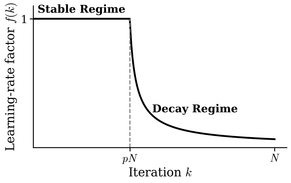
Refer to caption
Figure 22: Visualization of Stable-decay Scheduling.

For the stable-decay schedule, we set the learning rate to γk=γ0​f​(k)\gamma_{k}=\gamma_{0}f(k) with

f​(k)={1,k≤p​N,(1+τ​(k−p​N))−c,k>p​N,f(k)=\begin{cases}1,&k\leq pN,\\ \bigl(1+\tau(k-pN)\bigr)^{-c},&k>pN,\end{cases} (99)

where p,c∈(0,1)p,c\in(0,1) and τ>0\tau>0. In other words, the learning rate remains constant for the first p​NpN steps, and then decays polynomially with exponent cc for the remaining (1−p)​N(1-p)N steps.

Remark 3.

Note that ff depends on the total training steps NN. To be precise, we have to represent it as fNf_{N}, but for simplicity, we write it as ff throughout the analysis.

First, we will make an upper bound on the noise term under stable-decay scheduling.

G.1 Upper Bound of the Noise Term

Fix p<q<1p<q<1 close to 11 and split Lnoise​(N)L^{\text{noise}}(N) as

Lnoise​(N)\displaystyle L^{\text{noise}}(N) =2​γ02π​∑i=1MVi​∫0q​Nexp⁡(−4​λi​γ0π​∫zNf​(u)L​(u)​𝑑u)​f​(z)2​𝑑z\displaystyle=\frac{2\gamma_{0}^{2}}{\pi}\sum_{i=1}^{M}V_{i}\int_{0}^{qN}\exp\!\Bigl(-\tfrac{4\lambda_{i}\gamma_{0}}{\pi}\int_{z}^{N}\frac{f(u)}{\sqrt{L(u)}}\,du\Bigr)f(z)^{2}\,dz
+2​γ02π∑i=1MVi∫q​NNexp(−4​λi​γ0π∫zNf​(u)L​(u)du)f(z)2dz=:T≤q​N+T>q​N.\displaystyle\quad+\frac{2\gamma_{0}^{2}}{\pi}\sum_{i=1}^{M}V_{i}\int_{qN}^{N}\exp\!\Bigl(-\tfrac{4\lambda_{i}\gamma_{0}}{\pi}\int_{z}^{N}\frac{f(u)}{\sqrt{L(u)}}\,du\Bigr)f(z)^{2}\,dz=:T_{\leq qN}+T_{>qN}.
Bounding T>q​NT_{>qN}.

Note that f​(N)≂f​(z)f(N)\eqsim f(z) holds for q​N<z<NqN<z<N. So

∫q​NNexp⁡(−4​λi​γ0π​∫zNf​(u)L​(u)​𝑑u)​f​(z)2​𝑑z≂f​(N)2​∫q​NNexp⁡(−4​λi​γ0π​∫zNf​(u)L​(u)​𝑑u)​𝑑z.\int_{qN}^{N}\exp\!\Bigl(-\tfrac{4\lambda_{i}\gamma_{0}}{\pi}\int_{z}^{N}\frac{f(u)}{\sqrt{L(u)}}\,du\Bigr)f(z)^{2}\,dz\;\eqsim\;f(N)^{2}\int_{qN}^{N}\exp\!\Bigl(-\tfrac{4\lambda_{i}\gamma_{0}}{\pi}\int_{z}^{N}\frac{f(u)}{\sqrt{L(u)}}\,du\Bigr)dz.

For qq sufficiently close to 11, there exist constants c0,c1>0c_{0},c_{1}>0 such that for q​N<z<NqN<z<N

c0​(N−z)​f​(N)L​(N)≤∫zNf​(u)L​(u)​𝑑u≤c1​(N−z)​f​(N)L​(N).c_{0}\,\frac{(N-z)f(N)}{\sqrt{L(N)}}\;\leq\;\int_{z}^{N}\frac{f(u)}{\sqrt{L(u)}}\,du\;\leq\;c_{1}\,\frac{(N-z)f(N)}{\sqrt{L(N)}}.

Therefore,

T>q​N\displaystyle T_{>qN} ≤2​γ02π​f​(N)2​∑i=1MVi​∫q​NNexp⁡(−4​λi​γ0π​c0​(N−z)​f​(N)L​(N))​𝑑z\displaystyle\leq\frac{2\gamma_{0}^{2}}{\pi}\,f(N)^{2}\sum_{i=1}^{M}V_{i}\int_{qN}^{N}\exp\!\Bigl(-\tfrac{4\lambda_{i}\gamma_{0}}{\pi}\,c_{0}\,\frac{(N-z)f(N)}{\sqrt{L(N)}}\Bigr)dz
≂2​γ02π​f​(N)2​∑i=1MVi​π​L​(N)4​λi​γ0​c0​f​(N)≂γ0​f​(N)​L​(N)​∑i=1MViλi\displaystyle\eqsim\frac{2\gamma_{0}^{2}}{\pi}\,f(N)^{2}\sum_{i=1}^{M}V_{i}\,\frac{\pi\,\sqrt{L(N)}}{4\lambda_{i}\gamma_{0}\,c_{0}\,f(N)}\;\eqsim\;\gamma_{0}\,f(N)\,\sqrt{L(N)}\sum_{i=1}^{M}\frac{V_{i}}{\lambda_{i}}
≂γ0f(N)L​(N)Tr(diag(K)1/2)≂γ0f(N)L​(N)M0.5.\displaystyle\eqsim\gamma_{0}\,f(N)\,\sqrt{L(N)}\,\operatorname{Tr}\!\bigl(\operatorname{diag}(K)^{1/2}\bigr)\;\eqsim\;\gamma_{0}\,f(N)\,\sqrt{L(N)}\,M^{0.5}.

To summarize, we have

T>q​N≲γ0​f​(N)​L​(N)​M0.5≂γ0​M1/2​N−c​L​(N).T_{>qN}\ \lesssim\ \gamma_{0}\,f(N)\,\sqrt{L(N)}\,M^{0.5}\eqsim\ \gamma_{0}\,M^{1/2}N^{-c}\sqrt{L(N)}.
Bounding T≤q​NT_{\leq qN}.

Let Q​(z,N)=4​γ0π​∫zNf​(u)L​(u)​𝑑uQ(z,N)=\frac{4\gamma_{0}}{\pi}\int_{z}^{N}\frac{f(u)}{\sqrt{L(u)}}\,du. Then

T≤q​N\displaystyle T_{\leq qN} =2​γ02π​∑i=1M(wi𝖳​𝑲σ​K​ui)​∫0q​Ne−4​γ0π​λi​(𝑲¯)​∫zNf​(u)L​(u)​𝑑u​f​(z)2​𝑑z\displaystyle=\frac{2\gamma_{0}^{2}}{\pi}\sum_{i=1}^{M}(w_{i}^{\mathsf{T}}{\bm{K}}_{\sigma}Ku_{i})\int_{0}^{qN}e^{-\frac{4\gamma_{0}}{\pi}\lambda_{i}(\overline{{\bm{K}}})\int_{z}^{N}\frac{f(u)}{\sqrt{L(u)}}\,du}\,f(z)^{2}dz
=2​γ02π​∑i=1MTr⁡(𝑲σ​K​ui​wi𝖳)​∫0q​Ne−λi​(𝑲¯)​Q​(z,N)​f​(z)2​𝑑z\displaystyle=\frac{2\gamma_{0}^{2}}{\pi}\sum_{i=1}^{M}\operatorname{Tr}({\bm{K}}_{\sigma}Ku_{i}w_{i}^{\mathsf{T}})\int_{0}^{qN}e^{-\lambda_{i}(\overline{{\bm{K}}})Q(z,N)}\,f(z)^{2}dz
=2​γ02π​∫0q​N∑i=1MTr⁡(𝑲σ​K​ui​wi𝖳)​e−λi​(𝑲¯)​Q​(z,N)​f​(z)2​d​z\displaystyle=\frac{2\gamma_{0}^{2}}{\pi}\int_{0}^{qN}\sum_{i=1}^{M}\operatorname{Tr}({\bm{K}}_{\sigma}Ku_{i}w_{i}^{\mathsf{T}})e^{-\lambda_{i}(\overline{{\bm{K}}})Q(z,N)}\,f(z)^{2}dz
=2​γ02π​∫0q​NTr⁡(𝑲σ​K​∑i=1Me−λi​(𝑲¯)​Q​(z,N)​ui​wi𝖳)​f​(z)2​𝑑z\displaystyle=\frac{2\gamma_{0}^{2}}{\pi}\int_{0}^{qN}\operatorname{Tr}({\bm{K}}_{\sigma}K\sum_{i=1}^{M}e^{-\lambda_{i}(\overline{{\bm{K}}})Q(z,N)}u_{i}w_{i}^{\mathsf{T}})\,f(z)^{2}dz
=2​γ02π​∫0q​NTr⁡(𝑲σ​K​e−𝑲¯​Q​(z,N))​f​(z)2​𝑑z.\displaystyle=\frac{2\gamma_{0}^{2}}{\pi}\int_{0}^{qN}\operatorname{Tr}({\bm{K}}_{\sigma}Ke^{-\overline{{\bm{K}}}Q(z,N)})\,f(z)^{2}dz.

Using arcsin⁡x≈x\arcsin x\approx x approximation on 𝑲σ=arcsin(diag(K)−1/2⋅K⋅diag(K)−1/2){\bm{K}}_{\sigma}=\arcsin(\operatorname{diag}(K)^{-1/2}\cdot K\cdot\operatorname{diag}(K)^{-1/2}), we get

Tr⁡(𝑲σ​K​e−𝑲¯​Q​(z,N))=Tr⁡(𝑲σ​S​H1/2​e−𝑲¯1​Q​(z,N)​H1/2​S𝖳)\displaystyle\operatorname{Tr}({\bm{K}}_{\sigma}Ke^{-\overline{{\bm{K}}}Q(z,N)})=\operatorname{Tr}({\bm{K}}_{\sigma}SH^{1/2}e^{-\overline{{\bm{K}}}_{1}Q(z,N)}H^{1/2}S^{\mathsf{T}})
=Tr⁡(H1/2​S𝖳​𝑲σ​S​H1/2​e−𝑲¯1​Q​(z,N))≈Tr⁡(𝑲¯12​e−𝑲¯1​Q​(z,N)).\displaystyle=\operatorname{Tr}(H^{1/2}S^{\mathsf{T}}{\bm{K}}_{\sigma}SH^{1/2}e^{-\overline{{\bm{K}}}_{1}Q(z,N)})\approx\operatorname{Tr}(\overline{{\bm{K}}}_{1}^{2}e^{-\overline{{\bm{K}}}_{1}Q(z,N)}).

Using same contour representation method and deterministic approximation with Section E.2.2 we get

T≤q​N\displaystyle T_{\leq qN} ≂2​γ02π​∫0q​NTr⁡(𝑲¯12​e−𝑲¯1​Q​(z,N))​f​(z)2​𝑑z\displaystyle\eqsim\frac{2\gamma_{0}^{2}}{\pi}\int_{0}^{qN}\operatorname{Tr}(\overline{{\bm{K}}}_{1}^{2}e^{-\overline{{\bm{K}}}_{1}Q(z,N)})\,f(z)^{2}dz
=2​γ02π​∫0q​NTr⁡(−12​π​i​∮Γ2z12​e−Q​(z,N)​z1​(𝑲¯1−z1​𝑰)−1​𝑑z1)​f​(z)2​𝑑z\displaystyle=\frac{2\gamma_{0}^{2}}{\pi}\int_{0}^{qN}\operatorname{Tr}\left(\frac{-1}{2\pi i}\oint_{\Gamma_{2}}z_{1}^{2}e^{-Q(z,N)z_{1}}(\overline{{\bm{K}}}_{1}-z_{1}{\bm{I}})^{-1}\,dz_{1}\right)\,f(z)^{2}dz
≈2​γ02π​∫0q​NTr⁡(−12​π​i​∮Γpd2​z12​e−pd​Q​(z,N)​z1​ℛ​(z1)​𝑑z1)​f​(z)2​𝑑z\displaystyle\approx\frac{2\gamma_{0}^{2}}{\pi}\int_{0}^{qN}\operatorname{Tr}\left(\frac{-1}{2\pi i}\oint_{\Gamma}p_{d}^{2}z_{1}^{2}e^{-p_{d}Q(z,N)z_{1}}\mathcal{R}(z_{1})\,dz_{1}\right)\,f(z)^{2}dz
≂2​γ02π​M​∫0q​NTr⁡(−12​π​i​∮Γz12​e−pd​Q​(z,N)​z1​ℛ​(z1)​𝑑z1)​f​(z)2​𝑑z\displaystyle\eqsim\frac{2\gamma_{0}^{2}}{\pi}M\int_{0}^{qN}\operatorname{Tr}\left(\frac{-1}{2\pi i}\oint_{\Gamma}z_{1}^{2}e^{-p_{d}Q(z,N)z_{1}}\mathcal{R}(z_{1})\,dz_{1}\right)\,f(z)^{2}dz

Adopting the method in Paquette et al. (2024) same as Section K.1, we get

Tr⁡(−12​π​i​∮Γz12​e−pd​Q​(z,N)​z1​ℛ​(z1)​𝑑z1)≂(pd​Q​(z,N))−2+1/(2​α)≂(M1/2​Q​(z,N))−2+1/(2​α).\displaystyle\operatorname{Tr}\left(\frac{-1}{2\pi i}\oint_{\Gamma}z_{1}^{2}e^{-p_{d}Q(z,N)z_{1}}\mathcal{R}(z_{1})\,dz_{1}\right)\eqsim(p_{d}Q(z,N))^{-2+1/(2\alpha)}\eqsim(M^{1/2}Q(z,N))^{-2+1/(2\alpha)}.

It leads to

T≤q​N\displaystyle T_{\leq qN} ≂2​γ02π​M​∫0q​N(M1/2​Q​(z,N))−2+1/(2​α)​f​(z)2​𝑑z\displaystyle\eqsim\frac{2\gamma_{0}^{2}}{\pi}M\int_{0}^{qN}(M^{1/2}Q(z,N))^{-2+1/(2\alpha)}\,f(z)^{2}dz
≂γ02​M1/(4​α)​∫0q​N(Q​(z,N))−2+1/(2​α)​f​(z)2​𝑑z\displaystyle\eqsim\gamma_{0}^{2}M^{1/(4\alpha)}\int_{0}^{qN}(Q(z,N))^{-2+1/(2\alpha)}f(z)^{2}\,dz

Finally,

γ02​M1/(4​α)​∫0q​N(Q​(z,N))−2+1/(2​α)​f​(z)2​𝑑z\displaystyle\gamma_{0}^{2}M^{1/(4\alpha)}\int_{0}^{qN}(Q(z,N))^{-2+1/(2\alpha)}f(z)^{2}\,dz (100)
≂γ01/(2​α)​M1/(4​α)​∫0p​Nf​(z)2(∫zNf​(u)L​(u)​𝑑u)2−1/(2​α)​𝑑z+γ01/(2​α)​M1/(4​α)​∫p​Nq​Nf​(z)2(∫zNf​(u)L​(u)​𝑑u)2−1/(2​α)​𝑑z\displaystyle\eqsim\gamma_{0}^{1/(2\alpha)}M^{1/(4\alpha)}\int_{0}^{pN}\frac{f(z)^{2}}{(\int_{z}^{N}\frac{f(u)}{\sqrt{L(u)}}du)^{2-1/(2\alpha)}}\,dz+\gamma_{0}^{1/(2\alpha)}M^{1/(4\alpha)}\int_{pN}^{qN}\frac{f(z)^{2}}{(\int_{z}^{N}\frac{f(u)}{\sqrt{L(u)}}du)^{2-1/(2\alpha)}}\,dz
≲γ01/(2​α)​M1/(4​α)​∫0p​N1(p​N−zL​(0)+1L​(p​N)​∫p​NNf​(u)​𝑑u)2−1/(2​α)​𝑑z\displaystyle\lesssim\gamma_{0}^{1/(2\alpha)}M^{1/(4\alpha)}\int_{0}^{pN}\frac{1}{(\frac{pN-z}{\sqrt{L(0)}}+\frac{1}{\sqrt{L(pN)}}\int_{pN}^{N}f(u)du)^{2-1/(2\alpha)}}\,dz
+γ01/(2​α)​M1/(4​α)​∫p​Nq​Nf​(z)2(1L​(p​N)​∫q​NNf​(u)​𝑑u)2−1/(2​α)​𝑑z\displaystyle\qquad+\gamma_{0}^{1/(2\alpha)}M^{1/(4\alpha)}\int_{pN}^{qN}\frac{f(z)^{2}}{(\frac{1}{\sqrt{L(pN)}}\int_{qN}^{N}f(u)du)^{2-1/(2\alpha)}}\,dz
≲γ01/(2​α)​M1/(4​α)​∫0p​N1(p​N−zL​(0)+N1−cL​(p​N))2−1/(2​α)​𝑑z+γ01/(2​α)​M1/(4​α)​∫p​Nq​Nf​(z)2(N1−cL​(p​N))2−1/(2​α)​𝑑z\displaystyle\lesssim\gamma_{0}^{1/(2\alpha)}M^{1/(4\alpha)}\int_{0}^{pN}\frac{1}{(\frac{pN-z}{\sqrt{L(0)}}+\frac{N^{1-c}}{\sqrt{L(pN)}})^{2-1/(2\alpha)}}\,dz+\gamma_{0}^{1/(2\alpha)}M^{1/(4\alpha)}\int_{pN}^{qN}\frac{f(z)^{2}}{(\frac{N^{1-c}}{\sqrt{L(pN)}})^{2-1/(2\alpha)}}\,dz
≂γ01/(2​α)​M1/(4​α)​L​(0)​((N1−cL​(p​N))1/(2​α)−1−(p​N+N1−cL​(p​N))1/(2​α)−1)\displaystyle\eqsim\gamma_{0}^{1/(2\alpha)}M^{1/(4\alpha)}\sqrt{L(0)}((\frac{N^{1-c}}{\sqrt{L(pN)}})^{1/(2\alpha)-1}-(pN+\frac{N^{1-c}}{\sqrt{L(pN)}})^{1/(2\alpha)-1})
+γ01/(2​α)​M1/(4​α)​Nmax⁡(1−2​c,0)​(N1−cL​(p​N))1/(2​α)−2\displaystyle\qquad+\gamma_{0}^{1/(2\alpha)}M^{1/(4\alpha)}N^{\max(1-2c,0)}(\frac{N^{1-c}}{\sqrt{L(pN)}})^{1/(2\alpha)-2}
≲γ01/(2​α)​M1/(4​α)​N−(1−c)​(1−1/(2​α))​L​(p​N)(1/2−1/(4​α))≲γ01/(2​α)​M1/(4​α)​N−(1−c)​(1−1/(2​α))\displaystyle\lesssim\gamma_{0}^{1/(2\alpha)}M^{1/(4\alpha)}N^{-(1-c)(1-1/(2\alpha))}L(pN)^{(1/2-1/(4\alpha))}\lesssim\gamma_{0}^{1/(2\alpha)}M^{1/(4\alpha)}N^{-(1-c)(1-1/(2\alpha))}

So we have

T≤q​N≲γ01/(2​α)​M1/(4​α)​N−(1−c)​(1−1/(2​α)).T_{\leq qN}\lesssim\gamma_{0}^{1/(2\alpha)}M^{1/(4\alpha)}N^{-(1-c)(1-1/(2\alpha))}.

G.2 Combining Terms

Combining the bounds,

L​(N)≲M−(2​α+2​β−1)+(M0.5​γ0​N)−2​(2​α+2​β−1) 2​α+1−2​β+γ0​M0.5​N−c​L​(N)+γ012​α​M14​α​N−(1−c)​(1−12​α).L(N)\;\lesssim\;M^{-(2\alpha+2\beta-1)}\;+\;\bigl(M^{0.5}\gamma_{0}N\bigr)^{-\tfrac{2(2\alpha+2\beta-1)}{\,2\alpha+1-2\beta\,}}\;+\;\gamma_{0}M^{0.5}N^{-c}\sqrt{L(N)}\,\;+\;\gamma_{0}^{\tfrac{1}{2\alpha}}\,M^{\tfrac{1}{4\alpha}}\,N^{-(1-c)\,(1-\tfrac{1}{2\alpha})}.

We replaced the drift part with (M0.5​γ0​N)−2​(2​α+2​β−1) 2​α+1−2​β\bigl(M^{0.5}\gamma_{0}N\bigr)^{-\tfrac{2(2\alpha+2\beta-1)}{\,2\alpha+1-2\beta\,}} temporarily based on Remark 2, and justify this on our selected parameters in Remark 4. Solving the inequality asymptotically yields

L​(N)≲M−(2​α+2​β−1)+(M0.5​γ0​N)−2​(2​α+2​β−1) 2​α+1−2​β+γ02​M​N−2​c+γ012​α​M14​α​N−(1−c)​(1−12​α).L(N)\;\lesssim\;M^{-(2\alpha+2\beta-1)}\;+\;\bigl(M^{0.5}\gamma_{0}N\bigr)^{-\tfrac{2(2\alpha+2\beta-1)}{\,2\alpha+1-2\beta\,}}\;+\;\gamma_{0}^{2}\,M\,N^{-2c}\;+\;\gamma_{0}^{\tfrac{1}{2\alpha}}\,M^{\tfrac{1}{4\alpha}}\,N^{-(1-c)\,(1-\tfrac{1}{2\alpha})}.

Finally, substituting γ0=M−e\gamma_{0}=M^{-e} and N=𝔣/MN=\mathfrak{f}/M yields

R​(M,𝔣)≲\displaystyle R(M,\mathfrak{f})\;\lesssim\; M−(2​α+2​β−1)+(M−e−0.5​𝔣)−2​(2​α+2​β−1) 2​α+1−2​β+M1+2​c−2​e​𝔣−2​c\displaystyle\;M^{-(2\alpha+2\beta-1)}\;+\;\Bigl(M^{-e-0.5}\,\mathfrak{f}\Bigr)^{-\tfrac{2(2\alpha+2\beta-1)}{\,2\alpha+1-2\beta\,}}\;+\;M^{1+2c-2e}\,\mathfrak{f}^{-2c}
+M14​α−e2​α+(1−c)​(1−12​α)​𝔣−(1−c)​(1−12​α).\displaystyle\;+\;M^{\tfrac{1}{4\alpha}-\tfrac{e}{2\alpha}+(1-c)\,(1-\tfrac{1}{2\alpha})}\,\mathfrak{f}^{-(1-c)\,(1-\tfrac{1}{2\alpha})}.

Optimizing over MM gives a bound of the form R​(M⋆,𝔣)≤𝔣−h​(α,β,c,e)R(M^{\star},\mathfrak{f})\ \leq\ \mathfrak{f}^{-h(\alpha,\beta,c,e)}, and we then optimize over c,ec,e to maximize h​(α,β,c,e)h(\alpha,\beta,c,e).

G.3 Optimizing over c,ec,e to Maximize h​(α,β,c,e)h(\alpha,\beta,c,e)

Assume throughout α>0.5\alpha>0.5, β<0.5\beta<0.5, and 2​α+2​β>12\alpha+2\beta>1. Consider the upper bound

RU​(M,𝔣)=M−(2​α+2​β−1)+(M−e−0.5​𝔣)−2​(2​α+2​β−1)2​α+1−2​β+M1+2​c−2​e​𝔣−2​c+M14​α−e2​α+(1−c)​(1−12​α)​𝔣−(1−c)​(1−12​α).R_{U}(M,\mathfrak{f})=M^{-(2\alpha+2\beta-1)}+\Bigl(M^{-e-0.5}\,\mathfrak{f}\Bigr)^{-\tfrac{2(2\alpha+2\beta-1)}{2\alpha+1-2\beta}}+M^{1+2c-2e}\,\mathfrak{f}^{-2c}+M^{\tfrac{1}{4\alpha}-\tfrac{e}{2\alpha}+(1-c)\!\left(1-\tfrac{1}{2\alpha}\right)}\,\mathfrak{f}^{-(1-c)\!\left(1-\tfrac{1}{2\alpha}\right)}.

For large 𝔣\mathfrak{f}, define

Rmin​(𝔣):=minM>0⁡RU​(M,𝔣).R_{\min}(\mathfrak{f})\ :=\ \min_{M>0}\ R_{U}(M,\mathfrak{f}).

We show Rmin​(𝔣)≂𝔣h⋆​(α,β)R_{\min}(\mathfrak{f})\ \eqsim\ \mathfrak{f}^{\,h^{\star}(\alpha,\beta)} with h⋆​(α,β)<0h^{\star}(\alpha,\beta)<0, and identify c⋆​(α,β)c^{\star}(\alpha,\beta), e⋆​(α,β)e^{\star}(\alpha,\beta), and M=𝔣m⋆​(α,β)M=\mathfrak{f}^{\,m^{\star}(\alpha,\beta)}.

Logarithmic reduction to exponent balancing

Let M=𝔣mM=\mathfrak{f}^{\,m} with m∈ℝm\in\mathbb{R}. Writing each term as 𝔣Li\mathfrak{f}^{\,L_{i}} gives

L1​(m)\displaystyle L_{1}(m) =−(2​α+2​β−1)​m,\displaystyle=-(2\alpha+2\beta-1)\,m, (101)
L2​(m,e)\displaystyle L_{2}(m,e) =−2​(2​α+2​β−1)2​α+1−2​β+2​(2​α+2​β−1)2​α+1−2​β​m​(e+0.5),\displaystyle=-\frac{2(2\alpha+2\beta-1)}{2\alpha+1-2\beta}+\frac{2(2\alpha+2\beta-1)}{2\alpha+1-2\beta}\,m\bigl(e+0.5\bigr), (102)
L3​(m,c,e)\displaystyle L_{3}(m,c,e) =m​(1+2​c−2​e)−2​c,\displaystyle=m(1+2c-2e)-2c, (103)
L4​(m,c,e)\displaystyle L_{4}(m,c,e) =m​(14​α−e2​α+(1−c)​(1−12​α))−(1−c)​(1−12​α).\displaystyle=m\!\left(\frac{1}{4\alpha}-\frac{e}{2\alpha}+(1-c)\Bigl(1-\frac{1}{2\alpha}\Bigr)\right)-(1-c)\Bigl(1-\frac{1}{2\alpha}\Bigr). (104)

Thus minimizing RUR_{U} is equivalent to

minm,e∈ℝ, 0<c<1⁡max⁡{L1,L2,L3,L4}.\min_{m,e\in\mathbb{R},\ 0<c<1}\ \max\{L_{1},L_{2},L_{3},L_{4}\}. (105)

Introduce h∈ℝh\in\mathbb{R} and rewrite as

minm,c,e,h⁡hs.t.Li​(m,c,e)≤h​(i=1,2,3,4), 0<c<1.\min_{m,c,e,h}\ h\quad\text{s.t.}\quad L_{i}(m,c,e)\leq h\ (i=1,2,3,4),\ \ 0<c<1. (106)

At an interior optimum (0<c<10<c<1), constraints equalize:

L1=L2=L3=L4=h.L_{1}=L_{2}=L_{3}=L_{4}=h. (107)

Solving the equality yields

c⋆\displaystyle c^{\star} =−8​α​β+2​α+2​β−1 16​α2+8​α​β−6​α−2​β+1,\displaystyle=\frac{-8\alpha\beta+2\alpha+2\beta-1}{\,16\alpha^{2}+8\alpha\beta-6\alpha-2\beta+1\,}, (108)
e⋆\displaystyle e^{\star} =8​α2+16​α​β−4​α−4​β+1 2​(4​α−1),\displaystyle=\frac{8\alpha^{2}+16\alpha\beta-4\alpha-4\beta+1}{\,2(4\alpha-1)\,}, (109)
m⋆\displaystyle m^{\star} =2​(4​α−1) 16​α2+8​α​β+2​α−2​β−1,\displaystyle=\frac{2(4\alpha-1)}{\,16\alpha^{2}+8\alpha\beta+2\alpha-2\beta-1\,}, (110)
h⋆\displaystyle h^{\star} =−2​(4​α−1)​(2​α+2​β−1) 16​α2+8​α​β+2​α−2​β−1.\displaystyle=-\,\frac{2(4\alpha-1)\,(2\alpha+2\beta-1)}{\,16\alpha^{2}+8\alpha\beta+2\alpha-2\beta-1\,}. (111)

Feasibility. Since α>0.5\alpha>0.5, denominators are positive. The condition c⋆>0c^{\star}>0 is equivalent to

−8​α​β+2​α+2​β−1> 0⟺β<2​α−1 2​(4​α−1):=B⋆​(α),-8\alpha\beta+2\alpha+2\beta-1\ >\ 0\quad\Longleftrightarrow\quad\beta\ <\ \frac{2\alpha-1}{\,2(4\alpha-1)\,}\ :=\ B^{\star}(\alpha),

which is stricter than β<0.5\beta<0.5. Moreover, c⋆<1c^{\star}<1 holds automatically for β>0\beta>0. Hence, the interior solution is feasible whenever

0.5−α<β<B⋆(α)withB⋆​(α)=2​α−12​(4​α−1).\boxed{\quad 0.5-\alpha\ <\ \beta\ <\ B^{\star}(\alpha)\quad}\qquad\text{with}\quad B^{\star}(\alpha)=\frac{2\alpha-1}{2(4\alpha-1)}. (112)

In this band,

M=𝔣m⋆,Rmin​(𝔣)≂𝔣h⋆\boxed{\ M=\mathfrak{f}^{\,m^{\star}},\qquad R_{\min}(\mathfrak{f})\ \eqsim\ \mathfrak{f}^{\,h^{\star}}\ }

with m⋆,h⋆m^{\star},h^{\star} as in (110)–(111). Note m⋆>0m^{\star}>0 and h⋆<0h^{\star}<0.

Result As 𝔣→∞\mathfrak{f}\to\infty, the choice M=𝔣m⋆M=\mathfrak{f}^{\,m^{\star}} with

m⋆\displaystyle m^{\star} =2​(4​α−1)16​α2+8​α​β+2​α−2​β−1,\displaystyle=\frac{2(4\alpha-1)}{16\alpha^{2}+8\alpha\beta+2\alpha-2\beta-1},
c⋆\displaystyle c^{\star} =−8​α​β+2​α+2​β−116​α2+8​α​β−6​α−2​β+1,\displaystyle=\frac{-8\alpha\beta+2\alpha+2\beta-1}{16\alpha^{2}+8\alpha\beta-6\alpha-2\beta+1},
e⋆\displaystyle e^{\star} =8​α2+16​α​β−4​α−4​β+12​(4​α−1),\displaystyle=\frac{8\alpha^{2}+16\alpha\beta-4\alpha-4\beta+1}{2(4\alpha-1)},
h⋆\displaystyle h^{\star} =−2​(4​α−1)​(2​α+2​β−1)16​α2+8​α​β+2​α−2​β−1\displaystyle=-\frac{2(4\alpha-1)(2\alpha+2\beta-1)}{16\alpha^{2}+8\alpha\beta+2\alpha-2\beta-1}

is optimal for α>0.5\alpha>0.5, 0.5−α<β<B⋆​(α)0.5-\alpha<\beta<B^{\star}(\alpha), where

B⋆​(α)=2​α−12​(4​α−1).B^{\star}(\alpha)=\frac{2\alpha-1}{2(4\alpha-1)}.

This choice minimizes max⁡{L1,L2,L3,L4}\max\{L_{1},L_{2},L_{3},L_{4}\} in (105). Consequently,

Rmin​(𝔣)≂𝔣h⋆​(α,β)with ​h⋆​(α,β)<0.R_{\min}(\mathfrak{f})\ \eqsim\ \mathfrak{f}^{\,h^{\star}(\alpha,\beta)}\qquad\text{with }h^{\star}(\alpha,\beta)<0.
Remark 4 (Justification on drift term conversion).

Note that M=𝔣M⋆M=\mathfrak{f}^{M^{\star}} and N=𝔣1−M⋆N=\mathfrak{f}^{1-M^{\star}} holds for the selected parameters.

For p​NpN iterations the stable-decay scheduling behaves same as the constant learning rate. Let N0N_{0} be the crossover point in constant learning rate. Note that N≳N0N\gtrsim N_{0} holds, and NN is asymptotically strictly bigger than N0N_{0}. So L​(u)≲γ02​M+M−2​α−2​β+1L(u)\lesssim\gamma_{0}^{2}M+M^{-2\alpha-2\beta+1} holds for u≥N0u\geq N_{0}.

Also for selected γ0=M−e∗\gamma_{0}=M^{-e^{*}}, γ02​M≳M−2​α−2​β+1\gamma_{0}^{2}M\gtrsim M^{-2\alpha-2\beta+1} holds.

So we have L​(u)≲γ02​ML(u)\lesssim\gamma_{0}^{2}M for u≥N0u\geq N_{0}.

(M0.5​QL​(N))−2​α+2​β−12​α\displaystyle\bigl(M^{0.5}Q_{L}(N)\bigr)^{-\tfrac{2\alpha+2\beta-1}{2\alpha}} =(M0.5​4​γ0π​∫0Nf​(u)L​(u)​𝑑u)−2​α+2​β−12​α\displaystyle=\left(M^{0.5}\frac{4\gamma_{0}}{\pi}\int_{0}^{N}\frac{f(u)}{\sqrt{L(u)}}\,du\right)^{-\tfrac{2\alpha+2\beta-1}{2\alpha}}
≲(M0.5​4​γ0π​∫N0p​Nf​(u)L​(u)​𝑑u)−2​α+2​β−12​α\displaystyle\lesssim\left(M^{0.5}\frac{4\gamma_{0}}{\pi}\int_{N_{0}}^{pN}\frac{f(u)}{\sqrt{L(u)}}\,du\right)^{-\tfrac{2\alpha+2\beta-1}{2\alpha}}
≂(γ0​M0.5​∫N0p​N1L​(u)​𝑑u)−2​α+2​β−12​α\displaystyle\eqsim\left(\gamma_{0}M^{0.5}\int_{N_{0}}^{pN}\frac{1}{\sqrt{L(u)}}\,du\right)^{-\tfrac{2\alpha+2\beta-1}{2\alpha}}
≂(γ0​M0.5​∫N0p​N1γ02​M​𝑑u)−2​α+2​β−12​α\displaystyle\eqsim\left(\gamma_{0}M^{0.5}\int_{N_{0}}^{pN}\frac{1}{\sqrt{\gamma_{0}^{2}M}}\,du\right)^{-\tfrac{2\alpha+2\beta-1}{2\alpha}}
≂(p​N−N0)−2​α+2​β−12​α≂N−2​α+2​β−12​α\displaystyle\eqsim\left(pN-N_{0}\right)^{-\tfrac{2\alpha+2\beta-1}{2\alpha}}\eqsim N^{-\tfrac{2\alpha+2\beta-1}{2\alpha}}

For selected parameters M=𝔣M⋆M=\mathfrak{f}^{M^{\star}}, N=𝔣1−M⋆N=\mathfrak{f}^{1-M^{\star}}, c∗c^{*}, and γ0=M−e∗\gamma_{0}=M^{-e^{*}} following holds.

N−2​α+2​β−12​α≲γ02​M​N−2​c∗.N^{-\tfrac{2\alpha+2\beta-1}{2\alpha}}\lesssim\gamma_{0}^{2}MN^{-2c^{*}}.

As (M0.5​QL​(N))−2​α+2​β−12​α≲γ02​M​N−2​c∗(M^{0.5}Q_{L}(N)\bigr)^{-\tfrac{2\alpha+2\beta-1}{2\alpha}}\lesssim\gamma_{0}^{2}MN^{-2c^{*}}, replacing the drift term with a proxy does not alter the argument.

G.4 Analysis for Warmup-stable-decay

The analysis for warmup-stable-decay is almost identical to that for stable-decay. The only difference occurs in the step leading to (100), but the final bound is the same. Thus, the loss bound for warmup-stable-decay matches that for stable-decay. We provide the corresponding analysis to the procedure of (100) at the end of this subsection.

Finally, the bound

Rf​(M⋆,𝔣/M⋆,(M⋆)−e∗)≲𝔣−2​(4​α−1)​(2​α+2​β−1)16​α2+8​α​β+2​α−2​β−1.R_{f}(M^{\star},\mathfrak{f}/M^{\star},(M^{\star})^{-e^{*}})\;\lesssim\;\mathfrak{f}^{-\tfrac{2(4\alpha-1)(2\alpha+2\beta-1)}{16\alpha^{2}+8\alpha\beta+2\alpha-2\beta-1}}. (113)

introduced in (15) also holds for warmup-stable-decay.

For the warmup-stable-decay schedule, we set the learning rate to γk=γ0​f​(k)\gamma_{k}=\gamma_{0}f(k) with

f​(k)={k/(w​N),k≤w​N,1,w​N≤k≤p​N,(1+τ​(k−p​N))−c,k>p​N,f(k)=\begin{cases}k/(wN),&k\leq wN,\\ 1,&wN\leq k\leq pN,\\ \bigl(1+\tau(k-pN)\bigr)^{-c},&k>pN,\end{cases} (114)

where w,p,c∈(0,1)w,p,c\in(0,1) and τ>0\tau>0. ww is the ratio for the warmup stage, and we assume that ww is smaller than p/2p/2.

Following is the corresponding analysis to the procedure of (100).

γ02​M1/(4​α)​∫0q​N(Q​(z,N))−2+1/(2​α)​f​(z)2​𝑑z\displaystyle\gamma_{0}^{2}M^{1/(4\alpha)}\int_{0}^{qN}(Q(z,N))^{-2+1/(2\alpha)}f(z)^{2}\,dz
≂γ01/(2​α)​M1/(4​α)​∫0p​Nf​(z)2(∫zNf​(u)L​(u)​𝑑u)2−1/(2​α)​𝑑z+γ01/(2​α)​M1/(4​α)​∫p​Nq​Nf​(z)2(∫zNf​(u)L​(u)​𝑑u)2−1/(2​α)​𝑑z\displaystyle\eqsim\gamma_{0}^{1/(2\alpha)}M^{1/(4\alpha)}\int_{0}^{pN}\frac{f(z)^{2}}{(\int_{z}^{N}\frac{f(u)}{\sqrt{L(u)}}du)^{2-1/(2\alpha)}}\,dz+\gamma_{0}^{1/(2\alpha)}M^{1/(4\alpha)}\int_{pN}^{qN}\frac{f(z)^{2}}{(\int_{z}^{N}\frac{f(u)}{\sqrt{L(u)}}du)^{2-1/(2\alpha)}}\,dz
≲γ01/(2​α)​M1/(4​α)​∫0w​N1(p​N/2L​(0)+1L​(p​N)​∫p​NNf​(u)​𝑑u)2−1/(2​α)​𝑑z\displaystyle\lesssim\gamma_{0}^{1/(2\alpha)}M^{1/(4\alpha)}\int_{0}^{wN}\frac{1}{(\frac{pN/2}{\sqrt{L(0)}}+\frac{1}{\sqrt{L(pN)}}\int_{pN}^{N}f(u)du)^{2-1/(2\alpha)}}\,dz
+γ01/(2​α)​M1/(4​α)​∫w​Np​N1(p​N−zL​(0)+1L​(p​N)​∫p​NNf​(u)​𝑑u)2−1/(2​α)​𝑑z\displaystyle\qquad+\gamma_{0}^{1/(2\alpha)}M^{1/(4\alpha)}\int_{wN}^{pN}\frac{1}{(\frac{pN-z}{\sqrt{L(0)}}+\frac{1}{\sqrt{L(pN)}}\int_{pN}^{N}f(u)du)^{2-1/(2\alpha)}}\,dz
+γ01/(2​α)​M1/(4​α)​∫p​Nq​Nf​(z)2(1L​(p​N)​∫q​NNf​(u)​𝑑u)2−1/(2​α)​𝑑z\displaystyle\qquad+\gamma_{0}^{1/(2\alpha)}M^{1/(4\alpha)}\int_{pN}^{qN}\frac{f(z)^{2}}{(\frac{1}{\sqrt{L(pN)}}\int_{qN}^{N}f(u)du)^{2-1/(2\alpha)}}\,dz
≲γ01/(2​α)​M1/(4​α)​∫0w​N1(p​N/2L​(0)+N1−cL​(p​N))2−1/(2​α)​𝑑z+γ01/(2​α)​M1/(4​α)​∫w​Np​N1(p​N−zL​(0)+N1−cL​(p​N))2−1/(2​α)​𝑑z\displaystyle\lesssim\gamma_{0}^{1/(2\alpha)}M^{1/(4\alpha)}\int_{0}^{wN}\frac{1}{(\frac{pN/2}{\sqrt{L(0)}}+\frac{N^{1-c}}{\sqrt{L(pN)}})^{2-1/(2\alpha)}}\,dz+\gamma_{0}^{1/(2\alpha)}M^{1/(4\alpha)}\int_{wN}^{pN}\frac{1}{(\frac{pN-z}{\sqrt{L(0)}}+\frac{N^{1-c}}{\sqrt{L(pN)}})^{2-1/(2\alpha)}}\,dz
+γ01/(2​α)​M1/(4​α)​∫p​Nq​Nf​(z)2(N1−cL​(p​N))2−1/(2​α)​𝑑z\displaystyle\qquad+\gamma_{0}^{1/(2\alpha)}M^{1/(4\alpha)}\int_{pN}^{qN}\frac{f(z)^{2}}{(\frac{N^{1-c}}{\sqrt{L(pN)}})^{2-1/(2\alpha)}}\,dz
≂γ01/(2​α)​M1/(4​α)​w​N​(p​N/2L​(0))−2+1/(2​α)\displaystyle\eqsim\gamma_{0}^{1/(2\alpha)}M^{1/(4\alpha)}wN(\frac{pN/2}{\sqrt{L(0)}})^{-2+1/(2\alpha)}
+γ01/(2​α)​M1/(4​α)​L​(0)​((N1−cL​(p​N))1/(2​α)−1−(p​N−w​N+N1−cL​(p​N))1/(2​α)−1)\displaystyle\qquad+\gamma_{0}^{1/(2\alpha)}M^{1/(4\alpha)}\sqrt{L(0)}((\frac{N^{1-c}}{\sqrt{L(pN)}})^{1/(2\alpha)-1}-(pN-wN+\frac{N^{1-c}}{\sqrt{L(pN)}})^{1/(2\alpha)-1})
+γ01/(2​α)​M1/(4​α)​Nmax⁡(1−2​c,0)​(N1−cL​(p​N))1/(2​α)−2\displaystyle\qquad+\gamma_{0}^{1/(2\alpha)}M^{1/(4\alpha)}N^{\max(1-2c,0)}(\frac{N^{1-c}}{\sqrt{L(pN)}})^{1/(2\alpha)-2}
≲γ01/(2​α)​M1/(4​α)​N−(1−1/(2​α))+γ01/(2​α)​M1/(4​α)​N−(1−c)​(1−1/(2​α))​L​(p​N)(1/2−1/(4​α))\displaystyle\lesssim\gamma_{0}^{1/(2\alpha)}M^{1/(4\alpha)}N^{-(1-1/(2\alpha))}+\gamma_{0}^{1/(2\alpha)}M^{1/(4\alpha)}N^{-(1-c)(1-1/(2\alpha))}L(pN)^{(1/2-1/(4\alpha))}
≲γ01/(2​α)​M1/(4​α)​N−(1−c)​(1−1/(2​α))\displaystyle\lesssim\gamma_{0}^{1/(2\alpha)}M^{1/(4\alpha)}N^{-(1-c)(1-1/(2\alpha))}

G.5 Scheduling on SGD

In this subsection, we explain that the scheduling does not lift the compute-optimal exponent of SGD in the Phase I and Phase II. Assume a bounded scheduling function ff, and define F​(k)=∫0kf​(z)​𝑑zF(k)=\int_{0}^{k}f(z)\,dz.

Ferbach et al. (2025) proved

Rf​(M,N,γ0)≳M−2​α+max⁡(0,1−2​β)+(γ0​F​(N))−(2​α+2​β−1)/(2​α)+M−1​(γ0​F​(N))−1+1/(2​α)\displaystyle R_{f}(M,N,\gamma_{0})\gtrsim M^{-2\alpha+\max(0,1-2\beta)}+(\gamma_{0}F(N))^{-(2\alpha+2\beta-1)/(2\alpha)}+M^{-1}(\gamma_{0}F(N))^{-1+1/(2\alpha)}

for the risk Rf​(M,N,γ0)R_{f}(M,N,\gamma_{0}) with general bounded scheduling function ff.

Since ff is bounded, we have F​(N)≲NF(N)\lesssim N. Therefore,

Rf​(M,N,γ0)\displaystyle R_{f}(M,N,\gamma_{0}) ≳M−2​α+max⁡(0,1−2​β)+(γ0​F​(N))−(2​α+2​β−1)/(2​α)+M−1​(γ0​F​(N))−1+1/(2​α)\displaystyle\gtrsim M^{-2\alpha+\max(0,1-2\beta)}+(\gamma_{0}F(N))^{-(2\alpha+2\beta-1)/(2\alpha)}+M^{-1}(\gamma_{0}F(N))^{-1+1/(2\alpha)}
≳M−2​α+max⁡(0,1−2​β)+(γ0​N)−(2​α+2​β−1)/(2​α)+M−1​(γ0​N)−1+1/(2​α)\displaystyle\gtrsim M^{-2\alpha+\max(0,1-2\beta)}+(\gamma_{0}N)^{-(2\alpha+2\beta-1)/(2\alpha)}+M^{-1}(\gamma_{0}N)^{-1+1/(2\alpha)}
≳R1​(M,N,γ0),\displaystyle\gtrsim R_{1}(M,N,\gamma_{0}),

where R1​(M,N,γ0)R_{1}(M,N,\gamma_{0}) is the loss under a constant schedule f≡1f\equiv 1.

Thus, scheduling does not improve the compute-optimal exponent of SGD in Phase I and Phase II.

Appendix H Analysis for Linear Decaying Scheduling and Cosine Scheduling

H.1 Analysis for Linear Decaying Scheduling

In this section, we analyze the following linear decaying scheduling.

f​(t)=1−(1−1N)​tNf(t)=1-\left(1-\frac{1}{\sqrt{N}}\right)\frac{t}{N} (115)

It decays from 1 to 1N\frac{1}{\sqrt{N}} linearly.

We will focus on Phase Aa, and follow a similar procedure to stable-decay scheduling.

Note that we have to handle the following equation, where QL​(z):=4​γ0π​∫0zf​(u)L​(u)​𝑑uQ_{L}(z):=\frac{4\gamma_{0}}{\pi}\int_{0}^{z}\frac{f(u)}{\sqrt{L(u)}}\,du.

L​(N)≂\displaystyle L(N)\;\eqsim\; M−(2​α+2​β−1)+(M0.5​QL​(N))−2​α+2​β−12​α\displaystyle M^{-(2\alpha+2\beta-1)}\;+\;\bigl(M^{0.5}Q_{L}(N)\bigr)^{-\tfrac{2\alpha+2\beta-1}{2\alpha}}\;
+2​γ02π​∑i=1MVi​∫0Nexp⁡(−4​λi​γ0π​∫zNf​(u)L​(u)​𝑑u)​f​(z)2​𝑑z.\displaystyle+\;\frac{2\gamma_{0}^{2}}{\pi}\sum_{i=1}^{M}V_{i}\int_{0}^{N}\exp\!\Bigl(-\tfrac{4\lambda_{i}\gamma_{0}}{\pi}\int_{z}^{N}\frac{f(u)}{\sqrt{L(u)}}\,du\Bigr)f(z)^{2}\,dz.

In early iterations the drift term (M0.5​QL​(N))−2​α+2​β−12​α\bigl(M^{0.5}Q_{L}(N)\bigr)^{-\tfrac{2\alpha+2\beta-1}{2\alpha}} dominates. Solving L​(N)≂(M0.5​QL​(N))−2​α+2​β−12​αL(N)\eqsim\bigl(M^{0.5}Q_{L}(N)\bigr)^{-\tfrac{2\alpha+2\beta-1}{2\alpha}} yields

L​(N)≂(M0.5​γ0​F​(N))−2​(2​α+2​β−1) 2​α+1−2​β,F​(N):=∫0Nf​(u)​𝑑u.L(N)\;\eqsim\;\bigl(M^{0.5}\gamma_{0}F(N)\bigr)^{-\tfrac{2(2\alpha+2\beta-1)}{\,2\alpha+1-2\beta\,}},\qquad F(N):=\int_{0}^{N}f(u)\,du.

For linear decaying scheduling F​(N)≂NF(N)\eqsim N holds, so the drift term becomes (M0.5​γ0​N)−2​(2​α+2​β−1) 2​α+1−2​β\bigl(M^{0.5}\gamma_{0}N\bigr)^{-\tfrac{2(2\alpha+2\beta-1)}{\,2\alpha+1-2\beta\,}}.

Now we move to the noise term. We split the noise term Lnoise​(N)L^{\text{noise}}(N) as

Lnoise​(N)\displaystyle L^{\text{noise}}(N) =2​γ02π​∑i=1MVi​∫0N−Nexp⁡(−4​λi​γ0π​∫zNf​(u)L​(u)​𝑑u)​f​(z)2​𝑑z\displaystyle=\frac{2\gamma_{0}^{2}}{\pi}\sum_{i=1}^{M}V_{i}\int_{0}^{N-\sqrt{N}}\exp\!\Bigl(-\tfrac{4\lambda_{i}\gamma_{0}}{\pi}\int_{z}^{N}\frac{f(u)}{\sqrt{L(u)}}\,du\Bigr)f(z)^{2}\,dz
+2​γ02π∑i=1MVi∫N−NNexp(−4​λi​γ0π∫zNf​(u)L​(u)du)f(z)2dz=:T≤(N−N)+T>(N−N).\displaystyle\quad+\frac{2\gamma_{0}^{2}}{\pi}\sum_{i=1}^{M}V_{i}\int_{N-\sqrt{N}}^{N}\exp\!\Bigl(-\tfrac{4\lambda_{i}\gamma_{0}}{\pi}\int_{z}^{N}\frac{f(u)}{\sqrt{L(u)}}\,du\Bigr)f(z)^{2}\,dz=:T_{\leq(N-\sqrt{N})}+T_{>(N-\sqrt{N})}.
Bounding T>(N−N)T_{>(N-\sqrt{N})}.

Note that f​(N)≂f​(z)f(N)\eqsim f(z) holds for (N−N)<z<N(N-\sqrt{N})<z<N. So

∫(N−N)Nexp⁡(−4​λi​γ0π​∫zNf​(u)L​(u)​𝑑u)​f​(z)2​𝑑z≂f​(N)2​∫(N−N)Nexp⁡(−4​λi​γ0π​∫zNf​(u)L​(u)​𝑑u)​𝑑z.\int_{(N-\sqrt{N})}^{N}\exp\!\Bigl(-\tfrac{4\lambda_{i}\gamma_{0}}{\pi}\int_{z}^{N}\frac{f(u)}{\sqrt{L(u)}}\,du\Bigr)f(z)^{2}\,dz\;\eqsim\;f(N)^{2}\int_{(N-\sqrt{N})}^{N}\exp\!\Bigl(-\tfrac{4\lambda_{i}\gamma_{0}}{\pi}\int_{z}^{N}\frac{f(u)}{\sqrt{L(u)}}\,du\Bigr)dz.

There exist constants c0,c1>0c_{0},c_{1}>0 such that for (N−N)<z<N(N-\sqrt{N})<z<N

c0​(N−z)​f​(N)L​(N)≤∫zNf​(u)L​(u)​𝑑u≤c1​(N−z)​f​(N)L​(N).c_{0}\,\frac{(N-z)f(N)}{\sqrt{L(N)}}\;\leq\;\int_{z}^{N}\frac{f(u)}{\sqrt{L(u)}}\,du\;\leq\;c_{1}\,\frac{(N-z)f(N)}{\sqrt{L(N)}}.

Therefore,

T>q​N\displaystyle T_{>qN} ≤2​γ02π​f​(N)2​∑i=1MVi​∫(N−N)Nexp⁡(−4​λi​γ0π​c0​(N−z)​f​(N)L​(N))​𝑑z\displaystyle\leq\frac{2\gamma_{0}^{2}}{\pi}\,f(N)^{2}\sum_{i=1}^{M}V_{i}\int_{(N-\sqrt{N})}^{N}\exp\!\Bigl(-\tfrac{4\lambda_{i}\gamma_{0}}{\pi}\,c_{0}\,\frac{(N-z)f(N)}{\sqrt{L(N)}}\Bigr)dz
≂2​γ02π​f​(N)2​∑i=1MVi​π​L​(N)4​λi​γ0​c0​f​(N)≂γ0​f​(N)​L​(N)​∑i=1MViλi\displaystyle\eqsim\frac{2\gamma_{0}^{2}}{\pi}\,f(N)^{2}\sum_{i=1}^{M}V_{i}\,\frac{\pi\,\sqrt{L(N)}}{4\lambda_{i}\gamma_{0}\,c_{0}\,f(N)}\;\eqsim\;\gamma_{0}\,f(N)\,\sqrt{L(N)}\sum_{i=1}^{M}\frac{V_{i}}{\lambda_{i}}
≂γ0f(N)L​(N)Tr(diag(K)1/2)≂γ0f(N)L​(N)M0.5.\displaystyle\eqsim\gamma_{0}\,f(N)\,\sqrt{L(N)}\,\operatorname{Tr}\!\bigl(\operatorname{diag}(K)^{1/2}\bigr)\;\eqsim\;\gamma_{0}\,f(N)\,\sqrt{L(N)}\,M^{0.5}.

To summarize, we have

T>(N−N)≲γ0​f​(N)​L​(N)​M0.5≂γ0​M1/2​N−1/2​L​(N).T_{>(N-\sqrt{N})}\ \lesssim\ \gamma_{0}\,f(N)\,\sqrt{L(N)}\,M^{0.5}\eqsim\ \gamma_{0}\,M^{1/2}N^{-1/2}\sqrt{L(N)}.
Bounding T≤(N−N)T_{\leq(N-\sqrt{N})}.

Let Q​(z,N)=4​γ0π​∫zNf​(u)L​(u)​𝑑uQ(z,N)=\frac{4\gamma_{0}}{\pi}\int_{z}^{N}\frac{f(u)}{\sqrt{L(u)}}\,du.

By the same procedure as the stable-decaying case, we can get

T≤(N−N)\displaystyle T_{\leq(N-\sqrt{N})} ≂2​γ02π​M​∫0(N−N)(M1/2​Q​(z,N))−2+1/(2​α)​f​(z)2​𝑑z\displaystyle\eqsim\frac{2\gamma_{0}^{2}}{\pi}M\int_{0}^{(N-\sqrt{N})}(M^{1/2}Q(z,N))^{-2+1/(2\alpha)}\,f(z)^{2}dz
≂γ02​M1/(4​α)​∫0(N−N)(Q​(z,N))−2+1/(2​α)​f​(z)2​𝑑z.\displaystyle\eqsim\gamma_{0}^{2}M^{1/(4\alpha)}\int_{0}^{(N-\sqrt{N})}(Q(z,N))^{-2+1/(2\alpha)}f(z)^{2}\,dz.

We have

γ02​M1/(4​α)​∫0(N−N)(Q​(z,N))−2+1/(2​α)​f​(z)2​𝑑z\displaystyle\gamma_{0}^{2}M^{1/(4\alpha)}\int_{0}^{(N-\sqrt{N})}(Q(z,N))^{-2+1/(2\alpha)}f(z)^{2}\,dz (116)
≂γ01/(2​α)​M1/(4​α)​∫0(N−N)f​(z)2(∫zNf​(u)L​(u)​𝑑u)2−1/(2​α)​𝑑z\displaystyle\eqsim\gamma_{0}^{1/(2\alpha)}M^{1/(4\alpha)}\int_{0}^{(N-\sqrt{N})}\frac{f(z)^{2}}{(\int_{z}^{N}\frac{f(u)}{\sqrt{L(u)}}du)^{2-1/(2\alpha)}}\,dz
≲γ01/(2​α)​M1/(4​α)​∫0(N−N)f​(z)2(∫zNf​(u)L​(0)​𝑑u)2−1/(2​α)​𝑑z\displaystyle\lesssim\gamma_{0}^{1/(2\alpha)}M^{1/(4\alpha)}\int_{0}^{(N-\sqrt{N})}\frac{f(z)^{2}}{(\int_{z}^{N}\frac{f(u)}{\sqrt{L(0)}}du)^{2-1/(2\alpha)}}\,dz
≂γ01/(2​α)​M1/(4​α)​∫0(N−N)f​(z)2(∫zNf​(u)​𝑑u)2−1/(2​α)​𝑑z\displaystyle\eqsim\gamma_{0}^{1/(2\alpha)}M^{1/(4\alpha)}\int_{0}^{(N-\sqrt{N})}\frac{f(z)^{2}}{(\int_{z}^{N}f(u)du)^{2-1/(2\alpha)}}\,dz

Let the integral term be ℐ\mathcal{I}. First, we use the change of variables z=N−uz=N-u, which transforms the integration interval [0,N−N][0,N-\sqrt{N}] into [N,N][\sqrt{N},N]. In the regime of large NN, the linear schedule f​(N−u)f(N-u) can be approximated as

f​(N−u)=1−(1−1N)​N−uN≈1N​(1+uN).f(N-u)=1-\left(1-\frac{1}{\sqrt{N}}\right)\frac{N-u}{N}\approx\frac{1}{\sqrt{N}}\left(1+\frac{u}{\sqrt{N}}\right). (117)

Using this approximation, we evaluate the inner integral in the denominator:

∫N−uNf​(s)​𝑑s≈∫0u1N​(1+vN)​𝑑v=uN​(1+u2​N).\int_{N-u}^{N}f(s)\,ds\approx\int_{0}^{u}\frac{1}{\sqrt{N}}\left(1+\frac{v}{\sqrt{N}}\right)dv=\frac{u}{\sqrt{N}}\left(1+\frac{u}{2\sqrt{N}}\right). (118)

Substituting these terms back into ℐ\mathcal{I}, we obtain

ℐ≈∫NN[1N​(1+uN)]2[uN​(1+u2​N)]2−12​α​𝑑u.\mathcal{I}\approx\int_{\sqrt{N}}^{N}\frac{\left[\frac{1}{\sqrt{N}}\left(1+\frac{u}{\sqrt{N}}\right)\right]^{2}}{\left[\frac{u}{\sqrt{N}}\left(1+\frac{u}{2\sqrt{N}}\right)\right]^{2-\frac{1}{2\alpha}}}\,du. (119)

To decouple the dependency on NN, we apply the scaling u=N​yu=\sqrt{N}y, which implies d​u=N​d​ydu=\sqrt{N}dy. The integration limits change from [N,N][\sqrt{N},N] to [1,N][1,\sqrt{N}]. The integral is then reformulated as

ℐ\displaystyle\mathcal{I} ≈∫1N1N​(1+y)2(y​(1+y/2))2−12​α​N​𝑑y\displaystyle\approx\int_{1}^{\sqrt{N}}\frac{\frac{1}{N}(1+y)^{2}}{\left(y(1+y/2)\right)^{2-\frac{1}{2\alpha}}}\sqrt{N}\,dy (120)
=1N​∫1N(1+y)2y2−12​α​(1+y/2)2−12​α​𝑑y.\displaystyle=\frac{1}{\sqrt{N}}\int_{1}^{\sqrt{N}}\frac{(1+y)^{2}}{y^{2-\frac{1}{2\alpha}}(1+y/2)^{2-\frac{1}{2\alpha}}}\,dy.

The asymptotic behavior is determined by the convergence of the remaining integral. As y→∞y\to\infty, the integrand behaves as

y2y2−12​α​(y/2)2−12​α∝y2−2​(2−12​α)=y1α−2.\frac{y^{2}}{y^{2-\frac{1}{2\alpha}}(y/2)^{2-\frac{1}{2\alpha}}}\propto y^{2-2(2-\frac{1}{2\alpha})}=y^{\frac{1}{\alpha}-2}. (121)

Integrating this term from 11 to N\sqrt{N} leads to the following cases depending on the exponent 1α−2\frac{1}{\alpha}-2:

ℐ∼1N×{(N)1α−1=N12​α−12if ​1α−2>−1⟹α<1,ln⁡(N)∼ln⁡Nif ​1α−2=−1⟹α=1,constif ​1α−2<−1⟹α>1.\mathcal{I}\sim\frac{1}{\sqrt{N}}\times\begin{cases}(\sqrt{N})^{\frac{1}{\alpha}-1}=N^{\frac{1}{2\alpha}-\frac{1}{2}}&\text{if }\frac{1}{\alpha}-2>-1\implies\alpha<1,\\ \ln(\sqrt{N})\sim\ln N&\text{if }\frac{1}{\alpha}-2=-1\implies\alpha=1,\\ \text{const}&\text{if }\frac{1}{\alpha}-2<-1\implies\alpha>1.\end{cases} (122)

Simplifying the final exponents, we get the asymptotic order:

ℐ∼{𝒪​(N12​α−1)if ​0.5<α<1,𝒪​(N−12​ln⁡N)if ​α=1,𝒪​(N−12)if ​α>1.\mathcal{I}\sim\begin{cases}\mathcal{O}\left(N^{\frac{1}{2\alpha}-1}\right)&\text{if }0.5<\alpha<1,\\ \mathcal{O}\left(N^{-\frac{1}{2}}\ln N\right)&\text{if }\alpha=1,\\ \mathcal{O}\left(N^{-\frac{1}{2}}\right)&\text{if }\alpha>1.\end{cases} (123)

For 0.5<α<10.5<\alpha<1, we have

T≤(N−N)≲γ01/(2​α)​M1/(4​α)​N−(1−1/(2​α)).T_{\leq(N-\sqrt{N})}\lesssim\gamma_{0}^{1/(2\alpha)}M^{1/(4\alpha)}N^{-(1-1/(2\alpha))}.

For 0.5<α<10.5<\alpha<1, combining the bounds for the drift term and noise term, we have

L​(N)≲M−(2​α+2​β−1)+(M0.5​γ0​N)−2​(2​α+2​β−1) 2​α+1−2​β+γ0​M0.5​N−1/2​L​(N)+γ012​α​M14​α​N−(1−12​α).L(N)\;\lesssim\;M^{-(2\alpha+2\beta-1)}\;+\;\bigl(M^{0.5}\gamma_{0}N\bigr)^{-\tfrac{2(2\alpha+2\beta-1)}{\,2\alpha+1-2\beta\,}}\;+\;\gamma_{0}M^{0.5}N^{-1/2}\sqrt{L(N)}\,\;+\;\gamma_{0}^{\tfrac{1}{2\alpha}}\,M^{\tfrac{1}{4\alpha}}\,N^{-(1-\tfrac{1}{2\alpha})}.

In intersection of Area Aa⋆\text{Aa}^{\star} and 0.5<α<10.5<\alpha<1, with choice of e∗e^{*} in γ0=M−e∗\gamma_{0}=M^{-e^{*}} and c∗c^{*} we used for stable-decaying scheduling, we have

L​(N)≲M−(2​α+2​β−1)+(M0.5​γ0​N)−2​(2​α+2​β−1) 2​α+1−2​β+γ0​M0.5​N−c∗​L​(N)+γ012​α​M14​α​N−(1−c∗)​(1−12​α).L(N)\;\lesssim\;M^{-(2\alpha+2\beta-1)}\;+\;\bigl(M^{0.5}\gamma_{0}N\bigr)^{-\tfrac{2(2\alpha+2\beta-1)}{\,2\alpha+1-2\beta\,}}\;+\;\gamma_{0}M^{0.5}N^{-c^{*}}\sqrt{L(N)}\,\;+\;\gamma_{0}^{\tfrac{1}{2\alpha}}\,M^{\tfrac{1}{4\alpha}}\,N^{-(1-c^{*})\,(1-\tfrac{1}{2\alpha})}.

So in intersection of Area Aa⋆\text{Aa}^{\star} and 0.5<α<10.5<\alpha<1, we have

Rf​(M⋆,𝔣/M⋆,(M⋆)−e∗)≲𝔣−2​(4​α−1)​(2​α+2​β−1)16​α2+8​α​β+2​α−2​β−1.R_{f}(M^{\star},\mathfrak{f}/M^{\star},(M^{\star})^{-e^{*}})\;\lesssim\;\mathfrak{f}^{-\tfrac{2(4\alpha-1)(2\alpha+2\beta-1)}{16\alpha^{2}+8\alpha\beta+2\alpha-2\beta-1}}. (124)

Therefore, linear decaying scheduling has an advantage compared to constant learning rate in the intersection of Area Aa⋆\text{Aa}^{\star} and 0.5<α<10.5<\alpha<1.

H.2 Analysis for Cosine Scheduling

In this section, we analyze the following cosine scheduling.

f​(t)=1+1/N2+1−1/N2​cos⁡(πN​t)f(t)=\frac{1+1/N}{2}+\frac{1-1/N}{2}\cos\left(\frac{\pi}{N}t\right) (125)

It decays from 1 to 1N\frac{1}{N}.

We will focus on Phase Aa, and follow a similar procedure to stable-decay scheduling.

Note that we have to handle the following equation, where QL​(z):=4​γ0π​∫0zf​(u)L​(u)​𝑑uQ_{L}(z):=\frac{4\gamma_{0}}{\pi}\int_{0}^{z}\frac{f(u)}{\sqrt{L(u)}}\,du.

L​(N)≂\displaystyle L(N)\;\eqsim\; M−(2​α+2​β−1)+(M0.5​QL​(N))−2​α+2​β−12​α\displaystyle M^{-(2\alpha+2\beta-1)}\;+\;\bigl(M^{0.5}Q_{L}(N)\bigr)^{-\tfrac{2\alpha+2\beta-1}{2\alpha}}\;
+2​γ02π​∑i=1MVi​∫0Nexp⁡(−4​λi​γ0π​∫zNf​(u)L​(u)​𝑑u)​f​(z)2​𝑑z.\displaystyle+\;\frac{2\gamma_{0}^{2}}{\pi}\sum_{i=1}^{M}V_{i}\int_{0}^{N}\exp\!\Bigl(-\tfrac{4\lambda_{i}\gamma_{0}}{\pi}\int_{z}^{N}\frac{f(u)}{\sqrt{L(u)}}\,du\Bigr)f(z)^{2}\,dz.

In early iterations the drift term (M0.5​QL​(N))−2​α+2​β−12​α\bigl(M^{0.5}Q_{L}(N)\bigr)^{-\tfrac{2\alpha+2\beta-1}{2\alpha}} dominates. Solving L​(N)≂(M0.5​QL​(N))−2​α+2​β−12​αL(N)\eqsim\bigl(M^{0.5}Q_{L}(N)\bigr)^{-\tfrac{2\alpha+2\beta-1}{2\alpha}} yields

L​(N)≂(M0.5​γ0​F​(N))−2​(2​α+2​β−1) 2​α+1−2​β,F​(N):=∫0Nf​(u)​𝑑u.L(N)\;\eqsim\;\bigl(M^{0.5}\gamma_{0}F(N)\bigr)^{-\tfrac{2(2\alpha+2\beta-1)}{\,2\alpha+1-2\beta\,}},\qquad F(N):=\int_{0}^{N}f(u)\,du.

For cosine scheduling F​(N)≂NF(N)\eqsim N holds, so the drift term becomes (M0.5​γ0​N)−2​(2​α+2​β−1) 2​α+1−2​β\bigl(M^{0.5}\gamma_{0}N\bigr)^{-\tfrac{2(2\alpha+2\beta-1)}{\,2\alpha+1-2\beta\,}}.

Now we move to the noise term. We split the noise term Lnoise​(N)L^{\text{noise}}(N) as

Lnoise​(N)\displaystyle L^{\text{noise}}(N) =2​γ02π​∑i=1MVi​∫0N−Nexp⁡(−4​λi​γ0π​∫zNf​(u)L​(u)​𝑑u)​f​(z)2​𝑑z\displaystyle=\frac{2\gamma_{0}^{2}}{\pi}\sum_{i=1}^{M}V_{i}\int_{0}^{N-\sqrt{N}}\exp\!\Bigl(-\tfrac{4\lambda_{i}\gamma_{0}}{\pi}\int_{z}^{N}\frac{f(u)}{\sqrt{L(u)}}\,du\Bigr)f(z)^{2}\,dz
+2​γ02π∑i=1MVi∫N−NNexp(−4​λi​γ0π∫zNf​(u)L​(u)du)f(z)2dz=:T≤(N−N)+T>(N−N).\displaystyle\quad+\frac{2\gamma_{0}^{2}}{\pi}\sum_{i=1}^{M}V_{i}\int_{N-\sqrt{N}}^{N}\exp\!\Bigl(-\tfrac{4\lambda_{i}\gamma_{0}}{\pi}\int_{z}^{N}\frac{f(u)}{\sqrt{L(u)}}\,du\Bigr)f(z)^{2}\,dz=:T_{\leq(N-\sqrt{N})}+T_{>(N-\sqrt{N})}.
Bounding T>(N−N)T_{>(N-\sqrt{N})}.

Note that f​(N)≂f​(z)f(N)\eqsim f(z) holds for (N−N)<z<N(N-\sqrt{N})<z<N. So

∫(N−N)Nexp⁡(−4​λi​γ0π​∫zNf​(u)L​(u)​𝑑u)​f​(z)2​𝑑z≂f​(N)2​∫(N−N)Nexp⁡(−4​λi​γ0π​∫zNf​(u)L​(u)​𝑑u)​𝑑z.\int_{(N-\sqrt{N})}^{N}\exp\!\Bigl(-\tfrac{4\lambda_{i}\gamma_{0}}{\pi}\int_{z}^{N}\frac{f(u)}{\sqrt{L(u)}}\,du\Bigr)f(z)^{2}\,dz\;\eqsim\;f(N)^{2}\int_{(N-\sqrt{N})}^{N}\exp\!\Bigl(-\tfrac{4\lambda_{i}\gamma_{0}}{\pi}\int_{z}^{N}\frac{f(u)}{\sqrt{L(u)}}\,du\Bigr)dz.

There exist constants c0,c1>0c_{0},c_{1}>0 such that for (N−N)<z<N(N-\sqrt{N})<z<N

c0​(N−z)​f​(N)L​(N)≤∫zNf​(u)L​(u)​𝑑u≤c1​(N−z)​f​(N)L​(N).c_{0}\,\frac{(N-z)f(N)}{\sqrt{L(N)}}\;\leq\;\int_{z}^{N}\frac{f(u)}{\sqrt{L(u)}}\,du\;\leq\;c_{1}\,\frac{(N-z)f(N)}{\sqrt{L(N)}}.

Therefore,

T>q​N\displaystyle T_{>qN} ≤2​γ02π​f​(N)2​∑i=1MVi​∫(N−N)Nexp⁡(−4​λi​γ0π​c0​(N−z)​f​(N)L​(N))​𝑑z\displaystyle\leq\frac{2\gamma_{0}^{2}}{\pi}\,f(N)^{2}\sum_{i=1}^{M}V_{i}\int_{(N-\sqrt{N})}^{N}\exp\!\Bigl(-\tfrac{4\lambda_{i}\gamma_{0}}{\pi}\,c_{0}\,\frac{(N-z)f(N)}{\sqrt{L(N)}}\Bigr)dz
≂2​γ02π​f​(N)2​∑i=1MVi​π​L​(N)4​λi​γ0​c0​f​(N)≂γ0​f​(N)​L​(N)​∑i=1MViλi\displaystyle\eqsim\frac{2\gamma_{0}^{2}}{\pi}\,f(N)^{2}\sum_{i=1}^{M}V_{i}\,\frac{\pi\,\sqrt{L(N)}}{4\lambda_{i}\gamma_{0}\,c_{0}\,f(N)}\;\eqsim\;\gamma_{0}\,f(N)\,\sqrt{L(N)}\sum_{i=1}^{M}\frac{V_{i}}{\lambda_{i}}
≂γ0f(N)L​(N)Tr(diag(K)1/2)≂γ0f(N)L​(N)M0.5.\displaystyle\eqsim\gamma_{0}\,f(N)\,\sqrt{L(N)}\,\operatorname{Tr}\!\bigl(\operatorname{diag}(K)^{1/2}\bigr)\;\eqsim\;\gamma_{0}\,f(N)\,\sqrt{L(N)}\,M^{0.5}.

To summarize, we have

T>(N−N)≲γ0​f​(N)​L​(N)​M0.5≂γ0​M1/2​N−1​L​(N).T_{>(N-\sqrt{N})}\ \lesssim\ \gamma_{0}\,f(N)\,\sqrt{L(N)}\,M^{0.5}\eqsim\ \gamma_{0}\,M^{1/2}N^{-1}\sqrt{L(N)}.
Bounding T≤(N−N)T_{\leq(N-\sqrt{N})}.

Let Q​(z,N)=4​γ0π​∫zNf​(u)L​(u)​𝑑uQ(z,N)=\frac{4\gamma_{0}}{\pi}\int_{z}^{N}\frac{f(u)}{\sqrt{L(u)}}\,du.

By the same procedure as the stable-decaying case, we can get

T≤(N−N)\displaystyle T_{\leq(N-\sqrt{N})} ≂2​γ02π​M​∫0(N−N)(M1/2​Q​(z,N))−2+1/(2​α)​f​(z)2​𝑑z\displaystyle\eqsim\frac{2\gamma_{0}^{2}}{\pi}M\int_{0}^{(N-\sqrt{N})}(M^{1/2}Q(z,N))^{-2+1/(2\alpha)}\,f(z)^{2}dz
≂γ02​M1/(4​α)​∫0(N−N)(Q​(z,N))−2+1/(2​α)​f​(z)2​𝑑z.\displaystyle\eqsim\gamma_{0}^{2}M^{1/(4\alpha)}\int_{0}^{(N-\sqrt{N})}(Q(z,N))^{-2+1/(2\alpha)}f(z)^{2}\,dz.

We have

γ02​M1/(4​α)​∫0(N−N)(Q​(z,N))−2+1/(2​α)​f​(z)2​𝑑z\displaystyle\gamma_{0}^{2}M^{1/(4\alpha)}\int_{0}^{(N-\sqrt{N})}(Q(z,N))^{-2+1/(2\alpha)}f(z)^{2}\,dz (126)
≂γ01/(2​α)​M1/(4​α)​∫0(N−N)f​(z)2(∫zNf​(u)L​(u)​𝑑u)2−1/(2​α)​𝑑z\displaystyle\eqsim\gamma_{0}^{1/(2\alpha)}M^{1/(4\alpha)}\int_{0}^{(N-\sqrt{N})}\frac{f(z)^{2}}{(\int_{z}^{N}\frac{f(u)}{\sqrt{L(u)}}du)^{2-1/(2\alpha)}}\,dz
≲γ01/(2​α)​M1/(4​α)​∫0(N−N)f​(z)2(∫zNf​(u)L​(0)​𝑑u)2−1/(2​α)​𝑑z\displaystyle\lesssim\gamma_{0}^{1/(2\alpha)}M^{1/(4\alpha)}\int_{0}^{(N-\sqrt{N})}\frac{f(z)^{2}}{(\int_{z}^{N}\frac{f(u)}{\sqrt{L(0)}}du)^{2-1/(2\alpha)}}\,dz
≂γ01/(2​α)​M1/(4​α)​∫0(N−N)f​(z)2(∫zNf​(u)​𝑑u)2−1/(2​α)​𝑑z\displaystyle\eqsim\gamma_{0}^{1/(2\alpha)}M^{1/(4\alpha)}\int_{0}^{(N-\sqrt{N})}\frac{f(z)^{2}}{(\int_{z}^{N}f(u)du)^{2-1/(2\alpha)}}\,dz

Let the integral term be ℐ\mathcal{I}. First, we use the change of variables z=N−uz=N-u, which transforms the integration interval [0,N−N][0,N-\sqrt{N}] into [N,N][\sqrt{N},N]. The integral can be written as:

ℐ=∫NNf​(N−x)2(∫0xf​(N−v)​𝑑v)2−12​α​𝑑x.\mathcal{I}=\int_{\sqrt{N}}^{N}\frac{f(N-x)^{2}}{\left(\int_{0}^{x}f(N-v)\,dv\right)^{2-\frac{1}{2\alpha}}}\,dx. (127)

We evaluate the asymptotic magnitude of ℐ\mathcal{I} by analyzing the dominant contributions from the lower limit (x≈Nx\approx\sqrt{N}) and the upper limit (x≈Nx\approx N).

Contribution near the lower limit (x≈Nx\approx\sqrt{N}): In the region where xx is small, the learning rate approaches its minimum, f​(N−x)≈1Nf(N-x)\approx\frac{1}{N}. Consequently, the cumulative sum scales linearly with the inverse of NN, i.e., ∫0xf​(N−v)​𝑑v≈xN\int_{0}^{x}f(N-v)\,dv\approx\frac{x}{N}. Substituting these approximations, the integrand becomes:

(1/N)2(x/N)2−12​α=N−2⋅N2−12​α⋅x−2+12​α=N−12​α​x−2+12​α.\frac{(1/N)^{2}}{(x/N)^{2-\frac{1}{2\alpha}}}=N^{-2}\cdot N^{2-\frac{1}{2\alpha}}\cdot x^{-2+\frac{1}{2\alpha}}=N^{-\frac{1}{2\alpha}}x^{-2+\frac{1}{2\alpha}}. (128)

Integrating this term with respect to xx near the lower limit N\sqrt{N}:

N−12​α​[x−1+12​α]x=N∼N−12​α​(N)−1+12​α=N−12​α​N−12+14​α.N^{-\frac{1}{2\alpha}}\left[x^{-1+\frac{1}{2\alpha}}\right]_{x=\sqrt{N}}\sim N^{-\frac{1}{2\alpha}}(\sqrt{N})^{-1+\frac{1}{2\alpha}}=N^{-\frac{1}{2\alpha}}N^{-\frac{1}{2}+\frac{1}{4\alpha}}. (129)

Simplifying the exponents yields the scaling N−12−14​αN^{-\frac{1}{2}-\frac{1}{4\alpha}}.

Contribution near the upper limit (x≈Nx\approx N): In the region where xx is large, f​(N−x)∼𝒪​(1)f(N-x)\sim\mathcal{O}(1) and the cumulative sum scales as 𝒪​(x)\mathcal{O}(x). The integrand is dominated by x−(2−12​α)x^{-\left(2-\frac{1}{2\alpha}\right)}. Integrating this term near the upper limit NN:

[x−1+12​α]x=N∼N−1+12​α.\left[x^{-1+\frac{1}{2\alpha}}\right]^{x=N}\sim N^{-1+\frac{1}{2\alpha}}. (130)

The asymptotic behavior of ℐ\mathcal{I} is determined by the maximum of these two contributions. The contribution from the lower limit dominates when −12−14​α>−1+12​α-\frac{1}{2}-\frac{1}{4\alpha}>-1+\frac{1}{2\alpha}, which corresponds to α>1.5\alpha>1.5. Otherwise, the contribution from the upper limit dominates. Thus,

ℐ≂{N−12−14​αif ​α>1.5,N−1+12​αif ​0.5<α<1.5.\mathcal{I}\eqsim\begin{cases}N^{-\frac{1}{2}-\frac{1}{4\alpha}}&\text{if }\alpha>1.5,\\ N^{-1+\frac{1}{2\alpha}}&\text{if }0.5<\alpha<1.5.\end{cases} (131)

For 0.5<α<1.50.5<\alpha<1.5, we have

T≤(N−N)≲γ01/(2​α)​M1/(4​α)​N−(1−1/(2​α)).T_{\leq(N-\sqrt{N})}\lesssim\gamma_{0}^{1/(2\alpha)}M^{1/(4\alpha)}N^{-(1-1/(2\alpha))}.

For 0.5<α<1.50.5<\alpha<1.5, combining the bounds for the drift term and noise term, we have

L​(N)≲M−(2​α+2​β−1)+(M0.5​γ0​N)−2​(2​α+2​β−1) 2​α+1−2​β+γ0​M0.5​N−1​L​(N)+γ012​α​M14​α​N−(1−12​α).L(N)\;\lesssim\;M^{-(2\alpha+2\beta-1)}\;+\;\bigl(M^{0.5}\gamma_{0}N\bigr)^{-\tfrac{2(2\alpha+2\beta-1)}{\,2\alpha+1-2\beta\,}}\;+\;\gamma_{0}M^{0.5}N^{-1}\sqrt{L(N)}\,\;+\;\gamma_{0}^{\tfrac{1}{2\alpha}}\,M^{\tfrac{1}{4\alpha}}\,N^{-(1-\tfrac{1}{2\alpha})}.

In intersection of Area Aa⋆\text{Aa}^{\star} and 0.5<α<1.50.5<\alpha<1.5, with choice of e∗e^{*} in γ0=M−e∗\gamma_{0}=M^{-e^{*}} and c∗c^{*} we used for stable-decaying scheduling, we have

L​(N)≲M−(2​α+2​β−1)+(M0.5​γ0​N)−2​(2​α+2​β−1) 2​α+1−2​β+γ0​M0.5​N−c∗​L​(N)+γ012​α​M14​α​N−(1−c∗)​(1−12​α).L(N)\;\lesssim\;M^{-(2\alpha+2\beta-1)}\;+\;\bigl(M^{0.5}\gamma_{0}N\bigr)^{-\tfrac{2(2\alpha+2\beta-1)}{\,2\alpha+1-2\beta\,}}\;+\;\gamma_{0}M^{0.5}N^{-c^{*}}\sqrt{L(N)}\,\;+\;\gamma_{0}^{\tfrac{1}{2\alpha}}\,M^{\tfrac{1}{4\alpha}}\,N^{-(1-c^{*})\,(1-\tfrac{1}{2\alpha})}.

So in intersection of Area Aa⋆\text{Aa}^{\star} and 0.5<α<1.50.5<\alpha<1.5, we have

Rf​(M⋆,𝔣/M⋆,(M⋆)−e∗)≲𝔣−2​(4​α−1)​(2​α+2​β−1)16​α2+8​α​β+2​α−2​β−1.R_{f}(M^{\star},\mathfrak{f}/M^{\star},(M^{\star})^{-e^{*}})\;\lesssim\;\mathfrak{f}^{-\tfrac{2(4\alpha-1)(2\alpha+2\beta-1)}{16\alpha^{2}+8\alpha\beta+2\alpha-2\beta-1}}. (132)

Therefore, linear decaying scheduling has an advantage compared to constant learning rate in the intersection of Area Aa⋆\text{Aa}^{\star} and 0.5<α<1.50.5<\alpha<1.5.

Appendix I Analysis about Hypothesis for the Position of the Beneficial Area

In this section, we cover the analysis of stochastic gradient decay, which was deferred from Section 5.1.

We examine the decaying structure of the stochastic gradient. Assume a feature vector 𝒙{\bm{x}} is drawn from the distribution 𝒩​(0,𝑯){\mathcal{N}}(0,{\bm{H}}), and its label is y=⟨𝒙,𝒘∗⟩y=\langle{\bm{x}},{\bm{w}}^{*}\rangle. Then the stochastic gradient for that feature vector is

𝒈\displaystyle{\bm{g}} =2​(⟨𝑺​𝒙t,𝜽t−1⟩−y)​𝑺​𝒙t\displaystyle=2\big(\langle{\bm{S}}{\bm{x}}_{t},{\bm{\theta}}_{t-1}\rangle-y\big)\,{\bm{S}}{\bm{x}}_{t}
=2​𝑺​𝒙​𝒙𝖳​𝑺𝖳​(𝜽−𝜽∗)−2​𝑺​𝒙​𝒙𝖳​𝒘⟂.\displaystyle=2{\bm{S}}{\bm{x}}{\bm{x}}^{\mathsf{T}}{\bm{S}}^{\mathsf{T}}({\bm{\theta}}-{\bm{\theta}}^{*})-2{\bm{S}}{\bm{x}}{\bm{x}}^{\mathsf{T}}{\bm{w}}_{\perp}.

Taking the expectation of the stochastic gradient and using 𝑺​𝑯​𝒘⟂=0{\bm{S}}{\bm{H}}{\bm{w}}_{\perp}=0, we obtain

𝔼​[𝒈]\displaystyle\mathbb{E}[{\bm{g}}] =2​𝑺​𝑯​𝑺𝖳​(𝜽−𝜽∗)−2​𝑺​𝑯​𝒘⟂\displaystyle=2{\bm{S}}{\bm{H}}{\bm{S}}^{\mathsf{T}}({\bm{\theta}}-{\bm{\theta}}^{*})-2{\bm{S}}{\bm{H}}{\bm{w}}_{\perp}
=2​𝑺​𝑯​𝑺𝖳​(𝜽−𝜽∗).\displaystyle=2{\bm{S}}{\bm{H}}{\bm{S}}^{\mathsf{T}}({\bm{\theta}}-{\bm{\theta}}^{*}).

Lin et al. (2024) proved that the eigenvalues λi\lambda_{i} of 𝑺​𝑯​𝑺𝖳{\bm{S}}{\bm{H}}{\bm{S}}^{\mathsf{T}} satisfy λi≂i−2​α\lambda_{i}\eqsim i^{-2\alpha}. Let the eigenvalue decomposition of 𝑺​𝑯​𝑺𝖳{\bm{S}}{\bm{H}}{\bm{S}}^{\mathsf{T}} be 𝑺​𝑯​𝑺𝖳=𝑼​diag⁡(λi)​𝑼𝖳{\bm{S}}{\bm{H}}{\bm{S}}^{\mathsf{T}}={\bm{U}}\operatorname{diag}(\lambda_{i}){\bm{U}}^{\mathsf{T}}. Then

𝑼𝖳​𝔼​[𝒈]=2​diag⁡(λi)​𝑼𝖳​(𝜽−𝜽∗),{\bm{U}}^{\mathsf{T}}\mathbb{E}[{\bm{g}}]=2\operatorname{diag}(\lambda_{i})\,{\bm{U}}^{\mathsf{T}}({\bm{\theta}}-{\bm{\theta}}^{*}),

which provides the intuition that 𝔼​[𝒈]\mathbb{E}[{\bm{g}}], expressed in the basis of the columns of 𝑼{\bm{U}}, decays as i−2​αi^{-2\alpha}. Figure 23 shows that the expected gradient decays similarly to i−2​αi^{-2\alpha}. Also, note that a larger α\alpha leads to a steeper gradient decay.

Refer to caption
Figure 23: Decay of gradient under the basis of U{\bm{U}}. Colored solid lines show the average of gradients under the basis of 𝑼{\bm{U}} for the parameter (α,β)=(0.4,0.5),(0.6,0.5),(0.8,0.5)(\alpha,\beta)=(0.4,0.5),(0.6,0.5),(0.8,0.5). On the legend, we only noted the α\alpha. The dotted line is fitted for the average of gradients, and we noted its slope in the legend. Slope is similar to 2​α2\alpha within error 0.130.13.

Appendix J Scaling Law of Adam with Heuristic

First, we recall the Adam (Kingma and Ba, 2015) update and notation. For the stochastic gradient

𝒈k=2​(⟨𝑺​𝒙k,𝜽k⟩−yk)​𝑺​𝒙k.{\bm{g}}_{k}\ =2\bigl(\langle{\bm{S}}{\bm{x}}_{k},{\bm{\theta}}_{k}\rangle-y_{k}\bigr)\,{\bm{S}}{\bm{x}}_{k}.

Adam maintains first and second moment estimates

𝒎k\displaystyle{\bm{m}}_{k} =β1​𝒎k−1+(1−β1)​𝒈k,\displaystyle=\beta_{1}\,{\bm{m}}_{k-1}+(1-\beta_{1})\,{\bm{g}}_{k},
𝒗k\displaystyle{\bm{v}}_{k} =β2​𝒗k−1+(1−β2)​𝒈k⊙2,\displaystyle=\beta_{2}\,{\bm{v}}_{k-1}+(1-\beta_{2})\,{\bm{g}}_{k}^{\odot 2},

with bias corrections 𝒎^k=𝒎k/(1−β1k)\;\hat{\bm{m}}_{k}={\bm{m}}_{k}/(1-\beta_{1}^{k}), 𝒗^k=𝒗k/(1−β2k)\;\hat{\bm{v}}_{k}={\bm{v}}_{k}/(1-\beta_{2}^{k}). The update is

𝜽k+1=𝜽k−γk​𝒎^k⊙(ϵ​𝟏+𝒗^k)−1/2,{\bm{\theta}}_{k+1}={\bm{\theta}}_{k}-\gamma_{k}\,\hat{\bm{m}}_{k}\odot\bigl(\epsilon\mathbf{1}+\hat{\bm{v}}_{k}\bigr)^{-1/2},

where ⊙\odot denotes elementwise multiplication and the (−1/2)(-1/2) power is taken elementwise; ϵ>0\epsilon>0 is the usual damping (we will set ϵ=0\epsilon=0 in the asymptotic analysis).

Xiao et al. (2025) proposed a heuristic for Adam: take β2\beta_{2} sufficiently close to 11 so that the second moment can be treated as an expectation.

We present results under a same heuristic. In addition, Ferbach et al. (2025) prove that SGD with momentum obeys the same scaling law as SGD; motivated by this, we set β1=0\beta_{1}=0 and omit the first-moment term for simplicity.

Second-moment proxy and normalized update.

Under the heuristic of Xiao et al. (2025),

𝒗^k\displaystyle\hat{\bm{v}}_{k} ≈4​𝔼​[(𝑺​𝒙k)⊙2​(⟨𝑺​𝒙k,𝜽k⟩−yk)2|ℱk]\displaystyle\approx 4\mathbb{E}\!\Big[({\bm{S}}{\bm{x}}_{k})^{\odot 2}\,\bigl(\langle{\bm{S}}{\bm{x}}_{k},{\bm{\theta}}_{k}\rangle-y_{k}\bigr)^{2}\,\Big|\,\mathcal{F}_{k}\Big]

Let 𝝃:=𝑺​𝒙k\bm{\xi}:={\bm{S}}{\bm{x}}_{k} be the sketched feature vector. Under the Gaussian assumption on 𝒙k{\bm{x}}_{k}, 𝝃\bm{\xi} follows a multivariate Gaussian distribution with covariance 𝑲=𝑺​𝑯​𝑺𝖳{\bm{K}}={\bm{S}}{\bm{H}}{\bm{S}}^{\mathsf{T}}.

First, we analyze the residual term. Using the decomposition 𝒘∗=𝑺𝖳​𝜽∗+𝒘⟂{\bm{w}}^{*}={\bm{S}}^{\mathsf{T}}{\bm{\theta}}^{*}+{\bm{w}}_{\perp}, the residual at step kk is:

⟨𝑺​𝒙k,𝜽k⟩−yk\displaystyle\langle{\bm{S}}{\bm{x}}_{k},{\bm{\theta}}_{k}\rangle-y_{k} =𝒙k𝖳​𝑺𝖳​𝜽k−𝒙k𝖳​𝒘∗\displaystyle={\bm{x}}_{k}^{\mathsf{T}}{\bm{S}}^{\mathsf{T}}{\bm{\theta}}_{k}-{\bm{x}}_{k}^{\mathsf{T}}{\bm{w}}^{*}
=𝒙k𝖳​𝑺𝖳​𝜽k−𝒙k𝖳​(𝑺𝖳​𝜽∗+𝒘⟂)\displaystyle={\bm{x}}_{k}^{\mathsf{T}}{\bm{S}}^{\mathsf{T}}{\bm{\theta}}_{k}-{\bm{x}}_{k}^{\mathsf{T}}({\bm{S}}^{\mathsf{T}}{\bm{\theta}}^{*}+{\bm{w}}_{\perp})
=(𝑺​𝒙k)𝖳​(𝜽k−𝜽∗)−𝒙k𝖳​𝒘⟂\displaystyle=({\bm{S}}{\bm{x}}_{k})^{\mathsf{T}}({\bm{\theta}}_{k}-{\bm{\theta}}^{*})-{\bm{x}}_{k}^{\mathsf{T}}{\bm{w}}_{\perp}
=𝝃𝖳​δk−ζk,\displaystyle=\bm{\xi}^{\mathsf{T}}\delta_{k}-\zeta_{k},

where δk:=𝜽k−𝜽∗\delta_{k}:={\bm{\theta}}_{k}-{\bm{\theta}}^{*} is the parameter error, and ζk:=𝒙k𝖳​𝒘⟂\zeta_{k}:={\bm{x}}_{k}^{\mathsf{T}}{\bm{w}}_{\perp} is the irreducible residual term induced by approximation error.

We focus on the ii-th coordinate of the second moment vector. Let X:=(𝝃)iX:=(\bm{\xi})_{i} and Y:=𝝃𝖳​δk−ζkY:=\bm{\xi}^{\mathsf{T}}\delta_{k}-\zeta_{k} (the residual). Since both are linear combinations of the Gaussian vector 𝒙k{\bm{x}}_{k}, they are jointly Gaussian. We apply Isserlis’ theorem:

𝔼​[X2​Y2]=𝔼​[X2]​𝔼​[Y2]+2​(𝔼​[X​Y])2.\mathbb{E}[X^{2}Y^{2}]=\mathbb{E}[X^{2}]\mathbb{E}[Y^{2}]+2\bigl(\mathbb{E}[XY]\bigr)^{2}.

We evaluate each term:

  1. 1.

    Variance of the feature (𝔼​[X2]\mathbb{E}[X^{2}]):

    𝔼​[(𝝃)i2]=(𝑺​𝑯​𝑺𝖳)i​i=(diag⁡(𝑲))i.\mathbb{E}[(\bm{\xi})_{i}^{2}]=({\bm{S}}{\bm{H}}{\bm{S}}^{\mathsf{T}})_{ii}=(\operatorname{diag}({\bm{K}}))_{i}.
  2. 2.

    Variance of the residual (𝔼​[Y2]\mathbb{E}[Y^{2}]): By definition, the expected squared residual is the population risk:

    𝔼​[Y2]=𝔼​[(⟨𝑺​𝒙k,𝜽k⟩−yk)2]=L​(𝜽k).\mathbb{E}[Y^{2}]=\mathbb{E}\bigl[(\langle{\bm{S}}{\bm{x}}_{k},{\bm{\theta}}_{k}\rangle-y_{k})^{2}\bigr]=L({\bm{\theta}}_{k}).
  3. 3.

    Covariance term (𝔼​[X​Y]\mathbb{E}[XY]): This term involves the correlation between the feature and the residual.

    𝔼​[X​Y]\displaystyle\mathbb{E}[XY] =𝔼​[(𝝃)i​(𝝃𝖳​δk−ζk)]\displaystyle=\mathbb{E}\Bigl[(\bm{\xi})_{i}\bigl(\bm{\xi}^{\mathsf{T}}\delta_{k}-\zeta_{k}\bigr)\Bigr]
    =𝔼​[(𝑺​𝒙k)i​(𝒙k𝖳​𝑺𝖳​δk)]−𝔼​[(𝑺​𝒙k)i​(𝒙k𝖳​𝒘⟂)].\displaystyle=\mathbb{E}\Bigl[({\bm{S}}{\bm{x}}_{k})_{i}({\bm{x}}_{k}^{\mathsf{T}}{\bm{S}}^{\mathsf{T}}\delta_{k})\Bigr]-\mathbb{E}\Bigl[({\bm{S}}{\bm{x}}_{k})_{i}({\bm{x}}_{k}^{\mathsf{T}}{\bm{w}}_{\perp})\Bigr].

    The first part is the standard covariance calculation:

    𝔼​[(𝑺​𝒙k)i​(𝒙k𝖳​𝑺𝖳​δk)]=(𝑺​𝔼​[𝒙k​𝒙k𝖳]​𝑺𝖳​δk)i=(𝑺​𝑯​𝑺𝖳​δk)i=(𝑲​δk)i.\mathbb{E}\Bigl[({\bm{S}}{\bm{x}}_{k})_{i}({\bm{x}}_{k}^{\mathsf{T}}{\bm{S}}^{\mathsf{T}}\delta_{k})\Bigr]=\bigl({\bm{S}}\mathbb{E}[{\bm{x}}_{k}{\bm{x}}_{k}^{\mathsf{T}}]{\bm{S}}^{\mathsf{T}}\delta_{k}\bigr)_{i}=({\bm{S}}{\bm{H}}{\bm{S}}^{\mathsf{T}}\delta_{k})_{i}=({\bm{K}}\delta_{k})_{i}.

    The second part vanishes due to the orthogonality property of the projected solution (𝑺​𝑯​𝒘⟂=0{\bm{S}}{\bm{H}}{\bm{w}}_{\perp}=0):

    𝔼​[(𝑺​𝒙k)i​(𝒙k𝖳​𝒘⟂)]=(𝑺​𝔼​[𝒙k​𝒙k𝖳]​𝒘⟂)i=(𝑺​𝑯​𝒘⟂)i=0.\mathbb{E}\Bigl[({\bm{S}}{\bm{x}}_{k})_{i}({\bm{x}}_{k}^{\mathsf{T}}{\bm{w}}_{\perp})\Bigr]=\bigl({\bm{S}}\mathbb{E}[{\bm{x}}_{k}{\bm{x}}_{k}^{\mathsf{T}}]{\bm{w}}_{\perp}\bigr)_{i}=({\bm{S}}{\bm{H}}{\bm{w}}_{\perp})_{i}=0.

    Thus, 𝔼​[X​Y]=(𝑲​δk)i\mathbb{E}[XY]=({\bm{K}}\delta_{k})_{i}.

Substituting these back into Isserlis’ formula yields:

𝔼​[X2​Y2]=(diag⁡(𝑲))i​L​(𝜽k)+ 2​((𝑲​(𝜽k−𝜽∗))i)2.\mathbb{E}[X^{2}Y^{2}]=(\operatorname{diag}({\bm{K}}))_{i}\,L({\bm{\theta}}_{k})\;+\;2\bigl(({\bm{K}}({\bm{\theta}}_{k}-{\bm{\theta}}^{*}))_{i}\bigr)^{2}.

Stacking the coordinates gives the following equation.

𝔼​[(𝑺​𝒙k)⊙2​(⟨𝑺​𝒙k,𝜽k⟩−yk)2|ℱk]=diag⁡(𝑲)⋅L​(𝜽k)+ 2​(𝑲​(𝜽k−𝜽∗))⊙2.\mathbb{E}\!\Big[({\bm{S}}{\bm{x}}_{k})^{\odot 2}\,\bigl(\langle{\bm{S}}{\bm{x}}_{k},{\bm{\theta}}_{k}\rangle-y_{k}\bigr)^{2}\,\Big|\,\mathcal{F}_{k}\Big]=\operatorname{diag}({\bm{K}})\cdot L({\bm{\theta}}_{k})\;+\;2\,({\bm{K}}({\bm{\theta}}_{k}-{\bm{\theta}}^{*}))^{\odot 2}. (133)

Moreover, by Cauchy–Schwarz,

(𝑲​(𝜽k−𝜽∗))j2≤𝑲j​j​(𝜽k−𝜽∗)𝖳​𝑲​(𝜽k−𝜽∗)≤𝑲j​j​L​(𝜽k),({\bm{K}}({\bm{\theta}}_{k}-{\bm{\theta}}^{*}))_{j}^{2}\leq{\bm{K}}_{jj}\,({\bm{\theta}}_{k}-{\bm{\theta}}^{*})^{\mathsf{T}}{\bm{K}}({\bm{\theta}}_{k}-{\bm{\theta}}^{*})\leq{\bm{K}}_{jj}\,L({\bm{\theta}}_{k}),

and hence the exact second moment admits the coordinate-wise bounds

diag⁡(𝑲)⋅L​(𝜽k)⪯𝔼​[(𝑺​𝒙k)⊙2​(⟨𝑺​𝒙k,𝜽k⟩−yk)2|ℱk]⪯ 3​diag⁡(𝑲)⋅L​(𝜽k),\operatorname{diag}({\bm{K}})\cdot L({\bm{\theta}}_{k})\;\preceq\;\mathbb{E}\!\Big[({\bm{S}}{\bm{x}}_{k})^{\odot 2}\,\bigl(\langle{\bm{S}}{\bm{x}}_{k},{\bm{\theta}}_{k}\rangle-y_{k}\bigr)^{2}\,\Big|\,\mathcal{F}_{k}\Big]\;\preceq\;3\,\operatorname{diag}({\bm{K}})\cdot L({\bm{\theta}}_{k}), (134)

where ⪯\preceq denotes elementwise inequality. In particular, replacing the exact second moment by diag⁡(𝑲)⋅L​(𝜽k)=diag⁡(𝑺​𝑯​𝑺𝖳)⋅L​(𝜽k)\operatorname{diag}({\bm{K}})\cdot L({\bm{\theta}}_{k})=\operatorname{diag}({\bm{S}}{\bm{H}}{\bm{S}}^{\mathsf{T}})\cdot L({\bm{\theta}}_{k}) changes the normalization by at most a universal constant factor.

Hence, the (elementwise) normalized update satisfies

𝜽k+1−𝜽k≂−γk​(⟨𝑺​𝒙k,𝜽k⟩−yk)​𝑺​𝒙kdiag⁡(𝑺​𝑯​𝑺𝖳)⋅L​(𝜽k).{\bm{\theta}}_{k+1}-{\bm{\theta}}_{k}\eqsim-\gamma_{k}\frac{\bigl(\langle{\bm{S}}{\bm{x}}_{k},{\bm{\theta}}_{k}\rangle-y_{k}\bigr)\,{\bm{S}}{\bm{x}}_{k}}{\sqrt{\operatorname{diag}({\bm{S}}{\bm{H}}{\bm{S}}^{\mathsf{T}})\cdot L({\bm{\theta}}_{k})}}.
One-step update formula.

Recalling the Taylor expansion used for signSGD,

𝔼​[q​(𝜽k+1)−q​(𝜽k)|ℱk]=𝔼​[⟨∇q​(𝜽k),𝜽k+1−𝜽k⟩|ℱk]+12​𝔼​[⟨∇2q,(𝜽k+1−𝜽k)⊗2⟩|ℱk].\mathbb{E}\!\big[q({\bm{\theta}}_{k+1})-q({\bm{\theta}}_{k})\,\big|\,\mathcal{F}_{k}\big]=\mathbb{E}\!\Big[\big\langle\nabla q({\bm{\theta}}_{k}),\,{\bm{\theta}}_{k+1}-{\bm{\theta}}_{k}\big\rangle\,\Big|\,\mathcal{F}_{k}\Big]+\frac{1}{2}\,\mathbb{E}\!\Big[\big\langle\nabla^{2}q,\,({\bm{\theta}}_{k+1}-{\bm{\theta}}_{k})^{\otimes 2}\big\rangle\,\Big|\,\mathcal{F}_{k}\Big].

Gradient term:

𝔼​[⟨∇q​(𝜽k),𝜽k+1−𝜽k⟩|ℱk]≂−γk​⟨∇q​(𝜽k),𝑺​𝑯​𝑺𝖳​𝜽k−𝑺​𝑯​𝒘∗diag⁡(𝑺​𝑯​𝑺𝖳)⋅L​(𝜽k)⟩.\mathbb{E}\!\Big[\big\langle\nabla q({\bm{\theta}}_{k}),\,{\bm{\theta}}_{k+1}-{\bm{\theta}}_{k}\big\rangle\,\Big|\,\mathcal{F}_{k}\Big]\eqsim-\gamma_{k}\left\langle\nabla q({\bm{\theta}}_{k}),\,\frac{{\bm{S}}{\bm{H}}{\bm{S}}^{\mathsf{T}}\,{\bm{\theta}}_{k}-{\bm{S}}{\bm{H}}{\bm{w}}^{*}}{\sqrt{\operatorname{diag}({\bm{S}}{\bm{H}}{\bm{S}}^{\mathsf{T}})\cdot L({\bm{\theta}}_{k})}}\right\rangle.

Quadratic term:

𝔼​[⟨∇2q,(𝜽k+1−𝜽k)⊗2⟩|ℱk]\displaystyle\mathbb{E}\!\Big[\big\langle\nabla^{2}q,\,({\bm{\theta}}_{k+1}-{\bm{\theta}}_{k})^{\otimes 2}\big\rangle\,\Big|\,\mathcal{F}_{k}\Big]
≂γk2𝔼[⟨∇2q,diag(𝑺𝑯𝑺𝖳)−1/2𝑺𝒙k𝒙k𝖳𝑺𝖳diag(𝑺𝑯𝑺𝖳)−1/2⟩(⟨𝑺​𝒙k,𝜽k⟩−yk)2L​(𝜽k)|ℱk]\displaystyle\eqsim\gamma_{k}^{2}\mathbb{E}\!\Bigg[\Big\langle\nabla^{2}q,\,\operatorname{diag}({\bm{S}}{\bm{H}}{\bm{S}}^{\mathsf{T}})^{-1/2}\,{\bm{S}}{\bm{x}}_{k}{\bm{x}}_{k}^{\mathsf{T}}{\bm{S}}^{\mathsf{T}}\,\operatorname{diag}({\bm{S}}{\bm{H}}{\bm{S}}^{\mathsf{T}})^{-1/2}\Big\rangle\frac{\bigl(\langle{\bm{S}}{\bm{x}}_{k},{\bm{\theta}}_{k}\rangle-y_{k}\bigr)^{2}}{L({\bm{\theta}}_{k})}\;\Bigg|\,\mathcal{F}_{k}\Bigg]
=γk2L​(𝜽k)(⟨diag(𝑺𝑯𝑺𝖳)−1/2∇2qdiag(𝑺𝑯𝑺𝖳)−1/2,𝑺𝑯𝑺𝖳⟩L(𝜽k)\displaystyle=\frac{\gamma_{k}^{2}}{L({\bm{\theta}}_{k})}\Big(\big\langle\operatorname{diag}({\bm{S}}{\bm{H}}{\bm{S}}^{\mathsf{T}})^{-1/2}\nabla^{2}q\,\operatorname{diag}({\bm{S}}{\bm{H}}{\bm{S}}^{\mathsf{T}})^{-1/2},\,{\bm{S}}{\bm{H}}{\bm{S}}^{\mathsf{T}}\big\rangle\,L({\bm{\theta}}_{k})
+ 2⟨𝑺𝑯𝑺𝖳diag(𝑺𝑯𝑺𝖳)−1/2∇2qdiag(𝑺𝑯𝑺𝖳)−1/2𝑺𝑯𝑺𝖳,(𝜽k−𝜽∗)⊗2⟩).\displaystyle\hskip 45.5244pt+\,2\,\big\langle{\bm{S}}{\bm{H}}{\bm{S}}^{\mathsf{T}}\,\operatorname{diag}({\bm{S}}{\bm{H}}{\bm{S}}^{\mathsf{T}})^{-1/2}\nabla^{2}q\,\operatorname{diag}({\bm{S}}{\bm{H}}{\bm{S}}^{\mathsf{T}})^{-1/2}\,{\bm{S}}{\bm{H}}{\bm{S}}^{\mathsf{T}},\,({\bm{\theta}}_{k}-{\bm{\theta}}^{*})^{\otimes 2}\big\rangle\Big).

Combining the two contributions,

𝔼​[q​(𝜽k+1)−q​(𝜽k)|ℱk]\displaystyle\mathbb{E}\!\big[q({\bm{\theta}}_{k+1})-q({\bm{\theta}}_{k})\,\big|\,\mathcal{F}_{k}\big] ≂−γkL​(𝜽k)​⟨∇q​(𝜽k),𝑲¯​(𝜽k−𝜽∗)⟩+γk22​⟨∇2q,𝑲τ⟩\displaystyle\eqsim-\frac{\gamma_{k}}{\sqrt{L({\bm{\theta}}_{k})}}\,\big\langle\nabla q({\bm{\theta}}_{k}),\,\overline{{\bm{K}}}({\bm{\theta}}_{k}-{\bm{\theta}}^{*})\big\rangle+\frac{\gamma_{k}^{2}}{2}\,\big\langle\nabla^{2}q,\,{\bm{K}}_{\tau}\big\rangle
+γk2L​(𝜽k)⟨𝑺𝑯𝑺𝖳diag(𝑺𝑯𝑺𝖳)−1/2∇2qdiag(𝑺𝑯𝑺𝖳)−1/2𝑺𝑯𝑺𝖳,(𝜽k−𝜽∗)⊗2⟩,\displaystyle\quad+\frac{\gamma_{k}^{2}}{L({\bm{\theta}}_{k})}\,\big\langle{\bm{S}}{\bm{H}}{\bm{S}}^{\mathsf{T}}\,\operatorname{diag}({\bm{S}}{\bm{H}}{\bm{S}}^{\mathsf{T}})^{-1/2}\nabla^{2}q\,\operatorname{diag}({\bm{S}}{\bm{H}}{\bm{S}}^{\mathsf{T}})^{-1/2}\,{\bm{S}}{\bm{H}}{\bm{S}}^{\mathsf{T}},\,({\bm{\theta}}_{k}-{\bm{\theta}}^{*})^{\otimes 2}\big\rangle,

where 𝑲τ:=diag(𝑺𝑯𝑺𝖳)−1/2𝑺𝑯𝑺𝖳diag(𝑺𝑯𝑺𝖳)−1/2{\bm{K}}_{\tau}:=\operatorname{diag}({\bm{S}}{\bm{H}}{\bm{S}}^{\mathsf{T}})^{-1/2}\,{\bm{S}}{\bm{H}}{\bm{S}}^{\mathsf{T}}\,\operatorname{diag}({\bm{S}}{\bm{H}}{\bm{S}}^{\mathsf{T}})^{-1/2}.

Mode-wise recursion.

For ri​(k):=(𝜽k−𝜽∗)𝖳​(𝑲​𝒖i⊗𝒘i)​(𝜽k−𝜽∗)r_{i}(k):=({\bm{\theta}}_{k}-{\bm{\theta}}^{*})^{\mathsf{T}}({\bm{K}}{\bm{u}}_{i}\otimes{\bm{w}}_{i})\,({\bm{\theta}}_{k}-{\bm{\theta}}^{*}) (cf. Appendix E.1),

𝔼​[ri​(k+1)−ri​(k)|ℱk]\displaystyle\mathbb{E}\!\big[r_{i}(k+1)-r_{i}(k)\,\big|\,\mathcal{F}_{k}\big] ≂−2​γkL​(𝜽k)​λi​(𝑲¯)​ri​(k)+γk2​(𝒘i𝖳​𝑲τ​𝑲​𝒖i)+2​γk2L​(𝜽k)​λi​(𝑲¯)​ri​(k)\displaystyle\eqsim-\frac{2\gamma_{k}}{\sqrt{L({\bm{\theta}}_{k})}}\,\lambda_{i}(\overline{{\bm{K}}})\,r_{i}(k)+\gamma_{k}^{2}\,({\bm{w}}_{i}^{\mathsf{T}}{\bm{K}}_{\tau}{\bm{K}}{\bm{u}}_{i})+\frac{2\gamma_{k}^{2}}{L({\bm{\theta}}_{k})}\,\lambda_{i}(\overline{{\bm{K}}})\,r_{i}(k)
=−(2​γkL​(𝜽k)−2​γk2L​(𝜽k))​λi​(𝑲¯)​ri​(k)+γk2​(𝒘i𝖳​𝑲τ​𝑲​𝒖i).\displaystyle=-\Bigl(\frac{2\gamma_{k}}{\sqrt{L({\bm{\theta}}_{k})}}-\frac{2\gamma_{k}^{2}}{L({\bm{\theta}}_{k})}\Bigr)\lambda_{i}(\overline{{\bm{K}}})\,r_{i}(k)+\gamma_{k}^{2}\,({\bm{w}}_{i}^{\mathsf{T}}{\bm{K}}_{\tau}{\bm{K}}{\bm{u}}_{i}).

We now assume f≡1f\equiv 1, and γk=γ0\gamma_{k}=\gamma_{0} for simplicity. Passing to the ODE limit as in Section E.2 we get following ODE for P​(t)=L​(t/γ0)P(t)=L(t/\gamma_{0}) and pi​(t)=ri​(t/γ0)p_{i}(t)=r_{i}(t/\gamma_{0}).

d​pid​t≂−2​(1P​(t)−γ0P​(t))​λi​(𝑲¯)​pi​(t)+γ0​Vi′,\frac{dp_{i}}{dt}\eqsim-2\left(\frac{1}{\sqrt{P(t)}}-\frac{\gamma_{0}}{P(t)}\right)\,\lambda_{i}(\overline{{\bm{K}}})\,p_{i}(t)+\gamma_{0}\,V^{\prime}_{i}, (135)

where Vi′:=𝒘i𝖳​𝑲τ​𝑲​𝒖iV_{i}^{\prime}:={\bm{w}}_{i}^{\mathsf{T}}{\bm{K}}_{\tau}{\bm{K}}{\bm{u}}_{i}.

Interpreting the solution of the ODE as an implicit integral equation and summing over ii, similar to Section E.2, and writing

Q2​(N)=2​γ0​∫0N(1L​(u)−γ0​1L​(u))​𝑑u,Q_{2}(N)=2\gamma_{0}\int_{0}^{N}\!\Bigl(\frac{1}{\sqrt{L(u)}}-\gamma_{0}\frac{1}{L(u)}\Bigr)\,du,

we obtain the implicit integral inequality for some c1,c2>0c_{1},c_{2}>0.

∥𝑯1/2​𝒘⟂∥2+∑i=1Mri​(0)​exp⁡(−c1​λi​Q2​(N))\displaystyle\lVert{\bm{H}}^{1/2}{\bm{w}}_{\perp}\rVert^{2}+\sum_{i=1}^{M}r_{i}(0)\,\exp\!\Bigl(-c_{1}\lambda_{i}Q_{2}(N)\Bigr)
+γ02​∑i=1MVi′​∫0Nexp⁡(−2​c1​λi​γ0​∫zN(1L​(u)−γ0​1L​(u))​𝑑u)​𝑑z\displaystyle+\gamma_{0}^{2}\sum_{i=1}^{M}V_{i}^{\prime}\int_{0}^{N}\exp\!\Bigl(-2c_{1}\lambda_{i}\gamma_{0}\int_{z}^{N}\!\Bigl(\frac{1}{\sqrt{L(u)}}-\gamma_{0}\frac{1}{L(u)}\Bigr)\,du\Bigr)\,dz
≤L​(N)≤∥𝑯1/2​𝒘⟂∥2+∑i=1Mri​(0)​exp⁡(−c2​λi​Q2​(N))\displaystyle\leq L(N)\leq\lVert{\bm{H}}^{1/2}{\bm{w}}_{\perp}\rVert^{2}+\sum_{i=1}^{M}r_{i}(0)\,\exp\!\Bigl(-c_{2}\lambda_{i}Q_{2}(N)\Bigr)
+γ02​∑i=1MVi′​∫0Nexp⁡(−2​c2​λi​γ0​∫zN(1L​(u)−γ0​1L​(u))​𝑑u)​𝑑z.\displaystyle\quad+\gamma_{0}^{2}\sum_{i=1}^{M}V_{i}^{\prime}\int_{0}^{N}\exp\!\Bigl(-2c_{2}\lambda_{i}\gamma_{0}\int_{z}^{N}\!\Bigl(\frac{1}{\sqrt{L(u)}}-\gamma_{0}\frac{1}{L(u)}\Bigr)\,du\Bigr)\,dz.
Drift transformation and limit phase.

By the same drift/approximation transformation as in equation 35,

M−2​α+max⁡(0, 1−2​β)+(Mmin⁡(α,0.5)​Q2​(N))−2​α+2​β−12​α\displaystyle M^{-2\alpha+\max(0,\,1-2\beta)}+\bigl(M^{\min(\alpha,0.5)}\,Q_{2}(N)\bigr)^{-\tfrac{2\alpha+2\beta-1}{2\alpha}}
+ 1{α>0.5,β>0.5}​M−1​(Mmin⁡(α,0.5)​Q2​(N))−1+12​α+γ02​∑i=1MVi′​∫0Ne−2​c1​λi​γ0​∫zN(f​(u)L​(u)−γ0​f​(u)2L​(u))​𝑑u​f​(z)2​𝑑z\displaystyle+\;\mathbf{1}_{\{\alpha>0.5,\ \beta>0.5\}}\;M^{-1}\,\bigl(M^{\min(\alpha,0.5)}Q_{2}(N)\bigr)^{-1+\tfrac{1}{2\alpha}}+\gamma_{0}^{2}\sum_{i=1}^{M}V_{i}^{\prime}\int_{0}^{N}e^{-2c_{1}\lambda_{i}\gamma_{0}\int_{z}^{N}(\frac{f(u)}{\sqrt{L(u)}}-\gamma_{0}\frac{f(u)^{2}}{L(u)})\,du}\,f(z)^{2}\,dz
≲L​(N)≲M−2​α+max⁡(0, 1−2​β)+(Mmin⁡(α,0.5)​Q2​(N))−2​α+2​β−12​α\displaystyle\lesssim L(N)\lesssim M^{-2\alpha+\max(0,\,1-2\beta)}+\bigl(M^{\min(\alpha,0.5)}\,Q_{2}(N)\bigr)^{-\tfrac{2\alpha+2\beta-1}{2\alpha}}
+ 1{α>0.5,β>0.5}​M−1​(Mmin⁡(α,0.5)​Q2​(N))−1+12​α+γ02​∑i=1MVi′​∫0Ne−2​c2​λi​γ0​∫zN(f​(u)L​(u)−γ0​f​(u)2L​(u))​𝑑u​f​(z)2​𝑑z.\displaystyle\quad+\;\mathbf{1}_{\{\alpha>0.5,\ \beta>0.5\}}\;M^{-1}\,\bigl(M^{\min(\alpha,0.5)}Q_{2}(N)\bigr)^{-1+\tfrac{1}{2\alpha}}+\gamma_{0}^{2}\sum_{i=1}^{M}V_{i}^{\prime}\int_{0}^{N}e^{-2c_{2}\lambda_{i}\gamma_{0}\int_{z}^{N}(\frac{f(u)}{\sqrt{L(u)}}-\gamma_{0}\frac{f(u)^{2}}{L(u)})\,du}\,f(z)^{2}\,dz.

We will first handle the limit phase, similar to Section E.3.2. At stationarity, let pi​(t)→sip_{i}(t)\to s_{i} and P​(t)→L∞P(t)\to L_{\infty}, we must have

−2​(1L∞−γ0L∞)​λi​(𝑲¯)​si+γ0​Vi≂0⟹si≂γ0​L∞2​λi​(K¯)​Vi′​11−γ0L∞=γ0​L∞2​λi​(K¯)​(𝒘i𝖳​𝑲τ​𝑲​𝒖i)​11−γ0L∞.-2\left(\frac{1}{\sqrt{L_{\infty}}}-\frac{\gamma_{0}}{L_{\infty}}\right)\,\lambda_{i}(\overline{{\bm{K}}})\,s_{i}+\gamma_{0}\,V_{i}\eqsim 0\quad\Longrightarrow\quad s_{i}\eqsim\frac{\gamma_{0}\sqrt{L_{\infty}}}{2\,\lambda_{i}(\overline{K})}\,V^{\prime}_{i}\frac{1}{1-\frac{\gamma_{0}}{\sqrt{L_{\infty}}}}=\frac{\gamma_{0}\sqrt{L_{\infty}}}{2\,\lambda_{i}(\overline{K})}\,({\bm{w}}_{i}^{\mathsf{T}}{\bm{K}}_{\tau}{\bm{K}}{\bm{u}}_{i})\frac{1}{1-\frac{\gamma_{0}}{\sqrt{L_{\infty}}}}.

Using the loss decomposition P​(t)=∑i=1Mpi​(t)+∥𝑯1/2​𝒘⟂∥2P(t)=\sum_{i=1}^{M}p_{i}(t)+\lVert{\bm{H}}^{1/2}{\bm{w}}_{\perp}\rVert^{2}, we obtain

L∞\displaystyle L_{\infty} =∑i=1Msi+∥𝑯1/2​𝒘⟂∥2≂γ02​(∑i=1Mwi𝖳​𝑲τ​𝑲​uiλi​(K¯))​L∞​11−γ0L∞+∥𝑯1/2​𝒘⟂∥2\displaystyle=\sum_{i=1}^{M}s_{i}+\lVert{\bm{H}}^{1/2}{\bm{w}}_{\perp}\rVert^{2}\eqsim\frac{\gamma_{0}}{2}\Bigl(\sum_{i=1}^{M}\frac{w_{i}^{\mathsf{T}}{\bm{K}}_{\tau}{\bm{K}}u_{i}}{\lambda_{i}(\overline{K})}\Bigr)\sqrt{L_{\infty}}\frac{1}{1-\frac{\gamma_{0}}{\sqrt{L_{\infty}}}}+\lVert{\bm{H}}^{1/2}{\bm{w}}_{\perp}\rVert^{2}
=γ02Tr(diag(K)1/2𝑲τ)L∞11−γ0L∞+∥𝑯1/2𝒘⟂∥2\displaystyle=\frac{\gamma_{0}}{2}\,\operatorname{Tr}\!\bigl(\operatorname{diag}(K)^{1/2}{\bm{K}}_{\tau}\bigr)\sqrt{L_{\infty}}\frac{1}{1-\frac{\gamma_{0}}{\sqrt{L_{\infty}}}}+\lVert{\bm{H}}^{1/2}{\bm{w}}_{\perp}\rVert^{2}
=γ02Tr(diag(K)1/2)L∞11−γ0L∞+∥𝑯1/2𝒘⟂∥2.\displaystyle=\frac{\gamma_{0}}{2}\,\operatorname{Tr}\!\bigl(\operatorname{diag}(K)^{1/2}\bigr)\sqrt{L_{\infty}}\frac{1}{1-\frac{\gamma_{0}}{\sqrt{L_{\infty}}}}+\lVert{\bm{H}}^{1/2}{\bm{w}}_{\perp}\rVert^{2}.

Then we get

L∞≂max{γ02Tr(diag(K)1/2)2,∥𝑯1/2𝒘⟂∥2}≂max{γ02M 2−2​min⁡(α,0.5),M−2​α+max⁡(0, 1−2​β)}.L_{\infty}\;\eqsim\;\max\Bigl\{\gamma_{0}^{2}\,\operatorname{Tr}\!\bigl(\operatorname{diag}(K)^{1/2}\bigr)^{2},\ \lVert{\bm{H}}^{1/2}{\bm{w}}_{\perp}\rVert^{2}\Bigr\}\;\eqsim\;\max\Bigl\{\gamma_{0}^{2}\,M^{\,2-2\min(\alpha,0.5)},\ M^{-2\alpha+\max(0,\,1-2\beta)}\Bigr\}.

So we have the same floor as for signSGD.

Since ff is bounded and L​(N)≥γ02​M 2−2​min⁡(α,0.5)L(N)\geq\gamma_{0}^{2}M^{\,2-2\min(\alpha,0.5)},

f​(u)L​(u)γ0​f​(u)2L​(u)=L​(u)γ0​f​(u)≳M1−min⁡(α,0.5),\frac{\tfrac{f(u)}{\sqrt{L(u)}}}{\gamma_{0}\tfrac{f(u)^{2}}{L(u)}}=\frac{\sqrt{L(u)}}{\gamma_{0}f(u)}\gtrsim M^{1-\min(\alpha,0.5)},

so the subtraction inside Q2Q_{2} is asymptotically negligible and Q2​(N)≂Q​(N)Q_{2}(N)\eqsim Q(N). Hence, the drift contribution coincides with that of signSGD.

Scaling law (constant learning rate).

For f≡1f\equiv 1, Adam (under this heuristic) follows the same scaling law as signSGD:

R​(M,N,γ0)≂M−2​α+max⁡(0, 1−2​β)+(Mmin⁡(α,0.5)​N​γ0)−2​(2​α+2​β−1) 2​α+1−2​β\displaystyle R(M,N,\gamma_{0})\;\eqsim\;M^{-2\alpha+\max(0,\,1-2\beta)}+\bigl(M^{\min(\alpha,0.5)}\,N\,\gamma_{0}\bigr)^{-\tfrac{2(2\alpha+2\beta-1)}{\,2\alpha+1-2\beta\,}}
+(M6​α−1 4​α−2​N​γ0)−2​(2​α−1) 2​α+1+γ02​M 2−2​min⁡(α,0.5).\displaystyle+\bigl(M^{\tfrac{6\alpha-1}{\,4\alpha-2\,}}\,N\,\gamma_{0}\bigr)^{-\tfrac{2(2\alpha-1)}{\,2\alpha+1\,}}+\gamma_{0}^{2}\,M^{\,2-2\min(\alpha,0.5)}.

Since the loss formula R​(M,N,γ0)R(M,N,\gamma_{0}) is the same as signSGD, the compute-optimal scaling law will also be the same as signSGD. So we expect that Adam has the compute-optimal scaling law in Table 1. Figure 24 shows that exponents in the Table 1 and measured compute-optimal loss slope and optimal model size slope (in log-log plot) for Adam match well.

Refer to caption
Refer to caption
Refer to caption
Refer to caption
Refer to caption
Refer to caption
Refer to caption
Refer to caption
Figure 24: Measure of compute-optimal loss slope and optimal model size slope for Adam. We validate the exponent of R​(M⋆,𝔣M⋆,γ0⋆)R\left(M^{\star},\frac{\mathfrak{f}}{M^{\star}},\gamma_{0}^{\star}\right) and M⋆M^{\star} with respect to 𝔣\mathfrak{f} in the Table 1. The left plot shows the compute-optimal loss with respect to FLOPS 6​M​N6MN. The right plot shows the optimal model size with respect to FLOPS 6​M​N6MN. Each plot includes the measured slope and the theoretical slope from the Table 1. Parameters : β1=0.9\beta_{1}=0.9, β2=0.999\beta_{2}=0.999, ϵ=10−8\epsilon=10^{-8}, γ0=0.002\gamma_{0}=0.002.

Appendix K Omitted Analysis from Section E

K.1 Omitted Proof of (31) and (33)

In this section, we cover omitted proof of (31) and (33). Note that the proof is almost similar to Paquette et al. (2024), but we cover it briefly for completeness. Refer to Appendix F, G, H of Paquette et al. (2024) for more details.

It is enough to prove

−12​π​i​∮Γe−pd​Q​(N)​z​⟨ℒ​(z),v⊗2⟩​𝑑z\displaystyle-\frac{1}{2\pi\mathrm{i}}\oint_{\Gamma}e^{-p_{d}\,Q(N)z}\,\left\langle\mathcal{L}(z),\,v^{\otimes 2}\right\rangle\,dz ≂M−2​α+max⁡(0, 1−2​β)\displaystyle\;\eqsim\;M^{-2\alpha+\max(0,\,1-2\beta)}
+(Mmin⁡(α, 0.5)​Q​(N))−2​α+2​β−12​α\displaystyle\quad+\;\Bigl(M^{\min(\alpha,\,0.5)}\,Q(N)\Bigr)^{-\tfrac{2\alpha+2\beta-1}{2\alpha}}
+ 1{α>0.5,β>0.5}​M−1​(Mmin⁡(α, 0.5)​Q​(N))−1+12​α.\displaystyle\quad+\;1_{\{\alpha>0.5,\beta>0.5\}}M^{-1}\,\Bigl(M^{\min(\alpha,\,0.5)}\,Q(N)\Bigr)^{-1+\tfrac{1}{2\alpha}}.

From now on, we will use similar notation to Paquette et al. (2024), except in the inevitable case, to facilitate easy comparison for the reader. Note that we use MM and dd for model size and initial dimension before projection, while Paquette et al. (2024) uses dd and vv.

We use Γ\Gamma for the contour containing the spectrum of 𝑲{\bm{K}}, while Paquette et al. (2024) used Γ∪Γ0\Gamma\cup\Gamma_{0} for that, where Γ0\Gamma_{0} is a small circle containing the origin.

Let

ℱ​(N):=−12​π​i​∮Γ⟨ℛ​(z),(H1/2​w∗)⊗2⟩​e−pd​Q​(N)​z​𝑑z.\mathcal{F}(N)\;:=\;-\frac{1}{2\pi i}\oint_{\Gamma}\!\langle\mathcal{R}(z),(H^{1/2}w^{*})^{\otimes 2}\rangle\,e^{-p_{d}Q(N)\,z}\,dz. (136)

The exponential kernel e−pd​Q​(N)​ze^{-p_{d}Q(N)z} replaces all polynomial weights in the analysis of Paquette et al. (2024). The resulting leading orders remain the same while constants and exponents are altered in a transparent way; precise statements follow.

We can split the ℱ​(N)\mathcal{F}(N) by splitting the keyhole contour Γ\Gamma. We let

ℱ​(N)=ℱ0​(N)+ℱcaps​(N)+ℱC​(N)+(lower-order),\mathcal{F}(N)=\mathcal{F}_{0}(N)+\mathcal{F}_{\mathrm{caps}}(N)+\mathcal{F}_{C}(N)+\text{(lower-order)}, (137)

where ℱ0\mathcal{F}_{0} collects the small circle around the origin, ℱcaps\mathcal{F}_{\mathrm{caps}} collects the right/left caps adjacent to the positive real axis, and ℱC\mathcal{F}_{C} collects the central arc close to [0,1][0,1]. Refer to Appendix F of Paquette et al. (2024) for more details about the picture of contour and decomposition of contour.

In the following proposition the function (x)+:=max⁡(x,0)(x)_{+}:=\max(x,0) is used.

Proposition K.1.

ℱ0​(N)\mathcal{F}_{0}(N) is independent of NN and obeys

|ℱ0​(0)−∑j=1dj−2​α−2​β1+j−2​α​M2​α​κ​(d/M)|≤C​M−2​α+(2​β−1)+−1.\Bigl|\,\mathcal{F}_{0}(0)-\sum_{j=1}^{d}\frac{j^{-2\alpha-2\beta}}{1+j^{-2\alpha}M^{2\alpha}\,\kappa(d/M)}\,\Bigr|\;\leq\;C\,M^{-2\alpha+(2\beta-1)_{+}-1}.
Sketch.

Putting z=0z=0 to the exponential leads to 11, so we can reduce to the analysis of Paquette et al. (2024). So the error bound is identical. ∎

After this ℱ0​(N)≂M−2​α+max⁡(0, 1−2​β)\mathcal{F}_{0}(N)\eqsim M^{-2\alpha+\max(0,\,1-2\beta)} holds by identical procedure calculating ∑j=1dj−2​α−2​β1+j−2​α​M2​α​κ​(d/M)\sum_{j=1}^{d}\frac{j^{-2\alpha-2\beta}}{1+j^{-2\alpha}M^{2\alpha}\,\kappa(d/M)}.

Proposition K.2.

There exist functions f,g≥0f,g\geq 0 with

f​(N)≤C​exp⁡(−pd​Q​(N)​M−2​α),g​(N)≤C​exp⁡(−pd​Q​(N)),f(N)\leq C\exp\!\bigl(-p_{d}Q(N)\,M^{-2\alpha}\bigr),\qquad g(N)\leq C\exp\!\bigl(-p_{d}Q(N)\bigr),

so that

|ℱcaps​(N)|≤C​f​(N)​M−2​α+(1−2​β)++C​g​(N).\bigl|\mathcal{F}_{\mathrm{caps}}(N)\bigr|\;\leq\;C\,f(N)\,M^{-2\alpha+(1-2\beta)_{+}}+C\,g(N).
Sketch.

Use |m​(z)−1|≲M−min⁡{2​α,1}|m(z)-1|\lesssim M^{-\min\{2\alpha,1\}} (as in Paquette et al. (2024)) on a cap pushed 𝒪​(1)\mathcal{O}(1)-close to [0,1][0,1] to replace ⟨ℛ​(z),(H1/2​w∗)⊗2⟩\langle\mathcal{R}(z),(H^{1/2}w^{*})^{\otimes 2}\rangle by a simple partial fraction, and control the remainder by the real part of zz. ∎

The main contribution arises from the arc parameterized by z​(u)=u+i​η​(u)z(u)=u+i\eta(u) with u∈[M−2​α,1]u\in[M^{-2\alpha},1] and |η​(u)|≪u|\eta(u)|\ll u. Along this arc we have the uniform approximation

|m​(z​(u))−(1−π2​α​(c​(u)+i)​u−1/(2​α)​M−1)|≤ε​u−1/(2​α)​M−1\Bigl|\,m\bigl(z(u)\bigr)-\Bigl(1-\tfrac{\pi}{2\alpha}(c(u)+i)\,u^{-1/(2\alpha)}M^{-1}\Bigr)\,\Bigr|\;\leq\;\varepsilon\,u^{-1/(2\alpha)}M^{-1} (138)

for some bounded real c​(u)c(u). Inserting (138) in ℛ​(z)=(−z​I+m​(z)​H)−1\mathcal{R}(z)=(-zI+m(z)H)^{-1} and extracting the imaginary part produces two canonical integrals,

ℱp​p​(N):=12​α​∫01u(2​β−1)/(2​α)​e−pd​Q​(N)​u​𝑑u,ℱa​c​(N):=cβ2​α​∫M−2​α1u−1/(2​α)​M−1​e−pd​Q​(N)​u​𝑑u,\mathcal{F}_{pp}(N):=\frac{1}{2\alpha}\int_{0}^{1}u^{(2\beta-1)/(2\alpha)}e^{-p_{d}Q(N)u}\,du,\qquad\mathcal{F}_{ac}(N):=\frac{c_{\beta}}{2\alpha}\int_{M^{-2\alpha}}^{1}u^{-1/(2\alpha)}M^{-1}e^{-p_{d}Q(N)u}\,du, (139)

with cβ=∑j≥1j−2​βc_{\beta}=\sum_{j\geq 1}j^{-2\beta} if 2​β>12\beta>1 and cβ=0c_{\beta}=0 otherwise.

Proposition K.3.

There exists C>0C>0 such that for all N≥0N\geq 0, |ℱC​(N)|≤C​(ℱp​p​(N)+ℱa​c​(N))|\mathcal{F}_{C}(N)|\leq C\bigl(\mathcal{F}_{pp}(N)+\mathcal{F}_{ac}(N)\bigr). Moreover, there are A>0A>0 and a bounded function C​(N)>0C(N)>0 with C​(N)≤1+εC(N)\leq 1+\varepsilon whenever pd​Q​(N)∈[A,M2​α/A]p_{d}Q(N)\in[A,M^{2\alpha}/A], and

1C​(N)​(ℱp​p​(N)+ℱa​c​(N))≤ℱC​(N)≤C​(N)​(ℱp​p​(N)+ℱa​c​(N)).\frac{1}{C(N)}\bigl(\mathcal{F}_{pp}(N)+\mathcal{F}_{ac}(N)\bigr)\;\leq\;\mathcal{F}_{C}(N)\;\leq\;C(N)\bigl(\mathcal{F}_{pp}(N)+\mathcal{F}_{ac}(N)\bigr).
Sketch.

Parameterize ΓC\Gamma_{C} by uu and use (138) to separate real/imaginary parts. The imaginary terms integrate exactly to (139), while the real part is smaller by a factor 𝒪​(ε)\mathcal{O}(\varepsilon) since |η​(u)|≪u|\eta(u)|\ll u. ∎

Proposition K.4 (Asymptotics of ℱp​p\mathcal{F}_{pp}).

Assume 2​α+2​β>12\alpha+2\beta>1 and set X:=pd​Q​(N)X:=p_{d}Q(N). For any ε>0\varepsilon>0 there exists A>0A>0 such that for X≥AX\geq A,

|ℱp​p​(N)−gp​p​(N)|≤ε​gp​p​(N),\bigl|\mathcal{F}_{pp}(N)-g_{pp}(N)\bigr|\;\leq\;\varepsilon\,g_{pp}(N),

where

gp​p​(N):=(2​α)−1​X−(1+β/α)+1/(2​α)​Γ​(βα−12​α+1).g_{pp}(N)\;:=\;(2\alpha)^{-1}X^{-(1+\beta/\alpha)+1/(2\alpha)}\,\Gamma\!\Bigl(\tfrac{\beta}{\alpha}-\tfrac{1}{2\alpha}+1\Bigr).

Moreover, if X≤A~X\leq\widetilde{A} then c≤ℱp​p​(N)≤Cc\leq\mathcal{F}_{pp}(N)\leq C for constants c,C>0c,C>0, and if X≥A~​M2​αX\geq\widetilde{A}\,M^{2\alpha} then ℱp​p​(N)≤C~​ℱ0​(N)\mathcal{F}_{pp}(N)\leq\widetilde{C}\,\mathcal{F}_{0}(N) for some C~>0\widetilde{C}>0 independent of MM.

Sketch.

With the change of variables w=X​uw=Xu, we get

ℱp​p​(N)=(2​α)−1​X−(1+β/α)+1/(2​α)​∫0Xw(2​β−1)/(2​α)​e−w​𝑑w.\mathcal{F}_{pp}(N)=(2\alpha)^{-1}X^{-(1+\beta/\alpha)+1/(2\alpha)}\int_{0}^{X}w^{(2\beta-1)/(2\alpha)}e^{-w}dw.

Comparing to the complete gamma integral yields the relative error bound in terms of the upper incomplete gamma tail, which can be made ≤ε\leq\varepsilon by choosing AA large. The remaining bounds follow by monotonicity and elementary estimates. ∎

Proposition K.5 (Asymptotics of ℱa​c\mathcal{F}_{ac}).

Let X:=pd​Q​(N)X:=p_{d}Q(N). There exists C​(α,β)>0C(\alpha,\beta)>0 such that

ℱa​c​(N)≤{C​ℱ0​(N),2​β>1, 2​α<1,0,2​β<1.\mathcal{F}_{ac}(N)\leq\begin{cases}C\,\mathcal{F}_{0}(N),&2\beta>1,\;2\alpha<1,\\ 0,&2\beta<1.\end{cases}

If in addition 2​α>12\alpha>1 and 2​β>12\beta>1, then for any ε>0\varepsilon>0 there is A>0A>0 such that whenever X∈[A,M2​α/A]X\in[A,M^{2\alpha}/A],

|ℱa​c​(N)−ga​c​(N)|≤ε​ga​c​(N),ga​c​(N):=(∑j=1νj−2​β)​(2​α)−1​Γ​(1−12​α)​X−1+1/(2​α)​M−1.\bigl|\mathcal{F}_{ac}(N)-g_{ac}(N)\bigr|\leq\varepsilon\,g_{ac}(N),\qquad g_{ac}(N):=\Bigl(\sum_{j=1}^{\nu}j^{-2\beta}\Bigr)\,(2\alpha)^{-1}\,\Gamma\!\Bigl(1-\tfrac{1}{2\alpha}\Bigr)\,X^{-1+1/(2\alpha)}\,M^{-1}.

Furthermore, for any A~>0\widetilde{A}>0 there exist constants C,c>0C,c>0 (independent of MM) such that

ℱa​c​(N)≤{C​M−1,X≤A~,c​ℱ0​(N),X≥A~​M2​α.\mathcal{F}_{ac}(N)\leq\begin{cases}C\,M^{-1},&X\leq\widetilde{A},\\ c\,\mathcal{F}_{0}(N),&X\geq\widetilde{A}\,M^{2\alpha}.\end{cases}
Sketch.

Compare the truncated integral in (139) with its extension to [0,∞)[0,\infty) and control the two tails [0,M−2​α][0,M^{-2\alpha}] and [1,∞)[1,\infty) separately. The first is at most c~​M−2​α\widetilde{c}\,M^{-2\alpha}; the second is bounded by M−1​X−1​e−XM^{-1}X^{-1}e^{-X}. Normalizing by ga​c​(N)g_{ac}(N) shows both are relatively small for X∈[A,M2​α/A]X\in[A,M^{2\alpha}/A] with AA large. The endpoint bounds follow from dropping the exponential and from a crude ∫e−X​u​𝑑u≤X−1​e−X​M−2​α\int e^{-Xu}du\leq X^{-1}e^{-XM^{-2\alpha}} estimate when X≳M2​αX\gtrsim M^{2\alpha}. ∎

Finally we get

−12​π​i​∮Γe−pd​Q​(N)​z​⟨ℒ​(z),v⊗2⟩​𝑑z\displaystyle-\frac{1}{2\pi\mathrm{i}}\oint_{\Gamma}e^{-p_{d}\,Q(N)z}\,\left\langle\mathcal{L}(z),\,v^{\otimes 2}\right\rangle\,dz ≂ℱ0​(N)+ℱcaps​(N)+ℱC​(N)\displaystyle\;\eqsim\;\mathcal{F}_{0}(N)+\mathcal{F}_{\mathrm{caps}}(N)+\mathcal{F}_{C}(N)
≂M−2​α+max⁡(0, 1−2​β)+(pd​Q​(N))−2​α+2​β−12​α\displaystyle\eqsim M^{-2\alpha+\max(0,\,1-2\beta)}+\Bigl(p_{d}\,Q(N)\Bigr)^{-\tfrac{2\alpha+2\beta-1}{2\alpha}}
+1{α>0.5,β>0.5}​M−1​(pd​Q​(N))−1+12​α​M−2​α+max⁡(0, 1−2​β)\displaystyle+1_{\{\alpha>0.5,\beta>0.5\}}M^{-1}\,\Bigl(p_{d}\,Q(N)\Bigr)^{-1+\tfrac{1}{2\alpha}}M^{-2\alpha+\max(0,\,1-2\beta)}
≂M−2​α+max⁡(0, 1−2​β)+(Mmin⁡(α, 0.5)​Q​(N))−2​α+2​β−12​α\displaystyle\eqsim M^{-2\alpha+\max(0,\,1-2\beta)}+\;\Bigl(M^{\min(\alpha,\,0.5)}\,Q(N)\Bigr)^{-\tfrac{2\alpha+2\beta-1}{2\alpha}}
+ 1{α>0.5,β>0.5}​M−1​(Mmin⁡(α, 0.5)​Q​(N))−1+12​α.\displaystyle\quad+\;1_{\{\alpha>0.5,\beta>0.5\}}M^{-1}\,\Bigl(M^{\min(\alpha,\,0.5)}\,Q(N)\Bigr)^{-1+\tfrac{1}{2\alpha}}.

K.2 Note on the arcsin⁡x≈x\arcsin{x}\approx x Approximation

We explain that it is possible to replace the linear approximation arcsin⁡x≈x\arcsin{x}\approx x by an inequality, and the main results of our paper remain unchanged.

Replacing the arcsin\arcsin–linearization by a uniform sandwich. Fix 0<ρ≤10<\rho\leq 1 and define

c1​(ρ)≔inf|t|≤ρarcsin⁡tt=1,c2​(ρ)≔sup|t|≤ρarcsin⁡tt=arcsin⁡ρρ≤π2.c_{1}(\rho)\;\coloneqq\;\inf_{|t|\leq\rho}\frac{\arcsin t}{t}=1,\qquad c_{2}(\rho)\;\coloneqq\;\sup_{|t|\leq\rho}\frac{\arcsin t}{t}=\frac{\arcsin\rho}{\rho}\ \leq\ \frac{\pi}{2}.

For x∈ℝdx\in\mathbb{R}^{d} with ‖x‖∞≤ρ\|x\|_{\infty}\leq\rho, the entrywise odd and monotone map t↦arcsin⁡tt\mapsto\arcsin t satisfies the componentwise bounds

c1​(ρ)​x≤arcsin⁡(x)≤c2​(ρ)​x.c_{1}(\rho)\,x\ \leq\ \arcsin(x)\ \leq\ c_{2}(\rho)\,x.

In our update, put vk≔𝜽k−𝜽∗v_{k}\coloneqq{\bm{\theta}}_{k}-{\bm{\theta}}^{*} and

xk≔K¯​vkL​(𝜽k),so thatarcsin⁡(xk)=Dk​xk,x_{k}\;\coloneqq\;\frac{\overline{K}\,v_{k}}{\sqrt{L({\bm{\theta}}_{k})}},\qquad\text{so that}\quad\arcsin(x_{k})=D_{k}\,x_{k},

for some diagonal Dk=diag​(κk,1,…,κk,d)D_{k}=\mathrm{diag}(\kappa_{k,1},\dots,\kappa_{k,d}) with c1​(ρ)≤κk,j≤c2​(ρ)\,c_{1}(\rho)\leq\kappa_{k,j}\leq c_{2}(\rho). Using K𝖳=KK^{\mathsf{T}}=K and K𝖳​K¯=K¯𝖳​K𝖳K^{\mathsf{T}}\overline{K}=\overline{K}^{\mathsf{T}}K^{\mathsf{T}}, the one–step drift can be written as

𝔼​[ri​(k+1)−ri​(k)∣ℱk]=−2​γkπ​L​(𝜽k)​vk𝖳​(K​𝒖i​𝒘i𝖳+𝒘i​𝒖i𝖳​K)​Dk​K¯​vk+2​γk2π​(𝒘i𝖳​Kσ​K​𝒖i).\mathbb{E}\!\left[r_{i}(k\!+\!1)-r_{i}(k)\mid\mathcal{F}_{k}\right]=-\frac{2\gamma_{k}}{\pi\sqrt{L({\bm{\theta}}_{k})}}\,v_{k}^{\mathsf{T}}\!\left(K{\bm{u}}_{i}{\bm{w}}_{i}^{\mathsf{T}}+{\bm{w}}_{i}{\bm{u}}_{i}^{\mathsf{T}}K\right)D_{k}\,\overline{K}\,v_{k}\;+\;\frac{2\gamma_{k}^{2}}{\pi}\,({\bm{w}}_{i}^{\mathsf{T}}K_{\sigma}K{\bm{u}}_{i}).

Since DkD_{k} is diagonal with c1​(ρ)​I⪯Dk⪯c2​(ρ)​Ic_{1}(\rho)I\preceq D_{k}\preceq c_{2}(\rho)I, the quadratic form is sandwiched between the same expression with DkD_{k} replaced by c1​(ρ)​Ic_{1}(\rho)I and c2​(ρ)​Ic_{2}(\rho)I. Recalling the identity used earlier,

vk𝖳​(K​𝒖i​𝒘i𝖳+𝒘i​𝒖i𝖳​K)​K¯​vk=2​λi​(K¯)​ri​(k),v_{k}^{\mathsf{T}}\!\left(K{\bm{u}}_{i}{\bm{w}}_{i}^{\mathsf{T}}+{\bm{w}}_{i}{\bm{u}}_{i}^{\mathsf{T}}K\right)\overline{K}\,v_{k}=2\,\lambda_{i}(\overline{K})\,r_{i}(k),

we obtain the two–sided one–step bound

−4​c2​(ρ)​γkπ​L​(𝜽k)​λi​(K¯)​ri​(k)+2​γk2π​(𝒘i𝖳​Kσ​K​𝒖i)≤𝔼​[ri​(k+1)−ri​(k)∣ℱk]\displaystyle-\frac{4\,c_{2}(\rho)\,\gamma_{k}}{\pi\sqrt{L({\bm{\theta}}_{k})}}\,\lambda_{i}(\overline{K})\,r_{i}(k)\;+\;\frac{2\gamma_{k}^{2}}{\pi}\,({\bm{w}}_{i}^{\mathsf{T}}K_{\sigma}K{\bm{u}}_{i})\ \leq\ \mathbb{E}\!\left[r_{i}(k\!+\!1)-r_{i}(k)\mid\mathcal{F}_{k}\right]
≤−4​c1​(ρ)​γkπ​L​(𝜽k)​λi​(K¯)​ri​(k)+2​γk2π​(𝒘i𝖳​Kσ​K​𝒖i).\displaystyle\ \leq\ -\frac{4\,c_{1}(\rho)\,\gamma_{k}}{\pi\sqrt{L({\bm{\theta}}_{k})}}\,\lambda_{i}(\overline{K})\,r_{i}(k)\;+\;\frac{2\gamma_{k}^{2}}{\pi}\,({\bm{w}}_{i}^{\mathsf{T}}K_{\sigma}K{\bm{u}}_{i}).

Consequences for the ODE limit and the implicit integral equation. Let γk=γ0​f​(k)\gamma_{k}=\gamma_{0}f(k), t=k​γ0t=k\gamma_{0}, pi​(t)≔ri​(k)p_{i}(t)\coloneqq r_{i}(k), and P​(t)≔L​(𝜽k)P(t)\coloneqq L({\bm{\theta}}_{k}), as in Appendix E.2. Then we obtain the differential inequalities

−4​c2​(ρ)π​P​(t)​λi​(K¯)​f​(t/γ0)​pi​(t)+2​γ0π​f​(t/γ0)2​Vi≤p˙i​(t)≤−4​c1​(ρ)π​P​(t)​λi​(K¯)​f​(t/γ0)​pi​(t)+2​γ0π​f​(t/γ0)2​Vi,-\frac{4\,c_{2}(\rho)}{\pi\sqrt{P(t)}}\,\lambda_{i}(\overline{K})\,f(t/\gamma_{0})\,p_{i}(t)+\frac{2\gamma_{0}}{\pi}f(t/\gamma_{0})^{2}V_{i}\ \leq\ \dot{p}_{i}(t)\ \leq\ -\frac{4\,c_{1}(\rho)}{\pi\sqrt{P(t)}}\,\lambda_{i}(\overline{K})\,f(t/\gamma_{0})\,p_{i}(t)+\frac{2\gamma_{0}}{\pi}f(t/\gamma_{0})^{2}V_{i},

with Vi:=𝒘i𝖳​Kσ​K​𝒖iV_{i}:={\bm{w}}_{i}^{\mathsf{T}}K_{\sigma}K{\bm{u}}_{i}. Solving these linear comparison inequalities yields the bounds

pi(c2)​(t)≤pi​(t)≤pi(c1)​(t),P(c2)​(t)≤P​(t)≤P(c1)​(t),p_{i}^{(c_{2})}(t)\ \leq\ p_{i}(t)\ \leq\ p_{i}^{(c_{1})}(t),\qquad P^{(c_{2})}(t)\ \leq\ P(t)\ \leq\ P^{(c_{1})}(t),

where pi(c)​(⋅)p_{i}^{(c)}(\cdot) and P(c)​(⋅)P^{(c)}(\cdot) denote the solutions of the ODE/integral equations from Appendix E.2 with the factor 4π\tfrac{4}{\pi} replaced by 4​cπ\tfrac{4c}{\pi}. Equivalently, defining

Qc​(N)≔4​c​γ0π​∫0Nf​(u)P​(u)​𝑑u,Q_{c}(N)\ \coloneqq\ \frac{4c\,\gamma_{0}}{\pi}\int_{0}^{N}\frac{f(u)}{\sqrt{P(u)}}\,du,

the drift/noise expressions remain valid with Q​(N)Q(N) replaced by Qc​(N)Q_{c}(N), and all proofs carry through verbatim.

Only multiplicative constants change; scaling exponents and phases do not. Every appearance of Q​(N)Q(N) in the final formulas enters either through an exponential e−λ​Q​(N)e^{-\lambda Q(N)} or through a polynomial factor (Mμ​Q​(N))−ν(M^{\mu}Q(N))^{-\nu}. Replacing QQ by Qc=c​QQ_{c}=c\,Q only multiplies these terms by constants: e−λ​c​Qe^{-\lambda cQ} converts to (Mμ​c​Q)−ν=c−ν​(Mμ​Q)−ν(M^{\mu}cQ)^{-\nu}=c^{-\nu}(M^{\mu}Q)^{-\nu}. Hence the rates, exponents, and phase boundaries of the scaling laws are unchanged; only the prefactors are rescaled by fixed constants depending on c1​(ρ),c2​(ρ)∈[1,π/2]c_{1}(\rho),c_{2}(\rho)\in[1,\pi/2]. In particular, all “≂\eqsim” statements (equalities up to absolute constants) remain valid with the same exponents.

K.3 Note on Approximation Error

Though proof of Paquette et al. (2024) implicitly implies

‖𝑯1/2​𝒘⟂‖2≂M−2​α+max⁡(0, 1−2​β).\bigl\|{\bm{H}}^{1/2}{\bm{w}}_{\perp}\bigr\|^{2}\eqsim M^{-2\alpha+\max(0,\,1-2\beta)}.

It was not explicitly specified. So we clarify it here.

First,

−12​π​i​∮|z|=ε⟨(𝑲^−z​𝑰)−1,(𝑯1/2​𝒘∗)⊗2⟩​𝑑z≂M−2​α+max⁡(0, 1−2​β),-\frac{1}{2\pi i}\oint_{|z|=\varepsilon}\Big\langle(\widehat{{\bm{K}}}-z{\bm{I}})^{-1},\,({\bm{H}}^{1/2}{\bm{w}}^{*})^{\otimes 2}\Big\rangle\,dz\eqsim M^{-2\alpha+\max(0,\,1-2\beta)},

is directly implied from Proposition H.3 of Paquette et al. (2024). So it is enough to prove the following claim.

Claim. Let

𝑲^=𝑯1/2​𝑺𝖳​𝑺​𝑯1/2,𝒘∗=𝑺𝖳​𝜽∗+𝒘⟂,𝑺​𝑯​𝒘⟂=𝟎.\widehat{{\bm{K}}}={\bm{H}}^{1/2}{\bm{S}}^{\mathsf{T}}{\bm{S}}\,{\bm{H}}^{1/2},\qquad{\bm{w}}^{*}={\bm{S}}^{\mathsf{T}}{\bm{\theta}}^{*}+{\bm{w}}_{\perp},\qquad{\bm{S}}\,{\bm{H}}\,{\bm{w}}_{\perp}=\mathbf{0}.

For a sufficiently small circle |z|=ε|z|=\varepsilon enclosing only the eigenvalue 0 of 𝑲^\widehat{{\bm{K}}},

−12​π​i​∮|z|=ε⟨(𝑲^−z​𝑰)−1,(𝑯1/2​𝒘∗)⊗2⟩​𝑑z=‖𝑯1/2​𝒘⟂‖2.-\frac{1}{2\pi i}\oint_{|z|=\varepsilon}\Big\langle(\widehat{{\bm{K}}}-z{\bm{I}})^{-1},\,({\bm{H}}^{1/2}{\bm{w}}^{*})^{\otimes 2}\Big\rangle\,dz\;=\;\bigl\|{\bm{H}}^{1/2}{\bm{w}}_{\perp}\bigr\|^{2}.

Proof.

By the Riesz projection theorem (Dunford–Riesz functional calculus), for a small circle |z|=ε|z|=\varepsilon enclosing only the eigenvalue 0 of 𝑲^\widehat{{\bm{K}}},

Π0:=−12​π​i​∮|z|=ε(𝑲^−z​𝑰)−1​𝑑z\Pi_{0}\;:=\;-\frac{1}{2\pi i}\oint_{|z|=\varepsilon}(\widehat{{\bm{K}}}-z{\bm{I}})^{-1}\,dz

is the spectral Riesz projector onto the 0-eigenspace; since 𝑲^\widehat{{\bm{K}}} is Hermitian, Π0\Pi_{0} is the orthogonal projector onto ker⁡(𝑲^)\ker(\widehat{{\bm{K}}}).

Then we have

−12​π​i​∮|z|=ε⟨(𝑲^−z​𝑰)−1,(𝑯1/2​𝒘∗)⊗2⟩​𝑑z=⟨Π0,(𝑯1/2​𝒘∗)⊗2⟩=‖Π0​𝑯1/2​𝒘∗‖2 2.-\frac{1}{2\pi i}\oint_{|z|=\varepsilon}\Big\langle(\widehat{{\bm{K}}}-z{\bm{I}})^{-1},\,({\bm{H}}^{1/2}{\bm{w}}^{*})^{\otimes 2}\Big\rangle\,dz=\Big\langle\Pi_{0},\,({\bm{H}}^{1/2}{\bm{w}}^{*})^{\otimes 2}\Big\rangle=\bigl\|\Pi_{0}\,{\bm{H}}^{1/2}{\bm{w}}^{*}\bigr\|_{2}^{\,2}.

Since ker⁡(𝑲^)={𝒙:𝑺​𝑯1/2​𝒙=𝟎}=(Im​(𝑯1/2​𝑺𝖳))⟂\ker(\widehat{{\bm{K}}})=\{\,{\bm{x}}:\ {\bm{S}}\,{\bm{H}}^{1/2}{\bm{x}}=\mathbf{0}\,\}=\bigl(\mathrm{Im}({\bm{H}}^{1/2}{\bm{S}}^{\mathsf{T}})\bigr)^{\perp}, We have the orthogonal decomposition

𝑯1/2​𝒘∗=𝑯1/2​𝑺𝖳​𝜽∗⏟∈Im​(𝑯1/2​𝑺𝖳)+𝑯1/2​𝒘⟂⏟∈(Im​(𝑯1/2​𝑺𝖳))⟂,{\bm{H}}^{1/2}{\bm{w}}^{*}=\underbrace{{\bm{H}}^{1/2}{\bm{S}}^{\mathsf{T}}{\bm{\theta}}^{*}}_{\in\,\mathrm{Im}({\bm{H}}^{1/2}{\bm{S}}^{\mathsf{T}})}\;+\;\underbrace{{\bm{H}}^{1/2}{\bm{w}}_{\perp}}_{\in\,(\mathrm{Im}({\bm{H}}^{1/2}{\bm{S}}^{\mathsf{T}}))^{\perp}},

where the second membership uses 𝑺​𝑯​𝒘⟂=𝟎{\bm{S}}\,{\bm{H}}\,{\bm{w}}_{\perp}=\mathbf{0}. Hence Π0​𝑯1/2​𝒘∗=𝑯1/2​𝒘⟂\Pi_{0}\,{\bm{H}}^{1/2}{\bm{w}}^{*}={\bm{H}}^{1/2}{\bm{w}}_{\perp}, and therefore

⟨Π0,(𝑯1/2𝒘∗)⊗2⟩=∥𝑯1/2𝒘⟂∥2.□\Big\langle\Pi_{0},\,({\bm{H}}^{1/2}{\bm{w}}^{*})^{\otimes 2}\Big\rangle=\bigl\|{\bm{H}}^{1/2}{\bm{w}}_{\perp}\bigr\|^{2}.\qquad\Box

K.4 Proof of Matrix Inequality for diag(𝑺𝑯𝑺⊤)−1/2\operatorname{diag}({\bm{S}}{\bm{H}}{\bm{S}}^{\top})^{-1/2}

We will prove the inequality in the following form in this section.

c1Mmin⁡(0.5,α)I⪯diag(𝑺𝑯𝑺𝖳)−1/2⪯c2Mmin⁡(0.5,α)I\boxed{\;c_{1}\,M^{\min(0.5,\alpha)}\,I\;\preceq\;\operatorname{diag}({\bm{S}}{\bm{H}}{\bm{S}}^{\mathsf{T}})^{-1/2}\;\preceq\;c_{2}\,M^{\min(0.5,\alpha)}\,I\;}

Setup. Let 𝑺∈ℝM×d{\bm{S}}\in\mathbb{R}^{M\times d} have i.i.d. entries Si​j∼𝒩​(0,1/M)S_{ij}\sim{\mathcal{N}}(0,1/M), and let

𝑯=diag⁡(1−2​α, 2−2​α,…,d−2​α),α>0.{\bm{H}}=\operatorname{diag}\!\bigl(1^{-2\alpha},\,2^{-2\alpha},\,\dots,\,d^{-2\alpha}\bigr),\qquad\alpha>0.

Then, for each i∈{1,…,M}i\in\{1,\dots,M\},

[diag⁡(𝑺​𝑯​𝑺𝖳)]i​i=∑j=1dHj​j​Si​j2=1M​∑j=1dj−2​α​χj2,\bigl[\operatorname{diag}({\bm{S}}{\bm{H}}{\bm{S}}^{\mathsf{T}})\bigr]_{ii}=\sum_{j=1}^{d}H_{jj}S_{ij}^{2}=\frac{1}{M}\sum_{j=1}^{d}j^{-2\alpha}\chi^{2}_{j},

where χ12,…,χd2\chi^{2}_{1},\dots,\chi^{2}_{d} are i.i.d. χ2​(1)\chi^{2}(1).

Remark 5 (Rough intuition for what we will prove).
[diag⁡(𝑺​𝑯​𝑺𝖳)]i​i=1M​∑j=1dj−2​α​χj2≂{M−1,α>12,M−1​d 1−2​α≂M−2​α,α≤12​ with ​d≂M,\bigl[\operatorname{diag}({\bm{S}}{\bm{H}}{\bm{S}}^{\mathsf{T}})\bigr]_{ii}=\frac{1}{M}\sum_{j=1}^{d}j^{-2\alpha}\chi^{2}_{j}\;\eqsim\;\begin{cases}M^{-1},&\alpha>\tfrac{1}{2},\\[2.0pt] M^{-1}\,d^{\,1-2\alpha}\eqsim M^{-2\alpha},&\alpha\leq\tfrac{1}{2}\text{ with }d\eqsim M,\end{cases}

So, we want to obtain diag(𝑺𝑯𝑺𝖳)−1/2≂Mmin⁡(0.5,α)I\operatorname{diag}({\bm{S}}{\bm{H}}{\bm{S}}^{\mathsf{T}})^{-1/2}\eqsim M^{\min(0.5,\alpha)}I.

Define

Sd​(α)≔∑j=1dj−2​α​χj2⟹[diag⁡(𝑺​𝑯​𝑺𝖳)]i​i=1M​Sd​(α).S_{d}(\alpha)\;\coloneqq\;\sum_{j=1}^{d}j^{-2\alpha}\chi^{2}_{j}\quad\Longrightarrow\quad\bigl[\operatorname{diag}({\bm{S}}{\bm{H}}{\bm{S}}^{\mathsf{T}})\bigr]_{ii}=\frac{1}{M}\,S_{d}(\alpha).

Hence, any high–probability upper/lower bounds on Sd​(α)S_{d}(\alpha) translate into corresponding bounds on diag(𝑺𝑯𝑺𝖳)−1/2\operatorname{diag}({\bm{S}}{\bm{H}}{\bm{S}}^{\mathsf{T}})^{-1/2} via

1M​Sd​(α)≤U⟹[diag⁡(𝑺​𝑯​𝑺𝖳)]−1/2⪰MU​I,\displaystyle\frac{1}{M}\,S_{d}(\alpha)\;\leq\;U\quad\Longrightarrow\quad\bigl[\operatorname{diag}({\bm{S}}{\bm{H}}{\bm{S}}^{\mathsf{T}})\bigr]^{-1/2}\;\succeq\;\sqrt{\frac{M}{U}}\,I,
1M​Sd​(α)≥L⟹[diag⁡(𝑺​𝑯​𝑺𝖳)]−1/2⪯ML​I.\displaystyle\frac{1}{M}\,S_{d}(\alpha)\;\geq\;L\quad\Longrightarrow\quad\bigl[\operatorname{diag}({\bm{S}}{\bm{H}}{\bm{S}}^{\mathsf{T}})\bigr]^{-1/2}\;\preceq\;\sqrt{\frac{M}{L}}\,I.

We consider two regimes and then unify them through Mmin⁡(0.5,α)M^{\min(0.5,\alpha)}.

Regime I: α>12\alpha>\tfrac{1}{2} (summable weights)

In this regime, ∑j=1∞j−2​α=ζ​(2​α)<∞\sum_{j=1}^{\infty}j^{-2\alpha}=\zeta(2\alpha)<\infty. Write Xj≔j−2​α​(χj2−1)X_{j}\coloneqq j^{-2\alpha}(\chi^{2}_{j}-1), so that

Sd​(α)=𝔼​[Sd​(α)]+∑j=1dXj,𝔼​[Sd​(α)]=∑j=1dj−2​α≤ζ​(2​α).S_{d}(\alpha)=\mathbb{E}[S_{d}(\alpha)]+\sum_{j=1}^{d}X_{j},\qquad\mathbb{E}[S_{d}(\alpha)]=\sum_{j=1}^{d}j^{-2\alpha}\leq\zeta(2\alpha).

Moreover, Var​(Sd​(α))=2​∑j=1dj−4​α≤2​ζ​(4​α)\mathrm{Var}(S_{d}(\alpha))=2\sum_{j=1}^{d}j^{-4\alpha}\leq 2\zeta(4\alpha).

Upper tail (to lower–bound diag−1/2\operatorname{diag}^{-1/2}). For λ=12\lambda=\tfrac{1}{2},

𝔼​[eλ​Xj]=e−λ​j−2​α​(1−2​λ​j−2​α)−1/2≤exp⁡(12​j−4​α),\mathbb{E}\!\left[e^{\lambda X_{j}}\right]=e^{-\lambda j^{-2\alpha}}\,(1-2\lambda j^{-2\alpha})^{-1/2}\;\leq\;\exp\!\Bigl(\tfrac{1}{2}j^{-4\alpha}\Bigr),

hence

𝔼​[e12​(Sd​(α)−𝔼​Sd​(α))]≤exp⁡(12​∑j=1dj−4​α)≤exp⁡(12​ζ​(4​α)).\mathbb{E}\!\left[e^{\frac{1}{2}\,(S_{d}(\alpha)-\mathbb{E}S_{d}(\alpha))}\right]\leq\exp\!\Bigl(\tfrac{1}{2}\sum_{j=1}^{d}j^{-4\alpha}\Bigr)\leq\exp\!\Bigl(\tfrac{1}{2}\,\zeta(4\alpha)\Bigr).

By Markov and a union bound over the MM diagonal entries, setting the per–entry failure probability to δ0≔δtotal/M\delta_{0}\coloneqq\delta_{\text{total}}/M,

Pr⁡(Sd​(α)≤ζ​(2​α)+ζ​(4​α)+2​log⁡Mδtotal)≥ 1−δtotal.\Pr\!\left(S_{d}(\alpha)\leq\zeta(2\alpha)+\zeta(4\alpha)+2\log\frac{M}{\delta_{\text{total}}}\right)\;\geq\;1-\delta_{\text{total}}.

Therefore, with probability at least 1−δtotal1-\delta_{\text{total}},

diag(𝑺𝑯𝑺𝖳)−1/2⪰M(ζ​(2​α)+ζ​(4​α)+2​log⁡Mδtotal)1/2I.\operatorname{diag}({\bm{S}}{\bm{H}}{\bm{S}}^{\mathsf{T}})^{-1/2}\;\succeq\;\frac{\sqrt{M}}{\bigl(\zeta(2\alpha)+\zeta(4\alpha)+2\log\frac{M}{\delta_{\text{total}}}\bigr)^{1/2}}\,I.

Lower tail (to upper–bound diag−1/2\operatorname{diag}^{-1/2}). A Chernoff bound on the lower tail of Sd​(α)S_{d}(\alpha) (via the mgf of e−t​j−2​α​χ2e^{-t\,j^{-2\alpha}\chi^{2}}) gives, for any δ∈(0,1)\delta\in(0,1), the existence of a constant

c↓​(α)=(2​α−12)2​α−1/ 2 2​α−1c_{\downarrow}(\alpha)\;=\;\Bigl(\tfrac{2\alpha-1}{2}\Bigr)^{2\alpha-1}\!\!/\,2^{\,2\alpha-1}

such that

Pr⁡(Sd​(α)≥c↓​(α)​(log⁡(1/δ))−(2​α−1))≥ 1−δ.\Pr\!\left(S_{d}(\alpha)\;\geq\;c_{\downarrow}(\alpha)\,\bigl(\log(1/\delta)\bigr)^{-(2\alpha-1)}\right)\;\geq\;1-\delta.

With δ=δ0=δtotal/M\delta=\delta_{0}=\delta_{\text{total}}/M and a union bound over the MM rows, with probability at least 1−δtotal1-\delta_{\text{total}},

diag(𝑺𝑯𝑺𝖳)−1/2⪯M(c↓​(α))1/2(logMδtotal)2​α−12I.\operatorname{diag}({\bm{S}}{\bm{H}}{\bm{S}}^{\mathsf{T}})^{-1/2}\;\preceq\;\frac{\sqrt{M}}{\bigl(c_{\downarrow}(\alpha)\bigr)^{1/2}}\,\Bigl(\log\frac{M}{\delta_{\text{total}}}\Bigr)^{\frac{2\alpha-1}{2}}\;I.

Conclusion for α>12\alpha>\tfrac{1}{2}. Combining the two displays,

M(ζ​(2​α)+ζ​(4​α)+2​log⁡Mδtotal)1/2I⪯diag(𝑺𝑯𝑺𝖳)−1/2⪯M(c↓​(α))1/2(logMδtotal)2​α−12I(α>12).\boxed{\;\frac{\sqrt{M}}{\bigl(\zeta(2\alpha)+\zeta(4\alpha)+2\log\frac{M}{\delta_{\text{total}}}\bigr)^{1/2}}\,I\;\preceq\;\operatorname{diag}({\bm{S}}{\bm{H}}{\bm{S}}^{\mathsf{T}})^{-1/2}\;\preceq\;\frac{\sqrt{M}}{\bigl(c_{\downarrow}(\alpha)\bigr)^{1/2}}\,\Bigl(\log\frac{M}{\delta_{\text{total}}}\Bigr)^{\frac{2\alpha-1}{2}}\,I\;}\quad(\alpha>\tfrac{1}{2}).

Regime II: α≤12\alpha\leq\tfrac{1}{2} (diverging weights)

Assume d≥r​Md\geq r\,M for some fixed r>1r>1 (as in our setup). Then

𝔼​[Sd​(α)]=∑j=1dj−2​αsatisfies(d+1)1−2​α−11−2​α≤𝔼​[Sd​(α)]≤ 1+d1−2​α−11−2​α.\mathbb{E}[S_{d}(\alpha)]=\sum_{j=1}^{d}j^{-2\alpha}\quad\text{satisfies}\quad\frac{(d+1)^{1-2\alpha}-1}{1-2\alpha}\;\leq\;\mathbb{E}[S_{d}(\alpha)]\;\leq\;1+\frac{d^{1-2\alpha}-1}{1-2\alpha}.

Hence 𝔼​[Sd​(α)]≂d 1−2​α\mathbb{E}[S_{d}(\alpha)]\eqsim d^{\,1-2\alpha}. Moreover,

Var​(Sd​(α))=2​∑j=1dj−4​α​{=O​(1),α>14,=Θ​(d 1−4​α),α<14,\mathrm{Var}\bigl(S_{d}(\alpha)\bigr)=2\sum_{j=1}^{d}j^{-4\alpha}\;\begin{cases}=O(1),&\alpha>\tfrac{1}{4},\\[3.0pt] =\Theta\!\bigl(d^{\,1-4\alpha}\bigr),&\alpha<\tfrac{1}{4},\end{cases}

so in all cases Var​(Sd​(α))=o​(𝔼​[Sd​(α)])\sqrt{\mathrm{Var}(S_{d}(\alpha))}=o\bigl(\mathbb{E}[S_{d}(\alpha)]\bigr) as d→∞d\to\infty. Thus, by Bernstein and a union bound over the MM rows, for all sufficiently large MM we get, with probability at least 1−δtotal1-\delta_{\text{total}},

12​𝔼​[Sd​(α)]≤Sd​(α)≤32​𝔼​[Sd​(α)].\frac{1}{2}\,\mathbb{E}[S_{d}(\alpha)]\;\leq\;S_{d}(\alpha)\;\leq\;\frac{3}{2}\,\mathbb{E}[S_{d}(\alpha)].

Using d≥r​Md\geq rM and the integral bounds for 𝔼​[Sd​(α)]\mathbb{E}[S_{d}(\alpha)],

(r​M)1−2​α−12​(1−2​α)≤Sd​(α)≤32​(1+(r​M)1−2​α−11−2​α).\frac{(rM)^{1-2\alpha}-1}{2(1-2\alpha)}\;\leq\;S_{d}(\alpha)\;\leq\;\frac{3}{2}\Bigl(1+\frac{(rM)^{1-2\alpha}-1}{1-2\alpha}\Bigr).

Dividing by MM and inverting the square–root yields constants

CL​(α,r)≔(31−2​α​r 1−2​α)−1/2,CU​(α,r)≔(12​(1−2​α)​r 1−2​α)−1/2,C_{L}(\alpha,r)\;\coloneqq\;\left(\frac{3}{1-2\alpha}\,r^{\,1-2\alpha}\right)^{-1/2},\qquad C_{U}(\alpha,r)\;\coloneqq\;\left(\frac{1}{2(1-2\alpha)}\,r^{\,1-2\alpha}\right)^{-1/2},

such that, with probability at least 1−δtotal1-\delta_{\text{total}},

CL(α,r)MαI⪯diag(𝑺𝑯𝑺𝖳)−1/2⪯CU(α,r)MαI(α≤12).\boxed{\;C_{L}(\alpha,r)\,M^{\alpha}\,I\;\preceq\;\operatorname{diag}({\bm{S}}{\bm{H}}{\bm{S}}^{\mathsf{T}})^{-1/2}\;\preceq\;C_{U}(\alpha,r)\,M^{\alpha}\,I\;}\quad(\alpha\leq\tfrac{1}{2}).

Unified statement

Combining Regimes I and II, there exist positive constants c1​(α,r,δtotal)c_{1}(\alpha,r,\delta_{\text{total}}) and c2​(α,r,δtotal)c_{2}(\alpha,r,\delta_{\text{total}}) such that, with probability at least 1−δtotal1-\delta_{\text{total}},

c1(α,r,δtotal)Mmin⁡(0.5,α)I⪯diag(𝑺𝑯𝑺𝖳)−1/2⪯c2(α,r,δtotal)Mmin⁡(0.5,α)I\boxed{\;c_{1}(\alpha,r,\delta_{\text{total}})\,M^{\min(0.5,\alpha)}\,I\;\preceq\;\operatorname{diag}({\bm{S}}{\bm{H}}{\bm{S}}^{\mathsf{T}})^{-1/2}\;\preceq\;c_{2}(\alpha,r,\delta_{\text{total}})\,M^{\min(0.5,\alpha)}\,I\;}

with the following explicit choices:

  • •

    If α>12\alpha>\tfrac{1}{2}:

    c1​(α,⋅,δtotal)=(ζ​(2​α)+ζ​(4​α)+2​log⁡Mδtotal)−1/2,c2​(α,⋅,δtotal)=(c↓​(α))−1/2​(log⁡Mδtotal)2​α−12,c_{1}(\alpha,\cdot,\delta_{\text{total}})=\bigl(\zeta(2\alpha)+\zeta(4\alpha)+2\log\tfrac{M}{\delta_{\text{total}}}\bigr)^{-1/2},\qquad c_{2}(\alpha,\cdot,\delta_{\text{total}})=\bigl(c_{\downarrow}(\alpha)\bigr)^{-1/2}\Bigl(\log\tfrac{M}{\delta_{\text{total}}}\Bigr)^{\frac{2\alpha-1}{2}},

    where one admissible choice is c↓​(α)=(2​α−12) 2​α−1/ 2 2​α−1c_{\downarrow}(\alpha)=\bigl(\tfrac{2\alpha-1}{2}\bigr)^{\,2\alpha-1}\!/\,2^{\,2\alpha-1}.

  • •

    If α≤12\alpha\leq\tfrac{1}{2} and d≥r​Md\geq rM:

    c1​(α,r,⋅)=CL​(α,r),c2​(α,r,⋅)=CU​(α,r),c_{1}(\alpha,r,\cdot)=C_{L}(\alpha,r),\qquad c_{2}(\alpha,r,\cdot)=C_{U}(\alpha,r),

    with CL,CUC_{L},C_{U} as defined above.

Appendix L Analysis for the Case with Label Noise

For the case with label noise, only Phase Ia is solved for SGD by Lin et al. (2024). So we will focus on the Phase Ia where α>0.5\alpha>0.5 and β<0.5\beta<0.5 holds.

Now we set an assumption for label noise. For selected data xx, we assume that label yy satisfies

y=⟨𝒙,𝒘∗⟩+ϵy=\langle{\bm{x}},{\bm{w}}^{*}\rangle+\epsilon

where ϵ\epsilon is a label noise with mean 0 and variance σ2\sigma^{2} satisfying ϵ⟂⟂𝒙\epsilon\perp\!\!\!\perp{\bm{x}}.

Note that for the case with label noise L​(𝜽)=𝔼𝒙​[(⟨𝑺​𝒙,𝜽⟩−y)2]L({\bm{\theta}})=\mathbb{E}_{{\bm{x}}}\big[(\langle{\bm{S}}{\bm{x}},{\bm{\theta}}\rangle-y)^{2}\big] and L​(𝜽)=∥𝑯1/2​(𝑺𝖳​𝜽−𝒘∗)∥2L({\bm{\theta}})=\lVert{\bm{H}}^{1/2}({\bm{S}}^{\mathsf{T}}{\bm{\theta}}-{\bm{w}}^{*})\rVert^{2} are not equivalent.

So in this section, we will use a notation Ltrue​(𝜽)=𝔼𝒙​[(⟨𝑺​𝒙,𝜽⟩−y)2].L_{\text{true}}({\bm{\theta}})=\mathbb{E}_{{\bm{x}}}\big[(\langle{\bm{S}}{\bm{x}},{\bm{\theta}}\rangle-y)^{2}\big].

Then Ltrue​(𝜽)=∥𝑯1/2​(𝑺𝖳​𝜽−𝒘∗)∥2+σ2=L​(𝜽)+σ2L_{\text{true}}({\bm{\theta}})=\lVert{\bm{H}}^{1/2}({\bm{S}}^{\mathsf{T}}{\bm{\theta}}-{\bm{w}}^{*})\rVert^{2}+\sigma^{2}=L({\bm{\theta}})+\sigma^{2}

Here σ2\sigma^{2} is the irreducible risk. Lin et al. (2024) discussed compute-optimal scaling for L​(𝜽)=Ltrue​(𝜽)−σ2L({\bm{\theta}})=L_{\text{true}}({\bm{\theta}})-\sigma^{2}. Therefore, we will also discuss compute-optimal scaling for L​(𝜽)=Ltrue​(𝜽)−σ2L({\bm{\theta}})=L_{\text{true}}({\bm{\theta}})-\sigma^{2}.

Also in this section, we let R​(M,N,γ0)R(M,N,\gamma_{0}) as the Ltrue​(𝜽N)L_{\text{true}}({\bm{\theta}}_{N}) under learning rate γ0\gamma_{0} and fixed model size MM. We will discuss the scaling law of R​(M,N,γ0)−σ2R(M,N,\gamma_{0})-\sigma^{2}.

L.1 Deriving ODE and Integral Equation

For a quadratic function qq, by Taylor’s theorem, we have

𝔼[q(𝜽k+1)−q(𝜽k)|ℱk]=𝔼[⟨∇q(𝜽k),𝜽k+1−𝜽k⟩|ℱk]+12𝔼[⟨∇2q,(𝜽k+1−𝜽k)⊗2⟩|ℱk],\mathbb{E}\!\left[q({\bm{\theta}}_{k+1})-q({\bm{\theta}}_{k})\,\middle|\,\mathcal{F}_{k}\right]=\mathbb{E}\!\left[\langle\nabla q({\bm{\theta}}_{k}),{\bm{\theta}}_{k+1}-{\bm{\theta}}_{k}\rangle\,\middle|\,\mathcal{F}_{k}\right]+\tfrac{1}{2}\,\mathbb{E}\!\left[\langle\nabla^{2}q,({\bm{\theta}}_{k+1}-{\bm{\theta}}_{k})^{\otimes 2}\rangle\,\middle|\,\mathcal{F}_{k}\right],

where ℱk=σ​(𝑺,𝜽0,…,𝜽k)\mathcal{F}_{k}=\sigma({\bm{S}},{\bm{\theta}}_{0},\dots,{\bm{\theta}}_{k}). Since

𝜽k+1−𝜽k=−γk​sign⁡(⟨𝑺​𝒙k,𝜽k⟩−yk)​sign⁡(𝑺​𝒙k),{\bm{\theta}}_{k+1}-{\bm{\theta}}_{k}=-\gamma_{k}\,\operatorname{sign}(\langle{\bm{S}}{\bm{x}}_{k},{\bm{\theta}}_{k}\rangle-y_{k})\,\operatorname{sign}({\bm{S}}{\bm{x}}_{k}),

We can expand the two terms using sign-Gaussian identities. We let label noise for the same (𝒙k,yk)({\bm{x}}_{k},y_{k}) as ϵk\epsilon_{k} and yk=⟨𝒙k,w∗⟩+ϵky_{k}=\langle{\bm{x}}_{k},w^{*}\rangle+\epsilon_{k} holds.

Gradient term.
𝔼[⟨∇q(𝜽k),𝜽k+1−𝜽k⟩|ℱk]\displaystyle\mathbb{E}\!\left[\left\langle\nabla q\!\left({\bm{\theta}}_{k}\right),\,{\bm{\theta}}_{k+1}-{\bm{\theta}}_{k}\right\rangle\,\middle|\,\mathcal{F}_{k}\right]
=−γk⟨∇q(𝜽k),𝔼[sign(𝑺𝒙k)sign(⟨𝒙k,𝑺𝖳𝜽k−𝒘∗⟩−ϵk)|ℱk]⟩\displaystyle\quad=-\gamma_{k}\left\langle\nabla q\!\left({\bm{\theta}}_{k}\right),\,\mathbb{E}\!\left[\operatorname{sign}\!\left({\bm{S}}{\bm{x}}_{k}\right)\,\operatorname{sign}\!\left(\left\langle{\bm{x}}_{k},\,{\bm{S}}^{\mathsf{T}}{\bm{\theta}}_{k}-{\bm{w}}^{*}\right\rangle-\epsilon_{k}\right)\,\middle|\,\mathcal{F}_{k}\right]\right\rangle
=−γk​⟨∇q​(𝜽k),2π​arcsin⁡(diag(𝑺𝑯𝑺𝖳)−1/2𝑺𝑯(𝑺𝖳𝜽k−𝒘∗)(𝑺𝖳​𝜽k−𝒘∗)𝖳​𝑯​(𝑺𝖳​𝜽k−𝒘∗)+σ2)⟩\displaystyle\quad=-\gamma_{k}\left\langle\nabla q\!\left({\bm{\theta}}_{k}\right),\,\frac{2}{\pi}\arcsin\!\left(\frac{\operatorname{diag}\!\left({\bm{S}}{\bm{H}}{\bm{S}}^{\mathsf{T}}\right)^{-1/2}\,{\bm{S}}{\bm{H}}\left({\bm{S}}^{\mathsf{T}}{\bm{\theta}}_{k}-{\bm{w}}^{*}\right)}{\sqrt{\left({\bm{S}}^{\mathsf{T}}{\bm{\theta}}_{k}-{\bm{w}}^{*}\right)^{\mathsf{T}}{\bm{H}}\left({\bm{S}}^{\mathsf{T}}{\bm{\theta}}_{k}-{\bm{w}}^{*}\right)+\sigma^{2}}}\right)\right\rangle
=−γk​⟨∇q​(𝜽k),2π​arcsin⁡(diag(𝑲)−1/2𝑲(𝜽k−𝜽∗)‖𝑯1/2​(𝑺𝖳​𝜽k−𝒘∗)‖2+σ2)⟩,\displaystyle\quad=-\gamma_{k}\left\langle\nabla q\!\left({\bm{\theta}}_{k}\right),\,\frac{2}{\pi}\arcsin\!\left(\frac{\operatorname{diag}\!\left({\bm{K}}\right)^{-1/2}\,{\bm{K}}\left({\bm{\theta}}_{k}-{\bm{\theta}}^{*}\right)}{\sqrt{\left\lVert{\bm{H}}^{1/2}\!\left({\bm{S}}^{\mathsf{T}}{\bm{\theta}}_{k}-{\bm{w}}^{*}\right)\right\rVert^{2}+\sigma^{2}}}\right)\right\rangle,

where 𝑲=𝑺​𝑯​𝑺𝖳{\bm{K}}={\bm{S}}{\bm{H}}{\bm{S}}^{\mathsf{T}}.

Quadratic term.
𝔼[⟨∇2q,(𝜽k+1−𝜽k)⊗2⟩|ℱk]\displaystyle\mathbb{E}\!\left[\left\langle\nabla^{2}q,\,\left({\bm{\theta}}_{k+1}-{\bm{\theta}}_{k}\right)^{\otimes 2}\right\rangle\,\middle|\,\mathcal{F}_{k}\right]
=γk2⟨∇2q,𝔼[(sign(𝑺𝒙k)sign(⟨𝒙k,𝑺𝖳𝜽k−𝒘∗⟩−ϵk))⊗2|ℱk]⟩\displaystyle\quad=\gamma_{k}^{2}\left\langle\nabla^{2}q,\,\mathbb{E}\!\left[\left(\operatorname{sign}\!\left({\bm{S}}{\bm{x}}_{k}\right)\,\operatorname{sign}\!\left(\left\langle{\bm{x}}_{k},\,{\bm{S}}^{\mathsf{T}}{\bm{\theta}}_{k}-{\bm{w}}^{*}\right\rangle-\epsilon_{k}\right)\right)^{\otimes 2}\,\middle|\,\mathcal{F}_{k}\right]\right\rangle
=γk2⟨∇2q,𝔼[(sign(𝑺𝒙k))⊗2|ℱk]⟩\displaystyle\quad=\gamma_{k}^{2}\left\langle\nabla^{2}q,\,\mathbb{E}\!\left[\left(\operatorname{sign}\!\left({\bm{S}}{\bm{x}}_{k}\right)\right)^{\otimes 2}\,\middle|\,\mathcal{F}_{k}\right]\right\rangle
=γk2⟨∇2q,2πarcsin(diag(𝑺𝑯𝑺𝖳)−1/2𝑺𝑯𝑺𝖳diag(𝑺𝑯𝑺𝖳)−1/2)⟩\displaystyle\quad=\gamma_{k}^{2}\left\langle\nabla^{2}q,\,\frac{2}{\pi}\arcsin\!\left(\operatorname{diag}\!\left({\bm{S}}{\bm{H}}{\bm{S}}^{\mathsf{T}}\right)^{-1/2}\,{\bm{S}}{\bm{H}}{\bm{S}}^{\mathsf{T}}\operatorname{diag}\!\left({\bm{S}}{\bm{H}}{\bm{S}}^{\mathsf{T}}\right)^{-1/2}\right)\right\rangle
=γk2⟨∇2q,2πarcsin(diag(𝑲)−1/2𝑲diag(𝑲)−1/2)⟩.\displaystyle\quad=\gamma_{k}^{2}\left\langle\nabla^{2}q,\,\frac{2}{\pi}\arcsin\!\left(\operatorname{diag}\!\left({\bm{K}}\right)^{-1/2}\,{\bm{K}}\,\operatorname{diag}\!\left({\bm{K}}\right)^{-1/2}\right)\right\rangle.
One-step update formula.

Substituting the gradient and quadratic terms yields the desired one-step update formula for signSGD.

𝔼[q(𝜽k+1)−q(𝜽k)|ℱk]=−2​γkπ⟨∇q(𝜽k),arcsin(𝑲¯​(𝜽k−𝜽∗)L​(k)+σ2)⟩+γk2π⟨∇2q,𝑲σ⟩.\mathbb{E}\!\left[q\!\left({\bm{\theta}}_{k+1}\right)-q\!\left({\bm{\theta}}_{k}\right)\,\middle|\,\mathcal{F}_{k}\right]=-\frac{2\gamma_{k}}{\pi}\,\left\langle\nabla q\!\left({\bm{\theta}}_{k}\right),\,\arcsin\!\left(\frac{\overline{{\bm{K}}}\left({\bm{\theta}}_{k}-{\bm{\theta}}^{*}\right)}{\sqrt{L(k)+\sigma^{2}}}\right)\right\rangle+\frac{\gamma_{k}^{2}}{\pi}\,\left\langle\nabla^{2}q,\,{\bm{K}}_{\sigma}\right\rangle.

By the same procedure as the noiseless case, while L​(k)\sqrt{L(k)} in the denominator is replaced by L​(k)+σ2\sqrt{L(k)+\sigma^{2}}, we get the following ODE, where P​(t)=L​(t/γ0)P(t)=L(t/\gamma_{0}) and pi​(t)=ri​(t/γ0)p_{i}(t)=r_{i}(t/\gamma_{0}).

d​pid​t=−4π​P​(t)+σ2​λi​(𝑲¯)​f​(t/γ0)​pi​(t)+2​f​(t/γ0)2​γ0π​Vi.\frac{dp_{i}}{dt}=-\frac{4}{\pi\sqrt{P(t)+\sigma^{2}}}\,\lambda_{i}(\overline{{\bm{K}}})\,f(t/\gamma_{0})\,p_{i}(t)+\frac{2f(t/\gamma_{0})^{2}\gamma_{0}}{\pi}\,V_{i}. (140)
Integral equation.

Also, by the same procedure as the noiseless case, while L​(u)\sqrt{L(u)} in the denominator is replaced by L​(u)+σ2\sqrt{L(u)+\sigma^{2}}, we get the following integral equation.

L​(N)=∥𝑯1/2​𝒘⟂∥2+∑i=1Mri​(0)​e−4​λi​γ0π​∫0Nf​(u)L​(u)+σ2​𝑑u+2​γ02π​∑i=1MVi​∫0Ne−4​λi​γ0π​∫zNf​(u)L​(u)+σ2​𝑑u​f​(z)2​𝑑z.L(N)=\lVert{\bm{H}}^{1/2}{\bm{w}}_{\perp}\rVert^{2}+\sum_{i=1}^{M}r_{i}(0)\,e^{-\tfrac{4\lambda_{i}\gamma_{0}}{\pi}\int_{0}^{N}\tfrac{f(u)}{\sqrt{L(u)+\sigma^{2}}}\,du}+\frac{2\gamma_{0}^{2}}{\pi}\sum_{i=1}^{M}V_{i}\int_{0}^{N}e^{-\tfrac{4\lambda_{i}\gamma_{0}}{\pi}\int_{z}^{N}\tfrac{f(u)}{\sqrt{L(u)+\sigma^{2}}}\,du}\,f(z)^{2}\,dz. (141)

By using the same drift/approximation-term transformation as the noiseless case, we get

L​(N)≂M−2​α−2​β+1⏟approx+(M0.5​Q​(N))−2​α+2​β−12​α⏟drift\displaystyle L(N)\;\eqsim\;\underbrace{M^{-2\alpha-2\beta+1}}_{\textbf{approx}}\;+\;\underbrace{\bigl(M^{0.5}\,Q(N)\bigr)^{-\tfrac{2\alpha+2\beta-1}{2\alpha}}}_{\textbf{drift}}\; (142)
+2​γ02π​∑i=1MVi​∫0Nexp⁡(−4​γ0π​λi​(K¯)​∫zNd​uL​(u)+σ2)​𝑑z⏟noise.\displaystyle+\;\underbrace{\frac{2\gamma_{0}^{2}}{\pi}\sum_{i=1}^{M}V_{i}\int_{0}^{N}\exp\!\Bigl(-\frac{4\gamma_{0}}{\pi}\lambda_{i}(\overline{K})\!\!\int_{z}^{N}\!\frac{du}{\sqrt{L(u)+\sigma^{2}}}\Bigr)\,dz}_{\textbf{noise}}. (143)

where f​(z)≡1f(z)\equiv 1 (which means constant learning rate) and

Q​(N)=4​γ0π​∫0Nd​uL​(u)+σ2.Q(N)=\frac{4\gamma_{0}}{\pi}\int_{0}^{N}\frac{du}{\sqrt{L(u)+\sigma^{2}}}.

L.2 Early Stage for a Noisy Label

Similar to the noiseless case, we first solve for the early stage. Here we have to solve the following equation

L​(N)≂(M0.5​Q​(N))−2​α+2​β−12​αL(N)\;\eqsim\bigl(M^{0.5}\,Q(N)\bigr)^{-\tfrac{2\alpha+2\beta-1}{2\alpha}}

It can be converted to

L​(N)−2​α 2​α+2​β−1≂M0.5​γ0​∫0Nd​uL​(u)+σ2.L(N)^{-\tfrac{2\alpha}{\,2\alpha+2\beta-1\,}}\ \eqsim\ M^{0.5}\,\gamma_{0}\int_{0}^{N}\frac{du}{\sqrt{L(u)+\sigma^{2}}}. (144)

Replacing ≂\eqsim by equality in (144) and differentiating with respect to NN (viewed as a continuous time variable tt) yields

−2​α 2​α+2​β−1​L​(t)−2​α 2​α+2​β−1−1​L′​(t)≂M0.5​γ0​1L​(t)+σ2.-\frac{2\alpha}{\,2\alpha+2\beta-1\,}\,L(t)^{-\tfrac{2\alpha}{\,2\alpha+2\beta-1\,}-1}\,L^{\prime}(t)\;\eqsim\;M^{0.5}\,\gamma_{0}\,\frac{1}{\sqrt{L(t)+\sigma^{2}}}. (145)

Equivalently,

L​(t)A−1​L′​(t)≂M0.5​γ0​1L​(t)+σ2,A:=−2​α 2​α+2​β−1.L(t)^{A-1}\,L^{\prime}(t)\;\eqsim\;M^{0.5}\,\gamma_{0}\,\frac{1}{\sqrt{L(t)+\sigma^{2}}},\qquad A:=-\frac{2\alpha}{\,2\alpha+2\beta-1\,}. (146)

For any σ>0\sigma>0 and x≥0x\geq 0 we have the elementary bounds

12​min⁡(x−1/2,σ−1)≤1x+σ2≤min⁡(x−1/2,σ−1).\frac{1}{\sqrt{2}}\,\min\!\bigl(x^{-1/2},\;\sigma^{-1}\bigr)\ \leq\ \frac{1}{\sqrt{x+\sigma^{2}}}\ \leq\ \min\!\bigl(x^{-1/2},\;\sigma^{-1}\bigr). (147)

Indeed, if x≥σ2x\geq\sigma^{2} then x≤x+σ2≤2​xx\leq x+\sigma^{2}\leq 2x, so

12​x−1/2≤1x+σ2≤x−1/2,\frac{1}{\sqrt{2}}\,x^{-1/2}\;\leq\;\frac{1}{\sqrt{x+\sigma^{2}}}\;\leq\;x^{-1/2},

whereas if 0≤x≤σ20\leq x\leq\sigma^{2} then σ2≤x+σ2≤2​σ2\sigma^{2}\leq x+\sigma^{2}\leq 2\sigma^{2}, so

12​σ−1≤1x+σ2≤σ−1.\frac{1}{\sqrt{2}}\,\sigma^{-1}\;\leq\;\frac{1}{\sqrt{x+\sigma^{2}}}\;\leq\;\sigma^{-1}.

Combining the two cases yields (147). Applying (147) with x=L​(t)x=L(t) in (146), we obtain

L​(t)A−1​L′​(t)≂M0.5​γ0​{L​(t)−1/2,L​(t)≥σ2,σ−1,L​(t)≤σ2.L(t)^{A-1}L^{\prime}(t)\ \eqsim\ M^{0.5}\,\gamma_{0}\begin{cases}L(t)^{-1/2},&L(t)\ \geq\ \sigma^{2},\\[5.69054pt] \sigma^{-1},&L(t)\ \leq\ \sigma^{2}.\end{cases} (148)

This naturally splits the dynamics into a large-LL regime L≥σ2L\geq\sigma^{2} and a small-LL regime L≤σ2L\leq\sigma^{2}.

Suppose L​(t)≥σ2L(t)\geq\sigma^{2}. Then from (148) we have

L​(t)A−1​L′​(t)≂M0.5​γ0​L​(t)−1/2,L(t)^{A-1}L^{\prime}(t)\ \eqsim\ M^{0.5}\,\gamma_{0}L(t)^{-1/2},

or equivalently

L′​(t)≂M0.5​γ0​L​(t)1−A−12.L^{\prime}(t)\ \eqsim\ M^{0.5}\,\gamma_{0}\,L(t)^{1-A-\tfrac{1}{2}}. (149)

Define

ζ:= 1−A−12=−A+12=2​α 2​α+2​β−1+12.\zeta\;:=\;1-A-\frac{1}{2}\;=\;-\!A+\frac{1}{2}\;=\;\frac{2\alpha}{\,2\alpha+2\beta-1\,}+\frac{1}{2}.

The assumptions α>0.5\alpha>0.5, β<0.5\beta<0.5, and α+β>0.5\alpha+\beta>0.5 imply ζ>1\zeta>1. Then (149) takes the canonical form

d​Ld​t≂M0.5​γ0​Lζ.\frac{dL}{dt}\ \eqsim\ M^{0.5}\,\gamma_{0}\,L^{\zeta}.

Separating variables and integrating gives

∫L−ζ​𝑑L≂M0.5​γ0​∫𝑑t⟹L​(t)−(ζ−1)≂M0.5​γ0​t,\int L^{-\zeta}\,dL\ \eqsim\ M^{0.5}\,\gamma_{0}\int dt\quad\Longrightarrow\quad L(t)^{-(\zeta-1)}\ \eqsim\ M^{0.5}\,\gamma_{0}\,t,

where we have absorbed additive constants into the implicit comparison. Thus, in the large-LL regime,

L​(t)≂(M0.5​γ0​t)−1/(ζ−1).L(t)\ \eqsim\ \bigl(M^{0.5}\,\gamma_{0}\,t\bigr)^{-1/(\zeta-1)}. (150)

Writing

p:=1ζ−1=2​(2​α+2​β−1) 2​α+1−2​β,p:=\frac{1}{\zeta-1}=\frac{2(2\alpha+2\beta-1)}{\,2\alpha+1-2\beta\,},

we recover exactly the original early-phase exponent:

L​(t)≂(M0.5​γ0​t)−p,L​(t)≥σ2.L(t)\ \eqsim\ \bigl(M^{0.5}\,\gamma_{0}\,t\bigr)^{-p},\qquad L(t)\ \geq\ \sigma^{2}. (151)

In particular, the presence of L+σ2\sqrt{L+\sigma^{2}} in the denominator does not change the scaling exponent pp in the regime where LL is larger than the noise floor σ2\sigma^{2}; it only affects the constant factors hidden in ≂\eqsim.

Now suppose L​(t)≤σ2L(t)\leq\sigma^{2} and tt is sufficiently large so that the small-LL regime dominates. From (148) we obtain

L​(t)A−1​L′​(t)≂M0.5​γ0​σ−1.L(t)^{A-1}L^{\prime}(t)\ \eqsim\ M^{0.5}\,\gamma_{0}\,\sigma^{-1}.

Observing that dd​t​L​(t)A=A​L​(t)A−1​L′​(t)\frac{d}{dt}L(t)^{A}=AL(t)^{A-1}L^{\prime}(t), we can rewrite this as

dd​t​L​(t)A≂M0.5​γ0​σ−1.\frac{d}{dt}L(t)^{A}\ \eqsim\ M^{0.5}\,\gamma_{0}\,\sigma^{-1}.

Integrating in tt and absorbing additive constants into ≂\eqsim yields

L​(t)A≂M0.5​γ0​σ−1​t.L(t)^{A}\ \eqsim\ M^{0.5}\,\gamma_{0}\,\sigma^{-1}\,t.

Since A<0A<0, we invert this relation to obtain

L​(t)≂(M0.5​γ0​t/σ)1/A=(M0.5​γ0​t/σ)−p′,p′:=−1A=2​α+2​β−12​α.L(t)\ \eqsim\ \bigl(M^{0.5}\,\gamma_{0}\,t\bigr/\sigma)^{1/A}\ =\ \bigl(M^{0.5}\,\gamma_{0}\,t\bigr/\sigma)^{-p^{\prime}},\qquad p^{\prime}:=-\frac{1}{A}=\frac{2\alpha+2\beta-1}{2\alpha}. (152)

Thus, in the small-LL (noise-dominated) regime,

L​(t)≂(M0.5​γ0​t/σ)−p′,L​(t)≤σ2.L(t)\ \eqsim\ \bigl(M^{0.5}\,\gamma_{0}\,t\bigr/\sigma)^{-p^{\prime}},\qquad L(t)\ \leq\ \sigma^{2}. (153)

Combining (151) and (153), we obtain the following formula for the early-stage.

L​(t)≂(M0.5​γ0​t)−p+(M0.5​γ0​t/σ)−p′,p=2​(2​α+2​β−1) 2​α+1−2​β,p′=2​α+2​β−12​α.L(t)\ \eqsim\ \bigl(M^{0.5}\,\gamma_{0}\,t\bigr)^{-p}+\bigl(M^{0.5}\,\gamma_{0}\,t/\sigma\bigr)^{-p^{\prime}},\qquad p=\dfrac{2(2\alpha+2\beta-1)}{\,2\alpha+1-2\beta\,},\quad p^{\prime}=\dfrac{2\alpha+2\beta-1}{2\alpha}. (154)

L.3 Limit Stage for a Noisy Label

By the same procedure as Appendix E.3.2, we get an equation

L∞=γ0​π4Tr(diag(𝑲)1/2)L∞+σ2+∥𝑯1/2𝒘⟂∥2.\displaystyle L_{\infty}=\frac{\gamma_{0}\pi}{4}\,\operatorname{Tr}\!\bigl(\operatorname{diag}({\bm{K}})^{1/2}\bigr)\sqrt{L_{\infty}+\sigma^{2}}+\lVert{\bm{H}}^{1/2}{\bm{w}}_{\perp}\rVert^{2}.

Solving the quadratic equation, we get

L∞≂γ02Tr(diag(𝑲)1/2)2+σγ0Tr(diag(𝑲)1/2)+∥𝑯1/2𝒘⟂∥2L_{\infty}\eqsim\gamma_{0}^{2}\operatorname{Tr}\!\bigl(\operatorname{diag}({\bm{K}})^{1/2}\bigr)^{2}+\sigma\gamma_{0}\operatorname{Tr}\!\bigl(\operatorname{diag}({\bm{K}})^{1/2}\bigr)+\lVert{\bm{H}}^{1/2}{\bm{w}}_{\perp}\rVert^{2}

Under our setup,

Tr(diag(𝑲)1/2)=∑i=1M(𝑺​𝑯​𝑺𝖳)i​i≂M⋅1M​Mmax⁡(1−2​α,0)≂M1−min⁡(α, 0.5).\operatorname{Tr}(\operatorname{diag}({\bm{K}})^{1/2})=\sum_{i=1}^{M}\sqrt{({\bm{S}}{\bm{H}}{\bm{S}}^{\mathsf{T}})_{ii}}\eqsim M\cdot\sqrt{\frac{1}{M}M^{\max(1-2\alpha,0)}}\eqsim M^{1-\min(\alpha,\,0.5)}.

By the results from Paquette et al. (2024); Lin et al. (2024), and note in Appendix K.3,

∥𝑯1/2​𝒘⟂∥2≂M−2​α+max⁡(0, 1−2​β).\lVert{\bm{H}}^{1/2}{\bm{w}}_{\perp}\rVert^{2}\ \eqsim\ M^{-2\alpha+\max(0,\,1-2\beta)}.

Hence

L∞≂γ02​M+σ​γ0​M+M−(2​α+2​β−1)L_{\infty}\eqsim\gamma_{0}^{2}M+\sigma\gamma_{0}\sqrt{M}+M^{-(2\alpha+2\beta-1)}

L.4 Evaluating Compute-optimal Scaling

Combining the early stage and the limit stage, we get

R​(M,N,γ0)−σ2≂(M1/2​N​γ0)−2​(2​α+2​β−1) 2​α+1−2​β+(M1/2​N​γ0/σ)−2​α+2​β−12​α+γ02​M+σ​γ0​M+M−(2​α+2​β−1).R(M,N,\gamma_{0})-\sigma^{2}\eqsim\bigl(M^{1/2}N\gamma_{0}\bigr)^{-\tfrac{2(2\alpha+2\beta-1)}{\,2\alpha+1-2\beta\,}}+\bigl(M^{1/2}N\gamma_{0}\bigr/\sigma)^{-\tfrac{2\alpha+2\beta-1}{2\alpha}}+\gamma_{0}^{2}M+\sigma\gamma_{0}\sqrt{M}+M^{-(2\alpha+2\beta-1)}.

Note that we use RR instead of LL when we are writing the loss as a three-variable function.

We let γ0=M−e\gamma_{0}=M^{-e}. Also assume σ≂1\sigma\eqsim 1 (this covers values such as σ=1,0.2,0.01,\sigma=1,0.2,0.01, etc.).

Compute-optimal occurs when the three terms balance. For the loss formula in this section, compute-optimal occurs when (M1/2​N​γ0/σ)−2​α+2​β−12​α\bigl(M^{1/2}N\gamma_{0}\bigr/\sigma)^{-\tfrac{2\alpha+2\beta-1}{2\alpha}} and σ​γ0​M\sigma\gamma_{0}\sqrt{M} and M−(2​α+2​β−1)M^{-(2\alpha+2\beta-1)} balances. Solving σ​γ0​M=M−(2​α+2​β−1)\sigma\gamma_{0}\sqrt{M}=M^{-(2\alpha+2\beta-1)}, we get γ0⋆=M−(2​α+2​β−0.5)\gamma_{0}^{\star}=M^{-(2\alpha+2\beta-0.5)}. Solving (M1/2​N​γ0/σ)−2​α+2​β−12​α=M−(2​α+2​β−1)\bigl(M^{1/2}N\gamma_{0}\bigr/\sigma)^{-\tfrac{2\alpha+2\beta-1}{2\alpha}}=M^{-(2\alpha+2\beta-1)}, we get N=M4​α+2​β−1N=M^{4\alpha+2\beta-1} and it leads to 𝔣=M​N=M4​α+2​β\mathfrak{f}=MN=M^{4\alpha+2\beta}.

So finally we get

M⋆=𝔣1/(4​α+2​β),R​(M⋆,𝔣/M⋆,γ0⋆)−σ2≂𝔣−(2​α+2​β−1)/(4​α+2​β).M^{\star}=\mathfrak{f}^{1/(4\alpha+2\beta)},\quad R(M^{\star},\mathfrak{f}/M^{\star},\gamma_{0}^{\star})-\sigma^{2}\eqsim\mathfrak{f}^{-(2\alpha+2\beta-1)/(4\alpha+2\beta)}. (155)

Figure 25 shows that exponents in the (155) and measured compute-optimal loss slope and optimal model size slope (in log-log plot) for the case with the label noise match well. In the experiments, we used σ=0.1\sigma=0.1.

Refer to caption
Refer to caption
Refer to caption
Refer to caption
Figure 25: Measure of compute-optimal loss slope and optimal model size slope for the case with label noise. We validate the exponent of R​(M⋆,𝔣M⋆,γ0⋆)R\left(M^{\star},\frac{\mathfrak{f}}{M^{\star}},\gamma_{0}^{\star}\right) and M⋆M^{\star} with respect to 𝔣\mathfrak{f} for the case with label noise. The left plot shows the compute-optimal loss with respect to FLOPS 6​M​N6MN. The right plot shows the optimal model size with respect to FLOPS 6​M​N6MN. Note that we evaluate the region with big FLOPS, as we aim to evaluate asymptotic behavior.