A Sensitivity Analysis of the Surrogate Index Approach for Estimating Long-Term Treatment Effects^†^†thanks: An earlier version of this paper: “Distortion Surrogate Indices: Estimating Long-Term Treatment Effects More Robustly” was presented at “Stochastic Dominance and Quantile-based Methods in Financial Econometrics Workshop” in honour of Prof. Oliver Linton and Prof. Yoon-Jae Whang in June 2025, and “IAER Econometrics Workshop 2025” at Dongbei University of Finance and Economics in June 19-20, 2025. The current version of the paper was presented at “CUHK Workshop: Recent Advances in Econometrics” at Chinese University of Hong Kong in December 19, 2025. We thank the workshop participants for useful feedback.

Yanqin Fan, Carlos A. Manzanares, Hyeonseok Park, and Yuan Qi Department of Economics, University of Washington. Email: fany88@uw.eduAmazon. Email: manzcarl@amazon.comInstitute for Advanced Economic Research, Dongbei University of Finance and Economics. Email: hynskpark21@dufe.edu.cnDepartment of Economics, University of Washington. Email: ayqi@uw.edu

Abstract

This paper develops a sensitivity analysis of the surrogacy assumption for the surrogate index approach in Athey et al. (2025b). We introduce “Weighted Surrogate Indices (WSIs),” the analog of the surrogate index under the surrogacy assumption. We show that under comparability, the ATE on WSI identifies the ATE on the long-term outcome when a copula of the treatment and the long-term outcome conditional on baseline covariates and surrogates is known. When the copula is unknown, we establish the identified set of the ATE on the long-term outcome. Furthermore, we construct debiased estimators of the ATE for any given copula and develop asymptotically valid inference in both point-identified and partially identified cases. Using data from a poverty alleviation program in Pakistan, we demonstrate the importance of sensitivity checks as well as the usefulness of our approach.

Keywords: Copula; Debiased Estimation; Partial Identification; Weighted Surrogate Index.

1 Introduction

In a variety of applications, researchers are interested in the effect of a treatment on outcomes, where the outcomes take a substantial amount of time to mature. If so, it may be useful to measure the effect of treatment on a set of intermediate or “surrogate” outcomes, which are predictive of long-term outcomes. For example, when measuring the effect of a job training program on long-term employment and earnings outcomes, short-term employment and earnings may serve as useful surrogates.

A literature has characterized the assumptions required to identify average treatment effects of interventions through surrogates when researchers have access to two data samples, an experimental and an observational data sample (Athey et al. (2025b)). In this setting, the experimental data sample contains observations labeled with treatment assignments and surrogates. The observational data sample contains observations labeled with surrogates and long-term outcomes of interest. Both samples contain information on a set of pre-treatment characteristics. The goal is to identify the average treatment effect (ATE) on long-term outcomes of interest, even though long-term outcomes and treatments are observed in different data samples.

Athey et al. (2025b) introduce the Surrogate Index (SI) and show that under four assumptions, the ATE of the long-term outcome is identified as the ATE of the SI. The SI is the conditional expectation of the long-term outcome given the surrogates and pre-treatment characteristics in the observational data sample. A critical assumption in Athey et al. (2025b) is the Prentice Criterion (Prentice (1989)) or the surrogacy assumption. The surrogacy assumption requires that, conditional on surrogates and pre-treatment characteristics, treatment assignment is independent of long-term outcomes. If this assumption holds, the effect of the treatment is fully mediated by the surrogates. However, the surrogacy assumption is often not satisfied (Freedman et al. (1992)). In many cases, the ATE is only partially mediated by the surrogates. For example, in medical contexts, low-density lipoprotein cholesterol (LDL-c) is often used as a surrogate for long-term cardiovascular disease (CVD), given that low levels of LDL-c are correlated with better CVD outcomes. However, some hormone replacement therapies have been found to lower LDL-c but also increase CVD through other causal pathways (Yetley et al. (2017)). In education, smaller class size may lead to changes in non-cognitive traits not fully captured by standardized exams (Heckman et al. (2006)). In online advertising, increasing customer ad-load may generate short-term ad revenue but also frustrate customers, leading to long-term purchase drops not well-proxied by short-term ad-revenue (Hohnhold et al. (2015)).

When the surrogacy assumption fails, researchers have two available strategies.¹¹1When treatment is observed in the observational data set, the surrogacy assumption is not needed, see Athey et al. (2025a), Chen and Ritzwoller (2023), Obradović (2024), and Park and Sasaki (2024). First, they can find different surrogates or add more of them. Better surrogates or adding proxies of confounding surrogates may meet the surrogacy assumption, see Cai et al. (2024). However, there are many applications where this strategy fails (Bernard et al. (2023)). Second, they can evaluate worst-case bounds on the ATE leading to the worst-case identified set, see Athey et al. (2025b) for binary outcomes. The worst-case identified set shows how much ATEs can vary when the surrogate assumption fails.

This paper contributes a third strategy. This strategy extends the scope of applications of the SI approach in Athey et al. (2025b) from full mediation to partial mediation. This is accomplished by modeling the joint distribution of the long-term outcome and the treatment via a copula, conditional on surrogates and pre-treatment covariates. When the copula is the independence copula, the surrogacy assumption holds. Conversely, a general non-independence copula implies failure of the surrogacy assumption. It characterizes partial mediation of the surrogate variables on the effect of treatment on the long-term outcome.

We extend the identification result in Athey et al. (2025b) from full mediation (the independence copula) to partial mediation (any non-independence copula). Specifically, we introduce “weighted surrogate indices (WSIs)” and show that the ATE on the long-term outcome is identified as the “ATE on WSIs”, see Eq. 3.2. The WSIs reduce to the SI in Athey et al. (2025b) when the copula is the independence copula. Numerically, we provide evidence of the sensitivity of the ATE to the strength of the global dependence between treatment and long-term outcome (which parameterizes the copula). We also show the robustness of the ATE to the shape of the copula. Using the identification result, we establish the sign of the surrogacy bias for stochastically monotone copulas.

Our approach subsumes point identification of the ATE under the surrogacy assumption in Athey et al. (2025b) and the worst case bounds as special cases. For example, at one extreme, when the long-term outcome and treatment are independent (conditional on surrogates and pre-treatment variables), the surrogacy assumption holds and our result reduces to the point identification of the ATE in Athey et al. (2025b). At the other extreme, when the copula varies between the lower and upper bound copulas, our approach leads to the worst-case bounds on the ATE for any outcome type including binary outcomes as studied in Athey et al. (2025b). Researchers can evaluate the risk of the surrogacy assumption failing on ATEs for their application by evaluating the worst-case bounds.

More importantly, our identification result allows researchers to explicitly model scenarios in-between these two extremes. This is especially helpful when an application allows researchers to rule out certain relationships a priori. For example, in an educational setting, it may be reasonable to assume smaller class sizes are non-negatively related to future earnings after conditioning on short-term test score surrogates. These surrogates do not fully control for improvements in non-cognitive measures, which also improve future earnings. This can be achieved by varying the copula from an independence copula to the upper bound copula. Restricting the joint distribution of class size and future earnings in this way (conditional on short-term test scores) reduces the range of relevant ATE bounds.

We develop a complete set of estimation and inference methods for both the point identified case, when the copula is known, as well as the partially identified case, when the copula is unknown. Specifically, we construct doubly-robust estimators of the ATE for any given copula including the worst-case bounds. We establish the asymptotic normality of our doubly-robust estimator for any given copula. We also establish the joint normality of the doubly-robust estimators of the worst-case bounds. The orthogonal moment functions for non-independence copulas including the lower and upper Fréchet copulas are more complicated than those in Chen and Ritzwoller (2023) and Athey et al. (2025b). To verify the general conditions in Chernozhukov et al. (2018), we adapt the technical proofs in Chen and Ritzwoller (2023) , Dorn et al. (2024), and Semenova (2025) to our setting.

Empirically, using data from a poverty alleviation program in Pakistan (obtained from Banerjee et al. (2015)), we demonstrate that relaxing the surrogacy assumption can substantially alter conclusions. In particular, this often reverses the sign of the estimated treatment effect assuming surrogacy, which highlights the importance of these robustness checks.

The rest of the paper is organized as follows. Section 2 reviews the setup and identification of the ATE using the surrogacy assumption. Section 3 introduces weighted surrogate indices, showing the conditions under which the ATE is point identified. It also presents a numerical illustration of how the ATE changes as a function of Kendall’s tau, which describes the concordance relationship between the treatment and long-term outcome (conditional on surrogates). Section 4 focuses on the worst-case bounds, their debiased estimation, and inference results for the ATE when the surrogacy assumption fails. Section 5 generalizes results in Section 4 to a general copula and partial identification. Section 6 applies the proposed framework to a household poverty alleviation dataset (Banerjee et al., 2015), conducting sensitivity analysis and deriving partial identification bounds. Section 7 concludes. The technical details for the main result and the proof of the results in Section 5 are presented in a supplementary appendix.

2 Setup and Identification Under Surrogacy Assumption

To be self-contained, this section formally reviews the setup and three critical assumptions used in Athey et al. (2025b) to identify the ATE on the primary (long-term) outcome. This identification is achieved using two different datasets 1) an experimental data sample, which contains information on treatment assignment and baseline characteristics (but not the primary outcome), and 2) an observational data sample, which contains information on baseline characteristics and the primary outcome (but not treatment assignment). We also restate the surrogate index representation of the ATE in Athey et al. (2025b).

Let $W_{i}$ denote the treatment status (binary) of unit $i$ , $Y_{i}(0),Y_{i}(1)$ denote the potential primary (long-term) outcomes, $S_{i}(0),S_{i}(1)$ denote the potential short-term outcomes (surrogacy variables), and $X_{i}$ denote a vector of baseline covariates that are not affected by treatment. Further, let $Y_{i}:=W_{i}Y_{i}(1)+(1-W_{i})Y_{i}(0)$ and $S_{i}:=W_{i}S_{i}(1)+(1-W_{i})S_{i}(0)$ .

Assumption 2.1.

We have a single random sample of size $N$ drawn from the joint distribution of $(P_{i},X_{i},S_{i},W_{i},Y_{i})$ , where we observe for each unit in the sample $Z_{i}$ , where $Z_{i}:=(P_{i},X_{i},S_{i},\mathds{1}_{P_{i}=E}W_{i},\mathds{1}_{P_{i}=O}Y_{i})$ .

Assumption 2.1 states that sample information comes from two data sets: one labeled observational data that contains observations on $(P_{i}=O,X_{i},S_{i},Y_{i})$ and the other labeled experimental data that contains observations on $(P_{i}=E,X_{i},S_{i},W_{i})$ .

Remark 2.1.

We point out that Assumption 2.1 can be replaced with the following assumption: $\{X_{i},S_{i},Y_{i}\}_{P_{i}=O}$ and $\{X_{i},W_{i},S_{i}\}_{P_{i}=E}$ are two independent samples and each is a random sample. This makes it clear that treatment status is not found in the observational data sample.

The experimental data satisfy the following assumption.

Assumption 2.2 (Unconfounded Treatment Assignment/Strong Ignorability).

(i)

W_{i}\ \rotatebox[origin={c}]{90.0}{$\models$}\ (Y_{i}(0),Y_{i}(1),S_{i}(0),S_{i}(1))|X_{i},P_{i}=E;

(ii) $0<\rho(x)<1$ for all $x\in\mathcal{X}$ , where $\rho(x):=\mathbb{P}(W_{i}=1|X_{i}=x,P_{i}=E)$ is the propensity score.

Let $\tau$ denote the ATE on the primary outcome in the population from which the experimental sample is drawn:

\tau:=\mathbb{E}\left[Y_{i}(1)-Y_{i}(0)\mid P_{i}=E\right].

(2.1)

We are interested in identifying $\tau$ using the sample information satisfying Assumption 2.1.

Athey et al. (2025b) adopts two additional assumptions.

Assumption 2.3 (Surrogacy).

(i) $W_{i}\ \rotatebox[origin={c}]{90.0}{$\models$}\ Y_{i}|S_{i},X_{i},P_{i}=E;$ (ii) $0<\rho(s,x)<1$ for all $s\in\mathcal{S},x\in\mathcal{X}$ and $0<\mathbb{P}(P_{i}=E)<1$ , where $\rho(s,x):=\mathbb{P}(W_{i}=1|S_{i}=s,X_{i}=x,P_{i}=E)$ is the surrogacy score.

Assumption 2.3 (surrogacy) implies that the conditional distribution of $Y_{i}$ given $(W_{i},S_{i},X_{i},P_{i}=E)$ is the same as that of $Y_{i}$ given $(S_{i},X_{i},P_{i}=E)$ . Thus, given $X_{i}$ , the surrogate variable $S_{i}$ completely mediates the effect of $W_{i}$ on the primary outcome $Y_{i}$ for the experimental sample. For expositional simplicity, we refer to this scenario as full mediation.

Assumption 2.4 (Comparability of Samples).

(i) $P_{i}\ \rotatebox[origin={c}]{90.0}{$\models$}\ Y_{i}|S_{i},X_{i};$ (ii) $\varphi(s,x)<1$ for all $s\in\mathcal{S},x\in\mathcal{X}$ , where $\varphi(s,x)=\mathbb{P}(P_{i}=E|S_{i}=s,X_{i}=x)$ .

Definition 2.1 (Surrogate Index, Athey et al. (2025b)).

The surrogate index (SI) is the conditional expectation of the primary outcome given the surrogate outcomes and the pre-treatment variables, conditional on the sample:

\mu(s,x,p)=\mathbb{E}\left[Y_{i}|S_{i}=s,X_{i}=x,P_{i}=p\right],\mbox{ }p=O,E.

The SI $\mu(S_{i},X_{i},O)$ is identified from the observational data. Theorem 1 in Athey et al. (2025b) shows that Assumption 2.1-Assumption 2.4 imply that $\tau$ is identified as the ATE on the SI, $\mu(S_{i},X_{i},O)$ . We restate this result in the lemma below. The proof relies on the following expressions:

	$\displaystyle\mathbb{E}[Y_{i}(1)\|P_{i}=E]$	$\displaystyle=\mathbb{E}\left[\frac{1}{\rho(X_{i})}\mathbb{E}\left[Y_{i}W_{i}\|S_{i},X_{i},P_{i}=E\right]\mid P_{i}=E\right],$		(2.2)
	$\displaystyle\mathbb{E}[Y_{i}(0)\|P_{i}=E]$	$\displaystyle=\mathbb{E}\left[\frac{1}{1-\rho(X_{i})}\mathbb{E}\left[Y_{i}(1-W_{i})\|S_{i},X_{i},P_{i}=E\right]\|P_{i}=E\right].$		(2.3)

Lemma 2.1 (Athey et al. (2025b)).

Under Assumption 2.1-Assumption 2.4, $\tau$ is identified as

	$\displaystyle\tau$	$\displaystyle=\mathbb{E}\left[\mu(S_{i},X_{i},O)\frac{W_{i}}{\rho(X_{i})}\mid P_{i}=E\right]-\mathbb{E}\left[\mu(S_{i},X_{i},O)\left(\frac{1-W_{i}}{1-\rho(X_{i})}\right)\mid P_{i}=E\right]$
		$\displaystyle=\mathbb{E}\left[\frac{\rho(S_{i},X_{i})}{\rho(X_{i})(1-\rho(X_{i}))}\mu(S_{i},X_{i},O)\mid P_{i}=E\right]-\mathbb{E}\left[\frac{1}{1-\rho(X_{i})}\mu(S_{i},X_{i},O)\mid P_{i}=E\right].$

Remark 2.2.

Subsequent work such as Yang et al. (2024) extends the SI approach in Athey et al. (2025b) to CATE estimation and policy learning using SI $\mu(S_{i},X_{i},O)$ . Specifically, the CATE denoted as $\tau(x)$ is identified as

\displaystyle\tau(x)=\mathbb{E}\left[\mu(S_{i},x,O)\mid W_{i}=1,X_{i}=x,P_{i}=E\right]-\mathbb{E}\left[\mu(S_{i},x,O)\mid W_{i}=0,X_{i}=x,P_{i}=E\right]

and the first-best policy is $\mathds{1}(\tau(x)>0)$ .

3 Point Identification Without Surrogacy Assumption

The surrogate index $\mu(S_{i},X_{i},O)$ identified from the observational data plays a critical role in Athey et al. (2025b): under Assumption 2.1-Assumption 2.4, $\tau$ is identified as the ATE on the SI, $\mu(S_{i},X_{i},O)$ . Athey et al. (2025b) discuss the plausibility and implications of violation of either Assumption 2.3 or Assumption 2.4. Under Assumption 2.4, Athey et al. (2025b) state that without Assumption 2.3, the ATE on the SI may not identify the ATE on the primary outcome. Motivated by this and the abundant empirical evidence on the possible failure of Assumption 2.3, we propose a new framework to study identification of the ATE on the primary outcome relaxing the surrogacy assumption.

By the conditional version of Sklar’s Theorem, there exists a copula $C_{o}(u,v|S_{i},X_{i},P_{i}=E)$ , $(u,v)\in[0,1]^{2}$ , such that

\displaystyle(Y_{i},W_{i})|S_{i},X_{i},P_{i}=E

\displaystyle\sim C_{o}(F_{Y}(\cdot|S_{i},X_{i}.P_{i}=E),F_{W}(\cdot|S_{i},X_{i},P_{i}=E)|S_{i},X_{i}.P_{i}=E).

(3.1)

Assumption 3.1.

Suppose that $C_{o}$ in Eq. 3.1 is known.

Since $W$ is discrete, $C_{o}$ is not unique. However, as we show later, for continous outcomes, the identification result depends on the unique sub-copula only. In the special case that the sub-copula is the independence sub-copula, Assumption 3.1 is equivalent to Assumption 2.3 and the surrogate $S_{i}$ fully mediates the effect of $W_{i}$ on $Y_{i}$ given $X_{i}$ .

Example 3.1 (Families of Copulas).

(i) A Gaussian copula with constant correlation $\vartheta$ takes the following form:

C_{o}(u,v|S_{i},X_{i},P_{i}=E)=\Phi_{\vartheta}(\Phi^{-1}(u),\Phi^{-1}(v))=C_{o}(u,v|P_{i}=E),

where $\Phi(\cdot)$ is the cumulative distribution function of the standard normal distribution and $\Phi_{\vartheta}(\cdot,\cdot)$ is the cumulative distribution function of the standard bivariate normal distribution with correlation $\vartheta\in[0,1]$ .

(ii) Archimedean copulas are a widely used class of copulas defined by a generator function $\phi$ :

C(u_{1},\dots,u_{n})=\phi\left(\phi^{-1}(u_{1})+\cdots+\phi^{-1}(u_{n})\right),

where $\phi:[0,\infty)\to[0,1]$ is a strictly decreasing, convex function satisfying $\phi(0)=1$ and $\phi(\infty)=0$ . Notable examples of Archimedean copulas are Clayton with generator function $\phi(t)=(1+t)^{-1/\vartheta}$ for $\vartheta\in[-1,\infty)\setminus\{0\}$ ; Gumbel copula with $\phi(t)=\exp(-t^{1/\vartheta})$ for $\vartheta\in[1,\infty)$ ; and Frank copula with $\phi(t)=-\frac{1}{\vartheta}\log\left(1-(1-e^{-\vartheta})e^{-t}\right)$ for $\vartheta\in\mathbb{R}\setminus\{0\}$ .

(iii) Let $C_{-}(u,v):=\max(u+v-1,0)$ and $C_{+}(u,v):=\min(u,v)$ denote the Fréchet-Hoeffding lower and upper bound copulas. When $C_{o}=C_{-}$ or $C_{o}=C_{+}$ , Assumption 3.1 implies that $Y_{i}$ and $W_{i}$ are comonotonically dependent on each other given $S_{i},X_{i}$ so that $S_{i}$ does not mediate any effect of $W_{i}$ on $Y_{i}$ given $X_{i}$ .

In the rest of this section, we establish point identification of the ATE on the primary outcome under Assumption 3.1, extending the identification under full mediation or Assumption 2.3 in Athey et al. (2025b) to known partial mediation or Assumption 3.1.

For notational convenience, we sometimes ignore the conditional arguments in the copula and write $C_{o}(u,v)$ instead of $C_{o}(u,v|S_{i},X_{i},P_{i}=E)$ and denote the ATE as $\tau_{C_{o}}$ to indicate its dependence on the copula $C_{o}$ .

3.1 Weighted Surrogate Indices

Our identification strategy relies on the Weighted Surrogate Index (WSI) introduced in the following.

Definition 3.1 (Weighted Surrogate Indices).

Let $(U,V)\sim C_{o}(u,v)$ , where $C_{o}$ is defined in Assumption 3.1. For $\alpha\in(0,1)$ , let $C_{o}(\alpha|u):=\Pr(V\leq\alpha|U=u)$ . We define two Weighted Surrogate Indices associated with $w=0,1$ for each $p=E,O$ as

\displaystyle\mu_{C_{o},w}(S_{i},X_{i},p)=\int_{0}^{1}F_{Y}^{-1}(u|S_{i},X_{i},P_{i}=p)\sigma_{C_{o},w}(u;1-\rho(X_{i},S_{i}))du,

where $\sigma_{C_{o},w}(u;\alpha)=\left(w-C_{o}(\alpha|u)\right)/(w-\alpha).$

The WSIs in Definition 3.1 extend the SI in Athey et al. (2025b). We show in Theorem 3.1 that the ATE of the primary outcome is identified as ATE of the WSIs defined in Eq. 3.2. When the outcomes are continuous and $C_{o}$ is smooth in $u$ , the WSIs depend only on the unique sub-copula. To see this, we note that $\mu_{C_{o},1}$ ( $\mu_{C_{o},0}$ ) depends on $C_{o}(1-\rho(S_{i},X_{i})|u)=\partial_{u}C_{o}(u,1-\rho(S_{i},X_{i})$ (or $C_{o}(u,1-\rho(S_{i},X_{i})$ ) only: $C_{o}(u,1-\rho(S_{i},X_{i})$ is unique because the sup-copula of $Y$ and $W$ given $S_{i},X_{i},P_{i}=E$ is unique. When the sub-copula is the independence sub-copula, $\sigma_{C_{o},w}(u;\alpha)=1$ and

\mu_{C_{o},w}(S_{i},X_{i},O)=\int_{0}^{1}F_{Y}^{-1}(u|S_{i},X_{i},P_{i}=O)du=\mu(S_{i},X_{i},O),\mbox{ for }w=0,1

where $\mu(S_{i},X_{i},O)$ is the SI in Athey et al. (2025b). For a non-independence sub-copula, the weights $\sigma_{C_{o},1}(u;\alpha)$ and $\sigma_{C_{o},0}(u;\alpha)$ are generally non-constant functions of $u\in[0,1]$ and are not equal leading to two different surrogate indices $\mu_{C_{o},w}(S_{i},X_{i},O)$ for $w=0,1$ .

Remark 3.1.

It is interesting to observe that WSIs are closely related to two distinct classes of functions, one in finance and risk management and the other in social choice and welfare. Specifically, let

\displaystyle r:=\int_{0}^{1}F_{Y}^{-1}(u)\sigma(u)du.

When $\sigma(\cdot)$ is a non-decreasing function, $r$ is a Distortion Risk Measure, where higher ranked $Y$ ’s are given higher weight, see Pichler (2015) and Pflug (2006). When $\sigma(\cdot)$ is a non-increasing function, $r$ is known as Rank-dependent Social Welfare Function, where higher ranked $Y$ ’s are given lower weight, see Yaari (1987). For a general copula $C_{o}$ , the weight $\sigma_{C_{o},w}(u;\alpha)$ in WSIs may not be monotone.

Example 3.2 (AVaR and WSIs for Upper and Lower Bound Copulas).

When $\sigma(u)=\mathds{1}(u\in(\alpha,1])/(1-\alpha)$ for some $\alpha\in[0,1)$ , $r$ is the well-known AVaR of $Y$ at level $\alpha$ :

AVaR_{\alpha}(Y)=\frac{1}{1-\alpha}\int_{\alpha}^{1}F_{Y}^{-1}(u)du.

It is insightful to examine the WSIs when the outcome and treatment are perfectly dependent on each other conditional on the surrogates and pre-treatment covariates. When $C_{o}=C_{+}$ , for any $\alpha\in(0,1)$ , it holds that

\displaystyle\sigma_{C_{+},1}(u;\alpha)=\frac{\mathds{1}(u\in(\alpha,1])}{1-\alpha}\mbox{ and }\sigma_{C_{+},0}(u;\alpha)=\frac{\mathds{1}(u\in[0,\alpha])}{\alpha}.

Thus for $w=1$ , the top $\rho(X_{i},S_{i})$ percentile of the conditional distribution of $Y_{i}$ is given equal positive weight and the bottom $1-\rho(X_{i},S_{i})$ percentile is given zero weight; for $w=0$ , the bottom $1-\rho(X_{i},S_{i})$ percentile is given equal positive weight and the top $\rho(X_{i},S_{i})$ is given zero weight. Consequently,

	$\displaystyle\mu_{C_{+},1}(S_{i},X_{i},O)$	$\displaystyle=\int_{0}^{1}F_{Y}^{-1}(u\|S_{i},X_{i},P_{i}=O)\frac{\mathds{1}(u\in(1-\rho(X_{i},S_{i}),1])}{\rho(X_{i},S_{i})}du$
		$\displaystyle=AVaR_{1-\rho(X_{i},S_{i})}(Y_{i}\mid S_{i},X_{i},P_{i}=O)\mbox{ and}$
	$\displaystyle\mu_{C_{+},0}(S_{i},X_{i},O)$	$\displaystyle=-AVaR_{\rho(X_{i},S_{i})}(-Y_{i}\mid S_{i},X_{i},P_{i}=O).$

Similarly, for $C_{o}=C_{-}$ ,

\displaystyle\sigma_{C_{-},1}(u;\alpha)=\frac{\mathds{1}(u\in[0,1-\alpha])}{1-\alpha}\mbox{ and }\sigma_{C_{-},0}(u;\alpha)=\frac{\mathds{1}(u\in(1-\alpha,1])}{\alpha}.

As a result, $\mu_{C_{-},1}(S_{i},X_{i},O)$ is the conditional mean of $Y_{i}$ for the bottom $\rho(X_{i},S_{i})$ percentile of the conditional distribution of $Y_{i}$ and $\mu_{C_{-},0}(S_{i},X_{i},O)$ is the conditional mean of $Y_{i}$ for the top $1-\rho(X_{i},S_{i})$ percentile.

3.2 Identification of ATE

Theorem 3.1 below shows that “the ATE on WSIs” defined on the right hand side of Eq. 3.2 identifies the ATE of the primary outcome thus extending Lemma 2.1 or Theorem 1 in Athey et al. (2025b) under the surrogacy assumption to partial mediation.

Consider $\mathbb{E}[Y_{i}(1)|P_{i}=E]$ . Under Assumption 2.2 (unconfoundedness), Eq. 2.2 implies that

\mathbb{E}[Y_{i}(1)|P_{i}=E]=\mathbb{E}\left[\frac{\rho(X_{i},S_{i})}{\rho(X_{i})}\mathbb{E}\left[Y_{i}|W_{i}=1,S_{i},X_{i},P_{i}=E\right]\mid P_{i}=E\right].

Similarly,

\mathbb{E}[Y_{i}(0)|P_{i}=E]=\mathbb{E}\left[\frac{1-\rho(X_{i},S_{i})}{1-\rho(X_{i})}\mathbb{E}\left[Y_{i}|W_{i}=0,S_{i},X_{i},P_{i}=E\right]|P_{i}=E\right].

Below we extend Proposition 2 (iii) in Athey et al. (2025b) under the surrogacy assumption to any copula $C_{o}$ .

Proposition 3.1.

Under Assumption 2.4, it holds that

\mu_{C_{o},w}(S_{i},X_{i},O)=\mu_{C_{o},w}(S_{i},X_{i},E)=\mathbb{E}[Y_{i}|W_{i}=w,X_{i},S_{i},P_{i}=E]\mbox{ for }w=0,1.

Proposition 3.1 implies that $\mathbb{E}\left[Y_{i}|W_{i}=w,S_{i},X_{i},P_{i}=E\right]=\mu_{C_{o},w}(S_{i},X_{i},E)$ and under comparability, $\mu_{C_{o},w}(S_{i},X_{i},E)$ is identified as $\mu_{C_{o},w}(S_{i},X_{i},O)$ for any copula $C_{o}$ and hence Theorem 3.1 holds.

Theorem 3.1 (Known Sub-copula).

Suppose Assumption 2.1, Assumption 2.2, Assumption 2.4, and Assumption 3.1 hold. Then $\tau_{C_{o}}$ is identified as

	$\displaystyle\tau_{C_{o}}$	$\displaystyle=\mathbb{E}\left[\mu_{C_{o},1}(S_{i},X_{i},O)\frac{W_{i}}{\rho(X_{i})}\mid P_{i}=E\right]-\mathbb{E}\left[\mu_{C_{o},0}(S_{i},X_{i},O)\left(\frac{1-W_{i}}{1-\rho(X_{i})}\right)\mid P_{i}=E\right]$		(3.2)
		$\displaystyle=\mathbb{E}\left[\frac{\rho(X_{i},S_{i})}{\rho(X_{i})[1-\rho(X_{i})]}\mu_{C_{o},1}(S_{i},X_{i},O)\mid P_{i}=E\right]-\mathbb{E}\left[\frac{1}{1-\rho(X_{i})}\mu(S_{i},X_{i},O)\mid P_{i}=E\right].$

When the conditional distribution of $Y_{i}$ given $S_{i},X_{i},P_{i}=O$ is degenerate, $\tau_{C_{o}}=\tau_{\Pi}$ and is thus identified even if $C_{o}$ is unknown.

When the outcomes are continuous and $C_{o}$ is smooth in $u$ , the WSIs depend on the unique sub-copula only and $\tau_{C_{o}}$ is identified from the sub-copula. Equipped with the WSIs $\left(\mu_{C_{o},1}(S_{i},X_{i},O),\mu_{C_{o},0}(S_{i},X_{i},O)\right)$ , Theorem 3.1 allows to identify ATE of the primary outcome regardless of full or partial mediation of $S_{i}$ on the effect of $W_{i}$ on $Y_{i}$ as long as $C_{o}$ is known which includes the lower and upper bound copulas.

Remark 3.2.

Analogously to Yang et al. (2024), under Assumption 2.1, Assumption 2.2, Assumption 2.4, and Assumption 3.1, the CATE denoted as $\tau_{C_{o}}(x)$ is identified as

\displaystyle\tau_{C_{o}}(x)=\mathbb{E}\left[\mu_{C_{o},1}(S_{i},x,O)\mid W_{i}=1,X_{i}=x,P_{i}=E\right]-\mathbb{E}\left[\mu_{C_{o},0}(S_{i},x,O)\mid W_{i}=0,X_{i}=x,P_{i}=E\right]

and the first-best policy is $\mathds{1}(\tau_{C_{o}}(x)>0)$ .

3.3 Surrogacy Bias—Stochastically Monotone Copulas

Theorem 4 (ii) in Athey et al. (2025b) provides an expression for the surrogacy bias. For a copula $C_{o}$ , it follows directly from Theorem 3.1 that

\tau_{C_{o}}-\tau_{\Pi}=\mathbb{E}\left[\frac{\rho(X_{i},S_{i})}{\rho(X_{i})[1-\rho(X_{i})]}\left\{\mu_{C_{o},1}(S_{i},X_{i},O)-\mu(S_{i},X_{i},O)\right\}\mid P_{i}=E\right].

(3.3)

For the class of stochastically monotone copulas, we will establish the sign of the surrogacy bias.

Definition 3.2.

Let $(U,V)\sim C_{o}$ . Then $V$ is stochastically increasing (decreasing) in $U$ , if $C_{o}(\alpha|u)=\Pr(V\leq\alpha|U=u)$ decreases (increases) in $u$ for every $\alpha$ .

Commonly used copulas are monotone copulas. For example, the Gaussian and Frank copulas are monotonically increasing when $\vartheta>0$ and monotonically decreasing when $\vartheta<0$ . The Clayton copula is monotonically increasing for $\vartheta>0$ and monotonically decreasing for $\vartheta\in(-1,0)$ . The Gumbel copula is monotonically increasing. Definition 3.2 implies that when $V$ is stochastically increasing (decreasing) in $U$ , $\sigma_{C_{o},1}(u;\alpha)$ is an increasing (decreasing) function of $u\in[0,1]$ for every $\alpha$ and $\sigma_{C_{o},0}(u;\alpha)$ is a decreasing (increasing) function of $u\in[0,1]$ for every $\alpha$ . As a result, we expect $\tau_{C_{o}}$ to be larger (smaller) than $\tau_{\Pi}$ when $V$ is stochastically increasing (decreasing) in $U$ . We show in the rest of this section that this is indeed the case.

Definition 3.3 (Concordance Order).

The copula $C_{1}$ is smaller than the copula $C_{2}$ in concordance order denoted as $C_{1}\prec_{c}C_{2}$ iff $C_{1}(u,v)\leq C_{2}(u,v)$ for all $(u,v)\in[0,1]^{2}$ .

It follows from the proof of Proposition 3.1 that for any copula $C$ ,

\displaystyle\mu_{C,1}(s,x,O)=\frac{1}{\rho(s,x)}\int\int ywdC(F_{Y}(y|s,x,E),F_{W}(w|s,x,E)|s,x,E).

This and Theorem 1 of Cambanis et al. (1976) imply the statement for $\mu_{C,1}$ in Proposition 3.2 below. The statement for $\mu_{C,0}$ follows from that of $\mu_{C,1}$ and the following relation:

(1-\rho(s,x))\mu_{C,0}(s,x,O)=\mathbb{E}[Y]-\rho(s,x)\mu_{C,1}(s,x,O).

Proposition 3.2.

For any $(s,x)\in\mathcal{S}\otimes\mathcal{X}$ , if $C_{1}(.,.|s,x,E)\prec_{c}C_{2}(.,.|s,x,E)$ , then $\mu_{C_{1},1}(s,x,O)\leq\mu_{C_{2},1}(s,x,O)$ and $\mu_{C_{1},0}(s,x,O)\geq\mu_{C_{2},0}(s,x,O)$ .

If $\{C_{o}(\cdot|u)\}$ is stochastically increasing in $u$ , then $\Pi\prec_{c}C_{o}$ , see Sections 2.8 and 8.3 of Joe (2014). The following corollary follows from Proposition 3.2 and Eq. 3.3.

Corollary 3.1 (The Sign of the Surrogacy Bias).

Suppose Assumption 2.1, Assumption 2.2, and Assumption 2.4 hold. If $\{C_{o}(\cdot|u)\}$ is stochastically increasing (decreasing) in $u$ , then $\tau_{C_{o}}-\tau_{\Pi}>0\mbox{ }(<0)$ .

Consequently, if $\{C_{o}(\cdot|u)\}$ is stochastically increasing (decreasing) in $u$ , then the ATE of the SI under-estimates (over-estimates) $\tau_{C_{o}}$ , the ATE of the long term outcome.

3.4 A Numerical Illustration

In this section, we use several parametric families of copulas to gauge the sensitivity of $\tau_{C_{o}}$ on the shape of $C_{o}$ and the strength of global dependence by varying their parameters.

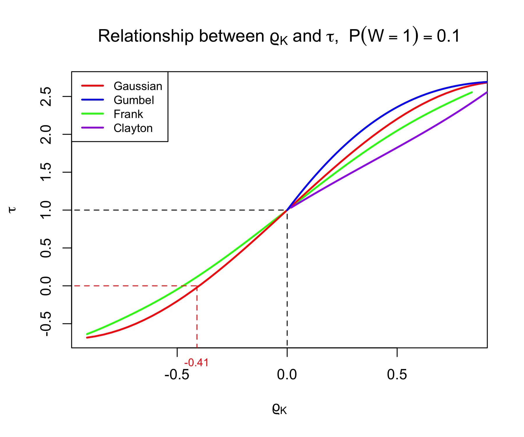
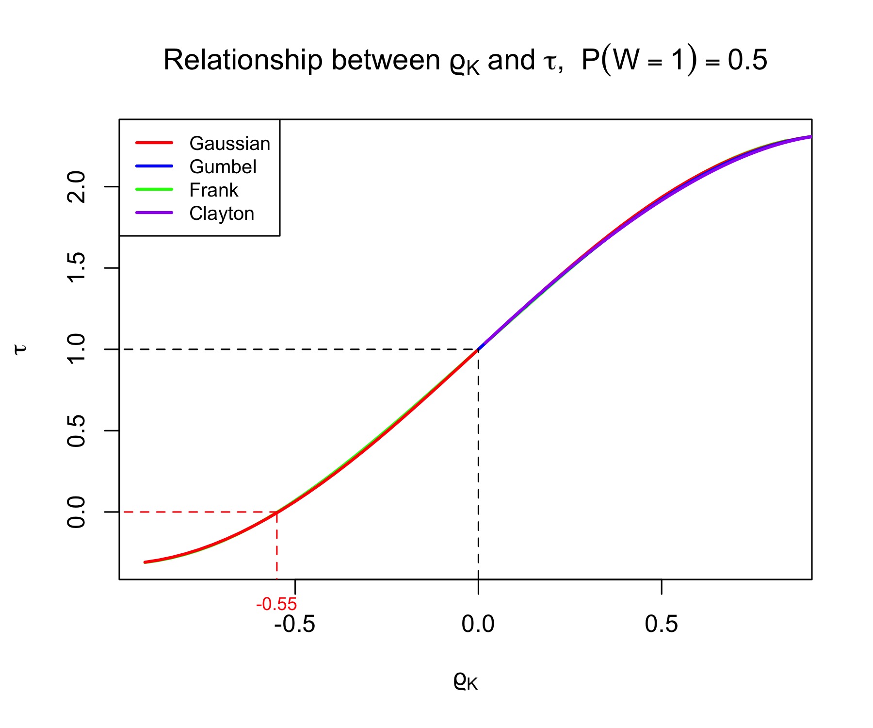
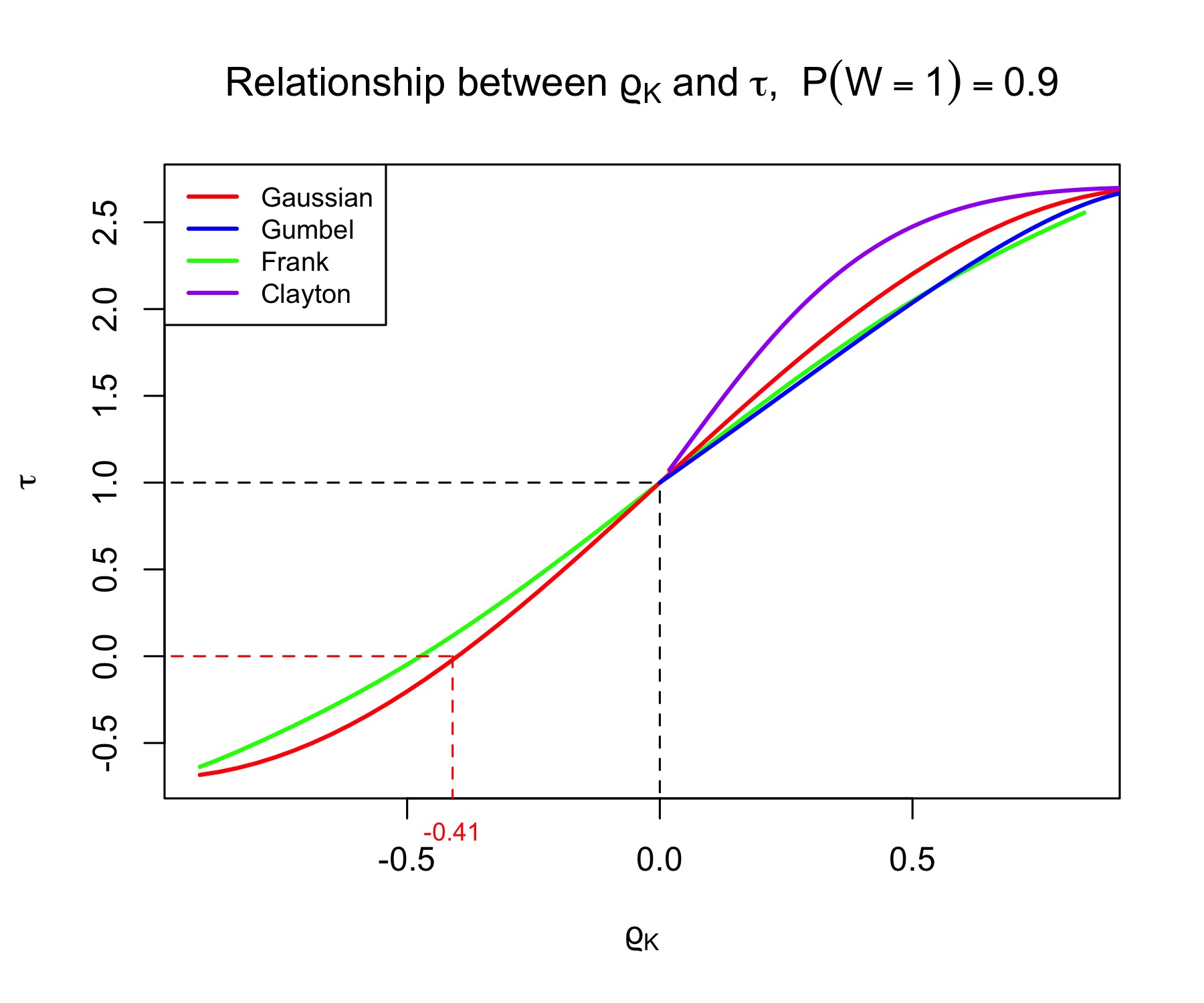
We consider the Gaussian copula and several copulas from the Archimedean family. For simplicity, we assume that the conditional copula is the same as the unconditional copula. For common (bivariate) copulas such as the Gaussian, Clayton, Gumbel, and Frank copulas, the dependency parameter can be expressed in terms of Kendall’s tau $\varrho_{K}$ , a rank-based measure of monotonic dependence. This parameterization makes dependency strength interpretable and comparable across different copula families. Appendix S.1 in the supplementary appendix collects the mapping between $\varrho_{K}$ and $\vartheta$ for the aforementioned copulas.

For illustration, consider the following data generating process for both the experimental and observational data samples:

X_{i}\sim U[0,1],\quad W_{i}\sim Bernoulli(\rho),\quad S_{i}=X_{i}+W_{i}+\eta_{i}^{S},\text{ where }\eta_{i}^{S}\sim\mathcal{N}(0,1),

Y_{i}=S_{i}+0.5X_{i}+\eta_{i}^{Y},\text{ where }\eta_{i}^{Y}\sim\mathcal{N}(0,1).

We investigate $\rho\in\{0.1,0.5,0.9\}$ . Following Assumption 3.1, $W_{i}|S_{i},X_{i}=I\{\epsilon_{i}>1-\rho(S_{i},X_{i})\}$ , where $\epsilon_{i}|S_{i},X_{i},P_{i}=E\sim U[0,1]$ , and the copula structure is for $\epsilon_{i}$ and $\eta_{i}^{Y}$ , independent of $S_{i},X_{i}$ . More specifically, we set $C_{o}(u,v;\vartheta|S_{i},X_{i},P_{i}=E)=C_{o}(u,v;\vartheta|P_{i}=E)$ , for $C_{o}(u,v;\vartheta|P_{i}=E)$ being the Gaussian, Clayton, Gumbel, and Frank copulas. For each copula family, we solve for $\vartheta$ for each $\varrho_{K}$ in the corresponding grid of appropriate $\varrho_{K}$ values. Note that the Clayton copula is more commonly used to model positive dependence, while the Gumbel copula exclusively models positive dependence. Therefore, the range of $\varrho_{K}$ is adjusted to ensure the corresponding $\vartheta$ falls within its valid range.

In Figure 1, we plot how $\tau_{C_{o}}$ in Theorem 3.1 changes with $\varrho_{K}$ , with computational details in Appendix S.1. Consistent with the DGP, Figure 1 shows that for any $\rho\in(0,1)$ , if $C_{o}(u,v;\vartheta\mid P_{i}=E)$ is the independence copula ( $\varrho_{K}=0$ ), the true long-term ATE is $\tau_{\Pi}=1$ . The surrogacy bias $\tau_{C_{o}}-\tau_{\Pi}$ increases in magnitude as $|\varrho_{K}|$ increases. When $\rho=0.5$ , the threshold for $\tau$ to change sign is $\varrho_{K}\approx-0.55$ , which is consistent across the copulas considered here that allow for negative dependence (Gaussian and Frank). In other words, if the negative dependence between $W$ and $Y$ is strong enough with Kendall’s tau smaller than $-0.55$ , assuming an independence copula will produce the wrong sign for the long-term ATE. For $\rho=0.1$ or $0.9$ , the same threshold for the Gaussian copula is around $-0.41$ . Note that the form of the copula is not crucial for $\rho=0.5$ . This is intuitive because values of $\rho(s,x)$ tend to be around $0.5$ as well, making the conditional dependence $C_{o}(1-\rho(s,x)|u)$ in $\sigma_{C_{o},1}(\cdot;\cdot)$ relatively insensitive to the copula family. In contrast, when $\rho$ takes more extreme values like $0.1$ or $0.9$ , differences in tail dependence across copula families lead to more pronounced variation in conditional behavior, thereby affecting $\tau_{C_{o}}$ . In general, in a randomized controlled trial with relatively balanced treatment and control groups, if $S$ depends only weakly on $W$ (i.e., $S$ carries limited information about $W$ ), the choice of copula serves mainly as a functional tool for achieving the desired dependence level, while $\varrho_{K}$ captures the essential dependence information relevant for $\tau_{C_{o}}$ .

Refer to caption — Figure 1: Relationship between Kendall’s tau $(\varrho_{K})$ and $\tau$ given $\rho\in\{0.1,0.5,0.9\}$ for the Gaussian, Clayton, Gumbel, and Frank copulas.

4 Worst-Case Bounds, Debiased Estimation, and Inference

In practice, the copula $C_{o}$ is rarely known. Section 3.4 provides a numerical illustration of the application of Theorem 3.1 to check sensitivity of $\tau_{\Pi}$ to the violation of the surrogacy assumption by letting the copula $C_{o}$ deviate from the independence copula. Theorem 3.1 can also be used to establish sharp bounds on $\tau_{C_{o}}$ when $C_{o}$ is unknown but lies between two known copulas.

The following corollary follows immediately from Theorem 3.1 and Proposition 3.2.

Corollary 4.1 (Identified Set).

Suppose Assumption 2.1, Assumption 2.2, and Assumption 2.4 hold. Furthermore, suppose the copula $C_{o}$ satisfies $C_{L}(\cdot,\cdot|s,x,E)\prec_{c}C_{o}(\cdot,\cdot|s,x,E)\prec_{c}C_{U}(\cdot,\cdot|s,x,E)$ for almost all $(s,x)\in\mathcal{S}\otimes\mathcal{X}$ , where $C_{L}(\cdot,\cdot|s,x,E)$ and $C_{U}(\cdot,\cdot|s,x,E)$ are two known copula functions. Then $\tau_{C_{o}}$ is partially identified with the identified set $[\tau_{C_{L}},\tau_{C_{U}}]$ . When the conditional distribution of $Y_{i}$ given $S_{i},X_{i},P_{i}=O$ is degenerate, the identified set is singleton: $\tau_{C_{L}}=\tau_{C_{U}}=\tau_{\Pi}$ .

Corollary 4.1 implies that the worst case bounds on $\tau_{C_{o}}$ are $\tau_{C_{-}}$ and $\tau_{C_{+}}$ . As a result, $\tau_{C_{-}}$ can be interpreted as the smallest ATE when the surrogacy assumption fails. Conversely, $\tau_{C_{+}}$ is the largest ATE when the surrogacy assumption fails. Another implication is that the ATE under the surrogacy assumption in Athey et al. (2025b) is the least ATE among copulas dominating the independence copula in concordance order. It is also the greatest ATE among copulas dominated by the independence copula in concordance order.

4.1 Comparison with Lemma 1 in Athey et al. (2025b)

We restate the expressions for $\tau_{C_{-}},\tau_{C_{+}}$ in the following proposition which also shows that they are the same as Lemma 1 (ii) in Athey et al. (2025b) for binary outcomes.

Proposition 4.1.

Suppose Assumption 2.1, Assumption 2.2, and Assumption 2.4 hold. Then the identified set of $\tau_{C_{o}}$ is $[\tau_{C_{-}},\tau_{C_{+}}]$ , where $\tau_{C_{-}},\tau_{C_{+}}\in\mathbb{R}$ are given by

	$\displaystyle\tau_{C_{-}}$	$\displaystyle=\mathbb{E}\left[\mu_{C_{-},1}(S_{i},X_{i},O)\frac{W_{i}}{\rho(X_{i})}\mid P_{i}=E\right]-\mathbb{E}\left[\mu_{C_{-},0}(S_{i},X_{i},O)\left(\frac{1-W_{i}}{1-\rho(X_{i})}\right)\mid P_{i}=E\right],$
	$\displaystyle\tau_{C_{+}}$	$\displaystyle=\mathbb{E}\left[\mu_{C_{+},1}(S_{i},X_{i},O)\frac{W_{i}}{\rho(X_{i})}\mid P_{i}=E\right]-\mathbb{E}\left[\mu_{C_{+},0}(S_{i},X_{i},O)\left(\frac{1-W_{i}}{1-\rho(X_{i})}\right)\mid P_{i}=E\right],$

in which

	$\displaystyle\mu_{C_{-},0}(S_{i},X_{i},O)$	$\displaystyle=AVaR_{\rho(X_{i},S_{i})}(Y_{i}\mid S_{i},X_{i},P_{i}=O),$
	$\displaystyle\mu_{C_{-},1}(S_{i},X_{i},O)$	$\displaystyle=-AVaR_{1-\rho(X_{i},S_{i})}(-Y_{i}\mid S_{i},X_{i},P_{i}=O),$
	$\displaystyle\mu_{C_{+},1}(S_{i},X_{i},O)$	$\displaystyle=AVaR_{1-\rho(X_{i},S_{i})}(Y_{i}\mid S_{i},X_{i},P_{i}=O),\mbox{ and }$
	$\displaystyle\mu_{C_{+},0}(S_{i},X_{i},O)$	$\displaystyle=-AVaR_{\rho(X_{i},S_{i})}(-Y_{i}\mid S_{i},X_{i},P_{i}=O).$

When the outcome is binary, the identified set $[\tau_{C_{-}},\tau_{C_{+}}]$ is the same as Lemma 1 (ii) in Athey et al. (2025b).

Proposition 4.1 implies that the ATE is partially identified regardless of the outcome type/range and for binary outcomes. The identified interval in Proposition 4.1 is the same as that in Lemma 1 (ii) in Section 5.2 of Athey et al. (2025b). However, it differs from Lemma 1 (i) in Section 5.2 of Athey et al. (2025b) which states that “If the outcome can take on values on the whole real line, then there is no value for the average treatment effect $\tau$ that can be ruled out.” Their proof seems to have ignored the fact that $F_{Y}(\cdot\mid s,x,E)$ is identified from $F_{Y}(\cdot\mid s,x,O)$ under Assumption 2.4. In contrast, our proof makes use of the identified $F_{Y}(\cdot\mid s,x,E)$ and the following expression for $\mu_{C_{o},1}(S_{i},X_{i},O)$ in Eq. 3.3:

\displaystyle\mu_{C_{o},1}(s,x,O)=\frac{1}{\rho(s,x)}\int\int ywdC_{o}(F_{Y}(y|s,x,E),F_{W}(w|s,x,E)|s,x,E).

Since both $F_{Y}(y|s,x,E)$ and $F_{W}(w|s,x,E)$ are point identified, Theorem 1 of Cambanis et al. (1976) implies that $\mu_{C_{o},1}(s,x,O)$ is partially identified.

4.2 Debiased Estimation

Athey et al. (2025b) and Chen and Ritzwoller (2023) develop debiased estimation of $\tau_{\Pi}$ for which WSIs reduce to the SI $\mu(S_{i},X_{i},O)=\mathbb{E}\left(Y_{i}\mid S_{i},X_{i},P_{i}=O\right)$ . For the worst-case bounds, the WSIs are related to conditional AVaR of $Y_{i}$ instead of the conditional mean of $Y_{i}$ and also depend on the surrogacy score $\rho(S_{i},X_{i})$ . As a result, it is more challenging to derive the orthogonal moment functions for the worst-case bounds $\tau_{C_{+}}$ and $\tau_{C_{-}}$ .

To proceed, we make use of the dual representations of the worst-case WSIs in terms of conditional means of the following newly defined functions:

\displaystyle H_{U}(Y_{i},s,\alpha):=s+\frac{1}{\alpha}\left(Y_{i}-s\right)_{+}\mbox{ and }H_{L}(Y_{i},s,\alpha):=s-\frac{1}{\alpha}\left(Y_{i}-s\right)_{-}.

Specifically, from the dual form of AVaR (c.f., Rockafellar and Uryasev (2002) and Acerbi and Tasche (2002)), it follows that

	$\displaystyle\mu_{C_{-},0}(S_{i},X_{i},O)$	$\displaystyle=\mathbb{E}[H_{U}(Y_{i},q_{C_{-}}(S_{i},X_{i},O),1-\rho(S_{i},X_{i}))\mid S_{i},X_{i},P_{i}=O],$
	$\displaystyle\mu_{C_{-},1}(S_{i},X_{i},O)$	$\displaystyle=\mathbb{E}[H_{L}(Y_{i},q_{C_{-}}(S_{i},X_{i},O),\rho(S_{i},X_{i}))\mid S_{i},X_{i},P_{i}=O],$
	$\displaystyle\mu_{C_{+},0}(S_{i},X_{i},O)$	$\displaystyle=\mathbb{E}[H_{L}(Y_{i},q_{C_{+}}(S_{i},X_{i},O),1-\rho(S_{i},X_{i}))\mid S_{i},X_{i},P_{i}=O],$
	$\displaystyle\mu_{C_{+},1}(S_{i},X_{i},O)$	$\displaystyle=\mathbb{E}[H_{U}(Y_{i},q_{C_{+}}(S_{i},X_{i},O),\rho(S_{i},X_{i}))\mid S_{i},X_{i},P_{i}=O],$

where

	$\displaystyle q_{C_{+}}(S_{i},X_{i},O)$	$\displaystyle:=F_{Y}^{-1}(1-\rho(X_{i},S_{i})\|S_{i},X_{i},O)\mbox{ and}$
	$\displaystyle q_{C_{-}}(S_{i},X_{i},O)$	$\displaystyle:=F_{Y}^{-1}(\rho(X_{i},S_{i})\|S_{i},X_{i},O).$

Let $\varphi(x):=\mathbb{P}(P_{i}=E|X_{i}=x)$ , $\varphi:=\mathbb{P}(P_{i}=E)$ , and for $w=0,1$ ,

	$\displaystyle\bar{\mu}_{C_{+},w}$	$\displaystyle:=\mathbb{E}[\mu_{C_{+},w}(S_{i},X_{i},O)\|W_{i}=w,X_{i},P_{i}=E]\mbox{ and}$
	$\displaystyle\bar{\mu}_{C_{-},w}$	$\displaystyle:=\mathbb{E}[\mu_{C_{-},w}(S_{i},X_{i},O)\|W_{i}=w,X_{i},P_{i}=E].$

Finally, let $\eta$ denote the collection of all the nuisance functions, i.e.,

\displaystyle\eta

\displaystyle=(\mu_{C_{-},0},\mu_{C_{-},1},\mu_{C_{+},0},\mu_{C_{+},1},\bar{\mu}_{C_{-},0},\bar{\mu}_{C_{-},1},\bar{\mu}_{C_{+},0},\bar{\mu}_{C_{+},1},q_{C_{+}},q_{C_{-}},\rho(s,x),\rho(x),\varphi(x),\varphi(s,x),\varphi).

Then $\tau_{C_{+}}$ satisfies the moment condition: $\mathbb{E}[m_{C_{+}}(Z_{i},\tau_{C_{+}},\eta)]=0,$ where

	$\displaystyle m_{C_{+}}(Z_{i},\tau_{C_{+}},\eta)$
	$\displaystyle=\frac{\mathds{1}_{P_{i}=E}}{\varphi}\Bigg[\frac{W_{i}}{\rho(X_{i})}(\mu_{C_{+},1}(S_{i},X_{i},O)-\bar{\mu}_{C_{+},1}(1,X_{i}))-\frac{1-W_{i}}{1-\rho(X_{i})}(\mu_{C_{+},0}(S_{i},X_{i},O)-\bar{\mu}_{C_{+},0}(0,X_{i}))\Bigg]$
	$\displaystyle\quad+\frac{\mathds{1}_{P_{i}=E}}{\varphi}(\bar{\mu}_{C_{+},1}(1,X_{i})-\bar{\mu}_{C_{+},0}(0,X_{i})-\tau_{C_{+}})$
	$\displaystyle\quad+\frac{\mathds{1}_{P_{i}=O}}{\varphi}\frac{\varphi(S_{i},X_{i})}{1-\varphi(S_{i},X_{i})}\Bigg[\frac{\rho(S_{i},X_{i})}{\rho(X_{i})}(H_{U}(Y_{i},q_{C_{+}}(S_{i},X_{i},O),\rho(S_{i},X_{i}))-\mu_{C_{+},1}(S_{i},X_{i},O))$
	$\displaystyle\quad\quad\quad-\frac{1-\rho(S_{i},X_{i})}{1-\rho(X_{i})}(H_{L}(Y_{i},q_{C_{+}}(S_{i},X_{i},O),1-\rho(S_{i},X_{i}))-\mu_{C_{+},0}(S_{i},X_{i},O))\Bigg]$
	$\displaystyle\quad+\frac{\mathds{1}_{P_{i}=E}}{\varphi}\frac{1}{\rho(X_{i})}\left[q_{C_{+}}(S_{i},X_{i},O)-\mu_{C_{+},1}(S_{i},X_{i},O)\right]\left(W_{i}-\rho(S_{i},X_{i})\right)$
	$\displaystyle\quad+\frac{\mathds{1}_{P_{i}=E}}{\varphi}\frac{1}{1-\rho(X_{i})}\left[q_{C_{+}}(S_{i},X_{i},O)-\mu_{C_{+},0}(S_{i},X_{i},O)\right]\left(W_{i}-\rho(S_{i},X_{i})\right).$

The first three terms in the orthogonal moment function $m_{C_{+}}$ are analogous to those in Equation (4.4) of Athey et al. (2025b) and Theorem 3.1 of Chen and Ritzwoller (2023), and the last two terms are new and correct for the effect of estimating $\rho(S_{i},X_{i})$ in the dual representations of the WSIs.

Similarly, $\tau_{C_{-}}$ satisfies: $\mathbb{E}[m_{C_{-}}(Z_{i},\tau_{C_{-}},\eta)]=0,$ where

	$\displaystyle m_{C_{-}}(Z_{i},\tau_{C_{-}},\eta)$
	$\displaystyle=\frac{\mathds{1}_{P_{i}=E}}{\varphi}\Bigg[\frac{W_{i}}{\rho(X_{i})}(\mu_{C_{-},1}(S_{i},X_{i},O)-\bar{\mu}_{C_{-},1}(1,X_{i}))-\frac{1-W_{i}}{1-\rho(X_{i})}(\mu_{C_{-},0}(S_{i},X_{i},O)-\bar{\mu}_{C_{-},0}(0,X_{i}))\Bigg]$
	$\displaystyle\quad+\frac{\mathds{1}_{P_{i}=E}}{\varphi}(\bar{\mu}_{C_{-},1}(1,X_{i})-\bar{\mu}_{C_{-},0}(0,X_{i})-\tau_{C_{-}})$
	$\displaystyle\quad+\frac{\mathds{1}_{P_{i}=O}}{\varphi}\frac{\varphi(S_{i},X_{i})}{1-\varphi(S_{i},X_{i})}\Bigg[\frac{\rho(S_{i},X_{i})}{\rho(X_{i})}(H_{L}(Y_{i},q_{C_{-}}(S_{i},X_{i},O),\rho(S_{i},X_{i}))-\mu_{C_{-},1}(S_{i},X_{i},O))$
	$\displaystyle\quad\quad\quad-\frac{1-\rho(S_{i},X_{i})}{1-\rho(X_{i})}(H_{U}(Y_{i},q_{C_{-}}(S_{i},X_{i},O),1-\rho(S_{i},X_{i}))-\mu_{C_{-},0}(S_{i},X_{i},O))\Bigg]$
	$\displaystyle\quad+\frac{\mathds{1}_{P_{i}=E}}{\varphi}\frac{1}{\rho(X_{i})}\left[q_{C_{-}}(S_{i},X_{i},O)-\mu_{C_{-},1}(S_{i},X_{i},O)\right]\left(W_{i}-\rho(S_{i},X_{i})\right)$
	$\displaystyle\quad+\frac{\mathds{1}_{P_{i}=E}}{\varphi}\frac{1}{1-\rho(X_{i})}\left[q_{C_{-}}(S_{i},X_{i},O)-\mu_{C_{-},0}(S_{i},X_{i},O)\right]\left(W_{i}-\rho(S_{i},X_{i})\right).$

Our debiased estimators $\widehat{\tau}_{C_{-}}$ and $\widehat{\tau}_{C_{+}}$ are defined as the solutions to $\frac{1}{n}\sum_{i=1}^{n}m_{C_{-}}(Z_{i},\tau,\widehat{\eta})=0$ and $\frac{1}{n}\sum_{i=1}^{n}m_{C_{+}}(Z_{i},\tau,\widehat{\eta})=0$ , respectively, where $\widehat{\eta}$ is estimated by cross-fitting over $K$ even folds, which ensures that the nuisance estimators remain independent of the samples to which they are applied (Chernozhukov et al., 2018).

Our orthogonal moment conditions in debiased estimation allow for greater flexibility in estimating nuisance parameters, enabling the use of both parametric regressions and machine learning methods. For example, the estimation of $\rho(x)$ , $\rho(s,x)$ , $\varphi(x)$ , and $\varphi(s,x)$ readily accommodates methods such as Lasso, random forests, gradient boosting, and neural networks. In contrast, estimating the worst-case WSIs ( $\mu_{C_{-},0}$ , $\mu_{C_{-},1}$ , $\mu_{C_{+},0}$ , and $\mu_{C_{+},1}$ ) relies on previously obtained cross-fitted estimates of $\rho(X_{i},S_{i})$ and is more involved due to the computation of conditional AVaRs. We follow the two-stage, locally robust approach of Olma (2021) with our chosen model specifications: the first stage requires estimating a conditional quantile, which we do nonparametrically using quantile forests; the second stage involves fitting a linear sieve model to a generated outcome variable whose derivative with respect to the conditional quantile, evaluated at the truth, is zero. With estimates of the worst-case WSIs as pseudo-outcomes, $\bar{\mu}_{C-,0}$ , $\bar{\mu}_{C-,1}$ , $\bar{\mu}_{C+,0}$ , and $\bar{\mu}_{C+,1}$ can then be estimated either parametrically or nonparametrically. Finally, $q_{C_{+}}$ and $q_{C_{-}}$ are again estimated using quantile forests with cross-fitted $\widehat{\rho}(X_{i},S_{i})$ . More details can be found in Algorithm 1 of Appendix S.1 in the supplementary materials.

4.3 Asymptotic Theory

We adopt conditions similar to those of Chen and Ritzwoller (2023), Dorn et al. (2024), and Semenova (2025) to establish the asymptotic joint normality of $\widehat{\tau}_{C_{-}}$ and $\widehat{\tau}_{C_{+}}$ .

Assumption 4.1 (Regularity Conditions).

(i) For a continuous outcome, we assume that it’s distribution is absolutely continuous with bounded support and conditional density function $f(y|s,x,O)$ that is continuous with respect to y for each $s$ and $x$ , and is uniformly bounded above and below by positive absolute constants; For a binary outcome, we assume that the random variable $\left[\mu(S_{i},X_{i},O)-\rho(S_{i},X_{i})\right]$ has bounded density.

(ii) There exists some absolute constant $t$ such that for each $w\in\{0,1\}$ and $b\in\{C_{-},C_{+}\}$ , either (1) or (2-1, 2-2) holds with probability one:

	$\displaystyle\text{(1) }\mathbb{E}[(\bar{\mu}_{b,1}(1,X_{i})-\bar{\mu}_{b,0}(0,X_{i})-\tau_{b})^{2}\|X_{i},P_{i}=E]>t\text{ or }$
	$\displaystyle\text{(2-1) }\mathrm{Var}\left(\frac{1}{\rho(X_{i})}(Y_{i}-q_{C_{+}}(S_{i},X_{i},O))_{+}+\frac{1}{1-\rho(X_{i})}(Y_{i}-q_{C_{+}}(S_{i},X_{i},O))_{-}\|S_{i},X_{i},O)\right)>t\text{ and }$
	$\displaystyle\text{(2-2) }\mathrm{Var}\left(\frac{1}{1-\rho(X_{i})}(Y_{i}-q_{C_{-}}(S_{i},X_{i},O))_{+}+\frac{1}{\rho(X_{i})}(Y_{i}-q_{C_{-}}(S_{i},X_{i},O)_{-}\|S_{i},X_{i},O)\right)>t.$

The assumption of bounded support of $Y$ and boundedness of the conditional density function in Assumption 4.1 (i) are similar to Semenova (2025). Assumption (1) or (2-1, 2-2) in Assumption 4.1 (ii) ensures that the asymptotic variances of $\tau_{C_{+}}$ and $\tau_{C_{-}}$ are positive.

Assumption 4.2 (Realization Set).

Let $q>2$ be a positive constant and $\epsilon$ be a constant such that $0<\epsilon<1/2$ , $\omega=(\omega_{\rho},\omega_{\varphi})$ with $\omega_{\rho}=(\rho(S_{i},X_{i}),\rho(X_{i})),\mbox{ }\omega_{\varphi}=(\varphi(S_{i},X_{i}),\varphi)$ , and

	$\displaystyle\kappa$	$\displaystyle=(\mu_{C_{+},1}(S_{i},X_{i},O),\mu_{C_{+},0}(S_{i},X_{i},O),\mu_{C_{-},1}(S_{i},X_{i},O),\mu_{C_{-},0}(S_{i},X_{i},O),$
		$\displaystyle\quad\quad\bar{\mu}_{C_{+},1}(1,X_{i}),\bar{\mu}_{C_{+},0}(0,X_{i}),\bar{\mu}_{C_{-},1}(1,X_{i}),\bar{\mu}_{C_{-},0}(0,X_{i}),q_{C_{+}}(S_{i},X_{i},O),q_{C_{-}}(S_{i},X_{i},O)).$

For all probability measures $P$ satisfying Assumptions 2.1, 2.2, and 2.4, the following condition holds; for some sequences $\Delta_{n}\to 0$ and $\delta_{n}\to 0$ with $\delta_{n}\geq n^{-1/2}$ with probability $1-\Delta_{n}$ , the estimator of nuisance parameter belongs to the realization set $R_{n}$ which contains $\widetilde{\eta}$ such that

	$\displaystyle\\|\widetilde{\eta}-\eta\\|_{P,q}\leq C,\mbox{ }\mathbb{P}(\epsilon\leq\widetilde{\rho}(S_{i},X_{i})\leq 1-\epsilon)=1,$
	$\displaystyle\mathbb{P}(\epsilon\leq\widetilde{\varphi}(S_{i},X_{i})\leq 1-\epsilon)=1,\mbox{ }\\|\widetilde{\eta}-\eta\\|_{P,2}\leq\delta_{n},$
	$\displaystyle\\|\widetilde{\omega}-\omega\\|_{P,2}\times\\|\widetilde{\kappa}-\kappa\\|_{P,2}\leq\delta_{n}n^{-1/2},$
	$\displaystyle\\|\widetilde{\omega}_{\rho}-\omega_{\rho}\\|_{P,2}\times\\|\widetilde{\omega}_{\varphi}-\omega_{\varphi}\\|_{P,2}\leq\delta_{n}n^{-1/2},$		(4.1)

and for continuous outcomes,

\displaystyle\|\widetilde{q}_{C_{+}}-q_{C_{+}}\|_{P,2}^{2}\leq\delta_{n}n^{-1/2};

(4.2)

for binary outcomes,

\displaystyle\|\widetilde{\mu}(S_{i},X_{i},O)-\mu(S_{i},X_{i},O)\|_{\infty}\leq\delta_{n},\|\widetilde{\mu}(S_{i},X_{i},O)-\mu(S_{i},X_{i},0)\|_{\infty}^{2}\leq\delta_{n}n^{-1/2}.

Most of the conditions in Assumption 4.2 are similar to those in Chen and Ritzwoller (2023). Since our moment function has additional correction terms for $\rho$ , we impose additional conditions on the rate of the cross-product in Eq. 4.1. Condition (4.2) and conditions for the binary case are similar to Dorn et al. (2024).

Theorem 4.1.

Suppose Assumptions 2.1, 2.2, 2.4, 4.1, and 4.2 hold. Then

\displaystyle\sqrt{n}\begin{pmatrix}\widehat{\tau}_{C_{+}}-\tau_{C_{+}}\\ \widehat{\tau}_{C_{-}}-\tau_{C_{-}}\end{pmatrix}\to N\left(\begin{pmatrix}0\\ 0\end{pmatrix},\begin{pmatrix}\sigma_{C_{+}}^{2}&\rho\sigma_{C_{+}}\sigma_{C_{-}}\\ \rho\sigma_{C_{+}}\sigma_{C_{-}}&\sigma_{C_{-}}^{2}\end{pmatrix}\right),

where $\sigma_{C_{+}}^{2}=\mathbb{E}[m(Z_{i},\tau_{C_{+}},\eta_{0})^{2}]>0$ , $\sigma_{C_{-}}^{2}=\mathbb{E}[m(Z_{i},\tau_{C_{-}},\eta_{0})^{2}]>0$ , and $-1\leq\rho\leq 1$ .

Our proof strategy builds on Chen and Ritzwoller (2023) and Dorn et al. (2024). Departing from Chen and Ritzwoller (2023) which checks the orthogonality condition in Assumption 3.1 and the statistical rate for second-order derivative of moment condition $r_{N}^{\prime}$ in Assumption 3.2 (c) in Chernozhukov et al. (2018), similar to Dorn et al. (2024), we directly verified the following high-level condition in the proof of Theorem 3.1 of Chernozhukov et al. (2018):

\displaystyle\sqrt{n}\|\mathbb{E}[m(W_{i},\tau_{C_{+}},\hat{\eta})|\mathcal{I}_{-k}]-\mathbb{E}[m(W_{i},\tau_{C_{+}},\eta)]\|=o_{p}(1).

Note that this high-level condition is satisfied when both the orthogonality condition in Assumption 3.1 in Chernozhukov et al. (2018) and the statistical rate for second-order derivative of moment condition $r_{N}^{\prime}$ in Assumption 3.2 (c) in Chernozhukov et al. (2018) hold.

Let $V$ denote the asymptotic variance-covariance matrix in Theorem 4.1. That is,

\displaystyle V=\mathbb{E}[(m_{C_{+}}(Z_{i},\tau_{C_{+}},\eta_{0}),m_{C_{-}}(Z_{i},\tau_{C_{-}},\eta_{0}))[(m_{C_{+}}(Z_{i},\tau_{C_{+}},\eta_{0}),m_{C_{-}}(Z_{i},\tau_{C_{-}},\eta_{0}))]^{\top}].

We provide a consistent estimator of $V$ by following Theorem 3.2 in Chernozhukov et al. (2018).

Theorem 4.2.

Suppose Assumptions 2.1, 2.2, 2.4, 4.1, and 4.2 hold. In addition, we assume that $\delta_{n}\geq n^{-[((1-2/q)\wedge 1/2]}$ for all $n\geq 1$ . Then, $V$ can be consistently estimated by

\displaystyle\frac{1}{K}\sum_{k=1}^{K}\mathbb{E}_{r,k}[(m_{C_{+}}(Z_{i},\hat{\tau}_{C_{+}},\hat{\eta}_{k}),m_{C_{-}}(Z_{i},\hat{\tau}_{C_{-}},\hat{\eta}_{k}))(m_{C_{+}}(Z_{i},\hat{\tau}_{C_{+}},\hat{\eta}_{k}),m_{C_{-}}(Z_{i},\hat{\tau}_{C_{-}},\hat{\eta}_{k}))^{\top}],

where $K$ is the number of folds in K-fold cross-fitting, and $r:=[n/K]$ is the number of observations in each fold, and $E_{r,k}$ is operator for sample expectation from empirical data in $k$ -the fold, i.e., $E_{r,k}[g(X_{i})]=r^{-1}\sum_{i\in\mathcal{F}_{k}}g(X_{i})$ where $\mathcal{F}_{k}$ is the $k$ -th fold of indices $\{1,\dotsc,n\}$ .

Wald inference on each bound is straightfoward and inference on the true ATE can be carried out by applying the misspecification-adaptive confidence interval in Stoye (2020) which allows for the covariance matrix to be degenerate.

5 Debiased Estimation and Inference—General Copula

The debiased estimators of $\tau_{C_{+}}$ and $\tau_{C_{-}}$ constructed in Section 4.2 rely critically on the dual representations of the WSIs (associated with $C_{+}$ and $C_{-}$ ) obtained from the existing dual representation of AVaR.

For a general copula $C_{o}$ , we establish dual representation for $r$ introduced in Remark 3.1 when $\sigma$ is of bounded variation in Lemma 5.1 below. Our proof builds on the proof of Pichler (2015) and Section 2.4.2. in Pflug and Römisch (2007) for non-decreasing function $\sigma(\cdot)$ and the dual representation for AVaR.

Lemma 5.1.

Assume that $Y$ is bounded and $\sigma(u)$ is of bounded variation on [0, 1]. Then,

	$\displaystyle r$	$\displaystyle=\sigma(0)\mathbb{E}[Y]+\int_{0}^{1}\left((1-u)F_{Y}^{-1}(u)+\mathbb{E}[[Y-F_{Y}^{-1}(u)]_{+}]\right)d\sigma(u)$		(5.1)
		$\displaystyle=\sigma(1)\mathbb{E}[Y]-\int_{0}^{1}\left(uF_{Y}^{-1}(u)-\mathbb{E}[[Y-F_{Y}^{-1}(u)]_{-}]\right)d\sigma(u).$		(5.2)

Lemma 5.1 extends the dual representation for AVaR to $r$ with a general weight function $\sigma$ . However, in contrast to AVaR for which $F_{Y}^{-1}(u)\in\operatorname{\mathop{\mathrm{argmin}}}_{G}\{(1-u)G(u)+\mathbb{E}[[Y-G(u)]_{+}\}$ , $F_{Y}^{-1}$ may not be an argmin of the following minimization problem:

\displaystyle\min_{G}\int_{0}^{1}\left((1-u)G(u)+\mathbb{E}[[Y-G(u)]_{+}]\right)d\sigma(u).

(5.3)

This is because the sign of the second-order derivative may not be positive in the minimization problem (5.3).

5.1 Orthogonal Moment Function and Debiased Estimator

We construct a debiased estimator of $\tau_{C_{o}}$ from the dual representation in Lemma 5.1 under the following assumption.

Assumption 5.1.

The outcome variable is continuous variable, and it has a bounded support. In addition, $C_{o}(\alpha|\cdot)$ is of bounded variation.

Lemma 5.1 implies that under Assumption 5.1,

	$\displaystyle\mu_{C_{o},1}(S_{i},X_{i},O)$	$\displaystyle=\mathbb{E}[h_{C_{o},1}(Y_{i};F_{Y}^{-1}(\cdot\|S_{i},X_{i},O),1-\rho(S_{i},X_{i}))\|S_{i},X_{i},P_{i}=O]\mbox{ and}$
	$\displaystyle\mu_{C_{o},0}(S_{i},X_{i},O)$	$\displaystyle=\mathbb{E}[h_{C_{o},0}(Y_{i};F_{Y}^{-1}(\cdot\|S_{i},X_{i},O),1-\rho(S_{i},X_{i}))\|S_{i},X_{i},P_{i}=O],$		(5.4)

where

	$\displaystyle h_{C_{o},1}(Y_{i};F_{Y}^{-1}(\cdot\|S_{i},X_{i},O),1-\rho(S_{i},X_{i}))$
	$\displaystyle=\sigma_{C_{o},1}(0;1-\rho(S_{i},X_{i}))Y_{i}$
	$\displaystyle+\int_{0}^{1}\left((1-u)F_{Y}^{-1}(u\|S_{i},X_{i},O)+\left[Y_{i}-F_{Y}^{-1}(u\|S_{i},X_{i},O)\right]_{+}\right)d\sigma_{C_{o},1}(u;1-\rho(S_{i},X_{i}))\mbox{ and}$
	$\displaystyle h_{C_{o},0}(Y_{i};F_{Y}^{-1}(\cdot\|S_{i},X_{i},O),1-\rho(S_{i},X_{i}))$
	$\displaystyle=\sigma_{C_{o},0}(1;1-\rho(S_{i},X_{i}))Y_{i}$
	$\displaystyle-\int_{0}^{1}\left(uF_{Y}^{-1}(u\|S_{i},X_{i},O)-\left[Y-F_{Y}^{-1}(u\|S_{i},X_{i},O)\right]_{-}\right)d\sigma_{C_{o},0}(u;1-\rho(S_{i},X_{i})).$

Similar to orthogonal moment functions in the worst case bounds in Section 4.2, we construct the following orthogonal moment function for a general $C_{o}$ using the dual representation of the WSIs in Section 5.1:

	$\displaystyle m_{C_{o}}(Z_{i},\tau,\eta)$		(5.5)
	$\displaystyle=\frac{\mathds{1}_{P_{i}=E}}{\varphi}\Bigg[\frac{W_{i}}{\rho(X_{i})}(\mu_{C_{o},1}(S_{i},X_{i},O)-\bar{\mu}_{C_{o},1}(1,X_{i}))-\frac{1-W_{i}}{1-\rho(X_{i})}(\mu_{C_{o},0}(S_{i},X_{i},O)-\bar{\mu}_{C_{o},0}(0,X_{i}))\Bigg]$
	$\displaystyle\quad+\frac{\mathds{1}_{P_{i}=E}}{\varphi}(\bar{\mu}_{C_{o},1}(1,X_{i})-\bar{\mu}_{C_{o},0}(0,X_{i})-\tau)$
	$\displaystyle\quad+\frac{\mathds{1}_{P_{i}=O}}{\varphi}\frac{\varphi(S_{i},X_{i})}{1-\varphi(S_{i},X_{i})}\Bigg[\frac{\rho(S_{i},X_{i})}{\rho(X_{i})}(h_{C_{o},1}(Y_{i},F_{Y}^{-1}(\cdot\|S_{i},X_{i},O),1-\rho(S_{i},X_{i}))-\mu_{C_{o},1}(S_{i},X_{i},O))$
	$\displaystyle\quad\quad\quad-\frac{1-\rho(S_{i},X_{i})}{1-\rho(X_{i})}(h_{C_{o},0}(Y_{i},F_{Y}^{-1}(\cdot\|S_{i},X_{i},O),1-\rho(S_{i},X_{i}))-\mu_{C_{o},0}(S_{i},X_{i},O))\Bigg]$
	$\displaystyle\quad+\frac{\mathds{1}_{P_{i}=E}}{\varphi}\frac{1}{\rho(X_{i})}(d_{C_{o}}(S_{i},X_{i})-\mu_{C_{o},1}(S_{i},X_{i},O))\left(W_{i}-\rho(S_{i},X_{i})\right)$
	$\displaystyle\quad+\frac{\mathds{1}_{P_{i}=E}}{\varphi}\frac{1}{1-\rho(X_{i})}(d_{C_{o}}(S_{i},X_{i})-\mu_{C_{o},0}(S_{i},X_{i},O))\left(W_{i}-\rho(S_{i},X_{i})\right),$		(5.6)

where

	$\displaystyle\eta$	$\displaystyle=(F_{Y}^{-1}(\cdot\|S_{i},X_{i},O),\rho(S_{i},X_{i}),\rho(X_{i}),\varphi,\varphi(S_{i},X_{i}),$
		$\displaystyle\mu_{C_{o},1}(S_{i},X_{i},O),\bar{\mu}_{C_{o},1}(1,X_{i}),\mu_{C_{o},0}(S_{i},X_{i},O),\bar{\mu}_{C_{o},0}(0,X_{i}),d_{C_{o}}).$

in which

	$\displaystyle\bar{\mu}_{C_{o},w}(w,X_{i})$	$\displaystyle=\mathbb{E}[\mu_{C_{o},w}(S_{i},X_{i},O)\|W_{i}=w,X_{i},P_{i}=E]\mbox{ and}$
	$\displaystyle d_{C_{o}}(S_{i},X_{i})$	$\displaystyle=\int_{0}^{1}F_{Y}^{-1}(u\|S_{i},X_{i},O)c_{o}(1-\rho(S_{i},X_{i})\|u)du.$

5.2 Asymptotic Theory

Assumption 5.2 (Regularity Conditions).

(i) There exists some absolute constant $t$ such that with probability 1, either (1) or (2) holds:

	$\displaystyle\textrm{(1) }\mathbb{E}[(\bar{\mu}_{C_{o},1}(1,X_{i})-\bar{\mu}_{C_{o},0}(0,X_{i})-\tau_{C_{o}})^{2}\|X_{i},P_{i}=E]>t;$
	$\displaystyle\textrm{(2) }\mathrm{Var}\left(\frac{\rho(S_{i},X_{i})}{\rho(X_{i})}h_{C_{o},1}(Y_{i},F_{Y}^{-1},1-\rho(S_{i},X_{i}))-\frac{1-\rho(S_{i},X_{i})}{1-\rho(X_{i})}h_{C_{o},0}(Y_{i},F_{Y}^{-1},1-\rho(S_{i},X_{i})\Big\|S_{i},X_{i},O)\right)>t.$

(ii) $C_{o}(\alpha|u)$ is continuously twice differentiable with respect to $u,\alpha$ , and

\displaystyle\sup_{\alpha\in[\epsilon,1-\epsilon],u\in[0,1]}\left|\frac{\partial C_{o}(\alpha|u)}{\partial u}\right|,\sup_{\alpha\in[\epsilon,1-\epsilon],u\in[0,1]}\left|\frac{\partial c_{o}(\alpha|u)}{\partial u}\right|,\sup_{\alpha\in[\epsilon,1-\epsilon],u\in[0,1]}\left|\frac{\partial^{2}c_{o}(\alpha|u)}{\partial\alpha\partial u}\right|,

$\sup_{\alpha\in[\epsilon,1-\epsilon],u\in[0,1]}|c_{o}(\alpha|u)|$ , and $\sup_{\alpha\in[\epsilon,1-\epsilon],u\in[0,1]}\left|\frac{\partial c_{o}(\alpha|u)}{\partial\alpha}\right|$ are all bounded from above by absolute positive constant for some $\epsilon>0$ .

The conditions in Assumption 5.2 (i) are identical to those in Assumption 4.1 (ii): Condition (2) in Assumption 5.2 (ii) is reduced to Condition (2) in Assumption 4.1 (ii) when $C_{o}$ is $C_{+}$ or $C_{-}$ . The conditions in Assumption 5.2 (iii) imply that $C_{o}(\alpha|u)$ and $c_{o}(\alpha|u)$ are absolute continuous with respect to $u$ so Lemma 5.1 is applicable.

Assumption 5.3 (Realization Set).

Let $q>2$ be a constant and $\epsilon$ be a constant such that $0<\epsilon<1/2$ , $\omega=(\omega_{\rho},\omega_{\varphi})$ in which $\omega_{\rho}=(\rho(S_{i},X_{i}),\rho(X_{i})),\omega_{\varphi}=(\varphi(S_{i},X_{i}),\varphi)$ , and

\displaystyle\kappa=(\mu_{C_{o},1},\bar{\mu}_{C_{o},1},\mu_{C_{o},0},\bar{\mu}_{C_{o},0},d_{C_{o}}(S_{i},X_{i},O),F_{Y}^{-1}(\cdot|S_{i},X_{i},O)).

and $\eta=(\omega,\kappa)$ . For all $P$ satisfying Assumptions 2.1, 2.2, and 2.4, the following condition holds: for some sequences $\Delta_{n}\to 0$ and $\delta_{n}\to 0$ with $\delta_{n}\geq n^{-1/2}$ with probability $1-\Delta_{n}$ , the estimator of nuisance parameter belongs to the realization set $R_{n}$ which contains $\widetilde{\eta}$ such that

	$\displaystyle\\|\widetilde{\eta}-\eta\\|_{P,q}\leq C,\mathbb{P}(\epsilon\leq\widetilde{\rho}(S_{i},X_{i})\leq 1-\epsilon)=1,\mathbb{P}(\epsilon\leq\widetilde{\varphi}(S_{i},X_{i})\leq 1-\epsilon)=1,$
	$\displaystyle\\|\widetilde{\omega}_{\rho}-\omega_{\rho}\\|_{P,2}\times\\|\widetilde{\omega}_{\varphi}-\omega_{\varphi}\\|_{P,2}\leq\delta_{n}n^{-1/2},\\|\hat{\omega}-\omega\\|_{P,2}\times\\|\hat{\kappa}-\kappa\\|_{P,2}\leq\delta_{n}n^{-1/2},$
	$\displaystyle\\|\widetilde{\rho}(S_{i},X_{i})-\rho(S_{i},X_{i})\\|_{P,2}^{2}\leq\delta_{n}n^{-1/2},$
	$\displaystyle\\|\widetilde{F}_{Y}^{-1}(\cdot\|S_{i},X_{i},O)-F_{Y}^{-1}(\cdot\|S_{i},X_{i},O)\\|_{P,2}^{2}\leq\delta_{n}n^{-1/2}.$

Here, with abuse of notation, we denote the $L_{q}$ norm of a function of the form of $G(u|S_{i},X_{i})$ where $u\in[0,1]$ by $\|G(\cdot|S_{i},X_{i})\|_{P,q}=\left(\mathbb{E}[\int_{0}^{1}G^{q}(u|S_{i},X_{i})du]\right)^{1/q}$ .

We verify conditions related to Theorem 3.1 in Chernozhukov et al. (2018). In particular, we verify Lemma B.1 in the appendix.

Theorem 5.1.

Under Assumptions 2.1, 2.2, 2.4, 3.1, 5.1, Assumption 4.1 (i), 5.2, and 5.3, $\sqrt{n}(\widehat{\tau}_{C_{o}}-\tau_{C_{o}})\to N(0,\sigma_{C_{o}}^{2})$ , where $\sigma_{C_{o}}^{2}=\mathbb{E}[m(Z_{i},\tau_{C_{0}},\eta)^{2}]$ .

Remark 5.1.

(i) When $C_{o}$ is known, Wald inference can be constructed from Theorem 5.1.

(ii) Suppose $C_{o}$ is unknown and satisfies $C_{L}(\cdot,\cdot|s,x,E)\prec_{c}C_{o}(\cdot,\cdot|s,x,E)\prec_{c}C_{U}(\cdot,\cdot|s,x,E)$ for almost all $(s,x)\in\mathcal{S}\otimes\mathcal{X}$ , where $C_{L}(\cdot,\cdot|s,x,E)$ and $C_{U}(\cdot,\cdot|s,x,E)$ are two known copula functions. Then Corollary 4.1 implies that $\tau_{C_{o}}$ is partially identified with the identified set $[\tau_{C_{L}},\tau_{C_{U}}]$ . Theorem 5.1 can be extended to the joint asymptotic normality of $(\widehat{\tau}_{C_{L}},\widehat{\tau}_{C_{U}})$ and inference for $\tau_{C_{o}}$ can be done in the same way as in Section 4.

6 Empirical Application

In the same spirit as Section 3.4, this section presents results from a sensitivity analysis using the household poverty alleviation dataset used in Banerjee et al. (2015). In this data set, the treatment program allocated productive assets to randomly selected households. The baseline variables are welfare-related measurements taken before treatment. The short-term outcomes consist of the same set of measurements taken two years after treatment, while the long-term outcome is one of these measurements recorded three years after treatment. We take the data from Pakistan, which has 446 treated units and 408 control units. For illustrative purposes, consider $X$ and $S$ to include the following five welfare indicators: per capita consumption, the food security index, the household asset index, the total amount borrowed, and agricultural income. The long-term outcome, $Y$ , represents the household asset value in dollars three years post-treatment.

The poverty alleviation data is both experimental and observational in that $W_{i}$ and $Y_{i}$ are observed for all households in the sample. To illustrate our method, we randomly and evenly split the Pakistan data into two parts, removing $Y_{i}$ from the experimental sample and $W_{i}$ from the observational sample. $\tau_{C_{\vartheta}}$ is estimated given $C_{\vartheta}$ , where $C_{\vartheta}$ is a Frank copula whose dependence parameter $\vartheta$ is calibrated to match values of Kendall’s tau in the set $\{-0.9,-0.75,-0.5,-0.25,-0.1,0,0.1,0.25,0.5,0.75,0.9\}$ . To estimate the nuisance components in the orthogonal moment function (5.6), we employ quantile forests (quantile_forest from the grf package) to estimate the conditional quantile function $F_{Y}^{-1}(\cdot\mid S_{i},X_{i},O)$ ; use Lasso regressions (cv.glmnet) to estimate the conditional expectation of the WSI $\bar{\mu}_{C_{o},w}(w,X_{i})$ ; and apply logistic Lasso regressions to estimate the propensity and surrogacy scores $\rho(X_{i})$ , $\rho(S_{i},X_{i})$ , as well as the selection probability $\varphi(S_{i},X_{i})$ . The nuisance functions are cross-fitted with three data folds. Figure 2 shows how $\hat{\tau}_{C_{\vartheta}}$ varies with Kendall’s tau. The estimated worst-case bounds are [ $-\mathdollar 131.8$ , $\mathdollar 148.8$ ], with 95% confidence intervals of [ $-\mathdollar 158.9$ , $-\mathdollar 104.8$ ] for the lower bound and [ $\mathdollar 124.3$ , $\mathdollar 173.4$ ] for the upper bound.

We then repeat the analysis using the Plackett copula. The results, reported in Figure 3, indicate that the estimated treatment effects are largely insensitive to the choice of copula family: for a given Kendall’s tau, the point estimates under the Plackett copula closely align with those obtained using the Frank copula. This robustness is consistent with the structure of the empirical application. In our data, both the estimated propensity score $\widehat{\rho}(X_{i})$ and the estimated surrogacy score $\widehat{\rho}(S_{i},X_{i})$ are tightly centered around $0.5$ (with means $\approx 0.54$ ), implying that most observations enter the conditional copula $C_{o}(1-\widehat{\rho}(s,x)\mid u)$ in regions far from the tails where copula families differ most sharply in their dependence behavior. Hence, the copula family itself has little influence on $\widehat{\tau}_{C_{\vartheta}}$ . What matters most for the sensitivity analysis is the overall dependence level captured by Kendall’s tau. The wide identified interval underscores the need for caution when interpreting the results under the surrogacy assumption. Even moderate departures from the assumed dependence structure can lead to substantial variation in the long-term treatment effect.

To further examine the behavior of the welfare estimate near the surrogacy benchmark, Figure 4 takes a closer look at small positive values of Kendall’s tau near zero. Specifically, we conduct a local sensitivity analysis over a fine grid of small positive dependence levels, re-estimating the long-term treatment effect at each value. This zoomed-in analysis allows us to pinpoint the minimum degree of dependence at which the welfare estimate becomes statistically distinguishable from zero. For Pakistan, once Kendall’s tau exceeds approximately 0.032, the confidence intervals no longer include zero, and the estimated effect remains significant thereafter. We interpret this Kendall’s tau as a practical breakpoint, capturing the minimum strength of conditional dependence between treatment and outcome required for the welfare effect to turn significant.

7 Concluding Remarks

In this paper, we have extended the SI approach for identifying and estimating long-term treatment effects in Athey et al. (2025b) from full mediation to partial mediation, substantially broadening the scope of application of the SI approach. Specifically, we develop two methodologies based on our identification result for a known copula: sensitivity analysis and partial identification analysis. The usefulness of both is illustrated via synthetic and real data. Complementing Athey et al. (2025b), we determine the sign of the surrogacy bias for stochastically monotone copulas and establish the worst-case bounds on the true ATE regardless of the type of the primary outcome. Our partial identification result applies to any copula bounds. When applied to copulas that dominate the independence copula in concordance order, the lower bound is the ATE under the surrogacy assumption in Athey et al. (2025b). This gives an alternative interpretation of ATE under the surrogacy assumption as the minimum ATE among all copulas that dominate the independence copula and thus are robust to such deviations from the surrogacy assumption.

Several extensions are worthwhile and are currently under investigation. First, in a companion article, the authors develop a sensitivity analysis to the comparability assumption. Second, the worst-case bounds are often wide, suggesting caution in making the surrogacy assumption. In addition to exploiting prior knowledge on the range of copulas to shrink the identified set, in specific applications, side information such as exclusion restrictions, monotone IV, monotone treatment response may be available. It is worthwhile exploring the possibility of tightening the worst-case bounds by exploring such information. Third, extensions to multi-valued treatments and continuous treatments would broaden the applicability of the SI approach further. Finally, on the technical side, it would be worthwhile exploring the possibility of extending the inference results to sub-copulas.

References

Acerbi and Tasche [2002] Carlo Acerbi and Dirk Tasche. On the coherence of expected shortfall. Journal of Banking & Finance, 26(7):1487–1503, July 2002. doi: 10.1016/S0378-4266(02)00283-2.
Athey et al. [2025a] Susan Athey, Raj Chetty, and Guido Imbens. The Experimental Selection Correction Estimator: Using Experiments to Remove Biases in Observational Estimates. Technical Report w33817, National Bureau of Economic Research, Cambridge, MA, May 2025a.
Athey et al. [2025b] Susan Athey, Raj Chetty, Guido W Imbens, and Hyunseung Kang. The Surrogate Index: Combining Short-Term Proxies to Estimate Long-Term Treatment Effects more Rapidly and Precisely. Review of Economic Studies, page rdaf087, September 2025b. ISSN 0034-6527, 1467-937X. doi: 10.1093/restud/rdaf087.
Banerjee et al. [2015] Abhijit Banerjee, Esther Duflo, Nathanael Goldberg, Dean Karlan, Robert Osei, William Parienté, Jeremy Shapiro, Bram Thuysbaert, and Christopher Udry. A multifaceted program causes lasting progress for the very poor: Evidence from six countries. Science, 348(6236):1260799, May 2015. doi: 10.1126/science.1260799.
Bernard et al. [2023] David Rhys Bernard, Jojo Lee, and Victor Yaneng Wang. Estimating long-term treatment effects without long-term outcome data. GPI Working Paper No. 13-2023, Global Priorities Institute, September 2023.
Cai et al. [2024] Ruichu Cai, Weilin Chen, Zeqin Yang, Shu Wan, Chen Zheng, Xiaoqing Yang, and Jiecheng Guo. Long-term causal effects estimation via latent surrogates representation learning. Neural Networks, 176:106336, August 2024. doi: 10.1016/j.neunet.2024.106336.
Cambanis et al. [1976] Stamatis Cambanis, Gordon Simons, and William Stout. Inequalities for E k(X, Y) when the marginals are fixed. Zeitschrift ffir Wahrscheinlichkeitstheorie und verwandte Gebiete, 36(4):285–294, 1976. doi: 10.1007/BF00532695.
Carter and Van Brunt [2000] M. Carter and B. Van Brunt. The Lebesgue-Stieltjes Integral. Undergraduate Texts in Mathematics. Springer New York, New York, NY, 2000. doi: 10.1007/978-1-4612-1174-7.
Chen and Ritzwoller [2023] Jiafeng Chen and David M. Ritzwoller. Semiparametric estimation of long-term treatment effects. Journal of Econometrics, 237(2):105545, December 2023. doi: 10.1016/j.jeconom.2023.105545.
Chernozhukov et al. [2018] Victor Chernozhukov, Denis Chetverikov, Mert Demirer, Esther Duflo, Christian Hansen, Whitney Newey, and James Robins. Double/debiased machine learning for treatment and structural parameters. The Econometrics Journal, 21(1):C1–C68, February 2018. doi: 10.1111/ectj.12097.
Convertito and Cruz-Uribe [2023] Gregory Convertito and David V. Cruz-Uribe. The Stieltjes integral. Chapman & Hall/CRC, Boca Raton, 2023.
Dorn et al. [2024] Jacob Dorn, Kevin Guo, and Nathan Kallus. Doubly-Valid/Doubly-Sharp Sensitivity Analysis for Causal Inference with Unmeasured Confounding. Journal of the American Statistical Association, pages 1–12, April 2024. doi: 10.1080/01621459.2024.2335588.
Freedman et al. [1992] Laurence S. Freedman, Barry I. Graubard, and Arthur Schatzkin. Statistical validation of intermediate endpoints for chronic diseases. Statistics in Medicine, 11(2):167–178, January 1992. doi: 10.1002/sim.4780110204.
Heckman et al. [2006] James J. Heckman, Jora Stixrud, and Sergio Urzua. The Effects of Cognitive and Noncognitive Abilities on Labor Market Outcomes and Social Behavior. Journal of Labor Economics, 24(3):411–482, July 2006. doi: 10.1086/504455.
Hewitt and Stromberg [1965] Edwin Hewitt and Karl Stromberg. Real and Abstract Analysis. Springer Berlin Heidelberg, Berlin, Heidelberg, 1965. doi: 10.1007/978-3-642-88044-5.
Hohnhold et al. [2015] Henning Hohnhold, Deirdre O’Brien, and Diane Tang. Focusing on the Long-term: It’s Good for Users and Business. In Proceedings of the 21th ACM SIGKDD International Conference on Knowledge Discovery and Data Mining, pages 1849–1858, Sydney NSW Australia, August 2015. ACM. doi: 10.1145/2783258.2788583.
Joe [2014] Harry Joe. Dependence Modeling with Copulas. Chapman and Hall/CRC, 0 edition, June 2014. doi: 10.1201/b17116.
Obradović [2024] Filip Obradović. Identification of Long-Term Treatment Effects via Temporal Links, Observational, and Experimental Data, November 2024. arXiv:2411.04380 [econ].
Olma [2021] Tomasz Olma. Nonparametric Estimation of Truncated Conditional Expectation Functions, September 2021. arXiv:2109.06150 [econ].
Park and Sasaki [2024] Yechan Park and Yuya Sasaki. The Informativeness of Combined Experimental and Observational Data under Dynamic Selection, March 2024. arXiv:2403.16177 [econ].
Pflug [2006] Georg Ch. Pflug. Subdifferential representations of risk measures. Mathematical Programming, 108(2-3):339–354, September 2006. doi: 10.1007/s10107-006-0714-8.
Pflug and Römisch [2007] Georg Ch Pflug and Werner Römisch. Modeling, Measuring and Managing Risk. WORLD SCIENTIFIC, August 2007. doi: 10.1142/6478.
Pichler [2015] Alois Pichler. Premiums and reserves, adjusted by distortions. Scandinavian Actuarial Journal, 2015(4):332–351, May 2015. doi: 10.1080/03461238.2013.830228.
Prentice [1989] Ross L. Prentice. Surrogate endpoints in clinical trials: Definition and operational criteria. Statistics in Medicine, 8(4):431–440, April 1989. doi: 10.1002/sim.4780080407.
Pötscher and Prucha [1997] Benedikt M. Pötscher and Ingmar R. Prucha. Dynamic Nonlinear Econometric Models. Springer Berlin Heidelberg, Berlin, Heidelberg, 1997. doi: 10.1007/978-3-662-03486-6.
Rockafellar and Uryasev [2002] R.Tyrrell Rockafellar and Stanislav Uryasev. Conditional value-at-risk for general loss distributions. Journal of Banking & Finance, 26(7):1443–1471, July 2002. doi: 10.1016/S0378-4266(02)00271-6.
Semenova [2025] Vira Semenova. Generalized Lee bounds. Journal of Econometrics, 251:106055, September 2025. doi: 10.1016/j.jeconom.2025.106055.
Stoye [2020] Jörg Stoye. A Simple, Short, but Never-Empty Confidence Interval for Partially Identified Parameters, December 2020. arXiv:2010.10484 [econ].
Yaari [1987] Menahem E. Yaari. The Dual Theory of Choice under Risk. Econometrica, 55(1):95, January 1987. doi: 10.2307/1911158.
Yang et al. [2024] Jeremy Yang, Dean Eckles, Paramveer Dhillon, and Sinan Aral. Targeting for Long-Term Outcomes. Management Science, 70(6):3841–3855, June 2024. doi: 10.1287/mnsc.2023.4881.
Yetley et al. [2017] Elizabeth A Yetley, David L DeMets, and William R Harlan. Surrogate disease markers as substitutes for chronic disease outcomes in studies of diet and chronic disease relations. The American Journal of Clinical Nutrition, 106(5):1175–1189, November 2017. doi: 10.3945/ajcn.117.164046.

Appendix A Proofs in Section 3

A.1 Proof of Theorem 3.1

Proof.

It follows from the proof of Lemma 2.1 that

	$\displaystyle\tau$	$\displaystyle=\mathbb{E}\left[Y_{i}(1)-Y_{i}(0)\mid P_{i}=E\right]$
		$\displaystyle=\mathbb{E}\left[\mathbb{E}\left[Y_{i}W_{i}\|S_{i}=s,X_{i}=x,P_{i}=E\right]\left(\frac{1}{\rho(X_{i})}+\frac{1}{1-\rho(X_{i})}\right)\mid P_{i}=E\right]$
		$\displaystyle\quad-\mathbb{E}\left[\frac{1}{1-\rho(X_{i})}\mathbb{E}\left[Y_{i}\|S_{i}=s,X_{i}=x,P_{i}=E\right]\mid P_{i}=E\right]$
		$\displaystyle=\mathbb{E}\left[\rho(S_{i},X_{i})\mathbb{E}\left[Y_{i}\|W_{i}=1,S_{i}=s,X_{i}=x,P_{i}=E\right]\left(\frac{1}{\rho(X_{i})}+\frac{1}{1-\rho(X_{i})}\right)\mid P_{i}=E\right]$
		$\displaystyle\quad-\mathbb{E}\left[\frac{1}{1-\rho(X_{i})}\mathbb{E}\left[Y_{i}\|S_{i}=s,X_{i}=x,P_{i}=E\right]\mid P_{i}=E\right].$

As a result of Proposition 3.1, we get

	$\displaystyle\tau_{C_{o}}$	$\displaystyle=\mathbb{E}\left[\frac{\rho(X_{i},S_{i})}{\rho(X_{i})[1-\rho(X_{i})]}\mu_{C_{o},1}(Y\mid S_{i},X_{i})\mid P_{i}=E\right]-\mathbb{E}\left[\frac{1}{1-\rho(X_{i})}\mu(S_{i},X_{i},O)\mid P_{i}=E\right]$
		$\displaystyle=\mathbb{E}\left[\mu_{C_{o},1}(Y\mid S_{i},X_{i})\frac{W_{i}}{\rho(X_{i})}\mid P_{i}=E\right]-\mathbb{E}\left[\mu_{C_{o},0}(Y\mid S_{i},X_{i})\left(\frac{1-W_{i}}{1-\rho(X_{i})}\right)\mid P_{i}=E\right],$

where the second equality follows from the definition of $\mu_{C_{o},w}$ .

In conclusion, $\tau_{C_{o}}$ is identified from the sample information, because (i) $F_{Y}^{-1}(u|S_{i},X_{i},P_{i}=O)$ is identified from the observational data and (ii) $\rho(X_{i},S_{i})$ is identified from the experimental data. ∎

A.2 Proof of Proposition 3.1

Proof.

Note that we have

\displaystyle\Pr(Y_{i}\leq y,W_{i}\leq w)=C_{o}(F_{Y}(y|S_{i},X_{i},P_{i}=E),F_{W}(w|S_{i},X_{i},P_{i}=E)|S_{i},X_{i},P_{i}=E).

Consequently, we get

	$\displaystyle\mathbb{E}\left[Y_{i}W_{i}\|S_{i},X_{i},P_{i}=E\right]$
	$\displaystyle=\int\int ywdC_{o}(F_{Y}(y\|S_{i},X_{i},P_{i}=E),F_{W}(w\|S_{i},X_{i},P_{i}=E)\|S_{i},X_{i},P_{i}=E)$
	$\displaystyle=\int_{0}^{1}\int_{0}^{1}F_{Y}^{-1}(u\|S_{i},X_{i},P_{i}=O)F_{W}^{-1}(v\|S_{i},X_{i},P_{i}=E)\|S_{i},X_{i},P_{i}=E)dC_{o}(u,v\|S_{i},X_{i},P_{i}=E)$
	$\displaystyle=\int_{(u,v)\in[0,1]\times(1-\rho(X_{i},S_{i}),1]}F_{Y}^{-1}(u\|S_{i},X_{i},P_{i}=O)dC_{o}(u,v\|S_{i},X_{i},P_{i}=E)$
	$\displaystyle=\int_{0}^{1}F_{Y}^{-1}(u\|S_{i},X_{i},P_{i}=O)\left(\int_{1-\rho(X_{i},S_{i})}^{1}dC_{o}(v\|u,S_{i},X_{i},P_{i}=E)\right)du$
	$\displaystyle=\int_{0}^{1}F_{Y}^{-1}(u\|S_{i},X_{i},P_{i}=O)(1-C_{o}(1-\rho(X_{i},S_{i})\|u,S_{i},X_{i},P_{i}=E))du$
	$\displaystyle=\rho(X_{i},S_{i})\int_{0}^{1}F_{Y}^{-1}(u\|S_{i},X_{i},P_{i}=O)\sigma_{C_{o},1}(u;1-\rho(X_{i},S_{i}))du$
	$\displaystyle=\rho(X_{i},S_{i})\mu_{C_{o},1}(Y\mid S_{i},X_{i}),$

where we have used Assumption 2.4 (comparability). Similarly,

	$\displaystyle\mathbb{E}\left[Y_{i}(1-W_{i})\|S_{i},X_{i},P_{i}=E\right]$
	$\displaystyle=\mathbb{E}\left[Y_{i}\|S_{i},X_{i},P_{i}=E\right]-\mathbb{E}\left[Y_{i}W_{i}\|S_{i},X_{i},P_{i}=E\right]$
	$\displaystyle=\int_{0}^{1}F_{Y}^{-1}(u\|S_{i},X_{i},P_{i}=O)du-\rho(X_{i},S_{i})\int_{0}^{1}F_{Y}^{-1}(u\|S_{i},X_{i},P_{i}=O)\sigma_{C_{o},1}(u;1-\rho(X_{i},S_{i}))du,$
	$\displaystyle=(1-\rho(X_{i},S_{i}))\int_{0}^{1}F_{Y}^{-1}(u\|S_{i},X_{i},P_{i}=O)\sigma_{C_{o},0}(u;1-\rho(X_{i},S_{i}))du$
	$\displaystyle=(1-\rho(X_{i},S_{i}))\mu_{C_{o},0}(Y\mid S_{i},X_{i}).$

∎

Appendix B Proofs for Section 4.2

B.1 Proof of Proposition 4.1

Proof of Proposition 4.1.

The proof of Proposition 4.1 consists of two parts. We will discuss the worst-case bound in Part 1 below and the binary case in Part 2 below.

Part 1. It follows from the Fréchet-Hoeffding inequality and Corollary 4.1 that the identified set of $\tau_{C_{o}}$ is $[\tau_{C_{-}},\tau_{C_{+}}]$ and the conclusion follows from Example 3.2. It is easy to see that

\displaystyle\sigma_{C_{+},1}(u;\alpha)=\frac{\mathds{1}(u\in(\alpha,1])}{1-\alpha}\mbox{ and }\sigma_{C_{+},0}(u;\alpha)=\frac{\mathds{1}(u\in[0,\alpha])}{\alpha}

for any $\alpha\in[0,1)$ . Thus

	$\displaystyle\mu_{C_{+},1}(S_{i},X_{i},O)$	$\displaystyle=\int_{0}^{1}F_{Y}^{-1}(u\|S_{i},X_{i},P_{i}=O)\sigma_{C_{+},1}(u;1-\rho(X_{i},S_{i}))du$
		$\displaystyle=\int_{0}^{1}F_{Y}^{-1}(u\|S_{i},X_{i},P_{i}=O)\frac{\mathds{1}(u\in(1-\rho(X_{i},S_{i}),1])}{\rho(X_{i},S_{i})}du$
		$\displaystyle=AVaR_{1-\rho(X_{i},S_{i})}(Y_{i}\mid S_{i},X_{i},P_{i}=O)\mbox{ and}$
	$\displaystyle\mu_{C_{+},0}(S_{i},X_{i},O)$	$\displaystyle=-AVaR_{\rho(X_{i},S_{i})}(-Y_{i}\mid S_{i},X_{i},P_{i}=O).$

Similarly,

\displaystyle\sigma_{C_{-},1}(u;\alpha)=\frac{\mathds{1}(u\in[0,1-\alpha])}{1-\alpha}\mbox{ and }\sigma_{C_{-},0}(u;\alpha)=\frac{\mathds{1}(u\in(1-\alpha,1])}{\alpha}.

As a result,

	$\displaystyle\mu_{C_{-},1}(S_{i},X_{i},O)$	$\displaystyle=-AVaR_{1-\rho(X_{i},S_{i})}(-Y_{i}\mid S_{i},X_{i},P_{i}=O)\mbox{ and }$
	$\displaystyle\mu_{C_{-},0}(S_{i},X_{i},O)$	$\displaystyle=AVaR_{\rho(X_{i},S_{i})}(Y_{i}\mid S_{i},X_{i},P_{i}=O).$

Part 2. Note that

	$\displaystyle\mathbb{E}\left[\mu_{C_{+},1}(S_{i},X_{i},O)\frac{\rho(S_{i},X_{i})}{\rho(X_{i})}\|P_{i}=E\right]$
	$\displaystyle=\mathbb{E}\left[\mathbb{E}\left[\mu_{C_{+},1}(S_{i},X_{i},O)\frac{\rho(S_{i},X_{i})}{\rho(X_{i})}\|S_{i},X_{i},P_{i}=E\right]\|P_{i}=E\right]$
	$\displaystyle=\mathbb{E}\left[\mathbb{E}\left[\mu_{C_{+},1}(S_{i},X_{i},O)\frac{W_{i}}{\rho(X_{i})}\|S_{i},X_{i},P_{i}=E\right]\|P_{i}=E\right]$
	$\displaystyle=\mathbb{E}\left[\mathbb{E}\left[\mu_{C_{+},1}(S_{i},X_{i},O)\frac{W_{i}}{\rho(X_{i})}\|X_{i},P_{i}=E\right]\|P_{i}=E\right]$
	$\displaystyle=\mathbb{E}\left[\mathbb{E}\left[\mu_{C_{+},1}(S_{i},X_{i},O)\|W_{i}=1,X_{i},P_{i}=E\right]\|P_{i}=E\right].$

Similarly, we have

\displaystyle\mathbb{E}\left[\mu_{C_{+},0}(S_{i},X_{i},O)\frac{1-\rho(S_{i},X_{i})}{1-\rho(X_{i})}|P_{i}=E\right]=\mathbb{E}\left[\mathbb{E}\left[\mu_{C_{+},0}(S_{i},X_{i},O)|W_{i}=0,X_{i},P_{i}=E\right]|P_{i}=E\right].

Then, according to Theorem 4 (ii) in Athey et al. [2025b] and its proof on p. 68, we have

$\displaystyle\tau_{C_{+}}$	$\displaystyle=\mathbb{E}\left[\mu_{C_{+},1}(S_{i},X_{i},O)\frac{\rho(S_{i},X_{i})}{\rho(X_{i})}-\mu_{C_{+},0}(S_{i},X_{i},O)\frac{1-\rho(S_{i},X_{i})}{1-\rho(X_{i})}\|P_{i}=E\right]$
	$\displaystyle=\mathbb{E}[\mu(S_{i}(1),X_{i},O)\|P_{i}=E]-\mathbb{E}[\mu(S_{i}(0),X_{i},O)\|P_{i}=E]$
	$\displaystyle\quad+\mathbb{E}\left[(\mu_{C_{+},1}(S_{i},X_{i},O)-\mu_{C_{+},0}(S_{i},X_{i},O))\left\{\frac{\rho(S_{i},X_{i})(1-\rho(S_{i},X_{i}))}{\rho(X_{i})(1-\rho(X_{i}))}\right\}\|P_{i}=E\right].$	(B.1)

When $Y$ is binary,

	$\displaystyle\mu_{C_{+},1}(S_{i},X_{i},O)$	$\displaystyle=AVaR_{1-\rho(S_{i},X_{i})}(Y_{i}\mid S_{i},X_{i},P_{i}=O)$
		$\displaystyle=\frac{1}{\rho(S_{i},X_{i})}\int_{1-\rho(S_{i},X_{i})}^{1}F_{Y}^{-1}(u)du$
		$\displaystyle=\frac{\mu(S_{i},X_{i},O)}{\rho(S_{i},X_{i})}\mathds{1}(\mu(S_{i},X_{i},O)<\rho(S_{i},X_{i}))+\mathds{1}(\mu(S_{i},X_{i},O)\geq\rho(S_{i},X_{i})),\mbox{ and}$
	$\displaystyle\mu_{C_{+},0}(S_{i},X_{i},O)$	$\displaystyle=-AVaR_{\rho(S_{i},X_{i})}(-Y_{i}\mid S_{i},X_{i},P_{i}=O)$
		$\displaystyle=\frac{1}{1-\rho(S_{i},X_{i})}\int_{0}^{1-\rho(S_{i},X_{i})}F_{Y}^{-1}(u)du$
		$\displaystyle=\frac{\mu(S_{i},X_{i},O)-\rho(S_{i},X_{i})}{1-\rho(S_{i},X_{i})}\mathds{1}(\mu(S_{i},X_{i},O)\geq\rho(S_{i},X_{i}))$
		$\displaystyle=-\frac{1-\mu(S_{i},X_{i},O)}{1-\rho(S_{i},X_{i})}\mathds{1}(\mu(S_{i},X_{i},O)\geq\rho(S_{i},X_{i}))+\mathds{1}(\mu(S_{i},X_{i},O)\geq\rho(S_{i},X_{i})).$

Consequently, we obtain that

	$\displaystyle\quad\ \mu_{C_{+},1}(S_{i},X_{i},O)-\mu_{C_{+},0}(S_{i},X_{i},O)$
	$\displaystyle=\frac{\mu(S_{i},X_{i},O)}{\rho(S_{i},X_{i})}\mathds{1}(\mu(S_{i},X_{i},O)<\rho(S_{i},X_{i}))+\frac{1-\mu(S_{i},X_{i},O)}{1-\rho(S_{i},X_{i})}\mathds{1}(\mu(S_{i},X_{i},O)\geq\rho(S_{i},X_{i}))$
	$\displaystyle=\min\left(\frac{\mu(S_{i},X_{i},O)}{\rho(S_{i},X_{i})},\frac{1-\mu(S_{i},X_{i},O)}{1-\rho(S_{i},X_{i})}\right).\text{ This equals $\Delta_{S}^{U}$ on page 72 of \cite[cite]{\@@bibref{Authors Phrase1YearPhrase2}{athey2025surrogate}{\@@citephrase{[}}{\@@citephrase{]}}}.}$

∎

B.2 Proof of Theorem 4.1

B.2.1 Introduction and Technical Lemma

The proof of Theorem 4.1 verifies the conditions for Theorem 3.1 of Chernozhukov et al. [2018]. In particular, we would verify the modified version of Assumption 3.2 in Chernozhukov et al. [2018] because the moment function is not differentiable for the binary case.

Consider the moment function with the following affine form.

\displaystyle m(Z_{i},\tau,\eta)=m^{a}(Z_{i},\eta)\tau+m^{b}(Z_{i},\eta).

We denote by $\{\delta_{n}\}_{n=1}^{\infty}$ and $\{\Delta_{n}\}_{n=1}^{\infty}$ the sequences of positive constants converge to zero such that $\delta_{n}\geq n^{-1/2}$ . We restate asymptotic theory for DML estimators in Chernozhukov et al. [2018] with preliminary conditions.

Lemma B.1 (c.f., Theorem 3.1 of Chernozhukov et al. [2018]).

. For $n\geq 3$ and $P\in\mathcal{P}_{N}$ , the true parameter $\tau$ and true nuisance parameter $\eta$ satisfy the moment condition $\mathbb{E}_{P}[m(W_{i},\tau,\eta)]$ , and the nuisance parameter $\widehat{\eta}_{n}:=\widehat{\eta}_{n}(\mathcal{F}_{i}^{c})$ belongs to the realization set $R_{n}$ with probability $1-\Delta_{n}$ , where $R_{n}$ contains true parameter $\eta$ and is governed by the following conditions.

(a)

(Identification condition) The singular values of the matrix $\mathbb{E}_{P}[m^{a}(Z_{i};\eta)]$ are between positive constants $t$ and $T$ .

(b)

(Moment conditions) For some $q>2$ ,

	$\displaystyle\sup_{\tilde{\eta}\in\mathbb{R}_{n}}\\|m^{a}(Z_{i},\widetilde{\eta})\\|_{P,q}\leq T,$		(B.2)
	$\displaystyle\sup_{\tilde{\eta}\in\mathbb{R}_{n}}\\|m(Z_{i},\tau,\widetilde{\eta})\\|_{P,q}\leq T.$		(B.3)

by some absolute positive constant $T$ .

(c)

(The statistical rates)

	$\displaystyle\sup_{\widetilde{\eta}\in R_{n}}\\|\mathbb{E}_{P}[m^{a}(Z_{i},\widetilde{\eta})]-\mathbb{E}_{P}[m^{a}(Z_{i},\eta)]\\|\leq\delta_{n},$		(B.4)
	$\displaystyle\sup_{\widetilde{\eta}\in R_{n}}\\|m(Z_{i},\tau,\widetilde{\eta})-m(Z_{i},\tau,\eta)\\|_{P,2}\leq\delta_{n},$		(B.5)
	$\displaystyle\lambda_{n}:=\sup_{\widetilde{\eta}\in R_{n}}\\|\mathbb{E}_{P}[m(Z_{i},\tau,\widetilde{\eta})-\mathbb{E}_{P}[m(Z_{i},\tau,\eta)]\\|\leq n^{-1/2}\delta_{n}$		(B.6)

The DML estimator follows the asymptotic normality with variance

\displaystyle\mathbb{E}_{P}[m(Z_{i},\tau,\eta)m(Z_{i},\tau,\eta)^{T}].

The asymptotic variance is positive definite when its singular values is bounded below by positive constant.

Note that Equation B.6 is a high-level condition that is verified in the proof of Theorem 3.1 of Chernozhukov et al. [2018]. Equation B.6 is satisfied when the near-orthogonality condition and the statistical rate of the second-order derivative in Assumptions 3.1 and 3.2 of Chernozhukov et al. [2018] are satisfied.

Proof.

It comes directly from the proof of Theorem 3.1 in Chernozhukov et al. [2018]. All conditions except Condition (B.6) and positive-definiteness of variance matrix are the same as Assumption 3.2 in Chernozhukov et al. [2018]. Therefore, all steps except Step 3 and Step 5 in the proof of Theorem 3.1 in Chernozhukov et al. [2018] works. Also, the proofs in Step 2 holds except for $\mathcal{I}_{4,k}$ . Therefore, it is enough to discuss $\mathcal{I}_{4,k}$ in the proof of Theorem 3.1.

Condition (B.6) directly verified that $\mathcal{I}_{4,k}$ in Equation (A.16) of Chernozhukov et al. [2018] is less than $\delta_{n}$ .

\displaystyle\mathcal{I}_{4,k}:=\sqrt{|\mathcal{F}_{k}|}\|\mathbb{E}[m(Z_{i},\tau,\widehat{\eta})-\mathbb{E}[m(Z_{i},\tau,\eta)]\|=O_{P_{n}}(\sqrt{n}\lambda_{n}).

Therefore, the asymptotic normality of DML estimators holds by the central limit theorem that allows degenerate case. (e.g., Theorem 10.2 (b) in Pötscher and Prucha [1997].) The asymptotic variance is positive definite when its singular values are bounded below by a positive constant. ∎

B.2.2 Main Proof

From Lemma B.1, it is sufficient to verify that conditions in Lemma B.1 holds for $m(W_{i},\tau,\eta)=[m_{C_{+}}(Z_{i},\tau_{C_{+}},\eta),m_{C_{-}}(Z_{i},\tau_{C_{-}},\eta)]^{T}$ , where $\tau=(\tau_{C_{+}},\tau_{C_{-}})^{T}$ . Note that we can write $m(Z_{i},\tau,\eta)$ in the following affine form.

\displaystyle m(Z_{i},\tau,\eta)=m^{a}(Z_{i},\eta)\tau+m^{b}(Z_{i},\eta),\text{ where }m^{a}(Z_{i},\eta)=\begin{pmatrix}\mathds{1}_{P_{i}=E}/\varphi&0\\ 0&\mathds{1}_{P_{i}=E}/\varphi\end{pmatrix}.

Lemma B.2.

Under Assumptions 2.1, 2.2, 2.4, 4.1, and 4.2, Conditions in Lemma B.1 hold. In addition,

\displaystyle\mathbb{E}[m_{C_{+}}^{2}(Z_{i},\tau_{C_{+}},\eta)]>c_{0}\text{ and }\mathbb{E}[m_{C_{-}}^{2}(Z_{i},\tau_{C_{-}},\eta)]>c_{0}

(B.7)

for some positive constant $c_{0}$ which only depends on $c$ and $\epsilon$ .

Proof of Lemma B.2 .

The proof is motivated by the proofs of Theorem 4.1 of Chen and Ritzwoller [2023] and Theorem 2 of Dorn et al. [2024]. In this proof, we focus on $m_{C_{+}}(Z_{i},\tau_{C_{+}},\eta)$ except for the verification of Condition (a). This is because we can have the similar result for $m_{C_{-}}(Z_{i},\tau_{C_{-}},\eta)$ , and we can use $(a^{2}+b^{2})^{1/2}\leq(|a|+|b|)$ to conclude results for $m(Z_{i},\tau,\eta)$ .

We introduce some notation for the reader’s convenience. Let $m_{C_{+}}^{a}(Z_{i},\eta)=\mathds{1}_{P_{i}=E}/\varphi$ , and

	$\displaystyle m_{1}(Z_{i},\tau_{C_{+}},\eta)$	$\displaystyle=\frac{\mathds{1}_{P_{i}=E}}{\varphi}\frac{W_{i}}{\rho(X_{i})}(\mu_{C_{+},1}(S_{i},X_{i},O)-\bar{\mu}_{C_{+},1}(1,X_{i})),$
	$\displaystyle m_{2}(Z_{i},\tau_{C_{+}},\eta)$	$\displaystyle=-\frac{\mathds{1}_{P_{i}=E}}{\varphi}\frac{1-W_{i}}{1-\rho(X_{i})}(\mu_{C_{+},0}(S_{i},X_{i},O)-\bar{\mu}_{C_{+},0}(0,X_{i})),$
	$\displaystyle m_{3}(Z_{i},\tau_{C_{+}},\eta)$	$\displaystyle=\frac{\mathds{1}_{P_{i}=E}}{\varphi}(\bar{\mu}_{C_{+},1}(1,X_{i})-\bar{\mu}_{C_{+},0}(0,X_{i})-\tau_{C_{+}}),$
	$\displaystyle m_{4}(Z_{i},\tau_{C_{+}},\eta)$	$\displaystyle=\frac{\mathds{1}_{P_{i}=O}}{\varphi}\frac{\varphi(S_{i},X_{i})}{1-\varphi(S_{i},X_{i})}\frac{\rho(S_{i},X_{i})}{\rho(X_{i})}(H_{U}(Y_{i},q_{C_{+}}(S_{i},X_{i},O),\rho(S_{i},X_{i}))-\mu_{C_{+},1}(S_{i},X_{i},O)),$
	$\displaystyle m_{5}(Z_{i},\tau_{C_{+}},\eta)$	$\displaystyle=-\frac{\mathds{1}_{P_{i}=O}}{\varphi}\frac{\varphi(S_{i},X_{i})}{1-\varphi(S_{i},X_{i})}\frac{1-\rho(S_{i},X_{i})}{1-\rho(X_{i})}(H_{L}(Y_{i},q_{C_{+}}(S_{i},X_{i},O),1-\rho(S_{i},X_{i}))-\mu_{C_{+},0}(S_{i},X_{i},O)),$
	$\displaystyle m_{6}(Z_{i},\tau_{C_{+}},\eta)$	$\displaystyle=\frac{\mathds{1}_{P_{i}=E}}{\varphi}\frac{1}{\rho(X_{i})}\left[q_{C_{+}}(S_{i},X_{i},O)-\mu_{C_{+},1}(S_{i},X_{i},O)\right]\left(W_{i}-\rho(S_{i},X_{i})\right),$
	$\displaystyle m_{7}(Z_{i},\tau_{C_{+}},\eta)$	$\displaystyle=\frac{\mathds{1}_{P_{i}=E}}{\varphi}\frac{1}{1-\rho(X_{i})}\left[q_{C_{+}}(S_{i},X_{i},O)-\mu_{C_{+},0}(S_{i},X_{i},O)\right]\left(W_{i}-\rho(S_{i},X_{i})\right).$

Note that

\displaystyle m_{C_{+}}(Z_{i},\tau_{C_{+}},\eta)=\sum_{j=1}^{7}m_{j}(Z_{i},\tau_{C_{+}},\eta).

Parts 1 to 4 below verify the conditions in Lemma B.1

Part 1: Verification of Condition (a). It holds because $\mathbb{E}_{P}[m^{a}(Z_{i},\eta)]=I_{2}$ .

Part 2: Verification of Condition (b). We verify conditions (B.2) and (B.3) in Parts 2-1 and 2-2 below.

Part 2-1: Verification of Condition (B.2). Condition (B.2) holds because

\displaystyle\sup_{\widetilde{\eta}\in\mathbb{R}_{n}}\|m_{C_{+}}^{a}(Z_{i},\widetilde{\eta})\|=\sup_{\widetilde{\eta}\in\mathbb{R}_{n}}\left|\frac{\varphi}{\widetilde{\varphi}}\right|\leq\frac{1-\epsilon}{\epsilon}.

Part 2-2: Verification of Condition (B.3). We will look at $\|m_{j}(Z_{i},\tau_{C_{+}},\widetilde{\eta})\|_{P,q}$ for $j=1,\dotsc,7$ . Note that $|Y|<T$ for some absolute constant $T$ under boundedness of $Y$ .

	$\displaystyle\\|m_{1}(Z_{i},\tau_{C_{+}},\widetilde{\eta})\\|_{P,q}$	$\displaystyle\leq\epsilon^{-2}\left\\|\widetilde{\mu}_{C_{+},1}(S_{i},X_{i},O)-\widetilde{\bar{\mu}}_{C_{+},1}(1,X_{i})\right\\|_{P,q}$
		$\displaystyle\leq\epsilon^{-2}\left\\|\widetilde{\mu}_{C_{+},1}(S_{i},X_{i},O)-\mu_{C_{+},1}(S_{i},X_{i},O)\right\\|_{P,q}$
		$\displaystyle\quad+\epsilon^{-2}\left\\|\widetilde{\bar{\mu}}_{C_{+},1}(1,X_{i})-\bar{\mu}_{C_{+},1}(1,X_{i})\right\\|_{P,q}$
		$\displaystyle\quad+\epsilon^{-2}\left\\|\mu_{C_{+},1}(S_{i},X_{i},O)\right\\|_{P,q}+\epsilon^{-2}\left\\|\bar{\mu}_{C_{+},1}(1,X_{i})\right\\|_{P,q}$
		$\displaystyle\leq T_{\epsilon}$

for some positive constant $T_{\epsilon}$ which only depends on $T$ and $\epsilon$ because of Assumptions 4.2 and the boundedness of $Y$ , which implies that $\mu_{C_{+},1}(S_{i},X_{i},O)$ and $\bar{\mu}_{C_{+},1}(1,X_{i})$ are bounded. Similar calculation shows that $\|m_{j}(Z_{i},\tau_{C_{+}},\widetilde{\eta})\|_{P,q}\leq T_{\epsilon}$ by some constant $T_{\epsilon}$ which only depends on $T$ and $\epsilon$ for $j=2,3,6,7$ .

	$\displaystyle\\|m_{4}(Z_{i},\tau_{C_{+}},\widetilde{\eta})\\|_{P,q}$	$\displaystyle\leq\frac{(1-\epsilon)}{\epsilon^{3}}\left\\|\widetilde{\rho}(S_{i},X_{i})\widetilde{q}_{C_{+}}(S_{i},X_{i},O)+[Y_{i}-\widetilde{q}_{C_{+}}(S_{i},X_{i},O)]_{+}-\widetilde{\rho}(S_{i},X_{i})\widetilde{\mu}_{C_{+},1}(S_{i},X_{i},O)\right\\|_{P,q}$
		$\displaystyle\leq\frac{(1-\epsilon)^{2}}{\epsilon^{3}}\left\\|\widetilde{q}_{C_{+}}(S_{i},X_{i},O)-q_{C_{+}}(S_{i},X_{i},O)\right\\|_{P,q}$
		$\displaystyle\qquad+\frac{(1-\epsilon)^{2}}{\epsilon^{3}}\left\\|\widetilde{\mu}_{C_{+},1}(S_{i},X_{i},O)-\mu_{C_{+},1}(S_{i},X_{i},O)\right\\|_{P,q}$
		$\displaystyle\qquad+\frac{(1-\epsilon)}{\epsilon^{3}}\left\\|[Y_{i}-\widetilde{q}_{C_{+}}(S_{i},X_{i},O)]_{+}-[Y_{i}-q_{C_{+}}(S_{i},X_{i},O)]_{+}\right\\|_{P,q}$
		$\displaystyle\frac{(1-\epsilon)^{2}+(1-\epsilon)}{\epsilon^{3}}\left\\|\widetilde{q}_{C_{+}}(S_{i},X_{i},O)-q_{C_{+}}(S_{i},X_{i},O)\right\\|_{P,q}$
		$\displaystyle\qquad+\frac{(1-\epsilon)^{2}}{\epsilon^{3}}\left\\|\widetilde{\mu}_{C_{+},1}(S_{i},X_{i},O)-\mu_{C_{+},1}(S_{i},X_{i},O)\right\\|_{P,q}\leq T_{\epsilon},$

where $T_{\epsilon}$ is a positive constant which only depends on $T$ and $\epsilon$ . Here, the second last equality holds because $r\mapsto[Y-r]_{+}$ is Lipchitz continuous. Similar calculation shows that $\|m_{5}(Z_{i},\tau_{C_{+}},\widetilde{\eta})\|_{P,q}\leq T_{\epsilon}$ . It concludes $\|m_{C_{+}}(Z_{i},\tau_{C_{+}},\widetilde{\eta})\|_{P,q}\leq T_{\epsilon}$ .

Part 3: Verification of Condition (b).

Part 3-1: Verification of Condition (B.4).

\displaystyle\sup_{\widetilde{\eta}\in R_{n}}\|\mathbb{E}[m_{C_{+}}^{a}(Z_{i},\widetilde{\eta})]-\mathbb{E}[m_{C_{+}}^{a}(Z_{i},\eta)]\|

\displaystyle=\mathbb{E}_{P}\left[\frac{\mathds{1}_{P_{i}=E}}{\varphi\widetilde{\varphi}}(\widetilde{\varphi}-\varphi)\right]\leq\epsilon^{-2}\|\hat{\varphi}-\hat{\varphi}\|_{P,2}\leq\epsilon^{-2}\delta_{n}.

Part 3-2: Verification of Condition (B.5).

Note that

\displaystyle\|m_{C_{+}}(Z_{i},\tau_{C_{+}},\widetilde{\eta})-m_{C_{+}}(Z_{i},\tau_{C_{+}},\eta)\|_{P,2}\leq\sum_{k=1}^{7}\|m_{k}(Z_{i},\tau_{C_{+}},\widetilde{\eta})-m_{k}(Z_{i},\tau_{C_{+}},\eta)\|_{P,2}

We will show in Parts 3-2-1 to 3-2-4 that

\displaystyle\|m_{k}(Z_{i},\tau_{C_{+}},\widetilde{\eta})-m_{k}(Z_{i},\tau_{C_{+}},\eta)\|_{P,2}\leq T_{\epsilon}\delta_{n}

for some positive constant $T_{\epsilon}$ which depends on $T$ and $\epsilon$ only. This concludes Part 3-2. Before we derive the bounds for the right-hand side, we mention that the boundedness of $Y$ implies that

	$\displaystyle\mathbb{E}_{P}[((Y_{i}-q_{C_{+}}(S_{i},X_{i},O)]_{+})^{2}\|S_{i},X_{i},P_{i}=0]\leq T_{0},$
	$\displaystyle\mathbb{E}_{P}[((Y_{i}-q_{C_{+}}(S_{i},X_{i},O)]_{-})^{2}\|S_{i},X_{i},P_{i}=0]\leq T_{0},$
	$\displaystyle\\|\bar{\mu}_{C_{+},1}(1,X_{i})-\bar{\mu}_{C_{+},0}(1,X_{i})-\tau_{C_{+}}\\|_{P,2}\leq T_{0},$
	$\displaystyle\\|\mu_{C_{+},1}(S_{i},X_{i},O)-\bar{\mu}_{C_{+},1}(1,X_{i})\\|_{P,2}\leq C,\quad\\|\mu_{C_{+},0}(S_{i},X_{i},O)-\bar{\mu}_{C_{+},0}(0,X_{i})\\|_{P,2}\leq T_{0}.$

for some positive constant $T_{0}$ .

Part 3-2-1: Bounds of $\|m_{k}(Z_{i},\tau_{C_{+}},\widetilde{\eta})-m_{k}(Z_{i},\tau_{C_{+}},\eta)\|_{P,2}$ for $j=1,2$ .

We focus on $\|m_{1}(Z_{i},\tau_{C_{+}},\widetilde{\eta})-m_{1}(Z_{i},\tau_{C_{+}},\eta)\|_{P,2}$ since $\|m_{2}(Z_{i},\tau_{C_{+}},\widetilde{\eta})-m_{2}(Z_{i},\tau_{C_{+}},\eta)\|_{P,2}$ can be dealt in a similar way.

	$\displaystyle\\|m_{1}(Z_{i},\tau_{C_{+}},\widetilde{\eta})-m_{1}(Z_{i},\tau_{C_{+}},\eta)\\|_{P,2}$
	$\displaystyle=\bigg\\|\frac{\mathds{1}_{P_{i}=E}}{\hat{\varphi}}\frac{W_{i}}{\hat{\rho}(X_{i})}(\tilde{\mu}_{C_{+},1}(S_{i},X_{i},O)-\hat{\bar{\mu}}_{C_{+},1}(1,X_{i}))-\frac{\mathds{1}_{P_{i}=E}}{{\varphi}}\frac{W_{i}}{{\rho}(X_{i})}(\mu_{C_{+},1}(S_{i},X_{i},O)-\bar{\mu}_{C_{+},1}(1,X_{i}))\bigg\\|_{P,2}$
	$\displaystyle\leq\epsilon^{-2}\bigg\\|\varphi\frac{1}{\hat{\rho}(X_{i})}(\tilde{\mu}_{C_{+},1}(S_{i},X_{i},O)-\hat{\bar{\mu}}_{C_{+},1}(1,X_{i}))-\hat{\varphi}\frac{1}{{\rho}(X_{i})}(\mu_{C_{+},1}(S_{i},X_{i},O)-\bar{\mu}_{C_{+},1}(1,X_{i}))\bigg\\|_{P,2}$
	$\displaystyle\leq\epsilon^{-2}\bigg\\|\frac{1}{\hat{\rho}(X_{i})}(\tilde{\mu}_{C_{+},1}(S_{i},X_{i},O)-\tilde{\bar{\mu}}_{C+,1}(1,X_{i}))-\frac{1}{{\rho}(X_{i})}(\mu_{C_{+},1}(S_{i},X_{i},O)-\bar{\mu}_{C+,1}(1,X_{i}))\bigg\\|_{P,2}$
	$\displaystyle\qquad+\epsilon^{-2}\bigg\\|(\varphi-\hat{\varphi})\frac{1}{{\rho}(X_{i})}(\mu_{C_{+},1}(S_{i},X_{i},O)-\bar{\mu}_{C_{+},1}(1,X_{i}))\bigg\\|_{P,2}$
	$\displaystyle\leq\epsilon^{-4}\bigg\\|\rho(X_{i})(\widetilde{\mu}_{C_{+},1}(S_{i},X_{i},O)-\widetilde{\bar{\mu}}_{C_{+},1}(1,X_{i}))-\hat{\rho}(X_{i})(\mu_{C_{+},1}(S_{i},X_{i},O)-\bar{\mu}_{C_{+},1}(1,X_{i}))\bigg\\|_{P,2}$
	$\displaystyle\qquad+\epsilon^{-3}\bigg\\|(\varphi-\hat{\varphi})(\mu_{C_{+},1}(S_{i},X_{i},O)-\bar{\mu}_{C_{+},1}(1,X_{i}))\bigg\\|_{P,2}$
	$\displaystyle\leq\epsilon^{-4}\bigg\\|(\tilde{\mu}_{C_{+},1}(S_{i},X_{i},O)-\mu_{C_{+},1}(S_{i},X_{i},O)\bigg\\|_{P,2}+\epsilon^{-4}\\|\widetilde{\bar{\mu}}_{C_{+},1}(1,X_{i})-\bar{\mu}_{C_{+},1}(1,X_{i})\bigg\\|_{P,2}$
	$\displaystyle\qquad+\epsilon^{-4}\bigg\\|(\rho(X_{i})-\hat{\rho}(X_{i}))(\mu_{C_{+},1}(S_{i},X_{i},O)-\bar{\mu}_{C_{+},1}(1,X_{i}))\bigg\\|_{P,2}$
	$\displaystyle\qquad+\epsilon^{-3}\Biggr(\mathbb{E}\Bigg[\bigg\|(\mu_{C_{+},1}(S_{i},X_{i},O)-\bar{\mu}_{C_{+},1}(1,X_{i}))\bigg\|^{2}\Bigg]\Biggr)^{1/2}\|\varphi-\hat{\varphi}\|$
	$\displaystyle\leq(2\epsilon^{-4}+\sqrt{T_{0}}\epsilon^{-4}+\sqrt{T_{0}}\epsilon^{-3})\delta_{n}.$

The first inequality comes from $|a/b-c/d|=|da-cb|/|bd|$ . Similarly, we can show that $\|m_{2}(Z_{i},\tau_{C_{+}},\widetilde{\eta})-m_{2}(Z_{i},\tau_{C_{+}},\eta)\|_{P,2}\leq T_{2}\delta_{n}$ where $T_{2}$ depends on $T$ and $\epsilon$ only.

Part 3-2-2: Bounds of $\|m_{3}(Z_{i},\tau_{C_{+}},\widetilde{\eta})-m_{3}(Z_{i},\tau_{C_{+}},\eta)\|_{P,2}$ .

	$\displaystyle\\|m_{3}(Z_{i},\tau_{C_{+}},\widetilde{\eta})-m_{3}(Z_{i},\tau_{C_{+}},\eta)\\|_{P,2}$
	$\displaystyle=\left\\|\frac{\mathds{1}_{P_{i}=E}}{\widetilde{\varphi}}(\widetilde{\bar{\mu}}_{C_{+},1}(1,X_{i})-\widetilde{\bar{\mu}}_{C_{+},0}(0,X_{i})-\tau_{C_{+}})-\frac{\mathds{1}_{P_{i}=E}}{\varphi}(\bar{\mu}_{C_{+},1}(1,X_{i})-\bar{\mu}_{C_{+},0}(0,X_{i})-\tau_{C_{+}})\right\\|_{P,2}$
	$\displaystyle\leq\epsilon^{-2}\left\\|\varphi(\widetilde{\bar{\mu}}_{C_{+},1}(1,X_{i})-\widetilde{\bar{\mu}}_{C_{+},0}(0,X_{i})-\tau_{U})-\widetilde{\varphi}(\bar{\mu}_{C_{+},1}(1,X_{i})-\bar{\mu}_{C_{+},0}(0,X_{i})-\tau_{C_{+}})\right\\|_{P,2}$
	$\displaystyle\leq\epsilon^{-2}\left\\|\varphi(\widetilde{\bar{\mu}}_{C_{+},1}(1,X_{i})-\bar{\mu}_{C_{+},1}(1,X_{i}))\right\\|_{P,2}+\epsilon^{-2}\left\\|\varphi(\widetilde{\bar{\mu}}_{C_{+},0}(0,X_{i})-\bar{\mu}_{C_{+},0}(0,X_{i}))\right\\|_{P,2}$
	$\displaystyle\qquad+\epsilon^{-2}\left\\|(\varphi-\tilde{\varphi})(\bar{\mu}_{C_{+},1}(1,X_{i})-\bar{\mu}_{C_{+},0}(0,X_{i})-\tau_{C_{+}})\right\\|_{P,2}$
	$\displaystyle\leq\epsilon^{-2}\left\\|\widetilde{\bar{\mu}}_{C_{+},1}(1,X_{i})-\bar{\mu}_{C_{+},1}(1,X_{i})\right\\|_{P,2}+\epsilon^{-2}\left\\|\widetilde{\bar{\mu}}_{C_{+},0}(0,X_{i})-\bar{\mu}_{C_{+},0}(0,X_{i})\right\\|_{P,2}$
	$\displaystyle\qquad+\epsilon^{-2}\left\\|\bar{\mu}_{C_{+},1}(1,X_{i})-\bar{\mu}_{C_{+},0}(0,X_{i})-\tau_{C_{+}}\right\\|_{P,2}\|\widetilde{\varphi}-\varphi\|$
	$\displaystyle\leq T_{3}\delta_{n}$

where $T_{3}$ only depends on $T$ and $\epsilon$ .

Part 3-2-3: Bounds of $\|m_{k}(Z_{i},\tau_{C_{+}},\widetilde{\eta})-m_{k}(Z_{i},\tau_{C_{+}},\eta)\|_{P,2}$ for $j=4,5$ .

Let’s define $V_{1}(S_{i},X_{i})$ and $V_{2}(S_{i},X_{i})$ by

	$\displaystyle\frac{1}{V_{1}(S_{i},X_{i})}=\frac{1}{{\varphi}}\frac{{\varphi}(S_{i},X_{i})}{1-{\varphi}(S_{i},X_{i})}\frac{1}{{\rho}(X_{i})},\quad\frac{1}{\widetilde{V}_{1}(S_{i},X_{i})}=\frac{1}{\tilde{\varphi}}\frac{\tilde{\varphi}(S_{i},X_{i})}{1-\tilde{\varphi}(S_{i},X_{i})}\frac{1}{\tilde{\rho}(X_{i})}$
	$\displaystyle V_{2}(S_{i},X_{i})=V_{1}(S_{i},X_{i})/\rho(S_{i},X_{i}),\quad\widetilde{V}_{2}(S_{i},X_{i})=\widetilde{V}_{1}(S_{i},X_{i})/\tilde{\rho}(S_{i},X_{i}).$

Under our assumption, we have $\min\{V_{1}(S_{i},X_{i}),\widetilde{V}_{1}(S_{i},X_{i})\}\geq\epsilon^{3}/(1-\epsilon):=\epsilon_{1}$ and $\min\{V_{2}(S_{i},X_{i}),\widetilde{V}_{2}(S_{i},X_{i})\}\geq\epsilon^{3}/(1-\epsilon)^{2}:=\epsilon_{2}$ . The Mean-value theorem implies that

	$\displaystyle\|\widetilde{V}_{1}(S_{i},X_{i})-V_{1}(S_{i},X_{i})\|$	$\displaystyle\leq C_{\epsilon}\left(\|\hat{\varphi}-\varphi\|+\|\tilde{\varphi}(S_{i},X_{i})-\varphi(S_{i},X_{i})\|+\|\tilde{\rho}(X_{i})-\rho(X_{i})\|\right)$
	$\displaystyle\|\widetilde{V}_{2}(S_{i},X_{i})-V_{2}(S_{i},X_{i})\|$	$\displaystyle\leq T_{\epsilon}\Big(\|\tilde{\varphi}-\varphi\|+\|\tilde{\varphi}(S_{i},X_{i})-\varphi(S_{i},X_{i})\|$
		$\displaystyle\quad\quad+\|\tilde{\rho}(X_{i})-\rho(X_{i})\|+\|\tilde{\rho}(S_{i},X_{i})-\rho(S_{i},X_{i})\|\Big),$

where $T_{\epsilon}$ is a positive number which only depends on $T$ and $\epsilon$ .

Therefore, the bound of $\|m_{4}(Z_{i},\tau_{C_{+}},\widetilde{\eta})-m_{4}(Z_{i},\tau_{C_{+}},\eta)\|_{P,2}$ can be derived as follows.

	$\displaystyle\\|m_{4}(Z_{i},\tau_{C_{+}},\widetilde{\eta})-m_{4}(Z_{i},\tau_{C_{+}},\eta)\\|_{P,2}$
	$\displaystyle=\Bigg\\|\frac{\mathds{1}_{P_{i}=O}}{\hat{\varphi}}\frac{\hat{\varphi}(S_{i},X_{i})}{1-\hat{\varphi}(S_{i},X_{i})}\frac{\hat{\rho}(S_{i},X_{i})}{\hat{\rho}(X_{i})}(H_{U}(Y_{i},\widetilde{q}_{C_{+}}(S_{i},X_{i},O),\tilde{\rho}(S_{i},X_{i}))-\tilde{\mu}_{C_{+},1}(S_{i},X_{i},O))$
	$\displaystyle\quad-\frac{\mathds{1}_{P_{i}=O}}{{\varphi}}\frac{{\varphi}(S_{i},X_{i})}{1-{\varphi}(S_{i},X_{i})}\frac{{\rho}(S_{i},X_{i})}{{\rho}(X_{i})}(H_{U}(Y_{i},q_{C_{+}}(S_{i},X_{i},O),{\rho}(S_{i},X_{i}))-\mu_{C_{+},1}(S_{i},X_{i},O))\Bigg\\|_{P,2}$
	$\displaystyle\leq\Bigg\\|\frac{\mathds{1}_{P_{i}=O}}{\widetilde{V}_{2}(S_{i},X_{i})}(\widetilde{q}_{C_{+}}(S_{i},X_{i},O)-\tilde{\mu}_{C_{+},1}(S_{i},X_{i},O))-\frac{\mathds{1}_{P_{i}=O}}{{V}_{2}(S_{i},X_{i})}(q_{C_{+}}(S_{i},X_{i},O)-\mu_{C_{+},1}(S_{i},X_{i},O))\Bigg\\|_{P,2}$
	$\displaystyle\quad+\Bigg\\|\frac{\mathds{1}_{P_{i}=O}}{\widetilde{V}_{1}(S_{i},X_{i})}(Y_{i}-\widetilde{q}_{C_{+}}(S_{i},X_{i},O))_{+}-\frac{\mathds{1}_{P_{i}=O}}{V_{1}(S_{i},X_{i})}(Y_{i}-{q}_{U}(S_{i},X_{i},O))_{+}\Bigg\\|_{P,2}$
	$\displaystyle\leq\epsilon_{2}^{-2}\Bigg\\|V_{2}(S_{i},X_{i})(\widetilde{q}_{C_{+}}(S_{i},X_{i},O)-\tilde{\mu}_{C_{+},1}(S_{i},X_{i},O))-\widetilde{V}_{2}(S_{i},X_{i})(q_{C_{+}}(S_{i},X_{i},O)-\mu_{C_{+},1}(S_{i},X_{i},O))\Bigg\\|_{P,2}$
	$\displaystyle\quad+\epsilon_{1}^{-2}\Bigg\\|\mathds{1}_{P_{i}=O}\bigg\|V_{1}(S_{i},X_{i})(Y_{i}-\widetilde{q}_{C_{+}}(S_{i},X_{i},O))_{+}-\widehat{V}_{1}(S_{i},X_{i})(Y_{i}-q_{C_{+}}(S_{i},X_{i},O))_{+}\bigg\|\Bigg\\|_{P,2}$
	$\displaystyle\leq\epsilon_{2}^{-2}\Bigg\\|V_{2}(S_{i},X_{i})\bigg((\widetilde{q}_{C_{+}}(S_{i},X_{i},O)-q_{C_{+}}(S_{i},X_{i},O))-(\tilde{\mu}_{C_{+},1}(S_{i},X_{i},O)-\mu_{C_{+},1}(S_{i},X_{i},O)\bigg)\Bigg\\|_{P,2}$
	$\displaystyle\quad+\epsilon_{2}^{-2}\Bigg\\|(V_{2}(S_{i},X_{i})-\widetilde{V}_{2}(S_{i},X_{i}))(q_{C_{+}}(S_{i},X_{i},O)-\mu_{C_{+},1}(S_{i},X_{i},O))\Bigg\\|_{P,2}$
	$\displaystyle\quad+\epsilon_{1}^{-2}\Bigg\\|\mathds{1}_{P_{i}=O}\bigg\|V_{1}(S_{i},X_{i})\bigg[(Y_{i}-\widetilde{q}_{C_{+}}(S_{i},X_{i},O))_{+}-(Y_{i}-{q}_{U}(S_{i},X_{i},O))_{+}\bigg]\bigg\|\Bigg\\|_{P,2}$
	$\displaystyle\quad+\epsilon_{1}^{-2}\Bigg\\|\mathds{1}_{P_{i}=O}\bigg\|\bigg(V_{1}(S_{i},X_{i})-\widetilde{V}_{1}(S_{i},X_{i})\bigg)(Y_{i}-q_{C_{+}}(S_{i},X_{i},O))_{+}\bigg\|^{2}\Bigg\\|_{P,2}$
	$\displaystyle\leq T_{4}\delta_{n}$

where $T_{4}$ depends on $T$ and $\epsilon$ only. We can similarly show that $\|m_{5}(Z_{i},\tau_{C_{+}},\widetilde{\eta})-m_{5}(Z_{i},\tau_{C_{+}},\eta)\|_{P,2}<T_{5}\delta_{n}$ where $T_{5}>0$ depends only on $T$ and $\epsilon$ .

Part 3-2-4: Bounds of $\|m_{k}(Z_{i},\tau_{C_{+}},\widetilde{\eta})-m_{k}(Z_{i},\tau_{C_{+}},\eta)\|_{P,2}$ for $j=6,7$ .

	$\displaystyle\\|m_{6}(Z_{i},\tau_{C_{+}},\widetilde{\eta})-m_{6}(Z_{i},\tau_{C_{+}},\eta)\\|_{P,2}$
	$\displaystyle=\Bigg\\|\frac{\mathds{1}_{P_{i}=E}}{\tilde{\varphi}}\frac{1}{\hat{\rho}(X_{i})}\left[\widetilde{q}_{C_{+}}(S_{i},X_{i},O)-\tilde{\mu}_{C_{+},1}(S_{i},X_{i},O)\right]\left(W_{i}-\tilde{\rho}(S_{i},X_{i})\right)$
	$\displaystyle\quad\quad-\frac{\mathds{1}_{P_{i}=E}}{\varphi}\frac{1}{\rho(X_{i})}\left[q_{C_{+}}(S_{i},X_{i},O)-\mu_{C_{+},1}(S_{i},X_{i},O)\right]\left(W_{i}-\rho(S_{i},X_{i})\right)\bigg\\|_{P,2}$
	$\displaystyle\leq\Bigg\\|\frac{\mathds{1}_{P_{i}=E}}{\hat{\varphi}}\frac{1}{\tilde{\rho}(X_{i})}\left[\widetilde{q}_{C_{+}}(S_{i},X_{i},O)-\tilde{\mu}_{C_{+},1}(S_{i},X_{i},O)\right]$
	$\displaystyle\quad\quad-\frac{\mathds{1}_{P_{i}=E}}{\varphi}\frac{1}{\rho(X_{i})}\left[q_{C_{+}}(S_{i},X_{i},O)-\mu_{C_{+},1}(S_{i},X_{i},O)\right]\Bigg\\|_{P,2}$
	$\displaystyle\quad+\Bigg\\|\frac{\mathds{1}_{P_{i}=E}}{\tilde{\varphi}}\frac{\tilde{\rho}(S_{i},X_{i})}{\tilde{\rho}(X_{i})}\left[\widetilde{q}_{C_{+}}(S_{i},X_{i},O)-\tilde{\mu}_{C_{+},1}(S_{i},X_{i},O)\right]$
	$\displaystyle\quad\quad-\frac{\mathds{1}_{P_{i}=E}}{\varphi}\frac{\rho(S_{i},X_{i})}{\rho(X_{i})}\left[q_{C_{+}}(S_{i},X_{i},O)-\mu_{C_{+},1}(S_{i},X_{i},O)\right]\Bigg\\|_{P,2}$
	$\displaystyle\leq\epsilon^{-4}\Bigg\\|\varphi\rho(X_{i})\left[\widetilde{q}_{C_{+}}(S_{i},X_{i},O)-\tilde{\mu}_{C_{+},1}(S_{i},X_{i},O)\right]-\tilde{\varphi}\hat{\rho(X_{i})}\left[q_{C_{+}}(S_{i},X_{i},O)-\mu_{C_{+},1}(S_{i},X_{i},O)\right]\Bigg\\|_{P,2}$
	$\displaystyle\quad+((1-\epsilon)/\epsilon^{2})^{2}\Bigg\\|\frac{\varphi\rho(X_{i})}{\rho(S_{i},X_{i})}\left[\widetilde{q}_{C_{+}}(S_{i},X_{i},O)-\tilde{\mu}_{C_{+},1}(S_{i},X_{i},O)\right]$
	$\displaystyle\quad\quad\quad\quad\quad\quad\quad\quad-\frac{\tilde{\varphi}\tilde{\rho}(X_{i})}{\tilde{\rho}(S_{i},X_{i})}\left[q_{C_{+}}(S_{i},X_{i},O)-\mu_{C_{+},1}(S_{i},X_{i},O)\right]\Bigg\\|_{P,2}$
	$\displaystyle\leq\epsilon^{-4}\Bigg\\|\varphi\rho(X_{i})\left[(\widetilde{q}_{C_{+}}(S_{i},X_{i},O)-\tilde{\mu}_{C_{+},1}(S_{i},X_{i},O))-(q_{C_{+}}(S_{i},X_{i},O)-\mu_{C_{+},1}(S_{i},X_{i},O))\right]\Bigg\\|_{P,2}$
	$\displaystyle\quad+\epsilon^{-4}\Bigg\\|(\varphi\rho(X_{i})-\tilde{\varphi}\tilde{\rho}(X_{i}))\left[q_{C_{+}}(S_{i},X_{i},O)-\mu_{C_{+},1}(S_{i},X_{i},O)\right]\Bigg\\|_{P,2}$
	$\displaystyle\quad+\frac{(1-\epsilon)^{2}}{\epsilon^{4}}\Bigg\\|\frac{\varphi\rho(X_{i})}{\rho(S_{i},X_{i})}\left[(\widetilde{q}_{C_{+}}(S_{i},X_{i},O)-\tilde{\mu}_{C_{+},1}(S_{i},X_{i},O))-(q_{C_{+}}(S_{i},X_{i},O)-\mu_{C_{+},1}(S_{i},X_{i},O))\right]\Bigg\|_{P,2}$
	$\displaystyle\quad+\frac{(1-\epsilon)^{2}}{\epsilon^{4}}\Bigg\\|\left(\frac{\varphi\rho(X_{i})}{\rho(S_{i},X_{i})}-\frac{\hat{\varphi}\hat{\rho}(X_{i})}{\hat{\rho}(S_{i},X_{i})}\right)\left[q_{C_{+}}(S_{i},X_{i},O)-\mu_{C_{+},1}(S_{i},X_{i},O)\right]\Bigg\\|_{P,2}$
	$\displaystyle\leq T_{6}\delta_{n}$

where $T_{6}$ depends on $T$ and $\epsilon$ only. We can similarly show that $\|m_{7}(Z_{i},\tau_{C_{+}},\widetilde{\eta})-m_{7}(Z_{i},\tau_{C_{+}},\eta)\|_{P,2}\leq T_{7}\delta_{n}$ where $T_{5}>0$ depends only on $T$ and $\epsilon$ .

Part 3-3: Verification of Condition (B.6).

Lemma S.2.1 in the supplementary appendix implies that we have

\displaystyle\mathbb{E}_{P}[m(W_{i},\tau_{C_{+}},\widetilde{\eta})-m(W_{i},\tau_{C_{+}},\eta)]

\displaystyle=\sum_{j=1}^{7}\mathbb{E}_{P}[m_{j}(W_{i},\tau_{C_{+}},\widetilde{\eta})-m_{j}(W_{i},\tau_{C_{+}},\eta)]=\sum_{j=1}^{8}\mathcal{J}_{j},

where

	$\displaystyle\mathcal{J}_{1}$	$\displaystyle=-\mathbb{E}_{P}\Bigg[\bigg(\frac{\mathds{1}_{P_{i}=E}}{\widetilde{\varphi}}\frac{W_{i}}{\widetilde{\rho}(X_{i})}-\frac{\mathds{1}_{P_{i}=E}}{\widetilde{\varphi}}\frac{W_{i}}{\rho(X_{i})}\bigg)(\widetilde{\bar{\mu}}_{C_{+},1}(1,X_{i})-\bar{\mu}_{C_{+},1}(1,X_{i}))\Bigg]$
	$\displaystyle\mathcal{J}_{2}$	$\displaystyle=\mathbb{E}_{P}\Bigg[\bigg(\frac{\mathds{1}_{P_{i}=E}}{\widetilde{\varphi}}\frac{1-W_{i}}{1-\widetilde{\rho}(X_{i})}-\frac{\mathds{1}_{P_{i}=E}}{\widetilde{\varphi}}\frac{1-W_{i}}{1-\rho(X_{i})}\bigg)(\widetilde{\bar{\mu}}_{C_{+},0}(1,X_{i})-\bar{\mu}_{C_{+},0}(1,X_{i}))\Bigg]$
	$\displaystyle\mathcal{J}_{3}$	$\displaystyle=\mathbb{E}_{P}\Bigg[\frac{\mathds{1}_{P_{i}=O}}{\widetilde{\varphi}}\frac{\widetilde{\varphi}(S_{i},X_{i})}{1-\widetilde{\varphi}(S_{i},X_{i})}\frac{1}{\widetilde{\rho}(X_{i})}$
		$\displaystyle\qquad\qquad\times\bigg[(\rho(S_{i},X_{i})\widetilde{q}_{C_{+}}(S_{i},X_{i},O)+[Y_{i}-\widetilde{q}_{C_{+}}(S_{i},X_{i},O)]_{+})$
		$\displaystyle\qquad\qquad\qquad-(\rho(S_{i},X_{i})q_{C_{+}}(S_{i},X_{i},O)+[Y_{i}-q_{C_{+}}(S_{i},X_{i},O)]_{+})\bigg]\Bigg]$
	$\displaystyle\mathcal{J}_{4}$	$\displaystyle=-\mathbb{E}_{P}\Bigg[\left(\frac{\mathds{1}_{P_{i}=O}}{\widetilde{\varphi}}\frac{\widetilde{\varphi}(S_{i},X_{i})}{1-\widetilde{\varphi}(S_{i},X_{i})}\frac{1}{\widetilde{\rho}(X_{i})}-\frac{\mathds{1}_{P_{i}=O}}{\widetilde{\varphi}}\frac{\varphi(S_{i},X_{i})}{1-\varphi(S_{i},X_{i})}\frac{1}{\widetilde{\rho}(X_{i})}\right)$
		$\displaystyle\qquad\qquad\times\bigg[\rho(S_{i},X_{i})(\widetilde{\mu}_{C_{+},1}(S_{i},X_{i},O))-\mu_{C_{+},1}(S_{i},X_{i},O))\bigg]\Bigg]$
	$\displaystyle\mathcal{J}_{5}$	$\displaystyle=\mathbb{E}_{P}\Bigg[\left(\frac{\mathds{1}_{P_{i}=O}}{\widetilde{\varphi}}\frac{\widetilde{\varphi}(S_{i},X_{i})}{1-\widetilde{\varphi}(S_{i},X_{i})}\frac{1}{\widetilde{\rho}(X_{i})}-\frac{\mathds{1}_{P_{i}=O}}{\widetilde{\varphi}}\frac{\varphi(S_{i},X_{i})}{1-\varphi(S_{i},X_{i})}\frac{1}{\widetilde{\rho}(X_{i})}\right)$
		$\displaystyle\qquad\qquad\times\bigg[(\widetilde{\rho}(S_{i},X_{i})-\rho(S_{i},X_{i}))(\widetilde{q}_{C_{+}}(S_{i},X_{i},O)-\widetilde{\mu}_{C_{+},1}(S_{i},X_{i},O))\Bigg]$
	$\displaystyle\mathcal{J}_{6}$	$\displaystyle=-\mathbb{E}_{P}\Bigg[\frac{\mathds{1}_{P_{i}=O}}{\widetilde{\varphi}}\frac{\widetilde{\varphi}(S_{i},X_{i})}{1-\widetilde{\varphi}(S_{i},X_{i})}\frac{1}{1-\widetilde{\rho}(X_{i})}$
		$\displaystyle\qquad\qquad\times\bigg[\big((1-\rho(S_{i},X_{i}))\widetilde{q}_{C_{+}}(S_{i},X_{i},O)-[Y_{i}-\widetilde{q}_{C_{+}}(S_{i},X_{i},O)]_{-})$
		$\displaystyle\qquad\qquad\qquad-\big((1-\rho(S_{i},X_{i}))q_{C_{+}}(S_{i},X_{i},O)-[Y_{i}-q_{C_{+}}(S_{i},X_{i},O)]_{-}\big)\bigg]\bigg\|\Bigg]$
	$\displaystyle\mathcal{J}_{7}$	$\displaystyle=\mathbb{E}_{P}\Bigg[\left(\frac{\mathds{1}_{P_{i}=O}}{\widetilde{\varphi}}\frac{\widetilde{\varphi}(S_{i},X_{i})}{1-\widetilde{\varphi}(S_{i},X_{i})}\frac{1}{1-\widetilde{\rho}(X_{i})}-\frac{\mathds{1}_{P_{i}=O}}{\widetilde{\varphi}}\frac{\varphi(S_{i},X_{i})}{1-\varphi(S_{i},X_{i})}\frac{1}{1-\widetilde{\rho}(X_{i})}\right)$
		$\displaystyle\qquad\qquad\times\bigg[(1-\rho(S_{i},X_{i}))(\widetilde{\mu}_{C_{+},0}(S_{i},X_{i},O))-\mu_{C_{+},0}(S_{i},X_{i},O))\bigg]\Bigg]$
	$\displaystyle\mathcal{J}_{8}$	$\displaystyle=\mathbb{E}_{P}\Bigg[\left(\frac{\mathds{1}_{P_{i}=O}}{\widetilde{\varphi}}\frac{\widetilde{\varphi}(S_{i},X_{i})}{1-\widetilde{\varphi}(S_{i},X_{i})}\frac{1}{1-\widetilde{\rho}(X_{i})}-\frac{\mathds{1}_{P_{i}=O}}{\widetilde{\varphi}}\frac{\varphi(S_{i},X_{i})}{1-\varphi(S_{i},X_{i})}\frac{1}{1-\widetilde{\rho}(X_{i})}\right)$
		$\displaystyle\qquad\qquad\times\bigg[(\widetilde{\rho}(S_{i},X_{i})-\rho(S_{i},X_{i}))(\widetilde{q}_{C_{+}}(S_{i},X_{i},O)-\widetilde{\mu}_{C_{+},0}(S_{i},X_{i},O))\Bigg].$

Because $Y$ is bounded and $\mathcal{P}(\epsilon\leq\varphi(S_{i},X_{i})\leq 1-\epsilon)=1$ and $\mathcal{P}(\epsilon\leq\rho(S_{i},X_{i})\leq 1-\epsilon)=1$ , we have the followings bounds for $\mathcal{J}_{j}$ for $j=1,\dotsc,8$ .

(1) Bounds for $\mathcal{J}_{1}$ , $\mathcal{J}_{2}$ , $\mathcal{J}_{4}$ , $\mathcal{J}_{7}$ .

	$\displaystyle\|\mathcal{J}_{1}\|$	$\displaystyle\leq T_{\epsilon}\\|\widetilde{\rho}(X_{i})-\rho(X_{i})\\|_{P,2}\times\\|\widetilde{\bar{\mu}}_{C_{+},1}(1,X_{i})-\bar{\mu}_{C_{+},1}(1,X_{i})\\|_{P,2}\leq T_{\epsilon}n^{-1/2}\delta_{n},$
	$\displaystyle\|\mathcal{J}_{2}\|$	$\displaystyle\leq T_{\epsilon}\\|\widetilde{\rho}(X_{i})-\rho(X_{i})\\|_{P,2}\times\\|\widetilde{\bar{\mu}}_{C_{+},0}(0,X_{i})-\bar{\mu}_{C_{+},0}(0,X_{i})\\|_{P,2}\leq T_{\epsilon}n^{-1/2}\delta_{n},$
	$\displaystyle\|\mathcal{J}_{4}\|$	$\displaystyle\leq T_{\epsilon}\\|\widetilde{\varphi}(S_{i},X_{i})-\varphi(S_{i},X_{i})\\|_{P,2}\times\\|\widetilde{\mu}_{C_{+},1}(S_{i},X_{i},O)-\mu_{C_{+},1}(S_{i},X_{i},O)\\|_{P,2}\leq T_{\epsilon}n^{-1/2}\delta_{n},$
	$\displaystyle\|\mathcal{J}_{7}\|$	$\displaystyle\leq T_{\epsilon}\\|\widetilde{\varphi}(S_{i},X_{i})-\varphi(S_{i},X_{i})\\|_{P,2}\times\\|\widetilde{\mu}_{C_{+},0}(S_{i},X_{i},O)-\mu_{C_{+},0}(S_{i},X_{i},O)\\|_{P,2}\leq T_{\epsilon}n^{-1/2}\delta_{n},$

for some positive absolute constant $T_{\epsilon}$ that only depends on $\epsilon$ and $T$ .

(2) Bounds for $\mathcal{J}_{5}$ and $\mathcal{J}_{8}$ . Note that

	$\displaystyle\mathcal{J}_{5}$	$\displaystyle=\mathbb{E}_{P}\Bigg[\frac{\mathds{1}_{P_{i}=O}}{\widetilde{\varphi}}\left(\frac{\widetilde{\varphi}(S_{i},X_{i})}{1-\widetilde{\varphi}(S_{i},X_{i})}-\frac{\varphi(S_{i},X_{i})}{1-\varphi(S_{i},X_{i})}\right)\frac{1}{\widetilde{\rho}(X_{i})}$
		$\displaystyle\quad\quad\times\bigg[(\widetilde{\rho}(S_{i},X_{i})-\rho(S_{i},X_{i}))(q_{C_{+}}(S_{i},X_{i},O)-\mu_{C_{+},1}(S_{i},X_{i},O))\Bigg]$
		$\displaystyle\quad+\mathbb{E}_{P}\Bigg[\frac{\mathds{1}_{P_{i}=O}}{\widetilde{\varphi}}\left(\frac{\widetilde{\varphi}(S_{i},X_{i})}{1-\widetilde{\varphi}(S_{i},X_{i})}-\frac{\varphi(S_{i},X_{i})}{1-\varphi(S_{i},X_{i})}\right)\frac{1}{\widetilde{\rho}(X_{i})}(\widetilde{\rho}(S_{i},X_{i})-\rho(S_{i},X_{i}))$
		$\displaystyle\quad\quad\quad\times\bigg[\Big[(\widetilde{q}_{C_{+}}(S_{i},X_{i},O)-\widetilde{\mu}_{C_{+},1}(S_{i},X_{i},O))-(q_{C_{+}}(S_{i},X_{i},O)-\mu_{C_{+},1}(S_{i},X_{i},O))\Big]\Bigg].$

It implies that

	$\displaystyle\|\mathcal{J}_{5}\|$	$\displaystyle\leq T_{\epsilon}\\|\widetilde{\varphi}(S_{i},X_{i})-\varphi(S_{i},X_{i})\\|_{P,2}\times\\|\widetilde{\rho}(S_{i},X_{i})-\rho(S_{i},X_{i})\\|_{P,2}$
		$\displaystyle\quad+T_{\epsilon}\\|\widetilde{\varphi}(S_{i},X_{i})-\varphi(S_{i},X_{i})\\|_{P,2}\times\\|\widetilde{q}_{C_{+}}(S_{i},X_{i},O)-q_{C_{+}}(S_{i},X_{i},O)\\|_{P,2}$
		$\displaystyle\quad+T_{\epsilon}\\|\widetilde{\varphi}(S_{i},X_{i})-\varphi(S_{i},X_{i})\\|_{P,2}\times\\|\widetilde{\mu}_{C_{+},1}(S_{i},X_{i},O)-\mu_{C_{+},1}(S_{i},X_{i},O)\\|_{P,2}$
		$\displaystyle\leq T_{\epsilon}n^{-1/2}\delta_{n},$

where $T_{\epsilon}$ is a positive constant that depends only on $\epsilon$ and $T$ .

Similarly, we have the following bounds for $\mathcal{J}_{8}$ .

	$\displaystyle\|\mathcal{J}_{8}\|$	$\displaystyle\leq T_{\epsilon}\\|\widetilde{\varphi}(S_{i},X_{i})-\varphi(S_{i},X_{i})\\|_{P,2}\times\\|\widetilde{\rho}(S_{i},X_{i})-\rho(S_{i},X_{i})\\|_{P,2}$
		$\displaystyle\quad+T_{\epsilon}\\|\widetilde{\varphi}(S_{i},X_{i})-\varphi(S_{i},X_{i})\\|_{P,2}\times\\|\widetilde{q}_{C_{+}}(S_{i},X_{i},O)-q_{C_{+}}(S_{i},X_{i},O)\\|_{P,2}$
		$\displaystyle\quad+T_{\epsilon}\\|\widetilde{\varphi}(S_{i},X_{i})-\varphi(S_{i},X_{i})\\|_{P,2}\times\\|\widetilde{\mu}_{C_{+},0}(S_{i},X_{i},O)-\mu_{C_{+},0}(S_{i},X_{i},O)\\|_{P,2}$
		$\displaystyle\leq T_{\epsilon}n^{-1/2}\delta_{n},$

where $T_{\epsilon}$ is a positive constant that depends only on $\epsilon$ and $T$ .

(3) Bounds for $\mathcal{J}_{3}$ and $\mathcal{J}_{6}$ . We focus on $\mathcal{J}_{3}$ since the bound of $\mathcal{J}_{6}$ can be derived in a similar way. This part is motivated by the proof of Theorem 2 in Dorn et al. [2024].

Note that

\displaystyle\mathcal{J}_{3}

\displaystyle=\mathbb{E}_{P}\Bigg[\frac{1-\varphi}{\widetilde{\varphi}}\frac{\widetilde{\varphi}(S_{i},X_{i})}{1-\widetilde{\varphi}(S_{i},X_{i})}\frac{\rho(S_{i},X_{i})}{\widetilde{\rho}(X_{i})}\mathcal{J}_{3}(S_{i},X_{i},O)\bigg|P_{i}=O,\Bigg].

where

	$\displaystyle\mathcal{J}_{3}(S_{i},X_{i},O)$	$\displaystyle=\bigg[\left(\widetilde{q}_{C_{+}}(S_{i},X_{i},O)+\frac{\mathbb{E}_{P}[[Y_{i}-\widetilde{q}_{C_{+}}(S_{i},X_{i},O)]_{+}\|S_{i},X_{i},P_{i}=O]}{\rho(S_{i},X_{i})}\right)$
		$\displaystyle\quad\quad\quad-\left(q_{C_{+}}(S_{i},X_{i},O)+\frac{\mathbb{E}_{P}[[Y_{i}-q_{C_{+}}(S_{i},X_{i},O)]_{+})\|S_{i},X_{i},P_{i}=O,]}{\rho(S_{i},X_{i})}\right)\bigg]$

(Continuous Case:) Lemma 2 in Dorn et al. [2024] and $\mathbb{P}(\epsilon\leq\rho(S_{i},X_{i})\leq 1-\epsilon)$ imply:

\displaystyle|\mathcal{J}_{3}|\leq T_{\epsilon}\|\widetilde{q}_{C_{+}}(S_{i},X_{i},O)-q_{C_{+}}(S_{i},X_{i},O)\|_{P,2}^{2}\leq T_{\epsilon}n^{-1/2}\delta_{n},

where $T_{\epsilon}$ depends on $\epsilon$ and $T$ only.

(Binary Case:) Note that

\displaystyle q_{C_{+}}(S_{i},X_{i},O)=\begin{cases}1&\text{ if }\mu(S_{i},X_{i},O)>\rho(S_{i},X_{i}),\\ 0&\text{ otherwise }\end{cases}

The discussion in Section C.8.2 in the supplementary material of Dorn et al. [2024] implies that

	$\displaystyle\bigg\|\left(\widetilde{q}_{C_{+}}(S_{i},X_{i},O)+\frac{\mathbb{E}_{P}[[Y_{i}-\widetilde{q}_{C_{+}}(S_{i},X_{i},O)]_{+}\|S_{i},X_{i},P_{i}=O]}{\rho(S_{i},X_{i})}\right)$
	$\displaystyle\quad-\left(q_{C_{+}}(S_{i},X_{i},O)+\frac{\mathbb{E}_{P}[[Y_{i}-q_{C_{+}}(S_{i},X_{i},O)]_{+})\|S_{i},X_{i},P_{i}=O]}{\rho(S_{i},X_{i})}\right)\Bigg\|$
	$\displaystyle=\bigg\|1-\frac{\mu(S_{i},X_{i},O)}{\rho(S_{i},X_{i})}\bigg\|\mathds{1}(\mu(S_{i},X_{i},O)\leq\rho(S_{i},X_{i})<\widetilde{\mu}(S_{i},X_{i},O)\text{ or }\widetilde{\mu}(S_{i},X_{i},O)\leq\rho(S_{i},X_{i})<\mu(S_{i},X_{i},O))$

If $\mu(S_{i},X_{i},O)\leq\rho(S_{i},X_{i})\leq\widetilde{\mu}(S_{i},X_{i},O)\text{ or }\widetilde{\mu}(S_{i},X_{i},O)\leq\rho(S_{i},X_{i})\leq\mu(S_{i},X_{i},O)$ , then $|\mu(S_{i},X_{i},O)-\rho(S_{i},X_{i})|\leq\|\widetilde{\mu}(S_{i},X_{i},O)-\mu(S_{i},X_{i},O)\|_{\infty}$ . Therefore, we have

	$\displaystyle\|\mathcal{J}_{3}(S_{i},X_{i},O)\|$	$\displaystyle=\bigg\|1-\frac{\mu(S_{i},X_{i},O)}{\rho(S_{i},X_{i})}\bigg\|\mathds{1}(\mu(S_{i},X_{i},O)\leq\rho(S_{i},X_{i})\leq\widetilde{\mu}(S_{i},X_{i},O)\text{ or }\widetilde{\mu}(S_{i},X_{i},O)\leq\rho(S_{i},X_{i})\leq\mu(S_{i},X_{i},O))$
		$\displaystyle\leq\bigg\|1-\frac{\mu(S_{i},X_{i},O)}{\rho(S_{i},X_{i})}\bigg\|\mathds{1}(\|\mu(S_{i},X_{i},O)-\rho(S_{i},X_{i})\|\leq\\|\widetilde{\mu}(S_{i},X_{i},O)-\mu(S_{i},X_{i},O)\\|_{\infty})$
		$\displaystyle\leq\frac{1}{\epsilon}\|\widetilde{\mu}(S_{i},X_{i},O)-\mu(S_{i},X_{i},O)\\|_{\infty}\mathds{1}(\|\mu(S_{i},X_{i},O)-\rho(S_{i},X_{i})\|\leq\\|\widetilde{\mu}(S_{i},X_{i},O)-\mu(S_{i},X_{i},O)\\|_{\infty}).$

This implies that when $\mu(S_{i},X_{i},O)-\rho(S_{i},X_{i})$ has the bounded density, we have

	$\displaystyle\|\mathcal{J}_{3}\|$	$\displaystyle\leq T_{\epsilon}\|\widetilde{\mu}(S_{i},X_{i},O)-\mu(S_{i},X_{i},O)\\|_{\infty}\mathbb{P}(\mathds{1}(\|\mu(S_{i},X_{i},O)-\rho(S_{i},X_{i})\|\leq\\|\widetilde{\mu}(S_{i},X_{i},O)-\mu(S_{i},X_{i},O)\\|_{\infty})$
		$\displaystyle\leq T_{\epsilon}\|\widetilde{\mu}(S_{i},X_{i},O)-\mu(S_{i},X_{i},O)\\|_{\infty}^{2}$
		$\displaystyle\leq T_{\epsilon}n^{-1/2}\delta_{n}.$

Similar reasoning gives the bound for $\mathcal{J}_{6}$ . Note that

\displaystyle\mathcal{J}_{6}=-\mathbb{E}_{P}\Bigg[\frac{\mathds{1}_{P_{i}=O}}{\widetilde{\varphi}}\frac{\widetilde{\varphi}(S_{i},X_{i})}{1-\widetilde{\varphi}(S_{i},X_{i})}\frac{1-\rho(S_{i},X_{i})}{1-\widetilde{\rho}(X_{i})}\mathcal{J}_{6}(S_{i},X_{i},O)\bigg|P_{i}=O\Bigg]

where

	$\displaystyle\mathcal{J}_{6}(S_{i},X_{i},O)$	$\displaystyle=\bigg[\big(\widetilde{q}_{C_{+}}(S_{i},X_{i},O)-\frac{\mathbb{E}_{P}[[Y_{i}-\widetilde{q}_{C_{+}}(S_{i},X_{i},O)]_{-}\|S_{i},X_{i},P_{i}=O]}{1-\rho(S_{i},X_{i})})$
		$\displaystyle\quad\quad\quad-\big((1-\rho(S_{i},X_{i}))q_{C_{+}}(S_{i},X_{i},O)-\frac{\mathbb{E}_{P}[[Y_{i}-q_{C_{+}}(S_{i},X_{i},O)]_{-}\|S_{i},X_{i},P_{i}=O]}{1-\rho(S_{i},X_{i})}\big)\bigg]\Bigg].$

Similar to $|\mathcal{J}_{3}|$ , $|\mathcal{J}_{6}(S_{i},X_{i},O)|$ have the following.

\displaystyle|\mathcal{J}_{6}(S_{i},X_{i},O)|=\left|1-\frac{1-\mu(S_{i},X_{i},O)}{1-\rho(S_{i},X_{i})}\right|\mathds{1}(\mu(S_{i},X_{i},O)\leq\rho(S_{i},X_{i})<\widetilde{\mu}(S_{i},X_{i},O)\text{ or }\widetilde{\mu}(S_{i},X_{i},O)\leq\rho(S_{i},X_{i})<\mu(S_{i},X_{i},O)).

With similar approach, we have

\displaystyle|\mathcal{J}_{6}|

\displaystyle\leq T_{\epsilon}|\widetilde{\mu}(S_{i},X_{i},O)-\mu(S_{i},X_{i},O)\|_{\infty}^{2}\leq T_{\epsilon}n^{-1/2}\delta_{n}.

This implies that

\displaystyle|\mathbb{E}_{P}[m(W_{i},\tau_{C_{+}},\widetilde{\eta})-m(W_{i},\tau_{C_{+}},\eta)]|\leq\sum_{j=1}^{8}|\mathcal{J}_{j}|\leq T_{\epsilon}n^{-1/2}\delta_{n}.

where $T_{\epsilon}$ depends only on $T$ and $\epsilon$ .

Part 4: Verification of Condition (B.7).

	$\displaystyle\mathbb{E}_{P}[m_{C_{+}}(Z_{i},\tau_{C_{+}},\eta)^{2}]$
	$\displaystyle=\mathbb{E}_{P}\Bigg[\bigg(\sum_{j=1}^{2}m_{j}(Z_{i},\tau_{C_{+}},\eta)+m_{3}(Z_{i},\tau_{C_{+}},\eta)+\sum_{j=6}^{7}m_{j}(Z_{i},\tau_{C_{+}},\eta)\bigg)^{2}\Bigg]+\mathbb{E}_{P}\Bigg[\bigg(\sum_{j=4}^{5}m_{j}(Z_{i},\tau_{C_{+}},\eta)\bigg)^{2}\Bigg]$
	$\displaystyle=\mathbb{E}_{P}\Bigg[\bigg(\sum_{j=1}^{2}m_{j}(Z_{i},\tau_{C_{+}},\eta)\bigg)^{2}\Bigg]+\mathbb{E}\Bigg[\bigg(\sum_{j=6}^{7}m_{j}(Z_{i},\tau_{C_{+}},\eta)\bigg)^{2}\Bigg]$
	$\displaystyle\qquad+2\mathbb{E}\Bigg[\bigg(\sum_{j=1}^{2}m_{j}(Z_{i},\tau_{C_{+}},\eta)\bigg)\bigg(\sum_{j=6}^{7}m_{j}(Z_{i},\tau_{C_{+}},\eta)\bigg)\Bigg]+\mathbb{E}_{P}[m_{3}^{2}(Z_{i},\tau_{C_{+}},\eta)]+\mathbb{E}_{P}\Bigg[\bigg(\sum_{j=4}^{5}m_{j}(Z_{i},\tau_{C_{+}},\eta)\bigg)^{2}\Bigg]$
	$\displaystyle\geq\mathbb{E}_{P}[m_{3}^{2}(Z_{i},\tau_{C_{+}},\eta)]+\mathbb{E}_{P}\Bigg[\bigg(\sum_{j=4}^{5}m_{j}(Z_{i},\tau_{C_{+}},\eta)\bigg)^{2}\Bigg]$
	$\displaystyle\geq t.$

∎

Appendix C Proofs for Section 5

C.1 Proof of Dual Form of $\mu_{C_{o},w}$

Proof of Lemma 5.1.

The proof of Lemma 5.1 comes from Pichler [2015] and Section 2.4.2 of Pflug and Römisch [2007] with the dual form of AVaR. The integration by parts can be applied for functions of bounded variation when one of them is continuous. (c.f. Theorem 5.3 of Convertito and Cruz-Uribe [2023], Theorem 6.2.2 of Carter and Van Brunt [2000]). Consequently, their proof works for our case. To be self-contained, we present it below.

Here, it is enough to show

	$\displaystyle r$	$\displaystyle=\sigma(0)\int_{0}^{1}F_{Y}^{-1}(u)du+\int_{0}^{1}\left(\int_{u}^{1}F_{Y}^{-1}(s)ds\right)d\sigma(u)$		(C.1)
		$\displaystyle=\sigma(1)\int_{0}^{1}F_{Y}^{-1}(u)du-\int_{0}^{1}\left(\int_{0}^{u}F_{Y}^{-1}(s)ds\right)d\sigma(u).$		(C.2)

First, Eq. C.2 can be derived as follows.

	$\displaystyle\sigma(1)\int_{0}^{1}F_{Y}^{-1}(s)ds-\int_{0}^{1}\left(\int_{0}^{u}F_{Y}^{-1}(s)ds\right)d\sigma(u)$
	$\displaystyle=\sigma(1)\int_{0}^{1}F_{Y}^{-1}(s)ds+\int_{0}^{1}\sigma(u)d\left(\int_{0}^{u}F_{Y}^{-1}(s)ds\right)-\sigma(1)\int_{0}^{1}F_{Y}^{-1}(s)ds$
	$\displaystyle=\int_{0}^{1}F_{Y}^{-1}(u)\sigma(u)du.$

The first equality comes from the integration by parts with functions of bounded variation where one of them is continuous. (c.f., see Theorem 5.3 of Convertito and Cruz-Uribe [2023], Theorem 21.67 and Remark 21.68 of Hewitt and Stromberg [1965], or Theorem 6.2.2 of Carter and Van Brunt [2000]) Note that $\sigma(u)$ is of bounded variation and $u\to\int_{0}^{u}F_{Y}^{-1}(s)ds$ is absolute continuous on $[0,1]$ .

Eq. C.1 and Eq. C.2 are identical because

	$\displaystyle\sigma(1)\int_{0}^{1}F_{Y}^{-1}(s)ds-\int_{0}^{1}\left(\int_{0}^{u}F_{Y}^{-1}(s)ds\right)d\sigma(u)$
	$\displaystyle=\sigma(1)\int_{0}^{1}F_{Y}^{-1}(s)ds-\int_{0}^{1}\left(\int_{0}^{1}F_{Y}^{-1}(s)ds-\int_{u}^{1}F_{Y}^{-1}(s)ds\right)d\sigma(u)$
	$\displaystyle=\sigma(1)\int_{0}^{1}F_{Y}^{-1}(s)ds-(\sigma(1)-\sigma(0))\int_{0}^{1}F_{Y}^{-1}(s)ds+\int_{0}^{1}\left(\int_{u}^{1}F_{Y}^{-1}(s)ds\right)d\sigma(u)$
	$\displaystyle=\sigma(0)\int_{0}^{1}F_{Y}^{-1}(s)ds+\int_{0}^{1}\left(\int_{u}^{1}F_{Y}^{-1}(s)ds\right)d\sigma(u).$

It concludes the proof. ∎

C.2 Main Proof for Theorem 5.1

From Lemma B.1, it is sufficient to verify that conditions in Lemma B.1 holds for $m_{C_{o}}(W_{i},\tau_{C_{o}},\eta)$ . Note that we can write $m_{C_{o}}(W_{i},\tau_{C_{o}},\eta)$ in the following affine form.

\displaystyle m_{C_{o}}(W_{i},\tau,\eta)=m_{C_{o}}^{a}(Z_{i},\eta)\tau+m_{C_{o}}^{b}(Z_{i},\eta),\text{ where }m_{C_{o}}^{a}(Z_{i},\eta)=\mathds{1}_{P_{i}=E}/\varphi.

Lemma C.1.

Under Assumptions 2.1, 2.2, 2.4, 3.1, 5.1, 4.1 (i), 5.2, and 5.3, Conditions in Lemma B.1 hold. In addition, $\mathbb{E}[m_{C_{o}}^{2}(Z_{i},\tau_{C_{o}},\eta)]>c_{0}$ for some positive constant $c_{0}$ which only depends on $c$ and $\epsilon$ .

The proof of Lemma C.1 is almost identical to the proof of Lemma B.2. The proof will be presented in Section S.3 of the supplementary appendix.

Appendix D Cross-Fitting Algorithm

Algorithm 1 Estimation of worst-case bounds for long-term treatment effect

1: Input: a

K

-fold random partition of the dataset

\{P_{i},X_{i},S_{i},\mathds{1}_{P_{i}=E}W_{i},\mathds{1}_{P_{i}=O}Y_{i}\}_{i=1}^{n}

, denoted as

\cup_{k=1}^{K}\mathcal{F}_{k}

, where

|\mathcal{F}_{k}|=n/K

2: for

k\in[K]

3: Construct

\widehat{\rho}^{-k(i)}(s,x)

and

\widehat{\rho}^{-k(i)}(x)

using

\{(X_{i},S_{i},W_{i}):i\in\mathcal{F}_{k}^{c}\land P_{i}=E\}

;

4: Construct

\widehat{\varphi}^{-k(i)}(s,x)

and

\widehat{\varphi}^{-k(i)}(x)

using

\{(X_{i},S_{i},P_{i}):i\in\mathcal{F}_{k}^{c}\}

5: For

\{(X_{i},S_{i}):i\in\mathcal{F}_{k}^{c}\land P_{i}=E\}

, compute

\widehat{\mu}_{C_{-},0}(S_{i},X_{i},O)

\widehat{\mu}_{C_{-},1}(S_{i},X_{i},O)

\widehat{\mu}_{C_{+},0}(S_{i},X_{i},O)

, and

\widehat{\mu}_{C_{+},1}(S_{i},X_{i},O)

using the two-stage estimator [Olma, 2021]:

1)

Compute $\widehat{\rho}(S_{i},X_{i})$ based on leave-one-out within $\{(X_{i},S_{i},Y_{i}):i\in\mathcal{F}_{k}^{c}\land P_{i}=E\}$ , and compute $\widehat{F}_{O}^{-1}(\cdot)$ based on leave-one-out within $\{(X_{i},S_{i},Y_{i}):i\in\mathcal{I}_{k}^{c}\land P_{i}=O\}$ using quantile forests.
2)

Construct a linear sieve model with the pseudo-outcome defined in Equation (3) of Olma [2021] and predict $\widehat{\mu}_{C_{-},0}(S_{i},X_{i},O)$ , $\widehat{\mu}_{C_{-},1}(S_{i},X_{i},O)$ , $\widehat{\mu}_{C_{+},0}(S_{i},X_{i},O)$ , and $\widehat{\mu}_{C_{+},1}(S_{i},X_{i},O)$ .

6: Construct

\widehat{\bar{\mu}}^{-k(i)}_{C_{-},0}(s,x),\widehat{\bar{\mu}}_{C_{-},1}^{-k(i)}(s,x),\widehat{\bar{\mu}}_{C_{+},0}^{-k(i)}(s,x)

, and

\widehat{\bar{\mu}}_{C_{+},1}^{-k(i)}(s,x)

using

\{(X_{i},S_{i}):i\in\mathcal{F}_{k}^{c}\land P_{i}=E\}

and the pseudo-outcomes from line 5.

7: for

i\in\mathcal{F}_{k}

8: Evaluate

\widehat{\rho}^{-k(i)}(S_{i},X_{i})

\widehat{\rho}^{-k(i)}(X_{i})

\widehat{\varphi}^{-k(i)}(S_{i},X_{i})

\widehat{\varphi}^{-k(i)}(X_{i})

\widehat{\varphi}^{-k(i)}=\frac{K|\{i\in\mathcal{F}_{k}^{c}:P_{i}=E\}|}{n(K-1)}

\widehat{\bar{\mu}}^{-k(i)}_{C_{-},0}(S_{i},X_{i})

\widehat{\bar{\mu}}^{-k(i)}_{C_{-},1}(S_{i},X_{i})

\widehat{\bar{\mu}}^{-k(i)}_{C_{+},0}(S_{i},X_{i})

, and

\widehat{\bar{\mu}}^{-k(i)}_{C_{+},1}(S_{i},X_{i})

, and compute

1)

$\widehat{\mu}_{C_{-},0}(S_{i},X_{i},O)$ , $\widehat{\mu}_{C_{-},1}(S_{i},X_{i},O)$ , $\widehat{\mu}_{C_{+},0}(S_{i},X_{i},O)$ , and $\widehat{\mu}_{C_{+},1}(S_{i},X_{i},O)$ using the two-stage estimator [Olma, 2021], where $\widehat{\rho}^{-k(i)}(S_{i},X_{i})$ is used, and $\widehat{F}_{O}^{-1}(\cdot)$ is estimated based on $\{(X_{i},S_{i},Y_{i}):i\in\mathcal{F}_{k}^{c}\land P_{i}=O\}$ ;
2)

$\widehat{q}_{C_{+}}(S_{i},X_{i},O)$ and $\widehat{q}_{C_{-}}(S_{i},X_{i},O)$ using quantile forests based on $\{(X_{i},S_{i},Y_{i}):i\in\mathcal{F}_{k}^{c}\land P_{i}=O\}$ , where $\widehat{\rho}^{-k(i)}(S_{i},X_{i})$ is used;

9: end for

10: end for

11: Compute

\widehat{\tau}_{C_{-}}

and

\widehat{\tau}_{C_{+}}

as closed-form solutions to

\frac{1}{n}\sum_{i=1}^{n}\widehat{m}_{C_{-}}(Z_{i},\tau,\widehat{\eta})=0

and

\frac{1}{n}\sum_{i=1}^{n}\widehat{m}_{C_{+}}(Z_{i},\tau,\widehat{\eta})=0

, respectively. For

i\in[n]

, recompute vectors

\Gamma_{C_{-}}:=\widehat{m}_{C_{-}}(Z_{i},\widehat{\tau}_{C_{-}},\widehat{\eta})

and

\Gamma_{C_{+}}:=\widehat{m}_{C_{+}}(Z_{i},\widehat{\tau}_{C_{+}},\widehat{\eta})

12: Return

(\widehat{\tau}_{C_{-}},\widehat{\tau}_{C_{+}})

and

\left(\left[\widehat{\tau}_{C_{-}}\pm\Phi^{-1}((1+\gamma)/2)\widehat{\mathrm{se}}_{C_{-}}\right],\left[\widehat{\tau}_{C_{+}}\pm\Phi^{-1}((1+\gamma)/2)\widehat{\mathrm{se}}_{C_{+}}\right]\right)

\gamma

-CIs, where

\widehat{\mathrm{se}}_{C_{-}}:=\sqrt{\frac{1}{n(n-1)}\sum_{i=1}^{n}\Gamma_{C_{-},i}^{2}}

and

\widehat{\mathrm{se}}_{C_{+}}:=\sqrt{\frac{1}{n(n-1)}\sum_{i=1}^{n}\Gamma_{C_{+},i}^{2}}

Supplement to “A Sensitivity Analysis of the Surrogate Index Approach for Estimating Long-Term Treatment Effects”

This manuscript presents the detailed explanations on numerical simulation, and the detailed calculation used in the proofs in the main text.

S.1 Common Copula Families, Kendall’s Tau, and Mathematical Details for ATE Computation

This section supplements Section 3.4 by collecting explicit formulas for the copula families used: the Archimedean generators, the one-to-one relationship between Kendall’s tau $\varrho_{K}$ and each family’s parameter $\vartheta$ , and the numerical steps for computing the ATE $\tau_{C_{o}}$ .

•

Gaussian Copula: The copula parameter $\vartheta$ is the linear correlation coefficient of the underlying normal distribution. Kendall’s tau is given by:

$\varrho_{K}=\frac{2}{\pi}\arcsin(\vartheta),\ \text{so}\ \vartheta=\sin\left(\frac{\pi}{2}\varrho_{K}\right).$
•

Clayton Copula: The generator function $\phi(t)=(1+t)^{-1/\vartheta}$ leads to:

$\varrho_{K}=\frac{\vartheta}{\vartheta+2},\ \text{so}\ \vartheta=\frac{2\varrho_{K}}{1-\varrho_{K}}.$
•

Gumbel Copula: $\phi(t)=\exp(-t^{1/\vartheta})$ yields:

$\varrho_{K}=1-\frac{1}{\vartheta},\ \text{so}\ \vartheta=\frac{1}{1-\varrho_{K}}.$
•

Frank Copula: With $\phi(t)=-\frac{1}{\vartheta}\log\left(1-(1-e^{-\vartheta})e^{-t}\right)$ ,

$\varrho_{K}=1-\frac{4}{\vartheta}\left(1-D_{1}(\vartheta)\right),$

where $D_{1}(\vartheta)$ is the Debye function:

$D_{1}(\vartheta)=\frac{1}{\vartheta}\int_{0}^{\vartheta}\frac{t}{e^{t}-1}\,dt.$

Solving for $\vartheta$ given $\varrho_{K}$ requires numerical root-finding, as the relationship is not analytically invertible.

In Figure 1, we approximate and plot how

\displaystyle\tau_{C_{o}}

\displaystyle=\mathbb{E}\left[\frac{\rho(X_{i},S_{i})}{\rho(X_{i})[1-\rho(X_{i})]}\mu_{C_{o},1}(S_{i},X_{i},O)\mid P_{i}=E\right]-\mathbb{E}\left[\frac{1}{1-\rho(X_{i})}\mu(S_{i},X_{i},O)\mid P_{i}=E\right]

changes with $\varrho_{K}$ . Note that in the DGP in Section 3.4 $,\rho(X_{i})=\rho$ , and $\rho(S_{i},X_{i})=\mathbb{P}(W=1|S,X)$ can be derived as follows: Using Bayes’ rule,

\mathbb{P}(W=1|S,X)=\frac{\mathbb{P}(S|W=1,X)\mathbb{P}(W=1|X)}{\mathbb{P}(S|W=1,X)\mathbb{P}(W=1|X)+\mathbb{P}(S|W=0,X)\mathbb{P}(W=0|X)}.

(S2)

Since $S|W=w,X\sim\mathcal{N}(X+w,1)$ , the conditional densities are:

\mathbb{P}(S|W=1,X)=\frac{1}{\sqrt{2\pi}}\exp\left(-\frac{(S-(X+1))^{2}}{2}\right),

\text{and }\mathbb{P}(S|W=0,X)=\frac{1}{\sqrt{2\pi}}\exp\left(-\frac{(S-X)^{2}}{2}\right).

Since $W\sim\text{Bernoulli}(\rho)$ , we have: $\mathbb{P}(W=1|X)=\rho$ and $\mathbb{P}(W=0|X)=1-\rho$ . Thus, (S2) simplifies to:

	$\displaystyle\mathbb{P}(W=1\|S,X)$	$\displaystyle=\frac{\rho\cdot\exp\left(-\frac{(S-(X+1))^{2}}{2}\right)}{\rho\cdot\exp\left(-\frac{(S-(X+1))^{2}}{2}\right)+(1-\rho)\cdot\exp\left(-\frac{(S-X)^{2}}{2}\right)}$
		$\displaystyle=\frac{1}{1+((1-\rho)/\rho)\cdot\exp\left(-\left[(S-X)^{2}-(S-(X+1))^{2}\right]/2\right)}$
		$\displaystyle=\frac{1}{1+((1-\rho)/\rho)\cdot e^{-(S-X-0.5)}}.$

To approximate the expectation over $(S_{i},X_{i})$ , we need the joint density of $(S_{i},X_{i})$ :

f_{S,X}(s,x)=f_{X}(x)\cdot f_{S|X}(s|x)=\begin{cases}(1-\rho)\cdot\phi(s-x)+\rho\cdot\phi(s-x-1),&0\leq x\leq 1,\\ 0,&\text{otherwise},\end{cases}

where $\phi(z)$ is the probability density function of the standard normal distribution. We truncate the range of $S$ to $(-4,6)$ , since the joint density of $(S,X)$ outside this range of $S$ is negligible. Then,

	$\displaystyle\tau_{C_{o}}$	$\displaystyle=\mathbb{E}\left[\frac{\rho(X_{i},S_{i})}{\rho(X_{i})[1-\rho(X_{i})]}\mu_{C_{o},1}(S_{i},X_{i},O)\right]-\mathbb{E}\left[\frac{1}{1-\rho(X_{i})}\mu(S_{i},X_{i},O)\right]$
		$\displaystyle\approx\int_{0}^{1}\int_{-4}^{6}\frac{\rho(x,s)}{\rho(1-\rho)}\left(\int_{0}^{1}F_{Y}^{-1}(u\|s,x)\sigma_{C_{o},1}(u;1-\rho(x,s))du\right)f_{S,X}(s,x)dsdx$
		$\displaystyle\quad-\int_{0}^{1}\int_{-4}^{6}\frac{\mu(s,x)}{1-\rho}f_{S,X}(s,x)dsdx,$

with $F_{Y}^{-1}(u|s,x)=s+0.5x+\Phi^{-1}(u)$ and $\mu(s,x)=s+0.5x$ based on the DGP. Inside $\sigma_{C_{o},1}(u;1-\rho(x,s))$ , $C_{o}(1-\rho(x,s)|u)$ is calculated using the analytical form of the conditional copula for each of the four copula families:

C_{o}(1-\rho(x,s)\mid u)=\frac{\partial C_{o}(u,1-\rho(x,s))}{\partial u}.

To compute $\tau_{C_{o}}$ , we use adaptIntegrate in R twice—first to evaluate $\mu_{C_{o},1}(S_{i},X_{i},O)$ for a given $(S_{i},X_{i})$ , and then to approximate the outer expectation over all $(S_{i},X_{i})$ .

S.2 Technical Lemmas for Lemma B.2

We remind you of notation used in the proof of Lemma B.2. Let $m_{C_{+}}^{a}(Z_{i},\eta)=\mathds{1}_{P_{i}=E}/\varphi$ , and

	$\displaystyle m_{1}(Z_{i},\tau_{C_{+}},\eta)$	$\displaystyle=\frac{\mathds{1}_{P_{i}=E}}{\varphi}\frac{W_{i}}{\rho(X_{i})}(\mu_{C_{+},1}(S_{i},X_{i},O)-\bar{\mu}_{C_{+},1}(1,X_{i})),$
	$\displaystyle m_{2}(Z_{i},\tau_{C_{+}},\eta)$	$\displaystyle=-\frac{\mathds{1}_{P_{i}=E}}{\varphi}\frac{1-W_{i}}{1-\rho(X_{i})}(\mu_{C_{+},0}(S_{i},X_{i},O)-\bar{\mu}_{C_{+},0}(0,X_{i})),$
	$\displaystyle m_{3}(Z_{i},\tau_{C_{+}},\eta)$	$\displaystyle=\frac{\mathds{1}_{P_{i}=E}}{\varphi}(\bar{\mu}_{C_{+},1}(1,X_{i})-\bar{\mu}_{C_{+},0}(0,X_{i})-\tau_{C_{+}}),$
	$\displaystyle m_{4}(Z_{i},\tau_{C_{+}},\eta)$	$\displaystyle=\frac{\mathds{1}_{P_{i}=O}}{\varphi}\frac{\varphi(S_{i},X_{i})}{1-\varphi(S_{i},X_{i})}\frac{\rho(S_{i},X_{i})}{\rho(X_{i})}(H_{U}(Y_{i},q_{C_{+}}(S_{i},X_{i},O),\rho(S_{i},X_{i}))-\mu_{C_{+},1}(S_{i},X_{i},O)),$
	$\displaystyle m_{5}(Z_{i},\tau_{C_{+}},\eta)$	$\displaystyle=-\frac{\mathds{1}_{P_{i}=O}}{\varphi}\frac{\varphi(S_{i},X_{i})}{1-\varphi(S_{i},X_{i})}\frac{1-\rho(S_{i},X_{i})}{1-\rho(X_{i})}(H_{L}(Y_{i},q_{C_{+}}(S_{i},X_{i},O),1-\rho(S_{i},X_{i}))-\mu_{C_{+},0}(S_{i},X_{i},O)),$
	$\displaystyle m_{6}(Z_{i},\tau_{C_{+}},\eta)$	$\displaystyle=\frac{\mathds{1}_{P_{i}=E}}{\varphi}\frac{1}{\rho(X_{i})}\left[q_{C_{+}}(S_{i},X_{i},O)-\mu_{C_{+},1}(S_{i},X_{i},O)\right]\left(W_{i}-\rho(S_{i},X_{i})\right),$
	$\displaystyle m_{7}(Z_{i},\tau_{C_{+}},\eta)$	$\displaystyle=\frac{\mathds{1}_{P_{i}=E}}{\varphi}\frac{1}{1-\rho(X_{i})}\left[q_{C_{+}}(S_{i},X_{i},O)-\mu_{C_{+},0}(S_{i},X_{i},O)\right]\left(W_{i}-\rho(S_{i},X_{i})\right).$

Note that

\displaystyle m_{C_{+}}(Z_{i},\tau_{C_{+}},\eta)=\sum_{j=1}^{7}m_{j}(Z_{i},\tau_{C_{+}},\eta).

We will show the following technical lemma.

Lemma S.2.1.

\displaystyle\mathbb{E}_{P}[m(W_{i},\tau_{C_{+}},\widetilde{\eta})-m(W_{i},\tau_{C_{+}},\eta)]

\displaystyle=\sum_{j=1}^{7}\mathbb{E}_{P}[m_{j}(W_{i},\tau_{C_{+}},\widetilde{\eta})-m_{j}(W_{i},\tau_{C_{+}},\eta)]=\sum_{j=1}^{8}\mathcal{J}_{j},

where

	$\displaystyle\mathcal{J}_{1}$	$\displaystyle=-\mathbb{E}_{P}\Bigg[\bigg(\frac{\mathds{1}_{P_{i}=E}}{\widetilde{\varphi}}\frac{W_{i}}{\widetilde{\rho}(X_{i})}-\frac{\mathds{1}_{P_{i}=E}}{\widetilde{\varphi}}\frac{W_{i}}{\rho(X_{i})}\bigg)(\widetilde{\bar{\mu}}_{C_{+},1}(1,X_{i})-\bar{\mu}_{C_{+},1}(1,X_{i}))\Bigg]$
	$\displaystyle\mathcal{J}_{2}$	$\displaystyle=\mathbb{E}_{P}\Bigg[\bigg(\frac{\mathds{1}_{P_{i}=E}}{\widetilde{\varphi}}\frac{1-W_{i}}{1-\widetilde{\rho}(X_{i})}-\frac{\mathds{1}_{P_{i}=E}}{\widetilde{\varphi}}\frac{1-W_{i}}{1-\rho(X_{i})}\bigg)(\widetilde{\bar{\mu}}_{C_{+},0}(1,X_{i})-\bar{\mu}_{C_{+},0}(1,X_{i}))\Bigg]$
	$\displaystyle\mathcal{J}_{3}$	$\displaystyle=\mathbb{E}_{P}\Bigg[\frac{\mathds{1}_{P_{i}=O}}{\widetilde{\varphi}}\frac{\widetilde{\varphi}(S_{i},X_{i})}{1-\widetilde{\varphi}(S_{i},X_{i})}\frac{1}{\widetilde{\rho}(X_{i})}$
		$\displaystyle\qquad\qquad\times\bigg[(\rho(S_{i},X_{i})\widetilde{q}_{C_{+}}(S_{i},X_{i},O)+[Y_{i}-\widetilde{q}_{C_{+}}(S_{i},X_{i},O)]_{+})$
		$\displaystyle\qquad\qquad\qquad-(\rho(S_{i},X_{i})q_{C_{+}}(S_{i},X_{i},O)+[Y_{i}-q_{C_{+}}(S_{i},X_{i},O)]_{+})\bigg]\Bigg]$
	$\displaystyle\mathcal{J}_{4}$	$\displaystyle=-\mathbb{E}_{P}\Bigg[\left(\frac{\mathds{1}_{P_{i}=O}}{\widetilde{\varphi}}\frac{\widetilde{\varphi}(S_{i},X_{i})}{1-\widetilde{\varphi}(S_{i},X_{i})}\frac{1}{\widetilde{\rho}(X_{i})}-\frac{\mathds{1}_{P_{i}=O}}{\widetilde{\varphi}}\frac{\varphi(S_{i},X_{i})}{1-\varphi(S_{i},X_{i})}\frac{1}{\widetilde{\rho}(X_{i})}\right)$
		$\displaystyle\qquad\qquad\times\bigg[\rho(S_{i},X_{i})(\widetilde{\mu}_{C_{+},1}(S_{i},X_{i},O))-\mu_{C_{+},1}(S_{i},X_{i},O))\bigg]\Bigg]$
	$\displaystyle\mathcal{J}_{5}$	$\displaystyle=\mathbb{E}_{P}\Bigg[\left(\frac{\mathds{1}_{P_{i}=O}}{\widetilde{\varphi}}\frac{\widetilde{\varphi}(S_{i},X_{i})}{1-\widetilde{\varphi}(S_{i},X_{i})}\frac{1}{\widetilde{\rho}(X_{i})}-\frac{\mathds{1}_{P_{i}=O}}{\widetilde{\varphi}}\frac{\varphi(S_{i},X_{i})}{1-\varphi(S_{i},X_{i})}\frac{1}{\widetilde{\rho}(X_{i})}\right)$
		$\displaystyle\qquad\qquad\times\bigg[(\widetilde{\rho}(S_{i},X_{i})-\rho(S_{i},X_{i}))(\widetilde{q}_{C_{+}}(S_{i},X_{i},O)-\widetilde{\mu}_{C_{+},1}(S_{i},X_{i},O))\Bigg]$
	$\displaystyle\mathcal{J}_{6}$	$\displaystyle=-\mathbb{E}_{P}\Bigg[\frac{\mathds{1}_{P_{i}=O}}{\widetilde{\varphi}}\frac{\widetilde{\varphi}(S_{i},X_{i})}{1-\widetilde{\varphi}(S_{i},X_{i})}\frac{1}{1-\widetilde{\rho}(X_{i})}$
		$\displaystyle\qquad\qquad\times\bigg[\big((1-\rho(S_{i},X_{i}))\widetilde{q}_{C_{+}}(S_{i},X_{i},O)-[Y_{i}-\widetilde{q}_{C_{+}}(S_{i},X_{i},O)]_{-})$
		$\displaystyle\qquad\qquad\qquad-\big((1-\rho(S_{i},X_{i}))q_{C_{+}}(S_{i},X_{i},O)-[Y_{i}-q_{C_{+}}(S_{i},X_{i},O)]_{-}\big)\bigg]\bigg\|\Bigg]$
	$\displaystyle\mathcal{J}_{7}$	$\displaystyle=\mathbb{E}_{P}\Bigg[\left(\frac{\mathds{1}_{P_{i}=O}}{\widetilde{\varphi}}\frac{\widetilde{\varphi}(S_{i},X_{i})}{1-\widetilde{\varphi}(S_{i},X_{i})}\frac{1}{1-\widetilde{\rho}(X_{i})}-\frac{\mathds{1}_{P_{i}=O}}{\widetilde{\varphi}}\frac{\varphi(S_{i},X_{i})}{1-\varphi(S_{i},X_{i})}\frac{1}{1-\widetilde{\rho}(X_{i})}\right)$
		$\displaystyle\qquad\qquad\times\bigg[(1-\rho(S_{i},X_{i}))(\widetilde{\mu}_{C_{+},0}(S_{i},X_{i},O))-\mu_{C_{+},0}(S_{i},X_{i},O))\bigg]\Bigg]$
	$\displaystyle\mathcal{J}_{8}$	$\displaystyle=\mathbb{E}_{P}\Bigg[\left(\frac{\mathds{1}_{P_{i}=O}}{\widetilde{\varphi}}\frac{\widetilde{\varphi}(S_{i},X_{i})}{1-\widetilde{\varphi}(S_{i},X_{i})}\frac{1}{1-\widetilde{\rho}(X_{i})}-\frac{\mathds{1}_{P_{i}=O}}{\widetilde{\varphi}}\frac{\varphi(S_{i},X_{i})}{1-\varphi(S_{i},X_{i})}\frac{1}{1-\widetilde{\rho}(X_{i})}\right)$
		$\displaystyle\qquad\qquad\times\bigg[(\widetilde{\rho}(S_{i},X_{i})-\rho(S_{i},X_{i}))(\widetilde{q}_{C_{+}}(S_{i},X_{i},O)-\widetilde{\mu}_{C_{+},0}(S_{i},X_{i},O))\Bigg]$

Proof of Lemma S.2.1.

We show the result by computing $\mathbb{E}_{P}[m_{j}(W_{i},\tau,\widetilde{\eta})-m_{j}(W_{i},\tau,\eta)]$ for $j=1,\dotsc,7$ .

Part 1: Calculation of $\mathbb{E}_{P}[m_{j}(W_{i},\tau,\widetilde{\eta})-m_{j}(W_{i},\tau,\eta)]$ for $j=1,\dotsc,7$ .

(1) $\mathbb{E}_{P}[m_{j}(W_{i},\tau_{C_{+}},\widetilde{\eta})-m_{j}(W_{i},\tau_{C_{+}},\eta)]$ for $j=1,2$ .

	$\displaystyle\mathbb{E}_{P}[m_{1}(W_{i},\tau_{C_{+}},\widetilde{\eta})-m_{1}(W_{i},\tau_{C_{+}},\eta)]$
	$\displaystyle=\mathbb{E}_{P}\Bigg[\frac{\mathds{1}_{P_{i}=E}}{\widetilde{\varphi}}\frac{W_{i}}{\widetilde{\rho}(X_{i})}(\widetilde{\mu}_{C_{+},1}(S_{i},X_{i},O)-\widetilde{\bar{\mu}}_{C_{+},1}(1,X_{i}))-\frac{\mathds{1}_{P_{i}=E}}{\varphi}\frac{W_{i}}{\rho(X_{i})}(\mu_{C_{+},1}(S_{i},X_{i},O)-\bar{\mu}_{C_{+},1}(1,X_{i}))\Bigg]$
	$\displaystyle=\mathbb{E}_{P}\Bigg[\frac{\mathds{1}_{P_{i}=E}}{\widetilde{\varphi}}\frac{W_{i}}{\widetilde{\rho}(X_{i})}\Big[(\widetilde{\mu}_{C_{+},1}(S_{i},X_{i},O)-\widetilde{\bar{\mu}}_{C_{+},1}(1,X_{i}))-(\mu_{C_{+},1}(S_{i},X_{i},O)-\bar{\mu}_{C_{+},1}(1,X_{i}))\Big]\Bigg]$
	$\displaystyle\quad+\underbrace{\mathbb{E}_{P}\Bigg[\mathds{1}_{P_{i}=E}\bigg(\frac{1}{\widetilde{\varphi}}\frac{W_{i}}{\widetilde{\rho}(X_{i})}-\frac{1}{\varphi}\frac{W_{i}}{\rho(X_{i})}\bigg)(\mu_{C_{+},1}(S_{i},X_{i},O)-\bar{\mu}_{C_{+},1}(1,X_{i}))\Bigg]}_{=0\text{ by the definition of $\bar{\mu}_{C_{+},1}(1,X_{i})$.}}$
	$\displaystyle=\mathbb{E}_{P}\Bigg[\frac{\mathds{1}_{P_{i}=E}}{\widetilde{\varphi}}\frac{W_{i}}{\widetilde{\rho}(X_{i})}(\widetilde{\mu}_{C_{+},1}(S_{i},X_{i},O)-\mu_{C_{+},1}(S_{i},X_{i},O))\Bigg]$
	$\displaystyle\quad-\mathbb{E}_{P}\Bigg[\frac{\mathds{1}_{P_{i}=E}}{\widetilde{\varphi}}\frac{W_{i}}{\widetilde{\rho}(X_{i})}(\widetilde{\bar{\mu}}_{C_{+},1}(1,X_{i}))-\bar{\mu}_{C_{+},1}(1,X_{i}))\Bigg]$
	$\displaystyle=\mathbb{E}_{P}\Bigg[\frac{\mathds{1}_{P_{i}=E}}{\widetilde{\varphi}}\frac{W_{i}}{\widetilde{\rho}(X_{i})}(\widetilde{\mu}_{C_{+},1}(S_{i},X_{i},O)-\mu_{C_{+},1}(S_{i},X_{i},O))\Bigg]$
	$\displaystyle\quad-\mathbb{E}_{P}\Bigg[\frac{\mathds{1}_{P_{i}=E}}{\widetilde{\varphi}}\frac{W_{i}}{\rho(X_{i})}(\widetilde{\bar{\mu}}_{C_{+},1}(1,X_{i}))-\bar{\mu}_{C_{+},1}(1,X_{i}))\Bigg]$
	$\displaystyle\quad-\mathbb{E}_{P}\Bigg[\bigg(\frac{\mathds{1}_{P_{i}=E}}{\widetilde{\varphi}}\frac{W_{i}}{\widetilde{\rho}(X_{i})}-\frac{\mathds{1}_{P_{i}=E}}{\widetilde{\varphi}}\frac{W_{i}}{\rho(X_{i})}\bigg)(\widetilde{\bar{\mu}}_{C_{+},1}(1,X_{i})-\bar{\mu}_{C_{+},1}(1,X_{i}))\Bigg].$

The first two terms will be canceled out when we sum all of $\mathbb{E}_{P}[m_{j}(W_{i},\tau,\hat{\eta}_{k})-m_{j}(W_{i},\tau,\eta)]$ for all $j=1,\dotsc,7$ . Therefore, the first term will be more important.

Similarly, we have the following result.

	$\displaystyle\mathbb{E}_{P}[m_{2}(W_{i},\tau_{C_{+}},\widetilde{\eta})-m_{2}(W_{i},\tau_{C_{+}},\eta)]$
	$\displaystyle=-\mathbb{E}_{P}\Bigg[\frac{\mathds{1}_{P_{i}=E}}{\widetilde{\varphi}}\frac{1-W_{i}}{1-\widetilde{\rho}(X_{i})}(\widetilde{\mu}_{C_{+},0}(S_{i},X_{i},O)-\mu_{C_{+},0}(S_{i},X_{i},O))\Bigg]$
	$\displaystyle\quad+\mathbb{E}_{P}\Bigg[\frac{\mathds{1}_{P_{i}=E}}{\widetilde{\varphi}}\frac{1-W_{i}}{1-\rho(X_{i})}(\widetilde{\bar{\mu}}_{C_{+},0}(0,X_{i})-\bar{\mu}_{C_{+},0}(0,X_{i}))\Bigg]$
	$\displaystyle\quad+\mathbb{E}_{P}\Bigg[\bigg(\frac{\mathds{1}_{P_{i}=E}}{\widetilde{\varphi}}\frac{1-W_{i}}{1-\widetilde{\rho}(X_{i})}-\frac{\mathds{1}_{P_{i}=E}}{\widetilde{\varphi}}\frac{1-W_{i}}{1-\rho(X_{i})}\bigg)(\widetilde{\bar{\mu}}_{C_{+},0}(0,X_{i})-\bar{\mu}_{C_{+},0}(0,X_{i}))\Bigg]$

(2) $\mathbb{E}_{P}[m_{j}(W_{i},\tau_{C_{+}},\tilde{\eta})-m_{j}(W_{i},\tau_{C_{+}}\eta)]$ for $j=3$ .

	$\displaystyle\mathbb{E}_{P}[m_{3}(W_{i},\tau_{C_{+}},\widetilde{\eta})-m_{3}(W_{i},\tau_{C_{+}},\eta)]$
	$\displaystyle=\mathbb{E}_{P}\left[\frac{\mathds{1}_{P_{i}=E}}{\widetilde{\varphi}}(\widetilde{\bar{\mu}}_{C_{+},1}(1,X_{i})-\widetilde{\bar{\mu}}_{C_{+},0}(0,X_{i})-\tau_{C_{+}})-\frac{\mathds{1}_{P_{i}=E}}{\varphi}(\bar{\mu}_{C_{+},1}(1,X_{i})-\bar{\mu}_{C_{+},0}(0,X_{i})-\tau_{C_{+}})\right]$
	$\displaystyle=\mathbb{E}_{P}\left[\frac{\mathds{1}_{P_{i}=E}}{\widetilde{\varphi}}\left[(\widetilde{\bar{\mu}}_{C_{+},1}(1,X_{i})-\widetilde{\bar{\mu}}_{C_{+},0}(0,X_{i}))-(\bar{\mu}_{C_{+},1}(1,X_{i})-\bar{\mu}_{C_{+},0}(0,X_{i}))\right]\right]$
	$\displaystyle\quad+\underbrace{\mathbb{E}_{P}\left[\left(\frac{\mathds{1}_{P_{i}=E}}{\widetilde{\varphi}}-\frac{\mathds{1}_{P_{i}=E}}{\varphi}\right)(\bar{\mu}_{C_{+},1}(1,X_{i})-\bar{\mu}_{C_{+},0}(0,X_{i})-\tau_{C_{+}})\right]}_{=0\text{, which comes from the definition of $\tau_{C_{+}}$, $\bar{\mu}_{C_{+},1}$, and $\bar{\mu}_{C_{+},1}$.}}$
	$\displaystyle=\mathbb{E}_{P}\left[\frac{\mathds{1}_{P_{i}=E}}{\widetilde{\varphi}}\left[(\widetilde{\bar{\mu}}_{C_{+},1}(1,X_{i})-\widetilde{\bar{\mu}}_{C_{+},0}(0,X_{i}))-(\bar{\mu}_{C_{+},1}(1,X_{i})-\bar{\mu}_{C_{+},0}(0,X_{i}))\right]\right].$

Note that this term will be canceled out by the second terms in $\mathbb{E}_{P}[m_{j}(W_{i},\tau_{C_{+}},\widetilde{\eta})-m_{j}(W_{i},\tau_{C_{+}},\eta)]$ for $j=1,2$ .

(3) $\mathbb{E}_{P}[m_{j}(W_{i},\tau_{C_{+}},\hat{\eta}_{k})-m_{j}(W_{i},\tau_{C_{+}},\eta)]$ for $j=4,5$ .

Note that

	$\displaystyle m_{4}(W_{i},\tau_{C_{+}},\eta)$	$\displaystyle=\frac{\mathds{1}_{P_{i}=O}}{\varphi}\frac{\varphi(S_{i},X_{i})}{1-\varphi(S_{i},X_{i})}\frac{1}{\rho(X_{i})}$
		$\displaystyle\quad\times(\rho(S_{i},X_{i})q_{C_{+}}(S_{i},X_{i},O)+[Y_{i}-q_{C_{+}}(S_{i},X_{i},O)]_{+}-\rho(S_{i},X_{i})\mu_{C_{+},1}(S_{i},X_{i},O)).$

	$\displaystyle\mathbb{E}_{P}[m_{4}(W_{i},\tau_{C_{+}},\hat{\eta}_{k})-m_{4}(W_{i},\tau_{C_{+}},\eta)]$
	$\displaystyle=\mathbb{E}_{P}\Bigg[\frac{\mathds{1}_{P_{i}=O}}{\widetilde{\varphi}}\frac{\widetilde{\varphi}(S_{i},X_{i})}{1-\widetilde{\varphi}(S_{i},X_{i})}\frac{\widetilde{\rho}(S_{i},X_{i})}{\widetilde{\rho}(X_{i})}\left(\widetilde{q}_{C_{+}}(S_{i},X_{i},O)+\frac{[Y_{i}-\widetilde{q}_{C_{+}}(S_{i},X_{i},O)]_{+}}{\widetilde{\rho}(S_{i},X_{i})}-\widetilde{\mu}_{C_{+},1}(S_{i},X_{i},O)\right)\Bigg]$
	$\displaystyle\quad-\mathbb{E}_{P}\Bigg[\frac{\mathds{1}_{P_{i}=O}}{\varphi}\frac{\varphi(S_{i},X_{i})}{1-\varphi(S_{i},X_{i})}\frac{\rho(S_{i},X_{i})}{\rho(X_{i})}\left(q_{C_{+}}(S_{i},X_{i},O)+\frac{[Y_{i}-q_{C_{+}}(S_{i},X_{i},O)]_{+}}{\rho(S_{i},X_{i})}-\mu_{C_{+},1}(S_{i},X_{i},O)\right)\Bigg]$
	$\displaystyle=\mathbb{E}_{P}\Bigg[\frac{\mathds{1}_{P_{i}=O}}{\widetilde{\varphi}}\frac{\widetilde{\varphi}(S_{i},X_{i})}{1-\widetilde{\varphi}(S_{i},X_{i})}\frac{1}{\widetilde{\rho}(X_{i})}$
	$\displaystyle\quad\quad\times\bigg[(\widetilde{\rho}(S_{i},X_{i})\widetilde{q}_{C_{+}}(S_{i},X_{i},O)+[Y_{i}-\widetilde{q}_{C_{+}}(S_{i},X_{i},O)]_{+}-\widetilde{\rho}(S_{i},X_{i})\widetilde{\mu}_{C_{+},1}(S_{i},X_{i},O))$
	$\displaystyle\quad\quad\quad-(\rho(S_{i},X_{i})q_{C_{+}}(S_{i},X_{i},O)+[Y_{i}-q_{C_{+}}(S_{i},X_{i},O)]_{+}-\rho(S_{i},X_{i})\mu_{C_{+},1}(S_{i},X_{i},O))\bigg]\Bigg]$
	$\displaystyle\quad+\mathbb{E}_{P}\Bigg[\left(\frac{\mathds{1}_{P_{i}=O}}{\widetilde{\varphi}}\frac{\widetilde{\varphi}(S_{i},X_{i})}{1-\widetilde{\varphi}(S_{i},X_{i})}\frac{1}{\widetilde{\rho}(X_{i})}-\frac{\mathds{1}_{P_{i}=O}}{\varphi}\frac{\varphi(S_{i},X_{i})}{1-\varphi(S_{i},X_{i})}\frac{1}{\rho(X_{i})}\right)$
	$\displaystyle\quad\quad\underbrace{\quad\times(\rho(S_{i},X_{i})q_{C_{+}}(S_{i},X_{i},O)+[Y_{i}-q_{C_{+}}(S_{i},X_{i},O)]_{+}-\rho(S_{i},X_{i})\mu_{C_{+},1}(S_{i},X_{i},O))\Bigg]}_{=0\text{ by definition of $\mu_{C_{+},1}$ and its dual representation.}}$
	$\displaystyle=\mathbb{E}_{P}\Bigg[\frac{\mathds{1}_{P_{i}=O}}{\widetilde{\varphi}}\frac{\widetilde{\varphi}(S_{i},X_{i})}{1-\widetilde{\varphi}(S_{i},X_{i})}\frac{1}{\widetilde{\rho}(X_{i})}$
	$\displaystyle\quad\quad\times\bigg[(\rho(S_{i},X_{i})\widetilde{q}_{C_{+}}(S_{i},X_{i},O)+[Y_{i}-\widetilde{q}_{C_{+}}(S_{i},X_{i},O)]_{+}-\rho(S_{i},X_{i})\widetilde{\mu}_{C_{+},1}(S_{i},X_{i},O))$
	$\displaystyle\quad\quad\quad-(\rho(S_{i},X_{i})q_{C_{+}}(S_{i},X_{i},O)+[Y_{i}-q_{C_{+}}(S_{i},X_{i},O)]_{+}-\rho(S_{i},X_{i})\mu_{C_{+},1}(S_{i},X_{i},O))\bigg]\Bigg]$
	$\displaystyle\quad+\mathbb{E}_{P}\Bigg[\frac{\mathds{1}_{P_{i}=O}}{\widetilde{\varphi}}\frac{\widetilde{\varphi}(S_{i},X_{i})}{1-\widetilde{\varphi}(S_{i},X_{i})}\frac{1}{\widetilde{\rho}(X_{i})}(\widetilde{\rho}(S_{i},X_{i})-\rho(S_{i},X_{i}))(\widetilde{q}_{C_{+}}(S_{i},X_{i},O)-\widetilde{\mu}_{C_{+},1}(S_{i},X_{i},O))\Bigg]$
	$\displaystyle=\mathbb{E}_{P}\Bigg[\frac{\mathds{1}_{P_{i}=O}}{\widetilde{\varphi}}\frac{\widetilde{\varphi}(S_{i},X_{i})}{1-\widetilde{\varphi}(S_{i},X_{i})}\frac{1}{\widetilde{\rho}(X_{i})}$
	$\displaystyle\quad\quad\times\bigg[(\rho(S_{i},X_{i})\widetilde{q}_{C_{+}}(S_{i},X_{i},O)+[Y_{i}-\widetilde{q}_{C_{+}}(S_{i},X_{i},O)]_{+})$
	$\displaystyle\quad\quad\quad-(\rho(S_{i},X_{i})q_{C_{+}}(S_{i},X_{i},O)+[Y_{i}-q_{C_{+}}(S_{i},X_{i},O)]_{+})\bigg]\Bigg]$
	$\displaystyle\quad-\mathbb{E}_{P}\Bigg[\left(\frac{\mathds{1}_{P_{i}=O}}{\widetilde{\varphi}}\frac{\widetilde{\varphi}(S_{i},X_{i})}{1-\widetilde{\varphi}(S_{i},X_{i})}\frac{1}{\widetilde{\rho}(X_{i})}-\frac{\mathds{1}_{P_{i}=O}}{\widetilde{\varphi}}\frac{\varphi(S_{i},X_{i})}{1-\varphi(S_{i},X_{i})}\frac{1}{\widetilde{\rho}(X_{i})}\right)$
	$\displaystyle\quad\quad\quad\quad\times\rho(S_{i},X_{i})(\widetilde{\mu}_{C_{+},1}(S_{i},X_{i},O))-\mu_{C_{+},1}(S_{i},X_{i},O))\Bigg]$
	$\displaystyle\quad-\mathbb{E}_{P}\Bigg[\frac{\mathds{1}_{P_{i}=O}}{\widetilde{\varphi}}\frac{\varphi(S_{i},X_{i})}{1-\varphi(S_{i},X_{i})}\frac{1}{\widetilde{\rho}(X_{i})}\rho(S_{i},X_{i})(\widetilde{\mu}_{C_{+},1}(S_{i},X_{i},O))-\mu_{C_{+},1}(S_{i},X_{i},O))\Bigg]$
	$\displaystyle\quad+\mathbb{E}_{P}\Bigg[\left(\frac{\mathds{1}_{P_{i}=O}}{\widetilde{\varphi}}\frac{\widetilde{\varphi}(S_{i},X_{i})}{1-\widetilde{\varphi}(S_{i},X_{i})}\frac{1}{\widetilde{\rho}(X_{i})}-\frac{\mathds{1}_{P_{i}=O}}{\widetilde{\varphi}}\frac{\varphi(S_{i},X_{i})}{1-\varphi(S_{i},X_{i})}\frac{1}{\widetilde{\rho}(X_{i})}\right)$
	$\displaystyle\quad\quad\quad\quad\times\bigg[(\widetilde{\rho}(S_{i},X_{i})-\rho(S_{i},X_{i}))(\widetilde{q}_{C_{+}}(S_{i},X_{i},O)-\widetilde{\mu}_{C_{+},1}(S_{i},X_{i},O))\Bigg]$
	$\displaystyle\quad+\mathbb{E}_{P}\Bigg[\frac{\mathds{1}_{P_{i}=O}}{\widetilde{\varphi}}\frac{\varphi(S_{i},X_{i})}{1-\varphi(S_{i},X_{i})}\frac{1}{\widetilde{\rho}(X_{i})}\bigg[(\widetilde{\rho}(S_{i},X_{i})-\rho(S_{i},X_{i}))(\widetilde{q}_{C_{+}}(S_{i},X_{i},O)-\widetilde{\mu}_{C_{+},1}(S_{i},X_{i},O))\Bigg]$

Note that

	$\displaystyle m_{5}(W_{i},\tau,\eta)$	$\displaystyle=-\frac{\mathds{1}_{P_{i}=O}}{\varphi}\frac{\varphi(S_{i},X_{i})}{1-\varphi(S_{i},X_{i})}\frac{(1-\rho(S_{i},X_{i}))}{1-\rho(X_{i})}$
		$\displaystyle\quad\times\left(q_{C_{+}}(S_{i},X_{i},O)-\frac{[Y_{i}-q_{C_{+}}(S_{i},X_{i},O)]_{-}}{(1-\rho(S_{i},X_{i}))}-\mu_{C_{+},0}(S_{i},X_{i},O)\right).$

Then, we have the following result.

	$\displaystyle\mathbb{E}_{P}[m_{5}(W_{i},\tau_{C_{+}},\widetilde{\eta})-m_{5}(W_{i},\tau_{C_{+}},\eta)]$
	$\displaystyle=-\mathbb{E}_{P}\Bigg[\frac{\mathds{1}_{P_{i}=O}}{\widetilde{\varphi}}\frac{\widetilde{\varphi}(S_{i},X_{i})}{1-\widetilde{\varphi}(S_{i},X_{i})}\frac{1}{1-\widetilde{\rho}(X_{i})}$
	$\displaystyle\quad\quad\quad\times\big((1-\widetilde{\rho}(S_{i},X_{i}))\widetilde{q}_{C_{+}}(S_{i},X_{i},O)-[Y_{i}-\widetilde{q}_{C_{+}}(S_{i},X_{i},O)]_{-}-(1-\widetilde{\rho}(S_{i},X_{i}))\widetilde{\mu}_{C_{+},0}(S_{i},X_{i},O)\big)\Bigg]$
	$\displaystyle\quad+\mathbb{E}_{P}\Bigg[\frac{\mathds{1}_{P_{i}=O}}{\varphi}\frac{\varphi(S_{i},X_{i})}{1-\varphi(S_{i},X_{i})}\frac{1}{1-\rho(X_{i})}$
	$\displaystyle\quad\quad\quad\times\big((1-\rho(S_{i},X_{i}))q_{C_{+}}(S_{i},X_{i},O)-[Y_{i}-q_{C_{+}}(S_{i},X_{i},O)]_{-}-(1-\rho(S_{i},X_{i}))\mu_{C_{+},0}(S_{i},X_{i},O)\big)\Bigg]$
	$\displaystyle=-\mathbb{E}_{P}\Bigg[\frac{\mathds{1}_{P_{i}=O}}{\widetilde{\varphi}}\frac{\widetilde{\varphi}(S_{i},X_{i})}{1-\widetilde{\varphi}(S_{i},X_{i})}\frac{1}{1-\widetilde{\rho}(X_{i})}$
	$\displaystyle\quad\quad\times\bigg[\big((1-\widetilde{\rho}(S_{i},X_{i}))\widetilde{q}_{C_{+}}(S_{i},X_{i},O)-[Y_{i}-\widetilde{q}_{C_{+}}(S_{i},X_{i},O)]_{-}-(1-\widetilde{\rho}(S_{i},X_{i}))\widetilde{\mu}_{C_{+},0}(S_{i},X_{i},O)\big)$
	$\displaystyle\quad\quad\quad-\big((1-\rho(S_{i},X_{i}))q_{C_{+}}(S_{i},X_{i},O)-[Y_{i}-q_{C_{+}}(S_{i},X_{i},O)]_{-}-(1-\rho(S_{i},X_{i}))\mu_{C_{+},0}(S_{i},X_{i},O)\big)\bigg]\Bigg]$
	$\displaystyle\quad-\mathbb{E}_{P}\Bigg[\left(\frac{\mathds{1}_{P_{i}=O}}{\widetilde{\varphi}}\frac{\widetilde{\varphi}(S_{i},X_{i})}{1-\widetilde{\varphi}(S_{i},X_{i})}\frac{1}{1-\widetilde{\rho}(X_{i})}-\frac{\mathds{1}_{P_{i}=O}}{\varphi}\frac{\varphi(S_{i},X_{i})}{1-\varphi(S_{i},X_{i})}\frac{1}{1-\rho(X_{i})}\right)$
	$\displaystyle\quad\quad\underbrace{\quad\times\big((1-\rho(S_{i},X_{i}))q_{C_{+}}(S_{i},X_{i},O)-[Y_{i}-q_{C_{+}}(S_{i},X_{i},O)]_{-}-(1-\rho(S_{i},X_{i}))\mu_{C_{+},0}(S_{i},X_{i},O)\big)\Bigg]}_{=0\text{ by definition of $\mu_{C_{+},1}$ and its dual representation.}}$
	$\displaystyle=-\mathbb{E}_{P}\Bigg[\frac{\mathds{1}_{P_{i}=O}}{\widetilde{\varphi}}\frac{\widetilde{\varphi}(S_{i},X_{i})}{1-\widetilde{\varphi}(S_{i},X_{i})}\frac{1}{1-\widetilde{\rho}(X_{i})}$
	$\displaystyle\quad\quad\quad\times\bigg[\big((1-\rho(S_{i},X_{i}))\widetilde{q}_{C_{+}}(S_{i},X_{i},O)-[Y_{i}-\widetilde{q}_{C_{+}}(S_{i},X_{i},O)]_{+}-(1-\rho(S_{i},X_{i}))\widetilde{\mu}_{C_{+},0}(S_{i},X_{i},O))$
	$\displaystyle\quad\quad\quad\quad-\big((1-\rho(S_{i},X_{i}))q_{C_{+}}(S_{i},X_{i},O)-[Y_{i}-q_{C_{+}}(S_{i},X_{i},O)]_{-}-(1-\rho(S_{i},X_{i}))\mu_{C_{+},0}(S_{i},X_{i},O))\bigg]\Bigg]$
	$\displaystyle\quad+\mathbb{E}_{P}\Bigg[\frac{\mathds{1}_{P_{i}=O}}{\widetilde{\varphi}}\frac{\widetilde{\varphi}(S_{i},X_{i})}{1-\widetilde{\varphi}(S_{i},X_{i})}\frac{1}{1-\widetilde{\rho}(X_{i})}\bigg[(\widetilde{\rho}(S_{i},X_{i})-\rho(S_{i},X_{i}))(\widetilde{q}_{C_{+}}(S_{i},X_{i},O)-\widetilde{\mu}_{C_{+},0}(S_{i},X_{i},O))\Bigg]$
	$\displaystyle=-\mathbb{E}_{P}\Bigg[\frac{\mathds{1}_{P_{i}=O}}{\widetilde{\varphi}}\frac{\widetilde{\varphi}(S_{i},X_{i})}{1-\widetilde{\varphi}(S_{i},X_{i})}\frac{1}{1-\widetilde{\rho}(X_{i})}$
	$\displaystyle\quad\quad\quad\times\bigg[\big((1-\rho(S_{i},X_{i}))\widetilde{q}_{C_{+}}(S_{i},X_{i},O)-[Y_{i}-\widetilde{q}_{C_{+}}(S_{i},X_{i},O)]_{-})$
	$\displaystyle\quad\quad\quad\quad-\big((1-\rho(S_{i},X_{i}))q_{C_{+}}(S_{i},X_{i},O)-[Y_{i}-q_{C_{+}}(S_{i},X_{i},O)]_{-}\big)\bigg]\Bigg]$
	$\displaystyle\quad+\mathbb{E}_{P}\Bigg[\left(\frac{\mathds{1}_{P_{i}=O}}{\widetilde{\varphi}}\frac{\widetilde{\varphi}(S_{i},X_{i})}{1-\widetilde{\varphi}(S_{i},X_{i})}\frac{1}{1-\widetilde{\rho}(X_{i})}-\frac{\mathds{1}_{P_{i}=O}}{\widetilde{\varphi}}\frac{\varphi(S_{i},X_{i})}{1-\varphi(S_{i},X_{i})}\frac{1}{1-\widetilde{\rho}(X_{i})}\right)$
	$\displaystyle\quad\quad\quad\quad\times\bigg[(1-\rho(S_{i},X_{i}))(\widetilde{\mu}_{C_{+},0}(S_{i},X_{i},O))-\mu_{C_{+},0}(S_{i},X_{i},O))\bigg]\Bigg]$
	$\displaystyle\quad+\mathbb{E}_{P}\Bigg[\frac{\mathds{1}_{P_{i}=O}}{\widetilde{\varphi}}\frac{\varphi(S_{i},X_{i})}{1-\varphi(S_{i},X_{i})}\frac{1}{1-\widetilde{\rho}(X_{i})}(1-\rho(S_{i},X_{i}))(\widetilde{\mu}_{C_{+},0}(S_{i},X_{i},O))-\mu_{C_{+},0}(S_{i},X_{i},O))\Bigg]$
	$\displaystyle\quad+\mathbb{E}_{P}\Bigg[\left(\frac{\mathds{1}_{P_{i}=O}}{\widetilde{\varphi}}\frac{\widetilde{\varphi}(S_{i},X_{i})}{1-\widetilde{\varphi}(S_{i},X_{i})}\frac{1}{1-\widetilde{\rho}(X_{i})}-\frac{\mathds{1}_{P_{i}=O}}{\widetilde{\varphi}}\frac{\varphi(S_{i},X_{i})}{1-\varphi(S_{i},X_{i})}\frac{1}{1-\widetilde{\rho}(X_{i})}\right)$
	$\displaystyle\quad\quad\quad\times\bigg[(\widetilde{\rho}(S_{i},X_{i})-\rho(S_{i},X_{i}))(\widetilde{q}_{C_{+}}(S_{i},X_{i},O)-\widetilde{\mu}_{C_{+},0}(S_{i},X_{i},O))\Bigg]$
	$\displaystyle\quad+\mathbb{E}_{P}\Bigg[\frac{\mathds{1}_{P_{i}=O}}{\widetilde{\varphi}}\frac{\varphi(S_{i},X_{i})}{1-\varphi(S_{i},X_{i})}\frac{1}{1-\widetilde{\rho}(X_{i})}\bigg[(\widetilde{\rho}(S_{i},X_{i})-\rho(S_{i},X_{i}))(\widetilde{q}_{C_{+}}(S_{i},X_{i},O)-\widetilde{\mu}_{C_{+},0}(S_{i},X_{i},O))\Bigg].$

(4) $\mathbb{E}[m_{j}(W_{i},\tau_{C_{+}},\widetilde{\eta})-m_{j}(W_{i},\tau_{C_{+}},\eta)]$ for $j=6,7$ .

	$\displaystyle\mathbb{E}[m_{6}(W_{i},\tau_{C_{+}},\widetilde{\eta})-m_{6}(W_{i},\tau_{C_{+}},\eta)]$
	$\displaystyle=\mathbb{E}_{P}\Bigg[\frac{\mathds{1}_{P_{i}=E}}{\widetilde{\varphi}}\frac{1}{\widetilde{\rho}(X_{i})}\left[\widetilde{q}_{C_{+}}(S_{i},X_{i},O)-\widetilde{\mu}_{C_{+},1}(S_{i},X_{i},O)\right]\left(W_{i}-\widetilde{\rho}(S_{i},X_{i})\right)\Bigg]$
	$\displaystyle\quad-\mathbb{E}_{P}\Bigg[\frac{\mathds{1}_{P_{i}=E}}{\varphi}\frac{1}{\rho(X_{i})}\left[q_{C_{+}}(S_{i},X_{i},O)-\mu_{C_{+},1}(S_{i},X_{i},O)\right]\left(W_{i}-\rho(S_{i},X_{i})\right)\Bigg]$
	$\displaystyle=-\mathbb{E}_{P}\Bigg[\frac{\mathds{1}_{P_{i}=E}}{\widetilde{\varphi}}\frac{1}{\widetilde{\rho}(X_{i})}\left[\widetilde{q}_{C_{+}}(S_{i},X_{i},O)-\widetilde{\mu}_{C_{+},1}(S_{i},X_{i},O)\right]\left(\widetilde{\rho}(S_{i},X_{i})-\rho(S_{i},X_{i})\right)\Bigg]$
	$\displaystyle\quad-\mathbb{E}_{P}\Bigg[\bigg(\frac{\mathds{1}_{P_{i}=E}}{\widetilde{\varphi}}\frac{1}{\widetilde{\rho}(X_{i})}\left[\widetilde{q}_{C_{+}}(S_{i},X_{i},O)-\widetilde{\mu}_{C_{+},1}(S_{i},X_{i},O)\right]$
	$\displaystyle\quad\quad\quad\quad\quad-\frac{\mathds{1}_{P_{i}=E}}{\varphi}\frac{1}{\rho(X_{i})}\left[q_{C_{+}}(S_{i},X_{i},O)-\mu_{C_{+},1}(S_{i},X_{i},O)\right]\bigg)$
	$\displaystyle\quad\quad\underbrace{\quad\times\left(W_{i}-\rho(S_{i},X_{i})\right)\Bigg].\quad\quad\quad\quad\quad\quad\quad\quad\quad\quad\quad\quad}_{=0\text{ by definition of $\rho(S_{i},X_{i})$}.}$
	$\displaystyle=-\mathbb{E}_{P}\Bigg[\frac{\mathds{1}_{P_{i}=E}}{\widetilde{\varphi}}\frac{1}{\widetilde{\rho}(X_{i})}\left[\widetilde{q}_{C_{+}}(S_{i},X_{i},O)-\widetilde{\mu}_{C_{+},1}(S_{i},X_{i},O)\right]\left(\widetilde{\rho}(S_{i},X_{i})-\rho(S_{i},X_{i})\right)\Bigg]$

	$\displaystyle\mathbb{E}_{P}[m_{7}(W_{i},\tau_{C_{+}},\widetilde{\eta})-m_{7}(W_{i},\tau_{C_{+}},\eta)]$
	$\displaystyle=\mathbb{E}_{P}\Bigg[\frac{\mathds{1}_{P_{i}=E}}{\widetilde{\varphi}}\frac{1}{1-\widetilde{\rho}(X_{i})}\left[\widetilde{q}_{C_{+}}(S_{i},X_{i},O)-\widetilde{\mu}_{C_{+},0}(S_{i},X_{i},O)\right]\left(W_{i}-\widetilde{\rho}(S_{i},X_{i})\right)\Bigg]$
	$\displaystyle\quad-\mathbb{E}_{P}\Bigg[\frac{\mathds{1}_{P_{i}=E}}{\varphi}\frac{1}{1-\rho(X_{i})}\left[q_{C_{+}}(S_{i},X_{i},O)-\mu_{C_{+},0}(S_{i},X_{i},O)\right]\left(W_{i}-\rho(S_{i},X_{i})\right)\Bigg]$
	$\displaystyle=-\mathbb{E}_{P}\Bigg[\frac{\mathds{1}_{P_{i}=E}}{\widetilde{\varphi}}\frac{1}{1-\widetilde{\rho}(X_{i})}\left[\widetilde{q}_{C_{+}}(S_{i},X_{i},O)-\widetilde{\mu}_{C_{+},0}(S_{i},X_{i},O)\right]\left(\widetilde{\rho}(S_{i},X_{i})-\rho(S_{i},X_{i})\right)\Bigg]$
	$\displaystyle\quad-\mathbb{E}_{P}\Bigg[\bigg(\frac{\mathds{1}_{P_{i}=E}}{\widetilde{\varphi}}\frac{1}{1-\widetilde{\rho}(X_{i})}\left[\widetilde{q}_{C_{+}}(S_{i},X_{i},O)-\widetilde{\mu}_{C_{+},0}(S_{i},X_{i},O)\right]$
	$\displaystyle\quad\quad\quad\quad\quad-\frac{\mathds{1}_{P_{i}=E}}{\varphi}\frac{1}{1-\rho(X_{i})}\left[q_{C_{+}}(S_{i},X_{i},O)-\mu_{C_{+},0}(S_{i},X_{i},O)\right]\bigg)$
	$\displaystyle\quad\quad\underbrace{\quad\times\left(W_{i}-\rho(S_{i},X_{i})\right)\Bigg].\quad\quad\quad\quad\quad\quad\quad\quad\quad\quad\quad\quad}_{=0\text{ by definition of $\rho(S_{i},X_{i})$}.}$
	$\displaystyle=-\mathbb{E}_{P}\Bigg[\frac{\mathds{1}_{P_{i}=E}}{\widetilde{\varphi}}\frac{1}{1-\widetilde{\rho}(X_{i})}\left[\widetilde{q}_{C_{+}}(S_{i},X_{i},O)-\widetilde{\mu}_{C_{+},0}(S_{i},X_{i},O)\right]\left(\widetilde{\rho}(S_{i},X_{i})-\rho(S_{i},X_{i})\right)\Bigg]$

Part 2. By combining all results in Part 1, we have

\displaystyle\mathbb{E}_{P}[m(W_{i},\tau_{C_{+}},\widetilde{\eta})-m(W_{i},\tau_{C_{+}},\eta)]

\displaystyle=\sum_{j=1}^{7}\mathbb{E}_{P}[m_{j}(W_{i},\tau_{C_{+}},\widetilde{\eta})-m_{j}(W_{i},\tau_{C_{+}},\eta)]=\sum_{j=1}^{8}\mathcal{J}_{j},

where

	$\displaystyle\mathcal{J}_{1}$	$\displaystyle=-\mathbb{E}_{P}\Bigg[\bigg(\frac{\mathds{1}_{P_{i}=E}}{\widetilde{\varphi}}\frac{W_{i}}{\widetilde{\rho}(X_{i})}-\frac{\mathds{1}_{P_{i}=E}}{\widetilde{\varphi}}\frac{W_{i}}{\rho(X_{i})}\bigg)(\widetilde{\bar{\mu}}_{C_{+},1}(1,X_{i})-\bar{\mu}_{C_{+},1}(1,X_{i}))\Bigg]$
	$\displaystyle\mathcal{J}_{2}$	$\displaystyle=\mathbb{E}_{P}\Bigg[\bigg(\frac{\mathds{1}_{P_{i}=E}}{\widetilde{\varphi}}\frac{1-W_{i}}{1-\widetilde{\rho}(X_{i})}-\frac{\mathds{1}_{P_{i}=E}}{\widetilde{\varphi}}\frac{1-W_{i}}{1-\rho(X_{i})}\bigg)(\widetilde{\bar{\mu}}_{C_{+},0}(1,X_{i})-\bar{\mu}_{C_{+},0}(1,X_{i}))\Bigg]$
	$\displaystyle\mathcal{J}_{3}$	$\displaystyle=\mathbb{E}_{P}\Bigg[\frac{\mathds{1}_{P_{i}=O}}{\widetilde{\varphi}}\frac{\widetilde{\varphi}(S_{i},X_{i})}{1-\widetilde{\varphi}(S_{i},X_{i})}\frac{1}{\widetilde{\rho}(X_{i})}$
		$\displaystyle\quad\quad\times\bigg[(\rho(S_{i},X_{i})\widetilde{q}_{C_{+}}(S_{i},X_{i},O)+[Y_{i}-\widetilde{q}_{C_{+}}(S_{i},X_{i},O)]_{+})$
		$\displaystyle\quad\quad\quad-(\rho(S_{i},X_{i})q_{C_{+}}(S_{i},X_{i},O)+[Y_{i}-q_{C_{+}}(S_{i},X_{i},O)]_{+})\bigg]\Bigg]$
	$\displaystyle\mathcal{J}_{4}$	$\displaystyle=-\mathbb{E}_{P}\Bigg[\left(\frac{\mathds{1}_{P_{i}=O}}{\widetilde{\varphi}}\frac{\widetilde{\varphi}(S_{i},X_{i})}{1-\widetilde{\varphi}(S_{i},X_{i})}\frac{1}{\widetilde{\rho}(X_{i})}-\frac{\mathds{1}_{P_{i}=O}}{\widetilde{\varphi}}\frac{\varphi(S_{i},X_{i})}{1-\varphi(S_{i},X_{i})}\frac{1}{\widetilde{\rho}(X_{i})}\right)$
		$\displaystyle\quad\quad\times\bigg[\rho(S_{i},X_{i})(\widetilde{\mu}_{C_{+},1}(S_{i},X_{i},O))-\mu_{C_{+},1}(S_{i},X_{i},O))\bigg]\Bigg]$
	$\displaystyle\mathcal{J}_{5}$	$\displaystyle=\mathbb{E}_{P}\Bigg[\left(\frac{\mathds{1}_{P_{i}=O}}{\widetilde{\varphi}}\frac{\widetilde{\varphi}(S_{i},X_{i})}{1-\widetilde{\varphi}(S_{i},X_{i})}\frac{1}{\widetilde{\rho}(X_{i})}-\frac{\mathds{1}_{P_{i}=O}}{\widetilde{\varphi}}\frac{\varphi(S_{i},X_{i})}{1-\varphi(S_{i},X_{i})}\frac{1}{\widetilde{\rho}(X_{i})}\right)$
		$\displaystyle\quad\quad\times\bigg[(\widetilde{\rho}(S_{i},X_{i})-\rho(S_{i},X_{i}))(\widetilde{q}_{C_{+}}(S_{i},X_{i},O)-\widetilde{\mu}_{C_{+},1}(S_{i},X_{i},O))\Bigg]$
	$\displaystyle\mathcal{J}_{6}$	$\displaystyle=-\mathbb{E}_{P}\Bigg[\frac{\mathds{1}_{P_{i}=O}}{\widetilde{\varphi}}\frac{\widetilde{\varphi}(S_{i},X_{i})}{1-\widetilde{\varphi}(S_{i},X_{i})}\frac{1}{1-\widetilde{\rho}(X_{i})}$
		$\displaystyle\quad\quad\times\bigg[\big((1-\rho(S_{i},X_{i}))\widetilde{q}_{C_{+}}(S_{i},X_{i},O)-[Y_{i}-\widetilde{q}_{C_{+}}(S_{i},X_{i},O)]_{-})$
		$\displaystyle\quad\quad\quad-\big((1-\rho(S_{i},X_{i}))q_{C_{+}}(S_{i},X_{i},O)-[Y_{i}-q_{C_{+}}(S_{i},X_{i},O)]_{-}\big)\bigg]\bigg\|\Bigg]$
	$\displaystyle\mathcal{J}_{7}$	$\displaystyle=\mathbb{E}_{P}\Bigg[\left(\frac{\mathds{1}_{P_{i}=O}}{\widetilde{\varphi}}\frac{\widetilde{\varphi}(S_{i},X_{i})}{1-\widetilde{\varphi}(S_{i},X_{i})}\frac{1}{1-\widetilde{\rho}(X_{i})}-\frac{\mathds{1}_{P_{i}=O}}{\widetilde{\varphi}}\frac{\varphi(S_{i},X_{i})}{1-\varphi(S_{i},X_{i})}\frac{1}{1-\widetilde{\rho}(X_{i})}\right)$
		$\displaystyle\quad\quad\times\bigg[(1-\rho(S_{i},X_{i}))(\widetilde{\mu}_{C_{+},0}(S_{i},X_{i},O))-\mu_{C_{+},0}(S_{i},X_{i},O))\bigg]\Bigg]$
	$\displaystyle\mathcal{J}_{8}$	$\displaystyle=\mathbb{E}_{P}\Bigg[\left(\frac{\mathds{1}_{P_{i}=O}}{\widetilde{\varphi}}\frac{\widetilde{\varphi}(S_{i},X_{i})}{1-\widetilde{\varphi}(S_{i},X_{i})}\frac{1}{1-\widetilde{\rho}(X_{i})}-\frac{\mathds{1}_{P_{i}=O}}{\widetilde{\varphi}}\frac{\varphi(S_{i},X_{i})}{1-\varphi(S_{i},X_{i})}\frac{1}{1-\widetilde{\rho}(X_{i})}\right)$
		$\displaystyle\quad\quad\times\bigg[(\widetilde{\rho}(S_{i},X_{i})-\rho(S_{i},X_{i}))(\widetilde{q}_{C_{+}}(S_{i},X_{i},O)-\widetilde{\mu}_{C_{+},0}(S_{i},X_{i},O))\Bigg]$

∎

S.3 Proof of Lemma C.1

S.3.1 Technical Lemma

With the abuse of the notation, we define

	$\displaystyle m_{1}(Z_{i},\tau,\widetilde{\eta})$	$\displaystyle=\frac{\mathds{1}_{P_{i}=E}}{\widetilde{\varphi}}\frac{W_{i}}{\widetilde{\rho}(X_{i})}(\widetilde{\mu}_{C_{o},1}(S_{i},X_{i},O)-\widetilde{\bar{\mu}}_{C_{0},1}(1,X_{i})),$
	$\displaystyle m_{2}(Z_{i},\tau,\widetilde{\eta})$	$\displaystyle=-\frac{\mathds{1}_{P_{i}=E}}{\widetilde{\varphi}}\frac{1-W_{i}}{1-\widetilde{\rho}(X_{i})}(\widetilde{\mu}_{C_{o},o}(S_{i},X_{i},O)-\widetilde{\bar{\mu}}_{C_{o},0}(0,X_{i})),$
	$\displaystyle m_{3}(Z_{i},\tau,\widetilde{\eta})$	$\displaystyle=\frac{\mathds{1}_{P_{i}=E}}{\widetilde{\varphi}}(\widetilde{\bar{\mu}}_{C_{o},1}(1,X_{i})-\widetilde{\bar{\mu}}_{C_{o},0}(0,X_{i})-\tau)$
	$\displaystyle m_{4}(Z_{i},\tau,\widetilde{\eta})$	$\displaystyle=\frac{\mathds{1}_{P_{i}=O}}{\widetilde{\varphi}}\frac{\widetilde{\varphi}(S_{i},X_{i})}{1-\widetilde{\varphi}(S_{i},X_{i})}\frac{\widetilde{\rho}(S_{i},X_{i})}{\widetilde{\rho}(X_{i})}(h_{C_{o},1}(Y_{i},\widetilde{F}_{Y}^{-1}(\cdot\|S_{i},X_{i},O),1-\widetilde{\rho}(S_{i},X_{i}))-\widetilde{\mu}_{C_{o},1}(S_{i},X_{i},O)),$
		$\displaystyle=\frac{\mathds{1}_{P_{i}=O}}{\widetilde{\varphi}}\frac{\widetilde{\varphi}(S_{i},X_{i})}{1-\widetilde{\varphi}(S_{i},X_{i})}\frac{1}{\widetilde{\rho}(X_{i})}(\widetilde{h}_{C_{o},1}(Y_{i},\widetilde{F}_{Y}^{-1}(\cdot\|S_{i},X_{i},O),\widetilde{\rho}(S_{i},X_{i}))-\widetilde{\rho}(S_{i},X_{i})\widetilde{\mu}_{C_{o},1}(S_{i},X_{i},O)),$
	$\displaystyle m_{5}(Z_{i},\tau,\widetilde{\eta})$	$\displaystyle=-\frac{\mathds{1}_{P_{i}=O}}{\widetilde{\varphi}}\frac{\widetilde{\varphi}(S_{i},X_{i})}{1-\widetilde{\varphi}(S_{i},X_{i})}\frac{1-\widetilde{\rho}(S_{i},X_{i})}{1-\widetilde{\rho}(X_{i})}(h_{C_{o},0}(Y_{i},\widetilde{F}_{Y}^{-1}(\cdot\|S_{i},X_{i},O),1-\widetilde{\rho}(S_{i},X_{i}))-\widetilde{\mu}_{C_{o},0}(S_{i},X_{i},O)),$
		$\displaystyle=-\frac{\mathds{1}_{P_{i}=O}}{\widetilde{\varphi}}\frac{\widetilde{\varphi}(S_{i},X_{i})}{1-\widetilde{\varphi}(S_{i},X_{i})}\frac{1}{1-\widetilde{\rho}(X_{i})}$
		$\displaystyle\qquad\times(\tilde{h}_{C_{o},0}(Y_{i},F_{Y}^{-1}(\cdot\|S_{i},X_{i},O),1-\rho(S_{i},X_{i}))-(1-\widetilde{\rho}(S_{i},X_{i}))\widetilde{\mu}_{C_{o},0}(S_{i},X_{i},O)),$
	$\displaystyle m_{6}(Z_{i},\tau,\widetilde{\eta})$	$\displaystyle=\frac{\mathds{1}_{P_{i}=E}}{\widetilde{\varphi}}\frac{1}{\widetilde{\rho}(X_{i})}(\widetilde{d}_{C_{o},1}(S_{i},X_{i})-\mu_{C_{o},1}(S_{i},X_{i},O))\left(W_{i}-\widetilde{\rho}(S_{i},X_{i})\right),$
	$\displaystyle m_{7}(Z_{i},\tau,\eta)$	$\displaystyle=\frac{\mathds{1}_{P_{i}=E}}{\widetilde{\varphi}}\frac{1}{1-\widetilde{\rho}(X_{i})}(\widetilde{d}_{C_{o},0}(S_{i},X_{i})-\mu_{C_{o},0}(S_{i},X_{i},O))\left(W_{i}-\widetilde{\rho}(S_{i},X_{i})\right).$

where

	$\displaystyle\tilde{h}_{C_{o},1}(Y_{i},F_{Y}^{-1}(\cdot\|S_{i},X_{i},O),\widetilde{\rho}(S_{i},X_{i}))$
	$\displaystyle=(1-C_{o}(1-\widetilde{\rho}(S_{i},X_{i})\|0))Y_{i}+\int_{0}^{1}\left((1-u)F_{Y}^{-1}(u\|S_{i},X_{i},O)+[Y_{i}-F_{Y}^{-1}(u\|S_{i},X_{i},O)]_{+}\right)d(1-C_{o}(1-\widetilde{\rho}(S_{i},X_{i})\|u),$
	$\displaystyle\tilde{h}_{C_{o},0}(Y_{i},F_{Y}^{-1}(\cdot\|S_{i},X_{i},O),1-\widetilde{\rho}(S_{i},X_{i}))$
	$\displaystyle=C_{o}(1-\widetilde{\rho}(S_{i},X_{i})\|1)Y_{i}-\int_{0}^{1}\left(uF_{Y}^{-1}(u\|S_{i},X_{i},O)-[Y_{i}-F_{Y}^{-1}(u\|S_{i},X_{i},O)]_{-}\right)dC_{o}(1-\widetilde{\rho}(S_{i},X_{i})\|u)$

Note that

\displaystyle m_{C_{o}}(Z_{i},\tau_{C_{o}},\eta)=\sum_{j=1}^{7}m_{j}(Z_{i},\tau_{C_{o}},\eta).

Lemma S.3.1.

\displaystyle\mathbb{E}_{P}[m(W_{i},\tau_{C_{o}},\widetilde{\eta})-m(W_{i},\tau_{C_{o}},\eta)]

\displaystyle=\sum_{j=1}^{7}\mathbb{E}_{P}[m_{j}(W_{i},\tau_{C_{o}},\widetilde{\eta})-m_{j}(W_{i},\tau_{C_{o}},\eta)]=\sum_{j=1}^{14}\mathcal{J}_{j},

where

	$\displaystyle\mathcal{J}_{1}$	$\displaystyle=-\mathbb{E}_{P}\Bigg[\bigg(\frac{\mathds{1}_{P_{i}=E}}{\widetilde{\varphi}}\frac{W_{i}}{\widetilde{\rho}(X_{i})}-\frac{\mathds{1}_{P_{i}=E}}{\widetilde{\varphi}}\frac{W_{i}}{\rho(X_{i})}\bigg)(\widetilde{\bar{\mu}}_{C_{+},1}(1,X_{i})-\bar{\mu}_{C_{+},1}(1,X_{i}))\Bigg]$
	$\displaystyle\mathcal{J}_{2}$	$\displaystyle=\mathbb{E}_{P}\Bigg[\bigg(\frac{\mathds{1}_{P_{i}=E}}{\widetilde{\varphi}}\frac{1-W_{i}}{1-\widetilde{\rho}(X_{i})}-\frac{\mathds{1}_{P_{i}=E}}{\widetilde{\varphi}}\frac{1-W_{i}}{1-\rho(X_{i})}\bigg)(\widetilde{\bar{\mu}}_{C_{+},0}(1,X_{i})-\bar{\mu}_{C_{+},0}(1,X_{i}))\Bigg]$

	$\displaystyle\mathcal{J}_{3}$	$\displaystyle=\mathbb{E}_{P}\Bigg[\frac{\mathds{1}_{P_{i}=O}}{\widetilde{\varphi}}\frac{\widetilde{\varphi}(S_{i},X_{i})}{1-\widetilde{\varphi}(S_{i},X_{i})}\frac{1}{\widetilde{\rho}(X_{i})}$
		$\displaystyle\qquad\qquad\times(\tilde{h}_{C_{o},1}(Y_{i},\widetilde{F}_{Y}^{-1}(\cdot\|S_{i},X_{i},O),\widetilde{\rho}(S_{i},X_{i}))-\tilde{h}_{C_{o},1}(Y_{i},F_{Y}^{-1}(\cdot\|S_{i},X_{i},O),\widetilde{\rho}(S_{i},X_{i}))\Bigg]$
	$\displaystyle\mathcal{J}_{4}$	$\displaystyle=\mathbb{E}_{P}\Bigg[\frac{\mathds{1}_{P_{i}=O}}{\widetilde{\varphi}}\bigg(\frac{\widetilde{\varphi}(S_{i},X_{i})}{1-\widetilde{\varphi}(S_{i},X_{i})}-\frac{\varphi(S_{i},X_{i})}{1-\varphi(S_{i},X_{i})}\bigg)\frac{1}{\widetilde{\rho}(X_{i})}$
		$\displaystyle\qquad\qquad\times(\tilde{h}_{C_{o},1}(Y_{i},F_{Y}^{-1}(\cdot\|S_{i},X_{i},O),\widetilde{\rho}(S_{i},X_{i}))-\tilde{h}_{C_{o},1}(Y_{i},F_{Y}^{-1}(\cdot\|S_{i},X_{i},O),\rho(S_{i},X_{i})))\Bigg]$
	$\displaystyle\mathcal{J}_{5}$	$\displaystyle=-\mathbb{E}_{P}\Bigg[\frac{\mathds{1}_{P_{i}=O}}{\widetilde{\varphi}}\bigg(\frac{\widetilde{\varphi}(S_{i},X_{i})}{1-\widetilde{\varphi}(S_{i},X_{i})}-\frac{\varphi(S_{i},X_{i})}{1-\varphi(S_{i},X_{i})}\bigg)\frac{1}{\widetilde{\rho}(X_{i})}(\widetilde{\rho}(S_{i},X_{i})-\rho(S_{i},X_{i}))\widetilde{\mu}_{C_{o},1}(S_{i},X_{i},O)\Bigg]$
	$\displaystyle\mathcal{J}_{6}$	$\displaystyle=-\mathbb{E}_{P}\Bigg[\frac{\mathds{1}_{P_{i}=O}}{\widetilde{\varphi}}\bigg(\frac{\widetilde{\varphi}(S_{i},X_{i})}{1-\widetilde{\varphi}(S_{i},X_{i})}-\frac{\varphi(S_{i},X_{i})}{1-\varphi(S_{i},X_{i})}\bigg)\frac{1}{\widetilde{\rho}(X_{i})}\rho(S_{i},X_{i})(\widetilde{\mu}_{C_{o},1}(S_{i},X_{i},O)-\mu_{C_{o},1}(S_{i},X_{i},O))\Bigg]$
	$\displaystyle\mathcal{J}_{7}$	$\displaystyle=\mathbb{E}_{P}\Bigg[\frac{\mathds{1}_{P_{i}=O}}{\widetilde{\varphi}}\frac{\varphi(S_{i},X_{i})}{1-\varphi(S_{i},X_{i})}\frac{1}{\widetilde{\rho}(X_{i})}$
		$\displaystyle\qquad\qquad\times(\tilde{h}_{C_{o},1}(Y_{i},F_{Y}^{-1}(\cdot\|S_{i},X_{i},O),\widetilde{\rho}(S_{i},X_{i}))-\tilde{h}_{C_{o},1}(Y_{i},F_{Y}^{-1}(\cdot\|S_{i},X_{i},O),\rho(S_{i},X_{i})))\Bigg]$

	$\displaystyle\mathcal{J}_{8}$	$\displaystyle=-\mathbb{E}_{P}\Bigg[\frac{\mathds{1}_{P_{i}=O}}{\widetilde{\varphi}}\frac{\widetilde{\varphi}(S_{i},X_{i})}{1-\widetilde{\varphi}(S_{i},X_{i})}\frac{1}{1-\widetilde{\rho}(X_{i})}$
		$\displaystyle\qquad\qquad\times(\tilde{h}_{C_{o},0}(Y_{i},\widetilde{F}_{Y}^{-1}(\cdot\|S_{i},X_{i},O),1-\widetilde{\rho}(S_{i},X_{i}))-\tilde{h}_{C_{o},0}(Y_{i},F_{Y}^{-1}(\cdot\|S_{i},X_{i},O),1-\widetilde{\rho}(S_{i},X_{i}))\Bigg]$
	$\displaystyle\mathcal{J}_{9}$	$\displaystyle=-\mathbb{E}_{P}\Bigg[\frac{\mathds{1}_{P_{i}=O}}{\widetilde{\varphi}}\bigg(\frac{\widetilde{\varphi}(S_{i},X_{i})}{1-\widetilde{\varphi}(S_{i},X_{i})}-\frac{\varphi(S_{i},X_{i})}{1-\varphi(S_{i},X_{i})}\bigg)\frac{1}{1-\widetilde{\rho}(X_{i})}$
		$\displaystyle\qquad\qquad\times(\tilde{h}_{C_{o},0}(Y_{i},F_{Y}^{-1}(\cdot\|S_{i},X_{i},O),1-\widetilde{\rho}(S_{i},X_{i}))-\tilde{h}_{C_{o},0}(Y_{i},F_{Y}^{-1}(\cdot\|S_{i},X_{i},O),1-\rho(S_{i},X_{i})))\Bigg]$
	$\displaystyle\mathcal{J}_{10}$	$\displaystyle=-\mathbb{E}_{P}\Bigg[\frac{\mathds{1}_{P_{i}=O}}{\widetilde{\varphi}}\bigg(\frac{\widetilde{\varphi}(S_{i},X_{i})}{1-\widetilde{\varphi}(S_{i},X_{i})}-\frac{\varphi(S_{i},X_{i})}{1-\varphi(S_{i},X_{i})}\bigg)\frac{1}{1-\widetilde{\rho}(X_{i})}(\widetilde{\rho}(S_{i},X_{i})-\rho(S_{i},X_{i}))\widetilde{\mu}_{C_{o},0}(S_{i},X_{i},O)\Bigg]$
	$\displaystyle\mathcal{J}_{11}$	$\displaystyle=\mathbb{E}_{P}\Bigg[\frac{\mathds{1}_{P_{i}=O}}{\widetilde{\varphi}}\bigg(\frac{\widetilde{\varphi}(S_{i},X_{i})}{1-\widetilde{\varphi}(S_{i},X_{i})}-\frac{\varphi(S_{i},X_{i})}{1-\varphi(S_{i},X_{i})}\bigg)\frac{1-\rho(S_{i},X_{i})}{1-\widetilde{\rho}(X_{i})}(\widetilde{\mu}_{C_{o},0}(S_{i},X_{i},O)-\mu_{C_{o},0}(S_{i},X_{i},O))\Bigg]$
	$\displaystyle\mathcal{J}_{12}$	$\displaystyle=-\mathbb{E}_{P}\Bigg[\frac{\mathds{1}_{P_{i}=O}}{\widetilde{\varphi}}\frac{\varphi(S_{i},X_{i})}{1-\varphi(S_{i},X_{i})}\frac{1}{\widetilde{\rho}(X_{i})}$
		$\displaystyle\qquad\qquad\times(\tilde{h}_{C_{o},0}(Y_{i},F_{Y}^{-1}(\cdot\|S_{i},X_{i},O),1-\widetilde{\rho}(S_{i},X_{i}))-\tilde{h}_{C_{o},0}(Y_{i},F_{Y}^{-1}(\cdot\|S_{i},X_{i},O),1-\rho(S_{i},X_{i})))\Bigg]$

	$\displaystyle\mathcal{J}_{13}$	$\displaystyle=-\mathbb{E}_{P}\Bigg[\frac{\mathds{1}_{P_{i}=E}}{\widetilde{\varphi}}\frac{1}{\widetilde{\rho}(X_{i})}\widetilde{d}_{C_{o},1}(S_{i},X_{i})\left(\widetilde{\rho}(S_{i},X_{i})-\rho(S_{i},X_{i})\right)\Bigg]$
	$\displaystyle\mathcal{J}_{14}$	$\displaystyle=-\mathbb{E}_{P}\Bigg[\frac{\mathds{1}_{P_{i}=E}}{\widetilde{\varphi}}\frac{1}{1-\widetilde{\rho}(X_{i})}\widetilde{d}_{C_{o},0}(S_{i},X_{i})\left(\widetilde{\rho}(S_{i},X_{i})-\rho(S_{i},X_{i})\right)\Bigg].$

Proof of Lemma S.3.1.

We show the result by computing $\mathbb{E}_{P}[m_{j}(W_{i},\tau,\widetilde{\eta})-m_{j}(W_{i},\tau,\eta)]$ for $j=1,\dotsc,7$ .

Part 1: Calculation of $\mathbb{E}_{P}[m_{j}(Z_{i},\tau_{C_{o}},\widetilde{\eta})-m_{j}(Z_{i},\tau_{C_{o}},\eta)]$ for $j=1,\dotsc,7$

(a) Calculation of $\mathbb{E}_{P}[m_{j}(Z_{i},\tau_{C_{o}},\widetilde{\eta})-m_{j}(Z_{i},\tau_{C_{o}},\eta)]$ for $j=1,2,3$ .

It is identical to the computation in the proof of Lemma S.2.1.

(b) Calculation of $\mathbb{E}_{P}[m_{j}(Z_{i},\tau_{C_{o}},\widetilde{\eta})-m_{j}(Z_{i},\tau_{C_{o}},\eta)]$ for $j=4,5$ .

	$\displaystyle\mathbb{E}_{P}[m_{4}(Z_{i},\tau_{C_{o}},\widetilde{\eta})-m_{4}(Z_{i},\tau_{C_{o}},\eta)]$
	$\displaystyle=\mathbb{E}_{P}\Bigg[\frac{\mathds{1}_{P_{i}=O}}{\widetilde{\varphi}}\frac{\widetilde{\varphi}(S_{i},X_{i})}{1-\widetilde{\varphi}(S_{i},X_{i})}\frac{1}{\widetilde{\rho}(X_{i})}(\tilde{h}_{C_{o},1}(Y_{i},\widetilde{F}_{Y}^{-1}(\cdot\|S_{i},X_{i},O),\widetilde{\rho}(S_{i},X_{i}))-\widetilde{\rho}(S_{i},X_{i})\widetilde{\mu}_{C_{o},1}(S_{i},X_{i},O))\Bigg]$
	$\displaystyle\quad-\mathbb{E}_{P}\Bigg[\frac{\mathds{1}_{P_{i}=O}}{\varphi}\frac{\varphi(S_{i},X_{i})}{1-\varphi(S_{i},X_{i})}\frac{1}{\rho(X_{i})}(\tilde{h}_{C_{o},1}(Y_{i},F_{Y}^{-1}(\cdot\|S_{i},X_{i},O),\rho(S_{i},X_{i}))-\rho(S_{i},X_{i})\mu_{C_{o},1}(S_{i},X_{i},O))\Bigg]$
	$\displaystyle=\mathbb{E}_{P}\Bigg[\frac{\mathds{1}_{P_{i}=O}}{\widetilde{\varphi}}\frac{\widetilde{\varphi}(S_{i},X_{i})}{1-\widetilde{\varphi}(S_{i},X_{i})}\frac{1}{\widetilde{\rho}(X_{i})}(\tilde{h}_{C_{o},1}(Y_{i},\widetilde{F}_{Y}^{-1}(\cdot\|S_{i},X_{i},O),\widetilde{\rho}(S_{i},X_{i}))-\widetilde{\rho}(S_{i},X_{i})\widetilde{\mu}_{C_{o},1}(S_{i},X_{i},O))\Bigg]$
	$\displaystyle\quad-\mathbb{E}_{P}\Bigg[\frac{\mathds{1}_{P_{i}=O}}{\widetilde{\varphi}}\frac{\widetilde{\varphi}(S_{i},X_{i})}{1-\widetilde{\varphi}(S_{i},X_{i})}\frac{1}{\widetilde{\rho}(X_{i})}(\tilde{h}_{C_{o},1}(Y_{i},F_{Y}^{-1}(\cdot\|S_{i},X_{i},O),\rho(S_{i},X_{i}))-\rho(S_{i},X_{i})\mu_{C_{o},1}(S_{i},X_{i},O))\Bigg]$
	$\displaystyle\quad+\mathbb{E}_{P}\Bigg[\bigg(\frac{\mathds{1}_{P_{i}=O}}{\widetilde{\varphi}}\frac{\widetilde{\varphi}(S_{i},X_{i})}{1-\widetilde{\varphi}(S_{i},X_{i})}\frac{1}{\widetilde{\rho}(X_{i})}-\frac{\mathds{1}_{P_{i}=O}}{\varphi}\frac{\varphi(S_{i},X_{i})}{1-\varphi(S_{i},X_{i})}\frac{1}{\rho(X_{i})}\bigg)$
	$\displaystyle\quad\quad\underbrace{\quad\times(\tilde{h}_{C_{o},1}(Y_{i},F_{Y}^{-1}(\cdot\|S_{i},X_{i},O),\rho(S_{i},X_{i}))-\rho(S_{i},X_{i})\mu_{C_{o},1}(S_{i},X_{i},O))\Bigg]}_{=0\text{ because of the definition of $\mu_{C_{o},1}(S_{i},X_{i},O)$ and its dual representation.}}$
	$\displaystyle=\mathbb{E}_{P}\Bigg[\frac{\mathds{1}_{P_{i}=O}}{\widetilde{\varphi}}\frac{\widetilde{\varphi}(S_{i},X_{i})}{1-\widetilde{\varphi}(S_{i},X_{i})}\frac{1}{\widetilde{\rho}(X_{i})}$
	$\displaystyle\quad\quad\times(\tilde{h}_{C_{o},1}(Y_{i},\widetilde{F}_{Y}^{-1}(\cdot\|S_{i},X_{i},O),\widetilde{\rho}(S_{i},X_{i}))-\tilde{h}_{C_{o},1}(Y_{i},F_{Y}^{-1}(\cdot\|S_{i},X_{i},O),\rho(S_{i},X_{i})))\Bigg]$
	$\displaystyle\quad-\mathbb{E}_{P}\Bigg[\frac{\mathds{1}_{P_{i}=O}}{\widetilde{\varphi}}\frac{\widetilde{\varphi}(S_{i},X_{i})}{1-\widetilde{\varphi}(S_{i},X_{i})}\frac{1}{\widetilde{\rho}(X_{i})}(\widetilde{\rho}(S_{i},X_{i})\widetilde{\mu}_{C_{o},1}(S_{i},X_{i},O)-\rho(S_{i},X_{i})\mu_{C_{o},1}(S_{i},X_{i},O))\Bigg]$
	$\displaystyle=\mathbb{E}_{P}\Bigg[\frac{\mathds{1}_{P_{i}=O}}{\widetilde{\varphi}}\frac{\widetilde{\varphi}(S_{i},X_{i})}{1-\widetilde{\varphi}(S_{i},X_{i})}\frac{1}{\widetilde{\rho}(X_{i})}$
	$\displaystyle\quad\quad\times(\tilde{h}_{C_{o},1}(Y_{i},\widetilde{F}_{Y}^{-1}(\cdot\|S_{i},X_{i},O),\widetilde{\rho}(S_{i},X_{i}))-\tilde{h}_{C_{o},1}(Y_{i},F_{Y}^{-1}(\cdot\|S_{i},X_{i},O),\widetilde{\rho}(S_{i},X_{i}))\Bigg]$
	$\displaystyle\quad+\mathbb{E}_{P}\Bigg[\frac{\mathds{1}_{P_{i}=O}}{\widetilde{\varphi}}\frac{\widetilde{\varphi}(S_{i},X_{i})}{1-\widetilde{\varphi}(S_{i},X_{i})}\frac{1}{\widetilde{\rho}(X_{i})}$
	$\displaystyle\quad\quad\times(\tilde{h}_{C_{o},1}(Y_{i},F_{Y}^{-1}(\cdot\|S_{i},X_{i},O),\widetilde{\rho}(S_{i},X_{i}))-\tilde{h}_{C_{o},1}(Y_{i},F_{Y}^{-1}(\cdot\|S_{i},X_{i},O),\rho(S_{i},X_{i})))\Bigg]$
	$\displaystyle\quad-\mathbb{E}_{P}\Bigg[\frac{\mathds{1}_{P_{i}=O}}{\widetilde{\varphi}}\frac{\widetilde{\varphi}(S_{i},X_{i})}{1-\widetilde{\varphi}(S_{i},X_{i})}\frac{1}{\widetilde{\rho}(X_{i})}(\widetilde{\rho}(S_{i},X_{i})-\rho(S_{i},X_{i}))\widetilde{\mu}_{C_{o},1}(S_{i},X_{i},O)\Bigg]$
	$\displaystyle\quad-\mathbb{E}_{P}\Bigg[\frac{\mathds{1}_{P_{i}=O}}{\widetilde{\varphi}}\frac{\widetilde{\varphi}(S_{i},X_{i})}{1-\widetilde{\varphi}(S_{i},X_{i})}\frac{1}{\widetilde{\rho}(X_{i})}\rho(S_{i},X_{i})(\widetilde{\mu}_{C_{o},1}(S_{i},X_{i},O)-\mu_{C_{o},1}(S_{i},X_{i},O))\Bigg]$
	$\displaystyle=\mathbb{E}_{P}\Bigg[\frac{\mathds{1}_{P_{i}=O}}{\widetilde{\varphi}}\frac{\widetilde{\varphi}(S_{i},X_{i})}{1-\widetilde{\varphi}(S_{i},X_{i})}\frac{1}{\widetilde{\rho}(X_{i})}$
	$\displaystyle\quad\quad\times(\tilde{h}_{C_{o},1}(Y_{i},\widetilde{F}_{Y}^{-1}(\cdot\|S_{i},X_{i},O),\widetilde{\rho}(S_{i},X_{i}))-\tilde{h}_{C_{o},1}(Y_{i},F_{Y}^{-1}(\cdot\|S_{i},X_{i},O),\widetilde{\rho}(S_{i},X_{i}))\Bigg]$
	$\displaystyle\quad+\mathbb{E}_{P}\Bigg[\frac{\mathds{1}_{P_{i}=O}}{\widetilde{\varphi}}\bigg(\frac{\widetilde{\varphi}(S_{i},X_{i})}{1-\widetilde{\varphi}(S_{i},X_{i})}-\frac{\varphi(S_{i},X_{i})}{1-\varphi(S_{i},X_{i})}\bigg)\frac{1}{\widetilde{\rho}(X_{i})}$
	$\displaystyle\quad\quad\times(\tilde{h}_{C_{o},1}(Y_{i},F_{Y}^{-1}(\cdot\|S_{i},X_{i},O),\widetilde{\rho}(S_{i},X_{i}))-\tilde{h}_{C_{o},1}(Y_{i},F_{Y}^{-1}(\cdot\|S_{i},X_{i},O),\rho(S_{i},X_{i})))\Bigg]$
	$\displaystyle\quad-\mathbb{E}_{P}\Bigg[\frac{\mathds{1}_{P_{i}=O}}{\widetilde{\varphi}}\bigg(\frac{\widetilde{\varphi}(S_{i},X_{i})}{1-\widetilde{\varphi}(S_{i},X_{i})}-\frac{\varphi(S_{i},X_{i})}{1-\varphi(S_{i},X_{i})}\bigg)\frac{1}{\widetilde{\rho}(X_{i})}(\widetilde{\rho}(S_{i},X_{i})-\rho(S_{i},X_{i}))\widetilde{\mu}_{C_{o},1}(S_{i},X_{i},O)\Bigg]$
	$\displaystyle\quad-\mathbb{E}_{P}\Bigg[\frac{\mathds{1}_{P_{i}=O}}{\widetilde{\varphi}}\bigg(\frac{\widetilde{\varphi}(S_{i},X_{i})}{1-\widetilde{\varphi}(S_{i},X_{i})}-\frac{\varphi(S_{i},X_{i})}{1-\varphi(S_{i},X_{i})}\bigg)\frac{1}{\widetilde{\rho}(X_{i})}\rho(S_{i},X_{i})(\widetilde{\mu}_{C_{o},1}(S_{i},X_{i},O)-\mu_{C_{o},1}(S_{i},X_{i},O))\Bigg]$
	$\displaystyle\quad+\mathbb{E}_{P}\Bigg[\frac{\mathds{1}_{P_{i}=O}}{\widetilde{\varphi}}\frac{\varphi(S_{i},X_{i})}{1-\varphi(S_{i},X_{i})}\frac{1}{\widetilde{\rho}(X_{i})}$
	$\displaystyle\quad\quad\times(\tilde{h}_{C_{o},1}(Y_{i},F_{Y}^{-1}(\cdot\|S_{i},X_{i},O),\widetilde{\rho}(S_{i},X_{i}))-\tilde{h}_{C_{o},1}(Y_{i},F_{Y}^{-1}(\cdot\|S_{i},X_{i},O),\rho(S_{i},X_{i})))\Bigg]$
	$\displaystyle\quad-\mathbb{E}_{P}\Bigg[\frac{\mathds{1}_{P_{i}=O}}{\widetilde{\varphi}}\frac{\varphi(S_{i},X_{i})}{1-\varphi(S_{i},X_{i})}\frac{1}{\widetilde{\rho}(X_{i})}(\widetilde{\rho}(S_{i},X_{i})-\rho(S_{i},X_{i}))\widetilde{\mu}_{C_{o},1}(S_{i},X_{i},O)\Bigg]$
	$\displaystyle\quad-\mathbb{E}_{P}\Bigg[\frac{\mathds{1}_{P_{i}=O}}{\widetilde{\varphi}}\frac{\varphi(S_{i},X_{i})}{1-\varphi(S_{i},X_{i})}\frac{1}{\widetilde{\rho}(X_{i})}\rho(S_{i},X_{i})(\widetilde{\mu}_{C_{o},1}(S_{i},X_{i},O)-\mu_{C_{o},1}(S_{i},X_{i},O))\Bigg].$

Similarly,

	$\displaystyle\mathbb{E}_{P}[m_{5}(Z_{i},\tau_{C_{o}},\widetilde{\eta})-m_{5}(Z_{i},\tau_{C_{o}},\eta)]$
	$\displaystyle=-\mathbb{E}_{P}\Bigg[\frac{\mathds{1}_{P_{i}=O}}{\widetilde{\varphi}}\frac{\widetilde{\varphi}(S_{i},X_{i})}{1-\widetilde{\varphi}(S_{i},X_{i})}\frac{1}{1-\widetilde{\rho}(X_{i})}$
	$\displaystyle\quad\quad\times(\tilde{h}_{C_{o},0}(Y_{i},\widetilde{F}_{Y}^{-1}(\cdot\|S_{i},X_{i},O),1-\widetilde{\rho}(S_{i},X_{i}))-\tilde{h}_{C_{o},0}(Y_{i},F_{Y}^{-1}(\cdot\|S_{i},X_{i},O),1-\widetilde{\rho}(S_{i},X_{i}))\Bigg]$
	$\displaystyle\quad-\mathbb{E}_{P}\Bigg[\frac{\mathds{1}_{P_{i}=O}}{\widetilde{\varphi}}\bigg(\frac{\widetilde{\varphi}(S_{i},X_{i})}{1-\widetilde{\varphi}(S_{i},X_{i})}-\frac{\varphi(S_{i},X_{i})}{1-\varphi(S_{i},X_{i})}\bigg)\frac{1}{1-\widetilde{\rho}(X_{i})}$
	$\displaystyle\quad\quad\times(\tilde{h}_{C_{o},0}(Y_{i},F_{Y}^{-1}(\cdot\|S_{i},X_{i},O),1-\widetilde{\rho}(S_{i},X_{i}))-\tilde{h}_{C_{o},0}(Y_{i},F_{Y}^{-1}(\cdot\|S_{i},X_{i},O),1-\rho(S_{i},X_{i})))\Bigg]$
	$\displaystyle\quad-\mathbb{E}_{P}\Bigg[\frac{\mathds{1}_{P_{i}=O}}{\widetilde{\varphi}}\bigg(\frac{\widetilde{\varphi}(S_{i},X_{i})}{1-\widetilde{\varphi}(S_{i},X_{i})}-\frac{\varphi(S_{i},X_{i})}{1-\varphi(S_{i},X_{i})}\bigg)\frac{1}{1-\widetilde{\rho}(X_{i})}(\widetilde{\rho}(S_{i},X_{i})-\rho(S_{i},X_{i}))\widetilde{\mu}_{C_{o},0}(S_{i},X_{i},O)\Bigg]$
	$\displaystyle\quad+\mathbb{E}_{P}\Bigg[\frac{\mathds{1}_{P_{i}=O}}{\widetilde{\varphi}}\bigg(\frac{\widetilde{\varphi}(S_{i},X_{i})}{1-\widetilde{\varphi}(S_{i},X_{i})}-\frac{\varphi(S_{i},X_{i})}{1-\varphi(S_{i},X_{i})}\bigg)\frac{1-\rho(S_{i},X_{i})}{1-\widetilde{\rho}(X_{i})}(\widetilde{\mu}_{C_{o},0}(S_{i},X_{i},O)-\mu_{C_{o},0}(S_{i},X_{i},O))\Bigg]$
	$\displaystyle\quad-\mathbb{E}_{P}\Bigg[\frac{\mathds{1}_{P_{i}=O}}{\widetilde{\varphi}}\frac{\varphi(S_{i},X_{i})}{1-\varphi(S_{i},X_{i})}\frac{1}{\widetilde{\rho}(X_{i})}$
	$\displaystyle\quad\quad\times(\tilde{h}_{C_{o},0}(Y_{i},F_{Y}^{-1}(\cdot\|S_{i},X_{i},O),1-\widetilde{\rho}(S_{i},X_{i}))-\tilde{h}_{C_{o},0}(Y_{i},F_{Y}^{-1}(\cdot\|S_{i},X_{i},O),1-\rho(S_{i},X_{i})))\Bigg]$
	$\displaystyle\quad-\mathbb{E}_{P}\Bigg[\frac{\mathds{1}_{P_{i}=O}}{\widetilde{\varphi}}\frac{\varphi(S_{i},X_{i})}{1-\varphi(S_{i},X_{i})}\frac{1}{1-\widetilde{\rho}(X_{i})}(\widetilde{\rho}(S_{i},X_{i})-\rho(S_{i},X_{i}))\widetilde{\mu}_{C_{o},0}(S_{i},X_{i},O)\Bigg]$
	$\displaystyle\quad+\mathbb{E}_{P}\Bigg[\frac{\mathds{1}_{P_{i}=O}}{\widetilde{\varphi}}\frac{\varphi(S_{i},X_{i})}{1-\varphi(S_{i},X_{i})}\frac{1-\rho(S_{i},X_{i})}{1-\widetilde{\rho}(X_{i})}(\widetilde{\mu}_{C_{o},0}(S_{i},X_{i},O)-\mu_{C_{o},0}(S_{i},X_{i},O))\Bigg]$

(7) Calculation of $\mathbb{E}_{P}[m_{j}(Z_{i},\tau_{C_{o}},\widetilde{\eta})-m_{j}(Z_{i},\tau_{C_{o}},\eta)]$ for $j=6,7$ .

	$\displaystyle\mathbb{E}_{P}[m_{6}(Z_{i},\tau_{C_{o}},\widetilde{\eta})-m_{6}(Z_{i},\tau_{C_{o}},\eta)]$
	$\displaystyle=\mathbb{E}_{P}\Bigg[\frac{\mathds{1}_{P_{i}=E}}{\widetilde{\varphi}}\frac{1}{\widetilde{\rho}(X_{i})}(\widetilde{d}_{C_{o},1}(S_{i},X_{i})-\widetilde{\mu}_{C_{o},1}(S_{i},X_{i},O))\left(W_{i}-\widetilde{\rho}(S_{i},X_{i})\right)\Bigg]$
	$\displaystyle\quad-\mathbb{E}_{P}\Bigg[\frac{\mathds{1}_{P_{i}=E}}{\varphi}\frac{1}{\rho(X_{i})}(d_{C_{o},1}(S_{i},X_{i})-\mu_{C_{o},1}(S_{i},X_{i},O))\left(W_{i}-\rho(S_{i},X_{i})\right)\Bigg]$
	$\displaystyle=-\mathbb{E}_{P}\Bigg[\frac{\mathds{1}_{P_{i}=E}}{\widetilde{\varphi}}\frac{1}{\widetilde{\rho}(X_{i})}(\widetilde{d}_{C_{o},1}(S_{i},X_{i})-\widetilde{\mu}_{C_{o},1}(S_{i},X_{i},O))\left(\widetilde{\rho}(S_{i},X_{i})-\rho(S_{i},X_{i})\right)\Bigg]$
	$\displaystyle\quad+\mathbb{E}_{P}\Bigg[\bigg(\frac{\mathds{1}_{P_{i}=E}}{\widetilde{\varphi}}\frac{1}{\widetilde{\rho}(X_{i})}(\widetilde{d}_{C_{o},1}(S_{i},X_{i})-\widetilde{\mu}_{C_{o},1}(S_{i},X_{i},O))-\frac{\mathds{1}_{P_{i}=E}}{\varphi}\frac{1}{\rho(X_{i})}(d_{C_{o},1}(S_{i},X_{i})-\mu_{C_{o},1}(S_{i},X_{i},O))\bigg)$
	$\displaystyle\quad\quad\quad\underbrace{\times\left(W_{i}-\rho(S_{i},X_{i})\right)\Bigg]\hskip 341.43306pt}_{=0\text{ by the definition of $\rho(S_{i},X_{i})$.}}$
	$\displaystyle=-\mathbb{E}_{P}\Bigg[\frac{\mathds{1}_{P_{i}=E}}{\widetilde{\varphi}}\frac{1}{\widetilde{\rho}(X_{i})}\widetilde{d}_{C_{o},1}(S_{i},X_{i})\left(\widetilde{\rho}(S_{i},X_{i})-\rho(S_{i},X_{i})\right)\Bigg]$
	$\displaystyle\quad+\mathbb{E}_{P}\Bigg[\frac{\mathds{1}_{P_{i}=E}}{\widetilde{\varphi}}\frac{1}{\widetilde{\rho}(X_{i})}\widetilde{\mu}_{C_{o},1}(S_{i},X_{i},O)\left(\widetilde{\rho}(S_{i},X_{i})-\rho(S_{i},X_{i})\right)\Bigg]$

Similarly, we have

	$\displaystyle\mathbb{E}_{P}[m_{7}(Z_{i},\tau_{C_{o}},\widetilde{\eta})-m_{7}(Z_{i},\tau_{C_{o}},\eta)]$
	$\displaystyle=-\mathbb{E}_{P}\Bigg[\frac{\mathds{1}_{P_{i}=E}}{\widetilde{\varphi}}\frac{1}{1-\widetilde{\rho}(X_{i})}\widetilde{d}_{C_{o},0}(S_{i},X_{i})\left(\widetilde{\rho}(S_{i},X_{i})-\rho(S_{i},X_{i})\right)\Bigg]$
	$\displaystyle\quad+\mathbb{E}_{P}\Bigg[\frac{\mathds{1}_{P_{i}=E}}{\widetilde{\varphi}}\frac{1}{1-\widetilde{\rho}(X_{i})}\widetilde{\mu}_{C_{o},0}(S_{i},X_{i},O)\left(\widetilde{\rho}(S_{i},X_{i})-\rho(S_{i},X_{i})\right)\Bigg]$

Part 2. By combining the results in Part 1, we have

\displaystyle\mathbb{E}_{P}[m(W_{i},\tau_{C_{o}},\widetilde{\eta})-m(W_{i},\tau_{C_{o}},\eta)]

\displaystyle=\sum_{j=1}^{7}\mathbb{E}_{P}[m_{j}(W_{i},\tau_{C_{o}},\widetilde{\eta})-m_{j}(W_{i},\tau_{C_{o}},\eta)]=\sum_{j=1}^{14}\mathcal{J}_{j},

where

	$\displaystyle\mathcal{J}_{1}$	$\displaystyle=-\mathbb{E}_{P}\Bigg[\bigg(\frac{\mathds{1}_{P_{i}=E}}{\widetilde{\varphi}}\frac{W_{i}}{\widetilde{\rho}(X_{i})}-\frac{\mathds{1}_{P_{i}=E}}{\widetilde{\varphi}}\frac{W_{i}}{\rho(X_{i})}\bigg)(\widetilde{\bar{\mu}}_{C_{+},1}(1,X_{i})-\bar{\mu}_{C_{+},1}(1,X_{i}))\Bigg]$
	$\displaystyle\mathcal{J}_{2}$	$\displaystyle=\mathbb{E}_{P}\Bigg[\bigg(\frac{\mathds{1}_{P_{i}=E}}{\widetilde{\varphi}}\frac{1-W_{i}}{1-\widetilde{\rho}(X_{i})}-\frac{\mathds{1}_{P_{i}=E}}{\widetilde{\varphi}}\frac{1-W_{i}}{1-\rho(X_{i})}\bigg)(\widetilde{\bar{\mu}}_{C_{+},0}(1,X_{i})-\bar{\mu}_{C_{+},0}(1,X_{i}))\Bigg]$

	$\displaystyle\mathcal{J}_{3}$	$\displaystyle=\mathbb{E}_{P}\Bigg[\frac{\mathds{1}_{P_{i}=O}}{\widetilde{\varphi}}\frac{\widetilde{\varphi}(S_{i},X_{i})}{1-\widetilde{\varphi}(S_{i},X_{i})}\frac{1}{\widetilde{\rho}(X_{i})}$
		$\displaystyle\quad\quad\times(\tilde{h}_{C_{o},1}(Y_{i},\widetilde{F}_{Y}^{-1}(\cdot\|S_{i},X_{i},O),\widetilde{\rho}(S_{i},X_{i}))-\tilde{h}_{C_{o},1}(Y_{i},F_{Y}^{-1}(\cdot\|S_{i},X_{i},O),\widetilde{\rho}(S_{i},X_{i}))\Bigg]$
	$\displaystyle\mathcal{J}_{4}$	$\displaystyle=\mathbb{E}_{P}\Bigg[\frac{\mathds{1}_{P_{i}=O}}{\widetilde{\varphi}}\bigg(\frac{\widetilde{\varphi}(S_{i},X_{i})}{1-\widetilde{\varphi}(S_{i},X_{i})}-\frac{\varphi(S_{i},X_{i})}{1-\varphi(S_{i},X_{i})}\bigg)\frac{1}{\widetilde{\rho}(X_{i})}$
		$\displaystyle\quad\quad\times(\tilde{h}_{C_{o},1}(Y_{i},F_{Y}^{-1}(\cdot\|S_{i},X_{i},O),\widetilde{\rho}(S_{i},X_{i}))-\tilde{h}_{C_{o},1}(Y_{i},F_{Y}^{-1}(\cdot\|S_{i},X_{i},O),\rho(S_{i},X_{i})))\Bigg]$
	$\displaystyle\mathcal{J}_{5}$	$\displaystyle=-\mathbb{E}_{P}\Bigg[\frac{\mathds{1}_{P_{i}=O}}{\widetilde{\varphi}}\bigg(\frac{\widetilde{\varphi}(S_{i},X_{i})}{1-\widetilde{\varphi}(S_{i},X_{i})}-\frac{\varphi(S_{i},X_{i})}{1-\varphi(S_{i},X_{i})}\bigg)\frac{1}{\widetilde{\rho}(X_{i})}(\widetilde{\rho}(S_{i},X_{i})-\rho(S_{i},X_{i}))\widetilde{\mu}_{C_{o},1}(S_{i},X_{i},O)\Bigg]$
	$\displaystyle\mathcal{J}_{6}$	$\displaystyle=-\mathbb{E}_{P}\Bigg[\frac{\mathds{1}_{P_{i}=O}}{\widetilde{\varphi}}\bigg(\frac{\widetilde{\varphi}(S_{i},X_{i})}{1-\widetilde{\varphi}(S_{i},X_{i})}-\frac{\varphi(S_{i},X_{i})}{1-\varphi(S_{i},X_{i})}\bigg)\frac{1}{\widetilde{\rho}(X_{i})}\rho(S_{i},X_{i})(\widetilde{\mu}_{C_{o},1}(S_{i},X_{i},O)-\mu_{C_{o},1}(S_{i},X_{i},O))\Bigg]$
	$\displaystyle\mathcal{J}_{7}$	$\displaystyle=\mathbb{E}_{P}\Bigg[\frac{\mathds{1}_{P_{i}=O}}{\widetilde{\varphi}}\frac{\varphi(S_{i},X_{i})}{1-\varphi(S_{i},X_{i})}\frac{1}{\widetilde{\rho}(X_{i})}$
		$\displaystyle\quad\quad\times(\tilde{h}_{C_{o},1}(Y_{i},F_{Y}^{-1}(\cdot\|S_{i},X_{i},O),\widetilde{\rho}(S_{i},X_{i}))-\tilde{h}_{C_{o},1}(Y_{i},F_{Y}^{-1}(\cdot\|S_{i},X_{i},O),\rho(S_{i},X_{i})))\Bigg]$

	$\displaystyle\mathcal{J}_{8}$	$\displaystyle=-\mathbb{E}_{P}\Bigg[\frac{\mathds{1}_{P_{i}=O}}{\widetilde{\varphi}}\frac{\widetilde{\varphi}(S_{i},X_{i})}{1-\widetilde{\varphi}(S_{i},X_{i})}\frac{1}{1-\widetilde{\rho}(X_{i})}$
		$\displaystyle\quad\quad\times(\tilde{h}_{C_{o},0}(Y_{i},\widetilde{F}_{Y}^{-1}(\cdot\|S_{i},X_{i},O),1-\widetilde{\rho}(S_{i},X_{i}))-\tilde{h}_{C_{o},0}(Y_{i},F_{Y}^{-1}(\cdot\|S_{i},X_{i},O),1-\widetilde{\rho}(S_{i},X_{i}))\Bigg]$
	$\displaystyle\mathcal{J}_{9}$	$\displaystyle=-\mathbb{E}_{P}\Bigg[\frac{\mathds{1}_{P_{i}=O}}{\widetilde{\varphi}}\bigg(\frac{\widetilde{\varphi}(S_{i},X_{i})}{1-\widetilde{\varphi}(S_{i},X_{i})}-\frac{\varphi(S_{i},X_{i})}{1-\varphi(S_{i},X_{i})}\bigg)\frac{1}{1-\widetilde{\rho}(X_{i})}$
		$\displaystyle\quad\quad\times(\tilde{h}_{C_{o},0}(Y_{i},F_{Y}^{-1}(\cdot\|S_{i},X_{i},O),1-\widetilde{\rho}(S_{i},X_{i}))-\tilde{h}_{C_{o},0}(Y_{i},F_{Y}^{-1}(\cdot\|S_{i},X_{i},O),1-\rho(S_{i},X_{i})))\Bigg]$
	$\displaystyle\mathcal{J}_{10}$	$\displaystyle=-\mathbb{E}_{P}\Bigg[\frac{\mathds{1}_{P_{i}=O}}{\widetilde{\varphi}}\bigg(\frac{\widetilde{\varphi}(S_{i},X_{i})}{1-\widetilde{\varphi}(S_{i},X_{i})}-\frac{\varphi(S_{i},X_{i})}{1-\varphi(S_{i},X_{i})}\bigg)\frac{1}{1-\widetilde{\rho}(X_{i})}(\widetilde{\rho}(S_{i},X_{i})-\rho(S_{i},X_{i}))\widetilde{\mu}_{C_{o},0}(S_{i},X_{i},O)\Bigg]$
	$\displaystyle\mathcal{J}_{11}$	$\displaystyle=\mathbb{E}_{P}\Bigg[\frac{\mathds{1}_{P_{i}=O}}{\widetilde{\varphi}}\bigg(\frac{\widetilde{\varphi}(S_{i},X_{i})}{1-\widetilde{\varphi}(S_{i},X_{i})}-\frac{\varphi(S_{i},X_{i})}{1-\varphi(S_{i},X_{i})}\bigg)\frac{1-\rho(S_{i},X_{i})}{1-\widetilde{\rho}(X_{i})}(\widetilde{\mu}_{C_{o},0}(S_{i},X_{i},O)-\mu_{C_{o},0}(S_{i},X_{i},O))\Bigg]$
	$\displaystyle\mathcal{J}_{12}$	$\displaystyle=-\mathbb{E}_{P}\Bigg[\frac{\mathds{1}_{P_{i}=O}}{\widetilde{\varphi}}\frac{\varphi(S_{i},X_{i})}{1-\varphi(S_{i},X_{i})}\frac{1}{\widetilde{\rho}(X_{i})}$
		$\displaystyle\quad\quad\times(\tilde{h}_{C_{o},0}(Y_{i},F_{Y}^{-1}(\cdot\|S_{i},X_{i},O),1-\widetilde{\rho}(S_{i},X_{i}))-\tilde{h}_{C_{o},0}(Y_{i},F_{Y}^{-1}(\cdot\|S_{i},X_{i},O),1-\rho(S_{i},X_{i})))\Bigg]$

	$\displaystyle\mathcal{J}_{13}$	$\displaystyle=-\mathbb{E}_{P}\Bigg[\frac{\mathds{1}_{P_{i}=E}}{\widetilde{\varphi}}\frac{1}{\widetilde{\rho}(X_{i})}\widetilde{d}_{C_{o},1}(S_{i},X_{i})\left(\widetilde{\rho}(S_{i},X_{i})-\rho(S_{i},X_{i})\right)\Bigg]$
	$\displaystyle\mathcal{J}_{14}$	$\displaystyle=-\mathbb{E}_{P}\Bigg[\frac{\mathds{1}_{P_{i}=E}}{\widetilde{\varphi}}\frac{1}{1-\widetilde{\rho}(X_{i})}\widetilde{d}_{C_{o},0}(S_{i},X_{i})\left(\widetilde{\rho}(S_{i},X_{i})-\rho(S_{i},X_{i})\right)\Bigg].$

∎

S.3.2 Proof of Lemma C.1

Proof of Lemma C.1.

The proof is almost identical to the proof of Lemma B.2. Therefore, we look at Eqs. B.3, B.5 and B.6 and asymptotic variance.

With abuse of the notation, we define

	$\displaystyle m_{1}(Z_{i},\tau,\widetilde{\eta})$	$\displaystyle=\frac{\mathds{1}_{P_{i}=E}}{\widetilde{\varphi}}\frac{W_{i}}{\widetilde{\rho}(X_{i})}(\widetilde{\mu}_{C_{o},1}(S_{i},X_{i},O)-\widetilde{\bar{\mu}}_{C_{0},1}(1,X_{i})),$
	$\displaystyle m_{2}(Z_{i},\tau,\widetilde{\eta})$	$\displaystyle=-\frac{\mathds{1}_{P_{i}=E}}{\widetilde{\varphi}}\frac{1-W_{i}}{1-\widetilde{\rho}(X_{i})}(\widetilde{\mu}_{C_{o},o}(S_{i},X_{i},O)-\widetilde{\bar{\mu}}_{C_{o},0}(0,X_{i})),$
	$\displaystyle m_{3}(Z_{i},\tau,\widetilde{\eta})$	$\displaystyle=\frac{\mathds{1}_{P_{i}=E}}{\widetilde{\varphi}}(\widetilde{\bar{\mu}}_{C_{o},1}(1,X_{i})-\widetilde{\bar{\mu}}_{C_{o},0}(0,X_{i})-\tau)$
	$\displaystyle m_{4}(Z_{i},\tau,\widetilde{\eta})$	$\displaystyle=\frac{\mathds{1}_{P_{i}=O}}{\widetilde{\varphi}}\frac{\widetilde{\varphi}(S_{i},X_{i})}{1-\widetilde{\varphi}(S_{i},X_{i})}\frac{\widetilde{\rho}(S_{i},X_{i})}{\widetilde{\rho}(X_{i})}(h_{C_{o},1}(Y_{i},\widetilde{F}_{Y}^{-1}(\cdot\|S_{i},X_{i},O),1-\widetilde{\rho}(S_{i},X_{i}))-\widetilde{\mu}_{C_{o},1}(S_{i},X_{i},O)),$
		$\displaystyle=\frac{\mathds{1}_{P_{i}=O}}{\widetilde{\varphi}}\frac{\widetilde{\varphi}(S_{i},X_{i})}{1-\widetilde{\varphi}(S_{i},X_{i})}\frac{1}{\widetilde{\rho}(X_{i})}(\widetilde{h}_{C_{o},1}(Y_{i},\widetilde{F}_{Y}^{-1}(\cdot\|S_{i},X_{i},O),\widetilde{\rho}(S_{i},X_{i}))-\widetilde{\rho}(S_{i},X_{i})\widetilde{\mu}_{C_{o},1}(S_{i},X_{i},O)),$
	$\displaystyle m_{5}(Z_{i},\tau,\widetilde{\eta})$	$\displaystyle=-\frac{\mathds{1}_{P_{i}=O}}{\widetilde{\varphi}}\frac{\widetilde{\varphi}(S_{i},X_{i})}{1-\widetilde{\varphi}(S_{i},X_{i})}\frac{1-\widetilde{\rho}(S_{i},X_{i})}{1-\widetilde{\rho}(X_{i})}(h_{C_{o},0}(Y_{i},\widetilde{F}_{Y}^{-1}(\cdot\|S_{i},X_{i},O),1-\widetilde{\rho}(S_{i},X_{i}))-\widetilde{\mu}_{C_{o},0}(S_{i},X_{i},O)),$
		$\displaystyle=-\frac{\mathds{1}_{P_{i}=O}}{\widetilde{\varphi}}\frac{\widetilde{\varphi}(S_{i},X_{i})}{1-\widetilde{\varphi}(S_{i},X_{i})}\frac{1}{1-\widetilde{\rho}(X_{i})}$
		$\displaystyle\qquad\times(\tilde{h}_{C_{o},0}(Y_{i},F_{Y}^{-1}(\cdot\|S_{i},X_{i},O),1-\rho(S_{i},X_{i}))-(1-\widetilde{\rho}(S_{i},X_{i}))\widetilde{\mu}_{C_{o},0}(S_{i},X_{i},O)),$
	$\displaystyle m_{6}(Z_{i},\tau,\widetilde{\eta})$	$\displaystyle=\frac{\mathds{1}_{P_{i}=E}}{\widetilde{\varphi}}\frac{1}{\widetilde{\rho}(X_{i})}(\widetilde{d}_{C_{o},1}(S_{i},X_{i})-\mu_{C_{o},1}(S_{i},X_{i},O))\left(W_{i}-\widetilde{\rho}(S_{i},X_{i})\right),$
	$\displaystyle m_{7}(Z_{i},\tau,\eta)$	$\displaystyle=\frac{\mathds{1}_{P_{i}=E}}{\widetilde{\varphi}}\frac{1}{1-\widetilde{\rho}(X_{i})}(\widetilde{d}_{C_{o},0}(S_{i},X_{i})-\mu_{C_{o},0}(S_{i},X_{i},O))\left(W_{i}-\widetilde{\rho}(S_{i},X_{i})\right).$

where

	$\displaystyle\tilde{h}_{C_{o},1}(Y_{i},F_{Y}^{-1}(\cdot\|S_{i},X_{i},O),\widetilde{\rho}(S_{i},X_{i}))$
	$\displaystyle=(1-C_{o}(1-\widetilde{\rho}(S_{i},X_{i})\|0))Y_{i}+\int_{0}^{1}\left((1-u)F_{Y}^{-1}(u\|S_{i},X_{i},O)+[Y_{i}-F_{Y}^{-1}(u\|S_{i},X_{i},O)]_{+}\right)d(1-C_{o}(1-\widetilde{\rho}(S_{i},X_{i})\|u),$
	$\displaystyle\tilde{h}_{C_{o},0}(Y_{i},F_{Y}^{-1}(\cdot\|S_{i},X_{i},O),1-\widetilde{\rho}(S_{i},X_{i}))$
	$\displaystyle=C_{o}(1-\widetilde{\rho}(S_{i},X_{i})\|1)Y_{i}-\int_{0}^{1}\left(uF_{Y}^{-1}(u\|S_{i},X_{i},O)-[Y_{i}-F_{Y}^{-1}(u\|S_{i},X_{i},O)]_{-}\right)dC_{o}(1-\widetilde{\rho}(S_{i},X_{i})\|u)$

Verification of Eq. B.3

We focus on $\|m_{j}(Z_{i},\tau_{C_{o}},\widetilde{\eta}\|_{P,q}\leq T_{\epsilon}$ for $j=4,\dotsc,7$ since Lemma B.2 shows that $\|m_{j}(Z_{i},\tau_{C_{o}},\widetilde{\eta}\|_{P,q}\leq T_{\epsilon}$ for $j=1,2,3$ .

Under Assumptions 5.3 and 5.3 with boundedness of $Y$ , we can show that

	$\displaystyle\\|m_{4}(Z_{i},\tau_{C_{o}},\widetilde{\eta}\\|_{P,q}$
	$\displaystyle\leq T_{\epsilon}\\|\mathds{1}_{P_{i}=E}\|\widetilde{h}_{C_{o},1}(Y_{i},\widetilde{F}_{Y}^{-1}(\cdot\|S_{i},X_{i},O),1-\widetilde{\rho}(S_{i},X_{i}))-\widetilde{h}_{C_{o},1}(Y_{i},F_{Y}^{-1}(\cdot\|S_{i},X_{i},O),1-\widetilde{\rho}(S_{i},X_{i}))\|\\|_{P,q}$
	$\displaystyle\quad+T_{\epsilon}\\|\mathds{1}_{P_{i}=E}\widetilde{h}_{C_{o},1}(Y_{i},F_{Y}^{-1}(\cdot\|S_{i},X_{i},O),1-\widetilde{\rho}(S_{i},X_{i}))\|\\|_{P,q}$
	$\displaystyle\quad+T_{\epsilon}\\|\widetilde{\mu}_{C_{o},1}(S_{i},X_{i},O)-\mu_{C_{o},1}(S_{i},X_{i},O)\\|_{P,q}+T_{\epsilon}\\|\mu_{C_{o},1}(S_{i},X_{i},O)\\|_{P,q}$
	$\displaystyle\leq T_{\epsilon}\\|\int_{0}^{1}\|\widetilde{F}^{-1}_{Y}(u\|S_{i},X_{i},O)-\widetilde{F}^{-1}_{Y}(u\|S_{i},X_{i},O)\|dC_{o}(1-\widetilde{\rho}(S_{i},X_{i})\|u)\\|_{P,q}$
	$\displaystyle\quad+T_{\epsilon}\\|\widetilde{h}_{C_{o},1}(Y_{i},F_{Y}^{-1}(\cdot\|S_{i},X_{i},O),1-\widetilde{\rho}(S_{i},X_{i}))\|\\|_{P,q}$
	$\displaystyle\quad+T_{\epsilon}\\|\widetilde{\mu}_{C_{o},1}(S_{i},X_{i},O)-\mu_{C_{o},1}(S_{i},X_{i},O)\\|_{P,q}+T_{\epsilon}\\|\mu_{C_{o},1}(S_{i},X_{i},O)\\|_{P,q}$
	$\displaystyle\leq T_{\epsilon}.$

We can show $\|m_{4}(Z_{i},\tau_{C_{o}},\widetilde{\eta}\|_{P,q}\leq T_{\epsilon}$ in a similar way.

	$\displaystyle\\|m_{6}(Z_{i},\tau_{C_{o}},\widetilde{\eta}\\|_{P,q}$	$\displaystyle\leq T_{\epsilon}\\|\widetilde{d}_{C_{o},1}(S_{i},X_{i})-\widetilde{\mu}_{C_{o},1}(S_{i},X_{i})\\|_{P,q}$
		$\displaystyle\leq T_{\epsilon}\\|\int_{0}^{1}F_{Y}^{-1}(u\|S_{i},X_{i},O)c_{o}(1-\widetilde{\rho}(S_{i},X_{i}\|u)du-\mu_{C_{o},1}(S_{i},X_{i})\\|_{P,q}$
		$\displaystyle\quad+T_{\epsilon}\\|\int_{0}^{1}\left\|F_{Y}^{-1}(u\|S_{i},X_{i},O)-F_{Y}^{-1}(u\|S_{i},X_{i},O)\right\|du\\|_{P,q}$
		$\displaystyle\quad+T_{\epsilon}\\|\widetilde{\mu}_{C_{o},1}(S_{i},X_{i})-\mu_{C_{o},1}(S_{i},X_{i})\\|_{P,q}$
		$\displaystyle\leq T_{\epsilon}.$

We can show $\|m_{7}(Z_{i},\tau_{C_{o}},\widetilde{\eta}\|_{P,q}\leq T_{\epsilon}$ in a similar way.

Verification of Eq. B.5

We consider $\|m_{j}(Z_{i},\tau_{C_{o}},\widetilde{\eta})-m_{j}(Z_{i},\tau_{C_{o}},\eta)\|_{P.2}$ for $j=4,5,6,7$ because $\|\|_{P.2}$ for $j=1,2,3$ are identical.

Let’s define $V_{1}(S_{i},X_{i})$ and $V_{2}(S_{i},X_{i})$ by

	$\displaystyle\frac{1}{V_{1}(S_{i},X_{i})}=\frac{1}{{\varphi}}\frac{{\varphi}(S_{i},X_{i})}{1-{\varphi}(S_{i},X_{i})}\frac{1}{{\rho}(X_{i})},\quad\frac{1}{\widehat{V}_{1}(S_{i},X_{i})}=\frac{1}{\hat{\varphi}}\frac{\hat{\varphi}(S_{i},X_{i})}{1-\hat{\varphi}(S_{i},X_{i})}\frac{1}{\hat{\rho}(X_{i})}$
	$\displaystyle V_{2}(S_{i},X_{i})=V_{1}(S_{i},X_{i})/\rho(S_{i},X_{i}),\quad\widehat{V}_{2}(S_{i},X_{i})=\widehat{V}_{1}(S_{i},X_{i})/\hat{\rho}(S_{i},X_{i}).$

Under our assumption, we have $\min{V_{1}(S_{i},X_{i}),\widehat{V}_{1}(S_{i},X_{i})}\geq\epsilon^{3}/(1-\epsilon):=\epsilon_{1}$ and $\min{V_{2}(S_{i},X_{i}),\widehat{V}_{2}(S_{i},X_{i})}\geq\epsilon^{3}/(1-\epsilon)^{2}:=\epsilon_{2}$ . Mean-value theorem implies that

	$\displaystyle\|\widehat{V}_{1}(S_{i},X_{i})-{V}_{1}(S_{i},X_{i})\|$	$\displaystyle\leq T_{\epsilon}\left(\|\hat{\varphi}-\varphi\|+\|\hat{\varphi}(S_{i},X_{i})-\varphi(S_{i},X_{i})\|+\|\hat{\rho}(X_{i})-\rho(X_{i})\|\right)$
	$\displaystyle\|\widehat{V}_{2}(S_{i},X_{i})-{V}_{2}(S_{i},X_{i})\|$	$\displaystyle\leq T_{\epsilon}\Big(\|\hat{\varphi}-\varphi\|+\|\hat{\varphi}(S_{i},X_{i})-\varphi(S_{i},X_{i})\|$
		$\displaystyle\quad\quad+\|\hat{\rho}(X_{i})-\rho(X_{i})\|+\|\hat{\rho}(S_{i},X_{i})-\rho(S_{i},X_{i})\|\Big)$

where $T_{\epsilon}$ is a positive number which only depends on $\epsilon$ .

Then, the bound for $\|m_{4}(Z_{i},\tau_{C_{o}},\widetilde{\eta})-m_{4}(Z_{i},\tau_{C_{o}},\eta)\|_{P,2}$ is given as follows.

	$\displaystyle\\|m_{4}(Z_{i},\tau_{C_{o}},\widetilde{\eta})-m_{4}(Z_{i},\tau_{C_{o}},\eta)\\|_{P,2}$
	$\displaystyle=\Biggr\\|\frac{\mathds{1}_{P_{i}=O}}{\widetilde{\varphi}}\frac{\widetilde{\varphi}(S_{i},X_{i})}{1-\widetilde{\varphi}(S_{i},X_{i})}\frac{\widetilde{\rho}(S_{i},X_{i})}{\widetilde{\rho}(X_{i})}(h_{C_{o},1}(Y_{i},\widetilde{F}_{Y}^{-1}(\cdot\|S_{i},X_{i},O),1-\widetilde{\rho}(S_{i},X_{i}))-\widetilde{\mu}_{C_{o},1}(S_{i},X_{i},O))$
	$\displaystyle\qquad-\frac{\mathds{1}_{P_{i}=O}}{{\varphi}}\frac{{\varphi}(S_{i},X_{i})}{1-{\varphi}(S_{i},X_{i})}\frac{{\rho}(S_{i},X_{i})}{{\rho}(X_{i})}(h_{C_{o},1}(Y_{i},F_{Y}^{-1}(\cdot\|S_{i},X_{i},O),1-{\rho}(S_{i},X_{i}))-\mu_{C_{o},1}(S_{i},X_{i},O))\Biggr\\|_{P,2}$
	$\displaystyle\leq\Biggr\\|\frac{\mathds{1}_{P_{i}=O}}{\widetilde{V}_{1}(S_{i},X_{i})}\widetilde{h}_{C_{o},1}(Y_{i},\widetilde{F}_{Y}^{-1}(\cdot\|S_{i},X_{i},O),\widetilde{\rho}(S_{i},X_{i}))-\frac{\mathds{1}_{P_{i}=O}}{V_{1}(S_{i},X_{i})}h_{C_{o},1}(Y_{i},F_{Y}^{-1}(\cdot\|S_{i},X_{i},O),\rho(S_{i},X_{i})))\Biggr\\|_{P,2}$
	$\displaystyle\qquad+\Biggr\\|\frac{\mathds{1}_{P_{i}=O}}{\widetilde{V}_{2}(S_{i},X_{i})}\widetilde{\mu}_{C_{o},1}(S_{i},X_{i},O))-\frac{\mathds{1}_{P_{i}=O}}{V_{2}(S_{i},X_{i})}\mu_{C_{o},1}(S_{i},X_{i},O))\Biggr\\|_{P,2}$
	$\displaystyle\leq\epsilon_{2}^{-2}\Biggr(\mathbb{E}\Bigg[\mathds{1}_{P_{i}=O}\bigg\|V_{1}(S_{i},X_{i})\widetilde{h}_{C_{o},1}(Y_{i},\widetilde{F}_{Y}^{-1}(\cdot\|S_{i},X_{i},O),\widetilde{\rho}(S_{i},X_{i})-\widetilde{V}_{1}(S_{i},X_{i})\widetilde{h}_{C_{o},1}(Y_{i},F_{Y}^{-1}(\cdot\|S_{i},X_{i},O),\rho(S_{i},X_{i}))\bigg\|^{2}\Bigg]\Biggr)^{1/2}$
	$\displaystyle\qquad+\epsilon_{2}^{-2}\Biggr(\mathbb{E}\Bigg[\mathds{1}_{P_{i}=O}\bigg\|V_{2}(S_{i},X_{i})\widetilde{\mu}_{C_{o},1}(S_{i},X_{i},O))-\widetilde{V}_{2}(S_{i},X_{i})\mu_{C_{o},1}(S_{i},X_{i},O))\bigg\|^{2}\Bigg]\Biggr)^{1/2}$
	$\displaystyle\leq\epsilon_{2}^{-2}\Biggr(\mathbb{E}\Bigg[\mathds{1}_{P_{i}=O}\bigg\|V_{1}(S_{i},X_{i})\bigg(\widetilde{h}_{C_{o},1}(Y_{i},\widetilde{F}_{Y}^{-1}(\cdot\|S_{i},X_{i},O),\widetilde{\rho}(S_{i},X_{i}))-\widetilde{h}_{C_{o},1}(Y_{i},{F}_{Y}^{-1}(\cdot\|S_{i},X_{i},O),{\rho}(S_{i},X_{i}))\bigg)\bigg\|^{2}\Bigg]\Biggr)^{1/2}$
	$\displaystyle\qquad+\epsilon_{2}^{-2}\Biggr(\mathbb{E}\Bigg[\mathds{1}_{P_{i}=O}\bigg\|(V_{1}(S_{i},X_{i})-\widehat{V}_{1}(S_{i},X_{i}))\widetilde{h}_{C_{o},1}(Y_{i},F_{Y}^{-1}(\cdot\|S_{i},X_{i},O),\rho(S_{i},X_{i}))\bigg\|^{2}\Bigg]\Biggr)^{1/2}$
	$\displaystyle\qquad+\epsilon_{2}^{-2}\Biggr(\mathbb{E}\Bigg[\bigg\|V_{2}(S_{i},X_{i})\bigg(\widetilde{\mu}_{C_{o},1}(S_{i},X_{i},O)-\mu_{C_{o},1}(S_{i},X_{i},O\bigg)\bigg\|^{2}\Bigg]\Biggr)^{1/2}$
	$\displaystyle\qquad+\epsilon_{2}^{-2}\Biggr(\mathbb{E}\Bigg[\bigg\|(V_{2}(S_{i},X_{i})-\widehat{V}_{2}(S_{i},X_{i}))\mu_{C_{o},1}(S_{i},X_{i},O))\bigg\|^{2}\Bigg]\Biggr)^{1/2}$
	$\displaystyle\leq\epsilon_{2}^{-2}\Biggr(\mathbb{E}\Bigg[\mathds{1}_{P_{i}=O}\bigg\|V_{1}(S_{i},X_{i})\bigg(\widetilde{h}_{C_{o},1}(Y_{i},\widetilde{F}_{Y}^{-1}(\cdot\|S_{i},X_{i},O),\widetilde{\rho}(S_{i},X_{i}))-\widetilde{h}_{C_{o},1}(Y_{i},F_{Y}^{-1}(\cdot\|S_{i},X_{i},O),\widetilde{\rho}(S_{i},X_{i}))\bigg)\bigg\|^{2}\Bigg]\Biggr)^{1/2}$
	$\displaystyle\qquad+\epsilon_{2}^{-2}\Biggr(\mathbb{E}\Bigg[\mathds{1}_{P_{i}=O}\bigg\|V_{1}(S_{i},X_{i})\bigg(\widetilde{h}_{C_{o},1}(Y_{i},F_{Y}^{-1}(\cdot\|S_{i},X_{i},O),\widetilde{\rho}(S_{i},X_{i}))-\widetilde{h}_{C_{o},1}(Y_{i},F_{Y}^{-1}(\cdot\|S_{i},X_{i},O),\rho(S_{i},X_{i}))\bigg)\bigg\|^{2}\Bigg]\Biggr)^{1/2}$
	$\displaystyle\qquad+\epsilon_{2}^{-2}\Biggr(\mathbb{E}\Bigg[\mathds{1}_{P_{i}=O}\bigg\|(V_{1}(S_{i},X_{i})-\widehat{V}_{1}(S_{i},X_{i}))\widetilde{h}_{C_{o},1}(Y_{i},F_{Y}^{-1}(\cdot\|S_{i},X_{i},O),\rho(S_{i},X_{i}))\bigg\|^{2}\Bigg]\Biggr)^{1/2}$
	$\displaystyle\qquad+\epsilon_{2}^{-2}\Biggr(\mathbb{E}\Bigg[\bigg\|V_{2}(S_{i},X_{i})\bigg(\widetilde{\mu}_{C_{o},1}(S_{i},X_{i},O)-\mu_{C_{o},1}(S_{i},X_{i},O\bigg)\bigg\|^{2}\Bigg]\Biggr)^{1/2}$
	$\displaystyle\qquad+\epsilon_{2}^{-2}\Biggr(\mathbb{E}\Bigg[\bigg\|(V_{2}(S_{i},X_{i})-\widehat{V}_{2}(S_{i},X_{i}))\mu_{C_{o},1}(S_{i},X_{i},O))\bigg\|^{2}\Bigg]\Biggr)^{1/2}$
	$\displaystyle\leq\epsilon_{2}^{-2}\Biggr(\mathbb{E}\Bigg[\mathds{1}_{P_{i}=O}\bigg\|V_{1}(S_{i},X_{i})\bigg(\int_{0}^{1}\|\widetilde{F}_{Y}^{-1}(u\|S_{i},X_{i},O)-F_{Y}^{-1}(u\|S_{i},X_{i},O)\|d(1-C_{o}(1-\widetilde{\rho}(S_{i},X_{i})))\bigg)\bigg\|^{2}\Bigg]\Biggr)^{1/2}$
	$\displaystyle\qquad+\epsilon_{2}^{-2}C_{\epsilon}\Biggr(\mathbb{E}\Bigg[\mathds{1}_{P_{i}=O}\bigg\|V_{1}(S_{i},X_{i})\bigg(\|\widetilde{\rho}(S_{i},X_{i})-\rho(S_{i},X_{i})\bigg)\bigg\|^{2}\Bigg]\Biggr)^{1/2}$
	$\displaystyle\qquad+\epsilon_{2}^{-2}\Biggr(\mathbb{E}\Bigg[\mathds{1}_{P_{i}=O}\bigg\|(V_{1}(S_{i},X_{i})-\widehat{V}_{1}(S_{i},X_{i}))\widetilde{h}_{C_{o},1}(Y_{i},F_{Y}^{-1}(\cdot\|S_{i},X_{i},O),\rho(S_{i},X_{i}))\bigg\|^{2}\Bigg]\Biggr)^{1/2}$
	$\displaystyle\qquad+\epsilon_{2}^{-2}\Biggr(\mathbb{E}\Bigg[\bigg\|V_{2}(S_{i},X_{i})\bigg(\widetilde{\mu}_{C_{o},1}(S_{i},X_{i},O)-\mu_{C_{o},1}(S_{i},X_{i},O\bigg)\bigg\|^{2}\Bigg]\Biggr)^{1/2}$
	$\displaystyle\qquad+\epsilon_{2}^{-2}\Biggr(\mathbb{E}\Bigg[\bigg\|(V_{2}(S_{i},X_{i})-\widehat{V}_{2}(S_{i},X_{i}))\mu_{C_{o},1}(S_{i},X_{i},O))\bigg\|^{2}\Bigg]\Biggr)^{1/2}$
	$\displaystyle\leq T_{4}\delta_{n}$

where $T_{4}$ depends on $\epsilon$ and $T$ only. Note that in the last inequality, we can show that

\displaystyle|\widetilde{h}_{C_{o},1}(Y_{i},F_{Y}^{-1}(\cdot|S_{i},X_{i},O),\widetilde{\rho}(S_{i},X_{i}))-\widetilde{h}_{C_{o},1}(Y_{i},F_{Y}^{-1}(\cdot|S_{i},X_{i},O),\rho(S_{i},X_{i}))|\leq T_{\epsilon}|\widetilde{\rho}(S_{i},X_{i})-\rho(S_{i},X_{i})|

under Assumption 5.2. We can similarly show that $\left(\mathbb{E}[|m_{5}(1)-m_{5}(0)|^{2}]\right)^{1/2}<T_{5}\delta_{n}$ where $T_{5}>0$ depends only on $T$ and $\epsilon$ .

The bound for $\|m_{6}(Z_{i},\tau_{C_{o}},\widetilde{\eta})-m_{6}(Z_{i},\tau_{C_{o}},\eta)\|_{P,2}$ is given as follows.

	$\displaystyle\\|m_{6}(Z_{i},\tau_{C_{o}},\widetilde{\eta})-m_{6}(Z_{i},\tau_{C_{o}},\eta)\\|_{P,2}$
	$\displaystyle=\Biggr(\mathbb{E}\Bigg[\bigg\|\frac{\mathds{1}_{P_{i}=E}}{\widetilde{\varphi}}\frac{\widetilde{\rho}(S_{i},X_{i})}{\widetilde{\rho}(X_{i})}(\widetilde{d}_{C_{o}}(S_{i},X_{i},O)-\widetilde{\mu}_{C_{o},1}(S_{i},X_{i},O))\left(W_{i}-\widetilde{\rho}(S_{i},X_{i})\right)$
	$\displaystyle\quad-\frac{\mathds{1}_{P_{i}=E}}{\varphi}\frac{\rho(S_{i},X_{i})}{\rho(X_{i})}(d_{C_{o},1}(S_{i},X_{i},O)-\mu_{C_{o},1}(S_{i},X_{i},O)\left(W_{i}-\rho(S_{i},X_{i})\right)\bigg\|^{2}\Bigg]\Biggr)^{1/2}$
	$\displaystyle\leq\Biggr(\mathbb{E}\Bigg[\bigg\|\frac{\mathds{1}_{P_{i}=E}}{\widetilde{\varphi}}\frac{\widetilde{\rho}(S_{i},X_{i})}{\widetilde{\rho}(X_{i})}\widehat{d}_{C_{o},1}(S_{i},X_{i},O)-\frac{\mathds{1}_{P_{i}=E}}{\varphi}\frac{\rho(S_{i},X_{i})}{\rho(X_{i})}d_{C_{o},1}(S_{i},X_{i},O)\bigg\|^{2}\Bigg]\Biggr)^{1/2}$
	$\displaystyle\quad+\Biggr(\mathbb{E}\Bigg[\bigg\|\frac{\mathds{1}_{P_{i}=E}}{\widetilde{\varphi}}\frac{\widetilde{\rho}^{2}(S_{i},X_{i})}{\widetilde{\rho}(X_{i})}\widehat{d}_{C_{o},1}(S_{i},X_{i},O)-\frac{\mathds{1}_{P_{i}=E}}{\varphi}\frac{\rho^{2}(S_{i},X_{i})}{\rho(X_{i})}d_{C_{o},1}(S_{i},X_{i},O)\bigg\|^{2}\Bigg]\Biggr)^{1/2}$
	$\displaystyle+\Biggr(\mathbb{E}\Bigg[\bigg\|\frac{\mathds{1}_{P_{i}=E}}{\widetilde{\varphi}}\frac{\widetilde{\rho}(S_{i},X_{i})}{\widetilde{\rho}(X_{i})}\widetilde{\mu}_{C_{o},1}(S_{i},X_{i},O)-\frac{\mathds{1}_{P_{i}=E}}{\varphi}\frac{\rho(S_{i},X_{i})}{\rho(X_{i})}\mu_{C_{o},1}(S_{i},X_{i},O)\bigg\|^{2}\Bigg]\Biggr)^{1/2}$
	$\displaystyle\quad+\Biggr(\mathbb{E}\Bigg[\bigg\|\frac{\mathds{1}_{P_{i}=E}}{\widetilde{\varphi}}\frac{\widetilde{\rho}^{2}(S_{i},X_{i})}{\widetilde{\rho}(X_{i})}\widetilde{\mu}_{C_{o},1}(S_{i},X_{i},O)-\frac{\mathds{1}_{P_{i}=E}}{\varphi}\frac{\rho^{2}(S_{i},X_{i})}{\rho(X_{i})}\mu_{C_{o},1}(S_{i},X_{i},O)\bigg\|^{2}\Bigg]\Biggr)^{1/2}$
	$\displaystyle\leq((1-\epsilon)/\epsilon^{2})^{2}\Biggr(\mathbb{E}\Bigg[\bigg\|\ \frac{\varphi\rho(X_{i})}{\rho(S_{i},X_{i})}\widetilde{d}_{C_{o},1}(S_{i},X_{i},O)-\frac{\widetilde{\varphi}\widetilde{\rho}(X_{i})}{\widetilde{\rho}(S_{i},X_{i})}d_{C_{o},1}(S_{i},X_{i},O)\bigg\|^{2}\Bigg]\Biggr)^{1/2}$
	$\displaystyle\quad+((1-\epsilon)^{2}/\epsilon^{2})^{2}\Biggr(\mathbb{E}\Bigg[\bigg\|\ \frac{\varphi\rho(X_{i})}{\rho^{2}(S_{i},X_{i})}\widetilde{d}_{C_{o},1}(S_{i},X_{i},O)-\frac{\widetilde{\varphi}\widetilde{\rho}(X_{i})}{\widetilde{\rho}^{2}(S_{i},X_{i})}d_{C_{o},1}(S_{i},X_{i},O)\bigg\|^{2}\Bigg]\Biggr)^{1/2}$
	$\displaystyle+((1-\epsilon)/\epsilon^{2})^{2}\Biggr(\mathbb{E}\Bigg[\bigg\|\ \frac{\varphi\rho(X_{i})}{\rho(S_{i},X_{i})}\widetilde{\mu}_{C_{o},1}(S_{i},X_{i},O)-\frac{\widetilde{\varphi}\widetilde{\rho}(X_{i})}{\widetilde{\rho}(S_{i},X_{i})}\mu_{C_{o},1}(S_{i},X_{i},O)\bigg\|^{2}\Bigg]\Biggr)^{1/2}$
	$\displaystyle\quad+((1-\epsilon)^{2}/\epsilon^{2})^{2}\Biggr(\mathbb{E}\Bigg[\bigg\|\ \frac{\varphi\rho(X_{i})}{\rho^{2}(S_{i},X_{i})}\widetilde{\mu}_{C_{o},1}(S_{i},X_{i},O)-\frac{\widetilde{\varphi}\widetilde{\rho}(X_{i})}{\widetilde{\rho}^{2}(S_{i},X_{i})}\mu_{C_{o},1}(S_{i},X_{i},O)\bigg\|^{2}\Bigg]\Biggr)^{1/2}$
	$\displaystyle\leq((1-\epsilon)/\epsilon^{2})^{2}\Biggr(\mathbb{E}\Bigg[\bigg\|\frac{\varphi\rho(X_{i})}{\rho(S_{i},X_{i})}\left[\widetilde{d}_{C_{o},1}(S_{i},X_{i},O)-d_{C_{o},1}(S_{i},X_{i},O)\right]\bigg\|^{2}\Bigg]\Biggr)^{1/2}$
	$\displaystyle\quad+((1-\epsilon)/\epsilon^{2})^{2}\Biggr(\mathbb{E}\Bigg[\bigg\|\left(\frac{\varphi\rho(X_{i})}{\rho(S_{i},X_{i})}-\frac{\widetilde{\varphi}\widetilde{\rho}(X_{i})}{\widetilde{\rho}(S_{i},X_{i})}\right)d_{C_{o},1}(S_{i},X_{i},O)\bigg\|^{2}\Bigg]\Biggr)^{1/2}$
	$\displaystyle\quad+((1-\epsilon)^{2}/\epsilon^{2})^{2}\Biggr(\mathbb{E}\Bigg[\bigg\|\frac{\varphi\rho(X_{i})}{\rho^{2}(S_{i},X_{i})}\left[\widetilde{d}_{C_{o},1}(S_{i},X_{i},O)-d_{C_{o},1}(S_{i},X_{i},O)\right]\bigg\|^{2}\Bigg]\Biggr)^{1/2}$
	$\displaystyle\quad+((1-\epsilon)/\epsilon^{2})^{2}\Biggr(\mathbb{E}\Bigg[\bigg\|\left(\frac{\varphi\rho(X_{i})}{\rho^{2}(S_{i},X_{i})}-\frac{\widetilde{\varphi}\widetilde{\rho}(X_{i})}{\widetilde{\rho}^{2}(S_{i},X_{i})}\right)d_{C_{o},1}(S_{i},X_{i},O)\bigg\|^{2}\Bigg]\Biggr)^{1/2}$
	$\displaystyle+((1-\epsilon)/\epsilon^{2})^{2}\Biggr(\mathbb{E}\Bigg[\bigg\|\frac{\varphi\rho(X_{i})}{\rho(S_{i},X_{i})}\left[\widetilde{\mu}_{C_{o},1}(S_{i},X_{i},O)-\mu_{C_{o},1}(S_{i},X_{i},O)\right]\bigg\|^{2}\Bigg]\Biggr)^{1/2}$
	$\displaystyle\quad+((1-\epsilon)/\epsilon^{2})^{2}\Biggr(\mathbb{E}\Bigg[\bigg\|\left(\frac{\varphi\rho(X_{i})}{\rho(S_{i},X_{i})}-\frac{\widetilde{\varphi}\widetilde{\rho}(X_{i})}{\widetilde{\rho}(S_{i},X_{i})}\right)\mu_{C_{o},1}(S_{i},X_{i},O)\bigg\|^{2}\Bigg]\Biggr)^{1/2}$
	$\displaystyle\quad+((1-\epsilon)^{2}/\epsilon^{2})^{2}\Biggr(\mathbb{E}\Bigg[\bigg\|\frac{\varphi\rho(X_{i})}{\rho^{2}(S_{i},X_{i})}\left[\widetilde{\mu}_{C_{o},1}(S_{i},X_{i},O)-\mu_{C_{o},1}(S_{i},X_{i},O)\right]\bigg\|^{2}\Bigg]\Biggr)^{1/2}$
	$\displaystyle\quad+((1-\epsilon)/\epsilon^{2})^{2}\Biggr(\mathbb{E}\Bigg[\bigg\|\left(\frac{\varphi\rho(X_{i})}{\rho^{2}(S_{i},X_{i})}-\frac{\widetilde{\varphi}\widetilde{\rho}(X_{i})}{\widetilde{\rho}^{2}(S_{i},X_{i})}\right)\mu_{C_{o},1}(S_{i},X_{i},O)\bigg\|^{2}\Bigg]\Biggr)^{1/2}$
	$\displaystyle\leq T_{6}\delta_{n}$

where $T_{6}$ depends on $\epsilon$ and $T$ only. We can similarly show that $\|m_{7}(Z_{i},\tau_{C_{o}},\widetilde{\eta})-m_{7}(Z_{i},\tau_{C_{o}},\eta)\|_{P,2}<T_{7}\delta_{n}$ where $T_{7}>0$ depends only on $T$ and $\epsilon$ .

Part 3: Verification of Eq. B.6

Lemma S.3.1 in the supplementary appendix implies that we have

\displaystyle\mathbb{E}_{P}[m(W_{i},\tau_{C_{o}},\widetilde{\eta})-m(W_{i},\tau_{C_{o}},\eta)]

\displaystyle=\sum_{j=1}^{7}\mathbb{E}_{P}[m_{j}(W_{i},\tau_{C_{o}},\widetilde{\eta})-m_{j}(W_{i},\tau_{C_{o}},\eta)]=\sum_{j=1}^{14}\mathcal{J}_{j},

where

	$\displaystyle\mathcal{J}_{1}$	$\displaystyle=-\mathbb{E}_{P}\Bigg[\bigg(\frac{\mathds{1}_{P_{i}=E}}{\widetilde{\varphi}}\frac{W_{i}}{\widetilde{\rho}(X_{i})}-\frac{\mathds{1}_{P_{i}=E}}{\widetilde{\varphi}}\frac{W_{i}}{\rho(X_{i})}\bigg)(\widetilde{\bar{\mu}}_{C_{+},1}(1,X_{i})-\bar{\mu}_{C_{+},1}(1,X_{i}))\Bigg]$
	$\displaystyle\mathcal{J}_{2}$	$\displaystyle=\mathbb{E}_{P}\Bigg[\bigg(\frac{\mathds{1}_{P_{i}=E}}{\widetilde{\varphi}}\frac{1-W_{i}}{1-\widetilde{\rho}(X_{i})}-\frac{\mathds{1}_{P_{i}=E}}{\widetilde{\varphi}}\frac{1-W_{i}}{1-\rho(X_{i})}\bigg)(\widetilde{\bar{\mu}}_{C_{+},0}(1,X_{i})-\bar{\mu}_{C_{+},0}(1,X_{i}))\Bigg]$

	$\displaystyle\mathcal{J}_{3}$	$\displaystyle=\mathbb{E}_{P}\Bigg[\frac{\mathds{1}_{P_{i}=O}}{\widetilde{\varphi}}\frac{\widetilde{\varphi}(S_{i},X_{i})}{1-\widetilde{\varphi}(S_{i},X_{i})}\frac{1}{\widetilde{\rho}(X_{i})}$
		$\displaystyle\qquad\qquad\times(\tilde{h}_{C_{o},1}(Y_{i},\widetilde{F}_{Y}^{-1}(\cdot\|S_{i},X_{i},O),\widetilde{\rho}(S_{i},X_{i}))-\tilde{h}_{C_{o},1}(Y_{i},F_{Y}^{-1}(\cdot\|S_{i},X_{i},O),\widetilde{\rho}(S_{i},X_{i}))\Bigg]$
	$\displaystyle\mathcal{J}_{4}$	$\displaystyle=\mathbb{E}_{P}\Bigg[\frac{\mathds{1}_{P_{i}=O}}{\widetilde{\varphi}}\bigg(\frac{\widetilde{\varphi}(S_{i},X_{i})}{1-\widetilde{\varphi}(S_{i},X_{i})}-\frac{\varphi(S_{i},X_{i})}{1-\varphi(S_{i},X_{i})}\bigg)\frac{1}{\widetilde{\rho}(X_{i})}$
		$\displaystyle\qquad\qquad\times(\tilde{h}_{C_{o},1}(Y_{i},F_{Y}^{-1}(\cdot\|S_{i},X_{i},O),\widetilde{\rho}(S_{i},X_{i}))-\tilde{h}_{C_{o},1}(Y_{i},F_{Y}^{-1}(\cdot\|S_{i},X_{i},O),\rho(S_{i},X_{i})))\Bigg]$
	$\displaystyle\mathcal{J}_{5}$	$\displaystyle=-\mathbb{E}_{P}\Bigg[\frac{\mathds{1}_{P_{i}=O}}{\widetilde{\varphi}}\bigg(\frac{\widetilde{\varphi}(S_{i},X_{i})}{1-\widetilde{\varphi}(S_{i},X_{i})}-\frac{\varphi(S_{i},X_{i})}{1-\varphi(S_{i},X_{i})}\bigg)\frac{1}{\widetilde{\rho}(X_{i})}(\widetilde{\rho}(S_{i},X_{i})-\rho(S_{i},X_{i}))\widetilde{\mu}_{C_{o},1}(S_{i},X_{i},O)\Bigg]$
	$\displaystyle\mathcal{J}_{6}$	$\displaystyle=-\mathbb{E}_{P}\Bigg[\frac{\mathds{1}_{P_{i}=O}}{\widetilde{\varphi}}\bigg(\frac{\widetilde{\varphi}(S_{i},X_{i})}{1-\widetilde{\varphi}(S_{i},X_{i})}-\frac{\varphi(S_{i},X_{i})}{1-\varphi(S_{i},X_{i})}\bigg)\frac{1}{\widetilde{\rho}(X_{i})}\rho(S_{i},X_{i})(\widetilde{\mu}_{C_{o},1}(S_{i},X_{i},O)-\mu_{C_{o},1}(S_{i},X_{i},O))\Bigg]$
	$\displaystyle\mathcal{J}_{7}$	$\displaystyle=\mathbb{E}_{P}\Bigg[\frac{\mathds{1}_{P_{i}=O}}{\widetilde{\varphi}}\frac{\varphi(S_{i},X_{i})}{1-\varphi(S_{i},X_{i})}\frac{1}{\widetilde{\rho}(X_{i})}(\tilde{h}_{C_{o},1}(Y_{i},F_{Y}^{-1}(\cdot\|S_{i},X_{i},O),\widetilde{\rho}(S_{i},X_{i}))-\tilde{h}_{C_{o},1}(Y_{i},F_{Y}^{-1}(\cdot\|S_{i},X_{i},O),\rho(S_{i},X_{i})))\Bigg]$

	$\displaystyle\mathcal{J}_{8}$	$\displaystyle=-\mathbb{E}_{P}\Bigg[\frac{\mathds{1}_{P_{i}=O}}{\widetilde{\varphi}}\frac{\widetilde{\varphi}(S_{i},X_{i})}{1-\widetilde{\varphi}(S_{i},X_{i})}\frac{1}{1-\widetilde{\rho}(X_{i})}$
		$\displaystyle\qquad\qquad\times(\tilde{h}_{C_{o},0}(Y_{i},\widetilde{F}_{Y}^{-1}(\cdot\|S_{i},X_{i},O),1-\widetilde{\rho}(S_{i},X_{i}))-\tilde{h}_{C_{o},0}(Y_{i},F_{Y}^{-1}(\cdot\|S_{i},X_{i},O),1-\widetilde{\rho}(S_{i},X_{i}))\Bigg]$
	$\displaystyle\mathcal{J}_{9}$	$\displaystyle=-\mathbb{E}_{P}\Bigg[\frac{\mathds{1}_{P_{i}=O}}{\widetilde{\varphi}}\bigg(\frac{\widetilde{\varphi}(S_{i},X_{i})}{1-\widetilde{\varphi}(S_{i},X_{i})}-\frac{\varphi(S_{i},X_{i})}{1-\varphi(S_{i},X_{i})}\bigg)\frac{1}{1-\widetilde{\rho}(X_{i})}$
		$\displaystyle\qquad\qquad\times(\tilde{h}_{C_{o},0}(Y_{i},F_{Y}^{-1}(\cdot\|S_{i},X_{i},O),1-\widetilde{\rho}(S_{i},X_{i}))-\tilde{h}_{C_{o},0}(Y_{i},F_{Y}^{-1}(\cdot\|S_{i},X_{i},O),1-\rho(S_{i},X_{i})))\Bigg]$
	$\displaystyle\mathcal{J}_{10}$	$\displaystyle=-\mathbb{E}_{P}\Bigg[\frac{\mathds{1}_{P_{i}=O}}{\widetilde{\varphi}}\bigg(\frac{\widetilde{\varphi}(S_{i},X_{i})}{1-\widetilde{\varphi}(S_{i},X_{i})}-\frac{\varphi(S_{i},X_{i})}{1-\varphi(S_{i},X_{i})}\bigg)\frac{1}{1-\widetilde{\rho}(X_{i})}(\widetilde{\rho}(S_{i},X_{i})-\rho(S_{i},X_{i}))\widetilde{\mu}_{C_{o},0}(S_{i},X_{i},O)\Bigg]$
	$\displaystyle\mathcal{J}_{11}$	$\displaystyle=\mathbb{E}_{P}\Bigg[\frac{\mathds{1}_{P_{i}=O}}{\widetilde{\varphi}}\bigg(\frac{\widetilde{\varphi}(S_{i},X_{i})}{1-\widetilde{\varphi}(S_{i},X_{i})}-\frac{\varphi(S_{i},X_{i})}{1-\varphi(S_{i},X_{i})}\bigg)\frac{1-\rho(S_{i},X_{i})}{1-\widetilde{\rho}(X_{i})}(\widetilde{\mu}_{C_{o},0}(S_{i},X_{i},O)-\mu_{C_{o},0}(S_{i},X_{i},O))\Bigg]$
	$\displaystyle\mathcal{J}_{12}$	$\displaystyle=-\mathbb{E}_{P}\Bigg[\frac{\mathds{1}_{P_{i}=O}}{\widetilde{\varphi}}\frac{\varphi(S_{i},X_{i})}{1-\varphi(S_{i},X_{i})}\frac{1}{\widetilde{\rho}(X_{i})}(\tilde{h}_{C_{o},0}(Y_{i},F_{Y}^{-1}(\cdot\|S_{i},X_{i},O),1-\widetilde{\rho}(S_{i},X_{i}))-\tilde{h}_{C_{o},0}(Y_{i},F_{Y}^{-1}(\cdot\|S_{i},X_{i},O),1-\rho(S_{i},X_{i})))\Bigg]$

	$\displaystyle\mathcal{J}_{13}$	$\displaystyle=-\mathbb{E}_{P}\Bigg[\frac{\mathds{1}_{P_{i}=E}}{\widetilde{\varphi}}\frac{1}{\widetilde{\rho}(X_{i})}\widetilde{d}_{C_{o},1}(S_{i},X_{i})\left(\widetilde{\rho}(S_{i},X_{i})-\rho(S_{i},X_{i})\right)\Bigg]$
	$\displaystyle\mathcal{J}_{14}$	$\displaystyle=-\mathbb{E}_{P}\Bigg[\frac{\mathds{1}_{P_{i}=E}}{\widetilde{\varphi}}\frac{1}{1-\widetilde{\rho}(X_{i})}\widetilde{d}_{C_{o},0}(S_{i},X_{i})\left(\widetilde{\rho}(S_{i},X_{i})-\rho(S_{i},X_{i})\right)\Bigg].$

(1) Bounds for $\mathcal{J}_{1}$ , $\mathcal{J}_{2}$ , $\mathcal{J}_{6}$ , $\mathcal{J}_{11}$ .

	$\displaystyle\|\mathcal{J}_{1}\|$	$\displaystyle\leq M\\|\widetilde{\rho}(X_{i})-\rho(X_{i})\\|_{P,2}\times\\|\widetilde{\bar{\mu}}_{C_{+},1}(1,X_{i})-\bar{\mu}_{C_{+},1}(1,X_{i})\\|_{P,2}\leq Mn^{-1/2}\delta_{n},$
	$\displaystyle\|\mathcal{J}_{2}\|$	$\displaystyle\leq M\\|\widetilde{\rho}(X_{i})-\rho(X_{i})\\|_{P,2}\times\\|\widetilde{\bar{\mu}}_{C_{+},0}(0,X_{i})-\bar{\mu}_{C_{+},0}(0,X_{i})\\|_{P,2}\leq Mn^{-1/2}\delta_{n},$
	$\displaystyle\|\mathcal{J}_{6}\|$	$\displaystyle\leq M\\|\widetilde{\varphi}(S_{i},X_{i})-\varphi(S_{i},X_{i})\\|_{P,2}\times\\|\widetilde{\mu}_{C_{+},1}(S_{i},X_{i},O)-\mu_{C_{+},1}(S_{i},X_{i},O)\\|_{P,2}\leq Mn^{-1/2}\delta_{n},$
	$\displaystyle\|\mathcal{J}_{11}\|$	$\displaystyle\leq M\\|\widetilde{\varphi}(S_{i},X_{i})-\varphi(S_{i},X_{i})\\|_{P,2}\times\\|\widetilde{\mu}_{C_{+},0}(S_{i},X_{i},O)-\mu_{C_{+},0}(S_{i},X_{i},O)\\|_{P,2}\leq Mn^{-1/2}\delta_{n},$

for some absolute constant $M$ that only depends on $\epsilon$ and $C$ .

(2) Bounds for $\mathcal{J}_{5}$ , $\mathcal{J}_{10}$ .

Note that

	$\displaystyle\mathcal{J}_{5}$	$\displaystyle=-\mathbb{E}_{P}\Bigg[\frac{\mathds{1}_{P_{i}=O}}{\widetilde{\varphi}}\bigg(\frac{\widetilde{\varphi}(S_{i},X_{i})}{1-\widetilde{\varphi}(S_{i},X_{i})}-\frac{\varphi(S_{i},X_{i})}{1-\varphi(S_{i},X_{i})}\bigg)\frac{1}{\widetilde{\rho}(X_{i})}(\widetilde{\rho}(S_{i},X_{i})-\rho(S_{i},X_{i}))\mu_{C_{o},1}(S_{i},X_{i},O)\Bigg]$
		$\displaystyle\qquad-\mathbb{E}_{P}\Bigg[\frac{\mathds{1}_{P_{i}=O}}{\widetilde{\varphi}}\bigg(\frac{\widetilde{\varphi}(S_{i},X_{i})}{1-\widetilde{\varphi}(S_{i},X_{i})}-\frac{\varphi(S_{i},X_{i})}{1-\varphi(S_{i},X_{i})}\bigg)\frac{1}{\widetilde{\rho}(X_{i})}(\widetilde{\rho}(S_{i},X_{i})-\rho(S_{i},X_{i}))(\widetilde{\mu}_{C_{o},1}(S_{i},X_{i},O)-\mu_{C_{o},1}(S_{i},X_{i},O))\Bigg].$

Therefore, we have

	$\displaystyle\|\mathcal{J}_{5}\|$	$\displaystyle\leq T_{\epsilon}\\|\widetilde{\varphi}(S_{i},X_{i})-\varphi(S_{i},X_{i})\\|_{P,2}\times\\|\widetilde{\mu}_{C_{+},1}(S_{i},X_{i},O)-\mu_{C_{+},1}(S_{i},X_{i},O)\\|_{P,2}$
		$\displaystyle\quad+T_{\epsilon}\\|\widetilde{\varphi}(S_{i},X_{i})-\varphi(S_{i},X_{i})\\|_{P,2}\times\\|\widetilde{\rho}(S_{i},X_{i})-\rho(S_{i},X_{i})\\|_{P,2}$
		$\displaystyle\leq T_{\epsilon}n^{-1/2}\delta_{n},$

where $T_{\epsilon}$ is a generic absolute constant which only depends on $T$ and $\epsilon$ .

Similarly, we can show that

	$\displaystyle\|\mathcal{J}_{10}\|$	$\displaystyle\leq T_{\epsilon}\\|\widetilde{\varphi}(S_{i},X_{i})-\varphi(S_{i},X_{i})\\|_{P,2}\times\\|\widetilde{\mu}_{C_{+},0}(S_{i},X_{i},O)-\mu_{C_{+},0}(S_{i},X_{i},O)\\|_{P,2}$
		$\displaystyle\quad+T_{\epsilon}\\|\widetilde{\varphi}(S_{i},X_{i})-\varphi(S_{i},X_{i})\\|_{P,2}\times\\|\widetilde{\rho}(S_{i},X_{i})-\rho(S_{i},X_{i})\\|_{P,2}$
		$\displaystyle\leq T_{\epsilon}n^{-1/2}\delta_{n}.$

(3) Bounds for $\mathcal{J}_{3}$ , $\mathcal{J}_{8}$ .

Similar to the proof in Part 3-3-2-(3) Lemma B.2, we can show that

	$\displaystyle\|\mathcal{J}_{3}\|$	$\displaystyle\leq T_{\epsilon}\mathbb{E}\Bigg[\int_{0}^{1}\left(\widetilde{F}_{Y}^{-1}(u\|S_{i},X_{i},O)-F_{Y}^{-1}(u\|S_{i},X_{i},O)\right)^{2}d(1-C_{o}(1-\widetilde{\rho}(S_{i},X_{i})\|u))\Bigg]$
		$\displaystyle\leq T_{\epsilon}\mathbb{E}\Bigg[\int_{0}^{1}\left(\widetilde{F}_{Y}^{-1}(u\|S_{i},X_{i},O)-F_{Y}^{-1}(u\|S_{i},X_{i},O)\right)^{2}du\Bigg]$
	$\displaystyle\leq T_{\epsilon}n^{-1/2}\delta_{n},$

where the last inequality works since $\sup_{\alpha\in[\epsilon,1-\epsilon],u\in[0,1]}\left|\frac{\partial C_{o}(\alpha|u)}{\partial u}\right|$ are bounded by Assumption 5.2 (3).

Similarly, we can show that

	$\displaystyle\|\mathcal{J}_{8}\|$	$\displaystyle\leq T_{\epsilon}\mathbb{E}\Bigg[\int_{0}^{1}\left(\widetilde{F}_{Y}^{-1}(u\|S_{i},X_{i},O)-F_{Y}^{-1}(u\|S_{i},X_{i},O)\right)^{2}d(1-C_{o}(1-\widetilde{\rho}(S_{i},X_{i})\|u))\Bigg]$
		$\displaystyle\leq T_{\epsilon}\mathbb{E}\Bigg[\int_{0}^{1}\left(\widetilde{F}_{Y}^{-1}(u\|S_{i},X_{i},O)-F_{Y}^{-1}(u\|S_{i},X_{i},O)\right)^{2}du\Bigg]$
		$\displaystyle\leq T_{\epsilon}n^{-1/2}\delta_{n}$

(4) Bounds for $\mathcal{J}_{4}$ , $\mathcal{J}_{9}$ .

Note that we can write $\mathcal{J}_{4}$ as follows.

	$\displaystyle\mathcal{J}_{4}$	$\displaystyle=\mathbb{E}_{P}\Bigg[\frac{\mathds{1}_{P_{i}=O}}{\widetilde{\varphi}}\bigg(\frac{\widetilde{\varphi}(S_{i},X_{i})}{1-\widetilde{\varphi}(S_{i},X_{i})}-\frac{\varphi(S_{i},X_{i})}{1-\varphi(S_{i},X_{i})}\bigg)\frac{1}{\widetilde{\rho}(X_{i})}$
		$\displaystyle\qquad\qquad\times\bigg(\int_{0}^{1}F_{Y}^{-1}(u\|S_{i},X_{i},O)(1-C_{o}(1-\widetilde{\rho}(S_{i},X_{i})\|u))du-\int_{0}^{1}F_{Y}^{-1}(u\|S_{i},X_{i},O)(1-C_{o}(1-\rho(S_{i},X_{i})\|u))du\bigg)\Bigg].$

by Lemma 5.1.

Then, under Assumption 5.2, we have the following.

\displaystyle\mathcal{J}_{4}

\displaystyle\leq T_{\epsilon}\|\widetilde{\varphi}(S_{i},X_{i})-\varphi(S_{i},X_{i})\|_{P,2}\times\|\widetilde{\rho}(S_{i},X_{i})-\rho(S_{i},X_{i})\|_{P,2}\leq Mn^{-1/2}\delta_{n}.

(5) Bounds for $\mathcal{J}_{7}+\mathcal{J}_{13}$ , $\mathcal{J}_{12}+\mathcal{J}_{14}$ .

We can write $\mathcal{J}_{7}+\mathcal{J}_{13}$ as follows.

	$\displaystyle\mathcal{J}_{7}+\mathcal{J}_{13}$
	$\displaystyle=\mathbb{E}_{P}\Bigg[\frac{\mathds{1}_{P_{i}=E}}{\widehat{\varphi}}\frac{1}{\widetilde{\rho}(S_{i},X_{i})}$
	$\displaystyle\qquad\times\bigg(-\int_{0}^{1}F_{Y}^{-1}(u\|S_{i},X_{i},O)C_{o}(1-\widetilde{\rho}(S_{i},X_{i})\|u)du+\int_{0}^{1}F_{Y}^{-1}(u\|S_{i},X_{i},O)C_{o}(1-\rho(S_{i},X_{i})\|u)du$
	$\displaystyle\qquad\qquad\qquad-(\widetilde{\rho}(S_{i},X_{i})-\rho(S_{i},X_{i}))\int_{0}^{1}F_{Y}^{-1}(u\|S_{i},X_{i},O)c_{o}(1-\widetilde{\rho}(S_{i},X_{i})\|u)du\bigg)$
	$\displaystyle\qquad\qquad\qquad-(\widetilde{\rho}(S_{i},X_{i})-\rho(S_{i},X_{i}))\int_{0}^{1}(\widetilde{F}_{Y}^{-1}(u\|S_{i},X_{i},O)-F_{Y}^{-1}(u\|S_{i},X_{i},O))c_{o}(1-\widetilde{\rho}(S_{i},X_{i})\|u)du\bigg)\Bigg].$

Under Assumption 5.2, we can see that

	$\displaystyle\|\mathcal{J}_{7}+\mathcal{J}_{13}\|$	$\displaystyle\leq T_{\epsilon}\\|\widehat{\rho}(S_{i},X_{i})-\rho(S_{i},X_{i})\\|_{P,2}^{2}$
		$\displaystyle\quad+T_{\epsilon}\\|\widehat{\rho}(S_{i},X_{i})-\rho(S_{i},X_{i})\\|_{P,2}\left(\mathbb{E}\left[\int_{0}^{1}(\widetilde{F}_{Y}^{-1}(u\|S_{i},X_{i},O)-F_{Y}^{-1}(u\|S_{i},X_{i},O))^{2}du\right]\right)^{1/2}$
		$\displaystyle\leq T_{\epsilon}n^{-1/2}\delta_{n}$

Similarly, we can show that

	$\displaystyle\|\mathcal{J}_{12}+\mathcal{J}_{14}\|$	$\displaystyle\leq M\\|\widehat{\rho}(S_{i},X_{i})-\rho(S_{i},X_{i})\\|_{P,2}^{2}$
		$\displaystyle\quad+M\\|\widehat{\rho}(S_{i},X_{i})-\rho(S_{i},X_{i})\\|_{P,2}\left(\mathbb{E}\left[\int_{0}^{1}(\widetilde{F}_{Y}^{-1}(u\|S_{i},X_{i},O)-F_{Y}^{-1}(u\|S_{i},X_{i},O))^{2}du\right]\right)^{1/2}$
		$\displaystyle\leq T_{\epsilon}n^{-1/2}\delta_{n}$

All computations in (1)-(5) in Part 3-2 implies that

\displaystyle\|\mathbb{E}_{P}[m_{C_{o}}(Z_{i},\tau_{C_{o}},\widetilde{\eta})-m_{C_{o}}(Z_{i},\tau_{C_{o}},\eta)]\|\leq\left\|\sum_{j=1}^{14}\mathcal{J}_{j}\right\|\leq T_{\epsilon}n^{-1/2}\delta_{n}

for some positive constant $T_{\epsilon}$ which only depends on $T$ and $\epsilon$ .

Step 4: Asymptotic Variance

With the similar calculation as in Part 4 in the proof of Lemma B.2, we can show that

\displaystyle\mathbb{E}[m_{C_{o}}^{2}(Z_{i},\tau,\eta)]\geq C_{\epsilon}\mathbb{E}[(\bar{\mu}_{C_{o},1}(1,X_{i})-\bar{\mu}_{C_{o},0}(0,X_{i})-\tau_{C_{o}})^{2}]+C_{\epsilon}\mathbb{E}[V(S_{i},X_{i},O)]>0,

where $C_{\epsilon}$ depends on $\epsilon$ and

\displaystyle V(S_{i},X_{i},O)=\mathrm{Var}\left(h_{C_{o},1}(Y_{i},F_{Y}^{-1},1-\rho(S_{i},X_{i}))-h_{C_{o},0}(Y_{i},F_{Y}^{-1},1-\rho(S_{i},X_{i}))\right).

∎

	$\displaystyle\mathbb{E}[Y_{i}(1)\|P_{i}=E]$	$\displaystyle=\mathbb{E}\left[\frac{1}{\rho(X_{i})}\mathbb{E}\left[Y_{i}W_{i}\|S_{i},X_{i},P_{i}=E\right]\mid P_{i}=E\right],$		(2.2)
	$\displaystyle\mathbb{E}[Y_{i}(0)\|P_{i}=E]$	$\displaystyle=\mathbb{E}\left[\frac{1}{1-\rho(X_{i})}\mathbb{E}\left[Y_{i}(1-W_{i})\|S_{i},X_{i},P_{i}=E\right]\|P_{i}=E\right].$		(2.3)

	$\displaystyle\\|\widetilde{\eta}-\eta\\|_{P,q}\leq C,\mbox{ }\mathbb{P}(\epsilon\leq\widetilde{\rho}(S_{i},X_{i})\leq 1-\epsilon)=1,$
	$\displaystyle\mathbb{P}(\epsilon\leq\widetilde{\varphi}(S_{i},X_{i})\leq 1-\epsilon)=1,\mbox{ }\\|\widetilde{\eta}-\eta\\|_{P,2}\leq\delta_{n},$
	$\displaystyle\\|\widetilde{\omega}-\omega\\|_{P,2}\times\\|\widetilde{\kappa}-\kappa\\|_{P,2}\leq\delta_{n}n^{-1/2},$
	$\displaystyle\\|\widetilde{\omega}_{\rho}-\omega_{\rho}\\|_{P,2}\times\\|\widetilde{\omega}_{\varphi}-\omega_{\varphi}\\|_{P,2}\leq\delta_{n}n^{-1/2},$		(4.1)

	$\displaystyle h_{C_{o},1}(Y_{i};F_{Y}^{-1}(\cdot\|S_{i},X_{i},O),1-\rho(S_{i},X_{i}))$
	$\displaystyle=\sigma_{C_{o},1}(0;1-\rho(S_{i},X_{i}))Y_{i}$
	$\displaystyle+\int_{0}^{1}\left((1-u)F_{Y}^{-1}(u\|S_{i},X_{i},O)+\left[Y_{i}-F_{Y}^{-1}(u\|S_{i},X_{i},O)\right]_{+}\right)d\sigma_{C_{o},1}(u;1-\rho(S_{i},X_{i}))\mbox{ and}$
	$\displaystyle h_{C_{o},0}(Y_{i};F_{Y}^{-1}(\cdot\|S_{i},X_{i},O),1-\rho(S_{i},X_{i}))$
	$\displaystyle=\sigma_{C_{o},0}(1;1-\rho(S_{i},X_{i}))Y_{i}$
	$\displaystyle-\int_{0}^{1}\left(uF_{Y}^{-1}(u\|S_{i},X_{i},O)-\left[Y-F_{Y}^{-1}(u\|S_{i},X_{i},O)\right]_{-}\right)d\sigma_{C_{o},0}(u;1-\rho(S_{i},X_{i})).$

	$\displaystyle\\|\widetilde{\eta}-\eta\\|_{P,q}\leq C,\mathbb{P}(\epsilon\leq\widetilde{\rho}(S_{i},X_{i})\leq 1-\epsilon)=1,\mathbb{P}(\epsilon\leq\widetilde{\varphi}(S_{i},X_{i})\leq 1-\epsilon)=1,$
	$\displaystyle\\|\widetilde{\omega}_{\rho}-\omega_{\rho}\\|_{P,2}\times\\|\widetilde{\omega}_{\varphi}-\omega_{\varphi}\\|_{P,2}\leq\delta_{n}n^{-1/2},\\|\hat{\omega}-\omega\\|_{P,2}\times\\|\hat{\kappa}-\kappa\\|_{P,2}\leq\delta_{n}n^{-1/2},$
	$\displaystyle\\|\widetilde{\rho}(S_{i},X_{i})-\rho(S_{i},X_{i})\\|_{P,2}^{2}\leq\delta_{n}n^{-1/2},$
	$\displaystyle\\|\widetilde{F}_{Y}^{-1}(\cdot\|S_{i},X_{i},O)-F_{Y}^{-1}(\cdot\|S_{i},X_{i},O)\\|_{P,2}^{2}\leq\delta_{n}n^{-1/2}.$

	$\displaystyle\tau$	$\displaystyle=\mathbb{E}\left[Y_{i}(1)-Y_{i}(0)\mid P_{i}=E\right]$
		$\displaystyle=\mathbb{E}\left[\mathbb{E}\left[Y_{i}W_{i}\|S_{i}=s,X_{i}=x,P_{i}=E\right]\left(\frac{1}{\rho(X_{i})}+\frac{1}{1-\rho(X_{i})}\right)\mid P_{i}=E\right]$
		$\displaystyle\quad-\mathbb{E}\left[\frac{1}{1-\rho(X_{i})}\mathbb{E}\left[Y_{i}\|S_{i}=s,X_{i}=x,P_{i}=E\right]\mid P_{i}=E\right]$
		$\displaystyle=\mathbb{E}\left[\rho(S_{i},X_{i})\mathbb{E}\left[Y_{i}\|W_{i}=1,S_{i}=s,X_{i}=x,P_{i}=E\right]\left(\frac{1}{\rho(X_{i})}+\frac{1}{1-\rho(X_{i})}\right)\mid P_{i}=E\right]$
		$\displaystyle\quad-\mathbb{E}\left[\frac{1}{1-\rho(X_{i})}\mathbb{E}\left[Y_{i}\|S_{i}=s,X_{i}=x,P_{i}=E\right]\mid P_{i}=E\right].$

Abstract

1 Introduction

2 Setup and Identification Under Surrogacy Assumption

Assumption 2.1.

Remark 2.1.

Assumption 2.2 (Unconfounded Treatment Assignment/Strong Ignorability).

Assumption 2.3 (Surrogacy).

Assumption 2.4 (Comparability of Samples).

Definition 2.1 (Surrogate Index, Athey et al. (2025b)).

Lemma 2.1 (Athey et al. (2025b)).

Remark 2.2.

3 Point Identification Without Surrogacy Assumption

Assumption 3.1.

Example 3.1 (Families of Copulas).

3.1 Weighted Surrogate Indices

Definition 3.1 (Weighted Surrogate Indices).

Remark 3.1.

Example 3.2 (AVaR and WSIs for Upper and Lower Bound Copulas).

3.2 Identification of ATE

Proposition 3.1.

Theorem 3.1 (Known Sub-copula).

Remark 3.2.

3.3 Surrogacy Bias—Stochastically Monotone Copulas

Definition 3.2.

Definition 3.3 (Concordance Order).

Proposition 3.2.

Corollary 3.1 (The Sign of the Surrogacy Bias).

3.4 A Numerical Illustration

4 Worst-Case Bounds, Debiased Estimation, and Inference

Corollary 4.1 (Identified Set).

4.1 Comparison with Lemma 1 in Athey et al. (2025b)

Proposition 4.1.

4.2 Debiased Estimation

4.3 Asymptotic Theory

Assumption 4.1 (Regularity Conditions).

Assumption 4.2 (Realization Set).

Theorem 4.1.

Theorem 4.2.

5 Debiased Estimation and Inference—General Copula

Lemma 5.1.

5.1 Orthogonal Moment Function and Debiased Estimator

Assumption 5.1.

5.2 Asymptotic Theory

Assumption 5.2 (Regularity Conditions).

Assumption 5.3 (Realization Set).

Theorem 5.1.

Remark 5.1.

6 Empirical Application

7 Concluding Remarks

References

Appendix A Proofs in Section 3

A.1 Proof of Theorem 3.1

Proof.

A.2 Proof of Proposition 3.1

Proof.

Appendix B Proofs for Section 4.2

B.1 Proof of Proposition 4.1

Proof of Proposition 4.1.

B.2 Proof of Theorem 4.1

B.2.1 Introduction and Technical Lemma

Lemma B.1 (c.f., Theorem 3.1 of Chernozhukov et al. [2018]).

Proof.

B.2.2 Main Proof

Lemma B.2.

Proof of Lemma B.2 .

Appendix C Proofs for Section 5

C.1 Proof of Dual Form of μCo,w\mu_{C_{o},w}

Proof of Lemma 5.1.

C.2 Main Proof for Theorem 5.1

Lemma C.1.

Appendix D Cross-Fitting Algorithm

Supplement to “A Sensitivity Analysis of the Surrogate Index Approach for Estimating Long-Term Treatment Effects”

S.1 Common Copula Families, Kendall’s Tau, and Mathematical Details for ATE Computation

S.2 Technical Lemmas for Lemma B.2

Lemma S.2.1.

Proof of Lemma S.2.1.

S.3 Proof of Lemma C.1

S.3.1 Technical Lemma

Lemma S.3.1.

Proof of Lemma S.3.1.

C.1 Proof of Dual Form of $\mu_{C_{o},w}$