Learning Robust Control Policies for Inverted Pose on Miniature Blimp Robots

As shown in Fig. 2, the MBR consists of an envelope and a gondola: the envelope is to supply the buoyancy, while the gondola is to provide a platform for housing thrusters and other electrical devices.

Based on the first principle and [15, 4], the dynamic model of the MBR can be expressed as:

where $\bm{\Gamma}^{d}$ denotes air drag, $\bm{\Gamma}^{t}$ and $\bm{\Gamma}^{e}$ correspond to thruster-generated and environmental forces and torques, respectively. $\bm{\Gamma}^{gb}$ involves the restoring force and torque.

The dynamic models near the upright and inverted poses are shown in Figures 2 (a) and (b), respectively. In both cases, the MBR operates at a constant velocity while holding a stable attitude. Based on the force analysis, we have

where $r_{t}^{b}$ is the distance between $c_{b}$ and $c_{t}$, $r_{z}^{b}$ is the distance between $c_{b}$ and $c_{g}$, and $m_{rb}$ is the MBR total mass.

According to (1) and (2), the MBR exhibits highly nonlinear dynamics, and its attitude control performance is sensitive to variations in model parameters. The objective of this study is to design a robust control policy, denoted as $\pi_{\alpha}$, that drives the MBR from its stable equilibrium state ($\bm{\Theta}_{0}$) to the unstable equilibrium state ($\bm{\Theta}_{d}$), and maintains stabilization in its vicinity. The orientation of the MBR is represented as $\bm{\Theta}=[\phi,\theta,\psi]^{T}$, where $\phi$, $\theta$, and $\psi$ denote roll, pitch, and yaw angles, respectively. The control objective can therefore be formulated as:

where $T_{b}$ is the dynamics transition from $\mathbf{\Theta}_{t-1}$ to $\mathbf{\Theta}_{t}$ under the control command $\bm{a}_{t}$ generated by the designed policy $\pi_{\alpha}$. $\mathbf{S}_{b}$ involves the parameters in the MBRs’ dynamic model.

The policy $\pi_{\alpha}$ aims to maximize the total cumulative reward the MBR receives over the long run through interaction with the environment, formulated as:

where $G_{t}$ is the cumulative reward, $\gamma$ is the discount factor, and $f_{r}$ is the designed reward function to evaluate the action $\bm{a}_{t}$ taken in state $\mathbf{s}_{t}$. $T_{b}^{v}$ and $\mathbf{S}_{b}^{v}$ represent the dynamics transition and the parameters of the MBR in the simulation environment, respectively.

Due to unmodeled dynamics and parameter mismatches in the training environment, bridging the gap between the simulated environment and the physical setting needs to be considered in the policy deployment phase. Assuming there is a mapping function $f_{m}$ that can bridge the gap, the problem is formulated as:

where the dynamics transition and parameters in the physical system are different from those in the simulated environment, $T_{b}^{p}\neq T_{b}^{v}$ and $\mathbf{S}_{b}^{v}\neq\mathbf{S}_{b}^{p}$. $\mathbf{s}_{d}$ denotes the desired state.

As illustrated in Fig. 4, Unity was adopted as the simulation platform to implement the MBR dynamics and construct the policy training environment. The Rigidbody component was used to reproduce the dynamics. Custom force and torque terms were implemented via the APIs AddForceAtPosition and AddRelativeTorque, including aerodynamic drag $\bm{\Gamma}^{d}$, restoring force and torque $\bm{\Gamma}^{gb}$, and added-mass and added-inertia effects ($\mathbf{M}_{a}$, $\mathbf{C}_{a}$). Model parameters were identified following [13, 14]. To improve suitability for inverted control training, three enhancements were introduced. First, a refined motor model was developed using experimental data and calibrated according to [16]:

where $g_{m}$ is the motor gain and $\eta\in[0,1]$ the control input. Varying $g_{m}$ enables simulation of actuator variability.

Second, the simulated MBR structure was modified (Fig. 5) by decomposing the total additional mass into two components, $m_{w_{1}}$ and $m_{w_{2}}$, facilitating inverted control training.

Third, a Python-based learning node was implemented to manage training interaction. It supports episode reset via the command $R_{e}$ and online configuration of MBR parameters $\mathbf{S}_{b}^{{}^{\prime}}$. The variables $\mathbf{S}_{b}$ and $\mathbf{s}_{t}$ denote the real-time system parameters and state, respectively.

As analyzed in Section II-A, the distances between the three center points ($c_{b}$, $c_{g}$, and $c_{t}$) play a dominant role in the dynamics of the MBR. Accordingly, the proposed domain randomization strategy perturbs these distances while preserving physical consistency. As shown in Fig. 5, the resultant gravitational force acts at $c_{g}$. The distance between $c_{g}$ and $c_{t}$ is

where the total mass $m_{rb}=m_{t}+m_{bat}+m_{e}+m_{h}+m_{w1}+m_{w2}$. $m_{t}$ and $m_{bat}$ are the weights of the gondola and the battery, respectively. $m_{w}=m_{w1}+m_{w2}$ is the extra weight to ensure that the MBR is in a neutrally buoyant state. $m_{e}$ is the weight of the envelope in the deflated state, while $m_{h}$ is the weight of the filled helium, calculated by $m_{h}=\rho_{h}V$, where $\rho_{h}$ is the density of helium and $V$ is the total volume of the inflated envelope. The distance between $c_{g}$ and $c_{b}$ is $r_{z}^{b}=r_{t}^{b}-h_{g}$, where $r_{t}^{b}=h_{t}+h_{e}$. $h_{t}$ and $h_{e}$ are half-heights of the gondola and the inflated envelope, respectively. Denote $m_{w1}=\lambda m_{w}$ and $m_{w2}=(1-\lambda)m_{w}$; $h_{g}$ can be expressed in a more simplified way as

where $d_{m}=m_{bat}h_{t}+(m_{e}+m_{h})r_{z}^{b}$. Adjusting $m_{w}$ and $\lambda$ can modify the distances between these center points. The key distinction is that only varying $\lambda$ allows $m_{w}$ to remain constant while altering $h_{g}$.

TD3 [5] consists of two interrelated processes: environment interaction and policy optimization. During environment interaction, trajectories of the MBR are sampled under different actions, and the outcome of each action is evaluated through a corresponding reward signal. As described in Algorithm 1, $N$ replay buffers are constructed to store MBR trajectories generated under different values of $\lambda$.

Once the replay buffers are sufficiently populated, a separate training thread is initiated to update the policy, as detailed in Algorithm 2.

The overall training framework follows the standard TD3 architecture and incorporates gradient clipping operations ($c_{\alpha}$ and $c_{\beta}$), adopted from PPO [12], to further improve training stability. Instead of updating the policy using a single replay buffer, the proposed method leverages $N$ distinct replay buffers, each containing trajectories generated under different MBR dynamic configurations. This multi-buffer training strategy encourages the policy to learn more generalized features, thereby improving its robustness across a wide range of dynamic conditions.

The state representation of the MBR consists of the rotation matrix $\mathbf{R}$ and the angular velocity vector $\bm{\omega}$. The action space is defined as the desired control torques about the three rotational axes. These torques are subsequently mapped to motor commands through the functional module $F_{cdl}$ shown in Fig. 3, implemented following the method described in [16].

The reward function comprises three components: an orientation reward $r_{rot}$, an angular velocity cost $r_{\omega}$, and an action cost $r_{a}$, which can be expressed as

where $r_{\omega}=-\frac{\sum_{i\in\{x,y,z\}}g_{\omega_{i}}|\omega_{i}|}{\omega_{max}}$. The parameter $g_{\omega_{i}}$ represents the weight assigned to each channel, and $\omega_{max}$ denotes the maximal angular velocity. The action cost is denoted by $r_{a}=-\sum_{i\in\{x,y,z\}}g_{ai}|\tau_{i}|$, where $g_{ai}$ is the parameter to shape the reward, and $\tau_{i}$ represents the expected torque of the $i$-th axis. The orientation reward is defined as

where $e_{\phi}=\frac{\varphi\mathbf{v}_{x}}{\pi}$, $e_{\theta}=\frac{\varphi\mathbf{v}_{y}}{\pi}$ and $e_{\psi}=\frac{\varphi\mathbf{v}_{z}}{\pi}$. The pair $(\mathbf{v},\varphi)$ represents the axis-angle parameterization of the orientation error $\mathbf{R_{e}}=\mathbf{R}^{T}\mathbf{R}_{d}$, where $\mathbf{R}_{d}=\text{diag}(1,-1,-1)$. The rotation angle $\varphi$ is calculated by $\varphi=\arccos{(\min(\max(\frac{tr(\mathbf{R}_{e})-1}{2},-1),1))}$, and the rotation axis is given by: $\mathbf{v}=\frac{1}{2\sin\varphi}\begin{bmatrix}\mathbf{R}_{e32}-\mathbf{R}_{e23}\\ \mathbf{R}_{e13}-\mathbf{R}_{e31}\\ \mathbf{R}_{e21}-\mathbf{R}_{e12}\end{bmatrix}$. The symbol $\mathbb{I}$ denotes the indicator function where the value is equal to 1 if the condition is true, 0 otherwise. The parameter $\zeta$ represents the threshold for the precision bonus.

Both the policy $\pi_{\alpha}$ and the action-value function $Q_{\beta}$ were approximated using fully connected neural networks with two hidden layers of 256 neurons each. All hidden layers employ Leaky ReLU activation functions, while the output layer of the policy uses a hyperbolic tangent (Tanh) activation. The reward function parameters are summarized in Table I. Higher weights are assigned to $\phi$ and $\theta$ deviations than to $\psi$, reflecting the priority of inverted pose stabilization.

The desired behavior for the MBR is to rapidly reach and maintain the inverted pose, and regulate the $\psi$ to zero, while minimizing energy consumption. The hyperparameters used in Algorithms 1 and 2 are listed in Table II.

The desired MBR behavior is to rapidly reach and maintain an inverted pose, followed by adjusting the $\psi$ to zero. At the same time, energy consumption must be minimized, as the reward function includes a penalty for action.

The parameters and their corresponding values used in Algorithms 1 and 2 are provided in Table II.

Ten buffers were used to store experiences sampled across different values of $\lambda$, which were constrained to the interval $[0.6,1.0]$, given the MBR parameters outlined in [16].

Table III summarizes the results obtained by varying the $m_{w}$, with $\lambda=1$ and $g_{m}=1.7$ held constant.

The parameter $m_{w}$ was varied from $5$ g to $25$ g, covering conditions from buoyancy-dominant (buoyancy $>$ gravity) to gravity-dominant (buoyancy $<$ gravity). When $m_{w}=5$ g, neither the learned policy nor the baseline controller completed the task. In this case, $c_{g}$ is too close to $c_{t}$, preventing the generation of sufficient rotational moment to invert the MBR under the fixed motor gain $g_{m}=1.7$. For all other values of $m_{w}$, the learned policy successfully achieved the inverted pose, whereas the baseline controller was effective only at $m_{w}=25$ g, its nominal tuning condition. These results suggest that the baseline controllers are sensitive to parameter variations, while the learned policy exhibits stronger robustness across different dynamic configurations. The $\phi$ responses are shown in Fig. 6, where $m_{w}^{\pi}$ and $m_{w}^{c}$ denote the policy and baseline controller, respectively.

As $m_{w}$ increases, the maximum achievable $\phi$ increases and eventually reaches $\pi$. The neutrally buoyant weight is approximately 23.35 g; thus, at $m_{w}=25$ g, gravity exceeds buoyancy. In this regime, $c_{g}$ moves closer to $c_{b}$, reducing the restoring moment and allowing a larger achievable $\phi$.

Varying $\lambda$ determines the position of $c_{g}$ while maintaining the MBR in a neutrally buoyant state. In this experiment, the extra weight and motor gain were set to $m_{w}=23.35$ g and $g_{m}=1.7$, respectively. Table IV presents the results for both the baseline controller and the learned policy, indicating that the baseline controller was only successful when $\lambda=1.0$.

The trained control policy completes the task for all $\lambda\in[0.6,1.0]$, demonstrating its robustness against variations in MBR parameters. The variations in the roll angle under these conditions are depicted in Fig. 7, in which the parameter for the policy is denoted as $\lambda^{\pi}$ and that for the controller as $\lambda^{c}$.

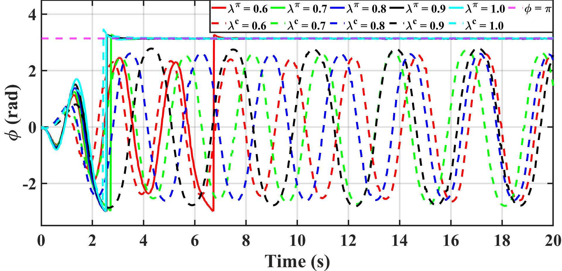
Unlike the variation in $m_{w}$, changes in $\lambda$ do not affect the magnitudes of buoyancy and gravity, but only influence the position of $c_{g}$. As $\lambda$ increases, $c_{g}$ moves closer to $c_{b}$. This results in larger maximum achievable roll angles (before reaching $\phi=\pi$) and reduces the time required to achieve the inverted state. When $\lambda=1.0$, the controller completed the task more quickly, as its parameters were specifically fine-tuned for this configuration.

To verify that the learned policy functions effectively across different motors, $m_{w}$ and $\lambda$ are configured to 23.35 g and 1.0, respectively. The results are shown in Table V.

Only when $g_{m}=0.5$ did both the learned policy and the baseline controller fail. Although each method could temporarily drive the MBR to the inverted pose, the motor thrust was insufficient to maintain it. The controller achieved inversion at approximately 9 s, while the policy did so at around 11 s, but both subsequently lost stability. For all other tested values of $g_{m}$, both the baseline controller and the learned policy successfully completed the task. However, their control behaviors differ noticeably, as illustrated in Fig. 8.

The results indicate that as $g_{m}$ increases, the policy requires less time to complete the task, owing to the corresponding increase in total force. When $g_{m}\geq 2.0$, only two rotations are necessary, a result consistent with the controller method. In contrast, for the controller, a higher $g_{m}$ results in a larger maximum achievable roll angle, which in turn requires more time to complete the task.

The parameters $m_{w}$, $\lambda$, and $g_{m}$ were varied simultaneously to further evaluate the robustness of the policy. The configurations and results are summarized in Table VI. The learned policy succeeded in all cases, whereas the baseline controller failed under these combined variations. The $\phi$ responses are shown in Fig. 9. In Case 2 (C2), the maneuver required a longer completion time due to the low motor gain $g_{m}$, which limited the available actuation capability.

To evaluate the contribution of the multi-buffer strategy and gradient clipping to training stability, an ablation study was conducted. The results are shown in Fig. 10. The proposed method, which combines multi-buffer experience storage with gradient clipping, converged within approximately 100 episodes. Removing gradient clipping while retaining the multi-buffer structure increased the convergence time to nearly 200 episodes. In contrast, using a single buffer with gradient clipping required at least 250 episodes—2.5 times slower than the proposed approach. For fairness, the capacity of the single buffer was set equal to the total capacity of all buffers in the multi-buffer configuration. These results demonstrate that the combination of multi-buffer sampling and gradient clipping significantly improves training stability and sample efficiency. The average return exhibits persistent fluctuations due to the continuous injection of exploration noise $\epsilon_{t}^{k}$ throughout training.

We transfer the learned policy to the real platform with only minimal parameter adjustments, avoiding additional training on physical data. As shown in Fig. 3, a mapping layer is introduced to mitigate the sim-to-real discrepancy during the inverted transition:

where $\mathbf{\tau}^{p}=[\tau_{x},\tau_{y},\tau_{z}]^{T}$ denotes the physical torque command. The term $\Delta_{\phi}=\pi-\phi$ represents the roll angle deviation, and $\varrho$ is the switching threshold. In experiments, $\mathbf{M}_{0}=\mathrm{diag}(m\phi,m_{\theta},m_{\psi})$ with $\varrho=0.8$. The parameters $m_{\theta}$ and $m_{\psi}$ are fixed at 0.1, while $m_{\phi}$ varies from 0.5 to 0.8. The results are shown in Fig. 11. The learned policy drives the MBR to the inverted pose, after which a PD controller stabilizes the system once angular velocities approach zero. The transition sequence for $m_{\phi}=0.7$ is illustrated in Fig. 12. Among the tested values, only $m_{\phi}=0.8$ failed. These results indicate that the proposed mapping layer effectively bridges the sim-to-real gap without policy retraining. Using $m_{\phi}=0.7$, additional physical experiments were conducted by varying $m_{w_{1}}$ and $m_{w_{2}}$ (Table VII). The MBR successfully achieved inversion in all cases (Fig. 13). Increasing $m_{w_{1}}$ shifts the $c_{g}$ toward the $c_{b}$, reducing transition time, whereas increasing $m_{w_{2}}$ moves $c_{g}$ toward the $c_{t}$, prolonging the maneuver. These observations are consistent with the simulation results in Sections IV-A and IV-B, further validating the effectiveness of the proposed method.

References

- [1] (2025) SLAM-enabled autonomous blimp for uav applications. In 2025 International Conference on Next Generation Communication & Information Processing (INCIP), pp. 1034–1039. Cited by: §I.
- [2] (2023) RGBlimp: robotic gliding blimp-design, modeling, development, and aerodynamics analysis. IEEE Robotics and Automation Letters 8 (11), pp. 7273–7280. Cited by: §I.
- [3] (2017) Autopilot design for a class of miniature autonomous blimps. In 2017 IEEE conference on control technology and applications (CCTA), pp. 841–846. Cited by: §I.
- [4] (2024) Adaptive output feedback trajectory tracking control of an indoor blimp: controller design and experiment validation. IEEE Transactions on Industrial Electronics. Cited by: §II-A.
- [5] (2018) Addressing function approximation error in actor-critic methods. In International conference on machine learning, pp. 1587–1596. Cited by: §III-C.
- [6] (2024) The flying warehouse delivery system with multi-commodity inventory management. Available at SSRN 4988309. Cited by: §I.
- [7] (2025) Reactive aerobatic flight via reinforcement learning. arXiv preprint arXiv:2505.24396. Cited by: §I.
- [8] (2022) Deep residual reinforcement learning based autonomous blimp control. In 2022 IEEE/RSJ International Conference on Intelligent Robots and Systems (IROS), pp. 12566–12573. Cited by: §I.
- [9] (2017) The visual inspection methodology for ceiling utilizing the blimp. Procedia Engineering 188, pp. 256–262. Cited by: §I.
- [10] (2006) Flying display: autonomous blimp with real-time visual tracking and image projection. In 2006 IEEE/RSJ International Conference on Intelligent Robots and Systems, pp. 131–136. Cited by: §I.
- [11] (2024) TinyBlimp: a promising frontier for autonomous miniature unmanned aerial vehicles. In Proceedings of the 10th Workshop on Micro Aerial Vehicle Networks, Systems, and Applications, pp. 1–6. Cited by: §I.
- [12] (2017) Proximal policy optimization algorithms. arXiv preprint arXiv:1707.06347. Cited by: §III-C.
- [13] (2018) Parameter identification of blimp dynamics through swinging motion. In 2018 15th International Conference on Control, Automation, Robotics and Vision (ICARCV), pp. 1186–1191. Cited by: §III-A.
- [14] (2020) Modeling and identification of coupled translational and rotational motion of underactuated indoor miniature autonomous blimps. In 2020 16th international conference on control, automation, robotics and vision (ICARCV), pp. 339–344. Cited by: §III-A.
- [15] (2021) Swing-reducing flight control system for an underactuated indoor miniature autonomous blimp. IEEE/ASME Transactions on Mechatronics 26 (4), pp. 1895–1904. Cited by: §I, §II-A.
- [16] (2020) Design and control of an indoor miniature autonomous blimp. Ph. D. dissertation, Georgia Institute of Technology. Cited by: §III-A, §III-C, §III-D.
- [17] (2021) Data-driven mpc for quadrotors. IEEE Robotics and Automation Letters 6 (2), pp. 3769–3776. Cited by: §I.
- [18] Unity: real-time development platform — 3d, 2d, vr & ar engine. External Links: Link Cited by: 1st item.
- [19] (2024) Achieving and maintaining inverted pose for miniature autonomous blimps. In 2024 American Control Conference (ACC), pp. 338–343. Cited by: §I, §IV.
- [20] (2025) Unlocking aerobatic potential of quadcopters: autonomous freestyle flight generation and execution. Science Robotics 10 (101), pp. eadp9905. Cited by: §I.
- [21] (2023) Learning agile flights through narrow gaps with varying angles using onboard sensing. IEEE Robotics and Automation Letters 8 (9), pp. 5424–5431. Cited by: §I.
- [22] (2023) Sblimp: design, model, and translational motion control for a swing-blimp. In 2023 IEEE/RSJ International Conference on Intelligent Robots and Systems (IROS), pp. 6977–6982. Cited by: §I.
- [23] (2025) MochiSwarm: a testbed for robotic blimps in realistic environments. arXiv preprint arXiv:2503.03077. Cited by: §I.
- [24] (2022) Design and simulation of a bio-inspired rigid-soft hybrid robotic blimp. In 2022 International Conference on Advanced Robotics and Mechatronics (ICARM), pp. 599–604. Cited by: §I, §I.
- [25] (2023) A novel miniature omnidirectional multi-rotor blimp. In 2023 IEEE 18th Conference on Industrial Electronics and Applications (ICIEA), pp. 1568–1573. Cited by: §I, §I.
- [26] (2023) Autonomous blimp control via robust deep residual reinforcement learning. In 2023 IEEE 19th International Conference on Automation Science and Engineering (CASE), pp. 1–8. Cited by: §I.