Acceleration of relativistic protons in a CME-perturbed solar wind
We investigate the impact of a Coronal Mass Ejection (CME) on the transport and acceleration of relativistic protons in the solar wind using a coupled 3D Magnetohydrodynamics (MHD) simulation and a test-particle approach. The CME is driven by a spheromak injected into a Parker solar wind at a heliocentric distance of 0.139 AU. The trajectories of 5 GeV protons, injected toward the CME from 3 AU, are integrated in the guiding-center approximation and scattered in velocity space with a mean free path . Our results show that the CME can increase the protons’ energy by several GeV. The acceleration occurs during the time particles stream along the portion of a magnetic field line downstream of the quasi-perpendicular portion of the CME-driven shock. In our configuration, the maximum energy gain, which is of the order of a few percent per passage through the acceleration region, occurs when the shock approaches 0.3 AU. Large energy gains require multiple passes through the acceleration region, which is made possible by the combined action of the mirror force and pitch angle scattering. The efficiency of the acceleration on time scales of the order of hours scales as . Energy spectra harden for decreasing parallel mean free path .
Key Words.:
Solar energetic particles – Magnetohydrodynamics (MHD) – Sun: coronal mass ejections (CMEs) Solar wind – Acceleration of particles – Methods: numerical1 Introduction
At Earth orbit, the interplanetary medium is mostly filled with protons and electrons at typical thermal energies of eV, streaming outward from the Sun at several km/s. In addition to these dominant components (in terms of pressure and mass density), a tenuous background of much more energetic particles is also observed. These include solar energetic particles (SEPs) accelerated during solar eruptions or at shock waves driven by coronal mass ejections (CMEs) (Desai and Giacalone, 2016; Klein and Dalla, 2017), reaching energies of several hundred MeV (Reames, 1997). Extra-heliospheric particles, such as anomalous cosmic rays (ACRs) and galactic cosmic rays (GCRs), cover an even larger range from a few MeV up to several PeV (see e.g. Lara et al. (2024) and references therein). Charged particles are sensitive to the electromagnetic field. Hence, modifications of the interplanetary electromagnetic structure by transients such as CMEs are expected to affect the transport of energetic particles throughout the heliosphere (see e.g. Cane (2000); Richardson (2004); Richardson and Cane (2011)). Many studies on the propagation of GCRs in the interplanetary medium have focused on the so-called ”Forbush decrease” (Forbush, 1937, 1938, 1958): a sudden drop in the GCR intensity in the wake of a CME (Cane, 2000; Dumbović et al., 2012; Kilpua et al., 2017). Fewer studies have addressed the question of the energy gain or loss of GCRs as they interact with the CME. One reason is that embarked instruments measure flux variations of GCRs for some selected energy channels and not the changes of the kinetic energy of a single GCR. In addition, spacecraft can only monitor the temporal variations at one given point in space. A more global view can be obtained by studying the propagation of GCRs in the electromagnetic field of a 3D time-dependent numerical simulation of a CME. In this work, we integrate the trajectories of individual protons in the guiding center approximation (GCA) as done in a previous work for 81 keV electrons in a steady solar wind (see Houeibib et al., 2025). Here, the background electromagnetic field is extracted from a 3D MHD simulation of a Parker-type solar wind perturbed by one single CME. We consider the propagation of relativistic 5 GeV protons for which the GCA remains valid for the fields in a CME propagating near 1 AU. The role of pitch-angle scattering by small scale turbulence (not included in the MHD simulation) will be extensively discussed. A popular complementary approach based on the focused transport equation (FTE) has been widely used to investigate the evolution of the velocity distribution function of energetic particles (e.g. Zhang, 2006; le Roux and Webb, 2009, 2012; van den Berg et al., 2020). The deterministic momentum-advection term of the FTE contains the energy changes associated with the gradient and curvature drifts in the motional electric field so that, when the phase-space diffusion coefficients are set to zero, the FTE description is equivalent to the guiding-center equations used here. The two approaches differ in practice: FTE-based studies generally focus on the structure of the diffusion coefficients for given models of the underlying turbulence, whereas the trajectory-based GCA approach adopted here allows us to follow individual particles through the full three-dimensional, time-dependent electromagnetic field of the MHD simulation. As shown by e.g. Marsh et al. (2013) and Dalla et al. (2013), the drifts can significantly affect the energy of SEPs traveling scatter-free through the electromagnetic field of an ideal Parker wind. Here we show that particles gain energy downstream of the quasi-perpendicular portion of a CME-driven shock, through the well-known energization of the gradient drift in the motional electric field. The mechanism is closely analogous to shock-drift acceleration, with the difference that in our configuration the dominant energy gain occurs in a finite region downstream of the shock rather than at the shock ramp itself. The novelty of the present work therefore does not reside in the acceleration mechanism itself, but in its application and quantification in a three-dimensional, time-dependent CME/spheromak configuration, where we show that the energy gain can substantially exceed the cumulated losses due to collisions (Ruffolo, 1995; Giacalone et al., 2002; Dalla et al., 2015; Houeibib et al., 2025) and to the drift motion in the unperturbed solar wind. The paper is structured as follows. The MHD simulation and the GCA equations are presented in Sect. 2. The physical mechanism responsible for the acceleration of the particles in the CME driven shock is discussed in Sect. 3. The role of scattering is discussed in Sect. 4 and a summary of the results is given in Sect. 5.
2 Model and numerical setup
We use an MHD code to simulate a three-dimensional, time-dependent, magnetized Parker-type wind perturbed by a CME. We then propagate energetic protons in the time-dependent electromagnetic field of the MHD simulation by numerically integrating the equations of motion in the guiding-center approximation.

2.1 MHD model for the solar wind and the CME
As in Houeibib et al. (2025), we use the three-dimensional MHD code (MPI-AMRVAC, (Keppens et al., 2023)) in the ideal MHD approximation to simulate the solar wind and the CME. The plasma is an ideal gas with polytropic index 5/3.


In order to convert from mass density and pressure to number density and temperature (which do not appear in the MHD equations) we assume a fully ionized proton-electron plasma where protons and electrons have the same temperature and same number density implying that with . The simulation domain is a Sun-centered spherical grid of size in , where is the radial coordinate, extending from = 0.139 AU to = 13.95 AU, is the polar angle, ranging from to , and is the azimuthal angle, ranging from to . The grid is uniform in and . On the other hand, to prevent an excessive longitudinal and latitudinal stretching of the cells, we adopt a stretching factor of 1.02 between adjacent cells in the direction of increasing . For simplicity, we adopt a Parker type wind and a positive magnetic monopole located at the Sun’s center, so that there is no induced heliospheric current sheet as in the case of a dipolar intrinsic field. At the Sun’s surface, the monopole field strength is . We assume that the inner boundary is rotating rigidly with the Sun. Consequently, the tangential velocity components of the plasma at the inner boundary are prescribed as , where with , corresponding to the angular rotation speed of the Sun. At the inner boundary, we impose a Neumann condition to the radial component of the plasma speed , a constant temperature and a constant mass density . A Neumann condition is also applied to the radial magnetic field component , while the tangential components vanish at the inner boundary. At the outer boundary, we impose zero-gradient conditions () for all physical quantities. We note that the inner boundary of the simulation domain is located beyond the sonic point, so that the wind starts supersonic at the boundary. After several rotations of the Sun the simulation reaches a steady state. Wind parameters at 1 AU in the equatorial plane of the simulation are given in Table 1. The simulated wind is somewhat underdense but otherwise typical of the real solar wind at 1 AU (Larrodera and Cid, 2020; Salem et al., 2023).
| Magnetic field strength | |
|---|---|
| Wind speed | |
| Number density | |
| Sound speed | |
| Alfvén speed | |
| Plasma beta |

Following previous authors (Verbeke et al., 2019; Kataoka et al., 2009; Shiota and Kataoka, 2016; Singh et al., 2020; Koehn et al., 2022) a Coronal Mass Ejection (CME) is triggered by injecting a force free spheromak-type magnetic structure through the inner domain boundary. The magnetic field of a spheromak is conveniently defined using a spherical coordinates system () where the prime refers to the spheromak frame. In this frame, for , the poloidal and toroidal components of the spheromak are given by:
| (1) | |||||
| (2) |
For all components are set to zero. In equations (1) and (2), is a reference field strength, the first two spherical Bessel functions and such that at the edge of the spheromak at . We note that at , the toroidal field vanishes while the poloidal field reduces to . defines the handedness of the magnetic structure via the orientation of the toroidal field. In our simulation we set nT and . The handedness of the spheromak is .

As shown in Figure 2, the spheromak is introduced into the simulation through its inner domain boundary in the equatorial plane (defined by the Sun’s rotation) at a constant radial speed of km/s. The axis of the spheromak has been oriented perpendicularly to the equatorial plane. The mean values of the plasma density and temperature in the spheromak are n = and T = , respectively. The equatorial cuts in Fig. 3 show temporal snapshots of the fluid temperature and radial velocity which both trace the propagation of the shock front through its heating and acceleration of the fluid it encounters. The inner edge of the high temperature arc also delimits the discontinuity separating the fluid heated by the shock from the magnetic driver of the CME (the spheromak ”remnant”). The full time evolution of these equatorial cuts is available as an online movie.
In Figure 4 we report the temporal profiles for various plasma parameters measured at a fixed position at 1 AU, represented by the cross in Figure 3. The time sequence can be decomposed as follows:
-
–
Shock arrival: The shock reaches the observation point at hours after the spheromak’s injection when the density rises by a factor of 3 and the magnetic field intensity increases from nT to nT.
-
–
Sheath region: Between and , the observation point is in a region of plasma compressed and heated by the shock.
-
–
CME Core (Ejecta): Between and , the observation point is in the ejecta (the spheromak ”remnant”). During the early phase of the period, the magnetic field lines move eastward () instead of general westward motion in the unperturbed wind (also see Figure 5). For , the profiles slowly recover pre-shock conditions.

2.2 The guiding center equations
Hereafter, we consider the motion of 5 GeV protons injected on three selected equatorial field lines in the CME perturbed solar wind described in Section 2. The three field lines, numbered 0, 1, and 2 evolve in time as shown in Figure 5. The corresponding time evolution is also available as an online movie. Hence, unlike Houeibib et al. (2025) who considered steady fields, we use the GC equations for the case of time-varying and fields. In the limit ( is speed of light), they can be written in the following form:
| (3) | |||||
| (4) | |||||
| (5) |
with . Note the factor in (3) which was mistakenly omitted in equation (1) of Houeibib et al. (2025). In the above equations, the subscripts and indicate projections parallel and perpendicular to . is the particle’s guiding center position, its velocity, its Lorentz factor, its magnetic moment, , and . Numerically, particles are advanced in time using the third-order accurate predictor-corrector scheme used by Houeibib et al. (2025) (also see Mignone et al. (2023)) with all fields and derivatives of the fields on the right-hand-side of the above GC equations computed within the MHD code and linearly interpolated from the MHD grid to the particle’s position. Fields are also linearly interpolated in time between consecutive MHD snapshots. The integration time step is given by: , where is the speed of light, and the scattering mean-free path (see Section 4). Although the structure of the GCA equations is much more complex than that of the full equations of motion, they offer a considerable advantage by eliminating the need for an integration time step smaller than the particle gyration period. This approach enables the integration of particle trajectories with higher precision and longer time scales at reduced computational costs.
3 Time evolution of a proton in the field of the CME (no scattering)
Let us first consider the propagation of a single 5 GeV proton injected on the magnetic field line 0, some days after the spheromak injection (red line in bottom-left panel of Fig. 5). The particle is initially positioned at with a pitch-angle (traveling toward the Sun) in order to be mirror reflected before reaching the inner boundary. The speed of a relativistic proton greatly exceeds that of the CME so that during its round trip one may assume the fields to be static, i.e. in (4). Also considering that (generally verified in the solar wind), we conclude that the proton’s kinetic energy evolves according to
| (6) | |||||
In the above equation, the right hand side terms correspond to the energy gain due to the curvature and gradient drifts, respectively. The latter are buried in Eq. 3 and are conveniently written as:
Noting that the energy variation associated with each term can be written as , where is a generic drift velocity, we plot their relative contributions as a function of time (top panel of Fig. 6) and of the distance to the mirror point (middle panel of Fig. 6). The acceleration is clearly ascribable to the gradient drift term. We denote as the time interval of strong acceleration, occurring in two stages, at and (see top panel of Figure 6). Both phases of acceleration occur during the period of time when the particle is located downstream of the shock where . The first acceleration step takes place as the particle moves inward (toward the Sun), the second as the particle moves outward after reflection at its mirror point.

The energy gain can therefore be written as
| (7) |
or, in terms of relative variation, as
| (8) |
Equations (7) and (8) show that the gain of energy is proportional to , i.e. proportional to the time the particle spends in the region where . In Fig. 7 we trace the energy gain of a fictitious 5 GeV proton (and same as in Fig. 6) moving along field line 0, at different phases of the CME’s expansion.
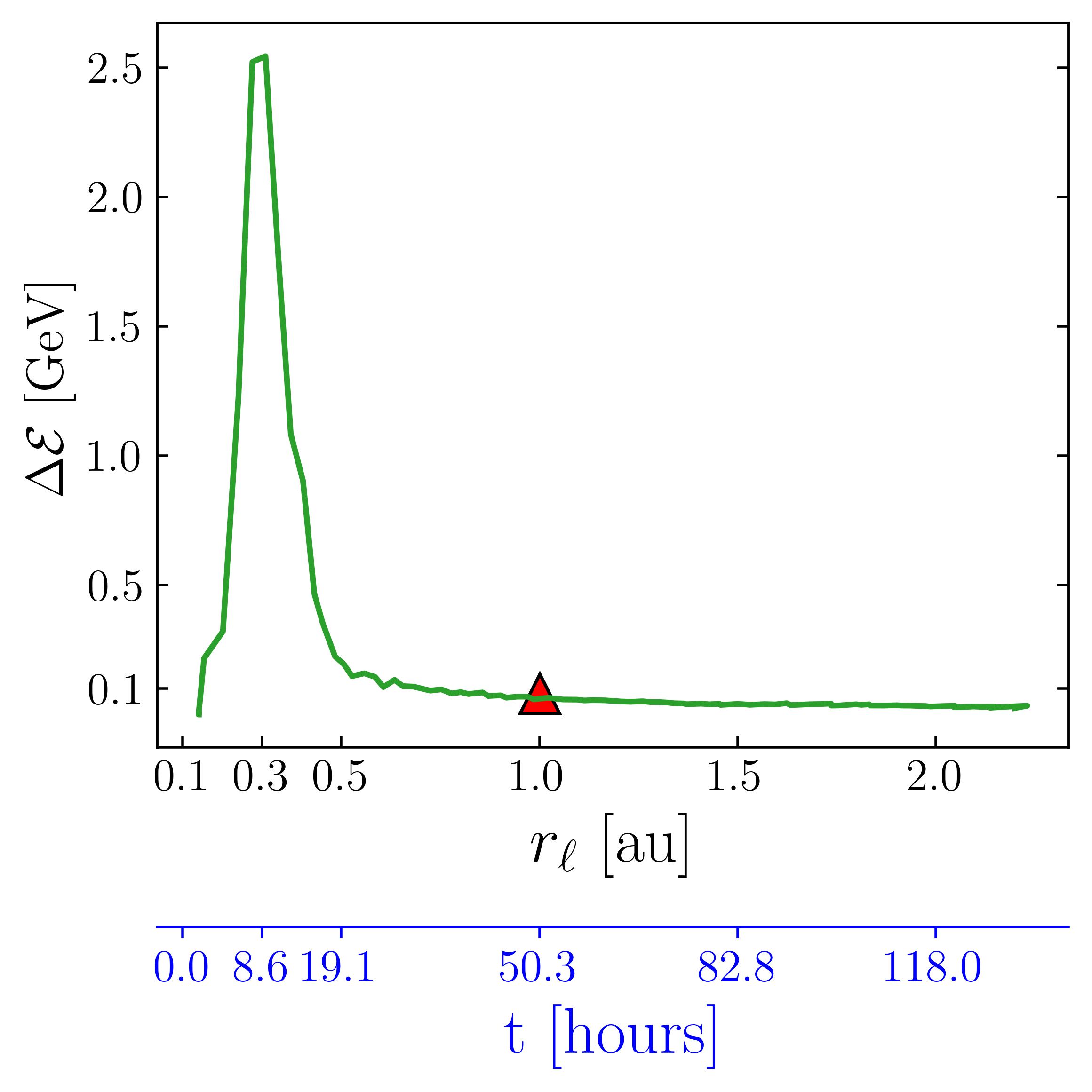

Clearly, efficiency peaks at the time the CME reaches AU, when the product of the three terms in equation (7) is at its maximum. The red diamond is the gain expected for a particle encountering the CME at 1 AU, which is the gain for the particle in Fig. 6.
Since the energization is proportional to the magnetic field gradient through , one may ask whether the gradient scale length in the acceleration region is set by the CME-driven compression or by numerical diffusion. Fig. 8 shows the ratio of the local grid spacing to along the trajectory of the particle of Fig. 6. The ratio remains below 0.17 everywhere, i.e. is resolved by at least grid cells even at the strongest gradients encountered by the particle. The acceleration region itself extends over AU, i.e. several tens of grid cells, well beyond the few cells over which the shock is numerically broadened. The gradients responsible for the energization are therefore not controlled by numerical diffusion.
4 Protons in the field of a CME (with scattering)
In Section 3, we did not consider the scattering effect in velocity space due to the particle’s interaction with small scale plasma turbulence not retained in the large scale MHD simulation. In the absence of scattering, the injected particles pass through the acceleration region at most two times; the first time as they stream toward the Sun and a second time as they stream away from the Sun after reflection at their mirror point. In the presence of scattering multiple crossings become possible. In this section, we let particles be pitch-angle scattered with a parallel mean free path . Two different values 0.1 AU and 0.5 AU are considered, covering the generally accepted range for a wide range of energies at 1 AU (Palmer, 1982; Bieber et al., 1994). Particles are hard-sphere scattered by scattering centers at rest in the solar wind frame (see Sect. 2.3 in Houeibib et al. (2025) for details). Note that the post-collision pitch-angle cosine is drawn as where is uniformly distributed in the range (see Sect. 2.3 in Houeibib et al. (2025) for a discussion on this point). To accumulate statistics, we consider mono-energetic protons of 5 GeV impulsively injected toward the Sun at h with a pitch angle . As in Houeibib et al. (2025), particles reaching the boundaries at r=0.14 AU and r=3 AU are instantly re-injected at r=3 AU on the same field line and with the same initial conditions implying a constant number of particles in the domain.


A particle subject to scattering may repeatedly pass through the acceleration region as it bounces back and forth between scattering centers or between mirror points and scattering centers. Given that on some privileged magnetic field lines, particles gain energy at each crossing, much larger energies can be achieved than in the no-scattering case of Section 3 provided the acceleration due to is sufficiently strong and long lasting. In order to illustrate the role of scattering, the 4 days cumulative energy distributions for protons injected along the field lines 0, 1, and 2 are shown in Fig. 9 for the case AU. The distributions are obtained by measuring the particles’ energies as they cross the spherical shell of radius 1 AU. Note that the same particle can contribute multiple times to the distribution if it crosses the 1 AU shell more than once. We stress that these cumulative spectra are diagnostics of the adopted numerical experiment rather than direct predictions of an observable spectrum: the reinjection procedure at AU maintains a driven, recirculating particle population and thereby controls the residence time of the particles and the number of possible passages through the acceleration region. The figure shows that acceleration is highest on line 0 and lowest on line 2. This is not very surprising as the three field lines are very unequally affected by the CME, with line 0 being the one with the longest portion in the region of strong magnetic compression (see Figure 5). We anticipate that for reasonable values of , the spectra harden with decreasing . Indeed, by reducing , the particles’ residence time in the acceleration region increases (also see Vainio et al. (2000)). The effect is illustrated in Fig. 10 where the cumulative spectra on line 0 are shown for the case AU and 0.1 AU, respectively. A semi-quantitative explanation can be given by observing that in a one-dimensional diffusion experiment where particles moving at a speed c are instantly injected at , the number density at any given point in space decreases asymptotically with time as . As the number of collisions experienced by a particle grows as and since the gain of energy for a particle is approximately proportional to the number of collisions ( is the energy gain per passage in the acceleration region), one obtains that the number of particles gaining an energy scales as . Consequently, reducing the mean free path increases the number of particles gaining a given energy . In our case, the number of particles accelerated to a given energy is expected to be larger by a factor for the case with respect to the case . This is effectively the factor separating the two curves in Fig. 10.
5 Conclusions
We compute the guiding center trajectories of relativistic 5 GeV protons in the field of an MHD simulation of a Parker-type solar wind perturbed by an equatorial CME. The CME is triggered by the gradual insertion of a spheromak through the inner boundary of the simulation domain at AU. The protons are injected sunward, from a heliocentric distance of 3 AU, along three equatorial magnetic field lines crossing the CME at different heliographic longitudes. The main findings are summarized below.
-
1.
Particles gain energy as they travel through the compressed plasma downstream of the CME-driven shock. The acceleration is due to the work of the motional electric field on the gradient drift, which is positive (, or equivalently ) when the particle is located downstream of the shock.
-
2.
A peak energy gain of up to 50 % for one single passage through the acceleration region has been observed at the time the CME shock front reaches 0.3 AU.
-
3.
In the case of pitch angle scattering, particles may pass through the acceleration region multiple times and reach substantially higher energies. For example, assuming hard sphere type scattering and a mean free path , some of the injected particles increase their energy by a factor six in days. These figures are specific to our numerical experiment, in which particles are continuously reinjected at AU, and should not be read as predictions of observable spectra.
- 4.
-
5.
The energy distributions harden for decreasing as the number of times the particles flow through the region of acceleration increases. The number of particles reaching a given energy is found to scale as , consistent with a heuristic 1D diffusion estimate.
Acknowledgements.
This work has been financially supported by the PLAS@PAR project and by the National Institute of Sciences of the Universe (INSU). AH is supported by the CNES (Centre National d’Études Spatiales).References
- Proton and electron mean free paths: the Palmer consensus revisited. The Astrophysical Journal 420, pp. 294. External Links: Document Cited by: §4.
- Coronal mass ejections and Forbush decreases. Space Science Reviews 93, pp. 55–77. External Links: Document Cited by: §1.
- Solar energetic particle drifts in the Parker spiral. Journal of Geophysical Research: Space Physics 118 (10), pp. 5979–5985. External Links: Document Cited by: §1.
- Drift-induced deceleration of solar energetic particles. The Astrophysical Journal 808 (1), pp. 62. External Links: Document Cited by: §1.
- Large gradual solar energetic particle events. Living Reviews in Solar Physics 13 (1), pp. 3. External Links: Document Cited by: §1.
- Cosmic ray modulation by different types of solar wind disturbances. Astronomy & Astrophysics 538, pp. A28. External Links: Document Cited by: §1.
- On the effects in cosmic-ray intensity observed during the recent magnetic storm. Physical Review 51 (12), pp. 1108–1109. External Links: Document Cited by: §1.
- On world-wide changes in cosmic-ray intensity. Physical Review 54 (12), pp. 975–988. External Links: Document Cited by: §1.
- Cosmic-ray intensity variations during two solar cycles. Journal of Geophysical Research 63 (4), pp. 651–669. External Links: Document Cited by: §1.
- Particle acceleration in solar wind compression regions. The Astrophysical Journal 573 (2), pp. 845–850. External Links: Document Cited by: §1.
- Dynamics of energetic electrons scattered in the solar wind – magnetohydrodynamics and test-particle simulations. Astronomy & Astrophysics 694, pp. A211. External Links: Document Cited by: §1, §2.1, §2.2, §2.2, §4.
- Three-dimensional MHD modeling of the solar wind structures associated with 13 december 2006 coronal mass ejection. Journal of Geophysical Research: Space Physics 114 (A10), pp. A10102. External Links: Document Cited by: §2.1.
- MPI-AMRVAC 3.0: updates to an open-source simulation framework. Astronomy & Astrophysics 673, pp. A66. External Links: Document Cited by: §2.1.
- Coronal mass ejections and their sheath regions in interplanetary space. Living Reviews in Solar Physics 14 (1), pp. 5. External Links: Document Cited by: §1.
- Acceleration and propagation of solar energetic particles. Space Science Reviews 212 (3-4), pp. 1107–1136. External Links: Document Cited by: §1.
- Successive interacting coronal mass ejections: how to create a perfect storm. The Astrophysical Journal 941 (2), pp. 139. External Links: Document Cited by: §2.1.
- Interaction of cosmic rays with magnetic flux ropes. Journal of Geophysical Research: Space Physics 129 (8), pp. e2024JA032478. External Links: Document Cited by: §1.
- Bimodal distribution of the solar wind at 1 AU. Astronomy & Astrophysics 635, pp. A44. External Links: Document Cited by: §2.1.
- Time-dependent acceleration of interstellar pickup ions at the heliospheric termination shock using a focused transport approach. The Astrophysical Journal 693 (1), pp. 534–551. External Links: Document Cited by: §1.
- A focused transport approach to the time-dependent shock acceleration of solar energetic particles at a fast traveling shock. The Astrophysical Journal 746 (1), pp. 104. External Links: Document Cited by: §1.
- Drift-induced perpendicular transport of solar energetic particles. The Astrophysical Journal 774 (1), pp. 4. External Links: Document Cited by: §1.
- A guiding center implementation for relativistic particle dynamics in the PLUTO code. Computer Physics Communications 285, pp. 108625. External Links: Document Cited by: §2.2.
- Transport coefficients of low-energy cosmic rays in interplanetary space. Reviews of Geophysics 20 (2), pp. 335–351. External Links: Document Cited by: §4.
- Energetic particles and the structure of coronal mass ejections. Geophysical Monograph Series 99, pp. 217–226. External Links: Document Cited by: §1.
- Galactic cosmic ray intensity response to interplanetary coronal mass ejections/magnetic clouds in 1995–2009. Solar Physics 270 (2), pp. 609–627. External Links: Document Cited by: §1.
- Energetic particles and corotating interaction regions in the solar wind. Space Science Reviews 111 (3), pp. 267–376. External Links: Document Cited by: §1.
- Effect of adiabatic deceleration on the focused transport of solar cosmic rays. The Astrophysical Journal 442, pp. 861. External Links: Document Cited by: §1.
- Precision electron measurements in the solar wind at 1 au from NASA’s Wind spacecraft. Astronomy & Astrophysics 675, pp. A162. External Links: Document Cited by: §2.1.
- Magnetohydrodynamic simulation of interplanetary propagation of multiple coronal mass ejections with internal magnetic flux rope (SUSANOO-CME). Space Weather 14 (2), pp. 56–75. External Links: Document Cited by: §2.1.
- A modified spheromak model suitable for coronal mass ejection simulations. The Astrophysical Journal 894 (1), pp. 49. External Links: Document Cited by: §2.1.
- Interplanetary and interacting protons accelerated in a parallel shock wave. The Astrophysical Journal 528 (2), pp. 1015–1025. External Links: Document Cited by: §4.
- A primer on focused solar energetic particle transport. basic physics and recent modelling results. Space Science Reviews 216, pp. 146. External Links: Document Cited by: §1.
- The evolution of coronal mass ejections in the inner heliosphere: implementing the spheromak model with EUHFORIA. Astronomy & Astrophysics 627, pp. A111. External Links: Document Cited by: §2.1.
- The theory of energetic particle transport in the magnetosphere: a noncanonical approach. Journal of Geophysical Research: Space Physics 111, pp. A04208. External Links: Document Cited by: §1.