跳到论文正文
W Papers独立论文阅读器 arXiv:2602.23561 论文正文 计算阅读时间 · 0%
引用这篇论文根据当前论文元数据生成,正式投稿前建议核对。


𝖵𝖺𝖲𝖲𝖳\mathsf{VaSST}: Variational Inference for Symbolic Regression using Soft Symbolic Trees

Somjit Roy
Department of Statistics
Texas A&M University
College Station, TX 77843
sroy_123@tamu.edu
&Pritam Dey
Department of Statistics
Texas A&M University
College Station, TX 77843
pritam.dey@tamu.edu
&Bani K. Mallick
Department of Statistics
Texas A&M University
College Station, TX 77843
bmallick@stat.tamu.edu
Corresponding author.
Abstract

Symbolic regression has recently gained traction in AI-driven scientific discovery, aiming to recover explicit closed-form expressions from data that reveal underlying physical laws. Despite recent advances, existing methods remain dominated by heuristic search algorithms or data-intensive approaches that assume low-noise regimes and lack principled uncertainty quantification. Fully probabilistic formulations are scarce, and existing Markov chain Monte Carlo–based Bayesian methods often struggle to efficiently explore the highly multimodal combinatorial space of symbolic expressions. We introduce 𝖵𝖺𝖲𝖲𝖳\mathsf{VaSST}, a scalable probabilistic framework for symbolic regression based on variational inference. 𝖵𝖺𝖲𝖲𝖳\mathsf{VaSST} employs a continuous relaxation of symbolic expression trees, termed soft symbolic trees, where discrete operator and feature assignments are replaced by soft distributions over allowable components. This relaxation transforms the combinatorial search over an astronomically large symbolic space into an efficient gradient-based optimization problem while preserving a coherent probabilistic interpretation. The learned soft representations induce posterior distributions over symbolic structures, enabling principled uncertainty quantification. Across simulated experiments and Feynman Symbolic Regression Database within SRBench, 𝖵𝖺𝖲𝖲𝖳\mathsf{VaSST} achieves superior performance in both structural recovery and predictive accuracy compared to state-of-the-art symbolic regression methods.

Keywords Symbolic Regression; Scientific Machine Learning; Uncertainty Quantification; Black-box Variational Inference; Automatic Differentiation.

1 Introduction

Symbolic regression for scientific discovery.

Scientific Machine Learning (SciML) has emerged as a powerful paradigm for integrating domain knowledge with data-driven modeling, enabling advances across materials science (Butler et al., 2018), climate and weather prediction (Zhang et al., 2025), biology (Boadu et al., 2025), and physics (Raissi et al., 2019). A central objective in these domains is the discovery of explicit governing equations that encode mechanistic structure rather than merely predictive relationships. In this setting, symbolic regression (SR) plays a pivotal role. Unlike classical prediction-centric regression methods (Tibshirani, 1996; Rasmussen and Williams, 2006; Chipman et al., 2010), SR operates directly over functional forms to recover concise, structurally interpretable mathematical expressions from experimental data. By identifying explicit equations underlying complex scientific phenomena, SR has enabled sparse discovery of nonlinear dynamical systems (Brunton et al., 2016), accelerated materials design (Wang et al., 2024), and uncovered fundamental scientific laws (Schmidt and Lipson, 2009).

Related work.

Existing SR methods can be broadly categorized into evolutionary, machine learning-based, and Bayesian approaches. Classical SR is dominated by genetic programming and related heuristic search algorithms (Davidson et al., 2003; Fortin et al., 2012; Stephens, 2016), which explore expressions through stochastic evolution but often suffer from high computational complexity, sensitivity to initialization, and the generation of overly complex formulas (Korns, 2011). More recent machine learning-driven methods cast SR as a sequential decision-making problem, learning to generate grammar rules, tree traversals, or executable symbolic strings via neural architectures (Udrescu and Tegmark, 2020; Petersen et al., 2021; Broløs et al., 2021; Kamienny et al., 2022). Although these methods enhance scalability and predictive performance, they remain inherently search-driven and computationally challenging due to the NP-hard nature of symbolic space exploration (Virgolin and Pissis, 2022). Moreover, their effectiveness is often contingent on large training datasets and low-noise regimes, as we demonstrate in Section 5. This review highlights that fully probabilistic formulations of SR remain limited.

Note that, scientific expressions possess an inherently hierarchical and compositional structure that aligns naturally with tree representations (see Figure 1). Tree models are ubiquitous in modern machine learning for capturing nonlinear interactions with strong predictive performance (Breiman et al., 1984; Breiman, 1996), while Bayesian tree formulations (Chipman et al., 1998; Dension et al., 1998; Chipman et al., 2010) provide a coherent inferential framework through priors over structures, principled model comparison, and uncertainty quantification. In context of SR, the Bayesian Machine Scientist (BMS) (Guimerà et al., 2020) represents an important step toward Bayesian equation discovery. However, it employs an ad hoc structural prior built from corpus parsing based on a priori knowledge, and performs inference using Metropolis-Hastings (MH) proposals over discrete symbolic tree structures. Given the highly multimodal and combinatorial posterior landscape, such local MH updates can exhibit poor mixing in complex discrete spaces (Bhamidi et al., 2008; Łatuszyński et al., 2025), leading to slow convergence and inefficient exploration of the symbolic model space. Similarly, Bayesian Symbolic Regression (BSR) (Jin et al., 2020) adopts a tree-based partial Bayesian formulation but uses plug-in ordinary least squares estimates for regression parameters. This incomplete parameter uncertainty propagation, combined with local stochastic MH structural updates, further impedes effective traversal of the symbolic model space and frequently produces overly complicated output expressions, as evidenced in Section 5.

Our contributions.

In light of these drawbacks, we propose a variational inference framework for SR that combines principled Bayesian modeling with improved computational scalability over existing probabilistic SR methods. Variational inference recasts Bayesian inference as an optimization problem (Blei et al., 2017), offering a scalable alternative to traditional Monte Carlo-based approaches for modern data-intensive settings (Jordan et al., 1999; Blei et al., 2003; Wainwright and Jordan, 2008; Graves, 2011). However, a naïve application of variational inference over the discrete structural space of symbolic expressions results in a combinatorial optimization problem that negates these scalability benefits (Williams, 1992; Koza, 1994).

To overcome this challenge, we introduce a novel representation of symbolic expressions using soft symbolic trees, in which each operator and feature assignment is replaced by a soft combination over all allowable operators and features. This relaxation transforms the discrete structural search into a continuous optimization problem, enabling efficient gradient-based exploration of the symbolic model space through black-box variational inference (Ranganath et al., 2014; Kucukelbir et al., 2017; Giordano et al., 2024). Structural interpretability is preserved by mapping the learned soft representations to hard symbolic trees through a randomized post-optimization procedure. This continuous relaxation trick is similar in spirit to soft relaxations used for variational inference in decision tree-based regression (Salazar, 2023). However, in context of SR the soft representations naturally induce probability distributions over hard symbolic tree structures, thereby providing a principled mechanism for quantifying uncertainty in the recovered symbolic expressions. We refer to this framework as, 𝖵𝖺𝖲𝖲𝖳\mathsf{VaSST}: Variational Inference for Symbolic Regression using Soft Symbolic Trees.

A primary goal in scientific equation discovery is to favor structural parsimony in accordance to the Occam’s razor principle (Jefferys and Berger, 1992). 𝖵𝖺𝖲𝖲𝖳\mathsf{VaSST} achieves this by controlling structural complexity via a depth-dependent regularizing prior that penalizes overly complex symbolic expressions. Through extensive experiments, we demonstrate that 𝖵𝖺𝖲𝖲𝖳\mathsf{VaSST} effectively balances structural discovery and predictive accuracy while maintaining computational stability, outperforming a range of state-of-the-art symbolic regression methods. A Python implementation of 𝖵𝖺𝖲𝖲𝖳\mathsf{VaSST} is available at anonymous.4open.science/r/VaSST-62C7.

2 Symbolic Tree Representation of Scientific Expressions

Scientific expressions can be constructed by combining primary features (e.g., x1,x2x_{1},x_{2}) and mathematical operators (e.g., exp,sin,+,×\exp,\sin,+,\times). We denote the full set of pp primary features as 𝒳\mathcal{X} and the set of allowed mathematical operators as 𝒪=𝒪u∪𝒪b\mathcal{O}=\mathcal{O}_{u}\cup\mathcal{O}_{b}, where 𝒪u\mathcal{O}_{u} and 𝒪b\mathcal{O}_{b} contain the unary and binary operators, respectively. Typical choices in scientific modeling include, 𝒪u={sin,cos,exp,2,3}\mathcal{O}_{u}=\{\sin,\cos,\exp,^{2},^{3}\} and 𝒪b={+,×,−,/}\mathcal{O}_{b}=\{+,\times,-,/\} (Udrescu and Tegmark, 2020).

Let ℰ\mathcal{E} denote the set of admissible feature-operator compositions. Any symbolic expression 𝔈∈ℰ\mathfrak{E}\in\mathcal{E} is defined recursively as one of, (a) primitive expression: 𝔈=x1\mathfrak{E}=x_{1}, where x1∈𝒳x_{1}\in\mathcal{X}; (b) binary composition: 𝔈=b​(𝔈1,𝔈2)\mathfrak{E}=b(\mathfrak{E}_{1},\mathfrak{E}_{2}), where 𝔈1,𝔈2∈ℰ\mathfrak{E}_{1},\mathfrak{E}_{2}\in\mathcal{E} and b∈𝒪bb\in\mathcal{O}_{b}, for e.g., x1+x2x_{1}+x_{2}; and (c) unary composition: 𝔈=u​(𝔈~)\mathfrak{E}=u(\tilde{\mathfrak{E}}), where 𝔈~∈ℰ\tilde{\mathfrak{E}}\in\mathcal{E} and u∈𝒪uu\in\mathcal{O}_{u}, for e.g., exp⁡(x1)\exp(x_{1}). This set of characterizations naturally maps each 𝔈∈ℰ\mathfrak{E}\in\mathcal{E} to a symbolic tree structure 𝒯​(𝔈)\mathcal{T}(\mathfrak{E}), where internal (nonterminal) nodes either represent unary (with 11 child node) or binary (with 22 children nodes) operators, while leaves (terminal nodes) correspond to primary features from 𝒳\mathcal{X}; see Figure 1. It is important to note that, unlike decision tree-based models (Breiman et al., 1984; Chipman et al., 2010), which recursively partition the input feature space, our framework interprets symbolic trees as compositional structures that assign input features from 𝒳\mathcal{X} to leaves and operators from 𝒪\mathcal{O} to internal nodes. Such tree representations of symbolic expressions are not necessarily unique, for e.g., x1​(x2+x3)x_{1}(x_{2}+x_{3}) is treated to be same as that of x1​x2+x1​x3x_{1}x_{2}+x_{1}x_{3}, in our framework.

++x1x_{1}x2x_{2}x1x_{1}x1x_{1}exp\exp(a) 𝒯​(𝔈)≡x1\mathcal{T}(\mathfrak{E})\equiv x_{1}(b) 𝒯​(𝔈)≡x1+x2\mathcal{T}(\mathfrak{E})\equiv x_{1}+x_{2}(c) 𝒯​(𝔈)≡exp⁡(x1)\mathcal{T}(\mathfrak{E})\equiv\exp(x_{1})
Figure 1: Symbolic tree representation.

Now, for 𝔈∈ℰ\mathfrak{E}\in\mathcal{E} and an instance 𝐱∈ℝp\mathbf{x}\in\mathbb{R}^{p} of the features in 𝒳\mathcal{X}, we define g​(𝐱;𝒯​(𝔈))g(\mathbf{x};\mathcal{T}(\mathfrak{E})) to be the real-valued evaluation of the symbolic expression 𝒯​(𝔈)\mathcal{T}(\mathfrak{E}) at 𝐱\mathbf{x}. With this setup in place, we formally present the 𝖵𝖺𝖲𝖲𝖳\mathsf{VaSST} modeling framework.

3 The 𝖵𝖺𝖲𝖲𝖳\mathsf{VaSST} Model

We outline the 𝖵𝖺𝖲𝖲𝖳\mathsf{VaSST} model which comprises two major components: (i) a symbolic ensemble consisting of a linear regression of the response variable over a forest of KK symbolic trees and (ii) a hierarchical prior specification over the model regression coefficients, the model noise variance, and the symbolic tree structures.

3.1 The Symbolic Ensemble Component

Let 𝒟n:={(𝐱i,yi)}i=1n\mathcal{D}_{n}:=\{(\mathbf{x}_{i},y_{i})\}_{i=1}^{n} be the collection of observed data units. 𝖵𝖺𝖲𝖲𝖳\mathsf{VaSST} models and structurally learns the hidden symbolic relationship between the responses yi∈ℝy_{i}\in\mathbb{R} and primary features in 𝐱i∈ℝp\mathbf{x}_{i}\in\mathbb{R}^{p} by using a collection of KK symbolic trees, {𝒯​(𝔈j)}j=1K\{\mathcal{T}(\mathfrak{E}_{j})\}_{j=1}^{K}, evaluated at 𝐱i\mathbf{x}_{i}, as:

yi=β0+∑j=1Kgj​(𝐱i)​βj+ϵi,i=1,…,n,\displaystyle y_{i}=\beta_{0}+\sum_{j=1}^{K}g_{j}(\mathbf{x}_{i})\beta_{j}+\epsilon_{i},\quad i=1,\ldots,n, (1)

where gj​(𝐱i)=g​(𝐱i;𝒯​(𝔈j))g_{j}(\mathbf{x}_{i})=g(\mathbf{x}_{i};\mathcal{T}(\mathfrak{E}_{j})), 𝜷=(β0,…,βK)⊤∈ℝK+1\boldsymbol{\beta}=(\beta_{0},\ldots,\beta_{K})^{\top}\in\mathbb{R}^{K+1} is the model regression coefficient vector, and ϵi∈ℝ\epsilon_{i}\in\mathbb{R} is the model noise with ϵi∼N1​(0,σ2)\epsilon_{i}\sim\mathrm{N}_{1}(0,\sigma^{2}) independently. From (1), we obtain the vector representation of the symbolic ensemble component:

𝐲=𝐓​𝜷+ϵ,ϵ∼Nn​(0n,σ2​𝐈𝐧),\mathbf{y}=\mathbf{T}\boldsymbol{\beta}+\boldsymbol{\epsilon},\quad\boldsymbol{\epsilon}\sim\mathrm{N}_{n}(0_{n},\sigma^{2}\mathbf{I_{n}}), (2)

where 𝐓=(gj​(𝐱i))1≤i≤n, 0≤j≤K∈ℝn×K+1¯\mathbf{T}=(g_{j}(\mathbf{x}_{i}))_{1\leq i\leq n,\;0\leq j\leq K}\in\mathbb{R}^{n\times\overline{K+1}} is the expression design matrix, g0​(𝐱i)=1g_{0}(\mathbf{x}_{i})=1 for all i=1,…,ni=1,\ldots,n, 𝐲=(y1,…,yn)⊤∈ℝn\mathbf{y}=(y_{1},\ldots,y_{n})^{\top}\in\mathbb{R}^{n} is the response vector, and ϵ=(ϵ1,…,ϵn)⊤∈ℝn\boldsymbol{\epsilon}=(\epsilon_{1},\ldots,\epsilon_{n})^{\top}\in\mathbb{R}^{n} is the model noise vector.

The model regression parameters (𝜷,σ2)(\boldsymbol{\beta},\sigma^{2}) jointly are endowed upon with the conjugate Normal Inverse-Gamma (NIG) prior viz., 𝜷∣σ2∼NK+1​(𝝁0,σ2​𝚺0)\boldsymbol{\beta}\mid\sigma^{2}\sim\mathrm{N}_{K+1}(\boldsymbol{\mu}_{0},\sigma^{2}\boldsymbol{\Sigma}_{0}) and σ2∼IG​(a0,b0)\sigma^{2}\sim\mathrm{IG}(a_{0},b_{0}), where 𝝁0∈ℝK+1\boldsymbol{\mu}_{0}\in\mathbb{R}^{K+1}, 𝚺0\boldsymbol{\Sigma}_{0} (positive definite matrix of order K+1K+1), and a0,b0>0a_{0},b_{0}>0 are the hyperparameters of the Normal and Inverse-Gamma prior distributions, respectively. We complete the 𝖵𝖺𝖲𝖲𝖳\mathsf{VaSST}model specification by describing the symbolic tree prior in Section 3.2.

3.2 The 𝖵𝖺𝖲𝖲𝖳\mathsf{VaSST} Symbolic Tree Prior

The 𝖵𝖺𝖲𝖲𝖳\mathsf{VaSST} symbolic tree probability model for each 𝒯​(𝔈j)\mathcal{T}(\mathfrak{E}_{j}) is constructed in two stages: (a) a probabilistic specification over a maximal binary tree skeleton and (b) a deterministic pruning operation that maps the skeleton tree to a valid symbolic tree, as depicted in Figure 2.

Full binary tree skeleton.

To decouple structural decisions from operator and feature assignments, we embed each symbolic tree 𝒯​(𝔈j)\mathcal{T}(\mathfrak{E}_{j}) into a full binary tree skeleton, denoted by 𝒮j(D)\mathcal{S}_{j}^{(D)}, of fixed maximum depth D∈ℕD\in\mathbb{N}. Let 𝒵D={0,1,…,N−1}\mathcal{Z}_{D}=\{0,1,\ldots,N-1\} index the skeleton tree nodes in heap order, where 0 is the root and the left and right children of a skeleton node ζ∈𝒵D\zeta\in\mathcal{Z}_{D} are given by L​(ζ)=2​ζ+1L(\zeta)=2\zeta+1 and R​(ζ)=2​ζ+2R(\zeta)=2\zeta+2, respectively. The total number of nodes is N=2D+1−1N=2^{D+1}-1. Also, let dζ∈{0,…,D}d_{\zeta}\in\{0,\ldots,D\} denote the depth of node ζ\zeta. For each skeleton node ζ∈𝒵D\zeta\in\mathcal{Z}_{D}, we introduce the following, (a) expansion indicator: ej​ζ∈{0,1}e_{j\zeta}\in\{0,1\}, where ej​ζ=1e_{j\zeta}=1 or ej​ζ=0e_{j\zeta}=0 indicates that ζ\zeta is an internal node or a leaf of 𝒯​(𝔈j)\mathcal{T}(\mathfrak{E}_{j}), respectively; (b) operator assignment: oj​ζ∈𝒪o_{j\zeta}\in\mathcal{O}, specifies the operator assigned to ζ\zeta if ej​ζ=1e_{j\zeta}=1; and (c) feature assignment: hj​ζ∈𝒳h_{j\zeta}\in\mathcal{X}, specifies the primary feature assigned to ζ\zeta if ej​ζ=0e_{j\zeta}=0.

root\mathrm{root}dζ=2d_{\zeta}=2dζ=1d_{\zeta}=1dζ=0d_{\zeta}=0ζ=1\zeta=1ζ=2\zeta=2ζ=0\zeta=0ζ=3\zeta=3ζ=4\zeta=4ζ=5\zeta=5ζ=6\zeta=6ej​ζ=0,oj​ζ∈𝒪,hj​ζ∈𝒳e_{j\zeta}=0,\;o_{j\zeta}\in\mathcal{O},\;h_{j\zeta}\in\mathcal{X}ej​ζ=1,oj​ζ∈𝒪b,hj​ζ∈𝒳e_{j\zeta}=1,\;o_{j\zeta}\in\mathcal{O}_{b},\;h_{j\zeta}\in\mathcal{X}[Π​(ej​ζ),pζ;Π​(oj​ζ∣𝐰op);Π​(hj​ζ∣𝐰ft)][\Pi(e_{j\zeta}),\;p_{\zeta};\;\Pi(o_{j\zeta}\mid\mathbf{w}_{\mathrm{op}});\;\Pi(h_{j\zeta}\mid\mathbf{w}_{\mathrm{ft}})](D,N)=(2,7),prior over​𝒮j(2)​and induced prior over​𝒯​(𝔈j)(D,N)=(2,7),\;\text{prior over}\;\mathcal{S}_{j}^{(2)}\;\text{and induced prior over}\;\mathcal{T}(\mathfrak{E}_{j})Node set of​𝒮j(2):{0,…,6};Node set of​𝒯​(𝔈j):{0,1,2,5,6}\text{Node set of}\;\mathcal{S}_{j}^{(2)}:\{0,\ldots,6\};\;\text{Node set of}\;\mathcal{T}(\mathfrak{E}_{j}):\{0,1,2,5,6\}
Figure 2: A live representation of the prior over 𝒮j(2)\mathcal{S}_{j}^{(2)} and the induced prior over 𝒯​(𝔈j)\mathcal{T}(\mathfrak{E}_{j}). In 𝒮j(2)\mathcal{S}_{j}^{(2)}, the children nodes ζ=3,4\zeta=3,4 of ζ=1\zeta=1 are pruned using 𝔭\mathfrak{p} as ej​1=0e_{j1}=0 to obtain the valid symbolic tree 𝒯​(𝔈j)\mathcal{T}(\mathfrak{E}_{j}).
Valid symbolic tree via deterministic pruning.

The skeleton 𝒮j(D)\mathcal{S}_{j}^{(D)} is an ambient representation. We obtain the corresponding valid symbolic tree 𝒯​(𝔈j)\mathcal{T}(\mathfrak{E}_{j}) by applying a deterministic pruning operator 𝔭\mathfrak{p} which proceeds as follows, (a) terminal pruning: if ej​ζ=0e_{j\zeta}=0, then all descendants of ζ\zeta in the skeleton are removed, making it a leaf; and (b) unary operator pruning: if ej​ζ=1e_{j\zeta}=1 and oj​ζ∈𝒪uo_{j\zeta}\in\mathcal{O}_{u}, then the right subtree rooted at R​(ζ)R(\zeta) is removed. Thus, the resulting symbolic tree is 𝒯​(𝔈j)=𝔭​(𝒮j(D))\mathcal{T}(\mathfrak{E}_{j})=\mathfrak{p}(\mathcal{S}_{j}^{(D)}).

Prior over full binary tree skeleton.

The prior specification over 𝒮j(D)\mathcal{S}_{j}^{(D)} is characterized by the prior over the latent skeleton variables, {ej​ζ,oj​ζ,hj​ζ:ζ∈𝒵D}\{e_{j\zeta},o_{j\zeta},h_{j\zeta}\;:\;\zeta\in\mathcal{Z}_{D}\}, as follows:

ej​ζ∼Ber​(pζ),pζ=α​(1+dζ)−δ,oj​ζ∣𝐰op∼Cat​(𝐰op),𝐰op∼Dir​(𝜼op),hj​ζ∣𝐰ft∼Cat​(𝐰ft),𝐰ft∼Dir​(𝜼ft),\displaystyle\begin{gathered}e_{j\zeta}\sim\mathrm{Ber}(p_{\zeta}),\;p_{\zeta}=\alpha(1+d_{\zeta})^{-\delta},\\ o_{j\zeta}\mid\mathbf{w}_{\mathrm{op}}\sim\mathrm{Cat}(\mathbf{w}_{\mathrm{op}}),\;\mathbf{w}_{\mathrm{op}}\sim\mathrm{Dir}(\boldsymbol{\eta}_{\mathrm{op}}),\\ h_{j\zeta}\mid\mathbf{w}_{\mathrm{ft}}\sim\mathrm{Cat}(\mathbf{w}_{\mathrm{ft}}),\;\mathbf{w}_{\mathrm{ft}}\sim\mathrm{Dir}(\boldsymbol{\eta}_{\mathrm{ft}}),\end{gathered} (6)

where j=1,…,Kj=1,\ldots,K, α∈(0,1)\alpha\in(0,1), δ>0\delta>0, and Ber​(⋅)\mathrm{Ber}(\cdot), Cat​(⋅)\mathrm{Cat}(\cdot), and Dir​(⋅)\mathrm{Dir}(\cdot) represents the Bernoulli, Categorical, and Dirichlet distributions, respectively. In (6), 𝐰op∈Δ|𝒪|\mathbf{w}_{\mathrm{op}}\in\Delta^{|\mathcal{O}|} and 𝐰ft∈Δp\mathbf{w}_{\mathrm{ft}}\in\Delta^{p} are the operator and feature weight vectors, where Δm={𝐳∈[0,∞)m∣𝟏m⊤​𝐳=1}\Delta^{m}=\{\mathbf{z}\in[0,\infty)^{m}\mid\mathbf{1}_{m}^{\top}\mathbf{z}=1\} is the mm-dimensional simplex; and 𝜼op∈(0,∞)|𝒪|\boldsymbol{\eta}_{\mathrm{op}}\in{(0,\infty)}^{|\mathcal{O}|} and 𝜼ft∈(0,∞)p\boldsymbol{\eta}_{\mathrm{ft}}\in{(0,\infty)}^{p} are the Dirichlet concentration hyperparameters. Therefore, using (6) the prior specification over Θ=({𝒮j(D)}j=1K,𝐰op,𝐰ft)\Theta=(\{\mathcal{S}_{j}^{(D)}\}_{j=1}^{K},\mathbf{w}_{\mathrm{op}},\mathbf{w}_{\mathrm{ft}}) is:

Π​(Θ)=Π​(𝐰op)​Π​(𝐰ft)​∏j=1K∏ζ∈𝒵DΠ​(ej​ζ)​Π​(oj​ζ∣𝐰op)​Π​(hj​ζ∣𝐰ft).\displaystyle\begin{split}&\Pi\left(\Theta\right)=\Pi(\mathbf{w}_{\mathrm{op}})\Pi(\mathbf{w}_{\mathrm{ft}})\prod_{j=1}^{K}\prod_{\zeta\in\mathcal{Z}_{D}}\Pi(e_{j\zeta})\Pi(o_{j\zeta}\mid\mathbf{w}_{\mathrm{op}})\Pi(h_{j\zeta}\mid\mathbf{w}_{\mathrm{ft}}).\end{split} (7)

Note that, the prior over the skeleton 𝒮j(D)\mathcal{S}_{j}^{(D)} in (7) induces a prior over 𝒯​(𝔈j)\mathcal{T}(\mathfrak{E}_{j}). We conclude with Remark 1 emphasizing the importance of the depth-dependent split probability in (6) as a mechanism for controlling symbolic expression complexity.

Remark 1 (Depth-dependent split probability).

Guided by the Occam’s razor principle (Jefferys and Berger, 1992), we aim to learn interpretable and parsimonious symbolic expressions which adequately captures the underlying scientific mechanism. This is achieved by the depth-dependent split probability pζp_{\zeta} in (6) which imparts a regularizing effect on the individual tree depths (Chipman et al., 1998).

4 Variational Inference for 𝖵𝖺𝖲𝖲𝖳\mathsf{VaSST}

Combining the data likelihood p​(𝐲∣𝐓,β,σ2)p(\mathbf{y}\mid\mathbf{T},\beta,\sigma^{2}), the joint prior over the model regression parameters in Section 3.1, and the 𝖵𝖺𝖲𝖲𝖳\mathsf{VaSST} symbolic tree prior in Section 3.2, the joint posterior distribution induced over all unknowns (Θ,𝜷,σ2)(\Theta,\boldsymbol{\beta},\sigma^{2}) is:

Π​(Θ,𝜷,σ2∣𝒟n)∝p​(𝐲∣𝐓,𝜷,σ2)​Π​(𝜷,σ2)​Π​(𝐰op)​Π​(𝐰ft)​∏j=1K∏ζ∈𝒵DΠ​(ej​ζ)​Π​(oj​ζ∣𝐰op)​Π​(hj​ζ∣𝐰ft).\displaystyle\begin{split}&\Pi(\Theta,\boldsymbol{\beta},\sigma^{2}\mid\mathcal{D}_{n})\propto p(\mathbf{y}\mid\mathbf{T},\boldsymbol{\beta},\sigma^{2})\Pi(\boldsymbol{\beta},\sigma^{2})\Pi(\mathbf{w}_{\mathrm{op}})\Pi(\mathbf{w}_{\mathrm{ft}})\prod_{j=1}^{K}\prod_{\zeta\in\mathcal{Z}_{D}}\Pi(e_{j\zeta})\Pi(o_{j\zeta}\mid\mathbf{w}_{\mathrm{op}})\Pi(h_{j\zeta}\mid\mathbf{w}_{\mathrm{ft}}).\end{split} (8)
Marginalization over model regression parameters.

The conjugate NIG prior over (β,σ2)(\beta,\sigma^{2}) enables marginalization in (8) and results into: Π​(Θ∣𝒟n)∝p​(𝐲∣𝐓)​Π​(Θ)\Pi(\Theta\mid\mathcal{D}_{n})\propto p(\mathbf{y}\mid\mathbf{T})\Pi(\Theta), where p​(𝐲∣𝐓)p(\mathbf{y}\mid\mathbf{T}) up to constants is:

log⁡p​(𝐲∣𝐓)=12​log⁡|𝚺n|−an​log⁡bn+log⁡Γ​(an),\displaystyle\log p(\mathbf{y}\mid\mathbf{T})=\tfrac{1}{2}\log|\boldsymbol{\Sigma}_{n}|-a_{n}\log b_{n}+\log\Gamma(a_{n}), (9)

where Γ​(⋅)\Gamma(\cdot) is the Gamma function, |𝚺n||\boldsymbol{\Sigma}_{n}| is the determinant of the matrix 𝚺n\boldsymbol{\Sigma}_{n}, and:

𝚺n−1=𝚺0−1+𝐓⊤​𝐓,𝝁n=𝚺n​(𝚺0−1​𝝁0+𝐓⊤​𝐲),an=a0+n2,bn=b0+12​(𝐲⊤​𝐲+𝝁0⊤​𝚺0−1​𝝁0−𝝁n⊤​𝚺n−1​𝝁n).\displaystyle\begin{gathered}\boldsymbol{\Sigma}_{n}^{-1}=\boldsymbol{\Sigma}_{0}^{-1}+\mathbf{T}^{\top}\mathbf{T},\quad\boldsymbol{\mu}_{n}=\boldsymbol{\Sigma}_{n}(\boldsymbol{\Sigma}_{0}^{-1}\boldsymbol{\mu}_{0}+\mathbf{T}^{\top}\mathbf{y}),\quad a_{n}=a_{0}+\tfrac{n}{2},\\ b_{n}=b_{0}+\tfrac{1}{2}(\mathbf{y}^{\top}\mathbf{y}+\boldsymbol{\mu}_{0}^{\top}\boldsymbol{\Sigma}_{0}^{-1}\boldsymbol{\mu}_{0}-\boldsymbol{\mu}_{n}^{\top}\boldsymbol{\Sigma}_{n}^{-1}\boldsymbol{\mu}_{n}).\end{gathered} (12)

See Appendix G.1 for complete derivations. Therefore, it remains to draw inference from Π​(Θ∣𝒟n)\Pi(\Theta\mid\mathcal{D}_{n}).

Variational family.

To conduct scalable and efficient inference, we adopt a variational inference routine for approximating the posterior Π​(Θ∣𝒟n)\Pi(\Theta\mid\mathcal{D}_{n}) with a tractable variational family qϕ​(Θ)q_{\phi}(\Theta) in (17) below, parameterized by variational parameters in ϕ\phi (Blei et al., 2017). Specifically, we choose a mean-field factorization (Jordan et al., 1999):

qϕ​(Θ)=qϕ​(𝐰op)​qϕ​(𝐰ft)​∏j=1K∏ζ∈𝒵Dqϕ​(ej​ζ)​qϕ​(oj​ζ)​qϕ​(hj​ζ),qϕ​(ej​ζ)≡Ber​(ej​ζ;p~j​ζ),qϕ​(oj​ζ)≡Cat​(oj​ζ;π~j​ζop),qϕ​(hj​ζ)≡Cat​(hj​ζ;π~j​ζft),qϕ​(𝐰op)≡Dir​(𝜼~op),qϕ​(𝐰ft)≡Dir​(𝜼~ft),\displaystyle\begin{gathered}q_{\phi}(\Theta)=q_{\phi}(\mathbf{w}_{\mathrm{op}})q_{\phi}(\mathbf{w}_{\mathrm{ft}})\prod_{j=1}^{K}\prod_{\zeta\in\mathcal{Z}_{D}}q_{\phi}(e_{j\zeta})q_{\phi}(o_{j\zeta})q_{\phi}(h_{j\zeta}),\\ q_{\phi}(e_{j\zeta})\equiv\mathrm{Ber}(e_{j\zeta};\tilde{p}_{j\zeta}),\\ q_{\phi}(o_{j\zeta})\equiv\mathrm{Cat}(o_{j\zeta};\tilde{\pi}_{j\zeta}^{\mathrm{op}}),\;q_{\phi}(h_{j\zeta})\equiv\mathrm{Cat}(h_{j\zeta};\tilde{\pi}_{j\zeta}^{\mathrm{ft}}),\\ q_{\phi}(\mathbf{w}_{\mathrm{op}})\equiv\mathrm{Dir}(\tilde{\boldsymbol{\eta}}_{\mathrm{op}}),\;q_{\phi}(\mathbf{w}_{\mathrm{ft}})\equiv\mathrm{Dir}(\tilde{\boldsymbol{\eta}}_{\mathrm{ft}}),\end{gathered} (17)

for j=1,…,Kj=1,\ldots,K and ζ∈𝒵D\zeta\in\mathcal{Z}_{D}, where:

logit​(p~j​ζ)=log⁡p~j​ζ1−p~j​ζ=ℓj​ζ,ℓj​ζ∈ℝπ~j​ζop=softmax​(𝐚j​ζop),softmax​(𝐚j​ζop)o=exp⁡(aj​ζ,oop)∑o=1|𝒪|exp⁡(aj​ζ,oop),o=1,…,|𝒪|,𝐚j​ζop∈ℝ|𝒪|,π~j​ζft=softmax​(𝐚j​ζft),softmax​(𝐚j​ζft)k=exp⁡(aj​ζ,kft)∑k=1pexp⁡(aj​ζ,kft),k=1,…,p,𝐚j​ζft∈ℝp.\displaystyle\begin{split}&\texttt{logit}(\tilde{p}_{j\zeta})=\log\tfrac{\tilde{p}_{j\zeta}}{1-\tilde{p}_{j\zeta}}=\ell_{j\zeta},\quad\ell_{j\zeta}\in\mathbb{R}\\ &\tilde{\pi}^{\mathrm{op}}_{j\zeta}=\texttt{softmax}(\mathbf{a}_{j\zeta}^{\mathrm{op}}),\quad\texttt{softmax}(\mathbf{a}_{j\zeta}^{\mathrm{op}})_{o}=\tfrac{\exp(a^{\mathrm{op}}_{j\zeta,o})}{\sum_{o=1}^{|\mathcal{O}|}\exp(a^{\mathrm{op}}_{j\zeta,o})},o=1,\ldots,|\mathcal{O}|,\quad\mathbf{a}_{j\zeta}^{\mathrm{op}}\in\mathbb{R}^{|\mathcal{O}|},\\ &\tilde{\pi}_{j\zeta}^{\mathrm{ft}}=\texttt{softmax}(\mathbf{a}_{j\zeta}^{\mathrm{ft}}),\quad\texttt{softmax}(\mathbf{a}_{j\zeta}^{\mathrm{ft}})_{k}=\tfrac{\exp(a^{\mathrm{ft}}_{j\zeta,k})}{\sum_{k=1}^{p}\exp(a^{\mathrm{ft}}_{j\zeta,k})},k=1,\ldots,p,\quad\mathbf{a}_{j\zeta}^{\mathrm{ft}}\in\mathbb{R}^{p}.\end{split}

Hence, ϕ\phi collects the parameters 𝜼~op\tilde{\boldsymbol{\eta}}_{\mathrm{op}}, 𝜼~ft\tilde{\boldsymbol{\eta}}_{\mathrm{ft}}, ℓj​ζ\ell_{j\zeta}, 𝐚j​ζop\mathbf{a}_{j\zeta}^{\mathrm{op}}, and 𝐚j​ζft\mathbf{a}_{j\zeta}^{\mathrm{ft}}.

Evidence lower bound.

The variational parameters in ϕ\phi are obtained by maximizing the evidence lower bound (ELBO):

ℒ​(ϕ)=𝔼qϕ​[log⁡p​(𝐲∣𝐓)]−KL​(qϕ​(Θ)∥Π​(Θ)),\displaystyle\begin{split}\mathcal{L}(\phi)&=\mathbb{E}_{q_{\phi}}[\log p(\mathbf{y}\mid\mathbf{T})]-\mathrm{KL}(q_{\phi}(\Theta)\parallel\Pi(\Theta)),\end{split} (18)

where the Kullback-Leibler (KL) divergence is: KL​(qϕ​(Θ)∥Π​(Θ))=∫qϕ​(Θ)​log⁡(qϕ​(Θ)/Π​(Θ))​𝑑Θ\mathrm{KL}(q_{\phi}(\Theta)\parallel\Pi(\Theta))=\int q_{\phi}(\Theta)\log(q_{\phi}(\Theta)/\Pi(\Theta))d\Theta. Now, we focus on the KL term in (18). Note that, owing to the mean-field variational family in (17), KL​(qϕ​(Θ)∥Π​(Θ))\mathrm{KL}(q_{\phi}(\Theta)\parallel\Pi(\Theta)) splits as:

KL​(qϕ​(Θ)∥Π​(Θ))=KL​(qϕ​(𝐰op)∥Π​(𝐰op))+KL​(qϕ​(𝐰ft)∥Π​(𝐰ft))+∑j=1K∑ζ∈𝒵D[KL(qϕ(ej​ζ)∥Π(ej​ζ))+𝔼qϕ​(𝐰op)[KL(qϕ(oj​ζ)∥Π(oj​ζ∣𝐰op))]+𝔼qϕ​(𝐰ft)[KL(qϕ(hj​ζ)∥Π(hj​ζ|𝐰ft))]],\displaystyle\begin{split}\mathrm{KL}(q_{\phi}(\Theta)\parallel\Pi(\Theta))&=\mathrm{KL}(q_{\phi}(\mathbf{w}_{\mathrm{op}})\parallel\Pi(\mathbf{w}_{\mathrm{op}}))+\mathrm{KL}(q_{\phi}(\mathbf{w}_{\mathrm{ft}})\parallel\Pi(\mathbf{w}_{\mathrm{ft}}))\\ &\quad+\sum_{j=1}^{K}\sum_{\zeta\in\mathcal{Z}_{D}}\bigg[\mathrm{KL}(q_{\phi}(e_{j\zeta})\parallel\Pi(e_{j\zeta}))+\mathbb{E}_{q_{\phi}(\mathbf{w}_{\mathrm{op}})}\left[\mathrm{KL}(q_{\phi}(o_{j\zeta})\parallel\Pi(o_{j\zeta}\mid\mathbf{w}_{\mathrm{op}}))\right]\\ &\quad+\mathbb{E}_{q_{\phi}(\mathbf{w}_{\mathrm{ft}})}\left[\mathrm{KL}(q_{\phi}(h_{j\zeta})\parallel\Pi(h_{j\zeta}|\mathbf{w}_{\mathrm{ft}}))\right]\bigg],\end{split} (19)

where:

KL​(qϕ​(ej​ζ)∥Π​(ej​ζ))=p~j​ζ​log⁡p~j​ζpζ+(1−p~j​ζ)​log⁡1−p~j​ζ1−pζ,\displaystyle\mathrm{KL}(q_{\phi}(e_{j\zeta})\parallel\Pi(e_{j\zeta}))=\tilde{p}_{j\zeta}\log\tfrac{\tilde{p}_{j\zeta}}{p_{\zeta}}+(1-\tilde{p}_{j\zeta})\log\tfrac{1-\tilde{p}_{j\zeta}}{1-p_{\zeta}},
KL​(qϕ​(𝐰op)∥Π​(𝐰op))=log⁡(ℬ​(𝜼op)/ℬ​(𝜼~op))+∑k=1|𝒪|(η~op,k−ηop,k)​(Ψ​(η~op,k)−Ψ​(𝟏|𝒪|⊤​𝜼~op)),\displaystyle\mathrm{KL}(q_{\phi}(\mathbf{w}_{\mathrm{op}})\parallel\Pi(\mathbf{w}_{\mathrm{op}}))=\log({\mathcal{B}(\boldsymbol{\eta}_{\mathrm{op}})}/{\mathcal{B}(\tilde{\boldsymbol{\eta}}_{\mathrm{op}})})+\sum_{k=1}^{|\mathcal{O}|}(\tilde{\eta}_{\mathrm{op},k}-\eta_{\mathrm{op},k})(\Psi(\tilde{\eta}_{\mathrm{op},k})-\Psi(\mathbf{1}_{|\mathcal{O}|}^{\top}\tilde{\boldsymbol{\eta}}_{\mathrm{op}})), (20)
𝔼qϕ​(𝐰op)[KL(qϕ(oj​ζ)∥Π(oj​ζ∣𝐰op))]=∑k=1|𝒪|π~j​ζ,kop[log(π~j​ζ,kop)−Ψ(η~op,k)+Ψ(𝟏|𝒪|⊤𝜼~op)],\displaystyle\mathbb{E}_{q_{\phi}(\mathbf{w}_{\mathrm{op}})}\left[\mathrm{KL}(q_{\phi}(o_{j\zeta})\parallel\Pi(o_{j\zeta}\mid\mathbf{w}_{\mathrm{op}}))\right]=\sum_{k=1}^{|\mathcal{O}|}\tilde{\pi}^{\mathrm{op}}_{j\zeta,k}\left[\log(\tilde{\pi}^{\mathrm{op}}_{j\zeta,k})-\Psi(\tilde{\eta}_{\mathrm{op},k})+\Psi(\mathbf{1}^{\top}_{|\mathcal{O}|}\tilde{\boldsymbol{\eta}}_{\mathrm{op}})\right],

where ℬ​(⋅)\mathcal{B}(\cdot) and Ψ​(⋅)\Psi(\cdot) are the multivariate Beta and Digamma functions, respectively. Also, KL​(qϕ​(𝐰ft)∥Π​(𝐰ft))\mathrm{KL}(q_{\phi}(\mathbf{w}_{\mathrm{ft}})\parallel\Pi(\mathbf{w}_{\mathrm{ft}})) and 𝔼qϕ​(𝐰ft)[KL(qϕ(hj​ζ)∥Π(hj​ζ∣𝐰ft))]\mathbb{E}_{q_{\phi}(\mathbf{w}_{\mathrm{ft}})}[\mathrm{KL}(q_{\phi}(h_{j\zeta})\parallel\Pi(h_{j\zeta}\mid\mathbf{w}_{\mathrm{ft}}))] are given analogously to the last two expressions in (4); see Appendix G.2 for details.

The term 𝔼qϕ​[log⁡p​(𝐲∣𝐓)]\mathbb{E}_{q_{\phi}}[\log p(\mathbf{y}\mid\mathbf{T})] in (18) does not admit an analytical form. A direct stochastic optimization is computationally prohibitive due to the combinatorial nature of the structural variables {ej​ζ,oj​ζ,hj​ζ:ζ∈𝒵D}j=1K\{e_{j\zeta},o_{j\zeta},h_{j\zeta}\;:\;\zeta\in\mathcal{Z}_{D}\}_{j=1}^{K}. The induced discrete model space grows exponentially with both tree depth (DD) and ensemble size (KK) having 𝖮​((2​p​|𝒪|)N⋅K)\mathsf{O}((2p|\mathcal{O}|)^{N\cdot K}) possible configurations. Combinatorial search over this astronomically large space is therefore infeasible. Moreover, gradient-based optimization over discrete variables would require high-variance score-function estimators (Williams, 1992; Ranganath et al., 2014) or specialized structured search procedures (Koza, 1994; Schmidt and Lipson, 2009), both of which scale poorly and become impractical even for moderate values of DD and KK. To overcome this computational bottleneck, 𝖵𝖺𝖲𝖲𝖳\mathsf{VaSST} introduces a differentiable relaxation of symbolic trees, regarded as soft symbolic trees, transforming discrete structural and labeling decisions into continuous approximations (Maddison et al., 2017; Liu et al., 2019).

Soft symbolic trees via continuous relaxations.

To construct soft symbolic trees, i.e., 𝒮j(D)→𝒮jsoft\mathcal{S}_{j}^{(D)}\to\mathcal{S}_{j}^{\mathrm{soft}} for j=1,…,Kj=1,\ldots,K, we implement the Binary Concrete (Maddison et al., 2017) and Gumbel-Softmax (Jang et al., 2016) continuous relaxations on the discrete structural variables {ej​ζ,oj​ζ,hj​ζ:ζ∈𝒵D}j=1K\{e_{j\zeta},o_{j\zeta},h_{j\zeta}\;:\;\zeta\in\mathcal{Z}_{D}\}_{j=1}^{K} as follows:

Binary Concrete:e~j​ζ=σ​(ℓj​ζ+log⁡uj​ζex−log⁡(1−uj​ζex)τex),Gumbel-Softmax:𝐨~j​ζ=softmax​(𝐚j​ζop+𝐠j​ζopτop),𝐡~j​ζ=softmax​(𝐚j​ζft+𝐠j​ζftτft),\displaystyle\begin{split}\text{\emph{Binary Concrete}}:\;&\tilde{e}_{j\zeta}=\sigma\!\left(\tfrac{\ell_{j\zeta}+\log u_{j\zeta}^{\mathrm{ex}}-\log(1-u_{j\zeta}^{\mathrm{ex}})}{\tau_{\mathrm{ex}}}\right),\\[6.0pt] \text{\emph{Gumbel-Softmax}}:\;&\mathbf{\tilde{o}}_{j\zeta}=\texttt{softmax}\!\left(\tfrac{\mathbf{a}_{j\zeta}^{\mathrm{op}}+\mathbf{g}_{j\zeta}^{\mathrm{op}}}{\tau_{\mathrm{op}}}\right),\\ &\mathbf{\tilde{h}}_{j\zeta}=\texttt{softmax}\!\left(\tfrac{\mathbf{a}_{j\zeta}^{\mathrm{ft}}+\mathbf{g}_{j\zeta}^{\mathrm{ft}}}{\tau_{\mathrm{ft}}}\right),\end{split} (21)

where σ​(⋅)\sigma(\cdot) is the sigmoid function, uj​ζex∼Unif​(0,1)u_{j\zeta}^{\mathrm{ex}}\sim\mathrm{Unif}(0,1), 𝐠j​ζop={−log⁡(−log⁡uj​ζ,rop)}r=1|𝒪|\mathbf{g}_{j\zeta}^{\mathrm{op}}=\{-\log(-\log u_{j\zeta,r}^{\mathrm{op}})\}_{r=1}^{|\mathcal{O}|}, 𝐠j​ζft={−log⁡(−log⁡uj​ζ,kft)}k=1p\mathbf{g}_{j\zeta}^{\mathrm{ft}}=\{-\log(-\log u_{j\zeta,k}^{\mathrm{ft}})\}_{k=1}^{p}, uj​ζ,rop∼Unif​(0,1)u_{j\zeta,r}^{\mathrm{op}}\sim\mathrm{Unif}(0,1), and uj​ζ,kft∼Unif​(0,1)u_{j\zeta,k}^{\mathrm{ft}}\sim\mathrm{Unif}(0,1). Also, all uniform random variables are mutually independent. Observe that, e~j​ζ∈ℝ\tilde{e}_{j\zeta}\in\mathbb{R}, 𝐨~j​ζ∈ℝ|𝒪|\tilde{\mathbf{o}}_{j\zeta}\in\mathbb{R}^{|\mathcal{O}|}, and 𝐡~j​ζ∈ℝp\tilde{\mathbf{h}}_{j\zeta}\in\mathbb{R}{{}^{p}} can be interpreted as the soft one-hot encoding of the corresponding original discrete structural variables. In (21), (τex,τop,τft)(\tau_{\mathrm{ex}},\tau_{\mathrm{op}},\tau_{\mathrm{ft}}) are temperature parameters controlling the sharpness of the Binary Concrete and Gumbel-Softmax relaxations. Particularly, higher temperatures yield smooth mixtures of structural configurations whereas for smaller temperatures the relaxed variables concentrate toward discrete structures. A careful annealing of these parameters allows for a balance between exploration and structural learning of symbolic expressions.

Evaluation of soft symbolic trees.

Given the soft symbolic tree 𝒮jsoft\mathcal{S}_{j}^{\mathrm{soft}} as discussed above, we now outline the algorithm for its corresponding evaluation at a given feature vector instance 𝐱i∈ℝp\mathbf{x}_{i}\in\mathbb{R}^{p}. This evaluation is done recursively over the nodes of 𝒮jsoft\mathcal{S}_{j}^{\mathrm{soft}}. For a given node ζ∈𝒵D\zeta\in\mathcal{Z}_{D}, the soft terminal (leaf) contribution is computed as a convex combination of the input features, 𝐡~j​ζ⊤​𝐱i\tilde{\mathbf{h}}_{j\zeta}^{\top}\mathbf{x}_{i}, which corresponds to a soft feature evaluation. If the node acts as nonterminal (internal), its output is obtained by a weighted mixture of unary and binary operations over its children. Specifically, the unary contribution aggregates, o~j​ζ,u⋅u​(𝒮jsoft​(𝐱i;L​(ζ)))\tilde{o}_{j\zeta,u}\cdot u(\mathcal{S}_{j}^{\mathrm{soft}}(\mathbf{x}_{i};L(\zeta))), over u∈𝒪uu\in\mathcal{O}_{u}, while the binary contribution aggregates, o~j​ζ,b⋅b​(𝒮jsoft​(𝐱i;L​(ζ)),𝒮jsoft​(𝐱i;R​(ζ)))\tilde{o}_{j\zeta,b}\cdot b(\mathcal{S}_{j}^{\mathrm{soft}}(\mathbf{x}_{i};L(\zeta)),\mathcal{S}_{j}^{\mathrm{soft}}(\mathbf{x}_{i};R(\zeta))), over b∈𝒪bb\in\mathcal{O}_{b}. The complete node evaluation is then obtained via soft gating:

𝒮jsoft​(𝐱i;ζ)=(1−e~j​ζ)​𝐡~j​ζ⊤​𝐱i+e~j​ζ​∑u∈𝒪uo~j​ζ,u⋅u​(𝒮jsoft​(𝐱i;L​(ζ)))+e~j​ζ​∑b∈𝒪bo~j​ζ,b⋅b​(𝒮jsoft​(𝐱i;L​(ζ)),𝒮jsoft​(𝐱i;R​(ζ))),\displaystyle\begin{split}\mathcal{S}_{j}^{\mathrm{soft}}(\mathbf{x}_{i};\zeta)&=(1-\tilde{e}_{j\zeta})\tilde{\mathbf{h}}_{j\zeta}^{\top}\mathbf{x}_{i}\;+\tilde{e}_{j\zeta}\sum_{u\in\mathcal{O}_{u}}\tilde{o}_{j\zeta,u}\cdot u(\mathcal{S}_{j}^{\mathrm{soft}}(\mathbf{x}_{i};L(\zeta)))\\ &\qquad+\;\tilde{e}_{j\zeta}\sum_{b\in\mathcal{O}_{b}}\tilde{o}_{j\zeta,b}\cdot b(\mathcal{S}_{j}^{\mathrm{soft}}(\mathbf{x}_{i};L(\zeta)),\mathcal{S}_{j}^{\mathrm{soft}}(\mathbf{x}_{i};R(\zeta))),\end{split} (22)

thus smoothly interpolating over all possible combinations of operators and features; see SoftEvalAtNode Algorithm 1 in Appendix C. Consequently, evaluating a soft symbolic tree corresponds to computing 𝒮jsoft​(𝐱i;ζ)\mathcal{S}_{j}^{\mathrm{soft}}(\mathbf{x}_{i};\zeta) from (22) at the root node ζ=0\zeta=0. Repeating this procedure for the collection of KK soft symbolic trees and all observations yields the soft design matrix, 𝐓soft∈ℝn×K+1¯\mathbf{T}_{\mathrm{soft}}\in\mathbb{R}^{n\times\overline{K+1}}, which includes the intercept column; see SoftEval Algorithm 2 in Appendix C.

Stochastic approximation of ℒ​(ϕ)\mathcal{L}(\phi).

The ELBO objective ℒ​(ϕ)\mathcal{L}(\phi) in (18) involves the analytically intractable term 𝔼q​(ϕ)​[log⁡p​(𝐲∣𝐓)]\mathbb{E}_{q(\phi)}[\log p(\mathbf{y}\mid\mathbf{T})], since 𝐓\mathbf{T} exhibits nonlinear dependence on the soft symbolic trees. We therefore approximate this term using Monte Carlo (MC) sampling from the distribution induced over {e~j​ζ,𝐨~j​ζ,𝐡~j​ζ:ζ∈𝒵D}j=1K\{\tilde{e}_{j\zeta},\tilde{\mathbf{o}}_{j\zeta},\tilde{\mathbf{h}}_{j\zeta}\;:\;\zeta\in\mathcal{Z}_{D}\}_{j=1}^{K} in (21), denoted as 𝒫ϕsoft\mathcal{P}_{\phi}^{\mathrm{soft}}. In particular, consider SS MC samples from 𝒫ϕsoft\mathcal{P}_{\phi}^{\mathrm{soft}} and invoking the SoftEval Algorithm 2 in Appendix C, we compute the soft design matrices 𝐓soft(s)\mathbf{T}_{\mathrm{soft}}^{(s)}, and hence log⁡p​(𝐲∣𝐓soft(s))\log p(\mathbf{y}\mid\mathbf{T}_{\mathrm{soft}}^{(s)}) using (9), for s=1,…,Ss=1,\ldots,S. Finally, the MC approximation of ℒ​(ϕ)\mathcal{L}(\phi) is obtained as:

ℒ^​(ϕ)=1S​∑s=1Slog⁡p​(𝐲∣𝐓soft(s))−KL​(qϕ​(Θ)∥Π​(Θ)),\displaystyle\widehat{\mathcal{L}}(\phi)=\tfrac{1}{S}\sum_{s=1}^{S}\log p(\mathbf{y}\mid\mathbf{T}_{\mathrm{soft}}^{(s)})-\mathrm{KL}(q_{\phi}(\Theta)\parallel\Pi(\Theta)), (23)

where KL​(qϕ​(Θ)∥Π​(Θ))\mathrm{KL}(q_{\phi}(\Theta)\parallel\Pi(\Theta)) is given by (19) and (4); see ApproxELBO Algorithm 3 in Appendix D. The stochastic approximation ℒ^​(ϕ)\widehat{\mathcal{L}}(\phi) in (23) is differentiable with respect to the variational parameters collected in ϕ\phi, thus enabling efficient gradient-based optimization.

Black-box optimization.

To obtain the optimal variational parameter vector ϕ⋆\phi^{\star}, we maximize ℒ^​(ϕ)\widehat{\mathcal{L}}(\phi) in (23) using gradient-based black-box variational inference (Ranganath et al., 2014; Kucukelbir et al., 2017), leveraging automatic differentiation (Rall, 1981) to compute ∇ϕℒ^​(ϕ)\nabla_{\phi}\widehat{\mathcal{L}}(\phi). The resulting objective is optimized using the AdamW optimizer (Loshchilov and Hutter, 2019). To progressively sharpen the continuous relaxations in (21), we employ an annealing schedule which linearly decreases the temperature across iterations, gradually transitioning from smooth structural mixtures to near-discrete symbolic trees over the course of the algorithm; refer to 𝖵𝖺𝖲𝖲𝖳\mathsf{VaSST} Algorithm 4 in Appendix E.

Uncertainty quantification via samples of hard symbolic trees.

We conclude variational inference for 𝖵𝖺𝖲𝖲𝖳\mathsf{VaSST} by generating hard symbolic trees using ϕ⋆\phi^{\star}. Concretely, for each draw s=1,…,Hs=1,\ldots,H and each tree j=1,…,Kj=1,\ldots,K, we sample:

e^j​ζ(s)∼Ber​(σ​(ℓj​ζ⋆)),o^j​ζ(s)∼Cat​(softmax​((𝐚j​ζop)⋆)),h^j​ζ(s)∼Cat​(softmax​((𝐚j​ζft)⋆)),\displaystyle\widehat{e}_{j\zeta}^{(s)}\sim\mathrm{Ber}(\sigma(\ell^{\star}_{j\zeta})),\quad\widehat{o}_{j\zeta}^{(s)}\sim\mathrm{Cat}(\texttt{softmax}((\mathbf{a}_{j\zeta}^{\mathrm{op}})^{\star})),\quad\widehat{h}_{j\zeta}^{(s)}\sim\mathrm{Cat}(\texttt{softmax}((\mathbf{a}_{j\zeta}^{\mathrm{ft}})^{\star})),

respectively for all ζ∈𝒵D\zeta\in\mathcal{Z}_{D}. This sampling defines a full depth-DD hard binary tree skeleton (𝒮^j(D))(s)(\widehat{\mathcal{S}}_{j}^{(D)})^{(s)}, which is then deterministically pruned to obtain:

𝒯​(𝔈j(s))=𝔭​((𝒮^j(D))(s)).\mathcal{T}(\mathfrak{E}_{j}^{(s)})=\mathfrak{p}((\widehat{\mathcal{S}}_{j}^{(D)})^{(s)}).

The expression design matrix 𝐓(s)\mathbf{T}^{(s)} is computed by evaluating 𝒯​(𝔈j(s))\mathcal{T}(\mathfrak{E}_{j}^{(s)}) at instances {𝐱i}i=1n\{\mathbf{x}_{i}\}_{i=1}^{n}. Conditioned on 𝐓(s)\mathbf{T}^{(s)} and 𝐲\mathbf{y}, the posterior mean estimates:

𝜷PM(s)=𝔼​[𝜷∣σ2,𝐓(s),𝐲],(σPM2)(s)=𝔼​[σ2∣𝐓(s),𝐲],\boldsymbol{\beta}^{(s)}_{\mathrm{PM}}=\mathbb{E}[\boldsymbol{\beta}\mid\sigma^{2},\mathbf{T}^{(s)},\mathbf{y}],\quad(\sigma^{2}_{\mathrm{PM}})^{(s)}=\mathbb{E}[\sigma^{2}\mid\mathbf{T}^{(s)},\mathbf{y}],

are computed using (12). These HH samples are then ranked according to the minimum in-sample root mean squared errors (RMSEs), which enables a balance between uncertainty quantification, structural learning of symbolic expressions, and predictive power; see Appendix F for SampleHard Algorithm 5.

5 𝖵𝖺𝖲𝖲𝖳\mathsf{VaSST} in Action

In this section, we empirically evaluate 𝖵𝖺𝖲𝖲𝖳\mathsf{VaSST} through simulation studies and a suite of canonical Feynman equations, assessing: (a) structural learning of symbolic expressions, (b) predictive accuracy (out-of-sample RMSE), (c) stability under experimental noise, and (d) computational scalability (runtime in seconds; against Bayesian SR methods). We compare 𝖵𝖺𝖲𝖲𝖳\mathsf{VaSST} with state-of-the-art SR modules spanning machine learning, genetic programming, and Bayesian paradigms, including QLattice (Broløs et al., 2021), gplearn (Stephens, 2016), Distributed Evolutionary Algorithms in Python (DEAP) (Fortin et al., 2012), Bayesian Machine Scientist (BMS) (Guimerà et al., 2020), and Bayesian Symbolic Regression (BSR) (Jin et al., 2020). For all methods, we adopt a 90/1090/10 train-test split; for 𝖵𝖺𝖲𝖲𝖳\mathsf{VaSST}, we report the symbolic expression achieving the minimum in-sample RMSE among H=2000H=2000 sampled hard symbolic trees and the operator set is taken as: 𝒪={+,×,−,/,exp,log,sin,cos,2}\mathcal{O}=\{+,\times,-,/,\exp,\log,\sin,\cos,^{2}\}. Experimental configurations are detailed in Appendix H.

5.1 Simulation Experiments

We consider two symbolic data-generating mechanisms of varying levels of structural complexity:

𝐲\displaystyle\mathbf{y} =𝐱02−𝐱1+12​𝐱22+ϵ,\displaystyle=\mathbf{x}_{0}^{2}-\mathbf{x}_{1}+\tfrac{1}{2}\mathbf{x}_{2}^{2}+\boldsymbol{\epsilon}, (24)
𝐲\displaystyle\mathbf{y} =6​sin⁡(𝐱0)​cos⁡(𝐱1)+ϵ,\displaystyle=6\sin(\mathbf{x}_{0})\cos(\mathbf{x}_{1})+\boldsymbol{\epsilon}, (25)

where 𝐱j∼Unif​(2​j,2​j+1)\mathbf{x}_{j}\sim\mathrm{Unif}(2j,2j+1) independently for j=0,1,2j=0,1,2, with sample size n=2000n=2000. We study two experimental regimes: (a) a noiseless setting (ϵ=𝟎\boldsymbol{\epsilon}=\boldsymbol{0}) and (b) noisy settings, where ϵ∼Nn​(𝟎n,σ2​𝐈n)\boldsymbol{\epsilon}\sim\mathrm{N}_{n}(\boldsymbol{0}_{n},\sigma^{2}\mathbf{I}_{n}) with σ2∈{0.12,0.22}\sigma^{2}\in\{0.1^{2},0.2^{2}\}.

Table 1: Symbolic expressions recovered by 𝖵𝖺𝖲𝖲𝖳\mathsf{VaSST} (K=3K=3 and D=3D=3) and competing methods in a single run when learning (24) under an added noise level of σ2=0.12\sigma^{2}=0.1^{2}.
Method Symbolic Expression Learned
\rowcolorvasstgray 𝖵𝖺𝖲𝖲𝖳\mathsf{VaSST} 0.0246+0.99​𝐱02−1.01​𝐱1+0.61​𝐱22¯0.0246+\underline{0.99\,\mathbf{x}_{0}^{2}-1.01\,\mathbf{x}_{1}+0.61\,\mathbf{x}_{2}^{2}}
BMS 𝐱22tan(a03)4+a0​𝐱1+|𝐱0𝐱1|\frac{\mathbf{x}_{2}^{2}}{\tan(a_{0}^{3})^{4}}+a_{0}\,\mathbf{x}_{1}+\left|\mathbf{x}_{0}^{\mathbf{x}_{1}}\right|; a0a_{0} is a constant learned by BMS
BSR −3.05+0.02​cos⁡((𝐱0−ln⁡(𝐱2))2)+0.50​𝐱22+0.59​e𝐱02-3.05+0.02\,\cos\!\left(\big(\mathbf{x}_{0}-\ln(\mathbf{x}_{2})\big)^{2}\right)+0.50\,\mathbf{x}_{2}^{2}+0.59\,e^{\mathbf{x}_{0}^{2}}
QLattice −1.00​𝐱1+1.03​(0.35−0.96​𝐱0)​(−1.04​𝐱0−0.34)+1.03​(21.62−3.76​𝐱2)​(−0.13​𝐱2−0.73)+16.64-1.00\,\mathbf{x}_{1}+1.03\,(0.35-0.96\,\mathbf{x}_{0})\,(-1.04\,\mathbf{x}_{0}-0.34)+1.03\,(21.62-3.76\,\mathbf{x}_{2})\,(-0.13\,\mathbf{x}_{2}-0.73)+16.64
gplearn 𝐱0​𝐱2​(𝐱1−𝐱2)(0.382​𝐱2−1)​(1+2​𝐱0​𝐱22)+0.373​𝐱22+𝐱2+𝐱0−𝐱1−1−𝐱0−𝐱2−𝐱0​𝐱2(𝐱02+0.382​𝐱2−1)​(𝐱1−0.438−0.382​𝐱22)\frac{\mathbf{x}_{0}\,\mathbf{x}_{2}\,(\mathbf{x}_{1}-\mathbf{x}_{2})}{(0.382\,\mathbf{x}_{2}-1)\big(1+2\,\mathbf{x}_{0}\mathbf{x}_{2}^{2}\big)}+0.373\,\mathbf{x}_{2}^{2}+\mathbf{x}_{2}+\mathbf{x}_{0}-\mathbf{x}_{1}-1-\frac{\mathbf{x}_{0}-\mathbf{x}_{2}-\mathbf{x}_{0}\mathbf{x}_{2}}{(\mathbf{x}_{0}^{2}+0.382\,\mathbf{x}_{2}-1)\,(\mathbf{x}_{1}-0.438-0.382\,\mathbf{x}_{2}^{2})}
DEAP 1.17​((𝐱0+1.412)×(𝐱2−4.78))+2​𝐱21.17\left((\mathbf{x}_{0}+1.41^{2})\times(\mathbf{x}_{2}-4.78)\right)+2\,\mathbf{x}_{2}
Table 2: Out-of-sample RMSEs (computed on a 10%10\% held-out test set) of 𝖵𝖺𝖲𝖲𝖳\mathsf{VaSST}(K=3K=3 and D=3D=3) and competing methods over 1010 repetitions (mean ±\pm standard deviation) for learning (24) across all noise settings.

Noiseless

Method Mean ±\pm Std. Dev.
\rowcolorvasstgray 𝖵𝖺𝖲𝖲𝖳\mathsf{VaSST} 0.002925±0.0006610.002925\pm 0.000661
QLattice 0.005195±0.0029530.005195\pm 0.002953
BMS 0.062021±0.0301560.062021\pm 0.030156
gplearn 0.298429±0.2042930.298429\pm 0.204293
BSR 0.601950±0.5869090.601950\pm 0.586909
DEAP 0.697424±0.2456980.697424\pm 0.245698

σ2=0.12\sigma^{2}=0.1^{2}

Method Mean ±\pm Std. Dev.
\rowcolorvasstgray 𝖵𝖺𝖲𝖲𝖳\mathsf{VaSST} 0.100255±0.0015240.100255\pm 0.001524
QLattice 0.101894±0.0026990.101894\pm 0.002699
BMS 0.119885±0.0160300.119885\pm 0.016030
gplearn 0.322157±0.1887650.322157\pm 0.188765
BSR 0.486881±0.4564200.486881\pm 0.456420
DEAP 0.724823±0.2599670.724823\pm 0.259967

σ2=0.22\sigma^{2}=0.2^{2}

Method Mean ±\pm Std. Dev.
\rowcolorvasstgray 𝖵𝖺𝖲𝖲𝖳\mathsf{VaSST} 0.200428±0.0030760.200428\pm 0.003076
QLattice 0.202036±0.0040990.202036\pm 0.004099
BMS 0.208089±0.0084590.208089\pm 0.008459
gplearn 0.353564±0.1522750.353564\pm 0.152275
BSR 0.532810±0.4367300.532810\pm 0.436730
DEAP 0.736821±0.2414990.736821\pm 0.241499
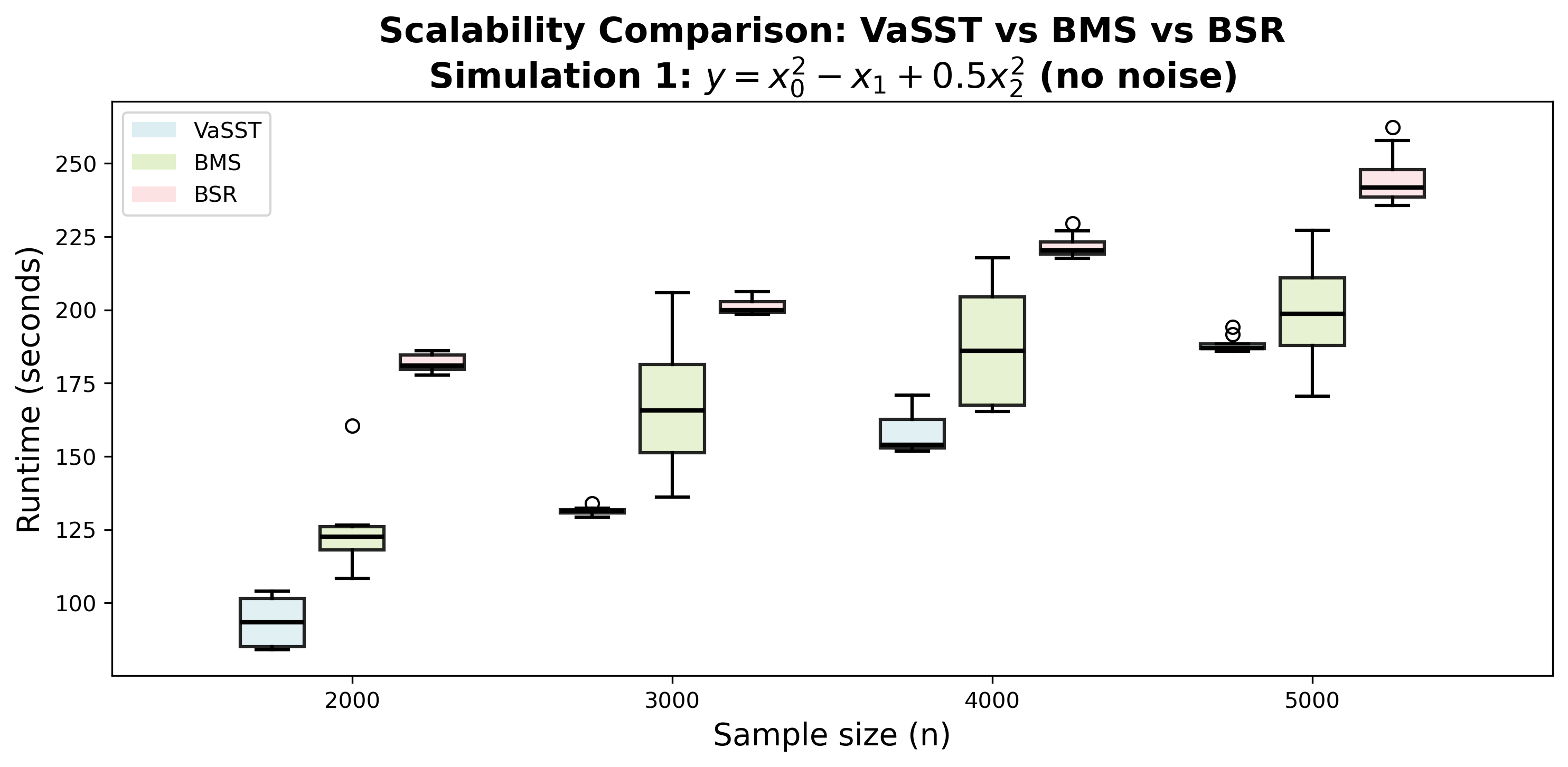
Refer to caption
Figure 3: Computational scalability of 𝖵𝖺𝖲𝖲𝖳\mathsf{VaSST}, BMS, BSR.

For a representative run under noise level σ2=0.12\sigma^{2}=0.1^{2}, Table 1 reports the symbolic expressions recovered by each method when learning (24); additional results for other noise levels are provided in Appendix I.1. 𝖵𝖺𝖲𝖲𝖳\mathsf{VaSST} accurately recovers the true structure while fitting K=3K=3 symbolic trees each of maximum depth D=3D=3, whereas competing methods largely fail to identify the underlying symbolic expression across noise levels, instead producing substantially more complicated expressions. When learning the simpler trigonometric expression in (25), results across noise levels are summarized in Appendix I.1. Here, 𝖵𝖺𝖲𝖲𝖳\mathsf{VaSST} (K=3K=3 and D=3D=3) again identifies the correct symbolic structure, alongside BMS. In contrast, BSR, QLattice, gplearn, and DEAP tend to generate unnecessarily complex output expressions. Notably, the structural recovery of 𝖵𝖺𝖲𝖲𝖳\mathsf{VaSST} (for both (24) and (25)) and of BMS (for the simpler model in (25)) remains consistent across increasing noise levels, reflecting stability of the learned symbolic structures under observational perturbations.

𝖵𝖺𝖲𝖲𝖳\mathsf{VaSST} effectively balances structural learning and predictive accuracy, achieving consistently low out-of-sample RMSEs across all noise levels when learning (24) (Table 2; see also Figure I.1 in Appendix I.2). Similar behavior is observed for (25) in Appendix I.2. Although BMS and QLattice perform competitively for the simpler model, QLattice (in general for both (24) and (25)) and BMS (for higher structural complexity as in (24)) frequently produce overly complex expressions indicative of overfitting, whereas 𝖵𝖺𝖲𝖲𝖳\mathsf{VaSST} outperforms by attaining the strongest predictive accuracy while maintaining structural parsimony. This structural parsimony is driven by the depth-adaptive split probability in (6), which penalizes unnecessarily complex expressions and consequently downweights them through small posterior mean estimates of 𝜷\boldsymbol{\beta}.

Furthermore, in learning (24) with no noise, Figure 3 highlights the computational scalability of 𝖵𝖺𝖲𝖲𝖳\mathsf{VaSST} relative to other Bayesian modules, i.e., BMS and BSR (maintained at similar configurations to that of 𝖵𝖺𝖲𝖲𝖳\mathsf{VaSST} for fair comparison). For increasing sample sizes n∈{2000,3000,4000,5000}n\in\{2000,3000,4000,5000\} with 1010 repetitions per nn, 𝖵𝖺𝖲𝖲𝖳\mathsf{VaSST} invariably records the lowest compute runtime, demonstrating superior scalability.

To quantify uncertainty over the learned symbolic tree structures for both (24) and (25) across all noise levels, we report in Appendix I.3 the top 55 symbolic expressions obtained from H=2000H=2000 sampled hard symbolic trees under 𝖵𝖺𝖲𝖲𝖳\mathsf{VaSST}(K=3K=3 and D=3D=3), ranked according to their minimum in-sample RMSE.

5.2 Application to Feynman Equations

We evaluate 𝖵𝖺𝖲𝖲𝖳\mathsf{VaSST} on benchmark SR problems from the Feynman Symbolic Regression Database (FSReD) (Udrescu and Tegmark, 2020) within SRBench, which contains over 100100 equations from the Feynman Lectures on Physics (Feynman et al., 2015) with 10510^{5} observations per equation. We consider four representative laws spanning electromagnetism, gravitation, and heat transfer with varying symbolic complexity, i.e., Coulomb’s law (CL), the change in gravitational potential energy (CPE), the Lorentz force on a moving charge in an electromagnetic field (FCE), and Fourier’s law of thermal conduction (FTC):

CL:F=0.08​q1​q2ϵ​r2,CPE:Δ​U=G​m1​m2​(1r2−1r1),\displaystyle\text{{CL}}:\;F=0.08\tfrac{q_{1}q_{2}}{\epsilon r^{2}},\;\text{{CPE}}:\;\Delta U=Gm_{1}m_{2}(\tfrac{1}{r_{2}}-\tfrac{1}{r_{1}}),
FCE:F=q​(Ef+v​B​sin⁡θ),FTC:P=κ​A​(T2−T1)d,\displaystyle\text{{FCE}}:\;F=q\left(E_{f}+vB\sin\theta\right),\;\text{{FTC}}:\;P=\tfrac{\kappa A(T_{2}-T_{1})}{d},

where the input features, responses, and constants are described in Appendix J. For each equation, we randomly subsample n=2000n=2000 observations. We consider three noise regimes: the original dataset (noiseless) and two settings with additive Gaussian noise of variance σ2∈{0.12,0.22}\sigma^{2}\in\{0.1^{2},0.2^{2}\} applied to the response variable to mimic measurement error and/or experimental perturbations. In all experiments 𝖵𝖺𝖲𝖲𝖳\mathsf{VaSST} fits K=3K=3 symbolic trees each of maximum depth D=3D=3.

Across all equation datasets and noise levels, the minimum RMSE model produced by 𝖵𝖺𝖲𝖲𝖳\mathsf{VaSST} recovers the correct symbolic expression. Among competing methods, BMS performs well for CL, CPE, and FCE across all noise levels but encounters numerical errors for FTC. The genetic programming module gplearn successfully identifies the correct expression in all but the more complex FCE case, where it yields unnecessarily complicated forms. The neural network-based QLattice fails to recover the true expressions in most cases and instead produces highly complex formulas, except for the relatively simple CL. Similarly, BSR and DEAP consistently favor overly complex symbolic expressions and do not recover the ground-truth equations. Table 3 summarizes symbolic recovery across all methods. As a representative example, Table 4 reports the expressions learned by each method for FTC at σ2=0.12\sigma^{2}=0.1^{2}, while the remaining results are provided in Appendix K.1.

Table 3: Exact symbolic recovery for the Feynman equations. ✓ and ✗ denote success and failure, respectively; symbols in each cell correspond to noiseless, σ2=0.12\sigma^{2}=0.1^{2}, σ2=0.22\sigma^{2}=0.2^{2}.
Method CL CPE FCE FTC
\rowcolorvasstgray 𝖵𝖺𝖲𝖲𝖳\mathsf{VaSST} ✓ ✓ ✓ ✓ ✓ ✓ ✓ ✓ ✓ ✓ ✓ ✓
BMS ✓ ✓ ✓ ✓ ✓ ✓ ✓ ✓ ✓ ✗ ✗ ✗
BSR ✗ ✗ ✗ ✗ ✗ ✗ ✗ ✗ ✗ ✗ ✗ ✗
DEAP ✗ ✗ ✗ ✗ ✗ ✗ ✗ ✗ ✗ ✗ ✗ ✗
gplearn ✓ ✓ ✓ ✓ ✓ ✓ ✗ ✗ ✗ ✓ ✓ ✓
QLattice ✓ ✓ ✓ ✗ ✗ ✗ ✗ ✗ ✗ ✓ ✗ ✗
Table 4: Symbolic expressions recovered by 𝖵𝖺𝖲𝖲𝖳\mathsf{VaSST} (K=3K=3 and D=3D=3) and competing methods for FTC: P=κ​A​(T2−T1)​d−1P=\kappa A(T_{2}-T_{1})d^{-1} under σ2=0.12\sigma^{2}=0.1^{2}. Out-of-sample RMSE is evaluated on a 10%10\% held-out test set, with all coefficients in the symbolic expression reported up to three decimal places across all methods.
Method Symbolic Expression Learned RMSE
\rowcolorvasstgray 𝖵𝖺𝖲𝖲𝖳\mathsf{VaSST} 0.002−0.943​κ​A​T1d+1.006​κ​A​T2d\displaystyle 0.002-0.943\,\frac{\kappa AT_{1}}{d}+1.006\,\frac{\kappa AT_{2}}{d} 1.00325×10−11.00325\times 10^{-1}
BMS BMS failed to return valid expression –
BSR 0.805−0.103​exp⁡(cos⁡(dA))+0.150​κ2​A​T12\displaystyle 0.805-0.103\,\exp\!\left(\cos\!\left(\frac{d}{\sqrt{A}}\right)\right)+0.150\,\kappa^{2}AT_{1}^{2} 4.06545×10−14.06545\times 10^{-1}
QLattice (0.469−0.518​T2T1)​(κ​A​T1+0.075)​exp⁡(−0.183​dA)−0.033\displaystyle(0.469-0.518\,\tfrac{T_{2}}{T_{1}})\,(\kappa\sqrt{A}T_{1}+0.075)\,\exp\!\left(-0.183\,\frac{d}{\sqrt{A}}\right)-0.033 1.01498×10−11.01498\times 10^{-1}
gplearn κ​A​(T2−T1)d\displaystyle\frac{\kappa A\,(T_{2}-T_{1})}{d} 1.00224×10−11.00224\times 10^{-1}
DEAP κ​A​T26​T1−5​[κ​A​T1−4.828​(1+T2T1)+dA​(−(T2T1)2+(T2T1)3+(T2T1)4+(T2T1)5)]−1\displaystyle{\kappa\sqrt{A}\,T_{2}^{6}\,T_{1}^{-5}}\left[{\kappa\sqrt{A}T_{1}-4.828\!\left(1+\frac{T_{2}}{T_{1}}\right)+\frac{d}{\sqrt{A}}\left(-\left(\frac{T_{2}}{T_{1}}\right)^{2}+\left(\frac{T_{2}}{T_{1}}\right)^{3}+\left(\frac{T_{2}}{T_{1}}\right)^{4}+\left(\frac{T_{2}}{T_{1}}\right)^{5}\right)}\right]^{-1} 1.00126×10−11.00126\times 10^{-1}

In terms of predictive performance, measured using out-of-sample RMSE, 𝖵𝖺𝖲𝖲𝖳\mathsf{VaSST} is consistently among the top-performing methods, typically alongside BMS, except for FTC where BMS fails due to numerical issues. Genetic programming-based gplearn and DEAP, and neural network-based QLattice often achieve competitive prediction accuracy but only through substantially more complex symbolic expressions. Lastly, BSR yields consistently higher prediction errors. A full comparison of out-of-sample RMSE values is provided in Appendix K.2.

Additionally, 𝖵𝖺𝖲𝖲𝖳\mathsf{VaSST} exhibits substantially faster runtimes than the Bayesian SR methods BMS and BSR across all Feynman equation datasets and noise settings, highlighting the computational advantages of the proposed variational inference framework. Detailed runtime comparisons are reported in Appendix K.3.

Finally, beyond competitive performance in prediction and structural learning, 𝖵𝖺𝖲𝖲𝖳\mathsf{VaSST} provides uncertainty quantification in symbolic equation discovery by producing multiple candidate symbolic ensembles ranked by minimum in-sample RMSE. The top 55 expressions across all Feynman equations and noise levels are reported in Appendix K.4.

6 Conclusion

We presented 𝖵𝖺𝖲𝖲𝖳\mathsf{VaSST}, a fully probabilistic framework for SR that leverages variational inference with continuous relaxations of symbolic trees. It enables scalable gradient-based optimization while preserving interpretability equipped with principled uncertainty quantification. Empirically, 𝖵𝖺𝖲𝖲𝖳\mathsf{VaSST} achieves strong structural recovery, competitive predictive accuracy, stability under noise, and notable computational gains over existing Bayesian SR methods.

This work opens promising future avenues for fully probabilistic and scalable variational inference–based SR, including the development of more structured optimization strategies for the variational objective to further enhance scalability relative to modern machine learning–based approaches.

References

  • Bhamidi et al. [2008] Shankar Bhamidi, Guy Bresler, and Allan Sly. Mixing time of exponential random graphs. In 49th Annual IEEE Symposium on Foundations of Computer Science, pages 803–812, 2008.
  • Blei et al. [2003] David M. Blei, Andrew Y. Ng, and Michael I. Jordan. Latent dirichlet allocation. Journal of Machine Learning Research, 3:993–1022, 2003.
  • Blei et al. [2017] David M. Blei, Alp Kucukelbir, and Jon D. McAuliffe. Variational Inference: A Review for Statisticians. Journal of the American Statistical Association, 112(518):859–877, 2017.
  • Boadu et al. [2025] Frimpong Boadu, Ahhyun Lee, and Jianlin Cheng. Deep learning methods for protein function prediction. PROTEOMICS, 25(1-2):2300471, 2025.
  • Breiman [1996] Leo Breiman. Bagging predictors. Machine Learning, 24(2):123–140, 1996.
  • Breiman et al. [1984] Leo Breiman, Jerome Friedman, R. A. Olshen, and Charles J. Stone. Classification and Regression Trees (1st ed.). Chapman and Hall/CRC, 1984.
  • Broløs et al. [2021] Kevin Broløs, Meera Vieira René, Machado, Chris Cave, Jaan Kasak, Valdemar Stentoft-Hansen, Victor Galindo Batanero, Tom Jelen, and Casper Wilstrup. An approach to symbolic regression using feyn. arXiv:2104.05417, 2021.
  • Brunton et al. [2016] Steven L. Brunton, Joshua L. Proctor, and J. Nathan Kutz. Discovering governing equations from data by sparse identification of nonlinear dynamical systems. Proceedings of the National Academy of Sciences, 113(15):3932–3937, 2016.
  • Butler et al. [2018] Keith T Butler, Daniel W Davies, Hugh Cartwright, Olexandr Isayev, and Aron Walsh. Machine learning for molecular and materials science. Nature, 559(7715):547–555, 2018.
  • Chipman et al. [1998] Hugh A. Chipman, Edward I. George, and Robert E. McCulloch. Bayesian CART Model Search. Journal of the American Statistical Association, 93(443):935–948, 1998.
  • Chipman et al. [2010] Hugh A. Chipman, Edward I. George, and Robert E. McCulloch. BART: Bayesian additive regression trees. The Annals of Applied Statistics, 4(1):266–298, 2010.
  • Davidson et al. [2003] J. W. Davidson, D. A. Savic, and G. A. Walters. Symbolic and numerical regression: experiments and applications. Information Sciences, 150(1–2):95–117, 2003.
  • Dension et al. [1998] David G. T. Dension, Bani K. Mallick, and Adrian F. M. Smith. A Bayesian CART algorithm. Biometrika, 85(2):363–377, 1998.
  • Feynman et al. [2015] R.P. Feynman, R.B. Leighton, and M. Sands. The Feynman Lectures on Physics, Vol. I: The New Millennium Edition: Mainly Mechanics, Radiation, and Heat. Number v. 1. Basic Books, 2015.
  • Fortin et al. [2012] Félix-Antoine Fortin, François-Michel De Rainville, Marc-André Gardner, Marc Parizeau, and Christian Gagné. DEAP: Evolutionary algorithms made easy. Journal of Machine Learning Research, 13(70):2171–2175, 2012.
  • Giordano et al. [2024] Ryan Giordano, Martin Ingram, and Tamara Broderick. Black box variational inference with a deterministic objective: Faster, more accurate, and even more black box. Journal of Machine Learning Research, 25(18):1–39, 2024.
  • Graves [2011] Alex Graves. Practical Variational Inference for Neural Networks. In Advances in Neural Information Processing Systems, volume 24, 2011.
  • Guimerà et al. [2020] Roger Guimerà, Ignasi Reichardt, Antoni Aguilar-Mogas, Francesco A Massucci, Manuel Miranda, Jordi Pallarès, and Marta Sales-Pardo. A bayesian machine scientist to aid in the solution of challenging scientific problems. Science advances, 6(5):eaav6971, 2020.
  • Jang et al. [2016] Eric Jang, Shixiang Gu, and Ben Poole. Categorical reparameterization with gumbel-softmax. arXiv:1611.01144, 2016.
  • Jefferys and Berger [1992] William H. Jefferys and James O. Berger. Ockham’s Razor and Bayesian Analysis. American Scientist, 80(1):64–72, 1992. ISSN 00030996.
  • Jin et al. [2020] Ying Jin, Weilin Fu, Jian Kang, Jiadong Guo, and Jian Guo. Bayesian Symbolic Regression. arXiv:1910.08892, 2020.
  • Jordan et al. [1999] Michael I Jordan, Zoubin Ghahramani, Tommi S Jaakkola, and Lawrence K Saul. An introduction to variational methods for graphical models. Machine learning, 37(2):183–233, 1999.
  • Kamienny et al. [2022] Pierre-Alexandre Kamienny, Stéphane d’Ascoli, Guillaume Lample, and François Charton. End-to-end symbolic regression with transformers. In Advances in Neural Information Processing Systems, 2022.
  • Korns [2011] Michael F. Korns. Accuracy in symbolic regression. In Genetic Programming Theory and Practice IX, pages 129–151. 2011.
  • Koza [1994] John R Koza. Genetic programming as a means for programming computers by natural selection. Statistics and computing, 4(2):87–112, 1994.
  • Kucukelbir et al. [2017] Alp Kucukelbir, Dustin Tran, Rajesh Ranganath, Andrew Gelman, and David M Blei. Automatic differentiation variational inference. Journal of machine learning research, 18(14):1–45, 2017.
  • Łatuszyński et al. [2025] Krzysztof Łatuszyński, Matthew T Moores, and Timothée Stumpf-Fétizon. MCMC for multi-modal distributions. arXiv:2501.05908, 2025.
  • Liu et al. [2019] Hanxiao Liu, Karen Simonyan, and Yiming Yang. DARTS: Differentiable architecture search. In International Conference on Learning Representations, 2019.
  • Loshchilov and Hutter [2019] Ilya Loshchilov and Frank Hutter. Decoupled Weight Decay Regularization. In International Conference on Learning Representations, 2019.
  • Maddison et al. [2017] Chris J. Maddison, Andriy Mnih, and Yee Whye Teh. The concrete distribution: A continuous relaxation of discrete random variables. arXiv:1611.00712, 2017.
  • Petersen et al. [2021] Brenden K Petersen, Mikel Landajuela Larma, Terrell N. Mundhenk, Claudio Prata Santiago, Soo Kyung Kim, and Joanne Taery Kim. Deep symbolic regression: Recovering mathematical expressions from data via risk-seeking policy gradients. In International Conference on Learning Representations, 2021.
  • Raissi et al. [2019] M. Raissi, P. Perdikaris, and G.E. Karniadakis. Physics-informed neural networks: A deep learning framework for solving forward and inverse problems involving nonlinear partial differential equations. Journal of Computational Physics, 378:686–707, 2019.
  • Rall [1981] Louis B Rall. Automatic differentiation: Techniques and applications. Springer, 1981.
  • Ranganath et al. [2014] Rajesh Ranganath, Sean Gerrish, and David M. Blei. Black Box Variational Inference. In International Conference on Artificial Intelligence and Statistics, volume 33, pages 814–822, 2014.
  • Rasmussen and Williams [2006] Carl Edward Rasmussen and Christopher K. I. Williams. Gaussian Processes for Machine Learning. MIT Press, 2006.
  • Salazar [2023] Sebastian Salazar. VaRT: Variational regression trees. In Advances in Neural Information Processing Systems, 2023.
  • Schmidt and Lipson [2009] Michael Schmidt and Hod Lipson. Distilling free-form natural laws from experimental data. Science, 324(5923):81–85, 2009.
  • Stephens [2016] Trevor Stephens. gplearn: Genetic Programming in Python, 2016. URL https://github.com/trevorstephens/gplearn.
  • Tibshirani [1996] Robert Tibshirani. Regression Shrinkage and Selection via the Lasso. Journal of the Royal Statistical Society. Series B (Methodological), 58(1):267–288, 1996.
  • Udrescu and Tegmark [2020] Silviu-Marian Udrescu and Max Tegmark. AI Feynman: A physics-inspired method for symbolic regression. Science Advances, 6(16):eaay2631, 2020.
  • Virgolin and Pissis [2022] Marco Virgolin and Solon P. Pissis. Symbolic regression is np-hard. In Proceedings of the Genetic and Evolutionary Computation Conference, 2022.
  • Wainwright and Jordan [2008] Martin J. Wainwright and Michael I. Jordan. Graphical Models, Exponential Families, and Variational Inference. Foundations and Trends in Machine Learning, 1(1–2):1–305, 2008.
  • Wang et al. [2024] Guanjie Wang, Erpeng Wang, Zefeng Li, Jian Zhou, and Zhimei Sun. Exploring the mathematic equations behind the materials science data using interpretable symbolic regression. Interdisciplinary Materials, 3(5):637–657, 2024.
  • Williams [1992] Ronald J Williams. Simple statistical gradient-following algorithms for connectionist reinforcement learning. Machine learning, 8(3):229–256, 1992.
  • Zhang et al. [2025] Huijun Zhang, Yaxin Liu, Chongyu Zhang, and Ningyun Li. Machine Learning Methods for Weather Forecasting: A Survey. Atmosphere, 16(1), 2025.

Supplementary Materials for 𝖵𝖺𝖲𝖲𝖳\mathsf{VaSST}: Variational Inference for Symbolic Regression using Soft Symbolic Trees

Appendix A Notations

Table A.1: Special functions and other notations.
Symbol Name Definition
ℕ\mathbb{N} Natural numbers Set {1,2,3,…}\{1,2,3,\dots\}
ℝ\mathbb{R} Real numbers Set of real numbers
ℝp\mathbb{R}^{p} pp-dimensional Euclidean space {𝐱=(x1,…,xp)⊤:xi∈ℝ}\{\mathbf{x}=(x_{1},\dots,x_{p})^{\top}:x_{i}\in\mathbb{R}\}
ℝm×n\mathbb{R}^{m\times n} Real matrix space Space of real m×nm\times n matrices
|A||A| Cardinality Number of elements in a finite set AA
Γ​(t)\Gamma(t) Gamma function Γ​(t)=∫0∞xt−1​e−x​𝑑x\displaystyle\Gamma(t)=\int_{0}^{\infty}x^{t-1}e^{-x}\,dx
Ψ​(t)\Psi(t) Digamma function Ψ​(t)=dd​t​log⁡Γ​(t)\displaystyle\Psi(t)=\frac{d}{dt}\log\Gamma(t)
ℬ​(𝜼)\mathcal{B}(\boldsymbol{\eta}) Multivariate Beta function ℬ​(𝜼)=∏k=1mΓ​(ηk)Γ​(∑k=1mηk)\displaystyle\mathcal{B}(\boldsymbol{\eta})=\frac{\prod_{k=1}^{m}\Gamma(\eta_{k})}{\Gamma\!\left(\sum_{k=1}^{m}\eta_{k}\right)}
𝟏m\mathbf{1}_{m} Vector of ones (1,…,1)⊤∈ℝm(1,\dots,1)^{\top}\in\mathbb{R}^{m}
𝟎m\boldsymbol{0}_{m} Vector of zeros (0,…,0)⊤∈ℝm(0,\dots,0)^{\top}\in\mathbb{R}^{m}
𝐈m\mathbf{I}_{m} Identity matrix of order mm (𝐈m)i​j=𝟏​{i=j},i,j=1,…,m(\mathbf{I}_{m})_{ij}=\mathbf{1}\{i=j\},\quad i,j=1,\dots,m
|𝐀||\mathbf{A}| Determinant Determinant of the matrix 𝐀∈ℝm×m\mathbf{A}\in\mathbb{R}^{m\times m}
Δm\Delta^{m} mm-dimensional simplex {𝐰∈[0,∞)m:𝟏m⊤​𝐰=1}\displaystyle\left\{\mathbf{w}\in[0,\infty)^{m}:\mathbf{1}_{m}^{\top}\mathbf{w}=1\right\}
𝖮​(g​(n))\mathsf{O}(g(n)) Order notation f​(n)=𝖮​(g​(n))f(n)=\mathsf{O}(g(n)) if |f​(n)|≤C​|g​(n)||f(n)|\leq C\,|g(n)| for some constant C>0C>0 and sufficiently large nn

Appendix B Parameterization Details of Distribution Families used in 𝖵𝖺𝖲𝖲𝖳\mathsf{VaSST}

The 𝖵𝖺𝖲𝖲𝖳\mathsf{VaSST} framework utilizes several standard probability distributions for model specification and prior construction. Although these distributions are widely used in the machine learning literature, multiple parameterizations are common for some of them across various sources. For clarity and reproducibility, we explicitly document the notation and parameterizations adopted in this work.

Normal Inverse-Gamma.

We use the conjugate Normal Inverse-Gamma (NIG\mathrm{NIG}) prior for Gaussian linear regression parameters:

𝜷∣σ2\displaystyle\boldsymbol{\beta}\mid\sigma^{2} ∼Nd​(𝝁0,σ2​𝚺0),σ2∼IG​(a0,b0),\displaystyle\sim\mathrm{N}_{d}(\boldsymbol{\mu}_{0},\sigma^{2}\boldsymbol{\Sigma}_{0}),\quad\sigma^{2}\sim\mathrm{IG}(a_{0},b_{0}), (B.1)

where d=K+1d=K+1, 𝝁0∈ℝd\boldsymbol{\mu}_{0}\in\mathbb{R}^{d}, 𝚺0∈ℝd×d\boldsymbol{\Sigma}_{0}\in\mathbb{R}^{d\times d} is symmetric positive definite, and a0,b0>0a_{0},b_{0}>0. Our Inverse-Gamma parameterization, i.e., IG​(a,b)\mathrm{IG}(a,b), uses the density:

Π​(σ2)=baΓ​(a)​(σ2)−(a+1)​exp⁡(−bσ2),σ2>0,\displaystyle\Pi(\sigma^{2})=\frac{b^{a}}{\Gamma(a)}(\sigma^{2})^{-(a+1)}\exp\!\left(-\frac{b}{\sigma^{2}}\right),\quad\sigma^{2}>0, (B.2)

where Γ​(⋅)\Gamma(\cdot) is the Gamma function in Table A.1. The conditional Gaussian density in (B.1) is:

Π​(𝜷∣σ2)=(2​π)−d2​(σ2)−d2​|𝚺0|−12​exp⁡{−12​σ2​(𝜷−𝝁0)⊤​𝚺0−1​(𝜷−𝝁0)}.\displaystyle\Pi(\boldsymbol{\beta}\mid\sigma^{2})=(2\pi)^{-\tfrac{d}{2}}(\sigma^{2})^{-\tfrac{d}{2}}|\boldsymbol{\Sigma}_{0}|^{-\tfrac{1}{2}}\exp\!\left\{-\frac{1}{2\sigma^{2}}(\boldsymbol{\beta}-\boldsymbol{\mu}_{0})^{\top}\boldsymbol{\Sigma}_{0}^{-1}(\boldsymbol{\beta}-\boldsymbol{\mu}_{0})\right\}. (B.3)

Equivalently, the joint prior is Π​(𝜷,σ2)=Π​(𝜷∣σ2)​Π​(σ2)\Pi(\boldsymbol{\beta},\sigma^{2})=\Pi(\boldsymbol{\beta}\mid\sigma^{2})\Pi(\sigma^{2}).

Bernoulli.

A Bernoulli random variable E∼Ber​(p)E\sim\mathrm{Ber}(p), with p∈(0,1)p\in(0,1), has support {0,1}\{0,1\} and probability mass function:

Π​(e)=pe​(1−p)1−e,e∈{0,1}.\displaystyle\Pi(e)=p^{e}(1-p)^{1-e},\quad e\in\{0,1\}. (B.4)

In our tree prior, the expansion indicator follows ej​ζ∼Ber​(pζ)e_{j\zeta}\sim\mathrm{Ber}(p_{\zeta}) with pζ=α​(1+dζ)−δp_{\zeta}=\alpha(1+d_{\zeta})^{-\delta}, where α∈(0,1)\alpha\in(0,1) and δ>0\delta>0.

Dirichlet.

For m≥2m\geq 2, a vector 𝐰∈Δm\mathbf{w}\in\Delta^{m} follows a Dirichlet distribution with concentration vector 𝜼=(η1,…,ηm)⊤∈(0,∞)m\boldsymbol{\eta}=(\eta_{1},\ldots,\eta_{m})^{\top}\in(0,\infty)^{m}, i.e., 𝐰∼Dir​(𝜼)\mathbf{w}\sim\mathrm{Dir}(\boldsymbol{\eta}), having density:

p​(𝐰∣𝜼)=1ℬ​(𝜼)​∏k=1mwkηk−1,𝐰∈Δm,\displaystyle p(\mathbf{w}\mid\boldsymbol{\eta})=\frac{1}{\mathcal{B}(\boldsymbol{\eta})}\prod_{k=1}^{m}w_{k}^{\eta_{k}-1},\quad\mathbf{w}\in\Delta^{m}, (B.5)

where ℬ​(⋅)\mathcal{B}(\cdot) is the multivariate Beta function and Δm\Delta^{m} is the mm-dimensional simplex, as defined in Table A.1. In 𝖵𝖺𝖲𝖲𝖳\mathsf{VaSST}, the operator and feature weight vectors follow 𝐰op∼Dir​(𝜼op)\mathbf{w}_{\mathrm{op}}\sim\mathrm{Dir}(\boldsymbol{\eta}_{\mathrm{op}}) and 𝐰ft∼Dir​(𝜼ft)\mathbf{w}_{\mathrm{ft}}\sim\mathrm{Dir}(\boldsymbol{\eta}_{\mathrm{ft}}), where 𝐰op∈Δ|𝒪|\mathbf{w}_{\mathrm{op}}\in\Delta^{|\mathcal{O}|} and 𝐰ft∈Δp\mathbf{w}_{\mathrm{ft}}\in\Delta^{p}, respectively.

Categorical.

Let 𝐰∈Δm\mathbf{w}\in\Delta^{m}. A Categorical random variable, c∼Cat​(𝐰)c\sim\mathrm{Cat}(\mathbf{w}), takes values in {1,…,m}\{1,\ldots,m\} with probability mass function:

Π​(c=j∣𝐰)=wj,j∈{1,…,m}\displaystyle\Pi(c=j\mid\mathbf{w})=w_{j},\qquad j\in\{1,\ldots,m\} (B.6)

In 𝖵𝖺𝖲𝖲𝖳\mathsf{VaSST}, conditional on weights, we assign operators and features via

oj​ζ∣𝐰op∼Cat​(𝐰op),hj​ζ∣𝐰ft∼Cat​(𝐰ft),oj​ζ∈𝒪,hj​ζ∈𝒳.\displaystyle o_{j\zeta}\mid\mathbf{w}_{\mathrm{op}}\sim\mathrm{Cat}(\mathbf{w}_{\mathrm{op}}),\quad h_{j\zeta}\mid\mathbf{w}_{\mathrm{ft}}\sim\mathrm{Cat}(\mathbf{w}_{\mathrm{ft}}),\quad o_{j\zeta}\in\mathcal{O},\;h_{j\zeta}\in\mathcal{X}. (B.7)

When needed, we identify 𝒪\mathcal{O} and 𝒳\mathcal{X} with index sets of sizes |𝒪||\mathcal{O}| and pp, respectively, so that (B.6) applies directly.

Uniform.

A continuous random variable u∼Unif​(a,b)u\sim\mathrm{Unif}(a,b), with a<ba<b, has support on the interval (a,b)(a,b) and probability density function:

Π​(u)=1b−a,a<u<b,\displaystyle\Pi(u)=\frac{1}{b-a},\quad a<u<b, (B.8)

and Π​(u)=0\Pi(u)=0 otherwise. In the Binary Concrete and Gumbel-Softmax continuous relaxations in Section 4, the Unif​(0,1)\mathrm{Unif}(0,1) distribution was used to reparameterize the discrete structural variables. Further, in simulation experiments in Section 5.1, uniform distributions were used to generate the input variables.

Appendix C Soft Evaluation Algorithms

C.1 Soft Evaluation At a Node

Input: A given node: ζ′\zeta^{\prime}; feature vector: 𝐱i∈ℝp\mathbf{x}_{i}\in\mathbb{R}^{p}; soft symbolic tree index: j∈{1,…,K}j\in\{1,\ldots,K\}; the operator set: 𝒪=𝒪u∪𝒪b\mathcal{O}=\mathcal{O}_{u}\cup\mathcal{O}_{b}; soft relaxations: {e~j​ζ,𝐨~j​ζ,𝐡~j​ζ:ζ∈𝒵D}\{\tilde{e}_{j\zeta},\tilde{\mathbf{o}}_{j\zeta},\tilde{\mathbf{h}}_{j\zeta}\;:\;\zeta\in\mathcal{Z}_{D}\}.
Output: 𝒮jsoft​(𝐱i;ζ′)∈ℝ\mathcal{S}_{j}^{\mathrm{soft}}(\mathbf{x}_{i};\zeta^{\prime})\in\mathbb{R}.
// Soft feature evaluation
Term​(𝐱i,j,ζ′)←𝐡~j​ζ′⊤​𝐱i\mathrm{Term}(\mathbf{x}_{i},j,\zeta^{\prime})\leftarrow\tilde{\mathbf{h}}^{\top}_{j\zeta^{\prime}}\mathbf{x}_{i}
// Soft operator evaluation
// L​(ζ′)L(\zeta^{\prime}) and R​(ζ′)R(\zeta^{\prime}) are the left and right children of ζ′\zeta^{\prime}, respectively
NontermUnary​(𝐱i,j,ζ′)←∑u∈𝒪uo~j​ζ′,u⋅u​(𝒮jsoft​(𝐱i,L​(ζ′)))\mathrm{NontermUnary}(\mathbf{x}_{i},j,\zeta^{\prime})\leftarrow\sum_{u\in\mathcal{O}_{u}}\tilde{o}_{j\zeta^{\prime},u}\cdot u(\mathcal{S}_{j}^{\mathrm{soft}}(\mathbf{x}_{i},L(\zeta^{\prime})))
NontermBinary​(𝐱i,j,ζ′)←∑b∈𝒪bo~j​ζ′,b⋅b​(𝒮jsoft​(𝐱i;L​(ζ′)),𝒮jsoft​(𝐱i;R​(ζ′)))\mathrm{NontermBinary}(\mathbf{x}_{i},j,\zeta^{\prime})\leftarrow\sum_{b\in\mathcal{O}_{b}}\tilde{o}_{j\zeta^{\prime},b}\cdot b(\mathcal{S}_{j}^{\mathrm{soft}}(\mathbf{x}_{i};L(\zeta^{\prime})),\;\mathcal{S}_{j}^{\mathrm{soft}}(\mathbf{x}_{i};R(\zeta^{\prime})))
Nonterm​(𝐱i,j,ζ′)←NontermUnary​(𝐱i,j,ζ′)+NontermBinary​(𝐱i,j,ζ′)\mathrm{Nonterm}(\mathbf{x}_{i},j,\zeta^{\prime})\leftarrow\mathrm{NontermUnary}(\mathbf{x}_{i},j,\zeta^{\prime})+\mathrm{NontermBinary}(\mathbf{x}_{i},j,\zeta^{\prime})
// Complete soft evaluation at ζ′\zeta^{\prime}
𝒮jsoft​(𝐱i;ζ′)←e~j​ζ′​Nonterm​(𝐱i,j,ζ′)+(1−e~j​ζ′)​Term​(𝐱i,j,ζ′)\mathcal{S}_{j}^{\mathrm{soft}}(\mathbf{x}_{i};\zeta^{\prime})\leftarrow\tilde{e}_{j\zeta^{\prime}}\mathrm{Nonterm}(\mathbf{x}_{i},j,\zeta^{\prime})+(1-\tilde{e}_{j\zeta^{\prime}})\mathrm{Term}(\mathbf{x}_{i},j,\zeta^{\prime})
return 𝒮jsoft​(𝐱i;ζ′)\mathcal{S}_{j}^{\mathrm{soft}}(\mathbf{x}_{i};\zeta^{\prime})
Algorithm 1 The SoftEvalAtNode(ζ′,𝐱i,j,𝒪,{e~j​ζ,𝐨~j​ζ,𝐡~j​ζ:ζ∈𝒵D})(\zeta^{\prime},\mathbf{x}_{i},j,\mathcal{O},\{\tilde{e}_{j\zeta},\tilde{\mathbf{o}}_{j\zeta},\tilde{\mathbf{h}}_{j\zeta}\;:\;\zeta\in\mathcal{Z}_{D}\}) algorithm for evaluating a soft symbolic subtree rooted at a given node ζ′\zeta^{\prime}.

C.2 Complete Soft Evaluation

Input: Feature vectors: {𝐱i∈ℝp:i=1,…,n}\{\mathbf{x}_{i}\in\mathbb{R}^{p}\;:\;i=1,\ldots,n\}; the operator set: 𝒪=𝒪u∪𝒪b\mathcal{O}=\mathcal{O}_{u}\cup\mathcal{O}_{b}; soft relaxations: {e~j​ζ,𝐨~j​ζ,𝐡~j​ζ:ζ∈𝒵D}j=1K\{\tilde{e}_{j\zeta},\tilde{\mathbf{o}}_{j\zeta},\tilde{\mathbf{h}}_{j\zeta}\;:\;\zeta\in\mathcal{Z}_{D}\}_{j=1}^{K}.
Output: 𝐓soft∈ℝn×K+1¯\mathbf{T}_{\mathrm{soft}}\in\mathbb{R}^{n\times\overline{K+1}}.
for i←1i\leftarrow 1 to nn do
    // Intercept term set to 11
    ti​0←1t_{i0}\leftarrow 1
    for j←1j\leftarrow 1 to KK do
       // jjth soft symbolic tree evaluated at root node for 𝐱i\mathbf{x}_{i}
       ti​j=𝒮jsoft​(𝐱i;ζ′=0)t_{ij}=\mathcal{S}_{j}^{\mathrm{soft}}(\mathbf{x}_{i};\zeta^{\prime}=0) from Algorithm 1: SoftEvalAtNode
      
   
𝐓soft←(ti​j)1≤i≤n, 0≤j≤K\mathbf{T}_{\mathrm{soft}}\leftarrow(t_{ij})_{1\leq i\leq n,\;0\leq j\leq K}
return 𝐓soft\mathbf{T}_{\mathrm{soft}}
Algorithm 2 The SoftEval({𝐱i∈ℝp:i=1,…,n},𝒪,{e~j​ζ,𝐨~j​ζ,𝐡~j​ζ:ζ∈𝒵D}j=1K)(\{\mathbf{x}_{i}\in\mathbb{R}^{p}\;:\;i=1,\ldots,n\},\mathcal{O},\{\tilde{e}_{j\zeta},\tilde{\mathbf{o}}_{j\zeta},\tilde{\mathbf{h}}_{j\zeta}\;:\;\zeta\in\mathcal{Z}_{D}\}_{j=1}^{K}) algorithm for evaluating an ensemble of KK soft symbolic trees.

Appendix D Algorithm for Approximation of ℒ​(ϕ)\mathcal{L}(\phi)

Input: Data: 𝒟n={(𝐱i,yi):i=1,…,n}\mathcal{D}_{n}=\{(\mathbf{x}_{i},y_{i})\;:\;i=1,\ldots,n\}; full set of prior hyperparameters: (𝝁0,𝚺0,a0,b0,𝜼op,𝜼ft,α,δ)(\boldsymbol{\mu}_{0},\boldsymbol{\Sigma}_{0},a_{0},b_{0},\boldsymbol{\eta}_{\mathrm{op}},\boldsymbol{\eta}_{\mathrm{ft}},\alpha,\delta); the operator set: 𝒪=𝒪u∪𝒪b\mathcal{O}=\mathcal{O}_{u}\cup\mathcal{O}_{b}; the variational parameter vector: ϕ\phi; the temperature parameters: (τex,τop,τft)(\tau_{\mathrm{ex}},\tau_{\mathrm{op}},\tau_{\mathrm{ft}}); the Monte Carlo sample size: SS.
Output: ℒ^​(ϕ)\widehat{\mathcal{L}}(\phi).
// Compute the Kullback-Leibler term
𝒦←KL​(qϕ​(Θ)∥Π​(Θ))\mathcal{K}\leftarrow\mathrm{KL}(q_{\phi}(\Theta)\parallel\Pi(\Theta)), using (19)
for s←1s\leftarrow 1 to SS do
    // Sample soft tree structural parameters from 𝒫ϕsoft\mathcal{P}_{\phi}^{\mathrm{soft}}
    {e~j​ζ(s),𝐨~j​ζ(s),𝐡~j​ζ(s):ζ∈𝒵D}j=1K∼𝒫ϕsoft\{\tilde{e}_{j\zeta}^{(s)},\tilde{\mathbf{o}}_{j\zeta}^{(s)},\tilde{\mathbf{h}}_{j\zeta}^{(s)}\>:\>\zeta\in\mathcal{Z}_{D}\}_{j=1}^{K}\sim\mathcal{P}^{\mathrm{soft}}_{\phi}, using the temperature parameters
    // Computing soft symbolic design matrix
    𝐓soft(s)←\mathbf{T}^{(s)}_{\mathrm{soft}}\leftarrow SoftEval({𝐱i∈ℝp:i=1,…,n},𝒪,{e~j​ζ(s),𝐨~j​ζ(s),𝐡~j​ζ(s):ζ∈𝒵D}j=1K)(\{\mathbf{x}_{i}\in\mathbb{R}^{p}\;:\;i=1,\ldots,n\},\mathcal{O},\{\tilde{e}_{j\zeta}^{(s)},\tilde{\mathbf{o}}_{j\zeta}^{(s)},\tilde{\mathbf{h}}_{j\zeta}^{(s)}\;:\;\zeta\in\mathcal{Z}_{D}\}_{j=1}^{K})
    // Computing the marginal likelihood at 𝐓soft(s)\mathbf{T}_{\mathrm{soft}}^{(s)}
    ML(s)←log⁡p​(𝐲∣𝐓soft(s))\mathrm{ML}^{(s)}\leftarrow\log p(\mathbf{y}\mid\mathbf{T}_{\mathrm{soft}}^{(s)}), using (9)
   
ℒ^​(ϕ)←1S​∑s=1SML(s)−𝒦\widehat{\mathcal{L}}(\phi)\leftarrow\tfrac{1}{S}\sum_{s=1}^{S}\mathrm{ML}^{(s)}-\mathcal{K}
return ℒ^​(ϕ)\widehat{\mathcal{L}}(\phi)
Algorithm 3 The ApproxELBO(𝒟n,(𝝁0,𝚺0,a0,b0,𝜼op,𝜼ft,α,δ),𝒪,ϕ,(τex,τop,τft),S)(\mathcal{D}_{n},(\boldsymbol{\mu}_{0},\boldsymbol{\Sigma}_{0},a_{0},b_{0},\boldsymbol{\eta}_{\mathrm{op}},\boldsymbol{\eta}_{\mathrm{ft}},\alpha,\delta),\mathcal{O},\phi,(\tau_{\mathrm{ex}},\tau_{\mathrm{op}},\tau_{\mathrm{ft}}),S) algorithm for computing Monte Carlo approximation of ℒ​(ϕ)\mathcal{L}(\phi).

Appendix E The 𝖵𝖺𝖲𝖲𝖳\mathsf{VaSST} Algorithm

Input: Data: 𝒟n={(𝐱i,yi):i=1,…,n}\mathcal{D}_{n}=\{(\mathbf{x}_{i},y_{i})\;:\;i=1,\ldots,n\}; full set of prior hyperparameters: (𝝁0,𝚺0,a0,b0,𝜼op,𝜼ft,α,δ)(\boldsymbol{\mu}_{0},\boldsymbol{\Sigma}_{0},a_{0},b_{0},\boldsymbol{\eta}_{\mathrm{op}},\boldsymbol{\eta}_{\mathrm{ft}},\alpha,\delta); the operator set: 𝒪=𝒪u∪𝒪b\mathcal{O}=\mathcal{O}_{u}\cup\mathcal{O}_{b}; initial variational parameter vector: ϕinit\phi^{\mathrm{init}}; number of steps: TT; temperature schedule: (τstart,τend,Tτ)(\tau_{\mathrm{start}},\tau_{\mathrm{end}},T_{\tau}); Monte Carlo sample size: SS; learning rate: γ\gamma; gradient clipping threshold: cc.
Output: Optimized variational parameter vector ϕ⋆\phi^{\star}.
Set ϕ0←ϕinit\phi_{0}\leftarrow\phi^{\mathrm{init}}
Initialize AdamW optimizer with learning rate γ\gamma
for t←1t\leftarrow 1 to TT do
    // Anneal temperature parameters
    τt←τstart+(τend−τstart)⋅min⁡{tTτ,1}\tau_{t}\leftarrow\tau_{\mathrm{start}}+(\tau_{\mathrm{end}}-\tau_{\mathrm{start}})\cdot\min\{\tfrac{t}{T_{\tau}},1\}
    Set (τex,τop,τft)←(τt,τt,τt)(\tau_{\mathrm{ex}},\tau_{\mathrm{op}},\tau_{\mathrm{ft}})\leftarrow(\tau_{t},\tau_{t},\tau_{t})
   
   Set all gradients to zero
   
   // Compute stochastic ELBO estimate
    ℒ^​(ϕ)←ApproxELBO\widehat{\mathcal{L}}(\phi)\leftarrow\textsc{ApproxELBO}(𝒟n,(𝝁0,𝚺0,a0,b0,𝜼op,𝜼ft,α,δ),𝒪,ϕ,(τex,τop,τft),S)(\mathcal{D}_{n},(\boldsymbol{\mu}_{0},\boldsymbol{\Sigma}_{0},a_{0},b_{0},\boldsymbol{\eta}_{\mathrm{op}},\boldsymbol{\eta}_{\mathrm{ft}},\alpha,\delta),\mathcal{O},\phi,(\tau_{\mathrm{ex}},\tau_{\mathrm{op}},\tau_{\mathrm{ft}}),S)
   
   𝒥←−ℒ^​(ϕ)\mathcal{J}\leftarrow-\widehat{\mathcal{L}}(\phi)
    // minimize negative objective
   
   if 𝒥\mathcal{J} is not finite then
       continue
      
   
   Backpropagate: compute ∇ϕ𝒥\nabla_{\phi}\mathcal{J}
   
   if any component of ∇ϕ𝒥\nabla_{\phi}\mathcal{J} is not finite then
       Set all gradients to zero; continue
      
   
   Clip gradients: ‖∇ϕ𝒥‖≤c\|\nabla_{\phi}\mathcal{J}\|\leq c
   
   ϕt←\phi_{t}\leftarrow AdamW update step on ϕ\phi
   
Set ϕ⋆←ϕT\phi^{\star}\leftarrow\phi_{T}
return ϕ⋆\phi^{\star}
Algorithm 4 The 𝖵𝖺𝖲𝖲𝖳\mathsf{VaSST}(𝒟n,(𝝁0,𝚺0,a0,b0,𝜼op,𝜼ft,α,δ),𝒪,ϕinit,T,(τstart,τend,Tτ),S,γ,c)(\mathcal{D}_{n},(\boldsymbol{\mu}_{0},\boldsymbol{\Sigma}_{0},a_{0},b_{0},\boldsymbol{\eta}_{\mathrm{op}},\boldsymbol{\eta}_{\mathrm{ft}},\alpha,\delta),\mathcal{O},\phi^{\mathrm{init}},T,(\tau_{\mathrm{start}},\tau_{\mathrm{end}},T_{\tau}),S,\gamma,c) algorithm for symbolic regression using automatic differentiation-based black-box variational inference

Appendix F Algorithm for Sampling Hard Symbolic Trees

Input: Data: 𝒟n={(𝐱i,yi):i=1,…,n}\mathcal{D}_{n}=\{(\mathbf{x}_{i},y_{i})\;:\;i=1,\ldots,n\}; full set of prior hyperparameters: (𝝁0,𝚺0,a0,b0,𝜼op,𝜼ft,α,δ)(\boldsymbol{\mu}_{0},\boldsymbol{\Sigma}_{0},a_{0},b_{0},\boldsymbol{\eta}_{\mathrm{op}},\boldsymbol{\eta}_{\mathrm{ft}},\alpha,\delta); optimizied variational parameter vector: ϕ⋆\phi^{\star}; the operator set 𝒪=𝒪u∪𝒪b\mathcal{O}=\mathcal{O}_{u}\cup\mathcal{O}_{b}; the number of hard symbolic tree samples: H.
Output: A collection of HH sampled hard symbolic ensembles and their corresponding posterior mean estimates of the model regression parameters: {{𝒯​(𝔈j(s))}j=1K,𝜷PM(s),(σ2)PM(s):s=1,…,H}\{\{\mathcal{T}(\mathfrak{E}_{j}^{(s)})\}_{j=1}^{K},\boldsymbol{\beta}^{(s)}_{\mathrm{PM}},(\sigma^{2})^{(s)}_{\mathrm{PM}}\;:\;s=1,\ldots,H\}.
for s←1s\leftarrow 1 to HH do
    // Sample one ensemble of KK hard symbolic trees
    for j←1j\leftarrow 1 to KK do
       // (i) sample expansion indicators
       e^j​ζ(s)∼Ber​(σ​(ℓj​ζ⋆))\widehat{e}^{(s)}_{j\zeta}\sim\mathrm{Ber}(\sigma(\ell^{\star}_{j\zeta})) for all ζ∈𝒵D\zeta\in\mathcal{Z}_{D}
       Enforce leaf constraint: e^j​ζ(s)←0\widehat{e}_{j\zeta}^{(s)}\leftarrow 0 for all ζ\zeta at depth DD
      
      // (ii) sample operator and feature labels
       o^j​ζ(s)∼Cat​(softmax​((𝐚j​ζop)⋆))\widehat{o}^{(s)}_{j\zeta}\sim\mathrm{Cat}(\texttt{softmax}((\mathbf{a}^{\mathrm{op}}_{j\zeta})^{\star}))
       h^j​ζ(s)∼Cat​(softmax​((𝐚j​ζft)⋆))\widehat{h}^{(s)}_{j\zeta}\sim\mathrm{Cat}(\texttt{softmax}((\mathbf{a}^{\mathrm{ft}}_{j\zeta})^{\star}))
      
      // (iii) Construct hard symbolic tree skeleton
       (𝒮^j(D))(s)←{e^j​ζ(s),o^j​ζ(s),h^j​ζ(s):ζ∈𝒵D}(\widehat{\mathcal{S}}_{j}^{(D)})^{(s)}\leftarrow\{\widehat{e}_{j\zeta}^{(s)},\widehat{o}_{j\zeta}^{(s)},\widehat{h}_{j\zeta}^{(s)}\;:\;\zeta\in\mathcal{Z}_{D}\}
      // (iv) symbolic trees via deterministic pruning of skeleton
       𝒯​(𝔈j(s))←𝔭​((𝒮^j(D))(s))\mathcal{T}(\mathfrak{E}_{j}^{(s)})\leftarrow\mathfrak{p}\left((\widehat{\mathcal{S}}_{j}^{(D)})^{(s)}\right)
      
      for i←1i\leftarrow 1 to nn do
          // Evaluate at sample 𝐱i\mathbf{x}_{i}
          ti​j(s)←g​(𝐱i;𝒯​(𝔈j(s)))t_{ij}^{(s)}\leftarrow g(\mathbf{x}_{i};\mathcal{T}(\mathfrak{E}_{j}^{(s)}))
      
   // Construct expression design matrix
    ti​0(s)←1t_{i0}^{(s)}\leftarrow 1 for all i=1,…,ni=1,\ldots,n
    𝐓(s)←((ti​j(s)))1≤i≤n,0≤j≤K\mathbf{T}^{(s)}\leftarrow((t_{ij}^{(s)}))_{1\leq i\leq n,0\leq j\leq K}
   
   // Compute posterior means of model regression parameters
    𝜷PM(s)←𝔼​[𝜷∣σ2,𝐓(s),𝐲]\boldsymbol{\beta}^{(s)}_{\mathrm{PM}}\leftarrow\mathbb{E}[\boldsymbol{\beta}\mid\sigma^{2},\mathbf{T}^{(s)},\mathbf{y}] and (σ2)PM(s)←𝔼​[σ2∣𝐓(s),𝐲](\sigma^{2})^{(s)}_{\mathrm{PM}}\leftarrow\mathbb{E}[\sigma^{2}\mid\mathbf{T}^{(s)},\mathbf{y}], using (G.2)
   
return {{𝒯​(𝔈j(s))}j=1K,𝛃PM(s),(σ2)PM(s):s=1,…,H}\{\{\mathcal{T}(\mathfrak{E}_{j}^{(s)})\}_{j=1}^{K},{\boldsymbol{\beta}}^{(s)}_{\mathrm{PM}},({\sigma}^{2})^{(s)}_{\mathrm{PM}}\;:\;s=1,\ldots,H\}
Algorithm 5 The SampleHard(𝒟n,(𝝁0,𝚺0,a0,b0,𝜼op,𝜼ft,α,δ),ϕ⋆,𝒪,H)(\mathcal{D}_{n},(\boldsymbol{\mu}_{0},\boldsymbol{\Sigma}_{0},a_{0},b_{0},\boldsymbol{\eta}_{\mathrm{op}},\boldsymbol{\eta}_{\mathrm{ft}},\alpha,\delta),\phi^{\star},\mathcal{O},H) algorithm to draw samples of hard symbolic trees from learned soft structural representations

Appendix G Technical Details

G.1 Marginalization of the Model Regression Parameters

The full joint posterior distribution as stated in (8) in Section 4 is:

Π​(Θ,𝜷,σ2∣𝒟n)∝p​(𝐲∣𝐓,𝜷,σ2)​Π​(𝜷,σ2)​Π​(𝐰op)​Π​(𝐰ft)​∏j=1K∏ζ∈𝒵DΠ​(ej​ζ)​Π​(oj​ζ∣𝐰op)​Π​(hj​ζ∣𝐰ft).\displaystyle\begin{split}\Pi(\Theta,\boldsymbol{\beta},\sigma^{2}\mid\mathcal{D}_{n})&\propto p(\mathbf{y}\mid\mathbf{T},\boldsymbol{\beta},\sigma^{2})\Pi(\boldsymbol{\beta},\sigma^{2})\Pi(\mathbf{w}_{\mathrm{op}})\Pi(\mathbf{w}_{\mathrm{ft}})\prod_{j=1}^{K}\prod_{\zeta\in\mathcal{Z}_{D}}\Pi(e_{j\zeta})\Pi(o_{j\zeta}\mid\mathbf{w}_{\mathrm{op}})\Pi(h_{j\zeta}\mid\mathbf{w}_{\mathrm{ft}}).\end{split} (G.1)

Under the Gaussian likelihood and the conjugate NIG\mathrm{NIG} prior:

𝐲∣𝜷,σ2,𝐓∼Nn​(𝐓​𝜷,σ2​𝐈n),𝜷∣σ2∼NK+1​(𝝁0,σ2​𝚺0),σ2∼IG​(a0,b0),\mathbf{y}\mid\boldsymbol{\beta},\sigma^{2},\mathbf{T}\sim\mathrm{N}_{n}(\mathbf{T}\boldsymbol{\beta},\sigma^{2}\mathbf{I}_{n}),\quad\boldsymbol{\beta}\mid\sigma^{2}\sim\mathrm{N}_{K+1}(\boldsymbol{\mu}_{0},\sigma^{2}\boldsymbol{\Sigma}_{0}),\quad\sigma^{2}\sim\mathrm{IG}(a_{0},b_{0}),

the posterior remains NIG\mathrm{NIG}:

𝜷∣σ2,𝐓,𝐲∼NK+1​(𝝁n,σ2​𝚺n),σ2∣𝐓,𝐲∼IG​(an,bn),\boldsymbol{\beta}\mid\sigma^{2},\mathbf{T},\mathbf{y}\sim\mathrm{N}_{K+1}(\boldsymbol{\mu}_{n},\sigma^{2}\boldsymbol{\Sigma}_{n}),\quad\sigma^{2}\mid\mathbf{T},\mathbf{y}\sim\mathrm{IG}(a_{n},b_{n}), (G.2)

where the posterior hyperparameters are:

𝚺n−1=𝚺0−1+𝐓⊤​𝐓,𝝁n=𝚺n​(𝚺0−1​𝝁0+𝐓⊤​𝐲),an=a0+n2,bn=b0+12​(𝐲⊤​𝐲+𝝁0⊤​𝚺0−1​𝝁0−𝝁n⊤​𝚺n−1​𝝁n).\boldsymbol{\Sigma}_{n}^{-1}=\boldsymbol{\Sigma}_{0}^{-1}+\mathbf{T}^{\top}\mathbf{T},\quad\boldsymbol{\mu}_{n}=\boldsymbol{\Sigma}_{n}(\boldsymbol{\Sigma}_{0}^{-1}\boldsymbol{\mu}_{0}+\mathbf{T}^{\top}\mathbf{y}),\quad a_{n}=a_{0}+\tfrac{n}{2},\quad b_{n}=b_{0}+\tfrac{1}{2}\left(\mathbf{y}^{\top}\mathbf{y}+\boldsymbol{\mu}_{0}^{\top}\boldsymbol{\Sigma}_{0}^{-1}\boldsymbol{\mu}_{0}-\boldsymbol{\mu}_{n}^{\top}\boldsymbol{\Sigma}_{n}^{-1}\boldsymbol{\mu}_{n}\right).

Integrating out (𝜷,σ2)(\boldsymbol{\beta},\sigma^{2}) yields the marginal likelihood:

p​(𝐲∣𝐓)\displaystyle p(\mathbf{y}\mid\mathbf{T}) =∫p​(𝐲∣𝐓,𝜷,σ2)​Π​(𝜷,σ2)​𝑑𝜷​𝑑σ2\displaystyle=\int p(\mathbf{y}\mid\mathbf{T},\boldsymbol{\beta},\sigma^{2})\Pi(\boldsymbol{\beta},\sigma^{2})\,d\boldsymbol{\beta}\,d\sigma^{2}
=Γ​(an)Γ​(a0)​|𝚺n|12|𝚺0|12​b0a0bnan​(2​π)−n2,\displaystyle=\frac{\Gamma(a_{n})}{\Gamma(a_{0})}\frac{|\boldsymbol{\Sigma}_{n}|^{\tfrac{1}{2}}}{|\boldsymbol{\Sigma}_{0}|^{\tfrac{1}{2}}}\frac{b_{0}^{a_{0}}}{b_{n}^{a_{n}}}(2\pi)^{-\tfrac{n}{2}}, (G.3)

where Γ​(⋅)\Gamma(\cdot) is the Gamma function as in Table A.1. Up to additive constants independent of 𝐓\mathbf{T}, the log-marginal likelihood is therefore:

log⁡p​(𝐲∣𝐓)=12​log⁡|𝚺n|−an​log⁡bn+log⁡Γ​(an)+C,\displaystyle\log p(\mathbf{y}\mid\mathbf{T})=\tfrac{1}{2}\log|\boldsymbol{\Sigma}_{n}|-a_{n}\log b_{n}+\log\Gamma(a_{n})+C, (G.4)

where CC collects terms independent of 𝐓\mathbf{T}. Consequently, the marginal posterior over the tree parameters Θ\Theta becomes:

Π​(Θ∣𝒟n)∝p​(𝐲∣𝐓)​Π​(𝐰op)​Π​(𝐰ft)​∏j=1K∏ζ∈𝒵DΠ​(ej​ζ)​Π​(oj​ζ∣𝐰op)​Π​(hj​ζ∣𝐰ft),\displaystyle\Pi(\Theta\mid\mathcal{D}_{n})\propto p(\mathbf{y}\mid\mathbf{T})\Pi(\mathbf{w}_{\mathrm{op}})\Pi(\mathbf{w}_{\mathrm{ft}})\prod_{j=1}^{K}\prod_{\zeta\in\mathcal{Z}_{D}}\Pi(e_{j\zeta})\Pi(o_{j\zeta}\mid\mathbf{w}_{\mathrm{op}})\Pi(h_{j\zeta}\mid\mathbf{w}_{\mathrm{ft}}), (G.5)

which is the quantity of interest we approximate using an optimal variational family obtained by optimizing the variational objective.

G.2 Derivation of the Analytical Kullback–Leibler Divergence Terms

In this section, we provide a detailed derivation of the Kullback-Leibler (KL\mathrm{KL}) term in (18) in Section 3.2. Specifically, this term corresponds to the KL\mathrm{KL} divergence between the variational posterior qϕ​(Θ)q_{\phi}(\Theta) in (17) and the prior Π​(Θ)\Pi(\Theta) over the tree parameters in (7):

KL(qϕ​(Θ)∥Π​(Θ))=𝔼qϕ​(Θ)​[log⁡qϕ​(Θ)Π​(Θ)]=𝔼qϕ​(Θ)​[log⁡qϕ​(𝐰op)​qϕ​(𝐰ft)​∏j=1K∏ζ∈𝒵Dqϕ​(ej​ζ)​qϕ​(oj​ζ)​qϕ​(hj​ζ)Π​(𝐰op)​Π​(𝐰ft)​∏j=1K∏ζ∈𝒵DΠ​(ej​ζ)​Π​(oj​ζ∣𝐰op)​Π​(hj​ζ∣𝐰ft)]=𝔼qϕ​(Θ)​[log⁡qϕ​(𝐰op)Π​(𝐰op)+log⁡qϕ​(𝐰ft)Π​(𝐰ft)+∑j=1K∑ζ∈𝒵D(log⁡qϕ​(ej​ζ)Π​(ej​ζ)+log⁡qϕ​(oj​ζ)Π​(oj​ζ∣𝐰op)+log⁡qϕ​(hj​ζ)Π​(hj​ζ∣𝐰ft))]=KL(qϕ(𝐰op)∥Π(𝐰op))+KL(qϕ(𝐰ft)∥Π(𝐰ft))+∑j=1K∑ζ∈𝒵D[KL(qϕ(ej​ζ)∥Π(ej​ζ))+𝔼qϕ​(𝐰op)[KL(qϕ(oj​ζ)∥Π(oj​ζ∣𝐰op))]+𝔼qϕ​(𝐰ft)[KL(qϕ(hj​ζ)∥Π(hj​ζ|𝐰ft))]].\displaystyle\begin{split}\mathrm{KL}&(q_{\phi}(\Theta)\parallel\Pi(\Theta))=\mathbb{E}_{q_{\phi}(\Theta)}\left[\log\frac{q_{\phi}(\Theta)}{\Pi(\Theta)}\right]\\ &=\mathbb{E}_{q_{\phi}(\Theta)}\left[\log\frac{q_{\phi}(\mathbf{w}_{\mathrm{op}})q_{\phi}(\mathbf{w}_{\mathrm{ft}})\prod_{j=1}^{K}\prod_{\zeta\in\mathcal{Z}_{D}}q_{\phi}(e_{j\zeta})q_{\phi}(o_{j\zeta})q_{\phi}(h_{j\zeta})}{\Pi(\mathbf{w}_{\mathrm{op}})\Pi(\mathbf{w}_{\mathrm{ft}})\prod_{j=1}^{K}\prod_{\zeta\in\mathcal{Z}_{D}}\Pi(e_{j\zeta})\Pi(o_{j\zeta}\mid\mathbf{w}_{\mathrm{op}})\Pi(h_{j\zeta}\mid\mathbf{w}_{\mathrm{ft}})}\right]\\ &=\mathbb{E}_{q_{\phi}(\Theta)}\left[\log\frac{q_{\phi}(\mathbf{w}_{\mathrm{op}})}{\Pi(\mathbf{w}_{\mathrm{op}})}+\log\frac{q_{\phi}(\mathbf{w}_{\mathrm{ft}})}{\Pi(\mathbf{w}_{\mathrm{ft}})}+\sum_{j=1}^{K}\sum_{\zeta\in\mathcal{Z}_{D}}\left(\log\frac{q_{\phi}(e_{j\zeta})}{\Pi(e_{j\zeta})}+\log\frac{q_{\phi}(o_{j\zeta})}{\Pi(o_{j\zeta}\mid\mathbf{w}_{\mathrm{op}})}+\log\frac{q_{\phi}(h_{j\zeta})}{\Pi(h_{j\zeta}\mid\mathbf{w}_{\mathrm{ft}})}\right)\right]\\ &=\mathrm{KL}(q_{\phi}(\mathbf{w}_{\mathrm{op}})\parallel\Pi(\mathbf{w}_{\mathrm{op}}))+\mathrm{KL}(q_{\phi}(\mathbf{w}_{\mathrm{ft}})\parallel\Pi(\mathbf{w}_{\mathrm{ft}}))+\sum_{j=1}^{K}\sum_{\zeta\in\mathcal{Z}_{D}}\bigg[\mathrm{KL}(q_{\phi}(e_{j\zeta})\parallel\Pi(e_{j\zeta}))\\ &\qquad\qquad\qquad\qquad\quad+\mathbb{E}_{q_{\phi}(\mathbf{w}_{\mathrm{op}})}[\mathrm{KL}(q_{\phi}(o_{j\zeta})\parallel\Pi(o_{j\zeta}\mid\mathbf{w}_{\mathrm{op}}))]+\mathbb{E}_{q_{\phi}(\mathbf{w}_{\mathrm{ft}})}[\mathrm{KL}(q_{\phi}(h_{j\zeta})\parallel\Pi(h_{j\zeta}|\mathbf{w}_{\mathrm{ft}}))]\bigg].\end{split} (G.6)

Now, we derive the analytic forms of each of the terms in the final sum in (G.6).

Lemma G.1 (KL\mathrm{KL} divergence between Dirichlet distributions).

Let q≡Dir​(𝛈~)q\equiv\mathrm{Dir}(\tilde{\boldsymbol{\eta}}) and π≡Dir​(𝛈)\pi\equiv\mathrm{Dir}(\boldsymbol{\eta}) on Δm\Delta^{m}, where 𝛈~,𝛈∈(0,∞)m\tilde{\boldsymbol{\eta}},\boldsymbol{\eta}\in(0,\infty)^{m}. Define η~0=∑k=1mη~k\tilde{\eta}_{0}=\sum_{k=1}^{m}\tilde{\eta}_{k}. Then:

KL​(Dir​(𝜼~)∥Dir​(𝜼))=log⁡ℬ​(𝜼)ℬ​(𝜼~)+∑k=1m(η~k−ηk)​[Ψ​(η~k)−Ψ​(η~0)],\displaystyle\mathrm{KL}\!\left(\mathrm{Dir}(\tilde{\boldsymbol{\eta}})\,\|\,\mathrm{Dir}(\boldsymbol{\eta})\right)=\log\frac{\mathcal{B}(\boldsymbol{\eta})}{\mathcal{B}(\tilde{\boldsymbol{\eta}})}+\sum_{k=1}^{m}(\tilde{\eta}_{k}-\eta_{k})\bigl[\Psi(\tilde{\eta}_{k})-\Psi(\tilde{\eta}_{0})\bigr], (G.7)

where ℬ​(⋅)\mathcal{B}(\cdot) and Ψ​(⋅)\Psi(\cdot) are the multivariate Beta and Digamma functions, respectively, as defined in Table A.1.

Proof.

Let 𝐰∈Δm\mathbf{w}\in\Delta^{m} such that 𝐰∼q\mathbf{w}\sim q. From the definition of KL\mathrm{KL} divergence, we conclude:

KL​(Dir​(𝜼~)∥Dir​(𝜼))=𝔼q​[log⁡q​(𝐰)π​(𝐰)]=𝔼q​[log⁡ℬ​(𝜼)ℬ​(𝜼~)+∑k=1m(η~k−ηk)​log⁡wk]=log⁡ℬ​(𝜼)ℬ​(𝜼~)+∑k=1m(η~k−ηk)​𝔼q​[log⁡wk].\displaystyle\begin{split}\mathrm{KL}\!\left(\mathrm{Dir}(\tilde{\boldsymbol{\eta}})\,\|\,\mathrm{Dir}(\boldsymbol{\eta})\right)&=\mathbb{E}_{q}\!\left[\log\frac{q(\mathbf{w})}{\pi(\mathbf{w})}\right]=\mathbb{E}_{q}\!\Bigg[\log\frac{\mathcal{B}(\boldsymbol{\eta})}{\mathcal{B}(\tilde{\boldsymbol{\eta}})}+\sum_{k=1}^{m}(\tilde{\eta}_{k}-\eta_{k})\log w_{k}\Bigg]\\ &=\log\frac{\mathcal{B}(\boldsymbol{\eta})}{\mathcal{B}(\tilde{\boldsymbol{\eta}})}+\sum_{k=1}^{m}(\tilde{\eta}_{k}-\eta_{k})\,\mathbb{E}_{q}[\log w_{k}].\end{split} (G.8)

It remains to compute 𝔼q​[log⁡wk]\mathbb{E}_{q}[\log w_{k}] under q≡Dir​(𝜼~)q\equiv\mathrm{Dir}(\tilde{\boldsymbol{\eta}}). For any k∈{1,…,m}k\in\{1,\ldots,m\}, using differentiation under the integral sign:

0\displaystyle 0 =∂∂η~k​∫Δmq​(𝐰)​𝑑𝐰=∫Δm∂∂η~k​q​(𝐰)​𝑑𝐰.\displaystyle=\frac{\partial}{\partial\tilde{\eta}_{k}}\int_{\Delta^{m}}q(\mathbf{w})\,d\mathbf{w}=\int_{\Delta^{m}}\frac{\partial}{\partial\tilde{\eta}_{k}}q(\mathbf{w})\,d\mathbf{w}. (G.9)

Moreover:

log⁡q​(𝐰)=−log⁡ℬ​(𝜼~)+∑r=1m(η~r−1)​log⁡wr⟹∂∂η~k​log⁡q​(𝐰)=−∂∂η~k​log⁡ℬ​(𝜼~)+log⁡wk⟹∂∂η~k​q​(𝐰)=q​(𝐰)​(−∂∂η~k​log⁡ℬ​(𝜼~)+log⁡wk).\displaystyle\begin{split}&\log q(\mathbf{w})=-\log\mathcal{B}(\tilde{\boldsymbol{\eta}})+\sum_{r=1}^{m}(\tilde{\eta}_{r}-1)\log w_{r}\\ \implies&\frac{\partial}{\partial\tilde{\eta}_{k}}\log q(\mathbf{w})=-\frac{\partial}{\partial\tilde{\eta}_{k}}\log\mathcal{B}(\tilde{\boldsymbol{\eta}})+\log w_{k}\\ \implies&\frac{\partial}{\partial\tilde{\eta}_{k}}q(\mathbf{w})=q(\mathbf{w})\left(-\frac{\partial}{\partial\tilde{\eta}_{k}}\log\mathcal{B}(\tilde{\boldsymbol{\eta}})+\log w_{k}\right).\end{split} (G.10)

Substituting (G.10) into (G.9) and noting that ∫Δmq​(𝐰)​𝑑𝐰=1\int_{\Delta^{m}}q(\mathbf{w})\,d\mathbf{w}=1 gives:

0\displaystyle 0 =−∂∂η~k​log⁡ℬ​(𝜼~)+∫Δmq​(𝐰)​log⁡wk​d​𝐰=−∂∂η~k​log⁡ℬ​(𝜼~)+𝔼q​[log⁡wk],\displaystyle=-\frac{\partial}{\partial\tilde{\eta}_{k}}\log\mathcal{B}(\tilde{\boldsymbol{\eta}})+\int_{\Delta^{m}}q(\mathbf{w})\log w_{k}\,d\mathbf{w}=-\frac{\partial}{\partial\tilde{\eta}_{k}}\log\mathcal{B}(\tilde{\boldsymbol{\eta}})+\mathbb{E}_{q}[\log w_{k}], (G.11)

and therefore:

𝔼q​[log⁡wk]=∂∂η~k​log⁡ℬ​(𝜼~)=∂∂η~k​[∑r=1mlog⁡Γ​(η~r)−log⁡Γ​(η~0)]=Ψ​(η~k)−Ψ​(η~0).\displaystyle\mathbb{E}_{q}[\log w_{k}]=\frac{\partial}{\partial\tilde{\eta}_{k}}\log\mathcal{B}(\tilde{\boldsymbol{\eta}})=\frac{\partial}{\partial\tilde{\eta}_{k}}\left[\sum_{r=1}^{m}\log\Gamma(\tilde{\eta}_{r})-\log\Gamma(\tilde{\eta}_{0})\right]=\Psi(\tilde{\eta}_{k})-\Psi(\tilde{\eta}_{0}). (G.12)

Substituting this expression into (G.8) gives (G.7), completing the proof. ∎

Now, an application of Lemma G.1 yields the following:

KL​(qϕ​(𝐰op)∥Π​(𝐰op))\displaystyle\mathrm{KL}(q_{\phi}(\mathbf{w}_{\mathrm{op}})\parallel\Pi(\mathbf{w}_{\mathrm{op}})) =log⁡ℬ​(𝜼op)ℬ​(𝜼~op)+∑k=1|𝒪|(η~op,k−ηop,k)​(Ψ​(η~op,k)−Ψ​(𝟏|𝒪|⊤​𝜼~op)),\displaystyle=\log\!\frac{\mathcal{B}(\boldsymbol{\eta}_{\mathrm{op}})}{\mathcal{B}(\tilde{\boldsymbol{\eta}}_{\mathrm{op}})}+\sum_{k=1}^{|\mathcal{O}|}(\tilde{\eta}_{\mathrm{op},k}-\eta_{\mathrm{op},k})\left(\Psi(\tilde{\eta}_{\mathrm{op},k})-\Psi(\mathbf{1}_{|\mathcal{O}|}^{\top}\tilde{\boldsymbol{\eta}}_{\mathrm{op}})\right), (G.13)
KL​(qϕ​(𝐰ft)∥Π​(𝐰ft))\displaystyle\mathrm{KL}(q_{\phi}(\mathbf{w}_{\mathrm{ft}})\parallel\Pi(\mathbf{w}_{\mathrm{ft}})) =log⁡ℬ​(𝜼ft)ℬ​(𝜼~ft)+∑k=1p(η~ft,k−ηft,k)​(Ψ​(η~ft,k)−Ψ​(𝟏p⊤​𝜼~ft)),\displaystyle=\log\!\frac{\mathcal{B}(\boldsymbol{\eta}_{\mathrm{ft}})}{\mathcal{B}(\tilde{\boldsymbol{\eta}}_{\mathrm{ft}})}+\sum_{k=1}^{p}(\tilde{\eta}_{\mathrm{ft},k}-\eta_{\mathrm{ft},k})\left(\Psi(\tilde{\eta}_{\mathrm{ft},k})-\Psi(\mathbf{1}_{p}^{\top}\tilde{\boldsymbol{\eta}}_{\mathrm{ft}})\right), (G.14)

where 𝟏m\mathbf{1}_{m} is a mm-dimensional vector of ones as in Table A.1. By definition, the KL\mathrm{KL} divergence between two Bernoulli distributions Ber​(p~)\mathrm{Ber}(\tilde{p}) and Ber​(p)\mathrm{Ber}(p) is:

KL​(Ber​(p~)∥Ber​(p))=p~​log⁡p~p+(1−p~)​log⁡1−p~1−p.\displaystyle\begin{split}\mathrm{KL}\!\left(\mathrm{Ber}(\tilde{p})\,\|\,\mathrm{Ber}(p)\right)=\tilde{p}\log\frac{\tilde{p}}{p}+(1-\tilde{p})\log\frac{1-\tilde{p}}{1-p}.\end{split} (G.15)

Consequently using (G.15):

KL​(qϕ​(ej​ζ)∥Π​(ej​ζ))=p~j​ζ​log⁡p~j​ζpζ+(1−p~j​ζ)​log⁡1−p~j​ζ1−pζ.\displaystyle\mathrm{KL}(q_{\phi}(e_{j\zeta})\parallel\Pi(e_{j\zeta}))=\tilde{p}_{j\zeta}\log\frac{\tilde{p}_{j\zeta}}{p_{\zeta}}+(1-\tilde{p}_{j\zeta})\log\frac{1-\tilde{p}_{j\zeta}}{1-p_{\zeta}}. (G.16)

Similarly, the KL\mathrm{KL} divergence between two categorial distributions Cat​(𝝅~)\mathrm{Cat}(\tilde{\boldsymbol{\pi}}) and Cat​(𝐰)\mathrm{Cat}(\mathbf{w}) is:

KL​(Cat​(𝝅~)∥Cat​(𝐰))\displaystyle\mathrm{KL}\!\left(\mathrm{Cat}(\tilde{\boldsymbol{\pi}})\,\|\,\mathrm{Cat}(\mathbf{w})\right) =∑k=1mπ~k​log⁡π~kwk=∑k=1mπ~k​[log⁡π~k−log⁡wk],\displaystyle=\sum_{k=1}^{m}\tilde{\pi}_{k}\log\frac{\tilde{\pi}_{k}}{w_{k}}=\sum_{k=1}^{m}\tilde{\pi}_{k}\left[\log\tilde{\pi}_{k}-\log w_{k}\right], (G.17)

which implies:

𝔼qϕ​(𝐰op)[KL(qϕ(oj​ζ)∥Π(oj​ζ∣𝐰op))]=∑k=1|𝒪|π~j​ζ,kop​[log⁡(π~j​ζ,kop)−𝔼qϕ​(𝐰op)​[log⁡wk]]=∑k=1|𝒪|π~j​ζ,kop​[log⁡(π~j​ζ,kop)−Ψ​(η~op,k)+Ψ​(𝟏|𝒪|⊤​𝜼~op)],\displaystyle\begin{split}\mathbb{E}_{q_{\phi}(\mathbf{w}_{\mathrm{op}})}\left[\mathrm{KL}(q_{\phi}(o_{j\zeta})\parallel\Pi(o_{j\zeta}\mid\mathbf{w}_{\mathrm{op}}))\right]&=\sum_{k=1}^{|\mathcal{O}|}\tilde{\pi}^{\mathrm{op}}_{j\zeta,k}\left[\log(\tilde{\pi}^{\mathrm{op}}_{j\zeta,k})-\mathbb{E}_{q_{\phi}(\mathbf{w}_{\mathrm{op}})}[\log w_{k}]\right]\\ &=\sum_{k=1}^{|\mathcal{O}|}\tilde{\pi}^{\mathrm{op}}_{j\zeta,k}\left[\log(\tilde{\pi}^{\mathrm{op}}_{j\zeta,k})-\Psi(\tilde{\eta}_{\mathrm{op},k})+\Psi(\mathbf{1}^{\top}_{|\mathcal{O}|}\tilde{\boldsymbol{\eta}}_{\mathrm{op}})\right],\end{split} (G.18)

where the last equality follows from (G.12) in the proof of Lemma G.1. Analogously:

𝔼qϕ​(𝐰ft)[KL(qϕ(hj​ζ)∥Π(hj​ζ∣𝐰ft))]=∑k=1pπ~j​ζ,kft[log(π~j​ζ,kft)−Ψ(η~ft,k)+Ψ(𝟏p⊤𝜼~ft)].\displaystyle\begin{split}\mathbb{E}_{q_{\phi}(\mathbf{w}_{\mathrm{ft}})}\left[\mathrm{KL}(q_{\phi}(h_{j\zeta})\parallel\Pi(h_{j\zeta}\mid\mathbf{w}_{\mathrm{ft}}))\right]=\sum_{k=1}^{p}\tilde{\pi}^{\mathrm{ft}}_{j\zeta,k}\left[\log(\tilde{\pi}^{\mathrm{ft}}_{j\zeta,k})-\Psi(\tilde{\eta}_{\mathrm{ft},k})+\Psi(\mathbf{1}^{\top}_{p}\tilde{\boldsymbol{\eta}}_{\mathrm{ft}})\right].\end{split} (G.19)

Putting together (G.13), (G.14), (G.16), (G.18), and (G.19) in (G.6), we get the following composite expression for the KL\mathrm{KL} component:

KL​(qϕ​(Θ)∥Π​(Θ))=log⁡ℬ​(𝜼op)ℬ​(𝜼~op)+∑k=1|𝒪|(η~op,k−ηop,k)​(Ψ​(η~op,k)−Ψ​(𝟏|𝒪|⊤​𝜼~op))+log⁡ℬ​(𝜼ft)ℬ​(𝜼~ft)\displaystyle\mathrm{KL}(q_{\phi}(\Theta)\parallel\Pi(\Theta))=\log\!\frac{\mathcal{B}(\boldsymbol{\eta}_{\mathrm{op}})}{\mathcal{B}(\tilde{\boldsymbol{\eta}}_{\mathrm{op}})}+\sum_{k=1}^{|\mathcal{O}|}(\tilde{\eta}_{\mathrm{op},k}-\eta_{\mathrm{op},k})\left(\Psi(\tilde{\eta}_{\mathrm{op},k})-\Psi(\mathbf{1}_{|\mathcal{O}|}^{\top}\tilde{\boldsymbol{\eta}}_{\mathrm{op}})\right)+\log\!\frac{\mathcal{B}(\boldsymbol{\eta}_{\mathrm{ft}})}{\mathcal{B}(\tilde{\boldsymbol{\eta}}_{\mathrm{ft}})} (G.20)
+∑k=1p(η~ft,k−ηft,k)(Ψ(η~ft,k)−Ψ(𝟏p⊤𝜼~ft))+∑j=1K∑ζ∈𝒵D[p~j​ζlogp~j​ζpζ+(1−p~j​ζ)log1−p~j​ζ1−pζ\displaystyle+\sum_{k=1}^{p}(\tilde{\eta}_{\mathrm{ft},k}-\eta_{\mathrm{ft},k})\left(\Psi(\tilde{\eta}_{\mathrm{ft},k})-\Psi(\mathbf{1}_{p}^{\top}\tilde{\boldsymbol{\eta}}_{\mathrm{ft}})\right)+\sum_{j=1}^{K}\sum_{\zeta\in\mathcal{Z}_{D}}\Bigg[\tilde{p}_{j\zeta}\log\frac{\tilde{p}_{j\zeta}}{p_{\zeta}}+(1-\tilde{p}_{j\zeta})\log\frac{1-\tilde{p}_{j\zeta}}{1-p_{\zeta}}
+∑k=1|𝒪|π~j​ζ,kop[log(π~j​ζ,kop)−Ψ(η~op,k)+Ψ(𝟏|𝒪|⊤𝜼~op)]+∑k=1pπ~j​ζ,kft[log(π~j​ζ,kft)−Ψ(η~ft,k)+Ψ(𝟏p⊤𝜼~ft)]].\displaystyle+\sum_{k=1}^{|\mathcal{O}|}\tilde{\pi}^{\mathrm{op}}_{j\zeta,k}\left[\log(\tilde{\pi}^{\mathrm{op}}_{j\zeta,k})-\Psi(\tilde{\eta}_{\mathrm{op},k})+\Psi(\mathbf{1}^{\top}_{|\mathcal{O}|}\tilde{\boldsymbol{\eta}}_{\mathrm{op}})\right]+\sum_{k=1}^{p}\tilde{\pi}^{\mathrm{ft}}_{j\zeta,k}\left[\log(\tilde{\pi}^{\mathrm{ft}}_{j\zeta,k})-\Psi(\tilde{\eta}_{\mathrm{ft},k})+\Psi(\mathbf{1}^{\top}_{p}\tilde{\boldsymbol{\eta}}_{\mathrm{ft}})\right]\Bigg].

Appendix H Configurations of 𝖵𝖺𝖲𝖲𝖳\mathsf{VaSST} and Competing Methods

H.1 Experimental Settings of 𝖵𝖺𝖲𝖲𝖳\mathsf{VaSST}

Here we outline the experimental configuration of 𝖵𝖺𝖲𝖲𝖳\mathsf{VaSST} used for learning the symbolic expressions in Section 5.1 and the Feynman equations in Section 5.2.

For both the simulation experiments in Section 5.1 and the Feynman equations in Section 5.2, we employ the operator set 𝒪={+,×,−,/,exp,log,sin,cos,2}\mathcal{O}=\{+,\times,-,/,\exp,\log,\sin,\cos,^{2}\}, and fix the number of symbolic trees to K=3K=3 and the maximum depth per tree to D=3D=3. This configuration provides adequate representational capacity in learning the symbolic structures considered in Sections 5.1 and 5.2. The depth-adaptive split probability prior in (6) is governed by (α,δ)=(0.95,2.00)(\alpha,\delta)=(0.95,2.00), which effectively penalizes overly complex output expressions and promotes structural parsimony. The prior hyperparameters over the model regression parameters (𝜷,σ2)(\boldsymbol{\beta},\sigma^{2}) in Section 3.1 are configured as: (𝝁0,𝚺0,a0,b0)=(𝟎K+1,10​𝐈K+1,2,2)(\boldsymbol{\mu}_{0},\boldsymbol{\Sigma}_{0},a_{0},b_{0})=(\boldsymbol{0}_{K+1},10\mathbf{I}_{K+1},2,2) along with the operator and feature assignments in (6) following uniform Dirichlet priors, i.e., 𝜼op=𝟏|𝒪|\boldsymbol{\eta}_{\mathrm{op}}=\mathbf{1}_{|\mathcal{O}|} and 𝜼ft=𝟏p\boldsymbol{\eta}_{\mathrm{ft}}=\mathbf{1}_{p}.

Variational optimization is performed using AdamW [Loshchilov and Hutter, 2019] (having a learning rate of γ=5×10⁻⁵\gamma=5\times 10^{-5}, optimizer hyperparameters set as (0.90,0.99)(0.90,0.99), and no weight decay) for 20002000 iterations (or steps), with S=8S=8 Monte Carlo samples per ELBO step and gradient clipping at c=1.0c=1.0. The Binary Concrete and Gumbel-Softmax temperatures in (21) are annealed linearly from τstart=1.0\tau_{\mathrm{start}}=1.0 to τend=0.5\tau_{\mathrm{end}}=0.5 over Tτ=1500T_{\tau}=1500 steps. After training on the 90%90\% train split, H=2000H=2000 hard symbolic tree ensembles are sampled from the learned variational distribution. For each sampled structure, the posterior mean estimates of (𝜷,σ2)(\boldsymbol{\beta},\sigma^{2}) are computed, and symbolic expressions are ranked according to minimum in-sample RMSE evaluated.

H.2 Experimental Settings of QLattice

QLattice [Broløs et al., 2021] is implemented via the Feyn Python interface111Feyn–Symbolic AI using QLattice: https://docs.abzu.ai/, a supervised machine learning framework designed to perform symbolic regression. We use the default configuration of QLattice across all applications in Sections 5.1 and 5.2, with the number of training epochs set to 2525.

The operator set, referred to as interactions in the QLattice–Feyn interface, is configured as 𝒪\mathcal{O} in Section H.1, ensuring consistency with the operator set used for 𝖵𝖺𝖲𝖲𝖳\mathsf{VaSST}. Predictive performance is assessed using out-of-sample RMSE computed on the 10%10\% held-out test set, following the same evaluation protocol adopted for 𝖵𝖺𝖲𝖲𝖳\mathsf{VaSST}.

H.3 Experimental Settings of gplearn and DEAP

gplearn.

We employ the gplearn [Stephens, 2016] symbolic regression framework222gplearn Github repository: https://github.com/trevorstephens/gplearn implemented in Python and outline its experimental configuration for learning the symbolic expressions in Section 5.1 and the Feynman equations in Section 5.2. The SymbolicRegressor is configured with a population size of 20002000 and evolved for 2020 generations using tournament selection with tournament size 2020. The function set is restricted to 𝒪\mathcal{O} as in Section H.1 to match that of 𝖵𝖺𝖲𝖲𝖳\mathsf{VaSST}. The fitness metric is set to RMSE, and a parsimony coefficient of 10−410^{-4} is used to penalize overly complex expressions. Predictive performance is evaluated as in 𝖵𝖺𝖲𝖲𝖳\mathsf{VaSST}, i.e., using out-of-sample RMSE on the 10%10\% held-out test split.

Distributed Evolutionary algorithms in Python (DEAP).

We implement genetic programming for symbolic regression using the DEAP333DEAP Github repository: https://github.com/DEAP/deap [Fortin et al., 2012] framework, a general-purpose evolutionary computation library in Python. The experimental configurations of DEAP used in Sections 5.1 and 5.2 are as follows. Symbolic expressions are evolved using a (μ+λ)(\mu+\lambda) evolutionary strategy with μ=200\mu=200 parent individuals and λ=200\lambda=200 offspring per generation, for 2020 generations. The crossover and mutation probabilities are set to 0.50.5 and 0.20.2, respectively. The primitive set includes binary and unary operators as in 𝒪\mathcal{O} specified in Section H.1, along with ephemeral random constants sampled from Unif​(−5,5)\mathrm{Unif}(-5,5). Fitness is measured using RMSE, and the best individual is selected from the Hall-of-Fame archive after evolution. Predictive accuracy is evaluated using out-of-sample RMSE on the 10%10\% held-out test set.

H.4 Experimental Settings of BMS and BSR

Bayesian Machine Scientist (BMS).

For BMS [Guimerà et al., 2020], we use the AutoRA implementation444AutoRA BMS implementation: https://github.com/AutoResearch/autora-theorist-bms with default prior specifications and restrict the symbolic grammar to match the operator set 𝒪\mathcal{O} used in 𝖵𝖺𝖲𝖲𝖳\mathsf{VaSST} in Section H.1 for both the simulation study (Section 5.1) and the Feynman equations (Section 5.2). Model discovery is carried out via MCMC over the symbolic grammar space, with training conducted for 20002000 epochs. All experiments are performed using the same 90/1090/10 train–test split as 𝖵𝖺𝖲𝖲𝖳\mathsf{VaSST}, and predictive performance is assessed using out-of-sample RMSE computed on the held-out 10%10\% test set.

Bayesian Symbolic Regression (BSR).

For BSR [Jin et al., 2020], we employ the AutoRA implementation555AutoRA BSR implementation: https://github.com/AutoResearch/autora-theorist-bsr with the number of trees aligned to the ensemble size used in 𝖵𝖺𝖲𝖲𝖳\mathsf{VaSST} in Section H.1 across both the simulation experiments (Section 5.1) and the Feynman equations (Section 5.2). The number of MCMC iterations is set to 20002000, and the operator set is restricted to 𝒪\mathcal{O}, as in 𝖵𝖺𝖲𝖲𝖳\mathsf{VaSST} in Section H.1, to ensure consistency. Default prior hyperparameters are retained. Structure proposals are generated through stochastic tree operations within the MCMC procedure. To ensure fairness in comparison, the split probability configuration for node expansion is matched to that used in 𝖵𝖺𝖲𝖲𝖳\mathsf{VaSST}, as specified in (6) with corresponding hyperparameters (α,δ)(\alpha,\delta) in Section H.1. After convergence, regression coefficients are estimated using ordinary least squares, and predictive accuracy is evaluated using out-of-sample RMSE on the held-out 10%10\% test split.

Appendix I Additional Results for Simulation Experiments

I.1 Symbolic Expressions Learned by 𝖵𝖺𝖲𝖲𝖳\mathsf{VaSST} and Competing Methods

For 𝐲=𝐱02−𝐱1+12​𝐱22\mathbf{y}=\mathbf{x}_{0}^{2}-\mathbf{x}_{1}+\tfrac{1}{2}\mathbf{x}_{2}^{2}.

Table I.1: Symbolic expressions recovered by 𝖵𝖺𝖲𝖲𝖳\mathsf{VaSST} (K=3K=3 and D=3D=3) and competing methods in a single run when learning (24) under noiseless setting. For gplearn: A=𝐱02+𝐱2𝐱1+4​𝐱2−𝐱0−1.286A=\mathbf{x}_{0}^{2}+\frac{\mathbf{x}_{2}}{\mathbf{x}_{1}}+4\mathbf{x}_{2}-\mathbf{x}_{0}-1.286, C=𝐱1−𝐱2AC=\frac{\mathbf{x}_{1}-\mathbf{x}_{2}}{A}, and B=1.843+C+0.373​𝐱22−0.08952​𝐱2B=1.843+C+0.373\,\mathbf{x}_{2}^{2}-0.08952\,\mathbf{x}_{2}.
Method Symbolic Expression Learned
\rowcolorvasstgray 𝖵𝖺𝖲𝖲𝖳\mathsf{VaSST}  0.003649+1.000895​(𝐱02−𝐱1)+0.533075​𝐱22¯+0.007762​𝐱2\,0.003649+\underline{1.000895(\mathbf{x}_{0}^{2}-\mathbf{x}_{1})+0.533075\mathbf{x}_{2}^{2}}+0.007762\mathbf{x}_{2}
BMS (a0+sin⁡(a0)𝐱1+𝐱2)𝐱2a0+𝐱0\left(a_{0}+\frac{\sin(a_{0})}{\mathbf{x}_{1}+\mathbf{x}_{2}}\right)^{\mathbf{x}_{2}^{\sqrt{a_{0}}}}+\mathbf{x}_{0}; a0a_{0} is a constant learned by BMS
BSR 17.26−1.94​ln⁡(𝐱1)+0.07​(𝐱1−𝐱0​𝐱2+1cos⁡(𝐱2))+0.02​e𝐱1​𝐱117.26-1.94\,\ln(\mathbf{x}_{1})+0.07\!\left(\mathbf{x}_{1}-\mathbf{x}_{0}\mathbf{x}_{2}+\frac{1}{\cos(\mathbf{x}_{2})}\right)+0.02\,e^{\mathbf{x}_{1}}\mathbf{x}_{1}
QLattice −1.24​(−0.26​𝐱0−0.22)​(3.14​𝐱0−2.65)−1.24​(0.07​𝐱2+0.42)​(0.98​𝐱1−5.20​𝐱2+24.17)+11.30-1.24(-0.26\,\mathbf{x}_{0}-0.22)(3.14\,\mathbf{x}_{0}-2.65)-1.24(0.07\,\mathbf{x}_{2}+0.42)(0.98\,\mathbf{x}_{1}-5.20\,\mathbf{x}_{2}+24.17)+11.30
gplearn 𝐱1−𝐱2(0.382​𝐱2−1)​B+0.373​𝐱22+𝐱2+𝐱0−𝐱1−1​𝐱0−𝐱2−𝐱0​𝐱2(𝐱03+0.382​𝐱2−1)​(𝐱1−0.438−0.382​𝐱22)\frac{\mathbf{x}_{1}-\mathbf{x}_{2}}{(0.382\,\mathbf{x}_{2}-1)\,B}+0.373\,\mathbf{x}_{2}^{2}+\mathbf{x}_{2}+\mathbf{x}_{0}-\mathbf{x}_{1}-1\frac{\mathbf{x}_{0}-\mathbf{x}_{2}-\mathbf{x}_{0}\mathbf{x}_{2}}{(\mathbf{x}_{0}^{3}+0.382\,\mathbf{x}_{2}-1)(\mathbf{x}_{1}-0.438-0.382\,\mathbf{x}_{2}^{2})}
DEAP 1.17​((𝐱0+1.412)×(𝐱2−4.78))+2​𝐱21.17\left((\mathbf{x}_{0}+1.41^{2})\times(\mathbf{x}_{2}-4.78)\right)+2\,\mathbf{x}_{2}
Table I.2: Symbolic expressions recovered by 𝖵𝖺𝖲𝖲𝖳\mathsf{VaSST} (K=3K=3 and D=3D=3) and competing methods in a single run when learning (24) under an added noise level of σ2=0.22\sigma^{2}=0.2^{2}.
Method Symbolic Expression Learned
\rowcolorvasstgray 𝖵𝖺𝖲𝖲𝖳\mathsf{VaSST} −0.007736+0.537259​(𝐱02+𝐱02)−1.037259​𝐱1+0.512466​𝐱22¯-0.007736+\underline{0.537259(\mathbf{x}_{0}^{2}+\mathbf{x}_{0}^{2})-1.037259\mathbf{x}_{1}+0.512466\mathbf{x}_{2}^{2}}
BMS a02​𝐱22−𝐱1+𝐱0¯\underline{a_{0}^{2}\,\mathbf{x}_{2}^{2}-\mathbf{x}_{1}+\mathbf{x}_{0}}; a0a_{0} is a constant learned by BMS
BSR −3.05+0.03​cos⁡((𝐱0−ln⁡(𝐱2))2)+0.50​𝐱22+0.59​exp⁡(𝐱02)-3.05+0.03\,\cos\!\big((\mathbf{x}_{0}-\ln(\mathbf{x}_{2}))^{2}\big)+0.50\,\mathbf{x}_{2}^{2}+0.59\,\exp(\mathbf{x}_{0}^{2})
QLattice −5.46​(1.68−0.00103​𝐱0)​(0.113​𝐱1−tanh⁡(0.620​𝐱2−3.55)−1.74+exp⁡(−0.122​(𝐱0−0.0565)2))+9.70-5.46(1.68-0.00103\,\mathbf{x}_{0})\Big(0.113\,\mathbf{x}_{1}-\tanh(0.620\,\mathbf{x}_{2}-3.55)-1.74+\exp(-0.122\,(\mathbf{x}_{0}-0.0565)^{2})\Big)+9.70
gplearn (𝐱1−𝐱2(0.382​𝐱2−1)​(1.843+𝐱1−𝐱2𝐱02+𝐱2𝐱1+4​𝐱2−𝐱0−1.286+0.373​𝐱22−0.0895​𝐱2)+0.373​𝐱22+𝐱2+𝐱0−𝐱1−1−𝐱0−𝐱2−𝐱0​𝐱2(𝐱03+0.382​𝐱2−1)​(𝐱1−0.438−0.382​𝐱22))\Bigg(\frac{\mathbf{x}_{1}-\mathbf{x}_{2}}{(0.382\,\mathbf{x}_{2}-1)\Big(1.843+\frac{\mathbf{x}_{1}-\mathbf{x}_{2}}{\mathbf{x}_{0}^{2}+\frac{\mathbf{x}_{2}}{\mathbf{x}_{1}}+4\mathbf{x}_{2}-\mathbf{x}_{0}-1.286}+0.373\,\mathbf{x}_{2}^{2}-0.0895\,\mathbf{x}_{2}\Big)}+0.373\,\mathbf{x}_{2}^{2}+\mathbf{x}_{2}+\mathbf{x}_{0}-\mathbf{x}_{1}-1-\frac{\mathbf{x}_{0}-\mathbf{x}_{2}-\mathbf{x}_{0}\mathbf{x}_{2}}{(\mathbf{x}_{0}^{3}+0.382\,\mathbf{x}_{2}-1)(\mathbf{x}_{1}-0.438-0.382\,\mathbf{x}_{2}^{2})}\Bigg)
DEAP 1.17​((𝐱0+1.412)×(𝐱2−4.78))+2​𝐱21.17\left((\mathbf{x}_{0}+1.41^{2})\times(\mathbf{x}_{2}-4.78)\right)+2\,\mathbf{x}_{2}

For 𝐲=6​sin⁡(𝐱0)​cos⁡(𝐱1)\mathbf{y}=6\sin(\mathbf{x}_{0})\cos(\mathbf{x}_{1}).

Table I.3: Symbolic expressions recovered by 𝖵𝖺𝖲𝖲𝖳\mathsf{VaSST} (K=3K=3 and D=3D=3) and competing methods in a single run when learning (25) under noiseless setting.
Method Symbolic Expression Learned
\rowcolorvasstgray 𝖵𝖺𝖲𝖲𝖳\mathsf{VaSST} −0.004604+0.001381​sin⁡(𝐱1)+0.001381​sin⁡(𝐱1)+5.992116​sin⁡(𝐱0)​cos⁡(𝐱1)¯-0.004604+0.001381\sin(\mathbf{x}_{1})+0.001381\sin(\mathbf{x}_{1})+\underline{5.992116\sin(\mathbf{x}_{0})\cos(\mathbf{x}_{1})}
BMS a0​sin⁡(𝐱0)​cos⁡(𝐱1)¯\underline{a_{0}\,\sin(\mathbf{x}_{0})\cos(\mathbf{x}_{1})}; a0a_{0} is a constat learned by BMS
BSR 4.62−3.83​(𝐱1−𝐱0)+0.758​𝐱12−3.10​(𝐱0​𝐱1)4.62-3.83\,(\mathbf{x}_{1}-\mathbf{x}_{0})+0.758\,\mathbf{x}_{1}^{2}-3.10\,(\mathbf{x}_{0}\mathbf{x}_{1})
QLattice 2.7271(−2.21173𝐱0−7.6632×10⁻⁵)exp(−0.183142(𝐱0−0.0397885)2−0.908395(−0.0990112𝐱1−1)2log(0.457843𝐱1−0.4763)2)−2.64677×10−42.7271\,(-2.21173\,\mathbf{x}_{0}-7.6632\times 10^{-5})\,\exp\!\Big(-0.183142(\mathbf{x}_{0}-0.0397885)^{2}-0.908395(-0.0990112\,\mathbf{x}_{1}-1)^{2}\,\log(0.457843\,\mathbf{x}_{1}-0.4763)^{2}\Big)-2.64677\times 10^{-4}
gplearn −𝐱00.413​𝐱1​(𝐱12−𝐱0−1.194)-\frac{\mathbf{x}_{0}}{0.413\,\mathbf{x}_{1}}\,\Big(\mathbf{x}_{1}^{2}-\mathbf{x}_{0}-1.194\Big)
DEAP −1.72​𝐱0​𝐱1-1.72\,\mathbf{x}_{0}\mathbf{x}_{1}
Table I.4: Symbolic expressions recovered by 𝖵𝖺𝖲𝖲𝖳\mathsf{VaSST} (K=3K=3 and D=3D=3) and competing methods in a single run when learning (25) under an added noise level of σ2=0.12\sigma^{2}=0.1^{2}.
Method Symbolic Expression Learned
\rowcolorvasstgray 𝖵𝖺𝖲𝖲𝖳\mathsf{VaSST} 0.007364−0.001479​cos⁡(cos⁡(cos⁡(𝐱0)))+0.005776​sin⁡(cos⁡(𝐱0))​cos⁡(𝐱0)+5.990218​sin⁡(𝐱0)​cos⁡(𝐱1)¯0.007364-0.001479\cos(\cos(\cos(\mathbf{x}_{0})))+0.005776\sin(\cos(\mathbf{x}_{0}))\cos(\mathbf{x}_{0})+\underline{5.990218\sin(\mathbf{x}_{0})\cos(\mathbf{x}_{1})}
BMS a0​sin⁡(𝐱0)​cos⁡(𝐱1)¯\displaystyle\underline{a_{0}\,\sin(\mathbf{x}_{0})\cos(\mathbf{x}_{1})} ; a0a_{0} is a constant learned by BMS
BSR −7.9825+9.51062​exp⁡((ln⁡(𝐱1))​(𝐱0))−1.32812​cos⁡(−sin⁡(𝐱0))\displaystyle-7.9825+9.51062\,\exp\!\big((\ln(\mathbf{x}_{1}))(\mathbf{x}_{0})\big)-1.32812\,\cos\!\big(-\sin(\mathbf{x}_{0})\big)
QLattice −2.7354​(1.86589​tanh⁡(1.30367​𝐱1−2.60134)+1.13614)​tanh⁡(0.805853​𝐱0−0.000700283)−0.00773843\displaystyle-2.7354\Big(1.86589\,\tanh(1.30367\,\mathbf{x}_{1}-2.60134)+1.13614\Big)\,\tanh(0.805853\,\mathbf{x}_{0}-0.000700283)-0.00773843
gplearn −𝐱00.413​𝐱1​(𝐱12−𝐱0−1.223)\displaystyle-\frac{\mathbf{x}_{0}}{0.413\,\mathbf{x}_{1}}\,\Big(\mathbf{x}_{1}^{2}-\mathbf{x}_{0}-1.223\Big)
DEAP −1.722​𝐱0​𝐱1-1.722\mathbf{x}_{0}\mathbf{x}_{1}
Table I.5: Symbolic expressions recovered by 𝖵𝖺𝖲𝖲𝖳\mathsf{VaSST} (K=3K=3 and D=3D=3) and competing methods in a single run when learning (25) under an added noise level of σ2=0.22\sigma^{2}=0.2^{2}.
Method Symbolic Expression Learned
\rowcolorvasstgray 𝖵𝖺𝖲𝖲𝖳\mathsf{VaSST} 0.001577−0.002600​cos⁡(cos⁡(cos⁡(𝐱0)))+0.007118​sin⁡(cos⁡(𝐱0))​cos⁡(𝐱0)+6.009543​sin⁡(𝐱0)​cos⁡(𝐱1)¯0.001577-0.002600\cos(\cos(\cos(\mathbf{x}_{0})))+0.007118\sin(\cos(\mathbf{x}_{0}))\cos(\mathbf{x}_{0})+\underline{6.009543\sin(\mathbf{x}_{0})\cos(\mathbf{x}_{1})}
BMS a0​sin⁡(𝐱0)​cos⁡(𝐱1)¯\displaystyle\underline{a_{0}\,\sin(\mathbf{x}_{0})\cos(\mathbf{x}_{1})} ; a0a_{0} is a constant learned by BMS
BSR −7.96754+9.54025​exp⁡((ln⁡(𝐱1))​(𝐱0))−1.37319​cos⁡(−sin⁡(𝐱0))\displaystyle-7.96754+9.54025\,\exp\!\big((\ln(\mathbf{x}_{1}))(\mathbf{x}_{0})\big)-1.37319\,\cos\!\big(-\sin(\mathbf{x}_{0})\big)
QLattice 2.80929​(−2.11692​𝐱0−0.0220998)​exp⁡(−0.348625​( 0.348892−𝐱0)2−16.9016​( 0.260553​𝐱1−1)4)+0.0240098\displaystyle 2.80929\,(-2.11692\,\mathbf{x}_{0}-0.0220998)\,\exp\!\Big(-0.348625\,(\,0.348892-\mathbf{x}_{0}\,)^{2}-16.9016\,(\,0.260553\,\mathbf{x}_{1}-1\,)^{4}\Big)+0.0240098
gplearn −𝐱00.413​(𝐱1+0.222)​(𝐱12−𝐱0−0.873)\displaystyle-\frac{\mathbf{x}_{0}}{0.413\,(\mathbf{x}_{1}+0.222)}\,\Big(\mathbf{x}_{1}^{2}-\mathbf{x}_{0}-0.873\Big)
DEAP −1.722​𝐱0​𝐱1-1.722\mathbf{x}_{0}\mathbf{x}_{1}

I.2 Out-of-sample RMSE for 𝖵𝖺𝖲𝖲𝖳\mathsf{VaSST} and competing methods

Refer to caption
Figure I.1: Out-of-sample RMSEs over 1010 repetitions of a 90/1090/10 train-test split for 𝖵𝖺𝖲𝖲𝖳\mathsf{VaSST} (K=3K=3 and D=3D=3) and competing methods across varying noise settings while learning 𝐲=𝐱02−𝐱1+12​𝐱22\mathbf{y}=\mathbf{x}_{0}^{2}-\mathbf{x}_{1}+\tfrac{1}{2}\mathbf{x}_{2}^{2} in (24).
Table I.6: Out-of-sample RMSEs (computed on a 10%10\% held-out test set) of 𝖵𝖺𝖲𝖲𝖳\mathsf{VaSST}(K=3K=3 and D=3D=3) and competing methods over 1010 repetitions (mean ±\pm standard deviation) for learning 𝐲=6​sin⁡(𝐱0)​cos⁡(𝐱1)\mathbf{y}=6\sin(\mathbf{x}_{0})\cos(\mathbf{x}_{1}) in (25) across all noise settings.

Noiseless

Method Mean ±\pm Std. Dev.
\rowcolorvasstgray 𝖵𝖺𝖲𝖲𝖳\mathsf{VaSST} 0.001679±0.0003780.001679\pm 0.000378
BMS 0.002887±0.0026600.002887\pm 0.002660
QLattice 0.003378±0.0015210.003378\pm 0.001521
gplearn 0.101421±0.0209900.101421\pm 0.020990
DEAP 0.231622±0.1266780.231622\pm 0.126678
BSR 0.418971±0.2901440.418971\pm 0.290144

σ2=0.12\sigma^{2}=0.1^{2}

Method Mean ±\pm Std. Dev.
\rowcolorvasstgray 𝖵𝖺𝖲𝖲𝖳\mathsf{VaSST} 0.099378±0.0009200.099378\pm 0.000920
QLattice 0.100077±0.0009490.100077\pm 0.000949
BMS 0.103367±0.0116090.103367\pm 0.011609
gplearn 0.142202±0.0147730.142202\pm 0.014773
DEAP 0.248676±0.1237580.248676\pm 0.123758
BSR 0.436781±0.2810880.436781\pm 0.281088

σ2=0.22\sigma^{2}=0.2^{2}

Method Mean ±\pm Std. Dev.
\rowcolorvasstgray 𝖵𝖺𝖲𝖲𝖳\mathsf{VaSST} 0.198707±0.0018310.198707\pm 0.001831
BMS 0.199005±0.0018490.199005\pm 0.001849
QLattice 0.200107±0.0020780.200107\pm 0.002078
gplearn 0.225375±0.0102390.225375\pm 0.010239
DEAP 0.311183±0.1065610.311183\pm 0.106561
BSR 0.478658±0.2645010.478658\pm 0.264501
Refer to caption
Figure I.2: Out-of-sample RMSEs over 1010 repetitions of a 90/1090/10 train-test split for 𝖵𝖺𝖲𝖲𝖳\mathsf{VaSST} (K=3K=3 and D=3D=3) and competing methods across varying noise settings while learning 𝐲=6​sin⁡(𝐱0)​cos⁡(𝐱1)\mathbf{y}=6\sin(\mathbf{x}_{0})\cos(\mathbf{x}_{1}) in (25).

I.3 Top Symbolic Expressions Learned by 𝖵𝖺𝖲𝖲𝖳\mathsf{VaSST}

For 𝐲=𝐱02−𝐱1+12​𝐱22\mathbf{y}=\mathbf{x}_{0}^{2}-\mathbf{x}_{1}+\tfrac{1}{2}\mathbf{x}_{2}^{2}.

Table I.7: Top 55 ranked symbolic expressions recovered by 𝖵𝖺𝖲𝖲𝖳\mathsf{VaSST} (K=3K=3 and D=3D=3) for a single run under the noiseless setting. Expressions are ranked by minimum in-sample RMSE among H=2000H=2000 sampled hard symbolic trees.
Rank Symbolic Expression
11 −0.00240249+0.999157​𝐱02−1.00014​𝐱1+0.512214​𝐱22-0.00240249+\hbox{\pagecolor{vassthilite}$\displaystyle 0.999157\,\mathbf{x}_{0}^{2}-1.00014\,\mathbf{x}_{1}+0.512214\,\mathbf{x}_{2}^{2}$}
22 −0.00247674​−1.000159​𝐱1−0.999152​𝐱02−0.51272​𝐱22-0.00247674\hbox{\pagecolor{vassthilite}$\displaystyle-1.000159\,\mathbf{x}_{1}-0.999152\,\mathbf{x}_{0}^{2}-0.51272\,\mathbf{x}_{2}^{2}$}
33 −0.00245781−0.00168​𝐱1+0.51272​𝐱22−0.999292​(𝐱1−𝐱02)-0.00245781-0.00168\,\mathbf{x}_{1}+\hbox{\pagecolor{vassthilite}$\displaystyle 0.51272\,\mathbf{x}_{2}^{2}-0.999292\,(\mathbf{x}_{1}-\mathbf{x}_{0}^{2})$}
44 −0.00302627+0.517348​𝐱22−0.998458​𝐱1+0.998458​𝐱02-0.00302627+\hbox{\pagecolor{vassthilite}$\displaystyle 0.517348\,\mathbf{x}_{2}^{2}-0.998458\,\mathbf{x}_{1}+0.998458\,\mathbf{x}_{0}^{2}$}
55 0.002406054+0.998763​𝐱02−0.991904​𝐱1+0.604618​𝐱220.002406054+\hbox{\pagecolor{vassthilite}$\displaystyle 0.998763\,\mathbf{x}_{0}^{2}-0.991904\,\mathbf{x}_{1}+0.604618\,\mathbf{x}_{2}^{2}$}
Table I.8: Top 55 ranked symbolic expressions recovered by 𝖵𝖺𝖲𝖲𝖳\mathsf{VaSST} (K=3K=3 and D=3D=3) for a single run under noise level σ2=0.12\sigma^{2}=0.1^{2}. Expressions are ranked by minimum in-sample RMSE among H=2000H=2000 sampled hard symbolic trees.
Rank Symbolic Expression
11 0.002462065+−1.000598​𝐱1+0.990598​𝐱02+0.606405​𝐱220.002462065+\hbox{\pagecolor{vassthilite}$\displaystyle-1.000598\,\mathbf{x}_{1}+0.990598\,\mathbf{x}_{0}^{2}+0.606405\,\mathbf{x}_{2}^{2}$}
22 0.002475559+0.990459​𝐱02−1.00633​𝐱1+0.606124​𝐱220.002475559+\hbox{\pagecolor{vassthilite}$\displaystyle 0.990459\,\mathbf{x}_{0}^{2}-1.00633\,\mathbf{x}_{1}+0.606124\,\mathbf{x}_{2}^{2}$}
33 0.0016037+1.001789​𝐱02−1.001789​𝐱1+0.524304​𝐱220.0016037+\hbox{\pagecolor{vassthilite}$\displaystyle 1.001789\,\mathbf{x}_{0}^{2}-1.001789\,\mathbf{x}_{1}+0.524304\,\mathbf{x}_{2}^{2}$}
44 −0.00775405+1.00917​𝐱02−1.00917​𝐱1+0.512341​𝐱22-0.00775405+\hbox{\pagecolor{vassthilite}$\displaystyle 1.00917\,\mathbf{x}_{0}^{2}-1.00917\,\mathbf{x}_{1}+0.512341\,\mathbf{x}_{2}^{2}$}
55 0.001851381+0.992129​𝐱02−1.202066​𝐱1+0.635361​𝐱220.001851381+\hbox{\pagecolor{vassthilite}$\displaystyle 0.992129\,\mathbf{x}_{0}^{2}-1.202066\,\mathbf{x}_{1}+0.635361\,\mathbf{x}_{2}^{2}$}
Table I.9: Top 55 ranked symbolic expressions recovered by 𝖵𝖺𝖲𝖲𝖳\mathsf{VaSST} (K=3K=3 and D=3D=3) for a single run under noise level σ2=0.22\sigma^{2}=0.2^{2}. Expressions are ranked by minimum in-sample RMSE among H=2000H=2000 sampled hard symbolic trees.
Rank Symbolic Expression
11 −0.000532+1.00432​𝐱02−1.00432​𝐱1+0.524445​𝐱22-0.000532+\hbox{\pagecolor{vassthilite}$\displaystyle 1.00432\,\mathbf{x}_{0}^{2}-1.00432\,\mathbf{x}_{1}+0.524445\,\mathbf{x}_{2}^{2}$}
22 0.001866003+0.983853​𝐱02−1.20505​𝐱1+0.635559​𝐱220.001866003+\hbox{\pagecolor{vassthilite}$\displaystyle 0.983853\,\mathbf{x}_{0}^{2}-1.20505\,\mathbf{x}_{1}+0.635559\,\mathbf{x}_{2}^{2}$}
33 0.00121585+0.489214​(𝐱02+𝐱02)−1.00486​𝐱1+0.583266​𝐱220.00121585+\hbox{\pagecolor{vassthilite}$\displaystyle 0.489214\,(\mathbf{x}_{0}^{2}+\mathbf{x}_{0}^{2})-1.00486\,\mathbf{x}_{1}+0.583266\,\mathbf{x}_{2}^{2}$}
44 0.002607317+1.015483​𝐱02−1.015483​𝐱1+0.610346​𝐱22−0.001047438​(𝐱0+𝐱2)0.002607317+\hbox{\pagecolor{vassthilite}$\displaystyle 1.015483\,\mathbf{x}_{0}^{2}-1.015483\,\mathbf{x}_{1}+0.610346\,\mathbf{x}_{2}^{2}$}-0.001047438(\mathbf{x}_{0}+\mathbf{x}_{2})
5 −0.00887898+0.983157​𝐱02−1.206414​𝐱1+0.531632​𝐱22-0.00887898+\hbox{\pagecolor{vassthilite}$\displaystyle 0.983157\,\mathbf{x}_{0}^{2}-1.206414\,\mathbf{x}_{1}+0.531632\,\mathbf{x}_{2}^{2}$}

For 𝐲=6​sin⁡(𝐱0)​cos⁡(𝐱1)\mathbf{y}=6\sin(\mathbf{x}_{0})\cos(\mathbf{x}_{1}).

Table I.10: Top 55 ranked symbolic expressions recovered by 𝖵𝖺𝖲𝖲𝖳\mathsf{VaSST} (K=3K=3 and D=3D=3) for a single run under the noiseless setting. Expressions are ranked by minimum in-sample RMSE among H=2000H=2000 sampled hard symbolic trees.
Rank Symbolic Expression
11 −0.004604+0.001381​sin⁡(𝐱1)+0.001381​sin⁡(𝐱1)+5.992116​sin⁡(𝐱0)​cos⁡(𝐱1)\,-0.004604+0.001381\sin(\mathbf{x}_{1})+0.001381\sin(\mathbf{x}_{1})+\hbox{\pagecolor{vassthilite}$\displaystyle 5.992116\sin(\mathbf{x}_{0})\cos(\mathbf{x}_{1})$}
22  0.085483−0.00162434​cos⁡(cos⁡(𝐱0))​cos⁡(sin⁡(𝐱0))+0.000628​sin⁡(sin⁡(𝐱1)​sin⁡(𝐱0))+5.984428​sin⁡(𝐱0)​cos⁡(𝐱1)\,0.085483-0.00162434\cos(\cos(\mathbf{x}_{0}))\cos(\sin(\mathbf{x}_{0}))+0.000628\sin(\sin(\mathbf{x}_{1})\sin(\mathbf{x}_{0}))+\hbox{\pagecolor{vassthilite}$\displaystyle 5.984428\sin(\mathbf{x}_{0})\cos(\mathbf{x}_{1})$}
33 −0.0050173−0.000305​cos⁡(𝐱12)+0.0061529​sin⁡(sin⁡(cos⁡(𝐱0)))+5.975079​sin⁡(𝐱0)​cos⁡(𝐱1)\,-0.0050173-0.000305\cos(\mathbf{x}_{1}^{2})+0.0061529\sin(\sin(\cos(\mathbf{x}_{0})))+\hbox{\pagecolor{vassthilite}$\displaystyle 5.975079\sin(\mathbf{x}_{0})\cos(\mathbf{x}_{1})$}
44 −0.0045536+0.0039723​cos⁡(sin⁡(𝐱0))+5.961262​sin⁡(𝐱0)​cos⁡(𝐱1)−0.0001790​𝐱12​𝐱03\,-0.0045536+0.0039723\cos(\sin(\mathbf{x}_{0}))+\hbox{\pagecolor{vassthilite}$\displaystyle 5.961262\sin(\mathbf{x}_{0})\cos(\mathbf{x}_{1})$}-0.0001790\,\mathbf{x}_{1}^{2}\mathbf{x}_{0}^{3}
55 −0.0049888+0.0081351​cos⁡(𝐱0)−0.0016211​𝐱1+5.938406​sin⁡(𝐱0)​cos⁡(𝐱1)\,-0.0049888+0.0081351\cos(\mathbf{x}_{0})-0.0016211\,\mathbf{x}_{1}+\hbox{\pagecolor{vassthilite}$\displaystyle 5.938406\sin(\mathbf{x}_{0})\cos(\mathbf{x}_{1})$}
Table I.11: Top 55 ranked symbolic expressions recovered by 𝖵𝖺𝖲𝖲𝖳\mathsf{VaSST} (K=3K=3 and D=3D=3) for a single run under noise level σ2=0.12\sigma^{2}=0.1^{2}. Expressions are ranked by the minimum in-sample RMSE among H=2000H=2000 sampled hard symbolic trees.
Rank Symbolic Expression
11  0.00180541−0.00344171​cos⁡(cos⁡(𝐱0))​cos⁡(sin⁡(𝐱0))+0.001757​sin⁡(sin⁡(𝐱1)​sin⁡(𝐱0))+5.973780​sin⁡(𝐱0)​cos⁡(𝐱1)\,0.00180541-0.00344171\cos(\cos(\mathbf{x}_{0}))\cos(\sin(\mathbf{x}_{0}))+0.001757\sin(\sin(\mathbf{x}_{1})\sin(\mathbf{x}_{0}))+\hbox{\pagecolor{vassthilite}$\displaystyle 5.973780\sin(\mathbf{x}_{0})\cos(\mathbf{x}_{1})$}
22 −0.005632+−0.000336sin(𝐱1)+−0.000336sin(𝐱1)+5.992481​sin⁡(𝐱0)​cos⁡(𝐱1)\,-0.005632+-0.000336\sin(\mathbf{x}_{1})+-0.000336\sin(\mathbf{x}_{1})+\hbox{\pagecolor{vassthilite}$\displaystyle 5.992481\sin(\mathbf{x}_{0})\cos(\mathbf{x}_{1})$}
33 −0.0015351+−0.001300cos(𝐱12)+0.0012336sin(sin(cos(𝐱0)))+5.988531​sin⁡(𝐱0)​cos⁡(𝐱1)\,-0.0015351+-0.001300\cos(\mathbf{x}_{1}^{2})+0.0012336\sin(\sin(\cos(\mathbf{x}_{0})))+\hbox{\pagecolor{vassthilite}$\displaystyle 5.988531\sin(\mathbf{x}_{0})\cos(\mathbf{x}_{1})$}
44 −0.0087869+0.0083538​cos⁡(sin⁡(𝐱0))+5.980441​sin⁡(𝐱0)​cos⁡(𝐱1)+0.003126​𝐱12​𝐱03\,-0.0087869+0.0083538\cos(\sin(\mathbf{x}_{0}))+\hbox{\pagecolor{vassthilite}$\displaystyle 5.980441\sin(\mathbf{x}_{0})\cos(\mathbf{x}_{1})$}+0.003126\mathbf{x}_{1}^{2}\mathbf{x}_{0}^{3}
55 −0.0029653+0.0035745​cos⁡(𝐱0)−0.005924​𝐱1+5.968753​sin⁡(𝐱0)​cos⁡(𝐱1)\,-0.0029653+0.0035745\cos(\mathbf{x}_{0})-0.005924\mathbf{x}_{1}+\hbox{\pagecolor{vassthilite}$\displaystyle 5.968753\sin(\mathbf{x}_{0})\cos(\mathbf{x}_{1})$}
Table I.12: Top 55 ranked symbolic expressions recovered by 𝖵𝖺𝖲𝖲𝖳\mathsf{VaSST} (K=3K=3 and D=3D=3) for a single run under noise level σ2=0.22\sigma^{2}=0.2^{2}. Expressions are ranked by the minimum in-sample RMSE among H=2000H=2000 sampled hard symbolic trees.
Rank Symbolic Expression
1 −0.00130203+0.00127353​cos⁡(sin⁡(𝐱0))+5.999621​sin⁡(𝐱0)​cos⁡(𝐱1)+0.008042​𝐱12​𝐱03\,-0.00130203+0.00127353\cos(\sin(\mathbf{x}_{0}))+\hbox{\pagecolor{vassthilite}$\displaystyle 5.999621\sin(\mathbf{x}_{0})\cos(\mathbf{x}_{1})$}+0.008042\mathbf{x}_{1}^{2}\mathbf{x}_{0}^{3}
22  0.0019471−0.002296​cos⁡(𝐱12)−0.0036858​sin⁡(sin⁡(cos⁡(𝐱0)))+6.001983​sin⁡(𝐱0)​cos⁡(𝐱1)\,0.0019471-0.002296\cos(\mathbf{x}_{1}^{2})-0.0036858\sin(\sin(\cos(\mathbf{x}_{0})))+\hbox{\pagecolor{vassthilite}$\displaystyle 6.001983\sin(\mathbf{x}_{0})\cos(\mathbf{x}_{1})$}
33  0.00275600+−0.00525907cos(cos(𝐱0))cos(sin(𝐱0))+0.002886sin(sin(𝐱1)sin(𝐱0))+5.963133​sin⁡(𝐱0)​cos⁡(𝐱1)\,0.00275600+-0.00525907\cos(\cos(\mathbf{x}_{0}))\cos(\sin(\mathbf{x}_{0}))+0.002886\sin(\sin(\mathbf{x}_{1})\sin(\mathbf{x}_{0}))+\hbox{\pagecolor{vassthilite}$\displaystyle 5.963133\sin(\mathbf{x}_{0})\cos(\mathbf{x}_{1})$}
44  0.000288+5.882739​sin⁡(sin⁡(𝐱0))​cos⁡(𝐱1)+−0.0073618𝐱02𝐱12+−0.0048759𝐱0\,0.000288+\hbox{\pagecolor{vassthilite}$\displaystyle 5.882739\sin(\sin(\mathbf{x}_{0}))\cos(\mathbf{x}_{1})$}+-0.0073618\mathbf{x}_{0}^{2}\mathbf{x}_{1}^{2}+-0.0048759\mathbf{x}_{0}
55 −0.009418−0.009862​cos⁡(𝐱0)+0.004362​𝐱1+5.999100​sin⁡(𝐱0)​cos⁡(𝐱1)\,-0.009418-0.009862\cos(\mathbf{x}_{0})+0.004362\mathbf{x}_{1}+\hbox{\pagecolor{vassthilite}$\displaystyle 5.999100\sin(\mathbf{x}_{0})\cos(\mathbf{x}_{1})$}

Appendix J Details on Feynman Equations

Table J.1: Response variables and input features for the Feynman equations in Section 5.2.
Feynman equation Variable Type Description
CL: F=0.08​q1​q2ϵ​r2F=0.08\tfrac{q_{1}q_{2}}{\epsilon r^{2}} FF Response Electrostatic force between two charges
q1,q2q_{1},q_{2} Input Charge of two particles
rr Input Distance between the two charges
ϵ\epsilon Constant Permittivity of the medium
CPE: Δ​U=G​m1​m2​(1r2−1r1)\Delta U=Gm_{1}m_{2}(\tfrac{1}{r_{2}}-\tfrac{1}{r_{1}}) Δ​U\Delta U Response Change in gravitational potential energy
m1,m2m_{1},m_{2} Input Mass of two objects
r1,r2r_{1},r_{2} Input Initial and final separation distances
GG Constant Gravitational constant
FCE: F=q​(Ef+v​B​sin⁡θ)F=q(E_{f}+vB\sin\theta) FF Response Force on a moving charge in an EM field
qq Input Electric charge of the particle
EfE_{f} Input Electric field strength
vv Input Particle velocity magnitude
BB Input Magnetic field strength
θ\theta Input Angle between velocity and magnetic field
FTC: P=κ​A​(T2−T1)dP=\tfrac{\kappa A(T_{2}-T_{1})}{d} PP Response Rate of heat transfer (thermal power)
AA Input Cross-sectional area for heat flow
T1,T2T_{1},T_{2} Input Temperature at first and second boundaries
dd Input Distance between the two temperature points
κ\kappa Constant Thermal conductivity of material

Appendix K Additional Results for Feynman Equations

K.1 Expression Learned by 𝖵𝖺𝖲𝖲𝖳\mathsf{VaSST} and Competing Methods

K.1.1 Learning CL

Table K.1: Symbolic expressions recovered by 𝖵𝖺𝖲𝖲𝖳\mathsf{VaSST} (K=3K=3 and D=3D=3) and competing methods for CL: F=0.08​ϵ−1​q1​q2​r−2F=0.08\epsilon^{-1}q_{1}q_{2}r^{-2} under the noiseless setting. Out-of-sample RMSE is evaluated on a 10%10\% held-out test set, with all coefficients in the symbolic expression reported up to three decimal places across all methods.
Method Symbolic Expression Learned RMSE
\rowcolorvasstgray 𝖵𝖺𝖲𝖲𝖳\mathsf{VaSST} 0.080​ϵ−1​q1​q2​r−2\displaystyle 0.080\,\epsilon^{-1}q_{1}q_{2}r^{-2} 4.67×10−54.67\times 10^{-5}
BMS 0.080​ϵ−1​q1​q2​r−2\displaystyle 0.080\,\epsilon^{-1}q_{1}q_{2}r^{-2} 0.00.0
BSR −1.305+0.579​ln⁡(ϵ−1​q12​r−2)−0.307​sin⁡(cos⁡(q2q1))\displaystyle-1.305+0.579\,\ln\!\left(\epsilon^{-1}q_{1}^{2}r^{-2}\right)-0.307\,\sin\!\left(\cos\!\left(\frac{q_{2}}{q_{1}}\right)\right) 2.29×10−22.29\times 10^{-2}
QLattice 0.080​ϵ−1​q1​q2​r−2\displaystyle 0.080\,\epsilon^{-1}q_{1}q_{2}r^{-2} 4.27×10−64.27\times 10^{-6}
gplearn 0.081​ϵ−1​q1​q2​r−2\displaystyle 0.081\,\epsilon^{-1}q_{1}q_{2}r^{-2} 5.71×10−35.71\times 10^{-3}
DEAP 0.209​ϵ−1​q12​r−2\displaystyle 0.209\,\epsilon^{-1}q_{1}^{2}r^{-2} 4.51×10−24.51\times 10^{-2}
Table K.2: Symbolic expressions recovered by 𝖵𝖺𝖲𝖲𝖳\mathsf{VaSST} (K=3K=3 and D=3D=3) and competing methods for CL: F=0.08​ϵ−1​q1​q2​r−2F=0.08\epsilon^{-1}q_{1}q_{2}r^{-2} under σ2=0.12\sigma^{2}=0.1^{2}. Out-of-sample RMSE is evaluated on a 10%10\% held-out test set, with all coefficients in the symbolic expression reported up to three decimal places across all methods.
Method Symbolic Expression Learned RMSE
\rowcolorvasstgray 𝖵𝖺𝖲𝖲𝖳\mathsf{VaSST} −0.008+0.088​ϵ−1​q1​q2​r−2\displaystyle-0.008+0.088\,\epsilon^{-1}q_{1}q_{2}r^{-2} 1.00314×10−11.00314\times 10^{-1}
BMS 0.079​ϵ−1​q1​q2​r−2\displaystyle 0.079\,\epsilon^{-1}q_{1}q_{2}r^{-2} 1.00488×10−11.00488\times 10^{-1}
BSR −1.250+0.559​ln⁡(ϵ−1​q12​r−2)−0.291​sin⁡(cos⁡(q2q1))\displaystyle-1.250+0.559\,\ln\!\left(\epsilon^{-1}q_{1}^{2}r^{-2}\right)-0.291\,\sin\!\left(\cos\!\left(\frac{q_{2}}{q_{1}}\right)\right) 1.02342×10−11.02342\times 10^{-1}
QLattice 0.073​ϵ−1​q1​q2​r−2−0.004\displaystyle 0.073\,\epsilon^{-1}q_{1}q_{2}r^{-2}-0.004 1.00534×10−11.00534\times 10^{-1}
gplearn 0.077​ϵ−1​q1​q2​r−2\displaystyle 0.077\,\epsilon^{-1}q_{1}q_{2}r^{-2} 1.00826×10−11.00826\times 10^{-1}
DEAP 0.209​ϵ−1​q12​r−2\displaystyle 0.209\,\epsilon^{-1}q_{1}^{2}r^{-2} 1.08960×10−11.08960\times 10^{-1}
Table K.3: Symbolic expressions recovered by 𝖵𝖺𝖲𝖲𝖳\mathsf{VaSST} (K=3K=3 and D=3D=3) and competing methods for CL: F=0.08​ϵ−1​q1​q2​r−2F=0.08\epsilon^{-1}q_{1}q_{2}r^{-2} under σ2=0.22\sigma^{2}=0.2^{2}. Out-of-sample RMSE is evaluated on a 10%10\% held-out test set, with all coefficients in the symbolic expression reported up to three decimal places across all methods.
Method Symbolic Expression Learned RMSE
\rowcolorvasstgray 𝖵𝖺𝖲𝖲𝖳\mathsf{VaSST} −0.016+0.096​ϵ−1​q1​q2​r−2\displaystyle-0.016+0.096\,\epsilon^{-1}q_{1}q_{2}r^{-2} 2.00629×10−12.00629\times 10^{-1}
BMS 0.078​ϵ−1​q1​q2​r−2\displaystyle 0.078\,\epsilon^{-1}q_{1}q_{2}r^{-2} 2.00976×10−12.00976\times 10^{-1}
BSR −1.194+0.540​ln⁡(ϵ−1​q12​r−2)−0.274​sin⁡(cos⁡(q2q1))\displaystyle-1.194+0.540\,\ln\!\left(\epsilon^{-1}q_{1}^{2}r^{-2}\right)-0.274\,\sin\!\left(\cos\!\left(\frac{q_{2}}{q_{1}}\right)\right) 2.01511×10−12.01511\times 10^{-1}
QLattice 0.075​ϵ−1​q1​q2​r−2+0.019\displaystyle 0.075\,\epsilon^{-1}q_{1}q_{2}r^{-2}+0.019 2.00925×10−12.00925\times 10^{-1}
gplearn 0.081​ϵ−1​q1​q2​r−2\displaystyle 0.081\,\epsilon^{-1}q_{1}q_{2}r^{-2} 2.01312×10−12.01312\times 10^{-1}
DEAP 0.209​ϵ−1​q12​r−2\displaystyle 0.209\,\epsilon^{-1}q_{1}^{2}r^{-2} 2.04751×10−12.04751\times 10^{-1}

K.1.2 Learning CPE

Table K.4: Symbolic expressions recovered by 𝖵𝖺𝖲𝖲𝖳\mathsf{VaSST} (K=3K=3 and D=3D=3) and competing methods for CPE: Δ​U=G​m1​m2​(r2−1−r1−1)\Delta U=Gm_{1}m_{2}(r_{2}^{-1}-r_{1}^{-1}) under the noiseless setting. Out-of-sample RMSE is evaluated on a 10%10\% held-out test set, with all coefficients in the symbolic expression reported up to three decimal places across all methods.
Method Symbolic Expression Learned RMSE
\rowcolorvasstgray 𝖵𝖺𝖲𝖲𝖳\mathsf{VaSST} −0.997​G​m1​m2​r1−1+1.011​G​m1​m2​r2−1\displaystyle-0.997\,Gm_{1}m_{2}r_{1}^{-1}+1.011\,Gm_{1}m_{2}r_{2}^{-1} 3.66×10−33.66\times 10^{-3}
BMS −G​m1​m2​r1−1+G​m1​m2​r2−1\displaystyle-Gm_{1}m_{2}r_{1}^{-1}+Gm_{1}m_{2}r_{2}^{-1} 0.00.0
BSR 0.011+0.011​exp⁡(cos⁡(r2r1))+0.053​G2​m14​r1−2\displaystyle 0.011+0.011\,\exp\!\left(\cos\!\left(\frac{r_{2}}{r_{1}}\right)\right)+0.053\,G^{2}m_{1}^{4}r_{1}^{-2} 8.448498.44849
QLattice 0.877(Gm12r1−1)(m2m1−0.018)(−0.019r2r1+exp(−0.161(1−0.224m2m1)2−0.243(−0.618r2r1−1)2)+1.450)−0.002\displaystyle\begin{aligned} 0.877\,\Big(Gm_{1}^{2}r_{1}^{-1}\Big)\left(\frac{m_{2}}{m_{1}}-0.018\right)\Big(-0.019\,\frac{r_{2}}{r_{1}}+\exp\!\big(-0.161(1-0.224\,\tfrac{m_{2}}{m_{1}})^{2}\\ -0.243(-0.618\,\tfrac{r_{2}}{r_{1}}-1)^{2}\big)+1.450\Big)-0.002\end{aligned} 3.09445×10−23.09445\times 10^{-2}
gplearn −G​m1​m2​r1−1+G​m1​m2​r2−1\displaystyle-Gm_{1}m_{2}r_{1}^{-1}+Gm_{1}m_{2}r_{2}^{-1} 8.61×10−168.61\times 10^{-16}
DEAP −G​m1​m2​r1−1+G​m12​r1−1\displaystyle-Gm_{1}m_{2}r_{1}^{-1}+Gm_{1}^{2}r_{1}^{-1} 8.32106×10−18.32106\times 10^{-1}
Table K.5: Symbolic expressions recovered by 𝖵𝖺𝖲𝖲𝖳\mathsf{VaSST} (K=3K=3 and D=3D=3) and competing methods for CPE: Δ​U=G​m1​m2​(r2−1−r1−1)\Delta U=Gm_{1}m_{2}(r_{2}^{-1}-r_{1}^{-1}) under noise σ2=0.12\sigma^{2}=0.1^{2}. Out-of-sample RMSE is evaluated on a 10%10\% held-out test set, with all coefficients in the symbolic expression reported up to three decimal places across all methods.
Method Symbolic Expression Learned RMSE
\rowcolorvasstgray 𝖵𝖺𝖲𝖲𝖳\mathsf{VaSST} −0.004−0.996​G​m1​m2​r1−1+1.017​G​m1​m2​r2−1\displaystyle-0.004-0.996\,Gm_{1}m_{2}r_{1}^{-1}+1.017\,Gm_{1}m_{2}r_{2}^{-1} 1.00194×10−11.00194\times 10^{-1}
BMS −G​m1​m2​r1−1+G​m1​m2​r2−1\displaystyle-Gm_{1}m_{2}r_{1}^{-1}+Gm_{1}m_{2}r_{2}^{-1} 1.00224×10−11.00224\times 10^{-1}
BSR 0.011+0.011​exp⁡(cos⁡(r2r1))+0.053​G2​m14​r1−2\displaystyle 0.011+0.011\,\exp\!\left(\cos\!\left(\frac{r_{2}}{r_{1}}\right)\right)+0.053\,G^{2}m_{1}^{4}r_{1}^{-2} 8.448698.44869
QLattice −4.351​G​m12​r1−1​(1.848​(0.116−0.121​m2m1)​exp⁡(0.825​exp⁡(−0.302​r2r1))−0.279)+0.040\displaystyle\begin{aligned} -4.351\,Gm_{1}^{2}r_{1}^{-1}\Big(1.848(0.116-0.121\,\tfrac{m_{2}}{m_{1}})\exp(0.825\,\exp(-0.302\,\tfrac{r_{2}}{r_{1}}))-0.279\Big)\\ +0.040\end{aligned} 1.10423×10−11.10423\times 10^{-1}
gplearn −G​m1​m2​r1−1+G​m1​m2​r2−1\displaystyle-Gm_{1}m_{2}r_{1}^{-1}+Gm_{1}m_{2}r_{2}^{-1} 1.00224×10−11.00224\times 10^{-1}
DEAP −G​m1​m2​r1−1+G​m12​r1−1\displaystyle-Gm_{1}m_{2}r_{1}^{-1}+Gm_{1}^{2}r_{1}^{-1} 8.41589×10−18.41589\times 10^{-1}
Table K.6: Symbolic expressions recovered by 𝖵𝖺𝖲𝖲𝖳\mathsf{VaSST} (K=3K=3 and D=3D=3) and competing methods for CPE: Δ​U=G​m1​m2​(r2−1−r1−1)\Delta U=Gm_{1}m_{2}(r_{2}^{-1}-r_{1}^{-1}) under σ2=0.22\sigma^{2}=0.2^{2}. Out-of-sample RMSE is evaluated on a 10%10\% held-out test set, with all coefficients in the symbolic expression reported up to three decimal places across all methods.
Method Symbolic Expression Learned RMSE
\rowcolorvasstgray 𝖵𝖺𝖲𝖲𝖳\mathsf{VaSST} 0.002−0.997​G​m1​m2​r1−1+1.020​G​m1​m2​r2−1\displaystyle 0.002-0.997\,Gm_{1}m_{2}r_{1}^{-1}+1.020\,Gm_{1}m_{2}r_{2}^{-1} 2.00318×10−12.00318\times 10^{-1}
BMS −G​m1​m2​r1−1+G​m1​m2​r2−1\displaystyle-Gm_{1}m_{2}r_{1}^{-1}+Gm_{1}m_{2}r_{2}^{-1} 2.00448×10−12.00448\times 10^{-1}
BSR 0.011+0.011​exp⁡(cos⁡(r2r1))+0.053​G2​m14​r1−2\displaystyle 0.011+0.011\,\exp\!\left(\cos\!\left(\frac{r_{2}}{r_{1}}\right)\right)+0.053\,G^{2}m_{1}^{4}r_{1}^{-2} 8.450088.45008
QLattice 0.199​G​m1​m2​r1−1​exp⁡(0.733​exp⁡(−0.437​r2r1))+0.048\displaystyle\begin{aligned} 0.199\,Gm_{1}m_{2}r_{1}^{-1}\,\exp\!\left(0.733\,\exp\!\left(-0.437\,\frac{r_{2}}{r_{1}}\right)\right)+0.048\end{aligned} 2.02777×10−12.02777\times 10^{-1}
gplearn −G​m1​m2​r1−1+G​m1​m2​r2−1\displaystyle-Gm_{1}m_{2}r_{1}^{-1}+Gm_{1}m_{2}r_{2}^{-1} 2.00448×10−12.00448\times 10^{-1}
DEAP −G​m1​m2​r1−1+G​m12​r1−1\displaystyle-Gm_{1}m_{2}r_{1}^{-1}+Gm_{1}^{2}r_{1}^{-1} 8.62690×10−18.62690\times 10^{-1}

K.1.3 Learning FCE

Table K.7: Symbolic expressions recovered by 𝖵𝖺𝖲𝖲𝖳\mathsf{VaSST} (K=3K=3 and D=3D=3) and competing methods for FCE: F=q​Ef+q​B​v​sin⁡θF=qE_{f}+qBv\sin\theta under the noiseless setting. Out-of-sample RMSE is evaluated on a 10%10\% held-out test set, with all coefficients in the symbolic expression reported up to three decimal places across all methods.
Method Symbolic Expression Learned RMSE
\rowcolorvasstgray 𝖵𝖺𝖲𝖲𝖳\mathsf{VaSST} −0.00285+0.00318​sin⁡(2​B​vEf)+0.0012​θ+1.068​(q​sin⁡(θ)​B​v+Ef​q)\displaystyle-0.00285+0.00318\,\sin\!\left(\frac{2Bv}{E_{f}}\right)+0.0012\,\theta+1.068\left(q\,\sin(\theta)Bv+E_{f}q\right) 1.30759×10−31.30759\times 10^{-3}
BMS Ef​q+q​B​v​sin⁡(θ)\displaystyle E_{f}q+qBv\,\sin(\theta) 0.00.0
BSR 0\displaystyle 0 20.9713620.97136
QLattice −33.408+95.466exp(−2(0.012θ+exp(−8.892(0.488−exp(−0.223(−0.615θ−1)2))2−1.530(0.076Efq−1)2)−0.915)2)\displaystyle\begin{aligned} -33.408+95.466\,\exp\!\Big(-2\big(0.012\,\theta+\exp(-8.892(0.488-\exp(-0.223(-0.615\,\theta-1)^{2}))^{2}\\ -1.530(0.076\,E_{f}q-1)^{2})-0.915\big)^{2}\Big)\end{aligned} 14.6077414.60774
gplearn (θθ2+Ef​q+1.143)−[(Ef​q+θθ2)⋅5.018θθ2+θ2⋅(Ef​q)+0.327]\left(\frac{\theta}{\theta^{2}+E_{f}q}+1.143\right)-\Big[(E_{f}q+\tfrac{\theta}{\theta^{2}})\cdot\frac{5.018}{\frac{\theta}{\theta^{2}}+\theta^{2}}\cdot(E_{f}q)+0.327\Big] 17.8222817.82228
DEAP 3.299\displaystyle 3.299 20.7111720.71117
Table K.8: Symbolic expressions recovered by 𝖵𝖺𝖲𝖲𝖳\mathsf{VaSST} (K=3K=3 and D=3D=3) and competing methods for FCE: F=q​Ef+q​B​v​sin⁡(θ)F=qE_{f}+qBv\sin(\theta) under σ2=0.12\sigma^{2}=0.1^{2}. Out-of-sample RMSE is evaluated on a 10%10\% held-out test set, with all coefficients in the symbolic expression reported up to three decimal places across all methods.
Method Symbolic Expression Learned RMSE
\rowcolorvasstgray 𝖵𝖺𝖲𝖲𝖳\mathsf{VaSST} −0.00286+0.00317​sin⁡(2​B​vEf)+0.0012​θ+1.068​(q​B​v​sin⁡(θ)+Ef​q)\displaystyle-0.00286+0.00317\,\sin\!\left(\frac{2Bv}{E_{f}}\right)+0.0012\,\theta+1.068\Big(qBv\sin(\theta)+E_{f}q\Big) 1.0031092×10−11.0031092\times 10^{-1}
BMS Ef​q​(1+B​vEf​sin⁡(θ))\displaystyle E_{f}q\Big(1+\frac{Bv}{E_{f}}\sin(\theta)\Big) 1.00532×10−11.00532\times 10^{-1}
BSR 0\displaystyle 0 20.9718520.97185
QLattice −417.608(−0.005B​vEf+(−0.274θ−0.614)(0.329θ+0.312)+0.117)×exp⁡(−1.979​(1−0.083​Ef​q)2−0.407​(−0.620​θ−1)2)−5.228\displaystyle\begin{aligned} &-417.608\Big(-0.005\,\frac{Bv}{E_{f}}+(-0.274\,\theta-0.614)(0.329\,\theta+0.312)+0.117\Big)\times\\ &\qquad\qquad\qquad\exp\!\Big(-1.979(1-0.083\,E_{f}q)^{2}-0.407(-0.620\,\theta-1)^{2}\Big)-5.228\end{aligned} 14.4730914.47309
gplearn θEf​q−(Ef​q​[0.378+𝒜]+0.327),𝒜=(−0.888+B​vEf)​Ef​q​θθ2+1​ℬθ2+Ef​q,ℬ=(−0.888+B​vEf)​(1.086​θ)​𝒟θ2+Ef​q−1,𝒟=θEf​q+2.431​Ef​q+B​vEf+4.162−3.322​Ef​qθ2+2.163​Ef​qθ4.\displaystyle\begin{aligned} &\frac{\theta}{E_{f}q}-\Big(E_{f}q\,[0.378+\mathcal{A}]+0.327\Big),\\[2.0pt] \mathcal{A}\;=\;&\Big(-0.888+\frac{Bv}{E_{f}}\Big)\,\frac{E_{f}q\,\theta}{\theta^{2}+1}\;\frac{\mathcal{B}}{\theta^{2}+E_{f}q},\\[2.0pt] \mathcal{B}\;=\;&\Big(-0.888+\frac{Bv}{E_{f}}\Big)\,(1.086\,\theta)\,\frac{\mathcal{D}}{\theta^{2}+E_{f}q}-1,\\[2.0pt] \mathcal{D}\;=\;&\frac{\theta}{E_{f}q}+2.431\,E_{f}q+\frac{Bv}{E_{f}}+4.162-3.322\,\frac{E_{f}q}{\theta^{2}}+2.163\,\frac{E_{f}q}{\theta^{4}}.\end{aligned} 18.0881318.08813
DEAP 3.299\displaystyle 3.299 20.7119720.71197
Table K.9: Symbolic expressions recovered by 𝖵𝖺𝖲𝖲𝖳\mathsf{VaSST} (K=3K=3 and D=3D=3) and competing methods for FCE: F=q​Ef+q​B​v​sin⁡(θ)F=qE_{f}+qBv\sin(\theta) under σ2=0.22\sigma^{2}=0.2^{2}. Out-of-sample RMSE is evaluated on a 10%10\% held-out test set, with all coefficients in the symbolic expression reported up to three decimal places across all methods.
Method Symbolic Expression Learned RMSE
\rowcolorvasstgray 𝖵𝖺𝖲𝖲𝖳\mathsf{VaSST} −0.00287+0.00316​sin⁡(2​B​vEf)+0.0012​θ+1.068​(q​B​v​sin⁡(θ)+Ef​q)\displaystyle-0.00287+0.00316\,\sin\!\left(\frac{2Bv}{E_{f}}\right)+0.0012\,\theta+1.068\Big(qBv\sin(\theta)+E_{f}q\Big) 1.92190×10−11.92190\times 10^{-1}
BMS Ef​q​(1+B​vEf​sin⁡(θ))\displaystyle E_{f}q\Big(1+\frac{Bv}{E_{f}}\sin(\theta)\Big) 2.01063×10−12.01063\times 10^{-1}
BSR 0\displaystyle 0 20.9728220.97282
QLattice 151.935exp(−0.033(0.746θ−1)2−2exp(−0.251(1−0.207θ)2×(−0.054Efq−0.764θ−1)2))−34.930\displaystyle\begin{aligned} 151.935\,\exp\!\Big(-0.033(0.746\,\theta-1)^{2}-2\exp\!\big(-0.251(1-0.207\,\theta)^{2}\\ \qquad\qquad\qquad\qquad\qquad\qquad\times(-0.054\,E_{f}q-0.764\,\theta-1)^{2}\big)\Big)-34.930\end{aligned} 14.2516014.25160
gplearn θ+Ef​qθ​(0.144+(θ+Ef​q)​𝒩𝒟),𝒟=−1.143+0.823Ef​qθ3[(2​θEf​q−θθ2+Ef​q)+(0.512Efq+θ2(B​vEf)​(θEf​q+1.143)+0.807)],𝒩=θ2B​vEf−[(θEf​q+0.512​Ef​q+θ2​(B​vEf+0.365)5.018​(B​vEf)2+0.807)​θEf​q].\displaystyle\begin{aligned} &\frac{\theta+E_{f}q}{\theta\Big(0.144+(\theta+E_{f}q)\,\frac{\mathcal{N}}{\mathcal{D}}\Big)},\\[2.0pt] \mathcal{D}\;=\;&-1.143+0.823\,\frac{E_{f}q}{\theta^{3}}\,\Bigg[\Bigg(\frac{2\theta}{E_{f}q}-\frac{\theta}{\theta^{2}+E_{f}q}\Bigg)\\ &+\Bigg(0.512\,E_{f}q+\frac{\theta^{2}}{(\tfrac{Bv}{E_{f}})(\tfrac{\theta}{E_{f}q}+1.143)}+0.807\Bigg)\Bigg],\\[2.0pt] \mathcal{N}\;=\;&\frac{\theta^{2}}{\tfrac{Bv}{E_{f}}}-\Bigg[\Bigg(\frac{\theta}{E_{f}q}+0.512\,E_{f}q+\frac{\theta^{2}(\tfrac{Bv}{E_{f}}+0.365)}{5.018\,(\tfrac{Bv}{E_{f}})^{2}}+0.807\Bigg)\frac{\theta}{E_{f}q}\Bigg].\end{aligned} 18.4048618.40486
DEAP 3.299\displaystyle 3.299 20.7132520.71325

K.1.4 Learning FTC

Table K.10: Symbolic expressions recovered by 𝖵𝖺𝖲𝖲𝖳\mathsf{VaSST} (K=3K=3 and D=3D=3) and competing methods for FTC: P=κ​A​(T2−T1)​d−1P=\kappa A(T_{2}-T_{1})d^{-1} under the noiseless setting. Out-of-sample RMSE is evaluated on a 10%10\% held-out test set, with all coefficients in the symbolic expression reported up to three decimal places across all methods.
Method Symbolic Expression Learned RMSE
\rowcolorvasstgray 𝖵𝖺𝖲𝖲𝖳\mathsf{VaSST} 0.001−0.975​κ​A​T1d+0.999​κ​A​T2d\displaystyle 0.001-0.975\,\frac{\kappa AT_{1}}{d}+0.999\,\frac{\kappa AT_{2}}{d} 1.26016×10−21.26016\times 10^{-2}
BMS BMS failed to return valid expression –
BSR 0.807−0.103​exp⁡(cos⁡(dA))+0.151​κ2​A​T12\displaystyle 0.807-0.103\,\exp\!\left(\cos\!\left(\frac{d}{\sqrt{A}}\right)\right)+0.151\,\kappa^{2}AT_{1}^{2} 3.93763×10−13.93763\times 10^{-1}
QLattice (1.000​T2T1−1.001)​κ​A​T1d\displaystyle\left(1.000\,\frac{T_{2}}{T_{1}}-1.001\right)\frac{\kappa AT_{1}}{d} 1.21977×10−41.21977\times 10^{-4}
gplearn κ​A​(T2−T1)d\displaystyle\frac{\kappa A\,(T_{2}-T_{1})}{d} 1.73076×10−161.73076\times 10^{-16}
DEAP κ​A​T25​T1−4κ​A​T1+4.828+dA​(T2T1+(T2T1)2+(T2T1)3+(T2T1)4)\displaystyle\frac{\kappa\sqrt{A}\,T_{2}^{5}\,T_{1}^{-4}}{\kappa\sqrt{A}\,T_{1}+4.828+\frac{d}{\sqrt{A}}\left(\frac{T_{2}}{T_{1}}+\left(\frac{T_{2}}{T_{1}}\right)^{2}+\left(\frac{T_{2}}{T_{1}}\right)^{3}+\left(\frac{T_{2}}{T_{1}}\right)^{4}\right)} 6.76437×10−46.76437\times 10^{-4}
Table K.11: Symbolic expressions recovered by 𝖵𝖺𝖲𝖲𝖳\mathsf{VaSST} (K=3K=3 and D=3D=3) and competing methods for FTC: P=κ​A​(T2−T1)​d−1P=\kappa A(T_{2}-T_{1})d^{-1} under σ2=0.22\sigma^{2}=0.2^{2}. Out-of-sample RMSE is evaluated on a 10%10\% held-out test set, with all coefficients in the symbolic expression reported up to three decimal places across all methods.
Method Symbolic Expression Learned RMSE
\rowcolorvasstgray 𝖵𝖺𝖲𝖲𝖳\mathsf{VaSST} 0.024−0.980​κ​A​T1d+1.013​κ​A​T2d\displaystyle 0.024-0.980\,\frac{\kappa AT_{1}}{d}+1.013\,\frac{\kappa AT_{2}}{d} 2.00103×10−12.00103\times 10^{-1}
BMS BMS failed to return valid expression –
BSR 0.803−0.103​exp⁡(cos⁡(dA))+0.150​κ2​A​T12\displaystyle 0.803-0.103\,\exp\!\left(\cos\!\left(\frac{d}{\sqrt{A}}\right)\right)+0.150\,\kappa^{2}AT_{1}^{2} 4.42201×10−14.42201\times 10^{-1}
QLattice −1.953​(0.062−0.288​T2T1)​(1.621−0.117​dA)​(0.293​κ​A​T1+0.106)−1.953​exp⁡(−2.637​(0.031​κ​A​T1−1)2−31.501​(0.167​dA−1)2)−0.233\begin{aligned} -1.953(0.062-0.288\,\tfrac{T_{2}}{T_{1}})(1.621-0.117\,\tfrac{d}{\sqrt{A}})(0.293\,\kappa\sqrt{A}T_{1}+0.106)\\ -1.953\,\exp\!\Big(-2.637(0.031\,\kappa\sqrt{A}T_{1}-1)^{2}-31.501(0.167\,\tfrac{d}{\sqrt{A}}-1)^{2}\Big)-0.233\end{aligned} 1.99987×10−11.99987\times 10^{-1}
gplearn κ​A​(T2−T1)d\displaystyle\frac{\kappa A(T_{2}-T_{1})}{d} 2.00448×10−12.00448\times 10^{-1}
DEAP κ​A​T1​κ​A​T1+dA+4.828​(3​(T2T1)3+2​(T2T1)2+T2T1+1)(T2T1)2​(κ​A​T1+dA+4.828​(3​(T2T1)3+2​(T2T1)2+T2T1+1)−2​dA)\begin{aligned} \frac{\kappa\sqrt{A}T_{1}\,\kappa\sqrt{A}T_{1}+\frac{d}{\sqrt{A}}+4.828\left(3\left(\tfrac{T_{2}}{T_{1}}\right)^{3}+2\left(\tfrac{T_{2}}{T_{1}}\right)^{2}+\tfrac{T_{2}}{T_{1}}+1\right)}{\left(\tfrac{T_{2}}{T_{1}}\right)^{2}\,\left(\kappa\sqrt{A}T_{1}+\frac{d}{\sqrt{A}}+4.828\left(3\left(\tfrac{T_{2}}{T_{1}}\right)^{3}+2\left(\tfrac{T_{2}}{T_{1}}\right)^{2}+\tfrac{T_{2}}{T_{1}}+1\right)-2\,\tfrac{d}{\sqrt{A}}\right)}\end{aligned} 2.00172×10−12.00172\times 10^{-1}

K.2 Out-of-sample RMSE for 𝖵𝖺𝖲𝖲𝖳\mathsf{VaSST}and Competing Methods

Table K.12: Out-of-sample RMSEs (computed on the 10%10\% held-out test split) of 𝖵𝖺𝖲𝖲𝖳\mathsf{VaSST} and competing methods across noiseless and noise levels σ2∈{0.12,0.22}\sigma^{2}\in\{0.1^{2},0.2^{2}\} for learning Feynman equations in Section 5.2.
Feynman equation Method Noiseless 𝝈𝟐=0.1𝟐\boldsymbol{\sigma^{2}=0.1^{2}} 𝝈=0.2𝟐\boldsymbol{\sigma=0.2^{2}}
\rowcolorvasstgray CL:  F=0.08​q1​q2ϵ​r2F=0.08\tfrac{q_{1}q_{2}}{\epsilon r^{2}} 𝖵𝖺𝖲𝖲𝖳\mathsf{VaSST} 4.67×10−54.67\times 10^{-5} 1.00314×10−11.00314\times 10^{-1} 2.00629×10−12.00629\times 10^{-1}
BMS 0.00.0 1.00488×10−11.00488\times 10^{-1} 2.00976×10−12.00976\times 10^{-1}
BSR 2.29×10−22.29\times 10^{-2} 1.02342×10−11.02342\times 10^{-1} 2.01511×10−12.01511\times 10^{-1}
QLattice 4.27×10−64.27\times 10^{-6} 1.00534×10−11.00534\times 10^{-1} 2.00925×10−12.00925\times 10^{-1}
gplearn 5.71×10−35.71\times 10^{-3} 1.00826×10−11.00826\times 10^{-1} 2.01312×10−12.01312\times 10^{-1}
DEAP 4.51×10−24.51\times 10^{-2} 1.08960×10−11.08960\times 10^{-1} 2.04751×10−12.04751\times 10^{-1}
\rowcolorvasstgray CPE: Δ​U=G​m1​m2​(1r2−1r1)\Delta U=Gm_{1}m_{2}(\tfrac{1}{r_{2}}-\tfrac{1}{r_{1}}) 𝖵𝖺𝖲𝖲𝖳\mathsf{VaSST} 3.66×10−33.66\times 10^{-3} 1.00194×10−11.00194\times 10^{-1} 2.00318×10−12.00318\times 10^{-1}
BMS 0.00.0 1.00224×10−11.00224\times 10^{-1} 2.00448×10−12.00448\times 10^{-1}
BSR 8.448498.44849 8.448698.44869 8.450088.45008
QLattice 3.09445×10−23.09445\times 10^{-2} 1.10423×10−11.10423\times 10^{-1} 2.02777×10−12.02777\times 10^{-1}
gplearn 8.61×10−168.61\times 10^{-16} 1.00224×10−11.00224\times 10^{-1} 2.00448×10−12.00448\times 10^{-1}
DEAP 8.32106×10−18.32106\times 10^{-1} 8.41589×10−18.41589\times 10^{-1} 8.62690×10−18.62690\times 10^{-1}
\rowcolorvasstgray FCE: F=q​(Ef+v​B​sin⁡θ)F=q(E_{f}+vB\sin\theta) 𝖵𝖺𝖲𝖲𝖳\mathsf{VaSST} 1.30759×10−31.30759\times 10^{-3} 1.0031092×10−11.0031092\times 10^{-1} 1.92190×10−11.92190\times 10^{-1}
BMS 0.00.0 1.00532×10−11.00532\times 10^{-1} 2.01063×10−12.01063\times 10^{-1}
BSR 20.9713620.97136 20.9718520.97185 20.9728220.97282
QLattice 14.6077414.60774 14.4730914.47309 14.2516014.25160
gplearn 17.8222817.82228 18.0881318.08813 18.4048618.40486
DEAP 20.7111720.71117 20.7119720.71197 20.7132520.71325
\rowcolorvasstgray FTC: P=κ​A​(T2−T1)dP=\tfrac{\kappa A(T_{2}-T_{1})}{d} 𝖵𝖺𝖲𝖲𝖳\mathsf{VaSST} 1.26016×10−21.26016\times 10^{-2} 1.00325×10−11.00325\times 10^{-1} 2.00103×10−12.00103\times 10^{-1}
BMS – – –
BSR 3.93763×10−13.93763\times 10^{-1} 4.06545×10−14.06545\times 10^{-1} 4.42201×10−14.42201\times 10^{-1}
QLattice 1.21977×10−41.21977\times 10^{-4} 1.01498×10−11.01498\times 10^{-1} 1.99987×10−11.99987\times 10^{-1}
gplearn 1.73076×10−161.73076\times 10^{-16} 1.00224×10−11.00224\times 10^{-1} 2.00448×10−12.00448\times 10^{-1}
DEAP 6.76437×10−46.76437\times 10^{-4} 1.00126×10−11.00126\times 10^{-1} 2.00172×10−12.00172\times 10^{-1}

K.3 Compute Runtimes for 𝖵𝖺𝖲𝖲𝖳\mathsf{VaSST}and Competing Bayesian Methods

Table K.13: Single-run compute runtimes (in seconds) of 𝖵𝖺𝖲𝖲𝖳\mathsf{VaSST} and competing Bayesian methods under noiseless and noise levels σ2∈{0.12,0.22}\sigma^{2}\in\{0.1^{2},0.2^{2}\} for learning the Feynman equations in Section 5.2.
Feynman equation Method Noiseless 𝝈𝟐=0.1𝟐\boldsymbol{\sigma^{2}=0.1^{2}} 𝝈𝟐=0.2𝟐\boldsymbol{\sigma^{2}=0.2^{2}}
\rowcolorvasstgray CL: F=0.08​q1​q2ϵ​r2F=0.08\tfrac{q_{1}q_{2}}{\epsilon r^{2}} 𝖵𝖺𝖲𝖲𝖳\mathsf{VaSST} 85.1985.19 101.52101.52 75.3575.35
BMS 107.33107.33 110.02110.02 112.47112.47
BSR 186.44186.44 188.53188.53 190.01190.01
\rowcolorvasstgray CPE: Δ​U=G​m1​m2​(1r2−1r1)\Delta U=Gm_{1}m_{2}(\tfrac{1}{r_{2}}-\tfrac{1}{r_{1}}) 𝖵𝖺𝖲𝖲𝖳\mathsf{VaSST} 103.72103.72 108.66108.66 92.7992.79
BMS 135.34135.34 129.87129.87 127.84127.84
BSR 180.93180.93 179.74179.74 188.77188.77
\rowcolorvasstgray FCE: F=q​(Ef+v​B​sin⁡θ)F=q(E_{f}+vB\sin\theta) 𝖵𝖺𝖲𝖲𝖳\mathsf{VaSST} 98.9298.92 114.19114.19 92.9592.95
BMS 135.30135.30 137.13137.13 130.74130.74
BSR 180.93180.93 193.00193.00 186.55186.55
\rowcolorvasstgray FTC: P=κ​A​(T2−T1)dP=\tfrac{\kappa A(T_{2}-T_{1})}{d} 𝖵𝖺𝖲𝖲𝖳\mathsf{VaSST} 104.23104.23 121.30121.30 91.3291.32
BMS 184.58184.58 201.51201.51 156.75156.75
BSR 185.52185.52 214.95214.95 187.56187.56

K.4 Top Symbolic Expressions Learned by 𝖵𝖺𝖲𝖲𝖳\mathsf{VaSST}

K.4.1 Learning CL

Table K.14: Top 55 ranked symbolic expressions recovered by 𝖵𝖺𝖲𝖲𝖳\mathsf{VaSST} (K=3K=3 and D=3D=3) for a single run across all noise levels when learning CL: F=0.08​ϵ−1​q1​q2​r−2F=0.08\epsilon^{-1}q_{1}q_{2}r^{-2}. Expressions are ranked by minimum in-sample RMSE among H=2000H=2000 sampled hard symbolic trees. Coefficients in the symbolic expression reported up to three decimal places.
Rank Symbolic Expression
Noiseless
11 0.080​ϵ−1​q1​q2​r−2\displaystyle 0.080\,\epsilon^{-1}q_{1}q_{2}r^{-2}
22 0.080​ϵ−1​q1​q2​r−2\displaystyle 0.080\,\epsilon^{-1}q_{1}q_{2}r^{-2}
3 0.080​ϵ−1​q1​q2​r−2\displaystyle 0.080\,\epsilon^{-1}q_{1}q_{2}r^{-2}
44 0.079​ϵ−1​q1​q2​r−2\displaystyle 0.079\,\epsilon^{-1}q_{1}q_{2}r^{-2}
55 0.079​ϵ−1​q1​q2​r−2\displaystyle 0.079\,\epsilon^{-1}q_{1}q_{2}r^{-2}
σ2=0.12\sigma^{2}=0.1^{2}
11 −0.008+0.088​ϵ−1​q1​q2​r−2−0.001​ϵ−1​q1−1​q23​r−2-0.008+\hbox{\pagecolor{vassthilite}$\displaystyle 0.088\,\epsilon^{-1}q_{1}q_{2}r^{-2}$}-0.001\,\epsilon^{-1}q_{1}^{-1}q_{2}^{3}r^{-2}
22 −0.006+0.087​ϵ−1​q1​q2​r−2−0.001​ϵ−1​q1−1​q23​r−2-0.006+\hbox{\pagecolor{vassthilite}$\displaystyle 0.087\,\epsilon^{-1}q_{1}q_{2}r^{-2}$}-0.001\,\epsilon^{-1}q_{1}^{-1}q_{2}^{3}r^{-2}
33 −0.009+0.088​ϵ−1​q1​q2​r−2−0.001​ϵ−1​q1−1​q23​r−2-0.009+\hbox{\pagecolor{vassthilite}$\displaystyle 0.088\,\epsilon^{-1}q_{1}q_{2}r^{-2}$}-0.001\,\epsilon^{-1}q_{1}^{-1}q_{2}^{3}r^{-2}
44 0.018+0.083​ϵ−1​q1​q2​r−2−0.009​q2q10.018+\hbox{\pagecolor{vassthilite}$\displaystyle 0.083\,\epsilon^{-1}q_{1}q_{2}r^{-2}$}-0.009\,\frac{q_{2}}{q_{1}}
55 −0.006+0.079​ϵ−1​q1​q2​r−2+0.013​ϵ−1​q12​r−2-0.006+\hbox{\pagecolor{vassthilite}$\displaystyle 0.079\,\epsilon^{-1}q_{1}q_{2}r^{-2}$}+0.013\,\epsilon^{-1}q_{1}^{2}r^{-2}
σ2=0.22\sigma^{2}=0.2^{2}
11 −0.016+0.096​ϵ−1​q1​q2​r−2−0.001​ϵ−1​q1−1​q23​r−2-0.016+\hbox{\pagecolor{vassthilite}$\displaystyle 0.096\,\epsilon^{-1}q_{1}q_{2}r^{-2}$}-0.001\,\epsilon^{-1}q_{1}^{-1}q_{2}^{3}r^{-2}
22 −0.012+0.095​ϵ−1​q1​q2​r−2−0.001​ϵ−1​q1−1​q23​r−2-0.012+\hbox{\pagecolor{vassthilite}$\displaystyle 0.095\,\epsilon^{-1}q_{1}q_{2}r^{-2}$}-0.001\,\epsilon^{-1}q_{1}^{-1}q_{2}^{3}r^{-2}
33 −0.041+0.191​ϵ−1​q12​r−2−0.001​ϵ−2​q24​r−4+0.002​ϵ−1​q1−2​q24​r−2-0.041+0.191\,\epsilon^{-1}q_{1}^{2}r^{-2}-0.001\,\epsilon^{-2}q_{2}^{4}r^{-4}+0.002\,\epsilon^{-1}q_{1}^{-2}q_{2}^{4}r^{-2}
44 −0.024+0.170​ϵ−1​q12​r−2+0.004​ϵ−1​q1−1​q23​r−2-0.024+0.170\,\epsilon^{-1}q_{1}^{2}r^{-2}+0.004\,\epsilon^{-1}q_{1}^{-1}q_{2}^{3}r^{-2}
55 −0.024+0.170​ϵ−1​q12​r−2+0.004​ϵ−1​q1−1​q23​r−2-0.024+0.170\,\epsilon^{-1}q_{1}^{2}r^{-2}+0.004\,\epsilon^{-1}q_{1}^{-1}q_{2}^{3}r^{-2}

K.4.2 Learning CPE

Table K.15: Top 55 ranked symbolic expressions recovered by 𝖵𝖺𝖲𝖲𝖳\mathsf{VaSST} (K=3K=3 and D=3D=3) for CPE: Δ​U=G​m1​m2​(r2−1−r1−1)\Delta U=Gm_{1}m_{2}(r_{2}^{-1}-r_{1}^{-1}) across all noise levels. Expressions are ranked by minimum in-sample RMSE among H=2000H=2000 sampled hard symbolic trees. Coefficients in the symbolic expression reported up to three decimal places.
Rank Symbolic Expression
Noiseless
11 −0.001+0.001​G2​m13​m2​r1−2​−0.997​G​m1​m2​r1−1+1.011​G​m1​m2r2-0.001+0.001\,G^{2}m_{1}^{3}m_{2}r_{1}^{-2}\hbox{\pagecolor{vassthilite}$\displaystyle-0.997\,Gm_{1}m_{2}r_{1}^{-1}+1.011\,\dfrac{Gm_{1}m_{2}}{r_{2}}$}
22 −0.021+0.003​r2r1+1.015​G​m1​m2r2−0.999​G​m1​m2​r1−1-0.021+0.003\,\dfrac{r_{2}}{r_{1}}+\hbox{\pagecolor{vassthilite}$\displaystyle 1.015\,\dfrac{Gm_{1}m_{2}}{r_{2}}-0.999\,Gm_{1}m_{2}r_{1}^{-1}$}
33 −0.009​−1.007​G​m1​m2​r1−1+1.007​G​m1​m2r2-0.009\hbox{\pagecolor{vassthilite}$\displaystyle-1.007\,Gm_{1}m_{2}r_{1}^{-1}+1.007\,\dfrac{Gm_{1}m_{2}}{r_{2}}$}
44 0.791+0.118​(m2m1​G​m12​r1−1+m2m1r2r1+1)+1.125​G2​m13​m2​r1−2+0.087​G​m1​m2​r1−1​(G​m12​r1−1+m2m1)r2r10.791+0.118\!\left(\dfrac{m_{2}}{m_{1}}\dfrac{Gm_{1}^{2}r_{1}^{-1}+\frac{m_{2}}{m_{1}}}{\frac{r_{2}}{r_{1}}}+1\right)+1.125\,G^{2}m_{1}^{3}m_{2}r_{1}^{-2}+0.087\,\dfrac{Gm_{1}m_{2}r_{1}^{-1}(Gm_{1}^{2}r_{1}^{-1}+\frac{m_{2}}{m_{1}})}{\frac{r_{2}}{r_{1}}}
55 1.082−0.610​(m2m1​r1r2+G​m1​m2​r1−1)​r2r1G​m12​r1−1+r2r1−1.049​G​m12​r1−1+1.829​G​m1​m2​r1−11.082-0.610\!\left(\dfrac{m_{2}}{m_{1}}\dfrac{r_{1}}{r_{2}}+Gm_{1}m_{2}r_{1}^{-1}\right)\!\dfrac{\frac{r_{2}}{r_{1}}}{Gm_{1}^{2}r_{1}^{-1}+\frac{r_{2}}{r_{1}}}-1.049\,Gm_{1}^{2}r_{1}^{-1}+1.829\,Gm_{1}m_{2}r_{1}^{-1}
σ2=0.12\sigma^{2}=0.1^{2}
11 −0.004​−0.996​G​m1​m2​r1−1+1.017​G​m1​m2r2-0.004\hbox{\pagecolor{vassthilite}$\displaystyle-0.996\,Gm_{1}m_{2}r_{1}^{-1}+1.017\,\dfrac{Gm_{1}m_{2}}{r_{2}}$}
22 −0.009​+1.017​G​m1​m2r2−0.998​G​m1​m2​r1−1-0.009\hbox{\pagecolor{vassthilite}$\displaystyle+1.017\,\dfrac{Gm_{1}m_{2}}{r_{2}}-0.998\,Gm_{1}m_{2}r_{1}^{-1}$}
33 −0.004​−1.009​G​m1​m2​r1−1+1.009​G​m1​m2r2-0.004\hbox{\pagecolor{vassthilite}$\displaystyle-1.009\,Gm_{1}m_{2}r_{1}^{-1}+1.009\,\dfrac{Gm_{1}m_{2}}{r_{2}}$}
44 0.789+0.118​(m2m1​G​m12​r1−1+m2m1r2r1+1)+1.124​G2​m13​m2​r1−2+0.088​G​m1​m2​r1−1​(G​m12​r1−1+m2m1)r2r10.789+0.118\!\left(\dfrac{m_{2}}{m_{1}}\dfrac{Gm_{1}^{2}r_{1}^{-1}+\frac{m_{2}}{m_{1}}}{\frac{r_{2}}{r_{1}}}+1\right)+1.124\,G^{2}m_{1}^{3}m_{2}r_{1}^{-2}+0.088\,\dfrac{Gm_{1}m_{2}r_{1}^{-1}(Gm_{1}^{2}r_{1}^{-1}+\frac{m_{2}}{m_{1}})}{\frac{r_{2}}{r_{1}}}
55 1.087−0.612​(m2m1​r1r2+G​m1​m2​r1−1)​r2r1G​m12​r1−1+r2r1−1.057​G​m12​r1−1+1.832​G​m1​m2​r1−11.087-0.612\!\left(\dfrac{m_{2}}{m_{1}}\dfrac{r_{1}}{r_{2}}+Gm_{1}m_{2}r_{1}^{-1}\right)\!\dfrac{\frac{r_{2}}{r_{1}}}{Gm_{1}^{2}r_{1}^{-1}+\frac{r_{2}}{r_{1}}}-1.057\,Gm_{1}^{2}r_{1}^{-1}+1.832\,Gm_{1}m_{2}r_{1}^{-1}
σ2=0.22\sigma^{2}=0.2^{2}
11 0.002​+1.020​G​m1​m2r2−0.997​G​m1​m2​r1−10.002\hbox{\pagecolor{vassthilite}$\displaystyle+1.020\,\dfrac{Gm_{1}m_{2}}{r_{2}}-0.997\,Gm_{1}m_{2}r_{1}^{-1}$}
22 −0.007​−0.995​G​m1​m2​r1−1+1.024​G​m1​m2r2-0.007\hbox{\pagecolor{vassthilite}$\displaystyle-0.995\,Gm_{1}m_{2}r_{1}^{-1}+1.024\,\dfrac{Gm_{1}m_{2}}{r_{2}}$}
33 −1.012​G​m1​m2​r1−1+1.012​G​m1​m2r2\displaystyle-1.012\,Gm_{1}m_{2}r_{1}^{-1}+1.012\,\dfrac{Gm_{1}m_{2}}{r_{2}}
44 0.787+0.119​(m2m1​G​m12​r1−1+m2m1r2r1+1)+1.123​G2​m13​m2​r1−2+0.088​G​m1​m2​r1−1​(G​m12​r1−1+m2m1)r2r10.787+0.119\!\left(\dfrac{m_{2}}{m_{1}}\dfrac{Gm_{1}^{2}r_{1}^{-1}+\frac{m_{2}}{m_{1}}}{\frac{r_{2}}{r_{1}}}+1\right)+1.123\,G^{2}m_{1}^{3}m_{2}r_{1}^{-2}+0.088\,\dfrac{Gm_{1}m_{2}r_{1}^{-1}(Gm_{1}^{2}r_{1}^{-1}+\frac{m_{2}}{m_{1}})}{\frac{r_{2}}{r_{1}}}
55 −0.604−1.253​G​m1​m2​r1−1-0.604-1.253\,Gm_{1}m_{2}r_{1}^{-1}

K.4.3 Learning FCE

Table K.16: Top 55 ranked symbolic expressions recovered by 𝖵𝖺𝖲𝖲𝖳\mathsf{VaSST} (K=3K=3 and D=3D=3) for FCE: F=q​Ef+q​B​v​sin⁡(θ)F=qE_{f}+qBv\sin(\theta) across all noise levels. Expressions are ranked by minimum in-sample RMSE among H=2000H=2000 sampled hard symbolic trees. Coefficients in the symbolic expression reported up to three decimal places.
Rank Symbolic Expression
Noiseless
11 −0.285+0.318​sin⁡(2​B​vEf)+0.012​θ+1.068​(B​v​q​sin⁡θ+Ef​q)-0.285+0.318\,\sin\!\left(\frac{2Bv}{E_{f}}\right)+0.012\,\theta+\hbox{\pagecolor{vassthilite}$\displaystyle 1.068\,(Bvq\sin\theta+E_{f}q)$}
22 0.667+0.054​[sin⁡(Ef​q+θ)+(Ef​q+θ)​B​v​q]+1.071​(B​v​q+sin⁡(B​vEf))​sin⁡θ+0.165​Ef​q​sin⁡(B​vEf)0.667+0.054\,[\sin(E_{f}q+\theta)+(E_{f}q+\theta)Bvq]+1.071\,(Bvq+\sin\!\left(\tfrac{Bv}{E_{f}}\right))\sin\theta+0.165\,E_{f}q\,\sin\!\left(\tfrac{Bv}{E_{f}}\right)
33 −0.729+0.053​(θ+Ef​q​θ2)+0.511​B​vEf+0.900​Ef​q​(1+B​vEf)​sin⁡θ-0.729+0.053\,(\theta+E_{f}q\,\theta^{2})+0.511\,\tfrac{Bv}{E_{f}}+0.900\,E_{f}q\!\left(1+\tfrac{Bv}{E_{f}}\right)\sin\theta
44 0.959−33.164​sin⁡θ+5.351​[(Ef​q+B​vEf)​sin⁡θ+sin⁡(sin⁡θ)]+0.895​Ef​q0.959-33.164\,\sin\theta+5.351\,[(E_{f}q+\tfrac{Bv}{E_{f}})\sin\theta+\sin(\sin\theta)]+0.895\,E_{f}q
55 −0.964+0.085​(3​Ef​q+B​vEf​θ)+0.344​(sin⁡(Ef​q)+2​B​vEf)+1.007​B​v​q​sin⁡θ-0.964+0.085\,(3E_{f}q+\tfrac{Bv}{E_{f}}\theta)+0.344\,(\sin(E_{f}q)+2\tfrac{Bv}{E_{f}})+1.007\,Bvq\sin\theta
σ2=0.12\sigma^{2}=0.1^{2}
11 −0.286+0.317​sin⁡(2​B​vEf)+0.012​θ+1.068​(B​v​q​sin⁡θ+Ef​q)-0.286+0.317\,\sin\!\left(\frac{2Bv}{E_{f}}\right)+0.012\,\theta+\hbox{\pagecolor{vassthilite}$\displaystyle 1.068\,(Bvq\sin\theta+E_{f}q)$}
22 0.660+0.054​[sin⁡(Ef​q+θ)+(Ef​q+θ)​B​v​q]+1.071​(B​v​q+sin⁡(B​vEf))​sin⁡θ+0.166​Ef​q​sin⁡(B​vEf)0.660+0.054\,[\sin(E_{f}q+\theta)+(E_{f}q+\theta)Bvq]+1.071\,(Bvq+\sin\!\left(\tfrac{Bv}{E_{f}}\right))\sin\theta+0.166\,E_{f}q\,\sin\!\left(\tfrac{Bv}{E_{f}}\right)
33 −0.727+0.053​(θ+Ef​q​θ2)+0.510​B​vEf+0.900​Ef​q​(1+B​vEf)​sin⁡θ-0.727+0.053\,(\theta+E_{f}q\,\theta^{2})+0.510\,\tfrac{Bv}{E_{f}}+0.900\,E_{f}q\!\left(1+\tfrac{Bv}{E_{f}}\right)\sin\theta
44 0.956−33.165​sin⁡θ+5.351​[(Ef​q+B​vEf)​sin⁡θ+sin⁡(sin⁡θ)]+0.895​Ef​q0.956-33.165\,\sin\theta+5.351\,[(E_{f}q+\tfrac{Bv}{E_{f}})\sin\theta+\sin(\sin\theta)]+0.895\,E_{f}q
55 −0.941+0.085​(3​Ef​q+B​vEf​θ)+0.342​(sin⁡(Ef​q)+2​B​vEf)+1.008​B​v​q​sin⁡θ-0.941+0.085\,(3E_{f}q+\tfrac{Bv}{E_{f}}\theta)+0.342\,(\sin(E_{f}q)+2\tfrac{Bv}{E_{f}})+1.008\,Bvq\sin\theta
σ2=0.22\sigma^{2}=0.2^{2}
11 −0.287+0.316​sin⁡(2​B​vEf)+0.012​θ+1.068​(B​v​q​sin⁡θ+Ef​q)-0.287+0.316\,\sin\!\left(\frac{2Bv}{E_{f}}\right)+0.012\,\theta+\hbox{\pagecolor{vassthilite}$\displaystyle 1.068\,(Bvq\sin\theta+E_{f}q)$}
22 0.653+0.054​[sin⁡(Ef​q+θ)+(Ef​q+θ)​B​v​q]+1.071​(B​v​q+sin⁡(B​vEf))​sin⁡θ+0.167​Ef​q​sin⁡(B​vEf)0.653+0.054\,[\sin(E_{f}q+\theta)+(E_{f}q+\theta)Bvq]+1.071\,(Bvq+\sin\!\left(\tfrac{Bv}{E_{f}}\right))\sin\theta+0.167\,E_{f}q\,\sin\!\left(\tfrac{Bv}{E_{f}}\right)
33 −0.724+0.053​(θ+Ef​q​θ2)+0.509​B​vEf+0.901​Ef​q​(1+B​vEf)​sin⁡θ-0.724+0.053\,(\theta+E_{f}q\,\theta^{2})+0.509\,\tfrac{Bv}{E_{f}}+0.901\,E_{f}q\!\left(1+\tfrac{Bv}{E_{f}}\right)\sin\theta
44 0.952−33.165​sin⁡θ+5.352​[(Ef​q+B​vEf)​sin⁡θ+sin⁡(sin⁡θ)]+0.896​Ef​q0.952-33.165\,\sin\theta+5.352\,[(E_{f}q+\tfrac{Bv}{E_{f}})\sin\theta+\sin(\sin\theta)]+0.896\,E_{f}q
55 −0.918+0.085​(3​Ef​q+B​vEf​θ)+0.340​(sin⁡(Ef​q)+2​B​vEf)+1.008​B​v​q​sin⁡θ-0.918+0.085\,(3E_{f}q+\tfrac{Bv}{E_{f}}\theta)+0.340\,(\sin(E_{f}q)+2\tfrac{Bv}{E_{f}})+1.008\,Bvq\sin\theta

K.4.4 Learning FTC

Table K.17: Top 55 ranked symbolic expressions recovered by 𝖵𝖺𝖲𝖲𝖳\mathsf{VaSST} (K=3K=3 and D=3D=3) for FTC: P=κ​A​(T2−T1)​d−1P=\kappa A(T_{2}-T_{1})d^{-1} across all noise levels. Expressions are ranked by minimum in-sample RMSE among H=2000H=2000 sampled hard symbolic trees. Coefficients in the symbolic expression reported up to three decimal places.
Rank Symbolic Expression
Noiseless
11 0.015+0.999​κ​A​T2d−0.905​A​T1​κd0.015+\hbox{\pagecolor{vassthilite}$\displaystyle 0.999\,\dfrac{\kappa AT_{2}}{d}-0.905\,\dfrac{AT_{1}\kappa}{d}$}
22 −0.175+0.041​dA+0.126​κ​A​(T2−2​T1)+2.045​κ​A​T2d2​A-0.175+0.041\,\dfrac{d}{\sqrt{A}}+0.126\,\kappa\sqrt{A}\,(T_{2}-2T_{1})+2.045\,\dfrac{\kappa AT_{2}}{d^{2}}\sqrt{A}
33 0.538−0.851​(1−κ​A​T2d)−0.051​(κ​A​T1−T2T1−1)0.538-0.851\!\left(1-\dfrac{\kappa AT_{2}}{d}\right)-0.051\!\left(\kappa\sqrt{A}T_{1}-\dfrac{T_{2}}{T_{1}}-1\right)
44 −0.321+0.774​κ​A​T2d+0.068​T2T1+0.003​A3/2​κ3​T13​(T2T1−κ​A​T1)-0.321+0.774\,\dfrac{\kappa AT_{2}}{d}+0.068\,\dfrac{T_{2}}{T_{1}}+0.003\,A^{3/2}\kappa^{3}T_{1}^{3}\!\left(\dfrac{T_{2}}{T_{1}}-\kappa\sqrt{A}T_{1}\right)
55 0.141−0.764​T1T2+0.804​κ​A​T1−0.867​κ​A​T1​(1−T2​AT1​d)0.141-0.764\,\dfrac{T_{1}}{T_{2}}+0.804\,\kappa\sqrt{A}T_{1}-0.867\,\kappa\sqrt{A}T_{1}\!\left(1-\dfrac{T_{2}\sqrt{A}}{T_{1}d}\right)
σ2=0.12\sigma^{2}=0.1^{2}
11 0.020+1.006​κ​A​T2d−0.943​A​T1​κd0.020+\hbox{\pagecolor{vassthilite}$\displaystyle 1.006\,\dfrac{\kappa AT_{2}}{d}-0.943\,\dfrac{AT_{1}\kappa}{d}$}
22 −0.181+0.044​dA+0.129​κ​A​(T2−2​T1)+1.982​κ​A​T2d2​A-0.181+0.044\,\dfrac{d}{\sqrt{A}}+0.129\,\kappa\sqrt{A}\,(T_{2}-2T_{1})+1.982\,\dfrac{\kappa AT_{2}}{d^{2}}\sqrt{A}
33 −0.349+0.778​κ​A​T2d+0.075​T2T1+0.002​A3/2​κ3​T13​(T2T1−κ​A​T1)-0.349+0.778\,\dfrac{\kappa AT_{2}}{d}+0.075\,\dfrac{T_{2}}{T_{1}}+0.002\,A^{3/2}\kappa^{3}T_{1}^{3}\!\left(\dfrac{T_{2}}{T_{1}}-\kappa\sqrt{A}T_{1}\right)
44 0.433−0.819​(1−κ​A​T2d)+0.041​κ​A​T1−0.066​(κ​A​T1−T2T1−1)0.433-0.819\!\left(1-\dfrac{\kappa AT_{2}}{d}\right)+0.041\,\kappa\sqrt{A}T_{1}-0.066\!\left(\kappa\sqrt{A}T_{1}-\dfrac{T_{2}}{T_{1}}-1\right)
55 −0.371−0.789​dA−κ​A​T1dA​T2T1+0.864​T2T1-0.371-0.789\,\dfrac{\frac{d}{\sqrt{A}}-\kappa\sqrt{A}T_{1}}{\frac{d}{\sqrt{A}}}\,\dfrac{T_{2}}{T_{1}}+0.864\,\dfrac{T_{2}}{T_{1}}
σ2=0.22\sigma^{2}=0.2^{2}
11 0.024+1.013​κ​A​T2d−0.980​A​T1​κd0.024+\hbox{\pagecolor{vassthilite}$\displaystyle 1.013\,\dfrac{\kappa AT_{2}}{d}-0.980\,\dfrac{AT_{1}\kappa}{d}$}
22 −0.377+0.756​κ​A​T2d+0.088​T2T1-0.377+0.756\,\dfrac{\kappa AT_{2}}{d}+0.088\,\dfrac{T_{2}}{T_{1}}
33 −0.384+0.087​T2T1+0.772​κ​A​T22d​T1−0.003​κ​A​T1+0.003​T2​AT1​d-0.384+0.087\,\dfrac{T_{2}}{T_{1}}+0.772\,\dfrac{\kappa AT_{2}^{2}}{d\,T_{1}}-0.003\,\kappa\sqrt{A}T_{1}+0.003\,\dfrac{T_{2}\sqrt{A}}{T_{1}d}
44 −0.388−0.785​dA−κ​A​T1dA​T2T1+0.866​T2T1-0.388-0.785\,\dfrac{\frac{d}{\sqrt{A}}-\kappa\sqrt{A}T_{1}}{\frac{d}{\sqrt{A}}}\,\dfrac{T_{2}}{T_{1}}+0.866\,\dfrac{T_{2}}{T_{1}}
55 −0.378+0.781​κ​A​T2d+0.082​T2T1-0.378+0.781\,\dfrac{\kappa AT_{2}}{d}+0.082\,\dfrac{T_{2}}{T_{1}}