The Orbital Eccentricity–Radius Distribution for Warm, Single Planets in TESS
Abstract
We characterize the radius-dependent eccentricity distribution of 347 warm (– days) systems with only one transiting planetary candidate identified during Sectors 1–69 of the TESS mission. Using the “photoeccentric effect” in a hierarchical Bayesian framework, we first model the population using discrete planetary size bins (sub-Neptunes, sub-Saturns, and Jovians). We then develop a continuous mixture model with weights governed by a logistic sigmoid function of radius. We find that the warm-single population is best described by two components: a dominant low-eccentricity mode ( ) and a secondary dynamically excited mode ( ). The fraction of planets belonging to this high-eccentricity component increases strongly with planet radius, characterized by a transition at a break radius of . This trend places warm sub-Saturns predominantly on the same low-eccentricity track as sub-Neptunes. In contrast, warm Jovians (8–16) are frequently eccentric, with of the population in the high eccentricity mode. We detect this bimodality at , providing statistically significant evidence that warm gas giants are sculpted by two distinct pathways, or a single mechanism with subsequent eccentricity excitation. Finally, we identify a non-negligible tail of highly eccentric sub-Neptunes (1–4), which comprise of the population, consistent with excitation by non-transiting external companions.
show]tfairnington@uchicago.edu
]jdongx@illinois.edu
]chelsea.huang@unisq.edu.au
]emma.nabbie@unisq.edu.au
]george.zhou@unisq.edu.au
]duncan.wright@unisq.edu.au
]karen.collins@cfa.harvard.edu
]ciardi@ipac.caltech.edu
]jon.jenkins@nasa.gov
]dlatham@cfa.harvard.edu
]grr@space.mit.edu
]squinn@cfa.harvard.edu
]profseager@mit.edu
]shporer@mit.edu
]roland@space.mit.edu
]jnwinn@princeton.edu
]abieryla@cfa.harvard.edu
]buchhave@space.dtu.dk
]dmitry.cheryasov@gmail.com
]jessie.christiansen@caltech.edu
]dressing@berkeley.edu
]afukui@g.ecc.u-tokyo.ac.jp
]garmash.alexey@gmail.com
]steven_giacalone@berkeley.edu
]hintz@byu.edu
]steve.b.howell@nasa.gov
]isogai@kusastro.kyoto-u.ac.jp
]jpdeleon@g.ecc.u-tokyo.ac.jp
]jlillo@cab.inta-csic.es
]fmurgas@iac.es
]narita@g.ecc.u-tokyo.ac.jp
]Louise.Nielsen@lmu.de
]epalle@iac.es
]mrabus@lco.global
]brackham@mit.edu
]rpschwarz@comcast.net
]gregorsrdoc@gmail.com
]denise_stephens@byu.edu
]gxwang22@gmail.com
]n-watanabe@g.ecc.u-tokyo.ac.jp
]wilkinf@union.edu
]jbwill2019@outlook.com
I Introduction
Orbital eccentricity encodes the formation and dynamical evolution of planetary systems. Disk migration and in-situ formation are expected to yield nearly circular orbits at the birth of planets. In contrast, post-disk dynamical processes—including planet–planet scattering and secular excitation (e.g., von Zeipel–Kozai–Lidov cycles and secular chaos)—can generate substantial eccentricities (e.g., Rasio and Ford 1996; Chatterjee et al. 2008; Kozai 1962; Lidov 1962; Naoz 2016; see Dawson and Johnson 2018 for a review). Observations of the eccentricity distribution are especially valuable for “warm” planets ( days) as their dynamical imprints are often preserved. Tidal circularization is typically inefficient for warm planets and their eccentricities more closely reflect the primordial values and the outcome of post-formation evolution (Eggleton et al., 1998; Dawson and Johnson, 2018). Characterizing the eccentricity distribution of warm planets therefore provides direct constraints on the relative importance of quiescent versus dynamically excited evolutionary pathways.
Transit surveys enable population-scale eccentricity studies across a wide range of planet sizes using the “photoeccentric effect”. The technique leverages the dependence of the light curve duration and shape on stellar density and orbital velocity, as a planet transiting near periastron (apoastron) moves faster (slower) than a circular analog (Dawson et al., 2012; Seager:2003). Early analyses of Kepler samples using this technique established that single-transiting (“singles”) systems are typically significantly more eccentric than compact multi-planet (“multis”) systems (Xie et al., 2016; Van Eylen and Albrecht, 2015; Van Eylen et al., 2019), consistent with singles preferentially tracing dynamically active architectures.
However, individual eccentricity measurements are often highly uncertain due to degeneracies with the argument of periastron and uncertainties in stellar parameters. To robustly recover population distributions from these noisy individual measurements, recent work has increasingly adopted Hierarchical Bayesian Modeling (HBM; Hogg:2010; DFM:2014). Using this framework, Van Eylen et al. (2019) refined the eccentricity distributions of Kepler small planets, while Gilbert:2025 conducted the first radius–eccentricity relation in a hierarchical model. More recently, analyses with NASA’s Transiting Exoplanet Survey Satellite (TESS) mission (Ricker:2015) of warm Jovians and sub-Saturns have revealed evidence for bimodal eccentricity distributions, suggesting diverse formation and dynamical evolution pathways (Dong et al., 2021; Fairnington:2025).
Despite these advances, TESS results have not been unified into a single homogeneous analysis spanning the full planet-radius range. Existing studies have typically been segmented by planet size categories—focusing on Jovians or sub-Saturns. This makes it difficult to trace how dynamical excitation evolves continuously from the sub-Neptunes to Jovians in the same observed population. Furthermore, while Kepler studies have explored radius trends (e.g., Gilbert:2025), the TESS yield of warm planets benefits from all-sky coverage, offering a statistically robust sample of these intrinsically rare objects that is distinct from the Kepler field and more amenable to future follow-up.
In this work, we present the first TESS-based population-level inference of the eccentricity distribution for warm, single-transiting (“single”) planets across the full radius range. By “single” we mean that only one transiting planet has been detected around the star. We construct a homogeneous sample of 347 warm singles from the TESS Prime and Extended Missions, derive precise stellar densities from Gaia DR3 (Gaia Collaboration et al., 2018; GaiaDR3) and independent stellar modeling, and infer the eccentricity distribution using HBM. To connect sub-Neptunes through gas giants within a single framework, we introduce a radius-continuous three-stage hierarchical mixture model that propagates radius uncertainties and quantifies how the eccentricity distribution evolves with planet size. The paper is organized as follows: Section §II describes the sample compilation and light curve processing; Section §III details the fitting of stellar and planetary parameters; Section §IV presents the inferred eccentricity distributions and their radius dependence; and Section §V interprets these results in the context of the literature.
II Data
II.1 Initial Sample
We analyze the 6881 readily available planet candidates from the TESS Object of Interest (TOI, Guerrero et al. 2021) catalog as at the conclusion of the second extended mission111Retrieved from the Exoplanet Archive on 2025-01-05 UT (NEA). This corresponds to all candidates identified through Sectors 1–69. We remove all candidates with host star brightness fainter than TESS-band magnitudes of 12. We restrict our sample to bright stars because high photometric precision is required to resolve the transit ingress and egress durations, which are critical for breaking the degeneracy between the impact parameter and the stellar density. We discuss the effect of SNR more in Section §II.3. We also remove targets with a Gaia Renormalized Unit Weight Error (RUWE) of (Wood:2021; Gaia Collaboration et al., 2018; GaiaDR3), as they are more likely to be associated with false positives. Due to the influence of planet-star interactions at short orbital periods, we restrict our sample to “warm” planets–those with orbital periods between 8 and 200 days–where the lower limit is the approximate period where tidal circularization falls off (Jackson et al., 2008; Millholland:2025). As our primary motivation for this study is to reveal the dynamical origins within the exoplanet population, in paper I, we focus on single planets. We also remove targets with False Positive (FP), False Alarm (FA) and/or Ambiguous Planet Candidate (APC) dispositions as reported by the TESS vetting team and/or TESS Follow-Up Observing Program (TFOP). Our initial sample therefore consists of 620 targets, 110 of which are confirmed and/or validated planets (18% of our sample)222HIP 113103c (TIC 121490076) was removed as it is a confirmed multi-transiting system (Lowson:2024) labeled as a single-TOI system.
II.2 Light Curve Retrieval
Individual light curves are retrieved and processed from Mikulski Archive for Space Telescopes (MAST) with the Lightkurve package (Lightkurve Collaboration et al., 2018). Each target uses data up to Sector 69 of TESS, where applicable. We take the shortest cadence for each sector, corresponding to 2-min cadence where the Science Processing Operations Center (SPOC, Jenkins et al. 2016) data is available, and 200-sec, 10-min or 30-min cadence for data processed by the MIT Quick-Look Pipeline (QLP, Huang et al. 2020). In all instances, we use the Simple Aperture Photometry (SAP) flux. We correct for contamination in SPOC SAP data (QLP SAP is already decontaminated). We enforce all quality flags to exclude any cadences affected by systematics and/or scattered light. We derive our own flux error for every dataset using 1.4826 the median absolute deviation (MAD) of the flux for each individual sector, as a robust method of characterizing noise in datasets with outliers (this method is standard in QLP). We do not perform detrending on the raw light curves at this stage. Light curves are simultaneously detrended with global fitting, as described in Section §III.2.
II.3 Signal-to-Noise Cuts

We require sufficient Signal-to-Noise (SNR) targets to derive a reliable eccentricity, and to identify Transit Timing Variations (TTVs), which may otherwise compromise the derived eccentricity (Kipping et al., 2013; Kipping:2025). We therefore restrict our study to targets with SNR’s above 15. As fitting all planets and deriving their SNR’s post-analysis is computationally inefficient, we apply a conservative approximation cut by requiring planets to satisfy one of two noise criteria. The first is a theoretical noise floor, derived from a characteristic polynomial of the star’s magnitude () that accounts for photon limits and instrumental read noise of TESS (Cooke et al., 2018). Alternatively, we calculate an empirical conservative noise metric by computing the standard deviation of the shortest-cadence data in a given sector and scaling the photometric noise to a one-hour noise estimate. We then apply the standard SNR formula using the planet-to-star radius ratio and transit duration from the TOI catalog, as well as the expected number of transits in the dataset by propagating the TOI period and epoch through a linear ephemeris through all observed sectors. Candidates are removed if they fail both of these estimates. This resulted in the removal of 182 low-SNR candidates, with 438 remaining. We perform additional reductions of the sample in Section §III.2 to exclude targets where their orbital characteristics are unconstrained or problematic for deriving eccentricity (i.e. period aliases and/or grazing transits). The final sample can be seen in Figure 1.
III Analysis
Our analysis proceeds in three stages. First, we derive independent constraints on the true stellar density, , using spectral energy distribution (SED) and isochrone fitting (or empirical relations for cool stars). Second, we fit each TESS transit light curve to measure the “pseudo” stellar density inferred under a circular-orbit assumption, , alongside the standard transit parameters. Third, we combine and to infer a joint posterior for each planet via the photoeccentric effect, prior to our hierarchical modeling.
III.1 Stellar density inference from SED and isochrone fitting
Independent constraints on are required to derive eccentricity from a transit light curve via the photoeccentric effect (Ford et al., 2008; Dawson et al., 2012; Kipping:2010). We therefore perform a uniform stellar analysis for the full sample using astroARIADNE to model each star’s SED, and then map the resulting stellar parameters onto Mesa Isochrones and Stellar Tracks (MIST) isochrones to infer .
We include a variety of the available stellar atmospheric models (Phoenixv2, Husser et al. 2013; BT-Settl, Allard et al. 2012; BT-NextGen, Allard et al. 2012; BT-Cond, Hauschildt et al. 1999; Allard et al. 2012; Kurucz93, Kurucz 1993) in our fits, leveraging Bayesian Model Averaging to weight the best-fitting posteriors. These results are then fed into the MIST isochrones to infer the best-fitting stellar density. Each SED is composed of photometry from the Gaia DR3 , and mags (GaiaDR3), Two-Micron All-Sky Survey (2MASS) , and (Skrutskie et al., 2006), Wide field Infrared Survey Explorer (WISE) and (Wright et al., 2010), as well as Tycho-2 B and V where available (Høg et al., 2000), resorting to the Johnson magnitudes333If the Johnson V magnitude is within 3 magnitudes of Gaia G magnitude where Tycho-2 is unavailable. We incorporate Gaia DR3 parallax measurements as a prior on the distance, supplemented with a prior on extinction using the galactic dust maps by Schlegel et al. (1998). Other stellar parameters, namely [Fe/H], and log(g), all have the astroARIADNE default empirical priors from the Radial Velocity (RAVE) survey (RAVE).
SED and subsequent isochrone inference are known to be less reliable for cool stars. For targets with K, we instead adopt empirical relations that yield more precise densities for M dwarfs. We infer stellar masses using the – relation from Mann:2019, and stellar radii using the probabilistic mass–radius relation from Kipping:2025, from which we compute .
III.2 Transit light-curve modeling and pseudo-density constraints
We constrain the eccentricity of each planet via the “photoeccentric” effect (Dawson et al., 2012). This technique compares the host star’s true density to the density derived from the light curve under the assumption of a circular orbit (Seager:2003). Since the light-curve density is determined by the transit duration and impact parameter, it will deviate from the true density if the orbit is eccentric. We refer to this as the “pseudo” stellar density, attributed to the assumptions extending beyond simply following a Keplerian orbit (Kipping et al., 2013; Gilbert:2022). Given a priori knowledge of the “true” stellar density, , which is enabled through Section §III.1, the eccentricity of a planet can be derived as
| (1) |
where
| (2) |
represents the ratio of the planets velocity during transit to that of its expected circular velocity for a given orbital period (Dawson et al., 2012; Kipping:2010). We thus compare the true stellar density, obtained from Section §III.1, to that of the pseudo stellar density by jointly modeling the eccentricity and argument of periastron through the photoeccentric relation, as described in Section §III.3.
To obtain precise constraints of , as well as the individual planets’ orbital parameters, we perform light curve modeling. The procedure largely follows that of Fairnington:2025. In brief: we simultaneously fit the planet transits with a third-order polynomial function of time to account for instrumental and astrophysical noise. To increase computational efficiency, we reduce the light curves to include only data within three transit durations of the expected transit time. For systems with potential TTVs (manually identified in the raw light curve and/or post-linear fit flagging), we first manually assign all mid-transit points before applying the truncation. The free parameters in our model consist of the planet’s orbital period, , reference transit center, , impact parameter, , the planet-to-star radius ratio, , the pseudo stellar density, , and the Kipping:LD reparameterization of the limb-darkening coefficients, . TTV fits have their transit times, , freed, where a linear approximation is derived with a least squares approach post hoc. Prior means and standard deviations are taken from the TOI catalog. We fit the pseudo stellar density in log-space to prevent biases between the b- covariance (Gilbert:2022). The full list of priors can be seen in Table 1.
We perform modeling with Hamiltonian Monte Carlo (HMC) using the PyMC package (Oriol et al., 2023), constructing a quadratically limb-darkened light curve with the exoplanet package. We use the No-U-Turn Sampler (Hoffman and Gelman, 2011) with 5000 tuning steps and a subsequent 5000 draws with a target acceptance of 0.99 to limit degeneracies from modeling the pseudo stellar density (Dong et al., 2021). We fit four chains simultaneously, with convergence satisfied through a Gelman-Rubin diagnostic (Vehtari et al., 2021) , as well as manual vetting of the corner plots, posterior chains and phase-folded light curve plots.
We remove targets with unresolved period aliases, as these compromise the interpretation of the planet’s eccentricity (17 targets removed), and those with of samples with , due to their highly degenerate posterior space and unconstrained radii (47 targets removed). 374 planets are therefore used in our final eccentricity distribution.
| Parameter | Linear Prior | TTV Prior |
|---|---|---|
| — | ||
| — | ||
| — |
Note. — “Linear” denotes fits with a linear ephemeris (fixed transit times), while “TTV” denotes fits in which individual transit times are free parameters. , , and denote uniform, normal, and Jeffreys priors, respectively. For and , and are the catalog-reported mean value and uncertainty from the TOI list. For TTV fits, is the manually identified mid-transit time used to initialize each prior (in days).
III.3 Individual eccentricity constraints from the photoeccentric effect
Prior to our population-level analysis, we first perform an individual eccentricity derivation for all targets in our final sample. With the posterior solutions for both and , we derive eccentricities following equation 1 by directly sampling the joint posterior distribution of eccentricity and argument of periastron. This approach constrains the properties of an unobserved parameter of interest, the planet eccentricity, through a related observed distribution, the pseudo stellar density, given a functional relation. In this case, the distributions are related via . Notably, we constrain the joint marginal posterior of , given they are degenerate in the solution (Dawson et al., 2012). We fit for the re-parameterized and in our analysis, each imposed with uniform priors of []. We use the same model strategy as our planet fitting for this analysis. We also perform a post-analysis Kolmogorov-Smirnov (KS) test to ensure that the posterior eccentricity provides a meaningful constraint rather than simply reflecting an uninformative distribution. We compare the marginalized eccentricity posterior samples (truncated to the physical domain [0,0.9]) against a uniform distribution. To avoid statistical overpowering due to large chain sizes, we subsample the posterior to N=1000 draws before calculating the KS statistic. Posteriors that are statistically indistinguishable from a uniform distribution (p0.05) imply that the light curve contains insufficient information to constrain the eccentricity through the transit shape. To avoid biasing the population inference, we assign these unconstrained systems a broad unconstrained value (). We tested the removal of these 13 targets ( of the sample) and the results/conclusions remained unchanged.

In Figure 2, we summarize the individual eccentricity constraints across the sample. We report the posterior mode and 68% credible intervals, since medians can be biased high near the physical boundary at . For confirmed planets with published eccentricities, we find agreement within uncertainties; illustrative comparisons are shown in Figure 3, including new high eccentricity small candidates. We also display the small candidates in Appendix 1 in the context of their host star properties.
IV Results
IV.1 Hierarchical inference of the population eccentricity distribution
Transiting planets dominate the census of confirmed exoplanets due to the scalability of the detection method and dedicated surveys. However, this comes with the compromise that transit light curves constrain eccentricity weakly. Unless the planet is highly eccentric, the uncertainty typically dominates any meaningful constraint in the joint space. Yet, while individual measurements may be uncertain, a sample of hundreds of transiting planets allows for the inference of the observed population distribution. Given that warm planets possess circularization timescales long enough to preserve primordial signatures, their eccentricity distribution offers a window into their formation channels.
To this end, we use Hierarchical Bayesian Modeling (HBM) to characterize the observed eccentricity distribution of warm, single planets in TESS. In HBM, we assume that each individual planet is drawn from a parent population governed by common formation channels and dynamical evolution mechanisms. This, in turn, structure allows the pooled data to inform the posteriors of individual objects, shrinking uncertainties as the sample size grows. We follow Dong et al. (2021) to apply HBM to the eccentricity distribution using the photoeccentric effect.
We assume the eccentricity distribution follows a Beta distribution, chosen for its flexibility and bounded domain on []. Previous literature has demonstrated the Beta distribution sufficiently capture shapes exhibited by planet populations (Kipping, 2014; Van Eylen et al., 2019; Dong et al., 2021; Gilbert:2025; Sagear:2025). We also use a Beta Mixture model (a linear combination of Beta models) to account for multiple sub-populations (Fairnington:2025), as it is able to better represent asymmetries and tails in eccentricity modes than that of a Gaussian mixture.

We first model the entire transiting sample () under both parametric assumptions. Our hierarchical model follows the structure described in Fairnington:2025, in which we infer the re-parameterized mean and concentration of the Beta distribution ( and ), which deterministically map to the shape parameters and . We approximate the observed parameters and as Gaussian, adding their uncertainties in quadrature. Previous literature has demonstrated that the results are consistent with those using full posterior chains (Dong et al., 2021; Fairnington:2025). To validate this, we performed a full population analysis using the full posterior chains and found our results are consistent consistent to well within 1. We also importantly reproduce asymmetric posterior eccentricities as expected, as seen in Figure 3.
Because our sample consists exclusively of planets that are observed to transit, the joint distribution of orbital parameters is not that of a random-orientation population. In particular, eccentric configurations have a higher geometric transit probability relative to circular orbits (Burke:2008; Kipping, 2014). Following the implementation by Dong et al. (2021), we incorporate this viewing-geometry effect directly in the likelihood by conditioning on the event that each system transits. For each planet , we include a factor proportional to the geometric transit probability,
| (3) |
with written in terms of and (e.g., Winn:2010; Burke:2008; Kipping 2014) and is zero at .
We emphasize that this treatment conditions our population inference on the fact that the planets are transiting, and therefore yields an “observed transiting” eccentricity distribution that accounts for viewing-geometry bias. It does not, however, correct for survey- and pipeline-dependent selection effects (e.g., detection efficiency, vetting, and sample definition). An intrinsic eccentricity distribution would require explicit modeling of the survey selection function, such as injection–recovery completeness tests, which are yet not well established for TESS.
We build our model with PyMC5, employing the Blackjax sampling backend (Blackjax) to leverage the significant speedup of JAX-based compilation (JAX). We found no logical changes in the results between the samplers, with two-to-three orders of magnitude speedup using Blackjax. Four chains, each with 40,000 tuning steps and 10,000 draws, are used in our analysis. Longer chains are required in the hierarchical analysis due to the increased difficulty in sampling with the weighting of Equation 3. We set a target acceptance rate of 0.99 to navigate the complex posterior space.

| Distribution | 1–16 | 1–4 | 4–8 | 8–16 | |
|---|---|---|---|---|---|
| Beta | Fitted: | ||||
| Derived: | |||||
| Beta Mixture | Fitted: | ||||
| Derived: | |||||
We also performed an archetype-motivated analysis, splitting the population into three distinct classes: sub-Neptunes (, N=134), sub-Saturns (, N=78), and Jovians (, N=135). While the boundaries of the sub-Saturn population are debated, the compositional diversity in this radius range distinguishes them from their smaller and larger counterparts (Thomas et al., 2025; Petigura et al., 2017). Additionally, typical radius uncertainties of imply that planets near a boundary may technically belong to an adjacent population. A further investigation of the radius dependency, with full propagation of radius uncertainty, is described in Section §IV.2. We display the results of each sub-population’s distribution in Figure 5. Additionally, the resulting posterior hyperparameters can be seen in Table 2
IV.2 Hierarchical modeling of the eccentricity–radius relation
A primary motivation for this work is to investigate fundamental relationships between eccentricity and planet size. Previous studies have approached this sequentially by modeling discrete radius bins and then fitting a curve to the results. This approach, however, ignores the probability that a planet near a bin edge belongs to a neighboring bin. Gilbert:2025 demonstrated the importance of propagating radius uncertainties into the model. Here, we develop a 3-stage hierarchical model to self-consistently incorporate radius uncertainty. We simultaneously infer both the size-marginalized population eccentricity distribution and the relation.
Extending the 2-stage HBM from Dong et al. (2021), we model the population as a linear combination of two Beta distributions (i.e., a Beta mixture), where the mixture weights are determined by a sigmoid function of radius. The two components correspond to a low-eccentricity and a high-eccentricity population. The mixture weights are governed by a logistic sigmoid function dependent on planet size, such that the probability of belonging to the low-eccentricity component transitions from small to large radii. This allows the data to probabilistically determine the fractional membership of each planet.
We denote with the probability that planet is drawn from the low- component (with for the high- component). We define the logistic sigmoid function as
| (4) |
and write the radius-dependent low- fraction as
| (5) | ||||
where describes the low- membership fraction for planets well below the break radius (), describes the same fraction for planets well above the break radius (), is the steepness of the transition between the two populations, and is the breakpoint radius at which the fractional membership changes.
Each component follows a Beta distribution parameterized by mean and concentration . To ensure identifiability, we impose , representing the transition from the low- to the high- population. The priors are specified as:
This framework captures the physical motivation of two origin channels while maintaining a fully self-consistent treatment of observational uncertainties. The resulting distribution naturally yields the vs. trend:
| (7) |
This serves as a probabilistic forecast of eccentricity given radius for the observed warm, single population.
We preferentially define the median eccentricity as a function of planet radius as the 50th percentile of the conditional cumulative distribution function (CDF), which we evaluate numerically by computing the mixture CDF on a dense grid in and inverting it via linear interpolation. This median is reported in our proceeding results.

We perform two individual analyses, the first being fitting a Beta distribution to the planet size range (1–16 ) with 1 bins, and the latter being our new approach. For the former, we split our population into 15 discrete radius bins encompassing 1-16 and fit a single Beta distribution to each. We run the model with PyMC5 again using the Blackjax backend. We use four chains each with 40,000 tuning steps and 10,000 draws, along with a 0.99 target acceptance rate. These are presented as the points in Figure 6. For the new hierarchical model, we perform a single analysis over the full size range. This composes the curve in Figure 6. The hyperparameter corner plot of the latter analysis can also be found in Appendix 2. We also demonstrate the effect of binning discretely at individual bin-sizes compared to the continuous model in Appendix 3.

To ensure robustness of the derived results, we performed a series of sample rejection tests to verify the integrity of the presented results. We did so by randomly dropping 30% of targets from our sample for each analysis. Specifically for the eccentricity vs radius trend, we performed the rejection across all radii ranges, and subsequently re-modeled the discrete beta distribution fits at matching bin intervals, as well as the simultaneous sigmoid hierarchical model. We find 1 consistency—albeit with larger uncertainties due to a decreased number of planets—between these tests and our fiducial results. This demonstrates that both methods are robust to alterations to the final sample. Given that a large number of these planets are confirmed, or have been cleared by ground-based instruments through the TESS Follow-Up Groups, this represents a conservative cut. This analysis is over plotted with our final results in Figure 7, with the corner plot of hyperparameters seen in Appendix 4
We also performed an independent analysis of the population with F-type stars removed ( K) to investigate the dependence on stellar type. We find that the small planet population remains consistent, but the reduced number of giants, and eccentric giants, alter the appearance of the high-end of the eccentricity distribution, suggesting that giant planet eccentricities may have a dependence on stellar type. This can be seen in Appendix 5.
V Discussion
| Sigmoid Mixture Hyperparameters | Radius-Marginalized Quantities | ||||
|---|---|---|---|---|---|
| Parameter | Fiducial | Robustness | Archetype | Fiducial | Robustness |
| () | Sub-Neptunes (1–4 ) | ||||
| Sub-Saturns (4–8 ) | |||||
| Jovians (8–16 ) | |||||
In this work, we characterize the eccentricity distribution of 347 warm, single planets from the TESS Prime and Extended missions using the photoeccentric effect (Dawson et al., 2012; Kipping:2010) within a hierarchical Bayesian framework. Because eccentricity is only weakly constrained for most individual transiting planets, the strength of this approach is that modeling the population jointly informs the parent distribution whilst shrinking individual-level uncertainties. Below we interpret the inferred population structure, then discuss the eccentricity–radius transition recovered by our radius-continuous hierarchical model, and finally place these results in the context of prior TESS and Kepler population studies.
V.1 Population-level eccentricity distribution
Under the assumption that the full warm-single population is best described by a single Beta distribution (Figure 4, left panel), we infer a distribution that is strongly concentrated around with an extended tail to high eccentricities, with posterior median population mean (Table 2). This result indicates that the typical warm single in our sample is consistent with moderate eccentricity.
However, a single continuous distribution can convolve substructure. When we adopt a two-component Beta mixture model (Figure 4, right panel), the population resolves into a primarily low-eccentricity component with weight and mean , plus a secondary high-eccentricity component with weight and mean (Table 2). The low- component is slightly elevated, but consistent with formation and/or migration pathways that preserve or damp eccentricities (e.g., disk migration or in-situ formation, Lin and Ida 1997; Batygin et al. 2016; Boley et al. 2016), whereas the high- component points to post-disk dynamical excitation in a non-negligible fraction of systems. We note that we do not compute Bayesian evidences for the hierarchical models considered here, so we use the mixture model primarily as a physically motivated description of the population rather than a formally selected model class.
We also examine archetype-motivated radius classes to compare with expectations in the literature, separating the population into sub-Neptunes (1–4 ), sub-Saturns (4–8 ) and Jovians (8–16 ). In single-Beta fits, both sub-Neptunes and sub-Saturns favor low-to-moderate eccentricities (means and , respectively), while Jovians show a substantially higher mean (Table 2). In the two-component mixture, the Jovian sample also exhibits the clearest high- contribution, with (and a credible interval of ), consistent with the view that warm giants more frequently exhibit signatures of strong dynamical excitation and are formed through multiple mechanisms (Dawson and Johnson, 2018; Dong et al., 2021).
V.2 The eccentricity–radius relationship
We investigated the eccentricity–radius dependence with two complementary approaches: a radius-binned (“discrete”) analysis and a radius-continuous hierarchical model that propagates radius uncertainties and allows the mixture fraction to vary smoothly with through a logistic sigmoid function. Qualitatively, the recovered trend from the discrete model is that small planets are predominantly drawn from a low-eccentricity component, while the contribution of a high-eccentricity component increases towards larger radii. This narrative is also reinforced through the uniform eccentricity analysis and the resulting contours in Figure 6. The discrete analysis is useful for a first-look visualization, but it is inherently sensitive to bin edges and becomes noisy when the effective number of planets per bin is modest. Moreover, it does not account for the non-negligible probability that planets near a boundary belong to adjacent bins when radius uncertainties are , which can bias inferred trends. Attempting to fit discrete mixture models are even more limited by small-number statistics within each bin, with the number of free parameters sometimes rivaling the number of planets, making such an analysis an overfitting problem.
The continuous 3-stage hierarchical model alleviates these limitations by using the full sample simultaneously, treating each planet’s radius as a latent variable, and inferring a smooth transition in the low- mixture fraction with radius. We recover a consistent trend to the discrete model, demonstrating that the continuous model recovers the same qualitative behavior while reducing binning-induced noise. In this model, the component means are and (Table 3). The transition in mixture fraction occurs at a break radius with steepness (Table 3).
As the components are mathematical limits, to report quantitatively useful results, we marginalize over aforementioned archetype size definitions and compute the bin-averaged low- fraction directly from posterior draws. For sub-Neptunes (1–4 ) we infer (corresponding to ), for sub-Saturns (4–8 ) (), and for Jovians (8–16 ) (). These are the quantities summarized by the colored points in Figure 8.
The random-drop tests in Figure 7 preserve this overall behavior, supporting the conclusion that the inferred transition is not driven purely by a small number of influential objects. Overall, the model indicates that a non-zero high-eccentricity component is present across the full radius range, with its relative contribution increasing toward larger planets through the decline of with .
V.3 Implications for formation and dynamical evolution across planet sizes

The inferred transition at suggests that warm planets below and above this size are typically shaped by different dynamical histories. Sub-Neptunes and sub-Saturns are primarily assigned to the low- component, with size-marginalized low- fractions of for 1–4 and for 4–8 (Figure 8). This is consistent with formation and/or migration pathways that do not typically produce large eccentricities, or with efficient damping during the gas-disk phase (Goldreich and Tremaine, 1980; Bitsch et al., 2013; Duffell and Chiang, 2015). The dynamical similarity between sub-Saturns and sub-Neptunes in our warm-single sample is notable given the compositional diversity often discussed for 4–8 planets (Thomas et al., 2025; Petigura et al., 2017). Nevertheless, our results also suggest a non-zero population of eccentric small planets (high- fractions and ), which should be of particular intrigue for future follow-up of the target list.
In contrast, warm giants show a substantially larger inferred contribution from the high- component. Marginalizing over the Jovian regime (8–16 ), we infer a high- fraction of (Figure 8). We note, however, that the high- component mean appears broadly consistent across planet size—a finding that is also evident in the contours of Figure 6—which may not be expected (e.g., and , Table 2). Disk-free migration channels such as planet-planet scattering and secular perturbations from external companions, such as the Kozai-Lidov mechanism and secular chaos, produce warm giants with elevated eccentricities (Rasio and Ford, 1996; Chatterjee et al., 2008; Wu and Lithwick, 2011; Naoz, 2016). Coplanar high-eccentricity migration has also been proposed as a route to high without necessarily generating large mutual inclinations (Petrovich, 2015), and can be tested with individual-level constraints in follow-up. The latter mechanism has also gained favor due to recent findings of predominantly aligned eccentric systems (Rice et al., 2022; Bieryla et al., 2025).

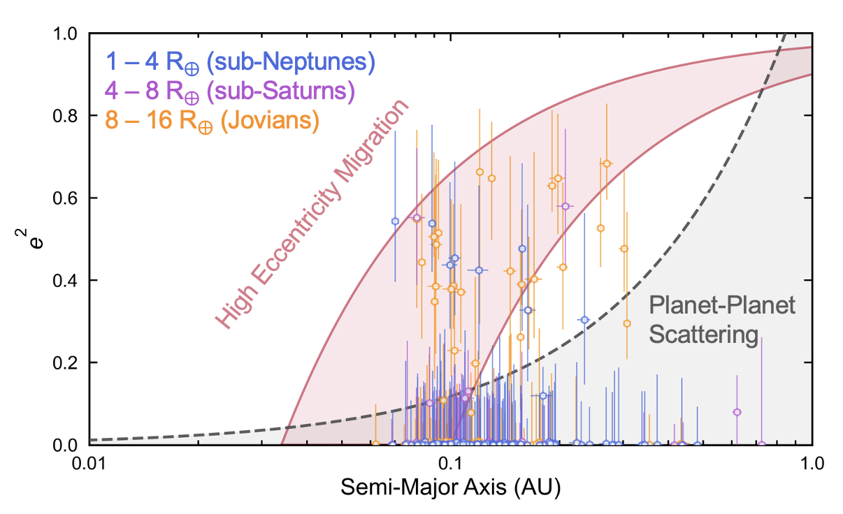
The inferred eccentricities of warm single giants in our analysis is equally consistent, however, with a population shaped by disk migration alone, whereby some fraction of Jovians undergo in-situ planet-planet scattering after the disk disappears. The maximum eccentricity that planet-planet scattering can create in-situ can be approximated as (Goldreich et al., 2004)
| (8) |
where is the Safronov number, defined as
| (9) |
and where is the escape velocity of the planet, is its orbital velocity assuming a circular orbit, is the planet’s mass, is the mass of the star, is the semi-major axis and is the radius of the planet. For a typical warm Jupiter (, , AU) around a Sun-like star (), this maximum eccentricity is of order unity, suggesting a Jovian-like planet can reach eccentricities high enough to trigger tidal migration via in-situ scattering, without the need to invoke more complex mechanisms. In Figure 9, we show theoretical upper limits under the assumption of empirical mass-radius relationships (Otegi et al., 2020; Bashi et al., 2017) for both the small (1–8 ) and giant (8–16 ) planets. This formation scenario also appears consistent with the mass-eccentricity trend and spin-orbit alignments of highly eccentric warm Jupiters (Dong et al. in prep).
Finally, the placement of above the canonical sub-Saturn regime implies that most sub-Saturns reside on the same low- track as sub-Neptunes in the warm-single population. This result disfavors a naive expectation that sub-Saturns should systematically share the dynamical signatures of giants if they were predominantly “failed gas giants” in the sense of being outcomes of a truncated runaway-accretion phase (Lee:2016), since dynamical excitation is often linked to giant planet interactions and scattering (Chatterjee et al., 2008; Ford:2008; Nagasawa and Ida, 2011). Instead, our inference is consistent with scenarios in which a large fraction of sub-Saturns represent an extension of sub-Neptune formation pathways and/or have architectures that experience fewer strong post-disk interactions.
V.4 A sub-population of eccentric small planets
Although small planets are dominated by the low- component, the radius-continuous mixture model assigns a non-zero probability that a small subset of sub-Neptunes belong to the dynamically excited component. Marginalizing over –, we infer a high- fraction of , comparable to (though not identical with) the – bin value of (Figure 8). To aid follow-up, Table 4 summarizes targets with whose eccentricity posterior mode exceeds .
| Target | (K) | () | () | SG1 | SG2 | SG3 | |
|---|---|---|---|---|---|---|---|
| Kepler-1656b (TOI-4584.01) | — | RV (lit.) | — | ||||
| TOI-3495.01 | LCO-CTIO | SMARTS/CHIRON | SOAR/HRCam | ||||
| TOI-1222.01 | LCO-SSO; PEST | SMARTS/CHIRON | Gemini/Zorro; SOAR/HRCam | ||||
| TOI-1687.01 | LCO (McD/CTIO/Teide); KeplerCam; MuSCAT3 | FLWO/TRES | WIYN/NESSI; Gemini/Alopeke; CAHA/AstraLux; SAI | ||||
| TOI-1744.01 | — | NOT/FIES; APF/Levy; Keck/HIRES | Keck/NIRC2; Gemini/Alopeke | ||||
| TOI-1664.01 | KeplerCam | FLWO/TRES; Keck/HIRES; LCO/NRES | WIYN/NESSI; Shane/ShARCS; CAHA/AstraLux; SAI | ||||
| HIP 97166b (TOI-1255.01) | — | RV (lit.) | — | ||||
| TOI-5789.01 | LCO-McD | Palomar/DBSP; FLWO/TRES | Palomar/PHARO; SOAR/HRCam; SAI | ||||
| TOI-2100.01 | LCO-McD | FLWO/TRES; Keck/HIRES | CAHA/AstraLux; Gemini/Alopeke; Keck/NIRC2; SAI | ||||
| TOI-1209.01 | LCO-CTIO | SMARTS/CHIRON | Gemini/Zorro; SOAR/HRCam |
Note. — A more detailed and precise table is available as an online format.
Two targets in this criteria range have been previously confirmed. Kepler-1656b is a warm sub-Saturn (Brady et al., 2018; angelo:2022). We infer (Figure 3), consistent with the published RV eccentricity of (angelo:2022). HIP 97166b (TOI-1255.01) illustrates a known limitation of photoeccentric constraints. While we infer , an RV analysis finds (Polanski:2024). The joint photometric–RV solution indicates a high impact parameter (), which can mimic a shortened duration and is partially degenerate with (MacDougall et al., 2021).
A straightforward interpretation of the remaining cases is dynamical excitation by additional companions (e.g., secular forcing or scattering). This scenario predicts that a substantial fraction should host massive outer companions detectable via RV trends and/or transit-timing variations. We note, however, that the false-positive probability is likely higher for this subset, reinforcing the importance of continued follow-up.
V.5 Comparison with previous work
This work provides the first homogeneous, all-sky characterization of the eccentricity distribution of warm ( days) planets across the full TESS radius range. By modeling the population with a radius-dependent mixture distribution, we show that the observed warm-planet sample is well described by a low-eccentricity component plus a dynamically excited high- component whose contribution increases strongly with planet size. This framework unifies previous Kepler and TESS results into a single picture in which the fraction of high-eccentricity systems rises from small planets to giant planets.
Studies of systems have consistently found eccentricity distributions that are inconsistent with a population shaped purely by disk-driven formation and evolution. Using a large Kepler–LAMOST sample with spectroscopically derived stellar densities, Xie et al. (2016) showed that planets exhibit moderate eccentricities, with a population mean of . Improved stellar density determination through astroseismology lead to more precise measurements of small-planet eccentricities, in which it was shown that small singles () exhibit a reduced pile-up at near-circular orbits and a broader eccentricity distribution relative to multi-transiting systems (Van Eylen et al., 2019). Together, these studies established that elevated eccentricities are a generic feature of populations across a wide range of planet sizes. We reinforce and extend these conclusions using a homogeneous, all-sky TESS sample and precise stellar densities from Gaia. We also note that several Kepler-based samples include planets at shorter orbital periods (no period cutoff in the former, and days in the latter), where tidal circularization is more effective. Including these shorter-period planets can lower the inferred eccentricity scale relative to the warm-planet regime ( days) studied here.
The growth of the TESS sample has enabled targeted studies of warm planets over longer orbital periods. Focusing on warm Jupiters (, days), Dong et al. (2021) inferred a bimodal eccentricity distribution with an approximately 55/45 split between low- and high-eccentricity components. While their analysis did not distinguish between single- and multi-transiting systems, the inferred high-eccentricity fraction is fully consistent with the Jovian high- fraction we recover, . Extending this work to smaller radii, Fairnington:2025 analyzed warm sub-Saturns (–, days) and found a similarly elevated eccentricity distribution for systems, including evidence for a 15% high-eccentricity sub-population. Our results reproduce this behavior and demonstrate that the emergence of a high- component continues into the sub-Neptune regime. Collectively, these TESS-based studies point to a population in which increasing planet size is accompanied by an increasing contribution from dynamically excited systems, rather than a uniform shift in eccentricity across all planets.
A qualitatively similar size-dependent trend was also reported for Kepler planets by Gilbert:2025, who found that eccentricity increases with planet radius and inferred a transition near . The smaller transition radius in that work likely reflects differences in both orbital-period coverage ( days) and the higher number of intrinsically rare planets that TESS samples. In particular, Gilbert:2025 aim to recover the intrinsic eccentricity distribution after accounting for geometric and detection selection effects, whereas our analysis (and the other studies discussed above) characterizes the observed transiting population. Because transiting samples are weighted toward configurations with higher transit probability, which can be enhanced for dynamically excited orbits, the observed warm planet population probed by TESS may exhibit a higher apparent contribution from excited systems. In this sense, the larger transition radius we infer () and the lower-radius transition inferred by Gilbert:2025 may represent complementary views of the same underlying population rather than a direct discrepancy.
V.6 Limitations and future work
Our constraints rely on the photoeccentric effect, which infers eccentricity primarily from transit durations and stellar densities (Dawson et al., 2012; Kipping, 2014). Our analysis corrects for the geometric over-representation of eccentric transiting orbits, but does not yet account for survey completeness and vetting selection as functions of period, radius, and host properties; a fully intrinsic distribution will require injection–recovery style forward modeling. In addition, we have removed targets with ambiguous orbital periods derived solely from TESS, which may inhibit the representation of long-period targets from our initial sample, especially if they have been confirmed via ground-based follow-up. This was necessary for a homogeneous analysis, but may remove targets of interest (e.g., TOI-2134c, Rescigno et al. 2024).
We note that this analysis makes use of both confirmed planets and current planet candidates. Despite performing extensive vetting to remove targets known to be false positives, not all of our sample are classified as bona fide planets. Follow-up of current candidates is therefore of high scientific value.
Although we attempt to mitigate systematics by deriving independent stellar densities from Gaia DR3 and SED fitting, unresolved binaries and blended photometry can bias densities and therefore photoeccentric constraints (Furlan and Howell, 2020). High-resolution imaging and spectroscopic vetting for subsets of the sample would help further increase the sample’s robustness.
Finally, we emphasize that our focus on warm planets is a deliberate choice that complements studies that combine singles and multis. Because dynamical stability constraints tend to favor low eccentricities in tightly packed multi-planet systems, contrasting warm singles against warm multis within a consistent framework can isolate dynamical excitation associated with lower-multiplicity architectures (Van Eylen et al., 2019; Gilbert:2025). Extending our analysis to warm multi-transiting systems in TESS is therefore a natural next step.
VI Conclusions
We have inferred the TESS warm-single (– days) eccentricity distribution with a sample of 347 planets spanning – using the photoeccentric effect within a hierarchical Bayesian framework. Our main findings are:
-
•
The warm-single population is well described by both a single Beta distribution peaking at zero and falling monotonically, and a two-component Beta mixture with a dominant low-eccentricity component () and a secondary dynamically excited component with mean .
-
•
The contribution of the high- component increases strongly with planet radius. In our radius-continuous mixture model, the low- membership fraction transitions with a break radius of and steepness , implying that dynamical excitation becomes increasingly common toward warm Jovians.
-
•
In archetype-motivated radius classes, sub-Neptunes and sub-Saturns are predominantly consistent with the low- component, while Jovians exhibit the clearest high- contribution, consistent with warm giants tracing a wider range of eccentricities and more dynamical histories.
-
•
Although small planets are dominated by low eccentricities, the model assigns a non-zero high- fraction among sub-Neptunes ( over –; similarly for –). We identify a set of small, high- candidates that are especially valuable targets for confirmation and mass determination.
These results support a picture in which warm singles comprise a mixture of relatively quiescent systems and a dynamically excited sub-population, with the latter becoming increasingly dominant at larger radii. Moving from the observed to the intrinsic eccentricity distribution will require forward modeling of survey completeness and vetting selection (e.g., injection-recovery), and an immediate next step is extending this framework to warm multi-transiting TESS systems to isolate eccentricity differences linked to planet multiplicity and low mutual inclinations.


References
- Models of very-low-mass stars, brown dwarfs and exoplanets. 370 (1968), pp. 2765–2777. External Links: Document, 1112.3591 Cited by: §III.1.
- Two empirical regimes of the planetary mass-radius relation. 604, pp. A83. External Links: Document, 1701.07654 Cited by: Figure 9, §V.3.
- In Situ Formation and Dynamical Evolution of Hot Jupiter Systems. ApJ 829 (2), pp. 114. External Links: Document, 1511.09157 Cited by: §V.1.
- TOI-2005b: an eccentric warm jupiter in spin-orbit alignment. 169 (5), pp. 273. External Links: ISSN 1538-3881, Link, Document Cited by: Figure 3, §V.3.
- Stellar irradiated discs and implications on migration of embedded planets. I. Equilibrium discs. A&A 549, pp. A124. External Links: Document, 1211.6345 Cited by: §V.3.
- The In Situ Formation of Giant Planets at Short Orbital Periods. ApJ 817 (2), pp. L17. External Links: Document, 1510.04276 Cited by: §V.1.
- Kepler-1656b: A Dense Sub-Saturn with an Extreme Eccentricity. 156 (4), pp. 147. External Links: Document, 1809.08436 Cited by: §V.4.
- Dynamical Outcomes of Planet-Planet Scattering. ApJ 686 (1), pp. 580–602. External Links: Document, astro-ph/0703166 Cited by: §I, §V.3, §V.3.
- Single site observations of TESS single transit detections. 619, pp. A175. External Links: Document, 1809.10687 Cited by: §II.3.
- The Photoeccentric Effect and Proto-hot Jupiters. II. KOI-1474.01, a Candidate Eccentric Planet Perturbed by an Unseen Companion. 761 (2), pp. 163. External Links: Document, 1206.5579 Cited by: §I, §III.1, §III.2, §III.2, §III.3, §V.6, §V.
- Origins of Hot Jupiters. 56, pp. 175–221. External Links: Document, 1801.06117 Cited by: §I, Figure 2, §V.1.
- Warm Jupiters in TESS Full-frame Images: A Catalog and Observed Eccentricity Distribution for Year 1. 255 (1), pp. 6. External Links: Document, 2104.01970 Cited by: §I, §III.2, §IV.1, §IV.1, §IV.1, §IV.1, §IV.2, §V.1, §V.5.
- Eccentric Jupiters via Disk-Planet Interactions. ApJ 812 (2), pp. 94. External Links: Document, 1507.08667 Cited by: §V.3.
- The Equilibrium Tide Model for Tidal Friction. ApJ 499 (2), pp. 853–870. External Links: Document, astro-ph/9801246 Cited by: §I.
- Characterizing the Orbital Eccentricities of Transiting Extrasolar Planets with Photometric Observations. 678 (2), pp. 1407–1418. External Links: Document, 0801.2591 Cited by: §III.1.
- Unresolved Binary Exoplanet Host Stars Fit as Single Stars: Effects on the Stellar Parameters. 898 (1), pp. 47. External Links: Document, 2006.06528 Cited by: §V.6.
- Gaia Data Release 2. Summary of the contents and survey properties. 616, pp. A1. External Links: Document, 1804.09365 Cited by: §I, §II.1.
- Disk-satellite interactions.. ApJ 241, pp. 425–441. External Links: Document Cited by: §V.3.
- Planet Formation by Coagulation: A Focus on Uranus and Neptune. 42 (1), pp. 549–601. External Links: Document, astro-ph/0405215 Cited by: §V.3.
- The TESS Objects of Interest Catalog from the TESS Prime Mission. 254 (2), pp. 39. External Links: Document, 2103.12538 Cited by: §II.1.
- A high-eccentricity warm jupiter orbiting toi-4127. 165 (6), pp. 234. External Links: ISSN 1538-3881, Link, Document Cited by: Figure 3.
- The NEXTGEN Model Atmosphere Grid. II. Spherically Symmetric Model Atmospheres for Giant Stars with Effective Temperatures between 3000 and 6800 K. 525 (2), pp. 871–880. External Links: Document, astro-ph/9907194 Cited by: §III.1.
- Characterization of seven transiting systems, including four warm jupiters from sophie and tess. 694, pp. A36. External Links: ISSN 1432-0746, Link, Document Cited by: Figure 3.
- The no-u-turn sampler: adaptively setting path lengths in hamiltonian monte carlo. External Links: 1111.4246, Link Cited by: §III.2.
- The Tycho-2 catalogue of the 2.5 million brightest stars. 355, pp. L27–L30. Cited by: §III.1.
- Photometry of 10 Million Stars from the First Two Years of TESS Full Frame Images: Part II. 4 (11), pp. 206. External Links: Document Cited by: §II.2.
- A new extensive library of phoenix stellar atmospheres and synthetic spectra. 553, pp. . External Links: Document Cited by: §III.1.
- Tidal Evolution of Close-in Extrasolar Planets. ApJ 678 (2), pp. 1396–1406. External Links: Document, 0802.1543 Cited by: §II.1.
- The TESS science processing operations center. In Software and Cyberinfrastructure for Astronomy IV, G. Chiozzi and J. C. Guzman (Eds.), Society of Photo-Optical Instrumentation Engineers (SPIE) Conference Series, Vol. 9913, pp. 99133E. External Links: Document Cited by: §II.2.
- The Hunt for Exomoons with Kepler (HEK). II. Analysis of Seven Viable Satellite-hosting Planet Candidates. 770 (2), pp. 101. External Links: Document, 1301.1853 Cited by: §II.3, §III.2.
- Bayesian priors for the eccentricity of transiting planets. 444 (3), pp. 2263–2269. External Links: Document, 1408.1393 Cited by: §IV.1, §IV.1, §IV.1, §V.6.
- Secular perturbations of asteroids with high inclination and eccentricity. AJ 67, pp. 591–598. External Links: Document Cited by: §I.
- SYNTHE spectrum synthesis programs and line data. Cited by: §III.1.
- The evolution of orbits of artificial satellites of planets under the action of gravitational perturbations of external bodies. Planet. Space Sci. 9 (10), pp. 719–759. External Links: Document Cited by: §I.
- Lightkurve: Kepler and TESS time series analysis in Python Note: Astrophysics Source Code Library, record ascl:1812.013 Cited by: §II.2.
- On the origin of massive eccentric planets. The Astrophysical Journal 477 (2), pp. 781. External Links: Document, Link Cited by: §V.1.
- The TESS-Keck Survey. VI. Two Eccentric Sub-Neptunes Orbiting HIP-97166. 162 (6), pp. 265. External Links: Document, 2110.05628 Cited by: §V.4.
- ORBITAL distributions of close-in planets and distant planets formed by scattering and dynamical tides. The Astrophysical JournalApJThe Astronomical JournalA&AThe Astronomical JournalNatureARA&AarXiv e-printsThe Astronomical JournalNature AstronomyA&AA&AA&AApJMNRASAJApJMNRASJ. Mach. Learn. Res.arXiv e-printsStatistical SciencearXiv e-printsMNRASAJApJApJPhilosophical Transactions of the Royal Society of London Series AAstronomy and AstrophysicsarXiv e-printsAJA&AAJApJAstronomy and AstrophysicsMNRASARA&AApJMonthly Notices of the Royal Astronomical SocietyResearch Notes of the American Astronomical SocietyPASPPASPApJMNRASPASPAJApJApJPASPApJSApJSMNRASA&AApJProceedings of the National Academy of SciencePeerJ Computer ScienceBayesian AnalysisApJApJarXiv e-printsApJMNRASIcarusAJMNRASApJSScienceAJIcarusAJApJMonthly Notices of the Royal Astronomical SocietyMNRASAJApJApJAJAJApJarXiv e-printsThe Journal of Open Source SoftwareMNRASA&AAJAJAJ 742 (2), pp. 72. External Links: Document, Link Cited by: §V.3.
- The Eccentric Kozai-Lidov Effect and Its Applications. ARA&A 54, pp. 441–489. External Links: Document, 1601.07175 Cited by: §I, §V.3.
- PyMC: a modern and comprehensive probabilistic programming framework in python. 9, pp. e1516. External Links: Document Cited by: §III.2.
- Revisited mass-radius relations for exoplanets below 120 M. 634, pp. A43. External Links: Document, 1911.04745 Cited by: Figure 9, §V.3.
- Four Sub-Saturns with Dissimilar Densities: Windows into Planetary Cores and Envelopes. 153 (4), pp. 142. External Links: Document, 1702.00013 Cited by: §IV.1, §V.3.
- Hot Jupiters from Coplanar High-eccentricity Migration. 805 (1), pp. 75. External Links: Document, 1409.8296 Cited by: §V.3.
- Dynamical instabilities and the formation of extrasolar planetary systems. 274, pp. 954–956. External Links: Document Cited by: §I, §V.3.
- A hot mini-Neptune and a temperate, highly eccentric sub-Saturn around the bright K-dwarf TOI-2134. 527 (3), pp. 5385–5407. External Links: Document, 2310.13623 Cited by: §V.6.
- A tendency toward alignment in single-star warm-jupiter systems. The Astronomical Journal 164 (3), pp. 104. External Links: Document, Link Cited by: §V.3.
- Maps of Dust Infrared Emission for Use in Estimation of Reddening and Cosmic Microwave Background Radiation Foregrounds. 500 (2), pp. 525–553. External Links: Document, astro-ph/9710327 Cited by: §III.1.
- The Two Micron All Sky Survey (2MASS). 131 (2), pp. 1163–1183. External Links: Document Cited by: §III.1.
- Evidence of a gap in the envelope mass fraction of sub-Saturns. A&A 703, pp. A221. External Links: Document, 2509.12120 Cited by: §IV.1, §V.3.
- The Orbital Eccentricity of Small Planet Systems. 157 (2), pp. 61. External Links: Document, 1807.00549 Cited by: §I, §I, §IV.1, §V.5, §V.6.
- Eccentricity from Transit Photometry: Small Planets in Kepler Multi-planet Systems Have Low Eccentricities. ApJ 808 (2), pp. 126. External Links: Document, 1505.02814 Cited by: §I.
- Rank-normalization, folding, and localization: an improved rˆ for assessing convergence of mcmc (with discussion). 16 (2). External Links: ISSN 1936-0975, Link, Document Cited by: §III.2.
- The Wide-field Infrared Survey Explorer (WISE): Mission Description and Initial On-orbit Performance. 140 (6), pp. 1868–1881. External Links: Document, 1008.0031 Cited by: §III.1.
- Secular Chaos and the Production of Hot Jupiters. ApJ 735 (2), pp. 109. External Links: Document, 1012.3475 Cited by: §V.3.
- Exoplanet orbital eccentricities derived from LAMOST-Kepler analysis. 113 (41), pp. 11431–11435. External Links: Document, 1609.08633 Cited by: §I, §V.5.
