remarkRemark \newsiamremarkhypothesisHypothesis \newsiamthmclaimClaim \newsiamremarkfactFact \headersA new polar factor retractionR. Jensen, and R. Zimmermann
An new polar factor retraction on the Stiefel manifold with closed-form inverse††thanks: Submitted to the editors DATE. \fundingThis work was supported by the Independent Research Foundation Denmark, DFF, grant nr. 3103-00094B
Abstract
Retractions are the workhorses in Riemannian computing applications, where computational efficiency is of the essence. This work introduces a new retraction on the compact Stiefel manifold of orthogonal frames. The retraction is second-order accurate under the Euclidean metric and features a closed-form inverse that can be efficiently computed.
A variety of retractions is known on the Stiefel manifold, including the Riemannian exponential map, the polar factor retraction, the QR-retraction, quasi–geodesics and the Cayley retraction. The Cayley retraction is second–order accurate under the canonical metric and features a closed-form inverse. The new retraction is the first one with the corresponding features under the Euclidean metric.
We present numerical experiments which illustrates the properties of the new retraction, as well as compare it to numerous of the currently available alternatives. In addition, we examine the performance of the retraction when used for interpolation and for computing a Riemannian barycenter.
keywords:
Stiefel manifold, retraction, manifold interpolation, manifold optimization, local coordinates, Riemannian exponential, geodesics, Riemannian computing15A16, 15B10, 53Z50, 65D05, 65F60
1 Introduction
Practical data processing on manifolds requires local coordinates, which make it possible to map data ‘there and back’: ‘There’ means mapping data from a Euclidean coordinate domain, for example on the tangent space, to the manifold. ‘Back’ refers to the reverse action of mapping manifold data into a coordinate domain. In certain applications, e.g., Riemannian optimization, only the ‘there’-direction is needed, but for manifold interpolation or for computing Riemannian averages, there must also be an efficient way to go ‘back’.
This work focuses on the Stiefel manifold of orthogonal frames. Popularized by [15], the Stiefel manifold features in a huge amount of applications in deep learning [31], computer vision [28, 27, 43], statistics, signal processing and clustering [10, 11, 12, 13, 25, 34, 35, 41], stochastic differential equations [29, 30], and general numerical linear algebra [8, 36], and the amount of literature is growing.
Structure–preserving interpolation of column-orthonormal matrices, hence interpolation on the Stiefel manifold, has mainly been applied in the context of parametric model-order reduction [16, 17, 48]. The task is, given measurements of the system at selected parameters, to produce a low–rank basis representing the dynamics of the system under varying parameter configurations.
Classically, interpolation tasks on manifolds have been carried out using the Riemannian normal coordinates, i.e., the Riemannian exponential and logarithm maps, which enjoy desirable geometric features. The Riemannian logarithm maps the sampled data to the tangent space at a designated point (the ‘back’), interpolation takes place in this linear space, and the interpolant is mapped back to the manifold via the Riemannian exponential (the ‘there’).
In applications where computational efficiency is essential, one often employs approximations of the Riemannian exponential map, called retractions. By definition, all retractions match the Riemannian exponential up to terms of (at least) first–order. Thus, they are local diffeomorphisms, and their inverses approximate the Riemannian logarithm.
Closed–form formulas for inverse retractions are relevant for vector transport, i.e., mapping vectors from one tangent space to another. For example, this is required in the Riemannian conjugate–gradient methods [45]. Inverse retractions are also needed for Riemannian interpolation [24, 39].
A second–order retraction is a retraction that matches the Riemannian exponential map up to terms of second order. Employing such retractions simplifies the convergence analysis of Riemannian trust–region methods [7, Section 6.4], since they preserve, in a certain sense, the Riemannian Hessian [7, Proposition 5.45]. Using higher–order retractions also increases regularity of subdivision schemes [14, 33], and often they allow for larger time steps when solving ODEs on manifolds [19].
Various retractions are known on the Stiefel manifold; we are aware of:
The Riemannian exponential map (1) is the reference when quantifying the order of a retraction. It depends on the chosen metric [23]. Computing the inverse requires an iterative algorithm [32, 40, 46]. The polar factor retraction (2) is of second order under the Euclidean metric. The QR-retraction (3) is of first order under any metric, and so is its Cholesky counterpart (4). Computing the inverse maps for the retractions (2) and (3) is based on solving a Sylvester/Riccati/Lyapunov-type matrix equation [25].
For the Cholesky QR-based retraction, we are not aware of any published work on computing the inverse. However, as with (2) and (3), a matrix equation is expected to arise in this task.
To the best of our knowledge, the Cayley retraction (5) and the quasi-geodesic retractions of (6) are the only ones on the list that feature a closed form inverse [45, 5]. These retractions are of order under the Euclidean metric, and it turns out that the Cayley retraction is second–order accurate under the canonical metric.
In this work, we introduce a new retraction on the Stiefel manifold that is based on an additional twist (quite literally) in the polar factor retraction. The main features of this retraction, which we call polar-light retraction, are:
-
•
It is second-order accurate under the Euclidean metric.
-
•
It has a closed-form inverse.
-
•
Evaluating its inverse incurs asymptotically the same computational cost as evaluating the retraction itself. Computing matrix functions and decompositions is necessary only for small matrices; with large matrices, only simple matrix–matrix multiplications arise.
- •
-
•
Unlike with the Cayley retraction, with appropriate matrix decompositions as an upfront investment, the associated retraction curves can be parameterized for efficient multi‑query use.
Our experiments show that the polar–light retraction is usually a better approximation to the Riemannian exponential map than the polar factor retraction. In special cases, it reproduces the Riemann exponential exactly.
Organization: Stiefel manifold essentials and the classical polar factor retraction are recapped in Section 2. The theoretical findings constitute Section 3. We will present several numerical experiments in Section 4, investigating the behavior of the polar–light retraction in comparison with the polar factor retraction, as well as with several of the previously mentioned alternatives. We conclude the paper in Section 5.
2 Background
The orthogonal group and special orthogonal group are
The Stiefel manifold is their rectangular relative
Here and throughout, we write for the -identity matrix. We single out the special Stiefel point
The dimension of the Stiefel manifold is , which reflects the number of independent parameters in a skew-symmetric ()-matrix and a rectangular -matrix. Fix with orthogonal completion so that . The tangent space at is
For details, see [1, 15]. We denote the set of symmetric positive definite ()-matrices by .
2.1 The classical Stiefel polar factor retraction
With the help of the polar decomposition, any rectangular real matrix with full rank can be expressed as the unique product of the symmetric positive definite matrix square root and the column-orthogonal –hence Stiefel– matrix ,
[22, Theorem 8.1]. This gives rise to the polar factor retraction:
| (1) |
see [1, eq. (4.7)]. Note that so that
Hence, sends the (non-orthogonal) -matrix to the Stiefel manifold by mapping it to the orthogonal factor of its full polar decomposition. For the sake of argument, we call it the full polar factor retraction. Inversion requires solving a Lyapunov equation [25]. Higher-order extensions are discussed in [19].
3 The polar-light retraction
Any Stiefel matrix can be split into sub-blocks with and . If invertible, a local coordinate representation can be obtained from a polar decomposition of the small block alone; hence the term ‘light’.
Lemma 3.1.
Consider the special point . The map
is a coordinate chart on a (relative) open, path-connected neighborhood around .
Below, we state the inverse map , which implicitly proves the lemma.
The chart can be interpreted as follows: A polar decomposition of the upper -block of yields a splitting
Because there is a continuous path from to , and thus from the upper block to the upper block , it holds , so that . The following restrictions of the matrix exponential
constitute a global diffeomorphism [34, Thm. 2.8] and a globally surjective local diffeomorphism [20, §. 3.11, Thm. 9], respectively. Hence, there is and such that and and
Therefore, maps a Stiefel point from a suitable neighborhood of to the coordinate matrices
Lemma 3.2.
The map is invertible; the inverse map is a local paramaterization and is given by
| (2) |
Proof 3.3.
Recalling that the subblocks of a Stiefel matrix are related by , it is straightforward to check the identities
The general pattern underlying is revealed by writing
Since is symmetric positive definite, the inverse and the square root of the inverse are uniquely defined. By construction, the coordinate center is
3.1 Changing the coordinate center
Suppose that is a point that we designate as the center of the coordinate chart. Let be an arbitrary but fixed orthogonal completion. Define
| (3) | ||||||
| (4) |
Formally, these maps constitute a parameterization and a corresponding chart with coordinate center , .
In practical computations, where , it is infeasible to actually form the completion . Fortunately, by standard Stiefel techniques we do not have to. Consider a tangent vector
A calculation validates the following matrix formulae:
| (5) | ||||
| (6) |
Since , computing the matrix exponential is efficient and stable.333Nevertheless, in practice, we will omit the matrix exponential by resorting to its Cayley approximation, which is second-order accurate. Rearranging terms, we get
| (7) |
With the SVD , the argument of the matrix logarithm that appears in is the orthogonal matrix . The expression reduces to
| (8) |
It is interesting to observe that is the solution to the Procrustes problem , i.e., it is the rotation that brings closest to , see [21, Section 6.4.1].
3.2 Retraction order
Retractions are approximations of the Riemannian exponential map. The Riemannian exponential depends on the chosen metric. Given a base point and an arbitrary but fixed orthogonal completion , the Riemannian exponential on the Stiefel manifold under the one-paramater family of metrics of [23] reads
| (9) |
see [49, eq. (11)]. The canonical and the Euclidean metric correspond to and , respectively. By definition, a retraction of order coincides with the Taylor expansion of around up to terms of ’th order. It holds that
| (10) |
where
| (11) |
The middle equation means , which is a classical fact from Riemannian geometry. Since this is independent of the metric parameter, any retraction is a (first-order) retraction for the whole metric family. It is well known that the classical polar factor retraction from (1) is of second-order under the Euclidean metric.444The Taylor expansion is The maps from (3) share this property.
Lemma 3.4.
Proof 3.5.
Using the series expressions for the matrix exponential, matrix inversion, and the matrix square root, a series expansion of at in the direction is seen to be
Hence,
and
so that
matches the Riemann exponential under any -metric up to terms of order one, and up to terms of order two under the Euclidean metric ().
Equation (5) reveals smooth, even analytic dependence on the base point .
For ease of notation, we will from now on denote the polar–light retraction (3) by .
Two special cases
Stiefel tangent vectors come in the form with a (skew-symmetric) component in and a component in . In this sense, we write
Lemma 3.6.
When both maps are restricted to , the polar-light retraction coincides with the Riemannian exponential
When restricted to , coincides with the full polar factor retraction (1)
Proof 3.7.
By the above lemma, we expect that for tangent vectors with dominant -component, the polar-light retraction will be closer to the Riemannian exponential than the full polar factor retraction. If the -component dominates, we expect that the full polar and the polar-light retraction produce similar results. This is confirmed by the numerical experiments in the next section.
3.3 Computing the polar–light retraction and its inverse
The Cayley transformations provide structure-preserving second order approximations for the matrix exponential and logarithm
Here, structure-preserving means that
As with the matrix logarithm, is only well-defined for matrices that do not feature as an eigenvalue. As with the matrix exponential, is well-defined for all skew-symmetric matrices: The eigenvalues of a skew-symmetric matrix are imaginary so that the matrix factor cannot be singular.
With all input data as introduced for (7), (8), the maps
| (12) | |||||
| (13) |
form a pair of retraction/inverse retraction of second order under the Euclidean metric.
Computing the real Schur form of the skew–symmetric matrix , , we obtain the block–diagonal matrix , featuring either blocks or zero blocks on the diagonal. Thus, we can efficiently evaluate the matrix exponential of matrices of this type, as well as compute , which feature in the Cayley transformation .
Given a fixed , consider the case that we want to evaluate the polar–light retraction ), for various . For this to be efficient, we can compute a QR decomposition of , and obtain , so that one only needs to form . One proceeds by computing the SVD , so that , for which the matrix square–root and –inverse can be efficiently computed by applying the operations on the diagonal elements of only, as it holds that . For the exponential term, compute the real Schur form and obtain . One can replace with for a Cayley–accelerated variant. For both variants, one can exploit the block–structure of when computing the matrix exponential [18, pp. 43], or the inverse .
3.4 The classical Stiefel Cayley retraction
For comparison purpose, we recall the classical Cayley retraction [44, 45] on the Stiefel manifold
| (14) |
with . While the Cayley transformation features in both and , the two retractions are inherently different. The economy-size equivalent to (14) is
| (15) |
analogous to [6, Proposition 5.2], [42, Proposition 4.5]. This is the form that we use in the numerical experiments. Note that computing Eq. 15 only requires inversion of a () matrix.
The Cayley retraction is second–order accurate under the canonical metric. We expect this to be known, but we could not find a literature reference. The differential terms of first and second order are
A comparison with the Taylor series (10),(11) of the Exponential map shows second-order consistency for (canonical metric) and first-order consistency for (Euclidean metric).
4 Experimental results
In this section we present five numerical experiments investigating the properties of the new polar-light retraction. We also compare it to other existing alternatives. The source code is publicly available.555https://github.com/JensenRasmus/PolarLightStiefel
4.1 Accuracy of the PL retraction relative to the (Eculidean) Riemann exponential
First, we evaluate the accuracy of the polar-light retraction by quantifying its deviation from the corresponding Riemannian geodesic. To this end, we compute a pseudo-random data triple , such that
where denotes the Euclidean Stiefel metric associated with in (9). The geodesic connecting is
To obtain a retraction connecting the same endpoints, we compute . This yields a tangent vector with . The retraction curve connecting the given endpoints is
We discretize the unit interval in equidistant steps and compute the error between the geodesic and the retraction curve . As retractions, we consider the polar factor retraction (1) and the polar–light retraction (7).


| max error PF | max error PL | |
|---|---|---|
| 400 | 1.99e-3 | 6.93e-4 |
| 200 | 3.27e-3 | 1.86e-3 |
| 100 | 5.86e-3 | 4.45e-3 |
| 50 | 1.12e-2 | 9.67e-3 |
As can be seen from the figure and the table, the polar-light retraction is consistently closer to the Riemannian geodesic than the full polar factor retraction. The difference is more pronounced for larger values of . Intuitively, this makes sense, since the difference between the PF- and the PL-retraction is only in the treatment of the -block , cf. (1) and (7). As shown in Lemma 3.6, if only the -component were present, the polar-light retraction would become the Riemannian exponential, while for it coincides with the full polar factor retraction.
4.2 Accuracy of the inverse polar–light retraction relative to the Riemannian logarithm
The next experiment addresses how close the inverse retraction is to the Riemannian logarithm (RL) under the Euclidean metric. Again, we start with a pseudo-random data triple , such that
and compute the geodesic
The geodesic is a manifold curve that we map back to the coordinate domain, in this case the tangent space, via the inverse of a retraction . To assess how close the inverse retraction under consideration is to the Riemannian logarithm, we compute the error
In theory, when the Riemannian logarithm is used as an inverse retraction, the tangent space curve is . However, the Riemannian logarithm is not available in closed form but has to be computed by an iterative procedure [49, 32]. Therefore, we also assess the accuracy
As inverse retractions, we use the inverses of the full polar factor retraction (PF) [25, Algorithm 1] and the inverse of the polar-light retraction (PL) (8). Figure 2 (a) and (b) displays the error curves for dimensions and .
We repeat the experiment in the exact same set-up, but replace the inverse polar-light retraction with its Cayley accelerated variant (PL Cay) of (13), The results are presented in Figure 2 (c) and (d). To the naked eye, the results are indifferent.


-
The maximal errors are listed in Table 2.
| max error RL (ref) | max error PF | max error PL | max error PL Cay | |
|---|---|---|---|---|
| 400 | 2.39e-12 | 5.18e-3 | 1.80e-3 | 2.31e-3 |
| 50 | 2.50e-13 | 2.94e-2 | 2.54e-2 | 2.56e-2 |
4.3 Computation time
To assess the computational effort, we create pseudo-random points of dimensions , and we fix a . Then, for each retraction included in the competition, we measure the computation time666Timing results are obtained with Python 3 on a MacBook Air M2 with 16GB RAM of performing calculations of . On the side, we also assess the identity by computing the norm averaged over the number of runs. In Table 3 we report the average runtime and residual norm for the full polar factor retraction (PF) of (1), the polar–light retraction (PL) of (7), the PL retraction with replaced with (PL Cay) as in (12), and the Cayley retraction (Cayley) of (15). Moreover, for reference, we consider the Grassmann–like quasi geodesic (QD. Gr–like) [5, Equation 3] and the QR retraction (QR) [1, Equation 4.8].
By comparing (1) to (7), it is clear that the (forward) polar-light retraction is more costly to evaluate than the full polar factor retraction. Apart from computations that do not depend on , the essential difference is that the former features a term , while for the latter, the corresponding term is only . The table shows that all retraction maps feature an acceptable round-off error with respect to the structure identity . For the dimensions of , the inverse Cayley retraction is the most efficient one to evaluate on a single-query basis. It is about five times faster than the inverse polar-light retraction, which ranks second, and is, in turn, about five times faster than the next best competitor. For the dimensions of , the ranking is the same, but the speed-up factor between Cayley and PL Cay is reduced to .
| Retraction | avg. time (s.) | avg. error | avg. time (s.) | avg. error |
|---|---|---|---|---|
| inv. PF | 0.099 | 2.13e-13 | 1.374 | 5.61e-13 |
| inv. PL | 0.093 | 1.54e-13 | 1.066 | 7.60e-13 |
| inv. PL Cay. | 0.021 | 7.76e-14 | 0.354 | 1.88e-13 |
| inv. QD. Gr–like | 0.116 | 1.54e-13 | 1.922 | 7.68e-13 |
| inv. QR | 0.298 | 4.41e-14 | 4.621 | 1.19e-13 |
| inv. Cayley | 0.004 | 5.27e-14 | 0.210 | 1.51e-13 |
To further measure the computation time, we compute a pseudo-random data triple , such that
where denotes the Euclidean Stiefel metric associated with in (9). We consider dimensions of and . In each case, we map the data ‘there and back’, i.e., we compute
We average the wallclock times over 10 random runs.

Figure 3 displays the results. On the left, we observe that is the most efficient to evaluate, and the same holds for its inverse. and its inverse show favorable growth both in forward and inverse mode, when compared to the polar factor retraction. This is confirmed by the right subplot of Figure 3, which shows the added costs of going ‘there and back’ with the retractions under consideration. At a dimension of , the is more than eight times faster than . is, by comparison, more than three times faster than . We observe that computing is slower to compute than . We find that this is due to the expensive matrix logarithm featuring in .
As a third experiment, we simulate a multi-queries scenario. Given data points , we consider the computational costs of obtaining a tangent vector
so that , and the subsequent costs of evaluating , where for . This mimics the procedures that are required for quasi-linear manifold interpolation.
In this setting, it is beneficial to implement –dependent formulas, so that one reuses matrix–matrix products and matrix decompositions, which allows for efficient probing of the curve .
For the and the Cayley–accelerated variant , this was discussed in Section 3.3. We compare these methods to five other retractions.
The polar factor retraction:
The PF retraction can be -parameterized by computing an SVD . This yields . Hence, we can avoid computing a dense matrix square root and –inverse for each , and we only need to compute the SVD of once. In the implementation, we only have to apply the square root- and the inverse operations on the diagonal of . Thus .
Quasi–geodesics: [5, Propostion 1] provides a formula for evaluations of a Grassmann–like quasi geodesic (QG Gr.). In the setting of geodesic interpolation, we can alternatively obtain a matrix and so that the curve connects two points [5, Algorithm 2] (QG St.). The terms featuring in the formula can be precomputed. Replacing the exponential term with the Cayley map, and using the inverse Cayley map instead of in Step 8 of [5, Algorithm 2] yields a Cayley accelerated variant (QG St. Cay).
QR retraction: We also include the QR retraction (QR), whose inverse can be computed by solving a sequence of linear equation systems and is provided in [25, Algorithm 1].
A –parametrization is not obvious, as we have to compute the unqiue QR decomposition .
Cayley retraction: The Cayley retraction cannot be -parameterized in the same way as the polar- or polar-light retraction, since the matrices and that appear under the inverse in (15) do not commute in general. We continue to use formula (15) to compute .
For each retraction , we measure the computation time of obtaining , as well as, where applicable, the time it takes to precompute relevant matrix decompositions and relevant matrix–matrix products (preprocessing). We then measure the total time it takes to compute the set of points using their –dependent formulations (interpolation), where we take .
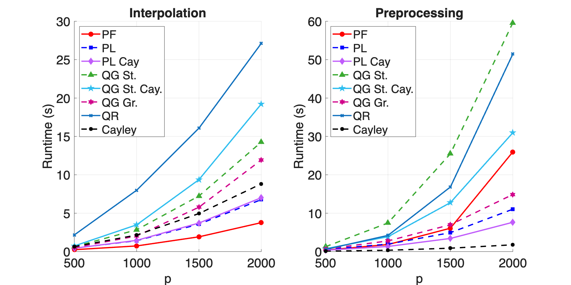
In Figure 4 we present the results on with and . We observe that the computational cost of the preprocessing step increases with , similar to what we observed in Figure 3. We see that the preprocessing time for computing is smaller than that of all the other retractions, and that the combined cost of interpolation and preprocessing at is also smallest for , despite the apparent higher cost of computing the points . When ignoring the preprocessing step, is most efficient in the interpolation step. fails to be as efficient as e.g. , since a dense () matrix has to be formed and inverted for each . It is noteworthy that computing the points is faster than computing . This is due to the efficient computation of the matrix exponential of a block–diagonal matrix. We observe that the preprocessing time for and ranks 2 and 3, respectively, in terms of runtime.
4.4 Interpolation of POD bases
As a practical example, we consider the interpolation of orthonormal bases obtained by computing the proper orthogonal decomposition of snapshot data from numerical integration of a partial differential equation (so–called POD bases). POD bases arise in the context of model order reduction [38], where they encode the essential dynamics of the system of interest. An important point is that neither the data nor the application dictates a specific metric. It is therefore a-priori unclear, which retraction to choose. We consider the Fisher–KKP equation with a diffusion term and Dirichlet boundary conditions
| (16) |
where and is a nonlinear function [2].
After a finite–differences approximation of the spatial term we consider the following forward Euler scheme
| (17) |
where is evaluated entry–wise on the vector and the matrix stems from the finite–differences approximation. We consider the initial value and evolve the system Eq. 17 with and , for . For each , we obtain a POD basis from the snapshot matrix by computing the dominant left–singular vectors of .
We would like to highlight that computing an analytic path of an SVD is challenging even when the singular values are distinct [9]. Algorithms for computing the SVD of a matrix curve may additionally introduce discontinuities in sampled singular vectors for and , due to sign switches. This issue can be overcome as in [47]: For a curve we fix and for each we compute and replace with and with . In the context of piecewise–linear interpolation, one can select one of the two endpoints as reference for each interval under consideration. Yet, in the experiment at hand, no sign adjustement was necessary.
We perform piecewise–linear interpolation. For a pair of data points , we compute the Riemannian logarithm or the inverse retraction and for we evaluate or , which yields the interpolated POD basis. The relative errors are shown in Figure 5, from which it can be seen that the polar–light retraction and Riemannian exponential are close. The smallest interpolation error is obtained using the Grassmann–like quasi geodesics. The polar factor retraction, while being locally second–order accurate, deviates significantly from the true data in comparison with the other methods. This is is most likely the result of instability of the Lyapunov equation one has to solve [25, Equation 19], since we obtain tangent vectors of large norm, relative to what we see for the other retractions. To check for analytic dependence on , one can plot the smallest singular value together with the immediate adjacent singular values of the snapshot matrix obtained from the scheme Eq. 17, and observe exponential-like growth as increases.
As the experiment involves matrices of small dimension, we have chosen to leave out timing information, and we refer the reader to Section 4.3 for a discussion involving larger matrices.

4.5 Computing the Riemannian barycenter of a geodesic triangle
The Riemannian center of mass (sometimes called the Fréchet– or Karcher mean) is the manifold generalization of computing the mean of a dataset and was studied in [26]. Given a set of points , the Riemannian center of mass is the solution of the following optimization problem
| (18) |
In contrast to the problem from Section 4.4, the formulation of the Riemannian barycenter inherently depends on the choice of a specific metric. Hence, one may expect that, when the metric is, for example, Euclidean, retractions adapted to the Euclidean metric will perform better. Solving (18) by means of Riemannian steepest descent was discussed in [4], and it is guaranteed that a solution exists and is unique, provided that all data lie in an open ball with [3, Theorem 2.1]777In general, for a complete Riemannian manifold , the radius is bounded by , where is the injectivity radius and is the lower bound on the sectional curvature, where if . For the Stiefel manifold equipped with the Euclidean metric, is the sharp upper bound on the sectional curvature [50], provided , and the injectivity radius is [51]., but in practice larger domains of convergence are often observed.
The Riemannian gradient is given by [26, Theorem 1.2]
| (19) |
Computing (19) requires numerous evaluations of the Riemannian logarithm, which can be computationally costly. In this experiment we replace with an inverse retraction , and compute a barycenter of a geodesic triangle using Riemannian steepest descent, as outlined in Algorithm 1. Whenever we replace with an inverse retraction , we use the corresponding retraction to compute the next iterate (Step 4). For more details on Riemannian optimization, see the standard textbooks [1, 7].
We work under the Euclidean metric. To set up the experiment, let and generate two random tangent vectors so that , and let cf. Figure 6. is generated so that it has a nonzero –block.

For each retraction we obtain a barycenter , which we then compare to the Riemannian barycenter obtained by solving the optimization problem (18) using the Riemannian exponential and –logarithm maps.
We run Algorithm 1 with tolerance and measure the computational cost (in seconds) required to compute the Riemannian gradient and to subsequently compute the next iterate (steps 3 and 4), with a fixed step size .
Figure 7 displays the results of applying Riemannian steepest descent with various retractions and their inverses replacing the Riemannian logarithm in (19). It is seen that using either of the retractions is significantly less costly than using the Riemannian exponential and –logarithm maps. Table 4 contains the results of the same experiment, as well as results of two additional experiments in smaller dimensions, where it is seen that the retractions in general allow for substantial reductions in computational costs, while the obtained barycenters remain relatively close to the one obtained using the Riemannian exponential and –logarithm. Using instead of leads to a slight decrease in accuracy, while being significantly faster.
Among the considered methods, the accuracy is lowest for the Cayley retraction. This showcases that the metric matters in this case, as the Cayley retraction is not a second–order retraction under the Euclidean metric. When running the same experiment under the canonical metric ( in (9)) (not shown), the Cayley retraction is found to be most beneficial in terms of both accuracy and speed.

| Iter. | Time (s.) | |||
|---|---|---|---|---|
| Exp | 1.54 | 32 | 0.71 | – |
| PF | 29 | 0.033 | 0.026 | |
| PL | 32 | 0.15 | 0.005 | |
| PL Cay | 32 | 0.022 | 0.009 | |
| Cayley | 31 | 0.006 | 0.07 | |
| Exp | 1.56 | 31 | 20.86 | – |
| PF | 30 | 2.27 | 0.003 | |
| PL | 31 | 2.54 | 7.12e-4 | |
| PL Cay | 31 | 0.65 | 0.001 | |
| Cayley | 31 | 0.13 | 0.02 | |
| Exp | 1.57 | 31 | 118.92 | – |
| PF | 30 | 10.26 | 0.002 | |
| PL | 31 | 10.08 | 3.52e-4 | |
| PL Cay | 31 | 3.54 | 6.13e-4 | |
| Cayley | 31 | 0.90 | 0.02 |
5 Conclusions and future work
By a modification of the classical polar factor retraction on the Stiefel manifold, we introduce a new Stiefel retraction, the polar-light retraction, which is second–order accurate under the Euclidean metric and admits a closed-form inverse.
The proposed polar–light retraction incurs a higher computational cost in forward evaluation compared to the classical polar factor retraction, mainly owing to an additional times matrix-matrix product in the factor in (8). However, its inverse can be computed more efficiently. This may be beneficial in logarithm–heavy computations, such as when computing Riemannian barycenters in large dimensions, as well as when performing Hermite interpolation, similar to [24] for the Grassmann manifold.
The formulas for the closed-form expression for the inverse polar-light retraction make it explicit how the independent parameters , of a Stiefel tangent matrix enters the calculation. Numerical experiments show that the polar-light retraction is consistently closer to the associated Stiefel geodesics than the classical polar factor retraction. In particular, the contribution of the -block is captured more accurately by the polar‑light retraction. (For , the polar-light retraction coincides with the full polar factor retraction.) To decrease computational costs, the matrix exponential and matrix logarithm functions may be consistently replaced with their Cayley approximations without compromising the second-order property of the retraction. Moreover, in light of Section 4.4, the inverse polar factor retraction may degenerate quicker than that of the polar-light.
We have implemented all the retractions considered in Section 4.3, except the QR retraction, so that one can obtain efficient –dependent realizations. Apart for interpolation tasks, this could also be beneficial in optimization, if line searching is conducted. It is an open question if this can be done for the QR retraction.
If one aims for speed, our numerical experiments indicate that the Cayley retraction (15) offers an efficient choice, which is also second–order accurate under the canonical metric. The –dependent implementation requires inverting a matrix, and is less efficient when comparing to e.g. the polar factor of polar-light retraction.
If one aims to approximate the Riemannian exponential map under the Euclidean metric with high precision, the polar–light retraction (8) or its Cayley-accelerated variant (12) appears to provide an efficient choice, in particular, if evaluating the inverse retraction is also of interest. They can additionally be implemented for efficient –dependent realizations.
We would like to emphasize that we do not advocate to use the Euclidean metric or any other metric as a default choice. The choice of metric is problem-dependent.
Acknowledgments
References
- [1] P.-A. Absil, R. Mahony, and R. Sepulchre, Optimization Algorithms on Matrix Manifolds, Princeton University Press, Princeton, New Jersey, 2008.
- [2] G. Adomian, Fisher-Kolmogorov equation, Appl. Math. Lett., 8 (1995), pp. 51–52.
- [3] B. Afsari, Riemannian center of mass: Existence, uniqueness, and convexity, Proc. Amer. Math. Soc., 139 (2011), pp. 655–655.
- [4] B. Afsari, R. Tron, and R. Vidal, On the convergence of gradient descent for finding the Riemannian center of mass, SIAM J. Control Optim., 51 (2013), pp. 2230–2260.
- [5] T. Bendokat and R. Zimmermann, Efficient quasi-geodesics on the Stiefel manifold, in Geometric Science of Information, F. Nielsen and F. Barbaresco, eds., Lecture Notes in Computer Science, Springer, 2021, pp. 763–771.
- [6] T. Bendokat and R. Zimmermann, The real symplectic Stiefel and Grassmann manifolds: metrics, geodesics and applications, Aug. 2021.
- [7] N. Boumal, An Introduction to Optimization on Smooth Manifolds, Cambridge University Press, Cambridge, 2023.
- [8] N. Boumal and P.-A. Absil, Low-rank matrix completion via preconditioned optimization on the Grassmann manifold, Linear Algebra Appl., 475 (2015), pp. 200–239.
- [9] A. Bunse-Gerstner, R. Byers, V. Mehrmann, and N. K. Nichols, Numerical computation of an analytic singular value decomposition of a matrix valued function, Numer. Math., 60 (1991), pp. 1–39.
- [10] H. Cai, H. Liu, D. Yang, G. Wu, B. Hu, and J. Chen, Estimating outlier-immunized common harmonic waves for brain network analyses on the Stiefel manifold, IEEE J. Biomed. Health Inform., 27 (2023), pp. 2411–2422.
- [11] R. Chakraborty and B. Vemuri, Statistics on the (compact) Stiefel manifold: Theory and applications, Ann. Statist., 47 (2018), pp. 415–438.
- [12] J. Chen, G. Han, H. Cai, D. Yang, P. J. Laurienti, M. Styner, and G. Wu, Learning common harmonic waves on Stiefel manifold – a new mathematical approach for brain network analyses, IEEE Trans. Med. Imag., 40 (2021), pp. 419–430.
- [13] A. Cichocki and S. Amari, Adaptive Blind Signal and Image Processing: Learning Algorithms and Applications, Wiley, 2002.
- [14] T. Duchamp, G. Xie, and T. P.-Y. Yu, Single basepoint subdivision schemes for manifold-valued data: Time-symmetry without space-symmetry, Lond. Math. S., 13 (2013), pp. 693–728.
- [15] A. Edelman, T. A. Arias, and S. T. Smith, The geometry of algorithms with orthogonality constraints, SIAM J. Matrix Anal. Appl., 20 (1998), pp. 303–353.
- [16] A. El Omari, M. El Khlifi, and L. Cordier, Stiefel manifold interpolation for non-intrusive model reduction of parameterized fluid flow problems, J. Comput. Phys., 521 (2025), p. 113564.
- [17] O. Friderikos, M. Olive, E. Baranger, D. Sagris, and C. David, A non-intrusive space-time interpolation from compact Stiefel manifolds of parametrized rigid-viscoplastic fem problems, Comput. Mech., 68 (2021), pp. 861–883.
- [18] J. Gallier and J. Quaintance, Differential Geometry and Lie Groups: A Computational Perspective, Geometry and Computing, Springer International Publishing, 2020.
- [19] E. S. Gawlik and M. Leok, High-order retractions on matrix manifolds using projected polynomials, SIAM J. Matrix Anal. Appl., 39 (2018), pp. 801–828.
- [20] R. Godement, Introduction to the Theory of Lie Groups, Universitext, Springer International Publishing, 2017.
- [21] G. H. Golub and C. F. Van Loan, Matrix Computations, The John Hopkins University Press, Baltimore, 4th ed., 2013.
- [22] N. J. Higham, Functions of Matrices: Theory and Computation, Society for Industrial and Applied Mathematics, Philadelphia, PA, USA, 2008.
- [23] K. Hüper, I. Markina, and F. Silva Leite, A Lagrangian approach to extremal curves on Stiefel manifolds, J. Geom. Mech., 13 (2021), pp. 55–72.
- [24] R. Jensen and R. Zimmermann, Canonically centered coordinates for Grassmann interpolation: Lagrange, Hermite, and errors, BIT, 66 (2026).
- [25] T. Kaneko, S. Fiori, and T. Tanaka, Empirical arithmetic averaging over the compact Stiefel manifold, IEEE Trans. Signal Process., 61 (2013), pp. 883–894.
- [26] H. Karcher, Riemannian center of mass and mollifier smoothing, Commun. Pure Appl. Math., 30 (1977), pp. 509–541.
- [27] Y. M. Lui, Advances in matrix manifolds for computer vision, Image Vision Comput., 30 (2012), pp. 380–388.
- [28] Y. Ma, J. Kosecka, and S. Sastry, Motion estimation in computer vision: optimization on Stiefel manifolds, in Proceedings of the 37th IEEE Conference on Decision and Control (Cat. No.98CH36171), vol. 4, 1998, pp. 3751–3756 vol.4.
- [29] G. Marjanovic, M. J. Piggott, and V. Solo, Numerical methods for stochastic differential equations in the Stiefel manifold made simple, in 2016 IEEE 55th Conference on Decision and Control (CDC), IEEE, 2016, pp. 2853–2860.
- [30] G. Marjanovic and V. Solo, An engineer’s guide to particle filtering on the Stiefel manifold, in 2017 IEEE International Conference on Acoustics, Speech and Signal Processing (ICASSP), IEEE, 2017, pp. 3834–3838.
- [31] E. M. Massart and V. Abrol, Coordinate descent on the Stiefel manifold for deep neural network training, in 31st European Symposium on Artificial Neural Networks, Computational Intelligence and Machine Learning, ESANN 2023, Bruges, Belgium, October 4-6, 2023, 2023, pp. 447–452.
- [32] S. Mataigne, R. Zimmermann, and N. Miolane, An efficient algorithm for the Riemannian logarithm on the Stiefel manifold for a family of Riemannian metrics, SIAM J. Matrix Anal. Appl., 46 (2025), pp. 879–905.
- [33] E. Nava-Yazdani and T. P. Y. Yu, On donoho’s log-exp subdivision scheme: Choice of retraction and time-symmetry, Multiscale Model. Sim., 9 (2011), pp. 1801–1828.
- [34] X. Pennec, Intrinsic statistics on Riemannian manifolds: Basic tools for geometric measurements, J. Math. Imaging Vis., 25 (2006), pp. 127–154.
- [35] C. Péalat, G. Bouleux, V. Cheutet, M. Maignan, L. Provoost, S. Pillet, and O. Mory, Using a manifold-based approach to extract clinical codes associated with winter respiratory viruses at an emergency department, Expert Syst. Appl., 230 (2023), p. 120620.
- [36] H. Sato, Riemannian Optimization and Its Applications, SpringerBriefs in Electrical and Computer Engineering, Springer International Publishing, 2021.
- [37] H. Sato and K. Aihara, Cholesky QR-based retraction on the generalized Stiefel manifold, Comput. Optim. Appl., 72 (2019), p. 293–308.
- [38] W. H. A. Schilders, H. A. Van der Vorst, and J. Rommes, eds., Model Order Reduction: Theory, Research Aspects and Applications, vol. 13 of Springer Series Mathematics in Industry, Springer, Berlin–Heidelberg, 2008.
- [39] A. Séguin and D. Kressner, Hermite interpolation with retractions on manifolds, BIT Numerical Mathematics, 64 (2024), p. 42.
- [40] M. Sutti, A single shooting method with approximate Frechet derivative for computing geodesics on the Stiefel manifold, Electron. Trans. Numer. Anal., 60 (2024), pp. 501–519.
- [41] J. Tian, J. Zhao, and C. Zheng, Clustering of cancer data based on Stiefel manifold for multiple views, BMC Bioinf., 22 (2021).
- [42] D. V. Tiep and N. T. Son, A Riemannian gradient descent method for optimization on the indefinite Stiefel manifold, 2025.
- [43] P. Turaga, A. Veeraraghavan, A. Srivastava, and R. Chellappa, Statistical computations on Grassmann and Stiefel manifolds for image and video-based recognition, IEEE Trans. Pattern Anal. Mach. Intell., 33 (2011), pp. 2273–2286.
- [44] Z. Wen and W. Yin, A feasible method for optimization with orthogonality constraints, Math. Program., 142 (2013), pp. 397–434.
- [45] X. Zhu and H. Sato, Riemannian conjugate gradient methods with inverse retraction, Comput. Optim. Appl., 77 (2020), pp. 779–810.
- [46] R. Zimmermann, A matrix-algebraic algorithm for the Riemannian logarithm on the Stiefel manifold under the canonical metric, SIAM J. Matrix Anal. Appl., 38 (2017), pp. 322–342.
- [47] R. Zimmermann, Hermite interpolation and data processing errors on Riemannian matrix manifolds, SIAM J. Sci. Comput., 42 (2020), pp. A2593–A2619.
- [48] R. Zimmermann and K. Debrabant, Parametric model reduction via interpolating orthonormal bases, in Numerical Mathematics and Advanced Applications ENUMATH 2017, F. A. Radu, K. Kumar, I. Berre, D. N. Nordbotten, and I. S. Pop, eds., Springer International Publishing, Cham, 2018.
- [49] R. Zimmermann and K. Hüper, Computing the Riemannian logarithm on the Stiefel manifold: Metrics, methods, and performance, SIAM J. Matrix Anal. Appl., 43 (2022), pp. 953–980.
- [50] R. Zimmermann and J. Stoye, High curvature means low rank: On the sectional curvature of Grassmann and Stiefel manifolds and the underlying matrix trace inequalities, SIAM J. Matrix Anal. Appl., 46 (2025), pp. 748–779.
- [51] R. Zimmermann and J. Stoye, The injectivity radius of the compact Stiefel manifold under the Euclidean metric, SIAM J. Matrix Anal. Appl., 46 (2025), pp. 298–309.