Observation of Robust and Coherent Non-Abelian Hadron Dynamics on Noisy Quantum Processors

We study the quench dynamics of a single meson propagating through a dynamical medium on a 60-site staggered lattice for up to 25 Trotter steps. For each evolution time $t_{n}$, we prepare and evolve two initial states on the QPU: the strong-coupling vacuum (SCV), and a state in which a meson is placed at the centre of the lattice on top of the SCV. In both cases, the qubits are measured in the $\sigma_{z}$ basis, and the corresponding probabilities are estimated from repeated experimental runs. This procedure is repeated for $t_{n}=1,2,3,\ldots,25$ time steps. A schematic representation of the protocol is shown in Fig. 1 (f) and (g).

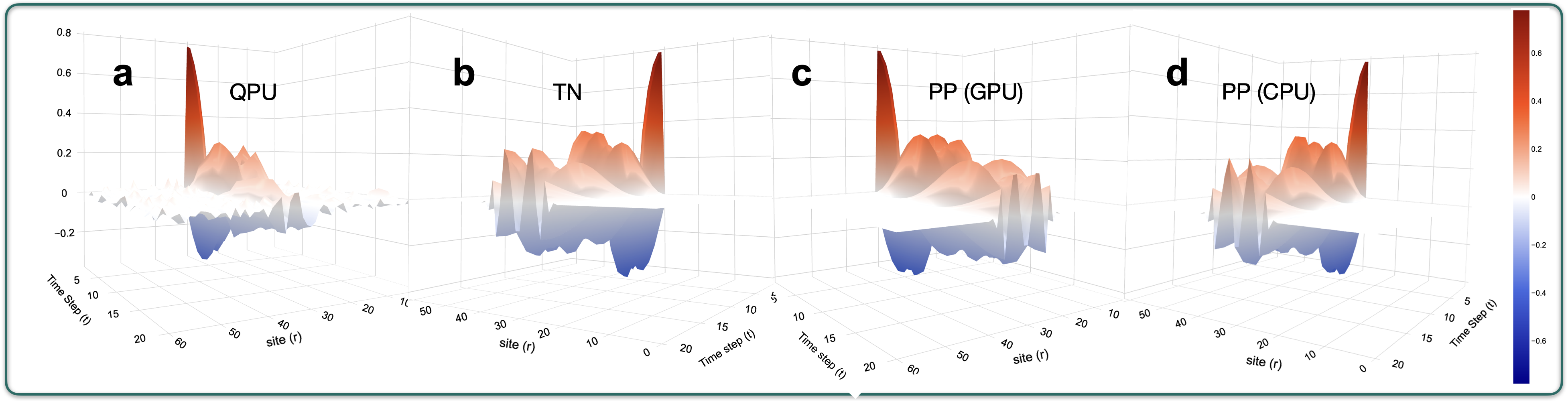
The observable used throughout this work is obtained by subtracting the probability distribution measured for the evolved SCV from that measured for the evolved mesonic state. This differential protocol suppresses background contributions and isolates the coherent signal associated with meson dynamics. The resulting space-time evolution is shown in Fig. 7. The QPU data, together with the classical baselines, reveal an early-time oscillatory mode within the mesonic profile in addition to the overall confined propagation. This oscillatory structure motivates the spectroscopic analysis presented below. In the present work, however, our emphasis remains on the experimentally accessible early-time regime, where the layered comparison between theory, approximation, circuit and hardware can be carried out in a controlled way.

The experiment on the QPU is performed with a circuit containing more than $17000$ two-qubit gates and $90000$ single-qubit gates, and a fixed $10,000$-shot budget per Trotter step. The depth of 2-qubit gates for simulating the Time evolution grows up to $259$ for $20$, and to $324$ for $25$ Trotter steps, respectively. Using only a low-cost readout error mitigation [12], the signal from QPU shows a coherent signal for propagation of a hadron by extending its size at each Trotter step, but confined within a ‘light-cone’. The edges of the ‘light cone’ trace a curved path instead of a straight line, denoting the constituent quarks to stay confined by the strong force instead of flying away freely.

The experimental observation is benchmarked by two classical computing methods: (i) Tensor Network (TN) calculations performed for the original LSH Hamiltonian and basis, via construction of Matrix Product Operators (MPO) and Matrix Product States (MPS) respectively, carefully created as a toolbox for LSH calculations [39, 29]. The time evolution is computed using a 2-site TDVP algorithm that is free of Trotterization error. The bosonic cut-off for this computation is set at $2j_{max}=5$, while a cut-off in bond dimension is set at $D_{max}=200$. (ii) The Pauli Propagation (PP) method [57] is used to simulate the noiseless digital circuit, with truncation introduced either through a cap on the number of retained Pauli terms or through a coefficient threshold. These two baselines serve different roles: TN provides a reference for the physical dynamics of the full theory over the accessible time window, whereas PP validates the digital implementation of the approximated dynamics.

Fig. 7 summarizes this validation hierarchy. Agreement between the TN and PP results supports the weak-coupling approximation and the digital algorithm over the accessible time window. Comparison between PP and QPU then isolates the effect of hardware noise on the experimentally observed signal. Across these comparisons, the main qualitative features, the confined propagation pattern and the internal oscillatory structure of the mesonic profile, remain robust.

Because exact dynamical results are not available for the full system size studied here, we quantify the quality of the observed particle-density dynamics $n_{f}(t)=\sum_{r=1}^{60}n_{f}(r,t)$ using two complementary diagnostics: (i) the spread across methods and (ii) the deviation from exactly known conserved global quantities. Globally conserved charges as per 1 are exactly known. For the chosen initial states, these should take the value $Q=60,q=0$ throughout the dynamics. The observable $n_{f}(r,t)$ is directly related to the on-site contribution to the global charge $Q$. These diagnostics provide a practical error estimate for the experimentally observed signal within the accessible time window.

The global charges $Q=\sum_{r=1}^{60}n_{o}(r)+n_{i}(r)\penalty 10000\ \&\penalty 10000\ q=\sum_{r=1}^{60}n_{o}(r)-n_{i}(r)$ remain close to their expected values throughout the observed dynamics as shown in Fig. 3, providing a sensitive indication that the evolution remains within the intended physical sector [40]. The corresponding $n_{f}(t)$ from QPU, TN and PP are statistically comparable within the reported uncertainty bands, while the computational cost of the classical baselines increases substantially over the same time window. For the tensor-network calculations, this deterioration is tied to the finite bond-dimension budget used in practice ; for PP, it reflects the growing cost of maintaining an accurate truncated Pauli expansion.

The tensor network experiment on classical computing hardware encounters an entanglement wall. The time complexity grows exponentially with the entanglement entropy. Ideally, it requires increasing the maximum allowed bond dimension $D_{max}$ to minimise the error. In this work, $D_{max}$ was limited to $200$ due to constraints on available computing resources. With this particular limit on $D_{max}$, the dynamics beyond 20 Trotter steps are obtained to contain errors which can not be neglected and hence are not reported. The details are reported as supplementary information. In summary, the available classical baselines become increasingly difficult to control as the accessible time window is extended at fixed computational budget, whereas the runtime on QPU remains set primarily by the shot budget. Within this experimentally accessible regime, the differential measurement protocol yields observables that remain robust against hardware noise. Invading long-time dynamics for $x\rightarrow\infty$ will ultimately require improved control over hardware noise and coherence. The reported dynamics of the observable exhibit noise resilience under the differential measurement protocol employed in this experiment.

A central physical observable in this work is the early-time internal oscillation of the mesonic profile. We extract a characteristic frequency from three related quantities: (i) oscillation in particle density at the central two sites of the lattice (ii) second moment of particle density distribution inside the confined meson and (iii) frequency of the fluctuation in $n_{f}$ as reported in Fig. 3. The frequency value obtained via these three methods remains consistent while the fluctuation in total number density is found to be dominated by the fluctuation at the central sites. We therefore interpret the resulting frequency as a spectroscopic proxy for the lowest excitation gap of the mesonic configuration above its initial state, $(E_{1}-E_{0})$. The frequencies are obtained with an error bar by fitting the data into a stretched damped oscillatory function as discussed in Methods.

The robustness of the quantum simulation protocol is further tested for different values of the coupling $x=50,80,200$, without changing the value of $m/g$, in order to study how the observed dynamics and the quality of the classical baselines evolve with coupling. The hardware data show the expected narrowing or widening of the confined propagation pattern across this range, while TN and PP provide corresponding reference calculations wherever they remain controlled. These results are summarized in Fig. 8. Clear signature of internal oscillations are present at all couplings, thereby demonstrating the robustness of the algorithm and its implementability on a QPU.

The coupling dependence of this frequency provides an additional consistency check. If the initial mesonic object is characterized by a length scale $L\sim ga=\frac{1}{\sqrt{x}}$, then a simple confined-particle picture suggests a gap scale proportional to $\frac{1}{L^{2}}$ or proportional to $x$. Interestingly, Fig. 8 demonstrates a linear relation between the breathing mode frequency $\omega$ and $x$ as obtained by QPU (and also using PP and TN data). The breathing mode frequency obtained from QPU for $x=80,100,200$ fits perfectly to a straight line with slope $0.00602299\pm 0.00016134$ when plotted against x, and the PP and TN data (whenever accessible) perfectly lie on this straight line as shown in Fig. 8. The error obtained in fitting the QPU data is only $2\%$.

For the QPU measurements, the runtime per time step is set primarily by the fixed shot budget. For PP, the runtime depends on the truncation strategy used to control the Pauli expansion, while for TN it depends on the bond-dimension resources required to maintain accuracy. These differences are relevant when comparing the practical reach of the available baselines. The Pauli propagation method [57] provides an efficient classical algorithm for simulating an error-free quantum circuit. This method is employed on the CPU, with an estimate of the max-term obtained by extrapolating exact results from small systems to minimise truncation error. We further employ another strategy, PP on GPU, in which terms with coefficients exceeding a threshold are considered. In summary, the PP calculations provide a useful circuit-level baseline for the noiseless digital dynamics, but their accuracy and cost depend on the truncation scheme used.

Although the circuit depth is held fixed across these coupling values, the cost and reliability of the classical baselines change significantly. In particular, the TN calculations become increasingly difficult to converge as $x$ is increased, and for $x=200$, they cease to provide a reliable reference beyond the early-time window shown. The PP calculations also show increasing sensitivity to truncation at larger $x$, as discussed in the Supplementary Information. These observations indicate that the available classical approximations become increasingly strained as the weak-coupling regime is approached at fixed system size.

In summary, the coupling scan shows that the experimentally observed mesonic signal remains robust across the values of $x$ studied here, while the available classical baselines become progressively harder to control within fixed resource budgets, and provides an empirical indication that the tested TN and PP strategies face increasing practical limitations in the same regime where the hardware measurements continue to yield a coherent differential signal. The extracted oscillation frequency remains sufficiently robust across the explored couplings to support a coupling-dependent spectroscopic analysis. For $x=50,80,100,200$, the QPU values follow an approximately linear trend, with PP and TN lying close to the same behaviour wherever reliable baseline data are available. At $x=200$, the deterioration of the TN reference is itself evident in Fig. 8, reinforcing that the coupling scan should be interpreted jointly as a spectroscopy result and as a practical comparison of currently available baselines.

The scaled Kogut-Susskind (KS) Hamiltonian describing SU(2) Yang Mills theory coupled to staggered fermions on $(1+1)$-d (1d spatial lattice and continuous time) [36] can be written as:

$\displaystyle W$

$\displaystyle=$

$\displaystyle H^{({\rm KS})}_{E}+\mu H_{M}+xH^{({\rm KS})}_{I}.$

(4)

The gauge link $U(r)$ is a $2\times 2$ unitary matrix defined on the link connecting sites $r$ and $r+1$. A temporal gauge is chosen to derive the above Hamiltonian, which sets the gauge link along the temporal direction equal to unity. The color electric fields $E_{L/R}^{a}$ are defined at the left $L$ and right $R$ sides of each link, and they satisfy the following commutation relations (SU(2) algebra) at each end:

	$\displaystyle[E_{L}^{a}(r),E_{L}^{b}(r^{\prime})]$	$\displaystyle=$	$\displaystyle i\epsilon^{abc}\delta_{rr^{\prime}}E_{L}^{c}(r),$
	$\displaystyle{[E_{R}^{a}(r),E_{R}^{b}(r^{\prime})]}$	$\displaystyle=$	$\displaystyle i\epsilon^{abc}\delta_{rr^{\prime}}E_{R}^{c}(r^{\prime}),$
	$\displaystyle{[E_{L}^{a}(r),E_{R}^{b}(r^{\prime})]}$	$\displaystyle=$	$\displaystyle 0,$		(5)

where $\epsilon^{abc}$ is the Levi-Civita symbol. The electric fields and the gauge link satisfy the following quantization conditions at each site,

	$\displaystyle[E_{L}^{a}(r),U(r^{\prime})]=-\frac{\sigma^{a}}{2}\delta_{rr^{\prime}}U(r),$
	$\displaystyle{[E_{R}^{a}(r),U(r^{\prime})]}=U(r)\delta_{rr^{\prime}}\frac{\sigma^{a}}{2},$		(6)

where $\sigma^{a}$ are the Pauli matrices. For a theory including matter fields, staggered fermionic fields $\psi^{\dagger\alpha}(r)$, for $\alpha=1,2$ are present at each lattice site. The Hamiltonian in (4) is gauge invariant as it commutes with the Gauss’ law operator,

$$G^{a}(r)=E^{a}_{L}(r)+E^{a}_{R}(r-1)+\psi^{\dagger}(r)\frac{\sigma^{a}}{2}\psi(r)$$

(7)

at each site $r$. The physical sector of the Hilbert space corresponds to the space consisting of states annihilated by (7). Solving the non-Abelian Gauss laws at each site $r$ as given in (7) is non-trivial, and engineering the same in an experiment is the most difficult job.

LSH formalism of lattice gauge theory is based on prepotential framework, where, the original canonical conjugate variables of the theory, i.e color electric field and link operators are replaced by a set of harmonic oscillator doublets, defined at each end of a link [42, 43, 41, 3, 4, 5, 55, 53, 56]. In prepotential framework, the SU(2) gauge group is confined to each lattice site allowing one to have local gauge invariant operators and states at each site, leading to a description of local loop segments. Combining prepotentials with staggered fermionic matter fields at each lattice site to form gauge invariant singlets, yields on-site string-end operators. Staggered matter fields also combine into local gauge-invariant configurations representing hadrons, likewise in the original understanding of the theory. Thus the gauge invariant and orthonormal LSH basis is characterized by a set of three integers $n_{l}(r),n_{i}(r),n_{o}(r)$, corresponding to the loop, incoming string, and outgoing string at each site (on-site hadron is equivalent to simultaneous presence of both the string ends). LSH basis states satisfy all the Gauss’ law constraints by the construction. The allowed values of the LSH quantum numbers are

$\displaystyle 0\leq n_{l}(r)\leq\infty,\penalty 10000\ \penalty 10000\ 0\leq n_{i}(r)\leq 1,\penalty 10000\ \penalty 10000\ 0\leq n_{o}(r)\leq 1,\penalty 10000\ \penalty 10000\ \penalty 10000\$

(8)

denoting $n_{l}$ to be a bosonic excitation, whereas $n_{i},n_{o}$ to be fermionic in nature, even though the string ends contain information of both gauge field and matter content.

A set of LSH operators consisting of both diagonal and ladder operators are defined locally at each site as:

	$\displaystyle\hat{n}_{l/i/o}|n_{l},n_{i},n_{o}\rangle$	$\displaystyle=$	$\displaystyle n_{l/i/o}|n_{l},n_{i},n_{o}\rangle$		(9)
	$\displaystyle\hat{\lambda}^{\pm}|n_{l},n_{i},n_{o}\rangle$	$\displaystyle=$	$\displaystyle|n_{l}\pm 1,n_{i},n_{o}\rangle$		(10)
	$\displaystyle\hat{\chi}_{i/o}^{+}|n_{l},n_{i},n_{o}\rangle$	$\displaystyle=$	$\displaystyle(1-\delta_{n_{i/o},1})|n_{l},n_{i/o}+1,n_{o/i}\rangle$		(11)
	$\displaystyle\hat{\chi}_{i/o}^{-}|n_{l},n_{i},n_{o}\rangle$	$\displaystyle=$	$\displaystyle(1-\delta_{n_{i/o},0})|n_{l},n_{i/o}-1,n_{o/i}\rangle$		(12)

The LSH basis states must satisfy the AGL, as explained in the main text to be counted as a valid loop-string-hadron segment of the global loop configurations present on the lattice.

Hamiltonian of the theory,

$\displaystyle W^{(\rm LSH)}=H^{(\rm LSH)}_{E}+\mu H^{(\rm LSH)}_{M}+xH^{(\rm LSH)}_{I}$

(13)

is exactly equivalent to the original Hamiltonian (4), with the following form of electric term, mass term and matter-gauge interaction term in terms of LSH operators:

	$\displaystyle H^{(\rm LSH)}_{E}$	$\displaystyle=$	$\displaystyle\sum_{r=0}^{N-2}\Bigg[\frac{\hat{n}_{l}(r)+\hat{n}_{o}(r)(1-\hat{n}_{i}(r))}{2},$		(14)
			$\displaystyle\times\left(\frac{\hat{n}_{l}(r)+\hat{n}_{o}(r)(1-\hat{n}_{i}(r))}{2}+1\right)\Bigg]$
	$\displaystyle H^{(\rm LSH)}_{M}$	$\displaystyle=$	$\displaystyle\sum_{r=0}^{N-1}(-1)^{r}(\hat{n}_{i}(r)+\hat{n}_{o}(r)),$		(15)
	$\displaystyle H^{(\rm LSH)}_{I}$	$\displaystyle=$	$\displaystyle\sum_{r=0}^{N-1}\frac{1}{\sqrt{\hat{n}_{l}(r)+\hat{n}_{o}(r)(1-\hat{n}_{i}(r))+1}}\times$
			$\displaystyle\Big[S_{o}^{++}(r)S_{i}^{+-}(r+1)+S_{o}^{--}(r)S_{i}^{-+}(r+1)$
			$\displaystyle+S_{o}^{+-}(r)S_{i}^{--}(r+1)+S_{o}^{-+}(r)S_{i}^{++}(r+1)\Big]$
		$\displaystyle\times$	$\displaystyle\frac{1}{\sqrt{\hat{n}_{l}(r+1)+\hat{n}_{i}(r+1)(1-\hat{n}_{o}(r+1))+1}}.$

Here (LSH Hamiltonian) contains LSH ladder operators in the following combinations (suppressing the explicit site index),

	$\displaystyle S_{o}^{++}$	$\displaystyle=$	$\displaystyle\hat{\chi}_{o}^{+}(\hat{\lambda}^{+})^{\hat{n}_{i}}\sqrt{\hat{n}_{l}+2-\hat{n}_{i}}$		(17)
	$\displaystyle S_{o}^{--}$	$\displaystyle=$	$\displaystyle\hat{\chi}_{o}^{-}(\hat{\lambda}^{-})^{\hat{n}_{i}}\sqrt{\hat{n}_{l}+2(1-\hat{n}_{i})}$		(18)
	$\displaystyle S_{o}^{+-}$	$\displaystyle=$	$\displaystyle\hat{\chi}_{i}^{+}(\hat{\lambda}^{-})^{1-\hat{n}_{o}}\sqrt{\hat{n}_{l}+2\hat{n}_{o}}$		(19)
	$\displaystyle S_{o}^{-+}$	$\displaystyle=$	$\displaystyle\hat{\chi}_{i}^{-}(\hat{\lambda}^{+})^{1-\hat{n}_{o}}\sqrt{\hat{n}_{l}+1+\hat{n}_{o})}$		(20)

and

	$\displaystyle S_{i}^{+-}$	$\displaystyle=$	$\displaystyle\hat{\chi}_{o}^{-}(\hat{\lambda}^{+})^{1-\hat{n}_{i}}\sqrt{\hat{n}_{l}+1+\hat{n}_{i})}$		(21)
	$\displaystyle S_{i}^{-+}$	$\displaystyle=$	$\displaystyle\hat{\chi}_{o}^{+}(\hat{\lambda}^{-})^{1-\hat{n}_{i}}\sqrt{\hat{n}_{l}+2\hat{n}_{i}}$		(22)
	$\displaystyle S_{i}^{--}$	$\displaystyle=$	$\displaystyle\hat{\chi}_{i}^{-}(\hat{\lambda}^{-})^{\hat{n}_{o}}\sqrt{\hat{n}_{l}+2(1-\hat{n}_{o})}$		(23)
	$\displaystyle S_{i}^{++}$	$\displaystyle=$	$\displaystyle\hat{\chi}_{i}^{+}(\hat{\lambda}^{+})^{\hat{n}_{o}}\sqrt{\hat{n}_{l}+2-\hat{n}_{o}}.$		(24)

The strong coupling ($x\gg 1,m/g=$fixed) vacuum of the LSH Hamiltonian is given by:

	$\displaystyle n_{l}(r)$	$\displaystyle=$	$\displaystyle 0\penalty 10000\ \penalty 10000\ \forall r$
	$\displaystyle n_{i}(r)$	$\displaystyle=$	$\displaystyle 1\penalty 10000\ ,\penalty 10000\ n_{o}(r)\penalty 10000\ =\penalty 10000\ 1\penalty 10000\ \penalty 10000\ \mbox{for $r$ odd}$		(25)
	$\displaystyle n_{i}(r)$	$\displaystyle=$	$\displaystyle 0\penalty 10000\ ,\penalty 10000\ n_{o}(r)\penalty 10000\ =\penalty 10000\ 0\penalty 10000\ \penalty 10000\ \mbox{for \penalty 10000\ $r$ even}$

which satisfy AGL on all the links. The spectrum and dynamics of the LSH Hamiltonian is obtained identical to the gauge invariant dynamics of the Kogut susskind Hamiltonian with the same value of bosonic cut-off using exact diagonalization [20]. The tensor network calculations reported in this work are based on the LSH framework and uses a bosonic cut-off $j_{max}=5/2$, using the tensor network toolbox [39].

We focus on open boundary condition, and allow an incoming flux $l_{i}$ to enter the lattice. Towards the weak coupling domain, the interacting vacuum is not dominated by a zero-flux state, SCV, rather it is expected to contain all possible flux states as the electric energy contribution is significantly low, compared to the intereaction energy. This allows us to choose $l_{i}>>0$, without any loss of generality [18]. Using AGL on each link, the value of $n_{l}$ at each site can be fully determined as

	$\displaystyle n_{l}(r)$	$\displaystyle=$	$\displaystyle l_{i}-n_{i}(r)\left(1-n_{o}(r)\right)+\sum_{r^{\prime}=0}^{r-1}\left(n_{o}(r^{\prime})-n_{i}(r^{\prime})\right)$
		$\displaystyle\approx$	$\displaystyle l_{i}-n_{i}(r)\left(1-n_{o}(r)\right)\penalty 10000\ \penalty 10000\ \mbox{for, }l_{i}>>0.$

Thus, any physical state in the LSH formalism in one spatial dimension is completely determined by $(n_{i},n_{o})$ quantum numbers at each site, and the interaction can be approximated to be local. This approximation is valid [18] if we focus on the weak coupling regime $x>>1$, and the off-diagonals contribute more to the dynamics. Choosing the global charge sector same as thar of the SCV i.e. with no net Baryon number and no net lattice flux $(\mathcal{B},q)=(0,0)$ (see the footnote in main text), the minimum energy strong coupling configuration of the string-ends still remain the same as the SCV.

We further make an approximation of

$$\frac{n_{l}}{n_{l}+1}\rightarrow 1\penalty 10000\ \penalty 10000\ \&\penalty 10000\ \penalty 10000\ \frac{n_{l}+1}{n_{l}+2}\rightarrow 1$$

for all the prefactors appearing in $H_{I}^{\mathrm{LSH}}$ considering the $l_{i}>>1$ scenario.

Within this approximation, the total electric part of the LSH Hamiltonian Hamiltonian is given by:

$\displaystyle H_{E}^{(\mathrm{approx})}=\frac{g^{2}a}{2}\left[Nh^{0}_{E}+\sum_{\{r^{\prime}\}}\left(\frac{l_{i}}{2}+\frac{3}{4}\right)\right]$

(26)

where, $\{r^{\prime}\}$ denotes the sites with fermionic configuration $n_{i}(r^{\prime})=0,n_{o}(r^{\prime})=1$ and $h^{0}_{E}$, corresponds to a global phase due to the background flux.

Mass Hamiltonian: The mass term (15), being independent of gauge field configuration remain the same in the weak coupling approximation.

$\displaystyle H_{M}^{(\mathrm{approx})}=\sum_{r}(-1)^{j}(\hat{n}_{i}(r)+\hat{n}_{o}(r))$

(27)

Interaction Hamiltonian: The matter-gauge field interaction term is the most complicated within the LSH framework, as detailed in (LSH Hamiltonian). In the strong coupling limit of the theory, this particular term gives small contribution to the Hamiltonian. However, in the weak coupling regime of interest, this term becomes significant. The approximation scheme that we follow casts the interaction Hamiltonian given in (LSH Hamiltonian) as,

	$\displaystyle H_{I}^{(\mathrm{approx})}$	$\displaystyle=$	$\displaystyle\sum_{r}\Big[\chi_{o}^{+}(r)\chi_{o}^{-}(r+1)+\chi_{o}^{+}(r+1)\chi_{o}^{-}(r)$		(28)
			$\displaystyle+\chi_{i}^{+}(r)\chi_{i}^{-}(r+1)+\chi_{i}^{+}(r+1)\chi_{i}^{-}(r)\Big]$

The purpose of the present approximation scheme is to bring the interaction Hamiltonian into simple form, yet describing matter gauge dynamics in the weak coupling regime reliably.

In the next section, we present the quantum algorithm construction, starting with the mapping of LSH quantum numbers to the hardware’s qubits and mapping the time evolution unitary for the weak coupling approximated Hamiltonian to a quantum circuit.

An open-boundary lattice of $N$ sites is simulated on $2N$ qubits. The numbers $n_{i}(r)$ and $n_{o}(r)$ are directly mapped to individual qubits, whereas the $n_{l}(r)$ numbers can be recovered using (Approximations for weak coupling regime). To make the qubits effectively fermions, the Jordan-Wigner transformation maps the ladder operators:

	$\displaystyle\hat{\chi}_{i}^{-}(r)$	$\displaystyle=\sigma^{+}(r)\prod_{r^{\prime}<r}(-\sigma^{z}(r^{\prime}))$		(33)
	$\displaystyle\hat{\chi}_{o}^{-}(r)$	$\displaystyle=\sigma^{+}(r+L)\prod_{r^{\prime}<r+N}(-\sigma^{z}(r^{\prime})),$

where the qubit ladder operators are defined as

	$\displaystyle\sigma^{+}=\begin{pmatrix}0&1\\ 0&0\end{pmatrix}\implies$	$\displaystyle\sigma^{+}\ket{0}=\sigma^{+}\begin{pmatrix}1\\ 0\end{pmatrix}=0,$		(34)
		$\displaystyle\sigma^{+}\ket{1}=\sigma^{+}\begin{pmatrix}0\\ 1\end{pmatrix}=\begin{pmatrix}1\\ 0\end{pmatrix}.$

The Hermitian conjugates are $\hat{\chi}_{i}^{+}(r)=(\hat{\chi}_{i}^{-}(r))^{\dagger}$ and $\hat{\chi}_{o}^{+}(r)=(\hat{\chi}_{o}^{-}(r))^{\dagger}$, with $\sigma^{-}=(\sigma^{+})^{\dagger}$.

The implied ordering of the variables where the first $N$ represent the $n_{i}$ quantum numbers, and the last $N$ the $n_{o}$ numbers, is relevant only within the mathematical construction, providing, for example, $\hat{\chi}^{+}\hat{\chi}^{-}$ products and the indices in matrix calculations. When considering the actual mapping to the hardware’s qubits, a different ordering can be used. The qubit layout we choose is a zigzag (alternating) sequence of $i$ and $o$ quantum numbers:

$$\ket{q_{2r}}\equiv\ket{n_{i}(r)},\quad\ket{q_{2r+1}}\equiv\ket{n_{o}(r)}.$$

(35)

This minimizes the number of SWAP layers throughout the circuit. Each $n_{i}(r)$ number needs to interact with both of its $i$ neighbours, $n_{i}(r-1)$ and $n_{i}(r+1)$, and similarly for $o$ numbers, while the electric Hamiltonian term acts on the $i-o$ pairs. All the SWAP gates required to enable this interaction can be arranged in two layers only for each trotter step (see Fig. 6), making this a highly efficient encoding whose depth depends only on the number of trotter steps, and not on the lattice site. Note that, in the initial Trotter step, the first layer of gates would have been the SWAPs to get the first interaction pairs adjacent, so the actual qubit initialization has an ordering that absorbs these SWAPs: $n_{i}(0)$, $n_{i}(1)$, $n_{o}(0)$, $n_{o}(1)$, $n_{i}(2)$, $n_{i}(3)$, $n_{o}(2)$, $n_{o}(3)$,…, while the layout at the end of each Trotter step follows the zigzag ordering above.

A single Trotter step applies the unitary

	$\displaystyle U(\delta_{\tau},c,\tilde{m},\theta)$	$\displaystyle=$	$\displaystyle e^{-i\delta_{\tau}H^{\prime}}$
		$\displaystyle\;\stackrel{{\scriptstyle\text{small }\delta_{\tau}}}{{\approx}}$	$\displaystyle e^{-i\tilde{m}H_{M}}e^{-i\delta_{\tau}H_{E}}e^{-icH_{I}}$

where $c=\delta_{\tau}x$, $\tilde{m}=\delta_{\tau}\mu$ are parameters appearing in the corresponding unitaries due to the interaction, and mass parts of the Hamiltonian.

The interaction part given in (28) translates into its qubit version as

$\displaystyle H_{I}^{\mathrm{approx}}$

$\displaystyle=-\sum_{\begin{subarray}{c}r=0\\ r\neq N-1\end{subarray}}^{2N-2}\left[\sigma^{-}(r)\sigma^{+}(r+1)+\sigma^{+}(r)\sigma^{-}(r+1)\right]$

(37)

The corresponding unitary takes the form

		$\displaystyle U_{I}=e^{-i\delta_{\tau}xH_{I}}$		(38)
		$\displaystyle\stackrel{{\scriptstyle\text{small }\delta_{\tau}}}{{\approx}}\prod_{r\neq N-1}exp\left[ic\left(\sigma^{-}(r)\sigma^{+}(r+1)+\sigma^{+}(r)\sigma^{-}(r+1)\right)\right]$
		$\displaystyle\;\;\;\;=\prod_{r\neq N-1}exp\left[ic\begin{pmatrix}0&0&0&0\\ 0&0&1&0\\ 0&1&0&0\\ 0&0&0&0\end{pmatrix}_{r\otimes r+1}\right]$
		$\displaystyle\;\;\;\;=\prod_{r\neq N-1}\begin{pmatrix}1&0&0&0\\ 0&\cos c&i\sin c&0\\ 0&i\sin c&\cos c&0\\ 0&0&0&1\end{pmatrix}_{r\otimes(r+1)}$

Here $c=\delta_{\tau}x$ is a real constant. Since each non-boundary-site qubit appears in two of the factors, corresponding to hopping in two directions, the algorithm is split into two layers with SWAP gates in between. Using matrix multiplication, the two-qubit hopping term in (37) is uncovered in terms of standard single- and two-qubit gates:

	$\displaystyle U_{I,r\otimes(r+1)}=$	$\displaystyle CNOT_{(r+1)\otimes r}(1\otimes H)\;CNOT_{r\otimes(r+1)}$		(39)
		$\displaystyle(1\otimes R_{z}(c))CNOT_{r\otimes(r+1)}(1\otimes R_{z}(-c))$
		$\displaystyle(1\otimes H)\;CNOT_{(r+1)\otimes r}$

After the two layers of this hopping unitary, SWAP gates get the qubits into the zigzag position for the electric and mass terms to be applied.

The electric part is

$$H_{E}=Nh^{0}_{E}+\sum_{\{r^{\prime}\}}\left(\frac{n_{l}}{2}+\frac{3}{4}\right)$$

(40)

with $\{r^{\prime}\}$ denoting the set of sites in the fermion configuration $01$ (corresponding to the second entry in the 2-qubit tensor product). The first term gives a global phase to the evolution of qubits, so we ignore it. This is also an approximation because the value of the average flux $h_{E}^{0}$ differs between basis states, but we approximate it to always be equal to the boundary flux. However, the phase correction in the $01$ case at every site and its entangling properties can be seen to increase the validity of the simulation. This second term in $H_{E}$ is translated into a circuit applied on each site’s qubit pair, which gives a certain phase in the required $01$ case, and a different phase in the other three cases (same for all three):

	$\displaystyle U_{E,x\otimes(r+1)}(\theta)=$	$\displaystyle(r\otimes R_{z}(\theta/2))CNOT_{x\otimes(r+1)}(1\otimes R_{z}(-\theta/2))$		(41)
		$\displaystyle CNOT_{x\otimes(r+1)}(R_{z}(\theta/2)\otimes 1)(r\otimes 1)$
	$\displaystyle=$	$\displaystyle\begin{pmatrix}e^{-i\theta/4}&0&0&0\\ 0&e^{i3\theta/4}&0&0\\ 0&0&e^{-i\theta/4}&0\\ 0&0&0&e^{-i\theta/4}\end{pmatrix}_{x\otimes(r+1)}$

which is a global phase plus an $e^{i\theta}$ phase in the desired case. The $x$ and $x+1$ here correspond to the $n_{i},\,n_{o}$ pair of any single lattice site.

References

- [1] (2025) Towards the understanding of heavy quarks hadronization: from leptonic to heavy-ion collisions. Eur. Phys. J. C 85 (1), pp. 16. External Links: 2405.19137, Document Cited by: The Physics and the Experiment, Outlook.
- [2] (2024) Entanglement entropy of a color flux tube in (2+1)D Yang-Mills theory. JHEP 12, pp. 177. External Links: 2410.00112, Document Cited by: The Physics and the Experiment.
- [3] (2009) Irreducible SU(3) Schhwinger Bosons. J. Math. Phys. 50, pp. 053503. External Links: 0901.0644, Document Cited by: LSH Hamiltonian.
- [4] (2010) Prepotential formulation of SU(3) lattice gauge theory. J. Phys. A 43, pp. 035403. External Links: 0909.2394, Document Cited by: LSH Hamiltonian.
- [5] (2014) SU(2) lattice gauge theory: Local dynamics on nonintersecting electric flux loops. Phys. Rev. D 90 (11), pp. 114503. External Links: 1408.6331, Document Cited by: LSH Hamiltonian, Encoding Non-Abelian Gauge Invariance.
- [6] (2023) Simulating one-dimensional quantum chromodynamics on a quantum computer: Real-time evolutions of tetra- and pentaquarks. Phys. Rev. Res. 5 (3), pp. 033184. External Links: 2207.03473, Document Cited by: ‣ Observation of Robust and Coherent Non-Abelian Hadron Dynamics on Noisy Quantum Processors .
- [7] (2021) SU(2) hadrons on a quantum computer via a variational approach. Nature Commun. 12 (1), pp. 6499. External Links: 2102.08920, Document Cited by: ‣ Observation of Robust and Coherent Non-Abelian Hadron Dynamics on Noisy Quantum Processors .
- [8] (2020) Review on Novel Methods for Lattice Gauge Theories. Rept. Prog. Phys. 83 (2), pp. 024401. External Links: 1910.00257, Document Cited by: Benchmarking via TN.
- [9] (2023) Tensor Network Algorithms: A Route Map. Ann. Rev. Condensed Matter Phys. 14, pp. 173–191. External Links: 2205.10345, Document Cited by: Benchmarking via TN.
- [10] (2023) Quantum simulation of fundamental particles and forces. Nature Rev. Phys. 5 (7), pp. 420–432. External Links: 2404.06298, Document Cited by: ‣ Observation of Robust and Coherent Non-Abelian Hadron Dynamics on Noisy Quantum Processors .
- [11] (2023) CuQuantum sdk: a high-performance library for accelerating quantum science. In 2023 IEEE International Conference on Quantum Computing and Engineering (QCE), Vol. 01, pp. 1050–1061. External Links: Document Cited by: Benchmarking via PP.
- [12] (2022) Model-free readout-error mitigation for quantum expectation values. Phys. Rev. A 105 (3), pp. 032620. External Links: 2012.09738, Document Cited by: ‣ Observation of Robust and Coherent Non-Abelian Hadron Dynamics on Noisy Quantum Processors , Validation hierarchy: theory, approximation, circuit, hardware.
- [13] (2026) Pathfinding quantum simulations of neutrinoless double- decay. Nature Commun. 17 (1), pp. 1826. External Links: 2506.05757, Document Cited by: ‣ Observation of Robust and Coherent Non-Abelian Hadron Dynamics on Noisy Quantum Processors .
- [14] (2021) Trailhead for quantum simulation of SU(3) Yang-Mills lattice gauge theory in the local multiplet basis. Phys. Rev. D 103 (9), pp. 094501. External Links: 2101.10227, Document Cited by: ‣ Observation of Robust and Coherent Non-Abelian Hadron Dynamics on Noisy Quantum Processors .
- [15] (2024) Quantum Simulation of SU(3) Lattice Yang-Mills Theory at Leading Order in Large-Nc Expansion. Phys. Rev. Lett. 133 (11), pp. 111901. External Links: 2402.10265, Document Cited by: ‣ Observation of Robust and Coherent Non-Abelian Hadron Dynamics on Noisy Quantum Processors .
- [16] (2025-07) Real-Time Dynamics in a (2+1)-D Gauge Theory: The Stringy Nature on a Superconducting Quantum Simulator. arXiv preprint arXiv:2507.08088. External Links: 2507.08088 Cited by: ‣ Observation of Robust and Coherent Non-Abelian Hadron Dynamics on Noisy Quantum Processors .
- [17] (2025) Visualizing dynamics of charges and strings in (2 + 1)D lattice gauge theories. Nature 642 (8067), pp. 315–320. External Links: 2409.17142, Document Cited by: ‣ Observation of Robust and Coherent Non-Abelian Hadron Dynamics on Noisy Quantum Processors .
- [18] (2022) Cold-atom quantum simulator for string and hadron dynamics in non-Abelian lattice gauge theory. Phys. Rev. A 105 (2), pp. 023322. External Links: 2009.13969, Document Cited by: Approximations for weak coupling regime, Approximations for weak coupling regime, Encoding Non-Abelian Gauge Invariance.
- [19] (2024) Scattering wave packets of hadrons in gauge theories: Preparation on a quantum computer. Quantum 8, pp. 1520. External Links: 2402.00840, Document Cited by: ‣ Observation of Robust and Coherent Non-Abelian Hadron Dynamics on Noisy Quantum Processors .
- [20] (2021) Search for efficient formulations for Hamiltonian simulation of non-Abelian lattice gauge theories. Phys. Rev. D 104 (7), pp. 074505. External Links: 2009.11802, Document Cited by: LSH Hamiltonian.
- [21] (2023) General quantum algorithms for Hamiltonian simulation with applications to a non-Abelian lattice gauge theory. Quantum 7, pp. 1213. External Links: 2212.14030, Document Cited by: Encoding Non-Abelian Gauge Invariance.
- [22] (2024) Quantum Computing for High-Energy Physics: State of the Art and Challenges. PRX Quantum 5 (3), pp. 037001. External Links: 2307.03236, Document Cited by: ‣ Observation of Robust and Coherent Non-Abelian Hadron Dynamics on Noisy Quantum Processors .
- [23] (2023) Preparations for quantum simulations of quantum chromodynamics in 1+1 dimensions. I. Axial gauge. Phys. Rev. D 107 (5), pp. 054512. External Links: 2207.01731, Document Cited by: ‣ Observation of Robust and Coherent Non-Abelian Hadron Dynamics on Noisy Quantum Processors .
- [24] (2023) Preparations for quantum simulations of quantum chromodynamics in 1+1 dimensions. II. Single-baryon -decay in real time. Phys. Rev. D 107 (5), pp. 054513. External Links: 2209.10781, Document Cited by: ‣ Observation of Robust and Coherent Non-Abelian Hadron Dynamics on Noisy Quantum Processors .
- [25] (2024) Quantum simulations of hadron dynamics in the Schwinger model using 112 qubits. Phys. Rev. D 109 (11), pp. 114510. External Links: 2401.08044, Document Cited by: ‣ Observation of Robust and Coherent Non-Abelian Hadron Dynamics on Noisy Quantum Processors .
- [26] (2022) Codebase release 0.3 for ITensor. SciPost Phys. Codebases, pp. 4–r0.3. External Links: Document, Link Cited by: Benchmarking via TN.
- [27] (2022) The ITensor Software Library for Tensor Network Calculations. SciPost Phys. Codebases, pp. 4. External Links: Document, Link Cited by: Benchmarking via TN.
- [28] (2025) Observation of string breaking on a (2 + 1)D Rydberg quantum simulator. Nature 642 (8067), pp. 321–326. External Links: 2410.16558, Document Cited by: ‣ Observation of Robust and Coherent Non-Abelian Hadron Dynamics on Noisy Quantum Processors .
- [29] (2026-03) String-breaking statics and dynamics in a (1+1)D SU(2) lattice gauge theory. External Links: 2603.24698 Cited by: End Notes, ‣ Observation of Robust and Coherent Non-Abelian Hadron Dynamics on Noisy Quantum Processors , Validation hierarchy: theory, approximation, circuit, hardware.
- [30] (1992) Series analysis of U(1) and SU(2) lattice gauge theory in (2+1)-dimensions. Phys. Rev. D 45, pp. 4652–4658. External Links: Document Cited by: The Hamiltonian and Its Continuum Limit.
- [31] (2025) Loop-string-hadron approach to su(3) lattice yang-mills theory, ii: operator representation for the trivalent vertex. External Links: 2512.11796, Link Cited by: Outlook.
- [32] (2025-04) Loop-string-hadron approach to su(3) lattice yang-mills theory: hilbert space of a trivalent vertex. Phys. Rev. D 111, pp. 074516. External Links: Document, Link Cited by: Outlook.
- [33] (2023-05) Loop-string-hadron formulation of an su(3) gauge theory with dynamical quarks. Phys. Rev. D 107, pp. 094513. External Links: Document, Link Cited by: Outlook.
- [34] (2023) Evidence for the utility of quantum computing before fault tolerance. Nature 618 (7965), pp. 500–505. External Links: Document Cited by: Encoding Non-Abelian Gauge Invariance.
- [35] (2020) SU(2) non-Abelian gauge field theory in one dimension on digital quantum computers. Phys. Rev. D 101 (7), pp. 074512. External Links: 1908.06935, Document Cited by: ‣ Observation of Robust and Coherent Non-Abelian Hadron Dynamics on Noisy Quantum Processors .
- [36] (1975) Hamiltonian Formulation of Wilson’s Lattice Gauge Theories. Phys. Rev. D 11, pp. 395–408. External Links: Document Cited by: Kogut-Susskind Hamiltonian, The Hamiltonian and Its Continuum Limit, Encoding Non-Abelian Gauge Invariance.
- [37] (2025) A framework for quantum advantage. External Links: 2506.20658, Link Cited by: Outlook.
- [38] (2016) Real-time dynamics of lattice gauge theories with a few-qubit quantum computer. Nature 534, pp. 516–519. External Links: 1605.04570, Document Cited by: ‣ Observation of Robust and Coherent Non-Abelian Hadron Dynamics on Noisy Quantum Processors .
- [39] (2025) Tensor-network toolbox for probing dynamics of non-Abelian gauge theories. PoS LATTICE2024, pp. 472. External Links: 2501.18301, Document Cited by: LSH Hamiltonian, Benchmarking via TN, Figure 8, Validation hierarchy: theory, approximation, circuit, hardware.
- [40] (2022) Protecting local and global symmetries in simulating (1+ 1) d non-abelian gauge theories. Physical Review D 106 (5), pp. 054510. Cited by: Figure 3, Symmetry protection and robustness.
- [41] (2010) SU(N) Irreducible Schwinger Bosons. J. Math. Phys. 51, pp. 093504. External Links: 1003.5487, Document Cited by: LSH Hamiltonian.
- [42] (2005) Harmonic oscillator prepotentials in SU(2) lattice gauge theory. J. Phys. A 38, pp. 10015–10026. External Links: hep-lat/0403029, Document Cited by: LSH Hamiltonian, Encoding Non-Abelian Gauge Invariance.
- [43] (2007) Loop Approach to Lattice Gauge Theories. Nucl. Phys. B 779, pp. 32–62. External Links: hep-lat/0702007, Document Cited by: LSH Hamiltonian, Encoding Non-Abelian Gauge Invariance.
- [44] (2025) Simulating two-dimensional lattice gauge theories on a qudit quantum computer. Nature Phys. 21 (4), pp. 570–576. External Links: 2310.12110, Document Cited by: ‣ Observation of Robust and Coherent Non-Abelian Hadron Dynamics on Noisy Quantum Processors .
- [45] (2020) A scalable realization of local U(1) gauge invariance in cold atomic mixtures. Science 367 (6482), pp. 1128–1130. External Links: 1909.07641, Document Cited by: ‣ Observation of Robust and Coherent Non-Abelian Hadron Dynamics on Noisy Quantum Processors .
- [46] (2025) Confinement in a lattice gauge theory on a quantum computer. Nature Phys. 21 (2), pp. 312–317. External Links: 2203.08905, Document Cited by: ‣ Observation of Robust and Coherent Non-Abelian Hadron Dynamics on Noisy Quantum Processors .
- [47] (2023) Quantum Computation of Dynamical Quantum Phase Transitions and Entanglement Tomography in a Lattice Gauge Theory. PRX Quantum 4 (3), pp. 030323. External Links: 2210.03089, Document Cited by: ‣ Observation of Robust and Coherent Non-Abelian Hadron Dynamics on Noisy Quantum Processors .
- [48] (2025) Quantum computing universal thermalization dynamics in a (2 + 1)D Lattice Gauge Theory. Nature Commun. 16 (1), pp. 5492. External Links: 2408.00069, Document Cited by: ‣ Observation of Robust and Coherent Non-Abelian Hadron Dynamics on Noisy Quantum Processors .
- [49] (2011) Entropy Creation in Relativistic Heavy Ion Collisions. Int. J. Mod. Phys. E 20, pp. 2235–2267. External Links: 1110.2378, Document Cited by: Outlook.
- [50] (2022-11) Quark-Hadron Transition and Entanglement. External Links: 2211.16265 Cited by: The Physics and the Experiment, Outlook.
- [51] (2026) CuPauliProp: a high-performance library for pauli propagation quantum simulators. Note: https://docs.nvidia.com/cuda/cuquantum/latest/cupauliprop/overview.htmlNVIDIA cuQuantum documentation, accessed 2026-03-11 Cited by: Benchmarking via PP.
- [52] (2019) Time-evolution methods for matrix-product states. Annals Phys. 411, pp. 167998. External Links: 1901.05824, Document Cited by: Benchmarking via TN.
- [53] (2014) Prepotential Formulation of Lattice Gauge Theory. PoS LATTICE2014, pp. 313. External Links: 1411.3068, Document Cited by: LSH Hamiltonian.
- [54] (2020) Loop, string, and hadron dynamics in SU(2) Hamiltonian lattice gauge theories. Phys. Rev. D 101 (11), pp. 114502. External Links: 1912.06133, Document Cited by: ‣ Observation of Robust and Coherent Non-Abelian Hadron Dynamics on Noisy Quantum Processors , Encoding Non-Abelian Gauge Invariance.
- [55] (2013) Prepotential Formulation of Lattice Gauge Theories. Ph.D. Thesis, Calcutta U.. Cited by: LSH Hamiltonian, Outlook.
- [56] (2019) Low energy spectrum of SU(2) lattice gauge theory: An alternate proposal via loop formulation. Eur. Phys. J. C 79 (3), pp. 235. External Links: 1804.01304, Document Cited by: LSH Hamiltonian, Encoding Non-Abelian Gauge Invariance.
- [57] (2025-05) Pauli Propagation: A Computational Framework for Simulating Quantum Systems. arXiv preprint arXiv:2505.21606. External Links: 2505.21606 Cited by: Benchmarking via PP, ‣ Observation of Robust and Coherent Non-Abelian Hadron Dynamics on Noisy Quantum Processors , Validation hierarchy: theory, approximation, circuit, hardware, Limits of current classical baselines.
- [58] (2011) The density-matrix renormalization group in the age of matrix product states. Annals Phys. 326, pp. 96–192. External Links: 1008.3477, Document Cited by: Benchmarking via TN.
- [59] (2025-05) Observation of hadron scattering in a lattice gauge theory on a quantum computer. External Links: 2505.20387 Cited by: ‣ Observation of Robust and Coherent Non-Abelian Hadron Dynamics on Noisy Quantum Processors .
- [60] (2019) Floquet approach to lattice gauge theories with ultracold atoms in optical lattices. Nature Phys. 15 (11), pp. 1168–1173. External Links: 1901.07103, Document Cited by: ‣ Observation of Robust and Coherent Non-Abelian Hadron Dynamics on Noisy Quantum Processors .
- [61] (2025-08) Real-time scattering and freeze-out dynamics in Rydberg-atom lattice gauge theory. External Links: 2508.06639 Cited by: ‣ Observation of Robust and Coherent Non-Abelian Hadron Dynamics on Noisy Quantum Processors .
- [62] (2020) Observation of gauge invariance in a 71-site Bose–Hubbard quantum simulator. Nature 587 (7834), pp. 392–396. External Links: 2003.08945, Document Cited by: ‣ Observation of Robust and Coherent Non-Abelian Hadron Dynamics on Noisy Quantum Processors .
- [63] (2022) Thermalization dynamics of a gauge theory on a quantum simulator. Science 377 (6603), pp. abl6277. External Links: 2107.13563, Document Cited by: ‣ Observation of Robust and Coherent Non-Abelian Hadron Dynamics on Noisy Quantum Processors .
Methods
The theory to be simulated
In this section, we briefly review the theory we aim to simulate, the Kogut-Susskind Hamiltonian formalism, represented in the loop-string-hadron basis. As discussed in the main text, the continuum limit weak-coupling regime of the theory, encoded in the gates of the current experiment.
Kogut-Susskind Hamiltonian