跳到论文正文
W Papers独立论文阅读器 arXiv:2602.08757 论文正文 计算阅读时间 · 0%
引用这篇论文根据当前论文元数据生成,正式投稿前建议核对。


Stability and stabilization of semilinear single-track vehicle models with distributed tire friction dynamics via singular perturbation analysis

Luigi Romano Corresponding author. Email: luigi.romano@liu.se. Department of Electrical Engineering, Linköping University, SE-581 83 Linköping, Sweden Department of Engineering Cybernetics, Norwegian University of Science and Technology, O. S. Bragstads plass 2, NO-7034, Trondheim, Norway Department of Mechanical and Aerospace Engineering, University of California San Diego, La Jolla, CA, 92093, USA Ole Morten Aamo Department of Engineering Cybernetics, Norwegian University of Science and Technology, O. S. Bragstads plass 2, NO-7034, Trondheim, Norway Miroslav Krstić Department of Mechanical and Aerospace Engineering, University of California San Diego, La Jolla, CA, 92093, USA Jan Aslund Department of Electrical Engineering, Linköping University, SE-581 83 Linköping, Sweden Erik Frisk Department of Electrical Engineering, Linköping University, SE-581 83 Linköping, Sweden

1 Introduction

The analysis and control of road vehicles have long been central topics in both automotive and control engineering. A key aspect of these studies is the modeling of tire–road interaction, which fundamentally determines the stability, handling, and safety of road vehicles. In most of the classical literature, the transient dynamics of tires are neglected, and tires are instead modeled as static nonlinearities that map slip conditions into forces [Pacejka2, Guiggiani, LibroMio]. This modeling choice has been extremely influential: it simplifies analysis, enables the adoption of low-order vehicle models, and underpins many of the widely adopted techniques for stability analysis, control design, and observer synthesis [Mojtaba1, Mojtaba3, Shao1, Shao3, Basilio2, Basilio4, LateralControl, Savaresi, Gerdes3, IEEEVT1, IEEEVT2, IEEEVT3].

As explained in [Takacs5], the informal justification behind this simplification lies in a perceived separation of time scales: vehicle rigid-body dynamics evolve relatively slowly compared to the fast rolling contact phenomena taking place inside the tire patch. Building on this consideration, it becomes reasonable to treat tire forces as quasi-stationary functions of slip [Pacejka2, Guiggiani], thereby enabling the application of well-established finite-dimensional control methods. The validity of this approximation appears evident if not pleonastic: a vast corpus of literature reports numerical validations, experimental verifications, and successful estimator [Mojtaba1, Mojtaba3, Shao1, Shao3] and controller implementations [Basilio2, Basilio4, LateralControl, Savaresi, Gerdes3, IEEEVT1, IEEEVT2, IEEEVT3] based on static tire models. Such models continue to serve as the backbone for advanced driver assistance systems, observer design for lateral dynamics, and even the development of automated driving technologies.

Despite this practical success, the lack of a rigorous theoretical foundation for neglecting tire transients has remained a notable gap. The separation-of-time-scales argument, whilst intuitively appealing, has not been systematically formalized in the context of stability and control of vehicle models. The omission becomes especially relevant when operating conditions depart from those for which static models are most accurate. For instance, recent research by [Takacs5, Takacs2, Takacs1, Takacs3, Beregi1, Beregi3, BicyclePDE] has highlighted differences between predictions obtained using conventional static tire models and those incorporating transient, distributed tire dynamics. These discrepancies are particularly pronounced at low rolling speeds, where the time scales of tire deformation and rigid-body motion are no longer well separated. Under these conditions, transient tire behavior manifest in nontrivial dynamical effects, including oscillatory instabilities and micro-shimmy phenomena, that static models cannot capture.

To address these limitations, distributed tire models expressed in terms of semilinear hyperbolic partial differential equations (PDEs) have been proposed in [LibroMio, TsiotrasConf, Tsiotras1, Tsiotras2, Deur0, Deur1, Deur2]. These models capture the spatiotemporal evolution of frictional stresses inside the contact patch and naturally account for the nonstationary generation of longitudinal and lateral forces. Incorporating such descriptions into complete vehicle models yields ODE-PDE interconnections, where the vehicle’s rigid-body states interact with the distributed dynamics of the tire-road interface [SemilinearV]. Whilst this modeling framework is more realistic and can reproduce subtle dynamical phenomena, it introduces new analytical and control-theoretic challenges: questions of well-posedness, stability, and controller synthesis would involve infinite-dimensional systems [Weiss, Zwart], with the established toolbox of finite-dimensional methods being not directly applicable.

Over the past two decades, significant progress has been made in the control of PDE and ODE-PDE interconnections, with powerful techniques developed in areas such as chemical process control, flexible structures, and flow dynamics [Coron, KrsticBook1, KrsticBook2, OleBook]. Notably, singular perturbation methods, typically restricted to ODEs, have been extended to analyze and stabilize hyperbolic PDE and ODE-PDE systems with multiple time scales in [Vazquez, Tikhonov1, Tikhonov2, Tikhonov3]. However, the application of such methods to vehicle dynamics has been limited, and a systematic connection between distributed tire models and standard vehicle dynamics theory has been missing.

The present paper aims to close this gap by providing the first rigorous justification for the use of conventional finite-dimensional tools in vehicle stability and control, when applied to models that include distributed tire dynamics. Specifically, this work focuses on simple semilinear single-track vehicle models with PDE-based representations of tire friction dynamics. Leveraging singular perturbation analysis, it demonstrates that, for sufficiently small values of a perturbation parameter – defined as the ratio between a characteristic length scale of the rolling contact process and the vehicle’s longitudinal speed – the semilinear ODE-PDE interconnection can be approximated by a reduced finite-dimensional subsystem. In this regime, classical tools of nonlinear stability analysis and controller design can be reliably applied. Importantly, this result formalizes the heuristic justification for neglecting transient tire dynamics at sufficiently high velocities, whilst simultaneously clarifying the conditions under which such simplifications fail. Building on this foundation, the stabilization problem is also addressed. Both state-feedback and output-feedback controllers are synthesized, relying on standard stabilizability and detectability assumptions. Although the proposed control strategies themselves are not new (being, in fact, the simplest known), the contribution of this work lies in establishing that their use is theoretically justified for ODE-PDE vehicle models under explicit conditions. In this way, the paper reconciles decades of empirical and simulation-based validation of static tire models with a rigorous mathematical framework.

The contributions of this paper are twofold. First, it provides novel singular-perturbation-based stability results for semilinear vehicle models with distributed tire dynamics, thereby extending the theoretical understanding of vehicle stability into the infinite-dimensional setting. Second, it demonstrates that widely adopted finite-dimensional design methods for vehicle control and observation can be systematically justified when tire dynamics evolve on faster time scales than the rigid-body motion. Albeit derived using simplified ODE-PDE vehicle models, these contributions not only advance the fundamental theory of vehicle dynamics but also open new avenues for the design of controllers and observers for ODE-PDE systems with distributed friction, which may ultimately improve the safety and robustness of future intelligent vehicles.

The remainder of the paper is organized as follows. Section 2 introduces the family of semilinear single-track vehicle models with distributed tire friction dynamics considered throughout the manuscript, and postulates some structural assumptions. A stability analysis is then conducted in Section 3 using singular perturbation theory, first by isolating the reduced ODE and boundary-layer PDE subsystems, and then by deriving local stability results for sufficiently small perturbation parameters. Section 4 addresses the stabilization problem, presenting state-feedback and output-feedback designs and extending their validity through singular perturbation arguments. Numerical simulations are discussed in Section 5. Finally, Section 6 concludes the paper with remarks on implications for vehicle dynamics and directions for future research.

Notation

In this paper, ℝ\mathbb{R} denotes the set of real numbers; ℝ>0\mathbb{R}_{>0} and ℝ≥0\mathbb{R}_{\geq 0} indicate the set of positive real numbers excluding and including zero, respectively. The set of n×mn\times m matrices with values in 𝔽\mathbb{F} (𝔽=ℝ\mathbb{F}=\mathbb{R}, ℝ>0\mathbb{R}_{>0}, or ℝ≥0\mathbb{R}_{\geq 0}) is denoted by 𝐌n×m​(𝔽)\mathbf{M}_{n\times m}(\mathbb{F}) (abbreviated as 𝐌n​(𝔽)\mathbf{M}_{n}(\mathbb{F}) whenever m=nm=n). 𝐆𝐋n​(𝔽)\mathbf{GL}_{n}(\mathbb{F}) and 𝐒𝐲𝐦n​(𝔽)\mathbf{Sym}_{n}(\mathbb{F}) represents the groups of invertible and symmetric matrices, respectively, with values in 𝔽\mathbb{F}; the identity matrix on ℝn\mathbb{R}^{n} is indicated with InI_{n}. A positive-definite matrix is noted as 𝐌n​(ℝ)∋Q≻0\mathbf{M}_{n}(\mathbb{R})\ni Q\succ 0. The standard Euclidean norm on ℝn\mathbb{R}^{n} is indicated with ∥⋅∥2\mathinner{\!\left\lVert\cdot\right\rVert}_{2}; matrix norms are simply denoted by ∥⋅∥\mathinner{\!\left\lVert\cdot\right\rVert}. L2​((0,1);ℝn)L^{2}((0,1);\mathbb{R}^{n}) denotes the Hilbert space of square-integrable functions on (0,1)(0,1) with values in ℝn\mathbb{R}^{n}, endowed with inner product ⟨ζ1,ζ2⟩L2​((0,1);ℝn)=∫01ζ1T​(ξ)​ζ2​(ξ)​d⁡ξ\langle\zeta_{1},\zeta_{2}\rangle_{L^{2}((0,1);\mathbb{R}^{n})}=\int_{0}^{1}\zeta_{1}^{\mathrm{T}}(\xi)\zeta_{2}(\xi)\operatorname{d\!}\xi and induced norm ‖ζ​(⋅)‖L2​((0,1);ℝn)\mathinner{\!\left\lVert\zeta(\cdot)\right\rVert}_{L^{2}((0,1);\mathbb{R}^{n})}. The Hilbert space H1​((0,1);ℝn)H^{1}((0,1);\mathbb{R}^{n}) consists of functions ζ∈L2​((0,1);ℝn)\zeta\in L^{2}((0,1);\mathbb{R}^{n}) whose weak derivative also belongs to L2​((0,1);ℝn)L^{2}((0,1);\mathbb{R}^{n}); it is naturally equipped with norm ‖ζ​(⋅)‖H1​((0,1);ℝn)2≜‖ζ​(⋅)‖L2​((0,1);ℝn)2+‖∂ζ​(⋅)∂ξ‖L2​((0,1);ℝn)2\mathinner{\!\left\lVert\zeta(\cdot)\right\rVert}_{H^{1}((0,1);\mathbb{R}^{n})}^{2}\triangleq\mathinner{\!\left\lVert\zeta(\cdot)\right\rVert}_{L^{2}((0,1);\mathbb{R}^{n})}^{2}+\mathinner{\!\left\lVert\tfrac{\partial{}\zeta(\cdot)}{\partial{\xi}}\right\rVert}_{L^{2}((0,1);\mathbb{R}^{n})}^{2}. For a matrix-valued function K​(ξ)K(\xi), ‖K​(⋅)‖∞≜supξ∈[0,1]‖K​(ξ)‖\mathinner{\!\left\lVert K(\cdot)\right\rVert}_{\infty}\triangleq\sup_{\xi\in[0,1]}\mathinner{\!\left\lVert K(\xi)\right\rVert}. Ck​([0,T];𝒵)C^{k}([0,T];\altmathcal{Z}) (k∈{1,2,…,∞}k\in\{1,2,\dots,\infty\}) denotes the space of kk-times continuously differentiable functions on [0,T][0,T] with values in 𝒵\altmathcal{Z} (for T=∞T=\infty, the interval [0,T][0,T] is identified with ℝ≥0\mathbb{R}_{\geq 0}). Given two Hilbert spaces 𝒱\altmathcal{V} and 𝒲\altmathcal{W}, ℒ​(𝒱;𝒲)\mathscr{L}(\altmathcal{V};\altmathcal{W}) denotes the spaces of linear operators from 𝒱\altmathcal{V} to 𝒲\altmathcal{W} (abbreviated ℒ​(𝒱)\mathscr{L}(\altmathcal{V}) if 𝒱=𝒲\altmathcal{V}=\altmathcal{W}).

2 Model description
and preliminaries

This section is dedicated to introducing the considered family of semilinear single-track models, along with the main assumptions formulated about their dynamics. In particular, the governing equations of the model are presented in Section 2.1, whereas mild structural assumptions are postulated in Section 2.2, where some preliminary results are also collected.

2.1 Model description

In the following, Section 2.1.1 reviews the governing equations of the semilinear single-track models to the extent that is necessary to understand the manuscript, whereas Section 2.1.2 introduces a compact state-space representation more amenable to mathematical analysis.

2.1.1 Lateral vehicle dynamics with distributed tire friction dynamics

As illustrated schematically in Figure 1, this paper examines semilinear single-track models that govern the lateral dynamics of a road vehicle traveling at a constant cruising speed, and subjected to slow-varying wind disturbances. The model presented here is adapted from [SemilinearV], but with some state variables restated in a nondimensional form that is more amenable to singular perturbation analysis.

Refer to caption
Figur 1: Single-track vehicle model.

In particular, for sufficiently small steering inputs, the linear ODE describing the rigid vehicle dynamics may be deduced to be [Guiggiani]

β˙​(t)\displaystyle\dot{\beta}(t) =−1m​vx​(Fy​1​(t)+Fy​2​(t)−Fw)−r​(t),\displaystyle=-\dfrac{1}{mv_{x}}\bigl(F_{y1}(t)+F_{y2}(t)-F_{\textnormal{w}}\bigr)-r(t), (1a)
r˙​(t)\displaystyle\dot{r}(t) =−1Iz​(l1​Fy​1​(t)−l2​Fy​2​(t)−lw​Fw),\displaystyle=-\dfrac{1}{I_{z}}\bigl(l_{1}F_{y1}(t)-l_{2}F_{y2}(t)-l_{\textnormal{w}}F_{\textnormal{w}}\bigr), t∈(0,T),\displaystyle t\in(0,T), (1b)

where the lumped states β​(t)\beta(t), r​(t)∈ℝr(t)\in\mathbb{R} are the vehicle’s sideslip angle and yaw rate, vx∈ℝ>0v_{x}\in\mathbb{R}_{>0} is its constant longitudinal speed, m∈ℝ>0m\in\mathbb{R}_{>0} and Iz∈ℝ>0I_{z}\in\mathbb{R}_{>0} denote respectively the vehicle mass and moment of inertia of the center of gravity around the vertical axis, and l1l_{1}, l2∈ℝ>0l_{2}\in\mathbb{R}_{>0} are the front and rear axle lengths. The external force Fw∈ℝF_{\textnormal{w}}\in\mathbb{R} represents a constant or slow-varying perturbation term generated by a lateral wind gust, and lw∈ℝl_{\textnormal{w}}\in\mathbb{R} denotes the offset of its point of application from the center of gravity [Guiggiani]. In turn, adopting a distributed friction model [DistrLuGre, FrBD], the tire forces Fy​1​(t)F_{y1}(t), Fy​2​(t)∈ℝF_{y2}(t)\in\mathbb{R} may be calculated as

Fy​i​(t)=Fz​i​∫01p¯i​(ξ)​[σ¯0,i​zi​(ξ,t)+σ¯1,i​d⁡z​(ξ,t)d⁡t]​d⁡ξ+2​Fz,i​σ¯2,i​αi​(β​(t),r​(t),δi​(t)),i∈{1,2},\displaystyle\begin{split}F_{yi}(t)&=F_{zi}\int_{0}^{1}\bar{p}_{i}(\xi)\biggl[\bar{\sigma}_{0,i}z_{i}(\xi,t)+\bar{\sigma}_{1,i}\mathinner{\dfrac{\operatorname{d\!}{}z(\xi,t)}{\operatorname{d\!}{t}}}\biggr]\operatorname{d\!}\xi\\ &\qquad+2F_{z,i}\bar{\sigma}_{2,i}\alpha_{i}\bigl(\beta(t),r(t),\delta_{i}(t)\bigr),\qquad i\in\{1,2\},\end{split} (2)

where the distributed state zi​(ξ,t)∈ℝz_{i}(\xi,t)\in\mathbb{R}, i={1,2}i=\{1,2\}, represents the nondimensional deflection of a bristle schematizing a tire rubber particle inside the contact patch, αi​(β​(t),r​(t),δi​(t))∈ℝ\alpha_{i}(\beta(t),r(t),\delta_{i}(t))\in\mathbb{R} the corresponding apparent slip angle, Fz​i∈ℝ>0F_{zi}\in\mathbb{R}_{>0} denotes the vertical force acting on the tire, p¯i∈C1​([0,1];ℝ≥0)\bar{p}_{i}\in C^{1}([0,1];\mathbb{R}_{\geq 0}) is the nondimensional vertical pressure distribution, and

σ¯0,i\displaystyle\bar{\sigma}_{0,i} ≜σ0,i​Li,\displaystyle\triangleq\sigma_{0,i}L_{i}, (3a)
σ¯1,i\displaystyle\bar{\sigma}_{1,i} ≜σ1,i​Li,\displaystyle\triangleq\sigma_{1,i}L_{i}, (3b)
σ¯2,i\displaystyle\bar{\sigma}_{2,i} ≜σ2,i​vx,i∈{1,2},\displaystyle\triangleq\sigma_{2,i}v_{x},\qquad i\in\{1,2\}, (3c)

being σ0,i∈ℝ>0\sigma_{0,i}\in\mathbb{R}_{>0} the normalized micro-stiffness coefficient, σ1,i∈ℝ≥0\sigma_{1,i}\in\mathbb{R}_{\geq 0} the normalized micro-damping coefficient, and σ2,i∈ℝ≥0\sigma_{2,i}\in\mathbb{R}_{\geq 0} the viscous coefficient [DistrLuGre]. In turn, for a tire with a rigid carcass, the bristle dynamics obeys the following semilinear PDE [SemilinearV]:

L¯vx​∂zi​(ξ,t)∂t+1L¯i​∂zi​(ξ,t)∂ξ=−1L¯i​σ¯0,i​|αi​(β​(t),r​(t),δi​(t))|εg¯i​(αi​(β​(t),r​(t),δi​(t)))×zi​(ξ,t)+2L¯i​μ¯i​(αi​(β​(t),r​(t),δi​(t)))g¯i​(αi​(β​(t),r​(t),δi​(t)))​αi​(β​(t),r​(t),δi​(t)),(ξ,t)∈(0,1)×(0,T),\displaystyle\begin{split}&\dfrac{\bar{L}}{v_{x}}\mathinner{\dfrac{\partial{}z_{i}(\xi,t)}{\partial{t}}}+\dfrac{1}{\bar{L}_{i}}\mathinner{\dfrac{\partial{}z_{i}(\xi,t)}{\partial{\xi}}}=-\dfrac{1}{\bar{L}_{i}}\dfrac{\bar{\sigma}_{0,i}\mathinner{\!\left\lvert\alpha_{i}\bigl(\beta(t),r(t),\delta_{i}(t)\bigr)\right\rvert}_{\varepsilon}}{\bar{g}_{i}\bigl(\alpha_{i}\bigl(\beta(t),r(t),\delta_{i}(t)\bigr)\bigr)}\\ &\qquad\times z_{i}(\xi,t)+\dfrac{2}{\bar{L}_{i}}\dfrac{\bar{\mu}_{i}\bigl(\alpha_{i}\bigl(\beta(t),r(t),\delta_{i}(t)\bigr)\bigr)}{\bar{g}_{i}\bigl(\alpha_{i}\bigl(\beta(t),r(t),\delta_{i}(t)\bigr)\bigr)}\alpha_{i}\bigl(\beta(t),r(t),\delta_{i}(t)\bigr),\\ &\hskip 17.00024pt\hskip 17.00024pt\hskip 17.00024pt\hskip 17.00024pt\hskip 17.00024pt\hskip 17.00024pt(\xi,t)\in(0,1)\times(0,T),\end{split} (4a)
zi​(0,t)=0,\displaystyle z_{i}(0,t)=0, (4b)

with

L¯i≜LiL¯,i∈{1,2},\displaystyle\bar{L}_{i}\triangleq\dfrac{L_{i}}{\bar{L}},\qquad i\in\{1,2\}, (5)

where Li∈ℝ>0L_{i}\in\mathbb{R}_{>0} indicates the contact patch length, μ¯i∈C0​(ℝ;[μmin,∞))\bar{\mu}_{i}\in C^{0}(\mathbb{R};[\mu_{\textnormal{min}},\infty)), with μmin∈ℝ>0\mu_{\textnormal{min}}\in\mathbb{R}_{>0}, the friction coefficient as a function of the slip angle, and the function |⋅|ε∈C0​(ℝ;ℝ≥0)\mathinner{\!\left\lvert\cdot\right\rvert}_{\varepsilon}\in C^{0}(\mathbb{R};\mathbb{R}_{\geq 0}) denotes the (possibly regularized111It is common in engineering practice to replace the absolute value with differentiable functions |⋅|ε∈C1​(ℝ;ℝ≥0)\mathinner{\!\left\lvert\cdot\right\rvert}_{\varepsilon}\in C^{1}(\mathbb{R};\mathbb{R}_{\geq 0}) [Rill, Rill0], such as |v|ε≜v2+ε\mathinner{\!\left\lvert v\right\rvert}_{\varepsilon}\triangleq\sqrt{v^{2}+\varepsilon}, for some ε∈ℝ>0\varepsilon\in\mathbb{R}_{>0}. This paper considers ε∈ℝ≥0\varepsilon\in\mathbb{R}_{\geq 0}.) absolute value, converging uniformly to |⋅|\mathinner{\!\left\lvert\cdot\right\rvert} in C0​(ℝ;ℝ≥0)C^{0}(\mathbb{R};\mathbb{R}_{\geq 0}) for ε→0\varepsilon\to 0. Distributed friction models accommodated by (2) and (4) include the Dahl model, as well as the LuGre and FrBD formulations with the damping term modeled as a linear function of the total time derivative of the bristle deformation222Model variants replacing the total time derivative with the partial one in the definition of the damping term in (2) do not fit the proposed singular perturbation framework. In this context, it is, however, worth mentioning that the partial time derivative does not represent a real deformation velocity, as opposed to the total one. Besides, there are also several mathematical arguments in favor of the adoption of the total time derivative, as extensively discussed in [DistrLuGre, FrBD]..

Alternatively, for a tire with a flexible tire carcass, and σ¯1,i=σ¯2,i=0\bar{\sigma}_{1,i}=\bar{\sigma}_{2,i}=0, i∈{1,2}i\in\{1,2\}, in (2) (which also implies g¯i​(⋅)=μ¯i​(⋅)\bar{g}_{i}(\cdot)=\bar{\mu}_{i}(\cdot), see [SemilinearV]), the PDE governing the bristle dynamics may be deduced as follows:

L¯vx​∂zi​(ξ,t)∂t+1L¯i​∂zi​(ξ,t)∂ξ=−1L¯i​σ¯0,i​|αi​(β​(t),r​(t),δi​(t))|εμ¯i​(αi​(β​(t),r​(t),δi​(t)))×(zi​(ξ,t)−ψi​∫01p¯i​(ξ)​zi​(ξ)​d⁡ξ)+ψiL¯i​(p¯i​(1)​zi​(1)−∫01d⁡p¯i​(ξ)d⁡ξ​zi​(ξ)​d⁡ξ)+2​ϕiL¯i​αi​(β​(t),r​(t),δi​(t)),(ξ,t)∈(0,1)×(0,T),\displaystyle\begin{split}&\dfrac{\bar{L}}{v_{x}}\mathinner{\dfrac{\partial{}z_{i}(\xi,t)}{\partial{t}}}+\dfrac{1}{\bar{L}_{i}}\mathinner{\dfrac{\partial{}z_{i}(\xi,t)}{\partial{\xi}}}=-\dfrac{1}{\bar{L}_{i}}\dfrac{\bar{\sigma}_{0,i}\mathinner{\!\left\lvert\alpha_{i}\bigl(\beta(t),r(t),\delta_{i}(t)\bigr)\right\rvert}_{\varepsilon}}{\bar{\mu}_{i}\bigl(\alpha_{i}\bigl(\beta(t),r(t),\delta_{i}(t)\bigr)\bigr)}\\ &\qquad\times\Biggl(z_{i}(\xi,t)-\psi_{i}\int_{0}^{1}\bar{p}_{i}(\xi)z_{i}(\xi)\operatorname{d\!}\xi\Biggr)\\ &\qquad+\dfrac{\psi_{i}}{\bar{L}_{i}}\Biggl(\bar{p}_{i}(1)z_{i}(1)-\int_{0}^{1}\mathinner{\dfrac{\operatorname{d\!}{}\bar{p}_{i}(\xi)}{\operatorname{d\!}{\xi}}}z_{i}(\xi)\operatorname{d\!}\xi\Biggr)\\ &\qquad+2\dfrac{\phi_{i}}{\bar{L}_{i}}\alpha_{i}\bigl(\beta(t),r(t),\delta_{i}(t)\bigr),\qquad(\xi,t)\in(0,1)\times(0,T),\end{split} (6a)
zi​(0,t)=0,\displaystyle z_{i}(0,t)=0, (6b)

where the constants ϕi∈(0,1]\phi_{i}\in(0,1] and ψi∈[0,1)\psi_{i}\in[0,1) are structural parameters connected with the flexibility of the tire carcass, identically satisfying ϕi+ψi=1\phi_{i}+\psi_{i}=1, i∈{1,2}i\in\{1,2\}.

Finally, the parameter L¯∈ℝ>0\bar{L}\in\mathbb{R}_{>0} appearing in both (4a) and (6a) represents a characteristic length of the problem (4). For a single-track vehicle model with rigid tire carcass, it may be defined, for instance, as L¯≜(L1+L2)/2\bar{L}\triangleq(L_{1}+L_{2})/2 or L¯≜L1​L2/(L1+L2)\bar{L}\triangleq L_{1}L_{2}/(L_{1}+L_{2}). For a model with flexible tire carcass, alternative formulations are given by L¯≜(λ1+λ2)/2\bar{L}\triangleq(\lambda_{1}+\lambda_{2})/2 or L¯≜λ1​λ2/(λ1+λ2)\bar{L}\triangleq\lambda_{1}\lambda_{2}/(\lambda_{1}+\lambda_{2}), where λi∈ℝ>0\lambda_{i}\in\mathbb{R}_{>0} denotes the relaxation length of the tire. For example, assuming a constant pressure distribution inside the contact patch gives λi≜Li/ϕi\lambda_{i}\triangleq L_{i}/\phi_{i}.

The apparent slip angles in (2), (4a), and (6a) are given by

α1​(β​(t),r​(t),δ1​(t))=β​(t)+l1vx​r​(t)−δ1​(t),\displaystyle\begin{split}\alpha_{1}\bigl(\beta(t),r(t),\delta_{1}(t)\bigr)&=\beta(t)+\dfrac{l_{1}}{v_{x}}r(t)-\delta_{1}(t),\end{split} (7a)
α2​(β​(t),r​(t),δ2​(t))=β​(t)−l2vx​r​(t)−χ​δ2​(t),\displaystyle\begin{split}\alpha_{2}\bigl(\beta(t),r(t),\delta_{2}(t)\bigr)&=\beta(t)-\dfrac{l_{2}}{v_{x}}r(t)-\chi\delta_{2}(t),\end{split} (7b)

being δ1​(t),δ2​(t)∈ℝ\delta_{1}(t),\delta_{2}(t)\in\mathbb{R} the steering inputs at the front and rear axles, respectively, and χ∈{0,1}\chi\in\{0,1\} a parameter describing the actuation at the rear wheels.

Equations (1)-(7) completely determine the lateral motion of the single-track model. As explained next in Section 2.1.2, they may be restated in a compact form which is more suited to mathematical analysis.

2.1.2 State-space representation

Introducing the time-scale parameter ℝ>0∋ϵ≜L¯/vx\mathbb{R}_{>0}\ni\epsilon\triangleq\bar{L}/v_{x}, and defining ℝ2∋X​(t)≜[β​(t)​r​(t)]T\mathbb{R}^{2}\ni X(t)\triangleq[\beta(t)\;r(t)]^{\mathrm{T}}, ℝ2∋z​(ξ,t)≜[z1​(ξ,t)​z2​(ξ,t)]T\mathbb{R}^{2}\ni z(\xi,t)\triangleq[z_{1}(\xi,t)\;z_{2}(\xi,t)]^{\mathrm{T}}, ℝ2∋U​(t)≜[δ1​(t)​δ2​(t)]T\mathbb{R}^{2}\ni U(t)\triangleq[\delta_{1}(t)\;\delta_{2}(t)]^{\mathrm{T}}, ℝ2∋α​(X​(t),U​(t))=[α1​(X​(t),U​(t))​α2​(X​(t),U​(t))]T≜[α1​(β​(t),r​(t),δ1​(t))​α2​(β​(t),r​(t),δ2​(t))]T\mathbb{R}^{2}\ni\alpha(X(t),U(t))=[\alpha_{1}(X(t),U(t))\;\alpha_{2}(X(t),U(t))]^{\mathrm{T}}\triangleq[\alpha_{1}(\beta(t),r(t),\delta_{1}(t))\;\alpha_{2}(\beta(t),r(t),\delta_{2}(t))]^{\mathrm{T}}, and ℝ2∋b≜[Fwm​vx​lw​FwIz]T\mathbb{R}^{2}\ni b\triangleq[\frac{F_{\textnormal{w}}}{mv_{x}}\;\frac{l_{\textnormal{w}}F_{\textnormal{w}}}{I_{z}}]^{\mathrm{T}}, (1)-(7) may be recast in the form333Alternatively, the term bb in (8a) may also model disturbances generated by road banking, for instance by specifying b=[g​sin⁡ϑ​cos⁡ϕ​ 0]Tb=[g\sin\vartheta\cos\phi\;0]^{\mathrm{T}}, where ϑ\vartheta denotes the bank angle, and ϕ\phi the angle between the heading of the vehicle and the tangent to the road path [Guiggiani2].

X˙​(t)=A1​X​(t)+G1​[(𝒦1​z)​(t)+Σ​(α​(X​(t),U​(t)))​(𝒦2​z)​(t)]+G1​h1​(α​(X​(t),U​(t)))+b,t∈(0,T),\displaystyle\begin{split}&\dot{X}(t)=A_{1}X(t)+G_{1}\Bigl[(\mathscr{K}_{1}z)(t)+\Sigma\bigl(\alpha\bigl(X(t),U(t)\bigr)\bigr)(\mathscr{K}_{2}z)(t)\Bigr]\\ &\hskip 17.00024pt\hskip 17.00024pt+G_{1}h_{1}\bigl(\alpha(X(t),U(t))\bigr)+b,\qquad t\in(0,T),\end{split} (8a)
ϵ​∂z​(ξ,t)∂t+Λ​∂z​(ξ,t)∂ξ=Σ​(α​(X​(t),U​(t)))×[z​(ξ,t)+(𝒦3​z)​(t)]+(𝒦4​z)​(t)+h2​(α​(X​(t),U​(t))),(ξ,t)∈(0,1)×(0,T),\displaystyle\begin{split}&\epsilon\mathinner{\dfrac{\partial{}z(\xi,t)}{\partial{t}}}+\Lambda\mathinner{\dfrac{\partial{}z(\xi,t)}{\partial{\xi}}}=\Sigma\Bigl(\alpha\bigl(X(t),U(t)\bigr)\Bigr)\\ &\hskip 17.00024pt\hskip 17.00024pt\times\bigl[z(\xi,t)+(\mathscr{K}_{3}z)(t)\bigr]+(\mathscr{K}_{4}z)(t)\\ &\hskip 17.00024pt\hskip 17.00024pt+h_{2}\Bigl(\alpha\bigl(X(t),U(t)\bigr)\Bigr),\qquad(\xi,t)\in(0,1)\times(0,T),\end{split} (8b)
z​(0,t)=0,t∈(0,T),\displaystyle z(0,t)=0,\qquad t\in(0,T), (8c)

where the apparent slip angle vector α∈C1​(ℝ4;ℝ2)\alpha\in C^{1}(\mathbb{R}^{4};\mathbb{R}^{2}) may be expressed as

α​(X,U)≜A2​X+G2​U.\displaystyle\alpha(X,U)\triangleq A_{2}X+G_{2}U. (9)

In (8) and (9), the matrix 𝐆𝐋2​(ℝ)∩𝐒𝐲𝐦2​(ℝ)∋Λ≻0\mathbf{GL}_{2}(\mathbb{R})\cap\mathbf{Sym}_{2}(\mathbb{R})\ni\Lambda\succ 0 collects the transport velocities, Σ∈C0​(ℝ2;𝐌2​(ℝ))\Sigma\in C^{0}(\mathbb{R}^{2};\mathbf{M}_{2}(\mathbb{R})) represents the nonlinear source matrix, A1,A2,G1,G2∈𝐌2​(ℝ)A_{1},A_{2},G_{1},G_{2}\in\mathbf{M}_{2}(\mathbb{R}) are matrices with constant coefficients, and h1,h2∈C0​(ℝ2;ℝ2)h_{1},h_{2}\in C^{0}(\mathbb{R}^{2};\mathbb{R}^{2}) are vector-valued functions. Finally, the operators (𝒦1​ζ)(\mathscr{K}_{1}\zeta), (𝒦2​ζ)(\mathscr{K}_{2}\zeta), (𝒦3​ζ)(\mathscr{K}_{3}\zeta), and (𝒦4​ζ)(\mathscr{K}_{4}\zeta) satisfy 𝒦1,𝒦2,𝒦3∈ℒ​(L2​((0,1);ℝ2);ℝ2)\mathscr{K}_{1},\mathscr{K}_{2},\mathscr{K}_{3}\in\mathscr{L}(L^{2}((0,1);\mathbb{R}^{2});\mathbb{R}^{2}), and 𝒦4∈ℒ​(H1​((0,1);ℝ2);ℝ2)\mathscr{K}_{4}\in\mathscr{L}(H^{1}((0,1);\mathbb{R}^{2});\mathbb{R}^{2}), with

(𝒦1​ζ)\displaystyle(\mathscr{K}_{1}\zeta) ≜∫01K1​(ξ)​ζ​(ξ)​d⁡ξ,\displaystyle\triangleq\int_{0}^{1}K_{1}(\xi)\zeta(\xi)\operatorname{d\!}\xi, (10a)
(𝒦2​ζ)\displaystyle(\mathscr{K}_{2}\zeta) ≜∫01K2​(ξ)​ζ​(ξ)​d⁡ξ,\displaystyle\triangleq\int_{0}^{1}K_{2}(\xi)\zeta(\xi)\operatorname{d\!}\xi, (10b)
(𝒦3​ζ)\displaystyle(\mathscr{K}_{3}\zeta) ≜∫01K3​(ξ)​ζ​(ξ)​d⁡ξ,\displaystyle\triangleq\int_{0}^{1}K_{3}(\xi)\zeta(\xi)\operatorname{d\!}\xi, (10c)
(𝒦4​ζ)\displaystyle(\mathscr{K}_{4}\zeta) ≜∫01K4​(ξ)​ζ​(ξ)​d⁡ξ+K5​ζ​(1),\displaystyle\triangleq\int_{0}^{1}K_{4}(\xi)\zeta(\xi)\operatorname{d\!}\xi+K_{5}\zeta(1), (10d)

where K1,K2,K3,K4∈C0​([0,1];𝐌2​(ℝ))K_{1},K_{2},K_{3},K_{4}\in C^{0}([0,1];\mathbf{M}_{2}(\mathbb{R})), and K5∈𝐌2​(ℝ)K_{5}\in\mathbf{M}_{2}(\mathbb{R}). Equations (8)-(10) accommodate semilinear single-track vehicle models with both a rigid and flexible tire carcass, as formalized below in Parametrizations 2.1 and 2.2.

Parametrization 2.1 (Semilinear single-track models with a rigid tire carcass).

Semilinear single-track models with a rigid carcass admit a state-space representation in the form described by (8)-(10), with

A1\displaystyle A_{1} ≜[0−100],G1≜−[1m​vx1m​vxl1Iz−l2Iz],\displaystyle\triangleq\begin{bmatrix}0&-1\\ 0&0\end{bmatrix},\qquad G_{1}\triangleq-\begin{bmatrix}\dfrac{1}{mv_{x}}&\dfrac{1}{mv_{x}}\\ \dfrac{l_{1}}{I_{z}}&-\dfrac{l_{2}}{I_{z}}\end{bmatrix},
K1​(ξ)\displaystyle K_{1}(\xi) ≜[Fz​1​σ¯0,1​p¯1​(ξ)00Fz​2​σ¯0,2​p¯2​(ξ)],\displaystyle\triangleq\begin{bmatrix}F_{z1}\bar{\sigma}_{0,1}\bar{p}_{1}(\xi)&0\\ 0&F_{z2}\bar{\sigma}_{0,2}\bar{p}_{2}(\xi)\end{bmatrix},
K2​(ξ)\displaystyle K_{2}(\xi) ≜[Fz​1​σ¯1,1​p¯1​(ξ)00Fz​2​σ¯1,2​p¯2​(ξ)],\displaystyle\triangleq\begin{bmatrix}F_{z1}\bar{\sigma}_{1,1}\bar{p}_{1}(\xi)&0\\ 0&F_{z2}\bar{\sigma}_{1,2}\bar{p}_{2}(\xi)\end{bmatrix},
Λ\displaystyle\Lambda ≜[1L¯1001L¯2],Σ​(α)≜[−σ¯0,1​|α1|εL¯1​g¯1​(α1)00−σ¯0,2​|α2|εL¯2​g¯2​(α2)],\displaystyle\triangleq\begin{bmatrix}\dfrac{1}{\bar{L}_{1}}&0\\ 0&\dfrac{1}{\bar{L}_{2}}\end{bmatrix},\qquad\Sigma(\alpha)\triangleq\begin{bmatrix}-\dfrac{\bar{\sigma}_{0,1}\mathinner{\!\left\lvert\alpha_{1}\right\rvert}_{\varepsilon}}{\bar{L}_{1}\bar{g}_{1}(\alpha_{1})}&0\\ 0&-\dfrac{\bar{\sigma}_{0,2}\mathinner{\!\left\lvert\alpha_{2}\right\rvert}_{\varepsilon}}{\bar{L}_{2}\bar{g}_{2}(\alpha_{2})}\end{bmatrix},
h1​(α)\displaystyle h_{1}(\alpha) ≜2​[Fz​1​(σ¯1,1​μ¯1​(α1)L¯1​g¯1​(α1)+σ¯2,1)​α1Fz​2​(σ¯1,2​μ¯2​(α2)L¯2​g¯2​(α2)+σ¯2,2)​α2],\displaystyle\triangleq 2\begin{bmatrix}F_{z1}\biggl(\bar{\sigma}_{1,1}\dfrac{\bar{\mu}_{1}(\alpha_{1})}{\bar{L}_{1}\bar{g}_{1}(\alpha_{1})}+\bar{\sigma}_{2,1}\biggr)\alpha_{1}\\ F_{z2}\biggl(\bar{\sigma}_{1,2}\dfrac{\bar{\mu}_{2}(\alpha_{2})}{\bar{L}_{2}\bar{g}_{2}(\alpha_{2})}+\bar{\sigma}_{2,2}\biggr)\alpha_{2}\end{bmatrix},
h2​(α)\displaystyle h_{2}(\alpha) ≜2​[μ¯1​(α1)L¯1​g¯1​(α1)​α1μ¯2​(α2)L¯2​g¯2​(α2)​α2],\displaystyle\triangleq 2\begin{bmatrix}\dfrac{\bar{\mu}_{1}(\alpha_{1})}{\bar{L}_{1}\bar{g}_{1}(\alpha_{1})}\alpha_{1}\\ \dfrac{\bar{\mu}_{2}(\alpha_{2})}{\bar{L}_{2}\bar{g}_{2}(\alpha_{2})}\alpha_{2}\end{bmatrix}, (11)

K3=K4=K5=0K_{3}=K_{4}=K_{5}=0, and the matrices in (9) reading

A2\displaystyle A_{2} ≜[1l1vx1−l2vx],G2≜−[100χ].\displaystyle\triangleq\begin{bmatrix}1&\dfrac{l_{1}}{v_{x}}\\ 1&-\dfrac{l_{2}}{v_{x}}\end{bmatrix},\qquad G_{2}\triangleq-\begin{bmatrix}1&0\\ 0&\chi\end{bmatrix}. (12)
Parametrization 2.2 (Semilinear single-track models with a flexible tire carcass).

Semilinear single-track models with a flexible tire carcass may be put compactly in the form described by (8)-(10), with A1A_{1}, G1G_{1}, K1K_{1}, and Λ\Lambda as in (2.1), K2=0K_{2}=0, h1​(α)=0h_{1}(\alpha)=0, A2A_{2} and G2G_{2} according to (12), and

K3​(ξ)\displaystyle K_{3}(\xi) ≜−[ψ1​p¯1​(ξ)00ψ2​p¯2​(ξ)],\displaystyle\triangleq-\begin{bmatrix}\psi_{1}\bar{p}_{1}(\xi)&0\\ 0&\psi_{2}\bar{p}_{2}(\xi)\end{bmatrix},
K4​(ξ)\displaystyle K_{4}(\xi) ≜−[ψ1L¯1​d⁡p¯1​(ξ)d⁡ξ00ψ2L¯2​d⁡p¯2​(ξ)d⁡ξ],\displaystyle\triangleq-\begin{bmatrix}\dfrac{\psi_{1}}{\bar{L}_{1}}\mathinner{\dfrac{\operatorname{d\!}{}\bar{p}_{1}(\xi)}{\operatorname{d\!}{\xi}}}&0\\ 0&\dfrac{\psi_{2}}{\bar{L}_{2}}\mathinner{\dfrac{\operatorname{d\!}{}\bar{p}_{2}(\xi)}{\operatorname{d\!}{\xi}}}\end{bmatrix},
K5\displaystyle K_{5} ≜[ψ1L¯1​p¯1​(1)00ψ2L¯2​p¯2​(1)],\displaystyle\triangleq\begin{bmatrix}\dfrac{\psi_{1}}{\bar{L}_{1}}\bar{p}_{1}(1)&0\\ 0&\dfrac{\psi_{2}}{\bar{L}_{2}}\bar{p}_{2}(1)\end{bmatrix},
Σ​(α)\displaystyle\Sigma(\alpha) ≜[−σ¯0,1​|α1|εL¯1​μ¯1​(α1)00−σ¯0,2​|α2|εL¯2​μ¯2​(α2)],\displaystyle\triangleq\begin{bmatrix}-\dfrac{\bar{\sigma}_{0,1}\mathinner{\!\left\lvert\alpha_{1}\right\rvert}_{\varepsilon}}{\bar{L}_{1}\bar{\mu}_{1}(\alpha_{1})}&0\\ 0&-\dfrac{\bar{\sigma}_{0,2}\mathinner{\!\left\lvert\alpha_{2}\right\rvert}_{\varepsilon}}{\bar{L}_{2}\bar{\mu}_{2}(\alpha_{2})}\end{bmatrix},
h2​(α)\displaystyle h_{2}(\alpha) ≜2​[ϕ1L¯100ϕ2L¯2]​α.\displaystyle\triangleq 2\begin{bmatrix}\dfrac{\phi_{1}}{\bar{L}_{1}}&0\\ 0&\dfrac{\phi_{2}}{\bar{L}_{2}}\end{bmatrix}\alpha. (13)

Equations (8)-(10) describe a semilinear hyperbolic ODE-PDE system. From a mathematical perspective, the ODE-PDE interconnection (8) is (locally) well-posed. In particular, this paper considers the Hilbert space 𝒳≜ℛ∈×ℒ∈((′,∞);ℛ∈)\altmathcal{X}\triangleq\mathbb{R}^{2}\times L^{2}((0,1);\mathbb{R}^{2}), equipped with norm ‖(Z,ζ​(⋅))‖𝒳2≜‖Z‖22+‖ζ​(⋅)‖L2​((0,1);ℝ2)2\mathinner{\!\left\lVert(Z,\zeta(\cdot))\right\rVert}_{\altmathcal{X}}^{2}\triangleq\mathinner{\!\left\lVert Z\right\rVert}_{2}^{2}+\mathinner{\!\left\lVert\zeta(\cdot)\right\rVert}_{L^{2}((0,1);\mathbb{R}^{2})}^{2}. Theorem 2.1 below enounces local well-posedness results for the mild solution of (8).

Theorem 2.1 (Local existence and uniqueness of mild solutions).

Suppose that Σ∈C0​(ℝ2;𝐌2​(ℝ))\Sigma\in C^{0}(\mathbb{R}^{2};\mathbf{M}_{2}(\mathbb{R})) and h1,h2∈C0​(ℝ2;ℝ2)h_{1},h_{2}\in C^{0}(\mathbb{R}^{2};\mathbb{R}^{2}) are locally Lipschitz continuous, and U∈C0​([0,T];ℝ2)U\in C^{0}([0,T];\mathbb{R}^{2}). Then, for all initial conditions (ICs) (X0,z0)≜(X​(0),z​(⋅,0))∈𝒳(X_{0},z_{0})\triangleq(X(0),z(\cdot,0))\in\altmathcal{X}, there exists tmax≤∞t_{\textnormal{max}}\leq\infty such that the ODE-PDE system (8) admits a unique mild solution (X,z)∈C0​([0,tmax);𝒳)(X,z)\in C^{0}([0,t_{\textnormal{max}});\altmathcal{X}). Moreover, if tmax<∞t_{\textnormal{max}}<\infty, ‖(X​(t),z​(⋅,t))‖𝒳→∞\mathinner{\!\left\lVert(X(t),z(\cdot,t))\right\rVert}_{\altmathcal{X}}\to\infty for t→tmaxt\to t_{\textnormal{max}}.

Bevis.

See [SemilinearV]. ∎

A schematic of the ODE-PDE system (8) is illustrated in Figure 2, where, for convenience of notation, ℝ2∋W1​(t)≜(ℱ1​(X,U,z))​(t)\mathbb{R}^{2}\ni W_{1}(t)\triangleq(\mathscr{F}_{1}(X,U,z))(t) and ℝ2∋W2​(ξ,t)≜(ℱ2​(X,U,z))​(ξ,t)\mathbb{R}^{2}\ni W_{2}(\xi,t)\triangleq(\mathscr{F}_{2}(X,U,z))(\xi,t), with (ℱ1​(X,U,z))​(t)≜G1​(𝒦1​z)​(t)+G1​Σ​(α​(X​(t),U​(t)))​(𝒦2​z)​(t)+G1​h1​(α​(X​(t),U​(t)))+b(\mathscr{F}_{1}(X,U,z))(t)\triangleq G_{1}(\mathscr{K}_{1}z)(t)+G_{1}\Sigma(\alpha(X(t),U(t)))(\mathscr{K}_{2}z)(t)+G_{1}h_{1}(\alpha(X(t),U(t)))+b and (ℱ2​(X,U,z))​(ξ,t)≜Σ​(α​(X​(t),U​(t)))​[z​(ξ,t)+(𝒦3​z)​(t)]+(𝒦4​z)​(t)+h2​(α​(X​(t),U​(t)))(\mathscr{F}_{2}(X,U,z))(\xi,t)\triangleq\Sigma(\alpha(X(t),U(t)))[z(\xi,t)+(\mathscr{K}_{3}z)(t)]+(\mathscr{K}_{4}z)(t)+h_{2}(\alpha(X(t),U(t))).

Refer to caption
Figur 2: Schematic representation of the ODE-PDE interconnection (8).

The objective of this paper consists of studying the (local) stability and stabilization of the hyperbolic ODE-PDE system (8), exploiting the time-scale separation between the slow ODE and fast PDE subsystems (8a) and (8b), respectively. Indeed, at sufficiently high longitudinal speeds vxv_{x}, the tire dynamics evolve much faster than the rigid body ones. This informal argument has traditionally motivated studying the stability of road vehicles using reduced-order descriptions that approximate the transient tire forces with their steady-state solutions. In a similar context, controllers and state observers are typically designed by neglecting tire dynamics.

In the output-feedback stabilization case, only the yaw rate r​(t)r(t) is supposed to be available for measurement, which is the standard assumption in the literature. Accordingly, the measurement output Y​(t)∈ℝY(t)\in\mathbb{R} may be specified in the form

Y​(t)=C​X​(t),\displaystyle Y(t)=CX(t), (14)

with C∈𝐌1×2​(ℝ)C\in\mathbf{M}_{1\times 2}(\mathbb{R}) reading

C≜[01].\displaystyle C\triangleq\begin{bmatrix}0&1\end{bmatrix}. (15)

2.2 Assumptions and preliminaries

This Section introduces the main assumptions required to synthesize the proposed controllers and observer.

2.2.1 Structural assumptions

The structural assumptions formulated in this paper concern the fast PDE subsystem (8b), and reflect the fact that rolling friction is a dissipative phenomenon.

Assumption 2.1 (Strict dissipativity).

There exists C0​([0,1];𝐒𝐲𝐦2​(ℝ))∋𝒬≜diag⁡{𝒬1,𝒬2}C^{0}([0,1];\mathbf{Sym}_{2}(\mathbb{R}))\ni\mathscr{Q}\triangleq\operatorname{\mathrm{diag}}\{\mathscr{Q}_{1},\mathscr{Q}_{2}\}, with 𝒬​(ξ)≻0\mathscr{Q}(\xi)\succ 0, such that, for all y∈ℝ2y\in\mathbb{R}^{2}, the unbounded operator (𝒜,𝒟​(𝒜))(\mathscr{A},\mathscr{D}(\mathscr{A})), defined by

(𝒜​ζ)​(ξ)\displaystyle(\mathscr{A}\zeta)(\xi) ≜−Λ​∂ζ​(ξ)∂ξ+(𝒦3​ζ)​(ξ),\displaystyle\triangleq-\Lambda\mathinner{\dfrac{\partial{}\zeta(\xi)}{\partial{\xi}}}+(\mathscr{K}_{3}\zeta)(\xi), (16a)
𝒟​(𝒜)\displaystyle\mathscr{D}(\mathscr{A}) ≜{ζ∈H1​((0,1);ℝ2)|ζ​(0)=0},\displaystyle\triangleq\Bigl\{\zeta\in H^{1}((0,1);\mathbb{R}^{2})\mathrel{\Big|}\zeta(0)=0\Bigr\}, (16b)

satisfies

Re⟨𝒜ζ,𝒬ζ⟩L2​((0,1);ℝ2)≤−ω‖ζ​(⋅)‖L2​((0,1);ℝ2)2,\displaystyle\begin{split}&\operatorname{Re}\langle\mathscr{A}\zeta,\mathscr{Q}\zeta\rangle_{L^{2}((0,1);\mathbb{R}^{2})}\leq-\omega\mathinner{\!\left\lVert\zeta(\cdot)\right\rVert}_{L^{2}((0,1);\mathbb{R}^{2})}^{2},\end{split} (17)

for all ζ∈𝒟​(𝒜)\zeta\in\mathscr{D}(\mathscr{A}) and some ω∈ℝ>0\omega\in\mathbb{R}_{>0}.

Assumption 2.1 implies that (𝒜,𝒟​(𝒜))(\mathscr{A},\mathscr{D}(\mathscr{A})) generates an exponentially stable C0C_{0}-semigroup on L2​((0,1);ℝ2)L^{2}((0,1);\mathbb{R}^{2}). Its physical interpretation is that rolling contact processes, when considered in isolation, are stable (in fact, they are even dissipative).

Assumption 2.2 (Dissipativity and Lipschitz continuity).

For every (y,ζ)∈ℝ2×L2​((0,1);ℝ2)(y,\zeta)\in\mathbb{R}^{2}\times L^{2}((0,1);\mathbb{R}^{2}), the matrix Σ​(y)∈𝐌2​(ℝ)\Sigma(y)\in\mathbf{M}_{2}(\mathbb{R}) satisfies

∫01ζT​(ξ)​𝒬​(ξ)​Σ​(y)​[ζ​(ξ)+(𝒦2​ζ)]​d⁡ξ≤0.\displaystyle\int_{0}^{1}\zeta^{\mathrm{T}}(\xi)\mathscr{Q}(\xi)\Sigma(y)\bigl[\zeta(\xi)+(\mathscr{K}_{2}\zeta)\bigr]\operatorname{d\!}\xi\leq 0. (18)

Additionally, it is globally Lipschitz continuous, that is, there exists LΣ∈ℝ≥0L_{\Sigma}\in\mathbb{R}_{\geq 0} such that

‖Σ​(y1)−Σ​(y2)‖\displaystyle\mathinner{\!\left\lVert\Sigma(y_{1})-\Sigma(y_{2})\right\rVert} ≤LΣ​‖y1−y2‖2,\displaystyle\leq L_{\Sigma}\mathinner{\!\left\lVert y_{1}-y_{2}\right\rVert}_{2}, (19)

for all y1,y2∈ℝ2y_{1},y_{2}\in\mathbb{R}^{2}.

Some comments are in order. First, the dissipativity inequalities (17) and (18) in Assumptions 2.1 and 2.2 are trivial to prove for ψi=0\psi_{i}=0, i∈{1,2}i\in\{1,2\}. More generally, the bounds (17) and (18) may be verified for several combinations of model parameters, for instance by resorting to passivity arguments, and choosing the matrix 𝒬​(ξ)\mathscr{Q}(\xi) as a multiple of K1​(ξ)K_{1}(\xi) (the reader may consult [PassExp] for further details on this matter). Finally, the Lipschitz condition (19) holds for the Dahl, LuGre, and FrBD models, as well as all the formulations considered in [SemilinearV]. In fact, in some cases, the matrix-valued function Σ∈C1​(ℝ2;𝐌2​(ℝ))\Sigma\in C^{1}(\mathbb{R}^{2};\mathbf{M}_{2}(\mathbb{R})) is uniformly bounded, which may ensure global well-posedness for the mild solutions of the open-loop ODE-PDE system (8) (see [SemilinearV]). Together, Assumptions 2.1 and 2.2 permit recovering some preliminary results, as formalized next in Proposition 2.1 and Lemma 2.1.

Proposition 2.1 (Strict dissipativity).

Suppose that Assumptions 2.1 and 2.2 hold. Then, for all y∈ℝ2y\in\mathbb{R}^{2}, the unbounded operator (𝒜Σ​(y),𝒟​(𝒜Σ​(y)))(\mathscr{A}_{\Sigma}(y),\mathscr{D}(\mathscr{A}_{\Sigma}(y))), defined by

(𝒜Σ​(y)​ζ)​(ξ)\displaystyle(\mathscr{A}_{\Sigma}(y)\zeta)(\xi) ≜Σ​(y)​[ζ​(ξ)+(𝒦2​ζ)]+(𝒜​ζ)​(ξ),\displaystyle\triangleq\Sigma(y)\bigl[\zeta(\xi)+(\mathscr{K}_{2}\zeta)\bigr]+(\mathscr{A}\zeta)(\xi), (20a)
𝒟​(𝒜Σ​(y))\displaystyle\mathscr{D}(\mathscr{A}_{\Sigma}(y)) =𝒟​(𝒜)≜{ζ∈H1​((0,1);ℝ2)|ζ​(0)=0},\displaystyle=\mathscr{D}(\mathscr{A})\triangleq\Bigl\{\zeta\in H^{1}((0,1);\mathbb{R}^{2})\mathrel{\Big|}\zeta(0)=0\Bigr\}, (20b)

also generates an exponentially stable C0C_{0}-semigroup on L2​((0,1);ℝ2)L^{2}((0,1);\mathbb{R}^{2}). In particular,

Re⟨𝒜Σ(y)ζ,𝒬ζ⟩L2​((0,1);ℝ2)≤−ω‖ζ​(⋅)‖L2​((0,1);ℝ2)2,\displaystyle\begin{split}&\operatorname{Re}\langle\mathscr{A}_{\Sigma}(y)\zeta,\mathscr{Q}\zeta\rangle_{L^{2}((0,1);\mathbb{R}^{2})}\leq-\omega\mathinner{\!\left\lVert\zeta(\cdot)\right\rVert}_{L^{2}((0,1);\mathbb{R}^{2})}^{2},\end{split} (21)

for all (y,ζ)∈ℝ2×𝒟​(𝒜Σ​(y))(y,\zeta)\in\mathbb{R}^{2}\times\mathscr{D}(\mathscr{A}_{\Sigma}(y)), with the same ω∈ℝ>0\omega\in\mathbb{R}_{>0} as in (17).

Bevis.

The assertion is an immediate consequence of the inequalities (17) and (18). ∎

Lemma 2.1.

Suppose that Assumptions 2.1 and 2.2 hold. Then, for every ℝ2∋y=[y1​y2]T\mathbb{R}^{2}\ni y=[y_{1}\;y_{2}]^{\mathrm{T}}, the nonlocal ODE

Λ​∂φ​(ξ,y)∂ξ=Σ​(y)​[φ​(ξ,y)+(𝒦3​φ)​(y)]+(𝒦4​φ)​(y)+h2​(y),ξ∈(0,1)\displaystyle\begin{split}\Lambda\mathinner{\dfrac{\partial{}\varphi(\xi,y)}{\partial{\xi}}}&=\Sigma(y)\bigl[\varphi(\xi,y)+(\mathscr{K}_{3}\varphi)(y)\bigr]+(\mathscr{K}_{4}\varphi)(y)\\ &\qquad+h_{2}(y),\qquad\xi\in(0,1)\end{split} (22a)
φ​(0,y)\displaystyle\varphi(0,y) =0,\displaystyle=0, (22b)

admits a unique solution φ​(⋅,y)∈C1​([0,1];ℝ2)\varphi(\cdot,y)\in C^{1}([0,1];\mathbb{R}^{2}), with ℝ2∋φ​(ξ,y)=[φ1​(ξ,y1)​φ2​(ξ,y2)]T\mathbb{R}^{2}\ni\varphi(\xi,y)=[\varphi_{1}(\xi,y_{1})\;\varphi_{2}(\xi,y_{2})]^{\mathrm{T}}.

Bevis.

The result is a consequence of inequality (21). ∎

For what follows, it is also beneficial to define the function ℝ2∋Φ​(⋅)≜[Φ1​(⋅)​Φ2​(⋅)]T\mathbb{R}^{2}\ni\Phi(\cdot)\triangleq[\Phi_{1}(\cdot)\;\Phi_{2}(\cdot)]^{\mathrm{T}} as

Φ​(y)≜(𝒦1​φ)​(y)+Σ​(y)​(𝒦2​φ)​(y)+h1​(y).\displaystyle\begin{split}\Phi(y)&\triangleq(\mathscr{K}_{1}\varphi)(y)+\Sigma(y)(\mathscr{K}_{2}\varphi)(y)+h_{1}(y).\end{split} (23)

Utilizing (22) and (23), the equilibria (X⋆,z⋆)∈ℝ2×𝒟​(𝒜)(X^{\star},z^{\star})\in\mathbb{R}^{2}\times\mathscr{D}(\mathscr{A}) of (8) associated with a constant input U⋆∈ℝ2U^{\star}\in\mathbb{R}^{2} are given by

A1​X⋆+G1​Fy⋆+b\displaystyle A_{1}X^{\star}+G_{1}F_{y}^{\star}+b =0,\displaystyle=0, (24a)
Fy⋆−Φ​(α⋆)\displaystyle F_{y}^{\star}-\Phi(\alpha^{\star}) =0,\displaystyle=0, (24b)
z⋆​(ξ)−φ​(ξ,α⋆)\displaystyle z^{\star}(\xi)-\varphi(\xi,\alpha^{\star}) =0,\displaystyle=0, (24c)
α⋆−A2​X⋆−G2​U⋆\displaystyle\alpha^{\star}-A_{2}X^{\star}-G_{2}U^{\star} =0,\displaystyle=0, (24d)

where ℝ2∋Fy⋆=[Fy​1⋆​Fy​2⋆]T\mathbb{R}^{2}\ni F_{y}^{\star}=[F_{y1}^{\star}\;F_{y2}^{\star}]^{\mathrm{T}} and ℝ2∋α⋆=[α1⋆​α2⋆]T\mathbb{R}^{2}\ni\alpha^{\star}=[\alpha_{1}^{\star}\;\alpha_{2}^{\star}]^{\mathrm{T}} denote respectively the steady-state tire forces and apparent slip angles.

In particular, the following Assumption 2.3 is postulated concerning the functions φ​(ξ,⋅)\varphi(\xi,\cdot) and Φ​(⋅)\Phi(\cdot).

Assumption 2.3.

The functions φ​(ξ,⋅)∈C1​([0,1]×ℝ2;ℝ2)\varphi(\xi,\cdot)\in C^{1}([0,1]\times\mathbb{R}^{2};\mathbb{R}^{2}), Φ∈C1​(ℝ2;ℝ2)\Phi\in C^{1}(\mathbb{R}^{2};\mathbb{R}^{2}). Moreover, there exists Mφ∈ℝ≥0M_{\varphi}\in\mathbb{R}_{\geq 0} such that

maxy∈ℝ2⁡‖∂φ​(⋅,y)∂y‖∞≤Mφ.\displaystyle\max_{y\in\mathbb{R}^{2}}\mathinner{\!\left\lVert\mathinner{\dfrac{\partial{}\varphi(\cdot,y)}{\partial{y}}}\right\rVert}_{\infty}\leq M_{\varphi}. (25)

Assumption 2.3 is always verified in practice. For instance, Figure 3 illustrates some typical trends for the function Φ​(⋅)\Phi(\cdot), obtained for constant and exponentially decreasing pressure distributions p¯i​(ξ)\bar{p}_{i}(\xi), i∈{1,2}i\in\{1,2\}.

Before moving to the next Section 2.2.2, it is useful to introduce the matrix C~​(α⋆)∈𝐌2​(ℝ)\tilde{C}(\alpha^{\star})\in\mathbf{M}_{2}(\mathbb{R}) of generalized cornering stiffnesses as

C~​(α⋆)=[C~1​(α1⋆)00C~2​(α2⋆)]≜[d⁡Φ1​(y1)d⁡y1|y1=α1⋆00d⁡Φ2​(y2)d⁡y2|y2=α2⋆]=d⁡Φ​(y)d⁡y|y=α⋆.\displaystyle\begin{split}\tilde{C}(\alpha^{\star})&=\begin{bmatrix}\tilde{C}_{1}(\alpha_{1}^{\star})&0\\ 0&\tilde{C}_{2}(\alpha_{2}^{\star})\end{bmatrix}\\ &\triangleq\begin{bmatrix}\mathinner{\mathinner{\dfrac{\operatorname{d\!}{}\Phi_{1}(y_{1})}{\operatorname{d\!}{y_{1}}}}\Biggr\rvert}_{y_{1}=\alpha_{1}^{\star}}&0\\ 0&\mathinner{\mathinner{\dfrac{\operatorname{d\!}{}\Phi_{2}(y_{2})}{\operatorname{d\!}{y_{2}}}}\Biggr\rvert}_{y_{2}=\alpha_{2}^{\star}}\end{bmatrix}=\mathinner{\mathinner{\dfrac{\operatorname{d\!}{}\Phi(y)}{\operatorname{d\!}{y}}}\Biggr\rvert}_{y=\alpha^{\star}}.\end{split} (26)

In the vehicle dynamics literature, the quantities C~1​(α1⋆),C~2​(α2⋆)∈ℝ\tilde{C}_{1}(\alpha_{1}^{\star}),\tilde{C}_{2}(\alpha_{2}^{\star})\in\mathbb{R} appearing in (26) are typically referred to as generalized cornering stiffnesses of the front and rear axle, respectively.

Refer to caption
Figur 3: Typical trends of the function Φ​(⋅)\Phi(\cdot) obtained for constant and exponentially decreasing pressure distributions p¯i​(ξ)\bar{p}_{i}(\xi), i∈{1,2}i\in\{1,2\}.

2.2.2 Assumptions for controller and observer design

A last set of assumptions is introduced to facilitate the design of state and output-feedback controllers. Specifically, the present work focuses on local stability and stabilization. In this context, it is necessary to define the matrices A~1​(α⋆),G~1​(α⋆)∈𝐌2​(ℝ)\tilde{A}_{1}(\alpha^{\star}),\tilde{G}_{1}(\alpha^{\star})\in\mathbf{M}_{2}(\mathbb{R}):

A~1​(α⋆)≜A1+G1​C~​(α⋆)​A2=−[C~1​(α1⋆)+C~2​(α2⋆)m​vxl1​C~1​(α1⋆)−l2​C~2​(α2⋆)m​vx+1l1​C~1​(α1⋆)−l2​C~2​(α2⋆)Izl12​C~1​(α1⋆)+l22​C~2​(α2⋆)Iz​vx],\displaystyle\begin{split}&\tilde{A}_{1}(\alpha^{\star})\triangleq A_{1}+G_{1}\tilde{C}(\alpha^{\star})A_{2}\\ &=-\begin{bmatrix}\dfrac{\tilde{C}_{1}(\alpha_{1}^{\star})+\tilde{C}_{2}(\alpha_{2}^{\star})}{mv_{x}}&\dfrac{l_{1}\tilde{C}_{1}(\alpha_{1}^{\star})-l_{2}\tilde{C}_{2}(\alpha_{2}^{\star})}{mv_{x}}+1\\ \dfrac{l_{1}\tilde{C}_{1}(\alpha_{1}^{\star})-l_{2}\tilde{C}_{2}(\alpha_{2}^{\star})}{I_{z}}&\dfrac{l_{1}^{2}\tilde{C}_{1}(\alpha_{1}^{\star})+l_{2}^{2}\tilde{C}_{2}(\alpha_{2}^{\star})}{I_{z}v_{x}}\end{bmatrix},\end{split} (27a)
G~1​(α⋆)≜G1​C~​(α⋆)​G2=[C~1​(α1⋆)m​vxχ​C~2​(α2⋆)m​vxl1​C~1​(α1⋆)Iz−χ​l2​C~2​(α2⋆)Iz].\displaystyle\begin{split}&\tilde{G}_{1}(\alpha^{\star})\triangleq G_{1}\tilde{C}(\alpha^{\star})G_{2}=\begin{bmatrix}\dfrac{\tilde{C}_{1}(\alpha_{1}^{\star})}{mv_{x}}&\chi\dfrac{\tilde{C}_{2}(\alpha_{2}^{\star})}{mv_{x}}\\ \dfrac{l_{1}\tilde{C}_{1}(\alpha_{1}^{\star})}{I_{z}}&-\chi\dfrac{l_{2}\tilde{C}_{2}(\alpha_{2}^{\star})}{I_{z}}\end{bmatrix}.\end{split} (27b)

Accordingly, stabilizability and detectability assumptions are formulated below.

Assumption 2.4 (Stabilizability).

The pair (A~1​(α⋆),G~1​(α⋆))(\tilde{A}_{1}(\alpha^{\star}),\tilde{G}_{1}(\alpha^{\star})) is stabilizable.

Assumption 2.5 (Detectability).

The pair (A~1​(α⋆),C)(\tilde{A}_{1}(\alpha^{\star}),C) is detectable.

Some important considerations about the validity of Assumption 2.4 and 2.5 are formalized below in Remark 1.

Remark 1.

Typically, C~1​(α1⋆)>0\tilde{C}_{1}(\alpha_{1}^{\star})>0 suffices to guarantee the controllability of the pair (A~1​(α⋆),G~1​(α⋆))(\tilde{A}_{1}(\alpha^{\star}),\tilde{G}_{1}(\alpha^{\star})) in Assumption 2.4. Additionally, the condition C~1​(α1⋆)​l1≠C~2​(α2⋆)​l2\tilde{C}_{1}(\alpha_{1}^{\star})l_{1}\not=\tilde{C}_{2}(\alpha_{2}^{\star})l_{2} ensures the observability of the pair (A~1​(α⋆),C)(\tilde{A}_{1}(\alpha^{\star}),C) in Assumption 2.5. Moreover, for C~1​(α1⋆)​l1=C~2​(α2⋆)​l2>0\tilde{C}_{1}(\alpha_{1}^{\star})l_{1}=\tilde{C}_{2}(\alpha_{2}^{\star})l_{2}>0, A~1​(α⋆)\tilde{A}_{1}(\alpha^{\star}) in (27a) is Hurwitz, which is enough to yield detectability. In practice, excluding maneuvers at the limit of handling where C~1​(α1⋆)=C~2​(α2⋆)=0\tilde{C}_{1}(\alpha_{1}^{\star})=\tilde{C}_{2}(\alpha_{2}^{\star})=0, Assumptions 2.4 and 2.5 are always fulfilled in normal operating conditions of the vehicle.

3 Stability

The present Section investigates the stability of the ODE-PDE system (8). Specifically, Section 3.1 adopts a singular perturbation approach, considering the reduced and boundary layer subsystems in isolation, whereas Section 3.2 recovers a Tikhonov-like stability result for sufficiently small values of the parameter ϵ\epsilon.

3.1 Analysis via singular perturbation
theory

By exploiting the timescale separation between the ODE and PDE equations, the stability of the interconnection (8) may be studied by considering the corresponding reduced ODE and boundary layer PDE subsystems, as separately done in Sections 3.1.1 and 3.1.2, respectively.

3.1.1 Reduced ODE subsystem

In proceeding with a singular perturbation analysis, the first step consists of deriving the reduced ODE subsystem. To this end, by setting ϵ=0\epsilon=0 in (8b), the following nonlocal ODE is deduced for fixed tt:

Λ​∂z​(ξ,t)∂ξ=Σ​(α​(X​(t),U​(t)))​[z​(ξ,t)+(𝒦3​z)​(t)]+(𝒦4​z)​(t)+h2​(α​(X​(t),U​(t))),(ξ,t)∈(0,1)×(0,T),\displaystyle\begin{split}&\Lambda\mathinner{\dfrac{\partial{}z(\xi,t)}{\partial{\xi}}}=\Sigma\bigl(\alpha(X(t),U(t))\bigr)\bigl[z(\xi,t)+(\mathscr{K}_{3}z)(t)\bigr]\\ &\hskip 17.00024pt\hskip 17.00024pt\hskip 17.00024pt+(\mathscr{K}_{4}z)(t)+h_{2}\Bigl(\alpha\bigl(X(t),U(t)\bigr)\Bigr),\\ &\hskip 17.00024pt\hskip 17.00024pt\hskip 17.00024pt\hskip 17.00024pt\hskip 17.00024pt(\xi,t)\in(0,1)\times(0,T),\end{split} (28a)
z​(0,t)=0,t∈(0,T).\displaystyle z(0,t)=0,\qquad t\in(0,T). (28b)

By Lemma 2.1, for every t∈(0,T)t\in(0,T), (28) admits a unique solution z​(⋅,t)∈C1​([0,1];ℝ2)z(\cdot,t)\in C^{1}([0,1];\mathbb{R}^{2}) satisfying the BC (28b) in the form

z​(ξ,t)=φ​(ξ,α​(X​(t),U​(t))),ξ∈[0,1].\displaystyle z(\xi,t)=\varphi\Bigl(\xi,\alpha\bigl(X(t),U(t)\bigr)\Bigr),\qquad\xi\in[0,1]. (29)

Substituting (29) into (8a) yields

X¯˙​(t)=A1​X¯​(t)+G1​Φ​(α​(X¯​(t),U¯​(t)))+b,t∈(0,T),\displaystyle\begin{split}\dot{\bar{X}}(t)&=A_{1}\bar{X}(t)+G_{1}\Phi\Bigl(\alpha\bigl(\bar{X}(t),\bar{U}(t)\bigr)\Bigr)+b,\qquad t\in(0,T),\end{split} (30)

where the bar notation has been introduced to indicate the ODE variables obtained for ϵ=0\epsilon=0.

An equilibrium (X⋆,U⋆)∈ℝ4(X^{\star},U^{\star})\in\mathbb{R}^{4} as in (24) is now considered, along with the variables ℝ2∋X¯δ​(t)≜X¯​(t)−X⋆\mathbb{R}^{2}\ni\bar{X}_{\delta}(t)\triangleq\bar{X}(t)-X^{\star} and ℝ2∋U¯δ​(t)≜U¯​(t)−U⋆\mathbb{R}^{2}\ni\bar{U}_{\delta}(t)\triangleq\bar{U}(t)-U^{\star}. Consequently, performing an exact first-order Taylor’s expansion under Assumption 2.3, and specifying U¯δ​(t)=0\bar{U}_{\delta}(t)=0 provides

X¯˙δ​(t)=A~1​(α⋆)​X¯δ​(t)+R​(X¯δ​(t),α⋆),t∈(0,T),\displaystyle\begin{split}\dot{\bar{X}}_{\delta}(t)&=\tilde{A}_{1}(\alpha^{\star})\bar{X}_{\delta}(t)+R\bigl(\bar{X}_{\delta}(t),\alpha^{\star}\bigr),\qquad t\in(0,T),\end{split} (31)

where, for every α⋆∈ℝ2\alpha^{\star}\in\mathbb{R}^{2}, R​(⋅,α⋆)∈C0​(ℝ2;ℝ2)R(\cdot,\alpha^{\star})\in C^{0}(\mathbb{R}^{2};\mathbb{R}^{2}) satisfies

lim‖Z‖2→0‖R​(Z,α⋆)‖2‖Z‖2=0.\displaystyle\lim_{\mathinner{\!\left\lVert Z\right\rVert}_{2}\to 0}\dfrac{\mathinner{\!\left\lVert R(Z,\alpha^{\star})\right\rVert}_{2}}{\mathinner{\!\left\lVert Z\right\rVert}_{2}}=0. (32)

Local exponential stability results for the reduced ODE subsystem (31), which is equivalent to (30), are enounced by Proposition 3.1 below.

Proposition 3.1.

Under Assumption 2.3, consider the reduced ODE subsystem (31) along with the equilibrium (X⋆,U⋆)(X^{\star},U^{\star}), and suppose that the matrix A~1​(α⋆)∈𝐌2​(ℝ)\tilde{A}_{1}(\alpha^{\star})\in\mathbf{M}_{2}(\mathbb{R}) in (27a) is Hurwitz. Then, there exists r∈ℝ>0r\in\mathbb{R}_{>0} such that, for all ICs X¯0≜X¯​(0)∈ℝ2\bar{X}_{0}\triangleq\bar{X}(0)\in\mathbb{R}^{2} with ‖X¯0−X⋆‖2<r\mathinner{\!\left\lVert\bar{X}_{0}-X^{\star}\right\rVert}_{2}<r, the unique solution X¯∈C0​(ℝ≥0;ℝ2)\bar{X}\in C^{0}(\mathbb{R}_{\geq 0};\mathbb{R}^{2}) to (30) satisfies

‖X¯​(t)−X⋆‖2≤β1​(α⋆)​e−σ1​(α⋆)​t​‖X¯0−X⋆‖2,t∈[0,T],\displaystyle\mathinner{\!\left\lVert\bar{X}(t)-X^{\star}\right\rVert}_{2}\leq\beta_{1}(\alpha^{\star})\mathrm{e}^{-\sigma_{1}(\alpha^{\star})t}\mathinner{\!\left\lVert\bar{X}_{0}-X^{\star}\right\rVert}_{2},\qquad t\in[0,T], (33)

for some β1​(α⋆),σ1​(α⋆)∈ℝ>0\beta_{1}(\alpha^{\star}),\sigma_{1}(\alpha^{\star})\in\mathbb{R}_{>0}.

Based on the assertion of Proposition 3.1, some interesting considerations are collected below.

Remark 2.

The condition on A~1​(α⋆)\tilde{A}_{1}(\alpha^{\star}) being Hurwitz is equivalent to C~1​(α1⋆)​l1<C~2​(α2⋆)​l2\tilde{C}_{1}(\alpha_{1}^{\star})l_{1}<\tilde{C}_{2}(\alpha_{2}^{\star})l_{2}, which is the famous understeer inequality encountered in the vehicle dynamics literature.

Remark 3.

The reduced ODE subsystem, in both its original and linearized variants (30) and (31), respectively, coincides with the formulations typically encountered in the literature, and obtained by disregarding the fast dynamics of the tires.

3.1.2 Boundary layer PDE subsystem

The second step requires deriving the boundary layer PDE subsystem. In particular, performing the transformation ℝ2∋ζ​(ξ,t)≜z​(ξ,t)−φ​(ξ,α​(X​(t),U​(t)))\mathbb{R}^{2}\ni\zeta(\xi,t)\triangleq z(\xi,t)-\varphi(\xi,\alpha(X(t),U(t))), and introducing the time-like variable ℝ≥0∋s≜t/ϵ\mathbb{R}_{\geq 0}\ni s\triangleq t/\epsilon gives

∂ζ​(ξ,s)∂s+Λ​∂ζ​(ξ,s)∂ξ=Σ​(α​(X​(t),U​(t)))×[ζ​(ξ,s)+(𝒦3​ζ)​(s)]+(𝒦4​ζ)​(s)−ϵ​∂φ​(ξ,α​(X​(t),U​(t)))∂t,(ξ,s)∈(0,1)×(0,S),\displaystyle\begin{split}&\mathinner{\dfrac{\partial{}\zeta(\xi,s)}{\partial{s}}}+\Lambda\mathinner{\dfrac{\partial{}\zeta(\xi,s)}{\partial{\xi}}}=\Sigma\bigl(\alpha(X(t),U(t))\bigr)\\ &\hskip 17.00024pt\times\bigl[\zeta(\xi,s)+(\mathscr{K}_{3}\zeta)(s)\bigr]+(\mathscr{K}_{4}\zeta)(s)\\ &\hskip 17.00024pt-\epsilon\mathinner{\dfrac{\partial{}\varphi\bigl(\xi,\alpha(X(t),U(t))\bigr)}{\partial{t}}},\qquad(\xi,s)\in(0,1)\times(0,S),\end{split} (34a)
ζ​(0,s)=0,s∈(0,S),\displaystyle\zeta(0,s)=0,\qquad s\in(0,S), (34b)

where the identity

Λ​∂φ​(ξ,α​(X​(t),U​(t)))∂ξ=Σ​(α​(X​(t),U​(t)))×[φ​(ξ,α​(X​(t),U​(t)))+(𝒦3​φ)​(α​(X​(t),U​(t)))]+(𝒦4​φ)​(α​(X​(t),U​(t)))+h2​(α​(X​(t),U​(t))),ξ∈[0,1]\displaystyle\begin{split}&\Lambda\mathinner{\dfrac{\partial{}\varphi\bigl(\xi,\alpha(X(t),U(t))\bigr)}{\partial{\xi}}}=\Sigma\bigl(\alpha(X(t),U(t))\bigr)\\ &\hskip 17.00024pt\times\Bigl[\varphi\bigl(\xi,\alpha(X(t),U(t))\bigr)+(\mathscr{K}_{3}\varphi)\bigl(\alpha(X(t),U(t))\bigr)\Bigr]\\ &\hskip 17.00024pt+(\mathscr{K}_{4}\varphi)\bigl(\alpha(X(t),U(t))\bigr)\\ &\hskip 17.00024pt+h_{2}\Bigl(\alpha\bigl(X(t),U(t)\bigr)\Bigr),\qquad\xi\in[0,1]\end{split} (35)

has been used. Therefore, by setting ϵ=0\epsilon=0 in (34), the dynamics of the boundary layer PDE subsystem may be deduced to obey

∂ζ¯​(ξ,s)∂s+Λ​∂ζ¯​(ξ,s)∂ξ=Σ​(α​(X​(t),U​(t)))×[ζ¯​(ξ,s)+(𝒦3​ζ¯)​(s)]+(𝒦4​ζ¯)​(s),(ξ,s)∈(0,1)×(0,S),\displaystyle\begin{split}&\mathinner{\dfrac{\partial{}\bar{\zeta}(\xi,s)}{\partial{s}}}+\Lambda\mathinner{\dfrac{\partial{}\bar{\zeta}(\xi,s)}{\partial{\xi}}}=\Sigma\bigl(\alpha(X(t),U(t))\bigr)\\ &\hskip 17.00024pt\hskip 17.00024pt\times\bigl[\bar{\zeta}(\xi,s)+(\mathscr{K}_{3}\bar{\zeta})(s)\bigr]+(\mathscr{K}_{4}\bar{\zeta})(s),\\ &\hskip 17.00024pt\hskip 17.00024pt\hskip 17.00024pt\hskip 17.00024pt\qquad(\xi,s)\in(0,1)\times(0,S),\end{split} (36a)
ζ¯​(0,s)=0,s∈(0,S),\displaystyle\bar{\zeta}(0,s)=0,\qquad s\in(0,S), (36b)

where the bar notation has again been adopted to indicate the PDE variables corresponding to ϵ=0\epsilon=0. Before enouncing the stability results for (36), it is worth clarifying that, in (36), the variable tt may be regarded as a parameter, and consequently X​(t)X(t) and U​(t)U(t) as frozen at a certain time.

Lemma 3.1.

Suppose that Assumptions 2.1 and 2.2 hold. Then, for all ICs ζ¯0≜ζ¯​(⋅,0)∈L2​((0,1);ℝ2)\bar{\zeta}_{0}\triangleq\bar{\zeta}(\cdot,0)\in L^{2}((0,1);\mathbb{R}^{2}) and (X​(t),U​(t))∈ℝ4(X(t),U(t))\in\mathbb{R}^{4}, the boundary layer PDE subsystem (36) admits a unique mild solution ζ¯∈C0​(ℝ≥0;L2​((0,1);ℝ2))\bar{\zeta}\in C^{0}(\mathbb{R}_{\geq 0};L^{2}((0,1);\mathbb{R}^{2})) satisfying

‖ζ¯​(⋅,s)‖L2​((0,1);ℝ2)≤β2​e−ω​s​‖ζ¯0​(⋅)‖L2​((0,1);ℝ2),s∈[0,S],\displaystyle\mathinner{\!\left\lVert\bar{\zeta}(\cdot,s)\right\rVert}_{L^{2}((0,1);\mathbb{R}^{2})}\leq\beta_{2}\mathrm{e}^{-\omega s}\mathinner{\!\left\lVert\bar{\zeta}_{0}(\cdot)\right\rVert}_{L^{2}((0,1);\mathbb{R}^{2})},\qquad s\in[0,S], (37)

for some β2∈ℝ>0\beta_{2}\in\mathbb{R}_{>0}.

Bevis.

For all ζ¯0∈L2​((0,1);ℝ2)\bar{\zeta}_{0}\in L^{2}((0,1);\mathbb{R}^{2}) and (X​(t),U​(t))∈ℝ4(X(t),U(t))\in\mathbb{R}^{4}, the existence and uniqueness of mild solutions ζ¯∈C0​(ℝ≥0;L2​((0,1);ℝ2))\bar{\zeta}\in C^{0}(\mathbb{R}_{\geq 0};L^{2}((0,1);\mathbb{R}^{2})) follow by standard semigroup arguments. The bound (37) is immediately implied by Assumptions 2.1 and 2.2. ∎

The assertions of Proposition 3.1 and Lemma 3.1 are formally valid only for ϵ=0\epsilon=0. The next Section 3.2 generalizes the singular perturbation analysis by considering sufficiently small values of ϵ\epsilon.

3.2 Stability analysis for sufficiently small ϵ\epsilon

Based on the preliminary results of Section 3.1, the local stability of the system (8) is studied for sufficiently small ϵ\epsilon. To this end, the ODE-PDE interconnection (8) may be recast as

X˙δ​(t)=A~1​(α⋆)​Xδ​(t)+R​(Xδ​(t),α⋆)+G1​(𝒦1​ζ)​(t)+G1​Σ​(α​(X​(t),U⋆))​(𝒦2​ζ)​(t),t∈(0,T),\displaystyle\begin{split}&\dot{X}_{\delta}(t)=\tilde{A}_{1}(\alpha^{\star})X_{\delta}(t)+R\bigl(X_{\delta}(t),\alpha^{\star}\bigr)+G_{1}(\mathscr{K}_{1}\zeta)(t)\\ &\hskip 17.00024pt\hskip 17.00024pt+G_{1}\Sigma\bigl(\alpha(X(t),U^{\star})\bigr)(\mathscr{K}_{2}\zeta)(t),\qquad t\in(0,T),\end{split} (38a)
∂ζ​(ξ,t)∂t+Λϵ​∂ζ​(ξ,t)∂ξ=1ϵ​Σ​(α​(X​(t),U⋆))×[ζ​(ξ,t)+(𝒦3​ζ)​(t)]+1ϵ​(𝒦4​ζ)​(t)−∂φ​(ξ,α​(X​(t),U⋆))∂α​A2×[A~1​(α⋆)​Xδ​(t)+R​(Xδ​(t),α⋆)]−∂φ​(ξ,α​(X​(t),U⋆))∂α​A2​G1×[(𝒦1​ζ)​(t)+Σ​(α​(X​(t),U⋆))​(𝒦2​ζ)​(t)],(ξ,t)∈(0,1)×(0,T),\displaystyle\begin{split}&\mathinner{\dfrac{\partial{}\zeta(\xi,t)}{\partial{t}}}+\dfrac{\Lambda}{\epsilon}\mathinner{\dfrac{\partial{}\zeta(\xi,t)}{\partial{\xi}}}=\dfrac{1}{\epsilon}\Sigma\bigl(\alpha(X(t),U^{\star})\bigr)\\ &\hskip 17.00024pt\hskip 17.00024pt\times\bigl[\zeta(\xi,t)+(\mathscr{K}_{3}\zeta)(t)\bigr]+\dfrac{1}{\epsilon}(\mathscr{K}_{4}\zeta)(t)\\ &\hskip 17.00024pt\hskip 17.00024pt-\mathinner{\dfrac{\partial{}\varphi\bigl(\xi,\alpha(X(t),U^{\star})\bigr)}{\partial{\alpha}}}A_{2}\\ &\hskip 17.00024pt\hskip 17.00024pt\times\bigl[\tilde{A}_{1}(\alpha^{\star})X_{\delta}(t)+R\bigl(X_{\delta}(t),\alpha^{\star}\bigr)\bigr]\\ &\hskip 17.00024pt\hskip 17.00024pt-\mathinner{\dfrac{\partial{}\varphi\bigl(\xi,\alpha(X(t),U^{\star})\bigr)}{\partial{\alpha}}}A_{2}G_{1}\\ &\hskip 17.00024pt\hskip 17.00024pt\times\Bigl[(\mathscr{K}_{1}\zeta)(t)+\Sigma\bigl(\alpha(X(t),U^{\star})\bigr)(\mathscr{K}_{2}\zeta)(t)\Bigr],\\ &\hskip 17.00024pt\hskip 17.00024pt\hskip 17.00024pt\hskip 17.00024pt\qquad(\xi,t)\in(0,1)\times(0,T),\end{split} (38b)
ζ​(0,t)=0,t∈(0,T),\displaystyle\zeta(0,t)=0,\qquad t\in(0,T), (38c)

The following Lyapunov function candidate is considered:

V1​(Xδ​(t))≜12​XδT​(t)​Q​(α⋆)​Xδ​(t),\displaystyle V_{1}\bigl(X_{\delta}(t)\bigr)\triangleq\dfrac{1}{2}X_{\delta}^{\mathrm{T}}(t)Q(\alpha^{\star})X_{\delta}(t), (39)

where 𝐒𝐲𝐦2​(ℝ)∋Q​(α⋆)≻0\mathbf{Sym}_{2}(\mathbb{R})\ni Q(\alpha^{\star})\succ 0 is chosen such that A~1T​(α⋆)​Q​(α⋆)+Q​(α⋆)​A~1​(α⋆)=−2​q\tilde{A}_{1}^{\mathrm{T}}(\alpha^{\star})Q(\alpha^{\star})+Q(\alpha^{\star})\tilde{A}_{1}(\alpha^{\star})=-2q for some q∈ℝ>0q\in\mathbb{R}_{>0}. Differentiating (39) along the dynamics (38a) yields

V˙1​(t)≤−q​‖Xδ​(t)‖22+XδT​(t)​Q​(α⋆)​G1×[(𝒦1​ζ)​(t)+Σ​(α​(X​(t),U⋆))​(𝒦2​ζ)​(t)]+‖Xδ​(t)‖2​‖Q​(α⋆)‖​‖R​(Xδ​(t),α⋆)‖2,t∈(0,T).\displaystyle\begin{split}\dot{V}_{1}(t)&\leq-q\mathinner{\!\left\lVert X_{\delta}(t)\right\rVert}_{2}^{2}+X_{\delta}^{\mathrm{T}}(t)Q(\alpha^{\star})G_{1}\\ &\qquad\times\Bigl[(\mathscr{K}_{1}\zeta)(t)+\Sigma\bigl(\alpha(X(t),U^{\star})\bigr)(\mathscr{K}_{2}\zeta)(t)\Bigr]\\ &\qquad+\mathinner{\!\left\lVert X_{\delta}(t)\right\rVert}_{2}\mathinner{\!\left\lVert Q(\alpha^{\star})\right\rVert}\mathinner{\!\left\lVert R\bigl(X_{\delta}(t),\alpha^{\star}\bigr)\right\rVert}_{2},\qquad t\in(0,T).\end{split} (40)

By Assumption 2.2, there exists bΣ​(α⋆)∈ℝ≥0b_{\Sigma}(\alpha^{\star})\in\mathbb{R}_{\geq 0} such that

‖Σ​(α​(X​(t),U⋆))‖≤LΣ​‖A2‖​‖Xδ​(t)‖2+bΣ​(α⋆),\displaystyle\begin{split}\mathinner{\!\left\lVert\Sigma\bigl(\alpha(X(t),U^{\star})\bigr)\right\rVert}&\leq L_{\Sigma}\mathinner{\!\left\lVert A_{2}\right\rVert}\mathinner{\!\left\lVert X_{\delta}(t)\right\rVert}_{2}+b_{\Sigma}(\alpha^{\star}),\end{split} (41)

which gives

V˙1​(t)≤−q​‖Xδ​(t)‖22+η1​(α⋆)​‖Xδ​(t)‖2​‖ζ​(⋅,t)‖L2​((0,1);ℝ2)+η2‖Xδ​(t)‖2(‖Xδ​(t)‖2‖ζ​(⋅,t)‖L2​((0,1);ℝ2)+‖R​(Xδ​(t),α⋆)‖2),t∈(0,T).\displaystyle\begin{split}\dot{V}_{1}(t)&\leq-q\mathinner{\!\left\lVert X_{\delta}(t)\right\rVert}_{2}^{2}+\eta_{1}(\alpha^{\star})\mathinner{\!\left\lVert X_{\delta}(t)\right\rVert}_{2}\mathinner{\!\left\lVert\zeta(\cdot,t)\right\rVert}_{L^{2}((0,1);\mathbb{R}^{2})}\\ &\qquad+\eta_{2}\mathinner{\!\left\lVert X_{\delta}(t)\right\rVert}_{2}\biggl(\mathinner{\!\left\lVert X_{\delta}(t)\right\rVert}_{2}\mathinner{\!\left\lVert\zeta(\cdot,t)\right\rVert}_{L^{2}((0,1);\mathbb{R}^{2})}\\ &\qquad+\mathinner{\!\left\lVert R\bigl(X_{\delta}(t),\alpha^{\star}\bigr)\right\rVert}_{2}\biggr),\qquad t\in(0,T).\end{split} (42)

with

η1​(α⋆)\displaystyle\eta_{1}(\alpha^{\star}) ≜‖Q​(α⋆)​G1‖​max⁡{‖K1​(⋅)‖∞,bΣ​(α⋆)​‖K2​(⋅)‖∞},\displaystyle\triangleq\mathinner{\!\left\lVert Q(\alpha^{\star})G_{1}\right\rVert}\max\Bigl\{\mathinner{\!\left\lVert K_{1}(\cdot)\right\rVert}_{\infty},b_{\Sigma}(\alpha^{\star})\mathinner{\!\left\lVert K_{2}(\cdot)\right\rVert}_{\infty}\Bigr\}, (43a)
η2\displaystyle\eta_{2} ≜max⁡{‖Q​(α⋆)​G1‖​LΣ​‖A2‖​‖K2​(⋅)‖∞,‖Q​(α⋆)‖}.\displaystyle\triangleq\max\Bigl\{\mathinner{\!\left\lVert Q(\alpha^{\star})G_{1}\right\rVert}L_{\Sigma}\mathinner{\!\left\lVert A_{2}\right\rVert}\mathinner{\!\left\lVert K_{2}(\cdot)\right\rVert}_{\infty},\mathinner{\!\left\lVert Q(\alpha^{\star})\right\rVert}\Bigr\}. (43b)

A second Lyapunov function candidate is then defined as

V2​(ζ​(⋅,t))≜∫01ζT​(ξ,t)​𝒬​(ξ)​ζ​(ξ,t)​d⁡ξ.\displaystyle V_{2}\bigl(\zeta(\cdot,t)\bigr)\triangleq\int_{0}^{1}\zeta^{\mathrm{T}}(\xi,t)\mathscr{Q}(\xi)\zeta(\xi,t)\operatorname{d\!}\xi. (44)

Differentiating (44) along the dynamics (38b) and imposing the BC (38c) yields

V˙2​(t)≤−ωϵ​‖ζ​(⋅,t)‖L2​((0,1);ℝ2)2+η3​‖ζ​(⋅,t)‖L2​((0,1);ℝ2)×(‖A~1​(α⋆)‖‖Xδ​(t)‖2+‖R​(Xδ​(t),α⋆)‖2+‖G1‖​‖K2​(⋅)‖∞​‖Σ​(α​(X​(t),U⋆))‖​‖ζ​(⋅,t)‖L2​((0,1);ℝ2)+‖G1​K1​(⋅)‖∞‖ζ​(⋅,t)‖L2​((0,1);ℝ2)),t∈(0,T),\displaystyle\begin{split}\dot{V}_{2}(t)&\leq-\dfrac{\omega}{\epsilon}\mathinner{\!\left\lVert\zeta(\cdot,t)\right\rVert}_{L^{2}((0,1);\mathbb{R}^{2})}^{2}+\eta_{3}\mathinner{\!\left\lVert\zeta(\cdot,t)\right\rVert}_{L^{2}((0,1);\mathbb{R}^{2})}\\ &\qquad\times\biggl(\mathinner{\!\left\lVert\tilde{A}_{1}(\alpha^{\star})\right\rVert}\mathinner{\!\left\lVert X_{\delta}(t)\right\rVert}_{2}+\mathinner{\!\left\lVert R\bigl(X_{\delta}(t),\alpha^{\star}\bigr)\right\rVert}_{2}\\ &\qquad+\mathinner{\!\left\lVert G_{1}\right\rVert}\mathinner{\!\left\lVert K_{2}(\cdot)\right\rVert}_{\infty}\mathinner{\!\left\lVert\Sigma\bigl(\alpha(X(t),U^{\star})\bigr)\right\rVert}\mathinner{\!\left\lVert\zeta(\cdot,t)\right\rVert}_{L^{2}((0,1);\mathbb{R}^{2})}\\ &\qquad+\mathinner{\!\left\lVert G_{1}K_{1}(\cdot)\right\rVert}_{\infty}\mathinner{\!\left\lVert\zeta(\cdot,t)\right\rVert}_{L^{2}((0,1);\mathbb{R}^{2})}\biggr),\qquad t\in(0,T),\end{split} (45)

with

η3≜Mφ​‖𝒬​(⋅)‖∞​‖A2‖.\displaystyle\eta_{3}\triangleq M_{\varphi}\mathinner{\!\left\lVert\mathscr{Q}(\cdot)\right\rVert}_{\infty}\mathinner{\!\left\lVert A_{2}\right\rVert}. (46)

Utilizing again (41) provides

V˙2​(t)≤−ωϵ​(1−ϵ​η4​(α⋆)ω)​‖ζ​(⋅,t)‖L2​((0,1);ℝ2)2+η5​‖Xδ​(t)‖2​‖ζ​(⋅,t)‖L2​((0,1);ℝ2)+η6‖ζ​(⋅,t)‖L2​((0,1);ℝ2)(‖R​(Xδ​(t),α⋆)‖2+‖Xδ​(t)‖2‖ζ​(⋅,t)‖L2​((0,1);ℝ2)),t∈(0,T).\displaystyle\begin{split}\dot{V}_{2}(t)&\leq-\dfrac{\omega}{\epsilon}\biggl(1-\epsilon\dfrac{\eta_{4}(\alpha^{\star})}{\omega}\biggr)\mathinner{\!\left\lVert\zeta(\cdot,t)\right\rVert}_{L^{2}((0,1);\mathbb{R}^{2})}^{2}\\ &\qquad+\eta_{5}\mathinner{\!\left\lVert X_{\delta}(t)\right\rVert}_{2}\mathinner{\!\left\lVert\zeta(\cdot,t)\right\rVert}_{L^{2}((0,1);\mathbb{R}^{2})}\\ &\qquad+\eta_{6}\mathinner{\!\left\lVert\zeta(\cdot,t)\right\rVert}_{L^{2}((0,1);\mathbb{R}^{2})}\biggl(\mathinner{\!\left\lVert R\bigl(X_{\delta}(t),\alpha^{\star}\bigr)\right\rVert}_{2}\\ &\qquad+\mathinner{\!\left\lVert X_{\delta}(t)\right\rVert}_{2}\mathinner{\!\left\lVert\zeta(\cdot,t)\right\rVert}_{L^{2}((0,1);\mathbb{R}^{2})}\biggr),\qquad t\in(0,T).\end{split} (47)

with

η4​(α⋆)\displaystyle\eta_{4}(\alpha^{\star}) ≜η3​max⁡{‖G1​K1​(⋅)‖∞,‖G1‖​‖K2​(⋅)‖∞​bΣ​(α⋆)},\displaystyle\triangleq\eta_{3}\max\Bigl\{\mathinner{\!\left\lVert G_{1}K_{1}(\cdot)\right\rVert}_{\infty},\mathinner{\!\left\lVert G_{1}\right\rVert}\mathinner{\!\left\lVert K_{2}(\cdot)\right\rVert}_{\infty}b_{\Sigma}(\alpha^{\star})\Bigr\}, (48a)
η5​(α⋆)\displaystyle\eta_{5}(\alpha^{\star}) ≜η3​‖A~1​(α⋆)‖,\displaystyle\triangleq\eta_{3}\mathinner{\!\left\lVert\tilde{A}_{1}(\alpha^{\star})\right\rVert}, (48b)
η6\displaystyle\eta_{6} ≜η3​max⁡{1,LΣ​‖G1‖​‖K2​(⋅)‖∞​‖A2‖}.\displaystyle\triangleq\eta_{3}\max\Bigl\{1,L_{\Sigma}\mathinner{\!\left\lVert G_{1}\right\rVert}\mathinner{\!\left\lVert K_{2}(\cdot)\right\rVert}_{\infty}\mathinner{\!\left\lVert A_{2}\right\rVert}\Bigr\}. (48c)

The final Lyapunov function is consequently assembled as

V​(Xδ​(t),ζ​(⋅,t))≜V1​(Xδ​(t))+V2​(ζ​(⋅,t)).\displaystyle V\bigl(X_{\delta}(t),\zeta(\cdot,t)\bigr)\triangleq V_{1}\bigl(X_{\delta}(t)\bigr)+V_{2}\bigl(\zeta(\cdot,t)\bigr). (49)

Accordingly, a straightforward application of Cauchy-Schwarz and the generalized Young’s inequality for products provides

V˙​(t)≤−q2​‖Xδ​(t)‖22−ωϵ​(1−ϵ​η7​(α⋆)ω)​‖ζ​(⋅,t)‖L2​((0,1);ℝ2)2+η8​(‖Xδ​(t)‖2+‖ζ​(⋅,t)‖L2​((0,1);ℝ2))×(‖R​(Xδ​(t),α⋆)‖2+‖Xδ​(t)‖2‖ζ​(⋅,t)‖L2​((0,1);ℝ2)),t∈(0,T),\displaystyle\begin{split}\dot{V}(t)&\leq-\dfrac{q}{2}\mathinner{\!\left\lVert X_{\delta}(t)\right\rVert}_{2}^{2}\\ &\qquad-\dfrac{\omega}{\epsilon}\biggl(1-\epsilon\dfrac{\eta_{7}(\alpha^{\star})}{\omega}\biggr)\mathinner{\!\left\lVert\zeta(\cdot,t)\right\rVert}_{L^{2}((0,1);\mathbb{R}^{2})}^{2}\\ &\qquad+\eta_{8}\biggl(\mathinner{\!\left\lVert X_{\delta}(t)\right\rVert}_{2}+\mathinner{\!\left\lVert\zeta(\cdot,t)\right\rVert}_{L^{2}((0,1);\mathbb{R}^{2})}\biggr)\\ &\qquad\times\biggl(\mathinner{\!\left\lVert R\bigl(X_{\delta}(t),\alpha^{\star}\bigr)\right\rVert}_{2}\\ &\qquad+\mathinner{\!\left\lVert X_{\delta}(t)\right\rVert}_{2}\mathinner{\!\left\lVert\zeta(\cdot,t)\right\rVert}_{L^{2}((0,1);\mathbb{R}^{2})}\biggr),\qquad t\in(0,T),\end{split} (50)

where

η7​(α⋆)\displaystyle\eta_{7}(\alpha^{\star}) ≜η4​(α⋆)+max{η1(α⋆),η5(α⋆)}22​q,\displaystyle\triangleq\eta_{4}(\alpha^{\star})+\dfrac{\max\bigl\{\eta_{1}(\alpha^{\star}),\eta_{5}(\alpha^{\star})\bigr\}^{2}}{2q}, (51a)
η8\displaystyle\eta_{8} ≜max⁡{η2,η6}.\displaystyle\triangleq\max\{\eta_{2},\eta_{6}\}. (51b)

Therefore, it may be inferred that there exists ϵ∗​(α⋆)∈ℝ>0\epsilon^{*}(\alpha^{\star})\in\mathbb{R}_{>0} such that, for every ϵ∈(0,ϵ∗​(α⋆))\epsilon\in(0,\epsilon^{*}(\alpha^{\star})),

V˙​(t)≤−γ0​(α⋆)​V​(t)+η9​(α⋆)​V12​(t)​(V​(t)+‖R​(Xδ​(t),α⋆)‖2),t∈(0,T),\displaystyle\begin{split}\dot{V}(t)&\leq-\gamma_{0}(\alpha^{\star})V(t)\\ &\qquad+\eta_{9}(\alpha^{\star})V^{\frac{1}{2}}(t)\biggl(V(t)+\mathinner{\!\left\lVert R\bigl(X_{\delta}(t),\alpha^{\star}\bigr)\right\rVert}_{2}\biggr),\\ &\hskip 17.00024pt\hskip 17.00024pt\hskip 17.00024pt\hskip 17.00024pt\hskip 17.00024pt\hskip 17.00024pt\hskip 17.00024pt\qquad t\in(0,T),\end{split} (52)

for some γ0​(α⋆),η9​(α⋆)∈ℝ>0\gamma_{0}(\alpha^{\star}),\eta_{9}(\alpha^{\star})\in\mathbb{R}_{>0}. Moreover, (32) implies that, for every γ1∈ℝ>0\gamma_{1}\in\mathbb{R}_{>0}, there exists rϵ∗​(α)r_{\epsilon}^{*}(\alpha) such that ‖R​(Xδ​(t),α⋆)‖2≤γ1​V12​(t)\mathinner{\!\left\lVert R(X_{\delta}(t),\alpha^{\star})\right\rVert}_{2}\leq\gamma_{1}V^{\frac{1}{2}}(t) for all V​(t)<rϵ∗​(α⋆)V(t)<r_{\epsilon}^{*}(\alpha^{\star}). Consider now rϵ∈(0,rϵ∗​(α⋆))r_{\epsilon}\in(0,r_{\epsilon}^{*}(\alpha^{\star})). For V​(t)<rϵV(t)<r_{\epsilon},

V˙​(t)≤−γ0​(α⋆)​V​(t)+η9​(α⋆)​(rϵ+γ1)​V​(t),t∈(0,T).\displaystyle\begin{split}\dot{V}(t)&\leq-\gamma_{0}(\alpha^{\star})V(t)+\eta_{9}(\alpha^{\star})\bigl(\sqrt{r_{\epsilon}}+\gamma_{1}\bigr)V(t),\qquad t\in(0,T).\end{split} (53)

Hence, choosing rϵr_{\epsilon} such that η9​(α⋆)​(rϵ+γ1)<γ0​(α⋆)\eta_{9}(\alpha^{\star})(\sqrt{r_{\epsilon}}+\gamma_{1})<\gamma_{0}(\alpha^{\star}) guarantees the existence of γ​(α⋆)∈ℝ>0\gamma(\alpha^{\star})\in\mathbb{R}_{>0} such that

V˙​(t)≤−γ​(α⋆)​V​(t),t∈(0,T),\displaystyle\dot{V}(t)\leq-\gamma(\alpha^{\star})V(t),\qquad t\in(0,T), (54)

for all V​(t)<rϵV(t)<r_{\epsilon}. The next Theorem 3.1 asserts the main result of the paper.

Theorem 3.1.

Under Assumptions 2.1-2.3, consider the ODE-PDE interconnection (8) along with the equilibrium (X⋆,U⋆)(X^{\star},U^{\star}), and the input U​(t)=U⋆U(t)=U^{\star}, and suppose that the matrix A~1​(α⋆)∈𝐌2​(ℝ)\tilde{A}_{1}(\alpha^{\star})\in\mathbf{M}_{2}(\mathbb{R}) in (27a) is Hurwitz. Then, there exist ϵ∗​(α⋆),rϵ∈ℝ>0\epsilon^{*}(\alpha^{\star}),r_{\epsilon}\in\mathbb{R}_{>0} such that, for all ϵ∈(0,ϵ∗​(α⋆))\epsilon\in(0,\epsilon^{*}(\alpha^{\star})) and ICs (X0,z0​(⋅))∈𝒳(X_{0},z_{0}(\cdot))\in\altmathcal{X} verifying V​(0)<rϵV(0)<r_{\epsilon}, with V​(Xδ​(t),ζ​(⋅,t))V(X_{\delta}(t),\zeta(\cdot,t)) as in (49), the ODE-PDE system (8) admits a unique mild solution (X,z)∈C0​(ℝ≥0;𝒳)(X,z)\in C^{0}(\mathbb{R}_{\geq 0};\altmathcal{X}) satisfying

‖(X​(t)−X⋆,ζ​(⋅,t))‖𝒳≤β​(α⋆)​e−σ​(α⋆)​t​‖(X0−X⋆,ζ0​(⋅))‖𝒳,t∈[0,T],\displaystyle\begin{split}&\mathinner{\!\left\lVert(X(t)-X^{\star},\zeta(\cdot,t))\right\rVert}_{\altmathcal{X}}\\ &\qquad\leq\beta(\alpha^{\star})\mathrm{e}^{-\sigma(\alpha^{\star})t}\mathinner{\!\left\lVert(X_{0}-X^{\star},\zeta_{0}(\cdot))\right\rVert}_{\altmathcal{X}},\qquad t\in[0,T],\end{split} (55)

for some β​(α⋆),σ​(α⋆)∈ℝ>0\beta(\alpha^{\star}),\sigma(\alpha^{\star})\in\mathbb{R}_{>0}.

Bevis.

It follows from standard semigroup arguments for semilinear problems (see, e.g., Theorem 11.1.5 in [Zwart] or 6.1.4 in [Pazy]) that the closed-loop ODE-PDE interconnection (38) admits a unique local mild solution (Xδ,ζ)∈C0​([0,tmax);𝒳)(X_{\delta},\zeta)\in C^{0}([0,t_{\textnormal{max}});\altmathcal{X}) for all ICs (Xδ,0,ζ0)≜(Xδ​(0),ζ​(⋅,0))∈𝒳(X_{\delta,0},\zeta_{0})\triangleq(X_{\delta}(0),\zeta(\cdot,0))\in\altmathcal{X}. Consequently, from the transformations X​(t)≜Xδ​(t)+X⋆X(t)\triangleq X_{\delta}(t)+X^{\star} and z​(ξ,t)≜ζ​(ξ,t)+φ​(ξ,α​(X​(t),U​(t)))z(\xi,t)\triangleq\zeta(\xi,t)+\varphi(\xi,\alpha(X(t),U(t))), with U​(t)=U⋆U(t)=U^{\star} and φ​(⋅,α​(X​(t),U​(t)))∈𝒟​(𝒜)\varphi(\cdot,\alpha(X(t),U(t)))\in\mathscr{D}(\mathscr{A}), it may be concluded the original ODE-PDE interconnection (8) also admits a unique mild solution (X,z)∈C0​([0,tmax);𝒳)(X,z)\in C^{0}([0,t_{\textnormal{max}});\altmathcal{X}) for all ICs (X0,z0)∈𝒳(X_{0},z_{0})\in\altmathcal{X}. Moreover, according to Theorem 2.1, to prove global well-posedness, it is sufficient to show that ‖(X​(t),z​(⋅,t))‖𝒳<∞\mathinner{\!\left\lVert(X(t),z(\cdot,t))\right\rVert}_{\altmathcal{X}}<\infty for all t∈ℝ≥0t\in\mathbb{R}_{\geq 0}, which is implied by inequality (54) under Assumption 2.3. In particular, for sufficiently regular solutions, an application of Grönwall-Bellman’s inequality, in conjunction with the fact that the Lyapunov function V​(Xδ​(t),ζ​(⋅,t))V(X_{\delta}(t),\zeta(\cdot,t)) is equivalent to the squared norm ‖(Xδ​(t),ζ​(⋅,t))‖𝒳2\mathinner{\!\left\lVert(X_{\delta}(t),\zeta(\cdot,t))\right\rVert}_{\altmathcal{X}}^{2} on 𝒳\altmathcal{X}, yields

‖(Xδ​(t),ζ​(⋅,t))‖𝒳≤β​(α⋆)​e−σ​(α⋆)​t​‖(Xδ,0,ζ0​(⋅))‖𝒳,t∈[0,T],\displaystyle\begin{split}&\mathinner{\!\left\lVert(X_{\delta}(t),\zeta(\cdot,t))\right\rVert}_{\altmathcal{X}}\\ &\qquad\leq\beta(\alpha^{\star})\mathrm{e}^{-\sigma(\alpha^{\star})t}\mathinner{\!\left\lVert(X_{\delta,0},\zeta_{0}(\cdot))\right\rVert}_{\altmathcal{X}},\qquad t\in[0,T],\end{split} (56)

which proves (55). The result may then be extended to mild solutions using standard density arguments. ∎

Before moving to the design of a stabilizing controller, some conclusive remarks are collected below.

Remark 4.

Typically, L¯<1\bar{L}<1 is treated as a fixed parameter, whereas vxv_{x} may vary over a broad range. Consequently, the perturbation parameter ϵ\epsilon mostly depends on the vehicle’s cruising speed. Therefore, Theorem 3.1 states that, for sufficiently small ϵ\epsilon (and thus high vxv_{x}), the stability of the semilinear single-track models may be studied using standard finite-dimensional approaches. In contrast, at sufficiently low values of vxv_{x}, ϵ\epsilon may approach unity, thereby invalidating the stability results derived from singular perturbation analysis. In particular, this happens at very low velocities, where the loss of time-scale separation can give rise to so-called micro-shimmy behaviors that models with static tires do not capture.

A counterexample to the results of Proposition 3.1 is provided graphically in Figure 4, where a local stability chart is illustrated for a semilinear single-track vehicle model (8) with distributed tires, using typical parameter values [SemilinearV]. The chart, produced using spectral methods, reveals the existence of unstable islands in understeer vehicles (C~1​(0)​l1<C~2​(0)​l2\tilde{C}_{1}(0)l_{1}<\tilde{C}_{2}(0)l_{2}) for sufficiently low values of the longitudinal speed vxv_{x}. As discussed in [Takacs5, BicyclePDE, SemilinearV], the unstable regions in Figure 4 are associated with micro-shimmy oscillations and are not predicted by the reduced order model (30).

Refer to caption
Figur 4: Local stability chart for a semilinear single-track vehicle model (8) with constant pressure distribution and flexible tire carcass (Parametrization 2.2) with b=0b=0, linearized around the zero equilibrium (X⋆,z⋆​(ξ),U⋆)=(0,0,0)(X^{\star},z^{\star}(\xi),U^{\star})=(0,0,0), for different values of the understeer index C~1​(0)​l1C~2​(0)​l2\frac{\tilde{C}_{1}(0)l_{1}}{\tilde{C}_{2}(0)l_{2}} and longitudinal speed vxv_{x}. The unstable regions (in white) correspond to combinations of parameters associated with micro-shimmy oscillations that are not detected by reduced order representations. Model parameters as in [SemilinearV].

4 Stabilization

Single-track vehicle models – especially oversteer ones – might be unstable. Therefore, the present section is dedicated to the synthesis of state and output-feedback controllers that (locally) exponentially stabilize (8) around a desired equilibrium X⋆∈ℝ2X^{\star}\in\mathbb{R}^{2} as in (24), corresponding to a stationary input U​(t)=U⋆U(t)=U^{\star}. Specifically, a state-feedback control law is designed in Section 4.1, whereas the output-feedback case is addressed in Section 4.2.

4.1 State-feedback stabilization

A state-feedback stabilizing controller is first synthesized in Section 4.1.1 via singular perturbation analysis. Section 4.1.2 works out the extension for sufficiently small values of the parameter ϵ\epsilon.

4.1.1 Analysis via singular perturbation
theory

Repeating analogous calculations as in Section 3.1.1 and specifying the input as U¯​(t)=U⋆+U¯δ​(t)\bar{U}(t)=U^{\star}+\bar{U}_{\delta}(t), with

U¯δ​(t)=F​(α⋆)​X¯δ​(t),\displaystyle\bar{U}_{\delta}(t)=F(\alpha^{\star})\bar{X}_{\delta}(t), (57)

where F​(α⋆)∈𝐌2​(ℝ)F(\alpha^{\star})\in\mathbf{M}_{2}(\mathbb{R}) is a matrix to be appropriately selected, produces, after an exact first-order Taylor’s expansion,

X¯˙δ​(t)=A~1∗​(α⋆)​X¯δ​(t)+R∗​(X¯δ​(t),α⋆),t∈(0,T),\displaystyle\begin{split}\dot{\bar{X}}_{\delta}(t)&=\tilde{A}_{1}^{*}(\alpha^{\star})\bar{X}_{\delta}(t)+R^{*}\bigl(\bar{X}_{\delta}(t),\alpha^{\star}\bigr),\qquad t\in(0,T),\end{split} (58)

where the matrix A~1∗​(α⋆)∈𝐌2​(ℝ)\tilde{A}_{1}^{*}(\alpha^{\star})\in\mathbf{M}_{2}(\mathbb{R}) is defined as

A~1∗​(α⋆)\displaystyle\tilde{A}_{1}^{*}(\alpha^{\star}) ≜A~1​(α⋆)+G~1​(α⋆)​F​(α⋆),\displaystyle\triangleq\tilde{A}_{1}(\alpha^{\star})+\tilde{G}_{1}(\alpha^{\star})F(\alpha^{\star}), (59)

and, for every α⋆∈ℝ2\alpha^{\star}\in\mathbb{R}^{2}, R∗​(⋅,α⋆)∈C0​(ℝ2;ℝ2)R^{*}(\cdot,\alpha^{\star})\in C^{0}(\mathbb{R}^{2};\mathbb{R}^{2}) satisfies

lim‖Z‖2→0‖R∗​(Z,α⋆)‖2‖Z‖2=0.\displaystyle\lim_{\mathinner{\!\left\lVert Z\right\rVert}_{2}\to 0}\dfrac{\mathinner{\!\left\lVert R^{*}(Z,\alpha^{\star})\right\rVert}_{2}}{\mathinner{\!\left\lVert Z\right\rVert}_{2}}=0. (60)

Local exponential stability results for the closed-loop reduced ODE subsystem (58) are asserted by Proposition 4.1 below.

Proposition 4.1.

Under Assumptions 2.3 and 2.4, consider the reduced ODE subsystem (58) along with the equilibrium (X⋆,U⋆)(X^{\star},U^{\star}), and the control law U¯​(t)=U⋆+U¯δ​(t)\bar{U}(t)=U^{\star}+\bar{U}_{\delta}(t), with U¯δ​(t)\bar{U}_{\delta}(t) as in (57) and the gain F​(α⋆)∈𝐌2​(ℝ)F(\alpha^{\star})\in\mathbf{M}_{2}(\mathbb{R}) designed such that the matrix A~1∗​(α⋆)∈𝐌2​(ℝ)\tilde{A}_{1}^{*}(\alpha^{\star})\in\mathbf{M}_{2}(\mathbb{R}) in (59) is Hurwitz. Then, there exists r∗∈ℝ>0r^{*}\in\mathbb{R}_{>0} such that, for all ICs X¯0≜X¯​(0)∈ℝ2\bar{X}_{0}\triangleq\bar{X}(0)\in\mathbb{R}^{2} with ‖X¯0−X⋆‖2<r∗\mathinner{\!\left\lVert\bar{X}_{0}-X^{\star}\right\rVert}_{2}<r^{*}, the unique solution X¯∈C0​(ℝ≥0;ℝ2)\bar{X}\in C^{0}(\mathbb{R}_{\geq 0};\mathbb{R}^{2}) to (58) satisfies

‖X¯​(t)−X⋆‖2≤β1∗​(α⋆)​e−σ1∗​(α⋆)​t​‖X¯0−X⋆‖2,t∈[0,T],\displaystyle\mathinner{\!\left\lVert\bar{X}(t)-X^{\star}\right\rVert}_{2}\leq\beta_{1}^{*}(\alpha^{\star})\mathrm{e}^{-\sigma_{1}^{*}(\alpha^{\star})t}\mathinner{\!\left\lVert\bar{X}_{0}-X^{\star}\right\rVert}_{2},\qquad t\in[0,T], (61)

for some β1∗​(α⋆),σ1∗​(α⋆)∈ℝ>0\beta_{1}^{*}(\alpha^{\star}),\sigma_{1}^{*}(\alpha^{\star})\in\mathbb{R}_{>0}.

The boundary layer PDE subsystem is still given by (36).

4.1.2 Stability analysis for sufficiently small ϵ\epsilon

Inspired by the analysis conducted in the previous Section 4.1.1, the control law is specified as U​(t)=U⋆+Uδ​(t)U(t)=U^{\star}+U_{\delta}(t), with Uδ​(t)∈ℝ2U_{\delta}(t)\in\mathbb{R}^{2} given by

Uδ​(t)=F​(α⋆)​Xδ​(t).\displaystyle U_{\delta}(t)=F(\alpha^{\star})X_{\delta}(t). (62)

With the above control law (62), the ODE-PDE interconnection (8) may be recast as

X˙δ​(t)=A~1∗​(α⋆)​Xδ​(t)+R∗​(Xδ​(t),α⋆)+G1​(𝒦1​ζ)​(t)+G1​Σ​(α​(X​(t),U⋆))​(𝒦2​ζ)​(t),t∈(0,T),\displaystyle\begin{split}&\dot{X}_{\delta}(t)=\tilde{A}_{1}^{*}(\alpha^{\star})X_{\delta}(t)+R^{*}\bigl(X_{\delta}(t),\alpha^{\star}\bigr)+G_{1}(\mathscr{K}_{1}\zeta)(t)\\ &\hskip 17.00024pt\hskip 17.00024pt+G_{1}\Sigma\bigl(\alpha(X(t),U^{\star})\bigr)(\mathscr{K}_{2}\zeta)(t),\qquad t\in(0,T),\end{split} (63a)
∂ζ​(ξ,t)∂t+Λϵ​∂ζ​(ξ,t)∂ξ=1ϵ​Σ​(α​(X​(t),U​(t)))×[ζ​(ξ,t)+(𝒦3​ζ)​(t)]+1ϵ​(𝒦4​ζ)​(t)−∂φ​(ξ,α​(X​(t),U​(t)))∂α​(A2+G2​F​(α⋆))×[A~1∗​(α⋆)​Xδ​(t)+R∗​(Xδ​(t),α⋆)+G1​(𝒦1​ζ)​(t)]−∂φ​(ξ,α​(X​(t),U​(t)))∂α​(A2+G2​F​(α⋆))×G1​Σ​(α​(X​(t),U​(t)))​(𝒦2​ζ)​(t),(ξ,t)∈(0,1)×(0,T),\displaystyle\begin{split}&\mathinner{\dfrac{\partial{}\zeta(\xi,t)}{\partial{t}}}+\dfrac{\Lambda}{\epsilon}\mathinner{\dfrac{\partial{}\zeta(\xi,t)}{\partial{\xi}}}=\dfrac{1}{\epsilon}\Sigma\bigl(\alpha(X(t),U(t))\bigr)\\ &\hskip 17.00024pt\times\bigl[\zeta(\xi,t)+(\mathscr{K}_{3}\zeta)(t)\bigr]+\dfrac{1}{\epsilon}(\mathscr{K}_{4}\zeta)(t)\\ &\hskip 17.00024pt-\mathinner{\dfrac{\partial{}\varphi\bigl(\xi,\alpha(X(t),U(t))\bigr)}{\partial{\alpha}}}\bigl(A_{2}+G_{2}F(\alpha^{\star})\bigr)\\ &\hskip 17.00024pt\times\bigl[\tilde{A}_{1}^{*}(\alpha^{\star})X_{\delta}(t)+R^{*}\bigl(X_{\delta}(t),\alpha^{\star}\bigr)+G_{1}(\mathscr{K}_{1}\zeta)(t)\bigr]\\ &\hskip 17.00024pt-\mathinner{\dfrac{\partial{}\varphi\bigl(\xi,\alpha(X(t),U(t))\bigr)}{\partial{\alpha}}}\bigl(A_{2}+G_{2}F(\alpha^{\star})\bigr)\\ &\hskip 17.00024pt\times G_{1}\Sigma\bigl(\alpha(X(t),U(t))\bigr)(\mathscr{K}_{2}\zeta)(t),\\ &\hskip 17.00024pt\hskip 17.00024pt\qquad(\xi,t)\in(0,1)\times(0,T),\end{split} (63b)
ζ​(0,t)=0,t∈(0,T),\displaystyle\zeta(0,t)=0,\qquad t\in(0,T), (63c)

Theorem 4.1 below represents the state-feedback counterpart of Theorem 3.1.

Theorem 4.1.

Under Assumptions 2.1-2.4, consider the ODE-PDE interconnection (8) along with the equilibrium (X⋆,U⋆)(X^{\star},U^{\star}), and the control law U​(t)=U⋆+Uδ​(t)U(t)=U^{\star}+U_{\delta}(t), with Uδ​(t)U_{\delta}(t) as in (62) and the gain F​(α⋆)∈𝐌2​(ℝ)F(\alpha^{\star})\in\mathbf{M}_{2}(\mathbb{R}) designed such that the matrix A~1∗​(α⋆)∈𝐌2​(ℝ)\tilde{A}_{1}^{*}(\alpha^{\star})\in\mathbf{M}_{2}(\mathbb{R}) in (59) is Hurwitz. Then, there exist ϵ∗∗​(α⋆),rϵ∗​(α⋆)∈ℝ>0\epsilon^{**}(\alpha^{\star}),r_{\epsilon}^{*}(\alpha^{\star})\in\mathbb{R}_{>0} such that, for all ϵ∈(0,ϵ∗∗​(α⋆))\epsilon\in(0,\epsilon^{**}(\alpha^{\star})) and ICs (X0,z0​(⋅))∈𝒳(X_{0},z_{0}(\cdot))\in\altmathcal{X} verifying ‖(X0−X⋆,ζ0​(⋅))‖𝒳<rϵ∗​(α⋆)\mathinner{\!\left\lVert(X_{0}-X^{\star},\zeta_{0}(\cdot))\right\rVert}_{\altmathcal{X}}<r_{\epsilon}^{*}(\alpha^{\star}), the ODE-PDE system (8) admits a unique mild solution (X,z)∈C0​(ℝ≥0;𝒳)(X,z)\in C^{0}(\mathbb{R}_{\geq 0};\altmathcal{X}) satisfying

‖(X​(t)−X⋆,ζ​(⋅,t))‖𝒳≤β∗​(α⋆)​e−σ∗​(α⋆)​t​‖(X0−X⋆,ζ0​(⋅))‖𝒳,t∈[0,T],\displaystyle\begin{split}&\mathinner{\!\left\lVert(X(t)-X^{\star},\zeta(\cdot,t))\right\rVert}_{\altmathcal{X}}\\ &\qquad\leq\beta^{*}(\alpha^{\star})\mathrm{e}^{-\sigma^{*}(\alpha^{\star})t}\mathinner{\!\left\lVert(X_{0}-X^{\star},\zeta_{0}(\cdot))\right\rVert}_{\altmathcal{X}},\qquad t\in[0,T],\end{split} (64)

for some β∗​(α⋆),σ∗​(α⋆)∈ℝ>0\beta^{*}(\alpha^{\star}),\sigma^{*}(\alpha^{\star})\in\mathbb{R}_{>0}.

Bevis.

The proof is similar to that of Theorem 3.1, and thus omitted. ∎

Theorem 4.1 provides a systematic way to stabilize the semilinear single-track model via state-feedback control. In reality, measurements of the lateral velocity vy​(t)v_{y}(t) are not commonly available, which motivates the design of an output-feedback controller, as addressed next in Section 4.2.

4.2 Output-feedback stabilization

An output-feedback stabilizing controller is first synthesized in Section 4.2.1 via singular perturbation analysis. Section 4.2.2 works out the extension for sufficiently small values of the parameter ϵ\epsilon.

4.2.1 Analysis via singular perturbation theory

Denoting with X^​(t)∈ℝ2\hat{X}(t)\in\mathbb{R}^{2} and Y^​(t)∈ℝ\hat{Y}(t)\in\mathbb{R} the estimates of X​(t)X(t) and Y​(t)Y(t), respectively, the following observer structure is proposed:

X^˙​(t)=A1​X^​(t)+G1​Φ​(α​(X^​(t),U​(t)))+b−L​(α⋆)​(Y​(t)−Y^​(t)),t∈(0,T),\displaystyle\begin{split}\dot{\hat{X}}(t)&=A_{1}\hat{X}(t)+G_{1}\Phi\Bigl(\alpha\bigl(\hat{X}(t),U(t)\bigr)\Bigr)\\ &\qquad+b-L(\alpha^{\star})\bigl(Y(t)-\hat{Y}(t)\bigr),\qquad t\in(0,T),\end{split} (65)

where L​(α⋆)∈𝐌2×1​(ℝ)L(\alpha^{\star})\in\mathbf{M}_{2\times 1}(\mathbb{R}) is a matrix to be appropriately selected.

Defining ℝ2∋X~​(t)≜X​(t)−X^​(t)\mathbb{R}^{2}\ni\tilde{X}(t)\triangleq X(t)-\hat{X}(t) and ℝ∋Y~​(t)≜Y​(t)−Y^​(t)\mathbb{R}\ni\tilde{Y}(t)\triangleq Y(t)-\hat{Y}(t) and subtracting (65) from (8a) provides

X~˙​(t)=A1​X~​(t)+G1​[(𝒦1​z)​(t)+Σ​(α​(X​(t),U​(t)))​(𝒦2​z)​(t)]+G1​h1​(α​(X​(t),U​(t)))−G1​Φ​(α​(X^​(t),U​(t)))+L​(α⋆)​Y~​(t),t∈(0,T).\displaystyle\begin{split}\dot{\tilde{X}}(t)&=A_{1}\tilde{X}(t)+G_{1}\Bigl[(\mathscr{K}_{1}z)(t)+\Sigma\bigl(\alpha\bigl(X(t),U(t)\bigr)\bigr)(\mathscr{K}_{2}z)(t)\Bigr]\\ &\qquad+G_{1}h_{1}\bigl(\alpha(X(t),U(t))\bigr)-G_{1}\Phi\Bigl(\alpha\bigl(\hat{X}(t),U(t)\bigr)\Bigr)\\ &\qquad+L(\alpha^{\star})\tilde{Y}(t),\qquad t\in(0,T).\end{split} (66)

Inserting (29) into (66) yields

X~¯˙​(t)=A1​X~¯​(t)+G1​Φ​(α​(X¯​(t),U¯​(t)))−G1​Φ​(α​(X^¯​(t),U¯​(t)))+L​(α⋆)​C​X~¯​(t),t∈(0,T),\displaystyle\begin{split}\dot{\bar{\tilde{X}}}(t)&=A_{1}\bar{\tilde{X}}(t)+G_{1}\Phi\Bigl(\alpha\bigl(\bar{X}(t),\bar{U}(t)\bigr)\Bigr)\\ &\qquad-G_{1}\Phi\Bigl(\alpha\bigl(\bar{\hat{X}}(t),\bar{U}(t)\bigr)\Bigr)+L(\alpha^{\star})C\bar{\tilde{X}}(t),\qquad t\in(0,T),\end{split} (67)

where the bar notation has again been adopted to indicate the variables corresponding to ϵ=0\epsilon=0. Hence, decomposing again U¯​(t)=U⋆+U¯δ​(t)\bar{U}(t)=U^{\star}+\bar{U}_{\delta}(t) and specifying the control law U¯δ​(t)\bar{U}_{\delta}(t) as

U¯δ​(t)=F​(α⋆)​(X^¯​(t)−X⋆)\displaystyle\bar{U}_{\delta}(t)=F(\alpha^{\star})\bigl(\bar{\hat{X}}(t)-X^{\star}\bigr) (68)

gives, after performing an exact first-order Taylor’s expansion around (X⋆,0)∈ℝ4(X^{\star},0)\in\mathbb{R}^{4},

[X¯˙δ​(t)X~¯˙​(t)]=A~∗​(α⋆)​[X¯δ​(t)X~¯​(t)]+R¯​((X¯δ​(t),X~¯​(t)),α⋆),t∈(0,T),\displaystyle\begin{split}\begin{bmatrix}\dot{\bar{X}}_{\delta}(t)\\ \dot{\bar{\tilde{X}}}(t)\end{bmatrix}&=\tilde{A}^{*}(\alpha^{\star})\begin{bmatrix}\bar{X}_{\delta}(t)\\ \bar{\tilde{X}}(t)\end{bmatrix}+\bar{R}\biggl(\Bigl(\bar{X}_{\delta}(t),\bar{\tilde{X}}(t)\Bigr),\alpha^{\star}\biggr),\\ &\hskip 17.00024pt\hskip 17.00024pt\hskip 17.00024pt\hskip 17.00024pt\hskip 17.00024pt\hskip 17.00024pt\qquad t\in(0,T),\end{split} (69)

where A~∗​(α⋆)∈𝐌4​(ℝ)\tilde{A}^{*}(\alpha^{\star})\in\mathbf{M}_{4}(\mathbb{R}) is given by

A~∗​(α⋆)=[A~1∗​(α⋆)A~2∗​(α⋆)0A~3∗​(α⋆)],\displaystyle\tilde{A}^{*}(\alpha^{\star})=\begin{bmatrix}\tilde{A}_{1}^{*}(\alpha^{\star})&\tilde{A}_{2}^{*}(\alpha^{\star})\\ 0&\tilde{A}_{3}^{*}(\alpha^{\star})\end{bmatrix}, (70)

with A~1∗​(α⋆)∈𝐌2​(ℝ)\tilde{A}_{1}^{*}(\alpha^{\star})\in\mathbf{M}_{2}(\mathbb{R}) reading according to (59), and A~2∗​(α⋆),A~3∗​(α⋆)∈𝐌2​(ℝ)\tilde{A}_{2}^{*}(\alpha^{\star}),\tilde{A}_{3}^{*}(\alpha^{\star})\in\mathbf{M}_{2}(\mathbb{R}) defined as

A~2∗​(α⋆)\displaystyle\tilde{A}_{2}^{*}(\alpha^{\star}) ≜−G1​C~​(α⋆)​G2​F​(α⋆),\displaystyle\triangleq-G_{1}\tilde{C}(\alpha^{\star})G_{2}F(\alpha^{\star}), (71a)
A~3∗​(α⋆)\displaystyle\tilde{A}_{3}^{*}(\alpha^{\star}) ≜A1+G1​C~​(α⋆)​A2+L​(α⋆)​C,\displaystyle\triangleq A_{1}+G_{1}\tilde{C}(\alpha^{\star})A_{2}+L(\alpha^{\star})C, (71b)

and

R¯​((X¯δ​(t),X~¯​(t)),α⋆)=[R¯1​((X¯δ​(t),X~¯​(t)),α⋆)R¯2​((X¯δ​(t),X~¯​(t)),α⋆)].\displaystyle\bar{R}\biggl(\Bigl(\bar{X}_{\delta}(t),\bar{\tilde{X}}(t)\Bigr),\alpha^{\star}\biggr)=\begin{bmatrix}\bar{R}_{1}\biggl(\Bigl(\bar{X}_{\delta}(t),\bar{\tilde{X}}(t)\Bigr),\alpha^{\star}\biggr)\\ \bar{R}_{2}\biggl(\Bigl(\bar{X}_{\delta}(t),\bar{\tilde{X}}(t)\Bigr),\alpha^{\star}\biggr)\end{bmatrix}. (72)

For every α⋆∈ℝ2\alpha^{\star}\in\mathbb{R}^{2}, the function R¯​(⋅,α⋆)∈C0​(ℝ4;ℝ4)\bar{R}(\cdot,\alpha^{\star})\in C^{0}(\mathbb{R}^{4};\mathbb{R}^{4}) appearing in (69) satisfies

lim‖Z‖2→0‖R¯​(Z,α⋆)‖2‖Z‖2=0.\displaystyle\lim_{\mathinner{\!\left\lVert Z\right\rVert}_{2}\to 0}\dfrac{\mathinner{\!\left\lVert\bar{R}(Z,\alpha^{\star})\right\rVert}_{2}}{\mathinner{\!\left\lVert Z\right\rVert}_{2}}=0. (73)

Exploiting the upper-triangular structure of the matrix A~∗​(α⋆)\tilde{A}^{*}(\alpha^{\star}) in (70), the following result is promptly obtained.

Proposition 4.2.

Under Assumptions 2.3, 2.4, and 2.5, consider the reduced ODE subsystem (69) along with the equilibrium (X⋆,U⋆)(X^{\star},U^{\star}), and the control law U¯​(t)=U⋆+U¯δ​(t)\bar{U}(t)=U^{\star}+\bar{U}_{\delta}(t), with U¯δ​(t)\bar{U}_{\delta}(t) as in (68) and the gains F​(α⋆)∈𝐌2​(ℝ)F(\alpha^{\star})\in\mathbf{M}_{2}(\mathbb{R}) and L​(α⋆)∈𝐌2×1​(ℝ)L(\alpha^{\star})\in\mathbf{M}_{2\times 1}(\mathbb{R}) designed such that the matrix A~∗​(α⋆)∈𝐌4​(ℝ)\tilde{A}^{*}(\alpha^{\star})\in\mathbf{M}_{4}(\mathbb{R}) in (70) is Hurwitz. Then, there exists r¯∈ℝ>0\bar{r}\in\mathbb{R}_{>0} such that, for all ICs (X¯0,X~¯0)≜(X¯​(0),X~¯​(0))∈ℝ4(\bar{X}_{0},\bar{\tilde{X}}_{0})\triangleq(\bar{X}(0),\bar{\tilde{X}}(0))\in\mathbb{R}^{4} with ‖(X¯0−X⋆,X~¯0)‖2<r¯\mathinner{\!\left\lVert(\bar{X}_{0}-X^{\star},\bar{\tilde{X}}_{0})\right\rVert}_{2}<\bar{r}, the unique solution (X¯,X~¯)∈C0​(ℝ≥0;ℝ4)(\bar{X},\bar{\tilde{X}})\in C^{0}(\mathbb{R}_{\geq 0};\mathbb{R}^{4}) to (69) satisfies

‖(X¯​(t)−X⋆,X~¯​(t))‖2≤β¯1​(α⋆)​e−σ¯1​(α⋆)​t​‖(X¯0−X⋆,X~¯0)‖2,t∈[0,T],\displaystyle\begin{split}&\mathinner{\!\left\lVert(\bar{X}(t)-X^{\star},\bar{\tilde{X}}(t))\right\rVert}_{2}\\ &\qquad\leq\bar{\beta}_{1}(\alpha^{\star})\mathrm{e}^{-\bar{\sigma}_{1}(\alpha^{\star})t}\mathinner{\!\left\lVert(\bar{X}_{0}-X^{\star},\bar{\tilde{X}}_{0})\right\rVert}_{2},\qquad t\in[0,T],\end{split} (74)

for some β¯1​(α⋆),σ¯1​(α⋆)∈ℝ>0\bar{\beta}_{1}(\alpha^{\star}),\bar{\sigma}_{1}(\alpha^{\star})\in\mathbb{R}_{>0}.

The boundary layer PDE subsystem is still given by (36).

4.2.2 Stability analysis for sufficiently small ϵ\epsilon

Inspired by the analysis conducted in the previous Section 4.2.1, the control law is specified as U​(t)=U⋆+Uδ​(t)U(t)=U^{\star}+U_{\delta}(t), with Uδ​(t)∈ℝ2U_{\delta}(t)\in\mathbb{R}^{2} given by

Uδ​(t)=F​(α⋆)​(X^​(t)−X⋆).\displaystyle U_{\delta}(t)=F(\alpha^{\star})\bigl(\hat{X}(t)-X^{\star}\bigr). (75)

With the above control law (62), the ODE-PDE interconnection (8) with the observer (65) may be recast as

[X¯˙δ​(t)X~¯˙​(t)]=A~∗​(α⋆)​[X¯δ​(t)X~¯​(t)]+R¯​((X¯δ​(t),X~¯​(t)),α⋆)+[I2I2]​G1​[(𝒦1​ζ)​(t)+Σ​(α​(X​(t),U​(t)))​(𝒦2​ζ)​(t)],t∈(0,T),\displaystyle\begin{split}&\begin{bmatrix}\dot{\bar{X}}_{\delta}(t)\\ \dot{\bar{\tilde{X}}}(t)\end{bmatrix}=\tilde{A}^{*}(\alpha^{\star})\begin{bmatrix}\bar{X}_{\delta}(t)\\ \bar{\tilde{X}}(t)\end{bmatrix}+\bar{R}\biggl(\Bigl(\bar{X}_{\delta}(t),\bar{\tilde{X}}(t)\Bigr),\alpha^{\star}\biggr)\\ &\hskip 17.00024pt+\begin{bmatrix}I_{2}\\ I_{2}\end{bmatrix}G_{1}\Bigl[(\mathscr{K}_{1}\zeta)(t)+\Sigma\bigl(\alpha\bigl(X(t),U(t)\bigr)\bigr)(\mathscr{K}_{2}\zeta)(t)\Bigr],\\ &\hskip 17.00024pt\hskip 17.00024pt\hskip 17.00024pt\hskip 17.00024pt\hskip 17.00024pt\hskip 17.00024pt\qquad t\in(0,T),\end{split} (76a)
∂ζ​(ξ,t)∂t+Λϵ​∂ζ​(ξ,t)∂ξ=1ϵ​Σ​(α​(X​(t),U​(t)))×[ζ​(ξ,t)+(𝒦3​ζ)​(t)]+1ϵ​(𝒦4​ζ)​(t)−∂φ​(ξ,α​(X​(t),U​(t)))∂α​(A2+G2​F​(α⋆))×[A~1∗​(α⋆)​Xδ​(t)+A~2∗​(α⋆)​X~​(t)+R¯1​((Xδ​(t),X~​(t)),α⋆)]+∂φ​(ξ,α​(X​(t),U​(t)))∂α​G2​F​(α⋆)×[A~3∗​(α⋆)​X~​(t)+R¯2​((Xδ​(t),X~​(t)),α⋆)]−∂φ​(ξ,α​(X​(t),U​(t)))∂α​A2×G1​[(𝒦1​ζ)​(t)+Σ​(α​(X​(t),U​(t)))​(𝒦2​ζ)​(t)],(ξ,t)∈(0,1)×(0,T),\displaystyle\begin{split}&\mathinner{\dfrac{\partial{}\zeta(\xi,t)}{\partial{t}}}+\dfrac{\Lambda}{\epsilon}\mathinner{\dfrac{\partial{}\zeta(\xi,t)}{\partial{\xi}}}=\dfrac{1}{\epsilon}\Sigma\bigl(\alpha(X(t),U(t))\bigr)\\ &\hskip 17.00024pt\times\bigl[\zeta(\xi,t)+(\mathscr{K}_{3}\zeta)(t)\bigr]+\dfrac{1}{\epsilon}(\mathscr{K}_{4}\zeta)(t)\\ &\hskip 17.00024pt-\mathinner{\dfrac{\partial{}\varphi\bigl(\xi,\alpha(X(t),U(t))\bigr)}{\partial{\alpha}}}\bigl(A_{2}+G_{2}F(\alpha^{\star})\bigr)\\ &\hskip 17.00024pt\times\Bigl[\tilde{A}_{1}^{*}(\alpha^{\star})X_{\delta}(t)+\tilde{A}_{2}^{*}(\alpha^{\star})\tilde{X}(t)+\bar{R}_{1}\bigl((X_{\delta}(t),\tilde{X}(t)),\alpha^{\star}\bigr)\Bigr]\\ &\hskip 17.00024pt+\mathinner{\dfrac{\partial{}\varphi\bigl(\xi,\alpha(X(t),U(t))\bigr)}{\partial{\alpha}}}G_{2}F(\alpha^{\star})\\ &\hskip 17.00024pt\times\Bigl[\tilde{A}_{3}^{*}(\alpha^{\star})\tilde{X}(t)+\bar{R}_{2}\bigl((X_{\delta}(t),\tilde{X}(t)),\alpha^{\star}\bigr)\Bigr]\\ &\hskip 17.00024pt-\mathinner{\dfrac{\partial{}\varphi\bigl(\xi,\alpha(X(t),U(t))\bigr)}{\partial{\alpha}}}A_{2}\\ &\hskip 17.00024pt\times G_{1}\Bigl[(\mathscr{K}_{1}\zeta)(t)+\Sigma\bigl(\alpha(X(t),U(t))\bigr)(\mathscr{K}_{2}\zeta)(t)\Bigr],\\ &\hskip 17.00024pt\hskip 17.00024pt\qquad(\xi,t)\in(0,1)\times(0,T),\end{split} (76b)
ζ​(0,t)=0,t∈(0,T).\displaystyle\zeta(0,t)=0,\qquad t\in(0,T). (76c)

Utilizing the ODE-PDE system (76), and resorting to similar arguments as those adopted in Section 3.2, it is straightforward to deduce the final result of the paper, formalized in Theorem 4.2.

Theorem 4.2.

Under Assumptions 2.1-2.5, consider the ODE-PDE interconnection (8) along with the equilibrium (X⋆,U⋆)(X^{\star},U^{\star}), the observer (65), and the control law U​(t)=U⋆+Uδ​(t)U(t)=U^{\star}+U_{\delta}(t), with Uδ​(t)U_{\delta}(t) as in (75) and the gains F​(α⋆)∈𝐌2​(ℝ)F(\alpha^{\star})\in\mathbf{M}_{2}(\mathbb{R}) and L​(α⋆)∈𝐌2×1​(ℝ)L(\alpha^{\star})\in\mathbf{M}_{2\times 1}(\mathbb{R}) designed such that the matrix A~∗​(α⋆)∈𝐌4​(ℝ)\tilde{A}^{*}(\alpha^{\star})\in\mathbf{M}_{4}(\mathbb{R}) in (70) is Hurwitz. Then, there exist ϵ¯∗​(α⋆),r¯ϵ​(α⋆)∈ℝ>0\bar{\epsilon}^{*}(\alpha^{\star}),\bar{r}_{\epsilon}(\alpha^{\star})\in\mathbb{R}_{>0} such that, for all ϵ∈(0,ϵ¯∗​(α⋆))\epsilon\in(0,\bar{\epsilon}^{*}(\alpha^{\star})) and ICs (X0,z0​(⋅),X~0)≜(X​(0),z​(⋅,0),X~​(0))∈𝒳×ℛ∈(X_{0},z_{0}(\cdot),\tilde{X}_{0})\triangleq(X(0),z(\cdot,0),\tilde{X}(0))\in\altmathcal{X}\times\mathbb{R}^{2} verifying ‖(X0−X⋆,ζ0​(⋅),X~0)‖𝒳×ℛ∈<r¯ϵ​(α⋆)\mathinner{\!\left\lVert(X_{0}-X^{\star},\zeta_{0}(\cdot),\tilde{X}_{0})\right\rVert}_{\altmathcal{X}\times\mathbb{R}^{2}}<\bar{r}_{\epsilon}(\alpha^{\star}), the ODE-PDE system (8) admits a unique mild solution (X,z,X~)∈C0​(ℝ≥0;𝒳×ℛ∈)(X,z,\tilde{X})\in C^{0}(\mathbb{R}_{\geq 0};\altmathcal{X}\times\mathbb{R}^{2}) satisfying

‖(X​(t)−X⋆,ζ​(⋅,t),X~​(t))‖𝒳×ℛ∈≤β¯​(α⋆)​e−σ¯​(α⋆)​t​‖(X0−X⋆,ζ0​(⋅),X~0)‖𝒳×ℛ∈,t∈[0,T],\displaystyle\begin{split}&\mathinner{\!\left\lVert(X(t)-X^{\star},\zeta(\cdot,t),\tilde{X}(t))\right\rVert}_{\altmathcal{X}\times\mathbb{R}^{2}}\\ &\qquad\leq\bar{\beta}(\alpha^{\star})\mathrm{e}^{-\bar{\sigma}(\alpha^{\star})t}\mathinner{\!\left\lVert(X_{0}-X^{\star},\zeta_{0}(\cdot),\tilde{X}_{0})\right\rVert}_{\altmathcal{X}\times\mathbb{R}^{2}},\qquad t\in[0,T],\end{split} (77)

for some β¯​(α⋆),σ¯​(α⋆)∈ℝ>0\bar{\beta}(\alpha^{\star}),\bar{\sigma}(\alpha^{\star})\in\mathbb{R}_{>0}.

Bevis.

The proof is similar to that of Theorem 3.1, and thus omitted. ∎

Before discussing some numerical simulations, the concluding remarks are summarized below.

Remark 5.

Theorems 4.1 and 4.2 state that, for sufficiently small ϵ\epsilon (or, equivalently, high longitudinal speeds vxv_{x}), state and output-feedback stabilizing controllers can be designed based solely on the reduced order single-track vehicle models obtained by disregarding the transient tire dynamics. This is the standard approach in the literature, but it has never been justified rigorously before.

5 Simulation results

The numerical values for the model parameters of the example discussed below are listed in Table 1. With the given combination of parameters, Assumptions 2.1-2.5 are all fulfilled. Moreover, the considered vehicle is oversteer, and hence inherently unstable for values of the longitudinal speed beyond a critical value.

In this context, the following numerical results refer to simulations conducted in MATLAB/Simulink® environment. The semilinear PDE subsystem was solved numerically using a finite difference scheme with a discretization step of 0.020.02, and combined with a time-marching algorithm with a fixed time step of 10−610^{-6} s. The ICs for the actual system were set to X0=[0.03−0.25]TX_{0}=[0.03\;-0.25]^{\mathrm{T}}, and z0​(ξ)=[0.027 0.033]Tz_{0}(\xi)=[0.027\;0.033]^{\mathrm{T}} (corresponding to ‖z0​(⋅)‖L2​((0,1);ℝ2)=0.043\mathinner{\!\left\lVert z_{0}(\cdot)\right\rVert}_{L^{2}((0,1);\mathbb{R}^{2})}=0.043), whereas those for the observer to X^0=[0 0]T\hat{X}_{0}=[0\;0]^{\mathrm{T}}. A control input delay of δU=0.02\delta_{U}=0.02 s was introduced, and the yaw rate measurements were corrupted with additive white noise having a standard deviation of 0.1 rad​s−1\text{rad}\,\text{s}^{-1} and a sample time of 0.005 s, which reflects the noise level typically observed in standard automotive sensors.

Parameter Description Unit Value
vxv_{x} Longitudinal speed m​s−1\textnormal{m}\,\textnormal{s}^{-1} 5050
mm Vehicle mass kg 1300
IzI_{z} Vertical moment of inertia kg​m2\textnormal{kg}\,\textnormal{m}^{2} 2000
l1l_{1} Front axle length m 1.4
l2l_{2} Rear axle length m 1
Fz​1F_{z1} Front vertical force N 2.66⋅1032.66\cdot 10^{3}
Fz​2F_{z2} Rear vertical force N 3.72⋅1033.72\cdot 10^{3}
FwF_{\textnormal{w}} Lateral wind force N 0
lwl_{\textnormal{w}} Wind force offset m 0
L1L_{1} Front contact patch length m 0.11
L2L_{2} Rear contact patch length m 0.09
σ0,1\sigma_{0,1} Front micro-stiffness m−1\textnormal{m}^{-1} 240
σ0,2\sigma_{0,2} Rear micro-stiffness m−1\textnormal{m}^{-1} 269
ϕ1\phi_{1} Front structural parameter - 0.92
ϕ2\phi_{2} Rear structural parameter - 0.92
μ¯1​(⋅)\bar{\mu}_{1}(\cdot) Front friction coefficient - 1
μ¯2​(⋅)\bar{\mu}_{2}(\cdot) Rear friction coefficient - 1
g¯1​(⋅)\bar{g}_{1}(\cdot) Front friction function - 1
g¯2​(⋅)\bar{g}_{2}(\cdot) Rear friction function - 1
χ\chi Rear steering actuation - 0
ε\varepsilon Regularization parameter - 0
Tabell 1: Model parameters

Figure 5 illustrates the unstable behavior of the uncontrolled vehicle driving at vx=50v_{x}=50 m​s−1\textnormal{m}\,\textnormal{s}^{-1}. The semilinear observer synthesized as in Section 4.2, with L∈𝐌2×1​(ℝ)L\in\mathbf{M}_{2\times 1}(\mathbb{R}) in (65) specified as

L=[−16.02−147.267],\displaystyle L=\begin{bmatrix}-16.02\\ -147.267\end{bmatrix}, (78)

predicts the true states with great accuracy, with the estimates converging approximately for t=3t=3 s.

Refer to caption
Figur 5: Open loop behavior of the lumped states and steering inputs, for LL as in (78): (a) kinematic variables; (b) axle forces; (c) steering inputs.

The closed loop trends of the kinematic variables, axle forces, and steering inputs obtained by setting

F=[2.034−0.045800],\displaystyle F=\begin{bmatrix}2.034&-0.0458\\ 0&0\end{bmatrix}, (79)

are depicted in Figure 6(a), (b), and (c), where a rapid convergence around zero may be observed concerning all the involved quantities, with small sustained oscillations caused by the noisy measurement. In particular, the steering angle δ1​(t)\delta_{1}(t) initially exhibits a pronounced transient, but never exceeds 4∘4^{\circ} in absolute value, confirming a posteriori the feasibility of the maneuver.

Similar considerations may be drawn by inspecting Figure 7, where closed loop dynamics of the PDE states ζ​(ξ,t)\zeta(\xi,t) are illustrated. Specifically, it may be observed that, under the action of the control input (75), the distributed states quickly approach zero, which is consistent with the observations reported above. Also in this case, residual oscillations of the state ζ1​(ξ,t)\zeta_{1}(\xi,t) should be ascribed to the noisy measurements, which affect the quality of the estimates and desired forces. Additional simulations were conducted by slightly varying the controller and observer gains, without appreciable differences in the qualitative behavior of the closed-loop system.
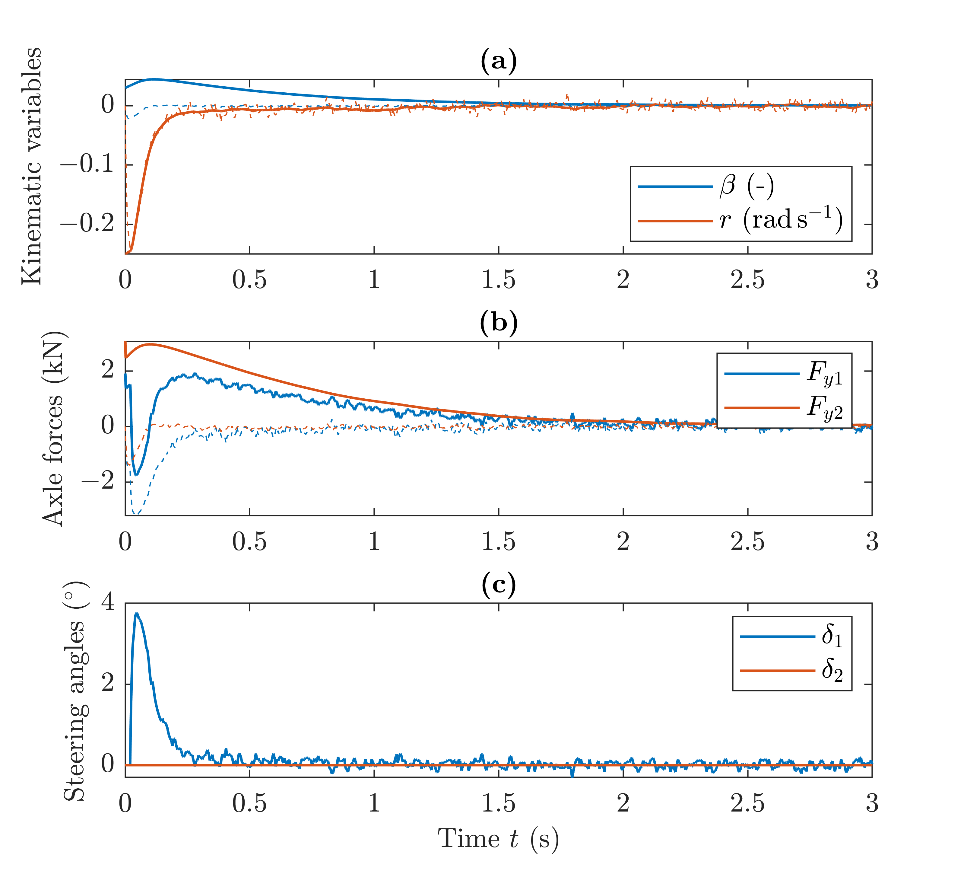
Refer to caption
Figur 6: Closed loop behavior of the lumped states and steering inputs, for LL and FF as in (78) and (79), respectively: (a) kinematic variables; (b) axle forces; (c) steering inputs.
Refer to caption
Figur 7: Evolution of the PDE states ζ​(ξ,t)\zeta(\xi,t), along with its IC (blue lines) and BC (orange lines).

The results asserted by Theorem 4.2 are of a local nature: ICs deviating largely from the target equilibrium may destabilize the closed loop system’s response. Additionally, relatively large values of the parameter ϵ\epsilon – which is essentially determined by the longitudinal speed vxv_{x} for constant L1L_{1} and L2L_{2} – may invalidate the conclusion of the singular perturbation analysis. In this context, the influence of different initial conditions X0=−k​[0.03−0.05]TX_{0}=-k[0.03\;-0.05]^{\mathrm{T}} on the closed loop dynamics of the ODE-PDE system is illustrated in Figure 8 for k=1k=1, 3, and 6. As intuitively expected, ICs that are further from the target equilibrium may slow down the convergence of the norm ‖(X​(t)−X⋆,ζ​(⋅,t),X~​(t))‖𝒳×ℛ∈\mathinner{\!\left\lVert(X(t)-X^{\star},\zeta(\cdot,t),\tilde{X}(t))\right\rVert}_{\altmathcal{X}\times\mathbb{R}^{2}}, which is particularly noticeable for k=6k=6. Finally, the effect of different values of vx=10v_{x}=10, 20, and 50 m​s−1\textnormal{m}\,\textnormal{s}^{-1} is investigated graphically in Figure 9, which demonstrates that the synthesized controller can successfully stabilize the ODE-PDE interconnection (8) on a wide range of longitudinal speeds.

Refer to caption
Figur 8: Closed loop behavior of ‖(X​(t)−X⋆,ζ​(⋅,t),X~​(t))‖𝒳×ℛ∈\mathinner{\!\left\lVert(X(t)-X^{\star},\zeta(\cdot,t),\tilde{X}(t))\right\rVert}_{\altmathcal{X}\times\mathbb{R}^{2}} for different values of k=1k=1, 3, and 6.
Refer to caption
Figur 9: Closed loop behavior of ‖(X​(t)−X⋆,ζ​(⋅,t),X~​(t))‖𝒳×ℛ∈\mathinner{\!\left\lVert(X(t)-X^{\star},\zeta(\cdot,t),\tilde{X}(t))\right\rVert}_{\altmathcal{X}\times\mathbb{R}^{2}} for different values of vx=10v_{x}=10, 20, and 50 m​s−1\textnormal{m}\,\textnormal{s}^{-1}.

6 Conclusions

The present paper investigated the stability and stabilization of semilinear single-track vehicle models with distributed tire friction dynamics using singular perturbation analysis. Specifically, it was shown that when an appropriate perturbation parameter – defined as the ratio between a characteristic length scale of the rolling contact problem and the vehicle’s longitudinal speed – is sufficiently small, standard finite-dimensional methods can successfully be applied to study the local stability of system equilibria and to design stabilizing state- and output-feedback controllers. Whilst the paper’s results do not introduce new observer or controller design strategies, they provide the first rigorous mathematical justification for long-standing practices in automotive research, establishing fundamental advances in vehicle dynamics and opening new perspectives for the control of semilinear ODE-PDE systems with distributed friction.

Future research will explore the design of nonlinear controllers, possibly in conjunction with adaptive observers for vehicle state and friction estimation, along with their impact on the dynamics of the full ODE-PDE interconnection. Additionally, the behavior of more complex vehicle models, incorporating the effect of large steering angles and suspension dynamics, should be studied.

Acknowledgments

This research was financially supported by the project FASTEST (Reg. no. 2023-06511), funded by the Swedish Research Council.

Declaration of interest

Declaration of interest: none.

Referenser