RAPiD: Reward-Guided Consistency Distillation of Diffusion Planners for Real-Time Autonomous Driving
Abstract
Diffusion-based trajectory planners can model multi-modal driving behavior, but their iterative denoising process introduces a latency bottleneck for real-time closed-loop deployment. We present RAPiD, a reward-guided consistency distillation framework that distills a pretrained DiffusionPlanner into a few-step consistency student while retaining multi-modal trajectory generation. The student is trained using deterministic teacher denoising steps from the frozen diffusion planner, together with a low-noise data anchor that keeps generated trajectories grounded in expert demonstrations. To make distillation safety-aware, we train an Implicit Q-Learning critic on a balanced mixture of ground-truth log-replay and DiffusionPlanner rollout trajectories, each scored using a modified PDM-style reward, providing trajectory-level supervision beyond conventional imitation learning. During deployment, the 2-step student generates trajectories, and the trained critic performs best-of- trajectory selection conditioned on the latent state. On nuPlan, RAPiD maintains comparable performance to the diffusion teacher on non-reactive closed-loop splits and remains competitive on reactive splits, while reducing complete-pipeline inference latency from 100.91 ms to 18.41 ms, corresponding to a speedup. On interPlan, RAPiD achieves the highest aggregate score among learning-based methods, demonstrating competitive generalization in interactive long-tail scenarios. These results show that reward-guided consistency distillation can convert a pretrained diffusion planner into a few-step closed-loop planner that substantially reduces inference cost while preserving safety-oriented trajectory selection.
Autonomous systems must make safe and reliable decisions within strict real-time constraints, yet many state-of-the-art diffusion-based planners remain too computationally expensive for practical deployment. This work demonstrates that high-quality, multimodal planning can be achieved with substantially lower inference latency, enabling faster, smoother, and safety-oriented decision-making for autonomous vehicles. Beyond self-driving cars, the proposed approach may benefit a wide range of robotics applications, including autonomous delivery, warehouse automation, and industrial robotics, where rapid and reliable decision-making is essential. By showing that planning efficiency can be improved without sacrificing behavioral diversity or safety, this work contributes toward developing more practical, trustworthy, and deployable AI systems for safety-critical real-world applications.
Autonomous driving, diffusion, path planning, reinforcement learning.
1 Introduction

In autonomous driving, generating safe and interactive trajectories in complex traffic scenarios remains a fundamental challenge [47, 20, 14, 5]. Traditional rule-based systems provide interpretability, but they often struggle to generalize across long-tail events and highly interactive traffic situations [45]. As a result, planning research has increasingly shifted toward large-scale data-driven planning, including generative models that can capture multi-modal driving behavior and generate diverse trajectories [39, 38, 5, 3, 35]. Among these, score-based diffusion models [44], and specifically DiffusionPlanner [49], have achieved strong closed-loop performance on high-fidelity benchmarks such as nuPlan [24]. Their strength lies in modeling the multimodal structure of human driving behavior. Here, multimodality refers to the existence of several distinct, physically valid future trajectory modes under the same scene context, such as merging left, yielding in-lane, or continuing forward at different speeds. Preserving these distinct trajectory modes is critical in interactive traffic, because a regression policy that averages them can produce an unsafe interpolated trajectory that commits to none of the valid maneuvers [10, 40]. However, this expressiveness comes with a deployment cost, i.e., diffusion planners generate trajectories through iterative denoising, requiring multiple network evaluations for trajectory generation. This creates a latency bottleneck for closed-loop autonomous driving, where planning must be both multimodal and responsive under strict real-time constraints.
Several recent approaches have attempted to reduce the diffusion-latency bottleneck, but each leaves open a different trade-off for closed-loop driving. Deterministic extraction methods such as SRPO [4] avoid iterative sampling by compiling a diffusion prior into a single fast policy, but their mode-seeking objective commits to one behavior and can discard alternative valid maneuvers. More broadly, recent surveys on diffusion models for intelligent transportation systems and knowledge distillation identify iterative sampling cost as a central barrier to deploying diffusion-based models in latency-sensitive settings [35, 32]. Consistency models provide a technical route to few-step generation by learning mappings along the diffusion trajectory [42, 27, 43]. However, existing consistency-based formulations do not directly address closed-loop autonomous driving, where the planner must preserve multiple valid trajectory modes while selecting among them using safety- and interaction-aware rewards. Thus, existing acceleration approaches do not directly address reward-guided distillation of a pretrained diffusion planner in which a learned safety critic guides both consistency distillation and deployment-time best-of- trajectory selection.
To address this gap, we propose RAPiD, a reward-guided consistency distillation framework that distills a pretrained DiffusionPlanner into a few-step closed-loop planner. Unlike deterministic extraction methods that reduce the diffusion prior to a single output, RAPiD distills the frozen DiffusionPlanner teacher [49] into a discrete consistency student that preserves the multiple valid trajectory modes. This student model is trained using deterministic DDIM teacher steps, which provide adjacent denoising targets from the frozen diffusion prior without requiring the full iterative sampling chain. This allows the student to approximate the teacher’s generative behavior while substantially reducing the number of network function evaluations. A low-noise data anchor is added to stabilize the high-noise consistency bootstrap and keep generated trajectories grounded in expert driving demonstrations. To make distillation safety-aware, we train an implicit Q-Learning critic [28] on the frozen latent state encodings produced by the pretrained DiffusionPlanner encoder. This critic is supervised using a balanced mixture of ground-truth log-replay and DiffusionPlanner rollout trajectories scored with the modified PDM-style reward adopted in Diffusion-ES [11, 48], emphasizing collision avoidance, drivable-area compliance, time-to-collision, comfort, speed-limit compliance, progress, and proximity to leading agents. During distillation, the critic is applied with a small reward weight to steer the student toward safer in-support modes without overpowering the generative prior. At deployment, the 2-step student generates multiple trajectories, and the trained critic performs best-of- trajectory selection conditioned on the latent state to choose the highest-reward trajectory for execution. Fig. 1 illustrates this trade-off, i.e., the diffusion baseline reacts later in a challenging closed-loop scene, whereas RAPiD produces a smoother and timely maneuver with substantially lower inference latency.
Extensive experiments validate both the efficiency and safety-oriented behavior of the proposed framework across high-fidelity closed-loop driving benchmarks and controlled offline-RL tasks. Beyond aggregate performance, our evaluations isolate the load-bearing mechanisms of the proposed architecture and reveal how different consistency-distillation topologies behave under reward guidance. The main contributions of this work are summarized as follows:
-
•
We introduce RAPiD, a reward-guided consistency distillation framework for closed-loop autonomous driving. RAPiD compresses a pretrained DiffusionPlanner teacher into a few-step discrete consistency student using deterministic DDIM teacher steps, while a low-noise data anchor keeps the student grounded in expert driving trajectories.
-
•
We integrate a PDM-trained implicit Q-Learning critic into both training and deployment. During distillation, the critic provides a small reward-guidance signal that steers the student toward safer in-support trajectory modes. During inference, the same critic performs best-of- selection over batched 2-step candidate trajectories conditioned on the frozen latent state.
-
•
We show through controlled ablations that both deployment components are load-bearing, i.e., critic ranking, rather than random candidate sampling, provides the selection gain, while the second denoising step is required to produce valid multimodal candidates. On our evaluation setup, RAPiD reduces complete-pipeline latency from 100.91 ms to 18.41 ms, a speedup over the diffusion teacher.
-
•
We evaluate RAPiD on nuPlan, interPlan, and D4RL. The method matches or slightly improves the diffusion teacher on non-reactive nuPlan splits, remains competitive on reactive splits with improved safety-oriented PDM submetrics, and demonstrates strong generalization among learning-based planners on interPlan. In D4RL, we further identify a reward-guidance dichotomy: discrete-time students maintain mode coverage in multimodal navigation, whereas continuous-time consistency students collapse under reward guidance in the same regime.
2 Related Work
2.1 Diffusion and Generative Trajectory Planners
Recent surveys of autonomous-driving planning and end-to-end driving systems highlight the shift from modular rule-based pipelines toward learning-based planners that jointly model perception, prediction, and planning [14, 6, 37]. Traditional autonomous-driving planners rely on rule-based, search-based, or optimization-based decision logic, including car-following models, lane-graph search, model predictive control, and hand-designed safety constraints [45, 11]. These methods are interpretable and often reliable in structured scenarios, but they require substantial engineering effort to handle rare, interactive, and long-tail traffic situations. Learning-based planners reduce this manual design burden by learning directly from driving logs, with imitation-learning and transformer-based approaches showing strong performance on closed-loop benchmarks [39, 22, 8, 7]. However, deterministic or regression-based policies remain vulnerable when the same scene admits multiple distinct valid futures. In such cases, minimizing an averaged imitation loss can produce a trajectory between valid modes, which may be neither physically plausible nor safe.
Generative trajectory models address this limitation by modeling a distribution over possible futures rather than a single point estimate [38, 23, 1, 9]. Diffusion models are especially attractive because their iterative denoising process can represent complex multimodal behavior distributions while conditioning on map, route, ego-history, and surrounding-agent context [19, 44]. In autonomous driving, DiffusionPlanner [49] demonstrates that a transformer-based diffusion planner can jointly model ego planning and neighboring-agent prediction, achieving strong closed-loop performance without rule-based refinement. DiffusionES [48] further combines diffusion priors with gradient-free trajectory search to optimize black-box driving rewards. These works establish diffusion as a powerful policy class for planning, but they inherit the deployment cost of iterative sampling, i.e., high-quality generation requires repeated network evaluations, and maintaining diversity often requires sampling multiple candidate trajectories. Our work targets this efficiency bottleneck while retaining the multimodal behavior distribution learned by a pretrained diffusion planner.

2.2 Accelerating and Distilling Generative Policies
A broad line of work accelerates diffusion models by improving the reverse sampling process. Higher-order solvers such as DDIM and DPM-Solver reduce the number of denoising steps required at inference [41, 31], but they still rely on an iterative reverse process. Consistency models provide a more direct alternative by learning to map noisy samples to clean data along the diffusion trajectory, enabling one-step or few-step generation [42]. Consistency Trajectory Models generalize this idea by learning mappings between arbitrary points along the probability-flow trajectory [27], while improved consistency training introduces more stable training procedures and robust losses [43]. These methods provide the technical foundation for few-step generative modeling, but they do not by themselves determine how a planner should choose among several valid trajectory modes when safety and interaction rewards differ.
In offline reinforcement learning and decision-making, generative policies are often coupled with value functions to select high-reward actions. Diffuser and related planning-as-generation methods use diffusion models for trajectory-level decision-making [23], while Diffusion-QL and IDQL use diffusion policies to represent multimodal action distributions and combine them with critic-based selection [46, 17]. These methods preserve expressive action distributions, but inference still requires diffusion sampling. SRPO [4] avoids this cost by extracting a fast deterministic policy from a pretrained diffusion prior using score regularization. However, its mode-seeking objective collapses the prior to a single committed behavior at inference. Reward-aware consistency trajectory distillation [12] shows that reward information can be incorporated into consistency distillation for offline RL. In contrast, our work studies reward-aware consistency distillation in closed-loop autonomous driving, where the student must simultaneously preserve valid trajectory modes, remain close to a pretrained diffusion planner, and support safety-guided selection under real-time constraints.
2.3 Safety-Aware Offline RL and Closed-Loop Driving Evaluation
Offline reinforcement learning is a natural framework for safety-aware planning because it allows logged demonstrations to be reweighted or selected according to reward signals rather than only imitation likelihood. Methods such as IQL [28] learn value functions from static datasets without requiring explicit behavior-policy estimation, reducing extrapolation to out-of-distribution actions. Advantage-weighted regression and related behavior-regularized methods use learned values to emphasize higher-quality actions while remaining close to the data distribution [36, 29, 28]. However, in driving, the reward must reflect closed-loop safety and interaction quality, not merely proximity to expert demonstrations. This motivates critics trained on trajectory-level safety scores, which can rank multiple plausible candidates according to collision risk, time-to-collision, comfort, drivable-area compliance, and progress.
Closed-loop benchmarks such as nuPlan [24] and interPlan [16] expose the limitations of open-loop displacement metrics by evaluating planners inside interactive simulation. Prior work has shown that open-loop accuracy can be misaligned with closed-loop driving quality, and that rule-based or hybrid planners such as PDM can remain competitive by enforcing safety-relevant priors [11]. The PDM scorer aggregates safety and quality terms such as collision avoidance, drivable-area compliance, driving direction, time-to-collision, comfort, and progress, making it a useful signal for distinguishing safe from unsafe trajectory candidates [11, 48]. Our method uses this perspective not only for evaluation but also for learning, i.e., PDM-scored ground-truth log-replay and DiffusionPlanner rollout trajectories supervise an IQL critic, which then guides consistency distillation and performs deployment-time best-of-K trajectory selection.
Despite these advances, existing approaches do not directly address reward-guided distillation of pretrained diffusion planners for closed-loop autonomous driving. RAPiD fills this gap by distilling a frozen DiffusionPlanner teacher into a 2-step discrete consistency student, while a PDM-trained critic guides distillation and selects among candidate trajectories during deployment.
3 Methodology
3.1 Problem Formulation
We consider closed-loop trajectory planning for an ego vehicle in an interactive driving scene. At decision step , the planner observes a raw scene context , which includes ego history, surrounding-agent states, map elements, traffic-light states, route information, and static scene context available in the nuPlan setting [24]. The objective is to predict a future ego trajectory over a planning horizon of steps,
| (1) |
where denotes position and denotes heading. Throughout this paper, we use to denote the action in the offline-RL formulation. This action corresponds to the full future trajectory rather than a low-level control command.
To connect trajectory planning with offline reinforcement learning, each logged transition is represented by a current context , next context , trajectory obtained from either ground-truth log replay or a DiffusionPlanner rollout, and scalar reward . The current and next latent states are obtained using the frozen DiffusionPlanner encoder,
| (2) |
where remains fixed throughout training. The reward is computed by evaluating each replay trajectory—ground-truth log replay or DiffusionPlanner rollout—with the PDM scorer.
| (3) |
The resulting offline dataset consists of replay tuples
| (4) |
For readability, we denote each tuple as in the remainder of the paper.
3.2 Pretrained Diffusion Planner
We use a pretrained DiffusionPlanner [49] as the frozen generative teacher. DiffusionPlanner is built on a diffusion-transformer architecture [34] and jointly models ego planning and neighboring-agent prediction, allowing it to represent multiple valid future trajectory modes under the same scene context. In RAPiD, we reuse both its encoder and denoising prior, i.e., the encoder produces latent scene embeddings used by the critic and student, while the denoising prior provides teacher targets for consistency distillation. All DiffusionPlanner parameters remain frozen.
Let denote a clean expert trajectory and let denote the frozen latent state embedding. The forward diffusion process corrupts at diffusion time according to
| (5) |
or equivalently,
| (6) |
where and are the teacher noise-schedule coefficients. We denote the frozen DiffusionPlanner denoiser by . Given a noised trajectory , diffusion time , and latent state , the teacher predicts a clean trajectory estimate
| (7) |
If the implementation is parameterized as noise prediction , the corresponding clean prediction is obtained as
| (8) |
This pretrained diffusion prior provides an expressive multimodal trajectory distribution, but sampling from it requires an iterative denoising process with multiple network function evaluations. We therefore do not deploy the teacher directly. Instead, we use deterministic DDIM teacher steps derived from this frozen denoiser as supervision for the few-step consistency student introduced in Section 3.5.
3.3 Consistency Distillation for Generative Policies
A direct way to reduce diffusion-policy inference cost is to avoid sampling from the diffusion model at deployment. Score Regularized Policy Optimization (SRPO) [4] follows this idea by extracting a deterministic policy from a pretrained diffusion behavior prior. Its objective can be written as
| (9) | ||||
where denotes the pretrained behavior prior and is a learned critic. The reverse-KL term makes the extracted policy mode-seeking: it encourages the policy to select a high-value mode of the behavior distribution rather than cover all plausible modes. This property is useful for efficient deterministic control, but it is undesirable in interactive driving scenes where multiple distinct maneuvers may be valid under the same context. A single extracted action can discard alternative safe modes that would be useful during closed-loop interaction.
Consistency models [42] provide a different route to fast inference. Instead of extracting a single deterministic action, a consistency student learns to map noised samples back to clean outputs along the teacher denoising trajectory, enabling one-step or few-step generation. Extensions such as Consistency Trajectory Models [27] and improved consistency training [43] further stabilize few-step generation by improving the trajectory-matching objective and training losses. In decision-making, reward-aware consistency trajectory distillation [12] shows that value guidance can steer a consistency student toward higher-reward samples. These methods suggest a promising alternative to deterministic extraction, i.e., compress the diffusion prior into a few-step generative student while preserving the ability to sample multiple valid modes.
In RAPiD, we adopt this consistency-distillation perspective for closed-loop trajectory planning. Rather than using SRPO to extract a single deterministic policy, we distill the frozen DiffusionPlanner teacher into a discrete consistency student that can generate multiple candidate trajectories. The critic is retained, but its role changes, i.e., it provides a small reward-guidance signal during distillation and ranks sampled candidates during deployment. This design preserves the multimodal structure of the diffusion teacher while avoiding the full iterative diffusion sampling chain.
3.4 Safety-Aware Reward Design via PDM Scorer
The critic requires a trajectory-level reward that reflects closed-loop driving quality rather than only imitation likelihood. We therefore use the modified PDM-Closed scoring function adopted in Diffusion-ES [48] as the trajectory-level reward for critic supervision. Given a raw scene context and replay trajectory , obtained from either ground-truth log replay or a DiffusionPlanner rollout, the reward is defined as
| (10) |
The PDM score aggregates safety- and comfort-oriented criteria, including collision avoidance, time-to-collision (TTC), drivable-area compliance, driving-direction compliance, speed-limit compliance, progress, passenger comfort, and proximity to the leading agent.
We use this PDM reward for critic supervision, not as a replacement for the official closed-loop benchmark scores. The purpose is to train a critic that can distinguish safer and more comfortable trajectory candidates within the support of the logged driving data. In particular, the enhanced PDM scorer used in Diffusion-ES [48] includes additional penalties for unsafe proximity to leading agents and speed-limit violations, which encourages the critic to prefer trajectories with larger safety margins and smoother behavior. The resulting critic is later used both during reward-guided consistency distillation and during deployment-time best-of- trajectory selection. Additional details of the PDM metrics are provided in Section S1 of the Supplementary Material.
3.5 Proposed Method
Fig. 2 summarizes the proposed RAPiD pipeline. The method consists of three stages: (i) construction of a PDM-scored offline replay buffer using the frozen DiffusionPlanner encoder, (ii) Implicit Q-Learning critic training on the scored latent-state transitions, and (iii) reward-guided consistency distillation of the frozen DiffusionPlanner teacher into a few-step student. At deployment, the student generates a batch of candidate trajectories using a 2-step sampler, and the trained critic selects the highest-reward candidate.
Stage 1: PDM-Scored Replay Buffer Construction. We construct the offline replay buffer from a balanced combination of transitions collected through ground-truth log replay and DiffusionPlanner simulation [18, 2]. For each recorded nuPlan simulation transition, let denote the raw driving context at planning step , including ego history, surrounding-agent states, map information, traffic-light states, and route information. At each step, denotes the complete 8-second future ego trajectory obtained from ground-truth log replay or predicted by DiffusionPlanner. The simulator advances to the next planning step using this trajectory, producing the next context . We use the frozen DiffusionPlanner encoder to obtain
| (11) |
The trajectory is treated as the offline-RL action rather than a low-level control command. Each trajectory is evaluated using the PDM scorer:
| (12) |
The reward reflects collision avoidance, drivable-area compliance, driving-direction compliance, time-to-collision, speed-limit compliance, progress, comfort, and proximity to the leading agent. The resulting offline replay buffer is
| (13) |
For readability, we write each tuple as in the remainder of the paper.
Stage 2: Critic Training via Implicit Q-Learning. We train an IQL critic on the PDM-scored replay buffer. The critic consists of a value function and twin action-value functions and , where is a candidate future trajectory. We define the averaged critic as
| (14) |
where . The value function is trained using expectile regression:
| (15) |
where
| (16) |
Using biases the value estimate toward higher-return trajectories while avoiding explicit behavior-policy queries. The twin Q-functions are trained with the temporal-difference objective
| (17) |
where is the discount factor. After training, the critic is frozen and the averaged value is used both as a reward-guidance signal during consistency distillation and as the ranking function for deployment-time best-of- selection.
Stage 3: Reward-Guided Consistency Distillation. We distill the frozen DiffusionPlanner teacher into a few-step consistency student , which maps a noised trajectory at diffusion time back to a clean trajectory conditioned on the latent state . Given a clean expert trajectory , forward noising is defined as
| (18) |
where and follow the frozen teacher’s noise schedule.
For an adjacent pair of time steps , the frozen DiffusionPlanner teacher provides a deterministic DDIM denoising step from to an earlier noised sample . Writing the teacher clean-trajectory prediction as , the implied noise estimate is
| (19) |
and the corresponding DDIM teacher target is
| (20) |
This teacher step is held under stop-gradient. With an exponential-moving-average target network , the consistency loss is
| (21) |
where is a time-dependent weighting term.
To stabilize the high-noise consistency bootstrap, we add a low-noise data anchor. For and , the anchor loss is
| (22) |
Here, denotes the per-dimension Huber loss with , summed over the trajectory dimensions. Finally, the frozen critic provides a small reward-guidance term. Let , where , denote the differentiable one-step readout used for critic guidance. The complete student objective is
| (23) |
where controls the data-anchor strength and is kept small so that critic guidance steers the student among in-support modes without overpowering the frozen diffusion prior.
Deployment: 2-Step Sampling with Critic Best-of-. At inference, the raw scene context is encoded once as . The student draws candidate trajectories using a 2-step sampler. Each candidate is initialized from Gaussian noise, decoded once at the highest noise level, re-noised to a lower intermediate time, and decoded again:
| (24) |
| (25) |
| (26) |
The final executed trajectory is selected by the frozen critic:
| (27) |
Thus, multimodality is preserved by candidate generation, while safety-oriented trajectory selection is performed by the PDM-trained critic.
4 Experiments
4.1 Experiment Setup
RAPiD is implemented in PyTorch [33] and trained using an NVIDIA RTX 4090 GPU with 24GB VRAM. The main driving evaluation is conducted on nuPlan [24] and interPlan [16]. We report nuPlan scores for closed-loop planning quality, interPlan scores for scenario-specific interactive performance, and PDM-style scorer metrics [48] for safety and comfort analysis. Representative comparison methods are listed in Tables 2 and 5. Additional controlled offline-RL experiments on D4RL [13], including AntMaze and Gym-MuJoCo tasks, are provided in S4 of the Supplementary Material. For those supplementary experiments, we reuse SRPO pretrained diffusion and critic checkpoints as the base initialization to isolate the effect of the proposed consistency-distillation and critic-selection modifications under a controlled comparison.
4.2 Evaluation Results
nuPlan Benchmark Performance. We evaluate our method against SOTA baselines, including learning-based planners (PDM-Open [11], UrbanDriver [39], Gameformer [22], Plan-TF [9], PLUTO [7], DiffusionPlanner [49]) and rule-based planners (IDM [45], PDM-Closed [11], PDM-Hybrid [11]). Table 2 summarizes performance on the nuPlan benchmark. On non-reactive (NR) splits, RAPiD maintains comparable performance to the DiffusionPlanner baseline while achieving marginally higher scores on Val14, Test14, and Test14-hard. Specifically, RAPiD achieves NR scores of 90.01, 89.88, and 76.01, compared with 89.87, 89.19, and 75.99 for DiffusionPlanner. Table 2 reports complete-pipeline inference latency, including input feeding, normalization, encoding, and output generation. RAPiD reduces latency from 100.91 ms for DiffusionPlanner to 18.41 ms, corresponding to a speedup, and is also substantially faster than UrbanDriver. RAPiD is slower than lightweight single-output baselines such as PDM-Open, PlanTF, and PLUTO because it generates multiple trajectories with a 2-step consistency sampler and ranks them using the critic for best-of- trajectory selection. This reflects the intended trade-off of RAPiD: retaining multimodal trajectory generation and safety-oriented selection while substantially reducing the iterative sampling cost of the diffusion teacher.
| Type | Methods | Val14 | Test14-hard | Test14 | |||
|---|---|---|---|---|---|---|---|
| NR | R | NR | R | NR | R | ||
| Expert | Log-replay | 93.53 | 80.32 | 85.96 | 68.80 | 94.03 | 75.86 |
| Rule-based & Hybrid | IDM [45] | 75.60 | 77.33 | 56.15 | 62.26 | 70.39 | 74.42 |
| PDM-Closed [11] | 92.84 | 92.12 | 65.08 | 75.19 | 90.05 | 91.63 | |
| PDM-Hybrid [11] | 92.77 | 92.11 | 65.99 | 76.07 | 90.10 | 91.28 | |
| GameFormer [22] | 79.94 | 79.78 | 68.70 | 67.05 | 83.88 | 82.05 | |
| PLUTO [7] | 92.88 | 76.88 | 80.08 | 76.88 | 92.23 | 90.29 | |
| Diffusion Planner w/ refine [49] | 94.26 | 92.90 | 78.87 | 82.00 | 94.80 | 91.75 | |
| Learning-based | PDM-Open* [11] | 53.53 | 54.24 | 33.51 | 35.83 | 52.81 | 57.23 |
| UrbanDriver [39] | 68.57 | 64.11 | 50.40 | 49.95 | 51.83 | 67.15 | |
| GameFormer w/o refine [22] | 13.32 | 8.69 | 7.08 | 6.69 | 11.36 | 9.31 | |
| PlanTF [9] | 84.27 | 76.95 | 69.70 | 61.61 | 85.62 | 79.58 | |
| PLUTO w/o refine* [7] | 88.89 | 78.11 | 70.03 | 59.74 | 89.90 | 78.62 | |
| DiffusionPlanner [49] | 89.87 | 82.80 | 75.99 | 69.22 | 89.19 | 82.93 | |
| RAPiD (Ours) | 90.01 | 82.13 | 76.01 | 67.34 | 89.88 | 82.01 | |
At deployment, the consistency student generates trajectories using a 2-step sampler, and the averaged twin critic selects the final trajectory through best-of- trajectory selection. Fig. 3 sweeps on Val14 reactive evaluation. Closed-loop score improves with diminishing returns and saturates at , with no further gain at larger . This behavior suggests that increasing improves coverage of high-quality trajectory modes up to a point, after which additional trajectories provide limited benefit and may expose the selection process to critic overestimation. We therefore use in deployment. Since the trajectories are generated in a single batched pass, best-of- selection adds limited overhead relative to the 2-step student forward pass. This sweep serves as a deployment ablation for the best-of- trajectory selection used in nuPlan. Since all other inference settings are fixed, the improvement from to indicates that generating multiple trajectories and selecting with the critic contributes to the closed-loop gain, while the saturation beyond motivates our deployment choice.
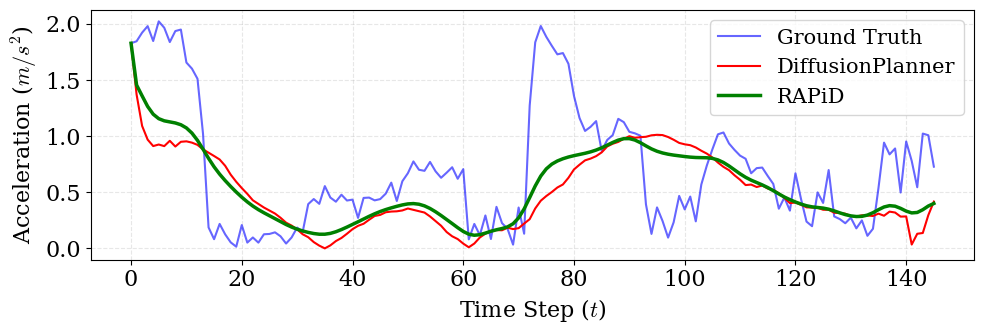
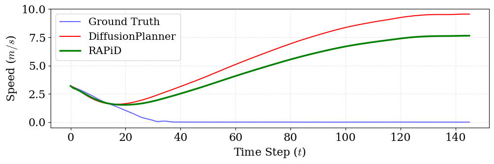
In the reactive (R) environment, RAPiD achieves competitive performance, obtaining 82.01 on Test14 compared with 82.93 for DiffusionPlanner. The reactive gap reflects a safety-progress trade-off induced by the PDM-style reward, which places stronger emphasis on comfort, proximity, and safety margins while reducing the relative emphasis on progress compared with the standard nuPlan scorer. In lane-following scenarios, RAPiD maintains closer alignment with the lane centerline and produces smoother acceleration patterns when following lead vehicles (Fig. 5(a-2)), compared with the DiffusionPlanner baseline in the corresponding scene (Fig. 5(a-1)). During stopping scenarios, RAPiD reduces speed earlier and maintains larger following distances (Fig. 5(b-2)), whereas DiffusionPlanner exhibits shorter following distances in the corresponding example (Fig. 5(b-1)). For lane changes, RAPiD executes more gradual merges with lower yaw rates (Fig. 5(c-2)) compared with the sharper maneuvers generated by DiffusionPlanner (Fig. 5(c-1)).
At intersections, DiffusionPlanner can exhibit hesitation followed by abrupt maneuvers, leading to near-collision or collision-prone behavior associated with delayed maneuvers (Fig. 5(d-1); Fig. 1(a-2)). In contrast, RAPiD produces smoother and more timely turns with controlled acceleration (Fig. 5l(d-2)) and avoids the collision-prone behavior shown in the corresponding baseline examples (Fig. 1(b-1,b-2)). See Section S7-A in the Supplementary Material for a detailed frame-by-frame analysis. These qualitative differences are consistent with the PDM-style reward used for critic training, which encourages trajectories with improved comfort, proximity, and safety margins, even when this reduces progress-oriented scoring in the reactive nuPlan setting.
| NFE | CLS | Progress | No Collision | TTC | Decoder Latency |
|---|---|---|---|---|---|
| 1 | 78.00 | 0.850 | 0.890 | 0.890 | 6.10 ms |
| 2 | 82.13 | 0.885 | 0.955 | 0.925 | 11.91 ms |
| 4 | 82.01 | 0.880 | 0.954 | 0.923 | 23.10 ms |
| 8 | 81.90 | 0.881 | 0.952 | 0.922 | 45.31 ms |
| Selection | CLS | Progress | No Collision | TTC | |
|---|---|---|---|---|---|
| 1 | None | 79.20 | 0.872 | 0.943 | 0.910 |
| 32 | Random | 79.15 | 0.879 | 0.939 | 0.919 |
| 32 | Critic | 82.13 | 0.885 | 0.955 | 0.925 |
| Type | Method | interPlan | Const. | Acc. | Jayw. | Nudge | Overt. | LTD | MTD | HTD |
| Rule- based | IDM [45] | 31 | 0 | 0 | 66 | 0 | 0 | 61 | 61 | 61 |
| IDM+MOBIL [26] | 31 | 21 | 0 | 66 | 0 | 0 | 71 | 21 | 70 | |
| PDM-Closed [11] | 42 | 18 | 0 | 48 | 74 | 9 | 62 | 62 | 62 | |
| Learning- based | Urban Driver [39] | 4 | 0 | 0 | 0 | 0 | 0 | 29 | 0 | 30 |
| GC-PGP [15] | 10 | 0 | 0 | 0 | 0 | 0 | 18 | 16 | 44 | |
| GameFormer [22] | 11 | 0 | 0 | 48 | 0 | 0 | 0 | 20 | 21 | |
| PDM-Open [11] | 25 | 13 | 0 | 56 | 36 | 8 | 29 | 29 | 26 | |
| DTPP [21] | 25 | 18 | 18 | 44 | 10 | 0 | 40 | 36 | 34 | |
| DiffusionPlanner [49] | 29 | 9 | 0 | 26 | 60 | 25 | 40 | 21 | 48 | |
| RAPiD (Ours) | 30 | 11 | 0 | 27 | 61 | 26 | 42 | 27 | 49 |

(a-1) DiffusionPlanner

(a-2) RAPiD

(b-1) DiffusionPlanner

(b-2) RAPiD
Acceleration Metrics
Speed Metrics

(c-1) DiffusionPlanner

(c-2) RAPiD

(d-1) DiffusionPlanner

(d-2) RAPiD

Yaw Rate Metrics

Speed Metrics
Deployment Ablations. Table 4 isolates the contribution of critic-based selection on nuPlan Val14-R. Randomly selecting one of candidates performs similarly to generating a single candidate, as expected because both return an unranked sample from the same distribution. In contrast, critic-based selection improves CLS from 79.15 to 82.13 and improves progress, collision avoidance, and TTC, showing that the gain arises from value-based ranking rather than candidate generation alone.
Table 3 evaluates the student sampling depth. The configured two-step sampler achieves the best CLS and safety metrics. One-step inference provides insufficient refinement, whereas additional evaluations do not improve performance because the student was distilled for the two-step schedule, while substantially increasing decoder latency. We therefore use NFE and for deployment.
interPlan Benchmark Analysis. We evaluate our approach against representative baselines, including learning-based planners (UrbanDriver [39], GC-PGP [15], GameFormer [22], PDM-Open [11], DTPP [21], DiffusionPlanner [49]) and rule-based planners (IDM [45], IDM+MOBIL [26], PDM-Closed [11]). The interPlan scorer extends standard nuPlan metrics (compliance, safety, and comfort) with scenario-specific requirements. It measures lane change completion rates relative to goal requirements and applies multiplicative progress penalties for failures to pass obstacles like parked cars or construction zones. Scenarios receive zero scores for collisions, drivable area violations, extended stationarity, or getting stuck behind obstacles. Direction compliance penalties are disabled for overtaking and accident scenarios where oncoming lane usage is necessary.
Table 5 presents results on the interPlan benchmark, which targets scenarios that are under-emphasized in standard nuPlan evaluation: achieving high scores through simple lane-following with minimal interaction. interPlan augments scenario goals to require multiple lane changes and initializes varying traffic densities by spawning agents around the ego vehicle at maximum spacings of 100m (low traffic density, LTD), 50m (medium traffic density, MTD), and 33m (high traffic density, HTD). The benchmark comprises 80 scenarios across eight categories testing planner generalization to long-tail situations. Lateral maneuvering is evaluated through construction zones (Const., navigating around traffic cones), accident sites (Acc., maneuvering around crashed vehicles), jaywalking pedestrians (Jayw., handling unexpected crossings at bus stops), nudging (carefully passing parked vehicles within lane), and overtaking (Overt., safe passage through oncoming lanes). Please see Section S7-B of Supplementary Material for details. Longitudinal interaction is tested through lane changes under LTD, MTD, and HTD conditions with varying traffic environments (conservative, assertive, and mixed). Each category contains 10 instances. Compared with standard nuPlan evaluation, where conservative lane-following can achieve strong scores, interPlan explicitly requires interactive maneuvering, proactive gap selection, and robust generalization to uncommon situations. Our approach achieves the highest interPlan score among learning-based methods with an aggregate score of 30, outperforming PDM-Open and DiffusionPlanner. For lateral maneuvers, our method scores 61 in nudging scenarios (versus DiffusionPlanner’s 60) and 26 in overtaking, i.e., the highest among both learning-based and rule-based methods. For longitudinal interactions, performance improvements increase with traffic density, i.e., 42 versus 40 in LTD, 27 versus 21 in MTD, and 49 versus 48 in HTD. These gains in denser conditions demonstrate our method’s ability to navigate between vehicles and complete required lane changes without freezing or causing safety violations. In MTD and HTD scenarios with reduced agent spacing (50m and 33m), our method shows improved gap selection and timing compared to DiffusionPlanner. While rule-based methods achieve highest performance on nuPlan, they fail to meet interPlan requirements in several scenarios. Our learning-based model demonstrates the adaptability required for interactive scenarios while maintaining competitive performance.
PDM-Based Safety and Comfort Analysis.
Fig. 4 provides a metric-level breakdown of PDM scores in the reactive environment across Val14, Test14, and Test14-hard splits. Both RAPiD and DiffusionPlanner are evaluated in the same reactive closed-loop setting, but this analysis reports the PDM-style safety and comfort metrics rather than the standard nuPlan score. The results help explain the reactive-score trade-off observed in Table 2, i.e., RAPiD improves several safety- and comfort-oriented metrics while reducing progress.
Safety Metrics.
RAPiD achieves higher collision-avoidance scores across all three splits. The no-collision score increases from 0.9467 to 0.9550 on Val14, from 0.9511 to 0.9595 on Test14, and from 0.9199 to 0.9310 on Test14-hard. Both methods maintain perfect drivable-area compliance. RAPiD also maintains high driving-direction compliance, with scores of 0.9890, 0.9880, and 0.9690 across Val14, Test14, and Test14-hard. Speed-limit compliance improves across all three splits, increasing from 0.9803 to 0.9880 on Val14, from 0.9727 to 0.9890 on Test14, and from 0.9712 to 0.9820 on Test14-hard. Time-to-collision (TTC) also improves from 0.9116 to 0.9250 on Val14, from 0.9249 to 0.9350 on Test14, and from 0.8849 to 0.8950 on Test14-hard. These improvements indicate that the PDM-trained critic tends to select trajectories with larger safety margins.
Comfort, Proximity, and Lane-Following Metrics.
RAPiD also improves comfort, proximity, and lane-following scores. On Val14, comfort increases from 0.9787 to 0.9850; on Test14, from 0.9823 to 0.9890; and on Test14-hard, from 0.9758 to 0.9800. Proximity scores similarly improve from 0.9694 to 0.9800 on Val14, from 0.9753 to 0.9820 on Test14, and from 0.9543 to 0.9610 on Test14-hard. Lane-following improves from 0.9237 to 0.9400 on Val14, from 0.9258 to 0.9450 on Test14, and from 0.9206 to 0.9250 on Test14-hard. These trends are consistent with the modified PDM-style reward used for critic training, where the comfort weight is increased from 2 to 5 and a proximity-to-leading-agent term is introduced with weight 5.
Progress Metrics.
The main trade-off appears in progress. Progress decreases from 0.9374 to 0.8850 on Val14, from 0.9408 to 0.8920 on Test14, and from 0.8977 to 0.8850 on Test14-hard. This reduction is consistent with the reward design, where the progress weight is reduced from 5 to 2 while comfort, proximity, TTC, and collision avoidance receive stronger emphasis. As a result, RAPiD tends to prefer more conservative trajectories with improved safety and comfort margins, which can lower the standard reactive nuPlan score when progress is weighted more heavily.
5 Conclusion
This work addresses the computational inefficiency and stochastic behavior of diffusion-based trajectory planning through efficient multimodal policy distillation. Rather than extracting a single deterministic action, which collapses the teacher’s multimodality and limits reactive closed-loop performance, we distill a pretrained DiffusionPlanner model into a few-step consistency student and deploy it with critic best-of- selection, preserving the teacher’s behavioral diversity while training with PDM-based safety scoring. By anchoring the student to the prior’s probability-flow ODE (Ordinary Differential Equation), generated trajectories remain within the support of valid driving behaviors, and the 2-step sampler reads out where the denoiser is accurate, yielding safe and comfortable trajectories at real-time inference. Evaluation on nuPlan and interPlan benchmarks demonstrates that our method matches the diffusion teacher on the non-reactive nuPlan splits and generalizes strongly among learning-based methods on interPlan, while delivering a speedup in complete-pipeline inference latency (18.41 ms versus 100.91 ms) compared to the diffusion baseline. On the reactive splits our method remains competitive with the teacher, with a small difference in score. Our work provides a practical pathway for deploying efficient, safety-focused planning systems in real-world autonomous driving by leveraging pretrained diffusion models without requiring costly training from scratch, bridging the gap between diffusion model expressiveness and the latency requirements of production autonomous vehicles.
Supplementary Material
RAPiD: Reward-Guided Consistency Distillation of Diffusion Planners for Real-Time Autonomous Driving
S1 Basics of Predictive Driver Model (PDM)
This Section compliments Section III-D of the main paper. PDM [11, 48] evaluates trajectory safety and quality through a composite of weighted metrics. While the full PDM Scorer includes continuous metrics such as speed limit compliance and comfort, Figure S1 provides a supplementary overview of the primary spatial components used for trajectory selection. This includes monitoring the distance from the leading vehicle, divergence from the lane centerline, and adherence to the agent’s reference path. A critical safety component is the maintenance of a Safe Distance from the leading vehicle, as shown in Figure S2. In the PDM framework, this is governed by high multiplier weights for Proximity and TTC (Time-to-Collision) within bounds, which penalize aggressive following behavior to minimize collision risk. As illustrated in Figure S3, Centerline Tracking is essential for maintaining Lane Following and Drivable Area Compliance. Precise centering ensures adequate clearance from neighboring vehicles, avoiding the penalties associated with drifting off-center. Finally, Figure S4 highlights Turning Behaviour, where Comfort metrics (weighted at 5 in PDM) penalize the aggressive lateral and longitudinal accelerations caused by late deceleration or overspeeding during maneuvers.


S2 Method Pseudocode
This Section compliments Section III-E of the main paper. The complete framework is detailed in Algorithm 1 (the three-stage training pipeline) and Algorithm 2 (deployment). Stage 1 constructs the offline replay buffer from a balanced mixture of PDM-scored ground-truth log-replay and DiffusionPlanner rollout transitions, Stage 2 trains the Implicit Q-Learning (IQL) critic, and Stage 3 distills a few-step consistency student from the frozen DiffusionPlanner [49] prior. At deployment, the student draws candidate trajectories with a 2-step sampler and acts with the critic-selected best.
S3 Consistency Distillation: Full Formulation
This Section complements Section III-E of the main paper and provides the complete mathematical specification of the deployed discrete consistency student, verified against our implementation.
S3.1 Teacher Noise Process (VP-SDE)
The frozen DiffusionPlanner teacher is trained under a variance-preserving (VP) diffusion process. For a clean trajectory and continuous time (), the forward marginal is , , with
| (28) |
where , , so that . The teacher predicts the noise conditioned on the latent state and is held frozen throughout distillation.
S3.2 Student Parameterization (EDM Preconditioning)
The consistency student maps a noised trajectory back to a clean one. We adopt EDM-style preconditioning [25] adapted to the VP process. Writing the variance-exploding-equivalent variable with and data scale ,
| (29) |
| (30) |
where is the trainable network. As , gives and , enforcing the consistency boundary condition . This boundary is essential: it prevents the consistency loss from collapsing to a trivial trajectory-constant solution and keeps the network input unit-scaled at every noise level.
S3.3 Teacher Probability-Flow ODE Step
The consistency target is anchored to one deterministic step of the teacher’s probability-flow ODE, implemented as a DDIM step [41] from a noisier node to an adjacent less-noisy node . Given , this step is computed under stop-gradient:
| (31) |
Gradients are never propagated through this teacher step; it serves only to produce the regression target .
S3.4 Distillation Time Grid
Distillation is performed on an ordered grid of nodes (). The default grid is uniform in ; an optional grid uniform in log-SNR, , equalizes the per-step teacher-ODE accuracy across nodes. At each step, an index selects the adjacent pair .
S3.5 Training Objective
The student minimizes a three-term objective,
| (32) |
combining critic guidance, prior-ODE self-consistency, and a low-noise data anchor.
Consistency term. For the sampled adjacent pair, with and the teacher-evolved target ,
| (33) |
where is an exponential-moving-average (EMA) target, updated as with and held under stop-gradient. The target network is evaluated in inference mode so that dropout does not perturb the regression target. The per-step weight defaults to (an optional SNR weighting is also supported). This term keeps the student on the prior’s probability-flow ODE, replacing iterative sampling while preserving the teacher’s support over valid driving behaviors.
Data anchor. To stabilize the high-noise consistency bootstrap, the student’s clean prediction is regressed directly to ground-truth trajectories at low noise , with :
| (34) |
Restricting this anchor to low noise provides a strong on-manifold signal without inducing the mode-averaging that regressing to the mean at high noise would cause.
Critic guidance. The reward term is computed on the one-step readout from pure noise, with , scored by the mean of the twin target critics:
| (35) |
The clip is load-bearing: its zero sub-gradient outside prevents value ascent from driving off-manifold into the critic’s out-of-distribution extrapolation regime. Normalizing by the running mean magnitude makes the reward weight comparable across environments. Following reward-aware consistency distillation [12], is kept small so that distillation dominates and the critic only steers among in-support modes.
Distance. The default distance is a per-dimension Huber loss () summed over action dimensions; squared-error and an iCT-style pseudo-Huber [43] are supported as alternatives.
S3.6 Deployment
At inference the student is sampled with : a one-step readout at followed by a renoise to a lower interior node and a second readout, where the denoiser is more accurate (Algorithm 2). Because a single deterministic readout averages opposing modes of the multimodal posterior, we draw candidates and act with the critic-selected best, . As established in the main paper, performance saturates at , the deployment setting.
S4 D4RL Benchmark Results
This Section complements Section IV of the main paper. We evaluate the deployed discrete consistency student on D4RL [13] to validate the distillation mechanism in a controlled setting. AntMaze is the closest D4RL proxy for closed-loop driving: multimodal, long-horizon, and sparse-reward, requiring the policy to commit to one of several valid routes rather than average across them. Locomotion (Gym-MuJoCo) is the complementary unimodal-precision regime. All results use best-of- deployment (, 2-step sampler).
| Dataset | Environment | BEAR | TD3+BC | IQL | SfBC | Diffuser | Diffusion-QL | QGPO | IDQL | SRPO | Ours |
|---|---|---|---|---|---|---|---|---|---|---|---|
| Medium-Expert | HalfCheetah | ||||||||||
| Medium-Expert | Hopper | ||||||||||
| Medium-Expert | Walker2d | ||||||||||
| Medium | HalfCheetah | ||||||||||
| Medium | Hopper | ||||||||||
| Medium | Walker2d | ||||||||||
| Medium-Replay | HalfCheetah | ||||||||||
| Medium-Replay | Hopper | ||||||||||
| Medium-Replay | Walker2d | ||||||||||
| Average (Locomotion) | |||||||||||
| Default | AntMaze-umaze | - | |||||||||
| Diverse | AntMaze-umaze | - | |||||||||
| Play | AntMaze-medium | - | |||||||||
| Diverse | AntMaze-medium | - | |||||||||
| Play | AntMaze-large | - | |||||||||
| Diverse | AntMaze-large | - | |||||||||
| Average (AntMaze) | - | ||||||||||
S4.1 Discussion
Three findings emerge. First, the multimodal regime is where the consistency student delivers. On AntMaze its aggregate score () exceeds SRPO [4] () and is competitive with the strongest sampling-based methods, IDQL () and QGPO (), despite acting in only two function evaluations rather than a full diffusion rollout. The student is strongest on the diverse mazes, reaching on umaze-diverse and on medium-diverse, both above SRPO ( and ). This validates the central claim that a few-step multimodal student recovers the decision quality a single deterministic action sacrifices, at near-deterministic inference cost.
Second, the gains are largest precisely where multiple valid routes must be distinguished (the diverse splits), and the student remains within range of the best methods on the play and large mazes. This is consistent with the mechanism: the benefit of a multimodal student over a deterministic policy grows with the number of competing modes the policy must represent.
Third, locomotion is the clear limitation. The student trails SRPO by a wide aggregate margin ( vs ), concentrated almost entirely in the hopper and halfcheetah-expert tasks. These are unimodal-precision problems: the dataset contains one near-optimal behavior, and a deterministic score-regularized policy reproduces it more faithfully than a stochastic few-step sampler, whose injected renoise adds variance with no multimodal benefit to offset it. This is not a failure of distillation but a regime mismatch, and it directly motivates the continuous-time student of Section S6, which is built for precisely this regime, together with the reward-guidance instability that confines it there.
S5 Ablations
This Section complements Section IV of the main paper and isolates the design choices the deployed student depends on: critic-based selection, the 2-step sampler, and the distillation grid. All ablations are run on D4RL AntMaze, the multimodal proxy for closed-loop driving, with candidates unless stated otherwise.
S5.1 Selection Rule: The Critic Ranking Is the Gain
We first ask whether the improvement comes from drawing multiple candidates or from ranking them with the critic. Table 7 compares acting on a single sample, selecting a random candidate from , and selecting the critic-argmax candidate. Drawing candidates without critic ranking is no better than a single sample (random-of-32 single across every maze); the entire gain comes from the critic selecting the highest-value mode, lifting medium-diverse from to and large-play from to . This directly supports the upgrade from a deterministic single action to critic-guided multimodal selection.
| Maze | single () | random-of-32 | critic-of-32 |
|---|---|---|---|
| medium-play | |||
| medium-diverse | |||
| large-play | |||
| large-diverse |
S5.2 Generation Steps: 2-Step Is the Sweet Spot
We next vary the number of denoise–renoise sampling steps (NFE). Table 8 shows that a single step fails entirely on every maze (score ), 2-step is best or tied, and additional steps yield no further gain. The 1-step failure is an accuracy failure, not a diversity failure: a single readout at the maximum noise level averages opposing modes of the multimodal posterior into an invalid action. The second step renoises to a lower noise level and reads out where the denoiser is accurate, placing the action on a real mode. This justifies the fast 2-step deployment.
| Maze | 1 | 2 | 4 | 8 |
|---|---|---|---|---|
| medium-diverse | ||||
| large-diverse | ||||
| large-play | ||||
| medium-play |
S5.3 Mechanism: Why 1-Step Collapses
Table 9 measures the cross-sample standard deviation over draws at each NFE. At 1-step the samples form a tight cluster (std ) far below the dataset action spread (): the draws collapse onto a single, mode-averaged estimate, which is why critic selection over 32 of them still scores , there is no valid mode to select. Moving to 2-step roughly doubles the spread (), restoring the diversity that makes best-of- effective. Beyond 2-step the spread saturates, consistent with the performance plateau above.
| NFE | 1 | 2 | 4 |
|---|---|---|---|
| cross-sample std |
S5.4 Distillation Time Grid
The consistency loss is evaluated on adjacent pairs of a time grid, and both its spacing and density affect distillation quality. Table 10 reports the effect on halfcheetah-medium-expert. Spacing the grid evenly in log-SNR rather than evenly in substantially improves the distilled student ( vs at ): a log-SNR grid equalizes the per-step teacher-ODE accuracy, whereas a linear grid leaves the largest, least accurate steps concentrated at high noise. Grid density shows the opposite of a “more is better” trend: increasing the node count from to degrades performance ( to ), as a denser grid shortens each consistency jump but accumulates per-step error over more steps. We therefore use a log-SNR grid with . These results are single-seed.
| Axis | Setting | Score |
|---|---|---|
| Spacing () | linear | |
| log-SNR | ||
| Density (log-SNR) | ||
S5.5 Summary
Together these ablations establish that both upgrades over deterministic single-action extraction are load-bearing: the critic ranking converts drawn candidates into a large performance gain (Table 7), and the 2-step sampler is required for those candidates to be valid in the first place (Tables 8, 9). The nuPlan best-of- sweep in the main paper confirms the same saturation behavior in closed-loop driving.
S6 Continuous-Time Student (sCM): The Non-Deployed Sibling
This Section complements Section IV of the main paper and provides the evidence for the reward-guidance dichotomy reported there. Alongside the deployed discrete student, we develop a continuous-time consistency student based on TrigFlow [30]. We present its formulation and results here, and show that while it excels in the unimodal-precision regime, reward guidance destabilizes it on multimodal navigation, which is why the discrete student is deployed for driving.
S6.1 Formulation
The continuous-time student uses the TrigFlow parameterization with data scale and prior at . The forward process is
| (36) |
and the consistency function is parameterized through a raw velocity network ,
| (37) |
which satisfies the boundary condition exactly. No EDM preconditioning, tanh, or dropout is used.
Teacher wrapping. The frozen VP teacher is reused by mapping TrigFlow time to VP time via . Solving the VP log-mean-coefficient relation gives the positive root
| (38) |
so that and the VP-noised state coincides with the TrigFlow state. The PF-ODE velocity from the teacher (stop-gradient) is
| (39) |
Continuous consistency loss. The tangent is obtained by a forward-mode JVP of along with tangent , and is pushed by the normalized tangent (sCM tangent normalization),
| (40) |
with constant . The raw is the consistency residual, logged and driven toward zero.
Velocity anchor. is jointly regressed to the true flow velocity at all ,
| (41) |
providing the coherent velocity field the consistency term sharpens. Times are drawn from . The full objective is , with structured as in the discrete student. Unlike the discrete student, there is no EMA target, no discrete time grid, and no low-noise data anchor; these are the structural differences that the dichotomy below depends on.
S6.2 The Reward-Guidance Dichotomy
Reward-free, sCM is stable and strong. Without the reward term, the continuous student excels on the unimodal-precision regime, exceeding the discrete student on the expert locomotion tasks (Table 11), and is even competitive on AntMaze.
| Task | sCM (reward-free) |
|---|---|
| walker2d-medium-expert | |
| halfcheetah-medium-expert | |
| hopper-medium | |
| walker2d-medium | |
| hopper-medium-replay | |
| walker2d-medium-replay | |
| antmaze-umaze | |
| antmaze-medium-diverse | |
| antmaze-medium-play |
Reward-on, sCM collapses on multimodal navigation. Activating the reward term collapses the continuous student on AntMaze: medium-diverse falls from to , and the large mazes drop to (Table 12). The collapse persists across reward weights ( on medium-diverse; on the large mazes), so it is not a single mis-set hyperparameter. The continuous student has no working reward integration in the multimodal regime.
| Task | sCM | |
|---|---|---|
| medium-diverse | ||
| large-diverse | ||
| large-diverse | ||
| large-play | ||
| large-play |
S6.3 Late-Training Stability by Regime
The dichotomy also appears in training dynamics on high-precision locomotion. On halfcheetah-medium-expert, the discrete student peaks early and then degrades over training: return rises to roughly by epoch 38 before falling to about by epoch 100, while its consistency loss drifts upward (). The continuous student on the same task is stable: return climbs to about and holds, with a flat consistency loss (). This is consistent with the dichotomy, as the continuous student’s all- velocity anchor maintains a coherent field on the single near-optimal mode, whereas the discrete student’s low-noise-only anchor does not fully constrain the high-noise consistency bootstrap in this precision regime. We note that this comparison is between two methods on the same task and is not a controlled isolation of any single component (the runs differ in more than one factor); it is reported as evidence for the regime split, not as a causal ablation of a single mechanism. This result is single-seed.
S6.4 Discussion
The two students are structural mirror images. The discrete student absorbs reward guidance on multimodal navigation, anchored by its low-noise denoising anchor, but trails on unimodal-precision locomotion. The continuous student is the opposite: stable and accurate in reward-free precision control, but lacking this data anchor, it has no anchor to keep it on the data manifold under reward guidance and collapses once reward guidance is applied to multimodal navigation. This dichotomy is why the discrete student is the one deployed for driving, where multimodal closed-loop reactivity under a safety reward is exactly the demanding regime. We note one honest limitation of this evidence: the reward-on collapse is demonstrated on AntMaze, the multimodal proxy, and we do not have reward-on continuous-student results on locomotion; the claim is therefore that reward guidance destabilizes the continuous student on multimodal navigation, not universally.
S7 Additional Qualitative Analysis
This Section compliments Section IV-B of the main paper.
S7.1 Inference Timing and Decision-Making Comparison
A direct comparison of the planning timelines reveals that RAPiD initiates safety maneuvers much earlier than the teacher model. As shown in Figure S5b(b-1), RAPiD has already initiated a right-turn trajectory, demonstrating its ability to plan ahead for the maneuver. In contrast, DiffusionPlanner [49] in Figure S5a(a-1) shows no indication of planning for the turn. In Figure S5a(a-2), the teacher model finally initiates a right-turn decision. However, this is a delayed decision that occurs too late to safely account for the surrounding traffic. As seen in Figure S5a(a-3), this later turn commitment is followed by a collision. The earlier commitment is consistent with the combined effects of lower inference latency and PDM-guided trajectory selection. By increasing the Comfort weight to 5 (from the nuPlan [24] weight of 2) and applying a Proximity multiplier of 5, the policy becomes more sensitive to hazardous spatial relationships. While the teacher model focuses on Progress Along Route (nuPlan weight: 5), the distilled policy prioritizes safety and comfort, allowing it to act to successfully avert the collision.
S7.2 interPlan Scenario Based Analysis
We present detailed qualitative analysis of four challenging scenarios from the interPlan [15] benchmark. Figures S6-S9 show representative frames where DiffusionPlanner (frames a-d) and RAPiD (frames e-h) exhibit different planning behaviors. The predicted trajectories are shown as overlays on the scene images. These scenarios were selected to demonstrate critical safety differences in handling construction zones, jaywalking pedestrians, lane obstructions (nudge), and overtaking maneuvers.
Construction Zone: In Figure S6(a), DiffusionPlanner begins moving away from the centerline toward the oncoming lane to navigate around the construction zone and workers. However, in Figure S6(b), we can see that despite this lateral movement, DiffusionPlanner does not maintain enough distance and comes dangerously close to the construction workers. In comparison, RAPiD begins its lateral maneuver earlier as shown in Figure S6(e), moving toward the oncoming lane while keeping a larger buffer from the construction zone. Figure S6(f) shows RAPiD successfully balancing between maintaining safe distance from the workers while not moving too far into the oncoming lane. Both planners return to the centerline after passing the construction zone, as seen in Figure S6(d) for DiffusionPlanner and Figure S6(h) for RAPiD.
Jaywalking: Figure S7(a) shows a pedestrian crossing the road mid-street (jaywalking), but DiffusionPlanner plans a trajectory that goes straight through where the pedestrian is standing. In Figure S7(b-c), we see that DiffusionPlanner does not adjust its plan in time and ends up colliding with the pedestrian. This represents a failure to prioritize safety over continuing along the route. In contrast, Figure S7(e) shows RAPiD planning to stop before reaching the pedestrian’s position. Figure S7(f) shows RAPiD has come to a near-complete stop to avoid hitting the pedestrian. Once the pedestrian has moved out of the lane in Figure S7(g), RAPiD resumes driving in its intended direction as shown in Figure S7(h).
Nudge: In the nudge scenario, a vehicle is blocking part of the lane. Figure S8(a) shows DiffusionPlanner making a sharp lateral movement away from the blocked portion of the lane. However, Figure S8(b) reveals that this distance is still insufficient, resulting in a near-collision where the ego vehicle almost side-swipes the parked vehicle. RAPiD’s approach in Figure S8(e) shows a smoother, more gradual lateral movement that begins earlier. Figure S8(f) demonstrates that RAPiD maintains a larger safety margin from the obstruction compared to DiffusionPlanner. This smoother trajectory planning allows RAPiD to avoid the near-collision situation entirely, as shown in Figure S8(g). Additionally, RAPiD returns to the lane center more smoothly in Figure S8(h), whereas DiffusionPlanner’s return in Figure S8(d) appears more abrupt.
Overtake: In Figure S9(a), DiffusionPlanner detects a parked vehicle blocking part of its lane and begins moving into the oncoming lane to pass it. Figure S9(b) shows DiffusionPlanner successfully maintaining distance from the parked vehicle during the overtake. However, Figure S9(c-d) reveals a problem: DiffusionPlanner continues drifting into the oncoming lane even after passing the obstacle and fails to return to its own lane. This creates a dangerous situation with high risk of head-on collision. RAPiD’s behavior in Figure S9(e) shows the beginning of its overtake maneuver, and Figure S9(f) demonstrates that RAPiD maintains a safe distance from the parked vehicle while minimizing how far it moves into the oncoming lane. Most importantly, Figure S9(g) shows that RAPiD has already returned to the center of its own lane immediately after passing the obstacle, completing the maneuver safely.

(a) DiffusionPlanner: Collision occurs at Frame 35 following a later turn commitment.

(b) RAPiD (Ours): Safe maneuver completed by Frame 20; the higher PDM safety and proximity weighting commits to the turn earlier, preserving clearance from the moving cross-traffic.


References
- [1] (2023) Is Conditional Generative Modeling all you need for Decision Making?. In The Eleventh International Conference on Learning Representations (ICLR), Cited by: §2.1.
- [2] (2023) Efficient online reinforcement learning with offline data. In International Conference on Machine Learning, pp. 1577–1594. Cited by: §3.5.
- [3] (2024) Machine learning for autonomous vehicle’s trajectory prediction: a comprehensive survey, challenges, and future research directions. Vehicular Communications 46, pp. 100733. Cited by: §1.
- [4] (2024) Score Regularized Policy Optimization through Diffusion Behavior. In The Twelfth International Conference on Learning Representations (ICLR), Cited by: §1, §2.2, §3.3, §S4.1.
- [5] (2024) End-to-end autonomous driving: challenges and frontiers. IEEE Transactions on Pattern Analysis and Machine Intelligence 46 (12), pp. 10164–10183. Cited by: §1.
- [6] (2024) A review of decision-making and planning for autonomous vehicles in intersection environments. World Electric Vehicle Journal 15 (3), pp. 99. Cited by: §2.1.
- [7] (2024) Pluto: pushing the limit of imitation learning-based planning for autonomous driving. arXiv preprint arXiv:2404.14327. Cited by: §2.1, §4.2, Table 2, Table 2, Table 2.
- [8] (2024) Rethinking imitation-based planners for autonomous driving. In 2024 IEEE International Conference on Robotics and Automation (ICRA), pp. 14123–14130. Cited by: §2.1.
- [9] (2025) Diffusion policy: Visuomotor policy learning via action diffusion. The International Journal of Robotics Research 44 (10-11), pp. 1684–1704. Cited by: §2.1, §4.2, Table 2, Table 2.
- [10] (2018) End-to-end Driving via Conditional Imitation Learning. In 2018 IEEE International Conference on Robotics and Automation (ICRA), pp. 4693–4700. Cited by: §1.
- [11] (2023) Parting with Misconceptions about Learning-based vehicle motion planning. In The 7th Conference on Robot Learning (CoRL 2023), Atlanta, USA, pp. 1268–1281. Cited by: §1, §S1, §2.1, §2.3, §4.2, §4.2, Table 2, Table 2, Table 2, Table 2, Table 5, Table 5.
- [12] (2025) Accelerating diffusion planners in offline rl via reward-aware consistency trajectory distillation. In NeurIPS 2025 Workshop: Second Workshop on Aligning Reinforcement Learning Experimentalists and Theorists, Cited by: §2.2, §3.3, §S3.5.
- [13] (2020) D4rl: datasets for deep data-driven reinforcement learning. arXiv preprint arXiv:2004.07219. Cited by: §4.1, Table 6, §S4.
- [14] (2024) A comprehensive review on deep learning-based motion planning and end-to-end learning for self-driving vehicle. IEEE Access 12, pp. 66031–66067. Cited by: §1, §2.1.
- [15] (2023) From prediction to planning with goal conditioned lane graph traversals. In 2023 IEEE 26th International Conference on Intelligent Transportation Systems (ITSC), pp. 951–958. Cited by: §4.2, Table 5, §S7.2.
- [16] (2024) Can vehicle motion planning generalize to realistic long-tail scenarios?. In 2024 IEEE/RSJ International Conference on Intelligent Robots and Systems (IROS), pp. 5388–5395. Cited by: §2.3, §4.1.
- [17] (2023) IDQL: Implicit Q-learning as an actor-critic method with diffusion policies. arXiv preprint arXiv:2304.10573. Cited by: §2.2.
- [18] (2018) Deep q-learning from demonstrations. In Proceedings of the AAAI conference on artificial intelligence, Vol. 32. Cited by: §3.5.
- [19] (2020) Denoising diffusion probabilistic models. Advances in Neural Information Processing Systems 34: Annual Conference on Neural Information Processing Systems 2020 (NeurIPS) 33, pp. 6840–6851. Cited by: §2.1.
- [20] (2025) A survey of decision-making and planning methods for self-driving vehicles. Frontiers in Neurorobotics 19, pp. 1451923. Cited by: §1.
- [21] (2024) DTPP: Differentiable Joint Conditional Prediction and Cost Evaluation for Tree Policy Planning in Autonomous Driving. In 2024 IEEE International Conference on Robotics and Automation (ICRA), pp. 6806–6812. Cited by: §4.2, Table 5.
- [22] (2023) GameFormer: Game-theoretic modeling and learning of transformer-based interactive prediction and planning for autonomous driving. In Proceedings of the IEEE/CVF International Conference on Computer Vision (ICCV), pp. 3903–3913. Cited by: §2.1, §4.2, §4.2, Table 2, Table 2, Table 5.
- [23] (2022) Planning with diffusion for flexible behavior synthesis. arXiv preprint arXiv:2205.09991. Cited by: §2.1, §2.2.
- [24] (2024) Towards learning-based planning: The nuplan benchmark for real-world autonomous driving. In 2024 IEEE International Conference on Robotics and Automation (ICRA), pp. 629–636. Cited by: §1, §2.3, §3.1, §4.1, §S7.1.
- [25] (2022) Elucidating the design space of diffusion-based generative models. Advances in neural information processing systems 35, pp. 26565–26577. Cited by: §S3.2.
- [26] (2007) General lane-changing model MOBIL for car-following models. Transportation Research Record 1999 (1), pp. 86–94. Cited by: §4.2, Table 5.
- [27] (2024) Consistency trajectory models: learning probability flow ode trajectory of diffusion. In International Conference on Learning Representations, Vol. 2024, pp. 44493–44525. Cited by: §1, §2.2, §3.3.
- [28] (2021) Offline Reinforcement Learning with Implicit Q-Learning. In Deep RL Workshop NeurIPS 2021, Cited by: §1, §2.3.
- [29] (2019) Stabilizing off-policy q-learning via bootstrapping error reduction. Advances in neural information processing systems: 33rd Conference on Neural Information Processing Systems (NeurIPS) 32. Cited by: §2.3.
- [30] (2025) Simplifying, stabilizing and scaling continuous-time consistency models. In International Conference on Learning Representations, Vol. 2025, pp. 50611–50649. Cited by: §S6.
- [31] (2022) Dpm-solver: a fast ode solver for diffusion probabilistic model sampling in around 10 steps. Advances in neural information processing systems 35, pp. 5775–5787. Cited by: §2.2.
- [32] (2024) A survey on knowledge distillation: recent advancements. Machine Learning with Applications 18, pp. 100605. Cited by: §1.
- [33] (2019) Pytorch: an imperative style, high-performance deep learning library. Advances in neural information processing systems 32. Cited by: §4.1.
- [34] (2023) Scalable diffusion models with transformers. In Proceedings of the IEEE/CVF International Conference on Computer Vision (ICCV), pp. 4195–4205. Cited by: §3.2.
- [35] (2025) Diffusion models for intelligent transportation systems: a survey. IEEE Transactions on Intelligent Transportation Systems. Cited by: §1, §1.
- [36] (2019) Advantage-weighted regression: simple and scalable off-policy reinforcement learning. arXiv preprint arXiv:1910.00177. Cited by: §2.3.
- [37] (2024) Path planning algorithms in the autonomous driving system: a comprehensive review. Robotics and Autonomous Systems 174, pp. 104630. Cited by: §2.1.
- [38] (2018) Deep imitative models for flexible inference, planning, and control. arXiv preprint arXiv:1810.06544. Cited by: §1, §2.1.
- [39] (2022) Urban driver: Learning to drive from real-world demonstrations using policy gradients. In Conference on Robot Learning (CoRL), pp. 718–728. Cited by: §1, §2.1, §4.2, §4.2, Table 2, Table 2, Table 5.
- [40] (2022) Behavior Transformers: Cloning $k$ modes with one stone. In Advances in Neural Information Processing Systems: 36th Conference on Neural Information Processing Systems (NeurIPS), A. H. Oh, A. Agarwal, D. Belgrave, and K. Cho (Eds.), External Links: Link Cited by: §1.
- [41] (2020) Denoising diffusion implicit models. arXiv preprint arXiv:2010.02502. Cited by: §2.2, §S3.3.
- [42] (2023) Consistency models. In Proceedings of the 40th International Conference on Machine Learning, pp. 32211–32252. Cited by: §1, §2.2, §3.3.
- [43] (2024) Improved techniques for training consistency models. In International Conference on Learning Representations, Vol. 2024, pp. 15078–15097. Cited by: §1, §2.2, §3.3, §S3.5.
- [44] (2021) Score-Based Generative Modeling through Stochastic Differential Equations. In International Conference on Learning Representations (ICLR), External Links: Link Cited by: §1, §2.1.
- [45] (2000) Congested traffic states in empirical observations and microscopic simulations. Physical review E 62 (2), pp. 1805. Cited by: §1, §2.1, §4.2, §4.2, Table 2, Table 5.
- [46] (2023) Diffusion Policies as an Expressive Policy Class for Offline Reinforcement Learning. In The Eleventh International Conference on Learning Representations (ICLR), External Links: Link Cited by: §2.2.
- [47] (2024) A survey of autonomous vehicle behaviors: trajectory planning algorithms, sensed collision risks, and user expectations. Sensors 24 (15), pp. 4808. Cited by: §1.
- [48] (2024) Diffusion-Es: Gradient-Free Planning with Diffusion for Autonomous and Instruction-Guided Driving. In 2024 IEEE/CVF Conference on Computer Vision and Pattern Recognition (CVPR), Vol. , pp. 15342–15353. External Links: Document Cited by: §1, §S1, §2.1, §2.3, §3.4, §3.4, §4.1.
- [49] (2025) Diffusion-Based Planning for Autonomous Driving with Flexible Guidance. In The Thirteenth International Conference on Learning Representations (ICLR), Cited by: §1, §1, Figure 2, §2.1, §S2, §3.2, §4.2, §4.2, Table 2, Table 2, Table 2, Table 5, §S7.1.