[MDP of the Third Kind]Markov Decision Processes of the Third Kind: Learning Distributions by Policy Gradient Descent
[N. Bäuerle]Nicole Bäuerle
[A. Vasileiadis]Athanasios Vasileiadis∗
Abstract.
The goal of this paper is to analyze distributional Markov Decision Processes as a class of control problems in which the objective is to learn policies that steer the distribution of a cumulative reward toward a prescribed target law, rather than optimizing an expected value or a risk functional. To solve the resulting distributional control problem in a model-free setting, we propose a policy-gradient algorithm based on neural-network parameterizations of randomized Markov policies, defined on an augmented state space and a sample-based evaluation of the characteristic-function loss. Under mild regularity and growth assumptions, we prove convergence of the algorithm to stationary points using stochastic approximation techniques. Several numerical experiments illustrate the ability of the method to match complex target distributions, recover classical optimal policies when they exist, and reveal intrinsic non-uniqueness phenomena specific to distributional control.
otsep5
- Key words:
-
Distributional MDPs, Policy Gradient, Randomized controls
1. Introduction
Since the introduction of Reinforcement Learning (RL), tremendous progress has been achieved in designing algorithms that allow agents to learn optimal behavior through interaction with uncertain environments. Markov Decision Processes (MDPs) has been so far the theoretical framework to model these problems, Puterman (1994); Bertsekas and Shreve (2007); Powell (2011); Bäuerle and Rieder (2011). When all the involved functions i.e. the dynamics and rewards/costs, are known and the spaces finite, we can use exact dynamic programming methods usually in a tabular form. When the spaces are continuous we need some form of function approximation. For what concerns this present article, RL is what we do when we only observe samples from the states actions and rewards, without access to any part of the theoretical model.
Classical RL methods focus on estimating the expected cumulative return, the classical value function of control, which has led to impressive successes across domains ranging from notoriously hard games like chess and GO to modern life robotics. We call this mathematical formulation MDPs of the first kind. However, not all problems we are facing can be solved by the classical value functions, for example portfolio selection under model uncertainty, robust control and in general risk aware optimization, Cont (2006); Bäuerle and Glauner (2022); Prashanth and Fu (2022); Coache and Jaimungal (2024, 2025); Bäuerle and Jaśkiewicz (2024); Guin et al. (2026) call for a different formulation under coherent risk measures and a time consistent dynamic programming principle, Artzner et al. (1999). We call collectively this mathematical formulation MDPs of the second kind. Finally, motivated by recent advances in finance, Lassance and Vrins (2023); Colaneri et al. (2023) and AI (especially generative AI), we are interested in optimal controls that stir the whole distribution of (discounted) cumulative rewards towards a certain target distribution. We call these (Distributional) MDPs, MDPs of the third kind. In this article we restrict to problems with a finite time hoizon.
In complete analogy, Distributional Reinforcement Learning (DRL) addresses the problem in a practical way, using only samples by modeling the entire distribution of returns, providing a richer representation that can enhance stability, performance, and risk-sensitive decision making.
1.1. Motivation
To motivate our results we start by giving an answer to a simple variant of our problem that we can actually solve analytically, so we get a flavor of what to expect in more complicated and general cases that we treat in the rest of the article.
Problem 1.
Find optimal controls that shift the distribution of a terminal cumulative (discounted) reward (cost) such that it matches a predefined target.
On a compact space, the Fourier representation of a probability measure is a sequence of coefficient and matching this is a finite dimensional problem. In particular we can match directly by identifying the coefficients of sequence.
To illustrate this, consider , the one dimensional torus endowed with its Borel -algebra. For a finite horizon consider the Markov Decision Process
where is an -measurable initial condition with distribution . The reward is given by for and Next, is the action chosen by the decision maker at stage which may depend on the observed history of the process. We consider randomized policies here. Finally, is an i.i.d. white noise sequence on , independent of . All sums are taken in and reduced modulo to lie again in .
The objective is to control the process in such a way that the distribution of the accumulated reward is as close as possible to a given target distribution on . The distance is measured as a distance of characteristic functions. We will be more precise later. For the purpose of illustration let us assume that . In this case we can compute the characteristic function of explicitly. First, consider Then the law of is a Gaussian centered at if is deterministic and if is stochastic with distribution then
i.e. the distribution of is given by the convolution Second, we need to consider the nonlinear transformation given by
In such a situation, if on and then the density of with respect to Lebesgue measure on is the wrapped Gaussian (or circular normal):
Thus, wrapping the distribution in gives
When we want to match a certain characteristic function we can do it by choosing accordingly. Note that the characteristic function of a distribution on is determined by the sequence for , see for example (Rudin, 1962, Chapter 1). Further note that the characteristic function of the wrapped Gaussian density centered at is given by
Thus, identifying the characteristic function of with the one of target distribution yields for all . Using the convolution property of the characteristic function and solving for the policy that we want to determine yields
It is relatively obvious from the discussion above that when we are considering only deterministic controls we just shift the initial condition without any hope to match any nontrivial target distribution.
1.2. Extension to Continuous Non Compact Spaces
Of course as illustrative and appealing as it is, this example is of limited use and we present it only for pedagogical reasons. The main question is how to extend to continuous non compact Borel spaces with non linear dynamics? When we cannot trace the functional form of the distribution of controls since we don’t have anymore convolutions and the Fourier representation cannot be broken down analytically.
To motivate our choices in Section 2 we first notice that to extend the problem in case of continuous non compact spaces we need to define a distance between the characteristic functions of the reward and a target characteristic function :
with some weight function (e.g. Gaussian) to make the integral finite and emphasize relevant frequencies. A natural choice for working directly with probability measures could also be the Wasserstein distance but with a serious caveat that it is not differentiable out of the box and thus not easy to use as a loss function for our purposes. The theoretical foundations of problems like this have been laid in Bäuerle et al. (2025). The authors there give a dynamic programming equation for the solution. However, the question still remains how these problems can numerically be solved efficiently. Thus, in this paper we use artificial neural networks (ANNs) to parametrize the controls where we condition them on the current state and reward and using some external noise in order to learn to sample optimally from the unknown action distribution when we have no access and or assumption on it. The ANN parameters are trained by a gradient descent scheme.
To wrap up, we design a model free policy gradient algorithm using only samples from the dynamics and rewards to minimize a characteristic function loss.
1.3. Choosing the Target
There are several ways to choose the target distribution. This may either be a desired risk-return distribution when we think about investment problems where a certain risk profile is targeted. Another setting could be the problem of imitating others: Suppose you can observe the rewards/outcome of an opponent but you do not know her/his actions. Then you can easily obtain her/his characteristic target function of cumulative rewards and use this to find out a control which is consistent with this behavior. A third application is to design a Markov model such that the behavior in terms of cumulative rewards behaves as observed in nature.
1.4. Literature Review
Distributional Reinforcement learning has gained in recent years a lot of attraction with several important contributions.
One of the most influential advances is the quantile-regression formulation of Dabney et al. (2018), which replaces the fixed-support categorical approximation of C51 from the seminal paper Bellemare et al. (2017) with a trainable quantile parameterization. This representation yields a theoretically consistent approximation of value-return distributions in the 1-Wasserstein metric and resolves several limitations of earlier approaches, most notably by providing unbiased stochastic gradient estimates via asymmetric quantile losses and by ensuring that the projected Bellman operator is a contraction.
Further along this line of research on value-based control the article of Bellemare et al. (2020) introduces the first convergence guarantees for a distributional RL algorithm combined with function approximation, addressing a central theoretical gap left open by earlier works such as C51 and its analysis by Bellemare et al. (2017). Its key contribution is the construction of a fully Cramér-based loss free of softmax and KL divergence which extends the Cramér distance to arbitrary real vectors and augments it with a normalization penalty, enabling a new algorithm (S51) whose updates are mathematically tractable. Using this generalized loss, the authors prove that the projected distributional Bellman operator converges under linear function approximation and quantify the resulting approximation error, showing, perhaps unexpectedly, that distributional methods can yield worse expected-value accuracy than classical TD under function approximation.
In Achab et al. (2023), the authors introduce a simplified distributional framework that resolves one of the central theoretical difficulties of classical distributional RL: the instability of the optimality operator in the control case. By restricting attention to the randomness induced by the first transition only, the authors construct one-step distributional Bellman operators that unlike the original distributional operators are -contractions in all Wasserstein metrics for both policy evaluation and control, leading to a unified almost-sure convergence theory even without assuming uniqueness of the optimal policy. Using these operators, they develop new Cramér-projected algorithms (tabular and deep variants such as OS-C51) whose categorical updates are simpler, cheaper, and provably convergent.
Nevertheless, this line of work remains fundamentally oriented toward value-based control: the goal is to estimate the distribution of the return induced by a fixed policy and to extract improved greedy or risk-sensitive actions from it. By contrast, the problem studied in this article is of a different nature: instead of estimating an endogenous return distribution, we aim to steer the distribution of a terminal random variable toward a prescribed target law by directly optimizing the policy. Whereas quantile-based DRL methods rely on Bellman recursions, additive rewards, and the value-function framework, our approach operates on a lifted state space of probability measures and optimizes a characteristic-function divergence akin to a policy iteration method. We show in Example 5.4 that our framework is general and flexible enough that it can accommodate solutions to some classical RL problems with minimal modifications.
Recent work has extended distributional reinforcement learning to the continuous-time setting by characterizing the evolution of return distributions through a distributional analogue of the backward Kolmogorov equation. In Wiltzer et al. (2022) the authors derived what they call the distributional HJB equation, but which is in fact a linear backward Kolmogorov PDE for the state-conditioned return CDF under a fixed policy, thereby providing the first continuous-time description of return distributions beyond expectations. To make this infinite-dimensional PDE numerically tractable, they introduced the statistical HJB (SHJB) loss, which replaces the full distribution by a finite set of statistics (e.g., quantiles) and measures the discrepancy between the approximate CDF and the PDE operator. However, that work did not establish whether minimizing the SHJB loss actually produces consistent approximations of the true return distribution. This gap is filled by Alhosh et al. (2025), who prove that if the chosen imputation strategy (mapping finite statistics to a distribution) satisfies a mild topological condition, namely convergence in the sense of tempered distributions then SHJB minimization is provably convergent: as the number of statistics increases, the approximate solutions converge to the true solution of the Kolmogorov PDE. Moreover, they show that the widely used quantile representation satisfies this condition and achieves an approximation error for the CDF, thereby giving the first rigorous justification that quantile-based continuous-time DRL is a sound and convergent discretization scheme for the distributional Kolmogorov equation.
In contrast to these works, which focus primarily on estimating the return distribution under a policy (or its continuous-time evolution), Bäuerle et al. (2025); Pires et al. (2025) introduce distributional dynamic programming, a general DP framework for optimizing arbitrary statistical functionals of the return distribution. Their approach is the closest to ours in this article. We agree on the definition of the distributional MDP which augments states with cumulative reward (stock) and combines with a distributional Bellman recursion defined over this augmented MDP, enabling principled optimization of objectives such as quantiles, CVaR, and other risk-sensitive functionals. In this way, distributional DP broadens the scope of distributional RL by integrating distributional objectives directly into the dynamic programming principle, complementing earlier work on distributional estimation in both discrete and continuous time. In contrast with Pires et al. (2025), like in Bäuerle et al. (2025) we resort to a lifted distributional MDP (see Section 2.2) to formally describe the Bellman recursion and identify the class of optimal policies, mainly for two reasons, first one being the deterministic nature of the lifted MDP and the time homogeneous Markovian structure of the augmented MDP.
Last but not least we mention two works that connect stochastic control with optimal transport and are very close in spirit to ours but different in methods. In Alouadi et al. (2025) the authors study time series generation through the Schrödinger Bridge (SB) framework, which formulates generative modeling as a stochastic control problem on path space: one selects a drift process minimizing a quadratic control (relative-entropy) cost with respect to a Brownian reference measure, subject to matching prescribed marginal distributions of the state process at given time points. The main conceptual difference lies in the location of the distributional objective: while the SB approach enforces distributional constraints directly on the state process itself, we consider controlled dynamics augmented with a cumulative reward variable and impose the distribution-matching objective on this derived random quantity rather than on the state trajectory. In this sense, rewards act as an additional layer on top of the dynamics, transforming path distributions into outcome distributions. Unlike the SB formulation, we are not aware of any optimal transport or entropic regularization interpretation on path space for our loss. Nevertheless, Alouadi et al. (2025) is very interesting in conjunction with Wiltzer et al. (2022) for a general bridge interpretation.
In Terpin et al. (2024) the authors consider fleets of identical agents whose dynamics are non-interacting, each agent evolves independently according to a common controlled transition map, and the population state evolves as the pushforward of the current distribution through this single-agent dynamics. Any coupling between agents arises exclusively through the objective function, via optimal transport discrepancies that compare the induced population distribution to a prescribed reference measure. As a result, the separation principle identified in that work critically relies on this absence of interaction in the dynamics. Here, we stress once more the difference that we operate in a lifted distributional MDP and rely on a direct policy method. However we find the connection with optimal transport very interesting at least in the case of value iteration.
1.5. Summary and Organisation of the Article
The remainder of the article is organized as follows. In Section 2, we formally introduce the distributional control problem, define the characteristic–function matching objective, and reformulate it as a lifted distributional Markov Decision Process on an augmented state space. We also specify the class of randomized Markov policies considered and state the standing assumptions on the dynamics, rewards, and neural-network parametrization. Section 3 presents the policy-gradient algorithm for distribution matching, including the discretization of the Fourier domain, the construction of an unbiased (up to finite-sample effects) stochastic gradient estimator, and the full learning procedure. In Section 4, we establish our main theoretical result, proving convergence of the proposed algorithm to a stationary point under standard stochastic approximation conditions. Section 5 illustrates the methodology on a series of numerical examples, namely linear–quadratic control, an investment problem, a compactly supported distribution and classical benchmark MDPs, highlighting both the flexibility and the intrinsic non-uniqueness of distributional optimal controls. Technical proofs and auxiliary results are collected in the Appendix.
2. The Problem and Assumptions
2.1. Problem Formulation
The main purpose of this section is to give a formal definition to our general problem. To this end, we assume a finite time horizon and let us denote the state space and action space with and , respectively. We assume that both are Borel subsets of . Let be a complete probability space and a sequence of i.i.d. standard normal random variables defined on this space. For ease of notation we consider a stationary model here, but the extension to non-stationary systems is immediate. The system evolves according to the stochastic dynamics:
| (1) |
with initial state deterministic or random -measurable. Furthermore, is a measurable transition function and is the action chosen at time point . We assume that the decision maker can decide about a policy where is the randomized, history dependent decision rule at time , i.e. .
Assume a measurable one-stage reward . The cumulative reward for a trajectory up to time is:
| (2) |
For this work we choose to see as a random variable and we are interested in its distribution. The distribution depends on the chosen policy , hence we denote it by .
When we are given a target distribution on , our goal is to find a policy such that
| (3) |
To formalize the matching, we introduce a divergence between probability distributions, the weighted squared distance between the characteristic functions:
| (4) |
where is the characteristic function of the real-valued random variable when policy is chosen, is the characteristic function of and is a suitable weighting function satisfying the weight moment assumptions
Distances like these are popular in statistics for testing distribution hypothesis, Epps and Pulley (1983); Baringhaus and Henze (1988). The problem becomes:
| (5) |
2.2. Lifted Distributional MDP Formulation
We now recast optimization problem (5) as a Markov Decision Process on an augmented state space that captures the distribution of outcomes.
To formulate first the distributional MDP, we retain the original notation and introduce an augmented state variable taking values in the product space , where is the set of possible cumulative rewards. The law of under a policy (and fixed initial distribution) is denoted , i.e., the joint distribution of . In particular, is the initial distribution of . The terminal law encodes the distribution of both the terminal state and the cumulative reward . Note that the marginal of on the -coordinate is precisely .
We can now define a lifted distributional MDP whose state at each time is the joint distribution of . The lifted model is specified as follows:
-
a)
State space: . An element is a joint distribution of the state and accumulated reward. At time , the lifted state is under the current policy . This lifted state encodes all the necessary information of the process.
-
b)
Action space: , the set of Markov (possibly randomized) decision rules on the augmented state. That is, is a conditional distribution prescribing an action distribution given state and cumulative reward . A lifted policy is a sequence with .
-
c)
One-stage reward: for each . Intermediate transitions are assigned zero reward, as only the terminal outcome matters.
-
d)
Terminal reward functional: is defined by
-
e)
State-transition operator: describes the evolution of the distribution under a policy. Given and , the next distribution is the law of where:
Formally, for any measurable set ,
This defines a finite-horizon deterministic dynamic program on the space of probability measures, with state variable . Any policy in the original model induces a sequence with terminal objective and similar any sequence of kernels in the lifted MDP defines a feasible path . It is possible to construct the sequence such that distribution sequences coincide (see Bäuerle et al. (2025) Prop. 2.2) Hence, the original problem (5) is equivalent to:
| (6) |
For completeness we define the value functional by:
| (7) |
Then gives the optimal value of the lifted problem and equals the value in (5). Finally, a key consequence of this formulation is that the search for an optimal policy may be restricted without loss of generality to actions on . Any history-dependent policy can be equivalently represented as a sequence producing the same law of outcomes, see (Bäuerle et al., 2025, Remark 2.2). However, due to the complicated state and action space in the lifted MDP it is computationally very hard to perform the value iteration algorithm (7). In order to circumvent this problem we define a parametrized policy class and use gradient descent to obtain the optimal policy.
2.3. Controls
Now, in contrast to value iteration methods based on we chose to use as a target function for a parametric policy iteration in line with Motivation 1.1. As we already explained, the lack of analytical traceability for the distribution of the actions calls us for function approximation. We will choose artificial neural nets (ANNs) to approximate the decision rules. Their use, in our work is very close in the spirit of Goodfellow et al. (2014), in particular, we learn an optimal sampling mechanism from the unknown distribution of controls, while making no assumption on their distribution. We stress that our method is likelihood and model free. Very relevant to ours but with a direct paramterization is Han and E (2016); Huré et al. (2021). In our work, we make use of Lipschitz assumptions and properties of the MDP to prove convergence of the algorithm. This has also been done in Pirotta et al. (2015) where, however the authors parametrize the probability law of the action. In Fatkhullin et al. (2023), the authors deal as well with an implicit method but assumpting a density.
More precisely we further assume that on our probability space there exists another sequence of i.i.d. standard normal random variables which is independent from . We define the control at time , sampled from the Markovian policy as
| (8) |
where is a neural network parametrised by . Note that we need to generated the randomness. W.l.o.g. we could also use a random variable uniformly distributed over or any other choice will do.
To summarize we have the following evolution for of the parametrized system where is a given state and :
and for
In general, we consider a feedforward neural network with hidden layers of width , taking as input ,222in practice we can either take one ”big” neural network including time as a separate input variable or have different neural networks each with a set of parameters , the two specifications give identical results applying the activation function component-wise and producing a scalar output. While our results hold for arbitrary for the sake of readability we assume a 2-layer neural network
| (9) |
where For convenience we will write
| (10) |
for and The convergence result for the algorithm that we later show also holds for multi-layer networks. We only need to readjust the constants to transfer the regularity via the different layers of the ANN.
2.4. Assumptions and Some Implications
Throughout we need several assumptions on the model data such that we can prove convergence of our algorithm.
2.4.1. Assumptions on the neural net data
We assume that the parameters of the neural net are taken from a compact set and that the activation function shows a high regularity in the sense that the following assumption holds.
Assumption 1.
The parameter set is compact and are Lipschitz-continuous and non-decreasing. We allow that does not exist at isolated points.
Note that for example the activation function or ReLu satisfy the requirements.
2.4.2. Assumptions on the growth of the state process
We do not want to bound the state process because this would rule out a number of interesting applications. Instead we assume that the Markov Decision Process possesses a bounding function. A concept which is often used to bound the value function (see e.g. Bäuerle and Rieder (2011), Sec. 7.3).
Assumption 2.
There exists a linear bounding function for the MDP, i.e. there exist such that for all and
From the assumption of a bounding function we now obtain:
In the next subsection we state a number of Lipschitz-continuity properties of our data.
2.4.3. Further Lipschitz-Continuity Assumptions on the Data
For the convergence of the algorithm we have to impose further Lipschitz-continuity properties of the data.
Assumption 3.
The transition function is Lipschitz-continuous in the third component, uniformly in i.e. there exits a constant such that
Assumption 4.
We assume
-
(i)
is Lipschitz continuous, i.e. for all there is a such that
-
(ii)
is Lipschitz continuous, i.e. for all and there is a such that
We denote by and the derivative w.r.t. the corresponding component and assume the following:
Assumption 5.
We assume
-
(i)
exist and are Lipschitz continuous, i.e. for all and for
-
(ii)
exist and are Lipschitz continuous, i.e. for all for
2.4.4. Bounds on the evolution of the process
From what we assumed so far, we can get bounds on the state evolution. More precisely, using the Gaussian Concentration Inequality (see Appendix 6.1) we obtain for constants
Suppose is given. If we choose , then Next let us define the event that the state process is not too far away from its expectation
| (11) |
We obtain
Further we bound the action process by choosing and define
In what follows we assume that for a given . This can be achieved by choosing and large enough.
Instead of assuming a compact state space we work with what we call the good event . As long as we have a bounded state and action process and thus also bounded rewards. More precisely we obtain on :
| (12) |
3. Gradient Descent Algorithm
In order to define a gradient descent scheme for the parameters of the ANN, we first reformulate the objective (5) given our ANN parametrisation as
| (13) |
For the gradient descent we need the gradient of with respect to the parameters of the ANN. It can be computed by a pathwise derivative:
| (14) |
In order to proceed we use three approximations for the gradient:
3.1. Conditioning on the Good Event
We first condition the expectation on the good event i.e. instead of etc. we consider
We are able to control the error that we make by this conditioning irrespective of We discuss this in more detail in the next remark.
Remark 3 (Error induced by conditioning on ).
Suppose is an increasing sequence of subset of such that and where necessarily W.l.o.g. we assume . Denote and note that . In Lemma 17 we show that is continuous, thus due to dominated convergence is also continuous. Hence minimum points of exist for all because is compact. Moreover, we obtain for and :
The right hand side obviously does not depend on and converges to zero for Thus, Thm A.1.5 in Bäuerle and Rieder (2011) implies that any sequence of minimum points has converging subsequences with limits being optimal for
3.2. Discretization of the Integral
In order to implement the algorithm we have to discretize the integral, unless we are in a special case which we discuss in Remark 4 below. We fix and a quadrature rule on given by nodes and nonnegative weights such that, for integrable ,
Here is the weight from the definition of and the weights. should be chosen large enough such that the missing integral term is small. Thus, we consider
| (15) |
3.3. Grid-based Stochastic Gradient
Finally, by coupling we draw iid samples of on the set and define the estimator for the gradient as follows. First define the empirical characteristic function and its derivative by
Thus, in the end we consider
with gradient
| (16) |
Remark 4.
A special pleasant case appears when we choose a standard normal as target and weight function. I.e. we have
In this case we can skip the procedure of integral approximation since the empirical target function has a very explicit representation. More precisely the empirical target function has the following explicit representation (see e.g. Epps and Pulley (1983); Baringhaus and Henze (1988)):
3.4. Algorithm
We conclude this section with the complete algorithm for our learning scheme. We want to stress again that the policy defines a sampling procedure, making it a likelihood-free generative model.
Remark 5.
While details about the specific choice of the input parameters will be given in Section 5, we want to comment that alternatives are possible for the implementation and our goal here is not to exhaustively tests all of them. Firstly, the outer look over all nodes can be avoided using the same noise per node making the computation cheaper without affecting biasedness of the estimator. Secondly, the variance of the estimator depends on the choice of the weighing function and the quadrature weights as it will become apparent in the following section. Of course, we can use in addition, other techniques to couple the noises along iterations to reduce the variance.
The main result of our paper is now the convergence of the algorithm against a stationary point.
4. Convergence of the Algorithm to a Stationary Point
In this section we state and prove our main convergence theorem. The problem (13) is highly non-convex with respect to parameter , and thus the best we can hope is convergence to a stationary point. We want also to emphasise that even if the loss was convex this will give a unique global minimum for the loss but no further information on the set of optimal controls. The optimal control doesn’t need to be unique as already noted in (Bellemare et al., 2023, Chapter 7.4, 7.5) and we will observe this also in Section 5. In order to address questions of uniqueness of optimal controls or even define a notion of uniqueness adapted to our needs we should investigate further the value function as defined in (7), in the spirit of Bäuerle et al. (2025).333We leave this for future works
Our proof follows the lines of Robbins Monro stochastic approximation result see for instance Borkar (2025) and (Bach, 2024, Chapter 5 and Exercise 5.30). The main difficulty is to prove the Lipschitzness of the gradient of (15). To this end, we need to work in steps, transfering the regularity from our control problem to the characteristic functions and finally to the gradients. One main difficulty, is that the noise, in both control and dynamics (independently) can accumulate in the system and cause divergence. To account for this case, we need to control the noise with the help of the good event on which the convergence happens.
We first prove the L-smoothness of the target function on , i.e. the fact that the gradient of the target function is Lipschitz-continuous on . The proof consists of a number of lemmas and is deferred to the appendix. In what follows is the usual Euclidian norm.
Theorem 6.
Under Assumptions 1-5 the mapping is globally Lipschitz continuous on with a constant , i.e.
Before we continue we need some estimates. Note that in the algorithm we have to simulate the and random variables for each iteration step , exactly times over the planning period Thus, we denote these random variables by and . In what follows we denote by the information available at iteration time of the algorithm, i.e. after simulations of the full state trajectory in the algorithm and we denote by the trace -algebra on the good event.
Lemma 7.
For the the main convergence result we need some further assumptions on the step sizes (which are the usual ones).
Assumption 6.
Let be a sequence of step sizes such that
In what follows we denote and as in the previous lemma.
Theorem 8 (Convergence to a stationary point).
Under Assumptions 1-6 we obtain for the iterated sequence of parameters from our algorithm given by that
| (21) | |||||
| (22) |
Thus, when we increase the number of iterations and the number of samples for the empirical gradient, then the average expected gradient tends to zero and thus the parametrization of the policy via to a stationary point. Note that for we have i.e. for the convergence it is more important to increase the number of iterations than the number of samples per gradient. See Liu et al. (2023) for a discussion on how to improve convergence rates.
Proof.
Fix and work conditionally on so that is deterministic. By –smoothness of , for we have the standard descent inequality
| (23) |
Taking conditional expectation and using linearity yields
| (24) |
Define the conditional bias vector
Then
5. Applications
We implemented directly the Algorithm 1 with the following set of parameters for discretization of the Fourier domain with a uniform grid with nodes with , for . For the smoothing weight we choose Gaussian and is a smoothing parameter (usually around in our examples).
The policy is implemented as a feed-forward neural network receiving the four inputs . The inputs are first concatenated and passed through a linear layer of width , followed by layer normalization and a ReLU activation. This is followed by residual blocks, each consisting of a linear map with layer normalization and ReLU, and a skip connection. A final linear layer maps the resulting hidden state to a scalar output. The output layer is initialized to zero so that the initial action distribution is unbiased. No activation function is applied to the final layer.
For all the examples we run the code until we obtain a loss of order , since the algorithm is stochastic and the problem nonconvex, the exact number of steps can vary a lot from run to run, this is especially true for the first example, while the others because of their structure are faster and converge in all runs. Whenever the loss is not below the threshold for iterations we rerun the algorithm.
The exact code for all numerical examples can be found here 444https://github.com/ThanosVasileiadis/Markov-Decision-Processes-of-the-Third-Kind-Learning-Distributions-by-Policy-Gradient-Descent with the exact parameter values. To run our examples we use the HAICORE server, courtesy of the Helmholtz Association. Smaller values of the parameters could run on an M1 Macbook air with 16GB of RAM.
5.1. Linear Quadratic Control Problem
We consider a discrete–time stochastic control problem over a finite horizon . The scalar state evolves under real–valued actions from a compact set according to
| (28) |
where is fixed and are i.i.d. standard normal random variables, independent of the initial condition . At each step, a one-stage reward (negative cost) is incurred,
| (29) |
and the cumulative reward is updated as
| (30) |
Note that our Assumptions 1,2 and 3 are satisfied and Assumption 4,5 are satisfied on the good event which is sufficient for our considerations. For example for Assumption 4 (i) we have on the good event , . We are now interested in the distribution of . We want to match it with a given distribution. Thus, we consider the lifted MDP: At time , the controller observes the current state , the cumulative reward , and the normalized time–to–go which we use instead of for the practical implementation. A randomized Markov policy is a sequence with stochastic kernels on , parametrized by . The distribution of is a standard Gaussian.
Target Distribution
In order to test the algorithm we choose as a target characteristic function one which can be attained by a deterministic policy. More precisely, we choose the optimal LQ feedback control and generate for the target characteristic function trajectories under the dynamics (28)–(30) for and define its empirical characteristic function as
| (31) |
The control objective is to choose so that the empirical law of matches the target distribution in the frequency domain as formulated in (13).
Numerical Results and Discussion
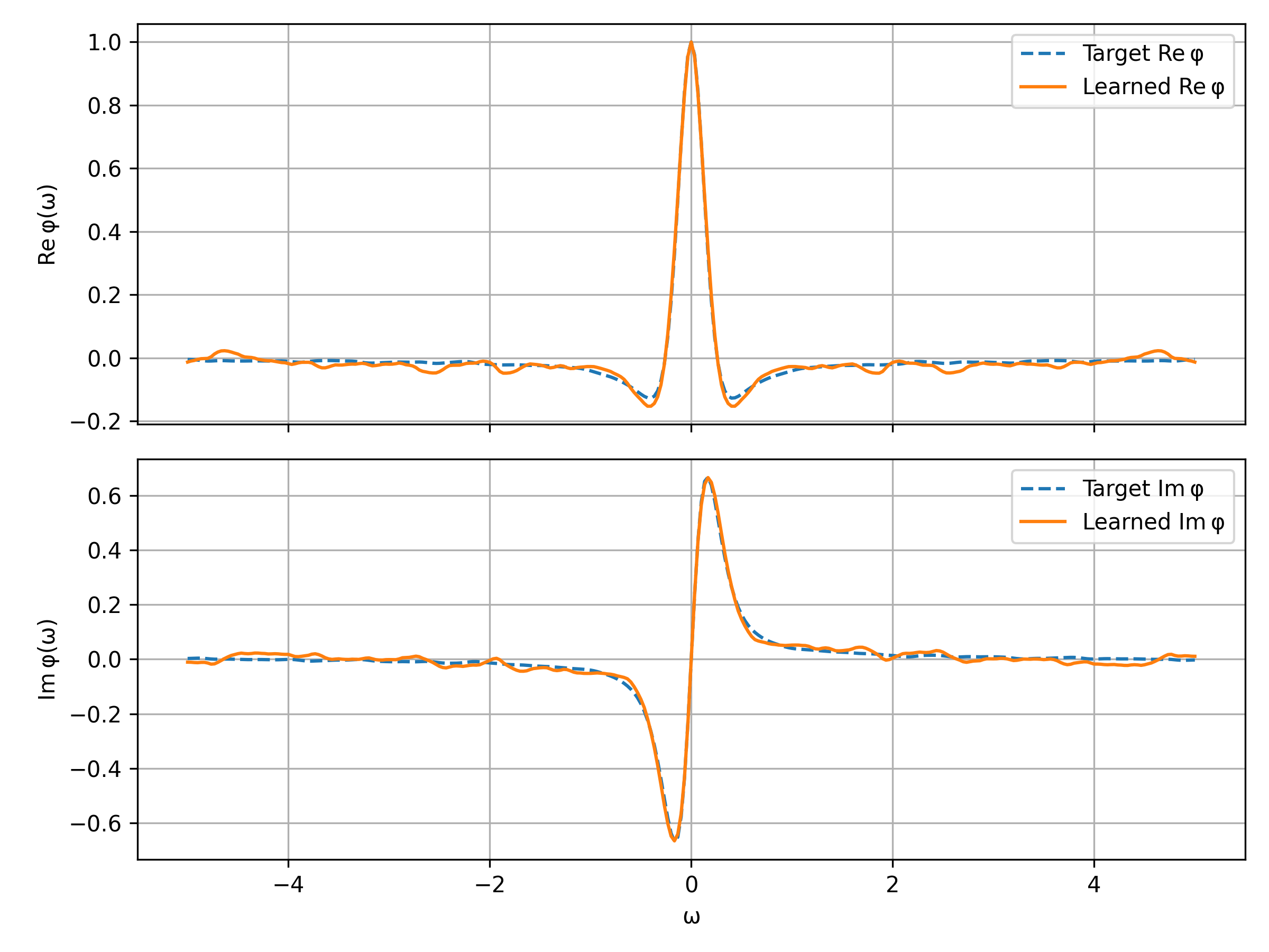
The policy gradient algorithm is capable of matching the distribution of cumulative results to the target. The loss is 0.000384 In Figure 1 (a) we see the discrete density of the target versus the learned distribution. In (b) we compare the real and imaginary part of the target and learned characteristic function.
As already explained there is an infinity of optimal action distribution and different runs of the algorithm result in different optimal action distributions as demonstrated by the Figure 2. In this figure we plot the action distribution from our parametrization for different state values and fixed and In most cases the action densities are peaked which means they are close to deterministic.
We emphasise that in accordance with our main Theorem 8 our policy gradient algorithm converges to a stationary point and thus it can get stuck in local minima, the results reported above concern only cases where we indeed successfully minimize the loss up to a threshold. There are cases where the algorithm doesn’t achieve the minimum loss threshold and gets stuck. We will come back to this point in future work to ”unstuck” the algorithm from local minima.
Finally, the number of trajectories , seems sufficient to eliminate the bias from the estimator and stabilize the descent, even if it converges to a local minimum.



5.2. Targeting Wealth Distributions by Investment
We consider a simple discretized Black Scholes model with length of time interval , i.e. the bond price evolution is given by for and and the stock price is given by and
for and and i.i.d. standard normal . If is the amount of money invested in the stock at time and it is decomposed as , where is the percentage of our wealth invested in the stock. Then the wealth at time is given as follows:
with
being the excess return over the bond. As in the motivating example we consider the reward to be non-stationary and set for and Thus we are interested in the distribution of the terminal wealth which is given by
| (32) |
Note that when we choose actions from a compact set (which is not really a restriction for applied problems) then Assumptions 1-5 are satisfied on the good event .
Target Distribution
For our target distribution, as in the LQ Example, we generate terminal-wealth samples from (32) under fixed, known investment policies. We distinguish the following two benchmark scenarios.
-
(1)
100% investment in the stock (). Here for all , so the entire wealth is invested in the risky asset at every time step. The wealth process follows a multiplicative recursion and can be written as
Consequently, is normally distributed and the terminal wealth follows a log-normal distribution,
-
(2)
Random investment fraction (). In this case, the investment proportions are sampled independently from the uniform distribution on and are independent of the market noise .
The induced distribution of has no closed-form expression; however, we can approximate this distribution numerically via Monte–Carlo simulation.
Remark 9.
Because the terminal wealth depends linearly on the control and multiplicatively on market noise, so randomizing the investment fraction adds negligible variance compared to market fluctuations, making a uniform policy and its mean indistinguishable at the level of the terminal distribution.
We discretize the horizon into rebalancing dates, hence =0.05. For the Black–Scholes dynamics we use initial wealth , risk-free rate , stock drift and volatility . In each epoch, we simulate a Monte–Carlo batch of independent trajectories by sampling i.i.d. standard Gaussians and iterating the recursion for wealth under the current policy.
Numerical Results and Discussion
For the first case we see in Figure 3(a) and 3(b) the histogram of the wealth distributions (target and learned) as well as the real and imaginary part of the target and learned characteristic functions. Both plots show good fits. From Figure 4 it is clear that the optimal action distribution produced by the algorithm is clearly deterministic and close to the theoretical one.
For the second case, we plot first in Figure 5(a) the comparison of the target density (blue) and the density of the terminal wealth learned by the algorithm (red). In Figure 5(b) we compare the real and imaginary part of the target and learned characteristic functions. Both plots show a good fit. The optimal action distribution shown in Figure 6 is as expected by Remark 9 close to the mean of the uniform and almost deterministic, i.e. with a very small variance. This discrepancy could be due to precision error of the calculation. We investigate further the accuracy of the approximation in the next example where we have an exact analytically traceable unique distribution for the optimal controls.
Case 1)


Case 2)


5.3. An Example with Compact Support
This example is related to the first one. Our goal is to exemplify a rather unique phenomenon. Due to the structure of the cost function we can identify a unique control distribution that stirs the discounted rewards towards the target. In contrast with Example 5.2, here the control enters inside a nonlinear function and together with the noise on the dynamics shape the reward distribution.
The policy gradient can indeed recover the unique control distribution when the length of the action interval permits unique identifiability of policies or otherwise only by enforcing the symmetry of the control distribution a posteriori.
In concrete, we consider linear dynamics with , a randomized (relaxed) control and additive Gaussian noise:
| (33) |
where is known and is a control random variable, independent of . Define the bounded performance variables and
| (34) |
thus, we are interested in the law of Obviously we can restrict to a compact set and our Assumption 1-5 are satisfied.
Target Distribution
Our target distribution is the Epanechnikov law on with density
| (35) |
its characteristic function admits the closed form
| (36) |
We seek a distribution of the randomized control such that the distribution of matches the Epanechnikov law. We assume takes values in a compact interval of length , so that its law is uniquely determined by its Fourier coefficients on . This ensures that the Fourier coefficients with fully characterize the distribution of and its characteristic function by
| (37) |
Exact matching condition
With the help of the Jacobi–Anger identity we can compute the characteristic function of as follows:
where is the -th Bessel function of the first kind. Thus the matching equation for the characteristic functions is
| (38) |
Truncation and linear system
Since and decay rapidly, we truncate to and select a finite frequency grid . The truncated system is
| (39) |
Note that the symmetry and makes the imaginary parts cancel. Solving for yields a least-squares (or exact solution). In addition both left and right-hand side are even, forcing for all odd . Then we reconstruct
| (40) |
The density on (of width ) follows by Fourier inversion:
| (41) |
Finally, we notice that is -periodic since all odd Fourier modes are zero.
Numerical Results and Discussion
First for the numerical solution of (39) we fix and in particular (for increased accuracy in our policy gradient since we used the same grid), and thus implement a least square solution. If we write the right-hand side of (39) in matrix form we need the corresponding matrix to have full rank - a condition easily verifiable in our case - in order to have a unique solution. For the MC samples we used trajectories per iteration.
We run two sets of experiments one on the interval to have uniquely identifiable actions and one on the interval to try and identify uniquely the optimal policy enforcing the symmetry of the distribution.
Case


First note that the density of learned distribution is rather close to the target distribution, cf. Figure 7(a). In Figure 7(b) we compare the real and imaginary part of the learned and target characteristic function. Since we restrict to , the imaginary part is not zero in the learned case, as it is in the target case. However, here the policy gradient algorithm can indeed find the unique action distribution. An attentive reader could notice that in Figure 8(b) the odd modes are not zero as they should be. This is due to the fact that we have a -periodic density and we have samples only on the one side of the density. To reveal the true symmetric density we need to have a look at the interval as we do in the next experiment.
So when only one period is used the symmetry cannot be obtain in terms of Fourier modes but the Wasserstein distance is effectively minimal .
Case
Here the Solver solution for (39) gives two periods of the -periodic density. The Policy gradient is not capable to identify correctly the complete periodic density since for the reward there is no way to differentiate between periodic actions and stays concentrated on the one of the two branches of the density (since the algorithm is stochastic the outcome may vary from run to run, meaning that sometimes the left lobe is selected and other times the right, cf. Figures 9(a) and 9(b) for the densities and characteristic functions of the rewards and Figures 10(a) and 10(b) for the action densities and Fourier modes of the action distribution.


Nevertheless, if we split equally and project the samples to the opposite interval after training we can recover the correct periodic density from the inflated one of Figure 8(a), see Figures 11(a) and 11(b).


Remark 10 (about the fit of the action distributions).
To test the best possible fit for the action distribution we augment the loss function with an additional matching objective for the Fourier modes that come from the numerical solution of (39). As one can see in Figure 12 the periodic densities are very close and thus the expressivity of the ANN enough. We don’t attempt here an exhaustive optimization of the architectures and the hyper-parameters since the goal is a proof of concept.

5.4. Writing a Classical MDP as a Special Case Distributional MDP
We give another example, the standard FrozenLake MDP from Towers et al. (2025), a pleasant variant of (SuttonBarto, Example 3.5). The episodic return of the MDP satisfies
Let
denote the success probability under policy . Then
Choose the target distribution as the ideal success law, If we consider the squared distance between characteristic functions,
where is a nonnegative weight function. A direct computation yields
with independent of
Thus, minimizing the characteristic function loss is equivalent to
Of course, this theoretical framework has to be adapted in practice to design practical algorithms since matching a Dirac is a difficult problem and also the issue of exploration has to be addressed.
Acknowledgment:
This work is supported by the Helmholtz Association Initiative and Networking Fund on the HAICORE@KIT partition. Apart from this, the authors received no financial support for the research, authorship, and/or publication of this article and have no competing interests to decalre.
6. Appendix
In what follows we use as norm the -norm i.e. for we have The norm is denoted by . Note that we always have
6.1. The Gaussian Concentration Inequality for Lipschitz Functions
The next result follows from the Gaussian Isoperimetric Inequality and will be used to control the fluctuations of our network’s output, for details see Ledoux (1994).
Lemma 11 (Gaussian Concentration for Lipschitz Functions).
Let be a Gaussian random vector with standard deviation in each direction. Suppose is a Lipschitz continuous function with constant . Then for any , the deviation of from its mean is exponentially small
In particular, with probability at least , one has
6.2. Bounds
In what follows we need bounds on several quantities. We consider everything on From (12) we obviously have constants and such that for all
| (42) |
We set Since is bounded we can define
| (43) |
Now we can prove by induction:
Lemma 12.
There exist constants such that
| (44) |
and we define
Proof.
The proof is by induction over . For the statement is obvious. Suppose the bounds are correct up to time We obtain by the continuity of
| (45) |
Further we have by continuity of
| (46) |
which proves the statement. ∎
In particular with Assumption 1 and on we can define
and The proof of the next lemma follows directly from our assumptions.
Last but not least we need bounds on
Lemma 14.
Under Assumption 5 we obtain constants such that on for all :
| (49) |
Proof.
We have that
| (50) | |||||
| (51) | |||||
| (52) |
From this it follows inductively that and the constants satisfy the following recursion:
As before we define ∎
6.3. Lipschitz properties
The proof of the following result is obvious, see e.g. Hinderer (2005), Lemma 2.1.
Lemma 15.
Let and be metric spaces.
-
a)
If are Lipschitz continuous with constant and respectively, then is Lipschitz continuous with constant .
-
b)
If are Lipschitz continuous with constant and respectively and and on respectively, then is Lipschitz continuous with constant
-
c)
Let . If is Lipschitz continuous separately in the components, i.e.
for suitable then for we have with
-
d)
If and are Lipschitz continuous with constant and respectively, then is again Lipschitz continuous with constant .
Next we investigate the Lipschitz properties of our neural net.
Lemma 16.
Let be the neural network defined in (9), i.e.
for and On we obtain
-
a)
is jointly Lipschitz-continuous in i.e.
with constant
-
b)
is jointly Lipschitz-continuous in i.e.
with constant
Proof.
a) According to Lemma 15 it is enough to show Lipschitz continuity separately in the components. We obtain
On the other hand we have
This implies part a).
b) The gradient involves products of parameters of the neural net and . More precisely we obtain:
and
In particular if are Lipschitz-continuous with constants and , then is Lipschitz-continuous with constant The Lipschitz constants can be obtained similar to part a). ∎
Lemma 17.
Proof.
We have
In what follows denote
We prove now that there exists constants such that for
| (53) |
which implies the statement. We do this by induction on . For we have with Lemma 16 that
Now suppose the statement is true up to time . From the state dynamics, the parametrization of the action and the definition of we obtain
-
(1)
-
(2)
.
-
(3)
These relations obviously imply that the statement in (53) is also true for time point . It is also possible to derive the following recursive equations for the Lipschitz constants for :
The recursion may be simplified when we use larger constants. ∎
Lemma 18.
Proof.
We have
| (54) |
In view of Lemma 15 we have to show that are all locally Lipschitz. The Lipschitz properties of follow from Assumption 5. The Lipschitz properties of follow from the previous proof. It remains to show the Lipschitz property of In what follows denote
We prove now that there exists constants such that for
| (55) |
As in the previous proof we proceed by induction. For we have with Lemma 16 that
Now suppose the statement is true up to time . Before we proceed with the induction step let us recall that and and Recall the bounds that we introduced on in subsection 6.2.
From the equation for in (54) we obtain:
It remains to discuss In order to do this we need a further look at compare (9):
Using these formulas we obtain for the first expression (the second expression is similar):
For the first expression we obtain:
For the second expression we obtain:
In total this yields
The Lipschitz constants for is the same. Thus, we obtain from (57) that
Finally, the induction step is complete and the statement follows. ∎
Proof.
of Theorem 6: First note that we can write the gradient more explicitly as
Now from Lemma 17 it follows that
are both Lipschitz-continuous with constant Lemma 17 together with Lemma 18 imply that
are both Lipschitz-continuous with constant Using the rules for the Lipschitz constants from Lemma 15 we obtain the following Lipschitz constant for using the -norm:
Noting that for we have we obtain the result with . ∎
Proof.
of Lemma 7: We fix an iteration index and work throughout conditionally on the –algebra . Under this conditioning, the parameter is deterministic, and all bounds derived on the good event hold pathwise. In particular, by Lemma 14
Let be i.i.d. copies of under the current parameter . Thus, these Monte Carlo samples are conditionally i.i.d. given . All expectations below are therefore taken with respect to these samples only, while is treated as fixed.
Step 1: Bias.
Fix a frequency node and, to simplify notation, suppress the index throughout this step. Recall that for this node the empirical characteristic function is given by
For each sample index , define the pathwise gradient contribution
With this notation, the contribution of the frequency node to the full estimator can be written as
We emphasize that the same Monte Carlo batch is used both to construct the empirical characteristic function and to evaluate the gradient terms . This coupling is the source of the finite-sample bias analyzed below. Taking conditional expectation and using linearity of ,
Because the samples are i.i.d., it suffices to compute :
Now , and we denote . Thus and we obtain
Plugging back yields
To bound the bias, use and , and , obtaining (19).
Step 2: Second moment. For each define
We have and . Hence, for all we obtain on
| (58) |
Next, by the triangle inequality,
Thus, we obatin
Therefore, on ,
| (59) |
Taking conditional expectations preserves the inequality, so we obtain the statement. ∎
References
- One-step distributional reinforcement learning. External Links: 2304.14421, Link Cited by: §1.4.
- Tractable representations for convergent approximation of distributional HJB equations. External Links: 2503.05563, Link Cited by: §1.4.
- Robust time series generation via Schrödinger bridge: a comprehensive evaluation. In Proceedings of the 6th ACM International Conference on AI in Finance (ICAIF ’25), New York, NY, USA, pp. 1–9. External Links: Document, ISBN 979-8-4007-2220-2 Cited by: §1.4.
- Coherent measures of risk. Mathematical Finance 9 (3), pp. 203–228. External Links: Document, Link, https://onlinelibrary.wiley.com/doi/pdf/10.1111/1467-9965.00068 Cited by: §1.
- Learning theory from first principles. Adaptive Computation and Machine Learning, The MIT Press, Cambridge, MA, USA. External Links: ISBN 9780262049443 Cited by: §4.
- A consistent test for multivariate normality based on the empirical characteristic function. Metrika 35 (1), pp. 339–348. Cited by: §2.1, Remark 4.
- Distributionally robust Markov Decision Processes and their connection to risk measures. Mathematics of Operations Research 47 (3), pp. 1757–1780. External Links: Document, Link, https://doi.org/10.1287/moor.2021.1187 Cited by: §1.
- Yet another Distributional Bellman equation. External Links: 2505.21098, Link Cited by: §1.2, §1.4, §2.1, §2.2, §2.2, §4.
- Markov Decision Processes with risk-sensitive criteria: an overview. Mathematical Methods of Operations Research 99 (1), pp. 141–178. External Links: Document, ISBN 1432-5217, Link Cited by: §1.
- Markov Decision Processes with applications to finance. Universitext, Springer, Heidelberg. External Links: Document, ISBN 978-3-642-18323-2, Link, MathReview (Ł. Stettner) Cited by: §1, §2.4.2, Remark 3.
- A distributional perspective on reinforcement learning. In Proceedings of the 34th International Conference on Machine Learning, Proceedings of Machine Learning Research, Vol. 70, pp. 449–458. Cited by: §1.4, §1.4.
- Distributional reinforcement learning. Adaptive Computation and Machine Learning, The MIT Press, Cambridge, Massachusetts. External Links: ISBN 9780262374026 Cited by: §4.
- Distributional reinforcement learning with linear function approximation. In Proceedings of the 23rd International Conference on Artificial Intelligence and Statistics (AISTATS), External Links: 1902.02973 Cited by: §1.4.
- Stochastic optimal control: the discrete-time case. Athena Scientific. External Links: ISBN 1886529035 Cited by: §1.
- Stochastic approximation and reinforcement learning: the interface and a little beyond. Statistical Science 40 (4), pp. 656–670. External Links: Document Cited by: §4.
- Reinforcement learning with dynamic convex risk measures. Mathematical Finance 34 (2), pp. 557–587. External Links: Document, Link, https://onlinelibrary.wiley.com/doi/pdf/10.1111/mafi.12388 Cited by: §1.
- Robust reinforcement learning with dynamic distortion risk measures. External Links: 2409.10096, Link Cited by: §1.
- Some optimisation problems in insurance with a terminal distribution constraint. Scandinavian Actuarial Journal 2023 (7), pp. 655–678. External Links: Document Cited by: §1.
- MODEL uncertainty and its impact on the pricing of derivative instruments. Mathematical Finance 16 (3), pp. 519–547. External Links: Document, Link, https://onlinelibrary.wiley.com/doi/pdf/10.1111/j.1467-9965.2006.00281.x Cited by: §1.
- Distributional reinforcement learning with quantile regression. In Proceedings of the AAAI Conference on Artificial Intelligence, Vol. 32. Cited by: §1.4.
- A test for normality based on the empirical characteristic function. Biometrika 70 (3), pp. 723–726. Cited by: §2.1, Remark 4.
- Stochastic policy gradient methods: improved sample complexity for fisher-non-degenerate policies. External Links: 2302.01734, Link Cited by: §2.3.
- Generative adversarial nets. In Advances in Neural Information Processing Systems, Vol. 27. Cited by: §2.3.
- An actor–critic algorithm with function approximation for risk sensitive cost Markov Decision Processes. IEEE Transactions on Automatic Control 71 (1), pp. 474–481. External Links: ISSN 2334-3303, Link, Document Cited by: §1.
- Deep learning approximation for stochastic control problems. External Links: 1611.07422, Link Cited by: §2.3.
- Lipschitz continuity of value functions in Markovian Decision Processes. Mathematical Methods of Operations Research 62 (1), pp. 3–22. Cited by: §6.3.
- Deep neural networks algorithms for stochastic control problems on finite horizon: convergence analysis. SIAM Journal on Numerical Analysis 59 (1), pp. 525–557. Cited by: §2.3.
- Portfolio selection: a target-distribution approach. European Journal of Operational Research 310 (1), pp. 302–314. External Links: Document Cited by: §1.
- Isoperimetry and gaussian analysis. École d’Été de Probabilités de Saint-Flour, Univeristé Paul-Sabatier. Note: Lecture notes from the 1994 Saint-Flour Summer School Cited by: §6.1.
- High probability convergence of stochastic gradient methods. In Proceedings of the 40th International Conference on Machine Learning, Proceedings of Machine Learning Research, Vol. 202, pp. 21833–21863. Cited by: §4.
- Optimizing return distributions with distributional dynamic programming. arXiv preprint arXiv:2501.13028. Cited by: §1.4.
- Policy gradient in Lipschitz Markov Decision Processes. Machine Learning 100 (2), pp. 255–283. Cited by: §2.3.
- Approximate dynamic programming: solving the curses of dimensionality. 2 edition, Wiley Series in Probability and Statistics, John Wiley & Sons, Hoboken, NJ. External Links: ISBN 978-0-470-60445-8 Cited by: §1.
- Risk-sensitive reinforcement learning via policy gradient search. Foundations and Trends in Machine Learning 15 (5), pp. 536–692. External Links: Document Cited by: §1.
- Markov Decision Processes: discrete stochastic dynamic programming. Wiley Series in Probability and Statistics, John Wiley & Sons, New York. External Links: Document, ISBN 978-0-471-61977-2, 978-0-470-31688-7 Cited by: §1.
- Fourier analysis on groups. Interscience Tracts in Pure and Applied Mathematics, Vol. 12, Interscience Publishers, New York. Cited by: §1.1.
- Dynamic programming in probability spaces via optimal transport. SIAM Journal on Control and Optimization 62 (2), pp. 1183–1206. External Links: Document Cited by: §1.4.
- Gymnasium: a standard interface for reinforcement learning environments. External Links: 2407.17032, Link Cited by: §5.4.
- Distributional Hamilton–Jacobi–Bellman equations for continuous-time reinforcement learning. In International Conference on Machine Learning, External Links: 2206.04315 Cited by: §1.4, §1.4.
