On Stein’s Method of Moments and Generalized Score Matching

The Method of Moments, Quandt and Ramsey (1978), is a strategy for the estimation of a parameter $\theta\in\mathbb{R}^{p}$ from the family of density functions $f(x\mid\theta)$ by solving $n^{-1}\sum_{i=1}^{n}x_{i}^{k}-g_{k}(\theta)=0$, for some integers $k$, where $g_{k}(\theta)=\int x^{k}\,f(x\mid\theta)\,dx$, and $x_{1:n}$ are a sample from the true density function with parameter value $\theta^{*}$. More generally, one uses a function $\lambda(x,\theta)$ satisfying $\int\lambda(x,\theta)\,f(x\mid\theta)\,dx=0,$ for all $\theta$. Here $\lambda$ can be a vector ($p$-dimensional) of functions.

A particular class of moment function is provided by Stein’s method of moments, see Stein (1972) and, for example, Ebner et al. (2024). This class uses

for to be chosen functions $\tau_{\theta}(x)$ and $w(x)$. Here and throughout ^′ represents differentiation with respect to $x$. There is no clear guidance on the choice of these functions, though a recommendation (Ebner et al. (2024)) is that $\tau_{\theta}(x)$ is taken to be a Stein kernel of the form

If $\theta$ is $p$-dimensional the usual procedure is to obtain $p$ equations by using $p$ functions $\underline{w}=(w_{j})_{j=1:p}$ so that (1) is represented by $p$ equations. The $\tau_{\theta}$ is taken to be a one-dimensional function.

More generally, where any single choice of $\underline{w}$ could be seen as lacking motivation, one could select a number of different $\underline{w}$ functions and to somehow combine outputs from each into a single estimator. This is the idea behind generalized method of moments (GMM), see Hansen (1982). Here we detail how to obtain the GMM estimator, see for example, Andrews (1999). In general, suppose we use functions $\lambda=(\lambda_{j})_{j=1:M}$. From each function we obtain the usual estimator $\widehat{\theta}_{j}$ by setting $\sum_{i=1}^{n}\lambda_{j}(x_{i},\theta)=0.$ To obtain a weight matrix, we construct the matrix $W$ with $(j,k)$ entry the sample covariance between $n$-vectors $z_{j}$ and $z_{k}$, where $z_{j}=(\lambda_{j}(x_{i}),\theta)_{i=1:n}$. The GMM estimator is obtained by minimizing $G(\theta)=z(\theta)^{\prime}\,W^{-1}\,z(\theta)$ where $z(\theta)=(z_{1}(\theta),\ldots,z_{M}(\theta))$ and $z_{j}(\theta)=\sum_{i=1}^{n}\lambda_{j}(x_{i},\theta).$ Properties of the estimator and related information can be found in Hall (2005).

A different approach to estimation is a generalized score matching estimator, see Yu et al. (2019), Scealy and Wood (2023), and Xu et al. (2025), which minimizes the empirical estimation of the weighted Fisher information distance given by

where $f$ and $s$ denote the true density and score functions, respectively and $s_{\theta}$ is the usual score function $(\partial/\partial x)\log f(x\mid\theta)$. Taking $w\equiv 1$ yields the score matching, or Hyvarinen estimator, see Hyvarinen (2005). Here the choice of the weight function $w$ is also problematic.

Our contribution is as follows and for convenience and clarity we list this as a sequence with the aim being to motivate a particular choice of $\tau_{\theta}$ and $w$ from (1):

1. Using the Stein class (1) we obtain the necessary $p$ equations by taking $w$ to be a one dimensional function and take $\tau_{\theta}(x)$ to be $\tau_{\theta}(x)=\nabla s_{\theta}(x)=(\partial/\partial\theta)s_{\theta}(x)$ and so is a $p$-vector of functions.

2. We show that with this choice of $\tau_{\theta}$ the Stein method of moment estimator coincides with the generalized score matching estimator with weight function $w$.

3. We show that the generalized score matching estimator is equivalent to a score matching estimator using the transformation of the data $Y=g(X)$ with $w(x)=(h^{\prime}(g(x)))^{2}$ where $h=g^{-1}$.

4. We argue that the optimal transformation is to produce the $Y$ sample as close to normal as possible. This can be achieved using the Box-Cox class, Box and Cox (1964), for example. The heuristic for now is that the score matching estimator, which comes from a normal sample and model, is precisely the MLE.

Note that recently, Barp et al. (2019), has shown that a score matching estimator is a special case of a Stein discrepancy estimator, see also Oates (2022). Note that Stein discrepancy estimators are not the same as Stein method of moment estimators. The former uses a discrepancy between distributions while the latter solves moment equations.

In Section 2 we describe the score matching and the generalized score matching estimation approaches and show they are connected by a transformation of the data. In Section 3 we elaborate on the connection between Stein’s method of moment estimator and the generalized score matching approach. We also provide motivation for the Stein class method of moment approach using the $w$ function to follow from a transformation of the data to a normal looking sample, using, for example, the Box-Cox family of transformations. Section 4 looks at the general set up and equations for the implementation of the GMM, our aim is to compare the GMM approach with the “optimal" approach of using the $w$ function based on a normal transformation. Section 5 presents a simuation study.

Models for which a maximum likelihood estimator (MLE) is difficult to obtain, due to an intractable normalizing constant, can be estimated using an alternative strategy based on score functions. The MLE is based on minimizing a Kullback-Leibler divergence between the family of density functions $f(x\mid\theta)$ indexed by the parameter $\theta\in\Theta$ and the true density function. With the true density being unknown, a sample Kullback-Leibler divergence estimator using the empirical measure is used instead, and this leads to the MLE. Other distances can be used provided it is possible to substitute the empirical for the true density and obtain a Monte Carlo approximation to the distance or divergence.

For ease of notation, we write $f(x\mid\theta^{*})$, the true density function with true parameter $\theta^{*}$, as $f(x)$, and $s_{\theta^{*}}(x)$ as $s(x)$. The Fisher Information distance, see, for example, Atkinson (1981), given by

allows for parameter estimation via a Monte Carlo approximation to the distance. Since it only depends on score functions, any intractable normalizing constant conveniently disappears.

The idea is to find the $\theta$ minimizing

and this distance will be approximated using the sample $x_{1:n}$. To this end, write $D(\theta)$ in the form in which it only depends on the $\theta$, i.e.

While the first term is set up for a Monte Carlo estimator, the second is not, and an integration by parts is required. For this to work, $f(x)\,s_{\theta}(x)$ needs to vanish at the boundary points for all $\theta$. Assuming this to be true, then, $D(\theta)=\int f(x)\,s^{2}_{\theta}(x)\,dx+2\int f(x)\,s^{{}^{\prime}}_{\theta}(x)\,dx,$ which is approximated from the sample as

The score estimator minimizes $\widehat{D}(\theta)$ and this approach to parameter estimation was proposed by Hyvarinen (2005).

More recently, motivated by constrained space estimation problems, weight functions have been introduced, with (3) being generalized to

See, for example, Yu et al. (2019), Scealy and Wood (2023) and Xu et al. (2025).

Here we show that (5) can be shown to arise from (3) by a transformation. If $s_{X}(x)$ is the score function for variable $X$ and we transform $Y=g(X)$, then straightforward calculations give $S_{Y}(y)=S_{X}(h(y))\,h^{\prime}(y)+(\,\,\log|h^{\prime}(y)|)^{\prime},$ where $h\equiv g^{-1}$. Hence, (3) becomes (5) with $w(x)=(h^{\prime}(g(x)))^{2}$. Note that this is invariant to linear transforms, i.e. if $\widetilde{g}=\alpha\,g+\beta$ then it is easy to show that $\widetilde{w}=w$.

By applying a similar argument for the boundary conditions, the minimizer of (5) is estimated by minimizing

Within this framework, the choice of function $w(x)$ is problematic. On the other hand, we can link up the generalized score matching approach to a method of moment estimator and then use GMM to determine optimal weights based on a set of functions.

In this section we provide a new perspective on the score matching approach and its connection with method of moments estimation; i.e. (1), for some differentiable function $g_{\theta}$. It turns out (see Lemma 3.2) that the condition for minimizing the Fisher distance (3) and its weighted version (5) can be expressed in terms of such functions.

We select the value of $\lambda$ by computing the Andersen-Darling statistic for each possible value of $\lambda$ and selecting the value which minimizes the statistics. See Anderson and Darling (1952). For the details, for each $\lambda$ we transform $Z_{i}=(x_{i}^{\lambda}-1)/\lambda$ for $i=1,\ldots,n$, and then standardize the data to $Z_{i}\to(Z_{i}-\bar{Z})/S_{Z}$, where $S_{Z}$ is the sample standard deviation, and then compute

where $(Z_{(i)})$ are the ordered values. We choose the $\lambda$ minimizing $A(\lambda)$.

To elaborate on the point of minimizing variance and the connection with a normal sample, suppose $f(x\mid\theta)$ is a member of the one parameter exponential family. Then following the transformation we would have $s_{\theta}(y)=\theta\,v(y)+a(y)$ for functions $v$ and $a$, and for which we get to choose $v$. To minimize the variance associated with minimizing (7) we would like the function $v$ to not change much as the $(y_{i})$ change; i.e. we want $v$ to be a constant, which would be a normal model. So we want to transform to a normal data.

We have shown how to derive an estimator based on the Stein class by choices of $w$ and $\tau_{\theta}$. An alternative way of dealing with the $w$ would be to use a GMM estimator based on multiple choices of $w$. Therefore, here we describe how GMM works for the Stein class with $\tau_{\theta}=\nabla s_{\theta}$. While we focus on exponential family, provided the score function is available, the following will all be able to be implemented though perhaps may depend on numerical methods. A member of the exponential family is defined by $f_{\theta}(x)\propto\exp\{\theta^{\top}\tilde{v}(x)+\tilde{c}(x)\}$ and therefore $s_{\theta}(x)=\partial\log f_{\theta}(x)/\partial x=\theta^{\top}v(x)+c(x)=(\theta^{\top},1)s(x)$ with $\tilde{v}^{\prime}(x)=v(x)$, $\tilde{c}^{\prime}(x)=c(x)$ and $s(x)^{\top}=(v(x)^{\top},c(x))$. Hence $\mbox{dim}(\theta)=\mbox{dim}(v(x))$ as well as that of $g_{\theta}(x)=w(x)\partial s_{\theta}(x)/\partial\theta=w(x)v(x)$, and so we obtain a vector function $\lambda$ as in (1):

where $A(x)=(w(x)v(x))^{\prime}+w(x)c(x)v(x)$ and $B(x)=-w(x)v(x)v(x)^{\top},$ with the multiplication performed component-wise since all but the vector $v(x)$ are scalar functions. Since $E(\lambda(\theta,X))=0$ we see that $E\{A(X)\}-E\{B(X)\}\theta=0$. If we are to consider $m$ weight functions, we have $m$ equations of the form $A_{k}-B_{k}\theta=0,\quad k=1,2,\dots,m,$ where $A_{k}=E\{(vw_{k})^{\prime}+w_{k}cv\}$ and $B_{k}=E\{v^{\top}vw_{k}\}$ with Monte Carlo estimators

Hence, we can use the GMM method (Andrews (1999)) to estimate $\theta$ by minimizing

for some weight matrix $W\in\mathbb{R}^{pm\times pm}$ with blocks $W_{jk}$ and $\mathcal{B}^{\top}=\begin{bmatrix}\bar{B}_{1},\ldots,\bar{B}_{m}\end{bmatrix}\in\mathbb{R}^{p\times mp},\quad a=\operatorname{vec}(\bar{A})\in\mathbb{R}^{pm}.$ Here $W$ is assumed known or estimated from the data. If $W$ is known, then we can obtain the minimizer of the quadratic function at

for invertible $\mathcal{B}^{T}W\mathcal{B}$. Otherwise we can use the pseudo-inverse or include a small regularizer, for some $\widehat{\theta}=(\mathcal{B}^{T}W\mathcal{B}+\lambda I)^{-1}\mathcal{B}^{T}Wa,\quad\lambda>0.$ Such a solution always exists as $\mathcal{B}^{T}W\mathcal{B}$ is always positive semi-definite if the weights functions are linearly independent and $W$ is positive definite the solution is unique.

In the GMM literature, the optimal choice of $W$ is given by the inverse of the covariance matrix of the moments, i.e. $W^{*}=\left(\operatorname{Cov}(\mathcal{B}\theta-a)\right)^{-1}.$ In other words, the optimal weight matrix is the optimal linear combination of all these consistent estimators such that minimal variance $F(\theta)$ is achieved, namely, the chosen $W$ gives more importance to those moments with smaller variance.

As this covariance matrix is unknown and needs to be estimated from the data as well, a valid choice of such an estimator is obtained adopting a two step GMM method to estimate $\theta$, where in the first step we use $W=I_{m}$ and in the second step we use the estimated covariance matrix of the moments to estimate $W$. We will not concern ourselves with these details as we only want to illustrate that it is possible to utilize the GMM framework for the case of many weighted score estimators. Since for the exponential family case the weighted score estimator can be expressed as a moment equation for each $j=1,\dots,m$, we can use many such equations with different weight functions to construct a GMM estimator that combines all these equations to produce an overall estimate of $\theta$.

In particular, we can use the sample covariance matrix of the moments to estimate $W$ in a two step procedure: Start with an initial choice of $W$ say identity, then estimate $\theta^{(1)}=(\bar{\mathcal{B}}^{T}W\bar{\mathcal{B}})^{-1}\bar{\mathcal{B}}^{T}W\bar{a}$ by using the Monte Carlo counterparts for $\bar{\mathcal{B}}$ and $\bar{a}$. After obtaining $\theta^{(1)}$, we can estimate $\widehat{W}=\left((\mathcal{B}\theta^{(1)}-a)(\mathcal{B}\theta^{(1)}-a)^{\top}\right)^{-1}.$ Then use this $\widehat{W}$ to derive the optimal $\theta^{(2)}$ as $\theta^{(2)}=(\bar{\mathcal{B}}^{\top}\widehat{W}\bar{\mathcal{B}})^{-1}\bar{\mathcal{B}}^{\top}\widehat{W}\bar{a}.$ This is referred to in the literature as the two step GMM estimator. As $n\to\infty$, $\theta^{(2)}$ converges to the optimal GMM estimator. Iterative convergence procedures can also be used to refine the estimate of $\theta$ further, but in practice as well as in our example, the two step GMM estimator is often sufficient. As constructed above, this estimator can be seen as a weighted average of many score functions for various weights. In fact, this GMM estimator can be computed in closed form by solving a linear system, which is also computationally efficient. In a simulation study, one can compare the performance of this GMM estimator with that of a list single weights function score estimator to see if there is any improvement in terms of bias, variance, or mean squared error.

In this section we compare the GMM approach with the optimal choice of weight function from Box-Cox and Andersen-Darling. We demonstrate with the gamma distribution, which is a member of the two parameter exponential family. We chose this distribution because the boundary conditions are satisfied for a variety of weight functions and the score function is straightforward to compute.

For the gamma density $f_{\theta}(x)=\beta^{\alpha}\,x^{\alpha-1}e^{-\beta x}/\Gamma(\alpha)$, with $\theta=(\alpha-1,\beta)$, we have $s_{\theta}(x)=\theta_{1}/x-\theta_{2}$ with $v(x)=(1/x,-1)^{\top}$ and $c(x)=0$. The corresponding $A(x)$ and $B(x)$ functions are

The Monte Carlo estimates for the entries of $A(x)$ and $B(x)$ are:

leading to

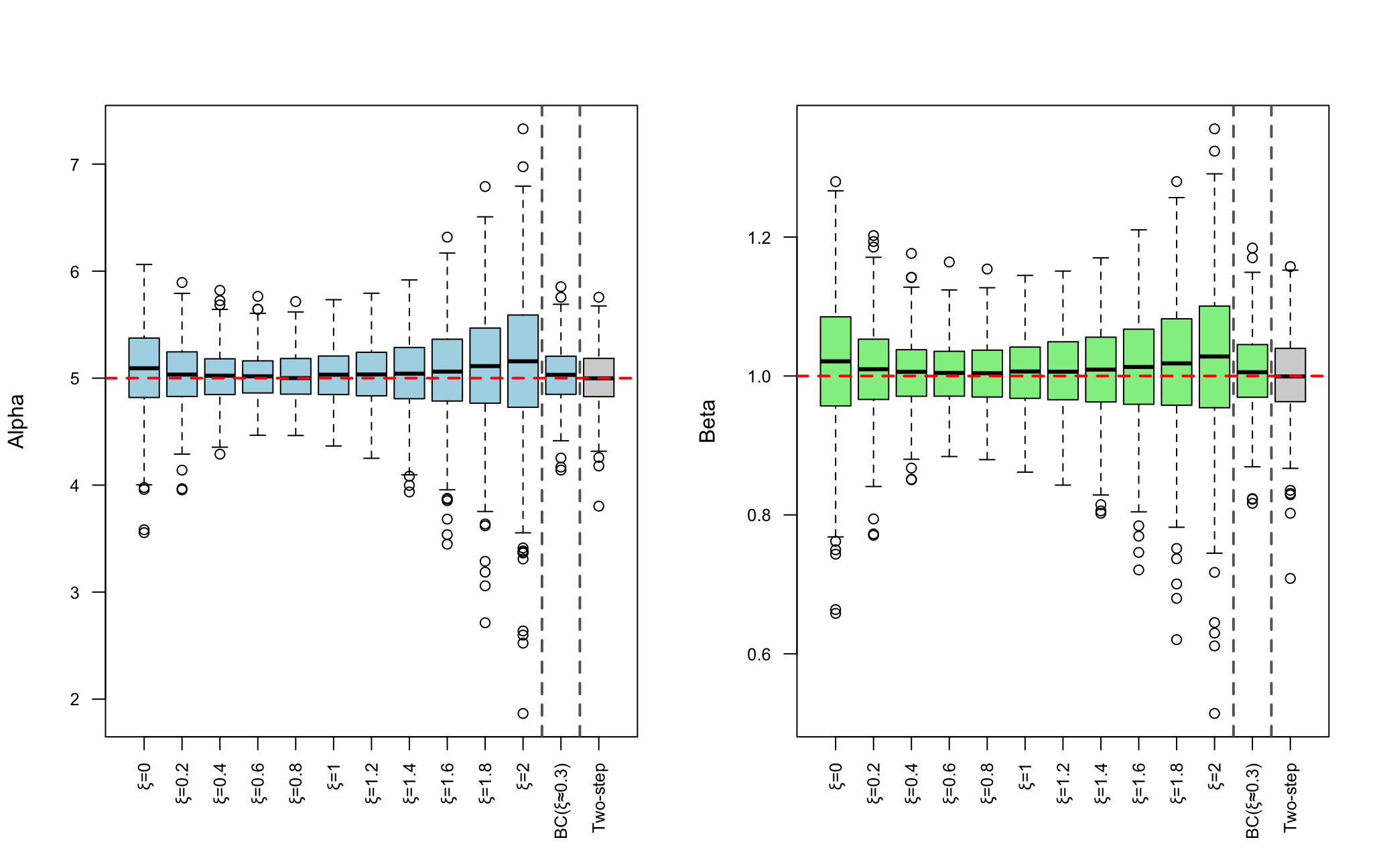
Fig. 1 shows the results from our simulation study comparing different GMM estimation methods with the original “good" weight functions and also with the Box-Cox motivated choice of optimal weight function. The weight functions chosen are $w_{j}(x)=x^{\xi_{j}}$ for $\xi=0,0.3,0.4,0.5,0.8,1.0,1.2,1.5,1.8,2.0$. Recall the weight function from the Box-Cox procedure would be of the form $w(x)=x^{2(1-\lambda)}$.

In particular, we run 1000 simulations for sample size of $n=500$ from a gamma(5,1) distribution. The case of $\xi=0$ corresponds to the standard score matching estimator without weighting. Each boxplot represents the distribution of parameter estimators ($\alpha$ and $\beta$) across the 1000 simulations for each $\xi$ value, as well as for the two-step GMM estimator that combines all $\xi$ values and the Box-Cox based estimator with the data driven $\lambda$s based on Box-Cox and the Andersen-Darling statistics.

As shown in Fig. 1, the Box-Cox estimator and the two-step GMM estimator (rightmost box in coral color) perform about the same. Given the simplicity of the Box-Cox procedure and the general applicability we would recommend this over GMM, particularly for non exponential family models where the GMM approach would be particularly complicated to implement.

On the other hand Fig. 2 shows the same results when this time some “bad" weights are included for the GMM. In this study we extended the powers for the weight functions to include powers between 2 and 3. Despite this apparently harmless extension it is seen that the GMM estimator is very sensitive to the choice of weights; the GMM estimator performing quite poorly. While we label the Fig. 2 as “bad" weights the point is that this could not be known upfront.

In this section we apply our method to a non exponential family model, the Weibull distribution. We compare the performance of the Box-Cox based estimator with a range of weight functions as well the maximum likelihood estimator. The score function and the corresponding weighted score matching objective function for the Weibull distribution is derived in the following. Note tha the optimal solution here needs to be obtained through numerical optimization, as the score function is now not linear in the parameters.

A random variable $X$ follows a Weibull distribution with shape $k>0$ and scale $\kappa>0$ if the probability density function is given by

and $\theta=(k,\kappa)$ is the parameter vector. The log-density is given by: $\ln f(x;\theta)=\ln k-k\ln\kappa+(k-1)\ln x-\left(x/\kappa\right)^{k}$ and the score function $s_{\theta}(x)$ is defined as the derivative with respect to $x$; i.e. $s_{\theta}(x)=\partial\ln f/\partial x=(k-1)/x-kx^{k-1}/\kappa^{k}$ and the derivative of the score function is given by $s_{\theta}^{\prime}(x)=-(k-1)/x^{2}-k(k-1)x^{k-2}/\kappa^{k}.$ To estimate $\theta=(k,\kappa)$, we minimize the weighted Fisher divergence $J_{\lambda}(\theta)$ using the weight function $w(x)=x^{2-2\lambda}$. The objective function is:

where the weight function and its derivative are $w(x)=x^{2-2\lambda}$ and $w^{\prime}(x)=(2-2\lambda)x^{1-2\lambda}$. Substituting the Weibull components into the objective function, we analyze the expression term by term.

1: $\frac{1}{2}w(x)s_{\theta}(x)^{2}$

$$\frac{1}{2}x^{2-2\lambda}\left(\frac{k-1}{x}-\frac{kx^{k-1}}{\kappa^{k}}\right)^{2}=\frac{(k-1)^{2}}{2}x^{-2\lambda}-\frac{k(k-1)}{\kappa^{k}}x^{k-2\lambda}+\frac{k^{2}}{2\kappa^{2k}}x^{2k-2\lambda}$$

2: $w(x)s_{\theta}^{\prime}(x)$

$$x^{2-2\lambda}\left(-\frac{k-1}{x^{2}}-\frac{k(k-1)x^{k-2}}{\kappa^{k}}\right)=-(k-1)x^{-2\lambda}-\frac{k(k-1)}{\kappa^{k}}x^{k-2\lambda}$$

3: $w^{\prime}(x)s_{\theta}(x)$

$$(2-2\lambda)x^{1-2\lambda}\left(\frac{k-1}{x}-\frac{kx^{k-1}}{\kappa^{k}}\right)=2(1-\lambda)(k-1)x^{-2\lambda}-\frac{2(1-\lambda)k}{\kappa^{k}}x^{k-2\lambda}$$

We apply the above method to a real dataset, the “TreesDBH" data set which comes from the R package “WeibullFit" and consists of 50,607 diameters of Brazilian eucalyptus trees measured at 4.5 feet off the ground. This is a standard way for measuring trees. We wrote our own MLE code which is the same as that from the R package “Weibullness". The analysis of estimators from various settings in presented in Fig. 3. The upper plot is concerned with the parameter $k$ and the lower plot is for $\kappa$. The red line in each case is the MLE. Each blue dot represents the estimator based on the given value of $\lambda$, i.e. taking the weight function to be $w(x)=x^{2(1-\lambda)}$. The green dot is the estimator based on the Box-Cox transformation which selects a value of $\lambda$. As can be seen, the Box-Cox based estimator is very close to the MLE. The sample size is quite large, $n=50,607$, which explains the small $y$-axes scales. Indeed, for such a large $n$, it is safe to assume that $\mbox{Var}(\widehat{\kappa})$ and $\mbox{Var}(\widehat{k})$ will be approximately normal with means the true $\kappa$ and $k$, respectively, and variance the reciprocal of $n$ times the respective Fisher information values evaluated at the MLE values. So we estimate 2 times the standard deviations of the MLEs as 0.034 and 0.030 for $\widehat{k}$ and $\widehat{\kappa}$, respectively. The Box-Cox estimator is within this interval while many of the other estimators are not.

First we look at the convergence of the Box-Cox estimated value of $\lambda$. From the observed data $X_{1:n}$ we construct

for $\lambda\in U$, and $U$ is a compact set of values, where $\bar{X}^{(}\lambda)$ and $S^{(}\lambda)$ are the sample mean and the sample variance of the $(X_{i}^{\lambda})$, respectively. Note that we would get the same values of $(Y_{i}^{(}\lambda))$ if we had used the full definition of the Box-Cox transform, i.e. $(X^{\lambda}-1)/\lambda$. The $\lambda_{n}$ minimizes $d(F_{n\lambda},\Phi)$ where

where $\phi$ and $\Phi$ are the density and distribution for the standard normal. The $F_{n\lambda}$ is the empirical distribution function of the $(Y_{i}^{(\lambda)})$ and so

Hence, $F_{n\lambda}(y)=F_{nX}\big((yS^{(}\lambda)+\bar{X}^{(}\lambda))^{1/\lambda}\big),$ where $F_{nX}$ is the empirical distribution function of the $(X_{i})$. We can use Andrews (1987) to show that