跳到论文正文
W Papers独立论文阅读器 arXiv:2602.05790 论文正文 计算阅读时间 · 0%
引用这篇论文根据当前论文元数据生成,正式投稿前建议核对。


License: CC BY 4.0
arXiv:2602.05790v2 [cs.IT] 15 Jun 2026

Price of metric universality in vector quantization is at most 0.11 bit

Alina Harbuzova Massachusetts Institute of Technology. Supported by MathWorks Fellowship and Siebel Scholarship    Or Ordentlich Hebrew University of Jerusalem. Supported by the Israel Science Foundation (ISF), grant No. 2878/25    Yury Polyanskiy Massachusetts Institute of Technology. Supported by NSF Grant No. 2112665 via subaward KR 704702 from the University of California, San Diego
Abstract

Fast computation of a matrix product W⊤​XW^{\top}X is a workhorse of modern LLMs. To make their deployment more efficient, a popular approach is that of using a low-precision approximation W^\widehat{W} in place of true WW (“weight-only quantization”). Information theory demonstrates that an optimal algorithm for reducing precision of WW depends on the (second order) statistics of XX and requires a careful alignment of vector quantization codebook with PCA directions of XX (a process known as “waterfilling allocation”). Dependence of the codebook on statistics of XX, however, is highly impractical. This paper proves that there exist a universal codebook that is simultaneously near-optimal for all possible statistics of XX, in the sense of being at least as good as an XX-adapted waterfilling codebook with rate reduced by 0.11 bit per dimension in the case when WW is Gaussian. Such universal codebook would be an ideal candidate for the low-precision storage format, a topic of active modern research, but alas the existence proof is non-constructive.

Equivalently, our result shows existence of a net in ℝn\mathbb{R}^{n} that is a nearly-optimal covering of a sphere simultaneously with respect to all Hilbert norms.

Keywords: vector quantization, oracle bounds, rate-distortion, waterfilling, regret, universality

1 Introduction

The most basic element of all modern AI is a neural unit: given a (dynamically changing) activation vector X∈ℝnX\in\mathbb{R}^{n} the unit needs to compute the output

Y=W⊤​X,Y=W^{\top}X\,,

where W∈ℝnW\in\mathbb{R}^{n} is a (static) weight. The problem, rapidly becoming central for economic deployment and continued evolution of large language models (LLMs), is to reduce storage/communication requirement by saving WW in “low-precision”. (The symmetric question of also converting XX to low-precision is outside of scope of this work, though see [16] for some recent theoretical analysis.)

Early deep learning models saved WW in full-precision (known as FP32, and corresponding to R=32R=32 bit / coordinate), but soon moved to half-precision (FP16/BF16, or R=16R=16 bit). In the domain of LLMs, pioneering work [9] showed that very little degradation is introduced if WW is approximated by rescaling it to appropriate range and then rounding each coordinate of normalized WW to nearest integer in {−128,−127,…,127}\{-128,-127,\ldots,127\}, a so called INT8 quantization. Subsequently, more sophisticated low-precision storage formats were introduced, with currently the most popular being NVFP4 (rate R=4.5R=4.5 bit) and MXFP4 (rate R=4.25R=4.25 bit), see [15, 18].

In this paper we are focusing on a fundamental question: what is the best way of reducing precision of WW? That is, how to replace WW by a version W^\widehat{W} that incurs minimal degradation of performance, i.e. W^⊤​X≈W⊤​X\widehat{W}^{\top}X\approx W^{\top}X, while admitting a short bit-length description. A natural way to do that, known as vector quantization, would be to pre-define a codebook 𝐂⊂ℝn\mathbf{C}\subset\mathbb{R}^{n} of size |𝐂|=2n​R|\mathbf{C}|=2^{nR}. Clearly, any element of 𝐂\mathbf{C} can be described by n​RnR bits, hence achieving rate RR of bits / coordinate. Given 𝐂\mathbf{C} we approximate WW as

W^=arg⁡minc∈𝐂⁡d​(W,c)\widehat{W}=\operatorname*{\arg\!\min}_{c\in\mathbf{C}}d(W,c)

for some distance metric d​(⋅,⋅)d(\cdot,\cdot). When dd is a standard Euclidean metric, then the problem reduces to a classical vector quantization problem in ℝn\mathbb{R}^{n}, with many classical solutions including lattices and trellis-coded constructions [11]. However, as was brilliantly shown by [10] large savings can be made if metric d​(⋅,⋅)d(\cdot,\cdot) is chosen with the knowledge of statistics of XX in mind.

Indeed, if XX is modeled as random with second-order statistics ΣX=𝔼​[X​X⊤]\Sigma_{X}=\mathbb{E}[XX^{\top}] then

𝔼X​[(Y−Y^)2]=𝔼X​[(W⊤​X−W^⊤​X)2]=(W−W^)⊤​ΣX​(W−W^).\mathbb{E}_{X}\left[(Y-\widehat{Y})^{2}\right]=\mathbb{E}_{X}\left[(W^{\top}X-\widehat{W}^{\top}X)^{2}\right]=(W-\widehat{W})^{\top}\Sigma_{X}(W-\widehat{W})\,.

Thus, we see that a natural choice of metric (given knowledge of ΣX\Sigma_{X}) is

dΣX​(W,W^)=𝔼X​[(W⊤​X−W^⊤​X)2]=(W−W^)⊤​ΣX​(W−W^).d_{\Sigma_{X}}(W,\widehat{W})=\mathbb{E}_{X}\left[(W^{\top}X-\widehat{W}^{\top}X)^{2}\right]=(W-\widehat{W})^{\top}\Sigma_{X}(W-\widehat{W})\,. (dΣXd_{\Sigma_{X}})

The easiest way to demonstrate how adaptation to ΣX\Sigma_{X} can significantly improve rate-distortion tradeoff is to consider a rank-1 case, i.e. when XX is always collinear with a fixed vector v∈ℝnv\in\mathbb{R}^{n}. In this case, a clever choice of the codebook 𝐂\mathbf{C} is {0,±ϵ​v,±2​ϵ​v,…}\{0,\pm\epsilon v,\pm 2\epsilon v,\ldots\}, i.e. very fine quantization along a single direction vv in ℝn\mathbb{R}^{n}. Indeed, by not needing to spread the points of 𝐂\mathbf{C} among all nn dimensions, one can get exponential improvement in quality of approximation of W⊤​XW^{\top}X, since only the scalar value W⊤​vW^{\top}v affects the result. Since activations in LLMs are notoriously low-rank, this adaptation of 𝐂\mathbf{C} to directions of principal variation (PCA) of XX understandably improves performance.

Herein, however, lies the main problem that we are trying to address: while adapting 𝐂\mathbf{C} to the statistics of the input XX is desirable, it may not be generally possible due to restrictions of hardware. Indeed, the mapping from actual bits (loaded from memory) to elements of 𝐂\mathbf{C} needs to be fixed at hardware design stage and cannot depend on statistics of XX (in particular, because the same hardware is used for implementing different neurons, facing different types of XX). Below we call this requirement, alternatively, as universal codebook or a ΣX\Sigma_{X}-oblivious decoder, to reflect the fact that 𝐂\mathbf{C} has to be universal across all possible choices of ΣX\Sigma_{X}.

To continue with more quantitative investigation, let us make a modeling assumption (well justified by empirical statistics of LLM weight matrices) that W∼𝒩​(0,In)W\sim\mathcal{N}(0,I_{n}). In this case a given codebook 𝐂\mathbf{C} under ΣX\Sigma_{X} statistics attains distortion:

D​(𝐂,ΣX):=1n​𝔼W​[minc∈𝐂⁡dΣX​(W,c)].D(\mathbf{C},\Sigma_{X}):=\frac{1}{n}\mathbb{E}_{W}\left[\min_{c\in\mathbf{C}}d_{\Sigma_{X}}(W,c)\right]\,. (1)

Classical information-theoretic field, known as rate-distortion theory, establishes that for a codebook 𝐂\mathbf{C} to achieve distortion D​(𝐂,ΣX)≤DD(\mathbf{C},\Sigma_{X})\leq D one must have

log⁡|𝐂|≥n​𝐑wf​(ΣX,D),\log|\mathbf{C}|\geq n\mathbf{R}_{\mathrm{wf}}(\Sigma_{X},D)\,,

where 𝐑wf\mathbf{R}_{\mathrm{wf}} is given by a so-called waterfilling formula, see Prop. 2.1.

The main question of this work: How much does the requirement of universality cost in terms of performance? For example, in the rank-1 case above the waterfilling codebook would allocate its elements along a single direction vv. This codebook, however, would be grossly suboptimal for another rank-1 ΣX\Sigma_{X} which has its PCA direction orthogonal to vv. Somewhat surprisingly, thus, we show that nevertheless the answer is not much. The main result of this work is demonstration of existence of a universal 𝐂\mathbf{C}, which is simultaneously near optimal for all possible ΣX\Sigma_{X}. Informally, we can state our main result as follows.

Theorem 1 (Informal: Universality costs ≤0.11\leq 0.11 Bits).

Let us assume that W∼𝒩​(0,In)W\sim\mathcal{N}(0,I_{n}) and let 𝐑wf​(ΣX,D)\mathbf{R}_{\mathrm{wf}}(\Sigma_{X},D) denote the information-theoretic (waterfilling) lower bound on rate needed to achieve distortion at most DD in the oracle setting, where codebook is optimized for a fixed ΣX\Sigma_{X}. There exists a universal codebook 𝐂\mathbf{C} with 2n​R2^{nR} points such that its distortion simultaneously for all ΣX∈𝕊+n\Sigma_{X}\in\mathbb{S}_{+}^{n} satisfies:

R≤𝐑wf​(ΣX,D​(𝐂,ΣX))+0.11​bit.R\leq\mathbf{R}_{\mathrm{wf}}(\Sigma_{X},D(\mathbf{C},\Sigma_{X}))+0.11\,\mathrm{bit}\,.

The implication for hardware design is clear: it is possible to create a universal low-precision storage format (for WW) that is optimal (up to rate gap of at most 0.110.11 bit) simultaneously for all kinds of distributions of statistics of the other factor (XX) in the inner-product. Our result can also be interpreted as a statement about metric entropy: There exists a universal net on a unit sphere, which covers unit sphere near-optimally simultaneously for all possible Hilbert norms on ℝn\mathbb{R}^{n}.

Paper organization.

The following Section 2 formalizes weight-only quantization for inner products under the distortion dΣXd_{\Sigma_{X}}. We then introduce the oracle benchmark given by the Gaussian rate–distortion tradeoff under weighted MSE, attained by the waterfilling solution in the setting where both encoder and decoder know the second-order statistics ΣX\Sigma_{X} (Prop. 2.1). Our main results are stated in Theorems 2 and 3. Theorem 2 shows the existence of a universal codebook achieving the explicit rate-distortion tradeoff (RDRC) over all ΣX\Sigma_{X}. Theorem 3 upper bounds the worst-case rate overhead incurred by this universal decoder relative to the oracle waterfilling benchmark.

Section 3 provides a proof sketch of Theorem 2 and the main geometric ideas: Section 3.1 describes the universal codebook construction and intuition, and Section 3.2 outlines the random-coding analysis leading to (RDRC).

Complete proofs are given in the Appendix. While the results in Section 2 are presented for W∼𝒩​(0,In)W\sim\mathcal{N}(0,I_{n}), we first establish a general bound for a fixed (non-random) WW in Section B. This result is then specialized to W∼𝒩​(0,In)W\sim\mathcal{N}(0,I_{n}) using concentration and covering argument in Section C, completing the proof of Theorem 2. Theorem 3 is proved in Section D: we derive explicit expressions for the rate-gap and prove that the maximum gap occurs at spectra with at most 22 distinct eigenvalues and vanishing distortions.

2 Main results and discussion

Consider an arbitrary ΣX⪰0\Sigma_{X}\succeq 0 and define a (square of) Hilbert metric with respect to ΣX\Sigma_{X} as in (dΣXd_{\Sigma_{X}}). We consider the problem of obtaining a low-precision (at rate RR bits per coordinate) representation W^\hat{W} of a random vector W∈ℝnW\in\mathbb{R}^{n} with the goal of minimizing dΣX​(W^,W)d_{\Sigma_{X}}(\hat{W},W). We focus presentation of results on the the standard setting in which WW is an isotropic Gaussian vector:

W∼𝒩​(0,In),W\sim\mathcal{N}(0,I_{n})\,,

though the key technical results hold for general WW (Section B). An (n,R)(n,R) quantization scheme consists of an encoder f:ℝn→[2n​R]f:\mathbb{R}^{n}\to\left[2^{nR}\right] and decoder g:[2n​R]→ℝng:\left[2^{nR}\right]\to\mathbb{R}^{n} and we set W^=g​(f​(W))\widehat{W}=g(f(W)). The image of gg is called the codebook 𝐂:=im​g\mathbf{C}:=\mathrm{im}\,g. The optimal encoder consists of finding a nearest to WW element of 𝐂\mathbf{C}, and hence we can equivalently think of a quantization scheme as completely defined by 𝐂\mathbf{C}. The distortion of 𝐂\mathbf{C} for a given ΣX\Sigma_{X} is denoted D​(𝐂,ΣX)D(\mathbf{C},\Sigma_{X}), cf. (1).

Let us start with a simple case of ΣX\Sigma_{X} fixed (and hence known to both encoder fΣXf_{\Sigma_{X}} and decoder gΣXg_{\Sigma_{X}}). In this case, the optimal tradeoff between the distortion DD and rate RR is given by waterfilling, which we review.

Let ΣX=U​Λ​U⊤\Sigma_{X}=U\Lambda U^{\top} be the eigendecomposition with Λ=diag(λ1,…,λn)\Lambda=\mathop{\mathrm{diag}}(\lambda_{1},\dots,\lambda_{n}). Consider a parametric curve

Dwf​(ΣX,t)=1n​∑i=1nmin⁡{λi,t}Rwf​(ΣX,t)=12​n​∑i=1nmax⁡{0,log⁡(λi/t)},D_{\mathrm{wf}}(\Sigma_{X},t)=\frac{1}{n}\sum_{i=1}^{n}\min\left\{\lambda_{i},t\right\}\quad R_{\mathrm{wf}}(\Sigma_{X},t)=\frac{1}{2n}\sum_{i=1}^{n}\max\left\{0,\log(\lambda_{i}/t)\right\}\,, (WF\mathrm{WF})

where tt is the parameter (waterfilling level). The above implicitly defines waterfilling distortion as a function of rate:

𝐃wf​(R,ΣX)≜Dwf​(ΣX,twf​(R)),where ​Rwf​(ΣX,twf​(R))=R.\mathbf{D}_{\mathrm{wf}}(R,\Sigma_{X})\triangleq D_{\mathrm{wf}}(\Sigma_{X},t_{\mathrm{wf}}(R))\,,\quad\text{where }R_{\mathrm{wf}}(\Sigma_{X},t_{\mathrm{wf}}(R))=R\,. (𝐃wf\mathbf{D}_{\mathrm{wf}})

It turns out that this function indeed determines the fundamental limits in the case of oracle-knowledge of ΣX\Sigma_{X}. More exactly, we have the following.

Proposition 2.1 (Waterfilling).

Let ΣX∈𝕊+n\Sigma_{X}\in\mathbb{S}_{+}^{n} . For any compression scheme of rate RR we have

𝔼​[dΣX​(W,g​(f​(W)))]≥n​𝐃wf​(R,ΣX).\mathbb{E}\left[d_{\Sigma_{X}}(W,g(f(W)))\right]\geq n\mathbf{D}_{\mathrm{wf}}(R,\Sigma_{X})\,. (2)

Conversely, for any B>0B>0 there exist a c=c​(B)>0c=c(B)>0 such that for any ΣX\Sigma_{X} there exist ff and gg (both depending on ΣX\Sigma_{X}) such that

𝔼​[dΣX​(W,g​(f​(W)))]≤n​𝐃wf​(R−c​log⁡nn,ΣX)+c​n−B​trΣX.\mathbb{E}\left[d_{\Sigma_{X}}(W,g(f(W)))\right]\leq n\mathbf{D}_{\mathrm{wf}}\left(R-c\sqrt{\frac{\log n}{n}},\Sigma_{X}\right)+cn^{-B}\mathop{\mathrm{tr}}\Sigma_{X}\,. (3)
Proof.

We give the proof of the lower bound (2) below; since the upper bound (3) is not relevant for the rest of this paper, we defer the brief of sketch of the proof to Appendix F. Though we do emphasize that the upper bound does not follow from classical theory, which concerns with separable (additive over coordinates) distortion measures, and we have to invoke more modern single-shot bounds, cf. [21, Chapter 25].

Let ΣX=U​Λ​U⊤\Sigma_{X}=U\Lambda U^{\top} with Λ=diag(λ1,…,λn)\Lambda=\mathop{\mathrm{diag}}(\lambda_{1},\dots,\lambda_{n}), and define W′≜U⊤​WW^{\prime}\triangleq U^{\top}W, W^′≜U⊤​W^\widehat{W}^{\prime}\triangleq U^{\top}\widehat{W}. Then

dΣX​(W,W^)=(W−W^)⊤​ΣX​(W−W^)=(W′−W^′)⊤​Λ​(W′−W^′)=∑i=1nλi​(Wi′−W^i′)2.d_{\Sigma_{X}}(W,\widehat{W})=(W-\widehat{W})^{\top}\Sigma_{X}(W-\widehat{W})=(W^{\prime}-\widehat{W}^{\prime})^{\top}\Lambda(W^{\prime}-\widehat{W}^{\prime})=\sum_{i=1}^{n}\lambda_{i}(W_{i}^{\prime}-\widehat{W}_{i}^{\prime})^{2}\,.

In the oracle setting (where both the encoder and decoder know ΣX\Sigma_{X}), we may equivalently compress W′W^{\prime}, reconstruct W^′\widehat{W}^{\prime}, and output W^=U​W^′\widehat{W}=U\widehat{W}^{\prime}. After this coordinate change, the problem becomes that of a weighted mean squared error. Since W′∼𝒩​(0,In)W^{\prime}\sim\mathcal{N}(0,I_{n}) has independent coordinates, a standard data-processing argument (see [21, Section 23.4 and Theorem 6.1]) gives:

n​R≥I​(W′;W^′)≥∑i=1nI​(Wi′;W^i′),nR\geq I(W^{\prime};\widehat{W}^{\prime})\geq\sum_{i=1}^{n}I(W^{\prime}_{i};\widehat{W}_{i}^{\prime})\,,

Writing Di≜𝔼​[(Wi′−W^i′)2]D_{i}\triangleq\mathbb{E}\left[(W_{i}^{\prime}-\widehat{W}_{i}^{\prime})^{2}\right], the smallest I​(Wi′;W^i′)=12​log⁡1DiI(W^{\prime}_{i};\hat{W}_{i}^{\prime})={\frac{1}{2}}\log{\frac{1}{D_{i}}} (given the value DiD_{i}) is then attained under Gaussian coupling, cf. [21, Section 26.1.2], which results in

R≥12​n​∑i=1nlog⁡1Diand1n​𝔼​[dΣX​(W,W^)]=1n​∑i=1nλi​Di.\displaystyle R\geq{\frac{1}{2n}}\sum_{i=1}^{n}\log{\frac{1}{D_{i}}}\qquad\text{and}\qquad\frac{1}{n}\mathbb{E}\left[d_{\Sigma_{X}}(W,\widehat{W})\right]={\frac{1}{n}}\sum_{i=1}^{n}\lambda_{i}D_{i}\,.

Minimizing 1n​∑iλi​Di\frac{1}{n}\sum_{i}\lambda_{i}D_{i} subject to the rate constraint via Lagrange multipliers gives the (reverse) waterfilling optimum, summarized by the parametric curve in (WF\mathrm{WF}). ∎

Now, as we discussed above, ΣX\Sigma_{X} describes distribution of activations and, practically speaking, is usually unavailable to decoder. Indeed, even if the eigenvalues Λ\Lambda were known, optimal waterfilling requires knowledge of the eigenbasis UU, since the decoder gΣXg_{\Sigma_{X}} essentially computes U⋅U⊤​W^U\cdot\widehat{U^{\top}W}, where U⊤​W^\widehat{U^{\top}W} is the closest codeword to U⊤​WU^{\top}W. Communicating U∈𝒪​(n)U\in\mathcal{O}(n) to the decoder is expensive: it requires approximating Θ​(n2)\Theta(n^{2}) real parameters, which will consume much larger than Θ​(n)\Theta(n) bits allocated for communicating WW itself.111In practice, GPU computes not a single inner product but W⊤​XW^{\top}X for W∈ℝn×aW\in\mathbb{R}^{n\times a} being a matrix with a≍na\asymp n. Thus, some of the cost of sending UU ammortizes over aa, but still makes it a highly suboptimal choice. Thus, the tradeoff in (WF\mathrm{WF}) is unattainable via a naïve “send WW and ΣX\Sigma_{X}” scheme when decoder lacks ΣX\Sigma_{X}.

To capture the limitation above, we need to assume that ΣX\Sigma_{X} is available at encoding time, but unavailable at decoding time (since the deployed dequantizer is fixed, possible even in hardware). So, formally we define a universal (n,R)(n,R) quantization scheme as a pair

f:ℝn×𝕊+n→[2n​R],g:[2n​R]→ℝn,f:\mathbb{R}^{n}\times\mathbb{S}_{+}^{n}\to[2^{nR}],\qquad g:[2^{nR}]\to\mathbb{R}^{n}\,, (f,gf,g)

where the encoder takes ΣX\Sigma_{X} as an input, while the decoder has no access to ΣX\Sigma_{X} and outputs W^=g​(f​(W,ΣX))\widehat{W}=g(f(W,\Sigma_{X})). Again, the image of gg is called the codebook 𝐂=im​g\mathbf{C}=\mathrm{im}\,g, which is independent of ΣX\Sigma_{X}.

The goal is to design a pair (f,g)(f,g) such that D​(𝐂,ΣX)D(\mathbf{C},\Sigma_{X}) were low simultaneously for all ΣX\Sigma_{X}. Our first main result proves existence of a universal codebook 𝐂\mathbf{C} with an explicit guarantee on the achieved distortion. To define that guarantee, again let ΣX∈𝕊+n\Sigma_{X}\in\mathbb{S}_{+}^{n} with tr(ΣX)=n\mathop{\mathrm{tr}}(\Sigma_{X})=n and spectrum λ=(λ1,…,λn)\lambda=(\lambda_{1},\dots,\lambda_{n}). The random-coding rate-distortion function is a parametric curve (with parameter T>0T>0) given by

Drc​(λ,T)=1n​∑i=1nλi1+λi​TRrc​(λ,T)=12​n​∑i=1nlog⁡(1+λi​T).D_{\mathrm{rc}}(\lambda,T)=\frac{1}{n}\sum_{i=1}^{n}\frac{\lambda_{i}}{1+\lambda_{i}T}\qquad R_{\mathrm{rc}}(\lambda,T)=\frac{1}{2n}\sum_{i=1}^{n}\log(1+\lambda_{i}T)\,. (RDRC)

Denote

𝐃rc​(λ,R)≕Drc​(λ,Trc​(λ,R)),where ​Rrc​(λ,Trc​(λ,R))=R.\mathbf{D}_{\mathrm{rc}}(\lambda,R)\eqcolon D_{\mathrm{rc}}(\lambda,T_{\mathrm{rc}}(\lambda,R))\,,\quad\text{where }R_{\mathrm{rc}}(\lambda,T_{\mathrm{rc}}(\lambda,R))=R\,. (𝐃rc\mathbf{D}_{\mathrm{rc}})
Theorem 2 (Main Result I: Universal Quantization Scheme for Gaussian Input).

Fix any constants R⋆,ε,η,B>0R^{\star},\varepsilon,\eta,B>0. There exists an encoder f:ℝn×𝕊+n×[0,1]→[2n​R]f:\mathbb{R}^{n}\times\mathbb{S}_{+}^{n}\times[0,1]\to\left[2^{nR}\right], a decoder g:[2n​R]×[0,1]→ℝng:\left[2^{nR}\right]\times[0,1]\to\mathbb{R}^{n} with R≤R⋆+εR\leq R^{\star}+\varepsilon, and a (shared) random variable S∈[0,1]S\in[0,1] with the following property. For W∼𝒩​(0,In)W\sim\mathcal{N}(0,I_{n}) and ΣX∈𝕊+n\Sigma_{X}\in\mathbb{S}^{n}_{+} we set W^​(ΣX)=g​(f​(W,ΣX,S),S)\widehat{W}(\Sigma_{X})=g\left(f(W,\Sigma_{X},S),S\right). Then, for sufficiently large n≥n0=n0​(ε,η,R⋆,B)n\geq n_{0}=n_{0}(\varepsilon,\eta,R^{\star},B), we have with probability at least 1−exp⁡(−nB)1-\exp\left(-n^{B}\right) over S∼Unif​[0,1]S\sim\mathrm{Unif}[0,1] that

1n​𝔼W​[dΣX​(W,W^​(ΣX))]≤𝐃rc​(spec(ΣX),R⋆)+η{\frac{1}{n}}\mathbb{E}_{W}\left[d_{\Sigma_{X}}(W,\widehat{W}(\Sigma_{X}))\right]\leq\mathbf{D}_{\mathrm{rc}}(\mathop{\mathrm{spec}}(\Sigma_{X}),R^{\star})+\eta

simultaneously for all ΣX\Sigma_{X} with trΣX=n\mathop{\mathrm{tr}}\Sigma_{X}=n.

Theorem 2 uses SS to generate an entire codebook 𝐂\mathbf{C} and shows that with high probability it achieves ≈𝐃rc​(ΣX,R)\approx\mathbf{D}_{\mathrm{rc}}(\Sigma_{X},R) distortion. Of course, by fixing a value of SS it implies existence of a single codebook 𝐂\mathbf{C} with the same property. Formally, we have a corollary.

Corollary 2.1.

Under the same assumptions as in Thm 2, there exists a codebook 𝐂\mathbf{C} of size log2⁡|𝐂|≤n​(R⋆+ε)\log_{2}|\mathbf{C}|\leq n(R^{\star}+\varepsilon) and an encoder-decoder pair f,gf,g (see Eq. (f,gf,g)) with the following property. Set W^​(ΣX)=g​(f​(W,ΣX))\widehat{W}(\Sigma_{X})=g(f(W,\Sigma_{X})). Then, simultaneously for all ΣX\Sigma_{X} we have

1n​𝔼W​[dΣX​(W,W^​(ΣX))]≤𝐃rc​(spec(ΣX),R⋆)+η​trΣXn.\frac{1}{n}\mathbb{E}_{W}\left[d_{\Sigma_{X}}(W,\widehat{W}(\Sigma_{X}))\right]\leq\mathbf{D}_{\mathrm{rc}}(\mathop{\mathrm{spec}}(\Sigma_{X}),R^{\star})+\eta{\frac{\mathop{\mathrm{tr}}\Sigma_{X}}{n}}\,.

The description of the scheme and intuition are in Sec. 3 and the full proof in Appendix C. While the results are presented for isotropic Gaussian WW, our proof proceeds by showing a more general result for a fixed non-random WW (see Sec. B). Then, the result for Gaussian WW is obtained by using concentration of measure (Sec. C).

What Theorem 2 shows is that, roughly speaking, there exists a universal codebook of rate RR which achieves distortion 𝐃rc​(spec(ΣX),R)\mathbf{D}_{\mathrm{rc}}(\mathop{\mathrm{spec}}(\Sigma_{X}),R) simultaneously for all ΣX\Sigma_{X}. A natural question is: how far is 𝐃rc​(spec(ΣX),R)\mathbf{D}_{\mathrm{rc}}(\mathop{\mathrm{spec}}(\Sigma_{X}),R) from the oracle waterfilling benchmark 𝐃wf​(spec(ΣX),R)\mathbf{D}_{\mathrm{wf}}(\mathop{\mathrm{spec}}(\Sigma_{X}),R)?

To make the comparison easier to interpret, we will phrase it in terms of rate overhead (of our codebook) compared to ΣX\Sigma_{X}-fine-tuned optimal codebook. Specifically, for a fixed spectrum λ=diag(λ1,…,λn)⪰0\lambda=\mathop{\mathrm{diag}}(\lambda_{1},\dots,\lambda_{n})\succeq 0 and a distortion level D⋆D^{\star}, let 𝐑wf​(λ,D⋆)=Rwf​(λ,t)\mathbf{R}_{\mathrm{wf}}(\lambda,D^{\star})=R_{\mathrm{wf}}(\lambda,t) be the minimum oracle rate achieving Dwf​(λ,t)=D⋆D_{\mathrm{wf}}(\lambda,t)=D^{\star} (see Eq. (WF\mathrm{WF})), and let 𝐑rc​(λ,D⋆)=Rrc​(λ,T)\mathbf{R}_{\mathrm{rc}}(\lambda,D^{\star})=R_{\mathrm{rc}}(\lambda,T) be the minimum random-coding rate achieving Drc​(λ,T)=D⋆D_{\mathrm{rc}}(\lambda,T)=D^{\star} (see Eq. (RDRC)). The difference 𝐑rc​(λ,D⋆)−𝐑wf​(λ,D⋆)\mathbf{R}_{\mathrm{rc}}(\lambda,D^{\star})-\mathbf{R}_{\mathrm{wf}}(\lambda,D^{\star}) is the rate overhead incurred by using a universal decoder gg that is agnostic to the covariance matrix ΣX\Sigma_{X} with spec(ΣX)=λ\mathop{\mathrm{spec}}(\Sigma_{X})=\lambda.

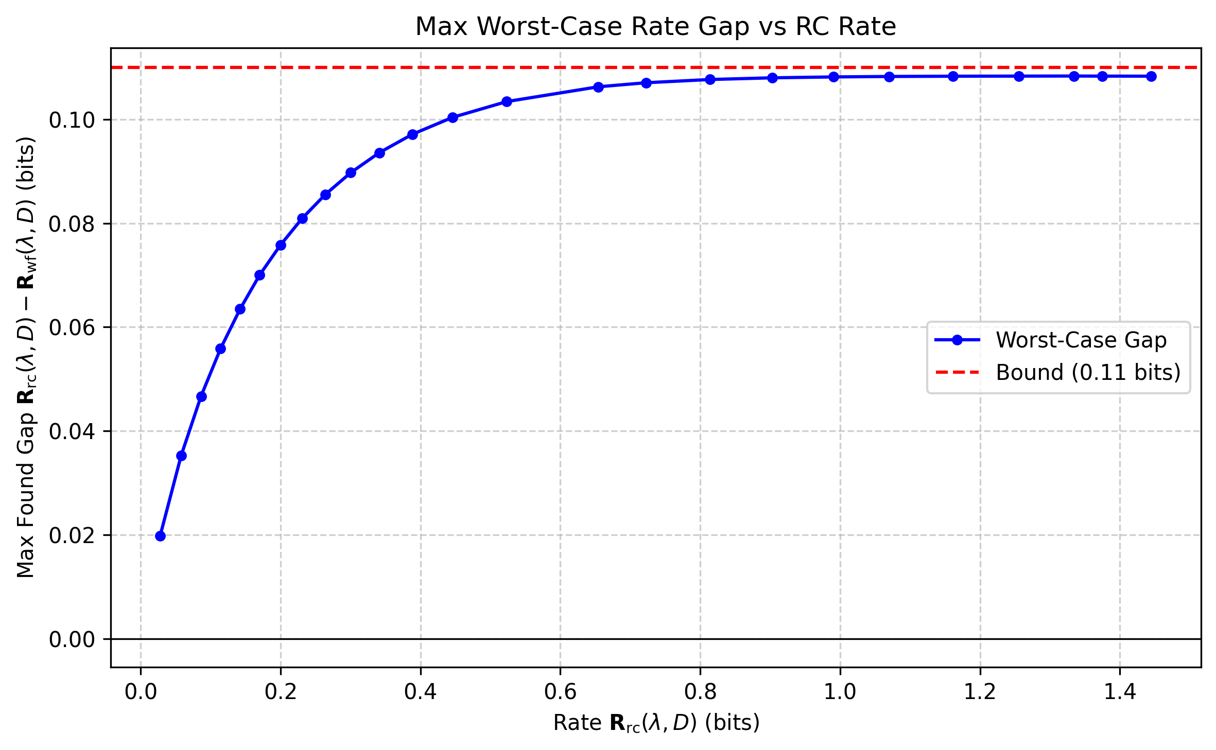
Our second main result in Theorem 3 shows that this overhead is uniformly bounded by 0.11 bit. Specifically, we derive precise expressions for 𝐑rc​(λ,D⋆)−𝐑wf​(λ,D⋆)\mathbf{R}_{\mathrm{rc}}(\lambda,D^{\star})-\mathbf{R}_{\mathrm{wf}}(\lambda,D^{\star}) that depend on λ=spec(ΣX)\lambda=\mathop{\mathrm{spec}}(\Sigma_{X}) and D⋆D^{\star} and prove that the maximum gaps occur at the spectra with at most 22 distinct eigenvalues and vanishing distortions (see Fig. 1 for the worst-case rate gap found at each R=𝐑rc​(λ,D⋆)R=\mathbf{R}_{\mathrm{rc}}(\lambda,D^{\star})). See Sec. D for the full proof.

Theorem 3 (Main Result II: Worst-Case Rate Gap to Oracle Setting).
supD⋆∈(0,1)supΛ{𝐑rc​(Λ,D⋆)−𝐑wf​(Λ,D⋆)}≤0.11,\sup_{D^{\star}\in(0,1)}\sup_{\Lambda}\left\{\mathbf{R}_{\mathrm{rc}}(\Lambda,D^{\star})-\mathbf{R}_{\mathrm{wf}}(\Lambda,D^{\star})\right\}\leq 0.11\,,

where the supremum is over Λ=diag(λ1,…,λn)⪰0\Lambda=\mathop{\mathrm{diag}}(\lambda_{1},\dots,\lambda_{n})\succeq 0 with tr(Λ)=n\mathop{\mathrm{tr}}(\Lambda)=n.

Refer to caption
Figure 1: Maximum rate gap found at each rate RR.

An intuitive way to see why the gap is bounded is to consider the most extreme of trΣX=n\mathop{\mathrm{tr}}\Sigma_{X}=n cases: the identity and the rank-1 case, for which 𝐑rc​(λ,D⋆)=𝐑wf​(λ,D⋆)\mathbf{R}_{\mathrm{rc}}(\lambda,D^{\star})=\mathbf{R}_{\mathrm{wf}}(\lambda,D^{\star}) by a simple computation. In fact, the gap vanishes for all matrices with semi-flat spectra λ=(n/m,…,n/m,0,…,0),m≤n\lambda=(n/m,\dots,n/m,0,\dots,0),m\leq n, a phenomenon we further discuss in Sec. 3.1.1.

Discussion and Open Questions.

Our results prove the existence of a universal codebook whose performance is uniformly within a constant rate gap of the ΣX\Sigma_{X}-aware (waterfilling) oracle benchmark, showing that universality is not, by itself, an information-theoretic bottleneck. Our random-coding-based proof is nonconstructive and does not yield an explicit codebook design or efficient encoder/decoder pair. Designing explicit and computationally efficient constructions is the most immediate open direction.

Often, low complexity quantizers are based on lattices. Indeed, for any fixed ΣX\Sigma_{X} a lattice randomly drawn from the natural Haar-Siegel measure will be a good quantizer with probability 1−e−Ω​(n)1-e^{-\Omega(n)}. This follows from the results of [19] that show that the covering radius of a random lattice is typically near-optimal with respect to any (fixed) norm. However, no lattice can be near-optimal simultaneously for all ΣX\Sigma_{X}, and the reason is simple: for any fixed lattice L⊂ℝnL\subset\mathbb{R}^{n} there is a rotation U⊤​LU^{\top}L that aligns its directions with the natural basis. Consequently, for this rotation U⊤​L=∏i=1n(αi​ℤ)U^{\top}L=\prod_{i=1}^{n}(\alpha_{i}\mathbb{Z}) for some α1,…,αn\alpha_{1},\ldots,\alpha_{n}. The integer lattice is a bad quantizer, and therefore any lattice quantizer must lose at least 12​log⁡2​π​e12≈0.254\frac{1}{2}\log\frac{2\pi e}{12}\approx 0.254 bits with respect to the waterfilling benchmark for some ΣX\Sigma_{X} (see [17] for more details). It therefore follows that ΣX\Sigma_{X}-universal near optimal schemes cannot solely rely on lattice quantizers.

One example of a lattice-based algorithm that provides a practical solution to the problem studied here is the GPTQ algorithm [10] (with appropriate shaping/entropy coding [17]). Its high-rate gap to the waterfilling benchmark, for particular ΣX\Sigma_{X}, is 12​log⁡2​π​e12+12​log⁡(AM−GM​(ΣX))\frac{1}{2}\log\frac{2\pi e}{12}+\frac{1}{2}\log(\mathrm{AM-GM}(\Sigma_{X})) where AM−GM​(ΣX)\mathrm{AM-GM}(\Sigma_{X}) is the ratio between arithmetic-mean and geometric-mean of the squared diagonal elements in the Cholesky decomposition of ΣX\Sigma_{X}, which can be unbounded in general [17]. When WW is a matrix consisting of a≫1a\gg 1 rows (rather than the vector case considered here), some of this gap can be reduced by sending to the decoder o​(n​a)o(na) bits of information on ΣX\Sigma_{X} (which has negligible effect on the rate). One such example is the WaterSIC quantization scheme [12].

Related literature.

The problem of vector quantization is classical [11], and its asymptotic behavior (for iid sources and additive distortion) is given by the famous rate-distortion formulas, e.g. [21, Part V]. A recent wave of interest, however, focuses on computing quantized inner-product and matrix multiplication.

On the practical side, the pioneering work of [9] demonstrated that substantial compression is possible via scaling plus uniform rounding (INT8 weight quantization), thus establishing the field of post-training quantization (PTQ). Notable PTQ works include SmoothQuant [26], which introduced calibration-based methods, i.e. those which depend on statistics of activations XX via ΣX\Sigma_{X}. GPTQ [10] and LDLQ [5], which are equivalent, simultaneously introduced an algorithm for ΣX\Sigma_{X}-dependent quantization. Going beyond simple integer-rounding, [23] consider lattice,  [22] consider nested lattice and [24] consider trellis quantization methods, respectively. Going beyond simple quadratic losses, are [25] and [4]. We note that [23] also reintroduced random Hadamard transform (RHT) as a way of mitigating outliers, following earlier usage in quantization of gradients, and classically. See [1, 13, 6] for other applications of RHT in PTQ.

On the theoretical side, the work [16] established fundamental limits of quantized matrix multiplication by leveraging nested lattice quantization. The GPTQ/LDLQ algorithm was understood as Babai’s nearest-plane algorithm applied after a Cholesky factorization of ΣX\Sigma_{X} in [8, 3], and as a successive interference cancellation (SIC) algorithm in [17], thus connecting weight-only quantization to lattice decoding and approximate closest vector problems [7, 2]. Authors of [17] developed theoretical high-rate analysis of GPTQ, showed it can be arbitrarily far from waterfilling and proposed an improved algorithm which provably matches waterfilling to within 0.255 bit in the high-rate regime.

The question considered here (ΣX\Sigma_{X}-oblivious quantization) in the special case of diagonal ΣX\Sigma_{X} falls under the umbrella of the compression with distortion as side-information proposed in [14]. This viewpoint connects modern LLM quantization to a long tradition in lattice decoding and approximate closest vector problems [7, 2].

3 Technical Overview

As in any source-coding problem, once the codebook 𝐂={c1,…,cM}⊂ℝn\mathbf{C}=\{c_{1},\ldots,c_{M}\}\subset\mathbb{R}^{n} is fixed, the optimal encoder computes i∗=i∗​(W)=arg⁡mini∈[M]⁡dΣX​(W,ci)i^{*}=i^{*}(W)=\operatorname*{\arg\!\min}_{i\in[M]}d_{\Sigma_{X}}(W,c_{i}), and sends the index i∗i^{*} to the decoder, which in turn outputs W^=ci∗\widehat{W}=c_{i^{*}}. Thus, the distortion of the codebook 𝐂\mathbf{C} is

n​D​(𝐂,ΣX)=𝔼​[mini∈[M]⁡dΣX​(W,ci)],\displaystyle nD(\mathbf{C},\Sigma_{X})=\mathbb{E}\left[\min_{i\in[M]}d_{\Sigma_{X}}(W,c_{i})\right], (4)

where the expectation is with respect to W∼𝒩​(0,In)W\sim\mathcal{N}(0,I_{n}). Even if we could design 𝐂\mathbf{C} based on ΣX\Sigma_{X}, the distortion D​(𝐂,ΣX)D(\mathbf{C},\Sigma_{X}) must satisfy (see Sec. 2) the waterfilling lower bound

D​(𝐂,ΣX)≥𝐃wf​(R,ΣX);D(\mathbf{C},\Sigma_{X})\geq\mathbf{D}_{\mathrm{wf}}(R,\Sigma_{X})\,;

the lower bound is also asymptotically achievable in the limit of large nn (see Proposition 2.1). The challenge is to find a single codebook 𝐂\mathbf{C} with M=2n​RM=2^{nR} codewords in ℝn\mathbb{R}^{n} that attains small D​(𝐂,ΣX)−𝐃wf​(R,ΣX)D(\mathbf{C},\Sigma_{X})-\mathbf{D}_{\mathrm{wf}}(R,\Sigma_{X}) simultaneously for all ΣX\Sigma_{X}.

As is standard, we prove the existence of such a codebook 𝐂\mathbf{C} by drawing a random code with M=2n​RM=2^{nR} iid codewords from a distribution PW^P_{\widehat{W}}. We show in Theorem 2 that for appropriate choice of PW^P_{\widehat{W}} we have that

Pr𝐂⁡[supΣX(D​(𝐂,ΣX)−𝐃rc​(spec(ΣX),R−ε))<η]≥1−exp⁡(−poly​(n))\displaystyle\Pr_{\mathbf{C}}\left[\sup_{\Sigma_{X}}\left(D(\mathbf{C},\Sigma_{X})-\mathbf{D}_{\mathrm{rc}}(\mathop{\mathrm{spec}}(\Sigma_{X}),R-\varepsilon)\right)<\eta\right]\geq 1-\exp\left(-\mathrm{poly}(n)\right) (5)

holds for any η,ε>0\eta,\varepsilon>0 and nn large enough, where spec(ΣX)\mathop{\mathrm{spec}}(\Sigma_{X}) is the vector of the eigenvalues of ΣX\Sigma_{X} and 𝐃rc\mathbf{D}_{\mathrm{rc}} is defined in Eq. (𝐃rc\mathbf{D}_{\mathrm{rc}}). Consequently there must exist a fixed rate-RR codebook 𝐂\mathbf{C} with

D​(𝐂,ΣX)≤𝐃rc​(spec(ΣX),R−ε)+η,∀ΣX∈𝕊+n​ with ​tr(ΣX)=n.\displaystyle D(\mathbf{C},\Sigma_{X})\leq\mathbf{D}_{\mathrm{rc}}(\mathop{\mathrm{spec}}(\Sigma_{X}),R-\varepsilon)+\eta,~~~\forall\Sigma_{X}\in\mathbb{S}_{+}^{n}\text{ with }\mathop{\mathrm{tr}}(\Sigma_{X})=n. (6)

3.1 Codebook Distribution

How should we choose PW^P_{\widehat{W}}? For a given ΣX\Sigma_{X} with spectral decomposition ΣX=U​Λ​U⊤\Sigma_{X}=U\Lambda U^{\top}, the optimal PW^P_{\widehat{W}} follows from the waterfilling solution. Specifically, for water-level 1/t1/t chosen so that RwfR_{\mathrm{wf}} defined in (WF\mathrm{WF}) equals RR, the optimal distribution is

PW^∗​(ΣX,R)\displaystyle P^{*}_{\widehat{W}}(\Sigma_{X},R) =PW^∗​(ΣX,t)=𝒩​(0,U​Γ​(Λ,t)​U⊤),\displaystyle=P^{*}_{\widehat{W}}(\Sigma_{X},t)=\mathcal{N}(0,U~\Gamma(\Lambda,t)~U^{\top}),
where​Γ​(Λ,t)=diag(max⁡{1−tλ1,0},⋯,max⁡{1−tλn,0}).\displaystyle\text{where}~~\Gamma(\Lambda,t)=\mathop{\mathrm{diag}}\left(\max\left\{1-\frac{t}{\lambda_{1}},0\right\},\cdots,\max\left\{1-\frac{t}{\lambda_{n}},0\right\}\right). (7)

We need to choose a single PW^P_{\widehat{W}} that “works well” for all ΣX\Sigma_{X}. Since there is no preference to any U∈𝒪nU\in\mathcal{O}_{n}, it makes sense to take an isotropic Gaussian PW^P_{\widehat{W}}. Observing that for any fixed ΣX\Sigma_{X} and t>0t>0 the covariance matrix for PW^∗​(ΣX,t)P^{*}_{\widehat{W}}(\Sigma_{X},t) satisfies U​Γ​(Λ,t)​U⊤⪯InU~\Gamma(\Lambda,t)~U^{\top}\preceq I_{n}, we will take

PW^​(τ)=𝒩​(0,τ2​In),\displaystyle P_{\widehat{W}}(\tau)=\mathcal{N}(0,\tau^{2}I_{n}), (8)

for some 0<τ<10<\tau<1.

An appealing feature of the isotropic Gaussian distribution is that drawing MM iid vectors from 𝒩​(0,τ2​In)\mathcal{N}(0,\tau^{2}I_{n}) is equivalent to first drawing them iid from 𝒩​(0,In)\mathcal{N}(0,I_{n}) and then scaling all of them by τ\tau. The consequence of this simple fact is that while we cannot perfectly match our codebook distribution to PW^∗​(ΣX,R)P^{*}_{\widehat{W}}(\Sigma_{X},R), the flexibility in the choice of τ=τ​(ΣX,R)\tau=\tau(\Sigma_{X},R) allows for a better match. Consequently, we draw the MM codewords of 𝐂\mathbf{C} from the 𝒩​(0,In)\mathcal{N}(0,I_{n}) distribution. The encoder, that knows ΣX\Sigma_{X}, computes τ​(ΣX,R)\tau(\Sigma_{X},R) that provides the smallest expected distortion, and sends a description of τ\tau to the decoder.222As we will see below, some further gain can be attained by allowing τ\tau to also depend on the source realization w∈ℝnw\in\mathbb{R}^{n}. With this procedure, the effective codebook 𝐂~=τ​𝐂\tilde{\mathbf{C}}=\tau\mathbf{C} is drawn from PW^=𝒩​(0,τ2​(ΣX,R)​In)P_{\widehat{W}}=\mathcal{N}(0,\tau^{2}(\Sigma_{X},R)I_{n}). The encoder then finds i∗=arg⁡mini∈[M]⁡dΣX​(W,c~i)=arg⁡mini∈[M]⁡dΣX​(W,τ​ci)i^{*}=\operatorname*{\arg\!\min}_{i\in[M]}d_{\Sigma_{X}}(W,\tilde{c}_{i})=\operatorname*{\arg\!\min}_{i\in[M]}d_{\Sigma_{X}}(W,\tau c_{i}) and sends i∗i^{*} as well as a high-resolution description of τ\tau in bits to the decoder.

3.1.1 Geometric Intuition

To get some intuition to why the “universal” codebook distribution PW^=𝒩​(0,τ2​(ΣX,R)​In)P_{\widehat{W}}=\mathcal{N}(0,\tau^{2}(\Sigma_{X},R)I_{n}) works well simultaneously for all ΣX\Sigma_{X}, let us restrict attention to the family of covariance matrices with semi-flat spectrum. In particular, for m≤nm\leq n let

𝒮mn={ΣX=U​Λ​U⊤:U∈𝒪n,λ1=⋯=λm=nm,λm+1=⋯=λn=0},\displaystyle\mathcal{S}_{m}^{n}=\left\{\Sigma_{X}=U\Lambda U^{\top}~:~U\in\mathcal{O}_{n},~\lambda_{1}=\cdots=\lambda_{m}=\frac{n}{m},~\lambda_{m+1}=\cdots=\lambda_{n}=0\right\}, (9)

be the collection of PSD matrices with m≤nm\leq n equal and non-zero singular values and m−nm-n zero singular values. From (7) we see that the ΣX\Sigma_{X}-matched optimal codebook distribution is of the form

PW^∗​(ΣX,R)=𝒩​(0,U⋅diag(τ2,⋯,τ2,0,⋯,0)​U⊤)\displaystyle P^{*}_{\widehat{W}}(\Sigma_{X},R)=\mathcal{N}\left(0,U\cdot\mathop{\mathrm{diag}}\left(\tau^{2},\cdots,\tau^{2},0,\cdots,0\right)U^{\top}\right) (10)

for some τ>0\tau>0. Thus the optimal procedure for random coding is to draw iid Gaussian codewords within the subspace U[m]U_{[m]} spanned by the first mm singular vectors. Our universal distribution, on the other hand, draws isotropic iid Gaussian codewords, and is hence very far from the optimal distribution. However, since the encoder searches for the nearest codeword under the dΣXd_{\Sigma_{X}} metric, it effectively projects both WW and the codebook 𝐂\mathbf{C} to U[m]U_{[m]} and finds the nearest codeword in ℓ2\ell_{2}-metric within this subspace. It therefore follows that what dictates performance of a random code 𝐂\mathbf{C} under dΣXd_{\Sigma_{X}} metric (for ΣX\Sigma_{X} with semi-flat spectrum) is the distribution of U[m]⊤​cU^{\top}_{[m]}c, where c∼PW^c\sim P_{\widehat{W}}. Thus, our universal PW^=𝒩​(0,τ2​In)P_{\widehat{W}}=\mathcal{N}(0,\tau^{2}I_{n}) is simultaneously optimal for all semi-flat ΣX\Sigma_{X} (with all possible m∈[n]m\in[n]), provided that we judiciously choose τ=τ​(ΣX,R)\tau=\tau(\Sigma_{X},R). Inspection of our ΣX\Sigma_{X}-universal rate-distortion tradeoff (RDRC) shows that indeed

𝐃rc​(spec(ΣX),R)=𝐃wf​(spec(ΣX),R),\mathbf{D}_{\mathrm{rc}}(\mathop{\mathrm{spec}}(\Sigma_{X}),R)=\mathbf{D}_{\mathrm{wf}}(\mathop{\mathrm{spec}}(\Sigma_{X}),R),

for all semi-flat ΣX\Sigma_{X}. Whenever the spectrum of ΣX\Sigma_{X} is not semi-flat the distribution of U⊤​cU^{\top}c for c∼PW^c\sim P_{\widehat{W}} does not match that of U⊤​cU^{\top}c under the optimal PW^∗​(ΣX,R)P^{*}_{\widehat{W}}(\Sigma_{X},R), and consequently in these cases our ΣX\Sigma_{X}-universal rate-distortion tradeoff (RDRC) is worse than the waterfilling rate-distortion tradeoff. Nevertheless, it turns out that the loss for this mismatch is at most 0.110.11 bits, as shown in Theorem 3.

3.2 Sketch of Proof

After we obtained intuition for the choice of using a random iid isotropic Gaussian codebook, with scale τ\tau determined by the encoder, we move on to giving an overview of the proof of Theorem 2. The detailed rigorous proof is given in Appendix C.

Let us first fix ΣX=U​Λ​U⊤\Sigma_{X}=U\Lambda U^{\top}, and analyze the performance of a codebook 𝐂={c1,…,cM}\mathbf{C}=\{c_{1},\ldots,c_{M}\}, M=2n​RM=2^{nR}, with ci∼i​i​d𝒩​(0,In)c_{i}\stackrel{{\scriptstyle iid}}{{\sim}}\mathcal{N}(0,I_{n}). We will show that 𝐂\mathbf{C} is “good” for ΣX\Sigma_{X} with probability 1−exp⁡(−eΩ​(n))1-\exp(-e^{\Omega(n)}), and from this we will deduce that a random 𝐂\mathbf{C} is “good” for all ΣX\Sigma_{X} by a covering argument.

The codebook 𝐂\mathbf{C} can describe a fixed w∈ℝnw\in\mathbb{R}^{n} with distortion ≤D\leq D if at least one of its τ\tau-scaled codewords is inside the region w+D​ℬΣXw+\sqrt{D}\mathcal{B}_{\Sigma_{X}}, where

ℬΣX={e∈ℝn:e⊤​ΣX​e≤n}.\displaystyle\mathcal{B}_{\Sigma_{X}}=\left\{e\in\mathbb{R}^{n}~:e^{\top}\Sigma_{X}e\leq n\right\}. (11)

Thus, the key to analyzing the tradeoff between rate and distortion is understanding how the success probability of a single codeword behaves as a function of DD. Since the codewords are 𝒩​(0,In)\mathcal{N}(0,I_{n}), their distribution is invariant to rotation, and therefore the success probability of a single codeword is

psuccess​(w,τ,ΣX,D)\displaystyle p_{\mathrm{success}}(w,\tau,\Sigma_{X},D) =ϕτ2​(w+D​ℬΣX)\displaystyle=\phi_{\tau^{2}}\left(w+\sqrt{D}\mathcal{B}_{\Sigma_{X}}\right)
=ϕτ2​(U⊤​w+D​ℬΛ)=psuccess​(U⊤​w,τ,Λ,D),\displaystyle=\phi_{\tau^{2}}\left(U^{\top}w+\sqrt{D}\mathcal{B}_{\Lambda}\right)=p_{\mathrm{success}}(U^{\top}w,\tau,\Lambda,D), (12)

where ϕτ2\phi_{\tau^{2}} denotes the probability distribution for 𝒩​(0,τ2​In)\mathcal{N}(0,\tau^{2}I_{n}). When psuccess<2−n​(R+ε)p_{\mathrm{success}}<2^{-n(R+\varepsilon)}, it is very unlikely to find a codeword in w+D​ℬΣXw+\sqrt{D}\mathcal{B}_{\Sigma_{X}}, and on the other hand, when psuccess>2−n​(R−ε)p_{\mathrm{success}}>2^{-n(R-\varepsilon)} we are very likely to find a codeword in w+D​ℬΣXw+\sqrt{D}\mathcal{B}_{\Sigma_{X}}. Thus, what we are looking for is the critical DD for which −1n​log⁡psuccess​(U⊤​w,τ,Λ,D)≈R-\frac{1}{n}\log p_{\mathrm{success}}(U^{\top}w,\tau,\Lambda,D)\approx R. Since the codebook’s scale τ\tau needs to be sent from the encoder to the decoder anyway, we may let it depend not only on Λ\Lambda but also on U⊤​wU^{\top}w. Therefore, given U⊤​w,ΛU^{\top}w,\Lambda and RR we choose τ=τ​(U⊤​w,Λ,R)\tau=\tau(U^{\top}w,\Lambda,R) for which the critical DD is small. A tedious but straightforward calculation shows that the optimal choice is

τ=τ​(U⊤​w,Λ,R)=(T​∑j(U⊤​w)j2​λj2(1+λj​T)2)1/2​(∑jλj1+λj​T)−1/2,\displaystyle\tau=\tau(U^{\top}w,\Lambda,R)=\left(T\sum_{j}\frac{(U^{\top}w)_{j}^{2}\lambda_{j}^{2}}{(1+\lambda_{j}T)^{2}}\right)^{1/2}\left(\sum_{j}\frac{\lambda_{j}}{1+\lambda_{j}T}\right)^{-1/2}, (13)

where T=T​(Λ,R)T=T(\Lambda,R) is such that Rrc​(Λ,T)=RR_{\mathrm{rc}}(\Lambda,T)=R, and Rrc​(Λ,T)R_{\mathrm{rc}}(\Lambda,T) is defined in (RDRC). Let

Drc​(U⊤​w)=Drc​(Λ,R,U⊤​w)=1n​∑i=1n(U⊤​w)i2​λi1+λi​T,\displaystyle D_{\mathrm{rc}}(U^{\top}w)=D_{\mathrm{rc}}(\Lambda,R,U^{\top}w)=\frac{1}{n}\sum_{i=1}^{n}\frac{(U^{\top}w)_{i}^{2}\lambda_{i}}{1+\lambda_{i}T}, (14)

where here as well T=T​(Λ,R)T=T(\Lambda,R). In Lemma B.2 we prove that

−log⁡psuccess​(U⊤​w,τ,Λ,Drc​(U⊤​w))=−log⁡ϕτ2​(U⊤​w+Drc​(U⊤​w)​ℬΛ)≈n​R.\displaystyle-\log p_{\mathrm{success}}(U^{\top}w,\tau,\Lambda,D_{\mathrm{rc}}(U^{\top}w))=-\log\phi_{\tau^{2}}\left(U^{\top}w+\sqrt{D_{\mathrm{rc}}(U^{\top}w)}\mathcal{B}_{\Lambda}\right)\approx nR. (15)

Thus, Drc​(U⊤​w)D_{\mathrm{rc}}(U^{\top}w) is the critical distortion for fixed w∈ℝnw\in\mathbb{R}^{n} and ΣX\Sigma_{X}. Note that for W∼𝒩​(0,In)W\sim\mathcal{N}(0,I_{n}) we have

𝔼W​[Drc​(U⊤​W)]=1n​∑i=1nλi1+λi​T=Drc​(Λ,R),\displaystyle\mathbb{E}_{W}\left[D_{\mathrm{rc}}(U^{\top}W)\right]=\frac{1}{n}\sum_{i=1}^{n}\frac{\lambda_{i}}{1+\lambda_{i}T}=D_{\mathrm{rc}}(\Lambda,R), (16)

where Drc​(Λ,R)D_{\mathrm{rc}}(\Lambda,R) is the distortion in (𝐃rc\mathbf{D}_{\mathrm{rc}}).

The proof of Lemma B.2 uses standard large deviation techniques, but note that what we really need for the analysis is a quantitative lower bound on psuccessp_{\mathrm{success}}, and this requires some more work beyond Chernoff bound. The choice of τ\tau from (13) is the one that minimizes the large deviations exponent, whereas the parameter TT in our rate-distortion tradeoff (RDRC) is just a rescaling of the parameter tt in Chernoff’s bound Pr⁡(X>D)≤e−t​D​𝔼​[et​X]\Pr(X>D)\leq e^{-tD}\mathbb{E}[e^{tX}].

By (15), for η>0\eta>0 we have that psuccess​(U⊤​w,τ,Λ,Drc​(U⊤​w)+η/2)≥2−n​(R−εη)p_{\mathrm{success}}(U^{\top}w,\tau,\Lambda,D_{\mathrm{rc}}(U^{\top}w)+\eta/2)\geq 2^{-n(R-\varepsilon_{\eta})} for some εη>0\varepsilon_{\eta}>0 (and nn large enough). Thus, ∀w∈ℝn\forall w\in\mathbb{R}^{n}

Pfailure​(w)\displaystyle P_{\mathrm{failure}}(w) =Pr𝐂⁡(1n​mini∈[M]⁡dΣX​(w,τ​ci)>Drc​(U⊤​w)+η/2)\displaystyle=\Pr_{\mathbf{C}}\left(\frac{1}{n}\min_{i\in[M]}d_{\Sigma_{X}}(w,\tau c_{i})>D_{\mathrm{rc}}(U^{\top}w)+\eta/2\right)
=1−(1−psuccess​(U⊤​w,τ,Λ,Drc​(U⊤​w)+η/2))M≤exp⁡(−2n​ε),\displaystyle=1-\left(1-p_{\mathrm{success}}\left(U^{\top}w,\tau,\Lambda,D_{\mathrm{rc}}(U^{\top}w)+\eta/2\right)\right)^{M}\leq\exp(-2^{n\varepsilon}), (17)

for some ε>0\varepsilon>0. For a fixed code 𝐂\mathbf{C} define

ℰfailure​(𝐂)={w∈ℝn:1n​mini∈[M]⁡dΣX​(w,τ​ci)>Drc​(U⊤​w)+η/2}.\displaystyle\mathcal{E}_{\mathrm{failure}}(\mathbf{C})=\left\{w\in\mathbb{R}^{n}~:~\frac{1}{n}\min_{i\in[M]}d_{\Sigma_{X}}(w,\tau c_{i})>D_{\mathrm{rc}}(U^{\top}w)+\eta/2\right\}. (18)

Assuming we can always encode ww to 0 (e.g., by setting τ=0\tau=0 if needed), for any W∼PWW\sim P_{W} we have

1n​D​(𝐂,Λ)\displaystyle\frac{1}{n}D(\mathbf{C},\Lambda) =𝔼​[mini∈[M]⁡dΣX​(W,τ​ci)]≤𝔼​[Drc​(U⊤​W)+η2+𝟙​{W∈ℰfailure​(𝐂)}​dΣX​(W,0)]\displaystyle=\mathbb{E}\left[\min_{i\in[M]}d_{\Sigma_{X}}(W,\tau c_{i})\right]\leq\mathbb{E}\left[D_{\mathrm{rc}}(U^{\top}W)+\frac{\eta}{2}+\mathds{1}\{W\in\mathcal{E}_{\mathrm{failure}}(\mathbf{C})\}d_{\Sigma_{X}}(W,0)\right]
≤𝔼​[Drc​(U⊤​W)]+η2+PW​[ℰfailure​(𝐂)]⋅𝔼​[dΣX2​(W,0)],\displaystyle\leq\mathbb{E}\left[D_{\mathrm{rc}}(U^{\top}W)\right]+\frac{\eta}{2}+\sqrt{P_{W}[\mathcal{E}_{\mathrm{failure}}(\mathbf{C})]}\cdot\sqrt{\mathbb{E}[d^{2}_{\Sigma_{X}}(W,0)]}, (19)

where the last inequality is Cauchy-Schwarz. If 𝔼W​[dΣX2​(W,0)]≤poly​(n)\mathbb{E}_{W}[d^{2}_{\Sigma_{X}}(W,0)]\leq\mathrm{poly}(n) under W∼PWW\sim P_{W},333e.g., 𝔼W​[dΣX2​(W,0)]≤O​(n2)\mathbb{E}_{W}[d^{2}_{\Sigma_{X}}(W,0)]\leq O(n^{2}) for W∼𝒩​(0,In)W\sim\mathcal{N}(0,I_{n}) it follows that whenever PW​[ℰfailure​(𝐂)]P_{W}\left[\mathcal{E}_{\mathrm{failure}}(\mathbf{C})\right] is sufficiently small, say ≤e−n\leq e^{-n}, the codebook 𝐂\mathbf{C} attains the desired

1n​D​(𝐂,Λ)≤𝔼​[Drc​(U⊤​W)]+η.\frac{1}{n}D(\mathbf{C},\Lambda)\leq\mathbb{E}\left[D_{\mathrm{rc}}(U^{\top}W)\right]+\eta\,.

PW​[ℰfailure​(𝐂)]P_{W}\left[\mathcal{E}_{\mathrm{failure}}(\mathbf{C})\right] can indeed be bounded: using (17) and Markov’s inequality we obtain that this holds for the vast majority of codebooks:

Pr𝐂⁡(PW​[ℰfailure​(𝐂)]>e−n)\displaystyle\Pr_{\mathbf{C}}\left(P_{W}[\mathcal{E}_{\mathrm{failure}}(\mathbf{C})]>e^{-n}\right) ≤en​𝔼𝐂​[PW​[ℰfailure​(𝐂)]]=en​𝔼𝐂,W​[Pfailure​(W)]\displaystyle\leq e^{n}\mathbb{E}_{\mathbf{C}}\left[P_{W}[\mathcal{E}_{\mathrm{failure}}(\mathbf{C})]\right]=e^{n}\mathbb{E}_{\mathbf{C},W}[P_{\mathrm{failure}}(W)]
≤exp⁡(−2n​ε+n).\displaystyle\leq\exp(-2^{n\varepsilon}+n). (20)

From this we conclude that for fixed PWP_{W} and any fixed ΣX\Sigma_{X}

Pr𝐂⁡([1n​D​(𝐂,Λ)−𝔼W​[Drc​(U⊤​W)]>η])≤exp⁡(−2n​ε′).\displaystyle\Pr_{\mathbf{C}}\left(\left[\frac{1}{n}D(\mathbf{C},\Lambda)-\mathbb{E}_{W}\left[D_{\mathrm{rc}}(U^{\top}W)\right]>\eta\right]\right)\leq\exp(-2^{n\varepsilon^{\prime}}). (21)

Specializing this to PW=𝒩​(0,In)P_{W}=\mathcal{N}(0,I_{n}) we obtain

Pr𝐂⁡([1n​D​(𝐂,Λ)−Drc​(Λ,R)]>η)≤exp⁡(−2n​ε′).\displaystyle\Pr_{\mathbf{C}}\left(\left[\frac{1}{n}D(\mathbf{C},\Lambda)-D_{\mathrm{rc}}(\Lambda,R)\right]>\eta\right)\leq\exp(-2^{n\varepsilon^{\prime}}). (22)

We have therefore obtained that for any fixed ΣX\Sigma_{X} the probability of drawing a “bad” codebook with [1n​D​(𝐂,Λ)−Drc​(Λ,R)]>η\left[\frac{1}{n}D(\mathbf{C},\Lambda)-D_{\mathrm{rc}}(\Lambda,R)\right]>\eta is double-exponentially small. From here, it is clear how to prove that a randomly drawn 𝐂\mathbf{C} will have

Pr𝐂⁡(supΣX[1n​D​(𝐂,ΛX)−Drc​(Λ,R)]>η)<exp⁡(−2n​ε′′).\displaystyle\Pr_{\mathbf{C}}\left(\sup_{\Sigma_{X}}\left[\frac{1}{n}D(\mathbf{C},\Lambda_{X})-D_{\mathrm{rc}}(\Lambda,R)\right]>\eta\right)<\exp(-2^{n\varepsilon^{\prime\prime}}). (23)

All we need is to find a dense cover of PSD matrices in Rn×nR^{n\times n} with trace nn whose size is exp⁡(−2o​(n))\exp(-2^{o(n)}). In particular, we need to find a collection of N=exp⁡(−2o​(n))N=\exp(-2^{o(n)}) PSD matrices with the property that for any valid PSD matrix ΣX\Sigma_{X} there exists a matrix Σi\Sigma_{i}, i∈[N]i\in[N] such that:

Drc​(spec(ΣX),R)≈Drc​(spec(Σi),R)and1n​D​(𝐂,ΣX)≈1n​D​(𝐂,Σi).D_{\mathrm{rc}}(\mathop{\mathrm{spec}}(\Sigma_{X}),R)\approx D_{\mathrm{rc}}(\mathop{\mathrm{spec}}(\Sigma_{i}),R)\qquad\text{and}\qquad\frac{1}{n}D(\mathbf{C},\Sigma_{X})\approx\frac{1}{n}D(\mathbf{C},\Sigma_{i})\,. (24)

Since NN is allowed to be so large, these two constraints can be met to arbitrary resolution (though the proof for this requires a lot of bookkeeping and is somewhat technical, see Sec. C.2).

We end this overview with listing some of the technical issues that our sketch of proof above ignored, and briefly mention how addressing them, as we of course do in the actual proofs, affects the results.

τ\tau quantization. While our sketch assumed that τ\tau can be conveyed to the decoder in perfect resolution, in reality, some of our n​RnR bits budget is allocated to the description of τ\tau. In order to compress τ\tau that depends on U⊤​WU^{\top}W, we require a high probability bound on ‖U⊤​W‖∞\|U^{\top}W\|_{\infty}. This norm constraint is also needed for the proof of our large deviations result (Lemma B.2).

Norm bound for codewords. The perturbation argument (24) for the dense cover must account for quantization and change in τ\tau. Since these errors are multiplied by codewords from 𝐂\mathbf{C}, we require a uniform norm bound ‖ci‖2<nB\|c_{i}\|_{2}<n^{B} for some B>1B>1 (say B=10B=10) to make their contribution to end-to-end distortion negligible. While the probability that this occurs is overwhelmingly large, it is only 1−exp⁡(−poly​(n))1-\exp(-\mathrm{poly}(n)) rather than double exponential. For this reason the probability of drawing a ΣX\Sigma_{X}-universal codebook is only 1−exp⁡(−poly​(n))1-\exp(-\mathrm{poly}(n)) (see Eq. (5)) rather than the 1−exp⁡(−2Ω​(n))1-\exp(-2^{\Omega(n)}) that our sketch of proof gives. Because event {‖ci‖2<nB​∀i∈[M]}\{\|c_{i}\|_{2}<n^{B}~~\forall i\in[M]\} is independent of ΣX\Sigma_{X}, it contributes only a single term to the union bound. Consequently, our dense grid is still allowed to be of size exp⁡(−2o​(n))\exp(-2^{o(n)}).

Rate-penalty. In the overview above, we assumed that if −ln⁡psuccess​(D)=R-\ln p_{\mathrm{success}}(D)=R, then for any η>0\eta>0 we have −ln⁡psuccess​(D+η)=R−εη-\ln p_{\mathrm{success}}(D+\eta)=R-\varepsilon_{\eta} for some εη>0\varepsilon_{\eta}>0. This is indeed the case whenever D′​(R)D^{\prime}(R) is finite. However, our results are for the supremum over all ΣX\Sigma_{X} with trace nn, and this cannot be guaranteed for all such matrices at all rates. Consequently, in Theorem 2 there is both a rate-penalty ε>0\varepsilon>0 and a distortion penalty η>0\eta>0 (which both can be made arbitrarily small for nn large enough), whereas in the sketch above we only had a distortion penalty.

Disclosure of LLM Assistance

The authors used ChatGPT to assist with editing, code generation for Fig. 1, and technical steps (e.g., perturbation analysis and derivative computations) in the proofs of main theorems. The final optimization step after the spectrum reduction in Theorem 3 was also suggested by ChatGPT. All model-generated code, computations, and proof steps were independently verified and adjusted by the authors. The authors take full responsibility for the correctness of all analytical and numerical results in the paper.

References

  • AMC+ [24] Saleh Ashkboos, Amirkeivan Mohtashami, Maximilian L. Croci, Bo Li, Pashmina Cameron, Martin Jaggi, Dan Alistarh, Torsten Hoefler, and James Hensman. Quarot: Outlier-free 4-bit inference in rotated llms, 2024. URL: https://arxiv.org/abs/2404.00456, arXiv:2404.00456.
  • Bab [86] László Babai. On lovász’lattice reduction and the nearest lattice point problem. Combinatorica, 6(1):1–13, 1986.
  • Bir [25] Johann Birnick. The lattice geometry of neural network quantization–a short equivalence proof of gptq and babai’s algorithm. arXiv preprint arXiv:2508.01077, 2025.
  • BS [23] Hicham Badri and Appu Shaji. Half-quadratic quantization of large machine learning models, November 2023. URL: https://mobiusml.github.io/hqq_blog/.
  • CCKS [24] Jerry Chee, Yaohui Cai, Volodymyr Kuleshov, and Christopher De Sa. Quip: 2-bit quantization of large language models with guarantees, 2024. URL: https://arxiv.org/abs/2307.13304, arXiv:2307.13304.
  • CEHA [25] Jiale Chen, Vage Egiazarian, Torsten Hoefler, and Dan Alistarh. Wush: Near-optimal adaptive transforms for llm quantization. arXiv preprint arXiv:2512.00956, 2025.
  • CS [82] John Conway and Neil Sloane. Fast quantizing and decoding and algorithms for lattice quantizers and codes. IEEE Transactions on Information Theory, 28(2):227–232, 1982.
  • CSC+ [25] Jiale Chen, Yalda Shabanzadeh, Elvir Crnčević, Torsten Hoefler, and Dan Alistarh. The geometry of llm quantization: Gptq as babai’s nearest plane algorithm. arXiv preprint arXiv:2507.18553, 2025.
  • DLBZ [22] Tim Dettmers, Mike Lewis, Younes Belkada, and Luke Zettlemoyer. Gpt3. int8 (): 8-bit matrix multiplication for transformers at scale. Advances in Neural Information Processing Systems, 35:30318–30332, 2022.
  • FAHA [23] Elias Frantar, Saleh Ashkboos, Torsten Hoefler, and Dan Alistarh. Gptq: Accurate post-training quantization for generative pre-trained transformers, 2023. URL: https://arxiv.org/abs/2210.17323, arXiv:2210.17323.
  • GG [12] Allen Gersho and Robert M Gray. Vector quantization and signal compression, volume 159. Springer Science & Business Media, 2012.
  • LSOP [26] Egor Lifar, Semyon Savkin, Or Ordentlich, and Yury Polyanskiy. Watersic: information-theoretically (near) optimal linear layer quantization. arXiv preprint arXiv:2603.04956, 2026.
  • LZF+ [25] Zechun Liu, Changsheng Zhao, Igor Fedorov, Bilge Soran, Dhruv Choudhary, Raghuraman Krishnamoorthi, Vikas Chandra, Yuandong Tian, and Tijmen Blankevoort. Spinquant: Llm quantization with learned rotations, 2025. URL: https://arxiv.org/abs/2405.16406, arXiv:2405.16406.
  • MWZ [08] Emin Martinian, Gregory W. Wornell, and Ram Zamir. Source coding with distortion side information. IEEE Transactions on Information Theory, 54(10):4638–4665, 2008. doi:10.1109/TIT.2008.928983.
  • N+ [25] NVIDIA et al. Pretraining large language models with NVFP4. arXiv preprint arXiv:2509.25149, 2025.
  • OP [25] Or Ordentlich and Yury Polyanskiy. Optimal quantization for matrix multiplication. IEEE Transactions on Information Theory, 2025.
  • OP [26] Or Ordentlich and Yury Polyanskiy. High-rate quantized matrix multiplication II. arXiv preprint arXiv:2605.13768, 2026.
  • Ope [23] Open Compute Project. OCP microscaling formats (MX) specification. Technical report, Open Compute Project, 2023. URL: https://www.opencompute.org/documents/ocp-microscaling-formats-mx-v1-0-spec-final-pdf.
  • ORW [22] Or Ordentlich, Oded Regev, and Barak Weiss. New bounds on the density of lattice coverings. Journal of the American Mathematical Society, 35(1):295–308, 2022.
  • OZ [11] Jan Ostergaard and Ram Zamir. Incremental refinement using a gaussian test channel. In 2011 IEEE International Symposium on Information Theory Proceedings, pages 2233–2237, 2011. doi:10.1109/ISIT.2011.6033957.
  • PW [24] Yury Polyanskiy and Yihong Wu. Information theory: From coding to learning. Cambridge university press, 2024.
  • SPOP [25] Semyon Savkin, Eitan Porat, Or Ordentlich, and Yury Polyanskiy. Nestquant: Nested lattice quantization for matrix products and llms, 2025. URL: https://arxiv.org/abs/2502.09720, arXiv:2502.09720.
  • TCS+ [24] Albert Tseng, Jerry Chee, Qingyao Sun, Volodymyr Kuleshov, and Christopher De Sa. Quip#: Even better llm quantization with hadamard incoherence and lattice codebooks, 2024. URL: https://arxiv.org/abs/2402.04396, arXiv:2402.04396.
  • TSHS [25] Albert Tseng, Qingyao Sun, David Hou, and Christopher De Sa. Qtip: Quantization with trellises and incoherence processing, 2025. URL: https://arxiv.org/abs/2406.11235, arXiv:2406.11235.
  • TSS [25] Albert Tseng, Zhaofeng Sun, and Christopher De Sa. Model-preserving adaptive rounding, 2025. URL: https://arxiv.org/abs/2505.22988, arXiv:2505.22988.
  • XLS+ [24] Guangxuan Xiao, Ji Lin, Mickael Seznec, Hao Wu, Julien Demouth, and Song Han. Smoothquant: Accurate and efficient post-training quantization for large language models, 2024. URL: https://arxiv.org/abs/2211.10438, arXiv:2211.10438.
  • Zam [02] Ram Zamir. The rate loss in the wyner-ziv problem. IEEE Transactions on Information Theory, 42(6):2073–2084, 2002.
  • ZB [02] Ram Zamir and Toby Berger. Multiterminal source coding with high resolution. IEEE Transactions on Information Theory, 45(1):106–117, 2002.

Appendix A Preliminaries and Notation

Notation.

We write Σ⪰0\Sigma\succeq 0 to denote that the matrix Σ∈ℝn×n\Sigma\in\mathbb{R}^{n\times n} is positive semidefinite; we define the set of positive semidefinite matrices as 𝕊+n={Σ∈ℝn×n:Σ⪰0}\mathbb{S}_{+}^{n}=\left\{\Sigma\in\mathbb{R}^{n\times n}:\,\Sigma\succeq 0\right\}.

For Σ∈𝕊+n\Sigma\in\mathbb{S}_{+}^{n} we denote the spectral decomposition as

EVD​(Σ)=U​Λ​U⊤,\mathrm{EVD}(\Sigma)=U\Lambda U^{\top}\,,

where U∈𝒪nU\in\mathcal{O}_{n} is orthogonal and Λ\Lambda is diagonal.

diag(v)\mathop{\mathrm{diag}}(v) for v∈ℝnv\in\mathbb{R}^{n} denotes an n×nn\times n diagonal matrix with diag(v)i​i=vi\mathop{\mathrm{diag}}(v)_{ii}=v_{i}. spec(A)\mathop{\mathrm{spec}}(A) for A∈ℝn×nA\in\mathbb{R}^{n\times n} denotes the vector of the eigenvalues of AA.

For A∈ℝn×aA\in\mathbb{R}^{n\times a} and Σ∈𝕊+n\Sigma\in\mathbb{S}_{+}^{n}, denote

‖A‖Σ≜tr(A⊤​Σ​A).\|A\|_{\Sigma}\triangleq\sqrt{\mathop{\mathrm{tr}}(A^{\top}\Sigma A)}\,.
Proposition A.1 (Hanson-Wright Concentration Inequality).

For X∼𝒩​(0,In)X\sim\mathcal{N}(0,I_{n}) and A∈ℝn×nA\in\mathbb{R}^{n\times n}, for every t≥0t\geq 0,

Pr⁡[|X⊤​A​X−trA|>t]≤2​exp⁡(−c​min⁡(t2K4​‖A‖F2,tK2​‖A‖o​p)),\Pr\left[|X^{\top}AX-\mathop{\mathrm{tr}}A|>t\right]\leq 2\exp\left(-c\min\left(\frac{t^{2}}{K^{4}\|A\|_{F}^{2}},\frac{t}{K^{2}\|A\|_{op}}\right)\right)\,,

for universal constants c,Kc,K.

Appendix B Random Coding: Worst-Case WW

In this section, for fixed ΣX∈𝕊+n\Sigma_{X}\in\mathbb{S}_{+}^{n}, we characterize the rate-distortion of quantizing a fixed vector W∈ℝnW\in\mathbb{R}^{n} under a distortion metric dΣXd_{\Sigma_{X}} using a random coding scheme. In particular, for a given ΣX=U⊤​Λ​U\Sigma_{X}=U^{\top}\Lambda U with Λ=diag(λ1,…,λn)\Lambda=\mathop{\mathrm{diag}}(\lambda_{1},\dots,\lambda_{n}), fixed vector W∈ℝnW\in\mathbb{R}^{n}, and constant R⋆>0R^{\star}>0, we define a generalized distortion function 𝐃rcλ​(U⊤​W,R⋆)\mathbf{D}_{\mathrm{rc}}^{\lambda}(U^{\top}W,R^{\star}) and demonstrate that it is achievable in Theorem 4.

General Rate-Distortion Function.

Let V,λ=(λ1,…,λn)⊤∈ℝnV,\lambda=(\lambda_{1},\dots,\lambda_{n})^{\top}\in\mathbb{R}^{n} be such that λi≥0\lambda_{i}\geq 0 for all i∈[n]i\in\left[n\right] and ∑iλi=n\sum_{i}\lambda_{i}=n. We define general random-coding rate-distortion function in dimension nn to be the following parametric curve for T>0T>0:

Drcλ​(V,T)=1n​∑i=1nVi2​λi1+λi​TandRrcλ​(T)=12​n​∑i=1nlog⁡(1+λi​T).D_{\mathrm{rc}}^{\lambda}(V,T)=\frac{1}{n}\sum_{i=1}^{n}\frac{V_{i}^{2}\lambda_{i}}{1+\lambda_{i}T}\qquad\text{and}\qquad R_{\mathrm{rc}}^{\lambda}(T)=\frac{1}{2n}\sum_{i=1}^{n}\log(1+\lambda_{i}T)\,. (RDRC)

Throughout, log\log denotes log2\log_{2} and ln\ln denotes the natural logarithm. Denote Trcλ​(R)T_{\mathrm{rc}}^{\lambda}(R) be a unique value TT, s.t. Rrcλ​(T)=RR_{\mathrm{rc}}^{\lambda}(T)=R (note that Trcλ​(R)T_{\mathrm{rc}}^{\lambda}(R) is independent of VV). Let

𝐃rcλ​(V,R)≜Drcλ​(V,Trcλ​(R)).\mathbf{D}_{\mathrm{rc}}^{\lambda}(V,R)\triangleq D_{\mathrm{rc}}^{\lambda}(V,T_{\mathrm{rc}}^{\lambda}(R))\,. (𝐃rc\mathbf{D}_{\mathrm{rc}})

We consider a task of quantizing a given vector W∈ℝnW\in\mathbb{R}^{n} under a distortion function (dΣXd_{\Sigma_{X}}).

Condition 1 (Admissible W,ΣXW,\Sigma_{X}).

We consider W∈ℝn,ΣX∈𝕊+nW\in\mathbb{R}^{n},\Sigma_{X}\in\mathbb{S}^{n}_{+} satisfying

  1. 1.

    EVD​(ΣX)=U​Λ​U⊤\mathrm{EVD}\left(\Sigma_{X}\right)=U\Lambda U^{\top} for U∈𝒪nU\in\mathcal{O}_{n} and Λ=diag(λ1,…,λn)⪰0\Lambda=\mathop{\mathrm{diag}}\left(\lambda_{1},\dots,\lambda_{n}\right)\succeq 0 with tr(Λ)=n\mathop{\mathrm{tr}}(\Lambda)=n;

  2. 2.

    ‖U⊤​W‖∞≤nα\|U^{\top}W\|_{\infty}\leq n^{\alpha} for a known constant α\alpha.

In Theorem 4 we show that there exists an encoder-decoder pair that, for any constant target rate R⋆>0R^{\star}>0 and fixed admissible W,ΣXW,\Sigma_{X} (Cond. 1), achieves rate R⋆R^{\star} and distortion 𝐃rcU⊤​W,λ​(R⋆)\mathbf{D}_{\mathrm{rc}}^{U^{\top}W,\lambda}(R^{\star}) asymptotically, with high probability over the randomness SS shared between encoder and decoder (from which a codebook is generated).444In the regime α<1/4\alpha<1/4, see the statement of Thm. 4.

Theorem 4 (Achievability of Random-Coding Rate-Distortion: Nonasymptotic Guarantee).

Fix any constants R⋆,ε∘,η∘>0R^{\star},\varepsilon_{\circ},\eta_{\circ}>0 and α>0\alpha>0. There exists an encoder f:ℝn×𝕊+n×[0,1]→[2n​R]f:\mathbb{R}^{n}\times\mathbb{S}_{+}^{n}\times[0,1]\to\left[2^{nR}\right], a decoder g:[2n​R]×[0,1]→ℝng:\left[2^{nR}\right]\times[0,1]\to\mathbb{R}^{n} with R≤R⋆+ε∘R\leq R^{\star}+\varepsilon_{\circ} and a (shared) random variable S∈[0,1]S\in[0,1] with the following property. For any fixed W,ΣXW,\Sigma_{X} (satisfying Cond. 1) we set W^=g​(f​(W,ΣX,S),S)\widehat{W}=g(f(W,\Sigma_{X},S),S). Then for any sufficiently large n≥n0=n0​(ε∘,η∘,R⋆,α)n\geq n_{0}=n_{0}(\varepsilon_{\circ},\eta_{\circ},R^{\star},\alpha) and any β>α−1/4\beta>\alpha-1/4 in case α≥1/4\alpha\geq 1/4 and β=0\beta=0 otherwise, we have

PrS⁡[1n​dΣX​(W,W^)≤𝐃rcλ​(U⊤​W,R⋆)+n2​β​η∘]≥1−exp⁡(−2n​ε∘​(1−c​n4​(α−β)−1)),\Pr_{S}\left[\frac{1}{n}d_{\Sigma_{X}}(W,\widehat{W})\leq\mathbf{D}_{\mathrm{rc}}^{\lambda}(U^{\top}W,R^{\star})+n^{2\beta}\eta_{\circ}\right]\geq 1-\exp\left(-2^{n\varepsilon_{\circ}(1-cn^{4(\alpha-\beta)-1})}\right)\,,

where dΣX​(W,W^)d_{\Sigma_{X}}(W,\widehat{W}) is the distortion function in Eq. (dΣXd_{\Sigma_{X}}) and c=c​(ε∘,η∘,R⋆,α)c=c(\varepsilon_{\circ},\eta_{\circ},R^{\star},\alpha).

Remark B.1.

In case of α<1/4\alpha<1/4, the distortion bound above simplifies to 𝐃rcλ​(U⊤​W,R⋆)+η\mathbf{D}_{\mathrm{rc}}^{\lambda}(U^{\top}W,R^{\star})+\eta (since β=0\beta=0).

B.1 Proof of Theorem 4

Quantization Scheme.

From the shared randomness SS, f,gf,g generate a Gaussian codebook 𝐂={c1,…,cM=2n​(R⋆+ε)}\mathbf{C}=\left\{c_{1},\dots,c_{M=2^{n(R^{\star}+\varepsilon)}}\right\} for ε=ε​(ε∘)\varepsilon=\varepsilon(\varepsilon_{\circ}) to be chosen later. Denote W~=U⊤​W\widetilde{W}=U^{\top}W. We define:

  • •

    Encoder ff: Let T≔Trcλ​(R⋆)T\coloneq T_{\mathrm{rc}}^{\lambda}(R^{\star}) and define the scaling parameter τ=τ​(W~,λ)\tau=\tau(\widetilde{W},\lambda) as

    τ=(T​∑jW~j2​λj2(1+λj​T)2)1/2​(∑jλj1+λj​T)−1/2.\tau=\left(T\sum_{j}\frac{\widetilde{W}_{j}^{2}\lambda_{j}^{2}}{(1+\lambda_{j}T)^{2}}\right)^{1/2}\left(\sum_{j}\frac{\lambda_{j}}{1+\lambda_{j}T}\right)^{-1/2}\,. (τ\tau def.)

    We set ff to be a tuple

    f​(W,ΣX,S)=(arg⁡mini∈[M]⁡dΣX​(W,τ​ci),q​(τ)),f(W,\Sigma_{X},S)=\left(\operatorname*{\arg\!\min}_{i\in\left[M\right]}d_{\Sigma_{X}}(W,\tau c_{i}),q(\tau)\right)\,,

    where q(τ)=δ∥W~∥∞⌊τ/(δ∥W~∥∞)⌉q(\tau)=\delta\|\widetilde{W}\|_{\infty}\lfloor\tau/(\delta\|\widetilde{W}\|_{\infty})\rceil is a rounding quantization scheme of precision δ\delta and recall the distortion function

    dΣX​(W,C)≔(W−C)⊤​ΣX​(W−C).d_{\Sigma_{X}}(W,C)\coloneq(W-C)^{\top}\Sigma_{X}(W-C)\,.
  • •

    Decoder gg:

    g​(i,q​(τ),S)=q​(τ)⋅ci.g(i,q(\tau),S)=q(\tau)\cdot c_{i}\,.
Rate-Distortion Bound.

In the quantization scheme above,

R=R⋆+ε⏟Gauss. codebook+1n​log⁡(1/δ)⏟τ​ quant..R=\underbrace{R^{\star}+\varepsilon}_{\text{Gauss. codebook}}+\underbrace{\frac{1}{n}\log(1/\delta)}_{\tau\text{ quant.}}\,.

The rest of the proof is to obtain a high probability bound on the resulting distortion that, given W^=g​(f​(W,ΣX,S),S)=q​(τ)⋅ci\widehat{W}=g(f(W,\Sigma_{X},S),S)=q(\tau)\cdot c_{i}, can be expressed as:

dΣX​(W,W^)=dΣX​(W,q​(τ)​ci)=(W−q​(τ)​ci)⊤​ΣX​(W−q​(τ)​ci).\displaystyle d_{\Sigma_{X}}(W,\widehat{W})=d_{\Sigma_{X}}(W,q(\tau)c_{i})=(W-q(\tau)c_{i})^{\top}\Sigma_{X}(W-q(\tau)c_{i})\,.

In what follows, denote D⋆≔𝐃rcλ​(W~,R⋆)D^{\star}\coloneq\mathbf{D}_{\mathrm{rc}}^{\lambda}(\widetilde{W},R^{\star}).

Before giving the proof we state two helpful claims that bound the effect of quantizing τ\tau in the scheme above. Proofs of Claim B.1 and B.2 are found in this subsection below.

Claim B.1 (Bound on τ\tau.).

The value τ\tau in Eq.(τ\tau def.) satisfies

0≤τ≤‖W~‖∞≤nα.0\leq\tau\leq\|\widetilde{W}\|_{\infty}\leq n^{\alpha}\,.
Claim B.2 (Bound on distortion from τ\tau quantization).

Given |q​(τ)−τ|=δτ≤δ​nα|q(\tau)-\tau|=\delta_{\tau}\leq\delta n^{\alpha}, with probability at least 1−2n​(R⋆+ε)​exp⁡(−C​t)1-2^{n(R^{\star}+\varepsilon)}\exp(-Ct) for a universal constant CC and any t>1/nt>1/n,

dΣX​(W,q​(τ)​ci)≤(dΣX​(W,τ​ci)+δ​nα​n​(1+t))2.d_{\Sigma_{X}}(W,q(\tau)c_{i})\leq\left(\sqrt{d_{\Sigma_{X}}(W,\tau c_{i})}+\delta n^{\alpha}\sqrt{n(1+t)}\right)^{2}\,.

The main part of the argument is essentially contained in the following Lemma B.1. The proof, which also explains the expressions for DrcD_{\mathrm{rc}} and RrcR_{\mathrm{rc}} is proven in a separate section B.2 due to its importance.

Lemma B.1.

(Gaussian Book Success) Let ε,η>0\varepsilon,\eta>0 be constants and 𝐂={c1,…,cM=2n​(R⋆+ε)}\mathbf{C}=\left\{c_{1},\dots,c_{M=2^{n(R^{\star}+\varepsilon)}}\right\}, ci∼i.i.d.𝒩​(0,In)c_{i}\sim_{i.i.d.}\mathcal{N}(0,I_{n}) be a randomly generated Gaussian codebook.

For admissible W,ΣXW,\Sigma_{X} (Cond. 1) with α<1/4\alpha<1/4,

Pr𝐂⁡[1n​mini∈[M]⁡dΣX​(W,τ​(W,ΣX)⋅ci)≤𝐃rcλ​(U⊤​W,R⋆)+η]≥1−exp⁡(−2n​ε​(1−c​n4​α−1)),\Pr_{\mathbf{C}}\left[\frac{1}{n}\min_{i\in\left[M\right]}d_{\Sigma_{X}}(W,\tau(W,\Sigma_{X})\cdot c_{i})\leq\mathbf{D}_{\mathrm{rc}}^{\lambda}(U^{\top}W,R^{\star})+\eta\right]\geq 1-\exp\left(-2^{n\varepsilon(1-cn^{4\alpha-1})}\right)\,,

where c=c​(ε,η,R⋆,α)c=c(\varepsilon,\eta,R^{\star},\alpha) is an explicit constant function, 𝐃rcλ​(U⊤​W,R⋆)\mathbf{D}_{\mathrm{rc}}^{\lambda}(U^{\top}W,R^{\star}) is defined in Eq. (𝐃𝑟𝑐\mathbf{D}_{\mathrm{rc}}), and τ​(W,ΣX)\tau(W,\Sigma_{X}) is defined in Eq. (τ\tau def.).

Proof.

(of Theorem 4) We apply Lemma B.1 to W′=n−β​WW^{\prime}=n^{-\beta}W for η=η​(η∘)\eta=\eta(\eta_{\circ}) to be chosen later and any constant β>α−1/4\beta>\alpha-1/4 in case α≥1/4\alpha\geq 1/4 and β=0\beta=0 otherwise. We have ‖U⊤​W′‖∞=n−β​‖U⊤​W‖∞≤nα−β=o​(n1/4)\|U^{\top}W^{\prime}\|_{\infty}=n^{-\beta}\|U^{\top}W\|_{\infty}\leq n^{\alpha-\beta}=o(n^{1/4}), and therefore,

Pr𝐂⁡[mini∈[M]⁡dΣX​(W,τ​ci)≤n​(𝐃rcλ​(W~,R⋆)⏟D⋆+n2​β​η)]\displaystyle\Pr_{\mathbf{C}}\left[\min_{i\in\left[M\right]}d_{\Sigma_{X}}(W,\tau c_{i})\leq n\big(\underbrace{\mathbf{D}_{\mathrm{rc}}^{\lambda}(\widetilde{W},R^{\star})}_{D^{\star}}+n^{2\beta}\eta\big)\right] =Pr𝐂⁡[mini∈[M]⁡dΣX​(W′,τ​n−β​ci)≤n​(𝐃rcλ​(U⊤​W′,R⋆)+η)]\displaystyle=\Pr_{\mathbf{C}}\left[\min_{i\in\left[M\right]}d_{\Sigma_{X}}(W^{\prime},\tau n^{-\beta}c_{i})\leq n\left(\mathbf{D}_{\mathrm{rc}}^{\lambda}(U^{\top}W^{\prime},R^{\star})+\eta\right)\right]
≥1−exp⁡(−2n​ε​(1−c​n4​(α−β)−1)).\displaystyle\geq 1-\exp\left(-2^{n\varepsilon(1-cn^{4(\alpha-\beta)-1})}\right)\,.

From Claim B.1, the simple rounding quantizer q(τ)=δ∥W~∥∞⌊τ/(δ∥W~∥∞)⌉q(\tau)=\delta\|\widetilde{W}\|_{\infty}\lfloor\tau/(\delta\|\widetilde{W}\|_{\infty})\rceil achieves |q​(τ)−τ|≤δ​nα|q(\tau)-\tau|\leq\delta n^{\alpha}, and therefore, by Claim B.2 and a union bound, with probability at least 1−exp⁡(−2n​ε​(1−c​n4​(α−β)−1))−2n​(R⋆+ε)​exp⁡(−C​t)1-\exp\left(-2^{n\varepsilon(1-cn^{4(\alpha-\beta)-1})}\right)-2^{n(R^{\star}+\varepsilon)}\exp(-Ct),

dΣX​(W,q​(τ)​ci)≤(n​(D⋆+n2​β​η)+δ​nα​n​(1+t))2.d_{\Sigma_{X}}(W,q(\tau)c_{i})\leq\left(\sqrt{n(D^{\star}+n^{2\beta}\eta)}+\delta n^{\alpha}\sqrt{n(1+t)}\right)^{2}\,. (25)

It remains to simplify the expression in Eq. (25). Let A>0A>0 be any constant and set

δ≕min⁡{14​1+t​(12​ln⁡2⋅R⋆+η)−1/2​n−A−2​α−1,12​(1+t)​n−(A+2​α+1)/2}.\delta\eqcolon\min\left\{\frac{1}{4\sqrt{1+t}}\left(\frac{1}{2\ln 2\cdot R^{\star}}+\eta\right)^{-1/2}n^{-A-2\alpha-1},\frac{1}{\sqrt{2(1+t)}}n^{-(A+2\alpha+1)/2}\right\}\,. (26)

Notice that since ∀i,λi1+2​T​λi≤12​T\forall i,\frac{\lambda_{i}}{1+2T\lambda_{i}}\leq\frac{1}{2T}, we have D⋆≤n2​α2​T≤n2​α2​ln⁡2⋅R⋆D^{\star}\leq\frac{n^{2\alpha}}{2T}\leq\frac{n^{2\alpha}}{2\ln 2\cdot R^{\star}}, where the last inequality is derived by ln⁡2⋅R⋆=12​n​∑iln⁡(1+2​λi​T)≤T\ln 2\cdot R^{\star}=\frac{1}{2n}\sum_{i}\ln(1+2\lambda_{i}T)\leq T. Plugging in the δ\delta value in Eq. (26) into Eq. (25), we obtain

dΣX​(W,q​(τ)​ci)\displaystyle d_{\Sigma_{X}}(W,q(\tau)c_{i}) ≤n​(D⋆+n2​β​η+2​δ​D⋆+n2​β​η⋅nα​1+t+δ2​n2​α​(1+t))\displaystyle\leq n\left(D^{\star}+n^{2\beta}\eta+2\delta\sqrt{D^{\star}+n^{2\beta}\eta}\cdot n^{\alpha}\sqrt{1+t}+\delta^{2}n^{2\alpha}(1+t)\right)
≤n​(D⋆+n2​β​η+12​n−A−1+12​n−A−1)=n​(D⋆+n2​β​η)+n−A.\displaystyle\leq n\left(D^{\star}+n^{2\beta}\eta+\frac{1}{2}n^{-A-1}+\frac{1}{2}n^{-A-1}\right)=n(D^{\star}+n^{2\beta}\eta)+n^{-A}\,.

We denote c′,C1,C2,C3,C4,C12c^{\prime},C_{1},C_{2},C_{3},C_{4},C_{12} to be explicit constants depending on ε,η,R⋆,α\varepsilon,\eta,R^{\star},\alpha (but not WW or ΣX\Sigma_{X}). Now plug in t=2n​ε+C−1​n​ln⁡2​(R⋆+ε)t=2^{n\varepsilon}+C^{-1}n\ln 2(R^{\star}+\varepsilon). The condition in Eq. (25) holds with probability at least

1−exp⁡(−2n​ε​(1−c​n4​(α−β)−1))−exp⁡(n​ln⁡2​(R⋆+ε))​exp⁡(−C​t)=1−exp⁡(−2n​ε​(1−c′​n4​(α−β)−1)).1-\exp\left(-2^{n\varepsilon(1-cn^{4(\alpha-\beta)-1})}\right)-\exp\left(n\ln 2(R^{\star}+\varepsilon)\right)\exp(-Ct)=1-\exp{\left(-2^{n\varepsilon(1-c^{\prime}n^{4(\alpha-\beta)-1})}\right)}\,.

Finally, the rate of this quantization scheme is R=R⋆+ε+1n​log⁡(1/δ)R=R^{\star}+\varepsilon+\frac{1}{n}\log(1/\delta), which we now bound:

log⁡(1/δ)\displaystyle\log(1/\delta) ≤max⁡{C1​log⁡n+12​log⁡(1+t)+2​α​log⁡n,C2​log⁡n+12​log⁡(1+t)+α​log⁡n}\displaystyle\leq\max\left\{C_{1}\log n+\frac{1}{2}\log(1+t)+2\alpha\log n,C_{2}\log n+\frac{1}{2}\log(1+t)+\alpha\log n\right\}
≤C12​log⁡n+12​log⁡(1+t)+2​α​log⁡n.\displaystyle\leq C_{12}\log n+\frac{1}{2}\log(1+t)+2\alpha\log n\,.

Plugging in the expression for tt, we obtain

log⁡(1+t)≤C3+n​ε+C4​log⁡n,\log(1+t)\leq C_{3}+n\varepsilon+C_{4}\log n\,,

and therefore,

R≤R⋆+32​ε+C⋅log⁡n+α​log⁡nn.R\leq R^{\star}+\frac{3}{2}\varepsilon+C\cdot\frac{\log n+\alpha\log n}{n}\,.

For sufficiently large nn, the RHS is ≤R⋆+2​ε\leq R^{\star}+2\varepsilon. Moreover, for sufficiently large nn, our final distortion bound simplifies to n​(D⋆+n2​β⋅2​η)n(D^{\star}+n^{2\beta}\cdot 2\eta). Setting ε=ε∘/2,η=η∘/2\varepsilon=\varepsilon_{\circ}/2,\eta=\eta_{\circ}/2, we conclude the proof. ∎

Proof of Claim B.1.

Since for all j∈[n]j\in\left[n\right], W~j2≤‖W~‖∞2\widetilde{W}_{j}^{2}\leq\|\widetilde{W}\|_{\infty}^{2} and λj1+λj​T≤1T\frac{\lambda_{j}}{1+\lambda_{j}T}\leq\frac{1}{T},

T​∑jW~j2​λj2(1+λj​T)2≤‖W~‖∞2​∑jλj1+λj​T,\displaystyle T\sum_{j}\frac{\widetilde{W}_{j}^{2}\lambda_{j}^{2}}{(1+\lambda_{j}T)^{2}}\leq\|\widetilde{W}\|_{\infty}^{2}\sum_{j}\frac{\lambda_{j}}{1+\lambda_{j}T}\,,

yielding 0≤τ≤‖W~‖∞0\leq\tau\leq\|\widetilde{W}\|_{\infty}.∎

Proof of Claim B.2.
dΣX​(W,q​(τ)​ci)\displaystyle\sqrt{d_{\Sigma_{X}}(W,q(\tau)c_{i})} =𝔼X​[‖(W−q​(τ)​ci)T​X‖22]\displaystyle=\sqrt{\mathbb{E}_{X}\left[\big\|(W-q(\tau)c_{i})^{T}X\big\|^{2}_{2}\right]}
≤dΣX​(W,τ​ci)+𝔼X​[‖(δτ⋅ci)T​X‖22]\displaystyle\leq\sqrt{d_{\Sigma_{X}}(W,\tau c_{i})}+\sqrt{\mathbb{E}_{X}\left[\big\|(\delta_{\tau}\cdot c_{i})^{T}X\big\|^{2}_{2}\right]}
=dΣX​(W,τ​ci)+δτ​ciT​ΣX​ci,\displaystyle=\sqrt{d_{\Sigma_{X}}(W,\tau c_{i})}+\delta_{\tau}\sqrt{c_{i}^{T}\Sigma_{X}c_{i}}\,,

where δτ=|q​(τ)−τ|≤δ​nα\delta_{\tau}=|q(\tau)-\tau|\leq\delta n^{\alpha}. By Hanson-Wright inequality (Prop. A.1) for any codeword jj, the second term can be bounded as

Pr⁡[|cjT​ΣX​cj−trΣX|>n​t]≤2​exp⁡(−c​min⁡(t2​n2K4​‖ΣX‖F2,t​nK2​‖ΣX‖o​p)),\Pr\left[|c_{j}^{T}\Sigma_{X}c_{j}-\mathop{\mathrm{tr}}\Sigma_{X}|>nt\right]\leq 2\exp\left(-c\min\left(\frac{t^{2}n^{2}}{K^{4}\|\Sigma_{X}\|_{F}^{2}},\frac{tn}{K^{2}\|\Sigma_{X}\|_{op}}\right)\right)\,,

for universal constants c,Kc,K, and therefore, with probability at least 1−exp⁡(−C​t​n/‖ΣX‖o​p)≥1−exp⁡(−C​t)1-\exp(-Ctn/\|\Sigma_{X}\|_{op})\geq 1-\exp(-Ct),

δτ​cjT​ΣX​cj≤δ​nα​n​(1+t).\delta_{\tau}\sqrt{c_{j}^{T}\Sigma_{X}c_{j}}\leq\delta n^{\alpha}\sqrt{n(1+t)}\,.

The statement of the Claim follows by a union bound over all 2n​(R⋆+ε)2^{n(R^{\star}+\varepsilon)} codewords. ∎

B.2 Proof of Lemma B.1: Success Probability of Random Gaussianå Code

Condition 1.

(Admissible W,ΣXW,\Sigma_{X}) We consider W∈ℝn,ΣX∈𝕊+nW\in\mathbb{R}^{n},\Sigma_{X}\in\mathbb{S}^{n}_{+} satisfying

  1. 1.

    SVD​(ΣX)=U​Λ​U⊤\mathrm{SVD}\left(\Sigma_{X}\right)=U\Lambda U^{\top} for U∈𝒪nU\in\mathcal{O}_{n} and Λ=diag(λ1,…,λn)⪰0\Lambda=\mathop{\mathrm{diag}}\left(\lambda_{1},\dots,\lambda_{n}\right)\succeq 0 with tr(Λ)=n\mathop{\mathrm{tr}}(\Lambda)=n;

  2. 2.

    ‖U⊤​W‖∞≤nα\|U^{\top}W\|_{\infty}\leq n^{\alpha} for a known α>0\alpha>0.

For W,C∈ℝnW,C\in\mathbb{R}^{n}, τ∈ℝ\tau\in\mathbb{R}, and Σ∈𝕊+n\Sigma\in\mathbb{S}^{n}_{+}, recall that we define the distortion function to be

dΣX​(W,τ​C)=(W−τ​C)⊤​ΣX​(W−τ​C).d_{\Sigma_{X}}(W,\tau C)=(W-\tau C)^{\top}\Sigma_{X}(W-\tau C)\,. (EE def.)

For admissible (W,ΣX)(W,\Sigma_{X}) (Cond. 1), denote T=Trcλ​(R⋆)T=T_{\mathrm{rc}}^{\lambda}(R^{\star}) to be a unique solution to Rrcλ​(T)=R⋆R_{\mathrm{rc}}^{\lambda}(T)=R^{\star} and define

τ​(W,ΣX)=(T​∑j(U⊤​W)j2​λj2(1+λj​T)2)1/2​(∑jλj1+λj​T)−1/2.\tau(W,\Sigma_{X})=\left(T\sum_{j}\frac{(U^{\top}W)_{j}^{2}\lambda_{j}^{2}}{(1+\lambda_{j}T)^{2}}\right)^{1/2}\left(\sum_{j}\frac{\lambda_{j}}{1+\lambda_{j}T}\right)^{-1/2}\,. (τ\tau def.)
Lemma B.1 (Gaussian Book Success).

Let ε,η>0\varepsilon,\eta>0 be constants and 𝐂={c1,…,cM=2n​(R⋆+ε)}\mathbf{C}=\left\{c_{1},\dots,c_{M=2^{n(R^{\star}+\varepsilon)}}\right\}, ci∼i.i.d.𝒩​(0,In)c_{i}\sim_{i.i.d.}\mathcal{N}(0,I_{n}) be a randomly generated Gaussian codebook.

For admissible W,ΣXW,\Sigma_{X} (Cond. 1) with α<1/4\alpha<1/4,

Pr𝐂⁡[1n​mini∈[M]⁡dΣX​(W,τ​(W,ΣX)⋅ci)≤𝐃rcλ​(U⊤​W,R⋆)+η]≥1−exp⁡(−2n​ε​(1−c​n4​α−1)),\Pr_{\mathbf{C}}\left[\frac{1}{n}\min_{i\in\left[M\right]}d_{\Sigma_{X}}(W,\tau(W,\Sigma_{X})\cdot c_{i})\leq\mathbf{D}_{\mathrm{rc}}^{\lambda}(U^{\top}W,R^{\star})+\eta\right]\geq 1-\exp\left(-2^{n\varepsilon(1-cn^{4\alpha-1})}\right)\,,

where c=c​(ε,η,R⋆,α)c=c(\varepsilon,\eta,R^{\star},\alpha) is an explicit constant function, 𝐃rcλ​(U⊤​W,R⋆)\mathbf{D}_{\mathrm{rc}}^{\lambda}(U^{\top}W,R^{\star}) is defined in Eq. (𝐃𝑟𝑐\mathbf{D}_{\mathrm{rc}}), and τ​(W,ΣX)\tau(W,\Sigma_{X}) is defined in Eq. (τ\tau def.).

The proof of Lemma B.1 relies on the following bound on a probability that a single codeword ci∼𝒩​(0,In)c_{i}\sim\mathcal{N}(0,I_{n}) achieves small distortion dΣXd_{\Sigma_{X}}.

Lemma B.2.

In the setting of Lemma B.1, denote

pn≔Prci∼𝒩​(0,In)⁡[1n​dΣX​(W,τ​(W,ΣX)⋅ci)≤𝐃rcλ​(U⊤​W,R⋆)+η].p_{n}\coloneq\Pr_{c_{i}\sim\mathcal{N}(0,I_{n})}\left[\frac{1}{n}d_{\Sigma_{X}}(W,\tau(W,\Sigma_{X})\cdot c_{i})\leq\mathbf{D}_{\mathrm{rc}}^{\lambda}(U^{\top}W,R^{\star})+\eta\right]\,.

Then,

ln⁡pn≥−n​R⋆​(1+O​(n4​α−1))=−n​R⋆​(1+o​(1)).\ln p_{n}\geq-nR^{\star}(1+O(n^{4\alpha-1}))=-nR^{\star}(1+o(1))\,.
Proof.

(of Lemma B.1) Denote D⋆=𝐃rcλ​(U⊤​W,R⋆)D^{\star}=\mathbf{D}_{\mathrm{rc}}^{\lambda}(U^{\top}W,R^{\star}), and τ=τ​(W,ΣX)\tau=\tau(W,\Sigma_{X}). Given the EVD​(ΣX)=U​Λ​U⊤\mathrm{EVD}\left(\Sigma_{X}\right)=U\Lambda U^{\top}, by definition of dΣXd_{\Sigma_{X}}, for all i∈[M]i\in\left[M\right],

dΣX​(W,τ⋅ci)\displaystyle d_{\Sigma_{X}}(W,\tau\cdot c_{i}) =(W−τ​ci)⊤​U​Λ​U⊤​(W−τ​ci)\displaystyle=(W-\tau c_{i})^{\top}U\Lambda U^{\top}(W-\tau c_{i})
=(U⊤​W−τ​U⊤​ci)⊤​Λ​(U⊤​W−τ​U⊤​ci)\displaystyle=(U^{\top}W-\tau U^{\top}c_{i})^{\top}\Lambda(U^{\top}W-\tau U^{\top}c_{i})
≕(W~−τ​c~i)⊤​Λ​(W~−τ​c~i),\displaystyle\eqcolon(\widetilde{W}-\tau\tilde{c}_{i})^{\top}\Lambda(\widetilde{W}-\tau\tilde{c}_{i})\,,

where we denote W~=U⊤​W\widetilde{W}=U^{\top}W and c~i=U⊤​ci\tilde{c}_{i}=U^{\top}c_{i}. Note that c~i∼𝒩​(0,In)\tilde{c}_{i}\sim\mathcal{N}(0,I_{n}) are independent.

We show that for the optimal choice of τ\tau in Eq. (τ\tau def.) and M=2n​(R⋆+ε)M=2^{n\left(R^{\star}+\varepsilon\right)}, with probability at least 1−exp⁡(−2n​ε​(1−c​‖W~‖∞4/n))1-\exp\left(-2^{n\varepsilon(1-c\|\widetilde{W}\|^{4}_{\infty}/n)}\right) (where ‖W~‖∞4/n≤n4​α−1\|\widetilde{W}\|^{4}_{\infty}/n\leq n^{4\alpha-1}),

1n​mini∈[M]⁡dΣX​(W,τ​ci)=1n​mini∈[M]​∑jλj​(W~j−τ​c~i​j)2≤D⋆+η.\frac{1}{n}\min_{i\in\left[M\right]}d_{\Sigma_{X}}(W,\tau c_{i})=\frac{1}{n}\min_{i\in\left[M\right]}\sum_{j}\lambda_{j}\left(\widetilde{W}_{j}-\tau\tilde{c}_{ij}\right)^{2}\leq D^{\star}+\eta\,.

By Lemma B.2, for any i∈[M]i\in\left[M\right],

ln⁡pn=ln⁡Pr⁡[1n​∑jλj​(W~j−τ​c~i​j)2≤D⋆+η]≥−n​R⋆​(1+O​(n4​α−1)).\ln p_{n}=\ln\Pr\left[\frac{1}{n}\sum_{j}\lambda_{j}\left(\widetilde{W}_{j}-\tau\tilde{c}_{ij}\right)^{2}\leq D^{\star}+\eta\right]\geq-nR^{\star}(1+O(n^{4\alpha-1}))\,.

Then, since c1,…,cMc_{1},\dots,c_{M} are independent,

Pr⁡[1n​mini∈M⁡dΣX​(W,τ​ci)≤D⋆+η]≥1−(1−pn)M\displaystyle\Pr\left[\frac{1}{n}\min_{i\in M}d_{\Sigma_{X}}(W,\tau c_{i})\leq D^{\star}+\eta\right]\geq 1-\left(1-p_{n}\right)^{M} ≥1−exp⁡(−2−n​R⋆​(1+O​(‖W~‖4/n))​2n​R⋆+n​ε)\displaystyle\geq 1-\exp\left(-2^{-nR^{\star}(1+O\left(\|\widetilde{W}\|^{4}/n\right))}2^{nR^{\star}+n\varepsilon}\right)
=1−exp⁡(−2n​ε​(1−O​(‖W~‖4/n)))\displaystyle=1-\exp\left(-2^{n\varepsilon(1-O\left(\|\widetilde{W}\|^{4}/n\right))}\right)
≥1−exp⁡(−2n​ε​(1−O​(n4​α−1))),\displaystyle\geq 1-\exp\left(-2^{n\varepsilon(1-O\left(n^{4\alpha-1}\right))}\right)\,,

which concludes the proof of Lemma B.1. ∎

Proof.

(of Lemma B.2) Denote Rnat=R⋆​ln⁡2R_{\mathrm{nat}}=R^{\star}\ln 2, D⋆=𝐃rcλ​(U⊤​W,R⋆)D^{\star}=\mathbf{D}_{\mathrm{rc}}^{\lambda}(U^{\top}W,R^{\star}), and τ=τ​(W,ΣX)\tau=\tau(W,\Sigma_{X}). First, for all j∈[n]j\in\left[n\right] denote μj=ℒ​(λj​(W~j−τ​c~i​j)2)\mu_{j}=\mathcal{L}\left(\lambda_{j}\left(\widetilde{W}_{j}-\tau\tilde{c}_{ij}\right)^{2}\right), where c~i​j∼𝒩​(0,1)\tilde{c}_{ij}\sim\mathcal{N}(0,1) and rewrite

pn=PrXj∼μj⁡[1n​∑jXj≤D⋆+η].p_{n}=\Pr_{X_{j}\sim\mu_{j}}\left[\frac{1}{n}\sum_{j}X_{j}\leq D^{\star}+\eta\right]\,.

Let t=−T/(2​τ2)t=-T/(2\tau^{2}), where T,τT,\tau are defined in Eq. (τ\tau def.). We have

ln⁡𝔼X∼μj​[et​X]=t​W~j2​λj1−2​t​λj​τ2−12​ln⁡(1−2​t​λj​τ2)≕Φj​(t).\displaystyle\ln\mathbb{E}_{X\sim\mu_{j}}\left[e^{tX}\right]=\frac{t\widetilde{W}_{j}^{2}\lambda_{j}}{1-2t\lambda_{j}\tau^{2}}-\frac{1}{2}\ln\left(1-2t\lambda_{j}\tau^{2}\right)\eqcolon\Phi_{j}(t)\,.

A direct computation yields

Φj′​(t)\displaystyle\Phi^{\prime}_{j}(t) =W~j2​λj(1−2​t​λj​τ2)2+λj​τ21−2​t​λj​τ2.\displaystyle=\frac{\widetilde{W}_{j}^{2}\lambda_{j}}{(1-2t\lambda_{j}\tau^{2})^{2}}+\frac{\lambda_{j}\tau^{2}}{1-2t\lambda_{j}\tau^{2}}\,. (27)

For each j∈[m]j\in\left[m\right], define a new probability measure μ~j\tilde{\mu}_{j} as d​μ~jd​μj​(x)=et​x−Φj​(t).\frac{d\tilde{\mu}_{j}}{d\mu_{j}}(x)=e^{tx-\Phi_{j}(t)}\,. We have ∫ℝ𝑑μ~j=e−Φj​(t)​∫ℝet​x​𝑑μj=1\int_{\mathbb{R}}d\tilde{\mu}_{j}=e^{-\Phi_{j}(t)}\int_{\mathbb{R}}e^{tx}d\mu_{j}=1. Since the exponential tilting above is applied to a noncentral χ2\chi^{2} distribution μ\mu, the transformation simply shifts/rescales the parameters of the χ2\chi^{2} distribution. We can explicitly compute

μ~j=ℒ​(𝒩​(mj,sj2)2),where ​mj=W~j​λj1/21−2​t​λj​τ2​ and ​sj2=λj​τ21−2​t​λj​τ2.\tilde{\mu}_{j}=\mathcal{L}\left(\mathcal{N}\left(m_{j},s_{j}^{2}\right)^{2}\right)\,,\qquad\text{where }m_{j}=\frac{\widetilde{W}_{j}\lambda_{j}^{1/2}}{1-2t\lambda_{j}\tau^{2}}\text{ and }s_{j}^{2}=\frac{\lambda_{j}\tau^{2}}{1-2t\lambda_{j}\tau^{2}}\,.

Plugging in the choice of τ\tau in Eq. (τ\tau def.) and T=−2​t​τ2T=-2t\tau^{2} into Eq. (27), we obtain

𝔼X∼μ~​∑jXj\displaystyle\mathbb{E}_{X\sim\tilde{\mu}}\sum_{j}X_{j} =∑j∫x​et​x−Φj​(t)​𝑑μj​(x)=∑jdd​t​ln​∫et​x​𝑑μj​(x)=∑jΦj′​(t)\displaystyle=\sum_{j}\int xe^{tx-\Phi_{j}(t)}d\mu_{j}(x)=\sum_{j}\frac{d}{dt}\ln\int e^{tx}d\mu_{j}(x)=\sum_{j}\Phi_{j}^{\prime}(t)
=∑jW~j2​λj1−2​t​λj​τ2=∑jW~j2​λj1+λj​T=n​D⋆.\displaystyle\qquad\qquad=\sum_{j}\frac{\widetilde{W}_{j}^{2}\lambda_{j}}{1-2t\lambda_{j}\tau^{2}}=\sum_{j}\frac{\widetilde{W}_{j}^{2}\lambda_{j}}{1+\lambda_{j}T}=nD^{\star}\,.

Then,

D​(μ~∥μ)=∑jD​(μ~j∥μj)=∑jt​Φj′​(t)−Φj=12​∑jln⁡(1−2​t​λj​τ2)=12​∑jln⁡(1+λj​T)=n​Rnat.\displaystyle D(\tilde{\mu}\|\mu)=\sum_{j}D(\tilde{\mu}_{j}\|\mu_{j})=\sum_{j}t\Phi_{j}^{\prime}(t)-\Phi_{j}=\frac{1}{2}\sum_{j}\ln(1-2t\lambda_{j}\tau^{2})=\frac{1}{2}\sum_{j}\ln(1+\lambda_{j}T)=nR_{\mathrm{nat}}\,.

Recall that we defined pn=PrXj∼μj⁡[∑jXj≤n​(D⋆+η)]p_{n}=\Pr_{X_{j}\sim\mu_{j}}\left[\sum_{j}X_{j}\leq n\left(D^{\star}+\eta\right)\right] and let p~n=PrXj∼μ~j⁡[∑jXj≤n​(D⋆+η)]\tilde{p}_{n}=\Pr_{X_{j}\sim\tilde{\mu}_{j}}\left[\sum_{j}X_{j}\leq n\left(D^{\star}+\eta\right)\right]. By DPI,

n​Rnat=D​(μ~∥μ)≥d​(p~n∥pn)≥−h​(p~n)+p~n​ln⁡1pn≥−ln⁡2+p~n​ln⁡1pn,\displaystyle nR_{\mathrm{nat}}=D(\tilde{\mu}\|\mu)\geq d\left(\tilde{p}_{n}\|p_{n}\right)\geq-h\left(\tilde{p}_{n}\right)+\tilde{p}_{n}\ln\frac{1}{p_{n}}\geq-\ln 2+\tilde{p}_{n}\ln\frac{1}{p_{n}}\,,

which yields

ln⁡pn≥−n​Rnat−ln⁡2p~n.\ln p_{n}\geq\frac{-nR_{\mathrm{nat}}-\ln 2}{\tilde{p}_{n}}\,. (28)

By Chebyshev’s inequality,

1−p~n=1−PrXj∼μ~j⁡[∑jXj≤𝔼​∑jXj+n​η]≤Var​[∑jXj]n2​η2.1-\tilde{p}_{n}=1-\Pr_{X_{j}\sim\tilde{\mu}_{j}}\left[\sum_{j}X_{j}\leq\mathbb{E}\sum_{j}X_{j}+n\eta\right]\leq\frac{\mathrm{Var}\left[\sum_{j}X_{j}\right]}{n^{2}\eta^{2}}\,.

In what follows we show that

Var​[∑jXj]=O​(n​‖W~‖∞4)=o​(n2),\mathrm{Var}\left[\sum_{j}X_{j}\right]=O\left(n\|\widetilde{W}\|_{\infty}^{4}\right)=o(n^{2})\,, (Var)

yielding 1−p~n=O​(‖W~‖∞4/n)=o​(1)1-\tilde{p}_{n}=O\left(\|\widetilde{W}\|_{\infty}^{4}/n\right)=o(1). Plugging this into Eq. (28), we get

ln⁡pn≥−n​Rnat−ln⁡21−O​(‖W~‖∞4/n)=−n​Rnat​(1+O​(‖W~‖∞4/n))\ln p_{n}\geq\frac{-nR_{\mathrm{nat}}-\ln 2}{1-O\left(\|\widetilde{W}\|_{\infty}^{4}/n\right)}=-nR_{\mathrm{nat}}(1+O\left(\|\widetilde{W}\|_{\infty}^{4}/n\right))

for sufficiently large nn.

It remains to obtain the bound in Eq. (Var). From the definition of RnatR_{\mathrm{nat}} and x1+x≤ln⁡(1+x)≤x\frac{x}{1+x}\leq\ln(1+x)\leq x for x>−1x>-1,

|t|​τ2​∑jλj1−2​t​λj​τ2≤n​Rnat=12​∑jln⁡(1−2​t​λj​τ2)≤|t|​τ2​n.|t|\tau^{2}\sum_{j}\frac{\lambda_{j}}{1-2t\lambda_{j}\tau^{2}}\leq nR_{\mathrm{nat}}=\frac{1}{2}\sum_{j}\ln(1-2t\lambda_{j}\tau^{2})\leq|t|\tau^{2}n\,.

Using λj1−2​t​λj​τ2≤12​|t|​τ2\frac{\lambda_{j}}{1-2t\lambda_{j}\tau^{2}}\leq\frac{1}{2|t|\tau^{2}} and (1−2​t​λj​τ2)2≥4​|t|​λj​τ2(1-2t\lambda_{j}\tau^{2})^{2}\geq 4|t|\lambda_{j}\tau^{2}, we obtain

Var​[Xj]=Λj′′​(t)\displaystyle\mathrm{Var}\left[X_{j}\right]=\Lambda_{j}^{\prime\prime}(t) =4​W~j2​λj2​τ2(1−2​t​λj​τ2)3+2​λj2​τ4(1−2​t​λj​τ2)2\displaystyle=\frac{4\widetilde{W}_{j}^{2}\lambda_{j}^{2}\tau^{2}}{(1-2t\lambda_{j}\tau^{2})^{3}}+\frac{2\lambda_{j}^{2}\tau^{4}}{(1-2t\lambda_{j}\tau^{2})^{2}}
≤4​W~j2​λj2​τ2(1−2​t​λj​τ2)⋅4​|t|​λj​τ2+τ2|t|⋅λj1−2​t​λj​τ2\displaystyle\leq\frac{4\widetilde{W}_{j}^{2}\lambda_{j}^{2}\tau^{2}}{(1-2t\lambda_{j}\tau^{2})\cdot 4|t|\lambda_{j}\tau^{2}}+\frac{\tau^{2}}{|t|}\cdot\frac{\lambda_{j}}{1-2t\lambda_{j}\tau^{2}}
=1|t|⋅W~j2​λj1−2​t​λj​τ2+τ2|t|⋅λj1−2​t​λj​τ2,\displaystyle=\frac{1}{|t|}\cdot\frac{\widetilde{W}_{j}^{2}\lambda_{j}}{1-2t\lambda_{j}\tau^{2}}+\frac{\tau^{2}}{|t|}\cdot\frac{\lambda_{j}}{1-2t\lambda_{j}\tau^{2}}\,,

and therefore,

Var​[∑jXj]≤n⋅(D⋆|t|+Rnat|t|2).\mathrm{Var}\left[\sum_{j}X_{j}\right]\leq n\cdot\left(\frac{D^{\star}}{|t|}+\frac{R_{\mathrm{nat}}}{|t|^{2}}\right)\,. (29)

We show a lower bound on parameter |t||t|. From the way we choose τ\tau in Eq. (τ\tau def.),

|t|=∑jλj1−2​t​λj​τ2∑j2​W~j2​λj2(1−2​t​λj​τ2)2≥2​Rnat‖W~‖∞2​∑jλj​‖W~‖∞21−2​t​λj​τ2∑j2​W~j2​λj1−2​t​λj​τ2≥Rnat‖W~‖∞2,\displaystyle|t|=\frac{\sum_{j}\frac{\lambda_{j}}{1-2t\lambda_{j}\tau^{2}}}{\sum_{j}\frac{2\widetilde{W}_{j}^{2}\lambda_{j}^{2}}{(1-2t\lambda_{j}\tau^{2})^{2}}}\geq\frac{2R_{\mathrm{nat}}}{\|\widetilde{W}\|_{\infty}^{2}}\frac{\sum_{j}\frac{\lambda_{j}\|\widetilde{W}\|_{\infty}^{2}}{1-2t\lambda_{j}\tau^{2}}}{\sum_{j}\frac{2\widetilde{W}_{j}^{2}\lambda_{j}}{1-2t\lambda_{j}\tau^{2}}}\geq\frac{R_{\mathrm{nat}}}{\|\widetilde{W}\|_{\infty}^{2}}\,, (30)

where we used λj1−2​t​λj​τ2≤12​|t|​τ2≤12​Rnat\frac{\lambda_{j}}{1-2t\lambda_{j}\tau^{2}}\leq\frac{1}{2|t|\tau^{2}}\leq\frac{1}{2R_{\mathrm{nat}}}. Plugging (30) into the bound for variance in (29) and using D⋆≤‖W~‖∞2T≤‖W~‖∞22​RnatD^{\star}\leq\frac{\|\widetilde{W}\|^{2}_{\infty}}{T}\leq\frac{\|\widetilde{W}\|^{2}_{\infty}}{2R_{\mathrm{nat}}}, we obtain

Var​[∑jXj]≤n⋅‖W~‖∞4​(12​(Rnat)2+1Rnat)=O​(n​‖W~‖∞4),\mathrm{Var}\left[\sum_{j}X_{j}\right]\leq n\cdot\|\widetilde{W}\|_{\infty}^{4}\left(\frac{1}{2(R_{\mathrm{nat}})^{2}}+\frac{1}{R_{\mathrm{nat}}}\right)=O\left(n\|\widetilde{W}\|_{\infty}^{4}\right)\,,

which is the desired inequality in Eq. (Var). Here we used that Rnat=Θ​(1)R_{\mathrm{nat}}=\Theta(1). ∎

∎

Appendix C Random Coding: Gaussian Isotropic WW

In this section we describe quantization of a Gaussian isotropic vector W∼𝒩​(0,In)∈ℝnW\sim\mathcal{N}(0,I_{n})\in\mathbb{R}^{n} using random coding.

Rate-Distortion Function.

Let λ=(λ1,…,λn)⊤∈ℝn\lambda=(\lambda_{1},\dots,\lambda_{n})^{\top}\in\mathbb{R}^{n} be such that λi≥0\lambda_{i}\geq 0 for all i∈[n]i\in\left[n\right] and ∑iλi=n\sum_{i}\lambda_{i}=n. We define random-coding rate-distortion function in dimension nn to be the following parametric curve for T>0T>0:

Drcλ​(T)=1n​∑i=1nλi1+λi​TandRrcλ​(T)=12​n​∑i=1nlog⁡(1+λi​T).D_{\mathrm{rc}}^{\lambda}(T)=\frac{1}{n}\sum_{i=1}^{n}\frac{\lambda_{i}}{1+\lambda_{i}T}\qquad\text{and}\qquad R_{\mathrm{rc}}^{\lambda}(T)=\frac{1}{2n}\sum_{i=1}^{n}\log(1+\lambda_{i}T)\,. (RDRC)

Throughout, log\log denotes log2\log_{2} and ln\ln denotes the natural logarithm. Denote Trcλ​(R)T_{\mathrm{rc}}^{\lambda}(R) to be a unique value TT, s.t. Rrcλ​(T)=RR_{\mathrm{rc}}^{\lambda}(T)=R. Let

𝐃rcλ​(R)≜Drcλ​(Trcλ​(R)).\mathbf{D}_{\mathrm{rc}}^{\lambda}(R)\triangleq D_{\mathrm{rc}}^{\lambda}(T_{\mathrm{rc}}^{\lambda}(R))\,. (𝐃rc\mathbf{D}_{\mathrm{rc}})

We consider a task of quantizing a vector W∼𝒩​(0,In)∈ℝnW\sim\mathcal{N}(0,I_{n})\in\mathbb{R}^{n} under a distortion function

dΣX​(W,W^)=𝔼X​[‖(W−W^)T​X‖22]=(W−W^)⊤​ΣX​(W−W^),d_{\Sigma_{X}}(W,\widehat{W})=\mathbb{E}_{X}\left[\big\|\left(W-\hat{W}\right)^{T}X\big\|^{2}_{2}\right]=(W-\widehat{W})^{\top}\Sigma_{X}(W-\widehat{W})\,, (dΣXd_{\Sigma_{X}})

where X∈ℝnX\in\mathbb{R}^{n} is a random vector with 𝔼​X​X⊤=ΣX∈𝕊+n\mathbb{E}XX^{\top}=\Sigma_{X}\in\mathbb{S}_{+}^{n}. Here we assume EVD​(ΣX)=U​Λ​U⊤\mathrm{EVD}\left(\Sigma_{X}\right)=U\Lambda U^{\top} for U∈𝒪nU\in\mathcal{O}_{n} and Λ=diag(λ1,…,λn)⪰0\Lambda=\mathop{\mathrm{diag}}\left(\lambda_{1},\dots,\lambda_{n}\right)\succeq 0 with tr(Λ)=n\mathop{\mathrm{tr}}(\Lambda)=n. Our goal is to obtain an upper bound on 𝔼W​[dΣX​(W,W^)]\mathbb{E}_{W}\left[d_{\Sigma_{X}}(W,\widehat{W})\right].

In Theorem 5 we show that there exists an encoder-decoder that, for any constant target rate R⋆>0R^{\star}>0 and admissible ΣX\Sigma_{X} as above, achieves rate R⋆R^{\star} and expected distortion 𝐃rcλ​(R⋆)\mathbf{D}_{\mathrm{rc}}^{\lambda}(R^{\star}) asymptotically, with high probability over the randomness SS shared between encoder and decoder (from which the codebook is generated).

Theorem 5 (Achievability of RC RD for Gaussian Input: Nonasymptotic Guarantee).

Fix any constants R⋆,ε∘,η∘,B>0R^{\star},\varepsilon_{\circ},\eta_{\circ},B>0. There exists an encoder f:ℝn×𝕊+n×[0,1]→[2n​R]f:\mathbb{R}^{n}\times\mathbb{S}_{+}^{n}\times[0,1]\to\left[2^{nR}\right], a decoder g:[2n​R]×[0,1]→ℝng:\left[2^{nR}\right]\times[0,1]\to\mathbb{R}^{n} with R≤R⋆+ε∘R\leq R^{\star}+\varepsilon_{\circ}, and a (shared) random variable S∈[0,1]S\in\left[0,1\right] with the following property.

For W∼𝒩​(0,In)W\sim\mathcal{N}(0,I_{n}), any ΣX\Sigma_{X} (with EVD​(ΣX)=U​Λ​U⊤\mathrm{EVD}(\Sigma_{X})=U\Lambda U^{\top} and Λ=diag(λ1,…,λn)\Lambda=\mathop{\mathrm{diag}}(\lambda_{1},\dots,\lambda_{n})) as above we set W^=g​(f​(W,ΣX,S),S)\widehat{W}=g(f(W,\Sigma_{X},S),S). Then for any sufficiently large n≥n0=n0​(ε∘,η∘,R⋆,B)n\geq n_{0}=n_{0}(\varepsilon_{\circ},\eta_{\circ},R^{\star},B) we have

PrS⁡[𝔼W​[1n​dΣX​(W,W^)]≤𝐃rcλ​(R⋆)+η∘]≥1−exp⁡(−nB),\Pr_{S}\left[\mathbb{E}_{W}\left[\frac{1}{n}d_{\Sigma_{X}}(W,\widehat{W})\right]\leq\mathbf{D}_{\mathrm{rc}}^{\lambda}(R^{\star})+\eta_{\circ}\right]\geq 1-\exp\left(-n^{B}\right)\,,

where dΣX​(W,W^)d_{\Sigma_{X}}(W,\widehat{W}) is the distortion function in Eq. (dΣXd_{\Sigma_{X}}).

In Theorem 2 we show that, in fact, the quantization scheme in Theorem 5 achieves the rate-distortion guarantee simultaneously for all ΣX∈𝕊+n\Sigma_{X}\in\mathbb{S}_{+}^{n} with tr(ΣX)=n\mathop{\mathrm{tr}}(\Sigma_{X})=n, with high probability over the shared randomness (i.e., the codebook 𝐂\mathbf{C})

Theorem 2.

(Achievability of RC RD for Gaussian Input: Worst-Case ΣX\Sigma_{X}) Fix any constants R⋆,ε∘,η∘,B>0R^{\star},\varepsilon_{\circ},\eta_{\circ},B>0. There exist an encoder f:ℝn×𝕊+n×[0,1]→[2n​R]f:\mathbb{R}^{n}\times\mathbb{S}_{+}^{n}\times[0,1]\to\left[2^{nR}\right], a decoder g:[2n​R]×[0,1]→ℝng:\left[2^{nR}\right]\times[0,1]\to\mathbb{R}^{n} with R≤R⋆+ε∘R\leq R^{\star}+\varepsilon_{\circ}, and a (shared) random variable S∈[0,1]S\in[0,1] with the following property.

For W∼𝒩​(0,In)W\sim\mathcal{N}(0,I_{n}) and ΣX∈𝕊+n\Sigma_{X}\in\mathbb{S}^{n}_{+} we set W^​(ΣX)=g​(f​(W,ΣX,S),S)\widehat{W}(\Sigma_{X})=g\left(f(W,\Sigma_{X},S),S\right). Then, for sufficiently large n≥n0=n0​(ε∘,η∘,R⋆,B)n\geq n_{0}=n_{0}(\varepsilon_{\circ},\eta_{\circ},R^{\star},B), we have

PrS⁡[supΣX∈𝕊+ntr(ΣX)=n(1n​𝔼W​[dΣX​(W,W^​(ΣX))]−𝐃rcspec(ΣX)​(R⋆))≤η∘]≥1−exp⁡(−nB),\Pr_{S}\left[\sup_{\begin{subarray}{c}\Sigma_{X}\in\mathbb{S}_{+}^{n}\\ \mathop{\mathrm{tr}}(\Sigma_{X})=n\end{subarray}}\left(\frac{1}{n}\mathbb{E}_{W}\left[d_{\Sigma_{X}}(W,\widehat{W}(\Sigma_{X}))\right]-\mathbf{D}_{\mathrm{rc}}^{\mathop{\mathrm{spec}}(\Sigma_{X})}(R^{\star})\right)\leq\eta_{\circ}\right]\geq 1-\exp\left(-n^{B}\right)\,,

where dΣX​(W,W^)d_{\Sigma_{X}}(W,\widehat{W}) is the distortion function in Eq. (dΣXd_{\Sigma_{X}}).

C.1 Proof of Theorem 5

The proof uses the result of Theorem 4, which obtains a distortion guarantee for any fixed vector W∈ℝnW\in\mathbb{R}^{n}. We adjust the quantization scheme to not rely on the Theorem 4 assumption ‖U⊤​W‖∞≤nα\|U^{\top}W\|_{\infty}\leq n^{\alpha} (Cond. 1): in the unlikely case of large ‖U⊤​W‖∞\|U^{\top}W\|_{\infty}, the decoder returns 0.

Quantization Scheme.

Fix any constant α∈(0,1/4)\alpha\in(0,1/4). From the shared randomness SS, f,gf,g generate a Gaussian codebook 𝐂={c1,…,cM=2n​(R⋆+ε)}\mathbf{C}=\left\{c_{1},\dots,c_{M=2^{n(R^{\star}+\varepsilon)}}\right\} for ε=ε​(ε∘)\varepsilon=\varepsilon(\varepsilon_{\circ}) to be chosen later. Denote W~=U⊤​W\widetilde{W}=U^{\top}W. We define:

  • •

    Encoder ff: Let T≔Trcλ​(R⋆)T\coloneq T_{\mathrm{rc}}^{\lambda}(R^{\star}) and define the scaling parameter τ=τ​(W~,λ)\tau=\tau(\widetilde{W},\lambda) as

    τ={(T​∑jW~j2​λj2(1+λj​T)2)1/2​(∑jλj1+λj​T)−1/2if ​‖W~‖∞≤nα0otherwise.\tau=\begin{cases}\left(T\sum_{j}\frac{\widetilde{W}_{j}^{2}\lambda_{j}^{2}}{(1+\lambda_{j}T)^{2}}\right)^{1/2}\left(\sum_{j}\frac{\lambda_{j}}{1+\lambda_{j}T}\right)^{-1/2}&\text{if }\|\widetilde{W}\|_{\infty}\leq n^{\alpha}\\ 0&\text{otherwise.}\end{cases} (τ\tau def.)

    We set ff to be a tuple

    f​(W,ΣX,S)=(arg⁡mini∈[M]⁡dΣX​(W,τ​ci),q​(τ)),f(W,\Sigma_{X},S)=\left(\operatorname*{\arg\!\min}_{i\in\left[M\right]}d_{\Sigma_{X}}(W,\tau c_{i}),q(\tau)\right)\,,

    where q(τ)=δ∥W~∥∞⌊τ/(δ∥W~∥∞)⌉q(\tau)=\delta\|\widetilde{W}\|_{\infty}\lfloor\tau/(\delta\|\widetilde{W}\|_{\infty})\rceil is a rounding quantization scheme of precision δ\delta and recall the distortion function

    dΣX​(W,C)=(W−C)⊤​ΣX​(W−C).d_{\Sigma_{X}}(W,C)=(W-C)^{\top}\Sigma_{X}(W-C)\,.
  • •

    Decoder gg:

    g​(i,q​(τ),S)=q​(τ)⋅ci.g(i,q(\tau),S)=q(\tau)\cdot c_{i}\,.
Rate-Distortion Bound.

Denote In the quantization scheme above,

R=R⋆+ε⏟Gauss. codebook+1n​log⁡(1/δ)⏟τ​ quant..R=\underbrace{R^{\star}+\varepsilon}_{\text{Gauss. codebook}}+\underbrace{\frac{1}{n}\log(1/\delta)}_{\tau\text{ quant.}}\,.

The rest of the proof is to obtain a high probability bound on the resulting distortion that, given W^=g​(f​(W,ΣX,S),S)=q​(τ)⋅ci\widehat{W}=g(f(W,\Sigma_{X},S),S)=q(\tau)\cdot c_{i}, can be expressed as:

dΣX​(W,W^)=dΣX​(W,q​(τ)​ci)=(W−q​(τ)​ci)⊤​ΣX​(W−q​(τ)​ci).\displaystyle d_{\Sigma_{X}}(W,\widehat{W})=d_{\Sigma_{X}}(W,q(\tau)c_{i})=(W-q(\tau)c_{i})^{\top}\Sigma_{X}(W-q(\tau)c_{i})\,.

In what follows, denote D⋆=𝐃rcλ​(R⋆)D^{\star}=\mathbf{D}_{\mathrm{rc}}^{\lambda}(R^{\star}). Let η=η​(η∘)\eta=\eta(\eta_{\circ}) be a constant to be chosen later. By Theorem 4, with an appropriate choice of parameter δ=δ​(ε,η,R⋆,α,n)\delta=\delta(\varepsilon,\eta,R^{\star},\alpha,n) in the quantization scheme above, we have for any fixed WW such that ‖U⊤​W‖∞≤nα\|U^{\top}W\|_{\infty}\leq n^{\alpha} and sufficiently large n≥n0=n0​(ε,η,α,R⋆)n\geq n_{0}=n_{0}(\varepsilon,\eta,\alpha,R^{\star}),

Pr𝐂⁡[1n​dΣX​(W,W^)≤𝐃rcλ​(U⊤​W,R⋆)+η]≥1−exp⁡(−2n​ε​(1−c​n4​α−1)),\Pr_{\mathbf{C}}\left[\frac{1}{n}d_{\Sigma_{X}}(W,\widehat{W})\leq\mathbf{D}_{\mathrm{rc}}^{\lambda}(U^{\top}W,R^{\star})+\eta\right]\geq 1-\exp\left(-2^{n\varepsilon(1-cn^{4\alpha-1})}\right)\,,

where c=c​(ε,η,α,R⋆)c=c(\varepsilon,\eta,\alpha,R^{\star}). At the same time, the rate can be bounded as R≤R⋆+ε∘R\leq R^{\star}+\varepsilon_{\circ} (for an appropriately chosen ε=ε​(ε∘)\varepsilon=\varepsilon(\varepsilon_{\circ})). Denote the event of the codebook failure as F​(W,𝐂):ℝn×(ℝn)M→{0,1}F(W,\mathbf{C}):\mathbb{R}^{n}\times\left(\mathbb{R}^{n}\right)^{M}\to\left\{0,1\right\}:

F​(W,𝐂)={‖U⊤​W‖∞≤nα​ and ​1n​dΣX​(W,W^)>𝐃rcλ​(U⊤​W,R⋆)+η}.F(W,\mathbf{C})=\left\{\|U^{\top}W\|_{\infty}\leq n^{\alpha}\text{ and }\frac{1}{n}d_{\Sigma_{X}}(W,\widehat{W})>\mathbf{D}_{\mathrm{rc}}^{\lambda}(U^{\top}W,R^{\star})+\eta\right\}\,. (FF def.)

Rewriting the result of Theorem 4, we obtain that

∀W∈ℝn:∥U⊤W∥∞≤nα:Pr𝐂[F(W,𝐂)]≤exp(−2n​ε​(1−c​n4​α−1)).\forall W\in\mathbb{R}^{n}:\ \|U^{\top}W\|_{\infty}\leq n^{\alpha}:\qquad\Pr_{\mathbf{C}}\left[F(W,\mathbf{C})\right]\leq\exp\left(-2^{n\varepsilon(1-cn^{4\alpha-1})}\right)\,.

Denote E𝐂E_{\mathbf{C}} to be the event E𝐂={∀i∈[M]:‖ci‖2≤nB}E_{\mathbf{C}}=\left\{\forall i\in\left[M\right]:\ \|c_{i}\|_{2}\leq n^{B}\right\} for some fixed constant B>10B>10 and note that

Pr𝐂⁡[E𝐂c]≤M⋅e−C​n2​B=en​ln⁡2​(R⋆+ε)−C​n2​B≤exp⁡(−c′​n2​B),\Pr_{\mathbf{C}}\left[E_{\mathbf{C}}^{c}\right]\leq M\cdot e^{-Cn^{2B}}=e^{n\ln 2(R^{\star}+\varepsilon)-Cn^{2B}}\leq\exp\left(-c^{\prime}n^{2B}\right)\,,

for constant c′=c′​(ε,R⋆)c^{\prime}=c^{\prime}(\varepsilon,R^{\star}) and sufficiently large (constant) nn. We denote 𝐂|E𝐂\mathbf{C}|E_{\mathbf{C}} to be the distribution of 𝐂\mathbf{C} conditioned on E𝐂E_{\mathbf{C}} and note that, since Pr𝐂⁡[E𝐂]≥1/2\Pr_{\mathbf{C}}\left[E_{\mathbf{C}}\right]\geq 1/2, Theorem 4 in fact yields

∀W∈ℝn:∥U⊤W∥∞≤nα:Pr𝐂|E𝐂[F(W,𝐂)]≤2exp(−2n​ε​(1−c​n4​α−1)).\forall W\in\mathbb{R}^{n}:\ \|U^{\top}W\|_{\infty}\leq n^{\alpha}:\qquad\Pr_{\mathbf{C}|E_{\mathbf{C}}}\left[F(W,\mathbf{C})\right]\leq 2\exp\left(-2^{n\varepsilon(1-cn^{4\alpha-1})}\right)\,.

We show in steps 1-2 that for any constant A>0A>0 and sufficiently large nn,

Pr𝐂|E𝐂⁡[𝔼W​[dΣX​(W,W^)]≤n​(𝐃rcλ​(R⋆)+η)+n−A]≥1−exp⁡(−2n​ε​(1−c′​n4​α−1)),\Pr_{\mathbf{C}|E_{\mathbf{C}}}\left[\mathbb{E}_{W}\left[d_{\Sigma_{X}}(W,\widehat{W})\right]\leq n(\mathbf{D}_{\mathrm{rc}}^{\lambda}(R^{\star})+\eta)+n^{-A}\right]\geq 1-\exp\left(-2^{n\varepsilon(1-c^{\prime}n^{4\alpha-1})}\right)\,,

and then conclude the proof in step 3 via a union bound.

Step 1: Bound on Pr𝐂|E𝐂⁡[PrW∼𝒩​(0,In)⁡[F​(W,𝐂)|𝐂]>p⋆]\Pr_{\mathbf{C}|E_{\mathbf{C}}}\left[\Pr_{W\sim\mathcal{N}(0,I_{n})}\left[F(W,\mathbf{C})|\mathbf{C}\right]>p^{\star}\right].

Denote the event EW={‖U⊤​W‖∞≤nα}E_{W}=\left\{\|U^{\top}W\|_{\infty}\leq n^{\alpha}\right\}. All expressions below assume W∼𝒩​(0,In)W\sim\mathcal{N}(0,I_{n}).

𝔼𝐂|E𝐂​[PrW⁡[F​(W,𝐂)|𝐂]]=PrW,𝐂|E𝐂⁡[F​(W,𝐂)]=PrW⁡[Pr𝐂|E𝐂⁡[F​(W,𝐂)|W]]≤PrW⁡[EW]⋅2​exp⁡(−2n​ε​(1−c​n4​α−1)).\displaystyle\mathbb{E}_{\mathbf{C}|E_{\mathbf{C}}}\left[\Pr_{W}\left[F(W,\mathbf{C})|\mathbf{C}\right]\right]=\Pr_{W,\mathbf{C}|E_{\mathbf{C}}}\left[F(W,\mathbf{C})\right]=\Pr_{W}\left[\Pr_{\mathbf{C}|E_{\mathbf{C}}}\left[F(W,\mathbf{C})|W\right]\right]\leq\Pr_{W}\left[E_{W}\right]\cdot 2\exp\left(-2^{n\varepsilon(1-cn^{4\alpha-1})}\right)\,.

Then, by Markov’s inequality,

Pr𝐂|E𝐂⁡[PrW⁡[F​(W,𝐂)|𝐂]>p⋆]≤PrW⁡[EW]⋅2​exp⁡(−2n​ε​(1−c​n4​α−1))p⋆.\Pr_{\mathbf{C}|E_{\mathbf{C}}}\left[\Pr_{W}\left[F(W,\mathbf{C})|\mathbf{C}\right]>p^{\star}\right]\leq\frac{\Pr_{W}\left[E_{W}\right]\cdot 2\exp\left(-2^{n\varepsilon(1-cn^{4\alpha-1})}\right)}{p^{\star}}\,. (31)
Step 2: Bound on 𝔼W​[dΣX​(W,W^)]\mathbb{E}_{W}\left[d_{\Sigma_{X}}(W,\widehat{W})\right] in case of codebook success in Eq. (31).

Fix any codebook 𝐂\mathbf{C} for which PrW⁡[F​(W,𝐂)|𝐂]≤p⋆\Pr_{W}\left[F(W,\mathbf{C})|\mathbf{C}\right]\leq p^{\star} and E𝐂E_{\mathbf{C}} hold. Expand

𝔼W​[dΣX​(W,W^)]=\displaystyle\mathbb{E}_{W}\left[d_{\Sigma_{X}}(W,\widehat{W})\right]= 𝔼W​[dΣX​(W,W^)​𝟙EW]⏟I+𝔼W​[dΣX​(W,W^)​𝟙EWc]⏟II.\displaystyle\underbrace{\mathbb{E}_{W}\left[d_{\Sigma_{X}}(W,\widehat{W})\mathbbm{1}_{E_{W}}\right]}_{\mathrm{I}}+\underbrace{\mathbb{E}_{W}\left[d_{\Sigma_{X}}(W,\widehat{W})\mathbbm{1}_{E_{W}^{c}}\right]}_{\mathrm{II}}\,.

First,

EW​[dΣX​(W,W^)​𝟙EW]≤\displaystyle E_{W}\left[d_{\Sigma_{X}}(W,\widehat{W})\mathbbm{1}_{E_{W}}\right]\leq p⋆​𝔼W​[dΣX​(W,W^)​𝟙EW|F​(W,𝐂)]+\displaystyle p^{\star}\mathbb{E}_{W}\left[d_{\Sigma_{X}}(W,\widehat{W})\mathbbm{1}_{E_{W}}|F(W,\mathbf{C})\right]+
PrW⁡[F​(W,𝐂)c]​𝔼W​[dΣX​(W,W^)​𝟙EW|F​(W,𝐂)c].\displaystyle\qquad\qquad\Pr_{W}\left[F(W,\mathbf{C})^{c}\right]\mathbb{E}_{W}\left[d_{\Sigma_{X}}(W,\widehat{W})\mathbbm{1}_{E_{W}}|F(W,\mathbf{C})^{c}\right]\,.

For any WW, we have, since q​(τ)≤nαq(\tau)\leq n^{\alpha} by Claim B.1,

dΣX​(W,W^)=(W−q​(τ)​ci)⊤​ΣX​(W−q​(τ)​ci)≤(‖U⊤​W‖∞+nα​‖U⊤​ci‖∞)2​n,d_{\Sigma_{X}}(W,\widehat{W})=(W-q(\tau)c_{i})^{\top}\Sigma_{X}(W-q(\tau)c_{i})\leq(\|U^{\top}W\|_{\infty}+n^{\alpha}\|U^{\top}c_{i}\|_{\infty})^{2}n\,,

and therefore, since the above is ≤n3​B\leq n^{3B} for W∈EWW\in E_{W} and 𝐂∈E𝐂\mathbf{C}\in E_{\mathbf{C}},

p⋆​EW​[dΣX​(W,W^)​𝟙EW|F​(W,𝐂)]≤p⋆⋅n3​B.p^{\star}E_{W}\left[d_{\Sigma_{X}}(W,\widehat{W})\mathbbm{1}_{E_{W}}|F(W,\mathbf{C})\right]\leq p^{\star}\cdot n^{3B}\,. (I​.1\mathrm{I}.1)

Moreover, by the definition of F​(W,𝐂)F(W,\mathbf{C}) in Eq. (FF def.),

PrW⁡[F​(W,𝐂)c]​𝔼W​[dΣX​(W,W^)​𝟙EW|F​(W,𝐂)c]\displaystyle\Pr_{W}\left[F(W,\mathbf{C})^{c}\right]\mathbb{E}_{W}\left[d_{\Sigma_{X}}(W,\widehat{W})\mathbbm{1}_{E_{W}}|F(W,\mathbf{C})^{c}\right] ≤n​𝔼W​[𝐃rcλ​(U⊤​W,R⋆)⋅𝟙F​(W,𝐂)c​𝟙EW]+n​η\displaystyle\leq n\mathbb{E}_{W}\left[\mathbf{D}_{\mathrm{rc}}^{\lambda}(U^{\top}W,R^{\star})\cdot\mathbbm{1}_{F(W,\mathbf{C})^{c}}\mathbbm{1}_{E_{W}}\right]+n\eta
≤𝔼W​[∑i(U⊤​W)i2​λi1+T​λi​𝟙EW]+n​η\displaystyle\leq\mathbb{E}_{W}\left[\sum_{i}\frac{(U^{\top}W)^{2}_{i}\lambda_{i}}{1+T\lambda_{i}}\mathbbm{1}_{E_{W}}\right]+n\eta
≤𝔼W​[∑i(U⊤​W)i2​λi1+T​λi]+n​η\displaystyle\leq\mathbb{E}_{W}\left[\sum_{i}\frac{(U^{\top}W)^{2}_{i}\lambda_{i}}{1+T\lambda_{i}}\right]+n\eta
=n​(D⋆+η).\displaystyle=n(D^{\star}+\eta)\,. (I​.2\mathrm{I}.2)

In the above we used that Rrcλ​(T)R_{\mathrm{rc}}^{\lambda}(T) is independent of vector U⊤​WU^{\top}W, and therefore both 𝐃rcλ​(U⊤​W,R⋆)\mathbf{D}_{\mathrm{rc}}^{\lambda}(U^{\top}W,R^{\star}) and 𝐃rcλ​(R⋆)\mathbf{D}_{\mathrm{rc}}^{\lambda}(R^{\star}) share the same parameter T>0T>0. Combining (I​.1\mathrm{I}.1) and (I​.2\mathrm{I}.2), we obtain

I≤n​(D⋆+η)+p⋆⋅n3​B.\mathrm{I}\leq n(D^{\star}+\eta)+p^{\star}\cdot n^{3B}\,. (I\mathrm{I})

Now in the case of EWcE_{W}^{c}, we have τ=0\tau=0, and therefore, dΣX​(W,W^)=W⊤​ΣX​W≤n​‖U⊤​W‖∞2d_{\Sigma_{X}}(W,\widehat{W})=W^{\top}\Sigma_{X}W\leq n\|U^{\top}W\|_{\infty}^{2}. Note that U⊤​W∼𝒩​(0,In)U^{\top}W\sim\mathcal{N}(0,I_{n}), so by the standard Gaussian tail bound,

II≤n​𝔼W​[‖U⊤​W‖∞2⋅𝟙‖U⊤​W‖∞>nα]=n​∫t=nα∞t2⋅2​n​e−t2/2≤4​n2+α​e−n2​α/2.\displaystyle\mathrm{II}\leq n\mathbb{E}_{W}\left[\|U^{\top}W\|_{\infty}^{2}\cdot\mathbbm{1}_{\|U^{\top}W\|_{\infty}>n^{\alpha}}\right]=n\int_{t=n^{\alpha}}^{\infty}t^{2}\cdot 2ne^{-t^{2}/2}\leq 4n^{2+\alpha}e^{-n^{2\alpha}/2}\,. (II\mathrm{II})

Combining (I\mathrm{I}) and (II\mathrm{II}) together, we obtain

𝔼W​[dΣX​(W,W^)]≤n​(D⋆+η)+p⋆⋅n3​B+4​n2+α​e−n2​α/2≤n​(D⋆+η)+n−A,\mathbb{E}_{W}\left[d_{\Sigma_{X}}(W,\widehat{W})\right]\leq n(D^{\star}+\eta)+p^{\star}\cdot n^{3B}+4n^{2+\alpha}e^{-n^{2\alpha}/2}\leq n(D^{\star}+\eta)+n^{-A}\,,

for sufficiently large constant nn and the choice p⋆=e−np^{\star}=e^{-n}.

Step 3: Bound on the probability of successful codebook 𝐂\mathbf{C}.

Recall that Pr𝐂⁡[E𝐂c]≤exp⁡(−c′​n2​B)\Pr_{\mathbf{C}}\left[E_{\mathbf{C}}^{c}\right]\leq\exp\left(-c^{\prime}n^{2B}\right). From Eq. (31) and the choice of p⋆p^{\star} above, we have for sufficiently large constant nn,

Pr𝐂|E𝐂⁡[PrW⁡[F​(W,𝐂)|𝐂]>p⋆]≤exp⁡(−2n​ε​(1−c​n4​α−1)+n)≤exp⁡(−c′​n2​B).\Pr_{\mathbf{C}|E_{\mathbf{C}}}\left[\Pr_{W}\left[F(W,\mathbf{C})|\mathbf{C}\right]>p^{\star}\right]\leq\exp\left(-2^{n\varepsilon(1-cn^{4\alpha-1})}+n\right)\leq\exp\left(-c^{\prime}n^{2B}\right)\,.

Then, by a union bound, the probability to select a good codebook is at least 1−exp⁡(−c′′​n2​B)1-\exp\left(-c^{\prime\prime}n^{2B}\right), so we conclude (since for sufficiently large nn, n−A<n​ηn^{-A}<n\eta),

Pr𝐂⁡[𝔼W​[1n​dΣX​(W,W^)]≤D⋆+2​η]≥1−exp⁡(−c′′​n2​B),\Pr_{\mathbf{C}}\left[\mathbb{E}_{W}\left[\frac{1}{n}d_{\Sigma_{X}}(W,\widehat{W})\right]\leq D^{\star}+2\eta\right]\geq 1-\exp\left(-c^{\prime\prime}n^{2B}\right)\,,

from which the statement of the theorem follows.

C.2 Proof of Theorem 2

We show Theorem 2 by applying the results of Theorem 5 for fixed ΣX\Sigma_{X} with a covering argument. The quantization scheme is the same as in the proof of Theorem 5; the technical challenge of Theorem 2 is to show that is succeeds simultaneously with high probability for all ΣX∈𝕊+n\Sigma_{X}\in\mathbb{S}_{+}^{n} with tr(ΣX)=n\mathop{\mathrm{tr}}(\Sigma_{X})=n.

We first recall some notation. In the quantization scheme of Theorem 5 we have a Gaussian codebook 𝐂={c1,…,cM}\mathbf{C}=\left\{c_{1},\dots,c_{M}\right\} for M=2n​(R⋆+ε)M=2^{n(R^{\star}+\varepsilon)} (where ε=ε​(ε∘)\varepsilon=\varepsilon(\varepsilon_{\circ}) is a constant) that is generated from the shared randomness S∈[0,1]S\in[0,1]. We denote EVD​(ΣX)=U​Λ​U⊤\mathrm{EVD}(\Sigma_{X})=U\Lambda U^{\top} for Λ=diag(λ1,…,λn)\Lambda=\mathop{\mathrm{diag}}(\lambda_{1},\dots,\lambda_{n}), and recall the distortion

dΣX​(W,C)=(W−C)⊤​ΣX​(W−C).d_{\Sigma_{X}}(W,C)=(W-C)^{\top}\Sigma_{X}(W-C)\,.

The quantizer then sets the optimal scaling factor τ=τ​(U⊤​W,Λ)\tau=\tau(U^{\top}W,\Lambda) in Eq. (τ\tau def.) and returns a tuple

f​(W,ΣX,S)=(arg⁡mini∈[M]⁡dΣX​(W,τ​ci),q​(τ)),f(W,\Sigma_{X},S)=\left(\operatorname*{\arg\!\min}_{i\in\left[M\right]}d_{\Sigma_{X}}(W,\tau c_{i}),q(\tau)\right)\,,

where q​(τ)q(\tau) is a simple rounding quantizer. The decoder is defined to be

g​((i,q​(τ)),S)=q​(τ)⋅ci.g((i,q(\tau)),S)=q(\tau)\cdot c_{i}\,.

Finally, for some constant B>10B>10, we denote

E𝐂={∀i∈[M]:‖ci‖2≤nB},Pr𝐂⁡[E𝐂c]≤exp⁡(−c′​n2​B)E_{\mathbf{C}}=\left\{\forall i\in\left[M\right]:\ \|c_{i}\|_{2}\leq n^{B}\right\}\,,\qquad\Pr_{\mathbf{C}}\left[E_{\mathbf{C}}^{c}\right]\leq\exp\left(-c^{\prime}n^{2B}\right)

and, denoting the conditional distribution 𝐂|E𝐂\mathbf{C}|E_{\mathbf{C}}, the proof of Theorem 5 shows for any α∈(0,1/4)\alpha\in(0,1/4) and η=η​(η∘)\eta=\eta(\eta_{\circ}) to be chosen later,

Pr𝐂|E𝐂⁡[𝔼W​[1n​dΣX​(W,W^)]≤𝐃rcλ​(R⋆)+η]≥1−exp⁡(−2n​ε​(1−c′​n4​α−1)),\Pr_{\mathbf{C}|E_{\mathbf{C}}}\left[\mathbb{E}_{W}\left[\frac{1}{n}d_{\Sigma_{X}}(W,\widehat{W})\right]\leq\mathbf{D}_{\mathrm{rc}}^{\lambda}(R^{\star})+\eta\right]\geq 1-\exp\left(-2^{n\varepsilon(1-c^{\prime}n^{4\alpha-1})}\right)\,, (32)

for sufficiently large n≥n0=n0​(ε,η,R⋆,α)n\geq n_{0}=n_{0}(\varepsilon,\eta,R^{\star},\alpha). Simultaneously, it is shown that the scheme above achieves final rate R≤R+ε∘R\leq R+\varepsilon_{\circ} for the appropriately chosen ε=ε​(ε∘)\varepsilon=\varepsilon(\varepsilon_{\circ}).

Step 1: Covering for U∈𝒪nU\in\mathcal{O}_{n} and Λ\Lambda.
Fact C.1 (Covering of 𝒪n\mathcal{O}_{n}).

For a universal constant cc,

N(γ,𝒪n,∥⋅∥o​p)≤(c/γ)n2.N(\gamma,\mathcal{O}_{n},\|\cdot\|_{op})\leq(c/\gamma)^{n^{2}}.

Consequently, there exists a γ\gamma-covering U1,…,UN∈𝒪nU_{1},\dots,U_{N}\in\mathcal{O}_{n} such that for all U∈𝒪nU\in\mathcal{O}_{n},

mini∈N⁡‖Ui−U‖o​p≤γ,\min_{i\in N}\|U_{i}-U\|_{op}\leq\gamma\,,

and N≤(c/γ)n2N\leq(c/\gamma)^{n^{2}}.

Fact C.2 (Covering of Λ\Lambda).

For a universal constant cc,

N(δ/d;B1d,∥⋅∥2)≤(c+c/δ)d.N\left(\delta/\sqrt{d};B_{1}^{d},\|\cdot\|_{2}\right)\leq\left(c+c/\delta\right)^{d}\,.

Consequently, there exists a (γ~​n)(\tilde{\gamma}\sqrt{n})-covering s~1,…,s~N′∈{s∈ℝ+n:∑jsj≤n}\tilde{s}_{1},\dots,\tilde{s}_{N^{\prime}}\in\left\{s\in\mathbb{R}_{+}^{n}:\,\sum_{j}s_{j}\leq n\right\} such that for all λ∈ℝ+n\lambda\in\mathbb{R}^{n}_{+} with ∑jλj≤n\sum_{j}\lambda_{j}\leq n,

mini∈N′⁡‖s~i−λ‖2≤γ~​n,\min_{i\in N^{\prime}}\|\tilde{s}_{i}-\lambda\|_{2}\leq\tilde{\gamma}\sqrt{n}\,,

and N′≤(c/γ~)nN^{\prime}\leq(c/\tilde{\gamma})^{n} for a universal constant cc.

Setting si≔arg⁡mins∈ℝ+n:∑jsj=n⁡‖s−s~i‖2s_{i}\coloneq\operatorname*{\arg\!\min}_{s\in\mathbb{R}_{+}^{n}:\sum_{j}s_{j}=n}\|s-\tilde{s}_{i}\|_{2} and applying Fact C.2 with γ~=γ/2\tilde{\gamma}=\gamma/2, we obtain:

Corollary C.1 (Of Fact C.2).

There exists a (γ​n)(\gamma\sqrt{n})-covering s1,…,sN′∈{s∈ℝ+n:∑jsj=n}s_{1},\dots,s_{N^{\prime}}\in\left\{s\in\mathbb{R}_{+}^{n}:\,\sum_{j}s_{j}=n\right\} such that for all λ∈ℝ+n\lambda\in\mathbb{R}^{n}_{+} with ∑jλj=n\sum_{j}\lambda_{j}=n,

mini∈N′⁡‖si−λ‖2=γ​n,\min_{i\in N^{\prime}}\|s_{i}-\lambda\|_{2}=\gamma\sqrt{n}\,,

and N′≤(c/γ)nN^{\prime}\leq(c/\gamma)^{n} for a universal constant cc.

Consider the γ\gamma-covering U1,…,UN∈𝒪nU_{1},\dots,U_{N}\in\mathcal{O}_{n} and (γ2​n)(\gamma_{2}\sqrt{n})-covering s1,…,sN′∈{s∈ℝ+n:∑jsj=n}s_{1},\dots,s_{N^{\prime}}\in\left\{s\in\mathbb{R}_{+}^{n}:\,\sum_{j}s_{j}=n\right\} from the facts above for γ\gamma to be chosen later. Denote Λi≔diag(si)\Lambda_{i}\coloneq\mathop{\mathrm{diag}}(s_{i}). By a union bound applied to Eq. (32),

Pr𝐂|E𝐂⁡[supΣX=Ui​Λj​Ui⊤(𝔼W​[1n​dΣX​(W,W^)]−𝐃rcsj​(R⋆))≤η]≥1−N​N′​exp⁡(−2n​ε​(1−c′​n4​α−1)).\Pr_{\mathbf{C}|E_{\mathbf{C}}}\left[\sup_{\Sigma_{X}=U_{i}\Lambda_{j}U_{i}^{\top}}\left(\mathbb{E}_{W}\left[\frac{1}{n}d_{\Sigma_{X}}(W,\widehat{W})\right]-\mathbf{D}_{\mathrm{rc}}^{s_{j}}(R^{\star})\right)\leq\eta\right]\geq 1-NN^{\prime}\exp\left(-2^{n\varepsilon(1-c^{\prime}n^{4\alpha-1})}\right)\,.
Step 2: Perturbation bound on 𝔼W​[dΣX​(W,W^)]\mathbb{E}_{W}\left[d_{\Sigma_{X}}(W,\widehat{W})\right].

Fix any constant A>0A>0 (say A=10A=10). We show the following distortion perturbation results.

Claim C.1 (Distortion Perturbation).

Let Λ=diag(λ),Λ~=diag(λ~)\Lambda=\mathop{\mathrm{diag}}(\lambda),\widetilde{\Lambda}=\mathop{\mathrm{diag}}(\widetilde{\lambda}) be s.t. Λ,Λ~⪰0\Lambda,\widetilde{\Lambda}\succeq 0 and tr(Λ)=tr(Λ~)=n\mathop{\mathrm{tr}}(\Lambda)=\mathop{\mathrm{tr}}(\widetilde{\Lambda})=n and U,U~∈𝒪nU,\widetilde{U}\in\mathcal{O}_{n} satisfy

‖Λ−Λ~‖2≤γ​nand‖U−U~‖o​p≤γ.\|\Lambda-\widetilde{\Lambda}\|_{2}\leq\gamma\sqrt{n}\qquad\text{and}\qquad\|U-\widetilde{U}\|_{op}\leq\gamma\,.

Denote

ΣX=U​Λ​U⊤andΣ~X=U~​Λ~​U~⊤.\Sigma_{X}=U\Lambda U^{\top}\quad\text{and}\quad\widetilde{\Sigma}_{X}=\widetilde{U}\widetilde{\Lambda}\widetilde{U}^{\top}\,.

If 𝐂={c1,…,cM}∈(ℝn)M\mathbf{C}=\left\{c_{1},\dots,c_{M}\right\}\in\left(\mathbb{R}^{n}\right)^{M} satisfies maxi∈[M]⁡‖ci‖2≤nB\max_{i\in\left[M\right]}\|c_{i}\|_{2}\leq n^{B}, then, in the setup above,

𝔼W∼𝒩​(0,In)​[dΣ~X​(W,W^)]≤𝔼W∼𝒩​(0,In)​[dΣX​(W,W^)]+12​n−A+γ​nO​(B)⋅24​n​R⋆,\mathbb{E}_{W\sim\mathcal{N}(0,I_{n})}\left[d_{\widetilde{\Sigma}_{X}}(W,\widehat{W})\right]\leq\mathbb{E}_{W\sim\mathcal{N}(0,I_{n})}\left[d_{\Sigma_{X}}(W,\widehat{W})\right]+\frac{1}{2}n^{-A}+\gamma n^{O(B)}\cdot 2^{4nR^{\star}}\,,

for any sufficiently large (constant) nn, where O​(B)O(B) hides constants in A,B,R⋆A,B,R^{\star}.

Plugging in γ=2−5​n​R⋆\gamma=2^{-5nR^{\star}}, the bound in Claim C.1 simplifies to n−An^{-A}, since for sufficiently large (constant) nn, γ​nO​(B)⋅24​n​R⋆≤12​n−A\gamma n^{O(B)}\cdot 2^{4nR^{\star}}\leq\frac{1}{2}n^{-A}. Moreover, as we will shortly see, |𝐃rcλ​(R⋆)−𝐃rcsj​(R⋆)|≤poly​(n)⋅‖λ−sj‖2≤poly​(n)⋅γ|\mathbf{D}_{\mathrm{rc}}^{\lambda}(R^{\star})-\mathbf{D}_{\mathrm{rc}}^{s_{j}}(R^{\star})|\leq\mathrm{poly}(n)\cdot\|\lambda-s_{j}\|_{2}\leq\mathrm{poly}(n)\cdot\gamma, so, for a fixed codebook 𝐂\mathbf{C} and sufficiently large nn,

supΣX=U​Λ​U⊤,U∈𝒪n(𝔼W​[dΣX​(W,W^)]−n​𝐃rcλ​(R⋆))≤supΣX=Ui​Λj​Ui⊤(𝔼W​[dΣX​(W,W^)]−n​𝐃rcsj​(R⋆))+n−A.\displaystyle\sup_{\Sigma_{X}=U\Lambda U^{\top},U\in\mathcal{O}_{n}}\left(\mathbb{E}_{W}\left[d_{\Sigma_{X}}(W,\widehat{W})\right]-n\mathbf{D}_{\mathrm{rc}}^{\lambda}(R^{\star})\right)\leq\sup_{\Sigma_{X}=U_{i}\Lambda_{j}U_{i}^{\top}}\left(\mathbb{E}_{W}\left[d_{\Sigma_{X}}(W,\widehat{W})\right]-n\mathbf{D}_{\mathrm{rc}}^{s_{j}}(R^{\star})\right)+n^{-A}\,.

Then,

Pr𝐂|E𝐂⁡[supΣX=U​Λ​U⊤,U∈𝒪n(𝔼W​[1n​dΣX​(W,W^)]−𝐃rcλ​(R⋆))≤η+n−A−1]≥1−N​N′​exp⁡(−2n​ε​(1−c′​n4​α−1)).\Pr_{\mathbf{C}|E_{\mathbf{C}}}\left[\sup_{\Sigma_{X}=U\Lambda U^{\top},U\in\mathcal{O}_{n}}\left(\mathbb{E}_{W}\left[\frac{1}{n}d_{\Sigma_{X}}(W,\widehat{W})\right]-\mathbf{D}_{\mathrm{rc}}^{\lambda}(R^{\star})\right)\leq\eta+n^{-A-1}\right]\geq 1-NN^{\prime}\exp\left(-2^{n\varepsilon(1-c^{\prime}n^{4\alpha-1})}\right)\,.

In the above, N​N′≤(c/γ)n2+n=25​(n3+n2)​R⋆NN^{\prime}\leq(c/\gamma)^{n^{2}+n}=2^{5(n^{3}+n^{2})R^{\star}}, so the probability on the RHS of the equation above is ≥1−exp⁡(−2n​ε​(1−c​n4​α−1))\geq 1-\exp\left(-2^{n\varepsilon(1-cn^{4\alpha-1})}\right) for a constant cc. The statement of Theorem 2 follows by a union bound and the fact that Pr𝐂⁡[E𝐂c]≤exp⁡(−c′​n2​B)\Pr_{\mathbf{C}}\left[E_{\mathbf{C}}^{c}\right]\leq\exp\left(-c^{\prime}n^{2B}\right) and choosing nn such that n−A−1≤ηn^{-A-1}\leq\eta.

It remains to verify that |𝐃rcλ​(R⋆)−𝐃rcsj​(R⋆)|≤poly​(n)⋅‖λ−sj‖2|\mathbf{D}_{\mathrm{rc}}^{\lambda}(R^{\star})-\mathbf{D}_{\mathrm{rc}}^{s_{j}}(R^{\star})|\leq\mathrm{poly}(n)\cdot\|\lambda-s_{j}\|_{2}. An explicit calculation (using the implicit function theorem) gives for all j∈[n]j\in\left[n\right]

∂n​𝐃rcλ​(R⋆)∂λj\displaystyle\frac{\partial n\mathbf{D}_{\mathrm{rc}}^{\lambda}(R^{\star})}{\partial\lambda_{j}} =1(1+λj​T)2+∑iλi2(1+λi​T)2⋅T1+λj​T∑iλi1+λi​T\displaystyle=\frac{1}{(1+\lambda_{j}T)^{2}}+\sum_{i}\frac{\lambda_{i}^{2}}{(1+\lambda_{i}T)^{2}}\cdot\frac{\frac{T}{1+\lambda_{j}T}}{\sum_{i}\frac{\lambda_{i}}{1+\lambda_{i}T}}
≤1(1+λj​T)2+11+λj​T≤2,\displaystyle\leq\frac{1}{(1+\lambda_{j}T)^{2}}+\frac{1}{1+\lambda_{j}T}\leq 2\,,

which yields the desired statement.

Proof.

(of Claim C.1) Denote τ=τ​(W,ΣX)\tau=\tau(W,\Sigma_{X}) and τ~=τ​(W,Σ~X)\widetilde{\tau}=\tau(W,\widetilde{\Sigma}_{X}). In our notation the claim statement is equivalent to, for W∼𝒩​(0,In)W\sim\mathcal{N}(0,I_{n}),

𝔼W​[dΣ~X​(W,q​(τ~)​ci)]≤𝔼W​[dΣX​(W,q​(τ)​cj)]+12​n−A+γ​nO​(B)⋅24​n​R⋆,\mathbb{E}_{W}\left[d_{\widetilde{\Sigma}_{X}}(W,q(\widetilde{\tau})c_{i})\right]\leq\mathbb{E}_{W}\left[d_{\Sigma_{X}}(W,q(\tau)c_{j})\right]+\frac{1}{2}n^{-A}+\gamma n^{O(B)}\cdot 2^{4nR^{\star}}\,,

where i=arg⁡mink⁡dΣ~X​(W,τ~​ck)i=\operatorname*{\arg\!\min}_{k}d_{\widetilde{\Sigma}_{X}}(W,\widetilde{\tau}c_{k}) and j=arg⁡mink⁡dΣX​(W,τ​ck)j=\operatorname*{\arg\!\min}_{k}d_{\Sigma_{X}}(W,\tau c_{k}).

Error from quantizing τ,τ~\tau,\widetilde{\tau}. We first uniformly bound the effect of quantizing τ,τ~\tau,\widetilde{\tau}. Similarly to Claim B.2,

|dΣX​(W,q​(τ)​cj)−dΣX​(W,τ​cj)|≤δτ​cj⊤​ΣX​cj≤δτ​nB+1.\Big|\sqrt{d_{\Sigma_{X}}(W,q(\tau)c_{j})}-\sqrt{d_{\Sigma_{X}}(W,\tau c_{j})}\Big|\leq\delta_{\tau}\sqrt{c_{j}^{\top}\Sigma_{X}c_{j}}\leq\delta_{\tau}n^{B+1}\,.

A standard Gaussian tail argument, combined with a bound max⁡{q​(τ),τ}≤‖U⊤​W‖∞\max\left\{q(\tau),\tau\right\}\leq\|U^{\top}W\|_{\infty}, shows that 𝔼W​[dΣX​(W,q​(τ)​cj)+dΣX​(W,τ​cj)]≤nP\mathbb{E}_{W}\left[\sqrt{d_{\Sigma_{X}}(W,q(\tau)c_{j})}+\sqrt{d_{\Sigma_{X}}(W,\tau c_{j})}\right]\leq n^{P} for a sufficiently large constant PP, so setting δτ≤18​n−B−1−P−A\delta_{\tau}\leq\frac{1}{8}n^{-B-1-P-A} incurs on​(1)o_{n}(1) factors in RR (see proof of Theorem 4) and achieves

|dΣX​(W,q​(τ)​cj)−dΣX​(W,τ​cj)|≤18​n−Aand|dΣ~X​(W,q​(τ~)​ci)−dΣ~X​(W,τ~​ci)|≤18​n−A.\Big|d_{\Sigma_{X}}(W,q(\tau)c_{j})-d_{\Sigma_{X}}(W,\tau c_{j})\Big|\leq\frac{1}{8}n^{-A}\quad\text{and}\quad\Big|d_{\widetilde{\Sigma}_{X}}(W,q(\widetilde{\tau})c_{i})-d_{\widetilde{\Sigma}_{X}}(W,\widetilde{\tau}c_{i})\Big|\leq\frac{1}{8}n^{-A}\,.

Thus, it is sufficient to show

𝔼W​[mini⁡dΣ~X​(W,τ~​ci)]≤𝔼W​[mini⁡dΣX​(W,τ​ci)]+14​n−A+γ​nO​(B)⋅24​n​R⋆.\mathbb{E}_{W}\left[\min_{i}d_{\widetilde{\Sigma}_{X}}(W,\widetilde{\tau}c_{i})\right]\leq\mathbb{E}_{W}\left[\min_{i}d_{\Sigma_{X}}(W,\tau c_{i})\right]+\frac{1}{4}n^{-A}+\gamma n^{O(B)}\cdot 2^{4nR^{\star}}\,.

Error from the tail WW event. First, denote the event EW={‖W‖2≤nB}E_{W}=\left\{\|W\|_{2}\leq n^{B}\right\}. We can expand

𝔼W​[mini⁡dΣX​(W,τ​ci)]=𝔼W​[mini⁡dΣX​(W,τ​ci)⋅𝟙EW]+𝔼W​[mini⁡dΣX​(W,τ​ci)⋅𝟙EWc],\displaystyle\mathbb{E}_{W}\left[\min_{i}d_{\Sigma_{X}}(W,\tau c_{i})\right]=\mathbb{E}_{W}\left[\min_{i}d_{\Sigma_{X}}(W,\tau c_{i})\cdot\mathbbm{1}_{E_{W}}\right]+\mathbb{E}_{W}\left[\min_{i}d_{\Sigma_{X}}(W,\tau c_{i})\cdot\mathbbm{1}_{E_{W}^{c}}\right]\,,

and, by definition of dΣX​(W,τ​ci)d_{\Sigma_{X}}(W,\tau c_{i}), the second term is

𝔼W​[mini⁡dΣX​(W,τ​ci)⋅𝟙EWc]\displaystyle\mathbb{E}_{W}\left[\min_{i}d_{\Sigma_{X}}(W,\tau c_{i})\cdot\mathbbm{1}_{E_{W}^{c}}\right] =𝔼W[mini(W−τci)⊤ΣX(W−τci)⋅𝟙EWc]\displaystyle=\mathbb{E}_{W}\left[\min_{i}(W-\tau c_{i})^{\top}\Sigma_{X}(W-\tau c_{i})\cdot\mathbbm{1}_{E_{W}^{c}}\right]
≤𝔼W​[n​‖U⊤​W‖∞2​(1+‖U⊤​ci‖∞)⋅𝟙EWc]\displaystyle\leq\mathbb{E}_{W}\left[n\|U^{\top}W\|^{2}_{\infty}(1+\|U^{\top}c_{i}\|_{\infty})\cdot\mathbbm{1}_{E_{W}^{c}}\right]
≤2​n21​𝔼W​[‖U⊤​W‖∞2⋅𝟙EWc]\displaystyle\leq 2n^{21}\mathbb{E}_{W}\left[\|U^{\top}W\|^{2}_{\infty}\cdot\mathbbm{1}_{E_{W}^{c}}\right]
≤2​n2​B+1​𝔼W​[‖W‖22⋅𝟙EWc]\displaystyle\leq 2n^{2B+1}\mathbb{E}_{W}\left[\|W\|^{2}_{2}\cdot\mathbbm{1}_{E_{W}^{c}}\right]
≤2​n2​B+1​∫t=nB∞t​e−cχ​t≤c′​n3​B​e−c′​nB≤14​n−A\displaystyle\leq 2n^{2B+1}\int_{t=n^{B}}^{\infty}te^{-c_{\chi}t}\leq c^{\prime}n^{3B}e^{-c^{\prime}n^{B}}\leq\frac{1}{4}n^{-A}

for sufficiently large nn, where we used τ≤‖U⊤​W‖∞\tau\leq\|U^{\top}W\|_{\infty}, see Claim B.1, and cχ,c′c_{\chi},c^{\prime} are universal constants.

Error from ΣX\Sigma_{X} perturbation. We now show that

𝔼W​[mini⁡dΣ~X​(W,τ~​ci)⋅𝟙EW]≤𝔼W​[mini⁡dΣX​(W,τ​ci)⋅𝟙EW]+γ​nO​(B)⋅24​n​R⋆,\mathbb{E}_{W}\left[\min_{i}d_{\widetilde{\Sigma}_{X}}(W,\widetilde{\tau}c_{i})\cdot\mathbbm{1}_{E_{W}}\right]\leq\mathbb{E}_{W}\left[\min_{i}d_{\Sigma_{X}}(W,\tau c_{i})\cdot\mathbbm{1}_{E_{W}}\right]+\gamma n^{O(B)}\cdot 2^{4nR^{\star}}\,, (33)

which, combined with the bound above yields the Claim. We use Lemma E.1 (proved in Sec. E), which bounds |τ​(W,ΣX)−τ​(W,Σ~X)|\big|\tau(W,\Sigma_{X})-\tau(W,\widetilde{\Sigma}_{X})\big| in terms of ‖U⊤​W−U~⊤​W‖∞\|U^{\top}W-\widetilde{U}^{\top}W\|_{\infty} and ‖Λ−Λ~‖2\|\Lambda-\widetilde{\Lambda}\|_{2}. Given that ‖U⊤​W‖∞,‖U~⊤​W‖∞≤‖W‖2≤nB\|U^{\top}W\|_{\infty},\|\widetilde{U}^{\top}W\|_{\infty}\leq\|W\|_{2}\leq n^{B} under the EWE_{W} event, Lemma E.1 gives a (crude) bound:

|τ−τ~|=|τ​(W,ΣX)−τ​(W,Σ~X)|≤‖U⊤​W−U~⊤​W‖∞+nO​(B)​‖Λ−Λ~‖2⋅24​n​R⋆.|\tau-\widetilde{\tau}|=\big|\tau(W,\Sigma_{X})-\tau(W,\widetilde{\Sigma}_{X})\big|\leq\|U^{\top}W-\widetilde{U}^{\top}W\|_{\infty}+n^{O(B)}\|\Lambda-\widetilde{\Lambda}\|_{2}\cdot 2^{4nR^{\star}}\,.

Plugging in ‖U⊤​W−U~⊤​W‖∞≤‖U−U~‖o​p​‖W‖2≤γ​nB\|U^{\top}W-\widetilde{U}^{\top}W\|_{\infty}\leq\|U-\widetilde{U}\|_{op}\|W\|_{2}\leq\gamma n^{B} and ‖Λ−Λ~‖2≤γ​n\|\Lambda-\widetilde{\Lambda}\|_{2}\leq\gamma\sqrt{n}, we obtain

|τ−τ~|≤γ​nO​(B)⋅24​n​R⋆.|\tau-\widetilde{\tau}|\leq\gamma n^{O(B)}\cdot 2^{4nR^{\star}}\,.

Additionally,

‖Σ~X−ΣX‖o​p\displaystyle\|\widetilde{\Sigma}_{X}-\Sigma_{X}\|_{op} ≤‖U⊤​(Λ−Λ~)​U‖o​p+‖U⊤​Λ~​U−U~⊤​Λ~​U~‖o​p\displaystyle\leq\|U^{\top}(\Lambda-\widetilde{\Lambda})U\|_{op}+\|U^{\top}\widetilde{\Lambda}U-\widetilde{U}^{\top}\widetilde{\Lambda}\widetilde{U}\|_{op}
≤‖Λ−Λ~‖2+‖(U−U~)⊤​Λ~​U~‖o​p+‖U~⊤​Λ~​(U−U~)‖o​p+‖(U−U~)⊤​Λ~​(U−U~)‖o​p\displaystyle\leq\|\Lambda-\widetilde{\Lambda}\|_{2}+\|(U-\widetilde{U})^{\top}\widetilde{\Lambda}\widetilde{U}\|_{op}+\|\widetilde{U}^{\top}\widetilde{\Lambda}(U-\widetilde{U})\|_{op}+\|(U-\widetilde{U})^{\top}\widetilde{\Lambda}(U-\widetilde{U})\|_{op}
≤γ​n+2​γ​n+γ2​n≤4​γ​n.\displaystyle\leq\gamma\sqrt{n}+2\gamma n+\gamma^{2}n\leq 4\gamma n\,.

Again denote j=arg⁡mink⁡dΣX​(W,τ​ck)j=\operatorname*{\arg\!\min}_{k}d_{\Sigma_{X}}(W,\tau c_{k}), and let x=W−τ​Cjx=W-\tau C_{j}, x~=W−τ~​Cj\widetilde{x}=W-\widetilde{\tau}C_{j}. Then,

mini⁡dΣ~X​(W,τ~​ci)⋅𝟙EW\displaystyle\min_{i}d_{\widetilde{\Sigma}_{X}}(W,\widetilde{\tau}c_{i})\cdot\mathbbm{1}_{E_{W}} ≤dΣ~X​(W,τ~​cj)⋅𝟙EW\displaystyle\leq d_{\widetilde{\Sigma}_{X}}(W,\widetilde{\tau}c_{j})\cdot\mathbbm{1}_{E_{W}}
=(W−τ~​cj)⊤​Σ~X​(W−τ~​cj)⋅𝟙EW\displaystyle=(W-\widetilde{\tau}c_{j})^{\top}\widetilde{\Sigma}_{X}(W-\widetilde{\tau}c_{j})\cdot\mathbbm{1}_{E_{W}}
=x~⊤​Σ~X​x~⋅𝟙EW\displaystyle=\widetilde{x}^{\top}\widetilde{\Sigma}_{X}\widetilde{x}\cdot\mathbbm{1}_{E_{W}}
=x⊤​ΣX​x⋅𝟙EW+(x~−x)⊤​Σ~X​x~⋅𝟙EW+x⊤​ΣX​(x~−x)⋅𝟙EW\displaystyle=x^{\top}\Sigma_{X}x\cdot\mathbbm{1}_{E_{W}}+(\widetilde{x}-x)^{\top}\widetilde{\Sigma}_{X}\widetilde{x}\cdot\mathbbm{1}_{E_{W}}+x^{\top}\Sigma_{X}(\widetilde{x}-x)\cdot\mathbbm{1}_{E_{W}}
+x⊤​(Σ~X−ΣX)​x~⋅𝟙EW.\displaystyle\qquad\qquad+x^{\top}(\widetilde{\Sigma}_{X}-\Sigma_{X})\widetilde{x}\cdot\mathbbm{1}_{E_{W}}\,.

Since max⁡{τ,τ~}≤max⁡{‖U⊤​W‖∞,‖U~⊤​W‖∞}≤‖W‖2\max\left\{\tau,\widetilde{\tau}\right\}\leq\max\left\{\|U^{\top}W\|_{\infty},\|\widetilde{U}^{\top}W\|_{\infty}\right\}\leq\|W\|_{2}, we can bound

‖x‖2⋅𝟙EW,‖x~‖2⋅𝟙EW≤‖W‖2​(1+‖Cj‖2)⋅𝟙EW≤2​n2​B\|x\|_{2}\cdot\mathbbm{1}_{E_{W}},\|\widetilde{x}\|_{2}\cdot\mathbbm{1}_{E_{W}}\leq\|W\|_{2}(1+\|C_{j}\|_{2})\cdot\mathbbm{1}_{E_{W}}\leq 2n^{2B}

and, using the bound on |τ−τ~||\tau-\widetilde{\tau}| above,

‖x−x~‖2≤|τ−τ~|⋅nB≤γ​nO​(B)⋅24​n​R⋆.\displaystyle\|x-\widetilde{x}\|_{2}\leq|\tau-\widetilde{\tau}|\cdot n^{B}\leq\gamma n^{O(B)}\cdot 2^{4nR^{\star}}\,.

Plugging this into our bound, we obtain

mini⁡dΣ~X​(W,τ~​ci)⋅𝟙EW\displaystyle\min_{i}d_{\widetilde{\Sigma}_{X}}(W,\widetilde{\tau}c_{i})\cdot\mathbbm{1}_{E_{W}} ≤mini⁡dΣX​(W,τ​ci)⋅𝟙EW+2​γ​nO​(B)⋅24​n​R⋆+4​n4​B⋅4​γ​n\displaystyle\leq\min_{i}d_{\Sigma_{X}}(W,\tau c_{i})\cdot\mathbbm{1}_{E_{W}}+2\gamma n^{O(B)}\cdot 2^{4nR^{\star}}+4n^{4B}\cdot 4\gamma n
≤mini⁡dΣX​(W,τ​ci)⋅𝟙EW+γ​nO​(B)⋅24​n​R⋆,\displaystyle\leq\min_{i}d_{\Sigma_{X}}(W,\tau c_{i})\cdot\mathbbm{1}_{E_{W}}+\gamma n^{O(B)}\cdot 2^{4nR^{\star}}\,,

which concludes the proof of this step and the claim. ∎

∎

Appendix D Worst-Case Gap Between Waterfilling and Random Coding: Theorem 3

Recall that for Λ=diag(λ1,…,λn)⪰0\Lambda=\mathop{\mathrm{diag}}\left(\lambda_{1},\dots,\lambda_{n}\right)\succeq 0 with tr(Λ)=n\mathop{\mathrm{tr}}(\Lambda)=n, the random-coding rate-distortion is given by a parametric relationship

Drc​(Λ,T)=1n​∑i=1nλi1+λi​TRrc​(Λ,T)=12​n​∑i=1nlog⁡(1+λi​T),D_{\mathrm{rc}}(\Lambda,T)=\frac{1}{n}\sum_{i=1}^{n}\frac{\lambda_{i}}{1+\lambda_{i}T}\qquad R_{\mathrm{rc}}(\Lambda,T)=\frac{1}{2n}\sum_{i=1}^{n}\log(1+\lambda_{i}T)\,, (RDRC)

and the waterfilling rate-distortion by

Dwf​(Λ,t)=1n​∑i=1nmin⁡{λi,t}Rwf​(Λ,t)=12​n​∑i=1nmax⁡{0,log⁡(λi/t)}.D_{\mathrm{wf}}(\Lambda,t)=\frac{1}{n}\sum_{i=1}^{n}\min\left\{\lambda_{i},t\right\}\qquad R_{\mathrm{wf}}(\Lambda,t)=\frac{1}{2n}\sum_{i=1}^{n}\max\left\{0,\log(\lambda_{i}/t)\right\}\,. (RDWF)

Throughout, log\log denotes the base-2 logarithm, and ln\ln denotes the natural logarithm. The goal of this section is to quantify, at a fixed target distortion D⋆D^{\star}, the rate overhead of our universal codebook, whose rate-distortion is given in Eq. (RDRC), compared to the ΣX\Sigma_{X}-fine-tuned optimal codebook, whose rate-distortion is given in Eq. (RDWF).

Denote555All of the Drc,Dwf,Rrc,RwfD_{\mathrm{rc}},D_{\mathrm{wf}},R_{\mathrm{rc}},R_{\mathrm{wf}} are monotone in T,tT,t. the implicit functions Trc​(Λ,D⋆)=T⋆T_{\mathrm{rc}}(\Lambda,D^{\star})=T^{\star} s.t. Drc​(Λ,T⋆)=D⋆D_{\mathrm{rc}}(\Lambda,T^{\star})=D^{\star} and twf​(Λ,D⋆)=t⋆t_{\mathrm{wf}}(\Lambda,D^{\star})=t^{\star} s.t. Dwf​(Λ,t⋆)=D⋆D_{\mathrm{wf}}(\Lambda,t^{\star})=D^{\star}. Denote

𝐑rc​(Λ,D⋆)=Rrc​(Λ,Trc​(Λ,D⋆))and𝐑wf​(Λ,D⋆)=Rwf​(Λ,twf​(Λ,D⋆)).\mathbf{R}_{\mathrm{rc}}(\Lambda,D^{\star})=R_{\mathrm{rc}}(\Lambda,T_{\mathrm{rc}}(\Lambda,D^{\star}))\qquad\text{and}\qquad\mathbf{R}_{\mathrm{wf}}(\Lambda,D^{\star})=R_{\mathrm{wf}}(\Lambda,t_{\mathrm{wf}}(\Lambda,D^{\star}))\,.

In this notation, the rate overhead incurred by our universal codebook is

supΛ{𝐑rc​(Λ,D⋆)−𝐑wf​(Λ,D⋆)},\sup_{\Lambda}\left\{\mathbf{R}_{\mathrm{rc}}(\Lambda,D^{\star})-\mathbf{R}_{\mathrm{wf}}(\Lambda,D^{\star})\right\}\,,

where the supremum is over Λ=diag(λ1,…,λn)⪰0\Lambda=\mathop{\mathrm{diag}}(\lambda_{1},\dots,\lambda_{n})\succeq 0 with tr(Λ)=n\mathop{\mathrm{tr}}(\Lambda)=n. In Theorem 3, we prove

supD⋆∈(0,1)supΛ{𝐑rc​(Λ,D⋆)−𝐑wf​(Λ,D⋆)}≤0.11.\sup_{D^{\star}\in(0,1)}\sup_{\Lambda}\left\{\mathbf{R}_{\mathrm{rc}}(\Lambda,D^{\star})-\mathbf{R}_{\mathrm{wf}}(\Lambda,D^{\star})\right\}\leq 0.11\,.

Concretely, we first verify that the maximum rate gap is approached at spectra containing at most 22 distinct eigenvalue and at vanishing distortions. The resulting gap expression can be directly bounded by 0.110.11 bit.

D.1 Proof of Theorem 3

Theorem 3.

(Worst-Case Gap Between Waterfilling and Random Coding)

supD⋆∈(0,1)supΛ{𝐑rc​(Λ,D⋆)−𝐑wf​(Λ,D⋆)}≤0.11,\sup_{D^{\star}\in(0,1)}\sup_{\Lambda}\left\{\mathbf{R}_{\mathrm{rc}}(\Lambda,D^{\star})-\mathbf{R}_{\mathrm{wf}}(\Lambda,D^{\star})\right\}\leq 0.11\,,

where the supremum is over Λ=diag(λ1,…,λn)⪰0\Lambda=\mathop{\mathrm{diag}}(\lambda_{1},\dots,\lambda_{n})\succeq 0 with tr(Λ)=n\mathop{\mathrm{tr}}(\Lambda)=n.

Theorem 3 follows immediately from a more general version of the same statement in Theorem 6. Let 𝒫​([0,∞))\mathcal{P}([0,\infty)) denote the space of Borel probability measures on [0,∞)[0,\infty), and define

𝒫1​([0,∞))={λ∈𝒫​([0,∞)):∫x​𝑑λ​(x)=1}.\mathcal{P}_{1}([0,\infty))=\left\{\lambda\in\mathcal{P}([0,\infty)):\int xd\lambda(x)=1\right\}\,.

We extend the finite-dimension rate-distortion curves in Eq. (RDRC) and (RDWF) as follows: for μ∈𝒫1​([0,∞))\mu\in\mathcal{P}_{1}([0,\infty)), let

Drc​(μ,T)=∫0∞x1+x​T​𝑑μ​(x),Rrc​(μ,T)=12​∫0∞log⁡(1+x​T)​𝑑μ​(x),D_{\mathrm{rc}}(\mu,T)=\int_{0}^{\infty}\frac{x}{1+xT}d\mu(x),\qquad R_{\mathrm{rc}}(\mu,T)=\frac{1}{2}\int_{0}^{\infty}\log(1+xT)d\mu(x),

and

Dwf​(μ,t)=∫0∞min⁡{x,t}​𝑑μ​(x),Rwf​(μ,t)=12​∫0∞max⁡{0,log⁡(x/t)}​𝑑μ​(x).D_{\mathrm{wf}}(\mu,t)=\int_{0}^{\infty}\min\left\{x,t\right\}d\mu(x),\qquad R_{\mathrm{wf}}(\mu,t)=\frac{1}{2}\int_{0}^{\infty}\max\left\{0,\log(x/t)\right\}d\mu(x).

Similarly to above, for each D⋆∈(0,1)D^{\star}\in(0,1), let Trc​(μ,D⋆)T_{\mathrm{rc}}(\mu,D^{\star}) and twf​(μ,D⋆)t_{\mathrm{wf}}(\mu,D^{\star}) be defined by Drc​(μ,Trc​(μ,D⋆))=D⋆D_{\mathrm{rc}}(\mu,T_{\mathrm{rc}}(\mu,D^{\star}))=D^{\star} and Dwf​(μ,twf​(μ,D⋆))=D⋆,D_{\mathrm{wf}}(\mu,t_{\mathrm{wf}}(\mu,D^{\star}))=D^{\star}, and set

𝐑rc​(μ,D⋆)=Rrc​(μ,Trc​(μ,D⋆)),𝐑wf​(μ,D⋆)=Rwf​(μ,twf​(μ,D⋆)).\mathbf{R}_{\mathrm{rc}}(\mu,D^{\star})=R_{\mathrm{rc}}(\mu,T_{\mathrm{rc}}(\mu,D^{\star})),\qquad\mathbf{R}_{\mathrm{wf}}(\mu,D^{\star})=R_{\mathrm{wf}}(\mu,t_{\mathrm{wf}}(\mu,D^{\star})).
Theorem 6 (Worst-Case Gap Between Waterfilling and Random Coding).
supD⋆∈(0,1)supμ{𝐑rc​(μ,D⋆)−𝐑wf​(μ,D⋆)}≤0.11,\sup_{D^{\star}\in(0,1)}\sup_{\mu}\left\{\mathbf{R}_{\mathrm{rc}}(\mu,D^{\star})-\mathbf{R}_{\mathrm{wf}}(\mu,D^{\star})\right\}\leq 0.11\,,

where the supremum is over probability measures μ∈𝒫1​([0,∞))\mu\in\mathcal{P}_{1}([0,\infty)).

Indeed, for any Λ=diag(λ1,…,λn)⪰0\Lambda=\mathop{\mathrm{diag}}(\lambda_{1},\dots,\lambda_{n})\succeq 0 with tr(Λ)=n\mathop{\mathrm{tr}}(\Lambda)=n, the empirical measure μΛ=1n​∑i=1nδλi\mu_{\Lambda}=\frac{1}{n}\sum_{i=1}^{n}\delta_{\lambda_{i}} belongs to 𝒫1​([0,∞))\mathcal{P}_{1}([0,\infty)).

Proof.

Denote the rate-gap

Δ​(μ,D⋆)=12​∫rTrc​(μ,D⋆),twf​(μ,D⋆)​(x)​𝑑μ​(x),rT,t​(x)={log⁡(1+x​T)if ​x≤tlog⁡(1+x​Tx/t)if ​x>t.\Delta(\mu,D^{\star})=\frac{1}{2}\int r_{T_{\mathrm{rc}}(\mu,D^{\star}),t_{\mathrm{wf}}(\mu,D^{\star})}(x)d\mu(x)\,,\qquad r_{T,t}(x)=\begin{cases}\log(1+xT)&\text{if }x\leq t\\ \log\left(\frac{1+xT}{x/t}\right)&\text{if }x>t\,.\end{cases}

It will be convenient to consider the following rescaling:

μ~≔(x→x/D⋆)♯​μ,\widetilde{\mu}\coloneq(x\to x/D^{\star})_{\sharp\mu}\,, (μ~\widetilde{\mu})

so that ∫x​𝑑μ~​(x)=(D⋆)−1>1\int xd\widetilde{\mu}(x)=(D^{\star})^{-1}>1. Accordingly, we define D⋆​(μ~)=(∫x​𝑑μ~​(x))−1D^{\star}(\widetilde{\mu})=\left(\int xd\widetilde{\mu}(x)\right)^{-1}. Additionally, rescale the implicitly defined parameters twft_{\mathrm{wf}} and TrcT_{\mathrm{rc}}:

t~wf​(μ~)≜twf​((x→x⋅D⋆)♯​μ~,D⋆​(μ~))/D⋆​(μ~)andT~rc​(μ~)≜Trc​((x→x⋅D⋆)♯​μ~,D⋆​(μ~))⋅D⋆​(μ~),\widetilde{t}_{\mathrm{wf}}(\widetilde{\mu})\triangleq t_{\mathrm{wf}}\left((x\to x\cdot D^{\star})_{\sharp\widetilde{\mu}},D^{\star}(\widetilde{\mu})\right)/D^{\star}(\widetilde{\mu})\qquad\text{and}\qquad\widetilde{T}_{\mathrm{rc}}(\widetilde{\mu})\triangleq T_{\mathrm{rc}}\left((x\to x\cdot D^{\star})_{\sharp\widetilde{\mu}},D^{\star}(\widetilde{\mu})\right)\cdot D^{\star}(\widetilde{\mu})\,,

i.e., t~wf​(μ~)=twf​(μ,D⋆)/D⋆\widetilde{t}_{\mathrm{wf}}(\widetilde{\mu})=t_{\mathrm{wf}}(\mu,D^{\star})/D^{\star} and T~rc​(μ~)=Trc​(μ,D⋆)⋅D⋆\widetilde{T}_{\mathrm{rc}}(\widetilde{\mu})=T_{\mathrm{rc}}(\mu,D^{\star})\cdot D^{\star} in the original parameters. The distortion conditions then correspond to

1=∫x1+x​T~​𝑑μ~​(x)=∫min⁡{x,t~}​𝑑μ~​(x),wheret~=t~wf​(μ~),T~=T~rc​(μ~).\displaystyle 1=\int\frac{x}{1+x\widetilde{T}}d\widetilde{\mu}(x)=\int\min\left\{x,\widetilde{t}\right\}d\widetilde{\mu}(x)\,,\quad\text{where}\quad\widetilde{t}=\widetilde{t}_{\mathrm{wf}}(\widetilde{\mu}),\widetilde{T}=\widetilde{T}_{\mathrm{rc}}(\widetilde{\mu})\,. (Dist)

We can now rewrite the optimization objective in terms of μ~\widetilde{\mu}:

Φ​(μ~)≜Δ​((x→x⋅D⋆)♯​μ~,D⋆​(μ~))=Δ​(μ,D⋆)=12​∫rT~,t~​(x)​𝑑μ~​(x).\Phi(\widetilde{\mu})\triangleq\Delta\left((x\to x\cdot D^{\star})_{\sharp\widetilde{\mu}},D^{\star}(\widetilde{\mu})\right)=\Delta(\mu,D^{\star})=\frac{1}{2}\int r_{\widetilde{T},\widetilde{t}}(x)d\widetilde{\mu}(x)\,. (Φ\Phi)

Finally, for technical reasons, we will consider μ~∈𝒫​([0,∞])⊇𝒫​([0,∞))\widetilde{\mu}\in\mathcal{P}([0,\infty])\supseteq\mathcal{P}([0,\infty)) with the natural extensions of functions x1+x​T~,log⁡(1+x​T~x/t~)\frac{x}{1+x\widetilde{T}},\log\left(\frac{1+x\widetilde{T}}{x/\widetilde{t}}\right). To prove the theorem it is then sufficient to show

supμ~∈𝒜Φ(μ~)≤0.11,where𝒜≜{\displaystyle\sup_{\widetilde{\mu}\in\mathcal{A}}\Phi(\widetilde{\mu})\leq 0.11\,,\quad\text{where}\quad\mathcal{A}\triangleq\Big\{ μ~∈𝒫([0,∞]):D⋆(μ~)∈(0,1)}.\displaystyle\widetilde{\mu}\in\mathcal{P}([0,\infty]):D^{\star}(\widetilde{\mu})\in(0,1)\Big\}\,.

In what follows, we will restrict the optimization scope 𝒜\mathcal{A} in three steps. For μ~\widetilde{\mu} as above, to simplify notation, when clear from the context, we write D⋆=D⋆​(μ~)D^{\star}=D^{\star}(\widetilde{\mu}), t~=t~wf​(μ~)\widetilde{t}=\widetilde{t}_{\mathrm{wf}}(\widetilde{\mu}), T~=T~rc​(μ~)\widetilde{T}=\widetilde{T}_{\mathrm{rc}}(\widetilde{\mu}).

Step I. Denote, for c=0.11​ln⁡2c=0.11\ln 2,

𝒜bd={μ~∈𝒜:t~wf​(μ~)∈[1,c−1],T~rc​(μ~)∈[c,1], and ​t~wf​(μ~)⋅T~rc​(μ~)≤1}.\mathcal{A}_{\mathrm{bd}}=\left\{\widetilde{\mu}\in\mathcal{A}:\ \widetilde{t}_{\mathrm{wf}}(\widetilde{\mu})\in\left[1,c^{-1}\right],\widetilde{T}_{\mathrm{rc}}(\widetilde{\mu})\in\left[c,1\right],\text{ and }\widetilde{t}_{\mathrm{wf}}(\widetilde{\mu})\cdot\widetilde{T}_{\mathrm{rc}}(\widetilde{\mu})\leq 1\right\}\,.

As a first step, we show

supμ~∈𝒜Φ​(μ~)≤max⁡{0.11,supμ~∈𝒜bdΦ​(μ~)}.\sup_{\widetilde{\mu}\in\mathcal{A}}\Phi(\widetilde{\mu})\leq\max\left\{0.11,\sup_{\widetilde{\mu}\in\mathcal{A}_{\mathrm{bd}}}\Phi(\widetilde{\mu})\right\}\,.

Let κ=κ​(μ~)≜∫t~+∞𝑑μ~​(x)\kappa=\kappa(\widetilde{\mu})\triangleq\int_{\widetilde{t}}^{+\infty}d\widetilde{\mu}(x) be the mass μ~\widetilde{\mu} puts to the waterfilling-active modes.666κ>0\kappa>0 from the water-filling distortion condition. Expanding ∫min⁡{x,t~}​𝑑μ~​(x)=∫0t~x​𝑑μ~​(x)+κ​t~\int\min\left\{x,\widetilde{t}\right\}d\widetilde{\mu}(x)=\int_{0}^{\widetilde{t}}xd\widetilde{\mu}(x)+\kappa\widetilde{t}, from Eq. (Dist) we conclude t~≥1\widetilde{t}\geq 1, T~≤1\widetilde{T}\leq 1, and t~​T~≤1\widetilde{t}\widetilde{T}\leq 1, where the last inequality is derived as follows:

1=∫x1+x​T~​𝑑μ~​(x)≤∫0t~x​𝑑μ~​(x)+κT~=(1−κ​t~)+κT~=1+κ​(−t~+1T~).\displaystyle 1=\int\frac{x}{1+x\widetilde{T}}d\widetilde{\mu}(x)\leq\int_{0}^{\widetilde{t}}xd\widetilde{\mu}(x)+\frac{\kappa}{\widetilde{T}}=(1-\kappa\widetilde{t})+\frac{\kappa}{\widetilde{T}}=1+\kappa\left(-\widetilde{t}+\frac{1}{\widetilde{T}}\right)\,.

We now obtain bounds on Φ​(μ~)\Phi(\widetilde{\mu}) in terms of t~,T~\widetilde{t},\widetilde{T}:

Φ​(μ~)\displaystyle\Phi(\widetilde{\mu}) =12​∫0t~log⁡(1+x​T~)​𝑑μ~​(x)⏟I+12​∫t~+∞log⁡(1+x​T~x/t~)​𝑑μ~​(x)⏟II.\displaystyle=\underbrace{\frac{1}{2}\int_{0}^{\widetilde{t}}\log(1+x\widetilde{T})d\widetilde{\mu}(x)}_{\mathrm{I}}+\underbrace{\frac{1}{2}\int_{\widetilde{t}}^{+\infty}\log\left(\frac{1+x\widetilde{T}}{x/\widetilde{t}}\right)d\widetilde{\mu}(x)}_{\mathrm{II}}\,.

From ∫min⁡{x,t~}​𝑑μ~​(x)=1\int\min\left\{x,\widetilde{t}\right\}d\widetilde{\mu}(x)=1 and log⁡(1+x)≤x/ln⁡2\log(1+x)\leq x/\ln 2, we bound I≤(1−κ)​T~2​ln⁡2\mathrm{I}\leq\frac{(1-\kappa)\widetilde{T}}{2\ln 2}. To bound II\mathrm{II}, notice that for x≥t~x\geq\widetilde{t}, log⁡(1+x​T~x/t~)=log⁡(t~​T~+t~/x)≤log⁡(t~​T~+1)≤t~​T~/ln⁡2\log\left(\frac{1+x\widetilde{T}}{x/\widetilde{t}}\right)=\log(\widetilde{t}\widetilde{T}+\widetilde{t}/x)\leq\log(\widetilde{t}\widetilde{T}+1)\leq\widetilde{t}\widetilde{T}/\ln 2, so overall,

I+II≤(1−κ)​T~2​ln⁡2+κ​t~​T~2​ln⁡2≤T~2​ln⁡2+T~2​ln⁡2=T~ln⁡2≤1t~​ln⁡2,\mathrm{I}+\mathrm{II}\leq\frac{(1-\kappa)\widetilde{T}}{2\ln 2}+\frac{\kappa\widetilde{t}\widetilde{T}}{2\ln 2}\leq\frac{\widetilde{T}}{2\ln 2}+\frac{\widetilde{T}}{2\ln 2}=\frac{\widetilde{T}}{\ln 2}\leq\frac{1}{\widetilde{t}\ln 2}\,, (34)

where the last inequality used previously derived t~​T~≤1\widetilde{t}\widetilde{T}\leq 1. Then, if t~≥c−1\widetilde{t}\geq c^{-1} or T~≤c\widetilde{T}\leq c, we obtain the desired bound Φ​(μ~)≤0.11\Phi(\widetilde{\mu})\leq 0.11, which concludes this step.

Step II. Second, we show that the largest gap is obtained at spectra, whose mass in the active tail (i.e., values ≥t~\geq\widetilde{t}) is distributed between endpoints t~\widetilde{t} and +∞+\infty. Concretely, we show that

supμ~∈𝒜bdΦ​(μ~)≤supμ~∈𝒜tailΦ​(μ~),\sup_{\widetilde{\mu}\in\mathcal{A}_{\mathrm{bd}}}\Phi(\widetilde{\mu})\leq\sup_{\widetilde{\mu}\in\mathcal{A}_{\mathrm{tail}}}\Phi(\widetilde{\mu})\,,

where

𝒜tail={μ~∈𝒜bd:for ​x≥t~wf​(μ~),θ∈[0,1],μ~​(x)∝θ⋅δt~​(x)+(1−θ)⋅δ+∞​(x)}.\mathcal{A}_{\mathrm{tail}}=\left\{\widetilde{\mu}\in\mathcal{A}_{\mathrm{bd}}:\ \text{for }x\geq\widetilde{t}_{\mathrm{wf}}(\widetilde{\mu}),\theta\in[0,1],\ \widetilde{\mu}(x)\propto\theta\cdot\delta_{\widetilde{t}}(x)+(1-\theta)\cdot\delta_{+\infty}(x)\right\}\,.

Recall the contribution to the rate gap of the active modes (those ≥t~\geq\widetilde{t}) is

12​∫t~+∞log⁡(1+x​T~x/t~)​𝑑μ~​(x)=12​∫t~+∞log⁡(t~⋅(x1+x​T~)−1)​𝑑μ~​(x).\frac{1}{2}\int_{\widetilde{t}}^{+\infty}\log\left(\frac{1+x\widetilde{T}}{x/\widetilde{t}}\right)d\widetilde{\mu}(x)=\frac{1}{2}\int_{\widetilde{t}}^{+\infty}\log\left(\widetilde{t}\cdot\left(\frac{x}{1+x\widetilde{T}}\right)^{-1}\right)d\widetilde{\mu}(x)\,.

The distortion constraints in Eq. (Dist) yield an equality ∫t~∞x1+x​T~​𝑑μ~​(x)=1−∫0t~x1+x​T~​𝑑μ~​(x)\int_{\widetilde{t}}^{\infty}\frac{x}{1+x\widetilde{T}}d\widetilde{\mu}(x)=1-\int_{0}^{\widetilde{t}}\frac{x}{1+x\widetilde{T}}d\widetilde{\mu}(x). Note that for x∈[t~,+∞]x\in[\widetilde{t},+\infty], x1+x​T~∈[t~1+t~​T~,1T~]\frac{x}{1+x\widetilde{T}}\in\left[\frac{\widetilde{t}}{1+\widetilde{t}\widetilde{T}},\frac{1}{\widetilde{T}}\right] and is a monotone function. Moreover, both the objective f​(y)=log⁡(t~​y−1)f(y)=\log(\widetilde{t}y^{-1}) and the first moment constraint are convex, so the supremum is obtained at

μ~​(x)∝θ⋅δt~​(x)+(1−θ)⋅δ+∞​(x)for ​x≥t~\widetilde{\mu}(x)\propto\theta\cdot\delta_{\widetilde{t}}(x)+(1-\theta)\cdot\delta_{+\infty}(x)\qquad\text{for }x\geq\widetilde{t}

for some θ∈[0,1]\theta\in[0,1]. Note that this suggests that the extremal regime occurs at vanishing distortions.

Step III. Finally, we show that the inactive modes (those ≤t~\leq\widetilde{t}) of the worst-case spectra μ~\widetilde{\mu} equalize, i.e.,

supμ~∈𝒜tailΦ​(μ~)≤supμ~∈𝒜2​p​tΦ​(μ~),\sup_{\widetilde{\mu}\in\mathcal{A}_{\mathrm{tail}}}\Phi(\widetilde{\mu})\leq\sup_{\widetilde{\mu}\in\mathcal{A}_{\mathrm{2pt}}}\Phi(\widetilde{\mu})\,,

where

𝒜2​p​t={μ~∈𝒜tail:for ​θ∈[0,1],μ~0≤t~wf​(μ~),μ~​(x)∝θ⋅δμ~0​(x)+(1−θ)⋅δ+∞​(x)}.\mathcal{A}_{\mathrm{2pt}}=\left\{\widetilde{\mu}\in\mathcal{A}_{\mathrm{tail}}:\ \text{for }\theta\in[0,1],\widetilde{\mu}_{0}\leq\widetilde{t}_{\mathrm{wf}}(\widetilde{\mu}),\ \widetilde{\mu}(x)\propto\theta\cdot\delta_{\widetilde{\mu}_{0}}(x)+(1-\theta)\cdot\delta_{+\infty}(x)\right\}\,.

For a given μ~∈𝒜tail\widetilde{\mu}\in\mathcal{A}_{\mathrm{tail}} with μ~∝(1−θ)⋅δ+∞​(x)\widetilde{\mu}\propto(1-\theta)\cdot\delta_{+\infty}(x) for x>t~x>\widetilde{t}, define a corresponding measure ν∈𝒜2​p​t\nu\in\mathcal{A}_{\mathrm{2pt}} as

ν∝θ⋅δμ~0+(1−θ)⋅δ+∞​(x),whereμ~0=∫0t~x​𝑑μ~​(x)θ.\nu\propto\theta\cdot\delta_{\widetilde{\mu}_{0}}+(1-\theta)\cdot\delta_{+\infty}(x)\,,\quad\text{where}\quad\widetilde{\mu}_{0}=\frac{\int_{0}^{\widetilde{t}}xd\widetilde{\mu}(x)}{\theta}\,.

To complete Step III, it is sufficient to show that Φ​(μ~)≤Φ​(ν)\Phi(\widetilde{\mu})\leq\Phi(\nu). Define a path μs=s⋅μ~+(1−s)⋅ν\mu_{s}=s\cdot\widetilde{\mu}+(1-s)\cdot\nu for s∈[0,1]s\in[0,1], and J​(s)≜Φ​(μs)J(s)\triangleq\Phi(\mu_{s}). We will show that ∂J​(s)∂s≤0\frac{\partial J(s)}{\partial s}\leq 0 for all s∈[0,1]s\in\left[0,1\right], yielding Φ​(μ~)=J​(1)≤J​(0)=Φ​(ν)\Phi(\widetilde{\mu})=J(1)\leq J(0)=\Phi(\nu).

For this, we compute:

∂T~rc​(μs)∂s\displaystyle\frac{\partial\widetilde{T}_{\mathrm{rc}}(\mu_{s})}{\partial s} =−∂∫x1+x​T~​𝑑μs​(x)∂s∂∫x1+x​T~​𝑑μs​(x)∂T~=∫x1+x​T~​d​(μ~​(x)−ν​(x))∫x2(1+x​T~)2​𝑑μs​(x).\displaystyle=-\frac{\frac{\partial\int\frac{x}{1+x\widetilde{T}}d\mu_{s}(x)}{\partial s}}{\frac{\partial\int\frac{x}{1+x\widetilde{T}}d\mu_{s}(x)}{\partial\widetilde{T}}}=\frac{\int\frac{x}{1+x\widetilde{T}}d(\widetilde{\mu}(x)-\nu(x))}{\int\frac{x^{2}}{(1+x\widetilde{T})^{2}}d\mu_{s}(x)}\,.

Note that for all s∈[0,1]s\in\left[0,1\right], t~wf​(μs)\widetilde{t}_{\mathrm{wf}}(\mu_{s}) is unchanged. Then,

∂2​J​(s)∂s\displaystyle\frac{\partial 2J(s)}{\partial s} =∂(∫0t~log⁡(1+x​T~)​𝑑μs​(x)+(1−θ)​log⁡(T~​t~))∂s\displaystyle=\frac{\partial\left(\int_{0}^{\widetilde{t}}\log(1+x\widetilde{T})d\mu_{s}(x)+(1-\theta)\log(\widetilde{T}\widetilde{t})\right)}{\partial s}
=∫0t~log⁡(1+x​T~)​d​(μ~​(x)−ν​(x))+1ln⁡2⋅(∫0t~x1+x​T~​𝑑μs​(x)+1−θT~)⋅∫x1+x​T~​d​(μ~​(x)−ν​(x))∫x2(1+x​T~)2​𝑑μs​(x)\displaystyle=\int_{0}^{\widetilde{t}}\log(1+x\widetilde{T})d(\widetilde{\mu}(x)-\nu(x))+\frac{1}{\ln 2}\cdot\left(\int_{0}^{\widetilde{t}}\frac{x}{1+x\widetilde{T}}d\mu_{s}(x)+\frac{1-\theta}{\widetilde{T}}\right)\cdot\frac{\int\frac{x}{1+x\widetilde{T}}d(\widetilde{\mu}(x)-\nu(x))}{\int\frac{x^{2}}{(1+x\widetilde{T})^{2}}d\mu_{s}(x)}
=∫0t~(log⁡(1+x​T~)+As⋅x1+x​T~)​d​(μ~​(x)−ν​(x)),\displaystyle=\int_{0}^{\widetilde{t}}\left(\log(1+x\widetilde{T})+A_{s}\cdot\frac{x}{1+x\widetilde{T}}\right)d(\widetilde{\mu}(x)-\nu(x))\,,

where As≥0A_{s}\geq 0. The function log⁡(1+x​T~)+As⋅x1+x​T~\log(1+x\widetilde{T})+A_{s}\cdot\frac{x}{1+x\widetilde{T}} is concave on x∈[0,t~]x\in[0,\widetilde{t}], yielding the final inequality ∂J​(s)∂s≤0\frac{\partial J(s)}{\partial s}\leq 0.

It remains to show supμ~∈𝒜2​p​tΦ​(μ~)≤0.11\sup_{\widetilde{\mu}\in\mathcal{A}_{\mathrm{2pt}}}\Phi(\widetilde{\mu})\leq 0.11. Recall that every μ~∈𝒜2​p​t\widetilde{\mu}\in\mathcal{A}_{\mathrm{2pt}} can be expressed for some μ~0≤t~wf​(μ~)\widetilde{\mu}_{0}\leq\widetilde{t}_{\mathrm{wf}}(\widetilde{\mu}) as

μ~​(x)=θ⋅δμ~0​(x)+(1−θ)⋅δ+∞​(x).\widetilde{\mu}(x)=\theta\cdot\delta_{\widetilde{\mu}_{0}}(x)+(1-\theta)\cdot\delta_{+\infty}(x)\,.

We can then express

2​Φ​(μ~)=θ​log⁡(1+μ~0​T~)+(1−θ)​log⁡(t~​T~),2\Phi(\widetilde{\mu})=\theta\log(1+\widetilde{\mu}_{0}\widetilde{T})+(1-\theta)\log(\widetilde{t}\widetilde{T})\,,

where from Eq. (Dist),

1=θ​μ~0+(1−θ)​t~=θ​μ~01+μ~0​T~+1−θT~.1=\theta\widetilde{\mu}_{0}+(1-\theta)\widetilde{t}=\frac{\theta\widetilde{\mu}_{0}}{1+\widetilde{\mu}_{0}\widetilde{T}}+\frac{1-\theta}{\widetilde{T}}\,.

The case θ=1\theta=1 is impossible for T~>0\widetilde{T}>0, so we will focus on the θ∈[0,1)\theta\in[0,1) case. We now further simplify this optimization problem to obtain the final 0.110.11 bound.

From the first distortion constraint, we express t~=(1−θ)−1−((1−θ)−1−1)​μ~0\widetilde{t}=(1-\theta)^{-1}-\left((1-\theta)^{-1}-1\right)\widetilde{\mu}_{0}. From the second distortion constraint, T~=θ​μ~0​T~1+μ~0​T~+1−θ\widetilde{T}=\frac{\theta\widetilde{\mu}_{0}\widetilde{T}}{1+\widetilde{\mu}_{0}\widetilde{T}}+1-\theta. Denoting α=μ~0​T~\alpha=\widetilde{\mu}_{0}\widetilde{T}, we then simplify t~​T~=(1−θ)−1​T~−((1−θ)−1−1)​α\widetilde{t}\widetilde{T}=(1-\theta)^{-1}\widetilde{T}-\left((1-\theta)^{-1}-1\right)\alpha. Plugging into the rate-gap expression:

2​Φ​(μ~)\displaystyle 2\Phi(\widetilde{\mu}) ≤θ​log⁡(1+α)+(1−θ)​log⁡(1+θ​α(1+α)​(1−θ)−α​θ1−θ)\displaystyle\leq\theta\log(1+\alpha)+(1-\theta)\log\left(1+\frac{\theta\alpha}{(1+\alpha)(1-\theta)}-\frac{\alpha\theta}{1-\theta}\right)
=θ​log⁡(1+α)+(1−θ)​log⁡(1−α2​θ(1+α)​(1−θ)),\displaystyle=\theta\log(1+\alpha)+(1-\theta)\log\left(1-\frac{\alpha^{2}\theta}{(1+\alpha)(1-\theta)}\right)\,,

where from the positivity of t~,T~\widetilde{t},\widetilde{T} we have 0≤θ<1+α1+α+α20\leq\theta<\frac{1+\alpha}{1+\alpha+\alpha^{2}} and 0≤α=μ~0​T~≤t~​T~≤10\leq\alpha=\widetilde{\mu}_{0}\widetilde{T}\leq\widetilde{t}\widetilde{T}\leq 1. Denoting ρ=θ1−θ\rho=\frac{\theta}{1-\theta} and differentiating with respect to α\alpha gives

ln⁡2​(1−θ)−1​∂(2​Φ​(μ~))∂α\displaystyle\ln 2(1-\theta)^{-1}\frac{\partial(2\Phi(\widetilde{\mu}))}{\partial\alpha} =ρ1+α−11−α2​ρ1+α⋅ρ⋅2​α+α2(1+α)2\displaystyle=\frac{\rho}{1+\alpha}-\frac{1}{1-\frac{\alpha^{2}\rho}{1+\alpha}}\cdot\rho\cdot\frac{2\alpha+\alpha^{2}}{(1+\alpha)^{2}}
=ρ1+α​(1−2​α+α21+α−α2​ρ).\displaystyle=\frac{\rho}{1+\alpha}\left(1-\frac{2\alpha+\alpha^{2}}{1+\alpha-\alpha^{2}\rho}\right)\,.

Setting this to 0 yields ρ=1−α−α2α2\rho=\frac{1-\alpha-\alpha^{2}}{\alpha^{2}}. At the boundary points α∈{0,5−12}\alpha\in\left\{0,\frac{\sqrt{5}-1}{2}\right\}, the objective function is below the objective of the Theorem. Plugging into the objective, we derive a one-parameter function

2​Δ⋆≤1−α−α21−α​log⁡(1+α)+α21−α​log⁡(1−1−α−α21+α).\displaystyle 2\Delta^{\star}\leq\frac{1-\alpha-\alpha^{2}}{1-\alpha}\log(1+\alpha)+\frac{\alpha^{2}}{1-\alpha}\log\left(1-\frac{1-\alpha-\alpha^{2}}{1+\alpha}\right)\,.

The maximum of this objective is achieved at α≈0.35\alpha\approx 0.35 and is ≈2⋅0.108<2⋅0.11\approx 2\cdot 0.108<2\cdot 0.11, which concludes the proof.

∎

Appendix E Proof of Lemma E.1

Lemma E.1 (τ\tau Perturbation).

Let R⋆R^{\star} be a fixed constant, CW=CW​(n)∈ℝC_{W}=C_{W}(n)\in\mathbb{R}, W∈ℝn,s∈ℝ+nW\in\mathbb{R}^{n},s\in\mathbb{R}_{+}^{n}, such that ‖W‖∞≤CW\|W\|_{\infty}\leq C_{W} and ∑jsj=n\sum_{j}s_{j}=n. Denote

τ​(W,s)=(T​∑jWj2​sj2(1+sj​T)2)1/2​(∑jsj1+sj​T)−1/2,\tau(W,s)=\left(T\sum_{j}\frac{W_{j}^{2}s_{j}^{2}}{(1+s_{j}T)^{2}}\right)^{1/2}\left(\sum_{j}\frac{s_{j}}{1+s_{j}T}\right)^{-1/2}\,,

where T=T​(s)T=T(s) is a unique solution to Rrcs​(T)=R⋆R_{\mathrm{rc}}^{s}(T)=R^{\star} (see Eq. (RDRC) for definition of Rrcs​(T)R_{\mathrm{rc}}^{s}(T)). If W,W^,s,s^∈ℝnW,\widehat{W},s,\widehat{s}\in\mathbb{R}^{n} satisfy ‖W‖∞,‖W^‖∞≤CW\|W\|_{\infty},\|\widehat{W}\|_{\infty}\leq C_{W} and ∑jsj=∑js^j=n\sum_{j}s_{j}=\sum_{j}\widehat{s}_{j}=n and

‖W−W^‖∞≤γ1​CWand‖s−s^‖2≤γ2​n,\|W-\widehat{W}\|_{\infty}\leq\gamma_{1}C_{W}\quad\text{and}\quad\|s-\widehat{s}\|_{2}\leq\gamma_{2}\sqrt{n}\,,

then

|τ​(W,s)−τ​(W^,s^)|≤γ1​CW+c⋅CW​γ2​n4​24​n​R⋆\big|\tau(W,s)-\tau(\widehat{W},\widehat{s})\big|\leq\gamma_{1}C_{W}+c\cdot C_{W}\gamma_{2}n^{4}2^{4nR^{\star}}

for sufficiently large nn and a constant c=c​(R⋆)c=c(R^{\star}).

Proof of Lemma E.1.

Denote T,T^T,\widehat{T} to be the solutions to Rrcs​(T)=R⋆R_{\mathrm{rc}}^{s}(T)=R^{\star} and Rrcs^​(T^)=R⋆R_{\mathrm{rc}}^{\widehat{s}}(\widehat{T})=R^{\star} respectively, where recall that RrcV,s=RrcsR_{\mathrm{rc}}^{V,s}=R_{\mathrm{rc}}^{s} does not depend on VV.

Step 1: Bound on |T−T^||T-\widehat{T}|.

First, we show that under the Lemma conditions,

|T−T^|≤γ2​n⋅24​n​R⋆.|T-\widehat{T}|\leq\gamma_{2}n\cdot 2^{4nR^{\star}}\,. (35)

First, since for each j∈[n]j\in\left[n\right], |log⁡(1+sj​T)−log⁡(1+s^j​T)|≤1ln⁡2⋅T1+min⁡(sj,s^j)​T⋅|sj−s^j|≤T​|sj−s^j|/ln⁡2\big|\log(1+s_{j}T)-\log(1+\widehat{s}_{j}T)\big|\leq\frac{1}{\ln 2}\cdot\frac{T}{1+\min(s_{j},\widehat{s}_{j})T}\cdot|s_{j}-\widehat{s}_{j}|\leq T|s_{j}-\widehat{s}_{j}|/\ln 2, we have

|Rrcs^​(T^)⏟R⋆−Rrcs^​(T)|=|Rrcs​(T)−Rrcs^​(T)|≤T​‖s−s^‖12​n​ln⁡2≤T​‖s−s^‖22​n​ln⁡2≤T​γ22​ln⁡2.\big|\underbrace{R_{\mathrm{rc}}^{{\widehat{s}}}(\widehat{T})}_{R^{\star}}-R_{\mathrm{rc}}^{{\widehat{s}}}(T)\big|=\big|{R_{\mathrm{rc}}^{s}(T)}-R_{\mathrm{rc}}^{{\widehat{s}}}(T)\big|\leq\frac{T\|s-\widehat{s}\|_{1}}{2n\ln 2}\leq\frac{T\|s-\widehat{s}\|_{2}}{2\sqrt{n}\ln 2}\leq\frac{T\gamma_{2}}{2\ln 2}\,.

By the mean value theorem, we have for some T¯∈[min⁡(T,T^),max⁡(T,T^)]\bar{T}\in\left[\min(T,\widehat{T}),\max(T,\widehat{T})\right],

|T−T^|=|Rrcs^​(T^)−Rrcs^​(T)|(Rrcs^)′​(T¯)≤T​γ22​ln⁡2⋅(Rrcs^)′​(T¯).|T-\widehat{T}|=\frac{\big|R_{\mathrm{rc}}^{{\widehat{s}}}(\widehat{T})-R_{\mathrm{rc}}^{{\widehat{s}}}(T)\big|}{(R_{\mathrm{rc}}^{{\widehat{s}}})^{\prime}(\bar{T})}\leq\frac{T\gamma_{2}}{2\ln 2\cdot(R_{\mathrm{rc}}^{{\widehat{s}}})^{\prime}(\bar{T})}\,.

A direct calculation gives (Rrcs^)′​(T¯)=12​n​ln⁡2​∑js^j1+s^j​T¯≥12​n​ln⁡2​(1+T¯)≥12​n​ln⁡2​(1+max⁡(T,T^))(R_{\mathrm{rc}}^{{\widehat{s}}})^{\prime}(\bar{T})=\frac{1}{2n\ln 2}\sum_{j}\frac{\widehat{s}_{j}}{1+\widehat{s}_{j}\bar{T}}\geq\frac{1}{2n\ln 2(1+\bar{T})}\geq\frac{1}{2n\ln 2(1+\max(T,\widehat{T}))}, where we used that maxj⁡s^j≥1\max_{j}\widehat{s}_{j}\geq 1. Moreover, for any s∈ℝ+ns\in\mathbb{R}_{+}^{n} with ‖s‖1=n\|s\|_{1}=n, 2​n​Rrcs​(T)≥log⁡(1+T)2nR_{\mathrm{rc}}^{{s}}(T)\geq\log(1+T), and therefore, 1+max⁡(T,T^)≤22​n​R⋆1+\max(T,\widehat{T})\leq 2^{2nR^{\star}}. This yields

|T−T^|≤γ2​n⋅T​(1+max⁡(T,T^))≤γ2​n⋅24​n​R⋆.|T-\widehat{T}|\leq\gamma_{2}n\cdot T(1+\max(T,\widehat{T}))\leq\gamma_{2}n\cdot 2^{4nR^{\star}}\,.
Step 2: Bound on |τ​(W,s)−τ​(W^,s)||\tau(W,s)-\tau(\widehat{W},s)|.

Here we show that

|τ​(W,s)−τ​(W^,s)|≤γ1​CW.|\tau(W,s)-\tau(\widehat{W},s)|\leq\gamma_{1}C_{W}\,. (36)

By triangle inequality and sj1+sj​T≤1T\frac{s_{j}}{1+s_{j}T}\leq\frac{1}{T},

|τ​(W,s)−τ​(W^,s)|\displaystyle|\tau(W,s)-\tau(\widehat{W},s)| ≤(T​∑j(Wj−W^j)2​sj2(1+sj​T)2)1/2​(∑jsj1+sj​T)−1/2\displaystyle\leq\left(T\sum_{j}\frac{(W_{j}-\widehat{W}_{j})^{2}s_{j}^{2}}{(1+s_{j}T)^{2}}\right)^{1/2}\left(\sum_{j}\frac{s_{j}}{1+s_{j}T}\right)^{-1/2}
≤γ1​CW⋅(T​∑jsj2(1+sj​T)2)1/2​(∑jsj1+sj​T)−1/2≤γ1​CW.\displaystyle\leq\gamma_{1}C_{W}\cdot\left(T\sum_{j}\frac{s_{j}^{2}}{(1+s_{j}T)^{2}}\right)^{1/2}\left(\sum_{j}\frac{s_{j}}{1+s_{j}T}\right)^{-1/2}\leq\gamma_{1}C_{W}\,.
Step 3: Bound on |τ​(W,s)−τ​(W,s^)||\tau(W,s)-\tau(W,\widehat{s})|.

Here we bound |τ​(W,s)−τ​(W,s^)||\tau(W,s)-\tau(W,\widehat{s})|. For convenience, denote dj=sj1+sj​Td_{j}=\frac{s_{j}}{1+s_{j}T} A​(s,T)≕∑jWj2​dj2A(s,T)\eqcolon\sum_{j}W_{j}^{2}d_{j}^{2}, B​(s,T)≕∑jdjB(s,T)\eqcolon\sum_{j}d_{j} and let A=A​(s,T),A^=A​(s^,T^)A=A(s,T),\widehat{A}=A(\widehat{s},\widehat{T}) and B=B​(s,T),B^=B​(s^,T^)B=B(s,T),\widehat{B}=B(\widehat{s},\widehat{T}), so that

|τ​(W,s)−τ​(W,s^)|=|T​AB−T^​A^B^|≤T​|AB−A^B^|+|T−T^|⋅A^B^≕I+II|\tau(W,s)-\tau(W,\widehat{s})|=\Big|\frac{\sqrt{TA}}{\sqrt{B}}-\frac{\sqrt{\widehat{T}\widehat{A}}}{\sqrt{\widehat{B}}}\Big|\leq\sqrt{T}\Big|\frac{\sqrt{A}}{\sqrt{B}}-\frac{\sqrt{\widehat{A}}}{\sqrt{\widehat{B}}}\Big|+\big|\sqrt{T}-\sqrt{\widehat{T}}\big|\cdot\frac{\sqrt{\widehat{A}}}{\sqrt{\widehat{B}}}\eqcolon\mathrm{I}+\mathrm{II}

by triangle inequality. To bound I\mathrm{I}, we use a triangle inequality I=T​|AB−A^B^|≤T​|A−A^|B+T​A^​|1B−1B^|\mathrm{I}=\sqrt{T}\Big|\frac{\sqrt{A}}{\sqrt{B}}-\frac{\sqrt{\widehat{A}}}{\sqrt{\widehat{B}}}\Big|\leq\sqrt{T}\frac{\big|\sqrt{A}-\sqrt{\widehat{A}}\big|}{\sqrt{B}}+\sqrt{T\widehat{A}}\Big|\frac{1}{\sqrt{B}}-\frac{1}{\sqrt{\widehat{B}}}\Big| and notice

|A−A^|=|‖W⊙d‖2−‖W⊙d^‖2|≤‖W‖∞​‖d−d^‖2≤CW​‖d−d^‖2.\big|\sqrt{A}-\sqrt{\widehat{A}}\big|=\big|\|W\odot d\|_{2}-\|W\odot\widehat{d}\|_{2}\big|\leq\|W\|_{\infty}\|d-\widehat{d}\|_{2}\leq C_{W}\|d-\widehat{d}\|_{2}\,.

Moreover,

|B−B^|=|‖d‖11/2−‖d^‖11/2|≤n​‖d−d^‖2B+B^.\big|\sqrt{B}-\sqrt{\widehat{B}}\big|=\big|\|d\|^{1/2}_{1}-\|\widehat{d}\|^{1/2}_{1}\big|\leq\frac{\sqrt{n}\|d-\widehat{d}\|_{2}}{\sqrt{B}+\sqrt{\widehat{B}}}\,.

For a uniform lower bound on B,B^B,\widehat{B} we use min⁡(B,B^)≥11+T\min(B,\widehat{B})\geq\frac{1}{1+T}, so the combined bound is

I\displaystyle\mathrm{I} ≤T​‖d−d^‖2​[CW​(1+T)1/2+A^​n​(1+T)3/2]\displaystyle\leq\sqrt{T}\|d-\widehat{d}\|_{2}\left[C_{W}(1+T)^{1/2}+\sqrt{\widehat{A}n}(1+T)^{3/2}\right]
≤2​‖d−d^‖2​CW​n​22​n​R⋆.\displaystyle\leq 2\|d-\widehat{d}\|_{2}C_{W}n2^{2nR^{\star}}\,.

where we used A^≤CW2​nT2\widehat{A}\leq C_{W}^{2}\frac{n}{T^{2}} and 1+T≤22​n​R⋆1+T\leq 2^{2nR^{\star}}. It remains to bound ‖d−d^‖2\|d-\widehat{d}\|_{2}. Denoting d​(s,T)=(sj1+sj​T)jd(s,T)=\left(\frac{s_{j}}{1+s_{j}T}\right)_{j} (so that d=d​(s,T)d=d(s,T) and d^=d​(s^,T^)\widehat{d}=d(\widehat{s},\widehat{T})), we have

‖d−d^‖2≤‖d​(s,T)−d​(s^,T)‖2+‖d​(s^,T)−d​(s^,T^)‖2.\displaystyle\|d-\widehat{d}\|_{2}\leq\|d(s,T)-d(\widehat{s},T)\|_{2}+\|d(\widehat{s},T)-d(\widehat{s},\widehat{T})\|_{2}\,.

Since |sj1+sj​T−s^j1+s^j​T|≤|sj−s^j|\Big|\frac{s_{j}}{1+s_{j}T}-\frac{\widehat{s}_{j}}{1+\widehat{s}_{j}T}\Big|\leq|s_{j}-\widehat{s}_{j}|, we have ‖d​(s,T)−d​(s^,T)‖2≤‖d​(s,T)−d​(s^,T)‖1≤‖s−s^‖1≤γ2​n\|d(s,T)-d(\widehat{s},T)\|_{2}\leq\|d(s,T)-d(\widehat{s},T)\|_{1}\leq\|s-\widehat{s}\|_{1}\leq\gamma_{2}n. Moreover, |sj1+sj​T−sj1+sj​T^|≤n2​|T−T^|\Big|\frac{s_{j}}{1+s_{j}T}-\frac{s_{j}}{1+s_{j}\widehat{T}}\Big|\leq n^{2}|T-\widehat{T}|, so we obtain

‖d−d^‖2≤γ2​n+2​γ2​n4​24​n​R⋆≤3​γ2​n4​24​n​R⋆,\|d-\widehat{d}\|_{2}\leq\gamma_{2}n+2\gamma_{2}n^{4}2^{4nR^{\star}}\leq 3\gamma_{2}n^{4}2^{4nR^{\star}}\,,

where we used |T−T^|≤2​γ2​n​24​n​R⋆|T-\widehat{T}|\leq 2\gamma_{2}n2^{4nR^{\star}} in Eq. (35). To bound II\mathrm{II}, we use the bound in Eq. (35) and the lower bound T≥2​R⋆​ln⁡2T\geq 2R^{\star}\ln 2 obtained in the proof of Thm. 4:

|T−T^|=|T−T^|T+T^≤γ2​n​24​n​R⋆2​R⋆​ln⁡2.\big|\sqrt{T}-\sqrt{\widehat{T}}\big|=\frac{\big|T-\widehat{T}\big|}{\sqrt{T}+\sqrt{\widehat{T}}}\leq\frac{\gamma_{2}n2^{4nR^{\star}}}{\sqrt{2R^{\star}\ln 2}}\,.

Then,

II≤γ2​n​24​n​R⋆2​R⋆​ln⁡2⋅CW​n2​T⋅1+T≤γ2​CW​n3/2​24​n​R⋆/(2​R⋆​ln⁡2).\mathrm{II}\leq\frac{\gamma_{2}n2^{4nR^{\star}}}{\sqrt{2R^{\star}\ln 2}}\cdot\frac{C_{W}\sqrt{n}}{2T}\cdot\sqrt{1+T}\leq\gamma_{2}C_{W}n^{3/2}2^{4nR^{\star}}/(2R^{\star}\ln 2)\,.

We have for the final bound

|τ​(W,s)−τ​(W,s^)|≤I+II\displaystyle|\tau(W,s)-\tau(W,\widehat{s})|\leq\mathrm{I}+\mathrm{II} ≤6​γ2​n4​24​n​R⋆​CW​n​22​n​R⋆+γ2​CW​n3/2​24​n​R⋆/(2​R⋆)\displaystyle\leq 6\gamma_{2}n^{4}2^{4nR^{\star}}C_{W}n2^{2nR^{\star}}+\gamma_{2}C_{W}n^{3/2}2^{4nR^{\star}}/(2R^{\star})
≤c⋅CW​γ2​n4​24​n​R⋆\displaystyle\leq c\cdot C_{W}\gamma_{2}n^{4}2^{4nR^{\star}}

for sufficiently large nn and a constant c=c​(R⋆)c=c(R^{\star}). Analogous bound holds for |τ​(W^,s)−τ​(W^,s^)||\tau(\widehat{W},s)-\tau(\widehat{W},\widehat{s})|.

Step 4: Final bound. Combining Steps 2,3 above, we obtain

|τ​(W,s)−τ​(W^,s^)|\displaystyle\big|\tau(W,s)-\tau(\widehat{W},\widehat{s})\big| ≤|τ​(W,s)−τ​(W^,s)|+|τ​(W^,s)−τ​(W^,s^)|\displaystyle\leq\big|\tau(W,s)-\tau(\widehat{W},s)\big|+\big|\tau(\widehat{W},s)-\tau(\widehat{W},\widehat{s})\big|
≤γ1​CW+c⋅CW​γ2​n4​24​n​R⋆.\displaystyle\leq\gamma_{1}C_{W}+c\cdot C_{W}\gamma_{2}n^{4}2^{4nR^{\star}}\,.

∎

Appendix F Proof of upper bound in oracle Proposition 2.1

Here we sketch proof of (3). First, since ff and gg are allowed to depend on ΣX\Sigma_{X} we can rotate ΣX\Sigma_{X} to eigenbasis, and thus assume from now on that ΣX=diag(λ1,…,λn)\Sigma_{X}=\mathop{\mathrm{diag}}(\lambda_{1},\ldots,\lambda_{n}). Fix tt and let Di=min⁡{t/λi,1}D_{i}=\min\{t/\lambda_{i},1\}. Let R0=Rwf​(ΣX,t)R_{0}=R_{\mathrm{wf}}(\Sigma_{X},t). Fix arbitrary ϵ>0\epsilon>0 and set rate R=R0+2​ϵR=R_{0}+2\epsilon. We will show that by generating codebook 𝐂\mathbf{C} randomly via sampling 1+2n​R1+2^{nR} codewords from distribution ∏i=1n𝒩​(0,1−Di)\prod_{i=1}^{n}\mathcal{N}(0,1-D_{i}) one can attain distortion

𝔼W​[minc∈𝐂⁡dΣX​(W,c)]≤n​Dwf​(ΣX,t)+(e−2n​ϵ+c1​e−c2​n​ϵ2)​trΣX,\mathbb{E}_{W}\left[\min_{c\in\mathbf{C}}d_{\Sigma_{X}}(W,c)\right]\leq nD_{\mathrm{wf}}(\Sigma_{X},t)+\left(e^{-2^{n\epsilon}}+c_{1}e^{-c_{2}n\epsilon^{2}}\right)\mathop{\mathrm{tr}}\Sigma_{X}\,, (37)

where c1,c2>0c_{1},c_{2}>0 are some absolute constants. From here the statement of the theorem follows by setting ϵn=c​log⁡nn\epsilon_{n}=c\sqrt{\frac{\log n}{n}} with an apropriate c>0c>0.

To show (37) let Yi∼iid𝒩​(0,1−Di)Y_{i}\stackrel{{\scriptstyle\mathrm{iid}}}{{\sim}}\mathcal{N}(0,1-D_{i}) independently. Let also Zi∼iid𝒩​(0,1)Z_{i}\stackrel{{\scriptstyle\mathrm{iid}}}{{\sim}}\mathcal{N}(0,1). Set

Wi=Yi+Di​ZiW_{i}=Y_{i}+\sqrt{D_{i}}Z_{i}

and notice that W=(W1,…,Wn)∼𝒩​(0,In)W=(W_{1},\ldots,W_{n})\sim\mathcal{N}(0,I_{n}). This coupling of WW to YY satisfies a useful property:

𝔼W​[dΣX​(W,Y)]=𝔼W​[∑i=1nλi​Di​Zi2]=Dwf​(ΣX,t).\mathbb{E}_{W}[d_{\Sigma_{X}}(W,Y)]=\mathbb{E}_{W}\left[\sum_{i=1}^{n}\lambda_{i}D_{i}Z_{i}^{2}\right]=D_{\mathrm{wf}}(\Sigma_{X},t)\,.

On the other hand, we have information density

i​(W;Y):=log⁡d​PW,Yd​(PW×PY)​(W,Y)=n​R0+log⁡e2​∑i=1nWi2−Zi2.i(W;Y):=\log{\frac{dP_{W,Y}}{d(P_{W}\times P_{Y})}}(W,Y)=nR_{0}+{\frac{\log e}{2}}\sum_{i=1}^{n}W_{i}^{2}-Z_{i}^{2}\,.

Note that 𝔼​[i​(W;Y)]=I​(W;Y)=n​R0\mathbb{E}[i(W;Y)]=I(W;Y)=nR_{0}. Note that while Wi,ZiW_{i},Z_{i} are jointly correlated Gaussians, they are independent for different ii’s. A fascinating property of information density (underlying information stability) of Gaussian processes is that its variance is uniformly bounded regardless of the distribution, see [21, (19.32)]. We will exploit this below to show “local” subgaussian estimate on the concentration of i​(W;Y)i(W;Y).

Define log-MGF function

f​(z):=1n​ln⁡𝔼W,Z​[ez​∑i=1nWi2−Zi2]=1n​∑i=1nln⁡𝔼Wi,Zi​[ez​(Wi2−Zi2)].f(z):={\frac{1}{n}}\ln\mathbb{E}_{W,Z}\left[e^{z\sum_{i=1}^{n}W_{i}^{2}-Z_{i}^{2}}\right]={\frac{1}{n}}\sum_{i=1}^{n}\ln\mathbb{E}_{W_{i},Z_{i}}\left[e^{z(W_{i}^{2}-Z_{i}^{2})}\right]\,.

It is not hard to show that there exists a neighborhood 𝒮\mathcal{S} of 0 on the complex plane ℂ\mathbb{C} and a constant cc such that

supz∈𝒮|f​(z)|≤c,\sup_{z\in\mathcal{S}}|f(z)|\leq c\,,

and crucially 𝒮\mathcal{S} and cc can be chosen independent of {Di}\{D_{i}\} (and hence of t,λit,\lambda_{i}). For this, one only needs to apply Cauchy-Scwharz to reduce to analysis of log-MGF of Wi2W_{i}^{2} and Zi2Z_{i}^{2}, which are just squares of 𝒩​(0,1)\mathcal{N}(0,1).

In addition to being analytic, ff also satisfies f​(0)=f′​(0)=0f(0)=f^{\prime}(0)=0 and f′′​(0)≤2​𝔼​[Wi4+Zi4]≤12f^{\prime\prime}(0)\leq 2\mathbb{E}[W_{i}^{4}+Z_{i}^{4}]\leq 12. Thus, by Cauchy formula we can uniformly bound f′′​(z)f^{\prime\prime}(z) inside any compact subset of 𝒮\mathcal{S}. Consequently, there exists a universal c′>0c^{\prime}>0 and z0>0z_{0}>0 such that for all real −z0<z<z0-z_{0}<z<z_{0} we have

f​(z)≤2​c′​z2.f(z)\leq 2c^{\prime}z^{2}\,.

Applying Chernoff estimate we find that for all ϵ<ϵ0\epsilon<\epsilon_{0} we have

ℙ​[i​(W;Y)>I​(W;Y)+n​ϵ]≤e−2​c2​n​ϵ2,\mathbb{P}[i(W;Y)>I(W;Y)+n\epsilon]\leq e^{-2c_{2}n\epsilon^{2}}\,, (38)

where crucially ϵ0,c2\epsilon_{0},c_{2} are absolute constants.

We are now ready to apply standard finite blocklength rate-distortion upper bound [21, Theorem 25.2], which claims existence of codebook 𝐂\mathbf{C} with distortion

𝔼W​[minc∈𝐂⁡dΣX​(W,c)]≤𝔼​[dΣX​(W,Y)]+𝔼​[dΣX​(W,0)]​e−2n​R/γ+𝔼​[dΣX​(W,Y)​1​{i​(W;Y)>log2⁡γ}],\mathbb{E}_{W}\left[\min_{c\in\mathbf{C}}d_{\Sigma_{X}}(W,c)\right]\leq\mathbb{E}[d_{\Sigma_{X}}(W,Y)]+\mathbb{E}[d_{\Sigma_{X}}(W,0)]e^{-2^{nR}/\gamma}+\mathbb{E}[d_{\Sigma_{X}}(W,Y)1\{i(W;Y)>\log_{2}\gamma\}]\,, (39)

where γ\gamma is arbitrary, but we set it to

log2⁡γ=n​R0+n​ϵ.\log_{2}\gamma=nR_{0}+n\epsilon\,.

Applying Cauchy-Schwarz and (38) to the last term in (39) we obtain (37).

Appendix G Additive rate-distortion for quantization of a colored XX

It is worth mentioning that the rate-distortion region (RDRC) we obtained also characterizes the tradeoff between rate and distortion of a particular quantization scheme in a different, but closely related setup.

In particular, let X∼𝒩​(0,ΣX)X\sim\mathcal{N}(0,\Sigma_{X}) be a Gaussian vector in ℝn\mathbb{R}^{n} to be quantized under the standard quadratic distortion measure D=1n​𝔼​‖X^−X‖22D=\frac{1}{n}\mathbb{E}\|\hat{X}-X\|_{2}^{2}. Clearly the optimal rate-distortion tradeoff for this problem is given by

R​(D)=1n​min⁡I​(X;X^)\displaystyle R(D)=\frac{1}{n}\min I(X;\hat{X}) (40)

where the minimum is over all PX^|XP_{\hat{X}|X} for which 1n​𝔼​‖X^−X‖22≤D\frac{1}{n}\mathbb{E}\|\hat{X}-X\|_{2}^{2}\leq D. As we already discussed, the optimal PX^|XP_{\hat{X}|X} is determined by the reverse waterfilling solution, and is given precisely by (WF\mathrm{WF}). In fact, we derived the oracle lower bound by showing that in the oracle setup, where the decoder also knows ΣX\Sigma_{X}, our problem is equivalent to that of quantizing XX under standard quadratic loss.

While the waterfilling solution gives the optimal tradeoff R∗​(D)R^{*}(D) function, any other valid choice of PX^|XP_{\hat{X}|X} yields an achievable R​(D)R(D). A very simple choice is to construct X^\hat{X} by first adding independent noise Z∼𝒩​(0,1T​In)Z\sim\mathcal{N}(0,\frac{1}{T}I_{n}) to XX and then performing minimum mean squared error (MMSE) estimation of XX from X+ZX+Z. The R​(D)R(D) tradeoff attained by this particular choice of PX^|XP_{\hat{X}|X} has been studied in the information theory literature (for sources that are not necessarily Gaussian) under the name additive rate-distortion function (ARDF) [27, 28, 20].

The MMSE estimator of XX from X+ZX+Z is linear and therefore X^=F​(X+Z)\hat{X}=F(X+Z), where

F=ΣX​(ΣX+1T​In)−1=U⋅diag(λ1​T1+λ1​T,…,λn​T1+λn​T)⋅U⊤\displaystyle F=\Sigma_{X}\left(\Sigma_{X}+\frac{1}{T}I_{n}\right)^{-1}=U\cdot\mathop{\mathrm{diag}}\left(\frac{\lambda_{1}T}{1+\lambda_{1}T},\ldots,\frac{\lambda_{n}T}{1+\lambda_{n}T}\right)\cdot U^{\top} (41)

and

1n​𝔼​‖X^−X‖22=1n​∑i=1nλi1+λi​T=Drc​(λ,T).\displaystyle\frac{1}{n}\mathbb{E}\|\hat{X}-X\|_{2}^{2}=\frac{1}{n}\sum_{i=1}^{n}\frac{\lambda_{i}}{1+\lambda_{i}T}=D_{\mathrm{rc}}(\lambda,T). (42)

Furthermore, if all singular values of ΣX\Sigma_{X} are positive, FF is invertible and

1n​I​(X;X^)=1n​I​(X;X+Z)=1n​∑i=1n12​log⁡(1+λi​T)=Rrc​(λ,T).\displaystyle\frac{1}{n}I(X;\hat{X})=\frac{1}{n}I(X;X+Z)=\frac{1}{n}\sum_{i=1}^{n}\frac{1}{2}\log(1+\lambda_{i}T)=R_{\mathrm{rc}}(\lambda,T). (43)

Thus, the ΣX\Sigma_{X} universal rate distortion tradeoff we derived for the problem of quantizing a white source 𝒩​(0,In)\mathcal{N}(0,I_{n}) under dΣXd_{\Sigma_{X}} metric known only to the encoder is precisely the additive rate-distortion function for quantizing X∼𝒩​(0,ΣX)X\sim\mathcal{N}(0,\Sigma_{X}) under standard quadratic loss.