Generalized quantum theory for accessing nonlinear systems: the cases of Liénard and Levinson-Smith equations
Abstract
We show that a recently introduced generalized scheme of quantum mechanics has connections to Liénard and Levinson-Smith classes of nonlinear systems.
For the Liénard type, which has coefficients of odd and odd symmetry, we demonstrate that closed form solutions exist on conversion to the Abel form.
For the Levinson-Smith equations, we find their relevance to position-dependent mass systems, with an interesting off-shoot that solitonic-like solutions emerge from the condition of the level surface in the system.
Keywords: Nonlinear quantum mechanics, Liénard equation, Jacobi Last Multiplier, exact solutions
PACS numbers: 3.65Ud, 3.657a, 05.45.-a, 11.10.Lm
I Introduction
Generalized theories of quantum mechanics have evoked a good deal of interest since Weinberg’s early attempt weinberg1 ; weinberg2 in this direction to explore equations undermining the time-dependence of the wave function as being no longer linear but are of Hamiltonian type. Subsequent work gisin1 ; gisin2 ; czachor1 ; czachor2 brought out the relevance of this setup to instantaneous messages which are of Einstein-Podolsky-Rosen kind when applied to many particle systems, as well as with the causality problem polchinski (see also mielnik ). For further developments in a broader context and handling of new operator integrability conditions, we refer to hsu and references therein.
In more recent times, a nonlinear quantum mechanics heuristic scheme (NLQM) was proposed in a series of papers by Chodos and Cooper cc1 ; cc2 ; cc3 . It is described by two state vectors that offers an extension of the conventional quantum mechanics which, as we know, is controlled by a single state vector. The basic motivation came from seeking cc1 a parallel with two mutually related nonlinear Schrödinger equations, which are interpreted in terms of a pair of fundamental ket vectors and . Soon after, a generalized NLQM was constructed cc3 whose Hamiltonian formulation depended on a coupled set of first-order differential equations.
Our purpose in this note is to point out that these equations can be profitably exploited to track down certain well known types of nonlinear systems. In particular, we show that connections to Levinson-Smith lev1 ; lev2 class of second-order ordinary differential equations, whose particular case contains the Li’enard form lie1 ; lie2 , can be readily established. By tuning the control parameters, we also provide viable solutions for them. A few words on these equations are in order. While Levinson-Smith describes self-sustained oscillations along with relaxation oscillations, and yields to novel Liouvillian integrable subfamilies demi , from the application perspective, Liénard equation appears in many branches of physics such as in optics dor , shallow water-wave studies zho and non-Hermitian quantum mechanics bag1 , as well as in other places pgag ; agpgk . Furthermore, in certain cases, its governing Hamiltonian through the employment of Jacobi Last Multiplier (JLM) whitt straightforwardly gives the associated Lagrangian car .
II Formulation of a generalized NLQM
To develop a certain class of NLQM, one replaces cc1 the standard Schrödinger equation333The unit is adopted. , defined in terms of a single ket-vector and described by the time-dependent Hamiltonian , by two different representations which are guided by the ket vectors and that are intertwined in the manner
In matrix notation, the above 2-parameter formulation can be cast as
| (3) |
where and represent the hermitian matrix
| (4) |
The fundamental quantities which play a crucial role in the dynamical behavior of the system are given by . Their time dependence can be worked out straightforwardly. It turns out that
| (5) |
These equations can be comprehensively solved to generate specific trigonometric and hyperbolic classes of solutions that are of potential physical interest. We do not go into the details of these calculations which are available in cc1 .
The diagonal matrix can be enlarged to include off-diagonal terms as well by introducing the following matrix
| (6) |
which is antihermitian but preserves the hermitian character of . Indeed, this is achieved by going for the combination , where
| (7) |
Note that along with (i=1, 2) and that is also hermitian: . The interesting aspect of the matrix is that every element of it is time-dependent through the presence of inner products and . Moreover, from the equations of motion, the constancy of constraint is implied and is equal to . Note that under phase transformations and , the equations of motion remain invariant. In such a general scenario, the number of parameters at work is eight: and .
In the following, we concentrate only on when most of the parameters become insignificant and the variables and obey the system of coupled nonlinear differential equations
| (8) | |||
| (9) |
Since closed-form exact solutions are hard to find, the integrability of 8 and 9 was examined cc3 for some special cases of the parameters and . The hyperbolic solutions for and were found to be preferred over non-physical trigonometric ones. In particular, the simpler case of (or ) pointed to and being a combination of and , respectively.
III Connecting to Liénard and Levinson-Smith equations
To tackle a more general situation, we take a derivative of equation 8 and use 9 to eliminate . As a consequence, is found to satisfy the following second-order differential equation
| (11) |
Similarly, elimination of shows that obeys
| (12) |
where we assume .
III.1 Liénard type
One notices that equation 11 belongs to the Liénard class whose usual dynamical formulation (see, for example, vill ; znojil ; bagchi1 ) in one degree of freedom in the presence of a restoring force and nonlinear damping has the form . The coefficients and are fundamental in determining the system’s symmetry, the existence of periodic orbits, and the bifurcation of limit cycles. In the present case, both the coefficients are odd and are relevant in the context of isochronicity, where all periodic solutions share the same period bagchi2 . We also see that a simplification of equation 11 takes place by fixing the parameter which gets rid of the damping term. As a result, we find
| (13) |
An inspection with the Jacobi elliptic function equation which reads
| (14) |
immediately shows that solves 13 subject to the constraint, , where . It then transpires from 8
| (15) |
is a viable solution for it.
To inquire into other plausible solutions for 11, we pursue the technique proposed in agc . To this end, we effect the substitution that facilitates conversion of 11 to the Abel form
| (16) |
Applying a change of variable through the transformation , converts 16 to
| (17) |
where note that the substitution enables us to get rid of the second term. We are thus left with
| (18) |
which yields the Bernoulli form of differential equation for the following two cases of the parameter
| (19) | |||
| (20) |
The explicit solution for is given by
| (21) |
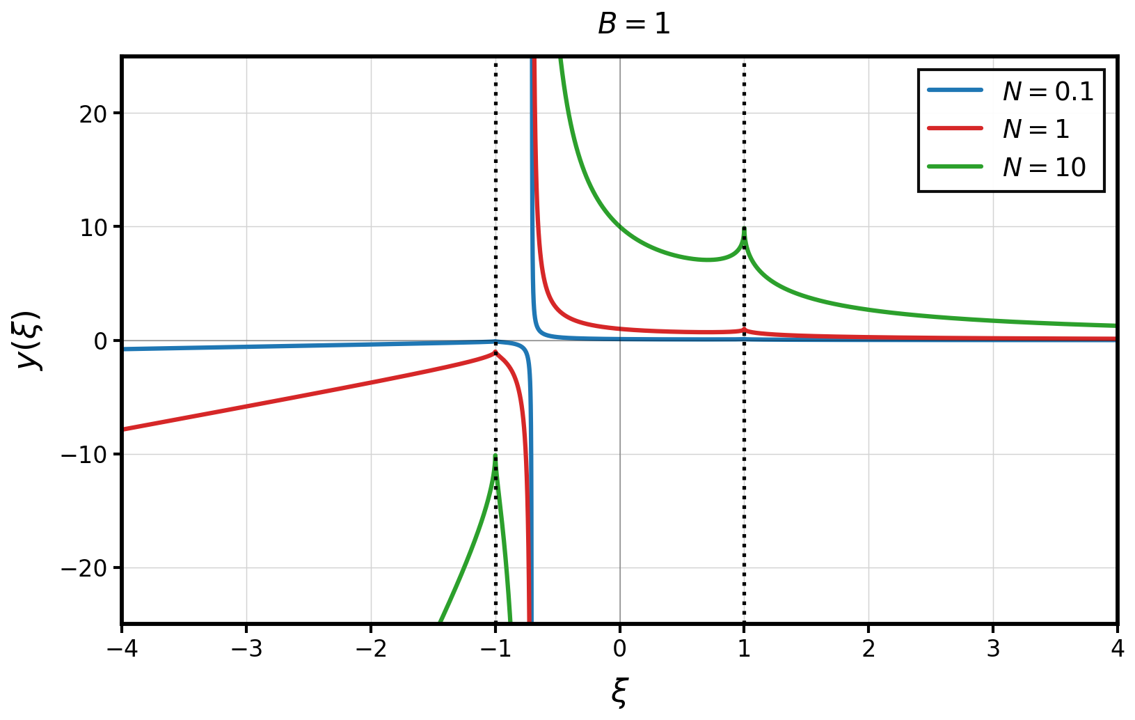
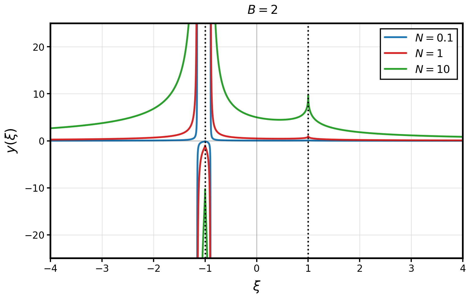
where is an arbitrary constant and we have employed . Its profile is illustrated in Fig. 1 for two sample values of and . These correspond to different input choices of . At , a cusp in the solution appears. For , the trajectory shows a definite tilt away from the negative -axis in contrast to the positive side, while for both and , the profile tends to overlap with both axes as asymptotes. For the other case , the solution is easily obtained by scaling .
III.2 Levinson-Smith type
Turning to 12, we see that it belongs to the following family of Levinson-Smith equations lev1 ; lev2 as given by
| (22) |
where , and and are differentiable functions of . In the present case, , and the quantities and correspond to the functions
| (23) |
One can express in the form of a total derivative, i.e., , where . Therefore, multiplying 12 by the quantity , which is basically the JLM nucci , and represents the factor , its first integral projects out as
| (24) |
The above constraint is indicative that a position-dependent mass (PDM) is at work. Written explicitly, the mass variable and the potential energy read
| (25) | |||
| (26) |
In PDM, the usual kinetic Hamiltonian, because of the ambiguity parameter-dependent contribution coming from the momentum
and mass-operator noncommutativity, gets modified. Precise operator ordering is then required to ensure the criterion of hermiticity and overall consistency of the system. Although initially pursued in condensed matter physics problems (see, for example, bast ) the field of PDM has flourished in many directions over the years (see ques1 ; ques2 . Indeed, varying mass problems have provided useful insights into new classes of phenomena that are hard to reconcile with the standard constant-mass prescription. Some of the physical problems in which the idea of PDM has been implemented include those of compositionally graded crystals geller , quantum dots serra , and liquid crystal problems barran .
In 25, for , there appears a potential singularity at x = 0, and the usual prescription requires bagchi2 to split the real axis into two halves, i.e., and , where the dynamics of the problem becomes exactly solvable for both branches. The singular mass profile has also been studied in the context of a one-dimensional crystalline lattice lima . Concerning the potential function , we see that it can also have a singular behavior at depending on the choice and sign of the parameters. The appearance of singular potentials is common in quantum mechanics: for instance, in the appearance of negative energy states and the encountering of the degeneracy problem panigrahi . On the other hand, the mass profile includes a power-law behavior for . In the literature, power representations for PDM have been studied for different contexts and their spectral signatures have been investigated mustafa .
On a level surface , where we assume , the following restriction holds
| (27) |
which can be transformed to the integral
| (28) |
where is an initial value of time.
To generate a solution that is acceptable from a physical point of view, let us focus on the simple case . Then the following form is implied
| (29) |
where we have ignored the constant of integration and applied the negative sign to ensure the positivity of both and . The above form corresponds to the standard type of solvable integral , with standing for , and where the two signs depend on whether or .
Solving 29 we get the expression
| (30) |
where since stands for the positive quantity , which incidentally corresponds to the square of the amplitude and hence stands for a kind of probability density. Thus the solution becomes regularized for large values of . It shows the existence of the well known uniformly bounded solitonic profile in which the argument is represented by a scaled variable of .
The transposed case where but is also similar. Discarding the constant of integration, we are led to the integral
| (31) |
where again the negative sign is kept. It belongs to the type , with given by . Since the parameter here is intrinsically positive for , the solution for can be easily extracted in the form
| (32) |
The solitonic profile is similar to that of 30 but with a nature for the magnitude of the amplitude and the nature of the argument.
Finally, let us remark that an exact solution to equation 12 also exists even when both and which is given by the following profile
| (33) |
A comparison with the two previous results shows that, as the parameters and vary, the nature of the amplitude changes, as well as the arguments of the solutions. The distinction is clearly unraveled in Fig., where as becomes very large, makes a gradual drop from its peak value and tends to flatten out.

IV Summary
In this paper we investigated the connections of a recently advanced NLQM scheme to systems of well known nonlinear equations that are governed by a pair of coupled first-order differential equations. Noting that these equations support
nontrivial equilibrium pints which are stable in character, we proceeded to develop a formalism that allows one to make connections to solvable nonlinear systems of Liénard and Levinson-Smith type that appear frequently in problems of physical systems while dealing with different nature of oscillations. The Levinson-Smith equation is well known to encompass the Liénard family which in the present case is typified by coefficients that preserve odd-odd symmetry.
To solve Liénard equation, we followed the procedure of transforming it to Abel’s equation and then applying an appropriate change of variable reducing it to a first-order form that is immediately tractable. Finally, we addressed another type of differential equation which has relevance to PDM system in the presence of a power-law mass profile or a singular one depending on the choice of the running parameter. Other types of related solutions that are discussed include a class of solitonic-like profiles which are obtained by suitably exploiting the condition on the level surface.
Acknowledgment:
We are very grateful to Sauvik Sen for his generous help in preparing the figures and checking the calculations.
Data-availability statement: All data supporting the findings of this study are included in the article.
Conflict of interest: The authors declare no conflict of interest.
References
- (1) S. Weinberg Phys. Rev. Lett. 62 (1989) 485
- (2) S. Weinberg Ann.Phys. (N.Y.) 194 (1989) 336
- (3) N. Gisin Helv.Phys.Acta 62 (1989) 363
- (4) N. Gisin Phys.Lett. A 143 (1990) 1
- (5) M. Czachor Found.Phys.Lett. 4 (1991) 351
- (6) M. Czachor Phys.Rev. A 57 (1998) 4122
- (7) J. Polchinski Phys.Rev.Lett. 66 (1991) 397
- (8) B. Mielnik Comments on: Weinberg’s Nonlinear Quantum Mechanics and Einstein-Podolsky-Rosen paradox, by Joseph Polchinski arXiv: 0012041v3 (2009)
- (9) S. D. H. Hsu Phys. Lett. B 872 (2026) 140053
- (10) A. Chodos and F. Cooper Phys. Scr. 98 (2023) 045227
- (11) A. Chodos and F. Cooper Symmetry 16 (2024) 887
- (12) A. Chodos and F. Cooper Symmetry 17 (2025) 1850
- (13) N. Levinson and O. K. Smith Duke Mathematical Journal 9 (1942)382–403.
- (14) N. Levinson J. Math. and Phys. 22 (1943) 41
- (15) A. Liénard Revue générale de l’électricité 23 (1928) 901
- (16) A. Liénard Revue générale de l’électricité 23 (1928) 946
- (17) M. V. Demina Int J Bifurcation and Chaos 33 (2023) 2350035
- (18) N J Doran and D Wood Optics Lett. 13 (1988) 56
- (19) J Zhou, S Sun and Z Liu App. Maths. and Comp. 161 (2005) 655
- (20) B. Bagchi, A. Ghose Choudhury and P. Guha J. Math. Phys. 56 (2015) 012105
- (21) P. Guha and A. Ghose-Choudhury Rev. Math. Phys. 25 (2013) 1330009
- (22) A. Ghose-Choudhury, P. Guha, and B. Khanra J. Math. Anal. Appl. 360 (2009) 651
- (23) E. T. Whittaker A Treatise on the Analytical Dynamics of Particles and Rigid Bodies Cambridge University Press (1988)
- (24) J. F. Cariñena, M. F. Rañada, and M. Santander J. Math. Phys. 46 (2005) 062703
- (25) G. Schmidt and A. Tondl Nonlinear Vibrations (Cambridge University Press, Cambridge), 1986
- (26) M. Lakshmanan and S. Rajasekar Nonlinear Dynamics: Integrability, Chaos and Patterns (Springer-Verlag, Heidelberg) (2003)
- (27) G. Villari and F. Zanolin Dyn. Systems and Appl. 25 (2016) 321
- (28) B. Bagchi, A. Ghosh and M. Znojil Symmetry 16 (2024) 860
- (29) B. Bagchi, A. Ghose-Choudhury, A. Ghosh and P. Guha Int. J. Theor. Phys. 64 (2025) 212
- (30) A. Ghosh, B. P. Mandal and B. Bagchi J. Math. Phys. 66 (2025) 082101
- (31) A. Ghose-Choudhurycand P. Guha Discontinuity, Nonlinearity, and Complexity 6 (2017) 65
- (32) A. D. Polyanin and V. Zaitsev Handbook of ordinary differential equations: CRC Press Inc (1995)
- (33) M C Nucci and P G L Leach J. Phys. A: Math. Gen. 37 (2004) 7743
- (34) G. Bastard Wave Mechanics Applied to Semiconductor Heterostructures, Editions de Physique, Les Ulis (1988)
- (35) B. Bagchi, A. Banerjee, C. Quesne, V.M. Tkachuk, J. Phys. A: Math. Gen. 38 (2005) 2929
- (36) C. Quesne SIGMA 5 (2009) 046
- (37) M R Geller and W Kohn Phys. Rev. Lett. 70 (1993) 3103
- (38) L Serra and E Lipparini Europhys. Lett. 40 (1997) 667
- (39) M Barranco, M Pi, S M Gatica, E S Hernández, and J Navarro Phys. Rev. B 56 (1997) 8997
- (40) F. C. E. Lima, F. M. Belchior and C. A. S. Almeida Phys Scripta 100 (2025) 015978
- (41) P. K. Panigrahi and U. P. Sukhatme Phys. Lett. A 178 (1993) 251
- (42) O. Mustafa J. Phys. A: Math. Theor. 44, (2011) 355303