Chaotic Dynamics in Extremal Black Holes: A Challenge to the Chaos Bound

The spherically symmetric black hole is considered here as a Reissner–Nordström black hole, described by the metric [40, 8],

$$ds^{2}=-f(r)dt^{2}+\frac{1}{f(r)}dr^{2}+r^{2}d\Omega^{2}~,~~~~~~~~~~~~~~\textrm{with}~~~~~~~~~~~~~~~~~~f(r)=\left(1-\frac{2M}{r}+\frac{Q^{2}}{r^{2}}\right)$$

(1)

and $M$ and $Q$ are the mass and electric charge of the black hole. The horizon radius is determined by the conditions $f(r)=0$, which yields two solutions: the outer ($r_{+}$) and the inner horizon ($r_{-}$) that are given as

$$r_{\pm}=M\pm\sqrt{M^{2}-Q^{2}}~.$$

(2)

The outer horizon is the event horizon, and the inner horizon is the Cauchy horizon. Since the Reissner-Nordström metric is spherically symmetric, the surface gravity for the event horizon can be obtained conventionally as,

$$\kappa=\frac{1}{2}f^{\prime}|_{r=r_{+}}=\frac{\sqrt{M^{2}-Q^{2}}}{r_{+}^{2}}=\frac{r_{+}-r_{-}}{2r_{+}^{2}}~.$$

(3)

The entropy of the black hole, following the Bekenstein–Hawking area law, is:

$\displaystyle S=\pi r_{+}^{2}=\pi\bigg(M+\sqrt{M^{2}-Q^{2}}\bigg)^{2}~.$

(4)

The extremal limit of the Reissner–Nordström black hole is reached when $Q=M$. The metric for an extremal black hole is given by,

$$ds^{2}=-f(r)dt^{2}+\frac{1}{f(r)}dr^{2}+r^{2}d\Omega^{2}~,~~~~~~~~~~~~~~\textrm{with}~~~~~~~~~~~~~~~~~~f(r)=\left(1-\frac{M}{r}\right)^{2}~.$$

(5)

In this case:

• •

  The two horizons for a Reissner–Nordström black hole coincide, that is, $r_{+}=r_{-}=M$.

• •

  The surface gravity, or the Hawking temperature, vanishes.

• •

  Yet, the entropy remains finite and non-zero: $S=\pi M^{2}=\pi r_{+}^{2}$.

The extremal case lies on the boundary between physical black holes and naked singularities, and represents a highly symmetric and stable configuration in both classical and quantum contexts.

The axisymmetric and rotating black hole is considered here as a Kerr black hole, described by the metric in Boyer-Lindquist coordinates [29, 49, 51],

$\displaystyle ds^{2}=-\left(1-\frac{2Mr}{\Sigma}\right)dt^{2}-\frac{4Mar\sin^{2}\theta}{\Sigma}dt\,d\phi+\frac{\Sigma}{\Delta}dr^{2}+\Sigma\,d\theta^{2}+\left(r^{2}+a^{2}+\frac{2Ma^{2}r\sin^{2}\theta}{\Sigma}\right)\sin^{2}\theta\,d\phi^{2}$

(6)

where

$\displaystyle\Sigma=r^{2}+a^{2}\cos^{2}\theta,\qquad\qquad\ \Delta=r^{2}-2Mr+a^{2}~.$

(7)

Here $M$ is the mass of the black hole, $a=J/M$ is the spin parameter (angular momentum per unit mass). The horizons (outer, inner) are determined by $\Delta=0$ and the horizons (event horizon $r_{+}$ and the inner Cauchy horizon $r_{-}$) are given as

$\displaystyle r_{\pm}=M\pm\sqrt{M^{2}-a^{2}}~.$

(8)

The Hawking temperature of the Kerr black hole is given as

$\displaystyle T=\frac{\kappa}{2\pi}~~~~~~~~~~~~~~~~\textrm{where}~~~~~~~~~~~~~~~~\kappa=\frac{r_{+}-r_{-}}{2(r_{+}^{2}+a^{2})}~.$

(9)

The entropy of the black hole is given as

$\displaystyle S=\pi(r_{+}^{2}+a^{2})~.$

(10)

In the extremal limit, where $a\rightarrow M$, one finds that the two horizons coincide: $r_{+}=r_{-}=M$. The spacetime metric of the Kerr black hole in the extremal limit is given as

	$\displaystyle ds^{2}$	$\displaystyle=-\left(1-\frac{2Mr}{\Sigma}\right)dt^{2}-\frac{4M^{2}r\sin^{2}\theta}{\Sigma}\,dt\,d\phi+\frac{\Sigma}{(r-M)^{2}}\,dr^{2}$
		$\displaystyle+\Sigma\,d\theta^{2}+\left(r^{2}+M^{2}+\frac{2M^{3}r\sin^{2}\theta}{\Sigma}\right)\sin^{2}\theta\,d\phi^{2}$		(11)

with

$\displaystyle\Sigma=r^{2}+M^{2}\cos^{2}\theta~.$

(12)

In that case, Hawking temperature again vanishes, yet entropy remains a non-zero vanishing quantity $S=2\pi M^{2}$. Thus, as in the Reissner–Nordström case, the extremal Kerr black hole challenges standard thermodynamic expectations by exhibiting zero temperature with non-zero entropy.

As discussed in the previous subsections, the Hawking temperature vanishes for all extremal black holes, while the entropy remains a finite, non-zero quantity. This apparently contradicts conventional thermodynamic intuition, leading to two contrasting viewpoints in the literature.

1. 1.

   The transition from nonextremal to extremal is continuous [2, 17, 1, 34, 30, 4], and extremal black holes can have truly non-zero entropy despite vanishing temperature due to specific underlying microstates. As shown in the seminal work of Strominger and Vafa [45], certain black holes correspond to the bound state of branes that can be attributed to a large degeneracy of BPS microstates, which yields a statistically significant entropy. This provides the explanations why the extremal black holes can have finite entropy, which originates from the underlying microscopic description and is independent of their thermal considerations.

2. 2.

   The transition from nonextremal to extremal black holes is not continuous. Consequently, extremal black holes should be treated as qualitatively distinct objects, and their thermodynamics should not be obtained merely by taking the extremal limit in the final result, originally obtained for the nonextremal black holes. Very recently, it has been demonstrated that when one carefully analyzes the near-horizon geometry of an extremal black hole, specifically by expanding the metric near the horizon up to second order, it leads to a surprising result: the temperature of the extremal black hole is no longer exactly zero. This finding challenges the conventional wisdom that extremal black holes are strictly zero-temperature objects and suggests a more subtle thermodynamic behavior in the extremal limit [38]. This result is also consistent with the previous finding that the Hawking temperature of an extremal black hole is completely arbitrary [18]. In this view, results derived for nonextremal black holes cannot simply be extrapolated to the extremal case by taking the extremal limit. This perspective has substantial support, particularly from topological and thermodynamic analyses [20, 26, 48, 42]. If correct, this implies that the conventional method of deriving temperature and entropy for nonextremal black holes and then taking the extremal limit is invalid.

Given these contrasting viewpoints, we aim to investigate whether the chaotic dynamics of an extremal black hole can be obtained as the limiting case of a non-extremal one. If this proves possible, as we shall demonstrate in the following analysis, then the situation becomes even more intriguing, as it hints at the possibility of obtaining results for extremal BHs via extrapolating the results of a near-extremal BH. As discussed earlier, the Hawking temperature of an extremal black hole vanishes when extrapolated from the non-extremal result. Consequently, if one extrapolates the Maldacena–Shenker–Stanford (MSS) bound to the extremal case, the Lyapunov exponent would be expected to become negative. However, what we find is that, although the chaotic dynamics of the extremal case can indeed be obtained as the limit of near-extremal black holes (with the Lyapunov exponent matching in both cases), the exponent remains positive. Thus, the MSS bound is violated in the extremal limit.

In the following, we present the dynamics of massless particles. Subsequently, we explore their behavior in the backgrounds of Reissner-Nordström and Kerr black hole spacetimes.

In this part, we summarize the dynamic equations of motion of a massless particle in a Reissner-Nordström (RN) black hole spacetime. In order to find the energy of the particle $E=-\zeta^{\alpha}p_{a}$ (where $\zeta^{\alpha}$ is the Killing vector and $p_{\alpha}$) is the particle’s four-momentum), we use the covariant form of the dispersion relation given by

$$g^{\alpha\beta}p_{\alpha}p_{\beta}=-m^{2}c^{2}~,$$

(13)

with $m$, being the mass of the particle. Now, using the dispersion relation 13 (with $c=1$) for the metric 1, we can get the energy of a massless particle ($m=0$) as follows (considering the +ve sign solution of $E$):

$$E=\sqrt{f(r)\Big[f(r)p_{r}^{2}+\dfrac{p_{\theta}^{2}}{r^{2}}\Big]}~,$$

(14)

where we have assumed the motion of the particle is in the poloidal plane with $p_{\phi}=0$.

Now, let us construct the dynamical equations of motion for a probe massless particle moving in the background geometry of the RN black hole. To prevent particle trajectories from crossing the horizon, we introduce harmonic confinement along the radial ($r$) and angular ($\theta$) directions, characterized by oscillator strengths $K_{r}$ and $K_{\theta}$, respectively. Adjusting these strengths allows particle trajectories to be confined within any desired finite region. The harmonic oscillators along radial and angular directions represent an external potential chosen explicitly for confinement purposes, and are not derived from any intrinsic physical property of the black hole background. Their role is crucial in this context because they ensure numerical stability, enabling the detailed investigation of particle dynamics near the horizon. Importantly, these harmonic potentials are explicitly static, do not introduce any external energy sources, or impose any time-dependent perturbations. Their sole purpose is to provide a stable equilibrium situation, ensuring the particle remains within a well-defined region for numerical analysis. Thus, any observed chaotic dynamics or instabilities are fundamentally gravitational in origin, driven by the intrinsic properties of the spacetime near the horizon rather than induced artificially.

We thus examine a scenario where a probe massless particle is subjected to two harmonic potentials, given by $\frac{1}{2}K_{r}(r-r_{c})^{2}$ and $\frac{1}{2}K_{\theta}(y-y_{c})^{2}$, along the radial and angular directions, respectively. Here, $K_{r}$ and $K_{\theta}$ denote the oscillator strengths in the radial and angular directions (while writing the dynamical equations, we introduce a new variable $y=r_{+}\theta$). The equilibrium positions of these harmonic potentials are denoted as $r_{c}$ and $y_{c}$. This modeling approach has previously been suggested in the literature (Ref. [25] for massive particles, and Refs. [10, 12, 3] for massless particles). It should be emphasized that replacing these harmonic potentials with alternative potentials could modify the particle dynamics. However, as discussed extensively in Ref. [10, 12], for massless particles, the radial motion remains unaffected by changes to the specific form of the potential.

Now the total energy of the probe particle under the influence of harmonic potentials for the metric (1) is given by

$\displaystyle E_{\text{RN}}=\sqrt{f(r)\Big[f(r)p_{r}^{2}+\dfrac{p_{\theta}^{2}}{r^{2}}\Big]}+\frac{1}{2}K_{r}(r-r_{0})^{2}+\frac{1}{2}K_{\theta}~r^{2}_{+}(\theta-\theta_{0})^{2}~.$

(15)

Let us note that the radial momenta $p_{r}$ and cross radial momenta $p_{\theta}$, which appear in the above energy expression, are the usual canonical momenta that can be derived from the Lagrangian of a massless particle in the Schwarzwald coordinate system.

Correspondingly, the dynamical equations of motion have the following form:

	$\displaystyle\dot{r}$	$\displaystyle=$	$\displaystyle\dfrac{\partial E_{\text{RN}}}{\partial p_{r}}=\frac{f^{2}(r)p_{r}}{\sqrt{f^{2}(r)p_{r}^{2}+\dfrac{f(r)p_{\theta}^{2}}{r^{2}}}}~,$		(16)
	$\displaystyle\dot{p_{r}}$	$\displaystyle=$	$\displaystyle-\frac{\partial E_{\text{RN}}}{\partial r}=-\dfrac{f(r)f^{\prime}(r)p_{r}^{2}}{\sqrt{f^{2}(r)p_{r}^{2}+\dfrac{f(r)p_{\theta}^{2}}{r^{2}}}}-K_{r}(r-r_{0})$
			$\displaystyle-\dfrac{f^{\prime}(r)p_{\theta}^{2}}{2r^{2}\sqrt{f^{2}(r)p_{r}^{2}+\dfrac{f(r)p_{\theta}^{2}}{r^{2}}}}+\dfrac{f(r)p_{\theta}^{2}}{r^{3}\sqrt{f^{2}(r)p_{r}^{2}+\dfrac{f(r)p_{\theta}^{2}}{r^{2}}}}~,$
	$\displaystyle\dot{\theta}$	$\displaystyle=$	$\displaystyle\frac{\partial E_{\text{RN}}}{\partial p_{\theta}}=\dfrac{f(r)p_{\theta}}{r^{2}\sqrt{f^{2}(r)p_{r}^{2}+\dfrac{f(r)p_{\theta}^{2}}{r^{2}}}}~,$		(18)
	$\displaystyle\dot{p_{\theta}}$	$\displaystyle=$	$\displaystyle-\frac{\partial E_{\text{RN}}}{\partial\theta}=-K_{\theta}~r^{2}_{+}(\theta-\theta_{0})~.$		(19)

where the derivative is taken with respect to an affine parameter $\tau$. These are the main equations for the studies of Lyapunov exponents in the later sections for the RN black hole.

In a similar way, we shall summarize the dynamical equations of motion of a massless particle in a Kerr black hole spacetime in this part. Using the dispersion relation, we find the energy of the massless particle in the Kerr background (6) as (considering the +ve sign solution of $E$):

$$E=\sqrt{\frac{2\Delta^{2}p_{r}^{2}+2\Delta\Sigma p_{\theta}^{2}}{\Sigma\left[a^{4}+2r^{4}+a^{2}r(2M+3r)+a^{2}\Delta\cos 2\theta\right]}}~.$$

(20)

Here also, we have assumed that the particle is moving only along the radial $r$ and the angular $\theta$ directions, keeping $p_{\phi}=0$.

Now, introducing the harmonic potentials just like the earlier section, we get the total energy of the system as:

$$E_{\text{Kerr}}=\sqrt{\frac{2\Delta^{2}p_{r}^{2}+2\Delta\Sigma p_{\theta}^{2}}{\Sigma\left[a^{4}+2r^{4}+a^{2}r(2M+3r)+a^{2}\Delta\cos 2\theta\right]}}+\frac{1}{2}K_{r}(r-r_{c})^{2}+\frac{1}{2}K_{\theta}~r^{2}_{+}(\theta-\theta_{c})^{2}~.$$

(21)

Correspondingly, the dynamical equations of motion are as follows:

	$\displaystyle\dot{r}=\dfrac{\partial E_{\text{Kerr}}}{\partial p_{r}}=\frac{\Delta\,p_{r}\left(a^{2}+r^{2}\right)\left(a^{2}+r^{2}+a^{2}\cos 2\theta\right)}{\Sigma^{2}\sqrt{\frac{\Delta\,p_{r}^{2}}{\Sigma}+\frac{p_{\theta}^{2}}{\Sigma^{2}}\frac{\left(a^{2}+r^{2}\right)^{2}-a^{2}\Delta\sin^{2}\theta}{\sin^{2}\theta}}}~,$		(22)
	$\displaystyle\dot{p_{r}}=-\dfrac{\partial E_{\text{Kerr}}}{\partial r}=-\frac{1}{2E}\Biggl[\frac{\partial}{\partial r}\left(\frac{\Delta}{\Sigma^{2}}\right)p_{r}^{2}+\frac{\partial}{\partial r}\left(\frac{1}{\Sigma}\right)p_{\theta}^{2}$
	$\displaystyle~~~~~~~-\frac{\partial}{\partial r}\left(\frac{a^{4}+2r^{4}+a^{2}r(2M+3r)+a^{2}\Delta\cos(2\theta)}{2\,\Delta\,\Sigma}\right)\frac{2\Delta^{2}p_{r}^{2}+2\Delta\Sigma p_{\theta}^{2}}{\Sigma\left[a^{4}+2r^{4}+a^{2}r(2M+3r)+a^{2}\Delta cos2\theta\right]}\Biggr]$
	$\displaystyle~~~~~~~-K_{r}(r-r_{c})~,$		(23)
	$\displaystyle\dot{\theta}=\frac{2p_{\theta}\sqrt{\Delta}}{\Sigma\sqrt{p_{\theta}^{2}+2p_{r}^{2}}}~,$		(24)
	$\displaystyle\dot{p_{\theta}}=-\frac{1}{2E}\frac{\partial}{\partial\theta}\left(\frac{2\Delta^{2}p_{r}^{2}+2\Delta\Sigma p_{\theta}^{2}}{\Sigma[a^{4}+2r^{4}+a^{2}r(2M+3r)+a^{2}\Delta\cos 2\theta]}\right)-K_{\theta}~r^{2}_{+}(\theta-\theta_{c})~.$		(25)

These are the equations which will be used to study the Lyapunov exponents in the later sections.

We begin by analyzing the Lyapunov exponent (LE) for the motion of a massless particle in the Reissner–Nordström (RN) black hole background, focusing on how it varies with the black hole’s charge. From the horizon structure of the RN black hole (8), it is evident that increasing the charge $Q$ leads to a decrease in the radius of the outer horizon $r_{+}$. We solve the associated dynamical equations of motion [refer to 16, LABEL:3.5, 18, and 19], employing the Runge-Kutta fourth-order scheme. The initial conditions for $r,p_{r}$ and $\theta$ are chosen as $3.5,20.0$ and $0.0$ respectively, and the initial condition for $p_{\theta}$ is determined from the constant value of the system energy $E=50$. The other parameter values are chosen as $K_{r}=100$, $K_{\theta}=25$, $\theta_{c}=0$, and $r_{c}=4.3$ and mass of the RN black hole as $M=1.0$.

1 illustrates the behavior of the largest Lyapunov exponent for RN black holes with varying charges: $Q=0.4,0.5,0.6,0.8,0.9$, as the system approaches the extremal limit at $Q=1.0$. Initially, the Lyapunov exponents exhibit fluctuations but eventually settle to some saturation values. Notably, as the charge increases toward extremality, these saturation values gradually decrease (for $Q=0.6,0.8$ and $0.9$, the largest LE values are respectively $0.027580,0.023793$ and $0.024924$), ultimately reaching approximately $0.015380$ in the extremal case ($Q=M=1.0$). These values remain well below the well-established MSS bound, except in the extremal case where the bound is violated, with the Lyapunov exponent saturating at a positive value of approximately $\sim 0.015380$.

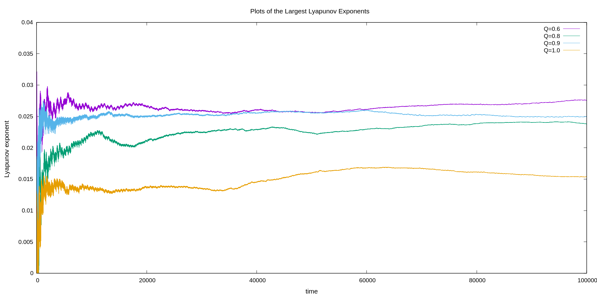
These results suggest that the motion of particles near an RN black hole becomes less chaotic as the black hole approaches the extremal limit. The drop in the Lyapunov exponent indicates that nearby particle trajectories diverge more slowly, pointing to a more stable dynamical system. In the extremal case, the chaos appears to be significantly reduced; nevertheless, a residual degree of chaos persists even though the surface gravity vanishes.

In 2, we specifically examine the extremal Reissner-Nordström black hole, characterized by the condition $Q=M=1.0$ (see the metric in 5). The Lyapunov exponent in this scenario exhibits significant fluctuations at first, but eventually settles at a moderate saturation value of 0.017518. This value is close to, but slightly higher than, the saturation value obtained when approaching extremality from the non-extremal side. The near agreement between these two approaches indicates that the extremal configuration can be viewed as a smooth continuation of the non-extremal case, with only minor quantitative differences in the chaotic indicators. Furthermore, in the extremal RN case, the Lyapunov exponent saturates at a finite positive value ($\lambda_{L}\sim 0.017519$), despite the vanishing surface gravity. This directly violates the MSS chaos bound, confirming that the extremal RN black hole follows a sustained residual chaotic dynamics beyond the expected thermodynamic limit.

Overall, these findings suggest that the motion of particles near RN black holes becomes progressively less chaotic as extremality is approached, and that the direct extremal background shares close dynamical characteristics with the near-extremal limit. Importantly, in all cases, the saturation values remain small compared to the MSS chaos bound, although the extremal case still demonstrates residual chaotic features despite the vanishing surface gravity. Therefore, it indicates one particular fact that extremal RN black holes are constituted with qualitatively distinct dynamical configurations from the non-extremal ones, as long as we are concerned about the chaos bound in the near-horizon regime.

To further substantiate the presence of chaotic behavior in the Reissner–Nordström background and to complement the Lyapunov exponent analysis presented earlier, we now study the Poincaré sections of the system. The Poincaré map serves as a powerful diagnostic tool for nonlinear dynamical systems, allowing us to visualize the transition from regular to chaotic motion in the reduced phase space.

In our setup, a massless test particle moves in the RN spacetime under the influence of the total energy function given in 15, which includes harmonic confinement terms along both the radial and angular directions. The inclusion of these harmonic terms ensures bounded motion of the particle, allowing us to probe the near-horizon dynamics over long evolution times without the trajectory escaping to infinity. As discussed earlier, these confining potentials are static and non-dissipative, serving solely as a numerical device to stabilize the orbits and to map the intrinsic gravitationally induced instabilities near the horizon. The same approach has been widely employed in previous analyses of horizon-induced chaos [25, 10, 12, 3, 15].

We numerically integrate the coupled equations of motion [16-19] using a fourth-order Runge–Kutta method with a fixed step size $h=0.01$. The parameters are set to $M=1.0$, $K_{r}=100$, $K_{\theta}=25$, $r_{0}=4.3$, and $\theta_{c}=0$. The initial conditions for the variables are chosen as $r=3.5$, $p_{r}=20.0$, and $\theta=0.0$, while $p_{\theta}$ is determined from the constant total energy $E=50$. For each black hole charge $Q$, we solve the system for a large number of random initial conditions in a small neighborhood of the reference point to ensure a representative sampling of the accessible phase space.

The Poincaré map is constructed by recording $(r,p_{r})$ whenever the trajectory crosses $\theta=0$ with $p_{\theta}>0$ (single orientation). Regular motion produces smooth KAM tori, whereas chaotic motion yields distorted or broken tori and scattered points.

3 shows the sections for $Q=0.6,\,0.8,\,0.9,\,1.0$ where increasing $Q$ moves the relevant horizon farther from the harmonic oscillator center $r_{0}$. Consistently, the phase-space structures regularize with growing $Q$: for $Q=0.6$ one observes noticeable torus distortions and scattered points near the outer lobes, while for $Q=0.8$ and $Q=0.9$ the broken tori progressively heal and the islands sharpen. At the extremal value $Q=1.0$, the section is dominated by nested, smooth tori around $r_{0}$, with only sparse remnants of irregularity. This trend corroborates the Lyapunov-exponent behavior reported above: as the horizon recedes from the bounded integrable core, near-horizon nonlinearity weakens and the dynamics revert toward quasi-integrable motion.

The dynamical equations of motion [refer to 22, 23, 24, and 25] are numerically solved employing the Runge-Kutta fourth-order scheme, keeping all the initial conditions and the parameter values the same as in the earlier section.

In 4, we show how the largest Lyapunov exponent evolves over time for Kerr black holes (see the metric in 6) with different rotation parameters: $a=0.1,0.5,0.6,0.8,0.9$, and the extremal limit $a=1.0$. For the nonextremal scenarios ($a<1.0$), the Lyapunov exponent initially fluctuates but then settles down to specific saturation values. As the rotation parameter increases and becomes closer to the extremal limit, these saturation values steadily increase (for $a=0.1,0.5,0.6,0.8,0.9$ we get the largest LE values respectively as $-0.0002,0.0001,0.0054,0.0062,0.0085$) which still respects the MSS bound but at the extremal limit ($a=M=1.0$) this value saturates at 0.0095 which clearly violates the MSS bound in this scenario. This clearly means that chaotic behavior gets stronger as the black hole spins faster. This trend suggests that rotation acts as a destabilizing factor in the dynamics of test particles near the Kerr black hole. Moreover, the monotonic growth of the Lyapunov exponent with increasing spin indicates a direct link between rotational energy and the system’s sensitivity to initial conditions.

These findings reinforce the idea that rotation amplifies dynamical instability in black hole spacetimes. Unlike the RN case, where chaos diminishes as extremality is approached, the Kerr scenario demonstrates that extremality, achieved through angular momentum, enhances chaos. This distinction highlights the fundamentally different roles played by electric charge and angular momentum in governing the dynamics of spacetime.

In 5, we specifically examine the extremal Kerr black hole case (see the metric in 2.2), characterized by the condition $a=M=1.0$. After significant initial fluctuations, the Lyapunov exponent settles to a saturation value of 0.0185. While this value is somewhat higher than the near-extremal case, the difference is moderate. Importantly, both results remain within the same order of magnitude, suggesting that the extremal configuration shares close dynamical properties with the limiting non-extremal case. However, one thing to notice here is that, in this case, the extremal Kerr black hole exhibits a finite positive Lyapunov exponent ($\lambda_{L}\sim 0.0185$), even at zero Hawking temperature, just like we have seen in the case of the extremal RN black hole in the previous section. This constitutes another clear violation of the MSS chaos bound, showing that extremal Kerr black holes support an even stronger chaotic regime than their non-extremal counterparts. Similar violations of the chaos bound have been observed in other contexts, such as for charged particle near Kerr–Newman–AdS black holes [22] and for homoclinic particle orbits in black holes with anisotropic matter fields [28]. Therefore, our analysis reveals that extremal geometry represents another universal setting in which such violations naturally occur.

Thus, unlike the RN scenario where chaos diminishes toward extremality, the Kerr case demonstrates a mild strengthening of chaotic features with increasing spin. The comparison between the near-extremal and exact extremal situations indicates continuity in behavior, with only quantitative differences in the degree of chaos. This suggests that the extremal Kerr geometry can be reasonably interpreted as a smooth extension of the non-extremal family, but with enhanced chaotic instability at exact extremality. Importantly, for the extremal Kerr black hole the Lyapunov exponent saturates at a finite positive value despite the vanishing Hawking temperature. This clear violation of the MSS chaos bound reveals that extremal black holes, whether it is a Kerr or an RN black hole, harbour a totally different dynamical structure in their near-horizon region from the maximal chaos bound perspective with respect to the non-extremal ones.

To complement the Lyapunov exponent analysis and visualize the emergence of chaos in the Kerr spacetime, we now present the corresponding Poincaré sections. The same numerical setup discussed earlier is used here. A massless test particle evolves according to the total energy function 21, which includes the static harmonic confinements along the $r$ and $\theta$ directions. These potentials ensure that the motion remains bounded, allowing for the identification of chaotic signatures in the near-horizon region over extended integration times.

The equations of motion [22-25] are solved using a fourth-order Runge-Kutta algorithm with a fixed step size $h=0.01$. Unless otherwise stated, the parameters are set as $M=1.0$, $K_{r}=100$, $K_{\theta}=25$, $r_{c}=4.3$, $\theta_{c}=0$, and the total energy $E=50$. Initial conditions are chosen as $r=3.5$, $p_{r}=20.0$, and $\theta=0.0$, while $p_{\theta}$ is obtained from the conserved energy constraint. The Poincaré map is constructed by recording $(r,p_{r})$ each time the trajectory crosses $\theta=0$ with $p_{\theta}>0$.

6 displays the resulting Poincaré sections for different values of the rotation parameter $a=0.1,0.5,0.6,0.8,0.9,$ and $1.0$. At small spin ($a=0.1$), the phase space is dominated by well-formed KAM tori, indicating nearly integrable motion. As $a$ increases to $0.5$ and $0.6$, the tori begin to distort, and isolated islands of instability appear near the outer regions of phase space. When the spin increases further to $a=0.8$ and $0.9$, the tori become progressively broken, and dense scattered points emerge, signaling the onset of chaotic dynamics. In the extremal case ($a=1.0$), the phase space becomes largely irregular, with most KAM structures destroyed and only small regular islands surviving near the center. This trend is consistent with the behavior of the Lyapunov exponents presented earlier, where higher spin enhances the system’s dynamical instability and amplifies the near-horizon nonlinear effects.

These results establish a clear correspondence between rotation and chaos: while the RN system becomes more regular as the horizon moves away from the bounded region, the Kerr system exhibits the opposite tendency, i.e. increasing spin strengthens the coupling between angular and radial motions, thereby promoting chaotic evolution.

References

- [1] (2013) Extremal Limits of Rotating Black Holes. JHEP 05, pp. 071. External Links: 1303.1756, Document Cited by: item 1.
- [2] (2007) Hawking radiation from extremal and non-extremal black holes. Phys. Rev. D 76, pp. 124010. External Links: 0710.0388, Document Cited by: item 1.
- [3] (2022-06) Quantum corrections enhance chaos: study of particle motion near a generalized schwarzschild black hole. Physics Letters B 829, pp. 137033. External Links: ISSN 0370-2693, Link, Document Cited by: §1, §3.1, §4.2.
- [4] (2019) General framework to study the extremal phase transition of black holes. Phys. Rev. D 99 (12), pp. 124047. External Links: 1903.03434, Document Cited by: item 1.
- [5] (1992) Chaos around a black hole. Class. Quant. Grav. 9, pp. 2573–2599. Cited by: §1.
- [6] (2009) Extremal limits and black hole entropy. JHEP 11, pp. 109. External Links: 0901.0931, Document Cited by: §1.
- [7] (2010) Hidden Conformal Symmetry of the Kerr Black Hole. Phys. Rev. D 82, pp. 024008. External Links: 1004.0996, Document Cited by: §1.
- [8] (1983) The mathematical theory of black holes. 1ST edition, The International series of monographs on physics 69, Vol. , Clarendon Press; Oxford University Press. External Links: ISBN 0198512910,9780198512912, Link Cited by: §2.1.
- [9] (1997) The Black hole and the pea. Phys. Rev. D 56, pp. 1903–1907. Cited by: §1.
- [10] (2019) Presence of horizon makes particle motion chaotic. Phys. Lett. B 788, pp. 486–493. External Links: 1803.06527 Cited by: §1, §3.1, §4.2.
- [11] (2020-08) Horizon induces instability locally and creates quantum thermality. Physical Review D 102 (4). External Links: ISSN 2470-0029, Link, Document Cited by: §1.
- [12] (2020) Induction of chaotic fluctuations in particle dynamics in a uniformly accelerated frame. Int. J. Mod. Phys. A 35 (18), pp. 2050081. External Links: 1904.11760 Cited by: §1, §3.1, §4.2.
- [13] (2020-12) Near-horizon local instability and quantum thermality. Physical Review D 102 (12). External Links: ISSN 2470-0029, Link, Document Cited by: §1.
- [14] (2022-03) Horizon thermalization of kerr black hole through local instability. Physics Letters B 826, pp. 136899. External Links: ISSN 0370-2693, Link, Document Cited by: §1.
- [15] (2024-12) Near-horizon chaos beyond einstein gravity. Physical Review D 110 (12). External Links: ISSN 2470-0029, Link, Document Cited by: §1, §4.2.
- [16] (2000) Chaos and fractals in geodesic motions around a nonrotating black hole with an external halo. Phys. Rev. E 61, pp. 6506–6516. External Links: chao-dyn/9910035 Cited by: §1.
- [17] (2011) Non-extremal black holes of N=2, d=4 supergravity. JHEP 07, pp. 041. External Links: 1105.3311, Document Cited by: item 1.
- [18] (1995-07) Temperatures of extremal black holes. External Links: gr-qc/9507032 Cited by: §1, item 2.
- [19] (2022) Chaotic Motion near Black Hole and Cosmological Horizons. Fortsch. Phys. 70 (1), pp. 2200001. External Links: 2112.02081, Document Cited by: §1.
- [20] (1995) Topology, entropy and Witten index of dilaton black holes. Phys. Rev. D 51, pp. 2839–2862. External Links: hep-th/9407118, Document Cited by: §1, item 2.
- [21] (2009) The Kerr/CFT Correspondence. Phys. Rev. D 80, pp. 124008. External Links: 0809.4266, Document Cited by: §1.
- [22] (2022) Violation of bound on chaos for charged probe in Kerr-Newman-AdS black hole. JHEP 09, pp. 026. External Links: 2203.07298, Document Cited by: §4.3, §5.
- [23] (2008) Chaos and dynamics of spinning particles in Kerr spacetime. Gen. Rel. Grav. 40, pp. 1831–1847. External Links: 1006.2229 Cited by: §1.
- [24] (2003) Dynamics of spinning test particles in Kerr space-time. Phys. Rev. D 67, pp. 024005. External Links: gr-qc/0210042 Cited by: §1.
- [25] (2017) Universality in Chaos of Particle Motion near Black Hole Horizon. Phys. Rev. D 95 (2), pp. 024007. External Links: 1610.06070 Cited by: §1, §3.1, §4.2, §4.
- [26] (1995) Entropy, Area, and black hole pairs. Phys. Rev. D 51, pp. 4302–4314. External Links: gr-qc/9409013, Document Cited by: item 2.
- [27] (2013) Geometric aspects of Extremal Kerr black hole entropy. J. Mod. Phys. 4, pp. 357. External Links: 1511.00594, Document Cited by: §1.
- [28] (2023) Homoclinic orbit and the violation of the chaos bound around a black hole with anisotropic matter fields. Phys. Rev. D 107 (10), pp. 104037. External Links: 2301.12198, Document Cited by: §4.3, §5.
- [29] (2007-06) Discovering the Kerr and Kerr-Schild metrics. In Kerr Fest: Black Holes in Astrophysics, General Relativity and Quantum Gravity, External Links: 0706.1109 Cited by: §2.2.
- [30] (1999) Hamiltonian evolution and quantization for extremal black holes. Annalen Phys. 8, pp. 67–81. External Links: gr-qc/9809005, Document Cited by: item 1.
- [31] (2020) Rotating black holes with an anisotropic matter field. Phys. Rev. D 101 (6), pp. 064067. External Links: 1912.09709, Document Cited by: §5.
- [32] (2024) Charged rotating black hole with an anisotropic matter field: Solution of the Maxwell field. AIP Conf. Proc. 2874 (1), pp. 020008. External Links: 2112.04131, Document Cited by: §5.
- [33] (2025) Dressing rotating black holes with anisotropic matter. Eur. Phys. J. C 85 (11), pp. 1245. External Links: 2503.06961, Document Cited by: §5.
- [34] (2011) Entropy of extremal black holes from entropy of quasiblack holes. Phys. Lett. B 695, pp. 37–40. External Links: 1011.2768, Document Cited by: item 1.
- [35] (2019) Chaotic motion of neutral and charged particles in a magnetized Ernst-Schwarzschild spacetime. Eur. Phys. J. Plus 134 (3), pp. 96. External Links: 1803.02119 Cited by: §1.
- [36] (2002) AdS / CFT duality and the black hole information paradox. Nucl. Phys. B 623, pp. 342–394. External Links: hep-th/0109154, Document Cited by: §1.
- [37] (2016-08) A bound on chaos. Journal of High Energy Physics 2016 (8). External Links: ISSN 1029-8479, Link, Document Cited by: §1, §4.
- [38] (2022) Hawking radiation as quantum mechanical reflection. Gen. Rel. Grav. 54 (10), pp. 120. External Links: 2203.06588, Document Cited by: §1, item 2.
- [39] (2013) Extremal Limits and Kerr Spacetime. Eur. Phys. J. C 73 (6), pp. 2470. External Links: 1108.2333, Document Cited by: §1.
- [40] (1916-01) Über die Eigengravitation des elektrischen Feldes nach der Einsteinschen Theorie. Zenodo. External Links: Document, Link Cited by: §2.1.
- [41] (1996-01) Numerical calculation of lyapunov exponents. Math. J. 6, pp. . Cited by: §4.
- [42] (2009) Quantum Entropy Function from AdS(2)/CFT(1) Correspondence. Int. J. Mod. Phys. A 24, pp. 4225–4244. External Links: 0809.3304, Document Cited by: §1, item 2.
- [43] (1996) Chaos in static axisymmetric space-times. 1: Vacuum case. Class. Quant. Grav. 13, pp. 1241–1260. External Links: gr-qc/9505036 Cited by: §1.
- [44] (1994) Nonlinear dynamics and chaos: with applications to physics, biology, chemistry, and engineering. edition, Studies in nonlinearity, Vol. , Addison-Wesley Pub. External Links: ISBN 0201543443,9780201543445,9780738204536,0738204536, Link Cited by: §4.
- [45] (1996) Microscopic origin of the Bekenstein-Hawking entropy. Phys. Lett. B 379, pp. 99–104. External Links: hep-th/9601029, Document Cited by: §1, item 1.
- [46] (1997) Chaos in Schwarzschild space-time: The motion of a spinning particle. Phys. Rev. D 55, pp. 4848–4859. External Links: gr-qc/9604020 Cited by: §1.
- [47] (2009) Chaotic motion of Charged Particles in an Electromagnetic Field Surrounding a Rotating Black Hole. Astrophys. J. 693, pp. 472–485. External Links: 0807.0277 Cited by: §1.
- [48] (1995) Action and entropy of extreme and nonextreme black holes. Phys. Rev. D 51, pp. 4315. Note: [Erratum: Phys.Rev.D 52, 6201 (1995)] External Links: hep-th/9410103, Document Cited by: item 2.
- [49] (2015) The Kerr Metric. Class. Quant. Grav. 32 (12), pp. 124006. External Links: 1410.2130, Document Cited by: §2.2.
- [50] (1996) Chaos around a Henon-Heiles inspired exact perturbation of a black hole. Phys. Rev. Lett. 76, pp. 1409–1412. External Links: gr-qc/9604037 Cited by: §1.
- [51] (2007-06) The Kerr spacetime: A Brief introduction. In Kerr Fest: Black Holes in Astrophysics, General Relativity and Quantum Gravity, External Links: 0706.0622 Cited by: §2.2.