Angle dependent dose transformer algorithm for fast proton therapy dose calculations
Abstract
Background: Accurate 3D dose calculation for Pencil Beam Scanning Proton Therapy (PBSPT) is typically performed using Monte Carlo (MC) dose engines. Although these engines represent the gold standard in terms of quality, their high computation time remains a bottleneck, especially for adaptive workflows and tasks that require repeated execution. Recently, deep learning models have been successfully proposed for fast and accurate 3D dose calculation.
Purpose and Methods: We address a critical limitation of existing proton dose calculation deep learning models: the requirement for orthogonality between proton rays and the CT grid, which necessitates computationally expensive beamlet-wise 3D grid reinterpolation. To overcome this, we propose the Angle-dependent Dose Transformer Algorithm (ADoTA), which augments the dose engine with an additional input channel encoding a fast analytical beamlet shape projection, thereby providing explicit beam direction information without grid rotation. The model was trained on CT data from 108 patients to predict beamlet dose distributions for initial energies ranging from to over an field, and evaluated on an independent, non-overlapping test cohort of 50 patients.
Results: The performance of our model is comparable to state-of-the-art methods found in literature. On the independent test set, our model achieved high gamma pass rates of (mean standard deviation) and in thoracic and abdominal/pelvic anatomical sites, respectively. Single beamlet inference was performed in . Furthermore, by introducing the fast beamlet shape projection, the time required for end-to-end 3D dose distribution calculation was reduced by compared to the fastest published methods requiring grid reinterpolation. On full treatment plans, the model achieved strong results for lung () and prostate () plans, measured as gamma pass rate with a 10% dose cut-off.
Conclusions: We introduce an beamlet angle-aware deep learning proton dose engine that eliminates the need for beamlet-specific grid reinterpolation by encoding beam direction through an analytical projection, substantially reducing computational overhead while preserving Monte Carlo–level dosimetric accuracy across heterogeneous anatomies.
Keywords: deep learning-based dose calculation, pencil beam scanning proton therapy, dose calculation, deep learning.
1 Introduction
Accurate calculation of the three-dimensional dose distribution is fundamental to the efficacy and safety of radiotherapy (RT) and is particularly critical in Pencil Beam Scanning Proton Therapy (PBSPT), where the steep dose gradients and range sensitivity inherent to proton beams demand precise modeling of energy deposition (Lomax2008IntensityUncertainties). In standard clinical workflows, treatment planning begins with the acquisition of a volumetric representation of the patient’s internal anatomy using Computed Tomography (CT). This CT image, combined with radiologist-defined anatomical delineations and therapeutic objectives set by the radiation oncologist, forms the basis of an individualized treatment plan (TP). The dose distribution is constructed from the cumulative contribution of a large number of narrow proton beamlets, each modulated in energy and direction to conform the dose to the target volume while sparing adjacent healthy tissues.
The accuracy of the calculated 3D dose distribution in PBSPT is particularly important due to its high sensitivity to anatomical heterogeneities, as well as range and setup errors (Malyapa2016EvaluationTherapy; Unkelbach2009ReducingPlanning; Schuemann2014Site-specificTherapy; PaganettiH2012_uncertainties). Clinically accurate dose estimation typically relies on Monte Carlo (MC) simulations, which explicitly model stochastic interactions of protons with patient-specific heterogeneous media represented by the CT image (Pereira2014TheFuture). Nevertheless, high accuracy comes with high computational cost (Keyvan2011ReviewPlanning), resulting in significant computation time (e.g., per beamlet for particles (Pastor-Serrano2022MillisecondAccuracy)). Faster, yet still accurate calculation of the 3D dose deposited by proton beamlets is important across multiple aspects of PBSPT. First, from the on-line adaptive point of view, fast and accurate dose calculation could be incorporated into the adaptive treatment planning workflow (Albertini2024). Second, robust treatment planning requires multiple scenarios (Unkelbach2018Robust1; Fredriksson2011MinimaxTherapy), which requires obtaining a large number of 3D dose distributions based on which robust plans can be prepared. Third, fast beamlet dose calculation is essential for accelerating the construction of the dose influence matrix , which encodes the dose contribution of beamlet to voxel and constitutes the core input for inverse planning and robust optimization. Since modern PBSPT treatment plans comprise thousands of beamlets and often require repeated recomputation of under multiple uncertainty scenarios, its calculation represents a dominant computational bottleneck in both planning and adaptive workflows.
Currently, the Pencil Beam Algorithm (PBA) is utilized as a fast dose engine for planning and optimization (Hong1996). However, PBA performance deteriorates in heterogeneous media, in particular in thoracic anatomical sites and head-and-neck regions (TaylorPA2017). To address the limitations of the PBA, several works have been performed. Bortfeld1997AnBeams proposed an analytical approximation of the Bragg curve in closed form, limiting its applicability to proton beamlets with initial energies between and MeV. Szymanowski2002Two-dimensionalMedia addressed the issue of deteriorated performance in heterogenous media by introducing additional scaling of the lateral proton fluence. Soukup2005ASimulations proposed an improvement to the PBA by fitting the MC results to effectively model nuclear interactions. Furthermore, daSilva2015FastModel extended the PBA using a double-Gaussian beam model to better account for the low-dose halo; notably, this work was also implemented on a Graphics Processing Unit (GPU). Recently, a GPU version of PBA implemented solely for the CUDA framework (NickollsScalablePROGRAMMING) was proposed by Bhattacharya2025ACalculation. Alongside published improvements of PBA, efforts have been made to utilize MC-like algorithms on GPUs, driven by the growing interest in hardware acceleration (XunJia2012; WenChanetal; Gajewski2021; MaJ2014; WanChanTseung2014ASimulation). Although GPU-based MC offers significant acceleration of the proton 3D dose distribution, the need for faster, sub-second methods remains. In recent years, deep learning models have shown great potential to play an important role in near real-time 3D dose distribution calculation.
The application of deep learning to proton dose calculation has expanded rapidly, although early efforts largely focused on surrogate tasks rather than direct physics-based dose computation. Initial studies employed 3D Convolutional Neural Networks (CNNs), such as U-Net–like architectures, either to denoise Monte Carlo–calculated dose distributions using noisy MC dose as input (Javaid2021DenoisingStudy), or to predict clinically acceptable plan doses from CT images and structure sets (Kearney2018DoseNet:Networks). While effective in their respective contexts, these approaches do not constitute true dose engines, as they either post-process MC-calculated dose or predict clinically acceptable dose distributions without explicitly modeling proton transport from patient geometry. More recent research has therefore shifted toward beamlet-level dose calculation models that explicitly aim to learn the underlying physics of proton transport. One of the first works to apply neural networks specifically for single proton beamlet dose calculation was proposed by Neishabouri2021. The authors introduced an Long Short-Term Memory (LSTM) (SeppHochreiter1997LongMemory) based model to predict 3D dose distributions. Crucially, this approach casts the dose calculation problem as a sequence prediction task: as a proton beam traverses the patient, it interacts sequentially with tissue layers, making recurrent architectures (like LSTMs (SeppHochreiter1997LongMemory)) or attention mechanisms (like Transformers (Attention2017)) theoretically superior to standard CNNs for capturing the longitudinal evolution of energy deposition.
A key limitation of Neishabouri’s method is its mono-energetic constraint; the network requires retraining for every energy level. Furthermore, the input geometry must be reinterpolated for each beamlet so that the CT grid aligns perpendicularly to the incident beam direction (Beam’s Eye View). To address the mono-energetic limitation, Pastor-Serrano2022MillisecondAccuracy proposed the Dose Transformer Algorithm (DoTA). This method uses a transformer encoder as the backbone of a UNet-like architecture (Ronneberger et al.; 2015) and incorporates the beamlet’s mean energy as an explicit input. While DoTA eliminates the need for energy-specific models, it still relies on the computationally expensive Beam’s Eye View transformation. More recently, 2 addressed the mono-energetic limitation of the original LSTM approach by proposing the Multi-Energy Dose LSTM (MED-LSTM). By embedding energy information directly into the initial hidden and cell states, this model allows for dose prediction across varying energy levels, effectively conditioning the LSTM on the beamlet’s energy. Parallel to these developments, Neishabouri2025 advanced the sequential modeling paradigm by introducing the CC-LSTM architecture. Moving beyond the flattening operations used in earlier RNN work, this model employs a "spatio-temporal" design that combines 2-layer CNNs for extracting spatial features from Beam’s Eye View slices with a custom Convolutional LSTM to propagate these features along the beam path. This architecture specifically addresses the loss of spatial coherence observed in previous LSTM iterations and demonstrates robust generalizability. Notably, compared to Transformer-based approaches such as DoTA, the CC-LSTM achieves comparable or superior beamlet-level accuracy while requiring substantially fewer learnable parameters (approximately a 98% reduction), enabling sub-second inference for full-field dose accumulation in the Beam’s Eye View. Importantly, these runtimes pertain to network inference and accumulation only, and do not account for the beamlet-specific preprocessing steps required for coordinate reorientation and grid interpolation.
Despite these architectural advancements, a systemic bottleneck remains across all four discussed methods (Neishabouri2021; Pastor-Serrano2022MillisecondAccuracy; 2; Neishabouri2025): the dependence on beamlet-specific coordinate alignment. These models require the 3D CT volume to be rotated and re-interpolated for every distinct beamlet direction to satisfy the input requirements. In our implementation, this pre-processing step introduces a computational overhead of approximately per beamlet, which drastically outweighs the network inference time itself, typically on the order of for LSTM- and Transformer-based models, thereby effectively constraining integration into real-time adaptive workflows where thousands of beamlets must be recalculated.
In this work, we address a critical limitation of existing deep learning–based proton dose engines: the requirement for perpendicular alignment between the CT grid and the incident proton beamlet direction, which imposes significant computational overhead and constrains clinical integration. To overcome this, we propose an enhanced version of the Dose Transformer Algorithm (DoTA) (Pastor-Serrano2022MillisecondAccuracy), modified to incorporate residual connections (HeDeepRecognition) for improved feature propagation. Crucially, to eliminate the orthogonality constraint, we introduce an additional input channel that encodes a fast projection of the proton beamlet’s lateral shape along its central axis. This projection is explicitly conditioned using the energy-dependent in-air spot sizes ( and ) extracted directly from the Beam Data Library (BDL), allowing the model to accurately account for beam optics on a grid aligned to the irradiation field, without the necessity of re-interpolation for the large number of beamlets.
2 Methods and Materials
2.1 Ground Truth Data Generation
A total of 108 CT scans were collected from two publicly available datasets hosted on The Cancer Imaging Archive (TCIA). The dataset composition was primarily focused on thoracic anatomies (92 scans from the LUNG-PET-CT-Dx collection (Li et al.; 2020)), prioritizing high-heterogeneity regions that pose the most significant challenge for proton dose calculation. This primary set was augmented with 16 scans from the Stage II Colorectal CT collection (Tong and Li; 2022) to incorporate representative samples of more homogeneous abdominal and pelvic anatomies. Only CT volumes with an in-plane resolution finer than 1.5 mm and a slice thickness not exceeding 2 mm were included. This selection criterion ensures that high-fidelity anatomical information is preserved during the subsequent standardization to an isotropic simulation grid, minimizing interpolation artifacts that would arise from upsampling coarser clinical scans. No distinction was made between different CT scanner vendors and models. For model development, we performed a patient-level stratified split to ensure balanced anatomical representation. Specifically, the training and validation subsets were constructed by independently allocating of the thoracic scans and of the abdominal/pelvic scans to training, with the remaining of each anatomical group retained for validation. To rigorously evaluate the model, we defined two distinct testing cohorts. First, an independent beamlet-level test set was curated comprising 20 additional thoracic scans from the LUNG-PET-CT-Dx collection (Li et al.; 2020) and 30 additional abdominal/pelvic scans from the Stage II Colorectal CT collection (Tong and Li; 2022). These subjects were strictly excluded from the development splits to ensure unbiased evaluation. Second, complementary to the beamlet-level analysis, we established a separate full-plan test dataset containing expert structure delineations to enable the subsequent reconstruction and assessment of full treatment plans. Specifically, prostate treatment plans were generated from the Prostate Anatomical Edge Cases collection (Thompson2023Stress-TestingCases). This dataset was selected to ensure inclusion of a broad range of clinically realistic pelvic anatomies, encompassing increased anatomical variability relative to standard prostate cohorts, without restricting the analysis to specific anatomical subcategories. Lung treatment plans were constructed using CT images and expert structure delineations from the NSCLC Radiomics collection (Aerts2014Data4), representing standard thoracic anatomies. All plans were generated in-house using the OpenTPS framework (Wuyckens et al.; 2023) with a standardized Intensity Modulated Proton Therapy (IMPT) planning procedure, including fixed dose prescription, PTV-based optimization objectives, and uniform beam and spot parameter settings across all cases. For both prostate and lung cases, treatment plans were optimized to deliver a prescribed target dose of Gy(RBE) with PTV coverage constrained to the range of Gy, while limiting dose to organs at risk using conservative maximum dose constraints of Gy for the Bladder and Rectum in prostate cases and for the Spinal Cord in lung cases. These datasets are distinct from those used for beamlet level model training and were utilized exclusively for end to end plan dose validation. Figure 1 represents the introduced dataset split.

To train and validate our model, we constructed a combined dataset containing a total of unique records. These records were generated to ensure adequate representation of variability in CT geometry, proton beamlet range, and angular direction. Crucially, to prevent data leakage, the train-validation split was performed at the patient level. Each data sample consisted of a 3D CT volume , a fast projection of the proton beamlet shape (along its central axis) , the mean proton beamlet energy , and the corresponding ground-truth dose distribution calculated using the MC dose engine MCsquare (SourisK2016). Here, , , and denote the depth, height, and width of the volume, respectively.
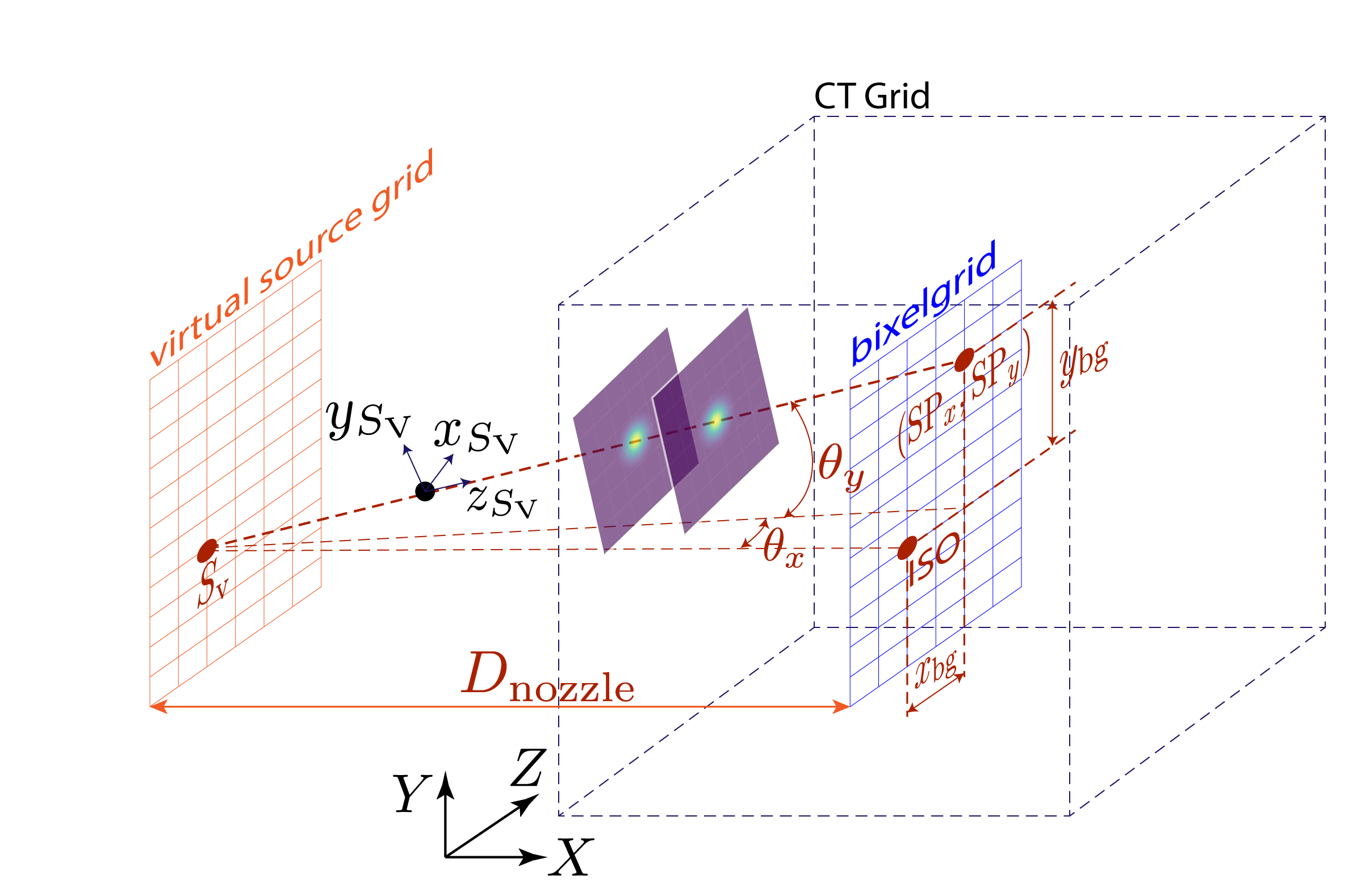
The generation of each training record was performed using in-house software. For every simulation, a random isocenter coordinate was first defined. For each patient CT, the image grid was resampled to an isotropic resolution. The grid was then rotated by a gantry angle , randomly sampled from the interval , around the z-axis passing through the sampled isocenter. A total of particles were simulated per beamlet, yielding a statistical uncertainty (SU) below . The virtual source was subsequently placed on the straight line passing through the sampled isocenter at a distance upstream of this point, where is the gantry nozzle to isocenter distance specified in the Beam Data Library (BDL) file. To directly simulate the variable deflection of the scanning magnets, the specific beamlet trajectory was established by randomly shifting the spot position relative to the sampled isocenter (ISO, , on Figure 2(a)). While clinical Pencil Beam Scanning (PBS) fields can span up to , we restricted the simulated deflection angles within to ensure that, across all available CT grids, the beamlet path and resulting 3D dose distribution remained within the imaged patient geometry, thereby avoiding edge cases where the beam traverses outside the CT extent and would require additional handling. Consequently, based on the nozzle geometry defined in the Beam Data Library (BDL), these angular constraints effectively limit the bixel shift area to a rectangle of . For each sampled spot position, two proton beamlet energies, and , were independently drawn from a uniform distribution , where for all anatomical sites, for thoracic anatomies, and for pelvic and abdominal sites. The sampling of two independent energies per beamlet allowed the model to learn from dose variations across distinct proton penetration depths. The initial sampling of the spot position defines the primary beamlet trajectory, characterized by the deflection angles and (Figure 2(a)). To account for the variability of scanning magnet deflections while preserving the same irradiated geometry, the virtual source was translated by a vector , resulting in a new source position (Figure 2(b)). This geometric transformation yields a secondary trajectory with modified incidence angles and . This procedure allows for the irradiation of the identical anatomy from a modified set of beamlet incidence angles, thereby enriching the dataset with necessary angular variability. Given the defined trajectory, we calculate the beamlet shape projection by evaluating the proton flux intensity at every voxel within the CT grid. To account for the beamlet’s angular direction, we transform the global coordinates into a beam-aligned frame (represented on Figures 2(a) and 2(b) as and , respectively) via rotation matrices and :
| (1) |
where denotes the beamlet entrance point to the CT grid geometry calculated as intersection between given ray’s straight and CT grid. The beamlet shape is then calculated as a Gaussian distribution dependent solely on the lateral components , effectively creating a continuous ray prolonged along the beam axis :
| (2) |
where and represent the energy dependent beam spot sizes derived from the BDL. Finally, for each trajectory, a MC dose calculation was performed using the corresponding proton beamlet energies. The resulting dose distributions were cropped to the volume of interest (VOI) of fixed size, centered around the Bragg peak region and, for training efficiency, resampled to a coarser isotropic grid of using trilinear interpolation.

In summary, the proposed data generation methodology systematically ensures both angular and energy variability within the dataset. For each cropped anatomical volume , the protocol samples two unique proton energies and two distinct beamlet incidence angles. This combinatorial sampling strategy ensures that the dataset contains identical anatomical heterogeneities irradiated under varying physical conditions, thereby introducing the necessary geometric and physical diversity required for model development.
2.2 Data Augmentation Technique
To further increase the number of training samples, two data augmentation strategies were incorporated into the training pipeline. During data generation, each extracted training record consisted of volume of interest , beamlet shape projection , the mean proton beamlet energy , and the corresponding ground truth 3D dose distribution , defined over spatial dimensions voxels (corresponding to a voxel volume under isotropic resolution). Based on the defined energy limits and angular constraints, we empirically determined that reduced dimensions of mm are sufficient to encompass the dose deposition for the vast majority of generated samples. However, we intentionally generated larger parent volumes to create a spatial margin for translational data augmentation. Consequently, during training, the model operates on randomly cropped sub-volumes , , and of size voxels, corresponding to a physical extent of under the isotropic grid resolution. This approach effectively samples a shifted subset of voxels from the original VOI, thereby simulating spatial variations without requiring additional Monte Carlo simulations.
To extract these sub-volumes, we applied random cropping around the Bragg peak while enforcing a cumulative dose retention criterion. The crop center was randomly shifted within the beam’s eye view (BEV) plane, i.e., in the beam-aligned lateral coordinates , by an offset sampled from the uniform distribution along each axis.
For each random shift, a new cropped sub-volume was generated according to the procedure implemented in the augmentation routine. The total dose deposited within the cropped sub-volume was then evaluated relative to the original dose distribution using the ratio , where and represent number of voxels of the cropped sub-volume and original dose distribution , respectively. The crop was accepted only if , ensuring that at least 99% of the deposited dose was retained within the augmented sub-volume. If the retention criterion remained unmet after the maximum number of attempts, typically due to beam overshooting, the spatial shifting was bypassed. In these instances, the original unshifted geometry was accepted into the dataset to ensure the representation of deep penetration cases, regardless of the dose retention threshold. This inclusion ensures that the model remains exposed to these challenging edge cases, thereby fostering robustness against anatomical variations that result in extended beam paths. Finally, to further enhance spatial variability, a random in plane rotation by an angle was applied to the CT, flux, and dose matrices, preserving the physical consistency of the dose distribution while increasing the effective dataset size. Implemented directly within the training generator, this strategy effectively expands the dataset by a factor of approximately per unique Monte Carlo simulation (combining a discrete grid of lateral voxel shifts with rotational symmetries).
2.3 Model Architecture: Angle-dependent Dose Transformer Algorithm (ADoTA)
The proposed model, ADoTA, adapts the hybrid architecture introduced by 3 from photon dose prediction to the specific requirements of proton therapy. We retain the core structural design of a 3D U-Net Ronneberger et al. (2015) integrated with a transformer encoder bottleneck and residual connections (HeDeepRecognition). While the original framework utilized secondary inputs for Multi-Leaf Collimator (MLC) shape projection, ADoTA repurposes this parallel pathway to encode the proton beamlet trajectory using a Gaussian projection that maps the beam path through the geometry based on the in-air spot sizes at the nozzle exit (Figure 3).
As input, the Angle-dependent Dose Transformer Algorithm (ADoTA) receives a five-dimensional tensor , where and represent batches of size containing the CT volumes and the corresponding fast beamlet shape projections along their central axis , respectively. In addition, ADoTA takes a secondary input , which specifies the initial proton beam energy associated with each record in the batch . The network outputs a batch of single-channel 3D dose distributions , spatially aligned with the corresponding CT geometry.
The encoder consists of consecutive convolutional encoder layers, each composed of convolutional blocks. Each convolutional block consists of a 3D convolutional layer followed by batch normalization (1) and ReLU activation function (Agarap; 2018). To progressively reduce the spatial resolution while retaining the depth information along the beam axis, anisotropic max pooling with a kernel of () is applied after each convolutional block, followed by layer normalization introduced by Ba et al. (2016).
Throughout the encoder, the number of feature channels and kernel size applied in each of the 3D convolutional layers are maintained at and , respectively, to balance representational capacity and computational efficiency. In the convolutional flattening layer presented in Figure 3, two additional 3D convolutional layers reduce the feature dimensionality from 64 to channels. This is followed by a slice-wise flattening operation that collapses only the spatial dimensions while preserving the depth axis. As a result, the latent tensor is obtained. This tensor encapsulates the total encoded information derived from the CT volumes and beamlet shape projections, transformed into vector embeddings, where denotes the batch size, corresponds to the number of depth slices, and is the token dimension defined as the product of the reduced spatial dimensions and the encoding feature parameter .
Beamlet energy conditioning is achieved by mapping the scalar mean energy into the same token space as the latent features using a dense linear layer. This operation projects the scalar energy value onto -dimensional embedding vector through a learnable linear transformation, allowing the energy information to be represented in the same feature domain as the spatial tokens. The projected energy embeddings are concatenated with the latent feature tensor obtained from the convolutional encoder along the depth dimension. This operation prepends the energy embedding as the initial token of the sequence, referred to as the energy-first token. This concatenation yields the energy-conditioned latent representation . Unlike the purely spatial tensor , this expanded representation explicitly incorporates the beam energy as a conditioning token. A learned positional embedding is then added elementwise to this concatenated sequence, assigning a unique positional vector to each token along the depth axis and enabling the model to encode the relative order of tokens along the proton beam path. Such prepared energy-conditioned latent space is provided to the sequentially stacked transformer encoder layers.
Each transformer encoder layer in ADoTA operates on the embedded and energy-conditioned latent representation and is implemented as a transfomer encoder layer (Attention2017) designed to capture long-range dependencies along the proton beam path. Each layer consists of a multi-head self-attention mechanism (Attention2017), followed by a two-layer feed-forward network with ReLU activation (Agarap; 2018). To enhance numerical stability, layer normalization is applied individually after the residual addition of each sub-module (the attention block and the feed-forward network, respectively). The resulting output sequence represents the energy-conditioned latent space in the dose domain.
Following the transformer processing, the auxiliary energy token is discarded via tensor slicing to restore the original sequence length. The remaining tokens are then mapped back to the spatial domain by reshaping the token dimension into the encoded feature channel and spatial dimensions. As a result, the dose-domain latent representation is obtained, matching the spatial geometry of the encoder’s output. The decoder mirrors the structure of the encoder: each decoding stage performs feature-wise concatenation with the corresponding encoder stage, followed by convolutional blocks sharing the same configuration as in the encoder. Each block consists of a 3D convolutional layer, batch normalization (1), and a ReLU activation function (Agarap; 2018). The final stage reduces the number of feature channels through two consecutive 3D convolutions, producing a single-channel output that represents the predicted 3D dose distribution.
Just like the architecture in 3, ADoTA is a transformer-augmented 3D U-Net architecture enhanced with residual connections (HeDeepRecognition) linking corresponding encoder and decoder layers, specifically designed for proton therapy dose prediction. By conditioning the latent representation on beamlet energy and incident angle through an angle-aware projection mechanism, ADoTA is designed to explicitly account for angle-dependent proton dose deposition. We performed a grid search to optimize the structural hyperparameters, specifically varying the number of convolutional blocks , the embedding size , the number of transformer encoders , and the number of downsampling and corresponding upsampling steps . Based on validation set performance, the optimal configuration of encoder and decoder was identified as and . Te best model contains transformer operating on input token size, with heads and hidden size.

2.4 Loss Function
Accurate modeling of proton dose deposition requires sensitivity to both local voxel-wise dose values and the steep longitudinal gradients characteristic of the Bragg peak. Approaches proposed in the literature typically rely on the Mean Squared Error (MSE) to optimize voxel wise fidelity (Pastor-Serrano2022MillisecondAccuracy; Neishabouri2025). However, since range sensitivity is particularly critical in proton therapy (PaganettiH2012_uncertainties), we additionally sensitized the model to discrepancies in the Integral Depth Dose (IDD) profile by augmenting the standard MSE with a proton specific depth loss. While this composite approach does not explicitly enforce full spatial awareness, it penalizes range errors by ensuring consistency between the predicted and ground truth longitudinal profiles. Accordingly, the total loss function used to train the ADoTA model is defined as:
| (3) |
where enforces voxel-level fidelity and encourages the model to reproduce the physical depth–dose profile characteristic of proton interactions. Notably, has been found near optimal through grid search.
Voxel-wise loss.
Let denote the predicted and Monte Carlo–simulated 3D dose distributions. The normalized MSE is:
| (4) |
averaged across all voxels and batch elements.
Depth-dose loss.
Let represents the 3D dose distribution. The IDD at depth k represents the integral of the dose over all voxels at the depth k:
| (5) |
where and represent pixel spacing. The IDD-based loss penalizes deviations between predicted and reference depth–dose profiles:
| (6) |
The combined formulation ensures both spatial accuracy and physically consistent depth–dose representation, guiding ADoTA to learn clinically meaningful proton range behavior.
2.5 Training details
ADoTA was trained using the composite loss function defined in Equation 3, optimized with the AdamW optimizer (Loshchilov and Hutter; 2017) and a weight decay of . Training is performed with a batch size of . The initial learning rate was set to . We utilized the ReduceLROnPlateau scheduler to decay the learning rate by a factor of 0.75 whenever the validation loss stagnated for more than 20 epochs (patience).
To enhance generalization, we apply data augmentation techniques described in detail in Section 2.2. Training was set to run for up to 400 epochs but utilized early stopping with a patience of 100 epochs to prevent overfitting. All experiments were carried out on an NVIDIA A40® GPU using the PyTorch framework (Paszke et al.; 2019).
2.6 Model evaluation
We benchmarked the performance of our model on the test set against published data from the Dose Transformer Algorithm (DoTA) (Pastor-Serrano2022MillisecondAccuracy), the spatio-temporal mono-energetic dose calculation model (CC-LSTM) (Neishabouri2025), the multi-energy dose LSTM (MED-LSTM) (2) and the PBA (Bhattacharya2025ACalculation). To quantify model performance, we used the gamma-index metric , introduced by Low et al. (1998). Since these methods reported their results using different test sets and gamma criteria, in this work we performed evaluations using a set of distinct criteria for consistency.
For comparison with DoTA (Pastor-Serrano2022MillisecondAccuracy), we adopted a dose threshold and a distance-to-agreement, with a dose cutoff at . For comparison with the CC-LSTM (Neishabouri2025) we used a dose threshold, a distance-to-agreement, and a dose cutoff. Finally, to compare against the MED-LSTM (2), we used and with a dose cutoff at . In the full treatment plan comparison, we applied with a dose cutoff.
As a supportive metric, the average relative error , Root Mean Square Error RMSE, Mean Absolute Percentage Error MAPE were used to explicitly compare dose differences between dose distributions. For the dose predicted by our model and the reference dose distribution , with voxels, is defined as
| (7) |
Moreover, we quantified the model performance using Root Mean Square Error (RMSE). Both metrics, RMSE and , were used in individualized beamlets experiment. Since MCsquare (SourisK2016) natively returns dose in the units of and Pastor-Serrano2022MillisecondAccuracy to calculate RMSE used the 3D dose distribution scaled to particles, in order to provide fair comparison, the same scaling has been applied.
Mean Absolute Percentage Error (MAPE) for each 3D dose distribution was calculated as
| (8) |
where is the number of eligible voxels, i.e. voxels where the reference dose is above 10% of the max dose in the considered reference 3D dose distribution calculated by MC.
Two distinct experiments were designed to test the performance and accuracy of the developed dose engine, using individual beamlets and full treatment plans.
-
•
Individual beamlets. The speed and accuracy of predicting dose distributions of individual beamlets were evaluated using data samples obtained from 50 unique CT images curated from the test sets (20 lung (Li et al.; 2020) and 30 abdominal–pelvic cases (Tong and Li; 2022)). From each CT image 70 unique records have been sampled using the same methodology as for generating the training and validation data. beamlets corresponded to lung anatomies and to abdominal–pelvic anatomies. For samples obtained from the lung CT scans, we uniformly sampled energy from the distribution . For samples obtained from the pelvic and abdominal CTs, energy was sampled from the distribution .
-
•
Full treatment plans. A total of eight treatment plans were constructed using the OpenTPS software (Wuyckens et al.; 2023). The evaluation included four prostate cases and four lung cases. For both prostate and lung cohorts, the corresponding CT images and delineations were obtained from the datasets of Thompson2023Stress-TestingCases and Aerts2014Data4, respectively. The primary objective of this experiment was to demonstrate the robustness of the proposed method in calculating full treatment plan doses; therefore, no effort was made to achieve clinical plan quality.
Since the main novelty of the proposed model is that it offers beamlet angle agnosticity, we performed experiments to test model performance across different energies level and beamlet angles, as well as the time savings and accuracy benefits of not requiring a separate perpendicular CT for each beamlet.
3 Results
3.1 Individualized beamlets
Table 1 summarizes the -index analysis comparing ADoTA predictions against Monte Carlo ground truth across 3500 independent beamlet test samples under multiple clinical evaluation criteria, providing a quantitative assessment of spatial dose agreement.
Complementary to this, Table 2 reports the relative dose error () and root mean squared error (RMSE), which capture voxel-wise intensity deviations and overall regression accuracy, respectively.
Figures 5, 6, and 7 present the best-, mean-, and worst-performing beamlet predictions from the thoracic test set, selected based on the local pass rate. Similarly, Figures 8, 9, and 10 show representative best-, mean-, and worst-performing samples from the abdominal and pelvic beamlet test set using the same criterion.
Model Site Energy (MeV) ADoTA (this work) Lung [70, 150] Abdominal and Pelvic [70, 270] CC-LSTM Neishabouri2025 Lung 48.1 MeV - - - Lung 79.17 MeV - - - Lung 102.6 MeV - - - DoTA Pastor-Serrano2022MillisecondAccuracy Lung [70, 140] - - - H&N [70, 140] - - - Prostate [70, 220] - - - MED-LSTM 2 Lung [69, 114.5] - - Nasopharynx [69, 161.4] - - Prostate [114.5, 200.8] - -
Model Anatomical site Relative Dose Error [%] Root Mean Square Error [Gy/] Mean std Min Max Mean std Min Max DoTA Combined 0.126 0.109 0.025 1.258 0.083 0.041 0.024 0.277 ADoTA Combined 0.044 0.035 0.0073 0.388 0.0104 0.0043 0.0042 0.0308 Lungs 0.0738 0.0437 0.009 0.388 0.013 0.005 0.0042 0.0308 Abdominal and Pelvic 0.0319 0.043 0.00730 0.2231 0.0087 0.0027 0.0049 0.022


Additionally, to assess the model performance across different penetration depths, we calculated the mean gamma pass rate for each lateral depth slice of the dose volume. Figure 11(a) illustrates the stability of the gamma pass rate () as a function of beamlet penetration depth. Complementary to this, Figure 11(b) shows the percentage of test set samples exhibiting non-zero dose deposition at each corresponding depth. The gradual decline in the number of samples with increasing depth reflects the finite proton range in the geometry, as fewer beamlets penetrate to the deeper geometric layers.


To assess the angle awareness of our method, the key novelty of this work, we conducted an experiment to verify robustness across varying beamlet scanning angles. First, we randomly selected one abdominal/pelvic CT and one thoracic CT from the test set described in Section 2.1. The isocenter was defined at the image center, and the CT grid was rotated by a randomly sampled gantry angle .
For each rotated CT grid we evaluated two distinct energy levels: low energy () and high energy (). Next we constructed a uniform bixelgrid of size , designed such that the beamlet scanning angles and spanned the range . Finally, to demonstrate the robustness of our method within a invariant geometric setting, we repeated the experiment on a homogeneous water phantom using the same energies and beamlet scanning angles grid. We used air layer at the entrance to the water phantom. The resulting dose passing rates between MC and ADoTA () for the patient geometries are presented in Figures 12(a) and 12(b) for the low energy beam, and in Figures 12(c) and 12(d) for the high energy beam. The corresponding validation on the water phantom, with criteria, is shown in Figures 12(e) and 12(f).


3.2 Treatment plans
To evaluate the suitability of implementing the proposed method in clinical practice, we employed ADoTA to compute the three-dimensional dose distribution for full treatment plans. The details about each plan are presented in Table 3. The results for all eight cases are summarized in Table 4, demonstrating consistent performance across the evaluated anatomical sites. The achieved performance is later compared in Table LABEL:tab:fullplan_comparison to the model performance reported in the work of (Pastor-Serrano2022MillisecondAccuracy) and (Pang2025LightweightEnergies).
Plan Identifier Anatomical Site No. of spots No. of beams Energy range [MeV] MC calc time [s] full plan MC calc time [s] Prostate 1 Prostate 1477 1 [175.4, 209.95] 332.53 614.198 Prostate 2 Prostate 4069 2 [149.15, 205.18] 816.69 672.88 Prostate 3 Prostate 2955 2 [165.61, 209.95] 348.26 653.88 Prostate 4 Prostate 3189 2 [129.65, 189.79] 357.55 620.88 Lung 1 Lung 13392 1 [85.082, 141.175] 1696.77 379.572 Lung 2 Lung 82 2 [126.31, 155.66] 11.31 358.87 Lung 3 Lung 1323 1 [110.51, 165.48] 344.34 447.0 Lung 4 Lung 2899 1 [86.58, 186.29] 326.00 524.58
Plan Identifier ADoTA Inference [s] Data Processing Overhead [s] (2%, 2 mm, 10%) [%] Prostate 1 5.63 213.13 99.19 Prostate 2 6.46 301.85 98.89 Prostate 3 5.95 242.86 98.67 Prostate 4 5.54 272.33 98.95 Lung 1 20.3 1918 97.56 Lung 2 0.302 11.74 98.54 Lung 3 2.33 255.33 98.87 Lung 4 4.93 552.38 98.78
Model Site Energy (MeV) Mean (%) Std (%) Min (%) Max (%) DoTA Pastor-Serrano2022MillisecondAccuracy Lung [70, 220] 99.69 0.04 99.64 99.73 H&N [70, 220] 99.63 0.2 99.39 99.88 Prostate [70, 220] 99.77 0.05 99.71 99.82 MED-LSTM 2 Lung Unspecified 99.42 0.17 — — nasopharynx Unspecified 98.38 0.12 — — Prostate Unspecified 99.97 0.02 — — ADoTA (this work) Lung [70, 200] 98.43 0.52 97.56 98.87 Prostate [70, 270] 98.93 0.18 98.67 99.19 DoseCUDA (Bhattacharya2025ACalculation) Avg (4 sites)* [70.2, 228.7] 96.0 5.1 — —
* Values represent the aggregate mean across prostate, oesophagus, brain, and lung cases.
Figures 13 and 14 represent 3D dose distribution obtained by reconstructed plan for plans Prostate 2 and Lung 1 (details of these plans can be found in Table 3).


3.3 Runtime
Dose prediction accuracy is the primary objective of this work; however, in the clinical context, the speed of dose calculation is equally important. Table LABEL:tab:inference_time_comparison reports the mean, standard deviation, as well as the fastest and slowest runtimes required by each model to predict a single beamlet. Table LABEL:tab:runtime_batch_size illustrates how the inference time per beamlet depends on the batch size used during the ADoTA forward pass. This analysis is motivated by the nature of treatment planning in proton therapy, where a large number of independent beamlets are used to construct a plan, and the computation of individual 3D dose distributions can therefore be efficiently parallelized.
| Model | Mean (ms) | Std (ms) | Fastest (ms) | Slowest (ms) |
|---|---|---|---|---|
| CC-LSTMa ( Neishabouri2025) | 3.6 | - | - | - |
| MED-LSTMa ( 2) | 200.0 | - | - | - |
| ADoTAb (this work) [] | 1.75 | 1.2 | 1.5 | 8.5 |
| DoTAb (Pastor-Serrano2022MillisecondAccuracy) | 5.0 | 4.9 | - | - |
| PBAc ( Cisternas et al. (2015)) | 728.3 | 30.9 | - | - |
| MCc (SourisK2016) | 43 636.9 | 12 291.6 | - | - |
| a | Nvidia® Quadro RTX 6000 64 Gb RAM. |
|---|---|
| b | 4 vCPUs—Nvidia® A40 40 Gb RAM. |
| c | 8 CPUs, Intel® Xeon® E5-2620, 16 Gb RAM. |
Batch Size () Batch inference time [ms] Beamlet inference time [ms] 1 10.40 10.40 8 21.81 2.74 16 34.54 2.17 32 59.67 1.89 56 96.56 1.75 200 329.15 1.74
Since the main novelty of our method lies in its beamlet-angle agnosticity, Figure 15 illustrates the time required to perform pre-processing (plan parsing, ray-tracing and input tensor generation), ADoTA inference, and post-processing (dose placement into the patient grid) per single beamlet. The left bar plot presents the time needed for each step. The figure also reports the average time required for grid reinterpolation to achieve alignment perpendicular to the proton beam, a computational step effectively eliminated by our method. While standard CPU-based reinterpolation typically requires approximately 6 seconds per volume (estimated based on the typical CT grid size, i.e. ), we utilized a high-performance GPU implementation to establish a rigorous baseline. This implementation leverages the SimpleITK framework for high-precision spatial resampling (LowekampB2013) and NVIDIA DALI for accelerated volume rotation. Finally, the right bar plot shows the difference in the end-to-end pipeline under two assumptions: grid reinterpolated to be perpendicular for every single beamlet (others) (red), grid reinterpolated to be perpendicular for the gantry angle only (this work) (purple).

4 Discussion
In this work, we address a central limitation of existing deep learning–based proton dose engines. Namely, the requirement to reinterpolate the CT volume for every beamlet to enforce perpendicular alignment between the beam direction and the voxel grid. To overcome this bottleneck, we introduce an additional input channel that encodes an analytically computed Gaussian beamlet–shape projection along the protons beam central axis, with and taken directly from the BDL. This explicit geometric conditioning removes the need for per-spot grid realignment, strictly limiting resampling operations to the number of irradiation fields rather than the total number of beamlets. In our implementation, this strategy reduces the geometric transformation overhead by approximately (from to per spot). Although the preprocessing time for determining the beamlet shape still exceeds the neural network inference time (), the removal of the specific reinterpolation bottleneck represents a fundamental shift toward real-time applicability.
Regarding geometric generalization, the model maintains high predictive accuracy regardless of beam orientation, confirming that the strict orthogonality between the proton ray and the voxel grid required by prior methods (Neishabouri2025; Pastor-Serrano2022MillisecondAccuracy; 2) is no longer a prerequisite. This is empirically supported by the stable Gamma pass rates observed across randomized gantry angles () and lateral scanning angles, where performance remained consistent for both phantom and patient geometries (Figures 12(a)–12(f)). By explicitly encoding the incident trajectory via the analytical beam-shape projection, the network effectively learns to map varying scanning deflections to the static voxel grid. This conditioning allows the model to operate entirely within a single field-aligned coordinate system, thereby avoiding the prohibitive per-spot resampling characteristic of prior approaches.
While the geometric performance is uniform, prediction fidelity exhibits specific dependencies on the physical beam range. We observed a reduction in agreement in the distal 25% of the calculation volume depth (Figure 11(a)). This trend arises from the combined effect of reduced representation of deep penetration regions in the training data and the increased physical complexity of dose deposition near the Bragg peak, where steep dose gradients and range straggling dominate. First, as illustrated in Figure 11(b), the training distribution exhibits an inherent imbalance with respect to penetration depth. While dose deposition occurs in the entrance region for every beamlet regardless of energy, the maximum penetration depth is a direct function of the initial beam energy. Second, this data sparsity coincides with the region of highest physical complexity—the Bragg peak—where steep gradients and range straggling dominate. This aligns with findings by Pastor-Serrano2022MillisecondAccuracy, who partitioned the beam path into four equal depth sections and showed that the final section, corresponding to the Bragg peak and distal fall-off, consistently exhibits the highest relative error. This confirms that the coupling of specific data sparsity and gradient complexity renders the distal edge the dominant challenge for deep learning-based dose engines. Overall, the strong performance across anatomical sites, energies, and orientations confirms that the proposed conditioning strategies allow the model to reliably reproduce the underlying physics of individual proton rays.
At the treatment–plan level, errors manifest primarily as systematic biases rather than the stochastic noise typical of Monte Carlo simulations (Mentzel2023AccurateSimulations). Because neighboring beamlets in Pencil Beam Scanning traverse highly similar anatomical heterogeneities, local prediction errors tend to accumulate rather than cancel during dose superposition. This effect is most pronounced in heterogeneous media (e.g., Lung), where density interfaces increase sensitivity to range inaccuracies. As noted by 2, these scattering complexities lead to non-uniform dose deposition patterns that are challenging to regress. Furthermore, the intrinsic spectral bias of convolutional networks (Gronberg2023DeepCancers) tends to attenuate high-frequency components, smoothing the sharpest gradients. Despite these localized discrepancies, global plan fidelity remains robust ( Gamma pass rate for Lung), suggesting that these systematic offsets are spatially confined and do not compromise total dosimetric coverage.
From a runtime perspective, the proposed pipeline capitalizes on the parallel nature of IMPT. While the neural network inference is computationally negligible, the current pipeline remains limited by the CPU-based geometric preprocessing (specifically ray-tracing and construction). However, these operations are inherently vectorizable. Standard algorithms for ray-tracing (e.g., Siddon’s algorithm (Siddon1985FastArray)) and grid-based Gaussian evaluation are staple candidates for GPU optimization (Jia2014GPU-basedTherapy). Porting these steps to a fully GPU-resident pipeline offers a clear pathway to reduce the total end-to-end runtime well into the sub-second range required for online adaptive therapy.
Several limitations must be acknowledged. First, the current framework is grid–dependent, trained on isotropic fixed size grid. Clinical deployment will require grid–agnostic architectures, such as neural operators (Kovachki2024NeuralSpaces), to handle arbitrary resolutions. Second, the model is implicitly tied to the specific beam model used for training; generalization across different machines will require explicit conditioning on beam optics parameters. Finally, the fixed crop depth () prevents prediction for very deep-seated targets. Future iterations must implement dynamic cropping or autoregressive depth extension to accommodate arbitrary path lengths. Addressing these limitations will be essential for establishing a generalizable, clinically deployable deep learning dose engine.
5 Conclusion
This study introduces a beamlet-angle-agnostic deep learning framework, built on a Transformer encoder architecture, for Monte Carlo accuracy proton dose calculation at arbitrary energies. The approach removes the perpendicularity requirement between proton ray directions and the CT voxel grid, reducing the number of necessary dose reinterpolations from the total number of beamlets to the number of irradiation fields. The method exhibits strong potential for integration into time-constrained online adaptive proton therapy workflows and for constructing the dose–influence matrix within robust optimization frameworks, where multiple spot-selection scenarios must be evaluated efficiently to ensure conformal and uncertainty-tolerant dose delivery.
Data availability statement
The main repository with the model architecture and auxiliary methods can be found at the
github.com/Medical-Physics-Technology/adota.
The data that support the findings of this study are available from the authors upon reasonable request.
Conflicts of interest
Zoltán Perkó is an associate professor at TU Delft and is employed as a Senior Applied Scientist at Radformation Inc.. His industry employment is unrelated to the submitted work. The remaining authors have no conflicts of interest to declare.
CRediT author and contributor statement
Mikołaj Stryja: Data Curation, Formal Analysis, Investigation, Methodology, Software, Validation, Visualization, Writing - Original Draft
Zoltán Perkó: Conceptualization, Formal Analysis, Funding Acquisition, Methodology, Project Administration, Supervision, Resources, Writing - Review and Editing
Danny Lathouwers: Conceptualization, Formal Analysis, Methodology, Project Administration, Supervision, Resources, Writing - Review and Editing
Declaration of generative AI and AI-assisted technologies in the manuscript preparation process
During the preparation of this work, the author(s) used GPT-5.2 (OpenAI) and Gemini 3 Pro (Google) to correct grammar and improve clarity. After using this tool/service, the author(s) reviewed and edited the content as needed and take(s) full responsibility for the content of the published article.
References
- [1] Cited by: §2.3, §2.3.
- [2] Cited by: §1, §1, §2.6, §2.6, Table 1, Table 5, Table 5, Table 5, Table 6, §4, §4.
- [3] Cited by: §2.3, §2.3.
- Deep learning using rectified linear units (relu). External Links: Link Cited by: §2.3, §2.3, §2.3.
- Layer normalization. External Links: Link Cited by: §2.3.
- MatRad – a multi-modality open source 3d treatment planning toolkit. In IFMBE Proceedings, Vol. 51, pp. 1608–1611. External Links: Document, ISBN 9783319193878, ISSN 16800737 Cited by: Table 6.
- A large-scale ct and pet/ct dataset for lung cancer diagnosis (lung-pet-ct-dx) [data set]. The Cancer Imaging Archive. External Links: Document, Link Cited by: 1st item, §2.1.
- Decoupled weight decay regularization. External Links: Link Cited by: §2.5.
- A technique for the quantitative evaluation of dose distributions. Medical Physics 25, pp. 656–661. External Links: Document, ISSN 00942405 Cited by: §2.6.
- PyTorch: an imperative style, high-performance deep learning library. External Links: Link Cited by: §2.5.
- U-net: convolutional networks for biomedical image segmentation. External Links: Link Cited by: §1, §2.3.
- Abdominal or pelvic enhanced ct images within 10 days before surgery of 230 patients with stage ii colorectal cancer (stageii-colorectal-ct) [dataset]. External Links: Link Cited by: 1st item, §2.1.
- OpenTPS – open-source treatment planning system for research in proton therapy. External Links: Link Cited by: 2nd item, §2.1, Table 3, Table 3.
