GraphVec: Cross-Domain Graph Vectorization for Graph-Level Representation Learning

Qi Feng Jicong Fan
School of Data Science
The Chinese University of Hong Kong, Shenzhen, Guangdong 518172, China
qifeng@link.cuhk.edu.cn, fanjicong@cuhk.edu.cn

Abstract

Learning universal graph representations across heterogeneous domains is difficult because graph datasets differ in topology, node-attribute semantics, feature dimensions, and even attribute availability. We propose GraphVec, a language-model-free graph vectorization model that maps diverse graphs into transferable fixed-dimensional embeddings for graph-level tasks. Instead of directly using incomparable raw node attributes, GraphVec constructs multi-scale global graphs over all nodes in each dataset and extracts spectral embeddings to obtain domain-agnostic relational features. To make these spectral features comparable across datasets, we introduce a density-maximization mean alignment algorithm over orthogonal transformations and prove its monotonic convergence. GraphVec further combines a GIN–Graph Transformer backbone with a multi-layer reference distribution module, which preserves node-level distributional information beyond standard pooling. We also provide a generalization error bound for the proposed model. Experiments on 13 datasets with more than 15 comparison methods demonstrate that GraphVec consistently outperforms strong graph pretraining baselines in cross-domain few-shot graph classification and graph clustering. Beyond graph-level tasks, GraphVec also yields strong node-level representations, achieving competitive performance on few-shot node classification against representative graph prompt learning methods.

1 Introduction

Graph data is a fundamental and widely prevalent form of structured data, representing entities as nodes and their relationships as edges. It plays a crucial role in diverse domains, including social networks, biological systems, citation networks, recommendation systems, and knowledge graphs. Given its ability to model complex relational patterns, graph data analysis has become a key focus in machine learning and data mining. In node-level tasks, the training set is usually a single but large graph, on which each node represents a sample. Node-level tasks include node embedding or representation (Grover and Leskovec, 2016; Cai et al., 2018), node classification (Kipf and Welling, 2017), node clustering (Wang et al., 2023), link prediction (Martínez et al., 2016), etc. For example, node classification might involve categorizing users in a social network, while link prediction could be used to recommend new connections.

On the other hand, graph-level tasks operate on entire graphs, where a dataset is composed of numerous graphs, and each graph is treated as a sample. Graph-level tasks address broader challenges such as graph comparison (Kobler et al., 2012), representation learning (Sun et al., 2020), classification (Xu et al., 2019), clustering (Cai et al., 2024), generation (Liao et al., 2019), etc. Graph comparison often relies on graph kernels (Gärtner et al., 2003; Vishwanathan et al., 2010; Shervashidze et al., 2011) or distances (Bunke, 1997; Zeng et al., 2009; Mémoli, 2011; Bento and Ioannidis, 2018) or deep learning methods (Sun and Fan, 2024) to measure similarity between different graphs, while graph representation learning aims to encode entire graphs into compact, informative embeddings for downstream tasks (You et al., 2020, 2021; Sun et al., 2023b). Representative graph-level representation methods range from substructure-based graph embeddings such as graph2vec (Narayanan et al., 2017) to self-supervised mutual-information and contrastive approaches such as InfoGraph, GraphCL, automated graph contrastive learning, and GCC (Sun et al., 2019; You et al., 2020, 2021; Qiu et al., 2020). Graph classification, for example, is critical in chemistry for predicting molecular properties (Gilmer et al., 2017; Wang and Fan, 2024), whereas graph generation enables the creation of novel structures, such as drug-like molecules in computational biology (Hoogeboom et al., 2022).

Most of the aforementioned methods are dataset-specific. That means, for one dataset, we have to train a new model, e.g., a graph neural network, to solve the corresponding problem. This leads to the following two limitations. First, training a model from scratch is very time-consuming, and it requires model selection and parameter tuning, which brings inconvenience to practical applications. Second, knowledge from historical data or tasks in the same domain or similar domains cannot be exploited well. These limitations motivate graph pretraining, which has attracted increasing attention following the success of pretraining in natural language processing and computer vision. A representative line of work is graph prompt learning (Sun et al., 2022; Fang et al., 2023; Sun et al., 2023a; Liu et al., 2023b; Fu et al., 2025), which aims to adapt a pretrained graph model to different downstream tasks by reducing the gap between pretraining objectives and task-specific objectives. However, most graph prompt methods are still developed and evaluated within single-dataset settings, where different tasks share the same graph distribution or feature space. Recently, graph foundation models (GFMs) (Liu et al., 2025) have also become an increasingly prominent area of research in graph data analysis due to their ability to pre-train on diverse datasets to enhance performance across multiple tasks and domains. Existing GFMs can be roughly grouped into LLM-based methods (Liu et al., 2023a; Kong et al., 2024; Xia and Huang, 2024) and non-LLM-based methods (Sun et al., 2025; Yuan et al., 2025b). Emerging studies (Galkin et al., 2023; Zheng et al., 2023) indicate that GFMs exhibit strong generalization capabilities, even when applied to previously unseen graph structures.

One key challenge in pretraining graph models is that graph patterns from different domains exhibit significant variation (Galkin et al., 2023), which is evident in both structural and feature representations. For example, in molecular graphs (Yang et al., 2016), the structure encodes 3D spatial arrangements and atomic bonds, while node features represent chemical properties. Conversely, in social networks (Dwivedi et al., 2023), the structure reflects user connections, and node features correspond to user profiles. These distribution differences make it difficult for a single model to learn domain-agnostic representations. A promising approach involves transforming both graph structures and node features into textual formats, then employing large language models (LLMs) to derive unified representations (Fatemi et al., 2023; Liu et al., 2023a; Tang et al., 2024; Wang et al., 2024a). Another approach is to improve existing graph learning paradigms (Liu et al., 2025) through innovations in the aspects of the backbone (Rong et al., 2020), pretraining (Qiu et al., 2020; You et al., 2020; Yu et al., 2025a), and adaptations (Fu et al., 2025; Yu et al., 2025c; Wang et al., 2025a).

Despite recent progress in graph pretraining, several important limitations remain. First, LLM-based graph pretraining methods convert graphs into textual descriptions, which can discard fine-grained topological patterns and node-feature information (Yu et al., 2025a). They also incur substantial computational costs due to the large scale of LLMs. Second, many existing pretrained graph models are primarily designed for node-level tasks (Zhao et al., 2024b; Wei et al., 2024; Wang et al., 2025a), while graph-level tasks have received comparatively less attention (Yu et al., 2025c; Fu et al., 2025). Third, it is still challenging to train a single graph model that can handle heterogeneous graph datasets from diverse domains and generalize reliably to unseen domains and downstream graph-level tasks.

This work proposes a graph representation model for graph-level tasks across diverse domains. Figure 1 shows the flowchart. Our contributions are: Our contributions are summarized as follows.

•

We propose GraphVec, a language-model-free cross-domain graph vectorization framework for graph-level tasks. GraphVec maps graphs from heterogeneous domains into a shared fixed-dimensional representation space without assuming comparable raw node attributes.
•

We introduce a global multi-graph feature construction strategy that converts domain-specific node attributes into multi-scale relational spectral features. This provides a unified input representation for graphs with different feature dimensions, semantics, or missing attributes.
•

We develop a density-maximization orthogonal alignment algorithm for spectral features and establish monotonic improvement and asymptotic stationarity of the alignment objective.
•

We design a multi-layer reference distribution learning mechanism for distribution-aware graph representation. This mechanism preserves information that is typically discarded by standard graph-level pooling.
•

We provide extensive experiments on cross-domain few-shot graph classification and graph clustering, together with ablations, robustness tests, scalability analysis, and comparisons with recent graph pretraining and prompt-tuning methods.

2 Related Work

Graph pretraining

Many studies have explored the “pre-train and adaptation" paradigm for graph models, leveraging message-passing or transformer-based GNN backbones. These approaches typically employ contrastive or generative self-supervised learning for pretraining, followed by fine-tuning a subset of model parameters to adapt to downstream tasks or datasets (Liu et al., 2025). Contrastive methods, including GCC (Qiu et al., 2020), InfoGraph (Sun et al., 2019), DGI (Veličković et al., 2019), SimGRACE (Xia et al., 2022), and GCOPE (Zhao et al., 2024a), maximize agreement between augmented views to learn transferable representations, while generative methods (Hou et al., 2022, 2023) pre-train via graph reconstruction or property prediction. Recently, graph prompt tuning (Sun et al., 2022; Fang et al., 2023; Sun et al., 2023a; Liu et al., 2023b; Fu et al., 2025) has emerged to bridge the pretraining–downstream gap, and many recent GFMs adopt this paradigm (Yuan et al., 2025b; Yu et al., 2025b). However, these works mainly emphasize adaptation, leaving the problem of learning unified graph representations underexplored. Due to space limitations, we defer more discussion of Graph pretraining and the related work on GFMs to Appendix B.

3 Methodology

3.1 Cross-Domain Graph Vectorization: Problem Setup

First of all, the major notations used in this paper are shown in Table 4. Let $\mathcal{D}=\{\mathcal{G}_{1},\mathcal{G}_{2},\ldots,\mathcal{G}_{M}\}$ be a union of $M$ datasets of labeled graphs from $M$ different domains, where $\mathcal{G}_{j}=\{(G^{(j)}_{1},y_{1}^{(j)}),(G^{(j)}_{2},y_{2}^{(j)}),\ldots,(G^{(j)}_{N_{j}},y_{N_{j}}^{(j)})\}$ . Here, each graph $G^{(j)}_{i}$ is denoted as $G^{(j)}_{i}=(\mathbf{A}_{i}^{(j)},\mathbf{X}_{i}^{(j)},y_{i}^{(j)})$ , where $\mathbf{A}_{i}^{(j)}\in\mathbb{R}^{n_{i}^{(j)}\times n_{i}^{(j)}}$ denotes the adjacency matrix, $\mathbf{X}_{i}^{(j)}\in\mathbb{R}^{n_{i}^{(j)}\times d^{(j)}}$ denotes the node attribute matrix, $n_{i}^{(j)}$ denotes the number of nodes, $d^{(j)}$ denotes the number of attributes, and $y_{i}^{(j)}$ denotes the graph label. Our goal is to use $\mathcal{D}$ to train a cross-domain graph representation model, denoted as

F:\mathbb{G}\rightarrow\mathbb{R}^{r}

(1)

to represent any graph from the space $\mathbb{G}$ as an $r$ -dimensional vector that is useful in downstream tasks such as graph classification, where $\mathbb{G}$ denotes the set of all graphs in the form of $(\mathbf{A},\mathbb{\mathbf{X}})$ . Therefore, $F$ serves as a universal graph representation model.

To learn $F$ from $\mathcal{D}$ , we need to address these challenges:

•

Attributes inconsistency The node attributes of graphs from different domains are different and not comparable at all. Thus the node attributes in $\mathcal{D}$ cannot be fed into $F$ directly.
•

Attributes absence Many graph datasets do not contain node attributes, making them very different from graph datasets with node attributes. The heuristic method of constructing node attributes, such as using node degrees, does not comply with the semantic attributes of other datasets.
•

Information loss in pooling Although there have been a few advanced graph pooling methods (Liu et al., 2022), converting nodes’ embeddings into a single vector cannot fully utilize the information.

Refer to caption — Figure 1: Flow-chart of GraphVec. $\mathcal{G}_{1},\ldots,\mathcal{G}_{M}$ are $M$ datasets from different domains. The model represents each graph $G_{i}^{(j)}$ as a single vector $\mathbf{g}_{i}^{(j)}$ that can be used in graph-level downstream tasks.

3.2 Domain-Agnostic Relational Features via Global Multi-Graphs

As mentioned, the node features of different domain graph datasets may vary significantly in semantics and dimensions. To capture domain-invariant features, we focus on the relationships among nodes across the entire dataset rather than the original features. The reason is that in many machine learning problems, using the relationships between samples or a graph constructed from the dataset can provide effective solutions. For instance, in spectral clustering (Ng et al., 2001), we use a similarity graph rather than the original features; in kernel support vector machine (Cortes and Vapnik, 1995), we can use a Gaussian kernel matrix, which is a similarity matrix of the data points.

Multi-Scale Global Relational Graphs For each graph dataset $\mathcal{G}_{j}$ , $j\in[M]$ , we propose to construct a similarity graph over all nodes in the dataset using a Gaussian kernel function, i.e.,

\mathbf{K}_{\lambda}^{(j)}=\left[\exp\left(-\frac{\left\|\mathbf{x}_{u}-\mathbf{x}_{v}\right\|_{2}^{2}}{2\lambda\mu^{2}}\right)\right]_{u,v=1}^{\bar{N}_{j}},\quad\bar{N}_{j}=\sum_{i=1}^{N_{j}}{n_{i}^{(j)}}

(2)

where $\mathbf{x}_{i}$ is the $i$ -th row of $\mathbf{X}:=\big|\big|_{i=1}^{N_{j}}\mathbf{X}_{i}^{(j)}$ (vertical concatenation), $\mu$ is the mean of the pairwise distances between all nodes in the dataset, and $\lambda$ controls the bandwidth of the kernel. This setting ensures translation, rotation, and scaling invariance, which is important to extract comparable features across diverse datasets. $\mathbf{K}_{\lambda}^{(j)}$ is the adjacency matrix of this global graph of the nodes in $\mathcal{G}_{j}$ . Note that a single $\mathbf{K}_{\lambda}^{(j)}$ exploits partial information of the node attributes of $\mathcal{G}_{j}$ and the optimal setting of $\lambda$ remains an open problem. Therefore, we use a number of different values for $\lambda$ , e.g. $\lambda_{1},\lambda_{2},\ldots,\lambda_{Q}$ , to construct multiple global graphs for the nodes in $\mathcal{G}_{j}$ :

\bm{\mathcal{K}}^{(j)}:=\left\{\mathbf{K}_{\lambda_{1}}^{(j)},\mathbf{K}_{\lambda_{2}}^{(j)},\ldots,\mathbf{K}_{\lambda_{Q}}^{(j)}\right\},\quad j\in[M]

(3)

Note that the diversity of $\bm{\mathcal{K}}^{(j)}$ can be further enhanced if more kernel families, e.g., $k(\mathbf{x}_{u},\mathbf{x}_{v})=\exp(-\alpha\|\mathbf{x}_{u}-\mathbf{x}_{v}\|_{1})$ , are considered.

Multi-Scale Relational Spectral Embedding For $\mathbf{K}_{\lambda_{q}}^{(j)}$ , we compute $\bar{d}$ -dimensional node embeddings using singular value decomposition (SVD):

\mathbf{Z}_{\lambda_{q}}^{(j)}=\mathbf{U}_{\bar{d}}\bm{\Sigma}_{\bar{d}}^{1/2},\quad~\mathbf{K}^{(j)}_{\lambda_{q}}=\mathbf{U}\bm{\Sigma}\mathbf{V}^{\top}

(4)

where $\mathbf{U}_{\bar{d}}\in\mathbb{R}^{\bar{N}_{j}\times\bar{d}}$ is composed of the first $\bar{d}$ columns of $\mathbf{U}$ and $\bm{\Sigma}_{\bar{d}}$ is a diagonal matrix consisting of the first (largest) $\bar{d}$ singular values. Then the final node feature matrix is obtained by concatenating embeddings from all scales, i.e.,

\displaystyle\mathbf{Z}^{(j)}

\displaystyle=\left[\mathbf{Z}_{\lambda_{1}}^{(j)},\ldots,\mathbf{Z}_{\lambda_{Q}}^{(j)}\right]=\left[\begin{matrix}\mathbf{Z}^{(j)}_{1}\\ \vdots\\ \mathbf{Z}^{(j)}_{N_{j}}\end{matrix}\right]\in\mathbb{R}^{\sum_{i=1}^{N_{j}}{n_{i}^{(j)}}\times Q\bar{d}},

(5)

where $j\in[M]$ . For datasets without node attributes, we generate node attributes using the truncated SVD of the self-looped adjacency matrix, i.e.,

\mathbf{X}_{i}^{(j)}=\mathrm{SVD}\left(\mathbf{A}_{i}^{(j)}+\mathbf{I}_{n_{i}^{(j)}}\right)\in\mathbb{R}^{n_{i}\times\bar{d}}

(6)

where $\mathrm{SVD}(\cdot)$ returns the singular vectors corresponding to the top- $\bar{d}$ singular values, similar to (4). Then we apply (2), (3), (4), and (5) to $\mathbf{X}_{i}^{(j)}$ to generate unified node embeddings. For large datasets, the Nyström approximation (Williams and Seeger, 2000) can be employed to accelerate the computation of the kernel matrix and SVD.

3.3 Convergent Density-Maximization Alignment for Spectral Features

In SVD, individual singular vectors have arbitrary signs (Bro et al., 2008). This sign ambiguity may make the embeddings of two similar graphs very different, leading to significant difficulties in both the training and testing stages. Moreover, if two singular values are the same, the order of the corresponding singular vectors cannot be determined, which further increase the difficulty in learning. In machine learning, to ensure learnability and generalization, we require that the training samples and the testing samples are from the same distribution, or at least, their means are similar. Therefore, we proposed to align the mean embeddings of different graphs via maximizing the density.

Specifically, consider the SVD embeddings of $M\times Q$ graphs generated by the method in Section 3.2, for each $\lambda_{q}$ , we compute the mean vectors of the embedding matrices $\mathbf{Z}_{\lambda_{q}}^{(j)}$ as $\bm{\mu}_{j}=\frac{1}{\bar{N}_{j}}\mathbf{Z}_{j}^{\top}\bm{1}_{\bar{N}_{j}}$ , where $j\in[M]$ and we have dropped the subscript $\lambda_{q}$ to simplify the notation for the following operations. For each graph $j$ , we introduce an orthonormal matrix $\mathbf{R}_{j}\in\mathbb{R}^{\bar{d}\times\bar{d}}$ , which will transform $\bm{\mu}_{j}$ as $\mathbf{R}_{j}\bm{\mu}_{j}$ , $j\in[M]$ , which means $\mathbf{R}_{j}\mathbf{Z}_{\lambda_{q}}^{(j)}$ is equivalent to $\mathbf{Z}_{\lambda_{q}}^{(j)}$ in preserving the information of $\mathbf{K}_{\lambda_{q}}^{(i)}$ . We align all mean vectors using the corresponding orthonormal matrices by maximizing the density of the mean vectors. The density of each mean vector can be calculated by the kernel density estimation (Parzen, 1962):

\hat{p}(\bm{\mu})=\frac{1}{M}\sum_{j=1}^{M}\frac{1}{(2\pi h)^{\bar{d}/2}}\exp\left(-\frac{\|\bm{\mu}-\bm{\mu}_{j}\|^{2}}{2h}\right)

(7)

where we use the Gaussian kernel with hyperparameter $h$ . Let $\mathcal{R}$ be the set of all orthonormal matrices of size $\bar{d}\times\bar{d}$ , i.e., $\mathcal{R}=\{\mathbf{R}\in\mathbb{R}^{\bar{d}\times\bar{d}}:\mathbf{R}^{\top}\mathbf{R}=\mathbf{I}_{\bar{d}}\}$ . Then we maximize the total density of the $M$ mean vectors:

\mathop{\text{maximize}}_{\mathbf{R}_{j}\in\mathcal{R},j\in[M]}~\frac{1}{M}\sum_{i=1}^{M}\sum_{j=1}^{M}\frac{1}{(2\pi h)^{\bar{d}/2}}\exp\left(-\frac{\|\mathbf{R}_{i}\bm{\mu}_{i}-\mathbf{R}_{j}\bm{\mu}_{j}\|^{2}}{2h}\right)

(8)

Letting $\gamma=\frac{1}{2h}$ , (8) is equivalent to the following problem

\displaystyle\mathop{\text{maximize}}_{\mathbf{R}_{j}\in\mathcal{R},j\in[M]}

\displaystyle\frac{1}{M}\sum_{i=1}^{M}\sum_{j=1}^{M}\exp\left(-\gamma\|\mathbf{R}_{i}\bm{\mu}_{i}-\mathbf{R}_{j}\bm{\mu}_{j}\|^{2}\right)\triangleq\mathcal{L}\left(\{\mathbf{R}_{j}\}_{j=1}^{M}\right)

(9)

Algorithm 1 Max-Density Mean Alignment

\bm{\mu}_{1},\bm{\mu}_{2},\ldots,\bm{\mu}_{M}

;

\gamma>0

;

\eta>0

;

T

1: Initialization:

\mathbf{R}_{j}^{(0)}=\mathbf{I}_{\bar{d}}

\forall j\in[M]

w_{ij}=\exp(-\gamma(\|\bm{\mu}_{i}\|^{2}+\|\bm{\mu}_{j}\|^{2}))

(i,j)\in[M]\times[M]

3: for

t=1

T

k_{ij}^{(t-1)}=\exp(2\gamma\langle\mathbf{R}_{i}^{(t-1)}\bm{\mu}_{i},\mathbf{R}_{j}^{(t-1)}\bm{\mu}_{j}\rangle)

(i,j)\in[M]\times[M]

5: for

i=1

M

\mathbf{H}_{i}^{(t)}=\sum_{j}w_{ij}k_{ij}^{(t-1)}\mathbf{R}_{j}^{(t-1)}\bm{\mu}_{j}\bm{\mu}_{i}^{\top}+\eta\mathbf{R}_{i}^{(t-1)}

7: SVD:

\mathbf{H}_{i}^{(t)}=\mathbf{U}_{i}\mathbf{S}_{i}\mathbf{V}^{\top}_{i}

\mathbf{R}_{i}^{(t)}=\mathbf{U}_{i}\mathbf{V}^{\top}_{i}

9: end for

10: end for

10:

\mathbf{R}_{1},\mathbf{R}_{2},\ldots,\mathbf{R}_{M}

0: Train datasets:

\mathcal{D}=\{\mathcal{G}_{j}\}_{j=1}^{M}

1: Compute

\{\mathbf{Z}^{(j)}\}_{j=1}^{M}

using (4) and (5)

\{\mathbf{R}_{j}^{\lambda_{q}}\}_{j=1}^{M}\leftarrow

Algorithm 1

\mathbf{Z}_{\lambda_{q}}^{(j)}\leftarrow\mathbf{Z}_{\lambda_{q}}^{(j)}{\mathbf{R}_{j}^{(\lambda_{q})}}^{\top},~~q\in[Q],~j\in[M]

4: repeat

5: for

j=1

M

6: for

i=1

S

7: Sample

\{\mathbf{G}_{i}^{(j)}=(\mathbf{Z}_{i}^{(j)},\mathbf{A}_{i}^{(j)})\}_{i\in\mathcal{B}}

\mathbf{g}_{i}^{(j)}\leftarrow F_{\mathcal{W},\mathcal{V},\gamma}\big(\mathbf{A}_{i}^{(j)},\mathbf{Z}_{i}^{(j)}\big)

i\in\mathcal{B}

\mathcal{W}\leftarrow\mathcal{W}-\alpha_{1}\nabla_{\mathcal{W}}\mathcal{L}\left(\mathcal{W},\mathcal{V},\gamma\right)

\mathcal{V}\leftarrow\mathcal{V}-\alpha_{1}\nabla_{\mathcal{V}}\mathcal{L}\left(\mathcal{W},\mathcal{V},\gamma\right)

\gamma\leftarrow\gamma-\alpha_{2}\nabla_{\gamma}\mathcal{L}\left(\mathcal{W},\mathcal{V},\gamma\right)

10: end for

11: end for

12: until Convergence conditions are met

12: Pretrained model

F_{\mathcal{W},\mathcal{V},\gamma}

Algorithm 2 pretraining model

The optimization is non-trivial due to the orthonormal constraints and the exponential functions. We propose an efficient algorithm in Algorithm 1. The detailed derivation for the algorithm is introduced in Appendix C. Theorem 3.1 provides a convergence guarantee for the optimization.

Theorem 3.1 (Monotonic convergence of Algorithm 1).

Let $\nu:=\max_{i}\|\bm{\mu}_{j}\|_{2}$ and suppose $\eta>4\gamma\nu^{4}M^{3/2}+\nu^{2}M$ . Then $\{L(\{\mathbf{R}_{j}^{(t)}\}_{j=1}^{M})\}_{t\geq 0}$ is monotonically non-decreasing and convergent. Moreover, $\sum_{j=1}^{M}\|\mathbf{R}_{j}^{(t)}-\mathbf{R}_{j}^{(t-1)}\|_{F}^{2}\rightarrow 0$ as $t\rightarrow\infty$ . Every accumulation point of $\{\mathbf{R}_{j}^{(t)}\}_{j=1}^{M}$ is a stationary point of the constrained maximization problem.

Once $\mathbf{R}_{1},\ldots,\mathbf{R}_{M}$ are optimized, we modify the embeddings of the $M\times Q$ global graphs as

\mathbf{Z}_{\lambda_{q}}^{(j)}\leftarrow\mathbf{Z}_{\lambda_{q}}^{(j)}{\mathbf{R}_{j}^{(\lambda_{q})}}^{\top},\quad q\in[Q],~j\in[M],

(10)

where $\mathbf{R}_{i}^{(\lambda_{q})}$ denotes the $\mathbf{R}_{j}$ we obtained for the kernel embeddings given by the $q$ -th kernel function. Recalling (5) and using (10), we here obtain the modified embeddings $\mathbf{Z}_{1}^{(j)},\ldots,\mathbf{Z}_{N_{j}}^{(j)}$ , $j\in[M]$ . It is worth noting that Algorithm 1 can also be applied to the generated attributes by (6) of graphs without inherent node attributes.

3.4 Local–Global Node Encoding with GIN and Graph Transformer

To design a universal graph representation model $F$ , we incorporate two main components: a GIN module $f$ (Xu et al., 2019) and a graph transformer (GT) (Rampášek et al., 2022) module $g$ . We build a GIN encoder followed by a graph transformer encoder $g_{\psi}\circ f_{\theta}\left(\cdot\right)$ , where $\theta$ and $\psi$ are the parameters. The GIN encoder specializes in learning local representations of the structure of a node’s immediate neighborhood, while the transformer computes all pairwise node interactions, enabling global reasoning through attention mechanisms. The node representations of $G_{i}^{(j)}$ obtained from the model can be formulated as

\displaystyle\mathbf{H}_{i}^{(j)}=g_{\psi}\circ

\displaystyle f_{\theta}\left(\mathbf{A}_{i}^{(j)},\mathbf{Z}_{i}^{(j)}\right)\Big\|f_{\theta}\left(\mathbf{A}_{i}^{(j)},\mathbf{Z}_{i}^{(j)}\right)

(11)

where $i\in[N_{j}]$ and $j\in[M]$ . For convenience, we let $\mathcal{W}=\{\psi,\theta\}$ , which is the set of all parameters of the GIN and GT.

3.5 Hierarchical Reference Distribution Encoding

Standard graph-level representations are usually obtained by pooling node embeddings into a single vector, which mainly captures aggregate statistics and may discard rich distributional information in the node representation space. Reference distribution learning characterizes a graph by comparing its node-embedding distribution with learnable prototype distributions (Wang and Fan, 2024). We extend this idea from a single readout module to a layer-wise distributional encoding mechanism: reference distributions are attached to multiple GIN and GT layers, so that each graph is represented by its similarities to learnable distributions at different structural ranges and abstraction levels. This hierarchical design helps preserve local, mid-level, and global node-distribution patterns for cross-domain graph vectorization.

Specifically, suppose for a certain layer $l\in[L]$ in the backbone, we have $R$ reference discrete distributions $\{\mathbf{V}^{(l)}_{1},\mathbf{V}^{(l)}_{2}\ldots,\mathbf{V}^{(l)}_{R}\}\triangleq\mathcal{V}^{(l)}$ , each $\mathbf{V}^{(l)}_{b}\in\mathbb{R}^{m\times d}$ is a learnable set of $m$ reference nodes and can be interpreted as a discrete reference distribution in the latent space. To obtain the graph representations from node embedding matrix $\mathbf{H}_{i}^{(j,l)}$ , we measure the similarity between the graph $G_{i}^{(j)}$ and the reference distributions $\{\mathbf{V}^{(l)}_{b}\}_{b=1}^{R}$ . Letting $\xi$ be a similarity measure between two distributions, the similarity between the graph $G_{i}^{(j)}$ and the reference distribution $\mathbf{V}^{(l)}_{b}$ is

s_{i}^{(j,l)}=\xi\left(\mathbf{H}_{i}^{(j,l)},\mathbf{V}^{(l)}_{b}\right),\quad b\in[R]

(12)

We let $\xi$ be the negative kernelized Maximum Mean Discrepancy (MMD) (Gretton et al., 2012) to be the similarity measure $\xi$ and have

		$\displaystyle s_{i,b}^{(j,l)}=-\text{MMD}\left(\mathbf{H}_{i}^{(j,l)},\mathbf{V}^{(l)}_{b}\right)$		(13)
		$\displaystyle=-\Big\\|\frac{1}{n_{i}}\sum_{p=1}^{n_{i}}\phi\left(\mathbf{h}_{p}^{(j,l)}\right)-\frac{1}{m}\sum_{q=1}^{m}\phi\left(\mathbf{v}_{q}^{(b,l)}\right)\Big\\|_{2}$
		$\displaystyle=-\Big[\frac{1}{n_{i}^{2}}\sum_{p,p^{\prime}\in[n_{i}]}k\left(\mathbf{h}_{p}^{(j,l)},\mathbf{h}_{p^{\prime}}^{(j,l)}\right)+\frac{1}{m^{2}}\sum_{q,q^{\prime}\in[m]}k\left(\mathbf{v}_{q}^{(b,l)},\mathbf{v}^{(b,l)}_{q^{\prime}}\right)-\frac{2}{mn_{i}}\sum_{p\in[n_{i}],q\in[m]}k\left(\mathbf{h}_{p}^{(j,l)},\mathbf{v}_{q}^{(b,l)}\right)\Big]^{\frac{1}{2}}$

where $\phi$ is the high-dimensional feature map induced by a kernel function, $\mathbf{h}_{p}^{(j)}$ is the $p$ -th row of $\mathbf{H}_{i}^{(j)}$ , $\mathbf{v}_{q}^{(b)}$ is the $q$ -th row of $\mathbf{V}_{b}$ , and $k(\mathbf{x},\mathbf{x}^{\prime})=\mathrm{exp}\left(-\gamma\|\mathbf{x}-\mathbf{x}^{\prime}\|^{2}\right)$ is the Gaussian kernel with a learnable parameter $\gamma$ . We apply the RD module after every layer in both the GT and GIN backbones, allowing the final graph embedding to capture hierarchical information from neighbors at different ranges. The final graph embedding $\mathbf{g}_{i}^{(j)}\in\mathbb{R}^{r}$ of graph $i$ in dataset $j$ combines the similarity vector $\mathbf{s}_{i}^{(j)}=\Big\|_{l\in[L]}\mathbf{s}_{i}^{(j,l)}$ from different layers with a readout vector $\mathbf{p}_{i}^{(j)}$ , i.e.,

\mathbf{g}_{i}^{(j)}=\mathbf{s}_{i}^{(j)}\big|\big|\mathbf{p}_{i}^{(j)},\quad i\in[N_{j}],j\in[M]

(14)

where $\mathbf{p}_{i}^{(j)}=\text{READOUT}(\mathbf{H}_{i}^{(j)})$ is obtained using a graph-level pooling operation.

3.6 Supervised and Unsupervised Cross-Dataset Pretraining

Different datasets $\mathcal{G}_{1},\mathcal{G}_{2},\ldots,\mathcal{G}_{M}$ may contain varying numbers of classes. To unify the training framework across different datasets and avoid changing classifiers during training, we adopt the supervised contrastive loss (SCL) (Oord et al., 2018). Therefore, we minimize the following loss

\displaystyle\mathcal{L}_{\text{SCL}}(\mathcal{W},\mathcal{V},\gamma)=-\sum_{j=1}^{M}\frac{1}{N_{j}}\sum_{i=1}^{N_{j}}\frac{1}{|C(i)|}\sum_{u\in C(i)}\log\left(p_{iu}^{(j)}\right)

(15)

where $p_{iu}^{(j)}={\exp\left(\zeta(\mathbf{g}_{i}^{(j)},\mathbf{g}_{u}^{(j)})\right)}/{\sum_{v\neq i}^{N_{j}}\exp\left(\zeta(\mathbf{g}_{i}^{(j)},\mathbf{g}_{v}^{(j)})\right)}$ , $\mathbf{g}_{i}^{(j)}=F_{\mathcal{W},\mathcal{V},\gamma}(\mathbf{A}_{i}^{(j)},\mathbf{Z}_{i}^{(j)})$ , $\zeta(\mathbf{u,\mathbf{v}})=\frac{\mathbf{u}^{\top}\mathbf{v}}{\varrho\|\mathbf{u}\|\cdot\|\mathbf{v}\|}$ , $C(i)$ denotes the set of samples from the same class as $\mathbf{g}_{i}^{(j)}$ , and $\varrho$ is a temperature hyperparameter. This objective encourages graphs from the same class to be close in the embedding space while pushing apart samples from different classes. See Algorithm 2.

GraphVec can also be trained in an unsupervised pretraining setting, where positive pairs are constructed through augmentations without using graph labels. Let $P(i)$ be the set of positive samples of $G_{i}$ obtained by augmentation, the unsupervised contrastive loss (USL) can be represented as

\displaystyle~\mathcal{L}_{\text{UCL}}(\mathcal{W},\mathcal{V},\gamma)=-\sum_{j=1}^{M}\frac{1}{N_{j}}\sum_{i=1}^{N_{j}}\frac{1}{|P(i)|}\sum_{u\in P(i)}\log\left(p_{iu}^{(j)}\right)

(16)

3.7 Downstream Inference with Aligned Graph Embeddings

When applying the pretrained model to graph-level downstream tasks, the output embeddings generated by the model can be directly utilized as input features for other machine learning models. Specifically, in few-shot graph classification, the mean alignment algorithm need to be performed on both train graphs and test graphs, the detailed formulation and algorithm are in Appendix G.2.

3.8 Generalization Analysis of GraphVec

Providing a theoretical guarantee for the generalization ability of GraphVec, i.e., its performance on unseen test datasets, is crucial yet challenging, primarily due to the model’s inherent complexity in objective and architecture. Since the loss defined in (15) cannot intuitively reflect the model performance, we consider a general metric learning loss $\ell\in[0,1]$ . An example is $\ell({G_{u},G_{v}})=(1-\varrho C_{uv}\zeta(\mathbf{g}_{u},\mathbf{g}_{v}))/2$ , where $C_{uv}=1$ if $G_{u}$ and $G_{v}$ are in the same class and $C_{uv}=-1$ otherwise.

Theorem 3.2.

Denote $\vartheta_{1}$ the number of layers of each of the $Q$ GINs, $\vartheta_{2}$ the number of layers of the GT, $\kappa_{1}$ the MLP depth in each GIN, and $\kappa_{2}$ the MLP depth in the GT. Let $\mathbf{W}$ be the weight matrix in a layer of the networks. Let $\tilde{\mathbf{Z}}$ be the whole input data matrix of the GINs and denote $\beta=\|\tilde{\mathbf{Z}}\|_{F}$ . Let $\varsigma=\max_{(i,j)\in[N]\times[M]}\|\mathbf{A}_{i}^{(j)}\|_{2}$ . Suppose $\ell$ is $\tau$ -Lipschitz continuous and the attention maps in GT are $\mu$ -Lipschitz continuous. Denote $\mathcal{L}(F)=\mathbb{E}_{G,G\sim\mathbb{G}}[\ell(G,G^{\prime})]$ . Then with probability $1-\delta$ over the training dataset $\mathcal{D}$ , the following inequality holds

\displaystyle{\mathcal{L}}(F)\leq\frac{1}{MN(N-1)}\sum_{j=1}^{M}\sum_{u\neq v}\ell(G_{u}^{(j)},G_{v}^{(j)})+\frac{16+48\tau L_{F}\beta Q\bar{d}\sqrt{\ln{(2Q\bar{d})}}\ln(MN/2)}{MN}+\sqrt{\frac{\ln(1/\delta)}{2MN}}

where $L_{F}=\left(4\sqrt{\frac{\gamma R}{{n}}}+\frac{1}{\sqrt{n}}\right)\left(\varsigma^{\vartheta_{1}}\max_{q\in[Q]}\prod_{j=1}^{\kappa_{1}}\|\mathbf{W}_{j}^{\text{GIN}_{q}}\|_{2}\right)\left(\mu^{\vartheta_{2}}\prod_{j}^{\kappa_{2}}\|\mathbf{W}_{j}^{\text{GT}}\|_{2}\right)$ .

The theorem has the following implications.

•

When the total number of training graphs $MN$ is larger, the bound is tighter, which is further verified by the experiments in Figure 2. Note that if we use the unsupervised contrastive loss to train the model, due to the data augmentation (though the samples are not independent), the generalization could be stronger.
•

Although $\beta$ often scales with $\sqrt{n}$ , we have a factor $\tfrac{1}{\sqrt{n}}$ in $L_{F}$ . This means that the number of nodes in each graph does not have a significant impact on the generalization, provided that the spectral norms of $\mathbf{A}_{i}^{(j)}$ increase slowly with $n$ . As a result, our model will generalize well to both small graphs (e.g., ENZYMES) and large graphs (e.g., REDDIT), as shown by Tables 1 and 2.
•

Since $L_{F}$ scales with $\mathcal{O}(\sqrt{\gamma R})$ , we could use a relatively large $R$ to enrich the final vector representation for each graph, thereby improving the expressiveness. Moreover, $L_{F}$ is not very sensitive to $\gamma$ , which is learned adaptively.

4 Experiments

Table 1: 50-shot graph classification performance comparison with different pretrained models. We color the best and second best models. The compared numbers of in-domain experiments are from EdgePrompt (Fu et al., 2025). We only demonstrate the most competitive results reported in EdgePrompt here due to space limitations. Full comparison can be found in Appendix H.2.

pretraining	Tuning Methods	ENZYMES	DD	NCI1	NCI109	Mutagenicity	Average
in-dataset	Classifier Only (You et al., 2020)	$27.07_{\pm 1.04}$	$61.77_{\pm 2.40}$	$61.27_{\pm 3.64}$	$62.12_{\pm 1.10}$	$67.36_{\pm 0.71}$	$55.92$
	GraphPrompt (Liu et al., 2023b)	$26.87_{\pm 1.47}$	$62.58_{\pm 1.84}$	$62.45_{\pm 1.52}$	$62.41_{\pm 0.69}$	$68.03_{\pm 0.78}$	$56.47$
	ALL-in-one (Sun et al., 2023a)	$25.73_{\pm 1.18}$	$65.16_{\pm 1.47}$	$58.52_{\pm 1.59}$	$62.01_{\pm 0.66}$	$64.43_{\pm 1.00}$	$55.17$
	GPF (Fang et al., 2023)	$28.53_{\pm 1.76}$	$65.64_{\pm 0.70}$	$61.45_{\pm 3.13}$	$61.90_{\pm 1.26}$	$67.19_{\pm 0.74}$	$56.94$
	GPF-plus (Fang et al., 2023)	$27.33_{\pm 2.01}$	$67.20_{\pm 1.56}$	$61.61_{\pm 2.89}$	$62.84_{\pm 0.23}$	$67.69_{\pm 0.64}$	$57.33$
	EdgePrompt (Fu et al., 2025)	$29.33_{\pm 2.30}$	$63.97_{\pm 2.14}$	$62.02_{\pm 3.02}$	$62.02_{\pm 1.03}$	$67.55_{\pm 0.85}$	$56.98$
	EdgePrompt+ (Fu et al., 2025)	$32.67_{\pm 2.53}$	$67.72_{\pm 1.62}$	${\color[rgb]{1,.5,0}\definecolor[named]{pgfstrokecolor}{rgb}{1,.5,0}\mathbf{67.07}}_{\pm 1.96}$	${\color[rgb]{1,.5,0}\definecolor[named]{pgfstrokecolor}{rgb}{1,.5,0}\mathbf{66.53}}_{\pm 1.30}$	${{68.31}}_{\pm 1.36}$	$60.46$
	GraphCL (You et al., 2020)	$30.50_{\pm 1.16}$	$62.89_{\pm 2.19}$	$62.49_{\pm 1.95}$	$61.68_{\pm 0.93}$	$66.62_{\pm 1.87}$	$56.84$
	GeMax (Sun et al., 2024)	$31.20_{\pm 5.92}$	$56.79_{\pm 1.12}$	$59.62_{\pm 1.41}$	$59.55_{\pm 0.85}$	$65.18_{\pm 1.98}$	$54.46$
cross-dataset	GCN (Kipf and Welling, 2017)	$43.33_{\pm 1.05}$	$65.84_{\pm 2.77}$	$61.36_{\pm 2.00}$	$62.17_{\pm 0.66}$	$60.46_{\pm 1.75}$	$58.63$
	BRIDGE (Yuan et al., 2025b)	$36.67_{\pm 5.96}$	$64.95_{\pm 3.38}$	$63.50_{\pm 2.27}$	$61.78_{\pm 1.63}$	$65.12_{\pm 2.83}$	$58.40$
	GFT (Wang et al., 2024b)	$34.61_{\pm 3.12}$	$56.00_{\pm 1.77}$	$59.16_{\pm 6.25}$	$60.50_{\pm 2.71}$	$67.82_{\pm 3.18}$	$55.61$
	RiemannGFM (Sun et al., 2025)	$34.27_{\pm 1.72}$	$68.74_{\pm 1.31}$	$55.10_{\pm 2.24}$	$59.86_{\pm 1.30}$	$62.56_{\pm 4.04}$	$56.11$
GraphVec		${\color[rgb]{1,0,0}\definecolor[named]{pgfstrokecolor}{rgb}{1,0,0}\mathbf{51.00}}_{\pm 3.22}$	${\color[rgb]{1,0,0}\definecolor[named]{pgfstrokecolor}{rgb}{1,0,0}\mathbf{75.94}}_{\pm 2.70}$	${\color[rgb]{1,0,0}\definecolor[named]{pgfstrokecolor}{rgb}{1,0,0}\mathbf{67.32}}_{\pm 1.51}$	${\color[rgb]{1,0,0}\definecolor[named]{pgfstrokecolor}{rgb}{1,0,0}\mathbf{67.90}}_{\pm 1.67}$	${\color[rgb]{1,0,0}\definecolor[named]{pgfstrokecolor}{rgb}{1,0,0}\mathbf{68.57}}_{\pm 1.62}$	${\color[rgb]{1,0,0}\definecolor[named]{pgfstrokecolor}{rgb}{1,0,0}\mathbf{66.14}}$
Unsupervised GraphVec		${\color[rgb]{1,.5,0}\definecolor[named]{pgfstrokecolor}{rgb}{1,.5,0}\mathbf{48.33}}_{\pm 2.36}$	${\color[rgb]{1,.5,0}\definecolor[named]{pgfstrokecolor}{rgb}{1,.5,0}\mathbf{74.02}}_{\pm 1.26}$	$66.11_{\pm 2.30}$	$64.34_{\pm 2.38}$	${\color[rgb]{1,.5,0}\definecolor[named]{pgfstrokecolor}{rgb}{1,.5,0}\mathbf{68.38}}_{\pm 2.88}$	${\color[rgb]{1,.5,0}\definecolor[named]{pgfstrokecolor}{rgb}{1,.5,0}\mathbf{64.23}}$

4.1 Few-Shot Graph Classification

Datasets and Baselines

Following (Fu et al., 2025), we use five datasets from TUDataset (Morris et al., 2020), including ENZYMES, DD, NCI1, NCI109, and Mutagencity, to conduct few-shot graph classification experiments. We evaluate our methods against baselines under two distinct settings:

1) In-dataset setting: In this setting, the training and testing sets are partitioned within the same dataset, and the model is fine-tuned using few-shot samples. We employ SimGRACE (Xia et al., 2022), the most competitive pretraining strategy reported in EdgePrompt for pretraining and adopt seven different tuning mechanisms, including prompt-tuning methods such as GraphPrompt, All-In-One (Sun et al., 2023a), GPF (Fang et al., 2023), and GPF-plus (Fang et al., 2023) as well as standard classifier training. We also compare GraphVec with 2 graph representation methods, including the classical method GraphCL (You et al., 2020) and the recent method GeMax (Sun et al., 2024).

2) Cross-dataset setting: This setting involves fine-tuning and testing on datasets that were unseen during the pretraining phase. Specifically, we adopt a leave-one-out strategy where each of the five datasets serves as the downstream target for testing, while the remaining four datasets are leveraged for pretraining. In cross domain setting we compared GraphVec with 3 recent strong GFM baselines, GFT (Wang et al., 2024b), BRIDGE (Yuan et al., 2025b), and RiemannGFM (Sun et al., 2025), and 1 classic GNN (Kipf and Welling, 2017). GraphVec is pretrained and evaluated under this setting.

To further evaluate the transferability of GraphVec in different domains, we conduct more experiments on 4 social network datasets, including COLLAB, REDDIT-BINARY, IMDB-BINARY, IMDB-MULTI and 3 computer vision datasets including Letter-med, COIL-RAG and Cuneiform using GraphVec pretrained on 5 bio-chemical datasets mentioned above. Our GraphVec is compared with 2 graph prompt based methods: ProNoG (Yu et al., 2025b) and EdgePrompt+ (Fu et al., 2025), 2 LLM-based GFMs: OFA (Liu et al., 2023a) and GOFA (Kong et al., 2024), and 4 non-LLM-based GFMs: GFT (Wang et al., 2024b), SAMGPT (Yu et al., 2025a), BRIDGE (Yuan et al., 2025b), and RiemannGFM (Sun et al., 2025). For a fairer graph-level comparison, we additionally equip GFT and RiemannGFM with DiffPool (Ying et al., 2018) as an advanced pooling mechanism. More details about the settings and datasets can be found in Appendix G.3 and G.1.

Results

Table 2: Few-shot graph classification on social network and computer vision datasets. 5-shot and 1-shot settings are used on COIL-RAG and Cuneiform, due to insufficient samples in some classes.

Dataset	COLLAB	REDDIT-B	IMDB-B	IMDB-M	Letter-med	COIL-RAG	Cuneiform
	50-shot	50-shot	50-shot	50-shot	50-shot	5-shot	1-shot
ProNoG (Yu et al., 2025b)	$46.88_{\pm 3.14}$	$74.33_{\pm 2.05}$	$60.8_{\pm 5.19}$	$40.53_{\pm 0.66}$	$56.98_{\pm 5.83}$	$34.97_{\pm 7.62}$	$10.00_{\pm 7.92}$
EdgePrompt+(Fu et al., 2025)	$\mathbf{68.76}_{\pm 1.60}$	$74.60_{\pm 1.60}$	${\mathbf{71.17}}_{\pm 1.07}$	$46.60_{\pm 0.50}$	$74.66_{\pm 1.69}$	$5.60_{\pm 0.21}$	$18.22_{\pm 0.72}$
OFA (Liu et al., 2023a)	$33.07_{\pm 0.43}$	$50.02_{\pm 0.99}$	$51.06_{\pm 0.67}$	$34.33_{\pm 0.50}$	$20.19_{\pm 0.37}$	$20.48_{\pm 0.79}$	$19.94_{\pm 0.67}$
GOFA (Kong et al., 2024)	$38.31_{\pm 1.02}$	$\mathrm{OOM}$	$49.49_{\pm 0.84}$	$34.67_{\pm 0.61}$	$11.11_{\pm 0.25}$	$3.84_{\pm 0.18}$	$6.25_{\pm 0.31}$
SAMGPT (Yu et al., 2025a)	$67.20_{\pm 0.91}$	$55.77_{\pm 0.90}$	$49.50_{\pm 0.50}$	$46.00_{\pm 6.30}$	$56.90_{\pm 0.74}$	$57.34_{\pm 1.66}$	$52.00_{\pm 6.96}$
GFT+DiffPool (Wang et al., 2024b)	$63.44_{\pm 1.35}$	$\mathrm{OOM}$	$65.83_{\pm 1.12}$	$46.30_{\pm 0.94}$	$37.83_{\pm 0.71}$	$7.68_{\pm 0.42}$	$10.34_{\pm 0.39}$
RiemannGFM+DiffPool (Sun et al., 2025)	$40.45_{\pm 0.88}$	$\mathrm{OOM}$	$55.53_{\pm 0.72}$	$34.31_{\pm 0.57}$	$45.76_{\pm 0.63}$	$12.45_{\pm 0.55}$	$11.05_{\pm 0.48}$
BRIDGE (Yuan et al., 2025b)	$54.52_{\pm 3.73}$	$57.80_{\pm 8.79}$	$50.20_{\pm 6.27}$	$36.60_{\pm 5.48}$	$35.40_{\pm 2.09}$	$27.02_{\pm 6.90}$	$23.07_{\pm 9.42}$
GraphVec	$\underline{68.09}_{\pm 2.99}$	$\mathbf{81.52}_{\pm 1.50}$	$\underline{68.39}_{\pm 4.06}$	$\mathbf{46.70}_{\pm 0.99}$	$\mathbf{85.60}_{\pm 1.44}$	$\mathbf{74.20}_{\pm 0.77}$	$\mathbf{55.86}_{\pm 8.15}$
Unsupervised GraphVec	$64.82_{\pm 1.87}$	$\underline{80.62}_{\pm 2.18}$	$66.61_{\pm 1.66}$	$45.00_{\pm 1.81}$	$\underline{80.63}_{\pm 1.87}$	$\underline{72.22}_{\pm 1.66}$	$\underline{53.79}_{\pm 5.97}$

The results are reported in Table 1 and Table 2. As shown in Table 1, our GraphVec consistently outperforms all baseline methods in the supervised pretraining paradigm and achieved second best in the unsupervised pretraining paradigm. Compared with in-domain baselines with different fine-tuning strategies under the cross-dataset setting, our model still achieves competitive performance. In social network and computer vision datasets that have a significant gap between pretraining datasets in both semantics and structure, our GraphVec consistently outperforms other baselines. This performance demonstrates that our pretrained model effectively learns generalizable graph embeddings across different domains without relying on delicately designed tuning methods. It also highlights the model’s capability to capture features from diverse domains while maintaining a strong generalization ability to new domains. Compared to the supervised pretrained model, the unsupervised pretrained model exhibits only a slight decrease in accuracy except for COLLAB and Letter-med. The unsupervised GraphVec still outperforms all four baselines on 4 of the 7 datasets.

4.2 Graph Clustering

Table 3: Graph clustering performance on ENZYMES, NCI1, COLLAB, REDDIT-BINARY, REDDIT-MULTI. The comparison numbers are from AMGC (Yang et al., 2025).

Method

ENZYMES

NCI1

COLLAB

REDDIT-BINARY

REDDIT-MULTI

ACC

NMI

ACC

NMI

ACC

NMI

ACC

NMI

ACC

NMI

InfoGraph +KM

22.1_{\pm 1.0}

2.4_{\pm 0.5}

54.1_{\pm 2.2}

1.3_{\pm 1.1}

59.6_{\pm 1.8}

14.4_{\pm 3.0}

51.3_{\pm 2.1}

2.3_{\pm 0.4}

20.3_{\pm 0.9}

0.5_{\pm 0.2}

InfoGraph +SC

23.8_{\pm 0.5}

4.6_{\pm 0.7}

54.9_{\pm 1.7}

0.9_{\pm 0.6}

60.9_{\pm 2.5}

15.4_{\pm 3.3}

50.8_{\pm 1.3}

1.6_{\pm 0.6}

24.7_{\pm 1.3}

4.8_{\pm 0.6}

GraphCL +KM

21.5_{\pm 0.2}

1.6_{\pm 0.1}

55.4_{\pm 1.7}

0.5_{\pm 0.3}

58.0_{\pm 1.2}

17.8_{\pm 2.0}

51.9_{\pm 3.3}

3.4_{\pm 1.2}

25.3_{\pm 0.9}

5.3_{\pm 0.3}

GraphCL +SC

25.3_{\pm 0.3}

4.8_{\pm 0.4}

50.8_{\pm 1.6}

0.6_{\pm 0.6}

57.8_{\pm 0.6}

17.0_{\pm 1.3}

55.9_{\pm 2.1}

3.2_{\pm 1.0}

27.3_{\pm 1.3}

5.4_{\pm 0.8}

JOAO + KM

21.7_{\pm 0.4}

4.9_{\pm 0.4}

51.1_{\pm 0.4}

0.4_{\pm 0.2}

58.3_{\pm 1.5}

18.7_{\pm 2.6}

54.3_{\pm 2.9}

4.2_{\pm 1.8}

26.6_{\pm 0.6}

3.6_{\pm 1.2}

JOAO + SC

24.4_{\pm 1.4}

3.2_{\pm 0.7}

51.5_{\pm 3.0}

0.9_{\pm 1.2}

58.2_{\pm 0.9}

17.1_{\pm 2.1}

55.9_{\pm 1.2}

6.7_{\pm 2.0}

25.6_{\pm 0.6}

2.5_{\pm 0.2}

GLCC(Ju et al., 2023)

24.4_{\pm 1.4}

3.2_{\pm 0.7}

60.9_{\pm 2.3}

5.3_{\pm 1.9}

60.3_{\pm 0.6}

18.2_{\pm 1.3}

{\color[rgb]{1,.5,0}\definecolor[named]{pgfstrokecolor}{rgb}{1,.5,0}\mathbf{67.6}}_{\pm 3.4}

9.2_{\pm 2.6}

32.4_{\pm 2.1}

11.8_{\pm 1.3}

AMGC(Yang et al., 2025)

{\color[rgb]{1,.5,0}\definecolor[named]{pgfstrokecolor}{rgb}{1,.5,0}\mathbf{26.7}}_{\pm 2.0}

{\color[rgb]{1,.5,0}\definecolor[named]{pgfstrokecolor}{rgb}{1,.5,0}\mathbf{5.2}}_{\pm 1.3}

{\color[rgb]{1,.5,0}\definecolor[named]{pgfstrokecolor}{rgb}{1,.5,0}\mathbf{62.7}}_{\pm 3.0}

{\color[rgb]{1,.5,0}\definecolor[named]{pgfstrokecolor}{rgb}{1,.5,0}\mathbf{6.4}}_{\pm 1.9}

{\color[rgb]{1,.5,0}\definecolor[named]{pgfstrokecolor}{rgb}{1,.5,0}\mathbf{61.2}}_{\pm 1.0}

{\color[rgb]{1,.5,0}\definecolor[named]{pgfstrokecolor}{rgb}{1,.5,0}\mathbf{20.5}}_{\pm 1.6}

64.3_{\pm 1.9}

{\color[rgb]{1,.5,0}\definecolor[named]{pgfstrokecolor}{rgb}{1,.5,0}\mathbf{12.1}}_{\pm 3.3}

{\color[rgb]{1,.5,0}\definecolor[named]{pgfstrokecolor}{rgb}{1,.5,0}\mathbf{35.5}}_{\pm 2.3}

{\color[rgb]{1,.5,0}\definecolor[named]{pgfstrokecolor}{rgb}{1,.5,0}\mathbf{16.1}}_{\pm 0.9}

GraphVec

{\color[rgb]{1,0,0}\definecolor[named]{pgfstrokecolor}{rgb}{1,0,0}\mathbf{29.1}}_{\pm 0.4}

{\color[rgb]{1,0,0}\definecolor[named]{pgfstrokecolor}{rgb}{1,0,0}\mathbf{7.7}}_{\pm 0.3}

{\color[rgb]{1,0,0}\definecolor[named]{pgfstrokecolor}{rgb}{1,0,0}\mathbf{64.8}}_{\pm 0.0}

{\color[rgb]{1,0,0}\definecolor[named]{pgfstrokecolor}{rgb}{1,0,0}\mathbf{6.5}}_{\pm 0.0}

{\color[rgb]{1,0,0}\definecolor[named]{pgfstrokecolor}{rgb}{1,0,0}\mathbf{61.8}}_{\pm 0.0}

{\color[rgb]{1,0,0}\definecolor[named]{pgfstrokecolor}{rgb}{1,0,0}\mathbf{21.2}}_{\pm 0.0}

{\color[rgb]{1,0,0}\definecolor[named]{pgfstrokecolor}{rgb}{1,0,0}\mathbf{71.6}}_{\pm 0.0}

{\color[rgb]{1,0,0}\definecolor[named]{pgfstrokecolor}{rgb}{1,0,0}\mathbf{20.7}}_{\pm 0.0}

{\color[rgb]{1,0,0}\definecolor[named]{pgfstrokecolor}{rgb}{1,0,0}\mathbf{40.0}}_{\pm 0.2}

{\color[rgb]{1,0,0}\definecolor[named]{pgfstrokecolor}{rgb}{1,0,0}\mathbf{17.3}}_{\pm 0.1}

To further validate the superiority of our proposed model on graph-level tasks and quality of the graph embeddings obtained from GraphVec, we conducted experiments on graph clustering: applying spectral clustering (Ng et al., 2001) to the graph representations produced by the pretrained model. As shown in Table 3, our methods perform best. The results validate the generalization ability of GraphVec and the transferability of the graph embeddings obtained from the pretrained model on unseen domains and unseen structures.

More Results Due to space limitations, we defer additional results on node classification, low-shot learning, raw-attribute semantic preservation, pretraining scale, clustering, ablations, robustness, and efficiency to Appendices H.3, H.6, H.7, H.5, H.11, H.14, H.18, and H.19.

5 Conclusions

This paper presented GraphVec, a graph vectorization model trained on multiple source datasets for graph-level representation learning. GraphVec maps graphs into fixed-dimensional vectors that can be directly used for downstream tasks. We introduced a multi-graph construction method to generate consistent node embeddings across datasets and a reference distribution module to better exploit node-embedding information. Experiments on few-shot graph classification and graph clustering demonstrated the superiority of GraphVec over competing methods. One limitation is that GraphVec does not support zero-shot learning, as it does not use language models or textual information. Future work will incorporate cross-modal alignment during training.

References

P. L. Bartlett, D. J. Foster, and M. J. Telgarsky (2017) Spectrally-normalized margin bounds for neural networks. Advances in neural information processing systems 30. Cited by: Lemma E.2, Lemma E.6.
J. Bento and S. Ioannidis (2018) A family of tractable graph distances. In Proceedings of the 2018 SIAM International Conference on Data Mining, pp. 333–341. Cited by: §1.
R. Bro, E. Acar, and T. G. Kolda (2008) Resolving the sign ambiguity in the singular value decomposition. Journal of Chemometrics: A Journal of the Chemometrics Society 22 (2), pp. 135–140. Cited by: §3.3.
H. Bunke (1997) On a relation between graph edit distance and maximum common subgraph. Pattern recognition letters 18 (8), pp. 689–694. Cited by: §1.
H. Cai, V. W. Zheng, and K. C. Chang (2018) A comprehensive survey of graph embedding: problems, techniques, and applications. IEEE T-KDE 30 (9), pp. 1616–1637. Cited by: §1.
J. Cai, Y. Zhang, J. Fan, Y. Du, and W. Guo (2024) Dual contrastive graph-level clustering with multiple cluster perspectives alignment. In Proceedings of the Thirty-Third International Joint Conference on Artificial Intelligence, IJCAI-24, pp. 3770–3779. Note: Main Track Cited by: §1.
[7] J. Chauhan, D. Nathani, and M. Kaul FEW-shot learning on graphs via super-classes based on graph spectral measures. In International Conference on Learning Representations, Cited by: Appendix B.
C. Cortes and V. Vapnik (1995) Support-vector networks. Machine Learning 20, pp. 273–297. Cited by: §3.2.
V. P. Dwivedi, C. K. Joshi, A. T. Luu, T. Laurent, Y. Bengio, and X. Bresson (2023) Benchmarking graph neural networks. Journal of Machine Learning Research 24 (43), pp. 1–48. Cited by: §1.
T. Fang, Y. Zhang, Y. Yang, C. Wang, and L. Chen (2023) Universal prompt tuning for graph neural networks. Advances in Neural Information Processing Systems 36, pp. 52464–52489. Cited by: Appendix B, Table 7, Table 7, Table 7, Table 7, Table 7, Table 7, Table 7, Table 7, Table 8, Table 8, §1, §2, §4.1, Table 1, Table 1.
B. Fatemi, J. Halcrow, and B. Perozzi (2023) Talk like a graph: encoding graphs for large language models. arXiv preprint arXiv:2310.04560. Cited by: Appendix B, §1.
B. Finkelshtein, İ. İ. Ceylan, M. Bronstein, and R. Levie (2025) Equivariance everywhere all at once: a recipe for graph foundation models. arXiv preprint arXiv:2506.14291. Cited by: Appendix B.
X. Fu, Y. He, and J. Li (2025) Edge prompt tuning for graph neural networks. In The Thirteenth International Conference on Learning Representations, External Links: Link Cited by: Appendix B, Appendix B, §G.3, Table 7, Table 7, Table 7, Table 7, Table 7, Table 7, Table 7, Table 7, Table 7, Table 7, Table 8, Table 8, §1, §1, §1, §2, §4.1, §4.1, Table 1, Table 1, Table 1, Table 1, Table 2.
M. Galkin, X. Yuan, H. Mostafa, J. Tang, and Z. Zhu (2023) Towards foundation models for knowledge graph reasoning. arXiv preprint arXiv:2310.04562. Cited by: §1, §1.
T. Gärtner, P. Flach, and S. Wrobel (2003) On graph kernels: hardness results and efficient alternatives. In Learning Theory and Kernel Machines, pp. 129–143. Cited by: §1.
J. Gilmer, S. S. Schoenholz, P. F. Riley, O. Vinyals, and G. E. Dahl (2017) Neural message passing for quantum chemistry. In ICML, pp. 1263–1272. Cited by: §1.
A. Gretton, K. M. Borgwardt, M. J. Rasch, B. Schölkopf, and A. Smola (2012) A kernel two-sample test. The Journal of Machine Learning Research 13 (1), pp. 723–773. Cited by: §3.5.
A. Grover and J. Leskovec (2016) Node2vec: scalable feature learning for networks. In SIGKDD, pp. 855–864. Cited by: §1.
K. Hassani (2022) Cross-domain few-shot graph classification. In Proceedings of the AAAI Conference on Artificial Intelligence, Vol. 36, pp. 6856–6864. Cited by: Appendix B.
E. Hoogeboom, V. G. Satorras, C. Vignac, and M. Welling (2022) Equivariant diffusion for molecule generation in 3d. In International conference on machine learning, pp. 8867–8887. Cited by: §1.
Z. Hou, Y. He, Y. Cen, X. Liu, Y. Dong, E. Kharlamov, and J. Tang (2023) Graphmae2: a decoding-enhanced masked self-supervised graph learner. In Proceedings of the ACM web conference 2023, pp. 737–746. Cited by: Appendix B, §2.
Z. Hou, X. Liu, Y. Cen, Y. Dong, H. Yang, C. Wang, and J. Tang (2022) Graphmae: self-supervised masked graph autoencoders. In Proceedings of the 28th ACM SIGKDD conference on knowledge discovery and data mining, pp. 594–604. Cited by: Appendix B, §2.
W. Ju, Y. Gu, B. Chen, G. Sun, Y. Qin, X. Liu, X. Luo, and M. Zhang (2023) Glcc: a general framework for graph-level clustering. In AAAI, Vol. 37, pp. 4391–4399. Cited by: Table 14, Table 3.
D. Kinga, J. B. Adam, et al. (2015) A method for stochastic optimization. In International conference on learning representations (ICLR), Vol. 5. Cited by: §G.3.
T. N. Kipf and M. Welling (2017) Semi-supervised classification with graph convolutional networks. In International Conference on Learning Representations, External Links: Link Cited by: Table 7, §1, §4.1, Table 1.
J. Kobler, U. Schöning, and J. Torán (2012) The graph isomorphism problem: its structural complexity. Springer Science & Business Media. Cited by: §1.
L. Kong, J. Feng, H. Liu, C. Huang, J. Huang, Y. Chen, and M. Zhang (2024) GOFA: a generative one-for-all model for joint graph language modeling. In The Thirteenth International Conference on Learning Representations, Cited by: §1, §4.1, Table 2.
R. Liao, Y. Li, Y. Song, S. Wang, W. Hamilton, D. K. Duvenaud, R. Urtasun, and R. Zemel (2019) Efficient graph generation with graph recurrent attention networks. Advances in neural information processing systems 32. Cited by: §1.
C. Liu, Y. Zhan, J. Wu, C. Li, B. Du, W. Hu, T. Liu, and D. Tao (2022) Graph pooling for graph neural networks: progress, challenges, and opportunities. arXiv preprint arXiv:2204.07321. Cited by: 3rd item.
H. Liu, J. Feng, L. Kong, N. Liang, D. Tao, Y. Chen, and M. Zhang (2023a) One for all: towards training one graph model for all classification tasks. arXiv preprint arXiv:2310.00149. Cited by: Appendix B, §1, §1, §4.1, Table 2.
J. Liu, C. Yang, Z. Lu, J. Chen, Y. Li, M. Zhang, T. Bai, Y. Fang, L. Sun, P. S. Yu, et al. (2025) Graph foundation models: concepts, opportunities and challenges. IEEE Transactions on Pattern Analysis and Machine Intelligence. Cited by: Appendix B, §1, §1, §2.
Z. Liu, X. Yu, Y. Fang, and X. Zhang (2023b) Graphprompt: unifying pre-training and downstream tasks for graph neural networks. In Proceedings of the ACM web conference 2023, pp. 417–428. Cited by: Appendix B, Appendix B, Table 7, Table 7, Table 7, Table 7, Table 8, §1, §2, Table 1.
V. Martínez, F. Berzal, and J. Cubero (2016) A survey of link prediction in complex networks. ACM computing surveys (CSUR) 49 (4), pp. 1–33. Cited by: §1.
C. McDiarmid et al. (1989) On the method of bounded differences. Surveys in combinatorics 141 (1), pp. 148–188. Cited by: Lemma E.1.
F. Mémoli (2011) Gromov–wasserstein distances and the metric approach to object matching. Foundations of computational mathematics 11, pp. 417–487. Cited by: §1.
C. Morris, N. M. Kriege, F. Bause, K. Kersting, P. Mutzel, and M. Neumann (2020) TUDataset: a collection of benchmark datasets for learning with graphs. In ICML 2020 Workshop on Graph Representation Learning and Beyond (GRL+ 2020), External Links: 2007.08663, Link Cited by: §H.13, §4.1.
A. Narayanan, M. Chandramohan, R. Venkatesan, L. Chen, Y. Liu, and S. Jaiswal (2017) Graph2vec: learning distributed representations of graphs. arXiv preprint arXiv:1707.05005. Cited by: §1.
A. Ng, M. Jordan, and Y. Weiss (2001) On spectral clustering: analysis and an algorithm. NeurIPS 14. Cited by: §3.2, §4.2.
A. v. d. Oord, Y. Li, and O. Vinyals (2018) Representation learning with contrastive predictive coding. arXiv preprint arXiv:1807.03748. Cited by: §3.6.
E. Parzen (1962) On estimation of a probability density function and mode. The annals of mathematical statistics 33 (3), pp. 1065–1076. Cited by: §3.3.
J. Qiu, Q. Chen, Y. Dong, J. Zhang, H. Yang, M. Ding, K. Wang, and J. Tang (2020) Gcc: graph contrastive coding for graph neural network pre-training. In Proceedings of the 26th ACM SIGKDD international conference on knowledge discovery & data mining, pp. 1150–1160. Cited by: Appendix B, §1, §1, §2.
L. Rampášek, M. Galkin, V. P. Dwivedi, A. T. Luu, G. Wolf, and D. Beaini (2022) Recipe for a general, powerful, scalable graph transformer. Advances in Neural Information Processing Systems 35, pp. 14501–14515. Cited by: §3.4.
Y. Rong, Y. Bian, T. Xu, W. Xie, Y. Wei, W. Huang, and J. Huang (2020) Self-supervised graph transformer on large-scale molecular data. NeurIPS 33, pp. 12559–12571. Cited by: §1.
P. H. Schönemann (1966) A generalized solution of the orthogonal procrustes problem. Psychometrika 31 (1), pp. 1–10. Cited by: Appendix C.
N. Shervashidze, P. Schweitzer, E. J. Van Leeuwen, K. Mehlhorn, and K. M. Borgwardt (2011) Weisfeiler-lehman graph kernels. JMLR 12 (9). Cited by: §1.
F. Sun, J. Hoffman, V. Verma, and J. Tang (2020) InfoGraph: unsupervised and semi-supervised graph-level representation learning via mutual information maximization. In ICLR, Cited by: §1.
F. Sun, J. Hoffmann, V. Verma, and J. Tang (2019) Infograph: unsupervised and semi-supervised graph-level representation learning via mutual information maximization. arXiv preprint arXiv:1908.01000. Cited by: Appendix B, §1, §2.
L. Sun, Z. Huang, S. Zhou, Q. Wan, H. Peng, and P. Yu (2025) Riemanngfm: learning a graph foundation model from riemannian geometry. In Proceedings of the ACM on Web Conference 2025, pp. 1154–1165. Cited by: Appendix B, Table 7, §1, §4.1, §4.1, Table 1, Table 2.
M. Sun, K. Zhou, X. He, Y. Wang, and X. Wang (2022) Gppt: graph pre-training and prompt tuning to generalize graph neural networks. In Proceedings of the 28th ACM SIGKDD Conference on Knowledge Discovery and Data Mining, pp. 1717–1727. Cited by: Appendix B, Table 8, §1, §2.
X. Sun, H. Cheng, J. Li, B. Liu, and J. Guan (2023a) All in one: multi-task prompting for graph neural networks. In Proceedings of the 29th ACM SIGKDD Conference on Knowledge Discovery and Data Mining, pp. 2120–2131. Cited by: Appendix B, Table 7, Table 7, Table 7, Table 7, Table 8, §1, §2, §4.1, Table 1.
Y. Sun and J. Fan (2024) MMD graph kernel: effective metric learning for graphs via maximum mean discrepancy. In ICLR, Cited by: §1.
Z. Sun, C. Ding, and J. Fan (2023b) Lovász principle for unsupervised graph representation learning. In Advances in Neural Information Processing Systems, Vol. 36, pp. 58290–58311. Cited by: §1.
Z. Sun, X. Wang, C. Ding, and J. Fan (2024) Learning graph representation via graph entropy maximization. In Forty-first International Conference on Machine Learning, Cited by: §4.1, Table 1.
J. Tang, Y. Yang, W. Wei, L. Shi, L. Su, S. Cheng, D. Yin, and C. Huang (2024) Graphgpt: graph instruction tuning for large language models. In Proceedings of the 47th International ACM SIGIR Conference on Research and Development in Information Retrieval, pp. 491–500. Cited by: §1.
P. Veličković, W. Fedus, W. L. Hamilton, P. Liò, Y. Bengio, and R. D. Hjelm (2019) Deep graph infomax. In ICLR, Cited by: Appendix B, §2.
S. V. N. Vishwanathan, N. N. Schraudolph, R. Kondor, and K. M. Borgwardt (2010) Graph kernels. JMLR 11, pp. 1201–1242. Cited by: §1.
H. Wang, S. Feng, T. He, Z. Tan, X. Han, and Y. Tsvetkov (2024a) Can language models solve graph problems in natural language?. Advances in Neural Information Processing Systems 36. Cited by: Appendix B, §1.
K. Wang and S. Luo (2024) Towards graph foundation models: the perspective of zero-shot reasoning on knowledge graphs. arXiv e-prints, pp. arXiv–2410. Cited by: Appendix B.
S. Wang, J. Yang, J. Yao, Y. Bai, and W. Zhu (2023) An overview of advanced deep graph node clustering. IEEE Transactions on Computational Social Systems 11 (1), pp. 1302–1314. Cited by: §1.
S. Wang, B. Wang, Z. Shen, B. Deng, and Z. Kang (2025a) Multi-domain graph foundation models: robust knowledge transfer via topology alignment. arXiv preprint arXiv:2502.02017. Cited by: Appendix B, §1, §1.
X. Wang, Z. Liu, J. Han, and S. Deng (2025b) RAG4GFM: bridging knowledge gaps in graph foundation models through graph retrieval augmented generation. In The Thirty-ninth Annual Conference on Neural Information Processing Systems, Cited by: Appendix B.
Z. Wang, Z. Zhang, N. Chawla, C. Zhang, and Y. Ye (2024b) Gft: graph foundation model with transferable tree vocabulary. Advances in Neural Information Processing Systems 37, pp. 107403–107443. Cited by: Table 7, §4.1, §4.1, Table 1, Table 2.
Z. Wang and J. Fan (2024) Graph classification via reference distribution learning: theory and practice. In Advances in Neural Information Processing Systems, Vol. 37, pp. 137698–137740. Cited by: §1, §3.5.
W. Wei, X. Ren, J. Tang, Q. Wang, L. Su, S. Cheng, J. Wang, D. Yin, and C. Huang (2024) Llmrec: large language models with graph augmentation for recommendation. In Proceedings of the 17th ACM International Conference on Web Search and Data Mining, pp. 806–815. Cited by: §1.
C. Williams and M. Seeger (2000) Using the nyström method to speed up kernel machines. Advances in neural information processing systems 13. Cited by: §3.2.
J. Xia, L. Wu, J. Chen, B. Hu, and S. Z. Li (2022) Simgrace: a simple framework for graph contrastive learning without data augmentation. In Proceedings of the ACM web conference 2022, pp. 1070–1079. Cited by: Appendix B, §2, §4.1.
L. Xia and C. Huang (2024) Anygraph: graph foundation model in the wild. arXiv preprint arXiv:2408.10700. Cited by: §1.
H. Xu, J. Liu, D. Luo, and L. Carin (2022) Representing graphs via gromov-wasserstein factorization. IEEE T-PAMI. Cited by: Table 14.
K. Xu, W. Hu, J. Leskovec, and S. Jegelka (2019) How powerful are graph neural networks?. In ICLR, Cited by: Appendix F, §1, §3.4.
J. Yang, J. Cai, Y. Zhang, S. Huang, and S. Wang (2025) Towards adaptive masked structural learning for graph-level clustering. IEEE Transactions on Network Science and Engineering. Cited by: Table 15, Table 15, Table 3, Table 3, Table 3.
Z. Yang, W. Cohen, and R. Salakhudinov (2016) Revisiting semi-supervised learning with graph embeddings. In International conference on machine learning, pp. 40–48. Cited by: §1.
Z. Ying, J. You, C. Morris, X. Ren, W. Hamilton, and J. Leskovec (2018) Hierarchical graph representation learning with differentiable pooling. Advances in neural information processing systems 31. Cited by: §4.1.
Y. You, T. Chen, Y. Shen, and Z. Wang (2021) Graph contrastive learning automated. In ICML, pp. 12121–12132. Cited by: §1.
Y. You, T. Chen, Y. Sui, T. Chen, Z. Wang, and Y. Shen (2020) Graph contrastive learning with augmentations. Advances in Neural Information Processing Systems 33, pp. 5812–5823. Cited by: Appendix B, §G.3, §1, §1, §4.1, Table 1, Table 1.
X. Yu, Z. Gong, C. Zhou, Y. Fang, and H. Zhang (2025a) SAMGPT: text-free graph foundation model for multi-domain pre-training and cross-domain adaptation. In Proceedings of the ACM on Web Conference 2025, pp. 1142–1153. Cited by: Appendix B, Appendix B, §1, §1, §4.1, Table 2.
X. Yu, Z. Liu, Y. Fang, Z. Liu, S. Chen, and X. Zhang (2024a) Generalized graph prompt: toward a unification of pre-training and downstream tasks on graphs. IEEE Transactions on Knowledge and Data Engineering. Cited by: Appendix B.
X. Yu, J. Zhang, Y. Fang, and R. Jiang (2025b) Non-homophilic graph pre-training and prompt learning. In Proceedings of the 31st ACM SIGKDD Conference on Knowledge Discovery and Data Mining V. 1, pp. 1844–1854. Cited by: Appendix B, §H.19, §2, §4.1, Table 2.
X. Yu, C. Zhou, Y. Fang, and X. Zhang (2024b) Multigprompt for multi-task pre-training and prompting on graphs. In Proceedings of the ACM Web Conference 2024, pp. 515–526. Cited by: Appendix B, Appendix B.
X. Yu, C. Zhou, Z. Kuai, X. Zhang, and Y. Fang (2025c) GCoT: chain-of-thought prompt learning for graphs. arXiv preprint arXiv:2502.08092. Cited by: §1, §1.
H. Yuan, Q. Sun, J. Shi, X. Fu, B. Hooi, J. Li, and P. S. Yu (2025a) GRAVER: generative graph vocabularies for robust graph foundation models fine-tuning. arXiv preprint arXiv:2511.05592. Cited by: Appendix B.
H. Yuan, Q. Sun, J. Shi, X. Fu, B. Hooi, J. Li, and P. S. Yu (2025b) How much can transfer? bridge: bounded multi-domain graph foundation model with generalization guarantees. In Forty-second International Conference on Machine Learning, Cited by: Appendix B, Appendix B, §H.19, Table 7, §1, §2, §4.1, §4.1, Table 1, Table 2.
Z. Zeng, A. K. Tung, J. Wang, J. Feng, and L. Zhou (2009) Comparing stars: on approximating graph edit distance. Proceedings of the VLDB Endowment 2 (1), pp. 25–36. Cited by: §1.
H. Zhao, A. Chen, X. Sun, H. Cheng, and J. Li (2024a) All in one and one for all: a simple yet effective method towards cross-domain graph pretraining. In Proceedings of the 30th ACM SIGKDD Conference on Knowledge Discovery and Data Mining, pp. 4443–4454. Cited by: Appendix B, §2.
J. Zhao, H. Mostafa, M. Galkin, M. Bronstein, Z. Zhu, and J. Tang (2024b) GraphAny: a foundation model for node classification on any graph. arXiv preprint arXiv:2405.20445. Cited by: §1.
W. Zheng, E. W. Huang, N. Rao, Z. Wang, and K. Subbian (2023) You only transfer what you share: intersection-induced graph transfer learning for link prediction. arXiv preprint arXiv:2302.14189. Cited by: §1.

Appendix A Notations

Symbol	Meaning	Symbol	Meaning
$x$	a real number	$\mathbf{x}$	a vector
$\mathbf{X}$	a matrix	$\mathbf{I}_{n}$	identity matrix of size $n\times n$
$G$	a graph	$\mathbf{g}$	vector representation of $G$
$\mathcal{G}$	a set of graphs	$\mathcal{D}$	a dataset
$\\|\mathbf{x}\\|$	the Euclidean norm of $\mathbf{x}$	$\\|\mathbf{x}\\|_{1}$	the $\ell_{1}$ norm of $\mathbf{x}$
$[M]$	the set $\{1,2,\ldots,M\}$	$\mathbf{X}\\|\mathbf{Y}$ or $[\mathbf{X},\mathbf{Y}]$	vertical concatenation
$\\|\mathbf{X}\\|_{F}$	Frobenius norm of matrix	$\\|\mathbf{X}\\|_{2}$	spectral norm of matrix

Table 4: Notations

Appendix B More about Related Work

Language Model-Free GFMs

Many studies have explored training GFMs using the “pre-train and adaptation" paradigm, leveraging message-passing-based or transformer-based GNNs as backbones. These approaches typically employ contrastive or generative self-supervised learning for pretraining, followed by fine-tuning a subset of model parameters to adapt to downstream tasks or datasets [Liu et al., 2025]. Contrastive methods [Qiu et al., 2020; Sun et al., 2019; Veličković et al., 2019; Xia et al., 2022] typically aim to produce generalized graph representations through maximizing the agreement between different augmentations of the same instance. For example, GraphCL [You et al., 2020] designs four types of graph data augmentations to learn invariant representations under specialized perturbations. GCOPE [Zhao et al., 2024a] employs a graph contrastive learning framework and introduces coordinators which are some virtual nodes that function as dynamic bridges between disparate graph datasets. Focused on node-level tasks, it effectively mitigates negative transfer effects when pretraining graph models on cross-domain datasets. In the meantime, generative methods pre-train GNNs through graph reconstruction or property prediction. For instance, GraphMAEs [Hou et al., 2022, 2023] employed the reconstruction of features with masking strategies. Recently, graph prompt tuning methods [Sun et al., 2022; Fang et al., 2023; Sun et al., 2023a; Liu et al., 2023b] have been proposed as an adaptation mechanism to bridge the gap between pretraining tasks and downstream tasks. GraphPrompt [Liu et al., 2023b] converts the pretraining task and downstream tasks to follow the same template based on subgraph similarity and uses learnable prompt vectors to implement different aggregation schemes for readout in different downstream tasks. EdgePrompt [Fu et al., 2025] manipulates input graphs by learning prompt vectors for edges and incorporates the edge prompts through message passing in the pretrained GNN models. As an effective adaptation mechanism, these methods have been widely adopted in subsequent GFMs [Yuan et al., 2025b, a; Wang et al., 2025a; Yu et al., 2024b, 2025a]. Recently, several notable Graph Foundation Models have been introduced. RiemannGFM [Sun et al., 2025] embeds nodes into a Riemann manifold using structural vocabulary of trees as circles, enable structral transferability across domains. TS-GNN [Finkelshtein et al., 2025] investigates symmetries that a graph foundation model must respect, which is mainly designed for node-level tasks. RAG4GFM [Wang et al., 2025b] applies the Retrieval-Augmented Generation (RAG) paradigm to Graph Foundation Models, allowing them to dynamically access and integrate graph knowledge at inference time. SCORE [Wang and Luo, 2024] utilizes KGs as a unified topological structure to tackle diverse tasks.

LLM-based GFMs

These models utilize the strong capacity of large language models to conduct graph analysis. For instance, GraphQA [Fatemi et al., 2023] converts graph connectivity into textual descriptions and uses LLMs to answer graph reasoning questions. By enriching these prompts with domain-specific context, GraphQA can effectively learn cross-domain structural representations, essentially serving as a structural GFM. Similar approaches include NLGraph [Wang et al., 2024a], which tackles tasks like shortest path finding by translating graphs into text, demonstrating another viable pathway for unified structure learning. For unifying node feature representations, the One For All (OFA) framework [Liu et al., 2023a] offers an innovative solution. It aggregates diverse graph datasets into a unified text-attributed graph (TAG) format, then leverages LLMs to jointly learn feature representations that transcend domain boundaries. This approach effectively bridges the gap between heterogeneous graph data sources.

GFM for Graph-Level Tasks

As mentioned before, most of the existing GFMs are designed for node-level tasks. There are a few studies that focus on graph-level tasks across domains. For instance, Chauhan et al. tries to pretrain GNNs on certain classes of a dataset and conduct few-shot classification on the remaining classes within the same dataset. Hassani [2022] adopts a meta-learning approach to learn model initialization for few-shot graph classification. These graph-level models are usually small and not general. Some GFMs can be adapted to graph-level tasks. For instance, GraphPrompt [Liu et al., 2023b], GraphPrompt+ [Yu et al., 2024a], and EdgePrompt [Fu et al., 2025] use learnable prompts to adjust graph-level pooling for obtaining domain-adaptive graph embeddings. Other works such as SAMGPT [Yu et al., 2025a], ProNoG [Yu et al., 2025b] MultiGPrompt [Yu et al., 2024b] , and BRIDGE [Yuan et al., 2025b] are also designed to effectively perform graph classification, but they mainly build on well-designed node embedding and use simple global pooling to apply the model to graph-level tasks.

Appendix C Derivation of Algorithm 1

Recall that we aim to solve

\mathop{\mathrm{maximize}}_{\mathbf{R}_{j}\in\mathcal{R},\,j\in[M]}~\frac{1}{M}\sum_{i=1}^{M}\sum_{j=1}^{M}\exp\left(-\gamma\|\mathbf{R}_{i}\bm{\mu}_{i}-\mathbf{R}_{j}\bm{\mu}_{j}\|_{2}^{2}\right)\triangleq\mathcal{L}\left(\{\mathbf{R}_{j}\}_{j=1}^{M}\right),

(17)

where

\mathcal{R}=\left\{\mathbf{R}\in\mathbb{R}^{\bar{d}\times\bar{d}}:\mathbf{R}^{\top}\mathbf{R}=\mathbf{I}_{\bar{d}}\right\}.

(18)

The factor $1/M$ does not affect the maximizer. Therefore, for notational simplicity, we consider the equivalent unnormalized objective

L(\mathbf{R})=\sum_{i=1}^{M}\sum_{j=1}^{M}\exp\left(-\gamma\|\mathbf{R}_{i}\bm{\mu}_{i}-\mathbf{R}_{j}\bm{\mu}_{j}\|_{2}^{2}\right),

(19)

where

\mathbf{R}:=\{\mathbf{R}_{j}\in\mathcal{R}\}_{j=1}^{M}.

(20)

Since each $\mathbf{R}_{j}$ is orthogonal, we have

\|\mathbf{R}_{j}\bm{\mu}_{j}\|_{2}=\|\bm{\mu}_{j}\|_{2}.

(21)

Thus,

	$\displaystyle L(\mathbf{R})$	$\displaystyle=\sum_{i=1}^{M}\sum_{j=1}^{M}\exp\left[-\gamma\left(\\|\bm{\mu}_{i}\\|_{2}^{2}+\\|\bm{\mu}_{j}\\|_{2}^{2}\right)\right]\exp\left(2\gamma\langle\mathbf{R}_{i}\bm{\mu}_{i},\mathbf{R}_{j}\bm{\mu}_{j}\rangle\right)$		(22)
		$\displaystyle=\sum_{i=1}^{M}\sum_{j=1}^{M}w_{ij}\exp\left(2\gamma\langle\mathbf{R}_{i}\bm{\mu}_{i},\mathbf{R}_{j}\bm{\mu}_{j}\rangle\right),$		(22)

where

w_{ij}:=\exp\left[-\gamma\left(\|\bm{\mu}_{i}\|_{2}^{2}+\|\bm{\mu}_{j}\|_{2}^{2}\right)\right].

(23)

Let $\mathbf{R}^{(t-1)}=\{\mathbf{R}_{j}^{(t-1)}\}_{j=1}^{M}$ be the current iterate. Define

k_{ij}^{(t-1)}:=\exp\left(2\gamma\left\langle\mathbf{R}_{i}^{(t-1)}\bm{\mu}_{i},\mathbf{R}_{j}^{(t-1)}\bm{\mu}_{j}\right\rangle\right).

(24)

The Euclidean gradient of $L$ with respect to $\mathbf{R}_{i}$ at $\mathbf{R}^{(t-1)}$ is

\nabla_{\mathbf{R}_{i}}L(\mathbf{R}^{(t-1)})=4\gamma\sum_{j=1}^{M}w_{ij}k_{ij}^{(t-1)}\mathbf{R}_{j}^{(t-1)}\bm{\mu}_{j}\bm{\mu}_{i}^{\top}.

(25)

For compactness, denote

\mathbf{A}_{i}^{(t)}:=\sum_{j=1}^{M}w_{ij}k_{ij}^{(t-1)}\mathbf{R}_{j}^{(t-1)}\bm{\mu}_{j}\bm{\mu}_{i}^{\top}.

(26)

Then

\nabla_{\mathbf{R}_{i}}L(\mathbf{R}^{(t-1)})=4\gamma\mathbf{A}_{i}^{(t)}.

(27)

At iteration $t$ , we maximize the following surrogate:

\displaystyle\widetilde{L}_{t}(\mathbf{R})=\sum_{i=1}^{M}\left\langle\nabla_{\mathbf{R}_{i}}L(\mathbf{R}^{(t-1)}),\mathbf{R}_{i}-\mathbf{R}_{i}^{(t-1)}\right\rangle-2\gamma\eta\sum_{i=1}^{M}\|\mathbf{R}_{i}-\mathbf{R}_{i}^{(t-1)}\|_{F}^{2},

(28)

subject to $\mathbf{R}_{i}\in\mathcal{R}$ for all $i\in[M]$ . Substituting (27) into (28), we obtain

\displaystyle\widetilde{L}_{t}(\mathbf{R})=4\gamma\sum_{i=1}^{M}\left\langle\mathbf{A}_{i}^{(t)},\mathbf{R}_{i}-\mathbf{R}_{i}^{(t-1)}\right\rangle-2\gamma\eta\sum_{i=1}^{M}\|\mathbf{R}_{i}-\mathbf{R}_{i}^{(t-1)}\|_{F}^{2}.

(29)

Because both $\mathbf{R}_{i}$ and $\mathbf{R}_{i}^{(t-1)}$ are orthogonal, we have

\|\mathbf{R}_{i}-\mathbf{R}_{i}^{(t-1)}\|_{F}^{2}=2\bar{d}-2\left\langle\mathbf{R}_{i}^{(t-1)},\mathbf{R}_{i}\right\rangle.

(30)

Therefore, after dropping constants independent of $\mathbf{R}$ and removing the positive factor $4\gamma$ , maximizing (29) is equivalent to

\mathop{\mathrm{maximize}}_{\mathbf{R}_{i}\in\mathcal{R},\,i\in[M]}~\sum_{i=1}^{M}\left\langle\mathbf{A}_{i}^{(t)}+\eta\mathbf{R}_{i}^{(t-1)},\mathbf{R}_{i}\right\rangle.

(31)

Let

\mathbf{H}_{i}^{(t)}:=\mathbf{A}_{i}^{(t)}+\eta\mathbf{R}_{i}^{(t-1)}=\sum_{j=1}^{M}w_{ij}k_{ij}^{(t-1)}\mathbf{R}_{j}^{(t-1)}\bm{\mu}_{j}\bm{\mu}_{i}^{\top}+\eta\mathbf{R}_{i}^{(t-1)}.

(32)

Then the subproblem separates over $i$ as

\mathbf{R}_{i}^{(t)}=\mathop{\arg\max}_{\mathbf{R}_{i}^{\top}\mathbf{R}_{i}=\mathbf{I}_{\bar{d}}}\left\langle\mathbf{H}_{i}^{(t)},\mathbf{R}_{i}\right\rangle.

(33)

This is the classical orthogonal Procrustes problem [Schönemann, 1966]. Let the singular value decomposition of $\mathbf{H}_{i}^{(t)}$ be

\mathbf{H}_{i}^{(t)}=\mathbf{U}_{i}\mathbf{S}_{i}\mathbf{V}_{i}^{\top}.

(34)

Then the optimal solution is

\mathbf{R}_{i}^{(t)}=\mathbf{U}_{i}\mathbf{V}_{i}^{\top}.

(35)

This gives the update rule used in Algorithm 1.

Appendix D Proof for Theorem 3.1

Proof.

Define

\phi_{ij}(\mathbf{R})=w_{ij}\exp\!\left(2\gamma\langle\mathbf{R}_{i}\bm{\mu}_{i},\mathbf{R}_{j}\bm{\mu}_{j}\rangle\right).

(36)

Since every $\mathbf{R}_{i}$ is orthogonal, we have

0<\phi_{ij}(\mathbf{R})=\exp\!\left(-\gamma\|\mathbf{R}_{i}\bm{\mu}_{i}-\mathbf{R}_{j}\bm{\mu}_{j}\|_{2}^{2}\right)\leq 1.

(37)

The Euclidean gradient of $\mathcal{L}$ with respect to $\mathbf{R}_{i}$ is

\nabla_{\mathbf{R}_{i}}\mathcal{L}(\mathbf{R})=4\gamma\sum_{j=1}^{M}\phi_{ij}(\mathbf{R})\mathbf{R}_{j}\bm{\mu}_{j}\bm{\mu}_{i}^{\top}.

(38)

We first bound the Lipschitz constant of $\nabla\mathcal{L}$ . For two feasible points $\mathbf{R}$ and $\mathbf{S}$ , let

\delta_{i}=\|\mathbf{R}_{i}-\mathbf{S}_{i}\|_{F},\qquad D=\left(\sum_{i=1}^{M}\delta_{i}^{2}\right)^{1/2}.

(39)

By the mean-value theorem and the bound $\phi_{ij}(\mathbf{R})\leq 1$ ,

|\phi_{ij}(\mathbf{R})-\phi_{ij}(\mathbf{S})|\leq 2\gamma\nu^{2}(\delta_{i}+\delta_{j}).

(40)

Therefore,

		$\displaystyle\left\\|\nabla_{\mathbf{R}_{i}}\mathcal{L}(\mathbf{R})-\nabla_{\mathbf{R}_{i}}\mathcal{L}(\mathbf{S})\right\\|_{F}$		(41)
		$\displaystyle\leq 4\gamma\sum_{j=1}^{M}\left[\|\phi_{ij}(\mathbf{R})-\phi_{ij}(\mathbf{S})\|\\|\mathbf{R}_{j}\bm{\mu}_{j}\bm{\mu}_{i}^{\top}\\|_{F}+\phi_{ij}(\mathbf{S})\\|(\mathbf{R}_{j}-\mathbf{S}_{j})\bm{\mu}_{j}\bm{\mu}_{i}^{\top}\\|_{F}\right]$
		$\displaystyle\leq 4\gamma\sum_{j=1}^{M}\left[2\gamma\nu^{4}(\delta_{i}+\delta_{j})+\nu^{2}\delta_{j}\right]$
		$\displaystyle\leq\left(16\gamma^{2}\nu^{4}M+4\gamma\nu^{2}\sqrt{M}\right)D.$

Taking the Frobenius norm over all blocks gives

	$\displaystyle\\|\nabla\mathcal{L}(\mathbf{R})-\nabla\mathcal{L}(\mathbf{S})\\|_{F}$	$\displaystyle=\left(\sum_{i=1}^{M}\left\\|\nabla_{\mathbf{R}_{i}}\mathcal{L}(\mathbf{R})-\nabla_{\mathbf{R}_{i}}\mathcal{L}(\mathbf{S})\right\\|_{F}^{2}\right)^{1/2}$		(42)
		$\displaystyle\leq\left(16\gamma^{2}\nu^{4}M^{3/2}+4\gamma\nu^{2}M\right)\\|\mathbf{R}-\mathbf{S}\\|_{F}.$		(42)

Thus $\nabla\mathcal{L}$ is $L_{\nabla}$ -Lipschitz continuous with

L_{\nabla}=16\gamma^{2}\nu^{4}M^{3/2}+4\gamma\nu^{2}M.

(43)

By the smoothness of $\mathcal{L}$ , we have

	$\displaystyle\mathcal{L}(\mathbf{R}^{(t)})\geq$	$\displaystyle\mathcal{L}(\mathbf{R}^{(t-1)})+\sum_{i=1}^{M}\left\langle\nabla_{\mathbf{R}_{i}}\mathcal{L}(\mathbf{R}^{(t-1)}),\mathbf{R}_{i}^{(t)}-\mathbf{R}_{i}^{(t-1)}\right\rangle$		(44)
		$\displaystyle-\frac{L_{\nabla}}{2}\sum_{i=1}^{M}\\|\mathbf{R}_{i}^{(t)}-\mathbf{R}_{i}^{(t-1)}\\|_{F}^{2}.$		(44)

Let

\mathbf{A}_{i}^{(t-1)}=\sum_{j=1}^{M}w_{ij}k_{ij}^{(t-1)}\mathbf{R}_{j}^{(t-1)}\bm{\mu}_{j}\bm{\mu}_{i}^{\top}.

(45)

Then

\nabla_{\mathbf{R}_{i}}\mathcal{L}(\mathbf{R}^{(t-1)})=4\gamma\mathbf{A}_{i}^{(t-1)}.

(46)

Algorithm 1 computes

\mathbf{R}_{i}^{(t)}=\arg\max_{\mathbf{R}_{i}^{\top}\mathbf{R}_{i}=\mathbf{I}}\left\langle\mathbf{A}_{i}^{(t-1)}+\eta\mathbf{R}_{i}^{(t-1)},\mathbf{R}_{i}\right\rangle.

(47)

Hence,

\left\langle\mathbf{A}_{i}^{(t-1)}+\eta\mathbf{R}_{i}^{(t-1)},\mathbf{R}_{i}^{(t)}-\mathbf{R}_{i}^{(t-1)}\right\rangle\geq 0.

(48)

Since both $\mathbf{R}_{i}^{(t)}$ and $\mathbf{R}_{i}^{(t-1)}$ are orthogonal,

\left\langle\mathbf{R}_{i}^{(t-1)},\mathbf{R}_{i}^{(t)}-\mathbf{R}_{i}^{(t-1)}\right\rangle=-\frac{1}{2}\|\mathbf{R}_{i}^{(t)}-\mathbf{R}_{i}^{(t-1)}\|_{F}^{2}.

(49)

Therefore,

\left\langle\mathbf{A}_{i}^{(t-1)},\mathbf{R}_{i}^{(t)}-\mathbf{R}_{i}^{(t-1)}\right\rangle\geq\frac{\eta}{2}\|\mathbf{R}_{i}^{(t)}-\mathbf{R}_{i}^{(t-1)}\|_{F}^{2}.

(50)

Substituting this into the smoothness inequality gives

\mathcal{L}(\mathbf{R}^{(t)})\geq\mathcal{L}(\mathbf{R}^{(t-1)})+\left(2\gamma\eta-\frac{L_{\nabla}}{2}\right)\sum_{i=1}^{M}\|\mathbf{R}_{i}^{(t)}-\mathbf{R}_{i}^{(t-1)}\|_{F}^{2}.

(51)

Since $\eta>L_{\nabla}/(4\gamma)$ , we have

2\gamma\eta-\frac{L_{\nabla}}{2}>0.

(52)

Thus $\mathcal{L}(\mathbf{R}^{(t)})$ is non-decreasing.

Moreover, because $0<\phi_{ij}(\mathbf{R})\leq 1$ ,

0<\mathcal{L}(\mathbf{R})\leq M^{2}.

(53)

Hence $\{\mathcal{L}(\mathbf{R}^{(t)})\}_{t\geq 0}$ converges. Summing the ascent inequality over $t$ gives

\sum_{t=1}^{\infty}\sum_{i=1}^{M}\|\mathbf{R}_{i}^{(t)}-\mathbf{R}_{i}^{(t-1)}\|_{F}^{2}<\infty.

(54)

Therefore,

\sum_{i=1}^{M}\|\mathbf{R}_{i}^{(t)}-\mathbf{R}_{i}^{(t-1)}\|_{F}^{2}\rightarrow 0.

(55)

Finally, the feasible set is compact because it is a product of orthogonal groups. Hence the sequence has accumulation points. Let $\mathbf{R}^{\star}$ be any accumulation point. Since

\mathbf{R}_{i}^{(t)}-\mathbf{R}_{i}^{(t-1)}\rightarrow\mathbf{0},

(56)

the optimality condition of the Procrustes update passes to the limit and gives

\mathbf{R}_{i}^{\star}=\arg\max_{\mathbf{R}_{i}^{\top}\mathbf{R}_{i}=\mathbf{I}}\left\langle\mathbf{A}_{i}^{\star}+\eta\mathbf{R}_{i}^{\star},\mathbf{R}_{i}\right\rangle.

(57)

This implies the first-order stationarity condition for the original constrained maximization problem. Therefore, every accumulation point is stationary. ∎

Appendix E Proof for Theorem 3.2

E.1 Main Proof

Since (15) does not explicitly show the error related to classification or metric learning, here we consider the following pair-wise loss function $\ell$ instead. An example is as

\ell({G_{u},G_{v}})=1-C_{uv}\cdot\zeta(\mathbf{g}_{u},\mathbf{g}_{v})

(58)

where $\zeta(\mathbf{g}_{u},\mathbf{g}_{v})=\frac{\mathbf{g}_{u}^{\top}\mathbf{g}_{v}}{\|\mathbf{g}_{u}\|\|\mathbf{g}_{v}\|}$ and $C_{uv}=1$ if $G_{u}$ and $G_{u}$ are in the same class and $C_{uv}=-1$ if they are in different classes. Note that $\mathbf{g}=F(G)$ , where $F\in\mathcal{F}$ . The empirical risk is

\hat{\mathcal{L}}_{\mathcal{D}}(F)=\frac{1}{M}\sum_{j=1}^{M}\frac{1}{N(N-1)}\sum_{u\neq v}\ell(G_{u}^{(j)},G_{v}^{(j)})\triangleq\frac{1}{M}\sum_{j=1}^{M}\bar{\mathcal{L}}_{G_{j}}(F)

(59)

where we have assumed $N_{1}=N_{2}=\cdots=N_{M}=N$ for convenience and $\bar{\mathcal{L}}_{G_{j}}(F)=\frac{1}{N(N-1)}\sum_{u\neq v}\ell(G_{u}^{(j)},G_{v}^{(j)})$ . The true risk is

\mathcal{L}(F)=\mathbb{E}_{G,G\sim\mathbb{G}}[\ell(G,G^{\prime})]

(60)

We would like to bound

\displaystyle\sup_{F\in\mathcal{F}}\{\mathcal{L}(F)-\hat{\mathcal{L}}_{\mathcal{D}}(F)\}

(61)

For any $\mathcal{D}=\{\mathcal{G}_{1},\ldots,\mathcal{G}_{j},\ldots,\mathcal{G}_{M}\}$ and $\tilde{\mathcal{D}}=\{\mathcal{G}_{1},\ldots,\tilde{\mathcal{G}}_{j},\ldots,\mathcal{G}_{M}\}$ , where ${\mathcal{G}}_{j}=\{G_{1}^{(j)},\ldots,{G}_{i}^{(j)},\ldots,G_{N}^{(j)}\}$ and $\tilde{\mathcal{G}}_{j}=\{G_{1}^{(j)},\ldots,\tilde{G}_{i}^{(j)},\ldots,G_{N}^{(j)}\}$ , we have

	$\displaystyle\left\|\sup_{F\in\mathcal{F}}\{\mathcal{L}(F)-\hat{\mathcal{L}}_{\mathcal{D}}(F)\}-\sup_{F\in\mathcal{F}}\{\mathcal{L}(F)-\hat{\mathcal{L}}_{\tilde{\mathcal{D}}}(F)\}\right\|$	(62)
$\displaystyle\leq$	$\displaystyle\sup_{F\in\mathcal{F}}\left\|\hat{\mathcal{L}}_{\mathcal{D}}(F)-\hat{\mathcal{L}}_{\tilde{\mathcal{D}}}(F)\right\|$
$\displaystyle=$	$\displaystyle\sup_{F\in\mathcal{F}}\left\|\frac{1}{MN(N-1)}\left(\sum_{\mathcal{G}_{j}:u\neq v}{\ell}(G_{u}^{(j)},G_{v}^{(j)})-\sum_{\tilde{\mathcal{G}}_{j}:u\neq v}{\ell}(G_{u}^{(j)},G_{v}^{(j)})\right)\right\|$
$\displaystyle\leq$	$\displaystyle\sup_{F\in\mathcal{F}}\left\|\frac{1}{MN(N-1)}\left(\sum_{v\neq i}\left({\ell}({G}_{i}^{(j)},G_{v}^{(j)})-{\ell}(\tilde{G}_{i}^{(j)},G_{v}^{(j)})\right)\right)\right\|$
$\displaystyle\leq$	$\displaystyle\sup_{F\in\mathcal{F}}\left\|\frac{1}{MN(N-1)}\left(\sum_{v\neq i}\left\|{\ell}({G}_{i}^{(j)},G_{v}^{(j)})-{\ell}(\tilde{G}_{i}^{(j)},G_{v}^{(j)})\right\|\right)\right\|$
$\displaystyle\leq$	$\displaystyle\frac{1}{MN}$

where the last inequality holds due to the fact that $0\leq\ell\leq 1$ . Applying the McDiarmid’s inequality (Lemma E.1) to $\sup_{F\in\mathcal{F}}\{\hat{\mathcal{L}}_{\mathcal{D}}(F)-\mathcal{L}(F)\}$ , with probability at least $1-\delta$ , we have

\sup_{F\in\mathcal{F}}\{\mathcal{L}(F)-\hat{\mathcal{L}}_{\mathcal{D}}(F)\}\leq\mathbb{E}_{\mathcal{D}}\left(\sup_{F\in\mathcal{F}}\{\mathcal{L}(F)-\hat{\mathcal{L}}_{\mathcal{D}}(F)\}\right)+\sqrt{\frac{\ln(1/\delta)}{2MN}}

(63)

For convenience, we let $\bar{\ell}(G_{u},G_{v})=\mathcal{L}(F)-\ell(G_{u},G_{v})$ , we have the following derivation

	$\displaystyle\mathbb{E}_{\mathcal{D}}\left(\sup_{F\in\mathcal{F}}\frac{1}{M}\sum_{j=1}^{M}\frac{1}{N(N-1)}\sum_{u\neq v}\bar{\ell}(G_{u}^{(j)},G_{v}{(j)})\right)$	(64)
$\displaystyle=$	$\displaystyle\mathbb{E}_{\mathcal{D}}\left(\sup_{F\in\mathcal{F}}\frac{1}{M}\sum_{j=1}^{M}\frac{1}{N!}\sum_{\pi}\frac{1}{\lfloor N/2\rfloor}\sum_{i=1}^{\lfloor N/2\rfloor}\bar{\ell}\left(G^{(j)}_{\pi(i)},G^{(j)}_{\pi(\lfloor N/2\rfloor+i)}\right)\right)$
$\displaystyle\leq$	$\displaystyle\mathbb{E}_{\mathcal{D}}\left(\frac{1}{N!}\sum_{\pi}\sup_{F\in\mathcal{F}}\frac{1}{M}\sum_{j=1}^{M}\frac{1}{\lfloor N/2\rfloor}\sum_{i=1}^{\lfloor N/2\rfloor}\bar{\ell}\left(G^{(j)}_{\pi(i)},G^{(j)}_{\pi(\lfloor N/2\rfloor+i)}\right)\right)$
$\displaystyle\leq$	$\displaystyle\frac{1}{N!}\sum_{\pi}\mathbb{E}_{\mathcal{D}}\left(\sup_{F\in\mathcal{F}}\frac{1}{M}\sum_{j=1}^{M}\frac{1}{\lfloor N/2\rfloor}\sum_{i=1}^{\lfloor N/2\rfloor}\bar{\ell}\left(G^{(j)}_{\pi(i)},G^{(j)}_{\pi(\lfloor N/2\rfloor+i)}\right)\right)$
$\displaystyle=$	$\displaystyle\mathbb{E}_{\mathcal{D}}\left(\sup_{F\in\mathcal{F}}\frac{1}{M}\sum_{j=1}^{M}\frac{1}{\lfloor N/2\rfloor}\sum_{i=1}^{\lfloor N/2\rfloor}\bar{\ell}\left(G^{(j)}_{\pi(i)},G^{(j)}_{\pi(\lfloor N/2\rfloor+i)}\right)\right)$
$\displaystyle=$	$\displaystyle\mathbb{E}_{\mathcal{D}}\left(\sup_{F\in\mathcal{F}}\left\{\mathcal{L}(F)-\tilde{\mathcal{L}}_{\mathcal{D}}(F)\right\}\right)$

where $\tilde{\mathcal{L}}_{\mathcal{D}}(F)=\frac{1}{M}\sum_{j=1}^{M}\frac{1}{\lfloor N/2\rfloor}\sum_{i=1}^{\lfloor N/2\rfloor}{\ell}\left(G^{(j)}_{\pi(i)},G^{(j)}_{\pi(\lfloor N/2\rfloor+i)}\right)$ .

For convenience, we let $S=M\lfloor N/2\rfloor$ and rename the graph-pair as $(G_{s},\bar{G}_{s})$ . So we have $S$ independent samples. By introducing a virtual dataset $\mathcal{D}^{\prime}\subset\mathbb{G}$ with size $S$ , we obtain

	$\displaystyle\mathbb{E}_{\mathcal{D}}\left(\sup_{F\in\mathcal{F}}\left\{\mathcal{L}(F)-\tilde{\mathcal{L}}_{\mathcal{D}}(F)\right\}\right)$	(65)
$\displaystyle=$	$\displaystyle\mathbb{E}_{\mathcal{D}}\left(\sup_{F\in\mathcal{F}}\left\{\mathcal{L}(F)-\frac{1}{S}\sum_{s=1}^{S}\ell\left(G_{s},\bar{G}_{s}\right)\right\}\right)$
$\displaystyle=$	$\displaystyle\mathbb{E}_{\mathcal{D}}\left(\sup_{F\in\mathcal{F}}\left\{\mathbb{E}_{\mathcal{D}^{\prime}}\left(\frac{1}{S}\sum_{s=1}^{S}\ell\left(G_{s}^{\prime},\bar{G}_{s}^{\prime}\right)\right)-\frac{1}{S}\sum_{s=1}^{S}\ell\left(G_{s},\bar{G}_{s}\right)\right\}\right)$
$\displaystyle\leq$	$\displaystyle\mathbb{E}_{\mathcal{D},\mathcal{D}^{\prime}}\left(\sup_{F\in\mathcal{F}}\frac{1}{S}\sum_{s=1}^{S}\left[\ell\left(G_{s}^{\prime},\bar{G}_{s}^{\prime}\right)-\ell\left(G_{s},\bar{G}_{s}\right)\right]\right)$

where the inequality holds due to Jensen’s inequality. By introducing the Rademacher variable $\epsilon_{s}\in\{-1,1\}$ , we have

	$\displaystyle\mathbb{E}_{\mathcal{D}}\left(\sup_{F\in\mathcal{F}}\left\{\mathcal{L}(F)-\tilde{\mathcal{L}}_{\mathcal{D}}(F)\right\}\right)$	(66)
$\displaystyle\leq$	$\displaystyle\mathbb{E}_{\mathcal{D},\mathcal{D}^{\prime}}\mathbb{E}_{\epsilon}\left(\sup_{F\in\mathcal{F}}\frac{1}{S}\sum_{s=1}^{S}\epsilon_{s}\left[\ell\left(G_{s}^{\prime},\bar{G}_{s}^{\prime}\right)-\ell\left(G_{s},\bar{G}_{s}\right)\right]\right)$
$\displaystyle\leq$	$\displaystyle\mathbb{E}_{\mathcal{D},\mathcal{D}^{\prime}}\mathbb{E}_{\epsilon}\left(\sup_{F\in\mathcal{F}}\left\{\frac{1}{S}\sum_{s=1}^{S}\epsilon_{s}\ell\left(G_{s},\bar{G}_{s}\right)\right\}+\sup_{F\in\mathcal{F}}\left\{\frac{1}{S}\sum_{s=1}^{S}(-\epsilon_{s})\left(G_{s}^{\prime},\bar{G}_{s}^{\prime}\right)\right\}\right)$
$\displaystyle\leq$	$\displaystyle 2\mathbb{E}_{\mathcal{D},\epsilon}\left(\sup_{F\in\mathcal{F}}\frac{1}{S}\sum_{s=1}^{S}\epsilon_{s}\ell\left(G_{s},\bar{G}_{s}\right)\right)$
$\displaystyle=$	$\displaystyle 2\mathbb{E}_{S}(\hat{\mathcal{R}}_{S}(\mathcal{F}))$

where $\mathcal{R}_{S}(\mathcal{F}):=\mathbb{E}_{S}(\hat{\mathcal{R}}_{S}(\mathcal{F}))$ is the Rademacher complexity.

Combining (63), we arrive at

\sup_{F\in\mathcal{F}}\{\mathcal{L}(F)-\hat{\mathcal{L}}_{\mathcal{D}}(F)\}\leq 2\mathcal{R}_{S}(\mathcal{F})+\sqrt{\frac{\ln(1/\delta)}{2MN}}

(67)

According to Lemma E.3, Lemma E.4, and Lemma E.5, the Lipschitz constants of the GIN, GT, and reference layer are

$\displaystyle L_{\text{GIN}}=$	$\displaystyle\max_{(i,p)\in[N]\times[M]}\\|\mathbf{A}_{i}^{(p)}\\|_{2}^{\vartheta}\prod_{j=1}^{\vartheta^{\prime}}\\|\mathbf{W}_{j}\\|_{2}$	(68)
$\displaystyle L_{\text{Ref}}=$	$\displaystyle 4\sqrt{\frac{\gamma R}{{n}}}$
$\displaystyle L_{\text{GT}}=$	$\displaystyle\mu^{\vartheta}\prod_{j=1}^{\vartheta\vartheta^{\prime}}\\|\mathbf{W}_{j}\\|_{2}$

Since there are $Q$ parallel GINs, according to Lemma E.7, the Lipschitz constant of their combinations is

L_{\text{QGIN}}=\max_{q}{L_{\text{GIN}}^{(q)}}

(69)

where $L_{\text{GIN}}^{(q)}=\max_{(i,p)\in[N]\times[M]}\|\mathbf{A}_{i}^{(p)}\|_{2}^{\vartheta}\prod_{j=1}^{\vartheta^{\prime}}\|\mathbf{W}_{j}^{(q)}\|_{2}$ . Based on the composition of these network components and their specific configurations, the Lipschitz constant of $F$ is

L_{F}=\left(4\sqrt{\frac{\gamma R}{{n}}}+\frac{1}{\sqrt{n}}\right)\left(\max_{(i,p)\in[N]\times[M]}\|\mathbf{A}_{i}^{(p)}\|_{2}^{\vartheta_{1}}\max_{q\in[Q]}\prod_{j=1}^{\kappa_{1}}\|\mathbf{W}_{j}^{\text{GIN}_{q}}\|_{2}\right)\left(\mu^{\vartheta_{2}}\prod_{j}^{\kappa_{2}}\|\mathbf{W}_{j}^{\text{GT}}\|_{2}\right)

(70)

where $\kappa_{1}$ is the maximum number of MLP layers in each GIN and $\kappa_{2}$ is the total number of weight matrices excluding those in the attention maps of the transformer. Suppose the loss function $\ell$ is $\tau$ -Lipschitz, then the Lipschitz constant of $\ell\circ\mathcal{F}$ is $L_{\ell\circ F}=\tau L_{F}$ .

Let $\tilde{\mathbf{Z}}^{(j)}=[\bar{\mathbf{A}}^{(j)}{\mathbf{Z}}_{1}^{(j)},\ldots,\bar{\mathbf{A}}^{(j)}{\mathbf{Z}}_{Q}^{(j)}]$ , where $\bar{\mathbf{A}}^{(j)}=\text{diag}({\mathbf{A}}^{(j)}_{1},\ldots,{\mathbf{A}}^{(j)}_{N})\in\mathbb{R}^{Nn\times Nn}$ . We further form $\hat{\mathbf{Z}}=[\tilde{\mathbf{Z}}^{(1)};\tilde{\mathbf{Z}}^{(2)};\ldots;\tilde{\mathbf{Z}}^{(M)}]\in\mathbb{R}^{MNn\times Q\bar{d}}$ . According to Lemma E.6, the covering number of $\mathcal{Z}=\{\hat{\mathbf{Z}}\in\mathbb{R}^{MNn\times Q\bar{d}}:\|\hat{\mathbf{Z}}\|_{F}\leq\beta\}$ is bounded as

\ln\mathcal{N}\left(\mathcal{Z},\epsilon,\|\cdot\|_{F}\right)\leq\frac{\beta^{2}Q^{2}\bar{d}^{2}\ln{(2Q\bar{d})}}{\epsilon^{2}}

(71)

Therefore, using Lemma E.8, the covering number of $\ell\circ\mathcal{F}\times\mathcal{Z}$ is bounded as

\ln\mathcal{N}\left(\ell\circ\mathcal{F},\epsilon,\|\cdot\|_{F}\right)\leq\frac{\tau^{2}L_{F}^{2}\beta^{2}Q^{2}\bar{d}^{2}\ln{(2Q\bar{d})}}{\epsilon^{2}}\triangleq\frac{\varphi}{\epsilon^{2}}

(72)

Using Lemma E.2, we can bound the Rademacher complexity of our model class as

$\displaystyle\mathcal{R}_{S}(\ell\circ\mathcal{F})\leq$	$\displaystyle\inf_{\alpha>0}\left(\frac{4\alpha}{\sqrt{S}}+\frac{12}{S}\int_{\alpha}^{\sqrt{S}}\frac{\sqrt{\varphi}}{\epsilon}\,d\epsilon\right)$	(73)
$\displaystyle\leq$	$\displaystyle\inf_{\alpha>0}\left(\frac{4\alpha}{\sqrt{S}}+\frac{12\sqrt{\varphi}}{S}\ln\left(\frac{\sqrt{S}}{\alpha}\right)\right)$
$\displaystyle\leq$	$\displaystyle\frac{4+12\sqrt{\varphi}\ln(S)}{S}$

where in the last inequality we have let $\alpha=1/\sqrt{S}$ .

Now combining (73), (72), and (67), we arrive at

\mathcal{L}(F)\leq\hat{\mathcal{L}}_{\mathcal{D}}(F)+\frac{16+48\tau L_{F}\beta Q\bar{d}\sqrt{\ln{(2Q\bar{d})}}\ln(MN/2)}{MN}+\sqrt{\frac{\ln(1/\delta)}{2MN}}

(74)

This completes the proof.

E.2 Supporting Lemmas and Their Proofs

Lemma E.1 (McDiarmid’s inequality [McDiarmid and others, 1989]).

Suppose $f:\prod_{k=1}^{m}\Omega_{k}\rightarrow\mathbb{R}$ with bounded differences $\left\{c_{k}\right\}_{k=1}^{m}$ then, for all $\epsilon>0$ , there holds

\operatorname{Pr}_{\mathbf{z}}\left\{f(\mathbf{z})-\mathbb{E}_{\mathbf{z}}f(\mathbf{z})\geq\epsilon\right\}\leq e^{-\frac{2\epsilon^{2}}{\sum_{k=1}^{m}c_{k}^{2}}}

Lemma E.2 (Dudley entropy integral bound [Bartlett et al., 2017]).

Let $\mathcal{F}$ be a real-valued function class taking values in $[0,1]$ , and assume that $\mathbf{0}\in\mathcal{F}$ . Then

\mathcal{R}_{S}(\mathcal{F})\leq\inf_{\alpha>0}\left(\frac{4\alpha}{\sqrt{S}}+\frac{12}{S}\int_{\alpha}^{\sqrt{S}}\sqrt{\ln\mathcal{N}\left(\epsilon,\mathcal{F},\rho\right)}\,d\epsilon\right).

Lemma E.3.

The Lipschitz constant of the reference layer is $L_{\text{ref}}=4\sqrt{\frac{\theta R}{{n}}}$ .

Proof.

According to the definition of MMD, we have

	$\displaystyle\left\|\mathrm{MMD}^{2}\left(\mathbf{H},\mathbf{V}\right)-\mathrm{MMD}^{2}\left(\mathbf{H}^{\prime},\mathbf{V}\right)\right\|\leq$	$\displaystyle\left\|\frac{1}{n^{2}}\sum_{i,j=1}^{n}\left[\exp{\left(-\theta\\|\mathbf{h}_{i}-\mathbf{h}_{j}\\|_{2}^{2}\right)}-\exp{\left(-\theta\\|\mathbf{h^{\prime}}_{i}-\mathbf{h^{\prime}}_{j}\\|_{2}^{2}\right)}\right]\right\|$
		$\displaystyle+\left\|\frac{2}{mn}\sum_{i=1}^{n}\sum_{j=1}^{m}\left[\exp{\left(-\theta\\|\mathbf{h}_{i}-\mathbf{v}_{j}\\|_{2}^{2}\right)}-\exp{\left(-\theta\\|\mathbf{h^{\prime}}_{i}-\mathbf{v}_{j}\\|_{2}^{2}\right)}\right]\right\|$
	$\displaystyle\overset{(a)}{\leq}$	$\displaystyle\frac{\sqrt{\theta}}{n^{2}}\sum_{i,j=1}^{n}\left\|\\|\mathbf{h}_{i}-\mathbf{h}_{j}\\|_{2}-\\|\mathbf{h^{\prime}}_{i}-\mathbf{h^{\prime}}_{j}\\|_{2}\right\|+\frac{2\sqrt{\theta}}{mn}\sum_{i=1}^{n}\sum_{j=1}^{m}\left\|\\|\mathbf{h}_{i}-\mathbf{v}_{j}\\|_{2}-\\|\mathbf{h^{\prime}}_{i}-\mathbf{v}_{j}\\|_{2}\right\|$
	$\displaystyle\overset{(b)}{\leq}$	$\displaystyle\frac{\sqrt{\theta}}{n^{2}}\sum_{i,j=1}^{n}\\|\left(\mathbf{h}_{i}-\mathbf{h^{\prime}}_{i}\right)-\left(\mathbf{h}_{j}-\mathbf{h^{\prime}}_{j}\right)\\|_{2}+\frac{2\sqrt{\theta}}{mn}\sum_{i=1}^{n}\sum_{j=1}^{m}\\|\left(\mathbf{h}_{i}-\mathbf{h^{\prime}}_{i}\right)-\left(\mathbf{v}_{j}-\mathbf{v}_{j}\right)\\|_{2}$
	$\displaystyle\leq$	$\displaystyle\frac{4\sqrt{\theta}}{n}\sum_{i=1}^{n}\\|\mathbf{h}_{i}-\mathbf{h^{\prime}}_{i}\\|_{2}$
	$\displaystyle\overset{(c)}{\leq}$	$\displaystyle 4\sqrt{\frac{\theta}{{n}}}\\|\mathbf{H}-\mathbf{H}^{\prime}\\|_{F}$

In the above derivation, (a) holds due to $\left|\exp{(-x^{2})}-\exp{(-y^{2})}\right|\leq|x-y|$ for any $x,y\geq 0$ , (b) holds due to the triangle inequality, and (c) holds by the Cauchy–Schwarz inequality.

The output of the layer is $\mathbf{S}$ , for which we have

	$\displaystyle\\|\mathbf{S}-\mathbf{S}^{\prime}\\|_{2}$	$\displaystyle=\sqrt{\sum_{i=1}^{N}\sum_{j=1}^{R}\|s_{ij}-s_{ij}^{\prime}\|^{2}}$
		$\displaystyle\leq 4\sqrt{\frac{\theta}{{n}}}\sqrt{\sum_{i=1}^{N}\sum_{j=1}^{R}\\|\mathbf{H}_{i}-\mathbf{H}_{i}^{\prime}\\|_{F}^{2}}$
		$\displaystyle=4\sqrt{\frac{\theta R}{{n}}}\\|\mathbf{H}-\mathbf{H}^{\prime}\\|_{F}$

This finished the proof.

∎

Lemma E.4.

Suppose the GIN $f$ has $Q$ layers and each layer has an MLP of $Q^{\prime}$ layers. Then the Lipschitz constant of $f$ is $L_{\text{GIN}}=\max_{i\in[N]}\|\mathbf{A}_{i}\|_{2}^{Q}\prod_{j=1}^{QQ^{\prime}}\|\mathbf{W}_{j}\|_{2}$ .

Proof.

Recall that the $l$ -th layer of the GIN can be formulated as

f^{(l)}\left(\mathbf{A},\mathbf{Z}^{(l-1)}\right)=\mathrm{MLP}^{(l)}\left(\left({\mathbf{A}}+\epsilon\mathbf{I}\right)\cdot\mathbf{Z}^{(l-1)}\right)

(75)

where $\mathbf{Z}^{(0)}=\mathbf{X}$ . For convenience, let $\epsilon=0$ . We put all adjacency matrices together to form a big block diagonal matrix $\bar{\mathbf{A}}$ of size $Nn\times Nn$ . Then the spectral norm of $\bar{\mathbf{A}}$ is $\max_{i\in[N]}\|\mathbf{A}_{i}\|_{2}$ . Similarly, we form a big matrix $\bar{\mathbf{Z}}$ of size $Nn\times d$ . Then we have

\bar{Z}^{(l)}=f^{(l)}\left(\bar{\mathbf{A}},\bar{\mathbf{Z}}^{(l-1)}\right)=\mathrm{MLP}^{(l)}\left(\bar{\mathbf{A}}\bar{\mathbf{Z}}^{(l-1)}\right)

(76)

Then the Lipschitz constant of $f^{(l)}$ is $\max_{i\in[N]}\|\mathbf{A}_{i}\|_{2}\prod_{j=1}^{Q}\rho_{j}\|\mathbf{W}_{j}\|_{2}$ , where $W_{j}$ is the weight matrix and $\rho_{j}$ is the Lipschitz constant of the layer. Since most activation functions such as ReLu and Sigmoid are $1$ -Lipschitz, we let $\rho_{i}=1$ $\forall i$ . Given that $f$ has $Q$ layers, we conclude that the Lipschitz constant is $\max_{i\in[N]}\|\mathbf{A}_{i}\|_{2}^{Q}\prod_{j=1}^{QQ^{\prime}}\|\mathbf{W}_{j}\|_{2}$ . ∎

Lemma E.5.

Suppose the graph transformer $g$ is composed of $Q$ blocks and each block has an MLP of $Q^{\prime}$ layers. Suppose the attention map is $\mu$ -Lipschitz. Then the Lipschitz constant of $g$ is $L_{\text{GT}}=\mu^{QQ^{\prime}}\prod_{j=1}^{QQ^{\prime}}\|\mathbf{W}_{j}\|_{2}$ .

Proof.

Recall that the self-attention is

\mathrm{attn}\left(\mathbf{\Gamma}_{i}^{(j)}\right)=\mathrm{softmax}\left(\frac{(\mathbf{\Gamma}_{i}^{(j)}\mathbf{W}_{Q})(\mathbf{\Gamma}_{i}^{(j)}\mathbf{W}_{K})^{\top}}{\sqrt{d^{\prime}}}\right)(\mathbf{\Gamma}_{i}^{(j)}\mathbf{W}_{V})

(77)

Assume that the softmax operation is $\mu$ -Lipschitz with respect to the input $\mathbf{\Gamma}_{i}^{(j)}$ . The Lipschitz constant of the self-attention mechanism is $\mu\|\mathbf{W}_{V}\|_{2}$ . The self-attention is then followed by a residual connection, layer normalization, and MLP of $Q$ -layers. We omit the residual connection and the layer normalization since they have a tiny impact on the analysis. For the MLP, the Lipschitz constant is $\prod_{j=1}^{Q^{\prime}}\|\mathbf{W}_{j}\|_{2}$ , where $\mathbf{W}_{j}$ is the weight matrix of layer $j$ and the activation functions are assumed to be $1$ -Lipschitz. Since $g$ has $Q$ sequential blocks, the total Lipschitz constant is $\mu^{QQ^{\prime}}\prod_{j=1}^{QQ^{\prime}}\|\mathbf{W}_{j}\|_{2}$ . ∎

Lemma E.6 (Lemma 3.2 in [Bartlett et al., 2017]).

Let conjugate exponents $(p,q)$ and $(r,s)$ be given with $p\leq 2$ , as well as positive reals $(a,b,\epsilon)$ and positive integer m. Let matrix $\mathbf{X}\in\mathbb{R}^{n\times d}$ be given with $\|\mathbf{X}\|_{p}\leq b$ . Then

\ln\mathcal{N}\left(\left\{\mathbf{XA}:\mathbf{A}\in\mathbb{R}^{d\times m},\|\mathbf{A}\|_{q,s}\leq a\right\},\epsilon,\|\cdot\|_{F}\right)\leq\Bigl\lceil\frac{a^{2}b^{2}m^{2/r}}{\epsilon^{2}}\Bigr\rceil\ln{(2dm)}

Lemma E.7.

Suppose $\mathbf{Z}_{i}\in\mathbb{R}^{n\times d}$ and $f_{i}(\mathbf{Z}_{i})$ is $L_{i}$ -Lipschitz continuous with respect to $\mathbf{Z}_{i}$ , where $i=1,\ldots,Q$ . Let $\bar{\mathbf{Z}}=[\mathbf{Z}_{i};\ldots;\mathbf{Z}_{Q}]\in\mathbb{R}^{n\times dQ}$ . Let $F=[f_{1},f_{2},\ldots,f_{Q}]$ . Then the Lipschitz constant of $F(\bar{\mathbf{Z}})$ with respect to $\bar{\mathbf{Z}}$ is $L_{F}=\max_{i}\alpha_{i}$ .

Proof.

Based on the settings, we have

	$\displaystyle\\|F(\bar{\mathbf{Z}})-F(\bar{\mathbf{Z}}^{\prime})\\|_{F}$	(78)
$\displaystyle=$	$\displaystyle\left\\|\begin{matrix}f_{1}({\mathbf{Z}}_{1})-f_{1}({\mathbf{Z}}_{1}^{\prime})&\ldots&f_{Q}({\mathbf{Z}}_{Q})-f_{Q}({\mathbf{Z}}_{Q}^{\prime})\end{matrix}\right\\|_{F}$
$\displaystyle=$	$\displaystyle\sqrt{\sum_{i=1}^{Q}\\|f_{i}({\mathbf{Z}}_{i})-f_{i}({\mathbf{Z}}_{i}^{\prime})\\|_{F}^{2}}$
$\displaystyle\leq$	$\displaystyle\sqrt{\sum_{i=1}^{Q}\alpha_{i}^{2}\\|{\mathbf{Z}}_{i}-{\mathbf{Z}}_{i}^{\prime}\\|_{F}^{2}}$
$\displaystyle\leq$	$\displaystyle\max_{i}\alpha_{i}\sqrt{\sum_{i=1}^{Q}\\|{\mathbf{Z}}_{i}-{\mathbf{Z}}_{i}^{\prime}\\|_{F}^{2}}$
$\displaystyle=$	$\displaystyle\max_{i}\alpha_{i}\\|\bar{\mathbf{Z}}-\bar{\mathbf{Z}}^{\prime}\\|_{F}$

∎

Lemma E.8.

Suppose $\phi$ is an $\alpha$ -Lipschitz continuous function, then $\ln\mathcal{N}(\epsilon,\phi\circ\mathcal{F},\rho)\leq\ln\mathcal{N}(\epsilon/\alpha,\mathcal{F},\rho)$ .

Proof.

This is a well-known result, and we will not repeat the proof. ∎

The theorem shows the impacts of model architecture, input data size, and weight matrices on the generalization ability of our model:

•

When the total number of training graphs $MN$ is larger, the bound is tighter, which is further verified by the experiments in Figure 2. Note that if we use the unsupervised contrastive loss to train the model, due to the data augmentation (though the samples are not independent), the generalization could be stronger.
•

Although $\beta$ often scales with $\sqrt{n}$ , we have a factor $\tfrac{1}{\sqrt{n}}$ in $L_{F}$ . This means that the number of nodes in each graph does not have a significant impact on the generalization, provided that the spectral norms of $\mathbf{A}_{i}^{(j)}$ increase slowly with $n$ . As a result, our model will generalize well to both small graphs (e.g., ENZYMES) and large graphs (e.g., REDDIT), as shown by Tables 1 and 2.
•

Since $L_{F}$ scales with $\mathcal{O}(\sqrt{\gamma R})$ , we could use a relatively large $R$ to enrich the final vector representation for each graph, thereby improving the expressiveness. Moreover, $L_{F}$ is not very sensitive to $\gamma$ , which is learned adaptively.

Appendix F Details of GIN and Graph Transformer based Model

To design a universal graph representation model $F$ , we incorporate two main components: a GNN module $f$ and a graph transformer module $g$ . We build a GIN encoder followed by a graph transformer encoder $g_{\psi}\circ f_{\theta}\left(\cdot\right)$ . The GNN encoder specializes in learning local representations of the structure of a node’s immediate neighborhood, while the transformer computes all pairwise node interactions, enabling global reasoning through attention mechanisms. Specifically, we adopt the Graph Isomorphism Network (GIN) [Xu et al., 2019] as the GNN encoder, and its $l$ -th layer can be formulated as

f^{(l)}\left(\mathbf{A}_{i}^{(j)},\mathbf{Z}_{i}^{(j)}\right)=\mathrm{MLP}^{(l)}\left(\left(\tilde{\mathbf{A}}_{i}^{(j)}+\epsilon\mathbf{I}\right)\cdot\mathbf{Z}_{i}^{(j)}\right)

(79)

where $\tilde{\mathbf{A}}_{i}^{(j)}$ is the adjacency matrix of $G_{i}^{(j)}$ with self-loops, $\epsilon$ is a hyperparameter, $\mathrm{MLP}^{(l)}$ is a multilayer perceptron (MLP) in layer $l$ , and the parameters to optimize are denoted as $\theta$ .

The graph transformer (GT) module consists of a self-attention mechanism and a feed-forward network, which is usually an MLP. Let $\mathbf{\Gamma}_{i}^{(j)}\in\mathbb{R}^{n_{i}\times d}$ represent the matrix of hidden states, and $\mathbf{W}_{Q}$ , $\mathbf{W}_{K}$ , and $\mathbf{W}_{V}$ of size $d\times d^{\prime}$ be projection matrices, the self-attention mechanism is

\mathrm{attn}\left(\mathbf{\Gamma}_{i}^{(j)}\right)=\mathrm{softmax}\left(\frac{(\mathbf{\Gamma}_{i}^{(j)}\mathbf{W}_{Q})(\mathbf{\Gamma}_{i}^{(j)}\mathbf{W}_{K})^{\top}}{\sqrt{d^{\prime}}}\right)(\mathbf{\Gamma}_{i}^{(j)}\mathbf{W}_{V})

(80)

which is further transformed to $\hat{\mathbf{\Gamma}}_{i}^{(j)}=\mathrm{Norm}\left(\mathbf{\Gamma}_{i}^{(j)}+\mathrm{attn}\left(\mathbf{\Gamma}_{i}^{(j)}\right)\right)$ . Then the $l$ -th transformer block can be formulated as

g^{(l)}\left(\mathbf{\Gamma}_{i}^{(j)}\right)=\mathrm{Norm}\left(\hat{\mathbf{\Gamma}}_{i}^{(j)}+\mathrm{FFN}\left(\hat{\mathbf{\Gamma}}_{i}^{(j)}\right)\right)

(81)

We denote the parameters of the transformer module as $\psi$ . Finally, we concatenate the outputs of the GIN and GT, leading to the following node representations of $G_{i}^{(j)}$ :

\mathbf{H}_{i}^{(j)}=g_{\psi}\circ f_{\theta}\left(\mathbf{A}_{i}^{(j)},\mathbf{Z}_{i}^{(j)}\right)\Big\|f_{\theta}\left(\mathbf{A}_{i}^{(j)},\mathbf{Z}_{i}^{(j)}\right),\quad i\in[N_{j}],\quad j\in[M].

(82)

For convenience, we let $\mathcal{W}=\{\psi,\theta\}$ , which is the set of all parameters of the GIN and GT.

Appendix G Details about Experimental Settings

G.1 Datasets

The basic information and statistics of the graph datasets we used in the experiments are shown in Table 5. In our experiments, the concatenation of the original node attributes and node labels in the datasets is used as initial input node features.

Table 5: Dataset Statistics.

Dataset	Domain	#Graphs	#Avg.Nodes	#Features	#Classes	Task
ENZYMES	Bioinformatics	600	32.63	21	6	Graph Classification/Graph Clustering
NCI1	Small molecules	4110	29.87	37	2	Graph Classification/Graph Clustering
NCI109	Small molecules	4127	29.68	38	2	Graph Classification
DD	Bioinformatics	1178	284.32	89	2	Graph Classification
Mutagenicity	Small molecules	4337	30.32	14	2	Graph Classification
COLLAB	Social networks	5000	74.49	0	2	Graph Classification/Graph Clustering
REDDIT-BINARY	Social networks	2000	429.63	0	2	Graph Classification/Graph Clustering
REDDIT-MULTI	Social networks	4999	508.52	0	5	Graph Clustering
IMDB-BINARY	Social networks	1000	19.77	0	2	Graph Classification
IMDB-MULTI	Social networks	1500	13.00	0	3	Graph Classification
Letter-med	Computer vision	2250	4.67	2	15	Graph Classification
COIL-RAG	Computer vision	3900	3.01	64	100	Graph Classification
Cuneiform	Computer vision	267	21.27	10	30	Graph Classification

G.2 Details of Model Testing in Few-Shot Graph Classification

Specifically, let the dataset in the downstream task be $\mathcal{G}^{\text{Down}}=\left\{\mathcal{G}^{\text{train}},\mathcal{G}^{\text{test}}\right\}$ , where $\mathcal{G}^{\text{train}}=\left\{\left(\mathbf{A}^{\text{train}}_{i},\mathbf{X}^{\text{train}}_{i}\right)\right\}_{i=1}^{N_{\text{train}}}$ and $\mathcal{G}^{\text{test}}=\left\{\left(\mathbf{A}^{\text{test}}_{i},\mathbf{X}^{\text{test}}_{i}\right)\right\}_{i=1}^{N_{\text{test}}}$ . For $\mathcal{G}^{\text{train}}$ , applying (2), (3), (4), and (5) sequentially, we obtain $\mathbf{Z}^{\text{train}}$ , the aligned node feature matrix of the training set, which is further modified by using Algorithm 1. Now we apply the pretrained model to $\mathbf{Z}^{\text{train}}$ to obtain the embedding vector of each training graph, i.e., $\mathbf{g}_{i}^{\text{train}}=F_{\mathcal{W},\mathcal{V},\gamma}(\mathbf{A}_{i}^{\text{train}},\mathbf{Z}_{i}^{\text{train}})$ , $i\in N_{\text{train}}$ .

Let the kernel matrix of the training set be $\mathbf{K}_{\lambda_{q}}^{\text{train}}=\mathbf{U}\bm{\Sigma}\mathbf{V}^{\top}$ , and the cross-kernel matrix between the test and training sets be $\mathbf{K}_{\lambda_{q}}^{\text{test}}$ . $\mathbf{Z}_{\lambda_{q}}^{\text{test}}=\mathbf{K}_{\lambda_{q}}^{\text{test}}\mathbf{V}_{\bar{d}}\bm{\Sigma}_{\bar{d}}^{-1/2}$ , $q\in[Q]$ . Then we obtain $\mathbf{Z}^{\text{test}}=\left[\mathbf{Z}_{\lambda_{1}}^{\text{test}},\mathbf{Z}_{\lambda_{2}}^{\text{test}},\ldots,\mathbf{Z}_{\lambda_{Q}}^{\text{test}}\right]$ , the aligned node feature matrix of the testing set, which is further modified by using Algorithm 1. Now, similar to the training data, we have $\mathbf{g}_{i}^{\text{test}}=F_{\mathcal{W},\mathcal{V},\gamma}(\mathbf{A}_{i}^{\text{test}},\mathbf{Z}_{i}^{\text{test}})$ , $i\in N_{\text{test}}$ . These steps are summarized in Algorithm 3, where the underlined values are frozen in Algorithm 1.

Algorithm 3 Few-shot graph classification

\mathcal{G}^{\text{Down}}=\big\{\mathcal{G}^{\text{train}},\mathcal{G}^{\text{test}}\big\}

\big\{\mathbf{R}_{\text{pre}}^{(j)}\big\}_{j=1}^{M}

\big\{\bm{\mu}_{\text{pre}}^{(j)}\big\}_{j=1}^{M}

1: Compute

\mathbf{Z}^{\text{train}}

\mathbf{Z}^{\text{test}}

using (4) and (5).

\mathbf{R}^{\text{train}}\leftarrow

Algorithm 1

\big(\bm{\mu}^{\text{train}},\big\{\bm{\mu}_{\text{pre}}^{(j)}\big\}_{j=1}^{M},\big\{\underline{\mathbf{R}}_{\text{pre}}^{(j)}\big\}_{j=1}^{M}\big)

\mathbf{R}^{\text{test}}\leftarrow

Algorithm 1

\big(\bm{\mu}^{\text{test}},\bm{\mu}^{\text{train}},\underline{\mathbf{R}}^{\text{train}},\big\{\bm{\mu}_{\text{pre}}^{(j)}\big\}_{j=1}^{M},\big\{\underline{\mathbf{R}}_{\text{pre}}^{(j)}\big\}_{j=1}^{M}\big)

3: Mean alignment:

\mathbf{Z}^{\text{train}}\leftarrow\mathbf{Z}^{\text{train}}\mathbf{R}^{\text{train}^{\top}}

\mathbf{Z}^{\text{test}}\leftarrow\mathbf{Z}^{\text{test}}\mathbf{R}^{\text{test}^{\top}}

4: Representation:

\mathbf{g}_{i}^{\text{train}}\leftarrow F_{\mathcal{W},\mathcal{V},\gamma}\big(\mathbf{A}_{i}^{\text{train}},\mathbf{Z}_{i}^{\text{train}}\big)

i\in[|\mathcal{G}^{\text{train}}|]

5: Train the softmax classifier

f_{c}

\{\mathbf{g}_{i}^{\text{train}}\}

\hat{\mathbf{y}}_{i}^{\text{test}}=f_{c}\circ F_{\mathcal{W},\mathcal{V},\gamma}\big(\mathbf{A}_{i}^{\text{test}},\mathbf{Z}_{i}^{\text{test}}\big)

i\in[|\mathcal{G}^{\text{test}}|]

6: Predicted graph labels

\{\hat{\mathbf{y}}_{i}^{\text{test}}\}

G.3 Inplementation Details

In our experiments, we use 6 Gaussian kernels with different $\lambda_{q}\in\{0.25,0.5,1,2,5,10\}$ . For all kernel matrices and the adjacency matrix, the truncated dimension of SVD $\bar{d}$ is set as 32. For each global graph obtained by Gaussian kernels, we use 6-GIN encoder to encode node features from different global graphs respectively. We implement each GIN encoder with 3 graph convolutional layers. The size of each hidden layer in GIN is set to 128. The graph transformer module consists of 3 equally wide layers, each containing 4 attention heads, with the dimension of each attention head set as 48. In the pretraining stage, all modules are optimized using Adam optimizer [Kinga et al., 2015] with fixed learning rate $\alpha_{1}=0.0005$ and a weight decay factor of $10^{-5}$ , trained for 50 epochs. The Gaussian kernel parameter $\gamma$ in the reference layer employs a separate learning rate $\alpha_{2}=0.1$ . The batch size for all datasets is fixed to 64.

Few-shot learning settings

In the downstream tasks of few-shot graph classification, the classifier is a softmax classifier, which follows the setting in EdgePrompt [Fu et al., 2025]. Regarding data splitting, we randomly choose 50 graphs in each class for training, and the remaining samples are used for testing. The number of epochs is set to 500, and the learning rate of the classifier is set to 0.001 for graph few-shot training. As the k-shot tasks are balanced classification, we employ accuracy as the evaluation metric following EdgePrompt.
For ProNoG, we used the provided checkpoint from the official open-source repository as the pretrained model. For BRIDGE, GFT, and RiemannGFM, we followed the recommended settings in their paper to pretrain the model. The official repository of RiemannGFM does not support graph classification, we extend it to graph level task by using mean pooling. In the downstream adaptation stage, we adopted the recommended hyperparameters for both methods. Experiments on COLLAB, REDDIT-B, IMDB-B, IMDB-M, and Letter-med are conducted under 50-shot setting following experiments in our paper. For COIL-RAG and Cuneiform, due to a lack of enough samples per class, we adopt 5-shot and 1-shot settings, respectively. Since the three baselines do not handle datasets without node attributes, to ensure fair comparison, we handle social network datasets without node attributes (COLLAB, REDDIT-B, IMDB-B, IMDB-M) uniformly across all methods. Following our proposed approach, we generate node attributes using truncated SVD on A+I (adjacency matrix with self-loops) as input for all baseline models. All the results of our method are obtained from models trained on 5 bio-chemical datasets (ENZYMES, DD, NCI1, NCI109, Mutagenicity) mentioned in the main part of the paper, which differ significantly from social networks and computer vision data in both semantics and structure.

In cross domain experiments, for graph-prompt-based baselines, which are designed to train and test within a single dataset, we preprocess the raw node attributes of each target dataset by PCA truncation to 32 dimensions; if the feature dimension is smaller than 32, we zero-pad it to 32 dimensions. Other baselines follow the same cross-domain protocol as GraphVec: they are pretrained on the five bio-chemical datasets (ENZYMES, DD, NCI1, NCI109, Mutagenicity) and evaluated on target graphs from other domains. In the downstream adaptation stage, we adopt the recommended hyperparameters for each baseline. Experiments on COLLAB, REDDIT-B, IMDB-B, IMDB-M, and Letter-med are conducted under the 50-shot setting. For COIL-RAG and Cuneiform, due to a lack of enough samples per class, we adopt 5-shot and 1-shot settings, respectively. SAMGPT is trained for 20 epochs, GOFA is fine-tuned for one epoch from the official checkpoint, and the remaining baselines are trained for 50 epochs. For LLM-based methods, raw graphs must first be converted into text-attributed graphs. Since the node features in our datasets are numerical rather than natural-language attributes, this conversion may produce highly similar text embeddings. In practice, we observe different degrees of representation collapse, which may explain the weak performance of LLM-based methods on several datasets. For datasets without node attributes, we handle them uniformly across all methods by generating structural node attributes using truncated SVD on $\mathbf{A}+\mathbf{I}$ , following the same setting as GraphVec.

Unsupervised pretraining settings Following You et al. [2020], we construct 3 augmentations using dropping nodes with a ratio of 0.1, permuting edges with a ratio of 0.1, and extracting subgraph for each graph before the global multi-graph construction and max-density mean alignment.

We conduct all experiments on a 14 vCPU Intel(R) Xeon(R) Gold 6348 CPU with one Nvidia A800-80G GPU, CUDA 11.8. We repeat five times with different random seeds and report the average results with standard deviation calculated by the numpy library function.

Appendix H More Results

H.1 Intuitive Example of the Global Graph Construction

Here we provide an intuitive example of synthetic data to show that our graph construction could be domain-agnostic. Suppose we have four datasets $\mathcal{D}_{1},\mathcal{D}_{2},\mathcal{D}_{3},\mathcal{D}_{4}$ drawn from the following four distributions respectively: 1) $\mathcal{N}(\mathbf{0},\mathbf{I}_{2})$ (2D Gaussian); 2) $\mathcal{N}(\mathbf{0},\mathbf{I}_{2})$ (2D Gaussian); 3) $\mathcal{N}(\mathbf{1},2\mathbf{I}_{3})$ (3D Gaussian); 4) $\mathcal{N}(-\mathbf{2},\mathbf{I}_{2})+\mathcal{N}(\mathbf{2},\mathbf{I}_{2})$ (2D Gaussian mixture model). Thus, $\mathcal{D}_{2}$ can be regarded as a dataset from the same domain as $\mathcal{D}_{1}$ , while $\mathcal{D}_{3}$ and $\mathcal{D}_{4}$ are from different domains. We calculate the Gromov-Wasserstein distances between the weighted graphs constructed from the four datasets using the method proposed in our paper. The results are shown in the following table (average of 5 runs). We see that the distance between $\mathcal{D}_{1}$ and $\mathcal{D}_{3}$ is close to that between $\mathcal{D}_{1}$ and $\mathcal{D}_{2}$ , meaning that the features generated by our multi-graph alignment method are indeed domain agnostic. The distance between $\mathcal{D}_{1}$ and $\mathcal{D}_{4}$ is much larger than that between $\mathcal{D}_{1}$ and $\mathcal{D}_{3}$ , meaning that our method can effectively identify the topological difference between the datasets.

Table 6: Gromov-Wasserstein distances between synthetic datasets (average of 5 runs)

	$\mathcal{D}_{1}\sim\mathcal{N}(\mathbf{0},\mathbf{I}_{2})$	$\mathcal{D}_{2}\sim\mathcal{N}(\mathbf{0},\mathbf{I}_{2})$	$\mathcal{D}_{3}\sim\mathcal{N}(\mathbf{1},2\mathbf{I}_{3})$	$\mathcal{D}_{4}\sim\mathcal{N}(-\mathbf{2},\mathbf{I}_{2})+\mathcal{N}(\mathbf{2},\mathbf{I}_{2})$
$\mathcal{D}_{1}\sim\mathcal{N}(\mathbf{0},\mathbf{I}_{2})$	0	0.004	0.015	0.069
$\mathcal{D}_{2}\sim\mathcal{N}(\mathbf{0},\mathbf{I}_{2})$	—	0	0.015	0.069
$\mathcal{D}_{3}\sim\mathcal{N}(\mathbf{1},2\mathbf{I}_{3})$	—	—	0	0.081
$\mathcal{D}_{4}\sim\mathcal{N}(-\mathbf{2},\mathbf{I}_{2})+\mathcal{N}(\mathbf{2},\mathbf{I}_{2})$	—	—	—	0

H.2 Full Results of Table 1

The full compared numbers in the baseline of Table 1 are provided in Table 7.

Table 7: 50-shot graph classification performance comparison with different pretrained models. We color the best and second best models. The compared numbers of in-domain experiments are from EdgePrompt [Fu et al., 2025].

pretraining	Tuning Methods	ENZYMES	DD	NCI1	NCI109	Mutagenicity	Average
GraphCL	Classifier Only	$30.50_{\pm 1.16}$	$62.89_{\pm 2.19}$	$62.49_{\pm 1.95}$	$61.68_{\pm 0.93}$	$66.62_{\pm 1.87}$	$56.84$
	GraphPrompt [Liu et al., 2023b]	$27.83_{\pm 1.61}$	$64.33_{\pm 1.79}$	$63.19_{\pm 1.71}$	$62.18_{\pm 0.48}$	$67.62_{\pm 0.65}$	$57.03$
	ALL-in-one [Sun et al., 2023a]	$25.92_{\pm 0.55}$	$66.54_{\pm 1.82}$	$57.52_{\pm 2.61}$	$62.74_{\pm 0.78}$	$63.43_{\pm 2.53}$	$55.23$
	GPF [Fang et al., 2023]	$30.08_{\pm 1.25}$	$64.54_{\pm 2.22}$	$62.66_{\pm 1.83}$	$62.29_{\pm 0.90}$	$66.54_{\pm 1.85}$	$57.22$
	GPF-plus [Fang et al., 2023]	$31.00_{\pm 1.50}$	$67.26_{\pm 2.29}$	$64.56_{\pm 1.10}$	$62.84_{\pm 0.22}$	$66.82_{\pm 1.63}$	$58.50$
	EdgePrompt [Fu et al., 2025]	$29.50_{\pm 1.57}$	$64.16_{\pm 2.13}$	$63.05_{\pm 2.11}$	$62.59_{\pm 0.93}$	$66.87_{\pm 1.88}$	$57.23$
	EdgePrompt+ [Fu et al., 2025]	${34.00}_{\pm 1.25}$	$67.98_{\pm 2.05}$	$66.30_{\pm 2.54}$	$66.52_{\pm 0.91}$	$67.47_{\pm 2.37}$	$60.45$
SimGRACE	Classifier Only	$27.07_{\pm 1.04}$	$61.77_{\pm 2.40}$	$61.27_{\pm 3.64}$	$62.12_{\pm 1.10}$	$67.36_{\pm 0.71}$	$55.92$
	GraphPrompt [Liu et al., 2023b]	$26.87_{\pm 1.47}$	$62.58_{\pm 1.84}$	$62.45_{\pm 1.52}$	$62.41_{\pm 0.69}$	$68.03_{\pm 0.78}$	$56.47$
	ALL-in-one [Sun et al., 2023a]	$25.73_{\pm 1.18}$	$65.16_{\pm 1.47}$	$58.52_{\pm 1.59}$	$62.01_{\pm 0.66}$	$64.43_{\pm 1.00}$	$55.17$
	GPF [Fang et al., 2023]	$28.53_{\pm 1.76}$	$65.64_{\pm 0.70}$	$61.45_{\pm 3.13}$	$61.90_{\pm 1.26}$	$67.19_{\pm 0.74}$	$56.94$
	GPF-plus [Fang et al., 2023]	$27.33_{\pm 2.01}$	$67.20_{\pm 1.56}$	$61.61_{\pm 2.89}$	$62.84_{\pm 0.23}$	$67.69_{\pm 0.64}$	$57.33$
	EdgePrompt [Fu et al., 2025]	$29.33_{\pm 2.30}$	$63.97_{\pm 2.14}$	$62.02_{\pm 3.02}$	$62.02_{\pm 1.03}$	$67.55_{\pm 0.85}$	$56.98$
	EdgePrompt+ [Fu et al., 2025]	$32.67_{\pm 2.53}$	$67.72_{\pm 1.62}$	${\color[rgb]{1,.5,0}\definecolor[named]{pgfstrokecolor}{rgb}{1,.5,0}\mathbf{67.07}}_{\pm 1.96}$	${\color[rgb]{1,.5,0}\definecolor[named]{pgfstrokecolor}{rgb}{1,.5,0}\mathbf{66.53}}_{\pm 1.30}$	${{68.31}}_{\pm 1.36}$	$60.46$
EP-GPPT	Classifier Only	$29.08_{\pm 1.35}$	$62.12_{\pm 2.82}$	$56.85_{\pm 4.35}$	$62.27_{\pm 0.78}$	$66.30_{\pm 1.78}$	$55.32$
	GraphPrompt [Liu et al., 2023b]	$26.67_{\pm 1.60}$	$61.61_{\pm 1.91}$	$58.77_{\pm 0.97}$	$62.16_{\pm 0.89}$	$66.37_{\pm 1.17}$	$55.12$
	ALL-in-one [Sun et al., 2023a]	$24.92_{\pm 1.33}$	$63.61_{\pm 2.12}$	$59.14_{\pm 2.12}$	$59.70_{\pm 1.37}$	$64.86_{\pm 1.60}$	$54.45$
	GPF [Fang et al., 2023]	$28.33_{\pm 1.73}$	$63.48_{\pm 2.08}$	$58.14_{\pm 4.16}$	$62.52_{\pm 1.39}$	$66.10_{\pm 0.96}$	$55.71$
	GPF-plus [Fang et al., 2023]	$29.25_{\pm 1.30}$	$66.92_{\pm 2.34}$	$62.93_{\pm 3.23}$	$64.13_{\pm 1.42}$	$67.57_{\pm 1.45}$	$58.16$
	EdgePrompt [Fu et al., 2025]	$28.33_{\pm 3.41}$	$64.03_{\pm 2.26}$	$59.85_{\pm 3.15}$	$62.98_{\pm 1.44}$	$66.36_{\pm 1.22}$	$56.31$
	EdgePrompt+ [Fu et al., 2025]	$32.75_{\pm 2.26}$	$66.16_{\pm 1.60}$	$63.58_{\pm 2.07}$	$65.15_{\pm 1.60}$	${{68.35}}_{\pm 1.57}$	$59.20$
EP- GraphPrompt	Classifier Only	$31.33_{\pm 3.22}$	$62.58_{\pm 2.40}$	$62.09_{\pm 2.31}$	$60.19_{\pm 1.71}$	$65.13_{\pm 0.81}$	$55.32$
	GraphPrompt [Liu et al., 2023b]	$30.20_{\pm 1.93}$	$64.72_{\pm 1.98}$	$62.57_{\pm 1.45}$	$62.32_{\pm 0.95}$	$65.85_{\pm 0.65}$	$57.13$
	ALL-in-one [Sun et al., 2023a]	$29.07_{\pm 1.16}$	$65.60_{\pm 2.38}$	$58.67_{\pm 2.42}$	$57.69_{\pm 1.08}$	$64.66_{\pm 0.76}$	$55.14$
	GPF [Fang et al., 2023]	$30.93_{\pm 1.76}$	$66.21_{\pm 1.66}$	$61.80_{\pm 2.78}$	$62.27_{\pm 1.18}$	$65.61_{\pm 0.59}$	$57.36$
	GPF-plus [Fang et al., 2023]	$30.67_{\pm 3.06}$	$67.50_{\pm 2.45}$	$62.59_{\pm 2.09}$	$61.98_{\pm 1.60}$	$65.51_{\pm 1.10}$	$57.65$
	EdgePrompt [Fu et al., 2025]	$30.80_{\pm 2.09}$	$65.87_{\pm 1.35}$	$61.75_{\pm 2.49}$	$62.33_{\pm 1.65}$	$65.77_{\pm 0.90}$	$57.30$
	EdgePrompt+ [Fu et al., 2025]	$33.27_{\pm 2.71}$	$67.47_{\pm 2.14}$	$65.06_{\pm 1.84}$	$64.64_{\pm 1.57}$	$66.42_{\pm 1.31}$	$59.37$
cross-domain	GCN [Kipf and Welling, 2017]	$43.33_{\pm 1.05}$	$65.84_{\pm 2.77}$	$61.36_{\pm 2.00}$	$62.17_{\pm 0.66}$	$60.46_{\pm 1.75}$	$58.63$
	BRIDGE [Yuan et al., 2025b]	$36.67_{\pm 5.96}$	$64.95_{\pm 3.38}$	$63.50_{\pm 2.27}$	$61.78_{\pm 1.63}$	$65.12_{\pm 2.83}$	$58.40$
	GFT [Wang et al., 2024b]	$34.61_{\pm 3.12}$	$56.00_{\pm 1.77}$	$59.16_{\pm 6.25}$	$60.50_{\pm 2.71}$	$67.82_{\pm 3.18}$	$55.61$
	RiemannGFM [Sun et al., 2025]	$34.27_{\pm 1.72}$	$68.74_{\pm 1.31}$	$55.10_{\pm 2.24}$	$59.86_{\pm 1.30}$	$62.56_{\pm 4.04}$	$56.11$
GraphVec		${\color[rgb]{1,0,0}\definecolor[named]{pgfstrokecolor}{rgb}{1,0,0}\mathbf{51.00}}_{\pm 3.22}$	${\color[rgb]{1,0,0}\definecolor[named]{pgfstrokecolor}{rgb}{1,0,0}\mathbf{75.94}}_{\pm 2.70}$	${\color[rgb]{1,0,0}\definecolor[named]{pgfstrokecolor}{rgb}{1,0,0}\mathbf{67.32}}_{\pm 1.51}$	${\color[rgb]{1,0,0}\definecolor[named]{pgfstrokecolor}{rgb}{1,0,0}\mathbf{67.90}}_{\pm 1.67}$	${\color[rgb]{1,0,0}\definecolor[named]{pgfstrokecolor}{rgb}{1,0,0}\mathbf{68.57}}_{\pm 1.62}$	${\color[rgb]{1,0,0}\definecolor[named]{pgfstrokecolor}{rgb}{1,0,0}\mathbf{66.14}}$
Unsupervised GraphVec		${{48.33}}_{\pm 2.36}$	${\color[rgb]{1,.5,0}\definecolor[named]{pgfstrokecolor}{rgb}{1,.5,0}\mathbf{74.02}}_{\pm 1.26}$	$66.11_{\pm 2.30}$	$64.34_{\pm 2.38}$	${\color[rgb]{1,.5,0}\definecolor[named]{pgfstrokecolor}{rgb}{1,.5,0}\mathbf{68.38}}_{\pm 2.88}$	${\color[rgb]{1,.5,0}\definecolor[named]{pgfstrokecolor}{rgb}{1,.5,0}\mathbf{64.23}}$
GraphVec w/o mean alignment		${\color[rgb]{1,.5,0}\definecolor[named]{pgfstrokecolor}{rgb}{1,.5,0}\mathbf{49.33}}_{\pm 1.48}$	${73.14}_{\pm 1.16}$	$65.80_{\pm 1.40}$	$65.21_{\pm 2.05}$	$67.00_{\pm 1.31}$	${{64.09}}$

H.3 Extension to Node Classification Task

Our model can also be extended to node-level tasks by retraining it with a node-level contrastive loss objective. Specifically, we maintain the construction of global multi-graphs and the mean alignment module from our original framework, while removing the reference distribution layers since graph-level representations are not required here. The node embeddings are obtained directly from the outputs of both the Graph Transformer and GIN modules. These embeddings are then fed into a linear classifier to perform the downstream node classification task.

The model was evaluated on 4 node classification datasets: Cora, CiteSeer, PubMed, and ogbn-arxiv. We follow a leave-one-dataset-out protocol: for each target dataset, GraphVec is pretrained on the remaining three datasets and then evaluated on the target dataset under the 5-shot setting. The node embeddings produced by the pretrained encoder are used to train a linear classifier with the labeled nodes, and the remaining nodes are used for testing. The results are shown as follows. This adaptation demonstrates that GraphVec can also be effectively extended to node-level tasks.

Table 8: 5-shot node classification results on node-level tasks

Methods	Cora	CiteSeer	Pubmed	ogbn-arxiv
GPPT [Sun et al., 2022]	41.28 $\pm$ 6.24	35.32 $\pm$ 1.27	53.41 $\pm$ 3.99	17.73 $\pm$ 1.66
GraphPrompt [Liu et al., 2023b]	31.65 $\pm$ 3.33	26.98 $\pm$ 1.24	44.18 $\pm$ 5.57	16.11 $\pm$ 1.42
ALL-in-one [Sun et al., 2023a]	31.57 $\pm$ 2.86	29.76 $\pm$ 1.53	46.89 $\pm$ 5.35	17.89 $\pm$ 1.21
GPF [Fang et al., 2023]	37.56 $\pm$ 3.81	29.74 $\pm$ 1.73	48.16 $\pm$ 3.32	17.64 $\pm$ 1.18
GPF-plus [Fang et al., 2023]	28.87 $\pm$ 3.18	26.65 $\pm$ 1.91	43.02 $\pm$ 4.59	17.39 $\pm$ 1.27
EdgePrompt [Fu et al., 2025]	37.26 $\pm$ 4.53	29.83 $\pm$ 1.01	45.49 $\pm$ 3.27	17.82 $\pm$ 1.59
EdgePrompt + [Fu et al., 2025]	56.41 $\pm$ 3.62	43.49 $\pm$ 2.62	61.51 $\pm$ 4.91	17.78 $\pm$ 2.12
GraphVec	58.66 $\pm$ 1.51	45.45 $\pm$ 1.26	65.72 $\pm$ 2.43	23.75 $\pm$ 1.39

H.4 The impact of Nyström Approximation

To address the computational complexity associated with large-scale graphs, we employ the Nyström approximation during pretraining. To systematically evaluate its impact, we pre-train GraphVec using the Nyström method with varying sample sizes, while keeping the pretraining datasets consistent with our main experiments. In the following table, we specifically report the wall-clock time required for constructing the global multi-graphs, and evaluate downstream performance via 50-shot graph classification accuracy on the Letter-med dataset. We see that, when the sample size is less than 2000, the time used for constructing global multi-graphs is acceptable. When adding the sample size to 4000, the wall-clock time increases sharply while the performance improvement is marginal (less than 0.1%).

Table 9: Accuracy–efficiency trade-off of Nyström approximation on Letter-med.

# Nyström samples	100	1000	2000	4000
Wall-clock time (s)	34.82	48.57	63.55	716.61
Accuracy (%)	$81.50\pm 2.21$	$82.47\pm 0.92$	$84.27\pm 1.10$	$84.33\pm 1.60$

H.5 Impact of Number of pretraining Datasets

Figure 2 shows the change of classification accuracy when the number of datasets used in pretraining increases from $1$ to $4$ . We can see that with more datasets used in pretraining, the performance in downstream tasks becomes better. This result indicates that the generalization ability of graph embeddings generated by our GraphVec can benefit from the increase in the number of training datasets, which is an important capability for cross domain pretrained graph model. It can also be observed that even using model pretrained on only 1 dataset, GraphVec still outperforms other baselines shown in Table 1.

H.6 Few-shot Learning with Fewer Labeled Samples

As shown in Figure 3, the classification accuracy of our method GraphVec increases as the number of labeled samples increases. Our GraphVec with 20-shot even outperforms the competitors with 50-shot in Table 1 of the main paper.

H.7 Comparison between Original Attributes and Similarity-based Features

Table 10: Supervised graph classification accuracy of a standard GIN using original node attributes and our similarity-based features. The train/validation/test split is 8/1/1.

Feature Type	PROTEINS	NCI1	NCI109	ENZYMES
Original node attributes	$72.81\pm 4.08$	$78.88\pm 1.50$	$81.60\pm 1.62$	$66.33\pm 6.09$
Similarity-based features	$71.43\pm 2.33$	$80.00\pm 1.99$	$78.31\pm 2.24$	$67.00\pm 5.81$

Table 10 shows that replacing the original attributes with the features produced by our global multi-graph construction leads to comparable supervised performance on datasets with semantically meaningful node attributes. The transformed features slightly outperform the raw attributes on NCI1 and ENZYMES, while remaining competitive on PROTEINS and NCI109. This result suggests that the proposed feature construction does not simply discard useful information; rather, it preserves a substantial portion of the task-relevant signal while converting heterogeneous attributes into a more transferable relational representation. In these experiments, mean alignment is applied to remove the sign ambiguity induced by SVD.

H.8 Comparison with Backbone-only Variants

Table 11: 50-shot cross-dataset graph classification accuracy on the five biochemical datasets. GraphVec denotes the full model, while GIN and GT are trained under the same evaluation protocol.

Method	ENZYMES	DD	NCI1	NCI109	Mutagenicity
GIN	43.53	60.53	59.45	60.84	64.34
GT	44.53	65.52	54.43	55.20	61.48
GraphVec	51.00	75.94	67.32	67.90	68.57

Table 11 addresses a potential confound: whether the performance gain mainly comes from the expressive backbone rather than from the proposed pretraining and alignment design. The answer is negative. Although GraphVec is built on top of GIN and graph transformer components, the full model consistently outperforms either backbone alone on all five datasets, with particularly large margins on DD, NCI1, and NCI109. Therefore, the improvement cannot be attributed only to backbone choice; the multi-graph feature construction, mean alignment, and reference distribution module contribute materially to the final performance.

H.9 Comparison with Simpler Cross-domain Feature Alternatives

Table 12: Cross-domain feature ablation on computer vision datasets. All models use the same mean alignment, backbone, reference layers, and training strategy; only the input feature construction is changed.

Feature Type	Letter-med	COIL-RAG	Cuneiform
Original node attributes	$55.33\pm 1.78$	$58.12\pm 1.97$	$33.56\pm 3.52$
PCA features	$56.73\pm 1.93$	$10.29\pm 0.45$	$28.05\pm 7.07$
Global multi-graph features	$85.60\pm 1.44$	$74.20\pm 0.77$	$55.86\pm 8.15$

Table 12 further shows that the advantage of GraphVec is not explained by dimensional alignment alone. When the global multi-graph features are replaced by zero-padded original attributes or PCA-based features, while keeping all other components unchanged, cross-domain performance drops substantially on all three computer vision datasets. The degradation is especially severe for PCA on COIL-RAG and Cuneiform, indicating that simple linear dimension reduction does not yield a transferable relational space. In contrast, the proposed global multi-graph construction provides much stronger cross-domain invariance, which supports the role of kernelized sample relationships as the key mechanism for bridging domain-specific feature spaces.

H.10 Evaluation on Generated Node Attributes $\text{SVD}(\mathbf{A}+\mathbf{I})$

For the dataset without original node attributes, the classification mainly relies on discriminating between different structures of graphs. While the topologically derived features may not carry explicit domain semantics like chemical properties or pixel coordinates, they can be viewed as a form of generic node attribute derived from the graph connectivity. The core of our methodology, specifically the global multi-graph, is designed to bridge the inherent semantic gaps between different domains, regardless of whether the original features are rich in semantics or purely structural.

To evaluate the impact of the feature generation method , we conducted a controlled experiment to replace truncated SVD with two kinds of node centrality. The results are shown in the Table 13.

Table 13: Evaluation on Generated Node Attributes.

	Degree Centrality	Betweenness Centrality	Degree + Betweenness	Our Method
REDDIT - B	73.95 $\pm$ 2.30	74.92 $\pm$ 1.68	77.79 $\pm$ 2.76	81.52 $\pm$ 1.50

As shown in the table, our method demonstrates a clear advantage over using only a single type of centrality, and also achieves a marginal improvement compared to combining both centrality measures. It is worth noting that the attributes generated by our approach can be viewed as a form of structural encoding. While other types of structural encodings may also be effective, the performance gain observed here can be largely attributed to our proposed global multi-graph construction, which enhances the model’s ability to capture feature information from different spaces.

H.11 More Graph Clustering Results

To further evaluate the performance of GraphVec in graph clustering task, we conduct experiments on 4 more datasets. The results are shown in Table 14. We also provide the full version of Table 3 with NMI in Table 15

Table 14: Graph clustering results on PTC-MM, MUTAG, COX2 and BZR

Dataset

PTC-MM

MUTAG

COX2

BZR

ACC

NMI

ARI

ACC

NMI

ARI

ACC

NMI

ARI

ACC

NMI

ARI

GraphCL+SC

62.09\pm 0.56

2.14\pm 0.43

3.36\pm 0.87

73.22\pm 2.66

\mathbf{32.19}\pm 2.05

23.44\pm 2.45

75.01\pm 2.12

1.24\pm 0.37

\mathbf{2.39}\pm 2.28

72.88\pm 1.66

\mathbf{1.90}\pm 0.38

\mathbf{3.47}\pm 0.59

GWF [Xu et al., 2022]+SC

53.02\pm 1.66

0.36\pm 0.28

0.21\pm 0.09

73.92\pm 4.30

18.35\pm 3.85

24.48\pm 4.69

58.83\pm 4.46

1.16\pm 0.41

1.45\pm 1.21

52.76\pm 0.80

3.47\pm 1.16

-0.71\pm 0.32

GLCC [Ju et al., 2023]

61.61\pm 0.24

0.63\pm 0.41

1.24\pm 1.38

71.99\pm 3.08

13.18\pm 6.93

16.89\pm 8.28

77.37\pm 1.11

0.02\pm 0.03

-0.30\pm 0.42

63.62\pm 9.79

1.18\pm 0.60

1.12\pm 0.97

Our Method

\mathbf{65.74}\pm 0.00

\mathbf{4.35}\pm 0.00

\mathbf{6.31}\pm 0.00

\mathbf{81.38}\pm 0.00

31.00\pm 0.00

\mathbf{38.96}\pm 0.00

\mathbf{78.58}\pm 0.00

\mathbf{2.37}\pm 0.00

2.19\pm 0.00

\mathbf{77.28}\pm 0.00

0.16\pm 0.00

1.50\pm 0.00

Table 15: Graph clustering performance on ENZYMES, NCI1, COLLAB, REDDIT-BINARY, REDDIT-MULTI. The comparison numbers are from AMGC [Yang et al., 2025].

Method

ENZYMES

NCI1

COLLAB

REDDIT-BINARY

REDDIT-MULTI

ACC

NMI

ARI

ACC

NMI

ARI

ACC

NMI

ARI

ACC

NMI

ARI

ACC

NMI

ARI

RW +SC

17.0_{\pm 0.0}

0.7_{\pm 0.0}

0.3_{\pm 0.0}

N/A

WL +SC

21.0_{\pm 0.0}

3.1_{\pm 0.0}

1.5_{\pm 0.0}

50.1_{\pm 0.0}

0.0_{\pm 0.0}

0.0_{\pm 0.0}

53.2_{\pm 0.0}

2.0_{\pm 0.0}

0.5_{\pm 0.0}

57.6_{\pm 0.0}

9.0_{\pm 0.0}

2.2_{\pm 0.0}

18.7_{\pm 0.0}

9.0_{\pm 0.0}

4.0_{\pm 0.0}

WL-OA +SC

20.0_{\pm 0.0}

1.4_{\pm 0.0}

0.3_{\pm 0.0}

53.2_{\pm 0.0}

0.9_{\pm 0.0}

0.8_{\pm 0.0}

54.2_{\pm 0.0}

0.2_{\pm 0.0}

2.6_{\pm 0.0}

53.8_{\pm 0.0}

5.6_{\pm 0.0}

3.8_{\pm 0.0}

20.9_{\pm 0.0}

9.6_{\pm 0.0}

3.2_{\pm 0.0}

SP +SC

22.0_{\pm 0.0}

2.6_{\pm 0.0}

1.7_{\pm 0.0}

50.1_{\pm 0.0}

0.1_{\pm 0.0}

0.0_{\pm 0.0}

48.7_{\pm 0.0}

17.9_{\pm 0.0}

{\color[rgb]{1,.5,0}\definecolor[named]{pgfstrokecolor}{rgb}{1,.5,0}\mathbf{13.9}}_{\pm 0.0}

57.8_{\pm 0.0}

2.2_{\pm 0.0}

2.2_{\pm 0.0}

20.3_{\pm 0.0}

6.1_{\pm 0.0}

0.1_{\pm 0.0}

LT +SC

17.0_{\pm 0.0}

0.4_{\pm 0.0}

0.0_{\pm 0.0}

N/A

GK +SC

17.1_{\pm 0.1}

0.8_{\pm 0.3}

0.0_{\pm 0.0}

52.9_{\pm 0.9}

0.7_{\pm 1.4}

0.3_{\pm 0.6}

56.8_{\pm 1.4}

15.5_{\pm 1.9}

9.3_{\pm 2.1}

50.3_{\pm 0.3}

0.2_{\pm 0.1}

0.0_{\pm 0.0}

18.7_{\pm 0.9}

7.2_{\pm 0.3}

0.3_{\pm 0.1}

InfoGraph +KM

22.1_{\pm 1.0}

2.4_{\pm 0.5}

1.3_{\pm 0.5}

54.1_{\pm 2.2}

1.3_{\pm 1.1}

0.9_{\pm 0.9}

59.6_{\pm 1.8}

14.4_{\pm 3.0}

6.6_{\pm 2.3}

51.3_{\pm 2.1}

2.3_{\pm 0.4}

0.6_{\pm 0.2}

20.3_{\pm 0.9}

0.5_{\pm 0.2}

0.0_{\pm 0.0}

InfoGraph +SC

23.8_{\pm 0.5}

4.6_{\pm 0.7}

2.2_{\pm 0.4}

54.9_{\pm 1.7}

0.9_{\pm 0.6}

1.0_{\pm 0.8}

60.9_{\pm 2.5}

15.4_{\pm 3.3}

9.3_{\pm 3.5}

50.8_{\pm 1.3}

1.6_{\pm 0.6}

0.6_{\pm 0.0}

24.7_{\pm 1.3}

4.8_{\pm 0.6}

3.2_{\pm 0.6}

GraphCL +KM

21.5_{\pm 0.2}

1.6_{\pm 0.1}

0.9_{\pm 0.1}

55.4_{\pm 1.7}

0.5_{\pm 0.3}

1.0_{\pm 0.9}

58.0_{\pm 1.2}

17.8_{\pm 2.0}

11.3_{\pm 0.6}

51.9_{\pm 3.3}

3.4_{\pm 1.2}

0.2_{\pm 0.0}

25.3_{\pm 0.9}

5.3_{\pm 0.3}

4.3_{\pm 0.6}

GraphCL +SC

25.3_{\pm 0.3}

4.8_{\pm 0.4}

2.0_{\pm 0.3}

50.8_{\pm 1.6}

0.6_{\pm 0.6}

1.1_{\pm 0.8}

57.8_{\pm 0.6}

17.0_{\pm 1.3}

10.1_{\pm 0.7}

55.9_{\pm 2.1}

3.2_{\pm 1.0}

0.3_{\pm 0.2}

27.3_{\pm 1.3}

5.4_{\pm 0.8}

4.2_{\pm 1.1}

JOAO + KM

21.7_{\pm 0.4}

4.9_{\pm 0.4}

2.1_{\pm 0.2}

51.1_{\pm 0.4}

0.4_{\pm 0.2}

0.1_{\pm 0.0}

58.3_{\pm 1.5}

18.7_{\pm 2.6}

11.1_{\pm 1.8}

54.3_{\pm 2.9}

4.2_{\pm 1.8}

0.8_{\pm 0.3}

26.6_{\pm 0.6}

3.6_{\pm 1.2}

2.5_{\pm 0.2}

JOAO + SC

24.4_{\pm 1.4}

3.2_{\pm 0.7}

1.7_{\pm 0.8}

51.5_{\pm 3.0}

0.9_{\pm 1.2}

0.4_{\pm 1.2}

58.2_{\pm 0.9}

17.1_{\pm 2.1}

10.6_{\pm 0.8}

55.9_{\pm 1.2}

6.7_{\pm 2.0}

1.4_{\pm 0.6}

25.6_{\pm 0.6}

2.5_{\pm 0.2}

3.4_{\pm 0.3}

GLCC

24.4_{\pm 1.4}

3.2_{\pm 0.7}

1.7_{\pm 0.8}

60.9_{\pm 2.3}

5.3_{\pm 1.9}

3.6_{\pm 2.6}

60.3_{\pm 0.6}

18.2_{\pm 1.3}

12.1_{\pm 0.9}

{\color[rgb]{1,.5,0}\definecolor[named]{pgfstrokecolor}{rgb}{1,.5,0}\mathbf{67.6}}_{\pm 3.4}

9.2_{\pm 2.6}

8.7_{\pm 1.7}

32.4_{\pm 2.1}

11.8_{\pm 1.3}

8.2_{\pm 1.6}

AMGC

{\color[rgb]{1,.5,0}\definecolor[named]{pgfstrokecolor}{rgb}{1,.5,0}\mathbf{26.7}}_{\pm 2.0}

{\color[rgb]{1,.5,0}\definecolor[named]{pgfstrokecolor}{rgb}{1,.5,0}\mathbf{5.2}}_{\pm 1.3}

{\color[rgb]{1,.5,0}\definecolor[named]{pgfstrokecolor}{rgb}{1,.5,0}\mathbf{2.8}}_{\pm 0.7}

{\color[rgb]{1,.5,0}\definecolor[named]{pgfstrokecolor}{rgb}{1,.5,0}\mathbf{62.7}}_{\pm 3.0}

{\color[rgb]{1,.5,0}\definecolor[named]{pgfstrokecolor}{rgb}{1,.5,0}\mathbf{6.4}}_{\pm 1.9}

{\color[rgb]{1,.5,0}\definecolor[named]{pgfstrokecolor}{rgb}{1,.5,0}\mathbf{6.4}}_{\pm 3.6}

{\color[rgb]{1,.5,0}\definecolor[named]{pgfstrokecolor}{rgb}{1,.5,0}\mathbf{61.2}}_{\pm 1.0}

{\color[rgb]{1,.5,0}\definecolor[named]{pgfstrokecolor}{rgb}{1,.5,0}\mathbf{20.5}}_{\pm 1.6}

12.9_{{}_{\pm 0.9}}

64.3_{\pm 1.9}

{\color[rgb]{1,.5,0}\definecolor[named]{pgfstrokecolor}{rgb}{1,.5,0}\mathbf{12.1}}_{\pm 3.3}

{\color[rgb]{1,.5,0}\definecolor[named]{pgfstrokecolor}{rgb}{1,.5,0}\mathbf{10.5}}_{\pm 2.7}

{\color[rgb]{1,.5,0}\definecolor[named]{pgfstrokecolor}{rgb}{1,.5,0}\mathbf{35.5}}_{\pm 2.3}

{\color[rgb]{1,.5,0}\definecolor[named]{pgfstrokecolor}{rgb}{1,.5,0}\mathbf{16.1}}_{\pm 0.9}

{\color[rgb]{1,.5,0}\definecolor[named]{pgfstrokecolor}{rgb}{1,.5,0}\mathbf{12.0}}_{\pm 0.7}

GraphVec

{\color[rgb]{1,0,0}\definecolor[named]{pgfstrokecolor}{rgb}{1,0,0}\mathbf{29.1}}_{\pm 0.4}

{\color[rgb]{1,0,0}\definecolor[named]{pgfstrokecolor}{rgb}{1,0,0}\mathbf{7.7}}_{\pm 0.3}

{\color[rgb]{1,0,0}\definecolor[named]{pgfstrokecolor}{rgb}{1,0,0}\mathbf{3.5}}_{\pm 0.2}

{\color[rgb]{1,0,0}\definecolor[named]{pgfstrokecolor}{rgb}{1,0,0}\mathbf{64.8}}_{\pm 0.0}

{\color[rgb]{1,0,0}\definecolor[named]{pgfstrokecolor}{rgb}{1,0,0}\mathbf{6.5}}_{\pm 0.0}

{\color[rgb]{1,0,0}\definecolor[named]{pgfstrokecolor}{rgb}{1,0,0}\mathbf{8.7}}_{\pm 0.0}

{\color[rgb]{1,0,0}\definecolor[named]{pgfstrokecolor}{rgb}{1,0,0}\mathbf{61.8}}_{\pm 0.0}

{\color[rgb]{1,0,0}\definecolor[named]{pgfstrokecolor}{rgb}{1,0,0}\mathbf{21.2}}_{\pm 0.0}

{\color[rgb]{1,0,0}\definecolor[named]{pgfstrokecolor}{rgb}{1,0,0}\mathbf{18.9}}_{\pm 0.0}

{\color[rgb]{1,0,0}\definecolor[named]{pgfstrokecolor}{rgb}{1,0,0}\mathbf{71.6}}_{\pm 0.0}

{\color[rgb]{1,0,0}\definecolor[named]{pgfstrokecolor}{rgb}{1,0,0}\mathbf{20.7}}_{\pm 0.0}

{\color[rgb]{1,0,0}\definecolor[named]{pgfstrokecolor}{rgb}{1,0,0}\mathbf{18.6}}_{\pm 0.0}

{\color[rgb]{1,0,0}\definecolor[named]{pgfstrokecolor}{rgb}{1,0,0}\mathbf{40.0}}_{\pm 0.2}

{\color[rgb]{1,0,0}\definecolor[named]{pgfstrokecolor}{rgb}{1,0,0}\mathbf{17.3}}_{\pm 0.1}

{\color[rgb]{1,0,0}\definecolor[named]{pgfstrokecolor}{rgb}{1,0,0}\mathbf{12.1}}_{\pm 0.2}

H.12 Visualization of aligned node embeddings

To qualitatively inspect whether the proposed alignment places node embeddings from heterogeneous datasets into a comparable coordinate system, we visualize the aligned node embeddings from biochemical, social-network, and computer-vision datasets using t-SNE. As shown in Figure 4, the embeddings from different datasets are not separated into completely isolated domain-specific regions. Instead, several datasets occupy overlapping or adjacent regions in the projected space, suggesting that the global multi-graph construction and density-maximization mean alignment reduce the gross distributional mismatch caused by heterogeneous raw attributes and feature dimensions.

The visualization also shows that the aligned space does not collapse all datasets into an indistinguishable distribution. Some datasets still form relatively compact local clusters or dataset-specific bands, which is expected because different domains preserve different structural and semantic regularities. Thus, the goal of the alignment is not to erase domain information, but to map node-level features into a shared relational space where cross-domain training becomes feasible. Since t-SNE is a qualitative projection and can distort global distances, this figure should be viewed as supporting evidence complementary to the downstream classification, clustering, and ablation results.

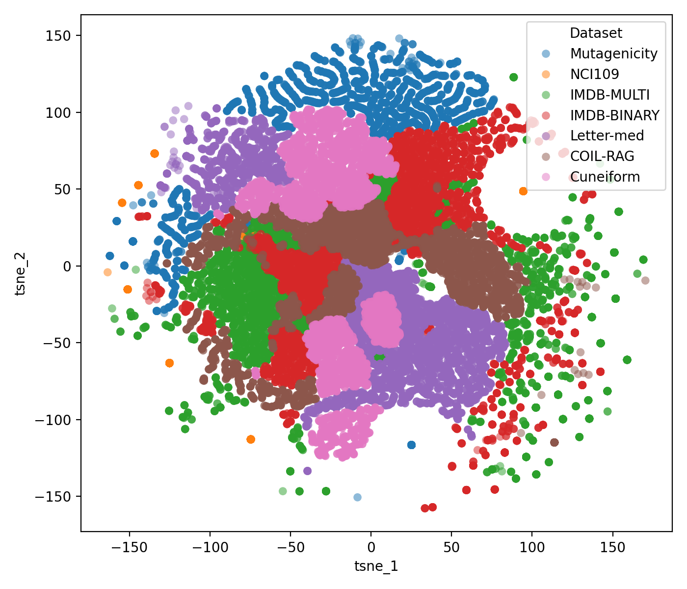
We further compare the node embeddings learned by GraphVec-FM with those obtained from two representative non-LLM-based GFMs, RiemannGFM and GFT. Figure 5 visualizes node embeddings from NCI109 and IMDB-MULTI, where colors denote datasets and markers denote graph classes. Compared with RiemannGFM and GFT, GraphVec-FM produces embeddings with stronger cross-dataset mixing while still preserving visible class-level structure. This qualitative comparison suggests that the proposed global multi-graph construction and density-based alignment better reduce dataset-specific feature mismatch, rather than merely separating nodes according to their source dataset. As with all t-SNE visualizations, this result is qualitative and should be interpreted together with the quantitative transfer results.

Table 16: Resource consumption for large-scale dataset evaluation. Note that COLOR-3 exhibits higher RAM consumption compared to reddit_threads, primarily due to its larger average number of nodes.

Dataset	Graphs	Avg. Nodes	RAM	Time
COLOR-3	10500	61.31	23.17GB	626.84s
reddit_threads	203088	23.93	6.01GB	3139.53s

H.13 Scalability to Large-scale Dataset

The construction and decomposition of global multi-graphs become computationally intensive when the downstream dataset contains a large number of graphs and nodes. To ensure scalability, except for employing the Nyström approximation (mentioned in Section 3.2) to handle large graphs efficiently and reduce the complexity of kernel matrix operations, we also reduce the computation cost by splitting datasets into small batches and computing the mini-batch global graphs.

To further validate the scale ability during evaluation, we test the time and memory consumption to evaluate on two large datasets COLOR-3 and reddit_threads [Morris et al., 2020] with more than 10k graphs and 20k graphs respectively. For these experiments, each dataset is divided into blocks of 128 graphs to build the corresponding multi‑graphs. The resulting resource usage is summarized in Table 16, demonstrating that the overhead remains manageable at this scale.

H.14 Ablation Study

To verify the effectiveness of our proposed methods and modules, we conduct ablation study on global multi-graph construction, mean alignment algorithm, and reference layer. For the global multi-graph, we vary the number of multi-graphs from 1-6. Figure 6 and Figure 7 demonstrate the impact of the number of kernel parameters on downstream few-shot graph classification accuracy. These results were obtained by incrementally increasing the set of Gaussian kernel bandwidths from $[0.25]$ to the full set $[0.25,0.5,1,2,5,10]$ used in our main experiments. It can be observed that classification accuracy improves with a greater number of global multi-graphs, particularly for datasets with original continuous node attributes. This observation further illustrates that the global multi-graphs constructed by using different kernel parameters help capture patterns from original features.

We conducted experiments using simple pooling without reference layers, and the results are presented in Table 17. After removing the reference layer module, the performance on all datasets shows degradation, especially on COLLAB, IMDB-BINARY, and Cuneiform. By removing the mean alignment, the performance on COLLAB, Letter-Med, and Cuneiform shows an evident decrease. Similarly, we also conduct experiments that remove the alignment module and both the alignment module and the reference layer. The overall impact of the two modules is shown in Table 18.

Table 17: Ablation study of reference layer and mean alignment module.

	Dataset
Model Variant	COLLAB	REDDIT-B	IMDB-B	IMDB-M	Letter-med	COIL-RAG	Cuneiform
	(50-shot)	(50-shot)	(50-shot)	(50-shot)	(50-shot)	(5-shot)	(1-shot)
Original Model	$\mathbf{68.09}\pm 2.99$	$\mathbf{81.52}\pm 1.50$	$\mathbf{68.39}\pm 4.06$	$\mathbf{46.70}\pm 0.99$	$\mathbf{85.60}\pm 1.44$	$\mathbf{74.20}\pm 0.77$	$\mathbf{55.86}\pm 8.15$
Mean Readout Only	$65.04\pm 2.75$	$77.79\pm 3.11$	$61.78\pm 2.59$	$46.07\pm 2.60$	$83.17\pm 0.99$	$72.87\pm 1.26$	$41.04\pm 3.64$
w/o alignment	$64.90\pm 1.81$	$76.74\pm 5.43$	$66.06\pm 4.44$	$45.78\pm 1.46$	$81.87\pm 1.31$	$72.14\pm 0.35$	$42.87\pm 5.18$

Table 18: The individual effect of alignment algorithm and reference layer on downstream cross-domain graph classification. The reported performance is averaged on 7 datasets.

Alignment	Reference layer	Avg. Acc. (%)
$\checkmark$	$\checkmark$	68.62
$\checkmark$	$\times$	63.95
$\times$	$\checkmark$	64.37
$\times$	$\times$	63.16

H.15 Kernel Function Analysis

Table 19: Analysis of different kernel functions used in the multi-graph construction module. The RBF kernel is used as the default choice in GraphVec.

Kernel	COLLAB	IMDB-BINARY	IMDB-MULTI	REDDIT-BINARY	Letter-med	COIL-RAG	Cuneiform
Laplacian	$65.28\pm 1.38$	$69.83\pm 1.79$	$46.33\pm 2.09$	$86.03\pm 3.23$	$83.47\pm 2.05$	$74.74\pm 0.96$	$47.00\pm 4.92$
Polynomial	$56.33\pm 3.81$	$60.56\pm 2.06$	$40.56\pm 3.24$	$71.53\pm 4.65$	$82.57\pm 1.42$	$62.55\pm 2.53$	$41.43\pm 4.79$
RBF	$68.09\pm 2.99$	$68.39\pm 4.06$	$46.70\pm 0.99$	$81.52\pm 1.50$	$85.60\pm 1.44$	$74.20\pm 0.77$	$55.86\pm 8.15$

We further study the effect of different kernel functions in the multi-graph construction module. Specifically, we compare the Laplacian kernel, polynomial kernel, and RBF kernel for constructing the global graphs over node attributes. As shown in Table 19, the RBF kernel achieves the best or competitive performance on most datasets, including COLLAB, IMDB-MULTI, Letter-med, and Cuneiform. Although the Laplacian kernel performs better on IMDB-BINARY, REDDIT-BINARY, and COIL-RAG, its performance drops substantially on Cuneiform compared with the RBF kernel. The polynomial kernel performs consistently worse than the other two kernels, suggesting that its induced similarity may be less suitable for capturing local node-attribute relationships across heterogeneous graph domains.

Overall, the RBF kernel provides the most stable performance across datasets. This is consistent with the motivation of our multi-graph construction strategy: the RBF kernel captures smooth local similarity in the node attribute space and is less dependent on the absolute scale or linear structure of the original attributes. Therefore, we use the RBF kernel as the default kernel function in GraphVec.

H.16 Comparison with Other Alignment Approaches

We further compare our density-maximization mean alignment with the alignment strategy adopted in AnyGraph under the same backbone and evaluation protocol. Although both methods rely on SVD-based representations, the two alignment mechanisms are fundamentally different. AnyGraph applies SVD directly to original node attributes and is mainly designed to handle heterogeneous feature dimensions, whereas our method first constructs kernelized global graphs and then aligns the resulting relational embeddings by explicitly maximizing the density of dataset means under orthogonal transformations.

The results in Table 20 show that our alignment strategy improves performance on all six cross-domain benchmarks. The gain is modest on IMDB-MULTI, but it becomes substantial on datasets with larger domain gaps, especially the computer vision datasets Letter-med, COIL-RAG, and Cuneiform. In particular, the large margin on COIL-RAG and Cuneiform suggests that directly aligning raw attribute spaces is not sufficient when datasets differ strongly in feature semantics, while our density-based alignment is better at matching datasets in a shared relational space. These results provide empirical support that the proposed alignment module is an important contributor to the transferability of GraphVec across domains.

Table 20: Comparison between the alignment strategy used in AnyGraph and our density-maximization mean alignment. Our alignment consistently improves cross-domain graph classification performance, especially on computer vision graph datasets.

Alignment Method	COLLAB	IMDB-BINARY	IMDB-MULTI	Letter-med	COIL-RAG	Cuneiform
AnyGraph’s Alignment	$62.93\pm 2.27$	$63.61\pm 2.92$	$45.33\pm 1.93$	$72.17\pm 1.25$	$29.05\pm 3.35$	$10.46\pm 2.09$
Our Alignment	$68.09\pm 2.99$	$68.39\pm 4.06$	$46.70\pm 0.99$	$85.60\pm 1.44$	$74.20\pm 0.77$	$55.86\pm 8.15$