Accelerating Scientific Research with Gemini:
Case Studies and Common Techniques
Abstract
Recent advances in large language models (LLMs) have opened new avenues for accelerating scientific research. While models are increasingly capable of assisting with routine tasks, their ability to contribute to novel, expert-level mathematical discovery is less understood. We present a collection of case studies demonstrating how researchers have successfully collaborated with advanced AI models, specifically Google’s Gemini-based models (in particular Gemini Deep Think and its advanced variants), to solve open problems, refute conjectures, and generate new proofs across diverse areas in theoretical computer science, as well as other areas such as economics, optimization, and physics. Based on these experiences, we extract common techniques for effective human-AI collaboration in theoretical research, such as iterative refinement, problem decomposition, and cross-disciplinary knowledge transfer. While the majority of our results stem from this interactive, conversational methodology, we also highlight specific instances that push beyond standard chat interfaces. These include deploying the model as a rigorous adversarial reviewer to detect subtle flaws in existing proofs, and embedding it within a "neuro-symbolic" loop that autonomously writes and executes code to verify complex derivations. Together, these examples highlight the potential of AI not just as a tool for automation, but as a versatile, genuine partner in the creative process of scientific discovery.
1 Introduction
The integration of artificial intelligence into the scientific workflow has traditionally focused on data analysis, simulation, and routine automation. However, the emergence of frontier large language models (LLMs) with enhanced reasoning capabilities suggests a shift towards AI systems that can act as an effective research collaborator, and contribute to the core intellectual tasks of research: formulating hypotheses, designing algorithms, developing novel techniques to tackle an open problem, and proving theorems.
This paper documents a series of independent experiments where researchers utilized advanced AI models to tackle specific, often long-standing, open problems in their respective fields. The results range from resolving conjectures in information theory and submodular maximization to deriving exact analytical spectra for cosmic strings and improving bounds for graph algorithms.
Key Contributions: Given the breadth of the fields and case studies covered, we highlight three primary contributions of this paper:
-
1.
Demonstrating the power of hybrid models: We show the potential of a hybrid human-AI model in tackling real, highly complex open problems across a diverse set of scientific and mathematical domains.
-
2.
Advancing state-of-the-art science: We make concrete, notable contributions to real problems in science, yielding novel results such as resolving conjectures, improving algorithmic bounds, and identifying critical flaws in literature.
-
3.
Showcasing the future of scientific discovery: We illustrate what the future of research looks like in practice. By detailing novel workflows, human-AI collaboration techniques, and interactive problem-solving strategies, we highlight the real implications for how science is likely to be conducted in the coming years.
Crucially, these are not hypothetical scenarios but real-world instances where AI played a pivotal role in advancing state-of-the-art research. By analyzing these diverse case studies, we identify recurring patterns and effective strategies for leveraging AI in such theoretical research. The significance of these results is the generality of these techniques and existence of common recipes that can be applied by probing publicly available Gemini models. These include:
-
•
Agentic Execution Loops: Moving beyond manual chat interfaces, models can be embedded in automated “neuro-symbolic" pipelines. In these setups, the AI proposes a mathematical solution, writes code to numerically verify it, and automatically ingests execution errors (e.g., Python tracebacks) to self-correct and autonomously prune invalid mathematical branches (see Section 6.1).
-
•
Deep Technical Review and Bug Detection: Beyond constructive tasks, AI models can act as adversarial reviewers. We present a case where an LLM, guided by an iterative self-correction protocol, identified a fatal flaw in a recent cryptography preprint claiming a major breakthrough (SNARGs from LWE) [52], a subtle inconsistency between a definition and a construction that had escaped initial human review.
-
•
Deep Literature Synthesis and Connection: AI models can identify obscure connections between disparate fields (e.g., linking Steiner trees to the Kirszbraun Extension Theorem) that human experts might overlook.
-
•
Counterexample Generation: Models are adept at constructing counterexamples to refute plausible conjectures, saving researchers from pursuing dead ends.
-
•
Algorithmic Insight and Optimization: In algorithmic research, AI can propose novel data structures or analysis techniques (e.g., adapting quadtrees for different norms) to improve time complexity bounds.
-
•
Automated Proof Generation and Verification: For well-defined subproblems, AI can generate rigorous proofs, sometimes requiring minimal human intervention, or verify complex manual derivations.
-
•
Interactive Refinement: A recurring theme is the iterative "conversation" where the researcher guides the model, correcting errors and refining the problem statement, which often leads to the final solution.
-
•
Theoretical Justification of Heuristics: AI models can bridge the gap between empirical success and theory by deriving rigorous justifications for heuristic methods, such as characterizing the implicit regularization induced by specific architectural choices like the Self-regularized Gumbel Sigmoid.
1.1 Model Description
Unless otherwise specified in the testimonials, the model used in this work is a Google-internal advanced version of Gemini Deep Think [73] – an enhanced reasoning model for complex problems that incorporates some of our latest research techniques, including parallel thinking, i.e., exploring multiple proof branches simultaneously. Similar models were also used recently in the International Mathematics Olympiad, achieving gold-medal standard performance [73]. This setup enables the model to simultaneously explore and combine multiple possible solutions before giving a final answer, rather than pursuing a single, linear chain of thought. This approach aligns with prior research demonstrating the efficacy of tree-based search methods in mathematical reasoning [44].
To make the most of the reasoning capabilities of Deep Think, we additionally trained this version of Gemini on novel reinforcement learning techniques that can leverage more multi-step reasoning, problem-solving and theorem-proving data. We also provided Gemini with access to a curated corpus of high-quality solutions to mathematics problems [73]. We also added a long linear chain of interactive verification calls at the output to increase reasoning depth and provide a lot of iterative verification, which was augmented by human expert verification.

1.2 Related Work
Recent advances in Large Language Models (LLMs) have spurred significant interest in their potential to accelerate scientific discovery. Several concurrent works explore the capabilities of AI in assisting mathematical and theoretical research. Here, we situate our contributions in the context of two particularly relevant studies: OpenAI’s investigation into GPT-5’s scientific capabilities [16] and the work of Nagda et al. on using AlphaEvolve for hardness of approximation [76].
Comparison with OpenAI’s GPT-5 Experiments.
Concurrent work by OpenAI [16] documents a series of case studies demonstrating GPT-5’s ability to contribute to research in fields ranging from biology and physics to mathematics. While both our work and theirs highlight the potential of frontier models as research assistants, there are differences in scope and focus. Our work places a heavier emphasis on Theoretical Computer Science (TCS), covering a wide array of subfields including algorithmic game theory, approximation algorithms, complexity theory, cryptography, graph theory, information theory, optimization, online algorithms, streaming algorithms, and query complexity.
Furthermore, recent activity on the Erdős Problem database has showcased the growing role of AI in resolving open mathematical conjectures. Notably, Erdős Problem #728, concerning factorial divisibility, was solved autonomously by an AI system (Aristotle), with GPT-5 playing a crucial role in generating the proof strategy and subsequent expositions [16]. This achievement, verified by Terence Tao and the broader community, underscores the capacity of these models not only to solve problems but also to rapidly iterate on and improve mathematical writing. Other problems, such as #729, #401, #205, #333, #281, and #460 have also seen AI-assisted progress or full resolutions, further validating the trend of AI-accelerated mathematical discovery. Our work complements these findings by providing a detailed methodology and a broader set of examples across TCS, demonstrating that these capabilities are not isolated incidents but part of a larger shift in research practices.
Comparison with AlphaEvolve for Hardness of Approximation.
Nagda, Raghavan, and Thakurta [76] present significant results in hardness of approximation for MAX-CUT, MAX-k-CUT, and TSP. Their primary methodology relies on AlphaEvolve [78], a specialized evolutionary algorithm that uses an LLM as a mutation operator to search for combinatorial structures (gadgets) that optimize a specific objective function (inapproximability ratios).
In contrast, our work focuses on the utility of general-purpose LLMs (specifically Gemini and its reasoning-enhanced variants like Deep Think) as conversational research partners. While AlphaEvolve is a powerful tool for search problems where a clear objective function exists (e.g., finding a gadget with specific properties), our case studies demonstrate that general-purpose models can be effective across a broader range of intellectual tasks where the "objective" is less well-defined, such as generating a proof idea, identifying a relevant theorem from a different field, or interactively refining a definition.
For instance, our derivation of the analytical spectrum for cosmic strings (Section 6.1) involved a tree-search over derivation strategies and mathematical concepts, rather than a direct optimization of a numerical value. Similarly, the resolution of the "Simplex is the Best for Graph Embeddings" conjecture (Section 4.2) relied on conceptual bridging (linking Steiner trees to Lipschitz extensions) rather than combinatorial search. Thus, our work complements [76] by showing that standard frontier models, without specialized evolutionary wrappers, can drive progress in theoretical research through dialogue and reasoning.
Concurrent Work.
A recent work [48] does mathematical discovery at scale using AI-assisted methodologies. Our work aligns with it in demonstrating the potential of AI as a collaborative partner in theoretical research, but we offer a distinct set of case studies and a focus on specific TCS domains. Additionally, we note independent works [89, 91] that further contribute to the growing body of literature on AI in mathematics and science.
Roadmap
The remainder of this paper is organized as follows. Section 2 synthesizes the common techniques and methodologies derived from these case studies. The sections after that give detailed and extensive testimonials from each collaboration, roughly categorized by the main role of the AI in the collaboration. Finally, Section 2.8 discusses the broader implications for the future of theoretical research.
2 Techniques for AI-Assisted Research
Across the various successful collaborations documented here, several common techniques emerged. These strategies represent a "playbook" for researchers looking to integrate AI into their theoretical work.
2.1 Iterative Prompting and Refinement
Rarely does a model solve a deep open problem in a single shot. Success often comes from an iterative dialogue.
-
•
Initial Broad Query: Start by asking the model to digest a relevant paper or problem statement to gauge its understanding.
-
•
Specific Sub-tasks: Break down the main problem into smaller, verifiable lemmas or calculations.
-
•
Error Correction: When the model makes a mistake (e.g., a wrong constant or invalid assumption), pointing it out specifically often leads to a correct and sometimes more elegant solution in the next turn.
-
•
Scaffolding: Providing the model with a high-level proof strategy or "scaffold" allows it to fill in the technical details effectively.
-
•
Adversarial Self-Correction for Review: When tasked with reviewing complex proofs, standard prompts often yield superficial results. A rigorous protocol instructing the model to (1) generate an initial review, (2) critique its own findings for hallucinations, and (3) iteratively refine the logic, enables deep technical critique. This was critical in identifying the flaw in the SNARGs paper (Section 3.2), where the model distinguished between a definition of perfect consistency and a construction of statistical consistency.
2.2 Cross-Pollination of Ideas
Models have ingested vast amounts of literature across all fields. They excel at:
-
•
Finding Analogies: Identifying similar problems in different domains (e.g., applying techniques from computational geometry to graph theory).
-
•
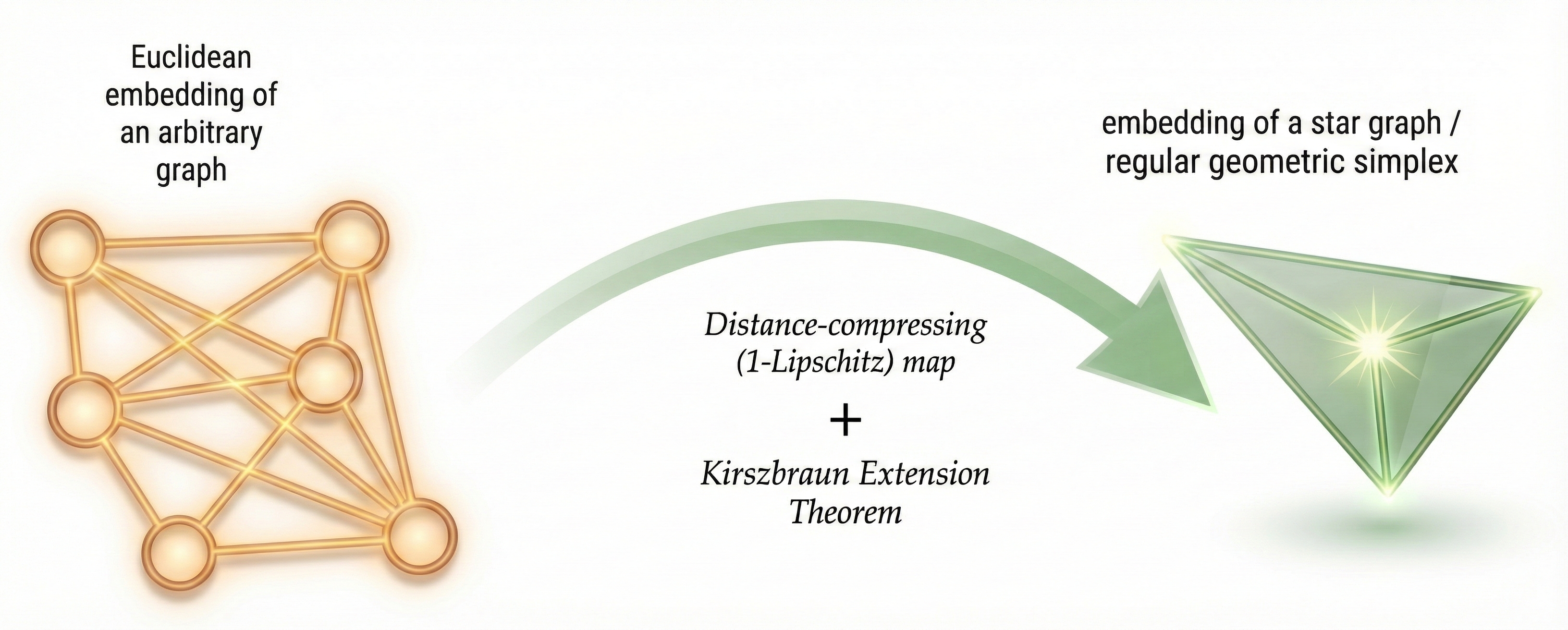
Retrieving obscure theorems: Bringing relevant but less-known theorems to the researcher’s attention (e.g., Stone-Weierstrass or Kirszbraun Extension Theorem) to bridge gaps in a proof.

2.3 Simulation and Counterexample Search
For conjectures, models can be tasked to:
-
•
Construct Counterexamples: Generating specific instances (graphs, matrices, set systems) that violate a proposed conjecture.
-
•
Verify Small Cases: Writing code to computationally verify a conjecture for small , providing empirical evidence before attempting a general proof.
2.4 Formalization and Rigor Checks
While models can hallucinate, they are increasingly capable of formal reasoning when prompted correctly.
-
•
Proof Sketch to Formal Proof: Asking the model to expand a high-level sketch into a rigorous LaTeX proof.
-
•
Sanity Checking: Using the model to check consistent usage of notation or to verify that all conditions of a theorem are met.
-
•
Mathematical Derivation: Researchers can offload the mechanical heavy lifting of complex derivations to the model, such as simplifying expressions, computing limits, or solving integrals, allowing them to focus on the high-level logic.
2.5 Interactive Proof Construction with External Validation
A powerful technique involves using the model to identify necessary external theorems and then validating those theorems with external sources.
-
•
Identifying Dependencies: Asking the model to list all external theorems required for a proof.
-
•
External Verification: The researcher finds the formal statements of these theorems (e.g., via Google Search or textbooks) and feeds them back to the model.
-
•
Self-Contained Proof Generation: The model then incorporates these verified statements to generate a rigorous, self-contained proof.
2.6 Agentic Tool-Use and Automated Feedback
While most of the collaborations documented here rely on manual, iterative dialogue, frontier models can also be deployed as agents within automated programmatic loops. For problems requiring heavy algebraic manipulation or where symbolic math must be rigorously grounded in numerical reality (e.g., the physics case study in Section 6.4), researchers can construct a “neuro-symbolic" pipeline consisting of the following steps:
-
•
Symbolic Proposal: The LLM generates a mathematical hypothesis or intermediate expression.
-
•
Code Generation: The LLM autonomously writes an executable script (e.g., in Python) to evaluate its proposed math against a known numerical baseline.
-
•
Automated Feedback: The system executes the code. If the code fails, hits a runtime error, or reveals numerical instability (such as catastrophic cancellation), the automated harness captures the exact execution traceback and injects it back into the LLM’s context window.
This programmatic loop allows the AI to systematically explore a tree of mathematical solutions, autonomously pruning dead-ends and self-correcting its algebra without requiring a human-in-the-loop for every intermediate step.
2.7 Human-AI Collaboration Dynamics
It is important to note that AI models like Gemini function best as powerful collaborators rather than autonomous researchers. In the successful case studies presented here, the partnership between the model and the human expert was key to the results.
-
•
Selection and Refinement: Models are capable of generating a high volume of diverse mathematical statements. Human expertise is valuable for filtering these outputs and identifying the most promising directions for further investigation.
-
•
Iterative Guidance: While models can solve some problems in a single shot, tackling deep open problems is often most successful through an iterative process. The researcher guides the model, refining the problem statement and narrowing the focus to achieve the desired result.
-
•
Standard Verification: As with any research collaboration, the AI can make mistakes, and AI-generated proofs and counterexamples benefit from rigorous verification. The model serves as an excellent accelerator for ideation and drafting, while the researcher validates the mathematical correctness.
-
•
Optimizing Context: Performance is often optimized by providing clear, self-contained definitions, particularly when using highly specialized notation that may deviate from standard literature.
-
•
Leveraging Literature: We found that incorporating relevant papers directly into the context significantly enhanced the model’s ability to construct correct proofs for specialized domains.
-
•
Context De-Identification: The model sometimes avoids non-trivial machinery (for example, the Kirszbraun extension theorem as in Section 4.2), treating such proofs as non-elementary, or it may do so because the prompt steers it toward conservatism to avoid hallucinations, causing it to abandon an otherwise viable approach. Separately, on occasion, when shown the paper as context in the prompt, it recognizes the statement to prove as a conjecture in the paper and refuses to attempt it on the grounds that it is an open problem. One way to bypass both issues is via context de-identification (remove the paper and provide only the problem statement and definitions), after which the model typically engages (and, in cases like Section 4.2, may ultimately draw on deeper results to resolve a conjecture).
We view the AI as a tireless, knowledgeable, and creative bright junior collaborator. Its value lies in its ability to synthesize vast amounts of information and generate novel hypotheses that human researchers can then validate and build upon.
2.8 Summary: The AI-Assisted Research Playbook
Taken together, the techniques outlined above represent a fundamental shift in how theoretical research can be conducted. The LLM is no longer acting merely as a search engine or a syntax formatter; it is functioning as a combinatorial reasoning engine and a sounding board for abstract ideation.
However, the most successful collaborations documented in the following case studies all share a common denominator: strong human orchestration. Although several of our successes came from a single “zero-shot" prompt, many required scaffolded reasoning, i.e., breaking down deep open problems into verifiable parts, testing hypotheses through adversarial prompting, and actively steering the model. Informally this interactive workflow has been called “vibe-proving".
By mastering the techniques outlined above—particularly iterative refinement and adversarial self-correction—researchers can effectively elevate the AI from a passive tool into an active, high-leverage research partner. The following sections document these dynamics in practice across a wide array of disciplines.
Chat interactions are presented using a light, color-coded design to distinguish speakers while maintaining a calm and unobtrusive appearance. When present, the overall chat box uses a sand-colored background, providing a warm, neutral container that visually groups multiple messages within a conversation. In cases where only a single message appears—such as an isolated user message or an isolated AI response—the surrounding chat box may be omitted, and only the message styling is shown. Messages authored by the user are displayed on a light, subtle blue background, chosen to clearly indicate user input while remaining easy to read for extended or technical text. AI-generated messages are shown on a very light red background; this tone is intentionally muted to avoid the visual intensity typically associated with red, while still providing a clear distinction from user messages. Across all elements, colors are kept near-white and low in saturation so that speaker differences are conveyed through hue rather than darkness, ensuring readability on screens, in print, and in accessibility-conscious settings.
3 Deep Technical Review and Counterexamples
In this section, we see how AI can act as a critical adversary, finding subtle bugs in human proofs, refuting plausible hypotheses, and hunting for counterexamples.
3.1 Online Algorithms: Submodular Welfare
Written by Morteza Zadimoghaddam and Vahab Mirrokni.
Problem Context
In online submodular welfare maximization, the Greedy algorithm achieves a competitive ratio of . A conjecture by Korula et al. (2015) suggested that the gain from "copying" an item to the end of the stream is bounded by the gain of "moving" it. Proving this would imply a competitive ratio of .
AI Contribution
The researcher provided the research paper that included the formal definitions as well as a conjecture statement, and tasked the model zero-shot with just identifying any open question in the paper and solving it. Throughout this paper we add a prompt that asks the model to be rigorous in its mathematical proofs and to thoroughly check its answers - we do not specify the details of this prompt.
Remarkably, the model chose the following counterexample and refuted it autonomously. The subsequent verification calculations were also generated by the model without extra interaction or supervision. This demonstrates its ability to construct valid, non-trivial instances that violate human-proposed conjectures. The human researchers defined the initial search parameters and independently verified the model’s arithmetic.
-
•
Refutation Strategy: The model independently selected the minimal non-trivial dimensions ( items, agents).
-
•
Autonomous Construction: In a single output, the model successfully defined the specific, valid submodular valuation functions (presented in Table 1) and the -perturbation required to strictly break the bound.
-
•
Automated Verification: Without human intervention, the model correctly performed the tedious calculations of expected marginal gains across all permutations to formally verify the violation.
Technical Details
In the problem of Online Submodular Welfare Maximization (Online SWM), items arrive one by one in a random order and must be irrevocably assigned to agents with submodular valuation functions. The goal is to maximize the total social welfare. It is well-established that the simple Greedy algorithm achieves a competitive ratio of in the adversarial setting. In the random order model, Korula et al. proved that Greedy achieves a ratio of at least , strictly beating [67].
To obtain a stronger bound, the authors proposed a natural conjecture (Conjecture 15) relating the expected marginal gain of the Greedy algorithm when an item is moved to the end of the sequence versus when it is duplicated at the end. If true, this conjecture would imply a competitive ratio of at least .
In this note, we refute this conjecture. We construct a counter-example involving a specific submodular valuation function and a set of items where the conjectured inequality fails to hold.
The Open Question
We focus on the definitions and conjecture provided in Section 5 of [67]. Let be a permutation of items.
Definition 3.1 (Permutation Variants [67]).
Fix a permutation .
-
•
Let be the permutation achieved by moving the item to the end of the sequence:
-
•
Let be the sequence of items achieved by copying to the end without removing the original :
Let denote the marginal gain that the Greedy algorithm obtains by allocating the -th arriving item in a sequence . Let be the set of all permutations. The conjecture proposed by Korula et al. is as follows:
Conjecture 3.2 (Conjecture 15 of [67]).
For any instance of the online submodular welfare maximization problem,
| (1) |
The Right Hand Side (RHS) of the inequality is equivalent to , as and share the same distribution. The conjecture essentially posits that the gain from a duplicated item at the end of the stream is, in expectation, bounded by the gain of the last item in a standard random permutation.
Refutation of the Conjecture
We answer the open question negatively. We show that there exist submodular valuation functions and instances where the expected marginal gain from the copied item exceeds the bound proposed in Conjecture 3.2.
Theorem 3.3.
Conjecture 3.2 is false. There exists an instance of Online SWM such that:
Counterexample Construction
We construct an instance with items and agents . We define the valuation functions and . Let . We define , where and are defined in Table 1.
| 0 | 0 | 0 | |
| 10 | 10 | 10.1 | |
| 10 | 7 | 10.1 | |
| 10 | 11 | 10.1 | |
| 15 | 17 | 15.2 | |
| 20 | 16 | 20.2 | |
| 20 | 16 | 20.2 | |
| 25 | 21 | 25.3 |
Verification of Validity We must verify that and are monotone and submodular.
-
1.
Monotonicity: It is clear from Table 1 that both and are monotone (i.e., if ).
-
2.
Submodularity of : We check the marginal gains (MG).
-
•
: , , , .
-
•
: , , , .
-
•
: , , , .
In all cases, the marginal gains are non-increasing as the conditioning set grows. Thus, is submodular.
-
•
-
3.
Submodularity of : We first check .
-
•
: , , , .
-
•
: , , , .
-
•
: , , , .
is submodular. Since is the sum of a submodular function and a modular function, is submodular.
-
•
Calculation of the RHS
The RHS is the sum of the expected gains of each item when it arrives last. Let denote this expectation for item .
-
1.
( arrives last). We consider the permutations of .
-
•
. : vs . .
: . . .
Gain of : . . Gain is 5.1. -
•
. : vs . .
: . . .
Gain of : 5.1.
Result: .
-
•
-
2.
( arrives last). We consider the permutations of .
-
•
. : vs . .
: . . .
Gain of : . . Gain is 5.1. -
•
. . . Gain of is 5.1.
Result: .
-
•
-
3.
( arrives last). We consider the permutations of .
-
•
. .
: . . .
Gain of : . . Gain is 10.1. -
•
. .
: . . .
Gain of : . . Gain is 10.1.
Result: .
-
•
Calculation of the LHS
The LHS is the expected total residual welfare. We calculate the total residual for all permutations. The residual of item , , is the maximum marginal gain of for any agent given the final allocation by Greedy on . (The agent who received has 0 marginal gain for a copy).
-
1.
.
. (7 vs 5.1). (10.1 vs 9).
Allocation: .
. . .
. -
2.
.
. (11 vs 10.1). (5.1 vs 5).
Allocation: .
. . .
. -
3.
.
. (10 vs 5.1). (10.1 vs 6).
Allocation: .
. . .
. -
4.
.
. . .
Allocation: .
. -
5.
.
. . .
Allocation: .
. -
6.
.
. . .
Allocation: .
.
The sum of the total residuals is .
Conclusion
We compare the LHS and the RHS.
Since , we have . This violates the inequality stated in Conjecture 15. Therefore, Conjecture 15 is false.
The failure of Conjecture 15 implies that the specific path to proving a competitive ratio proposed by [67] is invalid. While the Greedy algorithm is known to beat in the random order model, establishing the tightest possible bound remains an open challenge. Our result indicates that the interaction between duplicated items and previous greedy allocations is more complex than the “Move” vs “Copy” intuition suggests.
3.2 Cryptography: AI-Assisted Bug Detection in SNARGs
Written by Ziyi Guan, David P. Woodruff, and Eylon Yogev
Problem Context
Succinct non-interactive arguments (SNARGs) are among the most important and actively studied primitives in modern cryptography. A SNARG enables a prover to convince a verifier of some computational statement (such as knowledge of a solution to a complex equation or the validity of a transaction according to network rules) using a proof that is extremely short and efficient to verify. Remarkably, the proof size and verification time can be exponentially smaller than the time required to check the statement directly. The succinct proof and verification is critical for real-world applications. For instance:
-
•
Verifiable Outsourced Computation: A weak client (like a smartphone) can offload a heavy computation to a cloud server and receive a short proof that the result is correct, without trusting the server.
-
•
Blockchain Scalability: Blockchains can use SNARGs (often in the form of zk-SNARKs) to compress the verification of thousands of transactions into a single tiny proof, enabling massive throughput improvements (e.g., ZK-Rollups).
Constructions of SNARGs are notoriously difficult despite the active research. For decades, researchers have sought to build them based on standard cryptographic assumptions—assumptions that are widely believed to be true and have withstood years of cryptanalytic attacks. The “holy grail” in this area is to build a SNARG from the learning with errors (LWE) assumption. LWE is the foundation of modern lattice-based cryptography; it is believed to be secure even against quantum computers (post-quantum security) and allows for powerful functionalities like fully homomorphic encryptions.
Existing SNARG constructions typically fall short of this ideal in the following ways:
-
1.
Idealized Models: The most efficient SNARGs are usually constructed in the random oracle model (ROM), where hash functions are modeled as perfect random functions. However, random oracles cannot be instantiated in the real world and thus only provide heuristic security.
-
2.
Non-Standard Assumptions: Another common way to build SNARGs (with knowledge) relies on assumptions like “Knowledge of Exponent,” which are non-falsifiable and sometimes imply conclusions too strong to be true.
-
3.
Indistinguishability Obfuscation (iO): While iO can build almost anything, including SNARGs, current constructions of iO are extremely complex, inefficient, and rely on very heavy mathematical machinery.
The paper “SNARGs for NP from LWE” by Ziyi Guan and Eylon Yogev [52] claimed to achieve the breakthrough: a SNARG for all of NP based solely on the sub-exponential hardness of LWE. Their proposed construction involved two novel components: “PCP shadows” (a way to compress probabilistically checkable proofs) and “function vector commitments” (a lattice-based vector commitment scheme).
AI Contribution via Advanced Prompting
As part of an experiment to evaluate the capability of AI models in theoretical computer science research, we analyzed the preprint of the paper using a Google-internal LLM. Crucially, we did not simply ask the model to “check the proof,” as standard prompts often lead to superficial reviews or hallucinations when dealing with complex mathematical logic.
Instead, we employed a rigorous iterative self-correction prompt. The prompt was designed to force the model to act as a meticulous and adversarial reviewer. The explicit instructions are in Figure˜3.
Furthermore, the prompt included a specific protocol for mathematical rigor. It required the model to distinguish between a “Complete Proof” (only if every step was verified) and “Structured Partial Progress” (if any gaps were found). It also required the model to explicitly flag gaps or unproven assumptions using a specific tag. This approach was used by Google recently for providing preliminary feedback to authors of STOC submissions, see [23].
The Finding and Verification
Using this method, the model’s final review flagged a critical, fatal flaw in the paper’s construction of “PCP with shadow soundness” (Section 4).
The issue lay in the discrepancy between the definition of the scheme and its actual construction:
-
•
The Definition: Definition 4.1 (Property 3) of the paper required perfect consistency. This meant that for any two valid proofs that shared a local view, the generated “shadows” (succinct digests of the proof) must be identical for every single choice of randomness used in the shadow generation process.
-
•
The Construction: The construction presented in Section 4.3, however, only achieved imperfect consistency. This meant that the shadows would match with high probability over the choice of randomness, but there could exist bad randomness values where they differed.
The model argued that this was not a minor technicality. The security proof for the SNARG (specifically the soundness argument) relied heavily on the strong, perfect consistency definition. It assumed that once a commitment was opened, the underlying shadow was unique and well-defined. By only achieving statistical consistency, the construction opened the door to an adversary who could find specific bad randomness values to break the binding between the proof and its shadow. This would allow an adversary to forge a valid argument for a false statement, completely undermining the security of the SNARG.
Expert Verification and Outcome
To validate the model’s finding, we shared the detailed critique with cryptography experts Aayush Jain and Zhengzhong Jin. They performed an independent review of the paper and the model’s output.
Their assessment was definitive: the model was correct. They confirmed that the gap between the definition and construction of perfect consistency was a fatal flaw in the logic. They noted that while the model produced some noise (flagging other, less relevant issues), this specific insight was accurate and hit the core of the problem. Without perfect consistency, the reduction used in the security proof fails, and the main theorem does not hold.
We subsequently communicated these findings to the paper’s authors, Ziyi Guan and Eylon Yogev. They acknowledged the validity of the issue raised by the model. They agreed that the gap between the definition and construction of consistency was a significant error. Following this, they updated their paper on the Cryptology ePrint Archive. The updated manuscript includes a note in red text explicitly stating that a gap in the proof of the main theorem had been found.
This episode serves as a powerful testament to the evolving capabilities of large language models in scientific research. While LLMs are often criticized for their inability to reason or their tendency to hallucinate, this case shows that with the right prompting strategy—specifically one that enforces iterative self-correction and rigorous verification—they can identify subtle, deep technical flaws in state-of-the-art research.
4 Cross-Pollination of Ideas
In this section we see AI acting as an interdisciplinary bridge, retrieving obscure theorems from entirely different mathematical domains to overcome roadblocks.
4.1 Approximation Algorithms: Max-Cut
Written by Euiwoong Lee.
Problem Context
The Goemans-Williamson (GW) algorithm uses Semidefinite Programming (SDP) to achieve an optimal 0.878-approximation for Max-Cut. A long-standing open question asks whether rounding SDP solutions of bounded rank can yield a better approximation ratio. While known for , the case for general remained open.
I realized that this could be resolved if the following simple and natural geometric property held: Does the variance of a sum of random variables (where are unit vectors with bounded pairwise inner products) have a lower bound ?
AI Contribution
The model solved this geometric variance question.
-
•
Synthesizing Advanced Math: The model recognized this as a problem solvable via geometric functional analysis, a field outside the typical approximation algorithms toolkit.
-
•
Proof via Measure Theory: It constructed a proof using the compactness of the space of probability measures on the sphere.
-
•
Iterative Rigor: When we questioned the validity of using “relaxed" measure spaces, the model justified its steps by citing and applying the Stone-Weierstrass Theorem, the Riesz Representation Theorem, and properties of spherical harmonics.
Max-Cut on Bounded-dimension SDP Solutions
Max-Cut is one of the most fundamental problems in combinatorial optimization and approximation algorithms. Given an undirected graph , the goal is to partition into and to maximize the number of edges between and ; equivalently, compute to maximize .
While combinatorial or linear programming (LP)-based methods only yielded a -approximation (e.g., the returned solution’s value is at least half of the optimal value) in polynomial time, the celebrated result of Goemans and Williamson [51] used a semidefinite programming (SDP) relaxation to obtain an approximation ratio of , which was later proved to be optimal for all polynomial-time algorithms assuming the Unique Games Conjecture [65]. This tight relationship between algorithms, complexity, and SDPs was later extended to numerous other combinatorial optimization tasks, most notably all Constraint Satisfaction Problems (CSPs) [81].
Given the importance of this result, it is natural to ask which additional assumptions allow polynomial-time algorithms to achieve an approximation ratio for some constant . Structural properties of the input graph have been the most popular assumptions, which include when is dense (i.e., [4]), is bounded-degree [35, 58], or has a certain expansion property [9].
In order to motivate assumptions depending on the structure of SDP solutions, let us briefly recall Goemans-Williamson’s SDP relaxation. Given , their SDP relaxation, with a symmetric matrix as the variable, is as follows:
| maximize | |||
| subject to | |||
The fact that this SDP is a relaxation for Max-Cut (i.e., the SDP optimal value is at least the Max-Cut optimal value) is based on the fact that for any solution for Max-Cut, is a feasible solution for the SDP. For the -approximation, the algorithm is the following:
-
1.
Compute the optimal SDP solution .
-
2.
Compute its Gram decomposition for some . Let be the th row of .
-
3.
Sample a random Gaussian vector .
-
4.
For each , let . (I.e., if and otherwise.)
The -approximation can be proved by a simple edge-by-edge analysis where each edge contributes to the SDP objective, and to the Max-Cut objective in expectation (because it is the probability that ).
So, how about the structural properties of the optimal SDP solution ? Perhaps one of the most natural assumptions on is its rank; the gist of the Max-Cut problem itself is to force the rank of to be . Then the question is, if is a feasible solution to the SDP with rank , can we round to a Max-Cut solution of value at least times the SDP value of , where is a constant depending only on ?
This is a natural question asked since the Goemans-Williamson algorithm, and Goemans gave a positive answer when . Avidor and Zwick [5] refined it and gave a positive answer for as well, but to the best of my knowledge, even the case is open. It is surprising, especially given that analogous questions have already been answered for more general Grothendieck problems [14, 15]; however, they are not directly comparable, as the optimal ratios for Grothendieck problems are worse than .
While studying the recent result of Hsieh and Kothari [58], which simplifies and extends the result of Feige, Karpinski, and Langberg [35] for Max-Cut on bounded-degree graphs, I realized that their algorithmic framework could be applied to the bounded-dimension case as well, modulo one very natural geometric question, which is stated below.
The rest of the section details how the model “solved it.” Now, there exists a polynomial-time algorithm that, given an SDP solution of rank , produces a Max-Cut solution whose value is at least times the value of , for some . But, before detailing the answer, let us mention that the answer is not completely satisfactory in the sense that it does not produce any explicit expression for as a function of ; in contrast, when ’s degree is at most , the best-known approximation ratio is [58].
On the other hand, the proof is based on results from geometric analysis, including the compactness of a certain space of probability measures, which have not been used much in the design of approximation algorithms. Will it be among the first of many examples where such analytic tools are used in approximation algorithms (and inspire more “constructive proofs” with “more explicit bounds”)? In any case, this experience reinforces common beliefs that large language models can help researchers in areas where they are not experts.
Geometric Question
The original question I asked the model is depicted in Figure˜4.
Using the standard second-moment methods and the fact that , the model reduced it to the following equivalent question about the variance of , which is indeed the version one needs for the Max-Cut application.
Problem 4.2.
The variance of is , where . Is for some constant ?
Due to space constraints, let me not fully elaborate on how a positive answer to ˜4.2 leads to an improved algorithm for Max-Cut in the bounded-dimension case. It is simple to check formally, because one can just replace Lemma 7 of [58] with the answer to ˜4.2, and the rest of their (elegant) seven-page paper works as is. Intuitively, their algorithm, which is originally suggested by [35], performs the standard rounding algorithm mentioned above, followed by the natural local improvement step; if there is a way to flip the assignment to a vertex that strictly improves the value, execute it. (The actual algorithm implements it in a more conservative way.) In this context, ˜4.2 seems natural, because from the perspective of a vertex , the more variance its neighbors have, the bigger chance there is that the standard rounding algorithm (which already guarantees an -approximation) made a wrong decision for and the local improvement step further improves upon it by flipping . In particular, the answer to ˜4.2 is applied to the neighborhood of every vertex.
First Response
The response in this section is fully generated by the model, except for removing standard applications of second-order methods.
Interactions
The first response, though it looked like a natural and sound approach using geometric functional analysis, had some gaps in the proof and was not fully verifiable, partially due to my inexpertise on the topic. Two major hurdles were (1) the foundations of measure theory to establish the compactness of and (2) working knowledge of spherical harmonics to see how for all odd implies for any odd polynomial . Note that (2) was somewhat expected as the previous results for [5] and Grothendieck problems [14, 15] used spherical harmonics and related Gegenbauer polynomials, but the use of (1), via relaxing -point discrete measures to , is a type of an argument rarely used in the approximation algorithms literature. In order to formally understand it, one needs to review the foundations of measure theory. For example, what is the weak topology? How is the Stone-Weierstrass theorem formally applied here? How does for every odd imply is a symmetric measure?
After several iterations of asking for the reference behind each nontrivial step and manually searching each reference and feeding it back to the model, it produced the output in the next section. Now it is understandable to me, whose only formal exposure to analysis was an undergraduate course almost twenty years ago.
Second Response
This response is fully generated by the model, except for (1) removing standard applications of second-order methods, (2) adding two footnotes further justifying some steps, and (3) minor cosmetic changes.
4.2 Computational Geometry: Steiner Trees
Written by Karthik C. S.
Problem Context
The "Simplex is the Best for Graph Embeddings" conjecture states that among all graphs with edges embedded into Euclidean space as characteristic vectors, the star graph configuration yields the minimum Steiner tree cost. Proving this is a key step towards establishing APX-hardness for high-dimensional Steiner Tree problems.
AI Contribution
The model’s involvement was decisive.
-
•
The Crucial Link: The model suggested an approach based on the Kirszbraun Extension Theorem, which guarantees the existence of Lipschitz-preserving extensions of maps between Hilbert spaces.
-
•
Overcoming "Elementary" Bias: Initially, the model dismissed this approach as "non-elementary". However, when the researcher clarified that an elementary proof was not required, the model successfully formalized the argument.
-
•
Formal Proof: The model constructed a mapping from any graph embedding to the star graph embedding and used Kirszbraun’s theorem to show that a Steiner tree for the former can be transformed into a valid tree for the latter without increasing cost.
Technical Details: Steiner Trees and Graph Embeddings
In the Euclidean Steiner Tree problem, we are given as input a set of points (called terminals) in the -metric space, and the goal is to find the minimum-cost tree connecting them. Additional points from the space (called Steiner points) can be introduced as nodes in the solution.
The seminal works of Arora [3] and Mitchell [75] provide a Polynomial Time Approximation Scheme (PTAS) for solving the Euclidean Steiner Tree problem in fixed dimensions. However, the problem remains poorly understood in higher dimensions (such as when the dimension is logarithmic in the number of terminals). Ruling out a PTAS for the problem in high dimensions is a notoriously long-standing open problem (for example, see Trevisan [92]).
In [40], the authors proposed various conjectures related to Steiner trees in order to make progress on understanding the inapproximability of the high-dimensional Euclidean Steiner Tree problem. Assuming these, they could prove APX-hardness of the Euclidean Steiner Tree problem in dimensions polynomial in the input size.
The simplest such conjecture, called the Simplex is the Best for Graph Embeddings Conjecture in [40], was a special case of the widely open generalized Gilbert-Pollak conjecture [50, 60, 29]. In this report, we detail the resolution of this conjecture by Gemini, including the process.
First, we state the conjecture and provide the necessary context. Next, we describe our interaction with Gemini that led to its resolution. Finally, we present the proof produced by Gemini.
Research Context
A natural approach to prove the APX-hardness of the Euclidean Steiner Tree problem is via a reduction from the Vertex Cover problem on bounded degree graphs (for example, see [41]). A candidate reduction proposed in [40] is to embed a vertex cover instance graph into by mapping each edge to , where is the standard basis vector with in the coordinate indexed by and elsewhere. Thus, each edge is embedded as its characteristic vector. The embedding of the set of edges incident to a single node forms the vertices of a regular simplex of side length . The point configuration as a whole consists of the vertices of a regular simplicial complex (where we take the union of the simplices associated with each node).
Proving that the above reduction is gap-preserving, by analyzing the completeness and soundness cases, requires proving the following conjecture:
Conjecture 4.11 (Euclidean Steiner Tree for Regular Simplicial Complexes [40]).
For all constants and , there exist constants and sufficiently large so that, for all , given a regular, unit, simplicial complex on vertices:
-
1.
Completeness: If the vertices can be partitioned into the vertices of at most unit regular simplices, then the point configuration of the vertices admits a Euclidean Steiner tree of cost at most .
-
2.
Soundness: If the vertices cannot be partitioned into the vertices of fewer than unit regular simplices, then the point configuration of the vertices does not admit a Euclidean Steiner tree of cost less than .
As a first step toward proving the above conjecture, [40] proposed the following much simpler conjecture about Steiner ratios of specialized point-sets.
Conjecture 4.12 (Simplex is the Best for Graph Embeddings [40]).
Over all simple graphs with edges, the embedding333Here we allude to embedding each edge by its characteristic vector, as detailed in the aforementioned reduction from the Vertex Cover problem. of the star graph on edges has the minimum cost Steiner tree.
Observe that restricted to connected graphs with the same number of edges, the minimum spanning tree costs are identical. Consequently, Conjecture 4.12 over connected graphs is equivalent to finding the point configuration with the minimum Steiner ratio. In [40], the authors verified the conjecture computationally up to using the exact algorithm of Smith [90] and established the following structural property.
Lemma 4.13 (Fleischmann et al. [40]).
For any fixed , the graph of size whose embedding (as above) has the minimum cost Steiner tree has diameter at most .
Methodology
I requested David Woodruff to formulate a prompt to solve Conjecture 4.12 using the Google internal model, providing only the paper [40] as context.
The model proposed two approaches but did not offer a conclusive answer. The second approach involved starting from an arbitrary graph and applying local transformations that do not increase the optimal Steiner tree cost, eventually converging to the star graph. As we had already attempted this strategy, it offered no new insights.
The first approach, however, was based on the Kirszbraun Extension Theorem [66, 93]. I must confess that while I was aware of various extension theorems from my work on the computation of fixed-points (see, for example, [45]), I had not immediately seen the connection to Steiner trees. To my frustration, instead of exploring this direction further, the model noted that the proof of Kirszbraun Extension Theorem is non-elementary, and concluded that this approach would not yield an elementary proof of Conjecture 4.12.
As I was not seeking an elementary proof and indeed, had not requested one, this comment left me slightly frustrated, yet intrigued. Consequently, I decided to run my own experiments using Gemini Ultra (utilizing the standard “thinking” mode rather than “deep think”).
Initially, I provided the exact prompt used for the internal model, but Gemini consistently declined to attempt the problem, insisting that it was an open problem that could not be solved.
Next, I removed the paper from the context and provided only the problem statement along with the relevant definitions. At first, the model suggested a hand-waving argument; however, when I pointed out the parts that required formalization, it successfully provided them. It first derived the same lemma suggested by the internal model, though this time with a proof. As the proof remained somewhat informal, I provided Gemini with the summary of the internal model’s output and with its explanation of why it had abandoned the approach. At that point, Gemini successfully formalized the lemma using the Kirszbraun Extension Theorem (the tool it had been missing earlier).
Through this process, I have learned about the power of the Kirszbraun Extension Theorem for Steiner tree computation and analysis. To the best of my knowledge, this is a new connection (yet one that feels very natural!). This discovery makes me more optimistic about the prospects of establishing the APX-hardness of computing the Euclidean Steiner Tree in high dimensions.
Gemini’s Proof of Conjecture 4.12
4.3 Graph Theory: Computing Perfect Matchings in Regular Bipartite Graphs
Written by Ken-ichi Kawarabayashi
The main contribution of the AI here is to provide a solution to a problem in Graph Theory by pulling in tools from:
-
1.
Statistical Physics (Bethe Approximation),
-
2.
Number Theory (Coprime integers and integrality gaps)
-
3.
Spectral Analysis (Ihara-Bass identity)
Remark after the first version is posted
After we posted the first version on ArXiv, Leonid Gurvits made a few remarks, including (i) the AI and I missed several vital citations, including improvement over Schrijver’s bound below, and (ii) the AI’s suggestion based on spectral graph theory is, indeed, an important factor for the solution of Kadison-Singer problem by Adam Marcus, Daniel Spielman and Nikhil Srivastava, which is one of the most fascinating and, perhaps one of the most important breakthroughs in mathematics of 21-st century.
Below, we add these remarks (as mentioned in “Post Remark”). We sincerely thank Leonid Gurvits for these suggestions, which make this section even more interesting.
Problem Context
The goal was to improve bounds on the number of perfect matchings (permanents) in regular bipartite graphs. In 1998, Schrijver provided a lower bound with a superior base [86].
Theorem 4.16 (Schrijver, 1998).
Any -regular bipartite graph with vertices has at least
perfect matchings.
The base in Schrijver’s bound is best possible, as shown in [87], and the equality for all is shown by Schrijver [86]. The goal is to improve not the base, but a multiplicative factor.
Post Remark.
Both the AI and I missed the following important results [53, 55]. Gurvits has shown that the number of perfect matchings in -regular bipartite graphs with vertices is at least
Let us point out that the AI proved a slightly stronger form (in terms of the Bethe approximation, and this form may be of independent interest, slightly different from the improvement of Schrijver’s bound).
AI Contributions
We fed the Schrijver’s paper [86] to the model and asked it to improve the bound.
-
•
Iterative Proof Discovery via Integrality Gaps: The AI’s initial proof attempt had errors (misunderstanding of the proof in [86] and citing some wrong papers/theorems), but through an iterative prompting process, the AI successfully connected Schrijver’s bound to the Bethe permanent [54]. By identifying a number-theoretic integrality gap, the AI established a strictly stronger lower bound (a marginal improvement, but it shows a stronger form).
I should mention that the AI demonstrated a strong capacity for self-correction. Acting as its own adversarial peer reviewer (like “STOC” review), it critiqued its own intermediate proofs, identifying and correcting not only typographical errors but substantive logical flaws.
-
•
Generalization via Exact Bounds: The AI analyzed cubic bipartite graphs to extract exact boundary constants. By recovering Voorhoeve’s exact differential formula, it successfully extracted a strict asymptotic improvement factor.
-
•
A New Perspective: Finally, the AI suggested a strategy based on spectral graph theory to improve further. This insight was not obvious to the researchers as it was a consequence of the “worst” case analysis (i.e., by considering Ramanujan/expander graphs, the AI brought the Alon-Boppana theorem [77] and Kesten-McKay laws [64, 74])). Although the AI’s improvement is marginal (though it shows a slightly stronger form), this part is perhaps interesting.
In addition, this collaboration could serve as a prime example of AI-driven cross-pollination: to make progress on a pure graph-theoretic question, the AI autonomously synthesized tools from statistical physics, number theory, and spectral analysis.
-
•
Post Remark: It turns out that the AI’s suggestion for a strategy based on spectral graph theory to improve further was an essential factor for the solution of the Kadison-Singer problem by Marcus, Spielman, and Srivastava [72].
Thus, this suggestion appears highly promising, given the prior success. Indeed, it is surprising that, although their work is not directly connected to counting perfect matchings in regular bipartite graphs, the AI has already identified one of the most successful approaches in 21st-century mathematics.
Technical Details
For an matrix , let be the entry at the th row and th column. The permanent of is defined as
| (2) |
where is the set of all permutations of . Computing the permanent is known to be #P-complete [94].
We are interested in the case when is the bi-adjacency matrix of a -regular bipartite graph with vertices. In this case, equals the number of perfect matchings in (such a bipartite graph always has a perfect matching by Hall’s theorem (see [70]).
A famous result concerning the lower bound is the resolution of the Van der Waerden conjecture, proved by Falikman [33] and Egorychev [32], which asserts that the number of perfect matchings for a -regular bipartite graph with vertices is at least
This bound is approximately .
In 1998, Schrijver provided a different lower bound with a superior base [86], as in Theorem 4.16. Two new proofs are given in [25, 53]. The base in Schrijver’s bound is best possible, as shown in [87], and the equality for all is shown by Schrijver [86]. Let be the minimum number of perfect matchings in any -regular bipartite graph with vertices. As mentioned above, we cannot improve the base, but Schrijver mentioned:
[Question 1] It might be possible to derive a sharper lower bound for with the methods of the present paper.
This is the question the model is asked. Below, we basically present the AI’s answers and writeups.
Post Remark.
A slightly better bound on (Q1)
The model answers Q1 affirmatively for (but small improvement) by utilizing the connection between Schrijver’s bound and the Bethe approximation, relying on results by Gurvits [54] and Vontobel [95] (so the AI gives a stronger form). The proof and writeup below is given by the AI and its “revision” suggested by the AI when reviewing its proof and writeup (at the end, we (KK) will make remarks on the proof and writeup).
Remark 4.20.
While the AI generated a complete proof of this strict inequality (detailed above), human review revealed that the core logic could be streamlined: because and are consecutive, they are strictly coprime. This makes the Bethe approximation an irreducible, non-integer rational for . Since the true permanent must be an integer, it must be strictly greater than this rational.
Post Remark.
Regarding Bethe approximation, the best achievement in this context is deterministic polynomial time approximation of the permanent of nonnegative matrices [2]. Moreover, the solution of the asymptotic version of Friedland’s monomer-dimer conjecture, which is a generalization of Schrijver’s bound on matching of size for [56].
Further Discussion on Improvement (Q1)
While Theorem˜4.17 proves that Schrijver’s bound is never tight for , a deeper interpretation of Q1 asks whether the asymptotic improvement factor (i.e., ) is strictly greater than 1.
Case
For , . A 2-regular bipartite graph is a disjoint union of even cycles. The minimum number of perfect matchings occurs for a connected graph (a single cycle ), which has 2 perfect matchings. Thus .
Case
Theorem 4.21.
For cubic graphs, the asymptotic improvement factor is strictly bounded below by .
Proof.
-
1.
Schrijver’s Bound: Schrijver’s lower bound for [86] is defined as .
-
2.
The Exact Voorhoeve Lower Bound [96] (1979): It is a foundational result that the absolute minimum number of perfect matchings in any 3-regular bipartite graph with vertices () is strictly bounded below by the exact differential formula:
(Note: Schrijver [86] utilized Voorhoeve’s [96] local differential tree-pruning arguments to generalize the base to all , but absorbed the boundary conditions into terms for asymptotic simplicity. By retrieving the exact boundary constants from Voorhoeve’s original differential equation, we recover the explicit asymptotic surplus).
-
3.
Evaluating the Asymptotic Ratio: Evaluating the infimum ratio between the true deterministic limit and Schrijver’s bound as :
∎
Remark 4.22.
The human researcher noted that the crucial insight in the AI’s derivation was the rigorous extraction of the boundary constants. While Schrijver’s general asymptotic formulation omitted these for simplicity, the AI recognized that retrieving Voorhoeve’s exact bound allows for the recovery of the explicit asymptotic surplus.
Post Remark.
The bound corresponds to Gurvits’ bound above [53].
An AI-Proposed Spectral Roadmap
Below, the AI provides some attempts; To tackle the general case, the AI autonomously recognized the limitations of local combinatorial methods, identifying a ’Harmonic Divergence’. Remarkably, it proposed shifting the paradigm entirely to spectral graph theory. By invoking the Ihara-Bass identity and the Kesten-McKay spectral measure for Ramanujan graphs, the AI reframed the combinatorial roadblock as an analytic singularity, outlining a highly non-trivial roadmap for future research (That said, if spectral graph theory (by considering Ramanujan/expander graphs) plays a role, this is interesting).
Proving remains a significant open problem. The graphs that minimize the number of perfect matchings are expected to be those with the largest possible girth (i.e., Ramanujan/expander graphs), as they locally resemble the infinite -regular tree , for which the Bethe approximation (Schrijver’s bound) is exact (see below too).
Heuristic arguments based on correlation decay suggest that the convergence of the normalized log-permanent of a graph to the tree value depends exponentially on the girth . Since the maximum girth grows logarithmically with , this suggests that the ratio might tend to a constant greater than 1. However, rigorously identifying the structure of the minimizing graphs and proving these convergence rates are challenging open questions.
Post Remark.
It turns out that the AI’s suggestion for a strategy to shift the paradigm to spectral graph theory was an important factor for the solution of the Kadison-Singer problem by Marcus, Spielman, and Srivastava (MSS) [72], which is, perhaps, one of the most important breakthroughs in 21st-century mathematics.
Indeed, there is a similar flavor in the first paper of MSS’s work on Ramunajan graphs [71]. It is worth noting that, rather than spectral graph theory and linear operators, MSS took a different direction: real stability, which eventually led to a solution of the Kadison-Singer problem [72].
It is surprising that, given that their work is not directly connected to counting perfect matchings in regular bipartite graphs, the AI has already identified one of the most successful approaches in mathematics of the 21st century. That is, the last question: we need to write the discrete spectral sum for finite graphs (indeed, Ramanujan/expander graphs) with vertices more accurately.
Thus, this suggestion appears highly promising, given the prior success.
5 Using an AI-integrated IDE to “vibe-code”
In this section, we explore a different modality of interaction: embedding an LLM directly into a LaTeX integrated development environment (IDE). This setup allows the researcher to act as a high-level orchestrator while the AI autonomously drafts and refines technical proofs, effectively "vibe-coding" a research paper from scratch.
5.1 Search vs. Decision in
Written by Lance Fortnow.
Problem Context
The complexity class represents problems solvable by a game between two competing provers. A fundamental question is the relationship between the decision version (does a strategy exist?) and the search version (find the strategy). It was known that decision is in (Cai 2001), but the status of search was unclear.
AI Contribution
The researcher used an AI-powered IDE to write a paper on this topic from scratch.
-
•
"Vibe-Coding" a Paper: The researcher provided high-level prompts (e.g., "Plan a paper showing finding an witness is equivalent to ").
-
•
Autonomous Proof Discovery: The AI independently generated the proof of the main equivalence.
-
•
Self-Correction: When the AI made an incorrect assumption in a corollary (assuming a containment that is open), the researcher pointed it out, and the AI immediately corrected the proof to use a reduction instead.
Experiment Narrative
The story starts with a talk by Purdue philosophy of science professor Eamon Duede [30]. Duede argued that if artificial intelligence makes writing papers much easier, researchers will publish less important research results. He worried about an explosion of AI-generated mediocre research papers, but I saw the chance to get research out there that wouldn’t be there otherwise. AI itself can help sort through the papers.
But how about the premise itself, can AI simplify writing a quality paper, especially one that has a result that might not have otherwise been published? So I picked one of my theorems that I never wrote up and decided to try it out myself.
In short, the process worked even better than I expected. I created the paper [42] with eight prompts, not counting requests to compile. Surprisingly, it came up with the proof of the main result on its own though it did assume something it shouldn’t have for the corollary, which went away when I pointed it out.
I give the detailed discussions below followed by a few lessons. At the end, I give an informal description of the paper itself for those so inclined.
Details of the Process
I used Google Antigravity, an AI integrated development environment, with Gemini 3 Pro as the AI model. I had successfully used Antigravity to fix some old links on my blog, so why not try it for this paper? I used an IDE instead of a chatbot as I see LaTeX as code that produces a paper.
Below is a transcript between myself and Antigravity, lightly edited for clarity. The plan.md and paper.tex files mentioned below are available in a GitHub repository [43].
Not a bad start and it has the right ideas for the proof. But it doesn’t mention Cai’s work or the search versus decision angle.
I had expected to have to walk through the proof with the IDE, but it came up with the proof on its own. That surprised me. It isn’t a technically difficult theorem but it has never been written up before. But there was a mistaken assumption in the corollary.
That’s all it took to fix the proof of the corollary. Still Gemini got a little lazy in the write up.
The paper at this point was pretty well written but I wanted to change the emphasis to search versus decision.
I had been using a separate LaTeX editor to compile paper. Maybe I didn’t need to.
The citations weren’t going to the latest journal versions.
Finally I should come clean that I had AI write this paper.
And that’s how I "vibe-coded" a research paper in eight prompts, not counting the two used to compile. I did some light editing afterwards to get it ready for the arXiv submission but I didn’t need to.
Lessons
I did this as an experiment on a result that may never have seen the light of day otherwise, and I was fully open about how I had AI write the paper. Nevertheless, it felt wrong, like I cheated somehow. I felt a similar way when I first used LaTeX in the 1980s, a paper that looked far better than it deserved. After that all papers looked the same, and maybe with AI all papers will read the same.
The experience felt similar to working with a graduate student writing their first research paper. I would just make suggestions until they got it right.
In AI coding you can get better behavior when you give detailed instructions using markdown files like the plan.md that Gemini created for me. I could have taken the approach by creating a markdown file myself, instead of having AI create one for me. I could have a separate file that describes how I personally like papers written. This might lead to a system where you write mathematical papers in LaTeX without ever looking at the LaTeX produced and the markdown files become the true paper source.
Is low-friction research paper writing good for science? It’s a question that philosophers like Duede contemplate. But I see no one suggesting we go back to quill and scroll.
Informal Theorem Description
The complexity class [18, 82] can be thought of as an exponential-sized 0-1 matrix with the promise that either (a) there is a row of all ones or (b) a column of all zeros (you can’t have both). The decision problem for is to tell whether (a) or (b) holds, and the search problem is to find the appropriate row or column. An oracle is an extra capability to ask about existential questions, like does a specified row have a zero. Jin-Yi Cai [17] showed that the decision problem can be solved by a randomized algorithm with access to an oracle. But his proof did not necessarily find the row or column. The new result shows that the search problem is equivalent to a likely harder problem, total search problems verifiable with access to an NP oracle, a class called .
6 Autonomous Verification and Neuro-Symbolic Loops
Standard text-based chat interfaces are fundamentally limited by the AI’s tendency to hallucinate during long symbolic derivations. This section highlights a methodological leap: embedding the AI in an automated "neuro-symbolic" loop where it autonomously writes and executes code to numerically verify its own mathematical hypotheses, effectively pruning its own invalid reasoning branches.
6.1 Physics: Cosmic String Spectra
Written by Michael P. Brenner, Vincent Cohen-Addad, and David P. Woodruff.
Problem Context
Predicting the gravitational radiation emitted by cosmic strings requires solving a specific, notoriously difficult integral over the sphere. Cosmic strings are hypothetical one-dimensional topological defects that may have formed during symmetry-breaking phase transitions in the early universe. The study of these strings as sources of gravitational radiation has seen renewed interest following recent observations of a stochastic gravitational wave background by Pulsar Timing Arrays.
A critical quantity in predicting this radiation is the power spectrum of the -th harmonic emitted by a cosmic string loop. For the well-studied class of Garfinkle-Vachaspati strings, the power emitted at frequency (where is the loop length) is governed by a core integral evaluated over the unit sphere :
| (4) |
where is the mass per unit length. The core integral is defined as:
| (5) |
where and are projection factors. The vectors and are three-dimensional unit vectors characterizing the string trajectory, and the problem is defined entirely by the loop opening angle between them.
Evaluating this integral has been a persistent roadblock in theoretical astrophysics. The integrand features severe singularities at the poles (). Furthermore, as grows large, the integrand in angular coordinates becomes highly oscillatory—so spiky that it resembles a sea urchin—rendering standard numerical integration grids highly unstable and computationally prohibitive. Analytical expansions (e.g., using standard Legendre polynomials) are exceedingly difficult due to the non-matching weight functions in the denominator. Previous human and AI-assisted efforts yielded only partial solutions for odd or asymptotic approximations for large . Finding a unified, exact, closed-form analytical solution for arbitrary loop geometries remained a significant open problem. We do give an exact closed form analytical solution (with an infinite number of terms), though we do not give a simple expression for the asymptotics at large N for any alpha. While the formulae discovered are all in the form of infinite expansions of known functions, this can be used to derive effective asymptotic formulae. We will report on this in forthcoming work.
AI Contribution
To tackle this integral, we deployed a hybrid neuro-symbolic system combining the Gemini Deep Think reasoning engine with a systematic Tree Search (TS) algorithm. This interaction highlighted three remarkable capabilities of modern AI as an active research partner:
-
•
Automated Pruning and Grounded Verification: To bridge the gap between symbolic mathematical manipulation and ground-truth verification, we utilized an automated numerical feedback loop. At each node in the search space, the model proposed an intermediate mathematical expression in LaTeX and autonomously generated an executable Python function to evaluate it. The TS algorithm scored the node against a high-precision numerical baseline. If the proposed expression exhibited numerical instability (e.g., catastrophic cancellation) or divergence, the evaluation harness caught the exception and injected the Python traceback directly back into Gemini’s context window. This successfully pruned over 80% of the approximately 600 candidate branches early, keeping the LLM strictly grounded in mathematical reality.
-
•
Methodological Diversity via Negative Prompting: The system was highly adept at finding alternative mathematical routes. Once the model successfully found a valid solution path, we utilized negative prompting to force broader methodological exploration. By explicitly instructing the model, “One way of solving this problem is to use the following method… DO NOT use this method. Reflect on your plan and try a different plan,” the AI autonomously discovered six distinct analytical methods to solve the integral.
-
•
Hierarchical Refinement and Self-Correction: The most profound moment came during the final verification stage. The TS framework initially produced an exact solution for our preferred method (Method 6) expressed as an infinite tail sum of coefficients. We then passed this intermediate result to a larger, unconstrained version of Gemini Deep Think, asking it to rigorously verify the proofs and search for further simplifications. This advanced model independently spotted an algebraic oversight in a related recurrence (Method 5, where a denominator dependency had been missed). By correcting this, it established a mathematical equivalence between the two methods, and brilliantly recognized that a localized recurrence structure allowed the infinite tail sum to telescope into a finite, closed-form expression.
Technical Details: The AI’s Discovery Process
To demonstrate the depth of the AI’s mathematical exploration, we detail the progression of the six methods it discovered. The AI first recast the integral into the following general form over the unit sphere :
| (6) |
where and are unit vectors with . The function is defined as:
| (7) |
For convergence at the poles , must be an integer, and we define .
Class I: Monomial Basis Approaches (The Unstable Solutions)
The AI first explored expanding in a Taylor series monomial basis . It found the coefficients by expanding the right-hand side using the cosine power series:
| (8) |
Matching coefficients of yields the recurrence , implying:
| (9) |
Substituting this expansion into the integral yields a double sum:
| (10) |
To evaluate the angular moments , the AI discovered three separate sub-methods:
Method 1: Generating Function Approach. The AI defined a generating function . Letting and aligning the polar axis with , the AI integrated to find:
| (11) |
where . The AI then expanded :
| (12) |
This allowed the AI to compute via differentiation , resulting in an explicit sum involving factorials and powers of .
Method 2: Gaussian Integral Lifting. Alternatively, the AI lifted the basic equation into by introducing a Gaussian weight:
| (13) |
By switching to spherical coordinates , the radial integral separates and evaluates to , implying . Simultaneously, applying the differential operator identity directly to the standard Gaussian integral allowed the AI to evaluate analytically:
| (14) |
Equating the two representations of isolates .
Method 3: Hybrid Coordinate Transformation. The AI’s third approach projected the power series onto a Legendre basis , expanding , where are known analytical coefficients. Substituting this back into the Taylor expansion yielded .
AI Self-Correction: While mathematically correct, the AI’s automated Python verification routines revealed that all three Monomial methods were highly unstable. The calculation of the Taylor coefficients involves alternating sums of massive numbers. For large , this triggers catastrophic cancellation, rendering the methods computationally intractable without arbitrary-precision libraries. Recognizing this, the AI autonomously pivoted to Spectral methods.
Class II: Spectral Basis Approaches (The Pivot to Stability)
The AI recognized that because is a spherical self-convolution, expanding (where are standard Legendre polynomials) allows the direct application of the Funk-Hecke Convolution Theorem to diagonalize the integral:
| (15) |
The problem now reduced to finding the Legendre coefficients efficiently without relying on the unstable Taylor series. The AI found two stable methods to do this:
Method 4: Spectral Galerkin (Matrix Method). The AI formulated a linear system by defining . Substituting and projecting onto a test function yielded:
| (16) |
This forms a matrix equation . Using the recurrence identity , the AI deduced an explicit formula for the matrix elements and proved that is a symmetric positive-definite tridiagonal matrix. The RHS vector was evaluated using the Bauer plane wave expansion to yield , allowing the coefficients to be solved with high stability.
Method 5: Spectral Volterra (Recurrence Method). Pushing further, the AI derived a forward recurrence for . Starting from , the AI multiplied the Legendre differential equation by and integrated by parts:
| (17) |
Differentiating gives . Substituting this back into the integral brilliantly split the result into two tractable terms, and :
| (18) |
The AI evaluated via spherical Bessel functions as . It expanded into a telescoping sum structure, yielding a clean forward recurrence:
| (19) |
where is a running sum of lower-order coefficients.
Class III: The Exact Analytic Solution (Method 6)
While Methods 4 and 5 provided stable algorithmic resolutions, the crowning achievement was finding an exact analytic closed-form solution via the Gegenbauer Method.
The AI insightfully chose to expand not in standard Legendre polynomials, but in the basis of Gegenbauer polynomials :
| (20) |
It realized that Gegenbauer polynomials are orthogonal with respect to the specific weight . This specific weight miraculously cancels the problematic singular denominator in when determining the coefficients by orthogonality:
| (21) |
where is the standard normalization constant. By using the identity and integrating by parts, the boundary terms vanish (because the numerator evaluates to 0 at ), and the integral elegantly reduces to the Fourier transform of Legendre polynomials:
| (22) |
Using the expansion , the AI then relates the Legendre coefficients (from Equation 15) to these Gegenbauer coefficients via a tail sum:
| (23) |
noting a critical property: when , the sum of all Gegenbauer coefficients simply equals :
| (24) |
Finally, during the hierarchical refinement phase, the advanced Gemini model exploited a partial fraction decomposition of to telescope the series and find an exact analytical expression for :
| (25) |
Recognizing this final integral as the standard definition of the generalized cosine integral function , the AI produced the final, exact closed-form solution:
| (26) |
Combining, we obtain
| (27) |
Summary of Discovered Methods
The table below summarizes the AI’s discoveries and their computational tradeoffs. This AI-driven breakthrough provided a completely stable, closed-form analytic solution for the spectral coefficients.
| Method | Core Technique | Complexity | Numerical Stability |
|---|---|---|---|
| 1, 2, 3 | Monomial Expansions | Unstable (Catastrophic Cancellation) | |
| 4 | Spectral Galerkin Matrix | Stable (Tridiagonal SPD Matrix) | |
| 5 | Spectral Volterra Recurrence | Stable (Forward Step Recurrence) | |
| 6 | Gegenbauer Expansion | Stable (Exact Analytic Closed-Form) |
7 Algorithms and Bounds
In this section we see the AI acting as an algorithmic optimizer—tightening mathematical bounds, removing logarithmic factors, and discovering exact optimal constants.
7.1 Graph Theory: Biclique Partitions
Written by Benjamin Przybocki and Bernardo Subercaseaux.
Problem Context
Biclique partitions are a well-studied topic in graph theory with applications to secret sharing, circuit design, and graph compression. Together with Andrew Krapivin and Nicolás Sanhueza-Matamala, we recently proved that every -vertex graph admits an integral biclique partition of weight at most , matching an information-theoretic lower bound [68]. However, in the context of cryptographic secret sharing, fractional solutions to the biclique partition problem are also studied. Previous work by Csirmaz, Ligeti, and Tardos [26] had shown a fractional upper bound with a constant of , and a fractional lower bound of . Since we were able to match their fractional upper bound with integral solutions, a natural question was whether we could use our techniques to push the fractional upper bound strictly below .
AI Contribution
We had our paper fed to the model and asked it to resolve the open problem.
While its initial proof attempt had errors, it ultimately led us to solve the problem by providing a crucial insight on how one of our lemmas could be repurposed in a way we had not seen.
-
•
Proof Strategy: The AI suggested a strategy based on partitioning vertices into “good” (degree close to ) and “bad”. We had considered this before, so we had some understanding of the technical hurdle the AI would need to overcome to make it work.
-
•
Overcoming the Hurdle: In the AI’s proof attempt, it pointed out a crucial idea that allowed us to get better control on the proportion of bad vertices. This insight was not obvious to us as it was a consequence of a construction we had used for a different purpose.
-
•
From Insight to Proof: The AI’s initial proof attempt had errors (incorrect constants and Taylor approximations), but the core idea—that “bad” vertices actually help reduce the partition weight—was correct.
Technical Details: Fractional and Integral Biclique Partitions
Definition 7.1.
Given a graph , a fractional biclique partition is a function , where is the set of all complete bipartite subgraphs of , such that for all , we have
The weight of such a partition is . A fractional biclique partition is integral if for all .
The following notation will be useful for discussing the problem at hand.
Definition 7.2.
Given a graph , let (resp., ) be the minimum weight of an integral (resp., fractional) biclique partition of . Then, given , let
We had recently proven the following theorem regarding optimal integral biclique partitions:
Theorem 7.3 (Krapivin, Przybocki, Subercaseaux, and Sanhueza-Matamala [68]).
.
In turn, the best bounds for fractional biclique partitions were:
Theorem 7.4 (Csirmaz, Ligeti, and Tardos [26]).
.
Importantly, Csirmaz, Ligeti, and Tardos also proved that on graphs of large minimum degree, a better upper bound can be obtained:
Theorem 7.5 (C.L.T. [26]).
Let be a fixed constant, and let be a graph on vertices such that for every . Then,
In particular, for any graph with minimum degree at least (such as a graph, w.h.p.), this gives an upper bound strictly better than Theorem˜7.4. On the other hand, for graphs whose edge density is far from , we also have an improved upper bound, even for integral biclique partitions:
Theorem 7.6 (K.P.S.S.-M. [68]).
Let be such that . Then, given a graph of density , we have where is the binary entropy function.
Moreover, we also proved a similar result that applies when the degree of every vertex is bounded away from , even if the global density is close to :
Theorem 7.7 (K.P.S.S-M. [68]).
Let be such that . Then, given a graph such that , we have
Therefore, in light of Theorems˜7.5, 7.6 and 7.7, if it is not possible to improve the constant from Theorem˜7.4, then the problematic graphs must have a particular structure: (i) a constant fraction of vertices of degree at most , (ii) edge density , and (iii) a constant fraction of vertices whose degree is approximately .
Naturally, we thought of decomposing problematic graphs into different pieces that could be separately handled by the three aforementioned results. Roughly, the idea was to partition the vertices of a given graph into those whose degree is close to (call these ) and those whose degree is far from (call these ). Our hope was to use Csirmaz, Ligeti, and Tardos’s result to construct a biclique partition for and then try to construct a biclique partition for the remaining edges using a different method. But, in order for this to work, we needed to be a small proportion of the vertices, and it did not seem possible to ensure this with our strategy. We therefore left this as an open problem.
The AI model was fed our paper, and at our suggestion, was asked to resolve this open problem.555Initially, the AI model tried a different open problem from our paper, but its response did not seem very promising to us, and we were more interested in this problem anyway. The proof attempt generated by the AI was similar to the strategy outlined in the previous paragraph, which was impressive given that we did not share our ideas with the AI. But there was one crucial difference. The AI noticed that the construction we used for Theorem˜7.7 actually implies that we can improve the constant from Theorem˜7.4 whenever the average of is bounded away from 0. We neglected to consider this ourselves, since Theorem˜7.7, as stated here, is in fact a corollary of a stronger theorem in our paper bounding the maximum number of bicliques any given vertex belongs to; for this stronger result, it was necessary to assume that is bounded away from 0 for every vertex rather than merely on average.
However, despite the promising high-level strategy, the AI’s proof attempt contained several mistakes, which did not seem to be fixable by local modifications of the proof attempt at least as written. For example, the AI asserted that some expression is when it is actually , and it had a nonsensical asymptotic expression , where is a constant. Nevertheless, the AI’s observation in the previous paragraph turned out to be exactly what we needed to overcome the difficulties we had encountered in our first attempt, and we proved that every -vertex graph admits a fractional biclique partition of weight at most . We made no attempt to optimize the constant ; in fact, it seems to us that where the AI went wrong is trying too aggressively to optimize the constant in its proof, which resulted in overly complicated algebraic calculations that the AI struggled to accurately manipulate.
Final Proof
For technical reasons, Theorems˜7.6 and 7.7 require or to not be too close to 0 or 1. For similar reasons, it is convenient to define a “clipped” version of the binary entropy function, which allows us to state Lemma˜7.9, a lemma corresponding to the AI’s central insight mentioned above. The AI originally stated the lemma using the non-clipped binary entropy function, although the lemma is incorrect when stated that way. Interestingly, when the AI was asked the provide a rigorous proof of the lemma, it realized it could not be true as stated, although it did not discover that the clipped binary entropy function provides a simple way to salvage it that suffices for its application.
Definition 7.8.
Let be the binary entropy function, and let be defined by
Lemma 7.9.
Let be an -vertex graph, and let . Then,
The proof of Lemma˜7.9 is a relatively straightforward modification of the proof for Theorem˜7.7, which corresponds to [68, Theorem 26]. With it, the proof of the final result is surprisingly simple.
Theorem 7.10.
.
Proof.
Therefore, we may assume that . Then, every vertex of has degree at least , whence Theorem˜7.5 implies
Let be the graph with and . It remains to construct a fractional biclique partition for . Note that , from where the edge density of is at most . Hence, by Theorem˜7.6,
Since, , we have
7.2 Query Complexity: Local Search on General Graphs
Written by Simina Brânzei, Ioannis Panageas, Dimitris Paparas [13].
Problem Context
We analyze the query complexity of the abstract problem of finding a local minimum of a function defined on a general graph using rounds of interaction with the oracle. This theoretical model captures optimization tasks such as training neural networks, where the goal is to minimize a loss function, each “query” is an expensive loss evaluation, and batching queries is crucial for efficiency.
Prior work [12] resolved the query complexity of local search in rounds for the -dimensional grid. However, the problem remained open for general graphs, which are essential for modeling non-Euclidean geometries such as manifold discretizations.
AI Contribution
The AI was instrumental in obtaining the following results on the query complexity of local search on arbitrary graphs:
-
•
A deterministic upper bound as a function of the number of vertices , the number of rounds , and the separation number of the graph.
-
•
A randomized lower bound dependent on and .
These results constitute a research paper [13], developed entirely by iterating with the AI via a “scaffolded reasoning” process. Rather than asking the model to generate the paper from scratch, we treated it as a junior research assistant: we defined the lemmas and tasked the AI with writing the proofs, which we then rigorously verified and refined. We directed the model to expand unclear sections and flagged issues where applicable. This approach can be characterized as a form of “vibe proving”.
-
•
Algorithm Design: We tasked the AI with deriving an upper bound for two-round local search parameterized by the graph’s separation number. The model synthesized a two-round algorithm with queries and stated a supporting “Shattering Lemma” about separator decompositions.
-
•
Iterative Improvements: For all the upper and lower bounds, we guided the model to gradually generalize (e.g., obtain a lower bound for a tree in rounds and then generalize to any graph in rounds). We gave several relevant papers as context in all iterations.
-
•
Adversarial Hypothesis Testing: When we hypothesized a linear lower bound for local search in two rounds on constant-degree expanders, the AI refuted it by proposing a counter-algorithm (Randomized Parallel Steepest Descent) and demonstrating an upper bound of for it.
Problem choice. We chose this problem for several reasons. One of the authors has expertise on the topic of local search (with a prior paper that focuses on grids [12]). Investigating the query complexity for general geometries was written in an NSF grant by this author. Moreover, one of the journal reviewers of the paper on local search in rounds on grids [12] independently raised this question. Pedagogically, the problem seemed ideal for a collaboration with a student, as it allowed for a natural progression from simple cases—such as two-round search on trees—to general results.
Strengths. The AI model demonstrated distinct strengths during our collaboration. One of the key contributions was the model’s tailoring of the classical staircase construction to the round setting. While the staircase technique is well-known, the model’s instantiation ensured that in the hard distribution, every vertex is the (only) local minimum with equal probability. This created a recursive structure where, at the end of each round, the set of viable candidates forms a smaller instance of the original problem, enabling a clean inductive argument to go through. The elegance of this structure was a very nice surprise.
Weaknesses. The model also exhibited weaknesses, such as sometimes producing incorrect proofs or conveniently mis-interpreting the question so that it could answer it. For instance, when we first asked for a lower bound, it would often switch to proving an existential one. Specifically, when queried about a lower bound for local search on graphs with vertices and separation number , it created a “hard graph” for these parameters (such as a line where each vertex is connected to a clique of size ). We also encountered occasional hallucinations of non-existent results. Finally, when we prompted without suggesting graph features, the AI model gave upper bounds that were less interpretable.
Model and Results
Let be a connected undirected graph with vertex set . Let . We call a vertex a local minimum if for every neighbor of . In the local search problem, we are given and oracle access to the values of . The goal is to locate a local minimum using a minimum number of queries, where a query at vertex reveals .
Suppose the interaction with the oracle has rounds. In each round , the algorithm selects a set of queries based on the outcomes of rounds , submits them, and receives the answers. The algorithm terminates after round with a proposed solution.
Query Complexity.
The deterministic query complexity is the minimum number of queries required for an optimal deterministic algorithm to find a local minimum on a worst case instance.
The randomized query complexity is the minimum worst-case number of queries required by a randomized algorithm to compute the function with probability at least for every input666The constant can be replaced by any other constant strictly more than ..
Graph Features.
Let be the maximum degree of , and let denote the shortest-path distance between . Given a parameter and an integer , a subset is an -separator of if there is a partition of into disjoint sets satisfying: (a) ; (b) and ; (c) No edges connect and (i.e., ).
The separation number is the minimum such that every subgraph of admits an -separator. The separation number is within a constant factor of the graph’s treewidth.
Experiment Narrative
We started the investigation with trying to understand the query complexity for two rounds. One of the prompts used in the early stages of writing the paper is in Figure˜5.
The full response to this prompt is included below.
The separation number and treewidth are related by a constant factor; thus, approach (3) from the response is essentially the two-round algorithm presented in our full paper.
In subsequent interactions, we prompted the model to generalize this two-round strategy to rounds. The model successfully synthesized a -round algorithm anchored by a “Shattering Lemma”. The lemma is: “For any parameter , there exists a separator such that every connected component of has size at most , with . This lemma is folklore and was central to constructing the general strategy. We also included the vertex cover-based algorithm suggested by the model into the paper’s introduction as an example.
We obtained this way the following theorem.
Theorem 7.11 (Theorem 1 in [13]).
Let be a connected undirected graph with vertices. The deterministic query complexity of finding a local minimum on in rounds is at most where is the maximum degree and is the separation number of .
The development of the lower bounds was more iterative. Initially, the model insisted on constructing hard graphs (e.g., line graphs with cliques of size attached to each node) rather than finding a hard distribution of functions for a fixed graph. Some of the lower bounds derived in this stage were not correct, or relied on looking at the longest path in the graph or using Menger’s theorem.
Eventually we created a prompt that had the following elements:
-
•
explicitly clarifying it must keep the given graph fixed and find a hard input distribution (of functions) for that graph;
- •
-
•
asking it to focus on local search in two rounds on a tree and try to prove a lower bound of .
The prompt, given in Figure˜6, also contained the version of the paper up to that point, which contained only algorithmic results (Theorem 7.11).
The model’s response to the prompt is included below:
Building on the lower bound for trees in two rounds, we asked the model to generalize the result to any graph in two rounds. The proposed approach defines an arbitrary spanning tree of rooted at some vertex and a family of functions parameterized by each vertex that also depends on . In particular, for every , let be such that for all ,
| (28) |
where represents the distance between and in the spanning tree .
Moreover, we denote by the uniform distribution over . The distribution is the one used to obtain the lower bound for any graph and number of rounds. Unlike the two-round case where the round-1 queries are fixed, the round case requires analyzing adaptive histories. To handle the adaptivity, the model suggested the notion of candidate set. Suppose is a history reachable after rounds. The candidate set, denoted , represents the vertices of that could still be local minima given the history .


The model observed several properties of the candidate sets, which we consolidated into a key lemma stating that at the end of each round :
-
•
(a) each attainable candidate set is a sub-tree of the original spanning tree of ; and
-
•
(b) the candidate sets partition the graph, and there is a bijection from the set of histories reachable at the end of round and the set of candidate sets attainable at the end of round .
While the model’s intuition was correct, obtaining a rigorous proof for part (b) was more challenging. It initially treated the result as self-evident; when pressed for details, it produced a circular argument (very briefly, to prove the bijection, it assumed that the candidate sets already form a partition of the set of vertices). We tried guiding it toward an inductive proof, and later toward a direct non-inductive one, but the circular argument persisted in both. The turning point came when we gave it a hint: assume by contradiction that a vertex lies in two candidate sets, and use part (a) to analyze the roots of the trees underlying the two sets. With this hint, the model generated a correct proof that is now found in the paper.
The remainder of the -round lower bound argument was correct. Thus we obtained:
Theorem 7.13 (Theorem 2 in [13]).
Let be a connected undirected graph with vertices. The randomized query complexity of finding a local minimum on in rounds is .
We also asked the model to prove a linear lower bound for local search in two rounds on constant-degree expanders. Instead, it responded by proposing a Parallel Steepest Descent with a Warm Start algorithm. This algorithm has a query complexity slightly better than linear even for two rounds on any graph with constant maximum degree: . The bound given by this algorithm is stated next for any number of rounds.
Proposition 7.14 (Proposition 1 in [13]).
Let be a graph with vertices and maximum degree . The randomized query complexity of finding a local minimum in rounds is when and when .
Concluding Remarks.
Our experiment demonstrates that the model can expedite theoretical research when treated as a research assistant. For instance, when guided toward separation numbers, the model developed the divide-and-conquer algorithm and its proof, leveraging the ‘Shattering Lemma’ as a key component for the analysis. This process required vigilance; we had to rigorously audit the model’s claims, as illustrated by a circular argument we uncovered in one of the lower bound lemmas. Despite the need for verification, the interaction was very fruitful, yielding a lower bound construction with a surprisingly elegant recursive structure.
Acknowledgements.
Simina Brânzei was supported by US National Science Foundation grant CCF-2238372. Ioannis Panageas was supported by US National Science Foundation grant CCF-2454115.
7.3 Robust Coresets
Written by Yi Li, David P. Woodruff, and Xuan Wu.
Problem Context
In the standard coreset framework, one is given a finite weighted collection of functions , where each function is associated with a weight . The loss function for is defined as . An -coreset is a weighted subset such that
holds simultaneously for all possible values of . Classical problems such as -regression and clustering naturally fit into this framework. A typical approach to construct a coreset is sensitivity sampling, where each function is sampled with probability proportional to its sensitivity, defined as
For example, in -subspace embedding and regression, these sensitivities coincide with leverage scores. In the more general -subspace embedding and regression, exact sensitivities are harder to compute and Lewis weights are commonly used as an effective proxy. Similarly, in clustering, recent work [8] has shown that sensitivity sampling can achieve near-optimal coreset sizes. We also define the sensitivity of the function set as .
Robust coresets can be studied within the same framework by replacing the standard loss with a trimmed loss. Specifically, for an integer , the trimmed loss is defined as
which discards (at most) largest contributions to the loss. Correspondingly, an -robust coreset is a weighted subset such that
for all . When , this definition reduces to the standard -coreset. Prior work [59] has shown that if the total sensitivity of is bounded by (i.e. for any non-empty subset ), then there exists an -robust coreset of size , where denotes the size of a standard -coreset.
AI Contribution
AI provided a sharper analysis that eliminates the logarithmic factor, improving the robust coreset size bound to , which is known to be tight.
Technical Details
We first review the algorithms from [59] and the associated guarantees before presenting the tighter analysis produced by AI.
The algorithms from [59] are reproduced in Algorithms 1 to 3, where Algorithm 3 outputs the final robust coreset. A function is called contributing if there exists such that . The following guarantee of Algorithm 1 was established in Lemma 4.3 of [59].
Lemma 7.15.
Assume that is contributing, then with probability at least , the set returned by contains .
It was then argued in [59] that the number of contributing functions in is . Consequently, Algorithm 3 executes rounds of Algorithm 1 in order to capture all contributing functions with high probability, thereby forming the basis of the robust coreset that can handle outliers.
Now we describe our interactions with AI. We first entered the following prompt.
The AI produces the following bound on the number of contributing functions, which already improves the argument in [59].
Lemma 7.16.
The number of contributing functions in is .
Proof.
Let be the set of contributing functions, . Let be the output of a single execution of Algorithm 1. Algorithm 1 returns . By the assumption of strong total sensitivity , we have . Therefore, . This implies deterministically. Let . Consequently, the expected size of is bounded: .
The AI then proceeds with a modified version of Algorithm 3 by tracking the frequency of each function in and discarding the ones with low frequencies. It then presents a theorem as follows.
Theorem 7.17 (Improved Coreset Construction).
Algorithm 3-Modified constructs an -robust coreset for of expected size . The construction succeeds with high probability (at least ).
The proof is correct, though we omit it here, since the theorem states an expected size of the coreset, which is not desirable. We further make the following prompt.
AI returns a correct version of the theorem.
Theorem 7.18.
The Modified Algorithm constructs an -robust coreset for of size with probability at least 0.99.
The proof is correct, though somewhat suboptimal. It uses Markov’s inequality to bound the total number of sampled functions over rounds, which is unnecessary. This suboptimality arises from a weaker property generated by the AI, as presented in its response above. In particular, Point 1 already provides a deterministic bound , rendering the expected bound in Point 2 unnecessary.
Therefore, we further prompt the AI to improve the argument.
The results are correct and are reproduced below with minor modifications to fit the present context. The algorithm generated by the AI is presented in Algorithm 4, with slight simplifications.
Theorem 7.19.
Let and be a unit-weight function set with total sensitivity . Suppose that there exists an algorithm that computes a vanilla -coreset for of size . Then, Algorithm 4 computes an -robust coreset for of size , with probability at least .
Proof.
Size bound. We analyze the size of the set returned by the algorithm. Let be the total count of all functions captured across all iterations.
By the deterministic size bound property of Algorithm 1, we know for all . Therefore, is deterministically bounded:
Now we relate the size of to . By definition, if and only if for .
Therefore, we have a deterministic bound on :
Thus, , where . The size bound holds deterministically.
Correctness. We want to bound the probability that a contributing function is missed (). The count is a sum of independent indicators. If , we have . If , it means that . Use the Chernoff lower tail bound :
We apply a union bound over . By Lemma 7.16, .
The algorithm deterministically produces a set of size . With probability at least , the algorithm ensures . The remainder of the correctness proof follows exactly as in Theorem 4.1 of [59]. ∎
7.4 Submodular Function Maximization in a Stream
Written by Ola Svensson.
Problem context
We consider monotone submodular maximization under a cardinality constraint in the adversarial injection streaming model introduced in the paper “Robust Algorithms under Adversarial Injections” [46]. In this model, the stream consists of an (unknown) set of “genuine” elements arriving in uniformly random order, interleaved with an arbitrary set of injected elements placed by an adversary. The motivation of this semi-random model is to design algorithms in a beyond-worst-case model while not overfitting to the assumption (such as all elements arrive in a uniformly at random order). The goal is to output a set of size at most with value close to
where is a nonnegative monotone submodular function given by value-oracle access. We remark that it is important that is defined with respect to the optimal solution of elements in . Indeed, if were also allowed to contain elements of then the model would be equivalent to a fully adversarial one.
The above paper proposes a streaming algorithm for this setting (the tree algorithm for monotone submodular maximization), achieving an approximation factor around while storing a number of elements independent of (but exponential in ). Two concrete questions were left open for submodular maximization in this model: (i) whether one can reach the offline-optimal constant , and (ii) whether one can reduce memory to elements.
The tree algorithm and where the analysis bottleneck appears
At a high level, the tree algorithm maintains a rooted tree of depth whose root-to-leaf paths represent candidate size- solutions. When a new element arrives, the algorithm considers attaching beneath existing nodes based on its marginal contribution. The tree is kept from exploding by merging equal-marginal states: within each level, only one representative for each marginal-gain value is retained. This keeps the algorithm stream-length independent, but in the worst case still requires exponentially many stored elements as a function of .
The original approximation analysis proceeds by tracking a carefully chosen leaf as the (unknown) optimal elements from appear in the stream. A central technical device is a threshold parameter used in a case split comparing (i) the best “available” marginal gain since the last optimal element appeared, versus (ii) the marginal gain of the next unseen optimal element. This case split yields a recurrence that lower bounds the fraction of captured after “progress” through optimal elements with budget , with the final guarantee given by . In the paper, is chosen globally (independent of the state ); numerically, setting yields .
A key insight by Gemini—which ultimately enabled our improvement—is that is not an algorithm parameter.
It only appears in the analysis, meaning we are free to choose a different threshold in different states as long as the inequalities used in the proof remain valid.
AI Contribution
The AI identified a latent degree of freedom in the existing algorithmic analysis. By replacing a global threshold with a state-dependent threshold, the model autonomously derived and proved an optimized recurrence relation, strictly improving the algorithm’s approximation ratio from to .
We used Gemini to explore whether the analysis could be sharpened.
Gemini did not produce a new algorithm achieving , nor did it find a way to reduce the memory requirement to elements in this adversarial injection setting. However, it did identify a clean way to improve the existing analysis of the tree algorithm: replace the single global threshold by a state-dependent threshold in the recurrence.
Concretely, Gemini suggested using
and first predicted and then formally proved that the corresponding optimized recurrence achieves the exact constant
thereby improving the analyzed approximation ratio of the same underlying algorithm from to .
The remainder of this testimonial highlights the four prompts that led from “idea” to a complete, algorithm-level guarantee.
Prompt 1: exploratory questions, and the key analysis insight
In the first interaction with Gemini (fig.˜8), we gave a fairly general prompt with two open questions. Even though the response did not resolve the two open algorithmic questions, it pinpointed a previously unexplored degree of freedom in the analysis and proposed (correctly) that exploiting it improves the approximation factor.
Prompt 2: a rigorous (but asymptotic) derivation via continuous limits
In the second prompt, fig.˜9, we asked for a rigorous proof and Gemini responded with an argument in the asymptotic regime. Even though the ODE argument was “not exactly what we asked for”, it served as a highly effective derivation tool: it revealed the right closed-form threshold and the right constant before we invested time in a discrete induction.
Prompt 3: a complete discrete proof of the optimized recurrence
We next asked Gemini to prove the optimized recurrence formally, with the thresholds fixed to the candidate form, see fig.˜10 for the third prompt.
At this point, Gemini had delivered an almost complete proof of the mathematical core: the optimal solution of the improved recurrence. This was the key missing technical ingredient needed to upgrade the approximation factor.
Prompt 4: connecting the recurrence back to the tree algorithm (and a hidden monotonicity issue)
Finally, we asked Gemini to connect the recurrence to the original algorithm analysis, see Figure˜11. This step is subtle because the original paper uses a global in an inequality of the form , whereas our thresholds vary with .
This last step was important for correctness: it is easy to “solve” an abstract recurrence while accidentally breaking an inequality needed to justify the recurrence from the algorithm. Gemini not only identified the missing monotonicity condition but also proved it for the optimal threshold schedule, thereby completing the logical chain from the recurrence back to the streaming algorithm.
Outcome and takeaway
The outcome of this interaction was a strictly improved approximation guarantee for the same tree algorithm in the adversarial injection streaming model:
achieved by refining the analysis (via a sharper, state-dependent choice of thresholds).
From a “how to use Gemini” perspective, this case study highlights a valuable contribution:
even when a model does not solve the headline open problems (here, or memory),
it can still make a decisive contribution by (i) identifying a latent degree of freedom in an existing proof,
(ii) guessing the right closed form for an optimum constant/parameter schedule, and
(iii) producing formal proofs with minimal guidance.
The Formal Improved Analysis by Gemini
The following is the complete proof that was automatically generated by Gemini. We have kept the writing exactly as automatically produced.
Preliminaries and Notation
Submodularity.
A function is submodular if for all and , the marginal gain satisfies . It is monotone if for .
Lemma 7.20 (Average Marginal Bound).
Let be a set of size and be any partial solution. For a monotone submodular function , the expected marginal gain of a random element satisfies:
If and , then .
Proof.
This follows from the definition of submodularity. The sum of the marginals of elements in added to is at least the total gain . Taking the average yields the result. ∎
Stream Notation
Let be the input stream. . Let be the random permutation of . is the -th element of to arrive in the stream. . .
The Tree Algorithm
We briefly review the Tree Algorithm from [46]. For simplicity, we assume the algorithm knows and that the set of possible marginal gains is small (these assumptions can be removed using standard techniques involving discretization and guessing, as detailed in the appendix of [46]).
The algorithm maintains a rooted tree of height at most . Each node represents a partial solution (the set of elements on the path from the root to the node).
Analysis via Generalized Recurrence
The core of the analysis involves defining a specific path in the execution tree and lower bounding its expected value. We generalize the approach by introducing a state-dependent threshold.
The Generalized Recurrence Relation
We define the domain . We introduce a generalized recurrence which aims to lower bound the approximation ratio when the optimal solution has size and the algorithm’s budget is .
Definition 7.21 (Threshold Function).
We define a threshold function .
Definition 7.22 (Generalized Recurrence).
Let be defined as follows: for all . For with , let .
where
Adapted Path Selection Strategy
To utilize this recurrence, the analysis employs a path selection strategy that dynamically uses the threshold corresponding to the current subproblem. This strategy defines a path in the tree whose expected value we analyze.
We define the path inductively. We track the state : remaining OPT size, remaining budget, and index of the current OPT element. Initialize .
At step (for ): 1. Set the threshold . 2. Define (the best non-OPT element seen so far) and (the better of and the current OPT element ) relative to (as defined in [46]). 3. Apply the decision rule:
-
•
Case 1 (Greedy Choice): If . Set . Update: , .
-
•
Case 2 (Wait for OPT): Otherwise. Set . Update: , .
Connecting the Recurrence to the Algorithm
We now prove that bounds the performance of this strategy, provided the threshold function satisfies a monotonicity property.
Definition 7.23 (Monotonic Threshold Condition (MTC)).
A threshold function satisfies the Monotonic Threshold Condition (MTC) if for all :
Lemma 7.24.
If satisfies the MTC, then for all , letting :
Proof.
If , then . . Since , the inequality holds. Assume . By definition of the recurrence:
By the MTC, . Thus .
∎
We can now prove the main connection theorem.
Theorem 7.25.
If the threshold function satisfies the MTC, then for all instances of the problem and , the solution defined by the adapted strategy satisfies:
Proof.
We proceed by induction on .
Base Case (h=0): . . The theorem holds.
Inductive Step: Assume the theorem holds for . We prove it for , where . Let . We analyze the first step (). By Lemma 7.20, due to the random permutation, .
Case 1: . We set .
As argued in [46], is determined by the elements arriving before the first OPT element. Since the adversary injects noise without knowledge of the permutation , the set of elements in this prefix is independent of . Therefore, is independent of . Let .
We consider the remaining subproblem . It has OPT elements and budget . The function is . The optimum of the subproblem is . By submodularity and monotonicity, .
The remainder of the path corresponds exactly to the path constructed by our strategy applied to . By the Inductive Hypothesis (IH): .
We verify that . Since , . Since , . Thus, .
By the condition for Case 1 and Lemma 7.20, .
Case 2: . We set .
We consider the remaining subproblem . It depends on because both and the remaining OPT elements depend on . The parameters are . The function is .
We analyze the expected value over . .
By the IH applied to the subproblem (noting that conditional on , the remaining elements are still uniformly permuted): .
The expected optimum of the subproblem is . By submodularity: .
Combining these: .
We bound the loss term . Note that if , then must have arrived before , and since is the best element up to , it must be that .
We can obtain a bound using the Case 2 condition.
If , the marginal gain is 0. If , then .
Using the Case 2 condition : .
Substituting back into the main inequality: .
By definition of , for all . Thus . .
Crucially, by Lemma 7.24 (which relies on the MTC), the coefficient is non-negative. We substitute (Lemma 7.20).
In both cases, . The induction is complete. ∎
Analysis of the Specific Recurrence
We now analyze the recurrence using a specific threshold function that optimizes the fluid limit.
The Optimal Threshold Function
We define the threshold function .
Lemma 7.26.
The threshold function satisfies the Monotonic Threshold Condition (MTC).
Proof.
We need to show for . Let . is strictly decreasing for . . . We compare and . Since , . . . Since , and . . So . Since is decreasing, . Thus . ∎
Since satisfies the MTC, Theorem 7.25 applies. The approximation ratio of the Tree Algorithm is lower bounded by derived using this threshold function.
Solving the Recurrence
We now prove that the recurrence defined with evaluates to when .
Theorem 7.27.
Let be the recurrence defined using . Then for all , .
To prove this, we introduce continuous helper functions that represent the fluid limit of the recurrence and use them to establish bounds.
The Continuous Helper Functions Let and be defined as:
Note that . We define the comparison function for .
We establish key properties of these functions.
Lemma 7.28 (Properties of and ).
-
1.
Boundary values: .
-
2.
Concavity: is strictly concave on .
-
3.
Convex Auxiliary Function: is strictly convex on .
-
4.
Rate 1 Identity: . (Equivalently, ).
-
5.
Rate 2 Identity: .
-
6.
Threshold Relation: .
-
7.
Monotonicity of t: is strictly decreasing on .
Proof.
1. . .
2. . . Since , is strictly concave.
3. . . Since , is strictly convex.
4. .
5. Let . . LHS . RHS . RHS . LHS = RHS. (There was a slight algebraic error in the previous draft’s proof of this point, which is corrected here).
6. We want . By the Rate 2 identity, this is equivalent to , or . Since , . Since , . The inequality holds. Equality holds only if .
7. . This is negative for . ∎
We next give the proof of Theorem 7.27.
Proof.
We use a "Diagonal Sandwich" argument. We first prove a global lower bound , and then prove a tight upper bound at the diagonal .
Step 1: Global Lower Bound. We prove by strong induction that for all .
Base Conditions:
-
•
: . . Holds.
-
•
. . . . . . . Since and , . . Holds.
Inductive Step: Fix with . Assume for all lexicographically. Let . Let . We must show .
Analysis of : . By Lemma 7.28.6, . So .
Analysis of : Let . The previous state is . The ratio is . By IH, .
We want to show this is .
Let .
Multiplying by (which is positive):
By Lemma 7.28.4 (Rate 1 Identity), .
This inequality holds because is strictly convex (Lemma 7.28.3). A convex function lies above its tangent line: . Setting yields the result. Thus .
Analysis of : The previous state is . Let and . By IH, .
We want to show this is .
We analyze the relationship between and the ratios. . . Therefore, . So . (This assumes , so ).
Case 1: . In this case . and . Substituting :
The RHS is the slope of the secant line of from to . Since is concave (Lemma 7.28.2), the slope of the secant is less than the slope of the tangent at :
It is sufficient to prove:
By Lemma 7.28.5 (Rate 2 Identity) applied at : . We need to show:
Since , . . We need . Since is decreasing (Lemma 7.28.7) and , this holds. Thus when .
Case 2: . (). We want to show . Here . . The previous state is . . By IH, .
We check if this is .
RHS . The inequality holds. Thus .
Conclusion of Step 1: We have shown , , and . Therefore, for all . In particular, .
Step 2: Diagonal Upper Bound. We consider the upper bound at . By definition of the recurrence, . .
So, .
Conclusion of the Proof (Diagonal Sandwich): Since (Step 1) and (Step 2), we must have for all . ∎
Conclusion
We have rigorously established the connection between the Tree Algorithm for submodular maximization under adversarial injections and a generalized recurrence relation featuring a state-dependent threshold .
-
1.
We proved that if the threshold function satisfies the Monotonic Threshold Condition (MTC), the recurrence provides a lower bound on the expected approximation ratio of the algorithm (Theorem 7.25), correctly utilizing the inequalities inherent to submodular functions.
-
2.
We defined a specific threshold function and verified it satisfies the MTC (Lemma 7.26).
-
3.
We analyzed the resulting recurrence using a "Diagonal Sandwich" argument and proved that (Theorem 7.27).
This implies that the Tree Algorithm achieves an approximation ratio of at least in the adversarial injections model. This improves upon the 0.55 approximation derived in [46] using a fixed threshold analysis.
7.5 Streaming Algorithms: Entropy, Low Rank Approximation, and Chamfer Distance
Written by Ying Feng, David P. Woodruff, and Samson Zhou.
Problem Context
This case study examines several fundamental problems in streaming algorithms, but where the focus is on settings where space efficiency alone is not the only resource constraint. In addition to minimizing memory usage, modern systems often operate under limitations on write bandwidth, communication, or the frequency with which internal state can be modified. We consider four representative problems:
-
1.
Entropy Estimation: Can the Shannon entropy of a data stream be estimated with significantly fewer internal state changes than the current bound?
-
2.
Consistent LRA: Is the optimal low-rank approximation subspace stable under row updates?
-
3.
Efficient Encoding for LRA: Can low-rank sketches computed on different parts of the data be globally compressed without losing accuracy?
-
4.
Chamfer Distance: Can the fast Chamfer distance algorithm be extended to the metric?
Together, these problems highlight a common theme: understanding how algorithmic guarantees interact with more refined complexity measures beyond space, such as stability, recourse, and internal state changes.
AI Contribution
Across these problems, the model played a role in identifying structural properties that were not explicit in prior analyses and in turning those observations into concrete algorithmic improvements.
-
•
Entropy: The model observed that the standard algorithm only queries moments for , avoiding the high-variance regime () entirely. This immediately implied a polylogarithmic bound on the number of internal state changes.
-
•
LRA Stability: The model produced a proof showing that the optimal rank- subspace changes by at most a constant amount under a single row insertion, using eigenvalue interlacing and dimension arguments.
-
•
LRA Encoding: The model suggested decomposing local sketches into a global “head” and quantized “tail,” and proved that this representation preserves projection costs with small additive error.
-
•
Chamfer Distance: The model adapted the quadtree-based algorithm from to , introducing a dimensionality reduction step (Johnson-Lindenstrauss) to handle high dimensions efficiently.
7.5.1 Internal State Changes for Streaming Entropy
In streaming algorithms, the foremost priority is typically to minimize the amount of memory (space) required to process a stream, since data streams can be massive and cannot be stored in full. Recently, [62] noted that minimizing the number of internal state changes, which counts how often the algorithm updates its memory representation, is also a reasonable secondary priority, particularly in settings with limited write bandwidth or distributed monitoring systems.
In the streaming model considered here, the stream consists of a sequence of elements from , and the algorithm maintains a frequency vector , where denotes the number of times item has appeared in the data stream, so that each update to the stream increments the corresponding coordinate of by one. The number of internal state changes is the number of times the algorithm modifies its memory state over the duration of the data stream.
The moment estimation problem asks to approximate the -th frequency moment of the stream, defined as . Accurate estimation is fundamental because many other statistics can be expressed in terms of frequency moments. In particular, moments are central tools in streaming algorithms for estimating norms, identifying heavy hitters, and, as in this discussion, approximating Shannon entropy.
Shannon entropy, defined as with , measures the uncertainty or information content in a dataset. Estimating Shannon entropy is a fundamental problem with numerous applications, including network traffic analysis (to detect anomalies or DDoS attacks), database summarization (to quantify diversity), natural language processing (to measure information content of text corpora), and data compression (to determine optimal coding schemes). Because entropy is sensitive to the entire distribution of frequencies, accurately approximating it in a streaming setting is challenging and typically relies on sophisticated techniques, such as Chebyshev interpolation of multiple moment estimates, as observed by [57].
[62] analyzed the internal-state complexity required for approximating in one-pass insertion-only streams. Their main theorem distinguishes two regimes: for , a -approximation can be achieved with high probability using only internal state changes, while for , estimating requires internal state changes, which can be as large as when . In their discussion of Shannon entropy, they interpreted the Chebyshev interpolation observation by [57] and noted that it requires evaluating multiple moment estimates. They assumed the exponents lie in the range , which implies that estimating could be necessary. Because sketches can incur up to internal state changes, this led to the conclusion that Shannon entropy estimation inherits an state-change cost.
However, upon closer examination, the model noticed that all evaluation points in the interpolation procedure are of the form , where , and showed that for all , c.f., Lemma˜7.31. This implies that the entropy algorithm never requires estimates for , and all required frequency moments lie strictly within the low- regime. Consequently, the worst-case state-change barrier from the region is avoided. It then follows that the necessary estimates for use only internal state changes, c.f., Theorem˜7.29. As a result, the Shannon entropy algorithm can compute an additive -approximation using bits of space and internal state changes, significantly improving upon the previously believed bound.
Theorem 7.29.
[62] Let be an approximation parameter, be a failure probability, and be the domain size. There exists a one-pass insertion-only streaming algorithm for the -th frequency moment :
-
1.
For : The algorithm achieves a -approximation (w.h.p.) using internal state changes and bits of space.
-
2.
For : The algorithm outputs such that , with internal state changes. The space complexity depends on :
-
•
If : Space is .
-
•
If : Space is .
-
•
Lemma 7.30.
[57] To achieve an additive -approximation of the Shannon entropy, it suffices to implement Algorithm˜6 with using points with and for , where .
Lemma 7.31.
Let for , with . Then for all .
Proof.
Observe that if and only if or equivalently,
Since , this is equivalent to , which holds for all , since for all .
Similarly, observe that if and only if or equivalently,
Since for all , then
Then, the desired claim follows because . ∎
From Theorem˜7.29 and Lemma˜7.31, we have:
Corollary 7.32.
Given an accuracy parameter and a stream of length over a universe of size , there exists a one-pass insertion-only streaming algorithm that outputs an additive -approximation to the entropy of the data stream with high probability, using bits of space and internal state changes.
7.5.2 Consistent Low-Rank Approximation
Low-rank approximation is a central tool in data analysis and machine learning. Given a matrix , the goal is to find a rank- subspace, i.e., orthogonal matrix , that minimizes the approximation error , measured in Frobenius norm. In static settings, this problem is well understood: the optimal solution is given by the top singular vectors of , and efficient algorithms with strong guarantees are known.
Many modern applications, however, are inherently dynamic. Data arrive sequentially, are corrected, or are removed, and low-rank approximations are recomputed repeatedly as part of larger pipelines. In these settings, approximation quality alone is not sufficient. Each time the output subspace changes, downstream systems may need to retrain models, update features, or revalidate decisions, all of which can be expensive. This motivates a second objective beyond accuracy, namely consistency.
Consistent low-rank approximation is a relatively new problem formulation that makes this tradeoff explicit. Instead of computing a single low-rank approximation to a fixed dataset, the algorithm is asked to maintain a sequence of near-optimal subspaces as the data evolve, while keeping the changes between successive outputs small. Formally, we fix an accuracy parameter and a target rank . The input is a matrix that changes over time, e.g., rows of are revealed incrementally, or there is a sequence of updates to entries of . At each time step , the algorithm observes the current matrix and outputs a rank- orthogonal matrix .
The first requirement is accuracy. For every , the subspace should give a near-optimal rank- approximation to , in the sense that
where
is the optimal rank- approximation error at time .
The second requirement is stability. As the matrix evolves, the sequence of outputs should change minimally. We formalize this desideratum through the notion of recourse, defined as the squared Frobenius distance between consecutive subspaces. For two rank- matrices , let and be the orthogonal projection matrices onto their row spans, and define . The goal is to minimize the total recourse
while still meeting the approximation guarantee at every time step. This formulation reflects the practical intuition behind consistent low-rank approximation. The algorithm is allowed to adapt as the input evolves, but large or frequent rotations of the maintained subspace are discouraged, since they correspond to costly changes in downstream representations.
This notion of consistency is not addressed by standard streaming algorithms such as Frequent Directions [49], which may change their output subspaces frequently in order to achieve strong approximation guarantees, e.g., even small perturbations in the data can cause a complete change in the reported subspace and leading to large recourse. However, the model noticed that the optimal rank- subspace is inherently stable under row insertions. In other words, the recourse between the optimal subspaces before and after a row insertion is bounded by a fixed constant.
In particular, the model produced a complete and correct proof showing:
Theorem 7.33.
Suppose is obtained from by adding one new row. Let and denote the optimal rank- subspaces of the matrices before and after the update. Then the change between these two subspaces is at most .
Proof.
Consider the covariance matrices
Since is just with the new row appended, we have
so is a rank-one positive semidefinite update of . By the Eckart-Young theorem, the optimal rank- subspaces and are spanned by the top eigenvectors of and , respectively.
Next, we consider how much these subspaces can change. Define the subspace orthogonal to the new row as
which has dimension , assuming is nonzero. Let be the part of the old subspace that is unaffected by the new row. Using basic dimension counting, it follows that .
For any vector , we have , so is an eigenvector for both covariance matrices with the same eigenvalue. Let be the eigenvalues of and those of . By the Cauchy interlacing theorem,
Since , its vectors correspond to eigenvalues among the top of , and by interlacing they lie within the top eigenvectors of . From this, we conclude that the intersection of the old and new subspaces has dimension at least .
Finally, consider the projection matrices and onto and . Let , and let be the projection matrix onto .
If , the subspaces are identical and recourse is zero. If , then
where and are unit vectors orthogonal to the shared subspace. Then , so by the triangle inequality
Similarly, if , the difference involves four rank-one terms, giving . ∎
This result has immediate algorithmic implications and has been incorporated into a work accepted for publication at ICLR 2026 [97]. Although the theorem is stated for row insertions, the result also applies to row deletions by symmetry. Moreover, changes to a single entry of a matrix can be expressed as a row deletion followed by a row insertion. Thus, the result directly implies a constant upper bound on recourse for these operations, thereby establishing a amortized recourse bound for the dynamic model, where the matrix is updated by a sequence of entry modifications, row insertions, or row deletions.
7.5.3 Global Efficient Encoding for Low-Rank Approximation
In many applications, we work with a large matrix , where both dimensions and may be very large. Directly storing or processing such matrices can be computationally expensive, especially when we only care about their action on low-dimensional subspaces or rank- approximations. Low-rank approximations (LRA) provide a natural tool to reduce storage and computation by approximating with a matrix of rank at most , while preserving important properties such as the Frobenius or spectral norm. A more powerful guarantee is achieving a projection-cost preservation. In our specific context, the rows of an input matrix arrive sequentially and the goal is to compute a matrix such that for all rank- orthogonal projection matrices , we have
where denotes the Frobenius norm.
A common setting arises when can be decomposed as a concatenation of blocks,
where each block represents a submatrix of . This block structure naturally appears in streaming or distributed scenarios, where each corresponds to a portion of the data arriving at different times or stored across multiple nodes. For each block, one can compute a local low-rank approximation that summarizes while approximately preserving its projection costs, i.e., the squared Frobenius norm under all rank- orthogonal projections. In particular, it is known that it suffices for to just have subsampled and reweighted rows of [22]. However, naïvely storing all local approximations may still be expensive, especially if or the number of rows in each local approximation is large. The goal of the global efficient encoding is to compress these local sketches into a representation that:
-
1.
Uses significantly fewer bits of storage compared to storing all entries of explicitly.
-
2.
Allows efficient reconstruction of such that the concatenated matrix still forms a good approximation to the original matrix in the sense of low-rank approximation and projection-cost preservation.
-
3.
Preserves provable guarantees on the Frobenius norm and spectral norm errors, as well as the Loewner ordering of Gram matrices, which are important in downstream tasks such as regression, PCA, and clustering.
The model suggested the global efficient encoding for low-rank approximation depicted in Algorithm˜7.
The main idea behind the global encoding is to separate each block into a “head” component and a “tail” residual with respect to a global low-rank subspace determined by the top- singular vectors of a global sketch of . Specifically, for a matrix that is a -PCP of , we compute its top- right singular vectors and define the projections
The head coefficients capture the component of in the top- global subspace, while the tail residual contains the remaining information orthogonal to this subspace. The tail residuals are then quantized entry-wise to a precision , providing a compressed representation while controlling the additive projection-cost error. Reconstruction simply sums the head and tail contributions:
This approach ensures that the concatenated reconstructed matrix satisfies a projection-cost preservation guarantee with respect to , while using significantly less storage than the naive concatenation of the . Moreover, the method preserves Loewner orderings of the Gram matrices up to small additive errors, which is crucial for applications that rely on positive semi-definite approximations. The algorithm is thus globally efficient in both space and reconstruction time, while providing strong theoretical guarantees on approximation quality.
Toward establishing correctness of the proposed efficient encoding, the model first suggested the following auxiliary lemma that bounds the Frobenius norm of a projected matrix.
Lemma 7.34.
For any projection matrix , it holds that
where .
Proof.
Since is a -PCP of , we have
Because is the concatenation of the matrices , it follows that
Moreover, as is a -PCP of , we obtain
Combining these inequalities yields
∎
Using this result, the model then showed that the global efficient encoding results in a PCP with small additive error, which for our downstream applications can ultimately be absorbed into multiplicative error.
Lemma 7.35.
For every rank- orthogonal projection matrix and each ,
Proof.
Let and fix an arbitrary . It suffices to show that
Define . Then,
Consequently,
where the inequality follows from the Cauchy-Schwarz inequality. Since is a projection matrix, we have , which implies
By Lemma˜7.34, . Furthermore, since denotes the projection onto the top- singular vectors of ,
Substituting these bounds yields
Choosing completes the proof. ∎
Finally, we analyze the space complexity of the global efficient encoding.
Lemma 7.36.
The global encoding scheme can be represented using
bits of space in total.
Proof.
The storage cost consists of three components. First, the matrix is stored at high precision, requiring bits. Second, each head coefficient matrix is stored at high precision, contributing a total of bits across all . Finally, each tail residual is stored using entry-wise quantization with precision parameter . This quantization requires bits per entry, giving a total of
bits for all residuals. Summing these three contributions gives the stated space bound. ∎
The existence of a global efficient encoding has immediate implications for low-rank approximation. In particular, it enables the construction of projection-cost preservation sketches in a single pass over the data, using
words of space and input-sparsity runtime. Here, is a term related to the “condition number” of the data stream, which essentially captures the worst-case arrival of the matrix over the data stream, e.g., if “small” rows arrive first and the “larger” rows arrive later. This quantitatively matches the best known offline coreset constructions while improving over previous streaming algorithms by removing extra logarithmic factors, making the space essentially independent of for low-rank projections. Consequently, high-accuracy low-rank approximations are achievable efficiently in streaming settings, closing the gap between streaming and offline performance and enabling fast, memory-efficient dimensionality reduction and randomized matrix computations.
7.5.4 Even Faster Algorithm for the Chamfer Distance
The Chamfer distance is a popular quantification of the dissimilarity between point clouds. For any two -dimensional point sets of sizes up to , the Chamfer distance from to is defined as
where is the underlying norm defining the distance between two points, such as the Euclidean or Manhattan distance.
While the naive algorithm for the Chamfer distance takes time, recently, [7] proposed the first near-linear-time algorithm to approximate the Chamfer distance. Their algorithm works for the underlying norm being or , and outputs an -approximation in time . When is a constant, this leaves a gap of between the upper bound and the trivial lower bound.
Towards closing this gap, [38] proposed a faster algorithm for the norm. This leads to the natural question of whether the improvement generalizes to the norm. The model answers this question in affirmative.
Initial Improvement in the Low-Dimensional Regime
As summarized in Figure˜14, with a generic initial prompt, the model identifies the open problem and the key ingredient to focus on. It then gives a proof in the norm, which improves over the runtime of [7] in the low-dimensional regime ().
The proof focuses on a data structure called quadtree. A quadtree of depth is defined by a random offset vector . It assigns every point in with a sequence of hash values, using nested grids shifted by . Concretely, for any and any integer such that , it hashes .
[38] used two independent quadtrees to estimate the nearest neighbor distance for all in , i.e. estimating for all . The model follows a similar proof structure and analyzes the behavior of quadtrees in as follows:
Lemma 7.37.
For all and , if , then .
Proof.
If , then lie in the same -dimensional cube of side-length . The diameter of such a cube is . ∎
Lemma 7.38.
With probability , the following holds simultaneously for all : If , then .
Proof.
Lemma 3.4 of [38] shows that with probability . Combining this with the fact that concludes the proof. ∎
With the above lemmas, the model shows that in expectation, two quadtrees output good estimation to for all . The estimator is defined as:
-
1.
Identifying the smallest such that for some across the two quadtrees.777For simplicity, assume that we chose so that there always exists such .
-
2.
Assigning for arbitrary such that .
Lemma 7.39.
With probability , it holds for all that , where .
Proof.
We need the following fact:
Fact 7.40 ([7]).
.
Similar to Theorem 3.5 in [38], we condition on Lemma 7.38 and fix . Let . And let be the event that (recall that we identified a unique when defining the estimator). If occurs, the estimator is bounded by for . Thus
We split the sum based on and . The first part is bounded by
For the second part (), we fix . Event implies that in two independent quadtrees. Therefore,
because . Now we can bound the summation for :
Thus, , i.e. the approximation factor is . ∎
As outlined in Figure˜14, the rest of the algorithm in [38] works the same regardless of the underlying norm. And the total runtime can be derived from the bound on the approximation factor . This leads to the conclusion (Theorem 7.41).
Refined Improvement for Any Dimension. Following the initial response of the model, we asked the model to focus on improving the high-dimensional case. the model refines the previous Lemma 7.39 and combines it with a fast Johnson-Lindenstrauss Transform. This gives an algorithm for that matches the runtime of in [38] for any dimension , thus improving the previous best runtime from [7].
Lemma 7.42 (Refinement of Lemma 7.39).
With probability , it holds for all that , where .
Compared to Lemma 7.39, this proof switches from to in a later stage. This switch applies , thus introducing an extra factor of . Intuitively, we want this to happen after multiplying the probabilities of two independent quadtrees. This is precisely what the model changes.
Proof.
As before, we fix . But now we define . We again split based on and , and bound the first part by . For the second part,
Thus, . The approximation factor is . ∎
As mentioned in Figure˜15, this gives a . For -time algorithm, this improves the best known runtime of . Moreover, for , this already matches the best known runtime of . Finally, to handle larger , the model applies fast Johnson-Lindenstrauss transform to reduce the dimension, and then estimate the Chamfer distance.
Note that while the model claims the existence of an (unconditional) -time JL transform, which we are not aware of, there indeed exists an -time JL transform that reduces the dimension to [34], which suffices for the final conclusion (Theorem 7.43).
We have incorporated this result, together with other results on versions of Chamfer and in streaming models, into a submission [39]. The model was also very helpful for verifying correctness of different parts of the submission.
8 Resolving Conjectures and Complex Derivations
Distinct from the algorithmic optimizations in the previous section, here the AI acts as a heavy-lifting theoretical mathematician. These case studies showcase the AI’s ability to build theory from scratch—executing complex continuous derivations, extending theorems via measure theory, and constructing novel computational reductions.
8.1 Information Theory: The Courtade-Kumar Conjecture
Written by Adel Javanmard.
AI Contribution
The AI made two distinct contributions to the Courtade-Kumar conjecture. First, it successfully generalized a known theorem to unbalanced functions and improved entropy bounds in the high-noise regime using hypercontractivity and Taylor expansions (Section 8.1.1). Second, it made structural progress on the “unsymmetrized” version of the conjecture by analyzing continuous relaxations and proving local optimality (Section 8.1.2).
8.1.1 Part I: Generalization to Unbalanced Functions
The Courtade-Kumar Conjecture
An intriguing question in information theory, formalized by Courtade and Kumar [24] in 2014, asks how to optimally compress a noisy signal into a single bit to preserve information about the original source. Specifically, let be i.i.d Bernoulli and let be a noisy observation of , generated by passing the input through a memoryless binary symmetric channel with a crossover probability . The core optimization challenge is to identify a Boolean function that maximizes the mutual information , or equivalently . Courtade and Kumar conjectured that this quantity is bounded by
| (29) |
where represents the binary entropy function. This upper bound is achieved when is a “dictatorship” function, defined as for any fixed index . Essentially, the conjecture posits that no Boolean function is more informative than simply selecting the value of a single coordinate.
Recent Progress and Partial Results
In their original paper [24], the authors established the following result, which is a weaker version888It is a weaker form of the main conjecture because (29) is equivalent to by independence of ’s. of the conjecture:
Theorem 1[24]: If is equiprobable, then (30)
This is still a significant result given that the left hand side is the sum of mutual information terms, while the right-hand side does not depend on . Also, note that Theorem 1 above is only proved in the case of equiprobable boolean functions. In Section IV of [24], the authors ask the following question:
Does Theorem 1 continue to hold when is not equiprobable? Unfortunately, our Fourier-analytic proof of Theorem 1 appears to fail in this setting. Nonetheless, we feel that establishing this generalization of Theorem 1 should be considerably easier than establishing the main conjecture.
Since its introduction, the conjecture (29) has generated substantial interest, leading to several partial results. Chandar and Tchamkerten [19] established the bound:
| (31) |
Building on this, Ordentlich, Shayevitz, and Weinstein [79] derived the following bound for the interval :
| (32) |
This result provides a tighter bound than (31) within the range . Leveraging this improved bound, Samorodnitsky [83] successfully proved that the conjecture holds for all , where is an absolute constant. While these results represent significant milestones, the main conjecture (29) remains open in its full generality.
Partial Resolution of the Courtade-Kumar Conjecture by Gemini
We asked Gemini to try to solve the Courtade-Kumar conjecture and provided their paper as input.
As illustrated in Figure 16, while the model could not solve the main conjecture, it identified the open problem from Section IV of the paper and provided a complete resolution. Specifically it proves the following theorem, which confirms that Theorem 1 holds even when is not equiprobable.
Theorem 8.1 (Generalized Theorem 1).
Let be i.i.d. uniform on , and let be the output of a BSC with input . For any Boolean function ,
Gemini’s proof employs Fourier-analytic techniques analogous to those in [24] to establish Theorem 1, yet Gemini independently refined the derivation of Theorem 1 to address scenarios where the distribution of is non-uniform. For this problem, while we maintained minimal oversight throughout the process, many intermediate steps were cryptically generated, requiring us to query the system multiple times for clarification.
The formal proof of Theorem 8.1 is presented below. The proof outline involves an analysis of the optimization landscape, where we demonstrate that the objective function—viewed as a function of the squared level-1 Fourier coefficients—is convex. We then characterize the extreme points of the feasible region defined by Parseval’s identity and spectral bounds. Finally, the proof establishes a non-trivial inequality involving derivatives of the mutual information expression with respect to . A key distinction from the proof strategy in [24, Theorem 1] is our demonstration that the objective function is maximized by Boolean functions that are monotone in each coordinate (defined via a 1-d compression operator). Using this structure we can impose tighter constraints on the feasible set which allows us to generalize the result of [24, Theorem 1] to all Boolean functions.
Strengthening the High-Noise Regime Results
We further explored potential improvements to the results established by Samorodnitsky [83], which proved that the Courtade-Kumar conjecture holds in the high-noise regime—specifically, when the noise parameter is sufficiently close to (i.e., for an absolute constant ). Initially, when provided with [83] as input, the system produced a concise summary of the methodology in [83] without offering immediate novel insights.
However, this summary served as a useful primer for distilling the core proof techniques. Through iterative prompting and self-correction cycles, we tasked the system with refining Samorodnitsky’s result. After several rounds of checking its own logic, the model claimed to have established an improvement on the threshold .
Technical Verification and Error Correction. While the initial output appeared structurally sound and cited relevant literature correctly, a manual review revealed subtle technical inaccuracies. Specifically, the system invoked the Bonami-Beckner hypercontractivity inequality with an incorrect assumption:
“For a function supported on Fourier levels , and , .”
Our attempts to verify this claim led us to realize that the inequality holds for functions supported on Fourier levels , rather than . Upon being prompted to resolve this discrepancy, the system initially defended its original statement. However, after several rounds of probing, it provided a proof that allowed us to pinpoint a specific line where an inequality direction had been flipped. Once this error was identified, the system conceded the mistake—illustrating its tendency to present subtle errors with high confidence.
Final Result and Methodology. The system eventually derived an alternative proof that bypassed these initial errors. By incorporating our feedback regarding a seemingly trivial (but actually false) claim, the model produced a rigorous proof that improved upon the result of [83]. This final proof technique synthesizes the methodology of [83] with higher-moment analysis to establish optimal Fourier concentration for highly informative Boolean functions. We summarize the main result below.
Theorem 8.2 (Extended Range for the Conjecture).
There exists an absolute constant such that if the noise parameter , the Courtade-Kumar conjecture holds. Furthermore, is strictly larger than the thresholds previously established in [83].
Observations on AI-Assisted Research. Our interactions with the system on these theoretical problems yielded several key insights into its utility as a research partner:
-
•
Effective “Jumpstarting”: The model is exceptionally adept at identifying relevant ideas across disparate fields and literature, making it an excellent tool for generating an initial line of thought.
-
•
The “Mid-PhD” Analogy: Its performance is comparable to a mid-level PhD student; it is most effective when the researcher provides a high-level proof strategy and tasks the system with making the steps rigorous or connecting logical gaps. The results of this part were used to write a full paper [61] using a “vibe proving” methodology. In this workflow, we defined the lemmas and tasked the AI with drafting the proofs, which were then rigorously verified and refined by us.
-
•
Scale and Complexity Limits: While the system excels at solving isolated, small-scale problems (akin to IMO-style challenges), it still struggles with the expansive, multi-stage reasoning required for long-term research projects. Researchers must remain vigilant, as the system can be confidently incorrect regarding subtle technical details.
Proof of Theorem 8.1
Due to the complexity of this derivation, the AI struggled to generate a complete, flawless proof in a single shot. The formal proof below is the result of our “vibe-proving” methodology: it was drafted and rigorously verified by the human researchers, who stitched together the correct intermediate lemmas, structural insights, and Fourier-analytic techniques discovered iteratively by the AI.
Proof.
Recall the crossover probability and define .
Any Boolean function can be written in terms of its Fourier coefficients as
where are the orthonormal basis for the Fourier transform and are the Fourier coefficient defined by
For , we define .
Let be the bias, and be the level-1 Fourier coefficients. The objective function is:
| (33) |
Since the range of is , the entropy is determined by the bias , hence we can write . Using relation (34) from [24], we have
and since the marginal distribution of is uniform on , we get
| (34) |
Therefore we obtain where
Let . By (33), we want to maximize subject to the constraints on the Fourier coefficients of a Boolean function.
Step 1: Reduction to Monotone Functions. Let be a Boolean function. The 1-d compression operator along coordinate , denoted as , rearranges the values of the function along the -th dimension to make it “monotone” while preserving the total number of 1s. Specifically, for any input , let , where are all bits except . The operator acts on the pair of values :
| (35) |
We show that 1-d compression increases the objective function .
Lemma 8.3.
Let be the compression of along coordinate , making it non-decreasing in . The Fourier coefficients satisfy:
-
1.
for .
-
2.
.
Note that and the function is decreasing in , hence by Lemma 8.3 .
Thus, decreases under compression and increases. This implies that the maximum must be attained by a function that is monotone along each coordinate. We assume is non-decreasing, so , for , by the next lemma.
Lemma 8.4.
Suppose that is a non-decreasing Boolean function, i.e., for any input , changing the -th bit from to either increases the function value or keeps it the same: . Then .
We will also use the following lemma in the next step.
Lemma 8.5.
For any Boolean function , with and the level-1 Fourier coefficients, we have .
Step 2: Optimization over Monotone Functions. We analyze the structure of the optimization problem. Let . Define . It can be shown that is strictly convex for (Equivalently, is strictly concave in ).
We want to maximize the convex function subject to constraints on the Fourier coefficients.
The constraints are:
-
1.
-
2.
(Parseval’s theorem).
- 3.
The maximum of a convex function over this polytope is attained at an extreme point. Let . We analyze two cases based on the relationship between and . Without loss of generality, assume .
Step 3: Bounding the Maximum (Case 1: ). If the constraint is the dominant constraint. The extreme points (up to permutation) have coordinates equal to , one coordinate equal to (where , and the rest are . The maximum value is:
We verify that Note that . Since , we have . Using the convexity of and :
Thus, the maximum is bounded by:
Recall that and , and so and are determined by as follows:
Let where we made the dependence on explicit in the notation. We aim to show .
Writing more explicitly, we have
where we used that . Note that We want to show for .
Observe that for all , so it suffices to show that the derivative with respect to satisfies .
The derivative is calculated as:
Let . Then . The inequality is equivalent to:
Rearranging this inequality yields:
Let . The inequality is equivalent to . The Taylor series is , which is strictly increasing for . Since , we have , thus .
The inequality holds. Integrating from yields .
Step 4: Bounding the Maximum (Case 2: ). If , then . The Parseval constraint is inactive. We maximize the convex function subject to the box constraints . Therefore the maximum is attained at an extreme point. In addition, (as it represents mutual information). Also, , and so . Therefore, the maximum is attained when for all .
The objective value is:
Since (as it represents mutual information) and . From Step 3, we established .
In both cases, the total mutual information is bounded by . ∎
Proof of Lemma 8.3
We first prove that for .
Recall the definition of the Fourier coefficient . Since , is independent of . Let denote the bits of excluding index . We write
Now consider the compressed function . By definition, compression locally rearranges the pair into such that the sum is preserved :
Substituting this back into the expectation:
Thus, for .
We next show that . Expand the Fourier coefficient for index by conditioning on :
By definition, compression locally rearranges the pair into . Therefore, for any value of . Hence,
where in the first step we used the convexity of absolute value (). In the third equality, we used the assumption that is non-decreasing in the -th bit. Note that this also implies that , which completes the proof.
Proof of Lemma 8.4
We can expand the expectation by conditioning on the value of the random variable . Since is uniform, takes values and with probability each.
| (36) |
Substitute the value of into the expression:
| (37) | ||||
We are given that is non-decreasing bit-wise. Therefore, for every possible setting of the other bits , we have . Thus, .
Proof of Lemma 8.5
Let and respectively denote the average value of the function when the -th bit is fixed to and . Since outputs values in , we have . In addition, we have
Hence and and the claim follows from the fact that and .
Proof of Theorem 8.2
Preliminaries and Notation
We analyze functions on the Boolean hypercube . We follow the setup used in [83]. Let be a bounded, non-negative function, normalized such that . We assume . (When analyzing a Boolean function , we typically look at the indicator function of the event ).
Let be the noise parameter. The noise operator acts on as , where is obtained from by flipping coordinates with probability . Let . In the Fourier domain, acts as a multiplier:
We define the noise parameter . We consider the high noise regime, where is small.
We decompose into its even part and odd part :
Note that .
We define the noisy versions:
Note that . We define . Since , we have .
The Fourier coefficients satisfy and . (and ) are supported on even Fourier levels, while is supported on odd levels.
The level 1 Fourier weight is .
We utilize the entropy decomposition established in [83] (Lemma 6.2):
Lemma 8.6 (Entropy Decomposition).
It is known that (Lemma 5.4 in [83]).
We also rely on a crucial dominance property.
Lemma 8.7 (Dominance).
and .
Proof.
Note that by definition of the even and odd parts of , we have
Since , we have . The noise operator is a positive operator, preserving non-negativity and dominance. Thus . ∎
Hypercontractivity and Moment Bounds
We rely on the Bonami-Beckner Hypercontractivity Theorem. A standard application is for homogeneous polynomials.
Corollary 8.8 (Hypercontractivity for Homogeneous Polynomials).
Let be a homogeneous polynomial of degree . For ,
We must be careful when applying this to functions supported on multiple levels. We use the Minkowski inequality combined with Corollary 8.8 to establish rigorous moment bounds.
Lemma 8.9 (Moment Bounds).
Assuming is bounded by , the following bounds hold as :
-
1.
.
-
2.
.
-
3.
.
-
4.
.
-
5.
.
Proof.
We assume is small enough (e.g., ). Since is bounded, its norm is also bounded ().
Part 1: . is supported on even levels .
Part 2: . We analyze using the norm.
-
1.
Bounding . Use . The constant is 2.
. Thus, .
-
2.
Bounding .
-
3.
Combining the bounds. . Therefore, .
Part 3: . is supported on odd levels .
Part 4: . We decompose . We use the Minkowski inequality for the norm: .
- 1.
-
2.
Bounding . Use Minkowski inequality on .
Applying hypercontractivity to each :
Since , .
We sum this geometric series:
-
3.
Combining the bounds.
Therefore, .
Part 5: . We use the Cauchy-Schwarz inequality:
Using Part 4 and Part 1:
∎
Higher Order Term
We now bound the higher order term in the entropy decomposition (Lemma 8.6).
Lemma 8.10 (Higher Order Term).
.
Optimal Asymptotic Entropy Bound
We now prove the main technical result of this section, achieving the optimal error bound by employing a direct Taylor expansion.
Theorem 8.11 (Optimal Asymptotic Entropy Bound).
For any bounded nonnegative non-zero function with :
The proof, detailed below, relies on a direct Taylor expansion approach combined with rigorous moment bounds derived using hypercontractivity. Crucially, we employ a careful application of the Minkowski inequality over the Fourier decomposition to establish the necessary higher-moment bounds. The optimality of this bound is demonstrated by the fact that the error rate is tight for Boolean dictatorship functions.
Proof.
We start from the entropy decomposition (Lemma 8.6):
We know and by Lemma 8.10, the error term is . We analyze .
We use the Taylor expansion of around with the exact remainder:
This holds when . Let .
Term 1 (Expansion): . By Lemma 8.7, if , then . The indicator is redundant.
By Lemma 8.9(3) and (5):
Combining the terms for :
Substituting this back into the entropy decomposition:
We next show that the error term is asymptotically tight. We demonstrate this by analyzing the dictatorship functions which are believed to maximize the entropy (and mutual information).
Consider the Boolean dictatorship function . The mutual information is exactly the channel capacity, , where is the binary entropy function (in bits). We analyze the Taylor expansion of the capacity around (where ).
Recall and . The expansion of the binary entropy function around yields
Therefore, the capacity is:
For the dictatorship function, . Thus, the expansion matches the form in the theorem statement:
Since the expansion for the maximizing function includes a term, the general upper bound established in the theorem statement cannot be asymptotically improved beyond . ∎
Implications and Applications
The optimal error bound established in the previous section has significant consequences for the structural properties of highly informative functions and the range of validity of the Courtade-Kumar conjecture.
Linear Fourier Concentration
The error bound allows us to derive the strongest possible Fourier concentration result within this asymptotic framework.
Theorem 8.12 (Linear Fourier Concentration).
Let be a Boolean function satisfying (for some absolute constant ). If , then
Proof.
Let . We utilize the connection: .
We apply Theorem 8.11 by normalizing . Using , we have . Applying the theorem to :
The constant remains controlled because is bounded away from 0 by . Applying the same logic to , and noting :
We use the Taylor expansion of the channel capacity: . Combining this with the assumption :
Dividing by :
Rearranging:
By Parseval’s identity, . Therefore, the Fourier weight on levels 2 and higher is:
∎
This linear concentration is a significant improvement over the bound established in [83].
Extended Range for the Conjecture
The improved Fourier concentration directly translates to proving the Courtade-Kumar conjecture for a wider range of the noise parameter .
We are now ready to prove Theorem 8.2. We recall the theorem below.
Theorem 8.13 (Main Result - Extended Range).
There exists an absolute constant such that if the noise parameter , the Courtade-Kumar conjecture holds. Furthermore, is strictly larger than the threshold established using the error bound in [83].
Proof.
The proof strategy follows the established path in [83], relying on the combination of Fourier concentration and structural theorems for Boolean functions.
Theorem 8.12 implies that a highly informative function has most of its Fourier mass on level 1. Define . Theorem 5.5 in [83] at high level states that such a function must be close to a dictatorship. Concretely, by this theorem we have
| (38) | ||||
| (39) |
for some .999Note that in our notation takes its values in which corresponds to the notation in [83]. The next step involves analyzing the mutual information of near-dictatorship functions (Theorem 1.14 in [83]), by which Conjecture 29 holds provided that
| (40) |
for a small absolute constant .
There is also another constraint that needs to be satisfied and is implicit in the proof of Theorem 1.14 [83], which we discuss next. Define as follows: and . Also set . Then, another condition used in Proof of [83, Theorem 1.14 (page 30)] is that
| (41) |
for some small absolute constant . Invoking (38) and (39), . In Theorem 8.12, we proved that and so . Since , we have:
Hence, condition (41) becomes
| (42) |
for some absolute constant . Furthermore, using that , condition (40) is equivalent to
| (43) |
Condition (42) already implies Condition (43). In summary, Condition (42) defines the threshold .
In contrast, the analysis in [83], based on the error bound, yielded a Fourier concentration of . This led to the bound and a condition dominated by .
Since , the function approaches zero significantly faster than as . Therefore, the threshold satisfying the new, tighter inequality is strictly larger than the threshold derived from the analysis. ∎
8.1.2 Part II: The Unsymmetrized Conjecture and the Li-Médard’s Conjecture
Problem Context
Beyond the main conjecture, Li and Médard [69] proposed related conjectures on the -norm of the noise-stability operator . They conjectured that for balanced functions, the “unsymmetrized” norm is maximized by a dictatorship. This “Unsymmetrized Conjecture” implies the Courtade-Kumar conjecture.
AI Contribution
We provided the AI system with the research paper [10] as primary input, and prompted it to prove the Unsymmetrized Conjecture (Conjecture 1) or the Li-Médard Conjecture (Conjecture 3) therein.
-
•
Analyzing Relaxations: The AI analyzed a relaxation of the problem to maximizing under moment constraints. It identified that the dictatorship is a saddle point (not a global max) for this specific relaxation, revealing why standard approaches fail.
-
•
Structural Insights: It proved that any maximizer of the relaxed problem must be a distribution supported on at most two points (Lemma 8.15).
-
•
Local Optimality: It proved that the dictatorship function is a local maximum for the optimization problem over the Boolean Hull (Lemma 8.18).
-
•
Monotonicity: It established that the maximizer must be a monotone function (Lemma 8.17).
Technical Details: Unsymmetrized Courtade-Kumar Conjecture and the Li-Médard Conjecture
We begin by recalling the Courtade-Kumar conjecture [24]. Let be a random variable uniformly distributed over the -dimensional Hamming cube . We define as a noisy observation of obtained by passing each coordinate of through a memoryless Binary Symmetric Channel (BSC) with crossover probability .
Courtade and Kumar conjectured that for any Boolean function , the mutual information between the function output and the original input is bounded by:
where denotes the binary entropy function.
The conjecture posits that this maximum mutual information is achieved when is a dictatorship function—that is, a function that depends solely on a single input coordinate, such as for any .
Related Conjectures on Functionals of .
Beyond the primary Courtade-Kumar conjecture, several related conjectures have been proposed in [69, 1]. These works generally posit that dictatorship functions are the maximizers for various functionals of Boolean functions. Of particular relevance is the work of Li and Médard [69], which focuses on balanced Boolean functions (where ).
They investigate the -norm of the noise-stability operator, defined as:
| (44) |
Li and Médard conjecture that among all balanced functions , the quantity is maximized by a dictatorship function for . Specifically, they consider the unsymmetrized and symmetrized versions of these norms:
-
•
Unsymmetrized Norm:
-
•
Symmetrized Norm:
The Entropy Connection. For a balanced function , the mutual information can be expressed in terms of the noise operator. Since for balanced functions, we have:
| (45) |
This decomposition motivates an “unsymmetrized” version of the Courtade-Kumar conjecture, which focuses solely on the term .
Comparison of Conjectures. Let be a balanced Boolean function and be a dictatorship function. The various conjectures are summarized in Table 3.
| Conjecture | Name | Formal Statement |
|---|---|---|
| Conjecture 1 | Unsymmetrized C-K | |
| Conjecture 2 | Courtade-Kumar | |
| Conjecture 3 | Li-Médard () | for |
| Conjecture 4 | Symmetrized Li-Médard | for |
Prior work in [10] has established the following logical relationships between these conjectures:
| (46) |
Specifically, if the -norm conjectures hold, the corresponding Courtade-Kumar conjectures (symmetrized and unsymmetrized) follow for all balanced functions.
We prompted the Gemini AI system to prove either Conjecture 1 or Conjecture 3.
The system specifically analyzed a relaxed version of the optimization problem given by:
| (47) |
subject to the constraints and . The model’s analysis identified that the dictatorship distribution constitutes a saddle point for this relaxed problem. Consequently, this suggested that the current relaxation is insufficient to prove the primary conjecture, as the dictatorship function does not emerge as a definitive global maximizer under these constraints. Following an iterative review of the system’s detailed technical reports, we derived the following result (which we later noted is consistent with findings in [10, 19, 69]):
Lemma 8.14.
For any balanced Boolean function , and , where equality holds if and only if is a dictatorship function.
Leveraging this result, we provided the system with a specific strategy to pursue further refinements of the proof.
It revealed a subtle logical gap in the initial argument. To address this, the system investigated the relaxed optimization problems, demonstrating that the optimal solution is characterized by a two-point distribution. By leveraging this structural property, the system provided an analytical upper bound for the maximum objective value achievable by any balanced Boolean function.
Lemma 8.15.
Consider maximizing given by (47) over the set . Then the maximizing distribution is supported on two points , achieving the objective value: .
Note that the bound on the variance comes from Lemma 8.14 as . We also asked the AI system to plot the upper bound established by Lemma 8.15 along with the value achieved by the dictatorship functions (see Figure 20.)
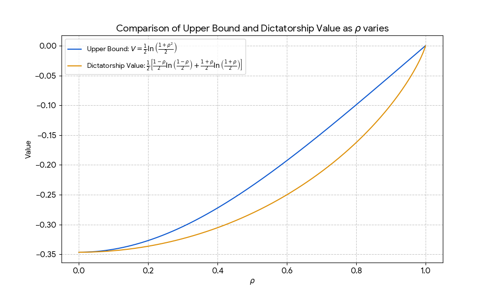
We next sought to tighten the relaxation by establishing an bound for the functions realizable by balanced Boolean functions. However, the system identified a technical flaw in our proposed bound and provided a concrete counter-example, leading us to pivot our strategy.
Our subsequent approach focused on leveraging the inverse of the noise operator. Given a correlation parameter , if , the original function can be recovered via the inverse transformation . Recall that the noise operator is linear and can be expressed as:
where the transition kernel is determined by the Hamming distance . To refine the optimization space, we relaxed the strict Boolean constraint to a pointwise box constraint, requiring for all . Combining this with the established constraints on the first and second moments of , we defined the following relaxed constraint set :
Interestingly it showed that the variance constraint is already implied by the other two. In addition, it showed that this relaxation is indeed tight, as discussed next.
Let be the set of balanced Boolean functions and define the entropy functional with . Let be the Boolean Hull (functions with ). Let be the feasible set for , which can then be characterized by the mean constraint and the pointwise box constraints .
Lemma 8.16.
(Convex Relaxation and Tightness). Maximizing over is equivalent to maximizing over .
This equivalence is an important milestone as it transforms the initial optimization over discrete Boolean functions into a continuous convex optimization.
In addition, it proves two other structural properties of the solution.
Lemma 8.17.
(Monotonicity). If maximizes , then can be assumed to be monotone.
Lemma 8.18.
(Local optimality). A dictatorship function is a local maximum of the problem of maximizing over .
The AI system also attempted to prove global optimality of the dictatorship functions by an inductive proof and identifies the remaining gaps. Concretely, consider the restrictions of the function to the -dimensional sub-cubes. Let be defined by and . Furthermore, let denote the noise operator acting on variables, and let represent the noise-evolved versions of these sub-functions. The functional admits the following decomposition:
where the kernel is defined as , with , and the parameters and are given by and .
The system then continues with the following response given the above notation.
We next conducted several further iterations of prompting to explore the inductive path. Specifically, we attempted to solidify the connection with Mrs. Gerber’s Lemma—which was also previously used in [83] to prove C-K conjecture in the high-noise regime. However, while the system could identify the relevance of the lemma, it ultimately failed to complete the formal analytical steps required for the proof.
Observations on AI-Assisted Research. Our interactions with the system on these theoretical problems yielded several key insights into its utility as a research partner:
-
•
Confirmation Bias in Prompting: The system exhibits a tendency to support the position or hypothesis presented in the prompt. When tasked with proving open-ended conjectures that are not necessarily true, it often attempts to bridge logical gaps with “hand-wavy” arguments that do not withstand rigorous scrutiny. We found that performance improves significantly when using neutral prompts (e.g., “prove or refute”), which encourages the system to evaluate multiple directions in parallel.
-
•
Effectiveness in Refutation: The system is remarkably adept at identifying counterexamples and pinpointing the “crux” of a problem. When provided with a precise but flawed idea, it can often explain exactly why a particular strategy fails, making it a valuable tool for early-stage proof debugging.
Proof of Lemma 8.15
To formally prove that the optimal distribution is supported on at most two points, we analyze the Karush-Kuhn-Tucker (KKT) conditions. This structural approach reveals how the moment constraints necessitate a sparse distribution. We seek to maximize , which is equivalent to minimizing . Defining as the size of the Hamming cube, we construct the Lagrangian with multipliers and for the mean and variance constraints:
where the quadratic constraint assumes the variance constraint is active at the maximum. Setting the partial derivative with respect to each to zero gives:
Rearranging this yields the transcendental equation . Let . Any optimal value of must lie at the intersection of and the constant . Since , which is strictly negative for all , is strictly concave. A strictly concave function can intersect a horizontal line at most at two distinct points, proving that the optimal can take at most two values, and . Let be the multiplicity of the value , such that indices take the value . The linear and quadratic constraints provide the following system:
Solving for and in terms of , we find:
The objective function can then be expressed as , where . To determine the behavior of , we examine its derivative via implicit differentiation of the constraints:
Assuming , we utilize the integral representation to rewrite the derivative:
This expression represents the difference between the integral of and the trapezoidal area under the chord connecting and . Calculating the derivatives of , we find , , and . Since for all , the function is strictly concave. For a strictly concave function, the area under the curve is strictly greater than the area of the trapezoid defined by the chord. Consequently, , meaning the objective function is strictly increasing over its feasible domain. The maximum is therefore achieved at the largest possible value of . Given the non-negativity constraint , the maximum occurs when . Solving for in this boundary condition yields , which results in . Substituting these values back into the objective yields the maximum value .
Proof of Lemma 8.16
Since is linear, is a convex polytope. Since is strictly convex, its maximum over is attained at an extreme point. The extreme points of are the images of the extreme points of , which are (the set of balanced Boolean functions). Thus, maximizing over is equivalent to maximizing over .
Proof of Lemma 8.17
We use decomposition along the -th coordinate. Let and . Let be the noise operator on variables. Let . The functional decomposes as:
where , with and . Let and . Then . Since is strictly convex, is strictly increasing in for fixed .
Consider the polarization defined by and . Note that is balanced since . Let . The means are preserved pointwise: . The differences are and .
Since is a positive operator (its kernel is non-negative as it represents probabilities), we have the inequality . Thus, . Since increases with , . By repeatedly applying this polarization, we conclude that the maximum must be attained by a monotone function.
Proof of Lemma 8.18
We verify that the Dictatorship is a local maximum by checking the KKT conditions for maximizing over the polytope . The set is defined by the constraints and , where .
We formulate the KKT conditions for maximization subject to and . The gradient condition is , where are the multipliers for and respectively (ignoring the equality constraint which adds a constant shift ). Let and . Complementary slackness implies:
-
•
If , then , which implies .
-
•
If , then , which implies .
Let be the noise operator applied to the dictatorship function , i.e., . Consequently, . Let and . We have on and on . We therefore require on and on .
The gradient condition is given by . Let . Since takes values on and on , must be constant on and :
| (48) |
where . Calculating , we obtain
| (49) |
where we used that and , by definition of the noise operator. We also have . The resulting constraints on are:
-
•
On (): .
-
•
On (): .
We require . Given that and , we have . This interval is non-empty (e.g., is a valid solution). Thus, the Dictatorship satisfies the KKT conditions and is a local maximum.
8.2 NP-hardness: Ratio Difference Maximization (RDM)
Written by Ravi Kumar and Silvio Lattanzi (on behalf of coauthors).
Problem Context
In a recent work [21], together with Flavio Chierichetti, Mirko Giacchini, Alessandro Panconesi, Erasmo Tani, and Andrew Tomkins, we were studying Multinomial Logits (MNLs), also known as Plackett–Luce models, that describe user preferences by assigning a weight to each item in a universe. When a user is presented a subset of items, they select one with probability proportional to its weight. In the paper, we consider the problem of learning an MNL by sampling from the conditional distributions induced on subsets of the universe.
Interestingly, even computing the worst-case error on arbitrary size subsets of the universe turns out to be a non-trivial problem. In [21] we introduce several approximation algorithms for this tasks. We also had the intuition that the problem was related to SUBSET-SUM and most likely NP-hard but we felt that the reduction was not immediate and hence we decided to test Gemini with such a question. We were happily surprised by receiving a zero-shot correct proof within a few minutes.
We then asked also to prove NP-hardness for a variation of the problem.
AI Contribution
Given only the formal definition of the Ratio Difference Maximization (RDM) problem, the AI zero-shot generated a flawless, polynomial-time NP-hardness reduction from the SUBSET-SUM problem. Upon a subsequent prompt, it successfully proved the NP-hardness of a related variation (MAX-DIFF-RATIO) using a similarly rigorous reduction.
More specifically, we used a math rigor prompt and we asked the model to show that the Ratio Difference Maximization (RDM) problem is NP-hard. This is the prompt that we used:
This is the output provided by Gemini that we verified to be correct:
Given the success of the first attempt, using the same prompt structure, we also asked to show that a variation of the problem is NP-hard. This is the second proof that we obtained in this way.
Consider the MAX-DIFF-RATIO (MDR) optimization problem: Given two lists and of positive integers, find that maximizes
8.3 Machine Learning Optimization: Self-regularized Gumbel Sigmoid
Written by Lin Chen, Gang Fu, and David P. Woodruff.
Problem Context
Subset selection is a core problem in machine learning, relevant to tasks like feature selection and embedding dimension optimization. Current methods like Dropout Feature Ranking (DFR) rely on explicit penalty terms (e.g., regularization) to control the number of selected features. However, tuning the regularization strength is difficult and sensitive, often hindering practical application. A new method, Self-regularized Gumbel Sigmoid (SrGS), was proposed to eliminate this hyperparameter by using an implicit regularization mechanism involving Softmax competition and budget-aware clipping. The theoretical question was to understand exactly why and how this parameterization enforces sparsity without an explicit penalty.
AI Contribution
The researchers provided the model with the mathematical definition of SrGS and asked for a theoretical analysis of its implicit regularization and behavior in the low-temperature limit.
-
•
Implicit Penalty: The model derived that in the low-temperature limit (), the variance of the Gumbel-Sigmoid distribution acts as an exact relaxation of the constraint, effectively penalizing non-binary solutions.
-
•
Adaptive Hybrid Regularization: It analyzed the deterministic limit (using expectations) and proved that the method induces a unique "hybrid" regularization: strong signals are subject to shrinkage (preserving magnitude), while weak signals competing for the remaining budget are suppressed by a non-convex penalty.
-
•
Theoretical Validation: These derivations provided the rigorous theoretical justification for the method’s empirical success, confirming it solves a relaxed subset selection problem without manual tuning.
Technical Details: Theoretical Analysis of SrGS
We employed the model to identify and resolve a key theoretical gap regarding the implicit mechanisms of the Self-regularized Gumbel Sigmoid (SrGS) method.
Problem Formulation
Subset selection is a core problem central to multiple optimization tasks in machine learning. Existing methods, such as Dropout Feature Ranking (DFR) (Chang et al., 2017), approach this by optimizing a variational dropout mask on the input layer. However, DFR relies on an explicit penalty term in the loss function to constrain the number of active features. The objective function is formulated as:
where the first term represents the task-specific prediction error (negative log-likelihood), is the batch size, is the number of features, and is the stochastic gate for the -th feature. Determining the optimal regularization strength requires extensive cross-validation and often becomes a blocker for successful application due to its sensitivity.
The SrGS method was proposed to overcome this limitation by eliminating the explicit penalty term . Instead, it introduces a structural “self-regularization” mechanism defined by the following process:
-
1.
Competition: For each feature , a learnable logit is normalized via Softmax to produce an attention score , enforcing global competition:
-
2.
Budgeting: The scores are scaled by the target budget and clipped to form selection probabilities , ensuring the expected number of selected features approximates :
-
3.
Stochastic Selection: The final binary masks are generated via the differentiable Gumbel-Sigmoid reparameterization:
While SrGS empirically demonstrates superior solution quality without hyperparameter tuning, the theoretical basis for this parameterization remains an open question. Specifically:
-
1.
Does this specific parameterization rigorously enforce sparsity in the low-temperature limit ()?
-
2.
What is the exact mathematical form of the implicit regularization induced by this mechanism when combined with standard weight decay?
Theoretical Findings
We answer these questions affirmatively. We utilized the model to analyze the method from two perspectives: the behavior of the stochastic objective in the low-temperature limit, and the implicit regularization induced by its parameterization.
Stochastic Analysis: Exact Relaxation. We first analyze the objective in the limit . In this limit, the expected loss decomposes into a deterministic loss and a variance penalty term . The optimization problem effectively minimizes:
The model derived that the variance penalty takes the form . Minimizing this concave function over the hypersimplex encourages solutions at the vertices (binary selection).
Theorem 8.21 (Implicit Penalty).
The implicit regularization induced by the variance penalty, defined as , is an exact penalty function for the constraint. Specifically:
This result mathematically validates that SrGS provides a continuous, exact relaxation of the combinatorial Best Subset Selection problem.
Deterministic Analysis: Adaptive Hybrid Regularization. We further analyzed the implicit regularization in the deterministic regime where the mask is replaced by its expectation , combined with regularization (weight decay) on .
The model discovered that under the budget constraint and the physical constraint , the optimization landscape induces a unique Adaptive Hybrid Regularization.
Theorem 8.22 (Hybrid Regularization).
The implicit regularizer partitions the features into two sets based on a data-dependent threshold :
-
•
A Saturated Set (): Features with strong signals () are assigned full probability . These features are subject to standard regularization (), which preserves signal magnitude.
-
•
A Fractional Set (): Features with weak signals compete for the remaining budget . These features are subject to an aggressive penalty:
This derivation reveals the mechanism behind SrGS’s superior performance: it automatically applies protection to key features while subjecting noise features to non-convex compression.
8.4 Mechanism Design: Revelation Principle Reduction Domain Extension
Written by Song Zuo and David P. Woodruff.
Problem Context
The main task for the model was to extend the key theoretical results of the paper “Mechanism Design for Large Language Models” [31] from rational bids () to real bids (). The original paper’s Revelation Principle (Theorem 3.5) relied on the countability of the bid space. The generalization was expected to heavily rely on order theory and topological arguments as the assumptions are much weaker than standard auction theory setups. To avoid the additional mathematical complexity, the authors restricted bids to be rational.
AI Contributions
We fed the original paper [31] to the model and asked it to bridge the rational to real bids gap for Theorem 3.5.
-
•
Proof Attempts and Improvement Reviews: The model initially came up with some coarse proofs from the initial ask. Then we also asked the model to review the draft and provide improvement suggestions. We iterated through this process with human selection as well as additional guidance, and finally reached the complete and rigorous results.
-
•
Free Bonus on Extension of Theorem 3.12: The model volunteered to also extend Theorem 3.12 to general settings.
-
•
Full Writing with Strategic Guideline and Suggestions from Human: The entire material in the next Technical Details section is fully written by the model with human suggestions (and some minor corrections).
Human Interventions
Throughout the iteration process, human interventions mainly happen at correcting the model generated review feedback. Sometimes, the model suggests something distracting, misleading, or even mathematically suspicious. Human interventions then can help the model get out of potential dead-loops.
Technical Details
The original paper [31] introduces a Token Auction Model where agents, represented by Large Language Models (LLMs), submit scalar bids to influence the generation of content. The mechanism consists of an aggregation function that combines agents’ preferred distributions based on their bids , and a payment function .
The paper establishes a Revelation Principle ([31, Theorem 3.5]), stating that any mechanism satisfying Payment Monotonicity and Consistent Aggregation is strategically equivalent to a mechanism with a Monotone Aggregation Function. The proof relies on the assumption that the bid space is , utilizing the countability of the bids to construct utility representations. Furthermore, the paper proves the existence of Stable Sampling ([31, Theorem 3.12]). The original proof implicitly requires the aggregation function to be absolutely continuous by relying on Lebesgue’s Differentiation Theorem and the Fundamental Theorem of Calculus.
Open Problem: Extend the Revelation Principle and the existence of Stable Sampling to the more natural domain of real-valued bids, , while minimizing additional assumptions and providing rigorous proofs that do not rely on countability or absolute continuity. We will show this is possible by assuming the token set is finite, which is standard in practice.
Key Definitions
We restate the key definitions from [31] for completeness. Let be the set of distributions over tokens . Let be the preference relation of agent over .
Definition 8.23 (Robust Preferences).
Given preferred distribution , if and .
Definition 8.24 (Payment Monotonicity).
Mechanism satisfies payment monotonicity if for all : .
Definition 8.25 (Consistent Aggregation).
is consistent if: if for some , then for all , .
Definition 8.26 (Monotone Aggregation Function).
is monotone if for all and : .
Methodology and Assumptions
We extend the bid space to . We assume the token set is finite. This ensures the space of distributions is a finite-dimensional simplex, which is a compact, metrizable, and second-countable space.
Extending the Revelation Principle
The main challenge in extending Theorem 3.5 is the failure of the countability argument used in [31]. Approach: We replace the countability arguments with topological and order-theoretic methods. We establish a utility representation using the topological properties of the codomain. Then, we prove a general Monotone Extension Lemma that allows extending the transformed monotone aggregation function from the image of the utility representation to the entire bid space . This approach relies only on the continuity of the underlying preferences and the compactness of , removing the need for continuity assumptions on the aggregation function . This approach requires the following assumptions:
Assumption 8.27 (A1: Continuous Preferences).
The partial order on is continuous (i.e., its graph is closed in ).
We also formalize an assumption that was inherent in the original framework:
Assumption 8.28 (A2: Anti-symmetry of Preferences).
The order is anti-symmetric (i.e., ( and ). Here denotes the symmetric component of . This means is a true partial order, not just a preorder.
Robust Preferences satisfy A1 and A2. However, we state A2 explicitly as the Revelation Principle applies to general partial orders. A2 is crucial to ensure that the transformed aggregation function is well-defined. Combined with Payment Monotonicity, it ensures that payments are invariant if the allocation remains the same, which is necessary for the transformed payment function to be well-defined.
It is worth noting that A2 is restrictive in the context of LLMs, where preferences are typically defined via continuous loss functions (e.g., KL-divergence) which naturally have non-trivial level sets (i.e., distinct distributions can be equally preferred). If A2 is relaxed, the Revelation Principle can still theoretically hold for preorders if the mechanism specifies a consistent tie-breaking rule across indifference classes (see the Discussion and Limitation section for the topological limitations of tie-breaking).
To ensure that payment functions and strategy mappings remain well-defined in the measure-theoretic sense (which will be essential for integration in later sections), we explicitly state the following measurability assumption:
Assumption 8.29 (A3: Measurability).
The initial aggregation function is Borel-measurable with respect to the bids .
By removing any continuity assumption on the aggregation function , our Extended Revelation Principle applies to a broad class of mechanisms, including those with discontinuous allocation rules (e.g., step functions) common in mechanism design.
Extending Stable Sampling.
The challenge in extending Theorem 3.12 is the reliance on differentiation in the original proof. Approach: We use a measure-theoretic approach. We associate Lebesgue-Stieltjes (LS) measures with the monotone components of the aggregation function and use the Radon-Nikodym theorem to characterize the transport of probability mass. We carefully define the measures on to rigorously handle the boundary at .
Importantly, the general Revelation Principle (Theorem 3.5) established in the next section guarantees the existence of an equivalent monotone mechanism, but it does not necessarily guarantee right-continuity without loss of generality. However, this technical assumption is standard for defining Lebesgue-Stieltjes measures associated with increasing functions. Thus, for the Stable Sampling construction, we explicitly require:
Assumption 8.30 (A4: Right-Continuity).
The aggregation function is right-continuous in .
Extended Revelation Principle
We now formally prove the extension of the Revelation Principle to , assuming A1, A2, and A3 hold.
Utility Representation
Lemma 8.31 (Extended Lemma 3.6).
Assume A1. Let the bid space be . For any distribution aggregation function , there exists a payment function such that mechanism is payment-monotone if and only if establishes a total order over for any fixed and .
Proof.
The “only if” direction follows directly from the definition of Payment Monotonicity. We prove the “if” direction. Fix . Let . By hypothesis, is a total order on . Let be the closure of in . Since is finite, the probability simplex is a compact metric space, making a compact metric space, which is second-countable under the subspace topology. By A1, is continuous, so the total order extends to a continuous total preorder on . Debreu’s Theorem [28] guarantees that there exists a continuous utility representation for the preference relation restricted to . We can always choose a bounded representation (e.g., by composing with a strictly increasing, bounded function). Defining the payment function yields a payment-monotone mechanism. ∎
Monotone Extension Lemmas
To extend the aggregation function from the image of the strategy mappings to the entire space , we need the following lemmas. We provide a supremum-based extension that naturally guarantees monotonicity.
Lemma 8.32 (1D Monotone Extension).
Let . Let be a compact metric space (e.g., ) with a continuous partial order (A1). Let be a monotone function (non-decreasing) such that its image is totally ordered by . Let denote the topological closure of a subset . Let . Let . Then the function defined by
is a monotone extension of .
Proof.
We first show is well-defined. Since is compact and is continuous, the closure of any totally ordered subset of is compact and totally ordered. Thus, for any where , its closure possesses a maximum element in . Similarly, since is a compact metric space and is a closed subset, is guaranteed to exist. Note that this construction does not require the domain to be compact.
Monotonicity: If . Case 1: . Then , which implies . Thus , so . Case 2: . . For any , since , it follows that , so by definition of , .
Extension property: If . Then . Since is monotone, is the maximum element of . Since and , . ∎
Lemma 8.33 (Monotonicity Preservation).
Under the assumptions of Lemma 8.32, let be another monotone function such that is totally ordered by . Let be another continuous partial order on . If for all , then their monotone extensions and satisfy for all .
Proof.
Fix . Case 0: (). and . Since and are monotone w.r.t. , and are realized as the limits of and respectively, for any sequence such that . We are given . By continuity of , taking the limit yields . Thus .
Case 1: . Let . Case 1a: . By the extension property in Lemma 8.32, and . Since , we have . Case 1b: . Since is the supremum of and does not belong to the set, it must be a limit point of the set . Therefore, there exists an increasing sequence such that . Since is monotone w.r.t. , is non-decreasing. As is the maximum of , . In a compact metric space with a continuous total order, bounded monotone sequences converge to their suprema (in the order topology, which coincides with the subspace metric topology here since the image is totally ordered and closed). Similarly, . We are given for all . By the continuity of the order (A1), the order is preserved in the limit. Thus, . ∎
Strategic Equivalence
Lemma 8.34 (Extended Lemma 3.7).
Assume A1, A2, and A3. Let the bid space be . Consider any consistent aggregation function . Suppose defines a total order over the aggregation set for any fixed and . Then there exists a profile of strategy mappings such that for some monotone aggregation function .
Proof.
We proceed in several steps.
Step 1: Induced Preference. Define the induced preference on : if for all . Consistency ensures this is a total preorder on .
Step 2: Strategy Mapping via Pull-back. We seek a utility representation for the induced preorder . Let be the image of for an arbitrary fixed reference profile . By the premise, is a total order on . Let be its closure in . Since the token set is finite, is a second-countable, compact metric space. By A1, the preference relation is continuous. The continuity of ensures that the total order property of transfers to its closure . Thus, is a continuous total preorder on . By Debreu’s theorem [28], the continuous preference relation on admits a continuous utility representation . We can assume without loss of generality that the image of is in (by composing with a strictly increasing, positive-valued function if necessary). We define the strategy mapping by pulling back the utility from the codomain: . By Assumption A3, is Borel-measurable. Since is continuous, the composition is measurable. The Consistent Aggregation property (Definition 8.25) ensures that the preference ordering induced by this mapping is independent of the choice of the reference profile . By definition of , . Thus, is a valid utility representation for . This rigorous construction bypasses the need for an order-density assumption on the bid space under the potentially disconnected topology induced by .
Step 3: Defining on the Image. Let be the image of , and . Define . We must show this is well-defined. If , then for all . This means for all . By A2 (Anti-symmetry), this implies equality of the distributions. We show by changing bids one by one. Let be the bid profile with the first bids from and the rest from . Since , we have . By A2, . Thus, . The function is monotone on by construction of . Furthermore, the 1D images of are totally ordered since the 1D images of are assumed to be totally ordered.
Step 4: Monotone Extension. We extend from to iteratively. In step , we extend the domain from to . We use Lemma 8.32 to extend along the -th dimension using the standard numerical order on the -th coordinate. This is possible because the required conditions (A1, compactness of , total order on 1D images) are met. We must ensure that this extension preserves the monotonicity w.r.t. other orders . For , this follows from Lemma 8.33 (with and ). For , the domain is already in the -th dimension, and the extension in the -th dimension also preserves monotonicity in the -th dimension by Lemma 8.33 (by viewing the -th coordinate as the parameter defining vs , and the -th coordinate as the domain being extended). This iterative process yields the monotone extension on . Furthermore, since the extended aggregation function is monotone in each coordinate by construction, it is continuous almost everywhere with respect to the Lebesgue measure, and thus preserves joint Borel-measurability on the entire domain (e.g., by Lebesgue’s theorem for monotone functions), thus satisfying the measurability requirement of the mechanism (Assumption A3). ∎
The Main Theorem
Theorem 8.35 (Extended Theorem 3.5).
Let the bid space be . Assume A1, A2, and A3. Any mechanism with a consistent aggregation function and a monotone payment function is strategically equivalent to a mechanism which has a monotone aggregation function and a monotone payment function .
Proof.
By Payment Monotonicity of and Lemma 8.31, the prerequisites for Lemma 8.34 are met. Lemma 8.34 yields the mappings and the monotone function . We define on the image by . If , then for all . As shown in the proof of Lemma 8.34 (Step 3), under A2 this implies . Since the outcomes are identical, by Payment Monotonicity, for all . Thus, is well-defined. satisfies Payment Monotonicity because does and are defined via the preference representation .
Finally, we extend from to . Note that the original mechanism is fixed, so its payment function is predetermined and may be unbounded. To accommodate this, we take the codomain for the extension to be the extended real line , which is a compact metric space under the standard order topology. The image of on is a subset of . Since is monotone in each component (with the standard order on ), we can apply the Monotone Extension Lemma (Lemmas 8.32 and 8.33 applied to the standard order on ) iteratively to extend to .
Note that the iterative dimension-by-dimension extension in Step 4 of Lemma 8.34 means that the final extended mechanism depends on the order in which the dimensions are processed. This renders the constructed equivalent mechanism non-unique. However, since the equivalence holds on the image of the strategy mappings, these choices correspond to off-path bids and do not affect the on-path behaviors, strategic properties, or equilibrium payments. ∎
Extended Stable Sampling
We now generalize Theorem 3.12 to using measure theory, relying on assumption A4 (Right-Continuity) for the monotone aggregation function. We utilize the definitions of and from Lemma 3.10 in [31]. For notational precision, we define limits at infinity as and .
Theorem 8.36 (Extended Theorem 3.12).
Given a monotone distribution aggregation function satisfying A4, for any agent with robust preferences (and fixed ), there exists a stable implementation of .
Proof.
Let . Following [31], define (weakly undersampled) and (strictly oversampled). These sets form a partition of . By Lemma 3.10 in [31], is non-decreasing for and non-increasing for . By A4, these functions are right-continuous.
Step 0: Setup and Trivial Case. We define associated Lebesgue-Stieltjes (LS) measures on . For , let be the LS measure of the non-decreasing function , defined such that for . For , let be the LS measure of the nondecreasing function , defined such that for . Let . Let be the LS measure of on . By the Right-Continuity assumption (A4), , which guarantees that the measure places no point mass at 0, i.e., . This ensures the integration domain is strictly as used in subsequent integrations. By conservation of probability, . Let be the total mass moved. If , then for all . Let . We define the implementation for the trivial case directly on by mapping all to a sample from . This is trivially stable. Assume .
Step 1: Measure Theoretic Setup. Since , is a finite measure, which strictly fulfills the -finite condition for the Radon-Nikodym theorem. Since on , is absolutely continuous w.r.t. . Let be the Radon-Nikodym derivative for . Note that these derivatives are unique only up to a set of -measure zero. Consequently, the sampling implementation constructed below is determined -almost everywhere. Using and as index variables for the respective subsets, we have and (-a.e.). We define a joint measure on representing the mass transport. For any measurable set , , and , the measure is defined via its action on measurable product sets:
Step 2: Construction of Stable Sampling . We define the randomness space and the implementation . Let and . Note . By the Right-Continuity assumption (A4), . Additionally, by the definition of the partition, we have the identity . Substituting these, the expression simplifies algebraically to . We define the randomness space as the disjoint union , where , , and . We equip with the -algebra formed by the disjoint union of the discrete -algebras on the finite sets and , and the Borel -algebra on (with the discrete topology on and ). We define the probability measure on as follows:
-
•
On : For , .
-
•
On : For , .
-
•
On : The restriction of the probability measure to is the joint measure on the Borel -algebra given by defined in Step 1.
We define the implementation for as follows: 1. If (Static ), . Set . 2. If (Static ), . Set . 3. If (Moving Mass), . Since , we set if , and if .
Step 3: Verification. Stability: By construction, for any realization , the output as a function of is either constant (cases 1 and 2) or switches exactly once from to at (case 3).
Measurability: By construction, the components of are either constant or simple indicator functions of the form for , which are Borel measurable. Thus, is a valid random variable with respect to .
Correctness: We verify the marginal probability for . . The first term is .
Since (-a.e.), this equals:
By right-continuity (A4), the LS measure satisfies . Thus, . The verification for is similar. ∎
Remark 8.37 (Algorithmic Constructiveness).
The proof of Theorem 8.36 provides an existence result for stable sampling based on a measure-theoretic construction involving Radon-Nikodym derivatives . While theoretically sound, this construction does not immediately yield an efficient sampling algorithm. Note that while the standard inverse-CDF method () is universally applicable to any 1D cumulative distribution function (requiring only right-continuity and non-decreasing properties), the difficulty in the multidimensional LLM implementation arises from the measure-theoretic coupling of probabilities across different tokens, rather than a lack of absolute continuity. In practical computational settings, the Radon-Nikodym derivatives can be approximated. For example, the bid space can be discretized into a fine grid to estimate the derivatives using finite differences on the empirical cumulative distributions, or one can parameterize the measures using continuously differentiable generative models where the densities are explicitly tractable.
Consequently, Proposition 3.13 (Myerson-style payment formula) also generalizes to . We note that the formula presented in the reference paper [31], , contained a sign error, leading to non-positive payments as the distance is decreasing in . We provide the corrected formula and its derivation.
Proposition 8.38 (Corrected Payment Formula).
Under robust preferences and a monotone aggregation function satisfying A4, the expected payment induced by the second price rule via stable sampling satisfies:
Proof.
We derive the payment formula using the stable implementation constructed in Theorem 8.36. Let be the random variable representing the ex-post payment for agent given a bid and a realization . Under the second-price rule, the payment is the critical bid at which the outcome changes. For a realization , where , the outcome changes from to at bid . Thus, if , and 0 otherwise. For , the outcome is constant, so the critical bid is 0, meaning . The expected payment is:
Using the definition of and the fact that and (-a.e.):
Recall that is the LS measure associated with the increasing, right-continuous function on . Using the standard integration by parts formula for Lebesgue-Stieltjes integrals on half-open intervals, . By setting , , and , the boundary term at evaluates directly as . Furthermore, noting that almost everywhere with respect to the Lebesgue measure , we obtain:
This yields the final integral directly without the need for the intermediate limit notation. This is the standard Myerson payment formula with allocation probability . Now we relate this to the distance. Let . Under robust preferences (Lemma 3.10 in [31]), let and explicitly define . We analyze the distance:
Since and , we have . We now evaluate the integral in the proposition statement:
Thus, . This confirms the corrected formula and ensures non-negative payments, as is non-increasing in . ∎
Discussion and Limitations
This note successfully extends the core theoretical results of the reference paper from rational to real-valued bids by employing topological and measure-theoretic tools, under the practical assumption of a finite token vocabulary. However, these generalizations reveal important limitations and suggest directions for future research.
Restrictiveness of the Anti-Symmetry Assumption (A2) in the LLM Context. The reliance on anti-symmetry (A2) for the Revelation Principle excludes scenarios where agents are indifferent between distinct distributions. This is a significant limitation in the context of LLMs, where preferences are typically defined via continuous loss functions (e.g., KL-divergence). Continuous loss functions naturally have non-trivial level sets (indifference classes), meaning distinct distributions can be equally preferred, which violates A2.
Topological Incompatibility of Tie-Breaking Rules. A natural attempt to satisfy the Anti-Symmetry assumption (A2) in the presence of indifference classes is to introduce a deterministic tie-breaking rule, such as a lexicographic ordering over the token probabilities. However, it is a well-established result in mathematical utility theory (e.g., [28], [85]) that lexicographic orders on spaces of dimension greater than one (such as for ) do not admit continuous utility representations. Specifically, such tie-breaking rules violate the Continuity Assumption (A1) by creating non-closed preference graphs (open sets of strictly preferred outcomes). Since the Extended Revelation Principle critically relies on Debreu’s Representation Theorem to construct the strategy mappings , violating A1 invalidates the utility representation step in Lemma 8.31 and Lemma 8.34. Therefore, A1 and A2 cannot be simultaneously satisfied by simply overlaying a standard tie-breaking rule on continuous loss functions. Relaxing A2 by designing appropriate tie-breaking mechanisms that preserve continuity remains an open problem.
The Continuity Gap in the Revelation Principle. There is a fundamental tension between the generality of the Extended Revelation Principle (Theorem 8.35) and the requirements for Stable Sampling (Theorem 8.36). The Revelation Principle applies broadly, even to discontinuous mechanisms, by constructing an equivalent monotone mechanism. However, this constructed mechanism is not guaranteed to be right-continuous (A4). Since the strategy mappings and the underlying aggregation function are not required to be continuous, the image space can be disconnected, and the utility values can have jumps. Consequently, any extension scheme—whether based on the supremum or the infimum—cannot universally guarantee right-continuity. Specifically, an infimum-based extension from the right would fail to be right-continuous at the boundary points of the gaps in .
While this leaves a theoretical gap between the mechanisms covered by the Revelation Principle and those implementable via Stable Sampling, it is important to emphasize that the Revelation Principle successfully establishes that we can, without loss of generality, focus on monotone mechanisms. This aligns with standard auction theory, where monotonicity is the cornerstone of incentive compatibility. Given the weak assumptions required, this is a positive foundational result. Bridging this gap—either by identifying conditions under which right-continuity can be preserved, extending Stable Sampling to left-continuous mechanisms, or proving that non-right-continuous mechanisms offer no strategic advantage—is an interesting direction for future research that goes beyond the scope of this note.
8.5 Networked Information Aggregation for Binary Classification
Written by MohammadHossein Bateni, Zahra Hadizadeh, MohammadTaghi Hajiaghayi, Mahdi JafariRaviz, and Shayan Taherijam.
Problem Context
Recent work by Kearns et al. [63] shows basic limits on information aggregation in distributed learning. In their framework, agents in a Directed Acyclic Graph (DAG) act in sequence and minimize Mean Squared Error (MSE), while each agent only sees a subset of the input features and the predictions made by earlier agents.
Moving from regression to binary classification, using a non-linear link function such as logistic regression, raises new challenges. MSE can still be used, but Binary Cross Entropy (BCE) is the standard loss for classification. BCE is harder to study because it is not quadratic. It is open whether the aggregation limits seen with MSE also show up in this classification setting.
AI Contribution
The AI acted as a theoretical collaborator to extend distributed learning limits from linear regression (MSE loss) to binary classification (Binary Cross Entropy loss). By breaking the proof into modular lemmas, the model successfully utilized KL-divergence and Pinsker’s inequality to rigorously bound the excess risk of the final agent in the network.
Overall, the structured prompt in Figure 23 below was instrumental in generating rigorous proofs at several stages of our experience to prove the full theorem.
Details of the Process
Aaron Roth, one of the authors of the original framework [63], shared how his team integrated AI into their research. He described treating the AI as a colleague, providing high-level mathematical intuition which the model expanded into formal proofs. He noted that while this accelerated their work, it required careful verification to catch “human-like” errors.
Adopting this approach, we considered replacing the loss in their framework with BCE using logistic regression. We asked Gemini 3 Pro to derive a theorem like the one in the linear regression setting. It produced a short chain of lemmas and a final theorem that bounds the excess loss of the last node in the DAG, compared to a logistic regression learner that has access to all input features.
While checking the output, we found one key first lemma (Lemma 8.41) and verified that Gemini proved it correctly. The lemma states that the minimizer of the BCE loss outputs predictions such that the residual (where is the binary label) is orthogonal to the input in expectation. Formally, . We knew this would matter because it is also the first building block in the MSE setting. The next lemma (Lemma 8.42) compared the loss of the optimal predictor to the loss of any other logistic predictor. Gemini correctly identified that the loss gap can be written using the Kullback–Leibler divergence between the predictors’ output distributions. The lemma itself was needed for the rest of the argument, but Gemini made a mistake near the end of the proof, and we fixed it.
The next step was the final theorem bounding the excess loss. The bound it gave was stronger than in the linear regression setting: there the bound was , while here Gemini claimed , which is smaller when . This is where Gemini started to go off track. Instead of breaking the proof into short lemmas, it wrote one long proof that was not correct. It also added a major new assumption: Assume the loss is -strongly convex.
We kept the theorem statement, including the assumption and the stronger bound, and asked Gemini to regenerate a proof in a fresh context. Here the prompt in Figure 23 was especially helpful and this time the proof was correct. However, the -strong convexity assumption felt indirect.
Next, we asked Gemini to remove the -strong convexity assumption and replace it with something closer to the boundedness assumptions used by Kearns et al. It produced a correct proof, with the weaker bound of , under a new assumption: the coefficient vectors of every agent’s predictor, and of the optimal predictor, have bounded norm. This was still a stronger assumption than what was needed in the linear regression setting, where the bound only applies to the optimal predictor.
We did not think this was a major issue, so we accepted the theorem statement. At that point, we believed the theorem and proof were correct. Still, we prompted Gemini to look for flaws in the proof or statement.
It found an error we had missed: you can compare convexity bounds for a parameter to the optimal parameter only when the loss is defined over the same set of indices. Gemini also suggested the fix: since lives on the full set of indices, we can pad with zeros to get , and also pad and add the predecessors’ parameter vectors in the same coordinate system. The problem was that we assumed has bounded norm, and now we would also need to have bounded norm. But depends on predecessors’ parameters through this padding-and-summing step, so the norm can grow quickly with depth, and it did not seem reasonable to assume it stays bounded.
We then took a different path. We noticed that the orthogonality lemma was mainly used for a predictor against its own subset of input indices, and orthogonality to predecessors’ logit outputs was not really used.
We changed the assumptions to only require boundedness of the optimal predictor, and asked Gemini to prove the theorem under this smaller assumption, hinting that it should use the orthogonality lemma. Again the prompt in Figure 23 was very helpful. As a result, Gemini did so by breaking the proof into lemmas, reusing the correct parts under the new assumption, and adding new helper lemmas to reach the final bound.
We then cleaned up the writing and the lemma flow, again using Gemini for rewriting and proofreading.
The theorem
We consider a distributed learning system where agents are arranged in a Directed Acyclic Graph (DAG). Let denote the set of predecessors of agent . Agents are indexed consistent with a topological sort of the graph. Each agent observes a local subset of features from the input and the logits from its predecessors. The agent computes its own logit and prediction (where is the sigmoid function ) using learnable parameters and :
Agents sequentially update their parameters to minimize the expected Binary Cross Entropy (BCE) loss with respect to the target :
We also use the notation , , and .
We now give the following definition.
Definition 8.39 (-Coverage Condition, from Kearns et al.[63]).
A path satisfies the -coverage condition if every contiguous subsequence of agents collectively observes all features .
We aim to prove the following theorem.
Theorem 8.40 (Global Convergence Rate).
Consider a DAG containing a path of length of agents satisfying the -coverage condition. Let be the global optimal logistic predictor over all features. Assume:
-
1.
Bounded second moments: for all .
-
2.
Bounded coefficients: for the optimal logits where .
Then the excess risk of the final agent is bounded by
We begin with the following lemma.
Lemma 8.41 (Orthogonality of Residuals).
Let be the optimal logistic predictor on a feature space . The residual error is orthogonal to the feature vector in expectation:
Proof.
The gradient of the logistic output is . So we get
The optimal parameters must satisfy the condition . Thus,
This orthogonality allows us to decompose the error of any suboptimal model. We will relate the excess loss of a logistic predictor by the optimal logistic predictor , using the expected Kullback-Leibler divergence of the Bernoulli distributions with parameters and . We denote this measure as defined by
Lemma 8.42 (Decomposing Loss).
Let be the optimal logistic predictor on a feature set , and let be any logistic predictor in . The loss decomposes as
Proof.
Using the identity , we write the loss with as
Expanding the difference , we obtain
Adding and subtracting inside the expectation yields
| (51) |
The second term is zero due to the orthogonality condition derived in Lemma 8.41. For the first term, we expand the definition of with and :
This matches the first term in Equation 8, completing the proof. ∎
To relate the KL divergence to the parameter error, we employ the following bound, which is a specific case of Pinsker’s inequality [80]. We include the proof for completeness.
Lemma 8.43.
For the expected KL divergence , the following inequality holds:
Proof.
We verify the inequality pointwise for any . We aim to show
| (52) |
Define the function . The first derivative with respect to is The second derivative is . For , the term has a maximum value of . Consequently, , which implies . Since is convex and satisfies , the point is a global minimum. Observing that , we conclude that for all . Taking the expectation of both sides in (52) yields the result:
We define the pointwise loss function:
Thus, we can write .
Lemma 8.44.
Let be any logistic predictor. Let be a subspace of features and be the predictor that minimizes over . Then, we have
| (53) |
Proof.
Let . The derivatives are and . Since , we have , implying is convex. Convexity implies that for any , . Rearranging implies the following:
| (54) |
We define the relationship between the losses and . Substituting , we assume the following inequality:
| (55) |
Expanding terms confirms this holds given the convexity of in Equation 54:
We consider a path of agents . Each agent receives the logit from its predecessor and trains a logistic predictor model using locally observed features , , and possibly some other predecessors’ logits. Since one option for the agent is to pass the logits through, we have that . We also get that Lemma 8.42 holds for and , since is in the stricter subspace of .
We use the notation for any function .
Lemma 8.45 (Residual Bound via Path Coverage).
Let be a path of agents where every feature is observed at least once. Let where be any logistic predictor over the whole space. Assume the coefficients of satisfy , and the features satisfy , for some and . Let . Then, we have
Proof.
Let . We bound the error term:
Consider a feature . Due to each feature being observed, this feature appears in the index set of some agent in the path. By orthogonality, . We decompose the expectation using the triangle inequality:
Applying the Cauchy-Schwarz inequality gives
Given , we bound using the loss difference . Applying Lemma 8.43, we get for any :
By the triangle inequality and Cauchy-Schwarz,
Combining these bounds with the constraint on gives
We are finally ready to prove Theorem 8.40. Combining Lemma 8.44 and Lemma 8.45, we obtain the relationship for a path of length . Extending this analysis over the full path satisfying the -coverage condition leads to our main convergence result.
Proof of Theorem 8.40.
We partition the path into disjoint blocks of length . By the Pigeonhole Principle, since the total loss reduction is bounded by the loss of the first agent , there exists at least one stable block where the reduction is at most the total reduction divided by . Suppose this block is on indices . Then, we have
Applying Lemma 8.44 and Lemma 8.45, we get that over this path . Next, note that since using achieves a loss of , and because the first agent optimizes within its domain then . Combined with the non-increasing losses, we get
Our theoretical analysis builds on the framework established by Kearns et al. [63] for linear regression. We extend their methods to the classification setting. Unlike their work, which relies on the geometry of Mean Squared Error (MSE), our analysis addresses the non-linearities of the sigmoid function and Binary Cross Entropy (BCE) loss. This necessitates the use of information-theoretic tools to bound the excess risk.
The proof strategy for Theorem 8.40 mirrors the methods of Kearns et al. [63]. Lemma 8.41 (Orthogonality) and Lemma 8.42 (Decomposition) establish the logistic equivalents of their linear regression results. However, since the logistic loss does not admit a simple Euclidean decomposition, we rely on KL-divergence and a Pinsker-type bound (Lemma 8.43) to relate the risk reduction to parameter error.
9 Conclusion and Future Directions
The diverse array of case studies presented in this manuscript demonstrates unequivocally that frontier AI models—specifically Gemini Deep Think and its advanced variants—have crossed a critical threshold. They are no longer merely tools for routine automation, data processing, or syntax formatting; they are now capable of acting as genuine, expert-level collaborators in mathematical and algorithmic discovery. Across theoretical computer science, economics, physics, and optimization, we have shown that LLMs can actively resolve open conjectures, tighten long-standing mathematical bounds, and identify obscure, cross-disciplinary theorems to bypass human roadblocks.
The value of the AI in these collaborations manifested in several distinct paradigms. In some instances, it acted as a cross-disciplinary bridge, retrieving theorems from distant mathematical domains (such as the Kirszbraun Extension Theorem) to resolve computational geometry roadblocks. In others, it served as a relentless adversarial reviewer, successfully identifying a fatal, deeply buried flaw regarding perfect versus statistical consistency in a state-of-the-art cryptography preprint.
Crucially, however, these successes were not achieved autonomously. They required a tightly coupled human-AI workflow characterized by iterative refinement, strategic scaffolding, and rigorous verification—a process some authors have colloquially termed “vibe-proving.”
9.1 Common Themes and Problem Suitability
Across these diverse case studies, clear themes emerge regarding the types of problems where this human-AI collaborative approach excels, and where it currently struggles.
Highly Suited Problem Classes: The model is exceptionally effective on problems that can be decomposed into verifiable steps, require cross-disciplinary knowledge retrieval (e.g., bridging graph theory with continuous measure theory), or involve generating counterexamples to bounded conjectures. It also thrives in settings where the human can provide a strategic “scaffold” while the AI fills in tactical derivations, or where automated execution loops can rapidly test and prune algebraic hypotheses against numerical ground-truths (as in the cosmic strings derivation).
Less Suited Problem Classes: One goal is to improve the model on problems requiring completely unconstrained, multi-page derivations, where intermediate steps cannot be easily verified or grounded. Problems that require establishing entirely novel mathematical frameworks from scratch, or those with extremely long, sparse reward horizons without intermediate feedback, exceed the autonomous capabilities of current models and require some amount of human orchestration.
Capabilities Needed for Expansion: To further expand the range of scientific problems that can be tackled, future AI capabilities likely should evolve beyond natural language and standard code execution. Models will need enhanced capacities for long-horizon logical planning to maintain context over lengthy proofs. Furthermore, seamless, native integration with interactive theorem provers (discussed in Section 9.3) are important to autonomously verify the logical soundness of deep reasoning steps and mitigate hallucination bottlenecks.
9.2 Understanding Current Limitations and Failure Modes
Left unchecked, current models exhibit distinct failure modes that researchers must actively manage. Across our experiments, several recurring limitations emerged:
-
•
Confirmation Bias: As noted in the information theory case studies (Section 8.1), models exhibit a strong tendency to support the hypothesis presented in a prompt. If tasked with proving a false conjecture, the AI will often attempt to bridge logical gaps with confident but “hand-wavy” arguments that do not withstand rigorous scrutiny. Neutral prompting (e.g., “prove or refute”) is essential.
-
•
Confident Technical Hallucinations: While models excel at high-level structural insights, they can occasionally make subtle algebraic errors, drop constraints, or confidently misapply theorems (e.g., flipping inequality signs in hypercontractivity bounds).
-
•
Alignment Friction: Standard safety and alignment guardrails can sometimes hinder scientific exploration. As noted in Section 2, the model may initially refuse to attempt a problem if it recognizes it as an “unsolved open problem” (requiring Context De-Identification to bypass).
Because of these limitations, the human researcher’s role is elevated rather than replaced. The scientist shifts from executing mechanical derivations to acting as an orchestrator, auditor, and strategic director of the AI’s combinatorial reasoning.
9.3 Future Directions: From Code Execution to Formal Verification
To overcome the limitations of LLM hallucinations, researchers must integrate pure language models with external verification environments. As outlined in Section 2.6 and demonstrated in our cosmic strings experiments (Section 6.4), we are already seeing success by embedding AI in “neuro-symbolic” loops—where the model autonomously writes code to numerically verify its proposed mathematical steps and uses traceback errors to prune invalid branches.
However, while numerical execution is a powerful grounding mechanism for applied mathematics and physics, it is fundamentally limited when dealing with abstract proofs. For pure mathematics and theoretical computer science, the natural evolution of this workflow is Formal Verification. As AI systems generate increasingly complex, multi-page mathematical proofs, human verification becomes an exhausting bottleneck. Future research must focus on building autoformalization pipelines that automatically translate LLM-generated informal mathematics into formal verification languages (such as Lean, Coq, or Isabelle). By pairing the creative, associative leaps of an LLM with the absolute rigorous certainty of an interactive theorem prover, the research community can systematically eliminate the hallucination problem in mathematical discovery.
9.4 The Shifting Bottleneck: An Impending Crisis in Peer Review
As AI drastically lowers the friction of generating highly technical, mathematically dense research papers—evidenced by the AI-integrated IDE workflow utilized in Section 5 — the scientific community faces an impending systemic challenge. If researchers can “vibe-code” comprehensive papers in a fraction of the traditional time, the fundamental bottleneck of science will shift entirely from the generation of ideas to the verification of those ideas.
The traditional human peer-review system is already strained and fundamentally unequipped to handle a massive influx of AI-accelerated literature. Consequently, the very same tools used to generate these papers must be adapted to evaluate them. The cryptography case study (Section 3.2) proves that AI models, when guided by rigorous, adversarial self-correction protocols, are already capable of finding subtle flaws in advanced proofs. Developing robust, AI-assisted peer-review systems will be vital to triaging submissions and maintaining the integrity of the scientific literature in the coming years.
9.5 Final Thoughts
Just as the advent of calculators and computational algebra systems revolutionized applied mathematics in previous decades, the ability to rapidly iterate on abstract reasoning with a tireless, knowledgeable AI collaborator promises to dramatically reduce the friction of theoretical execution.
Ultimately, the premise of this work is not just that AI can help solve specific, isolated research problems, but that it transforms how we do research. The implications for scientists are important: the day-to-day workflow of theoretical research will likely shift away from mechanical derivations and exhaustive literature hunting, moving instead toward high-level orchestration, hypothesis generation, and rigorous verification. By acting as a collaborative sounding board, AI lowers the barrier to entry for exploring complex, interdisciplinary ideas. This shift promises to empower a broader diversity of researchers, allowing them to tackle bigger, more ambitious problems than they could alone. By embracing this collaborative paradigm, understanding its failure modes, and building new automated verification pipelines, researchers can explore broader hypothesis spaces and ultimately accelerate the pace of scientific discovery.
Acknowledgments
The authors thank the Gemini team for access to early models and technical support. We also thank the support of Corinna Cortes, Jeff Dean, Demis Hassabis, and Koray Kavukcuoglu. We also acknowledge members of the Deep Think team that are not authors: Garrett Bingham, Irene Cai, Heng-Tze Cheng, Yong Cheng, Kristen Chiafullo, Paul Covington, Golnaz Ghiasi, Chenjie Gu, Huan Gui, Ana Hosseini, Dawsen Hwang, Vihan Jain, Ragha Kotikalapudi, Chenkai Kuang, Maciej Kula, Nate Kushman, Jane Labanowski, Quoc Le, Jonathan Lee, Zhaoqi Leng, Steve Li, YaGuang Li, Hanzhao (Maggie) Lin, Evan Liu, Yuan Liu, Thang Luong, Pol Moreno, Nigamaa Nayakanti, Aroonalok Pyne, Shubha Raghvendra, Sashank Reddi, Nikunj Saunshi, Siamak Shakeri, Archit Sharma, Xinying Song, Qijun Tan, Yi Tay, Trieu Trinh, Theophane Weber, Winnie Xu, Zicheng Xu, Shunyu Yao, Lijun Yu, Hao Zhou, and Honglei Zhuang.
References
- [1] Anantharam, V., Bogdanov, A., Chakrabarti, A., Jayram, T. S., and Nair, C. (2017). A conjecture regarding optimality of the dictator function under Hellinger distance. In Information Theory and Applications Workshop.
- [2] Anari, N., and Rezaei, A., A tight analysis of Bethe approximation for permanent. SIAM Journal on Computing 54 (4), 81–101
- [3] Arora, Sanjeev. Polynomial time approximation schemes for Euclidean traveling salesman and other geometric problems. Journal of the ACM, 45(5):753–782, 1998.
- [4] Arora, Sanjeev and Karger, David and Karpinski, Marek. Polynomial time approximation schemes for dense instances of NP-hard problems. Proceedings of the twenty-seventh annual ACM symposium on Theory of computing, pages 284–293, 1995.
- [5] Avidor, Adi and Zwick, Uri. Rounding two and three dimensional solutions of the SDP relaxation of MAX CUT. International Workshop on Approximation Algorithms for Combinatorial Optimization, pages 14–25, 2005.
- [6] Aygün, Eser et al. An AI system to help scientists write expert-level empirical software. arXiv preprint arXiv:2509.06503, 2025.
- [7] Bakshi, A., Indyk, P., Jayaram, R., Silwal, S., Waingarten, E. (2023). A near-linear time algorithm for the chamfer distance. NeurIPS 2023.
- [8] Bansal, Nikhil and Cohen-Addad, Vincent and Prabhu, Milind and Saulpic, David and Schwiegelshohn, Chris Sensitivity Sampling for -Means: Worst Case and Stability Optimal Coreset Bounds. Proceedings of the 65th IEEE Annual Symposium on Foundations of Computer Science (FOCS 2024), pages 1707–1723, 2024.
- [9] Barak, Boaz and Raghavendra, Prasad and Steurer, David. Rounding semidefinite programming hierarchies via global correlation. 2011 ieee 52nd annual symposium on foundations of computer science, pages 472–481, 2011.
- [10] Barnes, L. P., and Özgür, A. (2020, June). The Courtade-Kumar most informative Boolean function conjecture and a symmetrized Li-Médard conjecture are equivalent. IEEE International Symposium on Information Theory (ISIT), 2205-2209.
- [11] Bottcher, Julia and Pruessmann, Klaas P. and Taraz, Anusch and Würfl, Andreas. Bandwidth, expansion, treewidth, separators and universality for bounded-degree graphs. European Journal of Combinatorics, 31(5):1217–1227, 2010.
- [12] Brânzei, Simina and Li, Jiawei. The Query Complexity of Local Search and Brouwer in Rounds. COLT, 2022. In Mathematical Statistics and Learning, forthcoming.
- [13] Simina Brânzei, Ioannis Panageas, and Dimitris Paparas. The Query Complexity of Local Search in Rounds on General Graphs. arXiv:2601.13266 [cs.CC], 2026. https://arxiv.org/abs/2601.13266.
- [14] Briet, Jop and de Oliveira Filho, Fernando Mário and Vallentin, Frank. The positive semidefinite Grothendieck problem with rank constraint. International Colloquium on Automata, Languages, and Programming, pages 31–42, 2010.
- [15] Briet, Jop and de Oliveira Filho, Fernando Mário and Vallentin, Frank. Grothendieck Inequalities for Semidefinite Programs with Rank Constraint. Theory of Computing, 10(1):77–105, 2014.
- [16] Bubeck, Sébastien and Coester, Christian and Eldan, Ronen and Gowers, Timothy and Lee, Yin Tat and Lupsasca, Alexandru and Sawhney, Mehtaab and Scherrer, Robert and Sellke, Mark and Spears, Brian K et al. Early science acceleration experiments with GPT-5. arXiv preprint arXiv:2511.16072, 2025.
- [17] Cai, J.-Y. . Journal of Computer and System Sciences, 73(1):25–35, 2007.
- [18] Canetti, R. More on BPP and the polynomial-time hierarchy. Information Processing Letters, 57(5):237–241, 1996.
- [19] Chandar, Venkat and Tchamkerten, Aslan. Most informative quantization functions. Proc. ITA Workshop, San Diego, CA, USA, 2014.
- [20] Chang, Chun-Hao and Rampasek, Ladislav and Goldenberg, Anna. Dropout feature ranking for deep learning models. arXiv preprint arXiv:1712.08645, 2017.
- [21] F. Chierichetti, M. Giacchini, R. Kumar, S. Lattanzi, A. Panconesi, E. Tani, A. Tomkins. Beyond the Full Slate: Evaluating MNL Algorithms on All Slates. Private Communication.
- [22] M. B. Cohen, C. Musco, and C. Musco, Input sparsity time low-rank approximation via ridge leverage score sampling, Proceedings of the Twenty-Eighth Annual ACM-SIAM Symposium on Discrete Algorithms (SODA), pp. 1758–1777, 2017.
- [23] Cohen-Addad, V. and Woodruff, David P. Google Research Blog post, 2025. https://research.google/blog/gemini-provides-automated-feedback-for-theoretical-computer-scientists-at-stoc-2026/
- [24] Courtade, T. A., Kumar, G. R. (2014). Which Boolean functions maximize mutual information on noisy inputs? IEEE Transactions on Information Theory, 60(8), 4515–4525.
- [25] P. Csikvári. Lower matching conjecture, and a new proof of Schrijver’s and Gurvits’s theorems. Journal of the European Mathematical Society (EMS Publishing) 19 (6), 2017.
- [26] Csirmaz, L., Ligeti, P., Tardos, G. (2015). Erdős-Pyber theorem for hypergraphs and secret sharing. Graphs Combin., 31(5):1335–1346.
- [27] Cygan, M. and Fomin, F. V. and Kowalik, L. and Lokshtanov, D. and Marx, D. and Pilipczuk, M. and Pilipczuk, M. and Saurabh, S. Parameterized Algorithms. Springer, 2015.
- [28] Gerard Debreu. “Representation of a Preference Ordering by a Numerical Function”. Decision processes 3 (1954): 159-165.
- [29] Du, Ding-Zhu and Smith, Warren D. Disproofs of Generalized Gilbert Pollak Conjecture on the Steiner Ratio in Three or More Dimensions. Journal of Combinatorial Theory, Series A, 74(1):115–130, 1996.
- [30] Duede, E. Tail Novelty, Knowledge Collapse, and Useful Frictions in Science. Computer Science Seminar, Illinois Institute of Technology, November 17, 2025. https://bit.ly/iit-cs-seminar-duede
- [31] Paul Dütting, Vahab Mirrokni, Renato Paes Leme, Haifeng Xu, and Song Zuo. “Mechanism Design for Large Language Models”. In Proceedings of the ACM Web Conference 2024 (pp. 144-155).
- [32] G.P. Egorychev. Proof of the van der Waerden conjecture for permanents [in Russian]. Sibirskii Matematicheskii Zhurnal, 22:6, 65–71, 1981.
- [33] D.I. Falikman. Proof of the van der Waerden conjecture regarding the permanent of a doubly stochastic matrix [in Russian]. Matematicheskie Zametki, 29:931–938, 1981.
- [34] Fand, M. (2021). Fast Johnson-Lindenstrauss Transform. arXiv preprint arXiv:2104.05695.
- [35] Feige, Uriel and Karpinski, Marek and Langberg, Michael. Improved approximation of Max-Cut on graphs of bounded degree. Journal of Algorithms, 43(2):201–219, 2002.
- [36] T. Feng, T. Trinh, G. Bingham, J. Kang, S. Zhang, et al., Semi-Autonomous Mathematics Discovery with Gemini: A Case Study on the Erdős Problems, arXiv preprint arXiv:2601.22401 (2026). Available at: https://arxiv.org/abs/2601.22401.
- [37] T. Feng, T. H. Trinh, G. Bingham, D. Hwang, Y. Chervonyi, et al., Towards Autonomous Mathematics Research, arXiv preprint arXiv:2408.00000 (2026). Available at: https://storage.googleapis.com/deepmind-media/DeepMind.com/Blog/towards-autonomous-mathematics-research/Towards_Autonomous_Mathematics_Research.pdf
- [38] Feng, Y., Indyk, P. (2025). Even Faster Algorithm for the Chamfer Distance. ICALP 2025.
- [39] Feng, Y., Woodruff, David P. (2026). Fast Approximate Lp Chamfer Distance via Lopsided Embeddings and Structured JL. In submission 2026.
- [40] Fleischmann, H., Gamboa Quintero, G., Karthik C. S., Matějka, J., Petr, J. (2025). On Steiner Trees of the regular simplex. Journal of Computational Geometry, 16(1), 1–34.
- [41] Fleischmann, Henry and Gavva, Surya Teja and Karthik C. S.. On Approximability of Steiner Tree in -metrics. TheoretiCS, 4, 2025.
- [42] Fortnow, L. Search versus Decision for . arXiv preprint arXiv:2512.02808, 2025. https://arxiv.org/abs/2512.02808
- [43] L. Fortnow. fortnow/s2psearch: Files related to vibe-coding the “Search vs Decision for S2P” paper. GitHub repository, 2025. https://github.com/fortnow/s2psearch
- [44] Yao Fu, et al. Tree of Thoughts: Deliberate Problem Solving with Large Language Models. arXiv preprint arXiv:2305.10601, 2023.
- [45] Ganor, Anat and Karthik C. S. and Pálvölgyi, Dömötör. On Communication Complexity of Fixed Point Computation. ACM Trans. Economics and Comput., 9(4):25:1–25:27, 2021.
- [46] Paritosh Garg, Sagar Kale, Lars Rohwedder, and Ola Svensson. Robust Algorithms Under Adversarial Injections. Proceedings of the 47th International Colloquium on Automata, Languages, and Programming (ICALP), 2020, pages 56:1–56:15.
- [47] Gemini Deep Think. https://blog.google/products/gemini/gemini-2-5-deep-think/.
- [48] B. Georgiev, J. Gómez-Serrano, T. Tao, and A. Z. Wagner, Mathematical exploration and discovery at scale, arXiv preprint arXiv:2511.02864, 2025.
- [49] Ghashami, M., Liberty, E., Phillips, J. M., Woodruff, D. P. (2016). Frequent directions: Simple and deterministic matrix sketching. SIAM Journal on Computing, 45(5), 1762–1792.
- [50] Gilbert, Edgar N. and Pollak, Henry O. Steiner Minimal Trees. SIAM Journal on Applied Mathematics, 16(1):1–29, 1968.
- [51] Goemans, Michel X and Williamson, David P. Improved approximation algorithms for maximum cut and satisfiability problems using semidefinite programming. Journal of the ACM (JACM), 42(6):1115–1145, 1995.
- [52] Ziyi Guan and Eylon Yogev. SNARGs for NP from LWE. Cryptology ePrint Archive, Paper 2025/2328, 2025.
- [53] L. Gurvits. Van der Waerden/Schrijver-Valiant like conjectures and stable (aka hyperbolic) homogeneous polynomials: one theorem for all. Electron. J. Combin., 15(1), Research Paper 66, 2008.
- [54] L. Gurvits. Unleashing the power of Schrijver’s permanental inequality with the help of the Bethe Approximation. ArXiv preprint 1106.2844v11, 2011.
- [55] L. Gurvits. Boolean matrices with prescribed row/column sums and stable homogeneous polynomials: Combinatorial and algorithmic applications. Inf. Comput. 240 42-55 (2015)
- [56] L. Gurvits, A. Samorodnitsky: Bounds on the Permanent and Some Applications. FOCS 2014: 90-99
- [57] Harvey, Nicholas J. A. and Nelson, Jelani and Onak, Krzysztof. Sketching and streaming entropy via approximation theory. FOCS 2008, 489–498.
- [58] Hsieh, Jun Ting and Kothari, Pravesh K. Approximating Max-Cut on Bounded Degree Graphs: Tighter Analysis of the FKL Algorithm. 50th International Colloquium on Automata, Languages, and Programming, ICALP 2023, page 77, 2023.
- [59] In, Chansophea Wathanak and Li, Yi and Woodruff, David and Wu, Xuan. Robust Sparsification via Sensitivity. Proceedings of ICML 2025, pages 26446–26463, 2025.
- [60] Ivanov, Alexander O. and Tuzhilin, Alexey A. The Steiner Ratio Gilbert Pollak Conjecture Is Still Open: Clarification Statement. Algorithmica, 62(1-2):630–632, 2012.
- [61] Javanmard, A., and Woodruff, D. P. (2026). Progress on the Courtade-Kumar Conjecture: Optimal High-Noise Entropy Bounds and Generalized Coordinate-wise Mutual Information. arXiv preprint arXiv:2601.09679.
- [62] Jayaram, R., Woodruff, D. P., Zhou, S. (2024). Streaming Algorithms with Few State Changes. Proc. ACM Manag. Data, 2(2), 82.
- [63] M. Kearns, A. Roth, and E. Ryu. Networked information aggregation via machine learning. Proceedings of the Annual ACM-SIAM Symposium on Discrete Algorithms (SODA), 2026, 4799–4845.
- [64] H. Kesten. Symmetric random walks on groups, Trans. Am. Math. Soc. 92 (1959), 336–354.
- [65] Khot, Subhash and Kindler, Guy and Mossel, Elchanan and O’Donnell, Ryan. Optimal inapproximability results for MAX-CUT and other 2-variable CSPs? SIAM Journal on Computing, 37(1):319–357, 2007.
- [66] Kirszbraun, M. "Uber die zusammenziehende und Lipschitzsche Transformationen. Fundamenta Mathematicae, 22(1):77–108, 1934.
- [67] Korula, N., Mirrokni, V., Zadimoghaddam, M. (2015). Online submodular welfare maximization: Greedy beats 1/2 in random order. STOC 2015.
- [68] Krapivin, A., Przybocki, B., Sanhueza-Matamala, N., Subercaseaux, B. (2025). Optimal and efficient partite decompositions of hypergraphs. arXiv preprint arXiv:2511.11855.
- [69] Li, J., and Médard, M. (2020). Boolean functions: noise stability, non-interactive correlation distillation, and mutual information. IEEE Transactions on Information Theory, 67(2), 778-789.
- [70] L. Lovász, M. Plummer. Matching Theory. AMS Chelsea Publishing Series, 2009.
- [71] A. W. Marcus, D. A. Spielman and N. Srivastava, Interlacing families I: Bipartite Ramanujan graphs of all degrees, Annals of Mathematics 182 (2015), 307–325.
- [72] A. W. Marcus, D. A. Spielman and N. Srivastava, Interlacing families II: Mixed characteristic polynomials and the Kadison—Singer problem, Annals of Mathematics 182 (2015), 327–350.
- [73] Thang Luong and Edward Lockhart. Advanced version of Gemini with Deep Think officially achieves gold-medal standard at the International Mathematical Olympiad. Google DeepMind Blog, July 21, 2025.
- [74] B. D. McKay. The expected eigenvalue distribution of a large regular graph, Linear Algebra Appl. 40 (1981), 203–216.
- [75] Mitchell, Joseph S. B. Guillotine Subdivisions Approximate Polygonal Subdivisions: A Simple Polynomial-Time Approximation Scheme for Geometric TSP, -MST, and Related Problems. SIAM Journal on Computing, 28(4):1298–1309, 1999.
- [76] Nagda, Ansh and Raghavan, Prabhakar and Thakurta, Abhradeep. Reinforced Generation of Combinatorial Structures: Hardness of Approximation. arXiv preprint arXiv:2509.18057, 2025.
- [77] A. Nilli. On the second eigenvalue of a graph, Discrete Mathematics, 91 (1991), 207–210.
- [78] Novikov, Alexander, Vũ, Ngân and Eisenberger, Marvin and Dupont, Emilien and Huang, Po-Sen and Wagner, Adam Zsolt and Shirobokov, Sergey and Kozlovskii, Borislav and Ruiz, Francisco JR and Mehrabian, Abbas et al. AlphaEvolve: A coding agent for scientific and algorithmic discovery. arXiv preprint arXiv:2506.13131, 2025.
- [79] Ordentlich, Or and Shayevitz, Ofer and Weinstein, Omri. An improved upper bound for the most informative Boolean function conjecture. 2016 IEEE International Symposium on Information Theory (ISIT), pages 500–504, 2016.
- [80] M. S. Pinsker. Information and Information Stability of Random Variables and Processes. Holden–Day, 1964.
- [81] Raghavendra, Prasad. Optimal algorithms and inapproximability results for every CSP? Proceedings of the fortieth annual ACM symposium on Theory of computing, pages 245–254, 2008.
- [82] Russell, A. and Sundaram, R. Symmetric alternation captures BPP. Computational Complexity, 7(2):152–162, 1998.
- [83] Samorodnitsky, A. (2016). On the entropy of a noisy function. IEEE Transactions on Information Theory, 62(10), 5446-5464.
- [84] Santha, Miklos and Szegedy, Mario. Quantum and classical query complexities of local search are polynomially related. Proceedings of the thirty-sixth annual ACM symposium on Theory of computing, pages 494–501, 2004.
- [85] David Schmeidler. “A Condition for the Completeness of Partial Preference Relations”. In: Econometrica: Journal of the Econometric Society (1971), pp. 403–404.
- [86] A. Schrijver. Counting 1-Factors in Regular Bipartite Graphs. Journal of Combinatorial Theory, Series B, 72:122–135, 1998.
- [87] A. Schrijver, W.G. Valiant. On lower bounds for permanents. Indagationes Mathematicae, 42:425–427, 1980.
- [88] Schwartz, Jacob T. Nonlinear Functional Analysis. Gordon and Breach Science Publishers, New York, 1969.
- [89] M. Sellke and S. Yin, On Learning-Curve Monotonicity for Maximum Likelihood Estimators, arXiv preprint arXiv:2512.10220, 2025.
- [90] Smith, Warren D. How to find Steiner minimal trees in Euclidean -space. Algorithmica, 7:137–177, 1992.
- [91] N. Sothanaphan, Resolution of Erdős Problem #728: a writeup of Aristotle’s Lean proof, arXiv preprint arXiv:2601.07421, 2026.
- [92] Trevisan, Luca. When Hamming Meets Euclid: The Approximability of Geometric TSP and Steiner Tree. SIAM J. Comput., 30(2):475–485, 2000.
- [93] Valentine, F. A. A Lipschitz condition preserving extension for a vector function. American Journal of Mathematics, 67:83–93, 1945.
- [94] L. Valiant. The complexity of computing the permanent. Theoretical Computer Science, 8(2):189–201, 1979.
- [95] P. O. Vontobel. “The Bethe Permanent of a Non-Negative Matrix,” IEEE Transactions on Information Theory, vol. 59, no. 3, pp. 1866-1901, 2013. (Also arXiv:1107.4196).
- [96] M. Voorhoeve. A lower bound for the permanents of certain -matrices. Nederl. Akad. Wetensch. Indag. Math., 41(1):83–86, 1979.
- [97] Woodruff, David P. and Zhou, Samson. Consistent Low-Rank Approximation. The Fourteenth International Conference on Learning Representations (ICLR) 2026.
