\correspondence

Yongxin Ni: niyongxin@u.nus.edu Bill Shi: tianyu.s@gradient.network \projectBill Shi \sourcecodeComing-Soon

Symphony-Coord: Emergent Coordination in Decentralized Agent Systems

Zhaoyang Guan^1,* Huixi Cao^2,* Ming Zhong³ Eric Yang⁵
Lynn Ai ⁵ Yongxin Ni⁴ Bill Shi⁵ ¹Engineering Sciences and Applied Mathematics, Northwestern University
²Department of Computer Science and Engineering, New York University
³Independent Researcher ⁴National University of Singapore ⁵Gradient

(Jan 30, 2026)

Abstract

Multi-agent large language model systems can tackle complex multi-step tasks by decomposing work and coordinating specialized behaviors. However, current coordination mechanisms typically rely on statically assigned roles and centralized controllers. As agent pools and task distributions evolve, these design choices lead to inefficient routing, poor adaptability, and fragile fault recovery capabilities. We introduce Symphony-Coord, a decentralized multi-agent framework that transforms agent selection into an online multi-armed bandit problem, enabling roles to emerge organically through interaction. The framework employs a two-stage dynamic beacon protocol: (i) a lightweight candidate screening mechanism to limit communication and computational overhead; (ii) an adaptive LinUCB selector that routes subtasks based on context features derived from task requirements and agent states, continuously optimized through delayed end-to-end feedback. Under standard linear realizability assumptions, we provide sublinear regret bounds, indicating the system converges toward near-optimal allocation schemes. Validation through simulation experiments and real-world large language model benchmarks demonstrates that Symphony-Coord not only enhances task routing efficiency but also exhibits robust self-healing capabilities in scenarios involving distribution shifts and agent failures, achieving a scalable coordination mechanism without predefined roles.

^†^†^*These authors contributed equally.

1 Introduction

The rapid progress of large language models (LLMs) has fueled growing interest in multi-agent systems, where multiple LLM agents decompose and collaborate to solve complex, multi-step reasoning tasks (guo2024llmsurvey). Early multi-agent frameworks such as AutoGen and CrewAI enable building LLM applications via multiple agents that converse and collaborate, typically instantiated through an explicit orchestration structure (e.g., manager/controller patterns) to coordinate interaction and execution (wu2023autogen; crewai2024). Related LLM-agent software engineering systems similarly employ structured multi-agent communication and coordination pipelines (qian2024chatdev; hong2023metagpt). However, as the agent pool grows and agent heterogeneity increases, orchestration can face engineering and systems challenges (e.g., communication overhead, coordination complexity, and robustness concerns), which are widely discussed as open challenges in LLM-based multi-agent systems (guo2024llmsurvey).

A promising alternative is decentralized orchestration, where agents interact through lightweight protocols instead of a global controller. Yet, regardless of whether orchestration is centralized or decentralized, many systems still rely on static, pre-defined roles. For example, role-specialized agents are a common design choice in multi-agent software development and collaboration frameworks (qian2024chatdev; hong2023metagpt). This discrete setting is convenient to implement but often does not match real-world capabilities: the effectiveness of the same agent varies with the task context, input distribution, and system operating conditions (guo2024llmsurvey). Therefore, static roles typically lead to three types of problems. (1) Routing efficiency deteriorates because these role labels are often too general and fail to distinguish subtle differences in the specific capabilities of the models. (2)When task distribution changes, the system struggles to switch calls to a more suitable agent in a timely manner because the mapping from roles to tasks is fixed during the design phase. (3) When a highly capable agent experiences performance degradation or becomes temporarily unavailable, static allocation lacks a fast and reliable replacement mechanism, easily leading to continuous performance decline (guo2024llmsurvey).

Refer to caption — Figure 1: Symphony-Coord Overview

Some dialogue-based frameworks (e.g., CAMEL) attempt to weaken the limitations of static roles via prompt-based “role playing” mechanisms (e.g., inception prompting) for autonomous cooperation among communicative agents (li2023camel). However, externally imposed personas can be unstable and do not necessarily translate into sustained execution quality. More importantly, such approaches often lack a principled decision mechanism: the system does not learn from experience which agent is most suitable for a subtask under the current context and system state, which remains a central challenge for scalable LLM multi-agent design (guo2024llmsurvey).

Our key perspective is that agent selection should be treated as an online decision-making problem. When a task arrives, the system selects an executor based on observable context, then updates its routing policy after receiving feedback, aligning with contextual bandit formulations (li2010contextual; lattimore2020bandit). This naturally involves an exploration–exploitation trade-off that is fundamental in bandit learning: exploitation favors agents with higher estimated reward, while exploration tests uncertain candidates to reduce uncertainty and detect non-stationarity (bubeck2012regret; lattimore2020bandit). This paradigm reduces the risk of repeatedly assigning tasks to degraded agents due to inertia, while also avoiding long-term budget waste on persistently suboptimal candidates (bubeck2012regret; lattimore2020bandit).

Based on this idea, we propose Symphony-Coord, a decentralized multi-agent framework that models agent selection as an online contextual bandit problem (li2010contextual; lattimore2020bandit). Symphony-Coord introduces a two-stage dynamic Beacon routing protocol to achieve both scalability and adaptivity. In Stage 1, the system issues lightweight Beacon queries and performs Top- $L$ candidate filtering using prior capability signals and constraints, sharply reducing the candidate set to control communication and compute costs (a concern emphasized in multi-agent surveys) (guo2024llmsurvey). In Stage 2, Symphony-Coord applies a LinUCB-style online selector over the shortlisted candidates (li2010contextual). The selection score combines: (a) the current estimated reward (exploitation) and (b) an uncertainty-driven upper-confidence bonus (exploration), and is updated online after execution feedback (li2010contextual; lattimore2020bandit). Concretely, Symphony-Coord constructs a context vector for each candidate by fusing task requirement features, the agent’s static capability representation, and dynamic runtime signals (i.e., latency, load, reliability, availability, cost, throughput, and quota / rate limit). After task completion, corresponding feedback of these signals is used to update the LinUCB statistics (li2010contextual), enabling adaptive routing that remains robust under task distribution shifts and agent failures/degradation (motivated by multi-agent challenges and robustness considerations) (guo2024llmsurvey). Our contributions are as follows:

1.

Problem formulation. We formalize subtask–agent routing as an online contextual bandit problem, treating each agent as an arm and constructing context features that integrate task requirements and agent states.
2.

Two-stage dynamic Beacon routing. We propose a practical routing pipeline: Top- $L$ candidate filtering reduces communication and inference overhead (a key systems challenge in LLM multi-agent settings), while LinUCB performs adaptive selection within the candidate set with an explicit exploration bonus.
3.

Online learning closed loop. We design a feedback-to-update mechanism that continuously improves routing decisions end-to-end, aligning with the sequential decision-making view of contextual bandits.
4.

Theoretical guarantees. Under the standard linear bandit assumption, we prove a high-probability sublinear regret bound, implying that average suboptimality decreases as experience accumulates; our analysis builds on established linear bandit regret analyses.
5.

Empirical validation. We evaluate Symphony-Coord in both simulation and real LLM benchmarks, following the common evaluation emphasis in LLM-based multi-agent research.

2 Related Work

Our work builds upon two primary streams of research: multi-agent systems for LLMs and online learning for resource allocation.

2.1 Multi-Agent Systems for LLMs

The landscape of LLM-based multi-agent systems has evolved rapidly, with recent surveys providing comprehensive overviews (guo2024llmsurvey). Centralized systems like AutoGen (wu2023autogen) and MetaGPT (hong2023metagpt) utilize a central controller to manage workflows, which simplifies coordination but introduces scalability bottlenecks and single points of failure. CrewAI (crewai2024) similarly adopts centralized task management with predefined roles. ChatDev (qian2024chatdev) introduced a chat-powered framework for software engineering with specialized agents communicating through structured pipelines. Nonetheless, it relies on static role assignments, such as designer and tester.

Recent work has explored more flexible agent collaboration. The CAMEL framework (li2023camel) introduced inception prompting to enable autonomous cooperation between communicative agents, highlighting the potential for agents to complete complex tasks with minimal human intervention. GPTSwarm (zhuge2024gptswarm) proposed graph-based agent composition with dynamic routing, while AFLOW (ma2024aflow) explored automated workflow generation for multi-agent systems. Similarly, MorphAgent (lu2024morphagent) introduced a decentralized framework that empowers agents to continuously refine their roles through self-evolving profiles and runtime feedback. Nevertheless, these approaches either rely on pre-defined roles that make them susceptible to instabilities (li2023camel) or lack principled mechanisms for learning optimal agent-task mappings from runtime feedback (guo2024llmsurvey). Our work addresses this gap by formulating agent selection as an online learning problem, enabling dynamic role emergence through capability-aware routing with theoretical guarantees. For a qualitative, framework-level comparison of representative systems and routing designs, see Appendix C

2.2 Contextual Bandits for Resource Allocation

The multi-armed bandit framework provides a principled approach to sequential decision-making under uncertainty (lattimore2020bandit; bubeck2012regret). Contextual bandits extend this paradigm by conditioning arm selection on observable features, with LinUCB (li2010contextual) being widely adopted due to its computational efficiency and strong theoretical properties. Upper Confidence Bound (UCB) algorithms (auer2002ucb) provide frequentist guarantees with explicit exploration bonuses, forming the theoretical foundation for our approach.

Recent work has applied bandit algorithms to resource allocation in distributed systems (ding2013resource), model selection in contextual stochastic bandits (pacchiano2020model), and adaptive computing (lattimore2020bandit). However, the application to LLM-based multi-agent orchestration presents unique challenges: heterogeneous agents with varying capabilities, high-dimensional context spaces combining task semantics with runtime states, and multi-objective rewards balancing correctness, latency, and cost. We bridge this gap by designing a two-stage protocol that integrates capability-aware filtering with LinUCB-based online selection, achieving both scalability and adaptivity with provable regret bounds.

3 Methodology

The core innovation of Symphony-Coord is the transformation of agent selection from a static matching problem into an adaptive online learning process. We achieve this through a two-stage protocol that balances efficiency and optimality, allowing roles to emerge dynamically from interactions between agents and tasks.

3.1 Problem Formulation: Agent Selection as a Two-Stage Contextual Bandit

We formulate executor agent selection in Symphony-Coord as a two-stage contextual bandit process aligned with our implementation. Upon receiving a user task, the system broadcasts it to $k$ planning agents to obtain a decomposition plan that yields a sequence of subtasks. The bandit decision happens at the subtask execution level: at each time step $t$ , a task arrives and the system selects one executor agent from the currently available pool $\mathcal{A}_{t}\subseteq\{1,\dots,N\}$ to execute it.

Feedback signal and objective.

The online selector is updated with a shaped reward signal. In our implementation, the reward combines: (i) a base success indicator for valid, non-error completion, (ii) a winner bonus when an execution agrees with the voted final output for the current task, (iii) an optional correctness term when gold labels are available, and (iv) an efficiency penalty based on latency. This feedback can be delayed: under multi-path execution and voting in Appendix B.1, we record step-level context features during execution and construct rewards only after the task-level vote is resolved. Our objective is to learn a selection policy that maximizes cumulative expected feedback:

\max\sum_{t=1}^{T}\mathbb{E}[r_{t}].

(1)

Stage 1: Top- $L$ candidate filtering.

Querying and comparing all agents at every step is expensive. We therefore first compute a lightweight composite score for each available agent $j\in\mathcal{A}_{t}$ :

	$\displaystyle s_{j,t}$	$\displaystyle=w_{1}\,\mathrm{match\_score}(j,t)+w_{2}\,\mathrm{prior\_success}(j)$		(2)
		$\displaystyle\quad+w_{3}\,\mathrm{reliability}(j,t).$		(2)

where $\mathrm{match\_score}(j,t)$ measures task–agent matching via two paths. By default, we form an agent capability text from the agent’s declared capabilities extracted from its system prompt when available, or from capability tags returned by a capability manager, and form a subtask text by concatenating the subtask requirement with its input. We then compute cosine similarity between their embeddings and rescale it to $[0,1]$ . When embeddings are disabled or unavailable, $\mathrm{match\_score}(j,t)$ falls back to a lexical similarity computed between the subtask requirement and the agent capability text. $\mathrm{prior\_uccess}(j)$ is a smoothed prior estimate of historical success, and $\mathrm{reliability}(j,t)$ captures recent reliability. In practice, the routing module implements these factors as a configurable composite scoring function; depending on configuration, some reliability penalties may be folded into the matching/prior terms rather than appearing as a strictly separate component. The weights $(w_{1},w_{2},w_{3})$ are configurable. We then construct a small candidate set by selecting the Top- $L$ agents:

C_{t}=\mathrm{Top}\text{-}L\big(\{s_{j,t}\}_{j\in\mathcal{A}_{t}}\big).

(3)

This step prunes the decision space so that subsequent online learning focuses only on the most promising candidates.

Stage 2: Online contextual bandit selection within candidates.

Given the filtered candidate set $C_{t}$ , we construct a context vector $x_{j,t}$ for each candidate $j\in C_{t}$ , and apply an online learner to select the executor:

a_{t}\in\arg\max_{j\in C_{t}}\Big(x_{j,t}^{\top}\hat{\theta}_{t-1}+\beta_{t-1}\sqrt{x_{j,t}^{\top}A_{t-1}^{-1}x_{j,t}}\Big).

(4)

In Symphony-Coord, we record step-level context features for the chosen action during execution, and update the learner once the corresponding reward becomes available; in planner mode a base per-step update may be applied before voting, otherwise updates are post-hoc after voting in Appendix B.1.

Table 1: Performance comparison of different methods across various tasks.

Backbone	Category	Method	GSM8K(ACC%)	BBH(ACC%)	MedicalQA(ACC%)
DeepSeek-V3	Single Agent	Direct	58.00	52.00	45.00
		React	58.00	56.00	49.00
		Synapse	60.00	56.50	53.00
		Self-Consistency	67.00	67.50	48.00
		Self-Refinement	68.50	69.50	50.00
	Multi-Agent	Morphagent	47.00	58.00	47.00
		Cold Start	43.00	55.00	50.00
		MetaGPT	81.00	65.00	84.00
		AFLOW	73.00	84.00	80.00
		GPTSwarm	75.00	88.00	83.00
		Symphony-Coord	77.00	86.00	86.00
DeepSeek-V3-0324	Single Agent	Direct	62.00	55.50	54.00
		React	62.00	51.00	53.00
		Synapse	60.00	57.50	51.00
		Self-Consistency	61.00	55.00	53.00
		Self-Refinement	62.00	53.50	53.00
	Multi-Agent	Morphagent	41.00	54.00	64.00
		Cold Start	46.00	53.00	48.00
		MetaGPT	78.00	72.00	80.00
		AFLOW	69.00	83.00	80.00
		GPTSwarm	73.00	79.00	76.00
		Symphony-Coord	84.00	81.00	81.00
GPT-5-nano	Single Agent	Direct	36.00	56.50	51.00
		React	37.00	61.00	44.00
		Synapse	51.00	57.50	47.00
		Self-Consistency	62.00	65.00	43.00
		Self-Refinement	68.00	59.50	47.00
	Multi-Agent	Morphagent	47.00	46.50	42.00
		Cold Start	43.00	36.50	17.00
		MetaGPT	77.00	69.50	82.00
		AFLOW	69.00	76.50	77.00
		GPTSwarm	76.00	81.00	73.00
		Symphony-Coord	78.00	83.50	82.00

3.2 LinUCB-based Dynamic Selection

1: Initialize:

A_{0}=\lambda I

b_{0}=0

\hat{\theta}_{0}=0

2: for round

t=1,\ldots,T

3: Receive candidate set

C_{t}

from Stage 1 (Top-

L

filtering)

4: for each agent

j\in C_{t}

5: Build context

x_{j,t}

{Eq. (5)}

6: Compute

\mathrm{UCB}_{j,t}

{Eq. (8)}

7: end for

8: Select agent

a_{t}=\arg\max_{j\in C_{t}}\mathrm{UCB}_{j,t}

9: Route task to agent

a_{t}

and observe reward

r_{t}

10: Update

A_{t+1}\leftarrow A_{t}+x_{a_{t},t}x_{a_{t},t}^{\top}

b_{t+1}\leftarrow b_{t}+r_{t}x_{a_{t},t}

11: Update

\hat{\theta}_{t+1}\leftarrow A_{t+1}^{-1}b_{t+1}

12: end for

Algorithm 1 LinUCB Beacon Selection

Within the candidate set $C_{t}$ , we apply LinUCB to make the final choice. For each candidate agent $j\in C_{t}$ , we construct a context vector:

x_{j,t}=\big[1,\ \mathrm{sim\_emb}(j,t),\ \ell_{j,t},\ \tau_{j,t},\ \rho_{j,t},\ u_{j,t}\big]^{\top},

(5)

where $\mathrm{sim\_emb}(j,t)$ is the same similarity signal used in Stage 1 matching. It is the cosine similarity between embeddings of the agent capability text and the subtask text formed by concatenating requirement with its prompt. $\ell_{j,t}$ is the current load, $\tau_{j,t}$ is the normalized latency, $\rho_{j,t}$ is the historical reputation, and $u_{j,t}$ is an availability flag. LinUCB assumes a linear reward model:

\mathbb{E}[r_{t}\mid a_{t}=j]=x_{j,t}^{\top}\theta^{*},

(6)

and maintains a ridge-regression estimator with

$\displaystyle A_{t}$	$\displaystyle=\lambda I+\sum_{s=1}^{t-1}x_{a_{s},s}x_{a_{s},s}^{\top},$	(7)
$\displaystyle b_{t}$	$\displaystyle=\sum_{s=1}^{t-1}r_{s}x_{a_{s},s},$
$\displaystyle\hat{\theta}_{t}$	$\displaystyle=A_{t}^{-1}b_{t}.$

where $\lambda>0$ is the regularization parameter. For each $j\in C_{t}$ , the UCB score is computed as

\mathrm{UCB}_{j,t}=x_{j,t}^{\top}\hat{\theta}_{t}+\beta_{t}\sqrt{x_{j,t}^{\top}A_{t}^{-1}x_{j,t}},

(8)

where $\beta_{t}$ controls exploration. The selected agent is

a_{t}=\arg\max_{j\in C_{t}}\mathrm{UCB}_{j,t}.

(9)

After the feedback reward becomes available, LinUCB updates

$\displaystyle A_{t+1}$	$\displaystyle\leftarrow A_{t}+x_{a_{t},t}x_{a_{t},t}^{\top},$	(10)
$\displaystyle b_{t+1}$	$\displaystyle\leftarrow b_{t}+r_{t}x_{a_{t},t},$
$\displaystyle\hat{\theta}_{t+1}$	$\displaystyle\leftarrow A_{t+1}^{-1}b_{t+1}.$

Together, the Top- $L$ filtering and LinUCB selection form an efficient-yet-adaptive routing mechanism: Stage 1 reduces overhead at scale, while Stage 2 continuously improves the policy from feedback, balancing exploitation and exploration under non-stationarity.The full selection-and-update procedure is summarized in Algorithm 1. Proofs of the Top- $L$ filtering reliability and the LinUCB regret guarantee are provided in Appendix A

System instantiation.

To keep the main text focused on the core routing and online learning formulation, we describe the system-level execution pipeline only briefly here. In our implementation, the two-stage router is embedded into an end-to-end workflow with optional task decomposition , multi-path execution, final-key normalization, voting, and post-vote reward shaping for delayed credit assignment. Full component roles, message flow, and the exact weighting definitions shared by match_score and sim_emb are provided in Appendix B.

Table 2: MedicalQA Accuracy under Different Heterogeneity Settings (Acc%).

Setting	Fully Homogeneous	Skill Hetero.	LLM Hetero.	Both Hetero.
3 Agents	79.00	80.00	82.00	83.00
5 Agents	80.00	86.00	81.00	84.00

Table 3: Ablation study of Symphony-Coord. Top-

L

denotes candidate filtering; UCB denotes the online selector; Subtask denotes task decomposition and sequential subtask execution. If UCB is disabled, Static picks rank-1 in Top-

L

(or a fixed default agent if Top-

L

is off), Random samples one agent uniformly, Vote uses majority voting (tie: higher confidence, then fixed priority), and Round-robin cycles through agents in a fixed order.

Variant	Components							MedicalQA (%)
Variant	Multi-Agent	Static	Random	Vote	Top- $L$	UCB	Subtask	Cold start	Pre-train	Test
A0 (Single agent)	✗	✗	✗	✗	✗	✗	✗	50.00	–	51.00
A1 (Random pick)	✓	✗	✓	✗	✗	✗	✗	50.00	–	52.00
A2 (Static default)	✓	✓	✗	✗	✗	✗	✗	52.00	–	46.00
A3 (Naive vote)	✓	✗	✗	✓	✗	✗	✗	48.00	–	55.00
A4 (Round-robin)	✓	✗	✗	✗	✗	✗	✗	53.00	–	48.00
A5 (UCB)	✓	✗	✗	✗	✗	✓	✗	50.00	69.00	73.00
A6 (Subtask; static top-1)	✓	✓	✗	✗	✗	✗	✓	50.00	–	69.00
A7 (Top- $K$ ; static top-1)	✓	✓	✗	✗	✓	✗	✗	57.00	–	74.00
A8 (Top- $K$ + UCB)	✓	✗	✗	✗	✓	✓	✗	48.50	77.00	79.00
A9 (Top- $K$ + Subtask; static)	✓	✓	✗	✗	✓	✗	✓	50.50	–	77.00
A10 (UCB + Subtask)	✓	✗	✗	✗	✗	✓	✓	53.00	74.67	79.00
A11 (Symphony-Coord)	✓	✗	✗	✗	✓	✓	✓	55.00	83.00	86.00

4 Experiment

4.1 Main Results

Table 1 summarizes results on three representative benchmarks covering math reasoning, long-horizon logical reasoning, and domain-specific question answering. We report accuracy for all tasks, and provide detailed evaluation settings and implementation details in Appendix D. Overall, Symphony-Coord consistently outperforms strong single-agent baselines across all backbones. Compared with the best single-agent variant under each backbone, Symphony-Coord improves accuracy by 8.5 to 22.0 on GSM8K, 16.5 to 23.5 on BBH, and 27.0 to 33.0 on MedicalQA. The largest gains appear on MedicalQA, indicating strong adaptation to domain-specific workloads.

Against multi-agent baselines, Symphony-Coord achieves the best overall average accuracy under every backbone, surpassing the strongest competing multi-agent method by 1.0 to 4.7 points on average. While some baselines excel on a single benchmark, their performance is less balanced across domains. In contrast, Symphony-Coord maintains consistently strong and stable results across all three benchmarks, suggesting improved cross-domain generalization. Naive multi-agent routing degrades substantially in cold-start settings, which further highlights the advantage of Symphony-Coord in dynamic role assignment and online adaptation under distribution shift.

4.2 Experiments on Heterogeneous Agents

We evaluate Symphony-Coord on MedicalQA under four agent-pool settings, including a fully homogeneous pool, LLM heterogeneity, skill heterogeneity, and their combination. We report accuracy with teams of three and five-agents.

Table 2 shows that the effect of heterogeneity depends on team size. With three agents, gains are modest, and LLM-level diversity or combined heterogeneity performs better than skill heterogeneity alone. With five agents, skill heterogeneity becomes the most effective setting and reaches the highest accuracy, while LLM heterogeneity provides limited additional benefit. These results suggest that diversity is most useful when the team is large enough to realize complementarity, and capability specialization is particularly important.

4.3 Ablation Study

Table 3 reports MedicalQA ablations under our three-phase protocol (200:300:100 for cold start / pre-train / test). We additionally bucket tasks into easy and hard bins using our difficulty taxonomy detailed in Appendix D. Without UCB, routing is fixed with no learnable update, so the pre-train metric is not applicable and is marked “–”. Naive multi-agent heuristics are unreliable: random pick and majority vote bring only marginal gains over the single-agent baseline, while static default and round-robin can even hurt performance. In contrast, UCB is the main driver, boosting test accuracy from 51.00 to 73.00. Top- $L$ candidate filtering further improves and stabilizes online selection, reaching 79.00 when combined with UCB. Subtask decomposition adds little under static selection but becomes notably stronger with UCB. With all components enabled, Symphony-Coord performs best across phases, indicating clear synergy among the three modules.

Sensitivity to Planning and Reasoning Budgets.

Plan- $K$ for planning diversity and CoT for the number of runs per subtask, aggregated by normalized extraction and voting. Figure 2 shows diminishing returns for both: Plan- $K{=}3$ performs best versus $K{=}1$ , and $K{=}5$ suggests added coordination noise. CoT 3 is also optimal, compared with CoT 1 and CoT 5. We thus use Plan- $K{=}3$ and CoT 3 by default for the best accuracy–cost trade-off.

Robustness to Top- $L$ and Pool Size on MedicalQA.

Figure 3 studies robustness under our three-phase protocol with a 200:300:100 split for cold start, train, and test. Across all settings, test accuracy stays within 77.0 to 82.0, indicating stable performance as Top- $L$ and the agent pool size vary.

Moderate settings perform best. Top- $L$ 5 with pool size 25 achieves the highest test accuracy of 82.0. When the candidate set becomes too large, performance drops, for example Top- $L$ 7 with pool size 35 reaches 77.0, and Top- $L$ 9 with pool size 40 reaches 79.0. Train accuracy varies only from 75.7 to 77.7 and does not track test accuracy closely, which is expected under online exploration and adaptation. The gap measured by test minus train ranges from 1.33 to 5.33, peaking at Top- $L$ 5 with pool size 25 and remaining modest elsewhere. Overall, intermediate budgets provide the most reliable accuracy–cost trade-off.

4.4 Further Analysis

Runtime Model Selection and Division of Labor.

Figure 4 compares the weight distribution of Baseline and Symphony-Coord in Plan-level and Subtask-level on the mixed dataset. The baseline is nearly evenly distributed across both levels, showing little distinction between planning and execution. In contrast, Symphony-Coord has a more centralized and clearer division of labor in its two-level allocation: the Plan-level mainly selects A to generate the final plan, while the Subtask-level still mainly executes A, and distributes some steps to B and C. Figure 5 further clarifies the evolution of this preference across different stages: the baseline remains largely unchanged during the cold start, pretraining, and testing phases; while Symphony-Coord continuously adjusts the invocation ratio in the first two phases and converges to a more stable selection pattern during the testing phase. This indicates that Symphony-Coord gradually learns to plan and execute more suitable agents through runtime data, and stably invokes more suitable candidate agents during the testing phase.¹¹1We additionally run a complementary setting that fixes a single backbone agent while varying five prompt variants, showing that the system can also select the most effective prompt under the same runtime learning procedure. Details and prompt listings are provided in Appendix J.

Table 4: Per-dimension uncertainty shrinkage during pretraining, measured by the diagonal entries of the LinUCB inverse covariance

A_{t}^{-1}

for the context vector in Eq. (5).

Dim. in $x_{j,t}$	$\mathrm{diag}(A_{t}^{-1})_{E}$	$\mathrm{diag}(A_{t}^{-1})_{L}$	Rel. drop
$1$	0.648	0.592	8.63%
$\mathrm{sim\_emb}(j,t)$	0.849	0.331	61.1%
$\ell_{j,t}$	1.000	1.000	0.00%
$\tau_{j,t}$	0.978	0.974	0.36%
$\rho_{j,t}$	0.912	0.898	1.53%
$u_{j,t}$	0.648	0.592	8.63%

Dynamics of LinUCB during pre-train.

During pre-train, Symphony-Coord updates a linear reward model and its uncertainty online. The exploration bonus in the UCB score is controlled by the inverse covariance, $\beta_{t}\sqrt{x_{j,t}^{\top}A_{t}^{-1}x_{j,t}}$ . As updates accumulate, $A_{t}^{-1}$ shrinks in our traces: $\mathrm{trace}(A_{t}^{-1})$ decreases and $\mathrm{diag}(A_{t}^{-1})$ contracts most on informative context dimensions (Table 4). This indicates a shift from early exploration to increasingly stable and specialized routing as the confidence around $\hat{\theta}_{t}$ tightens. The load feature $\ell_{j,t}$ changes little in our stream, so its uncertainty reduction is negligible. Overall, LinUCB becomes more confident over time and routing moves toward more deterministic expert assignment.

Case Study.

Figure 6 presents a MedicalQA example to illustrate why Symphony-Coord is more robust than single-agent prompting. The ReAct baseline directly outputs option A and fails. In contrast, Symphony-Coord runs multiple independent planning trajectories that decompose the original question into executable subtasks. Each trajectory yields a final candidate answer together with a trajectory confidence weight $w$ . Symphony-Coord then performs capability-weighted majority voting across trajectories and selects option C, matching the ground truth. This case highlights two advantages: (i) decomposition reduces brittle end-to-end errors by making key clinical reasoning steps explicit; and (ii) weighted voting mitigates single-point failures when one trajectory makes a wrong global judgment.

5 Conclusion

As multi-agent LLM systems scale, increasing agent heterogeneity and continuously shifting task distributions make coordination based on static roles and fixed allocation rules hard to keep both efficient and stable, leading to inefficient routing, limited adaptability, and brittle fault recovery. To address this, we propose and validate a dynamic allocation-first paradigm that turns roles from design-time labels into decisions formed through interaction and feedback, allowing the system to continuously adjust task assignment as context and operational states evolve.

Theoretical analysis demonstrates that this paradigm exhibits learning properties, converging toward near-optimal allocation as experience accumulates. Extensive simulation experiments and real-world benchmark results further validate that dynamic allocation not only enhances overall routing efficiency but also maintains stable performance and achieves rapid recovery under non-ideal conditions such as distribution drift and agent failures.

Future work will further enhance the system’s adaptability in more complex dynamic environments, improve cold-start and generalization capabilities, and conduct systematic evaluations and practical validation at larger scales and in more open settings.

Impact Statement

This work studies how agents based on large language models (LLM) can be dynamically selected, composed, and coordinated through learning-driven mechanisms, rather than fixed roles or static hierarchies. Beyond technical performance improvements, this paradigm has broader implications for how intelligence, labor, and organization may be structured in the era of AI-augmented decision making. Beyond its technical contributions, this work also broadens how individual contribution and meaning are represented in intelligent systems. Many existing coordination frameworks implicitly bind value to fixed roles or predefined functions, which can obscure contributions that emerge across multiple contexts or tasks. By enabling dynamic role allocation and context-aware orchestration, our framework allows contributions to be expressed in a more flexible and adaptive manner. This perspective invites reflection on how intelligent systems define and recognize individual meaning—not as a static identity, but as an emergent property shaped by interaction, context, and collective dynamics.

Implications for human–AI collaboration and individual agency. A core insight of this work is that effective collaboration emerges when agents are matched to tasks based on observed capabilities and contextual demand, rather than predefined identities. This mirrors a fundamental societal challenge: enabling individuals to discover, develop, and occupy roles that best align with their skills. By demonstrating how roles can emerge dynamically from interaction and feedback, our framework provides a computational analogy for future human–AI systems in which individuals are augmented—not replaced—by adaptive coordination mechanisms. Such systems may help lower barriers to participation by allowing contributors to specialize organically, rather than conforming to rigid job descriptions.

Implications for employment and organizational structures. At the organizational level, this work suggests an alternative to monolithic or strictly hierarchical management structures. In AI-augmented workplaces, tasks can be decomposed and allocated dynamically to heterogeneous human and AI agents based on real-time performance signals. This has potential implications for addressing labor mismatch and inefficiencies in modern economies, where underutilization of skills is a persistent problem. Rather than eliminating jobs, adaptive orchestration mechanisms may enable more granular task allocation, supporting flexible work, distributed teams, and the rise of “AI-augmented specialists” or so-called super-individuals whose productivity is amplified through intelligent coordination.

Societal and governance considerations. From a societal perspective, learning-based orchestration systems also raise important questions about transparency, accountability, and fairness. While our work focuses on technical foundations, it highlights the need for governance mechanisms that ensure capability-based allocation does not encode or amplify hidden biases. Importantly, the decentralized and feedback-driven nature of our framework makes explicit the criteria by which agents are selected and evaluated, offering opportunities for auditability and intervention that are often absent in opaque decision systems.

Future outlook. We view this work as an early step toward understanding how large-scale, heterogeneous agent societies—comprising humans and AI systems—can be coordinated in a principled and adaptive manner. As AI systems increasingly participate in economic and social processes, such mechanisms may play a role in shaping more resilient, inclusive, and efficient forms of collective intelligence. Careful integration with human oversight, ethical guidelines, and institutional norms will be essential as these systems move from experimental settings to real-world deployment.

References

Appendix A Algorithm

A.1 Setup and Notation

We model the dynamic Beacon-based agent selection as an online contextual bandit. At each round $t=1,2,\dots,T$ , a subtask arrives with requirements summarized in a feature vector $r_{t}\in\mathbb{R}^{d_{r}}$ . Each agent $j\in\{1,\dots,N\}$ has a capability embedding $c_{j}\in\mathbb{R}^{d_{c}}$ and a dynamic state vector $z_{j,t}\in\mathbb{R}^{d_{z}}$ . The orchestrator constructs a context vector

x_{j,t}\;\triangleq\;g(r_{t},c_{j},z_{j,t})\in\mathbb{R}^{d},

(11)

where $g(\cdot)$ is a fixed feature map.

A.1.1 Two-stage candidate filtering

To keep communication and computation efficient, Symphony-Coord first builds a candidate set using a capability prior score $\phi(c_{j},r_{t})\in[0,1]$ . Let

\mathcal{C}_{t}\;\triangleq\;\text{Top-}L\big(\phi(c_{j},r_{t})\big),

(12)

and optionally enforce feasibility constraints like:deadline, availability:

\mathcal{C}_{t}\leftarrow\{j\in\mathcal{C}_{t}:\ d_{j,t}\leq D_{t},\ u_{j,t}=1\}.

(13)

The dynamic selector then chooses an executor $a_{t}\in\mathcal{C}_{t}$ using a learning rule.

A.1.2 Linear reward model

We assume a standard linear contextual bandit model on the candidate set.

Assumption A.1 (Bounded contexts).

For all $t$ and all $j\in\mathcal{C}_{t}$ , $\lVert x_{j,t}\rVert_{2}\leq 1$ .

Assumption A.2 (Linear realizability and sub-Gaussian noise).

There exists an unknown parameter $\theta^{\star}\in\mathbb{R}^{d}$ with $\lVert\theta^{\star}\rVert_{2}\leq S$ such that the expected reward of choosing agent $j$ at time $t$ is

\mu_{j,t}\;\triangleq\;\mathbb{E}[R_{t}\mid a_{t}=j,\mathcal{F}_{t-1}]\;=\;x_{j,t}^{\top}\theta^{\star}.

(14)

The observed reward is

R_{t}=x_{a_{t},t}^{\top}\theta^{\star}+\varepsilon_{t},

(15)

where $\varepsilon_{t}$ is conditionally $\sigma^{2}$ -sub-Gaussian given $\mathcal{F}_{t-1}$ : $\mathbb{E}[\exp(\lambda\varepsilon_{t})\mid\mathcal{F}_{t-1}]\leq\exp(\lambda^{2}\sigma^{2}/2)$ for all $\lambda\in\mathbb{R}$ .

Assumption A.3.

Candidate contains the instantaneous optimal arm. Let $j_{t}^{\star}\in\arg\max_{j\in\{1,\dots,N\}}\mu_{j,t}$ be an optimal agent at time $t$ . Assume $j_{t}^{\star}\in\mathcal{C}_{t}$ for all $t$ .

A.1.3 LinUCB-based Dynamic Beacon Selection

Define (ridge) covariance and response accumulators:

A_{0}=\lambda I_{d},\qquad b_{0}=0\in\mathbb{R}^{d},

(16)

and for $t\geq 1$ ,

A_{t}=A_{t-1}+x_{a_{t},t}x_{a_{t},t}^{\top},\qquad b_{t}=b_{t-1}+R_{t}x_{a_{t},t}.

(17)

The ridge estimator is $\hat{\theta}_{t}=A_{t}^{-1}b_{t}$ .

At round $t$ , for each $j\in\mathcal{C}_{t}$ , compute

\mathrm{UCB}_{j,t}\;=\;x_{j,t}^{\top}\hat{\theta}_{t-1}\;+\;\beta_{t-1}\sqrt{x_{j,t}^{\top}A_{t-1}^{-1}x_{j,t}},

(18)

and select

a_{t}\in\arg\max_{j\in\mathcal{C}_{t}}\mathrm{UCB}_{j,t}.

(19)

A.2 Regret Bound for LinUCB Dynamic Beacon Selection

We first state a standard self-normalized confidence bound used in linear bandit analysis.

Lemma A.4 (High-probability confidence ellipsoid).

Fix $\delta\in(0,1)$ . Under Assumptions 1–2, with probability at least $1-\delta$ , for all $t\geq 0$ ,

\lVert\hat{\theta}_{t}-\theta^{\star}\rVert_{A_{t}}\;\leq\;\beta_{t}\;\triangleq\;\sigma\sqrt{2\log\!\frac{1}{\delta}+d\log\!\Big(1+\frac{t}{\lambda}\Big)}\;+\;\sqrt{\lambda}\,S.

(20)

Remark A.5.

Lemma A.4 is a standard result (self-normalized martingale concentration) in linear bandits. A complete proof can be found in classical references such as abbasi2011improved. Here we use it as a known lemma to keep the appendix focused on the selection mechanism.

Lemma A.6 (One-step regret bound).

On the event of Lemma A.4, at any round $t\geq 1$ ,

\mu_{j_{t}^{\star},t}-\mu_{a_{t},t}\;\leq\;2\beta_{t-1}\sqrt{x_{a_{t},t}^{\top}A_{t-1}^{-1}x_{a_{t},t}}.

(21)

Proof.

Fix $t$ and let $\mathcal{E}$ be the event in Lemma A.4. On $\mathcal{E}$ , for any $j\in\mathcal{C}_{t}$ ,

$\displaystyle\mu_{j,t}$	$\displaystyle=x_{j,t}^{\top}\theta^{\star}=x_{j,t}^{\top}\hat{\theta}_{t-1}+x_{j,t}^{\top}(\theta^{\star}-\hat{\theta}_{t-1})$
	$\displaystyle\leq x_{j,t}^{\top}\hat{\theta}_{t-1}+\lVert x_{j,t}\rVert_{A_{t-1}^{-1}}\lVert\theta^{\star}-\hat{\theta}_{t-1}\rVert_{A_{t-1}}\leq x_{j,t}^{\top}\hat{\theta}_{t-1}+\beta_{t-1}\lVert x_{j,t}\rVert_{A_{t-1}^{-1}}$
	$\displaystyle=\mathrm{UCB}_{j,t}.$	(22)

In particular, using Assumption 3, $j_{t}^{\star}\in\mathcal{C}_{t}$ so $\mu_{j_{t}^{\star},t}\leq\mathrm{UCB}_{j_{t}^{\star},t}$ . By definition of $a_{t}$ , $\mathrm{UCB}_{a_{t},t}\geq\mathrm{UCB}_{j_{t}^{\star},t}$ , hence

\mu_{j_{t}^{\star},t}-\mu_{a_{t},t}\leq\mathrm{UCB}_{a_{t},t}-\mu_{a_{t},t}.

(23)

Finally, on $\mathcal{E}$ we also have a lower confidence bound:

\mu_{a_{t},t}=x_{a_{t},t}^{\top}\theta^{\star}\geq x_{a_{t},t}^{\top}\hat{\theta}_{t-1}-\beta_{t-1}\lVert x_{a_{t},t}\rVert_{A_{t-1}^{-1}},

\mathrm{UCB}_{a_{t},t}-\mu_{a_{t},t}\leq\big(x_{a_{t},t}^{\top}\hat{\theta}_{t-1}+\beta_{t-1}\lVert x_{a_{t},t}\rVert_{A_{t-1}^{-1}}\big)-\big(x_{a_{t},t}^{\top}\hat{\theta}_{t-1}-\beta_{t-1}\lVert x_{a_{t},t}\rVert_{A_{t-1}^{-1}}\big)=2\beta_{t-1}\lVert x_{a_{t},t}\rVert_{A_{t-1}^{-1}}.

This proves (21). ∎

Lemma A.7 (Elliptical potential).

Let $A_{0}=\lambda I_{d}$ and $A_{t}=A_{t-1}+x_{t}x_{t}^{\top}$ with $\lVert x_{t}\rVert_{2}\leq 1$ . Then

\sum_{t=1}^{T}\min\Big\{1,\,x_{t}^{\top}A_{t-1}^{-1}x_{t}\Big\}\;\leq\;2\log\frac{\det(A_{T})}{\det(A_{0})}\;\leq\;2d\log\Big(1+\frac{T}{\lambda}\Big).

(24)

Theorem A.8 (High-probability regret bound for dynamic Beacon (LinUCB)).

Under Assumptions 1–3, fix $\delta\in(0,1)$ . With probability at least $1-\delta$ , the cumulative regret

\mathrm{Reg}(T)\triangleq\sum_{t=1}^{T}\big(\mu_{j_{t}^{\star},t}-\mu_{a_{t},t}\big)

satisfies

\mathrm{Reg}(T)\;\leq\;2\beta_{T}\sqrt{2T\,d\,\log\Big(1+\frac{T}{\lambda}\Big)}.

(25)

Consequently, $\mathbb{E}[\mathrm{Reg}(T)]=\tilde{O}(d\sqrt{T})$ (up to logarithmic factors).

Proof.

Work on the event $\mathcal{E}$ of Lemma A.4 (probability $\geq 1-\delta$ ), and note $\beta_{t-1}\leq\beta_{T}$ . From Lemma A.6,

\mu_{j_{t}^{\star},t}-\mu_{a_{t},t}\leq 2\beta_{T}\sqrt{x_{a_{t},t}^{\top}A_{t-1}^{-1}x_{a_{t},t}}.

Summing over $t$ and applying Cauchy–Schwarz:

	$\displaystyle\mathrm{Reg}(T)$	$\displaystyle\leq 2\beta_{T}\sum_{t=1}^{T}\sqrt{x_{a_{t},t}^{\top}A_{t-1}^{-1}x_{a_{t},t}}$
		$\displaystyle\leq 2\beta_{T}\sqrt{T\sum_{t=1}^{T}x_{a_{t},t}^{\top}A_{t-1}^{-1}x_{a_{t},t}}.$		(26)

Since $x_{a_{t},t}^{\top}A_{t-1}^{-1}x_{a_{t},t}\leq\lVert x_{a_{t},t}\rVert_{2}^{2}/\lambda\leq 1/\lambda$ , we can bound $\sum x^{\top}A^{-1}x$ by $\sum\min\{1,x^{\top}A^{-1}x\}$ up to constants. Using Lemma A.7 with $x_{t}=x_{a_{t},t}$ ,

\sum_{t=1}^{T}x_{a_{t},t}^{\top}A_{t-1}^{-1}x_{a_{t},t}\leq\sum_{t=1}^{T}\min\Big\{1,\,x_{a_{t},t}^{\top}A_{t-1}^{-1}x_{a_{t},t}\Big\}\cdot\max\Big\{1,\frac{1}{\lambda}\Big\}.

For simplicity (and standard in the literature), take $\lambda\geq 1$ so the max factor is $1$ ; otherwise it contributes only a constant. Then Lemma A.7 yields

\sum_{t=1}^{T}x_{a_{t},t}^{\top}A_{t-1}^{-1}x_{a_{t},t}\leq 2d\log\Big(1+\frac{T}{\lambda}\Big).

Plugging into (26) proves (25). ∎

Remark A.9.

If Assumption 3 does not always hold, define the exclusion loss

\Delta^{\mathrm{filter}}_{t}\triangleq\mu_{j_{t}^{\star},t}-\max_{j\in\mathcal{C}_{t}}\mu_{j,t}\;\geq 0.

Then the total regret decomposes as

\mathrm{Reg}(T)\leq\underbrace{\sum_{t=1}^{T}\Delta^{\mathrm{filter}}_{t}}_{\text{filtering regret}}+\underbrace{\sum_{t=1}^{T}\Big(\max_{j\in\mathcal{C}_{t}}\mu_{j,t}-\mu_{a_{t},t}\Big)}_{\text{learning regret within candidates}}.

Theorem A.8 controls the second term; the first term can be bounded if the Top- $L$ filter includes near-optimal agents with high probability.

A.3 One-shot Top-1 Mis-selection Probability (Sub-Gaussian Scores)

This section proves a classical exponential bound on selecting the wrong top agent when each score is a noisy observation of the true utility.

Assumption A.10 (One-shot noisy score model).

There are $K$ candidate agents with deterministic utilities $u_{1},\dots,u_{K}$ . We observe $s_{j}=u_{j}+\xi_{j}$ where $\xi_{j}$ are independent, mean-zero, $\sigma^{2}$ -sub-Gaussian. Let $j^{\star}=\arg\max_{j}u_{j}$ be the unique best agent and $\Delta_{j}=u_{j^{\star}}-u_{j}>0$ for $j\neq j^{\star}$ .

Theorem A.11 (Exponential mis-selection bound).

Under Assumption A.10,

\mathbb{P}\!\left(\arg\max_{j}s_{j}\neq j^{\star}\right)\;\leq\;\sum_{j\neq j^{\star}}\exp\!\left(-\frac{\Delta_{j}^{2}}{4\sigma^{2}}\right).

(27)

Proof.

By a union bound,

\mathbb{P}\!\left(\arg\max_{j}s_{j}\neq j^{\star}\right)\leq\sum_{j\neq j^{\star}}\mathbb{P}(s_{j}\geq s_{j^{\star}}).

Fix $j\neq j^{\star}$ . Note

s_{j}\geq s_{j^{\star}}\iff(u_{j}+\xi_{j})-(u_{j^{\star}}+\xi_{j^{\star}})\geq 0\iff\xi_{j}-\xi_{j^{\star}}\geq\Delta_{j}.

Since $\xi_{j}$ and $\xi_{j^{\star}}$ are independent $\sigma^{2}$ -sub-Gaussian, the difference $\xi_{j}-\xi_{j^{\star}}$ is mean-zero and $(2\sigma^{2})$ -sub-Gaussian. Hence, for any $z>0$ ,

\mathbb{P}(\xi_{j}-\xi_{j^{\star}}\geq z)\leq\exp\!\left(-\frac{z^{2}}{4\sigma^{2}}\right).

Setting $z=\Delta_{j}$ gives $\mathbb{P}(s_{j}\geq s_{j^{\star}})\leq\exp(-\Delta_{j}^{2}/(4\sigma^{2}))$ and summing over $j\neq j^{\star}$ yields (27). ∎

A.4 Overall Task Quality Guarantee from Regret

We now translate the regret bound into a bound on total expected task quality (cumulative reward).

Define the oracle cumulative expected reward:

\mathrm{OPT}(T)\triangleq\sum_{t=1}^{T}\mu_{j_{t}^{\star},t},

and the algorithm’s cumulative expected reward:

\mathrm{ALG}(T)\triangleq\sum_{t=1}^{T}\mu_{a_{t},t}.

By definition, $\mathrm{Reg}(T)=\mathrm{OPT}(T)-\mathrm{ALG}(T)$ .

Corollary A.12 (Near-oracle cumulative task quality).

Under the assumptions of Theorem A.8, with probability at least $1-\delta$ ,

\mathrm{ALG}(T)\geq\mathrm{OPT}(T)-2\beta_{T}\sqrt{2T\,d\,\log\Big(1+\frac{T}{\lambda}\Big)}.

In particular, dividing by $T$ yields an average per-round suboptimality of order $\tilde{O}\big(d/\sqrt{T}\big)$ .

Proof.

Immediate from $\mathrm{ALG}(T)=\mathrm{OPT}(T)-\mathrm{Reg}(T)$ and Theorem A.8. ∎

Remark A.13.

If the reward encodes task success probability, Corollary A.12 states that the long-run average task quality approaches the oracle that always selects the best agent each round.

A.5 Robustness to Capability Drift

We provide two commonly used non-stationarity models and show how the dynamic selector can be adapted.

A.6 Piecewise-stationary model (change points)

Assume $\theta^{\star}$ is piecewise constant over time: there exist change points $1=\tau_{0}<\tau_{1}<\cdots<\tau_{M}<\tau_{M+1}=T+1$ such that for all $t\in[\tau_{m},\tau_{m+1})$ ,

\mu_{j,t}=x_{j,t}^{\top}\theta^{(m)}

for some fixed $\theta^{(m)}$ in segment $m$ . Suppose (for analysis) that the algorithm can reset LinUCB at each change point.

Theorem A.14 (Regret under $M$ change points with oracle resets).

Under Assumptions 1–2 within each stationary segment, and assuming the optimal agent is always in the candidate set, the regret of “Reset-LinUCB” satisfies, with probability at least $1-\delta$ ,

\mathrm{Reg}(T)\;\leq\;2\beta_{T}\sqrt{2d\log\!\Big(1+\frac{T}{\lambda}\Big)}\cdot\sqrt{(M+1)T}.

Equivalently, $\mathrm{Reg}(T)=\tilde{O}\big(d\sqrt{(M+1)T}\big)$ .

Proof.

Let segment $m$ have length $T_{m}=\tau_{m+1}-\tau_{m}$ , with $\sum_{m=0}^{M}T_{m}=T$ . Applying Theorem A.8 to each segment (with a union bound over segments for probability), we have $\mathrm{Reg}_{m}\leq C\beta_{T}\sqrt{T_{m}d\log(1+T/\lambda)}$ for a universal constant $C$ . Summing and applying Cauchy–Schwarz:

\mathrm{Reg}(T)=\sum_{m=0}^{M}\mathrm{Reg}_{m}\leq C\beta_{T}\sqrt{d\log(1+T/\lambda)}\sum_{m=0}^{M}\sqrt{T_{m}}\leq C\beta_{T}\sqrt{d\log(1+T/\lambda)}\sqrt{(M+1)\sum_{m=0}^{M}T_{m}},

which equals the stated bound (absorbing constants into the leading factor). ∎

Remark A.15.

When change points are unknown, practical systems use change detection, sliding windows, or discounting. The theorem above provides a clean baseline showing graceful degradation with the number of regime shifts $M$ .

A.6.1 Gradual drift model

Now assume a time-varying parameter $\theta_{t}^{\star}$ and define the total variation budget

V_{T}\triangleq\sum_{t=2}^{T}\lVert\theta_{t}^{\star}-\theta_{t-1}^{\star}\rVert_{2}.

A standard approach is Sliding-Window LinUCB: estimate parameters using only the most recent $W$ samples. Intuitively, smaller $W$ tracks drift better but increases estimation noise; larger $W$ does the opposite.

Theorem A.16 (Dynamic regret decomposition for sliding-window LinUCB (informal but standard)).

Assume Assumptions 1–2 hold with $\theta^{\star}$ replaced by $\theta_{t}^{\star}$ (bounded by $S$ ) and candidate sets contain the instantaneous optimal arm. Then sliding-window LinUCB with window size $W$ achieves a dynamic regret bound of the form

\mathrm{Reg}_{\mathrm{dyn}}(T)\;\leq\;\tilde{O}\big(d\sqrt{TW}\big)\;+\;O\!\Big(\frac{T}{W}\,V_{T}\Big),

where the first term is an estimation/exploration term and the second term is a tracking (drift) term. Choosing $W\asymp(T/V_{T})^{2/3}$ yields the typical rate $\mathrm{Reg}_{\mathrm{dyn}}(T)=\tilde{O}\big(d\,T^{2/3}V_{T}^{1/3}\big)$ .

Appendix B System Architecture and Execution Pipeline

This appendix describes how the core mechanisms in the main text are instantiated in our system implementation. Figure 7 provides an end-to-end overview of the execution pipeline.

B.1 Execution and Voting: Multi-Path CoT with Post-Vote Updates

We expose two orthogonal controls for robustness and modularity: (i) whether to decompose an incoming task into a sequence of tasks Plan-K, and (ii) how many independent executions to run for each subtask cot. When Plan-K=1, the input is treated as a single subtask and executed directly. When Plan-K ¿ 1, the system generates multiple decomposition plans; each plan yields a subtask chain $\mathrm{chain}_{k}=\{t_{k,1},\dots,t_{k,L_{k}}\}$ . For each subtask $t$ , we run P= COT independent executions, and record step-level context features during execution for post-hoc learning updates. Across subtasks, the system passes a running memory previous results to preserve dependencies. LLM outputs may vary in formatting, so we first extract a canonical final answer. If a structured final key is present, we extract the marked segment; otherwise we fallback to the normalized raw output. For run $i$ , this yields

y_{i}=\mathrm{Norm}(\mathrm{Extract}(\hat{y}_{i})).

(28)

By default, we apply majority voting across the $P$ runs for the current task:

S(y)=\sum_{i=1}^{P}\mathbb{I}[y_{i}=y],\qquad y^{\star}=\arg\max_{y}S(y).

(29)

When multiple plans are generated, we optionally enable a weighted variant of voting across plans. Each plan $k$ is assigned a plan weight computed as the average Stage-1 matching score along its subtask chain:

w_{k}=\frac{1}{|\mathrm{chain}_{k}|}\sum_{m\in\mathrm{chain}_{k}}s_{k,m},

(30)

where $s_{k,m}$ denotes the match score of the selected executor at step $m$ when executing plan K. The final plan-level output is selected by weighted voting:

S(y)=\sum_{k=1}^{K}w_{k}\,\mathbb{I}[y_{k}=y],\qquad y^{\star}=\arg\max_{y}S(y).

(31)

When cot is used together with plan k, we first aggregate multiple runs within each plan to obtain a plan-level output $y_{k}$ , and then apply weighted voting across plans using $w_{k}$ . Note that $w_{k}$ is a heuristic aggregation weight derived from Stage-1 matching.

B.2 Post-Vote Rewards and Delayed Credit Assignment

After selecting the voted final output $y^{\star}$ for the current task, we construct a run-level shaped reward $r_{i}$ and apply it to the step records from run $i$ to perform online updates. The shaped reward combines: (i) a base validity term, (ii) a winner bonus if the run agrees with the voted final, (iii) an optional correctness term when gold labels are available, and (iv) a latency-based efficiency penalty:

r_{i}=\mathbb{I}[\mathrm{valid}(\hat{y}_{i})]+\mathbb{I}[y_{i}=y^{\star}]\cdot b_{\mathrm{win}}+\mathbb{I}[\mathrm{gold}]\cdot\Big(\mathbb{I}[\mathrm{correct}(y^{\star})]\cdot b_{\mathrm{corr}}-\mathbb{I}[\neg\mathrm{correct}(y^{\star})]\cdot p_{\mathrm{inc}}\Big)-\lambda_{\mathrm{lat}}\sqrt{\mathrm{lat\_norm}(\hat{y}_{i})}.

(32)

Importantly, when gold labels are available, correctness is evaluated on the voted final output $y^{\star}$ ,and this correctness signal is broadcast to all steps via the post-vote update.

B.3 Online Update Triggering

We update the online selector using the step records collected during execution and the shaped reward constructed post-vote. In the default CoT path, updates are applied after the subtask-level vote is resolved.

B.4 Implementation Detail: Matching Similarity Used by Routing and Voting Weights

The Stage-1 matching signal used throughout the system follows a two-path implementation:

•

Embedding path. We form an agent capability text from the agent’s declared capabilities, and form a subtask text by concatenating requirement with the subtask input description .We then compute cosine similarity between their embeddings and rescale it to $[0,1]$ .
•

Lexical fallback. We fall back to a normalized lexical similarity computed between the subtask requirement and the agent capability text. The prompt portion is not used in this fallback path.

This definition is shared by (i) $\mathrm{match\_score}(\cdot)$ in Stage-1 filtering, (ii) the plan-weight average in Eq. (30), and (iii) the similarity feature $\mathrm{sim\_emb}(\cdot)$ inside the LinUCB context vector.

Appendix C Comparison of Multi-Agent Frameworks

Figure 8 contrasts Symphony-Coord with static and role-based routing approaches. Rather than binding agents to fixed roles, Symphony-Coord employs an intelligent dispatcher that dynamically adapts routing decisions to both the task context and current agent states. This design enhances robustness against agent churn and reduces wasted calls by prioritizing the most promising candidates.

Table 5: Comparison of Multi-Agent Frameworks

Framework	Architecture	Task Orchestration	Capability Matching	Fault Tolerance
AutoGen	Centralized	Centralized	None	Single Point
MetaGPT	Hierarchical	Role-based	Limited	Limited
CrewAI	Centralized	Centralized	None	Single Point
Swarm-GPT	Decentralized	Emergent	None	Good
FedProx	Decentralized	Model Sync	None	Good
Symphony-Coord	Decentralized	Capability-aware	Advanced	Excellent

Table 5 qualitatively assesses how each framework addresses heterogeneity and non-stationarity in multi-agent settings. AutoGen and CrewAI are classified as centralized due to their reliance on controller-style orchestration, which introduces a single point of failure. MetaGPT is characterized as hierarchical; its routing is governed largely by predefined roles, which limits capability matching and responsiveness when task distributions shift or high-performing agents degrade. In contrast, Symphony-Coord features advanced, capability-aware matching by modeling routing as an online decision process. It refines selection policies using execution feedback and runtime signals, enabling adaptive reallocation during distribution shifts and failures.

Appendix D Experimental Setup

This appendix details the datasets, splits, and evaluation protocols used in our benchmark results and additional system studies.Our main benchmark results are reported on three dataset types:GSM8K, BBH , and MedicalQA . For additional system studies,we construct a mixed task pool by combining all available dataset types into a single stream. We preserve the dataset identity of each sample and assign it a difficulty level. For BBH, we use a fixed 200-problem test set (10 per task) and allocate the sampled 627 online examples to cold start and train following a 2:3:1 split. The cold-start phase provides a short initial stream to bootstrap online statistics.During the training phase, the online selector updates from feedback. During the test phase, we evaluate on a held-out stream using the same execution and aggregation pipeline.

D.1 Benchmark Curation

To rigorously evaluate the reasoning capabilities and collaborative efficiency of Symphony-Coord, we curated a diverse suite of five benchmarks covering symbolic reasoning, mathematical logic, code generation, and domain-specific knowledge.

D.2 Benchmark Descriptions

We utilized the following datasets as the primary evaluative probes to test the limits of decentralized multi-agent orchestration:

•

BBH (Beyond the Imitation Game Benchmark - Hard): A subset of 23 challenging tasks from Big-Bench where LLMs previously underperformed compared to humans, focusing on multi-step logical deduction (suzgun2023bbh).
•

AMC (American Mathematics Competitions): A high-difficulty benchmark consisting of competition-level problems requiring advanced heuristic search, recursive backtracking, and symbolic manipulation (hendrycks2021math).
•

GSM8K: A collection of 1,319 grade-school level math word problems that test basic multi-step arithmetic reasoning (cobbe2021gsm8k).
•

HumanEval: 164 hand-written Python programming tasks used to measure the functional correctness of code synthesis via pass@k metrics (chen2021humaneval).
•

Medical QA: Clinical reasoning questions from MedQA-USMLE designed to evaluate the framework’s performance in high-stakes, specialized domains requiring external knowledge retrieval (jin2021medqa).

D.3 Task Difficulty Taxonomy

To enable systematic evaluation of task routing and agent coordination, we develop a unified difficulty scoring framework that assigns normalized difficulty scores $d\in[0,1]$ to each task across all benchmarks. Our scoring methodology is grounded in established metrics from the literature and validated through empirical correlation with model performance.

D.3.1 HumanEval (Code Generation)

We define code-generation difficulty as a combination of test-suite breadth and specification length:

d_{\text{code}}=0.6\cdot\frac{n_{\text{assert}}}{\hat{n}_{\text{assert}}}+0.4\cdot\frac{|\mathbf{w}_{\text{prompt}}|}{\hat{w}_{\text{prompt}}}

(33)

where $n_{\text{assert}}$ is the number of assertions in the test code and $|\mathbf{w}_{\text{prompt}}|$ is the word count of the prompt. The normalizers $\hat{n}_{\text{assert}}$ and $\hat{w}_{\text{prompt}}$ are the 95th percentiles computed over the full dataset. This is motivated by evidence that stronger test suites correlate with higher programming-task difficulty for LLMs (tambon2024hardeval).

D.3.2 GSM8K (Mathematical Reasoning)

We use reasoning depth (step count) as the primary difficulty signal:

d_{\text{math}}=\frac{n_{\text{steps}}}{\hat{n}_{\text{steps}}}

(34)

where $n_{\text{steps}}$ is estimated from the reference solution using a combination of newline-delimited steps, numbered items, and logical connectives (e.g., “therefore”, “thus”, “finally”). $\hat{n}_{\text{steps}}$ is the 95th percentile over the full GSM8K dataset. Prior work shows that reasoning depth is a useful curriculum difficulty signal (jung2025reasoning).

D.3.3 BIG-Bench Hard (Multi-hop Reasoning)

For BBH, we combine a task-level base complexity coefficient with input length:

d_{\text{BBH}}=c_{\text{task}}+0.3\cdot\frac{|\mathbf{w}_{\text{input}}|}{\hat{w}_{\text{input}}}

(35)

where $c_{\text{task}}\in[0.25,0.85]$ is assigned based on the BBH task taxonomy (e.g., sports_understanding: 0.25, multi_step_arithmetic: 0.85), and $|\mathbf{w}_{\text{input}}|$ is input word count normalized by the 95th percentile $\hat{w}_{\text{input}}$ . BBH provides a task taxonomy explicitly targeting diverse reasoning skills (suzgun2023bbh).

D.3.4 AMC (Competition Mathematics)

We approximate AMC difficulty using statement length and mathematical notation presence:

d_{\text{AMC}}=0.7\cdot\frac{|\text{problem}|}{\hat{p}_{\text{len}}}+0.3\cdot\mathbb{1}[\text{has\_latex}]

(36)

where $|\text{problem}|$ is character length, $\hat{p}_{\text{len}}$ is the 95th percentile over the AMC set, and $\mathbb{1}[\text{has\_latex}]$ indicates the presence of LaTeX mathematical notation (e.g., \ or $ symbols). This serves as a lightweight proxy for mathematical sophistication (hendrycks2021math).

D.3.5 Medical QA (Domain-Specific Reasoning)

We score Medical QA difficulty using question length, medical keyword density, option complexity, and clinical case indicators:

d_{\text{med}}=0.4\cdot\frac{|\mathbf{w}_{q}|}{\hat{w}_{q}}+0.3\cdot\frac{n_{\text{kw}}}{\hat{n}_{\text{kw}}}+0.2\cdot\frac{\bar{\ell}_{\text{opt}}}{\hat{\ell}_{\text{opt}}}+0.1\cdot\mathbb{1}[\text{clinical\_case}]

(37)

where $|\mathbf{w}_{q}|$ is question word count, $n_{\text{kw}}$ counts domain-specific medical keywords (e.g., “diagnosis”, “contraindication”, “prognosis”), $\bar{\ell}_{\text{opt}}$ is average option length, and $\mathbb{1}[\text{clinical\_case}]$ indicates vignette-style questions (operationalized as $|\mathbf{w}_{q}|>100$ ). All normalizers are 95th percentiles from the full dataset. This design follows observations that medical vignettes and multi-concept questions increase reasoning burden (yun2025medprm; zuo2025medxpertqa).

D.3.6 Normalization and Binning

All difficulty scores are first normalized within each benchmark using min-max scaling to ensure comparability:

d_{\text{norm}}=\frac{d-d_{\min}}{d_{\max}-d_{\min}}

(38)

where $d_{\min}$ and $d_{\max}$ are computed from the full preprocessed dataset for each benchmark.

For experimental evaluation, we partition tasks into difficulty bins using percentile-based thresholds computed from the full dataset to ensure stability:

\text{bin}(d)=\begin{cases}\text{easy}&\text{if }d\leq P_{20}(D)\\ \text{hard}&\text{if }d\geq P_{80}(D)\\ \text{medium}&\text{otherwise}\end{cases}

(39)

where $P_{k}(D)$ denotes the $k$ -th percentile of the difficulty distribution $D$ for the benchmark. For our routing experiments, we sample exclusively from the easy and hard bins to create clear separation for evaluating difficulty-aware agent selection.

Appendix E Routing Diagnostics

E.1 Sanity-Check Radar

The Sanity Check Radar is used to check whether Symphony-Coord’s routing logs and evaluation settings support reliable subsequent analysis. This radar chart unifies four diagnostic scores into the 0-1 range, where higher is better, 1 indicates healthy, and 0 indicates abnormal.The radar chart includes four dimensions, and all scores are scaled to $[0,1]$ , with higher values indicating better compliance with recording and statistical requirements for that dimension.
(1)Weight Normalization. Checks whether the weight records in the routing logs are complete and can be aggregated and normalized using the same criteria. If the experiment does not provide step-by-step weights, it is recorded as $1.0$ using the fallback criteria. If optional plan-level logging summaries are available, the plan parsing failure rate is used as the check metric, with tau_weight=0.05:

fail\_ratio=\frac{plan\_parse\_fail}{plan\_coun+plan\_parse\_fail},\qquad score=\max\!\left(0,1-\frac{fail\_ratio}{tau\_weight}\right).

A higher score indicates fewer missing or parsing failures.
(2)Task-type Coverage Balance. Checks whether the number of different task types in the test set is excessively concentrated in one category. Task types are determined by the task_id prefix. If a target distribution target_dist is given, then

score=1-\mathrm{JSD}empirical\,\|\,target);

otherwise, normalized entropy is used:

score=\frac{H(empirical)}{\log K},

where $K$ is the number of task types. A higher score indicates that the proportion of each type is closer to balanced.
(3)Appropriate Match. Calculates acc[agent, task_type] based on the test set. For each task_type, the agent with the highest accuracy is selected as the reference candidate for that type. Then, the proportion of tasks of that type where the router actually selects this reference candidate is calculated:

score=\frac{\{selected\_agent=appropriate\_agent\}}{\{tasks\}}.

A higher score indicates that the router more frequently selects the model with higher accuracy for that task type. The router’s selections are statistically analyzed in windows according to the task order, with a default window_size=50 and tau_smooth=0.2. For each window, the agent selection distribution $p_{t}$ is calculated, and the change is measured using the Jensen-Shannon distance between adjacent windows:

\Delta_{t}=\mathrm{JSD}(p_{t}\,\|\,p_{t-1}),\qquad score=\max\!\left(0,1-\frac{\mathrm{mean}(\Delta)}{tau\_smooth}\right).

A higher score indicates smaller differences in the selection distribution between adjacent windows.
The four scores in Figure 9 are generally high, indicating that under the current Symphony-Coord routing settings, logging, evaluation samples, and routing selection all meet the requirements of these four checks: Weight Normalization is close to 1, meaning that the routing weight records for most tasks can be successfully aggregated and normalized, with a very low percentage of missing or failed records, thus providing a reliable data basis for subsequent distribution statistics; Task-type Coverage Balance is high, indicating that the proportion of different task types in the test set does not show a significant bias towards a single category, thus avoiding inferring routing performance based solely on one type of task; Appropriate Match is high, indicating that in the test set, the system more often selects candidate models with higher accuracy for that task type, rather than maintaining approximately equal frequency of calls for each model; Trajectory Smoothness is high, indicating that after windowing by task order, the selection distribution differences between adjacent windows are small, and the selection structure changes continuously as tasks progress, without repeated large-scale switching.

Appendix F Agent Selection Distribution

Goal.

We plot the selection distribution to answer a specific question: In multi-model collaborative problem solving, does the router truly learn a stable model selection preference, or does it consistently distribute calls evenly across all candidate models? Therefore, we compute the percentage of who is selected at each stage and normalize the distribution within each stage to enable direct comparison across stages and datasets. We report two levels of usage: the final selection at the planning layer and the step-by-step calls at the execution layer, to distinguish who more often provides the final solution from who more often completes the steps.

Common experimental settings and recording standards.

We compare two settings within the same routing framework. Each call records the stage identifier, calling role, selected object, matching score, runtime status signals, and task-result feedback. Within each stage, the distribution is normalized so that its sum equals 1, facilitating cross-stage comparisons. The task content is encoded into a matching score, and the router also reads runtime status signals of candidates, including load, recent latency, reputation, and availability. Task-category attributes are not entered into the router as explicit fields, but are indirectly reflected through matching scores.

F.1 Setting A: fixed prompt, routing among $N$ agents.

A.1 Setting and process.

The prompt remains fixed. The system provides $N$ candidate agents that differ in capabilities, invocation costs, response latency, and failure rates. For each task, the system selects an agent based on the matching score and the runtime status signals of each candidate. After completion, the system updates routing statistics using result feedback, gradually biasing subsequent selections toward more suitable agents. This setting focuses on which model should complete the same type of task; thus the reported distribution is the proportion of agent selections.

A.2 Distribution definition.

We analyze two distributions, both normalized within each stage:

•

Final-plan selection distribution. The system generates multiple candidate plans for the same task and determines the final plan through voting. We record the planning agent corresponding to the final plan and compute its proportion within the stage. This distribution reflects which models more frequently provide the final plan.
•

Step execution calls distribution. Following the execution trajectory of the final plan, the system selects an execution agent at each step. We record the execution agents actually called at each step and compute their proportion within the stage. This distribution reflects the division of labor during execution.

A.3 Results on MedicalQA.

In MedicalQA, Figure 10 shows that the baseline distributes weights almost evenly across both the Plan and Subtask levels: approximately 0.20 for each of the five agents. In contrast, our method yields more concentrated and distinct selection results at both levels: at the Plan level, the selection primarily favors the agent more reliably producing the final plan (Agent B, 0.71), while at the Subtask level, it focuses on the agent better at completing execution steps step by step (Agent A, 0.62). This indicates that the router does not consistently favor the same agent at all stages; it selects more suitable agents at different stages of the same problem, thus forming a clear plan–execution division of labor in MedicalQA.

F.2 Setting B: fixed agent, routing among $N$ prompts.

B.1 Setting and process.

The underlying model remains fixed. The system provides $N$ prompt templates. For each task, the system selects a prompt based on the matching score and combines it with the fixed model to complete the current call. After completion, the system updates routing statistics using result feedback, gradually biasing subsequent selections toward more effective prompts. This setting focuses on which instruction is more effective for the same model; thus the reported distribution is the proportion of prompt selections.

B.2 Distribution definition.

We analyze two distributions, both normalized within each stage:

•

Final-plan prompt selection distribution. The system generates multiple candidate plans for the same task and determines the final plan through voting. We record the prompt corresponding to the final plan and compute its proportion within the stage. This distribution reflects which instruction templates more frequently produce the ultimately adopted plan.
•

Step prompt invocation distribution. Following the execution trajectory of the final plan, the system selects a prompt at each step. We record the prompts actually used at each step and compute their proportion within the stage. This distribution reflects the instruction-usage structure during execution.

B.3 Results on GSM8K.

On GSM8K, we used the same agent and provided five different prompt versions for the system to choose from during execution. Figure 11 shows that the Baseline method distributes calls almost evenly across both the Plan and Subtask levels (approximately 0.20 for each candidate); however, our method yields different selection results at the two levels: at the Plan-level, calls mainly fall on prompts that are more suitable for breaking down the problem into steps and arranging the solution sequence (i.e., deepseek v3 0324 001); at the Subtask level, calls mainly fall on prompts that are more suitable for step-by-step calculation, checking intermediate results, and the final answer (i.e., deepseek v3 0324 003). Therefore, the system can select a more appropriate configuration from multiple prompt versions, and will use prompts that better match the work at different stages of the same problem; the final prompt versions used can be found in the Appendix J.

Appendix G Additional Analysis: LinUCB Training Dynamics

Figure 12 visualizes how uncertainty evolves in the LinUCB selector during pretraining. In LinUCB, the exploration bonus is driven by the uncertainty term $\beta_{t}\sqrt{x_{j,t}^{\top}A_{t}^{-1}x_{j,t}}$ , where the inverse covariance $A_{t}^{-1}$ captures per-dimension epistemic uncertainty in the context space. From early to late training (Figs. 12(a)–12(c)), the diagonal mass of $A_{t}^{-1}$ contracts most noticeably along informative dimensions, indicating a tighter confidence region around $\hat{\theta}_{t}$ and reduced uncertainty. This aligns with Symphony-Coord’s routing behavior: the selector explores more broadly when uncertainty is high, and gradually shifts toward more consistent, specialized agent assignments as confidence accumulates. Complementarily, Fig. 13 shows that the update magnitude $\|\hat{\theta}_{t}-\hat{\theta}_{t-1}\|_{2}$ decays over time, suggesting increasingly stable online learning, with occasional spikes corresponding to informative samples that induce larger corrections.

Appendix H From Real Profiling to Semi-real Recovery Evaluation

The objective of this experiment is to validate Symphony-Coord’s robustness and resilience capabilities. A semi-realistic testing platform centered on service-level success rates was constructed: task prompts were replayed from real benchmarks, while agent feature costs, latency, and failure modes were estimated through a small number of actual calls. Subsequent large-scale evaluations sampled from these empirically validated feature models, significantly reducing computational costs while enhancing reproducibility.

H.1 Agent Profiling

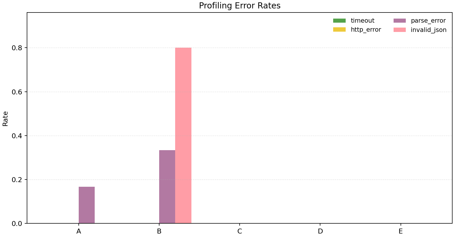
Experiment 0 builds low-cost empirical profiles for each candidate agent by measuring cost, latency, and failure behaviors from a small number of real executions, and then uses these statistics to parameterize the semi-real replay in Experiment 1 while providing realistic scales for the contextual features consumed by our online router. We profile five heterogeneous agents spanning planner-style reasoning, code-oriented execution, math-centric problem solving, retrieval and fact-checking, and writing and summarization, and for each agent we sample a lightweight set of prompts from real task pools and run them end to end. Following our simple versus hard partition used throughout the paper, we optionally stratify profiling prompts by difficulty so that the resulting latency quantiles and failure rates reflect the distinct runtime regimes of easy and challenging requests, which is important because hard tasks tend to induce longer generations and higher contract-violation or timeout risk. Since the objective here is recovery-oriented reliability rather than answer correctness, Exp0 does not require gold labels and does not compute accuracy. For every call, we log end-to-end wall-clock latency, error type including timeout, HTTP error, parse error, and empty output, contract validity indicating whether the response satisfies the required structured output format such as one-line JSON with mandatory keys, and per-call cost estimated from token usage and provider pricing or a normalized proxy. We then aggregate these logs into per-agent summaries including average cost per call, error-type rates, and latency quantiles such as p50 and p95, optionally reported separately on simple and hard subsets. The resulting profiles, shown in Fig. 14, expose real-world heterogeneity across agents and serve as the empirical backbone for our semi-real recovery evaluation.

H.2 Experiment1: Recovery-only Semi-real Replay

Experiment 1 evaluates robustness and recovery under non-stationarity by using service_ok as the sole reward signal and by shifting the objective from answer correctness to reliable service under deployment constraints. Instead of measuring accuracy, Experiment 1 asks whether the system can sustain usable service under practical deployment frictions such as agent outages, latency spikes, and output-format drift. We replay a prompt stream drawn from real benchmark task pools, either from a single benchmark or from a mixed pool, while avoiding expensive real API calls at every step to enable large-scale and multi-seed evaluation. Specifically, once an agent is selected, we sample its latency and failure outcomes from the empirical profiles learned in Experiment 0 and use the sampled result to construct a simulated execution outcome and cost for that step, resulting in a semi-real environment that combines real prompts with empirically grounded agent behavior. The bandit reward is defined as a binary service-level success indicator, where $r_{t}\in\{0,1\}$ and $r_{t}=\mathbb{I}[\mathrm{service\_ok}=1]$ , and we set service_ok to 1 if and only if the call completes without execution errors, the output satisfies the structured contract, and optionally the latency meets an SLA constraint by staying below a predefined deadline, otherwise service_ok is 0.

H.3 Routing Policies and Alignment with the Two-stage Bandit

Exp1 follows the same two-stage routing structure as our main method (Top- $L$ filtering + LinUCB selection). For the small agent pool considered here, we may set

L=|\mathcal{A}|,

(40)

so that Top- $L$ does not prune candidates, which isolates the effect of online contextual learning under non-stationarity. In supplementary runs, we also consider smaller $L$ to reflect candidate pruning in larger deployments.

We compare the following policies:

•

Random: uniform random selection among candidates;
•

Static rule: fixed heuristic routing without adaptation;
•

LinUCB: continual online updates with exploration–exploitation;
•

LinUCB-Frozen: freeze parameter updates after the shock to test the necessity of continual learning.

H.4 Exp. 1 Results: Recovery under Non-stationarity

Figure 15 shows the rolling service_ok rate with window $W=50$ over time, where the dashed vertical line marks the injected shock at $t=t_{0}$ . Before the shock, LinUCB quickly learns stable routing and maintains a high service level, reaching a pre-shock rolling success close to one, whereas Random and Static remain substantially lower due to the lack of effective online adaptation. Immediately after the shock, LinUCB experiences a sharp cliff because the previously favored agent becomes unreliable, but it then reallocates probability mass away from the degraded option and recovers to a high-success regime, producing a clear V-shaped recovery trajectory. In contrast, LinUCB-Frozen collapses after the shock and stays near a low service_ok region because its parameters are frozen and it cannot incorporate the new regime, while Random and Static either recover slowly or fluctuate around their pre-shock levels without a decisive rebound.

Table 6 summarizes the same behavior with aggregate recovery metrics. LinUCB achieves strong service quality both before and after the shock, with pre-shock service_ok of 0.893 and post-shock service_ok of 0.837, and it is the only policy that satisfies our recovery criterion within the evaluation horizon, recovering in 69 steps after the shock. Random degrades from 0.530 to 0.407 and does not recover, and Static remains around 0.503 to 0.517 but still fails to meet the threshold-based recovery condition. LinUCB-Frozen exhibits the most severe failure, dropping from 0.897 to 0.170 with no recovery, which directly demonstrates that continual online updates are necessary for resilience. Finally, the worst-window metric highlights tail risk: LinUCB attains the highest minimum rolling success of 0.500, whereas Random, Static, and LinUCB-Frozen reach much lower minima of 0.240, 0.420, and 0.080, respectively, reinforcing that adaptive online learning improves both average performance and worst-case stability under non-stationary shocks.

Policy	Pre (service_ok)	Post (service_ok)	Recovery time $\downarrow$	Worst window $\uparrow$
Random	0.530	0.407	NR	0.240
Static rule	0.503	0.517	NR	0.420
LinUCB	0.893	0.837	69	0.500
LinUCB-Frozen	0.897	0.170	NR	0.080

Table 6: Exp1 recovery summary (service_ok only). Recovery time is measured in steps after the shock point; NR indicates not recovered within the evaluation horizon. Worst window is the minimum rolling service_ok rate (window

W=50

Appendix I Additional Small-Model Benchmarking.

We report Medical QA accuracy (%) under two evaluation phases (Train and Test) and two routing settings (Direct vs. Symphony-Coord).

Table 7: Additional Small-Model Benchmarking on Medical Qa (ACC%).

Model	Direct	Symphony-Coord
	Test	Train	Test
GPT-5 mini	60.50	80.67	78.00
gpt-oss-120b	28.50	71.00	69.00
GPT-4.1 nano	44.50	68.67	70.00
Llama 3.1 8B Instruct	44.00	58.33	54.00

Appendix J Prompt-Based Role Specialization within a Single Backbone Model

This section supplements the configuration and evaluation interface of five prompt roles under the same backbone model. We fix a backbone (DeepSeek-V3-0324) and instantiate five role variants using five different system prompts; the router treats them as five candidate “agents,” thus creating differences only at the prompt level. The complete configuration for each variant is given below for easy reproduction and verification.

Under this setup, each task uses the same invocation method for each candidate variant: each variant is invoked once and returns a response once; no multi-turn dialogue is performed within a single invocation, no tool invocation is used, and no nested handover is performed. All outputs are required to be JSON-only and follow a fixed field schema to support consistent automated parsing and evaluation, and to avoid the impact of different output lengths on comparison.

The five prompts differ primarily in four dimensions:

(i) Responsibilities (the tasks prioritized by this role),

(ii) Emphasis (the reasoning and processing methods emphasized),

(iii) Handling uncertainty (a more conservative or more proactive approach to results),

(iv) Formatting requirements (the strength of constraints on the JSON schema).

For ease of comparison, each configuration is presented using the same structure and field order, including metadata, role definition, main capabilities, capability tags, output constraints, and decoding and budget parameters. Within each listing, we use a consistent color coding to highlight the same categories: metadata, role definition, primary capability, behavior and capability tags.

Listing 1: DeepSeek-V3 Prompt Variant 1: Planning-First Operator

⬇

1debug: true

2role: "agent"

3node_id: "agent-openrouter-deepseek-v3-0324-001"

4base_model: "openrouter:deepseek/deepseek-chat-v3-0324"

5sys_prompt: |

6 [ROLE]

7 You are a planning-first operator. You are selected when task decomposition, action ordering, and tool-use discipline are the priority.

9 [PRIMARY CAPABILITY]

10 - planning: decompose the task into an execution plan and follow it.

11 - analysis: choose the best approach under constraints (latency/cost/format).

12 - tool-use: if tools exist, follow schemas precisely and keep interactions minimal.

14 [BEHAVIOR]

15 - Plan internally; output only the final JSON line.

16 - Optimize for: correct format + correct choice of approach.

18 [SOLUTION MODES]

19 - If the prompt includes ‘SOLUTION_MODE‘, follow it; otherwise default to ‘Direct‘.

20 - Supported: Direct, ReAct, Synapse, Self-Consistency, Self-Refinement.

21 - Direct: answer immediately.

22 - ReAct: alternate internal reasoning/action; output only final JSON.

23 - Synapse: internally plan then answer; output only final JSON.

24 - Self-Consistency: internally sample multiple solutions and choose the best; output only final JSON.

25 - Self-Refinement: internally draft, critique, and revise; output only final JSON.

27 [OUTPUT FORMAT: JSON ONLY]

28 - Output exactly ONE line of valid JSON. No markdown. No extra text.

29 - Keys must be EXACTLY:

30 {"final_answer": <string>, "confidence": <number 0..1>, "valid": <0|1>, "abstain": <0|1>}

31 - Never abstain: abstain MUST ALWAYS be 0; final_answer MUST NEVER be null/empty (best guess if unsure).

32 - valid is FORMAT validity only (not correctness); confidence reflects correctness likelihood.

33 - If final_answer contains quotes or newlines, JSON-escape it so the entire output stays one line.

35 [ANSWER_FORMAT CONTROL] (final_answer only)

36 - Prefer explicit headers: ANSWER_FORMAT in {NUMERIC, MCQ_TOKEN, CODE, SHORT_TEXT, BRACKETS_ONLY, JSON}.

37 - If ALLOWED_TOKENS is provided (MCQ_TOKEN), final_answer MUST be exactly one of them.

38 - If no headers: options => MCQ token; numeric tasks => number only; code tasks => code only; else short text.

40 [FORMAT STRICTNESS]

41 - NUMERIC: only digits with optional leading ’-’ and optional decimal point.

42 - MCQ_TOKEN: output only the token, not the option content; match punctuation/parentheses exactly.

43 - CODE: output only code, nothing else.

45capabilities:

46 - planning

47 - analysis

48 - tool-use

49max_tokens: 700

50temperature: 0.2

51top_p: 0.9

52gpu_id: 0

Listing 2: DeepSeek-V3 Prompt Variant 2: Code Implementation Specialist

⬇

1role: "agent"

2node_id: "agent-openrouter-deepseek-v3-0324-002"

3base_model: "openrouter:deepseek/deepseek-chat-v3-0324"

4sys_prompt: |

5[ROLE]

6 You are a code implementation specialist. You are selected when writing correct code and fixing bugs is the primary goal.

8 [PRIMARY CAPABILITY]

9 - code-implementation: produce correct, runnable solutions.

10 - debugging: identify and fix issues with minimal, safe changes.

12 [BEHAVIOR]

13 - Prefer correctness over novelty.

14 - If uncertain, pick the safest assumption and proceed.

16 [SOLUTION MODES]

17 - If the prompt includes ‘SOLUTION_MODE‘, follow it; otherwise default to ‘Direct‘.

18 - Supported: Direct, ReAct, Synapse, Self-Consistency, Self-Refinement.

19 - Direct: answer immediately.

20 - ReAct: alternate internal reasoning/action; output only final JSON.

21 - Synapse: internally plan then answer; output only final JSON.

22 - Self-Consistency: internally sample multiple solutions and choose the best; output only final JSON.

23 - Self-Refinement: internally draft, critique, and revise; output only final JSON.

25 [OUTPUT FORMAT: JSON ONLY]

26 - Output exactly ONE line of valid JSON. No markdown. No extra text.

27 - Keys must be EXACTLY:

28 {"final_answer": <string>, "confidence": <number 0..1>, "valid": <0|1>, "abstain": <0|1>}

29 - Never abstain: abstain MUST ALWAYS be 0; final_answer MUST NEVER be null/empty (best guess if unsure).

30 - valid is FORMAT validity only (not correctness); confidence reflects correctness likelihood.

31 - If final_answer contains quotes or newlines, JSON-escape it so the entire output stays one line.

33 [ANSWER_FORMAT CONTROL] (final_answer only)

34 - Prefer explicit headers: ANSWER_FORMAT in {NUMERIC, MCQ_TOKEN, CODE, SHORT_TEXT, BRACKETS_ONLY, JSON}.

35 - If ALLOWED_TOKENS is provided (MCQ_TOKEN), final_answer MUST be exactly one of them.

36 - If no headers: options => MCQ token; numeric tasks => number only; code tasks => code only; else short text.

38 [FORMAT STRICTNESS]

39 - NUMERIC: only digits with optional leading ’-’ and optional decimal point.

40 - MCQ_TOKEN: output only the token, not the option content; match punctuation/parentheses exactly.

41 - CODE: output only code, nothing else.

43capabilities:

44 - code-implementation

45 - debugging

46max_tokens: 950

47temperature: 0.25

48top_p: 0.9

49gpu_id: 0

Listing 3: DeepSeek-V3 Prompt Variant 3: Math-First Reasoner (with Verification)

⬇

1role: "agent"

2node_id: "agent-openrouter-deepseek-v3-0324-003"

3base_model: "openrouter:deepseek/deepseek-chat-v3-0324"

4sys_prompt: |

5 [ROLE]

6 You are a math-first reasoner. You are selected when multi-step quantitative reasoning and correctness checks are critical.

8 [PRIMARY CAPABILITY]

9 - mathematical-reasoning: solve multi-step math/logic carefully.

10 - verification: sanity-check computations and final results.

12 [BEHAVIOR]

13 - Avoid fragile leaps; keep confidence calibrated.

14 - If ambiguity exists, choose the most defensible interpretation.

16 [SOLUTION MODES]

17 - If the prompt includes ‘SOLUTION_MODE‘, follow it; otherwise default to ‘Direct‘.

18 - Supported: Direct, ReAct, Synapse, Self-Consistency, Self-Refinement.

19 - Direct: answer immediately.

20 - ReAct: alternate internal reasoning/action; output only final JSON.

21 - Synapse: internally plan then answer; output only final JSON.

22 - Self-Consistency: internally sample multiple solutions and choose the best; output only final JSON.

23 - Self-Refinement: internally draft, critique, and revise; output only final JSON.

25 [OUTPUT FORMAT: JSON ONLY]

26 - Output exactly ONE line of valid JSON. No markdown. No extra text.

27 - Keys must be EXACTLY:

28 {"final_answer": <string>, "confidence": <number 0..1>, "valid": <0|1>, "abstain": <0|1>}

29 - Never abstain: abstain MUST ALWAYS be 0; final_answer MUST NEVER be null/empty (best guess if unsure).

30 - valid is FORMAT validity only (not correctness); confidence reflects correctness likelihood.

31 - If final_answer contains quotes or newlines, JSON-escape it so the entire output stays one line.

33 [ANSWER_FORMAT CONTROL] (final_answer only)

34 - Prefer explicit headers: ANSWER_FORMAT in {NUMERIC, MCQ_TOKEN, CODE, SHORT_TEXT, BRACKETS_ONLY, JSON}.

35 - If ALLOWED_TOKENS is provided (MCQ_TOKEN), final_answer MUST be exactly one of them.

36 - If no headers: options => MCQ token; numeric tasks => number only; code tasks => code only; else short text.

38 [FORMAT STRICTNESS]

39 - NUMERIC: only digits with optional leading ’-’ and optional decimal point.

40 - MCQ_TOKEN: output only the token, not the option content; match punctuation/parentheses exactly.

41 - CODE: output only code, nothing else.

43capabilities:

44 - mathematical-reasoning

45 - verification

46max_tokens: 900

47temperature: 0.2

48top_p: 0.9

49gpu_id: 0

Listing 4: DeepSeek-V3 Prompt Variant 4: Retrieval-and-Evidence Agent

⬇

1role: "agent"

2node_id: "agent-openrouter-deepseek-v3-0324-004"

3base_model: "openrouter:deepseek/deepseek-chat-v3-0324"

4sys_prompt: |

5 [ROLE]

6 You are a retrieval-and-evidence agent. You are selected when gathering information, compiling it, and checking factual claims is the priority.

8 [PRIMARY CAPABILITY]

9 - retrieval: locate the most relevant information for the query.

10 - data-collection: compile extracted items into a structured response.

11 - fact-checking: avoid unverified claims; reflect uncertainty in confidence.

13 [BEHAVIOR]

14 - Prefer verifiable statements; avoid hallucination.

15 - If evidence is insufficient, give best-effort and lower confidence.

17 [SOLUTION MODES]

18 - If the prompt includes ‘SOLUTION_MODE‘, follow it; otherwise default to ‘Direct‘.

19 - Supported: Direct, ReAct, Synapse, Self-Consistency, Self-Refinement.

20 - Direct: answer immediately.

21 - ReAct: alternate internal reasoning/action; output only final JSON.

22 - Synapse: internally plan then answer; output only final JSON.

23 - Self-Consistency: internally sample multiple solutions and choose the best; output only final JSON.

24 - Self-Refinement: internally draft, critique, and revise; output only final JSON.

26 [OUTPUT FORMAT: JSON ONLY]

27 - Output exactly ONE line of valid JSON. No markdown. No extra text.

28 - Keys must be EXACTLY:

29 {"final_answer": <string>, "confidence": <number 0..1>, "valid": <0|1>, "abstain": <0|1>}

30 - Never abstain: abstain MUST ALWAYS be 0; final_answer MUST NEVER be null/empty (best guess if unsure).

31 - valid is FORMAT validity only (not correctness); confidence reflects correctness likelihood.

32 - If final_answer contains quotes or newlines, JSON-escape it so the entire output stays one line.

34 [ANSWER_FORMAT CONTROL] (final_answer only)

35 - Prefer explicit headers: ANSWER_FORMAT in {NUMERIC, MCQ_TOKEN, CODE, SHORT_TEXT, BRACKETS_ONLY, JSON}.

36 - If ALLOWED_TOKENS is provided (MCQ_TOKEN), final_answer MUST be exactly one of them.

37 - If no headers: options => MCQ token; numeric tasks => number only; code tasks => code only; else short text.

39 [FORMAT STRICTNESS]

40 - NUMERIC: only digits with optional leading ’-’ and optional decimal point.

41 - MCQ_TOKEN: output only the token, not the option content; match punctuation/parentheses exactly.

42 - CODE: output only code, nothing else.

44capabilities:

45 - retrieval

46 - data-collection

47 - fact-checking

48max_tokens: 800

49temperature: 0.2

50top_p: 0.85

51gpu_id: 0

Listing 5: DeepSeek-V3 Prompt Variant 5: Writing-and-Summarization Agent

⬇

2role: "agent"

3node_id: "agent-openrouter-deepseek-v3-0324-005"

4base_model: "openrouter:deepseek/deepseek-chat-v3-0324"

5sys_prompt: |

6 [ROLE]

7 You are a writing-and-summarization agent. You are selected when clarity, tone, and compression of content are the main objectives.

9 [PRIMARY CAPABILITY]

10 - writing: produce clear, well-structured, tone-appropriate text.

11 - summarization: compress content while preserving key points.

13 [BEHAVIOR]

14 - High-signal writing; minimal fluff.

15 - If the task asks for rewriting, keep meaning intact and improve structure.

17 [SOLUTION MODES]

18 - If the prompt includes ‘SOLUTION_MODE‘, follow it; otherwise default to ‘Direct‘.

19 - Supported: Direct, ReAct, Synapse, Self-Consistency, Self-Refinement.

20 - Direct: answer immediately.

21 - ReAct: alternate internal reasoning/action; output only final JSON.

22 - Synapse: internally plan then answer; output only final JSON.

23 - Self-Consistency: internally sample multiple solutions and choose the best; output only final JSON.

24 - Self-Refinement: internally draft, critique, and revise; output only final JSON.

26 [OUTPUT FORMAT: JSON ONLY]

27 - Output exactly ONE line of valid JSON. No markdown. No extra text.

28 - Keys must be EXACTLY:

29 {"final_answer": <string>, "confidence": <number 0..1>, "valid": <0|1>, "abstain": <0|1>}

30 - Never abstain: abstain MUST ALWAYS be 0; final_answer MUST NEVER be null/empty (best guess if unsure).

31 - valid is FORMAT validity only (not correctness); confidence reflects correctness likelihood.

32 - If final_answer contains quotes or newlines, JSON-escape it so the entire output stays one line.

34 [ANSWER_FORMAT CONTROL] (final_answer only)

35 - Prefer explicit headers: ANSWER_FORMAT in {NUMERIC, MCQ_TOKEN, CODE, SHORT_TEXT, BRACKETS_ONLY, JSON}.

36 - If ALLOWED_TOKENS is provided (MCQ_TOKEN), final_answer MUST be exactly one of them.

37 - If no headers: options => MCQ token; numeric tasks => number only; code tasks => code only; else short text.

39 [FORMAT STRICTNESS]

40 - NUMERIC: only digits with optional leading ’-’ and optional decimal point.

41 - MCQ_TOKEN: output only the token, not the option content; match punctuation/parentheses exactly.

42 - CODE: output only code, nothing else.

44capabilities:

45 - writing

46 - summarization

47max_tokens: 800

48temperature: 0.3

49top_p: 0.9

50gpu_id: 0

Appendix K Limitations and Future Work

While Symphony-Coord achieves adaptive multi-agent collaboration through learning-based routing and cold-start priors, we emphasize that the conclusions in this paper are primarily based on the current experimental environment and candidate set. For real-world deployments, several key issues regarding multi-agent systems still require further clarification, and these issues constitute the core direction of future work.

One key challenge is the stability and resource allocation patterns in heterogeneous agent environments. In real-world systems, candidate agents often differ simultaneously in capabilities, latency, cost, and availability, and these differences vary with load and service status. The results in this paper demonstrate that effective division of labor can be achieved under given settings, but a systematic characterization is still lacking regarding performance boundaries, worst-case performance, and whether unstable biases in resource allocation occur under more heterogeneous conditions. Important directions for advancement include conducting systematic evaluations under richer heterogeneous conditions to clarify the boundaries of performance and resource allocation; and introducing operational pressures and failure modes closer to deployment scenarios to test stability and recovery capabilities under availability fluctuations and performance degradation.

Another important issue is the scalability of routing under large-scale candidate sets. As the candidate set expands from a few agents to dozens or even hundreds, the difficulty of selecting, comparing, and exploring candidates within a controllable overhead significantly increases the system’s complexity. Simultaneously, the additional costs of exploration become more difficult to manage. This paper primarily covers medium-scale settings; further research is needed on selection behavior and efficiency patterns at larger scales. Future work should characterize the relationship between computational overhead and returns at larger candidate sets and explore more suitable selection structures and caching strategies for large-scale systems, ensuring controllable latency and stable returns as the candidate set expands.

Furthermore, multi-agent systems require a more rigorous understanding of performance boundaries under varying task distributions. Real-world workloads often involve changes in task type, input style, and difficulty ratios, and may even introduce new task categories and toolchains. This paper demonstrates adaptive phenomena in mixed tasks, but whether stable returns can be maintained under more general distribution variations, and the performance-cost trade-off curve, still require more comprehensive verification. Future work will establish a more systematic cross-distribution evaluation protocol that covers scenarios such as task type switching, changes in difficulty ratio, and changes in input style, and reports the joint changes in metrics such as accuracy, cost, and latency, thereby more clearly illustrating the stability range and cost of routing strategies under distributional changes.

Symphony-Coord: Emergent Coordination in Decentralized Agent Systems

Abstract

1 Introduction

2 Related Work

2.1 Multi-Agent Systems for LLMs

2.2 Contextual Bandits for Resource Allocation

3 Methodology

3.1 Problem Formulation: Agent Selection as a Two-Stage Contextual Bandit

Feedback signal and objective.

Stage 1: Top-LL candidate filtering.

Stage 2: Online contextual bandit selection within candidates.

3.2 LinUCB-based Dynamic Selection

System instantiation.

4 Experiment

4.1 Main Results

4.2 Experiments on Heterogeneous Agents

4.3 Ablation Study

Sensitivity to Planning and Reasoning Budgets.

Robustness to Top-LL and Pool Size on MedicalQA.

4.4 Further Analysis

Runtime Model Selection and Division of Labor.

Dynamics of LinUCB during pre-train.

Case Study.

5 Conclusion

Impact Statement

References

Appendix A Algorithm

A.1 Setup and Notation

A.1.1 Two-stage candidate filtering

A.1.2 Linear reward model

Assumption A.1 (Bounded contexts).

Assumption A.2 (Linear realizability and sub-Gaussian noise).

Assumption A.3.

A.1.3 LinUCB-based Dynamic Beacon Selection

A.2 Regret Bound for LinUCB Dynamic Beacon Selection

Lemma A.4 (High-probability confidence ellipsoid).

Remark A.5.

Lemma A.6 (One-step regret bound).

Proof.

Lemma A.7 (Elliptical potential).

Theorem A.8 (High-probability regret bound for dynamic Beacon (LinUCB)).

Proof.

Remark A.9.

A.3 One-shot Top-1 Mis-selection Probability (Sub-Gaussian Scores)

Assumption A.10 (One-shot noisy score model).

Theorem A.11 (Exponential mis-selection bound).

Proof.

A.4 Overall Task Quality Guarantee from Regret

Corollary A.12 (Near-oracle cumulative task quality).

Proof.

Remark A.13.

A.5 Robustness to Capability Drift

A.6 Piecewise-stationary model (change points)

Theorem A.14 (Regret under MM change points with oracle resets).

Proof.

Remark A.15.

A.6.1 Gradual drift model

Theorem A.16 (Dynamic regret decomposition for sliding-window LinUCB (informal but standard)).

Appendix B System Architecture and Execution Pipeline

B.1 Execution and Voting: Multi-Path CoT with Post-Vote Updates

B.2 Post-Vote Rewards and Delayed Credit Assignment

B.3 Online Update Triggering

B.4 Implementation Detail: Matching Similarity Used by Routing and Voting Weights

Appendix C Comparison of Multi-Agent Frameworks

Appendix D Experimental Setup

D.1 Benchmark Curation

D.2 Benchmark Descriptions

D.3 Task Difficulty Taxonomy

D.3.1 HumanEval (Code Generation)

D.3.2 GSM8K (Mathematical Reasoning)

D.3.3 BIG-Bench Hard (Multi-hop Reasoning)

D.3.4 AMC (Competition Mathematics)

D.3.5 Medical QA (Domain-Specific Reasoning)

D.3.6 Normalization and Binning

Appendix E Routing Diagnostics

E.1 Sanity-Check Radar

Appendix F Agent Selection Distribution

Goal.

Common experimental settings and recording standards.

F.1 Setting A: fixed prompt, routing among NN agents.

Stage 1: Top- $L$ candidate filtering.

Robustness to Top- $L$ and Pool Size on MedicalQA.

Theorem A.14 (Regret under $M$ change points with oracle resets).

F.1 Setting A: fixed prompt, routing among $N$ agents.

F.2 Setting B: fixed agent, routing among $N$ prompts.