跳到论文正文
W Papers独立论文阅读器 arXiv:2602.00649 论文正文 计算阅读时间 · 0%
引用这篇论文根据当前论文元数据生成,正式投稿前建议核对。


License: CC BY 4.0
arXiv:2602.00649v2 [physics.plasm-ph] 29 Jul 2026

Central Equations and Band Structures of Linear Magnetohydrodynamic Waves in a Magneto-Lattice

Shiyu Sun Institute of Material Science and Information Technology, Anhui University, Hefei, Anhui 230601, China    Peifeng Fan corresponding author: pffan@ahu.edu.cn School of Physics, Anhui University, Hefei, Anhui 230601, China    Yulei Wang Institute of Science and Technology for Deep Space Exploration, Suzhou Campus, Nanjing University, Suzhou, 215163, People’s Republic of China State Key Laboratory of Lunar and Planetary Sciences, Macau University of Science and Technology, Macau, People’s Republic of China    Qiang Chen National Supercomputing Center in Zhengzhou, Zhengzhou University, Zhengzhou, Henan 450001, China    Xingkai Li School of Physics, Anhui University, Hefei, Anhui 230601, China    Weihua Wang corresponding author: whwang@ahu.edu.cn Institute of Material Science and Information Technology, Anhui University, Hefei, Anhui 230601, China
Abstract

We investigate the band structures and propagation properties of linear ideal magnetohydrodynamic (MHD) waves in a plasma with a spatially periodic background magnetic field (a “magneto-lattice”). We develop a plane-wave expansion approach in two equivalent forms: one written using the usual linearized MHD perturbation variables and another written in terms of the fluid displacement. We validate both formulations with numerical tests, including an empty-lattice limit that recovers the uniform-plasma dispersion. The method enables efficient computation of dispersion relations and reveals intrinsic frequency band gaps and cutoff behavior caused by magnetic periodicity. We show that the band gap width increases with the amplitude of the periodic magnetic-field modulation (relative to the uniform background field), leading to suppression of selected wave modes. In addition, the magnetic periodicity splits the Alfvén continuum into multiple branches, a feature absent in uniform plasmas. These results provide a framework for tailoring MHD wave propagation in structured plasmas and may be useful for future studies of plasma metamaterials and topological plasma waves.

magnetohydrodynamic waves, magneto-lattice, linearized ideal MHD equations, frequency band gap, Alfvén-wave splitting

I INTRODUCTION

The control of wave propagation using spatially periodic structures is a central research direction in modern physics materials science (Zangeneh-Nejad and Fleury, 2019; Lin et al., 2023; Yang et al., 2024). In particular, periodic mesoscale structures—such as photonic crystals and phononic crystals have been highly successful in enabling precise manipulation of electromagnetic waves (Zhang and Satpathy, 1990; Joannopoulos et al., 1997; Maigyte and Staliunas, 2015a; Zhang et al., 2012) and elastic waves (Wang et al., 2015; Liang et al., 2025). For example, photonic crystals reveal the band splitting and band gap effects of electromagnetic waves through the periodic spatial arrangement of dielectric constants, providing a theoretical basis for new optical devices (Botten et al., 2006; Nair and Vijaya, 2010; Maigyte and Staliunas, 2015b; Shen et al., 2016; Baryshevsky and Gurinovich, 2019; Butt et al., 2021; Luo et al., 2025; Jin et al., 2025). Phononic crystals have extended this idea to the field of elastic waves, utilizing the periodic combination of scatterers and substrates to achieve suppression and mode selection of acoustic/elastic wave propagation (Badreddine Assouar and Oudich, 2011; Hussein and Leamy, 2014; Ash et al., 2017; Vasileiadis et al., 2021). They have shown great potential in fields such as vibration reduction (Yu et al., 2008; Xiao et al., 2010; Bilal et al., 2018; Xiao et al., 2024), noise reduction (Pan et al., 2022; Rizvi et al., 2025; Zaky et al., 2025), and acoustic imaging (Profunser et al., 2006; Li et al., 2006; Qiu et al., 2005; Ma et al., 2022; Beoletto et al., 2024). These studies collectively reveal a universal law: spatial periodicity reshapes wave dispersion relations, and the emergence of band gaps enables novel strategies for active wave modulation.

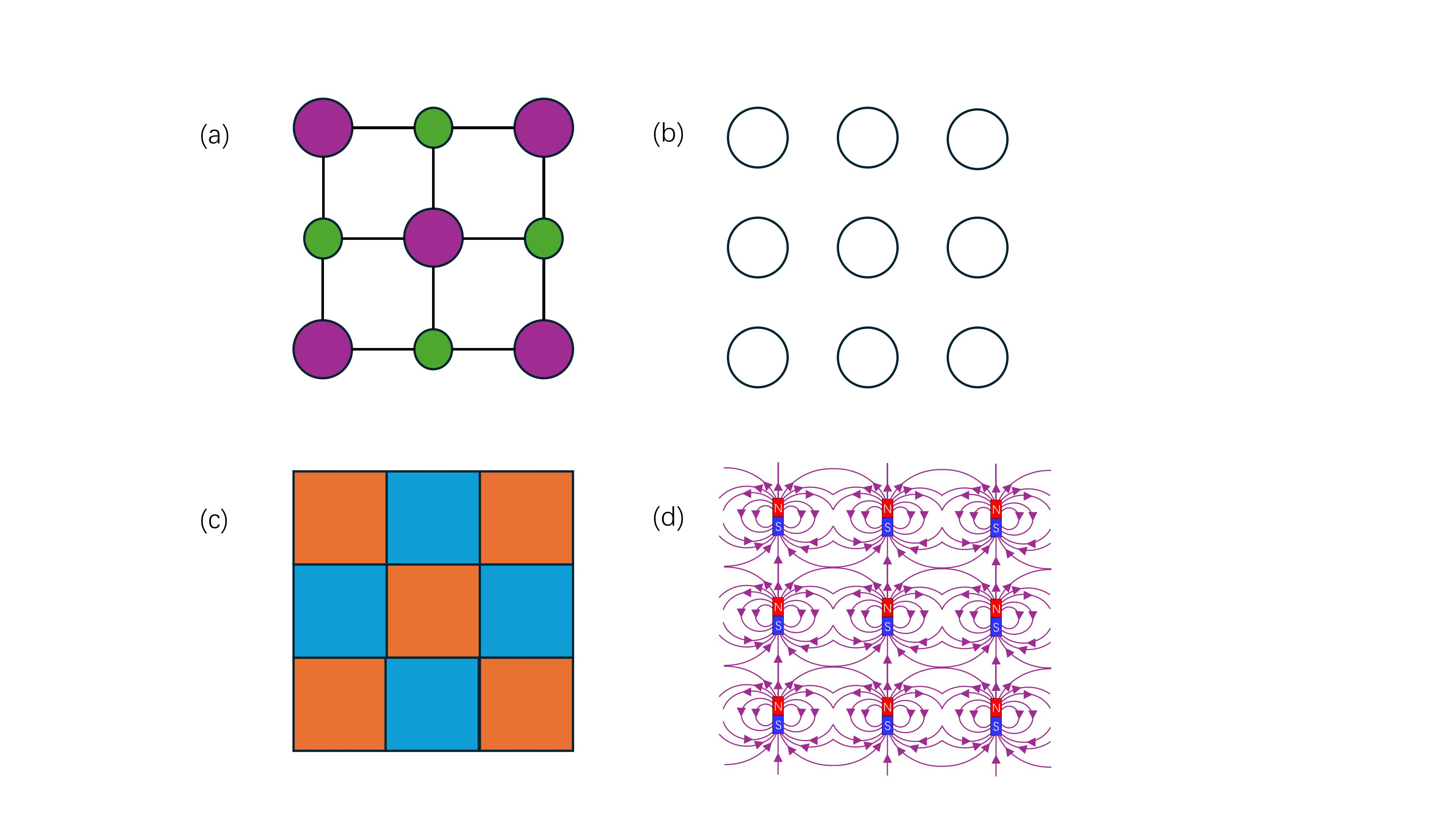
Magnetohydrodynamics (MHD) investigates the macroscopic behavior of electrically conducting fluids in magnetic fields and is widely applied in space physics (Zhou et al., 2004), controlled nuclear fusion (Freidberg, 1982, 2014; Ongena et al., 2016), and astrophysics (Nigro et al., 2004; Yamada et al., 2010; Lebedev et al., 2019; Nakariakov and Kolotkov, 2020; Zhou et al., 2024). As the fundamental disturbance modes in magnetized plasmas, MHD waves primarily include fast waves (FWs), slow waves (SWs), and Alfvén waves (AWs). Advances in the understanding of periodic structures have revealed that wave propagation can be profoundly modified by spatial periodicity. In particular, studies of photonic and phononic crystals have shown that periodic structures can give rise to characteristic band gaps (i.e., frequency gaps), within which wave propagation is forbidden. Motivated by this concept, this study explores the propagation behavior of MHD waves in spatially periodic magnetic field structures, referred to as magneto-lattices. This magneto-lattice configuration can be realized either by periodically arranging permanent magnets or by periodically arranging externally energized coils. For instance, Fig. 1(d) illustrates a 2D magneto-lattice formed by a spatially periodic arrangement of magnetic dipoles, analogous to an atomic crystal lattice and conceptually resembling a magnetic crystal.
Refer to caption
Figure 1: Schematic illustration of periodic lattice structures in different physical systems. (a) Atomic crystal lattice in condensed matter physics. (b) Periodic elastic lattice in a phononic crystal for manipulating acoustic or elastic waves. (c) Periodic dielectric lattice in a photonic crystal for controlling electromagnetic wave propagation. (d) Magneto-lattice formed by periodically arranged magnetic dipoles, producing a spatially modulated magnetic field for controlling the propagation of MHD waves.

In this study, we present a theoretical approach to investigate the propagation of linear MHD waves in a magneto-lattice. Starting from the ideal MHD equations, we employ a perturbative approach to derive the equilibrium configuration and the corresponding linearized MHD equations. The magneto-lattice induced equilibrium provides a stable background for MHD wave evolution, analogous to the controlled environments realized in laboratory photonic and phononic crystals. Starting from the linearized MHD equations and applying Bloch’s theorem together with the plane-wave expansion (PWE) method (Hsue et al., 2005; Poggetto and Serpa, 2020), we systematically derive the central equations in two equivalent representations: one expressed in terms of the perturbed physical fields (ρ,𝑩,𝒗)\left(\rho,\boldsymbol{B},\boldsymbol{v}\right) (perturbed mass density, magnetic field, and velocity), and the other formulated in terms of the perturbed displacement field 𝝃\boldsymbol{\xi}. To validate the two models, we consider a magnetic field that is uniform in direction (along the yy-axis) and sinusoidally modulated in magnitude along the xx-direction. The normalized magnetic field is given by 𝑩0​(x)=[1+Bm​sin​(x)]​𝒆y\boldsymbol{B}_{0}\left(x\right)=\left[1+B_{m}\mathrm{sin}\left(x\right)\right]\boldsymbol{e}_{y}. Two values of the modulation amplitude are considered: Bm=0B_{m}=0 corresponding to the empty-lattice (uniform-field) case, and Bm=0.1B_{m}=0.1. The results show excellent agreement between the two theoretical formulations. In addition, full MHD simulations are performed using the Athena++ code (Stone et al., 2020; Athena++ development team, 2021), with spectral properties extracted via fast Fourier transform (FFT). The simulation results closely match the band-gap locations and widths predicted by the central equations, confirming the effectiveness of periodic magnetic fields in generating band-gaps. Moreover, the numerical results show that periodic magnetic fields can produce substantial frequency gaps, with the band-gap width increasing as the modulation amplitude BmB_{m} grows. Notably, Alfvén waves split into multiple branches in a periodic magnetic field—a phenomenon absent in uniform plasma.

Beyond band gap physics, magneto-lattices may also serve as a useful platform for plasma-wave engineering in the spirit of metamaterials and topological wave systems. By tailoring the spatial profile of the equilibrium magnetic field, one can in principle reshape the dispersion and polarization properties of MHD waves, suggesting the possibility of tunable plasma-wave spectral control using externally energized coils or magnet arrays. In addition, the presence of spatial periodicity folds the spectrum into the first Brillouin zone, providing a natural setting for defining Berry phases and related topological quantities from Bloch eigenstates. While the present work focuses on establishing and benchmarking the band-theory framework, it lays the groundwork for future studies of topological band structures and interface modes in periodic magnetized plasmas.

The remainder of this paper is organized as follows. In Sec. II, we introduce the MHD equilibrium within a magneto-lattice and employ the PWE method to derive the central equations for linearized MHD waves. In Sec. III, we solve the truncated central equations to compute the band structures for two representative cases, discussing the physical significance of band folding. Section IV compares these analytical results with full nonlinear MHD simulations conducted using the Athena++ code. Finally, in the last section, we provide a brief discussion and summarize our main findings.

II Central equations in a magneto-lattice

In electronic materials, crystals are formed by the periodic arrangement of atoms or molecules, providing a stable foundational environment for electron motion. Analogously, in MHD systems, the evolution of waves requires a stable configuration, termed an MHD equilibrium. By extending the concept of a crystal lattice to MHD systems, we aim to establish a spatially periodic equilibrium configuration within a magneto-lattice. Just as electron behavior is described by wavefunctions in crystalline structures, MHD waves serve as their counterparts in MHD fluid. Thus, studying MHD waves fundamentally relies on first constructing such equilibrium states, mirroring how investigating electron waves necessitates a preexisting crystalline lattice framework.

We consider an equilibrium magnetic field 𝑩0\boldsymbol{B}_{0} that consists of a uniform background field 𝑩0​b\boldsymbol{B}_{0b} and a spatially periodic magneto-lattice component 𝑩0​L\boldsymbol{B}_{0L}, expressed as:

𝑩0​(𝒙)=B0​b​𝒆y+𝑩0​L​(𝒙).\boldsymbol{B}_{0}\left(\boldsymbol{x}\right)=B_{0b}\boldsymbol{e}_{y}+\boldsymbol{B}_{0L}\left(\boldsymbol{x}\right). (1)

The magneto-lattice field 𝑩0​L\boldsymbol{B}_{0L} satisfies the spatial periodicity condition 𝑩0​L​(𝒙+𝑹n)=𝑩0​L​(𝒙)\boldsymbol{B}_{0L}\left(\boldsymbol{x}+\boldsymbol{R}_{n}\right)=\boldsymbol{B}_{0L}\left(\boldsymbol{x}\right), where 𝑹n\boldsymbol{R}_{n} denotes the lattice vectors. In the absence of 𝑩0​L\boldsymbol{B}_{0L}, the equilibrium density and pressure are uniform constants, denoted by ρ0​b\rho_{0b} and P0​bP_{0b}, respectively. In the presence of the magneto-lattice field, the system is characterized by a spatially periodic mass density ρ0​(𝒙)\rho_{0}\left(\boldsymbol{x}\right) and pressure P0​(𝒙)P_{0}\left(\boldsymbol{x}\right) to satisfy the equilibrium force-balance condition:

∇P0=14​π​(∇×𝑩0)×𝑩0.\nabla P_{0}=\frac{1}{4\pi}\left(\nabla\times\boldsymbol{B}_{0}\right)\times\boldsymbol{B}_{0}. (2)

Assuming the equilibrium state is isothermal, the spatially dependent pressure P0​(𝒙)P_{0}\left(\boldsymbol{x}\right) and density ρ0​(𝒙)\rho_{0}\left(\boldsymbol{x}\right) satisfy the relation:

P0​bρ0​b=P0​(𝒙)ρ0​(𝒙),\frac{P_{0b}}{\rho_{0b}}=\frac{P_{0}\left(\boldsymbol{x}\right)}{\rho_{0}\left(\boldsymbol{x}\right)}, (3)

Consequently, the adiabatic sound speed remains uniform throughout the system, i.e., Cs2=γ​P0​b/ρ0​b≡Cs​b2C_{s}^{2}=\gamma P_{0b}/\rho_{0b}\equiv C_{sb}^{2}, where Cs​bC_{sb} is the constant background sound speed.

With the equilibrium profiles defined, we now proceed to derive the central equations for the system—a set of eigenvalue equations that essentially serve as the band model for our magneto-lattice. The concept of the central equation originates from condensed matter physics, where it plays a fundamental role in the analysis of wave phenomena within periodic media (Kittel, 1979). By exploiting discrete translational symmetry and applying a PWE alongside Bloch’s theorem, the governing equations are recast to explicitly couple different reciprocal lattice vectors. This mathematical transformation provides a robust method for determining band structures, predicting band gaps, and analyzing periodicity-induced mode hybridization. Just as the central equation serves as the foundational tool for studying electrons, phonons, and photonic crystals, we adapt this formalism here to magnetohydrodynamics. By deriving the central equations for linearized MHD waves in this section, we establish a formal mathematical parallel between structured plasmas and traditional crystalline solids.

Before deriving the central equations, we nondimensionalize the linearized magnetohydrodynamic equations to obtain a dimensionless formulation. All physical quantities are normalized by the uniform background density ρ0​b\rho_{0b} and magnetic field B0​bB_{0b}, and the nondimensional variables are defined as

ρ~1=ρ1ρ0​b,ρ~0​L=ρ0​Lρ0​b,ρ~0=ρ0ρ0​b\displaystyle\tilde{\rho}_{1}=\frac{\rho_{1}}{\rho_{0b}},\thinspace\tilde{\rho}_{0L}=\frac{\rho_{0L}}{\rho_{0b}},\thinspace\tilde{\rho}_{0}=\frac{\rho_{0}}{\rho_{0b}} (4)
𝑩~1=𝑩1|B0​b|,𝑩~0​L=𝑩0​L|B0​b|,𝑩~0=𝑩0|B0​b|=σ​𝒆z+𝑩~0​L,\displaystyle\tilde{\boldsymbol{B}}_{1}=\frac{\boldsymbol{B}_{1}}{\left|B_{0b}\right|},\thinspace\tilde{\boldsymbol{B}}_{0L}=\frac{\boldsymbol{B}_{0L}}{\left|B_{0b}\right|},\thinspace\tilde{\boldsymbol{B}}_{0}=\frac{\boldsymbol{B}_{0}}{\left|B_{0b}\right|}=\sigma\boldsymbol{e}_{z}+\tilde{\boldsymbol{B}}_{0L}, (5)
𝒗~1=𝒗1VA​b,\displaystyle\tilde{\boldsymbol{v}}_{1}=\frac{\boldsymbol{v}_{1}}{V_{Ab}}, (6)

where VA​b=B0​b2/4​π​ρ0​bV_{Ab}=\sqrt{B_{0b}^{2}/4\pi\rho_{0b}} is the Alfvén speed and σ=B0​b/|B0​b|=±1\sigma=B_{0b}/\left|B_{0b}\right|=\pm 1. Let sL=VcellD/2​πs_{L}=\sqrt[D]{V_{\mathrm{cell}}}/2\pi denote the characteristic length of a unit cell, where DD is the dimension of the lattice and VcellV_{\mathrm{cell}} is the volume of the unit cell. Using sLs_{L} and VA​bV_{Ab}, the characteristic time is given by t0=sL/VA​bt_{0}=s_{L}/V_{Ab}, which is referred to as the Alfvén time. The space and time coordinates are nondimensionalized as

𝒙~=𝒙sL,t~=tt0,\tilde{\boldsymbol{x}}=\frac{\boldsymbol{x}}{s_{L}},\quad\tilde{t}=\frac{t}{t_{0}}, (7)

with the corresponding nondimensional derivatives given by

∇~=sL​∇,∂∂t~=t0​∂∂t.\tilde{\boldsymbol{\nabla}}=s_{L}\boldsymbol{\nabla},\quad\frac{\partial}{\partial\tilde{t}}=t_{0}\frac{\partial}{\partial t}. (8)

Substituting the nondimensional variables from Eqs. (4) and (8) into the linear ideal MHD equations (see Eqs. (93) and (95) in Appendix A) and omitting tildes “~” and perturbation subscripts “1” for simplicity, yields the nondimensionalized equations

∂ρ∂t=−∇⋅(ρ0​𝒗),\displaystyle\frac{\partial\rho}{\partial t}=-\nabla\cdot\left(\rho_{0}\boldsymbol{v}\right), (9)
∂𝑩∂t=−∇⋅(𝒗​𝑩0−𝑩0​𝒗),\displaystyle\frac{\partial\boldsymbol{B}}{\partial t}=-\nabla\cdot\left(\boldsymbol{v}\boldsymbol{B}_{0}-\boldsymbol{B}_{0}\boldsymbol{v}\right), (10)
ρ0​∂𝒗∂t=−∇⋅[(β​ρ+𝑩0⋅𝑩)​𝑰−(𝑩0​𝑩1+𝑩​𝑩0)],\displaystyle\rho_{0}\frac{\partial\boldsymbol{v}}{\partial t}=-\nabla\cdot\left[\left(\beta\rho+\boldsymbol{B}_{0}\cdot\boldsymbol{B}\right)\boldsymbol{I}-\left(\boldsymbol{B}_{0}\boldsymbol{B}_{1}+\boldsymbol{B}\boldsymbol{B}_{0}\right)\right], (11)

where β=Cs2/VA​b2\beta=C_{s}^{2}/V_{Ab}^{2} and 𝑰\boldsymbol{I} is the identity tensor. The equilibrium condition become

∇P0=γβ​(∇×𝑩0)×𝑩0.\nabla P_{0}=\frac{\gamma}{\beta}\left(\nabla\times\boldsymbol{B}_{0}\right)\times\boldsymbol{B}_{0}. (12)

Introducing the nondimensional displacement 𝝃~=𝝃/sL\tilde{\boldsymbol{\xi}}=\boldsymbol{\xi}/s_{L} and applying the normalization schemes from Eqs. (7) and (8) into Eq. (96) (see Appendix A), while omitting tildes “~” for brevity, results in

ρ0∂2𝝃∂t2=∇⋅{[β(ρ0∇⋅𝝃+1γ𝝃⋅∇ρ0)−𝑩0⋅∇×(𝝃×𝑩0)]𝑰\displaystyle\rho_{0}\frac{\partial^{2}\boldsymbol{\xi}}{\partial t^{2}}=\nabla\cdot\left\{\left[\beta\left(\rho_{0}\nabla\cdot\boldsymbol{\xi}+\frac{1}{\gamma}\boldsymbol{\xi}\cdot\nabla\rho_{0}\right)-\boldsymbol{B}_{0}\cdot\nabla\times\left(\boldsymbol{\xi}\times\boldsymbol{B}_{0}\right)\right]\boldsymbol{I}\right.
+𝑩0∇×(𝝃×𝑩0)+∇×(𝝃×𝑩0)𝑩0}.\displaystyle\left.\vphantom{\frac{\boldsymbol{B}_{0}\left[\right]}{4\pi}}+\boldsymbol{B}_{0}\nabla\times\left(\boldsymbol{\xi}\times\boldsymbol{B}_{0}\right)+\nabla\times\left(\boldsymbol{\xi}\times\boldsymbol{B}_{0}\right)\boldsymbol{B}_{0}\right\}. (13)

II.1 Central equation in terms of (ρ,𝑩,𝒗)\left(\rho,\boldsymbol{B},\boldsymbol{v}\right)

We next using the PWE method to derive the central equation in terms of (ρ,𝑩,𝒗)\left(\rho,\boldsymbol{B},\boldsymbol{v}\right). Let 𝝍​(t,𝒙)=(ρ,𝑩,𝒗)\boldsymbol{\psi}\left(t,\boldsymbol{x}\right)=\left(\rho,\boldsymbol{B},\boldsymbol{v}\right). Assuming time-harmonic solutions, we write 𝝍​(t,𝒙)=𝝍​(𝒙)​e−i​ω​t\boldsymbol{\psi}\left(t,\boldsymbol{x}\right)=\boldsymbol{\psi}\left(\boldsymbol{x}\right)e^{-i\omega t}, where ω\omega is the dimensionless frequency (normalized by t0t_{0}, i.e., ω→ω​t0\omega\rightarrow\omega t_{0}). Substituting this ansatz into (9)-(11) yields the corresponding eigenvalue equations

−i​ω​ρ=−∇⋅(ρ0​𝒗),\displaystyle-i\omega\rho=-\nabla\cdot\left(\rho_{0}\boldsymbol{v}\right), (14)
−i​ω​𝑩=−∇⋅(𝒗​𝑩0−𝑩0​𝒗),\displaystyle-i\omega\boldsymbol{B}=-\nabla\cdot\left(\boldsymbol{v}\boldsymbol{B}_{0}-\boldsymbol{B}_{0}\boldsymbol{v}\right), (15)
−i​ω​ρ0​𝒗=−∇⋅[(β​ρ+𝑩0⋅𝑩)​𝑰−(𝑩0​𝑩+𝑩​𝑩0)].\displaystyle-i\omega\rho_{0}\boldsymbol{v}=-\nabla\cdot\left[\left(\beta\rho+\boldsymbol{B}_{0}\cdot\boldsymbol{B}\right)\boldsymbol{I}-\left(\boldsymbol{B}_{0}\boldsymbol{B}+\boldsymbol{B}\boldsymbol{B}_{0}\right)\right]. (16)

The equilibrium fields (ρ0,𝑩0)\left(\rho_{0},\boldsymbol{B}_{0}\right), which are spatially periodic with respect to the normalized lattice vectors 𝑹n\boldsymbol{R}_{n} (made dimensionless via 𝑹n→𝑹n/sL\boldsymbol{R}_{n}\rightarrow\boldsymbol{R}_{n}/s_{L}), can be expanded in a Fourier series as

(ρ0,𝑩0)=∑𝑮(ρ0​𝑮,𝑩0​𝑮)​ei​𝑮⋅𝒙,\left(\rho_{0},\boldsymbol{B}_{0}\right)=\sum_{\boldsymbol{G}}\left(\rho_{0\boldsymbol{G}},\boldsymbol{B}_{0\boldsymbol{G}}\right)e^{i\boldsymbol{G}\cdot\boldsymbol{x}}, (17)

where 𝑮\boldsymbol{G} denotes reciprocal lattice vectors. The corresponding Fourier coefficients are given by

(ρ0​𝑮,𝑩0​𝑮)=1Vcell​∫Vcell(ρ0,𝑩0)​e−i​𝑮⋅𝒙​𝑑𝒙.\displaystyle\left(\rho_{0\boldsymbol{G}},\boldsymbol{B}_{0\boldsymbol{G}}\right)=\frac{1}{V_{\mathrm{cell}}}\int_{V_{\mathrm{cell}}}\left(\rho_{0},\boldsymbol{B}_{0}\right)e^{-i\boldsymbol{G}\cdot\boldsymbol{x}}d\boldsymbol{x}. (18)

Here, VcellV_{\mathrm{cell}} denotes the dimensionless unit-cell volume normalized by sL3s_{L}^{3}, and thus satisfies Vcell=(2​π)3V_{\mathrm{cell}}=\left(2\pi\right)^{3}. Assuming the perturbed fields 𝝍\boldsymbol{\psi} satisfy periodic boundary conditions throughout the MHD fluid, they can be expanded in a Fourier series of the form:

𝝍​(𝒙)=∑𝒌𝝍𝒌​ei​𝒌⋅𝒙,\boldsymbol{\psi}\left(\boldsymbol{x}\right)=\sum_{\boldsymbol{k}}\boldsymbol{\psi}_{\boldsymbol{k}}e^{i\boldsymbol{k}\cdot\boldsymbol{x}}, (19)

where the expansion coefficients 𝝍𝒌\boldsymbol{\psi}_{\boldsymbol{k}} are given by

𝝍𝒌=1Vcry​∫Vcry𝝍​(𝒙)​e−i​𝒌⋅𝒙​𝑑𝒙.\displaystyle\boldsymbol{\psi}_{\boldsymbol{k}}=\frac{1}{V_{\mathrm{cry}}}\int_{V_{\mathrm{cry}}}\boldsymbol{\psi}\left(\boldsymbol{x}\right)e^{-i\boldsymbol{k}\cdot\boldsymbol{x}}d\boldsymbol{x}. (20)

Here, VcryV_{\mathrm{cry}} represents the dimensionless volume of the whole MHD fluid system (normalized by (sL/2​π)3\left(s_{L}/2\pi\right)^{3}), and 𝒌\boldsymbol{k} is the discrete wave vector quantized by the periodic boundary conditions.

Substituting Eqs.(17)-Eq.(20) into Eqs.(14)-(16), the continuity equation (14) becomes

∑𝒌ω​ρ𝒌​ei​𝒌⋅𝒙=∑𝒌∑𝑮ρ0​𝑮​(𝒌+𝑮)⋅𝒗𝒌​ei​(𝒌+𝑮)⋅𝒙=∑𝒌∑𝑮ρ0​𝑮​𝒌⋅𝒗𝒌−𝑮​ei​𝒌⋅𝒙,\sum_{\boldsymbol{k}}\omega\rho_{\boldsymbol{k}}e^{i\boldsymbol{k}\cdot\boldsymbol{x}}=\sum_{\boldsymbol{k}}\sum_{\boldsymbol{G}}\rho_{0\boldsymbol{G}}\left(\boldsymbol{k}+\boldsymbol{G}\right)\cdot\boldsymbol{v}_{\boldsymbol{k}}e^{i\left(\boldsymbol{k}+\boldsymbol{G}\right)\cdot\boldsymbol{x}}=\sum_{\boldsymbol{k}}\sum_{\boldsymbol{G}}\rho_{0\boldsymbol{G}}\boldsymbol{k}\cdot\boldsymbol{v}_{\boldsymbol{k}-\boldsymbol{G}}e^{i\boldsymbol{k}\cdot\boldsymbol{x}}, (21)

where we have redefined the summation index 𝒌→𝒌−𝑮\boldsymbol{k}\rightarrow\boldsymbol{k}-\boldsymbol{G} for each 𝑮\boldsymbol{G} in the last step. This is permitted because the sum runs over all wave vectors in the Brillouin zone (BZ). Similarly, equation (15) transforms into

∑𝒌ω​𝑩𝒌​ei​𝒌⋅x=∑𝒌∑𝑮(𝒌+𝑮)⋅(𝒗𝒌​𝑩0​𝑮−𝑩0​𝑮​𝒗𝒌)​ei​(𝒌+𝑮)⋅𝒙\displaystyle\sum_{\boldsymbol{k}}\omega\boldsymbol{B}_{\boldsymbol{k}}e^{i\boldsymbol{k}\cdot x}=\sum_{\boldsymbol{k}}\sum_{\boldsymbol{G}}\left(\boldsymbol{k}+\boldsymbol{G}\right)\cdot\left(\boldsymbol{v}_{\boldsymbol{k}}\boldsymbol{B}_{0\boldsymbol{G}}-\boldsymbol{B}_{0\boldsymbol{G}}\boldsymbol{v}_{\boldsymbol{k}}\right)e^{i\left(\boldsymbol{k}+\boldsymbol{G}\right)\cdot\boldsymbol{x}}
=∑𝒌∑𝑮𝒌⋅(𝒗𝒌−𝑮​𝑩0​𝑮−𝑩0​𝑮​𝒗𝒌−𝑮)​ei​𝒌⋅𝒙.\displaystyle=\sum_{\boldsymbol{k}}\sum_{\boldsymbol{G}}\boldsymbol{k}\cdot\left(\boldsymbol{v}_{\boldsymbol{k}-\boldsymbol{G}}\boldsymbol{B}_{0\boldsymbol{G}}-\boldsymbol{B}_{0\boldsymbol{G}}\boldsymbol{v}_{\boldsymbol{k}-\boldsymbol{G}}\right)e^{i\boldsymbol{k}\cdot\boldsymbol{x}}. (22)

By manipulating the left-hand side (LHS) of the momentum equation (16) into

∑𝒌∑𝑮ω​ρ0​𝑮​𝒗𝒌​ei​(𝒌+𝑮)⋅𝒙=∑𝒌∑𝑮ω​ρ0​𝑮​𝒗𝒌−𝑮​ei​𝒌⋅𝒙,\sum_{\boldsymbol{k}}\sum_{\boldsymbol{G}}\omega\rho_{0\boldsymbol{G}}\boldsymbol{v}_{\boldsymbol{k}}e^{i\left(\boldsymbol{k}+\boldsymbol{G}\right)\cdot\boldsymbol{x}}=\sum_{\boldsymbol{k}}\sum_{\boldsymbol{G}}\omega\rho_{0\boldsymbol{G}}\boldsymbol{v}_{\boldsymbol{k}-\boldsymbol{G}}e^{i\boldsymbol{k}\cdot\boldsymbol{x}}, (23)

equation (16) is then transformed into

∑𝒌∑𝑮ωρ0​𝑮𝒗𝒌−𝑮ei​𝒌⋅𝒙=∑𝒌∑𝑮[β𝒌ρ𝒌δ0​𝑮+(𝒌+𝑮)(𝑩0​𝑮⋅𝑩𝒌)\displaystyle\sum_{\boldsymbol{k}}\sum_{\boldsymbol{G}}\omega\rho_{0\boldsymbol{G}}\boldsymbol{v}_{\boldsymbol{k}-\boldsymbol{G}}e^{i\boldsymbol{k}\cdot\boldsymbol{x}}=\sum_{\boldsymbol{k}}\sum_{\boldsymbol{G}}\left[\beta\boldsymbol{k}\rho_{\boldsymbol{k}}\delta_{0\boldsymbol{G}}+\left(\boldsymbol{k}+\boldsymbol{G}\right)\left(\boldsymbol{B}_{0\boldsymbol{G}}\cdot\boldsymbol{B}_{\boldsymbol{k}}\right)\right.
−(𝒌+𝑮)⋅(𝑩0​𝑮𝑩𝒌+𝑩𝒌𝑩0​𝑮)]ei​(𝒌+𝑮)⋅𝒙\displaystyle\left.\vphantom{e^{i\left(\boldsymbol{k}+\boldsymbol{G}\right)\cdot\boldsymbol{x}}}-\left(\boldsymbol{k}+\boldsymbol{G}\right)\cdot\left(\boldsymbol{B}_{0\boldsymbol{G}}\boldsymbol{B}_{\boldsymbol{k}}+\boldsymbol{B}_{\boldsymbol{k}}\boldsymbol{B}_{0\boldsymbol{G}}\right)\right]e^{i\left(\boldsymbol{k}+\boldsymbol{G}\right)\cdot\boldsymbol{x}}
=∑𝒌∑𝑮[βρ𝒌−𝑮δ0​𝑮𝒌+𝒌(𝑩0​𝑮⋅𝑩𝒌−𝑮)\displaystyle=\sum_{\boldsymbol{k}}\sum_{\boldsymbol{G}}\left[\beta\rho_{\boldsymbol{k}-\boldsymbol{G}}\delta_{0\boldsymbol{G}}\boldsymbol{k}+\boldsymbol{k}\left(\boldsymbol{B}_{0\boldsymbol{G}}\cdot\boldsymbol{B}_{\boldsymbol{k}-\boldsymbol{G}}\right)\right.
−𝒌⋅(𝑩0​𝑮𝑩𝒌−𝑮+𝑩𝒌−𝑮𝑩0​𝑮)]ei​𝒌⋅𝒙,\displaystyle\left.\vphantom{e^{i\left(\boldsymbol{k}+\boldsymbol{G}\right)\cdot\boldsymbol{x}}}-\boldsymbol{k}\cdot\left(\boldsymbol{B}_{0\boldsymbol{G}}\boldsymbol{B}_{\boldsymbol{k}-\boldsymbol{G}}+\boldsymbol{B}_{\boldsymbol{k}-\boldsymbol{G}}\boldsymbol{B}_{0\boldsymbol{G}}\right)\right]e^{i\boldsymbol{k}\cdot\boldsymbol{x}}, (24)

where

δ0​𝑮={1𝑮=0,0𝑮≠0.\delta_{0\boldsymbol{G}}=\begin{cases}1&\boldsymbol{G}=0,\\ 0&\boldsymbol{G}\neq 0.\end{cases} (25)

By invoking the uniqueness of Fourier decompositions in Eqs. (21), (22) and (24), we derive the central equations

∑𝑮(−ω​δ0​𝑮​ρ𝒌−𝑮+ρ0​𝑮​𝒌⋅𝒗𝒌−𝑮)=0,\displaystyle\sum_{\boldsymbol{G}}\left(-\omega\delta_{0\boldsymbol{G}}\rho_{\boldsymbol{k}-\boldsymbol{G}}+\rho_{0\boldsymbol{G}}\boldsymbol{k}\cdot\boldsymbol{v}_{\boldsymbol{k}-\boldsymbol{G}}\right)=0, (26)
∑𝑮[−ω​δ0​𝑮​𝑩𝒌−𝑮+𝒌⋅(𝒗𝒌−𝑮​𝑩0​𝑮−𝑩0​𝑮​𝒗𝒌−𝑮)]=0,\displaystyle\sum_{\boldsymbol{G}}\left[-\omega\delta_{0\boldsymbol{G}}\boldsymbol{B}_{\boldsymbol{k}-\boldsymbol{G}}+\boldsymbol{k}\cdot\left(\boldsymbol{v}_{\boldsymbol{k}-\boldsymbol{G}}\boldsymbol{B}_{0\boldsymbol{G}}-\boldsymbol{B}_{0\boldsymbol{G}}\boldsymbol{v}_{\boldsymbol{k}-\boldsymbol{G}}\right)\right]=0, (27)
∑𝑮[−ω​ρ0​𝑮​𝒗𝒌−𝑮+β​δ0​𝑮​𝒌​ρ𝒌−𝑮+𝒌​(𝑩0​𝑮⋅𝑩𝒌−𝑮)−𝒌⋅(𝑩0​𝑮​𝑩𝒌−𝑮+𝑩𝒌−𝑮​𝑩0​𝑮)]=0.\displaystyle\sum_{\boldsymbol{G}}\left[-\omega\rho_{0\boldsymbol{G}}\boldsymbol{v}_{\boldsymbol{k}-\boldsymbol{G}}+\beta\delta_{0\boldsymbol{G}}\boldsymbol{k}\rho_{\boldsymbol{k}-\boldsymbol{G}}+\boldsymbol{k}\left(\boldsymbol{B}_{0\boldsymbol{G}}\cdot\boldsymbol{B}_{\boldsymbol{k}-\boldsymbol{G}}\right)-\boldsymbol{k}\cdot\left(\boldsymbol{B}_{0\boldsymbol{G}}\boldsymbol{B}_{\boldsymbol{k}-\boldsymbol{G}}+\boldsymbol{B}_{\boldsymbol{k}-\boldsymbol{G}}\boldsymbol{B}_{0\boldsymbol{G}}\right)\right]=0. (28)

These equations can be compactly expressed in matrix form

∑𝑮𝑵​(ω,𝒌,𝑮)⋅𝝍𝒌−𝑮=0,𝒌∈BZ,\sum_{\boldsymbol{G}}\boldsymbol{N}\left(\omega,\boldsymbol{k},\boldsymbol{G}\right)\cdot\boldsymbol{\psi_{k-G}}=0,\quad\boldsymbol{k}\in\mathrm{BZ}, (29)

where the tensor 𝑵​(ω,𝒌,𝑮)\boldsymbol{N}\left(\omega,\boldsymbol{k},\boldsymbol{G}\right) separates naturally into a frequency-independent part and a term linear in ω\omega:

𝑵​(ω,𝒌,𝑮)≡𝔸​(𝒌,𝑮)−ω​𝔹​(𝑮),\displaystyle\boldsymbol{N}\left(\omega,\boldsymbol{k},\boldsymbol{G}\right)\equiv\mathbb{A}\left(\boldsymbol{k},\boldsymbol{G}\right)-\omega\mathbb{B}\left(\boldsymbol{G}\right), (30)

with

𝔸​(𝒌,𝑮)=(00ρ0​𝑮​𝒌00𝑩0​𝑮​𝒌−(𝒌⋅𝑩0​𝑮)​𝑰β​δ0​𝑮​𝒌(𝒌​𝑩0​𝑮−𝑩0​𝑮​𝒌)−(𝒌⋅𝑩0​𝑮)​𝑰0),\displaystyle\mathbb{A}\left(\boldsymbol{k},\boldsymbol{G}\right)=\left(\begin{array}[]{ccc}0&0&\rho_{0\boldsymbol{G}}\boldsymbol{k}\\ 0&0&\boldsymbol{B}_{0\boldsymbol{G}}\boldsymbol{k}-\left(\boldsymbol{k}\cdot\boldsymbol{B}_{0\boldsymbol{G}}\right)\boldsymbol{I}\\ \beta\delta_{0\boldsymbol{G}}\boldsymbol{k}&\left(\boldsymbol{k}\boldsymbol{B}_{0\boldsymbol{G}}\boldsymbol{-}\boldsymbol{B}_{0\boldsymbol{G}}\boldsymbol{k}\right)-\left(\boldsymbol{k}\cdot\boldsymbol{B}_{0\boldsymbol{G}}\right)\boldsymbol{I}&0\end{array}\right), (34)
𝔹​(𝑮)=(δ0​𝑮000δ0​𝑮​𝑰000ρ0​𝑮​𝑰).\displaystyle\mathbb{B}\left(\boldsymbol{G}\right)=\left(\begin{array}[]{ccc}\delta_{0\boldsymbol{G}}&0&0\\ 0&\delta_{0\boldsymbol{G}}\boldsymbol{I}&0\\ 0&0&\rho_{0\boldsymbol{G}}\boldsymbol{I}\end{array}\right). (38)

Explicitly, in any Cartesian coordinate system, 𝑵​(ω,𝒌,𝑮)\boldsymbol{N}\left(\omega,\boldsymbol{k},\boldsymbol{G}\right) takes the 7×77\times 7 matrix form

𝑵​(ω,𝒌,𝑮)=(−ω​δ0​𝑮000ρ0​𝑮​kxρ0​𝑮​kyρ0​𝑮​kz0−ω​δ0​𝑮00−B0​𝑮​ky0000−ω​δ0​𝑮0B0​𝑮​kx0B0​𝑮​kz000−ω​δ0​𝑮00−B0​G​kyβ​δ0​𝑮​kx−B0​𝑮​kyB0​𝑮​kx0−ω​ρ0​𝑮00β​δ0​𝑮​ky−B0​𝑮​kx−B0​𝑮​ky−B0​𝑮​kz0−ω​ρ0​𝑮0β​δ0​𝑮​kz0B0​𝑮​kz−B0​𝑮​ky00−ω​ρ0​𝑮).\boldsymbol{N}\left(\omega,\boldsymbol{k},\boldsymbol{G}\right)=\left(\begin{array}[]{ccccccc}-\omega\delta_{0\boldsymbol{G}}&0&0&0&\rho_{0\boldsymbol{G}}k_{x}&\rho_{0\boldsymbol{G}}k_{y}&\rho_{0\boldsymbol{G}}k_{z}\\ 0&-\omega\delta_{0\boldsymbol{G}}&0&0&-B_{0\boldsymbol{G}}k_{y}&0&0\\ 0&0&-\omega\delta_{0\boldsymbol{G}}&0&B_{0\boldsymbol{G}}k_{x}&0&B_{0\boldsymbol{G}}k_{z}\\ 0&0&0&-\omega\delta_{0\boldsymbol{G}}&0&0&-B_{0G}k_{y}\\ \beta\delta_{0\boldsymbol{G}}k_{x}&-B_{0\boldsymbol{G}}k_{y}&B_{0\boldsymbol{G}}k_{x}&0&-\omega\rho_{0\boldsymbol{G}}&0&0\\ \beta\delta_{0\boldsymbol{G}}k_{y}&-B_{0\boldsymbol{G}}k_{x}&-B_{0\boldsymbol{G}}k_{y}&-B_{0\boldsymbol{G}}k_{z}&0&-\omega\rho_{0\boldsymbol{G}}&0\\ \beta\delta_{0\boldsymbol{G}}k_{z}&0&B_{0\boldsymbol{G}}k_{z}&-B_{0\boldsymbol{G}}k_{y}&0&0&-\omega\rho_{0\boldsymbol{G}}\end{array}\right). (39)

In its present form, the central equation couples different wave vectors 𝒌\boldsymbol{k} (29) and reciprocal lattice vectors 𝑮\boldsymbol{G} that share the same difference 𝒌−𝑮\boldsymbol{k}-\boldsymbol{G}, because 𝒌\boldsymbol{k} ranges over the entire BZ. To obtain a decoupled set of equations, we restrict 𝒌\boldsymbol{k} to the first Brillouin zone (1st BZ) and re-index the reciprocal lattice vectors. The central equation then becomes

∑ν𝓝μ​ν​(ω,𝒌)⋅𝝍𝒌+𝑮ν=0,𝒌∈1​s​t​B​Z.\sum_{\nu}\boldsymbol{\mathcal{N}}_{\mu\nu}\left(\omega,\boldsymbol{k}\right)\cdot\boldsymbol{\psi}_{\boldsymbol{k}+\boldsymbol{G}_{\nu}}=0,\quad\boldsymbol{k}\in\mathrm{1st}\mathrm{BZ}. (40)

where the matrix elements 𝓝μ​ν​(ω,𝒌)\boldsymbol{\mathcal{N}}_{\mu\nu}(\omega,\boldsymbol{k}) are themselves 7×77\times 7 matrices defined by

𝓝μ​ν​(ω,𝒌)=𝑵​(ω,𝒌+𝑮μ,𝑮μ−𝑮ν).\boldsymbol{\mathcal{N}}_{\mu\nu}(\omega,\boldsymbol{k})=\boldsymbol{N}\left(\omega,\boldsymbol{k}+\boldsymbol{G}_{\mu},\boldsymbol{G}_{\mu}-\boldsymbol{G}_{\nu}\right). (41)

Here, each reciprocal lattice vector is assigned a Greek letter index, such as μ\mu or ν\nu, and denoted by 𝑮μ\boldsymbol{G}_{\mu} or 𝑮ν\boldsymbol{G}_{\nu} accordingly. A detailed derivation of this decoupling procedure is provided in Appendix B.

Consider the "empty-lattice" case where the lattice field modulation amplitude 𝑩0​L=0\boldsymbol{B}_{0L}=0. In this scenario, the entire MHD fluid is uniform: the equilibrium magnetic field 𝑩0=𝑩0​b\boldsymbol{B}_{0}=\boldsymbol{B}_{0b} and mass density ρ0\rho_{0} are spatially constant. For normalization, we set 𝑩0​b=𝒆y\boldsymbol{B}_{0b}=\boldsymbol{e}_{y} and ρ0=1\rho_{0}=1 . Notably, only the reciprocal lattice vector 𝑮=0\boldsymbol{G}=0 contributes non-zero Fourier coefficients: (ρ0​𝑮,𝑩0​𝑮)=(1,𝒆y)(\rho_{0\boldsymbol{G}},\boldsymbol{B}_{0\boldsymbol{G}})=(1,\boldsymbol{e}_{y}) when 𝑮=0\boldsymbol{G}=0 , while (ρ0​𝑮,𝑩0​𝑮)=(0,𝟎)(\rho_{0\boldsymbol{G}},\boldsymbol{B}_{0\boldsymbol{G}})=(0,\boldsymbol{0}) for all 𝑮≠0\boldsymbol{G}\neq 0. Under these uniform-field conditions, Eq. (29) or reduces to

(⋱𝟎𝟎𝟎𝟎𝟎𝑵​(ω,𝒌−𝑮1,0)𝟎𝟎𝟎𝟎𝟎𝑵​(ω,𝒌,0)𝟎𝟎𝟎𝟎𝟎𝑵​(ω,𝒌+𝑮1,0)𝟎𝟎𝟎𝟎𝟎⋱)⋅(⋮𝝍𝒌−𝑮1𝝍𝒌𝝍𝒌+𝑮1⋮)=0,𝒌∈1​s​t​B​Z,\left(\begin{array}[]{ccccc}\ddots&\boldsymbol{0}&\boldsymbol{0}&\boldsymbol{0}&\boldsymbol{0}\\ \boldsymbol{0}&\boldsymbol{N}\left(\omega,\boldsymbol{k}-\boldsymbol{G}_{1},0\right)&\boldsymbol{0}&\boldsymbol{0}&\boldsymbol{0}\\ \boldsymbol{0}&\boldsymbol{0}&\boldsymbol{N}\left(\omega,\boldsymbol{k},0\right)&\boldsymbol{0}&\boldsymbol{0}\\ \boldsymbol{0}&\boldsymbol{0}&\boldsymbol{0}&\boldsymbol{N}\left(\omega,\boldsymbol{k}+\boldsymbol{G}_{1},0\right)&\boldsymbol{0}\\ \boldsymbol{0}&\boldsymbol{0}&\boldsymbol{0}&\boldsymbol{0}&\ddots\end{array}\right)\cdot\left(\begin{array}[]{c}\vdots\\ \boldsymbol{\psi}_{\boldsymbol{k}-\boldsymbol{G}_{1}}\\ \boldsymbol{\psi}_{\boldsymbol{k}}\\ \boldsymbol{\psi}_{\boldsymbol{k}+\boldsymbol{G}_{1}}\\ \vdots\end{array}\right)=0,\quad\boldsymbol{k}\in\mathrm{1st}\mathrm{BZ}, (42)

where 𝑮1\boldsymbol{G}_{1} denotes the first reciprocal lattice vector in reciprocal space. To obtain nontrivial solutions for Eq. (42), the determinant of the system must vanish, which implies

⋯​(det𝑵​(ω,𝒌−𝑮1,0))⋅(det𝑵​(ω,𝒌,0))⋅(det𝑵​(ω,𝒌+𝑮1,0))​⋯=0,\cdots\left(\det\boldsymbol{N}\left(\omega,\boldsymbol{k}-\boldsymbol{G}_{1},0\right)\right)\cdot\left(\det\boldsymbol{N}\left(\omega,\boldsymbol{k},0\right)\right)\cdot\left(\det\boldsymbol{N}\left(\omega,\boldsymbol{k}+\boldsymbol{G}_{1},0\right)\right)\cdots=0, (43)

where 𝒌\boldsymbol{k} is restricted to the 1st BZ. Because the infinite product vanishes if any single determinant equals zero, this condition simplifies to

det𝑵​(ω,𝒌+𝑮μ,0)=0,𝒌∈1st BZ.\det\boldsymbol{N}\left(\omega,\boldsymbol{k}+\boldsymbol{G}_{\mu},0\right)=0,\quad\boldsymbol{k}\in\text{1st BZ}. (44)

Note that here 𝒌\boldsymbol{k} is confined to the 1st BZ, while 𝑮μ\boldsymbol{G}_{\mu} extends the coverage to the full reciprocal space. Equivalently, one may absorb 𝑮μ\boldsymbol{G}_{\mu} by allowing 𝒌\boldsymbol{k} to roam over the entire BZ, yielding the compact form

det𝑵​(ω,𝒌,0)=0,𝒌∈BZ.\det\boldsymbol{N}\left(\omega,\boldsymbol{k},0\right)=0,\quad\boldsymbol{k}\in\mathrm{BZ}. (45)

The two equations share the same form but differ crucially in the domain of 𝒌\boldsymbol{k}: the first restricts 𝒌\boldsymbol{k} to the 1st BZ (with 𝑮\boldsymbol{G} supplying the lattice shifts), while the second lets 𝒌\boldsymbol{k} range over the whole BZ. It is important to emphasize that the empty-lattice model is not merely a numerical benchmark to validate the PWE code (see Sec. IV); it possesses profound physical significance in band theory. By artificially imposing a periodicity on a uniform plasma, the continuous dispersion curves are folded into the 1​s​t\mathrm{1st} BZ. This band folding creates numerous crossing points, representing states of high degeneracy. When a periodic magnetic modulation is actually introduced (i.e., transitioning to a true magneto-lattice), these crossing points indicate the precise locations where Bragg reflection is strongest. Consequently, the degeneracy at these crossings are lifted, leading to the opening of frequency band gaps. Therefore, the empty-lattice folded band structure serves as a fundamental baseline and a highly effective predictive criterion for identifying the positions of band gaps in structured plasma. By calculating this determinant we obtain the dispersion equation as

ω​(ω2−ky2)​[ω4−(1+β2)​k2​ω2+β2​ky2​k2]=0,\omega\left(\omega^{2}-k_{y}^{2}\right)\left[\omega^{4}-\left(1+\beta^{2}\right)k^{2}\omega^{2}+\beta^{2}k_{y}^{2}k^{2}\right]=0, (46)

where k2=kx2+ky2+kz2k^{2}=k_{x}^{2}+k_{y}^{2}+k_{z}^{2}. The result of Eqs. (46) is consistent with the well known results (Hirota and Fukumoto, 2008). Equation (46) can be readily solved as

ω=0,\displaystyle\omega=0, (47)
ω=±ky,\displaystyle\omega=\pm k_{y}, (48)
ω2=k22​[(1+β)+(1+β)2−4​β​ky2/k2],\displaystyle\omega^{2}=\frac{k^{2}}{2}\left[\left(1+\beta\right)+\sqrt{\left(1+\beta\right)^{2}-4\beta k_{y}^{2}/k^{2}}\right], (49)
ω2=k22​[(1+β)−(1+β)2−4​β​ky2/k2].\displaystyle\omega^{2}=\frac{k^{2}}{2}\left[\left(1+\beta\right)-\sqrt{\left(1+\beta\right)^{2}-4\beta k_{y}^{2}/k^{2}}\right]. (50)

Here, equations (48)-(50) describe the AWs, FWs and SWs, respectively. Equation (47) corresponds to the zero-frequency mode, which are often not examined in standard theoretical analyses.

II.2 Central equation in terms of the displacement 𝝃\boldsymbol{\xi}

Given the utility of formulating MHD equations in terms of 𝝃\boldsymbol{\xi}, and to benchmark this formulation against the previously derived central equations for (ρ,𝑩,𝒗)\left(\rho,\boldsymbol{B},\boldsymbol{v}\right), we now derive the central equation in terms of 𝝃\boldsymbol{\xi}. We begin with Eq. (13). Building on the methodology employed in the preceding subsection, we assume a time-harmonic form for the perturbed displacement field, i.e., 𝝃​(t,𝒙)=𝝃​(𝒙)​e−i​ω​t\boldsymbol{\xi}\left(t,\boldsymbol{x}\right)=\boldsymbol{\xi}\left(\boldsymbol{x}\right)e^{-i\omega t}. Substituting this ansatz into Eq. (13), yields the eigenvalue equation

−ω2ρ𝝃=∇⋅{[β(ρ0∇⋅𝝃+1γ𝝃⋅∇ρ0)−𝑩0⋅∇×(𝝃×𝑩0)]𝑰\displaystyle-\omega^{2}\rho\boldsymbol{\xi}=\nabla\cdot\left\{\left[\beta\left(\rho_{0}\nabla\cdot\boldsymbol{\xi}+\frac{1}{\gamma}\boldsymbol{\xi}\cdot\nabla\rho_{0}\right)-\boldsymbol{B}_{0}\cdot\nabla\times\left(\boldsymbol{\xi}\times\boldsymbol{B}_{0}\right)\right]\boldsymbol{I}\right.
+𝑩0∇×(𝝃×𝑩0)+∇×(𝝃×𝑩0)𝑩0}.\displaystyle\left.\vphantom{\frac{\boldsymbol{B}_{0}\cdot\left[\right]}{4\pi}}+\boldsymbol{B}_{0}\nabla\times\left(\boldsymbol{\xi}\times\boldsymbol{B}_{0}\right)+\nabla\times\left(\boldsymbol{\xi}\times\boldsymbol{B}_{0}\right)\boldsymbol{B}_{0}\right\}. (51)

Assuming the perturbed displacement field 𝝃\boldsymbol{\xi} satisfies periodic boundary conditions over the MHD fluid domain, it can be expanded in a Fourier series as

𝝃​(𝒙)=∑𝒌𝝃𝒌​ei​𝒌⋅𝒙,\displaystyle\boldsymbol{\xi}\left(\boldsymbol{x}\right)=\sum_{\boldsymbol{k}}\boldsymbol{\xi}_{\boldsymbol{k}}e^{i\boldsymbol{k}\cdot\boldsymbol{x}}, (52)

where the wave vector 𝒌\boldsymbol{k} is quantized by the periodicity, and the expansion coefficients are given by the inverse transform

𝝃𝒌=1Vcry​∫Vcry𝝃​(𝒙)​e−i​𝒌⋅𝒙​𝑑𝒙.\boldsymbol{\xi}_{\boldsymbol{k}}=\frac{1}{V_{\mathrm{cry}}}\int_{V_{\mathrm{cry}}}\boldsymbol{\xi}\left(\boldsymbol{x}\right)e^{-i\boldsymbol{k}\cdot\boldsymbol{x}}d\boldsymbol{x}. (53)

By substituting Eqs. (17) and (52) into Eq. (51), and following a procedure analogous to that in Subsec. II.1, we obtain the central equation for 𝝃\boldsymbol{\xi}. This requires expanding each term in Eq. (51) using the PWE method

−ω2​ρ0​𝝃=−ω2​∑𝒌∑𝑮ρ0​𝑮​𝝃𝒌−𝑮​ei​𝒌⋅𝒙,\displaystyle-\omega^{2}\rho_{0}\boldsymbol{\xi}=-\omega^{2}\sum_{\boldsymbol{k}}\sum_{\boldsymbol{G}}\rho_{0\boldsymbol{G}}\boldsymbol{\xi}_{\boldsymbol{k}-\boldsymbol{G}}e^{i\boldsymbol{k}\cdot\boldsymbol{x}}, (54)
∇×(𝝃×𝑩0)=∑𝒌∑𝑮i​𝒌×(𝝃𝒌−𝑮×𝑩0​𝑮)​ei​𝒌⋅𝒙,\displaystyle\nabla\times\left(\boldsymbol{\xi}\times\boldsymbol{B}_{0}\right)=\sum_{\boldsymbol{k}}\sum_{\boldsymbol{G}}i\boldsymbol{k}\times\left(\boldsymbol{\xi}_{\boldsymbol{k}-\boldsymbol{G}}\times\boldsymbol{B}_{0\boldsymbol{G}}\right)e^{i\boldsymbol{k}\cdot\boldsymbol{x}}, (55)
𝑩0∇×(𝝃×𝑩0)=∑𝒌∑𝑮∑𝑮′i𝑩0​𝑮′{[(𝒌−𝑮′)⋅𝑩0​𝑮]𝝃𝒌−𝑮−𝑮′\displaystyle\boldsymbol{B}_{0}\nabla\times\left(\boldsymbol{\xi}\times\boldsymbol{B}_{0}\right)=\sum_{\boldsymbol{k}}\sum_{\boldsymbol{G}}\sum_{\boldsymbol{G}^{{}^{\prime}}}i\boldsymbol{B}_{0\boldsymbol{G}^{{}^{\prime}}}\left\{\left[\left(\boldsymbol{k}-\boldsymbol{G}^{{}^{\prime}}\right)\cdot\boldsymbol{B}_{0\boldsymbol{G}}\right]\boldsymbol{\xi}_{\boldsymbol{k}-\boldsymbol{G}-\boldsymbol{G}^{{}^{\prime}}}\right.
−𝑩0​𝑮(𝒌−𝑮′)⋅𝝃𝒌−𝑮−𝑮′}ei​𝒌⋅𝒙,\displaystyle\left.\vphantom{\frac{\boldsymbol{B}_{0}\cdot\left[\right]}{4\pi}}-\boldsymbol{B}_{0\boldsymbol{G}}\left(\boldsymbol{k}-\boldsymbol{G}^{{}^{\prime}}\right)\cdot\boldsymbol{\xi}_{\boldsymbol{k}-\boldsymbol{G}-\boldsymbol{G}^{{}^{\prime}}}\right\}e^{i\boldsymbol{k}\cdot\boldsymbol{x}}, (56)
𝑩0⋅∇×(𝝃×𝑩0)=∑𝒌∑𝑮∑𝑮′i{[(𝒌−𝑮′)⋅𝑩0​𝑮]𝑩0​𝑮′\displaystyle\boldsymbol{B}_{0}\cdot\nabla\times\left(\boldsymbol{\xi}\times\boldsymbol{B}_{0}\right)=\sum_{\boldsymbol{k}}\sum_{\boldsymbol{G}}\sum_{\boldsymbol{G}^{{}^{\prime}}}i\left\{\left[\left(\boldsymbol{k}-\boldsymbol{G}^{{}^{\prime}}\right)\cdot\boldsymbol{B}_{0\boldsymbol{G}}\right]\boldsymbol{B}_{0\boldsymbol{G}^{{}^{\prime}}}\right.
−(𝑩0​𝑮⋅𝑩0​𝑮′)(𝒌−𝑮′)}⋅𝝃𝒌−𝑮−𝑮′ei​𝒌⋅𝒙,\displaystyle\left.\vphantom{\frac{\boldsymbol{B}_{0}\cdot\left[\right]}{4\pi}}-\left(\boldsymbol{B}_{0\boldsymbol{G}}\cdot\boldsymbol{B}_{0\boldsymbol{G}^{{}^{\prime}}}\right)\left(\boldsymbol{k}-\boldsymbol{G}^{{}^{\prime}}\right)\right\}\cdot\boldsymbol{\xi}_{\boldsymbol{k}-\boldsymbol{G}-\boldsymbol{G}^{{}^{\prime}}}e^{i\boldsymbol{k}\cdot\boldsymbol{x}}, (57)
∇×(𝝃×𝑩0)𝑩0=∑𝒌∑𝑮∑𝑮′i{[(𝒌−𝑮′)⋅𝑩0​𝑮]𝝃𝒌−𝑮−𝑮′\displaystyle\nabla\times\left(\boldsymbol{\xi}\times\boldsymbol{B}_{0}\right)\boldsymbol{B}_{0}=\sum_{\boldsymbol{k}}\sum_{\boldsymbol{G}}\sum_{\boldsymbol{G}^{{}^{\prime}}}i\left\{\left[\left(\boldsymbol{k}-\boldsymbol{G}^{{}^{\prime}}\right)\cdot\boldsymbol{B}_{0\boldsymbol{G}}\right]\boldsymbol{\xi}_{\boldsymbol{k}-\boldsymbol{G}-\boldsymbol{G}^{{}^{\prime}}}\right.
−𝑩0​𝑮(𝒌−𝑮′)⋅𝝃𝒌−𝑮−𝑮′}𝑩0​𝑮′ei​𝒌⋅𝒙,\displaystyle\left.\vphantom{\frac{\boldsymbol{B}_{0}\cdot\left[\right]}{4\pi}}-\boldsymbol{B}_{0\boldsymbol{G}}\left(\boldsymbol{k}-\boldsymbol{G}^{{}^{\prime}}\right)\cdot\boldsymbol{\xi}_{\boldsymbol{k}-\boldsymbol{G}-\boldsymbol{G}^{{}^{\prime}}}\right\}\boldsymbol{B}_{0\boldsymbol{G}^{{}^{\prime}}}e^{i\boldsymbol{k}\cdot\boldsymbol{x}}, (58)
β​(ρ0​∇⋅𝝃+1γ​𝝃⋅∇ρ0)=∑𝒌∑𝑮∑𝑮′i​β​δ0​𝑮′​ρ0​𝑮​(𝒌−γ−1γ​𝑮)⋅𝝃𝒌−𝑮−𝑮′​ei​𝒌⋅𝒙.\displaystyle\beta\left(\rho_{0}\nabla\cdot\boldsymbol{\xi}+\frac{1}{\gamma}\boldsymbol{\xi}\cdot\nabla\rho_{0}\right)=\sum_{\boldsymbol{k}}\sum_{\boldsymbol{G}}\sum_{\boldsymbol{G}^{{}^{\prime}}}i\beta\delta_{0\boldsymbol{G}^{{}^{\prime}}}\rho_{0\boldsymbol{G}}\left(\boldsymbol{k}-\frac{\gamma-1}{\gamma}\boldsymbol{G}\right)\cdot\boldsymbol{\xi}_{\boldsymbol{k}-\boldsymbol{G}-\boldsymbol{G}^{{}^{\prime}}}e^{i\boldsymbol{k}\cdot\boldsymbol{x}}. (59)

Substituting Eq. (54)-Eq. (59) into Eq. (51) yields the following eigenvalue equation

−ω2​∑𝒌∑𝑮ρ0​𝑮​𝝃𝒌−𝑮​ei​𝒌⋅𝒙\displaystyle-\omega^{2}\sum_{\boldsymbol{k}}\sum_{\boldsymbol{G}}\rho_{0\boldsymbol{G}}\boldsymbol{\xi}_{\boldsymbol{k}-\boldsymbol{G}}e^{i\boldsymbol{k}\cdot\boldsymbol{x}}
=−∑𝒌∑𝑮∑𝑮′{βρ0​𝑮δ0​𝑮′𝒌(𝒌−γ−1γ𝑮)\displaystyle=-\sum_{\boldsymbol{k}}\sum_{\boldsymbol{G}}\sum_{\boldsymbol{G}^{{}^{\prime}}}\left\{\beta\rho_{0\boldsymbol{G}}\delta_{0\boldsymbol{G}^{{}^{\prime}}}\boldsymbol{k}\left(\boldsymbol{k}-\frac{\gamma-1}{\gamma}\boldsymbol{G}\right)\right.
−[(𝒌−𝑮′)⋅𝑩0​𝑮]​𝒌​𝑩0​𝑮′+(𝑩0​𝑮⋅𝑩0​𝑮′)​𝒌​(𝒌−𝑮′)\displaystyle-\left[\left(\boldsymbol{k}-\boldsymbol{G}^{{}^{\prime}}\right)\cdot\boldsymbol{B}_{0\boldsymbol{G}}\right]\boldsymbol{k}\boldsymbol{B}_{0\boldsymbol{G}^{{}^{\prime}}}+\left(\boldsymbol{B}_{0\boldsymbol{G}}\cdot\boldsymbol{B}_{0\boldsymbol{G}^{{}^{\prime}}}\right)\boldsymbol{k}\left(\boldsymbol{k}-\boldsymbol{G}^{{}^{\prime}}\right)
+[(𝒌⋅𝑩0​𝑮′)​(𝒌−𝑮′)⋅𝑩0​𝑮]​𝑰−(𝒌⋅𝑩0​𝑮′)​𝑩0​𝑮​(𝒌−𝑮′)\displaystyle+\left[\left(\boldsymbol{k}\cdot\boldsymbol{B}_{0\boldsymbol{G}^{{}^{\prime}}}\right)\left(\boldsymbol{k}-\boldsymbol{G}^{{}^{\prime}}\right)\cdot\boldsymbol{B}_{0\boldsymbol{G}}\right]\boldsymbol{I}-\left(\boldsymbol{k}\cdot\boldsymbol{B}_{0\boldsymbol{G}^{{}^{\prime}}}\right)\boldsymbol{B}_{0\boldsymbol{G}}\left(\boldsymbol{k}-\boldsymbol{G}^{{}^{\prime}}\right)
+[(𝒌−𝑮′)⋅𝑩0​𝑮]𝑩0​𝑮′𝒌−(𝒌⋅𝑩0​𝑮)𝑩0​𝑮′(𝒌−𝑮′)}⋅𝝃𝒌−𝑮−𝑮′ei​𝒌⋅𝒙.\displaystyle\left.\vphantom{\frac{\boldsymbol{B}_{0}\cdot\left[\right]}{4\pi}}+\left[\left(\boldsymbol{k}-\boldsymbol{G}^{{}^{\prime}}\right)\cdot\boldsymbol{B}_{0\boldsymbol{G}}\right]\boldsymbol{B}_{0\boldsymbol{G}^{{}^{\prime}}}\boldsymbol{k}-\left(\boldsymbol{k}\cdot\boldsymbol{B}_{0\boldsymbol{G}}\right)\boldsymbol{B}_{0\boldsymbol{G}^{{}^{\prime}}}\left(\boldsymbol{k}-\boldsymbol{G}^{{}^{\prime}}\right)\right\}\cdot\boldsymbol{\xi}_{\boldsymbol{k}-\boldsymbol{G}-\boldsymbol{G}^{{}^{\prime}}}e^{i\boldsymbol{k}\cdot\boldsymbol{x}}. (60)

By the uniqueness of Fourier decomposition in Eq. (60), we obtain the central equations

∑𝑮∑𝑮′𝑴​(ω,𝒌,𝑮,𝑮′)⋅𝝃𝒌−𝑮−𝑮′=0,𝒌∈BZ,\sum_{\boldsymbol{G}}\sum_{\boldsymbol{G}^{{}^{\prime}}}\boldsymbol{M}\left(\omega,\boldsymbol{k},\boldsymbol{G},\boldsymbol{G}^{{}^{\prime}}\right)\cdot\boldsymbol{\xi}_{\boldsymbol{k}-\boldsymbol{G}-\boldsymbol{G}^{{}^{\prime}}}=0,\quad\boldsymbol{k}\in\mathrm{BZ}, (61)

where 𝑴​(ω,𝒌,𝑮,𝑮′)\boldsymbol{M}\left(\omega,\boldsymbol{k},\boldsymbol{G},\boldsymbol{G}^{{}^{\prime}}\right) is defined as

𝑴​(ω,𝒌,𝑮,𝑮′)=ℍ​(𝒌,𝑮,𝑮′)−ω2​𝕀​(𝑮,𝑮′),\boldsymbol{M}\left(\omega,\boldsymbol{k},\boldsymbol{G},\boldsymbol{G}^{{}^{\prime}}\right)=\mathbb{H}\left(\boldsymbol{k},\boldsymbol{G},\boldsymbol{G}^{{}^{\prime}}\right)-\omega^{2}\mathbb{I}\left(\boldsymbol{G},\boldsymbol{G}^{{}^{\prime}}\right), (62)

and the tensors ℍ​(𝒌,𝑮,𝑮′)\mathbb{H}\left(\boldsymbol{k},\boldsymbol{G},\boldsymbol{G}^{{}^{\prime}}\right) and 𝕀​(𝑮,𝑮′)\mathbb{I}\left(\boldsymbol{G},\boldsymbol{G}^{{}^{\prime}}\right) are given by

ℍ​(𝒌,𝑮,𝑮′)=β​ρ0​𝑮​δ0​𝑮′​𝒌​(𝒌−γ−1γ​𝑮)−[(𝒌−𝑮′)⋅𝑩0​𝑮]​𝒌​𝑩0​𝑮′\displaystyle\mathbb{H}\left(\boldsymbol{k},\boldsymbol{G},\boldsymbol{G}^{{}^{\prime}}\right)=\beta\rho_{0\boldsymbol{G}}\delta_{0\boldsymbol{G}^{{}^{\prime}}}\boldsymbol{k}\left(\boldsymbol{k}-\frac{\gamma-1}{\gamma}\boldsymbol{G}\right)-\left[\left(\boldsymbol{k}-\boldsymbol{G}^{{}^{\prime}}\right)\cdot\boldsymbol{B}_{0\boldsymbol{G}}\right]\boldsymbol{k}\boldsymbol{B}_{0\boldsymbol{G}^{{}^{\prime}}}
+(𝑩0​𝑮⋅𝑩0​𝑮′)​𝒌​(𝒌−𝑮′)+[(𝒌⋅𝑩0​𝑮′)​(𝒌−𝑮′)⋅𝑩0​𝑮]​𝑰\displaystyle+\left(\boldsymbol{B}_{0\boldsymbol{G}}\cdot\boldsymbol{B}_{0\boldsymbol{G}^{{}^{\prime}}}\right)\boldsymbol{k}\left(\boldsymbol{k}-\boldsymbol{G}^{{}^{\prime}}\right)+\left[\left(\boldsymbol{k}\cdot\boldsymbol{B}_{0\boldsymbol{G}^{{}^{\prime}}}\right)\left(\boldsymbol{k}-\boldsymbol{G}^{{}^{\prime}}\right)\cdot\boldsymbol{B}_{0\boldsymbol{G}}\right]\boldsymbol{I}
−(𝒌⋅𝑩0​𝑮′)​𝑩0​𝑮​(𝒌−𝑮′)+[(𝒌−𝑮′)⋅𝑩0​𝑮]​𝑩0​𝑮′​𝒌\displaystyle-\left(\boldsymbol{k}\cdot\boldsymbol{B}_{0\boldsymbol{G}^{{}^{\prime}}}\right)\boldsymbol{B}_{0\boldsymbol{G}}\left(\boldsymbol{k}-\boldsymbol{G}^{{}^{\prime}}\right)+\left[\left(\boldsymbol{k}-\boldsymbol{G}^{{}^{\prime}}\right)\cdot\boldsymbol{B}_{0\boldsymbol{G}}\right]\boldsymbol{B}_{0\boldsymbol{G}^{{}^{\prime}}}\boldsymbol{k}
−(𝒌⋅𝑩0​𝑮)​𝑩0​𝑮′​(𝒌−𝑮′),\displaystyle-\left(\boldsymbol{k}\cdot\boldsymbol{B}_{0\boldsymbol{G}}\right)\boldsymbol{B}_{0\boldsymbol{G}^{{}^{\prime}}}\left(\boldsymbol{k}-\boldsymbol{G}^{{}^{\prime}}\right), (63)
𝕀​(𝑮,𝑮′)=ρ0​𝑮​δ0​𝑮′​𝑰.\displaystyle\mathbb{I}\left(\boldsymbol{G},\boldsymbol{G}^{{}^{\prime}}\right)=\rho_{0\boldsymbol{G}}\delta_{0\boldsymbol{G}^{{}^{\prime}}}\boldsymbol{I}. (64)

The central equations (61) couple unknowns across different wave vectors. To decouple them, we fold all wave vectors into the 1st BZ and re-index the double summation see (Appendix  B for details), yielding

∑ν𝓜μ​ν​(ω,𝒌)⋅𝝃𝒌+𝑮ν=0,𝒌∈1​s​t​BZ,\sum_{\nu}\boldsymbol{\mathcal{M}}_{\mu\nu}\left(\omega,\boldsymbol{k}\right)\cdot\boldsymbol{\xi}_{\boldsymbol{k}+\boldsymbol{G}_{\nu}}=0,\quad\boldsymbol{k}\in\mathrm{1st\,BZ}, (65)

where the matrix elements are

𝓜μ​ν​(ω,𝒌)=∑𝑮𝑴​(ω,𝒌+𝑮μ,𝑮,𝑮μ−𝑮ν−𝑮).\boldsymbol{\mathcal{M}}_{\mu\nu}\left(\omega,\boldsymbol{k}\right)=\sum_{\boldsymbol{G}}\boldsymbol{M}\left(\omega,\boldsymbol{k}+\boldsymbol{G}_{\mu},\boldsymbol{G},\boldsymbol{G}_{\mu}-\boldsymbol{G}_{\nu}-\boldsymbol{G}\right). (66)

Similar to Subsec. (II.1), we consider “empty lattice” case. Under this condition, Eq. (61) becomes

(⋱𝟎𝟎𝟎𝟎𝟎𝑴​(ω,𝒌−𝑮1,0,0)𝟎𝟎𝟎𝟎𝟎𝑴​(ω,𝒌,0,0)𝟎𝟎𝟎𝟎𝟎𝑴​(ω,𝒌+𝑮1,0,0)𝟎𝟎𝟎𝟎𝟎⋱)⋅(⋮𝝃𝒌−𝑮1𝝃𝒌𝝃𝒌+𝑮1⋮)=0,𝒌∈1st BZ,\left(\begin{array}[]{ccccc}\ddots&\boldsymbol{0}&\boldsymbol{0}&\boldsymbol{0}&\boldsymbol{0}\\ \boldsymbol{0}&\boldsymbol{M}\left(\omega,\boldsymbol{k}-\boldsymbol{G}_{1},0,0\right)&\boldsymbol{0}&\boldsymbol{0}&\boldsymbol{0}\\ \boldsymbol{0}&\boldsymbol{0}&\boldsymbol{M}\left(\omega,\boldsymbol{k},0,0\right)&\boldsymbol{0}&\boldsymbol{0}\\ \boldsymbol{0}&\boldsymbol{0}&\boldsymbol{0}&\boldsymbol{M}\left(\omega,\boldsymbol{k}+\boldsymbol{G}_{1},0,0\right)&\boldsymbol{0}\\ \boldsymbol{0}&\boldsymbol{0}&\boldsymbol{0}&\boldsymbol{0}&\ddots\end{array}\right)\cdot\left(\begin{array}[]{c}\vdots\\ \boldsymbol{\xi}_{\boldsymbol{k}-\boldsymbol{G}_{1}}\\ \boldsymbol{\xi}_{\boldsymbol{k}}\\ \boldsymbol{\xi}_{\boldsymbol{k}+\boldsymbol{G}_{1}}\\ \vdots\end{array}\right)=0,\quad\boldsymbol{k}\in\text{1st BZ}, (67)

For nontrivial solutions, this further leads to

⋯​(det𝑴​(ω,𝒌−𝑮1,0,0))⋅(det𝑴​(ω,𝒌,0,0))⋅(det𝑴​(ω,𝒌+𝑮1,0,0))​⋯=0,𝒌∈1st BZ.\cdots\left(\det\boldsymbol{M}\left(\omega,\boldsymbol{k}-\boldsymbol{G}_{1},0,0\right)\right)\cdot\left(\det\boldsymbol{M}\left(\omega,\boldsymbol{k},0,0\right)\right)\cdot\left(\det\boldsymbol{M}\left(\omega,\boldsymbol{k}+\boldsymbol{G}_{1},0,0\right)\right)\cdots=0,\quad\boldsymbol{k}\in\text{1st BZ}. (68)

Equation (68) can be equivalently rewritten as

det𝓜​(ω,𝒌,0,0)=0,𝒌∈BZ.\det\mathcal{\boldsymbol{\mathcal{M}}}\left(\omega,\boldsymbol{k},0,0\right)=0,\quad\boldsymbol{k}\in\mathrm{BZ}. (69)

Evaluating this determinant yields

(ω2−ky2)​[ω4−(1+β2)​k2​ω2+β​ky2​k2]=0.\left(\omega^{2}-k_{y}^{2}\right)\left[\omega^{4}-\left(1+\beta^{2}\right)k^{2}\omega^{2}+\beta k_{y}^{2}k^{2}\right]=0. (70)

The result of Eq. (70) is consistent with that of Eq. (46), with the only exception being the absence of the ω=0\omega=0 solution.

III truncated central equations and band structure in a sinusoidal magneto-lattice

With the central equations formally established, we proceed to their numerical implementation for calculating the wave band structure in a magneto-lattice. For a simple yet non-trivial configuration, we construct a magneto-lattice by superimposing a spatially sinusoidal magnetic field onto a uniform background, the normalized equilibrium magnetic field in this setup is then given by

𝑩0​(x)=[1+Bm​sin⁡(x)]​𝒆y.\boldsymbol{B}_{0}\left(x\right)=\left[1+B_{m}\sin\left(x\right)\right]\boldsymbol{e}_{y}. (71)

Here, we take σ=1\sigma=1. The normalized equilibrium pressure and density are defined respectively as

P0​(x)=1+P0​L​(x),\displaystyle P_{0}\left(x\right)=1+P_{0L}\left(x\right), (72)
ρ0​(x)=1+ρ0​L​(x).\displaystyle\rho_{0}\left(x\right)=1+\rho_{0L}\left(x\right). (73)

To satisfy the MHD equilibrium condition (92), P0​(x)P_{0}\left(x\right) and ρ0​(x)\rho_{0}\left(x\right) must be consistent with 𝑩0​(x)\boldsymbol{B}_{0}\left(x\right). Substituting Eq. (72) into Eq. (12) yields the balance relation

dd​x​P0​(x)=−γβ​B0​(x)​d​B0​(x)d​x.\frac{d}{dx}P_{0}\left(x\right)=-\frac{\gamma}{\beta}B_{0}\left(x\right)\frac{dB_{0}\left(x\right)}{dx}. (74)

Integrating with respect to xx gives the explicit equilibrium pressure

P0​(x)=1+γβ​[−Bm​sin​(x)+Bm24​cos​(2​x)].P_{0}\left(x\right)=1+\frac{\gamma}{\beta}\left[-B_{m}\mathrm{sin}\left(x\right)+\frac{B_{m}^{2}}{4}\mathrm{cos}\left(2x\right)\right]. (75)

Assuming the lattice field relaxes under isothermal conditions Eq. (3), the normalized equilibrium density follows directly as

ρ0​(x)=1+γβ​[−Bm​sin​(x)+Bm24​cos​(2​x)].\rho_{0}\left(x\right)=1+\frac{\gamma}{\beta}\left[-B_{m}\mathrm{sin}\left(x\right)+\frac{B_{m}^{2}}{4}\mathrm{cos}\left(2x\right)\right]. (76)

Having derived Eqs. (71) and (76), the Fourier components of 𝑩0\boldsymbol{B}_{0} and ρ0\rho_{0} can be calculated by using Eqs. (18), which is listed in the following table.

Table 1: Fourier coefficients of magnetic fields and densities for different GG values
GG ≤−2\leq-2 −2-2 −1-1 0 11 22 ≥2\geq 2
ρ0​G\rho_{0G} 0 γ8​β​Bm2{\displaystyle\frac{\gamma}{8\beta}B_{m}^{2}} −γ2​β​i​Bm{\displaystyle-\frac{\gamma}{2\beta}iB_{m}} 0 γ2​β​i​Bm{\displaystyle\frac{\gamma}{2\beta}iB_{m}} γ8​β​Bm2{\displaystyle\frac{\gamma}{8\beta}B_{m}^{2}} 0
|𝑩0​G|\left|\boldsymbol{B}_{0G}\right| 0 0 −12​i​Bm{\displaystyle-\frac{1}{2}iB_{m}} 0 −12​i​Bm{\displaystyle-\frac{1}{2}iB_{m}} 0 0

Although the central equations (29) and (61) theoretically describe the propagation behavior of linear MHD waves in a magneto-lattice, they are formally infinite dimensional as they involve the coupling of all reciprocal lattice vectors 𝑮\boldsymbol{G}, making direct numerical solution infeasible. To convert this into a computable finite dimensional matrix eigenvalue problem, truncation of the reciprocal lattice vector set is necessary. We proceed to calculate the dispersion equation and determine the band structure of this 1D magneto-lattice using the central equation formulated in terms of (ρ,𝑩,𝒗)\left(\rho,\boldsymbol{B},\boldsymbol{v}\right) (see Eq. (29)). Focusing on the region covered by the 1st BZ, we specifically limit the reciprocal lattice vectors 𝑮\boldsymbol{G} to 0,±1,±20,\pm 1,\pm 2, thereby truncating the infinite sum in the central equation into a numerically tractable finite form.

∑G=−22𝑵​(ω,kx,G)⋅𝝍kx−G=0,kz\sum_{G=-2}^{2}\boldsymbol{N}\left(\omega,k_{x},G\right)\cdot\boldsymbol{\psi}_{k_{x}-G}=0,\;k_{z} (77)

where fixed values are adopted for kyk_{y} and kzk_{z}. To solve for all possible 𝝍kx\boldsymbol{\psi}_{k_{x}}, we first fold all energy bands into the 1st BZ, such that kx∈1st BZk_{x}\in\text{1st BZ}. This folding, combined with the truncation, reduces the central equations to the following 3×33\times 3 systems:

𝑵​(ω,kx−1,0)⋅𝝍kx−1+𝑵​(ω,kx−1,−1)⋅𝝍kx+𝑵​(ω,kx−1,−2)⋅𝝍kx+1=0,\displaystyle\boldsymbol{N}\left(\omega,k_{x}-1,0\right)\cdot\boldsymbol{\psi}_{k_{x}-1}+\boldsymbol{N}\left(\omega,k_{x}-1,-1\right)\cdot\boldsymbol{\psi}_{k_{x}}+\boldsymbol{N}\left(\omega,k_{x}-1,-2\right)\cdot\boldsymbol{\psi}_{k_{x}+1}=0,
𝑵​(ω,kx,1)⋅𝝍kx−1+𝑵​(ω,kx,0)⋅𝝍kx+𝑵​(ω,kx,−1)⋅𝝍kx+1=0,\displaystyle\boldsymbol{N}\left(\omega,k_{x},1\right)\cdot\boldsymbol{\psi}_{k_{x}-1}+\boldsymbol{N}\left(\omega,k_{x},0\right)\cdot\boldsymbol{\psi}_{k_{x}}+\boldsymbol{N}\left(\omega,k_{x},-1\right)\cdot\boldsymbol{\psi}_{k_{x}+1}=0,
𝑵​(ω,kx+1,2)⋅𝝍kx−1+𝑵​(ω,kx+1,1)⋅𝝍kx+𝑵​(ω,kx+1,0)⋅𝝍kx+1=0.\displaystyle\boldsymbol{N}\left(\omega,k_{x}+1,2\right)\cdot\boldsymbol{\psi}_{k_{x}-1}+\boldsymbol{N}\left(\omega,k_{x}+1,1\right)\cdot\boldsymbol{\psi}_{k_{x}}+\boldsymbol{N}\left(\omega,k_{x}+1,0\right)\cdot\boldsymbol{\psi}_{k_{x}+1}=0. (78)

Equivalently, these equations follow from truncating Eq. (40) to |μ|,|ν|≤2|\mu|,|\nu|\leq 2, i.e., ∑ν=−22𝓝μ​ν​(ω,𝒌)⋅𝝍kx+Gν=0\sum_{\nu=-2}^{2}\boldsymbol{\mathcal{N}}_{\mu\nu}(\omega,\boldsymbol{k})\cdot\boldsymbol{\psi}_{k_{x}+G_{\nu}}=0. To determine the dispersion relation, we require the system of equations to have a non-trivial solution, which imposes the condition that the determinant of the coefficient matrix must be zero. This leads to the following dispersion equation

det(𝑵​(ω,kx−1,0)𝑵​(ω,kx−1,−1)𝑵​(ω,kx−1,−2)𝑵​(ω,kx,1)𝑵​(ω,kx,0)𝑵​(ω,kx,−1)𝑵​(ω,kx+1,2)𝑵​(ω,kx+1,1)𝑵​(ω,kx+1,0))=0.\det\left(\begin{array}[]{ccc}\boldsymbol{N}\left(\omega,k_{x}-1,0\right)&\boldsymbol{N}\left(\omega,k_{x}-1,-1\right)&\boldsymbol{N}\left(\omega,k_{x}-1,-2\right)\\ \boldsymbol{N}\left(\omega,k_{x},1\right)&\boldsymbol{N}\left(\omega,k_{x},0\right)&\boldsymbol{N}\left(\omega,k_{x},-1\right)\\ \boldsymbol{N}\left(\omega,k_{x}+1,2\right)&\boldsymbol{N}\left(\omega,k_{x}+1,1\right)&\boldsymbol{N}\left(\omega,k_{x}+1,0\right)\end{array}\right)=0. (79)

To benchmark the 𝝃\boldsymbol{\xi}-based central equations against the (ρ,𝑩,𝒗)\left(\rho,\boldsymbol{B},\boldsymbol{v}\right)-based formulation developed in the preceding section, we now apply the same truncation scheme to the 𝝃\boldsymbol{\xi}-dependent system. Consistent with the truncation used for the (ρ,𝑩,𝒗)\left(\rho,\boldsymbol{B},\boldsymbol{v}\right) equations, we restrict the reciprocal lattice vectors GG and G′G^{{}^{\prime}} to 0,±1,±20,\pm 1,\pm 2. The central equation (61) can thus be truncated as

∑G=−22∑G′=−2−2𝑴​(ω,kx,G,G′)⋅𝝃kx−G−G′=0,kx∈BZ,\sum_{G=-2}^{2}\sum_{G^{{}^{\prime}}=-2}^{-2}\boldsymbol{M}\left(\omega,k_{x},G,G^{{}^{\prime}}\right)\cdot\boldsymbol{\xi}_{k_{x}-G-G^{{}^{\prime}}}=0,\quad k_{x}\in\mathrm{BZ}, (80)

where kyk_{y} and kzk_{z} are held fixed. Folding the perturbed displacement components 𝝃kx\boldsymbol{\xi}_{k_{x}} into the 1st BZ and truncating the equation to |ν|≤2|\nu|\leq 2, we obtain

∑ν=−22𝓜μ​ν​𝝃kx−Gν=0,kx∈1​s​t​BZ.\sum_{\nu=-2}^{2}\boldsymbol{\mathcal{M}}_{\mu\nu}\boldsymbol{\xi}_{k_{x}-G_{\nu}}=0,\;k_{x}\in\mathrm{1st\>BZ}. (81)

This yields the 3×33\times 3 system

𝓜−1−1⋅𝝃kx−1+𝓜−10⋅𝝃kx+𝓜−11⋅𝝃kx+1=0,\displaystyle\boldsymbol{\mathcal{M}}_{-1-1}\cdot\boldsymbol{\xi}_{k_{x}-1}+\boldsymbol{\mathcal{M}}_{-10}\cdot\boldsymbol{\xi}_{k_{x}}+\boldsymbol{\mathcal{M}}_{-11}\cdot\boldsymbol{\xi}_{k_{x}+1}=0,
𝓜0−1⋅𝝃kx−1+𝓜00⋅𝝃kx+𝓜01⋅𝝃kx+1=0,\displaystyle\boldsymbol{\mathcal{M}}_{0-1}\cdot\boldsymbol{\xi}_{k_{x}-1}+\mathcal{\boldsymbol{\mathcal{M}}}_{00}\cdot\boldsymbol{\xi}_{k_{x}}+\boldsymbol{\mathcal{M}}_{01}\cdot\boldsymbol{\xi}_{k_{x}+1}=0,
𝓜1−1⋅𝝃kx−1+𝓜10⋅𝝃kx+𝓜11⋅𝝃kx+1=0,\displaystyle\boldsymbol{\mathcal{M}}_{1-1}\cdot\boldsymbol{\xi}_{k_{x}-1}+\boldsymbol{\mathcal{M}}_{10}\cdot\boldsymbol{\xi}_{k_{x}}+\boldsymbol{\mathcal{M}}_{11}\cdot\boldsymbol{\xi}_{k_{x}+1}=0, (82)

where the matrix elements 𝓜μ​ν\boldsymbol{\mathcal{M}}_{\mu\nu} are approximated by

𝓜−1−1≈𝑴​(ω,kx−1,−1,1)+𝑴​(ω,kx−1,0,0)+𝑴​(ω,kx−1,1,−1),\displaystyle\boldsymbol{\mathcal{M}}_{-1-1}\approx\boldsymbol{M}\left(\omega,k_{x}-1,-1,1\right)+\boldsymbol{M}\left(\omega,k_{x}-1,0,0\right)+\boldsymbol{M}\left(\omega,k_{x}-1,1,-1\right),
𝓜−10≈𝑴​(ω,kx−1,−1,0)+𝑴​(ω,kx−1,0,−1),\displaystyle\boldsymbol{\mathcal{M}}_{-10}\approx\boldsymbol{M}\left(\omega,k_{x}-1,-1,0\right)+\boldsymbol{M}\left(\omega,k_{x}-1,0,-1\right),
𝓜−11≈𝑴​(ω,kx−1,−2,0)+𝑴​(ω,kx−1,−1,−1)+𝑴​(ω,kx−1,0,−2),\displaystyle\boldsymbol{\mathcal{M}}_{-11}\approx\boldsymbol{M}\left(\omega,k_{x}-1,-2,0\right)+\boldsymbol{M}\left(\omega,k_{x}-1,-1,-1\right)+\boldsymbol{M}\left(\omega,k_{x}-1,0,-2\right),
𝓜0−1≈𝑴​(ω,kx,0,1)+𝑴​(ω,kx,1,0),\displaystyle\boldsymbol{\mathcal{M}}_{0-1}\approx\boldsymbol{M}\left(\omega,k_{x},0,1\right)+\boldsymbol{M}\left(\omega,k_{x},1,0\right),
𝓜00≈𝑴​(ω,kx,−1,1)+𝑴​(ω,kx,0,0)+𝑴​(ω,kx,1,−1),\displaystyle\mathcal{\boldsymbol{\mathcal{M}}}_{00}\approx\boldsymbol{M}\left(\omega,k_{x},-1,1\right)+\boldsymbol{M}\left(\omega,k_{x},0,0\right)+\boldsymbol{M}\left(\omega,k_{x},1,-1\right),
𝓜01≈𝑴​(ω,kx,−1,0)+𝑴​(ω,kx,0,−1),\displaystyle\boldsymbol{\mathcal{M}}_{01}\approx\boldsymbol{M}\left(\omega,k_{x},-1,0\right)+\boldsymbol{M}\left(\omega,k_{x},0,-1\right),
𝓜1−1≈𝑴​(ω,kx+1,0,2)+𝑴​(ω,kx+1,1,1)+𝑴​(ω,kx+1,2,0),\displaystyle\boldsymbol{\mathcal{M}}_{1-1}\approx\boldsymbol{M}\left(\omega,k_{x}+1,0,2\right)+\boldsymbol{M}\left(\omega,k_{x}+1,1,1\right)+\boldsymbol{M}\left(\omega,k_{x}+1,2,0\right),
𝓜10≈𝑴​(ω,kx+1,0,1)+𝑴​(ω,kx+1,1,0),\displaystyle\boldsymbol{\mathcal{M}}_{10}\approx\boldsymbol{M}\left(\omega,k_{x}+1,0,1\right)+\boldsymbol{M}\left(\omega,k_{x}+1,1,0\right),
𝓜11≈𝑴​(ω,kx+1,−1,1)+𝑴​(ω,kx+1,0,0)+𝑴​(ω,kx+1,1,−1).\displaystyle\boldsymbol{\mathcal{M}}_{11}\approx\boldsymbol{M}\left(\omega,k_{x}+1,-1,1\right)+\boldsymbol{M}\left(\omega,k_{x}+1,0,0\right)+\boldsymbol{M}\left(\omega,k_{x}+1,1,-1\right). (83)

The corresponding dispersion equation thus can be obtained by setting the determinant of the coefficient matrix to zero:

det(𝓜−1−1𝓜−10𝓜−11𝓜0−1𝓜00𝓜01𝓜1−1𝓜10𝓜11)=0.\det\left(\begin{array}[]{ccc}\boldsymbol{\mathcal{M}}_{-1-1}&\boldsymbol{\mathcal{M}}_{-10}&\boldsymbol{\mathcal{M}}_{-11}\\ \boldsymbol{\mathcal{M}}_{0-1}&\mathcal{\boldsymbol{\mathcal{M}}}_{00}&\boldsymbol{\mathcal{M}}_{01}\\ \boldsymbol{\mathcal{M}}_{1-1}&\boldsymbol{\mathcal{M}}_{10}&\boldsymbol{\mathcal{M}}_{11}\end{array}\right)=0. (84)

The band structure can be calculated using Eq. (79) or Eq. (84), respectively. As a benchmark of the two truncated models, we consider two cases, Bm=0B_{m}=0 and Bm=0.1B_{m}=0.1, and solve Eqs. (79) and (84) numerically using Python. The results are shown in Fig. 2, demonstrating excellent agreement between the two central equation models. Results from the two formulations are plotted on the same graphs and distinguished by solid dots and hollow circles. As seen in Fig. (2), the solid dots are nearly coincident with the hollow circles, indicating strong consistency between the two dispersion relations. To further quantify the agreement, we analyze the error distribution between the two central equations. The maximum discrepancy remains on the order of 10−310^{-3} for different values of BmB_{m}. This confirms that the differences between the two formulations are well within an acceptable range. Note that the spike-like features in Fig. 2(d) are numerical artifacts caused by reciprocal-space truncation when comparing the two equivalent formulations, and their spacing in kxk_{x} has no physical relation to the characteristic wavenumber of the background magnetic field.

Refer to caption
Refer to caption
Refer to caption
Refer to caption
Figure 2: Band-structure (dispersion-relation) benchmark for two central equations with ky=1k_{y}=1 and kz=0k_{z}=0. (a) Dispersion relations at Bm=0B_{m}=0. Hollow circles and solid dots denote results obtained from the (ρ,𝑩,𝒗)\left(\rho,\boldsymbol{B},\boldsymbol{v}\right), formulation and the 𝝃\boldsymbol{\xi} formulation, respectively. (b) Maximum frequency difference Δ​ω\Delta\omega between the two dispersion relations as a function of kxk_{x} at Bm=0B_{m}=0. (c) Same as (a), but for Bm=0.1B_{m}=0.1. (d) Same as (b), but for Bm=0.1B_{m}=0.1.

To further quantify the modulation effect on the band structure, we examine the dependence of the fast-wave band gap width Δ​ω\Delta\omega on the magnetic modulation amplitude BmB_{m}. The result is summarized in Fig. 3, which clearly shows a linear scaling Δ​ω∝Bm\Delta\omega\propto B_{m} in the weak-modulation regime.

This linear dependence can be understood analytically from the central equations. At the 1st BZ boundary kx=k∗=−1/2k_{x}=k_{*}=-1/2 (ky=1k_{y}=1, kz=0k_{z}=0), the empty-lattice (Bm=0B_{m}=0) fast-wave branch is doubly degenerate: the plane-wave components with reciprocal lattice vectors 𝑮=0\boldsymbol{G}=0 and 𝑮=(1,0,0)\boldsymbol{G}=\left(1,0,0\right) share the same frequency ωF​0\omega_{F0}. When a weak magnetic modulation is switched on, these two components are coupled through the Fourier coefficients ρ0,±1\rho_{0,\pm 1} and 𝑩0,±1\bm{B}_{0,\pm 1}, which, according to Table 1 are exactly linear in BmB_{m}.

Refer to caption
Figure 3: Variation of the fast-wave band gap width Δ​ω\Delta\omega with the magnetic modulation amplitude BmB_{m}, calculated at the boundary of 1st BZ, i.e., kx=k∗=−1/2k_{x}=k_{*}=-1/2. The band gap width exhibits an approximately linear dependence on BmB_{m} over the investigated range.

Let the determinant on the left-hand side of Eq. (79) be denoted by F​(ω,kx;Bm)F\left(\omega,k_{x};B_{m}\right). For Bm=0B_{m}=0, the degeneracy of ω​(kx)\omega\left(k_{x}\right) at kx=k∗k_{x}=k_{*} makes the derivative [∂F/∂ω](ωF​0,k∗)\left[\partial F/\partial\omega\right]_{\left(\omega_{F0},k_{*}\right)} vanish. Furthermore, because a modulation of the form Bm​sin⁡(2​π​x/a)B_{m}\sin(2\pi x/a) is physically equivalent to the case −Bm-B_{m} up to a half-period translation, the eigenfrequency spectrum must be an even function of BmB_{m}: ω​(Bm)=ω​(|Bm|)\omega\left(B_{m}\right)=\omega\left(\left|B_{m}\right|\right), Consequently, FF must satisfy F​(ω,kx;Bm)=F​(ω,kx;−Bm)F\left(\omega,k_{x};B_{m}\right)=F\left(\omega,k_{x};-B_{m}\right). Denoting ∂F/∂Bm≡FBm\partial F/\partial B_{m}\equiv F_{B_{m}}, we have FBm​(ω,kx;Bm)=−FBm​(ω,kx;−Bm)F_{B_{m}}\left(\omega,k_{x};B_{m}\right)=-F_{B_{m}}\left(\omega,k_{x};-B_{m}\right), which implies FBm​(ω,kx;0)≡0F_{B_{m}}\left(\omega,k_{x};0\right)\equiv 0, and also [∂2F/∂ω​∂Bm](ωF​0,k∗)=0\left[\partial^{2}F/\partial\omega\partial B_{m}\right]_{\left(\omega_{F0},k_{*}\right)}=0 when Bm=0B_{m}=0. Expanding the smooth function FF around the degenerate point (ωF​0,k∗)(\omega_{F0},k_{*}) and using the fact that derivatives ∂F/∂ω\partial F/\partial\omega, ∂F/∂Bm\partial F/\partial B_{m} and ∂2F/∂ω​∂Bm\partial^{2}F/\partial\omega\partial B_{m} vanish at degeneracy, the leading-order terms are

F​(ω,Bm)≈12​∂2F∂ω2|(ωF​0,k∗)​(ω−ωF​0)2+12​∂2F∂Bm2|(ωF​0,k∗)​Bm2=0.F(\omega,B_{m})\approx\frac{1}{2}\frac{\partial^{2}F}{\partial\omega^{2}}\Big|_{(\omega_{F0},k_{*})}(\omega-\omega_{F0})^{2}+\frac{1}{2}\frac{\partial^{2}F}{\partial B_{m}^{2}}\Big|_{(\omega_{F0},k_{*})}B_{m}^{2}=0. (85)

This equation can be written as

A​(ω−ω0)2−C​Bm2=0,A>0,C>0,A(\omega-\omega_{0})^{2}-CB_{m}^{2}=0,\quad A>0,\;C>0, (86)

so the split eigenfrequencies are ω±=ω0±C/A​|Bm|\omega_{\pm}=\omega_{0}\pm\sqrt{C/A}|B_{m}|, yielding a gap width

Δ​ω≡ω+−ω−=2​CA​|Bm|∝Bm.\Delta\omega\equiv\omega_{+}-\omega_{-}=2\sqrt{\frac{C}{A}}|B_{m}|\propto B_{m}. (87)

This provides a symmetry-based explanation for the linear dependence observed numerically in Fig. 3.

IV Full nonlinear MHD simulations

The direct numerical simulations were performed using the Athena++ code (Stone et al., 2020). Although ATHENA++ solves the full nonlinear ideal MHD equations, we use perturbations of sufficiently small amplitude such that the simulated wave response remains in the linear regime throughout the runs considered here. The computational domain was set to x∈[−280​π,280​π]x\in\left[-280\pi,280\pi\right], y∈[−π,π]y\in\left[-\pi,\pi\right], and z∈[−1,1]z\in\left[-1,1\right], discretized with a mesh of 8192×64×18192\times 64\times 1 cells. This configuration prioritizes high resolution along the direction of magnetic field modulation xx while maintaining computational efficiency. The plasma was modeled with the adiabatic index γ=5/3\gamma=5/3 and the parameter of β=5/6\beta=5/6. The computational domain is designed with periodic boundary conditions applied globally. To excite a broad spectrum of linear waves, initial velocity perturbations were imposed: for vxv_{x}, 500 random disturbance points were seeded in the xx-direction and 30 in the yy-direction; for vzv_{z}, 30 points were seeded in xx and 3 in yy, all within the amplitude range of (−0.001,0.001)\left(-0.001,0.001\right). Each simulation ran for a total of 500 Alfvén time. For spectral analysis, we selected wavenumbers with kxk_{x} in [−1.5,1.5]\left[-1.5,1.5\right], kyk_{y} near 11 and kzk_{z} near 0 with the resulting bands folded into the 1st BZ for direct analysis.

Refer to caption
Figure 4: Comparison of results from three models under the empty lattice approximation. The solid curves represent the analytical solution, the discrete points represent the results from the truncated central equations, and the heatmap represents the background power spectrum of the full MHD simulation performed with the Athena++ code. The dispersion relations for fast waves, slow waves, and Alfvén waves were calculated individually and subsequently folded into the 1st BZ.

We first computed the band structure via the empty lattice approximation introduced in Sec. III, i,e., with Bm=0B_{m}=0 and 𝑩0=𝒆y\boldsymbol{B}_{0}=\boldsymbol{e}_{y}. We employed three distinct models: the full MHD model governed by the ideal MHD equations, the analytical model referenced in Eq. (47)-(50), and the truncated central equation model referenced in Eq. (79) or Eq. (84). Benchmark results are presented in Fig. 4, where the background power spectrum, discrete points, and solid curves correspond to the results of the full MHD model, truncated central equation model, and analytical model, respectively. The findings demonstrate excellent consistency across all three models.

We next computed the band structure using the truncated central equation and full MHD simulations for sinusoidal periodic magnetic modulation with Bm=0.1B_{m}=0.1 and Bm=0.2B_{m}=0.2. The results are summarized in Fig. 5. The discrete points represent the results derived from the truncated central equation (79), while the heatmaps of the power spectrum correspond to the full MHD evolution simulated with the Athena++ code. The power spectrum of the FWs and AWs are extracted through fast Fourier transformation (FFT) of the velocity fields vxv_{x}(t,𝒙)\left(t,\boldsymbol{x}\right) and vz​(t,𝒙)v_{z}\left(t,\boldsymbol{x}\right) respectively, with both velocity fields obtained from the Athena++ simulations. The truncated model shows good agreement with the full MHD simulations regarding the key spectral characteristics of both wave types.

As illustrated in Fig. 5, the distinct physical phenomena induced by periodic magnetic modulation are clearly exhibited. For the case of Bm=0.1B_{m}=0.1, a prominent frequency band gap appears in the FWs branch [Fig. 5(a)], which corresponds to the suppression of wave propagation within a specific frequency range. This suppression is a direct result of the spatial periodicity of the magneto-lattice. Meanwhile, the AWs branch splits into discrete sub-branches [Fig. 5(b)], an effect that is absent in uniform plasma. When the modulation amplitude is increased to Bm=0.2B_{m}=0.2, the width of the FWs band gap increases [Fig. 5(c)], and the splitting of the AWs branch becomes more pronounced [Fig. 5(d)]. These results confirm that the intensity of the effects induced by such periodicity is positively correlated with BmB_{m}. The above observations demonstrate that MHD-wave propagation can be tuned via periodic magnetic structures, whose adjustable band gaps enable targeted suppression of undesirable wave modes.

Refer to caption
Refer to caption
Refer to caption
Refer to caption
Figure 5: Comparison between Athena++ simulations and the truncated central equation. The solid line represents the result from the truncated central equation, while the power spectrum shows the numerical result from the Athena++ simulation. (a) fast wave with Bm=0.1B_{m}=0.1, (b) Alfvén wave with Bm=0.1B_{m}=0.1, (c) fast wave with Bm=0.2B_{m}=0.2, (d) Alfvén wave with Bm=0.2B_{m}=0.2.

V DISCUSSION and CONCLUSION

Beyond band-structure formation, a magneto-lattice also provides a natural pathway to topological plasma waves. Recent pioneering studies have identified non-trivial topological modes in continuous, uniform plasmas Parker et al. (2020); Fu and Qin (2021); Qin and Fu (2023). However, in a uniform plasma the wavevector 𝒌∈ℝd\boldsymbol{k}\in\mathbb{R}^{d} is non-compact, so defining quantized topological invariants typically requires additional compactification assumptions. In contrast, spatial periodicity folds the spectrum into the first Brillouin zone (BZ), which is a naturally compact manifold. As a result, Berry curvature and Chern numbers can be defined in the standard way from Bloch eigenstates. For completeness, Appendix C summarizes the ρ0\rho_{0}-weighted inner product and the generalized Hermitian structure of our eigenproblem, and provides the corresponding Berry-phase and Chern-number formulas appropriate for the generalized PWE formulation.

In this work, we established and validated a band-theory framework for linear MHD waves in a periodic equilibrium magnetic structure (a magneto-lattice). Using a plane-wave expansion (PWE), we derived two equivalent sets of governing equations: one written in terms of the first-order variables (ρ,𝑩,𝒗)(\rho,\boldsymbol{B},\boldsymbol{v}) and the other based on the displacement field 𝝃\boldsymbol{\xi}. These formulations constitute practical tools for computing dispersion relations and band structures in periodic MHD equilibrium.

As benchmarks, we investigated a 1D sinusoidally modulated magnetic field. The band structures computed from the two formulations agree with each other and with analytical results, including the uniform-field limit Bm→0B_{m}\to 0. Full nonlinear MHD simulations with random initial perturbations further confirm that the truncated central equations capture the intrinsic band gaps and cutoff phenomena induced by periodic magnetic structuring, including the splitting of Alfvén wave branches into multiple bands.

Looking ahead, we will extend the present approach to 2D and 3D magneto-lattices (e.g., periodic magnetic islands) and explore regimes with stronger modulation, where nonlinear effects may become important. More broadly, the framework developed here enables systematic investigations of topological band structures and interface modes in periodic plasmas, as outlined in Appendix C.

Appendix A A brief review of linear ideal MHD equations

In this section, we brief review the derivation of linear ideal MHD equations. We begin with the conservative ideal MHD equations (Freidberg, 2014; Visconti and Ruggieri, 2020)

∂ρ∂t=−∇⋅(ρ​𝒗),\displaystyle\frac{\partial\rho}{\partial t}=-\nabla\cdot\left(\rho\boldsymbol{v}\right), (88)
∂𝑩∂t=−∇⋅(𝒗​𝑩−𝑩​𝒗),\displaystyle\frac{\partial\boldsymbol{B}}{\partial t}=-\nabla\cdot\left(\boldsymbol{v}\boldsymbol{B}-\boldsymbol{B}\boldsymbol{v}\right), (89)
∂∂t​(ρ​𝒗)=−∇⋅[ρ​𝒗​𝒗+(P+𝑩28​π)​𝑰−𝑩​𝑩4​π],\displaystyle\frac{\partial}{\partial t}\left(\rho\boldsymbol{v}\right)=-\nabla\cdot\left[\rho\boldsymbol{v}\boldsymbol{v}+\left(P+\frac{\boldsymbol{B}^{2}}{8\pi}\right)\boldsymbol{I}-\frac{\boldsymbol{B}\boldsymbol{B}}{4\pi}\right], (90)
dd​t​(Pργ)=0,\displaystyle\frac{d}{dt}\left(\frac{P}{\rho^{\gamma}}\right)=0, (91)

where 𝑩\boldsymbol{B} is the magnetic field, γ\gamma is the adiabatic index, and ρ\rho, PP and 𝒗\boldsymbol{v} represent the mass density, thermal pressure, and velocity of the MHD fluid, respectively. Let each physical field be generically denoted as QQ, where QQ represents quantities such as ρ\rho, PP, 𝒗\boldsymbol{v}, and others. For a MHD fluid with perturbed fluctuations, each field QQ can be decomposed into a stationary equilibrium component Q0Q_{0} and a perturbed component Q1Q_{1}, i.e., Q=Q0+Q1Q=Q_{0}+Q_{1}. Since the equilibrium state is time-independent and lacks background flow, (i.e., ∂Q0/∂t=0\partial Q_{0}/\partial t=0 and 𝒗0=0\boldsymbol{v}_{0}=0), the MHD equilibrium equation reduces to

∇⋅[(P0+𝑩028​π)​𝑰−𝑩0​𝑩04​π]=0,\nabla\cdot\left[\left(P_{0}+\frac{\boldsymbol{B}_{0}^{2}}{8\pi}\right)\boldsymbol{I}-\frac{\boldsymbol{B}_{0}\boldsymbol{B}_{0}}{4\pi}\right]=0, (92)

which can be easily transformed into Eq. (2). Substituting Q=Q0+Q1Q=Q_{0}+Q_{1} into Eqs. (88)-(91), neglecting higher-order terms, and simplifying the resulting expressions yields the linearized MHD equations governing the perturbations

∂ρ1∂t=−∇⋅(ρ0​𝒗1),\displaystyle\frac{\partial\rho_{1}}{\partial t}=-\nabla\cdot\left(\rho_{0}\boldsymbol{v}_{1}\right), (93)
∂𝑩1∂t=−∇⋅(𝒗1​𝑩0−𝑩0​𝒗1),\displaystyle\frac{\partial\boldsymbol{B}_{1}}{\partial t}=-\nabla\cdot\left(\boldsymbol{v}_{1}\boldsymbol{B}_{0}-\boldsymbol{B}_{0}\boldsymbol{v}_{1}\right), (94)
ρ0​∂𝒗1∂t=−∇⋅[(Cs2​ρ1+𝑩0⋅𝑩14​π)​𝑰−𝑩0​𝑩1+𝑩1​𝑩04​π],\displaystyle\rho_{0}\frac{\partial\boldsymbol{v}_{1}}{\partial t}=-\nabla\cdot\left[\left(C_{s}^{2}\rho_{1}+\frac{\boldsymbol{B}_{0}\cdot\boldsymbol{B}_{1}}{4\pi}\right)\boldsymbol{I}-\frac{\boldsymbol{B}_{0}\boldsymbol{B}_{1}+\boldsymbol{B}_{1}\boldsymbol{B}_{0}}{4\pi}\right], (95)

where Cs2=γ​P0/ρ0C_{s}^{2}=\gamma P_{0}/\rho_{0} is the sound speed squared.

The linearized MHD equations formulated in terms of the perturbed variables (ρ1,𝑩1,𝒗1)\left(\rho_{1},\boldsymbol{B}_{1},\boldsymbol{v}_{1}\right) involve seven dynamical variables and constitute a system of seven coupled first-order partial differential equations. Alternatively, by introducing the perturbation displacement field 𝝃​(t,𝒙)\boldsymbol{\xi}\left(t,\boldsymbol{x}\right), which satisfies 𝒗1=∂𝝃/∂t\boldsymbol{v}_{1}=\partial\boldsymbol{\xi}/\partial t, the system can be reformulated as three coupled second-order partial differential equations for the components of 𝝃\boldsymbol{\xi}. In this formulation, the linearized MHD equations reduce to a compact governing equation,

ρ0∂2𝝃∂t2=∇⋅{[(γP0∇⋅𝝃+𝝃⋅∇P0)−𝑩04​π⋅[∇×(𝝃×𝑩0)]]𝑰\displaystyle\rho_{0}\frac{\partial^{2}\boldsymbol{\xi}}{\partial t^{2}}=\nabla\cdot\left\{\left[\left(\gamma P_{0}\nabla\cdot\boldsymbol{\xi}+\boldsymbol{\xi}\cdot\nabla P_{0}\right)-\frac{\boldsymbol{B}_{0}}{4\pi}\cdot\left[\nabla\times\left(\boldsymbol{\xi}\times\boldsymbol{B}_{0}\right)\right]\right]\boldsymbol{I}\right.
+𝑩0​[∇×(𝝃×𝑩0)]+[∇×(𝝃×𝑩0)]​𝑩04​π},\displaystyle\left.\vphantom{\frac{\boldsymbol{B}_{0}\cdot\left[\right]}{4\pi}}+\frac{\boldsymbol{B}_{0}\left[\nabla\times\left(\boldsymbol{\xi}\times\boldsymbol{B}_{0}\right)\right]+\left[\nabla\times\left(\boldsymbol{\xi}\times\boldsymbol{B}_{0}\right)\right]\boldsymbol{B}_{0}}{4\pi}\right\}, (96)

where the perturbed fields ρ1\rho_{1}, P1P_{1} and 𝑩1\boldsymbol{B}_{1} are expressed in terms of 𝝃\boldsymbol{\xi} as

ρ1=−∇⋅(ρ0​𝝃),\displaystyle\rho_{1}=-\nabla\cdot\left(\rho_{0}\boldsymbol{\xi}\right), (97)
P1=−γ​P0​∇⋅𝝃−𝝃⋅∇P0,\displaystyle P_{1}=-\gamma P_{0}\nabla\cdot\boldsymbol{\xi}-\boldsymbol{\xi}\cdot\nabla P_{0}, (98)
𝑩1=∇×(𝝃×𝑩0).\displaystyle\boldsymbol{B}_{1}=\nabla\times\left(\boldsymbol{\xi}\times\boldsymbol{B}_{0}\right). (99)

Such a displacement-based formulation is widely employed in investigations of MHD instabilities. This displacement-based formulation provides an alternative yet fully equivalent description of linear magnetohydrodynamics and is mathematically equivalent to the original seven-variable first-order system. Accordingly, either Eq. (93)-(95) or equation (96) may be employed to determine the linear perturbations of MHD waves.

Appendix B Derivation of the decoupled central equations

We start from the central equation governing linear MHD waves in a magneto-lattice,

∑ν𝑵​(ω,𝒌,𝑮ν)⋅𝝍𝒌−𝑮ν=0,𝒌∈BZ,\sum_{\nu}\boldsymbol{N}\left(\omega,\boldsymbol{k},\boldsymbol{G}_{\nu}\right)\cdot\boldsymbol{\psi}_{\boldsymbol{k}-\boldsymbol{G}_{\nu}}=0,\quad\boldsymbol{k}\in\mathrm{BZ}, (100)

where the reciprocal lattice vectors are enumerated by an integer index ν\nu: each 𝑮\boldsymbol{G} is assigned a unique integer ν\nu and is denoted by 𝑮ν\boldsymbol{G}_{\nu}. In particular, 𝑮0=(0,0,0)\boldsymbol{G}_{0}=(0,0,0) and 𝑮−ν=−𝑮ν\boldsymbol{G}_{-\nu}=-\boldsymbol{G}_{\nu}. Since wave vector 𝒌\boldsymbol{k} runs over the whole BZ, the components are coupled. To separate them into independent sets, we fold the wave vectors back into the 1st BZ. Substituting 𝒌→𝒌+𝑮μ\boldsymbol{k}\to\boldsymbol{k}+\boldsymbol{G}_{\mu} with 𝒌∈1​s​t​BZ\boldsymbol{k}\in\mathrm{1st\,BZ} and μ∈ℤ\mu\in\mathbb{Z} into Eq. (100) yields

∑ν𝑵​(ω,𝒌+𝑮μ,𝑮ν)⋅𝝍𝒌+𝑮μ−𝑮ν=0,𝒌∈1​s​t​BZ,μ∈ℤ.\sum_{\nu}\boldsymbol{N}\left(\omega,\boldsymbol{k}+\boldsymbol{G}_{\mu},\boldsymbol{G}_{\nu}\right)\cdot\boldsymbol{\psi}_{\boldsymbol{k}+\boldsymbol{G}_{\mu}-\boldsymbol{G}_{\nu}}=0,\quad\boldsymbol{k}\in\mathrm{1st\,BZ},\;\mu\in\mathbb{Z}. (101)

Now let 𝑮σ=𝑮μ−𝑮ν\boldsymbol{G}_{\sigma}=\boldsymbol{G}_{\mu}-\boldsymbol{G}_{\nu}; as ν\nu runs over all integers, σ\sigma also runs over all integers. Then 𝝍𝒌+𝑮μ−𝑮ν=𝝍𝒌+𝑮σ\boldsymbol{\psi}_{\boldsymbol{k}+\boldsymbol{G}_{\mu}-\boldsymbol{G}_{\nu}}=\boldsymbol{\psi}_{\boldsymbol{k}+\boldsymbol{G}_{\sigma}} and 𝑮ν=𝑮μ−𝑮σ\boldsymbol{G}_{\nu}=\boldsymbol{G}_{\mu}-\boldsymbol{G}_{\sigma}. Eq. (101) becomes

∑σ𝑵​(ω,𝒌+𝑮μ,𝑮μ−𝑮σ)⋅𝝍𝒌+𝑮σ=0.\sum_{\sigma}\boldsymbol{N}\left(\omega,\boldsymbol{k}+\boldsymbol{G}_{\mu},\boldsymbol{G}_{\mu}-\boldsymbol{G}_{\sigma}\right)\cdot\boldsymbol{\psi}_{\boldsymbol{k}+\boldsymbol{G}_{\sigma}}=0. (102)

Relabeling the dummy index σ\sigma as ν\nu, we obtain

∑ν𝑵​(ω,𝒌+𝑮μ,𝑮μ−𝑮ν)⋅𝝍𝒌+𝑮ν=0,𝒌∈1​s​t​BZ,μ∈ℤ.\sum_{\nu}\boldsymbol{N}\left(\omega,\boldsymbol{k}+\boldsymbol{G}_{\mu},\boldsymbol{G}_{\mu}-\boldsymbol{G}_{\nu}\right)\cdot\boldsymbol{\psi}_{\boldsymbol{k}+\boldsymbol{G}_{\nu}}=0,\quad\boldsymbol{k}\in\mathrm{1st\,BZ},\;\mu\in\mathbb{Z}. (103)

Defining the reduced matrix

𝓝μ​ν​(ω,𝒌)=𝑵​(ω,𝒌+𝑮μ,𝑮μ−𝑮ν),\boldsymbol{\mathcal{N}}_{\mu\nu}(\omega,\boldsymbol{k})=\boldsymbol{N}\left(\omega,\boldsymbol{k}+\boldsymbol{G}_{\mu},\boldsymbol{G}_{\mu}-\boldsymbol{G}_{\nu}\right), (104)

the equation takes the compact matrix form

∑ν𝓝μ​ν​(ω,𝒌)​𝝍𝒌+𝑮ν=0,𝒌∈1​s​t​BZ.\sum_{\nu}\boldsymbol{\mathcal{N}}_{\mu\nu}\left(\omega,\boldsymbol{k}\right)\boldsymbol{\psi}_{\boldsymbol{k}+\boldsymbol{G}_{\nu}}=0,\quad\boldsymbol{k}\in\mathrm{1st\,BZ}. (105)

Let 𝚿ν​(𝒌)=𝝍𝒌+𝑮ν\boldsymbol{\Psi}_{\nu}\left(\boldsymbol{k}\right)=\boldsymbol{\psi}_{\boldsymbol{k}+\boldsymbol{G}_{\nu}} and 𝚿​(𝒌)=(⋯,𝚿−1​(𝒌),𝚿0​(𝒌),𝚿1​(𝒌),⋯)T\boldsymbol{\Psi}\left(\boldsymbol{k}\right)=\left(\cdots,\boldsymbol{\Psi}_{-1}\left(\boldsymbol{k}\right),\boldsymbol{\Psi}_{0}\left(\boldsymbol{k}\right),\boldsymbol{\Psi}_{1}\left(\boldsymbol{k}\right),\cdots\right)^{T}, and introduce the large matrix 𝓝​(ω,𝒌)=[𝒩μ​ν​(ω,𝒌)]\boldsymbol{\mathcal{N}}\left(\omega,\boldsymbol{k}\right)=\left[\mathcal{N}_{\mu\nu}\left(\omega,\boldsymbol{k}\right)\right], whose dimension is determined by the number of reciprocal lattice vectors retained. Equation ((105)) can then be written in the simple form

𝓝​(ω,𝒌)⋅𝚿​(𝒌)=0,\boldsymbol{\mathcal{N}}\left(\omega,\boldsymbol{k}\right)\cdot\boldsymbol{\Psi}\left(\boldsymbol{k}\right)=0, (106)

or explicitly as

(⋱⋮⋮⋮⋰⋯𝓝−1−1𝓝−10𝓝−11⋯⋯𝓝0−1𝓝00𝓝01⋯⋯𝓝1−1𝓝10𝓝11⋯⋰⋮⋮⋮⋱)​(⋮𝚿−1𝚿0𝚿1⋮)=0.\left(\begin{array}[]{ccccc}\ddots&\vdots&\vdots&\vdots&\iddots\\ \cdots&\boldsymbol{\mathcal{N}}_{-1-1}&\boldsymbol{\mathcal{N}}_{-10}&\boldsymbol{\mathcal{N}}_{-11}&\cdots\\ \cdots&\boldsymbol{\mathcal{N}}_{0-1}&\boldsymbol{\mathcal{N}}_{00}&\boldsymbol{\mathcal{N}}_{01}&\cdots\\ \cdots&\boldsymbol{\mathcal{N}}_{1-1}&\boldsymbol{\mathcal{N}}_{10}&\boldsymbol{\mathcal{N}}_{11}&\cdots\\ \iddots&\vdots&\vdots&\vdots&\ddots\end{array}\right)\left(\begin{array}[]{c}\vdots\\ \boldsymbol{\Psi}_{-1}\\ \boldsymbol{\Psi}_{0}\\ \boldsymbol{\Psi}_{1}\\ \vdots\end{array}\right)=0. (107)

It can also be cast as a generalized eigenvalue problem,

𝓐​(𝒌)⋅𝚿​(𝒌)=ω​𝓑⋅𝚿​(𝒌),\mathcal{\boldsymbol{A}}\left(\boldsymbol{k}\right)\cdot\boldsymbol{\Psi}\left(\boldsymbol{k}\right)=\omega\boldsymbol{\mathcal{B}}\cdot\boldsymbol{\Psi}\left(\boldsymbol{k}\right), (108)

where the matrix elements are defined as

𝓐μ​ν​(𝒌)\displaystyle\boldsymbol{\mathcal{A}}_{\mu\nu}\left(\boldsymbol{k}\right) =𝔸​(𝒌+𝑮μ,𝑮μ−𝑮ν),\displaystyle=\mathbb{A}\left(\boldsymbol{k}+\boldsymbol{G}_{\mu},\boldsymbol{G}_{\mu}-\boldsymbol{G}_{\nu}\right), (109)
𝓑μ​ν\displaystyle\boldsymbol{\mathcal{B}}_{\mu\nu} =𝔹​(𝑮μ−𝑮ν).\displaystyle=\mathbb{B}\left(\boldsymbol{G}_{\mu}-\boldsymbol{G}_{\nu}\right). (110)

We now turn to the original central equation expressed in terms of the alternative variable 𝝃\boldsymbol{\xi}, which takes the form

∑𝑮∑𝑮′𝑴​(ω,𝒌,𝑮,𝑮′)⋅𝝃𝒌−𝑮−𝑮′=0,𝒌∈BZ\sum_{\boldsymbol{G}}\sum_{\boldsymbol{G}^{{}^{\prime}}}\boldsymbol{M}\left(\omega,\boldsymbol{k},\boldsymbol{G},\boldsymbol{G}^{{}^{\prime}}\right)\cdot\boldsymbol{\xi}_{\boldsymbol{k}-\boldsymbol{G}-\boldsymbol{G}^{{}^{\prime}}}=0,\quad\boldsymbol{k}\in\mathrm{BZ} (111)

where the wave vector 𝒌\boldsymbol{k} runs over the entire BZ. In this formulation, the unknown eigen vectors 𝝃𝒌−𝑮−𝑮′\boldsymbol{\xi}_{\boldsymbol{k}-\boldsymbol{G}-\boldsymbol{G}^{{}^{\prime}}} are coupled across different values of 𝒌\boldsymbol{k}, because the same wave vector 𝒌−𝑮−𝑮′\boldsymbol{k}-\boldsymbol{G}-\boldsymbol{G}^{\prime} can arise from many different combinations of 𝒌\boldsymbol{k}, 𝑮\boldsymbol{G}, and 𝑮′\boldsymbol{G}^{{}^{\prime}}. To obtain a decoupled set of equations restricted to the 1st BZ, we proceed as follows. As the same before, substituting 𝒌→𝒌+𝑮μ\boldsymbol{k}\to\boldsymbol{k}+\boldsymbol{G}_{\mu} with 𝒌∈1​s​t​BZ\boldsymbol{k}\in\mathrm{1st\,BZ} and μ∈ℤ\mu\in\mathbb{Z} into Eq. ((111)) yields

∑𝑮∑𝑮′𝑴​(ω,𝒌+𝑮μ,𝑮,𝑮′)⋅𝝃𝒌+𝑮μ−𝑮−𝑮′=0,𝒌∈1​s​t​BZ.\sum_{\boldsymbol{G}}\sum_{\boldsymbol{G}^{{}^{\prime}}}\boldsymbol{M}\left(\omega,\boldsymbol{k}+\boldsymbol{G}_{\mu},\boldsymbol{G},\boldsymbol{G}^{{}^{\prime}}\right)\cdot\boldsymbol{\xi}_{\boldsymbol{k}+\boldsymbol{G}_{\mu}-\boldsymbol{G}-\boldsymbol{G}^{{}^{\prime}}}=0,\quad\boldsymbol{k}\in\mathrm{1st\,BZ}. (112)

We now re-index the reciprocal lattice vectors by introducing

𝑮ν=𝑮μ−𝑮−𝑮′⟺𝑮′=𝑮μ−𝑮ν−𝑮.\boldsymbol{G}_{\nu}=\boldsymbol{G}_{\mu}-\boldsymbol{G}-\boldsymbol{G}^{{}^{\prime}}\quad\Longleftrightarrow\quad\boldsymbol{G}^{{}^{\prime}}=\boldsymbol{G}_{\mu}-\boldsymbol{G}_{\nu}-\boldsymbol{G}. (113)

The argument of 𝝃\boldsymbol{\xi} becomes 𝒌+𝑮ν\boldsymbol{k}+\boldsymbol{G}_{\nu}, and the double sum over 𝑮\boldsymbol{G} and 𝑮′\boldsymbol{G}^{{}^{\prime}} is replaced by sums over 𝑮\boldsymbol{G} and 𝑮ν\boldsymbol{G}_{\nu}. The equation then reads

∑ν[∑𝑮𝑴​(ω,𝒌+𝑮μ,𝑮,𝑮μ−𝑮ν−𝑮)]⋅𝝃𝒌+𝑮ν=0,𝒌∈1​s​t​BZ.\sum_{\nu}\left[\sum_{\boldsymbol{G}}\boldsymbol{M}\left(\omega,\boldsymbol{k}+\boldsymbol{G}_{\mu},\boldsymbol{G},\boldsymbol{G}_{\mu}-\boldsymbol{G}_{\nu}-\boldsymbol{G}\right)\right]\cdot\boldsymbol{\xi}_{\boldsymbol{k}+\boldsymbol{G}_{\nu}}=0,\quad\boldsymbol{k}\in\mathrm{1st\,BZ}. (114)

Defining the reduced matrix elements

𝓜μ​ν​(ω,𝒌)=∑𝑮𝑴​(ω,𝒌+𝑮μ,𝑮,𝑮μ−𝑮ν−𝑮),\boldsymbol{\mathcal{M}}_{\mu\nu}(\omega,\boldsymbol{k})=\sum_{\boldsymbol{G}}\boldsymbol{M}\left(\omega,\boldsymbol{k}+\boldsymbol{G}_{\mu},\boldsymbol{G},\boldsymbol{G}_{\mu}-\boldsymbol{G}_{\nu}-\boldsymbol{G}\right), (115)

we arrive at the decoupled form

∑ν𝓜μ​ν​(ω,𝒌)⋅𝝃𝒌+𝑮ν=0,𝒌∈1​s​t​BZ.\sum_{\nu}\boldsymbol{\mathcal{M}}_{\mu\nu}(\omega,\boldsymbol{k})\cdot\boldsymbol{\xi}_{\boldsymbol{k}+\boldsymbol{G}_{\nu}}=0,\quad\boldsymbol{k}\in\mathrm{1st\,BZ}. (116)

Let 𝚵ν​(𝒌)=𝝃𝒌+𝑮ν\boldsymbol{\Xi}_{\nu}\left(\boldsymbol{k}\right)=\boldsymbol{\xi}_{\boldsymbol{k}+\boldsymbol{G}_{\nu}} and 𝚵​(𝒌)=(⋯,𝚵−1​(𝒌),𝚵0​(𝒌),𝚵1​(𝒌),⋯)T\boldsymbol{\Xi}\left(\boldsymbol{k}\right)=\left(\cdots,\boldsymbol{\Xi}_{-1}\left(\boldsymbol{k}\right),\boldsymbol{\Xi}_{0}\left(\boldsymbol{k}\right),\boldsymbol{\Xi}_{1}\left(\boldsymbol{k}\right),\cdots\right)^{T}, and introduce the large matrix 𝓜​(ω,𝒌)=[𝓜μ​ν​(ω,𝒌)]\boldsymbol{\mathcal{M}}(\omega,\boldsymbol{k})=\left[\boldsymbol{\mathcal{M}}_{\mu\nu}(\omega,\boldsymbol{k})\right]. Equation ((114)) can then be written in the simple form

𝓜​(ω,𝒌)⋅𝚵​(𝒌)=0,\boldsymbol{\mathcal{M}}(\omega,\boldsymbol{k})\cdot\boldsymbol{\Xi}\left(\boldsymbol{k}\right)=0, (117)

or explicitly as

(⋱⋮⋮⋮⋰⋯𝓜−1−1𝓜−10𝓜−11⋯⋯𝓜0−1𝓜00𝓜01⋯⋯𝓜1−1𝓜10𝓜11⋯⋰⋮⋮⋮⋱)​(⋮𝚵−1𝚵0𝚵1⋮)=0.\left(\begin{array}[]{ccccc}\ddots&\vdots&\vdots&\vdots&\iddots\\ \cdots&\boldsymbol{\mathcal{M}}_{-1-1}&\boldsymbol{\mathcal{M}}_{-10}&\boldsymbol{\mathcal{M}}_{-11}&\cdots\\ \cdots&\boldsymbol{\mathcal{M}}_{0-1}&\mathcal{\boldsymbol{\mathcal{M}}}_{00}&\boldsymbol{\mathcal{M}}_{01}&\cdots\\ \cdots&\boldsymbol{\mathcal{M}}_{1-1}&\boldsymbol{\mathcal{M}}_{10}&\boldsymbol{\mathcal{M}}_{11}&\cdots\\ \iddots&\vdots&\vdots&\vdots&\ddots\end{array}\right)\left(\begin{array}[]{c}\vdots\\ \boldsymbol{\Xi}_{-1}\\ \boldsymbol{\Xi}_{0}\\ \boldsymbol{\Xi}_{1}\\ \vdots\end{array}\right)=0. (118)

Similarly, it can also be rewritten as a generalized eigenvalue problem,

𝓗​(𝒌)⋅𝚵​(𝒌)=ω2​𝓘⋅𝚵​(𝒌),\boldsymbol{\mathcal{H}}\left(\boldsymbol{k}\right)\cdot\boldsymbol{\Xi}\left(\boldsymbol{k}\right)=\omega^{2}\boldsymbol{\mathcal{I}}\cdot\boldsymbol{\Xi}\left(\boldsymbol{k}\right), (119)

where the matrix elements are defined by

𝓗μ​ν=∑𝑮ℍ​(𝒌+𝑮μ,𝑮,𝑮μ−𝑮ν−𝑮),\displaystyle\boldsymbol{\mathcal{H}}_{\mu\nu}=\sum_{\boldsymbol{G}}\mathbb{H}\left(\boldsymbol{k}+\boldsymbol{G}_{\mu},\boldsymbol{G},\boldsymbol{G}_{\mu}-\boldsymbol{G}_{\nu}-\boldsymbol{G}\right), (120)
𝓘μ​ν=∑𝑮𝕀​(𝑮,𝑮μ−𝑮ν−𝑮)=∑𝑮ρ0​𝑮​δ0,𝑮μ−𝑮ν−𝑮​𝑰=ρ0,𝑮μ−𝑮ν​𝑰.\displaystyle\boldsymbol{\mathcal{I}}_{\mu\nu}=\sum_{\boldsymbol{G}}\mathbb{I}\left(\boldsymbol{G},\boldsymbol{G}_{\mu}-\boldsymbol{G}_{\nu}-\boldsymbol{G}\right)=\sum_{\boldsymbol{G}}\rho_{0\boldsymbol{G}}\delta_{0,\boldsymbol{G}_{\mu}-\boldsymbol{G}_{\nu}-\boldsymbol{G}}\boldsymbol{I}=\rho_{0,\boldsymbol{G}_{\mu}-\boldsymbol{G}_{\nu}}\boldsymbol{I}. (121)

Appendix C Bloch expansion, weighted inner product and topological invariants discussion

This appendix collects several technical ingredients used in the PWE formulation of the linearized ideal MHD eigenproblem in a periodic medium. We adopt a Bloch decomposition and fix a coefficient convention in which the eigenvector components coincide with the Fourier amplitudes of the physical displacement field, 𝚵n​μ​(𝒌)≡𝝃n,𝒌+𝑮μ\boldsymbol{\Xi}_{n\mu}(\boldsymbol{k})\equiv\boldsymbol{\xi}_{n,\boldsymbol{k}+\boldsymbol{G}_{\mu}}. We then introduce the natural ρ0\rho_{0}-weighted inner product motivated by the kinetic energy, which leads to a generalized Hermitian eigenvalue problem of the form 𝓗​(𝒌)⋅𝑼n=ωn2​(𝒌)​𝓘⋅𝑼n\boldsymbol{\mathcal{H}}(\boldsymbol{k})\cdot\boldsymbol{U}_{n}=\omega_{n}^{2}(\boldsymbol{k})\boldsymbol{\mathcal{I}}\cdot\boldsymbol{U}_{n}. Finally, once the eigenvectors are normalized in the 𝓘\boldsymbol{\mathcal{I}}-metric, Berry connection/curvature and the Chern number can be defined in a way that is consistent with the generalized eigenproblem and is convenient for numerical evaluation.

C.1 Bloch expansion and ρ0\rho_{0}-weighted inner product

Let nn be the band index. For 𝒌\boldsymbol{k} restricted to the 1st BZ, we define the eigenvector components as the Fourier amplitudes of the displacement field, 𝚵n​μ​(𝒌)≡𝝃n,𝒌+𝑮μ\boldsymbol{\Xi}_{n\mu}\left(\boldsymbol{k}\right)\equiv\boldsymbol{\xi}_{n,\boldsymbol{k}+\boldsymbol{G}_{\mu}}. With this convention, the cell-periodic part and the full Bloch field can be written as

un​𝒌​(𝒙)=∑μ𝚵n​μ​(𝒌)​ei​𝑮μ⋅𝒙,𝒌∈1​s​t​BZ,\displaystyle u_{n\boldsymbol{k}}\left(\boldsymbol{x}\right)=\sum_{\mu}\boldsymbol{\Xi}_{n\mu}\left(\boldsymbol{k}\right)e^{i\boldsymbol{G}_{\mu}\cdot\boldsymbol{x}},\;\boldsymbol{k}\in\mathrm{1st\thinspace BZ}, (122)
𝝃n​𝒌​(𝒙)=∑μ𝚵n​μ​(𝒌)​ei​(𝒌+𝑮μ)⋅𝒙=ei​𝒌⋅𝒙​un​𝒌​(𝒙),𝒌∈1​s​t​BZ.\displaystyle\boldsymbol{\xi}_{n\boldsymbol{k}}\left(\boldsymbol{x}\right)=\sum_{\mu}\boldsymbol{\Xi}_{n\mu}\left(\boldsymbol{k}\right)e^{i\left(\boldsymbol{k}+\boldsymbol{G}_{\mu}\right)\cdot\boldsymbol{x}}=e^{i\boldsymbol{k}\cdot\boldsymbol{x}}u_{n\boldsymbol{k}}\left(\boldsymbol{x}\right),\;\boldsymbol{k}\in\mathrm{1st\thinspace BZ}. (123)

The periodic part satisfies

un​𝒌​(𝒙)=un​𝒌​(𝒙+𝑹),u_{n\boldsymbol{k}}\left(\boldsymbol{x}\right)=u_{n\boldsymbol{k}}\left(\boldsymbol{x}+\boldsymbol{R}\right), (124)

for any lattice vector 𝑹\boldsymbol{R}, which follows directly from the identity ei​𝑮μ⋅𝑹=1e^{i\boldsymbol{G}_{\mu}\cdot\boldsymbol{R}}=1. The perturbed displacement field, decomposed by Eq. (52), can then be rewritten as

𝝃​(𝒙)=∑n,𝒌𝝃n​𝒌​(𝒙),𝒌∈1​s​t​BZ.\boldsymbol{\xi}\left(\boldsymbol{x}\right)=\sum_{n,\boldsymbol{k}}\boldsymbol{\xi}_{n\boldsymbol{k}}\left(\boldsymbol{x}\right),\;\boldsymbol{k}\in\mathrm{1st\thinspace BZ}. (125)

For later use, we also introduce the normalized plane-wave basis on the unit cell,

ϕμ​(𝒙)=1Vcell​ei​𝑮μ⋅𝒙.\phi_{\mu}(\boldsymbol{x})=\frac{1}{\sqrt{V_{\mathrm{cell}}}}e^{i\boldsymbol{G}_{\mu}\cdot\boldsymbol{x}}. (126)

The scalar basis {ϕμ}\{\phi_{\mu}\} is orthonormal with respect to the ordinary (unweighted) inner product over one unit cell,

⟨ϕμ,ϕν⟩≡∫Vcellϕμ∗​(𝒙)​ϕν​(𝒙)​d3​𝒙=δμ​ν,\left\langle\phi_{\mu},\phi_{\nu}\right\rangle\equiv\int_{V_{\mathrm{cell}}}\phi_{\mu}^{*}(\boldsymbol{x})\phi_{\nu}(\boldsymbol{x})d^{3}\boldsymbol{x}=\delta_{\mu\nu}, (127)

and satisfies the completeness relation in the periodic Hilbert space:

∑μϕμ​(𝒙)​ϕμ∗​(𝒙′)=∑𝑹nδ​(𝒙−𝒙′−𝑹n)≡δper​(𝒙−𝒙′).\sum_{\mu}\phi_{\mu}(\boldsymbol{x})\phi_{\mu}^{*}(\boldsymbol{x}^{\prime})=\sum_{\boldsymbol{R}_{n}}\delta\left(\boldsymbol{x}-\boldsymbol{x}^{\prime}-\boldsymbol{R}_{n}\right)\equiv\delta_{\mathrm{per}}\left(\boldsymbol{x}-\boldsymbol{x}^{\prime}\right). (128)

In this basis, Eq. (122) becomes

un​𝒌​(𝒙)=∑μ𝑼n​μ​(𝒌)​ϕμ​(𝒙),𝑼n​μ​(𝒌)=Vcell​𝚵n​μ​(𝒌).u_{n\boldsymbol{k}}\left(\boldsymbol{x}\right)=\sum_{\mu}\boldsymbol{U}_{n\mu}\left(\boldsymbol{k}\right)\phi_{\mu}(\boldsymbol{x}),\quad\boldsymbol{U}_{n\mu}\left(\boldsymbol{k}\right)=\sqrt{V_{\mathrm{cell}}}\boldsymbol{\Xi}_{n\mu}\left(\boldsymbol{k}\right). (129)

For a time-harmonic mode, the kinetic energy over one unit cell is

T=12​∫Vcellρ0​(𝒙)​|𝝃˙|2​d3​𝒙=ω22​∫Vcellρ0​(𝒙)​|𝒖n​𝒌|2​d3​𝒙,T=\frac{1}{2}\int_{V_{\mathrm{cell}}}\rho_{0}(\boldsymbol{x})\left|\dot{\boldsymbol{\xi}}\right|^{2}d^{3}\boldsymbol{x}=\frac{\omega^{2}}{2}\int_{V_{\mathrm{cell}}}\rho_{0}(\boldsymbol{x})\left|\boldsymbol{u}_{n\boldsymbol{k}}\right|^{2}d^{3}\boldsymbol{x}, (130)

since |ei​𝒌⋅𝒙|=1|e^{i\boldsymbol{k}\cdot\boldsymbol{x}}|=1 . This motivates the ρ0\rho_{0}-weighted inner product

⟨𝒖,𝒗⟩ρ0:=∫Vcellρ0​(𝒙)​𝒖∗​(𝒙)⋅𝒗​(𝒙)​d3​𝒙.\left\langle\boldsymbol{u},\boldsymbol{v}\right\rangle_{\rho_{0}}:=\int_{V_{\mathrm{cell}}}\rho_{0}(\boldsymbol{x})\boldsymbol{u}^{*}\left(\boldsymbol{x}\right)\cdot\boldsymbol{v}\left(\boldsymbol{x}\right)d^{3}\boldsymbol{x}. (131)

By inserting the PWE 𝒖​(𝒙)=∑μ𝑼μ​ϕμ​(𝒙)\boldsymbol{u}\left(\boldsymbol{x}\right)=\sum_{\mu}\boldsymbol{U}_{\mu}\phi_{\mu}(\boldsymbol{x}) and 𝒗​(𝒙)=∑μ𝑽μ​ϕμ​(𝒙)\boldsymbol{v}\left(\boldsymbol{x}\right)=\sum_{\mu}\boldsymbol{V}_{\mu}\phi_{\mu}(\boldsymbol{x}), we obtain

⟨𝒖,𝒗⟩ρ0=∑μ,ν𝑼μ†⋅𝓘μ​ν⋅𝑽ν,\left\langle\boldsymbol{u},\boldsymbol{v}\right\rangle_{\rho_{0}}=\sum_{\mu,\nu}\boldsymbol{U}_{\mu}^{\dagger}\cdot\boldsymbol{\mathcal{I}}_{\mu\nu}\cdot\boldsymbol{V}_{\nu}, (132)

where 𝓘μ​ν\boldsymbol{\mathcal{I}}_{\mu\nu} is defined in Eq. (121). In deriving equation (132), we used

⟨ϕμ,ϕν⟩ρ0=1Vcell​∫Vcelle−i​(𝑮μ−𝑮ν)⋅𝒙​ρ0​(𝒙)​d3​𝒙=ρ0,𝑮μ−𝑮ν.\left\langle\phi_{\mu},\phi_{\nu}\right\rangle_{\rho_{0}}=\frac{1}{V_{\mathrm{cell}}}\int_{V_{\mathrm{cell}}}e^{-i(\boldsymbol{G}_{\mu}-\boldsymbol{G}_{\nu})\cdot\boldsymbol{x}}\rho_{0}(\boldsymbol{x})d^{3}\boldsymbol{x}=\rho_{0,\boldsymbol{G}_{\mu}-\boldsymbol{G}_{\nu}}. (133)

Because ρ0​(𝒓)>0\rho_{0}(\boldsymbol{r})>0 and the basis functions are linearly independent, the matrix 𝓘\boldsymbol{\mathcal{I}} is Hermitian and positive definite; indeed, 𝑼†⋅𝓘⋅𝑼=∫ρ0​|𝒖|2​d3​𝒙>0\boldsymbol{U}^{\dagger}\cdot\boldsymbol{\mathcal{I}}\cdot\boldsymbol{U}=\int\rho_{0}|\boldsymbol{u}|^{2}d^{3}\boldsymbol{x}>0 for any 𝑼≠𝟎\boldsymbol{U}\neq\mathbf{0}.

C.2 Self-adjointness and generalized Hermiticity

Introduce the (linear) force operator 𝑭\boldsymbol{F}, so that the linearized ideal MHD equation (51) can be written as

−ρ0​ω2​𝝃=𝑭​(𝝃).-\rho_{0}\omega^{2}\boldsymbol{\xi}=\boldsymbol{F}(\boldsymbol{\xi}). (134)

with 𝑭\boldsymbol{F} explicitly given in Eq. (51). Define the operator

𝓛=𝑭/ρ0,\boldsymbol{\mathcal{L}}=\boldsymbol{F}/\rho_{0}, (135)

so that Eq. (134) becomes

𝓛​(𝝃)+ω2​𝝃=0\boldsymbol{\mathcal{L}}(\boldsymbol{\xi})+\omega^{2}\boldsymbol{\xi}=0 (136)

In a periodic domain, 𝑭\boldsymbol{F} is self-adjoint under the ordinary (unweighted) inner product Freidberg (2014). It follows immediately that 𝓛\boldsymbol{\mathcal{L}} is self-adjoint under the ρ0\rho_{0}-weighted inner product:

⟨𝝃,𝓛​(𝜼)⟩ρ0=⟨𝓛​(𝝃),𝜼⟩ρ0,\left\langle\boldsymbol{\xi},\boldsymbol{\mathcal{L}}(\boldsymbol{\eta})\right\rangle_{\rho_{0}}=\left\langle\boldsymbol{\mathcal{L}}(\boldsymbol{\xi}),\boldsymbol{\eta}\right\rangle_{\rho_{0}}, (137)

because

⟨𝝃,𝓛​(𝜼)⟩ρ0=∫ρ0​𝝃∗⋅[ρ0−1​𝑭​(𝜼)]=∫𝝃∗⋅𝑭​(𝜼)=⟨𝑭​(𝝃),𝜼⟩=⟨𝓛​(𝝃),𝜼⟩ρ0.\langle\boldsymbol{\xi},\boldsymbol{\mathcal{L}}(\boldsymbol{\eta})\rangle_{\rho_{0}}=\int\rho_{0}\boldsymbol{\xi}^{*}\cdot[\rho_{0}^{-1}\boldsymbol{F}(\boldsymbol{\eta})]=\int\boldsymbol{\xi}^{*}\cdot\boldsymbol{F}(\boldsymbol{\eta})=\langle\boldsymbol{F}(\boldsymbol{\xi}),\boldsymbol{\eta}\rangle=\langle\boldsymbol{\mathcal{L}}(\boldsymbol{\xi}),\boldsymbol{\eta}\rangle_{\rho_{0}}. (138)

After factoring out the Bloch phase, define the reduced operator acting on cell-periodic functions,

𝓛𝒌:=e−i​𝒌⋅𝒙​𝓛​ei​𝒌⋅𝒙,\boldsymbol{\mathcal{L}}_{\boldsymbol{k}}:=e^{-i\boldsymbol{k}\cdot\boldsymbol{x}}\boldsymbol{\mathcal{L}}e^{i\boldsymbol{k}\cdot\boldsymbol{x}}, (139)

Then 𝓛𝒌\boldsymbol{\mathcal{L}}_{\boldsymbol{k}} remains self-adjoint under ⟨⋅,⋅⟩ρ0\left\langle\cdot,\cdot\right\rangle_{\rho_{0}} when restricted to periodic functions:

⟨𝒖,𝓛𝒌​(𝒗)⟩ρ0=⟨𝓛𝒌​(𝒖),𝒗⟩ρ0.\left\langle\boldsymbol{u},\boldsymbol{\mathcal{L}}_{\boldsymbol{k}}\left(\boldsymbol{v}\right)\right\rangle_{\rho_{0}}=\left\langle\boldsymbol{\mathcal{L}}_{\boldsymbol{k}}\left(\boldsymbol{u}\right),\boldsymbol{v}\right\rangle_{\rho_{0}}. (140)

The eigenproblem for the periodic part reads

𝓛𝒌​(𝒖n​𝒌​(𝒙))+ωn2​(𝒌)​𝒖n​𝒌​(𝒙)=0.\boldsymbol{\mathcal{L}}_{\boldsymbol{k}}\left(\boldsymbol{u}_{n\boldsymbol{k}}(\boldsymbol{x})\right)+\omega_{n}^{2}(\boldsymbol{k})\boldsymbol{u}_{n\boldsymbol{k}}(\boldsymbol{x})=0. (141)

Taking the the ρ0\rho_{0}-weighted inner product of Eq. (141) with ϕμ​(𝒙)\phi_{\mu}(\boldsymbol{x}), we obtain

⟨ϕμ​(𝒙),𝓛𝒌​(𝒖n​𝒌​(𝒙))⟩ρ0+ωn2​(𝒌)​⟨ϕμ​(𝒙),𝒖n​𝒌​(𝒙)⟩ρ0=0.\left\langle\phi_{\mu}(\boldsymbol{x}),\boldsymbol{\mathcal{L}}_{\boldsymbol{k}}\left(\boldsymbol{u}_{n\boldsymbol{k}}(\boldsymbol{x})\right)\right\rangle_{\rho_{0}}+\omega_{n}^{2}(\boldsymbol{k})\left\langle\phi_{\mu}(\boldsymbol{x}),\boldsymbol{u}_{n\boldsymbol{k}}(\boldsymbol{x})\right\rangle_{\rho_{0}}=0. (142)

The second term in Eq. (142) is

⟨ϕμ​(𝒙),𝒖n​𝒌​(𝒙)⟩ρ0=⟨ϕμ​(𝒙),∑ν𝑼n​ν​(𝒌)​ϕν​(𝒙)⟩ρ0\displaystyle\left\langle\phi_{\mu}(\boldsymbol{x}),\boldsymbol{u}_{n\boldsymbol{k}}(\boldsymbol{x})\right\rangle_{\rho_{0}}=\left\langle\phi_{\mu}(\boldsymbol{x}),\sum_{\nu}\boldsymbol{U}_{n\nu}\left(\boldsymbol{k}\right)\phi_{\nu}(\boldsymbol{x})\right\rangle_{\rho_{0}}
=∑ν[⟨ϕμ​(𝒙),ϕν​(𝒙)⟩ρ0​𝑼n​ν​(𝒌)]=𝓘μ​ν⋅𝑼n​ν​(𝒌).\displaystyle=\sum_{\nu}\left[\left\langle\phi_{\mu}(\boldsymbol{x}),\phi_{\nu}(\boldsymbol{x})\right\rangle_{\rho_{0}}\boldsymbol{U}_{n\nu}\left(\boldsymbol{k}\right)\right]=\boldsymbol{\mathcal{I}}_{\mu\nu}\cdot\boldsymbol{U}_{n\nu}\left(\boldsymbol{k}\right). (143)

where we used Eq. (133). The first term in Eq. (142) is

⟨ϕμ​(𝒙),𝓛𝒌​(𝒖n​𝒌​(𝒙))⟩ρ0=∫Vcellρ0​(𝒙)​ϕμ∗​(𝒙)​𝓛𝒌​(∑ν𝑼n​ν​(𝒌)​ϕν​(𝒙))​d3​𝒙\displaystyle\left\langle\phi_{\mu}(\boldsymbol{x}),\boldsymbol{\mathcal{L}}_{\boldsymbol{k}}\left(\boldsymbol{u}_{n\boldsymbol{k}}(\boldsymbol{x})\right)\right\rangle_{\rho_{0}}=\int_{V_{\mathrm{cell}}}\rho_{0}\left(\boldsymbol{x}\right)\phi_{\mu}^{*}(\boldsymbol{x})\boldsymbol{\mathcal{L}}_{\boldsymbol{k}}\left(\sum_{\nu}\boldsymbol{U}_{n\nu}\left(\boldsymbol{k}\right)\phi_{\nu}(\boldsymbol{x})\right)d^{3}\boldsymbol{x}
=∑ν[∫Vcellρ0​(𝒙)​ϕμ∗​(𝒙)​𝓛𝒌​(ϕν​(𝒙)​𝑼n​ν​(𝒌))​d3​𝒙]=−∑ν𝓗μ​ν⋅𝑼n​ν​(𝒌).\displaystyle=\sum_{\nu}\left[\int_{V_{\mathrm{cell}}}\rho_{0}\left(\boldsymbol{x}\right)\phi_{\mu}^{*}(\boldsymbol{x})\boldsymbol{\mathcal{L}}_{\boldsymbol{k}}\left(\phi_{\nu}(\boldsymbol{x})\boldsymbol{U}_{n\nu}\left(\boldsymbol{k}\right)\right)d^{3}\boldsymbol{x}\right]=-\sum_{\nu}\boldsymbol{\mathcal{H}}_{\mu\nu}\cdot\boldsymbol{U}_{n\nu}\left(\boldsymbol{k}\right). (144)

The derivation of Eq. (133) can be performed by directly evaluating the integral, and can also be obtained by comparison with Eq. (119) and Eq. (142) since the latter two equations are equivalent. Substituting Eqs. (143) and (144) into Eq. (142) gives

∑ν𝓗μ​ν​(𝒌)⋅𝑼n​ν​(𝒌)=ωn2​∑ν𝓘μ​ν⋅𝑼n​ν​(𝒌).\sum_{\nu}\boldsymbol{\mathcal{H}}_{\mu\nu}\left(\boldsymbol{k}\right)\cdot\boldsymbol{U}_{n\nu}\left(\boldsymbol{k}\right)=\omega_{n}^{2}\sum_{\nu}\boldsymbol{\mathcal{I}}_{\mu\nu}\cdot\boldsymbol{U}_{n\nu}\left(\boldsymbol{k}\right). (145)

Equivalently, in compact form,

𝓗​(𝒌)⋅𝑼n​(𝒌)=ωn2​𝓘⋅𝑼n​(𝒌).\boldsymbol{\mathcal{H}}\left(\boldsymbol{k}\right)\cdot\boldsymbol{U}_{n}\left(\boldsymbol{k}\right)=\omega_{n}^{2}\boldsymbol{\mathcal{I}}\cdot\boldsymbol{U}_{n}\left(\boldsymbol{k}\right). (146)

Since the operator 𝓛𝒌\boldsymbol{\mathcal{L}}_{\boldsymbol{k}} is self-adjoint, we have

⟨ϕμ​(𝒙)​𝒆α,𝓛𝒌​(ϕν​(𝒙)​𝒆β)⟩ρ0=⟨𝓛​(ϕμ​(𝒙)​𝒆α),ϕν​(𝒙)​𝒆β⟩ρ0=⟨ϕν​(𝒙)​𝒆β,𝓛​(ϕμ​(𝒙)​𝒆α)⟩ρ0∗,\left\langle\phi_{\mu}(\boldsymbol{x})\boldsymbol{e}_{\alpha},\boldsymbol{\mathcal{L}}_{\boldsymbol{k}}\left(\phi_{\nu}(\boldsymbol{x})\boldsymbol{e}_{\beta}\right)\right\rangle_{\rho_{0}}=\left\langle\boldsymbol{\mathcal{L}}\left(\phi_{\mu}(\boldsymbol{x})\boldsymbol{e}_{\alpha}\right),\phi_{\nu}(\boldsymbol{x})\boldsymbol{e}_{\beta}\right\rangle_{\rho_{0}}=\left\langle\phi_{\nu}(\boldsymbol{x})\boldsymbol{e}_{\beta},\boldsymbol{\mathcal{L}}\left(\phi_{\mu}(\boldsymbol{x})\boldsymbol{e}_{\alpha}\right)\right\rangle_{\rho_{0}}^{*}, (147)

The LHS of Eq. (147) equals −𝒆α⋅𝓗μ​ν⋅𝒆β-\boldsymbol{e}_{\alpha}\cdot\boldsymbol{\mathcal{H}}_{\mu\nu}\cdot\boldsymbol{e}_{\beta}, and the RHS equals −𝒆β⋅𝓗ν​μ∗⋅𝒆α-\boldsymbol{e}_{\beta}\cdot\boldsymbol{\mathcal{H}}_{\nu\mu}^{*}\cdot\boldsymbol{e}_{\alpha}, which yields

𝒆α⋅𝓗μ​ν⋅𝒆β=𝒆β⋅𝓗ν​μ∗⋅𝒆α=𝒆α⋅(𝓗ν​μT)∗⋅𝒆β,\boldsymbol{e}_{\alpha}\cdot\boldsymbol{\mathcal{H}}_{\mu\nu}\cdot\boldsymbol{e}_{\beta}=\boldsymbol{e}_{\beta}\cdot\boldsymbol{\mathcal{H}}_{\nu\mu}^{*}\cdot\boldsymbol{e}_{\alpha}=\boldsymbol{e}_{\alpha}\cdot\left(\boldsymbol{\mathcal{H}}_{\nu\mu}^{T}\right)^{*}\cdot\boldsymbol{e}_{\beta}, (148)

meaning that the matrix 𝓗\boldsymbol{\mathcal{H}} is Hermitian, i.e.,

𝓗=𝓗†.\boldsymbol{\mathcal{H}}=\boldsymbol{\mathcal{H}}^{\dagger}. (149)

C.3 Berry connection, curvature and Chern number

In numerical PWE calculations, the reciprocal lattice set {𝑮μ}\{\boldsymbol{G}_{\mu}\} is truncated to a finite subset, producing finite matrices 𝓗¯​(𝒌)\bar{\boldsymbol{\mathcal{H}}}(\boldsymbol{k}) and 𝓘¯\bar{\boldsymbol{\mathcal{I}}}. Due to truncation and numerical roundoff, 𝓗¯​(𝒌)\bar{\boldsymbol{\mathcal{H}}}(\boldsymbol{k}) may not be exactly Hermitian; a common practice is to enforce Hermiticity by symmetrization,

𝓗~​(𝒌)=12​[𝓗¯​(𝒌)+𝓗¯†​(𝒌)].\tilde{\boldsymbol{\mathcal{H}}}\left(\boldsymbol{k}\right)=\frac{1}{2}\left[\bar{\boldsymbol{\mathcal{H}}}(\boldsymbol{k})+\bar{\boldsymbol{\mathcal{H}}}^{\dagger}(\boldsymbol{k})\right]. (150)

and solve the truncated generalized eigenproblem

𝓗~​(𝒌)⋅𝑼¯n​(𝒌)=ωn2​𝓘¯⋅𝑼¯n​(𝒌).\tilde{\boldsymbol{\mathcal{H}}}\left(\boldsymbol{k}\right)\cdot\bar{\boldsymbol{U}}_{n}\left(\boldsymbol{k}\right)=\omega_{n}^{2}\bar{\boldsymbol{\mathcal{I}}}\cdot\bar{\boldsymbol{U}}_{n}\left(\boldsymbol{k}\right). (151)

Since ρ0​(𝒙)>0\rho_{0}(\boldsymbol{x})>0, the truncated mass matrix 𝓘¯\bar{\boldsymbol{\mathcal{I}}} remains Hermitian positive definite.

A natural normalization for (151) is the 𝓘¯\bar{\boldsymbol{\mathcal{I}}}-metric normalization

𝑼¯n†​(𝒌)⋅𝓘¯⋅𝑼¯n​(𝒌)=1,\bar{\boldsymbol{U}}_{n}^{\dagger}(\boldsymbol{k})\cdot\bar{\boldsymbol{\mathcal{I}}}\cdot\bar{\boldsymbol{U}}_{n}(\boldsymbol{k})=1, (152)

The eigenvector is defined up to a 𝒌\boldsymbol{k}-dependent phase, 𝑼¯n​(𝒌)→ei​θn​(𝒌)​𝑼¯n​(𝒌)\bar{\boldsymbol{U}}_{n}(\boldsymbol{k})\to e^{i\theta_{n}(\boldsymbol{k})}\bar{\boldsymbol{U}}_{n}(\boldsymbol{k}). This gauge freedom motivates the Berry-phase description.

With this metric, the Berry connection of band nn is defined as

𝓐n​(𝒌):=i​𝑼¯n†​(𝒌)⋅𝓘¯⋅∇𝒌𝑼¯n​(𝒌).\boldsymbol{\mathcal{A}}_{n}(\boldsymbol{k}):=i\bar{\boldsymbol{U}}_{n}^{\dagger}(\boldsymbol{k})\cdot\bar{\boldsymbol{\mathcal{I}}}\cdot\nabla_{\boldsymbol{k}}\bar{\boldsymbol{U}}_{n}(\boldsymbol{k}). (153)

Under the gauge transformation 𝑼¯n→ei​θn​(𝒌)​𝑼¯n\bar{\boldsymbol{U}}_{n}\rightarrow e^{i\theta_{n}(\boldsymbol{k})}\bar{\boldsymbol{U}}_{n}, one obtains 𝓐n→𝓐n+∇𝒌θn\boldsymbol{\mathcal{A}}_{n}\rightarrow\boldsymbol{\mathcal{A}}_{n}+\nabla_{\boldsymbol{k}}\theta_{n}, where we used Eq. (152). The corresponding Berry curvature is

𝛀n​(𝒌)=∇𝒌×𝓐n.\boldsymbol{\Omega}_{n}(\boldsymbol{k})=\nabla_{\boldsymbol{k}}\times\boldsymbol{\mathcal{A}}_{n}. (154)

which is gauge invariant due to ∇𝒌×(∇𝒌θn)=0\nabla_{\boldsymbol{k}}\times\left(\nabla_{\boldsymbol{k}}\theta_{n}\right)=0. For a two-dimensional BZ (or a fixed 2D slice of a 3D BZ), the Chern number is

Cn=12​π​∫1​s​t​BZ𝛀n,z​(𝒌)​d2​𝒌∈ℤ.C_{n}=\frac{1}{2\pi}\int_{\mathrm{1st\thinspace BZ}}\boldsymbol{\Omega}_{n,z}(\boldsymbol{k})d^{2}\boldsymbol{k}\in\mathbb{Z}. (155)

Here 𝛀n,z\boldsymbol{\Omega}_{n,z} is the out-of-plane component of 𝛀n\boldsymbol{\Omega}_{n}.

Acknowledgements.
P. F. is grateful to Dr. Zhaoyang Liu, Dr. Jianyuan Xiao, Dr. Linlin An, Dr. Jinhong Yang, Dr. Zhenzhen Ren and Dr. Zhoufei Liu for fruitful discussions. This work is supported by the National Natural Science Foundation of China (Grant No. 12275001 and 12473057).

References