Polync varieties and multiparameter Kulikov models

Philip Engel Department of Mathematics, Statistics, and Computer Science, University of Illinois in Chicago (UIC), 851 S Morgan St, Chicago, IL 60607, USA pengel@uic.edu

Abstract.

We study “polync varieties”, whose singularities are locally products of normal crossing (nc) singularities. We introduce the notion of $d$ -semistability of such varieties, and generalize work of Friedman and Kawamata–Namikawa to address the smoothability of $d$ -semistable, $K$ -trivial, polync varieties. These results are applications of recent breakthroughs on the logarithmic Bogomolov–Tian–Todorov theorem, due to Chan–Leung–Ma and Felten–Filip–Ruddat. We generalize the combinatorial description of Kulikov models for K3 surfaces to the setting of a multiparameter base and describe some interesting examples.

1. Polync varieties

Definition 1.1.

A polync variety, or polync analytic space, is an algebraic variety, resp. analytic space, that is étale, resp. analytically, locally isomorphic to a product

(1)

\displaystyle\prod_{i\in I}\,\{x_{i}^{(1)}\cdots x_{i}^{(m_{i})}=0\}

of normal crossing (nc) singularities, $m_{i}\geq 2$ , and a smooth space ${\mathbb{C}}^{m}$ . We say that a polync variety/analytic space $X_{0}$ is polysnc if the irreducible components of $X_{0}$ are smooth.

Such singularities have also been called “generalized semi-stable”, see [33, Sec. 0].

Example 1.2.

Any nc variety $X_{0}$ is polync; we need only $|I|=1$ factor in the local equation (1), at any point $x\in X_{0}$ . Any product of nc varieties is polync.

Definition 1.3.

A polysimplex is a polyhedron, which is a product of simplices $P_{I}\coloneqq\prod_{i\in I}\sigma_{m_{i}-1}$ for $m_{i}\geq 2$ (for $P_{I}$ a point, we take the empty product). It has real dimension $\sum_{i\in I}(m_{i}-1)$ .

Example 1.4.

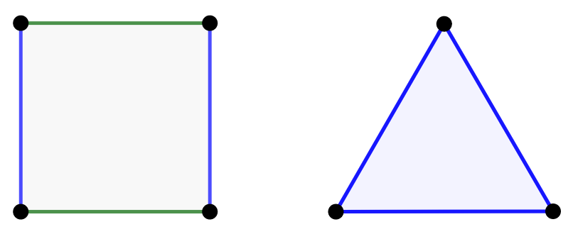
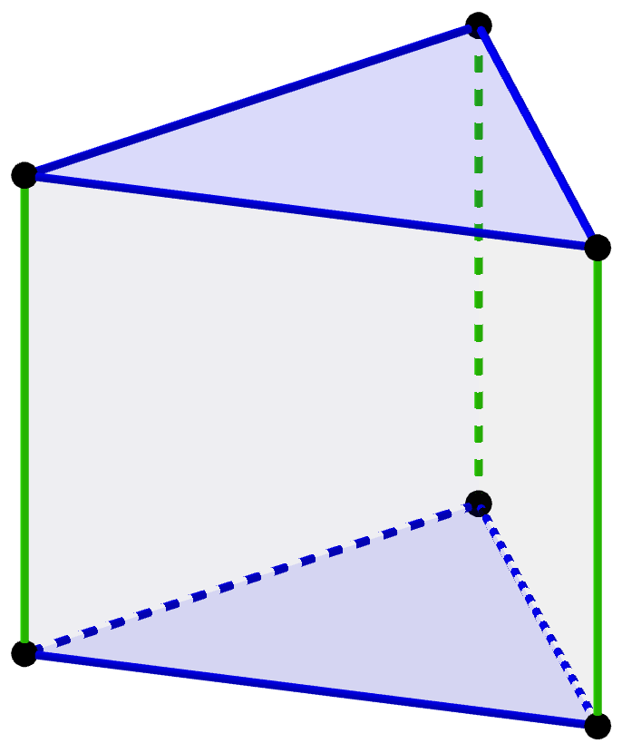
Any simplex is a polysimplex with only one factor. A cube in any dimension is a polysimplex, being a product of intervals, i.e. $1$ -simplices. A triangular prism is a polysimplex, as the product of a $1$ -simplex and a $2$ -simplex. See Figure 1.

Let $X_{0}$ be polync. A closed stratum $X_{\sigma}\subset X_{0}$ is an irreducible component of an intersection of components of $X_{0}$ . The corresponding open stratum $(X_{\sigma})^{\circ}\subset X_{\sigma}$ is the complement of all lower-dimensional closed strata $X_{\tau}\subsetneq X_{\sigma}$ . Along $(X_{\sigma})^{\circ}$ , we have a local product form (1). We denote by $I=I(\sigma)$ the indexing set for the local nc factors appearing in this product.

Refer to caption — Figure 1. Two $2$ -dimensional polysimplices and one $3$ -dimensional polysimplex

Definition 1.5.

The dual complex $\Gamma(X_{0})$ of a polync variety is a polyhedral complex defined as follows: For each open singular stratum $(X_{\sigma})^{\circ}\subset X_{0}$ along which $X_{0}$ has the local form given by (1), we take a polysimplex $P_{\sigma}\coloneqq\prod_{i\in I(\sigma)}\sigma_{m_{i}-1}.$ If we have an inclusion $X_{\tau}\subset X_{\sigma}$ then $P_{\tau}$ naturally contains $P_{\sigma}$ as a face. Then, we glue along the poset of singular strata $\{X_{\sigma}\}$ of $X_{0}$ to get a polyhedral complex

\textstyle\Gamma(X_{0})=\bigcup_{\sigma}P_{\sigma}.

Definition 1.6.

A polyhedral complex $\Gamma=\bigcup_{\sigma}P_{\sigma}$ whose cells are polysimplices, is a polysimplicial complex. A polysimplicial complex is colorable if there exists a finite set $S$ , together with a collection of injective maps $\phi_{\sigma}\,\colon I(\sigma)\to S$ , one for each polysimplex $P_{\sigma}\subset\Gamma$ , such that the functions $\phi_{\sigma}$ are compatible along inclusions of faces. That is, $\phi_{\tau}|_{I(\sigma)}=\phi_{\sigma}$ for any face $P_{\sigma}\subset P_{\tau}$ . We call $\{\phi_{\sigma}\}$ an $S$ -coloring of $\Gamma$ .

That is, there is a coloring of each positive-dimensional simplex factor of $P_{\sigma}$ by distinct elements of $S$ . Furthermore, these colorings are compatible with inclusions $P_{\sigma}\subset P_{\tau}$ of polysimplices. See Figures 2 and 5. In particular, the $1$ -skeleton $\Gamma^{[1]}\subset\Gamma$ is an $S$ -colored graph, as any $1$ -dimensional polysimplex is a $1$ -simplex, and so has only one simplex factor; $I=\{i\}$ .

Notation 1.7.

We write $\phi_{\sigma}(i)=s(i)\in S$ for the color of the $i$ th simplex factor of $P_{\sigma}$ .

Example 1.8.

Any simplicial complex is colorable by a single color $S=\{s\}$ . It is also sometimes possible to use multiple colors. For example, a $1$ -dimensional simplicial complex is a graph $G$ . One may take $S=E(G)$ to be the edges, assigning each edge a different color.

Definition 1.9.

We say that a polync variety $X_{0}$ is colorable if its dual polysimplicial complex $\Gamma(X_{0})$ is colorable; an $S$ -coloring of $X_{0}$ is an $S$ -coloring of $\Gamma(X_{0})$ .

Definition 1.10.

Suppose $X_{0}$ is an $S$ -colored, polync variety. The color $s\in S$ singular locus $(X_{0})_{\rm sing}^{s}\subset(X_{0})_{\rm sing}$ is the union of all strata $X_{\sigma}$ for which $s$ appears as a color of a simplex factor of $P_{\sigma}\subset\Gamma(X_{0})$ , or equivalently, $s\in{\rm im}(\phi_{\sigma})$ .

Remark 1.11.

$(X_{0})_{\rm sing}^{s}\subset X_{0}$ is a divisor because every stratum $X_{\sigma}$ involving $s\in S$ is contained in a codimension $1$ stratum of color $s$ , associated to any edge of the polysimplex $P_{\sigma}$ of color $s$ . We have a decomposition $(X_{0})_{\rm sing}=\bigcup_{s\in S}(X_{0})_{\rm sing}^{s}$ and the intersection $(X_{0})_{\rm sing}^{s}\cap(X_{0})_{\rm sing}^{s^{\prime}}$ for $s\neq s^{\prime}\in S$ contains no divisors, corresponding to the fact that the graph $\Gamma(X_{0})^{[1]}$ is $S$ -colored.

See Figure 6 for a polync surface and the color components of its singular locus.

Proposition 1.12.

Let $X_{0}$ be an $S$ -colored, polync variety. The sheaf ${\mathcal{E}}xt^{1}(\Omega^{1}_{X_{0}},{\mathcal{O}}_{X_{0}})\simeq\textstyle\bigoplus_{s\in S}{\mathcal{L}}_{s}$ is a direct sum of line bundles ${\mathcal{L}}_{s}$ supported on $(X_{0})_{\rm sing}^{s}$ .

Proof.

We first show the analogous local statement:

(2)

\displaystyle{\mathcal{E}}xt^{1}(\Omega^{1}_{U},{\mathcal{O}}_{U})\simeq\textstyle\bigoplus_{i\in I}{\mathcal{O}}_{(U_{i})_{\rm sing}}

where $U\simeq\prod_{i\in I}U_{i}\times{\mathbb{C}}^{m}$ and $U_{i}\simeq\{x_{i}^{(1)}\cdots x_{i}^{(m_{i})}=0\}\subset{\mathbb{C}}^{m_{i}}$ is the local product form (1). The isomorphism (2) follows from the Künneth formula:

(3)

\displaystyle\textstyle{\mathcal{E}}xt^{1}(\Omega^{1}_{U},{\mathcal{O}}_{U})\simeq\bigoplus_{i\in I}{\mathcal{E}}xt^{1}(\Omega^{1}_{U_{i}},{\mathcal{O}}_{U_{i}})\simeq\bigoplus_{i\in I}{\mathcal{O}}_{(U_{i})_{\rm sing}}.

The second isomorphism in (3) is the well-known statement that the first-order deformations of nc singularities are $1$ -dimensional. The local statement globalizes to the desired global statement by the colorability, which ensures that a summand ${\mathcal{O}}_{(U_{i})_{\rm sing}}$ in (3) of a given color $s(i)=s\in S$ is identified in an overlapping local coordinate patch with a factor of the same color $s$ . ∎

Definition 1.13.

An $S$ -colored, polync variety is $d$ -semistable if ${\mathcal{L}}_{s}\simeq{\mathcal{O}}_{(X_{0})^{s}_{\rm sing}}$ for all $s\in S$ .

As we will see, this generalizes Friedman’s original notion of $d$ -semistability [19, Def. 1.13] for normal crossing degenerations over a $1$ -parameter base, to higher-dimensional bases.

Definition 1.14.

An $S$ -colored, polync variety $X_{0}$ is smoothable if there is a flat, proper family

\textstyle X\to{\rm Spec}\,\,{\mathbb{C}}[[u_{s}]]_{s\in S}

such that the central fiber is $X_{0}$ and there is a local form (1) on $X_{0}$ extending to a local form

(4)

\displaystyle\textstyle\prod_{i\in I}\{x_{i}^{(1)}\cdots x_{i}^{(m_{i})}=u_{s(i)}\}

on $X$ . Here $s(i)$ is the color of the $i$ th factor. Similarly, we say $X_{0}$ is formally smoothable if we have a formal deformation ${\widehat{X}}\to{\rm Spf}\,\,{\mathbb{C}}[[u_{s}]]_{s\in S}$ with the same local form.

Definition 1.15.

We call a morphism $X\to Y$ over a smooth base, which is étale- or analytically-locally of the form (4) a semistable morphism, following [2, Sec. 0.3], [3, Sec. 1.1]. If additionally, $\Gamma(X_{0})$ is a cube complex (i.e. every polysimplex is a product of intervals), we say that $X\to Y$ is a nodal morphism, see [14, Def. 5.1], [15, Def. 2.4].

In particular, the total space $X$ of a semistable morphism, or a smoothing, is regular.

Proposition 1.16.

A (formally) smoothable, $S$ -colored, polync variety is $d$ -semistable.

Proof.

Consider the Kodaira–Spencer map

\displaystyle{\rm ks}\colon T_{0}\,{\rm Spec}\,\,{\mathbb{C}}[[u_{s}]]_{s\in S}\to{\rm Ext}^{1}(\Omega^{1}_{X_{0}},{\mathcal{O}}_{X_{0}}).

We have a map $\phi\colon{\rm Ext}^{1}(\Omega^{1}_{X_{0}},{\mathcal{O}}_{X_{0}})\to H^{0}(X_{0},\,{\mathcal{E}}xt^{1}(\Omega^{1}_{X_{0}},{\mathcal{O}}_{X_{0}}))$ by the local-to-global spectral sequence. It sends a global first-order deformation to a collection of compatible local first-order deformations. By the required local form (4) of a smoothing, $(\phi\circ{\rm ks})(\tfrac{\partial}{\partial u_{s}})$ represents a nowhere vanishing local section of ${\mathcal{L}}_{s}$ along $(X_{0})^{s}_{\rm sing}$ with respect to the local product expansion (3). It follows that ${\mathcal{L}}_{s}\simeq{\mathcal{O}}_{(X_{0})^{s}_{\rm sing}}$ for all $s\in S$ . ∎

Remark 1.17.

“Polysnc” is the smallest class of singularities on fibers of a flat morphism, achievable by alteration. More precisely, let $f\colon X\to Y$ be any morphism of varieties. By the resolution of the Abramovich–Karu conjecture [2, Thm. 0.3], [3, Thm. 4.5], there is an alteration $Y^{\prime}\to Y$ and a birational modification of the base change $f^{\prime}\colon X^{\prime}\to Y^{\prime}$ for which $f^{\prime}$ is (flat and) semistable. And by Hodge-/weight-theoretic considerations, it is impossible to achieve a “better” result. In this sense, polysnc singularities and semistable morphisms, over bases of arbitrary dimension, play exactly the same role as snc singularities and semistable morphisms over $1$ -parameter bases.

2. Interpretation via log structures

Following French conventions, let ${\mathbb{N}}\coloneqq{\mathbb{Z}}_{\geq 0}$ . Let $0^{S}:={\rm Spec}({\mathbb{N}}^{S}\to{\mathbb{C}})$ denote the “logarithmic point” with ghost sheaf ${\mathbb{N}}^{S}$ . It is the log structure on ${\rm Spec}\,{\mathbb{C}}$ with monoid ${\mathbb{C}}^{*}\oplus{\mathbb{N}}^{S}$ and structural morphism $(c,\sum_{s\in S}n_{s}e_{s})\mapsto c\cdot 0^{\sum_{s\in S}n_{s}}$ , where by convention $0^{0}=1$ . It is the pullback of the divisorial log structure on ${\rm Spec}\,{\mathbb{C}}[[u_{s}]]_{s\in S}$ associated to the union of the coordinate hyperplanes, to the origin $0\in{\rm Spec}\,{\mathbb{C}}[[u_{s}]]_{s\in S}$ . See [1] for background on logarithmic geometry.

Definition 2.1.

Let $X_{0}$ be an $S$ -colored, polync variety. A log structure of semistable type on $X_{0}$ is the following data:

(1)

a log structure ${\mathcal{M}}_{0}$ on $X_{0}$ admitting étale charts

	$\displaystyle\left(\textstyle\bigoplus_{i\in I}{\mathbb{N}}^{m_{i}}\right)\oplus{\mathbb{N}}^{S\setminus\phi(I)}$	$\displaystyle\to{\mathcal{O}}_{X_{0},\,\textrm{\'{e}t}}(U)$
	$\displaystyle e_{i}^{(j)}$	$\displaystyle\mapsto x_{i}^{(j)}\textrm{ for }i\in I,\,j\in\{1,\dots,m_{i}\},$
	$\displaystyle e_{s}$	$\displaystyle\mapsto 0\textrm{ for }s\in S\setminus\phi(I),$

where $x_{i}^{(j)}$ define étale-local coordinate charts on $U$ to the local form (1), and $\phi$ is the local $S$ -coloring of the factors $i\in I$ ,

(2)

a morphism $f\colon(X_{0},{\mathcal{M}}_{0})\to({\rm Spec}\,{\mathbb{C}},0^{S})$ of log schemes, which is given in local charts by the monoid morphism $f^{\flat}\colon{\mathbb{N}}^{S}\to\left(\bigoplus_{i\in I}{\mathbb{N}}^{m_{i}}\right)\oplus{\mathbb{N}}^{S\setminus\phi(I)}$ sending

	$\displaystyle\textstyle f^{\flat}e_{s}$	$\displaystyle=\textstyle\sum_{j=1}^{m_{i}}e_{i}^{(j)}\textrm{ if }s=\phi(i),$
	$\displaystyle f^{\flat}e_{s}$	$\displaystyle=e_{s}\textrm{ for }s\in S\setminus\phi(I).$

We will henceforth drop the ét subscript in the structure sheaf. Definition 2.1 is very closely related to a similar notion defined in [33, Def. 5.5], which does not require $S$ -colorability, but in a sense, only demands the existence of $f$ “along the diagonal” $({\rm Spec}\,{\mathbb{C}},0)\hookrightarrow({\rm Spec}\,{\mathbb{C}},0^{S})$ .

Proposition 2.2.

Let $X_{0}$ be an $S$ -colored, polync variety. Then $X_{0}$ is $d$ -semistable if and only if it admits a log structure of semistable type, as in Definition 2.1.

Proof.

When $X_{0}$ is a normal crossing variety and $S=\{s\}$ is a singleton, this is [30, Prop. 1.1], see also [28, Thm. 11.7] and its arXiv version [27, Thm. 11.2]. The same proof as [27] applies nearly verbatim, but we outline the necessary changes here for completeness. To prove the forward direction, suppose $X_{0}$ is $d$ -semistable, i.e.

(5)

\displaystyle\textstyle{\mathcal{E}}xt^{1}(\Omega^{1}_{X_{0}},{\mathcal{O}}_{X_{0}})\simeq\bigoplus_{s\in S}{\mathcal{O}}_{(X_{0})_{\rm sing}^{s}}.

Then, we may choose elements of ${\bf 1}_{s}\in H^{0}(X_{0},\,{\mathcal{E}}xt^{1}(\Omega^{1}_{X_{0}},{\mathcal{O}}_{X_{0}}))$ where via an isomorphism (5), ${\bf 1}_{s}=(f_{s^{\prime}})_{s^{\prime}\in S}$ with $f_{s}=1$ and $f_{s^{\prime}}=0$ for $s^{\prime}\neq s$ . Taking the (Künneth) product of the formula given in [27, Lem. 12.1], we have, in a local coordinate chart (1), an isomorphism

\textstyle{\mathcal{E}}xt^{1}(\Omega^{1}_{X_{0}},{\mathcal{O}}_{X_{0}})\simeq\bigoplus_{s\in S}({\mathcal{I}}_{X_{0}}/{\mathcal{I}}_{X_{0}}{\mathcal{I}}_{(X_{0})_{\rm sing}^{s}})^{\vee}\otimes{\mathcal{O}}_{(X_{0})_{\rm sing}^{s}}

where ${\mathcal{I}}_{X_{0}}=(x_{i}^{(1)}\cdots x_{i}^{(m_{i})})_{i\in I}$ is the ideal of $X_{0}\subset\prod_{i\in I}{\mathbb{C}}^{m_{i}}\times{\mathbb{C}}^{m}$ . Following [27, Prop. 12.3], we have a projection $p_{s}\colon{\mathcal{I}}_{X_{0}}/{\mathcal{I}}_{X_{0}}^{2}\to{\mathcal{I}}_{X_{0}}/{\mathcal{I}}_{X_{0}}{\mathcal{I}}_{(X_{0})_{\rm sing}^{s}}$ and the section of the latter sheaf corresponding to ${\bf 1}_{s}$ is, locally over an open cover $\{U_{\lambda}^{s}\}$ of $(X_{0})_{\rm sing}^{s}$ , the projection of a section

p_{s}(v_{s}x_{i}^{(1)}\cdots x_{i}^{(m_{i})})

where $s(i)=s$ and $v_{s}\in{\mathcal{O}}_{X_{0}}^{*}(U_{\lambda}^{s})$ . Set

\zeta_{i}^{(j),\,\lambda}\coloneqq\left\{\begin{array}[]{lll}v_{s}x_{i}^{(1)}&\mbox{if }j=1,\\ x_{i}^{(j)}&\mbox{if }j=2,\dots,m_{i},\\ 1&\mbox{if }j=m_{i}+1,\dots,\dim X_{0}+1.\end{array}\right.

Then it follows exactly as in [27, Prop. 12.2] that there is a “transition system” of units $u_{s}^{(j),\,{\lambda\mu}}\in{\mathcal{O}}_{X_{0}}^{*}(U_{\lambda}^{s}\cap U_{\mu}^{s})$ and a permutation $\sigma\in S_{m_{i}}$ such that

\zeta_{i}^{(\sigma\cdot j),\,\lambda}=\zeta_{i^{\prime}}^{(j),\,\mu}u_{s}^{(j),\,\lambda\mu}.

Here $i^{\prime}\in I^{\prime}$ is the index for the coordinate chart $U_{\mu}^{s}$ satisfying $s(i^{\prime})=s$ . Furthermore, it follows that $\prod_{j}u_{s}^{(j),\,\lambda\mu}|_{(X_{0})_{\rm sing}^{s}}=1$ by the condition that the $\zeta_{i}^{(j),\,\lambda}$ are produced from a global section of ${\mathcal{I}}_{X_{0}}/{\mathcal{I}}_{X_{0}}{\mathcal{I}}_{(X_{0})_{\rm sing}^{s}}$ . By the same formula as in [27, Proof of Prop. 12.3], it is possible to modify the transition system

\{u_{s}^{(j),\,\lambda\mu}\}_{j,\lambda,\mu}

(for each $s\in S$ ) to a new transition system which satisfies the stronger property $\prod_{j}u_{s}^{(j),\,\lambda\mu}=1$ on all of $U^{s}_{\lambda}\cap U_{\mu}^{s}$ .

Take a common refinement of the collections $\{U_{\lambda}^{s}\}$ for all $s\in S$ and adjoin étale coordinate charts covering $X_{0}\setminus(X_{0})_{\rm sing}$ to produce an étale open cover ${\mathfrak{U}}\coloneqq\{U_{\lambda}\}$ of $X_{0}$ . Then, for every $s\in S$ , the transition system of color $s$ defined in the previous paragraph restricts to this common cover and satisfies $\prod_{j}u_{s}^{(j),\lambda\mu}=1$ on every double overlap of the color $s$ subcover ${\mathfrak{U}}_{s}$ .

Using [27, Eqn. (12)], we define charts of a log structure $\zeta\colon\left(\bigoplus_{i\in I}{\mathbb{N}}^{m_{i}}\right)\oplus{\mathbb{N}}^{S\setminus\phi(I)}\to{\mathcal{O}}_{X_{0}}(U_{\lambda})$ on $U_{\lambda}$ by sending $e_{i}^{(j)}\mapsto\zeta_{i}^{(j),\,\lambda}$ for $i\in I$ , and $e_{s}\mapsto 0$ for $s\in S\setminus\phi(I)$ . Call it ${\mathcal{M}}_{\lambda}$ and let ${\mathcal{M}}_{\lambda}^{s}\subset{\mathcal{M}}_{\lambda}$ be the sub-log structure corresponding to the color $s\in S$ . Note that this definition is valid on open sets $U_{\lambda}$ involving singular strata of multiple colors; the local coordinates $\zeta_{i}^{(j),\,\lambda}$ for each color are chosen independently.

(1)

When $U_{\lambda}$ , $U_{\mu}\in{\mathfrak{U}}_{s}$ , the transition system $\{u_{s}^{(j),\,\lambda\mu}\}$ , together with the corresponding coordinate permutations defines an isomorphism $\alpha_{\lambda\mu}^{s}\colon{\mathcal{M}}_{\lambda}^{s}|_{U_{\lambda\mu}}\to{\mathcal{M}}_{\mu}^{s}|_{U_{\lambda\mu}}$ between the color $s$ part of the log structure on a double overlap of $U_{\lambda}$ , $U_{\mu}\in{\mathfrak{U}}_{s}$ , as in [27, Eqn. (13)]. Since $\prod_{j}u_{s}^{(j),\,\lambda\mu}=1$ , it identifies $\sum_{j}e_{i}^{(j)}$ and $\sum_{j}e_{i^{\prime}}^{(j)}$ , where $s(i)=s(i^{\prime})=s$ .
(2)

When $U_{\lambda}\in{\mathfrak{U}}_{s}$ and $U_{\mu}\notin{\mathfrak{U}}_{s}$ (or vice versa), we uniquely specify an isomorphism $\alpha_{\lambda\mu}^{s}\colon{\mathcal{M}}_{\lambda}^{s}|_{U_{\lambda\mu}}\to{\mathcal{M}}_{\mu}^{s}|_{U_{\lambda\mu}}$ by requiring that it act trivially on units and identify the elements $\sum_{j}e_{i}^{(j)}\leftrightarrow e_{s}$ where $s(i)=s.$
(3)

When $U_{\lambda}$ , $U_{\mu}\notin{\mathfrak{U}}_{s}$ we demand that the isomorphism $\alpha_{\lambda\mu}^{s}$ respect the element $e_{s}$ and act trivially on units.

Then, the above isomorphisms $\alpha_{\lambda\mu}^{s}$ defined in (1, 2, 3) for all $s\in S$ collectively determine a unique isomorphism $\alpha_{\lambda\mu}\colon{\mathcal{M}}_{\lambda}|_{U_{\lambda\mu}}\to{\mathcal{M}}_{\mu}|_{U_{\lambda\mu}}$ .

For each $s\in S$ , the cocycle condition holds for the isomorphisms $\alpha_{\lambda\mu}^{s}$ on triple overlaps of elements of ${\mathfrak{U}}_{s}$ by [27, p. 28, Step 1]. Every other triple overlap is disjoint from $(X_{0})_{\rm sing}^{s}$ so here the characteristic monoid in color $s$ is ${\mathbb{N}}$ , and the cocycle condition follows from the uniqueness of the isomorphisms fixing units and identifying the distinguished generators of the log charts. So the isomorphisms $\alpha_{\lambda\mu}$ satisfy the cocycle condition and the local log structures ${\mathcal{M}}_{\lambda}$ glue to give a global log structure $(X_{0},{\mathcal{M}}_{0})$ .

Finally, as in [27, p. 29, Step 2], define on each $U_{\lambda}$ a homomorphism

	$\displaystyle f_{\lambda}^{\flat}\colon{\mathbb{C}}^{*}\oplus{\mathbb{N}}^{S}$	$\displaystyle\to{\mathcal{O}}_{X_{0}}^{*}(U_{\lambda})\oplus_{\zeta}\textstyle\left(\left(\bigoplus_{i\in I}{\mathbb{N}}^{m_{i}}\right)\oplus{\mathbb{N}}^{S\setminus\phi(I)}\right),$
	$\displaystyle f_{\lambda}^{\flat}(1,e_{s})$	$\displaystyle\coloneqq\left\{\begin{array}[]{ll}(1,\sum_{j=1}^{m_{i}}e_{i}^{(j)})&\mbox{if }s=\phi(i),\\ (1,e_{s})&\mbox{if }s\notin\phi(I).\end{array}\right.$

By construction, $\alpha_{\lambda\mu}$ identifies $f_{\lambda}^{\flat}(1,e_{s})$ with $f_{\mu}^{\flat}(1,e_{s})$ for every $s\in S$ . In case (1), this follows from $\prod_{j}u_{s}^{(j),\,\lambda\mu}=1$ , and in cases (2) and (3) it holds by definition. Consequently, the local homomorphisms $f_{\lambda}^{\flat}$ glue to give a global morphism of log schemes

f\colon(X_{0},{\mathcal{M}}_{0})\to({\rm Spec}\,{\mathbb{C}},0^{S}).

This completes the proof of the forward direction. We omit the reverse direction, which follows in the same manner as [27], taking into account the above modifications. ∎

Proposition 2.3.

Suppose that $X_{0}$ is a $d$ -semistable, $S$ -colored, polync variety. The corresponding log structure of semistable type $(X_{0},{\mathcal{M}}_{0})\to({\rm Spec}\,{\mathbb{C}},0^{S})$ is log smooth and saturated.

Proof.

This holds by [29, Thm. 3.5] and applying the definition of saturated morphisms. ∎

It follows from [29, 4.5] that the logarithmic deformations of $(X_{0},{\mathcal{M}}_{0})\to B_{0}=({\rm Spec}\,{\mathbb{C}},0^{S})$ are flat in the usual sense. Furthermore, as a log smooth morphism, the log cotangent bundle $\Omega_{X_{0}/B_{0}}^{\rm log}$ is a vector bundle, and the log canonical bundle $\omega_{X_{0}/B_{0}}^{\rm log}=\wedge^{\dim X_{0}}\Omega_{X_{0}/B_{0}}^{\rm log}$ is a line bundle. Then, we say that:

Definition 2.4.

$X_{0}$ is log Calabi–Yau (over $B_{0}$ ) if $\omega_{X_{0}/B_{0}}^{\rm log}\simeq{\mathcal{O}}_{X_{0}}$ .

In general, for log structures, this does not mean that the usual dualizing sheaf $\omega_{X_{0}}$ is trivial. For instance, $X_{0}$ could be a smooth projective variety with a nontrivial snc divisor $D_{0}\in|-K_{X_{0}}|$ and ${\mathcal{M}}_{0}$ could be the divisorial log structure associated to $D_{0}$ . But in the case of a log structure of semistable type, we do have $\omega_{X_{0}/B_{0}}^{\rm log}=\omega_{X_{0}}$ .

Sections of the logarithmic cotangent, resp. canonical, bundle $\Omega_{X_{0}/B_{0}}^{\rm log}$ , resp. $\omega_{X_{0}/B_{0}}^{\rm log}$ , are logarithmic one-forms, resp. top-forms, on the components, whose residues cancel on double loci. These facts follow easily from the nc case, by taking direct sums, resp. tensor products, of the relevant sheaves on nc factors of (1).

Finally, we observe that ${\mathbb{N}}^{S}$ is a sharp toric monoid—it is finitely generated, integral, saturated, torsion-free, and (the sharpness condition) $0\in{\mathbb{N}}^{S}$ is the only invertible element. Combined with Proposition 2.3, we may apply the main result [18, Thm. 1.1] (similar results were obtained earlier in [11, 17]; we found the presentation [18] quite clear) to deduce:

Theorem 2.5.

Suppose that $X_{0}$ is a proper, $d$ -semistable, $S$ -colored, polync variety with trivial dualizing sheaf $\omega_{X_{0}}\simeq{\mathcal{O}}_{X_{0}}$ and all algebraic components. Let ${\mathcal{M}}_{0}$ be a log structure on $X_{0}$ of $d$ -semistable type. The log smooth deformations of $(X_{0},{\mathcal{M}}_{0})/B_{0}=({\rm Spec}\,{\mathbb{C}},0^{S})$ are unobstructed.

Corollary 2.6.

There is a universal formal log smooth deformation

{\widehat{X}}\to{\widehat{B}}\coloneqq{\rm Def}_{X_{0}/B_{0}}\simeq{\rm Spf}\,{\mathbb{C}}[[u_{s},v_{t}]]_{s\in S,\,t\in T}

where $\{0\}\times{\rm Spf}\,{\mathbb{C}}[[v_{t}]]_{t\in T}$ is the locus of locally trivial, log smooth deformations of $X_{0}/B_{0}$ .

Proof.

By [28, Thm. 8.7], the logarithmic deformation functor admits a miniversal formal deformation $\pi\colon{\widehat{X}}\to{\widehat{B}}$ . By Theorem 2.5, ${\widehat{B}}$ is formally smooth, and hence has the above form.

Let $\eta_{0}$ be a generator of $\omega_{X_{0}/B_{0}}^{\rm log}\simeq{\mathcal{O}}_{X_{0}}$ . It lifts to a (nonvanishing) generator $\eta$ of $\omega_{{\widehat{X}}/{\widehat{B}}}^{\rm log}$ by the local freeness of the (logarithmic) Hodge bundle

{\mathcal{H}}^{d,0}\coloneqq\pi_{*}\omega_{{\widehat{X}}/{\widehat{B}}}^{\rm log}

for $d=\dim X_{0}$ , see [26, Thm. 7.1]. Contraction with $\eta$ gives an isomorphism

\Theta_{{\widehat{X}}/{\widehat{B}}}^{\rm log}\simeq\wedge^{d-1}\Omega_{{\widehat{X}}/{\widehat{B}}}^{{\rm log}}

where $\Theta^{\rm log}_{{\widehat{X}}/{\widehat{B}}}$ is the relative logarithmic tangent bundle. Again by [26, Thm. 7.1],

{\mathcal{H}}^{d-1,0}\coloneqq\pi_{*}(\wedge^{d-1}\Omega_{{\widehat{X}}/{\widehat{B}}}^{{\rm log}})

is a vector bundle, so $H^{0}(X_{b},\Theta_{X_{b}}^{\rm log})$ has constant dimension for $b\in{\widehat{B}}$ . Since ${\widehat{B}}$ is smooth, and in particular reduced, Wavrik’s criterion [37, Thm. 4.2] shows that the miniversal deformation is universal (the proof of the criterion applies in the log smooth setting, with vertical vector fields replaced by logarithmic vertical vector fields). ∎

Alternatively, there is an analytic smoothing $X\to B=\Delta^{S}\times\Delta^{T}$ over a polydisk, which agrees with the family ${\widehat{X}}$ up to any specified order [36, Thm. B.1]. In particular, once $X$ and ${\widehat{X}}$ agree up to order $2$ , $X$ is a smooth analytic space, i.e. a complex manifold, and the morphism $X\to B$ is an analytic, semistable morphism (see Def. 1.15). Its logarithmic Kodaira–Spencer map is an isomorphism, so $X\to B$ is miniversal. The formal completion is therefore isomorphic to ${\widehat{X}}\to{\widehat{B}}$ , by Corollary 2.6, and so $X\to B$ is universal as well.

If additionally, $X_{0}$ is a projective variety with ample line bundle $L_{0}$ then by [16, Ch. 11], the deformations of the pair $(X_{0},L_{0})$ are also unobstructed. In turn, by Grothendieck algebraization, we can produce not just a formal smoothing, but a projective algebraic smoothing $(X,L)\to{\rm Spec}\,{\mathbb{C}}[[u_{s},v_{t}]]_{s\in S,\,t\in T^{\prime}}$ where $|T^{\prime}|\leq|T|$ could be smaller, because we only take deformations keeping the line bundle.

Remark 2.7.

The original version of Theorem 2.5 is Friedman’s result [19, Thm. 5.10] on the smoothability of $d$ -semistable, normal crossings K3 surfaces $X_{0}$ (see Def. 2.8 below). The “disadvantage” of a classical deformation theory approach is that ${\rm Def}_{X_{0}}=\Delta^{20}\cup_{\Delta^{19}}\Delta^{N}$ is a union of two components. One is the smoothing component $\Delta^{20}$ over which the general fiber is an analytic K3 surface. The other “undesirable” component $\Delta^{N}$ is a large component of locally trivial nc deformations, whose general fiber is not $d$ -semistable. These components meet along a divisor $\Delta^{19}\subset\Delta^{20}$ of locally trivial, $d$ -semistable deformations.

On the other hand, the “log smooth deformations” ${\rm Def}_{X_{0}/B_{0}}$ map into the smoothing component $\Delta^{20}$ , as the fibers over $\Delta^{N}\setminus\Delta^{19}$ are not $d$ -semistable, and so do not admit a log structure (of semistable type). Though, caveat lector: In the Type III snc case, $\dim{\rm Def}_{X_{0}/B_{0}}=21$ and to recover a $20$ -dimensional base, we would have to rigidify the deformation functor ${\rm Def}_{X_{0}/B_{0}}$ . See Propositions 2.9, 2.10, and 3.15.

The first generalization of Friedman’s work to higher-dimensional $K$ -trivial varieties was the work of Kawamata–Namikawa [30], who reinterpreted it in terms of logarithmic geometry, and extended it to $K$ -trivial, $d$ -semistable, nc varieties, that satisfy the additional hypotheses $H^{\dim X_{0}-1}(X_{0},{\mathcal{O}}_{X_{0}})=0$ and $H^{\dim X_{0}-2}(X_{0}^{\nu},{\mathcal{O}}_{X_{0}^{\nu}})=0$ for $X_{0}^{\nu}=\bigsqcup_{i}X_{i}$ the normalization.

The key insight leading to a more general statement (a Bogomolov–Tian–Todorov type unobstructedness theorem for the log smooth deformations of a general log smooth, log Calabi–Yau variety, with no additional technical hypotheses) came in the work of Chan–Leung–Ma [11], who introduced the correct dGLA-theoretic set-up, of “ $\Lambda$ -curved Batalin–Vilkovisky algebras”. We recommend Felten [16] for an excellent exposition on the topic and its history.

Until recent work [11, 17, 18], the smoothability question has largely focused on $1$ -parameter degenerations. But as [14, 15] show, multiparameter degenerations can, by virtue of their additional combinatorial information, be powerful tools to address questions about algebraic cycles, (stable) rationality, etc. In particular, multiparameter semistable degenerations, such as the universal deformation of a $d$ -semistable, $S$ -colored, polync variety have the remarkable property that their total space $X$ is smooth, allowing one to specialize algebraic cycle classes transverse to the central fiber, see e.g. [15, Lem. 2.16, Lem. 4.14].

Definition 2.8.

A Kulikov model $f\colon X\to Y$ is a relatively $K$ -trivial, semistable morphism.

As noted, Theorem 2.5 implies that the universal log smooth deformation $X\to B$ of a $d$ -semistable, $S$ -colored, polync, $K$ -trivial variety is a Kulikov model. Furthermore, the restriction to any $S$ -dimensional polydisk $Y\subset B\simeq\Delta^{S}\times\Delta^{T}$ in the universal deformation, transversely intersecting the deepest stratum $\{0\}\times\Delta^{T}$ , is also a Kulikov model.

Proposition 2.9.

Fix $X_{0}/B_{0}$ as in Theorem 2.5. Then the formal torus $\widehat{{\mathbb{G}}}_{m}^{S}$ acts naturally on ${\widehat{B}}$ . The forgetful morphism ${\widehat{B}}\to\operatorname{Def}_{X_{0}}$ is invariant under this action.

Proof.

An $A$ -valued point of ${\widehat{B}}$ , for an Artinian local ${\mathbb{C}}$ -algebra $A$ , consists of a log smooth family $f\colon X_{A}\to({\rm Spec}\,A,\mathcal{M}_{A}),$ a morphism $\alpha\colon{\rm Spec}\,A\to{\rm Spf}\,{\mathbb{C}}[[u_{s}]]_{s\in S}$ defining the log structure $\mathcal{M}_{A}$ on the base, and a distinguished identification of its closed fiber with $X_{0}/B_{0}$ .

Let $t=(t_{s})_{s\in S}\in\widehat{{\mathbb{G}}}_{m}^{S}(A)=(1+\mathfrak{m}_{A})^{S}.$ Define a new morphism $t\cdot\alpha$ by

(t\cdot\alpha)^{*}(u_{s})=t_{s}\alpha^{*}(u_{s}).

The new morphism determines a log structure $\mathcal{M}_{A}^{t}$ on ${\rm Spec}\,A$ . Multiplication of the defining chart by the units $t_{s}$ induces an isomorphism

\iota_{t}\colon({\rm Spec}\,A,\mathcal{M}_{A})\xrightarrow{\sim}({\rm Spec}\,A,\mathcal{M}_{A}^{t})

whose underlying morphism of schemes is the identity. We define

t\cdot(f,\alpha)=(\iota_{t}\circ f,t\cdot\alpha).

Since $t_{s}\equiv 1$ mod $\mathfrak{m}_{A}$ , the isomorphism $\iota_{t}$ restricts to the identity on the closed log point $B_{0}$ . Thus the distinguished identification of the closed fiber with $X_{0}/B_{0}$ is preserved.

This construction is functorial in $A$ and compatible with multiplication of $t_{1},t_{2}\in\widehat{{\mathbb{G}}}_{m}^{S}$ . So, by pro-representability, it defines an action on ${\widehat{B}}={\rm Def}_{X_{0}/B_{0}}$ . The underlying family of schemes $X_{A}\to{\rm Spec}\,A$ is unchanged, so the forgetful morphism to $\operatorname{Def}_{X_{0}}$ is $\widehat{{\mathbb{G}}}_{m}^{S}$ -invariant. ∎

Let $D_{s}\coloneqq(X_{0})_{\rm sing}^{s}$ and suppose that $D_{s}$ is connected for every $s\in S$ .¹¹1This is a natural condition to impose. Suppose $d$ -semistability (Def. 1.13) holds for an $S$ -colored, polync variety $X_{0}$ . Then the same holds for an extended color set $S^{\prime}$ , indexed by the connected components of $(X_{0})_{\rm sing}^{s}$ for all $s\in S$ . Furthermore, now $(X_{0})_{\rm sing}^{s^{\prime}}$ is connected, for all $s^{\prime}\in S^{\prime}$ and by Corollary 2.6, we still have a universal smoothing, but this time with more smoothing parameters. Let

{\mathcal{T}}^{1}_{X_{0}}={\mathcal{E}}xt^{1}(\Omega^{1}_{X_{0}},{\mathcal{O}}_{X_{0}})

be the sheaf of first-order local deformations of $X_{0}$ . As in [34, p. 426], the choice of $d$ -semistable log structure ${\mathcal{M}}_{0}$ corresponds to a trivialization of ${\mathcal{T}}^{1}_{X_{0}}\simeq\bigoplus_{s\in S}{\mathcal{O}}_{D_{s}}$ along every $D_{s}$ . By the connectedness of $D_{s}$ , the space of such trivializations is a torsor over ${\mathbb{G}}_{m}^{S}$ .

It follows that we have a homomorphism

(6)

\displaystyle\rho\colon{\rm Aut}^{0}(X_{0})\to{\mathbb{G}}_{m}^{S}

where ${\rm Aut}^{0}(X_{0})$ acts by pullback on trivializations of ${\mathcal{T}}_{X_{0}}^{1}$ . Note that $\ker\rho={\rm Aut}^{0}(X_{0},{\mathcal{M}}_{0})$ and ${\rm im}\,\rho\subset{\mathbb{G}}_{m}^{S}$ is a subtorus. Let

{\mathbb{G}}\subset{\mathbb{G}}_{m}^{S}

be a complementary subtorus to ${\rm im}\,\rho$ . We have the following proposition:

Proposition 2.10.

Continue in the setting of Proposition 2.9 under the additional hypothesis that $(X_{0})_{\rm sing}^{s}$ is connected for all $s\in S$ . The action of $\widehat{{\mathbb{G}}}$ on ${\widehat{B}}$ is free, and the quotient ${\widehat{B}}/\widehat{{\mathbb{G}}}$ exists. It is the base of a semi-universal, $d$ -semistable deformation of $X_{0}$ . This deformation is furthermore universal when ${\mathbb{G}}={\mathbb{G}}_{m}^{S}.$

Proof.

Let $\Theta_{X_{0}}$ denote the ordinary tangent sheaf of $X_{0}$ and let $\Theta^{\rm log}_{X_{0}/B_{0}}$ denote the logarithmic tangent bundle. We have an exact sequence

(7)

\displaystyle 0\to\Theta_{X_{0}/B_{0}}^{\rm log}\to\Theta_{X_{0}}\to{\mathcal{T}}_{X_{0}}^{1}\to 0.

This is the logarithmic analogue of the relative tangent sequence for a normal crossings variety; see [28, Prop. 5.4 and Ex. 5.7]. The same calculation as loc.cit. applies to the product charts defining a polync variety.

Since every $D_{s}$ is connected, the $d$ -semistability gives

\textstyle H^{0}(X_{0},{\mathcal{T}}^{1}_{X_{0}})\simeq\bigoplus_{s\in S}H^{0}(D_{s},{\mathcal{O}}_{D_{s}})\simeq{\mathbb{C}}^{S}.

Under this identification, the coboundary map associated to the exact sequence (7) is

\partial\colon{\mathbb{C}}^{S}\to H^{1}(X_{0},\Theta^{\rm log}_{X_{0}/B_{0}}).

The differential at the identity of the $\widehat{{\mathbb{G}}}_{m}^{S}$ -action of Proposition 2.9 is precisely $\partial$ . Indeed, an infinitesimal coordinate rescaling changes the chosen trivializations of ${\mathcal{T}}^{1}_{X_{0}}$ and $\partial$ measures whether this change is induced by an infinitesimal automorphism of $X_{0}$ . This is also the infinitesimal form of the torsor description in [34, p. 426]. Thus,

{\rm Lie}({\mathbb{G}})\subset{\rm Lie}({\mathbb{G}}_{m}^{S})={\mathbb{C}}^{S}

maps isomorphically onto its image under $\partial$ , whereas ${\rm Lie}({\rm im}\,\rho)$ forms the kernel of $\partial$ .

On the level of tangent spaces, the forgetful map from logarithmic deformations to deformations is given by the middle downward morphism of

Here the bottom short exact sequence is the local-to-global sequence. The connectedness of $D_{s}$ ensures the rightmost downward arrow is an isomorphism, and in turn, the commutativity is what ensures the surjectivity of $T_{0}{\rm Def}_{X_{0}}\to H^{0}(X_{0},{\mathcal{T}}^{1}_{X_{0}})$ .

It follows that

(8)

\displaystyle\ker(T_{0}{\widehat{B}}\to T_{0}{\rm Def}_{X_{0}})\simeq{\rm im}(\partial)\simeq{\rm Lie}({\mathbb{G}}).

The formal deformation space ${\widehat{B}}$ is smooth by Theorem 2.5. It follows from (8) that the action of $\widehat{{\mathbb{G}}}$ on ${\widehat{B}}$ is free, as infinitesimally, it acts by translations on $H^{1}(X_{0},\Theta_{X_{0}/B_{0}}^{\rm log})\subset T_{0}{\widehat{B}}$ .

Hence, there exists a smooth slice ${\widehat{B}}\simeq\widehat{{\mathbb{G}}}\times{\widehat{C}}$ and $T_{0}{\widehat{C}}\to T_{0}{\rm Def}_{X_{0}}$ is injective. The restriction of the universal family ${\widehat{X}}\to{\widehat{B}}$ to ${\widehat{C}}$ is complete for $d$ -semistable deformations of $X_{0}$ as all such deformations lift to logarithmic deformations of $(X_{0},{\mathcal{M}}_{0})/B_{0}$ which can in turn be translated by $\widehat{{\mathbb{G}}}$ to land in ${\widehat{C}}$ . Thus, the restriction of ${\widehat{X}}$ to ${\widehat{C}}$ is semi-universal for the $d$ -semistable deformations of $X_{0}$ .

When ${\mathbb{G}}={\mathbb{G}}_{m}^{S}$ we have ${\rm ker}(\partial)=0$ . Hence $h^{0}(X_{0},\Theta_{X_{0}})=h^{0}(X_{0},\Theta_{X_{0}/B_{0}}^{\rm log})$ from the long exact sequence of (7). The same equality holds for the generic fiber of ${\widehat{X}}\to{\widehat{B}}$ , which is smooth. Since, $h^{0}(X_{b},\Theta_{X_{b}}^{\log})$ is constant (see Cor. 2.6) and $h^{0}(X_{b},\Theta_{X_{b}})$ is upper semicontinuous, we conclude that $h^{0}(X_{b},\Theta_{X_{b}})$ is constant for all $b\in{\widehat{B}}$ . Then Wavrik’s criterion [37, Thm. 4.2] applies again to upgrade the semi-universal deformation over ${\widehat{C}}$ to a universal deformation. ∎

We note that one may also slice the universal analytic log smooth deformation family, giving a polydisk $C\subset B\simeq\Delta^{S}\times\Delta^{T}$ , where $C\simeq\Delta^{S}\times\Delta^{T^{\prime}}$ with $|T|=|T^{\prime}|+|S|-\dim({\rm im}\,\rho)$ .

Definition 2.11.

We write $C={\rm smDef}_{X_{0}}\subset{\rm Def}_{X_{0}}$ for the semi-universal $d$ -semistable deformation of $X_{0}$ . It is the smoothing component of ${\rm Def}_{X_{0}}$ .

The term smoothing component is justified by the fact that the general fiber of $X\to B$ is smooth with trivial log structure. Thus, at the general fiber, the logarithmic and classical deformation problems coincide. It follows that the forgetful map $B\to C\to{\rm Def}_{X_{0}}$ dominates a component of the Kuranishi space. Since $T_{0}C\hookrightarrow T_{0}{\rm Def}_{X_{0}}$ injects, this component is, on the level of germs, identified with $C$ .

3. Polysnc $K$ -trivial surfaces

We assume throughout this section that $X_{0}$ is a proper algebraic space (e.g. that the components of the normalization are proper varieties). By Definition 1.6, we have:

Observation 3.1.

A $2$ -dimensional, $S$ -colored polysimplicial complex $\Gamma$ is a polyhedral complex built from triangles and squares, admitting an $S$ -coloring of the edges $E(\Gamma^{[1]})\to S$ such that:

(1)

all three sides of a triangle are the same color,
(2)

opposite sides of a square are the same color, and
(3)

each square uses exactly two colors.

Definition 3.2.

A poly(s)nc log Calabi–Yau pair $(V,D)$ is a smooth proper variety $V$ , together with an anticanonical divisor $D\in|-K_{V}|$ , such that $D$ is reduced and poly(s)nc.

It follows easily from adjunction that a poly(s)nc variety with $\omega_{X_{0}}\simeq{\mathcal{O}}_{X_{0}}$ is a union of poly(s)nc log CY pairs, glued along anticanonical divisors, so that no boundary remains.

In particular, since poly(s)nc singularities in dimension $1$ are just nodes/(s)nc singularities, a poly(s)nc log CY surface $(V,D)$ is just a smooth proper surface with a reduced, (s)nc anticanonical divisor $D\in|-K_{V}|$ , also called a Looijenga pair. See [20] for a survey on their geometry. Such pairs break into three natural classes:

(1)

When $D$ has nodes, $V$ is rational and $D$ is a cycle of smooth rational curves.
(2)

When $D$ is smooth, either $V$ is rational and $D$ is a smooth elliptic curve, or
(3)

$V$ is ruled over an elliptic curve, and $D$ is a disjoint union of two elliptic sections.

Proposition 3.3.

Let $X_{0}$ be a $d$ -semistable, $S$ -colored, polync surface with $\omega_{X_{0}}\simeq{\mathcal{O}}_{X_{0}}$ . Then $\Gamma(X_{0})$ is a point, an interval, a circle, or a triangle-squarulation of the two-sphere ${\mathbb{S}}^{2}$ or the two-torus ${\mathbb{T}}^{2}$ . For ${\mathbb{S}}^{2}$ or the interval, the general fiber $X_{t}$ of the universal log smooth deformation $X\to\Delta^{S}\times\Delta^{T}$ is a K3 surface, and for ${\mathbb{T}}^{2}$ or the circle, it is an abelian surface.

Observe that case (1) above occurs exactly when $\Gamma(X_{0})$ is $2$ -dimensional, and cases (2, 3) occur exactly when $\Gamma(X_{0})$ is $1$ -dimensional.

Proof.

We will reduce to the same statement but for nc varieties. When $\dim_{\mathbb{R}}\Gamma(X_{0})\leq 1$ , nc and polync are the same, and the result follows from [31, 35], see also [22, Table 1, p. 12].

Consider the diagonal $\Delta\hookrightarrow\Delta^{S}$ and then further embed

\Delta\hookrightarrow\Delta^{S}\simeq\Delta^{S}\times\{0\}\hookrightarrow\Delta^{S}\times\Delta^{T}

into the base of the universal (log smooth) deformation. Let $X_{\Delta}\to\Delta$ be the pulled back deformation. The local equation of the singularities of the universal family $X\to\Delta^{S}\times\Delta^{T}$ is given by (4). The base change to $\Delta$ corresponds to setting $u_{s}=u$ for all $s\in S$ , where $u$ is a coordinate on $\Delta$ (and $v_{t}=0$ , for all $t\in T$ ). It follows that the local equation of $X_{\Delta}\to\Delta$ is

(9)

\displaystyle x_{i}y_{i}=x_{j}y_{j}=u

for each square of $\Gamma(X_{0})$ colored by $s(i)\neq s(j)$ , and is $x_{i}y_{i}z_{i}=u$ for each triangle of $\Gamma(X_{0})$ . Then analytically, $X_{\Delta}\to\Delta$ admits a small, crepant resolution ${\widetilde{X}}_{\Delta}\to\Delta$ by taking either resolution of the conifold singularity (9). The central fiber ${\widetilde{X}}_{0}$ is still an algebraic space, and the resulting family ${\widetilde{X}}_{\Delta}\to\Delta$ is a Kulikov model, now over a $1$ -parameter base.

Furthermore, the homeomorphism type of $\Gamma(X_{0})$ is the same as $\Gamma({\widetilde{X}}_{0})$ , with the only difference being that all squares in $\Gamma(X_{0})$ have been subdivided into two triangles. The result now reduces to [31, 35, 22], which implies the proposition for a $1$ -dimensional base. ∎

The argument of Proposition 3.3 is quite general. It shows that the homeomorphism type of the dual complex of a Kulikov model is the same, whether one considers a multiparameter degeneration, or a resolution of a $1$ -parameter degeneration hitting the origin.

We now briefly overview how to generalize the classical theory of Kulikov models and their period map [23, 6] to the polync setting.

Definition 3.4.

Let $X_{0}=\bigcup_{i}(V_{i},\sum_{j}D_{ij})$ be an $S$ -colored, poly(s)nc union of log CY surface pairs, glued along isomorphisms $D_{ij}\to D_{ji}$ . We say that $X_{0}$ is numerically $d$ -semistable if $\textstyle{{\mathcal{E}}xt}^{1}(\Omega^{1}_{X_{0}},{\mathcal{O}}_{X_{0}})\simeq\bigoplus_{s\in S}{\mathcal{L}}_{s}$ where ${\mathcal{L}}_{s}\in{\rm Pic}^{0}((X_{0})_{\rm sing}^{s})$ are numerically trivial for all $s\in S$ . If additionally $\Gamma(X_{0})\simeq{\mathbb{S}}^{2}$ , we call $X_{0}$ a poly(s)nc Type III K3 surface. And if $\Gamma(X_{0})$ is an interval, we call $X_{0}$ an snc Type II K3 surface.

Note that any polync Type II K3 surface is simply snc. For convenience, we will henceforth assume that $X_{0}$ is polysnc and therefore, that polysimplices are embedded into $\Gamma(X_{0})$ , i.e. not glued to themselves along faces. Most of the results here continue to hold in the more general setting, but for example, formula (13) and Definition 3.6 below must be adjusted.

Exercise 3.5.

Let $X_{0}$ be a polysnc, Type III K3 surface. Then $X_{0}$ is numerically $d$ -semistable if for all irreducible double curves ${\mathbb{P}}^{1}\simeq D_{ij}\subset V_{i}\cap V_{j}$ , we have

(13)

\displaystyle D_{ij}^{2}+D_{ji}^{2}=\left\{\begin{array}[]{lll}0&\mbox{when }\textrm{the associated edge of }\Gamma(X_{0})\textrm{ lies on two squares},\\ -1&\mbox{when }\textrm{the associated edge of }\Gamma(X_{0})\textrm{ lies on a square and a triangle},\\ -2&\mbox{when }\textrm{the associated edge of }\Gamma(X_{0})\textrm{ lies on two triangles}.\end{array}\right.

Here by convention $D_{ij}\subset V_{i}$ and $D_{ji}\subset V_{j}$ . This formula is the polysnc analogue of the classical “triple point formula” for $1$ -parameter Kulikov models [22, p. 8].

The condition that $X_{0}$ be numerically $d$ -semistable is a combinatorial condition on $X_{0}$ in the sense that the locally trivial deformations of $X_{0}$ do not affect this property.

Definition 3.6.

The numerically Cartier classes on a polysnc Type III K3 surface $X_{0}$ are

\widetilde{\Lambda}(X_{0})\coloneqq\ker\left(\textstyle\bigoplus_{i}H^{2}(V_{i},{\mathbb{Z}})\to\bigoplus_{i<j}H^{2}(D_{ij},{\mathbb{Z}})\right).

Following [23, Sec. 3] or [6, Sec. 4], we may define a period map $\varphi_{X_{0}}\colon\widetilde{\Lambda}(X_{0})\to{\mathbb{C}}^{*}$ as follows: Since each component $V_{i}$ is rational and each double locus $D_{ij}\subset V_{i}\cap V_{j}$ is isomorphic to ${\mathbb{P}}^{1}$ , we have $H^{2}(V_{i},{\mathbb{Z}})={\rm Pic}(V_{i})$ and $H^{2}(D_{ij},{\mathbb{Z}})={\rm Pic}(D_{ij})$ .

Let $\alpha=(\alpha_{i})\in\widetilde{\Lambda}(X_{0})$ . Then each $\alpha_{i}$ defines canonically a line bundle ${\mathcal{L}}_{i}\to V_{i}$ and the condition that $\alpha_{i}\cdot D_{ij}=\alpha_{j}\cdot D_{ji}$ implies that we may glue ${\mathcal{L}}_{i}$ and ${\mathcal{L}}_{j}$ along $D_{ij}$ . In this manner, we may successively glue the ${\mathcal{L}}_{i}$ together until only one component $V_{n}$ remains. Then this glued line bundle ${\mathcal{L}}\to\bigcup_{i\neq n}V_{i}\subset X_{0}$ and the line bundle ${\mathcal{L}}_{n}\to V_{n}$ differ by some

\textstyle\varphi_{X_{0}}(\alpha)\in{\mathbb{C}}^{*}\simeq{\rm Pic}^{0}(\sum_{j}D_{nj})

upon restriction to the anticanonical cycle $D_{n}=\sum_{j}D_{nj}\in|-K_{V_{n}}|$ . The construction in Type II is similar, see [6, Constrs. 4.2, 4.3].

The element $\varphi_{X_{0}}(\alpha)\in{\mathbb{C}}^{*}$ can be checked to be independent of the choice of a “last” component $V_{n}$ . It only depends on a choice of orientation of ${\mathbb{S}}^{2}$ , which in turn orients the anticanonical cycle on any component $V_{i}\subset X_{0}$ (the identification ${\rm Pic}^{0}(D_{i})\simeq{\mathbb{C}}^{*}$ requires a choice of orientation of the cycle $D_{i}=\sum_{j}D_{ij}\subset V_{i}$ of rational curves). We have an isomorphism

{\rm Pic}(X_{0})\simeq\ker(\varphi_{X_{0}}).

That is, $\varphi_{X_{0}}$ measures the obstruction to lifting a numerically Cartier class to a Cartier class.

Recall that $\Gamma(X_{0})$ is an $S$ -colored graph. Let ${\rm I}(X_{0})$ be the intersection complex, which is the polyhedral decomposition of ${\mathbb{S}}^{2}$ dual to $\Gamma(X_{0})$ . The vertices of ${\rm I}(X_{0})$ are $3$ - and $4$ -valent, and the $1$ -skeleton ${\rm I}(X_{0})^{[1]}$ is also $S$ -colored. The color $s$ subgraph ${\rm I}_{s}(X_{0})^{[1]}\subset{\rm I}(X_{0})^{[1]}$ is a graph with trivalent and bivalent vertices, corresponding respectively to triangles and squares which use the color $s$ . See Figure 6 for an example.

Definition 3.7.

A slab of color $s\in S$ is a union of components $\bigcup_{i\in G}V_{i}$ corresponding to a connected component of ${\rm I}(X_{0})\setminus{\rm I}_{s}(X_{0})^{[1]}$ .

Remark 3.8.

The notion of a slab generalizes to $S$ -colored, polysnc varieties of any dimension, by considering the codimension $1$ faces of ${\rm I}(X_{0})$ dual to edges in $\Gamma(X_{0})^{[1]}$ of color $s$ .

Example 3.9.

If $X_{0}$ is snc and $S=\{s\}$ , then the slabs of color $s$ are just the irreducible components $V_{i}\subset X_{0}$ because every codimension $1$ cell of ${\rm I}(X_{0})$ has color $s$ , and so the connected components in Definition 3.7 are the maximal dimension cells of ${\rm I}(X_{0})$ .

It follows from the local form of a semistable morphism (4) that the slabs of color $s$ deform to the irreducible components over the coordinate hyperplane $V(u_{s})\subset\Delta^{S}\times\Delta^{T}$ , because the singular loci of every other color $s^{\prime}\neq s$ are smoothed.

On the total space $X$ , we have a line bundle ${\mathcal{L}}_{G}\coloneqq{\mathcal{O}}_{X}(V_{G})$ where $V_{G}$ is the irreducible component over $V(u_{s})$ corresponding to the slab indexed by $G\subset\{\textrm{components of }X_{0}\}$ . Thus the condition that $X_{0}$ is smoothable implies that ${\mathcal{O}}_{X}(G)|_{X_{0}}$ defines an element of ${\rm Pic}(X_{0})$ . The numerical Cartier class of ${\mathcal{O}}_{X}(V_{G})|_{X_{0}}$ is easy to compute; it is

\xi_{G}=\!\!\!\!\!\sum_{\begin{subarray}{c}\textrm{oriented edges }e_{ij}\textrm{ of}\\ \textrm{color }s\textrm{ bounding }G\end{subarray}}\!\!\!\!\![D_{ji}]-[D_{ij}]\in\widetilde{\Lambda}(X_{0}).

So to be smoothable, we certainly need $\varphi_{X_{0}}(\xi_{G})=1$ for any slab $G$ . And conversely:

Proposition 3.10.

Let $X_{0}$ be a polysnc Type III K3 surface. Then $X_{0}$ is $d$ -semistable if and only if $\varphi_{X_{0}}(\xi_{G})=1$ for all slabs $G$ of all colors $s\in S$ .

Proof.

When $S=\{s\}$ , this is [6, Prop. 4.4]. Fix a color $s\in S$ and set $C_{s}\coloneqq(X_{0})_{\rm sing}^{s}$ . Since $X_{0}$ is numerically $d$ -semistable, ${\mathcal{L}}_{s}$ has degree zero on every irreducible component of $C_{s}$ . As these components are rational, ${\mathcal{L}}_{s}$ is determined by its gluing monodromy, which defines a character

H_{1}({\rm I}_{s}(X_{0})^{[1]},{\mathbb{Z}})\to{\mathbb{C}}^{*}.

The same computation as in the snc case shows that the value of this character on the oriented boundary of a slab $G$ is $\varphi_{X_{0}}(\xi_{G})$ . The oriented boundaries of the slabs generate $H_{1}({\rm I}_{s}(X_{0})^{[1]},{\mathbb{Z}})$ . Consequently, ${\mathcal{L}}_{s}$ is trivial if and only if $\varphi_{X_{0}}(\xi_{G})=1$ for every slab $G$ of color $s$ . Applying this independently for every $s\in S$ proves the result. ∎

Remark 3.11.

If $X_{0}$ is smoothable, then by base changing to a $1$ -parameter family and resolving to a $1$ -parameter Kulikov model as in Proposition 3.3, we get a morphism ${\widetilde{X}}_{0}\to X_{0}$ which defines a bijection on components. For two of the irreducible components ${\widetilde{V}}_{i}\to V_{i}$ corresponding to a vertex $v_{i}\in\Gamma(X_{0})^{[0]}$ adjacent to a square, this modification restricts to the blow-up of a node of the anticanonical cycle $D_{i}=\sum_{j}D_{ij}\in|-K_{V_{i}}|$ .

Thus, via pullback, we get an inclusion $\iota\colon\widetilde{\Lambda}(X_{0})\hookrightarrow\widetilde{\Lambda}({\widetilde{X}}_{0})$ and it is easily seen from Definition 3.6 that $\varphi_{X_{0}}=\varphi_{{\widetilde{X}}_{0}}\circ\iota$ . So the period $\varphi_{X_{0}}$ can be computed via the resolution to a Kulikov model of a $1$ -parameter base change.

Corollary 3.12.

Any polysnc Type III K3 surface $X_{0}$ admits a locally trivial deformation to one which is $d$ -semistable (and in particular, smoothable).

Proof.

Build an snc surface ${\widetilde{X}}_{0}\to X_{0}$ by subdividing every square of $\Gamma(X_{0})$ into two triangles, performing the corresponding corner blowups on components of $X_{0}$ . Then ${\widetilde{X}}_{0}$ is an snc Type III K3 surface by Exercise 3.5. Thus, there is a locally trivial deformation ${\widetilde{Y}}_{0}$ of ${\widetilde{X}}_{0}$ which is $d$ -semistable, e.g. by taking the “standard blow-ups and gluings” [25, Lem. 2.8], [6, Prop. 7.11] for which $\varphi_{{\widetilde{Y}}_{0}}=1$ . Let ${\widetilde{Y}}_{\Delta}\to\Delta$ be a smoothing of ${\widetilde{Y}}_{0}$ . The diagonal subdivision of each square corresponds to a double curve $E_{ij}\subset{\widetilde{Y}}_{0}$ satisfying $E_{ij}^{2}=E_{ji}^{2}=-1$ .

Thus the $E_{ij}$ are analytically contractible in the total space ${\widetilde{Y}}_{\Delta}\to\Delta$ . We let $Y_{\Delta}\to\Delta$ be the contraction, and $Y_{0}$ be its central fiber. We have that $Y_{0}$ is a locally trivial deformation of $X_{0}$ . Furthermore, $Y_{0}$ is $d$ -semistable by Proposition 3.10, the fact that ${\widetilde{Y}}_{0}$ is, and the identity $\varphi_{Y_{0}}=\varphi_{{\widetilde{Y}}_{0}}|_{\widetilde{\Lambda}(Y_{0})}$ on period homomorphisms. ∎

Corollary 3.12 grants the existence of a smoothable polysnc Type III K3 surface, within the locally trivial deformation class of a fixed numerically $d$ -semistable one. This justifies why the examples in Section 4 are smoothable.

We now make some basic parameter counts, to determine the dimension of the space of locally trivial, $d$ -semistable deformations. First, we have the “conservation of charge”:

Proposition 3.13.

Let $X_{0}$ be a polync Type III (or II) K3 surface. Then $\sum_{i}Q(V_{i},\sum_{j}D_{ij})=24$ where $Q(V,D)\coloneqq\chi_{\rm top}(V\setminus D)$ is the “charge” of $(V,D)$ .

Proof.

Two simple proofs are as follows: We can reduce to the snc case, by taking an nc “resolution” ${\widetilde{X}}_{0}\to X_{0}$ as in Proposition 3.3 or Corollary 3.12. Then the log CY components $({\widetilde{V}}_{i},{\widetilde{D}}_{i})\subset{\widetilde{X}}_{0}$ are all corner blow-ups of the components $(V_{i},D_{i})\subset X_{0}$ and thus $\chi_{\rm top}({\widetilde{V}}_{i}\setminus{\widetilde{D}}_{i})=\chi_{\rm top}(V_{i}\setminus D_{i})$ . So the formula follows from the $1$ -parameter case [21, Prop. 3.7].

Alternatively, we note that after a topologically trivial deformation, $X_{0}$ is smoothable by Corollary 3.12. Let $X_{t}$ be the smooth general fiber. It is a K3 surface by Proposition 3.3. Then by [14, Sec. 5.2], there is a multivariable Clemens collapsing map $c_{t}\colon X_{t}\to X_{0}$ which is a $({\mathbb{S}}^{1})^{r}$ -bundle over the codimension $r$ singular strata of $X_{0}$ . It follows from additivity and multiplicativity of the Euler characteristic that $24=\chi_{\rm top}(X_{t})=\sum_{i}\chi_{\rm top}(V_{i}\setminus D_{i})$ . ∎

Proposition 3.14.

Let $X_{0}$ be a $d$ -semistable polysnc Type III K3 surface. The naive parameter count of the space of $d$ -semistable, locally trivial deformations is $20-|S|.$

Proof.

The parameter count of the space of all locally trivial deformations, possibly not $d$ -semistable, is given by $e+24-2v$ where $e$ is the number of edges of $\Gamma(X_{0})$ and $v$ is the number of vertices. This is because there is a ${\mathbb{C}}^{*}$ -worth of regluings $D_{ij}\to D_{ji}$ of each double curve, each non-toric blow-up of a toric pair varies in a copy of ${\mathbb{C}}^{*}$ , and the number of non-toric blow-ups is $\sum_{i}Q(V_{i},D_{i})=24$ by Proposition 3.13. This gives $e+24$ parameters, but we must quotient by re-parameterizations, corresponding to the automorphism groups $({\mathbb{C}}^{*})^{2}$ of toric models $({\overline{V}}_{i},{\overline{D}}_{i})$ of each component $(V_{i},D_{i})$ , see e.g. [6, Sec. 7.2].

Imposing $d$ -semistability then amounts to $\sum_{s\in S}(n_{s}-1)$ conditions, where $n_{s}$ is the number of slabs of color $s$ , i.e. the number of connected components of ${\rm I}(X_{0})\setminus{\rm I}_{s}(X_{0})^{[1]}$ . We subtract $1$ from $n_{s}$ because the sum of all slab classes of color $s$ is $0\in\widetilde{\Lambda}(X_{0})$ . Thus, we get a naive parameter count of

\textstyle e+24-2v-\sum_{s\in S}(n_{s}-1)

for the $d$ -semistable surfaces in the deformation class of $X_{0}$ . Recall that the color $s$ subgraph ${\rm I}_{s}(X_{0})^{[1]}$ is a graph of valencies $2$ , $3$ with the vertices of valence $2$ corresponding to squares with opposite sides of color $s$ , and vertices of valence $3$ corresponding to triangles of color $s$ . We deduce from Gauss-Bonnet that $n_{s}=2+\tfrac{1}{2}n_{\triangle,s}$ where $n_{\triangle,s}$ is the number of triangles of color $s$ in $\Gamma(X_{0})$ . In turn, our parameter count becomes

e+24-2v-|S|-\tfrac{1}{2}n_{\triangle}

where $n_{\triangle}$ is the total number of triangles of $\Gamma(X_{0})$ . Let $n_{\square}$ be the number of squares in $\Gamma(X_{0})$ . Again by Gauss–Bonnet, we have $v-e+n_{\triangle}+n_{\square}=2.$ Furthermore, $3n_{\triangle}+4n_{\square}=2e$ . Eliminating $n_{\square}$ gives $\textstyle v=2+\tfrac{1}{2}e-\tfrac{1}{4}n_{\triangle}$ and finally substituting into the parameter count above gives a final answer of $20-|S|.$ ∎

The parameter count in Proposition 3.14 is valid, if and only if the signed restriction map $\bigoplus_{i}H^{2}(V_{i},{\mathbb{Q}})\to\bigoplus_{i<j}H^{2}(D_{ij},{\mathbb{Q}})$ is surjective.

Proposition 3.15.

Let $X\to B\simeq\Delta^{S}\times\Delta^{T}$ be the universal log smooth deformation of a $d$ -semistable polync K3 surface, endowed with a log structure of semistable type. Then $B$ is relatively smooth over $\Delta^{S}$ of relative dimension $|T|=20$ .

Proof.

The relative tangent space of $B/\Delta^{S}$ is $T_{0}(B/\Delta^{S})\simeq H^{1}(X_{0},\Theta^{\rm log}_{X_{0}/B_{0}})$ . Contraction with a logarithmic non-vanishing two-form $\eta$ gives an isomorphism

H^{1}(X_{0},\Theta^{\rm log}_{X_{0}/B_{0}})\xrightarrow{\;\lrcorner\,\eta\;}H^{1}(X_{0},\Omega^{\rm log}_{X_{0}/B_{0}}).

The latter space satisfies $H^{1}(X_{0},\Omega^{\rm log}_{X_{0}/B_{0}})\simeq{\mathbb{C}}^{20}$ by the constancy of the logarithmic Hodge number, since the nearby smooth fiber is a K3 surface.

Since $B$ is smooth over $\Delta^{S}$ by Theorem 2.5, it follows that $\dim(B/\Delta^{S})=20$ . ∎

Remark 3.16.

The same argument as Proposition 3.15 applies more generally in the setting of Theorem 2.5 and Corollary 2.6, and showing that $B\simeq\Delta^{S}\times\Delta^{T}$ with $|T|=h^{d-1,1}(X_{b})$ , $d=\dim X_{b}$ for a smooth $K$ -trivial fiber $X_{b}$ of the universal deformation $X\to B$ .

A potentially confusing aspect of Proposition 3.15 is that $\dim B=20+|S|$ , not $20$ . This is because ${\rm Def}_{X_{0}/B_{0}}$ is the deformation functor of the logarithmic morphism, rather than the ordinary deformation functor of $X_{0}$ . The forgetful map ${\rm Def}_{X_{0}/B_{0}}\to{\rm Def}_{X_{0}}$ can have positive-dimensional fibers, see Propositions 2.9, 2.10. In our case, the component ${\rm smDef}_{X_{0}}\subset{\rm Def}_{X_{0}}$ in which ${\rm Def}_{X_{0}/B_{0}}$ lands (Def. 2.11) satisfies

{\rm smDef}_{X_{0}}\simeq\Delta^{S}\times\Delta^{20-|S|+r}.

Here ${\rm Aut}^{0}(X_{0})$ is necessarily an algebraic torus, and ${\rm Aut}^{0}(X_{0})\simeq({\mathbb{C}}^{*})^{r}$ by the infinitesimal injectivity of (6), which in turn follows from

h^{0}(X_{0},\Theta^{\rm log}_{X_{0}/B_{0}})=h^{0}(X_{0},\Omega^{\rm log}_{X_{0}/B_{0}})=h^{1,0}(X_{b})=0.

Proposition 3.17.

Let $T_{s}\colon H^{2}(X_{t},{\mathbb{Z}})\to H^{2}(X_{t},{\mathbb{Z}})$ be the Picard–Lefschetz transform about $V(u_{s})$ on the general fiber of the universal smoothing $X\to{\rm smDef}_{X_{0}}=\Delta^{S}\times\Delta^{T^{\prime}}$ of a $d$ -semistable polysnc K3 surface $X_{0}$ . Let $N_{s}\coloneqq\log T_{s}$ . There is an isotropic vector $\delta\in H^{2}(X_{t},{\mathbb{Z}})$ and a collection of vectors $\lambda_{s}\in\delta^{\perp}/\delta$ , $s\in S$ , such that:

(1)

$N_{s}(x)=(x\cdot\lambda_{s})\delta-(x\cdot\delta)\lambda_{s}$ ,
(2)

$\lambda_{s}\in{\mathcal{C}}_{\delta}^{+}$ lies in the rational closure of the positive cone ${\mathcal{C}}_{\delta}\subset\delta^{\perp}/\delta\otimes{\mathbb{R}}$ ,
(3)

$\lambda_{s}\cdot\lambda_{s}=n_{\triangle,s}$ is the number of triangles in $\Gamma(X_{0})$ of color $s\in S$ ,
(4)

$\lambda_{s}\cdot\lambda_{s^{\prime}}=n_{\square,s,s^{\prime}}$ is the number of squares in $\Gamma(X_{0})$ colored by $s\neq s^{\prime}\in S$ ,
(5)

if $\{\lambda_{s}\}_{s\in S}$ are linearly independent and $(X_{0})_{\rm sing}^{s}$ is connected for all $s\in S$ , ${\rm smDef}_{X_{0}}\simeq\Delta^{S}\times\Delta^{20-|S|}$ and an appropriate boundary period map is a local isomorphism.

We call the ${\mathbb{R}}_{\geq 0}$ -span of $\{\lambda_{s}\}_{s\in S}$ in ${\mathcal{C}}_{\delta}^{+}$ the monodromy cone of the degeneration.

Sketch..

Item (1) follows from generalities on the weight filtration of a degeneration of Hodge structures of weight $2$ and type $(1,h,1)$ over a polydisk.

Items (2) and (3) follow from taking a generic $1$ -parameter degeneration $X_{s}\to\Delta_{s}\subset\Delta^{S}\times\Delta^{T^{\prime}}$ via base change along $u_{s}=u$ and $u_{s^{\prime}}={\rm const}\in\Delta^{*}$ for $s^{\prime}\neq s$ (and $v_{t}=0$ ). This is a $1$ -parameter Kulikov model transversely slicing the divisor $V(u_{s})$ . So we may apply the result [23, Prop. 7.1], which gives the formula $\lambda_{s}\cdot\lambda_{s}=\#\{\textrm{triple points of }(X_{s})_{0}\}$ . Here the key point is that the triangles of color $s$ in $\Gamma(X_{0})$ are in bijection with the triple points of $(X_{s})_{0}$ .

To prove (4), take a $1$ -parameter degeneration $X_{s,s^{\prime}}\to\Delta_{s,s^{\prime}}$ via the base change $u_{s}=u_{s^{\prime}}=u$ and $u_{s^{\prime\prime}}={\rm const}\in\Delta^{*}$ for $s^{\prime\prime}\neq s,s^{\prime}$ . The base changed degeneration is not Kulikov, but becomes Kulikov after passing to a crepant resolution ${\widetilde{X}}_{s,s^{\prime}}\to\Delta_{s,s^{\prime}}$ as in Proposition 3.3. The resolution ${\widetilde{X}}_{s,s^{\prime}}$ corresponds to subdividing every square in $\Gamma(X_{0})$ associated to a conifold point $x_{i}y_{i}=x_{j}y_{j}=u$ with colors $\{s(i),s(j)\}=\{s,s^{\prime}\}$ into two triangles—each such square introduces two triple points to $({\widetilde{X}}_{s,s^{\prime}})_{0}$ in addition to those already on $(X_{s,s^{\prime}})_{0}$ coming from triangles of color $s$ or $s^{\prime}$ . Note that the monodromy over $\Delta_{s,s^{\prime}}^{*}$ is the product of the monodromies over $\Delta_{s}^{*}$ and $\Delta_{s^{\prime}}^{*}$ because $\pi_{1}((\Delta^{*})^{S}\times\Delta^{T^{\prime}})\simeq{\mathbb{Z}}^{S}$ . Hence the logarithms of monodromy satisfy $N_{s,s^{\prime}}=N_{s}+N_{s^{\prime}}$ . It again follows by applying [23, Prop. 7.1] that

(\lambda_{s}+\lambda_{s^{\prime}})\cdot(\lambda_{s}+\lambda_{s^{\prime}})=n_{\triangle,s}+2n_{\square,s,s^{\prime}}+n_{\triangle,s^{\prime}}.

Expanding the left-hand side and applying (3) gives (4). We prove (5) in Lemma 3.18. ∎

Lemma 3.18.

Suppose $X_{0}$ is an $S$ -colored, polync K3 surface with each $(X_{0})_{\rm sing}^{s}$ connected. Then ${\rm Aut}^{0}(X_{0})\simeq({\mathbb{C}}^{*})^{r}$ where $r$ is the rank of the space of linear relations amongst the $\{\lambda_{s}\}_{s\in S}$ .

Furthermore, when $r=0$ , there is a local holomorphic period map $\Phi\colon{\rm smDef}_{X_{0}}\to X(\sigma)$ to a smooth 20-dimensional variety which is a local isomorphism.

Proof.

As in Proposition 2.10, the long exact sequence of (7) contains

0\to H^{0}(X_{0},\Theta_{X_{0}})\to{\mathbb{C}}^{S}\xrightarrow{\partial}H^{1}(X_{0},\Theta^{\rm log}_{X_{0}/B_{0}}),

where we have used $H^{0}(X_{0},\Theta^{\rm log}_{X_{0}/B_{0}})=0$ . The first map is the differential of $\rho$ in (6).

Let $\pi\colon X\to B$ be the universal log smooth deformation and let $B^{\circ}\subset B$ be its smooth locus. The Deligne extension of $R^{2}\pi^{\circ}_{*}\underline{{\mathbb{Z}}}_{X^{\circ}}\otimes{\mathcal{O}}_{B^{\circ}}$ carries a logarithmic Gauss–Manin connection $\nabla$ and an extended Hodge filtration ${\mathcal{F}}^{\bullet}$ . In our case, we have an isomorphism

(14)

\displaystyle H^{1}(X_{0},\Theta^{\rm log}_{X_{0}/B_{0}})\simeq{\rm Hom}(H^{0}(X_{0},\omega_{X_{0}}^{\rm log})\to H^{1}(X_{0},\Omega^{\rm log}_{X_{0}/B_{0}}))={\rm Hom}({\mathcal{F}}^{2}_{0},{\mathcal{F}}^{1}_{0}/{\mathcal{F}}^{2}_{0})

given by contraction with a logarithmic two-form, see Proposition 3.15. The associated graded of the logarithmic connection gives the logarithmic Higgs field

{\rm gr}_{\mathcal{F}}(\nabla)=\textstyle\sum{\rm gr}_{\mathcal{F}}^{p}(\nabla)\in\bigoplus_{p+q=2}{\rm Hom}({\mathcal{F}}^{p}/{\mathcal{F}}^{p+1},{\mathcal{F}}^{p-1}/{\mathcal{F}}^{p})\otimes\Omega^{\rm log}_{B}.

Furthermore, we have as in the classical calculation relating the Gauss–Manin connection to the Kodaira–Spencer map, an equality

(15)

\displaystyle\iota_{u_{s}\partial_{s}}\circ{\rm gr}^{2}_{\mathcal{F}}(\nabla)=\partial(e_{s})

under the isomorphism (14). Here $u_{s}\partial_{s}\in\Theta_{B,\,0}^{\rm log}$ is a logarithmic tangent vector at $0\in B$ and $\iota$ denotes the contraction.

If $N_{s}=\log T_{s}$ , then $N_{s}$ defines a weight $-2$ endomorphism of the mixed Hodge structure $({\mathbb{V}}_{0},{\mathcal{F}}^{\bullet}_{0},W_{\bullet})$ on the logarithmic de Rham cohomology over $0\in B$ . By [12, Prop. II.3.11],

(16)

\displaystyle{\rm Res}_{V(u_{s})}(\nabla)=\iota_{u_{s}\partial_{s}}\circ\nabla=-(2\pi i)^{-1}N_{s}

In the Type III case, $W_{0}={\mathbb{Z}}\delta$ and $W_{2}/W_{0}=\delta^{\perp}/\delta$ . The weight-graded part of $N_{s}$ is therefore

	$\displaystyle{\rm gr}_{2}^{W}(N_{s})\colon\delta^{\perp}/\delta$	$\displaystyle\to{\mathbb{Z}}\delta,$
	$\displaystyle x$	$\displaystyle\mapsto(x\cdot\lambda_{s})\delta.$

with $\lambda_{s}$ as in Proposition 3.17. The condition that ${\mathcal{F}}^{\bullet}_{0}$ define a mixed Hodge structure for the weight filtration $W_{\bullet}$ implies that we can identify

(17)

\displaystyle T_{[{\mathcal{F}}^{\bullet}_{0}]}{\mathbb{D}}^{\vee}={\rm Hom}({\mathcal{F}}^{2}_{0},{\mathcal{F}}^{1}_{0}/{\mathcal{F}}^{2}_{0})\simeq{\rm Hom}(\delta^{\perp}/\delta,\,{\mathbb{Z}}\delta)\otimes{\mathbb{C}}\simeq\delta^{\perp}/\delta\otimes{\mathbb{C}}

where ${\mathbb{D}}^{\vee}=\{x\cdot x=0\}\subset{\mathbb{P}}(L_{\rm K3}\otimes{\mathbb{C}})$ ; the latter spaces are the tangent space to the mixed period domain for $W_{\bullet}$ . See e.g. [9, Prop. 2]. Furthermore, we have ${\rm gr}_{\mathcal{F}}^{2}(N_{s})\leftrightarrow{\rm gr}^{W}_{2}(N_{s})$ under the identification (17). It follows from (15, 16) that, up to a scalar, $\partial$ can be identified with the mapping $e_{s}\mapsto\lambda_{s}\in\delta^{\perp}/\delta\otimes{\mathbb{C}}$ .

Hence $r=0$ if and only if $\lambda_{s}$ are linearly independent. More generally, the exact sequence above identifies the Lie algebra $H^{0}(X_{0},\Theta_{X_{0}})$ of ${\rm Aut}^{0}(X_{0})$ with $\ker(\partial)$ , which is the space of linear relations amongst the monodromy vectors $\lambda_{s}$ . Since $\rho$ in (6) has finite kernel and toric image, it follows that ${\rm Aut}^{0}(X_{0})\simeq({\mathbb{C}}^{*})^{r}$ .

In the Type II case, we have that the number $|S|$ of connected components of $(X_{0})_{\rm sing}$ minus one is exactly the number $r$ of intermediate ruled components of $X_{0}$ . Furthermore, all $\lambda_{s}$ are equal to the same isotropic vector $\lambda$ . Hence ${\rm Aut}^{0}(X_{0})\simeq({\mathbb{C}}^{*})^{r}$ where $r=|S|-1$ is the rank of the linear relations amongst the $\lambda_{s}=\lambda$ . This completes the proof of the first part.

We now consider the second part of the proposition. Let ${\mathbb{D}}_{\delta}\coloneqq\{x\in{\mathbb{D}}^{\vee}\,:\,x\cdot\delta\neq 0\}$ and let $U_{\delta}\subset{\rm Stab}_{O(L_{\rm K3})}(\delta)$ be the unipotent radical $U_{\delta}$ . We have an analytic open embedding

{\mathbb{D}}_{\delta}/U_{\delta}\hookrightarrow\delta^{\perp}/\delta\otimes{\mathbb{C}}^{*}\simeq({\mathbb{C}}^{*})^{20},

see [6, Prop. 4.13]. Then, the monodromy $\pi_{1}(B^{\circ})\to O(L_{\rm K3})$ factors through $U_{\delta}$ and hence, we have a well defined period map $\Phi^{\circ}\colon B^{\circ}\to\delta^{\perp}/\delta\otimes{\mathbb{C}}^{*}$ . Let $Y(\sigma)$ be the affine toroidal extension associated to the rational polyhedral cone $\sigma={\mathbb{R}}_{\geq 0}\{\lambda_{s}\}_{s\in S}$ . By the multivariable nilpotent orbit theorem [10, Thm. 2.1], $\Phi^{\circ}$ extends holomorphically to a map $\Phi^{\prime}\colon B\to Y(\sigma)$ .

Choose a finite index sublattice $L\subset\delta^{\perp}/\delta$ for which $\{\lambda_{s}\}_{s\in S}$ form part of a basis of $L$ . Then there is a toroidal extension $X(\sigma)$ of $L\otimes{\mathbb{C}}^{*}$ together with a finite map $X(\sigma)\to Y(\sigma)$ restricting to the isogeny $L\otimes{\mathbb{C}}^{*}\to\delta^{\perp}/\delta\otimes{\mathbb{C}}^{*}$ on the open torus orbit. The map $\Phi^{\prime}$ lifts to a map

\Phi\colon B\to X(\sigma).

We have that $X(\sigma)\simeq{\mathbb{C}}^{S}\times({\mathbb{C}}^{*})^{20-|S|}$ is smooth, and the restriction of $\Phi$ to a transverse slice $\Delta^{S}\times\{0\}\subset\Delta^{S}\times\Delta^{T}\simeq B$ transversely slices the deepest toroidal boundary stratum $\partial_{\sigma}\simeq\{0\}\times({\mathbb{C}}^{*})^{20-|S|}\subset X(\sigma)$ . Let $B^{\rm lt}=\{0\}\times\Delta^{T}$ and let $C^{\rm lt}=C\cap B^{\rm lt}$ with $C\simeq{\rm smDef}_{X_{0}}$ the slice of Proposition 2.10. Consider the logarithmic differential

d^{\rm log}\Phi_{0}\colon T_{0}^{\rm log}B\to T_{\Phi(0)}^{\rm log}X(\sigma)

i.e. the infinitesimal logarithmic period map of $\Phi$ . By (14), its restriction to the subspace $T_{0}B^{\rm lt}=H^{1}(X_{0},\Theta_{X_{0}/B_{0}}^{\rm log})$ is an isomorphism onto $T_{\Phi(0)}^{\rm log}X(\sigma)$ . Denote this isomorphism by $\ell$ . Let $V_{\sigma}={\mathbb{C}}\langle\lambda_{s}\rangle_{s\in S}$ . We have shown $\ell(\partial(e_{s}))=\lambda_{s}$ and $\ell\colon{\rm im}(\partial)\to V_{\sigma}$ restricts to an isomorphism, by the hypothesis $r=0$ .

The period map $\Phi$ is invariant under the reparameterization action of Proposition 2.10 and hence factors through the quotient/slice $C$ . So we have an identification

T_{0}C^{\rm lt}\simeq H^{1}(X_{0},\Theta_{X_{0}/B_{0}}^{\rm log})/{\rm im}(\partial).

We therefore have a commutative diagram

The bottom row is the logarithmic tangent sequence of the deepest toric stratum. The first two vertical arrows are isomorphisms, and hence so is the third. So $C^{\rm lt}\to\partial_{\sigma}$ is a local isomorphism. Combined with the fact that $\Phi$ restricted to $\Delta^{S}\times\{0\}$ transversely slices $\partial_{\sigma}$ we deduce that $\Phi|_{C}$ itself is a local isomorphism. ∎

4. Examples

Now we arrive at the main point of the present work; to give concrete examples of multiparameter Kulikov models, and explicit recipes for building them in various cases.

Combinatorial diagrams for snc Type III K3 surfaces have already appeared quite a bit in the literature, starting with [21], and with many more explicit examples in [13, 8, 4, 5, 7]. It is typical to draw the intersection complex, so that the polyhedral $2$ -cells correspond to components of $X_{0}$ , the $1$ -cells to double curves of $X_{0}$ , and $0$ -cells to point strata of $X_{0}$ . Thus, in the snc case, all vertices are trivalent, whereas in the polysnc case they will be $3$ - and $4$ -valent. We first give some snc examples as a warm-up:

Example 4.1 (snc platonic solids).

Let $\Gamma$ be a platonic solid whose faces are triangles. So $\Gamma\in\{\textrm{tetrahedron, octahedron, icosahedron}\}$ . Then $\Gamma=\Gamma(X_{0})$ is the dual complex of an snc surface $X_{0}=\bigcup_{i}V_{i}$ defined as follows: Let $(V^{k},D^{k})$ be a log CY surface pair for which $D^{k}$ is a cycle of $2\leq k\leq 6$ curves of self-intersection $-1$ (the analogue for $k=1$ is actually a pair $(V^{1},D^{1})$ where $D^{1}$ is an irreducible nodal anticanonical divisor of self intersection $+1$ ). Then $X_{0}$ is defined by gluing copies of $(V^{k},D^{k})$ exactly so that $\Gamma(X_{0})=\Gamma$ .

For example, $(V^{3},D^{3})$ is the blow-up of $({\mathbb{P}}^{2},\triangle)$ at six smooth points of an anticanonical triangle, two on each of the three lines. $(V^{4},D^{4})$ is the blow-up of $({\mathbb{P}}^{1}\times{\mathbb{P}}^{1},\square)$ at four points, one on each of the four edges of an anticanonical square. And $(V^{5},D^{5})$ is a del Pezzo surface of degree $5$ with an anticanonical pentagon of $(-1)$ -curves. The intersection complexes ${\rm I}(X_{0})$ of the snc Type III K3 surfaces glued from these pairs are depicted in Figure 3.

Each of the three planar diagrams in Figure 3 should be viewed as living on ${\mathbb{S}}^{2}$ with the “outer” face containing $\infty\in{\mathbb{S}}^{2}$ . The double curves $D_{ij}=V_{i}\cap V_{j}$ are depicted in black and the triple points in cyan. Each edge is labeled by two red integers; the integer in the $2$ -cell for $V_{i}$ denotes $D_{ij}^{2}$ and the integer in the $2$ -cell for $V_{j}$ denotes $D_{ji}^{2}$ .

These surfaces $X_{0}$ are examples of Kulikov models in $(-1)$ -form, since every double curve $D_{ij}$ (which is not irreducible nodal) satisfies $D_{ij}^{2}=-1$ . Up to Atiyah flops, every snc Type III model can be put in $(-1)$ -form by the Miranda–Morrison $(-1)$ -theorem [22, Ch. V]. Deformation classes of $(-1)$ -forms correspond to convex triangulations of the sphere [32].

Of course, not every Kulikov model is in $(-1)$ -form. For example, see Figure 4. The key points here are that (1) the depicted graph is trivalent, (2) the labels satisfy $D_{ij}^{2}+D_{ji}^{2}=-2$ , and (3) for all cells $i$ , the cycle of integers $(D_{ij}^{2})$ for $j$ cyclically ordered, appear as the self-intersection sequence of an anticanonical cycle on a log CY surface pair (a good exercise for the reader is to check this for a few randomly chosen $2$ -cells).

We now give some examples of legitimately multiparameter Kulikov models.

Example 4.2 (Rhombicuboctahedron).

We will build a multiparameter Kulikov model over a $4$ -dimensional base $X\to\Delta^{4}$ . We set $\Gamma$ to be the rhombicuboctahedron (one of the Archimedean solids), which is a polysimplicial complex of dimension $2$ , consisting of $n_{\triangle}=8$ triangles and $n_{\square}=18$ squares; see Figure 5. It admits an $S$ -coloring as in Definition 1.6 by the four element set $S=\{{\rm red},\,{\rm yellow},\,{\rm green},\,{\rm blue}\}$ , as depicted in Figure 5.

The corresponding intersection complex ${\rm I}$ is shown in the plane in Figure 6. We define a polysnc Type III K3 surface $X_{0}$ such that $\Gamma(X_{0})=\Gamma$ is the rhombicuboctahedron, so that ${\rm I}(X_{0})={\rm I}$ . We set $X_{0}=\textstyle\bigcup_{i=1}^{24}(V,D)$ to be a union of $24$ copies of the same anticanonical pair $(V,D)$ , which is the blow-up of $({\mathbb{P}}^{1}\times{\mathbb{P}}^{1},\square)$ at a single non-torus fixed point on the anticanonical square. The $24$ copies are glued according to the combinatorics of Figure 6. This is a nice demonstration of the conservation of charge formula, Proposition 3.13, since $Q(V,D)=1$ .

We now compute the monodromy cone, generated by $\lambda_{\rm red}$ , $\lambda_{\rm yellow}$ , $\lambda_{\rm green}$ , $\lambda_{\rm blue}$ as defined in Proposition 3.17. We have the following values:

	$\displaystyle n_{\triangle,\,{\rm red}}=8,$	$\displaystyle n_{\triangle,\,{\rm yellow}}=n_{\triangle,\,{\rm green}}=n_{\triangle,\,{\rm blue}}=0,$
	$\displaystyle n_{\square,\,{\rm red},\,s}=4$	$\displaystyle\textrm{for }s\in\{\textrm{yellow, green, blue}\},$
	$\displaystyle n_{\square,\,s,\,s^{\prime}}=2$	$\displaystyle\textrm{for }s\neq s^{\prime}\in\{\textrm{yellow, green, blue}\}.$

By Proposition 3.17(3, 4), the intersection matrix of $(\lambda_{\rm red},\,\lambda_{\rm yellow},\,\lambda_{\rm green},\,\lambda_{\rm blue})$ is

\begin{pmatrix}8&4&4&4\\ 4&0&2&2\\ 4&2&0&2\\ 4&2&2&0\\ \end{pmatrix},

which is non-degenerate. Furthermore, the singular locus $(X_{0})_{\rm sing}^{s}$ of every color is connected. It follows from Proposition 3.17(5) that the universal $d$ -semistable deformation of $X_{0}$ is

X\to\Delta^{4}\times\Delta^{16}

where $\Delta^{16}$ parameterizes the locally trivial, $d$ -semistable deformations of $X_{0}$ . Taking any transverse slice, such as $\Delta^{4}\times\{0\}$ , we get a Kulikov model over a $4$ -parameter base.

Over the generic point of $V(u_{\rm red})$ , the fiber is an snc Type III K3 surface in the same locally trivial deformation class as the octahedral surface depicted in the middle of Figure 3. Over the generic point of $V(u_{\rm yellow})$ , $V(u_{\rm green})$ , or $V(u_{\rm blue})$ , the fiber is an snc Type II K3 surface, which is the union of two rational log CY pairs, along a smooth elliptic curve. There are two blue slabs, two green slabs, two yellow slabs, and six red slabs. For example, over $V(u_{\rm blue})$ , each blue slab deforms to a smooth rational surface, and the blue octagon of ${\mathbb{P}}^{1}$ s in $X_{0}$ deforms to a smooth elliptic double curve of the resulting snc Type II K3 surface. These facts are most easily ascertained by blurring one’s eyes and focusing on only one color, in Figure 6.

Over a $3$ -dimensional transverse slice of the coordinate axis $V(u_{\rm yellow},u_{\rm green},u_{\rm blue})$ , we get a Kulikov model with three colors, whose dual complex is the cube.

Example 4.3 (Elliptic K3 surfaces with an additional involution).

Consider Figure 7. It defines a triangle-squarulation $\Gamma$ of ${\mathbb{S}}^{2}$ by gluing the sequence of $19$ segments along the bottom edge, all given by the vector $\langle 1,0\rangle$ in ${\mathbb{R}}^{2}$ , to the corresponding sequence of $19$ segments along the top edge, successively given by the vectors $\langle 1,10-n\rangle$ , for $n=1,\dots,19$ .

The coloring by a $10$ -element set $S=\{1,2,3,4,5,6,7,8,9,10\}$ depicted in Figure 7 satisfies Observation 3.1. Index the colors successively by the rainbow, as in the caption of Figure 7. To describe the log CY pairs appearing as components (corresponding to the black vertices in Figure 7), we first define an integral-affine structure on ${\mathbb{S}}^{2}$ by declaring that the gluing map of the paired edges is the unique shear in $\operatorname{SL}_{2}({\mathbb{Z}})$ preserving vertical lines and identifying the given edges. See [4, Sec. 7A] for further details. Then, we may interpret the local integral-affine structure in the neighborhood of a vertex as the pseudofan or tropicalization of a log CY pair $(V_{i},D_{i})$ , see e.g. [24, Sec. 1.2], [13, Def. 3.8], [4, Defs. 5.5, 5.9].

There are $20$ pairs $(V_{i},D_{i})$ for which $Q(V_{i},D_{i})>0$ and they exactly correspond to the integral-affine singularities, i.e. the vertices along the bottom boundary (note that this equals the top boundary because of the gluing). Their charges $Q(V_{i},D_{i})$ are successively $3,1,1,\dots,1,1,3$ , summing to $24$ , and their deformation types are denoted $X_{3}I_{1}I_{1}\dots I_{1}I_{1}X_{3}$ in [4, Sec. 7B]. For example, $(V_{1},D_{1})\simeq(V_{20},D_{20})$ are both the unique rational elliptic surface admitting a cycle of nine $(-2)$ -curves as the anticanonical divisor/double locus.

All other log CY pairs $(V_{j},D_{j})$ modeling a vertex are toric; there are $552$ such toric pairs, corresponding to the black lattice points in the strict interior of Figure 7. The vast majority of them are isomorphic to $({\mathbb{P}}^{1}\times{\mathbb{P}}^{1},\square)$ . Then we build a $d$ -semistable polysnc Type III surface

\textstyle X_{0}=\bigcup_{i=1}^{20}(V_{i},D_{i})\cup\bigcup_{j=21}^{572}(V_{j},D_{j})

by gluing the log CY pairs along their anticanonical boundaries, in such a way that $\Gamma(X_{0})=\Gamma$ , and $X_{0}$ is $d$ -semistable, see Proposition 3.12.

A refinement $\widetilde{\Gamma}$ decomposing each square into triangles corresponds to an snc “resolution” with $\Gamma({\widetilde{X}}_{0})=\widetilde{\Gamma}$ as in Proposition 3.3. The resulting snc Type III surfaces ${\widetilde{X}}_{0}$ which so arise are Kulikov models of elliptic K3 surface degenerations, as described by [4, Sec. 7].

	$1$	$2$	$3$	$4$	$5$	$6$	$7$	$8$	$9$	$10$
$1$	$18$	$18$	$18$	$18$	$18$	$18$	$18$	$18$	$18$	$9$
$2$	$18$	$16$	$16$	$16$	$16$	$16$	$16$	$16$	$16$	$8$
$3$	$18$	$16$	$14$	$14$	$14$	$14$	$14$	$14$	$14$	$7$
$4$	$18$	$16$	$14$	$12$	$12$	$12$	$12$	$12$	$12$	$6$
$5$	$18$	$16$	$14$	$12$	$10$	$10$	$10$	$10$	$10$	$5$
$6$	$18$	$16$	$14$	$12$	$10$	$8$	$8$	$8$	$8$	$4$
$7$	$18$	$16$	$14$	$12$	$10$	$8$	$6$	$6$	$6$	$3$
$8$	$18$	$16$	$14$	$12$	$10$	$8$	$6$	$4$	$4$	$2$
$9$	$18$	$16$	$14$	$12$	$10$	$8$	$6$	$4$	$2$	$1$
$10$	$9$	$8$	$7$	$6$	$5$	$4$	$3$	$2$	$1$	$0$

Table 1. Table of values, with diagonal entries

n_{\triangle,s}

and off-diagonal entries

n_{\square,s,s^{\prime}}

Regarding counts of triangles and squares, Table 1 collects the values. By Proposition 3.17, these counts are exactly the Gram matrix $(\lambda_{s}\cdot\lambda_{s^{\prime}})_{s,s^{\prime}\in S}$ . The matrix is non-degenerate, of determinant $-2^{8}\cdot 3^{2}$ . Let $X^{+}\to\Delta^{S}\times\Delta^{10}$ be the universal $d$ -semistable deformation of $X_{0}$ . There is a $10$ -dimensional nilpotent orbit $\Delta^{S}\times\{0\}$ corresponding exactly to those fibers of $X^{+}$ admitting an $H\oplus E_{8}(2)$ -polarization (we have assumed $X_{0}$ has trivial periods $\varphi_{X_{0}}=1$ ). Let

X\to\Delta^{S}\simeq\Delta^{S}\times\{0\}

denote the restriction. It is a semistable degeneration of K3 surfaces, over a $10$ -parameter base. Then $(\Delta^{*})^{S}$ maps to the $10$ -dimensional moduli space $F_{H\oplus E_{8}(2)}$ of lattice-polarized K3 surfaces. The period image contains an analytic open subset near the Type III cusp of $F_{H\oplus E_{8}(2)}$ corresponding to an isotropic vector $\delta\in(H\oplus E_{8}(2))^{\perp}$ satisfying $\delta^{\perp}/\delta\simeq H\oplus E_{8}(2)$ . The lattice $\bigoplus_{s\in S}{\mathbb{Z}}\lambda_{s}\subset\delta^{\perp}/\delta$ generated by the monodromy cone has index $3$ , for example $\lambda_{1}$ is $3$ -divisible by [4, Cor. 7.33]. This corresponds to the fact that the determinant of the Gram matrix is $-3^{2}\cdot 2^{8}$ rather than $-2^{8}$ , as it would be for a basis of $H\oplus E_{8}(2)$ .

The fibers $X_{t}$ of the family $X\to\Delta^{S}$ over $(\Delta^{*})^{S}$ are smooth, elliptic K3 surfaces $X_{t}\to{\mathbb{P}}^{1}$ with section, admitting an involution $\iota_{t}$ equivariant over an involution of ${\mathbb{P}}^{1}$ , whose quotient $X_{t}/\iota_{t}=Y_{t}\to{\mathbb{P}}^{1}$ is a rational elliptic surface with section. See the $(r,a,\delta)=(10,8,0)$ entry of [5, Sec. 2A]. The fibers $X_{t}$ over $V(u_{10})\setminus\bigcup_{s\neq 10}V(u_{s})$ are snc Type II Kulikov surfaces; more precisely, the union of two isomorphic rational elliptic surfaces along the same elliptic fiber. All other fibers of $X\to\Delta^{S}$ are of Type III. The number of triple points of the snc Kulikov models over each coordinate hyperplane $V(u_{s})\setminus\bigcup_{t\neq s}V(u_{t})$ are the diagonal entries of Table 1.

Remark 4.4.

It is also possible to construct polysnc, $d$ -semistable varieties $X_{0}$ which occus as central fibers of semistable degenerations of abelian varieties. These are abstractly smoothable by Theorem 2.5, or one can explicitly construct smoothings using toric geometry and the Mumford construction; see [14, Constrs. 3.21, 3.38]. The combinatorial data required to define such a degeneration of principally polarized abelian $g$ -folds is a collection of convex ${\mathbb{Q}}{\rm PL}$ functions $b_{s}\colon{\mathbb{R}}^{g}\to{\mathbb{R}}$ , for $s\in S$ , satisfying the property that $b_{s}(x+y)-b_{s}(x)$ is linear for all $y\in{\mathbb{Z}}^{g}$ . The bending loci ${\rm Bend}(b_{s})\subset{\mathbb{R}}^{g}/{\mathbb{Z}}^{g}$ must satisfy certain tropical smoothness and transversality conditions, to ensure that the resulting degeneration $X\to\Delta^{S}$ is semistable. The central fiber $X_{0}$ is a union of smooth toric varieties, whose polytopes are the cells of the polyhedral decomposition $\bigcup_{s\in S}{\rm Bend}(b_{s})\subset{\mathbb{R}}^{g}/{\mathbb{Z}}^{g}$ . See [14, Def. 4.18, Ex. 4.20] for examples of nodal degenerations (see Def. 1.15), which can be associated to a regular matroid.

5. Acknowledgments

I thank Nathan Chen and Stefan Schreieder for useful discussions, and Simon Felten for his comments and pointing out the reference [33]. This research was partially supported by NSF CAREER grant DMS-2441240 and a Sloan Research Fellowship.

ChatGPT was used to critically review an earlier version of this manuscript. It helped identify a number of errors, and suggested material for the revised draft (Corollary 2.6, Propositions 2.9, 2.10, 3.15, and Lemma 3.18). Mathematical arguments and conclusions were independently verified by the author, who takes full responsibility for the contents of the paper.

References

[1] Dan Abramovich, Qile Chen, Danny Gillam, Yuhao Huang, Martin Olsson, Matthew Satriano, and Shenghao Sun. Logarithmic geometry and moduli. In Handbook of Moduli: Volume I, volume 24 of Advanced Lectures in Mathematics (ALM), pages 1–61. International Press, Somerville, MA, 2013.
[2] Dan Abramovich and Kalle Karu. Weak semistable reduction in characteristic 0. Inventiones Mathematicae, 139:241–273, 02 2000.
[3] K. Adiprasito, G. Liu, and M. Temkin. Semistable reduction in characteristic 0. Séminaire Lotharingien de Combinatoire, 82B:Art. 25, 10, 2020.
[4] Valery Alexeev, Adrian Brunyate, and Philip Engel. Compactifications of moduli of elliptic K3 surfaces: stable pair and toroidal. Geom. Topol., 26(8):3525–3588, 2022.
[5] Valery Alexeev and Philip Engel. Compactifications of moduli spaces of K3 surfaces with a nonsymplectic involution. arXiv:2208.10383, 2022.
[6] Valery Alexeev and Philip Engel. Compact moduli of K3 surfaces. Ann. of Math. (2), 198(2):727–789, 2023.
[7] Valery Alexeev, Philip Engel, D. Zack Garza, and Luca Schaffler. Compact moduli of Enriques surfaces of degree 2. Nagoya Mathematical Journal, 259:581–624, 2025.
[8] Valery Alexeev, Philip Engel, and Alan Thompson. Stable pair compactification of moduli of K3 surfaces of degree 2. J. Reine Angew. Math., 799:1–56, 2023.
[9] James A. Carlson. Extensions of mixed Hodge structures. In Arnaud Beauville, editor, Géométrie algébrique (Angers, 1979), pages 107–127. Sijthoff & Noordhoff, Alphen aan den Rijn, 1980.
[10] Eduardo Cattani and Aroldo Kaplan. Degenerating variations of Hodge structure. In Théorie de Hodge, number 179–180 in Astérisque, pages 67–96. Société Mathématique de France, 1989.
[11] Kwokwai Chan, Naichung Conan Leung, and Ziming Nikolas Ma. Geometry of the Maurer-Cartan equation near degenerate Calabi-Yau varieties. J. Differential Geom., 125(1):1–84, 2023.
[12] Pierre Deligne. Équations différentielles à points singuliers réguliers, volume 163 of Lecture Notes in Mathematics. Springer-Verlag, Berlin, 1970.
[13] Philip Engel. Looijenga’s conjecture via integral-affine geometry. J. Differential Geom., 109(3):467–495, 2018.
[14] Philip Engel, Olivier de Gaay Fortman, and Stefan Schreieder. Combinatorics and Hodge theory of degenerations of abelian varieties: A survey of the Mumford construction, 2025. https://philip-engel.github.io/SurveyMumford.pdf.
[15] Philip Engel, Olivier de Gaay Fortman, and Stefan Schreieder. Matroids and the integral Hodge conjecture for abelian varieties, 2025. https://philip-engel.github.io/IHCforAV.pdf.
[16] Simon Felten. Global logarithmic deformation theory, volume 2373 of Lecture Notes in Mathematics. Springer, Cham, 2025.
[17] Simon Felten, Matej Filip, and Helge Ruddat. Smoothing toroidal crossing spaces. Forum Math. Pi, 9:e7, 36, 2021.
[18] Simon Felten and Andrea Petracci. The logarithmic Bogomolov-Tian-Todorov theorem. Bull. Lond. Math. Soc., 54(3):1051–1066, 2022.
[19] Robert Friedman. Global smoothings of varieties with normal crossings. Ann. of Math. (2), 118(1):75–114, 1983.
[20] Robert Friedman. On the geometry of anticanonical pairs. arXiv:1502.02560, 2015.
[21] Robert Friedman and Rick Miranda. Smoothing cusp singularities of small length. Math. Ann., 263(2):185–212, 1983.
[22] Robert Friedman and David R. Morrison. The birational geometry of degenerations: an overview. In The birational geometry of degenerations (Cambridge, Mass., 1981), volume 29 of Progr. Math., pages 1–32. Birkhäuser, Boston, MA, 1983.
[23] Robert Friedman and Francesco Scattone. Type ${\rm III}$ degenerations of $K3$ surfaces. Invent. Math., 83(1):1–39, 1986.
[24] Mark Gross, Paul Hacking, and Sean Keel. Mirror symmetry for log Calabi-Yau surfaces I. Publ. Math. Inst. Hautes Études Sci., 122:65–168, 2015.
[25] Mark Gross, Paul Hacking, and Sean Keel. Moduli of surfaces with an anti-canonical cycle. Compos. Math., 151(2):265–291, 2015.
[26] Luc Illusie, Kazuya Kato, and Chikara Nakayama. Erratum to: “Quasi-unipotent logarithmic Riemann-Hilbert correspondences” [J. Math. Sci. Univ. Tokyo 12 (2005), no. 1, 1–66; mr2126784]. J. Math. Sci. Univ. Tokyo, 14(1):113–116, 2007.
[27] Fumiharu Kato. Log smooth deformation theory. arXiv: alg-geom/9406004, 1994.
[28] Fumiharu Kato. Log smooth deformation theory. Tohoku Math. J. (2), 48(3):317–354, 1996.
[29] Kazuya Kato. Logarithmic structures of Fontaine-Illusie. In Algebraic analysis, geometry, and number theory (Baltimore, MD, 1988), pages 191–224. Johns Hopkins Univ. Press, Baltimore, MD, 1989.
[30] Yujiro Kawamata and Yoshinori Namikawa. Logarithmic deformations of normal crossing varieties and smoothing of degenerate Calabi-Yau varieties. Invent. Math., 118(3):395–409, 1994.
[31] Viktor S. Kulikov. Degenerations of $K3$ surfaces and Enriques surfaces. Izv. Akad. Nauk SSSR Ser. Mat., 41(5):1008–1042, 1199, 1977.
[32] Radu Laza. Triangulations of the sphere and degenerations of K3 surfaces. arXiv:0809.0937, 2008.
[33] Ting Li. Log structures on generalized semi-stable varieties. Acta Math. Sin. (Engl. Ser.), 23(7):1217–1232, 2007.
[34] Martin C. Olsson. Universal log structures on semi-stable varieties. Tohoku Math. J. (2), 55(3):397–438, 2003.
[35] Ulf Persson and Henry Pinkham. Degeneration of surfaces with trivial canonical bundle. Ann. of Math. (2), 113(1):45–66, 1981.
[36] Helge Ruddat and Bernd Siebert. Period integrals from wall structures via tropical cycles, canonical coordinates in mirror symmetry and analyticity of toric degenerations. Publ. Math. Inst. Hautes Études Sci., 132:1–82, 2020.
[37] John J. Wavrik. Obstructions to the existence of a space of moduli. In Shokichi Iyanaga and Donald C. Spencer, editors, Global Analysis: Papers in Honor of K. Kodaira, pages 403–414. University of Tokyo Press, Tokyo, 1969.

Polync varieties and multiparameter Kulikov models

Abstract.

1. Polync varieties

Definition 1.1.

Example 1.2.

Definition 1.3.

Example 1.4.

Definition 1.5.

Definition 1.6.

Notation 1.7.

Example 1.8.

Definition 1.9.

Definition 1.10.

Remark 1.11.

Proposition 1.12.

Proof.

Definition 1.13.

Definition 1.14.

Definition 1.15.

Proposition 1.16.

Proof.

Remark 1.17.

2. Interpretation via log structures

Definition 2.1.

Proposition 2.2.

Proof.

Proposition 2.3.

Proof.

Definition 2.4.

Theorem 2.5.

Corollary 2.6.

Proof.

Remark 2.7.

Definition 2.8.

Proposition 2.9.

Proof.

Proposition 2.10.

Proof.

Definition 2.11.

3. Polysnc KK-trivial surfaces

Observation 3.1.

Definition 3.2.

Proposition 3.3.

Proof.

Definition 3.4.

Exercise 3.5.

Definition 3.6.

Definition 3.7.

Remark 3.8.

Example 3.9.

Proposition 3.10.

Proof.

Remark 3.11.

Corollary 3.12.

Proof.

Proposition 3.13.

Proof.

Proposition 3.14.

Proof.

Proposition 3.15.

Proof.

Remark 3.16.

Proposition 3.17.

Sketch..

Lemma 3.18.

Proof.

4. Examples

Example 4.1 (snc platonic solids).

Example 4.2 (Rhombicuboctahedron).

Example 4.3 (Elliptic K3 surfaces with an additional involution).

Remark 4.4.

5. Acknowledgments

References

3. Polysnc $K$ -trivial surfaces