跳到论文正文
W Papers独立论文阅读器 arXiv:2601.21047 论文正文 计算阅读时间 · 0%
引用这篇论文根据当前论文元数据生成,正式投稿前建议核对。


Classification of non-Fermi liquids and universal superconducting fluctuations

Shubham Kukreja†    Dawson M. Willerton†    Sung-Sik Lee 1Department of Physics & Astronomy, McMaster University, Hamilton ON L8S 4M1, Canada 2Perimeter Institute for Theoretical Physics, Waterloo ON N2L 2Y5, Canada † These are the co-first authors.
Abstract

In quantum critical metals, a plethora of different non-Fermi liquids arises depending on the nature of critical fluctuations coupled to Fermi surfaces. In this paper, we classify non-Fermi liquids that arise from long-wavelength (q=0q=0) critical fluctuations and characterize their universal superconducting fluctuations. The essential tool is the projective fixed points, which generalizes the notion of fixed points to fixed trajectories that take into account the incessant running of the Fermi momentum under the renormalization group flow. Based on the topology of bundles of projective fixed points, non-Fermi liquids are first grouped into seven superuniversality classes. Each superuniversality class includes multiple universality classes, which are further classified by the universal pairing interactions and emergent symmetries. Despite the pairing interaction generated by critical fluctuations, some non-Fermi liquids remain stable down to zero temperature due to the incoherence of excitations and the lack of scale invariance caused by Fermi momentum. Depending on the strength and span of the universal pairing interaction in momentum space, the emergent symmetry of non-Fermi liquids may or may not be lower than that of Fermi liquids. In non-Fermi liquids that become superconductors at low temperatures, the universal data of the parent metal determine the lower bound for the superconducting transition temperature and the associated pairing symmetry. In superuniversality classes that contain non-Fermi liquids prone to non-s-wave superconducting instabilities, the critical angular momentum above which pairing instability becomes inevitable is sensitive to the Fermi momentum, and the associated superconducting transition temperature oscillates as a function of the density. We use physical examples, as well as a toy model, to elucidate the universal low-energy physics of all superuniversality classes.

Notation and Glossary

  • •

    Λ′\Lambda^{\prime}: the high-energy cutoff below which the low-energy effective theory is valid

  • •

    Λ\Lambda: a UV energy cutoff, which is generally lower than Λ′\Lambda^{\prime}, below which a non-Fermi liquid physics sets in

  • •

    TcT_{c} : superconducting transition temperature

  • •

    μ\mu: floating energy scale at which the scale-dependent coupling functions are matched with the vertex function

  • •

    l=log⁡Λ/μl=\log\Lambda/\mu: logarithmic length scale

  • •

    lS​Cl_{SC}: logarithmic length scale at which superconductivity occurs

  • •

    𝐊F,θ{\bf K}_{F,\theta} : the magnitude of Fermi momentum at angle θ\theta

  • •

    𝐤F=12​π​∫𝑑θ​𝐊F,θ{\bf k}_{F}=\frac{1}{2\pi}\int d\theta{\bf K}_{F,\theta} : the average Fermi momentum

  • •

    θ¯\bar{\theta} : proper angular coordinate, where d​θ¯/μd\bar{\theta}/{\sqrt{\mu}} represents the number of scatterings a fermion needs to undergo with critical bosons at energy scale μ\mu to traverse between θ\theta and θ+d​θ\theta+d\theta near the Fermi surface

  • •

    ℕ​(l){\mathbb{N}}(l) : the number of scatterings that a fermion needs to undergo with critical bosons to traverse the entire Fermi surface once at scale ll

  • •

    y(m)​(l)=log⁡[mℕ​(l)]y^{(m)}(l)=\log\left[\frac{m}{{\mathbb{N}}(l)}\right] : the logarithm of the angular momentum mm normalized by ℕ​(l){\mathbb{N}}(l)

  • •

    Vy′V_{y}^{\prime} : the pairing interaction at the logarithmic angular momentum yy

  • •

    Projective fixed point (PFP): a one-dimensional trajectory of the renormalization group flow along which 𝐤F/μ{\bf k}_{F}/\mu grows incessantly

  • •

    ±∞\pm\infty-asymptotic fixed points: the small/large 𝐤F/μ{\bf k}_{F}/\mu limit of a projective fixed point

  • •

    V±∞′⁣∙/V±∞′⁣∘/V±∞′⁣V_{\pm\infty}^{\prime\,\bullet}/V_{\pm\infty}^{\prime\,\circ}/V_{\pm\infty}^{\prime\,\hbox to4.21pt{\vbox to4.21pt{\pgfpicture\makeatletter\hbox{\>\lower-2.10709pt\hbox to0.0pt{\pgfsys@beginscope\pgfsys@invoke{ }\definecolor{pgfstrokecolor}{rgb}{0,0,0}\pgfsys@color@rgb@stroke{0}{0}{0}\pgfsys@invoke{ }\pgfsys@color@rgb@fill{0}{0}{0}\pgfsys@invoke{ }\pgfsys@setlinewidth{\the\pgflinewidth}\pgfsys@invoke{ }\nullfont\hbox to0.0pt{\pgfsys@beginscope\pgfsys@invoke{ } {{}}\hbox{\hbox{{\pgfsys@beginscope\pgfsys@invoke{ }{{}{}{{ {}{}}}{ {}{}} {{}{{}}}{{}{}}{}{{}{}} { }{{{{}}\pgfsys@beginscope\pgfsys@invoke{ }\pgfsys@transformcm{1.0}{0.0}{0.0}{1.0}{0.0pt}{0.0pt}\pgfsys@invoke{ }\hbox{{\definecolor{pgfstrokecolor}{rgb}{0,0,0}\pgfsys@color@rgb@stroke{0}{0}{0}\pgfsys@invoke{ }\pgfsys@color@rgb@fill{0}{0}{0}\pgfsys@invoke{ }\hbox{{}} }}\pgfsys@invoke{ }\pgfsys@endscope}}} \pgfsys@invoke{ }\pgfsys@endscope}}} {}{{}}{}{{{}}{}{}{}{}{}{}{}{}}\pgfsys@beginscope\pgfsys@invoke{ }\pgfsys@setlinewidth{\the\pgflinewidth}\pgfsys@invoke{ }{}\pgfsys@moveto{0.0pt}{0.0pt}\pgfsys@moveto{1.70709pt}{0.0pt}\pgfsys@curveto{1.70709pt}{0.94281pt}{0.94281pt}{1.70709pt}{0.0pt}{1.70709pt}\pgfsys@curveto{-0.94281pt}{1.70709pt}{-1.70709pt}{0.94281pt}{-1.70709pt}{0.0pt}\pgfsys@curveto{-1.70709pt}{-0.94281pt}{-0.94281pt}{-1.70709pt}{0.0pt}{-1.70709pt}\pgfsys@curveto{0.94281pt}{-1.70709pt}{1.70709pt}{-0.94281pt}{1.70709pt}{0.0pt}\pgfsys@closepath\pgfsys@moveto{0.0pt}{0.0pt}\pgfsys@stroke\pgfsys@invoke{ } \pgfsys@invoke{ }\pgfsys@endscope{}{{}}{}{{}{}{}{{}}{{{{}{}{}{}}} {{}{}{}{}}}}{} {} {} {} {}{} {}\pgfsys@beginscope\pgfsys@invoke{ }\color[rgb]{0,0,0}\definecolor[named]{pgfstrokecolor}{rgb}{0,0,0}\pgfsys@color@gray@stroke{0}\pgfsys@invoke{ }\pgfsys@color@gray@fill{0}\pgfsys@invoke{ }\definecolor[named]{pgffillcolor}{rgb}{0,0,0}\pgfsys@moveto{1.70709pt}{0.0pt}\pgfsys@curveto{1.70709pt}{0.94281pt}{0.94281pt}{1.70709pt}{0.0pt}{1.70709pt}\pgfsys@curveto{-0.94281pt}{1.70709pt}{-1.70709pt}{0.94281pt}{-1.70709pt}{0.0pt}\pgfsys@closepath\pgfsys@fill\pgfsys@invoke{ } \pgfsys@invoke{ }\pgfsys@endscope{}{{}}{} {}{}\pgfsys@beginscope\pgfsys@invoke{ }\pgfsys@setlinewidth{\the\pgflinewidth}\pgfsys@invoke{ }{}\pgfsys@moveto{-1.70709pt}{0.0pt}\pgfsys@lineto{1.70709pt}{0.0pt}\pgfsys@stroke\pgfsys@invoke{ } \pgfsys@invoke{ }\pgfsys@endscope \pgfsys@invoke{ }\pgfsys@endscope{{ {}{}{}}}{}{}\hss}\pgfsys@discardpath\pgfsys@invoke{ }\pgfsys@endscope\hss}}\endpgfpicture}}}: stable/unstable/marginal ±∞\pm\infty-asymptotic fixed point

  • •

    ℬxI​R​(U​V){\cal B}^{IR(UV)}_{x} : the basin of attraction of the asymptotic fixed point xx under the renormalization group flow with decreasing (increasing) energy scale

  • •

    Metallic PFP: the PFP that emanates from V∞′⁣∙V_{\infty}^{\prime\,\bullet} or V∞′⁣V_{\infty}^{\prime\,\hbox to4.21pt{\vbox to4.21pt{\pgfpicture\makeatletter\hbox{\>\lower-2.10709pt\hbox to0.0pt{\pgfsys@beginscope\pgfsys@invoke{ }\definecolor{pgfstrokecolor}{rgb}{0,0,0}\pgfsys@color@rgb@stroke{0}{0}{0}\pgfsys@invoke{ }\pgfsys@color@rgb@fill{0}{0}{0}\pgfsys@invoke{ }\pgfsys@setlinewidth{\the\pgflinewidth}\pgfsys@invoke{ }\nullfont\hbox to0.0pt{\pgfsys@beginscope\pgfsys@invoke{ } {{}}\hbox{\hbox{{\pgfsys@beginscope\pgfsys@invoke{ }{{}{}{{ {}{}}}{ {}{}} {{}{{}}}{{}{}}{}{{}{}} { }{{{{}}\pgfsys@beginscope\pgfsys@invoke{ }\pgfsys@transformcm{1.0}{0.0}{0.0}{1.0}{0.0pt}{0.0pt}\pgfsys@invoke{ }\hbox{{\definecolor{pgfstrokecolor}{rgb}{0,0,0}\pgfsys@color@rgb@stroke{0}{0}{0}\pgfsys@invoke{ }\pgfsys@color@rgb@fill{0}{0}{0}\pgfsys@invoke{ }\hbox{{}} }}\pgfsys@invoke{ }\pgfsys@endscope}}} \pgfsys@invoke{ }\pgfsys@endscope}}} {}{{}}{}{{{}}{}{}{}{}{}{}{}{}}\pgfsys@beginscope\pgfsys@invoke{ }\pgfsys@setlinewidth{\the\pgflinewidth}\pgfsys@invoke{ }{}\pgfsys@moveto{0.0pt}{0.0pt}\pgfsys@moveto{1.70709pt}{0.0pt}\pgfsys@curveto{1.70709pt}{0.94281pt}{0.94281pt}{1.70709pt}{0.0pt}{1.70709pt}\pgfsys@curveto{-0.94281pt}{1.70709pt}{-1.70709pt}{0.94281pt}{-1.70709pt}{0.0pt}\pgfsys@curveto{-1.70709pt}{-0.94281pt}{-0.94281pt}{-1.70709pt}{0.0pt}{-1.70709pt}\pgfsys@curveto{0.94281pt}{-1.70709pt}{1.70709pt}{-0.94281pt}{1.70709pt}{0.0pt}\pgfsys@closepath\pgfsys@moveto{0.0pt}{0.0pt}\pgfsys@stroke\pgfsys@invoke{ } \pgfsys@invoke{ }\pgfsys@endscope{}{{}}{}{{}{}{}{{}}{{{{}{}{}{}}} {{}{}{}{}}}}{} {} {} {} {}{} {}\pgfsys@beginscope\pgfsys@invoke{ }\color[rgb]{0,0,0}\definecolor[named]{pgfstrokecolor}{rgb}{0,0,0}\pgfsys@color@gray@stroke{0}\pgfsys@invoke{ }\pgfsys@color@gray@fill{0}\pgfsys@invoke{ }\definecolor[named]{pgffillcolor}{rgb}{0,0,0}\pgfsys@moveto{1.70709pt}{0.0pt}\pgfsys@curveto{1.70709pt}{0.94281pt}{0.94281pt}{1.70709pt}{0.0pt}{1.70709pt}\pgfsys@curveto{-0.94281pt}{1.70709pt}{-1.70709pt}{0.94281pt}{-1.70709pt}{0.0pt}\pgfsys@closepath\pgfsys@fill\pgfsys@invoke{ } \pgfsys@invoke{ }\pgfsys@endscope{}{{}}{} {}{}\pgfsys@beginscope\pgfsys@invoke{ }\pgfsys@setlinewidth{\the\pgflinewidth}\pgfsys@invoke{ }{}\pgfsys@moveto{-1.70709pt}{0.0pt}\pgfsys@lineto{1.70709pt}{0.0pt}\pgfsys@stroke\pgfsys@invoke{ } \pgfsys@invoke{ }\pgfsys@endscope \pgfsys@invoke{ }\pgfsys@endscope{{ {}{}{}}}{}{}\hss}\pgfsys@discardpath\pgfsys@invoke{ }\pgfsys@endscope\hss}}\endpgfpicture}}}

  • •

    Separatrix PFP: the PFP that forms the boundary of ℬV−∞′⁣∙I​R{\cal B}^{IR}_{V_{-\infty}^{\prime\,\bullet}} or ℬV−∞′⁣I​R{\cal B}^{IR}_{V_{-\infty}^{\prime\,\hbox to4.21pt{\vbox to4.21pt{\pgfpicture\makeatletter\hbox{\>\lower-2.10709pt\hbox to0.0pt{\pgfsys@beginscope\pgfsys@invoke{ }\definecolor{pgfstrokecolor}{rgb}{0,0,0}\pgfsys@color@rgb@stroke{0}{0}{0}\pgfsys@invoke{ }\pgfsys@color@rgb@fill{0}{0}{0}\pgfsys@invoke{ }\pgfsys@setlinewidth{\the\pgflinewidth}\pgfsys@invoke{ }\nullfont\hbox to0.0pt{\pgfsys@beginscope\pgfsys@invoke{ } {{}}\hbox{\hbox{{\pgfsys@beginscope\pgfsys@invoke{ }{{}{}{{ {}{}}}{ {}{}} {{}{{}}}{{}{}}{}{{}{}} { }{{{{}}\pgfsys@beginscope\pgfsys@invoke{ }\pgfsys@transformcm{1.0}{0.0}{0.0}{1.0}{0.0pt}{0.0pt}\pgfsys@invoke{ }\hbox{{\definecolor{pgfstrokecolor}{rgb}{0,0,0}\pgfsys@color@rgb@stroke{0}{0}{0}\pgfsys@invoke{ }\pgfsys@color@rgb@fill{0}{0}{0}\pgfsys@invoke{ }\hbox{{}} }}\pgfsys@invoke{ }\pgfsys@endscope}}} \pgfsys@invoke{ }\pgfsys@endscope}}} {}{{}}{}{{{}}{}{}{}{}{}{}{}{}}\pgfsys@beginscope\pgfsys@invoke{ }\pgfsys@setlinewidth{\the\pgflinewidth}\pgfsys@invoke{ }{}\pgfsys@moveto{0.0pt}{0.0pt}\pgfsys@moveto{1.70709pt}{0.0pt}\pgfsys@curveto{1.70709pt}{0.94281pt}{0.94281pt}{1.70709pt}{0.0pt}{1.70709pt}\pgfsys@curveto{-0.94281pt}{1.70709pt}{-1.70709pt}{0.94281pt}{-1.70709pt}{0.0pt}\pgfsys@curveto{-1.70709pt}{-0.94281pt}{-0.94281pt}{-1.70709pt}{0.0pt}{-1.70709pt}\pgfsys@curveto{0.94281pt}{-1.70709pt}{1.70709pt}{-0.94281pt}{1.70709pt}{0.0pt}\pgfsys@closepath\pgfsys@moveto{0.0pt}{0.0pt}\pgfsys@stroke\pgfsys@invoke{ } \pgfsys@invoke{ }\pgfsys@endscope{}{{}}{}{{}{}{}{{}}{{{{}{}{}{}}} {{}{}{}{}}}}{} {} {} {} {}{} {}\pgfsys@beginscope\pgfsys@invoke{ }\color[rgb]{0,0,0}\definecolor[named]{pgfstrokecolor}{rgb}{0,0,0}\pgfsys@color@gray@stroke{0}\pgfsys@invoke{ }\pgfsys@color@gray@fill{0}\pgfsys@invoke{ }\definecolor[named]{pgffillcolor}{rgb}{0,0,0}\pgfsys@moveto{1.70709pt}{0.0pt}\pgfsys@curveto{1.70709pt}{0.94281pt}{0.94281pt}{1.70709pt}{0.0pt}{1.70709pt}\pgfsys@curveto{-0.94281pt}{1.70709pt}{-1.70709pt}{0.94281pt}{-1.70709pt}{0.0pt}\pgfsys@closepath\pgfsys@fill\pgfsys@invoke{ } \pgfsys@invoke{ }\pgfsys@endscope{}{{}}{} {}{}\pgfsys@beginscope\pgfsys@invoke{ }\pgfsys@setlinewidth{\the\pgflinewidth}\pgfsys@invoke{ }{}\pgfsys@moveto{-1.70709pt}{0.0pt}\pgfsys@lineto{1.70709pt}{0.0pt}\pgfsys@stroke\pgfsys@invoke{ } \pgfsys@invoke{ }\pgfsys@endscope \pgfsys@invoke{ }\pgfsys@endscope{{ {}{}{}}}{}{}\hss}\pgfsys@discardpath\pgfsys@invoke{ }\pgfsys@endscope\hss}}\endpgfpicture}}}}

  • •

    Universality class (also called individual universality class): a class of microscopic theories that are in one phase

  • •

    Superuniversality class: a group of universality classes that share a common topology of bundles of projective fixed points

  • •

    Critical superuniversality class: a superuniversality class that arises at the boundary between two topologically stable superuniversality classes

  • •

    Stable non-Fermi liquid: an individual non-Fermi liquid universality class that does not require fine tuning of the bare fermion-fermion coupling

  • •

    Critical non-Fermi liquid: an individual non-Fermi liquid universality class that requires some fine tuning of the bare fermion-fermion coupling

  • •

    Quasi-universal non-Fermi liquid: an individual non-Fermi liquid universality class that is realized between Λ\Lambda and TcT_{c} in the presence of hierarchy Tc/Λ≪1T_{c}/\Lambda\ll 1

I Introduction

Fermi liquids[1, 2] are fragile states of matter that become unstable against superconductivity at low temperatures in the presence of arbitrarily weak attractive interactions[3, 4, 5]. At the same time, superconducting instabilities of Fermi liquids are weak and non-universal: an attractive pairing interaction perturbatively added to Fermi liquids grows only logarithmically with decreasing temperature[6, 7], and the superconducting transition temperature and the pairing symmetry are sensitive to the bare interaction introduced at high-energy scales. These reflect the indecisive nature of Fermi liquids, which are neither stable as metals nor strongly superconducting. It is, then, curious to know whether and how these delicate features of Fermi liquids are altered in various non-Fermi liquids that arise in the presence of quantum critical fluctuations[8, 9, 10, 11, 12, 13, 14, 15, 16, 17, 18, 19, 20, 21, 22, 23, 24, 25, 26, 27, 28, 29, 30]. More specifically, the question can be refined into the following ones:

  • •

    Can non-Fermi liquids remain stable down to zero temperature in spite of the strong pairing interaction generated from critical fluctuations?

  • •

    In non-Fermi liquids that become superconductors at low temperatures, how do the universal data of the parent metals constrain the pairing symmetry and the transition temperature of the superconducting states?

  • •

    How are the distinct non-Fermi liquids classified?

The goal of this paper is to address these questions for non-Fermi liquids that support hot Fermi surfaces of incoherent fermions in the clean limit111For clean non-Fermi liquids with hot spots, see Refs. [31, 18, 26, 32]. For recent progress in understanding the interplay between quantum critical fluctuations and superconductivity in the presence of disorder, see Refs. [33, 34, 35, 36, 37, 38]. Understanding superconducting fluctuations is important not only for determining the ultimate fate of metals in the low temperature limit[39, 40, 41, 42, 43, 44, 45, 46, 47, 48, 49, 50, 51], but also for classifying the universal low-energy behaviors of metals, as the superconducting fluctuations encode universal properties of non-Fermi liquids, such as emergent symmetry[52, 27].

Refer to caption
Figure 1: Three ingredients that determine universal superconducting fluctuations in non-Fermi liquids.

The possibility of realizing non-Fermi liquids that are stable against superconductivity arises due to the pair-breaking effect of incoherence[53, 54, 55, 56, 32]. Fermions strongly dressed by quantum fluctuations acquire some resistance to superconducting instabilities because Cooper pairs inherit a large uncertainty in energy from the incoherent constituents and are less prone to Bose-Einstein condensation. However, the pair-breaking effect of incoherence is only one of multiple factors that determine the fate of non-Fermi liquids. The critical fluctuations that cause incoherence also provide a glue for the formation of Cooper pairs that promotes superconducting instabilities[57, 58]. Generally, the more incoherent the excitations are, the stronger the universal pairing interactions become. Precisely weighing these two opposing forces is further complicated by the lack of scale invariance, which is caused by the Fermi momentum[32, 59]. Therefore, superconducting fluctuations and instabilities of non-Fermi liquids are determined by the scale-dependent competition between pair-breaking incoherence and pair-forming glue, as illustrated in Fig. 1.

Refer to caption
Figure 2: A schematic renormalization group (RG) flow from Fermi liquids to non-Fermi liquids and their descendant superconductors. The RG flows from Fermi liquids to non-Fermi liquids are triggered by coupling Fermi surfaces with various types of critical fluctuations and tuning the four-fermion coupling. Different types of polygons represent microscopic theories that exhibit qualitatively different behaviors at low energies. For example, the triangles, that represents a Fermi surface coupled with U(1) gauge field, can flow to a stable non-Fermi liquid (NFL), a superconductor (SC) or a critical NFL, depending on the bare fermion-fermion coupling. The pentagons represent a Ising-nematic quantum critical metal, which becomes unstable against pairing irrespective of the bare coupling. A subset of such unstable non-Fermi liquids may still exhibit a quasi-universal physics at intermediate energy scales due to an incomplete but significant focus of the RG flow toward a universal profile. The squares represent a critical case that is between the former two classes of non-Fermi liquids.

There are many different types of non-Fermi liquids, and their behaviors vary among them. A schematic renormalization group (RG) flow that illustrates various possibilities is shown in Fig. 2. If the incoherence dominates over the universal pairing interaction, the resulting non-Fermi liquid can be stable against pairing down to zero temperature as long as the bare pairing interaction is not too attractive. If the pairing glue generated from critical fluctuations prevails over incoherence, however, the ground states will be superconductors, irrespective of the bare coupling. In the latter case, the resulting superconducting instabilities are expected to be more universal and stronger. They will be less sensitive to the microscopic details than in Fermi liquids because a non-Fermi liquid generally has fewer tunable (marginal) parameters in each universality class.222Although there can be many distinct non-Fermi liquid universality classes, as will be discussed in this paper. For example, superconducting instabilities can be driven by the universal pairing interaction that is largely insensitive to the bare coupling defined at the lattice scale[57, 58]. Generic non-Fermi liquids are also expected to host stronger superconductivity because the critical fluctuations that generate the pairing glue are strongly coupled with fermions. When superconductivity dominates the incoherence, one generically expects it to win by a finite ‘margin’ rather than ‘marginally’; although, a priori, it is hard to know which one wins.

Refer to caption
Figure 3: The Fermi momentum is relevant: the dimensionless ratio between Fermi momentum 𝐤F{\bf k}_{F} and the thickness of the shell of energy μ\mu near the Fermi surface continues to increases as μ\mu is lowered. vFv_{F} is Fermi velocity.

How can one systematically chart the landscape of non-Fermi liquids that exhibit different behaviors at low energies? The incoherence of excitations and their universal pairing interaction are intrinsic features that define non-Fermi liquids as low-temperature states of quantum matter. Therefore, one should be able to classify non-Fermi liquids and characterize their superconducting fluctuations through low-energy effective theories. Traditionally, it was thought that metallic universality classes, like other phases of matter, can be identified with scale-invariant fixed points of the renormalization group (RG) flow, and their instabilities can be understood as runaway flows from (real or complex) fixed points[3, 4, 5]. This idea is at the heart of the patch theory, which selects a few patches of the Fermi surface and approximates them with non-compact manifolds[11]. One can hope to define a fixed point for the patch theory because a non-compact Fermi surface has no finite scale, and a scale transformation leaves it invariant.

However, replacing the Fermi surface with a few non-compact patches is justified only if inter-patch couplings are weak. When there are strong inter-patch couplings, one must consider the entire Fermi surface as it is. Closed Fermi surfaces cannot be scale-invariant due to the finite scales associated with their sizes. The Fermi momentum 𝐤F{\bf k}_{F} is a strictly relevant parameter. Relative to the floating momentum scale lowered under a coarse-graining procedure, such as the thickness of the low-energy shell near the Fermi surface, the dimensionless Fermi momentum increases without bound[32, 59] (see Fig. 3).

Refer to caption
Figure 4: The trajectory of RG flow and its projections to the subspace of various couplings. (a) Even in non-metallic critical systems, the dimensionless ratio between a UV scale Λ\Lambda associated with irrelevant couplings and the RG energy scale μ\mu increases as μ\mu decreases. Thus, the RG flow of marginal/relevant couplings are generally scale-dependent at high energies. However, there exists a crossover scale μ∼Λ\mu\sim\Lambda below which all low-energy observables are determined by the Λ/μ→∞\Lambda/\mu\rightarrow\infty limit. (b) In metals, 𝐤F/μ{\bf k}_{F}/\mu formally plays a similar role as Λ/μ\Lambda/\mu. However, the situation is different because there are infinitely many couplings and infinitely many crossover energy scales that become vanishingly small. The incessant cascade of crossovers is a part of the universal low-energy physics.

As a matter of fact, all effective theories come with some scales. Associated with an irrelevant coupling gig_{i}, one can define a momentum scale Λi\Lambda_{i}, below which the coupling is suppressed. One can study the physics of crossover by tracking the RG flow of the irrelevant coupling and its feedback to other couplings as the energy scale is lowered across Λi\Lambda_{i}. Along the RG trajectory, Λi/μ\Lambda_{i}/\mu continues to grow, and the flows of the other couplings are generally scale-dependent. In non-metallic systems, however, there exists a non-zero energy scale Λ≡mini⁡Λi\Lambda\equiv\min_{i}\Lambda_{i} below which the flow of relevant and marginal couplings is captured by the Λi/μ→∞\Lambda_{i}/\mu\rightarrow\infty limit modulo corrections that vanish in negative powers of Λi/μ\Lambda_{i}/\mu. Since the Λi/μ→∞\Lambda_{i}/\mu\rightarrow\infty limit is well defined, one can set Λi/μ=∞\Lambda_{i}/\mu=\infty upfront to study the low-energy physics using renormalizable theories that include only the relevant and marginal couplings. This is illustrated in Fig. 4 (a). One may hope to treat 𝐤F/μ{\bf k}_{F}/\mu in the same way as Λi/μ\Lambda_{i}/\mu for irrelevant couplings. However, this cannot be done[32]. Since there are infinitely many couplings in metals, the crossover energy scales can be arbitrarily small. We elaborate this point below.

Refer to caption
(a)
Refer to caption
(b)
Refer to caption
(c)
Figure 5: The origin of the angular momentum dependent crossover in the universal pairing interaction generated by critical fluctuations. Suppose that the critical fluctuations induce scattering with a positive-definite scattering amplitude. The typical momentum qq carried by critical fluctuations depend on the energy scale. (a) At a high energy, qq connects peaks and troughs of the Cooper pair wavefunction of angular momentum nn, mediating an attractive interaction in that channel. (b) At low energies, qq becomes smaller than the pitch of that wavefunction 2​π​𝐤F/n2\pi{\bf k}_{F}/n. Critical fluctuations create scatterings primarily within branches of the same sign, mediating a repulsive interaction. (c) At a higher angular momentum channel n′n^{\prime}, the same qq in (b) connects peaks and troughs of the pairing wavefunction, still mediating the attractive interaciton. In the angular momentum channel n′n^{\prime}, the pairing interaction crossovers to a repulsive one at a lower energy scale.

The difference between 𝐤F{\bf k}_{F} and other high-energy cutoffs manifests in how the Fermi momentum controls the universal pairing interaction in quantum critical metals. As the energy scale is lowered, the momenta carried by bosonic critical fluctuations become smaller, and the fermion-fermion interaction generated from them becomes increasingly singular. In non-metallic critical states, only the interaction at a specific momentum, e.g., zero momentum, matters for low-energy physics because gapless modes exist only at discrete points in momentum space. In metals, however, the entire profile of the momentum-dependent interaction remains important at low energies because there are infinitely many gapless fermions with continuously varying momentum. For example, the coupling function in the pairing channel Vk→,k→′V_{\vec{k},\vec{k}^{\prime}} scatters a low-energy Cooper pair from momenta (k→\vec{k}, −k→-\vec{k}) to (k→′\vec{k}^{\prime}, −k→′-\vec{k}^{\prime}). Being an interaction vertex for gapless modes on the Fermi surface, Vk→′,k→V_{\vec{k}^{\prime},\vec{k}} for all k→′\vec{k}^{\prime} and k→\vec{k} on the Fermi surface is low-energy data. While |k→′−k→||\vec{k}^{\prime}-\vec{k}| ranges from 0 to 2​𝐤F2{\bf k}_{F}, the contribution of the critical fluctuation to Vk→′,k→V_{\vec{k}^{\prime},\vec{k}} is peaked at |k→′−k→|∼qμ|\vec{k}^{\prime}-\vec{k}|\sim q_{\mu} at energy scale μ\mu, where qμq_{\mu} is a μ\mu-dependent momentum that approaches zero with a decreasing energy scale μ\mu. Therefore, the RG flow of the coupling function Vk→′,k→V_{\vec{k}^{\prime},\vec{k}} depends on 𝐤F/μ{\bf k}_{F}/\mu that keeps growing under the RG flow.

This scale-dependence effectively makes the angular momentum of the Cooper pair run under the RG flow. Let VnV_{n} be the pairing interaction at angular momentum nn. The way VnV_{n} is renormalized by critical fluctuations is sensitive to whether qμq_{\mu} is greater than or less than the crossover scale 2​π​𝐤F/n2\pi{\bf k}_{F}/n, as illustrated in Fig. 5333Without full rotational symmetry, the original angular momentum is not a good quantum number. Even in such cases, one can still use the same integer to label Cooper pair wavefunctions preserved under interaction. . As qμq_{\mu} is lowered across the crossover scale, the contribution of the critical fluctuations to VnV_{n} typically change sign from a repulsive interaction to an attractive one (or vise versa). Since the renormalization of VnV_{n} is controlled by the dimensionless ratio n​qμ/𝐤Fnq_{\mu}/{\bf k}_{F}, under the RG flow, VnV_{n} runs with lowering μ\mu as if nn itself is gradually lowered. Namely, Vn′V_{n^{\prime}} of large n′n^{\prime} is renormalized at a low energy scale in the same way that VnV_{n} of small nn is renormalized at a high energy scale.

The pairing interactions in low angular momentum channels eventually become scale invariant at sufficiently low energies. One may conclude that full scale invariance should emerge once VnV_{n} for all nn saturate to their low-energy limits at sufficiently small μ\mu. However, this never happens at any non-zero energy scale because nn is unbounded, and the crossover energy scale approaches zero in the large nn limit. At any non-zero μ\mu, no matter how small it is, VnV_{n} at sufficiently large nn has yet to reach its ‘low-energy’ limit. This is illustrated in Fig. 4 (b).

Refer to caption
Figure 6: (a) A universality class of non-metallic phase is identified with an infrared fixed point of the RG flow toward which microscopic theories within a basin of attraction are attracted. (b) In metals, there is no scale invariant fixed point because incessant crossovers persist down to zero energy limit in the infinite dimensional space of coupling functions. Nonetheless, a sense of universality arises as the RG trajectories of microscopic theories within a basin of attraction converge at low energies. Consequently, a metallic universality class is identified with an one-dimensional RG trajectory that emerges in the low-energy limit.

The incessant crossovers that continue at arbitrarily low energies are among the universal low-energy behaviors of metals. Therefore, each metallic universality class should be identified with the RG trajectory indefinitely extended from a UV cutoff scale to the zero energy limit, not just a fixed point (see Fig. 6). The one-dimensional RG trajectory, toward which microscopic theories within a common basin of attraction converge, is referred to as a projective fixed point[32, 59]. They are the closest objects that can be regarded as ‘fixed points’ in metals, but without strict scale invariance. Due to the flow of the dimensionless Fermi momentum, a sense of scale invariance can be defined only modulo a rescaling of the Fermi momentum.

Refer to caption
(a)
Refer to caption
(b)
Figure 7: Projective fixed points drawn in the plane of 𝐤F/μ{\bf k}_{F}/\mu and one coupling, such as the pairing interaction VnV_{n} in the angular momentum channel nn. The bundle consists of RG trajectories with various bare couplings. Within this subspace, there can be asymptotic fixed points in the long-distance and short-distance limits; the filled (open) circles denote stable (unstable) asymptotic fixed points. Since the crossover from a short-distance asymptotic fixed point to a long-distance asymptotic fixed point occurs at an arbitrarily low energy in the large nn limit, the crossovers themselves are parts of the universal low-energy data of a metallic universality class. The trajectories can be first classified by the topology of the bundle that are robust against smooth deformations. The toplogical data consists of the number and type of the asymptotic fixed points, and the connectivity formed between the asymptotic fixed points in the small 𝐤F/μ{\bf k}_{F}/\mu region and those in the large 𝐤F/μ{\bf k}_{F}/\mu region. The bundles in (a) and (b) are topologically distinct, giving rise to distinct superuniversality classes. The topological phase transition from (a) to (b), which can be induced by tuning kinematic data or marginal parameters of the theory, occurs when a pair of long-distance asymptotic fixed points are annihilated.

In this paper, we classify universality classes of non-Fermi liquids through their projective fixed points and characterize their superconducting fluctuations and emergent symmetries. There is a large body of literature on superconductivity in non-Fermi liquids, which is primarily based on the Eliashberg formalism, the RG flow of the pairing interaction for low angular momentum channels, and numerical simulations[57, 58, 60, 61, 62, 63, 64, 65, 66, 67, 68, 69, 58, 31, 70, 71, 72, 73, 74, 66, 75, 76]. In this work, we use the field-theoretic functional renormalization group formalism[32] for capturing all universal low-energy crossovers that are present in non-Fermi liquids. The field-theoretic functional RG is similar to the traditional functional RG[77, 78, 79, 80, 81, 82, 83, 84, 85, 86, 87, 88, 89, 90, 91, 92, 93, 94, 95, 96, 97, 98, 99, 100, 101, 102, 103, 104, 105] in that it keeps track of the RG flow in the space of coupling functions, but it has a different goal. The goal of the field-theoretic functional RG is to isolate the minimal set of coupling functions, in terms of which all low-energy observables are determined within errors that vanish as positive powers of the energy scale. While its validity is limited to the low-energy realm, it is easier to control where it is valid. Therefore, it uses renormalizable field theories, which include all gapless degrees of freedom, but with the minimal set of coupling functions needed for characterizing universal low-energy physics. However, some complications arise in metallic renormalizable theories, compared with relativistic field theories. Low-energy modes can, in principle, exchange large momenta and bring the Fermi momentum scale into the low-energy scaling, altering the nature of an operator from what the dimensional analysis naively suggests[32, 106, 107, 108]. One should include all couplings that give rise to infrared singularities, even though they are seemingly ‘irrelevant’ by power counting.

From the universal low-energy sector of the functional RG trajectories, we consider a bundle of projective fixed points that captures the functional RG flow associated with a collection of bare coupling functions. Here, it is convenient to consider bundles composed of varying non-marginal couplings only because marginal couplings act as fixed parameters at low energies. Those bundles evolve as the marginal parameters or the kinematic data, such as the spatial dimension and the field content of the theory, are tuned. However, the topological features of the bundle, such as the connectivity of the short-distance part of the bundle with the long-distance part, are robust against smooth deformation. This is illustrated in Fig. 7. Based on the topology of the bundle of projective fixed points, universality classes of non-Fermi liquids can be grouped into superuniversality classes, each of which generally contains multiple universality classes that share the same topology. Distinct non-Fermi liquids within each superuniversality class are further classified by their dynamical properties, such as emergent symmetries and critical exponents.

Refer to caption
Figure 8: The schematic phase diagram for superuniversality classes. There are three topologically stable superuniversality classes (A,B,C), divided by critical superuniversality classes (AB, AC, BC). Class ABC at the center is a double-critical superuniversality class. Classes A, AB, AC and ABC host stable non-Fermi liquids, while all non-Fermi liquids in other classes are bound to become superconductors at sufficiently low temperatures. In classes B, C and BC, individual universality classes proximate to class A (in the shaded region) exhibit quasi-universal behaviors, governed by the non-Fermi liquids realized in intermediate energy scales.

We show that there are seven distinct superuniversality classes of non-Fermi liquids. Three of them are topologically stable. The remaining ones describe critical superuniversality classes associated with changes in the topology of the bundles of projective fixed points. The schematic phase diagram for superuniversality classes is shown in Fig. 8. The three generic superuniversality classes are as follows:

  • •

    Stable non-Fermi liquid superuniversality class (class A)

    This superuniversality class contains the most stable type of non-Fermi liquids. A necessary condition to realize stable non-Fermi liquids is that the universal pairing interaction generated from critical fluctuations is repulsive (or not too attractive) in the s-wave channel. However, this is not a sufficient condition. Even if the universal pairing interaction is repulsive in the s-wave channel, there always exist higher angular momentum channels in which the pairing interactions are attractive. The more repulsive the interaction is in the s-wave channel, the stronger the attractive interaction becomes at high angular momentum channels. Based on this observation, it may be argued that most, if not all, non-Fermi liquids are unstable against superconductivity in one angular momentum channel or another. Nonetheless, non-Fermi liquids have two defense mechanisms against superconductivity. The first, which applies to all angular momentum channels, is the pair-breaking effect of incoherence[53, 54, 55, 56, 32]. Incoherent fermions are intrinsically less susceptible to pairing instability. Thanks to this pair-breaking effect, incoherent fermions can tolerate attractive interactions to some extent, and the Kohn-Luttinger instability[109] can be avoided. The second mechanism is effective in deterring instabilities in non-zero angular momentum channels when the universal pairing interaction is strongly attractive in non-zero angular momentum channels and repulsive in the s-wave channel. In such cases, the attractive interactions generated in the non-zero angular momentum channels are bound to be transient in RG ‘time’. Namely, the attractive interaction turns into a repulsive one at sufficiently low energies due to the effective running of the angular momentum. If superconductivity does not arise before the sign change occurs, superconducting instability is averted by the crossover of the universal pairing interaction generated by critical fluctuations. In such cases, the pairing interaction exhibits a non-monotonic behavior as a function of energy scale.

  • •

    s-wave superconducting superuniversality class (class C)

    This superuniversality class contains non-Fermi liquids in which the universal pairing interaction generated by critical fluctuations is strong enough that even the incoherence of fermions does not prevent an instability in the s-wave channel. The s-wave channel is special in that it acts as the ‘fixed-point’ for the running angular momentum, and the second defense mechanism discussed above does not apply. If the attractive interaction is stronger than a critical strength in the s-wave channel, it is permanent in the RG time, and a superconducting instability is inevitable.

  • •

    Non-s-wave superconducting superuniversality class (class B)

    This superuniversality class includes non-Fermi liquids that are prone to instabilities in non-s-wave pairing channels. There exists a non-zero critical angular momentum above which pairing instabilities are unavoidable irrespective of the bare couplings. Unconventional pairing arises in non-Fermi liquids if the universal pairing interaction is repulsive in the s-wave channel but strongly attractive in non-zero angular momentum channels. Such non-Fermi liquids are rarer than the previous two cases because the universal attractive interaction needs to be strong enough to overcome both the pair-breaking effect of incoherence and its transient nature. Because superconducting instabilities in this class are controlled by the running of the angular momentum, which is caused by the Fermi momentum, the superconducting transition temperature and the pairing symmetry are strongly dependent on the Fermi momentum.

Each of the three topologically stable superuniversality classes occupies a finite region in the space of the marginal couplings and kinematic data. The boundaries between generic superuniversality classes are spaces of codimension one in which critical superuniversality classes are realized. There are three distinct critical superuniversality classes associated with three different boundaries (AB, AC and BC). The critical superuniversality classes describe topological phase transitions of the bundle of projective fixed points. For example, superuniversality class A transitions to class C as the universal pairing interaction in the s-wave channel becomes strong enough to overcome the pair-breaking effect of incoherent fermions. At the boundary, a critical superuniversality class (class AC) is realized, characterized by the strongest possible universal s-wave pairing interaction that incoherent fermions can withstand without instability. The superuniversality class AB is realized when the universal attractive interaction at non-zero angular momenta reaches the critical strength and is on the verge of becoming the non-s-wave superconducting superuniversality class (class B). Similarly, the superuniversality class BC arises when the universal pairing interaction in the s-wave channel reaches critical strength, while the interaction in non-zero angular momentum channels is strong enough to cause instability in non-s-wave pairing channels. Finally, the multi-critical superuniversality class (class ABC) is realized in the codimension-two space where all three generic classes meet. The phase diagram of the seven superuniversality classes takes the form of Fig. 8.

Refer to caption
(a)
Refer to caption
(b)
Figure 9: A schematic RG flow and the associated phase diagram for superuniversality classes A, AB, AC and ABC. Here, PFP denotes projective fixed point. The running Fermi momentum is not shown. The marginal parameters are the Fermi velocity and the shape of the Fermi surface. In these classes, the stable non-Fermi liquid state is realized over an extended region of the fermion-fermion coupling. As an attractive bare 44-fermion (or 4​n4n-fermion) coupling is cranked up, a quantum phase transition occurs from the stable non-Fermi liquid to a (charge-2​n2n) superconducting state. The critical point is described by a critical non-Fermi liquid.

Each superuniversality class generally includes multiple universality classes. Two non-Fermi liquids that arise from distinct superuniversality classes are necessarily distinct. Nonetheless, it is convenient to broadly categorize individual universality classes into stable non-Fermi liquids, critical non-Fermi liquids, and superconductors.

  1. a)

    Stable non-Fermi liquids

    Each of the superuniversality classes A, AB, AC and ABC supports one stable non-Fermi liquid universality class that can be realized without fine-tuning of the bare four-fermion coupling. They are characterized by unique universal superconducting fluctuations. Due to the unboundedness of angular momentum and the running of the Fermi momentum, there always exist channels with large enough angular momentum whose universal couplings undergo crossovers with lowering energy.

  2. b)

    Critical non-Fermi liquids

    The stable non-Fermi liquids serve as platforms for generating infinitely many critical non-Fermi liquids. The absence of an immediate charge 22-superconducting instability opens the possibility of realizing a broad range of critical non-Fermi liquids with a judicious choice of the microscopic interaction. A critical non-Fermi liquid refers to an individual non-Fermi liquid universality class, which is not to be confused with a critical superuniversality class. It is realized by tuning an irrelevant four-fermion or higher-order coupling to a critical strength, which drives a quantum phase transition from a stable non-Fermi liquid to a state with broken symmetry. Of particular interest is the critical states that arise at continuous phase transitions between the stable non-Fermi liquid and a charge 2​n2n-superconductor, driven by a 4​n4n-fermion coupling for positive integer nn. This is illustrated in Fig. 9(a).

    Refer to caption
    (a)
    Refer to caption
    (b)
    Figure 10: A schematic RG flow and the associated phase diagram for superuniversality classes B, C and BC in proximity with class A. If the bare fermion-fermion couplings are not too attractive, the theory is first attracted toward a quasi-projective fixed point, exhibiting a quasi-universal non-Fermi liquid behavior within an intermediate energy scale before it becomes a superconductor at low energies. In that case, the pairing symmetry and the transition temperature are largely determined from the universal data of the non-Fermi liquid. At a sufficiently strong attractive bare fermion-fermion coupling, the ground state switches to a ‘non-universal’ superconductor picked by the bare coupling (likely through a first-order transition).
  3. c)

    Superconductors

    Superconductors that arise from non-Fermi liquids can be loosely divided into two types, depending on the ratio Tc/ΛT_{c}/\Lambda, where TcT_{c} is the superconducting transition temperature and Λ\Lambda is the energy scale below which the non-Fermi liquid physics sets in.

    • •

      Non-universal superconductors

      If Tc/Λ∼1T_{c}/\Lambda\sim 1, the superconductivity emerges out of a normal state that hasn’t yet settled into a universal non-Fermi liquid state. In these cases, superconducting instabilities are driven by ‘high-energy’ physics. Such non-universal superconductors can arise in any superuniversality classes if the bare four-fermion couplings are strongly attractive in any angular momentum channel (see Fig. 10(a)). Non-universal superconductors can also arise without a strong bare pairing interaction for non-Fermi liquids in superuniversality classes B, C and BC if the universal pairing interaction is strong enough that TcT_{c} is intrinsically comparable with Λ\Lambda [58].

      Refer to caption
      (a)
      Refer to caption
      (b)
      Figure 11: (a) Suppose a metal settles into a non-Fermi liquid in superuniversality class B at energy scale Λ\Lambda. The critical fluctuations that scatter fermions within the shell of energy Λ\Lambda near the Fermi surface carry momentum that is order of q∼𝐤F​Λq\sim\sqrt{{\bf k}_{F}\Lambda}. Typically, in class B, the critical fluctuations generate a positive interaction vertex for Cooper pairs that suppresses the pairing in the s-wave channel. However, an oscillating phase of the Cooper pair wavefunction can turn the positive vertex to an attractive pairing interactions at non-zero angular momentum channels[110]. The strongest attractive interaction is generated for an optimal angular momentum nO∗∼𝐤FΛn_{O}^{*}\sim\sqrt{\frac{{\bf k}_{F}}{\Lambda}} for which qq connect the peak of the pair wavefunction with the trough. (b) At a generic 𝐤F{\bf k}_{F}, nO∗n_{O}^{*} is not an integer and the superconducting instability arises in the angular momentum channel nn that is closest to nO∗n_{O}^{*}. nO∗n_{O}^{*} becomes integers at a discrete set of ‘resonant’ Fermi momenta. As 𝐤F{\bf k}_{F} is continuously increased, nn increases in a stepwise manner, exhibiting a local maximum in TcT_{c} at each resonant Fermi momentum.
    • •

      Quasi-universal superconductors

      Non-Fermi liquids in superuniversality classes B, C and BC are bound to become superconductors at low temperatures irrespective of the bare four-fermion coupling. However, some non-Fermi liquids in these superuniversality classes are proximate to the superuniversality class A, indicated by the shaded region in Fig. 8. In those non-Fermi liquids, the universal pairing interaction is relatively weak that a hierarchy of Tc/Λ≪1T_{c}/\Lambda\ll 1 is present. This creates a large window of energy scale controlled by a non-Fermi liquid state. Accordingly, the nature of the superconducting state that emerges at low energies is largely determined by the universal data of the non-Fermi liquid444The two-dimensional antiferromagnetic quantum critical metal at a small nesting angle belongs to this type[32].. This situation is depicted in Fig. 10. A candidate for the quasi-universal superconductor is the Fermi surface coupled with multiple critical bosons that mediate the pairing interaction with opposite signs, thus weakening the net universal pairing interaction without suppressing Λ\Lambda. For classes B, C and BC, the quasi-universal superconductors will be the focus of our discussion.

      • –

        Quasi-universal non-Fermi liquids

        For those non-Fermi liquids that arise within the window of intermediate energy scales between Λ\Lambda and TcT_{c}, the physics still depends on the microscopic information to a certain degree because there is only a finite RG time before the RG flow is cut off by a superconducting instability. However, for theories with Tc/Λ≪1T_{c}/\Lambda\ll 1, a quasi-universal behavior emerges in the intermediate energy scale between Λ\Lambda and TcT_{c} with a weak dependence on the microscopic details. These non-Fermi liquid states are characterized by the quasi-universal pairing interactions that mediate strong inter-patch couplings. In these cases, one can first understand the physics of non-Fermi liquids realized in the intermediate energy scales and then determine the universal properties of the low-temperature superconducting states in terms of the universal data of the normal state.

      • –

        S-wave superconductors

        Non-Fermi liquids in class C have a non-zero minimum TcT_{c}[57, 58] in the s-wave channel. In other words, the pairing instability in the s-wave channel is inevitable irrespective of how the bare coupling is chosen in that channel with the lower bound fixed by the universal data of the normal metal. Superconducting instability in the s-wave channel is largely insensitive to the running of the Fermi momentum because the s-wave channel is the fixed point of the running angular momentum. Consequently, the lower bound of TcT_{c} is independent of the Fermi momentum.

      • –

        Non-s-wave superconductors

        For all non-Fermi liquids in superuniversality classes B and BC, non-s-wave superconducting instabilities are unavoidable. There exists a critical angular momentum above which superconductivity is inevitable, irrespective of their bare couplings. For the angular momentum channels above the critical angular momentum, there exists a universal lower bound for TcT_{c}. Contrary to the s-wave superconductors, the Fermi momentum plays prominent roles in determining the properties of the non-s-wave superconductors. For example, the superconducting transition temperature TcT_{c} exhibits an oscillatory behavior as a function of the Fermi momentum (or doping), as is illustrated in Fig. 11. Such relations between TcT_{c} and 𝐤F{\bf k}_{F} arise because the superconducting instability is triggered by a ‘resonance’ between the momentum of critical fluctuations and the pitch of the pairing wavefunction 2​π​𝐤F/n2\pi{\bf k}_{F}/n.

The stable, critical, and quasi-universal non-Fermi liquids represent distinct metallic states. The former two persist down to zero temperature, whereas the last one is realized only in intermediate energy scales. The strength and range of the inter-patch coupling created by the universal pairing interaction are the key determining factors of the emergent symmetry.

Refer to caption
Figure 12: Two one parameter families of theories considered in this paper as physical examples. The first describes the Ising-nematic quantum critical metal with varying space dimension 2≤d≤5/22\leq d\leq 5/2. The second describes the Fermi surface coupled to both the U(1) gauge field and the Ising-nematic critical boson. As the ratio between the two Yukawa couplings, which is marginal to the leading order in ϵ\epsilon, is tuned, the theory interpolates the pure U(1) gauge theory with decoupled Ising-nematic boson to the pure Ising-nematic critical metal with decoupled gauge boson.

Here is the outline of the paper. Sec. II introduces the low-energy effective theories that describe Fermi surfaces coupled with critical bosons of various types. Although we are ultimately interested in the non-Fermi liquids that arise in the space dimension d=2d=2, we use the dimensional regularization scheme that tunes the codimension of the Fermi surface. It provides controlled access to the low-energy physics of the models near the upper critical dimension dc=5/2d_{c}=5/2. It is possible that non-perturbative effects, not taken into account near the upper critical dimension, render a two-dimensional non-Fermi liquid belong to a universality class different from what is predicted near the upper critical dimension. However, the general classification itself, discussed in Sec. IV, does not rely on the perturbative control of a particular theory. In Sec. III, we discuss the beta functionals that describe the functional renormalization group flow of the Fermi momentum, Fermi velocity, Yukawa coupling functions, and the pairing interaction. We then introduce the central object used in our classification: projective fixed points (PFPs) that geometrically capture the simultaneous flow of the Fermi momentum and the coupling functions. In particular, our focus is on the projective fixed points realized in the space of the pairing interaction. Sec. IV begins with the classification of the topology of the bundles of projective fixed points. Each topologically distinct class, referred to as superuniversality class, contains multiple non-Fermi liquid universality classes. We then provide a general discussion on the individual non-Fermi liquid universality classes that arise from each superuniversality class with emphasis on their universal properties and the emergent symmetries. Before we delve into the real examples, in Sec. V, we introduce a toy model whose projective fixed points can be obtained exactly. The ‘phase diagram’ of the superuniversality classes constructed thereby reveals the physical nature of parameters that are to be tuned to traverse across different superuniversality classes. Then, we proceed to the physical examples. To facilitate the determination of the superuniversality classes in Sec. VI, we introduce some practical diagnostics. Secs. VII- IX discuss concrete examples of physical theories that realize three of the seven superuniversality classes. In Sec. VII, we consider the U(1) gauge theory coupled with the Fermi surface, which will be shown to be in class A in all dimensions to the leading order in the ϵ=5/2−d\epsilon=5/2-d expansion. Sec. VIII considers an Ising-nematic critical metal. We show that it evolves from class A to class C through critical class AC as dd is lowered from 5/25/2 toward 22. Sec. IX is dedicated to a theory with multiple critical bosons, where the Fermi surface, which is already coupled with the U(1) gauge field is undergoing an Ising-nematic phase transition. In this example, there is an additional marginal parameter, to the leading order in ϵ\epsilon, which can be tuned to interpolate the pure gauge theory and the pure Ising-nematic theory. Various physical theories considered in these three sections are summarized in Fig. 12. We discuss the physical properties of individual non-Fermi liquid universality classes that arise from each of those superuniversality classes in detail. In Sec. X, we return to the toy model to discuss the universal low-energy physics of the non-Fermi liquids contained in the remaining four superuniversality classes not realized by the theories considered in this paper. This section also serves as a summary of superuniversal properties that only depend on superuniversality classes. In Sec. XI, we conclude with a summary and discussion.

From this point on, the paper can be read in multiple ways. Secs. II-IV are recommended to all readers as they motivate the following discussions and introduce the basic terminology. The reader who are mainly interested in the general classification of superuniversality classes can continue to read Secs. V and X. The reader who are interested in the physical examples can choose to read one or more of Secs. VII - IX after reading Sec. VI.

II Low-energy effective field theory

We start with a general theory that describes a Fermi surface coupled with a collection of critical bosons in (2+1)-dimensions,

S\displaystyle S =∫df3​𝐤​ψj†​(k0,δ,θ)​[i​k0+vF,θ​δ]​ψj​(k0,δ,θ)+12​∑t∫db3​𝐪​|𝐪|2​ϕt∗​(𝐪)​ϕt​(𝐪)\displaystyle=\int d_{f}^{3}{\bf k}~\psi_{j}^{\dagger}(k_{0},\delta,\theta)\Bigl[ik_{0}+v_{F,\theta}\delta\Bigr]\psi_{j}(k_{0},\delta,\theta)+\frac{1}{2}\sum_{t}\int d_{b}^{3}{\bf q}~|{\bf q}|^{2}\phi_{t}^{*}(\mathbf{q})\phi_{t}({\bf q}) (1)
+1N∑t∫df3𝐤db3𝐪𝒆Θ​(θ,q→),θt(φ)ϕt(𝐪)ψj†(k0+q0,Δ(δ,θ,q→),Θ(θ,q→))ψj(k0,δ,θ)+∫df3𝐤df3𝐤′db3𝐪𝝀(Θ​(θ,q→)θ′θΘ​(θ′,q→))×\displaystyle+\frac{1}{\sqrt{N}}\sum_{t}\int d_{f}^{3}{\bf k}~d_{b}^{3}{\bf q}~{\boldsymbol{e}}^{t}_{\Theta(\theta,\vec{q}),\theta}(\varphi)\phi_{t}(\mathbf{q})\psi^{\dagger}_{j}\left(k_{0}+q_{0},\Delta(\delta,\theta,\vec{q}),\Theta(\theta,\vec{q})\right)\psi_{j}(k_{0},\delta,\theta)+\int d_{f}^{3}{\bf k}~d_{f}^{3}{\bf k}^{\prime}~d_{b}^{3}{\bf q}~{\boldsymbol{\lambda}}_{\left(\begin{smallmatrix}\Theta(\theta,\vec{q})&\theta^{\prime}\\ \theta&\Theta(\theta^{\prime},\vec{q})\end{smallmatrix}\right)}~\times
ψj1†​(k0+q0,Δ​(δ,θ,q→),Θ​(θ,q→))​ψj1​(k0,δ,θ)​ψj2†​(k0′,δ′,θ′)​ψj2​(k0′+q0,Δ​(δ′,θ′,q→),Θ​(θ′,q→)).\displaystyle\hskip 28.45274pt\psi^{\dagger}_{j_{1}}\left(k_{0}+q_{0},\Delta(\delta,\theta,\vec{q}),\Theta(\theta,\vec{q})\right)\psi_{j_{1}}(k_{0},\delta,\theta)\psi^{\dagger}_{j_{2}}(k^{\prime}_{0},\delta^{\prime},\theta^{\prime})\psi_{j_{2}}\left(k^{\prime}_{0}+q_{0},\Delta(\delta^{\prime},\theta^{\prime},\vec{q}),\Theta(\theta^{\prime},\vec{q})\right).

Here, ψj​(k0,δ,θ)\psi_{j}(k_{0},\delta,\theta) is the fermionic field with frequency k0k_{0} and Fermi-polar coordinates (δ,θ)(\delta,\theta): the spatial momentum of the fermion is written as k→=(𝐊F,θ+δ)​(cos⁡(θ),sin⁡(θ))\vec{k}=({\bf K}_{F,\theta}+\delta)(\cos(\theta),\sin(\theta)), where 𝐊F,θ{\bf K}_{F,\theta} is the angle-dependent Fermi momentum, and δ\delta is the radial displacement of the fermion away from the Fermi surface. We consider the cases in which the Fermi surface is globally convex and 𝐊F,θ{\bf K}_{F,\theta} is unique for each θ\theta. jj is the flavour index that runs from 1 to NN. Repeated indices are understood to be summed over. ϕt​(𝐪)\phi_{t}(\mathbf{q}) represents a real boson of type tt with 𝐪=(q0,q→)\mathbf{q}=(q_{0},\vec{q}), where q0q_{0} is the frequency and the spatial momentum is q→=q​(cos⁡(φ),sin⁡(φ))\vec{q}=q(\cos(\varphi),\sin(\varphi)), with (qq,φ\varphi) being the usual polar coordinates. ∫df3​𝐤≡∫d​k02​π​∫d​δ2​π​∫−ππd​θ2​π​𝐊F,θ\int d_{f}^{3}{\bf k}\equiv\int\frac{dk_{0}}{2\pi}\int\frac{d\delta}{2\pi}\int_{-\pi}^{\pi}\frac{d\theta}{2\pi}{\bf K}_{F,\theta} and ∫db3​𝐪≡∫d​q02​π​∫d​q​q2​π​∫−ππd​φ2​π\int d_{b}^{3}{\bf q}\equiv\int\frac{dq_{0}}{2\pi}\int\frac{dqq}{2\pi}\int_{-\pi}^{\pi}\frac{d\varphi}{2\pi} represent the Cartesian measure of fermion and boson, respectively, expressed in terms of their respective coordinate systems. vF,θv_{F,\theta} is the angle-dependent Fermi velocity. 𝒆Θ​(θ,q→),θt​(φ){\boldsymbol{e}}^{t}_{\Theta(\theta,\vec{q}),\theta}(\varphi) is the Yukawa coupling function that describes the interaction in which a low-energy fermion at angle θ\theta absorbs momentum q→=q​(cos⁡(φ),sin⁡(φ))\vec{q}=q(\cos(\varphi),\sin(\varphi)) from the boson of type tt. (Θ​(θ,q→),Δ​(δ,θ,q→))\left(\Theta(\theta,\vec{q}),\Delta(\delta,\theta,\vec{q})\right) denotes the Fermi-polar coordinate of the momentum k→+q→\vec{k}+\vec{q}. For q,δ≪𝐊F,θq,\delta\ll{\bf K}_{F,\theta}, Θ​(θ,q→)\Theta(\theta,\vec{q}) and Δ​(δ,θ,q→)\Delta(\delta,\theta,\vec{q}) can be written as

Θ​(θ,q→)=θ+𝒜φ,θ​q𝐊F,θ,Δ​(δ,θ,q→)=δ+ℱφ,θ​q+𝒢φ,θ​q2𝐊F,θ+q​δ𝐊F,θ​ℐφ,θ,\displaystyle\Theta(\theta,\vec{q})=\theta+\mathscr{A}_{\varphi,\theta}\frac{q}{{\bf K}_{F,\theta}},~~~~~\Delta(\delta,\theta,\vec{q})=\delta+\mathscr{F}_{\varphi,\theta}q+\mathscr{G}_{\varphi,\theta}\frac{q^{2}}{{\bf K}_{F,\theta}}+\frac{q\delta}{{\bf K}_{F,\theta}}\mathscr{I}_{\varphi,\theta}, (2)

where

𝒜φ,θ=sin⁡(φ−θ),ℱφ,θ=(cos⁡(φ−θ)−sin⁡(φ−θ)​𝐊F,θ′𝐊F,θ),\displaystyle\mathscr{A}_{\varphi,\theta}=\sin(\varphi-\theta),~~\mathscr{F}_{\varphi,\theta}=\left(\cos(\varphi-\theta)-\sin(\varphi-\theta)\frac{{\bf K}^{\prime}_{F,\theta}}{{\bf K}_{F,\theta}}\right), (3)
𝒢φ,θ=12​(sin2⁡(φ−θ)​[1−𝐊F,θ′′𝐊F,θ]+sin⁡(2​(φ−θ))​𝐊F,θ′𝐊F,θ),ℐφ,θ=𝐊F,θ′𝐊F,θ​sin⁡(φ−θ).\displaystyle\mathscr{G}_{\varphi,\theta}=\frac{1}{2}\left(\sin^{2}(\varphi-\theta)\left[1-\frac{{\bf K}^{\prime\prime}_{F,\theta}}{{\bf K}_{F,\theta}}\right]+\sin\left(2\left(\varphi-\theta\right)\right)\frac{{\bf K}^{\prime}_{F,\theta}}{{\bf K}_{F,\theta}}\right),~~\mathscr{I}_{\varphi,\theta}=\frac{{\bf K}_{F,\theta}^{\prime}}{{\bf K}_{F,\theta}}\sin\left(\varphi-\theta\right).

Here, 𝐊F,θ′{\bf K}_{F,\theta}^{\prime} and 𝐊F,θ′′{\bf K}_{F,\theta}^{\prime\prime} represent the first and second derivatives, respectively, of the Fermi momentum with respect to θ\theta. At low energies, q→\vec{q} is small, which allows us to expand 𝒆Θ​(θ,q→),θt​(φ)=𝒆θ,θt​(φ)+..{\boldsymbol{e}}^{t}_{\Theta(\theta,\vec{q}),\theta}(\varphi)={\boldsymbol{e}}^{t}_{\theta,\theta}(\varphi)+... We denote the leading order term as 𝒆θt​(φ)=𝒆θ,θt​(φ){\boldsymbol{e}}^{t}_{\theta}(\varphi)={\boldsymbol{e}}^{t}_{\theta,\theta}(\varphi). 𝝀(Θ​(θ,q→)θ′θΘ​(θ′,q→)){\boldsymbol{\lambda}}_{\left(\begin{smallmatrix}\Theta(\theta,\vec{q})&\theta^{\prime}\\ \theta&\Theta(\theta^{\prime},\vec{q})\end{smallmatrix}\right)} is the four-fermion coupling function for the short-range interaction in which fermions at angles θ\theta and Θ​(θ′,q→)\Theta(\theta^{\prime},\vec{q}) scatter to angles Θ​(θ,q→)\Theta(\theta,\vec{q}) and θ′\theta^{\prime}, respectively. For the four-fermion coupling, q→\vec{q} represents the momentum transfer. One can, in principle, include the quartic boson couplings, but they are not important at low energies.

Refer to caption
(a)
Refer to caption
(b)
Figure 13: Critical bosons generate the pairing interaction that scatters Cooper pairs tangentially along the Fermi surface. The sign of the resulting four-fermion vertex is given by Eq. (5).

The number and type of critical bosons, as well as the angle-dependence of the coupling functions, are the kinematic data that determine the fate of the theory in the low-energy limit. For the Ising-nematic quantum critical metal that describes a phase transition that spontaneously breaks C2​nC_{2n}-symmetry to CnC_{n}-symmetry, 𝒆θ​(φ)∼cos⁡(n​θ){\boldsymbol{e}}_{\theta}(\varphi)\sim\cos(n\theta)555For general nn, the symmetry can be broken down to various different subgroups[111]. . For the Fermi surface coupled with U(1) gauge field a→\vec{a}, ϕ\phi represents the transverse gauge field in the Coulomb gauge through ai=1−∂i2​ϵi​j​∂jϕa_{i}=\frac{1}{\sqrt{-\partial_{i}^{2}}}\epsilon_{ij}\partial_{j}\phi. The minimal coupling between the gauge field and current, a→⋅j→\vec{a}\cdot\vec{j}, gives 𝒆θ​(φ)∼i​sin⁡(φ−θ){\boldsymbol{e}}_{\theta}(\varphi)\sim i\sin(\varphi-\theta). While there are infinitely many different ways for a critical boson to couple with the Fermi surface, they can be divided into two groups based on the sign of the four-fermion interaction generated by the boson. Integrating out the critical boson of type tt generates the four-fermion interaction in the pairing channel,

sθt​(φ)N​|𝐪|2​ψj†​(k0+q0,Δ​(δ,θ,q→),Θ​(θ,q→))​ψj​(k0,δ,θ)​ψj′†​(k0′−q0,Δ​(δ′,θ+π,−q→),Θ​(θ+π,−q→))​ψj′​(k0′,δ′,θ+π),\displaystyle\frac{s^{t}_{\theta}(\varphi)}{N|{\bf q}|^{2}}\psi^{\dagger}_{j}\left(k_{0}+q_{0},\Delta(\delta,\theta,\vec{q}),\Theta(\theta,\vec{q})\right)\psi_{j}(k_{0},\delta,\theta)\psi^{\dagger}_{j^{\prime}}\left(k_{0}^{\prime}-q_{0},\Delta(\delta^{\prime},\theta+\pi,-\vec{q}),\Theta(\theta+\pi,-\vec{q})\right)\psi_{j^{\prime}}(k_{0}^{\prime},\delta^{\prime},\theta+\pi), (4)

where

sθt​(φ)≡−𝒆θt​(φ)​𝒆θ+πt​(φ+π).\displaystyle s^{t}_{\theta}(\varphi)\equiv-{\boldsymbol{e}}^{t}_{\theta}\left(\varphi\right){\boldsymbol{e}}^{t}_{\theta+\pi}\left(\varphi+\pi\right). (5)

sθt​(φ)s^{t}_{\theta}(\varphi) determines the nature of the interaction mediated by the critical boson for Cooper pairs, as shown in Fig. 13. For the Ising-nematic theories with even nn, sθt​(φ)<0s^{t}_{\theta}(\varphi)<0 except for the discrete cold spots at which the coupling vanishes. In this case, the critical fluctuations mediate an attractive pairing interaction in the s-wave channel. For the Ising-nematic theories with odd nn and the gauge theory, sθt​(φ)>0s^{t}_{\theta}(\varphi)>0, which gives rise to a repulsive interaction in the s-wave channel. In general, we refer to the theories with positive (negative) sθt​(φ)s^{t}_{\theta}(\varphi) as s-wave repulsive (s-wave attractive) theories. More generally, a Fermi surface can be coupled with multiple bosons of different types. For example, the critical metal that describes a nematic quantum phase transition in the presence of the U(1) gauge field has two critical bosons, ϕ1\phi_{1} and ϕ2\phi_{2} with 𝒆θ1​(φ)∼cos⁡(n​θ){\boldsymbol{e}}^{1}_{\theta}(\varphi)\sim\cos(n\theta) and 𝒆θ2​(φ)∼i​sin⁡(φ−θ){\boldsymbol{e}}^{2}_{\theta}(\varphi)\sim i\sin(\varphi-\theta). Theories with multiple bosons of mixed signs of sθt​(φ)s^{t}_{\theta}(\varphi) are called hybrid theories.

Since the theory becomes strongly coupled at low energies, we introduce a small parameter to perturbatively access the interacting non-Fermi liquids by increasing codimension of the Fermi surface. However, our general classification is largely independent of the perturbative scheme. The generalized (d+1)(d+1)-dimensional theory describes the one-dimensional Fermi surface embedded in dd-dimensional momentum space coupled with the critical bosons,

S\displaystyle S =∫′dfd+1​𝐤​Ψ~j​(𝐊,δ,θ)​[i​𝚪~⋅𝐊+i​vF,θ​δ]​Ψj​(𝐊,δ,θ)+12​∑t∫dbd+1​𝐪​q2​|ϕt​(𝐪)|2\displaystyle=\int^{{}^{\prime}}d_{f}^{d+1}{\bf k}~\tilde{\Psi}_{j}(\mathbf{K},\delta,\theta)\Bigl[i{\bf\tilde{\Gamma}}\cdot{\bf K}+iv_{F,\theta}\delta\Bigr]\Psi_{j}(\mathbf{K},\delta,\theta)+\frac{1}{2}\sum_{t}\int d_{b}^{d+1}{\bf q}~q^{2}|\phi_{t}(\mathbf{q})|^{2} (6)
+μ3−d2N​∑t∫′dfd+1​𝐤​∫dbd+1​𝐪​𝒆Θ​(θ,q→),θt​(φ)​ϕt​(𝐪)​Ψ~j​(𝐊+𝐐,Δ​(δ,θ,q→),Θ​(θ,q→))​𝒯t​Ψj​(𝐊,δ,θ)\displaystyle+\frac{\mu^{\frac{3-d}{2}}}{\sqrt{N}}\sum_{t}\int^{{}^{\prime}}d_{f}^{d+1}{\bf k}~\int d_{b}^{d+1}{\bf q}~{\boldsymbol{e}}^{t}_{\Theta(\theta,\vec{q}),\theta}(\varphi)\phi_{t}(\mathbf{q})\tilde{\Psi}_{j}\left(\mathbf{K}+\mathbf{Q},\Delta(\delta,\theta,\vec{q}),\Theta(\theta,\vec{q})\right)\mathscr{T}_{t}\Psi_{j}(\mathbf{K},\delta,\theta)
+μ1−d​∑ν∑s=d,e∫′dfd+1​𝐤​dfd+1​𝐤′​∫dbd+1​𝐪​λθ′,θ(ν,s)​(q→)​𝐎(ν,s)​(𝐊′,δ′,θ′;𝐊,δ,θ;𝐐,q→).\displaystyle+\mu^{1-d}\sum_{\nu}\sum_{s=d,e}\int^{{}^{\prime}}d_{f}^{d+1}{\bf k}~d_{f}^{d+1}{\bf k}^{\prime}~\int d_{b}^{d+1}{\bf q}~~\lambda^{(\nu,s)}_{\theta^{\prime},\theta}(\vec{q})~{\bf O}^{(\nu,s)}(\mathbf{K}^{\prime},\delta^{\prime},\theta^{\prime};\mathbf{K},\delta,\theta;\mathbf{Q},\vec{q}).

Here, Ψj​(𝐊,δ,θ)=(ψj​(𝐊,δ,θ)ψj†​(−𝐊,δ,θ+π))\Psi_{j}({\bf K},\delta,\theta)=\left(\begin{array}[]{c}\psi_{j}({\bf K},\delta,\theta)\\ \psi_{j}^{\dagger}(-{\bf K},\delta,\theta+\pi)\end{array}\right) is a two-component spinor that combines fermion field at angle θ\theta and θ+π\theta+\pi. (d+1)(d+1)-dimensional momentum is composed of the original two-dimensional vector k→\vec{k} and the (d−2)(d-2)-dimensional vector (k0,k1,..,kd−2)(k_{0},k_{1},..,k_{d-2}) which includes the frequency k0k_{0} and (d−2)(d-2) additional components for the added codimensions. (δ,θ)(\delta,\theta) and (δ′,θ′)(\delta^{\prime},\theta^{\prime}) are the fermionic polar coordinates for k→\vec{k} and k→′\vec{k}^{\prime}, respectively. The bosonic measure is ∫dbd+1​𝐪≡∫dd−1​𝐐2​π​∫d​q​q2​π​∫−ππd​φ2​π\int d_{b}^{d+1}{\bf q}\equiv\int\frac{d^{d-1}{\bf Q}}{2\pi}\int\frac{dqq}{2\pi}\int_{-\pi}^{\pi}\frac{d\varphi}{2\pi} with 𝐪=(𝐐,q→)\mathbf{q}=(\mathbf{Q},\vec{q}) being the (d+1)(d+1)-dimensional boson frequency-momentum vector. However, the fermionic measure is written as ∫′dfd+1​𝐤≡∫dd−1​𝐊(2​π)d−1​∫d​δ2​π​∫−π/2+θ0π/2+θ0d​θ2​π​𝐊F,θ\int^{{}^{\prime}}d_{f}^{d+1}{\bf k}\equiv\int\frac{d^{d-1}{\bf K}}{(2\pi)^{d-1}}\int\frac{d\delta}{2\pi}\int_{-\pi/2+\theta_{0}}^{\pi/2+\theta_{0}}\frac{d\theta}{2\pi}{\bf K}_{F,\theta}, where the angle is integrated over the fundamental domain [−π/2+θ0,π/2+θ0][-\pi/2+\theta_{0},\pi/2+\theta_{0}] of width π\pi because the spinors at angle θ\theta and θ+π\theta+\pi satisfy the constraint,

Ψj​(𝐊,δ,θ+π)=σx​Ψj∗​(−𝐊,δ,θ).\displaystyle\Psi_{j}({\bf K},\delta,\theta+\pi)=\sigma_{x}\Psi_{j}^{*}(-{\bf K},\delta,\theta). (7)

The center of the fundamental domain is denoted as θ0\theta_{0}. Because of Eq. (7), the action is independent of θ0\theta_{0} which is a gauge freedom. For now, θ0\theta_{0} is left unfixed, but it will be fixed to a specific value later when it is needed to simplify calculations. Although the spinors are independent only within the fundamental domain, Ψj​(𝐊,δ,θ)\Psi_{j}({\bf K},\delta,\theta) is defined everywhere in the extended domain, θ∈[−π,π)\theta\in[-\pi,\pi). This allows us to seamlessly write the Umklapp-like scatterings where a fermion is scattered across the boundaries of the fundamental domain. For example, the boson-fermion or fermion-fermion interaction in Eq. (6) can scatter a fermion from an angle θ\theta within the fundamental domain to Θ​(θ,q→)\Theta(\theta,\vec{q}), which can be anywhere in the extended domain. We use Ψ~=−i​Ψ†​σz\tilde{\Psi}=-i\Psi^{\dagger}\sigma_{z} as the conjugate of Ψ\Psi.666In the earlier works[21], Ψ¯=Ψ†​σy\bar{\Psi}=\Psi^{\dagger}\sigma_{y} was used as the conjugate field. Whether we use Ψ¯\bar{\Psi} or Ψ~\tilde{\Psi} in the path integration is a mere convention. Here, we use Ψ~\tilde{\Psi} as it simplifies the discussion of the symmetry of various types of theories. 𝚪~=(γ~0,γ~1,…,γ~d−2)\tilde{\mathbf{\Gamma}}=(\tilde{\gamma}_{0},\tilde{\gamma}_{1},...,\tilde{\gamma}_{d-2}) together with 𝐊=(k0,k1,..,kd−2)\mathbf{K}=(k_{0},k_{1},..,k_{d-2}) transform as (d−1)(d-1)-dimensional vectors under the S​O​(d−1)SO(d-1) rotation. The remaining gamma matrices {γ~d−1,..,γ~2}\{\tilde{\gamma}_{d-1},..,\tilde{\gamma}_{2}\} form a vector under the S​O​(4−d)SO(4-d). In d=2d=2, the choice of γ~0=i​σz\tilde{\gamma}_{0}=i\sigma_{z}, γ~1=−i​σx\tilde{\gamma}_{1}=-i\sigma_{x} and γ~2=−i​σy\tilde{\gamma}_{2}=-i\sigma_{y} reproduces the original action. The gamma matrices are normalized as {γ~a,γ~b}=−2​δa,b\{\tilde{\gamma}_{a},\tilde{\gamma}_{b}\}=-2\delta_{a,b}. In d=2d=2, the cubic interaction takes the form of ϕ​Ψ~j​𝒯​Ψj\phi\tilde{\Psi}_{j}\mathscr{T}\Psi_{j}, where 𝒯=i​𝟙\mathscr{T}=i\mathbbm{1} for the s-wave attractive theories and 𝒯=γ~1​γ~2\mathscr{T}=\tilde{\gamma}_{1}\tilde{\gamma}_{2} for the s-wave repulsive theories. In d=2d=2, both i​Ψ~j​𝟙​Ψji\tilde{\Psi}_{j}\mathbbm{1}\Psi_{j} and Ψ~j​γ~1​γ~2​Ψj\tilde{\Psi}_{j}\tilde{\gamma}_{1}\tilde{\gamma}_{2}\Psi_{j} are scalars under S​O​(d−1)×S​O​(4−d)SO(d-1)\times SO(4-d). In general dd, the former remains a scalar, but the latter forms the (4−d)​(3−d)2\frac{(4-d)(3-d)}{2}-dimensional representation spanned by {γ~α​γ~β|d−1≤α<β≤2}\{\tilde{\gamma}_{\alpha}\tilde{\gamma}_{\beta}|d-1\leq\alpha<\beta\leq 2\}. Accordingly, the boson that couples to the fermion bilinear becomes a scalar and a rank-two antisymmetric tensor for the s-wave attractive and repulsive theories, respectively. Each non-Fermi liquid has a fixed set of tt that determines the number and type of critical bosons in the system. For example, t∈{1}t\in\{1\} with 𝒯1=i​𝟙\mathscr{T}_{1}=i\mathbbm{1} for the Ising-nematic critical metal with an even nn, and t={(α,β)|d−1≤α<β≤2}t=\{(\alpha,\beta)|d-1\leq\alpha<\beta\leq 2\} with 𝒯α​β=γ~α​γ~β\mathscr{T}_{\alpha\beta}=\tilde{\gamma}_{\alpha}\tilde{\gamma}_{\beta} for the U(1) gauge theory. For the hybrid theory with both types of bosons, t∈{1}∪{(α,β)|d−1≤α,β≤2}t\in\{1\}\cup\{(\alpha,\beta)|d-1\leq\alpha,\beta\leq 2\}. λθ′,θ(ν,s)​(q→)\lambda^{(\nu,s)}_{\theta^{\prime},\theta}(\vec{q}) is the channel-dependent four-fermion coupling associated with the four-fermion operator,

𝐎(ν,s)​(𝐊′,δ′,θ′;𝐊,δ,θ;𝐐,q→)≡T(j1j2j4j3)(ν,s)​om;j1,j4(ν)​(𝐤′,𝐤′+𝐪)​om;j2,j3(ν)​(𝐤+𝐪,𝐤).\displaystyle{\bf O}^{(\nu,s)}(\mathbf{K}^{\prime},\delta^{\prime},\theta^{\prime};\mathbf{K},\delta,\theta;\mathbf{Q},\vec{q})\equiv T^{(\nu,s)}_{\left(\begin{smallmatrix}j_{1}&j_{2}\\ j_{4}&j_{3}\end{smallmatrix}\right)}o_{m;j_{1},j_{4}}^{(\nu)}(\mathbf{k}^{\prime},\mathbf{k}^{\prime}+\mathbf{q})o_{m;j_{2},j_{3}}^{(\nu)}(\mathbf{k}+\mathbf{q},\mathbf{k}). (8)

Here,

om;j1,j2(ν)​(𝐤+𝐪,𝐤)≡Ψ~j1​(𝐊+𝐐,Δ​(δ,θ,q→),Θ​(θ,q→))​I~m(ν)​Ψj2​(𝐊,δ,θ),\displaystyle o_{m;j_{1},j_{2}}^{(\nu)}(\mathbf{k+q},\mathbf{k})\equiv\tilde{\Psi}_{j_{1}}\left(\mathbf{K}+\mathbf{Q},\Delta(\delta,\theta,\vec{q}),\Theta(\theta,\vec{q})\right)\tilde{I}^{(\nu)}_{m}\Psi_{j_{2}}(\mathbf{K},\delta,\theta), (9)

represents a particle-hole fermion bi-linear with momentum 𝐪{\bf q} for ν=F±\nu=F_{\pm} and a particle-particle fermion bi-linear with the center of mass momentum 𝐪{\bf q} for ν=P\nu=P created at angle θ\theta and θ+π\theta+\pi. ν=F+​(F−)\nu=F_{+}(F_{-}) represents the forward-scattering in even (odd) angular momentum channel, while ν=P\nu=P denotes the pairing channel. For each ν=F+,F−,P\nu=F_{+},F_{-},P, mm is summed over 11, (d−1)(d-1) and (4−d)(4-d) matrices, respectively, where their elements are given by

I~(F+)=i𝟙,I~(F−)=(γ~0,..,γ~d−2),I~P=i(γ~d−1,γ~d,…,γ~2).\displaystyle\tilde{I}^{(F_{+})}=i\mathbbm{1},~~~\tilde{I}^{(F_{-})}=(\tilde{\gamma}_{0},..,\tilde{\gamma}_{d-2}),~~~\tilde{I}^{P}=i(\tilde{\gamma}_{d-1},\tilde{\gamma}_{d},.,\tilde{\gamma}_{2}). (10)

T(j1j2j4j3)(ν,s)T^{(\nu,s)}_{\left(\begin{smallmatrix}j_{1}&j_{2}\\ j_{4}&j_{3}\end{smallmatrix}\right)} for s=d,es=d,e contracts the flavour indices in the direct and exchange channels, respectively,

T(j1j2j4j3)(ν,s)={δj1,j4​δj2,j3,ν=F±,s=dδj1,j3​δj2,j4,ν=F±,s=e​or​ν=P,s=dδj1,j2​δj3,j4,ν=P,s=e.\displaystyle T^{(\nu,s)}_{\left(\begin{smallmatrix}j_{1}&j_{2}\\ j_{4}&j_{3}\end{smallmatrix}\right)}=\left\{\begin{array}[]{cl}\delta_{j_{1},j_{4}}\delta_{j_{2},j_{3}},&\nu=F_{\pm},~s=d\\ \delta_{j_{1},j_{3}}\delta_{j_{2},j_{4}},&\nu=F_{\pm},~s=e~~~\mbox{or}~~~\nu=P,~s=d\\ \delta_{j_{1},j_{2}}\delta_{j_{3},j_{4}},&\nu=P,~s=e\end{array}\right.. (14)

In addition to Z2:ψ→−ψZ_{2}:\psi\rightarrow-\psi under which fermion bi-linears are invariant, the theory is also invariant under S​O​(d−1)×S​O​(4−d)SO(d-1)\times SO(4-d) in general dimensions. In d=2d=2, the symmetry group is reduced to Z2×S​O​(2)Z_{2}\times SO(2), where S​O​(2)SO(2) is identified as U​(1)/Z2U(1)/Z_{2} of the original U(1) charge conservation. Under the S​O​(2)SO(2) group, om;j1,j2(F±)o^{(F\pm)}_{m;j_{1},j_{2}} is a singlet and om;j1,j2(P)o^{(P)}_{m;j_{1},j_{2}} transforms as a vector. In d=3d=3, the original U(1) symmetry is lowered to Z2Z_{2} by the Higgs mass term that gaps out fermions away from the line nodes in the direction of the added dimensions. However, the new S​O​(2)SO(2) symmetry, which rotates k0k_{0} and k1k_{1}, arises. The symmetry of the theory in general dd is Z2×S​O​(d−1)×S​O​(4−d)Z_{2}\times SO(d-1)\times SO(4-d).

It is instructive to write the pairing vertex for Cooper pairs with zero center of mass momentum explicitly in d=2d=2,

𝐎θ′,θ(P,s)\displaystyle{\bf O}^{(P,s)}_{\theta^{\prime},\theta} =2​T(j1j2j4j3)(P,s)​[ψj1†​(θ′)​ψj4†​(θ′+π)​ψj2​(θ+π)​ψj3​(θ)+ψj2†​(θ)​ψj3†​(θ+π)​ψj1​(θ′+π)​ψj4​(θ′)].\displaystyle=2T^{(P,s)}_{\left(\begin{smallmatrix}j_{1}&j_{2}\\ j_{4}&j_{3}\end{smallmatrix}\right)}\left[\psi^{\dagger}_{j_{1}}\left(\theta^{\prime}\right)\psi^{\dagger}_{j_{4}}\left(\theta^{\prime}+\pi\right)\psi_{j_{2}}\left(\theta+\pi\right)\psi_{j_{3}}\left(\theta\right)+\psi_{j_{2}}^{\dagger}\left(\theta\right)\psi^{\dagger}_{j_{3}}\left(\theta+\pi\right)\psi_{j_{1}}\left(\theta^{\prime}+\pi\right)\psi_{j_{4}}\left(\theta^{\prime}\right)\right]. (15)

This is Hermitian and symmetric under the exchange of θ\theta and θ′\theta^{\prime}. Accordingly, the coupling function λθ′,θ(P,s)​(q→)\lambda^{(P,s)}_{\theta^{\prime},\theta}(\vec{q}) must be real and symmetric. Besides this, there is the anti-symmetric Hermitian operator,

𝐎θ′,θ(P,s)′\displaystyle{\bf O}^{{}^{\prime}(P,s)}_{\theta^{\prime},\theta} =2​i​T(j1j2j4j3)(P,s)​[ψj1†​(θ′)​ψj4†​(θ′+π)​ψj2​(θ+π)​ψj3​(θ)−ψj2†​(θ)​ψj3†​(θ+π)​ψj1​(θ′+π)​ψj4​(θ′)]\displaystyle=2iT^{(P,s)}_{\left(\begin{smallmatrix}j_{1}&j_{2}\\ j_{4}&j_{3}\end{smallmatrix}\right)}\left[\psi^{\dagger}_{j_{1}}\left(\theta^{\prime}\right)\psi^{\dagger}_{j_{4}}\left(\theta^{\prime}+\pi\right)\psi_{j_{2}}\left(\theta+\pi\right)\psi_{j_{3}}\left(\theta\right)-\psi_{j_{2}}^{\dagger}\left(\theta\right)\psi^{\dagger}_{j_{3}}\left(\theta+\pi\right)\psi_{j_{1}}\left(\theta^{\prime}+\pi\right)\psi_{j_{4}}\left(\theta^{\prime}\right)\right] (16)

and the anti-symmetric real coupling function, λθ′,θ(P,s)′​(q→)\lambda^{{}^{\prime}(P,s)}_{\theta^{\prime},\theta}(\vec{q}). Eq. (16) can be alternatively written as

∑m1,m2=12ϵm1,m2​T(j1j2i1i2)(P,s)​om1;j1,i1(P)​(𝐤,𝐤)​om2;j2,i2(P)​(𝐤′,𝐤′).\displaystyle\sum_{m_{1},m_{2}=1}^{2}\epsilon^{m_{1},m_{2}}T^{(P,s)}_{\left(\begin{smallmatrix}j_{1}&j_{2}\\ i_{1}&i_{2}\end{smallmatrix}\right)}o_{m_{1};j_{1},i_{1}}^{(P)}(\mathbf{k},\mathbf{k})o_{m_{2};j_{2},i_{2}}^{(P)}(\mathbf{k}^{\prime},\mathbf{k}^{\prime}). (17)

In general dd, it is generalized to a 2​(4−d)2(4-d)-fermion vertex that is invariant under Z2×S​O​(4−d)Z_{2}\times SO(4-d),

𝐎θ1,..,θ4−d(P,s)′≡∑m1,m2,..,m4−d=d−12ϵm1,m2,..,m4−dT(j1j2..j4−di1i2..i4−d)(P,s)om1;j1,i1(P)(𝐤1,𝐤1)..om4−d;j4−d,i4−d(P)(𝐤4−d,𝐤4−d),\displaystyle{\bf O}^{{}^{\prime}(P,s)}_{\theta_{1},..,\theta_{4-d}}\equiv\sum_{m_{1},m_{2},..,m_{4-d}=d-1}^{2}\epsilon^{m_{1},m_{2},..,m_{4-d}}T^{(P,s)}_{\left(\begin{smallmatrix}j_{1}&j_{2}&..&j_{4-d}\\ i_{1}&i_{2}&..&i_{4-d}\end{smallmatrix}\right)}o_{m_{1};j_{1},i_{1}}^{(P)}(\mathbf{k}_{1},\mathbf{k}_{1})..o_{m_{4-d};j_{4-d},i_{4-d}}^{(P)}(\mathbf{k}_{4-d},\mathbf{k}_{4-d}), (18)

where ϵm1,m2,..,m4−d\epsilon^{m_{1},m_{2},..,m_{4-d}} is the (4−d)(4-d)-dimensional Levi-Civita tensor, and its coupling function is a totally anti-symmetric tensor of (4−d)(4-d) angles, λθ1,..,θ4−d(P,s)′\lambda^{{}^{\prime}(P,s)}_{\theta_{1},..,\theta_{4-d}}. In the most general case, one has to consider both λθ1,θ2(P,s)\lambda^{(P,s)}_{\theta_{1},\theta_{2}} and λθ1,..,θ4−d(P,s)′\lambda^{{}^{\prime}(P,s)}_{\theta_{1},..,\theta_{4-d}}. However, the latter breaks the time-reversal symmetry. In this paper, we focus on the theories with time-reversal symmetry, and set λθ1,..,θ4−d(P,s)′=0\lambda^{{}^{\prime}(P,s)}_{\theta_{1},..,\theta_{4-d}}=0.

III Beta functionals

In this section, we discuss the beta functionals for the coupling functions. To the leading order in the ϵ\epsilon-expansion, the feedback of the four-fermion coupling to the rest of the coupling functions can be ignored. Therefore, we first discuss the beta functionals and their solutions for the Fermi momentum, Fermi velocity and the Yukawa coupling functions. Then, we discuss the beta functional for the four-fermion coupling function. Since the forward scattering is irrelevant in all dd, at least to the leading order in ϵ\epsilon, the Landau function is completely fixed by other coupling functions[59]. Therefore, we will focus on the four-fermion coupling function in the pairing channel.

III.1 Fermi momentum, Fermi velocity and fermion-boson coupling functions

All coupling functions are defined to be dimensionless angle-dependent vertex functions defined at the energy scale μ\mu (see Appendix A). In particular, the dimensionless Fermi momentum reads

KF,θ=𝐊F,θμ.\displaystyle K_{F,\theta}=\frac{{\bf K}_{F,\theta}}{\mu}. (19)

μ\mu is the energy scale that is lowered to generate the functional RG flow of the coupling functions. The angle-dependent Fermi momentum can be further decomposed into the average Fermi momentum and the normalized function as

𝐤F=12​π​∫𝑑θ​𝐊F,θ,κF,θ=𝐊F,θ/𝐤F.\displaystyle{\bf k}_{F}=\frac{1}{2\pi}\int d\theta{\bf K}_{F,\theta},~~~~~\kappa_{F,\theta}={\bf K}_{F,\theta}/{\bf k}_{F}. (20)

𝐤F{\bf k}_{F} set the scale for the overall size of the Fermi surface and κF,θ\kappa_{F,\theta} specifies the shape of the Fermi surface. All low-energy observables at and below the energy scale μ\mu can be expressed in terms of {vF,θ,KF,θ,eθt​(φ),λθ1,θ2​(q→)}\{v_{F,\theta},K_{F,\theta},e^{t}_{\theta}(\varphi),\lambda_{\theta_{1},\theta_{2}}\left(\vec{q}\right)\} up to errors that vanish in powers of μ\mu in the low-energy limit[59]. The expansion is organized by the effective Yukawa coupling, gθt=1N​|eθt|4/3​|Xθ|​|χϑ−1​(θ)|1/3vF,θ1/3​KF,θ1/3g^{t}_{\theta}=\frac{1}{N}\frac{\left|e^{t}_{\theta}\right|^{4/3}|X_{\theta}||\chi_{\vartheta^{-1}(\theta)}|^{1/3}}{v_{F,\theta}^{1/3}K_{F,\theta}^{1/3}} given by the ratio of the Yukawa coupling of boson tt to the product of the Fermi velocity and Fermi momentum at angle θ\theta with Xθ=sin⁡(ϑ−1​(θ)−θ)X_{\theta}=\sin\left(\vartheta^{-1}(\theta)-\theta\right) and χφ=sin⁡(φ−ϑ​(φ))​[1−𝐊F,ϑ​(φ)′′𝐊F,ϑ​(φ)+(𝐊F,ϑ​(φ)′𝐊F,ϑ​(φ))2]+cos⁡(φ−ϑ​(φ))​𝐊F,ϑ​(φ)′𝐊F,ϑ​(φ)\chi_{\varphi}=\sin(\varphi-\vartheta(\varphi))\left[1-\frac{\mathbf{K}^{\prime\prime}_{F,\vartheta(\varphi)}}{\mathbf{K}_{F,\vartheta(\varphi)}}+\left(\frac{\mathbf{K}^{\prime}_{F,\vartheta(\varphi)}}{\mathbf{K}_{F,\vartheta(\varphi)}}\right)^{2}\right]\quad+\cos(\varphi-\vartheta(\varphi))\frac{\mathbf{K}^{\prime}_{F,\vartheta(\varphi)}}{\mathbf{K}_{F,\vartheta(\varphi)}}, where ϑ​(φ)=φ−arctan⁡(𝐊F,ϑ​(φ)𝐊F,ϑ​(φ)′)\vartheta(\varphi)=\varphi-\arctan\left(\frac{\mathbf{K}_{F,\vartheta(\varphi)}}{\mathbf{K}^{\prime}_{F,\vartheta(\varphi)}}\right) is the angle at which q→=q​(cos⁡(φ),sin⁡(φ))\vec{q}=q(\cos(\varphi),\sin(\varphi)) is tangential to the Fermi surface. Furtheremore, the dynamical critical exponent and anomalous dimensions of the fields are determined by the net effective Yukawa coupling,

g¯θ=∑tgθt\displaystyle\bar{g}_{\theta}=\sum_{t}g^{t}_{\theta} (21)

given by the sum of gθtg^{t}_{\theta} over all critical bosons. In particular, each boson contributes to the anomalous dimension. To the leading order, the dynamical critical exponent zz, the boson anomalous dimension ηϕ\eta_{\phi}, and the angle-dependent fermion anomalous dimension ηψ,θ\eta_{\psi,\theta} are given by

z=1+u1​(d)​g¯0,ηϕ=−d−12​u1​(d)​g¯0,ηψ,θ=u1​(d)2​(g¯θ−d​g¯0),\displaystyle z=1+u_{1}(d)\bar{g}_{0},~~~\eta_{\phi}=-\frac{d-1}{2}u_{1}(d)\bar{g}_{0},~~~\eta_{\psi,\theta}=\frac{u_{1}(d)}{2}\left(\bar{g}_{\theta}-d\,\bar{g}_{0}\right), (22)

where u1​(d)=13​3​Ωd−1(2​π)d−1​Γ​(d2)​Γ​(d−13)​Γ​(d−12)​Γ​(11−2​d6)Γ​(12)​Γ​(d−16)​Γ​(5​d−26)u_{1}(d)=\frac{1}{3\sqrt{3}}\frac{\Omega_{d-1}}{(2\pi)^{d-1}}\frac{\Gamma\left(\frac{d}{2}\right)\Gamma\left(\frac{d-1}{3}\right)\Gamma\left(\frac{d-1}{2}\right)\Gamma\left(\frac{11-2d}{6}\right)}{\Gamma\left(\frac{1}{2}\right)\Gamma\left(\frac{d-1}{6}\right)\Gamma\left(\frac{5d-2}{6}\right)}. Each boson contributes additively to the dynamical critical exponent and the anomalous dimensions of fields, irrespective of the sign of the pairing interaction it generates. If the Fermi surface is coupled to both attractive and repulsive bosons, the net pairing interaction is determined by the difference of gθtg^{t}_{\theta}, whereas the incoherence is given by their sum. This makes it possible to tune the strength of the universal pairing interaction relative to the incoherence in hybrid theories that include multiple critical bosons.

The beta functionals of the Fermi momentum, Fermi velocity, and the effective Yukawa coupling function read

d​KF,θd​l′=KF,θ,d​vF,θd​l′=u1​(d)​(g¯0−g¯θ)​vF,θ,\displaystyle\frac{dK_{F,\theta}}{dl^{\prime}}=K_{F,\theta},~~~~~\frac{dv_{F,\theta}}{dl^{\prime}}=u_{1}(d)\left(\bar{g}_{0}-\bar{g}_{\theta}\right)v_{F,\theta}, (23)
d​g¯θd​l′=g¯θ​[5−2​d3+5−2​d3​u1​(d)​g¯0−u1​(d)​g¯θ],dd​l′​(g¯θtg¯θ)=0.\displaystyle\frac{d\bar{g}_{\theta}}{dl^{\prime}}=\bar{g}_{\theta}\left[\frac{5-2d}{3}+\frac{5-2d}{3}u_{1}(d)\,\bar{g}_{0}-u_{1}(d)\bar{g}_{\theta}\right],~~~~~\frac{d}{dl^{\prime}}\left(\frac{\bar{g}^{t}_{\theta}}{\bar{g}_{\theta}}\right)=0. (24)

Here, l′≡log⁡Λ′/μl^{\prime}\equiv\log\Lambda^{\prime}/\mu is the logarithmic length scale associated with μ\mu relative to a high-energy cutoff scale Λ′\Lambda^{\prime} below which our low-energy effective theory is valid. With increasing l′l^{\prime}, the coupling functions evolve as[59] and

KF,θ​(l′)=KF,θU​V​el′,vF,θ​(l′)=g¯0U​Vg¯θU​V​g¯θ​(l′)g¯0​(l′)​vF,θU​V,\displaystyle K_{F,\theta}(l^{\prime})=K_{F,\theta}^{UV}e^{l^{\prime}},~~~~~v_{F,\theta}(l^{\prime})=\frac{\bar{g}_{0}^{UV}}{\bar{g}_{\theta}^{UV}}\frac{\bar{g}_{\theta}(l^{\prime})}{\bar{g}_{0}(l^{\prime})}v_{F,\theta}^{UV},
g¯θ​(l′)=g¯θU​V​g¯0U​V​e5−2​d3​l​(2​(d−1)5−2​d​u1​(d)​g¯0U​V​(e5−2​d3​l′−1)+1)5−2​d2​(d−1)g¯θU​V​(2​(d−1)5−2​d​u1​(d)​g¯0U​V​(e5−2​d3​l′−1)+1)32​(d−1)+(g¯0U​V−g¯θU​V).\displaystyle\bar{g}_{\theta}(l^{\prime})=\frac{\bar{g}^{UV}_{\theta}\bar{g}^{UV}_{0}e^{\frac{5-2d}{3}l}\left(\frac{2(d-1)}{5-2d}u_{1}(d)\bar{g}_{0}^{UV}\left(e^{\frac{5-2d}{3}l^{\prime}}-1\right)+1\right)^{\frac{5-2d}{2(d-1)}}}{\bar{g}^{UV}_{\theta}\left(\frac{2(d-1)}{5-2d}u_{1}(d)\bar{g}_{0}^{UV}\left(e^{\frac{5-2d}{3}l^{\prime}}-1\right)+1\right)^{\frac{3}{2(d-1)}}+\left(\bar{g}^{UV}_{0}-\bar{g}^{UV}_{\theta}\right)}. (25)

In the low-energy limit, the net effective Yukawa coupling flows to an angle-independent value

g¯∗=5−2​d2​(d−1)​1u1​(d),\displaystyle\bar{g}^{*}=\frac{5-2d}{2(d-1)}\frac{1}{u_{1}(d)}, (26)

except for the cold spots at which g¯θU​V=0\bar{g}_{\theta}^{UV}=0, if cold spots exist. The angle-dependent Fermi velocity becomes vF,θ∗=g¯0U​Vg¯θU​V​vF,θU​Vv_{F,\theta}^{*}=\frac{\bar{g}_{0}^{UV}}{\bar{g}_{\theta}^{UV}}v_{F,\theta}^{UV}. While the Fermi velocity is subject to renormalization, it saturates to a function that depends on the bare Fermi velocity and the bare coupling. Therefore, the Fermi velocity is a marginal parameter whose renormalized value can be changed by tuning the bare parameters. At the one-loop order, the relative couplings are also marginal as gθt/g¯θg^{t}_{\theta}/\bar{g}_{\theta} is not renormalized. 777However, the relative magnitude is expected to be fixed at higher orders. For instance, the fermion self-energy can, in principle, be renormalized by the pairing interaction, which couples fermions on antipodal patches. In those quantum corrections, different bosons generally contribute differently to the self-energy, and the RG flow depends on the relative ratio between the Yukawa couplings. The marginal parameters of the theory at the one-loop order consist of {κF,θ,vF,θ,g¯θtg¯θ}\left\{\kappa_{F,\theta},v_{F,\theta},\frac{\bar{g}^{t}_{\theta}}{\bar{g}_{\theta}}\right\}. It is likely that only κF,θ\kappa_{F,\theta} and vF,θv_{F,\theta} remain marginal once higher-order corrections are included. In the low-energy limit, the dynamical critical exponent and anomalous dimensions become

z∗=32​(d−1),ηϕ∗=2​d−54,ηψ,θ∗=2​d−54.\displaystyle z^{*}=\frac{3}{2(d-1)},~~~\eta^{*}_{\phi}=\frac{2d-5}{4},~~~\eta^{*}_{\psi,\theta}=\frac{2d-5}{4}. (27)

The fermion anomalous dimension becomes angle-independent, except for the measure zero cold spots if present.

III.2 Four-fermion coupling in pairing channel

We now turn to the beta functional for the four-fermion coupling functions in the pairing channel. Our primary goal is to examine the RG flow of the pairing interaction governed by the universal physics of the non-Fermi liquid at low energies. Let us first discuss the range of energy scales in which the following discussion is valid. Λ′\Lambda^{\prime} is the ‘true’ high-energy cutoff scale, such as the bandwidth, below which the low-energy effective theory is valid. We now consider Λ\Lambda, which is lower than Λ′\Lambda^{\prime}, below which the effective Yukawa coupling g¯θ\bar{g}_{\theta} in Eq. (25) is saturated to Eq. (26) almost everywhere on the Fermi surface. To be precise, let’s suppose that there exists a cold spot θc​s{\theta_{cs}} at which the bare Yukawa coupling vanishes (g¯θc​s​(0)=0\bar{g}_{{\theta_{cs}}}(0)=0). Such cold spots arise in the Ising-nematic quantum critical metal, for example. At the cold spots, g¯θc​s​(l)\bar{g}_{{\theta_{cs}}}(l) never saturates to Eq. (26). For the angle-dependent bare Yukawa coupling 𝒆θt{\boldsymbol{e}}^{t}_{\theta} that vanishes linearly in θ−θc​s\theta-{\theta_{cs}} near the cold spot, the effective coupling behaves as g¯θ∼|θ−θc​s|4/3\bar{g}_{\theta}\sim|\theta-{\theta_{cs}}|^{4/3} at the energy scale Λ′\Lambda^{\prime}. At energy scale Λ\Lambda, g¯θ\bar{g}_{\theta} reaches Eq. (26) within an error that vanishes as (ΛΛ′)5−2​d3\left(\frac{\Lambda}{\Lambda^{\prime}}\right)^{\frac{5-2d}{3}} except for the ‘lukewarm’ region of angular span Δ​θ∼(ΛΛ′)3​(5−2​d)8​(d−1)\Delta\theta\sim\left(\frac{\Lambda}{\Lambda^{\prime}}\right)^{\frac{3(5-2d)}{8(d-1)}} near the cold spot. 888According to Eq. (25), the effective Yukawa coupling near the cold spot saturates to the fixed-point value only at the logarithmic length scale lθ∼8​(d−1)3​(5−2​d)​log⁡1|Δ​θ|l_{\theta}\sim\frac{8(d-1)}{3(5-2d)}\log\frac{1}{|\Delta\theta|}. Here, we choose Λ\Lambda so that Δ​θ≪1\Delta\theta\ll 1. Below that energy scale Λ\Lambda, the superconducting fluctuations are dominated by hot electrons away from the cold spots. To the leading order in Λ/Λ′\Lambda/\Lambda^{\prime}, we now set g¯θ=g¯∗\bar{g}_{\theta}=\bar{g}^{*} at all θ\theta. In the rest of the paper, we will use Λ\Lambda as our UV cutoff scale and l≡log⁡Λ/μl\equiv\log\Lambda/\mu as the logarithmic length scale instead of l′≡log⁡Λ′/μl^{\prime}\equiv\log\Lambda^{\prime}/\mu.

The beta functional for the angle-dependent pairing interaction at zero center of mass momentum is (see Appendix B for derivations)

d​V~±d​l=W~d​V~±−𝒰~⋅V~±−V~±⋅𝒰~−Rd​(V~±⋅V~±+V~±⋅h~±4+h~±4⋅V~±)+S~±,\displaystyle\frac{\mathrm{d}\tilde{V}^{\pm}}{dl}=\tilde{W}_{d}\tilde{V}^{\pm}-\tilde{\mathcal{U}}\cdot\tilde{V}^{\pm}-\tilde{V}^{\pm}\cdot\tilde{\mathcal{U}}-R_{d}\left(\tilde{V}^{\pm}\cdot\tilde{V}^{\pm}+\tilde{V}^{\pm}\cdot\frac{\tilde{h}^{\pm}}{4}+\frac{\tilde{h}^{\pm}}{4}\cdot\tilde{V}^{\pm}\right)+\tilde{S}^{\pm}, (28)

where V~θ1,θ2±=KF,θ1​KF,θ2vF,θ1​vF,θ2​[λθ1,θ2(P,d)​(q→=0)±λθ1,θ2(P,e)​(q→=0)]\tilde{V}^{\pm}_{\theta_{1},\theta_{2}}=\sqrt{\frac{K_{F,\theta_{1}}K_{F,\theta_{2}}}{v_{F,\theta_{1}}v_{F,\theta_{2}}}}\left[\lambda^{(P,d)}_{\theta_{1},\theta_{2}}(\vec{q}=0)\pm\lambda^{(P,e)}_{\theta_{1},\theta_{2}}(\vec{q}=0)\right] represents the effective pairing interaction that scatters a Cooper pair at angle θ2\theta_{2} and θ2+π\theta_{2}+\pi to θ1\theta_{1} and θ1+π\theta_{1}+\pi. The superscript ±\pm denotes the symmetric and anti-symmetric representations of the Cooper pair under the flavour group. For the SU(2) spin, ++ and −- denote the triplet and singlet representations, respectively. The fermionic statistics forces V~θ1,θ2+\tilde{V}^{+}_{\theta_{1},\theta_{2}} (V~θ1,θ2−\tilde{V}^{-}_{\theta_{1},\theta_{2}}) to be odd (even) under the π\pi rotation of the angles around the Fermi surface : V~θ1+π,θ2±=V~θ1,θ2+π±=∓V~θ1,θ2±\tilde{V}^{\pm}_{\theta_{1}+\pi,\theta_{2}}=\tilde{V}^{\pm}_{\theta_{1},\theta_{2}+\pi}=\mp\tilde{V}^{\pm}_{\theta_{1},\theta_{2}}. V~θ1,θ2±\tilde{V}^{\pm}_{\theta_{1},\theta_{2}} is real and symmetric under the exchange of θ1\theta_{1} and θ2\theta_{2} in the presence of time reversal symmetry. The original four-fermion interaction λ\lambda has been normalized by the Fermi velocity because this ratio controls the physical observables, such as the anomalous dimensions. In addition, the Fermi momentum multiplied to λ\lambda accounts for the phase space available to Cooper pairs at angle θ\theta; the larger the Fermi momentum, the greater the phase space per unit angle. With this normalization, the measure of the angular integration for virtual Cooper pairs in the loop takes the simple form: (A⋅B)θ1,θ2=∫−π2π2d​θ2​π​Aθ1,θ​Bθ,θ2\left(A\cdot B\right)_{\theta_{1},\theta_{2}}=\int_{-\frac{\pi}{2}}^{\frac{\pi}{2}}\frac{d\theta}{2\pi}A_{\theta_{1},\theta}B_{\theta,\theta_{2}}. W~d=[2−d+(3−3​d)​(z−1)]\tilde{W}_{d}=\left[2-d+(3-3d)(z-1)\right] is the tree-level scaling dimension of V~\tilde{V}, which is bigger than that of λ\lambda by 11 due to the contribution of Fermi momentum, corrected by the dynamical critical exponent. 𝒰~θ1,θ2=4​π​ηψ,θ1​δ​(θ1−θ2)\tilde{\mathcal{U}}_{\theta_{1},\theta_{2}}=4\pi\eta_{\psi,\theta_{1}}\delta\left(\theta_{1}-\theta_{2}\right) is a diagonal matrix that represents the shift of the scaling dimension due to the anomalous dimension of the fermion field. V~±⋅V~±\tilde{V}^{\pm}\cdot\tilde{V}^{\pm} represents the renormalization of the quartic fermion coupling by itself, which is responsible for the BCS instability in Fermi liquids. V~±⋅h~±4\tilde{V}^{\pm}\cdot\frac{\tilde{h}^{\pm}}{4} and h~±4⋅V~±\frac{\tilde{h}^{\pm}}{4}\cdot\tilde{V}^{\pm} describe the mixing of the quartic paring interaction mediated by the critical boson. h~θ1,θ2±\tilde{h}^{\pm}_{\theta_{1},\theta_{2}} mixes V~θ1′,θ1±\tilde{V}^{\pm}_{\theta_{1}^{\prime},\theta_{1}} with V~θ1′,θ2±\tilde{V}^{\pm}_{\theta_{1}^{\prime},\theta_{2}}, and V~θ2,θ2′±\tilde{V}^{\pm}_{\theta_{2},\theta_{2}^{\prime}} with V~θ1,θ2′±\tilde{V}^{\pm}_{\theta_{1},\theta_{2}^{\prime}}[59]. The mixing matrix is given by (see Appendix B.4.2 for details)

h~θ1,θ2±\displaystyle\tilde{h}^{\pm}_{\theta_{1},\theta_{2}} =∑t𝔰(t)​{KF,θ12¯​(eθ12¯t)2​μ2N​vF,θ12¯​1q​(θ1,θ2)2+αd​βd​(N​gθ12¯t​𝐊F,θ12¯|Xθ12¯|​|χϑ−1​(θ12¯)|​vF,θ12¯)32​μ32q​(θ1,θ2)2+μ2∓(θ1→θ1+π)}.\displaystyle=\sum_{t}\mathfrak{s}^{(t)}\left\{\frac{K_{F,\theta_{\overline{12}}}(e^{t}_{\theta_{\overline{12}}})^{2}\mu^{2}}{Nv_{F,\theta_{\overline{12}}}}\frac{1}{q(\theta_{1},\theta_{2})^{2}+\alpha_{d}\beta_{d}\left(\frac{Ng^{t}_{\theta_{\overline{12}}}\mathbf{K}_{F,\theta_{\overline{12}}}}{\left|X_{\theta_{\overline{12}}}\right|\left|\chi_{\vartheta^{-1}\left(\theta_{\overline{12}}\right)}\right|v_{F,\theta_{\overline{12}}}}\right)^{\frac{3}{2}}\frac{\mu^{\frac{3}{2}}}{\sqrt{q(\theta_{1},\theta_{2})^{2}+\mu^{2}}}}\mp(\theta_{1}\rightarrow\theta_{1}+\pi)\right\}. (29)

Here, the contributions of all critical bosons are summed over with 𝔰(t)=d4−d\mathfrak{s}^{(t)}=\frac{d}{4-d} (−1-1) for the boson that mediates a repulsive (attractive) pairing interaction in the s-wave channel.

Rd=2d−1​Ωd−1​Γ​(d+12)​Γ​(4−d2)​Γ2​(d2)Γ​(32)​(2​π)d−1​Γ​(d),αd=(Rd​(2​π)d−12​Ωd−1)d−1d−2,βd=Γ2​(d2)2d−1​πd−12​Γ​(d)​Γ​(d−12)​|c​o​s​(π​d2)|\displaystyle R_{d}=\frac{2^{d-1}\Omega_{d-1}\Gamma\left(\frac{d+1}{2}\right)\Gamma\left(\frac{4-d}{2}\right)\Gamma^{2}\left(\frac{d}{2}\right)}{\Gamma\left(\frac{3}{2}\right)(2\pi)^{d-1}\Gamma(d)},~~~~\alpha_{d}=\left(\frac{R_{d}(2\pi)^{d-1}}{2\Omega_{d-1}}\right)^{\frac{d-1}{d-2}},~~~~\beta_{d}=\frac{\Gamma^{2}(\frac{d}{2})}{2^{d-1}\pi^{\frac{d-1}{2}}\Gamma(d)\Gamma(\frac{d-1}{2})|cos(\frac{\pi d}{2})|} (30)

are O​(1)O(1) constants. q​(θ1,θ2)q\left(\theta_{1},\theta_{2}\right)999q​(θ1,θ2)=𝐊F,θ12+𝐊F,θ22−2​𝐊F,θ1​𝐊F,θ2​cos⁡(θ1−θ2)q\left(\theta_{1},\theta_{2}\right)=\sqrt{\mathbf{K}^{2}_{F,\theta_{1}}+\mathbf{K}^{2}_{F,\theta_{2}}-2\mathbf{K}_{F,\theta_{1}}\mathbf{K}_{F,\theta_{2}}\cos\left(\theta_{1}-\theta_{2}\right)} is the momentum that connects angles θ1\theta_{1} and θ2\theta_{2} on the Fermi surface. The 1/q​(θ1,θ2)21/q\left(\theta_{1},\theta_{2}\right)^{2} decay of the mixing matrix at large q​(θ1,θ2)q\left(\theta_{1},\theta_{2}\right) reflects the fact that the mixing induced by the critical boson decays according to the boson propagator at large momenta. The anomalous dimension of the boson, if present, would modify the exponent in qq[32]. However, it can be ignored to the leading order in ϵ\epsilon because the Yukawa vertex already suppresses the magnitude of the mixing matrix. Finally, S~θ1,θ2±\tilde{S}^{\pm}_{\theta_{1},\theta_{2}}, which is generated from Fig. 63(g), represents the pairing interaction generated by the critical boson. It is closely related to the mixing matrix h~±\tilde{h}^{\pm} because the same critical bosons generate both the mixing and the pairing interaction. S~θ1,θ2±\tilde{S}^{\pm}_{\theta_{1},\theta_{2}} can be viewed as the vertex obtained by mixing the four-fermion vertex generated by the critical boson in Fig. 13(b) through another critical boson. In particular, S~θ1,θ2±\tilde{S}^{\pm}_{\theta_{1},\theta_{2}} can be written as the convolution of two mixing matrices for |θ1−θ2|≫μ/𝐤F|\theta_{1}-\theta_{2}|\gg\sqrt{\mu/{\bf k}_{F}}. This allows us to write S~θ1,θ2±=−Rd​h~±⋅h~±16+δ​S~θ1,θ2±\tilde{S}^{\pm}_{\theta_{1},\theta_{2}}=-R_{d}\frac{\tilde{h}^{\pm}\cdot\tilde{h}^{\pm}}{16}+\delta\tilde{S}^{\pm}_{\theta_{1},\theta_{2}}, where δ​S~θ1,θ2±\delta\tilde{S}^{\pm}_{\theta_{1},\theta_{2}} is the difference between S~θ1,θ2±\tilde{S}^{\pm}_{\theta_{1},\theta_{2}} and the convolution of two mixing matrices, which vanishes at large |θ1−θ2||\theta_{1}-\theta_{2}|. Being quartic in the fermion-boson coupling, δ​S~θ1,θ2±​(μ)\delta\tilde{S}^{\pm}_{\theta_{1},\theta_{2}}(\mu) is negligible to the leading order in the ϵ\epsilon expansion. Its explicit expression can be found in Eq. (257), but we won’t need it.

Notably, the beta functional depends on the RG energy scale μ\mu explicitly through the energy-dependent width of the mixing matrix, Δ​θ∼(μ/𝐊F,θ)1/2\Delta\theta\sim(\mu/{\bf K}_{F,\theta})^{1/2}. The width decreases with decreasing energy scale because momenta carried by critical bosons decrease with decreasing μ\mu. Since the variation of the coupling functions is negligible within this range, the mixing matrix that connects θ1\theta_{1} and θ2\theta_{2} can be expressed in terms of the coupling functions evaluated at the middle point, θ12¯=θ1+θ22\theta_{\overline{12}}=\frac{\theta_{1}+\theta_{2}}{2} at low energies. While the momentum range of critical bosons becomes small at low energies, the four-fermion coupling itself can induce large-angle scatterings, depending on the angular profile of V~θ1,θ2±\tilde{V}^{\pm}_{\theta_{1},\theta_{2}}. The symmetrization/anti-symmetrization ensures that h~θ1,θ2±\tilde{h}^{\pm}_{\theta_{1},\theta_{2}} satisfies the same boundary condition as V~θ1,θ2±\tilde{V}^{\pm}_{\theta_{1},\theta_{2}}. It is noted that h~θ1,θ2±\tilde{h}_{\theta_{1},\theta_{2}}^{\pm} can multiply V~±\tilde{V}^{\pm} either from the left or right in the beta functional because the pairing vertex can mix through either incoming or outgoing Cooper pairs.

Refer to caption
(a)
Refer to caption
(b)
Figure 14: (a) For the C4C_{4} symmetric Ising-critical metal with the bare Yukawa coupling eθ∼cos⁡(2​θ)e_{\theta}\sim\cos(2\theta) and the angle-independent bare Fermi velocity, the renormalized Fermi velocity becomes bigger near the cold spots near θ=±π/4,±3​π/4\theta=\pm\pi/4,\pm 3\pi/4[59]. The thickness of the momentum shell of low-energy fermions with energy less than μ\mu, denoted by the shaded region, scales as μ/vF,θ\mu/v_{F,\theta}. Near the cold spot, the large Fermi velocity pinches the shell, forcing fermions to go through more tangential scattering with smaller momentum transfers to traverse the same angular displacement Δ​θ\Delta\theta, compared to the region far away from the cold spot. (b) Consequently, θ¯\bar{\theta}, which is a measure of the proper distance felt by those low-energy fermions, increases more steeply near the cold spots. For the plot, we use bare parameters, 𝐊F,θ=1+0.025​cos⁡(4​θ){\bf K}_{F,\theta}=1+0.025\cos(4\theta), eθ=0.1​cos⁡(2​θ)e_{\theta}=0.1\cos(2\theta), vF,θ=1v_{F,\theta}=1 and NN = 1 in d=2d=2.

In the low-energy limit, the anomalous dimension of the fermion ηψ,θ\eta_{\psi,\theta} becomes angle independent. Furthermore, the weight of the mixing matrix given by

∫−π2π2d​θ′2​π​h~d;θ,θ′±​(μ)=2​ηdg¯∗​Rd​𝔰(t)​gt⁣∗\displaystyle\int_{-\frac{\pi}{2}}^{\frac{\pi}{2}}\frac{d\theta^{\prime}}{2\pi}\tilde{h}^{\pm}_{d;\theta,\theta^{\prime}}\left(\mu\right)=\frac{2\eta_{d}}{\bar{g}^{*}R_{d}}\mathfrak{s}^{(t)}g^{t*} (31)

with

ηd=13​3​Rd​g¯∗(αd​βd)13\displaystyle\eta_{d}=\frac{1}{3\sqrt{3}}\frac{R_{d}\bar{g}^{*}}{\left(\alpha_{d}\beta_{d}\right)^{\frac{1}{3}}} (32)

also become independent of θ\theta in the low-energy limit. This suggests that there is an emergent rotational symmetry in the low-energy limit although vF,θv_{F,\theta} and KF,θK_{F,\theta} are generally angle-dependent. The emergent rotational symmetry can be made explicit in a new angular coordinate θ¯\bar{\theta}, called proper angle, related to the original angle through the non-linear coordinate transformation[59], θ=a​(θ¯)\theta=a(\bar{\theta}) with

a′​(θ¯)≡d​θd​θ¯=βd13​(N​g¯∗​|Xθ||χϑ−1​(θ)|​𝐊F,θ​vF,θ∗)12.\displaystyle a^{\prime}(\bar{\theta})\equiv\frac{d\theta}{d\bar{\theta}}=\beta_{d}^{\frac{1}{3}}\left(\frac{N\bar{g}^{*}\left|X_{\theta}\right|}{|\chi_{\vartheta^{-1}(\theta)}|{\bf K}_{F,\theta}v^{*}_{F,\theta}}\right)^{\frac{1}{2}}. (33)

Here, g¯∗=∑tgt⁣∗\bar{g}^{*}=\sum_{t}g^{t*}. The proper angle θ¯\bar{\theta} has dimension 1/21/2 because of 1/𝐊F,θ1/\sqrt{{\bf K}_{F,\theta}} in d​θ/d​θ¯d\theta/d\bar{\theta}. The non-linear coordinate transformation in Eq. (33) maps a fixed angular span of d​θd\theta to a larger d​θ¯d\bar{\theta} in the region where the 𝐊F,θ​vF,θ∗{\bf K}_{F,\theta}v_{F,\theta}^{*} is greater. This can be understood in the following way. At energy scale μ\mu, the thickness of the low-energy shell scales as μ/vF,θ\mu/v_{F,\theta} at angle θ\theta, and the magnitude of the maximum momentum that a fermion can absorb in the tangential direction while staying within the shell of energy μ\mu is

qθ​(μ)=μ​𝐊F,θvF,θ.\displaystyle q_{\theta}(\mu)=\sqrt{\frac{\mu{\bf K}_{F,\theta}}{v_{F,\theta}}}. (34)

This is also reflected in the width of h~θ1,θ2±\tilde{h}^{\pm}_{\theta_{1},\theta_{2}} in Eq. (29). Therefore, the number of scatterings a fermion must go through to traverse the angular displacement of Δ​θ\Delta\theta while staying within the low-energy shell goes as 𝐊F,θ​Δ​θqθ​(μ)∼vF,θ​𝐊F,θμ​Δ​θ\frac{{\bf K}_{F,\theta}\Delta\theta}{q_{\theta}(\mu)}\sim\sqrt{\frac{v_{F,\theta}{\bf K}_{F,\theta}}{\mu}}\Delta\theta. The coordinate transformation in Eq. (33) is chosen so that Δ​θ¯\Delta\bar{\theta} is proportional to this number of scatterings. To be quantitative, we introduce an angle-dependent metric

𝗀θ,θ=14​π2​βd2/3​|χϑ−1​(θ)|​𝐊F,θ​vF,θ∗N​μ​g¯∗​|Xθ|,\displaystyle\mathsf{g}_{\theta,\theta}=\frac{1}{4\pi^{2}\beta_{d}^{2/3}}\frac{|\chi_{\vartheta^{-1}(\theta)}|{\bf K}_{F,\theta}v^{*}_{F,\theta}}{N\mu\bar{g}^{*}\left|X_{\theta}\right|}, (35)

such that the proper distance between θ\theta and θ+Δ​θ\theta+\Delta\theta is given by 𝗀θ,θ​Δ​θ\sqrt{\mathsf{g}_{\theta,\theta}}\Delta\theta. In the region with larger 𝗀θ,θ\mathsf{g}_{\theta,\theta}, it takes more scatterings for fermions to traverse a fixed angular span Δ​θ\Delta\theta, as illustrated in Fig. 14(b). The new angular coordinate θ¯\bar{\theta} corresponds to this proper distance, θ¯​(θ)=2​π​μ​∫0θ𝑑θ′​𝗀θ,θ​(θ′)\bar{\theta}(\theta)=2\pi\sqrt{\mu}\int_{0}^{\theta}d\theta^{\prime}\sqrt{\mathsf{g}_{\theta,\theta}(\theta^{\prime})} with θ¯​(0)=0\bar{\theta}(0)=0, where the factor of μ{\sqrt{\mu}} is added for convenience so that the overall size of θ¯\bar{\theta} flows to a finite number in the low-energy limit. The folded angular space is spanned by −θ¯m​a​x≤θ¯<θ¯m​a​x-\bar{\theta}_{max}\leq\bar{\theta}<\bar{\theta}_{max} with

θ¯m​a​x=θ¯​(π/2)=γ​𝐤F,\displaystyle\bar{\theta}_{max}=\bar{\theta}(\pi/2)=\gamma\sqrt{{\bf k}_{F}}, (36)

where γ=2​π​μ𝐤F​∫0π2𝑑θ​𝗀θ,θ​(θ)=π2​μ𝐤F​ℕ​(l)\gamma=2\pi\sqrt{\frac{\mu}{{\bf k}_{F}}}\int_{0}^{\frac{\pi}{2}}d\theta\sqrt{\mathsf{g}_{\theta,\theta}(\theta)}=\frac{\pi}{2}\sqrt{\frac{\mu}{{\bf k}_{F}}}{\mathbb{N}}(l) and

ℕ​(l)=∫π−π𝑑θ​𝗀θ,θ​(θ)\displaystyle{\mathbb{N}}(l)=\int_{\pi}^{-\pi}d\theta\sqrt{\mathsf{g}_{\theta,\theta}(\theta)} (37)

is the total number of scatterings a fermion needs to undergo to traverse around the Fermi surface once at energy scale μ\mu. γ\gamma is a dimensionless parameter fixed by the marginal coupling functions.

To keep the uniformity of the angular measure, we further rescale the pairing interaction as

V¯θ¯1,θ¯2±≡μ​a′​(θ¯1)​a′​(θ¯2)​V~θ1,θ2±.\displaystyle\bar{V}^{\pm}_{\bar{\theta}_{1},\bar{\theta}_{2}}\equiv\sqrt{\mu a^{\prime}(\bar{\theta}_{1})a^{\prime}(\bar{\theta}_{2})}\tilde{V}^{\pm}_{\theta_{1},\theta_{2}}. (38)

For this rescaled pairing interaction, Eq. (28) becomes

d​V¯±d​l\displaystyle\frac{\mathrm{d}\bar{V}^{\pm}}{dl} =−𝐇d​V¯±−Rd​(V¯±+h¯±4)⋅(V¯±+h¯±4)+δ​S¯θ¯1,θ¯2±,\displaystyle=-{\bf H}_{d}\bar{V}^{\pm}-R_{d}\left(\bar{V}^{\pm}+\frac{\bar{h}^{\pm}}{4}\right)\cdot\left(\bar{V}^{\pm}+\frac{\bar{h}^{\pm}}{4}\right)+\delta\bar{S}^{\pm}_{\bar{\theta}_{1},\bar{\theta}_{2}}, (39)

where (A⋅B)θ¯1,θ¯2=∫−θ¯maxθ¯maxd​θ¯2​π​μ​Aθ¯1,θ¯​Bθ¯,θ¯2(A\cdot B)_{\bar{\theta}_{1},\bar{\theta}_{2}}=\int_{-\bar{\theta}_{\mathrm{max}}}^{\bar{\theta}_{\mathrm{max}}}\frac{d\bar{\theta}}{2\pi\sqrt{\mu}}A_{\bar{\theta}_{1},\bar{\theta}}B_{\bar{\theta},\bar{\theta}_{2}} and δ​S¯θ¯1,θ¯2±≡μ​a′​(θ¯1)​a′​(θ¯2)​δ​S~θ1,θ2±\delta\bar{S}^{\pm}_{\bar{\theta}_{1},\bar{\theta}_{2}}\equiv\sqrt{\mu a^{\prime}(\bar{\theta}_{1})a^{\prime}(\bar{\theta}_{2})}\delta\tilde{S}^{\pm}_{\theta_{1},\theta_{2}}. 𝐇d=d−32+3​(d−1)​(z−1)+4​ηψ{\bf H}_{d}=d-\frac{3}{2}+3(d-1)(z-1)+4\eta_{\psi}. h¯θ¯1,θ¯2+\bar{h}^{+}_{\bar{\theta}_{1},\bar{\theta}_{2}} (h¯θ¯1,θ¯2−\bar{h}^{-}_{\bar{\theta}_{1},\bar{\theta}_{2}}) satisfies the anti-periodic (periodic) boundary condition when one of the angle is shifted by 2​θ¯m​a​x2\bar{\theta}_{max}. At low energies, it is sharply peaked at θ¯1≈θ¯2\bar{\theta}_{1}\approx\bar{\theta}_{2}. For |θ¯1−θ¯2|≪θ¯m​a​x|\bar{\theta}_{1}-\bar{\theta}_{2}|\ll\bar{\theta}_{max}, it becomes

h¯θ¯1,θ¯2±=∑t𝔰t​(gt⁣∗)32βd13​g¯∗12​|θ¯1−θ¯2|​μ|θ¯1−θ¯2|3+αd​(gt⁣∗g¯∗​μ)32.\displaystyle\bar{h}^{\pm}_{\bar{\theta}_{1},\bar{\theta}_{2}}=\sum_{t}\mathfrak{s}^{t}\frac{\left(g^{t*}\right)^{\frac{3}{2}}}{\beta_{d}^{\frac{1}{3}}\bar{g}^{*\frac{1}{2}}}\frac{\left|\bar{\theta}_{1}-\bar{\theta}_{2}\right|\mu}{\left|\bar{\theta}_{1}-\bar{\theta}_{2}\right|^{3}+\alpha_{d}\left(\frac{g^{t*}}{\bar{g}^{*}}\mu\right)^{\frac{3}{2}}}. (40)

In the proper angular coordinate θ¯\bar{\theta}, the width of the mixing matrix for boson of type tt is given by Δ​θ¯t∼αd1/3​(gt⁣∗g¯∗​μ)12\Delta\bar{\theta}_{t}\sim\alpha_{d}^{1/3}\left(\frac{g^{t*}}{\bar{g}^{*}}\mu\right)^{\frac{1}{2}}. Therefore, the sum of its squares is universally given by

∑t(Δ​θ¯t)2∼αd2/3​μ,\displaystyle\sum_{t}(\Delta\bar{\theta}_{t})^{2}\sim\alpha_{d}^{2/3}\mu, (41)

where αd\alpha_{d} defined in Eq. (30) is O(1) constant.

The beta functional in Eq. (39) is composed of the three main ingredients illustrated in Fig. 1. Firstly, 𝐇d{\bf H}_{d} contains the effects of fermion incoherence through the dynamical critical exponent and the anomalous dimension. The more incoherent the fermion is, the larger 𝐇d{\bf H}_{d} becomes, making the pairing interaction less relevant. This encodes the pair-breaking effect of fermion incoherence. Secondly, h¯±\bar{h}^{\pm} describes the universal pairing interaction generated by the critical fluctuations. In addition to the conventional BCS scattering process, denoted by V¯±⋅V¯±\bar{V}^{\pm}\cdot\bar{V}^{\pm}, the critical bosons mix the four-fermion coupling defined at different angles through V¯±⋅h¯±4\bar{V}^{\pm}\cdot\frac{\bar{h}^{\pm}}{4} and h¯±4⋅V¯±\frac{\bar{h}^{\pm}}{4}\cdot\bar{V}^{\pm}. Furthermore, the critical bosons themselves generate a pairing interaction through h¯±4⋅h¯±4\frac{\bar{h}^{\pm}}{4}\cdot\frac{\bar{h}^{\pm}}{4}. If h¯±\bar{h}^{\pm}, as a matrix defined in the angular space, supports an eigenvector with a sufficiently negative eigenvalue, the four-fermion coupling becomes relevant, leading to a superconducting instability. Because h¯±\bar{h}^{\pm} is traceless, it always supports both positive and negative eigenvalues, except for the fine-tuned case in which h¯±\bar{h}^{\pm} is identically zero. Thirdly, the RG flow equation, which describes the renormalization of the pairing interaction from μ\mu to μ​e−d​l\mu e^{-dl}, does depend on the energy scale μ\mu explicitly. In particular, the width of h¯θ¯1,θ¯2±\bar{h}^{\pm}_{\bar{\theta}_{1},\bar{\theta}_{2}} as a function of θ¯1−θ¯2\bar{\theta}_{1}-\bar{\theta}_{2} scales as μ\sqrt{\mu}. The explicit appearance of the RG scale in the beta function is a unique phenomenon that arises in metals, in contrast to relativistic field theories. It is caused by the running of the dimensionless Fermi momentum, 𝐊F,θ/μ{\bf K}_{F,\theta}/\mu. Therefore, superconducting fluctuations of non-Fermi liquids are determined by the scale-dependent competition between pair-breaking incoherence and pairing-forming glue.

Refer to caption
Figure 15: The eigen functions of the renormalized pairing interaction Vθ1,θ2′V_{\theta_{1},\theta_{2}}^{\prime} that emerge in the low-energy limit. While the eigen functions are labeled by ‘angular momentum’ m∈ℤm\in\mathbb{Z} that counts the number of nodes, they don’t have the perfect sinusoidal form in θ\theta due to the angle-dependent metric created by critical fluctuations. Here, we consider the C4C_{4} symmetric Fermi surface at the Ising-nematic quantum critical point with bare parameters, 𝐊F,θ=1+0.025​cos⁡(4​θ){\bf K}_{F,\theta}=1+0.025\cos(4\theta), eθ=0.1​cos⁡(2​θ)e_{\theta}=0.1\cos(2\theta), vF,θ=1v_{F,\theta}=1 and N=1N=1 in d=2d=2. In the low-energy limit, the effective Yukawa coupling gθ∗g^{*}_{\theta} becomes independent of angle, but vF,θ∗v^{*}_{F,\theta} becomes larger near the cold spots at θ=±π/4,±3​π/4\theta=\pm\pi/4,\pm 3\pi/4 (see Eq. (25))[59]. Consequently, the metric 𝗀θ,θ\mathsf{g}_{\theta,\theta} in Eq. (35) becomes larger near the cold spots, causing the phase of the pairing wavefunction to change more rapidly as a function of θ\theta.

In Eq. (39), the quantum corrections depend on the short-range four-ferminon interaction (V¯\bar{V}) and the interaction mediated by the critical bosons (h¯d\bar{h}_{d}) through the net two-body interaction Vθ¯1,θ¯2′⁣±=V¯θ¯1,θ¯2±+h¯θ¯1,θ¯2±4V_{\bar{\theta}_{1},\bar{\theta}_{2}}^{\prime\,\pm}=\bar{V}^{\pm}_{\bar{\theta}_{1},\bar{\theta}_{2}}+\frac{\bar{h}^{\pm}_{\bar{\theta}_{1},\bar{\theta}_{2}}}{4}. From now on, we consider the RG flow of that net two-body interaction. It is also convenient to consider the pairing interaction in the angular momentum basis. Due to the emergent rotational symmetry, the angular momentum conjugate to θ¯\bar{\theta} is conserved, and there is no mixing between different angular momentum channels in the low-energy limit. The coupling in the angular momentum channel m∈ℤm\in\mathbb{Z} is

𝔙m′=∫−θ¯maxθ¯maxd​θ¯2​π​μ​Vθ¯1,θ¯1+θ¯′⁣±​ei​m​π2​θ¯max​θ¯,\displaystyle{\mathfrak{V}}_{m}^{\prime}=\int_{-\bar{\theta}_{\text{max}}}^{\bar{\theta}_{\text{max}}}\frac{d\bar{\theta}}{2\pi\sqrt{\mu}}\,V_{\bar{\theta}_{1},\bar{\theta}_{1}+\bar{\theta}}^{\prime\,\pm}\,e^{i\frac{m\pi}{2\bar{\theta}_{\text{max}}}\bar{\theta}}, (42)

where mm are even (odd) integers for V′⁣−V^{\prime\,-} (V′⁣+V^{\prime\,+}). 𝔙m′{\mathfrak{V}}_{m}^{\prime} is real because Vθ¯1,θ¯2′⁣±V_{\bar{\theta}_{1},\bar{\theta}_{2}}^{\prime\,\pm} as a matrix of two continuous indices θ¯1\bar{\theta}_{1} and θ¯2\bar{\theta}_{2} is Hermitian. Since 𝔙m′⁣+{\mathfrak{V}}_{m}^{\prime\,+} and 𝔙m′⁣−{\mathfrak{V}}_{m}^{\prime\,-} have different conjugate momenta, we drop ±\pm in 𝔙m′{\mathfrak{V}}_{m}^{\prime}. In the original angular space, the pairing wavefunction associated with angular momentum mm is deformed from pure sinusoidal functions due to the non-linear relation between θ\theta and θ¯\bar{\theta}. Nonetheless, mm is still referred to as angular momentum since it is quantized and counts the number of nodes that the Cooper pair wavefunction has around the Fermi surface. See Fig. 15 for the pairing wavefunction cos⁡(m​π2​θ¯m​a​x​θ¯​(θ))\cos\left(\frac{m\pi}{2\bar{\theta}_{max}}\bar{\theta}(\theta)\right) plotted in the original angular space for a few selected angular momenta mm.

The coupling in the angular momentum basis obeys the beta function,

d​𝔙m′d​l=−Rd​𝔙m′⁣ 2+(12−𝐇d)​𝔙m′+𝕊m′​(l),\frac{d{\mathfrak{V}}_{m}^{\prime}}{dl}=-R_{d}{\mathfrak{V}}_{m}^{\prime\,2}+\Big(\tfrac{1}{2}-{\bf H}_{d}\Big){\mathfrak{V}}_{m}^{\prime}+{\mathbb{S}}_{m}^{\prime}(l), (43)

where 𝕊m′​(l)=∫−θ¯maxθ¯maxd​θ¯2​π​μ​Sθ¯1,θ¯1+θ¯′⁣±​ei​m​π2​θ¯max​θ¯{\mathbb{S}}_{m}^{\prime}(l)=\int_{-\bar{\theta}_{\text{max}}}^{\bar{\theta}_{\text{max}}}~\frac{d\bar{\theta}}{2\pi\sqrt{\mu}}S_{\bar{\theta}_{1},\bar{\theta}_{1}+\bar{\theta}}^{\prime\,\pm}\,e^{i\frac{m\pi}{2\bar{\theta}_{\text{max}}}\bar{\theta}} with Sθ¯1,θ¯1+θ¯′⁣±=(𝐇d−dd​ln⁡μ)​h¯θ1,θ1+θ¯±4+δ​Sθ¯1,θ¯1+θ¯±S_{\bar{\theta}_{1},\bar{\theta}_{1}+\bar{\theta}}^{\prime\,\pm}=\left({\bf H}_{d}-\frac{d}{d\ln\mu}\right)\frac{\bar{h}^{\pm}_{\theta_{1},\theta_{1}+\bar{\theta}}}{4}+\delta S^{\pm}_{\bar{\theta}_{1},\bar{\theta}_{1}+\bar{\theta}} being the source term generated from the critical boson. To the leading order in ϵ\epsilon, δ​Sθ¯1,θ¯1+θ¯±\delta S^{\pm}_{\bar{\theta}_{1},\bar{\theta}_{1}+\bar{\theta}} can be ignored and will be dropped henceforth. It is noted that 𝕊m′​(l){\mathbb{S}}_{m}^{\prime}(l) depends not only on mm but also on the RG scale because the width of Sθ¯1,θ¯1+θ¯′⁣±S_{\bar{\theta}_{1},\bar{\theta}_{1}+\bar{\theta}}^{\prime\,\pm} is μ\sqrt{\mu}. Furthermore, the tracelessness of Eq. (40) guarantees that

∑m=−∞∞𝕊m′​(l)=0.\displaystyle\sum_{m=-\infty}^{\infty}{\mathbb{S}}_{m}^{\prime}(l)=0. (44)

This implies that the universal pairing interaction generated from critical fluctuations cannot be entirely repulsive or attractive across all angular momentum channels.

Refer to caption
(a)
Refer to caption
(b)
Figure 16: At energy scale μ=Λ​e−l\mu=\Lambda e^{-l}, the typical momentum carried by critical boson (represented by the arrows) is given by q∼μ​𝐊F,θ∼e−l/2q\sim\sqrt{\mu{\bf K}_{F,\theta}}\sim e^{-l/2}. (a) ℕ​(l){\mathbb{N}}(l) denotes the number of steps needed to traverse the entire Fermi surface with each step of size qq at scale ll. (b) The universal pairing interaction generated in angular momentum channel mm at scale ll is a function of x=m/ℕ​(l)x=m/{\mathbb{N}}(l), which represents the number of oscillations that the pairing wavefunction undergoes with momentum transfer qq. In this figure, m=10m=10 and ℕ​(l)=5{\mathbb{N}}(l)=5, which gives x=2x=2. As ll increases, xx decreases as e−l/2e^{-l/2} since a fermion scattered by a boson experiences fewer oscillations.

In principle, one must solve the scale-dependent beta function for each angular momentum channel separately. However, this task can be greatly simplified because the coupling of a large angular momentum channel is renormalized at low energy in the same manner as the coupling of a small angular momentum is renormalized at high energy. This scaling relation arises because the pairing source for the angular momentum channel m is determined by 1m​𝐤Fμ\frac{1}{m}\sqrt{\frac{{\bf k}_{F}}{\mu}} which is the ratio between the pitch of the pair wavefunction along the Fermi surface 𝐤F/m{\bf k}_{F}/m and the typical momentum q∼μ​𝐤Fq\sim\sqrt{\mu{\bf k}_{F}} that critical fluctuations carry at energy μ\mu. To check this explicitly, we introduce a rescaled angular variable θ^=θ¯​el/2\hat{\theta}=\bar{\theta}e^{l/2} and single out the scale dependence in the source term as 𝕊m′​(l)=∫−θ¯max​el/2θ¯max​el/2d​θ^2​π​Λ​S^θ^1,θ^1+θ^±​ei​π​m​μ2​θ¯max​θ^Λ{\mathbb{S}}_{m}^{\prime}(l)=\int_{-\bar{\theta}_{\text{max}}e^{l/2}}^{\bar{\theta}_{\text{max}}e^{l/2}}\frac{d\hat{\theta}}{2\pi\sqrt{\Lambda}}\hat{S}^{\pm}_{\hat{\theta}_{1},\hat{\theta}_{1}+\hat{\theta}}\,e^{i\frac{\pi m{\sqrt{\mu}}}{2\bar{\theta}_{\text{max}}}\frac{\hat{\theta}}{\sqrt{\Lambda}}}. Here, S^θ^1,θ^2±=Se−l/2​θ^1,e−l/2​θ^2′⁣±\hat{S}^{\pm}_{\hat{\theta}_{1},\hat{\theta}_{2}}=S_{e^{-l/2}\hat{\theta}_{1},e^{-l/2}\hat{\theta}_{2}}^{\prime\,\pm} is independent of ll for fixed θ^i\hat{\theta}_{i}. At sufficiently large ll, we can set θ¯m​a​x​el/2\bar{\theta}_{max}e^{l/2} to ∞\infty provided that S^θ^1,θ^2±\hat{S}^{\pm}_{\hat{\theta}_{1},\hat{\theta}_{2}} decays sufficiently fast in θ^\hat{\theta}. In this low-energy limit, we note that 𝕊m′​(l)=Sm​el′/2′​(l+l′){\mathbb{S}}_{m}^{\prime}(l)=S_{me^{l^{\prime}/2}}^{\prime}(l+l^{\prime}). This implies the followings. Firstly, the scale-dependence of the beta function is entirely encoded in the rescaled angular momentum m~=m​e−l/2\tilde{m}=me^{-l/2}, which runs under the RG flow. Secondly, the beta function at a fixed rescaled angular momentum m~\tilde{m} takes the same form irrespective of what the actual angular momentum mm is. In particular, the source term is a function of one variable x=π​m​μ2​θ¯maxx=\frac{\pi m{\sqrt{\mu}}}{2\bar{\theta}_{\text{max}}}. Its physical meaning becomes clear once it is written as x=m/ℕ​(l)x=m/{\mathbb{N}}(l), where ℕ​(l){\mathbb{N}}(l) defined in Eq. (37) denotes the number of tangential scatterings a fermion need to go through with bosons at scale ll to go around the Fermi surface once. Hence, xx corresponds to the number of oscillations that the pairing wavefunction has over the range of the typical momentum a critical boson carries at scale ll. See Fig. 16 for illustration.

This allows us to consider a single flow equation in the plane of the rescaled angular momentum and the coupling, instead of solving an infinite set of scale-dependent beta functions. In formalizing this, it is more convenient to consider the logarithm of xx that runs linearly in ll. Since the rescaling does not change the sign of the rescaled angular momentum, it is sufficient to consider m≥0m\geq 0 at a time. In the presence of time reversal symmetry, 𝔙−m′=𝔙m′{\mathfrak{V}}_{-m}^{\prime}={\mathfrak{V}}_{m}^{\prime}. If not, we can consider the flow of the time-reversal counterpart (𝔙m′{\mathfrak{V}}_{m}^{\prime} with m≤0m\leq 0) separately. So, we label angular momentum in terms of the logarithm of log⁡mℕ​(l)\log\frac{m}{{\mathbb{N}}(l)},

y(m)​(l)=log⁡[mℕ​(l)]=log⁡[m​Λ​π2​θ¯max]−l2.\displaystyle y^{(m)}(l)=\log\left[\frac{m}{{\mathbb{N}}(l)}\right]=\log\left[m\frac{\sqrt{\Lambda}\pi}{2\bar{\theta}_{\max}}\right]-\frac{l}{2}. (45)

We then introduce a two-dimensional plane (y,V′)(y,V^{\prime}) to represent the coupling in each angular momentum channel. At scale ll, the point (y(m)​(l),𝔙m′​(l))\left(y^{(m)}(l),{\mathfrak{V}}_{m}^{\prime}(l)\right) in the plane represents the running logarithmic angular momentum and the value of the coupling in angular momentum channel mm. The RG flow of the coupling function in the pairing channel can be now understood as the flow of a collection of points in the (y,V′)(y,V^{\prime}) plane. At the UV cutoff scale (l=0l=0), the set {(y(m)​(0),𝔙m′​(0))|m∈ℤ+}\left\{(y^{(m)}(0),{\mathfrak{V}}_{m}^{\prime}(0))|m\in\mathbb{Z}+\right\} specifies the bare coupling in all angular momentum channels. We note that the UV couplings for the pairing interaction can be tuned in two ways. One can tune the bare four-fermion coupling Vy(m)′V_{y^{(m)}}^{\prime} at fixed y(m)y^{(m)}, which affects the vertical location in the plane. One can also tune the Fermi momentum (or the fermion density), which shifts the horizontal location through the 𝐤F{\bf k}_{F} dependence in y(m)y^{(m)}. With increasing ll, the coupling in each angular momentum channel flows, obeying the beta functional. At the same time, the rescaled angular momentum is dilated by e−l/2e^{-l/2}, which causes yy to shift as y→y−l/2y\rightarrow y-l/2. Therefore, each point defined in the space of (y,V′)(y,V^{\prime}) flows, obeying a two-dimensional flow equation:

dd​l​(y,V′)=(−12,βV′​(y)).\displaystyle\frac{\mathrm{d}}{dl}\left(y,V^{\prime}\right)=\left(-\frac{1}{2},\beta_{V^{\prime}}(y)\right). (46)

Here, −12-\frac{1}{2} is the horizontal component of the flow velocity, and

βV′​(y)=−Rd​Vy′2+(12−𝐇d)​Vy′+Sy′\displaystyle\beta_{V^{\prime}}(y)=-R_{d}V_{y}^{\prime\,{}^{2}{}}+\left(\frac{1}{2}-{\bf H}_{d}\right)V_{y}^{\prime\,{}}+S_{y}^{\prime} (47)

is the vertical flow velocity. Sy′=𝕊2​θ¯m​a​x​eyπ​μ′S_{y}^{\prime}={\mathbb{S}}_{\frac{2\bar{\theta}_{max}e^{y}}{\pi\sqrt{\mu}}}^{\prime} is the source for the net two-body interaction generated from the critical bosons at the logarithmic angular momentum yy. In the 𝐤F≫μ{\bf k}_{F}\gg\mu limit, Sy′S_{y}^{\prime} becomes

Sy′\displaystyle S_{y}^{\prime} =∑t𝔰t​gt⁣∗8​3​π3/2​αd13​βd13{2(𝐇d−1)G1,75,1((gt⁣∗)3​e6​y​αd2g¯∗3​46656|−130,16,13,23,23,12,56)\displaystyle=\sum_{t}\frac{\mathfrak{s}^{t}g^{t*}}{8\sqrt{3}\pi^{3/2}\alpha_{d}^{\frac{1}{3}}\beta_{d}^{\frac{1}{3}}}\left\{2({\bf H}_{d}-1)G_{1,7}^{5,1}\left(\frac{\left(g^{t*}\right)^{3}e^{6y}\alpha_{d}^{2}}{\bar{g}^{*3}46656}|\begin{array}[]{c}-\frac{1}{3}\\ 0,\frac{1}{6},\frac{1}{3},\frac{2}{3},\frac{2}{3},\frac{1}{2},\frac{5}{6}\\ \end{array}\right)\right. (48)
+(2𝐇d+1)G1,75,1((gt⁣∗)3​e6​y​αd2g¯∗3​46656|230,13,23,23,76,12,56)}.\displaystyle\hskip 91.04872pt\left.+(2{\bf H}_{d}+1)G_{1,7}^{5,1}\left(\frac{\left(g^{t*}\right)^{3}e^{6y}\alpha_{d}^{2}}{\bar{g}^{*3}46656}|\begin{array}[]{c}\frac{2}{3}\\ 0,\frac{1}{3},\frac{2}{3},\frac{2}{3},\frac{7}{6},\frac{1}{2},\frac{5}{6}\\ \end{array}\right)\right\}.
Refer to caption
Figure 17: At a scale ll, the pairing interaction is specified by an infinite set of points, (y(m)​(l),Vy(m)​(l)′​(l))\left(y^{(m)}(l),V_{y^{(m)}(l)}^{\prime}(l)\right) in the y−V′y-V^{\prime} plane. With increasing ll, each point drifts with the flow velocity given in Eq. (46). The horizontal velocity is fixed to be −1/2-1/2, but the vertical velocity βV′​(y)\beta_{V^{\prime}}(y) depends on both yy and V′V^{\prime}. Each coupling takes a trajectory in the plane, which is a particular solution of Eq. (49).

Under the infinitesimal RG step, the yy coordinate changes by −12​d​l-\frac{1}{2}dl and the V′V^{\prime} coordinate by βV′​(y)​d​l\beta_{V^{\prime}}(y)dl, as is shown in Fig. 17 Namely, each point that represents the pairing interaction in one angular momentum channel flows with the velocity U→=(−12,βV′)\vec{U}=\left(-\frac{1}{2},\beta_{V^{\prime}}\right) in the two-dimensional plane. The vertical velocity βV′​(y)\beta_{V^{\prime}}(y) captures the flow caused by angular-momentum-dependent quantum corrections. The horizontal velocity −1/2-1/2 reflects the fact that the rescaled angular momentum has the scaling dimension −1/2-1/2 and runs. At general l>0l>0, the renormalized coupling is captured by the set of (ym​(l),Vy(m)​(l)′)(y_{m}(l),V_{y^{(m)}(l)}^{\prime}). The advantage of Eq. (46) is two-fold. Firstly, it is independent of the RG scale, unlike Eq. (39). The scale-dependence of the beta function in Eq. (39) has been traded for the flow of yy, which effectively makes βV′​(y)\beta_{V^{\prime}}(y) scale-dependent. Namely, the pairing interaction at each angular momentum channel is effectively subject to the scale-dependent quantum corrections due to the horizontal flow of yy. Secondly, this single two-dimensional flow equation describes the flow of the couplings in all angular momentum channels. Since the flow velocity depends only on yy and V′V^{\prime}, the RG flow of all angular momentum channels can be viewed as the collection of trajectories followed by the infinite set of ‘particles’ scattered in the plane, where each particle obeys the same flow equation. The collective behavior of those particles determines the fate of the theory in the low-energy limit. Therefore, the RG flow of the coupling functions is entirely encoded in the solutions of

−12​∂yVy′=−Rd​Vy′2+(12−𝐇d)​Vy′+Sy′.\displaystyle-\frac{1}{2}\partial_{y}V_{y}^{\prime}=-R_{d}V_{y}^{\prime\,{}^{2}{}}+\left(\frac{1}{2}-{\bf H}_{d}\right)V_{y}^{\prime\,{}}+S_{y}^{\prime}. (49)

Eq. (49), which is referred to as the projective fixed point (PFP) equation, is the central object that will be used repeatedly in the rest of the paper. Henceforth, we use Vy′V_{y}^{\prime} without argument ll to denote a solution of Eq. (49), which represents a geometric trajectory of the RG flow in the plane.

IV Classification of metallic universality classes

Distinct universality classes of matter are usually identified as ‘fixed points’ of the RG flow. In metals, the RG flow equations include the incessant growth of the dimensionless Fermi momentum in Eq. (24). Unlike other high-energy scales, the flow of the Fermi momentum introduces explicit scale dependence in the beta functional of the pairing interaction in Eq. (49). What sets metals apart from other forms of matter is the presence of infinitely many couplings and arbitrarily small crossover energy scales. In this section, we classify distinct non-Fermi liquid universality classes through the solutions of Eq. (49). Obviously, its solutions generally depend on the four-fermion couplings defined at the UV scale. Therefore, we divide our discussion into two parts. We first consider the general solutions of Eq. (49), and classify them based on the topology of the ‘phase space’ portraits of the differential equation[112]. Each topologically distinct general solution defines a superuniversality class. Each superuniversality class generally contains multiple non-Fermi liquid universality classes that share the same topological properties. We then identify individual non-Fermi universality classes in terms of their universal superconducting fluctuations.

IV.1 Projective fixed points

Let’s begin our discussion by asking whether there can be fixed points at which couplings cease to flow under the RG flow. Generally, the answer is no because of the yy-dependence in the beta function and the flow of yy, which prevents couplings from settling into a fixed value. However, the beta function approaches yy-independent forms asymptotically in the large |y||y| limit. Therefore, we first consider these asymptotic limits. In the large angular momentum limit (y→∞y\rightarrow\infty), S∞′=0S_{\infty}^{\prime}=0. This is guaranteed by the fact that the quantum corrections generated at a non-zero RG energy scale are smooth in the momentum space due to locality, and their Fourier transformations vanish in the large angular momentum limit. In the small angular momentum limit (y→−∞y\rightarrow-\infty), the source saturates to a non-zero value, S−∞′S_{-\infty}^{\prime} whose sign is set by the universal pairing interaction generated in the s-wave channel through Eq. (5). Generally, the source behaves as

Sy′≈{0for y≫wLS−∞′for y≪wS,\displaystyle S_{y}^{\prime}\approx\begin{cases}0&\text{for $y\gg w_{L}$}\\ S_{-\infty}^{\prime}&\text{for $y\ll w_{S}$}\end{cases}, (50)

where wLw_{L} and wSw_{S} are crossover angular momentum scales. The ∞\infty and −∞-\infty asymptotic behaviors hold in y≫wLy\gg w_{L} and y≪wSy\ll w_{S}, respectively. The crossover scales wLw_{L} and wSw_{S} depend on the theory. However, wLw_{L} and wSw_{S} can be shifted by changing the overall scale of the proper angle θ¯\bar{\theta} in Eq. (33). Here, we already made a specific choice of θ¯\bar{\theta} such that Eq. (41) is satisfied. In this choice, the universal pairing interaction is peaked around Δ​θ¯/μ∼1\Delta\bar{\theta}/{\sqrt{\mu}}\sim 1. Since eye^{y} is conjugate to θ¯/μ\bar{\theta}/{\sqrt{\mu}}, the crossover between the two opposite asymptotic limits occurs around y∼0y\sim 0. Therefore, we should view only a combination wL−wSw_{L}-w_{S} as an independent parameter of the theory.

In the large |y||y| limit, the beta function becomes independent of yy and one can consider asymptotic fixed points at which βV′​(y)\beta_{V^{\prime}}(y) vanishes. These asymptotic fixed points play an important role in the classification of metallic universality classes. For sufficiently large and negative Vy′V_{y}^{\prime}, it always flows to −∞-\infty at low energies. Therefore, Vy′=−∞V_{y}^{\prime}=-\infty always acts as an asymptotic fixed point. The number and type of additional asymptotic fixed points is determined by the discriminant

ηP,y=(2​𝐇d−1)2+16​Rd​Sy′\displaystyle\eta_{P,y}=(2{\bf H}_{d}-1)^{2}+16R_{d}S_{y}^{\prime} (51)

in the y→±∞y\rightarrow\pm\infty limit. The discriminant encapsulates the competition between the incoherence of fermions encoded in the scaling dimension 𝐇d{\bf H}_{d} and the universal pairing interaction Sy′S_{y}^{\prime} generated from critical fluctuations. In the large 𝐇d{\bf H}_{d} limit with a fixed Sy′S_{y}^{\prime}, ηP,y>0\eta_{P,y}>0. In this case, fermions are highly incoherent, and they are resistant to pairing instabilities. In the opposite limit with a large and negative Sy′S_{y}^{\prime}, ηP,y<0\eta_{P,y}<0 and fermions become susceptible to pairing instabilities. Consequently, the number of additional asymptotic fixed points decreases with decreasing ηP,y\eta_{P,y}. There are 22, 11 and 0 additional asymptotic fixed points for ηP,y>0\eta_{P,y}>0, ηP,y=0\eta_{P,y}=0 and ηP,y<0\eta_{P,y}<0, respectively, in the large |y||y| limit.

Let us first consider the y→∞y\rightarrow\infty limit. Here, we assume (𝐇d−1/2)>0({\bf H}_{d}-1/2)>0, which is satisfied by all non-Fermi liquids considered here. The equality is saturated for the non-interacting theory in d=2d=2. Since ηP,∞>0\eta_{P,\infty}>0, three asymptotic fixed points arise at y=∞y=\infty,

V∞′⁣∙=0,V∞′⁣∘=−1Rd​(𝐇d−12),V∞′⁣S​C=−∞.\displaystyle V_{\infty}^{\prime\,\bullet}=0,~~~~V_{\infty}^{\prime\,\circ}=-\frac{1}{R_{d}}\left({\bf H}_{d}-\frac{1}{2}\right),~~~~V_{\infty}^{\prime\,SC}=-\infty. (52)

V∞′⁣∙V_{\infty}^{\prime\,\bullet} and V∞′⁣∘V_{\infty}^{\prime\,\circ} describe fixed points with zero and finite pairing interactions in the infinite angular momentum limit. For (𝐇d−1/2)>0({\bf H}_{d}-1/2)>0, which is satisfied for all physical examples considered here, the former is stable and the latter is unstable against linear perturbations.101010For (𝐇d−1/2)<0({\bf H}_{d}-1/2)<0, the following discussion holds once V∞′⁣∙V_{\infty}^{\prime\,\bullet} and V∞′⁣∘V_{\infty}^{\prime\,\circ} are switched. V∞′⁣S​CV_{\infty}^{\prime\,SC} represents the stable fixed point of infinitely negative interaction, corresponding to a superconducting (SC) asymptotic fixed point. For a large negative Vy′⁣S​CV_{y}^{\prime\,SC}, the fermion bi-linear Ψ~j​(𝐊+𝐐,Δ​(δ,θ,q→),Θ​(θ,q→))​I~m(ν)​Ψj′​(𝐊,δ,θ)\tilde{\Psi}_{j}\left(\mathbf{K}+\mathbf{Q},\Delta(\delta,\theta,\vec{q}),\Theta(\theta,\vec{q})\right)\tilde{I}^{(\nu)}_{m}\Psi_{j^{\prime}}(\mathbf{K},\delta,\theta) in Eq. (8) is expected to acquire a non-zero expectation value at (𝐐,q→)=0({\bf Q},\vec{q})=0, picking one of the 4−d4-d direction for m=d−1,..,2m=d-1,..,2 in the pairing channel. It breaks Z2×S​O​(d−1)×S​O​(4−d)Z_{2}\times SO(d-1)\times SO(4-d) to Z2×S​O​(d−1)Z_{2}\times SO(d-1). In d=2d=2, this is nothing but the spontaneous breaking of the charge U​(1)U(1) symmetry to its Z2Z_{2} subgroup. Even in general dd, this marks a non-trivial symmetry-breaking phase transition. V∞′⁣S​CV_{\infty}^{\prime\,SC} is stable because Vy′V_{y}^{\prime} with a sufficiently negative initial value always flows to −∞-\infty. We refer to V∞′⁣∙V_{\infty}^{\prime\,\bullet}/ V∞′⁣∘V_{\infty}^{\prime\,\circ}/ V∞′⁣S​CV_{\infty}^{\prime\,SC} as stable/ unstable/ superconducting ∞\infty-asymptotic fixed points, respectively.

One can also look for asymptotic fixed points in the y→−∞y\rightarrow-\infty limit where the beta function also becomes independent of yy. At y=−∞y=-\infty, V−∞′⁣S​C=−∞V_{-\infty}^{\prime\,SC}=-\infty remains to be a fixed point. For ηP,−∞>0\eta_{P,-\infty}>0, there exist one stable (V−∞′⁣∙V_{-\infty}^{\prime\,\bullet}) and one unstable (V−∞′⁣∘V_{-\infty}^{\prime\,\circ}) additional fixed points at

V−∞′⁣∙=−(2​𝐇d−1)+ηP,−∞4​Rd,\displaystyle V_{-\infty}^{\prime\,\bullet}=\frac{-(2{\bf H}_{d}-1)+\sqrt{\eta_{P,-\infty}}}{4R_{d}}, V−∞′⁣∘=−(2​𝐇d−1)−ηP,−∞4​Rd.\displaystyle V_{-\infty}^{\prime\,\circ}=\frac{-(2{\bf H}_{d}-1)-\sqrt{\eta_{P,-\infty}}}{4R_{d}}. (53)

They are referred to as stable and unstable −∞-\infty-asymptotic fixed points, respectively. If ηP,−∞<0\eta_{P,-\infty}<0, there is no additional asymptotic fixed point for real V−∞′V_{-\infty}^{\prime} besides the superconducting one at y=−∞y=-\infty. In this case, VyV_{y}, which is real for the Hermitian theories, is bound to flow to V−∞′⁣S​CV_{-\infty}^{\prime\,SC} at y=−∞y=-\infty. Namely, the strong attractive interaction generated by the critical fluctuations makes normal states unstable against superconductivity. If ηP,−∞=0\eta_{P,-\infty}=0, there is a marginal −∞-\infty-asymptotic fixed point, which is denoted as V−∞′⁣V_{-\infty}^{\prime\,\hbox to4.21pt{\vbox to4.21pt{\pgfpicture\makeatletter\hbox{\>\lower-2.10709pt\hbox to0.0pt{\pgfsys@beginscope\pgfsys@invoke{ }\definecolor{pgfstrokecolor}{rgb}{0,0,0}\pgfsys@color@rgb@stroke{0}{0}{0}\pgfsys@invoke{ }\pgfsys@color@rgb@fill{0}{0}{0}\pgfsys@invoke{ }\pgfsys@setlinewidth{\the\pgflinewidth}\pgfsys@invoke{ }\nullfont\hbox to0.0pt{\pgfsys@beginscope\pgfsys@invoke{ } {{}}\hbox{\hbox{{\pgfsys@beginscope\pgfsys@invoke{ }{{}{}{{ {}{}}}{ {}{}} {{}{{}}}{{}{}}{}{{}{}} { }{{{{}}\pgfsys@beginscope\pgfsys@invoke{ }\pgfsys@transformcm{1.0}{0.0}{0.0}{1.0}{0.0pt}{0.0pt}\pgfsys@invoke{ }\hbox{{\definecolor{pgfstrokecolor}{rgb}{0,0,0}\pgfsys@color@rgb@stroke{0}{0}{0}\pgfsys@invoke{ }\pgfsys@color@rgb@fill{0}{0}{0}\pgfsys@invoke{ }\hbox{{}} }}\pgfsys@invoke{ }\pgfsys@endscope}}} \pgfsys@invoke{ }\pgfsys@endscope}}} {}{{}}{}{{{}}{}{}{}{}{}{}{}{}}\pgfsys@beginscope\pgfsys@invoke{ }\pgfsys@setlinewidth{\the\pgflinewidth}\pgfsys@invoke{ }{}\pgfsys@moveto{0.0pt}{0.0pt}\pgfsys@moveto{1.70709pt}{0.0pt}\pgfsys@curveto{1.70709pt}{0.94281pt}{0.94281pt}{1.70709pt}{0.0pt}{1.70709pt}\pgfsys@curveto{-0.94281pt}{1.70709pt}{-1.70709pt}{0.94281pt}{-1.70709pt}{0.0pt}\pgfsys@curveto{-1.70709pt}{-0.94281pt}{-0.94281pt}{-1.70709pt}{0.0pt}{-1.70709pt}\pgfsys@curveto{0.94281pt}{-1.70709pt}{1.70709pt}{-0.94281pt}{1.70709pt}{0.0pt}\pgfsys@closepath\pgfsys@moveto{0.0pt}{0.0pt}\pgfsys@stroke\pgfsys@invoke{ } \pgfsys@invoke{ }\pgfsys@endscope{}{{}}{}{{}{}{}{{}}{{{{}{}{}{}}} {{}{}{}{}}}}{} {} {} {} {}{} {}\pgfsys@beginscope\pgfsys@invoke{ }\color[rgb]{0,0,0}\definecolor[named]{pgfstrokecolor}{rgb}{0,0,0}\pgfsys@color@gray@stroke{0}\pgfsys@invoke{ }\pgfsys@color@gray@fill{0}\pgfsys@invoke{ }\definecolor[named]{pgffillcolor}{rgb}{0,0,0}\pgfsys@moveto{1.70709pt}{0.0pt}\pgfsys@curveto{1.70709pt}{0.94281pt}{0.94281pt}{1.70709pt}{0.0pt}{1.70709pt}\pgfsys@curveto{-0.94281pt}{1.70709pt}{-1.70709pt}{0.94281pt}{-1.70709pt}{0.0pt}\pgfsys@closepath\pgfsys@fill\pgfsys@invoke{ } \pgfsys@invoke{ }\pgfsys@endscope{}{{}}{} {}{}\pgfsys@beginscope\pgfsys@invoke{ }\pgfsys@setlinewidth{\the\pgflinewidth}\pgfsys@invoke{ }{}\pgfsys@moveto{-1.70709pt}{0.0pt}\pgfsys@lineto{1.70709pt}{0.0pt}\pgfsys@stroke\pgfsys@invoke{ } \pgfsys@invoke{ }\pgfsys@endscope \pgfsys@invoke{ }\pgfsys@endscope{{ {}{}{}}}{}{}\hss}\pgfsys@discardpath\pgfsys@invoke{ }\pgfsys@endscope\hss}}\endpgfpicture}}}. As ηP,−∞\eta_{P,-\infty} changes sign from positive to negative, the asymptotic fixed points collide and become complex[32].

Since yy decreases with increasing length scale, the ∞\infty-asymptotic fixed points correspond to the ‘short’-distance limit of a projective fixed point (but still above the length scales associated with high-energy scales). It can also be viewed as the small 𝐤F{\bf k}_{F} limit where the pairing interactions in most angular momentum channels are renormalized in the same way that the coupling in the infinite angular momentum channel is renormalized (see Fig. 5). On the other hand, the −∞-\infty-asymptotic fixed points correspond to the long-distance (large 𝐤F{\bf k}_{F}) limit of a projective fixed point. There is a sense in which ∞\infty and −∞-\infty asymptotic fixed points act as UV and IR fixed points, respectively, as the pairing interaction of a large but fixed angular momentum channel flows from a stable ∞\infty asymptotic fixed point to a stable −∞-\infty asymptotic fixed point under the RG flow. However, one key difference from the conventional RG flow lies in the fact that there are infinitely many couplings. In the angular momentum channel nn, the coupling crossovers from the ∞\infty-asymptotic fixed point to the −∞-\infty-asymptotic fixed point at a scale μn∼𝐤Fn2\mu_{n}\sim\frac{{\bf k}_{F}}{n^{2}}; the crossover occurs when the typical momentum of critical boson in Eq. (34) becomes comparable to the pitch of the pairing wavefunction 𝐤F/n{\bf k}_{F}/n around the Fermi surface. Since μn\mu_{n} goes to zero in the large nn limit, there are infinitely many angular momentum channels whose couplings are near the stable ∞\infty-asymptotic fixed point at any non-zero energy scale. Therefore, not only the −∞-\infty-asymptotic fixed points but also the ∞\infty-asymptotic fixed points and the crossovers between them play important roles in determining the infrared physics of the theory. The presence of the infinite set of couplings and the incessant running of yy prevent us from using the usual notion of fixed points in metals. In particular, it is not possible for all couplings to be close to either of the asymptotic fixed points within errors that vanish with powers of e−le^{-l} at any finite ll. Since the entire set of couplings constitutes the low-energy observables, metals cannot exhibit scale invariance as a whole.

The lack of scale invariance in metal is a direct consequence of the running of the Fermi momentum under the RG flow. While there is no conventional fixed point in metals, universality classes are characterized by projective fixed points (PFPs), which represent one-dimensional manifolds defined in the space of coupling functions that include Fermi momentum[59]. These manifolds are non-compact as kFk_{F} increases toward ∞\infty. Being a subset of the full coupling functions, the pairing interaction also exhibits PFPs, which correspond to yy-dependent profiles of Vy′V_{y}^{\prime} that satisfy Eq. (49). A PFP of the pairing interaction can be understood as a one-dimensional manifold that is invariant under the two-dimensional flow equation in Eq. (46). Eq. (49) is a first-order differential equation, and the general solution is a one-parameter family of solutions. We refer to this set as general PFP. A particular PFP is the solution that satisfies an ‘initial’ condition imposed at one yy. Since couplings at different angular momentum channels can be tuned independently, they generally traverse different particular PFPs under the RG flow.

The first step for classifying universality classes of non-Fermi liquids is to classify general PFPs, which are independent of the bare four-fermion couplings. General PFPs are determined from the kinematic data (such as the spatial dimensions and the number/type of critical bosons) and the marginal coupling functions (Fermi velocity and the dimensionless shape of the Fermi surface). A superuniversality class, which corresponds to a topologically distinct general PFP, contains multiple non-Fermi liquid universality classes that have distinct universal four-fermion coupling functions. Once the superuniversality classes are identified through general PFPs, we identify individual non-Fermi liquid universality classes contained within each superuniversality class. Distinct non-Fermi liquid universality classes within one superuniversality class can be accessed by tuning the bare four-fermion couplings. Among the infinitely many particular PFPs within one general PFP, the PFPs connected to the asymptotic fixed points constrain the behavior of all other PFPs to the extent that classifying general PFPs amounts to identifying all possible ways in which the asymptotic fixed points are connected through particular PFPs. Before we delve into a systematic classification, we first illustrate the basic idea using some examples.

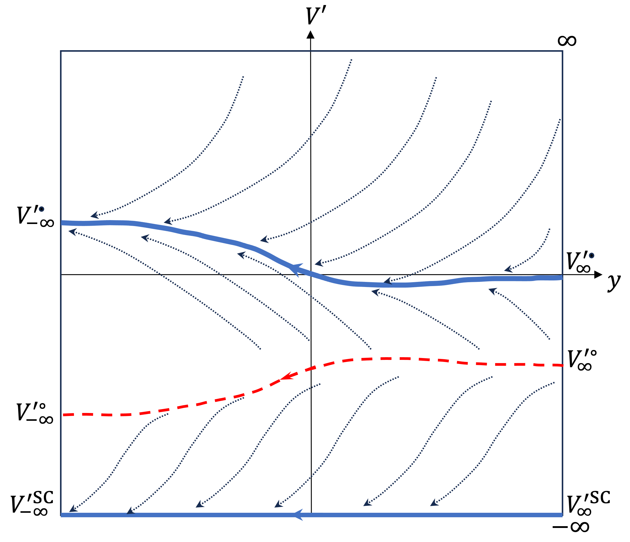
Refer to caption
(a)
Refer to caption
(b)
Figure 18: The portraits of the general PFPs (the collection of all particular PFPs) that arise from (a) the Fermi liquids in d=2d=2, and (b) the U(1) gauge theory at a finite chemical potential. The metallic and separatrix PFPs are denoted by the blue solid curve and the red dashed curve, respectively. In Fermi liquids, the metallic PFP which emanates from V∞′⁣V_{\infty}^{\prime\,\hbox to4.21pt{\vbox to4.21pt{\pgfpicture\makeatletter\hbox{\>\lower-2.10709pt\hbox to0.0pt{\pgfsys@beginscope\pgfsys@invoke{ }\definecolor{pgfstrokecolor}{rgb}{0,0,0}\pgfsys@color@rgb@stroke{0}{0}{0}\pgfsys@invoke{ }\pgfsys@color@rgb@fill{0}{0}{0}\pgfsys@invoke{ }\pgfsys@setlinewidth{\the\pgflinewidth}\pgfsys@invoke{ }\nullfont\hbox to0.0pt{\pgfsys@beginscope\pgfsys@invoke{ } {{}}\hbox{\hbox{{\pgfsys@beginscope\pgfsys@invoke{ }{{}{}{{ {}{}}}{ {}{}} {{}{{}}}{{}{}}{}{{}{}} { }{{{{}}\pgfsys@beginscope\pgfsys@invoke{ }\pgfsys@transformcm{1.0}{0.0}{0.0}{1.0}{0.0pt}{0.0pt}\pgfsys@invoke{ }\hbox{{\definecolor{pgfstrokecolor}{rgb}{0,0,0}\pgfsys@color@rgb@stroke{0}{0}{0}\pgfsys@invoke{ }\pgfsys@color@rgb@fill{0}{0}{0}\pgfsys@invoke{ }\hbox{{}} }}\pgfsys@invoke{ }\pgfsys@endscope}}} \pgfsys@invoke{ }\pgfsys@endscope}}} {}{{}}{}{{{}}{}{}{}{}{}{}{}{}}\pgfsys@beginscope\pgfsys@invoke{ }\pgfsys@setlinewidth{\the\pgflinewidth}\pgfsys@invoke{ }{}\pgfsys@moveto{0.0pt}{0.0pt}\pgfsys@moveto{1.70709pt}{0.0pt}\pgfsys@curveto{1.70709pt}{0.94281pt}{0.94281pt}{1.70709pt}{0.0pt}{1.70709pt}\pgfsys@curveto{-0.94281pt}{1.70709pt}{-1.70709pt}{0.94281pt}{-1.70709pt}{0.0pt}\pgfsys@curveto{-1.70709pt}{-0.94281pt}{-0.94281pt}{-1.70709pt}{0.0pt}{-1.70709pt}\pgfsys@curveto{0.94281pt}{-1.70709pt}{1.70709pt}{-0.94281pt}{1.70709pt}{0.0pt}\pgfsys@closepath\pgfsys@moveto{0.0pt}{0.0pt}\pgfsys@stroke\pgfsys@invoke{ } \pgfsys@invoke{ }\pgfsys@endscope{}{{}}{}{{}{}{}{{}}{{{{}{}{}{}}} {{}{}{}{}}}}{} {} {} {} {}{} {}\pgfsys@beginscope\pgfsys@invoke{ }\color[rgb]{0,0,0}\definecolor[named]{pgfstrokecolor}{rgb}{0,0,0}\pgfsys@color@gray@stroke{0}\pgfsys@invoke{ }\pgfsys@color@gray@fill{0}\pgfsys@invoke{ }\definecolor[named]{pgffillcolor}{rgb}{0,0,0}\pgfsys@moveto{1.70709pt}{0.0pt}\pgfsys@curveto{1.70709pt}{0.94281pt}{0.94281pt}{1.70709pt}{0.0pt}{1.70709pt}\pgfsys@curveto{-0.94281pt}{1.70709pt}{-1.70709pt}{0.94281pt}{-1.70709pt}{0.0pt}\pgfsys@closepath\pgfsys@fill\pgfsys@invoke{ } \pgfsys@invoke{ }\pgfsys@endscope{}{{}}{} {}{}\pgfsys@beginscope\pgfsys@invoke{ }\pgfsys@setlinewidth{\the\pgflinewidth}\pgfsys@invoke{ }{}\pgfsys@moveto{-1.70709pt}{0.0pt}\pgfsys@lineto{1.70709pt}{0.0pt}\pgfsys@stroke\pgfsys@invoke{ } \pgfsys@invoke{ }\pgfsys@endscope \pgfsys@invoke{ }\pgfsys@endscope{{ {}{}{}}}{}{}\hss}\pgfsys@discardpath\pgfsys@invoke{ }\pgfsys@endscope\hss}}\endpgfpicture}}} and the separatrix that forms the boundary of the basin of attraction of V−∞′⁣V_{-\infty}^{\prime\,\hbox to4.21pt{\vbox to4.21pt{\pgfpicture\makeatletter\hbox{\>\lower-2.10709pt\hbox to0.0pt{\pgfsys@beginscope\pgfsys@invoke{ }\definecolor{pgfstrokecolor}{rgb}{0,0,0}\pgfsys@color@rgb@stroke{0}{0}{0}\pgfsys@invoke{ }\pgfsys@color@rgb@fill{0}{0}{0}\pgfsys@invoke{ }\pgfsys@setlinewidth{\the\pgflinewidth}\pgfsys@invoke{ }\nullfont\hbox to0.0pt{\pgfsys@beginscope\pgfsys@invoke{ } {{}}\hbox{\hbox{{\pgfsys@beginscope\pgfsys@invoke{ }{{}{}{{ {}{}}}{ {}{}} {{}{{}}}{{}{}}{}{{}{}} { }{{{{}}\pgfsys@beginscope\pgfsys@invoke{ }\pgfsys@transformcm{1.0}{0.0}{0.0}{1.0}{0.0pt}{0.0pt}\pgfsys@invoke{ }\hbox{{\definecolor{pgfstrokecolor}{rgb}{0,0,0}\pgfsys@color@rgb@stroke{0}{0}{0}\pgfsys@invoke{ }\pgfsys@color@rgb@fill{0}{0}{0}\pgfsys@invoke{ }\hbox{{}} }}\pgfsys@invoke{ }\pgfsys@endscope}}} \pgfsys@invoke{ }\pgfsys@endscope}}} {}{{}}{}{{{}}{}{}{}{}{}{}{}{}}\pgfsys@beginscope\pgfsys@invoke{ }\pgfsys@setlinewidth{\the\pgflinewidth}\pgfsys@invoke{ }{}\pgfsys@moveto{0.0pt}{0.0pt}\pgfsys@moveto{1.70709pt}{0.0pt}\pgfsys@curveto{1.70709pt}{0.94281pt}{0.94281pt}{1.70709pt}{0.0pt}{1.70709pt}\pgfsys@curveto{-0.94281pt}{1.70709pt}{-1.70709pt}{0.94281pt}{-1.70709pt}{0.0pt}\pgfsys@curveto{-1.70709pt}{-0.94281pt}{-0.94281pt}{-1.70709pt}{0.0pt}{-1.70709pt}\pgfsys@curveto{0.94281pt}{-1.70709pt}{1.70709pt}{-0.94281pt}{1.70709pt}{0.0pt}\pgfsys@closepath\pgfsys@moveto{0.0pt}{0.0pt}\pgfsys@stroke\pgfsys@invoke{ } \pgfsys@invoke{ }\pgfsys@endscope{}{{}}{}{{}{}{}{{}}{{{{}{}{}{}}} {{}{}{}{}}}}{} {} {} {} {}{} {}\pgfsys@beginscope\pgfsys@invoke{ }\color[rgb]{0,0,0}\definecolor[named]{pgfstrokecolor}{rgb}{0,0,0}\pgfsys@color@gray@stroke{0}\pgfsys@invoke{ }\pgfsys@color@gray@fill{0}\pgfsys@invoke{ }\definecolor[named]{pgffillcolor}{rgb}{0,0,0}\pgfsys@moveto{1.70709pt}{0.0pt}\pgfsys@curveto{1.70709pt}{0.94281pt}{0.94281pt}{1.70709pt}{0.0pt}{1.70709pt}\pgfsys@curveto{-0.94281pt}{1.70709pt}{-1.70709pt}{0.94281pt}{-1.70709pt}{0.0pt}\pgfsys@closepath\pgfsys@fill\pgfsys@invoke{ } \pgfsys@invoke{ }\pgfsys@endscope{}{{}}{} {}{}\pgfsys@beginscope\pgfsys@invoke{ }\pgfsys@setlinewidth{\the\pgflinewidth}\pgfsys@invoke{ }{}\pgfsys@moveto{-1.70709pt}{0.0pt}\pgfsys@lineto{1.70709pt}{0.0pt}\pgfsys@stroke\pgfsys@invoke{ } \pgfsys@invoke{ }\pgfsys@endscope \pgfsys@invoke{ }\pgfsys@endscope{{ {}{}{}}}{}{}\hss}\pgfsys@discardpath\pgfsys@invoke{ }\pgfsys@endscope\hss}}\endpgfpicture}}} are the same. In the U(1) gauge theory, the metallic PFP emanates from V∞′⁣∙V_{\infty}^{\prime\,\bullet} and the separatrix is the boundary of the basin of attraction of V−∞′⁣∙V_{-\infty}^{\prime\,\bullet}, which are distinct.

The first example is Fermi liquids in d=2d=2. For Fermi liquids, z=1z=1, ηψ=0\eta_{\psi}=0 and Sy′=0S_{y}^{\prime}=0. This leads to only marginal asymptotic fixed points, V±∞′⁣=0V_{\pm\infty}^{\prime\,\hbox to4.21pt{\vbox to4.21pt{\pgfpicture\makeatletter\hbox{\>\lower-2.10709pt\hbox to0.0pt{\pgfsys@beginscope\pgfsys@invoke{ }\definecolor{pgfstrokecolor}{rgb}{0,0,0}\pgfsys@color@rgb@stroke{0}{0}{0}\pgfsys@invoke{ }\pgfsys@color@rgb@fill{0}{0}{0}\pgfsys@invoke{ }\pgfsys@setlinewidth{\the\pgflinewidth}\pgfsys@invoke{ }\nullfont\hbox to0.0pt{\pgfsys@beginscope\pgfsys@invoke{ } {{}}\hbox{\hbox{{\pgfsys@beginscope\pgfsys@invoke{ }{{}{}{{ {}{}}}{ {}{}} {{}{{}}}{{}{}}{}{{}{}} { }{{{{}}\pgfsys@beginscope\pgfsys@invoke{ }\pgfsys@transformcm{1.0}{0.0}{0.0}{1.0}{0.0pt}{0.0pt}\pgfsys@invoke{ }\hbox{{\definecolor{pgfstrokecolor}{rgb}{0,0,0}\pgfsys@color@rgb@stroke{0}{0}{0}\pgfsys@invoke{ }\pgfsys@color@rgb@fill{0}{0}{0}\pgfsys@invoke{ }\hbox{{}} }}\pgfsys@invoke{ }\pgfsys@endscope}}} \pgfsys@invoke{ }\pgfsys@endscope}}} {}{{}}{}{{{}}{}{}{}{}{}{}{}{}}\pgfsys@beginscope\pgfsys@invoke{ }\pgfsys@setlinewidth{\the\pgflinewidth}\pgfsys@invoke{ }{}\pgfsys@moveto{0.0pt}{0.0pt}\pgfsys@moveto{1.70709pt}{0.0pt}\pgfsys@curveto{1.70709pt}{0.94281pt}{0.94281pt}{1.70709pt}{0.0pt}{1.70709pt}\pgfsys@curveto{-0.94281pt}{1.70709pt}{-1.70709pt}{0.94281pt}{-1.70709pt}{0.0pt}\pgfsys@curveto{-1.70709pt}{-0.94281pt}{-0.94281pt}{-1.70709pt}{0.0pt}{-1.70709pt}\pgfsys@curveto{0.94281pt}{-1.70709pt}{1.70709pt}{-0.94281pt}{1.70709pt}{0.0pt}\pgfsys@closepath\pgfsys@moveto{0.0pt}{0.0pt}\pgfsys@stroke\pgfsys@invoke{ } \pgfsys@invoke{ }\pgfsys@endscope{}{{}}{}{{}{}{}{{}}{{{{}{}{}{}}} {{}{}{}{}}}}{} {} {} {} {}{} {}\pgfsys@beginscope\pgfsys@invoke{ }\color[rgb]{0,0,0}\definecolor[named]{pgfstrokecolor}{rgb}{0,0,0}\pgfsys@color@gray@stroke{0}\pgfsys@invoke{ }\pgfsys@color@gray@fill{0}\pgfsys@invoke{ }\definecolor[named]{pgffillcolor}{rgb}{0,0,0}\pgfsys@moveto{1.70709pt}{0.0pt}\pgfsys@curveto{1.70709pt}{0.94281pt}{0.94281pt}{1.70709pt}{0.0pt}{1.70709pt}\pgfsys@curveto{-0.94281pt}{1.70709pt}{-1.70709pt}{0.94281pt}{-1.70709pt}{0.0pt}\pgfsys@closepath\pgfsys@fill\pgfsys@invoke{ } \pgfsys@invoke{ }\pgfsys@endscope{}{{}}{} {}{}\pgfsys@beginscope\pgfsys@invoke{ }\pgfsys@setlinewidth{\the\pgflinewidth}\pgfsys@invoke{ }{}\pgfsys@moveto{-1.70709pt}{0.0pt}\pgfsys@lineto{1.70709pt}{0.0pt}\pgfsys@stroke\pgfsys@invoke{ } \pgfsys@invoke{ }\pgfsys@endscope \pgfsys@invoke{ }\pgfsys@endscope{{ {}{}{}}}{}{}\hss}\pgfsys@discardpath\pgfsys@invoke{ }\pgfsys@endscope\hss}}\endpgfpicture}}}=0 at ±∞\pm\infty. The PFP equation in Eq. (49) is reduced to

12​∂yVy′−Rd​Vy′⁣ 2=0.\displaystyle\frac{1}{2}\partial_{y}V_{y}^{\prime}-R_{d}V_{y}^{\prime\,2}=0. (54)

Besides the superconducting PFP (Vy′⁣S​C=−∞V_{y}^{\prime\,SC}=-\infty), there exists another particular PFP of importance: Vy′⁣=0V_{y}^{\prime\,\hbox to4.21pt{\vbox to4.21pt{\pgfpicture\makeatletter\hbox{\>\lower-2.10709pt\hbox to0.0pt{\pgfsys@beginscope\pgfsys@invoke{ }\definecolor{pgfstrokecolor}{rgb}{0,0,0}\pgfsys@color@rgb@stroke{0}{0}{0}\pgfsys@invoke{ }\pgfsys@color@rgb@fill{0}{0}{0}\pgfsys@invoke{ }\pgfsys@setlinewidth{\the\pgflinewidth}\pgfsys@invoke{ }\nullfont\hbox to0.0pt{\pgfsys@beginscope\pgfsys@invoke{ } {{}}\hbox{\hbox{{\pgfsys@beginscope\pgfsys@invoke{ }{{}{}{{ {}{}}}{ {}{}} {{}{{}}}{{}{}}{}{{}{}} { }{{{{}}\pgfsys@beginscope\pgfsys@invoke{ }\pgfsys@transformcm{1.0}{0.0}{0.0}{1.0}{0.0pt}{0.0pt}\pgfsys@invoke{ }\hbox{{\definecolor{pgfstrokecolor}{rgb}{0,0,0}\pgfsys@color@rgb@stroke{0}{0}{0}\pgfsys@invoke{ }\pgfsys@color@rgb@fill{0}{0}{0}\pgfsys@invoke{ }\hbox{{}} }}\pgfsys@invoke{ }\pgfsys@endscope}}} \pgfsys@invoke{ }\pgfsys@endscope}}} {}{{}}{}{{{}}{}{}{}{}{}{}{}{}}\pgfsys@beginscope\pgfsys@invoke{ }\pgfsys@setlinewidth{\the\pgflinewidth}\pgfsys@invoke{ }{}\pgfsys@moveto{0.0pt}{0.0pt}\pgfsys@moveto{1.70709pt}{0.0pt}\pgfsys@curveto{1.70709pt}{0.94281pt}{0.94281pt}{1.70709pt}{0.0pt}{1.70709pt}\pgfsys@curveto{-0.94281pt}{1.70709pt}{-1.70709pt}{0.94281pt}{-1.70709pt}{0.0pt}\pgfsys@curveto{-1.70709pt}{-0.94281pt}{-0.94281pt}{-1.70709pt}{0.0pt}{-1.70709pt}\pgfsys@curveto{0.94281pt}{-1.70709pt}{1.70709pt}{-0.94281pt}{1.70709pt}{0.0pt}\pgfsys@closepath\pgfsys@moveto{0.0pt}{0.0pt}\pgfsys@stroke\pgfsys@invoke{ } \pgfsys@invoke{ }\pgfsys@endscope{}{{}}{}{{}{}{}{{}}{{{{}{}{}{}}} {{}{}{}{}}}}{} {} {} {} {}{} {}\pgfsys@beginscope\pgfsys@invoke{ }\color[rgb]{0,0,0}\definecolor[named]{pgfstrokecolor}{rgb}{0,0,0}\pgfsys@color@gray@stroke{0}\pgfsys@invoke{ }\pgfsys@color@gray@fill{0}\pgfsys@invoke{ }\definecolor[named]{pgffillcolor}{rgb}{0,0,0}\pgfsys@moveto{1.70709pt}{0.0pt}\pgfsys@curveto{1.70709pt}{0.94281pt}{0.94281pt}{1.70709pt}{0.0pt}{1.70709pt}\pgfsys@curveto{-0.94281pt}{1.70709pt}{-1.70709pt}{0.94281pt}{-1.70709pt}{0.0pt}\pgfsys@closepath\pgfsys@fill\pgfsys@invoke{ } \pgfsys@invoke{ }\pgfsys@endscope{}{{}}{} {}{}\pgfsys@beginscope\pgfsys@invoke{ }\pgfsys@setlinewidth{\the\pgflinewidth}\pgfsys@invoke{ }{}\pgfsys@moveto{-1.70709pt}{0.0pt}\pgfsys@lineto{1.70709pt}{0.0pt}\pgfsys@stroke\pgfsys@invoke{ } \pgfsys@invoke{ }\pgfsys@endscope \pgfsys@invoke{ }\pgfsys@endscope{{ {}{}{}}}{}{}\hss}\pgfsys@discardpath\pgfsys@invoke{ }\pgfsys@endscope\hss}}\endpgfpicture}}}=0 that connects the marginal asymptotic fixed points at ±∞\pm\infty. PFPs that are above (below) Vy′⁣V_{y}^{\prime\,\hbox to4.21pt{\vbox to4.21pt{\pgfpicture\makeatletter\hbox{\>\lower-2.10709pt\hbox to0.0pt{\pgfsys@beginscope\pgfsys@invoke{ }\definecolor{pgfstrokecolor}{rgb}{0,0,0}\pgfsys@color@rgb@stroke{0}{0}{0}\pgfsys@invoke{ }\pgfsys@color@rgb@fill{0}{0}{0}\pgfsys@invoke{ }\pgfsys@setlinewidth{\the\pgflinewidth}\pgfsys@invoke{ }\nullfont\hbox to0.0pt{\pgfsys@beginscope\pgfsys@invoke{ } {{}}\hbox{\hbox{{\pgfsys@beginscope\pgfsys@invoke{ }{{}{}{{ {}{}}}{ {}{}} {{}{{}}}{{}{}}{}{{}{}} { }{{{{}}\pgfsys@beginscope\pgfsys@invoke{ }\pgfsys@transformcm{1.0}{0.0}{0.0}{1.0}{0.0pt}{0.0pt}\pgfsys@invoke{ }\hbox{{\definecolor{pgfstrokecolor}{rgb}{0,0,0}\pgfsys@color@rgb@stroke{0}{0}{0}\pgfsys@invoke{ }\pgfsys@color@rgb@fill{0}{0}{0}\pgfsys@invoke{ }\hbox{{}} }}\pgfsys@invoke{ }\pgfsys@endscope}}} \pgfsys@invoke{ }\pgfsys@endscope}}} {}{{}}{}{{{}}{}{}{}{}{}{}{}{}}\pgfsys@beginscope\pgfsys@invoke{ }\pgfsys@setlinewidth{\the\pgflinewidth}\pgfsys@invoke{ }{}\pgfsys@moveto{0.0pt}{0.0pt}\pgfsys@moveto{1.70709pt}{0.0pt}\pgfsys@curveto{1.70709pt}{0.94281pt}{0.94281pt}{1.70709pt}{0.0pt}{1.70709pt}\pgfsys@curveto{-0.94281pt}{1.70709pt}{-1.70709pt}{0.94281pt}{-1.70709pt}{0.0pt}\pgfsys@curveto{-1.70709pt}{-0.94281pt}{-0.94281pt}{-1.70709pt}{0.0pt}{-1.70709pt}\pgfsys@curveto{0.94281pt}{-1.70709pt}{1.70709pt}{-0.94281pt}{1.70709pt}{0.0pt}\pgfsys@closepath\pgfsys@moveto{0.0pt}{0.0pt}\pgfsys@stroke\pgfsys@invoke{ } \pgfsys@invoke{ }\pgfsys@endscope{}{{}}{}{{}{}{}{{}}{{{{}{}{}{}}} {{}{}{}{}}}}{} {} {} {} {}{} {}\pgfsys@beginscope\pgfsys@invoke{ }\color[rgb]{0,0,0}\definecolor[named]{pgfstrokecolor}{rgb}{0,0,0}\pgfsys@color@gray@stroke{0}\pgfsys@invoke{ }\pgfsys@color@gray@fill{0}\pgfsys@invoke{ }\definecolor[named]{pgffillcolor}{rgb}{0,0,0}\pgfsys@moveto{1.70709pt}{0.0pt}\pgfsys@curveto{1.70709pt}{0.94281pt}{0.94281pt}{1.70709pt}{0.0pt}{1.70709pt}\pgfsys@curveto{-0.94281pt}{1.70709pt}{-1.70709pt}{0.94281pt}{-1.70709pt}{0.0pt}\pgfsys@closepath\pgfsys@fill\pgfsys@invoke{ } \pgfsys@invoke{ }\pgfsys@endscope{}{{}}{} {}{}\pgfsys@beginscope\pgfsys@invoke{ }\pgfsys@setlinewidth{\the\pgflinewidth}\pgfsys@invoke{ }{}\pgfsys@moveto{-1.70709pt}{0.0pt}\pgfsys@lineto{1.70709pt}{0.0pt}\pgfsys@stroke\pgfsys@invoke{ } \pgfsys@invoke{ }\pgfsys@endscope \pgfsys@invoke{ }\pgfsys@endscope{{ {}{}{}}}{}{}\hss}\pgfsys@discardpath\pgfsys@invoke{ }\pgfsys@endscope\hss}}\endpgfpicture}}} are attracted to Vy′⁣V_{y}^{\prime\,\hbox to4.21pt{\vbox to4.21pt{\pgfpicture\makeatletter\hbox{\>\lower-2.10709pt\hbox to0.0pt{\pgfsys@beginscope\pgfsys@invoke{ }\definecolor{pgfstrokecolor}{rgb}{0,0,0}\pgfsys@color@rgb@stroke{0}{0}{0}\pgfsys@invoke{ }\pgfsys@color@rgb@fill{0}{0}{0}\pgfsys@invoke{ }\pgfsys@setlinewidth{\the\pgflinewidth}\pgfsys@invoke{ }\nullfont\hbox to0.0pt{\pgfsys@beginscope\pgfsys@invoke{ } {{}}\hbox{\hbox{{\pgfsys@beginscope\pgfsys@invoke{ }{{}{}{{ {}{}}}{ {}{}} {{}{{}}}{{}{}}{}{{}{}} { }{{{{}}\pgfsys@beginscope\pgfsys@invoke{ }\pgfsys@transformcm{1.0}{0.0}{0.0}{1.0}{0.0pt}{0.0pt}\pgfsys@invoke{ }\hbox{{\definecolor{pgfstrokecolor}{rgb}{0,0,0}\pgfsys@color@rgb@stroke{0}{0}{0}\pgfsys@invoke{ }\pgfsys@color@rgb@fill{0}{0}{0}\pgfsys@invoke{ }\hbox{{}} }}\pgfsys@invoke{ }\pgfsys@endscope}}} \pgfsys@invoke{ }\pgfsys@endscope}}} {}{{}}{}{{{}}{}{}{}{}{}{}{}{}}\pgfsys@beginscope\pgfsys@invoke{ }\pgfsys@setlinewidth{\the\pgflinewidth}\pgfsys@invoke{ }{}\pgfsys@moveto{0.0pt}{0.0pt}\pgfsys@moveto{1.70709pt}{0.0pt}\pgfsys@curveto{1.70709pt}{0.94281pt}{0.94281pt}{1.70709pt}{0.0pt}{1.70709pt}\pgfsys@curveto{-0.94281pt}{1.70709pt}{-1.70709pt}{0.94281pt}{-1.70709pt}{0.0pt}\pgfsys@curveto{-1.70709pt}{-0.94281pt}{-0.94281pt}{-1.70709pt}{0.0pt}{-1.70709pt}\pgfsys@curveto{0.94281pt}{-1.70709pt}{1.70709pt}{-0.94281pt}{1.70709pt}{0.0pt}\pgfsys@closepath\pgfsys@moveto{0.0pt}{0.0pt}\pgfsys@stroke\pgfsys@invoke{ } \pgfsys@invoke{ }\pgfsys@endscope{}{{}}{}{{}{}{}{{}}{{{{}{}{}{}}} {{}{}{}{}}}}{} {} {} {} {}{} {}\pgfsys@beginscope\pgfsys@invoke{ }\color[rgb]{0,0,0}\definecolor[named]{pgfstrokecolor}{rgb}{0,0,0}\pgfsys@color@gray@stroke{0}\pgfsys@invoke{ }\pgfsys@color@gray@fill{0}\pgfsys@invoke{ }\definecolor[named]{pgffillcolor}{rgb}{0,0,0}\pgfsys@moveto{1.70709pt}{0.0pt}\pgfsys@curveto{1.70709pt}{0.94281pt}{0.94281pt}{1.70709pt}{0.0pt}{1.70709pt}\pgfsys@curveto{-0.94281pt}{1.70709pt}{-1.70709pt}{0.94281pt}{-1.70709pt}{0.0pt}\pgfsys@closepath\pgfsys@fill\pgfsys@invoke{ } \pgfsys@invoke{ }\pgfsys@endscope{}{{}}{} {}{}\pgfsys@beginscope\pgfsys@invoke{ }\pgfsys@setlinewidth{\the\pgflinewidth}\pgfsys@invoke{ }{}\pgfsys@moveto{-1.70709pt}{0.0pt}\pgfsys@lineto{1.70709pt}{0.0pt}\pgfsys@stroke\pgfsys@invoke{ } \pgfsys@invoke{ }\pgfsys@endscope \pgfsys@invoke{ }\pgfsys@endscope{{ {}{}{}}}{}{}\hss}\pgfsys@discardpath\pgfsys@invoke{ }\pgfsys@endscope\hss}}\endpgfpicture}}} (Vy′⁣S​CV_{y}^{\prime\,SC}) in the small yy limit. Therefore, Vy′⁣V_{y}^{\prime\,\hbox to4.21pt{\vbox to4.21pt{\pgfpicture\makeatletter\hbox{\>\lower-2.10709pt\hbox to0.0pt{\pgfsys@beginscope\pgfsys@invoke{ }\definecolor{pgfstrokecolor}{rgb}{0,0,0}\pgfsys@color@rgb@stroke{0}{0}{0}\pgfsys@invoke{ }\pgfsys@color@rgb@fill{0}{0}{0}\pgfsys@invoke{ }\pgfsys@setlinewidth{\the\pgflinewidth}\pgfsys@invoke{ }\nullfont\hbox to0.0pt{\pgfsys@beginscope\pgfsys@invoke{ } {{}}\hbox{\hbox{{\pgfsys@beginscope\pgfsys@invoke{ }{{}{}{{ {}{}}}{ {}{}} {{}{{}}}{{}{}}{}{{}{}} { }{{{{}}\pgfsys@beginscope\pgfsys@invoke{ }\pgfsys@transformcm{1.0}{0.0}{0.0}{1.0}{0.0pt}{0.0pt}\pgfsys@invoke{ }\hbox{{\definecolor{pgfstrokecolor}{rgb}{0,0,0}\pgfsys@color@rgb@stroke{0}{0}{0}\pgfsys@invoke{ }\pgfsys@color@rgb@fill{0}{0}{0}\pgfsys@invoke{ }\hbox{{}} }}\pgfsys@invoke{ }\pgfsys@endscope}}} \pgfsys@invoke{ }\pgfsys@endscope}}} {}{{}}{}{{{}}{}{}{}{}{}{}{}{}}\pgfsys@beginscope\pgfsys@invoke{ }\pgfsys@setlinewidth{\the\pgflinewidth}\pgfsys@invoke{ }{}\pgfsys@moveto{0.0pt}{0.0pt}\pgfsys@moveto{1.70709pt}{0.0pt}\pgfsys@curveto{1.70709pt}{0.94281pt}{0.94281pt}{1.70709pt}{0.0pt}{1.70709pt}\pgfsys@curveto{-0.94281pt}{1.70709pt}{-1.70709pt}{0.94281pt}{-1.70709pt}{0.0pt}\pgfsys@curveto{-1.70709pt}{-0.94281pt}{-0.94281pt}{-1.70709pt}{0.0pt}{-1.70709pt}\pgfsys@curveto{0.94281pt}{-1.70709pt}{1.70709pt}{-0.94281pt}{1.70709pt}{0.0pt}\pgfsys@closepath\pgfsys@moveto{0.0pt}{0.0pt}\pgfsys@stroke\pgfsys@invoke{ } \pgfsys@invoke{ }\pgfsys@endscope{}{{}}{}{{}{}{}{{}}{{{{}{}{}{}}} {{}{}{}{}}}}{} {} {} {} {}{} {}\pgfsys@beginscope\pgfsys@invoke{ }\color[rgb]{0,0,0}\definecolor[named]{pgfstrokecolor}{rgb}{0,0,0}\pgfsys@color@gray@stroke{0}\pgfsys@invoke{ }\pgfsys@color@gray@fill{0}\pgfsys@invoke{ }\definecolor[named]{pgffillcolor}{rgb}{0,0,0}\pgfsys@moveto{1.70709pt}{0.0pt}\pgfsys@curveto{1.70709pt}{0.94281pt}{0.94281pt}{1.70709pt}{0.0pt}{1.70709pt}\pgfsys@curveto{-0.94281pt}{1.70709pt}{-1.70709pt}{0.94281pt}{-1.70709pt}{0.0pt}\pgfsys@closepath\pgfsys@fill\pgfsys@invoke{ } \pgfsys@invoke{ }\pgfsys@endscope{}{{}}{} {}{}\pgfsys@beginscope\pgfsys@invoke{ }\pgfsys@setlinewidth{\the\pgflinewidth}\pgfsys@invoke{ }{}\pgfsys@moveto{-1.70709pt}{0.0pt}\pgfsys@lineto{1.70709pt}{0.0pt}\pgfsys@stroke\pgfsys@invoke{ } \pgfsys@invoke{ }\pgfsys@endscope \pgfsys@invoke{ }\pgfsys@endscope{{ {}{}{}}}{}{}\hss}\pgfsys@discardpath\pgfsys@invoke{ }\pgfsys@endscope\hss}}\endpgfpicture}}} acts as the attractor from the repulsive side, and as the separatrix that divides the basins of attraction of Vy′⁣V_{y}^{\prime\,\hbox to4.21pt{\vbox to4.21pt{\pgfpicture\makeatletter\hbox{\>\lower-2.10709pt\hbox to0.0pt{\pgfsys@beginscope\pgfsys@invoke{ }\definecolor{pgfstrokecolor}{rgb}{0,0,0}\pgfsys@color@rgb@stroke{0}{0}{0}\pgfsys@invoke{ }\pgfsys@color@rgb@fill{0}{0}{0}\pgfsys@invoke{ }\pgfsys@setlinewidth{\the\pgflinewidth}\pgfsys@invoke{ }\nullfont\hbox to0.0pt{\pgfsys@beginscope\pgfsys@invoke{ } {{}}\hbox{\hbox{{\pgfsys@beginscope\pgfsys@invoke{ }{{}{}{{ {}{}}}{ {}{}} {{}{{}}}{{}{}}{}{{}{}} { }{{{{}}\pgfsys@beginscope\pgfsys@invoke{ }\pgfsys@transformcm{1.0}{0.0}{0.0}{1.0}{0.0pt}{0.0pt}\pgfsys@invoke{ }\hbox{{\definecolor{pgfstrokecolor}{rgb}{0,0,0}\pgfsys@color@rgb@stroke{0}{0}{0}\pgfsys@invoke{ }\pgfsys@color@rgb@fill{0}{0}{0}\pgfsys@invoke{ }\hbox{{}} }}\pgfsys@invoke{ }\pgfsys@endscope}}} \pgfsys@invoke{ }\pgfsys@endscope}}} {}{{}}{}{{{}}{}{}{}{}{}{}{}{}}\pgfsys@beginscope\pgfsys@invoke{ }\pgfsys@setlinewidth{\the\pgflinewidth}\pgfsys@invoke{ }{}\pgfsys@moveto{0.0pt}{0.0pt}\pgfsys@moveto{1.70709pt}{0.0pt}\pgfsys@curveto{1.70709pt}{0.94281pt}{0.94281pt}{1.70709pt}{0.0pt}{1.70709pt}\pgfsys@curveto{-0.94281pt}{1.70709pt}{-1.70709pt}{0.94281pt}{-1.70709pt}{0.0pt}\pgfsys@curveto{-1.70709pt}{-0.94281pt}{-0.94281pt}{-1.70709pt}{0.0pt}{-1.70709pt}\pgfsys@curveto{0.94281pt}{-1.70709pt}{1.70709pt}{-0.94281pt}{1.70709pt}{0.0pt}\pgfsys@closepath\pgfsys@moveto{0.0pt}{0.0pt}\pgfsys@stroke\pgfsys@invoke{ } \pgfsys@invoke{ }\pgfsys@endscope{}{{}}{}{{}{}{}{{}}{{{{}{}{}{}}} {{}{}{}{}}}}{} {} {} {} {}{} {}\pgfsys@beginscope\pgfsys@invoke{ }\color[rgb]{0,0,0}\definecolor[named]{pgfstrokecolor}{rgb}{0,0,0}\pgfsys@color@gray@stroke{0}\pgfsys@invoke{ }\pgfsys@color@gray@fill{0}\pgfsys@invoke{ }\definecolor[named]{pgffillcolor}{rgb}{0,0,0}\pgfsys@moveto{1.70709pt}{0.0pt}\pgfsys@curveto{1.70709pt}{0.94281pt}{0.94281pt}{1.70709pt}{0.0pt}{1.70709pt}\pgfsys@curveto{-0.94281pt}{1.70709pt}{-1.70709pt}{0.94281pt}{-1.70709pt}{0.0pt}\pgfsys@closepath\pgfsys@fill\pgfsys@invoke{ } \pgfsys@invoke{ }\pgfsys@endscope{}{{}}{} {}{}\pgfsys@beginscope\pgfsys@invoke{ }\pgfsys@setlinewidth{\the\pgflinewidth}\pgfsys@invoke{ }{}\pgfsys@moveto{-1.70709pt}{0.0pt}\pgfsys@lineto{1.70709pt}{0.0pt}\pgfsys@stroke\pgfsys@invoke{ } \pgfsys@invoke{ }\pgfsys@endscope \pgfsys@invoke{ }\pgfsys@endscope{{ {}{}{}}}{}{}\hss}\pgfsys@discardpath\pgfsys@invoke{ }\pgfsys@endscope\hss}}\endpgfpicture}}} and Vy′⁣S​CV_{y}^{\prime\,SC}. The corresponding diagram of general PFP is shown in Fig. 18(a).

As the second example, let us consider the general PFP shown in Fig. 18(b). Here, each line represents a particular PFP with the arrows pointing toward the direction of increasing length scale. This example is drawn from the U(1) gauge theory coupled with the Fermi surface, but we do not have to worry about the details yet. For now, we are mainly concerned with the topology formed by the collection of PFPs. In addition to the superconducting asymptotic fixed points, there are stable and unstable asymptotic fixed points at both y=∞y=\infty and −∞-\infty. The existence of the stable −∞-\infty-asymptotic fixed point is attributed to the fact that the U(1) gauge field mediates a repulsive pairing interaction in the s-wave channel. Naturally, the superconducting asymptotic fixed points at y=±∞y=\pm\infty are interpolated by the PFP, Vy′=−∞V_{y}^{\prime}=-\infty. For understanding the behaviors of other PFPs, we start by defining the basin of attraction of the stable −∞-\infty-asymptotic fixed points,

ℬV−∞′⁣∙I​R={(y,V′)|the PFP that goes through (y,V′) converges to V−∞′⁣∙ in the y→−∞ limit}.\displaystyle{\cal B}^{IR}_{V_{-\infty}^{\prime\,\bullet}}=\{(y,V^{\prime})|\mbox{the PFP that goes through $(y,V^{\prime})$ converges to $V_{-\infty}^{\prime\,\bullet}$ in the $y\rightarrow-\infty$ limit}\}. (55)

ℬV−∞′⁣∙I​R{\cal B}^{IR}_{V_{-\infty}^{\prime\,\bullet}} is an open set in the usual topology of the plane. Its closure is denoted as ℬ¯V−∞′⁣∙I​R\bar{\cal B}^{IR}_{V_{-\infty}^{\prime\,\bullet}}, and ∂ℬV−∞′⁣∙I​R≡ℬ¯V−∞′⁣∙I​R−ℬV−∞′⁣∙I​R\partial{\cal B}^{IR}_{V_{-\infty}^{\prime\,\bullet}}\equiv\bar{\cal B}^{IR}_{V_{-\infty}^{\prime\,\bullet}}-{\cal B}^{IR}_{V_{-\infty}^{\prime\,\bullet}} represents its boundary. One can also define the basins of attraction for V−∞′⁣S​CV_{-\infty}^{\prime\,SC} and V−∞′⁣∘V_{-\infty}^{\prime\,\circ}, respectively. It is noted that ∂ℬV−∞′⁣∙I​R=∂ℬV−∞′⁣S​CI​R=ℬV−∞′⁣∘I​R\partial{\cal B}^{IR}_{V_{-\infty}^{\prime\,\bullet}}=\partial{\cal B}^{IR}_{V_{-\infty}^{\prime\,SC}}={\cal B}^{IR}_{V_{-\infty}^{\prime\,\circ}}. One crucial factor for deciding the general PFP is which basin of attraction V∞′⁣∙V_{\infty}^{\prime\,\bullet} belongs to. V∞′⁣∙V_{\infty}^{\prime\,\bullet} can be either in ℬV−∞′⁣∙I​R{\cal B}^{IR}_{V_{-\infty}^{\prime\,\bullet}}, ℬV−∞′⁣S​CI​R{\cal B}^{IR}_{V_{-\infty}^{\prime\,SC}}, or ℬV−∞′⁣∘I​R{\cal B}^{IR}_{V_{-\infty}^{\prime\,\circ}}. In the next section, we will go over all possibilities. Here, we focus on the current example in which V∞′⁣∙∈ℬV−∞′⁣∙I​RV_{\infty}^{\prime\,\bullet}\in{\cal B}^{IR}_{V_{-\infty}^{\prime\,\bullet}}. Namely, the PFP that emanates from V∞′⁣∙V_{\infty}^{\prime\,\bullet} converges to V−∞′⁣∙V_{-\infty}^{\prime\,\bullet} in the small yy limit. It is denoted as the thick blue line in Fig. 18(b). Naturally, ∂ℬV−∞′⁣∙I​R\partial{\cal B}^{IR}_{V_{-\infty}^{\prime\,\bullet}} is a particular PFP that acts as the separatrix. It turns out that this separatrix PFP connects V∞′⁣∘V_{\infty}^{\prime\,\circ} and V−∞′⁣∘V_{-\infty}^{\prime\,\circ}. To see that there must exist a PFP that connects them, it is useful to consider the UV beta function, which is the negative of Eq. (46), dd​log⁡μ​(y,Vy′)=(12,−βV′​(y))\frac{\mathrm{d}}{d\log\mu}(y,V_{y}^{\prime})=\left(\frac{1}{2},-\beta_{V^{\prime}}(y)\right). This UV beta function describes the evolution of couplings with increasing energy scale μ\mu. The trajectories of PFPs and the asymptotic fixed points of the UV beta functions are identical to those of the IR beta functions. However, the direction of the flow is reversed, and the stability of the asymptotic fixed points is inverted. Namely, the stable (unstable) asymptotic fixed points of the IR beta function become unstable (stable) under the reversed RG flow. Under the reversed RG flow, V∞′⁣∘V_{\infty}^{\prime\,\circ} is an attractor, and it has an extended basin of attraction,

ℬV∞′⁣∘U​V={(y,V′)|the PFP that goes through (y,V′) converges to V∞′⁣∘ in the y→∞ limit}.\displaystyle{\cal B}^{UV}_{V_{\infty}^{\prime\,\circ}}=\{(y,V^{\prime})|\mbox{the PFP that goes through $(y,V^{\prime})$ converges to $V_{\infty}^{\prime\,\circ}$ in the $y\rightarrow\infty$ limit}\}. (56)

The closure and boundary are defined similarly. Under the reversed RG flow, V∞′=∞V_{\infty}^{\prime}=\infty is another stable ∞\infty-asymptotic fixed point with its own basin of attraction. The PFP that interpolates V∞′⁣∙V_{\infty}^{\prime\,\bullet} and V−∞′⁣∙V_{-\infty}^{\prime\,\bullet} is the separatrix PFP under the reversed RG flow; a PFP that is above (below) that PFP heads to +∞+\infty (V∞′⁣∘V_{\infty}^{\prime\,\circ}) under the reversed flow. This guarantees V−∞′⁣∘∈ℬV∞′⁣∘U​VV_{-\infty}^{\prime\,\circ}\in{\cal B}^{UV}_{V_{\infty}^{\prime\,\circ}}, and the PFP that emanates from V−∞′⁣∘V_{-\infty}^{\prime\,\circ} converges to V∞′⁣∘V_{\infty}^{\prime\,\circ} under the reversed RG flow. This implies that there exists a PFP that connects V∞′⁣∘V_{\infty}^{\prime\,\circ} and V−∞′⁣∘V_{-\infty}^{\prime\,\circ}, which is denoted by the dashed red line in Fig. 18(b). This PFP is the separatrix PFP under the original IR RG flow and is identical to ∂ℬV−∞′⁣∙I​R\partial{\cal B}^{IR}_{V_{-\infty}^{\prime\,\bullet}}.

The particular PFPs that emanate from V∞′⁣∙V_{\infty}^{\prime\,\bullet} and V∞′⁣S​CV_{\infty}^{\prime\,SC} are denoted as Vy′⁣∙V_{y}^{\prime\,\bullet} and Vy′⁣S​CV_{y}^{\prime\,SC}. The separatrix PFP is denoted as Vy′⁣∘V_{y}^{\prime\,\circ}. The PFP that connects the two stable asymptotic fixed points acts as an attractor under the original PFP equation (not the reversed one) because PFPs that deviate slightly away from it at a finite yy are attracted to it as yy decreases. Therefore, the pairing interactions that emerge in the low-energy limit are controlled by this PFP. The topology of the general PFP is completely fixed by Vy′⁣∙V_{y}^{\prime\,\bullet}, Vy′⁣S​CV_{y}^{\prime\,SC} and Vy′⁣∘V_{y}^{\prime\,\circ}: the region above (below) Vy′⁣∘V_{y}^{\prime\,\circ} corresponds to the basin of attraction of Vy′⁣∙V_{y}^{\prime\,\bullet} (Vy′⁣S​CV_{y}^{\prime\,SC}) under the IR beta function, and the points on Vy′⁣∘V_{y}^{\prime\,\circ} stay on it. In this example, the number and type of asymptotic fixed points and their connectivity are robust against small deformations, such as a change in the spatial dimension and a deformation of the marginal coupling functions (Fermi velocity and shape of the Fermi surface). Therefore, this general PFP is topologically stable.

The above examples illustrate that the PFP that emanates from the stable or marginal ∞\infty-asymptotic fixed point attracts nearby PFPs at least at large yy. Since that PFP governs the universal pairing interaction in the normal state, it is referred to as metallic PFP and denoted as Vy′⁣MV_{y}^{\prime M}. On the other hand, ∂ℬV−∞′⁣∙I​R\partial{\cal B}^{IR}_{V_{-\infty}^{\prime\,\bullet}} or ∂ℬV−∞′⁣I​R\partial{\cal B}^{IR}_{V_{-\infty}^{\prime\,\hbox to4.21pt{\vbox to4.21pt{\pgfpicture\makeatletter\hbox{\>\lower-2.10709pt\hbox to0.0pt{\pgfsys@beginscope\pgfsys@invoke{ }\definecolor{pgfstrokecolor}{rgb}{0,0,0}\pgfsys@color@rgb@stroke{0}{0}{0}\pgfsys@invoke{ }\pgfsys@color@rgb@fill{0}{0}{0}\pgfsys@invoke{ }\pgfsys@setlinewidth{\the\pgflinewidth}\pgfsys@invoke{ }\nullfont\hbox to0.0pt{\pgfsys@beginscope\pgfsys@invoke{ } {{}}\hbox{\hbox{{\pgfsys@beginscope\pgfsys@invoke{ }{{}{}{{ {}{}}}{ {}{}} {{}{{}}}{{}{}}{}{{}{}} { }{{{{}}\pgfsys@beginscope\pgfsys@invoke{ }\pgfsys@transformcm{1.0}{0.0}{0.0}{1.0}{0.0pt}{0.0pt}\pgfsys@invoke{ }\hbox{{\definecolor{pgfstrokecolor}{rgb}{0,0,0}\pgfsys@color@rgb@stroke{0}{0}{0}\pgfsys@invoke{ }\pgfsys@color@rgb@fill{0}{0}{0}\pgfsys@invoke{ }\hbox{{}} }}\pgfsys@invoke{ }\pgfsys@endscope}}} \pgfsys@invoke{ }\pgfsys@endscope}}} {}{{}}{}{{{}}{}{}{}{}{}{}{}{}}\pgfsys@beginscope\pgfsys@invoke{ }\pgfsys@setlinewidth{\the\pgflinewidth}\pgfsys@invoke{ }{}\pgfsys@moveto{0.0pt}{0.0pt}\pgfsys@moveto{1.70709pt}{0.0pt}\pgfsys@curveto{1.70709pt}{0.94281pt}{0.94281pt}{1.70709pt}{0.0pt}{1.70709pt}\pgfsys@curveto{-0.94281pt}{1.70709pt}{-1.70709pt}{0.94281pt}{-1.70709pt}{0.0pt}\pgfsys@curveto{-1.70709pt}{-0.94281pt}{-0.94281pt}{-1.70709pt}{0.0pt}{-1.70709pt}\pgfsys@curveto{0.94281pt}{-1.70709pt}{1.70709pt}{-0.94281pt}{1.70709pt}{0.0pt}\pgfsys@closepath\pgfsys@moveto{0.0pt}{0.0pt}\pgfsys@stroke\pgfsys@invoke{ } \pgfsys@invoke{ }\pgfsys@endscope{}{{}}{}{{}{}{}{{}}{{{{}{}{}{}}} {{}{}{}{}}}}{} {} {} {} {}{} {}\pgfsys@beginscope\pgfsys@invoke{ }\color[rgb]{0,0,0}\definecolor[named]{pgfstrokecolor}{rgb}{0,0,0}\pgfsys@color@gray@stroke{0}\pgfsys@invoke{ }\pgfsys@color@gray@fill{0}\pgfsys@invoke{ }\definecolor[named]{pgffillcolor}{rgb}{0,0,0}\pgfsys@moveto{1.70709pt}{0.0pt}\pgfsys@curveto{1.70709pt}{0.94281pt}{0.94281pt}{1.70709pt}{0.0pt}{1.70709pt}\pgfsys@curveto{-0.94281pt}{1.70709pt}{-1.70709pt}{0.94281pt}{-1.70709pt}{0.0pt}\pgfsys@closepath\pgfsys@fill\pgfsys@invoke{ } \pgfsys@invoke{ }\pgfsys@endscope{}{{}}{} {}{}\pgfsys@beginscope\pgfsys@invoke{ }\pgfsys@setlinewidth{\the\pgflinewidth}\pgfsys@invoke{ }{}\pgfsys@moveto{-1.70709pt}{0.0pt}\pgfsys@lineto{1.70709pt}{0.0pt}\pgfsys@stroke\pgfsys@invoke{ } \pgfsys@invoke{ }\pgfsys@endscope \pgfsys@invoke{ }\pgfsys@endscope{{ {}{}{}}}{}{}\hss}\pgfsys@discardpath\pgfsys@invoke{ }\pgfsys@endscope\hss}}\endpgfpicture}}}} (the boundary of the basin of attraction of V−∞′⁣∙V_{-\infty}^{\prime\,\bullet} or V−∞′⁣V_{-\infty}^{\prime\,\hbox to4.21pt{\vbox to4.21pt{\pgfpicture\makeatletter\hbox{\>\lower-2.10709pt\hbox to0.0pt{\pgfsys@beginscope\pgfsys@invoke{ }\definecolor{pgfstrokecolor}{rgb}{0,0,0}\pgfsys@color@rgb@stroke{0}{0}{0}\pgfsys@invoke{ }\pgfsys@color@rgb@fill{0}{0}{0}\pgfsys@invoke{ }\pgfsys@setlinewidth{\the\pgflinewidth}\pgfsys@invoke{ }\nullfont\hbox to0.0pt{\pgfsys@beginscope\pgfsys@invoke{ } {{}}\hbox{\hbox{{\pgfsys@beginscope\pgfsys@invoke{ }{{}{}{{ {}{}}}{ {}{}} {{}{{}}}{{}{}}{}{{}{}} { }{{{{}}\pgfsys@beginscope\pgfsys@invoke{ }\pgfsys@transformcm{1.0}{0.0}{0.0}{1.0}{0.0pt}{0.0pt}\pgfsys@invoke{ }\hbox{{\definecolor{pgfstrokecolor}{rgb}{0,0,0}\pgfsys@color@rgb@stroke{0}{0}{0}\pgfsys@invoke{ }\pgfsys@color@rgb@fill{0}{0}{0}\pgfsys@invoke{ }\hbox{{}} }}\pgfsys@invoke{ }\pgfsys@endscope}}} \pgfsys@invoke{ }\pgfsys@endscope}}} {}{{}}{}{{{}}{}{}{}{}{}{}{}{}}\pgfsys@beginscope\pgfsys@invoke{ }\pgfsys@setlinewidth{\the\pgflinewidth}\pgfsys@invoke{ }{}\pgfsys@moveto{0.0pt}{0.0pt}\pgfsys@moveto{1.70709pt}{0.0pt}\pgfsys@curveto{1.70709pt}{0.94281pt}{0.94281pt}{1.70709pt}{0.0pt}{1.70709pt}\pgfsys@curveto{-0.94281pt}{1.70709pt}{-1.70709pt}{0.94281pt}{-1.70709pt}{0.0pt}\pgfsys@curveto{-1.70709pt}{-0.94281pt}{-0.94281pt}{-1.70709pt}{0.0pt}{-1.70709pt}\pgfsys@curveto{0.94281pt}{-1.70709pt}{1.70709pt}{-0.94281pt}{1.70709pt}{0.0pt}\pgfsys@closepath\pgfsys@moveto{0.0pt}{0.0pt}\pgfsys@stroke\pgfsys@invoke{ } \pgfsys@invoke{ }\pgfsys@endscope{}{{}}{}{{}{}{}{{}}{{{{}{}{}{}}} {{}{}{}{}}}}{} {} {} {} {}{} {}\pgfsys@beginscope\pgfsys@invoke{ }\color[rgb]{0,0,0}\definecolor[named]{pgfstrokecolor}{rgb}{0,0,0}\pgfsys@color@gray@stroke{0}\pgfsys@invoke{ }\pgfsys@color@gray@fill{0}\pgfsys@invoke{ }\definecolor[named]{pgffillcolor}{rgb}{0,0,0}\pgfsys@moveto{1.70709pt}{0.0pt}\pgfsys@curveto{1.70709pt}{0.94281pt}{0.94281pt}{1.70709pt}{0.0pt}{1.70709pt}\pgfsys@curveto{-0.94281pt}{1.70709pt}{-1.70709pt}{0.94281pt}{-1.70709pt}{0.0pt}\pgfsys@closepath\pgfsys@fill\pgfsys@invoke{ } \pgfsys@invoke{ }\pgfsys@endscope{}{{}}{} {}{}\pgfsys@beginscope\pgfsys@invoke{ }\pgfsys@setlinewidth{\the\pgflinewidth}\pgfsys@invoke{ }{}\pgfsys@moveto{-1.70709pt}{0.0pt}\pgfsys@lineto{1.70709pt}{0.0pt}\pgfsys@stroke\pgfsys@invoke{ } \pgfsys@invoke{ }\pgfsys@endscope \pgfsys@invoke{ }\pgfsys@endscope{{ {}{}{}}}{}{}\hss}\pgfsys@discardpath\pgfsys@invoke{ }\pgfsys@endscope\hss}}\endpgfpicture}}}) is the separatrix PFP, denoted as Vy′⁣SV_{y}^{\prime S}. In the first example, Vy′⁣M=Vy′⁣S=Vy′⁣V_{y}^{\prime M}=V_{y}^{\prime S}=V_{y}^{\prime\,\hbox to4.21pt{\vbox to4.21pt{\pgfpicture\makeatletter\hbox{\>\lower-2.10709pt\hbox to0.0pt{\pgfsys@beginscope\pgfsys@invoke{ }\definecolor{pgfstrokecolor}{rgb}{0,0,0}\pgfsys@color@rgb@stroke{0}{0}{0}\pgfsys@invoke{ }\pgfsys@color@rgb@fill{0}{0}{0}\pgfsys@invoke{ }\pgfsys@setlinewidth{\the\pgflinewidth}\pgfsys@invoke{ }\nullfont\hbox to0.0pt{\pgfsys@beginscope\pgfsys@invoke{ } {{}}\hbox{\hbox{{\pgfsys@beginscope\pgfsys@invoke{ }{{}{}{{ {}{}}}{ {}{}} {{}{{}}}{{}{}}{}{{}{}} { }{{{{}}\pgfsys@beginscope\pgfsys@invoke{ }\pgfsys@transformcm{1.0}{0.0}{0.0}{1.0}{0.0pt}{0.0pt}\pgfsys@invoke{ }\hbox{{\definecolor{pgfstrokecolor}{rgb}{0,0,0}\pgfsys@color@rgb@stroke{0}{0}{0}\pgfsys@invoke{ }\pgfsys@color@rgb@fill{0}{0}{0}\pgfsys@invoke{ }\hbox{{}} }}\pgfsys@invoke{ }\pgfsys@endscope}}} \pgfsys@invoke{ }\pgfsys@endscope}}} {}{{}}{}{{{}}{}{}{}{}{}{}{}{}}\pgfsys@beginscope\pgfsys@invoke{ }\pgfsys@setlinewidth{\the\pgflinewidth}\pgfsys@invoke{ }{}\pgfsys@moveto{0.0pt}{0.0pt}\pgfsys@moveto{1.70709pt}{0.0pt}\pgfsys@curveto{1.70709pt}{0.94281pt}{0.94281pt}{1.70709pt}{0.0pt}{1.70709pt}\pgfsys@curveto{-0.94281pt}{1.70709pt}{-1.70709pt}{0.94281pt}{-1.70709pt}{0.0pt}\pgfsys@curveto{-1.70709pt}{-0.94281pt}{-0.94281pt}{-1.70709pt}{0.0pt}{-1.70709pt}\pgfsys@curveto{0.94281pt}{-1.70709pt}{1.70709pt}{-0.94281pt}{1.70709pt}{0.0pt}\pgfsys@closepath\pgfsys@moveto{0.0pt}{0.0pt}\pgfsys@stroke\pgfsys@invoke{ } \pgfsys@invoke{ }\pgfsys@endscope{}{{}}{}{{}{}{}{{}}{{{{}{}{}{}}} {{}{}{}{}}}}{} {} {} {} {}{} {}\pgfsys@beginscope\pgfsys@invoke{ }\color[rgb]{0,0,0}\definecolor[named]{pgfstrokecolor}{rgb}{0,0,0}\pgfsys@color@gray@stroke{0}\pgfsys@invoke{ }\pgfsys@color@gray@fill{0}\pgfsys@invoke{ }\definecolor[named]{pgffillcolor}{rgb}{0,0,0}\pgfsys@moveto{1.70709pt}{0.0pt}\pgfsys@curveto{1.70709pt}{0.94281pt}{0.94281pt}{1.70709pt}{0.0pt}{1.70709pt}\pgfsys@curveto{-0.94281pt}{1.70709pt}{-1.70709pt}{0.94281pt}{-1.70709pt}{0.0pt}\pgfsys@closepath\pgfsys@fill\pgfsys@invoke{ } \pgfsys@invoke{ }\pgfsys@endscope{}{{}}{} {}{}\pgfsys@beginscope\pgfsys@invoke{ }\pgfsys@setlinewidth{\the\pgflinewidth}\pgfsys@invoke{ }{}\pgfsys@moveto{-1.70709pt}{0.0pt}\pgfsys@lineto{1.70709pt}{0.0pt}\pgfsys@stroke\pgfsys@invoke{ } \pgfsys@invoke{ }\pgfsys@endscope \pgfsys@invoke{ }\pgfsys@endscope{{ {}{}{}}}{}{}\hss}\pgfsys@discardpath\pgfsys@invoke{ }\pgfsys@endscope\hss}}\endpgfpicture}}}. In the second example, Vy′⁣M=Vy′⁣∙V_{y}^{\prime M}=V_{y}^{\prime\,\bullet} and Vy′⁣S=Vy′⁣∘V_{y}^{\prime S}=V_{y}^{\prime\,\circ}, which are distinct.

Refer to caption
Figure 19: In a metal that supports a general PFP of the form shown in Fig. 18(b), a stable non-Fermi liquid arises if the bare pairing interactions lie above the separatrix PFP. At low energies, the pairing interactions in all angular-momentum channels flow into the universal profile set by the metallic PFP. For generic non-Fermi liquids, the metallic PFP has a non-trivial yy-dependence, which reflects the scale-dependent pairing interaction generated by critical fluctuations. Due to the drift of yy under the RG flow, the universal couplings associated with the infinite chain of angular momenta undergo the incessant crossovers within the metallic PFP.

In Fermi liquids, the metallic PFP is simply Vy′⁣M=0V_{y}^{\prime\,M}=0. Therefore, there are no intrinsic superconducting fluctuations in the low-energy limit. In the second example, the universal pairing interactions that emerge at low energies is controlled by the metallic PFP which has a non-trivial yy-dependence. Because the angular momentum is unbounded and yy shifts incessantly under the RG flow, there always exist some angular momentum channels that are in the region of crossover from the ∞\infty asymptotic region to the −∞-\infty asymptotic region (see Fig. 19). This incessant crossover prevents the non-Fermi liquid from exhibiting a scale invariant universal pairing interaction, even if there is no instability.

IV.2 Linear stability of PFP

Since the topology of general PFPs is determined by the metallic and separatrix PFPs, it is useful to understand their linear stability. The stability of a PFP can be understood in terms of the linearized flow of a small perturbation added to the PFP. Let Vy′V_{y}^{\prime} be a PFP. We consider a nearby PFP, Vy′=Vy′+δ​Vy′V_{y}^{\prime\,{}}=V_{y}^{\prime}+\delta V_{y}^{\prime\,{}}. The deviation δ​Vy′\delta V_{y}^{\prime} as a function of yy obeys

12​∂yδ​Vy′+χy​δ​Vy′=0,\displaystyle\frac{1}{2}\partial_{y}\delta V_{y}^{\prime}+\chi_{y}\delta V_{y}^{\prime}=0, (57)

to the linear order in δ​Vy′\delta V_{y}^{\prime}, where

χy=−12​(4​Rd​Vy′+2​𝐇d−1).\displaystyle\chi_{y}=-\frac{1}{2}\left(4R_{d}V_{y}^{\prime}+2{\bf H}_{d}-1\right). (58)

This equation describes how the deviation evolves with decreasing yy through δ​Vy′′=Ay′;y​δ​Vy′\delta V_{y^{\prime}}^{\prime}=A_{y^{\prime};y}\delta V_{y}^{\prime}, where

Ay′;y=exp⁡(2​∫y′y𝑑y′′​χy′′).\displaystyle A_{y^{\prime};y}=\exp{2\int_{y^{\prime}}^{y}dy^{\prime\prime}\chi_{y^{\prime\prime}}}. (59)

Here, the sign of χy\chi_{y} determines the stability of a PFP locally at yy. For χy<0\chi_{y}<0 (χy>0\chi_{y}>0), the nearby PFP approaches (moves away from) Vy′V_{y}^{\prime} with decreasing yy. We say that a PFP is locally stable, unstable, and marginal at yy if χy<0\chi_{y}<0. χy>0\chi_{y}>0, and χy=0\chi_{y}=0, respectively. From Eq. (58), we note that a PFP is locally stable (unstable) at yy if Vy′>−2​𝐇d−14​RdV_{y}^{\prime}>-\frac{2{\bf H}_{d}-1}{4R_{d}} (Vy′<−2​𝐇d−14​RdV_{y}^{\prime}<-\frac{2{\bf H}_{d}-1}{4R_{d}}).

Refer to caption
Figure 20: PFPs are locally stable (unstable) in the region with Vy′>−2​𝐇d−14​RdV_{y}^{\prime}>-\frac{2{\bf H}_{d}-1}{4R_{d}} (Vy′<−2​𝐇d−14​RdV_{y}^{\prime}<-\frac{2{\bf H}_{d}-1}{4R_{d}}). A PFP which is locally unstable within finite segments of yy is globally stable as long as nearby PFPs are attracted to the PFP outside the finite locally unstable region.

Another notion of stability, which turns out to be the more useful one, is global stability.

  • •

    A PFP is globally stable if for all yy and ϵ′>0\epsilon^{\prime}>0, there exists y′′y^{\prime\prime} such that Ay′;y<ϵ′A_{y^{\prime};y}<\epsilon^{\prime} for all y′<y′′y^{\prime}<y^{\prime\prime}. In this case, PFPs that are close to the PFP at any point in yy become arbitrarily close to it at sufficiently small yy.

  • •

    A PFP is marginal if Ay′;yA_{y^{\prime};y} approaches a non-zero finite value in the small y′y^{\prime} limit for some yy.

  • •

    A PFP is unstable if there exists a yy for which Ay′;yA_{y^{\prime};y} becomes arbitrarily large for some y′<yy^{\prime}<y. In this case, a perturbation added to the PFP at yy grows without a bound as yy approaches y′y^{\prime}.

A PFP that is locally stable at all yy is globally stable. However, the converse is not necessarily true. Vy′V_{y}^{\prime}, which is unstable locally in some regions of yy, is globally stable if it satisfies the following conditions: (a) it is regular, that is, Vy′V_{y}^{\prime} is finite for all yy, (b) χy>0\chi_{y}>0 only within a finite support X=∪i{y|yi−<y<yi+}X=\cup_{i}\{y|y^{-}_{i}<y<y^{+}_{i}\}, where yi±y^{\pm}_{i} are finite, (c) there exist positive constants δ′′\delta^{\prime\prime} and ϵ′′\epsilon^{\prime\prime} such that χy<−ϵ′′\chi_{y}<-\epsilon^{\prime\prime} in the supplement of Xδ′′=∪i{y|yi−−δ′′<y<yi++δ′′}X_{\delta^{\prime\prime}}=\cup_{i}\{y|y^{-}_{i}-\delta^{\prime\prime}<y<y^{+}_{i}+\delta^{\prime\prime}\}. Vy′V_{y}^{\prime} that satisfies these conditions is globally stable because a PFP that is near Vy′V_{y}^{\prime} at a yy can diverge away from Vy′V_{y}^{\prime} with decreasing yy only in XX and the diverging rate χy\chi_{y} is bounded. In the small yy limit, however, the neighboring PFP is destined to be attracted toward Vy′V_{y}^{\prime} with Ay′;yA_{y^{\prime};y} approaching 0 due to the attraction it experiences over an arbitrarily large range of yy outside Xδ′′X_{\delta^{\prime\prime}}. This is illustrated in Fig. 20. The metallic PFP in Fig. 18(b) is globally stable. This follows from the fact that the presence of asymptotic fixed points in both y→±∞y\rightarrow\pm\infty limits guarantees that the region XX of negative χy\chi_{y} is finite, if present. The separatrix PFP in Fig. 18(b) is globally unstable as a small perturbation diverges with decreasing yy. The separatrix PFP in 18(a), which is also the metallic PFP, is marginal. For marginal PFP, one has to include non-linear effects to understand stability. In Fermi liquids, the separatrix PFP is marginally stable (unstable) for perturbations with δ​Vy′>0\delta V_{y}^{\prime}>0 (δ​Vy′<0\delta V_{y}^{\prime}<0).

IV.3 Classification of superuniversality classes

Refer to caption
Figure 21: Portraits of the seven topologically distinct general PFPs, each of which corresponds to a superuniversality class. Three at the ‘corners’ (A,B,C) are the topologically stable classes that are robust against small changes of the marginal couplings and kinematic data. Three at the ‘edges’ (AB, BC, AC) are critical classes that require one fine tuning. They describe superuniversality phase transition between two stable classes. The one at the center (ABC) is the double critical class. The thick blue line represents the metallic PFP that emanates from V∞′⁣∙V_{\infty}^{\prime\,\bullet}. The thick red dashed line represents the separatrix PFP that forms the boundary of the basin of attraction for the stable or marginal −∞-\infty asymptotic fixed point. In classes AB and ABC, the metallic PFP and the separatrix PFP coincide.

In this section, we classify all topologically distinct general PFPs, each of which defines one superuniversality class. Distinct general PFPs are characterized by (i) the number and local stability of asymptotic fixed points and (ii) their connectivity formed by particular PFPs. These are topological data that are insensitive to the geometric shape of PFPs. We first classify topologically stable classes of PFPs.

Class A

Stable non-Fermi liquid superuniversality class

At y=∞y=\infty, there are always one stable (V∞′⁣∙V_{\infty}^{\prime\,\bullet}) and one unstable (V∞′⁣∘V_{\infty}^{\prime\,\circ}) asymptotic fixed points shown in Eq. (52). 111111Because S∞′=0S_{\infty}^{\prime}=0, ηP,∞>0\eta_{P,\infty}>0. At y=−∞y=-\infty, there can be 22, 11 or 0 asymptotic fixed points on the real axis of V−∞′V_{-\infty}^{\prime}. Let us first consider the cases with two −∞-\infty-asymptotic fixed points. From the quadratic nature of the beta function, one (V−∞′⁣∙V_{-\infty}^{\prime\,\bullet}) is stable and the other (V−∞′⁣∘V_{-\infty}^{\prime\,\circ}) is unstable. Since βV′​(y)\beta_{V^{\prime}}(y) in Eq. (47) is negative for large |V′||V^{\prime}|, V−∞′⁣∙>V−∞′⁣∘V_{-\infty}^{\prime\,\bullet}>V_{-\infty}^{\prime\,\circ}. The first type of general PFPs is the one in which V∞′⁣∙∈ℬV−∞′⁣∙I​RV_{\infty}^{\prime\,\bullet}\in{\cal B}^{IR}_{V_{-\infty}^{\prime\,\bullet}}. This implies that the metallic PFP (Vy′⁣MV_{y}^{\prime M}), which emanates from V∞′⁣∙V_{\infty}^{\prime\,\bullet}, converges to V−∞′⁣∙V_{-\infty}^{\prime\,\bullet} in the small yy limit. In this case, V∞′⁣∘V_{\infty}^{\prime\,\circ} and V−∞′⁣∘V_{-\infty}^{\prime\,\circ} must be connected by a PFP as is discussed below Eq. (55). That PFP is the separatrix PFP, Vy′⁣SV_{y}^{\prime S} which forms ∂ℬV−∞′⁣∙I​R\partial{\cal B}^{IR}_{V_{-\infty}^{\prime\,\bullet}}. The metallic and separatrix PFPs give rise to the topology of Fig. 21 (A) for the general PFP, which is identical to the second example we considered in Fig. 18. We refer to the superuniversality class of this general PFP as stable non-Fermi liquid superuniversality class (or class A, in short). As the name suggests, this superuniversality class contains non-Fermi liquids that survive down to zero temperature without fine tuning the bare pairing interaction.

Class B

Non-s-wave superconducting superuniversality class

Let us proceed with the next class where there are still two −∞-\infty-asymptotic fixed points but with a distinct connectivity to the +∞+\infty-asymptotic fixed points. If V∞′⁣∙∉ℬV−∞′⁣∙I​RV_{\infty}^{\prime\,\bullet}\notin{\cal B}^{IR}_{V_{-\infty}^{\prime\,\bullet}}, V∞′⁣∙V_{\infty}^{\prime\,\bullet} must be generically in ℬV−∞′⁣S​CI​R{\cal B}^{IR}_{V_{-\infty}^{\prime\,SC}} because V−∞′⁣S​CV_{-\infty}^{\prime\,SC} is the only other stable −∞-\infty-asymptotic fixed point. Therefore, the metallic PFP must reach V′=−∞V^{\prime}=-\infty. Alternatively, the metallic PFP can flow into V−∞′⁣∘V_{-\infty}^{\prime\,\circ}, but it requires fine-tuning. Such critical classes will be discussed separately. The particular PFP that emanates from V∞′⁣∘V_{\infty}^{\prime\,\circ} must also reach V′=−∞V^{\prime}=-\infty because it has to stay below the metallic PFP.121212Distinct PFPs cannot cross due to the uniqueness of the solution of the first-order differential equation. The fates of PFPs that are connected to the −∞-\infty-asymptotic fixed points can be readily understood through the reverse RG flow. Since V−∞′⁣∘V_{-\infty}^{\prime\,\circ} is not in ℬ¯V∞′⁣∘U​V\bar{\cal B}^{UV}_{V_{\infty}^{\prime\,\circ}} under the reversed RG flow131313If it were, there would be a PFP that connects V±∞′⁣∘V_{\pm\infty}^{\prime\,\circ}. But this is not the case. , the PFP that is connected to the former must reach V′=∞V^{\prime}=\infty, the only other stable ∞\infty-asymptotic fixed point for the reversed RG flow. The PFP connected to V−∞′⁣∙V_{-\infty}^{\prime\,\bullet} must reach V′=∞V^{\prime}=\infty as well because it should stay above the PFP connected to V−∞′⁣∘V_{-\infty}^{\prime\,\circ}. This fixes the topology of this class of general PFP to be that of Fig. 21 (B). This class is referred to as non-s-wave superconducting superuniversality class (or class B) because a non-s-wave superconducting instability is unavoidable in this class.

Class C

S-wave superconducting superuniversality class

The final superuniversality class that can be realized without fine-tuning is associated with general PFPs with no −∞-\infty-asymptotic fixed points. In this case, ηP,−∞<0\eta_{P,-\infty}<0, and the vertical beta function is negative definite in the y→−∞y\rightarrow-\infty limit. Therefore, all PFPs that emanate from y=∞y=\infty reach V′=−∞V^{\prime}=-\infty at some yy. The topology of the general PFP in this class is depicted in Fig. 21 (C). We call this s-wave superconducting superuniversality class (or class C) because the s-wave superconducting instability is present in all non-Fermi liquids in this superuniversality class.

The above three cases exhaust all generic superuniversality classes that can be realized without fine tuning of marginal couplings or the kinematic data. Now, we consider the classes that require fine tuning. Those critical superuniversality classes can be viewed as transitions between superuniversality classes (not between individual phases). These superuniversality phase transitions are associated with changes in the topology of the portraits of general PFPs.

Class AB

NFL to non-s-wave SC critical superuniversality class

The critical superuniversality class that is at the border between classes A and B has two asymptotic fixed points, both at y=∞y=\infty and −∞-\infty, but they are connected differently from classes A and B. Namely, V∞′⁣∙V_{\infty}^{\prime\,\bullet} is neither in ℬV−∞′⁣∙I​R{\cal B}^{IR}_{V_{-\infty}^{\prime\,\bullet}} nor in ℬV−∞′⁣S​CI​R{\cal B}^{IR}_{V_{-\infty}^{\prime\,SC}}. Instead, V∞′⁣∙V_{\infty}^{\prime\,\bullet} is in ℬV−∞′⁣∘I​R{\cal B}^{IR}_{V_{-\infty}^{\prime\,\circ}}, as shown in Fig. 21 (AB). Because V−∞′⁣∘V_{-\infty}^{\prime\,\circ} is locally unstable, this requires tuning one parameter; hence, it corresponds to a critical superuniversality class. In this class, the metallic PFP coincides with the separatrix PFP because the PFP that emanates from V∞′⁣∙V_{\infty}^{\prime\,\bullet} forms ∂ℬV−∞′⁣∙I​R\partial{\cal B}^{IR}_{V_{-\infty}^{\prime\,\bullet}} This class is referred to as NFL to non-s-wave SC critical superuniversality class (or class AB).

Class AC

NFL to s-wave SC critical superuniversality class

In the critical superuniversality class that arises at the transition from classes A to C, the −∞-\infty-asymptotic fixed points are on the verge of moving off the real axis as they merge into a marginal fixed point at V−∞′⁣V_{-\infty}^{\prime\,\hbox to4.21pt{\vbox to4.21pt{\pgfpicture\makeatletter\hbox{\>\lower-2.10709pt\hbox to0.0pt{\pgfsys@beginscope\pgfsys@invoke{ }\definecolor{pgfstrokecolor}{rgb}{0,0,0}\pgfsys@color@rgb@stroke{0}{0}{0}\pgfsys@invoke{ }\pgfsys@color@rgb@fill{0}{0}{0}\pgfsys@invoke{ }\pgfsys@setlinewidth{\the\pgflinewidth}\pgfsys@invoke{ }\nullfont\hbox to0.0pt{\pgfsys@beginscope\pgfsys@invoke{ } {{}}\hbox{\hbox{{\pgfsys@beginscope\pgfsys@invoke{ }{{}{}{{ {}{}}}{ {}{}} {{}{{}}}{{}{}}{}{{}{}} { }{{{{}}\pgfsys@beginscope\pgfsys@invoke{ }\pgfsys@transformcm{1.0}{0.0}{0.0}{1.0}{0.0pt}{0.0pt}\pgfsys@invoke{ }\hbox{{\definecolor{pgfstrokecolor}{rgb}{0,0,0}\pgfsys@color@rgb@stroke{0}{0}{0}\pgfsys@invoke{ }\pgfsys@color@rgb@fill{0}{0}{0}\pgfsys@invoke{ }\hbox{{}} }}\pgfsys@invoke{ }\pgfsys@endscope}}} \pgfsys@invoke{ }\pgfsys@endscope}}} {}{{}}{}{{{}}{}{}{}{}{}{}{}{}}\pgfsys@beginscope\pgfsys@invoke{ }\pgfsys@setlinewidth{\the\pgflinewidth}\pgfsys@invoke{ }{}\pgfsys@moveto{0.0pt}{0.0pt}\pgfsys@moveto{1.70709pt}{0.0pt}\pgfsys@curveto{1.70709pt}{0.94281pt}{0.94281pt}{1.70709pt}{0.0pt}{1.70709pt}\pgfsys@curveto{-0.94281pt}{1.70709pt}{-1.70709pt}{0.94281pt}{-1.70709pt}{0.0pt}\pgfsys@curveto{-1.70709pt}{-0.94281pt}{-0.94281pt}{-1.70709pt}{0.0pt}{-1.70709pt}\pgfsys@curveto{0.94281pt}{-1.70709pt}{1.70709pt}{-0.94281pt}{1.70709pt}{0.0pt}\pgfsys@closepath\pgfsys@moveto{0.0pt}{0.0pt}\pgfsys@stroke\pgfsys@invoke{ } \pgfsys@invoke{ }\pgfsys@endscope{}{{}}{}{{}{}{}{{}}{{{{}{}{}{}}} {{}{}{}{}}}}{} {} {} {} {}{} {}\pgfsys@beginscope\pgfsys@invoke{ }\color[rgb]{0,0,0}\definecolor[named]{pgfstrokecolor}{rgb}{0,0,0}\pgfsys@color@gray@stroke{0}\pgfsys@invoke{ }\pgfsys@color@gray@fill{0}\pgfsys@invoke{ }\definecolor[named]{pgffillcolor}{rgb}{0,0,0}\pgfsys@moveto{1.70709pt}{0.0pt}\pgfsys@curveto{1.70709pt}{0.94281pt}{0.94281pt}{1.70709pt}{0.0pt}{1.70709pt}\pgfsys@curveto{-0.94281pt}{1.70709pt}{-1.70709pt}{0.94281pt}{-1.70709pt}{0.0pt}\pgfsys@closepath\pgfsys@fill\pgfsys@invoke{ } \pgfsys@invoke{ }\pgfsys@endscope{}{{}}{} {}{}\pgfsys@beginscope\pgfsys@invoke{ }\pgfsys@setlinewidth{\the\pgflinewidth}\pgfsys@invoke{ }{}\pgfsys@moveto{-1.70709pt}{0.0pt}\pgfsys@lineto{1.70709pt}{0.0pt}\pgfsys@stroke\pgfsys@invoke{ } \pgfsys@invoke{ }\pgfsys@endscope \pgfsys@invoke{ }\pgfsys@endscope{{ {}{}{}}}{}{}\hss}\pgfsys@discardpath\pgfsys@invoke{ }\pgfsys@endscope\hss}}\endpgfpicture}}} while V∞′⁣∙∈ℬV−∞′⁣I​RV_{\infty}^{\prime\,\bullet}\in{\cal B}^{IR}_{V_{-\infty}^{\prime\,\hbox to4.21pt{\vbox to4.21pt{\pgfpicture\makeatletter\hbox{\>\lower-2.10709pt\hbox to0.0pt{\pgfsys@beginscope\pgfsys@invoke{ }\definecolor{pgfstrokecolor}{rgb}{0,0,0}\pgfsys@color@rgb@stroke{0}{0}{0}\pgfsys@invoke{ }\pgfsys@color@rgb@fill{0}{0}{0}\pgfsys@invoke{ }\pgfsys@setlinewidth{\the\pgflinewidth}\pgfsys@invoke{ }\nullfont\hbox to0.0pt{\pgfsys@beginscope\pgfsys@invoke{ } {{}}\hbox{\hbox{{\pgfsys@beginscope\pgfsys@invoke{ }{{}{}{{ {}{}}}{ {}{}} {{}{{}}}{{}{}}{}{{}{}} { }{{{{}}\pgfsys@beginscope\pgfsys@invoke{ }\pgfsys@transformcm{1.0}{0.0}{0.0}{1.0}{0.0pt}{0.0pt}\pgfsys@invoke{ }\hbox{{\definecolor{pgfstrokecolor}{rgb}{0,0,0}\pgfsys@color@rgb@stroke{0}{0}{0}\pgfsys@invoke{ }\pgfsys@color@rgb@fill{0}{0}{0}\pgfsys@invoke{ }\hbox{{}} }}\pgfsys@invoke{ }\pgfsys@endscope}}} \pgfsys@invoke{ }\pgfsys@endscope}}} {}{{}}{}{{{}}{}{}{}{}{}{}{}{}}\pgfsys@beginscope\pgfsys@invoke{ }\pgfsys@setlinewidth{\the\pgflinewidth}\pgfsys@invoke{ }{}\pgfsys@moveto{0.0pt}{0.0pt}\pgfsys@moveto{1.70709pt}{0.0pt}\pgfsys@curveto{1.70709pt}{0.94281pt}{0.94281pt}{1.70709pt}{0.0pt}{1.70709pt}\pgfsys@curveto{-0.94281pt}{1.70709pt}{-1.70709pt}{0.94281pt}{-1.70709pt}{0.0pt}\pgfsys@curveto{-1.70709pt}{-0.94281pt}{-0.94281pt}{-1.70709pt}{0.0pt}{-1.70709pt}\pgfsys@curveto{0.94281pt}{-1.70709pt}{1.70709pt}{-0.94281pt}{1.70709pt}{0.0pt}\pgfsys@closepath\pgfsys@moveto{0.0pt}{0.0pt}\pgfsys@stroke\pgfsys@invoke{ } \pgfsys@invoke{ }\pgfsys@endscope{}{{}}{}{{}{}{}{{}}{{{{}{}{}{}}} {{}{}{}{}}}}{} {} {} {} {}{} {}\pgfsys@beginscope\pgfsys@invoke{ }\color[rgb]{0,0,0}\definecolor[named]{pgfstrokecolor}{rgb}{0,0,0}\pgfsys@color@gray@stroke{0}\pgfsys@invoke{ }\pgfsys@color@gray@fill{0}\pgfsys@invoke{ }\definecolor[named]{pgffillcolor}{rgb}{0,0,0}\pgfsys@moveto{1.70709pt}{0.0pt}\pgfsys@curveto{1.70709pt}{0.94281pt}{0.94281pt}{1.70709pt}{0.0pt}{1.70709pt}\pgfsys@curveto{-0.94281pt}{1.70709pt}{-1.70709pt}{0.94281pt}{-1.70709pt}{0.0pt}\pgfsys@closepath\pgfsys@fill\pgfsys@invoke{ } \pgfsys@invoke{ }\pgfsys@endscope{}{{}}{} {}{}\pgfsys@beginscope\pgfsys@invoke{ }\pgfsys@setlinewidth{\the\pgflinewidth}\pgfsys@invoke{ }{}\pgfsys@moveto{-1.70709pt}{0.0pt}\pgfsys@lineto{1.70709pt}{0.0pt}\pgfsys@stroke\pgfsys@invoke{ } \pgfsys@invoke{ }\pgfsys@endscope \pgfsys@invoke{ }\pgfsys@endscope{{ {}{}{}}}{}{}\hss}\pgfsys@discardpath\pgfsys@invoke{ }\pgfsys@endscope\hss}}\endpgfpicture}}}} but V∞′⁣∙∉∂ℬV−∞′⁣I​RV_{\infty}^{\prime\,\bullet}\notin\partial{\cal B}^{IR}_{V_{-\infty}^{\prime\,\hbox to4.21pt{\vbox to4.21pt{\pgfpicture\makeatletter\hbox{\>\lower-2.10709pt\hbox to0.0pt{\pgfsys@beginscope\pgfsys@invoke{ }\definecolor{pgfstrokecolor}{rgb}{0,0,0}\pgfsys@color@rgb@stroke{0}{0}{0}\pgfsys@invoke{ }\pgfsys@color@rgb@fill{0}{0}{0}\pgfsys@invoke{ }\pgfsys@setlinewidth{\the\pgflinewidth}\pgfsys@invoke{ }\nullfont\hbox to0.0pt{\pgfsys@beginscope\pgfsys@invoke{ } {{}}\hbox{\hbox{{\pgfsys@beginscope\pgfsys@invoke{ }{{}{}{{ {}{}}}{ {}{}} {{}{{}}}{{}{}}{}{{}{}} { }{{{{}}\pgfsys@beginscope\pgfsys@invoke{ }\pgfsys@transformcm{1.0}{0.0}{0.0}{1.0}{0.0pt}{0.0pt}\pgfsys@invoke{ }\hbox{{\definecolor{pgfstrokecolor}{rgb}{0,0,0}\pgfsys@color@rgb@stroke{0}{0}{0}\pgfsys@invoke{ }\pgfsys@color@rgb@fill{0}{0}{0}\pgfsys@invoke{ }\hbox{{}} }}\pgfsys@invoke{ }\pgfsys@endscope}}} \pgfsys@invoke{ }\pgfsys@endscope}}} {}{{}}{}{{{}}{}{}{}{}{}{}{}{}}\pgfsys@beginscope\pgfsys@invoke{ }\pgfsys@setlinewidth{\the\pgflinewidth}\pgfsys@invoke{ }{}\pgfsys@moveto{0.0pt}{0.0pt}\pgfsys@moveto{1.70709pt}{0.0pt}\pgfsys@curveto{1.70709pt}{0.94281pt}{0.94281pt}{1.70709pt}{0.0pt}{1.70709pt}\pgfsys@curveto{-0.94281pt}{1.70709pt}{-1.70709pt}{0.94281pt}{-1.70709pt}{0.0pt}\pgfsys@curveto{-1.70709pt}{-0.94281pt}{-0.94281pt}{-1.70709pt}{0.0pt}{-1.70709pt}\pgfsys@curveto{0.94281pt}{-1.70709pt}{1.70709pt}{-0.94281pt}{1.70709pt}{0.0pt}\pgfsys@closepath\pgfsys@moveto{0.0pt}{0.0pt}\pgfsys@stroke\pgfsys@invoke{ } \pgfsys@invoke{ }\pgfsys@endscope{}{{}}{}{{}{}{}{{}}{{{{}{}{}{}}} {{}{}{}{}}}}{} {} {} {} {}{} {}\pgfsys@beginscope\pgfsys@invoke{ }\color[rgb]{0,0,0}\definecolor[named]{pgfstrokecolor}{rgb}{0,0,0}\pgfsys@color@gray@stroke{0}\pgfsys@invoke{ }\pgfsys@color@gray@fill{0}\pgfsys@invoke{ }\definecolor[named]{pgffillcolor}{rgb}{0,0,0}\pgfsys@moveto{1.70709pt}{0.0pt}\pgfsys@curveto{1.70709pt}{0.94281pt}{0.94281pt}{1.70709pt}{0.0pt}{1.70709pt}\pgfsys@curveto{-0.94281pt}{1.70709pt}{-1.70709pt}{0.94281pt}{-1.70709pt}{0.0pt}\pgfsys@closepath\pgfsys@fill\pgfsys@invoke{ } \pgfsys@invoke{ }\pgfsys@endscope{}{{}}{} {}{}\pgfsys@beginscope\pgfsys@invoke{ }\pgfsys@setlinewidth{\the\pgflinewidth}\pgfsys@invoke{ }{}\pgfsys@moveto{-1.70709pt}{0.0pt}\pgfsys@lineto{1.70709pt}{0.0pt}\pgfsys@stroke\pgfsys@invoke{ } \pgfsys@invoke{ }\pgfsys@endscope \pgfsys@invoke{ }\pgfsys@endscope{{ {}{}{}}}{}{}\hss}\pgfsys@discardpath\pgfsys@invoke{ }\pgfsys@endscope\hss}}\endpgfpicture}}}}. Namely, the metallic PFP converges to the marginal −∞-\infty-asymptotic fixed point within the interior of ℬV−∞′⁣I​R{\cal B}^{IR}_{V_{-\infty}^{\prime\,\hbox to4.21pt{\vbox to4.21pt{\pgfpicture\makeatletter\hbox{\>\lower-2.10709pt\hbox to0.0pt{\pgfsys@beginscope\pgfsys@invoke{ }\definecolor{pgfstrokecolor}{rgb}{0,0,0}\pgfsys@color@rgb@stroke{0}{0}{0}\pgfsys@invoke{ }\pgfsys@color@rgb@fill{0}{0}{0}\pgfsys@invoke{ }\pgfsys@setlinewidth{\the\pgflinewidth}\pgfsys@invoke{ }\nullfont\hbox to0.0pt{\pgfsys@beginscope\pgfsys@invoke{ } {{}}\hbox{\hbox{{\pgfsys@beginscope\pgfsys@invoke{ }{{}{}{{ {}{}}}{ {}{}} {{}{{}}}{{}{}}{}{{}{}} { }{{{{}}\pgfsys@beginscope\pgfsys@invoke{ }\pgfsys@transformcm{1.0}{0.0}{0.0}{1.0}{0.0pt}{0.0pt}\pgfsys@invoke{ }\hbox{{\definecolor{pgfstrokecolor}{rgb}{0,0,0}\pgfsys@color@rgb@stroke{0}{0}{0}\pgfsys@invoke{ }\pgfsys@color@rgb@fill{0}{0}{0}\pgfsys@invoke{ }\hbox{{}} }}\pgfsys@invoke{ }\pgfsys@endscope}}} \pgfsys@invoke{ }\pgfsys@endscope}}} {}{{}}{}{{{}}{}{}{}{}{}{}{}{}}\pgfsys@beginscope\pgfsys@invoke{ }\pgfsys@setlinewidth{\the\pgflinewidth}\pgfsys@invoke{ }{}\pgfsys@moveto{0.0pt}{0.0pt}\pgfsys@moveto{1.70709pt}{0.0pt}\pgfsys@curveto{1.70709pt}{0.94281pt}{0.94281pt}{1.70709pt}{0.0pt}{1.70709pt}\pgfsys@curveto{-0.94281pt}{1.70709pt}{-1.70709pt}{0.94281pt}{-1.70709pt}{0.0pt}\pgfsys@curveto{-1.70709pt}{-0.94281pt}{-0.94281pt}{-1.70709pt}{0.0pt}{-1.70709pt}\pgfsys@curveto{0.94281pt}{-1.70709pt}{1.70709pt}{-0.94281pt}{1.70709pt}{0.0pt}\pgfsys@closepath\pgfsys@moveto{0.0pt}{0.0pt}\pgfsys@stroke\pgfsys@invoke{ } \pgfsys@invoke{ }\pgfsys@endscope{}{{}}{}{{}{}{}{{}}{{{{}{}{}{}}} {{}{}{}{}}}}{} {} {} {} {}{} {}\pgfsys@beginscope\pgfsys@invoke{ }\color[rgb]{0,0,0}\definecolor[named]{pgfstrokecolor}{rgb}{0,0,0}\pgfsys@color@gray@stroke{0}\pgfsys@invoke{ }\pgfsys@color@gray@fill{0}\pgfsys@invoke{ }\definecolor[named]{pgffillcolor}{rgb}{0,0,0}\pgfsys@moveto{1.70709pt}{0.0pt}\pgfsys@curveto{1.70709pt}{0.94281pt}{0.94281pt}{1.70709pt}{0.0pt}{1.70709pt}\pgfsys@curveto{-0.94281pt}{1.70709pt}{-1.70709pt}{0.94281pt}{-1.70709pt}{0.0pt}\pgfsys@closepath\pgfsys@fill\pgfsys@invoke{ } \pgfsys@invoke{ }\pgfsys@endscope{}{{}}{} {}{}\pgfsys@beginscope\pgfsys@invoke{ }\pgfsys@setlinewidth{\the\pgflinewidth}\pgfsys@invoke{ }{}\pgfsys@moveto{-1.70709pt}{0.0pt}\pgfsys@lineto{1.70709pt}{0.0pt}\pgfsys@stroke\pgfsys@invoke{ } \pgfsys@invoke{ }\pgfsys@endscope \pgfsys@invoke{ }\pgfsys@endscope{{ {}{}{}}}{}{}\hss}\pgfsys@discardpath\pgfsys@invoke{ }\pgfsys@endscope\hss}}\endpgfpicture}}}}. The separatrix PFP that forms ∂ℬV−∞′⁣I​R\partial{\cal B}^{IR}_{V_{-\infty}^{\prime\,\hbox to4.21pt{\vbox to4.21pt{\pgfpicture\makeatletter\hbox{\>\lower-2.10709pt\hbox to0.0pt{\pgfsys@beginscope\pgfsys@invoke{ }\definecolor{pgfstrokecolor}{rgb}{0,0,0}\pgfsys@color@rgb@stroke{0}{0}{0}\pgfsys@invoke{ }\pgfsys@color@rgb@fill{0}{0}{0}\pgfsys@invoke{ }\pgfsys@setlinewidth{\the\pgflinewidth}\pgfsys@invoke{ }\nullfont\hbox to0.0pt{\pgfsys@beginscope\pgfsys@invoke{ } {{}}\hbox{\hbox{{\pgfsys@beginscope\pgfsys@invoke{ }{{}{}{{ {}{}}}{ {}{}} {{}{{}}}{{}{}}{}{{}{}} { }{{{{}}\pgfsys@beginscope\pgfsys@invoke{ }\pgfsys@transformcm{1.0}{0.0}{0.0}{1.0}{0.0pt}{0.0pt}\pgfsys@invoke{ }\hbox{{\definecolor{pgfstrokecolor}{rgb}{0,0,0}\pgfsys@color@rgb@stroke{0}{0}{0}\pgfsys@invoke{ }\pgfsys@color@rgb@fill{0}{0}{0}\pgfsys@invoke{ }\hbox{{}} }}\pgfsys@invoke{ }\pgfsys@endscope}}} \pgfsys@invoke{ }\pgfsys@endscope}}} {}{{}}{}{{{}}{}{}{}{}{}{}{}{}}\pgfsys@beginscope\pgfsys@invoke{ }\pgfsys@setlinewidth{\the\pgflinewidth}\pgfsys@invoke{ }{}\pgfsys@moveto{0.0pt}{0.0pt}\pgfsys@moveto{1.70709pt}{0.0pt}\pgfsys@curveto{1.70709pt}{0.94281pt}{0.94281pt}{1.70709pt}{0.0pt}{1.70709pt}\pgfsys@curveto{-0.94281pt}{1.70709pt}{-1.70709pt}{0.94281pt}{-1.70709pt}{0.0pt}\pgfsys@curveto{-1.70709pt}{-0.94281pt}{-0.94281pt}{-1.70709pt}{0.0pt}{-1.70709pt}\pgfsys@curveto{0.94281pt}{-1.70709pt}{1.70709pt}{-0.94281pt}{1.70709pt}{0.0pt}\pgfsys@closepath\pgfsys@moveto{0.0pt}{0.0pt}\pgfsys@stroke\pgfsys@invoke{ } \pgfsys@invoke{ }\pgfsys@endscope{}{{}}{}{{}{}{}{{}}{{{{}{}{}{}}} {{}{}{}{}}}}{} {} {} {} {}{} {}\pgfsys@beginscope\pgfsys@invoke{ }\color[rgb]{0,0,0}\definecolor[named]{pgfstrokecolor}{rgb}{0,0,0}\pgfsys@color@gray@stroke{0}\pgfsys@invoke{ }\pgfsys@color@gray@fill{0}\pgfsys@invoke{ }\definecolor[named]{pgffillcolor}{rgb}{0,0,0}\pgfsys@moveto{1.70709pt}{0.0pt}\pgfsys@curveto{1.70709pt}{0.94281pt}{0.94281pt}{1.70709pt}{0.0pt}{1.70709pt}\pgfsys@curveto{-0.94281pt}{1.70709pt}{-1.70709pt}{0.94281pt}{-1.70709pt}{0.0pt}\pgfsys@closepath\pgfsys@fill\pgfsys@invoke{ } \pgfsys@invoke{ }\pgfsys@endscope{}{{}}{} {}{}\pgfsys@beginscope\pgfsys@invoke{ }\pgfsys@setlinewidth{\the\pgflinewidth}\pgfsys@invoke{ }{}\pgfsys@moveto{-1.70709pt}{0.0pt}\pgfsys@lineto{1.70709pt}{0.0pt}\pgfsys@stroke\pgfsys@invoke{ } \pgfsys@invoke{ }\pgfsys@endscope \pgfsys@invoke{ }\pgfsys@endscope{{ {}{}{}}}{}{}\hss}\pgfsys@discardpath\pgfsys@invoke{ }\pgfsys@endscope\hss}}\endpgfpicture}}}} connects V∞′⁣∘V_{\infty}^{\prime\,\circ} and V−∞′⁣V_{-\infty}^{\prime\,\hbox to4.21pt{\vbox to4.21pt{\pgfpicture\makeatletter\hbox{\>\lower-2.10709pt\hbox to0.0pt{\pgfsys@beginscope\pgfsys@invoke{ }\definecolor{pgfstrokecolor}{rgb}{0,0,0}\pgfsys@color@rgb@stroke{0}{0}{0}\pgfsys@invoke{ }\pgfsys@color@rgb@fill{0}{0}{0}\pgfsys@invoke{ }\pgfsys@setlinewidth{\the\pgflinewidth}\pgfsys@invoke{ }\nullfont\hbox to0.0pt{\pgfsys@beginscope\pgfsys@invoke{ } {{}}\hbox{\hbox{{\pgfsys@beginscope\pgfsys@invoke{ }{{}{}{{ {}{}}}{ {}{}} {{}{{}}}{{}{}}{}{{}{}} { }{{{{}}\pgfsys@beginscope\pgfsys@invoke{ }\pgfsys@transformcm{1.0}{0.0}{0.0}{1.0}{0.0pt}{0.0pt}\pgfsys@invoke{ }\hbox{{\definecolor{pgfstrokecolor}{rgb}{0,0,0}\pgfsys@color@rgb@stroke{0}{0}{0}\pgfsys@invoke{ }\pgfsys@color@rgb@fill{0}{0}{0}\pgfsys@invoke{ }\hbox{{}} }}\pgfsys@invoke{ }\pgfsys@endscope}}} \pgfsys@invoke{ }\pgfsys@endscope}}} {}{{}}{}{{{}}{}{}{}{}{}{}{}{}}\pgfsys@beginscope\pgfsys@invoke{ }\pgfsys@setlinewidth{\the\pgflinewidth}\pgfsys@invoke{ }{}\pgfsys@moveto{0.0pt}{0.0pt}\pgfsys@moveto{1.70709pt}{0.0pt}\pgfsys@curveto{1.70709pt}{0.94281pt}{0.94281pt}{1.70709pt}{0.0pt}{1.70709pt}\pgfsys@curveto{-0.94281pt}{1.70709pt}{-1.70709pt}{0.94281pt}{-1.70709pt}{0.0pt}\pgfsys@curveto{-1.70709pt}{-0.94281pt}{-0.94281pt}{-1.70709pt}{0.0pt}{-1.70709pt}\pgfsys@curveto{0.94281pt}{-1.70709pt}{1.70709pt}{-0.94281pt}{1.70709pt}{0.0pt}\pgfsys@closepath\pgfsys@moveto{0.0pt}{0.0pt}\pgfsys@stroke\pgfsys@invoke{ } \pgfsys@invoke{ }\pgfsys@endscope{}{{}}{}{{}{}{}{{}}{{{{}{}{}{}}} {{}{}{}{}}}}{} {} {} {} {}{} {}\pgfsys@beginscope\pgfsys@invoke{ }\color[rgb]{0,0,0}\definecolor[named]{pgfstrokecolor}{rgb}{0,0,0}\pgfsys@color@gray@stroke{0}\pgfsys@invoke{ }\pgfsys@color@gray@fill{0}\pgfsys@invoke{ }\definecolor[named]{pgffillcolor}{rgb}{0,0,0}\pgfsys@moveto{1.70709pt}{0.0pt}\pgfsys@curveto{1.70709pt}{0.94281pt}{0.94281pt}{1.70709pt}{0.0pt}{1.70709pt}\pgfsys@curveto{-0.94281pt}{1.70709pt}{-1.70709pt}{0.94281pt}{-1.70709pt}{0.0pt}\pgfsys@closepath\pgfsys@fill\pgfsys@invoke{ } \pgfsys@invoke{ }\pgfsys@endscope{}{{}}{} {}{}\pgfsys@beginscope\pgfsys@invoke{ }\pgfsys@setlinewidth{\the\pgflinewidth}\pgfsys@invoke{ }{}\pgfsys@moveto{-1.70709pt}{0.0pt}\pgfsys@lineto{1.70709pt}{0.0pt}\pgfsys@stroke\pgfsys@invoke{ } \pgfsys@invoke{ }\pgfsys@endscope \pgfsys@invoke{ }\pgfsys@endscope{{ {}{}{}}}{}{}\hss}\pgfsys@discardpath\pgfsys@invoke{ }\pgfsys@endscope\hss}}\endpgfpicture}}}. Points above (below) the separatrix PFP flow toward the metallic (supeconducting) PFP in the small yy limit. This class is called NFL to s-wave SC critical superuniversality class (or class AC), and its general PFP is illustrated in Fig. 21 (AC).

Class BC

S-wave to non-s-wave SC critical superuniversality class

This critical superuniversality class describes the transition from classes B to C. In this case, the −∞-\infty-asymptotic fixed points collide to form a marginal fixed point, while the metallic PFP diverges to −∞-\infty at a finite yy, as is the case in class B. This case, illustrated in Fig. 21 (BC), is called s-wave to non-s-wave SC critical superuniversality class (or class BC).

Finally, there is a multi-critical superuniversality class where all three generic superuniversality classes converge.

Class ABC

Double-critical superuniversality class

This multi-critical superuniversality class can be reached from one of the critical superuniversality class with one additional fine-tuning. For example, one can start from class AC (NFL to s-wave SC critical superuniversality class) and tune a second parameter such that the metallic PFP and the separatrix PFP merge while maintaining the marginality of V−∞′⁣V_{-\infty}^{\prime\,\hbox to4.21pt{\vbox to4.21pt{\pgfpicture\makeatletter\hbox{\>\lower-2.10709pt\hbox to0.0pt{\pgfsys@beginscope\pgfsys@invoke{ }\definecolor{pgfstrokecolor}{rgb}{0,0,0}\pgfsys@color@rgb@stroke{0}{0}{0}\pgfsys@invoke{ }\pgfsys@color@rgb@fill{0}{0}{0}\pgfsys@invoke{ }\pgfsys@setlinewidth{\the\pgflinewidth}\pgfsys@invoke{ }\nullfont\hbox to0.0pt{\pgfsys@beginscope\pgfsys@invoke{ } {{}}\hbox{\hbox{{\pgfsys@beginscope\pgfsys@invoke{ }{{}{}{{ {}{}}}{ {}{}} {{}{{}}}{{}{}}{}{{}{}} { }{{{{}}\pgfsys@beginscope\pgfsys@invoke{ }\pgfsys@transformcm{1.0}{0.0}{0.0}{1.0}{0.0pt}{0.0pt}\pgfsys@invoke{ }\hbox{{\definecolor{pgfstrokecolor}{rgb}{0,0,0}\pgfsys@color@rgb@stroke{0}{0}{0}\pgfsys@invoke{ }\pgfsys@color@rgb@fill{0}{0}{0}\pgfsys@invoke{ }\hbox{{}} }}\pgfsys@invoke{ }\pgfsys@endscope}}} \pgfsys@invoke{ }\pgfsys@endscope}}} {}{{}}{}{{{}}{}{}{}{}{}{}{}{}}\pgfsys@beginscope\pgfsys@invoke{ }\pgfsys@setlinewidth{\the\pgflinewidth}\pgfsys@invoke{ }{}\pgfsys@moveto{0.0pt}{0.0pt}\pgfsys@moveto{1.70709pt}{0.0pt}\pgfsys@curveto{1.70709pt}{0.94281pt}{0.94281pt}{1.70709pt}{0.0pt}{1.70709pt}\pgfsys@curveto{-0.94281pt}{1.70709pt}{-1.70709pt}{0.94281pt}{-1.70709pt}{0.0pt}\pgfsys@curveto{-1.70709pt}{-0.94281pt}{-0.94281pt}{-1.70709pt}{0.0pt}{-1.70709pt}\pgfsys@curveto{0.94281pt}{-1.70709pt}{1.70709pt}{-0.94281pt}{1.70709pt}{0.0pt}\pgfsys@closepath\pgfsys@moveto{0.0pt}{0.0pt}\pgfsys@stroke\pgfsys@invoke{ } \pgfsys@invoke{ }\pgfsys@endscope{}{{}}{}{{}{}{}{{}}{{{{}{}{}{}}} {{}{}{}{}}}}{} {} {} {} {}{} {}\pgfsys@beginscope\pgfsys@invoke{ }\color[rgb]{0,0,0}\definecolor[named]{pgfstrokecolor}{rgb}{0,0,0}\pgfsys@color@gray@stroke{0}\pgfsys@invoke{ }\pgfsys@color@gray@fill{0}\pgfsys@invoke{ }\definecolor[named]{pgffillcolor}{rgb}{0,0,0}\pgfsys@moveto{1.70709pt}{0.0pt}\pgfsys@curveto{1.70709pt}{0.94281pt}{0.94281pt}{1.70709pt}{0.0pt}{1.70709pt}\pgfsys@curveto{-0.94281pt}{1.70709pt}{-1.70709pt}{0.94281pt}{-1.70709pt}{0.0pt}\pgfsys@closepath\pgfsys@fill\pgfsys@invoke{ } \pgfsys@invoke{ }\pgfsys@endscope{}{{}}{} {}{}\pgfsys@beginscope\pgfsys@invoke{ }\pgfsys@setlinewidth{\the\pgflinewidth}\pgfsys@invoke{ }{}\pgfsys@moveto{-1.70709pt}{0.0pt}\pgfsys@lineto{1.70709pt}{0.0pt}\pgfsys@stroke\pgfsys@invoke{ } \pgfsys@invoke{ }\pgfsys@endscope \pgfsys@invoke{ }\pgfsys@endscope{{ {}{}{}}}{}{}\hss}\pgfsys@discardpath\pgfsys@invoke{ }\pgfsys@endscope\hss}}\endpgfpicture}}}, as is shown in Fig. 21 (ABC). This is referred to as double-critical superuniversality class. Once the metallic PFP leaves the basin of attraction of V−∞′⁣V_{-\infty}^{\prime\,\hbox to4.21pt{\vbox to4.21pt{\pgfpicture\makeatletter\hbox{\>\lower-2.10709pt\hbox to0.0pt{\pgfsys@beginscope\pgfsys@invoke{ }\definecolor{pgfstrokecolor}{rgb}{0,0,0}\pgfsys@color@rgb@stroke{0}{0}{0}\pgfsys@invoke{ }\pgfsys@color@rgb@fill{0}{0}{0}\pgfsys@invoke{ }\pgfsys@setlinewidth{\the\pgflinewidth}\pgfsys@invoke{ }\nullfont\hbox to0.0pt{\pgfsys@beginscope\pgfsys@invoke{ } {{}}\hbox{\hbox{{\pgfsys@beginscope\pgfsys@invoke{ }{{}{}{{ {}{}}}{ {}{}} {{}{{}}}{{}{}}{}{{}{}} { }{{{{}}\pgfsys@beginscope\pgfsys@invoke{ }\pgfsys@transformcm{1.0}{0.0}{0.0}{1.0}{0.0pt}{0.0pt}\pgfsys@invoke{ }\hbox{{\definecolor{pgfstrokecolor}{rgb}{0,0,0}\pgfsys@color@rgb@stroke{0}{0}{0}\pgfsys@invoke{ }\pgfsys@color@rgb@fill{0}{0}{0}\pgfsys@invoke{ }\hbox{{}} }}\pgfsys@invoke{ }\pgfsys@endscope}}} \pgfsys@invoke{ }\pgfsys@endscope}}} {}{{}}{}{{{}}{}{}{}{}{}{}{}{}}\pgfsys@beginscope\pgfsys@invoke{ }\pgfsys@setlinewidth{\the\pgflinewidth}\pgfsys@invoke{ }{}\pgfsys@moveto{0.0pt}{0.0pt}\pgfsys@moveto{1.70709pt}{0.0pt}\pgfsys@curveto{1.70709pt}{0.94281pt}{0.94281pt}{1.70709pt}{0.0pt}{1.70709pt}\pgfsys@curveto{-0.94281pt}{1.70709pt}{-1.70709pt}{0.94281pt}{-1.70709pt}{0.0pt}\pgfsys@curveto{-1.70709pt}{-0.94281pt}{-0.94281pt}{-1.70709pt}{0.0pt}{-1.70709pt}\pgfsys@curveto{0.94281pt}{-1.70709pt}{1.70709pt}{-0.94281pt}{1.70709pt}{0.0pt}\pgfsys@closepath\pgfsys@moveto{0.0pt}{0.0pt}\pgfsys@stroke\pgfsys@invoke{ } \pgfsys@invoke{ }\pgfsys@endscope{}{{}}{}{{}{}{}{{}}{{{{}{}{}{}}} {{}{}{}{}}}}{} {} {} {} {}{} {}\pgfsys@beginscope\pgfsys@invoke{ }\color[rgb]{0,0,0}\definecolor[named]{pgfstrokecolor}{rgb}{0,0,0}\pgfsys@color@gray@stroke{0}\pgfsys@invoke{ }\pgfsys@color@gray@fill{0}\pgfsys@invoke{ }\definecolor[named]{pgffillcolor}{rgb}{0,0,0}\pgfsys@moveto{1.70709pt}{0.0pt}\pgfsys@curveto{1.70709pt}{0.94281pt}{0.94281pt}{1.70709pt}{0.0pt}{1.70709pt}\pgfsys@curveto{-0.94281pt}{1.70709pt}{-1.70709pt}{0.94281pt}{-1.70709pt}{0.0pt}\pgfsys@closepath\pgfsys@fill\pgfsys@invoke{ } \pgfsys@invoke{ }\pgfsys@endscope{}{{}}{} {}{}\pgfsys@beginscope\pgfsys@invoke{ }\pgfsys@setlinewidth{\the\pgflinewidth}\pgfsys@invoke{ }{}\pgfsys@moveto{-1.70709pt}{0.0pt}\pgfsys@lineto{1.70709pt}{0.0pt}\pgfsys@stroke\pgfsys@invoke{ } \pgfsys@invoke{ }\pgfsys@endscope \pgfsys@invoke{ }\pgfsys@endscope{{ {}{}{}}}{}{}\hss}\pgfsys@discardpath\pgfsys@invoke{ }\pgfsys@endscope\hss}}\endpgfpicture}}}, the metallic PFP becomes divergent, and the general PFP becomes that of class BC (s-wave to non-s-wave critical superuniversality class). Similarly, this double-critical superuniversality class can be understood as the critical superuniversality class realized in the transition from classes AC to AB, or from classes AB to BC. The general PFP for the double-critical class is shown in Fig. 21 (ABC).

The primary goal of the rest of this paper is to understand the universal and superuniversal properties of individual non-Fermi liquids that arise in each class. First, we do this by focusing on the general topological constraints imposed on non-Fermi liquids in each class. In Secs. VII- X, we revisit them more quantitatively through examples.

IV.4 Classification of individual universality classes
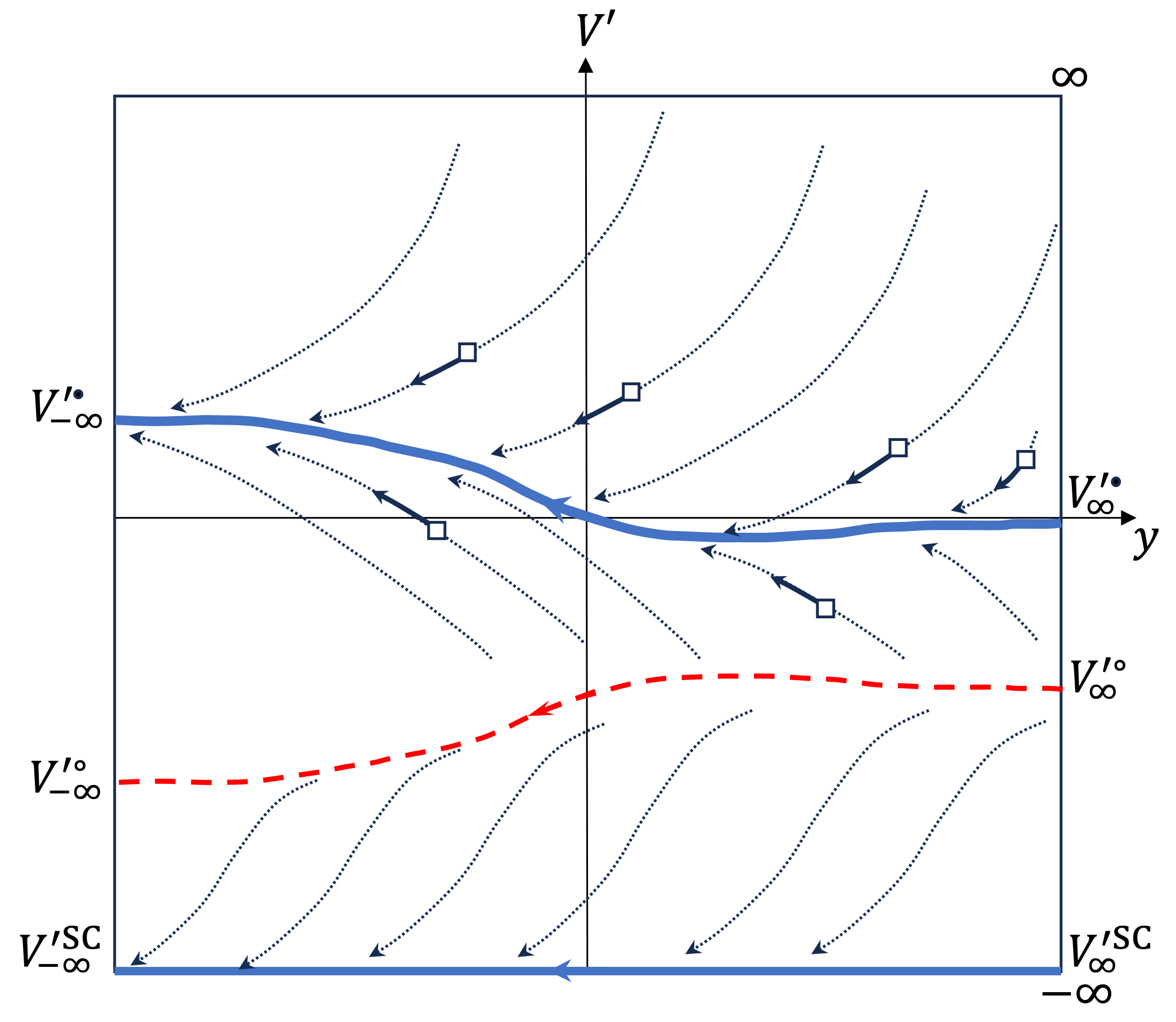
Refer to caption
(a)
Refer to caption
(b)
Refer to caption
(c)
Figure 22: Non-Fermi liquid to superconductor quantum phase transition in superuniversality class A. The similar picture holds for superuniversality classes AB, AC and ABC. (a) If all bare couplings denoted by open squares are above the separatrix PFP (dashed line), they are attracted to the metallic PFP (solid line above the separatrix PFP) at low energies, realizing the stable non-Fermi liquid. (b) If one of the couplings is outside the basin of attraction of the metallic PFP, the ground state is the superconducting state. (c) At the critical point, one of the couplings is on the separatrix PFP, realizing a critical non-Fermi liquid differentiated from the parent non-Fermi liquid by the critical pairing interaction.

Within each superuniversality class, there are multiple universality classes that are differentiated by their dynamical properties, such as superconducting fluctuations/instabilities and emergent symmetries. Here, we discuss individual universality classes that arise from each superuniversality class and explain their key properties in general terms.

  • •

    Stable non-Fermi liquids

    The superuniversality classes A, AB, AC and ABC support regular metallic PFPs: they are non-divergent and extended from y=∞y=\infty to −∞-\infty. Furthermore, there exists a separatrix PFP. In classes A and AC, the separatrix PFP is distinct from the metallic PFP, but in classes AB and ABC, the two coincide. If the bare couplings in all angular momentum channels are above the separatrix PFP, the metallic states survive to zero temperature. These non-Fermi liquids are stable against small perturbations of the bare four-fermion couplings because the region above the separatrix is extended in the (y,V′)(y,V^{\prime}) plane. The stable non-Fermi liquids that arise in different superuniversality classes are differentiated from each other in terms of their universal pairing interactions that emerge in the low-energy limit. In classes A, AC and ABC, the metallic PFP is the attractor for the couplings above the separatrix PFP (for example, see Fig. 22(a) for class A). Consequently, the universal pairing interactions are entirely fixed by the metallic PFP in these classes.

    Refer to caption
    Figure 23: In class AB, the metallic PFP, which is the same as the separatrix PFP, is locally stable (unstable) for y>yby>y_{b} (y<yb)(y<y_{b}). At a large but finite ll, the couplings that are initially above the separatrix PFP end up being close to the metallic PFP (V−∞′⁣∙V_{-\infty}^{\prime\,\bullet}) at large (small) angular momentum channels. Consequently, the quasi-universal pairing interaction that emerges at large ll, which is denoted as the thick grey line, interpolates the metallic PFP to V−∞′⁣∙V_{-\infty}^{\prime\,\bullet} across an ll-dependent crossover angular momentum scale yc​(l)y_{c}(l).

    The stable non-Fermi liquid realized in superuniversality class AB is unique in that the metallic PFP is connected to V−∞′⁣∘V_{-\infty}^{\prime\,\circ} whose basin of attraction is only the separatrix itself. While couplings at large angular momentum channels are attracted to the metallic PFP at intermediate energy scales, they eventually crossover to V−∞′⁣∙V_{-\infty}^{\prime\,\bullet} in the low energy limit. Consequently, the pairing interaction that emerges at low energies from a generic choice of bare couplings interpolates the metallic PFP at large yy to V−∞′⁣∙V_{-\infty}^{\prime\,\bullet} at small yy, as shown in Fig. 23. Due to this crossover, which becomes sharper with lowering energy, the universal pairing interaction that arises in class AB exhibits a stronger yy-dependence. This will be discussed in greater detail in Sec. X.

  • •

    Critical non-Fermi liquids

    In each superuniversality class (A, AB, AC, ABC) that supports the stable non-Fermi liquid, there are infinitely many critical non-Fermi liquid universality classes that can be obtained by tuning irrelevant couplings such as the four-fermion or higher-order couplings. Let us first consider the four-fermion coupling. If the coupling in one angular momentum channel is in the basin of attraction of the superconducting PFP, a superconducting instability occurs in that channel (Fig. 22(b)). A ‘critical’ non-Fermi liquid that describes a phase transition between the stable non-Fermi liquid and the superconducting state has the coupling in one angular momentum channel on the separatrix PFP with all other couplings above the separatrix PFP. These are illustrated in Fig. 22(c) for class A. This critical non-Fermi liquid has one relevant direction in the space of four-fermion coupling. The non-Fermi liquid to superconductor phase transition can be induced either by tuning the strength of the coupling or by tuning the Fermi momentum. The former and latter change the vertical and horizontal location of the bare coupling in the (y,V′)(y,V^{\prime}) plane, respectively. Critical non-Fermi liquids that arise from distinct superuniversality classes exhibit different critical exponents and represent distinct universality classes. There also exist multi-critical non-Fermi liquids where the pairing interactions in multiple angular momentum channels are placed on the separatrix through fine tuning. More generally, one can crank up a higher-order fermion coupling, such as the eight-fermion coupling. They can drive a phase transition from the stable non-Fermi liquid to a superconductor with charge 44 or higher. Generally, those critical points represent yet another distinct non-Fermi liquids.

  • •

    Superconductors

    The superuniversality classes B, C and BC do not have regular metallic PFP. This implies that there exist angular momentum channels for which the pairing interaction flows to −∞-\infty at low energies, irrespective of the choice of the bare coupling. Therefore, all non-Fermi liquids in these superuniversality classes become superconductors in the low-energy limit. The nature of the superconducting states realized at low temperatures is largely determined by the superuniversality class if there is a large separation of scale between Λ\Lambda and the superconducting transition temperature. Below, we discuss the universal features of the superconducting state in such cases.

    • –

      Superconductors in class C

      In this class, the universal pairing interaction is strong enough that incoherence of fermions can not prevent the pairing instability in the s-wave channel even if instabilities in non-s-wave channels can be avoided for some choices of bare four-fermion couplings. While the superconducting transition temperature TcT_{c} depends on the bare four-fermion coupling, the minimum s-wave superconducting transition temperature is fixed by the universal data of the superuniversality class.

    • –

      Superconductors in class B

      Refer to caption
      (a)
      Refer to caption
      (b)
      Figure 24: The metallic PFP (thick blue solid line) and the separatrix PFP (red dashed line) in superuniversality class B. The separatrix (metallic) PFP diverges to ∞\infty (−∞-\infty) at yS∗y^{*}_{S} (yM∗y^{*}_{M}). (a) Consider the case where all bare couplings are repulsive and large. In this case, there is no superconducting instability for the angular momentum channels with y(m)​(0)≤yS∗y^{(m)}(0)\leq y^{*}_{S} because they flow to V−∞′⁣∙V_{-\infty}^{\prime\,\bullet} or V−∞′⁣∘V_{-\infty}^{\prime\,\circ} in the low energy limit. Among the angular momentum channels with y(n)​(0)>yS∗y^{(n)}(0)>y^{*}_{S}, the superconductivity arises in the channel whose y(n)​(0)y^{(n)}(0) is closest to the optimal yy, denoted as yO∗y_{O}^{*}. The existence of yO∗y_{O}^{*} can be understood as follows. If y(n)​(0)y^{(n)}(0) is too close to yS∗y_{S}^{*} (y1y_{1} in the figure), it tracks the separatrix PFP for a large RG time before it diverges. If y(n)​(0)y^{(n)}(0) is too large (y2y_{2} in the figure), it is first attracted to the metallic PFP and diverges near yM∗y^{*}_{M}, which also makes lS​C∼2​(y2−yM∗)l_{SC}\sim 2(y_{2}-y^{*}_{M}) large. Because lS​Cl_{SC} diverges in both limits, there should exist yO∗y^{*}_{O} between yS∗y^{*}_{S} and ∞\infty at which lS​Cl_{SC} is minimized. (b) At a given 𝐤F{\bf k}_{F}, the channel whose y(n)​(0)y^{(n)}(0) is closest to yO∗y^{*}_{O} (denoted as mm in the figure) determines TcT_{c}. As 𝐤F{\bf k}_{F} is tuned with the bare coupling fixed, the relative position of y(m)​(0)y^{(m)}(0) to yO∗y^{*}_{O} changes, creating a local maximum of TcT_{c} at a specific choice of 𝐤F{\bf k}_{F} that satisfies y(m)​(0)=yO∗y^{(m)}(0)=y^{*}_{O}. If 𝐤F{\bf k}_{F} is increased, the bare couplings gradually shifts to left in the (y,V′)(y,V^{\prime}) plane until y(m+1)​(0)y^{(m+1)}(0) becomes closer to yO∗y_{O}^{*} than y(m)​(0)y^{(m)}(0) beyond a certain critical value of 𝐤F{\bf k}_{F}. This causes the jump of the angular momentum channel of superconducting instability from mm to m+1m+1 and an oscillation of TcT_{c} as a function of 𝐤F{\bf k}_{F}, as is shown in Fig. 11.

      In class B, a superconducting instability is inevitable above a non-zero critical angular momentum yS∗y^{*}_{S}, while the instability is absent below the critical angular momentum for sufficiently repulsive bare couplings. In y(m)​(0)<yS∗y^{(m)}(0)<y^{*}_{S}, which includes the s-wave channel, there is an extended basin of attraction that flows to V−∞′⁣∙V_{-\infty}^{\prime\,\bullet} under the RG flow. If the bare couplings lie in ℬV−∞∙I​R{\cal B}^{IR}_{V^{\bullet}_{-\infty}}, they flows to V−∞′⁣∙V_{-\infty}^{\prime\,\bullet} at low energies without causing an instability. The boundary of ℬV−∞∙I​R{\cal B}^{IR}_{V^{\bullet}_{-\infty}} is the separatrix PFP connected to V−∞′⁣∘V_{-\infty}^{\prime\,\circ}. The separatrix PFP diverges to ∞\infty at yS∗y_{S}^{*} under the reverse RG flow.141414If it does not diverge, it should be connected to V∞′⁣∙V_{\infty}^{\prime\,\bullet} or V∞′⁣∘V_{\infty}^{\prime\,\circ}, which results in either class AB or A. Since all points in the (y,V′)(y,V^{\prime}) plane with y>yS∗y>y_{S}^{*} lie outside ℬV−∞′⁣∙I​R{\cal B}^{IR}_{V_{-\infty}^{\prime\,\bullet}}, angular momentum channels with y(m)​(0)>yS∗y^{(m)}(0)>y_{S}^{*} cannot escape superconducting instabilities, no matter how large and repulsive the bare couplings are. In the limit that the bare couplings are large and repulsive, the angular momentum channel that exhibits the smallest lS​Cl_{SC}, the length scale for superconducting instability, is given by the channel whose y(m)​(0)y^{(m)}(0) is closest to an optimal yy, denoted as yO∗y^{*}_{O}. The optimal angular momentum exists between yS∗y^{*}_{S} and ∞\infty because lS​Cl_{SC} diverges as y(m)​(0)y^{(m)}(0) approaches either yS∗y^{*}_{S} or ∞\infty (see Fig. 24(a)). If 𝐤F{\bf k}_{F} is increased, {y(n)​(0)}\{y^{(n)}(0)\} shifts to the left, and mm for which y(m)​(0)y^{(m)}(0) is closest to yO∗y^{*}_{O} jumps from one angular momentum to the next at discrete values of 𝐤F{\bf k}_{F}. This results in a stepwise increase of mm for superconducting instability and an oscillation of TcT_{c} as a function of 𝐤F{\bf k}_{F}, as is shown in Fig. 11. See Fig. 24(b) for a more detailed illustration.

      Refer to caption
      (a)
      Refer to caption
      (b)
      Figure 25: (a) For a small nOn_{O} in Eq. (60), the set of (y(m)​(0),Vy(m)​(0)′​(0))\left(y^{(m)}(0),V_{y^{(m)}(0)}^{\prime}(0)\right) associated with the bare couplings is spare in the yy axis around yO∗y^{*}_{O}. Consequently, the angular momentum channel closest to yO∗y^{*}_{O} is generically well separated from yO∗y^{*}_{O}. If the bare coupling is not far from the metallic PFP, it is first attracted to the metallic PFP before it diverges near yM∗y^{*}_{M}. (b) In the large nOn_{O} limit, the bare couplings become dense in the yy axis near yO∗y^{*}_{O}. If the bare coupling is large and weakly dependent on the angular momentum, the superconducting instability occurs in the channel with y(m)​(0)≈yO∗y^{(m)}(0)\approx y^{*}_{O}.

      The superconducting transition temperature is not universal because it depends on the bare coupling. However, Tc/𝐤FzT_{c}/{\bf k}_{F}^{z}, where zz is the dynamical critical exponent, becomes insensitive to the bare coupling in certain limits. Such universality arises when the set of discrete bare couplings composed of (y(m)​(0),Vy(m)​(0)′​(0))\left(y^{(m)}(0),V_{y^{(m)}(0)}^{\prime}(0)\right) becomes dense or sparse near yS∗y_{S}^{*}. The angular momentum that corresponds to yO∗y_{O}^{*} is given by

      nO=2​γ​𝐤Fπ​Λ​eyO∗\displaystyle n_{O}=\frac{2\gamma\sqrt{{\bf k}_{F}}}{\pi\sqrt{\Lambda}}e^{y_{O}^{*}} (60)

      from Eq. (45). Near this angular momentum, the spacing between bare couplings in the y-axis is y(nO+1)​(0)−y(nO)​(0)=log⁡(nO+1)−log⁡nOy^{(n_{O}+1)}(0)-y^{(n_{O})}(0)=\log(n_{O}+1)-\log n_{O}. For a small nOn_{O}, y(n)​(0)y^{(n)}(0) becomes sparse near yO∗y^{*}_{O}, and the distance between y(n)​(0)y^{(n)}(0) with y(n)​(0)>yS∗y^{(n)}(0)>y^{*}_{S} and yO∗y^{*}_{O} is generically not small, as illustrated in Fig. 25(a). As a result, there is some RG time during which the coupling is attracted to the metallic PFP before it diverges at the superconducting scale. In such cases, y(n)​(0)−lS​C/2y^{(n)}(0)-l_{SC}/2 is close to yM∗y_{M}^{*} when the bare coupling is not too far from the metallic PFP. Since y(n)​(0)∼log⁡n​Λ𝐤Fy^{(n)}(0)\sim\log\frac{n\sqrt{\Lambda}}{\sqrt{{\bf k}_{F}}} and Tc∼e−z​lS​CT_{c}\sim e^{-zl_{SC}}, the ratio between Tc,nT_{c,n} and 𝐤Fz{\bf k}_{F}^{z} becomes

      Λz−1​Tc,n𝐤Fz≈(2​γn​π)2​z​e2​z​yM∗.\displaystyle\frac{\Lambda^{z-1}T_{c,n}}{{\bf k}_{F}^{z}}\approx\bigg(\frac{2\gamma}{n\pi}\bigg)^{2z}e^{2zy_{M}^{*}}. (61)

      In the large nOn_{O} limit, on the other hand, y(nO+1)​(0)−y(nO)​(0)∼1/nOy^{(n_{O}+1)}(0)-y^{(n_{O})}(0)\sim 1/n_{O}, which causes y(n)​(0)y^{(n)}(0) to be densely populated near yO∗y^{*}_{O}, as shown in Fig. 25(b). If the bare coupling is strongly repulsive and weakly depends on yy, there exists an angular momentum channel whose bare coupling is very close to the PFP that emanates from (yO∗,∞)(y_{O}^{*},\infty). In that case, superconducting instability occurs in channel nn with y(n)​(0)≈yO∗y^{(n)}(0)\approx y_{O}^{*} and the superconducting scale lS​Cl_{SC} satisfies y(n)​(0)−lS​C/2≈yS​C,O∗y^{(n)}(0)-l_{SC}/2\approx y_{SC,O}^{*}, where yS​C,O∗y_{SC,O}^{*} is the location at which the PFP from (yO∗,∞)(y_{O}^{*},\infty) diverges to −∞-\infty. In this case, Tc/𝐤FzT_{c}/{\bf k}_{F}^{z} is given by Eq. (61) with yM∗y_{M}^{*} replaced with yS​C,O∗y_{SC,O}^{*}. In Sec. X, we will discuss this in detail, including the corrections that depend on the bare coupling.

    • –

      Superconductors in class BC

      The superconducting state in this class is similar to that of class B in that the non-s-wave superconducting instability is inevitable. The universal Tc/𝐤FzT_{c}/{\bf k}_{F}^{z} relation and the oscillatory behavior of TcT_{c} vs 𝐤F{\bf k}_{F} hold similarly in this class. The main difference is that the pairing interactions at low angular momenta, including the s-wave channel, approach their universal values more ‘slowly’ with lowering energy scale due to the marginality of the −∞-\infty-asymptotic fixed point to which the couplings are attracted from above in the low-angular momentum channels.

  • •

    Quasi-universal non-Fermi liquids

    In superuniversality classes B, C and BC, the normal state is not stable at zero temperature. Because the RG flow is cut off by the superconductivity at low energies, one can’t have a true universal behavior in the non-Fermi liquid states realized above TcT_{c}. Nonetheless, the non-Fermi liquids exhibit quasi-universal behavior if Λ/Tc≫1\Lambda/T_{c}\gg 1, where Λ\Lambda is the energy scale below which the non-Fermi liquid physics sets in. This quasi-universal behavior is governed by a PFP, which is referred to as the regularized metallic PFP, toward which couplings are attracted at intermediate energy scales between Λ\Lambda and TcT_{c}. The regularized metallic PFP is identical to the metallic PFP in the range of yy in which the metallic PFP is locally stable and attractive. In the region of yy where the metallic PFP is locally unstable or absent, the coupling function is attracted to the profile for which the RG flow is stalled over a finite but large window of length scale.

As discussed above, there are three large families of non-Fermi liquids. The first is the family of stable non-Fermi liquids realized in classes A, AB, AC and ABC. The second is composed of critical non-Fermi liquids obtained by tuning some irrelevant couplings to critical values in the stable non-Fermi liquids. These two families are stable down to zero temperature. The third includes the quasi-universal non-Fermi liquids that arise in the intermediate energy scales above non-zero superconducting transition temperatures in classes B, BC and C. In the stable non-Fermi liquids, the scattering of Cooper pairs decays fast enough in the angle around the Fermi surface that the inter-patch coupling is negligible. Due to the suppression of the large-angle scatterings, these non-Fermi liquids possess the same emergent symmetry as Fermi liquids. On the other hand, the latter two families invariably exhibit a slow decay of large-angle scatterings of Cooper pairs. Due to the strong inter-patch couplings, the emergent symmetry is lower than that of Fermi liquids. To understand this, we need more dynamical information, which will be discussed in detail through examples in Sec. VII-X. In the next section, we discuss some subtleties that arise in determining the emergent symmetry of metals.

IV.5 Emergent symmetries of metals

In Fermi liquids, the number of particles is independently conserved at ‘every’ angle in the low-energy limit due to the lack of non-forward scatterings[52]. Consequently, the U(1) group for global number conservation is promoted to the loop U(1) (LU(1)) group, under which the fermion field at angle θ\theta is transformed as

Tζ:ψ​(θ)→ei​ζ​(θ)​ψ​(θ),\displaystyle T_{\zeta}:\psi(\theta)\rightarrow e^{i\zeta(\theta)}\psi(\theta), (62)

where ζ​(θ)\zeta(\theta) is a general smooth function of angle. For simplicity, we focus on d=2d=2 in this section. The emergent symmetry of non-Fermi liquids is less clear because of the presence of universal non-forward interactions, such as the pairing interaction. The emergent symmetry depends on the type of non-Fermi liquids: some non-Fermi liquids have the full LU(1) group[27], but others only retain a proper subgroup of the LU(1) group. In this section, we discuss a subtlety that arises from the projective nature of metallic fixed points when determining the emergent symmetry.

While microscopic symmetry is a property of the Hamiltonian, the emergent symmetry is a property of low-energy observables. Roughly speaking, a symmetry emerges if low-energy observables are invariant under the corresponding transformation, even if it is not a symmetry of the microscopic Hamiltonian. As an example of low-energy observables, let us consider the 2​n2n-point fermion vertex function,

Γ\displaystyle\Gamma =\displaystyle= ∑n∫[∏i=12​ndωidk→i]Γ(2​n)({ωi},{k→i})δ(∑i=1nωi−∑i=n+12​nωi)δ(∑i=1nk→i−∑i=n+12​nk→i)×\displaystyle\sum_{n}\int\left[\prod_{i=1}^{2n}d\omega_{i}d\vec{k}_{i}\right]\Gamma^{(2n)}\left(\{\omega_{i}\},\{\vec{k}_{i}\}\right)\delta\left(\sum_{i=1}^{n}\omega_{i}-\sum_{i=n+1}^{2n}\omega_{i}\right)\delta\left(\sum_{i=1}^{n}\vec{k}_{i}-\sum_{i=n+1}^{2n}\vec{k}_{i}\right)\times (63)
ψ†(ω1,k→1)ψ†(ω2,k→2)..ψ†(ωn,k→n)ψ(ωn+1,k→n+1)ψ(ωn+2,k→n+2)..ψ(ω2​n,k→2​n)\displaystyle\psi^{\dagger}(\omega_{1},\vec{k}_{1})\psi^{\dagger}(\omega_{2},\vec{k}_{2})..\psi^{\dagger}(\omega_{n},\vec{k}_{n})\psi(\omega_{n+1},\vec{k}_{n+1})\psi(\omega_{n+2},\vec{k}_{n+2})..\psi(\omega_{2n},\vec{k}_{2n})

measured at low frequencies. In general, one can choose any momenta {k→i}\{\vec{k}_{i}\}, but for low-energy observables, we focus on the set of momenta at which the vertex function is non-analytic as a function of frequencies in the ωi→0\omega_{i}\rightarrow 0 limit, S​i​n​g​K(n)={{k→i}|Γ(n)​({ωi},{k→i})​ is non-analytic at​ωi=0}SingK^{(n)}=\left\{\{\vec{k}_{i}\}\Bigl|\Gamma^{(n)}\left(\{\omega_{i}\},\{\vec{k}_{i}\}\right)\mbox{ is non-analytic at}~~\omega_{i}=0\Bigr.\right\}. Momenta outside S​i​n​g​K(n)SingK^{(n)} only contribute to the short-time (high-energy) dynamics and can be ignored in the long-time (low-energy) limit. In metal, S​i​n​g​K(n)SingK^{(n)} corresponds to the set of Fermi momenta, {𝐊F,θ|0≤θ<2​π}\{{\bf K}_{F,\theta}|0\leq\theta<2\pi\}. A necessary condition for TζT_{\zeta} to be an emergent symmetry is that the vertex function is invariant under TζT_{\zeta} in the low-frequency limit at all external momenta on the Fermi surface. In Fermi liquids, only the forward scatterings survive in the low-energy limit, and the LU(1) indeed emerges as a low-energy symmetry.

In non-Fermi liquids, in addition to the forward scattering, there exist non-zero universal pairing interactions generated from the critical fluctuations. Because the forward scattering does not change the symmetry, even in non-Fermi liquids, we focus here on the pairing channel. The universal pairing interaction is encoded in the coupling function via the renormalization condition,

λθ1,θ2(P)​(μ)∼μd−1​Γ(4)​({ωi},{𝐊F,θ2,𝐊F,θ2+π,𝐊F,θ1+π,𝐊F,θ1})ωi=αi​μ,\displaystyle\lambda^{(P)}_{\theta_{1},\theta_{2}}(\mu)\sim\mu^{d-1}\Gamma^{(4)}\left(\{\omega_{i}\},\{{\bf K}_{F,\theta_{2}},{\bf K}_{F,\theta_{2}+\pi},{\bf K}_{F,\theta_{1}+\pi},{\bf K}_{F,\theta_{1}}\}\right)_{\omega_{i}=\alpha_{i}\mu}, (64)

where αi\alpha_{i} are RG scheme-dependent numbers that are O​(1)O(1). The precise relation between the coupling function and the vertex function depends on the RG scheme encoded in the choice of αi\alpha_{i}. See Appendix A for the scheme used in this paper. The factor of μd−1\mu^{d-1} is introduced to make the left-hand side a dimensionless quantity. The one-particle irreducible vertex function λθ1,θ2(P)\lambda^{(P)}_{\theta_{1},\theta_{2}} is related to the net two-body interaction Vθ¯1,θ¯2′V_{\bar{\theta}_{1},\bar{\theta}_{2}}^{\prime} through

Vθ¯1,θ¯2′⁣±=μ​a′​(θ¯1)​a′​(θ¯2)​KF,θ1​KF,θ2vF,θ1​vF,θ2​[λθ1,θ2(P,d)​(q→=0)±λθ1,θ2(P,e)​(q→=0)]+h¯d;θ¯1,θ¯2±4,\displaystyle V_{\bar{\theta}_{1},\bar{\theta}_{2}}^{\prime\,\pm}=\sqrt{\mu a^{\prime}(\bar{\theta}_{1})a^{\prime}(\bar{\theta}_{2})}\sqrt{\frac{K_{F,\theta_{1}}K_{F,\theta_{2}}}{v_{F,\theta_{1}}v_{F,\theta_{2}}}}\left[\lambda^{(P,d)}_{\theta_{1},\theta_{2}}(\vec{q}=0)\pm\lambda^{(P,e)}_{\theta_{1},\theta_{2}}(\vec{q}=0)\right]+\frac{\bar{h}^{\pm}_{d;\bar{\theta}_{1},\bar{\theta}_{2}}}{4}, (65)

where the net two-body interaction is written as a function of the proper angle θ¯\bar{\theta}, which is in one-to-one correspondence with the original angle θ\theta (see Eq. (33)). Since physical observables such as the anomalous dimension generated from the four-fermion coupling and the critical boson is determined from V′⁣±V^{\prime\,\pm}, it is convenient to use Vθ¯1,θ¯2′⁣±V_{\bar{\theta}_{1},\bar{\theta}_{2}}^{\prime\,\pm} to determine the emergent symmetry. Under TζT_{\zeta}, Vθ¯1,θ¯2′⁣±​(μ)V_{\bar{\theta}_{1},\bar{\theta}_{2}}^{\prime\,\pm}(\mu) is transformed into

[Tζ​V′⁣±]θ¯1,θ¯2​(μ)=exp⁡{−i​[ζ​(θ1)+ζ​(θ1+π)−ζ​(θ2)−ζ​(θ2+π)]}​Vθ¯1,θ¯2′⁣±​(μ).\displaystyle[T_{\zeta}V^{\prime\,\pm}]_{\bar{\theta}_{1},\bar{\theta}_{2}}(\mu)=\exp\left\{-i\left[\zeta(\theta_{1})+\zeta(\theta_{1}+\pi)-\zeta(\theta_{2})-\zeta(\theta_{2}+\pi)\right]\right\}V_{\bar{\theta}_{1},\bar{\theta}_{2}}^{\prime\,\pm}(\mu). (66)

To be concrete, let us consider an example of the form,

Vθ¯+Δ​θ¯,θ¯′⁣±​(μ)∼{1,for​|Δ​θ¯|≪μ,|μΔ​θ¯|Δfor​μ≪|Δ​θ¯|≪1\displaystyle V_{\bar{\theta}+\Delta\bar{\theta},\bar{\theta}}^{\prime\,\pm}(\mu)\sim\left\{\begin{array}[]{cc}1,&\mbox{for}~~~|\Delta\bar{\theta}|\ll\sqrt{\mu},\\ \left|\frac{\sqrt{\mu}}{\Delta\bar{\theta}}\right|^{\Delta}&\mbox{for}~~~\sqrt{\mu}\ll|\Delta\bar{\theta}|\ll 1\end{array}\right. (69)

with Δ>0\Delta>0. In Secs. VII - X, we will see that this type of universal pairing interaction arises in physical examples, where Δ\Delta is the universal exponent specific to each universality class. In Eq. (69), the pairing interaction vanishes in the small μ\mu limit for any fixed θ1≠θ2\theta_{1}\neq\theta_{2}. As a result,

Vθ¯1,θ¯2′⁣±​(μ)−[Tζ​V′⁣±]θ¯1,θ¯2​(μ)\displaystyle V_{\bar{\theta}_{1},\bar{\theta}_{2}}^{\prime\,\pm}(\mu)-[T_{\zeta}V^{\prime\,\pm}]_{\bar{\theta}_{1},\bar{\theta}_{2}}(\mu) (70)

goes to zero for any smooth ζ​(θ)\zeta(\theta) in the small μ\mu limit. From this, one may conclude that the full LU(1) symmetry emerges in the low-energy limit as long as Δ>0\Delta>0. However, this is not necessarily true because there can be other low-energy observables that are not invariant under the general LU(1) transformation for some Δ>0\Delta>0. This subtlety arises because metals have infinitely many low-energy observables, and observables that probe the entire Fermi surface are more sensitive than others to large-angle scatterings.

Refer to caption
(a)
Refer to caption
(b)
Figure 26: Either the four-fermion operator in the pairing channel (a) or a higher-order composite operator that includes a Cooper pair in the external legs (b) acquires an anomalous dimension through virtual Cooper pairs that can be created across the Fermi surface. The external legs dressed by V′V^{\prime} are in the Cooper channel; θ​(θ¯1+2​θ¯m​a​x)=θ​(θ¯1)+π\theta(\bar{\theta}_{1}+2\bar{\theta}_{max})=\theta(\bar{\theta}_{1})+\pi.

One such observable is the anomalous dimension of composite operators of fermions. The vertex correction shown in Fig. 26 contributes

η​[V′⁣±]=∫d​θ¯2​π​μ​Vθ¯1,θ¯1+θ¯′⁣±\displaystyle\eta[V^{\prime\,\pm}]=\int\frac{d\bar{\theta}}{2\pi\sqrt{\mu}}V_{\bar{\theta}_{1},\bar{\theta}_{1}+\bar{\theta}}^{\prime\,\pm} (71)

to the anomalous dimension of the composite operator whose external momenta for the pair of fermions are in the s-wave channel. In the beta function in Eq. (43), the term that is quadratic in 𝔙′{\mathfrak{V}}^{\prime} (which is the same as V′V^{\prime}) is nothing but the contribution of the anomalous dimension of the two-body interaction generated from the two-body interaction itself. If Δ≤1\Delta\leq 1, the contribution from θ¯≫μ\bar{\theta}\gg\sqrt{\mu} is large although Vθ¯1,θ¯1+θ¯′⁣±V_{\bar{\theta}_{1},\bar{\theta}_{1}+\bar{\theta}}^{\prime\,\pm} is negligible at individual θ¯\bar{\theta}. What is crucial is the measure d​θ¯μ\frac{d\bar{\theta}}{\sqrt{\mu}} that increases with decreasing μ\mu in the expression of the anomalous dimension. It captures the fact that the critical boson carries a typical momentum qθ​(μ)∼μ​𝐤Fq_{\theta}(\mu)\sim\sqrt{\mu{\bf k}_{F}} at the energy scale μ\mu as shown in Eq. (34), and two fermions separated by an angle larger than qμ/𝐊F,θq_{\mu}/{\bf K}_{F,\theta} contribute to the anomalous dimension independently[113]. Δ​θ¯μ\frac{\Delta\bar{\theta}}{\sqrt{\mu}} denotes the number of such patches within Δ​θ¯\Delta\bar{\theta} that additively contribute to the anomalous dimension. As a result, the net anomalous dimension is proportional to the size of the Fermi surface measured in the proper angle. The angular metric in Eq. (35), which increases with decreasing μ\mu, accounts for the fact that the number of such patches increases with decreasing energy. For Δ≤1\Delta\leq 1, the integral becomes ‘UV’-divergent in the KF→∞K_{F}\to\infty limit, as the contribution from large-angle scatterings accumulates. Therefore,

limμ→0η​[Tζ​V′⁣±]−η​[V′⁣±]≠0\displaystyle\lim_{\mu\rightarrow 0}\eta[T_{\zeta}V^{\prime\,\pm}]-\eta[V^{\prime\,\pm}]\neq 0 (72)

for general smooth function of ζ​(θ)\zeta(\theta) if Δ≤1\Delta\leq 1. In this case, the anomalous dimension is invariant only under the proper subgroup OLU​(1)\text{OLU}(1) [59] for which ζ​(θ)\zeta(\theta) is constrained to satisfy

ζ​(θ+π)=−ζ​(θ).\displaystyle\zeta(\theta+\pi)=-\zeta(\theta). (73)

Another example that we will encounter in physical examples has a universal pairing interaction of the form,

Vθ¯+Δ​θ¯,θ¯′⁣±​(μ)∼μθ¯m​a​x.\displaystyle V_{\bar{\theta}+\Delta\bar{\theta},\bar{\theta}}^{\prime\,\pm}(\mu)\sim\frac{\sqrt{\mu}}{\bar{\theta}_{max}}. (74)

At each angle, it has a vanishingly small overall amplitude in the low-energy limit. However, its amplitude does not decay at large angles. The large-angle scatterings add up to give rise to a non-trivial anomalous dimension in Eq. (71) in the low-energy limit. Therefore, the universal pairing interaction of the form in Eq. (74) also breaks the LU(1) to OLU(1).

V Toy model

As the first example, we consider a toy model for which the beta functional of the pairing interaction is exactly solvable. While the toy model is not realistic, its role is to offer an economical and analytical route to realizing distinct superuniversality classes, given that topology of general PFPs is insensitive to the details of the theory. Furthermore, it provides useful insight into how various features of general PFPs are affected by the tunable parameters of the model.

Refer to caption
(a)
Refer to caption
(b)
Figure 27: (a) The source Sy′S_{y}^{\prime} that describes the universal pairing interaction generated from the U(1) gauge field as a function of the logarithmic angular momentum yy in d=2d=2. (b) A toy source S′⁣(toy)S^{\prime\,(\text{toy})} that has been tailored to mimic the source of the gauge theory. The example shown uses h−∞=S−∞′h_{-\infty}=S^{\prime}_{-\infty} and hw=−0.12h_{w}=-0.12, w=1.5w=1.5 for the intermediate region.

We begin by writing the differential equation for PFPs as

12​∂yVy′=Rd​(Vy′+2​𝐇d−14​Rd)2−116​Rd​ηP,y,\displaystyle\frac{1}{2}\partial_{y}V_{y}^{\prime}=R_{d}\bigg(V_{y}^{\prime}+\frac{2{\bf H}_{d}-1}{4R_{d}}\bigg)^{2}-\frac{1}{16R_{d}}\eta_{P,y}, (75)

where ηP,y=(2​𝐇d−1)2+16​Rd​Sy′\eta_{P,y}=(2{\bf H}_{d}-1)^{2}+16R_{d}S_{y}^{\prime} is the yy-dependent discriminant. This differential equation has qualitatively distinct solutions, depending on the scaling dimension 𝐇d{\bf H}_{d} and the angular momentum-dependent source Sy′S_{y}^{\prime}. However, it is difficult to solve it exactly because of the yy-dependence of the source. For example, the source generated from the U(1) gauge field is shown in Fig. 27(a). The source has three qualitatively important features. Firstly, it vanishes in the large yy limit, as is required by locality. The pairing interaction generated from critical fluctuations at a non-zero energy scale must be an analytic function of angle, and its Fourier component must vanish in the large angular momentum limit. Secondly, the source in the y→−∞y\rightarrow-\infty limit is dictated by the s-wave pairing interaction generated by critical fluctuations. Its sign is given by Eq. (5). For the U(1) gauge field, the Amperian law implies that a pair of fermions with opposite momenta repel each other, resulting in a repulsive source. On the other hand, the C4C_{4} symmetric Ising nematic critical fluctuations generate an attractive interaction in the s-wave channel, and its Sy′S_{y}^{\prime} is opposite to that of the U(1) gauge theory. Sy′S_{y}^{\prime} is well approximated by S∞′S_{\infty}^{\prime} and S−∞′S_{-\infty}^{\prime} in y≫wLy\gg w_{L} and y≪wSy\ll w_{S}, respectively, where wLw_{L} and wLw_{L} denote the crossover scales. Finally, there is a transient region of finite yy between wSw_{S} and wLw_{L} in which |Sy′||S_{y}^{\prime}| is significant, and the sign of the source is opposite to that of the s-wave limit. The existence of the transient region is guaranteed by the traceless condition of the source in Eq. (44): if the source is repulsive (attractive) in the s-wave limit, there must be a range of angular momentum in which it is attractive (repulsive). In the U(1) gauge theory, the interaction vertex is positive definite in angular space, giving rise to the repulsive pairing interaction in the s-wave channel. Nonetheless, it gives rise to an attractive interaction in non-zero angular momentum channels in which critical bosons predominantly scatter Cooper pairs between parts of the Fermi surface that have opposite phases in the pairing wavefunction.

For our toy model, we consider a piece-wise constant Sy′S_{y}^{\prime}, which captures these three features of the sources. The source of the toy model reads

Sy′⁣(toy)={0fory≥wL(region I)hwforwS<y<wL(region II)h−∞​fory≤wS(region III).\displaystyle S_{y}^{\prime\,(\text{toy})}=\begin{cases}0~~~~~~~~\text{for}\quad y\geq w_{L}~&~\text{(region I)}\\ h_{w}~~~~~~\text{for}\quad w_{S}<y<w_{L}~&~\text{(region II)}\\ h_{-\infty}~~~\text{for}\quad y\leq w_{S}~&~\text{(region III)}\end{cases}. (76)

As discussed below Eq. (50), only wL−wSw_{L}-w_{S} is the independent parameter. Accordingly, the superuniversality class only depends on the width of the intermediate region, w≡wL−wSw\equiv w_{L}-w_{S}. From now on, we set wS=0w_{S}=0 and wL=ww_{L}=w. The region I represents the large yy limit where the source of the four-fermion coupling is negligible. The region II with width ww represents a crossover region where the source takes a ‘transient’ value hwh_{w}. The region III is the asymptotic small-angular momentum region where the source takes a constant value of h−∞h_{-\infty}, which represents the source in the s-wave limit. The tunable parameters of the toy model are ww, hwh_{w} and h−∞h_{-\infty} along with the scaling dimension 𝐇d{\bf H}_{d}. We will see that the toy model with these parameters is general enough to provide access to all superuniversality classes discussed in the previous section.

To begin our analysis of the toy model, let us first consider the general PFP solution. This is given by the piecewise function Vy′V_{y}^{\prime} valid in each region, where

Vy′=14​Rd​[−η​tanh⁡(12​η​y+Φ)−2​𝐇d+1],\displaystyle V_{y}^{\prime}=\frac{1}{4R_{d}}\Big[-\sqrt{\eta}\tanh\Big(\frac{1}{2}\sqrt{\eta}y+\Phi\Big.)-2{\bf H}_{d}+1\Big], (77)

where

η={ηP,∞,y≥w,ηP,w,for 0<y<w,ηP,−∞,for y≤0\displaystyle\eta=\begin{cases}\eta_{P,\infty},&\text{$y\geq w$},\\ \eta_{P,w},&\text{for $0<y<w$},\\ \eta_{P,-\infty},&\text{for $y\leq 0$}\end{cases} (78)

represents the discriminant in each region. This expression with real Φ\Phi makes the reality of Vy′V_{y}^{\prime} manifest in the region with a positive discriminant η\eta. For η<0\eta<0, we analytically continue η→i​−η\sqrt{\eta}\rightarrow i\sqrt{-\eta} and Φ→i​Φ~\Phi\rightarrow i\tilde{\Phi} to write the general solution as

Vy′=14​Rd​[−η​tan⁡(12​−η​y+Φ~)−2​𝐇d+1].\displaystyle V_{y}^{\prime}=\frac{1}{4R_{d}}\Big[\sqrt{-\eta}\tan\Big(\frac{1}{2}\sqrt{-\eta}y+\tilde{\Phi}\Big.)-2{\bf H}_{d}+1\Big]. (79)

Because Sy′=0S_{y}^{\prime}=0 in region I, ηP,∞≥0\eta_{P,\infty}\geq 0. While ηP,w\eta_{P,w} and ηP,−∞\eta_{P,-\infty} can take either sign, we can focus on the cases with ηP,w<0\eta_{P,w}<0 without loss of generality. This is because an intermediate region of ηP,w≥0\eta_{P,w}\geq 0 can be essentially merged into region I and does not generate topologically new classes. The constants Φ\Phi (alternatively Φ~\tilde{\Phi}) are fixed by a boundary condition that a particular PFP satisfies. The most important particular solutions for identifying the topological class of a general PFP are the metallic and separatrix PFPs. In the toy model, the metallic PFP is the one that satisfies limy→∞Vy′=V∞′⁣∙\lim_{y\rightarrow\infty}V_{y}^{\prime}=V_{\infty}^{\prime\,\bullet},

Vy′⁣M=14​Rd​{ηP,∞−2​𝐇d+1fory≥w−ηP,w​tan⁡(12​−ηP,w​y+Φ~I​IM)−2​𝐇d+1for0<y<w−ηP,−∞​tanh⁡(12​ηP,−∞​y+ΦI​I​IM)−2​𝐇d+1fory≤0.\displaystyle V_{y}^{\prime\,M}=\frac{1}{4R_{d}}\begin{cases}\sqrt{\eta_{P,\infty}}-2{\bf H}_{d}+1&\text{for}\quad y\geq w\\ \sqrt{-\eta_{P,w}}\tan\Big(\frac{1}{2}\sqrt{-\eta_{P,w}}y+\tilde{\Phi}_{II}^{M}\Big.)-2{\bf H}_{d}+1&\text{for}\quad 0<y<w\\ -\sqrt{\eta_{P,-\infty}}\tanh\Big(\frac{1}{2}\sqrt{\eta_{P,-\infty}}y+\Phi_{III}^{M}\Big.)-2{\bf H}_{d}+1~~~&\text{for}\quad y\leq 0\end{cases}. (80)

It is understood that ηP,−∞\sqrt{\eta_{P,-\infty}} and ΦI​I​IM\Phi_{III}^{M} are imaginary if ηP,−∞<0\eta_{P,-\infty}<0. For the metallic PFP, the phases in regions II and III are

Φ~I​IM\displaystyle\tilde{\Phi}_{II}^{M} =\displaystyle= −12​−ηP,w​w+arctan⁡(ηP,∞−ηP,w),\displaystyle-\frac{1}{2}\sqrt{-\eta_{P,w}}w+\arctan\Big(\frac{\sqrt{\eta_{P,\infty}}}{\sqrt{-\eta_{P,w}}}\Big.),
ΦI​I​IM\displaystyle\Phi_{III}^{M} =\displaystyle= −arctanh​{−ηP,wηP,−∞​tan⁡[−12​−ηP,w​w+arctan⁡(ηP,∞−ηP,w)]}.\displaystyle-\text{arctanh}\left\{\frac{\sqrt{-\eta_{P,w}}}{\sqrt{\eta_{P,-\infty}}}\tan[-\frac{1}{2}\sqrt{-\eta_{P,w}}w+\arctan\Big(\frac{\sqrt{\eta_{P,\infty}}}{\sqrt{-\eta_{P,w}}}\Big.)\Big]\right\}. (81)

It is noted that in the first line of Eq. (80), the combination ηP,∞−2​𝐇d+1\sqrt{\eta_{P,\infty}}-2{\bf H}_{d}+1 is equal to zero because S∞′=0S_{\infty}^{\prime}=0. However, we will continue writing expressions as has been done above to keep the separate roles of ηP,∞\sqrt{\eta_{P,\infty}} and −2​𝐇d+1-2{\bf H}_{d}+1 more manifest. For ηP,−∞≥0\eta_{P,-\infty}\geq 0, there exists the separatrix PFP that satisfies limy→−∞Vy′⁣S=14​Rd​(−ηP,−∞−2​𝐇d+1)\lim_{y\rightarrow-\infty}V_{y}^{\prime\,S}=\frac{1}{4R_{d}}\left(-\sqrt{\eta_{P,-\infty}}-2{\bf H}_{d}+1\right),

Vy′⁣S=14​Rd​{−ηP,∞​tanh⁡(12​ηP,∞​y+ΦIS)−2​𝐇d+1fory≥w−ηP,w​tan⁡(12​−ηP,w​y+Φ~I​IS)−2​𝐇d+1for0<y<w−ηP,−∞−2​𝐇d+1fory≤0\displaystyle V_{y}^{\prime\,S}=\frac{1}{4R_{d}}\begin{cases}-\sqrt{\eta_{P,\infty}}\tanh\Big(\frac{1}{2}\sqrt{\eta_{P,\infty}}y+\Phi_{I}^{S}\Big.)-2{\bf H}_{d}+1&\text{for}\quad y\geq w\\ \sqrt{-\eta_{P,w}}\tan\Big(\frac{1}{2}\sqrt{-\eta_{P,w}}y+\tilde{\Phi}^{S}_{II}\Big.)-2{\bf H}_{d}+1&\text{for}\quad 0<y<w\\ -\sqrt{\eta_{P,-\infty}}-2{\bf H}_{d}+1~~~&\text{for}\quad y\leq 0\end{cases} (82)

with

ΦIS\displaystyle\Phi_{I}^{S} =\displaystyle= −12​ηP,∞​w−arctanh​{−ηP,wηP,∞​tan⁡[12​−ηP,w​w−arctan⁡(ηP,−∞−ηP,w)]},\displaystyle-\frac{1}{2}\sqrt{\eta_{P,\infty}}w-\text{arctanh}\left\{\frac{\sqrt{-\eta_{P,w}}}{\sqrt{\eta_{P,\infty}}}\tan[\frac{1}{2}\sqrt{-\eta_{P,w}}w-\arctan\Big(\frac{\sqrt{\eta_{P,-\infty}}}{\sqrt{-\eta_{P,w}}}\Big.)\Big]\right\},
Φ~I​IS\displaystyle\tilde{\Phi}^{S}_{II} =\displaystyle= −arctan⁡(ηP,−∞−ηP,w).\displaystyle-\arctan\Big(\frac{\sqrt{\eta_{P,-\infty}}}{\sqrt{-\eta_{P,w}}}\Big.). (83)
Refer to caption
Figure 28: The superuniversality phase diagram of the toy model with 𝐇d=1{\bf H}_{d}=1 and ηP,w=−1\eta_{P,w}=-1. The boundary between classes A and B represents the line of critical widths given by ηP,−∞​(w)=tan2⁡[12​(w−π2)]\eta_{P,-\infty}(w)=\tan^{2}\big[\frac{1}{2}(w-\frac{\pi}{2})\big].

The topology of the general PFPs is determined by the behaviors of the metallic and separatrix PFPs. While all parameters of the toy model can be tuned, we do not need to do so because all seven superuniversality classes can be realized for fixed 𝐇d{\bf H}_{d} and ηP,w<0\eta_{P,w}<0. Therefore, we only tune ηP,−∞\eta_{P,-\infty} and ww (note that ηP,∞\eta_{P,\infty} is fixed by 𝐇d{\bf H}_{d}). ηP,−∞\eta_{P,-\infty} controls the strength of the universal pairing interaction relative to the incoherence of fermions in the s-wave channel. The stronger the attractive s-wave pairing interaction is, and the more coherent the fermions are, the smaller ηP,−∞\eta_{P,-\infty} becomes. When ηP,−∞\eta_{P,-\infty} is negative, the metallic PFP behaves as a tangent function in region III and is guaranteed to diverge. On the other hand, ww is the range of the non-zero angular momentum on the logarithmic scale in which the attractive interaction is strong enough to overcome the pair-breaking effect of incoherent fermions and make ηP,w\eta_{P,w} negative. For a wide ‘well’, the coupling of a large angular momentum channel is renormalized with the attractive pairing interaction over a long RG time before the drift of yy brings the coupling to region III, increasing the propensity for non-s-wave superconductivity. If the width is sufficiently large, the metallic PFP diverges to −∞-\infty, which can occur either in region II or III. Since the topology of the general PFP does not depend on where the metallic PFP diverges, for the topological classification, we focus on the cases in which the metallic PFP diverges in region III. This is more convenient for studying the phase transition to class A because the metallic PFP is bound to diverge in region III near the boundary with class A. In this case, both metallic and separatrix PFPs remain regular in region II, and the width is bounded by w<wm​a​x≡1−ηP,w​[π+2​min⁡{arctan⁡((ηP,∞−ηP,w)),arctan⁡((ηP,−∞−ηP,w))}]w<w_{max}\equiv\frac{1}{\sqrt{-\eta_{P,w}}}\Big[\pi+2\min\Big\{\arctan{\Big(\frac{\sqrt{\eta_{P,\infty}}}{\sqrt{-\eta_{P,w}}}\Big)},\arctan{\Big(\frac{\sqrt{\eta_{P,-\infty}}}{\sqrt{-\eta_{P,w}}}\Big)}\Big\}\Big].

Fig. 28 is the ‘phase diagram’ of superuniversality classes realized in the plane of ηP,−∞\eta_{P,-\infty} and ww. For ηP,−∞<0\eta_{P,-\infty}<0, the attractive pairing interaction in the s-wave channel is strong enough to overcome the incoherence. In this case, the s-wave superconducting instability is unavoidable, and class C is realized. For ηP,−∞>0\eta_{P,-\infty}>0, there are two asymptotic fixed-points in the small yy regime – one stable and one unstable. In such situations, the s-wave superconducting instability can be avoided with a repulsive bare coupling. Then, either class A, AB, or B is realized depending on the choice of ww. If ww is smaller than the critical width,

wc≡2−ηP,w​[arctan⁡(ηP,−∞−ηP,w)+arctan⁡(ηP,∞−ηP,w)],\displaystyle w_{c}\equiv\frac{2}{\sqrt{-\eta_{P,w}}}\Big[\arctan\Big(\frac{\sqrt{\eta_{P,-\infty}}}{\sqrt{-\eta_{P,w}}}\Big.)+\arctan\Big(\frac{\sqrt{\eta_{P,\infty}}}{\sqrt{-\eta_{P,w}}}\Big.)\Big], (84)

the range of non-zero angular momenta with strong attractive interaction is not wide enough to cause a singularity in the metallic PFP. In this case, the real part of ΦI​I​IM\Phi^{M}_{III} is negative, and the metallic PFP, which takes the form of either a hyperbolic tangent or hyperbolic cotangent in region III, remains regular for y<0y<0. Therefore, the general PFP belongs to the stable NFL class (class A). For large enough widths (w>wcw>w_{c}) 151515But still smaller than wm​a​xw_{max} so that the profile stays regular in region II., the metallic PFP lies outside ℬV−∞′⁣∙I​R{\cal B}^{IR}_{V_{-\infty}^{\prime\,\bullet}}, and enters region III below V−∞′⁣∘V_{-\infty}^{\prime\,\circ}. In this case, the non-s-wave SC class (class B) is realized. If w=wcw=w_{c}, the metallic PFP flows to V−∞′⁣∘V_{-\infty}^{\prime\,\circ} in the small yy limit. This corresponds to class AB. wcw_{c} marks the critical point for the topological phase transition between classes A and B.

The final three superuniversality classes are realized when ηP,−∞=0\eta_{P,-\infty}=0. In this case, there exists a marginal −∞-\infty asymptotic fixed point. This requires fine-tuning of the universal pairing interaction in the s-wave channel relative to the anomalous dimension. On the critical line of ηP,−∞=0\eta_{P,-\infty}=0, the sign of w−wcw-w_{c} determines which of the classes AC, ABC, or BC is realized. For this, it is useful to have the profile of the metallic PFP in the ηP,−∞→0+\eta_{P,-\infty}\to 0^{+} limit,

Vy,I​I​I′⁣M=14​Rd​{−−ηP,w​tan⁡[12​−ηP,w​(w−wc)]1+12​−ηP,w​tan⁡[12​−ηP,w​(w−wc)]​y−2​𝐇d+1}for ​ηP,−∞=0,\displaystyle V_{y,III}^{\prime\,M}=\frac{1}{4R_{d}}\Bigg\{-\frac{\sqrt{-\eta_{P,w}}\tan[\frac{1}{2}\sqrt{-\eta_{P,w}}(w-w_{c})\Big]}{1+\frac{1}{2}\sqrt{-\eta_{P,w}}\tan[\frac{1}{2}\sqrt{-\eta_{P,w}}(w-w_{c})\Big]\,y}-2{\bf H}_{d}+1\Bigg\}~~~~\text{for }\sqrt{\eta_{P,-\infty}}=0, (85)

where the argument of the tangent function has been written in terms of the deviation δ​w=w−wc\delta w=w-w_{c} from critical width as defined above. When w<wcw<w_{c}, the metallic PFP is within ℬV−∞′⁣I​R{\cal B}^{IR}_{V_{-\infty}^{\prime\,\hbox to4.21pt{\vbox to4.21pt{\pgfpicture\makeatletter\hbox{\>\lower-2.10709pt\hbox to0.0pt{\pgfsys@beginscope\pgfsys@invoke{ }\definecolor{pgfstrokecolor}{rgb}{0,0,0}\pgfsys@color@rgb@stroke{0}{0}{0}\pgfsys@invoke{ }\pgfsys@color@rgb@fill{0}{0}{0}\pgfsys@invoke{ }\pgfsys@setlinewidth{\the\pgflinewidth}\pgfsys@invoke{ }\nullfont\hbox to0.0pt{\pgfsys@beginscope\pgfsys@invoke{ } {{}}\hbox{\hbox{{\pgfsys@beginscope\pgfsys@invoke{ }{{}{}{{ {}{}}}{ {}{}} {{}{{}}}{{}{}}{}{{}{}} { }{{{{}}\pgfsys@beginscope\pgfsys@invoke{ }\pgfsys@transformcm{1.0}{0.0}{0.0}{1.0}{0.0pt}{0.0pt}\pgfsys@invoke{ }\hbox{{\definecolor{pgfstrokecolor}{rgb}{0,0,0}\pgfsys@color@rgb@stroke{0}{0}{0}\pgfsys@invoke{ }\pgfsys@color@rgb@fill{0}{0}{0}\pgfsys@invoke{ }\hbox{{}} }}\pgfsys@invoke{ }\pgfsys@endscope}}} \pgfsys@invoke{ }\pgfsys@endscope}}} {}{{}}{}{{{}}{}{}{}{}{}{}{}{}}\pgfsys@beginscope\pgfsys@invoke{ }\pgfsys@setlinewidth{\the\pgflinewidth}\pgfsys@invoke{ }{}\pgfsys@moveto{0.0pt}{0.0pt}\pgfsys@moveto{1.70709pt}{0.0pt}\pgfsys@curveto{1.70709pt}{0.94281pt}{0.94281pt}{1.70709pt}{0.0pt}{1.70709pt}\pgfsys@curveto{-0.94281pt}{1.70709pt}{-1.70709pt}{0.94281pt}{-1.70709pt}{0.0pt}\pgfsys@curveto{-1.70709pt}{-0.94281pt}{-0.94281pt}{-1.70709pt}{0.0pt}{-1.70709pt}\pgfsys@curveto{0.94281pt}{-1.70709pt}{1.70709pt}{-0.94281pt}{1.70709pt}{0.0pt}\pgfsys@closepath\pgfsys@moveto{0.0pt}{0.0pt}\pgfsys@stroke\pgfsys@invoke{ } \pgfsys@invoke{ }\pgfsys@endscope{}{{}}{}{{}{}{}{{}}{{{{}{}{}{}}} {{}{}{}{}}}}{} {} {} {} {}{} {}\pgfsys@beginscope\pgfsys@invoke{ }\color[rgb]{0,0,0}\definecolor[named]{pgfstrokecolor}{rgb}{0,0,0}\pgfsys@color@gray@stroke{0}\pgfsys@invoke{ }\pgfsys@color@gray@fill{0}\pgfsys@invoke{ }\definecolor[named]{pgffillcolor}{rgb}{0,0,0}\pgfsys@moveto{1.70709pt}{0.0pt}\pgfsys@curveto{1.70709pt}{0.94281pt}{0.94281pt}{1.70709pt}{0.0pt}{1.70709pt}\pgfsys@curveto{-0.94281pt}{1.70709pt}{-1.70709pt}{0.94281pt}{-1.70709pt}{0.0pt}\pgfsys@closepath\pgfsys@fill\pgfsys@invoke{ } \pgfsys@invoke{ }\pgfsys@endscope{}{{}}{} {}{}\pgfsys@beginscope\pgfsys@invoke{ }\pgfsys@setlinewidth{\the\pgflinewidth}\pgfsys@invoke{ }{}\pgfsys@moveto{-1.70709pt}{0.0pt}\pgfsys@lineto{1.70709pt}{0.0pt}\pgfsys@stroke\pgfsys@invoke{ } \pgfsys@invoke{ }\pgfsys@endscope \pgfsys@invoke{ }\pgfsys@endscope{{ {}{}{}}}{}{}\hss}\pgfsys@discardpath\pgfsys@invoke{ }\pgfsys@endscope\hss}}\endpgfpicture}}}}, and it converges to V−∞′⁣V_{-\infty}^{\prime\,\hbox to4.21pt{\vbox to4.21pt{\pgfpicture\makeatletter\hbox{\>\lower-2.10709pt\hbox to0.0pt{\pgfsys@beginscope\pgfsys@invoke{ }\definecolor{pgfstrokecolor}{rgb}{0,0,0}\pgfsys@color@rgb@stroke{0}{0}{0}\pgfsys@invoke{ }\pgfsys@color@rgb@fill{0}{0}{0}\pgfsys@invoke{ }\pgfsys@setlinewidth{\the\pgflinewidth}\pgfsys@invoke{ }\nullfont\hbox to0.0pt{\pgfsys@beginscope\pgfsys@invoke{ } {{}}\hbox{\hbox{{\pgfsys@beginscope\pgfsys@invoke{ }{{}{}{{ {}{}}}{ {}{}} {{}{{}}}{{}{}}{}{{}{}} { }{{{{}}\pgfsys@beginscope\pgfsys@invoke{ }\pgfsys@transformcm{1.0}{0.0}{0.0}{1.0}{0.0pt}{0.0pt}\pgfsys@invoke{ }\hbox{{\definecolor{pgfstrokecolor}{rgb}{0,0,0}\pgfsys@color@rgb@stroke{0}{0}{0}\pgfsys@invoke{ }\pgfsys@color@rgb@fill{0}{0}{0}\pgfsys@invoke{ }\hbox{{}} }}\pgfsys@invoke{ }\pgfsys@endscope}}} \pgfsys@invoke{ }\pgfsys@endscope}}} {}{{}}{}{{{}}{}{}{}{}{}{}{}{}}\pgfsys@beginscope\pgfsys@invoke{ }\pgfsys@setlinewidth{\the\pgflinewidth}\pgfsys@invoke{ }{}\pgfsys@moveto{0.0pt}{0.0pt}\pgfsys@moveto{1.70709pt}{0.0pt}\pgfsys@curveto{1.70709pt}{0.94281pt}{0.94281pt}{1.70709pt}{0.0pt}{1.70709pt}\pgfsys@curveto{-0.94281pt}{1.70709pt}{-1.70709pt}{0.94281pt}{-1.70709pt}{0.0pt}\pgfsys@curveto{-1.70709pt}{-0.94281pt}{-0.94281pt}{-1.70709pt}{0.0pt}{-1.70709pt}\pgfsys@curveto{0.94281pt}{-1.70709pt}{1.70709pt}{-0.94281pt}{1.70709pt}{0.0pt}\pgfsys@closepath\pgfsys@moveto{0.0pt}{0.0pt}\pgfsys@stroke\pgfsys@invoke{ } \pgfsys@invoke{ }\pgfsys@endscope{}{{}}{}{{}{}{}{{}}{{{{}{}{}{}}} {{}{}{}{}}}}{} {} {} {} {}{} {}\pgfsys@beginscope\pgfsys@invoke{ }\color[rgb]{0,0,0}\definecolor[named]{pgfstrokecolor}{rgb}{0,0,0}\pgfsys@color@gray@stroke{0}\pgfsys@invoke{ }\pgfsys@color@gray@fill{0}\pgfsys@invoke{ }\definecolor[named]{pgffillcolor}{rgb}{0,0,0}\pgfsys@moveto{1.70709pt}{0.0pt}\pgfsys@curveto{1.70709pt}{0.94281pt}{0.94281pt}{1.70709pt}{0.0pt}{1.70709pt}\pgfsys@curveto{-0.94281pt}{1.70709pt}{-1.70709pt}{0.94281pt}{-1.70709pt}{0.0pt}\pgfsys@closepath\pgfsys@fill\pgfsys@invoke{ } \pgfsys@invoke{ }\pgfsys@endscope{}{{}}{} {}{}\pgfsys@beginscope\pgfsys@invoke{ }\pgfsys@setlinewidth{\the\pgflinewidth}\pgfsys@invoke{ }{}\pgfsys@moveto{-1.70709pt}{0.0pt}\pgfsys@lineto{1.70709pt}{0.0pt}\pgfsys@stroke\pgfsys@invoke{ } \pgfsys@invoke{ }\pgfsys@endscope \pgfsys@invoke{ }\pgfsys@endscope{{ {}{}{}}}{}{}\hss}\pgfsys@discardpath\pgfsys@invoke{ }\pgfsys@endscope\hss}}\endpgfpicture}}} in the small yy limit. This corresponds to class AC. When w>wcw>w_{c}, the prefactor on yy in the denominator is positive, and the metallic PFP diverges at a finite yM∗y_{M}^{*} in region III. In this case, the metallic PFP is outside ℬV−∞′⁣I​R{\cal B}^{IR}_{V_{-\infty}^{\prime\,\hbox to4.21pt{\vbox to4.21pt{\pgfpicture\makeatletter\hbox{\>\lower-2.10709pt\hbox to0.0pt{\pgfsys@beginscope\pgfsys@invoke{ }\definecolor{pgfstrokecolor}{rgb}{0,0,0}\pgfsys@color@rgb@stroke{0}{0}{0}\pgfsys@invoke{ }\pgfsys@color@rgb@fill{0}{0}{0}\pgfsys@invoke{ }\pgfsys@setlinewidth{\the\pgflinewidth}\pgfsys@invoke{ }\nullfont\hbox to0.0pt{\pgfsys@beginscope\pgfsys@invoke{ } {{}}\hbox{\hbox{{\pgfsys@beginscope\pgfsys@invoke{ }{{}{}{{ {}{}}}{ {}{}} {{}{{}}}{{}{}}{}{{}{}} { }{{{{}}\pgfsys@beginscope\pgfsys@invoke{ }\pgfsys@transformcm{1.0}{0.0}{0.0}{1.0}{0.0pt}{0.0pt}\pgfsys@invoke{ }\hbox{{\definecolor{pgfstrokecolor}{rgb}{0,0,0}\pgfsys@color@rgb@stroke{0}{0}{0}\pgfsys@invoke{ }\pgfsys@color@rgb@fill{0}{0}{0}\pgfsys@invoke{ }\hbox{{}} }}\pgfsys@invoke{ }\pgfsys@endscope}}} \pgfsys@invoke{ }\pgfsys@endscope}}} {}{{}}{}{{{}}{}{}{}{}{}{}{}{}}\pgfsys@beginscope\pgfsys@invoke{ }\pgfsys@setlinewidth{\the\pgflinewidth}\pgfsys@invoke{ }{}\pgfsys@moveto{0.0pt}{0.0pt}\pgfsys@moveto{1.70709pt}{0.0pt}\pgfsys@curveto{1.70709pt}{0.94281pt}{0.94281pt}{1.70709pt}{0.0pt}{1.70709pt}\pgfsys@curveto{-0.94281pt}{1.70709pt}{-1.70709pt}{0.94281pt}{-1.70709pt}{0.0pt}\pgfsys@curveto{-1.70709pt}{-0.94281pt}{-0.94281pt}{-1.70709pt}{0.0pt}{-1.70709pt}\pgfsys@curveto{0.94281pt}{-1.70709pt}{1.70709pt}{-0.94281pt}{1.70709pt}{0.0pt}\pgfsys@closepath\pgfsys@moveto{0.0pt}{0.0pt}\pgfsys@stroke\pgfsys@invoke{ } \pgfsys@invoke{ }\pgfsys@endscope{}{{}}{}{{}{}{}{{}}{{{{}{}{}{}}} {{}{}{}{}}}}{} {} {} {} {}{} {}\pgfsys@beginscope\pgfsys@invoke{ }\color[rgb]{0,0,0}\definecolor[named]{pgfstrokecolor}{rgb}{0,0,0}\pgfsys@color@gray@stroke{0}\pgfsys@invoke{ }\pgfsys@color@gray@fill{0}\pgfsys@invoke{ }\definecolor[named]{pgffillcolor}{rgb}{0,0,0}\pgfsys@moveto{1.70709pt}{0.0pt}\pgfsys@curveto{1.70709pt}{0.94281pt}{0.94281pt}{1.70709pt}{0.0pt}{1.70709pt}\pgfsys@curveto{-0.94281pt}{1.70709pt}{-1.70709pt}{0.94281pt}{-1.70709pt}{0.0pt}\pgfsys@closepath\pgfsys@fill\pgfsys@invoke{ } \pgfsys@invoke{ }\pgfsys@endscope{}{{}}{} {}{}\pgfsys@beginscope\pgfsys@invoke{ }\pgfsys@setlinewidth{\the\pgflinewidth}\pgfsys@invoke{ }{}\pgfsys@moveto{-1.70709pt}{0.0pt}\pgfsys@lineto{1.70709pt}{0.0pt}\pgfsys@stroke\pgfsys@invoke{ } \pgfsys@invoke{ }\pgfsys@endscope \pgfsys@invoke{ }\pgfsys@endscope{{ {}{}{}}}{}{}\hss}\pgfsys@discardpath\pgfsys@invoke{ }\pgfsys@endscope\hss}}\endpgfpicture}}}}, and the critical class BC is realized. When ww is tuned towards the critical value from above, yM∗→−∞y_{M}^{*}\to-\infty as the tangent function approaches zero. At w=wcw=w_{c}, the metallic PFP is in ∂ℬV−∞′⁣I​R\partial{\cal B}^{IR}_{V_{-\infty}^{\prime\,\hbox to4.21pt{\vbox to4.21pt{\pgfpicture\makeatletter\hbox{\>\lower-2.10709pt\hbox to0.0pt{\pgfsys@beginscope\pgfsys@invoke{ }\definecolor{pgfstrokecolor}{rgb}{0,0,0}\pgfsys@color@rgb@stroke{0}{0}{0}\pgfsys@invoke{ }\pgfsys@color@rgb@fill{0}{0}{0}\pgfsys@invoke{ }\pgfsys@setlinewidth{\the\pgflinewidth}\pgfsys@invoke{ }\nullfont\hbox to0.0pt{\pgfsys@beginscope\pgfsys@invoke{ } {{}}\hbox{\hbox{{\pgfsys@beginscope\pgfsys@invoke{ }{{}{}{{ {}{}}}{ {}{}} {{}{{}}}{{}{}}{}{{}{}} { }{{{{}}\pgfsys@beginscope\pgfsys@invoke{ }\pgfsys@transformcm{1.0}{0.0}{0.0}{1.0}{0.0pt}{0.0pt}\pgfsys@invoke{ }\hbox{{\definecolor{pgfstrokecolor}{rgb}{0,0,0}\pgfsys@color@rgb@stroke{0}{0}{0}\pgfsys@invoke{ }\pgfsys@color@rgb@fill{0}{0}{0}\pgfsys@invoke{ }\hbox{{}} }}\pgfsys@invoke{ }\pgfsys@endscope}}} \pgfsys@invoke{ }\pgfsys@endscope}}} {}{{}}{}{{{}}{}{}{}{}{}{}{}{}}\pgfsys@beginscope\pgfsys@invoke{ }\pgfsys@setlinewidth{\the\pgflinewidth}\pgfsys@invoke{ }{}\pgfsys@moveto{0.0pt}{0.0pt}\pgfsys@moveto{1.70709pt}{0.0pt}\pgfsys@curveto{1.70709pt}{0.94281pt}{0.94281pt}{1.70709pt}{0.0pt}{1.70709pt}\pgfsys@curveto{-0.94281pt}{1.70709pt}{-1.70709pt}{0.94281pt}{-1.70709pt}{0.0pt}\pgfsys@curveto{-1.70709pt}{-0.94281pt}{-0.94281pt}{-1.70709pt}{0.0pt}{-1.70709pt}\pgfsys@curveto{0.94281pt}{-1.70709pt}{1.70709pt}{-0.94281pt}{1.70709pt}{0.0pt}\pgfsys@closepath\pgfsys@moveto{0.0pt}{0.0pt}\pgfsys@stroke\pgfsys@invoke{ } \pgfsys@invoke{ }\pgfsys@endscope{}{{}}{}{{}{}{}{{}}{{{{}{}{}{}}} {{}{}{}{}}}}{} {} {} {} {}{} {}\pgfsys@beginscope\pgfsys@invoke{ }\color[rgb]{0,0,0}\definecolor[named]{pgfstrokecolor}{rgb}{0,0,0}\pgfsys@color@gray@stroke{0}\pgfsys@invoke{ }\pgfsys@color@gray@fill{0}\pgfsys@invoke{ }\definecolor[named]{pgffillcolor}{rgb}{0,0,0}\pgfsys@moveto{1.70709pt}{0.0pt}\pgfsys@curveto{1.70709pt}{0.94281pt}{0.94281pt}{1.70709pt}{0.0pt}{1.70709pt}\pgfsys@curveto{-0.94281pt}{1.70709pt}{-1.70709pt}{0.94281pt}{-1.70709pt}{0.0pt}\pgfsys@closepath\pgfsys@fill\pgfsys@invoke{ } \pgfsys@invoke{ }\pgfsys@endscope{}{{}}{} {}{}\pgfsys@beginscope\pgfsys@invoke{ }\pgfsys@setlinewidth{\the\pgflinewidth}\pgfsys@invoke{ }{}\pgfsys@moveto{-1.70709pt}{0.0pt}\pgfsys@lineto{1.70709pt}{0.0pt}\pgfsys@stroke\pgfsys@invoke{ } \pgfsys@invoke{ }\pgfsys@endscope \pgfsys@invoke{ }\pgfsys@endscope{{ {}{}{}}}{}{}\hss}\pgfsys@discardpath\pgfsys@invoke{ }\pgfsys@endscope\hss}}\endpgfpicture}}}}, and the multi-critical universality class ABC is realized.

VI Diagnostics

Later in this paper, we will consider physical examples. The first challenge that we face in discussing physical examples is to determine which superuniversality class a given theory belongs to. Ideally, one can do this through the general solution of the PFP equation. However, it is generally difficult to solve the equation exactly. Fortunately, it is often possible to infer the superuniversality class through less direct but more practical routes that rely on our ability to place it within a suitable bound. We begin this section by developing practical diagnostics that will be useful later in the following sections.

  1. a)

    A necessary condition for regular metallic PFP (classes A, AB, AC and ABC)

    In classes A, AB, AC and ABC, the metallic PFP is non-divergent. In those classes, Eq. (49) has a regular solution that is extended from y=−∞y=-\infty to ∞\infty. In the large ll limit, the projective fixed point equation for a regular PFP can be written in the rescaled angular space θ^=θ¯​el/2\hat{\theta}=\bar{\theta}e^{l/2}, which is extended from −∞-\infty to ∞\infty. For V^θ^1,θ^2±=Vθ^1​e−l/2,θ^2​e−l/2±′\hat{V}^{\pm}_{\hat{\theta}_{1},\hat{\theta}_{2}}=V^{{}^{\prime}\pm}_{\hat{\theta}_{1}e^{-l/2},\hat{\theta}_{2}e^{-l/2}}, Eq. (49) becomes[32]

    −𝐇d​V^±−12​(L⋅V^±+V^±⋅L†)−Rd​V^±⋅V^±+S^θ^1,θ^2±=0,\displaystyle-{\bf H}_{d}\hat{V}^{\pm}-\frac{1}{2}\left(L\cdot\hat{V}^{\pm}+\hat{V}^{\pm}\cdot L^{\dagger}\right)-R_{d}\hat{V}^{\pm}\cdot\hat{V}^{\pm}+\hat{S}^{\pm}_{\hat{\theta}_{1},\hat{\theta}_{2}}=0, (86)

    where S^θ^1,θ^2±=Sθ^1​e−l/2,θ^2​e−l/2±′\hat{S}^{\pm}_{\hat{\theta}_{1},\hat{\theta}_{2}}=S^{{}^{\prime}\pm}_{\hat{\theta}_{1}e^{-l/2},\hat{\theta}_{2}e^{-l/2}} and LL is an operator that dilates the rescaled angular variable, Lθ^1,θ^2=2​π​Λ​θ^1​∂θ^1δ​(θ^1−θ^2)L_{\hat{\theta}_{1},\hat{\theta}_{2}}=2\pi\sqrt{\Lambda}\hat{\theta}_{1}\partial_{\hat{\theta}_{1}}\delta\left(\hat{\theta}_{1}-\hat{\theta}_{2}\right). Thanks to the rescaling of the angular variable, Eq. (86) is independent of scale ll. This projective fixed point equation can be cast into a simple form,

    U1​U2=D,\displaystyle U_{1}U_{2}=D, (87)

    where

    U1=(V^±+𝐇d​I+L2​Rd),U2=(V^±+𝐇d​I+L†2​Rd),D=14​Rd2​(𝐇d​I+L)⋅(𝐇d​I+L†)+S^±Rd\displaystyle U_{1}=\left(\hat{V}^{\pm}+\frac{{\bf H}_{d}I+L}{2R_{d}}\right),~~~U_{2}=\left(\hat{V}^{\pm}+\frac{{\bf H}_{d}I+L^{\dagger}}{2R_{d}}\right),~~~D=\frac{1}{4R_{d}^{2}}\left({\bf H}_{d}I+L\right)\cdot\left({\bf H}_{d}I+L^{\dagger}\right)+\frac{\hat{S}^{\pm}}{R_{d}} (88)

    with Iθ^1,θ^2=2​π​Λ​δ​(θ^1−θ^2)I_{\hat{\theta}_{1},\hat{\theta}_{2}}=2\pi\sqrt{\Lambda}\delta\left(\hat{\theta}_{1}-\hat{\theta}_{2}\right). For a Hermitian V^±\hat{V}^{\pm}, U2U_{2} = U1†U_{1}^{\dagger} and Eq. (88) admits a solution only if DD is non-negative. This leads to a necessary condition for a regular metallic PFP:

    A regular metallic PFP exists only if all eigenvalues of DD are non-negative. (89)

    If DD has negative eigenvalues, there is no regular solution that is Hermitian. In this case, the system must be in class B, C or BC, and Hermitian PFPs are bound to be singular. However, there still exist regular non-Hermitian solutions (complex PFPs). Although they are not directly physical, the RG flow in the space of Hermitian theories can be constrained by complex PFPs. An example will be discussed in Sec. VIII.

    This diagnostic can be used beyond the metals with hot Fermi surface. Even if there is no emergent rotational symmetry, Eq. (86) is valid. It was used to show that the antiferromagnetic quantum critical metal must be unstable against pairing instability in two dimensions in the limit that the nesting angle is small[32].

  2. b)

    A sufficient condition for class A (stable NFL superuniversality class)

    To understand whether there is a superconducting instability, it is helpful to consider the discriminant in Eq. (51). If Eq. (51) is non-negative at all yy, βV′​(y)=0\beta_{V^{\prime}}(y)=0 at Vy′⁣∙=−(2​𝐇d−1)+ηP,y4​RdV_{y}^{\prime\,\bullet}=\frac{-\left(2{\bf H}_{d}-1\right)+\sqrt{\eta_{P,y}}}{4R_{d}} and Vy′⁣∘=−(2​𝐇d−1)−ηP,y4​RdV_{y}^{\prime\,\circ}=\frac{-\left(2{\bf H}_{d}-1\right)-\sqrt{\eta_{P,y}}}{4R_{d}}. In this case, the metallic PFP (Vy′⁣MV_{y}^{\prime M}) must stay above the horizontal line of V′⁣H=−(2​𝐇d−1)4​RdV^{\prime\,H}=-\frac{\left(2{\bf H}_{d}-1\right)}{4R_{d}}: because βV′​(y)≥0\beta_{V^{\prime}}(y)\geq 0 at V′⁣HV^{\prime\,H}, the metallic PFP, which starts at V∞′⁣∙>V′⁣HV_{\infty}^{\prime\,\bullet}>V^{\prime\,H} in the large yy limit, does not dip below that line as yy decreases. This excludes a singular metallic PFP in this case. Therefore, we conclude that

     A general PFP is in class A if ​ηP,y≥0,∀y.\displaystyle\mbox{ A general PFP is in class A if }\eta_{P,y}\geq 0,\quad\forall y. (90)
  3. c)

    A sufficient condition for class C (s-wave SC superuniversality class)

    If it were not for the lack of scale invariance, Eq. (90) would also be a necessary condition for the stable NFL superuniversality class. With the incessant horizontal flow, however, metallic states acquire some tolerance against pairing instability, even in the presence of a strong attractive interaction within a finite range of yy. If ηP;y>0\eta_{P;y}>0 at small yy, the coupling in each angular momentum channel spends only a finite RG ‘time’ in the region of a negative discriminant, and the metallic PFP may remain regular. For instance, suppose there is only a small region in the yy space over which ηP,y<0\eta_{P,y}<0. The metallic PFP decreases with decreasing yy in that region but may not diverge to −∞-\infty before the discriminant becomes positive, pushing the metallic PFP toward V−∞′⁣∙V_{-\infty}^{\prime\,\bullet} at small yy. Therefore, it takes a sufficiently large region of negative discriminant for the metallic PFP to diverge. In general, it is difficult to determine whether the metallic PFP is regular or not. An exception is the situation in which the discriminant is negative in the y→−∞y\rightarrow-\infty limit. Here, the RG time that each channel is exposed to a strong attractive interaction is infinite, and the metallic PFP is bound to diverge at small yy. The s-wave channel (y=−∞y=-\infty) is special in that its beta function does not change with decreasing energy. This leads to the following general statement:

    A general PFP is in class C if ​ηP,−∞<0.\displaystyle\mbox{A general PFP is in class C if }\eta_{P,-\infty}<0. (91)
  4. d)

    A sufficient condition for regular metallic PFP (classes A, AB, AC and ABC)

    If Eq. (91) is not satisfied, the s-wave SC superuniversality class is excluded. However, it may still belong to the non-s-wave SC superuniversality class, depending on whether the minimum value of V′V^{\prime} on the metallic PFP (denoted as Vm​i​n′⁣MV_{min}^{\prime M}) is finite or not. The condition we discuss here is useful for excluding such non-s-wave SC superuniversality class when there is a finite range of yy in which ηP;y<0\eta_{P;y}<0. Suppose there exist ycy_{c} below which the discriminant is positive definite and Vc′V_{c}^{\prime} such that

    βVc′​(y)≥0,∀y≤yc.\displaystyle\beta_{V_{c}^{\prime}}(y)\geq 0,\quad\forall y\leq y_{c}. (92)

    In this case, the stable NFL superuniversality class is realized as far as Vyc′⁣M≥Vc′V_{y_{c}}^{\prime M}\geq V_{c}^{\prime} because Vy′⁣MV_{y}^{\prime M} for y<ycy<y_{c} stays above Vc′V_{c}^{\prime}. Although it is hard to compute Vyc′⁣MV_{y_{c}}^{\prime M} exactly, we can place a lower bound on it. For this, we rewrite the PFP equation as

    −∂yVy′=−2​Rd​Vy′​(Vy′+2​𝐇d−12​Rd)+2​Sy′.-\partial_{y}V_{y}^{\prime}=-2R_{d}V_{y}^{\prime}\bigg(V_{y}^{\prime}+\frac{2{\bf H}_{d}-1}{2R_{d}}\bigg)+2S_{y}^{\prime}. (93)

    In this form, we note that so long as Vy′⁣M≥−2​𝐇d−12​RdV_{y}^{\prime M}\geq-\frac{2{\bf H}_{d}-1}{2R_{d}} for y>ycy>y_{c}, Vyc′⁣MV_{y_{c}}^{\prime M} is bounded as 161616This statement use the fact that V∞′⁣∙=0V_{\infty}^{\prime\,\bullet}=0.,

    Vyc′⁣M≥2​∫yc∞𝑑y​Sy′​Θ​(−Sy′).V_{y_{c}}^{\prime M}\geq 2\int^{\infty}_{y_{c}}dy\,S_{y}^{\prime}\Theta(-S_{y}^{\prime}). (94)

    Therefore, we conclude that

     A general PFP is in class A, AB, AC or ABC if ​2​∫yc∞𝑑y​Sy′​Θ​(−Sy′)≥max​(Vc′,−2​𝐇d−12​Rd).\displaystyle\mbox{ A general PFP is in class A, AB, AC or ABC if }2\int^{\infty}_{y_{c}}dyS_{y}^{\prime}\Theta(-S_{y}^{\prime})\geq\mbox{max}\left(V_{c}^{\prime},~-\frac{2{\bf H}_{d}-1}{2R_{d}}\right). (95)

In the next three sections, we discuss three physical examples of non-Fermi liquids. In each example, we identify its superuniversality class and discuss the universal properties of non-Fermi liquids that arise from it. While we are ultimately interested in the theories at d=2d=2, we consider them in general dd between the physical dimension 22 and the upper critical dimension 5/25/2 primarily because we do not yet have non-perturbative tools for studying general strongly coupled theories at d=2d=2 with a few exceptions[25, 26]. The perturbative approach may place a specific two-dimensional theory into the wrong superuniversality class. Indeed, we will discuss an example in which the superuniversality class changes as the spatial dimension is lowered from 5/25/2 toward 22. However, the perturbative solution allows us to understand how the behavior of the theory evolves as the dimension approaches the physical dimension. Here, the space dimension also serves as a theoretical knob that can be tuned to explore different non-Fermi liquid universality classes that are inaccessible within the currently known examples. Unfortunately, the physical examples that we discuss here do not span all seven superuniversality classes. In the last section, we return to the toy model to discuss some universal properties of non-Fermi liquids that arise from superuniversality classes not realized through the physical examples.

VII Example 1: U(1) gauge field coupled to Fermi surface

The first physical example is the Fermi surface coupled to the dynamical U(1) gauge field. This theory describes, for example, the U(1) spin liquid state that supports the spinon Fermi surface[114, 115]. As the theory becomes strongly coupled in d=2d=2[16], we consider the theory in general 2≤d≤5/22\leq d\leq 5/2, where dc=5/2d_{c}=5/2 is the upper critical dimension[21]. Our regularization scheme, introduced in Sec. II, is symmetric under Z2×S​O​(d−1)×S​O​(4−d)Z_{2}\times SO(d-1)\times SO(4-d). In d=2d=2, it is reduced to Z2×S​O​(2)Z_{2}\times SO(2) with S​O​(2)=U​(1)/Z2SO(2)=U(1)/Z_{2} for the U(1) charge conservation. A further superconducting instability, which can occur in the presence of strong attractive interaction, would further break S​O​(4−d)SO(4-d). In d=2d=2, for example, a charge 22 superconductivity completely breaks S​O​(2)SO(2), leaving only Z2Z_{2}. The transverse component of the U(1) gauge field in d=2d=2 is viewed as the rank 22 anti-symmetric tensor of S​O​(2)SO(2). In general dd, the rank 22 anti-symmetric tensor of S​O​(4−d)SO(4-d) has (4−d)​(3−d)2\frac{(4-d)(3-d)}{2} components.

VII.1 The metallic PFP

Refer to caption
Figure 29: The yy-dependent discriminant ηP,y\eta_{P,y} of the U(1) gauge theory in space dimensions between d=2d=2 and 5/25/2. In d<dc2d<d_{c_{2}}, there exists a range of angular momentum, bounded by the dashed line, in which the attractive interaction generated by the gauge field is strong enough to dominate over the anomalous dimension to make ηP,y<0\eta_{P,y}<0.

We begin the discussion on the U(1) gauge theory by displaying the discriminant as a function of yy and dd in Fig. 29. In all dd, the discriminant is positive in the y→∞y\rightarrow\infty limit because the pairing source generated from the gauge field vanishes in the large angular momentum limit. In the y→−∞y\rightarrow-\infty limit, the discriminant is even more positive because the gauge field mediates a repulsive interaction in the ss-wave pairing channel. This rules out the s-wave SC superuniversality class (class C). In an intermediate range of yy, Sy′S_{y}^{\prime} is negative. Whether the attractive interaction at those non-zero angular momenta is strong enough to overcome the incoherence and make the discriminant negative depends on the dimension. In dimensions above dc2=2.3d_{c_{2}}=2.3, ηP,y\eta_{P,y} remains positive for all yy. In those dimensions, the diagnostic in Eq. (90) immediately implies that the non-Fermi liquid belongs to class A (the stable NFL superuniversality class). In dimensions below dc2d_{c_{2}}, ηP,y\eta_{P,y} is negative within a window of yy, X={y|y−<y<y+}X=\{y|y^{-}<y<y^{+}\} with y−,y+∼O​(1)y^{-},y^{+}\sim O(1).

This is in accordance with the fact that at lower dimensions, the gauge coupling becomes stronger, generating a stronger pairing interaction. At scale ll, the angular momentum channels with y(m)​(l)∈Xy^{(m)}(l)\in X are renormalized by the attractive pairing interaction that is strong enough to overcome the pair-breaking effect of incoherence. This occurs as the typical momentum of the critical boson in Eq. (34) connects a crest and a nearby trough of the pairing wavefunction, satisfying qθ​(μ)∼𝐊F,θmq_{\theta}(\mu)\sim\frac{{\bf K}_{F,\theta}}{m}. Namely, the oscillating phase of the pairing wavefunction turns the matrix element of the Cooper pair from positive to negative within a range of angular momenta (see Fig. 5(a)). If there were no drift of yy under the RG flow, the attractive interaction strong enough to make the discriminant negative would create superconducting instabilities in d<dc2d<d_{c_{2}} at a non-zero angular momentum channel. However, we have to take into account the effective running of angular momentum to determine the fate of the theory. The question is whether that attractive interaction is strong enough to make the metallic PFP diverge to −∞-\infty at a finite yy, realizing the non-s-wave superuniversality class (class B). Alternatively, the metallic PFP can remain regular, keeping the system in the stable NFL superuniversality class (class A).

Refer to caption
Figure 30: The portrait of the general PFP for the U(1) gauge theory in d=2d=2, obtained to the leading order in the ϵ\epsilon-expansion.

To determine the fate of the theory in d<dc2d<d_{c_{2}}, we resort to the diagnostics in Eq. (95). For this, we choose ycy_{c} to be the point at which the source changes sign (Syc′=0S_{y_{c}}^{\prime}=0) and Vc′V_{c}^{\prime} to be V∞′⁣∘=−2​𝐇d−12​RdV_{\infty}^{\prime\,\circ}=-\frac{2{\bf H}_{d}-1}{2R_{d}}. This choice is convenient because βVc′​(y)=Sy′>0\beta_{V_{c}^{\prime}}(y)=S_{y}^{\prime}>0 for all y<ycy<y_{c}. Numerically, we find that 2​∫yc∞𝑑y​Sy′​Θ​(−Sy′)>Vc′2\int^{\infty}_{y_{c}}dyS_{y}^{\prime}\Theta(-S_{y}^{\prime})>V_{c}^{\prime}. 171717In particular, ∫yc∞𝑑y​Sy′>−0.2\int_{y_{c}}^{\infty}dy\,S_{y}^{\prime}>-0.2 and Vc′=−2​𝐇d−12​Rd<−0.78V_{c}^{\prime}=-\frac{2{\bf H}_{d}-1}{2R_{d}}<-0.78 everywhere in 2≤d≤5/22\leq d\leq 5/2. This shows that the metallic PFP is regular and that the theory belongs to the stable NFL superuniversality class at all 2≤d≤5/22\leq d\leq 5/2 to the leading order in the ϵ\epsilon-expansion. The regularity of the metallic PFP implies that there exists a separatrix PFP that divides the basin of attraction for the metallic PFP from that for the superconducting PFP. The metallic PFP and the separatrix PFP then completely determine the topology of the general PFP, as shown in Fig. 30.

In principle, higher-order corrections in the ϵ\epsilon-expansion can make the metallic PFP singular in d=2d=2. In that case, the U(1) gauge theory would be in the non-s-wave SC superuniversality class (B). Despite this uncertainty in the fate of the theory in d=2d=2, the PFP equation illustrates the mechanism by which a non-Fermi liquid, subject to strong attractive interactions in non-zero angular momentum channels, can avert superconducting instabilities. The first is the incoherence of electrons. The large anomalous dimension of incoherent electrons makes the scaling dimension of the pairing interaction 𝐇d{\bf H}_{d} large, which makes ηP,y\eta_{P,y} less negative. The second is the constant drift of yy that arises from the effective flow of angular momentum. Although fermions are subject to strong attractive interactions mediated by the gauge field in non-zero angular momentum channels, that interaction is only ‘transient’ in RG time because the nature of the pairing interaction changes from attractive to repulsive in the low-energy limit. This is because, as energy decreases, the critical boson transfers increasingly small momenta to Cooper pairs, and the interaction generated by the gauge field becomes increasingly more s-wave-like, which is repulsive.

Refer to caption
Figure 31: The asymptotic value of tan−1⁡Vy′\tan^{-1}V_{y}^{\prime} in Eq. (96) in the y→−∞y\rightarrow-\infty limit plotted as a function of Vy′′V_{y^{\prime}}^{\prime} at y′≈−7y^{\prime}\approx-7 in d=2d=2.

Although it is difficult to obtain a closed-form expression of PFPs, the profile of PFPs can be analytically computed in the small yy limit. For this, we expand the pairing source at small yy as Sy′=d4−d​ηd4​Rd​(1−αd2/3(3−d)​(4−d)​e2​y)+S2′​y​e4​y+..S^{\prime}_{y}=\frac{d}{4-d}\frac{\eta_{d}}{4R_{d}}\left(1-\frac{\alpha_{d}^{2/3}}{(3-d)(4-d)}e^{2y}\right)+S^{\prime}_{2}ye^{4y}+.., where ηd\eta_{d}, defined in Eq. (32), denotes the magnitude of the anomalous dimension generated by the critical fluctuations for the s-wave pairing interaction and S2′=−3​316​π​d​ηd​αd43Rd​(4−d)3​(3−d)2S^{\prime}_{2}=-\frac{3\sqrt{3}}{16\pi}\frac{d\eta_{d}\alpha_{d}^{\frac{4}{3}}}{R_{d}(4-d)^{3}(3-d)^{2}}. In the small yy limit, the general PFP is written as

Vy′={−14​Rd[1+𝒞y(c1​[J−1−12​ηP,−∞​(𝒞y)−J1−12​ηP,−∞​(𝒞y)]c1​J−12​ηP,−∞​(𝒞y)+Γ​(1+ηP,−∞2)​J12​ηP,−∞​(𝒞y)+Γ​(1+ηP,−∞2)​[J−1+12​ηP,−∞​(𝒞y)−J1+12​ηP,−∞​(𝒞y)]c1​J−12​ηP,−∞​(𝒞y)+Γ​(1+ηP,−∞2)​J12​ηP,−∞​(𝒞y))]d≠dc1,−14​Rd​[1+𝒞y​([J0​(𝒞y)−J2​(𝒞y)]−c1′​2​[Y0​(𝒞y)−Y2​(𝒞y)]J1​(𝒞y)−c1′​2​Y1​(𝒞y))],d=dc1.\displaystyle V_{y}^{\prime}=. (96)

Here, Jα​(x)J_{\alpha}(x) and Yα​(x)Y_{\alpha}(x) are the Bessel functions of the first and second kinds, respectively. 𝒞y=d​ηd(4−d)2​(3−d)​αd13​ey\mathscr{C}_{y}=\sqrt{\frac{d\eta_{d}}{(4-d)^{2}(3-d)}}\alpha_{d}^{\frac{1}{3}}e^{y}. When ηP,−∞\eta_{P,-\infty} becomes 44, which happens at d=dc1≈2.37d=d_{c_{1}}\approx 2.37, the expression in general dd exhibits an apparent singularity. However, the divergence is actually canceled only to give rise to a logarithmic correction in eye^{y}. c1c_{1} (c1′c_{1}^{\prime}) is a constant of integration that specifies a particular PFP. We can express c1c_{1}(c1′c_{1}^{\prime}) in terms of the coupling at a fixed y′y^{\prime},

c1\displaystyle c_{1} =−Γ​(1+ηP,−∞2)​𝒞y′−1​(1+4​Rd​Vy′′⁣∗)​JηP,−∞2​(𝒞y′)+J−1+ηP,−∞2​(𝒞y′)−J1+ηP,−∞2​(𝒞y′)𝒞y′−1​(1+4​Rd​Vy′′⁣∗)​J−ηP,−∞2​(𝒞y′)+J−1−ηP,−∞2​(𝒞y′)−J1−ηP,−∞2​(𝒞y′)\displaystyle=-\Gamma\left(1+\frac{\sqrt{\eta_{P,-\infty}}}{2}\right)\frac{\mathscr{C}_{y^{\prime}}^{-1}\left(1+4R_{d}V_{y^{\prime}}^{\prime\,*}\right)J_{\frac{\sqrt{\eta_{P,-\infty}}}{2}}\left(\mathscr{C}_{y^{\prime}}\right)+\ J_{-1+\frac{\sqrt{\eta_{P,-\infty}}}{2}}\left(\mathscr{C}_{y^{\prime}}\right)-J_{1+\frac{\sqrt{\eta_{P,-\infty}}}{2}}\left(\mathscr{C}_{y^{\prime}}\right)}{\mathscr{C}_{y^{\prime}}^{-1}\left(1+4R_{d}V_{y^{\prime}}^{\prime\,*}\right)J_{-\frac{\sqrt{\eta_{P,-\infty}}}{2}}\left(\mathscr{C}_{y^{\prime}}\right)+J_{-1-\frac{\sqrt{\eta_{P,-\infty}}}{2}}\left(\mathscr{C}_{y^{\prime}}\right)-J_{1-\frac{\sqrt{\eta_{P,-\infty}}}{2}}\left(\mathscr{C}_{y^{\prime}}\right)} (97)
c1′\displaystyle c_{1}^{\prime} =J1​(𝒞y′)​(1+4​Rd​Vy′′⁣∗)+𝒞y′​(J0​(𝒞y′)−J2​(𝒞y′))2​Y1​(𝒞y′)​(1+4​Rd​Vy′′⁣∗)+2​𝒞y′​(Y0​(𝒞y′)−Y2​(𝒞y′)).\displaystyle=\frac{J_{1}\left(\mathscr{C}_{y^{\prime}}\right)\left(1+4R_{d}V_{y^{\prime}}^{\prime\,*}\right)+\mathscr{C}_{y^{\prime}}\left(J_{0}\left(\mathscr{C}_{y^{\prime}}\right)-J_{2}\left(\mathscr{C}_{y^{\prime}}\right)\right)}{2Y_{1}\left(\mathscr{C}_{y^{\prime}}\right)(1+4R_{d}V_{y^{\prime}}^{\prime\,*})+2\mathscr{C}_{y^{\prime}}\left(Y_{0}\left(\mathscr{C}_{y^{\prime}}\right)-Y_{2}\left(\mathscr{C}_{y^{\prime}}\right)\right)}.

As Vy′′V_{y^{\prime}}^{\prime} is decreased from ∞\infty to −∞-\infty, limy→−∞Vy′\lim_{y\rightarrow-\infty}V_{y}^{\prime} exhibits a jump from V−∞′⁣∙V_{-\infty}^{\prime\,\bullet} to −∞-\infty through V−∞′⁣∘V_{-\infty}^{\prime\,\circ}, as shown in Fig. 31. This is expected because V−∞′⁣∙V_{-\infty}^{\prime\,\bullet} and V−∞′⁣S​CV_{-\infty}^{\prime\,SC} are stable asymptotic fixed points with extensive basins of attraction, while V−∞′⁣∘V_{-\infty}^{\prime\,\circ} is an unstable asymptotic fixed point whose basin of attraction is only the separatrix PFP. The separatrix PFP is reached at c1=0c_{1}=0. In the small yy limit, the separatrix PFP takes the form of

Vy′⁣S=V−∞′⁣∘+bS​e2​y+bS′​y​e4​y+..V_{y}^{\prime S}=V_{-\infty}^{\prime\,\circ}+b^{S}e^{2y}+b^{S^{\prime}}ye^{4y}+.. (98)

in the y→−∞y\rightarrow-\infty limit, where bS=d​ηd​αd2/32​(4−d)2​(3−d)​Rd​(2+ηP,−∞)b^{S}=\frac{d\eta_{d}\alpha_{d}^{2/3}}{2(4-d)^{2}(3-d)R_{d}(2+\sqrt{\eta_{P,-\infty}})} and bS′=3​38​π​d​ηd​αd43(4+ηP,−∞)​Rd​(4−d)3​(3−d)2b^{S^{\prime}}=\frac{3\sqrt{3}}{8\pi}\frac{d\eta_{d}\alpha_{d}^{\frac{4}{3}}}{(4+\sqrt{\eta_{P,-\infty}})R_{d}(4-d)^{3}(3-d)^{2}}.

Refer to caption
Figure 32: Vy′′⁣MV_{y^{\prime}}^{\prime M} and Vy′′⁣SV_{y^{\prime}}^{\prime S} evaluated at y′≈−7y^{\prime}\approx-7 as functions of dd. Since two distinct PFP cannot intersect, the metallic PFP is strictly above the separatrix PFP at all yy in the U(1) gauge theory.

The metallic PFP is strictly above the separatrix PFP in all dd, as shown in Fig. 32. This shows that the U(1) gauge theory is in class A in all dd to the leading order in the ϵ\epsilon expansion. Despite the fact that the gauge field mediates an attractive interaction that is strong enough to overcome the incoherence of fermions at non-zero angular momentum channels near d=2d=2, the running of the Fermi momentum prevents superconducting instability by limiting the window of length scales in which each angular momentum channel is exposed to the strong attractive renormalization. Had we not taken into account the projective nature of the fixed point associated with the running Fermi momentum, we would have reached a different conclusion.

In the small yy limit, the metallic PFP becomes

Vy′⁣M=V−∞′⁣∙+bM​eηP,−∞​y+bM⁣′​e2​y,\displaystyle V_{y}^{\prime M}=V_{-\infty}^{\prime\,\bullet}+b^{M}e^{\sqrt{\eta_{P,-\infty}}y}+b^{M\prime}e^{2y}, (99)

where bM=−ηP,−∞​Γ​(1−ηP,−∞2)2​Rd​c1​(𝒞02)ηP,−∞b^{M}=-\frac{\sqrt{\eta_{P,-\infty}}\Gamma\left(1-\frac{\sqrt{\eta_{P,-\infty}}}{2}\right)}{2R_{d}c_{1}}\left(\frac{\mathscr{C}_{0}}{2}\right)^{\sqrt{\eta_{P,-\infty}}} and bM⁣′=d​ηd​αd2/32​(4−d)2​(3−d)​Rd​(2−ηP,−∞)b^{M\prime}=\frac{d\eta_{d}\alpha_{d}^{2/3}}{2(4-d)^{2}(3-d)R_{d}(2-\sqrt{\eta_{P,-\infty}})}. In d>dc1d>d_{c_{1}} (d<dc1d<d_{c_{1}}), ηP,−∞<4\eta_{P,-\infty}<4 (ηP,−∞>4\eta_{P,-\infty}>4) and the second (third) term in Eq. (99) is dominant in the small yy limit. In the d→dc1d\rightarrow d_{c_{1}} limit, ηP,−∞→4\eta_{P,-\infty}\rightarrow 4 and c1→1c_{1}\rightarrow 1. At dc1d_{c_{1}}, the singularities in bMb^{M} and bM′b^{M^{\prime}} are canceled, giving rise to a logarithmic correction, Vy′⁣M=V−∞′⁣∙+3​αd238​(3−d)​(4−d)​Rd​y​e2​yV_{y}^{\prime M}=V_{-\infty}^{\prime\,\bullet}+\frac{3\alpha_{d}^{\frac{2}{3}}}{8(3-d)(4-d)R_{d}}ye^{2y}.

VII.2 Stable non-Fermi liquid and critical non-Fermi liquids

Now, we consider individual non-Fermi liquid universality classes that arise in this stable NFL superuniversality class.

VII.2.1 Stable non-Fermi liquid

Refer to caption
(a)
Refer to caption
(b)
Figure 33: (a) At a finite ll, the region of crossover, where Vy′⁣MV_{y}^{\prime\,M} changes significantly as a function of yy, is occupied with a sparse set of angular momenta. The discreteness of mm in Eq. (100) prevents a scale invariance of the universal pairing interaction even if all couplings are already on the metallic PFP. (b) In the large ll limit, the region of crossover is densely populated. The region of y∼log⁡Λ/𝐤F−l/2y\sim\log\Lambda/{\bf k}_{F}-l/2 is still occupied with points with large spacings, y(m+1)​(l)−y(m)​(l)∼O​(1)y^{(m+1)}(l)-y^{(m)}(l)\sim O(1), but Vy′⁣MV_{y}^{\prime\,M} at small yy reaches V−∞′⁣∙V_{-\infty}^{\prime\,\bullet} up to a correction suppressed by a positive power of eye^{y}. Therefore, Eq. (100) can be turned into Eq. (101) up to a correction that vanishes as e−l/2e^{-l/2}.

If all bare four-fermion couplings lie above the separatrix PFP, they flow to the metallic PFP at low energies. The resulting low-energy state is a stable non-Fermi liquid that can be reached without fine-tuning of the four-fermion coupling. In this non-Fermi liquid phase, two marginal coupling functions κF,θ\kappa_{F,\theta} and vF,θv_{F,\theta} completely determine the universal low-energy physics. In particular, the superconducting fluctuation in each angular momentum channel is dictated by the metallic PFP in the low energy limit. In the angular space, the coupling function at scale ll is given by the inverse Fourier transform of the metallic PFP,

Vθ¯1,θ¯1+θ¯′⁣±​(l)=π​μθ¯max​∑mVy(m)​(l)′⁣M​e−i​m​π2​θ¯max​θ¯.\displaystyle V_{\bar{\theta}_{1},\bar{\theta}_{1}+\bar{\theta}}^{\prime\,\pm}(l)=\frac{\pi\sqrt{\mu}}{\bar{\theta}_{\text{max}}}\sum_{m}V_{y^{(m)}(l)}^{\prime\,M}e^{-i\frac{m\pi}{2\bar{\theta}_{\text{max}}}\bar{\theta}}. (100)

Here, mm is summed over even (odd) integers for Vθ¯1,θ¯1+θ¯′⁣−V_{\bar{\theta}_{1},\bar{\theta}_{1}+\bar{\theta}}^{\prime\,-} (Vθ¯1,θ¯1+θ¯′⁣+V_{\bar{\theta}_{1},\bar{\theta}_{1}+\bar{\theta}}^{\prime\,+}). The measure of the inverse Fourier transformation is determined by Eq. (42). If the renormalized couplings haven’t yet flowed to the metallic PFP completely, Eq. (100) would have corrections. Such corrections are exponentially small in ll because the metallic PFP is globally stable in class A and any deviation from it decays exponentially in ll. If all couplings are precisely on the metallic PFP, there are no such corrections. Even in that case, however, Eq. (100) does not exhibit a scale invariance at a finite ll because the coupling still flows within the metallic PFP. Furthermore, the discreteness of mm prevents one from relating the coupling in one angular momentum channel with another under a continuous scale transformation. This is illustrated in Fig. 19. This is a key difference between metallic projective fixed points and the usual fixed points of relativisitic systems. In the latter cases, physical observables exhibit the scale invariance even at finite length scales provided that all couplings are chosen to be the fixed point values - this is hard to achieve, in practice, but can be done, in principle. In metals, however, one cannot have a scale invariance at any finite length scale even if all couplings are tuned to be on the projective fixed point because of the incessant running of the coupling within the projective fixed point.

Even when the couplings are on the metallic PFP, only in the large ll limit does a sense of scale invariance arise in metals. In the large ll limit, the spacing between y(m)​(l)y^{(m)}(l) approaches zero at any finite yy. This allows one to treat yy as a continuous variable (see Fig. 33) and write the renormalized coupling function as

Vθ¯1,θ¯1+θ¯′⁣±​(l)=2​∫−∞∞𝑑y​ey​Vy′⁣M​cos⁡(ey​θ¯μ)+O​(e−l/2).\displaystyle V_{\bar{\theta}_{1},\bar{\theta}_{1}+\bar{\theta}}^{\prime\,\pm}(l)=2\int_{-\infty}^{\infty}dy~e^{y}~V_{y}^{\prime\,M}\cos\left(e^{y}\frac{\bar{\theta}}{\sqrt{\mu}}\right)+O(e^{-l/2}). (101)

The factor of 22 is the contribution of negative mm in the presence of time reversal symmetry. Without time reversal symmetry, one needs to add the negative mm contribution separately. The difference between the Riemann sum in Eq. (100) and the integration in Eq. (101), scales as e−l/2e^{-l/2}. Normally, one would immediately ignore such corrections at large ll. In metals, however, we need to be more careful. Since some observables, such as the anomalous dimension of operators shown in Fig. 26, are given by the integration over the entire Fermi surface with the measure d​θ¯μ\frac{d\bar{\theta}}{\sqrt{\mu}}, the corrections that are of the order of e−l/2e^{-l/2} can make an order of O​(1)O(1) difference if the support of the correction is extensive in the space of θ¯\bar{\theta}. In the present non-Fermi liquid, Vθ¯1,θ¯1+θ¯′⁣±​(l)V_{\bar{\theta}_{1},\bar{\theta}_{1}+\bar{\theta}}^{\prime\,\pm}(l) itself goes to zero in the θ¯/μ→∞\bar{\theta}/\sqrt{\mu}\rightarrow\infty limit, and the support of the correction in the space of θ¯\bar{\theta} also vanishes in the low-energy limit. Therefore, in this case, the O​(e−l/2)O(e^{-l/2}) correction can be safely ignored in Eq. (101).

Refer to caption
Figure 34: Profile of metallic PFP in the rescaled angular space for U(1) gauge theory in d=2d=2.

The universal coupling function becomes scale invariant if the low-energy limit is taken with fixed θ¯/μ\bar{\theta}/\sqrt{\mu}. The profile of the universal pairing interaction is shown in Fig. 34. It consists of an attractive core at small angular separation and a repulsive interaction for |θ¯1−θ¯2|>μ|\bar{\theta}_{1}-\bar{\theta}_{2}|>\sqrt{\mu}. For |θ¯1−θ¯2|≫μ|\bar{\theta}_{1}-\bar{\theta}_{2}|\gg\sqrt{\mu} but with |θ¯1−θ¯2|≪𝐤F|\bar{\theta}_{1}-\bar{\theta}_{2}|\ll\sqrt{{\bf k}_{F}}, the universal pairing interaction is governed by the small yy limit of Eq. (99),

Vθ¯1,θ¯2′⁣M∼|μθ¯1−θ¯2|1+ηP,−∞.\displaystyle V_{\bar{\theta}_{1},\bar{\theta}_{2}}^{\prime M}\sim\left|\frac{\sqrt{\mu}}{\bar{\theta}_{1}-\bar{\theta}_{2}}\right|^{1+\sqrt{\eta_{P,-\infty}}}. (102)

It decays in |μ/Δ​θ¯|Δ\left|\sqrt{\mu}/\Delta\bar{\theta}\right|^{\Delta} with the exponent Δ\Delta that monotonically increases with decreasing dd from Δ=2\Delta=2 at d=5/2d=5/2. At the leading order in the ϵ\epsilon-expansion, Δ≈4\Delta\approx 4 at d=2d=2. Consequently, the net two-body interaction at large angular separation decays faster than μ/|θ¯1−θ¯2|\sqrt{\mu}/|\bar{\theta}_{1}-\bar{\theta}_{2}|. The particle number in each patch remains conserved in the low-energy limit, and the full L​U​(1)LU(1) symmetry emerges. This implies that inter-patch couplings are unimportant at low energies, and the patch theory is a legitimate description. Although the separatrix is not directly related to physical observables181818The separatrix can be realized only if the pairing interactions at all angular momentum channels are tuned to be on the separatrix., its profile is given by

Vθ¯1,θ¯2′⁣S∼|μθ¯1−θ¯2|5.V_{\bar{\theta}_{1},\bar{\theta}_{2}}^{\prime S}\sim\left|\frac{\sqrt{\mu}}{\bar{\theta}_{1}-\bar{\theta}_{2}}\right|^{5}. (103)

In this stable non-Fermi liquid, the four-fermion coupling and higher-order couplings are fixed by the marginal parameters (κF,θ,vF,θ)(\kappa_{F,\theta},v_{F,\theta}). Consequently, small perturbations added to that universal coupling flow to zero at low energies, and they are irrelevant. If one of those irrelevant couplings is dialed up beyond a critical strength, however, a superconducting instability arises. In the next two sections, we discuss new types of non-Fermi liquids that emerge at such phase transitions.

VII.2.2 Critical non-Fermi Liquids at charge-22 superconducting critical points

If the bare 4-fermion coupling in one angular momentum channel is within ℬV−∞′⁣S​CI​R{\cal B}^{IR}_{V_{-\infty}^{\prime\,SC}}, the coupling in that angular momentum channel diverges to −∞-\infty and the system becomes superconducting at low energies. At the critical point that divides the superconducting phase and the stable non-Fermi liquid phase, a new type of non-Fermi liquid arises (see Fig. 9). The resulting non-Fermi liquid is described by the pairing interaction in one angular momentum channel on the separatrix PFP and all others on the metallic PFP. This critical non-Fermi liquid, which is distinct from the stable one, has one relevant perturbation because the pairing interaction on the separatrix PFP requires fine-tuning. There also exist multi-critical non-Fermi liquids with couplings in x>1x>1 different angular momentum channels on the separatrix PFP. We refer to them as the xthx^{\text{th}} critical non-Fermi liquid (NFLx\text{NFL}_{\text{x}}).

Let us first consider NFL1\text{NFL}_{1} and extract the critical exponent z​νz\nu in

Tc∼|δ​V′|z​ν,\displaystyle T_{c}\sim|\delta V^{\prime}|^{z\nu}, (104)

where TcT_{c} is the superconducting transition temperature and δ​V′\delta V^{\prime} is the deviation of the bare coupling in angular momentum channel nn away from the critical strength. In the low-energy limit, the universal pairing interaction at general angular momentum mm becomes

𝔙m′​(l)={Vy(m)​(l)′⁣M,m≠nVy(m)​(l)′⁣S,m=n,{\mathfrak{V}}_{m}^{\prime}(l)=\begin{cases}V_{y^{(m)}(l)}^{\prime M},&m\neq n\\ V_{y^{(m)}(l)}^{\prime\,S},&m=n,\end{cases} (105)

where y(m)​(l)y^{(m)}(l) is defined in Eq. (45). In the angular space, the universal pairing interaction at energy scale μ\mu becomes

Vθ¯1,θ¯2′⁣∗=Vθ¯1,θ¯2′⁣M+2​π​μθ¯max​(V−∞′⁣∘−V−∞′⁣∙)​cos⁡(n​π​(θ¯1−θ¯2)2​θ¯max),\displaystyle V_{\bar{\theta}_{1},\bar{\theta}_{2}}^{\prime\,*}=V_{\bar{\theta}_{1},\bar{\theta}_{2}}^{\prime M}+\frac{2\pi\sqrt{\mu}}{\bar{\theta}_{\text{max}}}\left(V_{-\infty}^{\prime\,\circ}-V_{-\infty}^{\prime\,\bullet}\right)\cos\left(\frac{n\pi(\bar{\theta}_{1}-\bar{\theta}_{2})}{2\bar{\theta}_{\text{max}}}\right), (106)

where Vθ¯1,θ¯2′⁣MV_{\bar{\theta}_{1},\bar{\theta}_{2}}^{\prime M} is the universal interaction of the stable non-Fermi liquid in Eq. (102). It is assumed that l=log⁡Λ/μl=\log\Lambda/\mu is large enough that Vy(n)−l/2′⁣M≈V−∞′⁣∙V_{y^{(n)}-l/2}^{\prime M}\approx V_{-\infty}^{\prime\,\bullet} and Vy(n)−l/2′⁣S≈V−∞′⁣∘V_{y^{(n)}-l/2}^{\prime\,S}\approx V_{-\infty}^{\prime\,\circ}. Similarly, the universal pairing interaction for NFLx\text{NFL}_{x} takes the form of

Vθ¯1,θ¯2′⁣∗=Vθ¯1,θ¯2′⁣M+2​π​Λ​e−l/2θ¯max​(V−∞′⁣∘−V−∞′⁣∙)​∑i=1xcos⁡(ni​π​(θ¯1−θ¯2)2​θ¯max),\displaystyle V_{\bar{\theta}_{1},\bar{\theta}_{2}}^{\prime\,*}=V_{\bar{\theta}_{1},\bar{\theta}_{2}}^{\prime M}+\frac{2\pi\sqrt{\Lambda}e^{-l/2}}{\bar{\theta}_{\text{max}}}\left(V_{-\infty}^{\prime\,\circ}-V_{-\infty}^{\prime\,\bullet}\right)\sum_{i=1}^{x}\cos\left(\frac{n_{i}\pi(\bar{\theta}_{1}-\bar{\theta}_{2})}{2\bar{\theta}_{\text{max}}}\right), (107)

where {ni|1≤i≤x}\{n_{i}|1\leq i\leq x\} is the set of angular momentum channels whose pairing interactions are tuned to be on the separatrix.

In the small μ\mu limit, Vθ¯1,θ¯2′⁣∗V_{\bar{\theta}_{1},\bar{\theta}_{2}}^{\prime\,*} in Eqs. (106) and (107) approach Vθ¯1,θ¯2′⁣MV_{\bar{\theta}_{1},\bar{\theta}_{2}}^{\prime M} at any fixed (θ¯1,θ¯2)(\bar{\theta}_{1},\bar{\theta}_{2}). One may conclude that the difference between Vθ¯1,θ¯2′⁣∗V_{\bar{\theta}_{1},\bar{\theta}_{2}}^{\prime\,*} and Vθ¯1,θ¯2′⁣MV_{\bar{\theta}_{1},\bar{\theta}_{2}}^{\prime\,M} is negligible and that the critical non-Fermi liquid also respects the LU(1) symmetry, as is the case for the parent stable non-Fermi liquid. However, this is not the case because of the O​(e−l/2)O(e^{-l/2}) correction. Unlike Eq. (100), the support of the O​(e−l/2)O(e^{-l/2}) correction is extensive; its magnitude does not decay at large θ¯1−θ¯2\bar{\theta}_{1}-\bar{\theta}_{2}. Consequently, the anomalous dimension generated by this universal coupling function for composite operators, whose expression is similar to Eq. Eq. (71) but in angular momentum channels that include nin_{i}, is not invariant under the general LU(1) transformation due to large-angle scatterings. This implies that the critical non-Fermi liquid only has the OLU​(1)\text{OLU}(1) symmetry (see Eq. (73)), and the patch description is not valid. Furthermore, the universal pairing interaction does not exhibit scale invariance, either in the space of angular momentum or in angular space.

Suppose the bare coupling in the angular momentum channel nn is tuned away from the separatrix PFP by δ​V′\delta V^{\prime}. For δ​V′<0\delta V^{\prime}<0, the ground state becomes a superconductor. The relation between TcT_{c} and δ​V′\delta V^{\prime} can be obtained through the PFP that passes through (y0,Vy0′⁣S+δ​V′)\left(y_{0},V_{y_{0}}^{\prime\,S}+\delta V^{\prime}\right), where y0≡y(n)​(0)=log⁡[Λ2​θ¯max​n​π]y_{0}\equiv y^{(n)}(0)=\log\left[\frac{\sqrt{\Lambda}}{2\bar{\theta}_{\max}}n\pi\right]. If that PFP diverges to −∞-\infty at yS​Cy_{SC}, the superconducting transition temperature is expressed as Tc=Λ​e−2​z​(y0−yS​C)T_{c}=\Lambda e^{-2z\left(y_{0}-y_{SC}\right)}, where zz is the dynamical critical exponent and the factor of 22 in the exponent arises due to the fact that yy runs as −l/2-l/2 with increasing logarithmic length scale ll. Since the TcT_{c} vs. δ​V′\delta V^{\prime} relation takes different forms depending on how δ​V′\delta V^{\prime} and nn are tuned, we consider three different cases separately.

  • •

    Small δ​V′\delta V^{\prime} limit for a small fixed nn

    Let us first consider the small δ​V′\delta V^{\prime} limit with a fixed nn with y0<wLy_{0}<w_{L}, where wLw_{L} is the crossover logarithmic angular momentum above which the ∞\infty-asymptotic behavior holds (see Eq. (50)). In this case, the coupling does not spend any significant RG time in the ∞\infty-asymptotic region. For small δ​V′\delta V^{\prime}, the coupling diverges to −∞-\infty surely in the −∞-\infty-asymptotic region. The evolution of the PFP can be understood in three steps. We first choose a small but fixed scale y′y^{\prime} such that y′≪wSy^{\prime}\ll w_{S}. For y<y′y<y^{\prime}, the PFP is well described by the y→−∞y\rightarrow-\infty limit of the PFP equation. In the first stage, the PFP is evolved from y0y_{0} to y′y^{\prime}. In the small δ​V′\delta V^{\prime} limit, δ​V′\delta V^{\prime} at y′y^{\prime} should remain small and proportional to δ​V′\delta V^{\prime}. For y<y′y<y^{\prime}, the growth of the deformation is well approximated by δ​Vy′=δ​Vy′′​eηP,−∞​(y′−y)\delta V_{y}^{\prime}=\delta V_{y^{\prime}}^{\prime}e^{\sqrt{\eta_{P,-\infty}}(y^{\prime}-y)} through the PFP equation linearized near the separatrix. δ​Vy′\delta V_{y}^{\prime} becomes O​(1)O(1) at y1∼y′−1ηP,−∞​log⁡1|δ​Vy′′|y_{1}\sim y^{\prime}-\frac{1}{\sqrt{\eta_{P,-\infty}}}\log\frac{1}{|\delta V_{y^{\prime}}^{\prime}|}. In y<y1y<y_{1}, we can no longer use the linearized PFP equation; however, the PFP is expected to diverge at yS​C=y1−O​(1)y_{SC}=y_{1}-O(1). Therefore, the superconducting transition temperature, which can be written as Tc=Λ​e−2​z​(y0−y1+O​(1))T_{c}=\Lambda e^{-2z(y_{0}-y_{1}+O(1))}, scales as

    Tc∼Λ​|δ​V′|2​zηP,−∞\displaystyle T_{c}\sim\Lambda\left|\delta V^{\prime}\right|^{\frac{2z}{\sqrt{\eta_{P,-\infty}}}} (108)

    in δ​V′\delta V^{\prime}. The critical exponent is determined from the discriminant in the −∞-\infty asymptotic region because the most growth of the coupling occurs in the small yy limit.

  • •

    Small δ​V′\delta V^{\prime} limit for a large fixed nn

    Refer to caption
    Figure 35: TcΛ​|δ​V′|2​zη−∞\frac{T_{c}}{\Lambda\left|\delta V^{\prime}\right|^{\frac{2z}{\sqrt{\eta_{-\infty}}}}} for the critical non-Fermi liquid realized in the U(1) gauge theory and the Ising-nematic quantum critical metal in d≈2.485d\approx 2.485. Both theories belong to class A in that dimension. In the U(1) gauge theory (Ising-nematic critical metal), the pairing interaction is repulsive (attractive) in the s-wave channel and ηP,∞/ηP,−∞<1\eta_{P,\infty}/\eta_{P,-\infty}<1 (ηP,∞/ηP,−∞>1\eta_{P,\infty}/\eta_{P,-\infty}>1). This results in the opposite trends for the superconducting transition temperature as a function of the angular momentum when the stable non-Fermi liquids are deformed by a four-fermion coupling beyond the critical strength. For the plot, we use |δ​V′|=0.1|\delta V^{\prime}|=0.1.

    If y0≫wLy_{0}\gg w_{L}, the coupling spends a significant RG time in the ∞\infty-asymptotic region before reaching y′y^{\prime}. Nonetheless, it diverges to −∞-\infty in the −∞-\infty-asymptotic region in the small δ​V′\delta V^{\prime} limit. The only additional factor we need to consider compared to the previous case is the growth of the coupling that occurs between y0y_{0} and y′y^{\prime}: δ​Vy′′∼δ​V′​eηP,∞​y0\delta V_{y^{\prime}}^{\prime}\sim\delta V^{\prime}e^{\sqrt{\eta_{P,\infty}}y_{0}}. Keeping all y0y_{0} dependences in Tc∼Λ​e−2​z​(y0−y1)T_{c}\sim\Lambda e^{-2z(y_{0}-y_{1})}, we obtain

    Tc∼Λ​n2​z​(ηP,∞ηP,−∞−1)​|δ​V′|2​zηP,−∞.\displaystyle T_{c}\sim\Lambda n^{2z\left(\sqrt{\frac{\eta_{P,\infty}}{\eta_{P,-\infty}}}-1\right)}\left|\delta V^{\prime}\right|^{\frac{2z}{\sqrt{\eta_{P,-\infty}}}}. (109)

    The dependence on δ​V′\delta V^{\prime} is the same as Eq. (108). What is new here is the dependence on nn. As nn increases, TcT_{c} increases (decreases) for ηP,∞>ηP,−∞\eta_{P,\infty}>\eta_{P,-\infty} (ηP,∞<ηP,−∞\eta_{P,\infty}<\eta_{P,-\infty}). As nn increases, the coupling spends longer RG time in the ∞\infty asymptotic region and less RG time in the −∞-\infty asymptotic region. If the growth is faster (slower) in the ∞\infty asymptotic region than in the −∞-\infty asymptotic region, TcT_{c} is enhanced (suppressed) with increasing nn. It is noted that ηP,∞/ηP,−∞>1\eta_{P,\infty}/\eta_{P,-\infty}>1 (ηP,∞/ηP,−∞<1\eta_{P,\infty}/\eta_{P,-\infty}<1) for theories in which the universal pairing interaction is attractive (repulsive) in the s-wave channel. In the U(1) gauge theory, TcT_{c} is suppressed with increasing nn due to the repulsive nature of the universal pairing interaction in the s-wave channel. This feature is determined entirely by the discriminant in the asymptotic regions and does not depend on the details of the crossovers. Hence, the way TcT_{c} depends on nn in critical non-Fermi liquids can be used to infer the nature of the critical fluctuations. In the next section, we will discuss the Ising-nematic critical metal. It is still in class A above a critical dimension, but the attractive interaction in the s-wave channel gives rise to the opposite trend as is shown in Fig. 35.

  • •

    Large nn limit for a small but fixed δ​V′\delta V^{\prime}

    In this limit, the PFP that goes through (y0,Vy0′⁣S+δ​V′)\left(y_{0},V_{y_{0}}^{\prime\,S}+\delta V^{\prime}\right) diverges in the region with y≫wLy\gg w_{L}. Since the growth of the coupling is controlled by the discriminant in the ∞\infty asymptotic region, the critical exponent is given by that of the ∞\infty asymptotic fixed point,

    Tc∼Λ​|δ​V′|2​zηP,∞.\displaystyle T_{c}\sim\Lambda\left|\delta V^{\prime}\right|^{\frac{2z}{\sqrt{\eta_{P,\infty}}}}. (110)

VII.2.3 Critical non-Fermi Liquids at charge-2​n2n superconducting critical points

Refer to caption
(a)
Refer to caption
(b)
Figure 36: The 4​n4n-fermion interaction in the pairing channel describes scatterings of 2​n2n fermions placed near the Fermi surface with zero center of mass momentum to a different low-energy configuration of 2​n2n fermions. (a) For n=2n=2, a low-energy 44-fermion state must be composed of pairs of fermions located at antipodal points on the Fermi surface. (b) For n>2n>2, however, there are enough internal degrees of freedom so that the 2​n2n low-energy fermions do not have to be made of pairs of fermions with opposite momenta.

Now let us consider critical non-Fermi liquids that arise at the phase transitions from the stable non-Fermi liquid to a charge 2​n2n superconductor with n≥2n\geq 2. In stable non-Fermi liquids, there is no immediate charge-22 superconducting instability that preempts other instabilities, and it is, in principle, possible to realize a charge 2​n2n-superconductivity with n≥2n\geq 2. Such phase transitions can be driven by tuning the strength of the 4​n4n-fermion interaction. For example, let us consider an angle-independent 4​n4n-fermion interaction,

S4​n\displaystyle S_{4n} =\displaystyle= μ1−(2​n−1)​d∫′∏i=12​n[dfd+1𝐤idfd+1𝐤i′]δd+1(∑a=12​n(𝐤a+𝐤a′))λ(θ1′,..,θ2​n−2′);(θ1,..,θ2​n−2)(4​n)×\displaystyle\mu^{1-(2n-1)d}\int^{{}^{\prime}}\prod_{i=1}^{2n}\left[d_{f}^{d+1}{\bf k}_{i}d_{f}^{d+1}{\bf k}_{i}^{\prime}\right]~\delta^{d+1}\left(\sum_{a=1}^{2n}({\bf k}_{a}+{\bf k}^{\prime}_{a})\right)~\lambda^{(4n)}_{(\theta_{1}^{\prime},..,\theta_{2n-2}^{\prime});(\theta_{1},..,\theta_{2n-2})}\times
TR,R′A,A′oA(2​n)​R(𝐤1,𝐤2,..,𝐤2​n)oA′(2​n)​R′(𝐤1′,𝐤2′,..,𝐤2​n′)\displaystyle~~~~~~~~~~~~~~~~~~~~T_{R,R^{\prime}}^{A,A^{\prime}}o^{(2n)R}_{A}({\bf k}_{1},{\bf k}_{2},..,{\bf k}_{2n})o^{(2n)R^{\prime}}_{A^{\prime}}({\bf k}^{\prime}_{1},{\bf k}^{\prime}_{2},..,{\bf k}^{\prime}_{2n})

where

oA(2​n)​R(𝐤1,𝐤2,..,𝐤2​n)=tAi1,j1,..,in,jnsm1,..,mnRom1;i1,j1(P)(𝐤1,−𝐤2)om2;i2,j2(P)(𝐤3,−𝐤4)..omn;in,jn(P)(𝐤2​n−1,−𝐤2​n)\displaystyle o^{(2n)R}_{A}({\bf k}_{1},{\bf k}_{2},..,{\bf k}_{2n})=t_{A}^{i_{1},j_{1},..,i_{n},j_{n}}s^{R}_{m_{1},..,m_{n}}~o_{m_{1};i_{1},j_{1}}^{(P)}(\mathbf{k}_{1},-\mathbf{k}_{2})o_{m_{2};i_{2},j_{2}}^{(P)}(\mathbf{k}_{3},-\mathbf{k}_{4})..o_{m_{n};i_{n},j_{n}}^{(P)}(\mathbf{k}_{2n-1},-\mathbf{k}_{2n}) (112)

represent 2​n2n-fermion operators that carry charge 2​n2n or −2​n-2n under the global U(1) in d=2d=2: oA′(2​n)​R′∼ψ2​no^{(2n)R^{\prime}}_{A^{\prime}}\sim\psi^{2n} and oA(2​n)​R∼(ψ†)2​no^{(2n)R}_{A}\sim(\psi^{\dagger})^{2n}. In general dd, the 2​n2n-fermion operator in the 2​n2n-particle channel is selected by the choice of tAi1,j1,..,in,jnt^{i_{1},j_{1},..,i_{n},j_{n}}_{A} that specifies the quantum numbers of the operator under the S​O​(4−d)SO(4-d) spinor symmetry. Similarly, sm1,..,mnRs^{R}_{m_{1},..,m_{n}} determines the quantum numbers of the operator for the flavour symmetry. TR,R′A,A′T^{A,A^{\prime}}_{R,R^{\prime}} is an invariant tensor under the symmetry. θa\theta_{a} and θa′\theta_{a}^{\prime} are the polar angles associated with 𝐤a{\bf k}_{a} and 𝐤a′{\bf k}^{\prime}_{a}, respectively. The interaction vertex describes the scattering of 2​n2n low-energy fermions with the center of momentum close to zero, to another set of 2​n2n low-energy fermions. The associated coupling function λ(4​n)\lambda^{(4n)} generally depends on 2×(2​n−2)2\times(2n-2) angles because (2​n−2)(2n-2) of the 2​n2n incoming (outgoing) fermions can be placed anywhere around the Fermi surface, modulo some global constraints, while keeping all fermions close to the Fermi surface with zero total momentum. The examples of n=2,3n=2,3 are illustrated in Fig. 36. At a large and negative 4​n4n-fermion coupling, the 2​n2n-fermion operator will condense, breaking the U​(1)U(1) to Z2​nZ_{2n} in d=2d=2. This is a charge 2​n2n-superconductor.

If the transition is continuous, a metallic state with critical 2​n2n-pairing fluctuations arises at the critical point. In addition to the original critical bosons, the effective theory includes a new gapless boson Δ(2​n)AR\Delta^{(2n)}{}^{R}_{A} coupled with the 2​n2n-linear fermionic operator through,

SΔ\displaystyle S_{\Delta} =\displaystyle= ∫′dbd+1𝐪(|𝐐|2+cΔ2|q→|2)TR,R′A,A′Δ(2​n)(𝐪)ARΔ(2​n)(−𝐪)A′R′,\displaystyle\int^{{}^{\prime}}d_{b}^{d+1}{\bf q}\left(|{\bf Q}|^{2}+c_{\Delta}^{2}|\vec{q}|^{2}\right)T_{R,R^{\prime}}^{A,A^{\prime}}\Delta^{(2n)}{}^{R}_{A}({\bf q})\Delta^{(2n)}{}^{R^{\prime}}_{A^{\prime}}(-{\bf q}),
SΔ−ψ\displaystyle S_{\Delta-\psi} =\displaystyle= μ3−(2​n−1)​d2∫′∏i=12​n[dfd+1𝐤i]dbd+1𝐪δd+1(∑a=1n𝐤a+𝐪)e(θ1,..,θ2​n−2)(2​n)TR,R′A,A′oA(2​n)​R(𝐤1,𝐤2,..,𝐤2​n)Δ(2​n)(𝐪)A′R′.\displaystyle\mu^{\frac{3-(2n-1)d}{2}}\int^{{}^{\prime}}\prod_{i=1}^{2n}\left[d_{f}^{d+1}{\bf k}_{i}\right]d_{b}^{d+1}{\bf q}~\delta^{d+1}\left(\sum_{a=1}^{n}{\bf k}_{a}+{\bf q}\right)~e^{(2n)}_{(\theta_{1},..,\theta_{2n-2})}T_{R,R^{\prime}}^{A,A^{\prime}}o^{(2n)R}_{A}({\bf k}_{1},{\bf k}_{2},..,{\bf k}_{2n})\Delta^{(2n)}{}^{R^{\prime}}_{A^{\prime}}({\bf q}).

The nature of the resulting non-Fermi liquid depends on whether e(2​n)e^{(2n)} is relevant or irrelevant at the decoupled fixed point with e(2​n)=0e^{(2n)}=0. While the coupling is clearly irrelevant near the upper critical dimension, the fate of the coupling is unclear near d=2d=2. Here, we leave this as an open question and remark on the nature of the critical non-Fermi liquid in the two scenarios. If e(2​n)e^{(2n)} remains irrelevant in d=2d=2, the critical non-Fermi liquid is described by a theory composed of two decoupled sectors: one for the stable non-Fermi liquid phase and the other for the critical boson Δ(2​n)\Delta^{(2n)}{}. In this case, the universal low-energy physics is essentially identical to that of the parent non-Fermi liquid state. If e(2​n)e^{(2n)} is relevant, on the other hand, one expects that the low-energy physics is described by yet another type of non-Fermi liquid. In particular, the emergent symmetry of the resulting metallic state crucially depends on nn. For n=2n=2, the low-energy charge 44 operator with zero center of mass momentum must include a fermion at angle θ\theta and another at θ+π\theta+\pi (see Fig. 36 a). Therefore, the critical fluctuations of the charge 44 operator still leave the OLU(1) group intact. For n≥3n\geq 3, however, the 2​n2n-fermion composite has enough internal degrees of freedom that one does not need to place a pair of fermions at anti-podal points to ensure net zero momentum (see Fig. 36 b). Therefore, the non-Fermi liquids that arise at the charge 66 or higher superconducting phase transition are expected to possess only the global U(1) group [116] in the low-energy limit if e(2​n)e^{(2n)} is relevant.

VIII Example 2: C2​nC_{2n} Ising-nematic quantum critical metal

Refer to caption
(a)
Refer to caption
(b)
Figure 37: (a) Sy′S_{y}^{\prime} for the C4C_{4}-symmetric Ising-nematic quantum critical metal in d=2d=2. (b) ηP,−∞\eta_{P,-\infty} plotted as a function of dd for the Ising-nematic quantum critical metal.

In the Ising-nematic quantum critical metal, Eq. (5) is negative, and the pairing interaction generated from the critical boson is the opposite of that in the gauge theory, as shown in Fig. 37(a). Consequently, Sy′S_{y}^{\prime} generates an attractive interaction in the s-wave limit and becomes repulsive at intermediate angular momenta before approaching zero in the large angular momentum limit. Whether the system has the s-wave pairing instability or not is determined by ηP,−∞\eta_{P,-\infty}. In Fig. 37(b), we plot ηP,−∞\eta_{P,-\infty} as a function of dd. Near the upper critical dimension, the combination of the weak attractive interaction and the small density of states caused by the large co-dimension of the Fermi surface results in ηP,−∞>0\eta_{P,-\infty}>0, excluding class C. Near d=2d=2, on the other hand, ηP,−∞\eta_{P,-\infty} becomes negative due to the strong attractive interaction and the large density of states, despite the incoherence of fermions.191919Interestingly, 𝐇d{\bf H}_{d} remains 11 in all dd to the leading order in ϵ\epsilon as the dd-dependence in the factor of d−3/2d-3/2. As dd decreases, the decreasing co-dimension is compensated by the increasing anomalous dimensions, 3​(d−1)​(z−1)+4​ηψ3(d-1)(z-1)+4\eta_{\psi}. The sign of ηP,−∞\eta_{P,-\infty} changes at a critical dimension dSC≈2.44d_{\text{SC}}\approx 2.44202020Compared with dSC(0)d_{\text{SC}}^{(0)} obtained in Ref. [59], the current critical dimension is larger due to the contribution of the Vy′⁣ 2V_{y}^{\prime\,2} term in the beta function, which was not included in the previous study. at which the general PFP undergoes the topological phase transition. In the following, we discuss the three cases separately: (1) d>dSCd>d_{\text{SC}}, (2) d=dSCd=d_{\text{SC}}, and (3) d<dSCd<d_{\text{SC}}.

VIII.1 d>dSCd>d_{\text{SC}}: stable non-Fermi liquid superuniversality class

Since ηP,y\eta_{P,y} is positive at all yy, the metallic PFP is regular. From Eq. (90), we conclude that the theory belongs to the stable NFL superuniversality class. Most conclusions obtained for the U(1) gauge theory apply to this case with only quantitative changes. At small yy, the source term becomes Sy′≈−ηd4​Rd​(1−αd2/32​e2​y)S_{y}^{\prime}\approx-\frac{\eta_{d}}{4R_{d}}\left(1-\frac{\alpha_{d}^{2/3}}{2}e^{2y}\right), and the general PFP reads

Vy′=−14​Rd(1+𝒞~y[c2​Γ​(1−ηP,−∞2)​[I−1−12​ηP,−∞​(𝒞~y)+I1−12​ηP,−∞​(𝒞~y)]c2​Γ​(1−ηP,−∞2)​I−12​ηP,−∞​(𝒞~y)+iηP,−∞​Γ​(1+ηP,−∞2)​I12​ηP,−∞​(𝒞~y)\displaystyle V_{y}^{\prime}=-\frac{1}{4R_{d}}\left(1+\tilde{\mathscr{C}}_{y}\left[\frac{c_{2}\Gamma\left(1-\frac{\sqrt{\eta_{P,-\infty}}}{2}\right)\left[I_{-1-\frac{1}{2}\sqrt{\eta_{P,-\infty}}}\left(\tilde{\mathscr{C}}_{y}\right)+I_{1-\frac{1}{2}\sqrt{\eta_{P,-\infty}}}\left(\tilde{\mathscr{C}}_{y}\right)\right]}{c_{2}\Gamma\left(1-\frac{\sqrt{\eta_{P,-\infty}}}{2}\right)I_{-\frac{1}{2}\sqrt{\eta_{P,-\infty}}}\left(\tilde{\mathscr{C}}_{y}\right)+i^{\sqrt{\eta_{P,-\infty}}}\Gamma\left(1+\frac{\sqrt{\eta_{P,-\infty}}}{2}\right)I_{\frac{1}{2}\sqrt{\eta_{P,-\infty}}}\left(\tilde{\mathscr{C}}_{y}\right)}\right.\right. (114)
+iηP,−∞​Γ​(1+ηP,−∞2)​[I−1+12​ηP,−∞​(𝒞~y)+I1+12​ηP,−∞​(𝒞~y)]c2​Γ​(1−ηP,−∞2)​I−12​ηP,−∞​(𝒞~y)+iηP,−∞​Γ​(1+ηP,−∞2)​I12​ηP,−∞​(𝒞~y)]),\displaystyle\left.\left.+\frac{i^{\sqrt{\eta_{P,-\infty}}}\Gamma\left(1+\frac{\sqrt{\eta_{P,-\infty}}}{2}\right)\left[I_{-1+\frac{1}{2}\sqrt{\eta_{P,-\infty}}}\left(\tilde{\mathscr{C}}_{y}\right)+I_{1+\frac{1}{2}\sqrt{\eta_{P,-\infty}}}\left(\tilde{\mathscr{C}}_{y}\right)\right]}{c_{2}\Gamma\left(1-\frac{\sqrt{\eta_{P,-\infty}}}{2}\right)I_{-\frac{1}{2}\sqrt{\eta_{P,-\infty}}}\left(\tilde{\mathscr{C}}_{y}\right)+i^{\sqrt{\eta_{P,-\infty}}}\Gamma\left(1+\frac{\sqrt{\eta_{P,-\infty}}}{2}\right)I_{\frac{1}{2}\sqrt{\eta_{P,-\infty}}}\left(\tilde{\mathscr{C}}_{y}\right)}\right]\right),

where

𝒞~y=ηd2​αd13​ey,\displaystyle\tilde{\mathscr{C}}_{y}=\sqrt{\frac{\eta_{d}}{2}}\alpha^{\frac{1}{3}}_{d}e^{y}, (115)

and c2c_{2} is the constant of integration. As in the U(1) gauge theory, c2=0c_{2}=0 for the separatrix PFP. 212121In order for Eq. (114) to be real, c2=iηP,−∞​c~2c_{2}=i^{\sqrt{\eta_{P,-\infty}}}\tilde{c}_{2} for a real c~2\tilde{c}_{2} with c~2\displaystyle\tilde{c}_{2} =\displaystyle= −Γ​(1+ηP,−∞2)Γ​(1−ηP,−∞2)​𝒞~0−1​(1+4​Rd​V0′⁣M)​IηP,−∞2​(𝒞~0)+I−1+ηP,−∞2​(𝒞~0)+I1+ηP,−∞2​(𝒞~0)𝒞~0−1​(1+4​Rd​V0′⁣M)​I−ηP,−∞2​(𝒞~0)+I−1−ηP,−∞2​(𝒞~0)+I1−ηP,−∞2​(𝒞~0).\displaystyle-\frac{\Gamma\left(1+\frac{\sqrt{\eta_{P,-\infty}}}{2}\right)}{\Gamma\left(1-\frac{\sqrt{\eta_{P,-\infty}}}{2}\right)}\frac{\tilde{\mathscr{C}}_{0}^{-1}\left(1+4R_{d}V_{0}^{\prime M}\right)I_{\frac{\sqrt{\eta_{P,-\infty}}}{2}}\left(\tilde{\mathscr{C}}_{0}\right)+\ I_{-1+\frac{\sqrt{\eta_{P,-\infty}}}{2}}\left(\tilde{\mathscr{C}}_{0}\right)+I_{1+\frac{\sqrt{\eta_{P,-\infty}}}{2}}\left(\tilde{\mathscr{C}}_{0}\right)}{\tilde{\mathscr{C}}_{0}^{-1}\left(1+4R_{d}V_{0}^{\prime M}\right)I_{-\frac{\sqrt{\eta_{P,-\infty}}}{2}}\left(\tilde{\mathscr{C}}_{0}\right)+I_{-1-\frac{\sqrt{\eta_{P,-\infty}}}{2}}\left(\tilde{\mathscr{C}}_{0}\right)+I_{1-\frac{\sqrt{\eta_{P,-\infty}}}{2}}\left(\tilde{\mathscr{C}}_{0}\right)}. (116) The separatrix PFP is given by Eqs. (98) and (103) with the replacement of d(4−d)2​(3−d)​ηd→−ηd2\frac{d}{(4-d)^{2}(3-d)}\eta_{d}\rightarrow-\frac{\eta_{d}}{2} in bSb^{S} and d(4−d)3​(3−d)2​ηd→−ηd4\frac{d}{(4-d)^{3}(3-d)^{2}}\eta_{d}\rightarrow-\frac{\eta_{d}}{4} in bS′b^{S^{\prime}}.

Refer to caption
Figure 38: Vy′′⁣MV_{y^{\prime}}^{\prime M} and Vy′′⁣SV_{y^{\prime}}^{\prime S} at y′≈−7.2y^{\prime}\approx-7.2 plotted as functions of dd between dS​C≈2.44d_{SC}\approx 2.44 and dC=5/2d_{C}=5/2. Although the two PFPs approach as dd decreases, they remain separated all the way to d=dS​Cd=d_{SC}.

For d≥dS​Cd\geq d_{SC}, the metallic PFP is strictly above the separatrix PFP, as shown in Fig 38. One important quantitative difference from the U(1) gauge theory is that ηP,−∞<1\eta_{P,-\infty}<1, as opposed to ηP,−∞>1\eta_{P,-\infty}>1 in the U(1) gauge theory. This gives rise to two observable differences from the U(1) gauge theory. The first is that the metallic PFP, which is given by Vy′⁣M=V−∞′⁣∙+bM​eηP,−∞​yV_{y}^{\prime M}=V_{-\infty}^{\prime\,\bullet}+b^{M}e^{\sqrt{\eta_{P,-\infty}}y} with bM=−ηP,−∞2​Rd​c2​i−ηP,−∞​(𝒞~02)ηP,−∞b^{M}=-\frac{\sqrt{\eta_{P,-\infty}}}{2R_{d}c_{2}i^{-\sqrt{\eta_{P,-\infty}}}}\left(\frac{\tilde{\mathscr{C}}_{0}}{2}\right)^{\sqrt{\eta_{P,-\infty}}}, decays as 1/|θ¯1−θ¯2|Δ1/|\bar{\theta}_{1}-\bar{\theta}_{2}|^{\Delta} with Δ<2\Delta<2. 222222We note that the Fermi liquid correction shifts the exponent from 2​Δd=2−2​ηd2\Delta_{d}=2-2\eta_{d} calculated in [59] to 1+ηP,−∞1+\sqrt{\eta_{P,-\infty}}. The slower decay of the large-angle scattering, compared with the U(1) gauge theory, is caused by the attractive pairing interaction generated by the Ising-nematic fluctuations. Despite this quantitative difference, the large-angle scatterings remain irrelevant above the critical dimension[59] because Δ>1\Delta>1 in d>dS​Cd>d_{SC}. The second difference is that ηP,∞/ηP,−∞>1\eta_{P,\infty}/\eta_{P,-\infty}>1 in the Ising-nematic critical metal. This results in the increasing behavior of TcT_{c} with increasing angular momentum nn when the pairing interaction in that angular momentum channel is tuned beyond the critical value, as shown in Fig. 108.

VIII.2 d=dSCd=d_{\text{SC}}: NFL to s-wave SC critical superuniversality class

Refer to caption
Figure 39: The portrait of the general PFP for the C4C_{4}-symmetric Ising-nematic quantum critical metal at the critical dimension dS​Cd_{SC}.

As dd approaches dS​Cd_{SC}, two −∞-\infty-asymptotic fixed points become closer. At dS​Cd_{SC}, they collide and merge into one marginal −∞-\infty-asymptotic fixed point, V−∞′⁣=−14​RdV_{-\infty}^{\prime\,\hbox to4.21pt{\vbox to4.21pt{\pgfpicture\makeatletter\hbox{\>\lower-2.10709pt\hbox to0.0pt{\pgfsys@beginscope\pgfsys@invoke{ }\definecolor{pgfstrokecolor}{rgb}{0,0,0}\pgfsys@color@rgb@stroke{0}{0}{0}\pgfsys@invoke{ }\pgfsys@color@rgb@fill{0}{0}{0}\pgfsys@invoke{ }\pgfsys@setlinewidth{\the\pgflinewidth}\pgfsys@invoke{ }\nullfont\hbox to0.0pt{\pgfsys@beginscope\pgfsys@invoke{ } {{}}\hbox{\hbox{{\pgfsys@beginscope\pgfsys@invoke{ }{{}{}{{ {}{}}}{ {}{}} {{}{{}}}{{}{}}{}{{}{}} { }{{{{}}\pgfsys@beginscope\pgfsys@invoke{ }\pgfsys@transformcm{1.0}{0.0}{0.0}{1.0}{0.0pt}{0.0pt}\pgfsys@invoke{ }\hbox{{\definecolor{pgfstrokecolor}{rgb}{0,0,0}\pgfsys@color@rgb@stroke{0}{0}{0}\pgfsys@invoke{ }\pgfsys@color@rgb@fill{0}{0}{0}\pgfsys@invoke{ }\hbox{{}} }}\pgfsys@invoke{ }\pgfsys@endscope}}} \pgfsys@invoke{ }\pgfsys@endscope}}} {}{{}}{}{{{}}{}{}{}{}{}{}{}{}}\pgfsys@beginscope\pgfsys@invoke{ }\pgfsys@setlinewidth{\the\pgflinewidth}\pgfsys@invoke{ }{}\pgfsys@moveto{0.0pt}{0.0pt}\pgfsys@moveto{1.70709pt}{0.0pt}\pgfsys@curveto{1.70709pt}{0.94281pt}{0.94281pt}{1.70709pt}{0.0pt}{1.70709pt}\pgfsys@curveto{-0.94281pt}{1.70709pt}{-1.70709pt}{0.94281pt}{-1.70709pt}{0.0pt}\pgfsys@curveto{-1.70709pt}{-0.94281pt}{-0.94281pt}{-1.70709pt}{0.0pt}{-1.70709pt}\pgfsys@curveto{0.94281pt}{-1.70709pt}{1.70709pt}{-0.94281pt}{1.70709pt}{0.0pt}\pgfsys@closepath\pgfsys@moveto{0.0pt}{0.0pt}\pgfsys@stroke\pgfsys@invoke{ } \pgfsys@invoke{ }\pgfsys@endscope{}{{}}{}{{}{}{}{{}}{{{{}{}{}{}}} {{}{}{}{}}}}{} {} {} {} {}{} {}\pgfsys@beginscope\pgfsys@invoke{ }\color[rgb]{0,0,0}\definecolor[named]{pgfstrokecolor}{rgb}{0,0,0}\pgfsys@color@gray@stroke{0}\pgfsys@invoke{ }\pgfsys@color@gray@fill{0}\pgfsys@invoke{ }\definecolor[named]{pgffillcolor}{rgb}{0,0,0}\pgfsys@moveto{1.70709pt}{0.0pt}\pgfsys@curveto{1.70709pt}{0.94281pt}{0.94281pt}{1.70709pt}{0.0pt}{1.70709pt}\pgfsys@curveto{-0.94281pt}{1.70709pt}{-1.70709pt}{0.94281pt}{-1.70709pt}{0.0pt}\pgfsys@closepath\pgfsys@fill\pgfsys@invoke{ } \pgfsys@invoke{ }\pgfsys@endscope{}{{}}{} {}{}\pgfsys@beginscope\pgfsys@invoke{ }\pgfsys@setlinewidth{\the\pgflinewidth}\pgfsys@invoke{ }{}\pgfsys@moveto{-1.70709pt}{0.0pt}\pgfsys@lineto{1.70709pt}{0.0pt}\pgfsys@stroke\pgfsys@invoke{ } \pgfsys@invoke{ }\pgfsys@endscope \pgfsys@invoke{ }\pgfsys@endscope{{ {}{}{}}}{}{}\hss}\pgfsys@discardpath\pgfsys@invoke{ }\pgfsys@endscope\hss}}\endpgfpicture}}}=-\frac{1}{4R_{d}}. A small perturbation δ​V−∞′\delta V_{-\infty}^{\prime} added to the asymptotic fixed point decays (grows) logarithmically in energy for positive (negative) δ​V−∞′\delta V_{-\infty}^{\prime}; δ​V´−∞​(l)=δ​V´−∞​(0)1+Rd​δ​V´−∞​(0)​l\delta\acute{V}_{-\infty}(l)=\frac{\delta\acute{V}_{-\infty}(0)}{1+R_{d}\delta\acute{V}_{-\infty}(0)l}. In Fig. 39, we show the general PFPs at dS​Cd_{SC}. The theory at dS​Cd_{SC} can be, in principle, in class AC, BC, or ABC. The deciding factor is whether the metallic PFP that emanates from V∞′⁣∙V_{\infty}^{\prime\,\bullet} is in ℬV−∞′⁣I​R−∂ℬV−∞′⁣I​R{\cal B}^{IR}_{V_{-\infty}^{\prime\,\hbox to4.21pt{\vbox to4.21pt{\pgfpicture\makeatletter\hbox{\>\lower-2.10709pt\hbox to0.0pt{\pgfsys@beginscope\pgfsys@invoke{ }\definecolor{pgfstrokecolor}{rgb}{0,0,0}\pgfsys@color@rgb@stroke{0}{0}{0}\pgfsys@invoke{ }\pgfsys@color@rgb@fill{0}{0}{0}\pgfsys@invoke{ }\pgfsys@setlinewidth{\the\pgflinewidth}\pgfsys@invoke{ }\nullfont\hbox to0.0pt{\pgfsys@beginscope\pgfsys@invoke{ } {{}}\hbox{\hbox{{\pgfsys@beginscope\pgfsys@invoke{ }{{}{}{{ {}{}}}{ {}{}} {{}{{}}}{{}{}}{}{{}{}} { }{{{{}}\pgfsys@beginscope\pgfsys@invoke{ }\pgfsys@transformcm{1.0}{0.0}{0.0}{1.0}{0.0pt}{0.0pt}\pgfsys@invoke{ }\hbox{{\definecolor{pgfstrokecolor}{rgb}{0,0,0}\pgfsys@color@rgb@stroke{0}{0}{0}\pgfsys@invoke{ }\pgfsys@color@rgb@fill{0}{0}{0}\pgfsys@invoke{ }\hbox{{}} }}\pgfsys@invoke{ }\pgfsys@endscope}}} \pgfsys@invoke{ }\pgfsys@endscope}}} {}{{}}{}{{{}}{}{}{}{}{}{}{}{}}\pgfsys@beginscope\pgfsys@invoke{ }\pgfsys@setlinewidth{\the\pgflinewidth}\pgfsys@invoke{ }{}\pgfsys@moveto{0.0pt}{0.0pt}\pgfsys@moveto{1.70709pt}{0.0pt}\pgfsys@curveto{1.70709pt}{0.94281pt}{0.94281pt}{1.70709pt}{0.0pt}{1.70709pt}\pgfsys@curveto{-0.94281pt}{1.70709pt}{-1.70709pt}{0.94281pt}{-1.70709pt}{0.0pt}\pgfsys@curveto{-1.70709pt}{-0.94281pt}{-0.94281pt}{-1.70709pt}{0.0pt}{-1.70709pt}\pgfsys@curveto{0.94281pt}{-1.70709pt}{1.70709pt}{-0.94281pt}{1.70709pt}{0.0pt}\pgfsys@closepath\pgfsys@moveto{0.0pt}{0.0pt}\pgfsys@stroke\pgfsys@invoke{ } \pgfsys@invoke{ }\pgfsys@endscope{}{{}}{}{{}{}{}{{}}{{{{}{}{}{}}} {{}{}{}{}}}}{} {} {} {} {}{} {}\pgfsys@beginscope\pgfsys@invoke{ }\color[rgb]{0,0,0}\definecolor[named]{pgfstrokecolor}{rgb}{0,0,0}\pgfsys@color@gray@stroke{0}\pgfsys@invoke{ }\pgfsys@color@gray@fill{0}\pgfsys@invoke{ }\definecolor[named]{pgffillcolor}{rgb}{0,0,0}\pgfsys@moveto{1.70709pt}{0.0pt}\pgfsys@curveto{1.70709pt}{0.94281pt}{0.94281pt}{1.70709pt}{0.0pt}{1.70709pt}\pgfsys@curveto{-0.94281pt}{1.70709pt}{-1.70709pt}{0.94281pt}{-1.70709pt}{0.0pt}\pgfsys@closepath\pgfsys@fill\pgfsys@invoke{ } \pgfsys@invoke{ }\pgfsys@endscope{}{{}}{} {}{}\pgfsys@beginscope\pgfsys@invoke{ }\pgfsys@setlinewidth{\the\pgflinewidth}\pgfsys@invoke{ }{}\pgfsys@moveto{-1.70709pt}{0.0pt}\pgfsys@lineto{1.70709pt}{0.0pt}\pgfsys@stroke\pgfsys@invoke{ } \pgfsys@invoke{ }\pgfsys@endscope \pgfsys@invoke{ }\pgfsys@endscope{{ {}{}{}}}{}{}\hss}\pgfsys@discardpath\pgfsys@invoke{ }\pgfsys@endscope\hss}}\endpgfpicture}}}}-\partial{\cal B}^{IR}_{V_{-\infty}^{\prime\,\hbox to4.21pt{\vbox to4.21pt{\pgfpicture\makeatletter\hbox{\>\lower-2.10709pt\hbox to0.0pt{\pgfsys@beginscope\pgfsys@invoke{ }\definecolor{pgfstrokecolor}{rgb}{0,0,0}\pgfsys@color@rgb@stroke{0}{0}{0}\pgfsys@invoke{ }\pgfsys@color@rgb@fill{0}{0}{0}\pgfsys@invoke{ }\pgfsys@setlinewidth{\the\pgflinewidth}\pgfsys@invoke{ }\nullfont\hbox to0.0pt{\pgfsys@beginscope\pgfsys@invoke{ } {{}}\hbox{\hbox{{\pgfsys@beginscope\pgfsys@invoke{ }{{}{}{{ {}{}}}{ {}{}} {{}{{}}}{{}{}}{}{{}{}} { }{{{{}}\pgfsys@beginscope\pgfsys@invoke{ }\pgfsys@transformcm{1.0}{0.0}{0.0}{1.0}{0.0pt}{0.0pt}\pgfsys@invoke{ }\hbox{{\definecolor{pgfstrokecolor}{rgb}{0,0,0}\pgfsys@color@rgb@stroke{0}{0}{0}\pgfsys@invoke{ }\pgfsys@color@rgb@fill{0}{0}{0}\pgfsys@invoke{ }\hbox{{}} }}\pgfsys@invoke{ }\pgfsys@endscope}}} \pgfsys@invoke{ }\pgfsys@endscope}}} {}{{}}{}{{{}}{}{}{}{}{}{}{}{}}\pgfsys@beginscope\pgfsys@invoke{ }\pgfsys@setlinewidth{\the\pgflinewidth}\pgfsys@invoke{ }{}\pgfsys@moveto{0.0pt}{0.0pt}\pgfsys@moveto{1.70709pt}{0.0pt}\pgfsys@curveto{1.70709pt}{0.94281pt}{0.94281pt}{1.70709pt}{0.0pt}{1.70709pt}\pgfsys@curveto{-0.94281pt}{1.70709pt}{-1.70709pt}{0.94281pt}{-1.70709pt}{0.0pt}\pgfsys@curveto{-1.70709pt}{-0.94281pt}{-0.94281pt}{-1.70709pt}{0.0pt}{-1.70709pt}\pgfsys@curveto{0.94281pt}{-1.70709pt}{1.70709pt}{-0.94281pt}{1.70709pt}{0.0pt}\pgfsys@closepath\pgfsys@moveto{0.0pt}{0.0pt}\pgfsys@stroke\pgfsys@invoke{ } \pgfsys@invoke{ }\pgfsys@endscope{}{{}}{}{{}{}{}{{}}{{{{}{}{}{}}} {{}{}{}{}}}}{} {} {} {} {}{} {}\pgfsys@beginscope\pgfsys@invoke{ }\color[rgb]{0,0,0}\definecolor[named]{pgfstrokecolor}{rgb}{0,0,0}\pgfsys@color@gray@stroke{0}\pgfsys@invoke{ }\pgfsys@color@gray@fill{0}\pgfsys@invoke{ }\definecolor[named]{pgffillcolor}{rgb}{0,0,0}\pgfsys@moveto{1.70709pt}{0.0pt}\pgfsys@curveto{1.70709pt}{0.94281pt}{0.94281pt}{1.70709pt}{0.0pt}{1.70709pt}\pgfsys@curveto{-0.94281pt}{1.70709pt}{-1.70709pt}{0.94281pt}{-1.70709pt}{0.0pt}\pgfsys@closepath\pgfsys@fill\pgfsys@invoke{ } \pgfsys@invoke{ }\pgfsys@endscope{}{{}}{} {}{}\pgfsys@beginscope\pgfsys@invoke{ }\pgfsys@setlinewidth{\the\pgflinewidth}\pgfsys@invoke{ }{}\pgfsys@moveto{-1.70709pt}{0.0pt}\pgfsys@lineto{1.70709pt}{0.0pt}\pgfsys@stroke\pgfsys@invoke{ } \pgfsys@invoke{ }\pgfsys@endscope \pgfsys@invoke{ }\pgfsys@endscope{{ {}{}{}}}{}{}\hss}\pgfsys@discardpath\pgfsys@invoke{ }\pgfsys@endscope\hss}}\endpgfpicture}}}} (class AC), ∂ℬV−∞′⁣I​R\partial{\cal B}^{IR}_{V_{-\infty}^{\prime\,\hbox to4.21pt{\vbox to4.21pt{\pgfpicture\makeatletter\hbox{\>\lower-2.10709pt\hbox to0.0pt{\pgfsys@beginscope\pgfsys@invoke{ }\definecolor{pgfstrokecolor}{rgb}{0,0,0}\pgfsys@color@rgb@stroke{0}{0}{0}\pgfsys@invoke{ }\pgfsys@color@rgb@fill{0}{0}{0}\pgfsys@invoke{ }\pgfsys@setlinewidth{\the\pgflinewidth}\pgfsys@invoke{ }\nullfont\hbox to0.0pt{\pgfsys@beginscope\pgfsys@invoke{ } {{}}\hbox{\hbox{{\pgfsys@beginscope\pgfsys@invoke{ }{{}{}{{ {}{}}}{ {}{}} {{}{{}}}{{}{}}{}{{}{}} { }{{{{}}\pgfsys@beginscope\pgfsys@invoke{ }\pgfsys@transformcm{1.0}{0.0}{0.0}{1.0}{0.0pt}{0.0pt}\pgfsys@invoke{ }\hbox{{\definecolor{pgfstrokecolor}{rgb}{0,0,0}\pgfsys@color@rgb@stroke{0}{0}{0}\pgfsys@invoke{ }\pgfsys@color@rgb@fill{0}{0}{0}\pgfsys@invoke{ }\hbox{{}} }}\pgfsys@invoke{ }\pgfsys@endscope}}} \pgfsys@invoke{ }\pgfsys@endscope}}} {}{{}}{}{{{}}{}{}{}{}{}{}{}{}}\pgfsys@beginscope\pgfsys@invoke{ }\pgfsys@setlinewidth{\the\pgflinewidth}\pgfsys@invoke{ }{}\pgfsys@moveto{0.0pt}{0.0pt}\pgfsys@moveto{1.70709pt}{0.0pt}\pgfsys@curveto{1.70709pt}{0.94281pt}{0.94281pt}{1.70709pt}{0.0pt}{1.70709pt}\pgfsys@curveto{-0.94281pt}{1.70709pt}{-1.70709pt}{0.94281pt}{-1.70709pt}{0.0pt}\pgfsys@curveto{-1.70709pt}{-0.94281pt}{-0.94281pt}{-1.70709pt}{0.0pt}{-1.70709pt}\pgfsys@curveto{0.94281pt}{-1.70709pt}{1.70709pt}{-0.94281pt}{1.70709pt}{0.0pt}\pgfsys@closepath\pgfsys@moveto{0.0pt}{0.0pt}\pgfsys@stroke\pgfsys@invoke{ } \pgfsys@invoke{ }\pgfsys@endscope{}{{}}{}{{}{}{}{{}}{{{{}{}{}{}}} {{}{}{}{}}}}{} {} {} {} {}{} {}\pgfsys@beginscope\pgfsys@invoke{ }\color[rgb]{0,0,0}\definecolor[named]{pgfstrokecolor}{rgb}{0,0,0}\pgfsys@color@gray@stroke{0}\pgfsys@invoke{ }\pgfsys@color@gray@fill{0}\pgfsys@invoke{ }\definecolor[named]{pgffillcolor}{rgb}{0,0,0}\pgfsys@moveto{1.70709pt}{0.0pt}\pgfsys@curveto{1.70709pt}{0.94281pt}{0.94281pt}{1.70709pt}{0.0pt}{1.70709pt}\pgfsys@curveto{-0.94281pt}{1.70709pt}{-1.70709pt}{0.94281pt}{-1.70709pt}{0.0pt}\pgfsys@closepath\pgfsys@fill\pgfsys@invoke{ } \pgfsys@invoke{ }\pgfsys@endscope{}{{}}{} {}{}\pgfsys@beginscope\pgfsys@invoke{ }\pgfsys@setlinewidth{\the\pgflinewidth}\pgfsys@invoke{ }{}\pgfsys@moveto{-1.70709pt}{0.0pt}\pgfsys@lineto{1.70709pt}{0.0pt}\pgfsys@stroke\pgfsys@invoke{ } \pgfsys@invoke{ }\pgfsys@endscope \pgfsys@invoke{ }\pgfsys@endscope{{ {}{}{}}}{}{}\hss}\pgfsys@discardpath\pgfsys@invoke{ }\pgfsys@endscope\hss}}\endpgfpicture}}}} (class ABC), or ℬV−∞′⁣S​CI​R{\cal B}^{IR}_{V_{-\infty}^{\prime\,SC}} (class BC). To determine this, we find the expression for the general PFP in the small yy limit,

Vy′=−14​Rd​(1+(αd)13​ey2​I1​((αd)13​ey2​2)−2​c3​K1​((αd)13​ey2​2)I0​((αd)13​ey2​2)+2​c3​K0​((αd)13​ey2​2)),\displaystyle V_{y}^{\prime}=-\frac{1}{4R_{d}}\left(1+\frac{\left(\alpha_{d}\right)^{\frac{1}{3}}e^{y}}{\sqrt{2}}\frac{I_{1}\left(\frac{\left(\alpha_{d}\right)^{\frac{1}{3}}e^{y}}{2\sqrt{2}}\right)-2c_{3}K_{1}\left(\frac{\left(\alpha_{d}\right)^{\frac{1}{3}}e^{y}}{2\sqrt{2}}\right)}{I_{0}\left(\frac{\left(\alpha_{d}\right)^{\frac{1}{3}}e^{y}}{2\sqrt{2}}\right)+2c_{3}K_{0}\left(\frac{\left(\alpha_{d}\right)^{\frac{1}{3}}e^{y}}{2\sqrt{2}}\right)}\right), (117)

where Iα​(x)I_{\alpha}(x) and Kα​(x)K_{\alpha}(x) are the modified Bessel functions of the first and second kind, respectively, and c3c_{3} is the constant of integration.

Refer to caption
Figure 40: tan−1⁡V−∞′\tan^{-1}V_{-\infty}^{\prime} in Eq. (117) plotted as a function of Vy′′V_{y^{\prime}}^{\prime} with y′≈−7.2y^{\prime}\approx-7.2. As Vy′′V_{y^{\prime}}^{\prime} crosses the critical value, which is close to Vy′′⁣SV_{y^{\prime}}^{\prime\,S}, V−∞′V_{-\infty}^{\prime} jumps from the marginal −∞-\infty asymptotic fixed point to −∞-\infty.

In Fig. 40, we plot V−∞′V_{-\infty}^{\prime} as a function of Vy′′V_{y^{\prime}}^{\prime} for a fixed y′y^{\prime}. As is shown in Fig. 38, Vy′′⁣M>Vy′′⁣SV_{y^{\prime}}^{\prime M}>V_{y^{\prime}}^{\prime S}. Since two distinct PFPs cannot cross, the metallic PFP is strictly above the separatrix PFP at all y>−∞y>-\infty. This can also be checked through the asymptotic analytic solutions. The separatrix PFP, which arises at c3=0c_{3}=0, becomes

Vy′⁣S=−14​Rd−αd2/332​Rd​e2​y−3​3512​π​αd43Rd​y​e4​y\displaystyle V_{y}^{\prime S}=-\frac{1}{4R_{d}}-\frac{\alpha_{d}^{2/3}}{32R_{d}}e^{2y}-\frac{3\sqrt{3}}{512\pi}\frac{\alpha_{d}^{\frac{4}{3}}}{R_{d}}ye^{4y} (118)

in the small yy limit. The metallic PFP, which satisfies the asymptotic boundary condition of limy→∞Vy′⁣M=V∞′⁣∙\lim_{y\rightarrow\infty}V_{y}^{\prime M}=V_{\infty}^{\prime\,\bullet}232323The constant of integration for the metallic PFP is c3≈0.838253c_{3}\approx 0.838253. becomes

Vy′⁣M=−14​Rd−12​Rd​1y\displaystyle V_{y}^{\prime M}=-\frac{1}{4R_{d}}-\frac{1}{2R_{d}}\frac{1}{y} (119)

in the small yy limit. Note that Vy′⁣MV_{y}^{\prime M} is strictly above Vy′⁣SV_{y}^{\prime S} for small yy where these solutions are valid. The difference between Vy′⁣MV_{y}^{\prime M} and Vy′⁣SV_{y}^{\prime S} also shows up in its local stability. The profile of a small perturbation added to Vy′⁣MV_{y}^{\prime M} is given by

δ​Vy′′=(yy′)2​δ​Vy′\delta V_{y^{\prime}}^{\prime}=\left(\frac{y}{y^{\prime}}\right)^{2}\delta V_{y}^{\prime} (120)

in the small yy limit. Clearly, δ​Vy′′δ​Vy′\frac{\delta V_{y^{\prime}}^{\prime}}{\delta V_{y}^{\prime}} decays as 1/y′⁣21/y^{\prime 2} in the small y′y^{\prime} limit, irrespective of the sign of δ​Vy\delta V_{y}. This implies that the metallic PFP is in ℬV−∞′⁣I​R−∂ℬV−∞′⁣I​R{\cal B}^{IR}_{V_{-\infty}^{\prime\,\hbox to4.21pt{\vbox to4.21pt{\pgfpicture\makeatletter\hbox{\>\lower-2.10709pt\hbox to0.0pt{\pgfsys@beginscope\pgfsys@invoke{ }\definecolor{pgfstrokecolor}{rgb}{0,0,0}\pgfsys@color@rgb@stroke{0}{0}{0}\pgfsys@invoke{ }\pgfsys@color@rgb@fill{0}{0}{0}\pgfsys@invoke{ }\pgfsys@setlinewidth{\the\pgflinewidth}\pgfsys@invoke{ }\nullfont\hbox to0.0pt{\pgfsys@beginscope\pgfsys@invoke{ } {{}}\hbox{\hbox{{\pgfsys@beginscope\pgfsys@invoke{ }{{}{}{{ {}{}}}{ {}{}} {{}{{}}}{{}{}}{}{{}{}} { }{{{{}}\pgfsys@beginscope\pgfsys@invoke{ }\pgfsys@transformcm{1.0}{0.0}{0.0}{1.0}{0.0pt}{0.0pt}\pgfsys@invoke{ }\hbox{{\definecolor{pgfstrokecolor}{rgb}{0,0,0}\pgfsys@color@rgb@stroke{0}{0}{0}\pgfsys@invoke{ }\pgfsys@color@rgb@fill{0}{0}{0}\pgfsys@invoke{ }\hbox{{}} }}\pgfsys@invoke{ }\pgfsys@endscope}}} \pgfsys@invoke{ }\pgfsys@endscope}}} {}{{}}{}{{{}}{}{}{}{}{}{}{}{}}\pgfsys@beginscope\pgfsys@invoke{ }\pgfsys@setlinewidth{\the\pgflinewidth}\pgfsys@invoke{ }{}\pgfsys@moveto{0.0pt}{0.0pt}\pgfsys@moveto{1.70709pt}{0.0pt}\pgfsys@curveto{1.70709pt}{0.94281pt}{0.94281pt}{1.70709pt}{0.0pt}{1.70709pt}\pgfsys@curveto{-0.94281pt}{1.70709pt}{-1.70709pt}{0.94281pt}{-1.70709pt}{0.0pt}\pgfsys@curveto{-1.70709pt}{-0.94281pt}{-0.94281pt}{-1.70709pt}{0.0pt}{-1.70709pt}\pgfsys@curveto{0.94281pt}{-1.70709pt}{1.70709pt}{-0.94281pt}{1.70709pt}{0.0pt}\pgfsys@closepath\pgfsys@moveto{0.0pt}{0.0pt}\pgfsys@stroke\pgfsys@invoke{ } \pgfsys@invoke{ }\pgfsys@endscope{}{{}}{}{{}{}{}{{}}{{{{}{}{}{}}} {{}{}{}{}}}}{} {} {} {} {}{} {}\pgfsys@beginscope\pgfsys@invoke{ }\color[rgb]{0,0,0}\definecolor[named]{pgfstrokecolor}{rgb}{0,0,0}\pgfsys@color@gray@stroke{0}\pgfsys@invoke{ }\pgfsys@color@gray@fill{0}\pgfsys@invoke{ }\definecolor[named]{pgffillcolor}{rgb}{0,0,0}\pgfsys@moveto{1.70709pt}{0.0pt}\pgfsys@curveto{1.70709pt}{0.94281pt}{0.94281pt}{1.70709pt}{0.0pt}{1.70709pt}\pgfsys@curveto{-0.94281pt}{1.70709pt}{-1.70709pt}{0.94281pt}{-1.70709pt}{0.0pt}\pgfsys@closepath\pgfsys@fill\pgfsys@invoke{ } \pgfsys@invoke{ }\pgfsys@endscope{}{{}}{} {}{}\pgfsys@beginscope\pgfsys@invoke{ }\pgfsys@setlinewidth{\the\pgflinewidth}\pgfsys@invoke{ }{}\pgfsys@moveto{-1.70709pt}{0.0pt}\pgfsys@lineto{1.70709pt}{0.0pt}\pgfsys@stroke\pgfsys@invoke{ } \pgfsys@invoke{ }\pgfsys@endscope \pgfsys@invoke{ }\pgfsys@endscope{{ {}{}{}}}{}{}\hss}\pgfsys@discardpath\pgfsys@invoke{ }\pgfsys@endscope\hss}}\endpgfpicture}}}}-\partial{\cal B}^{IR}_{V_{-\infty}^{\prime\,\hbox to4.21pt{\vbox to4.21pt{\pgfpicture\makeatletter\hbox{\>\lower-2.10709pt\hbox to0.0pt{\pgfsys@beginscope\pgfsys@invoke{ }\definecolor{pgfstrokecolor}{rgb}{0,0,0}\pgfsys@color@rgb@stroke{0}{0}{0}\pgfsys@invoke{ }\pgfsys@color@rgb@fill{0}{0}{0}\pgfsys@invoke{ }\pgfsys@setlinewidth{\the\pgflinewidth}\pgfsys@invoke{ }\nullfont\hbox to0.0pt{\pgfsys@beginscope\pgfsys@invoke{ } {{}}\hbox{\hbox{{\pgfsys@beginscope\pgfsys@invoke{ }{{}{}{{ {}{}}}{ {}{}} {{}{{}}}{{}{}}{}{{}{}} { }{{{{}}\pgfsys@beginscope\pgfsys@invoke{ }\pgfsys@transformcm{1.0}{0.0}{0.0}{1.0}{0.0pt}{0.0pt}\pgfsys@invoke{ }\hbox{{\definecolor{pgfstrokecolor}{rgb}{0,0,0}\pgfsys@color@rgb@stroke{0}{0}{0}\pgfsys@invoke{ }\pgfsys@color@rgb@fill{0}{0}{0}\pgfsys@invoke{ }\hbox{{}} }}\pgfsys@invoke{ }\pgfsys@endscope}}} \pgfsys@invoke{ }\pgfsys@endscope}}} {}{{}}{}{{{}}{}{}{}{}{}{}{}{}}\pgfsys@beginscope\pgfsys@invoke{ }\pgfsys@setlinewidth{\the\pgflinewidth}\pgfsys@invoke{ }{}\pgfsys@moveto{0.0pt}{0.0pt}\pgfsys@moveto{1.70709pt}{0.0pt}\pgfsys@curveto{1.70709pt}{0.94281pt}{0.94281pt}{1.70709pt}{0.0pt}{1.70709pt}\pgfsys@curveto{-0.94281pt}{1.70709pt}{-1.70709pt}{0.94281pt}{-1.70709pt}{0.0pt}\pgfsys@curveto{-1.70709pt}{-0.94281pt}{-0.94281pt}{-1.70709pt}{0.0pt}{-1.70709pt}\pgfsys@curveto{0.94281pt}{-1.70709pt}{1.70709pt}{-0.94281pt}{1.70709pt}{0.0pt}\pgfsys@closepath\pgfsys@moveto{0.0pt}{0.0pt}\pgfsys@stroke\pgfsys@invoke{ } \pgfsys@invoke{ }\pgfsys@endscope{}{{}}{}{{}{}{}{{}}{{{{}{}{}{}}} {{}{}{}{}}}}{} {} {} {} {}{} {}\pgfsys@beginscope\pgfsys@invoke{ }\color[rgb]{0,0,0}\definecolor[named]{pgfstrokecolor}{rgb}{0,0,0}\pgfsys@color@gray@stroke{0}\pgfsys@invoke{ }\pgfsys@color@gray@fill{0}\pgfsys@invoke{ }\definecolor[named]{pgffillcolor}{rgb}{0,0,0}\pgfsys@moveto{1.70709pt}{0.0pt}\pgfsys@curveto{1.70709pt}{0.94281pt}{0.94281pt}{1.70709pt}{0.0pt}{1.70709pt}\pgfsys@curveto{-0.94281pt}{1.70709pt}{-1.70709pt}{0.94281pt}{-1.70709pt}{0.0pt}\pgfsys@closepath\pgfsys@fill\pgfsys@invoke{ } \pgfsys@invoke{ }\pgfsys@endscope{}{{}}{} {}{}\pgfsys@beginscope\pgfsys@invoke{ }\pgfsys@setlinewidth{\the\pgflinewidth}\pgfsys@invoke{ }{}\pgfsys@moveto{-1.70709pt}{0.0pt}\pgfsys@lineto{1.70709pt}{0.0pt}\pgfsys@stroke\pgfsys@invoke{ } \pgfsys@invoke{ }\pgfsys@endscope \pgfsys@invoke{ }\pgfsys@endscope{{ {}{}{}}}{}{}\hss}\pgfsys@discardpath\pgfsys@invoke{ }\pgfsys@endscope\hss}}\endpgfpicture}}}} and the Ising-nematic quantum critical metal at d=dS​Cd=d_{SC} belongs to class AC (the NFL to s-wave SC superuniversality class).

If all bare couplings are in the basin of attraction of the metallic PFP, the normal state is stable down to zero temperature. The universal pairing interaction of the resulting non-Fermi liquid is governed by the metallic PFP. In the angular space, the metallic PFP takes the form of[117]

Vθ¯1,θ¯2′⁣M∼μ|θ¯1−θ¯2|​log2⁡(|θ¯1−θ¯2|μ).\displaystyle V_{\bar{\theta}_{1},\bar{\theta}_{2}}^{\prime M}\sim\frac{\sqrt{\mu}}{\left|\bar{\theta}_{1}-\bar{\theta}_{2}\right|\log^{2}\left(\frac{\left|\bar{\theta}_{1}-\bar{\theta}_{2}\right|}{\sqrt{\mu}}\right)}. (121)

Unlike the stable non-Fermi liquids in class A, large-angle scattering is only marginally suppressed in class AC.

If the bare coupling in one (or more) angular momentum channel is tuned across the separatrix PFP, a quantum phase transition is induced from the stable non-Fermi liquid to a superconducting state. In this superuniversality class AC, the critical non-Fermi liquid is characterized by a slower rise of TcT_{c} with the deformation. This is because the deformation only grows logarithmically in energy at small yy due to the marginal nature of the −∞-\infty asymptotic fixed point. Suppose that the bare coupling in the angular momentum channel nn is deformed below the separatrix PFP. Let y0=y(n)​(0)y_{0}=y^{(n)}(0) and δ​V′=δ​Vy0′​(0)\delta V^{\prime}=\delta V_{y_{0}}^{\prime}(0) denote the logarithmic angular momentum nn and the deformation made in that angular momentum channel away from the separatrix. At small yy, the PFP connected to (y0,Vy0′⁣S+δ​V′)\left(y_{0},V_{y_{0}}^{\prime\,S}+\delta V^{\prime}\right) can be written as

Vy′=−14​Rd​(1−114​Rd​δ​Vy′′−12​(y−y′)),\displaystyle V_{y}^{\prime}=-\frac{1}{4R_{d}}\left(1-\frac{1}{\frac{1}{4R_{d}\delta V_{y^{\prime}}^{\prime}}-\frac{1}{2}(y-y^{\prime})}\right), (122)

where y′≪0y^{\prime}\ll 0 is a fixed reference scale below which the asymptotic expression of PFP in Eq. (117) is valid, and δ​Vy′′\delta V_{y^{\prime}}^{\prime} is the deformation away from the separatrix PFP at y′y^{\prime}. For y0y_{0} that is not large, δ​Vy′′=c​δ​V′\delta V_{y^{\prime}}^{\prime}=c\delta V^{\prime} for O​(1)O(1) coefficient cc. For δ​V′<0\delta V^{\prime}<0, the PFP diverges to −∞-\infty at yS​C=y0+12​c​Rd​δ​V′+O​(1)y_{SC}=y_{0}+\frac{1}{2cR_{d}\delta V^{\prime}}+O(1) and the superconducting transition temperature Tc∼Λ​e−2​z​(y0−yS​C)T_{c}\sim\Lambda e^{-2z(y_{0}-y_{SC})} scales as

Tc∼Λ​exp⁡{−zc​Rd​|δ​V′|}\displaystyle T_{c}\sim\Lambda\exp\left\{-\frac{z}{cR_{d}|\delta V^{\prime}|}\right\} (123)

for a constant cc. For large y0y_{0}, cc becomes large due to the growth of the deformation that takes place between y0y_{0} and y′y^{\prime}: c=c′​ey0c=c^{\prime}e^{y_{0}}, where c′c^{\prime} is a constant that depends only on y′y^{\prime} and the details of the separatrix PFP. This leads to

Tc∼Λ​(1n​𝐤FΛ)2​z​exp⁡{−2​γ​zc′​Rd​n​π​𝐤FΛ​1|δ​V′|}\displaystyle T_{c}\sim\Lambda\left(\frac{1}{n}\sqrt{\frac{\mathbf{k}_{F}}{\Lambda}}\right)^{2z}\exp\left\{-\frac{2\gamma z}{c^{\prime}R_{d}n\pi}\sqrt{\frac{\mathbf{k}_{F}}{\Lambda}}\frac{1}{|\delta V^{\prime}|}\right\} (124)

for a constant c′c^{\prime}. As nn increases for a fixed and small |δ​V′||\delta V^{\prime}|, TcT_{c} increases. This is because the faster growth of the coupling in the large yy region, compared with the growth in the small yy region, expedites superconducting instabilities with increasing nn. This trend is expected from Eq. (109) because ηP,∞>ηP,−∞=0\eta_{P,\infty}>\eta_{P,-\infty}=0 in class AC. The dependence of TcT_{c} on δ​V′\delta V^{\prime} is similar to that of Fermi liquids; in both cases, the perturbation grows logarithmically in energy. However, the non-Fermi liquids in class AC exhibits the strong angular momentum dependence of TcT_{c} unlike in Fermi liquids. This is attributed to the universal pairing interaction that strongly depends on angular momentum.

VIII.3 d<dSCd<d_{\text{SC}}: s-wave superconducting superuniversality class

In d<dS​Cd<d_{SC}, the −∞-\infty-asymptotic fixed points become complex, and the s-wave pairing interaction exhibits a one-way flow to −∞-\infty. This can be also seen from the violation of Eq. (89) for small dd (see Appendix C). Therefore, it belongs to the s-wave SC superuniversality class (class C). For non-s-wave pairing channels, instabilities can be suppressed at least above the s-wave superconducting transition temperature by tuning down the Fermi momentum, which shifts y(m)​(0)y^{(m)}(0) to the region of larger yy with ηP,y>0\eta_{P,y}>0, and by making the bare four-fermion coupling more repulsive. The flow of the s-wave pairing interaction can be obtained in closed form thanks to the lack of flow of yy at y=−∞y=-\infty,

V−∞′​(l)=−14​Rd+−ηP,−∞4​Rd​tan⁡[−14​−ηP,−∞​l+arctan⁡(4​Rd​V−∞′⁣UV+1−ηP,−∞)].V_{-\infty}^{\prime}(l)=-\frac{1}{4R_{d}}+\frac{\sqrt{-\eta_{P,-\infty}}}{4R_{d}}\tan\left[-\frac{1}{4}\sqrt{-\eta_{P,-\infty}}\,l+\arctan\left(\frac{4R_{d}V_{-\infty}^{\prime\,\text{UV}}+1}{\sqrt{-\eta_{P,-\infty}}}\right)\right]. (125)

Here, V−∞′⁣U​VV_{-\infty}^{\prime\,UV} is the bare s-wave coupling defined at l=0l=0. The superconducting transition temperature becomes Tc∼Λ​e−z​lSC;−∞T_{c}\sim\Lambda e^{-zl_{\text{SC};-\infty}}, where zz is the dynamical critical exponent and lSCl_{\text{SC}} is the logarithmic length scale at which the coupling diverges,

lSC;−∞=2​π+4​arctan⁡(4​Rd​V−∞′⁣UV+1−ηP,−∞)−ηP,−∞.l_{\text{SC};-\infty}=\frac{2\pi+4\arctan\left(\frac{4R_{d}V_{-\infty}^{\prime\,\text{UV}}+1}{\sqrt{-\eta_{P,-\infty}}}\right)}{\sqrt{-\eta_{P,-\infty}}}. (126)

No matter how repulsive the bare coupling in the s-wave channel is, the superconducting scale and TcT_{c} are bounded as

lS​C;−∞<lS​C,m​a​x=4​π−ηP,−∞,Tc>Tc,m​i​n=Λ​e−4​π​z−ηP,−∞.\displaystyle l_{SC;-\infty}<l_{SC,max}=\frac{4\pi}{\sqrt{-\eta_{P,-\infty}}},~~~~~T_{c}>T_{c,min}=\Lambda e^{-\frac{4\pi z}{\sqrt{-\eta_{P,-\infty}}}}. (127)

At d=2d=2, it is expected that both zz and −ηP,−∞-\eta_{P,-\infty} are O​(1)O(1), and the superconducting transition temperature may not be very different from Λ\Lambda below which the non-Fermi liquid sets in. In that case, our low-energy effective theory does not have much to say about the normal state, which is largely governed by non-universal high-energy physics. In dd close to dS​Cd_{SC}, however, there is a large hierarchy between Λ\Lambda and TcT_{c} because limd→dS​C−Tc,m​i​n/Λ=0\lim_{d\rightarrow d_{SC}^{-}}T_{c,min}/\Lambda=0. In such cases, one expects universal behaviors to emerge in the normal state above the superconducting transition temperature but below the UV cutoff. In the remainder of this section, we discuss the quasi-universal behaviors that emerge in the normal state of non-Fermi liquids in class C proximate to class A with Tc≪ΛT_{c}\ll\Lambda. In Sec. IX, we will discuss a more physical example that exhibits a large Λ/Tc\Lambda/T_{c}. Everything we discuss here can be directly applied to that example.

VIII.3.1 Complex asymptotic fixed points

Refer to caption
(a)
Refer to caption
(b)
Refer to caption
(c)
Figure 41: As dd decreases from (a) above dS​Cd_{SC} to (c) below dS​Cd_{SC} through (b) the critical dimension dS​Cd_{SC}, the stable and unstable −∞-\infty asymptotic fixed points denoted by the red dots in (a) collide, becomes a marginal fixed point in (b), and become complex in (c). Below dS​Cd_{SC}, the physical coupling in the real axis flows to −∞-\infty, leading to the superconducting instability in the s-wave channel. Near the complex fixed points, the RG flow exhibits an oscillatory behavior with the ‘frequency’ that is proportional to −ηP,−∞\sqrt{-\eta_{P,-\infty}}.

In d<dS​Cd<d_{SC}, a pair of non-Hermitian (complex) fixed points arise at (see Fig. 41)

V−∞;±′⁣⊗=14​Rd​(−1±i​−ηP,−∞).V_{-\infty;\pm}^{\prime\,\otimes}=\frac{1}{4R_{d}}\left(-1\pm i\sqrt{-\eta_{P,-\infty}}\right). (128)

While the s-wave coupling runs toward −∞-\infty on the real axis, the coupling near the complex asymptotic fixed point exhibits the circular flow. A small perturbation δ​V−∞′\delta V_{-\infty}^{\prime} added to V−∞;±′⁣⊗V_{-\infty;\pm}^{\prime\,\otimes} evolves as

d​δ​V−∞′d​l=∓i​Ω⊗​δ​V−∞′,\frac{d\delta V_{-\infty}^{\prime}}{dl}=\mp i\Omega^{\otimes}\,\delta V_{-\infty}^{\prime}, (129)

where Ω⊗=−ηP,−∞2\Omega^{\otimes}=\frac{\sqrt{-\eta_{P,-\infty}}}{2} is the frequency with which the perturbation oscillates around the complex fixed point with increasing ll[118, 119, 74, 120, 121]. This oscillatory behavior is shown in Fig. 41.

Near dS​Cd_{SC}, the complex asymptotic fixed points are close to the real axis, and the RG flow becomes slow near

Vb′=−14​Rd.\displaystyle V_{b}^{\prime}=-\frac{1}{4R_{d}}. (130)

We refer to this region of coupling as bottleneck region. If the coupling enters this bottleneck region from the repulsive side, it takes a logarithmic scale of

lb=2​π−ηP,−∞=lS​C,m​a​x2\displaystyle l_{b}=\frac{2\pi}{\sqrt{-\eta_{P,-\infty}}}=\frac{l_{SC,max}}{2} (131)

to pass through it. This is the scale that it takes for the s-wave coupling to flow from the center of the bottleneck, V−∞′=−14​RdV_{-\infty}^{\prime}=-\frac{1}{4R_{d}} to −∞-\infty, or alternatively from ∞\infty to the center of the bottleneck. For small |ηP,−∞||\eta_{P,-\infty}|, lbl_{b} becomes large, and the RG flow becomes severely stagnated in this region.

The complex fixed points themselves are not of direct interest to us because the physical theories are Hermitian with real Vy′V_{y}^{\prime}. Nonetheless, the existence of the complex fixed points has non-trivial consequences for the behavior of the Hermitian theories due to the analyticity of the beta functional. To see this, we consider the general PFP in the small yy limit,

Vy′=−14​Rd(1+𝒞~y[c4​Γ​(1−i​−ηP,−∞2)​[I−1−i​−ηP,−∞2​(𝒞~y)+I1−i​−ηP,−∞2​(𝒞~y)]c4​Γ​(1−i​−ηP,−∞2)​I−i​−ηP,−∞2​(𝒞~y)+e−π2​−ηP,−∞​Γ​(1+i​−ηP,−∞2)​Ii​−ηP,−∞2​(𝒞~y)\displaystyle V_{y}^{\prime}=-\frac{1}{4R_{d}}\left(1+\tilde{\mathscr{C}}_{y}\left[\frac{c_{4}\Gamma\left(1-i\frac{\sqrt{-\eta_{P,-\infty}}}{2}\right)\left[I_{-1-i\frac{\sqrt{-\eta_{P,-\infty}}}{2}}\left(\tilde{\mathscr{C}}_{y}\right)+I_{1-i\frac{\sqrt{-\eta_{P,-\infty}}}{2}}\left(\tilde{\mathscr{C}}_{y}\right)\right]}{c_{4}\Gamma\left(1-i\frac{\sqrt{-\eta_{P,-\infty}}}{2}\right)I_{-i\frac{\sqrt{-\eta_{P,-\infty}}}{2}}\left(\tilde{\mathscr{C}}_{y}\right)+e^{-\frac{\pi}{2}\sqrt{-\eta_{P,-\infty}}}\Gamma\left(1+i\frac{\sqrt{-\eta_{P,-\infty}}}{2}\right)I_{i\frac{\sqrt{-\eta_{P,-\infty}}}{2}}\left(\tilde{\mathscr{C}}_{y}\right)}\right.\right. (132)
+e−π2​−ηP,−∞​Γ​(1+i​−ηP,−∞2)​[I−1+i​−ηP,−∞2​(𝒞~y)+I1+i​−ηP,−∞2​(𝒞~y)]c4​Γ​(1−i​−ηP,−∞2)​I−i​−ηP,−∞2​(𝒞~y)+e−π2​−ηP,−∞​Γ​(1+i​−ηP,−∞2)​Ii​−ηP,−∞2​(𝒞~y)]),\displaystyle\left.\left.+\frac{e^{-\frac{\pi}{2}\sqrt{-\eta_{P,-\infty}}}\Gamma\left(1+i\frac{\sqrt{-\eta_{P,-\infty}}}{2}\right)\left[I_{-1+i\frac{\sqrt{-\eta_{P,-\infty}}}{2}}\left(\tilde{\mathscr{C}}_{y}\right)+I_{1+i\frac{\sqrt{-\eta_{P,-\infty}}}{2}}\left(\tilde{\mathscr{C}}_{y}\right)\right]}{c_{4}\Gamma\left(1-i\frac{\sqrt{-\eta_{P,-\infty}}}{2}\right)I_{-i\frac{\sqrt{-\eta_{P,-\infty}}}{2}}\left(\tilde{\mathscr{C}}_{y}\right)+e^{-\frac{\pi}{2}\sqrt{-\eta_{P,-\infty}}}\Gamma\left(1+i\frac{\sqrt{-\eta_{P,-\infty}}}{2}\right)I_{i\frac{\sqrt{-\eta_{P,-\infty}}}{2}}\left(\tilde{\mathscr{C}}_{y}\right)}\right]\right),

where c4c_{4} takes the form of c4=−e−π2​−ηP,−∞+i​2​τdc_{4}=-e^{-\frac{\pi}{2}\sqrt{-\eta_{P,-\infty}}+i2\tau_{d}} with τd∈ℝ\tau_{d}\in\mathbb{R} for real Vy′V_{y}^{\prime}. For the metallic PFP, τd\tau_{d} is fixed by the asymptotic boundary condition imposed at y=∞y=\infty, but its precise value is not important. In the small |ηP,−∞||\eta_{P,-\infty}| limit, τd\tau_{d} for the metallic PFP scales as242424Alternatively, we can express τd\tau_{d} in terms of V0′⁣MV_{0}^{\prime\,M} as τdM=arg⁡{Γ​(1+i​−ηP,−∞2)​(𝒞~0−1​(1+4​Rd​V0′⁣M)​Ii​−ηP,−∞2​(𝒞~0)+I−1+i​−ηP,−∞2​(𝒞~0)+I1+i​−ηP,−∞2​(𝒞~0))}.\displaystyle\tau_{d}^{M}=\arg\left\{\Gamma\left(1+i\frac{\sqrt{-\eta_{P,-\infty}}}{2}\right)\left(\tilde{\mathscr{C}}_{0}^{-1}\left(1+4R_{d}V_{0}^{\prime\,M}\right)I_{i\frac{\sqrt{-\eta_{P,-\infty}}}{2}}\left(\tilde{\mathscr{C}}_{0}\right)+I_{-1+i\frac{\sqrt{-\eta_{P,-\infty}}}{2}}\left(\tilde{\mathscr{C}}_{0}\right)+I_{1+i\frac{\sqrt{-\eta_{P,-\infty}}}{2}}\left(\tilde{\mathscr{C}}_{0}\right)\right)\right\}. (133) As d→dS​C−d\rightarrow d_{SC}^{-}, τd≈arg⁡{1.1332−0.363926​ηP,−∞+i​0.0109144​−ηP,−∞}\tau_{d}\approx\arg\left\{1.1332-0.363926\eta_{P,-\infty}+i~0.0109144\sqrt{-\eta_{P,-\infty}}\right\} . In the limit of small ηP,−∞\eta_{P,-\infty}, we obtain, τd≈0.01​−ηP,−∞\tau_{d}\approx 0.01\sqrt{-\eta_{P,-\infty}}.

τdM∼−ηP,−∞.\displaystyle\tau_{d}^{M}\sim\sqrt{-\eta_{P,-\infty}}. (134)

Using Iα​(x)I_{\alpha}(x) ≈\approx 1Γ​(1+α)​(x2)α\frac{1}{\Gamma\left(1+\alpha\right)}\left(\frac{x}{2}\right)^{\alpha} for small xx, we can simplify the expression for the metallic PFP at small yy as

Vy′⁣M=−14​Rd​{1+−ηP,−∞​cot​[Ω⊗​(y+log​(αd13​ηd2​2))−τdM]}.\displaystyle V_{y}^{\prime M}=-\frac{1}{4R_{d}}\left\{1+\sqrt{-\eta_{P,-\infty}}\mathrm{cot}\left[\Omega^{\otimes}~\left(y+\mathrm{log}\left(\frac{\alpha_{d}^{\frac{1}{3}}\sqrt{\eta_{d}}}{2\sqrt{2}}\right)\right)-\tau_{d}^{M}\right]\right\}. (135)

This shows that the coupling function in the metallic PFP ‘oscillates’ in the logarithmic angular momentum yy with a frequency 2​Ω⊗2\Omega^{\otimes}. However, the oscillation of Vy′⁣MV_{y}^{\prime M} in yy does not span more than one period because it ends when it diverges at

yM∗=(−π+τdM)Ω⊗+log⁡(2​2αd1/3​ηd).\displaystyle y^{*}_{M}=\frac{(-\pi+\tau_{d}^{M})}{\Omega^{\otimes}}+\log\left(\frac{2\sqrt{2}}{\alpha_{d}^{1/3}\sqrt{\eta_{d}}}\right). (136)

VIII.3.2 Quasi-universality

Refer to caption
(a)
Refer to caption
(b)
Refer to caption
(c)
Figure 42: (a) PFPs that are near the metallic PFP first approach the metallic PFP as yy decreases until they get closest at yby_{b} and deviate farther away from the metallic PFP as yy decreases below yby_{b}. (b) The vertical distance between the metallic PFP and a nearby PFP that passes through (y1,Vy1′⁣M+δ​Vy1′)(y_{1},V_{y_{1}}^{\prime M}+\delta V_{y_{1}}^{\prime}) plotted as a function of yy. (c) The minimum distance between the metallic PFP and the nearby PFP considered in (b) plotted as a function of y1y_{1} for a fixed δ​Vy1′\delta V_{y_{1}}^{\prime}. For the plot, we use d≈2.432d\approx 2.432.

Although a superconducting instability is inevitable in class C, one still expects to see some universal behaviors in theories with small |ηP,−∞||\eta_{P,-\infty}| because the bottleneck generates a large window of energy scale in which the coupling function flows into a quasi-universal profile. To understand this, we first examine the profile of individual PFPs that describe the RG flow of the couplings in individual angular momentum channels. Suppose the metallic PFP enters the bottleneck region at yby_{b}, where yby_{b} is determined by Vyb′⁣M=Vb′V_{y_{b}}^{\prime\,M}=V_{b}^{\prime}. Near dS​Cd_{SC}, this scale is given by

yb=(−π2+τdM)Ω⊗+log⁡(2​2αd1/3​ηd).\displaystyle y_{b}=\frac{(-\frac{\pi}{2}+\tau_{d}^{M})}{\Omega^{\otimes}}+\log\left(\frac{2\sqrt{2}}{\alpha_{d}^{1/3}\sqrt{\eta_{d}}}\right). (137)

For |ηP,−∞|≪1|\eta_{P,-\infty}|\ll 1, yb∼yM∗/2≪0y_{b}\sim y^{*}_{M}/2\ll 0. The bottleneck also marks the region where the metallic PFP changes its local stability. It is locally stable and unstable in y>yby>y_{b} and y<yby<y_{b}, respectively252525The bottleneck yby_{b} also corresponds to the point at which the metallic PFP is flattest. This can be checked from the derivative of Eq. (135) with respect to yy, ∂yVy′⁣M=−ηP,−∞8​Rd​csc2⁡[Ω⊗​(y+log​(αd13​ηd2​2))−τd]\partial_{y}V_{y}^{\prime M}=-\frac{\eta_{P,-\infty}}{8R_{d}}\csc^{2}\left[\Omega^{\otimes}~\left(y+\mathrm{log}\left(\frac{\alpha_{d}^{\frac{1}{3}}\sqrt{\eta_{d}}}{2\sqrt{2}}\right)\right)-\tau_{d}\right], which reaches a minimum at y=yby=y_{b}.. Consequently, PFPs that are near the metallic PFP at y1≫yby_{1}\gg y_{b} first approach it as yy decreases, get closest to it at yby_{b}, and then diverge away from it in y<yby<y_{b}, as shown in Fig. 42(a) and Fig. 42(b). To be more quantitative, we consider a PFP that is δ​Vy1′\delta V_{y_{1}}^{\prime} away from the metallic PFP at y1y_{1}. To the linear order in δ​Vy1′\delta V_{y_{1}}^{\prime}, the PFP is given by Vy′=Vy′⁣M+|sin⁡(Ω⊗​log⁡(𝒞d​(y1)2)−τd)sin⁡(Ω⊗​log⁡(𝒞d​(y)2)−τd)|2​δ​Vy1′V_{y}^{\prime}=V_{y}^{\prime M}+\left|\frac{\sin\left(\Omega^{\otimes}\log\left(\frac{\mathscr{C}_{d}(y_{1})}{2}\right)-\tau_{d}\right)}{\sin\left(\Omega^{\otimes}\log\left(\frac{\mathscr{C}_{d}(y)}{2}\right)-\tau_{d}\right)}\right|^{2}\delta V_{y_{1}}^{\prime}. At y=yby=y_{b}, the distance to the metallic PFP reaches the minimum, |Vyb′−Vyb′⁣M|=cos2⁡(Ω⊗​(y1−yb))​δ​Vy1′|V_{y_{b}}^{\prime}-V_{y_{b}}^{\prime M}|=\cos^{2}\left(\Omega^{\otimes}(y_{1}-y_{b})\right)\delta V_{y_{1}}^{\prime}. As the UV angular momentum y1y_{1} increases, the minimum distance decreases because the deformation decays over a longer RG time, as shown in Fig. 42(c). At y1∼O​(1)y_{1}\sim O(1), the distance becomes as small as |ηP,−∞|​δ​Vy1′|\eta_{P,-\infty}|\delta V_{y_{1}}^{\prime}. The PFPs that started at y1≫1y_{1}\gg 1 get even closer to the metallic PFP than this by an additional factor of e−ηP,∞​y1≪1e^{-\sqrt{\eta_{P,\infty}}y_{1}}\ll 1 because the deformed PFP approaches the metallic PFP between 0<y<y10<y<y_{1}.

Based on this information, we can now understand the quasi-universal profile of the renormalized coupling function that emerges around the bottleneck scale lbl_{b} for |ηP,−∞|≪1|\eta_{P,-\infty}|\ll 1. Those UV couplings of large angular momenta with y(m)​(lb)>yby^{(m)}(l_{b})>y_{b} are still on the right side of the bottleneck and they are renormalized to the values that are very close to the metallic PFP. Those UV couplings with y(m)​(lb)<yby^{(m)}(l_{b})<y_{b} are first funneled to Vb′V_{b}^{\prime} and stay at that coupling up to a long RG time lbl_{b}. This is because the vertical speed of the RG flow is very slow at the bottleneck: βV′|V′=Vb′∼ηP,−∞\left.\beta_{V^{\prime}}\right|_{V^{\prime}=V_{b}^{\prime}}\sim\eta_{P,-\infty}. Consequently, the horizontal line V′=Vb′V^{\prime}=V_{b}^{\prime} serves as the quasi-attractor; the couplings that started from the more repulsive UV couplings are attracted to Vb′V_{b}^{\prime} in low angular momentum channels with y(m)​(lb)<yby^{(m)}(l_{b})<y_{b}. In summary, the coupling function as a whole is attracted to a regular profile given by

Vy′⁣R​M={Vyb′⁣My≤yb,Vy′⁣My>yb\displaystyle V_{y}^{\prime\,RM}=\begin{cases}V_{y_{b}}^{\prime M}&y\leq y_{b},\\ V_{y}^{\prime M}&y>y_{b}\end{cases} (138)

at intermediate length scales around lbl_{b}. We refer to this as the regularized metallic PFP. This controls the quasi-universal behavior of the normal state that arises above TcT_{c}. Since superconductivity cuts off the RG flow at low energies, the couplings that emerge at intermediate energies still depend on the bare couplings to some extent. However, the theories with small |ηP,−∞||\eta_{P,-\infty}| exhibit a strong universality due to the large hierarchy between TcT_{c} and the UV cutoff.

Refer to caption
(a)
Refer to caption
(b)
Refer to caption
(c)
Refer to caption
(d)
Refer to caption
(e)
Refer to caption
(f)
Figure 43: Trajectories of PFPs that start from UV couplings specified by (y(m)​(0),𝔙m′)(y^{(m)}(0),{\mathfrak{V}}_{m}^{\prime}) with m=1,6,10,17,30,40,60,200,500,5000,5×104,1×105,2×105,4×105,6×105,3.6×106,1.2×107,3.6×107,9.6×107,1.08×109,1.08×1010,1.08×1011m=1,6,10,17,30,40,60,200,500,5000,5\crossproduct 10^{4},1\crossproduct 10^{5},2\crossproduct 10^{5},4\crossproduct 10^{5},6\crossproduct 10^{5},3.6\crossproduct 10^{6},1.2\crossproduct 10^{7},3.6\crossproduct 10^{7},9.6\crossproduct 10^{7},1.08\crossproduct 10^{9},1.08\crossproduct 10^{10},1.08\crossproduct 10^{11} for (a)-(c), and m=15,19,25,35,46,55,62,79,100,120,135,150,1050,1978,5111m=15,19,25,35,46,55,62,79,100,120,135,150,1050,1978,5111 for (d)-(f). The UV couplings are denoted as the open squares. Here, {𝔙m′}\{{\mathfrak{V}}_{m}^{\prime}\} is chosen randomly above Vy′⁣MV_{y}^{\prime\,M} and 𝐤F/Λ=10000{\bf k}_{F}/\Lambda=10000 is used. The RG flow is stopped at the scale lbl_{b} that takes the renormalized couplings closest to the regularized metallic PFP. The renormalized couplings at lbl_{b} are denoted as the filled squares. (a), (b), (c) are for three choices of UV couplings in d≈2.432d\approx 2.432 slightly below dS​Cd_{SC}. (d), (e), (f) are for three choices of UV couplings in d=2d=2.
Refer to caption
(a)
Refer to caption
(b)
Figure 44: The distance between the renormalized couplings and the regularized metallic PFP defined in Eq. (139) for the UV couplings used in Fig. 43 for (a) d=2.432d=2.432 and (b) d=2d=2. The distance is minimized around the bottleneck scales, which are lb≈22.7l_{b}\approx 22.7 and 2.42.4 at d=2.432d=2.432 and 22, respectively.

To confirm the attractive nature of the regularized metallic PFP, we plot PFPs associated with a collection of UV couplings (y(m)​(0),𝔙m′)(y^{(m)}(0),{\mathfrak{V}}_{m}^{\prime}) in Fig. 43, where the bare couplings are denoted as open squares and 𝔙m′{\mathfrak{V}}_{m}^{\prime}’s are chosen randomly above the bottleneck coupling. Along the RG flow, we monitor the ‘distance’ of the renormalized couplings to the regularized metallic PFP using a measure of normalized distance defined as

D​(l)=∑m|Vy(m)​(l)′⁣(y(m)​(0),𝔙m′)−Vy(m)​(l)′⁣R​M|2∑m|Vy(m)​(l)′⁣R​M|2,\displaystyle D(l)=\sqrt{\frac{\sum_{m}\left|V_{y^{(m)}(l)}^{\prime\,(y^{(m)}(0),{\mathfrak{V}}_{m}^{\prime})}-V_{y^{(m)}(l)}^{\prime\,RM}\right|^{2}}{\sum_{m}\left|V_{y^{(m)}(l)}^{\prime\,RM}\right|^{2}}}, (139)

where Vy′⁣(y(m)​(0),𝔙m′)V_{y}^{\prime\,(y^{(m)}(0),{\mathfrak{V}}_{m}^{\prime})} denotes the PFP that goes through (y(m)​(0),𝔙m′)(y^{(m)}(0),{\mathfrak{V}}_{m}^{\prime}). The normalized distance reaches its minimum around lbl_{b}, as shown in Fig. 44. The profiles of the renormalized couplings evaluated at lbl_{b}, denoted as the filled squares in Fig. 43, are indeed close to the regularized metallic PFP. The emergent profile of the couplings indeed exhibits a stronger universality (less dependence on the bare couplings) near dS​Cd_{SC} than in d=2d=2.

Having identified the quasi-attractor of the functional RG flow, we now describe the universal properties governed by it. In class C, the ground state is bound to be a superconductor. Because the critical boson generates the strongest attractive interaction at y=−∞y=-\infty, the superconducting instability is strongest in the s-wave channel for spinful fermions, and the p-wave channel for spinless fermions. 262626Here, we assume 𝐊F,θ≫Λ{\bf K}_{F,\theta}\gg\Lambda that y≪0y\ll 0 for the pp-wave channel. However, a superconducting instability may arise in a higher angular momentum channel if the bare coupling in that channel is significantly less repulsive than the rest. Below, we discuss quasi-universal properties in various situations.

VIII.3.3 Quasi-universal pairing interaction

Suppose the UV couplings are such that the coupling diverges to −∞-\infty in the lowest allowed angular momentum channel at scale lS​Cl_{SC}. If lS​C≫1l_{SC}\gg 1, which occurs near dS​Cd_{SC}, there is a large window of length scale 0≪l≪lS​C0\ll l\ll l_{SC} for couplings to converge to the regularized metallic PFP, and the renormalized couplings exhibit quasi-universal behavior with a weak dependence on the UV data. One can then define an approximate basin of attraction for the regularized metallic PFP. Let the basin of attraction of tolerance 𝒯\mathcal{T} be the set of (y0,Vy0′⁣UV)(y_{0},V_{y_{0}}^{\prime\,\text{UV}}) whose RG trajectory approaches the regularized metallic PFP within a tolerance 𝒯\mathcal{T} before ll reaches lS​Cl_{SC}. Namely, (y0,Vy0′⁣UVy_{0},V_{y_{0}}^{\prime\,\text{UV}}) is in the basin of attraction of tolerance 𝒯\mathcal{T} if there exists l<lS​Cl<l_{SC} at which |Vy0−l/2′−Vy0−l/2′⁣R​M|<𝒯|V_{y_{0}-l/2}^{\prime}-V_{y_{0}-l/2}^{\prime\,RM}|<\mathcal{T} where Vy′V_{y}^{\prime} is a PFP that satisfies the initial condition, Vy0′=Vy0′⁣UVV_{y_{0}}^{\prime}=V_{y_{0}}^{\prime\,\text{UV}}.

Refer to caption
(a)
Refer to caption
(b)
Refer to caption
(c)
Figure 45: Basins of attraction with tolerance 𝒯=0.045\mathcal{T}=0.045 for (a) the spinful fermions in d=2.432d=2.432, (b) the spinful fermions in d=2d=2, and (c) the spinless fermions in d=2d=2 with 𝐊F=10​Λ\mathbf{K}_{F}=10\Lambda. The color at each point in the basin of attraction represents the logarithmic length scale that it takes for the coupling to approach the regularized metallic PFP within tolerance 𝒯\mathcal{T}. The uncolored (white) region is outside the basin of attraction with tolerance 𝒯\mathcal{T} either because those points never approach the regularized PFP or because it takes RG time longer than that of the superconducting instability that arises in the lowest allowed angular momentum channel. The vertical lines represent the yy values for a few low angular momenta next to the lowest angular momentum.

In Figs. 45(a) and 45(b), we show the basin of attraction of tolerance 𝒯=0.045\mathcal{T}=0.045 for the spinful case, assuming that TcT_{c} in the s-wave channel is Eq. (127) at d≈2.432d\approx 2.432 just below dS​Cd_{SC} and at d=2d=2, respectively. The intersections between the vertical lines and the shaded region denote the basin of attraction in the pp, dd and ff-wave channels. As expected, the basin of attraction is much larger in the dimension near dSCd_{\text{SC}} than in d=2d=2. For the spinless case, the s-wave channel is not allowed. Before the p-wave superconductivity sets in, one can similarly identify the basin of attraction of the same tolerance as is shown in Fig. 45(c). We use TcT_{c} for the pp-wave pairing in the limit that the bare coupling is large in that channel.

Refer to caption
(a)
Refer to caption
(b)
Refer to caption
(c)
Figure 46: The regularized metallic PFP plotted as a function of the rescaled angular coordinate for (a) d=2.432d=2.432 and (b) d=2d=2. As a function of θ¯/μ\bar{\theta}/\sqrt{\mu}, the regularized metallic PFP exhibits oscillations with periodicity 2​π/xb2\pi/x_{b}, where xb=eybx_{b}=e^{y_{b}}. (c) The numerical integration of Eq. (138), shown in the logarithmic scale for d=2.432d=2.432. For a large range of Δ​θ¯≫μ\Delta\bar{\theta}\gg{\sqrt{\mu}}, it decays as a power law with exponent close to −1-1, but the oscillatory component obscures the power-law decay.

The renormalized couplings that become largely insensitive to the bare couplings will give rise to the quasi-universal pair susceptibility above TcT_{c}272727We will discuss the detailed expression of the universal pair susceptibility in the forthcoming paper.. In the space of θ¯\bar{\theta}, the quasi-universal coupling that emerges at the bottleneck scale is given by the inverse Fourier transformation of the regularized metallic PFP (Eq. (101)),

Vθ¯1+θ¯,θ¯1′⁣R​M=2​∫𝑑y​ey​Vy′⁣R​M​e−i​θ¯μ​ey.\displaystyle V_{\bar{\theta}_{1}+\bar{\theta},\bar{\theta}_{1}}^{\prime\,RM}=2\int dy~e^{y}~V_{y}^{\prime\,RM}e^{-i\frac{\bar{\theta}}{\sqrt{\mu}}e^{y}}. (140)

At the bottleneck scale μb=Λ​e−lb\mu_{b}=\Lambda e^{-l_{b}}, this leads to 282828From an integration by part, we can write θ^Λ​Vθ^1+θ^,θ^1′⁣R​M=2​i​∫𝑑x​ei​θ^Λ​x​∂xVlog⁡|x|′⁣R​M,\frac{\hat{\theta}}{\sqrt{\Lambda}}V_{\hat{\theta}_{1}+\hat{\theta},\hat{\theta}_{1}}^{\prime\,RM}=2i\int dxe^{i\frac{\hat{\theta}}{\sqrt{\Lambda}}x}\partial_{x}V_{\log|x|}^{\prime\,RM}, where θ^=θ¯​el/2\hat{\theta}=\bar{\theta}e^{l/2}. The large θ^\hat{\theta} limit of this is governed by the kink of Vlog⁡|x|′⁣R​MV_{\log|x|}^{\prime\,RM} at the bottleneck scale |x|=eyb|x|=e^{y_{b}}. Writing Vy′⁣R​M=−14​Rd−ηP,−∞8​Rd​(y−yb)​Θ​(y−yb)V_{y}^{\prime\,RM}=-\frac{1}{4R_{d}}-\frac{\eta_{P,-\infty}}{8R_{d}}(y-y_{b})\Theta(y-y_{b}) near the kink, we have ∂xVlog⁡x′⁣R​M=−ηP,−∞8​Rd​∑s=±[1x​Θ​(|x|−xb)+log⁡|x|xb​δ​(x−xb)−log⁡|x|xb​δ​(x+xb)]\partial_{x}V_{\log x}^{\prime\,RM}=-\frac{\eta_{P,-\infty}}{8R_{d}}\sum_{s=\pm}\left[\frac{1}{x}\Theta(|x|-x_{b})+\log\frac{|x|}{x_{b}}\delta(x-x_{b})-\log\frac{|x|}{x_{b}}\delta(x+x_{b})\right], where xb=eybx_{b}=e^{y_{b}}.

Vθ¯1+θ¯,θ¯1′⁣R​M∼μb|θ¯|​[π−2​S​i​(xb​|θ¯|μb)],\displaystyle V_{\bar{\theta}_{1}+\bar{\theta},\bar{\theta}_{1}}^{\prime\,RM}\sim\frac{\sqrt{\mu_{b}}}{|\bar{\theta}|}\left[\pi-2Si\left(x_{b}\frac{|\bar{\theta}|}{\sqrt{\mu_{b}}}\right)\right], (141)

where xb=eyb=2​π​2π​αd1/3​ηd​e−(π2−τd)Ω⊗x_{b}=e^{y_{b}}=\frac{2\pi\sqrt{2}}{\pi\alpha_{d}^{1/3}\sqrt{\eta_{d}}}e^{-\frac{(\frac{\pi}{2}-\tau_{d})}{\Omega^{\otimes}}}. The direct inverse Fourier transformation of the regularized metallic PFP is shown in Fig. 46. The profile of the quasi-universal coupling that emerges at the bottleneck scale exhibits two notable features. Firstly, the oscillatory modulation of the coupling function in the dimensionless angular coordinate θ¯/μb\bar{\theta}/\sqrt{\mu_{b}} has a pitch set by 2​πxb\frac{2\pi}{x_{b}}, which depends on Ω⊗\Omega^{\otimes}, the ‘frequency’ with which the deformation of the coupling rotates around the −∞-\infty asymptotic complex fixed point. Through the profile of the coupling function, we can indirectly probe this property of the complex asymptotic fixed points. Secondly, the envelope of the coupling function decays as μb|θ¯|\frac{\sqrt{\mu_{b}}}{|\bar{\theta}|} at large angles. To see this, we note that the argument of the sine-integral function in Eq. (141) is bounded by xb​|θ¯m​a​x|μb∼𝐤FΛ​elb2+yb∼𝐤FΛx_{b}\frac{|\bar{\theta}_{max}|}{\sqrt{\mu_{b}}}\sim\sqrt{\frac{{\bf k}_{F}}{\Lambda}}e^{\frac{l_{b}}{2}+y_{b}}\sim\sqrt{\frac{{\bf k}_{F}}{\Lambda}} due to Eqs. (131), (134) and (137). Since [π−2​S​i​(xb​|θ¯|μb)]\left[\pi-2Si\left(x_{b}\frac{|\bar{\theta}|}{\sqrt{\mu_{b}}}\right)\right] in Eq. (141) approaches a non-zero constant at the largest possible θ¯\bar{\theta}, the quasi-universal coupling function scales as Vθ¯1+θ¯,θ¯1′​(lb)∼μb|θ¯|V_{\bar{\theta}_{1}+\bar{\theta},\bar{\theta}_{1}}^{\prime}(l_{b})\sim\frac{\sqrt{\mu_{b}}}{|\bar{\theta}|} at large θ¯/μb\bar{\theta}/\sqrt{\mu_{b}}. Importantly, this non-zero constant does not decrease with increasing lbl_{b}. The slow decay of the coupling function in the angular space originates from the kink of Vy′⁣R​MV_{y}^{\prime\,RM} at y=yby=y_{b} in Eq. (138). However, the kink that arises from actual RG flow is not infinitely sharp, as shown in Fig. 43. Nonetheless, it is sharp enough to give rise to the μ/θ¯{\sqrt{\mu}}/\bar{\theta} decay up to a range of angle that does not become small in the large lbl_{b} limit. This will be discussed in Sec. X and Appendix D.7. Due to the large-angle scattering, the quasi-universal non-Fermi liquid that arises in class C only respects OLU(1).

VIII.3.4 Quasi-universal Tc/𝐤FzT_{c}/{\bf k}_{F}^{z} for non-s-wave superconductors

Refer to caption
(a)
Refer to caption
(b)
Refer to caption
(c)
Figure 47: (a) PFPs that emanate from (y,Vy′)(y,V_{y}^{\prime}) with y≫yby\gg y^{b} and Vy′>V∞′⁣∘V_{y}^{\prime}>V_{\infty}^{\prime\,\circ} first get attracted toward the metallic PFP, denoted as the thick blue line, and diverge to −∞-\infty close to yM∗y^{*}_{M}. This leads Tc/𝐤FzT_{c}/{\bf k}_{F}^{z} that depends on the UV couplings only weakly. (b) δ​y∗\delta y^{*} in Eq. (146) for the p-wave channel plotted as a function of the UV coupling in d=2.432d=2.432. (c) δ​y∗\delta y^{*} in Eq. (146) in the f-wave channel plotted as a function of the UV coupling in d=2d=2.

Suppose that superconductivity occurs in a non-zero angular momentum channel nn with y0=log⁡[Λ2​θ¯max​n​π]y_{0}=\log\left[\frac{\sqrt{\Lambda}}{2\bar{\theta}_{\max}}n\pi\right] greater than yby_{b}. This can happen if the bare couplings in other angular momentum channels are significantly more repulsive than the coupling in that channel. If the bare coupling is on the metallic PFP, the superconducting transition temperature is given by Tc=Λ​e−2​z​(y0−yM∗)T_{c}=\Lambda e^{-2z(y_{0}-y^{*}_{M})}, where yM∗∼2​yby^{*}_{M}\sim 2y_{b} is the value of yy at which the metallic PFP diverges to −∞-\infty. If the bare coupling is deformed away from the metallic PFP as Vy0′⁣U​V=Vy0′⁣M+δ​V′V_{y_{0}}^{\prime\,UV}=V_{y_{0}}^{\prime M}+\delta V^{\prime}, TcT_{c} is modified. If y0≫yby_{0}\gg y_{b}, however, the coupling is first attracted to the metallic PFP, and the PFP is expected to diverge at yS​Cy_{SC} that is close to yM∗y^{*}_{M}. This is shown in Fig. 47(a). Let us examine how yS​Cy_{SC} depends on δ​V′\delta V^{\prime}. At a fixed intermediate scale y′y^{\prime} with yb≪y′≪0y_{b}\ll y^{\prime}\ll 0, the deformation is reduced to δ​Vy′′=c′​e−y0​δ​V′\delta V_{y^{\prime}}^{\prime}=c^{\prime}e^{-y_{0}}\delta V^{\prime} due to the attractive RG flow toward the metallic PFP, where c′c^{\prime} is a constant that depends on y′y^{\prime} and the profile of the metallic PFP. The PFP that goes through (y′,Vy′′=Vy′′⁣M+δ​Vy′′)(y^{\prime},V_{y^{\prime}}^{\prime}=V_{y^{\prime}}^{\prime M}+\delta V_{y^{\prime}}^{\prime}) takes the form of

Vy′=−14​Rd​{1+−ηP,−∞​cot​[Ω⊗​(y+log​(αd13​ηd2​2))−τ​(y′,Vy′′)]}\displaystyle V_{y}^{\prime}=-\frac{1}{4R_{d}}\left\{1+\sqrt{-\eta_{P,-\infty}}\mathrm{cot}\left[\Omega^{\otimes}\left(y+\mathrm{log}\left(\frac{\alpha_{d}^{\frac{1}{3}}\sqrt{\eta_{d}}}{2\sqrt{2}}\right)\right)-\tau\left(y^{\prime},V_{y^{\prime}}^{\prime}\right)\right]\right\} (142)

in y<y′y<y^{\prime}, where

τ​(y′,Vy′′)=arg⁡{Γ​(1+i​−ηP,−∞2)​[𝒞~y′−1​Ii​−ηP,−∞2​(𝒞~y′)​(1+4​Rd​Vy′′)+I−1+i​−ηP,−∞2​(𝒞~y′)+I1+i​−ηP,−∞2​(𝒞~y′)]}.\displaystyle\tau\left(y^{\prime},V_{y^{\prime}}^{\prime}\right)=\arg\left\{\Gamma\left(1+i\frac{\sqrt{-\eta_{P,-\infty}}}{2}\right)\left[\tilde{\mathscr{C}}_{y^{\prime}}^{-1}I_{i\frac{\sqrt{-\eta_{P,-\infty}}}{2}}\left(\tilde{\mathscr{C}}_{y^{\prime}}\right)(1+4R_{d}V_{y^{\prime}}^{\prime})+I_{-1+i\frac{\sqrt{-\eta_{P,-\infty}}}{2}}\left(\tilde{\mathscr{C}}_{y^{\prime}}\right)+I_{1+i\frac{\sqrt{-\eta_{P,-\infty}}}{2}}\left(\tilde{\mathscr{C}}_{y^{\prime}}\right)\right]\right\}. (143)

This PFP diverges to −∞-\infty at

yS​C​(y′,Vy′′)=−π+τ​(y′,Vy′′)Ω⊗+log⁡(2​2αd13​ηd).\displaystyle y_{SC}\left(y^{\prime},V_{y^{\prime}}^{\prime}\right)=\frac{-\pi+\tau\left(y^{\prime},V_{y^{\prime}}^{\prime}\right)}{\Omega^{\otimes}}+\log\left(\frac{2\sqrt{2}}{\alpha_{d}^{\frac{1}{3}}\sqrt{\eta_{d}}}\right). (144)

Using Vy′′=Vy′′⁣M+c′​e−y0​δ​V′V_{y^{\prime}}^{\prime}=V_{y^{\prime}}^{\prime M}+c^{\prime}e^{-y_{0}}\delta V^{\prime}, we obtain yS​C​(y0,Vy0′)=yS​C​(y′,Vy′′)=yM∗+δ​y∗y_{SC}(y_{0},V_{y_{0}}^{\prime})=y_{SC}(y^{\prime},V_{y^{\prime}}^{\prime})=y^{*}_{M}+\delta y^{*}, where292929Here, we use τ​(y,Vy′)\displaystyle\tau\left(y,V_{y}^{\prime}\right) =arg{[1+4RdVy′]cos(Ω⊗log(𝒞~y2))−−ηP,−∞sin(Ω⊗log(𝒞~y2))\displaystyle=\arg\left\{\left[1+4R_{d}V_{y}^{\prime}\right]\cos\left(\Omega^{\otimes}\log\left(\frac{\tilde{\mathscr{C}}_{y}}{2}\right)\right)-\sqrt{-\eta_{P,-\infty}}\sin\left(\Omega^{\otimes}\log\left(\frac{\tilde{\mathscr{C}}_{y}}{2}\right)\right)\right. (145) +i[−ηP,−∞cos(Ω⊗log(𝒞~y2))+(1+4RdVy′)sin(Ω⊗log(𝒞~y2))]}.\displaystyle\left.+i\left[\sqrt{-\eta_{P,-\infty}}\cos\left(\Omega^{\otimes}\log\left(\frac{\tilde{\mathscr{C}}_{y}}{2}\right)\right)+\left(1+4R_{d}V_{y}^{\prime}\right)\sin\left(\Omega^{\otimes}\log\left(\frac{\tilde{\mathscr{C}}_{y}}{2}\right)\right)\right]\right\}.

δ​y∗=d​yS​C​(y′,Vy′′)d​Vy′′|Vy′′=Vy′′⁣M​c′​e−y0​δ​V′∼𝐤FΛ​δ​V′n.\delta y^{*}=\left.\frac{dy_{SC}(y^{\prime},V_{y^{\prime}}^{\prime})}{dV_{y^{\prime}}^{\prime}}\right|_{V_{y^{\prime}}^{\prime}=V_{y^{\prime}}^{\prime M}}c^{\prime}e^{-y_{0}}\delta V^{\prime}\sim\sqrt{\frac{{\bf k}_{F}}{\Lambda}}\frac{\delta V^{\prime}}{n}. (146)

Tc=Λ​e−2​z​(y0−yS​C)T_{c}=\Lambda e^{-2z(y_{0}-y_{SC})} along with Eqs. (45) and (36) gives a quasi-universal relation between the superconducting transition temperature and the Fermi momentum,

log[Λz−1​Tc,n𝐤Fz(π​n2​γ)2​z]Vy0′=Vy0′⁣M+δ​V′log[Λz−1​Tc,n𝐤Fz(π​n2​γ)2​z]Vy0′=Vy0′⁣M=1+δ​y∗yM∗.\frac{\log\left[\frac{\Lambda^{z-1}T_{c,n}}{{\bf k}_{F}^{z}}\left(\frac{\pi n}{2\gamma}\right)^{2z}\right]_{V_{y_{0}}^{\prime}=V_{y_{0}}^{\prime M}+\delta V^{\prime}}}{\log\left[\frac{\Lambda^{z-1}T_{c,n}}{{\bf k}_{F}^{z}}\left(\frac{\pi n}{2\gamma}\right)^{2z}\right]_{V_{y_{0}}^{\prime}=V_{y_{0}}^{\prime M}}}=1+\frac{\delta y^{*}}{y_{M}^{*}}. (147)

Here, [Λz−1​Tc,n𝐤Fz]Vy0′=Vy0′⁣M=(8αd2/3​ηd)z​exp⁡(−2​z​(π−τdM)Ω⊗)​(2​γn​π)2​z\left[\frac{\Lambda^{z-1}T_{c,n}}{{\bf k}_{F}^{z}}\right]_{V_{y_{0}}^{\prime}=V_{y_{0}}^{\prime M}}=\left(\frac{8}{\alpha_{d}^{2/3}\eta_{d}}\right)^{z}\exp\left(\frac{-2z(\pi-\tau_{d}^{M})}{\Omega^{\otimes}}\right)\left(\frac{2\gamma}{n\pi}\right)^{2z} is the ratio between the superconducting transition temperature and the Fermi momentum for the bare coupling on the metallic PFP. The correction scales as

δ​y∗yM∗∼𝐤FΛ​−ηP,−∞n​δ​V′.\displaystyle\frac{\delta y^{*}}{y_{M}^{*}}\sim\sqrt{\frac{{\bf k}_{F}}{\Lambda}}\frac{\sqrt{-\eta_{P,-\infty}}}{n}\delta V^{\prime}. (148)

In class C proximate to class A, |ηP,−∞|≪1|\eta_{P,-\infty}|\ll 1 and Eq. (147) becomes rather insensitive to δ​V′\delta V^{\prime}. This is confirmed through the direct integration of the PFP equation in Figs. 47(b) and 47(c). The ratio becomes more weakly dependent on the bare coupling near dS​Cd_{SC} than in d=2d=2 due to the proximity to class A. For large nn, δ​y∗/yM∗\delta y^{*}/y_{M}^{*} becomes further suppressed because there is a large window of RG time for the coupling to flow close to the metallic PFP before it diverges close to yM∗y^{*}_{M}.

Refer to caption
(a)
Refer to caption
(b)
Refer to caption
(c)
Figure 48: The shaded region shows the set of angular momenta and UV couplings (y0,Vy0′⁣U​V)(y_{0},V_{y_{0}}^{\prime\,UV}) that exhibits superconducting instability at temperatures higher than Tc,m​i​nT_{c,min} in the lowest allowed angular momentum channel, while exhibiting the universal Tc,n/𝐤FzT_{c,n}/{\bf k}_{F}^{z} relation within tolerance |δ​ySCyM∗|≤0.1\left|\frac{\delta y_{\text{SC}}}{y^{*}_{M}}\right|\leq 0.1 for (a) spinful fermions in d=2.2432d=2.2432, (b) spinful fermions in d=2d=2, and (c) spinless fermions in d=2d=2. The color at each point represents the value of yS​Cy_{SC} at which the associated PFP diverges to −∞-\infty. For the plot, we use 𝐊F/Λ=8\mathbf{K}_{F}/\Lambda=8.

In Fig. 48, we identify the set of angular momentum y0y_{0} and its UV coupling Vy0′⁣U​VV_{y_{0}}^{\prime\,UV} that becomes superconducting at a length scale shorter than lS​C;m​a​xl_{SC;max} in Eq. (127), and obeys the universal relation within a tolerance, in a spatial dimension just below dSCd_{\text{SC}} and in d=2d=2, respectively. Near dSCd_{\text{SC}}, the pp-wave channel exhibits a quasi-universal ratio for a large range of UV coupling. In contrast, in two dimensions, the strong ss-wave superconducting instability dominates, significantly reducing the region of quasi-universality.

As will be shown later, the universal Tc/𝐤FzT_{c}/{\bf k}_{F}^{z} ratio becomes more robust for superconducting states that emerge in the superuniversality classes B and BC. In those classes, there is no superconducting instability in low angular momentum channels, including the s-wave channel, if the bare couplings in those channels are chosen to be in the basin of attraction of the stable (marginal) −∞-\infty-asymptotic fixed point. As a result, there is a larger window of RG time for the couplings in large angular momentum channels to converge toward the metallic PFP and exhibit a stronger universality in yS​Cy_{SC}. Unfortunately, these superuniversality classes are not realized within the physical examples we consider here. In Sec. X, we will use the toy model to discuss the physical properties of non-Fermi liquids realized in those superuniversality classes.

VIII.3.5 Crossover from universal to non-universal superconductors

Refer to caption
(a)
Refer to caption
(b)
Refer to caption
(c)
Refer to caption
(d)
Figure 49: Families of PFPs with different UV couplings imposed at logarithmic angular momentum scale y=4.95y=4.95 for (a) d=2.432d=2.432 and (b) d=2d=2. The thick solid line is the metallic PFP (Vy′⁣MV_{y}^{\prime M}), and the dashed dotted line represents the quasi-separatrix PFP (Vy′⁣Q​SV_{y}^{\prime\,QS}). If the bare couplings lie above the quasi-separatrix PFP, the resulting superconducting state exhibits a quasi-universal behavior. Tc𝐤Fz\tfrac{T_{c}}{{\bf k}_{F}^{z}} in angular mometum channel n=5n=5 plotted for (c) d=2.432d=2.432 and (d) d=2d=2 as a function of the UV coupling in the corresponding angular momentum channel. The ratio becomes less sensitive to the bare coupling for the bare coupling chosen above the quasi-separatrix PFP. Here, 𝐤F/Λ≈14{\bf k}_{F}/\Lambda\approx 14 is used.

In class C, all PFPs that start below V∞′⁣∙V_{\infty}^{\prime\,\bullet} in the large yy limit become singular at y>yM∗y>y^{*}_{M} as their trajectories are below the metallic PFP which diverges to −∞-\infty at yM∗y^{*}_{M}. Among those PFPs, there is a special one that emanates from V∞′⁣∘V_{\infty}^{\prime\,\circ} in the large yy limit. This singular PFP serves as a quasi-separatrix PFP: PFPs that are above (below) this separatrix tend to get closer to (farther away from) the metallic PFP as yy decreases before they eventually diverge. This is illustrated in Figs. 49(a) and 49(b). This quasi-separatrix manifests itself as a sharp crossover in Tc/𝐤FzT_{c}/{\bf k}_{F}^{z}. Suppose one of the bare four-fermion couplings in y>yM∗y>y^{*}_{M} is tuned across this quasi-separatrix PFP. As discussed above, yS​Cy_{SC}, at which the renormalized coupling diverges to −∞-\infty, changes as a function of the bare coupling. Since the quasi-separatrix repels nearby PFPs, yS​Cy_{SC} changes most steeply when the bare coupling crosses the quasi-separatrix PFP, as is shown in Figs. 49(c) and 49(d). The weak (strong) dependence of yS​Cy_{SC} on the bare coupling is directly translated into the quasi-universality (and the lack thereof) in Tc/𝐤FzT_{c}/{\bf k}_{F}^{z}.

Refer to caption
Figure 50: A phase diagram of the Ising-nematic quantum critical metal. dd is the space dimension and δ​V′\delta V^{\prime} is the deformation added to the pairing interaction at a non-zero angular momentum channel nn relative to the separatrix PFP in class A (for d>dS​Cd>d_{SC}) and class AC (for d=dS​Cd=d_{SC}), and the quasi-separatrix PFP in class C (for d<dS​Cd<d_{SC}). In the non-universal superconducting state, Tc/𝐤FzT_{c}/{\bf k}_{F}^{z} is sensitive to nn and δ​V′\delta V^{\prime}. On the other hand, the ratio is only weakly dependent on nn and δ​V′\delta V^{\prime} in the quasi-universal superconducting state. A stronger sense of universality arises closer to the boundary with the stable non-Fermi liquid. Two superconducting states are separated by a crossover in d<dS​Cd<d_{SC}. In d≥dS​Cd\geq d_{SC}, the crossover becomes a sharp phase transition as TcT_{c} becomes zero for δ​V′≥0\delta V^{\prime}\geq 0. In the hybrid theory considered in the next section, the transition from classes A to C can be driven by tuning a marginal coupling at a fixed dimension.

For the UV theories with the bare coupling above the quasi-separatrix, Tc/𝐤FzT_{c}/{\bf k}_{F}^{z} is largely insensitive to the bare coupling because the PFP trajectory is first attracted to the metallic PFP and diverges close to it. For the UV theories whose bare couplings are below the quasi-separatrix, Tc/𝐤FzT_{c}/{\bf k}_{F}^{z} is sensitive to the bare coupling because the PFP diverges far from the metallic PFP. Since the nature of the ground state does not change, this is merely a crossover from a quasi-universal superconductor to a non-universal superconductor. However, the crossover becomes sharper near dS​Cd_{SC}. At dS​Cd_{SC}, the quasi-separatrix becomes the true separatrix, and the crossover becomes the phase transition from the stable metal to a superconductor. This is illustrated in Fig. 50.

IX Example 3: Hybrid theories

In this section, we consider an example with two types of critical bosons, where one mediates an attractive interaction and the other a repulsive interaction in the s-wave channel. One such example is the U​(1)U(1) spin liquid with spinon Fermi surface that undergoes the Ising-nematic phase transition. With the gauge boson being massless in the U(1) spin liquid phase, one only needs to tune the mass of the Ising-nematic critical boson to realize this state. Since the gauge boson is viewed as an anti-symmetric tensor in our dimensional regularization scheme, in general dd, there are (4−d)​(3−d)2\frac{(4-d)(3-d)}{2} repulsive (gauge) bosons and one attractive (Ising-nematic) boson with effective Yukawa couplings g1∗g^{*}_{1} and g2∗g^{*}_{2}, respectively. The cases with (g1⁣∗,g2⁣∗)=g¯∗​(1,0)(g^{1*},g^{2*})=\bar{g}^{*}(1,0) and (g1⁣∗,g2⁣∗)=g¯∗​(0,1)(g^{1*},g^{2*})=\bar{g}^{*}(0,1) are the two limits considered in the previous sections. In this hybrid theory, what controls the dynamical critical exponent and the anomalous dimension of the fermion is the sum of the Yukawa couplings in Eq. (21), which is fixed to be Eq. (26) in the low-energy limit. However, the relative coupling g1⁣∗/g2⁣∗g^{1*}/g^{2*} is marginal and freely tunable to leading order in the ϵ\epsilon-expansion. While the relative coupling may not survive as a marginal parameter when higher-order effects are included, here we examine how the nature of the non-Fermi liquid evolves between the two limits.

IX.1 Candidate for the non-s-wave supeconducting superuniversality class

Refer to caption
(a)
Refer to caption
(b)
Figure 51: Phase diagram of a quantum critical metal coupled to attractive and repulsive bosons, characterized by effective Yukawa couplings g1⁣∗g^{1*} and g2⁣∗g^{2*}, respectively. (a) Color plot of ηP,−∞\eta_{P,-\infty} as a function of tan−1⁡(g1⁣∗g2⁣∗)\tan^{-1}\left(\frac{g^{1*}}{g^{2*}}\right) and spatial dimension. The dashed line is the phase boundary with ηP,−∞=0\eta_{P,-\infty}=0. (b) The color map of arctan⁡Vmin′⁣M\arctan V_{\text{min}}^{\prime M}. In the deep red region, Vmin′⁣M=−∞V_{\text{min}}^{\prime M}=-\infty and the system is unstable against superconductivity. The region of Vmin′⁣M=−∞V_{\text{min}}^{\prime M}=-\infty in (b) coincides with the region of ηP,−∞<0\eta_{P,-\infty}<0 in (a). Above (below) this line, superuniversality class A (C) is realized. The dotted line in the stable non-Fermi liquid phase denotes the location of the local minimum of Vmin′⁣MV_{\text{min}}^{\prime M} as a function of g1⁣∗/g2⁣∗g^{1*}/g^{2*} at each dd.

Since the fermions in this hybrid theory are as incoherent as they are in either the pure U(1) gauge theory or the Ising-nematic quantum critical metal, 𝐇d{\bf H}_{d} is independent of the relative coupling. On the other hand, the pairing interaction generated from the critical bosons is sensitive to the relative coupling because Sy′S_{y}^{\prime} in Eq. (48) is the sum of the contributions with opposite signs. The gauge boson generates a pairing interaction of overall strength g1⁣∗g^{1*}, which is repulsive in the s-wave channel and becomes attractive beyond a crossover angular momentum y1′y^{\prime}_{1}. On the other hand, the Ising-nematic boson generates an interaction with strength g2⁣∗g^{2*}, which is attractive in the s-wave channel and becomes repulsive in angular momentum y>y2′y>y^{\prime}_{2}. The crossover angular momentum is determined from the effective Yukawa coupling for each boson,

yt′≈0.79+log⁡(αd−13​g¯∗gt⁣∗).\displaystyle y^{\prime}_{t}\approx 0.79+\log\left(\alpha_{d}^{-\frac{1}{3}}\sqrt{\frac{\bar{g}^{*}}{g^{t*}}}\right). (149)

It is noted that yt′y^{\prime}_{t} increases with decreasing gt⁣∗g^{t*}. This is because the patch size Δ​θ\Delta\theta associated with a unit proper angular distance Δ​θ¯∼1\Delta{\bar{\theta}}\sim 1 is proportional to gt⁣∗\sqrt{g^{t*}} as can be seen in Eq. (33). eye^{y}, which is the conjugate to the angle, should have a characteristic scale that is proportional to 1/gt⁣∗1/\sqrt{g^{t*}}. As the relative coupling is tuned, the strengths and the crossover angular momenta change simultaneously.

The theory with g2⁣∗=0g^{2*}=0 is the pure U(1) gauge theory. In this theory, the repulsive pairing interaction in the s-wave channel prevents the s-wave superconducting instability. Although the pairing interaction is attractive in large angular momentum channels, it does not lead to instability due to the flow of the rescaled angular momentum, as discussed in Sec. VII. As g2⁣∗g^{2*} is increased from 0, ηP,−∞\eta_{P,-\infty} decreases monotonically as

ηP,−∞=1+4​ηdg¯∗​((3−d)​d2​g1⁣∗−g2⁣∗).\eta_{P,-\infty}=1+\frac{4\eta_{d}}{\bar{g}^{*}}\left(\frac{(3-d)d}{2}g^{1*}-g^{2*}\right). (150)

This is expected because the Ising-nematic fluctuations promote the s-wave pairing instability. Therefore, there is a phase boundary at which ηP,−∞=0\eta_{P,-\infty}=0 in the plane of dd and g1⁣∗/g2⁣∗g^{1*}/g^{2*} as is shown in Fig. 51(a). Below this phase boundary, the system is unstable against s-wave pairing, and the theory belongs to the s-wave superconducting superuniversality class (class C), the same class to which the pure Ising-nematic critical metal belongs near d=2d=2. Above this boundary, there is no s-wave superconducting instability, and the theory is either in the stable NFL superuniversality class (class A) or the non-s-wave SC superuniversality class (class B), generically. To determine which of the two superuniversality classes the theory of general g1⁣∗/g2⁣∗g^{1*}/g^{2*} belongs to, we plot the minimum of the metallic PFP in Fig. 51(b). It turns out that Vy′⁣MV_{y}^{\prime M} is regular everywhere in the region with ηP,−∞>0\eta_{P,-\infty}>0, and therefore, the theory outside the region of the s-wave superuniversality class belongs to the stable NFL superuniversality class.

Refer to caption
(a)
Refer to caption
(b)
Figure 52: (a) The angular momentum-dependent pairing interaction generated from the U(1) gauge field (S1;y′S_{1;y}^{\prime}) and the C4C_{4} Ising-nematic boson (S2;y′S_{2;y}^{\prime}) for a small but non-zero g2⁣∗g^{2*} with tan−1⁡g1⁣∗/g2⁣∗=1.51\tan^{-1}g^{1*}/g^{2*}=1.51 in d=2d=2. For this choice of couplings, the universal pairing interactions generated from the gauge field and the Ising-nematic boson are both attractive within a range of angular momentum. (b) The attractive interaction generated from both bosons causes the metallic PFP to dip to the lowest value for tan−1⁡g1⁣∗/g2⁣∗=1.51\tan^{-1}g^{1*}/g^{2*}=1.51.

Near d=2d=2, however, higher-order effects can, in principle, alter the phase diagram. Among various possibilities, let us consider the one that realizes the non-s-wave superuniversality class (class B). Although the non-s-wave superuniversality class is not realized anywhere at the leading order, the leading order result points to promising candidates for realizing class B upon including higher-order corrections. In the pure U(1) gauge theory, the metallic PFP is regular, but it dips below zero in a range of yy due to the attractive pairing interaction at finite angular momenta. To realize the non-s-wave SC superuniversality class, one needs a stronger attractive interaction that makes the dip deeper to the extent that Vy′⁣MV_{y}^{\prime M} diverge to −∞-\infty. As g2⁣∗g^{2*} is turned on, the overall strength of the interaction from the U(1) gauge field weakens, but the Ising-nematic boson kicks in and provides an attractive pairing interaction in y<y2′y<y_{2}^{\prime}. At a small g2⁣∗g^{2*}, the attractive interaction from the Ising-nematic fluctuations spans a wide range of yy from y=−∞y=-\infty to y2′≫1y^{\prime}_{2}\gg 1. This creates a window of yy in which both the U(1) gauge field and the Ising-nematic fluctuations mediate an attractive pairing interaction for a small g2⁣∗g^{2*}, as shown in Fig. 52(a). As a result, Vy′⁣MV_{y}^{\prime M} dips to the lowest value for a small but non-zero g2⁣∗g^{2*}, as shown in Fig. 52(b). This suggests that the non-s-wave SC superuniversality class has the best chance of being realized close to the pure U(1) gauge theory with a small component of the Ising-nematic coupling in d=2d=2.

The theory with g1⁣∗=g2⁣∗g^{1*}=g^{2*} is special in that the critical bosons generate no pairing interaction at all: Sy′=0S_{y}^{\prime}=0. As a result, the metallic PFP has a vanishing universal pairing interaction, Vy′⁣M=0V_{y}^{\prime M}=0, as is shown in Fig. 52(b). The vanishing pairing interaction results from the perfect cancelation between the pairing interaction generated by the gauge field and that from the Ising-nematic boson. This corresponds to the most stable non-Fermi liquid in that miny​ηy\mbox{min}_{y}\eta_{y} is the largest.

IX.2 Class C proximate to class A

In this section, we revisit the s-wave SC superuniversality class. Although we already discussed this class extensively for the pure Ising-nematic critical metal, the hybrid theory provides an opportunity to realize a theory that is ultimately unstable against the s-wave superconductivity but is in a close proximity to the stable NFL superuniversality class with small |ηP,−∞||\eta_{P,-\infty}|. In such cases, a stronger quasi-universal behavior emerges in the intermediate energy scales due to the large hierarchy between the superconducting transition temperature and the energy scale below which the non-Fermi liquid physics sets in. While such quasi-universal behaviors also arise in the pure Ising-nematic critical metal in dd slightly below dS​Cd_{SC}, the current example is more physical in that this can, in principle, arise in d=2d=2.

Refer to caption
(a)
Refer to caption
(b)
Figure 53: (a) The color at each point represents the logarithmic scale ll that it takes for that coupling to approach the regularized metallic PFP within the tolerance 𝒯=0.045\mathcal{T}=0.045 with ll less than lS​C;m​a​x=79.99l_{SC;max}=79.99 in Eq. (127) for the hybrid theory with g1⁣∗≈3.86g^{1*}\approx 3.86 and g2⁣∗≈4.99g^{2*}\approx 4.99 in d=2d=2. The white region is outside the basin of attraction. (b) The set of UV couplings at non-zero angular momentum channels that exhibit the universal Tc/𝐤FzT_{c}/{\bf k}_{F}^{z} ratio within tolerance |δ​y∗/yM∗|≤0.1\left|\delta y^{*}/y^{*}_{M}\right|\leq 0.1. For the plot, we use 𝐤F/Λ=10{\bf k}_{F}/\Lambda=10. The color represents the value of yS​Cy_{SC} at which the associated PFP diverges to −∞-\infty.

To be concrete, let us consider the theory with g1⁣∗≈3.86g^{1*}\approx 3.86 and g2⁣∗≈4.99g^{2*}\approx 4.99 in d=2d=2. In this theory, ηP,−∞≈−0.02\eta_{P,-\infty}\approx-0.02 and the theory is barely in the s-wave SC superuniversality class. The complex −∞-\infty-asymptotic fixed points that are close to the real axis create a tight bottleneck. If a superconducting instability occurs in the s-wave channel, the transition temperature in Eq. (127) is low enough that the couplings in other pairing channels are attracted close to the metallic PFP as is shown in Fig. 53(a). In this case, the pairing interactions in high-angular momentum channels are controlled by the regularized metallic PFP. If the superconducting instability occurs in a non-s-wave channel, either because the fermion is spinless or because the bare coupling is highly repulsive in the s-wave channel, the coupling in the non-s-wave channel first becomes attracted to the metallic PFP before it diverges near yM∗y^{*}_{M}. Then, the ratio between TcT_{c} and 𝐤Fz{\bf k}_{F}^{z} is expected to obey the universal relation in Eq. (147) to a great degree of accuracy. This is illustrated in Fig. 53(b).

X Example 4: Back to the toy model

The final example we consider is the toy model introduced in Section V, which has been demonstrated to be sufficiently flexible to realize all seven superuniversality classes. The primary purpose of returning to the toy model is to spell out the universal physics of the four remaining classes (B, AB, BC, and ABC) that are not discussed in our physical example. Having the universal properties of all superuniversality classes in one place also makes it easy to understand their differences.

X.1 Superuniversal and universal observables

The toy model is a useful tool for classifying the topology of the superuniversality classes. However, can it also be used to predict more fine-grained observables, such as critical exponents? We answer this question by discussing which universal properties the toy model can and cannot capture. This is most conveniently done by comparing the predictions of the toy model against those obtained from the physical examples. For this, we consider the U(1) gauge theory that is in class A. The universal superconducting fluctuations of the non-Fermi liquid are characterized by the metallic PFP. For the U(1) gauge theory, we do not have a closed-form expression of the metallic PFP for general yy, but its asymptotic form in the small yy limit is given by Eq. (99). In the toy model, the entire profile of the metallic PFP can be obtained as

Vy′⁣M=14​Rd​{ηP,∞−2​𝐇d+1for ​y>0−ηP,−∞​tanh⁡[12​ηP,−∞​y−arctanh​(ηP,∞ηP,−∞)]−2​𝐇d+1for ​y≤0.\displaystyle V_{y}^{\prime\,M}=\frac{1}{4R_{d}}\begin{cases}\sqrt{\eta_{P,\infty}}-2{\bf H}_{d}+1~~~~&\text{for }y>0\\ -\sqrt{\eta_{P,-\infty}}\tanh[\frac{1}{2}\sqrt{\eta_{P,-\infty}}y-\text{arctanh}\Big(\frac{\sqrt{\eta_{P,\infty}}}{\sqrt{\eta_{P,-\infty}}}\Big)\Big]-2{\bf H}_{d}+1~~~~&\text{for }y\leq 0\end{cases}. (151)

In the y→−∞y\to-\infty limit, it is reduced to

Vy′⁣M=V−∞′⁣∙+bM​eηP,−∞​y+(e2​ηP,−∞​y),\displaystyle V_{y}^{\prime\,M}=V_{-\infty}^{\prime\,\bullet}+b^{M}e^{\sqrt{\eta_{P,-\infty}}y}+\order{e^{2\sqrt{\eta_{P,-\infty}}y}}, (152)

where V−∞′⁣∙=ηP,−∞−2​𝐇d+14​RdV_{-\infty}^{\prime\,\bullet}=\frac{\sqrt{\eta_{P,-\infty}}-2{\bf H}_{d}+1}{4R_{d}} and bM=ηP,−∞2​Rd​ηP,∞−ηP,−∞ηP,−∞+ηP,∞b^{M}=\frac{\sqrt{\eta_{P,-\infty}}}{2R_{d}}\frac{\sqrt{\eta_{P,\infty}}-\sqrt{\eta_{P,-\infty}}}{\sqrt{\eta_{P,-\infty}}+\sqrt{\eta_{P,\infty}}}. This gives rise to the universal pairing interaction that decays as

Vθ¯1,θ¯2′⁣s​u​p​e​r∼|μθ¯1−θ¯2|1+ηP,−∞\displaystyle V_{\bar{\theta}_{1},\bar{\theta}_{2}}^{\prime\,super}\sim\left|\frac{\sqrt{\mu}}{\bar{\theta}_{1}-\bar{\theta}_{2}}\right|^{1+\sqrt{\eta_{P,-\infty}}} (153)

at large angular separations with Δ​θ¯≫μ\Delta{\bar{\theta}}\gg{\sqrt{\mu}}. This prediction from the toy model coincides with the universal pairing interaction of the U(1) gauge theory in Eq. (102) to the leading order in μ/Δ​θ¯{\sqrt{\mu}}/\Delta{\bar{\theta}}. This contribution is entirely determined by the universal pairing interaction in the −∞-\infty-asymptotic region. It is common among all non-Fermi liquids within the superuniversality class A, and is referred to as the superuniversal pairing interaction. This superuniversal pairing interaction is what is captured by the toy model.

However, the toy model has its limitations. Since it models the scale-dependent pairing interaction through a piecewise-constant function, it does not encode the detailed angular momentum dependent crossover. For example, the source for the universal pairing interaction in the U(1) gauge theory (Eq. (49)) approaches its asymptotic value as

Sy′=S−∞′+s1​ea​y\displaystyle S_{y}^{\prime}=S_{-\infty}^{\prime}+s_{1}e^{ay} (154)

in the small yy limit, where a>0a>0 is an exponent that depends on individual universality classes. This yy-dependent source gives rise to an additional contribution to the universal pairing interaction,

Vθ¯,θ¯+Δ​θ¯′⁣n​o​n−s​u​p​e​r∼|μΔ​θ¯|1+a.\displaystyle V_{{\bar{\theta}},{\bar{\theta}}+\Delta{\bar{\theta}}}^{\prime\,non-super}\sim\Big|\frac{{\sqrt{\mu}}}{\Delta\bar{\theta}}\Big|^{1+a}. (155)

This contribution is only universal but not superuniversal because it generally varies among individual universality classes. Hence, Eq. (155) is referred to as non-superuniversal pairing interaction. For the U(1) gauge theory, the non-superuniversal interaction gives rise to a subdominant contribution of Vθ¯,θ¯+Δ​θ¯′⁣n​o​n−s​u​p​e​r∼|μΔ​θ¯|5V_{{\bar{\theta}},{\bar{\theta}}+\Delta{\bar{\theta}}}^{\prime\,non-super}\sim\Big|\frac{{\sqrt{\mu}}}{\Delta\bar{\theta}}\Big|^{5} to the leading order in the ϵ\epsilon-expansion. However, we cannot exclude the possibility that the universal contribution dominates the superuniversal contribution.

With this limitation in mind, we extract superuniversal observables of all classes using the toy model in this section. The derivations of the results discussed in this section can be found in Appendix D.

X.2 Superuniversality classes A, AB, AC, and ABC

In this subsection, we collect superuniversal properties of the classes that contain stable non-Fermi liquids.

X.2.1 Stable NFLs

A AB AC  ABC
 Vθ¯+Δ​θ¯,θ¯′⁣s​t​a​b​l​eV_{\bar{\theta}+\Delta\bar{\theta},\bar{\theta}}^{\prime\,stable}  |μΔ​θ¯|1+ηP,−∞\Big|\frac{{\sqrt{\mu}}}{\Delta\bar{\theta}}\Big|^{1+\sqrt{\eta_{P,-\infty}}}  |μΔ​θ¯|​f​(Δ​θ¯θ¯c​(l))\left|\frac{{\sqrt{\mu}}}{\Delta\bar{\theta}}\right|f\left(\frac{\Delta{\bar{\theta}}}{{\bar{\theta}}_{c}(l)}\right)  |μ|Δθ¯|​1log2⁡(|Δ​θ¯|μ)\left|\frac{{\sqrt{\mu}}}{|\Delta\bar{\theta}}\right|\frac{1}{\log^{2}\big(\frac{|\Delta\bar{\theta}|}{{\sqrt{\mu}}}\big)}  0
Table 1: The superuniversal pairing interactions that arise in the stable non-Fermi liquids for Δ​θ¯≫μ\Delta\bar{\theta}\gg{\sqrt{\mu}}. In class AB, f​(x)f(x) is a crossover function that decays to zero for x≫1x\gg 1, where θ¯c​(l)∼Λ​exp⁡(−12​ηP,−∞ηP,∞+ηP,−∞​l){\bar{\theta}}_{c}(l)\sim\sqrt{\Lambda}\exp{-\frac{1}{2}\frac{\sqrt{\eta_{P,-\infty}}}{\sqrt{\eta_{P,\infty}}+\sqrt{\eta_{P,-\infty}}}l} is the scale-dependent crossover angle in class AB.

In classes A, AB, AC, and ABC, the stable metallic states persist down to zero temperature as long as the bare couplings lie above the separatrix PFP. In the low-energy limit, each non-Fermi liquid exhibits a unique universal pairing interaction. The full pairing interaction consists of the superuniversal piece captured by the toy model and the non-superuniversal piece in Eq. (155). The superuniversal pairing interactions for the stable non-Fermi liquids are summarized in Table 1.

In classes A, AC, and ABC, the entire region above the separatrix is the basin of attraction for the metallic PFP (see Fig. 18(b) for class A, for example). Therefore, all couplings that are placed above the separatrix at the UV scale flow to the metallic PFP at low energies, and the universal pairing interaction is given by the Fourier transform of Vy′⁣MV_{y}^{\prime\,M}, as written in Eq. (101). The expressions for the superuniversal pairing interaction in classes A and AC are shown in Eqs. (102) and (121), respectively. They are precisely reproduced by the toy model. In the small yy limit, the metallic PFP in class ABC takes the same form as the separatrix PFP of class AC; as one approaches ABC from AC, the metallic PFP merges with the separatrix PFP whose form does not change throughout that topological phase transition. In the toy model, the separatrix PFP is yy-independent in the small yy limit. Accordingly, the superuniversal pairing interaction in class ABC is 0, and the universal pairing interaction is solely given by the non-superuniversal contribution.

From Sec. IV.5, we recall that large-angle scattering is marginal if the universal pairing interaction decays as μ/Δ​θ¯\sqrt{\mu}/\Delta{\bar{\theta}} in the large Δ​θ¯\Delta{\bar{\theta}} limit. In classes A and ABC, the superuniversal pairing interactions decay faster than the marginal case by a positive power of μ/Δ​θ¯{\sqrt{\mu}}/\Delta{\bar{\theta}} at large angles. Therefore, the large-angle scatterings are strictly irrelevant. In class AC, the superuniversal pairing interaction is suppressed by log2⁡θ¯/μ\log^{2}\sqrt{{\bar{\theta}}/\mu}, and the large angle scatterings are marginally irrelevant.

The universal coupling in class AB is somewhat different from the three classes considered above. Because the metallic PFP connects V∞′⁣∙V_{\infty}^{\prime\,\bullet} and V−∞′⁣∘V_{-\infty}^{\prime\,\circ}, its local stability changes from stable to unstable as yy decreases, that is, χy\chi_{y} changes from −ηP,∞2<0-\frac{\sqrt{\eta_{P,\infty}}}{2}<0 to ηP,−∞2>0\frac{\sqrt{\eta_{P,-\infty}}}{2}>0 as yy decreases from ∞\infty to −∞-\infty303030Consequently, the basin of attraction of the metallic PFP is no more than the metallic PFP itself.. This implies that couplings at large angular momentum channels are first attracted toward the metallic PFP at intermediate energy scales before they flow to V−∞′⁣∙V_{-\infty}^{\prime\,\bullet} in the low-energy limit. Therefore, the universal pairing interaction that emerges at low energies exhibits a crossover from the metallic PFP to V−∞′⁣∙V_{-\infty}^{\prime\,\bullet}, as shown in Fig. 23. Since we will encounter such crossovers in classes B and C as well, here we discuss the angle-dependent pairing interactions that emerge in such cases in a general context.

Refer to caption
Figure 54: In class AB, the renormalized pairing interaction at scale ll exhibits a crossover from V−∞′⁣∙V_{-\infty}^{\prime\,\bullet} at low angular momentum to Vy′⁣MV_{y}^{\prime\,M} at large angular. In other classes, similar crossovers occurs, but interpolating different limits. The width Δ​y​(l)\Delta y(l) determines the range of the μ/|Δ​θ¯|{\sqrt{\mu}}/|\Delta{\bar{\theta}}| decay for the renormalized pairing interaction in the angular space through Eq. (157).

Suppose that the renormalized coupling function at scale ll exhibits a crossover at yc​(l)y_{c}(l), and let Δ​V\Delta V be the jump of the universal pairing interaction, and Δ​y​(l)\Delta y(l), the range of yy over which the crossover occurs (see Fig. 54). If Δ​y​(l)\Delta y(l) was zero, the sharp step function would generate

Vθ¯1,θ¯1+Δ​θ¯′∼Δ​V​sin⁡(eyc​(l)​Δ​θ¯μ)​|μΔ​θ¯|.\displaystyle V_{{\bar{\theta}}_{1},{\bar{\theta}}_{1}+\Delta{\bar{\theta}}}^{\prime}\sim\Delta V\sin\left(e^{y_{c}(l)}\frac{\Delta{\bar{\theta}}}{{\sqrt{\mu}}}\right)\left|\frac{{\sqrt{\mu}}}{\Delta{\bar{\theta}}}\right|. (156)

For a smooth profile with a non-zero width Δ​y​(l)\Delta y(l), Eq. (156) is valid only for Δ​θ¯<θ¯c​(l)\Delta{\bar{\theta}}<{\bar{\theta}}_{c}(l). Here,

θ¯c​(l)=ΛΔ​x~\displaystyle{\bar{\theta}}_{c}(l)=\frac{\sqrt{\Lambda}}{\Delta\tilde{x}} (157)

is the crossover angle, where Δ​x~=el/2​(eyc+​(l)−eyc−​(l))\Delta\tilde{x}=e^{l/2}\left(e^{y_{c}^{+}(l)}-e^{y_{c}^{-}(l)}\right) with yc±​(l)=yc​(l)±Δ​y​(l)2y_{c}^{\pm}(l)=y_{c}(l)\pm\frac{\Delta y(l)}{2} represents the width of the jump in the angular momentum space. For θ≪θ¯c\theta\ll{\bar{\theta}}_{c}, the associated uncertainty in yy is larger than Δ​y\Delta y that the crossover can be regarded as a sharp jump and Eq. (156) is valid. For θ≫θ¯c\theta\gg{\bar{\theta}}_{c}, however, the uncertainty in yy is small enough to resolve the smooth crossover, and Vθ¯1,θ¯1+Δ​θ¯′V_{{\bar{\theta}}_{1},{\bar{\theta}}_{1}+\Delta{\bar{\theta}}}^{\prime} decays faster than μ/Δ​θ¯{\sqrt{\mu}}/\Delta{\bar{\theta}} for θ≫θ¯c\theta\gg{\bar{\theta}}_{c}. In class AB, the crossover occurs at

yc​(l)≈−12​ηP,∞ηP,∞+ηP,−∞​l\displaystyle y_{c}(l)\approx-\frac{1}{2}\frac{\sqrt{\eta_{P,\infty}}}{\sqrt{\eta_{P,\infty}}+\sqrt{\eta_{P,-\infty}}}l (158)

at large ll, and the width of the crossover is Δ​y∼O​(1)\Delta y\sim O(1). See Appendix D-D.2 for the derivations of yc​(l)y_{c}(l) and Δ​y\Delta y. This causes the renormalized pairing interaction to have a sharp jump around

nc​(l)∼𝐤FΛ​exp⁡(12​ηP,−∞ηP,∞+ηP,−∞​l).\displaystyle n_{c}(l)\sim\sqrt{\frac{{\bf k}_{F}}{\Lambda}}\exp{\frac{1}{2}\frac{\sqrt{\eta_{P,-\infty}}}{\sqrt{\eta_{P,\infty}}+\sqrt{\eta_{P,-\infty}}}l}. (159)

The μ/θ¯{\sqrt{\mu}}/\bar{\theta} decay of the superuniversal pairing interaction is valid up to Eq. (157), which approaches zero in the low-energy limit. At larger angles, the pairing interaction decays faster due to the smooth profile in the yy space.

In all four stable non-Fermi liquid universality classes, the superuniversal large-angle scatterings decay faster than μ/Δ​θ¯{\sqrt{\mu}}/\Delta{\bar{\theta}} and the full LU(1) emerges in the low-energy limit. However, there are subtle differences among them. In class AB, the large-angle scattering is suppressed only for Δ​θ¯≫θ¯c​(l)≫μ\Delta{\bar{\theta}}\gg\bar{\theta}_{c}(l)\gg{\sqrt{\mu}}, whereas it is suppressed for Δ​θ¯≫μ\Delta{\bar{\theta}}\gg{\sqrt{\mu}} in classes A and ABC. Therefore, the number of conserved charges increases more slowly in class AB than in classes A and ABC. In class AC, the large-angle scattering is only marginally suppressed.

X.2.2 Critical NFLs

A AB AC ABC
 Vθ¯,θ¯+Δ​θ¯′⁣c​r​i​t​i​c​a​l−Vθ¯,θ¯+Δ​θ¯′⁣s​t​a​b​l​eV_{\bar{\theta},\bar{\theta}+\Delta\bar{\theta}}^{\prime\,critical}-V_{\bar{\theta},\bar{\theta}+\Delta\bar{\theta}}^{\prime\,stable}  μθ¯max​cos⁡(n​π​(θ¯1−θ¯2)2​θ¯max)\frac{{\sqrt{\mu}}}{\bar{\theta}_{\text{max}}}\cos\left(\frac{n\pi(\bar{\theta}_{1}-\bar{\theta}_{2})}{2\bar{\theta}_{\text{max}}}\right)  {μθ¯max​cos⁡(n​π​(θ¯1−θ¯2)2​θ¯max)for n≪nc​(l)0for n≫nc​(l)\begin{cases}\frac{{\sqrt{\mu}}}{\bar{\theta}_{\text{max}}}\cos\left(\frac{n\pi(\bar{\theta}_{1}-\bar{\theta}_{2})}{2\bar{\theta}_{\text{max}}}\right)&\text{for $n\ll n_{c}(l)$}\\ 0&\text{for $n\gg n_{c}(l)$}\end{cases}  μθ¯max​log⁡(Λμ)​cos⁡(n​π​(θ¯1−θ¯2)2​θ¯max)\frac{{\sqrt{\mu}}}{\bar{\theta}_{\text{max}}\log\left(\frac{\Lambda}{\mu}\right)}\cos\left(\frac{n\pi(\bar{\theta}_{1}-\bar{\theta}_{2})}{2\bar{\theta}_{\text{max}}}\right)  0
Table 2: The superuniversal pairing interaction for the critical non-Fermi liquid realized by tuning the pairing interaction in the angular momentum channel nn to its critical value. nc​(l)n_{c}(l) is the crossover angular momentum (see Eq. (159)) in class AB below (above) which the deviation from the parent stable non-Fermi liquid is significant (negligible).

In classes A, AB, AC and ABC, one can tune an irrelevant coupling to a critical strength to realize a critical non-Fermi liquid at the phase transition between the stable non-Fermi liquid and a superconductor. Here, we examine the universal properties of the critical non-Fermi liquids realized at the charge-22 superconducting critical point.

Refer to caption
Figure 55: If the coupling at angular momentum channel nn is tuned to the critical value set by the separatrix PFP, denoted by the red dashed line, the emergent universal pairing interaction differs from that of the parent stable non-Fermi liquid by 2​π​μθ¯max​Δ​V′​cos⁡(n​π​(θ¯1−θ¯2)2​θ¯max)\frac{2\pi{\sqrt{\mu}}}{\bar{\theta}_{\text{max}}}\Delta V^{\prime}\cos\left(\frac{n\pi(\bar{\theta}_{1}-\bar{\theta}_{2})}{2\bar{\theta}_{\text{max}}}\right), where Δ​V′\Delta V^{\prime} denotes the difference between the coupling on the separatrix (solid square) and the coupling in the stable non-Fermi liquid (open square) in the angular momentum channel nn. Here, Δ​V′=V−∞′⁣∘−V−∞′⁣∙\Delta V^{\prime}=V_{-\infty}^{\prime\,\circ}-V_{-\infty}^{\prime\,\bullet} in class A and class AB with y(m)​(l)≪yc​(l)y^{(m)}(l)\ll y_{c}(l), and Δ​V′=0\Delta V^{\prime}=0 in classes AC (in the low-energy limit) and ABC as well as class AB with y(m)​(l)≫yc​(l)y^{(m)}(l)\gg y_{c}(l).

Table 2 summarizes the universal pairing interaction that emerges at low energies when the four-fermion pairing interaction in the angular momentum channel nn is tuned to the critical value set by the separatrix PFP. While the coupling in that angular momentum channel flows along the separatrix, all other couplings flow toward the universal profile associated with the parent stable non-Fermi liquid. Therefore, the superuniversal pairing interaction in the critical non-Fermi liquid is given by the sum of Vθ¯+Δ​θ¯,θ¯′⁣s​t​a​b​l​eV_{\bar{\theta}+\Delta\bar{\theta},\bar{\theta}}^{\prime\,stable} given in Table 1 and a correction that arises from the critically tuned coupling. In class A, the correction is non-zero, as shown in Eq. (107), because the separatrix PFP is distinct from the metallic PFP. In class AB, the correction is negligible for n≫nc​(l)n\gg n_{c}(l), while it takes the same form as in class A for n≪nc​(l)n\ll n_{c}(l). Since nc​(l)n_{c}(l) increases with increasing ll, the correction survives over a larger range of nn as the energy is lowered. In class AC, the correction flows to zero logarithmically in energy because the difference between the separatrix PFP and the metallic PFP decays as 1/y1/y in the y→−∞y\rightarrow-\infty limit (see Eqs. (118) and (119)). In class ABC, the separatrix PFP is identical to the metallic PFP and the correction is absent. This is illustrated in Fig. 55.

In the critical non-Fermi liquids, there exist components of superuniversal pairing interactions whose strengths do not decay as a function of θ¯{\bar{\theta}} with a μ\mu-dependent overall magnitude. As discussed in Sec. IV.5, such large angle scattering is exactly marginal if the overall magnitude scales as μ\sqrt{\mu}. This is the case for classes A and AB, and the symmetry of the critical non-Fermi liquids is lowered to OLU(1). In classes AC and ABC, the critical non-Fermi liquids have the full LU(1) in the low-energy limit as far as the superuniversal contribution is concerned.

A AB AC ABC
δ​V′→0\delta V^{\prime}\to 0 |δ​V′|2​zηP,−∞|\delta V^{\prime}|^{{}^{\frac{2z}{\sqrt{\eta_{P,-\infty}}}}} |δ​V′|2​zηP,−∞|\delta V^{\prime}|^{{}^{\frac{2z}{\sqrt{\eta_{P,-\infty}}}}} e−C|δ​V′|e^{-\frac{C}{|\delta V^{\prime}|}} e−C|δ​V′|e^{-\frac{C}{|\delta V^{\prime}|}}
n→∞n\to\infty C′C^{\prime} n−2​z​(1+ηP,∞ηP,−∞)n^{-2z\Big(1+\frac{\sqrt{\eta_{P,\infty}}}{\sqrt{\eta_{P,-\infty}}}\Big)} C′C^{\prime} n−2​z​e−C′​nηP,∞n^{-2z}e^{-C^{\prime}n^{\sqrt{\eta_{P,\infty}}}}
Table 3: The TcT_{c} versus δ​V′\delta V^{\prime} scaling relation for the onset of superconductivity across the stable non-Fermi liquid to superconductor phase transition. Here, δ​V′\delta V^{\prime} denotes the deviation of the bare pairing interaction from the critical value in angular momentum channel nn. The second row shows the δ​V′\delta V^{\prime} dependence of TcT_{c} in the small δ​V′\delta V^{\prime} limit for a fixed nn. The third row shows the nn dependence of TcT_{c} in the large nn limit for a fixed δ​V′\delta V^{\prime}. CC and C′C^{\prime} are constants that are independent of δ​V′\delta V^{\prime} and nn, respectively. The constants are different in different classes, in general.

Next, we consider the scaling relation that governs the growth of TcT_{c} upon adding the bare four-fermion coupling beyond the critical strength. We start with the critical non-Fermi liquid in which the pairing interaction in the angular momentum channel nn is tuned to the critical value. If we further deform the bare coupling in that angular momentum channel by δ​V′<0\delta V^{\prime}<0, a superconductor is realized below the critical temperature TcT_{c}. The universal relation between TcT_{c} and δ​V′\delta V^{\prime} for small |δ​V′||\delta V^{\prime}| is shown in Table 3 for each superuniversality class that supports the stable non-Fermi liquid to superconductor phase transition.

The second row of the table shows how TcT_{c} scales with δ​V′\delta V^{\prime} in the small |δ​V′||\delta V^{\prime}| limit for a fixed nn. In this case, the PFP associated with (y(n)​(0),Vy(n)​(0)′⁣S+δ​V′)\left(y^{(n)}(0),V_{y^{(n)}(0)}^{\prime\,S}+\delta V^{\prime}\right) diverges to −∞-\infty in the region of small yy. In classes A and AB, the perturbation added to the separatrix PFP grows exponentially in ll (algebraically in energy) with the eigenvalue ηP,−∞2\frac{\sqrt{\eta_{P,-\infty}}}{2} in the y→−∞y\rightarrow-\infty limit. This results in a power-law scaling relation between TcT_{c} and δ​V′\delta V^{\prime}. In classes AC and ABC, the separatrix is connected to the marginal −∞-\infty asymptotic fixed point, and the perturbation added to the separatrix PFP grows only algebraically in ll (logarithmically in energy), leading to sub-algebraic growth of TcT_{c} in δ​V′\delta V^{\prime} with an essential singularity.

Refer to caption
Figure 56: If the bare coupling in one angular momentum channel is tuned below the separatrix PFP, superconducting instability occurs in that channel. In classes A and AC, TcT_{c} saturates to a finite value as the n→∞n\rightarrow\infty limit is taken for a fixed δ​V′<0\delta V^{\prime}<0. In those classes, the coupling placed below the separatrix decreases right from the high energy scale, and TcT_{c} takes the same form as in the first row of Table 3 with ηP,−∞\eta_{P,-\infty} replaced with ηP,∞\eta_{P,\infty}. In classes AB and ABC, TcT_{c} approaches zero in the large nn limit because the coupling placed below the separatrix is attracted to the separatrix PFP up to scale l1∼2​log⁡nl_{1}\sim 2\log n. At scale l1l_{1}, the deviation away from the separatrix shrinks to δ​Vn,1′∼δ​V′​e−ηP,∞2​l1\delta V_{n,1}^{\prime}\sim\delta V^{\prime}e^{-\frac{\sqrt{\eta_{P,\infty}}}{2}l_{1}}. Then, it takes another long RG scale l2l_{2} for δ​Vn,1′\delta V_{n,1}^{\prime} to diverge −∞-\infty. Since the growth of the coupling occurs in the small yy limit, the relation between l2l_{2} and δ​Vn,1′\delta V_{n,1}^{\prime} can be inferred from the first row of Table 3: l2∼2ηP,−∞​log⁡1δ​Vn,1′l_{2}\sim\frac{2}{\sqrt{\eta_{P,-\infty}}}\log\frac{1}{\delta V_{n,1}^{\prime}} in class AB, and l2∼1δ​Vn,1′l_{2}\sim\frac{1}{\delta V_{n,1}^{\prime}} in class ABC. This gives rise to Tc∼Λ​e−z​(l1+l2)T_{c}\sim\Lambda e^{-z(l_{1}+l_{2})} shown in the third row of Table 3.

The third row shows how TcT_{c} scales with nn when the large nn limit is taken at a fixed δ​V′\delta V^{\prime}. In classes A and AC, the separatrix is locally unstable in the large yy limit, and the PFP associated with the perturbed coupling diverges in the y→∞y\rightarrow\infty asymptotic region. Therefore, TcT_{c} saturates to a constant in the large nn limit for a fixed δ​V′\delta V^{\prime}. In classes AB and ABC, however, the separatrix is locally stable (χy<0\chi_{y}<0) at large yy because it is connected to V∞′⁣∙V_{\infty}^{\prime\,\bullet}. Therefore, a perturbation added at a large angular momentum channel first decays to a smaller value under the RG flow before it enters the small yy region with χy>0\chi_{y}>0. The larger nn is, the smaller the perturbation becomes as it enters the region with χy<0\chi_{y}<0. Consequently, TcT_{c} decreases with increasing nn. TcT_{c} decreases more steeply with increasing nn in class ABC compared with class AB because the perturbation grows more slowly in the region of small yy due to the marginality of the −∞-\infty asymptotic fixed point. For more details, see Fig. 56 and its caption.

In classes A and AC, the toy model reproduces the same critical exponents as the physical theories available for those classes. This is expected because these exponents are solely controlled by the y→±∞y\rightarrow\pm\infty limits and are superuniversal.

X.3 Superuniversality classes B and BC

In this subsection, we discuss the superuniversal properties of the non-Fermi liquids that arise in classes B and BC, which are prone to non-s-wave superconducting instabilities.

X.3.1 Quasi-universal superconductivity

In superuniversality classes B and BC, the separatrix PFP diverges to ∞\infty at a finite yy, denoted as yS∗y^{*}_{S} (see Fig. 21). The location of divergence determines the critical angular momentum for non-s-wave superconductivity. For angular momentum channels with y(m)​(0)>yS∗y^{(m)}(0)>y^{*}_{S}, superconducting instability is unavoidable, irrespective of the choice of bare coupling (see the discussion in Sec. IV.4). In contrast, one can avoid superconducting instability in channels with y(m)​(0)≤yS∗y^{(m)}(0)\leq y^{*}_{S} by choosing sufficiently repulsive bare couplings. The value of yS∗y^{*}_{S} depends on the detailed profile of the separatrix PFP. Since yS∗y^{*}_{S} is infinite in superuniversality classes (A, AB, AC, ABC) that support stable non-Fermi liquids, yS∗y^{*}_{S} increases as classes B and BC approach classes AB and ABC, respectively. We can use δ​w=w−wc\delta w=w-w^{c} as the tuning parameter that drives the superuniversality class phase transitions from B to AB (or from BC to ABC), where ww is the logarithmic range of intermediate angular momenta in which the pairing interaction is strongly attractive, and wcw^{c} is the critical width. As δ​w\delta w decreases, yS∗y^{*}_{S} increases as 1ηP,∞​ln⁡1δ​w\frac{1}{\sqrt{\eta_{P,\infty}}}\ln\frac{1}{\delta w} in both classes B and BC. This implies that the critical angular momentum for the superconducting instability is given by

nS=2​γπ​𝐤FΛ​δ​w−1/ηP,∞,\displaystyle n_{S}=\frac{2\gamma}{\pi}\sqrt{\frac{{\bf k}_{F}}{\Lambda}}\delta w^{-1/\sqrt{\eta_{P,\infty}}}, (160)

where γ\gamma is defined in Eq. (36). The phase transition from class B to AB (or from class BC to ABC) occurs as the range of angular momentum that is ‘immune’ to superconducting instability diverges as δ​w\delta w approaches zero. In this sense, 1/ηP,∞1/\sqrt{\eta_{P,\infty}} in Eq. (160) corresponds to a critical exponent that governs the superuniversality phase transitions.

While TcT_{c} depends on the bare couplings, the minimum TcT_{c} is realized when the bare couplings are ∞\infty in all angular momentum channels. If the bare coupling is infinitely repulsive, the PFP associated with angular momentum channel mm emanates from (y(m)​(0),∞)(y^{(m)}(0),\infty). In class B, the couplings in the channels with y(m)​(0)<yS∗y^{(m)}(0)<y^{*}_{S} (y(m)​(0)=yS∗y^{(m)}(0)=y^{*}_{S}) flow to V−∞′⁣∙V_{-\infty}^{\prime\,\bullet} (V−∞′⁣∘V_{-\infty}^{\prime\,\circ}) in the low-energy limit. In class BC, the couplings in channels with y(m)​(0)≤yS∗y^{(m)}(0)\leq y^{*}_{S} flow to V−∞′⁣V_{-\infty}^{\prime\,\hbox to4.21pt{\vbox to4.21pt{\pgfpicture\makeatletter\hbox{\>\lower-2.10709pt\hbox to0.0pt{\pgfsys@beginscope\pgfsys@invoke{ }\definecolor{pgfstrokecolor}{rgb}{0,0,0}\pgfsys@color@rgb@stroke{0}{0}{0}\pgfsys@invoke{ }\pgfsys@color@rgb@fill{0}{0}{0}\pgfsys@invoke{ }\pgfsys@setlinewidth{\the\pgflinewidth}\pgfsys@invoke{ }\nullfont\hbox to0.0pt{\pgfsys@beginscope\pgfsys@invoke{ } {{}}\hbox{\hbox{{\pgfsys@beginscope\pgfsys@invoke{ }{{}{}{{ {}{}}}{ {}{}} {{}{{}}}{{}{}}{}{{}{}} { }{{{{}}\pgfsys@beginscope\pgfsys@invoke{ }\pgfsys@transformcm{1.0}{0.0}{0.0}{1.0}{0.0pt}{0.0pt}\pgfsys@invoke{ }\hbox{{\definecolor{pgfstrokecolor}{rgb}{0,0,0}\pgfsys@color@rgb@stroke{0}{0}{0}\pgfsys@invoke{ }\pgfsys@color@rgb@fill{0}{0}{0}\pgfsys@invoke{ }\hbox{{}} }}\pgfsys@invoke{ }\pgfsys@endscope}}} \pgfsys@invoke{ }\pgfsys@endscope}}} {}{{}}{}{{{}}{}{}{}{}{}{}{}{}}\pgfsys@beginscope\pgfsys@invoke{ }\pgfsys@setlinewidth{\the\pgflinewidth}\pgfsys@invoke{ }{}\pgfsys@moveto{0.0pt}{0.0pt}\pgfsys@moveto{1.70709pt}{0.0pt}\pgfsys@curveto{1.70709pt}{0.94281pt}{0.94281pt}{1.70709pt}{0.0pt}{1.70709pt}\pgfsys@curveto{-0.94281pt}{1.70709pt}{-1.70709pt}{0.94281pt}{-1.70709pt}{0.0pt}\pgfsys@curveto{-1.70709pt}{-0.94281pt}{-0.94281pt}{-1.70709pt}{0.0pt}{-1.70709pt}\pgfsys@curveto{0.94281pt}{-1.70709pt}{1.70709pt}{-0.94281pt}{1.70709pt}{0.0pt}\pgfsys@closepath\pgfsys@moveto{0.0pt}{0.0pt}\pgfsys@stroke\pgfsys@invoke{ } \pgfsys@invoke{ }\pgfsys@endscope{}{{}}{}{{}{}{}{{}}{{{{}{}{}{}}} {{}{}{}{}}}}{} {} {} {} {}{} {}\pgfsys@beginscope\pgfsys@invoke{ }\color[rgb]{0,0,0}\definecolor[named]{pgfstrokecolor}{rgb}{0,0,0}\pgfsys@color@gray@stroke{0}\pgfsys@invoke{ }\pgfsys@color@gray@fill{0}\pgfsys@invoke{ }\definecolor[named]{pgffillcolor}{rgb}{0,0,0}\pgfsys@moveto{1.70709pt}{0.0pt}\pgfsys@curveto{1.70709pt}{0.94281pt}{0.94281pt}{1.70709pt}{0.0pt}{1.70709pt}\pgfsys@curveto{-0.94281pt}{1.70709pt}{-1.70709pt}{0.94281pt}{-1.70709pt}{0.0pt}\pgfsys@closepath\pgfsys@fill\pgfsys@invoke{ } \pgfsys@invoke{ }\pgfsys@endscope{}{{}}{} {}{}\pgfsys@beginscope\pgfsys@invoke{ }\pgfsys@setlinewidth{\the\pgflinewidth}\pgfsys@invoke{ }{}\pgfsys@moveto{-1.70709pt}{0.0pt}\pgfsys@lineto{1.70709pt}{0.0pt}\pgfsys@stroke\pgfsys@invoke{ } \pgfsys@invoke{ }\pgfsys@endscope \pgfsys@invoke{ }\pgfsys@endscope{{ {}{}{}}}{}{}\hss}\pgfsys@discardpath\pgfsys@invoke{ }\pgfsys@endscope\hss}}\endpgfpicture}}}. In both classes, the couplings in the channels with y(m)​(0)>yS∗y^{(m)}(0)>y^{*}_{S} diverge to −∞-\infty at sufficiently low energies. The actual superconducting instability occurs in the channel with the smallest y(m)​(0)−yS​C∗y^{(m)}(0)-y^{*}_{SC}, where yS​C∗y^{*}_{SC} is the location at which the PFP that emanates from (y(m)​(0),∞)(y^{(m)}(0),\infty) diverges to −∞-\infty. As discussed in Sec. IV.4, this occurs in the channel whose y(m)​(0)y^{(m)}(0) is closest to the optimal value, yO∗y^{*}_{O} (see Fig. 24(a) and the discussion below it). In class B and BC, yO∗y^{*}_{O} is given by yO,B∗=−1ηP,∞​ln⁡δ​wy^{*}_{O,B}=-\frac{1}{\sqrt{\eta_{P,\infty}}}\ln\delta w and yO,B​C∗=−2ηP,∞​ln⁡(δ​w)y^{*}_{O,BC}=-\frac{2}{\sqrt{\eta_{P,\infty}}}\ln(\delta w), respectively. This translates to the ‘optimal’ angular momentum,

nO={2​γπ​𝐤FΛ​δ​w−1/ηP,∞for class B,2​γπ​𝐤FΛ​δ​w−2/ηP,∞for class BC\displaystyle n_{O}=\begin{cases}\frac{2\gamma}{\pi}\sqrt{\frac{{\bf k}_{F}}{\Lambda}}\delta w^{-1/\sqrt{\eta_{P,\infty}}}&\text{for class B},\\ \frac{2\gamma}{\pi}\sqrt{\frac{{\bf k}_{F}}{\Lambda}}\delta w^{-2/\sqrt{\eta_{P,\infty}}}&\text{for class BC}\end{cases} (161)

to the leading order in δ​w\delta w. In class BB, nO≈nSn_{O}\approx n_{S}; the angular momentum channel at which superconductivity arises for highly repulsive bare couplings is close to the critical angular momentum below which there is no instability. In class B​CBC, nO≫nSn_{O}\gg n_{S}. At the optimal angular momentum, the superconducting transition temperature becomes

Tc,O={δ​w2​z​(1ηP,∞+1ηP,−∞)for class B,δ​w4​zηP,∞​e8​zηP,w​δ​wfor class BC\displaystyle T_{c,O}=\begin{cases}\delta w^{2z\Big(\frac{1}{\sqrt{\eta_{P,\infty}}}+\frac{1}{\sqrt{\eta_{P,-\infty}}}\Big)}&\text{for class B},\\ \delta w^{\frac{4z}{\sqrt{\eta_{P,\infty}}}}e^{\frac{8z}{\eta_{P,w}\delta w}}&\text{for class BC}\end{cases} (162)

to the leading order in δ​w\delta w.

Refer to caption
Figure 57: The minimum superconducting transition temperature realized for the highly repulsive bare couplings plotted as a function of 𝐤F{\bf k}_{F}. The transition temperature reaches a local maximum as a function of 𝐤F{\bf k}_{F} whenever the pitch of the pairing wavefunction satisfies the resonance condition with the typical momentum carried by the critical boson in Eq. (163). In the toy model, we take ηP,∞=1,ηP,w=−10\eta_{P,\infty}=1,\eta_{P,w}=-10, and ηP,−∞=10\eta_{P,-\infty}=10 for the discriminants and w=wc​(1+0.1)≈0.2w=w_{c}(1+0.1)\approx 0.2. With γ=π/2\gamma=\pi/2, the resonance condition in Eq. (163) can be satisfied for n≥5n\geq 5 in the region of 𝐤F/Λ≥1{\bf k}_{F}/\Lambda\geq 1.

For a generic 𝐤F{\bf k}_{F}, there is no angular momentum channel that satisfies y(m)​(0)=yO∗y^{(m)}(0)=y^{*}_{O} because mm is discrete. The superconducting instability occurs at angular momentum mm whose y(m)​(0)y^{(m)}(0) is closest to yO∗y^{*}_{O}. If the Fermi momentum is increased, (y(m)​(0),∞)(y^{(m)}(0),\infty) shifts horizontally to the left (see Fig. 24(b)). Within a range of Fermi momentum, y(m)​(0)y^{(m)}(0) remains closest to yO∗y^{*}_{O} for one particular mm, and superconductivity occurs in that channel. Within that window, there exists a special choice of Fermi momentum

𝐤F∗=m(π​m2​γ​yO∗)2Λ\displaystyle{\bf k}_{F}^{*}{}_{m}=\left(\frac{\pi m}{2\gamma y_{O}^{*}}\right)^{2}\Lambda (163)

at which y(m)​(0)y^{(m)}(0) coincides with yO∗y^{*}_{O}. At this Fermi momentum, TcT_{c} reaches the maximum value shown in Eq. (162). As the Fermi momentum is tuned away from the critical value, TcT_{c} decreases as

Tc=Tc,O​e−z​ξ​(δ​𝐤F)22(𝐤F∗)m2,\displaystyle T_{c}=T_{c,O}e^{-\frac{z\xi(\delta{\bf k}_{F})^{2}}{2({\bf k}_{F}^{*}{}_{m})^{2}}}, (164)

where δ𝐤F=𝐤F−𝐤F∗m\delta{\bf k}_{F}={\bf k}_{F}-{\bf k}_{F}^{*}{}_{m} and ξ\xi is constant. See Appendix D-D.5 and D-D.6 for the derivation and the expressions for ξ\xi. As 𝐤F{\bf k}_{F} increases beyond the window associated with angular momentum mm, yO∗y^{*}_{O} becomes closest to the next angular momentum channel, and superconductivity occurs in the angular momentum channel m+1m+1. Within the window of 𝐤F{\bf k}_{F} in which y(m+1)​(0)y^{(m+1)}(0) is closest to yO∗y^{*}_{O}, the highest TcT_{c} is realized at another Fermi momentum 𝐤F∗m+1{\bf k}_{F}^{*}{}_{m+1}. The ratio between two consecutive optimal Fermi momenta is

𝐤F∗m+1𝐤F∗m=(m+1)2m2.\displaystyle\frac{{\bf k}_{F}^{*}{}_{m+1}}{{\bf k}_{F}^{*}{}_{m}}=\frac{(m+1)^{2}}{m^{2}}. (165)

This causes TcT_{c} to oscillate as a function of the Fermi momentum, as is shown in Fig. 57 for class B. Even if the bare couplings are not infinite, the oscillatory behavior of TcT_{c} as a function of 𝐤F{\bf k}_{F} persists, but the local maximum of TcT_{c} is no longer universal. A similar oscillatory behavior arises in class BC as well.

Refer to caption
(a)
Refer to caption
(b)
Refer to caption
(c)
Refer to caption
(d)
Figure 58: (a), (b) δ​y∗/|yM∗|\delta y^{*}/|y^{*}_{M}| plotted as a function of deformation δ​V′\delta V^{\prime} added to the metallic PFP at logarithmic angular momentum y0y_{0} for δ​w=0.3​wc\delta w=0.3w_{c} in (a) class B with y0y_{0} increases from 1.5​w1.5w to 2​w2w, and (b) class BC with y0y_{0} ranging from 2​w2w to 3​w3w along the directions of the arrows. In both plots, δ​w=0.3​wc\delta w=0.3w_{c} is used. As the angular momentum increases, δ​y∗/|yM∗|\delta y^{*}/|y^{*}_{M}| becomes less sensitive to δ​V′\delta V^{\prime}. (c), (d) δ​y∗/|yM∗|\delta y^{*}/|y^{*}_{M}| plotted as a function of δ​w/wc\delta w/w_{c} for deformations δ​V′\delta V^{\prime} added to the metallic PFP at yS∗y^{*}_{S} in (c) class B and (d) class BC with δ​V′\delta V^{\prime} ranging from 0.1×4​Rd​ηP,∞0.1\times 4R_{d}\sqrt{\eta_{P,\infty}} to 4​Rd​ηP,∞4R_{d}\sqrt{\eta_{P,\infty}} in both plots. For all plots, we use ηP,∞=ηP,−∞=1\eta_{P,\infty}=\eta_{P,-\infty}=1, ηP,w=−1\eta_{P,w}=-1. Proximity to class A with smaller δ​w\delta w reduces the dependence of the ratio on δ​V′\delta V^{\prime} in class B, but not in class BC.

The flip side of the existence of ncn_{c} above which superconducting instability is unavoidable is that the metallic PFP diverges to −∞-\infty at a finite yy denoted as yM∗y^{*}_{M}. Like yS∗y^{*}_{S}, the precise value of yM∗y^{*}_{M} depends on the detailed profile of the metallic PFP. However, yM∗y^{*}_{M} diverges to −∞-\infty as one approaches the boundaries with class AB or ABC. The leading order expression of yM∗y^{*}_{M} in the δ​w\delta w limit is given by

yM∗≈{−1ηP,−∞​log⁡1δ​wfor case B−4|ηP,w|​δ​wfor case BC.\displaystyle y^{*}_{M}\approx\begin{cases}-\frac{1}{\sqrt{\eta_{P,-\infty}}}\log\frac{1}{\delta w}&\text{for case B}\\ -\frac{4}{\absolutevalue{\eta_{P,w}}\delta w}&\text{for case BC}\end{cases}. (166)

Since the metallic PFP attracts nearby PFPs at large yy, PFPs that start at large yy and large Vy′V_{y}^{\prime} follow more or less along the metallic PFP at small yy and diverge close to yM∗y^{*}_{M} (see the discussion in Sec. IV.4). To be quantitative, let us suppose that superconducting instability occurs in the angular momentum channel nn and the bare coupling in that channel is Vy0′⁣M+δ​V′V_{y_{0}}^{\prime\,M}+\delta V^{\prime}, where y0=y(n)​(0)y_{0}=y^{(n)}(0) is the logarithmic angular momentum and δ​V′\delta V^{\prime} is the deviation from the metallic PFP. Let the PFP that emanates from (y0,Vy0′⁣M+δ​V′)(y_{0},V_{y_{0}}^{\prime\,M}+\delta V^{\prime}) diverge to −∞-\infty at yS​C∗=yM∗+δ​y∗y^{*}_{SC}=y^{*}_{M}+\delta y^{*}, where δ​y∗\delta y^{*} is proportional to δ​V′\delta V^{\prime} for small δ​V′\delta V^{\prime}. As nn increases, the RG time during which the PFP is attracted to the metallic PFP increases as l∼2​log⁡nl\sim 2\log n. This long RG time suppresses the deviation of the coupling from that of the metallic PFP to e−χ∞​l​δ​V′∼δ​V′nηP,∞e^{-\chi_{\infty}l}\delta V^{\prime}\sim\frac{\delta V^{\prime}}{n^{\sqrt{\eta_{P,\infty}}}}, where χ∞=ηP,∞2\chi_{\infty}=\frac{\sqrt{\eta_{P,\infty}}}{2} is the eigenvalue that controls the attraction of nearby PFPs to the metallic PFP at large yy. This causes δ​y∗\delta y^{*} to depend on the bare coupling only through δ​V′nηP,∞\frac{\delta V^{\prime}}{n^{\sqrt{\eta_{P,\infty}}}}. It gives rise to a quasi-universal ratio between Tc,nT_{c,n} and 𝐤F{\bf k}_{F} in Eq. (147) with

δ​y∗|yM∗|=−2​RdηP,∞×{1|log⁡(ηP,−∞−ηP,w4​ηP,−∞​δ​w)|​(nsn)ηP,∞​δ​V′,for class B,(nsn)ηP,∞​δ​V′for class BC.\displaystyle\frac{\delta y^{*}}{|y^{*}_{M}|}=-\frac{2R_{d}}{\sqrt{\eta_{P,\infty}}}\times\begin{cases}\frac{1}{\left|\log\big(\frac{\eta_{P,-\infty}-\eta_{P,w}}{4\sqrt{\eta_{P,-\infty}}}\delta w\big.)\right|}\left(\frac{n_{s}}{n}\right)^{\sqrt{\eta_{P,\infty}}}\delta V^{\prime},&\text{for class B},\\ \left(\frac{n_{s}}{n}\right)^{\sqrt{\eta_{P,\infty}}}\delta V^{\prime}&\text{for class BC}\end{cases}. (167)

In class B, δ​y∗/|yM∗|\delta y^{*}/|y^{*}_{M}| becomes less sensitive to the bare coupling as the angular momentum increases and δ​w\delta w decreases. In class BC, the ratio is suppressed only at large angular momentum. This is shown in Fig. 58.

Eqs. (147) and (167) represent the insensitivity of Tc/𝐤FzT_{c}/{\bf k}_{F}^{z} to the bare coupling at large angular momentum channels. A similar universality arises in the limit of highly repulsive bare couplings in classes B and BC proximate to class A. For infinitely positive bare couplings, the superconducting instability arises at the angular momentum channel closest to nOn_{O} in Eq. (161). In the small δ​w\delta w limit, nOn_{O} becomes large, and the spacing between y(n)​(0)y^{(n)}(0) for discrete angular momenta becomes small: y(nO+1)​(0)−y(nO)​(0)∼1/nOy^{(n_{O}+1)}(0)-y^{(n_{O})}(0)\sim 1/n_{O}. Therefore, the discrete bare couplings can be approximately regarded as the line of bare coupling (y,Vy′​(0))(y,V_{y}^{\prime}(0)) for continuously varying yy around y∼log⁡nOy\sim\log n_{O} to the leading order in nOn_{O}. At the infinite bare coupling, superconducting instability arises in the angular momentum channel that is very close to nOn_{O}, and the ratio between TcT_{c} and 𝐤Fz{\bf k}_{F}^{z} is given by

Λz−1​Tc,n𝐤Fz=(2​γπ​n)2​z​e2​z​yS​C,O∗,\displaystyle\frac{\Lambda^{z-1}T_{c,n}}{{\bf k}_{F}^{z}}=\left(\frac{2\gamma}{\pi n}\right)^{2z}e^{2zy_{SC,O}^{*}}, (168)

where yS​C,O∗y_{SC,O}^{*} is the location at which the optimal PFP diverges to −∞-\infty,

yS​C,O∗={−1ηP,−∞​ln⁡1δ​w+(1)for class B,−4|ηP,w|​1δ​w+(1)for class BC.\displaystyle y_{SC,O}^{*}=\begin{cases}-\frac{1}{\sqrt{\eta_{P,-\infty}}}\ln\frac{1}{\delta w}+\order{1}&\text{for class B},\\ -\frac{4}{|\eta_{P,w}|}\frac{1}{\delta w}+\order{1}&\text{for class BC}\end{cases}. (169)

yS​C,O∗y^{*}_{SC,O} in Eq. (169) is the same as yM∗y^{*}_{M} in Eq. (166) modulo (1)\order{1} correction; what is the same is the singular dependence on δ​w\delta w. Because yO∗y^{*}_{O} is large, the optimal PFP that emanates from (yO∗,∞)(y^{*}_{O},\infty) has long RG time to be attracted to the metallic PFP.

For a finite bare coupling, Tc/𝐤FT_{c}/{\bf k}_{F} is corrected but only slightly if the bare coupling is large. Suppose the yy-dependent bare coupling is given by Vy′=V′⁣U​V+Δ​V′​(y)V_{y}^{\prime}=V^{\prime\,UV}+\Delta V^{\prime}(y), where V′⁣U​VV^{\prime\,UV} is a large and positive constant, and Δ​V′​(y)\Delta V^{\prime}(y) is an angular momentum-dependent component. In this case, the ratio obeys

log[Λz−1​Tc,n𝐤Fz(π​n2​γ)2​z]Vy′=V′⁣U​V+Δ​V′​(y)log[Λz−1​Tc,n𝐤Fz(π​n2​γ)2​z]Vy′=∞=1+δ​y∗yS​C,O∗.\frac{\log\left[\frac{\Lambda^{z-1}T_{c,n}}{{\bf k}_{F}^{z}}\left(\frac{\pi n}{2\gamma}\right)^{2z}\right]_{V_{y}^{\prime}=V^{\prime\,UV}+\Delta V^{\prime}(y)}}{\log\left[\frac{\Lambda^{z-1}T_{c,n}}{{\bf k}_{F}^{z}}\left(\frac{\pi n}{2\gamma}\right)^{2z}\right]_{V_{y}^{\prime}=\infty}}=1+\frac{\delta y^{*}}{y_{SC,O}^{*}}. (170)

where δ​y∗=−14​Rd​(V′⁣U​V)2​1ξ​d​Δ​V′d​y|y=yO∗\delta y^{*}=-\frac{1}{4R_{d}(V^{\prime\,UV})^{2}}\frac{1}{\xi}\frac{\text{d}\Delta V^{\prime}}{\text{d}y}\Big|_{y=y^{*}_{O}} is the correction that arises from finite couplings. This expression holds for both classes B and BC, while the value of ξ\xi is different in the two classes. It becomes small for large V′⁣U​VV^{\prime\,UV}.

Refer to caption
(a)
Refer to caption
(b)
Figure 59: The set of UV couplings that exhibit quasi-universal Tc/𝐤FzT_{c}/{\bf k}_{F}^{z} within tolerance |δ​y∗/yM∗|≤0.1\left|\delta y^{*}/y^{*}_{M}\right|\leq 0.1. (a) Class B with ηP,∞=1\eta_{P,\infty}=1, ηP,w≈−1.04\eta_{P,w}\approx-1.04, ηP,−∞≈0.11\eta_{P,-\infty}\approx 0.11 and δ​w=0.05\delta w=0.05. (b) Class BC with ηP,∞=1\eta_{P,\infty}=1, ηP,w≈−1.04\eta_{P,w}\approx-1.04 and δ​w=0.1\delta w=0.1. The color represents the value of yS​Cy_{SC} at which the associated PFP diverges to −∞-\infty.

Fig. 59 shows the approximate basin of attraction in which the couplings diverge to −∞-\infty close to the metallic PFP within a finite tolerance.

X.3.2 Quasi-universal NFLs

Refer to caption
Figure 60: In classes B and BC, there is a sharp crossover in the regularized metallic PFP (denoted by the thick grey line) around yS∗−l/2y_{S}^{*}-l/2 in the renormalized pairing interaction if the bare couplings are large and repulsive. This is because the couplings in y(n)​(0)<yS∗y^{(n)}(0)<y_{S}^{*} are attracted toward the stable or marginal −∞-\infty asymptotic fixed point, whereas the couplings at larger angular momenta are attracted toward the metallic PFP. The solid and dashed lines represent the metallic and separatrix PFPs, respectively.

If a non-Fermi liquid in the superuniversality class B or BC is proximate to class A, the hierarchy between Λ\Lambda and TcT_{c} creates a large window of energy scales in which the normal state exhibits a quasi-universal behavior. While the metallic PFP itself is singular, the universal pairing interaction that emerges at intermediate energy scales is controlled by the regularized metallic PFP, which is discussed in Sec. VIII.3.3 for class C. Here, we extend that discussion to classes B and BC.

In these classes, the regularized metallic PFP is determined by the fact that the couplings flow to different values depending on their locations in the (y,V′)(y,V^{\prime}) plane relative to the separatrix PFP. The couplings above the separatrix PFP are attracted to V−∞′⁣∙V_{-\infty}^{\prime\,\bullet} in class B and the separatrix PFP in class BC313131In the toy model for class BC, the separatrix PFP is identical to V−∞′⁣V_{-\infty}^{\prime\,\hbox to4.21pt{\vbox to4.21pt{\pgfpicture\makeatletter\hbox{\>\lower-2.10709pt\hbox to0.0pt{\pgfsys@beginscope\pgfsys@invoke{ }\definecolor{pgfstrokecolor}{rgb}{0,0,0}\pgfsys@color@rgb@stroke{0}{0}{0}\pgfsys@invoke{ }\pgfsys@color@rgb@fill{0}{0}{0}\pgfsys@invoke{ }\pgfsys@setlinewidth{\the\pgflinewidth}\pgfsys@invoke{ }\nullfont\hbox to0.0pt{\pgfsys@beginscope\pgfsys@invoke{ } {{}}\hbox{\hbox{{\pgfsys@beginscope\pgfsys@invoke{ }{{}{}{{ {}{}}}{ {}{}} {{}{{}}}{{}{}}{}{{}{}} { }{{{{}}\pgfsys@beginscope\pgfsys@invoke{ }\pgfsys@transformcm{1.0}{0.0}{0.0}{1.0}{0.0pt}{0.0pt}\pgfsys@invoke{ }\hbox{{\definecolor{pgfstrokecolor}{rgb}{0,0,0}\pgfsys@color@rgb@stroke{0}{0}{0}\pgfsys@invoke{ }\pgfsys@color@rgb@fill{0}{0}{0}\pgfsys@invoke{ }\hbox{{}} }}\pgfsys@invoke{ }\pgfsys@endscope}}} \pgfsys@invoke{ }\pgfsys@endscope}}} {}{{}}{}{{{}}{}{}{}{}{}{}{}{}}\pgfsys@beginscope\pgfsys@invoke{ }\pgfsys@setlinewidth{\the\pgflinewidth}\pgfsys@invoke{ }{}\pgfsys@moveto{0.0pt}{0.0pt}\pgfsys@moveto{1.70709pt}{0.0pt}\pgfsys@curveto{1.70709pt}{0.94281pt}{0.94281pt}{1.70709pt}{0.0pt}{1.70709pt}\pgfsys@curveto{-0.94281pt}{1.70709pt}{-1.70709pt}{0.94281pt}{-1.70709pt}{0.0pt}\pgfsys@curveto{-1.70709pt}{-0.94281pt}{-0.94281pt}{-1.70709pt}{0.0pt}{-1.70709pt}\pgfsys@curveto{0.94281pt}{-1.70709pt}{1.70709pt}{-0.94281pt}{1.70709pt}{0.0pt}\pgfsys@closepath\pgfsys@moveto{0.0pt}{0.0pt}\pgfsys@stroke\pgfsys@invoke{ } \pgfsys@invoke{ }\pgfsys@endscope{}{{}}{}{{}{}{}{{}}{{{{}{}{}{}}} {{}{}{}{}}}}{} {} {} {} {}{} {}\pgfsys@beginscope\pgfsys@invoke{ }\color[rgb]{0,0,0}\definecolor[named]{pgfstrokecolor}{rgb}{0,0,0}\pgfsys@color@gray@stroke{0}\pgfsys@invoke{ }\pgfsys@color@gray@fill{0}\pgfsys@invoke{ }\definecolor[named]{pgffillcolor}{rgb}{0,0,0}\pgfsys@moveto{1.70709pt}{0.0pt}\pgfsys@curveto{1.70709pt}{0.94281pt}{0.94281pt}{1.70709pt}{0.0pt}{1.70709pt}\pgfsys@curveto{-0.94281pt}{1.70709pt}{-1.70709pt}{0.94281pt}{-1.70709pt}{0.0pt}\pgfsys@closepath\pgfsys@fill\pgfsys@invoke{ } \pgfsys@invoke{ }\pgfsys@endscope{}{{}}{} {}{}\pgfsys@beginscope\pgfsys@invoke{ }\pgfsys@setlinewidth{\the\pgflinewidth}\pgfsys@invoke{ }{}\pgfsys@moveto{-1.70709pt}{0.0pt}\pgfsys@lineto{1.70709pt}{0.0pt}\pgfsys@stroke\pgfsys@invoke{ } \pgfsys@invoke{ }\pgfsys@endscope \pgfsys@invoke{ }\pgfsys@endscope{{ {}{}{}}}{}{}\hss}\pgfsys@discardpath\pgfsys@invoke{ }\pgfsys@endscope\hss}}\endpgfpicture}}} in the small yy limit.. On the other hand, the couplings below the separatrix are first attracted to the metallic PFP at intermediate energy scales and eventually diverge to −∞-\infty at sufficiently low energies. If the bare couplings are highly repulsive, the relative location of the couplings with respect to the separatrix is determined by their angular momentum. For angular momentum channel mm with y(m)​(0)<yS∗y^{(m)}(0)<y_{S}^{*}, the couplings flow to V−∞′⁣∙V_{-\infty}^{\prime\,\bullet} or V−∞′⁣V_{-\infty}^{\prime\,\hbox to4.21pt{\vbox to4.21pt{\pgfpicture\makeatletter\hbox{\>\lower-2.10709pt\hbox to0.0pt{\pgfsys@beginscope\pgfsys@invoke{ }\definecolor{pgfstrokecolor}{rgb}{0,0,0}\pgfsys@color@rgb@stroke{0}{0}{0}\pgfsys@invoke{ }\pgfsys@color@rgb@fill{0}{0}{0}\pgfsys@invoke{ }\pgfsys@setlinewidth{\the\pgflinewidth}\pgfsys@invoke{ }\nullfont\hbox to0.0pt{\pgfsys@beginscope\pgfsys@invoke{ } {{}}\hbox{\hbox{{\pgfsys@beginscope\pgfsys@invoke{ }{{}{}{{ {}{}}}{ {}{}} {{}{{}}}{{}{}}{}{{}{}} { }{{{{}}\pgfsys@beginscope\pgfsys@invoke{ }\pgfsys@transformcm{1.0}{0.0}{0.0}{1.0}{0.0pt}{0.0pt}\pgfsys@invoke{ }\hbox{{\definecolor{pgfstrokecolor}{rgb}{0,0,0}\pgfsys@color@rgb@stroke{0}{0}{0}\pgfsys@invoke{ }\pgfsys@color@rgb@fill{0}{0}{0}\pgfsys@invoke{ }\hbox{{}} }}\pgfsys@invoke{ }\pgfsys@endscope}}} \pgfsys@invoke{ }\pgfsys@endscope}}} {}{{}}{}{{{}}{}{}{}{}{}{}{}{}}\pgfsys@beginscope\pgfsys@invoke{ }\pgfsys@setlinewidth{\the\pgflinewidth}\pgfsys@invoke{ }{}\pgfsys@moveto{0.0pt}{0.0pt}\pgfsys@moveto{1.70709pt}{0.0pt}\pgfsys@curveto{1.70709pt}{0.94281pt}{0.94281pt}{1.70709pt}{0.0pt}{1.70709pt}\pgfsys@curveto{-0.94281pt}{1.70709pt}{-1.70709pt}{0.94281pt}{-1.70709pt}{0.0pt}\pgfsys@curveto{-1.70709pt}{-0.94281pt}{-0.94281pt}{-1.70709pt}{0.0pt}{-1.70709pt}\pgfsys@curveto{0.94281pt}{-1.70709pt}{1.70709pt}{-0.94281pt}{1.70709pt}{0.0pt}\pgfsys@closepath\pgfsys@moveto{0.0pt}{0.0pt}\pgfsys@stroke\pgfsys@invoke{ } \pgfsys@invoke{ }\pgfsys@endscope{}{{}}{}{{}{}{}{{}}{{{{}{}{}{}}} {{}{}{}{}}}}{} {} {} {} {}{} {}\pgfsys@beginscope\pgfsys@invoke{ }\color[rgb]{0,0,0}\definecolor[named]{pgfstrokecolor}{rgb}{0,0,0}\pgfsys@color@gray@stroke{0}\pgfsys@invoke{ }\pgfsys@color@gray@fill{0}\pgfsys@invoke{ }\definecolor[named]{pgffillcolor}{rgb}{0,0,0}\pgfsys@moveto{1.70709pt}{0.0pt}\pgfsys@curveto{1.70709pt}{0.94281pt}{0.94281pt}{1.70709pt}{0.0pt}{1.70709pt}\pgfsys@curveto{-0.94281pt}{1.70709pt}{-1.70709pt}{0.94281pt}{-1.70709pt}{0.0pt}\pgfsys@closepath\pgfsys@fill\pgfsys@invoke{ } \pgfsys@invoke{ }\pgfsys@endscope{}{{}}{} {}{}\pgfsys@beginscope\pgfsys@invoke{ }\pgfsys@setlinewidth{\the\pgflinewidth}\pgfsys@invoke{ }{}\pgfsys@moveto{-1.70709pt}{0.0pt}\pgfsys@lineto{1.70709pt}{0.0pt}\pgfsys@stroke\pgfsys@invoke{ } \pgfsys@invoke{ }\pgfsys@endscope \pgfsys@invoke{ }\pgfsys@endscope{{ {}{}{}}}{}{}\hss}\pgfsys@discardpath\pgfsys@invoke{ }\pgfsys@endscope\hss}}\endpgfpicture}}} at large ll. On the other hand, the coupling at angular momentum channel mm with y(m)​(0)>yS∗y^{(m)}(0)>y_{S}^{*} becomes close to the metallic PFP. This inevitably creates a sharp crossover like Fig. 54 with yc​(l)=ys∗−l/2y_{c}(l)=y_{s}^{*}-l/2. Therefore, the profile of the renormalized couplings is attracted toward the regularized metallic PFP given by

Vy′⁣R​M​(l)={{V−∞′⁣∙for y<yS∗−l2Vy′⁣Mfor y>yS∗−l2for class B{Vy′⁣Sfor y<yS∗−l2Vy′⁣Mfor y>yS∗−l2for class BC.\displaystyle V_{y}^{\prime\,RM}(l)=\begin{cases}\begin{cases}V_{-\infty}^{\prime\,\bullet}&\text{for $y<y^{*}_{S}-\frac{l}{2}$}\\ V_{y}^{\prime M}&\text{for $y>y^{*}_{S}-\frac{l}{2}$}\end{cases}&\text{for class B}\\ &\\ \begin{cases}V_{y}^{\prime S}&\text{for $y<y^{*}_{S}-\frac{l}{2}$}\\ V_{y}^{\prime M}&\text{for $y>y^{*}_{S}-\frac{l}{2}$}\end{cases}&\text{for class BC}\end{cases}. (171)

In contrast to class C, Eq. (171) depends on ll because the location of the crossover shifts as yc​(l)≈yS∗−l/2y_{c}(l)\approx y^{*}_{S}-l/2. The scale-dependence of the regularized metallic PFP in classes B and BC originates from the fact that the Fermi momentum affects the non-s-wave pairing instability strongly, unlike in class C. The schematic form of the regularized metallic PFP is depicted in Fig. 60. While the jump in the crossover is not infinitely sharp, the width is small enough that θ¯c​(l)\bar{\theta}_{c}(l) in Eq. (157) is O​(1)O(1) in both classes B and BC. This is shown in Appendices D-D.5 and D-D.6. Consequently, the quasi-universal pairing interaction takes the form of

Vθ¯,θ¯+Δ​θ¯′⁣s​u​p​e​r∼μ|Δ​θ¯|​sin⁡(eyS∗​|Δ​θ¯|Λ)\displaystyle V_{\bar{\theta},\bar{\theta}+\Delta\bar{\theta}}^{\prime\,super}\sim\frac{{\sqrt{\mu}}}{|\Delta\bar{\theta}|}\sin\Big(e^{y^{*}_{S}}\frac{|\Delta\bar{\theta}|}{\sqrt{\Lambda}}\Big.) (172)

up to Δ​θ¯/Λ∼e−yS∗\Delta{\bar{\theta}}/\sqrt{\Lambda}\sim e^{-y_{S}^{*}}. The range of the large-angle scattering with the μ/θ¯{\sqrt{\mu}}/{\bar{\theta}} decay does not decrease with decreasing energy scale. Therefore, LU(1) is lowered to OLU(1) in the quasi-universal non-Fermi liquids realized in classes B and BC.

Refer to caption
(a)
Refer to caption
(b)
Refer to caption
(c)
Refer to caption
(d)
Refer to caption
(e)
Refer to caption
(f)
Figure 61: Trajectories of PFPs that start from UV couplings specified by (y(m)​(0),𝔙m′)(y^{(m)}(0),{\mathfrak{V}}_{m}^{\prime}) with m=1,6,20,40,70,100,150,200,400,500,1000,1500,2000,3000,4000,5000,7500,104,2×104,3×104,4×104,5×104,1×105,2×105,4×105,6×105,3.6×106,1.2×107,3.6×107,9.6×107,1.08×109,1.08×1010,1.08×1011,1.08×1012,1.08×1013,1.08×1014,1.08×1015,1.08×1016,1.08×1017,1.08×1018,1.08×1019,1.08×1020m=1,6,20,40,70,100,150,200,400,500,1000,1500,2000,3000,4000,5000,7500,10^{4},2\crossproduct 10^{4},3\crossproduct 10^{4},4\crossproduct 10^{4},5\crossproduct 10^{4},1\crossproduct 10^{5},2\crossproduct 10^{5},4\crossproduct 10^{5},6\crossproduct 10^{5},3.6\crossproduct 10^{6},1.2\crossproduct 10^{7},3.6\crossproduct 10^{7},9.6\crossproduct 10^{7},1.08\crossproduct 10^{9},1.08\crossproduct 10^{10},1.08\crossproduct 10^{11},1.08\crossproduct 10^{12},1.08\crossproduct 10^{13},1.08\crossproduct 10^{14},1.08\crossproduct 10^{15},1.08\crossproduct 10^{16},1.08\crossproduct 10^{17},1.08\crossproduct 10^{18},1.08\crossproduct 10^{19},1.08\crossproduct 10^{20} with three sets of UV couplings: (a), (b), (c) in class B and (d), (e), (f) in class BC. The UV couplings are denoted as the open squares. Here, 𝔙m′{\mathfrak{V}}_{m}^{\prime} are chosen randomly in the range −0.3≤𝔙m′≤3-0.3\leq{\mathfrak{V}}_{m}^{\prime}\leq 3 and 𝐤F/Λ=10000{\bf k}_{F}/\Lambda=10000 is used. The RG flow is stopped at the scale lbl_{b} that takes the renormalized couplings closest to the regularized metallic PFP shown in Fig. 60. The renormalized couplings at lbl_{b} are denoted as the filled squares. For class B, we use ηP,∞=1\eta_{P,\infty}=1, ηP,w≈−1.04\eta_{P,w}\approx-1.04, ηP,−∞≈0.11\eta_{P,-\infty}\approx 0.11 and δ​w=0.05\delta w=0.05. For class BC, we use ηP,∞=1\eta_{P,\infty}=1, ηP,w≈−1.04\eta_{P,w}\approx-1.04 and δ​w=0.1\delta w=0.1. The jumps around y=0y=0 are artifacts of the discontinuous source Sy′S_{y}^{\prime} adopted in the toy model. In physical theories with continuous sources, those jumps will disappear. However, the jumps that arise around yc​(lb)=yS∗−lb/2y_{c}(l_{b})=y^{*}_{S}-l_{b}/2 indicated by the arrows are genuine crossovers: yc​(lb)≈−7.34,−7.5,−7.43,−23.64,−25.86,−25.24y_{c}(l_{b})\approx-7.34,-7.5,-7.43,-23.64,-25.86,-25.24 for (a)-(f), respectively. They are caused by the fact that the couplings with y(m)​(0)<yS∗y^{(m)}(0)<y^{*}_{S} are attracted to the −∞-\infty asymptotic fixed point, while those with y(m)​(0)>yS∗y^{(m)}(0)>y^{*}_{S} are attracted toward the metallic PFP.

The emergence of the regularized metallic PFP in intermediate energy scales can be directly confirmed through the solution of the PFP equation in the toy model. In Fig. 61, we show the RG flow of the couplings for various ‘random’ choices of the bare couplings. With increasing ll, the couplings at small angular momentum channels are attracted toward the −∞-\infty asymptotic fixed point. On the other hand, the couplings at large angular momentum channels converge toward the metallic PFP, causing a crossover at yc​(l)∼yS∗−l/2y_{c}(l)\sim y_{S}^{*}-l/2.

Refer to caption
(a)
Refer to caption
(b)
Figure 62: The scale-dependent distance between the renormalized couplings and the regularized metallic PFP shown in Fig. 60 for the UV couplings used in Fig. 61 for (a) class B and (b) class BC. The distance reaches the minimum around the bottleneck scale at which the renormalized couplings denoted by the filled squares in Fig. 60 approximately take the form of the regularized metallic PFP in Eq. (171). The local minimum that arises at a short distance scale in (a) is of no great physical significance; it arises because the couplings temporarily move away from the regularized metallic PFP at high energy scales.

In Fig. 62, the distance Eq. (139) between the renormalized coupling functions and the regularized metallic PFP is plotted as a function of RG length scale. At small ll, the profile of the couplings approach the regularized metallic PFP with increasing ll as the couplings are attracted to the −∞-\infty asymptotic fixed point and the metallic PFP, depending on their angular momenta. At the bottleneck scale lbl_{b}, the distance reaches the minimum. As ll increases beyond lbl_{b}, the distance bounces up because the couplings with y(m)​(0)>yS∗y^{(m)}(0)>y^{*}_{S} head toward −∞-\infty, reflecting the imminent superconducting instabilities.

X.4 Superuniversality class C

The physics of superuniversality class C is different from both the first group, which contains classes A, AB, AC, and ABC, and the second group, which contains classes B and BC. As discussed in Sec. VIII, the most prominent feature of class C is the presence of superconducting instability in the s-wave channel, with a minimum TcT_{c} set by ηP,−∞\eta_{P,-\infty} (see Eq. (127)). In non-Fermi liquids proximate to class A, the quasi-universal pairing interaction emerges in the intermediate energy scale. The profile of the quasi-universal pairing interaction obtained from the toy model agrees with Eq. (141) for Δ​θ¯≫μ\Delta{\bar{\theta}}\gg{\sqrt{\mu}}. See Appendix D-D.7 for details. Even in class C, non-s-wave superconductors can be realized if the bare couplings in higher angular momentum channels are chosen such that TcT_{c} in a non-zero angular momentum channel is higher than that of the s-wave channel. For the reasons discussed in the previous section, as well as in Sec. VIII.3.4, the ratio between TcT_{c} and 𝐤Fz{\bf k}_{F}^{z} for a non-s-wave superconductivity exhibits a weak dependence on the bare coupling. If the superconducting instability occurs in the angular momentum channel nn, Eq. (147) holds with

δ​y∗|yM∗|=−8​Rd​|ηP,−∞|π​|ηP,∞−ηP,−∞|​(2​γ​𝐤FΛ​π)ηP,∞​δ​V′nηP,∞.\displaystyle\frac{\delta y^{*}}{|y^{*}_{M}|}=-\frac{8R_{d}\sqrt{|\eta_{P,-\infty}|}}{\pi\big|\eta_{P,\infty}-\eta_{P,-\infty}\big|}\bigg(\frac{2\gamma\sqrt{{\bf k}_{F}}}{\sqrt{\Lambda}\pi}\bigg)^{\sqrt{\eta_{P,\infty}}}\frac{\delta V^{\prime}}{n^{\sqrt{\eta_{P,\infty}}}}. (173)

Proximate to class A (|ηP,−∞|≪1|\eta_{P,-\infty}|\ll 1), the dependence of Tc/𝐤FzT_{c}/{\bf k}_{F}^{z} on the UV coupling becomes weak. All these features obtained from the toy model agree with the results obtained for the Ising-nematic critical metal in Sec. VIII (see Appendix D for details).

XI Summary and Discussion

In this paper, we classify non-Fermi liquids using their universal superconducting fluctuations as fingerprints. Characterizing superconducting fluctuations in metals requires taking into account three ingredients. The first is the incoherence of the fermions, which renders non-Fermi liquids less susceptible to superconducting instabilities. The second is the universal pairing glue generated by quantum critical fluctuations. The third is the lack of scale invariance caused by the Fermi momentum. Albeit a large momentum scale, the Fermi momentum does not decouple from low-energy physics, causing the balance between pair breaking incoherence and the universal pairing interaction to be intrinsically scale-dependent.

Since the RG flow is defined in the infinite dimensional space of couplings, the crossover energy scales can be arbitrarily small for some couplings. As a result, metals do not have scale invariant fixed points under the RG flow. Instead, metallic universality classes are identified with the universal RG trajectories (projective fixed points) that emerge at low energies. Within each projective fixed point, which forms an one-dimensional manifold in the space of coupling functions, the dimensionless Fermi momentum continues to grow, creating explicit scale-dependence in the flow of other couplings. A bundle of projective fixed points composed of RG trajectories with varying bare couplings defines a topological invariant associated with the connectivity of the short-distance part of the bundle to the long-distance part. Based on the topology of the bundle of projective fixed points, universality classes of non-Fermi liquids are first grouped into seven topologically distinct superuniversality classes. Three of them are topologically stable, while the other four classes describe topological phase transitions from one class to another. Within each superuniversality class, individual non-Fermi liquids are further classified by their universal superconducting fluctuations and emergent symmetries.

 Superuniversality class Individual NFL   Low-energy symmetry
A, AB Stable NFLs LU(1)
2-critical NFLs OLU(1)
  44-critical NFLs   LU(1) or OLU(1)?
  2​n2n-critical NFLs with n≥3n\geq 3   LU(1) or U(1)?
AC, ABC Stable NFLs LU(1)
2-critical NFLs LU(1)
  44-critical NFLs   LU(1) or OLU(1)?
  2​n2n-critical NFLs with n≥3n\geq 3   LU(1) or U(1)?
B, C, BC  Quasi-universal NFLs OLU(1)
Table 4: Low-energy symmetries of various individual non-Fermi liquid universality classes. Here, the 2​n2n-critical NFL refers to a critical non-Fermi liquid realized at the phase transition between the stable non-Fermi liquid and a charge 2​n2n superconductor. For n≥2n\geq 2, the low-energy symmetry is determined by whether the coupling between fermions and the charge-2​n2n critical boson is relevant or not at the decoupled fixed point.

Non-Fermi liquids that persist down to zero temperature can be categorized into stable non-Fermi liquids, which can be realized without fine tuning of the pairing interaction, and critical non-Fermi liquids, which require fine tuning. In the superuniversality classes that are bound to become superconductors at low temperatures, the superconducting transition temperature and the pairing symmetry are largely determined by the quasi-universal non-Fermi liquids realized above TcT_{c}, provided that there is a hierarchy between the energy scale below which non-Fermi liquids set in and TcT_{c}. For non-Fermi liquids that are prone to non-s-wave pairing instabilities and have a hierarchy of scales, we uncover robust relations between TcT_{c} and the Fermi momentum, which are caused by the close interplay between the Fermi momentum and the pairing instabilities. They include a universal ratio between TcT_{c} and 𝐤Fz{\bf k}_{F}^{z} with z being the dynamical critical exponent, and an oscillatory behavior of TcT_{c} as a function of 𝐤F{\bf k}_{F}.

The emergent symmetries of stable, critical, and quasi-universal non-Fermi liquids are determined by the strengths of the inter-patch coupling generated by critical superconducting fluctuations. In some non-Fermi liquids, the emergent symmetry remains the same as that of Fermi liquids[27], but in others, large-angle scatterings lower the symmetry to a proper subgroup. The emergent symmetries of various individual non-Fermi liquids are summarized in Table 4. Now, we conclude with several open questions and future directions.

  • •

    Stable metal and high-TcT_{c} superconductor;

    Although we use the ϵ\epsilon-expansion to determine the universality classes to which the physical theories belong near the upper critical dimension, we still do not know the definite answers in two spatial dimensions. The final answer has to wait for non-perturbative solutions of the two-dimensional theories[32]. However, our work reveals the physical mechanisms by which metals can evade superconducting instabilities down to zero temperature, as well as the pathways through which metals can transition to superconducting states. One way to evade superconducting instabilities is to keep fermions incoherent while the universal pairing interactions generated from multiple critical fluctuations are canceled, as discussed in Sec. IX. It will be interesting to establish the stability of such strongly interacting metallic states in two dimensions non-perturbatively. On the other hand, one route to realizing higher TcT_{c} is by increasing the energy scale Λ\Lambda below which non-Fermi liquid physics sets in for metals that are in one of the superconducting superuniversality classes. In this regard, it will be interesting to consider metallic states realized by doping conformal field theories (CFTs). Suppose that a CFT with global U(1) charge conservation and fermionic charged operators is realized below a UV cutoff scale ΛC​F​T\Lambda_{CFT}. If the theory is doped with Fermi energy EF<ΛC​F​TE_{F}<\Lambda_{CFT}, the crossover from the high-energy CFT to a low-energy metallic theory occurs around the energy scale E∼EFE\sim E_{F}. In this case, the superuniversality class and the ‘bare’ coupling for the low-energy metal should be fixed by the CFT to the leading order in EF/ΛC​F​TE_{F}/\Lambda_{CFT} (see Ref. [122] for constraints imposed on Landau parameters by such high-energy data). Since EFE_{F} plays the role of the UV cutoff for the non-Fermi liquid, it is expected that TcT_{c} is of the order of EFE_{F} for a generic strongly coupled CFT, if the resulting metallic state belongs to one of the superconducting superuniversality classes. In this case, TcT_{c} will increase linearly if both ΛC​F​T\Lambda_{CFT} and EFE_{F} are increased with a fixed ratio.

  • •

    Toward the realization of the non-s-wave superconducting superuniversality class;

    In the physical examples considered in this paper, the non-s-wave superconducting superuniversality class (classs B) is not realized at leading order in the ϵ\epsilon-expansion. One possible route to realizing the class is to consider critical fluctuations that mediate more singular interactions. For example, a Lifshitz critical boson with kinetic energy, (q02+|q→|4)​|ϕ​(q)|2(q_{0}^{2}+|\vec{q}|^{4})|\phi(q)|^{2}, is expected to promote pairing at higher angular momentum channels and may realize the non-s-wave superconducting superuniversality class.

  • •

    Discrete scale invariance;

    Due to Fermi momentum, metals do not possess scale invariance as a whole. In other words, there is no scale transformation that maps the entire set of low-energy observables into itself. However, this does not exclude the possibility that a subset of low-energy observables exhibits a scale invariance. One such example is the universal pairing interaction that arises in the stable non-Fermi liquids. The universal pairing interaction in Eq. (102) is invariant under the scale transformation within the range of angles θ¯∼μ{\bar{\theta}}\sim{\sqrt{\mu}}. Alternatively, one can have discrete scale invariance in Fourier space. In stable non-Fermi liquids whose universal coupling is governed by a metallic projective fixed point, the coupling in angular momentum mm at scale ll is related to the coupling in angular momentum m′m^{\prime} at scale l′l^{\prime} provided that the two scales are related by l′−l=2​log⁡m′/ml^{\prime}-l=2\log m^{\prime}/m (see Fig. 19). This has observable consequences for the angular momentum dependent pair susceptibility of stable non-Fermi liquids.

  • •

    Lukewarm fermions;

    In the present paper, we consider the superconducting fluctuations of the hot Fermi surface by ignoring the cold spots at which the coupling between the Fermi surface and critical fluctuations vanishes. This is justified for the purpose of understanding the behavior of hot electrons at low energies because the size of the lukewarm region around the cold spots, if present, becomes vanishingly small in the low-energy limit. Although lukewarm fermions are minor players in the superconducting fluctuations of non-Fermi liquids, it will still be interesting to study the physics of lukewarm fermions for various reasons. Firstly, the lukewarm regions act as buffers between the hot segments of the Fermi surface. The cold regions embedded in the Fermi surface play an important role in regulating the entanglement formed across disjoint hot segments. This is already manifest in Fig. 14, which shows that the parts of the Fermi surface that used to be lukewarm at high energy scales give rise to longer proper distances after they become hot at low energies, making it harder for Cooper pairs to traverse that region through scattering. Secondly, it may be possible to understand the dynamics of the lukewarm fermions on their own in a controlled manner, even in two spatial dimensions.

  • •

    Non-Fermi liquids with geometric criticality;

    In globally convex Fermi surfaces, rotational invariance emerges in the proper angular space θ¯{\bar{\theta}}. This is why we could use the angular momentum, which is conjugate to the proper angle, as a good quantum number for Cooper pairs. It will be interesting to consider non-Fermi liquids whose Fermi surfaces contain inflection points and to understand how geometric critical points associated with the change in the sign of local curvature affect the nature of non-Fermi liquids[41]. This consideration can be further extended to the topological critical metals that exhibit van Hove singularities.

  • •

    Non-universal superconductors;

    The superconductors considered in this paper are the ones that emerge at temperatures well below the onset temperature of the non-Fermi liquid behavior. Universal properties of such superconductors are determined by the projective fixed points of the parent non-Fermi liquids. To understand non-universal superconductors whose transition temperatures are comparable to the onset temperature of non-Fermi liquid behavior, one must take into account the emergence of non-Fermi liquids along with superconductivity. Technically, this requires including additional scale dependence in the beta functionals for the pairing interaction, which arises from the running fermion-boson coupling function and the Fermi velocity. It will be interesting to see if there is any sense of universality in how such ‘non-universal’ superconductors arise out of non-Fermi liquids in the making.

  • •

    Fermiological criticality;

    In this paper, we consider non-Fermi liquids that result from critical bosonic fluctuations. If soft fluctuations originate from criticalities of fermiology, such as Kondo screening or Fermi surface topology [123, 36, 124, 52, 125, 126, 127, 128], one should take into account more general form of critical fluctuations, which may alter the properties of metals differently. It is of great interest to understand the universal physics of such critical metals within low-energy effective theories.

Appendix A Field-theoretic functional renormalization group scheme

In this section, we briefly discuss the functional RG conditions. Let Γ(2​m,n)​({𝐤i})\varGamma^{(2m,n)}(\{\mathbf{k}_{i}\}) denote the momentum-dependent vertex function for 2​m2m fermions and nn bosons. The vertex functions evaluated as functions of angles around the Fermi surface at external frequencies ∼μ\sim\mu define the renormalized coupling functions at that energy scale. The two-point and three-point functions define the Fermi momentum, Fermi velocity, the boson-fermion coupling as well as the field renormalizations through[59]

Re[tr⁡(−i​Γ(2,0)​(𝐤))𝐤⁣=⁣(μ​1^d−1,δ=0,θ)]=0,\displaystyle\real\left[\tr{-i\varGamma^{(2,0)}({\bf k})}_{{\bf k}=(\mu\hat{1}_{d-1},\delta=0,\theta)}\right]=0, (174)
i2​(d−1)​tr⁡(𝚪~⋅∇𝐊Γ(2,0)​(𝐤))𝐤⁣=⁣(μ​1^d−1,δ=0,θ)=1+ℱ1;θ,\displaystyle\frac{i}{2(d-1)}\tr{{\tilde{\bf\Gamma}}\cdot\nabla_{{\bf K}}\varGamma^{(2,0)}({\bf k})}_{{\bf k}=(\mu\hat{1}_{d-1},\delta=0,\theta)}=1+{\bf\mathcal{F}}_{1;\theta}, (175)
12​Re[tr⁡(−i​∂∂δ​Γ(2,0)​(𝐤))𝐤⁣=⁣(μ​1^d−1,δ=0,θ)]=vF,θ+ℱ2;θ,\displaystyle\frac{1}{2}\real\left[\tr{-i\frac{\partial}{\partial\delta}\varGamma^{(2,0)}({\bf k})}_{{\bf k}=(\mu\hat{1}_{d-1},\delta=0,\theta)}\right]=v_{F,\theta}+\mathcal{F}_{2;\theta}, (176)
∂∂q2​Γ(0,2)​(𝐪)|𝐪=(μ​1^d−1,q→=0)=1+ℱ3,\displaystyle\frac{\partial}{\partial q^{2}}\varGamma^{(0,2)}\left(\mathbf{q}\right)\bigg|_{{\bf q}=\left(\mu\hat{1}_{d-1},\vec{q}=0\right)}=1+\mathcal{F}_{3}, (177)
−N2​μ3−d2​tr⁡(𝒯t​Γ(2,1)​(𝐤+𝐪,𝐤))𝐪=(μ​1^d−1,q​(θ′,θ),φ)𝐤=(μ1^d−1,δ=0,θ)=eθ′,θt​(φ)+ℱ4;θ′,θt​(φ).\displaystyle-\frac{\sqrt{N}}{2\mu^{\frac{3-d}{2}}}\tr{\mathscr{T}_{t}\varGamma^{(2,1)}({\bf k+\bf q},{\bf k})}_{\scriptsize\begin{array}[]{l}{\bf q}=(\mu\hat{1}_{d-1},q(\theta^{\prime},\theta),\varphi)\\ {\bf k}=(\mu\hat{1}_{d-1},\delta=0,\theta)\end{array}}=e^{t}_{\theta^{\prime},\theta}(\varphi)+\mathcal{F}^{t}_{4;\theta^{\prime},\theta}(\varphi). (180)

Here, the traces in the above expression are over the spinor indices. The freedom to rescale frequency relative to momentum is used to set vF,0=1v_{F,0}=1. q​(θ′,θ)=𝐊F,θ′2+𝐊F,θ2−2​𝐊F,θ′​𝐊F,θ​cos⁡(θ′−θ)q(\theta^{\prime},\theta)=\sqrt{\mathbf{K}^{2}_{F,\theta^{\prime}}+\mathbf{K}^{2}_{F,\theta}-2\mathbf{K}_{F,\theta^{\prime}}\mathbf{K}_{F,\theta}\cos(\theta^{\prime}-\theta)} represents the momentum that connects two points on the Fermi surface at angles θ\theta and θ′\theta^{\prime}. 1^d−1\hat{1}_{d-1} is a unit vector in the (d−1)(d-1)-dimensional space, which can point in any direction due to the S​O​(d−1)SO(d-1) symmetry. The four-fermion coupling functions is defined through the quartic vertex function,

1μ1−d​∫{d​𝑲~i}​Γ{ji};{ai}(4,0)​({𝐤i})|𝐤i=𝒌~i​𝒢μ​(𝐊~1,𝐊~4)​𝒢μ​(𝑲~2,𝑲~3)=T(j1j2j4j3)(ν,s)​(I~m(ν))a1​a2​(I~m(ν))a3​a4​[λθ1,θ2(ν,s)​(q→)+ℱ5;θ1,θ2(ν,s)​(q→)].\displaystyle\frac{1}{\mu^{1-d}}\int\left\{d\tilde{\bm{K}}_{i}\right\}\varGamma^{(4,0)}_{\{j_{i}\};\{a_{i}\}}(\left\{{\bf k}_{i}\right\})\bigg|_{{\bf k}_{i}=\tilde{\bm{k}}_{i}}\mathscr{G}_{\mu}(\tilde{\mathbf{K}}_{1},\tilde{\mathbf{K}}_{4})\mathscr{G}_{\mu}(\tilde{\bm{K}}_{2},\tilde{\bm{K}}_{3})=T^{(\nu,s)}_{\left(\begin{smallmatrix}j_{1}&j_{2}\\ j_{4}&j_{3}\end{smallmatrix}\right)}\left(\tilde{I}_{m}^{(\nu)}\right)_{a_{1}a_{2}}\left(\tilde{I}_{m}^{(\nu)}\right)_{a_{3}a_{4}}\left[\lambda^{(\nu,s)}_{\theta_{1},\theta_{2}}(\vec{q})+\mathcal{F}^{(\nu,s)}_{5;\theta_{1},\theta_{2}}(\vec{q})\right].
(181)

The vertex function is evaluated at external momenta on the Fermi surface,

𝒌~1\displaystyle\tilde{\bm{k}}_{1} =(𝑲~1,0,θ1),𝒌~2=(𝑲~2,Δ​(0,θ2,q→),Θ​(θ2,q→)),𝒌~3\displaystyle=\left(\tilde{\bm{K}}_{1},0,\theta_{1}\right),\quad\tilde{\bm{k}}_{2}=\left(\tilde{\bm{K}}_{2},\Delta(0,\theta_{2},\vec{q}),\Theta(\theta_{2},\vec{q})\right),\quad\tilde{\bm{k}}_{3} =(𝑲~3,0,θ2),𝒌~4=(𝑲~4,Δ​(0,θ1,q→),Θ​(θ1,q→)).\displaystyle=\left(\tilde{\bm{K}}_{3},0,\theta_{2}\right),\quad\tilde{\bm{k}}_{4}=\left(\tilde{\bm{K}}_{4},\Delta(0,\theta_{1},\vec{q}),\Theta(\theta_{1},\vec{q})\right). (182)

Instead of choosing a fixed set of external frequencies, we average the vertex function over a distribution of external frequencies,

𝒢μ​(𝐏,𝐐)=𝒢μ+​(𝐏+𝐐)​𝒢μ−​(𝐏−𝐐).\displaystyle\mathscr{G}_{\mu}(\mathbf{P},\mathbf{Q})=\mathscr{G}_{\mu}^{+}(\mathbf{P}+\mathbf{Q})\mathscr{G}_{\mu}^{-}(\mathbf{P}-\mathbf{Q}). (183)

Here, 𝒢μ−​(𝐏−𝐐)\mathscr{G}_{\mu}^{-}(\mathbf{P}-\mathbf{Q}) determines the distribution of the net frequency that a particle-hole or particle-particle pair carries. We choose

𝒢μ−​(𝐏−𝐐)=1Ωd−1​∫𝑑𝝁^​δd−1​(𝐏−𝐐−2​𝝁),\displaystyle\mathscr{G}_{\mu}^{-}(\mathbf{P}-\mathbf{Q})=\frac{1}{\Omega_{d-1}}\int d\hat{\bm{\mu}}~\delta^{d-1}(\mathbf{P}-\mathbf{Q}-2\bm{\mu}), (184)

where 1Ωd−1​∫𝑑𝝁^\frac{1}{\Omega_{d-1}}\int d\hat{\bm{\mu}} averages over the direction of the (d−1)(d-1)-dimensional unit vector. 𝒢μ+​(𝐏+𝐐)\mathscr{G}_{\mu}^{+}(\mathbf{P}+\mathbf{Q}) sets the distribution for the relative frequency. The choice of 𝒢μ+​(𝐏+𝐐)\mathscr{G}_{\mu}^{+}(\mathbf{P}+\mathbf{Q}) is part of the RG scheme. We will specify it in Appendix B.4.2 to simplify the beta functional for the pairing interaction while satisfying the normalization condition, ∫𝑑𝐏​𝑑𝐐​𝒢μ​(𝐏,𝐐)=1\int d\mathbf{P}d\mathbf{Q}~\mathscr{G}_{\mu}(\mathbf{P},\mathbf{Q})=1. In Eqs. (175)-(181), ℱi;{θi}\mathcal{F}_{i;\{\theta_{i}\}} are the scheme-dependent corrections that remain regular in the limit μ→0\mu\to 0. One must also ensure that the contribution of the corrections to physical observables are regular. For this, we also require that ∫𝑑θ′​KF,θ′​ℱ5;θ,θ′​fθ′\int d\theta^{\prime}\,K_{F,\theta^{\prime}}\,\mathcal{F}_{5;\theta,\theta^{\prime}}\,f_{\theta^{\prime}} remains regular for any normalizable function fθ′f_{\theta^{\prime}}[32].

To enforce the renormalization conditions in Eqs. (174)-(181), we add a local counter-term action,

SC​T\displaystyle\hskip-60.0ptS_{CT} =∫′dfd+1​𝐤​Ψ~j​(𝐊,δ,θ)​[i​A1​(θ)​𝚪~⋅𝐊+i​vF,θ​{A2​(θ)​δ+c​(θ)​μ}]​Ψj​(𝐊,δ,θ)\displaystyle=\int^{{}^{\prime}}d_{f}^{d+1}{\bf k}~\tilde{\Psi}_{j}(\mathbf{K},\delta,\theta)\Bigl[iA_{1}(\theta)\tilde{{\bf\Gamma}}\cdot{\bf K}+iv_{F,\theta}\left\{A_{2}(\theta)\delta+c(\theta)\mu\right\}\Bigr]\Psi_{j}(\mathbf{K},\delta,\theta) (185)
+A32​∫dbd+1​𝐪​q2​|ϕt​(𝐪)|2+μ3−d2N​∫′dfd+1​𝐤​∫dbd+1​𝐪​A4​(Θ​(θ,q→),θ,φ)​eΘ​(θ,q→),θt​(φ)\displaystyle+\frac{A_{3}}{2}\int d_{b}^{d+1}{\bf q}~q^{2}\left|\phi_{t}(\mathbf{q})\right|^{2}+\frac{\mu^{\frac{3-d}{2}}}{\sqrt{N}}\int^{{}^{\prime}}d_{f}^{d+1}{\bf k}\int d_{b}^{d+1}{\bf q}~A_{4}\left(\Theta(\theta,\vec{q}),\theta,\varphi\right)~e^{t}_{\Theta(\theta,\vec{q}),\theta}(\varphi)
×ϕt​(𝐪)​Ψ~j​(𝐊+𝐐,Δ​(δ,θ,q→),Θ​(θ,q→))​𝒯t​Ψj​(𝐊,δ,θ)\displaystyle~~~~\times\phi_{t}(\mathbf{q})\tilde{\Psi}_{j}\left(\mathbf{K}+\mathbf{Q},\Delta(\delta,\theta,\vec{q}),\Theta(\theta,\vec{q})\right)\mathscr{T}_{t}\Psi_{j}(\mathbf{K},\delta,\theta)
+μ1−d​∑ν∑s=d,e∫′dfd+1​𝐤​dfd+1​𝐤′​∫dbd+1​𝐪​A5(ν,s)​(θ′,θ,q→)​λθ′,θ(ν,s)​(q→)​𝐎(ν,s)​(𝐊′,δ′,θ′;𝐊,δ,θ;𝐐,q→).\displaystyle+\mu^{1-d}\sum_{\nu}\sum_{s=d,e}\int^{{}^{\prime}}d_{f}^{d+1}{\bf k}d_{f}^{d+1}{\bf k}^{\prime}\int d_{b}^{d+1}{\bf q}~A^{(\nu,s)}_{5}\left(\theta^{\prime},\theta,\vec{q}\right)\lambda^{(\nu,s)}_{\theta^{\prime},\theta}(\vec{q}){\bf O}^{(\nu,s)}(\mathbf{K}^{\prime},\delta^{\prime},\theta^{\prime};\mathbf{K},\delta,\theta;\mathbf{Q},\vec{q}).

The bare quantities and the renormalized quantities are related through

𝐊B=Zτ​𝐊,δB=δ+c​(θ)Z2​(θ)​μ,θB=θ,𝐐B=Zτ​𝐐,qB=q,φB=φ,\displaystyle\mathbf{K}_{B}=Z_{\tau}\mathbf{K},~~\delta_{B}=\delta+\frac{c(\theta)}{Z_{2}(\theta)}\mu,~~\theta_{B}=\theta,~~\mathbf{Q}_{B}=Z_{\tau}\mathbf{Q},~~q_{B}=q,~~\varphi_{B}=\varphi, (186)
Ψj​B​(𝐊B,δB,θB)=Zψ​(θ)​Ψj​(𝐊,δ,θ),ϕB​(𝐐B,qB,φB)=Zϕ​ϕ​(𝐐,q,φ),\displaystyle\Psi_{jB}(\mathbf{K}_{B},\delta_{B},\theta_{B})=\sqrt{Z_{\psi}(\theta)}\Psi_{j}(\mathbf{K},\delta,\theta),~~\phi_{B}(\mathbf{Q}_{B},q_{B},\varphi_{B})=\sqrt{Z_{\phi}}\phi(\mathbf{Q},q,\varphi),
vF​B,θB=ZvF​(θ)​vF,θ,𝐊F​B,θB=μ​[KF,θ−c​(θ)Z2​(θ)],𝒆B,θ1​B,θ2​B​(φB)=Ze​(θ1,θ2,φ)​μ3−d2​eθ1,θ2​(φ),\displaystyle v_{FB,\theta_{B}}=Z_{v_{F}}(\theta)v_{F,\theta},~~{\bf K}_{FB,\theta_{B}}=\mu\left[K_{F,\theta}-\frac{c(\theta)}{Z_{2}(\theta)}\right],~~{\boldsymbol{e}}_{B,\theta_{1B},\theta_{2B}}(\varphi_{B})=Z_{e}(\theta_{1},\theta_{2},\varphi)\mu^{\frac{3-d}{2}}e_{\theta_{1},\theta_{2}}(\varphi),
𝝀B,θB′,θB(ν,s)​(qB,φB)=Zλ(ν,s)​(θ′,θ,q→)​μ1−d​λθ′,θ(ν,s)​(q→),\displaystyle{\boldsymbol{\lambda}}^{(\nu,s)}_{B,\theta_{B}^{\prime},\theta_{B}}(q_{B},\varphi_{B})=Z^{(\nu,s)}_{\lambda}(\theta^{\prime},\theta,\vec{q})\mu^{1-d}\lambda^{(\nu,s)}_{\theta^{\prime},\theta}(\vec{q}),

where

Zτ=Z1​(0)Z2​(0),Zψ​(θ)=Z1​(θ)​(Z2​(0)Z1​(0))d,Zϕ=Z3​(Z2​(0)Z1​(0))d−1,ZvF​(θ)=Z2​(θ)Z1​(θ)​Z1​(0)Z2​(0),\displaystyle Z_{\tau}=\frac{Z_{1}(0)}{Z_{2}(0)},~~Z_{\psi}(\theta)=Z_{1}(\theta)\left(\frac{Z_{2}(0)}{Z_{1}(0)}\right)^{d},~~Z_{\phi}=Z_{3}\left(\frac{Z_{2}(0)}{Z_{1}(0)}\right)^{d-1},~~Z_{v_{F}}(\theta)=\frac{Z_{2}(\theta)}{Z_{1}(\theta)}\frac{Z_{1}(0)}{Z_{2}(0)}, (187)
Ze​(θ1,θ2)=Z4​(θ1,θ2)Z1​(θ1)​Z1​(θ2)​Z3​(Z1​(0)Z2​(0))3−d2,Zλ(ν,s)​(θ1,θ2,q→)=Z5(ν,s)​(θ1,θ2,q→)​(Z1​(0)Z2​(0))3−d​∏i=141Z1​(θi)\displaystyle Z_{e}(\theta_{1},\theta_{2})=\frac{Z_{4}(\theta_{1},\theta_{2})}{\sqrt{Z_{1}(\theta_{1})Z_{1}(\theta_{2})Z_{3}}}\left(\frac{Z_{1}(0)}{Z_{2}(0)}\right)^{\frac{3-d}{2}},~~Z^{(\nu,s)}_{\lambda}\left(\theta_{1},\theta_{2},\vec{q}\right)=Z^{(\nu,s)}_{5}\left(\theta_{1},\theta_{2},\vec{q}\right)\left(\frac{Z_{1}(0)}{Z_{2}(0)}\right)^{3-d}\prod_{i=1}^{4}\frac{1}{\sqrt{Z_{1}(\theta_{i})}}

with Zi​(θ)=1+Ai​(θ)Z_{i}(\theta)=1+A_{i}(\theta). Here, ZτZ_{\tau} is a factor by which the renormalized frequency is dilated relative to the bare frequency. Because the frequency is dilated such that vF,θ=0=1v_{F,\theta=0}=1, ZvF​(0)=1Z_{v_{F}}(0)=1 and ZτZ_{\tau} is determined from Z1​(0)Z_{1}(0) and Z2​(0)Z_{2}(0). The bare Fermi momentum is determined from 𝐊F​B,θB+δB=𝐊F,θ+δ{\bf K}_{FB,\theta_{B}}+\delta_{B}={\bf K}_{F,\theta}+\delta. See Ref. [59] for more details.

Appendix B Quantum corrections

Refer to caption
(a)
Refer to caption
(b)
Refer to caption
(c)
Refer to caption
(d)
Refer to caption
(e)
Refer to caption
(f)
Refer to caption
(g)
Figure 63: The one-loop diagrams that contribute to the self-energies and the vertex corrections. The solid line represents the fermion propagator. The dashed line represents the short-range four-fermion interaction. The wiggly line with label tt denotes the boson propagator of type tt, dressed with the self-energy in Fig. 63(a). For internal boson propagators, tt is summed over all types.

In this section, we derive quantum corrections generated from the diagrams shown in Fig. 63. We consider the theory that contains both types of critical bosons, namely, one repulsive and one attractive bosons. The results for the theory that has only one type of boson can be readily obtained by setting one of the fermion-boson couplings to zero.

B.1 Boson self-energy

The one loop boson quantum effective action is given by

δ​S(0,2)=12​∫dbd+1​𝐪​Πt,t′​(𝐪)​ϕt​(𝐪)​ϕt′​(−𝐪),\displaystyle\delta S^{(0,2)}=\frac{1}{2}\int d_{b}^{d+1}~\mathbf{q}\Pi_{t,t^{\prime}}(\mathbf{q})\phi_{t}(\mathbf{q})\phi_{t^{\prime}}(-\mathbf{q}), (188)

where the boson self-energy is written as

Πt,t′​(𝐪)=−[−∫′dfd+1​𝐥​(−𝒆Θ​(θ,q→),θt​(φ))​(−𝒆θ,Θ​(θ,q→)t′​(φ+π))​Tr​{𝒯t​G~0​(𝐥+𝐪)​𝒯t′​G~0​(𝐥)}].\displaystyle\Pi_{t,t^{\prime}}(\mathbf{q})=-\left[-\int^{{}^{\prime}}d_{f}^{d+1}\mathbf{l}\left(-{\boldsymbol{e}}^{t}_{\Theta(\theta,\vec{q}),\theta}(\varphi)\right)\left(-{\boldsymbol{e}}^{t^{\prime}}_{\theta,\Theta(\theta,\vec{q})}(\varphi+\pi)\right)\mathrm{\mathrm{Tr}}\left\{\mathscr{T}_{t}\tilde{G}_{0}(\mathbf{l}+\mathbf{q})\mathscr{T}_{t^{\prime}}\tilde{G}_{0}(\mathbf{l})\right\}\right]. (189)

Here 𝐥=(𝐋,δ,θ)\mathbf{l}=(\mathbf{L},\delta,\theta), 𝐪=(𝐐,q→)\mathbf{q}=(\mathbf{Q},\vec{q}), and 𝐥+𝐪=(𝐋+𝐐,Δ​(δ,θ,q→),Θ​(θ,q→))\mathbf{l+q}=(\mathbf{L}+\mathbf{Q},\Delta(\delta,\theta,\vec{q}),\Theta(\theta,\vec{q})) with Δ​(δ,θ,q→)\Delta(\delta,\theta,\vec{q}) and Θ​(θ,q→)\Theta(\theta,\vec{q}) given in Eq. (2). Here, (t,t′)∈{1}∪{(α<β)|d−1≤α,β≤2}\left(t,t^{\prime}\right)\in\{1\}\cup\{(\alpha<\beta)|d-1\leq\alpha,\beta\leq 2\}. The free fermion propagator G~0\tilde{G}_{0} is given as

G~0​(𝐥)=1i​1𝚪~⋅𝐋+vF,θ​δ≡1i​−𝚪~⋅𝐋+vF,θ​δ|𝐋|2+vF,θ2​δ2.\displaystyle\tilde{G}_{0}(\mathbf{l})=\frac{1}{i}\frac{1}{\tilde{\mathbf{\Gamma}}\cdot\mathbf{L}+v_{F,\theta}\delta}\equiv\frac{1}{i}\frac{-\tilde{\mathbf{\Gamma}}\cdot\mathbf{L}+v_{F,\theta}\delta}{|\mathbf{L}|^{2}+v_{F,\theta}^{2}\delta^{2}}. (190)

We write the trace inside Eq. (189) as Tr​{𝒯t​G~0​(𝐥+𝐪)​𝒯t′​G~0​(𝐥)}=𝒩t,t′𝒟\mathrm{\mathrm{Tr}}\left\{\mathscr{T}_{t}\tilde{G}_{0}(\mathbf{l}+\mathbf{q})\mathscr{T}_{t^{\prime}}\tilde{G}_{0}(\mathbf{l})\right\}=\frac{\mathcal{N}_{t,t^{\prime}}}{\mathcal{D}} with

𝒩t,t′\displaystyle\mathcal{N}_{t,t^{\prime}} =Tr{𝒯tΓ~k𝒯t′Γ~l(L+Q)kLl−𝒯t𝒯t′Γ~lvF,Θ​(θ,q→)Δ(δ,θ,q→)Ll\displaystyle=\mathrm{\mathrm{Tr}}\{\mathscr{T}_{t}\tilde{\Gamma}_{k}\mathscr{T}_{t^{\prime}}\tilde{\Gamma}_{l}(L+Q)_{k}L_{l}-\mathscr{T}_{t}\mathscr{T}_{t^{\prime}}\tilde{\Gamma}_{l}v_{F,\Theta(\theta,\vec{q})}\Delta(\delta,\theta,\vec{q})L_{l} (191)
−𝒯tΓ~k𝒯t′vF,θδ(L+Q)k+𝒯t𝒯t′vF,Θ​(θ,q→)Δ(δ,θ,q→)vF,θδ},\displaystyle-\mathscr{T}_{t}\tilde{\Gamma}_{k}\mathscr{T}_{t^{\prime}}v_{F,\theta}\delta(L+Q)_{k}+\mathscr{T}_{t}\mathscr{T}_{t^{\prime}}v_{F,\Theta(\theta,\vec{q})}\Delta(\delta,\theta,\vec{q})v_{F,\theta}\delta\},
𝒟\displaystyle\mathcal{D} =i2​(|𝐋+𝐐|2+vF,Θ​(θ,q→)2​Δ​(δ,θ,q→)2)​(|𝐋|2+vF,θ2​δ2).\displaystyle=i^{2}\left(|\mathbf{L}+\mathbf{Q}|^{2}+v^{2}_{F,\Theta(\theta,\vec{q})}\Delta(\delta,\theta,\vec{q})^{2}\right)\left(|\mathbf{L}|^{2}+v^{2}_{F,\theta}\delta^{2}\right).

Using

[𝒯t,Γ~i]=0,\displaystyle\left[\mathscr{T}_{t},\tilde{\Gamma}_{i}\right]=0, (192)

the numerator in Eq. (191) can be simplified to

𝒩t,t′=2​δt,t′​(𝐋⋅(𝐋+𝐐)−vF,Θ​(θ,q→)​vF,θ​δ​Δ​(δ,θ,q→)).\displaystyle\mathcal{N}_{t,t^{\prime}}=2\delta_{t,t^{\prime}}\left(\mathbf{L}\cdot(\mathbf{L+Q})-v_{F,\Theta(\theta,\vec{q})}v_{F,\theta}\delta\Delta(\delta,\theta,\vec{q})\right). (193)

From Eqs. (189) - (193), the boson self-energy can be derived in the same way as in Ref. [59],

Πt,t′​(𝐪)=vd​∫′d​θ2​π​𝐊F,θvF,θ​|𝒆θt​(φ)|2​Q2(Q2+(Lθ​(q→))2)4−d2​δt,t′,\displaystyle\Pi_{t,t^{\prime}}(\mathbf{q})=v_{d}\int^{\prime}\frac{d\theta}{2\pi}\frac{{\bf K}_{F,\theta}}{v_{F,\theta}}\left|{\boldsymbol{e}}^{t}_{\theta}(\varphi)\right|^{2}\frac{Q^{2}}{\left(Q^{2}+\left(L_{\theta}\left(\vec{q}\right)\right)^{2}\right)^{\frac{4-d}{2}}}\delta_{t,t^{\prime}}, (194)

where vd=12​Ωd−1​Γ​(d−12)​Γ​(4−d2)​Γ2​(d2)Γ​(32)​(2​π)d−1​Γ​(d)v_{d}=\frac{1}{2}\frac{\Omega_{d-1}\Gamma\left(\frac{d-1}{2}\right)\Gamma\left(\frac{4-d}{2}\right)\Gamma^{2}\left(\frac{d}{2}\right)}{\Gamma\left(\frac{3}{2}\right)(2\pi)^{d-1}\Gamma\left(d\right)} and Ωd=2​πd2Γ​(d2)\Omega_{d}=\frac{2\pi^{\frac{d}{2}}}{\Gamma\left(\frac{d}{2}\right)} is the solid angle subtended by a (d−1d-1)-dimensional spherical surface. In the low-energy limit, the variation of the coupling functions over Δ​θ∼qμ/𝐤F\Delta\theta\sim q_{\mu}/{\bf k}_{F} becomes negligible, where qμq_{\mu} is the typical momentum that the critical boson carries at energy scale μ\mu. This allows us to use the adiabatic approximation to set 𝒆Θ​(θ,q→),θt​(φ)≈𝒆θ,θt​(φ)≡𝒆θt​(φ){\boldsymbol{e}}^{t}_{\Theta(\theta,\vec{q}),\theta}(\varphi)\approx{\boldsymbol{e}}^{t}_{\theta,\theta}(\varphi)\equiv{\boldsymbol{e}}^{t}_{\theta}(\varphi). Lθ​(q→)L_{\theta}(\vec{q}) is the energy of the a particle-hole pair with momentum q→\vec{q} created near the Fermi surface at angle θ\theta,

Lθ​(q→)=vF,θ​(ℱφ,θ​q+𝒢φ,θ𝐊F,θ​q2).\displaystyle L_{\theta}(\vec{q})=v_{F,\theta}\left(\mathscr{F}_{\varphi,\theta}q+\frac{\mathscr{G}_{\varphi,\theta}}{{\bf K}_{F,\theta}}q^{2}\right). (195)

The most singular correction is given by

Πt,t′​(𝐪)=𝒇d,φt​|𝐐|d−1q​δt,t′,\displaystyle\Pi_{t,t^{\prime}}(\mathbf{q})=\bm{f}^{t}_{d,\varphi}\frac{|\mathbf{Q}|^{d-1}}{q}\delta_{t,t^{\prime}}, (196)

where 𝒇d,φt=βd​𝐊F,ϑ​(φ)​|𝒆ϑ​(φ)(t)|2|χφ|​vF,ϑ​(φ)2\bm{f}^{t}_{d,\varphi}=\beta_{d}\frac{\mathbf{K}_{F,\vartheta(\varphi)}\left|{\boldsymbol{e}}^{(t)}_{\vartheta(\varphi)}\right|^{2}}{|\chi_{\varphi}|v^{2}_{F,\vartheta(\varphi)}} with βd=Γ2​(d2)2d−1​πd−12​Γ​(d)​Γ​(d−12)​|cos⁡(π​d2)|\beta_{d}=\frac{\Gamma^{2}\left(\frac{d}{2}\right)}{2^{d-1}\pi^{\frac{d-1}{2}}\Gamma(d)\Gamma\left(\frac{d-1}{2}\right)\left|\cos\left(\frac{\pi d}{2}\right)\right|} and 𝒆ϑ​(φ)t≡𝒆ϑ​(φ)t​(φ){\boldsymbol{e}}^{t}_{\vartheta(\varphi)}\equiv{\boldsymbol{e}}^{t}_{\vartheta(\varphi)}(\varphi). In the Q≫qQ\gg q limit, Eq. (194) becomes

Πt,t′​(𝐪)=vd​Qd−2​∫′d​θ2​π​𝐊F,θvF,θ​|𝒆θt​(φ)|2​δt,t′.\displaystyle\Pi_{t,t^{\prime}}(\mathbf{q})=v_{d}Q^{d-2}\int^{\prime}\frac{d\theta}{2\pi}\frac{{\bf K}_{F,\theta}}{v_{F,\theta}}\left|{\boldsymbol{e}}^{t}_{\theta}(\varphi)\right|^{2}\delta_{t,t^{\prime}}. (197)

It is noted that there is no mixing between the attractive and repulsive bosons. If there are multiple bosons in one sector, they can be mixed through the off-diagonal self-energies.

B.2 Fermion self-energy

The one-loop fermion self-energy reads

Σ1​(𝐤)=−22!​1N​∫d​𝐋​d​δ(2​π)d​∫02​π𝐊F,θ​d​θ2​π​(−𝒆θ,θ1t​(φ))​(−𝒆θ1,θt​(φ+π))​(𝒯t​G~0​(𝐥)​𝒯t)​D1t​(𝐥−𝐤).\displaystyle\Sigma_{1}(\mathbf{k})=-\frac{2}{2!}\frac{1}{N}\int\frac{d\mathbf{L}d\delta}{(2\pi)^{d}}\int_{0}^{2\pi}\frac{{\bf K}_{F,\theta}d\theta}{2\pi}(-{\boldsymbol{e}}^{t}_{\theta,\theta_{1}}(\varphi))(-{\boldsymbol{e}}^{t}_{\theta_{1},\theta}(\varphi+\pi))(\mathscr{T}_{t}\tilde{G}_{0}(\mathbf{l})\mathscr{T}_{t})D_{1}^{t}(\mathbf{l}-\mathbf{k}). (198)

Here, φ\varphi is the angular direction of the boson, which implicitly depends on loop momenta. The counter term to the self-energy then reads

A1​(θ1)=12​N​(d−1)​tr⁡{𝚪⋅∇𝐊​∫d​𝐋​d​δ​𝐊F,θ​d​θ(2​π)d+1​D1;μt​(𝐋−𝐊,θ,θ1)​−𝚪⋅𝐋+vF,θ​δ​γd−1|𝐋|2+vF,θ2​δ2​|𝒆θ1,θt|​|𝒆θ,θ1t|}|𝐊=𝝁,\displaystyle A_{1}\left(\theta_{1}\right)=\frac{1}{2N(d-1)}\tr\left\{\mathbf{\Gamma}\cdot\nabla_{\mathbf{K}}\int\frac{d\mathbf{L}d\delta{\bf K}_{F,\theta}d\theta}{(2\pi)^{d+1}}D^{t}_{1;\mu}\left(\mathbf{L}-\mathbf{K},\theta,\theta_{1}\right)\frac{-\mathbf{\Gamma}\cdot\mathbf{L}+v_{F,\theta}\delta\gamma_{d-1}}{\left|\mathbf{L}\right|^{2}+v^{2}_{F,\theta}\delta^{2}}\left|\bm{e}^{t}_{\theta_{1},\theta}\right|\left|\bm{e}^{t}_{\theta,\theta_{1}}\right|\right\}\bigg|_{\mathbf{K}=\bm{\mu}}, (199)

where D1;μt​(𝐋,θ1,θ2)=1q​(θ1,θ2)2+𝒇d,ϑ−1​(θ12¯)t​|𝐋|d−1q​(θ1,θ2)2+μ2D^{t}_{1;\mu}\left(\mathbf{L},\theta_{1},\theta_{2}\right)=\frac{1}{q(\theta_{1},\theta_{2})^{2}+\bm{f}^{t}_{d,\vartheta^{-1}\left(\theta_{\overline{12}}\right)}\frac{|\mathbf{L}|^{d-1}}{\sqrt{q(\theta_{1},\theta_{2})^{2}+\mu^{2}}}} is the boson propagator regularized with an infrared energy cutoff μ\mu with q​(θ1,θ2)=q(\theta_{1},\theta_{2})= 𝐊F,θ12+𝐊F,θ22−2​𝐊F,θ1​𝐊F,θ2​cos⁡(θ1−θ2)\sqrt{\mathbf{K}^{2}_{F,\theta_{1}}+\mathbf{K}^{2}_{F,\theta_{2}}-2\mathbf{K}_{F,\theta_{1}}\mathbf{K}_{F,\theta_{2}}\cos\left(\theta_{1}-\theta_{2}\right)} and eθ!,θ2≡eθ1,θ2​(ϑ−1​(θ12¯))e_{\theta_{!},\theta_{2}}\equiv e_{\theta_{1},\theta_{2}}(\vartheta^{-1}\left(\theta_{\overline{12}}\right)) 323232φ\varphi is evaluate at angle tangential to the average of the angles as it does not affect the singular part of the self-energy.. The log μ\mu derivative of Eq. (199) under the adiabatic approximation can be calculated in the same way as was done in Ref. [59],

ω~θ1≡∂Z1​(θ1)∂log⁡μ=g¯θ1​u1​(d),\displaystyle\tilde{\omega}_{\theta_{1}}\equiv\frac{\partial Z_{1}\left(\theta_{1}\right)}{\partial\log\mu}=\bar{g}_{\theta_{1}}u_{1}(d), (200)

to the leading order in ϵ=52−d\epsilon=\frac{5}{2}-d. Here, g¯θ=∑tgθ1t\bar{g}_{\theta}=\sum_{t}g^{t}_{\theta_{1}} is the sum of all effective Yukawa couplings in the theory with gθt=1N​|eθt|4/3​|Xθ|​|χϑ−1​(θ)|1/3vF,θ1/3​KF,θ1/3g^{t}_{\theta}=\frac{1}{N}\frac{\left|e^{t}_{\theta}\right|^{4/3}\left|X_{\theta}\right||\chi_{\vartheta^{-1}(\theta)}|^{1/3}}{v^{1/3}_{F,\theta}K_{F,\theta}^{1/3}}. Xθ=sin⁡(ϑ−1​(θ)−θ)X_{\theta}=\sin\left(\vartheta^{-1}(\theta)-\theta\right) and χφ=sin⁡(φ−ϑ​(φ))​[1−𝐊F,ϑ​(φ)′′𝐊F,ϑ​(φ)+(𝐊F,ϑ​(φ)′𝐊F,ϑ​(φ))2]+cos⁡(φ−ϑ​(φ))​𝐊F,ϑ​(φ)′𝐊F,ϑ​(φ)\chi_{\varphi}=\sin\left(\varphi-\vartheta(\varphi)\right)\left[1-\frac{\mathbf{K}^{\prime\prime}_{F,\vartheta(\varphi)}}{\mathbf{K}_{F,\vartheta(\varphi)}}+\left(\frac{\mathbf{K}^{\prime}_{F,\vartheta(\varphi)}}{\mathbf{K}_{F,\vartheta(\varphi)}}\right)^{2}\right]+\cos\left(\varphi-\vartheta(\varphi)\right)\frac{\mathbf{K}^{\prime}_{F,\vartheta(\varphi)}}{\mathbf{K}_{F,\vartheta(\varphi)}} . u1​(d)=13​3​1βd13​Ωd−1(2​π)d−1​Γ​(d2)​Γ​(d−13)​Γ​(d−12)​Γ​(11−2​d6)Γ​(12)​Γ​(d−16)​Γ​(5​d−26)u_{1}(d)=\frac{1}{3\sqrt{3}}\frac{1}{\beta_{d}^{\frac{1}{3}}}\frac{\Omega_{d-1}}{(2\pi)^{d-1}}\frac{\Gamma(\frac{d}{2})\Gamma\left(\frac{d-1}{3}\right)\Gamma\left(\frac{d-1}{2}\right)\Gamma\left(\frac{11-2d}{6}\right)}{\Gamma\left(\frac{1}{2}\right)\Gamma\left(\frac{d-1}{6}\right)\Gamma\left(\frac{5d-2}{6}\right)} is an O​(1)O(1) dimension-dependent constant.

B.3 Cubic vertex correction

The vertex correction can be written as

Γt′​(𝐤,𝐪)=\displaystyle\Gamma_{t^{\prime}}(\mathbf{k},\mathbf{q})= −3×23!​1N32​∫d​𝐋​d​δ(2​π)d​∫02​π𝐊F,θ​d​θ2​π​(−𝒆Θ​(θ1,q→),Θ​(θ,q→)t​(φ1+π))​(−𝒆Θ​(θ,q→),θt′​(φ))​(−𝒆θ,θ1t​(φ1))\displaystyle-\frac{3\times 2}{3!}\frac{1}{N^{\frac{3}{2}}}\int\frac{d\mathbf{L}d\delta}{(2\pi)^{d}}\int_{0}^{2\pi}\frac{{\bf K}_{F,\theta}d\theta}{2\pi}(-{\boldsymbol{e}}^{t}_{\Theta\left(\theta_{1},\vec{q}\right),\Theta(\theta,\vec{q})}(\varphi_{1}+\pi))(-{\boldsymbol{e}}^{t^{\prime}}_{\Theta(\theta,\vec{q}),\theta}(\varphi))(-{\boldsymbol{e}}^{t}_{\theta,\theta_{1}}(\varphi_{1})) (201)
×(𝒯t​G~0​(𝐥+𝐪)​𝒯t′​G~0​(𝐥)​𝒯t)​D1t​(𝐥−𝐤),\displaystyle\times\left(\mathscr{T}_{t}\tilde{G}_{0}(\mathbf{l}+\mathbf{q})\mathscr{T}_{t^{\prime}}\tilde{G}_{0}(\mathbf{l})\mathscr{T}_{t}\right)D^{t}_{1}(\mathbf{l}-\mathbf{k}),

where tt is summed over upto terms that are regular. The rescaling δ→δ/vF,θ\delta\rightarrow\delta/v_{F,\theta} gives

Γt′​(𝐤,0)=vt,t′​𝒯t′N32​∫d​𝐋​d​θ(2​π)d​𝐊F,θvF,θ​|𝒆θ1,θt​(φ1)|2​𝒆θ,θt′​(φ)​D1t​(𝐥−𝐤)​∫d​δ2​π​(δ2−|𝐋|2)(|𝐋|2+δ2)2\displaystyle\Gamma_{t^{\prime}}(\mathbf{k},0)=\frac{v_{t,t^{\prime}}\mathscr{T}_{t^{\prime}}}{N^{\frac{3}{2}}}\int\frac{d\mathbf{L}d\theta}{(2\pi)^{d}}\frac{{\bf K}_{F,\theta}}{v_{F,\theta}}\left|\bm{e}^{t}_{\theta_{1},\theta}\left(\varphi_{1}\right)\right|^{2}\bm{e}^{t^{\prime}}_{\theta,\theta}\left(\varphi\right)D_{1}^{t}(\mathbf{l}-\mathbf{k})\int\frac{d\delta}{2\pi}\frac{\left(\delta^{2}-|\mathbf{L}|^{2}\right)}{\left(|\mathbf{L}|^{2}+\delta^{2}\right)^{2}} (202)

at 𝐪=0{\bf q}=0 with

vt,t′={d2+d−4(3−d)​(4−d),t=t′={(α,β)|d−1≤α<β≤2},1,otherwise.\displaystyle v_{t,t^{\prime}}=. (203)

For t=t′={(α,β)|d−1≤α<β≤2}t=t^{\prime}=\{(\alpha,\beta)|d-1\leq\alpha<\beta\leq 2\}, we use γ~α​γ~β​γ~μ​γ~ν​γ~α​γ~β=4​(δν,α​δβ,μ−δμ,α​δν,β)​γ~α​γ~β+2​δμ,α​γ~α​γ~ν−2​δν,α​γ~α​γ~μ+2​δμ,β​γ~β​γ~ν−2​δν,β​γ~β​γ~μ−γ~μ​γ~ν\tilde{\gamma}_{\alpha}\tilde{\gamma}_{\beta}\tilde{\gamma}_{\mu}\tilde{\gamma}_{\nu}\tilde{\gamma}_{\alpha}\tilde{\gamma}_{\beta}=4(\delta_{\nu,\alpha}\delta_{\beta,\mu}-\delta_{\mu,\alpha}\delta_{\nu,\beta})\tilde{\gamma}_{\alpha}\tilde{\gamma}_{\beta}+2\delta_{\mu,\alpha}\tilde{\gamma}_{\alpha}\tilde{\gamma}_{\nu}-2\delta_{\nu,\alpha}\tilde{\gamma}_{\alpha}\tilde{\gamma}_{\mu}+2\delta_{\mu,\beta}\tilde{\gamma}_{\beta}\tilde{\gamma}_{\nu}-2\delta_{\nu,\beta}\tilde{\gamma}_{\beta}\tilde{\gamma}_{\mu}-\tilde{\gamma}_{\mu}\tilde{\gamma}_{\nu} to obtain

1(3−d)​(4−d)​∑α≠βγ~α​γ~β​γ~μ​γ~ν​γ~α​γ~β=−d2+d−4(3−d)​(4−d)​γ~μ​γ~ν\displaystyle\frac{1}{(3-d)(4-d)}\sum_{\alpha\neq\beta}\tilde{\gamma}_{\alpha}\tilde{\gamma}_{\beta}\tilde{\gamma}_{\mu}\tilde{\gamma}_{\nu}\tilde{\gamma}_{\alpha}\tilde{\gamma}_{\beta}=-\frac{d^{2}+d-4}{(3-d)(4-d)}\tilde{\gamma}_{\mu}\tilde{\gamma}_{\nu} (204)

For other cases, it is straightforward to derive vt,t′v_{t,t^{\prime}} from Eq. (192). Eq. (202) vanishes upon integration over δ\delta.

B.4 Four fermion coupling

The quantum corrections to the four-fermion vertex can be written as

δ​S4\displaystyle\delta S_{4} =∫′∏i=14dfd+1​𝐤i​Γ{ji};a​b​c​d​(𝐤1,𝐤2,𝐤3,𝐤4)​Ψ~j1;a​(𝐤1)​Ψj4;b​(𝐤4)​Ψ~j2;c​(𝐤2)​Ψj3;d​(𝐤3)​δ​(𝐤1+𝐤2−𝐤3−𝐤4).\displaystyle=\int^{{}^{\prime}}\prod_{i=1}^{4}d_{f}^{d+1}{\bf k}_{i}~\Gamma_{\{j_{i}\};abcd}\left(\mathbf{k}_{1},\mathbf{k}_{2},\mathbf{k}_{3},\mathbf{k}_{4}\right)~~\tilde{\Psi}_{j_{1};a}(\mathbf{k}_{1})\Psi_{j_{4};b}\left(\mathbf{k}_{4}\right)\tilde{\Psi}_{j_{2};c}\left(\mathbf{k}_{2}\right)\Psi_{j_{3};d}(\mathbf{k}_{3})\delta(\mathbf{k}_{1}+\mathbf{k}_{2}-\mathbf{k}_{3}-\mathbf{k}_{4}). (205)

The vertex function evaluated over the distribution of the external frequencies in Eq. (181) is

∫{d​𝑲i~}​Γ{ji};a​b​c​d​(𝒌~1,𝒌~2,𝒌~3,𝒌~4)​𝒢μ​(𝑲~1,𝑲~4)​𝒢μ​(𝑲~2,𝑲~3)=∑ν,sΓμ(ν,s)​(θ1,θ2,q→;μ)​(I~m(ν))a​b​(I~m(ν))c​d​T(j1j2j4j3)(ν,s).\displaystyle\int\{d\tilde{\bm{K}_{i}}\}\Gamma_{\{j_{i}\};abcd}\left(\tilde{\bm{k}}_{1},\tilde{\bm{k}}_{2},\tilde{\bm{k}}_{3},\tilde{\bm{k}}_{4}\right)\mathscr{G}_{\mu}(\tilde{\bm{K}}_{1},\tilde{\bm{K}}_{4})\mathscr{G}_{\mu}(\tilde{\bm{K}}_{2},\tilde{\bm{K}}_{3})=\sum_{\nu,s}\Gamma^{(\nu,s)}_{\mu}\left(\theta_{1},\theta_{2},\vec{q};\mu\right)\left(\tilde{I}^{(\nu)}_{m}\right)_{ab}\left(\tilde{I}^{(\nu)}_{m}\right)_{cd}T^{(\nu,s)}_{\left(\begin{smallmatrix}j_{1}&j_{2}\\ j_{4}&j_{3}\end{smallmatrix}\right)}. (206)

Here, I~m(ν)\tilde{I}^{(\nu)}_{m} and T(j1j2j4j3)(ν,s)T^{(\nu,s)}_{\left(\begin{smallmatrix}j_{1}&j_{2}\\ j_{4}&j_{3}\end{smallmatrix}\right)} are defined in Eqs. (10) and (14), respectively. The distribution of the external frequency is to be chosen so that the counter term, Γμ,θ1,θ2C​T;(ν,s)​(q→)=−Γμ(ν,s)​(θ1,θ2,q→;μ)\Gamma^{CT;(\nu,s)}_{\mu,\theta_{1},\theta_{2}}\left(\vec{q}\right)=-\Gamma^{(\nu,s)}_{\mu}\left(\theta_{1},\theta_{2},\vec{q};\mu\right) takes a simple form.

B.4.1 λ2\lambda^{2}

We first consider the quantum correction that arises from Fig. 63(d),

Γ{ji};a​b​c​d(2)​(𝒌~1,𝒌~2,𝒌~3,𝒌~4)\displaystyle\Gamma^{(2)}_{\{j_{i}\};abcd}\left(\tilde{\bm{k}}_{1},\tilde{\bm{k}}_{2},\tilde{\bm{k}}_{3},\tilde{\bm{k}}_{4}\right) =−42!T(j1j2′j4j1′)(ν1,s1)T(j1′j2j2′j3)(ν2,s2)(I~m(ν1))a​b(I~m′(ν2))c​d×\displaystyle=-\frac{4}{2!}T^{(\nu_{1},s_{1})}_{\left(\begin{smallmatrix}j_{1}&j_{2}^{\prime}\\ j_{4}&j_{1}^{\prime}\end{smallmatrix}\right)}T^{(\nu_{2},s_{2})}_{\left(\begin{smallmatrix}j_{1}^{\prime}&j_{2}\\ j_{2}^{\prime}&j_{3}\end{smallmatrix}\right)}\left(\tilde{I}^{(\nu_{1})}_{m}\right)_{ab}\left(\tilde{I}^{(\nu_{2})}_{m^{\prime}}\right)_{cd}\times (207)
{−∫′dfd+1​𝐥​(−𝝀θ1,θ(ν1,s1)​(q→))​(−𝝀θ,θ2(ν2,s2)​(q→))​Tr​{I~m(ν1)​G~0​(𝐥)​I~m′(ν2)​G~0​(𝐥+𝐪)}},\displaystyle\left\{-\int^{{}^{\prime}}d^{d+1}_{f}\mathbf{l}\left(-\bm{\lambda}^{(\nu_{1},s_{1})}_{\theta_{1},\theta}\left(\vec{q}\right)\right)\left(-\bm{\lambda}^{(\nu_{2},s_{2})}_{\theta,\theta_{2}}\left(\vec{q}\right)\right)\mathrm{Tr}\left\{\tilde{I}^{(\nu_{1})}_{m}\tilde{G}_{0}(\mathbf{l})\tilde{I}^{(\nu_{2})}_{m^{\prime}}\tilde{G}_{0}(\mathbf{l+q})\right\}\right\},

where 𝐥=(𝐋,δ,θ)\mathbf{l}=\left(\mathbf{L},\delta,\theta\right) is the loop momentum and 𝐥+𝐪=(𝐋+𝑲~2−𝑲~3,Δ​(δ,θ,q→),Θ​(θ,q→))\mathbf{l+q}=(\mathbf{L}+\tilde{\bm{K}}_{2}-\tilde{\bm{K}}_{3},\Delta(\delta,\theta,\vec{q}),\Theta(\theta,\vec{q})). Using Eq. (14), we can average Eq. (207) over external frequencies with the distribution function defined in Eqs. (183) and (184) as

∫{d​𝑲i~}​Γ{ji};a​b​c​d​(𝒌~1,𝒌~2,𝒌~3,𝒌~4)​𝒢μ​(𝑲~1,𝑲~4)​𝒢μ​(𝑲~2,𝑲~3)=∑ν,s(I~m(ν))a​b​(I~m(ν))c​d​T(j1j2j4j3)(ν,s)\displaystyle\int\{d\tilde{\bm{K}_{i}}\}\Gamma_{\{j_{i}\};abcd}\left(\tilde{\bm{k}}_{1},\tilde{\bm{k}}_{2},\tilde{\bm{k}}_{3},\tilde{\bm{k}}_{4}\right)\mathscr{G}_{\mu}(\tilde{\bm{K}}_{1},\tilde{\bm{K}}_{4})\mathscr{G}_{\mu}(\tilde{\bm{K}}_{2},\tilde{\bm{K}}_{3})=\sum_{\nu,s}\left(\tilde{I}^{(\nu)}_{m}\right)_{ab}\left(\tilde{I}^{(\nu)}_{m}\right)_{cd}T^{(\nu,s)}_{\left(\begin{smallmatrix}j_{1}&j_{2}\\ j_{4}&j_{3}\end{smallmatrix}\right)} (208)
×∫{d𝑲i~}Γμ(ν,s)(θ1,θ2,q→;|𝑲~2−𝑲~3|2)𝒢μ(𝑲~1,𝑲~4)𝒢μ(𝑲~2,𝑲~3)\displaystyle\hskip 85.35826pt\times\int\{d\tilde{\bm{K}_{i}}\}\Gamma^{(\nu,s)}_{\mu}\left(\theta_{1},\theta_{2},\vec{q};\frac{\left|\tilde{\bm{K}}_{2}-\tilde{\bm{K}}_{3}\right|}{2}\right)\mathscr{G}_{\mu}(\tilde{\bm{K}}_{1},\tilde{\bm{K}}_{4})\mathscr{G}_{\mu}(\tilde{\bm{K}}_{2},\tilde{\bm{K}}_{3})

with Γμ(ν,s)​(θ1,θ2,q→;|𝑲~2−𝑲~3|2)\Gamma^{(\nu,s)}_{\mu}\left(\theta_{1},\theta_{2},\vec{q};\frac{\left|\tilde{\bm{K}}_{2}-\tilde{\bm{K}}_{3}\right|}{2}\right) being the same as in Eq. (D60) of Ref. [59], except for the replacement of 2μ\mu by |𝑲~2−𝑲~3||\tilde{\bm{K}}_{2}-\tilde{\bm{K}}_{3}|, as this is the frequency flowing into the quantum correction,

Γμ(ν,s)​(θ1,θ2,q→;|𝑲~2−𝑲~3|2)=\displaystyle\Gamma^{(\nu,s)}_{\mu}\left(\theta_{1},\theta_{2},\vec{q};\frac{\left|\tilde{\bm{K}}_{2}-\tilde{\bm{K}}_{3}\right|}{2}\right)= Ms1,s2(ν,s)∫−π2π2d​θ2​π𝐊F,θvF,θ𝝀θ1,θ(ν,s1)(q→)𝝀θ,θ2(ν,s2)(q→)[−14​(2−d)A+(ν)​(d)​T+​(d)((Lθ​(q→))2+|𝑲~2−𝑲~3|2)2−d2\displaystyle M^{(\nu,s)}_{s_{1},s_{2}}\mathop{\text{\LARGE$\int_{\text{\normalsize$\scriptstyle\kern-2.04861pt-\frac{\pi}{2}$}}^{\text{\normalsize$\scriptstyle\frac{\pi}{2}$}}$}}\nolimits\frac{d\theta}{2\pi}\frac{{\bf K}_{F,\theta}}{v_{F,\theta}}\bm{\lambda}^{\left(\nu,s_{1}\right)}_{\theta_{1},\theta}\left(\vec{q}\right)\bm{\lambda}^{\left(\nu,s_{2}\right)}_{\theta,\theta_{2}}\left(\vec{q}\right)\left[-\frac{1}{4(2-d)}\frac{A_{+}^{(\nu)}(d)T_{+}(d)}{\left(\left(L_{\theta}\left(\vec{q}\right)\right)^{2}+|\tilde{\bm{K}}_{2}-\tilde{\bm{K}}_{3}|^{2}\right)^{\frac{2-d}{2}}}\right. (209)
+A−(ν)​(d)​T−​(d)​μ22​((Lθ​(q→))2+|𝑲~2−𝑲~3|2)4−d2].\displaystyle\left.+\frac{A_{-}^{(\nu)}(d)T_{-}(d)\mu^{2}}{2\left(\left(L_{\theta}\left(\vec{q}\right)\right)^{2}+|\tilde{\bm{K}}_{2}-\tilde{\bm{K}}_{3}|^{2}\right)^{\frac{4-d}{2}}}\right].

Here, the matrix that determines the mixing between different flavour channels is given by

Ms1,s2(F±,d)={N,(s1,s2)=(d,d)1,(s1,s2)=(e,d)​or​(d,e)0,otherwise,\displaystyle M^{(F_{\pm},d)}_{s_{1},s_{2}}=, Ms1,s2(F±,e)={1,(s1,s2)=(e,e)0,otherwise,\displaystyle~~~~~~M^{(F_{\pm},e)}_{s_{1},s_{2}}=, (210)
Ms1,s2(P,d)={1,(s1,s2)=(d,d)​or​(e,e)0,otherwise,\displaystyle M^{(P,d)}_{s_{1},s_{2}}=, Ms1,s2(P,e)={1,(s1,s2)=(e,d)​or​(d,e)0otherwise,\displaystyle~~~~~~M^{(P,e)}_{s_{1},s_{2}}=,

and A±(ν)​(d)=A1(ν)​(d)±A2(ν)​(d)A_{\pm}^{(\nu)}(d)=A_{1}^{(\nu)}(d)\pm A_{2}^{(\nu)}(d) with

A1(F+)​(d)=1,A2(F+)​(d)=−1,A1(F−)​(d)=3−dd−1,A2(F−)​(d)=−1,A1(P)​(d)=1,A2(P)​(d)=1.\displaystyle A_{1}^{(F_{+})}(d)=1,~~A_{2}^{(F_{+})}(d)=-1,~~A_{1}^{(F_{-})}(d)=\frac{3-d}{d-1},~~A_{2}^{(F_{-})}(d)=-1,~~A_{1}^{(P)}(d)=1,~~A_{2}^{(P)}(d)=1. (211)

T+​(d)=4​Ωd−1​Γ​(d+12)​Γ​(4−d2)​Γ2​(d2)Γ​(32)​(2​π)d−1​Γ​(d),T−​(d)=4​Ωd−1​Γ​(d−12)​Γ​(4−d2)​Γ2​(d2)Γ​(32)​(2​π)d−1​Γ​(d)T_{+}(d)=\frac{4\Omega_{d-1}\Gamma\left(\frac{d+1}{2}\right)\Gamma\left(\frac{4-d}{2}\right)\Gamma^{2}\left(\frac{d}{2}\right)}{\Gamma\left(\frac{3}{2}\right)(2\pi)^{d-1}\Gamma(d)},T_{-}(d)=\frac{4\Omega_{d-1}\Gamma\left(\frac{d-1}{2}\right)\Gamma\left(\frac{4-d}{2}\right)\Gamma^{2}\left(\frac{d}{2}\right)}{\Gamma\left(\frac{3}{2}\right)(2\pi)^{d-1}\Gamma(d)} are O​(1)O(1) dimension dependent constants and Lθ​(q→)L_{\theta}\left(\vec{q}\right) is given in Eq. (195). The integration over 𝑲~1\tilde{\bm{K}}_{1} and 𝑲~4\tilde{\bm{K}}_{4} can be done using the normalization condition of the distribution function in Eqs. (183) and (184). The integrations over 𝑲~2\tilde{\bm{K}}_{2} and 𝑲~3\tilde{\bm{K}}_{3} result in the contribution to the beta functional[59],

μd−1d​Γμ,θ1,θ2C​T;(2);(ν,s)​(q→)d​ln​μ=−Ms1,s2(ν,s)∫′d​θ2​π​μ𝐊F,θvF,θλθ1,θ(ν,s1)(q→)λθ,θ2(ν,s2)(q→)[A+(ν)​(d)​T+​(d)((ℒμ,θ​(q→))2+4)4−d2\displaystyle\mu^{d-1}\frac{d~\Gamma^{CT;(2);(\nu,s)}_{\mu,\theta_{1},\theta_{2}}\left(\vec{q}\right)}{d~\mathrm{ln}~\mu}=-M^{(\nu,s)}_{s_{1},s_{2}}\mathop{\text{\LARGE$\int^{\text{\normalsize$\scriptstyle\prime$}}$}}\nolimits\frac{d\theta}{2\pi\mu}\frac{{\bf K}_{F,\theta}}{v_{F,\theta}}\lambda^{\left(\nu,s_{1}\right)}_{\theta_{1},\theta}\left(\vec{q}\right)\lambda^{\left(\nu,s_{2}\right)}_{\theta,\theta_{2}}\left(\vec{q}\right)\left[\frac{A_{+}^{(\nu)}(d)T_{+}(d)}{\left(\left(\mathscr{L}_{\mu,\theta}\left(\vec{q}\right)\right)^{2}+4\right)^{\frac{4-d}{2}}}\right. (212)
+A−(ν)​(d)​T−​(d)​((ℒμ,θ​(q→))2+2​(d−2))((ℒμ,θ​(q→))2+4)6−d2],\displaystyle\left.+\frac{A_{-}^{(\nu)}(d)T_{-}(d)\left(\left(\mathscr{L}_{\mu,\theta}\left(\vec{q}\right)\right)^{2}+2(d-2)\right)}{\left(\left(\mathscr{L}_{\mu,\theta}\left(\vec{q}\right)\right)^{2}+4\right)^{\frac{6-d}{2}}}\right],

where ℒμ,θ​(q→)=Lθ​(q→)μ\mathscr{L}_{\mu,\theta}\left(\vec{q}\right)=\frac{L_{\theta}\left(\vec{q}\right)}{\mu}. It is noted that Eq. (212) does not depend on the form of the distribution function as long as it is normalized.

B.4.2 λ1\lambda^{1}

Next, we consider the quantum corrections that are linear in the quartic coupling in Figs. 63(e) and 63(f),

Γ{ji};a​b​c​d(1)​(𝒌~1,𝒌~2,𝒌~3,𝒌~4)\displaystyle\Gamma^{(1)}_{\{j_{i}\};abcd}\left(\tilde{\bm{k}}_{1},\tilde{\bm{k}}_{2},\tilde{\bm{k}}_{3},\tilde{\bm{k}}_{4}\right) =−3×23!1NT(j1j2j4j3)(ν,s)∫dfd+1𝐥{(−𝝀θ1,θ(ν,s)(q→))(−𝒆Θ​(θ2,q→),Θ​(θ,q→)t(φ1+π))(−𝒆θ,θ2t(φ1))\displaystyle=-\frac{3\times 2}{3!}\frac{1}{N}T^{(\nu,s)}_{\left(\begin{smallmatrix}j_{1}&j_{2}\\ j_{4}&j_{3}\end{smallmatrix}\right)}\int d_{f}^{d+1}\mathbf{l}~\left\{\left(-{\boldsymbol{\lambda}}^{(\nu,s)}_{\theta_{1},\theta}\left(\vec{q}\right)\right)\left(-{\boldsymbol{e}}^{t}_{\Theta\left(\theta_{2},\vec{q}\right),\Theta(\theta,\vec{q})}(\varphi_{1}+\pi)\right)\left(-{\boldsymbol{e}}^{t}_{\theta,\theta_{2}}(\varphi_{1})\right)\right. (213)
×D1t(𝐥−𝒌~3)(I~m(ν))a​b(𝒯tG~0(𝐥+𝐪)I~m(ν)G~0(𝐥)𝒯t)c​d}.\displaystyle\left.\times D_{1}^{t}\left(\mathbf{l}-\tilde{\bm{k}}_{3}\right)\left(\tilde{I}^{(\nu)}_{m}\right)_{ab}\left(\mathscr{T}_{t}\tilde{G}_{0}(\mathbf{l+q})\tilde{I}^{(\nu)}_{m}\tilde{G}_{0}(\mathbf{l})\mathscr{T}_{t}\right)_{cd}\right\}.

Here, 𝐥=(𝐋,δ,θ)\mathbf{l}=\left(\mathbf{L},\delta,\theta\right) and ∫dfd+1​𝐥=∫dd−1​𝐋(2​π)d−1​∫d​δ2​π​∫02​π𝐊F,θ​d​θ2​π\int d_{f}^{d+1}\mathbf{l}=\int\frac{d^{d-1}\mathbf{L}}{(2\pi)^{d-1}}\int\frac{d\delta}{2\pi}\int_{0}^{2\pi}\frac{{\bf K}_{F,\theta}d\theta}{2\pi}333333The angular integration should be over the entire Fermi surface in Eq. (D65) in Ref. [59]. φ1\varphi_{1} is the angle of boson with momenta l→−k~→3\vec{l}-\vec{\tilde{k}}_{3}. Finally, 𝐥+𝐪=(𝐋+𝑲~2−𝑲~3,Δ​(δ,θ,q→),Θ​(θ,q→))\mathbf{l+q}=(\mathbf{L}+\tilde{\bm{K}}_{2}-\tilde{\bm{K}}_{3},\Delta(\delta,\theta,\vec{q}),\Theta(\theta,\vec{q})). Let us define a rank-4 tensor as

(I~m(ν))a​b​(𝒯t​G~0​(𝐥+𝐪)​I~m(ν)​G~0​(𝐥)​𝒯t)c​d=𝒩a​b​c​d(1);(ν)𝒟(1).\displaystyle\left(\tilde{I}^{(\nu)}_{m}\right)_{ab}\left(\mathscr{T}_{t}\tilde{G}_{0}(\mathbf{l+q})\tilde{I}^{(\nu)}_{m}\tilde{G}_{0}(\mathbf{l})\mathscr{T}_{t}\right)_{cd}=\frac{\mathcal{N}^{(1);(\nu)}_{abcd}}{\mathcal{D}^{(1)}}. (214)

Here, 𝒟(1)=i2​(|𝐋+𝑲~2−𝑲~3|2+vF,Θ​(θ,q→)2​Δ​(δ,θ,q→)2)​(|𝐋|2+vF,θ2​δ2)\mathcal{D}^{(1)}=i^{2}\left(|\mathbf{L}+\tilde{\bm{K}}_{2}-\tilde{\bm{K}}_{3}|^{2}+v_{F,\Theta(\theta,\vec{q})}^{2}\Delta(\delta,\theta,\vec{q})^{2}\right)\left(|\mathbf{L}|^{2}+v_{F,\theta}^{2}\delta^{2}\right). With the replacement,

(Γ~j)a​b​(Γ~k)c​d​Lj​(L+K~2−K~3)k→δj​kd−1​(𝚪~a​b⋅𝚪~c​d)​[𝐋⋅(𝐋+𝑲~2−𝑲~3)],\displaystyle\left(\tilde{\Gamma}_{j}\right)_{ab}\left(\tilde{\Gamma}_{k}\right)_{cd}L_{j}(L+\tilde{K}_{2}-\tilde{K}_{3})_{k}\rightarrow\frac{\delta_{jk}}{d-1}({\tilde{\bf\Gamma}}_{ab}\cdot{\tilde{\bf\Gamma}}_{cd})\left[\mathbf{L}\cdot(\mathbf{L}+\tilde{\bm{K}}_{2}-\tilde{\bm{K}}_{3})\right], (215)

the singular-contribution in the numerator is obtained to be

𝒩a​b​c​d(1);(F+)\displaystyle\mathcal{N}^{(1);(F+)}_{abcd} =1d−1​(i​𝟙)a​b​(𝒯t​Γ~k​(i​𝟙)​Γ~k​𝒯t)c​d​𝐋⋅(𝐋+𝑲~2−𝑲~3)+(i​𝟙)a​b​(𝒯t​(i​𝟙)​𝒯t)c​d​vF,θ​vF,Θ​(θ,q→)​δ​Δ​(δ,θ,q→)\displaystyle=\frac{1}{d-1}\left(i\mathbbm{1}\right)_{ab}(\mathscr{T}_{t}\tilde{\Gamma}_{k}(i\mathbbm{1})\tilde{\Gamma}_{k}\mathscr{T}_{t})_{cd}\mathbf{L}\cdot(\mathbf{L}+\tilde{\bm{K}}_{2}-\tilde{\bm{K}}_{3})+\left(i\mathbbm{1}\right)_{ab}\left(\mathscr{T}_{t}(i\mathbbm{1})\mathscr{T}_{t}\right)_{cd}v_{F,\theta}v_{F,\Theta(\theta,\vec{q})}\delta\Delta(\delta,\theta,\vec{q}) (216)
𝒩a​b​c​d(1);(F−)\displaystyle\mathcal{N}^{(1);(F-)}_{abcd} =1d−1​(Γ~m)a​b​(𝒯t​Γ~k​Γ~m​Γ~k​𝒯t)c​d​𝐋⋅(𝐋+𝑲~2−𝑲~3)+(Γ~m)a​b​(𝒯t​Γ~m​𝒯t)c​d​vF,θ​vF,Θ​(θ,q→)​δ​Δ​(δ,θ,q→)\displaystyle=\frac{1}{d-1}\left(\tilde{\Gamma}_{m}\right)_{ab}\left(\mathscr{T}_{t}\tilde{\Gamma}_{k}\tilde{\Gamma}_{m}\tilde{\Gamma}_{k}\mathscr{T}_{t}\right)_{cd}\mathbf{L}\cdot(\mathbf{L}+\tilde{\bm{K}}_{2}-\tilde{\bm{K}}_{3})+\left(\tilde{\Gamma}_{m}\right)_{ab}\left(\mathscr{T}_{t}\tilde{\Gamma}_{m}\mathscr{T}_{t}\right)_{cd}v_{F,\theta}v_{F,\Theta(\theta,\vec{q})}\delta\Delta(\delta,\theta,\vec{q})
𝒩a​b​c​d(1);(P)\displaystyle\mathcal{N}^{(1);(P)}_{abcd} =1d−1​(I~m(P))a​b​(𝒯t​Γ~k​I~m(P)​Γ~k​𝒯t)c​d​𝐋⋅(𝐋+𝑲~2−𝑲~3)+(I~m(P))a​b​(𝒯t​I~m(P)​𝒯t)c​d​vF,θ​vF,Θ​(θ,q→)​δ​Δ​(δ,θ,q→).\displaystyle=\frac{1}{d-1}\left(\tilde{I}^{(P)}_{m}\right)_{ab}(\mathscr{T}_{t}\tilde{\Gamma}_{k}\tilde{I}^{(P)}_{m}\tilde{\Gamma}_{k}\mathscr{T}_{t})_{cd}\mathbf{L}\cdot(\mathbf{L}+\tilde{\bm{K}}_{2}-\tilde{\bm{K}}_{3})+\left(\tilde{I}^{(P)}_{m}\right)_{ab}\left(\mathscr{T}_{t}\tilde{I}^{(P)}_{m}\mathscr{T}_{t}\right)_{cd}v_{F,\theta}v_{F,\Theta(\theta,\vec{q})}\delta\Delta(\delta,\theta,\vec{q}).

Eq. (214) can be simplified as

𝒩a​b​c​d(1);(ν)𝒟(1)={−𝐋⋅(𝐋+𝑲~2−𝑲~3)−vF,θ​vF,Θ​(θ,q→)​δ​Δ​(δ,θ,q→)(|𝐋+𝑲~2−𝑲~3|2+vF,Θ​(θ,q→)2​Δ​(δ,θ,q→)2)​(|𝐋|2+vF,θ2​δ2)​(i​𝟙)a​b​(i​𝟙)c​d,ν=F+​and​∀t,−3−dd−1​𝐋⋅(𝐋+𝑲~2−𝑲~3)−vF,θ​vF,Θ​(θ,q→)​δ​Δ​(δ,θ,q→)(|𝐋+𝑲~2−𝑲~3|2+vF,Θ​(θ,q→)2​Δ​(δ,θ,q→)2)​(|𝐋|2+vF,θ2​δ2)​𝚪~a​b⋅𝚪~c​d,ν=F−​and​∀t,ν=P:{𝐋⋅(𝐋+𝑲~2−𝑲~3)+vF,θ​vF,Θ​(θ,q→)​δ​Δ​(δ,θ,q→)(|𝐋+𝑲~2−𝑲~3|2+vF,Θ​(θ,q→)2​Δ​(δ,θ,q→)2)​(|𝐋|2+vF,θ2​δ2)​(I~m(P))a​b​(I~m(P))c​d,t=1,−d4−d​𝐋⋅(𝐋+𝑲~2−𝑲~3)+vF,θ​vF,Θ​(θ,q→)​δ​Δ​(δ,θ,q→)(|𝐋+𝑲~2−𝑲~3|2+vF,Θ​(θ,q→)2​Δ​(δ,θ,q→)2)​(|𝐋|2+vF,θ2​δ2)​(I~m(P))a​b​(I~m(P))c​d,t={(α,β)|d−1≤α,β≤2}.\displaystyle\frac{\mathcal{N}^{(1);(\nu)}_{abcd}}{\mathcal{D}^{(1)}}= (217)

It is straightforward to verify that Eq. (217) follows from Eq. (216) for ν=F±\nu=F_{\pm} channels.

It is noted that the quantum correction to the forward-scattering channels does not depend on whether the critical boson is attractive or repulsive in the pairing channel because the particle-hole pair is scattered within a small patch. In the pairing channel, the sign of the vertex correction depends on the nature of the boson. For the repulsive boson, we use ∑α≠β(γ~m)a​b​(γ~α​γ~β​γ~m​γ~α​γ~β)c​d=(∑α≠β)⁡d4−d​(γ~m)a​b​(γ~m)c​d\sum_{\alpha\neq\beta}(\tilde{\gamma}_{m})_{ab}\left(\tilde{\gamma}_{\alpha}\tilde{\gamma}_{\beta}\tilde{\gamma}_{m}\tilde{\gamma}_{\alpha}\tilde{\gamma}_{\beta}\right)_{cd}=(\sum_{\alpha\neq\beta})\frac{d}{4-d}(\tilde{\gamma}_{m})_{ab}(\tilde{\gamma}_{m})_{cd}. With this replacement and a shift 𝐋→𝐋+𝑲~3\mathbf{L}\rightarrow\mathbf{L}+\tilde{\bm{K}}_{3}, the quantum correction becomes

Γμ(1);(ν,s)​(θ1,θ2,q→;μ)\displaystyle\Gamma^{(1);(\nu,s)}_{\mu}\left(\theta_{1},\theta_{2},\vec{q};\mu\right) =−𝔰(ν,t)N​∫𝑑𝑲~2​𝑑𝑲~3​∫d​𝐋​d​δ​𝐊F,θ​d​θ(2​π)d+1​𝝀θ1,θ(ν,s)​(q→)​|𝒆Θ​(θ2,q→),Θ​(θ,q→)t​(φ1)|​|𝒆θ,θ2t​(φ1)|\displaystyle=-\frac{\mathfrak{s}^{(\nu,t)}}{N}\int d\tilde{\bm{K}}_{2}d\tilde{\bm{K}}_{3}\int\frac{d\mathbf{L}d\delta{\bf K}_{F,\theta}d\theta}{(2\pi)^{d+1}}\bm{\lambda}^{(\nu,s)}_{\theta_{1},\theta}\left(\vec{q}\right)\left|{\boldsymbol{e}}^{t}_{\Theta\left(\theta_{2},\vec{q}\right),\Theta(\theta,\vec{q})}\left(\varphi_{1}\right)\right|~\left|{\boldsymbol{e}}^{t}_{\theta,\theta_{2}}\left(\varphi_{1}\right)\right| (218)
×D1t​((𝐋,l→−k~→3))​Kd(ν)​(𝐋+𝑲~3,𝑲~3−𝑲~22,δ,θ,q→)​𝒢μ​(𝑲~2,𝑲~3),\displaystyle\times D_{1}^{t}\left(\left(\mathbf{L},\vec{l}-\vec{\tilde{k}}_{3}\right)\right)K^{(\nu)}_{d}\left(\mathbf{L}+\tilde{\bm{K}}_{3},\frac{\tilde{\bm{K}}_{3}-\tilde{\bm{K}}_{2}}{2},\delta,\theta,\vec{q}\right)\mathscr{G}_{\mu}(\tilde{\bm{K}}_{2},\tilde{\bm{K}}_{3}),

where

Kd(ν)​(𝐋,𝝁,δ,θ,q→)=A1(ν)​(d)​𝐋⋅(𝐋−2​𝝁)+A2(ν)​(d)​vF,θ​vF,Θ​(θ,q→)​δ​Δ​(δ,θ,q→)(|𝐋−2​𝝁|2+vF,Θ​(θ,q→)2​Δ​(δ,θ,q→)2)​(|𝐋|2+vF,θ2​δ2)\displaystyle K^{(\nu)}_{d}\left(\mathbf{L},\bm{\mu},\delta,\theta,\vec{q}\right)=\frac{A^{(\nu)}_{1}(d)\mathbf{L}\cdot(\mathbf{L}-2\bm{\mu})+A^{(\nu)}_{2}(d)v_{F,\theta}v_{F,\Theta(\theta,\vec{q})}\delta\Delta(\delta,\theta,\vec{q})}{(|\mathbf{L}-2\bm{\mu}|^{2}+v_{F,\Theta(\theta,\vec{q})}^{2}\Delta(\delta,\theta,\vec{q})^{2})(|\mathbf{L}|^{2}+v_{F,\theta}^{2}\delta^{2})} (219)

and

𝔰(ν,t)={1ν=F±,Npt​(d)ν=P\displaystyle\mathfrak{s}^{(\nu,t)}= (220)

with

Npt​(d)={−1,t∈{1}d4−d,t∈{(α,β)|d−1≤α,β≤2}.\displaystyle N^{t}_{p}(d)=. (221)

The derivative of the counter term with respect to log⁡μ\log\mu, which determines the beta functional, becomes

μd−1​d​Γμ,θ1,θ2C​T;(1);(ν,s)​(q→)d​log⁡μ\displaystyle\mu^{d-1}\frac{d~\Gamma^{CT;(1);(\nu,s)}_{\mu,\theta_{1},\theta_{2}}\left(\vec{q}\right)}{d~\log\mu} =−𝔰(ν,t)4∫02​πd​θ2​π​μ𝐊F,θvF,θλθ1,θ(ν,s)(q→)[A+(ν)​(d)​T+​(d)((ℒμ,θ​(q→))2+4)4−d2(h+;θ,θ2t(q→;μ))†\displaystyle=-\frac{\mathfrak{s}^{(\nu,t)}}{4}\int_{0}^{2\pi}\frac{d\theta}{2\pi\mu}\frac{{\bf K}_{F,\theta}}{v_{F,\theta}}\lambda^{(\nu,s)}_{\theta_{1},\theta}\left(\vec{q}\right)\left[\frac{A_{+}^{(\nu)}(d)T_{+}(d)}{\left(\left(\mathscr{L}_{\mu,\theta}\left(\vec{q}\right)\right)^{2}+4\right)^{\frac{4-d}{2}}}\left(h^{t}_{+;\theta,\theta_{2}}\left(\vec{q};\mu\right)\right)^{\dagger}\right. (222)
+A−(ν)​(d)​T−​(d)​((ℒμ,θ​(q→))2+2​(d−2))((ℒμ,θ​(q→))2+4)6−d2(h−;θ,θ2t(q→;μ))†].\displaystyle\left.+\frac{A_{-}^{(\nu)}(d)T_{-}(d)\left(\left(\mathscr{L}_{\mu,\theta}\left(\vec{q}\right)\right)^{2}+2(d-2)\right)}{\left(\left(\mathscr{L}_{\mu,\theta}\left(\vec{q}\right)\right)^{2}+4\right)^{\frac{6-d}{2}}}\left(h^{t}_{-;\theta,\theta_{2}}\left(\vec{q};\mu\right)\right)^{\dagger}\right].

Similarly, the contribution of Fig. 63(f) can be written as

μd−1​d​Γμ,θ1,θ2C​T;(1′);(ν,s)​(q→)d​log⁡μ\displaystyle\mu^{d-1}\frac{d~\Gamma^{CT;\left(1^{\prime}\right);(\nu,s)}_{\mu,\theta_{1},\theta_{2}}\left(\vec{q}\right)}{d~\log\mu} =−𝔰(ν,t)4∫02​πd​θ2​π​μ𝐊F,θvF,θ[h+;θ1,θt(q→;μ)A+(ν)​(d)​T+​(d)((ℒμ,θ​(q→))2+4)4−d2\displaystyle=-\frac{\mathfrak{s}^{(\nu,t)}}{4}\int_{0}^{2\pi}\frac{d\theta}{2\pi\mu}\frac{{\bf K}_{F,\theta}}{v_{F,\theta}}\left[h^{t}_{+;\theta_{1},\theta}\left(\vec{q};\mu\right)\frac{A_{+}^{(\nu)}(d)T_{+}(d)}{\left(\left(\mathscr{L}_{\mu,\theta}\left(\vec{q}\right)\right)^{2}+4\right)^{\frac{4-d}{2}}}\right. (223)
+h−;θ1,θt(q→;μ)A−(ν)​(d)​T−​(d)​((ℒμ,θ​(q→))2+2​(d−2))((ℒμ,θ​(q→))2+4)6−d2]λ(ν,s)θ,θ2(q→),\displaystyle\left.+h^{t}_{-;\theta_{1},\theta}\left(\vec{q};\mu\right)\frac{A_{-}^{(\nu)}(d)T_{-}(d)\left(\left(\mathscr{L}_{\mu,\theta}\left(\vec{q}\right)\right)^{2}+2(d-2)\right)}{\left(\left(\mathscr{L}_{\mu,\theta}\left(\vec{q}\right)\right)^{2}+4\right)^{\frac{6-d}{2}}}\right]\lambda^{(\nu,s)}_{\theta,\theta_{2}}\left(\vec{q}\right),

where the mixing matrices are defined as343434The Yukawa couplings have been redefined in the same manner as was done in the calculation of fermion self-energy.

h+;θ1,θ2t​(q→;μ)\displaystyle h^{t}_{+;\theta_{1},\theta_{2}}\left(\vec{q};\mu\right) =−2​|𝒆θ1,θ2t|2​μN​((ℒμ,θ2​(q→))2+4)4−d2T+​(d)​∫𝑑𝑲~2​𝑑𝑲~3​∫d​𝐋​d​E(2​π)d​D1;μt​(𝐋,θ1,θ2)\displaystyle=-2\frac{\left|{\boldsymbol{e}}^{t}_{\theta_{1},\theta_{2}}\right|^{2}\mu}{N}\frac{\left(\left(\mathscr{L}_{\mu,\theta_{2}}\left(\vec{q}\right)\right)^{2}+4\right)^{\frac{4-d}{2}}}{T_{+}(d)}\int d\tilde{\bm{K}}_{2}d\tilde{\bm{K}}_{3}\int\frac{d\mathbf{L}dE}{(2\pi)^{d}}D^{t}_{1;\mu}\left(\mathbf{L},\theta_{1},\theta_{2}\right) (224)
×K~+​(𝐋+𝑲~3,𝑲~3−𝑲~22,E,θ2,q→)​∂log⁡μ𝒢μ​(𝑲~2,𝑲~3),\displaystyle\times\tilde{K}_{+}\left(\mathbf{L}+\tilde{\bm{K}}_{3},\frac{\tilde{\bm{K}}_{3}-\tilde{\bm{K}}_{2}}{2},E,\theta_{2},\vec{q}\right)\partial_{\log\mu}\mathscr{G}_{\mu}(\tilde{\bm{K}}_{2},\tilde{\bm{K}}_{3}),
h−;θ1,θ2t​(q→;μ)\displaystyle h^{t}_{-;\theta_{1},\theta_{2}}\left(\vec{q};\mu\right) =−2​|𝒆θ1,θ2t|2​μN​((ℒμ,θ2​(q→))2+4)6−d2T−​(d)​((ℒμ,θ2​(q→))2+2​(d−2))​∫𝑑𝑲~2​𝑑𝑲~3​∫d​𝐋​d​E(2​π)d​D1;μt​(𝐋,θ1,θ2)\displaystyle=-2\frac{\left|{\boldsymbol{e}}^{t}_{\theta_{1},\theta_{2}}\right|^{2}\mu}{N}\frac{\left(\left(\mathscr{L}_{\mu,\theta_{2}}\left(\vec{q}\right)\right)^{2}+4\right)^{\frac{6-d}{2}}}{T_{-}(d)\left(\left(\mathscr{L}_{\mu,\theta_{2}}\left(\vec{q}\right)\right)^{2}+2(d-2)\right)}\int d\tilde{\bm{K}}_{2}d\tilde{\bm{K}}_{3}\int\frac{d\mathbf{L}dE}{(2\pi)^{d}}D^{t}_{1;\mu}\left(\mathbf{L},\theta_{1},\theta_{2}\right) (225)
×K~−​(𝐋+𝑲~3,𝑲~3−𝑲~22,E,θ2,q→)​∂log⁡μ𝒢μ​(𝑲~2,𝑲~3)\displaystyle\times\tilde{K}_{-}\left(\mathbf{L}+\tilde{\bm{K}}_{3},\frac{\tilde{\bm{K}}_{3}-\tilde{\bm{K}}_{2}}{2},E,\theta_{2},\vec{q}\right)\partial_{\log\mu}\mathscr{G}_{\mu}\left(\tilde{\bm{K}}_{2},\tilde{\bm{K}}_{3}\right)

with E=vF,θ​δE=v_{F,\theta}\delta being the energy of the virtual fermions and

K~±​(𝐋,𝝁,E,θ,q→)=𝐋⋅(𝐋−2​𝝁)±E​(E+Lθ​(q→))(|𝐋−2​𝝁|2+(E+Lθ​(q→))2)​(|𝐋|2+E2).\displaystyle\tilde{K}_{\pm}\left(\mathbf{L},\bm{\mu},E,\theta,\vec{q}\right)=\frac{\mathbf{L}\cdot(\mathbf{L}-2\bm{\mu})\pm E\left(E+L_{\theta}(\vec{q})\right)}{\left(|\mathbf{L}-2\bm{\mu}|^{2}+\left(E+L_{\theta}(\vec{q})\right)^{2}\right)\left(|\mathbf{L}|^{2}+E^{2}\right)}. (226)

Lθ​(q→)L_{\theta}(\vec{q}) is defined in Eq. (195).

Now, we focus on the linear mixing matrices in the pairing channel at zero center of mass momentum, for which the contribution of h−th^{t}_{-} vanishes due to Eq. (211). The mixing matrix that absorbs the angle-dependent phase space volume becomes

h~θ1,θ2​(μ)\displaystyle\tilde{h}_{\theta_{1},\theta_{2}}\left(\mu\right) =∑t𝔰(P,t)​KF,θ1​KF,θ2vF,θ1​vF,θ2​h+;θ1,θ2t​(0;μ)\displaystyle=\sum_{t}\mathfrak{s}^{(P,t)}\sqrt{\frac{K_{F,\theta_{1}}K_{F,\theta_{2}}}{v_{F,\theta_{1}}v_{F,\theta_{2}}}}h^{t}_{+;\theta_{1},\theta_{2}}\left(0;\mu\right) (227)
=−4Rd​∑t𝔰(P,t)​|𝒆~θ1,θ2t|2​μN​∫d​𝐋(2​π)d−1​D1;μt​(𝐋,θ1,θ2)​W​(L,μ),\displaystyle=-\frac{4}{R_{d}}\sum_{t}\mathfrak{s}^{(P,t)}\frac{\left|\tilde{{\boldsymbol{e}}}^{t}_{\theta_{1},\theta_{2}}\right|^{2}\mu}{N}\int\frac{d\mathbf{L}}{(2\pi)^{d-1}}D^{t}_{1;\mu}\left(\mathbf{L},\theta_{1},\theta_{2}\right)W(L,\mu),

where h+th^{t}_{+} is defined in Eq. (224), 𝒆~θ1,θ2t=𝒆θ1,θ2t​(KF,θ1​KF,θ2vF,θ1​vF,θ2)14\tilde{{\boldsymbol{e}}}^{t}_{\theta_{1},\theta_{2}}={\boldsymbol{e}}^{t}_{\theta_{1},\theta_{2}}\left(\frac{K_{F,\theta_{1}}K_{F,\theta_{2}}}{v_{F,\theta_{1}}v_{F,\theta_{2}}}\right)^{\frac{1}{4}}, and

W​(L,μ)=∂log⁡μ∫𝑑𝑲~2​𝑑𝑲~3​∫d​E2​π​(𝐋+𝑲~3)⋅(𝐋+𝑲~2)+E2(|𝐋+𝑲~2|2+E2)​(|𝐋+𝑲~3|2+E2)​𝒢μ​(𝑲~2,𝑲~3)\displaystyle W(L,\mu)=\partial_{\log\mu}\int d\tilde{\bm{K}}_{2}d\tilde{\bm{K}}_{3}\int\frac{dE}{2\pi}\frac{(\mathbf{L}+\tilde{\bm{K}}_{3})\cdot(\mathbf{L}+\tilde{\bm{K}}_{2})+E^{2}}{\left(|\mathbf{L}+\tilde{\bm{K}}_{2}|^{2}+E^{2}\right)\left(|\mathbf{L}+\tilde{\bm{K}}_{3}|^{2}+E^{2}\right)}\mathscr{G}_{\mu}(\tilde{\bm{K}}_{2},\tilde{\bm{K}}_{3}) (228)

with L=|𝐋|L=|{\bf L}|. Among many possible 𝒢μ+\mathscr{G}_{\mu}^{+}, we choose the one in which the mixing matrix takes the same form as the boson propagator regularized with an infrared cutoff that is proportional to μ\mu[32],

h~θ1,θ2​(μ)=∑t𝔰(P,t)​|e~θ1,θ2t|2N​μ2​D1;μt​(αd1d−1​μ,θ1,θ2),\displaystyle\tilde{h}_{\theta_{1},\theta_{2}}\left(\mu\right)=\sum_{t}\mathfrak{s}^{(P,t)}\frac{\left|\tilde{e}^{t}_{\theta_{1},\theta_{2}}\right|^{2}}{N}\mu^{2}D^{t}_{1;\mu}\left(\alpha_{d}^{\frac{1}{d-1}}\mu,\theta_{1},\theta_{2}\right), (229)

where 𝒆θ1,θ2t=μ3−d2​eθ1,θ2t{\boldsymbol{e}}^{t}_{\theta_{1},\theta_{2}}=\mu^{\frac{3-d}{2}}e^{t}_{\theta_{1},\theta_{2}} and αd\alpha_{d} is O​(1)O(1) number to be fixed later. This can be achieved if we choose the distribution function that satisfies

W​(L,μ)=−(2​π)d−1Ωd−1​Rd4​|𝝁|d−2​∫𝑑𝝁^​δd−1​(𝐋−αd1d−1​𝝁).\displaystyle W(L,\mu)=-\frac{(2\pi)^{d-1}}{\Omega_{d-1}}\frac{R_{d}}{4}|\bm{\mu}|^{d-2}\int d\hat{\bm{\mu}}~\delta^{d-1}(\mathbf{L}-\alpha_{d}^{\frac{1}{d-1}}\bm{\mu}). (230)

To find the distribution that satisfies Eq. (230), we first integrate over EE in Eq. (228) to obtain

W​(L,μ)=12​∂log⁡μ∫𝑑𝑲~2​𝑑𝑲~3​𝒦​((𝐋+𝑲~2),(𝐋+𝑲~3))​𝒢μ​(𝑲~2,𝑲~3),\displaystyle W(L,\mu)=\frac{1}{2}\partial_{\log\mu}\int d\tilde{\bm{K}}_{2}d\tilde{\bm{K}}_{3}\mathscr{K}\left((\mathbf{L}+\tilde{\bm{K}}_{2}),(\mathbf{L}+\tilde{\bm{K}}_{3})\right)\mathscr{G}_{\mu}(\tilde{\bm{K}}_{2},\tilde{\bm{K}}_{3}), (231)

where 𝒦​((𝐋+𝑲~2),(𝐋+𝑲~3))=1|𝐋+𝑲~2|+|𝐋+𝑲~3|​((𝐋+𝑲~3)⋅(𝐋+𝑲~2)|𝐋+𝑲~3|​|𝐋+𝑲~2|+1)\mathscr{K}\left((\mathbf{L}+\tilde{\bm{K}}_{2}),(\mathbf{L}+\tilde{\bm{K}}_{3})\right)=\frac{1}{|\mathbf{L}+\tilde{\bm{K}}_{2}|+|\mathbf{L}+\tilde{\bm{K}}_{3}|}\left(\frac{(\mathbf{L}+\tilde{\bm{K}}_{3})\cdot(\mathbf{L}+\tilde{\bm{K}}_{2})}{|\mathbf{L}+\tilde{\bm{K}}_{3}||\mathbf{L}+\tilde{\bm{K}}_{2}|}+1\right). We can rewrite Eq. (231) in Fourier space as

W​(L,μ)=12​∂log⁡μ∫𝑑𝑲~2​𝑑𝑲~3​d​𝑻~2​d​𝑻~3​d​𝑻~2′​d​𝑻~3′(2​π)4​(d−1)​ei​(𝑻~2⋅(𝐋+𝑲~2)+𝑻~3⋅(𝐋+𝑲~3))​𝒦′​(𝑻~2,𝑻~3)​ei​(𝑻~2′⋅𝑲~2+𝑻~3′⋅𝑲~3)​𝒢μ′​(𝑻~2′,𝑻~3′).\displaystyle W(L,\mu)=\frac{1}{2}\partial_{\log\mu}\int d\tilde{\bm{K}}_{2}d\tilde{\bm{K}}_{3}\frac{d\tilde{\bm{T}}_{2}d\tilde{\bm{T}}_{3}d\tilde{\bm{T}}^{\prime}_{2}d\tilde{\bm{T}}^{\prime}_{3}}{(2\pi)^{4(d-1)}}e^{i\left(\tilde{\bm{T}}_{2}\cdot(\mathbf{L}+\tilde{\bm{K}}_{2})+\tilde{\bm{T}}_{3}\cdot(\mathbf{L}+\tilde{\bm{K}}_{3})\right)}\mathscr{K}^{\prime}\left(\tilde{\bm{T}}_{2},\tilde{\bm{T}}_{3}\right)e^{i\left(\tilde{\bm{T}}^{\prime}_{2}\cdot\tilde{\bm{K}}_{2}+\tilde{\bm{T}}^{\prime}_{3}\cdot\tilde{\bm{K}}_{3}\right)}\mathscr{G}_{\mu}^{\prime}(\tilde{\bm{T}}^{\prime}_{2},\tilde{\bm{T}}^{\prime}_{3}). (232)

Integrating over 𝑲~2,𝑲~3,𝑻~2′\tilde{\bm{K}}_{2},\tilde{\bm{K}}_{3},\tilde{\bm{T}}^{\prime}_{2} and 𝑻~3′\tilde{\bm{T}}^{\prime}_{3}, we obtain

W​(L,μ)=(2​π)−2​d+22​∂log⁡μ∫𝑑𝑻~2​𝑑𝑻~3​ei​𝐋⋅(𝑻~2+𝑻~3)​𝒦′​(𝑻~2,𝑻~3)​𝒢μ′​(−𝑻~2,−𝑻~3).\displaystyle W(L,\mu)=\frac{(2\pi)^{-2d+2}}{2}\partial_{\log\mu}\int d\tilde{\bm{T}}_{2}d\tilde{\bm{T}}_{3}e^{i\mathbf{L}\cdot\left(\tilde{\bm{T}}_{2}+\tilde{\bm{T}}_{3}\right)}\mathscr{K}^{\prime}\left(\tilde{\bm{T}}_{2},\tilde{\bm{T}}_{3}\right)\mathscr{G}_{\mu}^{\prime}(-\tilde{\bm{T}}_{2},-\tilde{\bm{T}}_{3}). (233)

A change of variables 𝑻=𝑻~2+𝑻~3\bm{T}=\tilde{\bm{T}}_{2}+\tilde{\bm{T}}_{3}, 𝒕=𝑻~2−𝑻~3\bm{t}=\tilde{\bm{T}}_{2}-\tilde{\bm{T}}_{3} leads to

W​(L,μ)=21−d​(2​π)−2​d+22​∂log⁡μ∫𝑑𝒕​𝑑𝑻​ei​𝐋⋅𝑻​𝒦~​(𝒕,𝑻)​𝒢μ~−​(𝒕)​𝒢μ~+​(𝑻),\displaystyle W(L,\mu)=\frac{2^{1-d}(2\pi)^{-2d+2}}{2}\partial_{\log\mu}\int d\bm{t}d\bm{T}e^{i\mathbf{L}\cdot\bm{T}}\tilde{\mathscr{K}}\left(\bm{t},\bm{T}\right)\tilde{\mathscr{G}_{\mu}}^{-}(\bm{t})\tilde{\mathscr{G}_{\mu}}^{+}(\bm{T}), (234)

where 𝒦~​(𝑻,𝒕)=𝒦′​(𝑻+𝒕2,𝑻−𝒕2)\tilde{\mathscr{K}}(\bm{T},\bm{t})=\mathscr{K}^{\prime}(\frac{\bm{T}+\bm{t}}{2},\frac{\bm{T}-\bm{t}}{2}), 𝒢μ~−​(𝒕)=𝒢μ−′​(−𝒕)\tilde{\mathscr{G}_{\mu}}^{-}(\bm{t})=\mathscr{G}_{\mu}^{{}^{\prime}-}(-\bm{t}) and 𝒢μ~+​(𝑻)=𝒢μ+′​(−𝑻)\tilde{\mathscr{G}_{\mu}}^{+}(\bm{T})=\mathscr{G}_{\mu}^{{}^{\prime}+}(-\bm{T}). 𝒢μ+′​(𝑻)\mathscr{G}_{\mu}^{{}^{\prime}+}(\bm{T}) and 𝒢μ−​(𝑲~2−𝑲~3)\mathscr{G}_{\mu}^{-}(\tilde{\bm{K}}_{2}-\tilde{\bm{K}}_{3}) are defined as

𝒢μ+′​(𝑻)=21−d​∫d​(𝑲~2+𝑲~3)​e−i​𝑻⋅𝑲~2+𝑲~32​𝒢μ+​(𝑲~2+𝑲~3),𝒢μ−′​(𝒕)=∫d​(𝑲~2−𝑲~3)​e−i​𝒕⋅𝑲~2−𝑲~32​𝒢μ−​(𝑲~2−𝑲~3).\displaystyle\mathscr{G}_{\mu}^{{}^{\prime}+}(\bm{T})=2^{1-d}\int d(\tilde{\bm{K}}_{2}+\tilde{\bm{K}}_{3})e^{-i\bm{T}\cdot\frac{\tilde{\bm{K}}_{2}+\tilde{\bm{K}}_{3}}{2}}\mathscr{G}_{\mu}^{+}(\tilde{\bm{K}}_{2}+\tilde{\bm{K}}_{3}),~~\mathscr{G}_{\mu}^{{}^{\prime}-}(\bm{t})=\int d(\tilde{\bm{K}}_{2}-\tilde{\bm{K}}_{3})e^{-i\bm{t}\cdot\frac{\tilde{\bm{K}}_{2}-\tilde{\bm{K}}_{3}}{2}}\mathscr{G}_{\mu}^{-}(\tilde{\bm{K}}_{2}-\tilde{\bm{K}}_{3}). (235)

Rewriting the right hand side of Eq. (230) as

W​(L,μ)=−Rd4​Ωd−1​|𝝁|d−2​∫𝑑𝝁^​∫𝑑𝑻​ei​𝑻⋅(𝐋−αd1d−1​𝝁),\displaystyle W(L,\mu)=-\frac{R_{d}}{4\Omega_{d-1}}|\bm{\mu}|^{d-2}\int d\hat{\bm{\mu}}~\int d\bm{T}e^{i\bm{T}\cdot(\mathbf{L}-\alpha_{d}^{\frac{1}{d-1}}\bm{\mu})}, (236)

and equating Eqs. (234) and (236), we obtain

21−d​(2​π)−2​d+22​∂log⁡μ(𝒢μ~+​(𝑻)​∫𝑑𝒕​𝒦~​(𝒕,𝑻)​𝒢μ~−​(𝒕))=−Rd4​Ωd−1​|𝝁|d−2​∫𝑑𝝁^​e−i​𝑻⋅αd1d−1​𝝁.\displaystyle\frac{2^{1-d}(2\pi)^{-2d+2}}{2}\partial_{\log\mu}\left(\tilde{\mathscr{G}_{\mu}}^{+}(\bm{T})\int d\bm{t}\tilde{\mathscr{K}}\left(\bm{t},\bm{T}\right)\tilde{\mathscr{G}_{\mu}}^{-}(\bm{t})\right)=-\frac{R_{d}}{4\Omega_{d-1}}|\bm{\mu}|^{d-2}\int d\hat{\bm{\mu}}~e^{-i\bm{T}\cdot\alpha_{d}^{\frac{1}{d-1}}\bm{\mu}}. (237)

We use 𝒢μ~−​(𝒕)=1Ωd−1​∫𝑑𝝁^​ei​𝒕⋅𝝁\tilde{\mathscr{G}_{\mu}}^{-}(\bm{t})=\frac{1}{\Omega_{d-1}}\int d\hat{\bm{\mu}}~e^{i\bm{t}\cdot\bm{\mu}} and

∫𝑑𝒕​𝒦~​(𝒕,𝑻)​𝒢μ~−​(𝒕)=(2​π)d−1​2d−1Ωd−1​∫𝑑𝝁^​∫𝑑𝑲~+​e−i​𝑻⋅𝑲~+​1|𝑲~++𝝁|+|𝑲~+−𝝁|​((𝑲~++𝝁)⋅(𝑲~+−𝝁)|𝑲~++𝝁|​|𝑲~+−𝝁|+1)\displaystyle\int d\bm{t}\tilde{\mathscr{K}}\left(\bm{t},\bm{T}\right)\tilde{\mathscr{G}_{\mu}}^{-}(\bm{t})=\frac{(2\pi)^{d-1}2^{d-1}}{\Omega_{d-1}}\int d\hat{\bm{\mu}}~\int d\tilde{\bm{K}}^{+}e^{-i\bm{T}\cdot\tilde{\bm{K}}^{+}}\frac{1}{|\tilde{\bm{K}}^{+}+\bm{\mu}|+|\tilde{\bm{K}}^{+}-\bm{\mu}|}\left(\frac{(\tilde{\bm{K}}^{+}+\bm{\mu})\cdot(\tilde{\bm{K}}^{+}-\bm{\mu})}{|\tilde{\bm{K}}^{+}+\bm{\mu}||\tilde{\bm{K}}^{+}-\bm{\mu}|}+1\right) (238)

to obtain

𝒢μ~+​(𝑻)=Rd​(2​π)d−12​∫𝑑𝝁′^​∫μ∞𝑑μ′​μ′⁣(d−3)​e−i​𝑻⋅αd1d−1​𝝁′∫𝑑𝝁^​∫𝑑𝑲~+​e−i​𝑻⋅𝑲~+​1|𝑲~++𝝁|+|𝑲~+−𝝁|​((𝑲~++𝝁)⋅(𝑲~+−𝝁)|𝑲~++𝝁|​|𝑲~+−𝝁|+1).\displaystyle\tilde{\mathscr{G}_{\mu}}^{+}(\bm{T})=\frac{R_{d}(2\pi)^{d-1}}{2}\frac{\int d\hat{\bm{\mu}^{\prime}}~\int^{\infty}_{\mu}d\mu^{\prime}\mu^{\prime(d-3)}e^{-i\bm{T}\cdot\alpha_{d}^{\frac{1}{d-1}}\bm{\mu}^{\prime}}}{\int d\hat{\bm{\mu}}~\int d\tilde{\bm{K}}^{+}e^{-i\bm{T}\cdot\tilde{\bm{K}}^{+}}\frac{1}{|\tilde{\bm{K}}^{+}+\bm{\mu}|+|\tilde{\bm{K}}^{+}-\bm{\mu}|}\left(\frac{(\tilde{\bm{K}}^{+}+\bm{\mu})\cdot(\tilde{\bm{K}}^{+}-\bm{\mu})}{|\tilde{\bm{K}}^{+}+\bm{\mu}||\tilde{\bm{K}}^{+}-\bm{\mu}|}+1\right)}. (239)

αd\alpha_{d} in Eq. (80) is fixed through the normalization condition, 𝒢μ~+​(0)=1\tilde{\mathscr{G}_{\mu}}^{+}(0)=1. From

lim𝐓→0𝒢μ~+​(𝑻)=Rd​(2​π)d−12​αd−d−2d−1​lim𝐓→0∫𝑑𝝁′^​∫αd1d−1​μ∞𝑑μ′​μ′⁣(d−3)​e−i​𝑻⋅𝝁′∫𝑑𝝁^​∫𝑑Ωd−1​∫μ∞𝑑K~+​K~d+−3​e−i​𝑻⋅𝑲~+=Rd​(2​π)d−12​Ωd−1​αd−d−2d−1=1,\displaystyle\lim_{{\bf T}\rightarrow 0}\tilde{\mathscr{G}_{\mu}}^{+}(\bm{T})=\frac{R_{d}(2\pi)^{d-1}}{2}\alpha_{d}^{-\frac{d-2}{d-1}}\lim_{{\bf T}\rightarrow 0}\frac{\int d\hat{\bm{\mu}^{\prime}}~\int^{\infty}_{\alpha_{d}^{\frac{1}{d-1}}\mu}d\mu^{\prime}\mu^{\prime(d-3)}e^{-i\bm{T}\cdot\bm{\mu}^{\prime}}}{\int d\hat{\bm{\mu}}~\int d\Omega_{d-1}\int_{\mu}^{\infty}d\tilde{K}^{+}\tilde{K}^{{}^{+}d-3}e^{-i\bm{T}\cdot\tilde{\bm{K}}^{+}}}=\frac{R_{d}(2\pi)^{d-1}}{2\Omega_{d-1}}\alpha_{d}^{-\frac{d-2}{d-1}}=1, (240)

we obtain353535As a consistency check, one can compute the weight of the linear mixing matrix as Rd4​∫d​θ22​π​h~θ1,θ2​(μ)=g¯θ1​ρd\frac{R_{d}}{4}\int\frac{d\theta_{2}}{2\pi}\tilde{h}_{\theta_{1},\theta_{2}}\left(\mu\right)=\bar{g}_{\theta_{1}}\rho_{d} with ρd=16​3​Rd(αd​βd)13≡16​3​(2​Ωd−1(2​π)d−1)d−13​(d−2)​Rd2​d−53​(d−2)βd13\rho_{d}=\frac{1}{6\sqrt{3}}\frac{R_{d}}{(\alpha_{d}\beta_{d})^{\frac{1}{3}}}\equiv\frac{1}{6\sqrt{3}}\left(\frac{2\Omega_{d-1}}{(2\pi)^{d-1}}\right)^{\frac{d-1}{3(d-2)}}\frac{R_{d}^{\frac{2d-5}{3(d-2)}}}{\beta_{d}^{\frac{1}{3}}}. This is to be compared with ρd\rho_{d} used in Ref. [59] in the pairing channel: ρd=16​3​Ωd−1​Γ​(11−2​d6)​Γ​(d+12)(2​π)d−1​βd13​Γ​(d−16)​Γ​(32)​∫01∫01𝑑x​𝑑y​yd−76​(1−y)12​({(2​x−1)2​(−y2+2​y−1)−y+1}2​d−56+{−(2​x​y−2​x+y+1)2+3​y+1}2​d−56).\rho_{d}=\frac{1}{6\sqrt{3}}\frac{\Omega_{d-1}\Gamma\left(\frac{11-2d}{6}\right)\Gamma\left(\frac{d+1}{2}\right)}{(2\pi)^{d-1}\beta_{d}^{\frac{1}{3}}\Gamma\left(\frac{d-1}{6}\right)\Gamma\left(\frac{3}{2}\right)}\int_{0}^{1}\int_{0}^{1}dx~dy~y^{\frac{d-7}{6}}(1-y)^{\frac{1}{2}}\left(\{(2x-1)^{2}(-y^{2}+2y-1)-y+1\}^{\frac{2d-5}{6}}+\{-(2xy-2x+y+1)^{2}+3y+1\}^{\frac{2d-5}{6}}\right). These two expressions of ρd\rho_{d} agree at d=5/2d=5/2 because both correspond to the coefficient of the logarithmically divergent term at the upper critical dimension: ρ5/2=13​3​Ω3/2(2​π)32​β5/213\rho_{5/2}=\frac{1}{3\sqrt{3}}\frac{\Omega_{3/2}}{(2\pi)^{\frac{3}{2}}\beta_{5/2}^{\frac{1}{3}}}.

αd=(Rd​(2​π)d−12​Ωd−1)d−1d−2.\displaystyle\alpha_{d}=\left(\frac{R_{d}(2\pi)^{d-1}}{2\Omega_{d-1}}\right)^{\frac{d-1}{d-2}}. (241)

αd\alpha_{d} is O​(1)O(1) number in 2≤d≤5/22\leq d\leq 5/2 as shown in Fig. 64.

Refer to caption
Figure 64: αd\alpha_{d} as a function of dimension.

At d=2d=2, we can find the distribution function in a closed form by noting that

∫𝑑𝑲~+​e−i​𝑻⋅𝑲~+​1|𝑲~++𝝁|+|𝑲~+−𝝁|​((𝑲~++𝝁)⋅(𝑲~+−𝝁)|𝑲~++𝝁|​|𝑲~+−𝝁|+1)=−2​Ci​(T​μ),\displaystyle\int d\tilde{\bm{K}}^{+}e^{-i\bm{T}\cdot\tilde{\bm{K}}^{+}}\frac{1}{|\tilde{\bm{K}}^{+}+\bm{\mu}|+|\tilde{\bm{K}}^{+}-\bm{\mu}|}\left(\frac{(\tilde{\bm{K}}^{+}+\bm{\mu})\cdot(\tilde{\bm{K}}^{+}-\bm{\mu})}{|\tilde{\bm{K}}^{+}+\bm{\mu}||\tilde{\bm{K}}^{+}-\bm{\mu}|}+1\right)=-2\text{Ci}(T\mu), (242)

where Ci is cosine integral function. Using Eqs. (239), (241) and (242), we obtain 𝒢μ~+​(𝑻)=1\tilde{\mathscr{G}_{\mu}}^{+}(\bm{T})=1, which in the frequency space becomes

𝒢μ+′​(𝑲~1+𝑲~2)=δ​(𝑲~1+𝑲~22).\displaystyle\mathscr{G}_{\mu}^{{}^{\prime}+}(\tilde{\bm{K}}_{1}+\tilde{\bm{K}}_{2})=\delta\left(\frac{\tilde{\bm{K}}_{1}+\tilde{\bm{K}}_{2}}{2}\right). (243)

For 2<d<32<d<3, we don’t have the closed form expression for the distribution function. However, it suffices to check that it is peaked at external frequencies that are (μ)\order{\mu}. For T​μ≪1T\mu\ll 1, Eq. (240) gives 𝒢μ~+​(𝑻)∼Rd​(2​π)d−12​Ωd−1​(αd2−dd−1+αd2−dd−1−1Γ​(d−1)​|T​μ|d−2)\tilde{\mathscr{G}_{\mu}}^{+}(\bm{T})\sim\frac{R_{d}(2\pi)^{d-1}}{2\Omega_{d-1}}\left(\alpha_{d}^{\frac{2-d}{d-1}}+\frac{\alpha_{d}^{\frac{2-d}{d-1}}-1}{\Gamma(d-1)}|T\mu|^{d-2}\right). For |𝑲~2+𝑲~3|≫μ|\tilde{\bm{K}}_{2}+\tilde{\bm{K}}_{3}|\gg\mu, the distribution decays as

𝒢μ+′​(𝑲~1+𝑲~2)∼μ1−d​|μ𝑲~1+𝑲~2|2​d−3.\displaystyle\mathscr{G}_{\mu}^{{}^{\prime}+}(\tilde{\bm{K}}_{1}+\tilde{\bm{K}}_{2})\sim\mu^{1-d}\left|\frac{\mu}{\tilde{\bm{K}}_{1}+\tilde{\bm{K}}_{2}}\right|^{2d-3}. (244)

As expected, the distribution decays faster than μ/|𝑲~|\mu/|\tilde{\bm{K}}| at large frequencies in d≥2d\geq 2, and the main contribution arises from |𝑲~|≤μ|\tilde{\bm{K}}|\leq\mu.

The contribution to the beta functional becomes

μd−1​KF,θ1​KF,θ2vF,θ1​vF,θ2​d​(Γμ,θ1,θ2C​T;(1);(P,d)​(0)±Γμ,θ1,θ2C​T;(1);(P,e)​(0))d​log⁡μ\displaystyle\mu^{d-1}\sqrt{\frac{K_{F,\theta_{1}}K_{F,\theta_{2}}}{v_{F,\theta_{1}}v_{F,\theta_{2}}}}\frac{d~\left(\Gamma^{CT;(1);(P,d)}_{\mu,\theta_{1},\theta_{2}}\left(0\right)\pm\Gamma^{CT;(1);(P,e)}_{\mu,\theta_{1},\theta_{2}}\left(0\right)\right)}{d~\log\mu} =−Rd4​∫02​πd​θ2​π​V~θ1,θ±​h~θ,θ2​(μ)≡−Rd4​∫′d​θ2​π​V~θ1,θ±​h~θ,θ2±​(μ),\displaystyle=-\frac{R_{d}}{4}\int_{0}^{2\pi}\frac{d\theta}{2\pi}\tilde{V}^{\pm}_{\theta_{1},\theta}\tilde{h}_{\theta,\theta_{2}}\left(\mu\right)\equiv-\frac{R_{d}}{4}\int^{\prime}\frac{d\theta}{2\pi}\tilde{V}^{\pm}_{\theta_{1},\theta}\tilde{h}^{\pm}_{\theta,\theta_{2}}\left(\mu\right), (245)

where

h~θ1,θ2±​(μ)=h~θ1,θ2​(μ)∓h~θ1+π,θ2​(μ).\displaystyle\tilde{h}^{\pm}_{\theta_{1},\theta_{2}}\left(\mu\right)=\tilde{h}_{\theta_{1},\theta_{2}}\left(\mu\right)\mp\tilde{h}_{\theta_{1}+\pi,\theta_{2}}\left(\mu\right). (246)

Here, we have broken down the angular integration range into half and then used the fact that V~θ1,θ2+π±=∓V~θ1,θ2±\tilde{V}^{\pm}_{\theta_{1},\theta_{2}+\pi}=\mp\tilde{V}^{\pm}_{\theta_{1},\theta_{2}}.

B.4.3 λ0\lambda^{0}

The quantum correction from Fig. 63(g) reads363636The angular integration associated with momenta 𝐤1\mathbf{k}_{1} and 𝐥\mathbf{l} in Eqs. (D103) and (D107) in Ref. [59] should be over the entire Fermi surface.

δ​S4(0)=\displaystyle\delta S^{(0)}_{4}= −6×24!​1N2​∫dfd+1​𝐤1​∫′dfd+1​𝐤3​∫dbd+1​𝐪​∫dfd+1​𝐥​(−𝒆θ1,θt​(φ1))​(−𝒆θ,θ2t′​(φ2))​(−𝒆Θ​(θ2,q→),Θ​(θ,q→)t′​(φ2+π))\displaystyle-\frac{6\times 2}{4!}\frac{1}{N^{2}}\int d_{f}^{d+1}{\bf k}_{1}\int^{\prime}d_{f}^{d+1}{\bf k}_{3}\int d_{b}^{d+1}{\bf q}\int d^{d+1}_{f}\mathbf{l}~\left(-{\boldsymbol{e}}^{t}_{\theta_{1},\theta}(\varphi_{1})\right)\left(-{\boldsymbol{e}}^{t^{\prime}}_{\theta,\theta_{2}}(\varphi_{2})\right)\left(-{\boldsymbol{e}}^{t^{\prime}}_{\Theta\left(\theta_{2},\vec{q}\right),\Theta(\theta,\vec{q})}(\varphi_{2}+\pi)\right) (247)
×(−𝒆Θ​(θ,q→),Θ​(θ1,q→)t​(φ1+π))​D1t′​(𝐥−𝐤3)​D1t​(𝐥−𝐤1)​(𝒯t​G~0​(𝐥)​𝒯t′)a​d​(𝒯t′​G~0​(𝐥+𝐪)​𝒯t)c​b\displaystyle\times\left(-{\boldsymbol{e}}^{t}_{\Theta(\theta,\vec{q}),\Theta\left(\theta_{1},\vec{q}\right)}(\varphi_{1}+\pi)\right)D^{t^{\prime}}_{1}\left(\mathbf{l}-\mathbf{k}_{3}\right)D^{t}_{1}\left(\mathbf{l}-\mathbf{k}_{1}\right)\left(\mathscr{T}_{t}\tilde{G}_{0}(\mathbf{l})\mathscr{T}_{t^{\prime}}\right)_{ad}\left(\mathscr{T}_{t^{\prime}}\tilde{G}_{0}(\mathbf{l+q})\mathscr{T}_{t}\right)_{cb}
×Ψ~j1;a​(𝐤1)​Ψj1;d​(𝐤3)​Ψ~j2;c​(𝐤3+𝐪)​Ψj2;b​(𝐤1+𝐪).\displaystyle\times\tilde{\Psi}_{j_{1};a}(\mathbf{k}_{1})\Psi_{j_{1};d}(\mathbf{k}_{3})\tilde{\Psi}_{j_{2};c}\left(\mathbf{k}_{3}+{\bf q}\right)\Psi_{j_{2};b}\left(\mathbf{k}_{1}+{\bf q}\right).

It is noted that the angles of the outgoing and virtual fermion can lie anywhere on the Fermi surface in the extended domain. φ1\varphi_{1} and φ2\varphi_{2} are the the angles of bosons with momenta l→−k→1\vec{l}-\vec{k}_{1} and l→−k→3\vec{l}-\vec{k}_{3}, respectively. Let us define (𝒯t​G~0​(𝐥)​𝒯t′)a​d​(𝒯t′​G~0​(𝐥+𝐪)​𝒯t)c​b=𝒩a​d​c​b;(t,t′)(0)𝒟(0)\left(\mathscr{T}_{t}\tilde{G}_{0}(\mathbf{l})\mathscr{T}_{t^{\prime}}\right)_{ad}\left(\mathscr{T}_{t^{\prime}}\tilde{G}_{0}(\mathbf{l+q})\mathscr{T}_{t}\right)_{cb}=\frac{\mathcal{N}^{(0)}_{adcb;(t,t^{\prime})}}{\mathcal{D}^{(0)}} with 𝒟(0)=i2​(|𝐋+𝐐|2+vF,Θ​(θ,q→)2​Δ​(δ,θ,q→)2)​(|𝐋|2+vF,θ2​δ2)\mathcal{D}^{(0)}=i^{2}\left(|\mathbf{L}+\mathbf{Q}|^{2}+v_{F,\Theta(\theta,\vec{q})}^{2}\Delta(\delta,\theta,\vec{q})^{2}\right)\left(|\mathbf{L}|^{2}+v_{F,\theta}^{2}\delta^{2}\right) and the singular contribution in the numerator

𝒩a​d​c​b;(t,t′)(0)=1d−1​𝐋⋅(𝐋+𝐐)​(𝒯t​Γ~n​𝒯t′)a​d​(𝒯t′​Γ~n​𝒯t)c​b+vF,θ​vF,Θ​(θ,q→)​δ​Δ​(δ,θ,q→)​(𝒯t​𝒯t′)a​d​(𝒯t′​𝒯t)c​b.\displaystyle\mathcal{N}^{(0)}_{adcb;(t,t^{\prime})}=\frac{1}{d-1}\mathbf{L}\cdot\left(\mathbf{L}+\mathbf{Q}\right)(\mathscr{T}_{t}\tilde{\Gamma}_{n}\mathscr{T}_{t^{\prime}})_{ad}(\mathscr{T}_{t^{\prime}}\tilde{\Gamma}_{n}\mathscr{T}_{t})_{cb}+v_{F,\theta}v_{F,\Theta(\theta,\vec{q})}\delta\Delta(\delta,\theta,\vec{q})\left(\mathscr{T}_{t}\mathscr{T}_{t^{\prime}}\right)_{ad}\left(\mathscr{T}_{t^{\prime}}\mathscr{T}_{t}\right)_{cb}. (248)

Using the Fierz transformation [59], we obtain

𝒩a​d​c​b;(t,t′)(0)={1d−1​𝐋⋅(𝐋+𝐐)​Cν;(t,t′)(1)+vF,θ​vF,Θ​(θ,q→)​δ​Δ​(δ,θ,q→)​Cν;(t,t′)(2)}​(I~m(ν))a​b​(I~m(ν))c​d,\displaystyle\mathcal{N}^{(0)}_{adcb;(t,t^{\prime})}=\left\{\frac{1}{d-1}\mathbf{L}\cdot\left(\mathbf{L}+\mathbf{Q}\right)C^{(1)}_{\nu;(t,t^{\prime})}+v_{F,\theta}v_{F,\Theta(\theta,\vec{q})}\delta\Delta(\delta,\theta,\vec{q})C^{(2)}_{\nu;(t,t^{\prime})}\right\}\left(\tilde{I}^{(\nu)}_{m}\right)_{ab}\left(\tilde{I}^{(\nu)}_{m}\right)_{cd}, (249)

where

Cν;(t,t′)(1)\displaystyle C^{(1)}_{\nu;(t,t^{\prime})} =𝒩ν−2​Tr⁡{𝒯t​Γ~n​𝒯t′​(I~m′(ν))†​𝒯t′​Γ~n​𝒯t​(I~m′(ν))†},Cν;(t,t′)(2)\displaystyle=\mathscr{N}_{\nu}^{-2}\Tr\{\mathscr{T}_{t}\tilde{\Gamma}_{n}\mathscr{T}_{t^{\prime}}\left(\tilde{I}^{\left(\nu\right)}_{m^{\prime}}\right)^{\dagger}\mathscr{T}_{t^{\prime}}\tilde{\Gamma}_{n}\mathscr{T}_{t}\left(\tilde{I}^{\left(\nu\right)}_{m^{\prime}}\right)^{\dagger}\Bigg\},~~C^{(2)}_{\nu;(t,t^{\prime})} =𝒩ν−2​Tr⁡{𝒯t​𝒯t′​(I~m′(ν))†​𝒯t′​𝒯t​(I~m′(ν))†}\displaystyle=\mathscr{N}_{\nu}^{-2}\Tr\{\mathscr{T}_{t}\mathscr{T}_{t^{\prime}}\left(\tilde{I}^{\left(\nu\right)}_{m^{\prime}}\right)^{\dagger}\mathscr{T}_{t^{\prime}}\mathscr{T}_{t}\left(\tilde{I}^{\left(\nu\right)}_{m^{\prime}}\right)^{\dagger}\Bigg\} (250)

are the Fierz coefficients. To obtain Eq. (250), we multiply (I~m′(ν′))b​a†​(I~m′(ν′))d​c†\left(\tilde{I}^{\left(\nu^{\prime}\right)}_{m^{\prime}}\right)^{\dagger}_{ba}\left(\tilde{I}^{\left(\nu^{\prime}\right)}_{m^{\prime}}\right)^{\dagger}_{dc}, and sum over m′m^{\prime} and spinor indices a,b,c,da,b,c,d on the right-hand sides of Eqs. (248) and (249). Then we can use the fact that ∑m,m′(Tr⁡{(I~m(ν))†​(I~m′(ν′))})2=𝒩ν2​δν​ν′\sum_{m,m^{\prime}}\left(\Tr\left\{\left(\tilde{I}^{\left(\nu\right)}_{m}\right)^{\dagger}\left(\tilde{I}^{\left(\nu^{\prime}\right)}_{m^{\prime}}\right)\right\}\right)^{2}=\mathscr{N}_{\nu}^{2}\delta_{\nu\nu^{\prime}} with 𝒩ν=(2,2​d−1,2​4−d)\mathscr{N}_{\nu}=\left(2,2\sqrt{d-1},2\sqrt{4-d}\right) to simplify the right-hand side of Eq. (249). Solving for Cν;(t,t′)(1)C^{(1)}_{\nu;(t,t^{\prime})} and Cν;(t,t′)(2)C^{(2)}_{\nu;(t,t^{\prime})} yields Eq. (250).

The coefficients Cν;(t,t′)(1)C^{(1)}_{\nu;(t,t^{\prime})} and Cν;(t,t′)(2)C^{(2)}_{\nu;(t,t^{\prime})} can be explicitly calculated as

Cν;(t,t′)(1)=\displaystyle C^{(1)}_{\nu;(t,t^{\prime})}= 12​{(d−1),ν=F+,∀t,t′(3−d),ν=F−,∀t,t′(d−1)​Npt​(d)​Npt′​(d),ν=P,\displaystyle\frac{1}{2}, (251)
Cν;(t,t′)(2)=\displaystyle C^{(2)}_{\nu;(t,t^{\prime})}= 12​{−1,ν=F+,∀t,t′−1,ν=F−,∀t,t′Npt​(d)​Npt′​(d),ν=P,\displaystyle\frac{1}{2},

where Npt​(d)N^{t}_{p}(d) is given in Eq. (221). To derive the Fierz coefficient, we first note from the cyclic property of the trace operation that Cν;(t,t′)(i)=Cν;(t′,t)(i)C^{(i)}_{\nu;(t,t^{\prime})}=C^{(i)}_{\nu;(t^{\prime},t)}. These coefficients can be obtained straightforwardly in the ν=F±\nu=F_{\pm} channels ∀t,t′\forall t,t^{\prime}, as well as in the ν=P\nu=P channel for t,t′∈{1}t,t^{\prime}\in\{1\} and t≠t′t\neq t^{\prime}. To evaluate them in the pairing channel for t,t′∈{(α,β)|d−1≤α,β≤2}t,t^{\prime}\in\{(\alpha,\beta)\,|\,d-1\leq\alpha,\beta\leq 2\}, we use the following steps. The quantum correction has ten gamma matrices (two from the fermion propagators and eight from four fermion-boson vertices): Tr⁡{γ~μ​γ~ν​γ~α​γ~β​γ~m​γ~α​γ~β​γ~μ​γ~ν​γ~m}\Tr\{\tilde{\gamma}_{\mu}\tilde{\gamma}_{\nu}\tilde{\gamma}_{\alpha}\tilde{\gamma}_{\beta}\tilde{\gamma}_{m}\tilde{\gamma}_{\alpha}\tilde{\gamma}_{\beta}\tilde{\gamma}_{\mu}\tilde{\gamma}_{\nu}\tilde{\gamma}_{m}\}, where mm is summed over. Repeated use of the anticommutation relations for gamma matrices yields

Tr⁡{γ~μ​γ~ν​γ~α​γ~β​γ~m​γ~α​γ~β​γ~μ​γ~ν​γ~m}=\displaystyle\Tr\{\tilde{\gamma}_{\mu}\tilde{\gamma}_{\nu}\tilde{\gamma}_{\alpha}\tilde{\gamma}_{\beta}\tilde{\gamma}_{m}\tilde{\gamma}_{\alpha}\tilde{\gamma}_{\beta}\tilde{\gamma}_{\mu}\tilde{\gamma}_{\nu}\tilde{\gamma}_{m}\}=  2[−Tr{γ~μγ~νγ~αγ~βγ~βγ~μγ~νγ~α}+Tr{γ~μγ~νγ~αγ~βγ~αγ~μγ~νγ~β}\displaystyle 2\big[-\Tr\{\tilde{\gamma}_{\mu}\tilde{\gamma}_{\nu}\tilde{\gamma}_{\alpha}\tilde{\gamma}_{\beta}\tilde{\gamma}_{\beta}\tilde{\gamma}_{\mu}\tilde{\gamma}_{\nu}\tilde{\gamma}_{\alpha}\}+\Tr\{\tilde{\gamma}_{\mu}\tilde{\gamma}_{\nu}\tilde{\gamma}_{\alpha}\tilde{\gamma}_{\beta}\tilde{\gamma}_{\alpha}\tilde{\gamma}_{\mu}\tilde{\gamma}_{\nu}\tilde{\gamma}_{\beta}\} (252)
−Tr{γ~μγ~νγ~αγ~βγ~αγ~βγ~νγ~μ}+Tr{γ~μγ~νγ~αγ~βγ~αγ~βγ~μγ~ν}]\displaystyle\quad-\Tr\{\tilde{\gamma}_{\mu}\tilde{\gamma}_{\nu}\tilde{\gamma}_{\alpha}\tilde{\gamma}_{\beta}\tilde{\gamma}_{\alpha}\tilde{\gamma}_{\beta}\tilde{\gamma}_{\nu}\tilde{\gamma}_{\mu}\}+\Tr\{\tilde{\gamma}_{\mu}\tilde{\gamma}_{\nu}\tilde{\gamma}_{\alpha}\tilde{\gamma}_{\beta}\tilde{\gamma}_{\alpha}\tilde{\gamma}_{\beta}\tilde{\gamma}_{\mu}\tilde{\gamma}_{\nu}\}\big]
−(4−d)​Tr⁡{γ~μ​γ~ν​γ~α​γ~β​γ~α​γ~β​γ~μ​γ~ν}.\displaystyle\quad-(4-d)\,\Tr\{\tilde{\gamma}_{\mu}\tilde{\gamma}_{\nu}\tilde{\gamma}_{\alpha}\tilde{\gamma}_{\beta}\tilde{\gamma}_{\alpha}\tilde{\gamma}_{\beta}\tilde{\gamma}_{\mu}\tilde{\gamma}_{\nu}\}.

The first trace reduces to −Tr⁡{γ~μ​γ~ν​γ~α​γ~μ​γ~ν​γ~α}-\Tr\{\tilde{\gamma}_{\mu}\tilde{\gamma}_{\nu}\tilde{\gamma}_{\alpha}\tilde{\gamma}_{\mu}\tilde{\gamma}_{\nu}\tilde{\gamma}_{\alpha}\}. To evaluate it, we make the replacement as an average over all allowed index permutations in the same sprit as was done for other quantum corrections:

1(3−d)2​(4−d)2​∑μ≠ν,α≠βTr⁡{γ~μ​γ~ν​γ~α​γ~μ​γ~ν​γ~α}=84−d−2.\frac{1}{(3-d)^{2}(4-d)^{2}}\sum_{\mu\neq\nu,\,\alpha\neq\beta}\Tr\{\tilde{\gamma}_{\mu}\tilde{\gamma}_{\nu}\tilde{\gamma}_{\alpha}\tilde{\gamma}_{\mu}\tilde{\gamma}_{\nu}\tilde{\gamma}_{\alpha}\}=\frac{8}{4-d}-2. (253)

The second trace in Eq. (252) gives the same magnitude as Eq. (253) but with opposite sign. The fourth and fifth traces each evaluate to 22, while the third trace is −2-2. Collecting all results, one can simplify Eq. (252) to

1(3−d)2​(4−d)2​∑μ≠ν,α≠βTr⁡{γ~μ​γ~ν​γ~α​γ~β​γ~m​γ~α​γ~β​γ~μ​γ~ν​γ~m}=−2​d24−d.\frac{1}{(3-d)^{2}(4-d)^{2}}\sum_{\mu\neq\nu,\,\alpha\neq\beta}\Tr\{\tilde{\gamma}_{\mu}\tilde{\gamma}_{\nu}\tilde{\gamma}_{\alpha}\tilde{\gamma}_{\beta}\tilde{\gamma}_{m}\tilde{\gamma}_{\alpha}\tilde{\gamma}_{\beta}\tilde{\gamma}_{\mu}\tilde{\gamma}_{\nu}\tilde{\gamma}_{m}\}=-\frac{2d^{2}}{4-d}. (254)

Using Eqs. (248) - (251), Eq. (247) now becomes

δ​S4(0)=\displaystyle\delta S^{(0)}_{4}= −∑ν𝔰(ν,t)​𝔰(ν,t′)4​N2​∫dfd+1​𝐤1​∫′dfd+1​𝐤3​∫dbd+1​𝐪​∫dfd+1​𝐥\displaystyle-\sum_{\nu}\frac{\mathfrak{s}^{(\nu,t)}\mathfrak{s}^{(\nu,t^{\prime})}}{4N^{2}}\int d_{f}^{d+1}{\bf k}_{1}\int^{\prime}d_{f}^{d+1}{\bf k}_{3}\int d_{b}^{d+1}{\bf q}\int d_{f}^{d+1}\mathbf{l}~ (255)
{|𝒆θ1,θt(φ1)||𝒆θ,θ2t′(φ2)||𝒆Θ​(θ2,q→),Θ​(θ,q→)t′(φ2)||𝒆Θ​(θ,q→),Θ​(θ1,q→)t(φ1)|\displaystyle\left\{\left|{\boldsymbol{e}}^{t}_{\theta_{1},\theta}(\varphi_{1})\right|\left|{\boldsymbol{e}}^{t^{\prime}}_{\theta,\theta_{2}}(\varphi_{2})\right|\left|{\boldsymbol{e}}^{t^{\prime}}_{\Theta\left(\theta_{2},\vec{q}\right),\Theta(\theta,\vec{q})}(\varphi_{2})\right|\left|{\boldsymbol{e}}^{t}_{\Theta(\theta,\vec{q}),\Theta\left(\theta_{1},\vec{q}\right)}(\varphi_{1})\right|\right.
×Kd(ν)(𝐋,−𝐐/2,δ,θ,q→)D1t′(𝐥−𝐤3)D1t(𝐥−𝐤1)(I~m(ν))a​b(I~m(ν))c​d+reg. terms}\displaystyle\left.\times K^{(\nu)}_{d}\left(\mathbf{L},-\mathbf{Q}/2,\delta,\theta,\vec{q}\right)D^{t^{\prime}}_{1}\left(\mathbf{l}-\mathbf{k}_{3}\right)D^{t}_{1}\left(\mathbf{l}-\mathbf{k}_{1}\right)\left(\tilde{I}_{m}^{\left(\nu\right)}\right)_{ab}\left(\tilde{I}_{m}^{\left(\nu\right)}\right)_{cd}+\text{reg. terms}\right\}
×Ψ~j1;a​(𝐤1)​Ψj2;b​(𝐤1+𝐪)​Ψ~j2;c​(𝐤3+𝐪)​Ψj1;d​(𝐤3),\displaystyle\times\tilde{\Psi}_{j_{1};a}\left(\mathbf{k}_{1}\right)\Psi_{j_{2};b}\left(\mathbf{k}_{1}+{\bf q}\right)\tilde{\Psi}_{j_{2};c}\left(\mathbf{k}_{3}+{\bf q}\right)\Psi_{j_{1};d}\left(\mathbf{k}_{3}\right),

where Kd(ν)​(𝐋,𝝁,δ,θ,q→)K^{(\nu)}_{d}\left(\mathbf{L},\bm{\mu},\delta,\theta,\vec{q}\right) is defined in Eq. (219). The contribution to the beta function then reads

μd−1​d​Γμ,θ1,θ2C​T;(0);(ν,s)​(q→)d​log⁡μ=𝔰(ν,t)​𝔰(ν,t′)​δs,sν8​μ6−d​∫02​πd​θ2​π​μ​𝐊F,θvF,θ​|eθ1,θt|2​|eθ,θ2t′|2N2​∫{d​𝑲~i}​∫d​𝐋​d​E(2​π)d​∑i=±Ai(ν)​(d)\displaystyle\mu^{d-1}\frac{d~\Gamma^{CT;\left(0\right);(\nu,s)}_{\mu,\theta_{1},\theta_{2}}\left(\vec{q}\right)}{d~\log\mu}=\mathfrak{s}^{(\nu,t)}\mathfrak{s}^{(\nu,t^{\prime})}\frac{\delta_{s,s_{\nu}}}{8}\mu^{6-d}\int_{0}^{2\pi}\frac{d\theta}{2\pi\mu}\frac{{\bf K}_{F,\theta}}{v_{F,\theta}}\frac{\left|e^{t}_{\theta_{1},\theta}\right|^{2}\left|e^{t^{\prime}}_{\theta,\theta_{2}}\right|^{2}}{N^{2}}\int\{d\tilde{\bm{K}}_{i}\}\int\frac{d\mathbf{L}dE}{(2\pi)^{d}}\sum_{i=\pm}A_{i}^{(\nu)}(d) (256)
×D1;μt​(𝐋−𝑲~1,θ1,θ)​K~i​(𝐋,𝑲~1−𝑲~42,E,θ,q→)​D1;μt′​(𝐋−𝑲~3,θ,θ2)​∂log⁡μ(𝒢μ​(𝑲~2,𝑲~3)​𝒢μ​(𝑲~1,𝑲~4)),\displaystyle\times D^{t}_{1;\mu}\left(\mathbf{L}-\tilde{\bm{K}}_{1},\theta_{1},\theta\right)\tilde{K}_{i}\left(\mathbf{L},\frac{\tilde{\bm{K}}_{1}-\tilde{\bm{K}}_{4}}{2},E,\theta,\vec{q}\right)D^{t^{\prime}}_{1;\mu}\left(\mathbf{L}-\tilde{\bm{K}}_{3},\theta,\theta_{2}\right)\partial_{\log\mu}\left(\mathscr{G}_{\mu}(\tilde{\bm{K}}_{2},\tilde{\bm{K}}_{3})\mathscr{G}_{\mu}(\tilde{\bm{K}}_{1},\tilde{\bm{K}}_{4})\right),

where sF±=es_{F_{\pm}}=e, sP=ds_{P}=d and K~±​(𝐋,𝝁,E,θ,q→)\tilde{K}_{\pm}\left(\mathbf{L},\bm{\mu},E,\theta,\vec{q}\right) is defined in Eq. (226).

In the pairing channel, Eq. (256) gives rise to the source,

S~θ1,θ2(μ)=μd−1KF,θ1​KF,θ2vF,θ1​vF,θ2d​Γμ,θ1,θ2C​T;(0);(P,d)​(0)d​log⁡μ=∑t,t′𝔰(P,t)​𝔰(P,t′)4μ6−d∂log⁡μ[∫02​πd​θ2​π|e~θ1,θt|2​|e~θ,θ2t′|2N2\displaystyle\tilde{S}_{\theta_{1},\theta_{2}}\left(\mu\right)=\mu^{d-1}\sqrt{\frac{K_{F,\theta_{1}}K_{F,\theta_{2}}}{v_{F,\theta_{1}}v_{F,\theta_{2}}}}\frac{d~\Gamma^{CT;\left(0\right);(P,d)}_{\mu,\theta_{1},\theta_{2}}\left(0\right)}{d~\log\mu}=\sum_{t,t^{\prime}}\frac{\mathfrak{s}^{(P,t)}\mathfrak{s}^{(P,t^{\prime})}}{4}\mu^{6-d}\partial_{\log\mu}\left[\int_{0}^{2\pi}\frac{d\theta}{2\pi}\frac{\left|\tilde{e}^{t}_{\theta_{1},\theta}\right|^{2}\left|\tilde{e}^{t^{\prime}}_{\theta,\theta_{2}}\right|^{2}}{N^{2}}\right. (257)
×∫d​𝐋​d​E(2​π)d∫{d𝑲~i}D1;μt(𝐋−𝑲~1,θ1,θ)K~+(𝐋,𝑲~1−𝑲~42,E)D1;μt′(𝐋−𝑲~3,θ,θ2)𝒢μ(𝑲~2,𝑲~3)𝒢μ(𝑲~1,𝑲~4)].\displaystyle\left.\times\int\frac{d\mathbf{L}dE}{(2\pi)^{d}}\int\{d\tilde{\bm{K}}_{i}\}D^{t}_{1;\mu}\left(\mathbf{L}-\tilde{\bm{K}}_{1},\theta_{1},\theta\right)\tilde{K}_{+}\left(\mathbf{L},\frac{\tilde{\bm{K}}_{1}-\tilde{\bm{K}}_{4}}{2},E\right)D^{t^{\prime}}_{1;\mu}\left(\mathbf{L}-\tilde{\bm{K}}_{3},\theta,\theta_{2}\right)\mathscr{G}_{\mu}(\tilde{\bm{K}}_{2},\tilde{\bm{K}}_{3})\mathscr{G}_{\mu}(\tilde{\bm{K}}_{1},\tilde{\bm{K}}_{4})\right].

In the inter-patch limit, q​(θ1,θ2)≫μ​𝐤Fq(\theta_{1},\theta_{2})\gg\sqrt{\mu{\bf k}_{F}}, and the loop variable θ\theta can be close to either θ1\theta_{1} or θ2\theta_{2}. For example, when θ\theta is close to θ1\theta_{1}, one of the boson propagators in Eq. (257) can be factored out of the frequency integrations and we can shift 𝐋→𝐋+𝑲~1\mathbf{L}\rightarrow\mathbf{L}+\tilde{\bm{K}}_{1} followed by trivial integrations over 𝑲~2\tilde{\bm{K}}_{2} and 𝑲~3\tilde{\bm{K}}_{3}. Then, one can perform the integration over 𝑲~1,𝑲~4\tilde{\bm{K}}_{1},\tilde{\bm{K}}_{4} and 𝐋\mathbf{L} using Eq. (230) to obtain

S~θ1,θ2​(μ)=−Rd16​∑t′𝔰(P,t′)​|e~θ1,θ2t′|2N​μ2q​(θ1,θ2)2​∫02​πd​θ2​π​h~θ1,θ​(μ).\displaystyle\tilde{S}_{\theta_{1},\theta_{2}}\left(\mu\right)=-\frac{R_{d}}{16}\sum_{t^{\prime}}\mathfrak{s}^{(P,t^{\prime})}\frac{\left|\tilde{e}^{t^{\prime}}_{\theta_{1},\theta_{2}}\right|^{2}}{N}\frac{\mu^{2}}{q(\theta_{1},\theta_{2})^{2}}\int_{0}^{2\pi}\frac{d\theta}{2\pi}\tilde{h}_{\theta_{1},\theta}(\mu). (258)

Similarly, when θ∼θ2\theta\sim\theta_{2}, we can shift 𝐋→𝐋+𝑲~3\mathbf{L}\rightarrow\mathbf{L}+\tilde{\bm{K}}_{3} to obtain

S~θ1,θ2​(μ)=−Rd16​∑t𝔰(P,t)​|e~θ1,θ2t|2N​μ2q​(θ1,θ2)2​∫02​πd​θ2​π​h~θ,θ2​(μ).\displaystyle\tilde{S}_{\theta_{1},\theta_{2}}\left(\mu\right)=-\frac{R_{d}}{16}\sum_{t}\mathfrak{s}^{(P,t)}\frac{\left|\tilde{e}^{t}_{\theta_{1},\theta_{2}}\right|^{2}}{N}\frac{\mu^{2}}{q(\theta_{1},\theta_{2})^{2}}\int_{0}^{2\pi}\frac{d\theta}{2\pi}\tilde{h}_{\theta,\theta_{2}}(\mu). (259)

In general, the source can be written as

S~θ1,θ2​(μ)\displaystyle\tilde{S}_{\theta_{1},\theta_{2}}\left(\mu\right) =−Rd16​∫02​πd​θ2​π​h~θ1,θ​(μ)​h~θ,θ2​(μ)+δ​S~θ1,θ2​(μ),\displaystyle=-\frac{R_{d}}{16}\int_{0}^{2\pi}\frac{d\theta}{2\pi}\tilde{h}_{\theta_{1},\theta}(\mu)\tilde{h}_{\theta,\theta_{2}}(\mu)+\delta\tilde{S}_{\theta_{1},\theta_{2}}(\mu), (260)

where δ​S~θ1,θ2​(μ)\delta\tilde{S}_{\theta_{1},\theta_{2}}(\mu) is the correction that arises for q​(θ1,θ2)∼μ​𝐤Fq(\theta_{1},\theta_{2})\sim\sqrt{\mu{\bf k}_{F}}.

To project Eq. (260) into symmetric or antisymmetric channels, we first write down,

δ​Γ4(0)=∫d​𝝁(2​π)d−1​∫′d​θ22​π​∫02​πd​θ12​π​{[−Rd16​∫02​πd​θ2​π​h~θ1,θ​(μ)​h~θ,θ2​(μ)]+δ​S~θ1,θ2​(μ)}​(o+​(θ1)​o+​(θ2)+o−​(θ1)​o−​(θ2)),\displaystyle\delta\Gamma_{4}^{(0)}=\int\frac{d\bm{\mu}}{(2\pi)^{d-1}}\int^{\prime}\frac{d\theta_{2}}{2\pi}\int_{0}^{2\pi}\frac{d\theta_{1}}{2\pi}\left\{\left[-\frac{R_{d}}{16}\int_{0}^{2\pi}\frac{d\theta}{2\pi}\tilde{h}_{\theta_{1},\theta}(\mu)\tilde{h}_{\theta,\theta_{2}}(\mu)\right]+\delta\tilde{S}_{\theta_{1},\theta_{2}}(\mu)\right\}\left(o^{+}(\theta_{1})o^{+}(\theta_{2})+o^{-}(\theta_{1})o^{-}(\theta_{2})\right), (261)

where o±​(θ1)​o±​(θ2)=T~(j1j2j4j3)(±)​Ψj1​(θ1)​I~m(P)​Ψj4​(θ1)​Ψ~j2​(θ2)​I~m(P)​Ψj3​(θ2)o^{\pm}(\theta_{1})o^{\pm}(\theta_{2})=\tilde{T}^{(\pm)}_{\left(\begin{smallmatrix}j_{1}&j_{2}\\ j_{4}&j_{3}\end{smallmatrix}\right)}\Psi_{j_{1}}\left(\theta_{1}\right)\tilde{I}_{m}^{\left(P\right)}\Psi_{j_{4}}\left(\theta_{1}\right)\tilde{\Psi}_{j_{2}}\left(\theta_{2}\right)\tilde{I}_{m}^{\left(P\right)}\Psi_{j_{3}}\left(\theta_{2}\right) with T~±\tilde{T}^{\pm} being the tensors that are symmetric or antisymmetric for the flavors of outgoing or incoming fermions in the component form373737The quantum correction independent of four-fermion coupling is only generated in the direct channel and corresponding flavor channel can be decomposed as: T(j1j2j4j3)(P,d)=T~(j1j2j4j3)(+)+T~(j1j2j4j3)(−)T^{(P,d)}_{\left(\begin{smallmatrix}j_{1}&j_{2}\\ j_{4}&j_{3}\end{smallmatrix}\right)}=\tilde{T}^{(+)}_{\left(\begin{smallmatrix}j_{1}&j_{2}\\ j_{4}&j_{3}\end{smallmatrix}\right)}+\tilde{T}^{(-)}_{\left(\begin{smallmatrix}j_{1}&j_{2}\\ j_{4}&j_{3}\end{smallmatrix}\right)} . We can rewrite Eq. (261) using Eq. (246) as

δ​Γ4(0)=\displaystyle\delta\Gamma_{4}^{(0)}= ∫d​𝝁(2​π)d−1​∫′d​θ22​π​∫02​πd​θ12​π​{[−Rd64​∫02​πd​θ2​π​(h~θ1,θ+​(μ)+h~θ1,θ−​(μ))​(h~θ,θ2+​(μ)+h~θ,θ2−​(μ))]+δ​S~θ1,θ2​(μ)}\displaystyle\int\frac{d\bm{\mu}}{(2\pi)^{d-1}}\int^{\prime}\frac{d\theta_{2}}{2\pi}\int_{0}^{2\pi}\frac{d\theta_{1}}{2\pi}\left\{\left[-\frac{R_{d}}{64}\int_{0}^{2\pi}\frac{d\theta}{2\pi}\left(\tilde{h}^{+}_{\theta_{1},\theta}(\mu)+\tilde{h}^{-}_{\theta_{1},\theta}(\mu)\right)\left(\tilde{h}^{+}_{\theta,\theta_{2}}(\mu)+\tilde{h}^{-}_{\theta,\theta_{2}}(\mu)\right)\right]+\delta\tilde{S}_{\theta_{1},\theta_{2}}(\mu)\right\} (262)
×(o+​(θ1)​o+​(θ2)+o−​(θ1)​o−​(θ2)).\displaystyle\times\left(o^{+}(\theta_{1})o^{+}(\theta_{2})+o^{-}(\theta_{1})o^{-}(\theta_{2})\right).

One can first break down the integration over θ1\theta_{1} into two terms spanning over the half angular range. Then, shifting θ1→θ1+π\theta_{1}\rightarrow\theta_{1}+\pi and using the facts: h~θ1+π,θ2±=∓h~θ1,θ2±\tilde{h}^{\pm}_{\theta_{1}+\pi,\theta_{2}}=\mp\tilde{h}^{\pm}_{\theta_{1},\theta_{2}} and o±​(θ+π)=∓o±​(θ)o^{\pm}(\theta+\pi)=\mp o^{\pm}(\theta), we obtain

δΓ4(0)=∫d​𝝁(2​π)d−1∫′d​θ1​d​θ2(2​π)2{[−Rd32(∫02​πd​θ2​π(h~θ1,θ+(μ)h~θ,θ2+(μ)+h~θ1,θ+(μ)h~θ,θ2−(μ)))+δS~θ1,θ2(μ)−δS~θ1+π,θ2]\displaystyle\delta\Gamma_{4}^{(0)}=\int\frac{d\bm{\mu}}{(2\pi)^{d-1}}\int^{\prime}\frac{d\theta_{1}d\theta_{2}}{(2\pi)^{2}}\left\{\left[-\frac{R_{d}}{32}\left(\int_{0}^{2\pi}\frac{d\theta}{2\pi}\left(\tilde{h}^{+}_{\theta_{1},\theta}(\mu)\tilde{h}^{+}_{\theta,\theta_{2}}(\mu)+\tilde{h}^{+}_{\theta_{1},\theta}(\mu)\tilde{h}^{-}_{\theta,\theta_{2}}(\mu)\right)\right)+\delta\tilde{S}_{\theta_{1},\theta_{2}}(\mu)-\delta\tilde{S}_{\theta_{1}+\pi,\theta_{2}}\right]\right. (263)
×o+(θ1)o+(θ2)+[−Rd32(∫02​πd​θ2​π(h~θ1,θ−(μ)h~θ,θ2+(μ)+h~θ1,θ−(μ)h~θ,θ2−(μ)))+δS~θ1,θ2(μ)+δS~θ1+π,θ2(μ)]o−(θ1)o−(θ2)}.\displaystyle\left.\times o^{+}(\theta_{1})o^{+}(\theta_{2})+\left[-\frac{R_{d}}{32}\left(\int_{0}^{2\pi}\frac{d\theta}{2\pi}\left(\tilde{h}^{-}_{\theta_{1},\theta}(\mu)\tilde{h}^{+}_{\theta,\theta_{2}}(\mu)+\tilde{h}^{-}_{\theta_{1},\theta}(\mu)\tilde{h}^{-}_{\theta,\theta_{2}}(\mu)\right)\right)+\delta\tilde{S}_{\theta_{1},\theta_{2}}(\mu)+\delta\tilde{S}_{\theta_{1}+\pi,\theta_{2}}(\mu)\right]o^{-}(\theta_{1})o^{-}(\theta_{2})\right\}.

From the same procedure for θ\theta, we obtain

δ​Γ4(0)=\displaystyle\delta\Gamma_{4}^{(0)}= ∫d​𝝁(2​π)d−1∫′d​θ1​d​θ2(2​π)2{[(−Rd16∫′d​θ2​πh~θ1,θ+(μ)h~θ,θ2+(μ))+δS~θ1,θ2+(μ)]o+(θ1)o+(θ2)\displaystyle\int\frac{d\bm{\mu}}{(2\pi)^{d-1}}\int^{\prime}\frac{d\theta_{1}d\theta_{2}}{(2\pi)^{2}}\left\{\left[\left(-\frac{R_{d}}{16}\int^{\prime}\frac{d\theta}{2\pi}\tilde{h}^{+}_{\theta_{1},\theta}(\mu)\tilde{h}^{+}_{\theta,\theta_{2}}(\mu)\right)+\delta\tilde{S}^{+}_{\theta_{1},\theta_{2}}(\mu)\right]o^{+}(\theta_{1})o^{+}(\theta_{2})\right. (264)
+[(−Rd16∫′d​θ2​πh~θ1,θ−(μ)h~θ,θ2−(μ))+δS~θ1,θ2−(μ)]o−(θ1)o−(θ2)},\displaystyle\left.+\left[\left(-\frac{R_{d}}{16}\int^{\prime}\frac{d\theta}{2\pi}\tilde{h}^{-}_{\theta_{1},\theta}(\mu)\tilde{h}^{-}_{\theta,\theta_{2}}(\mu)\right)+\delta\tilde{S}^{-}_{\theta_{1},\theta_{2}}(\mu)\right]o^{-}(\theta_{1})o^{-}(\theta_{2})\right\},

where δ​Sθ1,θ2±​(μ)=δ​S~θ1,θ2​(μ)∓δ​S~θ1+π,θ2​(μ)\delta S^{\pm}_{\theta_{1},\theta_{2}}(\mu)=\delta\tilde{S}_{\theta_{1},\theta_{2}}(\mu)\mp\delta\tilde{S}_{\theta_{1}+\pi,\theta_{2}}(\mu). Finally, Eq. (260) projected onto symmetric and antisymmetric channels read

S~θ1,θ2±​(μ)\displaystyle\tilde{S}^{\pm}_{\theta_{1},\theta_{2}}\left(\mu\right) =−Rd16​∫′d​θ2​π​h~θ1,θ±​(μ)​h~θ,θ2±​(μ)+δ​Sθ1,θ2±​(μ).\displaystyle=-\frac{R_{d}}{16}\int^{\prime}\frac{d\theta}{2\pi}\tilde{h}^{\pm}_{\theta_{1},\theta}(\mu)\tilde{h}^{\pm}_{\theta,\theta_{2}}(\mu)+\delta S^{\pm}_{\theta_{1},\theta_{2}}(\mu). (265)

Appendix C The absence of finite Hermitian fixed point

Refer to caption
(a)
Refer to caption
(b)
Figure 65: (a) A color plot of the expectation value of the discriminant as a function of the dimension and the width of the gaussian Ansatz in Eq. (267). The dashed line denotes the points at which ⟨D⟩=0\langle D\rangle=0. It asymptotically approaches d≈2.31d\approx 2.31 in the large σ\sigma limit. Being a variational calculation, this sets a lower bound for dS​Cd_{SC} below which superconducting instability is present. The actual critical dimension is dS​C≈2.44d_{SC}\approx 2.44, as discussed in Sec. VIII. (b) ⟨D⟩\langle D\rangle plotted as a function of σ\sigma at d≈2.31d\approx 2.31.

In this Appendix, we use Eq. (89) to show that the Ising-nematic quantum critical metal must be unstable against superconductivity below a critical dimension dS​Cd_{SC}. For this, we consider a square integrable Ansatz FF for the pairing wavefunction and evaluate ⟨D⟩≡⟨F±|​D​|F±⟩=∫d​θ^1​d​θ^2(2​π​Λ)2​Fθ^1∗±​Dθ^1,θ^2​Fθ^2±\langle D\rangle\equiv\bra{F^{\pm}}D\ket{F^{\pm}}=\int\frac{d\hat{\theta}_{1}d\hat{\theta}_{2}}{(2\pi\sqrt{\Lambda})^{2}}F_{\hat{\theta}_{1}}^{*\pm}D_{\hat{\theta}_{1},\hat{\theta}_{2}}F^{\pm}_{\hat{\theta}_{2}}, where Fθ^+2​θ¯max​el/2±=∓Fθ^±F^{\pm}_{\hat{\theta}+2\bar{\theta}_{\text{max}}e^{l/2}}=\mp F^{\pm}_{\hat{\theta}}. The expectation value of the discriminant becomes

⟨D⟩\displaystyle\langle D\rangle =14​Rd2{∫d​θ^12​π​Λ(F^θ^1∗F^θ^1(𝐇d−1)2−(𝐇d−1)F^θ^1∗θ^1∂θ^1F^θ^1−(𝐇d−1)F^θ^1θ^1∂θ^1F^θ^1∗+θ^12∂θ^1F^θ^1∗∂θ^1F^θ^1)\displaystyle=\frac{1}{4R_{d}^{2}}\Bigg\{\int\frac{d\hat{\theta}_{1}}{2\pi\sqrt{\Lambda}}\left(\hat{F}^{*}_{\hat{\theta}_{1}}\hat{F}_{\hat{\theta}_{1}}({\bf H}_{d}-1)^{2}-({\bf H}_{d}-1)\hat{F}^{*}_{\hat{\theta}_{1}}\hat{\theta}_{1}\partial_{\hat{\theta}_{1}}\hat{F}_{\hat{\theta}_{1}}-({\bf H}_{d}-1)\hat{F}_{\hat{\theta}_{1}}\hat{\theta}_{1}\partial_{\hat{\theta}_{1}}\hat{F}^{*}_{\hat{\theta}_{1}}+\hat{\theta}_{1}^{2}\partial_{\hat{\theta}_{1}}\hat{F}_{\hat{\theta}_{1}}^{*}\partial_{\hat{\theta}_{1}}\hat{F}_{\hat{\theta}_{1}}\right) (266)
−3​32ηd∫d​θ^1​d​θ^2(2​π​Λ)2F^θ^1∗2​(𝐇d−1)​|θ^1−θ^2|4​Λ+(2​𝐇d+1)​|θ^1−θ^2|​Λ52(|θ^1−θ^2|3+Λ32)2F^θ^2},\displaystyle-\frac{3\sqrt{3}}{2}\eta_{d}\int\frac{d\hat{\theta}_{1}d\hat{\theta}_{2}}{\left(2\pi\sqrt{\Lambda}\right)^{2}}\hat{F}_{\hat{\theta}_{1}}^{*}\frac{2({\bf H}_{d}-1)\left|\hat{\theta}_{1}-\hat{\theta}_{2}\right|^{4}\Lambda+(2{\bf H}_{d}+1)\left|\hat{\theta}_{1}-\hat{\theta}_{2}\right|\Lambda^{\frac{5}{2}}}{\left(\left|\hat{\theta}_{1}-\hat{\theta}_{2}\right|^{3}+\Lambda^{\frac{3}{2}}\right)^{2}}\hat{F}_{\hat{\theta}_{2}}\Bigg\},

where all dimension-dependent factors are pulled outside of the integration by rescaling θ^\hat{\theta} through F^θ^=Fαd1/3​θ^\hat{F}_{\hat{\theta}}=F_{\alpha_{d}^{1/3}\hat{\theta}}383838In the first term of Eq. (266), the factors of αd\alpha_{d} that arise from the rescaling are neutralized by the normalization of the eigenvector. The second term remains dependent on αd\alpha_{d} through ηd\eta_{d}. . The first term depends on 𝐇d{\bf H}_{d}, which captures the degree of incoherence of fermions and the effect of the dilation of the rescaled angular variable that acquires a positive scaling dimension due to 𝐤F{\bf k}_{F}. The second term is negative for a positive definite Ansatz. This reflects the attractive nature of the universal pairing interaction generated for the s-wave channel. The prefactor is the anomalous dimension[59] ηd=13​3​Rd​g¯∗(αd​βd)13\eta_{d}=\frac{1}{3\sqrt{3}}\frac{R_{d}\bar{g}^{*}}{\left(\alpha_{d}\beta_{d}\right)^{\frac{1}{3}}}. As dd decreases, ηd\eta_{d} increases monotonically. Therefore, the second term becomes increasingly more important relative to the first term as dd decreases. For a gaussian Ansatz,

F^θ^1=(8​π)14σ​e−(θ^1Λ​σ)2,\displaystyle\hat{F}_{\hat{\theta}_{1}}=\frac{(8\pi)^{\frac{1}{4}}}{\sqrt{\sigma}}e^{-\left(\frac{\hat{\theta}_{1}}{\sqrt{\Lambda}\sigma}\right)^{2}}, (267)

the discriminant becomes

⟨D⟩=14​Rd2​{34−9​ηd4​π3​G2,55,2​(1216​σ6|16,230,13,23,23,76)}\displaystyle\langle D\rangle=\frac{1}{4R_{d}^{2}}\left\{\frac{3}{4}-\frac{9\eta_{d}}{4\pi^{3}}G_{2,5}^{5,2}\left(\frac{1}{216\sigma^{6}}|\begin{array}[]{c}\frac{1}{6},\frac{2}{3}\\ 0,\frac{1}{3},\frac{2}{3},\frac{2}{3},\frac{7}{6}\\ \end{array}\right)\right\} (268)

for 𝐇d=1{\bf H}_{d}=1, where Gp,qm,nG^{m,n}_{p,q} is Meiger G-function. As shown in Fig. 65, the discriminant becomes negative for d<2.31d<2.31. This implies that dS​Cd_{SC} is bounded by 2.312.31 from below.

Appendix D Derivations of superuniversal properties from the toy model

The purpose of this appendix is to provide the details of the results quoted in Sec. X. We first discuss the ‘A-family’ composed of classes A, AB, AC, and ABC, which includes stable non-Fermi liquids. Then, we discuss classes B, BC and C, which include non-Fermi liquids that inevitably become superconductors at low temperatures.

D.1 Stable NFL superuniversality class (A)

For class A, ηP,−∞>0\eta_{P,-\infty}>0. Since the intermediate region with negative discriminant does not play an important role, we set w=0w=0 without loss of generality. Both the metallic and separatrix PFPs are regular,

Vy′⁣M=14​Rd​{ηP,∞−2​𝐇d+1for ​y>0−ηP,−∞​tanh⁡[12​ηP,−∞​y−arctanh​(ηP,∞ηP,−∞)]−2​𝐇d+1for ​y≤0\displaystyle V_{y}^{\prime\,M}=\frac{1}{4R_{d}}\begin{cases}\sqrt{\eta_{P,\infty}}-2{\bf H}_{d}+1~~~~&\text{for }y>0\\ -\sqrt{\eta_{P,-\infty}}\tanh[\frac{1}{2}\sqrt{\eta_{P,-\infty}}y-\text{arctanh}\Big(\frac{\sqrt{\eta_{P,\infty}}}{\sqrt{\eta_{P,-\infty}}}\Big)\Big]-2{\bf H}_{d}+1~~~~&\text{for }y\leq 0\end{cases} (269)

and

Vy′⁣S=14​Rd​{−ηP,∞​tanh⁡[12​ηP,∞​y+arctanh​(ηP,−∞ηP,∞)]−2​𝐇d+1for ​y>0−ηP,−∞−2​𝐇d+1for ​y≤0.\displaystyle V_{y}^{\prime\,S}=\frac{1}{4R_{d}}\begin{cases}-\sqrt{\eta_{P,\infty}}\tanh[\frac{1}{2}\sqrt{\eta_{P,\infty}}y+\text{arctanh}\Big(\frac{\sqrt{\eta_{P,-\infty}}}{\sqrt{\eta_{P,\infty}}}\Big)\Big]-2{\bf H}_{d}+1~~~~&\text{for }y>0\\ -\sqrt{\eta_{P,-\infty}}-2{\bf H}_{d}+1~~~~&\text{for }y\leq 0\end{cases}. (270)

For the U(1) gauge theory, the PFPs could be determined analytically only in the small yy limit in Eqs. (98) and (99). In the toy model, the corresponding expressions in the y→−∞y\to-\infty limit are given by

Vy′⁣M=V−∞∙+bM​eηP,−∞​y+(e2​ηP,−∞​y),Vy′⁣S=V−∞∘,\displaystyle V_{y}^{\prime\,M}=V^{\bullet}_{-\infty}+b^{M}e^{\sqrt{\eta_{P,-\infty}}y}+\order{e^{2\sqrt{\eta_{P,-\infty}}y}},~~~~~V_{y}^{\prime\,S}=V^{\circ}_{-\infty}, (271)

where V−∞′⁣∙=ηP,−∞−2​𝐇d+14​RdV_{-\infty}^{\prime\,\bullet}=\frac{\sqrt{\eta_{P,-\infty}}-2{\bf H}_{d}+1}{4R_{d}}, bM=ηP,−∞2​Rd​ηP,∞−ηP,−∞ηP,−∞+ηP,∞b^{M}=\frac{\sqrt{\eta_{P,-\infty}}}{2R_{d}}\frac{\sqrt{\eta_{P,\infty}}-\sqrt{\eta_{P,-\infty}}}{\sqrt{\eta_{P,-\infty}}+\sqrt{\eta_{P,\infty}}} and V−∞′⁣∘=−ηP,−∞−2​𝐇d+14​RdV_{-\infty}^{\prime\,\circ}=\frac{-\sqrt{\eta_{P,-\infty}}-2{\bf H}_{d}+1}{4R_{d}}. In the y→−∞y\to-\infty limit, these expressions agree with those obtained from the physical example to the leading order in eye^{y}. At finite yy, differences arise because the toy model ignores the sub-leading terms in Sy′S_{y}^{\prime}. That is why the separatrix PFP has no yy dependence, and the metallic PFP retains only the (eηP,−∞​y)\order{e^{\sqrt{\eta_{P},-\infty}y}} terms. The same exercise can be done for the large-yy asymptotic region, where the solutions of the metallic and separatrix PFPs agree with those of the physical examples modulo vanishing terms in the asymptotic limit. The universal coupling that emerges in the stable non-Fermi liquid is entirely determined by the metallic PFP.

D.1.1 Non-Fermi liquid to superconductor phase transition

When it comes to computing superuniversal observables that are controlled entirely by the asymptotic fixed points V±∞′⁣∘V_{\pm\infty}^{\prime\,\circ} and V±∞′⁣∙V_{\pm\infty}^{\prime\,\bullet}, the toy model is expected to give the same answer as the physical theories. To see this, let us extract the critical exponent z​νz\nu in Eq. (104). Recall that a critical non-Fermi liquid with one relevant direction for the four-fermion coupling is realized if the coupling in one angular momentum channel is on the separatrix. Consider a PFP that is deformed away from the separatrix by δ​V′\delta V^{\prime} at the logarithmic angular momentum y0≡y(n)​(0)y_{0}\equiv y^{(n)}(0). The PFP that goes through (y0,Vy0′⁣S+δ​V′)(y_{0},V_{y_{0}}^{\prime S}+\delta V^{\prime}) can be written as

Vy′=14​Rd​{−ηP,∞​tanh⁡{12​ηP,∞​(y−y0)−arctanh​[4​Rd​(Vy0′⁣S+δ​V′)+2​𝐇d−1ηP,∞]}−2​𝐇d+1for y>0 with y0>0−ηP,−∞​tanh⁡[12​ηP,−∞​(y−y0)−arctanh​(4​Rd​δ​V′ηP,−∞−1)]−2​𝐇d+1for y≤0 with y0<0.\displaystyle V_{y}^{\prime}=\frac{1}{4R_{d}}\begin{cases}-\sqrt{\eta_{P,\infty}}\tanh\{\frac{1}{2}\sqrt{\eta_{P,\infty}}(y-y_{0})-\text{arctanh}\bigg[\frac{4R_{d}\big(V_{y_{0}}^{\prime\,S}+\delta V^{\prime}\big)+2{\bf H}_{d}-1}{\sqrt{\eta_{P,\infty}}}\bigg]\bigg\}-2{\bf H}_{d}+1~~~~&\text{for $y>0$ with $y_{0}>0$}\\ -\sqrt{\eta_{P,-\infty}}\tanh[\frac{1}{2}\sqrt{\eta_{P,-\infty}}(y-y_{0})-\text{arctanh}\bigg(\frac{4R_{d}\delta V^{\prime}}{\sqrt{\eta_{P,-\infty}}}-1\bigg)\bigg]-2{\bf H}_{d}+1~~~~&\text{for $y\leq 0$ with $y_{0}<0$}\end{cases}. (272)

Thanks to the exact solvability of the toy model, this expression is valid for any δ​V′\delta V^{\prime}.

Let us first consider the case with y0≤0y_{0}\leq 0. For δ​V′<0\delta V^{\prime}<0, we use arctanh​(x)=arccoth​(x)±i​π2\text{arctanh}(x)=\text{arccoth}(x)\pm i\frac{\pi}{2} for |x|>1|x|>1. Using tanh​(x±i​π/2)=coth​(x)\text{tanh}(x\pm i\pi/2)=\text{coth}(x), we find that the coupling diverges in region III at

yS​C∗=y0+2ηP,−∞​arccoth​(4​Rd​δ​V′ηP,−∞−1).\displaystyle y_{SC}^{*}=y_{0}+\frac{2}{\sqrt{\eta_{P,-\infty}}}\text{arccoth}\bigg(\frac{4R_{d}\delta V^{\prime}}{\sqrt{\eta_{P,-\infty}}}-1\bigg). (273)

For small negative δ​V′\delta V^{\prime}, arccoth​(4​Rd​δ​V′ηP,−∞−1)≈12​log⁡2​Rd​|δ​V′|ηP,−∞\text{arccoth}\bigg(\frac{4R_{d}\delta V^{\prime}}{\sqrt{\eta_{P,-\infty}}}-1\bigg)\approx\frac{1}{2}\log\frac{2R_{d}|\delta V^{\prime}|}{\sqrt{\eta_{P,-\infty}}} and the superconducting transition temperature becomes

Tc≈Λ​e−2​z​(y0−yS​C∗)=Λ​|2​RdηP,−∞​δ​V′|2​zηP,−∞.\displaystyle T_{c}\approx\Lambda e^{-2z(y_{0}-y^{*}_{SC})}=\Lambda\left|\frac{2R_{d}}{\sqrt{\eta_{P,-\infty}}}\delta V^{\prime}\right|^{\frac{2z}{\sqrt{\eta_{P,-\infty}}}}. (274)

For y0>0y_{0}>0, the coupling may diverge in either region. If the coupling diverges in region I, the location of the divergence can similarly be written as

yS​C∗=y0+2ηP,∞​arccoth​[4​Rd​(Vy0′⁣S+δ​V′)+2​𝐇d−1ηP,∞].\displaystyle y_{SC}^{*}=y_{0}+\frac{2}{\sqrt{\eta_{P,\infty}}}\text{arccoth}\bigg[\frac{4R_{d}\Big(V_{y_{0}}^{\prime\,S}+\delta V^{\prime}\Big)+2{\bf H}_{d}-1}{\sqrt{\eta_{P,\infty}}}\bigg]. (275)

If the coupling diverges instead in region III, yS​C∗y_{SC}^{*} can be written as

yS​C∗=y0I​I​I+2ηP,−∞​arccoth​(4​Rd​δ​Vy0I​I​I′⁣∗ηP,−∞−1),\displaystyle y_{SC}^{*}=y_{0}^{III}+\frac{2}{\sqrt{\eta_{P,-\infty}}}\text{arccoth}\bigg(\frac{4R_{d}\delta V_{y^{III}_{0}}^{\prime\,*}}{\sqrt{\eta_{P,-\infty}}}-1\bigg), (276)

where δ​Vy0I​I​I′⁣∗\delta V_{y^{III}_{0}}^{\prime\,*} is the the finite deformation measured at an intermediate y=y0I​I​Iy=y_{0}^{III} in region III.

When we consider a small perturbation in a large angular momentum channel, the asymptotic form of yS​C∗y^{*}_{SC} differs depending on whether we take the large y0y_{0} limit first or the small δ​V′\delta V^{\prime} limit first. If we take the small δ​V′\delta V^{\prime} limit first for a fixed y0>0y_{0}>0, the coupling diverges in region III and its divergence is controlled by Eq. (276). TcT_{c} is given by

Tc≈Λ​|κI​I​I(A)​δ​V′|2​zηP,−∞\displaystyle T_{c}\approx\Lambda\Big|\kappa^{(A)}_{III}\delta V^{\prime}\Big|^{\frac{2z}{\sqrt{\eta_{P,-\infty}}}} (277)

with κI​I​I(A)=2​RdηP,−∞​ηP,∞−ηP,−∞ηP,∞​cosh2⁡[12​ηP,∞​y0+arctanh​(ηP,−∞ηP,∞)]​e−ηP,−∞​y0\kappa^{(A)}_{III}=\frac{2R_{d}}{\sqrt{\eta_{P,-\infty}}}\frac{\eta_{P,\infty}-\eta_{P,-\infty}}{\eta_{P,\infty}}\cosh^{2}\Big[\frac{1}{2}\sqrt{\eta_{P,\infty}}y_{0}+\text{arctanh}\Big(\frac{\sqrt{\eta_{P,-\infty}}}{\sqrt{\eta_{P,\infty}}}\Big)\Big]e^{-\sqrt{\eta_{P,-\infty}}y_{0}}. This notation is not to be confused with κF,θ\kappa_{F,\theta} which denotes the shape of the Fermi surface.

Conversely, in the large y0y_{0} limit with a fixed δ​V′\delta V^{\prime}, the divergence of the PFP is controlled by Eq. (275), and TcT_{c} becomes

Tc≈Λ​|κI(A)​δ​V′|2​zηP,∞\displaystyle T_{c}\approx\Lambda\Big|\kappa^{(A)}_{I}\delta V^{\prime}\Big|^{\frac{2z}{\sqrt{\eta_{P,\infty}}}} (278)

to the leading order in δ​V′\delta V^{\prime} with κI(A)=2​Rd/ηP,∞\kappa^{(A)}_{I}=2R_{d}/\sqrt{\eta_{P,\infty}}. With y0=y(n)​(0)y_{0}=y^{(n)}(0), Eqs. (277) and (278) are to be directly compared with Eqs. (108)-(110). As expected, the critical exponent ν​z\nu z precisely match.

D.2 NFL to non-s-wave SC critical superuniversality class (AB)

In superuniversality class AB, the −∞-\infty asymptotic fixed points V−∞′⁣∙V_{-\infty}^{\prime\,\bullet} and V−∞′⁣∘V_{-\infty}^{\prime\,\circ} are present as in class A. However, the metallic and separatrix PFPs coincide. In the toy model, this profile can be written

Vy′⁣M/S=14​Rd​{ηP,∞−2​𝐇d+1for ​y>wc−ηP,w​tan⁡[12​−ηP,w​y−arctan⁡(ηP,−∞−ηP,w)]−2​𝐇d+1for ​0<y<wc−ηP,−∞−2​𝐇d+1for ​y≤0\displaystyle V_{y}^{\prime\,M/S}=\frac{1}{4R_{d}}\begin{cases}\sqrt{\eta_{P,\infty}}-2{\bf H}_{d}+1~~~~&\text{for }y>w_{c}\\ \sqrt{-\eta_{P,w}}\tan[\frac{1}{2}\sqrt{-\eta_{P,w}}\,y-\arctan\Big(\frac{\sqrt{\eta_{P,-\infty}}}{\sqrt{-\eta_{P,w}}}\Big.)\Big]-2{\bf H}_{d}+1&\text{for }0<y<w_{c}\\ -\sqrt{\eta_{P,-\infty}}-2{\bf H}_{d}+1&\text{for }y\leq 0\end{cases} (279)

with the critical width

wc=2−ηP,w​[arctan⁡(ηP,−∞−ηP,w)+arctan⁡(ηP,∞−ηP,w)].\displaystyle w_{c}=\frac{2}{\sqrt{-\eta_{P,w}}}\Bigg[\arctan\Bigg(\frac{\sqrt{\eta_{P,-\infty}}}{\sqrt{-\eta_{P,w}}}\Bigg.)+\arctan\Bigg(\frac{\sqrt{\eta_{P,\infty}}}{\sqrt{-\eta_{P,w}}}\Bigg.)\Bigg]. (280)

D.2.1 Universal pairing interaction

Refer to caption
Figure 66: Schematic plot of the crossover that renormalized couplings exhibit in class AB. The dotted line represents the profile of the renormalized coupling that emerges at large scale ll from the bare couplings that are highly repulsive. The solid blue curve connected to V−∞′⁣∘V_{-\infty}^{\prime\,\circ} represents Vy′⁣MV_{y}^{\prime\,M}. The green, black and purple lines, which end on the dotted line from left to right, depict the PFPs that emanate from (yc−,U​V​(l),∞)(y^{-,UV}_{c}(l),\infty), (ycU​V​(l),∞)(y^{UV}_{c}(l),\infty), (yc+,U​V​(l),∞)(y^{+,UV}_{c}(l),\infty), and end at (yc−​(l),V−∞′⁣∙+ε​(Vyc−​(l)′⁣M−V−∞′⁣∙))\left(y_{c}^{-}(l),V_{-\infty}^{\prime\,\bullet}+\varepsilon(V_{y_{c}^{-}(l)}^{\prime M}-V_{-\infty}^{\prime\,\bullet})\right), (yc​(l),(V−∞′⁣∙+Vyc​(l)′⁣M)/2)\left(y_{c}(l),(V_{-\infty}^{\prime\,\bullet}+V_{y_{c}(l)}^{\prime M})/2\right), (yc+​(l),Vyc+​(l)′⁣M+ε​(V−∞′⁣∙−Vyc+​(l)′⁣M))\left(y_{c}^{+}(l),V_{y_{c}^{+}(l)}^{\prime M}+\varepsilon(V_{-\infty}^{\prime\,\bullet}-V_{y_{c}^{+}(l)}^{\prime M})\right), respectively, where yc−​(l)=yc−,U​V−l/2y_{c}^{-}(l)=y_{c}^{-,UV}-l/2, yc​(l)=ycU​V−l/2y_{c}(l)=y_{c}^{UV}-l/2 and yc+​(l)=yc+,U​V−l/2y_{c}^{+}(l)=y_{c}^{+,UV}-l/2. It is understood that all crossover yy scales are generally ll dependent.

The main difference from class A is that here the metallic PFP changes stability as it passes from the large- to small-yy regions. This has a couple of important consequences. Firstly, the universal profile that emerges at low energies is not strictly controlled by the metallic PFP, since the metallic PFP becomes repulsive in the small yy asymptotic regime. In the strict l→∞l\to\infty limit, all couplings saturate to V−∞′⁣∙V_{-\infty}^{\prime\,\bullet}, instead of staying close to Vy′⁣MV_{y}^{\prime\,M}. For a large but finite ll, the renormalized coupling interpolates the metallic PFP and V−∞′⁣∙V_{-\infty}^{\prime\,\bullet} as the angular momentum is lowered. The precise form of the crossover that the renormalized couplings exhibit depends on the bare coupling. However, the dependence of the renormalized coupling function on the bare coupling becomes weak as ll increases. This is explicitly demonstrated in Sec. VIII.3.3 in class C. In the following, we consider the crossover that emerges when the bare couplings are highly repulsive.

We first find the center of the crossover ycU​Vy_{c}^{UV}. For this, and for later calculations, it is convenient to introduce the shifted and rescaled coupling

vy′≡4​Rd​Vy′+2​𝐇d−1.\displaystyle v^{\prime}_{y}\equiv 4R_{d}V_{y}^{\prime}+2{\bf H}_{d}-1. (281)

In this coordinate, ycU​Vy_{c}^{UV} is defined by the condition that the PFP emanating from (ycU​V​(l),∞)(y_{c}^{UV}(l),\infty) reaches vy′=0v^{\prime}_{y}=0 at y=ycU​V​(l)−l/2y=y_{c}^{UV}(l)-l/2. At large ll, this results in the equation for yc​(l)≡ycU​V​(l)−l/2y_{c}(l)\equiv y_{c}^{UV}(l)-l/2,

−ηP,−∞​tanh⁡[12​ηP,−∞​yc​(l)+arctanh​(1−2​ηP,∞ηP,−∞​ηP,−∞−ηP,wηP,∞−ηP,w​eηP,∞​(wc−yc​(l)−l/2))]=0.\displaystyle-\sqrt{\eta_{P,-\infty}}\tanh[\frac{1}{2}\sqrt{\eta_{P,-\infty}}y_{c}(l)+\text{arctanh}\bigg(1-2\frac{\sqrt{\eta_{P,\infty}}}{\sqrt{\eta_{P,-\infty}}}\frac{\eta_{P,-\infty}-\eta_{P,w}}{\eta_{P,\infty}-\eta_{P,w}}e^{\sqrt{\eta_{P,\infty}}(w_{c}-y_{c}(l)-l/2)}\bigg)\bigg]=0. (282)

Its solution is given by

yc​(l)≈−12​(ηP,∞ηP,∞+ηP,−∞)​l+1ηP,∞+ηP,−∞​{ηP,∞​wc+ln⁡[ηP,∞​(ηP,−∞−ηP,w)ηP,−∞​(ηP,∞−ηP,w)]}.\displaystyle y_{c}(l)\approx-\frac{1}{2}\Bigg(\frac{\sqrt{\eta_{P,\infty}}}{\sqrt{\eta_{P,\infty}}+\sqrt{\eta_{P,-\infty}}}\Bigg)l+\frac{1}{\sqrt{\eta_{P,\infty}}+\sqrt{\eta_{P,-\infty}}}\Bigg\{\sqrt{\eta_{P,\infty}}w_{c}+\ln[\frac{\sqrt{\eta_{P,\infty}}(\eta_{P,-\infty}-\eta_{P,w})}{\sqrt{\eta_{P,-\infty}}(\eta_{P,\infty}-\eta_{P,w})}\Bigg]\Bigg\}. (283)

Similarly, we determine yc+,U​Vy_{c}^{+,UV} and yc−,U​Vy_{c}^{-,UV} by requiring that the PFPs emanating from (yc+,U​V​(l),∞)(y_{c}^{+,UV}(l),\infty) and (yc−,U​V​(l),∞)(y_{c}^{-,UV}(l),\infty) to the right and left of ycU​V​(l)y_{c}^{UV}(l) reach close to the metallic PFP and V−∞′⁣∙V_{-\infty}^{\prime\,\bullet}, respectively, within a relative distance ε\varepsilon (see Fig. 66). In particular, they are obtained from setting vyc​(l)±=∓(1−2​ε)​ηP,−∞v^{\pm}_{y_{c}(l)}=\mp(1-2\varepsilon)\sqrt{\eta_{P,-\infty}}, where yc±​(l)=yc±,U​V​(l)−l/2y_{c}^{\pm}(l)=y_{c}^{\pm,UV}(l)-l/2. In the large ll limit, this becomes

−ηP,−∞​tanh⁡[12​ηP,−∞​yc±​(l)+arctanh​(1−2​ηP,∞ηP,−∞​ηP,−∞−ηP,wηP,∞−ηP,w​eηP,∞​(wc−yc±​(l)−l/2))]=∓(1−2​ε)​ηP,−∞,\displaystyle\begin{aligned} -\sqrt{\eta_{P,-\infty}}\tanh[\frac{1}{2}\sqrt{\eta_{P,-\infty}}y^{\pm}_{c}(l)+\text{arctanh}\bigg(1-2\frac{\sqrt{\eta_{P,\infty}}}{\sqrt{\eta_{P,-\infty}}}\frac{\eta_{P,-\infty}-\eta_{P,w}}{\eta_{P,\infty}-\eta_{P,w}}e^{\sqrt{\eta_{P,\infty}}(w_{c}-y^{\pm}_{c}(l)-l/2)}\bigg)\bigg]=\mp(1-2\varepsilon)\sqrt{\eta_{P,-\infty}}\end{aligned},

which leads to

yc±,U​V​(l)≈ycU​V​(l)±2ηP,∞+ηP,−∞​arctanh​(1−2​ε).\displaystyle y_{c}^{\pm,UV}(l)\approx y_{c}^{UV}(l)\pm\frac{2}{\sqrt{\eta_{P,\infty}}+\sqrt{\eta_{P,-\infty}}}\text{arctanh}(1-2\varepsilon). (285)

It is noted that

Δ​y​(l)=yc+,U​V​(l)−yc−,U​V​(l)∼4ηP,∞+ηP,−∞​arctanh​(1−2​ε)\displaystyle\Delta y(l)=y_{c}^{+,UV}(l)-y_{c}^{-,UV}(l)\sim\frac{4}{\sqrt{\eta_{P,\infty}}+\sqrt{\eta_{P,-\infty}}}\text{arctanh}(1-2\varepsilon) (286)

is independent of ll. As a result, Δ​x~\Delta\tilde{x} in Eq. (157) increases as Δ​x~∼exp⁡(12​(ηP,−∞ηP,∞+ηP,−∞)​l)\Delta\tilde{x}\sim\exp{\frac{1}{2}\Bigg(\frac{\sqrt{\eta_{P,-\infty}}}{\sqrt{\eta_{P,\infty}}+\sqrt{\eta_{P,-\infty}}}\Bigg)l} with increasing ll.

D.2.2 Non-Fermi liquid to superconductor phase transition

When the bare interaction is deformed below the separatrix by δ​V′\delta V^{\prime} at angular momentum nn to induce the non-Fermi liquid to superconductor phase transition, it does not matter whether the large nn or small δ​V′\delta V^{\prime} limit is taken first since the small deformation is reduced in region I and diverges in region III. Therefore, TcT_{c} is determined by Eq. (277) with κI​I​I(A)\kappa^{(A)}_{III} replaced by κI​I​I(A​B)\kappa^{(AB)}_{III},

κI​I​I(A​B)=2​RdηP,−∞​{eηP,∞​wc​ηP,−∞−ηP,wηP,∞−ηP,w​e−(ηP,−∞+ηP,∞)​y0for ​y0>wc1for ​y0<0,\displaystyle\kappa_{III}^{(AB)}=\frac{2R_{d}}{\sqrt{\eta_{P,-\infty}}}\begin{cases}e^{\sqrt{\eta_{P,\infty}}w_{c}}\frac{\eta_{P,-\infty}-\eta_{P,w}}{\eta_{P,\infty}-\eta_{P,w}}e^{-\big(\sqrt{\eta_{P,-\infty}}+\sqrt{\eta_{P,\infty}}\big)y_{0}}~~~~&\text{for }y_{0}>w_{c}\\ 1~~~~&\text{for }y_{0}<0\end{cases}, (287)

where y0≡y(n)​(0)y_{0}\equiv y^{(n)}(0). Unlike class A, TcT_{c} always decreases with increasing nn, irrespective of ηP,∞\eta_{P,\infty} and ηP,−∞\eta_{P,-\infty} in class AB.

D.3 NFL to s-wave SC critical superuniversality class (AC)

Without loss of generality, we set w=0w=0. The metallic and separatrix PFPs can be obtained by taking the ηP,−∞→0\eta_{P,-\infty}\to 0 limit in Eq. (269) and Eq. (270). This yields

Vy′⁣M=14​Rd​{ηP,∞−2​𝐇d+1for ​y>0ηP,∞1−12​ηP,∞​y−2​𝐇d+1for ​y≤0,\displaystyle V_{y}^{\prime\,M}=\frac{1}{4R_{d}}\begin{cases}\sqrt{\eta_{P,\infty}}-2{\bf H}_{d}+1~~~~&\text{for }y>0\\ \frac{\sqrt{\eta_{P,\infty}}}{1-\frac{1}{2}\sqrt{\eta_{P,\infty}}y}-2{\bf H}_{d}+1&\text{for }y\leq 0\end{cases}, (288)

for the metallic PFP and

Vy′⁣S=14​Rd​{−ηP,∞​tanh⁡(12​ηP,∞​y)−2​𝐇d+1for ​y>0−2​𝐇d+1for ​y≤0\displaystyle V_{y}^{\prime\,S}=\frac{1}{4R_{d}}\begin{cases}-\sqrt{\eta_{P,\infty}}\tanh\Big(\frac{1}{2}\sqrt{\eta_{P,\infty}}y\Big.)-2{\bf H}_{d}+1~~~~&\text{for }y>0\\ -2{\bf H}_{d}+1&\text{for }y\leq 0\end{cases} (289)

for the separatrix. In the small-yy limit, these expressions become

Vy′⁣M=V−∞′⁣+cM​1y+(1y2),Vy′⁣S=V−∞′⁣,\displaystyle V_{y}^{\prime\,M}=V_{-\infty}^{\prime\,\hbox to4.21pt{\vbox to4.21pt{\pgfpicture\makeatletter\hbox{\>\lower-2.10709pt\hbox to0.0pt{\pgfsys@beginscope\pgfsys@invoke{ }\definecolor{pgfstrokecolor}{rgb}{0,0,0}\pgfsys@color@rgb@stroke{0}{0}{0}\pgfsys@invoke{ }\pgfsys@color@rgb@fill{0}{0}{0}\pgfsys@invoke{ }\pgfsys@setlinewidth{\the\pgflinewidth}\pgfsys@invoke{ }\nullfont\hbox to0.0pt{\pgfsys@beginscope\pgfsys@invoke{ } {{}}\hbox{\hbox{{\pgfsys@beginscope\pgfsys@invoke{ }{{}{}{{ {}{}}}{ {}{}} {{}{{}}}{{}{}}{}{{}{}} { }{{{{}}\pgfsys@beginscope\pgfsys@invoke{ }\pgfsys@transformcm{1.0}{0.0}{0.0}{1.0}{0.0pt}{0.0pt}\pgfsys@invoke{ }\hbox{{\definecolor{pgfstrokecolor}{rgb}{0,0,0}\pgfsys@color@rgb@stroke{0}{0}{0}\pgfsys@invoke{ }\pgfsys@color@rgb@fill{0}{0}{0}\pgfsys@invoke{ }\hbox{{}} }}\pgfsys@invoke{ }\pgfsys@endscope}}} \pgfsys@invoke{ }\pgfsys@endscope}}} {}{{}}{}{{{}}{}{}{}{}{}{}{}{}}\pgfsys@beginscope\pgfsys@invoke{ }\pgfsys@setlinewidth{\the\pgflinewidth}\pgfsys@invoke{ }{}\pgfsys@moveto{0.0pt}{0.0pt}\pgfsys@moveto{1.70709pt}{0.0pt}\pgfsys@curveto{1.70709pt}{0.94281pt}{0.94281pt}{1.70709pt}{0.0pt}{1.70709pt}\pgfsys@curveto{-0.94281pt}{1.70709pt}{-1.70709pt}{0.94281pt}{-1.70709pt}{0.0pt}\pgfsys@curveto{-1.70709pt}{-0.94281pt}{-0.94281pt}{-1.70709pt}{0.0pt}{-1.70709pt}\pgfsys@curveto{0.94281pt}{-1.70709pt}{1.70709pt}{-0.94281pt}{1.70709pt}{0.0pt}\pgfsys@closepath\pgfsys@moveto{0.0pt}{0.0pt}\pgfsys@stroke\pgfsys@invoke{ } \pgfsys@invoke{ }\pgfsys@endscope{}{{}}{}{{}{}{}{{}}{{{{}{}{}{}}} {{}{}{}{}}}}{} {} {} {} {}{} {}\pgfsys@beginscope\pgfsys@invoke{ }\color[rgb]{0,0,0}\definecolor[named]{pgfstrokecolor}{rgb}{0,0,0}\pgfsys@color@gray@stroke{0}\pgfsys@invoke{ }\pgfsys@color@gray@fill{0}\pgfsys@invoke{ }\definecolor[named]{pgffillcolor}{rgb}{0,0,0}\pgfsys@moveto{1.70709pt}{0.0pt}\pgfsys@curveto{1.70709pt}{0.94281pt}{0.94281pt}{1.70709pt}{0.0pt}{1.70709pt}\pgfsys@curveto{-0.94281pt}{1.70709pt}{-1.70709pt}{0.94281pt}{-1.70709pt}{0.0pt}\pgfsys@closepath\pgfsys@fill\pgfsys@invoke{ } \pgfsys@invoke{ }\pgfsys@endscope{}{{}}{} {}{}\pgfsys@beginscope\pgfsys@invoke{ }\pgfsys@setlinewidth{\the\pgflinewidth}\pgfsys@invoke{ }{}\pgfsys@moveto{-1.70709pt}{0.0pt}\pgfsys@lineto{1.70709pt}{0.0pt}\pgfsys@stroke\pgfsys@invoke{ } \pgfsys@invoke{ }\pgfsys@endscope \pgfsys@invoke{ }\pgfsys@endscope{{ {}{}{}}}{}{}\hss}\pgfsys@discardpath\pgfsys@invoke{ }\pgfsys@endscope\hss}}\endpgfpicture}}}+c^{M}\frac{1}{y}+\order{\frac{1}{y^{2}}},~~~~~V_{y}^{\prime\,S}=V_{-\infty}^{\prime\,\hbox to4.21pt{\vbox to4.21pt{\pgfpicture\makeatletter\hbox{\>\lower-2.10709pt\hbox to0.0pt{\pgfsys@beginscope\pgfsys@invoke{ }\definecolor{pgfstrokecolor}{rgb}{0,0,0}\pgfsys@color@rgb@stroke{0}{0}{0}\pgfsys@invoke{ }\pgfsys@color@rgb@fill{0}{0}{0}\pgfsys@invoke{ }\pgfsys@setlinewidth{\the\pgflinewidth}\pgfsys@invoke{ }\nullfont\hbox to0.0pt{\pgfsys@beginscope\pgfsys@invoke{ } {{}}\hbox{\hbox{{\pgfsys@beginscope\pgfsys@invoke{ }{{}{}{{ {}{}}}{ {}{}} {{}{{}}}{{}{}}{}{{}{}} { }{{{{}}\pgfsys@beginscope\pgfsys@invoke{ }\pgfsys@transformcm{1.0}{0.0}{0.0}{1.0}{0.0pt}{0.0pt}\pgfsys@invoke{ }\hbox{{\definecolor{pgfstrokecolor}{rgb}{0,0,0}\pgfsys@color@rgb@stroke{0}{0}{0}\pgfsys@invoke{ }\pgfsys@color@rgb@fill{0}{0}{0}\pgfsys@invoke{ }\hbox{{}} }}\pgfsys@invoke{ }\pgfsys@endscope}}} \pgfsys@invoke{ }\pgfsys@endscope}}} {}{{}}{}{{{}}{}{}{}{}{}{}{}{}}\pgfsys@beginscope\pgfsys@invoke{ }\pgfsys@setlinewidth{\the\pgflinewidth}\pgfsys@invoke{ }{}\pgfsys@moveto{0.0pt}{0.0pt}\pgfsys@moveto{1.70709pt}{0.0pt}\pgfsys@curveto{1.70709pt}{0.94281pt}{0.94281pt}{1.70709pt}{0.0pt}{1.70709pt}\pgfsys@curveto{-0.94281pt}{1.70709pt}{-1.70709pt}{0.94281pt}{-1.70709pt}{0.0pt}\pgfsys@curveto{-1.70709pt}{-0.94281pt}{-0.94281pt}{-1.70709pt}{0.0pt}{-1.70709pt}\pgfsys@curveto{0.94281pt}{-1.70709pt}{1.70709pt}{-0.94281pt}{1.70709pt}{0.0pt}\pgfsys@closepath\pgfsys@moveto{0.0pt}{0.0pt}\pgfsys@stroke\pgfsys@invoke{ } \pgfsys@invoke{ }\pgfsys@endscope{}{{}}{}{{}{}{}{{}}{{{{}{}{}{}}} {{}{}{}{}}}}{} {} {} {} {}{} {}\pgfsys@beginscope\pgfsys@invoke{ }\color[rgb]{0,0,0}\definecolor[named]{pgfstrokecolor}{rgb}{0,0,0}\pgfsys@color@gray@stroke{0}\pgfsys@invoke{ }\pgfsys@color@gray@fill{0}\pgfsys@invoke{ }\definecolor[named]{pgffillcolor}{rgb}{0,0,0}\pgfsys@moveto{1.70709pt}{0.0pt}\pgfsys@curveto{1.70709pt}{0.94281pt}{0.94281pt}{1.70709pt}{0.0pt}{1.70709pt}\pgfsys@curveto{-0.94281pt}{1.70709pt}{-1.70709pt}{0.94281pt}{-1.70709pt}{0.0pt}\pgfsys@closepath\pgfsys@fill\pgfsys@invoke{ } \pgfsys@invoke{ }\pgfsys@endscope{}{{}}{} {}{}\pgfsys@beginscope\pgfsys@invoke{ }\pgfsys@setlinewidth{\the\pgflinewidth}\pgfsys@invoke{ }{}\pgfsys@moveto{-1.70709pt}{0.0pt}\pgfsys@lineto{1.70709pt}{0.0pt}\pgfsys@stroke\pgfsys@invoke{ } \pgfsys@invoke{ }\pgfsys@endscope \pgfsys@invoke{ }\pgfsys@endscope{{ {}{}{}}}{}{}\hss}\pgfsys@discardpath\pgfsys@invoke{ }\pgfsys@endscope\hss}}\endpgfpicture}}}, (290)

with cM=−12​Rdc^{M}=-\frac{1}{2R_{d}}, which is consistent with the result obtained from the Ising-nematic theory at d=ds​cd=d_{sc}. Once again, discrepancies arise with the separatrix due to the fact that the toy model does not capture the leading yy-dependence of the source.

D.3.1 Non-Fermi liquid to superconductor phase transition

We now consider how TcT_{c} is turned on as the bare coupling in the angular momentum channel nn is deformed below the separatrix by δ​V′\delta V^{\prime}. If we take y0≡y(n)​(0)y_{0}\equiv y^{(n)}(0) to be large first for a fixed δ​V′\delta V^{\prime}, we again arrive at the expression in Eq. (278). If we instead take the small δ​V′\delta V^{\prime} limit for a fixed y0y_{0}, we obtain

Tc≈Λ​{exp⁡{−[2​z​y0+4​zRd​e−ηP,∞​y0​1|δ​V′|]}for ​y0>0exp⁡{−zRd​1|δ​V′|}for ​y0≤0,\displaystyle T_{c}\approx\Lambda\begin{cases}\exp\{-\left[2zy_{0}+\frac{4z}{R_{d}}\,e^{-{\sqrt{\eta_{P,\infty}}}y_{0}}\frac{1}{\big|\delta V^{\prime}\big|}\right]\bigg\}~~~~&\text{for }y_{0}>0\\ \exp\{-\frac{z}{R_{d}}\frac{1}{\big|\delta V^{\prime}\big|}\bigg\}&\text{for }y_{0}\leq 0\end{cases}, (291)

where y0≡y(n)​(0)=log⁡Λ​π​n2​γ​𝐤Fy_{0}\equiv y^{(n)}(0)=\log\frac{\sqrt{\Lambda}\pi n}{2\gamma\sqrt{{\bf k}_{F}}} and we have combined the result obtained from Eq. (273) for y0≤0y_{0}\leq 0.

D.4 Double-critical superuniversality class (ABC)

In the double-critical class, the metallic/separatrix PFP can be obtained from Eq. (279) by setting ηP,−∞=0\eta_{P,-\infty}=0, giving

Vy′⁣M/S=14​Rd​{ηP,∞−2​𝐇d+1for ​y>wc−ηP,w​tan⁡(12​−ηP,w​y)−2​𝐇d+1for ​0<y<wc−2​𝐇d+1for ​y≤0\displaystyle V_{y}^{\prime\,M/S}=\frac{1}{4R_{d}}\begin{cases}\sqrt{\eta_{P,\infty}}-2{\bf H}_{d}+1~~~~&\text{for }y>w_{c}\\ \sqrt{-\eta_{P,w}}\tan\Big(\frac{1}{2}\sqrt{-\eta_{P,w}}\,y\Big.)-2{\bf H}_{d}+1&\text{for }0<y<w_{c}\\ -2{\bf H}_{d}+1&\text{for }y\leq 0\end{cases} (292)

with the critical width becoming

wc=2−ηP,w​arctan⁡(ηP,∞−ηP,w).\displaystyle w_{c}=\frac{2}{\sqrt{-\eta_{P,w}}}\arctan\Bigg(\frac{\sqrt{\eta_{P,\infty}}}{\sqrt{-\eta_{P,w}}}\Bigg.). (293)

D.4.1 Non-Fermi liquid to superconductor phase transition

For the non-Fermi liquid to superconductor phase transition, TcT_{c} scales as

Tc≈Λ​{exp⁡{−[2​z​y0+zRd​(1−ηP,∞ηP,w)​e−ηP,∞​wc​eηP,∞​y0​1|δ​V′|]}for ​y0>0exp⁡{−zRd​1|δ​V′|}for ​y0≤0,\displaystyle T_{c}\approx\Lambda\begin{cases}\exp\{-\left[2zy_{0}+\frac{z}{R_{d}}\,\Big(1-\frac{\eta_{P,\infty}}{\eta_{P,w}}\Big)e^{-\sqrt{\eta_{P,\infty}}w_{c}}e^{\sqrt{\eta_{P,\infty}}y_{0}}\frac{1}{\big|\delta V^{\prime}\big|}\right]\bigg\}~~~~&\text{for }y_{0}>0\\ \exp\{-\frac{z}{R_{d}}\frac{1}{\big|\delta V^{\prime}\big|}\bigg\}&\text{for }y_{0}\leq 0\end{cases}, (294)

where y0≡y(n)​(0)y_{0}\equiv y^{(n)}(0) and δ​V′\delta V^{\prime} is the deformation to the four-fermion coupling in angular momentum channel nn.

The difference between classes A and AC and classes AB and ABC can be contrasted by considering how δ​V′\delta V^{\prime} should be tuned with increasing nn to keep Tc​e2​z​y0T_{c}e^{2zy_{0}} fixed. Under the increase of y0→s​y0y_{0}\to sy_{0} with s>1s>1, the deformation scales as

δ​V′→{s−ηP,∞​δ​V′in classes A, ACsηP,∞​δ​V′in classes AB, ABC.\displaystyle\delta V^{\prime}\to\begin{cases}s^{-\sqrt{\eta_{P,\infty}}}\delta V^{\prime}~~~~&\text{in classes A, AC}\\ s^{\sqrt{\eta_{P,\infty}}}\delta V^{\prime}~~~~&\text{in classes AB, ABC}\end{cases}. (295)

In classes AB and ABC, the separatrices are locally stable in the large-yy asymptotic region due to their coincidence with the respective metallic PFPs. Perturbations added below the separatrices are thus renormalized to smaller values in region I before the coupling enters region III. By increasing y0y_{0}, the RG time spent in region I is increased, and a larger perturbation is required in order to preserve the same Tc​e2​z​y0T_{c}e^{2zy_{0}}. This causes δ​V′\delta V^{\prime} to increase with increasing ss. Conversely, the separatrices in classes A and AC are unstable in both asymptotic regions, and the perturbation strictly grows. An increase in y0y_{0} must then be balanced with a shrinking δ​V′\delta V^{\prime}.

D.5 Non-s-wave SC superuniversality class (B)

In class B proximate to class A, the metallic and separatrix PFPs diverge in regions III and I respectively. The metallic PFP is given by

Vy′⁣M=14​Rd​{ηP,∞−2​𝐇d+1for ​y≥w−ηP,w​tan⁡[12​−ηP,w​(y−w)+arctan⁡(ηP,∞−ηP,w)]−2​𝐇d+1for ​0<y<w−ηP,−∞​coth⁡[12​ηP,−∞​(y−yM∗)]−2​𝐇d+1for ​y≤0\displaystyle V_{y}^{\prime\,M}=\frac{1}{4R_{d}}\begin{cases}\sqrt{\eta_{P,\infty}}-2{\bf H}_{d}+1~~~~&\text{for }y\geq w\\ \sqrt{-\eta_{P,w}}\tan[\frac{1}{2}\sqrt{-\eta_{P,w}}\,(y-w)+\arctan\Big(\frac{\sqrt{\eta_{P,\infty}}}{\sqrt{-\eta_{P,w}}}\Big.)\Big]-2{\bf H}_{d}+1&\text{for }0<y<w\\ -\sqrt{\eta_{P,-\infty}}\coth[\frac{1}{2}\sqrt{\eta_{P,-\infty}}(y-y^{*}_{M})\Big]-2{\bf H}_{d}+1&\text{for }y\leq 0\end{cases} (296)

while the separatrix is given by

Vy′⁣S=14​Rd​{−ηP,∞​coth⁡[12​ηP,∞​(y−yS∗)]−2​𝐇d+1for ​y≥w−ηP,w​tan⁡[12​−ηP,w​y−arctan⁡(ηP,−∞−ηP,w)]−2​𝐇d+1for ​0<y<w−ηP,−∞−2​𝐇d+1for ​y≤0.\displaystyle V_{y}^{\prime\,S}=\frac{1}{4R_{d}}\begin{cases}-\sqrt{\eta_{P,\infty}}\coth[\frac{1}{2}\sqrt{\eta_{P,\infty}}\,(y-y^{*}_{S})\Big]-2{\bf H}_{d}+1&\text{for }y\geq w\\ \sqrt{-\eta_{P,w}}\tan[\frac{1}{2}\sqrt{-\eta_{P,w}}\,y-\arctan\Big(\frac{\sqrt{\eta_{P,-\infty}}}{\sqrt{-\eta_{P,w}}}\Big.)\Big]-2{\bf H}_{d}+1&\text{for }0<y<w\\ -\sqrt{\eta_{P,-\infty}}-2{\bf H}_{d}+1&\text{for }y\leq 0\end{cases}. (297)

Here, yM∗y^{*}_{M} and yS∗y^{*}_{S} are the yy coordinates at which the metallic and separatrix PFPs diverge to −∞-\infty and ∞\infty, respectively (see Figs. 21 and 24), 393939Since we commit to the regime proximate to class A, each profile has only one singularity.

yM∗\displaystyle y^{*}_{M} =\displaystyle= −2ηP,−∞​arccoth​{−ηP,wηP,−∞​tan⁡[12​−ηP,w​w−arctan⁡(ηP,∞−ηP,w)]},\displaystyle-\frac{2}{\sqrt{\eta_{P,-\infty}}}\text{arccoth}\bigg\{\frac{\sqrt{-\eta_{P,w}}}{\sqrt{\eta_{P,-\infty}}}\tan[\frac{1}{2}\sqrt{-\eta_{P,w}}\,w-\arctan\bigg(\frac{\sqrt{\eta_{P,\infty}}}{\sqrt{-\eta_{P,w}}}\bigg.)\bigg]\bigg\},
yS∗\displaystyle y^{*}_{S} =\displaystyle= w+2ηP,∞​arccoth​{−ηP,wηP,∞​tan⁡[12​−ηP,w​w−arctan⁡(ηP,−∞−ηP,w)]}.\displaystyle w+\frac{2}{\sqrt{\eta_{P,\infty}}}\text{arccoth}\bigg\{\frac{\sqrt{-\eta_{P,w}}}{\sqrt{\eta_{P,\infty}}}\tan[\frac{1}{2}\sqrt{-\eta_{P,w}}\,w-\arctan\bigg(\frac{\sqrt{\eta_{P,-\infty}}}{\sqrt{-\eta_{P,w}}}\bigg.)\bigg]\bigg\}. (298)

At the leading order in the small δ​w\delta w limit, these expressions become

yM∗≈−1ηP,−∞​log⁡(4​ηP,−∞ηP,−∞−ηP,w​1δ​w),\displaystyle y^{*}_{M}\approx-\frac{1}{\sqrt{\eta_{P,-\infty}}}\log\bigg(\frac{4\sqrt{\eta_{P,-\infty}}}{\eta_{P,-\infty}-\eta_{P,w}}\frac{1}{\delta w}\bigg.), (299)
yS∗≈wc+1ηP,∞​log⁡(4​ηP,∞ηP,∞−ηP,w​1δ​w).\displaystyle y^{*}_{S}\approx w_{c}+\frac{1}{\sqrt{\eta_{P,\infty}}}\log\bigg(\frac{4\sqrt{\eta_{P,\infty}}}{\eta_{P,\infty}-\eta_{P,w}}\frac{1}{\delta w}\bigg.). (300)

yS∗y^{*}_{S} and yM∗y^{*}_{M} are in regions I and III, respectively, for class B proximate to class A. yS∗y^{*}_{S} acts as an angular momentum cutoff. In angular momentum channels with y(m)​(0)≤yS∗y^{(m)}(0)\leq y^{*}_{S}, superconductivity can be avoided as long as the bare couplings are not below the separatrix PFP. For angular momentum channels with y(m)​(0)>yS∗y^{(m)}(0)>y^{*}_{S}, however, superconducting instability is inevitable because the coupling is renormalized to −∞-\infty at low energies, irrespective of the bare coupling. For large angular momentum channels, the couplings are first attracted toward the metallic PFP before they diverge close to yM∗y^{*}_{M}. Therefore, yM∗y^{*}_{M} controls the quasi-universal Tc/𝐤FzT_{c}/{\bf k}_{F}^{z}, as discussed Sec. VIII.3.4.

D.5.1 Universal Tc/𝐤FzT_{c}/{\bf k}_{F}^{z}

Let us now discuss the quasi-universal superconductivity that arises in class B more quantitatively. Consider a channel at y0y_{0} with the bare coupling V′⁣U​VV^{\prime\,UV}. If (y0,V′⁣U​V)(y_{0},V^{\prime\,UV}) is below the separatrix, the PFP that emanates from (y0,V′⁣U​V)(y_{0},V^{\prime\,UV}) diverges to −∞-\infty at

yS​C∗=2ηP,−∞​arccoth​(4​Rd​V0′+2​𝐇d−1ηP,−∞),\displaystyle y^{*}_{SC}=\frac{2}{\sqrt{\eta_{P,-\infty}}}\text{arccoth}\bigg(\frac{4R_{d}V_{0}^{\prime}+2{\bf H}_{d}-1}{\sqrt{\eta_{P,-\infty}}}\bigg), (301)

where V0′V_{0}^{\prime} is the y=0y=0 value of the PFP that passes through (y0,V′⁣U​V)(y_{0},V^{\prime\,UV}). The argument of the inverse hyperbolic cotangent is less than −1-1. Explicitly, the relation between V0′V_{0}^{\prime} and (y0,V′⁣U​V)(y_{0},V^{\prime\,UV}) is given by

V0′=14​Rd​[−ηP,w​tan⁡(−12​−ηP,w​w−arctan​{ηP,∞−ηP,w​coth​[12​ηP,∞​(w−y0)​ −arccoth​(4​Rd​V′⁣U​V+2​𝐇d−1ηP,∞)]})−2​𝐇d+1].\displaystyle\begin{aligned} V_{0}^{\prime}=\frac{1}{4R_{d}}\bigg[\sqrt{-\eta_{P,w}}\tan\bigg(-\frac{1}{2}\sqrt{-\eta_{P,w}}w-\text{arctan}\bigg\{&\frac{\sqrt{\eta_{P,\infty}}}{\sqrt{-\eta_{P,w}}}\text{coth}\bigg[\frac{1}{2}\sqrt{\eta_{P,\infty}}(w-y_{0}){\\ }&-\text{arccoth}\bigg(\frac{4R_{d}V^{\prime\,UV}+2{\bf H}_{d}-1}{\sqrt{\eta_{P,\infty}}}\bigg)\bigg]\bigg\}\bigg.)-2{\bf H}_{d}+1\bigg].\end{aligned} (302)

Obviously, yS​C∗=yM∗y^{*}_{SC}=y^{*}_{M} if V′⁣U​V=Vy0′⁣MV^{\prime\,UV}=V_{y_{0}}^{\prime\,M}. As V′⁣U​VV^{\prime\,UV} increases (decreases) relative to Vy0′⁣MV_{y_{0}}^{\prime\,M}, superconducting instability occurs at larger (shorter) length scales, and yS​C∗y^{*}_{SC} decreases (increases). However, the shift of yS​C∗y^{*}_{SC} becomes smaller as y0y_{0} increases, as shown in Fig. 58. This is because, for large y0y_{0}, the PFP has a large window of length scale during which it is attracted to the metallic PFP and, as a consequence, diverges close to yM∗y^{*}_{M}. Let us now consider a small δ​V′=V′⁣U​V−Vy0′⁣M\delta V^{\prime}=V^{\prime\,UV}-V_{y_{0}}^{\prime\,M}, for which we can use the linearized flow to write V0′≈V0′⁣M+A0;y0​δ​V′V_{0}^{\prime}\approx V_{0}^{\prime\,M}+A_{0;y_{0}}\delta V^{\prime}. The shift of yy at which the coupling diverges is obtained to be

δ​y∗=−8​RdηP,−∞​(ηP,∞−ηP,w)​e−ηP,∞​(y0−wc)δ​w​δ​V′\displaystyle\begin{aligned} \delta y^{*}&=-\frac{8R_{d}}{\sqrt{\eta_{P,-\infty}}(\eta_{P,\infty}-\eta_{P,w})}\frac{e^{-\sqrt{\eta_{P,\infty}}(y_{0}-w_{c})}}{\delta w}\delta V^{\prime}\end{aligned} (303)

at the leading order in δ​w\delta w. Relative to |yM∗||y^{*}_{M}|, the shift becomes

δ​y∗|yM∗|=−2​RdηP,∞​e−ηP,∞​ΔS​y0|log⁡(ηP,−∞−ηP,w4​ηP,−∞​δ​w)|​δ​V′,\displaystyle\frac{\delta y^{*}}{|y^{*}_{M}|}=-\frac{2R_{d}}{\sqrt{\eta_{P,\infty}}}\frac{e^{-\sqrt{\eta_{P,\infty}}\Delta_{S}y_{0}}}{|\log\big(\frac{\eta_{P,-\infty}-\eta_{P,w}}{4\sqrt{\eta_{P,-\infty}}}\delta w\big.)|}\delta V^{\prime}, (304)

where ΔS​y0≡y0−yS∗\Delta_{S}y_{0}\equiv y_{0}-y^{*}_{S} is the deviation of the UV channel from yS∗y^{*}_{S}. For y0>yS∗y_{0}>y^{*}_{S}, the ratio depends weakly on δ​V′\delta V^{\prime} for small δ​w\delta w.

D.5.2 Oscillation of TcT_{c} with 𝐤F{\bf k}_{F}

Let us now consider the behavior of the minimum superconducting temperature in class B. Here, the existence of the scale yS∗y^{*}_{S} that divides the intrinsically unstable channels from the stable ones plays an important role as discussed in Fig. 24(a). In order to see this explicitly, we first note that a PFP that diverges to ∞\infty at large yy can be labeled by the location of its divergence y∞∗y^{*}_{\infty} as

Vy,I′=14​Rd​{−ηP,∞​coth⁡[12​ηP,∞​(y−y∞∗)]−2​𝐇d+1}.\displaystyle V_{y,I}^{\prime}=\frac{1}{4R_{d}}\Big\{-\sqrt{\eta_{P,\infty}}\coth[\frac{1}{2}\sqrt{\eta_{P,\infty}}\big(y-y^{*}_{\infty}\big)\Big]-2{\bf H}_{d}+1\Big\}. (305)

In class B, the PFP with y∞∗>yS∗y^{*}_{\infty}>y^{*}_{S} diverges to −∞-\infty at

yS​C∗​(y∞∗)=−2ηP,−∞​arcoth​{−ηP,wηP,−∞​tan⁡[12​−ηP,w​w+arctan⁡(ηP,∞−ηP,w​coth​{12​ηP,∞​[w−y∞∗]})]}.\displaystyle y^{*}_{SC}(y^{*}_{\infty})=-\frac{2}{\sqrt{\eta_{P,-\infty}}}\text{arcoth}\Bigg\{\frac{\sqrt{-\eta_{P,w}}}{\sqrt{\eta_{P,-\infty}}}\tan[\frac{1}{2}\sqrt{-\eta_{P,w}}w+\arctan\Bigg(\frac{\sqrt{\eta_{P,\infty}}}{\sqrt{-\eta_{P,w}}}\text{coth}\Bigg\{\frac{1}{2}\sqrt{\eta_{P,\infty}}\Big[w-y^{*}_{\infty}\Big]\Bigg\}\Bigg.)\Bigg]\Bigg\}.
(306)

We assume that δ​w\delta w is small enough that y∞∗y^{*}_{\infty} and yS​C∗y^{*}_{SC} are in region I and III, respectively. The minimum TcT_{c} arises when all bare couplings are ∞\infty. The superconducting transition temperature that arises in the angular momentum channel nn with ∞\infty bare coupling is given by Λ​e2​z​Δ​yS​C\Lambda e^{2z\Delta y_{SC}}, where Δ​yS​C=yS​C∗​(yn​(0))−yn​(0)\Delta y_{SC}=y^{*}_{SC}(y_{n}(0))-y_{n}(0). TcT_{c} is set by the channel nn that exhibits the largest Δ​yS​C​(n)\Delta y_{SC}(n).

It is useful to first consider the optimal yO∗y^{*}_{O} that maximizes Δ​yS​C\Delta y_{SC} with respect to continuously varying y∞∗y^{*}_{\infty}. This is obtained from

∂y∞∗Δ​yS​C|yO∗=0,\displaystyle\partial_{y^{*}_{\infty}}\Delta y_{SC}\big|_{y^{*}_{O}}=0, (307)

which yields

yO∗=w+2ηP,∞​arcoth​{−ηP,wηP,∞​csc⁡(12​−ηP,w​w)​[ηP,∞−ηP,wηP,−∞−ηP,w−cos⁡(12​−ηP,w​w)]}.\displaystyle y_{O}^{*}=w+\frac{2}{\sqrt{\eta_{P,\infty}}}\text{arcoth}\Bigg\{\frac{\sqrt{-\eta_{P,w}}}{\sqrt{\eta_{P,\infty}}}\csc\Big(\frac{1}{2}\sqrt{-\eta_{P,w}}w\Big.)\Bigg[\frac{\sqrt{\eta_{P,\infty}-\eta_{P,w}}}{\sqrt{\eta_{P,-\infty}-\eta_{P,w}}}-\cos\Big(\frac{1}{2}\sqrt{-\eta_{P,w}}w\Big.)\Bigg]\Bigg\}. (308)

This sets the angular momentum channel with the highest TcT_{c} when all bare couplings are highly repulsive. For the profile that takes y∞∗=yO∗y^{*}_{\infty}=y_{O}^{*}, the coupling diverges to negative infinity at

yS​C,O∗=2ηP,−∞arcoth[−ηP,wηP,−∞tan⁡(−12​−ηP,w​w​ +arctan⁡{csc⁡(12​−ηP,w​w)​[ηP,∞−ηP,wηP,−∞−ηP,w−cos⁡(12​−ηP,w​w)]})].\displaystyle\begin{aligned} y^{*}_{SC,O}=\frac{2}{\sqrt{\eta_{P,-\infty}}}\text{arcoth}\Bigg[\frac{\sqrt{-\eta_{P,w}}}{\sqrt{\eta_{P,-\infty}}}&\tan\Bigg(-\frac{1}{2}\sqrt{-\eta_{P,w}}w\hfil{\\ }&+\arctan\{\csc\Big(\frac{1}{2}\sqrt{-\eta_{P,w}}w\Big.)\Bigg[\frac{\sqrt{\eta_{P,\infty}-\eta_{P,w}}}{\sqrt{\eta_{P,-\infty}-\eta_{P,w}}}-\cos\Big(\frac{1}{2}\sqrt{-\eta_{P,w}}w\Big.)\Bigg]\Bigg\}\Bigg.)\Bigg].\end{aligned} (309)

Near the critical width, w=wc+δ​ww=w_{c}+\delta w, the above expressions can be written to the leading order in δ​w\delta w as

yO∗=wc+1ηP,∞​ln⁡1δ​w+1ηP,∞​ln⁡[4​(ηP,∞+ηP,∞​ηP,−∞)ηP,−∞​(ηP,∞−ηP,w)]+(δ​w),\displaystyle y^{*}_{O}=w_{c}+\frac{1}{\sqrt{\eta_{P,\infty}}}\ln\frac{1}{\delta w}+\frac{1}{\sqrt{\eta_{P,\infty}}}\ln[\frac{4(\eta_{P,\infty}+\sqrt{\eta_{P,\infty}}\sqrt{\eta_{P,-\infty}})}{\sqrt{\eta_{P,-\infty}}(\eta_{P,\infty}-\eta_{P,w})}\Big]+\order{\delta w}, (310)
yS​C,O∗=−1ηP,−∞​ln⁡1δ​w+1ηP,∞​ln⁡[ηP,∞​(ηP,−∞−ηP,w)4​(ηP,−∞+ηP,∞​ηP,−∞)]+(δ​w),\displaystyle y^{*}_{SC,O}=-\frac{1}{\sqrt{\eta_{P,-\infty}}}\ln\frac{1}{\delta w}+\frac{1}{\sqrt{\eta_{P,\infty}}}\ln[\frac{\sqrt{\eta_{P,\infty}}(\eta_{P,-\infty}-\eta_{P,w})}{4(\eta_{P,-\infty}+\sqrt{\eta_{P,\infty}}\sqrt{\eta_{P,-\infty}})}\Big]+\order{\delta w}, (311)

which result in

Δ​yS​C,O≈yM∗−yS∗−ln⁡[(ηP,∞+ηP,−∞ηP,−∞)1ηP,∞​(ηP,∞+ηP,−∞ηP,∞)1ηP,−∞].\displaystyle\Delta y_{SC,O}\approx y^{*}_{M}-y^{*}_{S}-\ln[\Bigg(\frac{\sqrt{\eta_{P,\infty}}+\sqrt{\eta_{P,-\infty}}}{\sqrt{\eta_{P,-\infty}}}\Bigg)^{\frac{1}{\sqrt{\eta_{P,\infty}}}}\Bigg(\frac{\sqrt{\eta_{P,\infty}}+\sqrt{\eta_{P,-\infty}}}{\sqrt{\eta_{P,\infty}}}\Bigg)^{\frac{1}{\sqrt{\eta_{P,-\infty}}}}\Bigg]. (312)

The optimal superconducting temperature associated with yO∗y^{*}_{O} is

Tc,O≈ςc,O​Λ​e2​z​(yM∗−yS∗),\displaystyle T_{c,O}\approx\varsigma_{c,O}\Lambda e^{2z(y^{*}_{M}-y^{*}_{S})}, (313)

where

ςc,O=[(ηP,−∞ηP,∞+ηP,−∞)1ηP,∞​(ηP,∞ηP,∞+ηP,−∞)1ηP,−∞]2​z<1.\displaystyle\varsigma_{c,O}=\Bigg[\Bigg(\frac{\sqrt{\eta_{P,-\infty}}}{\sqrt{\eta_{P,\infty}}+\sqrt{\eta_{P,-\infty}}}\Bigg)^{\frac{1}{\sqrt{\eta_{P,\infty}}}}\Bigg(\frac{\sqrt{\eta_{P,\infty}}}{\sqrt{\eta_{P,\infty}}+\sqrt{\eta_{P,-\infty}}}\Bigg)^{\frac{1}{\sqrt{\eta_{P,-\infty}}}}\Bigg]^{2z}<1. (314)

For actual theories, there will generally not be an angular momentum channel mm that exactly satisfies ym​(0)=yO∗y_{m}(0)=y^{*}_{O} since the mm is discrete. Therefore, TcT_{c} is set by the channel(s) whose ym​(0)y_{m}(0) is closest to yO∗y^{*}_{O}. When the actual angular momentum deviates slightly from the optimal value as ym​(0)=yO∗+δ​yy_{m}(0)=y^{*}_{O}+\delta y, we can write at the leading order in δ​y\delta y

Δ​yS​C≈Δ​yS​C,O−ξ​δ​y2\displaystyle\Delta y_{SC}\approx\Delta y_{SC,O}-\xi\delta y^{2} (315)

where ξ≡−12​∂y∞∗2Δ​yS​C|y∞∗=yO∗\xi\equiv-\frac{1}{2}\partial^{2}_{y^{*}_{\infty}}\Delta y_{SC}|_{y_{\infty}^{*}=y^{*}_{O}} is a positive number given by

ξ=18​ηP,w{(ηP,∞−ηP,wηP,∞)(ηP,−∞+ηP,w+(ηP,−∞−ηP,w)cos⁡(Φ))×sinh⁡[2​arccoth​(−ηP,wηP,∞​(ηP,∞−ηP,wηP,−∞−ηP,w−cos⁡(12​−ηP,w​w))​csc⁡(12​−ηP,w​w))]−2ηP,w(ηP,−∞−ηP,w)sin⁡(Φ)},\displaystyle\begin{aligned} \xi=&\frac{1}{8\eta_{P,w}}\Bigg\{\Big(\frac{\eta_{P,\infty}-\eta_{P,w}}{\sqrt{\eta_{P,\infty}}}\Big)\Big(\eta_{P,-\infty}+\eta_{P,w}+(\eta_{P,-\infty}-\eta_{P,w})\cos(\Phi)\Big)\\ &\times\sinh\Bigg[2\text{arccoth}\Big(\frac{\sqrt{-\eta_{P,w}}}{\sqrt{\eta_{P,\infty}}}\Big(\frac{\sqrt{\eta_{P,\infty}-\eta_{P,w}}}{\sqrt{\eta_{P,-\infty}-\eta_{P,w}}}-\cos\Big(\frac{1}{2}\sqrt{-\eta_{P,w}}w\Big.)\Big)\csc\Big(\frac{1}{2}\sqrt{-\eta_{P,w}}w\Big.)\Big)\Bigg]\\ &-2\sqrt{\eta_{P,w}}\big(\eta_{P,-\infty}-\eta_{P,w}\big)\sin(\Phi)\Bigg\},\end{aligned} (316)

where Φ=−ηP,w​w+2​arctan⁡[cot⁡(12​−ηP,w​w)−ηP,∞−ηP,wηP,−∞−ηP,w​csc⁡(12​−ηP,w​w)]\Phi=\sqrt{-\eta_{P,w}}w+2\arctan\left[\cot\Big(\frac{1}{2}\sqrt{-\eta_{P,w}}w\Big.)-\frac{\sqrt{\eta_{P,\infty}-\eta_{P,w}}}{\sqrt{\eta_{P,-\infty}-\eta_{P,w}}}\csc\Big(\frac{1}{2}\sqrt{-\eta_{P,w}}w\Big.)\right]. This translates to the angular momentum-dependent superconducting transition temperature,

Tc≈Tc,O​e−2​z​ξ​δ​y2\displaystyle T_{c}\approx T_{c,O}e^{-2z\xi\delta y^{2}} (317)

for theories with highly repulsive bare couplings in Eq. (164). Since the values of ym​(0)y_{m}(0) for fixed mm are shifted by tuning 𝐤F{\bf k}_{F}, the channel most proximate to yO∗y^{*}_{O} is modified as one varies the density of fermions. In addition, given that what matters is the deviation from yO∗y^{*}_{O} through Eq. (317), the same values of TcT_{c} are cycled as 𝐤F{\bf k}_{F} changes. This oscillatory behavior of TcT_{c} as a function of 𝐤F{\bf k}_{F} is shown in Fig. 57.

Now let us consider the behavior of the optimal Δ​yS​C\Delta y_{SC} for a finite but large UV coupling Vy0′=V′⁣U​V+Δ​V′​(y0)V_{y_{0}}^{\prime}=V^{\prime\,UV}+\Delta V^{\prime}(y_{0}) in the large V′⁣U​VV^{\prime\,UV} limit. Once again, a generic profile in region I can be written as in Eq. (305) with y∞∗y^{*}_{\infty} given by

y∞∗=y0+2ηP,∞​arccoth​{4​Rd​[V′⁣U​V+Δ​V′​(y0)]+2​𝐇d−1ηP,∞}.\displaystyle y^{*}_{\infty}=y_{0}+\frac{2}{\sqrt{\eta_{P,\infty}}}\text{arccoth}\Big\{\frac{4R_{d}\big[V^{\prime\,UV}+\Delta V^{\prime}(y_{0})\big]+2{\bf H}_{d}-1}{\sqrt{\eta_{P,\infty}}}\Big\}. (318)

In the limit of large V′⁣U​VV^{\prime\,UV}, this can be approximated as

y∞∗≈y0+2​(1v′⁣U​V)−8​(1v′⁣U​V)2​Rd​Δ​V′​(y0)\displaystyle y^{*}_{\infty}\approx y_{0}+2\Big(\frac{1}{v^{\prime\,UV}}\Big)-8\Big(\frac{1}{v^{\prime\,UV}}\Big)^{2}R_{d}\Delta V^{\prime}(y_{0}) (319)

to the second order in 1/v′⁣U​V1/v^{\prime\,UV}, where v′⁣U​V≡(4​Rd​V′⁣U​V+2​𝐇d−1)v^{\prime\,UV}\equiv(4R_{d}V^{\prime\,UV}+2{\bf H}_{d}-1). In order to solve for the optimal yOy_{O} that gives rise to the highest TcT_{c}, we perform the same procedure as before; however, y∞∗y^{*}_{\infty} is no longer coincident with y0y_{0}. The maximization of Δ​yS​C\Delta y_{SC} with respect to y0y_{0} leads to

d​Δ​yS​Cd​y0=∂y∞∗∂y0​∂yS​C∗∂y∞∗−1,\displaystyle\frac{\text{d}\Delta y_{SC}}{\text{d}y_{0}}=\frac{\partial y^{*}_{\infty}}{\partial y_{0}}\frac{\partial y^{*}_{SC}}{\partial y^{*}_{\infty}}-1, (320)

where yS​C∗​(y∞∗)y^{*}_{SC}(y^{*}_{\infty}) is the same as Eq. (306). The optimal value of y∞∗y^{*}_{\infty} denoted as y~O∗\tilde{y}^{*}_{O} is computed from

0=[1−8​(1v′⁣U​V)2​Rd​d​Δ​V′d​y0|y0=y~O∗]​∂yS​C∗∂y∞∗|y∞∗=y~O∗−1.\displaystyle 0=\bigg[1-8\Big(\frac{1}{v^{\prime\,UV}}\Big)^{2}R_{d}\frac{\text{d}\Delta V^{\prime}}{\text{d}y_{0}}\Big|_{y_{0}=\tilde{y}^{*}_{O}}\bigg]\frac{\partial y^{*}_{SC}}{\partial y^{*}_{\infty}}\Big|_{y^{*}_{\infty}=\tilde{y}^{*}_{O}}-1. (321)

Here, the derivative of Δ​V​(y0)\Delta V(y_{0}) is evaluated at y~O∗\tilde{y}^{*}_{O}, which gives rise to corrections starting at the third order in 1/v′⁣U​V1/v^{\prime\,UV}. The expression can be evaluated perturbatively in 1/v′⁣U​V1/v^{\prime\,UV} up to corrections that begin at (Δ​V′⁣ 2/(v′⁣U​V)3)\order{\Delta V^{\prime\,2}/(v^{\prime\,UV})^{3}} or (1/(v′⁣U​V)3)\order{1/(v^{\prime\,UV})^{3}}. This yields

yO≈yO∗−2​(1v′⁣U​V)+4​(1v′⁣U​V)2​Rd​[2​Δ​V′​(yO∗)−1ξ​d​Δ​V′d​y0|y0=yO∗],\displaystyle y_{O}\approx y^{*}_{O}-2\Big(\frac{1}{v^{\prime\,UV}}\Big)+4\Big(\frac{1}{v^{\prime\,UV}}\Big)^{2}R_{d}\bigg[2\Delta V^{\prime}(y^{*}_{O})-\frac{1}{\xi}\frac{\text{d}\Delta V^{\prime}}{\text{d}y_{0}}\Big|_{y_{0}=y^{*}_{O}}\bigg], (322)

where ξ\xi is in Eq. (315). The PFP diverges to −∞-\infty at

yS​C,yO∗≈yS​C,O∗−4​(1v′⁣U​V)2​Rdξ​d​Δ​V′d​y0|y0=yO∗.\displaystyle y^{*}_{SC,y_{O}}\approx y^{*}_{SC,O}-4\Big(\frac{1}{v^{\prime\,UV}}\Big)^{2}\frac{R_{d}}{\xi}\frac{\text{d}\Delta V^{\prime}}{\text{d}y_{0}}\Big|_{y_{0}=y^{*}_{O}}. (323)

This results in Eq. (170).

D.5.3 Universal pairing interaction

In class B, over some finite window of energy scales, couplings are generically attracted towards the metallic PFP or towards the stable asymptotic fixed point V−∞′⁣∙V_{-\infty}^{\prime\,\bullet} in the small yy regime depending on whether they begin to the left or right of yS∗y^{*}_{S}. This creates a sharp crossover in the profile of the renormalized couplings at intermediate energy scales. More precisely, such a profile emerges over the range of scales lbl_{b} satisfying

yS​C,O∗≪yO∗−lb2≪yO∗.\displaystyle y^{*}_{SC,O}\ll y^{*}_{O}-\frac{l_{b}}{2}\ll y^{*}_{O}. (324)

Here, the left inequality imposes the condition that superconductivity does not set in at scale lbl_{b} yet. The right inequality implies that lbl_{b} is large so that couplings have had a long RG time to be attracted towards the metallic PFP or stable asymptotic fixed point. In the following, we focus on subsets of lbl_{b} for which the crossovers occur in the −∞-\infty asymptotic region, and their forms become superuniversal. As will be discussed below, there are two distinct crossovers in class B and they become superuniversal at different energy scales.

To understand the crossover that arises in theories with highly repulsive UV couplings, we consider PFPs that emanate from a set of bare couplings given by (yU​V,∞)(y^{UV},\infty) with −∞<yU​V<∞-\infty<y^{UV}<\infty. We can use the separatrix PFP, which emanates from yS∗y_{S}^{*}, as the reference of crossover. For yU​V<yS∗y^{UV}<y_{S}^{*}, a crossover interpolates between the separatrix PFP and V−∞′⁣∙V_{-\infty}^{\prime\,\bullet}. For yU​V>yS∗y^{UV}>y_{S}^{*}, a crossover interpolates between the separatrix PFP and the metallic PFP.

Refer to caption
Figure 67: Schematic plot of the crossover that renormalized couplings with y(m)​(0)<yS∗y^{(m)}(0)<y^{*}_{S} exhibit in class B. The dotted line represents the profile of the renormalized coupling that emerges at large scale ll from the bare couplings that are highly repulsive. The curves have the same meaning as in Fig. 66, except that V−∞′⁣∘V_{-\infty}^{\prime\,\circ} plays the role of Vy′⁣MV_{y}^{\prime M}. The yy coordinates of the beginnings and ends of the PFPs are now labeled with a modified subscript to emphasize that they correspond to the jump that arises from couplings on the left-hand side of yS∗y^{*}_{S}.

Let us first consider the crossover between the separatrix and V−∞′⁣∙V_{-\infty}^{\prime\,\bullet}. To the left of yS∗y^{*}_{S}, the values of yU​Vy^{UV} whose renormalized couplings become V−∞′⁣∙+ε​(V−∞′⁣∘−V−∞′⁣∙)V_{-\infty}^{\prime\,\bullet}+\varepsilon(V_{-\infty}^{\prime\,\circ}-V_{-\infty}^{\prime\,\bullet}), V−∞′⁣∙+V−∞′⁣∘2\frac{V_{-\infty}^{\prime\,\bullet}+V_{-\infty}^{\prime\,\circ}}{2} and V−∞′⁣∘+ε​(V−∞′⁣∙−V−∞′⁣∘)V_{-\infty}^{\prime\,\circ}+\varepsilon(V_{-\infty}^{\prime\,\bullet}-V_{-\infty}^{\prime\,\circ}) at scale ll are denoted as yc​l−,U​V​(l)y^{-,UV}_{cl}(l), yc​lU​V​(l)y^{UV}_{cl}(l) and yc​l+,U​V​(l)y^{+,UV}_{cl}(l), respectively (see Fig. 67). The associated ‘IR’ logarithmic angular momenta shifted by −l/2-l/2 are denoted as yc​l±​(l)=yc​l±,U​V​(l)−l/2y^{\pm}_{cl}(l)=y^{\pm,UV}_{cl}(l)-l/2 and yc​l​(l)=yc​lU​V​(l)−l/2y_{cl}(l)=y^{UV}_{cl}(l)-l/2. For small δ​w\delta w, the crossover angular momentum obeys the transcendental equation given by

−ηP,−∞​ΔS​yc​lU​V​(l)+ln⁡(e−ηP,∞​ΔS​yc​lU​V​(l)−1)≈−12​ηP,−∞​(l−lc),\displaystyle-\sqrt{\eta_{P,-\infty}}\Delta_{S}y^{UV}_{cl}(l)+\ln\Big(e^{{-\sqrt{\eta_{P,\infty}}}\Delta_{S}y^{UV}_{cl}(l)}-1\Big.)\approx-\frac{1}{2}\sqrt{\eta_{P,-\infty}}(l-l_{c}), (325)

where ΔS​yc​lU​V​(l)≡yc​lU​V​(l)−yS∗\Delta_{S}y^{UV}_{cl}(l)\equiv y^{UV}_{cl}(l)-y_{S}^{*} and

lc≡2​(yS∗−yM∗)\displaystyle l_{c}\equiv 2(y^{*}_{S}-y^{*}_{M}) (326)

is a positive number. For l≪lcl\ll l_{c}, the right-hand side of the expression is large and positive, and ΔS​yc​lU​V\Delta_{S}y_{cl}^{UV} must be large and negative. For |ΔS​yc​lU​V|≫1/ηP,∞|\Delta_{S}y_{cl}^{UV}|\gg 1/\sqrt{\eta_{P,\infty}} this leads to

ΔS​yc​lU​V​(l)≈−12​ηP,−∞ηP,∞+ηP,−∞​(lc−l).\displaystyle\Delta_{S}y^{UV}_{cl}(l)\approx-\frac{1}{2}\frac{\sqrt{\eta_{P,-\infty}}}{\sqrt{\eta_{P,\infty}}+\sqrt{\eta_{P,-\infty}}}(l_{c}-l). (327)

In the other limit of l≫lcl\gg l_{c}, the negative logarithm on the LHS of Eq. (325) dominates and one obtains

ΔS​yc​lU​V​(l)≈−1ηP,∞​e−12​ηP,−∞​(l−lc).\displaystyle\Delta_{S}y^{UV}_{cl}(l)\approx-\frac{1}{\sqrt{\eta_{P,\infty}}}e^{-\frac{1}{2}\sqrt{\eta_{P,-\infty}}(l-l_{c})}. (328)

In class B, the metallic phase that exhibits universal behavior is confined to a finite window of energy scales since the system is unavoidably superconducting in the large ll limit. This limits the bottleneck scale lbl_{b} in which the quasi-universal behavior arises to lb≪lS​C∼2​(yO∗−yS​C,O∗)l_{b}\ll l_{SC}\sim 2(y_{O}^{*}-y_{SC,O}^{*}). Within this range, if lbl_{b} is larger than lb,m​i​nc​l=2​yS∗l_{b,min}^{cl}=2y^{*}_{S}, yc​l±​(lb)y_{cl}^{\pm}(l_{b}) is in the −∞-\infty asymptotic region, and the form of the crossover becomes superuniversal. This leads us to focus on the length scales in

2​(yS∗−yM∗)+2​ln⁡[(ηP,∞+ηP,−∞ηP,−∞)1ηP,∞​(ηP,∞+ηP,−∞ηP,∞)1ηP,−∞]≫lb≫2​yS∗,\displaystyle 2(y^{*}_{S}-y^{*}_{M})+2\ln[\Bigg(\frac{\sqrt{\eta_{P,\infty}}+\sqrt{\eta_{P,-\infty}}}{\sqrt{\eta_{P,-\infty}}}\Bigg)^{\frac{1}{\sqrt{\eta_{P,\infty}}}}\Bigg(\frac{\sqrt{\eta_{P,\infty}}+\sqrt{\eta_{P,-\infty}}}{\sqrt{\eta_{P,\infty}}}\Bigg)^{\frac{1}{\sqrt{\eta_{P,-\infty}}}}\Bigg]\gg l_{b}\gg 2y^{*}_{S}, (329)

which is a subset of Eq. (324). The difference lb−lcl_{b}-l_{c} over the range in Eq. (329) satisfies

C≫lb−lc≫2​yM∗,\displaystyle C\gg l_{b}-l_{c}\gg 2y^{*}_{M}, (330)

where CC is a positive constant given by the logarithmic term in Eq. (329). Since lb−lcl_{b}-l_{c} is large and negative for essentially the entire range of permissible bottleneck lbl_{b}, the form of yc​ly_{cl} that is appropriate is the one given by Eq. (327).

The crossover momenta yc​l±y_{cl}^{\pm} are similarly obtained from equation Eq. (325) under the replacements ΔS​yc​lU​V→ΔS​yc​l±,U​V\Delta_{S}y_{cl}^{UV}\to\Delta_{S}y_{cl}^{\pm,UV} and lc→lc±l_{c}\to l_{c}^{\pm}, with

lc±≡lc∓4ηP,−∞​arctanh​(1−2​ε).\displaystyle l_{c}^{\pm}\equiv l_{c}\mp\frac{4}{\sqrt{\eta_{P,-\infty}}}\text{arctanh}(1-2\varepsilon). (331)

This leads to ΔS​yc​l±,U​V​(l)\Delta_{S}y^{\pm,UV}_{cl}(l) given by the same approximate expressions as in Eq. (327) and Eq. (328) in the appropriate regimes, but with lc±l_{c}^{\pm} now playing the role of lcl_{c}. Eq. (330) implies that lb−lc±l_{b}-l_{c}^{\pm} is bounded as C±4ηP,−∞​arctanh​(1−2​ε)≫lb−lc±≫2​yM∗±4ηP,−∞​arctanh​(1−2​ε)C\pm\frac{4}{\sqrt{\eta_{P,-\infty}}}\text{arctanh}(1-2\varepsilon)\gg l_{b}-l_{c}^{\pm}\gg 2y^{*}_{M}\pm\frac{4}{\sqrt{\eta_{P,-\infty}}}\text{arctanh}(1-2\varepsilon), which becomes

C±2ηP,−∞​ln⁡(1ϵ)≫lb−lc±≫2​yM∗±2ηP,−∞​ln⁡(1ϵ)\displaystyle C\pm\frac{2}{\sqrt{\eta_{P,-\infty}}}\ln\bigg(\frac{1}{\epsilon}\bigg.)\gg l_{b}-l_{c}^{\pm}\gg 2y^{*}_{M}\pm\frac{2}{\sqrt{\eta_{P,-\infty}}}\ln\bigg(\frac{1}{\epsilon}\bigg.) (332)

for ε≪1\varepsilon\ll 1. For small ε\varepsilon, yc​l±,U​Vy_{cl}^{\pm,UV} can behave differently over a large range of energy scales depending on lbl_{b} relative to their respective crossovers. For this reason, we consider separately the jumps that exist on either side of yc​ly_{cl}.

For yc​l−y_{cl}^{-}, the appropriate form to use is the same as for yc​ly_{cl} since the effect of ε≠1\varepsilon\neq 1 is merely to shift the range of lb−lc−l_{b}-l_{c}^{-} into more negative values. The width associated with jump between yc​ly_{cl} and yc​l−y_{cl}^{-} is

|Δ​x~c​l−|≡|eyc​l−,U​V−eyc​lU​V|≈eyS∗−12​ηP,−∞ηP,∞+ηP,−∞​(lc−lb)​|ε1ηP,∞+ηP,−∞−1|.\displaystyle|\Delta\tilde{x}_{cl}^{-}|\equiv\left|e^{y_{cl}^{-,UV}}-e^{y_{cl}^{UV}}\right|\approx e^{y_{S}^{*}-\frac{1}{2}\frac{\sqrt{\eta_{P,-\infty}}}{\sqrt{\eta_{P,\infty}}+\sqrt{\eta_{P,-\infty}}}(l_{c}-l_{b})}\Big|\varepsilon^{\frac{1}{\sqrt{\eta_{P,\infty}}+\sqrt{\eta_{P,-\infty}}}}-1\Big|. (333)

Since lbl_{b} is less than lcl_{c}, the width of this jump is bounded from above by eyS∗≈ewc​[4​ηP,∞(ηP,∞−ηP,w)​δ​w]1ηP,∞e^{y^{*}_{S}}\approx e^{w_{c}}\Big[\frac{4\sqrt{\eta_{P,\infty}}}{(\eta_{P,\infty}-\eta_{P,w})\delta w}\Big]^{\frac{1}{\sqrt{\eta_{P,\infty}}}}.

For yc​l+y_{cl}^{+}, lb−lc+l_{b}-l_{c}^{+} is positive within a window of energy scales for small ε\varepsilon404040We still choose ε>εm​i​n​(δ​lb)\varepsilon>\varepsilon_{min}(\delta l_{b}) so that yc​l±,U​Vy_{cl}^{\pm,UV} are deep in region I, where εm​i​n​(δ​lb)∼δ​wηP,−∞ηP,∞​e−12​ηP,−∞​δ​lb\varepsilon_{min}(\delta l_{b})\sim\delta w^{\frac{\sqrt{\eta_{P,-\infty}}}{\sqrt{\eta_{P,\infty}}}}e^{-\frac{1}{2}\sqrt{\eta_{P,-\infty}}\delta l_{b}} with δ​lb≡lb−lb,m​i​nc​l\delta l_{b}\equiv l_{b}-l^{cl}_{b,min}.. The width of the second-half of the jump can similarly be computed, giving

|Δ​x~c​l+|≡|eyc​lU​V−eyc​l+,U​V|≈eyS∗​{e−12​ηP,−∞ηP,∞+ηP,−∞​(lc−lb)​ε−1ηP,∞+ηP,−∞for ​lb≪lc+1for ​lb≫lc+.\displaystyle|\Delta\tilde{x}_{cl}^{+}|\equiv\left|e^{y_{cl}^{UV}}-e^{y_{cl}^{+,UV}}\right|\approx e^{y^{*}_{S}}\begin{cases}e^{-\frac{1}{2}\frac{\sqrt{\eta_{P,-\infty}}}{\sqrt{\eta_{P,\infty}}+\sqrt{\eta_{P,-\infty}}}(l_{c}-l_{b})}\varepsilon^{-\frac{1}{\sqrt{\eta_{P,\infty}}+\sqrt{\eta_{P,-\infty}}}}~~~~~&\text{for }l_{b}\ll l_{c}^{+}\\ 1~~~~~&\text{for }l_{b}\gg l_{c}^{+}\end{cases}. (334)

|Δ​x~c​l+||\Delta\tilde{x}_{cl}^{+}| is also bounded by eyS∗e^{y^{*}_{S}}.

Refer to caption
Figure 68: Schematic plot of the crossover that renormalized couplings with y(m)​(0)>yS∗y^{(m)}(0)>y^{*}_{S} exhibit in class B. The dotted line represents the profile of the renormalized coupling that emerge at scale lbl_{b} from the highly-repulsive UV couplings. The green curve emanates from (yc​r−,U​V​(lb),∞)(y^{-,UV}_{cr}(l_{b}),\infty) and terminates at (yc​r−​(lb),Vyc​r−​(lb)′⁣S+ε​(Vyc​r−​(lb)′⁣M−Vyc​r−​(lb)′⁣S))\Big(y^{-}_{cr}(l_{b}),V_{y^{-}_{cr}(l_{b})}^{\prime\,S}+\varepsilon(V_{y^{-}_{cr}(l_{b})}^{\prime\,M}-V_{y^{-}_{cr}(l_{b})}^{\prime\,S})\Big), while the purple curve emanates from (yc​r+,U​V​(lb),∞)(y^{+,UV}_{cr}(l_{b}),\infty) and terminates at (yc​r+​(lb),Vyc​r+​(lb)′⁣M+ε​(Vyc​r+​(lb)′⁣S−Vyc​r+​(lb)′⁣M))\Big(y^{+}_{cr}(l_{b}),V_{y^{+}_{cr}(l_{b})}^{\prime\,M}+\varepsilon(V_{y^{+}_{cr}(l_{b})}^{\prime\,S}-V_{y^{+}_{cr}(l_{b})}^{\prime\,M})\Big). The shifted logarithmic angular momenta are related to their bare values through yc​r±​(lb)=yc​r±,U​V​(lb)−lb/2y_{cr}^{\pm}(l_{b})=y_{cr}^{\pm,UV}(l_{b})-l_{b}/2.

Now, let us consider the crossover of the couplings with angular momenta larger than the critical angular momentum, which begin to the right of yS∗y^{*}_{S}. To the right of yS∗y^{*}_{S}, the values of yU​Vy^{UV} whose renormalized couplings become Vyc​r−​(l)′⁣S+ε​(Vyc​r−​(l)′⁣M−Vyc​r−​(l)′⁣S)V_{y^{-}_{cr}(l)}^{\prime S}+\varepsilon(V_{y^{-}_{cr}(l)}^{\prime M}-V_{y^{-}_{cr}(l)}^{\prime S}), Vyc​r​(l)′⁣S+Vyc​r​(l)′⁣M2\frac{V_{y_{cr}(l)}^{\prime S}+V_{y_{cr}(l)}^{\prime M}}{2} and Vyc​r+​(l)′⁣M+ε​(Vyc​r+​(l)′⁣S−Vyc​r+​(l)′⁣M)V_{y^{+}_{cr}(l)}^{\prime M}+\varepsilon(V_{y^{+}_{cr}(l)}^{\prime S}-V_{y^{+}_{cr}(l)}^{\prime M}) at scale ll are denoted as yc​r−,U​V​(l)y^{-,UV}_{cr}(l), yc​rU​V​(l)y^{UV}_{cr}(l) and yc​r+,U​V​(l)y^{+,UV}_{cr}(l), respectively, where yc​r±​(l)=yc​r±,U​V​(l)−l/2y^{\pm}_{cr}(l)=y^{\pm,UV}_{cr}(l)-l/2 and yc​r​(l)=yc​rU​V​(l)−l/2y_{cr}(l)=y^{UV}_{cr}(l)-l/2. In the small δ​w\delta w limit, all trajectories are within a narrow gap between the metallic and separatrix PFPs. The width of the crossovers can be found by equating V0′⁣±−V0′⁣S=(12±ε′)​(V0′⁣M−V0′⁣S)V_{0}^{\prime\,\pm}-V_{0}^{\prime\,S}=(\frac{1}{2}\pm\varepsilon^{\prime})(V_{0}^{\prime\,M}-V_{0}^{\prime\,S}) with ε′≡12−ε\varepsilon^{\prime}\equiv\frac{1}{2}-\varepsilon, where Vy′⁣±V_{y}^{\prime\,\pm} is the PFP that emanates from yc​r±,U​Vy^{\pm,UV}_{cr}. This leads to

ΔS​yc​r±,U​V=−1ηP,∞​ln⁡(12∓ε′),\displaystyle\Delta_{S}y_{cr}^{\pm,UV}=-\frac{1}{\sqrt{\eta_{P,\infty}}}\ln\big(\frac{1}{2}\mp\varepsilon^{\prime}\big.), (335)

where ΔS​yc​r±,U​V=yc​r±,U​V−yS∗\Delta_{S}y^{\pm,UV}_{cr}=y_{cr}^{\pm,UV}-y^{*}_{S}. Therefore, the width of the crossover to the right of yS∗y^{*}_{S} is given by

Δ​x~c​r≈eyS∗​ε−1ηP,∞.\displaystyle\Delta\tilde{x}_{cr}\approx e^{y^{*}_{S}}\varepsilon^{-\frac{1}{\sqrt{\eta_{P,\infty}}}}. (336)

The minimum lbl_{b} required for this crossover to occur deep in region III and thus for Eq. (336) to hold is given by lb,m​i​nc​r≡2​yc​r+,U​V≈2​yS∗+2ηP,∞​ln⁡1εl_{b,min}^{cr}\equiv 2y^{+,UV}_{cr}\approx 2y^{*}_{S}+\frac{2}{\sqrt{\eta_{P,\infty}}}\ln\frac{1}{\varepsilon}. In the small δ​w\delta w limit with a small but fixed ε\varepsilon, there is a hierarchy of length scales: lb,m​i​nc​l≪lb,m​i​nc​r≪lS​Cl_{b,min}^{cl}\ll l_{b,min}^{cr}\ll l_{SC}. In lb,m​i​nc​l≪l≪lb,m​i​nc​rl_{b,min}^{cl}\ll l\ll l_{b,min}^{cr}, the crossover to the left of yS∗y^{*}_{S} takes the superuniversal form. In lb,m​i​nc​r≪l≪lS​Cl_{b,min}^{cr}\ll l\ll l_{SC}, the crossovers on both sides of yS∗y_{S}^{*} become superuniversal. As long as l≫lb,m​i​nc​ll\gg l_{b,min}^{cl}, there exists a crossover with Δ​x~∼(1)\Delta\tilde{x}\sim\order{1} and the universal pairing interaction in Eq. (156) exhibits the μ/θ¯{\sqrt{\mu}}/{\bar{\theta}} decay upto θ¯c∼(1){\bar{\theta}}_{c}\sim\order{1}.

D.6 S-wave to non-s-wave SC critical superuniversality class (BC)

The critical class BC is similar to the class B except that the stable and unstable asymptotic fixed points in small yy regime have merged into a single marginal one. Similarly to what was done in the analysis of class B, here we focus only on the class BC proximate to class A. The solutions for the metallic and separatrix PFPs may be obtained from taking the limit as ηP,−∞→0\eta_{P,-\infty}\to 0 in Eq. (296) and Eq. (297), giving

Vy′⁣M=14​Rd​{ηP,∞−2​𝐇d+1for ​y≥w−ηP,w​tan⁡[12​−ηP,w​(y−w)+arctan⁡(ηP,∞−ηP,w)]−2​𝐇d+1for ​0<y<w−2y−yM∗−2​𝐇d+1for ​y≤0\displaystyle V_{y}^{\prime\,M}=\frac{1}{4R_{d}}\begin{cases}\sqrt{\eta_{P,\infty}}-2{\bf H}_{d}+1~~~~&\text{for }y\geq w\\ \sqrt{-\eta_{P,w}}\tan[\frac{1}{2}\sqrt{-\eta_{P,w}}\,(y-w)+\arctan\Big(\frac{\sqrt{\eta_{P,\infty}}}{\sqrt{-\eta_{P,w}}}\Big.)\Big]-2{\bf H}_{d}+1&\text{for }0<y<w\\ -\frac{2}{y-y^{*}_{M}}-2{\bf H}_{d}+1&\text{for }y\leq 0\end{cases} (337)
Vy′⁣S=14​Rd​{−ηP,∞​coth⁡[12​ηP,∞​(y−yS∗)]−2​𝐇d+1for ​y≥w−ηP,w​tan⁡(12​−ηP,w​y)−2​𝐇d+1for ​0<y<w−2​𝐇d+1for ​y≤0.\displaystyle V_{y}^{\prime\,S}=\frac{1}{4R_{d}}\begin{cases}-\sqrt{\eta_{P,\infty}}\coth[\frac{1}{2}\sqrt{\eta_{P,\infty}}\,(y-y^{*}_{S})\Big]-2{\bf H}_{d}+1~~~~&\text{for }y\geq w\\ \sqrt{-\eta_{P,w}}\tan\Big(\frac{1}{2}\sqrt{-\eta_{P,w}}\,y\Big.)-2{\bf H}_{d}+1&\text{for }0<y<w\\ -2{\bf H}_{d}+1&\text{for }y\leq 0\end{cases}. (338)

Here, yM∗y_{M}^{*} and yS∗y_{S}^{*} are the locations at which the metallic and separatrix PFPs diverge to −∞-\infty and ∞\infty, respectively,

yM∗\displaystyle y_{M}^{*} =\displaystyle= −2−ηP,w​cot⁡[12​−ηP,w​w−arctan⁡(ηP,∞−ηP,w)],\displaystyle-\frac{2}{\sqrt{-\eta_{P,w}}}\cot[\frac{1}{2}\sqrt{-\eta_{P,w}}w-\arctan\bigg(\frac{\sqrt{\eta_{P,\infty}}}{\sqrt{-\eta_{P,w}}}\bigg.)\bigg],
yS∗\displaystyle y_{S}^{*} =\displaystyle= w+2ηP,∞​arccoth​[−ηP,wηP,∞​tan⁡(12​−ηP,w​w)].\displaystyle w+\frac{2}{\sqrt{\eta_{P,\infty}}}\text{arccoth}\bigg[\frac{\sqrt{-\eta_{P,w}}}{\sqrt{\eta_{P,\infty}}}\tan\bigg(\frac{1}{2}\sqrt{-\eta_{P,w}}\,w\bigg.)\bigg]. (339)

In the small δ​w\delta w limit, they become

yM∗≈−4|ηP,w|​δ​w,yS∗≈wc+1ηP,∞​log⁡(4​ηP,∞ηP,∞−ηP,w​1δ​w).\displaystyle y^{*}_{M}\approx-\frac{4}{\absolutevalue{\eta_{P,w}}\delta w},~~~~~y^{*}_{S}\approx w_{c}+\frac{1}{\sqrt{\eta_{P,\infty}}}\log\bigg(\frac{4\sqrt{\eta_{P,\infty}}}{\eta_{P,\infty}-\eta_{P,w}}\frac{1}{\delta w}\bigg.). (340)

D.6.1 Universal Tc/𝐤FzT_{c}/{\bf k}_{F}^{z} and oscillation of TcT_{c} with 𝐤F{\bf k}_{F}

As in the classes B and C, class BC exhibits universal TcT_{c}. The discussion from class B is largely applicable here, except that the starting point Eq. (301) is replaced with its ηP,−∞→0\eta_{P,-\infty}\to 0 limit. That PFP that emanates from (y0,Vy0′)(y_{0},V_{y_{0}}^{\prime}) diverges to −∞-\infty at

yS​C∗=24​Rd​V0′+2​𝐇d−1,\displaystyle y^{*}_{SC}=\frac{2}{4R_{d}V_{0}^{\prime}+2{\bf H}_{d}-1}, (341)

where V0′V_{0}^{\prime} is the PFP evaluated at y=0y=0. For Vy0′=Vy0′⁣M+δ​V′V_{y_{0}}^{\prime}=V_{y_{0}}^{\prime M}+\delta V^{\prime}, the PFP diverges at yS​C∗=yM∗+δ​y∗y^{*}_{SC}=y^{*}_{M}+\delta y^{*} with

δ​y∗≈−32​Rd|ηP,w​(ηP,∞−ηP,w)|​e−ηP,∞​(y0−wc)δ​w2​δ​V′\displaystyle\delta y^{*}\approx-\frac{32R_{d}}{\big|\eta_{P,w}(\eta_{P,\infty}-\eta_{P,w})\big|}\frac{e^{-\sqrt{\eta_{P,\infty}}(y_{0}-w_{c})}}{\delta w^{2}}\delta V^{\prime} (342)

to the leading order in δ​w\delta w. The reduced deviation becomes

δ​y∗|yM∗|≈−2​RdηP,∞​e−ηP,∞​ΔS​y0​δ​V′,\displaystyle\frac{\delta y^{*}}{|y^{*}_{M}|}\approx-\frac{2R_{d}}{\sqrt{\eta_{P,\infty}}}e^{-\sqrt{\eta_{P,\infty}}\Delta_{S}y_{0}}\delta V^{\prime}, (343)

where ΔS​y0=y0−yS∗\Delta_{S}y_{0}=y_{0}-y^{*}_{S}.

For highly repulsive bare coupling, the optimal value of angular momentum yO∗y^{*}_{O} for the highest TcT_{c} and the location at which the optimal PFP diverges to −∞-\infty are given by

yO∗\displaystyle y^{*}_{O} ≈\displaystyle\approx 2ηP,∞​ln⁡1δ​w+1ηP,∞​ln⁡[16​ηP,∞|ηP,w|​(ηP,∞−ηP,w)]+wc+(δ​w),\displaystyle\frac{2}{\sqrt{\eta_{P,\infty}}}\ln\frac{1}{\delta w}+\frac{1}{\sqrt{\eta_{P,\infty}}}\ln[\frac{16\eta_{P,\infty}}{|\eta_{P,w}|(\eta_{P,\infty}-\eta_{P,w})}\Big]+w_{c}+\order{\delta w},
yO,S​C∗\displaystyle y^{*}_{O,SC} ≈\displaystyle\approx −4|ηP,w|​1δ​w−1ηP,∞+(δ​w).\displaystyle-\frac{4}{|\eta_{P,w}|}\frac{1}{\delta w}-\frac{1}{\sqrt{\eta_{P,\infty}}}+\order{\delta w}. (344)

Although yO,S​C∗≈yM∗+(1)y^{*}_{O,SC}\approx y^{*}_{M}+\order{1} as is the case in class B, yO∗y^{*}_{O} is generally far to the right of yS∗y^{*}_{S} by ∼−1ηP,∞​ln⁡(δ​w)\sim-\frac{1}{\sqrt{\eta_{P,\infty}}}\ln{\delta w}. The discrepancy arises from the fact that while yS∗y^{*}_{S} is oblivious to the marginality of V∞′⁣V_{\infty}^{\prime\,\hbox to4.21pt{\vbox to4.21pt{\pgfpicture\makeatletter\hbox{\>\lower-2.10709pt\hbox to0.0pt{\pgfsys@beginscope\pgfsys@invoke{ }\definecolor{pgfstrokecolor}{rgb}{0,0,0}\pgfsys@color@rgb@stroke{0}{0}{0}\pgfsys@invoke{ }\pgfsys@color@rgb@fill{0}{0}{0}\pgfsys@invoke{ }\pgfsys@setlinewidth{\the\pgflinewidth}\pgfsys@invoke{ }\nullfont\hbox to0.0pt{\pgfsys@beginscope\pgfsys@invoke{ } {{}}\hbox{\hbox{{\pgfsys@beginscope\pgfsys@invoke{ }{{}{}{{ {}{}}}{ {}{}} {{}{{}}}{{}{}}{}{{}{}} { }{{{{}}\pgfsys@beginscope\pgfsys@invoke{ }\pgfsys@transformcm{1.0}{0.0}{0.0}{1.0}{0.0pt}{0.0pt}\pgfsys@invoke{ }\hbox{{\definecolor{pgfstrokecolor}{rgb}{0,0,0}\pgfsys@color@rgb@stroke{0}{0}{0}\pgfsys@invoke{ }\pgfsys@color@rgb@fill{0}{0}{0}\pgfsys@invoke{ }\hbox{{}} }}\pgfsys@invoke{ }\pgfsys@endscope}}} \pgfsys@invoke{ }\pgfsys@endscope}}} {}{{}}{}{{{}}{}{}{}{}{}{}{}{}}\pgfsys@beginscope\pgfsys@invoke{ }\pgfsys@setlinewidth{\the\pgflinewidth}\pgfsys@invoke{ }{}\pgfsys@moveto{0.0pt}{0.0pt}\pgfsys@moveto{1.70709pt}{0.0pt}\pgfsys@curveto{1.70709pt}{0.94281pt}{0.94281pt}{1.70709pt}{0.0pt}{1.70709pt}\pgfsys@curveto{-0.94281pt}{1.70709pt}{-1.70709pt}{0.94281pt}{-1.70709pt}{0.0pt}\pgfsys@curveto{-1.70709pt}{-0.94281pt}{-0.94281pt}{-1.70709pt}{0.0pt}{-1.70709pt}\pgfsys@curveto{0.94281pt}{-1.70709pt}{1.70709pt}{-0.94281pt}{1.70709pt}{0.0pt}\pgfsys@closepath\pgfsys@moveto{0.0pt}{0.0pt}\pgfsys@stroke\pgfsys@invoke{ } \pgfsys@invoke{ }\pgfsys@endscope{}{{}}{}{{}{}{}{{}}{{{{}{}{}{}}} {{}{}{}{}}}}{} {} {} {} {}{} {}\pgfsys@beginscope\pgfsys@invoke{ }\color[rgb]{0,0,0}\definecolor[named]{pgfstrokecolor}{rgb}{0,0,0}\pgfsys@color@gray@stroke{0}\pgfsys@invoke{ }\pgfsys@color@gray@fill{0}\pgfsys@invoke{ }\definecolor[named]{pgffillcolor}{rgb}{0,0,0}\pgfsys@moveto{1.70709pt}{0.0pt}\pgfsys@curveto{1.70709pt}{0.94281pt}{0.94281pt}{1.70709pt}{0.0pt}{1.70709pt}\pgfsys@curveto{-0.94281pt}{1.70709pt}{-1.70709pt}{0.94281pt}{-1.70709pt}{0.0pt}\pgfsys@closepath\pgfsys@fill\pgfsys@invoke{ } \pgfsys@invoke{ }\pgfsys@endscope{}{{}}{} {}{}\pgfsys@beginscope\pgfsys@invoke{ }\pgfsys@setlinewidth{\the\pgflinewidth}\pgfsys@invoke{ }{}\pgfsys@moveto{-1.70709pt}{0.0pt}\pgfsys@lineto{1.70709pt}{0.0pt}\pgfsys@stroke\pgfsys@invoke{ } \pgfsys@invoke{ }\pgfsys@endscope \pgfsys@invoke{ }\pgfsys@endscope{{ {}{}{}}}{}{}\hss}\pgfsys@discardpath\pgfsys@invoke{ }\pgfsys@endscope\hss}}\endpgfpicture}}}, yO∗y^{*}_{O} is the result of an optimization that is sensitive to the nature of the flow proximate to V∞′⁣V_{\infty}^{\prime\,\hbox to4.21pt{\vbox to4.21pt{\pgfpicture\makeatletter\hbox{\>\lower-2.10709pt\hbox to0.0pt{\pgfsys@beginscope\pgfsys@invoke{ }\definecolor{pgfstrokecolor}{rgb}{0,0,0}\pgfsys@color@rgb@stroke{0}{0}{0}\pgfsys@invoke{ }\pgfsys@color@rgb@fill{0}{0}{0}\pgfsys@invoke{ }\pgfsys@setlinewidth{\the\pgflinewidth}\pgfsys@invoke{ }\nullfont\hbox to0.0pt{\pgfsys@beginscope\pgfsys@invoke{ } {{}}\hbox{\hbox{{\pgfsys@beginscope\pgfsys@invoke{ }{{}{}{{ {}{}}}{ {}{}} {{}{{}}}{{}{}}{}{{}{}} { }{{{{}}\pgfsys@beginscope\pgfsys@invoke{ }\pgfsys@transformcm{1.0}{0.0}{0.0}{1.0}{0.0pt}{0.0pt}\pgfsys@invoke{ }\hbox{{\definecolor{pgfstrokecolor}{rgb}{0,0,0}\pgfsys@color@rgb@stroke{0}{0}{0}\pgfsys@invoke{ }\pgfsys@color@rgb@fill{0}{0}{0}\pgfsys@invoke{ }\hbox{{}} }}\pgfsys@invoke{ }\pgfsys@endscope}}} \pgfsys@invoke{ }\pgfsys@endscope}}} {}{{}}{}{{{}}{}{}{}{}{}{}{}{}}\pgfsys@beginscope\pgfsys@invoke{ }\pgfsys@setlinewidth{\the\pgflinewidth}\pgfsys@invoke{ }{}\pgfsys@moveto{0.0pt}{0.0pt}\pgfsys@moveto{1.70709pt}{0.0pt}\pgfsys@curveto{1.70709pt}{0.94281pt}{0.94281pt}{1.70709pt}{0.0pt}{1.70709pt}\pgfsys@curveto{-0.94281pt}{1.70709pt}{-1.70709pt}{0.94281pt}{-1.70709pt}{0.0pt}\pgfsys@curveto{-1.70709pt}{-0.94281pt}{-0.94281pt}{-1.70709pt}{0.0pt}{-1.70709pt}\pgfsys@curveto{0.94281pt}{-1.70709pt}{1.70709pt}{-0.94281pt}{1.70709pt}{0.0pt}\pgfsys@closepath\pgfsys@moveto{0.0pt}{0.0pt}\pgfsys@stroke\pgfsys@invoke{ } \pgfsys@invoke{ }\pgfsys@endscope{}{{}}{}{{}{}{}{{}}{{{{}{}{}{}}} {{}{}{}{}}}}{} {} {} {} {}{} {}\pgfsys@beginscope\pgfsys@invoke{ }\color[rgb]{0,0,0}\definecolor[named]{pgfstrokecolor}{rgb}{0,0,0}\pgfsys@color@gray@stroke{0}\pgfsys@invoke{ }\pgfsys@color@gray@fill{0}\pgfsys@invoke{ }\definecolor[named]{pgffillcolor}{rgb}{0,0,0}\pgfsys@moveto{1.70709pt}{0.0pt}\pgfsys@curveto{1.70709pt}{0.94281pt}{0.94281pt}{1.70709pt}{0.0pt}{1.70709pt}\pgfsys@curveto{-0.94281pt}{1.70709pt}{-1.70709pt}{0.94281pt}{-1.70709pt}{0.0pt}\pgfsys@closepath\pgfsys@fill\pgfsys@invoke{ } \pgfsys@invoke{ }\pgfsys@endscope{}{{}}{} {}{}\pgfsys@beginscope\pgfsys@invoke{ }\pgfsys@setlinewidth{\the\pgflinewidth}\pgfsys@invoke{ }{}\pgfsys@moveto{-1.70709pt}{0.0pt}\pgfsys@lineto{1.70709pt}{0.0pt}\pgfsys@stroke\pgfsys@invoke{ } \pgfsys@invoke{ }\pgfsys@endscope \pgfsys@invoke{ }\pgfsys@endscope{{ {}{}{}}}{}{}\hss}\pgfsys@discardpath\pgfsys@invoke{ }\pgfsys@endscope\hss}}\endpgfpicture}}} in the small yy regime. In class BC, TcT_{c} also exhibits the same oscillatory behavior as a function of 𝐤F{\bf k}_{F} as observed in class B, with the precise form of the oscillations being modified by the marginality of the small-yy asymptotic fixed point. Near one of the resonance Fermi momenta that give rise to the maximum TcT_{c}, TcT_{c} still obeys Eq. (164) with

ξ=−[ηP,∞csc2(12−ηP,ww+arctan[cot⁡(12​−ηP,w​w)−ηP,∞−ηP,w−ηP,wcsc⁡(12​−ηP,w​w)])×(2​ηP,∞​−ηP,w​ηP,∞−ηP,w​sin⁡(12​−ηP,w​w)ηP,∞−ηP,w​cos⁡(12​−ηP,w​w)−−ηP,w−ηP,∞(ηP,∞−ηP,w)×sinh{2arccoth[ηP,∞−ηP,w−−ηP,w​cos⁡(12​−ηP,w​w)ηP,∞csc⁡(12​−ηP,w​w)]})]/[ηP,∞+ηP,w+(ηP,∞−ηP,w)​cosh⁡{2​arccoth​[ηP,∞−ηP,w−−ηP,w​cos⁡(12​−ηP,w​w)ηP,∞​csc⁡(12​−ηP,w​w)]}]2.\displaystyle\begin{aligned} \xi=-&\Bigg[\eta_{P,\infty}\csc^{2}\bigg(\frac{1}{2}\sqrt{-\eta_{P,w}}w+\arctan[\cot\bigg(\frac{1}{2}\sqrt{-\eta_{P,w}}w\bigg.)-\frac{\sqrt{\eta_{P,\infty}-\eta_{P,w}}}{\sqrt{-\eta_{P,w}}}\csc\bigg(\frac{1}{2}\sqrt{-\eta_{P,w}}w\bigg.)\bigg]\bigg)\\ &\times\Bigg(\frac{2\eta_{P,\infty}\sqrt{-\eta_{P,w}}\sqrt{\eta_{P,\infty}-\eta_{P,w}}\sin\bigg(\frac{1}{2}\sqrt{-\eta_{P,w}}w\bigg.)}{\sqrt{\eta_{P,\infty}-\eta_{P,w}}\cos\bigg(\frac{1}{2}\sqrt{-\eta_{P,w}}w\bigg.)-\sqrt{-\eta_{P,w}}}-\sqrt{\eta_{P,\infty}}(\eta_{P,\infty}-\eta_{P,w})\\ &\times\sinh\bigg\{2\text{arccoth}\bigg[\frac{\sqrt{\eta_{P,\infty}-\eta_{P,w}}-\sqrt{-\eta_{P,w}}\cos\bigg(\frac{1}{2}\sqrt{-\eta_{P,w}}w\bigg.)}{\sqrt{\eta_{P,\infty}}}\csc\bigg(\frac{1}{2}\sqrt{-\eta_{P,w}}w\bigg.)\bigg]\bigg\}\Bigg)\Bigg]/\\ &\bigg[\eta_{P,\infty}+\eta_{P,w}+(\eta_{P,\infty}-\eta_{P,w})\cosh\{2\text{arccoth}\bigg[\frac{\sqrt{\eta_{P,\infty}-\eta_{P,w}}-\sqrt{-\eta_{P,w}}\cos\bigg(\frac{1}{2}\sqrt{-\eta_{P,w}}w\bigg.)}{\sqrt{\eta_{P,\infty}}}\csc\bigg(\frac{1}{2}\sqrt{-\eta_{P,w}}w\bigg.)\bigg]\bigg\}\bigg]^{2}.\end{aligned} (345)

D.6.2 Universal pairing interaction

Refer to caption
Figure 69: Schematic plot of the crossover that renormalized couplings exhibit in class BC. The curves have the same meaning as in Fig. 68 once V−∞′⁣∘V_{-\infty}^{\prime\,\circ} is replaced with V−∞′⁣V_{-\infty}^{\prime\,\hbox to4.21pt{\vbox to4.21pt{\pgfpicture\makeatletter\hbox{\>\lower-2.10709pt\hbox to0.0pt{\pgfsys@beginscope\pgfsys@invoke{ }\definecolor{pgfstrokecolor}{rgb}{0,0,0}\pgfsys@color@rgb@stroke{0}{0}{0}\pgfsys@invoke{ }\pgfsys@color@rgb@fill{0}{0}{0}\pgfsys@invoke{ }\pgfsys@setlinewidth{\the\pgflinewidth}\pgfsys@invoke{ }\nullfont\hbox to0.0pt{\pgfsys@beginscope\pgfsys@invoke{ } {{}}\hbox{\hbox{{\pgfsys@beginscope\pgfsys@invoke{ }{{}{}{{ {}{}}}{ {}{}} {{}{{}}}{{}{}}{}{{}{}} { }{{{{}}\pgfsys@beginscope\pgfsys@invoke{ }\pgfsys@transformcm{1.0}{0.0}{0.0}{1.0}{0.0pt}{0.0pt}\pgfsys@invoke{ }\hbox{{\definecolor{pgfstrokecolor}{rgb}{0,0,0}\pgfsys@color@rgb@stroke{0}{0}{0}\pgfsys@invoke{ }\pgfsys@color@rgb@fill{0}{0}{0}\pgfsys@invoke{ }\hbox{{}} }}\pgfsys@invoke{ }\pgfsys@endscope}}} \pgfsys@invoke{ }\pgfsys@endscope}}} {}{{}}{}{{{}}{}{}{}{}{}{}{}{}}\pgfsys@beginscope\pgfsys@invoke{ }\pgfsys@setlinewidth{\the\pgflinewidth}\pgfsys@invoke{ }{}\pgfsys@moveto{0.0pt}{0.0pt}\pgfsys@moveto{1.70709pt}{0.0pt}\pgfsys@curveto{1.70709pt}{0.94281pt}{0.94281pt}{1.70709pt}{0.0pt}{1.70709pt}\pgfsys@curveto{-0.94281pt}{1.70709pt}{-1.70709pt}{0.94281pt}{-1.70709pt}{0.0pt}\pgfsys@curveto{-1.70709pt}{-0.94281pt}{-0.94281pt}{-1.70709pt}{0.0pt}{-1.70709pt}\pgfsys@curveto{0.94281pt}{-1.70709pt}{1.70709pt}{-0.94281pt}{1.70709pt}{0.0pt}\pgfsys@closepath\pgfsys@moveto{0.0pt}{0.0pt}\pgfsys@stroke\pgfsys@invoke{ } \pgfsys@invoke{ }\pgfsys@endscope{}{{}}{}{{}{}{}{{}}{{{{}{}{}{}}} {{}{}{}{}}}}{} {} {} {} {}{} {}\pgfsys@beginscope\pgfsys@invoke{ }\color[rgb]{0,0,0}\definecolor[named]{pgfstrokecolor}{rgb}{0,0,0}\pgfsys@color@gray@stroke{0}\pgfsys@invoke{ }\pgfsys@color@gray@fill{0}\pgfsys@invoke{ }\definecolor[named]{pgffillcolor}{rgb}{0,0,0}\pgfsys@moveto{1.70709pt}{0.0pt}\pgfsys@curveto{1.70709pt}{0.94281pt}{0.94281pt}{1.70709pt}{0.0pt}{1.70709pt}\pgfsys@curveto{-0.94281pt}{1.70709pt}{-1.70709pt}{0.94281pt}{-1.70709pt}{0.0pt}\pgfsys@closepath\pgfsys@fill\pgfsys@invoke{ } \pgfsys@invoke{ }\pgfsys@endscope{}{{}}{} {}{}\pgfsys@beginscope\pgfsys@invoke{ }\pgfsys@setlinewidth{\the\pgflinewidth}\pgfsys@invoke{ }{}\pgfsys@moveto{-1.70709pt}{0.0pt}\pgfsys@lineto{1.70709pt}{0.0pt}\pgfsys@stroke\pgfsys@invoke{ } \pgfsys@invoke{ }\pgfsys@endscope \pgfsys@invoke{ }\pgfsys@endscope{{ {}{}{}}}{}{}\hss}\pgfsys@discardpath\pgfsys@invoke{ }\pgfsys@endscope\hss}}\endpgfpicture}}}.

As in class B, the renormalized couplings that emerge at intermediate energies exhibit a crossover. In class BC, we only need to consider the crossover of couplings that originate to the right of yS∗y^{*}_{S} at UV, since there is only a single marginal fixed point in region III. We once again consider bare couplings that are highly repulsive. The values of the logarithmic angular momentum yU​Vy^{UV} whose renormalized couplings become V−∞′⁣+ε​(Vyc−​(l)′⁣M−V−∞′⁣)V_{-\infty}^{\prime\,\hbox to4.21pt{\vbox to4.21pt{\pgfpicture\makeatletter\hbox{\>\lower-2.10709pt\hbox to0.0pt{\pgfsys@beginscope\pgfsys@invoke{ }\definecolor{pgfstrokecolor}{rgb}{0,0,0}\pgfsys@color@rgb@stroke{0}{0}{0}\pgfsys@invoke{ }\pgfsys@color@rgb@fill{0}{0}{0}\pgfsys@invoke{ }\pgfsys@setlinewidth{\the\pgflinewidth}\pgfsys@invoke{ }\nullfont\hbox to0.0pt{\pgfsys@beginscope\pgfsys@invoke{ } {{}}\hbox{\hbox{{\pgfsys@beginscope\pgfsys@invoke{ }{{}{}{{ {}{}}}{ {}{}} {{}{{}}}{{}{}}{}{{}{}} { }{{{{}}\pgfsys@beginscope\pgfsys@invoke{ }\pgfsys@transformcm{1.0}{0.0}{0.0}{1.0}{0.0pt}{0.0pt}\pgfsys@invoke{ }\hbox{{\definecolor{pgfstrokecolor}{rgb}{0,0,0}\pgfsys@color@rgb@stroke{0}{0}{0}\pgfsys@invoke{ }\pgfsys@color@rgb@fill{0}{0}{0}\pgfsys@invoke{ }\hbox{{}} }}\pgfsys@invoke{ }\pgfsys@endscope}}} \pgfsys@invoke{ }\pgfsys@endscope}}} {}{{}}{}{{{}}{}{}{}{}{}{}{}{}}\pgfsys@beginscope\pgfsys@invoke{ }\pgfsys@setlinewidth{\the\pgflinewidth}\pgfsys@invoke{ }{}\pgfsys@moveto{0.0pt}{0.0pt}\pgfsys@moveto{1.70709pt}{0.0pt}\pgfsys@curveto{1.70709pt}{0.94281pt}{0.94281pt}{1.70709pt}{0.0pt}{1.70709pt}\pgfsys@curveto{-0.94281pt}{1.70709pt}{-1.70709pt}{0.94281pt}{-1.70709pt}{0.0pt}\pgfsys@curveto{-1.70709pt}{-0.94281pt}{-0.94281pt}{-1.70709pt}{0.0pt}{-1.70709pt}\pgfsys@curveto{0.94281pt}{-1.70709pt}{1.70709pt}{-0.94281pt}{1.70709pt}{0.0pt}\pgfsys@closepath\pgfsys@moveto{0.0pt}{0.0pt}\pgfsys@stroke\pgfsys@invoke{ } \pgfsys@invoke{ }\pgfsys@endscope{}{{}}{}{{}{}{}{{}}{{{{}{}{}{}}} {{}{}{}{}}}}{} {} {} {} {}{} {}\pgfsys@beginscope\pgfsys@invoke{ }\color[rgb]{0,0,0}\definecolor[named]{pgfstrokecolor}{rgb}{0,0,0}\pgfsys@color@gray@stroke{0}\pgfsys@invoke{ }\pgfsys@color@gray@fill{0}\pgfsys@invoke{ }\definecolor[named]{pgffillcolor}{rgb}{0,0,0}\pgfsys@moveto{1.70709pt}{0.0pt}\pgfsys@curveto{1.70709pt}{0.94281pt}{0.94281pt}{1.70709pt}{0.0pt}{1.70709pt}\pgfsys@curveto{-0.94281pt}{1.70709pt}{-1.70709pt}{0.94281pt}{-1.70709pt}{0.0pt}\pgfsys@closepath\pgfsys@fill\pgfsys@invoke{ } \pgfsys@invoke{ }\pgfsys@endscope{}{{}}{} {}{}\pgfsys@beginscope\pgfsys@invoke{ }\pgfsys@setlinewidth{\the\pgflinewidth}\pgfsys@invoke{ }{}\pgfsys@moveto{-1.70709pt}{0.0pt}\pgfsys@lineto{1.70709pt}{0.0pt}\pgfsys@stroke\pgfsys@invoke{ } \pgfsys@invoke{ }\pgfsys@endscope \pgfsys@invoke{ }\pgfsys@endscope{{ {}{}{}}}{}{}\hss}\pgfsys@discardpath\pgfsys@invoke{ }\pgfsys@endscope\hss}}\endpgfpicture}}}+\varepsilon(V_{y_{c}^{-}(l)}^{\prime M}-V_{-\infty}^{\prime\,\hbox to4.21pt{\vbox to4.21pt{\pgfpicture\makeatletter\hbox{\>\lower-2.10709pt\hbox to0.0pt{\pgfsys@beginscope\pgfsys@invoke{ }\definecolor{pgfstrokecolor}{rgb}{0,0,0}\pgfsys@color@rgb@stroke{0}{0}{0}\pgfsys@invoke{ }\pgfsys@color@rgb@fill{0}{0}{0}\pgfsys@invoke{ }\pgfsys@setlinewidth{\the\pgflinewidth}\pgfsys@invoke{ }\nullfont\hbox to0.0pt{\pgfsys@beginscope\pgfsys@invoke{ } {{}}\hbox{\hbox{{\pgfsys@beginscope\pgfsys@invoke{ }{{}{}{{ {}{}}}{ {}{}} {{}{{}}}{{}{}}{}{{}{}} { }{{{{}}\pgfsys@beginscope\pgfsys@invoke{ }\pgfsys@transformcm{1.0}{0.0}{0.0}{1.0}{0.0pt}{0.0pt}\pgfsys@invoke{ }\hbox{{\definecolor{pgfstrokecolor}{rgb}{0,0,0}\pgfsys@color@rgb@stroke{0}{0}{0}\pgfsys@invoke{ }\pgfsys@color@rgb@fill{0}{0}{0}\pgfsys@invoke{ }\hbox{{}} }}\pgfsys@invoke{ }\pgfsys@endscope}}} \pgfsys@invoke{ }\pgfsys@endscope}}} {}{{}}{}{{{}}{}{}{}{}{}{}{}{}}\pgfsys@beginscope\pgfsys@invoke{ }\pgfsys@setlinewidth{\the\pgflinewidth}\pgfsys@invoke{ }{}\pgfsys@moveto{0.0pt}{0.0pt}\pgfsys@moveto{1.70709pt}{0.0pt}\pgfsys@curveto{1.70709pt}{0.94281pt}{0.94281pt}{1.70709pt}{0.0pt}{1.70709pt}\pgfsys@curveto{-0.94281pt}{1.70709pt}{-1.70709pt}{0.94281pt}{-1.70709pt}{0.0pt}\pgfsys@curveto{-1.70709pt}{-0.94281pt}{-0.94281pt}{-1.70709pt}{0.0pt}{-1.70709pt}\pgfsys@curveto{0.94281pt}{-1.70709pt}{1.70709pt}{-0.94281pt}{1.70709pt}{0.0pt}\pgfsys@closepath\pgfsys@moveto{0.0pt}{0.0pt}\pgfsys@stroke\pgfsys@invoke{ } \pgfsys@invoke{ }\pgfsys@endscope{}{{}}{}{{}{}{}{{}}{{{{}{}{}{}}} {{}{}{}{}}}}{} {} {} {} {}{} {}\pgfsys@beginscope\pgfsys@invoke{ }\color[rgb]{0,0,0}\definecolor[named]{pgfstrokecolor}{rgb}{0,0,0}\pgfsys@color@gray@stroke{0}\pgfsys@invoke{ }\pgfsys@color@gray@fill{0}\pgfsys@invoke{ }\definecolor[named]{pgffillcolor}{rgb}{0,0,0}\pgfsys@moveto{1.70709pt}{0.0pt}\pgfsys@curveto{1.70709pt}{0.94281pt}{0.94281pt}{1.70709pt}{0.0pt}{1.70709pt}\pgfsys@curveto{-0.94281pt}{1.70709pt}{-1.70709pt}{0.94281pt}{-1.70709pt}{0.0pt}\pgfsys@closepath\pgfsys@fill\pgfsys@invoke{ } \pgfsys@invoke{ }\pgfsys@endscope{}{{}}{} {}{}\pgfsys@beginscope\pgfsys@invoke{ }\pgfsys@setlinewidth{\the\pgflinewidth}\pgfsys@invoke{ }{}\pgfsys@moveto{-1.70709pt}{0.0pt}\pgfsys@lineto{1.70709pt}{0.0pt}\pgfsys@stroke\pgfsys@invoke{ } \pgfsys@invoke{ }\pgfsys@endscope \pgfsys@invoke{ }\pgfsys@endscope{{ {}{}{}}}{}{}\hss}\pgfsys@discardpath\pgfsys@invoke{ }\pgfsys@endscope\hss}}\endpgfpicture}}}) and Vyc+​(l)′⁣M+ε​(V−∞′⁣−Vyc+​(l)′⁣M)V_{y_{c}^{+}(l)}^{\prime M}+\varepsilon(V_{-\infty}^{\prime\,\hbox to4.21pt{\vbox to4.21pt{\pgfpicture\makeatletter\hbox{\>\lower-2.10709pt\hbox to0.0pt{\pgfsys@beginscope\pgfsys@invoke{ }\definecolor{pgfstrokecolor}{rgb}{0,0,0}\pgfsys@color@rgb@stroke{0}{0}{0}\pgfsys@invoke{ }\pgfsys@color@rgb@fill{0}{0}{0}\pgfsys@invoke{ }\pgfsys@setlinewidth{\the\pgflinewidth}\pgfsys@invoke{ }\nullfont\hbox to0.0pt{\pgfsys@beginscope\pgfsys@invoke{ } {{}}\hbox{\hbox{{\pgfsys@beginscope\pgfsys@invoke{ }{{}{}{{ {}{}}}{ {}{}} {{}{{}}}{{}{}}{}{{}{}} { }{{{{}}\pgfsys@beginscope\pgfsys@invoke{ }\pgfsys@transformcm{1.0}{0.0}{0.0}{1.0}{0.0pt}{0.0pt}\pgfsys@invoke{ }\hbox{{\definecolor{pgfstrokecolor}{rgb}{0,0,0}\pgfsys@color@rgb@stroke{0}{0}{0}\pgfsys@invoke{ }\pgfsys@color@rgb@fill{0}{0}{0}\pgfsys@invoke{ }\hbox{{}} }}\pgfsys@invoke{ }\pgfsys@endscope}}} \pgfsys@invoke{ }\pgfsys@endscope}}} {}{{}}{}{{{}}{}{}{}{}{}{}{}{}}\pgfsys@beginscope\pgfsys@invoke{ }\pgfsys@setlinewidth{\the\pgflinewidth}\pgfsys@invoke{ }{}\pgfsys@moveto{0.0pt}{0.0pt}\pgfsys@moveto{1.70709pt}{0.0pt}\pgfsys@curveto{1.70709pt}{0.94281pt}{0.94281pt}{1.70709pt}{0.0pt}{1.70709pt}\pgfsys@curveto{-0.94281pt}{1.70709pt}{-1.70709pt}{0.94281pt}{-1.70709pt}{0.0pt}\pgfsys@curveto{-1.70709pt}{-0.94281pt}{-0.94281pt}{-1.70709pt}{0.0pt}{-1.70709pt}\pgfsys@curveto{0.94281pt}{-1.70709pt}{1.70709pt}{-0.94281pt}{1.70709pt}{0.0pt}\pgfsys@closepath\pgfsys@moveto{0.0pt}{0.0pt}\pgfsys@stroke\pgfsys@invoke{ } \pgfsys@invoke{ }\pgfsys@endscope{}{{}}{}{{}{}{}{{}}{{{{}{}{}{}}} {{}{}{}{}}}}{} {} {} {} {}{} {}\pgfsys@beginscope\pgfsys@invoke{ }\color[rgb]{0,0,0}\definecolor[named]{pgfstrokecolor}{rgb}{0,0,0}\pgfsys@color@gray@stroke{0}\pgfsys@invoke{ }\pgfsys@color@gray@fill{0}\pgfsys@invoke{ }\definecolor[named]{pgffillcolor}{rgb}{0,0,0}\pgfsys@moveto{1.70709pt}{0.0pt}\pgfsys@curveto{1.70709pt}{0.94281pt}{0.94281pt}{1.70709pt}{0.0pt}{1.70709pt}\pgfsys@curveto{-0.94281pt}{1.70709pt}{-1.70709pt}{0.94281pt}{-1.70709pt}{0.0pt}\pgfsys@closepath\pgfsys@fill\pgfsys@invoke{ } \pgfsys@invoke{ }\pgfsys@endscope{}{{}}{} {}{}\pgfsys@beginscope\pgfsys@invoke{ }\pgfsys@setlinewidth{\the\pgflinewidth}\pgfsys@invoke{ }{}\pgfsys@moveto{-1.70709pt}{0.0pt}\pgfsys@lineto{1.70709pt}{0.0pt}\pgfsys@stroke\pgfsys@invoke{ } \pgfsys@invoke{ }\pgfsys@endscope \pgfsys@invoke{ }\pgfsys@endscope{{ {}{}{}}}{}{}\hss}\pgfsys@discardpath\pgfsys@invoke{ }\pgfsys@endscope\hss}}\endpgfpicture}}}-V_{y_{c}^{+}(l)}^{\prime M}) at scale ll are denoted as yc−,U​V​(l)y^{-,UV}_{c}(l) and yc+,U​V​(l)y^{+,UV}_{c}(l), respectively, where yc±​(l)=yc±,U​V​(l)−l/2y^{\pm}_{c}(l)=y^{\pm,UV}_{c}(l)-l/2. This is illustrated in Fig. 69. With ε′≡1/2−ε\varepsilon^{\prime}\equiv 1/2-\varepsilon, yc±,U​Vy_{c}^{\pm,UV} obeys

1v0′⁣−1​(yc±,U​V)−12​yc±=(12±ε′)​2yM∗−yc±,\displaystyle\frac{1}{v^{\prime-1}_{0}(y_{c}^{\pm,UV})-\frac{1}{2}y_{c}^{\pm}}=\left(\frac{1}{2}\pm\varepsilon^{\prime}\right)\frac{2}{y^{*}_{M}-y_{c}^{\pm}}, (346)

with

v0′​(yc±,U​V)=−ηP,w​tan⁡(−12​−ηP,w​w−arctan⁡{ηP,∞−ηP,w​coth⁡[12​ηP,∞​(w−yc±,U​V)]}).\displaystyle v^{\prime}_{0}(y_{c}^{\pm,UV})=\sqrt{-\eta_{P,w}}\tan\Bigg(-\frac{1}{2}\sqrt{-\eta_{P,w}}w-\arctan\{\frac{\sqrt{\eta_{P,\infty}}}{\sqrt{-\eta_{P,w}}}\coth[\frac{1}{2}\sqrt{\eta_{P,\infty}}(w-y_{c}^{\pm,UV})\Big]\Bigg\}\Bigg.). (347)

To the leading order in δ​w\delta w, this is simplified as

v0′​(yc±,U​V)≈−12​ηP,w​δ​w​(e−ηP,∞​ΔS​yc±,U​V−1),\displaystyle v^{\prime}_{0}(y_{c}^{\pm,UV})\approx-\frac{1}{2}\eta_{P,w}\delta w\Big(e^{-\sqrt{\eta_{P,\infty}}\Delta_{S}y_{c}^{\pm,UV}}-1\Big), (348)

where ΔS​yc±,U​V=yc±,U​V​(l)−yS∗\Delta_{S}y_{c}^{\pm,UV}=y^{\pm,UV}_{c}(l)-y^{*}_{S}. For l<lb,m​a​x∼1/δ​wl<l_{b,max}\sim 1/\delta w, yc±y_{c}^{\pm} are sub-leading in the denominators of equation Eq. (346). To the leading-order in yc±​δ​w≪1y_{c}^{\pm}\delta w\ll 1, we obtain

ΔS​yc±,U​V≈−1ηP,∞​ln⁡(12∓ε′),\displaystyle\Delta_{S}y_{c}^{\pm,UV}\approx-\frac{1}{\sqrt{\eta_{P,\infty}}}\ln\Big(\frac{1}{2}\mp\varepsilon^{\prime}\Big.), (349)

which follows from expanding both sides of Eq. (346). This gives rise to the width of the crossover,

|Δ​x~|≡|eyc+,U​V−eyc−,U​V|=eyS∗​|ε−1ηP,∞−(1−ε)−1ηP,∞|.\displaystyle|\Delta\tilde{x}|\equiv|e^{y_{c}^{+,UV}}-e^{y_{c}^{-,UV}}|=e^{y^{*}_{S}}\Big|\varepsilon^{-\frac{1}{\sqrt{\eta_{P,\infty}}}}-(1-\varepsilon)^{-\frac{1}{\sqrt{\eta_{P,\infty}}}}\Big|. (350)

For small ε\varepsilon, the width scales as Δ​x~∼(ε​δ​w)−1ηP,∞\Delta\tilde{x}\sim\big(\varepsilon\delta w\big)^{-\frac{1}{\sqrt{\eta_{P,\infty}}}}, which is independently of ll. Therefore, the crossover angle in Eq. (156) is independent of ll.

D.7 S-wave SC superuniversality class (C)

In class C, it suffices to set w=0w=0 since the intermediate region does not play any essential role in realizing the class. The metallic PFP, which emenates from V∞′⁣∙V_{\infty}^{\prime\,\bullet} is given by

Vy′⁣M=14​Rd​{ηP,∞−2​𝐇d+1for ​y>0−ηP,−∞​tan⁡[12​−ηP,−∞​(y−yM∗)−π2]−2​𝐇d+1for ​y≤0,\displaystyle V_{y}^{\prime\,M}=\frac{1}{4R_{d}}\begin{cases}\sqrt{\eta_{P,\infty}}-2{\bf H}_{d}+1~~~~&\text{for }y>0\\ \sqrt{-\eta_{P,-\infty}}\tan[\frac{1}{2}\sqrt{-\eta_{P,-\infty}}\,(y-y^{*}_{M})-\frac{\pi}{2}]-2{\bf H}_{d}+1&\text{for }y\leq 0\end{cases}, (351)

where yM∗y_{M}^{*} is the shifted logarithmic angular momentum at which the metallic PFP diverges to −∞-\infty,

yM∗=−2−ηP,−∞​[π2+arctan⁡(ηP,∞−ηP,−∞)].\displaystyle y^{*}_{M}=-\frac{2}{\sqrt{-\eta_{P,-\infty}}}\Bigg[\frac{\pi}{2}+\arctan\bigg(\frac{\sqrt{\eta_{P,\infty}}}{\sqrt{-\eta_{P,-\infty}}}\bigg.)\Bigg]. (352)

Since there is no real asymptotic fixed-point in the small-yy region, there is no separatrix PFP.

D.7.1 Universal Tc/𝐤FzT_{c}/{\bf k}_{F}^{z}

The PFP that goes through (y0,Vy0′⁣M+δ​V′)(y_{0},V_{y_{0}}^{\prime\,M}+\delta V^{\prime}) with y0>0y_{0}>0 diverges at

yS​C∗=−2−ηP,−∞​[π2+arctan⁡(4​Rd​V0′+2​𝐇d−1−ηP,−∞)],\displaystyle y^{*}_{SC}=-\frac{2}{\sqrt{-\eta_{P,-\infty}}}\Bigg[\frac{\pi}{2}+\arctan\bigg(\frac{4R_{d}V_{0}^{\prime}+2{\bf H}_{d}-1}{\sqrt{-\eta_{P,-\infty}}}\bigg.)\Bigg], (353)

where V0′V_{0}^{\prime} is the coupling of the PFP evaluated at y=0y=0. For small δ​V′=Vy0′−Vy0′⁣M\delta V^{\prime}=V_{y_{0}}^{\prime}-V_{y_{0}}^{\prime\,M}, the perturbation δ​V0′=V0′−V0′⁣M\delta V_{0}^{\prime}=V_{0}^{\prime}-V_{0}^{\prime\,M} at y=0y=0 is reduced to δ​V0′≈A0;y0​δ​V′\delta V_{0}^{\prime}\approx A_{0;y_{0}}\delta V^{\prime} with A0;y0=e−ηP,∞​y0A_{0;y_{0}}=e^{-\sqrt{\eta_{P,\infty}}y_{0}}. Since δ​V0′\delta V_{0}^{\prime} becomes smaller with increasing y0y_{0}, the deformed PFP diverges yS​C∗=yM∗+δ​y∗y^{*}_{SC}=y^{*}_{M}+\delta y^{*} closer to the metallic PFP,

δ​y∗=−8​Rd​e−ηP,∞​y0|ηP,∞−ηP,−∞|​δ​V′.\displaystyle\delta y^{*}=-\frac{8R_{d}e^{-\sqrt{\eta_{P,\infty}}y_{0}}}{\big|\eta_{P,\infty}-\eta_{P,-\infty}\big|}\delta V^{\prime}. (354)

This leads to the weak dependence of Tc/𝐤FzT_{c}/{\bf k}_{F}^{z} on the bare coupling when the superconducting instability occurs at a large angular momentum. This is consistent with the result obtained in the Ising-nematic theory (see Eq. (146)).

D.7.2 Universal pairing interaction

Now, we calculate the profile of the regularized metallic PFP that arises at the bottleneck scale lb=2​π−ηP,−∞l_{b}=\frac{2\pi}{\sqrt{-\eta_{P,-\infty}}}. For the bare couplings that are highly repulsive, the regularized metallic PFP that emerges at the bottleneck scale lbl_{b} becomes

Vy′⁣R​M=14​Rd​{ηP,∞​coth⁡[ηP,∞4​lb]−2​𝐇d+1for ​y>0,−ηP,−∞​tan⁡{−ηP,−∞2​y+arctan⁡[ηP,∞−ηP,−∞​coth⁡(ηP,∞2​(y+lb2))]}−2​𝐇d+1for −lb2<y≤0,−2​𝐇d+1for ​y≤−lb2,.\displaystyle V_{y}^{\prime\,RM}=\frac{1}{4R_{d}}. (355)
Refer to caption
Figure 70: The derivative of Eq. (355) with respect to yy plotted as a function of yy near the kink at the bottleneck scale lbl_{b}. For the ideal kink in Eq. (138), the derivative is the step function. For the actual profile that emerges at lbl_{b}, however, the ‘jump’ occurs over a finite width, starting at yc​(lb)=−lb/2y_{c}(l_{b})=-l_{b}/2. At the center of the width indicated by the dashed line, the second derivative is maximum. For the plot, we use ηP,−∞=−0.00001\eta_{P,-\infty}=-0.00001, ηP,∞=1\eta_{P,\infty}=1 and Rd=1R_{d}=1.

While the regularized metallic PFP is continuous, it exhibits a crossover at ybR​M=−lb2y_{b}^{RM}=-\frac{l_{b}}{2}. We note that ∂yVy′⁣R​M=0\partial_{y}V_{y}^{\prime\,RM}=0 for y<ybR​My<y_{b}^{RM} and ∂yVy′⁣R​M≈|ηP,−∞|8​Rd\partial_{y}V_{y}^{\prime\,RM}\approx\frac{|\eta_{P,-\infty}|}{8R_{d}} for y≫ybR​My\gg y_{b}^{RM}. These two limits are interpolated by a smooth crossover, as shown in Fig. 70. The center of the crossover is identified as the point at which ∂yVy′⁣R​M\partial_{y}V_{y}^{\prime\,RM} changes most rapidly and the second derivative of Vy′⁣R​MV_{y}^{\prime\,RM} reaches the maximum. At this point, the third derivative should vanish. Proximate to class A, Δ​y=y−ybR​M\Delta y=y-y_{b}^{RM} satisfies

∂y3Vy′⁣R​M≈ηP,∞​ηP,−∞16​Rd​tanh4⁡(η∞2​Δ​y)​csch2⁡(η∞2​Δ​y)​[2−csch2​(η∞2​Δ​y)]=0\displaystyle\partial_{y}^{3}V_{y}^{\prime\,RM}\approx\frac{\eta_{P,\infty}\eta_{P,-\infty}}{16R_{d}}\tanh^{4}\left(\frac{\sqrt{\eta_{\infty}}}{2}\Delta y\right)\csch^{2}\left(\frac{\sqrt{\eta_{\infty}}}{2}\Delta y\right)\left[2-\mathrm{csch}^{2}\left(\frac{\sqrt{\eta_{\infty}}}{2}\Delta y\right)\right]=0 (356)

to the leading order in |ηP,−∞||\eta_{P,-\infty}|. The solution is given by

Δ​y=2ηP,∞​arcsinh​(12),\displaystyle\Delta y=\frac{2}{\sqrt{\eta_{P,\infty}}}~\mathrm{arcsinh}\left(\frac{1}{\sqrt{2}}\right), (357)

and the width of the crossover at scale lbl_{b} becomes

|Δ​x~|≡elb/2​|eyc​(lb)+2​Δ​y−eyc​(lb)|∼(1).\displaystyle|\Delta\tilde{x}|\equiv e^{l_{b}/2}\left|e^{y_{c}(l_{b})+2\Delta y}-e^{y_{c}(l_{b})}\right|\sim\order{1}. (358)

Acknowledgement

This research was supported by the Natural Sciences and Engineering Research Council of Canada. Research at the Perimeter Institute is supported in part by the Government of Canada through Industry Canada, and by the Province of Ontario through the Ministry of Research and Information.

References

  • Landau [1957a] L. Landau. The theory of a fermi liquid. Sov. Phys. JETP, 3:920, 1957a. URL http://www.jetp.ac.ru/cgi-bin/dn/e_003_06_0920.pdf.
  • Landau [1957b] L. Landau. Oscillations in a fermi liquid. Sov. Phys. JETP, 5:101, 1957b. URL http://www.jetp.ac.ru/cgi-bin/dn/e_005_01_0101.pdf.
  • Benfatto and Gallavotti [1990] G. Benfatto and G. Gallavotti. Renormalization-group approach to the theory of the fermi surface. Phys. Rev. B, 42:9967–9972, Dec 1990. doi: 10.1103/PhysRevB.42.9967. URL https://link.aps.org/doi/10.1103/PhysRevB.42.9967.
  • Polchinski [1992] J. Polchinski. Effective Field Theory and the Fermi Surface. ArXiv High Energy Physics - Theory e-prints, October 1992.
  • Shankar [1994] R. Shankar. Renormalization-group approach to interacting fermions. Rev. Mod. Phys., 66:129–192, Jan 1994. doi: 10.1103/RevModPhys.66.129. URL http://link.aps.org/doi/10.1103/RevModPhys.66.129.
  • Bardeen et al. [1957a] J. Bardeen, L. N. Cooper, and J. R. Schrieffer. Microscopic theory of superconductivity. Phys. Rev., 106:162–164, Apr 1957a. doi: 10.1103/PhysRev.106.162. URL https://link.aps.org/doi/10.1103/PhysRev.106.162.
  • Bardeen et al. [1957b] J. Bardeen, L. N. Cooper, and J. R. Schrieffer. Theory of superconductivity. Phys. Rev., 108:1175–1204, Dec 1957b. doi: 10.1103/PhysRev.108.1175. URL https://link.aps.org/doi/10.1103/PhysRev.108.1175.
  • Hertz [1976] John A. Hertz. Quantum critical phenomena. Phys. Rev. B, 14:1165–1184, Aug 1976. doi: 10.1103/PhysRevB.14.1165. URL http://link.aps.org/doi/10.1103/PhysRevB.14.1165.
  • Millis [1993] A. J. Millis. Effect of a nonzero temperature on quantum critical points in itinerant fermion systems. Phys. Rev. B, 48:7183–7196, Sep 1993. doi: 10.1103/PhysRevB.48.7183. URL http://link.aps.org/doi/10.1103/PhysRevB.48.7183.
  • Varma et al. [1989] C. M. Varma, P. B. Littlewood, S. Schmitt-Rink, E. Abrahams, and A. E. Ruckenstein. Phenomenology of the normal state of cu-o high-temperature superconductors. Phys. Rev. Lett., 63:1996–1999, Oct 1989. doi: 10.1103/PhysRevLett.63.1996. URL https://link.aps.org/doi/10.1103/PhysRevLett.63.1996.
  • Polchinski [1994] Joseph Polchinski. Low-energy dynamics of the spinon-gauge system. Nuclear Physics B, 422(3):617–633, 1994. doi: 10.1016/0550-3213(94)90449-9. URL https://www.sciencedirect.com/science/article/pii/0550321394904499?via%3Dihub.
  • Lee [1989] Patrick A. Lee. Gauge field, aharonov-bohm flux, and high-Tc{T}_{c} superconductivity. Phys. Rev. Lett., 63:680–683, Aug 1989. doi: 10.1103/PhysRevLett.63.680. URL http://link.aps.org/doi/10.1103/PhysRevLett.63.680.
  • Altshuler et al. [1994] B. L. Altshuler, L. B. Ioffe, and A. J. Millis. Low-energy properties of fermions with singular interactions. Phys. Rev. B, 50:14048–14064, Nov 1994. doi: 10.1103/PhysRevB.50.14048. URL http://link.aps.org/doi/10.1103/PhysRevB.50.14048.
  • Kim et al. [1994] Yong Baek Kim, Akira Furusaki, Xiao-Gang Wen, and Patrick A. Lee. Gauge-invariant response functions of fermions coupled to a gauge field. Phys. Rev. B, 50:17917–17932, Dec 1994. doi: 10.1103/PhysRevB.50.17917. URL http://link.aps.org/doi/10.1103/PhysRevB.50.17917.
  • Abanov and Chubukov [2004] Ar. Abanov and A. Chubukov. Anomalous scaling at the quantum critical point in itinerant antiferromagnets. Phys. Rev. Lett., 93:255702, Dec 2004. doi: 10.1103/PhysRevLett.93.255702. URL http://link.aps.org/doi/10.1103/PhysRevLett.93.255702.
  • Lee [2009] Sung-Sik Lee. Low-energy effective theory of fermi surface coupled with u(1) gauge field in 2+12+1 dimensions. Phys. Rev. B, 80:165102, Oct 2009. doi: 10.1103/PhysRevB.80.165102. URL http://link.aps.org/doi/10.1103/PhysRevB.80.165102.
  • Metlitski and Sachdev [2010a] Max A. Metlitski and Subir Sachdev. Quantum phase transitions of metals in two spatial dimensions. i. ising-nematic order. Phys. Rev. B, 82:075127, Aug 2010a. doi: 10.1103/PhysRevB.82.075127. URL https://link.aps.org/doi/10.1103/PhysRevB.82.075127.
  • Metlitski and Sachdev [2010b] Max A. Metlitski and Subir Sachdev. Quantum phase transitions of metals in two spatial dimensions. ii. spin density wave order. Phys. Rev. B, 82:075128, Aug 2010b. doi: 10.1103/PhysRevB.82.075128. URL http://link.aps.org/doi/10.1103/PhysRevB.82.075128.
  • Nayak and Wilczek [1994] Chetan Nayak and Frank Wilczek. Renormalization group approach to low temperature properties of a non-fermi liquid metal. Nuclear Physics B, 430(3):534 – 562, 1994. ISSN 0550-3213. doi: https://doi.org/10.1016/0550-3213(94)90158-9. URL http://www.sciencedirect.com/science/article/pii/0550321394901589.
  • Schofield [1999] A. J. Schofield. Non-fermi liquids. Contemporary Physics, 40(2):95–115, 1999. doi: 10.1080/001075199181602. URL https://doi.org/10.1080/001075199181602.
  • Dalidovich and Lee [2013] Denis Dalidovich and Sung-Sik Lee. Perturbative non-fermi liquids from dimensional regularization. Phys. Rev. B, 88:245106, Dec 2013. doi: 10.1103/PhysRevB.88.245106. URL http://link.aps.org/doi/10.1103/PhysRevB.88.245106.
  • Senthil [2008] T. Senthil. Critical fermi surfaces and non-fermi liquid metals. Phys. Rev. B, 78:035103, Jul 2008. doi: 10.1103/PhysRevB.78.035103. URL http://link.aps.org/doi/10.1103/PhysRevB.78.035103.
  • Mross et al. [2010] David F. Mross, John McGreevy, Hong Liu, and T. Senthil. Controlled expansion for certain non-fermi-liquid metals. Phys. Rev. B, 82:045121, Jul 2010. doi: 10.1103/PhysRevB.82.045121. URL http://link.aps.org/doi/10.1103/PhysRevB.82.045121.
  • Fitzpatrick et al. [2013] A. Liam Fitzpatrick, Shamit Kachru, Jared Kaplan, and S. Raghu. Non-fermi-liquid fixed point in a wilsonian theory of quantum critical metals. Phys. Rev. B, 88:125116, Sep 2013. doi: 10.1103/PhysRevB.88.125116. URL http://link.aps.org/doi/10.1103/PhysRevB.88.125116.
  • Sur and Lee [2014] Shouvik Sur and Sung-Sik Lee. Chiral non-fermi liquids. Phys. Rev. B, 90:045121, Jul 2014. doi: 10.1103/PhysRevB.90.045121. URL http://link.aps.org/doi/10.1103/PhysRevB.90.045121.
  • Schlief et al. [2017] Andres Schlief, Peter Lunts, and Sung-Sik Lee. Exact critical exponents for the antiferromagnetic quantum critical metal in two dimensions. Phys. Rev. X, 7:021010, Apr 2017. doi: 10.1103/PhysRevX.7.021010. URL https://link.aps.org/doi/10.1103/PhysRevX.7.021010.
  • Else et al. [2021] Dominic V. Else, Ryan Thorngren, and T. Senthil. Non-fermi liquids as ersatz fermi liquids: General constraints on compressible metals. Phys. Rev. X, 11:021005, Apr 2021. doi: 10.1103/PhysRevX.11.021005. URL https://link.aps.org/doi/10.1103/PhysRevX.11.021005.
  • Debbeler and Metzner [2023] Lukas Debbeler and Walter Metzner. Non-fermi liquid behavior at flat hot spots from quantum critical fluctuations at the onset of charge- or spin-density wave order. Phys. Rev. B, 107:165152, Apr 2023. doi: 10.1103/PhysRevB.107.165152. URL https://link.aps.org/doi/10.1103/PhysRevB.107.165152.
  • Berg et al. [2019] Erez Berg, Samuel Lederer, Yoni Schattner, and Simon Trebst. Monte carlo studies of quantum critical metals. Annual Review of Condensed Matter Physics, 10(Volume 10, 2019):63–84, 2019. ISSN 1947-5462. doi: https://doi.org/10.1146/annurev-conmatphys-031218-013339. URL https://www.annualreviews.org/content/journals/10.1146/annurev-conmatphys-031218-013339.
  • Chang et al. [2025] Yung-Yeh Chang, Khoe Van Nguyen, Kim Remund, and Chung-Hou Chung. A mechanism for quantum-critical planckian metal phase in high-temperature cuprate superconductors. Reports on Progress in Physics, 88(4):048001, apr 2025. doi: 10.1088/1361-6633/adc330. URL https://doi.org/10.1088/1361-6633/adc330.
  • Abanov et al. [2003] Ar. Abanov, Andrey V. Chubukov, and J. Schmalian. Quantum-critical theory of the spin-fermion model and its application to cuprates: Normal state analysis. Adv. Phys., 52(3):119–218, 2003. doi: 10.1080/0001873021000057123. URL http://dx.doi.org/10.1080/0001873021000057123.
  • Borges et al. [2023] Francisco Borges, Anton Borissov, Ashutosh Singh, Andrés Schlief, and Sung-Sik Lee. Field-theoretic functional renormalization group formalism for non-fermi liquids and its application to the antiferromagnetic quantum critical metal in two dimensions. Annals of Physics, 450:169221, 2023. ISSN 0003-4916. doi: https://doi.org/10.1016/j.aop.2023.169221. URL https://www.sciencedirect.com/science/article/pii/S0003491623000064.
  • Patel et al. [2023] Aavishkar A. Patel, Haoyu Guo, Ilya Esterlis, and Subir Sachdev. Universal theory of strange metals from spatially random interactions. Science, 381(6659):790–793, 2023. doi: 10.1126/science.abq6011. URL https://www.science.org/doi/abs/10.1126/science.abq6011.
  • Bashan et al. [2024] Noga Bashan, Evyatar Tulipman, Jörg Schmalian, and Erez Berg. Tunable non-fermi liquid phase from coupling to two-level systems. Phys. Rev. Lett., 132:236501, Jun 2024. doi: 10.1103/PhysRevLett.132.236501. URL https://link.aps.org/doi/10.1103/PhysRevLett.132.236501.
  • Esterlis and Schmalian [2025] Ilya Esterlis and Joerg Schmalian. Quantum Critical Eliashberg Theory. arXiv e-prints, art. arXiv:2506.11952, June 2025. doi: 10.48550/arXiv.2506.11952.
  • Kondo [1964] Jun Kondo. Resistance minimum in dilute magnetic alloys. Progress of Theoretical Physics, 32(1):37–49, 07 1964. ISSN 0033-068X. doi: 10.1143/PTP.32.37. URL https://doi.org/10.1143/PTP.32.37.
  • Li et al. [2024] Chenyuan Li, Davide Valentinis, Aavishkar A. Patel, Haoyu Guo, Jörg Schmalian, Subir Sachdev, and Ilya Esterlis. Strange metal and superconductor in the two-dimensional yukawa-sachdev-ye-kitaev model. Phys. Rev. Lett., 133:186502, Oct 2024. doi: 10.1103/PhysRevLett.133.186502. URL https://link.aps.org/doi/10.1103/PhysRevLett.133.186502.
  • Sachdev [2025] Subir Sachdev. The foot, the fan, and the cuprate phase diagram: Fermi-volume-changing quantum phase transitions. Physica C: Superconductivity and its Applications, 633:1354707, 2025.
  • Stewart [2001] G. R. Stewart. Non-fermi-liquid behavior in dd- and ff-electron metals. Rev. Mod. Phys., 73:797–855, Oct 2001. doi: 10.1103/RevModPhys.73.797. URL http://link.aps.org/doi/10.1103/RevModPhys.73.797.
  • Taillefer [2010] Louis Taillefer. Scattering and pairing in cuprate superconductors. Annu. Rev. Condens. Matter Phys., 1(1):51–70, 2010.
  • Song et al. [2023] Hao Song, Han Ma, Catherine Kallin, and Sung-Sik Lee. Anomalous quasiparticle lifetime in geometric quantum critical metals. arXiv e-prints, art. arXiv:2310.07539, October 2023. doi: 10.48550/arXiv.2310.07539.
  • Jin et al. [2011] K Jin, NP Butch, K Kirshenbaum, J Paglione, and RL Greene. Link between spin fluctuations and electron pairing in copper oxide superconductors. Nature, 476(7358):73–75, 2011.
  • Sarkar et al. [2019] Tarapada Sarkar, PR Mandal, NR Poniatowski, Mun Keat Chan, and Richard L Greene. Correlation between scale-invariant normal-state resistivity and superconductivity in an electron-doped cuprate. Science Advances, 5(5):eaav6753, 2019.
  • Analytis et al. [2014] James G Analytis, HH Kuo, Ross D McDonald, Mark Wartenbe, PMC Rourke, NE Hussey, and IR Fisher. Transport near a quantum critical point in bafe2 (as1- x p x) 2. Nature Physics, 10(3):194–197, 2014.
  • Yuan et al. [2022] Jie Yuan, Qihong Chen, Kun Jiang, Zhongpei Feng, Zefeng Lin, Heshan Yu, Ge He, Jinsong Zhang, Xingyu Jiang, Xu Zhang, et al. Scaling of the strange-metal scattering in unconventional superconductors. Nature, 602(7897):431–436, 2022.
  • Jiang et al. [2023] Xingyu Jiang, Mingyang Qin, Xinjian Wei, Li Xu, Jiezun Ke, Haipeng Zhu, Ruozhou Zhang, Zhanyi Zhao, Qimei Liang, Zhongxu Wei, Zefeng Lin, Zhongpei Feng, Fucong Chen, Peiyu Xiong, Jie Yuan, Beiyi Zhu, Yangmu Li, Chuanying Xi, Zhaosheng Wang, Ming Yang, Junfeng Wang, Tao Xiang, Jiangping Hu, Kun Jiang, Qihong Chen, Kui Jin, and Zhongxian Zhao. Interplay between superconductivity and the strange-metal state in fese. Nature Physics, 19(3):365–371, 2023. doi: 10.1038/s41567-022-01894-4. URL https://doi.org/10.1038/s41567-022-01894-4.
  • Nguyen et al. [2021] D. H. Nguyen, A. Sidorenko, M. Taupin, G. Knebel, G. Lapertot, E. Schuberth, and S. Paschen. Superconductivity in an extreme strange metal. Nature Communications, 12(1):4341, 2021. doi: 10.1038/s41467-021-24670-z. URL https://doi.org/10.1038/s41467-021-24670-z.
  • Zhang et al. [2025] Ruozhou Zhang, Mingyang Qin, Chenyuan Li, Zhanyi Zhao, Zhongxu Wei, Juan Xu, Xingyu Jiang, Wenxin Cheng, Qiuyan Shi, Xuewei Wang, Jie Yuan, Yangmu Li, Qihong Chen, Tao Xiang, Subir Sachdev, Zi-Xiang Li, Kui Jin, and Zhongxian Zhao. Correlation between unconventional superconductivity and strange metallicity revealed by operando superfluid density measurements. Sci Adv, 11(34):eadu0795, Aug 2025. ISSN 2375-2548 (Electronic); 2375-2548 (Linking). doi: 10.1126/sciadv.adu0795.
  • Keimer et al. [2015] B. Keimer, S.A. Kivelson, M.R. Norman, S. Uchida, and J. Zaanen. From quantum matter to high-temperature superconductivity in copper oxides. Nature, 518(7538):179 – 186, 2015. doi: 10.1038/nature14165. URL https://www.scopus.com/inward/record.uri?eid=2-s2.0-84923084272&doi=10.1038%2fnature14165&partnerID=40&md5=c24eae0c1cdfdd623aefd53485cb1fda. Cited by: 2036.
  • Phillips et al. [2022] Philip W Phillips, Nigel E Hussey, and Peter Abbamonte. Stranger than metals. Science, 377(6602):eabh4273, 2022.
  • Cai et al. [2023] Shu Cai, Jinyu Zhao, Ni Ni, Jing Guo, Run Yang, Pengyu Wang, Jinyu Han, Sijin Long, Yazhou Zhou, Qi Wu, Xianggang Qiu, Tao Xiang, Robert J. Cava, and Liling Sun. The breakdown of both strange metal and superconducting states at a pressure-induced quantum critical point in iron-pnictide superconductors. Nature Communications, 14(1):3116, 2023. doi: 10.1038/s41467-023-38763-4. URL https://doi.org/10.1038/s41467-023-38763-4.
  • Haldane [2005] F. D. M. Haldane. Luttinger’s Theorem and Bosonization of the Fermi Surface. arXiv e-prints, art. cond-mat/0505529, May 2005.
  • Balatsky [1993] A. V. Balatsky. Superconducting instability in a non-fermi liquid scaling approach. Philosophical Magazine Letters, 68(4):251–256, 1993. doi: 10.1080/09500839308242421. URL https://doi.org/10.1080/09500839308242421.
  • Sudbø [1995] A. Sudbø. Pair susceptibilities and gap equations in non-fermi liquids. Phys. Rev. Lett., 74:2575–2578, Mar 1995. doi: 10.1103/PhysRevLett.74.2575. URL https://link.aps.org/doi/10.1103/PhysRevLett.74.2575.
  • Yin and Chakravarty [1996] Lan Yin and Sudip Chakravarty. Spectral anomaly and high temperature superconductors. International Journal of Modern Physics B, 10(07):805–845, 1996. doi: 10.1142/S0217979296000349. URL https://doi.org/10.1142/S0217979296000349.
  • Esterlis and Schmalian [2019] Ilya Esterlis and Jörg Schmalian. Cooper pairing of incoherent electrons: An electron-phonon version of the sachdev-ye-kitaev model. Phys. Rev. B, 100:115132, Sep 2019. doi: 10.1103/PhysRevB.100.115132. URL https://link.aps.org/doi/10.1103/PhysRevB.100.115132.
  • Son [1999] D. T. Son. Superconductivity by long-range color magnetic interaction in high-density quark matter. Phys. Rev. D, 59:094019, Apr 1999. doi: 10.1103/PhysRevD.59.094019. URL https://link.aps.org/doi/10.1103/PhysRevD.59.094019.
  • Metlitski et al. [2015] Max A. Metlitski, David F. Mross, Subir Sachdev, and T. Senthil. Cooper pairing in non-fermi liquids. Phys. Rev. B, 91:115111, Mar 2015. doi: 10.1103/PhysRevB.91.115111. URL https://link.aps.org/doi/10.1103/PhysRevB.91.115111.
  • Kukreja et al. [2024] Shubham Kukreja, Afshin Besharat, and Sung-Sik Lee. Projective fixed points for non-fermi liquids: A case study of the ising-nematic quantum critical metal. Phys. Rev. B, 110:155142, Oct 2024. doi: 10.1103/PhysRevB.110.155142. URL https://link.aps.org/doi/10.1103/PhysRevB.110.155142.
  • Abanov and Chubukov [2020] Artem Abanov and Andrey V. Chubukov. Interplay between superconductivity and non-fermi liquid at a quantum critical point in a metal. i. Phys. Rev. B, 102:024524, Jul 2020. doi: 10.1103/PhysRevB.102.024524. URL https://link.aps.org/doi/10.1103/PhysRevB.102.024524.
  • Wu et al. [2020a] Yi-Ming Wu, Artem Abanov, Yuxuan Wang, and Andrey V. Chubukov. Interplay between superconductivity and non-fermi liquid at a quantum critical point in a metal. ii. Phys. Rev. B, 102:024525, Jul 2020a. doi: 10.1103/PhysRevB.102.024525. URL https://link.aps.org/doi/10.1103/PhysRevB.102.024525.
  • Wu et al. [2020b] Yi-Ming Wu, Artem Abanov, and Andrey V. Chubukov. Interplay between superconductivity and non-fermi liquid behavior at a quantum critical point in a metal. iii. Phys. Rev. B, 102:094516, Sep 2020b. doi: 10.1103/PhysRevB.102.094516. URL https://link.aps.org/doi/10.1103/PhysRevB.102.094516.
  • Wu et al. [2021a] Yi-Ming Wu, Shang-Shun Zhang, Artem Abanov, and Andrey V. Chubukov. Interplay between superconductivity and non-fermi liquid at a quantum critical point in a metal. iv. Phys. Rev. B, 103:024522, Jan 2021a. doi: 10.1103/PhysRevB.103.024522. URL https://link.aps.org/doi/10.1103/PhysRevB.103.024522.
  • Wu et al. [2021b] Yi-Ming Wu, Shang-Shun Zhang, Artem Abanov, and Andrey V. Chubukov. Interplay between superconductivity and non-fermi liquid behavior at a quantum-critical point in a metal. v. Phys. Rev. B, 103:184508, May 2021b. doi: 10.1103/PhysRevB.103.184508. URL https://link.aps.org/doi/10.1103/PhysRevB.103.184508.
  • Zhang et al. [2021] Shang-Shun Zhang, Yi-Ming Wu, Artem Abanov, and Andrey V. Chubukov. Interplay between superconductivity and non-fermi liquid at a quantum critical point in a metal. vi. Phys. Rev. B, 104:144509, Oct 2021. doi: 10.1103/PhysRevB.104.144509. URL https://link.aps.org/doi/10.1103/PhysRevB.104.144509.
  • Wang et al. [2017a] Huajia Wang, Srinivas Raghu, and Gonzalo Torroba. Non-fermi-liquid superconductivity: Eliashberg approach versus the renormalization group. Phys. Rev. B, 95:165137, Apr 2017a. doi: 10.1103/PhysRevB.95.165137. URL https://link.aps.org/doi/10.1103/PhysRevB.95.165137.
  • Raghu et al. [2015] S. Raghu, Gonzalo Torroba, and Huajia Wang. Metallic quantum critical points with finite bcs couplings. Phys. Rev. B, 92:205104, Nov 2015. doi: 10.1103/PhysRevB.92.205104. URL https://link.aps.org/doi/10.1103/PhysRevB.92.205104.
  • Mandal [2016] Ipsita Mandal. Superconducting instability in non-fermi liquids. Phys. Rev. B, 94:115138, Sep 2016. doi: 10.1103/PhysRevB.94.115138. URL https://link.aps.org/doi/10.1103/PhysRevB.94.115138.
  • Chubukov and Schmalian [2005] Andrey V. Chubukov and Jörg Schmalian. Superconductivity due to massless boson exchange in the strong-coupling limit. Phys. Rev. B, 72:174520, Nov 2005. doi: 10.1103/PhysRevB.72.174520. URL https://link.aps.org/doi/10.1103/PhysRevB.72.174520.
  • Wang et al. [2017b] Xiaoyu Wang, Yoni Schattner, Erez Berg, and Rafael M. Fernandes. Superconductivity mediated by quantum critical antiferromagnetic fluctuations: The rise and fall of hot spots. Phys. Rev. B, 95:174520, May 2017b. doi: 10.1103/PhysRevB.95.174520. URL https://link.aps.org/doi/10.1103/PhysRevB.95.174520.
  • Lederer et al. [2017] Samuel Lederer, Yoni Schattner, Erez Berg, and Steven A. Kivelson. Superconductivity and non-fermi liquid behavior near a nematic quantum critical point. Proceedings of the National Academy of Sciences, 114(19):4905–4910, 2017. ISSN 0027-8424. doi: 10.1073/pnas.1620651114. URL https://www.pnas.org/content/114/19/4905.
  • Lederer et al. [2015] S. Lederer, Y. Schattner, E. Berg, and S. A. Kivelson. Enhancement of superconductivity near a nematic quantum critical point. Phys. Rev. Lett., 114:097001, Mar 2015. doi: 10.1103/PhysRevLett.114.097001. URL https://link.aps.org/doi/10.1103/PhysRevLett.114.097001.
  • Fulde and Ferrell [1964] Peter Fulde and Richard A. Ferrell. Superconductivity in a strong spin-exchange field. Phys. Rev., 135:A550–A563, Aug 1964. doi: 10.1103/PhysRev.135.A550. URL https://link.aps.org/doi/10.1103/PhysRev.135.A550.
  • LeClair et al. [2004] André LeClair, José María Román, and Germán Sierra. Russian doll renormalization group and superconductivity. Phys. Rev. B, 69:020505, Jan 2004. doi: 10.1103/PhysRevB.69.020505. URL https://link.aps.org/doi/10.1103/PhysRevB.69.020505.
  • Hauck et al. [2020] Daniel Hauck, Markus J. Klug, Ilya Esterlis, and Jörg Schmalian. Eliashberg equations for an electron–phonon version of the sachdev–ye–kitaev model: Pair breaking in non-fermi liquid superconductors. Annals of Physics, 417:168120, 2020. ISSN 0003-4916. doi: https://doi.org/10.1016/j.aop.2020.168120. URL https://www.sciencedirect.com/science/article/pii/S0003491620300531. Eliashberg theory at 60: Strong-coupling superconductivity and beyond.
  • Li et al. [2023] Zi-Xiang Li, Steven G. Louie, and Dung-Hai Lee. Emergent superconductivity and non-fermi liquid transport in a doped valence bond solid insulator. Phys. Rev. B, 107:L041103, Jan 2023. doi: 10.1103/PhysRevB.107.L041103. URL https://link.aps.org/doi/10.1103/PhysRevB.107.L041103.
  • Polchinski [1984] Joseph Polchinski. Renormalization and effective lagrangians. Nuclear Physics B, 231(2):269 – 295, 1984. ISSN 0550-3213. doi: 10.1016/0550-3213(84)90287-6. URL http://www.sciencedirect.com/science/article/pii/0550321384902876.
  • Wetterich [1993] Christof Wetterich. Exact evolution equation for the effective potential. Physics Letters B, 301(1):90 – 94, 1993. ISSN 0370-2693. doi: 10.1016/0370-2693(93)90726-X. URL http://www.sciencedirect.com/science/article/pii/037026939390726X.
  • Morris [1994] Tim R. Morris. The exact renormalization group and approximate solutions. Int. J. Mod. Phys. A., 9(14):2411 – 2449, 1994. doi: 10.1142/S0217751X94000972. URL https://www.worldscientific.com/doi/abs/10.1142/S0217751X94000972.
  • Reuter [1998] M. Reuter. Nonperturbative evolution equation for quantum gravity. Phys. Rev. D, 57:971–985, Jan 1998. doi: 10.1103/PhysRevD.57.971. URL https://link.aps.org/doi/10.1103/PhysRevD.57.971.
  • Rosa et al. [2001] L. Rosa, P. Vitale, and C. Wetterich. Critical exponents of the gross-neveu model from the effective average action. Phys. Rev. Lett., 86:958–961, Feb 2001. doi: 10.1103/PhysRevLett.86.958. URL https://link.aps.org/doi/10.1103/PhysRevLett.86.958.
  • Höfling et al. [2002] F. Höfling, C. Nowak, and C. Wetterich. Phase transition and critical behavior of the d=3 gross-neveu model. Phys. Rev. B, 66:205111, Nov 2002. doi: 10.1103/PhysRevB.66.205111. URL https://link.aps.org/doi/10.1103/PhysRevB.66.205111.
  • Honerkamp [2008] Carsten Honerkamp. Density waves and cooper pairing on the honeycomb lattice. Phys. Rev. Lett., 100:146404, Apr 2008. doi: 10.1103/PhysRevLett.100.146404. URL https://link.aps.org/doi/10.1103/PhysRevLett.100.146404.
  • Gies et al. [2010] Holger Gies, Lukas Janssen, Stefan Rechenberger, and Michael M. Scherer. Phase transition and critical behavior of d=3d=3 chiral fermion models with left-right asymmetry. Phys. Rev. D, 81:025009, Jan 2010. doi: 10.1103/PhysRevD.81.025009. URL https://link.aps.org/doi/10.1103/PhysRevD.81.025009.
  • Gies and Janssen [2010] Holger Gies and Lukas Janssen. Uv fixed-point structure of the three-dimensional thirring model. Phys. Rev. D, 82:085018, Oct 2010. doi: 10.1103/PhysRevD.82.085018. URL https://link.aps.org/doi/10.1103/PhysRevD.82.085018.
  • Braun et al. [2011] Jens Braun, Holger Gies, and Daniel D. Scherer. Asymptotic safety: A simple example. Phys. Rev. D, 83:085012, Apr 2011. doi: 10.1103/PhysRevD.83.085012. URL https://link.aps.org/doi/10.1103/PhysRevD.83.085012.
  • Metzner et al. [2012] Walter Metzner, Manfred Salmhofer, Carsten Honerkamp, Volker Meden, and Kurt Schönhammer. Functional renormalization group approach to correlated fermion systems. Rev. Mod. Phys., 84:299–352, Mar 2012. doi: 10.1103/RevModPhys.84.299. URL https://link.aps.org/doi/10.1103/RevModPhys.84.299.
  • Platt et al. [2013a] C. Platt, W. Hanke, and R. Thomale. Functional renormalization group for multi-orbital fermi surface instabilities. Advances in Physics, 62(4-6):453–562, 2013a. doi: 10.1080/00018732.2013.862020. URL https://doi.org/10.1080/00018732.2013.862020.
  • Zanchi and Schulz [2000] D. Zanchi and H. J. Schulz. Weakly correlated electrons on a square lattice: Renormalization-group theory. Phys. Rev. B, 61:13609–13632, May 2000. doi: 10.1103/PhysRevB.61.13609. URL https://link.aps.org/doi/10.1103/PhysRevB.61.13609.
  • Wang et al. [2009] Fa Wang, Hui Zhai, Ying Ran, Ashvin Vishwanath, and Dung-Hai Lee. Functional renormalization-group study of the pairing symmetry and pairing mechanism of the feas-based high-temperature superconductor. Phys. Rev. Lett., 102:047005, Jan 2009. doi: 10.1103/PhysRevLett.102.047005. URL https://link.aps.org/doi/10.1103/PhysRevLett.102.047005.
  • Halboth and Metzner [2000] Christoph J. Halboth and Walter Metzner. Renormalization-group analysis of the two-dimensional hubbard model. Phys. Rev. B, 61:7364–7377, Mar 2000. doi: 10.1103/PhysRevB.61.7364. URL https://link.aps.org/doi/10.1103/PhysRevB.61.7364.
  • Scherer et al. [2012] Michael M. Scherer, Stefan Uebelacker, and Carsten Honerkamp. Instabilities of interacting electrons on the honeycomb bilayer. Phys. Rev. B, 85:235408, Jun 2012. doi: 10.1103/PhysRevB.85.235408. URL https://link.aps.org/doi/10.1103/PhysRevB.85.235408.
  • Janssen and Gies [2012] Lukas Janssen and Holger Gies. Critical behavior of the (2+12+1)-dimensional thirring model. Phys. Rev. D, 86:105007, Nov 2012. doi: 10.1103/PhysRevD.86.105007. URL https://link.aps.org/doi/10.1103/PhysRevD.86.105007.
  • Mesterházy et al. [2012] D. Mesterházy, J. Berges, and L. von Smekal. Effect of short-range interactions on the quantum critical behavior of spinless fermions on the honeycomb lattice. Phys. Rev. B, 86:245431, Dec 2012. doi: 10.1103/PhysRevB.86.245431. URL https://link.aps.org/doi/10.1103/PhysRevB.86.245431.
  • Lee et al. [2013] Junhyun Lee, Philipp Strack, and Subir Sachdev. Quantum criticality of reconstructing fermi surfaces in antiferromagnetic metals. Phys. Rev. B, 87:045104, Jan 2013. doi: 10.1103/PhysRevB.87.045104. URL https://link.aps.org/doi/10.1103/PhysRevB.87.045104.
  • Eberlein and Metzner [2013] Andreas Eberlein and Walter Metzner. Effective interactions and fluctuation effects in spin-singlet superfluids. Phys. Rev. B, 87:174523, May 2013. doi: 10.1103/PhysRevB.87.174523. URL https://link.aps.org/doi/10.1103/PhysRevB.87.174523.
  • Platt et al. [2013b] C. Platt, W. Hanke, and R. Thomale. Functional renormalization group for multi-orbital fermi surface instabilities. Advances in Physics, 62(4-6):453–562, 2013b. doi: 10.1080/00018732.2013.862020.
  • Wang et al. [2014] Jing Wang, Andreas Eberlein, and Walter Metzner. Competing order in correlated electron systems made simple: Consistent fusion of functional renormalization and mean-field theory. Phys. Rev. B, 89:121116, Mar 2014. doi: 10.1103/PhysRevB.89.121116. URL https://link.aps.org/doi/10.1103/PhysRevB.89.121116.
  • Janssen and Herbut [2014] Lukas Janssen and Igor F. Herbut. Antiferromagnetic critical point on graphene’s honeycomb lattice: A functional renormalization group approach. Phys. Rev. B, 89:205403, May 2014. doi: 10.1103/PhysRevB.89.205403. URL https://link.aps.org/doi/10.1103/PhysRevB.89.205403.
  • Maier et al. [2014] Stefan A. Maier, Andreas Eberlein, and Carsten Honerkamp. Functional renormalization group for commensurate antiferromagnets: Beyond the mean-field picture. Phys. Rev. B, 90:035140, Jul 2014. doi: 10.1103/PhysRevB.90.035140. URL https://link.aps.org/doi/10.1103/PhysRevB.90.035140.
  • Eberlein [2014] Andreas Eberlein. Fermionic two-loop functional renormalization group for correlated fermions: Method and application to the attractive hubbard model. Phys. Rev. B, 90:115125, Sep 2014. doi: 10.1103/PhysRevB.90.115125. URL https://link.aps.org/doi/10.1103/PhysRevB.90.115125.
  • Eberlein [2015] Andreas Eberlein. Self-energy effects in functional renormalization group flows of the two-dimensional t−t′t\text{$-$}{t}^{{}^{\prime}} hubbard model away from van hove filling. Phys. Rev. B, 92:235146, Dec 2015. doi: 10.1103/PhysRevB.92.235146. URL https://link.aps.org/doi/10.1103/PhysRevB.92.235146.
  • Jakubczyk and Eberlein [2016] P. Jakubczyk and A. Eberlein. Thermodynamics of the two-dimensional 𝑋𝑌\mathit{XY} model from functional renormalization. Phys. Rev. E, 93:062145, Jun 2016. doi: 10.1103/PhysRevE.93.062145. URL https://link.aps.org/doi/10.1103/PhysRevE.93.062145.
  • Maier and Strack [2016] Stefan A. Maier and Philipp Strack. Universality in antiferromagnetic strange metals. Phys. Rev. B, 93:165114, Apr 2016. doi: 10.1103/PhysRevB.93.165114. URL http://link.aps.org/doi/10.1103/PhysRevB.93.165114.
  • Torres et al. [2018] Emilio Torres, Laura Classen, Igor F. Herbut, and Michael M. Scherer. Fermion-induced quantum criticality with two length scales in dirac systems. Phys. Rev. B, 97:125137, Mar 2018. doi: 10.1103/PhysRevB.97.125137. URL https://link.aps.org/doi/10.1103/PhysRevB.97.125137.
  • Ye et al. [2022] Weicheng Ye, Sung-Sik Lee, and Liujun Zou. Ultraviolet-infrared mixing in marginal fermi liquids. Phys. Rev. Lett., 128:106402, Mar 2022. doi: 10.1103/PhysRevLett.128.106402. URL https://link.aps.org/doi/10.1103/PhysRevLett.128.106402.
  • Borges et al. [2025] Francisco Borges, Peter Lunts, and Sung-Sik Lee. Ultraviolet/infrared mixing-driven suppression of kondo screening in the antiferromagnetic quantum critical metal. Phys. Rev. B, 112:L201113, Nov 2025. doi: 10.1103/f3lc-rq2n. URL https://link.aps.org/doi/10.1103/f3lc-rq2n.
  • Mandal and Lee [2015] Ipsita Mandal and Sung-Sik Lee. Ultraviolet/infrared mixing in non-fermi liquids. Phys. Rev. B, 92:035141, Jul 2015. doi: 10.1103/PhysRevB.92.035141. URL http://link.aps.org/doi/10.1103/PhysRevB.92.035141.
  • Kohn and Luttinger [1965] W. Kohn and J. M. Luttinger. New mechanism for superconductivity. Phys. Rev. Lett., 15:524–526, Sep 1965. doi: 10.1103/PhysRevLett.15.524. URL https://link.aps.org/doi/10.1103/PhysRevLett.15.524.
  • Scalapino et al. [1986] D. J. Scalapino, E. Loh, and J. E. Hirsch. dd-wave pairing near a spin-density-wave instability. Phys. Rev. B, 34:8190–8192, Dec 1986. doi: 10.1103/PhysRevB.34.8190. URL https://link.aps.org/doi/10.1103/PhysRevB.34.8190.
  • Sayyad et al. [2023] Sharareh Sayyad, Motoharu Kitatani, Abolhassan Vaezi, and Hideo Aoki. Nematicity-enhanced superconductivity in systems with a non-fermi liquid behavior. Journal of Physics: Condensed Matter, 35(24):245605, apr 2023. doi: 10.1088/1361-648X/acc6af. URL https://doi.org/10.1088/1361-648X/acc6af.
  • Anosov et al. [1988] D.V. Anosov, S.Kh. Aranson, V.I. Arnold, I.U. Bronshtein, V.Z. Grines, and Yu.S. Ilyashenko. Dynamical Systems I: Ordinary Differential Equations and Smooth Dynamical Systems, volume 1 of Encyclopaedia of Mathematical Sciences. Springer-Verlag, Heidelberg, 1988. ISBN 978-3540170006.
  • Lee [2008] Sung-Sik Lee. Stability of the u(1) spin liquid with a spinon fermi surface in 2+12+1 dimensions. Phys. Rev. B, 78:085129, Aug 2008. doi: 10.1103/PhysRevB.78.085129. URL https://link.aps.org/doi/10.1103/PhysRevB.78.085129.
  • Motrunich [2005] Olexei I. Motrunich. Variational study of triangular lattice spin-1/21/2 model with ring exchanges and spin liquid state in κ−(ET)2​cu2​(CN)3\kappa\text{$-$}{(\mathrm{ET})}_{2}{\mathrm{cu}}_{2}{(\mathrm{CN})}_{3}. Phys. Rev. B, 72:045105, Jul 2005. doi: 10.1103/PhysRevB.72.045105. URL https://link.aps.org/doi/10.1103/PhysRevB.72.045105.
  • Lee and Lee [2005] Sung-Sik Lee and Patrick A. Lee. U(1) gauge theory of the hubbard model: Spin liquid states and possible application to κ−(BEDT−TTF)2​cu2​(CN)3\kappa\mathrm{\text{$-$}}(\mathrm{BEDT}\mathrm{\text{$-$}}\mathrm{TTF}{)}_{2}{\mathrm{cu}}_{2}(\mathrm{CN}{)}_{3}. Phys. Rev. Lett., 95:036403, Jul 2005. doi: 10.1103/PhysRevLett.95.036403. URL https://link.aps.org/doi/10.1103/PhysRevLett.95.036403.
  • Grover and McGreevy [2025] Tarun Grover and John McGreevy. A critical theory for solidification of a liquid Fermi liquid. arXiv e-prints, art. arXiv:2504.06508, April 2025. doi: 10.48550/arXiv.2504.06508.
  • Wong and Lin [1978] R. Wong and J.F. Lin. Asymptotic expansions of fourier transforms of functions with logarithmic singularities. Journal of Mathematical Analysis and Applications, 64(1):173–180, 1978. ISSN 0022-247X. doi: https://doi.org/10.1016/0022-247X(78)90030-6. URL https://www.sciencedirect.com/science/article/pii/0022247X78900306.
  • Veytsman [1993] Boris A. Veytsman. Limit cycles in renormalization group flows: thermodynamics controls dances of space patterns. Physics Letters A, 183(4):315–318, 1993. ISSN 0375-9601. doi: https://doi.org/10.1016/0375-9601(93)90463-A. URL https://www.sciencedirect.com/science/article/pii/037596019390463A.
  • Głazek and Wilson [2002] Stanisław D. Głazek and Kenneth G. Wilson. Limit cycles in quantum theories. Phys. Rev. Lett., 89:230401, Nov 2002. doi: 10.1103/PhysRevLett.89.230401. URL https://link.aps.org/doi/10.1103/PhysRevLett.89.230401.
  • Głazek [2007] Stanisław D. Głazek. Limit cycles of effective theories. Phys. Rev. D, 75:025005, Jan 2007. doi: 10.1103/PhysRevD.75.025005. URL https://link.aps.org/doi/10.1103/PhysRevD.75.025005.
  • Curtright et al. [2012] Thomas L. Curtright, Xiang Jin, and Cosmas K. Zachos. Renormalization group flows, cycles, and cc-theorem folklore. Phys. Rev. Lett., 108:131601, Mar 2012. doi: 10.1103/PhysRevLett.108.131601. URL https://link.aps.org/doi/10.1103/PhysRevLett.108.131601.
  • Delacrétaz et al. [2025] Luca V. Delacrétaz, Subham Dutta Chowdhury, and Umang Mehta. Symmetry and causality constraints on fermi liquids. Journal of High Energy Physics, 2025(10):171, 2025. doi: 10.1007/JHEP10(2025)171. URL https://doi.org/10.1007/JHEP10(2025)171.
  • Senthil et al. [2003] T. Senthil, Subir Sachdev, and Matthias Vojta. Fractionalized fermi liquids. Phys. Rev. Lett., 90:216403, May 2003. doi: 10.1103/PhysRevLett.90.216403. URL https://link.aps.org/doi/10.1103/PhysRevLett.90.216403.
  • Rattazzi et al. [2008] Riccardo Rattazzi, Vyacheslav S. Rychkov, Erik Tonni, and Alessandro Vichi. Bounding scalar operator dimensions in 4 d cft. Journal of High Energy Physics, 2008(12):031, 2008. URL http://stacks.iop.org/1126-6708/2008/i=12/a=031.
  • Coleman et al. [2001] P Coleman, C Pépin, Qimiao Si, and R Ramazashvili. How do fermi liquids get heavy and die? Journal of Physics: Condensed Matter, 13(35):R723–R738, aug 2001. doi: 10.1088/0953-8984/13/35/202. URL https://doi.org/10.1088/0953-8984/13/35/202.
  • Georges and Kotliar [2024] Antoine Georges and Gabriel Kotliar. The hund-metal path to strong electronic correlations. Physics Today, 77(4):46–53, 04 2024. ISSN 0031-9228. doi: 10.1063/pt.wqrz.qpjx. URL https://doi.org/10.1063/pt.wqrz.qpjx.
  • Sunko et al. [2019] Veronika Sunko, Edgar Abarca Morales, Igor Marković, Mark E. Barber, Dijana Milosavljević, Federico Mazzola, Dmitry A. Sokolov, Naoki Kikugawa, Cephise Cacho, Pavel Dudin, Helge Rosner, Clifford W. Hicks, Philip D. C. King, and Andrew P. Mackenzie. Direct observation of a uniaxial stress-driven lifshitz transition in sr2ruo4. npj Quantum Materials, 4(1):46, 2019. doi: 10.1038/s41535-019-0185-9. URL https://doi.org/10.1038/s41535-019-0185-9.
  • Shi et al. [2017] X. Shi, Z-Q Han, X-L Peng, P. Richard, T. Qian, X-X Wu, M-W Qiu, S. C. Wang, J. P. Hu, Y-J Sun, and H. Ding. Enhanced superconductivity accompanying a lifshitz transition in electron-doped fese monolayer. Nature Communications, 8(1):14988, 2017. doi: 10.1038/ncomms14988. URL https://doi.org/10.1038/ncomms14988.